statistical complexity of sampled chaotic attractors
TRANSCRIPT
arX
iv:1
105.
3927
v1 [
nlin
.CD
] 1
9 M
ay 2
011
Statistical Complexity of
Sampled Chaotic Attractors
Luciana De Micco a,e, Juana Graciela Fernandez a,
Hilda A. Larrondo a,e,∗ Angelo Plastino b,e andOsvaldo A. Rosso d,c,e
aDepartamentos de Fısica y de Ingenierıa Electronica,Facultad de Ingenierıa,Universidad Nacional de Mar del Plata.
Av. Juan B. Justo 4302, 7600 Mar del Plata, ArgentinabInstituto de Fısica, CCT-Conicet
Universidad Nacional de La Plata (UNLP).C.C. 727, 1900 La Plata, Argentina.
cChaos & Biology Group, Instituto de Calculo,Facultad de Ciencias Exactas y Naturales, Universidad de Buenos Aires.
Pabellon II, Ciudad Universitaria.1428 Ciudad de Buenos Aires, Argentina.
dDepartamento de Fısica, Instituto de Ciencias Exatas,Universidade Federal de Minas Gerais.
Av. Antonio Carlos, 6627 - Campus Pampulha.31270-901 Belo Horizonte - MG, Brazil.
eFellow of CONICET-Argentina
Abstract
We analyze the statistical complexity vs. entropy plane-representation of sampledchaotic attractors as a function of the sampling period τ . It is shown that if theBandt and Pompe procedure is used to assign a probability distribution function(PDF) to the pertinent time series, the statistical complexity measure (SCM) at-tains a definite maximum for a specific sampling period tM . If the usual histogramapproach is used instead in order to assign the PDF to the time series, the SCMremains almost constant at any sampling period τ . The significance of tM is fur-ther investigated by comparing it with typical times given in the literature for thetwo main reconstruction processes: the Takens’ one in a delay-time embedding, andthe exact Nyquist-Shannon reconstruction. It is shown that tM is compatible withthose times recommended as adequate delay ones in Takens’ reconstruction. Thereported results correspond to three representative chaotic systems having correla-tion dimension 2 < D2 < 3. One recent experiment confirm the analysis presentedhere.
PACS: 05.45.-a 02.70.Rr 05.40.-a 07.05.-t;
Preprint submitted to Elsevier 20 May 2011
Version: V2-15
1 Introduction
The study of randomness started with Poincare, but it took almost 80 years fordigital electronics to make enough computational resources available so thatthe investigation on the transition from order to randomness could lead to thefascinating issue of deterministic chaos. One hallmark of chaotic systems is thepresence of recognizable patterns in their state space. Pattern-formation playsa fundamental role in the definition of i) structural complexity by Crutchfield[1] and ii) a number of other complexity measures, such as the so-called sta-tistical complexity (SCM), relevant for this paper. For an excellent review oncomplexity measures see [2]. The SCM, based on the notion of disequilibriumin Statistical Space, was proposed by Lopez Ruiz, Mancini and Calbet [3]and improved upon later in several papers [4,5,6]. The SCM version employedhere was advanced in [5]. In a related vein, the importance of using a “causal”Probability Distribution Function (PDF) to analyze the stochasticity-degreeof chaotic and pseudo stochastic systems was emphasized in [6] and [7,8,9].
In this field of endeavor it is of importance to study just how the samplingperiod τ -influences the final results given that digital instrumentation is widelyused in concomitant experiments. The most common sampling criterion isgiven by the sampling theorem by Nyquist and Shannon [10,11]. It stipulatesthat the exact reconstruction of a continuous signal is possible whenever itsFourier spectrum vanishes for frequencies above a certain B = fmax (thebandwidth). An infinite number of regularly sampled values is required andτ must satisfy the inequality τ < tNS = 1/(2B) where tNS is the Nyquist-Shannon minimum sampling interval. The exact original continuous signal isrecovered from the time series by using an ideal low pass filter. Note thatin actual scenarios the number N of samples is always finite and an exactreconstruction is not possible.
In a different vein, Takens [12] demonstrated that chaotic attractors generatedby dynamical systems may be reconstructed if one has access to the infinitetime series of regularly sampled values for just one state variable. Takens’
∗ Corresponding author. Phone: +54-223-481-6600Email addresses: [email protected] (Luciana De Micco),
[email protected] (Juana Graciela Fernandez), [email protected](Hilda A. Larrondo ), [email protected] (Angelo Plastino),[email protected], [email protected] (Osvaldo A. Rosso).
2
procedure allows one to obtain the main parameters characterizing the chaoticsystem, like Lyapunov exponents, dimensions, etc. For an impressive web-site containing very useful routines for nonlinear time series analysis see [13].The ensuing reconstruction procedure uses “delayed-samples” with tT as thedelay time, to generate a d-dimensional vector (in a d-dimensional embeddingspace). Note that the time delay tT must be a multiple of the sampling periodτ , since we only possess data gathered at those times. Let us remark that inthe context of Takens’ theorem the vocable reconstruction adopts a differentmeaning than that assigned by the Nyquist-Shannon theorem. In this paper wedifferentiate between a Takens reconstruction and a Nyquist reconstruction.We will carefully look at just how the representative point of a chaotic attractorin an entropy-complexity plane (H × C) changes with the sampling period. Itwill be shown that when the causal PDF prescribed by the Bandt and Pompeprocedure [14] is used, the ensuing complexity C = C(BP ) exhibits a maximumfor a given sampling period τ = tM . However, such maximum does not appearif the conventional histogram-approach is used instead in assigning a PDF tothe time series and thus a C = C(hist) is used. We call the later histogram-distribution a non-causal PDF. In point of fact, that of causality constitutesa difficult topic (see for instance [15]). In this paper a causal PDF is one thattakes into account the temporal correlation between successive samples, whichentails using a PDF with a symbol assigned to each trajectory’s piece of lengthL = d · τ .
It is of interest, for both the Takens and the Nyquist-Shannon reconstructionprocesses, to analyze the relation between i) tM and ii) other related tempo-ral quantities proposed in the literature such as tT or tNS. This is one of thetopics to be here investigated. In the case of Takens’ reconstruction it is wellknown that for a finite number of samples N the quality of the reconstructionrequires the selection of an adequate value for tT . There exist in the literatureseveral different recommendations for a “good” tT , like the first zero of theautocorrelation function, the first minimum of the mutual information func-tion, etc. [16]. For an interesting discussion see [17,18]. In the case of Nyquist’sreconstruction, a bandwidth criterium must be chosen in order to evaluate theNyquist-Shannon time τ = tNS (because the spectrum of chaotic systems isnot band-limited).
In Section 2 we review the Takens embedding theorem and the delay em-bedding reconstruction process. Section 3 deals with the Nyquist-Shannonreconstruction process. In Section 4 the specific SCM used in the paper isreviewed. Results for three paradigmatic examples: (a) the Lorenz ChaoticAttractor; (b) the Rossler Chaotic Attractor and (c) the chaotic attractornamed B7 by Chlouverakis and Sprott [19] are reported in Section 5. The firsttwo attractors have been extensively studied in the literature but they bothhave a correlation dimension D2 ≈ 2 while the attractor B7 has D2 ≈ 2.719,covering almost all the 3D state-space. Conclusions and remarks are included
3
in Section 6. It is interesting to remark that the analysis performed here hasbeen experimentally verified [20].
2 Takens’ embedding theorem
Let dx/dt = f(x) be an m-dimensional continuous dynamical system. A scalarmeasurement s(t) ≡ s(x(t)) is a projection of the state x onto an intervalI ∈ R. The goal of all the embedding theorems proposed in the literature is toobtain a d-dimensional embedding space A in which x(t) can be reconstructedby using only s(t). This reconstruction does not need to be exact, especially inthe case of chaotic dissipative systems that usually have attractors with boxcounting dimension DBC smaller than m, the dimension of the state space. Inthis context, reconstruction merely indicates that x(t) ∈ A shares with x(t)some characteristics. The main requirements a reconstructed space must fulfillare:
(a) Uniqueness of the dynamics in the reconstructed space.(b) The reconstructed attractor must have dimensions, Lyapunov exponents
and entropies identical to those of the original attractor.
Consequently, the embedding of a compact smooth manifold A into Rd is
defined to be a one-to-one C1 map F , with a Jacobian DF (x) which has
full rank everywhere. Let us assume that an infinite length-time scalar seriessn;n = 1, 2, · · · ,∞ is obtained by measuring one component of the m-dimensional vector field at evenly spaced times tn = n · τ , with τ the samplingperiod. A time-delayed vector field is constructed as follows:
x(1)n = sn ; x(2)
n = sn+1 ; · · · ; x(d)n = sn+d−1 . (1)
Takens proved [12] that time-delay maps of dimension 2d+1 have the genericproperty of being the embedding of a compact manifold with dimension d, if:(1) the measurement function s : A → R is C
2 and (2) either the dynamicsor the measurement couples all degrees of freedom. In the original versionby Takens, d is the integer dimension of a smooth manifold, the phase spacecontaining the attractor. Thus d can be much larger than the attractor dimen-sion. Sauer et al. [21] were able to generalize the theorem into what they callthe Fractal Delay Embedding Prevalence Theorem. Let DBC be now the boxcounting dimension of the (fractal) attractor. Then, for almost every smoothmeasurement function s and any sampling time τ > 0, the delay map intoR
d with d > 2DBC is an embedding if: (1) there are no periodic orbits ofthe system with period τ or 2τ and (2) there only exists a finite number ofperiodic orbits with period pτ , with p > 2. Thus the main result of the embed-ding theorems is that it is not the dimension m of the underlying state space
4
what is important for ascertaining the minimal dimension of the embeddingspace, but only the fractal dimension DBC of the support of the invariantmeasure generated by the dynamics in the state space. In dissipative systemsDBC can be much smaller than m. Let us further remark that in favorablecases an attractor might be reconstructed in spaces of dimension d such thatDBC ≤ d ≤ 2DBC . For example, for the determination of the correlation di-mension, events of measure zero can be neglected; thus any embedding witha dimension larger that DBC is sufficient.
From a mathematical point of view, and for an infinite number of data items(known with infinite precision as assumed in embedding theorems), the time-delay tT is an arbitrary multiple of τ . Thus, there exists no rigorous way ofdetermining tT ’s optimal value. But in a real scenario with a finite number Mof data items, the specific value adopted by the time delay is quite important.Moreover, it is even unclear what properties the optimal value should havefor best estimating a continuous system’s specific property. Many differentmethods have been suggested to estimate the time-delay [13,18,22,23]. In thecase of Takens’ reconstruction procedure it is possible to use a time delaytT > τ as pointed out above. Since in this paper the sample period τ will bemovable we will consider that both times are equal (tT = τ).
The analysis of (i) linear autocorrelations and (ii) average mutual informationfor a time series are two of the criteria often used in the literature to determinethe best tT -region. Several characteristic times have been recommended usingthese two types of analysis. Let us recapitulate.
(1) Time-delays induced by the discrete linear autocorrelation function. LetS ≡ s(n);n = 1, · · · ,M be the measured component of the vector field(the time series). The discrete linear autocorrelation function is a vectorRi defined as:
Ri =1
M
M−i−1∑
n=0
[s(n+ i)− < s >] · [s(n)− < s >] , (2)
with < s >=∑M
i=1 si the mean value for the time series.
Four characteristic time delays are considered here:(i) The first zero crossing of Ri (if it exists). Let τ and i0 be, respec-
tively, the sampling period and the first zero crossing of Ri. Thecharacteristic time is t0 = i0 τ .
(ii) The first zero crossing of R′
i = Ri+1 − Ri gives the first minimumof R. We call this characteristic time t1 = i1 τ .
(iii) The first zero crossing of R′′
i = R′
i+1 −R′
i yields the first curvature-change of R. We call this characteristic time t2 = i2 τ .
(iv) Let i = i1/e be the smallest i making Ri to decay to less than R0/e.
5
The corresponding characteristic time is t1/e = i1/e τ .
(2) Delay-time induced by the discrete Mutual Information function. Let S ≡s(n);n = 1, · · · ,M be the measured component of the vector field (thetime series). The discrete Mutual Information function is a vector Ii,defined as:
Ii = −∑
k,l
pkl(s(n), s(n+ i)) ln
[pk,l(s(n), s(n+ i))
pk(s(n)) · pl(s(n+ i))
]. (3)
Equation (3) is determined as follows: (a) the real interval [a, b] covered by thetime series is partitioned into Nbox subintervals, equal sized consecutive nonoverlapping subintervals; (b) pk is the probability to find a time series’ value,s(n), in the k-th interval, and pk,l is the joint probability for simultaneouslyencountering a time series’ value, s(n), in the k-th interval while the timeseries’ value found at the i-th posterior positions, s(n + i), falls into the thel-th interval. This quantity can be quite easily computed, for sufficiently smallsizes of the partition elements (sufficiently high values of Nbox), and, providedthe attractor dimension is ≤ 2, this expression has no systematic dependenceon Nbox [18,24].
There exist good arguments for asserting that, if the time-delayed mutualinformation exhibits a marked minimum for a certain value of the delay iI ,then this is a good candidate for a “reasonable” time delay. The correspondingcharacteristic time is given by tI = iI τ . Nevertheless when one finds thatthe minimum of the mutual information tI lies at considerably larger timesthan t1/e (the decay of autocorrelation function), it is worth optimizing thetime-lag inside this range [18].
3 Nyquist-Shannon theorem and the minimum sampling time
The well known Nyquist-Shannon sampling theorem [10,11] is based on theFourier Transform (FT). It states that a function s(t), t ∈ [−∞,∞], containingno frequencies higher than B in its FT, is completely determined by giving itscoordinates at an infinite series of points (samples) spaced τ < tNS = 1/(2B)apart.
Consider the case of chaotic signals that are not band-limited. A value of Bmay be defined from the Discrete FT as follows. Let S, be the Discrete FT(DFT) of s defined by
Sk =M∑
j=1
sj e−i 2π(j−1)(k−1)/M . (4)
6
The power contained in the first i frequency components of the DFT’s is givenby
PWi =i∑
k=1
Sk S∗
k , (5)
where ∗ refers to complex conjugation while the index i ≤ M . The full powerPW is given by Eq. (5) with i = M . To define B we choose the value i = iαin such a way as to make PWiα = αPW . The maximum frequency B forsuch α−value is then defined as B = iα/τ . Once this maximum frequency is
obtained, the Nyquist-Shannon criterion prescribes that t(α)NS = 1/(2B). Our
present calculations were made with 0.80 ≤ α ≤ 0.99.
4 The Statistical Complexity Measure C using Bandt and Pompe’s
prescription
The SCM C is an informational quantifier. As such, it is a functional of aprobability distribution function (PDF). In this case we refer to an appropriatePDF associated with a time series. Given the PDF, P ≡ pi; i = 1, · · · , N,there are several manners to obtain the functional and a full discussion of thesubject would exceed the scope of this presentation (for a comparison amongstdifferent complexity measures see the excellent paper by Wackerbauer et al.[2]).
In the present work we adopt for the SCM the functional form introduced inLopez Ruiz-Mancini-Calbet seminal paper [3] with the modifications advancedby Lamberti et al. [5]. This functional form is an intensive (in a thermody-namics sense) statistical complexity C[P ] given by
C[P ] = QJ [P, Pe] ·H [P ] , (6)
where H denotes the amount of “disorder” given by the normalized Shannonentropy
H [P ] = S[P ]/Smax, (7)
and QJ is the so-called “disequilibrium”, defined in terms of the extensiveJensen-Shannon divergence (which induces a squared metric) [5]:
QJ [P, Pe] = Q0 · J [P, Pe] = Q0 · S[(P + Pe)/2]− S[P ]/2− S[Pe]/2 .(8)
7
In these equations Pe = 1/N, · · · , 1/N stands for the uniform distribution,while S[P ] = −
∑Nj=1 pj ln(pj) is the Shannon entropy corresponding to the
PDF P . We use two normalization constants, namely,
Smax = S[Pe] = lnN , (9)
and
Q0 = −2(
N + 1
N
)ln(N + 1)− ln(2N) + lnN
−1
. (10)
The normalization constant Q0 is equal to the inverse of the maximum possiblevalue of J [P, Pe]. This value is obtained when one component of P , say pm,is equal to one and all the remaining pi’s are equal to zero. We have then0 ≤ H ≤ 1 and 0 ≤ QJ ≤ 1.
The disequilibrium QJ is an intensive thermodynamical quantity that reflectson the systems’ architecture, being different from zero only if there exist priv-ileged, or more likely states among the accessible ones. C[P ] quantifies thepresence of correlational structures as well [4,5]. The opposite extremes ofperfect order and maximal randomness possess no structure to speak of and,as a consequence, their C[P ] = 0. In between these two special instances awide range of possible degrees of physical structure exist, degrees that shouldbe reflected in the features of the underlying probability distribution.
The complexity measure constructed in this way is intensive, as many ther-modynamic quantities [5]. We stress the fact that the above SCM is not atrivial function of the entropy because it depends on two different probabili-ties distributions, the one associated to the system under analysis, P , and theuniform distribution, Pe. Furthermore, it was shown that for a given H value,there exists a range of possible SCM values [25]. Thus, it is clear that C car-ries important additional information (related to the correlational structurebetween the components of the physical system) that is not contained in theentropic functional.
A detailed analysis of the C-behavior demonstrates the existence of bounds toC that we called Cmax and Cmin. These bounds can be systematically evaluatedby recourse to a careful geometric analysis performed in the space of probabil-ities Ω [25]. The corresponding values of Cmax and Cmin depend only on theprobability space’s dimension and, of course, on the functional form adoptedby the amount of disorder H and the disequilibrium Q. H × C diagrams areimportant and yield system’s information independently of the values thatthe different control parameters may adopt. The bounds also provide us withrelevant information that depends on the system’s particular characteristics,
8
as for instance, the existence of global extrema, or the peculiarities of thesystem’s configuration
As pointed out above, the PDF P itself is not a uniquely defined object andseveral approaches have been employed in the literature to “associate” P to agiven time series. Just to mention some frequently used P−extraction (fromthe time series) procedures, one has: a) frequency counting [26], b) time serieshistograms [8], c) binary symbolic-dynamics [27], d) Fourier analysis [28], e)wavelet transforms [29,30], f) partition entropies [31], g) discrete entropies[32], h) permutation (Bandt-Pompe) entropies [14,33], among others. Thereis ample liberty to choose among them and the specific application must becarefully analyzed so as to make a good choice. Rosso et al. [6] showed thatthe last mentioned methodology may be profitably used in the plane H×C soas to separate and differentiate amongst stochastic, chaotic, and deterministicsystems. It was shown in [34,35] that temporal correlations are nicely displayedby the Bandt and Pompe PDF.
Summing up, different symbolic sequences may be assigned to a given timeseries. If one symbol a of the finite alphabet A is assigned to each xt of thetime series, the symbolic sequence can be regarded as a non causal coarse
grained description of the time series because the resulting PDF will nothave any causal information. The usual histogram-technique corresponds tothis kind of assignment. For extracting P via an histogram one divides theinterval [a, b] (with a and b the minimum and maximum values in the timeseries) into a finite number Nbin of non overlapping equal sized consecutivesubintervals Ai : [a, b] =
⋃Nbin
i=1 Ai and Ai⋂Aj = ∅ ∀i 6= j.
Note that N in equations (9) and (10) is equal to Nbin. Of course, in this ap-proach the temporal order of the time-series plays no role at all. The quantifiersobtained via the ensuing PDF-histogram are called in this paper, respectively,H(hist) and C(hist). Let us also point out that for time series with a finite al-phabet it is relevant to consider a judiciously chosen optimal value for Nbin
(see e.g. De Micco et al. [8]).
Causal information may be duly incorporated into the construction-processthat yields P if one symbol of a finite alphabet A is assigned to a trajectory’sportion, i.e., we assign “words” to each trajectory-portion. The Bandt andPompe methodology for extraction of the PDF corresponds to this type of as-signment and the resulting probability distribution P is thus a causal coarse
grained description of the system. Note that, in the Bandt and Pompe ap-proach a sort of coarse graining and word construction is effected (for method-ological detail see below). Note that there are other ways to get a causal PDF.The advantage of the Bandt and Pompe approach lies in the fact that it solvesthe problem of finding generation partitions.
9
Thus one expect that for increasing patterns’ length (embedding dimension)the Bandt and Pompe approach retains all relevant essentials of the originalcontinuous (in space) dynamics. The quantifiers obtained by appeal to thisPDF are denoted in this paper as H(BP ) and C(BP ), respectively. A notableBandt and Pompe result consists in yielding a clear improvement on the qual-ity of Information Theory-based quantifiers [6,7,8,9,34,35,36,37,38,39,40,41,42,43,54,44,45,46,47].
In summarizing now the approach, note that Bandt and Pompe [14] introduceda simple and robust method to evaluate the probability distribution takinginto account the time causality of the system dynamics. They suggested thatthe symbol sequence should arise naturally from the time series, without anymodel-based assumptions. Thus, they took partitions by comparing the orderof neighboring values rather than partitioning the amplitude into differentlevels. That is, given a time series S = xt; t = 1, · · · ,M, an embeddingdimension d > 1 (d ∈ N), and an embedding delay T (T ∈ N), the ordinalpattern of order d generated by
s 7→(xs−(d−1)T , xs−(d−2)T , · · · , xs−T , xs
), (11)
is to be considered. To each time s we assign a d-dimensional vector that resultsfrom the evaluation of the time series at times s−(d−1)T, · · · , s−T, s. Clearly,the higher the value of d, the more information about the past is incorporatedinto the ensuing vectors. By the ordinal pattern of order d related to the times we mean the permutation π = (r0, r1, · · · , rd−1) of (0, 1, · · · , d − 1) definedby
xs−rd−1T ≤ xs−rd−2T ≤ · · · ≤ xs−r1T ≤ xs−r0T . (12)
In this way the vector defined by Eq. (11) is converted into a unique symbol π.In order to get a unique result we consider that ri < ri−1 if xs−riT = xs−ri−1T .This is justified if the values of xt have a continuous distribution so that equalvalues are very unusual.
For all the d! possible orderings (permutations) πi when the embedding di-mension is d, their associated relative frequencies can be naturally computedby the number of times this particular order sequence is found in the timeseries divided by the total number of sequences,
p(πi) =♯s|s ≤ M − d+ 1; (s) has type πi
M − d+ 1. (13)
In the last expression the symbol ♯ stands for “number”.Thus, an ordinalpattern probability distribution P = p(πi), i = 1, · · · , d! is obtained fromthe time series.
10
It is clear that this ordinal time-series’ analysis entails losing some details ofthe original amplitude-information. Nevertheless, a meaningful reduction ofthe complex systems to their basic intrinsic structure is provided. Symboliz-ing time series, on the basis of a comparison of consecutive points allows foran accurate empirical reconstruction of the underlying phase-space of chaotictime-series affected by weak (observational and dynamical) noise [14]. Further-more, the ordinal-pattern probability distribution is invariant with respect tononlinear monotonous transformations. Thus, nonlinear drifts or scalings ar-tificially introduced by a measurement device do not modify the quantifiers’estimations, a relevant property for the analysis of experimental data. Theseadvantages make the BP approach more convenient than conventional meth-ods based on range partitioning. Additional advantages of the Bandt andPompe method reside in its simplicity (we need few parameters: the patternlength/embedding dimension d and the embedding time lag T ) and the ex-tremely fast nature of the pertinent calculation-process [33,48]. We stress thatthe Bandt and Pompe’s methodology is not restricted to time series repre-sentative of low dimensional dynamical systems but can be applied to anytype of time series (regular, chaotic, noisy, or reality based), with a very weakstationary assumption (for k = d, the probability for xt < xt+k should notdepend on t [14]).
The probability distribution P is obtained once we fix the embedding dimen-sion d and the embedding delay T . The former parameter plays an importantrole for the evaluation of the appropriate probability distribution, since d de-termines the number of accessible states, given by d!. Moreover, it was estab-lished that the length M of the time series must satisfy the condition M ≫ d!in order to achieve a proper differentiation between stochastic and determin-istic dynamics [6]. With respect to the selection of the parameters, Bandt andPompe suggest in their cornerstone paper [14] to work with 3 ≤ d ≤ 7 witha time lag T = 1 . This is what we do here (in the present work d = 6 andT = 1 are used). Of course it is also assumed that enough data are availablefor a correct attractor-reconstruction.
The time-causal nature of the Bandt and Pompe PDF allows for its successin separating chaotic from stochastic systems in different regions of the planeH(BP )×C(BP ) [6]. The main properties of the statistical complexity to be hereemployed are: (i) it is able to grasp essential details of the dynamics, becauseit employs a causal PDF, (ii) it is an intensive quantity (in the thermodynam-ical sense) and, (iii) it is capable of discerning both among different degreesof periodicity and of chaos [6]. Note that H(BP ) (the normalized Shannon per-mutation entropy) and C(BP ) (the permutation statistical complexity mea-sure), like other Information Theory measures (i.e. relative entropy, mutualinformation, etc.) are not system-invariant as fractal dimensions or Lyapunovexponents are. However, these quantifiers provide important and valuable in-formation on the dynamical system under analysis. For example, H(BP ) can
11
be consider a good approximation to the Kolmogorov-Sinai entropy [14], asystem invariant quantity. That is, even if different time series generated by anonlinear dynamical system are used for its evaluation, the global behavior ofthe system will be captured and characterized, independently of the particulartime series chosen.
5 Results
5.1 Preliminaries
Our results refer to three paradigmatic chaotic systems with a 3-dimensionalstate space, namely,
• The Rossler chaotic attractor, given by
x = b + x (y − c)
y = − x − z
z = y + a z
, (14)
where the parameters used here are a = 0.45, b = 2, and c = 4, correspond-ing to a chaotic attractor.
• The Lorenz chaotic attractor given by
x = σ(y − x)
y = rx − y − xz
z = xy − bz
, (15)
where the pertinent parameters are σ = 16, b = 4, and r = 45.92, corre-sponding to a chaotic attractor.
• The chaotic attractor B7 of [19]:
x = K + z (x − α y)
y = z (α x − ǫ y)
z = 1 − x1 − y2
, (16)
where K = 0.5, α = 7.0 and ǫ = 0.23.
12
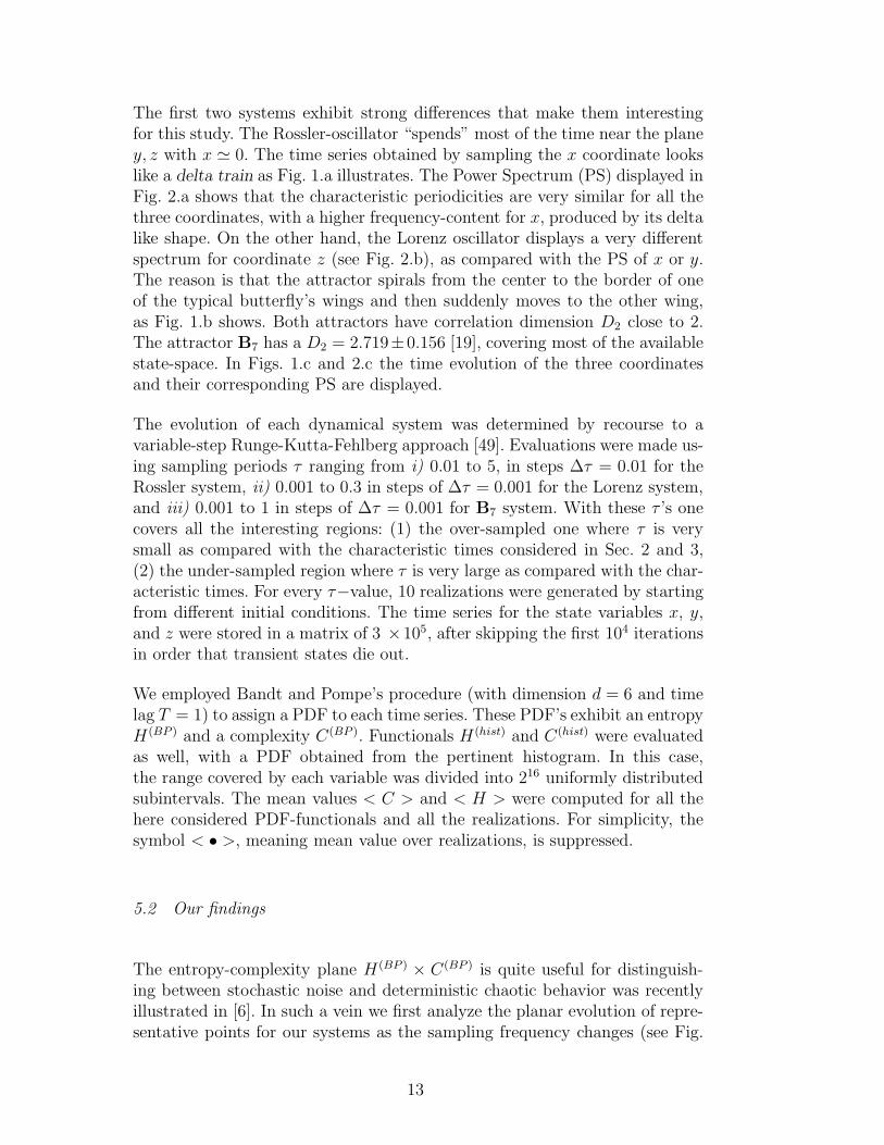
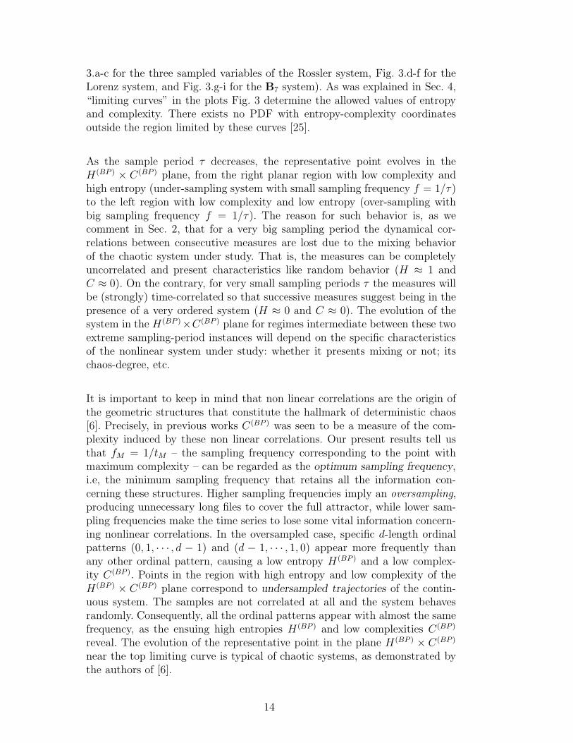
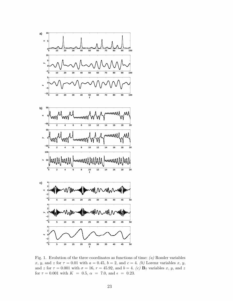
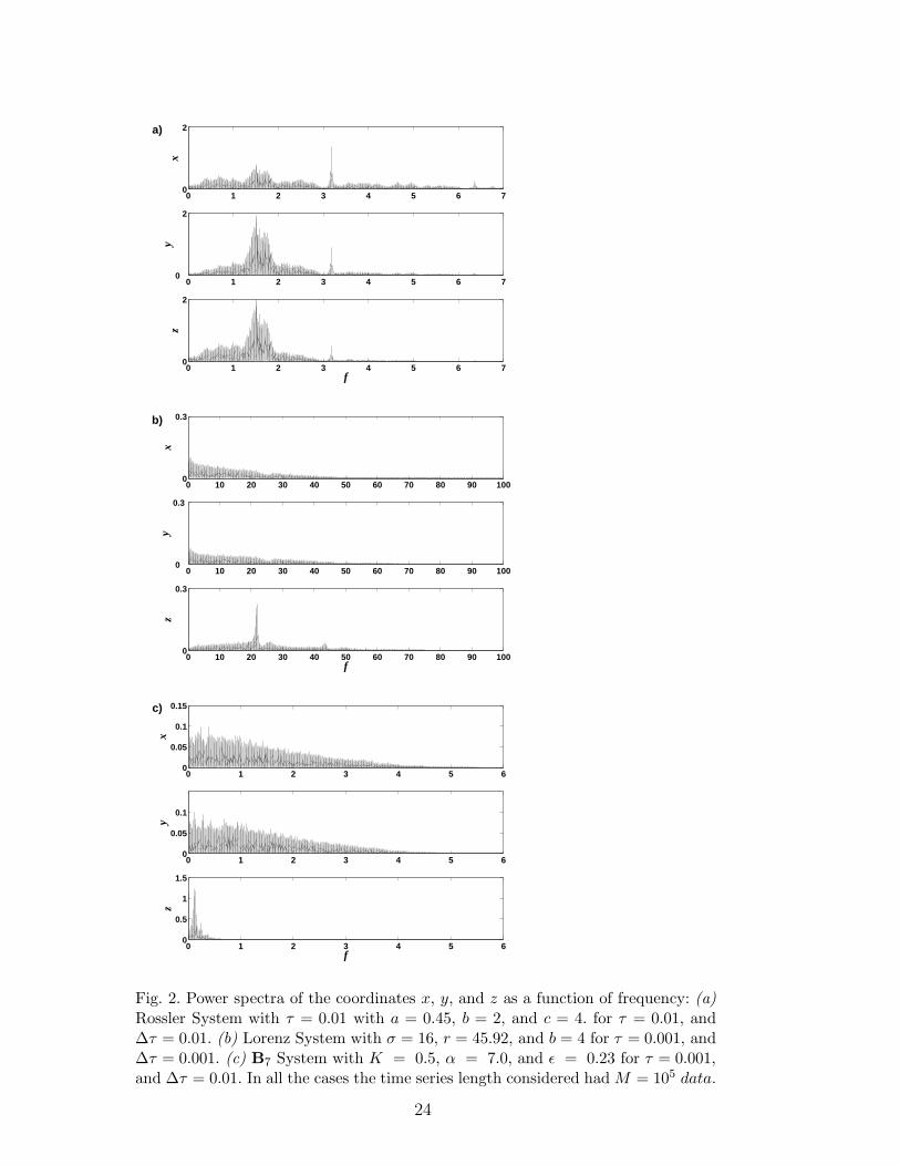
The first two systems exhibit strong differences that make them interestingfor this study. The Rossler-oscillator “spends” most of the time near the planey, z with x ≃ 0. The time series obtained by sampling the x coordinate lookslike a delta train as Fig. 1.a illustrates. The Power Spectrum (PS) displayed inFig. 2.a shows that the characteristic periodicities are very similar for all thethree coordinates, with a higher frequency-content for x, produced by its deltalike shape. On the other hand, the Lorenz oscillator displays a very differentspectrum for coordinate z (see Fig. 2.b), as compared with the PS of x or y.The reason is that the attractor spirals from the center to the border of oneof the typical butterfly’s wings and then suddenly moves to the other wing,as Fig. 1.b shows. Both attractors have correlation dimension D2 close to 2.The attractor B7 has a D2 = 2.719±0.156 [19], covering most of the availablestate-space. In Figs. 1.c and 2.c the time evolution of the three coordinatesand their corresponding PS are displayed.
The evolution of each dynamical system was determined by recourse to avariable-step Runge-Kutta-Fehlberg approach [49]. Evaluations were made us-ing sampling periods τ ranging from i) 0.01 to 5, in steps ∆τ = 0.01 for theRossler system, ii) 0.001 to 0.3 in steps of ∆τ = 0.001 for the Lorenz system,and iii) 0.001 to 1 in steps of ∆τ = 0.001 for B7 system. With these τ ’s onecovers all the interesting regions: (1) the over-sampled one where τ is verysmall as compared with the characteristic times considered in Sec. 2 and 3,(2) the under-sampled region where τ is very large as compared with the char-acteristic times. For every τ−value, 10 realizations were generated by startingfrom different initial conditions. The time series for the state variables x, y,and z were stored in a matrix of 3 ×10⁵, after skipping the first 104 iterationsin order that transient states die out.
We employed Bandt and Pompe’s procedure (with dimension d = 6 and timelag T = 1) to assign a PDF to each time series. These PDF’s exhibit an entropyH(BP ) and a complexity C(BP ). Functionals H(hist) and C(hist) were evaluatedas well, with a PDF obtained from the pertinent histogram. In this case,the range covered by each variable was divided into 216 uniformly distributedsubintervals. The mean values < C > and < H > were computed for all thehere considered PDF-functionals and all the realizations. For simplicity, thesymbol < • >, meaning mean value over realizations, is suppressed.
5.2 Our findings
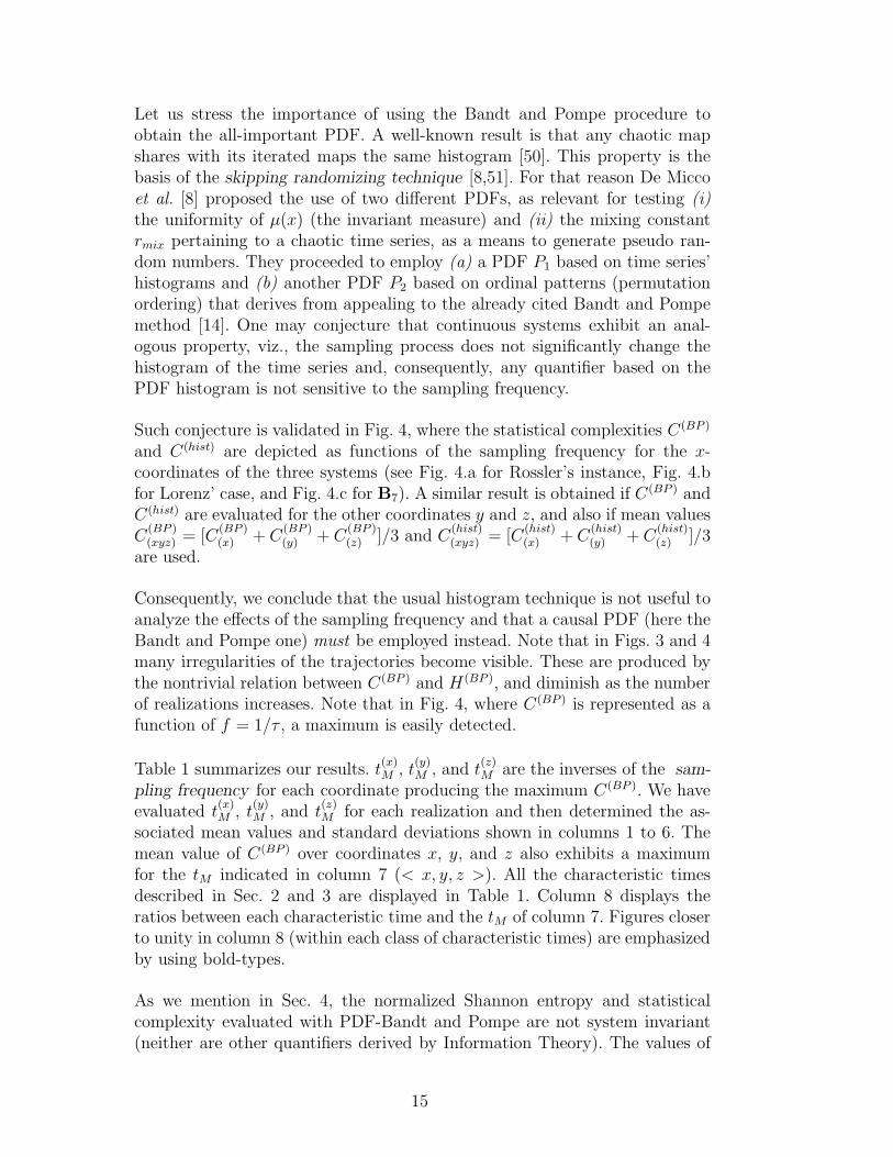
The entropy-complexity plane H(BP ) × C(BP ) is quite useful for distinguish-ing between stochastic noise and deterministic chaotic behavior was recentlyillustrated in [6]. In such a vein we first analyze the planar evolution of repre-sentative points for our systems as the sampling frequency changes (see Fig.
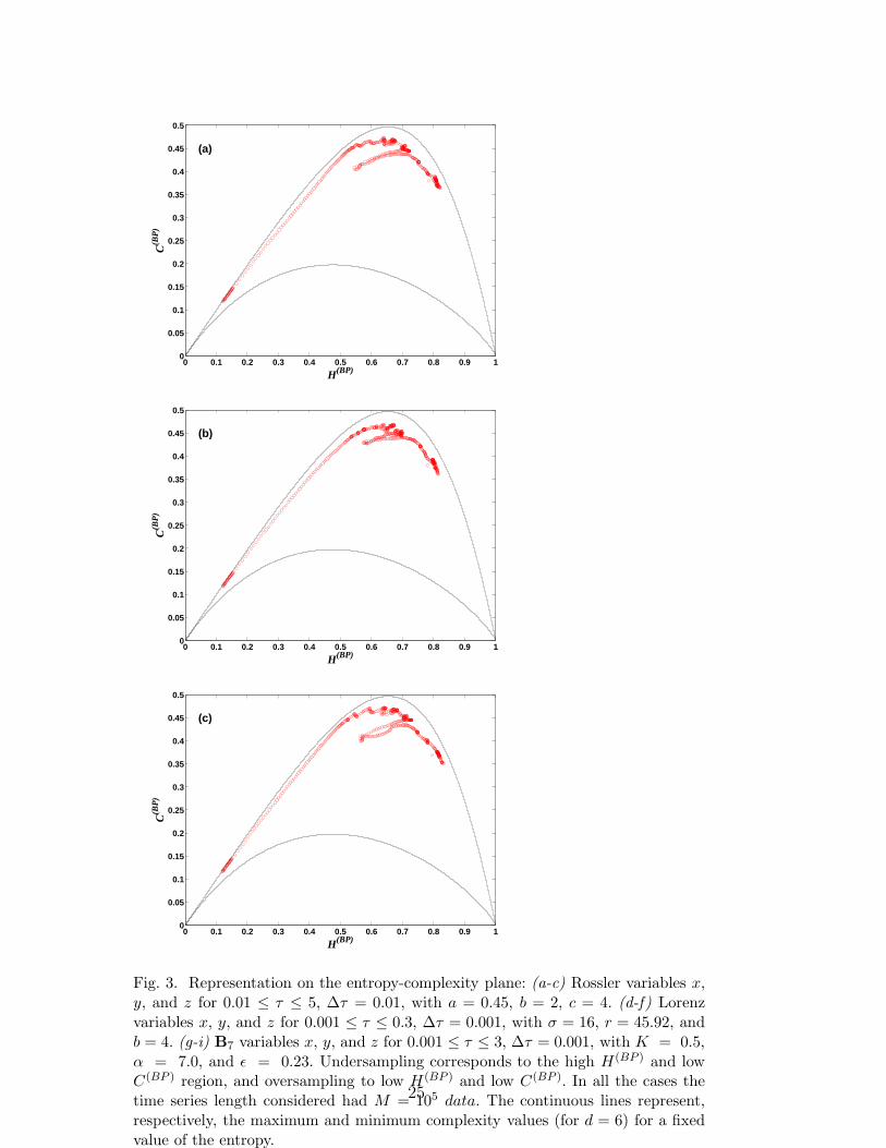
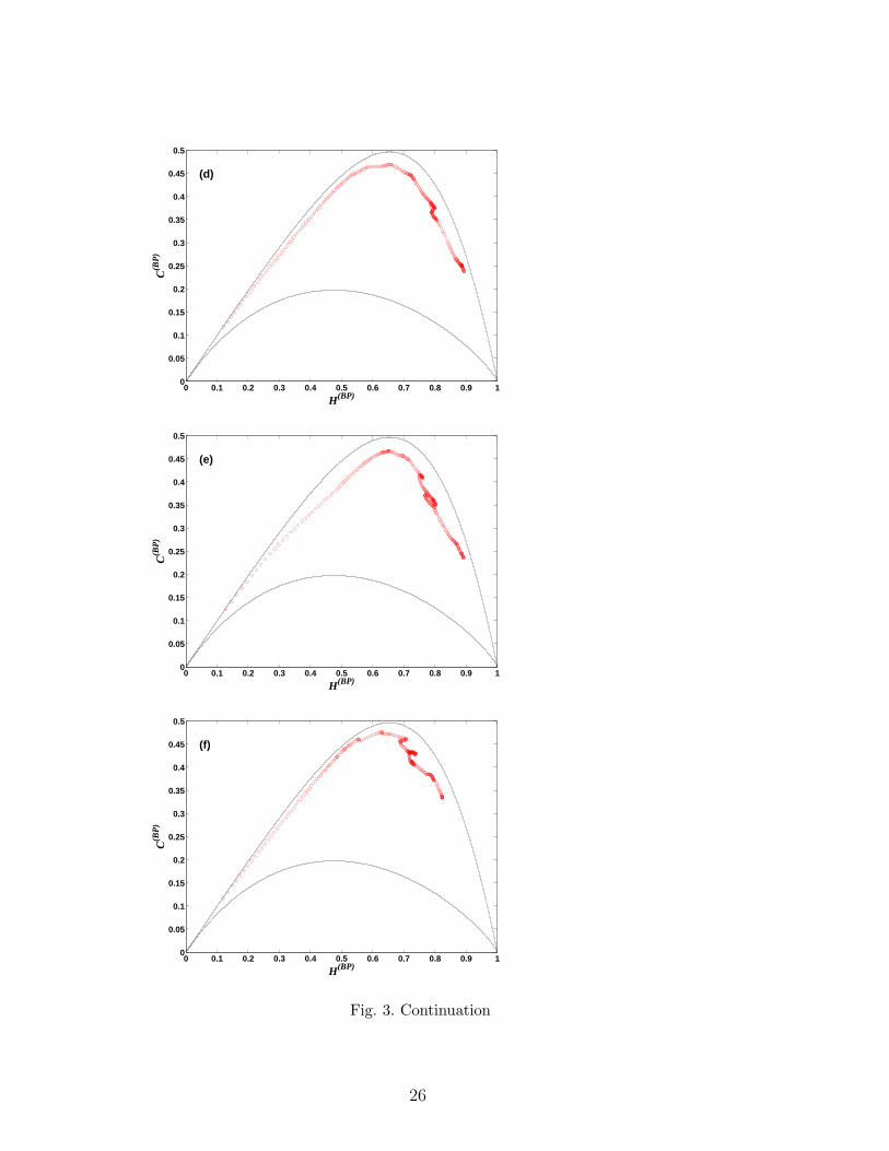
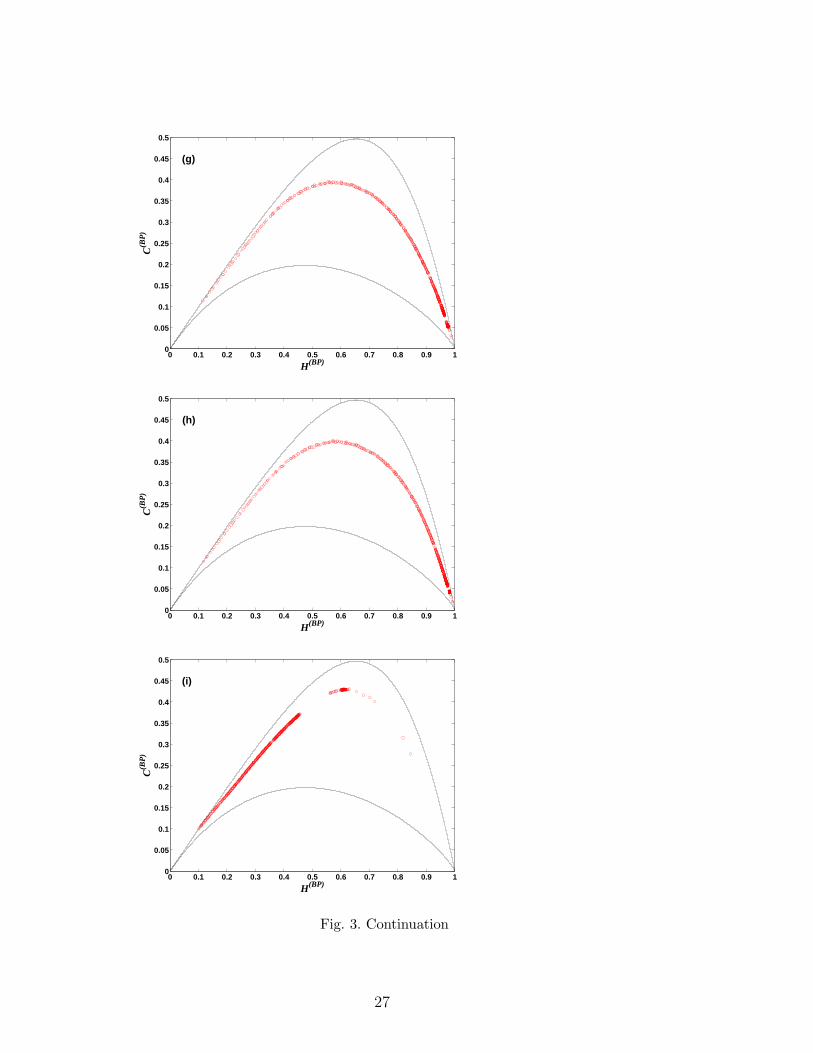
13
3.a-c for the three sampled variables of the Rossler system, Fig. 3.d-f for theLorenz system, and Fig. 3.g-i for the B7 system). As was explained in Sec. 4,“limiting curves” in the plots Fig. 3 determine the allowed values of entropyand complexity. There exists no PDF with entropy-complexity coordinatesoutside the region limited by these curves [25].
As the sample period τ decreases, the representative point evolves in theH(BP ) × C(BP ) plane, from the right planar region with low complexity andhigh entropy (under-sampling system with small sampling frequency f = 1/τ)to the left region with low complexity and low entropy (over-sampling withbig sampling frequency f = 1/τ). The reason for such behavior is, as wecomment in Sec. 2, that for a very big sampling period the dynamical cor-relations between consecutive measures are lost due to the mixing behaviorof the chaotic system under study. That is, the measures can be completelyuncorrelated and present characteristics like random behavior (H ≈ 1 andC ≈ 0). On the contrary, for very small sampling periods τ the measures willbe (strongly) time-correlated so that successive measures suggest being in thepresence of a very ordered system (H ≈ 0 and C ≈ 0). The evolution of thesystem in the H(BP )×C(BP ) plane for regimes intermediate between these twoextreme sampling-period instances will depend on the specific characteristicsof the nonlinear system under study: whether it presents mixing or not; itschaos-degree, etc.
It is important to keep in mind that non linear correlations are the origin ofthe geometric structures that constitute the hallmark of deterministic chaos[6]. Precisely, in previous works C(BP ) was seen to be a measure of the com-plexity induced by these non linear correlations. Our present results tell usthat fM = 1/tM – the sampling frequency corresponding to the point withmaximum complexity – can be regarded as the optimum sampling frequency,i.e, the minimum sampling frequency that retains all the information con-cerning these structures. Higher sampling frequencies imply an oversampling,producing unnecessary long files to cover the full attractor, while lower sam-pling frequencies make the time series to lose some vital information concern-ing nonlinear correlations. In the oversampled case, specific d-length ordinalpatterns (0, 1, · · · , d − 1) and (d − 1, · · · , 1, 0) appear more frequently thanany other ordinal pattern, causing a low entropy H(BP ) and a low complex-ity C(BP ). Points in the region with high entropy and low complexity of theH(BP ) × C(BP ) plane correspond to undersampled trajectories of the contin-uous system. The samples are not correlated at all and the system behavesrandomly. Consequently, all the ordinal patterns appear with almost the samefrequency, as the ensuing high entropies H(BP ) and low complexities C(BP )
reveal. The evolution of the representative point in the plane H(BP ) × C(BP )
near the top limiting curve is typical of chaotic systems, as demonstrated bythe authors of [6].
14
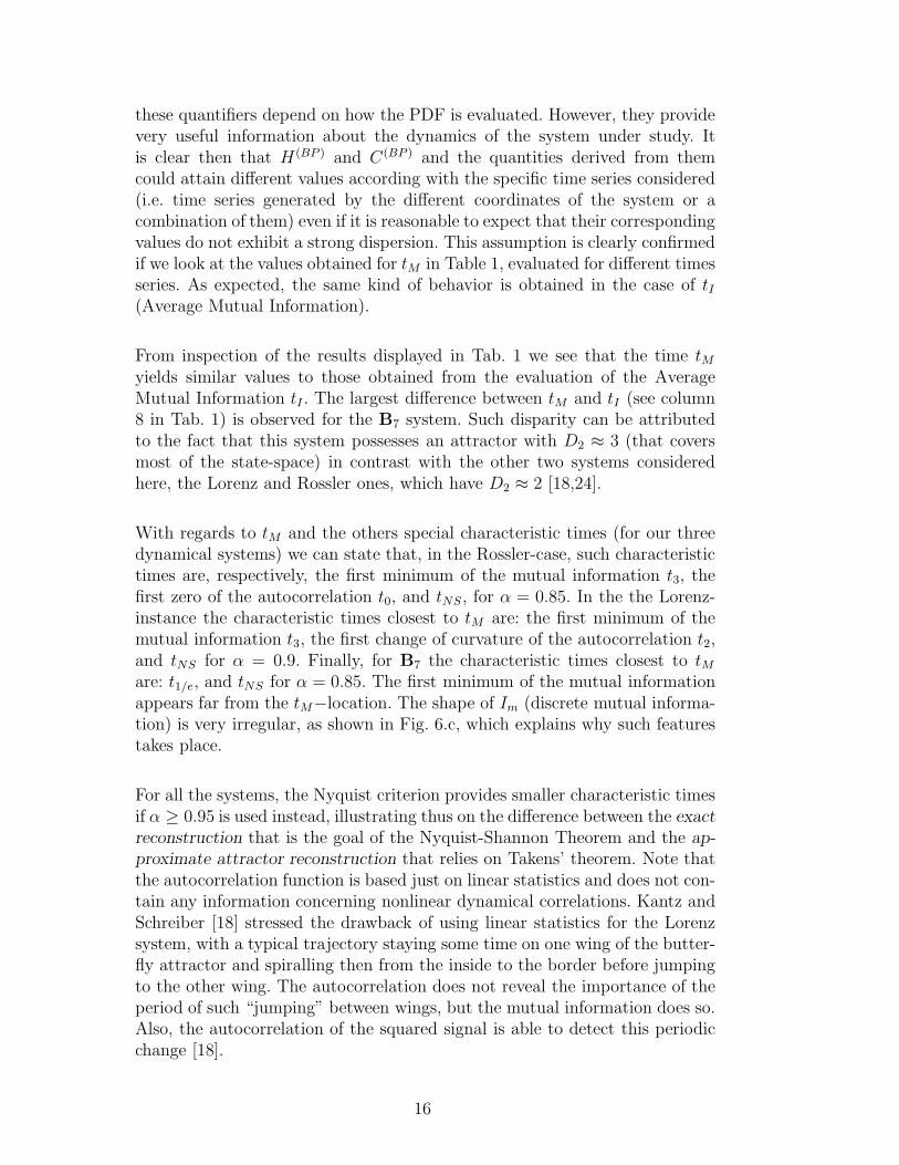
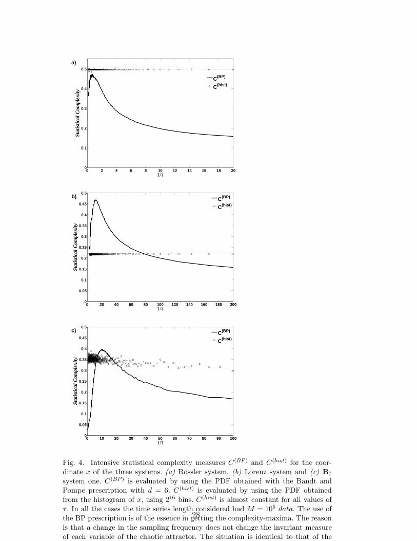
Let us stress the importance of using the Bandt and Pompe procedure toobtain the all-important PDF. A well-known result is that any chaotic mapshares with its iterated maps the same histogram [50]. This property is thebasis of the skipping randomizing technique [8,51]. For that reason De Miccoet al. [8] proposed the use of two different PDFs, as relevant for testing (i)the uniformity of µ(x) (the invariant measure) and (ii) the mixing constantrmix pertaining to a chaotic time series, as a means to generate pseudo ran-dom numbers. They proceeded to employ (a) a PDF P1 based on time series’histograms and (b) another PDF P2 based on ordinal patterns (permutationordering) that derives from appealing to the already cited Bandt and Pompemethod [14]. One may conjecture that continuous systems exhibit an anal-ogous property, viz., the sampling process does not significantly change thehistogram of the time series and, consequently, any quantifier based on thePDF histogram is not sensitive to the sampling frequency.
Such conjecture is validated in Fig. 4, where the statistical complexities C(BP )
and C(hist) are depicted as functions of the sampling frequency for the x-coordinates of the three systems (see Fig. 4.a for Rossler’s instance, Fig. 4.bfor Lorenz’ case, and Fig. 4.c for B7). A similar result is obtained if C(BP ) andC(hist) are evaluated for the other coordinates y and z, and also if mean valuesC
(BP )(xyz) = [C
(BP )(x) + C
(BP )(y) + C
(BP )(z) ]/3 and C
(hist)(xyz) = [C
(hist)(x) + C
(hist)(y) + C
(hist)(z) ]/3
are used.
Consequently, we conclude that the usual histogram technique is not useful toanalyze the effects of the sampling frequency and that a causal PDF (here theBandt and Pompe one) must be employed instead. Note that in Figs. 3 and 4many irregularities of the trajectories become visible. These are produced bythe nontrivial relation between C(BP ) and H(BP ), and diminish as the numberof realizations increases. Note that in Fig. 4, where C(BP ) is represented as afunction of f = 1/τ , a maximum is easily detected.
Table 1 summarizes our results. t(x)M , t
(y)M , and t
(z)M are the inverses of the sam-
pling frequency for each coordinate producing the maximum C(BP ). We haveevaluated t
(x)M , t
(y)M , and t
(z)M for each realization and then determined the as-
sociated mean values and standard deviations shown in columns 1 to 6. Themean value of C(BP ) over coordinates x, y, and z also exhibits a maximumfor the tM indicated in column 7 (< x, y, z >). All the characteristic timesdescribed in Sec. 2 and 3 are displayed in Table 1. Column 8 displays theratios between each characteristic time and the tM of column 7. Figures closerto unity in column 8 (within each class of characteristic times) are emphasizedby using bold-types.
As we mention in Sec. 4, the normalized Shannon entropy and statisticalcomplexity evaluated with PDF-Bandt and Pompe are not system invariant(neither are other quantifiers derived by Information Theory). The values of
15
these quantifiers depend on how the PDF is evaluated. However, they providevery useful information about the dynamics of the system under study. Itis clear then that H(BP ) and C(BP ) and the quantities derived from themcould attain different values according with the specific time series considered(i.e. time series generated by the different coordinates of the system or acombination of them) even if it is reasonable to expect that their correspondingvalues do not exhibit a strong dispersion. This assumption is clearly confirmedif we look at the values obtained for tM in Table 1, evaluated for different timesseries. As expected, the same kind of behavior is obtained in the case of tI(Average Mutual Information).
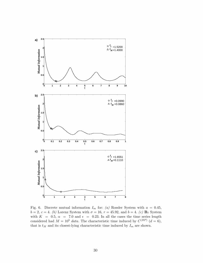
From inspection of the results displayed in Tab. 1 we see that the time tMyields similar values to those obtained from the evaluation of the AverageMutual Information tI . The largest difference between tM and tI (see column8 in Tab. 1) is observed for the B7 system. Such disparity can be attributedto the fact that this system possesses an attractor with D2 ≈ 3 (that coversmost of the state-space) in contrast with the other two systems consideredhere, the Lorenz and Rossler ones, which have D2 ≈ 2 [18,24].
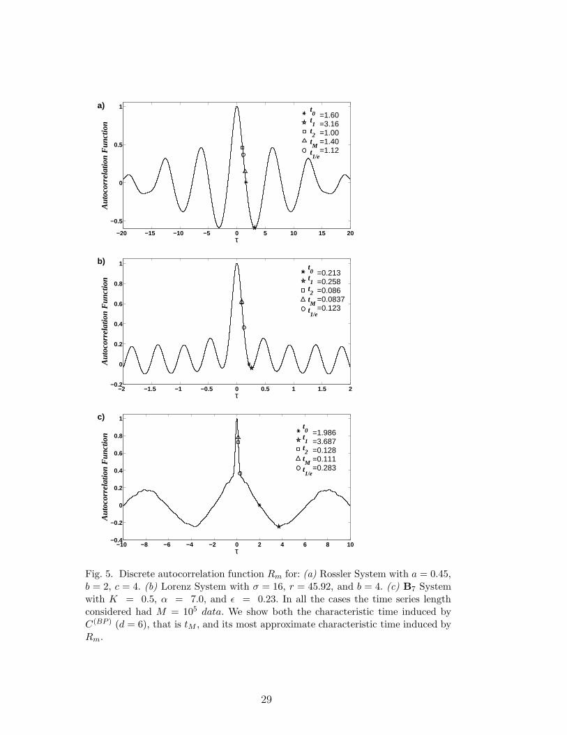
With regards to tM and the others special characteristic times (for our threedynamical systems) we can state that, in the Rossler-case, such characteristictimes are, respectively, the first minimum of the mutual information t3, thefirst zero of the autocorrelation t0, and tNS, for α = 0.85. In the the Lorenz-instance the characteristic times closest to tM are: the first minimum of themutual information t3, the first change of curvature of the autocorrelation t2,and tNS for α = 0.9. Finally, for B7 the characteristic times closest to tMare: t1/e, and tNS for α = 0.85. The first minimum of the mutual informationappears far from the tM−location. The shape of Im (discrete mutual informa-tion) is very irregular, as shown in Fig. 6.c, which explains why such featurestakes place.
For all the systems, the Nyquist criterion provides smaller characteristic timesif α ≥ 0.95 is used instead, illustrating thus on the difference between the exactreconstruction that is the goal of the Nyquist-Shannon Theorem and the ap-
proximate attractor reconstruction that relies on Takens’ theorem. Note thatthe autocorrelation function is based just on linear statistics and does not con-tain any information concerning nonlinear dynamical correlations. Kantz andSchreiber [18] stressed the drawback of using linear statistics for the Lorenzsystem, with a typical trajectory staying some time on one wing of the butter-fly attractor and spiralling then from the inside to the border before jumpingto the other wing. The autocorrelation does not reveal the importance of theperiod of such “jumping” between wings, but the mutual information does so.Also, the autocorrelation of the squared signal is able to detect this periodicchange [18].
16
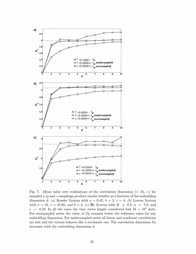
To assess the quality of the Takens’ reconstruction process using tM , D2 isevaluated for an embedding dimension ranging from d = 1 to 10 (see Fig. 7).The pertinent estimation of D2 is compared with values reported in the liter-ature for the continuous system [18,52,53]. The subroutine d2 of the TISEANpackage [13] was used for calculating D2.
Let us stress that the estimation of D2 poses a very delicate problem, so thatwe refer the readers to the documentation available for the TISEAN packageand also to the excellent book by Kantz and Schreiber [18]. Figs. 7 showthat τ = tM produces a time series with a D2 that turns out to be a betterestimation for the Correlation Dimension of the continuous system than thoseobtained with higher (under-sampled) or lower (over-sampled) values for τ .Similar results were obtained when we consider the evaluation of the maximumLyapunov exponent.
It is interesting to remark that the time tM , for which one detects a maximumin the entropy-complexity plane H(BP ) × C(BP ), is unique for the three dy-namical systems analyzed in the present work. We associate this sample-timewith the one needed to capture all the relevant information related to thedynamics’ nonlinear correlations.
Recently Soriano et al. [20] theoretically and experimentally studied a chaoticsemiconductor laser with optical feedback. This is an extremely interestingsystem because dynamical systems with time delay, like the Mackey-Glassor a laser with delay feedback, exhibit different relevant time scales [54,20].Consequently, additional complexity-maxima could be expected (in additionto the one encountered in dealing with the chaotic systems of this paper).In the case of the laser studied in [20] the main time scales are: i) τ ∗S, thefeedback-time providing the largest time scale, ii) TRO, that is the relaxationoscillation providing a shorter time scale, and finally iii) chaotic oscillations,that govern the fastest time scale. Soriano et al. experimentally confirmedthat our prescription for tM corresponds to a maximum of C(BP ), as foundin all the chaotic systems studied in this paper (see Fig. 10 in [20]). To ourknowledge, this is the first controlled experiment where our prescription hasbeen to hold.
Sharing the point of view of Abarbanel [24], our prescription for the sampleperiod τ = tM is based on the consideration of a fundamental aspect of chaos,namely, the generation of information. Thus, our choice is made by takinginto account an important property of the system we wish to describe. Re-mark that stable linear systems generate zero information. In consequence,information-generation [24] is a property of nonlinear dynamics not shared bylinear evolutions.
Finally, another issue to be aware of is the influence of noise. To verify the
17
robustness of the criterion here advanced, gaussian noise was added to eachsystem and the value of tM was obtained as a function of the signal to noiseS/N ratio (σ) of this gaussian noise. In all cases, the value of tM remainedconstant (up to three significant decimal digits) for S/N > 20 dB. If the noise-strength is higher, tM suddenly decreases as the representative point in theplane H(BP )×C(BP ) moves to the rightwards region (stochastic region), whereordering-patterns are strongly affected by noise.
6 Conclusions
Our main goal here was to show that a particular version of the StatisticalComplexity Measure C(BP ), evaluated by recourse to the probability distribu-tion obtained via the Bandt and Pompe procedure, allows one to determine,under the light of a Takens’ reconstruction procedure, convenient samplingperiods. This is done so as to get time series useful for investigating chaoticbehavior.
This sampling-period was called tM , and the procedure was illustrated viaa detailed consideration of three paradigmatic systems. On the basis of thesesignificant examples we conjecture that our optimality criterion may be of gen-eral application for chaotic systems, since C(BP ) is a measure of the geometricstructures produced by nonlinear correlations, always present in this class ofdynamical systems. We showed that tM is compatible with those specific timesrecommended in the literature as adequate delay-ones in Takens’ reconstruc-tion. Our results closely approach the exact Nyquist-Shannon reconstruction.This is so because high frequencies of the Fourier Spectrum are due to chaoticoscillations, and this is the case for the systems studied here.
To our knowledge, controlled experiments for different sampling times of themeasured variables and large numbers of data have not yet been reportedin the literature and the highest sampling frequency allowed by the digitalacquisition system is the one usually adopted (as an exception see [20]). Inthe light of our present results it would be better, in practice, to assess thecorrect tM−value for a clever choosing of the sampling period. This permitsone to cover the whole attractor-basin and retain in the reconstruction processthe most important properties of chaotic systems.
In view of the extensive use of digital acquisition systems in all kinds of exper-iments, we hope that experimentalists may consider the present contributionas a practical tool in their activities and may thus be able to validate ourproposal.
18
Acknowledgments
This work was partially supported by the Consejo Nacional de InvestigacionesCientıficas y Tecnicas (CONICET), Argentina (PIP 112-200801-01420), AN-PCyT and UNMDP Argentina (PICT 11-21409/04). O. A. Rosso gratefullyacknowledge support from CAPES, PVE fellowship, Brazil.
References
[1] J. P. Crutchfield, K. Young. Inferring statistical complexity. Phys. Rev. Lett.63 (1989) 105–108.
[2] R. Wackerbauer, A. Witt, H. Atmanspacher, J. Kurths, H. Scheingraber. Acomparative classification of complexity measures. Chaos, Solitons & Fractals,4 (1994) 133–173.
[3] R. Lopez-Ruiz, H. L. Mancini, X. Calbet. A statistical measure of complexity.Phys. Lett. A 209 (1995) 321–326.
[4] M. T. Martın, A. Plastino, and O. A. Rosso. Statistical complexity anddisequilibrium. Phys. Lett. A 11 (2003) 126–132.
[5] P. W. Lamberti, M. T. Martın, A. Plastino, and O. A. Rosso. Intensive entropicnon-triviality measure. Physica A 334 (2004) 119–131.
[6] O. A. Rosso, H. A. Larrondo, M. T. Martın, A. Plastino, M. A. Fuentes.Distinguishing noise from chaos. Phys. Rev. Lett. 99 (2007) 154102.
[7] O. A. Rosso, L. Zunino, D. G. Perez, A. Figliola, H. A. Larrondo, M. Garavaglia,M. T. Martın, A. Plastino. Extracting features of gaussian selfsimilar stochasticprocesses via the Bandt & Pompe approach. Phys. Rev. E, 76 (2007) 061114.
[8] L. De Micco, C. M. Gonzalez, H. A. Larrondo, M. T. Martın, A. Plastino, O.A. Rosso. Randomizing nonlinear maps via symbolic dynamics. Physica A 387(2008) 3373–3383.
[9] L. De Micco, H. Larrondo, A. Plastino, O. A. Rosso. Quantifiers for stochasticityof chaotic pseudo random number generators. Phil. Trans. Royal Soc. A 367(2009) 3281–3296.
[10] H. Nyquist. Certain topics in telegraph transmission theory. Trans. AIEE 47(1928) 617–644.
[11] C. E. Shannon. Communication in the presence of noise. Proc. Institute of RadioEngineers 37 (1949) 10–21.
[12] F. Takens. Detecting strange attractors in turbulence. Lecture Notes inMathematics 898 (1981) 366–381.
19
[13] R. Hegger, H. Kantz, and T. Schreiber. Practical implementation of nonlineartime series methods: The tisean package. Chaos 9 (1999) 413–435.
[14] C. Bandt, B. Pompe. Permutation entropy: a natural complexity measure fortime series. Phys. Rev. Lett. 88 (2002) 174102.
[15] J. Pearl. Causality: models, reasoning, and inference. Cambridge UniversityPress, 2009.
[16] A. M. Fraser, H. L. Swinney. Independent coordinates for strange attractorsfrom mutual information. Phys. Rev. A 33 (1986) 1134–1140.
[17] J. P. Crutchfield, B. McNamara. Equations of motion from a data series.Complex Systems 1 (1989) 417–452.
[18] H. Kantz, T. Shreiber. Nonlinear Time Series Analysis. Cambridge UniversityPress, 1999.
[19] K. E. Chlouverakis and J. C. Sprott. A comparison of correlation and lyapunovdimensions. Physica D 200 (2005) 156–164.
[20] M. C. Soriano, L. Zunino, O. A. Rosso, I. Fischer, C. R. Mirasso. Time scales ofchaotic semiconductor laser with optical feedback under the lens of permutationinformation analysis. IEEE J. Quantum Electronics 47 (2011) 252–261.
[21] T. Sauer, J. A. Yorke, M. Casdagli. Embedology. Journal of Statistical Physics65 (1991) 579–616.
[22] M. Casdagli, S. Eubank, J. D. Farmer, J. Gibson. State space reconstruction inthe presence of noise. Physica D 51 (1991) 52–98.
[23] J. Gibson, J. D. Farmer, M. Casdagli, S. Eubank. An analytical approach topractical state space reconstruction. Physica D 57 (1992) 1–30.
[24] H. D. I. Abarbanel. Analysis of observed chaotic data. Springer-Verlag, NewYork, 1996.
[25] M. T. Martın, A. Plastino, O. A. Rosso. Generalized statistical complexitymeasures: geometrical and analytical properties. Physica A 369 (2006) 439–462.
[26] O. A. Rosso, H. Craig, P. Moscato, Shakespeare and other English renaissanceauthors as characterized by Information Theory complexity quantifiers. PhysicaA 388 (2009) 916–926
[27] K. Mischaikow, M. Mrozek, J. Reiss, A. Szymczak. Construction of symbolicdynamics from experimental time series. Phys. Rev. Lett., 82 (1999) 1114–1147.
[28] G. E. Powell, I. C. Percival. A spectral entropy method for distinguishing regularand irregular motion of hamiltonian systems. J. Phys. A: Math. Gen. 12 (1979)2053–2071.
[29] S. Blanco, A. Figliola, R. Quian Quiroga, O. A. Rosso, E. Serrano. Time-frequency analysis of electroencephalogram series (III): Wavelet packets andinformation cost function. Phys. Rev. E 57 (1998) 932–940.
20
[30] O. A. Rosso, S. Blanco, J. Jordanova, V. Kolev, A. Figliola, M. Schurmann,E. Bassar. Wavelet entropy: a new tool for analysis of short duration brainelectrical signals. Journal of Neuroscience Methods 105 (2001) 65–75.
[31] W. Ebeling, R. Steuer. Partition-based entropies of deterministic and stochasticmaps. Stochastics and Dynamics, 1 (2001) 1–17.
[32] J. M. Amigo, L. Kocarev, I. Tomovski. Discrete entropy. Physica D 228 (2007)77–85.
[33] K. Keller, M. Sinn. Ordinal analysis of time series. Physica A 356 (2005) 114–120.
[34] O. A. Rosso, C. Masoller. Detecting and quantifying stochastic and coherenceresonances via information theory complexity measurements. Phys. Rev. E 79(2009) 040106(R).
[35] O. A. Rosso, C. Masoller. Detecting and quantifying temporal correlations instochastic resonance via information theory measures. European Phys. JournalB, 69 (2009) 37–43.
[36] H. A. Larrondo, C. M. Gonzalez, M. T. Martın, A. Plastino, O. A. Rosso.Intensive statistical complexity measure of pseudorandom number generators.Physica A 356 (2005) 133–138.
[37] H. A. Larrondo, M. T. Martın, C.M. Gonzalez, A. Plastino, O. A. Rosso.Random number generators and causality. Phys. Lett. A 352 (2006) 421–425.
[38] A. M. Kowalski, M. T. Martın, A. Plastino, O. A. Rosso. Bandt-Pompeapproach to the classical-quantum transition. Physica D 233 (2007) 21–31.
[39] L. Zunino, D. G. Perez, M. T. Martın, A. Plastino, M. Garavaglia, O. A. Rosso.Characterization of gaussian self-similar stochastic processes using wavelet-based informational tools. Phys. Rev. E 75 (2007) 021115.
[40] O. A. Rosso, R. Vicente, C. R. Mirasso. Encryption test of pseudo-aleatorymessages embedded on chaotic laser signals: an information theory approach.Phys. Lett. A 372 (2008) 1018–1023.
[41] L. Zunino, D. G. Perez, M. T. Martın, M. Garavaglia, A. Plastino, O. A. Rosso.Permutation entropy of fractional brownian motion and fractional gaussiannoise. Physics Letters A 372 (2008) 4768–4774.
[42] L. Zunino, D. G. Perez, A. Kowalski, M. T. Martın, M. Garavaglia, A. Plastino,O. A. Rosso. Fractional Brownian motion, fractional Gaussian noise, and Tsallispermutation entropy. Physica A 387 (2008) 6057–6068
[43] L. Zunino, M. Zanin, B. M. Tabak, D. Perez, and O. A. Rosso. Forbiddenpatterns, permutation entropy and stock market inefficiency. Physica A 388(2009) 2854–2864
[44] L. Zunino, M. Zanin, B. M. Tabak, D. G. Perez, O. A. Rosso. Complexity-entropy causality plane: a useful approach to quantify the stock marketinefficiency. Physica A 389 (2010) 1891–1901.
21
[45] O. A. Rosso, L. De Micco, H. Larrondo, M. T. Martın, A. Plastino. Generalizedstatistical complexity measure. Int. J. Bif. and Chaos 20 (2010) 775–785.
[46] O. A. Rosso, L. De Micco, A. Plastino, H. A. Larrondo. Info-quantifiers’ map-characterization revisited. Physica A 389 (2010) 4604–4612.
[47] P. M. Saco, L. C. Carpi, A. Figliola, E. Serrano, and O. A. Rosso. EntropyAnalysis of the Dynamics of EL Nino/Southern Oscillation during the Holocene.Physica A 389 (2010) 5022–5027.
[48] K. Keller, H. Lauffer. Symbolic analysis of high-dimensional time series. Int. J.Bifurcation and Chaos 13 (2003) 2657–2668.
[49] W. H. Press, S. A. Teikolsky, W. T. Vetterling, B. P. Flannery. NumericalRecipes in C. Cambridge University Press, 1995.
[50] G. Setti, G. Mazzini, R. Rovatti, and S. Callegari. Statistical modeling ofdiscrete-time chaotic processes: Basic finite-dimensional tools and applications.Proceedings of the IEEE 90 (2002) 662–689.
[51] S. Callegari, R. Rovatti, and G. Setti. Chaos-based fm signals: applicationand implementation issues. IEEE Transactions on Circuits and Systems I:Fundamental Theory and Applications 50 (2003) 1141–1147.
[52] J. C. Sprott. Lyapunov exponent and dimension of the lorenz attractor.http://sprott.physics.wisc.edu/chaos/lorenzle.htm, 2005.
[53] J. C. Sprott, C. Rowlands. Improved correlation dimension calculation. Int. J.Bifurcation and Chaos 11 (2001) 1865–1880.
[54] L. Zunino, M. C. Soriano, I. Fischer, O. A. Rosso, C. R. Mirasso. Permutation-information-theory approach to unveil delay dynamics from time-series analysis.Phys. Rev. E 82 (2010) 046212.
22
0 10 20 30 40 50 60 70 80 90 1000
5
10
x
0 10 20 30 40 50 60 70 80 90 100−5
0
5
10
y
0 10 20 30 40 50 60 70 80 90 100−10
−5
0
5
t
z
a)
0 2 4 6 8 10 12 14 16 18 20−50
0
50
x
0 2 4 6 8 10 12 14 16 18 20−50
0
50
y
0 2 4 6 8 10 12 14 16 18 200
50
100
t
z
b)
0 5 10 15 20 25 30 35 40 45 50−4
−2
0
2
4
x
0 5 10 15 20 25 30 35 40 45 50−4
−2
0
2
4
y
0 5 10 15 20 25 30 35 40 45 50−4
−2
0
2
4
z
t
c)
Fig. 1. Evolution of the three coordinates as functions of time: (a) Rossler variablesx, y, and z for τ = 0.01 with a = 0.45, b = 2, and c = 4. (b) Lorenz variables x, y,and z for τ = 0.001 with σ = 16, r = 45.92, and b = 4. (c) B7 variables x, y, and zfor τ = 0.001 with K = 0.5, α = 7.0, and ǫ = 0.23.
23
0 1 2 3 4 5 6 70
2
x
0 1 2 3 4 5 6 70
2
y
0 1 2 3 4 5 6 70
2
z
f
a)
0 10 20 30 40 50 60 70 80 90 1000
0.3
x
0 10 20 30 40 50 60 70 80 90 1000
0.3
y
0 10 20 30 40 50 60 70 80 90 1000
0.3
z
f
b)
0 1 2 3 4 5 60
0.05
0.1
0.15
x
0 1 2 3 4 5 60
0.05
0.1
y
0 1 2 3 4 5 60
0.5
1
1.5
z
f
c)
Fig. 2. Power spectra of the coordinates x, y, and z as a function of frequency: (a)Rossler System with τ = 0.01 with a = 0.45, b = 2, and c = 4. for τ = 0.01, and∆τ = 0.01. (b) Lorenz System with σ = 16, r = 45.92, and b = 4 for τ = 0.001, and∆τ = 0.001. (c) B7 System with K = 0.5, α = 7.0, and ǫ = 0.23 for τ = 0.001,and ∆τ = 0.01. In all the cases the time series length considered had M = 105 data.
24
0 0.1 0.2 0.3 0.4 0.5 0.6 0.7 0.8 0.9 10
0.05
0.1
0.15
0.2
0.25
0.3
0.35
0.4
0.45
0.5
H(BP)
C(B
P)
(a)
0 0.1 0.2 0.3 0.4 0.5 0.6 0.7 0.8 0.9 10
0.05
0.1
0.15
0.2
0.25
0.3
0.35
0.4
0.45
0.5
H(BP)
C(B
P)
(b)
0 0.1 0.2 0.3 0.4 0.5 0.6 0.7 0.8 0.9 10
0.05
0.1
0.15
0.2
0.25
0.3
0.35
0.4
0.45
0.5
H(BP)
C(B
P)
(c)
Fig. 3. Representation on the entropy-complexity plane: (a-c) Rossler variables x,y, and z for 0.01 ≤ τ ≤ 5, ∆τ = 0.01, with a = 0.45, b = 2, c = 4. (d-f) Lorenzvariables x, y, and z for 0.001 ≤ τ ≤ 0.3, ∆τ = 0.001, with σ = 16, r = 45.92, andb = 4. (g-i) B7 variables x, y, and z for 0.001 ≤ τ ≤ 3, ∆τ = 0.001, with K = 0.5,α = 7.0, and ǫ = 0.23. Undersampling corresponds to the high H(BP ) and lowC(BP ) region, and oversampling to low H(BP ) and low C(BP ). In all the cases thetime series length considered had M = 105 data. The continuous lines represent,respectively, the maximum and minimum complexity values (for d = 6) for a fixedvalue of the entropy.
25
0 0.1 0.2 0.3 0.4 0.5 0.6 0.7 0.8 0.9 10
0.05
0.1
0.15
0.2
0.25
0.3
0.35
0.4
0.45
0.5
H(BP)
C(B
P)
(d)
0 0.1 0.2 0.3 0.4 0.5 0.6 0.7 0.8 0.9 10
0.05
0.1
0.15
0.2
0.25
0.3
0.35
0.4
0.45
0.5
H(BP)
C(B
P)
(e)
0 0.1 0.2 0.3 0.4 0.5 0.6 0.7 0.8 0.9 10
0.05
0.1
0.15
0.2
0.25
0.3
0.35
0.4
0.45
0.5
H(BP)
C(B
P)
(f)
Fig. 3. Continuation
26
0 0.1 0.2 0.3 0.4 0.5 0.6 0.7 0.8 0.9 10
0.05
0.1
0.15
0.2
0.25
0.3
0.35
0.4
0.45
0.5
H(BP)
C(B
P)
(g)
0 0.1 0.2 0.3 0.4 0.5 0.6 0.7 0.8 0.9 10
0.05
0.1
0.15
0.2
0.25
0.3
0.35
0.4
0.45
0.5
H(BP)
C(B
P)
(h)
0 0.1 0.2 0.3 0.4 0.5 0.6 0.7 0.8 0.9 10
0.05
0.1
0.15
0.2
0.25
0.3
0.35
0.4
0.45
0.5
H(BP)
C(B
P)
(i)
Fig. 3. Continuation
27
0 2 4 6 8 10 12 14 16 18 200
0.1
0.2
0.3
0.4
0.5
Stat
istic
al C
ompl
exity
1/τ
C(BP)
C(hist)
a)
0 20 40 60 80 100 120 140 160 180 2000
0.05
0.1
0.15
0.2
0.25
0.3
0.35
0.4
0.45
0.5
Stat
istic
al C
ompl
exity
1/τ
C(BP)
C(hist)
b)
0 10 20 30 40 50 60 70 80 90 1000
0.05
0.1
0.15
0.2
0.25
0.3
0.35
0.4
0.45
0.5
Stat
istic
al C
ompl
exity
1/τ
C(BP)
C(hist)
c)
Fig. 4. Intensive statistical complexity measures C(BP ) and C(hist) for the coor-dinate x of the three systems. (a) Rossler system, (b) Lorenz system and (c) B7
system one. C(BP ) is evaluated by using the PDF obtained with the Bandt andPompe prescription with d = 6. C(hist) is evaluated by using the PDF obtainedfrom the histogram of x, using 216 bins. C(hist) is almost constant for all values ofτ . In all the cases the time series length considered had M = 105 data. The use ofthe BP prescription is of the essence in getting the complexity-maxima. The reasonis that a change in the sampling frequency does not change the invariant measureof each variable of the chaotic attractor. The situation is identical to that of the
28
−20 −15 −10 −5 0 5 10 15 20
−0.5
0
0.5
1
τ
Aut
ocor
rela
tion
Fun
ctio
n
data1data2data3data4data5
a) t0
t1
t2
tM
t1/e
=1.60=3.16=1.00=1.40=1.12
−2 −1.5 −1 −0.5 0 0.5 1 1.5 2−0.2
0
0.2
0.4
0.6
0.8
1
τ
Aut
ocor
rela
tion
Fun
ctio
n
data1data2data3data4data5
b)t0
t1
t2
tM
t1/e
=0.213=0.258=0.086=0.0837=0.123
−10 −8 −6 −4 −2 0 2 4 6 8 10−0.4
−0.2
0
0.2
0.4
0.6
0.8
1
τ
Aut
ocor
rela
tion
Fun
ctio
n
data1data2data3data4data5
c)t0
t1
t2
tM
t1/e
=1.986=3.687=0.128=0.111=0.283
Fig. 5. Discrete autocorrelation function Rm for: (a) Rossler System with a = 0.45,b = 2, c = 4. (b) Lorenz System with σ = 16, r = 45.92, and b = 4. (c) B7 Systemwith K = 0.5, α = 7.0, and ǫ = 0.23. In all the cases the time series lengthconsidered had M = 105 data. We show both the characteristic time induced byC(BP ) (d = 6), that is tM , and its most approximate characteristic time induced byRm.
29
0 1 2 3 4 5 6 7 8 9 100
0.5
1
1.5
2
2.5
τ
Mut
ual I
nfor
mat
ion
data1data2
a)
tI
tM
=1.5200=1.4000
0 0.1 0.2 0.3 0.4 0.5 0.6 0.7 0.8 0.9 10
0.5
1
1.5
2
2.5
τ
Mut
ual I
nfor
mat
ion
data1data2
b)tI
tM
=0.0990=0.0860
0 1 2 3 4 5 6 7 80
0.5
1
1.5
2
2.5
τ
Mut
ual I
nfor
mat
ion
data1data2
c)tI
tM
=1.6551=0.1110
Fig. 6. Discrete mutual information Im for: (a) Rossler System with a = 0.45,b = 2, c = 4. (b) Lorenz System with σ = 16, r = 45.92, and b = 4. (c) B7 Systemwith K = 0.5, α = 7.0 and ǫ = 0.23. In all the cases the time series lengthconsidered had M = 105 data. The characteristic time induced by C(BP ) (d = 6),that is tM and its closest-lying characteristic time induced by Im are shown.
30
1 2 3 4 5 6 7 8 9 101
1.2
1.4
1.6
1.8
2
2.2
d
D2
a)
τ tM
τ tM
(undersampled)τ t
M (oversampled)
=0.1390==0.5000>>=0.0009<<
1 2 3 4 5 6 7 8 9 101
1.2
1.4
1.6
1.8
2
2.2
d
D2
b)
τ tM
τ tM
(undersampled)τ t
M (oversampled)
=0.0932==0.3000<<=0.0009>>
1 2 3 4 5 6 7 8 9 10
1
1.5
2
2.5
3
d
D2
c)
=0.0103==0.1000>>=0.0010<<
τ tM
τ tM
(undersampled)τ t
M (oversampled)
Fig. 7. Mean value over realizations of the correlation dimension (< D2 >) forsampled x (y and z samplings produce similar results) as a function of the embeddingdimension d: (a) Rossler System with a = 0.45, b = 2, c = 4. (b) Lorenz Systemwith σ = 16, r = 45.92, and b = 4. (c) B7 System with K = 0.5, α = 7.0, andǫ = 0.23. In all the cases the time series length considered had M = 105 data.For oversampled series the value of D2 remains below the reference value for anyembedding dimension. For undersampled series all linear and nonlinear correlationsare lost and the system behaves like a stochastic one. The correlation dimension D2
increases with the embedding dimension d.
31
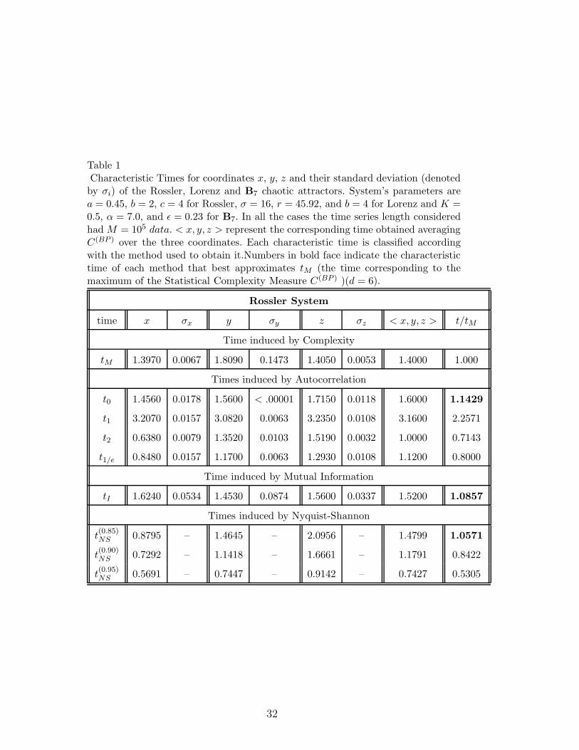
Table 1Characteristic Times for coordinates x, y, z and their standard deviation (denotedby σi) of the Rossler, Lorenz and B7 chaotic attractors. System’s parameters area = 0.45, b = 2, c = 4 for Rossler, σ = 16, r = 45.92, and b = 4 for Lorenz and K =0.5, α = 7.0, and ǫ = 0.23 for B7. In all the cases the time series length consideredhad M = 105 data. < x, y, z > represent the corresponding time obtained averagingC(BP ) over the three coordinates. Each characteristic time is classified accordingwith the method used to obtain it.Numbers in bold face indicate the characteristictime of each method that best approximates tM (the time corresponding to themaximum of the Statistical Complexity Measure C(BP ) )(d = 6).
Rossler System
time x σx y σy z σz < x, y, z > t/tM
Time induced by Complexity
tM 1.3970 0.0067 1.8090 0.1473 1.4050 0.0053 1.4000 1.000
Times induced by Autocorrelation
t0 1.4560 0.0178 1.5600 < .00001 1.7150 0.0118 1.6000 1.1429
t1 3.2070 0.0157 3.0820 0.0063 3.2350 0.0108 3.1600 2.2571
t2 0.6380 0.0079 1.3520 0.0103 1.5190 0.0032 1.0000 0.7143
t1/e 0.8480 0.0157 1.1700 0.0063 1.2930 0.0108 1.1200 0.8000
Time induced by Mutual Information
tI 1.6240 0.0534 1.4530 0.0874 1.5600 0.0337 1.5200 1.0857
Times induced by Nyquist-Shannon
t(0.85)NS 0.8795 – 1.4645 – 2.0956 – 1.4799 1.0571
t(0.90)NS 0.7292 – 1.1418 – 1.6661 – 1.1791 0.8422
t(0.95)NS 0.5691 – 0.7447 – 0.9142 – 0.7427 0.5305
32
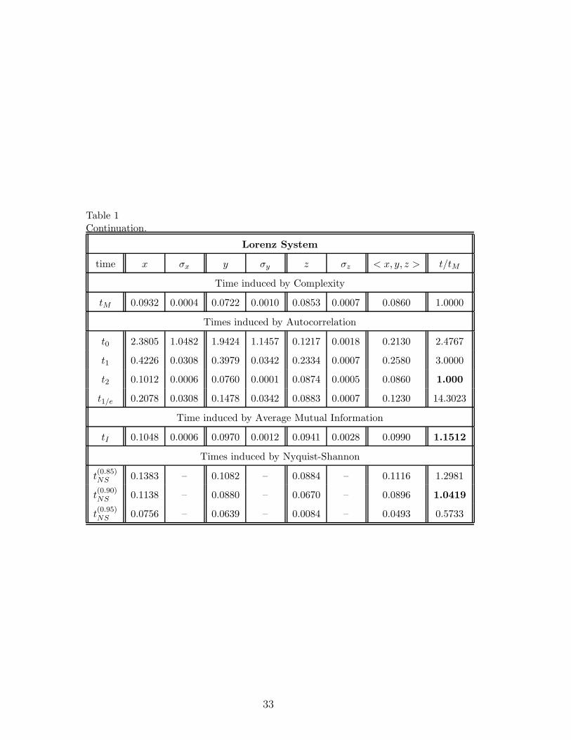
Table 1Continuation.
Lorenz System
time x σx y σy z σz < x, y, z > t/tM
Time induced by Complexity
tM 0.0932 0.0004 0.0722 0.0010 0.0853 0.0007 0.0860 1.0000
Times induced by Autocorrelation
t0 2.3805 1.0482 1.9424 1.1457 0.1217 0.0018 0.2130 2.4767
t1 0.4226 0.0308 0.3979 0.0342 0.2334 0.0007 0.2580 3.0000
t2 0.1012 0.0006 0.0760 0.0001 0.0874 0.0005 0.0860 1.000
t1/e 0.2078 0.0308 0.1478 0.0342 0.0883 0.0007 0.1230 14.3023
Time induced by Average Mutual Information
tI 0.1048 0.0006 0.0970 0.0012 0.0941 0.0028 0.0990 1.1512
Times induced by Nyquist-Shannon
t(0.85)NS 0.1383 – 0.1082 – 0.0884 – 0.1116 1.2981
t(0.90)NS 0.1138 – 0.0880 – 0.0670 – 0.0896 1.0419
t(0.95)NS 0.0756 – 0.0639 – 0.0084 – 0.0493 0.5733
33
Table 1Continuation.
B7 System
time x σx y σy z σz < x, y, z > t/tM
Time induced by Complexity
tM 0.1030 < 0.001 0.0930 < 0.001 0.9540 < 0.001 0.3833 1.0000
Times induced by Autocorrelation
t0 0.5459 0.3775 0.5635 0.4363 1.9985 0.0258 1.9860 5.1808
t1 0.4509 0.1332 0.3915 0.0957 3.9141 0.1161 3.6870 9.6182
t2 0.1301 0.0129 0.1301 0.0127 1.5631 0.0227 0.1280 0.3339
t1/e 0.1813 0.1332 0.1747 0.0957 1.4504 0.1161 0.2830 0.7382
Time induced by Average Mutual Information
tI 1.5289 0.2240 1.5951 0.2212 1.7905 0.1041 1.6551 4.3176
Times induced by Nyquist-Shannon
t(0.85)NS 0.1901 – 0.1968 – 0.5319 – 0.3062 0.7987
t(0.90)NS 0.1683 – 0.1736 – 0.0731 – 0.1383 0.3607
t(0.95)NS 0.0539 – 0.1441 – 0.0076 – 0.06853 0.1787
34