shannon meets nyquist: capacity of sampled gaussian
TRANSCRIPT

1
Shannon Meets Nyquist:Capacity of Sampled Gaussian Channels
Yuxin Chen, Yonina C. Eldar, and Andrea J. Goldsmith
Abstract—We explore two fundamental questions at the in-tersection of sampling theory and information theory: howchannel capacity is affected by sampling below the channel’sNyquist rate, and what sub-Nyquist sampling strategy shouldbe employed to maximize capacity. In particular, we derivethe capacity of sampled analog channels for three prevalentsampling strategies: sampling with filtering, sampling with filterbanks, and sampling with modulation and filter banks. Thesesampling mechanisms subsume most nonuniform sampling tech-niques applied in practice. Our analyses illuminate interestingconnections between under-sampled channels and multiple-inputmultiple-output channels. The optimal sampling structures areshown to extract out the frequencies with the highest SNRfrom each aliased frequency set, while suppressing aliasingand out-of-band noise. We also highlight connections betweenundersampled channel capacity and minimum mean-squarederror (MSE) estimation from sampled data. In particular, weshow that the filters maximizing capacity and the ones minimizingMSE are equivalent under both filtering and filter-bank samplingstrategies. These results demonstrate the effect upon channelcapacity of sub-Nyquist sampling techniques, and characterizethe tradeoff between information rate and sampling rate.
Index Terms—sampling rate, channel capacity, sampled analogchannels, sub-Nyquist sampling
I. INTRODUCTION
The capacity of continuous-time Gaussian channels andthe corresponding capacity-achieving water-filling power al-location strategy over frequency are well-known [1], andprovide much insight and performance targets for practicalcommunication system design. These results implicitly assumesampling above the Nyquist rate at the receiver end. However,channels that are not bandlimited have an infinite Nyquist rateand hence cannot be sampled at that rate. Moreover, hardwareand power limitations often preclude sampling at the Nyquistrate associated with the channel bandwidth, especially forwideband communication systems. This gives rise to severalnatural questions at the intersection of sampling theory and
Y. Chen is with the Department of Electrical Engineering and the Depart-ment of Statistics, Stanford University, Stanford, CA 94305, USA (email:[email protected]). Y. C. Eldar is with the Department of ElectricalEngineering, Technion, Israel Institute of Technology Haifa, Israel 32000,and has been a visiting professor at Stanford University (email: [email protected]). A. J. Goldsmith is with the Department of Elec-trical Engineering, Stanford University, Stanford, CA 94305, USA (email:[email protected]). The contact author is Y. Chen. This work wassupported in part by the NSF Center for Science of Information, the In-terconnect Focus Center of the Semiconductor Research Corporation, andBSF Transformative Science Grant 2010505. It was presented in part at theIEEE International Conference on Acoustics, Speech and Signal Processing(ICASSP) 2011, the 49 Annual Allerton Conference on Communication,Control, and Computing, and IEEE Information Theory Workshop 2011.
Copyright (c) 2012 IEEE. Personal use of this material is permitted.However, permission to use this material for any other purposes must beobtained from the IEEE by sending a request to [email protected].
information theory, which we will explore in this paper: (1)how much information, in the Shannon sense, can be conveyedthrough undersampled analog channels; (2) under a sub-Nyquist sampling-rate constraint, which sampling structuresshould be chosen in order to maximize information rate.
A. Related WorkThe derivation of the capacity of linear time-invariant (LTI)
channels was pioneered by Shannon [2]. Making use ofthe asymptotic spectral properties of Toeplitz operators [3],this capacity result established the optimality of a water-filling power allocation based on signal-to-noise ratio (SNR)across the frequency domain [1]. Similar results for discrete-time Gaussian channels have also been derived using Fourieranalysis [4]. On the other hand, the Shannon-Nyquist samplingtheorem, which dictates that channel capacity is preservedwhen the received signal is sampled at or above the Nyquistrate, has frequently been used to transform analog channelsinto their discrete counterparts (e.g. [5], [6]). For instance, thisparadigm of discretization was employed by Medard to boundthe maximum mutual information in time-varying channels[7]. However, all of these works focus on analog channelcapacity sampled at or above the Nyquist rate, and do notaccount for the effect upon capacity of reduced-rate sampling.
The Nyquist rate is the sampling rate required for perfect re-construction of bandlimited analog signals or, more generally,the class of signals lying in shift-invariant subspaces. Vari-ous sampling methods at this sampling rate for bandlimitedfunctions have been proposed. One example is recurrent non-uniform sampling proposed by Yen [8], which samples thesignal in such a way that all sample points are divided intoblocks where each block contains N points and has a recurrentperiod. Another example is generalized multi-branch samplingfirst analyzed by Papoulis [9], in which the input is sampledthrough M linear systems. For perfect recovery, these methodsrequire sampling at an aggregate rate above the Nyquist rate.
In practice, however, the Nyquist rate may be excessivefor perfect reconstruction of signals that possess certainstructures. For example, consider multiband signals, whosespectral content resides continuously within several subbandsover a wide spectrum, as might occur in a cognitive radiosystem. If the spectral support is known a priori, then thesampling rate requirement for perfect recovery is the sum ofthe subband bandwidths, termed the Landau rate [10]. Onetype of sampling mechanism that can reconstruct multibandsignals sampled at the Landau rate is a filter bank followed bysampling, studied in [11], [12]. The basic sampling paradigmof these works is to apply a bank of prefilters to the input,each followed by a uniform sampler.
arX
iv:1
109.
5415
v3 [
cs.I
T]
17
Mar
201
3
2
When the channel or signal structure is unknown, sub-Nyquist sampling approaches have been recently developedto exploit the structure of various classes of input signals,such as multiband signals [13]. In particular, sampling withmodulation and filter banks is very effective for signal recon-struction, where the key step is to scramble spectral contentsfrom different subbands through the modulation operation. Ex-amples includes the modulated wideband converter proposedby Mishali et al. [13], [14]. In fact, modulation and filter-bank sampling represents a very general class of realizablenonuniform sampling techniques applied in practice.
Most of the above sampling theoretic work aims at find-ing optimal sampling methods that admit perfect recoveryof a class of analog signals from noiseless samples. Therehas also been work on minimum reconstruction error fromnoisy samples based on certain statistical measures (e.g. meansquared error (MSE)). Another line of work pioneered byBerger et. al. [15]–[18] investigated joint optimization ofthe transmitted pulse shape and receiver prefiltering in pulseamplitude modulation over a sub-sampled analog channel. Inthis work the optimal receiver prefilter that minimizes theMSE between the original signal and the reconstructed signalis shown to prevent aliasing. However, this work does notconsider optimal sampling techniques based on capacity asa metric. The optimal filters derived in [15], [16] are used todetermine an SNR metric which in turn is used to approximatesampled channel capacity based on the formula for capacityof bandlimited AWGN channels. However, this approximationdoes not correspond to the precise channel capacity we deriveherein, nor is the capacity of more general undersampledanalog channels considered.
The tradeoff between capacity and hardware complexity hasbeen studied in another line of work on sampling precision[19], [20]. These works demonstrate that, due to quantization,oversampling can be beneficial in increasing achievable datarates. The focus of these works is on the effect of oversamplingupon capacity loss due to quantization error, rather than theeffect of quantization-free subsampling upon channel capacity.
B. Contribution
In this paper, we explore sampled Gaussian channels withthe following three classes of sampling mechanisms: (1) a filterfollowed by sampling: the analog channel output is prefilteredby an LTI filter followed by an ideal uniform sampler (see Fig.2); (2) filter banks followed by sampling: the analog channeloutput is passed through a bank of LTI filters, each followedby an ideal uniform sampler (see Fig. 3); (3) modulationand filter banks followed by sampling: the channel output ispassed through M branches, where each branch is prefilteredby an LTI filter, modulated by different modulation sequences,passed through another LTI filter and then sampled uniformly.Our main contributions are summarized as follows.• Filtering followed by sampling. We derive the sampled
channel capacity in the presence of both white andcolored noise. Due to aliasing, the sampled channelcan be represented as a multiple-input single output(MISO) Gaussian channel in the spectral domain, while
Table ISUMMARY OF NOTATION AND PARAMETERS
L1 set of measurable functions f such that∫|f | dµ <∞
S+ set of positive semidefinite matricesh(t),H(f) impulse response, and frequency response of the analog
channelsi(t), Si(f) impulse response, and frequency response of the ith
post-modulation filterpi(t), Pi(f) impulse response, and frequency response of the ith
pre-modulation filterSη(f), Sx(f) power spectral density of the noise η(t) and the
stationary input signal x(t)M number of prefiltersfs, Ts aggregate sampling rate, and the corresponding
sampling interval (Ts = 1/fs)qi(t) modulating sequence in the ith channelTq period of the modulating sequence qi(t)‖·‖F, ‖·‖2 Frobenius norm, `2 norm[x]+, log+ x max {x, 0}, max {log x, 0}
the optimal input effectively performs maximum ratiocombining. The optimal prefilter is derived and shownto extract out the frequency with the highest SNR whilesuppressing signals from all other frequencies and hencepreventing aliasing. This prefilter also minimizes theMSE between the original signal and the reconstructedsignal, illuminating a connection between capacity andMMSE estimation.
• Filter banks followed by sampling. A closed-formexpression for sampled channel capacity is derived, alongwith analysis that relates it to a multiple-input multiple-output (MIMO) Gaussian channel. We also derive optimalfilter banks that maximize capacity. The M filters selectthe M frequencies with highest SNRs and zero outsignals from all other frequencies. This alias-suppressingstrategy is also shown to minimize the MSE betweenthe original and reconstructed signals. This mechanismoften achieves larger sampled channel capacity than asingle filter followed by sampling if the channel isnon-monotonic, and it achieves the analog capacity ofmultiband channels at the Landau rate if the number ofbranches is appropriately chosen.
• Modulation and filter banks followed by sampling.For modulation sequences that are periodic with periodTq , we derive the sampled channel capacity and showits connection to a general MIMO Gaussian channel inthe frequency domain. For sampling following a singlebranch of modulation and filtering, we provide an algo-rithm to identify the optimal modulation sequence forpiece-wise flat channels when Tq is an integer multipleof the sampling period. We also show that the optimalsingle-branch mechanism is equivalent to an optimal filterbank with each branch sampled at a period Tq .
One interesting fact we discover for all these techniques isthe non-monotonicity of capacity with sampling rate, whichindicates that at certain sampling rates, channel degrees offreedom are lost. Thus, more sophisticated sampling tech-niques are needed to maximize achievable data rates at sub-Nyquist sampling rates in order to preserve all channel degreesof freedom.
3
C. OrganizationThe remainder of this paper is organized as follows. In
Section II, we describe the problem formulation of sampledanalog channels. The capacity results for three classes ofsampling strategies are presented in Sections III–V. In eachsection, we analyze and interpret the main theorems basedon Fourier analysis and MIMO channel capacity, and identifysampling structures that maximize capacity. The connectionbetween the capacity-maximizing samplers and the MMSEsamplers is provided in Section VI. Proofs of the maintheorems are provided in the appendices, and the notation issummarized in Table I.
II. PRELIMINARIES: CAPACITY OF UNDERSAMPLEDCHANNELS
A. Capacity DefinitionWe consider the continuous-time additive Gaussian channel
(see [1, Chapter 8]), where the channel is modeled as anLTI filter with impulse response h(t) and frequency responseH(f) =
∫∞−∞ h(t) exp(−j2πft)dt. The transmit signal x(t)
is time-constrained to the interval (0, T ]. The analog channeloutput is given as
r(t) = h(t) ∗ x(t) + η(t), (1)
and is observed over1 (0, T ], where η(t) is stationary zero-mean Gaussian noise. We assume throughout the paper thatperfect channel state information, i.e. perfect knowledge ofh(t), is known at both the transmitter and the receiver. Theanalog channel capacity is defined as [1, Section 8.1]
C = limT→∞
1
Tsup I
({x(t)}Tt=0 ; {r(t)}Tt=0
),
where the supremum is over all input distributions subject to anaverage power constraint E( 1
T
∫ T0|x(τ)|2 dτ) ≤ P . Since any
given analog channel can be converted to a countable numberof independent parallel discrete channels by a Karhunen-Loevedecomposition, the capacity metric quantifies the maximummutual information between the input and output of thesediscrete channels. If we denote [x]+ = max{x, 0} andlog+ x = max {0, log x}, then the analog channel capacityis given as follows.
Theorem 1. [1, Theorem 8.5.1] Consider an analog channelwith power constraint P and noise power spectral densitySη(f). Assume that |H(f)|2 /Sη(f) is bounded and inte-grable, and that either
∫∞−∞ Sη(f)df < ∞ or that Sη(f)
is white. Then the analog channel capacity is given by
C =1
2
∫ ∞
−∞log+
(ν|H (f)|2Sη(f)
)df, (2)
where ν satisfies∫ ∞
−∞
[ν − Sη(f)
|H (f)|2
]+
df = P. (3)
1We impose the assumption that both the transmit signal and the observedsignal are constrained to finite time intervals to allow for a rigorous definitionof channel capacity. In particular, as per Gallager’s analysis [1, Chapter 8],we first calculate the capacity for finite time intervals and then take the limitof the interval to infinity.
For a channel whose bandwidth lies in [−B,B], if weremove the noise outside the channel bandwidth via prefilter-ing and sample the output at a rate f ≥ 2B, then we canperfectly recover all information conveyed within the channelbandwidth, which allows (2) to be achieved without samplingloss. For this reason, we will use the terminology Nyquist-ratechannel capacity for the analog channel capacity (2), whichis commensurate with sampling at or above the Nyquist rateof the received signal after optimized prefiltering.
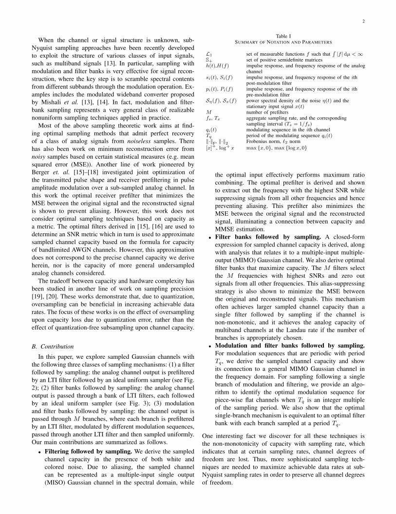
Under sub-Nyquist sampling, the capacity depends on thesampling mechanism and its sampling rate. Specifically, thechannel output r(t) is now passed through the receiver’sanalog front end, which may include a filter, a bank of Mfilters, or a bank of preprocessors consisting of filters andmodulation modules, yielding a collection of analog outputs{yi(t) : 1 ≤ i ≤M}. We assume that the analog outputs areobserved over the time interval (0, T ] and then passed throughideal uniform samplers, yielding a set of digital sequences{yi[n] : n ∈ Z, 1 ≤ i ≤M}, as illustrated in Fig. 1. Here,each branch is uniformly sampled at a sampling rate of fs/Msamples per second.
Analog Channel
Sampler
Preprosessor 1
Preprosessor
Preprosessor
Figure 1. Sampled Gaussian channel. The input x(t), constrained to (0, T ],is passed through M branches of the receiver analog front end to yieldanalog outputs {yi(t) : 1 ≤ i ≤M}; each yi(t) is observed over (0, T ]and uniformly sampled at a rate fs/M to yield the sampled sequence yi[n].The preprocessor can be a filter, or combination of a filter and a modulator.
Define y[n] = [y1[n], · · · , yM [n]], and denote byI({x(t)}Tt=0 ; {y[n]}Tt=0) the mutual information between theinput x(t) on the interval 0 < t ≤ T and the samples {y[n]}observed on the interval 0 < t ≤ T . We pose the problem offinding the capacity C(fs) of sampled channels as quantifyingthe maximum mutual information in the limit as T →∞. Thesampled channel capacity can then be expressed as
C(fs) = limT→∞
1
Tsup I
({x(t)}Tt=0 ; {y[n]}Tt=0
),
where the supremum is over all possible input distributionssubject to an average power constraint E( 1
T
∫ T0|x(τ)|2 dτ) ≤
P . We restrict the transmit signal x(t) to be continuous withbounded variance (i.e. supt E |x(t)|2 < ∞), and restrict theprobability measure of x(t) to be uniformly continuous. Thisrestriction simplifies some mathematical analysis, while stillencompassing most practical signals of interests 2.
B. Sampling MechanismsIn this subsection, we describe three classes of sampling
strategies with increasing complexity. In particular, we start
2Note that this condition is not necessary for our main theorems. Analternative proof based on correlation functions is provided in [21], whichdoes not require this condition.
4
from sampling following a single filter, and extend our resultsto incorporate filter banks and modulation banks.
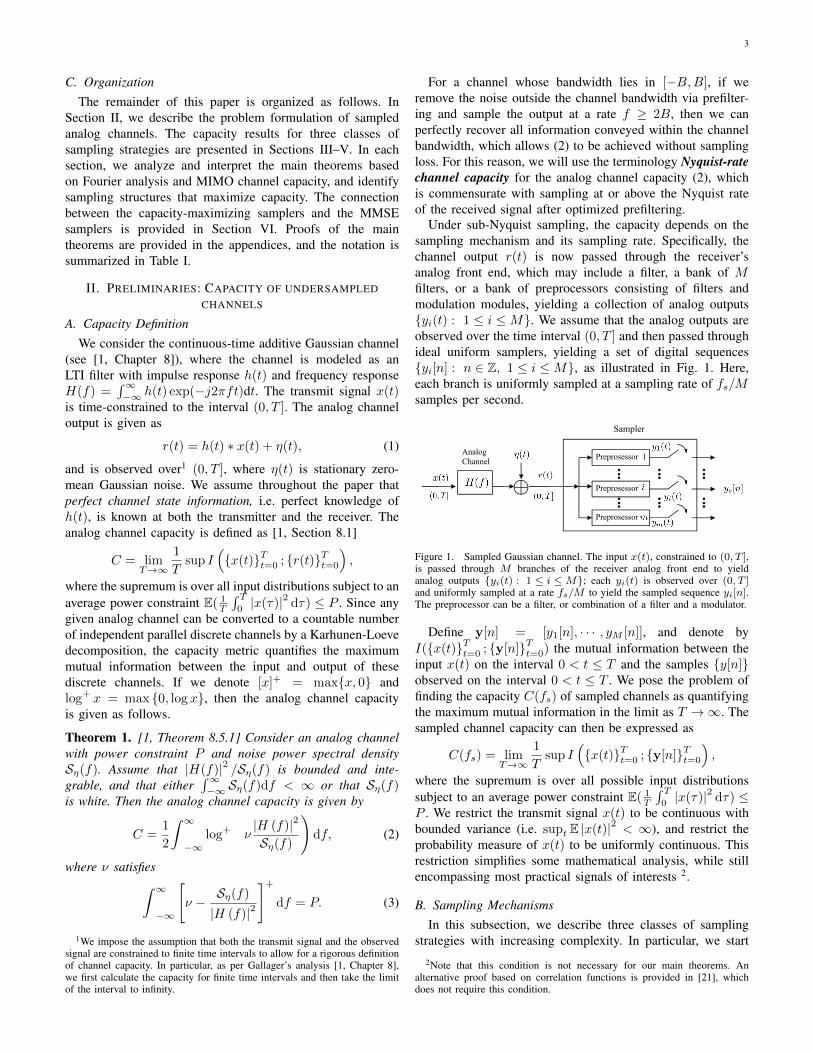
1) Filtering followed by sampling: Ideal uniform samplingis performed by sampling the analog signal uniformly at a ratefs = T−1
s , where Ts denotes the sampling interval. In orderto avoid aliasing, suppress out-of-band noise, and compensatefor linear distortion of practical sampling devices, a prefilteris often added prior to the ideal uniform sampler [22]. Oursampling process thus includes a general analog prefilter, asillustrated in Fig. 2. Specifically, before sampling, we prefilterthe received signal with an LTI filter that has impulse responses(t) and frequency response S (f), where we assume that h(t)and s(t) are both bounded and continuous. The filtered outputis observed over (0, T ] and can be written as
y(t) = s(t) ∗ (h(t) ∗ x(t) + η(t)) , t ∈ (0, T ] . (4)
We then sample y(t) using an ideal uniform sampler, leadingto the sampled sequence
y[n] = y(nTs).
h(t)
)(th
)(tη
)(tx )(ts
snTt =
][ny
h(t)
noise) (white )(tη
)(tx
snTt =
][ny
)(tr y(t)
Figure 2. Filtering followed by sampling: the analog channel output r(t) islinearly filtered prior to ideal uniform sampling.
h(t)
)(th
)(tη
)(tx
)(1 ts
)(tsi
sM (t)
t = n(MTs )
t = n(MTs )
t = n(MTs )
][1 ny
][nyi
yM [n]
)(tr
y1(t)
yi (t)
yM (t)
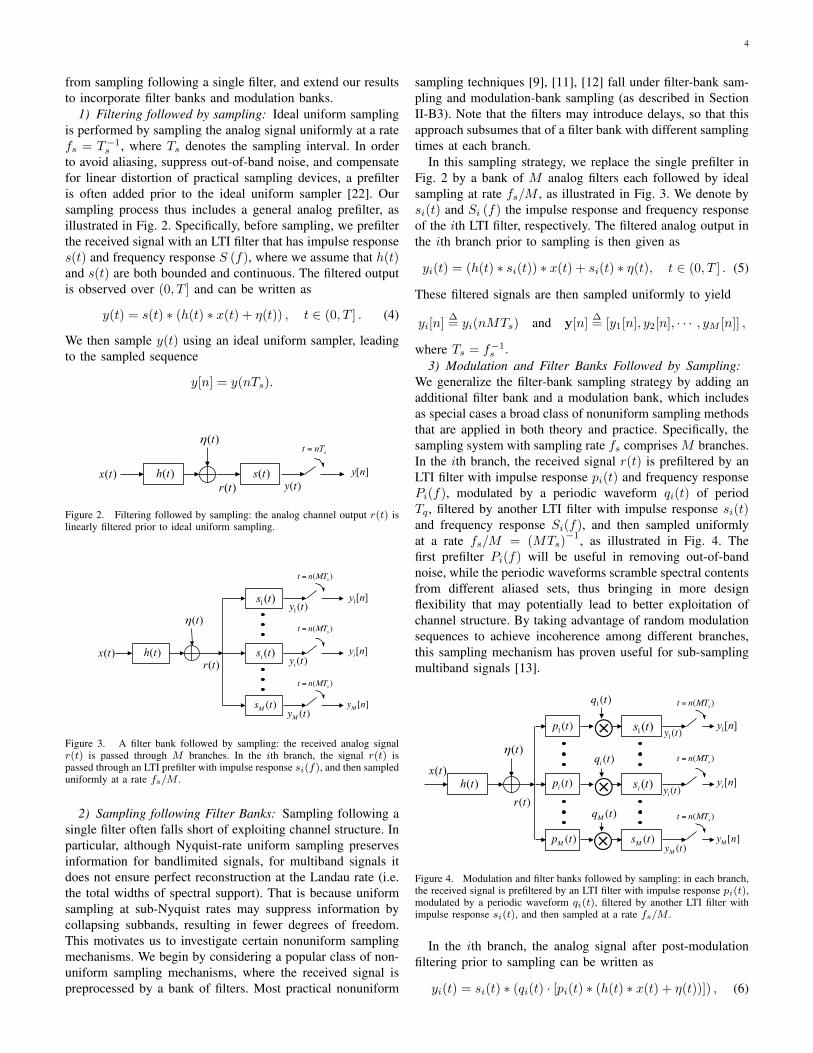
Figure 3. A filter bank followed by sampling: the received analog signalr(t) is passed through M branches. In the ith branch, the signal r(t) ispassed through an LTI prefilter with impulse response si(f), and then sampleduniformly at a rate fs/M .
2) Sampling following Filter Banks: Sampling following asingle filter often falls short of exploiting channel structure. Inparticular, although Nyquist-rate uniform sampling preservesinformation for bandlimited signals, for multiband signals itdoes not ensure perfect reconstruction at the Landau rate (i.e.the total widths of spectral support). That is because uniformsampling at sub-Nyquist rates may suppress information bycollapsing subbands, resulting in fewer degrees of freedom.This motivates us to investigate certain nonuniform samplingmechanisms. We begin by considering a popular class of non-uniform sampling mechanisms, where the received signal ispreprocessed by a bank of filters. Most practical nonuniform
sampling techniques [9], [11], [12] fall under filter-bank sam-pling and modulation-bank sampling (as described in SectionII-B3). Note that the filters may introduce delays, so that thisapproach subsumes that of a filter bank with different samplingtimes at each branch.
In this sampling strategy, we replace the single prefilter inFig. 2 by a bank of M analog filters each followed by idealsampling at rate fs/M , as illustrated in Fig. 3. We denote bysi(t) and Si (f) the impulse response and frequency responseof the ith LTI filter, respectively. The filtered analog output inthe ith branch prior to sampling is then given as
yi(t) = (h(t) ∗ si(t)) ∗ x(t) + si(t) ∗ η(t), t ∈ (0, T ] . (5)
These filtered signals are then sampled uniformly to yield
yi[n]∆= yi(nMTs) and y[n]
∆= [y1[n], y2[n], · · · , yM [n]] ,
where Ts = f−1s .
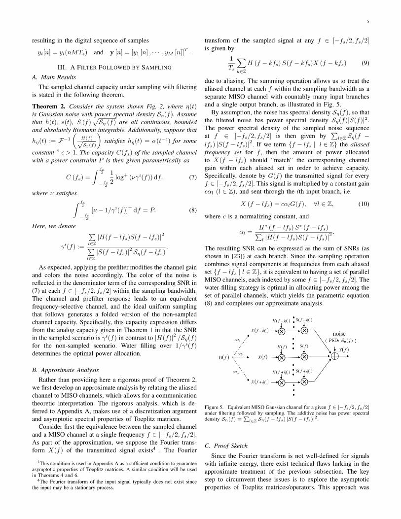
3) Modulation and Filter Banks Followed by Sampling:We generalize the filter-bank sampling strategy by adding anadditional filter bank and a modulation bank, which includesas special cases a broad class of nonuniform sampling methodsthat are applied in both theory and practice. Specifically, thesampling system with sampling rate fs comprises M branches.In the ith branch, the received signal r(t) is prefiltered by anLTI filter with impulse response pi(t) and frequency responsePi(f), modulated by a periodic waveform qi(t) of periodTq , filtered by another LTI filter with impulse response si(t)and frequency response Si(f), and then sampled uniformlyat a rate fs/M = (MTs)
−1, as illustrated in Fig. 4. Thefirst prefilter Pi(f) will be useful in removing out-of-bandnoise, while the periodic waveforms scramble spectral contentsfrom different aliased sets, thus bringing in more designflexibility that may potentially lead to better exploitation ofchannel structure. By taking advantage of random modulationsequences to achieve incoherence among different branches,this sampling mechanism has proven useful for sub-samplingmultiband signals [13].
h(t)
)(th
)(tη
)(1 ts
)(tsi
sM (t)
t = n(MTs )
t = n(MTs )
t = n(MTs )
][1 ny
][nyi
yM [n]
⊗q1(t)
⊗qi (t)
⊗qM (t)
r(t)
y1(t)
yi (t)
yM (t)
p1(t)
pi (t)
pM (t)
)(tx
Figure 4. Modulation and filter banks followed by sampling: in each branch,the received signal is prefiltered by an LTI filter with impulse response pi(t),modulated by a periodic waveform qi(t), filtered by another LTI filter withimpulse response si(t), and then sampled at a rate fs/M .
In the ith branch, the analog signal after post-modulationfiltering prior to sampling can be written as
yi(t) = si(t) ∗ (qi(t) · [pi(t) ∗ (h(t) ∗ x(t) + η(t))]) , (6)
5
resulting in the digital sequence of samples
yi[n] = yi(nMTs) and y [n] = [y1 [n] , · · · , yM [n]]T.
III. A FILTER FOLLOWED BY SAMPLING
A. Main Results
The sampled channel capacity under sampling with filteringis stated in the following theorem.
Theorem 2. Consider the system shown Fig. 2, where η(t)is Gaussian noise with power spectral density Sη(f). Assumethat h(t), s(t), S (f)
√Sη (f) are all continuous, bounded
and absolutely Riemann integrable. Additionally, suppose that
hη(t) := F−1
(H(f)√Sη(f)
)satisfies hη(t) = o (t−ε) for some
constant 3 ε > 1. The capacity C(fs) of the sampled channelwith a power constraint P is then given parametrically as
C (fs) =
∫ fs2
− fs2
1
2log+ (νγs(f)) df, (7)
where ν satisfies∫ fs
2
− fs2[ν − 1/γs(f)]
+df = P. (8)
Here, we denote
γs(f) :=
∑l∈Z|H(f − lfs)S(f − lfs)|2
∑l∈Z|S(f − lfs)|2 Sη(f − lfs)
.
As expected, applying the prefilter modifies the channel gainand colors the noise accordingly. The color of the noise isreflected in the denominator term of the corresponding SNR in(7) at each f ∈ [−fs/2, fs/2] within the sampling bandwidth.The channel and prefilter response leads to an equivalentfrequency-selective channel, and the ideal uniform samplingthat follows generates a folded version of the non-sampledchannel capacity. Specifically, this capacity expression differsfrom the analog capacity given in Theorem 1 in that the SNRin the sampled scenario is γs(f) in contrast to |H(f)|2 /Sη(f)for the non-sampled scenario. Water filling over 1/γs(f)determines the optimal power allocation.
B. Approximate Analysis
Rather than providing here a rigorous proof of Theorem 2,we first develop an approximate analysis by relating the aliasedchannel to MISO channels, which allows for a communicationtheoretic interpretation. The rigorous analysis, which is de-ferred to Appendix A, makes use of a discretization argumentand asymptotic spectral properties of Toeplitz matrices.
Consider first the equivalence between the sampled channeland a MISO channel at a single frequency f ∈ [−fs/2, fs/2].As part of the approximation, we suppose the Fourier trans-form X(f) of the transmitted signal exists4 . The Fourier
3This condition is used in Appendix A as a sufficient condition to guaranteeasymptotic properties of Toeplitz matrices. A similar condition will be usedin Theorems 4 and 6.
4The Fourier transform of the input signal typically does not exist sincethe input may be a stationary process.
transform of the sampled signal at any f ∈ [−fs/2, fs/2]is given by
1
Ts
∑
k∈ZH (f − kfs)S(f − kfs)X (f − kfs) (9)
due to aliasing. The summing operation allows us to treat thealiased channel at each f within the sampling bandwidth as aseparate MISO channel with countably many input branchesand a single output branch, as illustrated in Fig. 5.
By assumption, the noise has spectral density Sη(f), so thatthe filtered noise has power spectral density Sη(f)|S(f)|2.The power spectral density of the sampled noise sequenceat f ∈ [−fs/2, fs/2] is then given by
∑l∈Z Sη(f −
lfs) |S(f − lfs)|2. If we term {f − lfs | l ∈ Z} the aliasedfrequency set for f , then the amount of power allocatedto X(f − lfs) should “match” the corresponding channelgain within each aliased set in order to achieve capacity.Specifically, denote by G(f) the transmitted signal for everyf ∈ [−fs/2, fs/2]. This signal is multiplied by a constant gaincαl (l ∈ Z), and sent through the lth input branch, i.e.
X (f − lfs) = cαlG(f), ∀l ∈ Z, (10)
where c is a normalizing constant, and
αl =H∗ (f − lfs)S∗ (f − lfs)∑l |H(f − lfs)S(f − lfs)|2
.
The resulting SNR can be expressed as the sum of SNRs (asshown in [23]) at each branch. Since the sampling operationcombines signal components at frequencies from each aliasedset {f − lfs | l ∈ Z}, it is equivalent to having a set of parallelMISO channels, each indexed by some f ∈ [−fs/2, fs/2]. Thewater-filling strategy is optimal in allocating power among theset of parallel channels, which yields the parametric equation(8) and completes our approximate analysis.
( )fY( )fX
( )skffX −
( )skffX +
)( skffH −
⊗)( fH
⊗)( skffH +
⊗
)( skffS −
⊗)( fS
⊗)( skffS +
⊗
( )fG
c!k
c!!k
c!0
noise
Figure 5. Equivalent MISO Gaussian channel for a given f ∈ [−fs/2, fs/2]under filtering followed by sampling. The additive noise has power spectraldensity Sn(f) =
∑l∈Z Sη(f − lfs) |S(f − lfs)|2.
C. Proof Sketch
Since the Fourier transform is not well-defined for signalswith infinite energy, there exist technical flaws lurking in theapproximate treatment of the previous subsection. The keystep to circumvent these issues is to explore the asymptoticproperties of Toeplitz matrices/operators. This approach was
6
used by Gallager [1, Theorem 8.5.1] to prove the analogchannel capacity theorem. Under uniform sampling, however,the sampled channel no longer acts as a Toeplitz operator, butinstead becomes a block-Toeplitz operator. Since conventionalapproaches [1, Chapter 8.4] do not accommodate for block-Toeplitz matrices, a new analysis framework is needed. Weprovide here a roadmap of our analysis framework, and deferthe complete proof to Appendix A.
1) Discrete Approximation: The channel response and thefilter response are both assumed to be continuous, whichmotivates us to use a discrete-time approximation in orderto transform the continuous-time operator into its discretecounterpart. We discretize a time domain process by point-wise sampling with period ∆, e.g. h(t) is transformed into{h[n]} by setting h[n] = h(n∆). For any given T , thisallows us to use a finite-dimensional matrix to approximatethe continuous-time block-Toeplitz operator. Then, due to thecontinuity assumption, an exact capacity expression can beobtained by letting ∆ go to zero.
2) Spectral properties of block-Toeplitz matrices: Afterdiscretization, the input-output relation is similar to a MIMOdiscrete-time system. Applying MIMO channel capacity re-sults leads to the capacity for a given T and ∆. The channelcapacity is then obtained by taking T to infinity and ∆ tozero, which can be related to the channel matrix’s spectrumusing Toeplitz theory. Since the filtered noise is non-whiteand correlated across time, we need to whiten it first. This,however, destroys the Toeplitz properties of the original systemmatrix. In order to apply established results in Toeplitz theory,we make use of the concept of asymptotic equivalence [24]that builds connections between Toeplitz matrices and non-Toeplitz matrices. This allows us to relate the capacity limitwith spectral properties of the channel and filter response.
D. Optimal Prefilters
1) Derivation of optimal prefilters: Since different prefilterslead to different channel capacities, a natural question is howto choose S(f) to maximize capacity. The optimizing prefilteris given in the following theorem.
Theorem 3. Consider the system shown in Fig. 2, and define
γl(f) :=|H (f − lfs)|2Sη (f − lfs)
for any integer l. Suppose that in each aliased set{f − lfs | l ∈ Z}, there exists k such that
γk(f) = supl∈Z
γl(f).
Then the capacity in (7) is maximized by the filter withfrequency response
S(f − kfs) =
{1, if γk(f) = supl∈Z γl(f),
0, otherwise,(11)
for any f ∈ [−fs/2, fs/2].
Proof: It can be observed from (7) that the frequencyresponse S(f) at any f can only affect the SNR at f mod fs,
indicating that we can optimize for frequencies f1 andf2
(f1 6= f2; f1, f2 ∈
[− fs2 ,
fs2
])separately. Specifically, the
SNR at each f in the aliased channel is given by
γs(f) =∑
l∈Zγl(f)λl(f),
where
λl(f) =Sη(f − lfs) |S(f − lfs)|2∑l∈Z |S(f − lfs)|2 Sη(f − lfs)
,
and∑l λl(f) = 1. That said, γs(f) is a convex combination
of {γl, l ∈ Z}, and is thus upper bounded by supl∈Z γl. Thisbound can be attained by the filter given in (11).
The optimal prefilter puts all its mass in those fre-quencies with the highest SNR within each aliased set{f − lfs | l ∈ Z}. Even if the optimal prefilter does not exist,we can find a prefilter that achieves an information ratearbitrarily close to the maximum capacity once supl∈Z γl(f)exists. The existence of the supremum is guaranteed undermild conditions, e.g. when γl(f) is bounded.
2) Interpretations: Recall that S(f) is applied after thenoise is added. One distinguishing feature in the subsampledchannel is the non-invertibility of the prefiltering operation,i.e. we cannot recover the analog channel output from sub-Nyquist samples. As shown above, the aliased SNR is a convexcombination of SNRs at all aliased branches, indicating thatS(f) plays the role of “weighting” different branches. Asin maximum ratio combining (MRC), those frequencies withlarger SNRs should be given larger weight, while those thatsuffer from poor channel gains should be suppressed.
The problem of finding optimal prefilters corresponds tojoint optimization over all input and filter responses. Lookingat the equivalent aliased channel for a given frequency f ∈[−fs/2, fs/2] as illustrated in Fig. 5, we have full control overboth X(f) and S(f). Although MRC at the transmitter sidemaximizes the combiner SNR for a MISO channel [23], itturns out to be suboptimal for our joint optimization problem.Rather, the optimal solution is to perform selection combining[23] by setting S(f − lfs) to one for some l = l0, as wellas noise suppression by setting S(f − lfs) to zero for allother ls. In fact, setting S(f) to zero precludes the undesiredeffects of noise from low SNR frequencies, which is crucialin maximizing data rate.
Another interesting observation is that optimal prefilteringequivalently generates an alias-free channel. After passingthrough an optimal prefilter, all frequencies modulo fs exceptthe one with the highest SNR are removed, and hence theoptimal prefilter suppresses aliasing and out-of-band noise.This alias-suppressing phenomena, while different from manysub-Nyquist works that advocate mixing instead of alias sup-pressing [13], arises from the fact that we have control overthe input shape.
E. Numerical examples
1) Additive Gaussian Noise Channel without Prefiltering:The first example we consider is the additive Gaussian noisechannel. The channel gain is flat within the channel bandwidth

78
!1 !0.8 !0.6 !0.4 !0.2 0 0.2 0.4 0.6 0.8 1
!0.2
0
0.2
0.4
0.6
0.8
1
1.2
frequency: f
Channel gain and power spectral density of noise
noise PSD
channel gain
(a)
0 0.5 1 1.5 20
0.5
1
1.5
2
2.5
3
3.5
4
4.5
5
Sampling rate: fs
Sam
pled
cap
acity
Channel capacity vs Sampling rate (AWGN channel)
analog channel capacitysampled channel capacity Channel
bandwidthTwice the Channel
Bandwidth
Twice the Noise Bandwidth
(b)
Figure 6. Additive Gaussian noise channel. The channel gain and thepower spectral density of the noise is plotted in the left plot. The samplingmechanism employed here is ideal uniform sampling without filtering. Thepower constraint is P = 5. The sampled capacity, as illustrated in the rightplot, does not achieve analog capacity when sampling at a rate equal to twicethe channel bandwidth, but does achieve it when sampling at a rate equal totwice the noise bandwidth.
maximizes the mutual information of the sampled channelis an MRC filter which indeed mixes different frequencycomponents from each aliased set. But joint optimization overboth the input and the prefilter yields an input whose frequencysupport is equal to the sampling bandwidth, thus resulting inan alias-suppressing filter in order to remove noise.
E. Numerical examples1) Additive Gaussian Noise Channel without Prefiltering:
The first example we consider is the additive Gaussian noisechannel. The channel gain is flat within the channel bandwidthB = 0.5, i.e. H(f) = 1 if f ∈ [−B, B] and H(f) = 0 oth-erwise. The noise is modeled as a measurable and stationaryGaussian process with the power spectral density plotted inFig. 6(a). This is the noise model adopted by Lapidoth in [38]to approximate white noise, which avoids the infinite varianceof the standard model for unfiltered white noise6. We employ
6In fact, the white noise process only exists as a “generalized process”in stochastic calculus, and ideal uniform sampling operating on white noisewithout prefiltering brings in noise from high-frequency components, whichresults in a folded noise process with infinite spectral density. In order toavoid this mathematical difficulty, we consider in this example Lapidoth’snoise model.
ideal point-wise sampling without filtering.Since the noise bandwidth is larger than the channel band-
width, ideal uniform sampling without prefiltering does notallow analog capacity to be achieved when sampling at arate equal to twice the channel bandwidth, i.e. the Nyquistrate. Increasing the sampling rate above twice the channelbandwidth (but below the noise bandwidth) spreads the totalnoise power over a larger sampling bandwidth, reducing thenoise density at each frequency. This allows the sampledcapacity to continue increasing when sampling above theNyquist rate, as illustrated in Fig. 6(b). It can be seen that thecapacity does not increase monotonically with the samplingrate, which will be discussed in Section III-E3. Note thatcapacity does not increase when the sampling rate exceedstwice the noise bandwidth, since oversampling at any rateabove twice the noise bandwidth preserves all the informationcontents of the channel output.
2) Optimally Prefiltered Channel: In general, the frequencyresponse of the optimal prefilter is discontinuous, which maybe hard to realize in practice. However, for certain classes ofchannel models, the prefilter has a smooth frequency response.One example of this channel class is a monotone channel,whose channel response obeys
|H(f1)|2Sη(f1)
≥ |H(f2)|2Sη(f2)
for any f1 > f2. Theorem 3 implies that the optimizingprefilter for a monotone channel reduces to a low-pass filterwith cutoff frequency fs/2, and the capacity for this channelclass is non-decreasing with the sampling rate fs.
For non-monotone channels, the optimal prefilter may notbe a low-pass filter, as illustrated in Fig. 7. Fig. 7(b) showsthe optimal filter for the channel given in Fig. 7(a) with fs =0.4fNYQ. This filter is no longer a low-pass filter but is ofsupport size 0.4fNYQ.
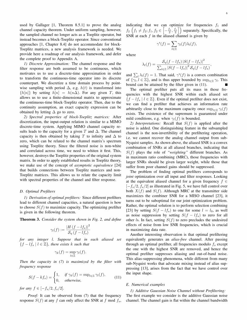
3) Capacity Non-monotonicity: When the channel is notmonotone, a somewhat counter-intuitive fact arises: the chan-nel capacity C(fs) is not necessarily a non-decreasing functionof the sampling rate fs. This occurs, for example, in multibandchannels as illustrated in Fig. 8. Here, the Fourier transformof the channel response is concentrated in two sub-intervalswithin the overall channel bandwidth. Specifically, the entirechannel bandwidth is contained in [−0.5, 0.5] with Nyquistrate fNYQ = 1, and that the channel frequency response isgiven by
H(f) =
�1, if |f | ∈
�110 , 1
5
�� �25 , 1
2
�;
0, otherwise.(15)
If this channel is sampled at a rate fs = 35fNYQ, then aliasing
occurs and leads to an aliased channel with one subband(and hence one degree of freedom). However, if sampling isperformed at a rate fs = 2
5fNYQ, it can be easily verifiedthat the two subbands remain non-overlapping in the aliasedchannel, resulting in two degrees of freedom. The tradeoffcurve between capacity and sampling rate with an optimalprefilter is plotted in Fig. 8(b). This curve indicates thatincreasing the sampling rate may not necessarily increasecapacity for certain channel structures. In other words, a single
(a)
88
!1 !0.8 !0.6 !0.4 !0.2 0 0.2 0.4 0.6 0.8 1
!0.2
0
0.2
0.4
0.6
0.8
1
1.2
frequency: f
Channel gain and power spectral density of noise
noise PSD
channel gain
(a)
0 0.5 1 1.5 20
0.5
1
1.5
2
2.5
3
3.5
4
4.5
5
Sampling rate: fs
Sam
pled
cap
acity
Channel capacity vs Sampling rate (AWGN channel)
analog channel capacitysampled channel capacity Channel
bandwidthTwice the Channel
Bandwidth
Twice the Noise Bandwidth
(b)
Figure 6. Additive Gaussian noise channel. The channel gain and thepower spectral density of the noise is plotted in the left plot. The samplingmechanism employed here is ideal uniform sampling without filtering. Thepower constraint is P = 5. The sampled capacity, as illustrated in the rightplot, does not achieve analog capacity when sampling at a rate equal to twicethe channel bandwidth, but does achieve it when sampling at a rate equal totwice the noise bandwidth.
maximizes the mutual information of the sampled channelis an MRC filter which indeed mixes different frequencycomponents from each aliased set. But joint optimization overboth the input and the prefilter yields an input whose frequencysupport is equal to the sampling bandwidth, thus resulting inan alias-suppressing filter in order to remove noise.
E. Numerical examples1) Additive Gaussian Noise Channel without Prefiltering:
The first example we consider is the additive Gaussian noisechannel. The channel gain is flat within the channel bandwidthB = 0.5, i.e. H(f) = 1 if f ∈ [−B, B] and H(f) = 0 oth-erwise. The noise is modeled as a measurable and stationaryGaussian process with the power spectral density plotted inFig. 6(a). This is the noise model adopted by Lapidoth in [38]to approximate white noise, which avoids the infinite varianceof the standard model for unfiltered white noise6. We employ
6In fact, the white noise process only exists as a “generalized process”in stochastic calculus, and ideal uniform sampling operating on white noisewithout prefiltering brings in noise from high-frequency components, whichresults in a folded noise process with infinite spectral density. In order toavoid this mathematical difficulty, we consider in this example Lapidoth’snoise model.
ideal point-wise sampling without filtering.Since the noise bandwidth is larger than the channel band-
width, ideal uniform sampling without prefiltering does notallow analog capacity to be achieved when sampling at arate equal to twice the channel bandwidth, i.e. the Nyquistrate. Increasing the sampling rate above twice the channelbandwidth (but below the noise bandwidth) spreads the totalnoise power over a larger sampling bandwidth, reducing thenoise density at each frequency. This allows the sampledcapacity to continue increasing when sampling above theNyquist rate, as illustrated in Fig. 6(b). It can be seen that thecapacity does not increase monotonically with the samplingrate, which will be discussed in Section III-E3. Note thatcapacity does not increase when the sampling rate exceedstwice the noise bandwidth, since oversampling at any rateabove twice the noise bandwidth preserves all the informationcontents of the channel output.
2) Optimally Prefiltered Channel: In general, the frequencyresponse of the optimal prefilter is discontinuous, which maybe hard to realize in practice. However, for certain classes ofchannel models, the prefilter has a smooth frequency response.One example of this channel class is a monotone channel,whose channel response obeys
|H(f1)|2Sη(f1)
≥ |H(f2)|2Sη(f2)
for any f1 > f2. Theorem 3 implies that the optimizingprefilter for a monotone channel reduces to a low-pass filterwith cutoff frequency fs/2, and the capacity for this channelclass is non-decreasing with the sampling rate fs.
For non-monotone channels, the optimal prefilter may notbe a low-pass filter, as illustrated in Fig. 7. Fig. 7(b) showsthe optimal filter for the channel given in Fig. 7(a) with fs =0.4fNYQ. This filter is no longer a low-pass filter but is ofsupport size 0.4fNYQ.
3) Capacity Non-monotonicity: When the channel is notmonotone, a somewhat counter-intuitive fact arises: the chan-nel capacity C(fs) is not necessarily a non-decreasing functionof the sampling rate fs. This occurs, for example, in multibandchannels as illustrated in Fig. 8. Here, the Fourier transformof the channel response is concentrated in two sub-intervalswithin the overall channel bandwidth. Specifically, the entirechannel bandwidth is contained in [−0.5, 0.5] with Nyquistrate fNYQ = 1, and that the channel frequency response isgiven by
H(f) =
�1, if |f | ∈
�110 , 1
5
�� �25 , 1
2
�;
0, otherwise.(15)
If this channel is sampled at a rate fs = 35fNYQ, then aliasing
occurs and leads to an aliased channel with one subband(and hence one degree of freedom). However, if sampling isperformed at a rate fs = 2
5fNYQ, it can be easily verifiedthat the two subbands remain non-overlapping in the aliasedchannel, resulting in two degrees of freedom. The tradeoffcurve between capacity and sampling rate with an optimalprefilter is plotted in Fig. 8(b). This curve indicates thatincreasing the sampling rate may not necessarily increasecapacity for certain channel structures. In other words, a single
(a)
0 0.5 1 1.5 20
0.5
1
1.5
2
2.5
3
3.5
4
4.5
5
Sampling rate: fs
Sam
ple
d c
apaci
ty
Channel capacity vs Sampling rate (AWGN channel)
analog channel capacity
sampled channel capacity
Twice the noisebandwidthTwice the channel
bandwidth
(b)
Figure 6. Capacity of sampled additive Gaussian noise channel under idealuniform sampling without filtering. (a) The channel gain and the PSD ofthe noise. (b) Sampled channel capacity v.s. analog channel capacity under apower constraint P = 5.
maximizes the mutual information of the sampled channelis an MRC filter which indeed mixes different frequencycomponents from each aliased set. But joint optimization overboth the input and the prefilter yields an input whose frequencysupport is equal to the sampling bandwidth, thus resulting inan alias-suppressing filter in order to remove noise.
E. Numerical examples
1) Additive Gaussian Noise Channel without Prefiltering:The first example we consider is the additive Gaussian noisechannel. The channel gain is flat within the channel bandwidthB = 0.5, i.e. H(f) = 1 if f ∈ [−B, B] and H(f) = 0 oth-erwise. The noise is modeled as a measurable and stationaryGaussian process with the power spectral density plotted inFig. 6(a). This is the noise model adopted by Lapidoth in [38]to approximate white noise, which avoids the infinite varianceof the standard model for unfiltered white noise6. We employideal point-wise sampling without filtering.
Since the noise bandwidth is larger than the channel band-width, ideal uniform sampling without prefiltering does notallow analog capacity to be achieved when sampling at a
6In fact, the white noise process only exists as a “generalized process”in stochastic calculus, and ideal uniform sampling operating on white noisewithout prefiltering brings in noise from high-frequency components, whichresults in a folded noise process with infinite spectral density. In order toavoid this mathematical difficulty, we consider in this example Lapidoth’snoise model.
rate equal to twice the channel bandwidth, i.e. the Nyquistrate. Increasing the sampling rate above twice the channelbandwidth (but below the noise bandwidth) spreads the totalnoise power over a larger sampling bandwidth, reducing thenoise density at each frequency. This allows the sampledcapacity to continue increasing when sampling above theNyquist rate, as illustrated in Fig. 6(b). It can be seen that thecapacity does not increase monotonically with the samplingrate, which will be discussed in Section III-E3. Note thatcapacity does not increase when the sampling rate exceedstwice the noise bandwidth, since oversampling at any rateabove twice the noise bandwidth preserves all the informationcontents of the channel output.
2) Optimally Prefiltered Channel: In general, the frequencyresponse of the optimal prefilter is discontinuous, which maybe hard to realize in practice. However, for certain classes ofchannel models, the prefilter has a smooth frequency response.One example of this channel class is a monotone channel,whose channel response obeys
|H(f1)|2Sη(f1)
≥ |H(f2)|2Sη(f2)
for any f1 > f2. Theorem 3 implies that the optimizingprefilter for a monotone channel reduces to a low-pass filterwith cutoff frequency fs/2, and the capacity for this channelclass is non-decreasing with the sampling rate fs.
For non-monotone channels, the optimal prefilter may notbe a low-pass filter, as illustrated in Fig. 7. Fig. 7(b) showsthe optimal filter for the channel given in Fig. 7(a) with fs =0.4fNYQ. This filter is no longer a low-pass filter but is ofsupport size 0.4fNYQ.
!0.5 0 0.5!0.2
0
0.2
0.4
0.6
0.8
1
1.2
1.4
Original Channel Response
Frequency: f
Ch
an
ne
l Re
spo
nse
: H
(f)
!0.5 0 0.5!0.2
0
0.2
0.4
0.6
0.8
1
1.2
Frequency: f
Ch
an
ne
l Re
spo
nse
: H
(f)
Optimal Prefilter
(a) (b)
!0.5 0 0.5!0.2
0
0.2
0.4
0.6
0.8
1
1.2
1.4
Frequency: f
Ch
an
ne
l Re
spo
nse
: H
(f)
Optimally Prefiltered Channel
0 0.2 0.4 0.6 0.8 1 1.20
0.1
0.2
0.3
0.4
0.5
0.6
0.7
0.8
0.9
1
Sampling rate
Sa
mp
led
ca
pa
city
Channel capacity vs Sampling rate
optimal filter
matched filter
super!Nyquistregime
sub!Nyquist regime
(c) (d)
Figure 7. Capacity of optimally prefiltered channel: (a) frequency responseof the original channel; (b) optimal prefilter associated with this channel forsampling rate 0.4; (c) optimally prefiltered channel response with samplingrate 0.4; (d) capacity vs sampling rate for the optimal prefilter and for thematched filter. The optimal prefilter has support size fs in the frequencydomain, hence its output is alias-free. In the sub-Nyquist regime, this alias-suppressing filter outperforms the matched filter in terms of capacity.
(b)
Figure 6. Capacity of sampled additive Gaussian noise channel under idealuniform sampling without filtering. (a) The channel gain and the PSD ofthe noise. (b) Sampled channel capacity v.s. analog channel capacity under apower constraint P = 5.
B = 0.5, i.e. H(f) = 1 if f ∈ [−B,B] and H(f) = 0 oth-erwise. The noise is modeled as a measurable and stationaryGaussian process with the power spectral density plotted inFig. 6(a). This is the noise model adopted by Lapidoth in [25]to approximate white noise, which avoids the infinite varianceof the standard model for unfiltered white noise. We employideal point-wise sampling without filtering.
Since the noise bandwidth is larger than the channel band-width, ideal uniform sampling without prefiltering does notallow analog capacity to be achieved when sampling at arate equal to twice the channel bandwidth, i.e. the Nyquistrate. Increasing the sampling rate above twice the channelbandwidth (but below the noise bandwidth) spreads the totalnoise power over a larger sampling bandwidth, reducing thenoise density at each frequency. This allows the sampledcapacity to continue increasing when sampling above theNyquist rate, as illustrated in Fig. 6(b). It can be seen that thecapacity does not increase monotonically with the samplingrate. We will discuss this phenomena in more detail in SectionIII-E3.
2) Optimally Filtered Channel: In general, the frequencyresponse of the optimal prefilter is discontinuous, which maybe hard to realize in practice. However, for certain classesof channel models, the prefilter has a smooth frequencyresponse. One example of this channel class is a monotonechannel, whose channel response obeys |H(f1)|2 /Sη(f1) ≥|H(f2)|2 /Sη(f2) for any f1 > f2. Theorem 3 implies thatthe optimizing prefilter for a monotone channel reduces to alow-pass filter with cutoff frequency fs/2.
For non-monotone channels, the optimal prefilter may notbe a low-pass filter, as illustrated in Fig. 7. Fig. 7(b) showsthe optimal filter for the channel given in Fig. 7(a) with fs =0.4fNYQ, which is no longer a low-pass filter.
88
!1 !0.8 !0.6 !0.4 !0.2 0 0.2 0.4 0.6 0.8 1
!0.2
0
0.2
0.4
0.6
0.8
1
1.2
frequency: f
Channel gain and power spectral density of noise
noise PSD
channel gain
(a)
0 0.5 1 1.5 20
0.5
1
1.5
2
2.5
3
3.5
4
4.5
5
Sampling rate: fs
Sam
pled
cap
acity
Channel capacity vs Sampling rate (AWGN channel)
analog channel capacitysampled channel capacity Channel
bandwidthTwice the Channel
Bandwidth
Twice the Noise Bandwidth
(b)
Figure 6. Additive Gaussian noise channel. The channel gain and thepower spectral density of the noise is plotted in the left plot. The samplingmechanism employed here is ideal uniform sampling without filtering. Thepower constraint is P = 5. The sampled capacity, as illustrated in the rightplot, does not achieve analog capacity when sampling at a rate equal to twicethe channel bandwidth, but does achieve it when sampling at a rate equal totwice the noise bandwidth.
maximizes the mutual information of the sampled channelis an MRC filter which indeed mixes different frequencycomponents from each aliased set. But joint optimization overboth the input and the prefilter yields an input whose frequencysupport is equal to the sampling bandwidth, thus resulting inan alias-suppressing filter in order to remove noise.
E. Numerical examples1) Additive Gaussian Noise Channel without Prefiltering:
The first example we consider is the additive Gaussian noisechannel. The channel gain is flat within the channel bandwidthB = 0.5, i.e. H(f) = 1 if f ∈ [−B, B] and H(f) = 0 oth-erwise. The noise is modeled as a measurable and stationaryGaussian process with the power spectral density plotted inFig. 6(a). This is the noise model adopted by Lapidoth in [38]to approximate white noise, which avoids the infinite varianceof the standard model for unfiltered white noise6. We employ
6In fact, the white noise process only exists as a “generalized process”in stochastic calculus, and ideal uniform sampling operating on white noisewithout prefiltering brings in noise from high-frequency components, whichresults in a folded noise process with infinite spectral density. In order toavoid this mathematical difficulty, we consider in this example Lapidoth’snoise model.
ideal point-wise sampling without filtering.Since the noise bandwidth is larger than the channel band-
width, ideal uniform sampling without prefiltering does notallow analog capacity to be achieved when sampling at arate equal to twice the channel bandwidth, i.e. the Nyquistrate. Increasing the sampling rate above twice the channelbandwidth (but below the noise bandwidth) spreads the totalnoise power over a larger sampling bandwidth, reducing thenoise density at each frequency. This allows the sampledcapacity to continue increasing when sampling above theNyquist rate, as illustrated in Fig. 6(b). It can be seen that thecapacity does not increase monotonically with the samplingrate, which will be discussed in Section III-E3. Note thatcapacity does not increase when the sampling rate exceedstwice the noise bandwidth, since oversampling at any rateabove twice the noise bandwidth preserves all the informationcontents of the channel output.
2) Optimally Prefiltered Channel: In general, the frequencyresponse of the optimal prefilter is discontinuous, which maybe hard to realize in practice. However, for certain classes ofchannel models, the prefilter has a smooth frequency response.One example of this channel class is a monotone channel,whose channel response obeys
|H(f1)|2Sη(f1)
≥ |H(f2)|2Sη(f2)
for any f1 > f2. Theorem 3 implies that the optimizingprefilter for a monotone channel reduces to a low-pass filterwith cutoff frequency fs/2, and the capacity for this channelclass is non-decreasing with the sampling rate fs.
For non-monotone channels, the optimal prefilter may notbe a low-pass filter, as illustrated in Fig. 7. Fig. 7(b) showsthe optimal filter for the channel given in Fig. 7(a) with fs =0.4fNYQ. This filter is no longer a low-pass filter but is ofsupport size 0.4fNYQ.
3) Capacity Non-monotonicity: When the channel is notmonotone, a somewhat counter-intuitive fact arises: the chan-nel capacity C(fs) is not necessarily a non-decreasing functionof the sampling rate fs. This occurs, for example, in multibandchannels as illustrated in Fig. 8. Here, the Fourier transformof the channel response is concentrated in two sub-intervalswithin the overall channel bandwidth. Specifically, the entirechannel bandwidth is contained in [−0.5, 0.5] with Nyquistrate fNYQ = 1, and that the channel frequency response isgiven by
H(f) =
�1, if |f | ∈
�110 , 1
5
�� �25 , 1
2
�;
0, otherwise.(15)
If this channel is sampled at a rate fs = 35fNYQ, then aliasing
occurs and leads to an aliased channel with one subband(and hence one degree of freedom). However, if sampling isperformed at a rate fs = 2
5fNYQ, it can be easily verifiedthat the two subbands remain non-overlapping in the aliasedchannel, resulting in two degrees of freedom. The tradeoffcurve between capacity and sampling rate with an optimalprefilter is plotted in Fig. 8(b). This curve indicates thatincreasing the sampling rate may not necessarily increasecapacity for certain channel structures. In other words, a single
(a)
0 0.5 1 1.5 20
0.5
1
1.5
2
2.5
3
3.5
4
4.5
5
Sampling rate: fs
Sa
mp
led c
ap
aci
ty
Channel capacity vs Sampling rate (AWGN channel)
analog channel capacity
sampled channel capacity
Twice the noisebandwidthTwice the channel
bandwidth
(b)
Figure 6. Capacity of sampled additive Gaussian noise channel under idealuniform sampling without filtering. (a) The channel gain and the PSD ofthe noise. (b) Sampled channel capacity v.s. analog channel capacity under apower constraint P = 5.
maximizes the mutual information of the sampled channelis an MRC filter which indeed mixes different frequencycomponents from each aliased set. But joint optimization overboth the input and the prefilter yields an input whose frequencysupport is equal to the sampling bandwidth, thus resulting inan alias-suppressing filter in order to remove noise.
E. Numerical examples
1) Additive Gaussian Noise Channel without Prefiltering:The first example we consider is the additive Gaussian noisechannel. The channel gain is flat within the channel bandwidthB = 0.5, i.e. H(f) = 1 if f ∈ [−B, B] and H(f) = 0 oth-erwise. The noise is modeled as a measurable and stationaryGaussian process with the power spectral density plotted inFig. 6(a). This is the noise model adopted by Lapidoth in [38]to approximate white noise, which avoids the infinite varianceof the standard model for unfiltered white noise6. We employideal point-wise sampling without filtering.
Since the noise bandwidth is larger than the channel band-width, ideal uniform sampling without prefiltering does notallow analog capacity to be achieved when sampling at a
6In fact, the white noise process only exists as a “generalized process”in stochastic calculus, and ideal uniform sampling operating on white noisewithout prefiltering brings in noise from high-frequency components, whichresults in a folded noise process with infinite spectral density. In order toavoid this mathematical difficulty, we consider in this example Lapidoth’snoise model.
rate equal to twice the channel bandwidth, i.e. the Nyquistrate. Increasing the sampling rate above twice the channelbandwidth (but below the noise bandwidth) spreads the totalnoise power over a larger sampling bandwidth, reducing thenoise density at each frequency. This allows the sampledcapacity to continue increasing when sampling above theNyquist rate, as illustrated in Fig. 6(b). It can be seen that thecapacity does not increase monotonically with the samplingrate, which will be discussed in Section III-E3. Note thatcapacity does not increase when the sampling rate exceedstwice the noise bandwidth, since oversampling at any rateabove twice the noise bandwidth preserves all the informationcontents of the channel output.
2) Optimally Prefiltered Channel: In general, the frequencyresponse of the optimal prefilter is discontinuous, which maybe hard to realize in practice. However, for certain classes ofchannel models, the prefilter has a smooth frequency response.One example of this channel class is a monotone channel,whose channel response obeys
|H(f1)|2Sη(f1)
≥ |H(f2)|2Sη(f2)
for any f1 > f2. Theorem 3 implies that the optimizingprefilter for a monotone channel reduces to a low-pass filterwith cutoff frequency fs/2, and the capacity for this channelclass is non-decreasing with the sampling rate fs.
For non-monotone channels, the optimal prefilter may notbe a low-pass filter, as illustrated in Fig. 7. Fig. 7(b) showsthe optimal filter for the channel given in Fig. 7(a) with fs =0.4fNYQ. This filter is no longer a low-pass filter but is ofsupport size 0.4fNYQ.
!0.5 0 0.5!0.2
0
0.2
0.4
0.6
0.8
1
1.2
1.4
Original Channel Response
Frequency: f
Channel R
esp
onse
: H
(f)
!0.5 0 0.5!0.2
0
0.2
0.4
0.6
0.8
1
1.2
Frequency: f
Channel R
esp
onse
: H
(f)
Optimal Prefilter
(a) (b)
!0.5 0 0.5!0.2
0
0.2
0.4
0.6
0.8
1
1.2
1.4
Frequency: f
Channel R
esp
onse
: H
(f)
Optimally Prefiltered Channel
0 0.2 0.4 0.6 0.8 1 1.20
0.1
0.2
0.3
0.4
0.5
0.6
0.7
0.8
0.9
1
Sampling rate
Sam
ple
d c
apaci
ty
Channel capacity vs Sampling rate
optimal filter
matched filter
super!Nyquistregime
sub!Nyquist regime
(c) (d)
Figure 7. Capacity of optimally prefiltered channel: (a) frequency responseof the original channel; (b) optimal prefilter associated with this channel forsampling rate 0.4; (c) optimally prefiltered channel response with samplingrate 0.4; (d) capacity vs sampling rate for the optimal prefilter and for thematched filter. The optimal prefilter has support size fs in the frequencydomain, hence its output is alias-free. In the sub-Nyquist regime, this alias-suppressing filter outperforms the matched filter in terms of capacity.
(b)
Figure 6. Capacity of sampled additive Gaussian noise channel under idealuniform sampling without filtering. (a) The channel gain and the PSD ofthe noise. (b) Sampled channel capacity v.s. analog channel capacity under apower constraint P = 5.
B = 0.5, i.e. H(f) = 1 if f ∈ [−B, B] and H(f) = 0 oth-erwise. The noise is modeled as a measurable and stationaryGaussian process with the power spectral density plotted inFig. 6(a). This is the noise model adopted by Lapidoth in [37]to approximate white noise, which avoids the infinite varianceof the standard model for unfiltered white noise6. We employideal point-wise sampling without filtering.
Since the noise bandwidth is larger than the channel band-width, ideal uniform sampling without prefiltering does notallow analog capacity to be achieved when sampling at arate equal to twice the channel bandwidth, i.e. the Nyquistrate. Increasing the sampling rate above twice the channelbandwidth (but below the noise bandwidth) spreads the totalnoise power over a larger sampling bandwidth, reducing thenoise density at each frequency. This allows the sampledcapacity to continue increasing when sampling above theNyquist rate, as illustrated in Fig. 6(b). It can be seen that thecapacity does not increase monotonically with the samplingrate, which will be discussed in Section III-E3. Note thatcapacity does not increase when the sampling rate exceedstwice the noise bandwidth, since oversampling at any rateabove twice the noise bandwidth preserves all the information
6In fact, the white noise process only exists as a “generalized process”in stochastic calculus, and ideal uniform sampling operating on white noisewithout prefiltering brings in noise from high-frequency components, whichresults in a folded noise process with infinite spectral density. In order toavoid this mathematical difficulty, we consider in this example Lapidoth’snoise model.
contents of the channel output.2) Optimally Filtered Channel: In general, the frequency
response of the optimal prefilter is discontinuous, which maybe hard to realize in practice. However, for certain classes ofchannel models, the prefilter has a smooth frequency response.One example of this channel class is a monotone channel,whose channel response obeys
|H(f1)|2Sη(f1)
≥ |H(f2)|2Sη(f2)
for any f1 > f2. Theorem 3 implies that the optimizingprefilter for a monotone channel reduces to a low-pass filterwith cutoff frequency fs/2, and the capacity for this channelclass is non-decreasing with the sampling rate fs.
For non-monotone channels, the optimal prefilter may notbe a low-pass filter, as illustrated in Fig. 7. Fig. 7(b) showsthe optimal filter for the channel given in Fig. 7(a) with fs =0.4fNYQ. This filter is no longer a low-pass filter but is ofsupport size 0.4fNYQ.
!0.5 0 0.5
0
0.5
1
1.5Original Channel Response
Frequency: f
Ch
an
ne
l Re
spo
nse
: H
(f)
!0.5 0 0.5!0.2
0
0.2
0.4
0.6
0.8
1
Frequency: f
Ch
an
ne
l Re
spo
nse
: H
(f)
Optimal Prefilter
(a) (b)
!0.5 0 0.5
0
0.5
1
1.5
Frequency: f
Ch
an
ne
l Re
spo
nse
: H
(f)
Optimally Prefiltered Channel
0 0.5 10
0.2
0.4
0.6
0.8
1
Sampling rate: fs
Sa
mp
led
Ca
pa
city
Channel capacity vs Sampling rate
optimal filter
matched filter
sub!Nyquist regime
super!Nyquistregime
(c) (d)
Figure 7. Capacity of optimally filtered channel: (a) frequency responseof the original channel; (b) optimal prefilter associated with this channel forsampling rate 0.4; (c) optimally filtered channel response with sampling rate0.4; (d) capacity vs sampling rate for the optimal prefilter and for the matchedfilter.
3) Capacity Non-monotonicity: When the channel is notmonotone, a somewhat counter-intuitive fact arises: the chan-nel capacity C(fs) is not necessarily a non-decreasing functionof the sampling rate fs. This occurs, for example, in multibandchannels as illustrated in Fig. 8. Here, the Fourier transformof the channel response is concentrated in two sub-intervalswithin the overall channel bandwidth. Specifically, the entirechannel bandwidth is contained in [−0.5, 0.5] with Nyquistrate fNYQ = 1, and that the channel frequency response isgiven by
H(f) =
�1, if |f | ∈
�110 , 1
5
�� �25 , 1
2
�;
0, otherwise.(13)
88
!1 !0.8 !0.6 !0.4 !0.2 0 0.2 0.4 0.6 0.8 1
!0.2
0
0.2
0.4
0.6
0.8
1
1.2
frequency: f
Channel gain and power spectral density of noise
noise PSD
channel gain
(a)
0 0.5 1 1.5 20
0.5
1
1.5
2
2.5
3
3.5
4
4.5
5
Sampling rate: fs
Sam
pled
cap
acity
Channel capacity vs Sampling rate (AWGN channel)
analog channel capacitysampled channel capacity Channel
bandwidthTwice the Channel
Bandwidth
Twice the Noise Bandwidth
(b)
Figure 6. Additive Gaussian noise channel. The channel gain and thepower spectral density of the noise is plotted in the left plot. The samplingmechanism employed here is ideal uniform sampling without filtering. Thepower constraint is P = 5. The sampled capacity, as illustrated in the rightplot, does not achieve analog capacity when sampling at a rate equal to twicethe channel bandwidth, but does achieve it when sampling at a rate equal totwice the noise bandwidth.
maximizes the mutual information of the sampled channelis an MRC filter which indeed mixes different frequencycomponents from each aliased set. But joint optimization overboth the input and the prefilter yields an input whose frequencysupport is equal to the sampling bandwidth, thus resulting inan alias-suppressing filter in order to remove noise.
E. Numerical examples1) Additive Gaussian Noise Channel without Prefiltering:
The first example we consider is the additive Gaussian noisechannel. The channel gain is flat within the channel bandwidthB = 0.5, i.e. H(f) = 1 if f ∈ [−B, B] and H(f) = 0 oth-erwise. The noise is modeled as a measurable and stationaryGaussian process with the power spectral density plotted inFig. 6(a). This is the noise model adopted by Lapidoth in [38]to approximate white noise, which avoids the infinite varianceof the standard model for unfiltered white noise6. We employ
6In fact, the white noise process only exists as a “generalized process”in stochastic calculus, and ideal uniform sampling operating on white noisewithout prefiltering brings in noise from high-frequency components, whichresults in a folded noise process with infinite spectral density. In order toavoid this mathematical difficulty, we consider in this example Lapidoth’snoise model.
ideal point-wise sampling without filtering.Since the noise bandwidth is larger than the channel band-
width, ideal uniform sampling without prefiltering does notallow analog capacity to be achieved when sampling at arate equal to twice the channel bandwidth, i.e. the Nyquistrate. Increasing the sampling rate above twice the channelbandwidth (but below the noise bandwidth) spreads the totalnoise power over a larger sampling bandwidth, reducing thenoise density at each frequency. This allows the sampledcapacity to continue increasing when sampling above theNyquist rate, as illustrated in Fig. 6(b). It can be seen that thecapacity does not increase monotonically with the samplingrate, which will be discussed in Section III-E3. Note thatcapacity does not increase when the sampling rate exceedstwice the noise bandwidth, since oversampling at any rateabove twice the noise bandwidth preserves all the informationcontents of the channel output.
2) Optimally Prefiltered Channel: In general, the frequencyresponse of the optimal prefilter is discontinuous, which maybe hard to realize in practice. However, for certain classes ofchannel models, the prefilter has a smooth frequency response.One example of this channel class is a monotone channel,whose channel response obeys
|H(f1)|2Sη(f1)
≥ |H(f2)|2Sη(f2)
for any f1 > f2. Theorem 3 implies that the optimizingprefilter for a monotone channel reduces to a low-pass filterwith cutoff frequency fs/2, and the capacity for this channelclass is non-decreasing with the sampling rate fs.
For non-monotone channels, the optimal prefilter may notbe a low-pass filter, as illustrated in Fig. 7. Fig. 7(b) showsthe optimal filter for the channel given in Fig. 7(a) with fs =0.4fNYQ. This filter is no longer a low-pass filter but is ofsupport size 0.4fNYQ.
3) Capacity Non-monotonicity: When the channel is notmonotone, a somewhat counter-intuitive fact arises: the chan-nel capacity C(fs) is not necessarily a non-decreasing functionof the sampling rate fs. This occurs, for example, in multibandchannels as illustrated in Fig. 8. Here, the Fourier transformof the channel response is concentrated in two sub-intervalswithin the overall channel bandwidth. Specifically, the entirechannel bandwidth is contained in [−0.5, 0.5] with Nyquistrate fNYQ = 1, and that the channel frequency response isgiven by
H(f) =
�1, if |f | ∈
�110 , 1
5
�� �25 , 1
2
�;
0, otherwise.(15)
If this channel is sampled at a rate fs = 35fNYQ, then aliasing
occurs and leads to an aliased channel with one subband(and hence one degree of freedom). However, if sampling isperformed at a rate fs = 2
5fNYQ, it can be easily verifiedthat the two subbands remain non-overlapping in the aliasedchannel, resulting in two degrees of freedom. The tradeoffcurve between capacity and sampling rate with an optimalprefilter is plotted in Fig. 8(b). This curve indicates thatincreasing the sampling rate may not necessarily increasecapacity for certain channel structures. In other words, a single
(a)
0 0.5 1 1.5 20
0.5
1
1.5
2
2.5
3
3.5
4
4.5
5
Sampling rate: fs
Sa
mp
led c
ap
aci
ty
Channel capacity vs Sampling rate (AWGN channel)
analog channel capacity
sampled channel capacity
Twice the noisebandwidthTwice the channel
bandwidth
(b)
Figure 6. Capacity of sampled additive Gaussian noise channel under idealuniform sampling without filtering. (a) The channel gain and the PSD ofthe noise. (b) Sampled channel capacity v.s. analog channel capacity under apower constraint P = 5.
maximizes the mutual information of the sampled channelis an MRC filter which indeed mixes different frequencycomponents from each aliased set. But joint optimization overboth the input and the prefilter yields an input whose frequencysupport is equal to the sampling bandwidth, thus resulting inan alias-suppressing filter in order to remove noise.
E. Numerical examples
1) Additive Gaussian Noise Channel without Prefiltering:The first example we consider is the additive Gaussian noisechannel. The channel gain is flat within the channel bandwidthB = 0.5, i.e. H(f) = 1 if f ∈ [−B, B] and H(f) = 0 oth-erwise. The noise is modeled as a measurable and stationaryGaussian process with the power spectral density plotted inFig. 6(a). This is the noise model adopted by Lapidoth in [38]to approximate white noise, which avoids the infinite varianceof the standard model for unfiltered white noise6. We employideal point-wise sampling without filtering.
Since the noise bandwidth is larger than the channel band-width, ideal uniform sampling without prefiltering does notallow analog capacity to be achieved when sampling at a
6In fact, the white noise process only exists as a “generalized process”in stochastic calculus, and ideal uniform sampling operating on white noisewithout prefiltering brings in noise from high-frequency components, whichresults in a folded noise process with infinite spectral density. In order toavoid this mathematical difficulty, we consider in this example Lapidoth’snoise model.
rate equal to twice the channel bandwidth, i.e. the Nyquistrate. Increasing the sampling rate above twice the channelbandwidth (but below the noise bandwidth) spreads the totalnoise power over a larger sampling bandwidth, reducing thenoise density at each frequency. This allows the sampledcapacity to continue increasing when sampling above theNyquist rate, as illustrated in Fig. 6(b). It can be seen that thecapacity does not increase monotonically with the samplingrate, which will be discussed in Section III-E3. Note thatcapacity does not increase when the sampling rate exceedstwice the noise bandwidth, since oversampling at any rateabove twice the noise bandwidth preserves all the informationcontents of the channel output.
2) Optimally Prefiltered Channel: In general, the frequencyresponse of the optimal prefilter is discontinuous, which maybe hard to realize in practice. However, for certain classes ofchannel models, the prefilter has a smooth frequency response.One example of this channel class is a monotone channel,whose channel response obeys
|H(f1)|2Sη(f1)
≥ |H(f2)|2Sη(f2)
for any f1 > f2. Theorem 3 implies that the optimizingprefilter for a monotone channel reduces to a low-pass filterwith cutoff frequency fs/2, and the capacity for this channelclass is non-decreasing with the sampling rate fs.
For non-monotone channels, the optimal prefilter may notbe a low-pass filter, as illustrated in Fig. 7. Fig. 7(b) showsthe optimal filter for the channel given in Fig. 7(a) with fs =0.4fNYQ. This filter is no longer a low-pass filter but is ofsupport size 0.4fNYQ.
!0.5 0 0.5!0.2
0
0.2
0.4
0.6
0.8
1
1.2
1.4
Original Channel Response
Frequency: f
Channel R
esp
onse
: H
(f)
!0.5 0 0.5!0.2
0
0.2
0.4
0.6
0.8
1
1.2
Frequency: f
Channel R
esp
onse
: H
(f)
Optimal Prefilter
(a) (b)
!0.5 0 0.5!0.2
0
0.2
0.4
0.6
0.8
1
1.2
1.4
Frequency: f
Channel R
esp
onse
: H
(f)
Optimally Prefiltered Channel
0 0.2 0.4 0.6 0.8 1 1.20
0.1
0.2
0.3
0.4
0.5
0.6
0.7
0.8
0.9
1
Sampling rate
Sam
ple
d c
apaci
ty
Channel capacity vs Sampling rate
optimal filter
matched filter
super!Nyquistregime
sub!Nyquist regime
(c) (d)
Figure 7. Capacity of optimally prefiltered channel: (a) frequency responseof the original channel; (b) optimal prefilter associated with this channel forsampling rate 0.4; (c) optimally prefiltered channel response with samplingrate 0.4; (d) capacity vs sampling rate for the optimal prefilter and for thematched filter. The optimal prefilter has support size fs in the frequencydomain, hence its output is alias-free. In the sub-Nyquist regime, this alias-suppressing filter outperforms the matched filter in terms of capacity.
(b)
Figure 6. Capacity of sampled additive Gaussian noise channel under idealuniform sampling without filtering. (a) The channel gain and the PSD ofthe noise. (b) Sampled channel capacity v.s. analog channel capacity under apower constraint P = 5.
B = 0.5, i.e. H(f) = 1 if f ∈ [−B, B] and H(f) = 0 oth-erwise. The noise is modeled as a measurable and stationaryGaussian process with the power spectral density plotted inFig. 6(a). This is the noise model adopted by Lapidoth in [37]to approximate white noise, which avoids the infinite varianceof the standard model for unfiltered white noise6. We employideal point-wise sampling without filtering.
Since the noise bandwidth is larger than the channel band-width, ideal uniform sampling without prefiltering does notallow analog capacity to be achieved when sampling at arate equal to twice the channel bandwidth, i.e. the Nyquistrate. Increasing the sampling rate above twice the channelbandwidth (but below the noise bandwidth) spreads the totalnoise power over a larger sampling bandwidth, reducing thenoise density at each frequency. This allows the sampledcapacity to continue increasing when sampling above theNyquist rate, as illustrated in Fig. 6(b). It can be seen that thecapacity does not increase monotonically with the samplingrate, which will be discussed in Section III-E3. Note thatcapacity does not increase when the sampling rate exceedstwice the noise bandwidth, since oversampling at any rateabove twice the noise bandwidth preserves all the information
6In fact, the white noise process only exists as a “generalized process”in stochastic calculus, and ideal uniform sampling operating on white noisewithout prefiltering brings in noise from high-frequency components, whichresults in a folded noise process with infinite spectral density. In order toavoid this mathematical difficulty, we consider in this example Lapidoth’snoise model.
contents of the channel output.2) Optimally Filtered Channel: In general, the frequency
response of the optimal prefilter is discontinuous, which maybe hard to realize in practice. However, for certain classes ofchannel models, the prefilter has a smooth frequency response.One example of this channel class is a monotone channel,whose channel response obeys
|H(f1)|2Sη(f1)
≥ |H(f2)|2Sη(f2)
for any f1 > f2. Theorem 3 implies that the optimizingprefilter for a monotone channel reduces to a low-pass filterwith cutoff frequency fs/2, and the capacity for this channelclass is non-decreasing with the sampling rate fs.
For non-monotone channels, the optimal prefilter may notbe a low-pass filter, as illustrated in Fig. 7. Fig. 7(b) showsthe optimal filter for the channel given in Fig. 7(a) with fs =0.4fNYQ. This filter is no longer a low-pass filter but is ofsupport size 0.4fNYQ.
!0.5 0 0.5
0
0.5
1
1.5Original Channel Response
Frequency: f
Ch
an
ne
l Re
spo
nse
: H
(f)
!0.5 0 0.5!0.2
0
0.2
0.4
0.6
0.8
1
Frequency: f
Ch
an
ne
l Re
spo
nse
: H
(f)
Optimal Prefilter
(a) (b)
!0.5 0 0.5
0
0.5
1
1.5
Frequency: f
Ch
an
ne
l Re
spo
nse
: H
(f)
Optimally Prefiltered Channel
0 0.5 10
0.2
0.4
0.6
0.8
1
Sampling rate: fs
Sa
mp
led
Ca
pa
city
Channel capacity vs Sampling rate
optimal filter
matched filter
sub!Nyquist regime
super!Nyquistregime
(c) (d)
Figure 7. Capacity of optimally filtered channel: (a) frequency responseof the original channel; (b) optimal prefilter associated with this channel forsampling rate 0.4; (c) optimally filtered channel response with sampling rate0.4; (d) capacity vs sampling rate for the optimal prefilter and for the matchedfilter.
3) Capacity Non-monotonicity: When the channel is notmonotone, a somewhat counter-intuitive fact arises: the chan-nel capacity C(fs) is not necessarily a non-decreasing functionof the sampling rate fs. This occurs, for example, in multibandchannels as illustrated in Fig. 8. Here, the Fourier transformof the channel response is concentrated in two sub-intervalswithin the overall channel bandwidth. Specifically, the entirechannel bandwidth is contained in [−0.5, 0.5] with Nyquistrate fNYQ = 1, and that the channel frequency response isgiven by
H(f) =
�1, if |f | ∈
�110 , 1
5
�� �25 , 1
2
�;
0, otherwise.(13)
(a) (b)
88
!1 !0.8 !0.6 !0.4 !0.2 0 0.2 0.4 0.6 0.8 1
!0.2
0
0.2
0.4
0.6
0.8
1
1.2
frequency: f
Channel gain and power spectral density of noise
noise PSD
channel gain
(a)
0 0.5 1 1.5 20
0.5
1
1.5
2
2.5
3
3.5
4
4.5
5
Sampling rate: fs
Sam
pled
cap
acity
Channel capacity vs Sampling rate (AWGN channel)
analog channel capacitysampled channel capacity Channel
bandwidthTwice the Channel
Bandwidth
Twice the Noise Bandwidth
(b)
Figure 6. Additive Gaussian noise channel. The channel gain and thepower spectral density of the noise is plotted in the left plot. The samplingmechanism employed here is ideal uniform sampling without filtering. Thepower constraint is P = 5. The sampled capacity, as illustrated in the rightplot, does not achieve analog capacity when sampling at a rate equal to twicethe channel bandwidth, but does achieve it when sampling at a rate equal totwice the noise bandwidth.
maximizes the mutual information of the sampled channelis an MRC filter which indeed mixes different frequencycomponents from each aliased set. But joint optimization overboth the input and the prefilter yields an input whose frequencysupport is equal to the sampling bandwidth, thus resulting inan alias-suppressing filter in order to remove noise.
E. Numerical examples1) Additive Gaussian Noise Channel without Prefiltering:
The first example we consider is the additive Gaussian noisechannel. The channel gain is flat within the channel bandwidthB = 0.5, i.e. H(f) = 1 if f ∈ [−B, B] and H(f) = 0 oth-erwise. The noise is modeled as a measurable and stationaryGaussian process with the power spectral density plotted inFig. 6(a). This is the noise model adopted by Lapidoth in [38]to approximate white noise, which avoids the infinite varianceof the standard model for unfiltered white noise6. We employ
6In fact, the white noise process only exists as a “generalized process”in stochastic calculus, and ideal uniform sampling operating on white noisewithout prefiltering brings in noise from high-frequency components, whichresults in a folded noise process with infinite spectral density. In order toavoid this mathematical difficulty, we consider in this example Lapidoth’snoise model.
ideal point-wise sampling without filtering.Since the noise bandwidth is larger than the channel band-
width, ideal uniform sampling without prefiltering does notallow analog capacity to be achieved when sampling at arate equal to twice the channel bandwidth, i.e. the Nyquistrate. Increasing the sampling rate above twice the channelbandwidth (but below the noise bandwidth) spreads the totalnoise power over a larger sampling bandwidth, reducing thenoise density at each frequency. This allows the sampledcapacity to continue increasing when sampling above theNyquist rate, as illustrated in Fig. 6(b). It can be seen that thecapacity does not increase monotonically with the samplingrate, which will be discussed in Section III-E3. Note thatcapacity does not increase when the sampling rate exceedstwice the noise bandwidth, since oversampling at any rateabove twice the noise bandwidth preserves all the informationcontents of the channel output.
2) Optimally Prefiltered Channel: In general, the frequencyresponse of the optimal prefilter is discontinuous, which maybe hard to realize in practice. However, for certain classes ofchannel models, the prefilter has a smooth frequency response.One example of this channel class is a monotone channel,whose channel response obeys
|H(f1)|2Sη(f1)
≥ |H(f2)|2Sη(f2)
for any f1 > f2. Theorem 3 implies that the optimizingprefilter for a monotone channel reduces to a low-pass filterwith cutoff frequency fs/2, and the capacity for this channelclass is non-decreasing with the sampling rate fs.
For non-monotone channels, the optimal prefilter may notbe a low-pass filter, as illustrated in Fig. 7. Fig. 7(b) showsthe optimal filter for the channel given in Fig. 7(a) with fs =0.4fNYQ. This filter is no longer a low-pass filter but is ofsupport size 0.4fNYQ.
3) Capacity Non-monotonicity: When the channel is notmonotone, a somewhat counter-intuitive fact arises: the chan-nel capacity C(fs) is not necessarily a non-decreasing functionof the sampling rate fs. This occurs, for example, in multibandchannels as illustrated in Fig. 8. Here, the Fourier transformof the channel response is concentrated in two sub-intervalswithin the overall channel bandwidth. Specifically, the entirechannel bandwidth is contained in [−0.5, 0.5] with Nyquistrate fNYQ = 1, and that the channel frequency response isgiven by
H(f) =
�1, if |f | ∈
�110 , 1
5
�� �25 , 1
2
�;
0, otherwise.(15)
If this channel is sampled at a rate fs = 35fNYQ, then aliasing
occurs and leads to an aliased channel with one subband(and hence one degree of freedom). However, if sampling isperformed at a rate fs = 2
5fNYQ, it can be easily verifiedthat the two subbands remain non-overlapping in the aliasedchannel, resulting in two degrees of freedom. The tradeoffcurve between capacity and sampling rate with an optimalprefilter is plotted in Fig. 8(b). This curve indicates thatincreasing the sampling rate may not necessarily increasecapacity for certain channel structures. In other words, a single
(a)
0 0.5 1 1.5 20
0.5
1
1.5
2
2.5
3
3.5
4
4.5
5
Sampling rate: fs
Sa
mp
led c
ap
aci
ty
Channel capacity vs Sampling rate (AWGN channel)
analog channel capacity
sampled channel capacity
Twice the noisebandwidthTwice the channel
bandwidth
(b)
Figure 6. Capacity of sampled additive Gaussian noise channel under idealuniform sampling without filtering. (a) The channel gain and the PSD ofthe noise. (b) Sampled channel capacity v.s. analog channel capacity under apower constraint P = 5.
maximizes the mutual information of the sampled channelis an MRC filter which indeed mixes different frequencycomponents from each aliased set. But joint optimization overboth the input and the prefilter yields an input whose frequencysupport is equal to the sampling bandwidth, thus resulting inan alias-suppressing filter in order to remove noise.
E. Numerical examples
1) Additive Gaussian Noise Channel without Prefiltering:The first example we consider is the additive Gaussian noisechannel. The channel gain is flat within the channel bandwidthB = 0.5, i.e. H(f) = 1 if f ∈ [−B, B] and H(f) = 0 oth-erwise. The noise is modeled as a measurable and stationaryGaussian process with the power spectral density plotted inFig. 6(a). This is the noise model adopted by Lapidoth in [38]to approximate white noise, which avoids the infinite varianceof the standard model for unfiltered white noise6. We employideal point-wise sampling without filtering.
Since the noise bandwidth is larger than the channel band-width, ideal uniform sampling without prefiltering does notallow analog capacity to be achieved when sampling at a
6In fact, the white noise process only exists as a “generalized process”in stochastic calculus, and ideal uniform sampling operating on white noisewithout prefiltering brings in noise from high-frequency components, whichresults in a folded noise process with infinite spectral density. In order toavoid this mathematical difficulty, we consider in this example Lapidoth’snoise model.
rate equal to twice the channel bandwidth, i.e. the Nyquistrate. Increasing the sampling rate above twice the channelbandwidth (but below the noise bandwidth) spreads the totalnoise power over a larger sampling bandwidth, reducing thenoise density at each frequency. This allows the sampledcapacity to continue increasing when sampling above theNyquist rate, as illustrated in Fig. 6(b). It can be seen that thecapacity does not increase monotonically with the samplingrate, which will be discussed in Section III-E3. Note thatcapacity does not increase when the sampling rate exceedstwice the noise bandwidth, since oversampling at any rateabove twice the noise bandwidth preserves all the informationcontents of the channel output.
2) Optimally Prefiltered Channel: In general, the frequencyresponse of the optimal prefilter is discontinuous, which maybe hard to realize in practice. However, for certain classes ofchannel models, the prefilter has a smooth frequency response.One example of this channel class is a monotone channel,whose channel response obeys
|H(f1)|2Sη(f1)
≥ |H(f2)|2Sη(f2)
for any f1 > f2. Theorem 3 implies that the optimizingprefilter for a monotone channel reduces to a low-pass filterwith cutoff frequency fs/2, and the capacity for this channelclass is non-decreasing with the sampling rate fs.
For non-monotone channels, the optimal prefilter may notbe a low-pass filter, as illustrated in Fig. 7. Fig. 7(b) showsthe optimal filter for the channel given in Fig. 7(a) with fs =0.4fNYQ. This filter is no longer a low-pass filter but is ofsupport size 0.4fNYQ.
!0.5 0 0.5!0.2
0
0.2
0.4
0.6
0.8
1
1.2
1.4
Original Channel Response
Frequency: f
Channel R
esp
onse
: H
(f)
!0.5 0 0.5!0.2
0
0.2
0.4
0.6
0.8
1
1.2
Frequency: f
Channel R
esp
onse
: H
(f)
Optimal Prefilter
(a) (b)
!0.5 0 0.5!0.2
0
0.2
0.4
0.6
0.8
1
1.2
1.4
Frequency: f
Channel R
esp
onse
: H
(f)
Optimally Prefiltered Channel
0 0.2 0.4 0.6 0.8 1 1.20
0.1
0.2
0.3
0.4
0.5
0.6
0.7
0.8
0.9
1
Sampling rate
Sam
ple
d c
apaci
ty
Channel capacity vs Sampling rate
optimal filter
matched filter
super!Nyquistregime
sub!Nyquist regime
(c) (d)
Figure 7. Capacity of optimally prefiltered channel: (a) frequency responseof the original channel; (b) optimal prefilter associated with this channel forsampling rate 0.4; (c) optimally prefiltered channel response with samplingrate 0.4; (d) capacity vs sampling rate for the optimal prefilter and for thematched filter. The optimal prefilter has support size fs in the frequencydomain, hence its output is alias-free. In the sub-Nyquist regime, this alias-suppressing filter outperforms the matched filter in terms of capacity.
(b)
Figure 6. Capacity of sampled additive Gaussian noise channel under idealuniform sampling without filtering. (a) The channel gain and the PSD ofthe noise. (b) Sampled channel capacity v.s. analog channel capacity under apower constraint P = 5.
B = 0.5, i.e. H(f) = 1 if f ∈ [−B, B] and H(f) = 0 oth-erwise. The noise is modeled as a measurable and stationaryGaussian process with the power spectral density plotted inFig. 6(a). This is the noise model adopted by Lapidoth in [37]to approximate white noise, which avoids the infinite varianceof the standard model for unfiltered white noise6. We employideal point-wise sampling without filtering.
Since the noise bandwidth is larger than the channel band-width, ideal uniform sampling without prefiltering does notallow analog capacity to be achieved when sampling at arate equal to twice the channel bandwidth, i.e. the Nyquistrate. Increasing the sampling rate above twice the channelbandwidth (but below the noise bandwidth) spreads the totalnoise power over a larger sampling bandwidth, reducing thenoise density at each frequency. This allows the sampledcapacity to continue increasing when sampling above theNyquist rate, as illustrated in Fig. 6(b). It can be seen that thecapacity does not increase monotonically with the samplingrate, which will be discussed in Section III-E3. Note thatcapacity does not increase when the sampling rate exceedstwice the noise bandwidth, since oversampling at any rateabove twice the noise bandwidth preserves all the information
6In fact, the white noise process only exists as a “generalized process”in stochastic calculus, and ideal uniform sampling operating on white noisewithout prefiltering brings in noise from high-frequency components, whichresults in a folded noise process with infinite spectral density. In order toavoid this mathematical difficulty, we consider in this example Lapidoth’snoise model.
contents of the channel output.2) Optimally Filtered Channel: In general, the frequency
response of the optimal prefilter is discontinuous, which maybe hard to realize in practice. However, for certain classes ofchannel models, the prefilter has a smooth frequency response.One example of this channel class is a monotone channel,whose channel response obeys
|H(f1)|2Sη(f1)
≥ |H(f2)|2Sη(f2)
for any f1 > f2. Theorem 3 implies that the optimizingprefilter for a monotone channel reduces to a low-pass filterwith cutoff frequency fs/2, and the capacity for this channelclass is non-decreasing with the sampling rate fs.
For non-monotone channels, the optimal prefilter may notbe a low-pass filter, as illustrated in Fig. 7. Fig. 7(b) showsthe optimal filter for the channel given in Fig. 7(a) with fs =0.4fNYQ. This filter is no longer a low-pass filter but is ofsupport size 0.4fNYQ.
!0.5 0 0.5
0
0.5
1
1.5Original Channel Response
Frequency: f
Ch
an
ne
l Re
spo
nse
: H
(f)
!0.5 0 0.5!0.2
0
0.2
0.4
0.6
0.8
1
Frequency: f
Ch
an
ne
l Re
spo
nse
: H
(f)
Optimal Prefilter
(a) (b)
!0.5 0 0.5
0
0.5
1
1.5
Frequency: f
Ch
an
ne
l Re
spo
nse
: H
(f)
Optimally Prefiltered Channel
0 0.5 10
0.2
0.4
0.6
0.8
1
Sampling rate: fs
Sa
mp
led
Ca
pa
city
Channel capacity vs Sampling rate
optimal filter
matched filter
sub!Nyquist regime
super!Nyquistregime
(c) (d)
Figure 7. Capacity of optimally filtered channel: (a) frequency responseof the original channel; (b) optimal prefilter associated with this channel forsampling rate 0.4; (c) optimally filtered channel response with sampling rate0.4; (d) capacity vs sampling rate for the optimal prefilter and for the matchedfilter.
3) Capacity Non-monotonicity: When the channel is notmonotone, a somewhat counter-intuitive fact arises: the chan-nel capacity C(fs) is not necessarily a non-decreasing functionof the sampling rate fs. This occurs, for example, in multibandchannels as illustrated in Fig. 8. Here, the Fourier transformof the channel response is concentrated in two sub-intervalswithin the overall channel bandwidth. Specifically, the entirechannel bandwidth is contained in [−0.5, 0.5] with Nyquistrate fNYQ = 1, and that the channel frequency response isgiven by
H(f) =
�1, if |f | ∈
�110 , 1
5
�� �25 , 1
2
�;
0, otherwise.(13)
88
!1 !0.8 !0.6 !0.4 !0.2 0 0.2 0.4 0.6 0.8 1
!0.2
0
0.2
0.4
0.6
0.8
1
1.2
frequency: f
Channel gain and power spectral density of noise
noise PSD
channel gain
(a)
0 0.5 1 1.5 20
0.5
1
1.5
2
2.5
3
3.5
4
4.5
5
Sampling rate: fs
Sam
pled
cap
acity
Channel capacity vs Sampling rate (AWGN channel)
analog channel capacitysampled channel capacity Channel
bandwidthTwice the Channel
Bandwidth
Twice the Noise Bandwidth
(b)
Figure 6. Additive Gaussian noise channel. The channel gain and thepower spectral density of the noise is plotted in the left plot. The samplingmechanism employed here is ideal uniform sampling without filtering. Thepower constraint is P = 5. The sampled capacity, as illustrated in the rightplot, does not achieve analog capacity when sampling at a rate equal to twicethe channel bandwidth, but does achieve it when sampling at a rate equal totwice the noise bandwidth.
maximizes the mutual information of the sampled channelis an MRC filter which indeed mixes different frequencycomponents from each aliased set. But joint optimization overboth the input and the prefilter yields an input whose frequencysupport is equal to the sampling bandwidth, thus resulting inan alias-suppressing filter in order to remove noise.
E. Numerical examples1) Additive Gaussian Noise Channel without Prefiltering:
The first example we consider is the additive Gaussian noisechannel. The channel gain is flat within the channel bandwidthB = 0.5, i.e. H(f) = 1 if f ∈ [−B, B] and H(f) = 0 oth-erwise. The noise is modeled as a measurable and stationaryGaussian process with the power spectral density plotted inFig. 6(a). This is the noise model adopted by Lapidoth in [38]to approximate white noise, which avoids the infinite varianceof the standard model for unfiltered white noise6. We employ
6In fact, the white noise process only exists as a “generalized process”in stochastic calculus, and ideal uniform sampling operating on white noisewithout prefiltering brings in noise from high-frequency components, whichresults in a folded noise process with infinite spectral density. In order toavoid this mathematical difficulty, we consider in this example Lapidoth’snoise model.
ideal point-wise sampling without filtering.Since the noise bandwidth is larger than the channel band-
width, ideal uniform sampling without prefiltering does notallow analog capacity to be achieved when sampling at arate equal to twice the channel bandwidth, i.e. the Nyquistrate. Increasing the sampling rate above twice the channelbandwidth (but below the noise bandwidth) spreads the totalnoise power over a larger sampling bandwidth, reducing thenoise density at each frequency. This allows the sampledcapacity to continue increasing when sampling above theNyquist rate, as illustrated in Fig. 6(b). It can be seen that thecapacity does not increase monotonically with the samplingrate, which will be discussed in Section III-E3. Note thatcapacity does not increase when the sampling rate exceedstwice the noise bandwidth, since oversampling at any rateabove twice the noise bandwidth preserves all the informationcontents of the channel output.
2) Optimally Prefiltered Channel: In general, the frequencyresponse of the optimal prefilter is discontinuous, which maybe hard to realize in practice. However, for certain classes ofchannel models, the prefilter has a smooth frequency response.One example of this channel class is a monotone channel,whose channel response obeys
|H(f1)|2Sη(f1)
≥ |H(f2)|2Sη(f2)
for any f1 > f2. Theorem 3 implies that the optimizingprefilter for a monotone channel reduces to a low-pass filterwith cutoff frequency fs/2, and the capacity for this channelclass is non-decreasing with the sampling rate fs.
For non-monotone channels, the optimal prefilter may notbe a low-pass filter, as illustrated in Fig. 7. Fig. 7(b) showsthe optimal filter for the channel given in Fig. 7(a) with fs =0.4fNYQ. This filter is no longer a low-pass filter but is ofsupport size 0.4fNYQ.
3) Capacity Non-monotonicity: When the channel is notmonotone, a somewhat counter-intuitive fact arises: the chan-nel capacity C(fs) is not necessarily a non-decreasing functionof the sampling rate fs. This occurs, for example, in multibandchannels as illustrated in Fig. 8. Here, the Fourier transformof the channel response is concentrated in two sub-intervalswithin the overall channel bandwidth. Specifically, the entirechannel bandwidth is contained in [−0.5, 0.5] with Nyquistrate fNYQ = 1, and that the channel frequency response isgiven by
H(f) =
�1, if |f | ∈
�110 , 1
5
�� �25 , 1
2
�;
0, otherwise.(15)
If this channel is sampled at a rate fs = 35fNYQ, then aliasing
occurs and leads to an aliased channel with one subband(and hence one degree of freedom). However, if sampling isperformed at a rate fs = 2
5fNYQ, it can be easily verifiedthat the two subbands remain non-overlapping in the aliasedchannel, resulting in two degrees of freedom. The tradeoffcurve between capacity and sampling rate with an optimalprefilter is plotted in Fig. 8(b). This curve indicates thatincreasing the sampling rate may not necessarily increasecapacity for certain channel structures. In other words, a single
(a)
0 0.5 1 1.5 20
0.5
1
1.5
2
2.5
3
3.5
4
4.5
5
Sampling rate: fs
Sa
mp
led c
ap
aci
ty
Channel capacity vs Sampling rate (AWGN channel)
analog channel capacity
sampled channel capacity
Twice the noisebandwidthTwice the channel
bandwidth
(b)
Figure 6. Capacity of sampled additive Gaussian noise channel under idealuniform sampling without filtering. (a) The channel gain and the PSD ofthe noise. (b) Sampled channel capacity v.s. analog channel capacity under apower constraint P = 5.
maximizes the mutual information of the sampled channelis an MRC filter which indeed mixes different frequencycomponents from each aliased set. But joint optimization overboth the input and the prefilter yields an input whose frequencysupport is equal to the sampling bandwidth, thus resulting inan alias-suppressing filter in order to remove noise.
E. Numerical examples
1) Additive Gaussian Noise Channel without Prefiltering:The first example we consider is the additive Gaussian noisechannel. The channel gain is flat within the channel bandwidthB = 0.5, i.e. H(f) = 1 if f ∈ [−B, B] and H(f) = 0 oth-erwise. The noise is modeled as a measurable and stationaryGaussian process with the power spectral density plotted inFig. 6(a). This is the noise model adopted by Lapidoth in [38]to approximate white noise, which avoids the infinite varianceof the standard model for unfiltered white noise6. We employideal point-wise sampling without filtering.
Since the noise bandwidth is larger than the channel band-width, ideal uniform sampling without prefiltering does notallow analog capacity to be achieved when sampling at a
6In fact, the white noise process only exists as a “generalized process”in stochastic calculus, and ideal uniform sampling operating on white noisewithout prefiltering brings in noise from high-frequency components, whichresults in a folded noise process with infinite spectral density. In order toavoid this mathematical difficulty, we consider in this example Lapidoth’snoise model.
rate equal to twice the channel bandwidth, i.e. the Nyquistrate. Increasing the sampling rate above twice the channelbandwidth (but below the noise bandwidth) spreads the totalnoise power over a larger sampling bandwidth, reducing thenoise density at each frequency. This allows the sampledcapacity to continue increasing when sampling above theNyquist rate, as illustrated in Fig. 6(b). It can be seen that thecapacity does not increase monotonically with the samplingrate, which will be discussed in Section III-E3. Note thatcapacity does not increase when the sampling rate exceedstwice the noise bandwidth, since oversampling at any rateabove twice the noise bandwidth preserves all the informationcontents of the channel output.
2) Optimally Prefiltered Channel: In general, the frequencyresponse of the optimal prefilter is discontinuous, which maybe hard to realize in practice. However, for certain classes ofchannel models, the prefilter has a smooth frequency response.One example of this channel class is a monotone channel,whose channel response obeys
|H(f1)|2Sη(f1)
≥ |H(f2)|2Sη(f2)
for any f1 > f2. Theorem 3 implies that the optimizingprefilter for a monotone channel reduces to a low-pass filterwith cutoff frequency fs/2, and the capacity for this channelclass is non-decreasing with the sampling rate fs.
For non-monotone channels, the optimal prefilter may notbe a low-pass filter, as illustrated in Fig. 7. Fig. 7(b) showsthe optimal filter for the channel given in Fig. 7(a) with fs =0.4fNYQ. This filter is no longer a low-pass filter but is ofsupport size 0.4fNYQ.
!0.5 0 0.5!0.2
0
0.2
0.4
0.6
0.8
1
1.2
1.4
Original Channel Response
Frequency: f
Channel R
esp
onse
: H
(f)
!0.5 0 0.5!0.2
0
0.2
0.4
0.6
0.8
1
1.2
Frequency: f
Channel R
esp
onse
: H
(f)
Optimal Prefilter
(a) (b)
!0.5 0 0.5!0.2
0
0.2
0.4
0.6
0.8
1
1.2
1.4
Frequency: f
Channel R
esp
onse
: H
(f)
Optimally Prefiltered Channel
0 0.2 0.4 0.6 0.8 1 1.20
0.1
0.2
0.3
0.4
0.5
0.6
0.7
0.8
0.9
1
Sampling rate
Sam
ple
d c
apaci
ty
Channel capacity vs Sampling rate
optimal filter
matched filter
super!Nyquistregime
sub!Nyquist regime
(c) (d)
Figure 7. Capacity of optimally prefiltered channel: (a) frequency responseof the original channel; (b) optimal prefilter associated with this channel forsampling rate 0.4; (c) optimally prefiltered channel response with samplingrate 0.4; (d) capacity vs sampling rate for the optimal prefilter and for thematched filter. The optimal prefilter has support size fs in the frequencydomain, hence its output is alias-free. In the sub-Nyquist regime, this alias-suppressing filter outperforms the matched filter in terms of capacity.
(b)
Figure 6. Capacity of sampled additive Gaussian noise channel under idealuniform sampling without filtering. (a) The channel gain and the PSD ofthe noise. (b) Sampled channel capacity v.s. analog channel capacity under apower constraint P = 5.
B = 0.5, i.e. H(f) = 1 if f ∈ [−B, B] and H(f) = 0 oth-erwise. The noise is modeled as a measurable and stationaryGaussian process with the power spectral density plotted inFig. 6(a). This is the noise model adopted by Lapidoth in [37]to approximate white noise, which avoids the infinite varianceof the standard model for unfiltered white noise6. We employideal point-wise sampling without filtering.
Since the noise bandwidth is larger than the channel band-width, ideal uniform sampling without prefiltering does notallow analog capacity to be achieved when sampling at arate equal to twice the channel bandwidth, i.e. the Nyquistrate. Increasing the sampling rate above twice the channelbandwidth (but below the noise bandwidth) spreads the totalnoise power over a larger sampling bandwidth, reducing thenoise density at each frequency. This allows the sampledcapacity to continue increasing when sampling above theNyquist rate, as illustrated in Fig. 6(b). It can be seen that thecapacity does not increase monotonically with the samplingrate, which will be discussed in Section III-E3. Note thatcapacity does not increase when the sampling rate exceedstwice the noise bandwidth, since oversampling at any rateabove twice the noise bandwidth preserves all the information
6In fact, the white noise process only exists as a “generalized process”in stochastic calculus, and ideal uniform sampling operating on white noisewithout prefiltering brings in noise from high-frequency components, whichresults in a folded noise process with infinite spectral density. In order toavoid this mathematical difficulty, we consider in this example Lapidoth’snoise model.
contents of the channel output.2) Optimally Filtered Channel: In general, the frequency
response of the optimal prefilter is discontinuous, which maybe hard to realize in practice. However, for certain classes ofchannel models, the prefilter has a smooth frequency response.One example of this channel class is a monotone channel,whose channel response obeys
|H(f1)|2Sη(f1)
≥ |H(f2)|2Sη(f2)
for any f1 > f2. Theorem 3 implies that the optimizingprefilter for a monotone channel reduces to a low-pass filterwith cutoff frequency fs/2, and the capacity for this channelclass is non-decreasing with the sampling rate fs.
For non-monotone channels, the optimal prefilter may notbe a low-pass filter, as illustrated in Fig. 7. Fig. 7(b) showsthe optimal filter for the channel given in Fig. 7(a) with fs =0.4fNYQ. This filter is no longer a low-pass filter but is ofsupport size 0.4fNYQ.
!0.5 0 0.5
0
0.5
1
1.5Original Channel Response
Frequency: f
Ch
an
ne
l Re
spo
nse
: H
(f)
!0.5 0 0.5!0.2
0
0.2
0.4
0.6
0.8
1
Frequency: f
Ch
an
ne
l Re
spo
nse
: H
(f)
Optimal Prefilter
(a) (b)
!0.5 0 0.5
0
0.5
1
1.5
Frequency: f
Ch
an
ne
l Re
spo
nse
: H
(f)
Optimally Prefiltered Channel
0 0.5 10
0.2
0.4
0.6
0.8
1
Sampling rate: fs
Sa
mp
led
Ca
pa
city
Channel capacity vs Sampling rate
optimal filter
matched filter
sub!Nyquist regime
super!Nyquistregime
(c) (d)
Figure 7. Capacity of optimally filtered channel: (a) frequency responseof the original channel; (b) optimal prefilter associated with this channel forsampling rate 0.4; (c) optimally filtered channel response with sampling rate0.4; (d) capacity vs sampling rate for the optimal prefilter and for the matchedfilter.
3) Capacity Non-monotonicity: When the channel is notmonotone, a somewhat counter-intuitive fact arises: the chan-nel capacity C(fs) is not necessarily a non-decreasing functionof the sampling rate fs. This occurs, for example, in multibandchannels as illustrated in Fig. 8. Here, the Fourier transformof the channel response is concentrated in two sub-intervalswithin the overall channel bandwidth. Specifically, the entirechannel bandwidth is contained in [−0.5, 0.5] with Nyquistrate fNYQ = 1, and that the channel frequency response isgiven by
H(f) =
�1, if |f | ∈
�110 , 1
5
�� �25 , 1
2
�;
0, otherwise.(13)
(c) (d)
Figure 7. Capacity of optimally filtered channel: (a) frequency responseof the original channel; (b) optimal prefilter associated with this channel forsampling rate 0.4; (c) optimally filtered channel response with sampling rate0.4; (d) capacity vs sampling rate for the optimal prefilter and for the matchedfilter.
3) Capacity Non-monotonicity: When the channel is notmonotone, a somewhat counter-intuitive fact arises: the chan-nel capacity C(fs) is not necessarily a non-decreasing functionof the sampling rate fs. This occurs, for example, in multibandchannels as illustrated in Fig. 8. Here, the Fourier transformof the channel response is concentrated in two sub-intervalswithin the overall channel bandwidth. Specifically, the entirechannel bandwidth is contained in [−0.5, 0.5] with Nyquistrate fNYQ = 1, and that the channel frequency response isgiven by
H(f) =
{1, if |f | ∈
[110 ,
15
]⋃ [25 ,
12
];
0, otherwise.(12)
If this channel is sampled at a rate fs = 35fNYQ, then aliasing
occurs and leads to an aliased channel with one subband(and hence one degree of freedom). However, if sampling isperformed at a rate fs = 2
5fNYQ. It can be easily verifiedthat the two subbands remain non-overlapping in the aliasedchannel, resulting in two degrees of freedom.
The tradeoff curve between capacity and sampling rate withan optimal prefilter is plotted in Fig. 8(b). This curve indicatesthat increasing the sampling rate may not necessarily increasecapacity for certain channel structures. In other words, a singlefilter followed by sampling largely constrains our ability toexploit channel and signal structures. This is not the casefor more general sampling structures, as we show in the nextsection.
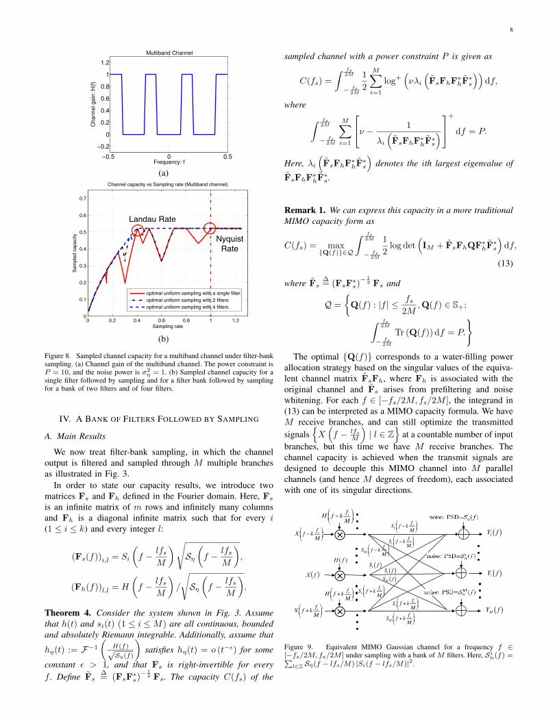
89
!0.5 0 0.5
!0.2
0
0.2
0.4
0.6
0.8
1
1.2
Multiband Channel
Frequency: f
Channel g
ain
: H
(f)
(a)
−0.5 0 0.5−0.2
0
0.2
0.4
0.6
0.8
1
1.2
1.4
Original Channel Response
Frequency: f
Chan
nel R
espo
nse:
H(f)
−0.5 0 0.5−0.2
0
0.2
0.4
0.6
0.8
1
1.2
Frequency: f
Chan
nel R
espo
nse:
H(f)
Optimal Prefilter
(a) (b)
−0.5 0 0.5−0.2
0
0.2
0.4
0.6
0.8
1
1.2
1.4
Frequency: f
Chan
nel R
espo
nse:
H(f)
Optimally Prefiltered Channel
0 0.2 0.4 0.6 0.8 1 1.20
0.1
0.2
0.3
0.4
0.5
0.6
0.7
0.8
0.9
1
Sampling rate
Sam
pled
cap
acity
Channel capacity vs Sampling rate
optimal filtermatched filter
super!Nyquistregime
sub!Nyquist regime
(c) (d)
Fig. 2. The sampled capacity for a given channel with channel band-width 1. (a) frequency response of the original channel; (b) optimalprefilter associated with this channel with sampling rate 0.4; (c) opti-mally prefiltered channel response with sampling rate 0.4; (d) capac-ity vs sampling rate for both optimal prefilter and matched filter. Theoptimal prefilter has support size fs in frequency domain, resultingin the prefiltered channel which allows aliased-free sampling. In thesub-Nyquist regime, this aliasing-suppressing filter outperforms thematched filter in maximizing data rate.
sampling. Examples include a specific multiband channel as illus-trated in Fig. 3. If the channel is sampled at a rate fs = 3
5fNYQ
(above Landau rate), aliasing occurs and leads to only one active in-terval (and hence one degree of freedom). However, if sampling isdone at a rate fs = 2
5fNYQ (the Landau rate), it can be easily ver-
ified that two shifted subbands remain non-overlapping, resulting intwo degrees of freedom. The tradeoff curve between capacity andsampling rate with optimal prefilters is plotted in Fig. 3. The under-lying reason for the wiggle in the tradeoff curve is that the uniformsampling grid largely constrains our ability in exploiting channel andsignal structures.
3. MULTI-CHANNEL UNIFORM SAMPLING
As we show, oversampling above Landau rate may not be beneficialif it does not favor the channel structure. When operating upon sig-nals with specific structure, such sampling mechanism may possiblysuppress information by mixing up useful resources. These call foran exploration of more general non-uniform sampling. These callfor an exploration of more general non-uniform sampling.
In order to incorporate non-uniformness, we replace the samplerblock in Fig. 1(a) by a filter bank followed by uniform samplingat rate fs/m at each branch, as illustrated in Fig. 1(b), which is aclass of commonly used non-uniform sampling techniques. Denoteby si(t) and Si,c (f) the impulse response and frequency responseof the ith filter, respectively. The filtered output in the ith branch is
yc,i(t) =
�si(t) ∗ (h(t)x(t) + η(t)) if t ∈ (0, T ];
0 otherwise.(7)
−0.5 0 0.5−0.4
−0.2
0
0.2
0.4
0.6
0.8
1
1.2
1.4Multiband channel
f:frequency
H(f):
cha
nnel
gai
n
0 0.2 0.4 0.6 0.8 1 1.20
0.1
0.2
0.3
0.4
0.5
0.6
0.7
Sampling rate
Sam
pled
cap
acity
Channel capacity vs Sampling rate (Multiband channel)
optimal uniform sampling with a single filteroptimal uniform sampling with 2 filtersoptimal uniform sampling with 4 filters
Landau Rate
NyquistRate
Fig. 3. The sampled channel capacity vs sampling rate for (1) single-channel with an optimal pre-filter; and (2) 5-channel prefilteredsampling with optimal filter bank. The channel bandwidth is as-sumed to be
�− 1
2, 1
2
�, the power constraint P = 10, and the noise
power σ2η = 1. The frequency response is given as H(f) = 1 for
|f | ∈�
110
, 15
�� �25, 1
2
�and H(f) = 0 otherwise.
Landau Rate
Nyquist Rate
(b)
Figure 8. Sampled channel capacity for multiband channel under filter-banksampling. (a) Channel gain of the multiband channel. The power constraintP = 10, and the noise power σ2
η = 1. (b) Sampled channel capacity for asingle filter followed by sampling and for a filter bank followed by samplingfor a bank of two filters and of four filters.
If this channel is sampled at a rate fs = 35fNYQ, then aliasing
occurs and leads to an aliased channel with one subband(and hence one degree of freedom). However, if sampling isperformed at a rate fs = 2
5fNYQ, it can be easily verifiedthat the two subbands remain non-overlapping in the aliasedchannel, resulting in two degrees of freedom. The tradeoffcurve between capacity and sampling rate with an optimalprefilter is plotted in Fig. 8(b). This curve indicates thatincreasing the sampling rate may not necessarily increasecapacity for certain channel structures. In other words, a singlefilter followed by sampling largely constrains our ability toexploit channel and signal structures. This is not the casefor more general sampling structures, as we show in the nextsection.
IV. A BANK OF FILTERS FOLLOWED BY SAMPLING
A. Main ResultsWe now treat filter-bank sampling, in which the channel
output is filtered and sampled through M multiple branchesas illustrated in Fig. 3. Since the sampled outputs at thesebranches are all functions of the same input and noise, theyare mutually dependent. The optimal transmit signal shouldbe chosen to decouple mutual interference across differentbranches. This is reflected in the capacity expression givenin Theorem 4.
In order to state our theorem, we introduce two matrices Fs
and Fh defined in the Fourier domain. Here, Fs is an infinitematrix of m rows and infinitely many columns and Fh is adiagonal infinite matrix such that ∀1 ≤ i ≤ k, ∀l ∈ Z:
(Fs(f))i,l = Si
�f − lfs
M
��Sη
�f − lfs
M
�,
(Fh(f))l,l =H�f − lfs
M
�
�Sη
�f − lfs
M
� .
Theorem 4. Consider the system shown in Fig. 3. Assumethat h(t) and si(t) (1 ≤ i ≤ M) are all continuous, boundedand absolutely Riemann integrable. Additionally, assume that
hη(t) := F−1
�H(f)√Sη(f)
�satisfies hη(t) = o (t−�) for some
constant � > 1, and that Fs is right-invertible for everyf . Define Fs
∆= (FsF
∗s)
− 12 Fs. The capacity C(fs) of the
sampled channel with a power constraint P can be given as
C(fs) =
� fs2M
− fs2M
1
2
M�
i=1
log+�νλi
�FsFhF
∗hF
∗s
��df,
where� fs
2M
− fs2M
M�
i=1
�ν − λi
�FsFhF
∗hF
∗s
��+df = P.
Here, λi
�FsFhF
∗hF
∗s
�denotes the ith largest eigenvalue of
FsFhF∗hF
∗s .
Remark 1. We can express this capacity in a more traditionalMIMO capacity form as
C(fs) = max{Q(f)}∈Q
� fs2M
− fs2M
1
2log det
�IM + FsFhQF∗
hF∗s
�df,
(14)
where Fs∆= (FsF
∗s)
− 12 Fs and
Q =
�Q(f) : |f | ≤ fs
2M,Q(f) ∈ S+;
� fs2M
− fs2M
Tr (Q(f)) df = P.
�
The optimal {Q(f)} corresponds to a water-filling power al-location strategy based on the singular values of the equivalentchannel matrix FsFh, where Fh is associated with the original
(a)
−0.5 0 0.5−0.2
0
0.2
0.4
0.6
0.8
1
1.2
1.4
Original Channel Response
Frequency: f
Cha
nnel
Res
pons
e: H
(f)
−0.5 0 0.5−0.2
0
0.2
0.4
0.6
0.8
1
1.2
Frequency: f
Cha
nnel
Res
pons
e: H
(f)
Optimal Prefilter
(a) (b)
−0.5 0 0.5−0.2
0
0.2
0.4
0.6
0.8
1
1.2
1.4
Frequency: f
Cha
nnel
Res
pons
e: H
(f)
Optimally Prefiltered Channel
0 0.2 0.4 0.6 0.8 1 1.20
0.1
0.2
0.3
0.4
0.5
0.6
0.7
0.8
0.9
1
Sampling rate
Sam
pled
cap
acity
Channel capacity vs Sampling rate
optimal filtermatched filter
super−Nyquistregime
sub−Nyquist regime
(c) (d)
Fig. 2. The sampled capacity for a given channel with channel band-width 1. (a) frequency response of the original channel; (b) optimalprefilter associated with this channel with sampling rate 0.4; (c) opti-mally prefiltered channel response with sampling rate 0.4; (d) capac-ity vs sampling rate for both optimal prefilter and matched filter. Theoptimal prefilter has support size fs in frequency domain, resultingin the prefiltered channel which allows aliased-free sampling. In thesub-Nyquist regime, this aliasing-suppressing filter outperforms thematched filter in maximizing data rate.
sampling. Examples include a specific multiband channel as illus-trated in Fig. 3. If the channel is sampled at a rate fs = 3
5fNYQ
(above Landau rate), aliasing occurs and leads to only one active in-terval (and hence one degree of freedom). However, if sampling isdone at a rate fs = 2
5fNYQ (the Landau rate), it can be easily ver-
ified that two shifted subbands remain non-overlapping, resulting intwo degrees of freedom. The tradeoff curve between capacity andsampling rate with optimal prefilters is plotted in Fig. 3. The under-lying reason for the wiggle in the tradeoff curve is that the uniformsampling grid largely constrains our ability in exploiting channel andsignal structures.
3. MULTI-CHANNEL UNIFORM SAMPLING
As we show, oversampling above Landau rate may not be beneficialif it does not favor the channel structure. When operating upon sig-nals with specific structure, such sampling mechanism may possiblysuppress information by mixing up useful resources. These call foran exploration of more general non-uniform sampling. These callfor an exploration of more general non-uniform sampling.
In order to incorporate non-uniformness, we replace the samplerblock in Fig. 1(a) by a filter bank followed by uniform samplingat rate fs/m at each branch, as illustrated in Fig. 1(b), which is aclass of commonly used non-uniform sampling techniques. Denoteby si(t) and Si,c (f) the impulse response and frequency responseof the ith filter, respectively. The filtered output in the ith branch is
yc,i(t) =
!si(t) ! (h(t)x(t) + !(t)) if t " (0, T ];
0 otherwise.(7)
−0.5 0 0.5−0.4
−0.2
0
0.2
0.4
0.6
0.8
1
1.2
1.4Multiband channel
f:frequency
H(f)
: cha
nnel
gai
n
0 0.2 0.4 0.6 0.8 1 1.20
0.1
0.2
0.3
0.4
0.5
0.6
0.7
Sampling rate
Sam
pled
cap
acity
Channel capacity vs Sampling rate (Multiband channel)
optimal uniform sampling with a single filteroptimal uniform sampling with 2 filtersoptimal uniform sampling with 4 filters
Landau Rate
NyquistRate
Fig. 3. The sampled channel capacity vs sampling rate for (1) single-channel with an optimal pre-filter; and (2) 5-channel prefilteredsampling with optimal filter bank. The channel bandwidth is as-sumed to be
"# 1
2, 1
2
#, the power constraint P = 10, and the noise
power "2! = 1. The frequency response is given as H(f) = 1 for
|f | ""
110
, 15
# $ "25, 1
2
#and H(f) = 0 otherwise.
Landau Rate
Nyquist Rate
(b)
Figure 8. Sampled channel capacity for a multiband channel under filter-banksampling. (a) Channel gain of the multiband channel. The power constraint isP = 10, and the noise power is σ2
η = 1. (b) Sampled channel capacity for asingle filter followed by sampling and for a filter bank followed by samplingfor a bank of two filters and of four filters.
IV. A BANK OF FILTERS FOLLOWED BY SAMPLING
A. Main Results
We now treat filter-bank sampling, in which the channeloutput is filtered and sampled through M multiple branchesas illustrated in Fig. 3.
In order to state our capacity results, we introduce twomatrices Fs and Fh defined in the Fourier domain. Here, Fsis an infinite matrix of m rows and infinitely many columnsand Fh is a diagonal infinite matrix such that for every i(1 ≤ i ≤ k) and every integer l:
(Fs(f))i,l = Si
(f − lfs
M
)√Sη(f − lfs
M
),
(Fh(f))l,l = H
(f − lfs
M
)/
√Sη(f − lfs
M
).
Theorem 4. Consider the system shown in Fig. 3. Assumethat h(t) and si(t) (1 ≤ i ≤M) are all continuous, boundedand absolutely Riemann integrable. Additionally, assume that
hη(t) := F−1
(H(f)√Sη(f)
)satisfies hη(t) = o (t−ε) for some
constant ε > 1, and that Fs is right-invertible for everyf . Define Fs
∆= (FsF
∗s)− 1
2 Fs. The capacity C(fs) of the
sampled channel with a power constraint P is given as
C(fs) =
∫ fs2M
− fs2M
1
2
M∑
i=1
log+(νλi
(FsFhF
∗hF∗s
))df,
where
∫ fs2M
− fs2M
M∑
i=1
ν − 1
λi
(FsFhF∗hF
∗s
)
+
df = P.
Here, λi(FsFhF
∗hF∗s
)denotes the ith largest eigenvalue of
FsFhF∗hF∗s .
Remark 1. We can express this capacity in a more traditionalMIMO capacity form as
C(fs) = max{Q(f)}∈Q
∫ fs2M
− fs2M
1
2log det
(IM + FsFhQF∗hF
∗s
)df,
(13)
where Fs∆= (FsF
∗s)− 1
2 Fs and
Q =
{Q(f) : |f | ≤ fs
2M,Q(f) ∈ S+;
∫ fs2M
− fs2M
Tr (Q(f)) df = P.
}
The optimal {Q(f)} corresponds to a water-filling powerallocation strategy based on the singular values of the equiva-lent channel matrix FsFh, where Fh is associated with theoriginal channel and Fs arises from prefiltering and noisewhitening. For each f ∈ [−fs/2M,fs/2M ], the integrand in(13) can be interpreted as a MIMO capacity formula. We haveM receive branches, and can still optimize the transmittedsignals
{X(f − lfs
M
)| l ∈ Z
}at a countable number of input
branches, but this time we have M receive branches. Thechannel capacity is achieved when the transmit signals aredesigned to decouple this MIMO channel into M parallelchannels (and hence M degrees of freedom), each associatedwith one of its singular directions.
( )fX
X f ! k fsM
"
#$
%
&'
X f + k fsM
!
"#
$
%&
H f ! k fsM
"
#$
%
&'
⊗
)( fH
⊗H f + k fs
M!
"#
$
%&
⊗
Yi f( )
Y1 f( )
YM f( )
S1 f( )
SM f + k fsM
!
"#
$
%&
Si f( )
Si f ! k fsM
"
#$
%
&'
S1 f + k fsM
!
"#
$
%&
SM f( )
SM f ! k fsM
"
#$
%
&'
Si f + k fsM
!
"#
$
%&
S1 f ! k fsM
"
#$
%
&'
Figure 9. Equivalent MIMO Gaussian channel for a frequency f ∈[−fs/2M, fs/2M ] under sampling with a bank of M filters. Here, Sin(f) =∑l∈Z Sη(f − lfs/M) |Si(f − lfs/M)|2.
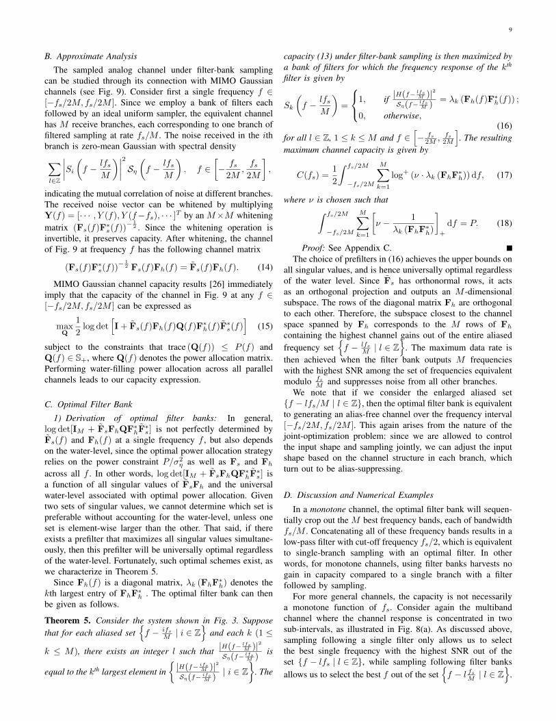
9
B. Approximate Analysis
The sampled analog channel under filter-bank samplingcan be studied through its connection with MIMO Gaussianchannels (see Fig. 9). Consider first a single frequency f ∈[−fs/2M,fs/2M ]. Since we employ a bank of filters eachfollowed by an ideal uniform sampler, the equivalent channelhas M receive branches, each corresponding to one branch offiltered sampling at rate fs/M . The noise received in the ithbranch is zero-mean Gaussian with spectral density
∑
l∈Z
∣∣∣∣Si(f − lfs
M
)∣∣∣∣2
Sη(f − lfs
M
), f ∈
[− fs
2M,fs
2M
],
indicating the mutual correlation of noise at different branches.The received noise vector can be whitened by multiplyingY(f) = [· · · , Y (f), Y (f−fs), · · · ]T by an M×M whiteningmatrix (Fs(f)F∗s(f))
− 12 . Since the whitening operation is
invertible, it preserves capacity. After whitening, the channelof Fig. 9 at frequency f has the following channel matrix
(Fs(f)F∗s(f))− 1
2 Fs(f)Fh(f) = Fs(f)Fh(f). (14)
MIMO Gaussian channel capacity results [26] immediatelyimply that the capacity of the channel in Fig. 9 at any f ∈[−fs/2M,fs/2M ] can be expressed as
maxQ
1
2log det
[I + Fs(f)Fh(f)Q(f)F∗h(f)F∗s(f)
](15)
subject to the constraints that trace (Q(f)) ≤ P (f) andQ(f) ∈ S+, where Q(f) denotes the power allocation matrix.Performing water-filling power allocation across all parallelchannels leads to our capacity expression.
C. Optimal Filter Bank
1) Derivation of optimal filter banks: In general,log det[IM + FsFhQF∗hF
∗s] is not perfectly determined by
Fs(f) and Fh(f) at a single frequency f , but also dependson the water-level, since the optimal power allocation strategyrelies on the power constraint P/σ2
η as well as Fs and Fhacross all f . In other words, log det[IM + FsFhQF∗hF
∗s] is
a function of all singular values of FsFh and the universalwater-level associated with optimal power allocation. Giventwo sets of singular values, we cannot determine which set ispreferable without accounting for the water-level, unless oneset is element-wise larger than the other. That said, if thereexists a prefilter that maximizes all singular values simultane-ously, then this prefilter will be universally optimal regardlessof the water-level. Fortunately, such optimal schemes exist, aswe characterize in Theorem 5.
Since Fh(f) is a diagonal matrix, λk (FhF∗h) denotes the
kth largest entry of FhF∗h . The optimal filter bank can then
be given as follows.
Theorem 5. Consider the system shown in Fig. 3. Supposethat for each aliased set
{f − ifs
M | i ∈ Z}
and each k (1 ≤
k ≤ M), there exists an integer l such that |H(f− lfsM )|2Sη(f− lfsM )
is
equal to the kth largest element in{|H(f− ifsM )|2Sη(f− ifsM )
| i ∈ Z}
. The
capacity (13) under filter-bank sampling is then maximized bya bank of filters for which the frequency response of the kth
filter is given by
Sk
(f − lfs
M
)=
1, if |H(f− lfsM )|2Sη(f− lfsM )
= λk (Fh(f)F∗h(f)) ;
0, otherwise,(16)
for all l ∈ Z, 1 ≤ k ≤M and f ∈[− fs
2M , fs2M
]. The resulting
maximum channel capacity is given by
C(fs) =1
2
∫ fs/2M
−fs/2M
M∑
k=1
log+ (ν · λk (FhF∗h)) df, (17)
where ν is chosen such that∫ fs/2M
−fs/2M
M∑
k=1
[ν − 1
λk (FhF∗h)
]
+
df = P. (18)
Proof: See Appendix C.The choice of prefilters in (16) achieves the upper bounds on
all singular values, and is hence universally optimal regardlessof the water level. Since Fs has orthonormal rows, it actsas an orthogonal projection and outputs an M -dimensionalsubspace. The rows of the diagonal matrix Fh are orthogonalto each other. Therefore, the subspace closest to the channelspace spanned by Fh corresponds to the M rows of Fhcontaining the highest channel gains out of the entire aliasedfrequency set
{f − lfs
M | l ∈ Z}
. The maximum data rate isthen achieved when the filter bank outputs M frequencieswith the highest SNR among the set of frequencies equivalentmodulo fs
M and suppresses noise from all other branches.We note that if we consider the enlarged aliased set
{f − lfs/M | l ∈ Z}, then the optimal filter bank is equivalentto generating an alias-free channel over the frequency interval[−fs/2M,fs/2M ]. This again arises from the nature of thejoint-optimization problem: since we are allowed to controlthe input shape and sampling jointly, we can adjust the inputshape based on the channel structure in each branch, whichturn out to be alias-suppressing.
D. Discussion and Numerical Examples
In a monotone channel, the optimal filter bank will sequen-tially crop out the M best frequency bands, each of bandwidthfs/M . Concatenating all of these frequency bands results in alow-pass filter with cut-off frequency fs/2, which is equivalentto single-branch sampling with an optimal filter. In otherwords, for monotone channels, using filter banks harvests nogain in capacity compared to a single branch with a filterfollowed by sampling.
For more general channels, the capacity is not necessarilya monotone function of fs. Consider again the multibandchannel where the channel response is concentrated in twosub-intervals, as illustrated in Fig. 8(a). As discussed above,sampling following a single filter only allows us to selectthe best single frequency with the highest SNR out of theset {f − lfs | l ∈ Z}, while sampling following filter banksallows us to select the best f out of the set
{f − l fsM | l ∈ Z
}.
10
Consequently, the channel capacity with filter-bank samplingexceeds that of sampling with a single filter, but neithercapacity is monotonically increasing in fs. This is shown inFig. 8(b). Specifically, we see in this figure that when we applya bank of two filters prior to sampling, the capacity curve isstill non-monotonic but outperforms a single filter followed bysampling.
Another consequence of our results is that when the numberof branches is optimally chosen, the Nyquist-rate channelcapacity can be achieved by sampling at any rate above theLandau rate. In order to show this, we introduce the followingnotion of a channel permutation. We call H(f) a permutationof a channel response H(f) at rate fs if, for any f ,{|H(f − lfs)|2Sη(f − lfs)
| l ∈ Z
}=
{|H(f − lfs)|2Sη(f − lfs)
| l ∈ Z
}.
The following proposition characterizes a sufficient conditionthat allows the Nyquist-rate channel capacity to be achievedat any sampling rate above the Landau rate.
Proposition 1. If there exists a permutation H(f) of H(f)at rate fs
M such that the support of H(f) is [−fL/2, fL/2],then optimal sampling following a bank of M filters achievesNyquist-rate capacity when fs ≥ fL.
Examples of channels satisfying Proposition 1 include anymultiband channel with N subbands among which K sub-bands have non-zero channel gain. For any fs ≥ fL = K
N fNYQ,we are always able to permute the channel at rate fs/K togenerate a band-limited channel of spectral support size fL.Hence, sampling above the Landau rate following K filtersachieves the Nyquist-rate channel capacity. This is illustratedin Fig. 8(b) where sampling with a four-branch filter bank has ahigher capacity than sampling with a single filter, and achievesthe Nyquist-rate capacity whenever fs ≥ 2
5fNYQ. The optimalfilter-bank sampling for most general channels is identifiedin [21], where both the number of branches and per-branchsampling rate are allowed to vary.
V. MODULATION AND FILTER BANKS FOLLOWED BYSAMPLING
A. Main Results
We now treat modulation and filter banks followed bysampling. Assume that Ts := MTs = b
aTq where a andb are coprime integers, and that the Fourier transform ofqi(t) is given as
∑l cliδ(f − lfq). Before stating our theorem,
we introduce the following two Fourier symbol matrices Fη
and Fh. The aM × ∞-dimensional matrix Fη contains Msubmatrices with the αth submatrix given by an a × ∞-dimensional matrix FηαFpα. Here, for any v ∈ Z, 1 ≤ l ≤ a,and 1 ≤ α ≤M , we have
(Fηα)l,v = (Fpα)v,v
[∑
u
cuαSα
(−f + ufq + v
fqb
)
· exp
(−j2πlMTs
(f − ufq − v
fqb
))].
The matrices Fpα and Fh are infinite diagonal matrices suchthat for every integer l:
(Fpα)l,l = Pα
(−f + l
fqb
)√Sη(−f + l
fqb
),
(Fh)l,l
=H(−f + l
fqb
)
√Sη(−f + l
fqb
) .
Theorem 6. Consider the system shown in Fig. 4. Assume thath(t), pi(t) and si(t) (1 ≤ i ≤M) are all continuous, boundedand absolutely Riemann integrable, Fη is right invertible, andthat the Fourier transform of qi(t) is given as
∑l cliδ(f−lfq).
Additionally, suppose that hη(t) := F−1
(H(f)√Sη(f)
)satisfies
hη(t) = o (t−ε) for some constant ε > 1. We further assumethat aMTs = bTq where a and b are coprime integers. Thecapacity C(fs) of the sampled channel with a power constraintP is given by
C(fs) =
∫ fs2aM
− fs2aM
1
2
aM∑
i=1
log+(νλi
((FηFη∗)−
12 FηFh·
Fh∗Fη∗ (FηFη∗)−12
))df, (19)
where ν is chosen such that
P =
∫ fs2aM
− fs2aM
aM∑
i=1
[ν − λ−1
i
((FηFη∗)−
12 FηFh·
Fh∗Fη∗ (FηFη∗)−12
)]+df.
Remark 2. The right invertibility of Fη ensures that the sam-pling method is non-degenerate, e.g. the modulation sequencecannot be zero.
The optimal ν corresponds to a water-filling power alloca-tion strategy based on the singular values of the equivalentchannel matrix (FηFη∗)−
12 FηFh, where (FηFη∗)−
12 is due
to noise prewhitening and FηFh is the equivalent channelmatrix after modulation and filtering. This result can again beinterpreted by viewing (19) as the MIMO Gaussian channelcapacity of the equivalent channel. We note that a closed-form capacity expression may be hard to obtain for generalmodulating sequences qi(t). This is because the multiplicationoperation corresponds to convolution in the frequency domainwhich does not preserve Toeplitz properties of the originaloperator associated with the channel filter. When qi(t) isperiodic, however, it can be mapped to a spike train in thefrequency domain, which preserves block Toeplitz properties,as described in more detail in Appendix D.
B. Approximate Analysis
The Fourier transform of the signal prior to modulation inthe ith branch at a given frequency f can be expressed asPi(f)R(f), where R(f) = H(f)X(f)+N(f). Multiplicationof this pre-modulation signal with the modulation sequenceqi(t) =
∑l cliδ (f − lfq) corresponds to convolution in the
frequency domain.

11
Recall that bTq = aMTs with integers a and b. Wetherefore divide all samples {yi[k] | k ∈ Z} in the ith branchinto a groups, where the lth (0 ≤ l < a) group contains{yi[l + ka] | k ∈ Z}. Hence, each group is equivalent to thesamples obtained by sampling at rate fs/Ma = fq/b. Thesampling system, when restricted to the output on each groupof the sampling set, can be treated as LTI, thus justifying itsequivalent representation in the spectral domain. Specifically,for the ith branch, we denote by
giη(t, τ) :=
∫si(t− τ1)qi(τ1)p(τ1 − τ)dτ1
the output response of the preprocessing system at time t dueto an input impulse at time τ . We then introduce a new LTIimpulse response gil(t) associated with the lth group such thatgil(t) := giη(lTs, lTs − t). It can easily be shown that when
the same sampling set{
(l + ka) Ts | k ∈ Z}
is employed, thepreprocessing system associated with giη(t, τ) results in thesame sampled output as the one associated with gil(t). Thisallows us to treat the samples of each distinct group as theones obtained by an LTI preprocessing system followed byuniform sampling.
Suppose the channel output R(f) is passed through theLTI preprocessing system associated with the lth group ofthe ith branch, i.e. the one associated with gil(t). The Fouriertransform of the output of this LTI system prior to uniformsampling, as marked in Fig 10(b), can be written as
Y li (f)
∆=Pi(f)R(f)
(Si(f) exp
(j2πflTs
)∗∑
u
cui δ (f − ufq))
=Pi(f)R(f)∑
u
cui Si (f − ufq) exp(j2πlTs (f − ufq)
).
After uniform sampling at rate fq/b, the Fourier transform ofthe samples in the lth group can be expressed as
Y li (f) =∑
v
Y li
(f − vfq
b
)
=∑
v
Pi
(f − vfq
b
)R
(f − vfq
b
)∑
u
cui ·
Si
(f − ufq −
vfqb
)exp
(j2πlTs
(f − ufq −
vfqb
))
=∑
v
Ail,v(f)Pi
(f − v fq
b
)R
(f − v fq
b
),
where
Ail,v(f)∆=∑
u
cui Si
(f − ufq −
vfqb
)·
exp
(j2πlTs
(f − ufq −
vfqb
)). (20)
Since the sampled outputs of the original sampling systemare equivalent to the union of samples obtained by Ma LTIsystems each followed by uniform sampling at rate fq/b, wecan transform the true sampling system into a MIMO Gaussianchannel with an infinite number of input branches and finitely
X f( )
X f !fqb
"
#$
%
&'
X f +fqb
!
"#
$
%&
H f !fqb
"
#$
%
&'
⊗
)( fH
⊗
H f +fqb
!
"#
$
%&
⊗
N f !fqb
"
#$
%
&'
)( fN
N f +fqb
!
"#
$
%&
R f !fqb
"
#$
%
&'
R f +fqb
!
"#
$
%&
R f( )
1st branchf
ith branchf
Mth branchf
group a
group 1 Y11 f( )Y1
a f( )
group a
group 1 Yi1 f( )Yi
a f( )
group a
group 1 YM1 f( )YM
a f( )
(a)
R f( )
R f !fqb
"
#$
%
&'
R f +fqb
!
"#
$
%&
Pi f !fqb
"
#$
%
&'
⊗
Pi ( f )
⊗
Pi f +fqb
!
"#
$
%&
⊗
Ail,1( f )
⊗
Ail,0 ( f )
⊗
Ail,!1( f )
⊗
!Y li f !
fqb
"
#$
%
&'
!Y li f( )
!Y li f +
fqb
!
"#
$
%&
Y li f( )
the lth group in the ith branch
associated with the samples
yi l + ka[ ] k ! Z{ }
(b)
Figure 10. Equivalent MIMO Gaussian channel for a given f ∈ [0, fq/b)under sampling with modulation banks and filter banks. (a) The overall MIMOrepresentation, where each branch has a output each corresponding to adistinct group. (b) The MISO representation of the lth group in the ith branch,where Ail,v(f) is defined in (20). This is associated with the set of samples{yi[l + ka] | k ∈ Z}.
many output branches, as illustrated in Fig. 10. The well-known formula for the capacity of a MIMO channel can nowbe used to derive our capacity results.
We note that due to the convolution in the spectral domain,the frequency response of the sampled output at frequencyf is a linear combination of frequency components {X(f)}and {N(f)} from several different aliased frequency sets. Wedefine the modulated aliased frequency set as a generalizationof the aliased set. Specifically, for each f , the modulatedaliased set is given by5
{f − lfq − kfs | l, k ∈ Z
}. By our
assumption that fq = ba fs with a and b being relatively prime,
simple results in number theory imply that{f0 − lfq − kfs | l, k ∈ Z
}= {f0 − lfq/b | l ∈ Z}
={f0 − lfs/a | l ∈ Z
}.
In other words, for a given f0 ∈ [−fq/2b, fq/2b],the sampled output at f0 depends on the input in theentire modulated aliased set. Since the sampling band-width at each branch is fs, all outputs at frequencies
5We note that although each modulated aliased set is countable, it may bea dense set when fq/fs is irrational. Under the assumption in Theorem 6,however, the elements in the set have a minimum spacing of fq/b.
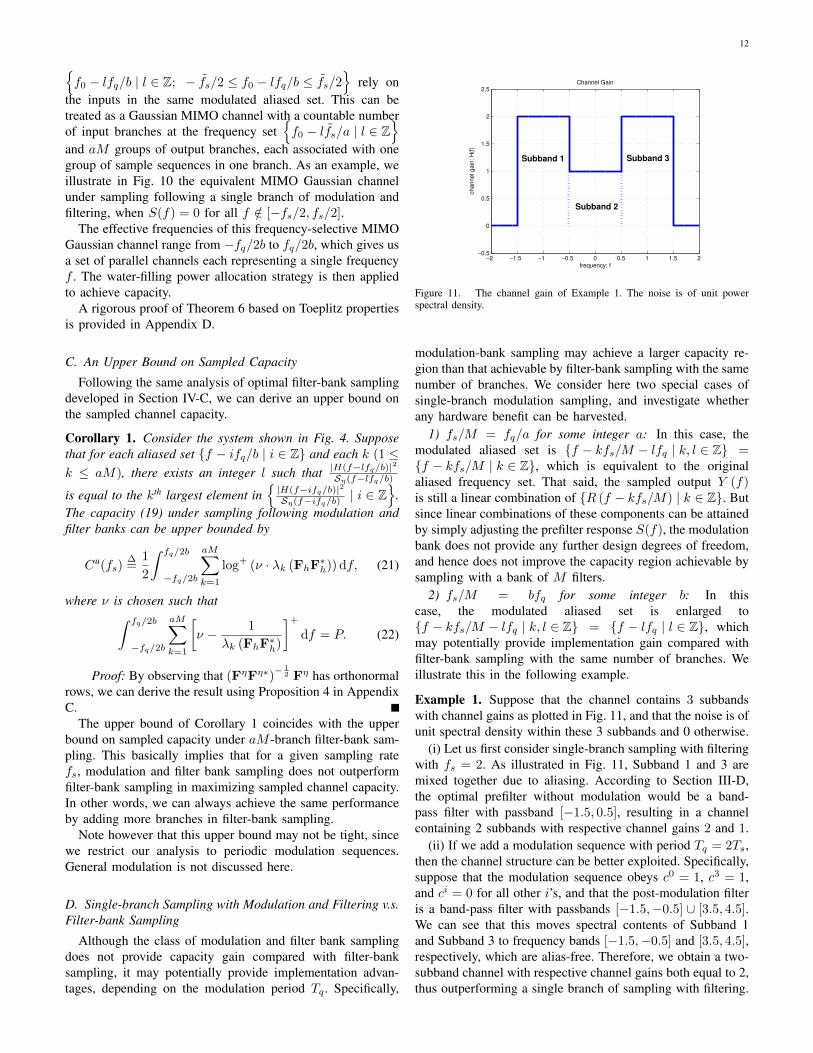
12
{f0 − lfq/b | l ∈ Z; − fs/2 ≤ f0 − lfq/b ≤ fs/2
}rely on
the inputs in the same modulated aliased set. This can betreated as a Gaussian MIMO channel with a countable numberof input branches at the frequency set
{f0 − lfs/a | l ∈ Z
}
and aM groups of output branches, each associated with onegroup of sample sequences in one branch. As an example, weillustrate in Fig. 10 the equivalent MIMO Gaussian channelunder sampling following a single branch of modulation andfiltering, when S(f) = 0 for all f /∈ [−fs/2, fs/2].
The effective frequencies of this frequency-selective MIMOGaussian channel range from −fq/2b to fq/2b, which gives usa set of parallel channels each representing a single frequencyf . The water-filling power allocation strategy is then appliedto achieve capacity.
A rigorous proof of Theorem 6 based on Toeplitz propertiesis provided in Appendix D.
C. An Upper Bound on Sampled Capacity
Following the same analysis of optimal filter-bank samplingdeveloped in Section IV-C, we can derive an upper bound onthe sampled channel capacity.
Corollary 1. Consider the system shown in Fig. 4. Supposethat for each aliased set {f − ifq/b | i ∈ Z} and each k (1 ≤k ≤ aM), there exists an integer l such that |H(f−lfq/b)|2
Sη(f−lfq/b)is equal to the kth largest element in
{|H(f−ifq/b)|2Sη(f−ifq/b) | i ∈ Z
}.
The capacity (19) under sampling following modulation andfilter banks can be upper bounded by
Cu(fs)∆=
1
2
∫ fq/2b
−fq/2b
aM∑
k=1
log+ (ν · λk (FhF∗h)) df, (21)
where ν is chosen such that∫ fq/2b
−fq/2b
aM∑
k=1
[ν − 1
λk (FhF∗h)
]+
df = P. (22)
Proof: By observing that (FηFη∗)−12 Fη has orthonormal
rows, we can derive the result using Proposition 4 in AppendixC.
The upper bound of Corollary 1 coincides with the upperbound on sampled capacity under aM -branch filter-bank sam-pling. This basically implies that for a given sampling ratefs, modulation and filter bank sampling does not outperformfilter-bank sampling in maximizing sampled channel capacity.In other words, we can always achieve the same performanceby adding more branches in filter-bank sampling.
Note however that this upper bound may not be tight, sincewe restrict our analysis to periodic modulation sequences.General modulation is not discussed here.
D. Single-branch Sampling with Modulation and Filtering v.s.Filter-bank Sampling
Although the class of modulation and filter bank samplingdoes not provide capacity gain compared with filter-banksampling, it may potentially provide implementation advan-tages, depending on the modulation period Tq . Specifically,
35
!2 !1.5 !1 !0.5 0 0.5 1 1.5 2!0.5
0
0.5
1
1.5
2
2.5
frequency: f
cha
nne
l gain
: H
(f)
Channel Gain
Subband 1 Subband 3
Subband 2
0
50
100
0
50
100
0
500
1000
1500
2000
2500
Y(f!fs/2)
X(f+fs/2)
X(f)
Y(f)
X(f!fs/2)
Figure 13. The left plot illustrates the channel gain, where the sampling rate is fs = 2. The right plot illustrates the signal
components of the sampled response under modulation followed by sampling.
and that the noise is of unit spectral density within these 3 subbands and zero otherwise. Here, single-
branch filtering followed by sampling is employed, where the sampling rate is fs = 2 and the period
of the modulation sequence Tq = 2Ts. Due to aliasing, Subband 1 and Subband 3 (as illustrated in Fig.
13) are mixed together. According to Section III-D, the optimal prefilter without modulation would be a
band-pass filter with passband −1.5 ≤ f ≤ 0.5, resulting in a channel consisting of two subbands with
respective channel gains 2 and 1.
Now if we employ modulation sampling with a lowpass filter, the channel structure can be better
exploited. Specifically, suppose that the modulation sequence has a period of 2Ts and obeys c0 = 1,
c1 = 100, c2 = 1, c−2 = 1000 and ci = 0 for all other i’s, and that the cutoff frequency of the low-pass
filter is fcutoff = 1. By simple manipulation,
exp
�jπTq
�f − fs
2
��Y�f − fs
2
�
exp (jπTqf) Y (f)
=
2 100 1001
100 1 0
2X�f − fs
2
�+ N
�f − fs
2
�
X (f) + N (f)
2X�f + fs
2
�+ N
�f + fs
2
�
for all f ∈�0, fs
2
�. Through noise whitening and eigenvalue decomposition, we can derive a pair of
equivalent parallel channels experiencing respective channel gains 2 and 1.99, which outperforms non-
modulated sampling following optimal filtering. As illustrated in Fig. 13, Y (f − fs
2 ) primarily depends
on the frequency component at f + fs
2 , while Y (f) primarily depends on the frequency component at
f − fs
2 : both frequencies have SNR 4. In fact, by increasing c−2 and c1 correspondingly, we can obtain
Figure 11. The channel gain of Example 1. The noise is of unit powerspectral density.
modulation-bank sampling may achieve a larger capacity re-gion than that achievable by filter-bank sampling with the samenumber of branches. We consider here two special cases ofsingle-branch modulation sampling, and investigate whetherany hardware benefit can be harvested.
1) fs/M = fq/a for some integer a: In this case, themodulated aliased set is {f − kfs/M − lfq | k, l ∈ Z} ={f − kfs/M | k ∈ Z}, which is equivalent to the originalaliased frequency set. That said, the sampled output Y (f)is still a linear combination of {R (f − kfs/M) | k ∈ Z}. Butsince linear combinations of these components can be attainedby simply adjusting the prefilter response S(f), the modulationbank does not provide any further design degrees of freedom,and hence does not improve the capacity region achievable bysampling with a bank of M filters.
2) fs/M = bfq for some integer b: In thiscase, the modulated aliased set is enlarged to{f − kfs/M − lfq | k, l ∈ Z} = {f − lfq | l ∈ Z}, whichmay potentially provide implementation gain compared withfilter-bank sampling with the same number of branches. Weillustrate this in the following example.
Example 1. Suppose that the channel contains 3 subbandswith channel gains as plotted in Fig. 11, and that the noise is ofunit spectral density within these 3 subbands and 0 otherwise.
(i) Let us first consider single-branch sampling with filteringwith fs = 2. As illustrated in Fig. 11, Subband 1 and 3 aremixed together due to aliasing. According to Section III-D,the optimal prefilter without modulation would be a band-pass filter with passband [−1.5, 0.5], resulting in a channelcontaining 2 subbands with respective channel gains 2 and 1.
(ii) If we add a modulation sequence with period Tq = 2Ts,then the channel structure can be better exploited. Specifically,suppose that the modulation sequence obeys c0 = 1, c3 = 1,and ci = 0 for all other i’s, and that the post-modulation filteris a band-pass filter with passbands [−1.5,−0.5] ∪ [3.5, 4.5].We can see that this moves spectral contents of Subband 1and Subband 3 to frequency bands [−1.5,−0.5] and [3.5, 4.5],respectively, which are alias-free. Therefore, we obtain a two-subband channel with respective channel gains both equal to 2,thus outperforming a single branch of sampling with filtering.

13
More generally, let us consider the following scenario.Suppose that the channel of bandwidth W = 2L
K fs is equallydivided into 2L subbands each of bandwidth fq = fs/K forsome integers K and L. The SNR |H (f)|2 /Sη(f) withineach subband is assumed to be flat. For instance, in thepresence of white noise, if fq � Bc with Bc being thecoherence bandwidth [23], the channel gain (and hence theSNR) is roughly equal across the subband. Algorithm 1 givenbelow generates an alias-free sampled analog channel, whichis achieved by moving the K subbands with the highestSNRs to alias-free locations. By Corollary 1, this algorithmdetermines an optimal sampling mechanism that maximizescapacity under a single branch of sampling with modulationand filtering. Specifically, take any f ∈ [−fq/2, fq/2], and thealgorithm works as follows.
Algorithm 11. Initialize. Find the K largest elements in{|H(f−lfq)|2Sη(f−lfq) | l ∈ Z,−L ≤ l ≤ L− 1
}. Denote by
{li | 1 ≤ i ≤ K} the index set of these K elementssuch that l1 > l2 > · · · > lK . SetL∗ := min {k | k ∈ Z, k ≥ 2L, k mod K = 0} .2. For i = 1 : K
Let α := i · L∗ + i− li.Set cα = 1, and S(f + αfp) = 1.
Algorithm 1 first selects the K subbands with the highestSNR, and then moves each of the selected subbands to anew location by appropriately setting
{ci}
, which guaranteesthat (1) the movement does not corrupt any of the previouslychosen locations; (2) the contents in the newly chosen loca-tions will be alias-free. The post-modulation filter is appliedto suppress the frequency contents outside the set of newlychosen subband locations. One drawback of this algorithm isthat we need to preserve as many as 2LK subbands in orderto make it work.
The performance of Algorithm 1 is equivalent to the oneusing an optimal filter bank followed by sampling with sam-pling rate fq at each branch. Hence, single-branch samplingeffectively achieves the same performance as multi-branchfilter-bank sampling. This approach may be preferred sincebuilding multiple analog filters is often expensive (in terms ofpower consumption, size, or cost). We note, however, that fora given overall sampling rate, modulation-bank sampling doesnot outperform filter-bank sampling with an arbitrary numberof branches. The result is formally stated as follows.
Proposition 2. Consider the setup in Theorem 6. For agiven overall sampling rate fs, sampling with M branches ofoptimal modulation and filter banks does not achieve highersampled capacity compared to sampling with an optimal bankof aM filters.
Hence, the main advantage of applying a modulation bankis a hardware benefit, namely, using fewer branches and henceless analog circuitry to achieve the same capacity.
VI. CONNECTIONS BETWEEN CAPACITY AND MMSE
In Sections III-D and IV-C, we derived respectively theoptimal prefilter and the optimal filter bank that maximizecapacity. It turns out that such choices of sampling methodscoincide with the optimal prefilter / filter bank that minimizethe MSE between the Gaussian channel input and the signalreconstructed from sampling the channel output, as detailedbelow.
Consider the following sampling problem. Let x(t) bea zero-mean wide-sense stationary (WSS) stochastic signalwhose power spectral density (PSD) SX(f) satisfies a powerconstraint 6
∫∞−∞ SX(f)df = P . This input is passed through
a channel consisting of an LTI filter and additive stationaryGaussian noise. We sample the channel output using a filterbank at a fixed rate fs/M in each branch, and recover a linearMMSE estimate x(t) of x(t) from its samples in the sense ofminimizing E(|x(t)− x(t)|2) for t ∈ R. We propose to jointlyoptimize x(t) and the sampling method. Specifically, our jointoptimization problem can now be posed as follows: for whichinput process x(t) and for which filter bank is the estimationerror E(|x(t)− x(t)|2) minimized for t ∈ R.
It turns out that the optimal input and the optimal filterbank coincide with those maximizing channel capacity, whichis captured in the following proposition.
Proposition 3. Suppose the channel input x(t) is any WSSsignal. For a given sampling system, let x(t) denote theoptimal linear estimate of x(t) from the digital sequence{y[n]}. Then the capacity-optimizing filter bank given in (16)and its corresponding optimal input x(t) minimize the linearMSE E(|x(t)− x(t)|2) over all possible LTI filter banks.
Proof: See Appendix E.Proposition 3 implies that the input signal and the filter bank
optimizing channel capacity also minimize the MSE betweenthe original input signal and its reconstructed output. Wenote that if the samples {y[n]} and x(t) are jointly Gaussianrandom variables, then the MMSE estimate x(t) for a giveninput process x(t) is linear in {y[n]}. That said, for Gaus-sian inputs passed through Gaussian channels, the capacity-maximizing filter bank also minimizes the MSE even if wetake into account nonlinear estimation. Thus, under samplingwith filter-banks for Gaussian channels, information theoryreconciles with sampling theory through the SNR metric whendetermining optimal systems. Intuitively, high SNR typicallyleads to large capacity and small MSE.
Proposition 3 includes the optimal prefilter under single-prefilter sampling as a special case. We note that a similarMSE minimization problem was investigated decades ago withapplications in PAM [17], [18]: a given random input x(t) isprefiltered, corrupted by noise, uniformly sampled, and thenpostfiltered to yield a linear estimate x(t). The goal in thatwork was to minimize the MSE between x(t) and x(t) over allprefiltering (or pulse shaping) and postfiltering mechanisms.While our problem differs from this PAM design problem by
6We restrict our attention to WSS input signals. This restriction, whilefalling short of generality, allows us to derive sampling results in a simpleway.
14
optimizing directly over the random input instead of the pulseshape, the two problems are similar in spirit and result in thesame alias-suppressing filter. However, earlier work did notaccount for filter-bank sampling or make connections betweenminimizing MSE and maximizing capacity.
VII. CONCLUSIONS AND FUTURE WORK
We have characterized sampled channel capacity as a func-tion of sampling rate for different sampling methods, therebyforming a new connection between sampling theory and infor-mation theory. We show how the capacity of a sampled analogchannel is affected by reduced sampling rate and identifyoptimal sampling structures for several classes of samplingmethods, which exploit structure in the sampling design. Theseresults also indicate that capacity is not always monotonic insampling rate, and illuminate an intriguing connection betweenMIMO channel capacity and capacity of undersampled analogchannels. The capacity optimizing sampling structures areshown to extract the frequency components with highest SNRsfrom each aliased set, and hence suppress aliasing and out-of-band noise. We also show that for Gaussian inputs over Gaus-sian channels, the optimal filter / filter bank also minimizes theMSE between the channel input and the reconstructed signal.Our work establishes a framework for using the information-theoretic metric of capacity to optimize sampling structures,offering a different angle from traditional design of samplingmethods based on other performance metrics.
Our work uncovers additional questions at the intersectionof sampling theory and information theory. For instance, anupper bound on sampled capacity under sampling rate con-straints for more general nonuniform sampling methods wouldallow us to evaluate which sampling mechanisms are capacity-achieving for any channel. Moreover, for channels where thereis a gap between achievable rates and the capacity upperbound, these results might provide insight into new samplingmechanisms that might close the gap to capacity. Investigationof capacity under more general nonuniform sampling tech-niques is an interesting topic that is studied in our companionpaper [21]. In addition, the optimal sampling structure fortime-varying channels will require different analysis than usedin the time-invariant case. It is also interesting to investigatewhat sampling mechanisms are optimal for channels when thechannel state is partially or fully unknown. A deeper under-standing of how to exploit channel structure may also guidethe design of sampling mechanisms for multiuser channels thatrequire more sophisticated cooperation schemes among usersand are impacted in a more complex way by subsampling.
APPENDIX APROOF OF THEOREM 2
We begin by an outline of the proof. A discretizationargument is first used to approximate arbitrarily well theanalog signals by discrete-time signals, which allows us tomake use of the properties of Toeplitz matrices instead ofthe more general Toeplitz operators. By noise whitening, weeffectively convert the sampled channel to a MIMO channelwith i.i.d. noise for any finite time interval. Finally, the
asymptotic properties of Toeplitz matrices are exploited inorder to relate the eigenvalue distribution of the equivalentchannel matrix with the Fourier representation of both channelfilters and prefilters. The proofs of several auxiliary lemmasare deferred to Appendix F.
Instead of directly proving Theorem 2, we prove the the-orem for a simpler scenario where the noise η(t) is of unitspectral density. In this case, our goal is to prove that thecapacity is equivalent to
C(fs) =1
2
∫ fs2
− fs2log+
ν
∑l∈Z|H(f − lfs)S(f − lfs)|2
∑l∈Z|S(f − lfs)|2
df
where the water level ν can be calculated through the follow-ing equation∫ fs
2
− fs2
(ν −
∑l |S(f − lfs)|2∑
l |H(f − lfs)S(f − lfs)|2
)+
df = P.
This capacity result under white noise can then be immedi-ately extended to accommodate for colored noise. Supposethe additive noise is of power spectral density Sη(f). Wecan then split the channel filter H (f) into two parts withrespective frequency response H (f) /
√Sη(f) and
√Sη(f).
Equivalently, the channel input is passed through an LTI filterwith frequency response H (f) /
√Sη(f), contaminated by
white noise, and then passed through a filter with transferfunction
√Sη(f)S(f) followed by an ideal sampler with
rate fs. This equivalent representation immediately leads tothe capacity in the presence of colored noise by substitutingcorresponding terms into the capacity with white noise.
A. Channel Discretization and Diagonalization
Given that h(t) is continuous and Riemann integrable, oneapproach to study the continuous-time problem is via reductionto an equivalent discrete-time problem [27, Chapter 16]. Inthis subsection, we describe the method of obtaining ourequivspace discretization approximations to the continuous-time problems, which will allow us to exploit the propertiesof block-Toeplitz matrices instead of the more complicatedblock-Toeplitz operators.
For notational simplicity, we define
gu,v =1
∆
∫ ∆
0
g (uTs − v∆ + τ) dτ
for any function g(t). If g(t) is a continuous function, thenlim∆→0 gu,v = g (uTs − v∆), where v may be a function of∆. We also define h(t) := h(t) ∗ s(t). Set T = nTs andTs = k∆ for some integers n and k, and define
hi := ∆ ·[hi,0, hi,1, · · · , hi,k−1
],
si := ∆ · [si,0, si,1, · · · , si,k−1] ,
(xn)i :=1
∆
∫ ∆
0
x (i∆ + τ) dτ (0 ≤ i < nk) ,
(η)i :=1
∆
∫ ∆
0
η (i∆ + τ) dτ (i ∈ Z) .
15
We also define
Hn :=
h0 h−1 · · · h−n+1
h1 h0 · · · h−n+2
...... · · ·
...hn−1 hn−2 · · · h0
,
Sn :=
· · · s0 s−1 · · ·· · · s1 s0 · · ·· · ·
...... · · ·
· · · sn−1 sn−2 · · ·
.
With these definitions, the original channel model can beapproximated with the following discretized channel:
yn = Hnxn + Snη. (23)
As can be seen, Hn is a fat block Toeplitz matrix. Moreover,SnSn∗ is asymptotically equivalent to a Toeplitz matrix, aswill be shown in Appendix A-C. We note that each elementηi is a zero-mean Gaussian variable with variance E(|ηi|2) =1/∆. In addition, E (ηiη
∗l ) = 0 for any i 6= l, implying that η
is an i.i.d. Gaussian vector. The filtered noise Snη is no longeri.i.d. Gaussian, which motivates us to whiten the noise first.
The prewhitening matrix is given by Snw := (SnSn∗)−12 ,
which follows from the fact that
ESnwSnη (SnwSnη)∗
= SnwSnE (ηη∗) Sn∗Sn∗w
=1
∆(SnSn∗)−
12 SnSn∗ (SnSn∗)−
12 =
1
∆In.
This basically implies that SnwSn projects the i.i.d. Gaussiannoise η onto an n-dimensional subspace, and that Snw (Snη) isnow n-dimensional i.i.d. Gaussian noise. Left-multiplicationwith this whitening matrix yields a new output
yn : = (SnSn∗)−12
(Hnxn + Snη
)
= (SnSn∗)−12 Hnxn + ηn.
Here, ηn consists of independent zero-mean Gaussian ele-ments with variance 1/∆. Since the prewhitening operationSnw is invertible, we have
I (xn; yn) = I (xn; yn) . (24)
In this paper, we will use Ik,∆ (xn; yn) and I (xn; yn) in-terchangeably to denote the mutual information between thenk-dimensional vector xn and yn.
Moreover, when x(t) is of bounded variance (i.e.supt E |x(t)|2 ≤ ∞) and the additive noise is Gaus-sian, it has been shown [28] that the mutual informationis weakly continuous in the input distribution. Therefore,limk→∞ Ik,∆ (xn; yn) → I
({x (t)}Tt=0 ; {y [n]}Tt=0
). As k
increases, the discretized sequence becomes a finer approxi-mation to the continuous-time signal. The uniform continuityof the probability measure of x(t) and the continuity of mutualinformation immediately imply that limn→∞ 1
nTsIk,∆ (xn; yn)
converges uniformly in k. We also observe that for every givenn, limk→∞ Ik,∆ (xn; yn) exists due to the continuity condition
of the mutual information. Therefore, applying the Moore-Osgood theorem in real analysis allows us to exchange theorder of limits.
Based on the above arguments, the capacity of the sampledanalog channel can be expressed as the following limit
C(fs) = limk→∞
limn→∞
1
nTssup
p(x): 1nkE(‖xn‖22)≤P
Ik,∆ (xn,yn)
= limk→∞
limn→∞
fsn
supp(x): 1
nkE(‖xn‖22)≤PIk,∆ (xn, yn) .
Note that it suffices to investigate the case where T is an inte-ger multiple of Ts since limT→∞ 1
T sup I (x(0, T ]; {y[n]}) =limn→∞ 1
nTssup I (x(0, nTs]; {y[n]}).
B. Preliminaries on Toeplitz Matrices
Before proceeding to the proof of the theorem, we brieflyintroduce several basic definitions and properties related toToeplitz matrices. Interested readers are referred to [3], [24]for more details.
A Toeplitz matrix is an n× n matrix Tn where (Tn)k,l =tk−l, which implies that a Toeplitz matrix Tn is uniquelydefined by the sequence {tk}. A special case of Toeplitzmatrices is circulant matrices where every row of the matrixCn is a right cyclic shift of the row above it. The Fourier series(or symbol) with respect to the sequence of Toeplitz matrices{Tn := [tk−l; k, l = 0, 1, · · · , n− 1] : n ∈ Z} is given by
F (ω) =
+∞∑
k=−∞tk exp (jkω) , ω ∈ [−π, π] . (25)
Since the sequence {tk} uniquely determines F (ω) and viceversa, we denote by Tn(F ) the Toeplitz matrix generated byF (and hence {tk}). We also define a related circulant matrixCn(F ) with top row (c
(n)0 , c
(n)1 , · · · , c(n)
n−1), where
c(n)k =
1
n
n−1∑
i=0
F
(2πi
n
)exp
(2πjik
n
). (26)
One key concept in our proof is asymptotic equivalence,which is formally defined as follows [24].
Definition 1 (Asymptotic Equivalence). Two sequences ofn×n matrices {An} and {Bn} are said to be asymptoticallyequivalent if
(1) An and Bn are uniformly bounded, i.e. there exists aconstant c independent of n such that
‖An‖2 , ‖Bn‖2 ≤ c <∞, n = 1, 2, · · · (27)
(2) limn→∞ 1√n‖An −Bn‖F = 0.
We will abbreviate asymptotic equivalence of {An} and{Bn} by An ∼ Bn. Two important results regarding asymp-totic equivalence are given in the following lemmas [24].
Lemma 1. Suppose An ∼ Bn with eigenvalues {αn,k}and {βn,k}, respectively. Let g(x) be an arbitrary continuous
16
function. Then if the limits limn→∞ 1n
∑n−1k=0 g (αn,k) and
limn→∞ 1n
∑n−1k=0 g (βn,k) exist, we have
limn→∞
1
n
n−1∑
k=0
g (αn,k) = limn→∞
1
n
n−1∑
k=0
g (βn,k) . (28)
Lemma 2. (a) Suppose a sequence of Toeplitz matricesTn where (Tn)ij = ti−j satisfies that {ti} is absolutelysummable. Suppose the Fourier series F (ω) related to Tn
is positive and Tn is Hermitian. Then we have
Tn(F ) ∼ Cn(F ). (29)
If we further assume that there exists a constant ε > 0 suchthat F (ω) ≥ ε > 0 for all ω ∈ [0, 2π], then we have
Tn(F )−1 ∼ Cn(F )−1 = Cn(1/F ) ∼ Tn (1/F ) . (30)
(b) Suppose An ∼ Bn and Cn ∼ Dn, then AnCn ∼BnDn.
Toeplitz or block Toeplitz matrices have well-known asymp-totic spectral properties [3], [29]. The notion of asymptoticequivalence allows us to approximate non-Toeplitz matricesby Toeplitz matrices, which will be used in the next subsectionto analyze the spectral properties of the channel matrix.
C. Capacity via Convergence of the Discrete Model
After channel discretization, we can calculate the capacityfor each finite duration T using well-known MIMO Gaussianchannel capacity, which, however, depends on the spectrum ofthe truncated channel and may vary dramatically for differentT . By our definition of capacity, we will pass T to infintyand see whether the finite-duration capacity converges, andif so, whether there is a closed-form expression for thelimit. Fortunately, the beautiful asymptotic properties of block-Toeplitz matrices guarantees the existance of the limit andallows for a closed-form solution using the frequency responseof h(t) and s(t).
To see this, we first construct a new channel whose capacityis easier to obtain, and will show that the new channel hasasymptotically equivalent channel capacity as the originalchannel. As detailed below, each key matrix associated withthe new channel is a Toeplitz matrix, whose spectrum can bewell approximated in the asymptotic regime [24].
Consider the spectral properties of the Hermitian matricesHnHn∗ and SnSn∗ . We can see that
(HnHn∗
)ij
=(HnHn∗
)∗ji
=
n−j∑
t=−j+1
hj−i+th∗t . (31)
Obviously, HnHn∗ is not a Toeplitz matrix. Instead of in-vestigating the eigenvalue distribution of HnHn∗ directly, welook at a new Hermitian Toeplitz matrix Hn associated withHnHn∗ such that for any i ≤ j:
(Hn)ij
=(Hn)∗ij
=
∞∑
t=−∞hj−i+th
∗t . (32)
Lemma 3. The above definition of Hn implies that
Hn ∼ HnHn∗. (33)
Proof: See Appendix F-A.On the other hand, for any 1 ≤ i ≤ j ≤ n, we have
(SnSn∗)ij = (SnSn∗)∗ji =
∞∑
t=−∞sj−i+ts
∗t . (34)
Hence, the Hermitian matrix Sn := SnSn∗ is still Toeplitz.However, the matrix of interest in the capacity will be(SnSn∗)−1/2 instead. We therefore construct an asymptoti-cally equivalent circulant matrix Cn as defined in (26), whichwill preserves the Toeplitz property when we take (Cn)
−1/2
[24]. Formally speaking, (SnSn∗)−1 can be related to (Cn)−1
as follows.
Lemma 4. If there exists some constant εs > 0 such that forall f ∈
[− fs2 ,
fs2
],∑
l∈Z|S (f − lfs)|2 ≥ εs > 0 (35)
holds, then (Cn)−1 ∼ (SnSn∗)−1.
Proof: See Appendix F-B.One of the most useful properties of a circulant matrix Cn
is that its eigenvectors{
u(m)c
}are
u(m)c =
1√n
(1, e−2πjm/n, · · · , e−2πj(n−1)m/n
). (36)
Suppose the eigenvalue decomposition of Cn is given as
Cn = UcΛcU∗c , (37)
where Uc is a Fourier coefficient matrix, and Λc is a diagonalmatrix where each element in the diagonal is positive.
The concept of asymptotic equivalence allows us to explic-itly relate our matrices of interest to both circulant matricesand Toeplitz matrices, whose asymptotic spectral densitieshave been well studied.
Lemma 5. For any continuous function g(x), we have
limn→∞
1
n
n∑
i=1
g (λi)
=Ts
∫ fs2
− fs2g
(∑l∈Z |H(f − lfs)S(f − lfs)|2∑
l∈Z |S(f − lfs)|2
)df,
where λi denotes the ith eigenvalue of(SnSn∗)−
12 HnHn∗ (SnSn∗)−
12 .
Proof: See Appendix F-C.We can now prove the capacity result. The standard capacity
results for parallel channels [1, Theorem 7.5.1] implies that thecapacity of the discretized sampled analog channel is given bythe parametric equations
CT =1
2T
∑
i
log+ (νλi) , (38)
Pnk
1/∆=∑
i
[ν − 1/λi]+, (39)
where ν is the water level of the optimal power alloca-tion over this discrete model, as can be calculated through
17
(39). Since this capacity depends on the eigenvalues of(SnSn∗)−
12 HnHn∗ (SnSn∗)−
12 , then by Lemma 5, the con-
vergence as T → ∞ is guaranteed and the capacity C =limT→∞ CT can be expressed using H(f) and S(f). Specif-ically,
limT→∞
CT (ν) = limT→∞
1
T
∑
i
1
2log+ [νλi]
=1
2
∫ fs/2
−fs/2log+
(ν
∑l∈Z |H(f − lfs)S(f − lfs)|2∑
l∈Z |S(f − lfs)|2
)df.
Similarly, (39) can be transformed into
PTs =Pk
1/∆=
1
n
∑
i
[ν − 1/λi]+
=Ts
∫ fs/2
−fs/2
[ν −
∑l∈Z |S(f − lfs)|2∑
l∈Z |H(f − lfs)S(f − lfs)|2
]+
df,
which completes the proof.
APPENDIX BPROOF OF THEOREM 4
We follow similar steps as in the proof of Theorem 2: weapproximate the sampled channel using a discretized modelfirst, whiten the noise, and then find capacity of the equivalentchannel matrix. Due to the use of filter banks, the equivalentchannel matrix is no longer asymptotically equivalent to aToeplitz matrix, but instead a block-Toeplitz matrix. Thismotivates us to exploit the asymptotic properties of block-Toeplitz matrices.
A. Channel Discretization and DiagonalizationLet Ts = MTs, and suppose we have T = nTs and Ts =
k∆ with integers n and k. Similarly, we can define
hi(t) := h(t) ∗ si(t), and
hli =[hi
(lTs
), hi
(lTs −∆
), · · · , hi
(lTs − (k − 1)∆
)].
We introduce the following two matrices as
Hni =
h0i h−1
i · · · h−n+1i
h1i h0
i · · · h−n+2i
......
......
hn−1i hn−2
i · · · h0i
and Sni =
· · · s0i s−1
i · · ·· · · s1
i s0i · · ·
......
......
· · · sn−1i sn−2
i · · ·
.
We also set (xn)i = 1∆
∫∆
0x (i∆ + τ) dτ (0 ≤ i < nk),
and (η)i = 1∆
∫∆
0η (i∆ + τ) dτ (i ∈ Z). Defining yn =
[y1[0], · · · , y1[n− 1], y2[0], · · · , y2[n− 1], · · · , yM [n− 1]]T
leads to the discretized channel model
yn =
Hn1
Hn2
...HnM
xn +
Sn1Sn2...
SnM
η.
Whitening the noise gives us
yn =
Sn1Sn2...
SnM
[
Sn∗1 · · · Sn∗M]
− 12
Hn1
Hn2
...HnM
xn+ η,
where η is i.i.d. Gaussian variable with variance 1/∆. We canexpress capacity of the sampled analog channel under filter-bank sampling as the following limit
C(fs) = limk→∞
limn→∞
fsMn
sup I (xn; yn) ,
Here, the supremum is taken over all distribution of xn subjectto a power constraint 1
nkE(‖xn‖22
)≤ P .
B. Capacity via Convergence of the Discrete Model
We can see that for any 1 ≤ u, v ≤ m,
SnuSn∗v = Snu,v, (40)
where the Toeplitz matrix Snu,v is defined such that for any1 ≤ i ≤ j ≤ n
(Snu,v
)i,j
=
∞∑
t=−∞sj−i+tu
(stv)∗. (41)
Let Sn = [Sn∗1 ,Sn∗2 , · · · ,Sn∗M ]∗. Then the Hermitian block
Toeplitz matrix
Sn :=
Sn1,1 Sn1,2 · · · Sn1,MSn2,1 Sn2,2 · · · Sn2,M
......
......
SnM,1 SnM,2 · · · SnM,M
satisfies Sn = SnSn∗. Additionally, we defineHnu,v (1 ≤ u, v ≤M) , where
(Hnu,v
)i,j
=
∞∑
t=−∞hj−i+tu
(htv
)∗, (42)
and we let Hn =[Hn∗
1 , Hn∗2 , · · · , Hn∗
M
]∗. The block Toeplitz
matrix
Hn :=
Hn1,1 Hn
1,2 · · · Hn1,M
Hn2,1 Hn
2,2 · · · Hn2,M
......
......
HnM,1 Hn
M,2 · · · HnM,M
satisfies
limn→∞
1√nM
∥∥∥Hn − HnHn∗∥∥∥
F
≤ limn→∞
1√M
∑
1≤u,v≤M
1√n
∥∥∥Hnu,v − Hn
uHn∗v
∥∥∥ = 0.
=⇒ Hn ∼ HnHn∗. (43)

18
The M ×M Fourier symbol matrix Fs(f) associated withSn has elements [Fs (f)]u,v given by
[Fs (f)]u,v
=∆2
T 2s
k−1∑
i=0
(∑
l1
Su
(−f + l1fs
)exp
(−j2π
(f − l1fs
)i∆))
(∑
l2
Sv
(−f + l2fs
)exp
(−j2π
(f − l2fs
)i∆))∗
=∆2
T 2s
k−1∑
i=0
∑
l1,l2
Su
(−f + l1fs
)S∗v(−f + l2fs
)
exp(−j2π (l2 − l1) fsi∆
))
=∆
Ts
∑
l∈ZSu
(−f + lfs
)S∗v(−f + lfs
).
Denote by{Tn(F−1s
)}the sequence of block Toeplitz ma-
trices generated by F−1s (f), and denote by Tn
l1,l2
(F−1s
)the
(l1, l2) Toeplitz block of Tn(F−1s
). It can be verified that
M∑
l2=1
Tnl1,l2
(F−1s
)· Snl2,l3 ∼ Tn
(M∑
l2=1
[F−1s
]l1,l2
[Fs]l2,l3
)
= Tn (δ[l1 − l3]) ,
which immediately yields
Tn(F−1s
)Sn ∼ I =⇒ Tn
(F−1s
)∼(Sn)−1
∼ (SnSn∗)−1.
(44)Therefore, for any continuous function g(x), [29, Theorem5.4] implies that
limn→∞
1
nM
nM∑
i=1
g(λi
{(SnSn∗)−
12 HnHn∗ (SnSn∗)−
12
})
=
∫ fs2M
− fs2M
M∑
i=1
g(λi
(F− 1
2
s FhF− 1
2
s
))df.
Denote F‡s = (FsF∗s)− 1
2 Fs, then the capacity of parallelchannels [1], which is achieved via water filling power al-location, yields
C(fs)
= limn→∞
∑nMi=1 log+
(νλi
{(SnSn∗)−
12 HnHn∗ (SnSn∗)−
12
})
2nMTs
=
∫ fs2M
− fs2M
1
2
M∑
i=1
log+(νλi
(F− 1
2
s FhF− 1
2
s
))df
=1
2
∫ fs2M
− fs2M
M∑
i=1
log+(νλi
(F‡sFhF
∗hF‡∗s
))df,
where
P =
∫ fs2M
− fs2M
M∑
i=1
ν − 1
λi
(F− 1
2
s FhF− 1
2
s
)
+
df
=
∫ fs2M
− fs2M
M∑
i=1
[ν − 1
λiF‡sFhF∗hF
‡∗s
]+
df.
This completes the proof.
APPENDIX CPROOF OF THEOREM 5
Theorem 5 immediately follows from the following propo-sition.
Proposition 4. The kth largest eigenvalue λk of the positivesemidefinite matrix FsFhF
∗hF∗s is bounded by
0 ≤ λk ≤ λk (FhF∗h) , 1 ≤ k ≤M. (45)
These upper bounds can be attained simultaneously by thefilter (16).
Proof: Recall that at a given f , Fh is an infinite diagonalmatrix satisfying (Fh)l,l = H
(f − lfs
M
)for all l ∈ Z, and
that Fs = (FsF∗s)− 1
2 Fs. Hence, FsFhF∗hF∗s is an M ×M
dimensional matrix. We observe that
Fs
(Fs
)∗= (FsF
∗s)− 1
2 FsF∗s (FsF
∗s)− 1
2 = I, (46)
which indicates that the rows of Fs are orthonormal. Hence,the operator norm of Fs is no larger than 1, which leads to
λ1
(FsFhF
∗hF∗s
)=∥∥∥FsFh
∥∥∥2
2≤ ‖Fh‖22 = λ1 (FhF
∗h) .
Denote by {ek, k ≥ 1} the standard basis where ek isa vector with a 1 in the kth coordinate and 0 otherwise.We introduce the index set {i1, i2, · · · , iM} such that eik(1 ≤ k ≤M) is the eigenvector associated with the kth largesteigenvalues of the diagonal matrix FhF
∗h.
Suppose that vk is the eigenvector associated with the kthlargest eigenvalue λk of FsFhF
∗hF∗s , and denote by
(Fs
)k
the kth column of Fs. Since FsFhF∗hF∗s is Hermitian posi-
tive semidefinite, its eigendecomposition yields an orthogonalbasis of eigenvectors. Observe that {v1, · · · ,vk} spans a k-
dimensional space and that{(
Fs
)j, 1 ≤ j ≤ k − 1
}spans
a subspace of dimension no more than k − 1. For any k ≥ 2,there exists k scalars a1, · · · , ak such that
k∑
i=1
aivi ⊥{(
Fs
)ij, 1 ≤ j ≤ k − 1
}and
k∑
i=1
aivi 6= 0.
(47)This allows us to define the following unit vector
vk∆=
k∑
i=1
ai√∑kj=1 |aj |
2vi, (48)
19
which is orthogonal to{(
Fs
)j, 1 ≤ j ≤ k − 1
}. We observe
that
∥∥∥FsFhF∗hF∗svk∥∥∥
2
2=
∥∥∥∥∥∥
k∑
i=1
ai√∑kj=1 |aj |
2FsFhF
∗hF∗svi
∥∥∥∥∥∥
2
2
=
∥∥∥∥∥∥
k∑
i=1
aiλi√∑kj=1 |aj |
2vi
∥∥∥∥∥∥
2
2
=
k∑
i=1
λ2i |ai|2∑kj=1 |aj |
2≥ λ2
k. (49)
Define uk := F∗svk. From (47) we can see that (uk)i =⟨(Fs
)i, vi
⟩= 0 holds for all i ∈ {i1, i2, · · · , ik−1}. In other
words, uk ⊥{ei1 , · · · , eik−1
}. This further implies that
λ2k ≤
∥∥∥FsFhF∗hF∗svk∥∥∥
2
2≤∥∥∥Fs
∥∥∥2
2
∥∥∥FhF∗hF∗svk∥∥∥
2
2
≤ ‖FhF∗huk‖22 (50)
≤ supx⊥span{ei1 ,··· ,eik−1}
‖FhF∗hx‖22 (51)
= λ2k (FhF
∗h) (52)
by observing that FhF∗h is a diagonal matrix.
Setting
Sk
(f − lfs
M
)
=
1, if∣∣∣H(f − lfs
M
)∣∣∣2
= λk (Fh(f)F∗h(f)) ,
0, otherwise,
yields Fs = Fs and hence FsFhF∗hFs is a diagonal matrix
such that (FsFhF
∗hF∗s
)k,k
= λk (FhF∗h) . (53)
Apparently, this choice of Sk(f) allows the upper bounds
λk
(FsFhF
∗hF∗s
)= λk (FhF
∗h) , ∀1 ≤ k ≤M (54)
to be attained simultaneously.By extracting out the M frequencies with the highest SNR
from each aliased set {f − lfs/M | l ∈ Z}, we achieve λk =λk (FhF
∗h), thus achieving the maximum capacity.
APPENDIX DPROOF OF THEOREM 6
Following similar steps as in the proof of Theorem 4, weapproximately convert the sampled channel into its discretecounterpart, and calculate the capacity of the discretizedchannel model after noise whitening. We note that the impulseresponse of the sampled channel is no longer LTI due to theuse of modulation banks. But the periodicity assumption of themodulation sequences allows us to treat the channel matrix asblockwise LTI, which provides a way to exploit the propertiesof block-Toeplitz matrices.
Again, we give a proof for the scenario where noise iswhite Gaussian with unit spectral density. The capacity ex-pression in the presence of colored noise can immediately bederived by replacing Pi(f) with Pi(f)
√Sη(f) and H(f) with
H(f)/√Sη(f).
In the ith branch, the noise component at time t is given by
si (t) ∗ (qi(t) · (pi(t) ∗ η(t)))
=
∫
τ1
dτ1si (t− τ1)
∫
τ2
qi (τ1) pi (τ1 − τ2) η (τ2) dτ2
=
∫
τ2
(∫
τ1
si (t− τ1) qi (τ1) pi (τ1 − τ2) dτ1
)η (τ2) dτ2
=
∫
τ2
gηi (t, τ2)η(τ2)dτ2,
where gηi (t, τ2)∆=
∫
τ1
si (t− τ1) qi (τ1) pi (τ1 − τ2) dτ1.
Let Ts = MTs. Our assumption bTq = aTs immediatelyleads to
gηi
(t+ aTs, τ + bTq
)
=
∫
τ1
si
(t+ aTs − τ1
)qi (τ1) pi
(τ1 − τ − aTs
)dτ1
=
∫
τ1
si (t− τ1) qi (τ1 + bTq) pi (τ1 − τ) dτ1
=
∫
τ1
si (t− τ1) qi (τ1) pi (τ1 − τ) dτ1 = gηi (t, τ) ,
implying that gηi (t, τ) is a block-Toeplitz function.Similarly, the signal component
si (t) ∗ (qi(t) · (pi(t) ∗ h(t) ∗ x(t))) =
∫
τ2
ghi (t, τ2)x(τ2)dτ2,
where
ghi (t, τ2)∆=
∫
τ1
si (t− τ1) qi (τ1)
∫
τ3
pi (τ1 − τ2 − τ3)h(τ3)dτ3dτ1,
which also satisfies the block-Toeplitz propertyghi
(t+ aTs, τ + bTq
)= ghi (t, τ).
Suppose that T = nTs and Ts = k∆ hold for some integersn and k. We can introduce two matrices Gη
i and Ghi such that
∀m ∈ Z, 0 ≤ l < n
(Gηi )l,m = gηi
(lTs,m∆
),
(Ghi
)l,m
= ghi
(lTs,m∆
).
Setting yni = [yi[0], yi[1], · · · , yi[n− 1]]T leads to similar
discretized approximation as in the proof of Theorem 2:
yni = Ghi x
n + Gηi η. (55)
Here, η is a i.i.d. zero-mean Gaussian vector where each entryis of variance 1/∆.
Hence, Ghi and Gη
i are block Toeplitz matrices satisfying(Ghi
)l+a,m+ak
=(Ghi
)l,m
and (Gηi )l+a,m+ak = (Gη
i )l,m.

20
Using the same definition of xn and η as in Appendix B, wecan express the system equation as
yn =
Gh1
Gh2
...GhM
xn +
Gη1
Gη2
...GηM
η. (56)
Whitening the noise component yields
yn =
Gη1
Gη2
...GηM
Gη1
Gη2
...GηM
∗
− 12
Gh1
Gh2
...GhM
xn + η, (57)
where η is i.i.d. Gaussian noise with variance 1/∆.In order to calculate the capacity limit, we need to investi-
gate the Fourier symbols associated with these block Toeplitzmatrices.
Lemma 6. At a given frequency f , the Fourier symbolwith respect to Gη
αGηβ is given by akFηαFpαFp∗β Fη∗β , and
the Fourier symbol with respect to GhαGh
β is given byakFηαFpαFhFh∗Fp∗β Fη∗β . Here for any (l, v) such that v ∈ Zand 1 ≤ l ≤ a, we have
(Fηα)l,v =∑
u
cuαSα
(−f + ufq + v
fqb
)·
exp
(−j2πl Ts
M
(f − ufq − v
fqb
)).
Also, Fpα and Fh are infinite diagonal matrices such that forall l ∈ Z
(Fpα)l,l = Pα
(−f + l
fqb
),
(Fh)l,l
= H(−f + l
fqb
).
Proof: See Appendix F-D.Define Gη such that its (α, β) subblock is Gη
αGη∗β , and Gh
such that its (α, β) subblock is GhαGh∗
β . Proceeding similarlyas in the proof of Theorem 4, we obtain
F (Gη) = akFηFη∗ and F(Gh)
= akFηFhFh∗Fη∗,
where Fη contain M × 1 submatrices. The (α, 1) submatrixof Fη is given by FηαFpα.
Denote Fη‡∆= (FηFη∗)−
12 Fη . For any continuous function
g(x), [29, Theorem 5.4] implies that
limn→∞
1
naM
naM∑
i=1
g(λi
{(Gη)
− 12 Gh (Gη)
− 12
})
=
∫ fs2a
− fs2a
aM∑
i=1
g(λi(Fη‡FhFh∗Fη‡∗
))df.
Then capacity of parallel channels, achieved via water-fillingpower allocation, yields
C(fs) = limn→∞
naM∑
i=1
log+(νλi
{(Gη)
− 12 Gh (Gη)
− 12
})
naM
=
∫ fs2a
− fs2a
1
2
aM∑
i=1
log+(νλi
(Fη‡FhFh∗Fη‡∗
))df,
where the water level ν can be computed through the followingparametric equation
P = limn→∞
1
naM
naM∑
i=1
ν − 1
λi
{(Gη)
− 12 Gh (Gη)
− 12
}
+
=
∫ fs2a
− fs2a
aM∑
i=1
ν − 1
λi
{(Gη)
− 12 Gh (Gη)
− 12
}
+
df.
APPENDIX EPROOF OF PROPOSITION 3
Denote by yk(t) the analog signal after passing through thekth prefilter prior to ideal sampling. When both the input signalx(t) and the noise η(t) are Gaussian, the MMSE estimator ofx(t) from samples
{yk[n] | 1 ≤ k ≤M
}is linear. Recall that
Ts = MTs and fs = fs/M . A linear estimator of x(t) fromy[n] can be given as
x(t) =∑
k∈ZgT (t− kTs) · y(kTs), (58)
where we use the vector form g(t) = [g1(t), · · · , gM (t)]T andy(t) = [y1(t), · · · , yM (t)]T for notational simplicity. Here,gl(t) denotes the interpolation function operating upon thesamples in the lth branch. We propose to find the optimalestimator g(t) that minimizes the mean square estimation errorE(|x(t)− x(t)|2
)for some t.
From the orthogonality principle, the MMSE estimate x(t)obeys
E(x(t)y∗(lTs)
)= E
(x(t)y∗(lTs)
), ∀l ∈ Z. (59)
Since x(t) and η(t) are both stationary Gaussian processes,we can define RXY (τ) := E (x(t)y∗(t− τ)) to be the crosscorrelation function between x(t) and y(t), and RY (τ) :=E (y(t)y∗(t− τ)) the autocorrelation function of y(t). Plug-ging (58) into (59) leads to the following relation
RXY
(t− lTs
)=∑
k∈ZgT(t− kTs
)RY
(kTs − lTs
).
Replacing t by t+ lTs , we can equivalently express it as
RXY (t) =∑
k∈ZgT(t+ lTs − kTs
)RY
(kTs − lTs
)
=∑
l∈ZgT(t− lTs
)RY
(lTs
), (60)
which is equivalent to the convolution of g(t) and RY (t) ·∑l∈Z δ
(t− lTs
).
21
Let F(·) denote Fourier transform operator. Define thecross spectral density SXY (f) := F (RXY (t)) and SY (f) =F (RY (t)). By taking the Fourier transform on both sides of(60) , we have
SXY (f) = G(f)F(
RY (τ)∑
l∈Zδ(τ − lTs)
),
which immediately yields that ∀f ∈[−fs/2, fs/2
]
G(f) = SXY (f)
[F(
RY (τ)∑
l∈Zδ(τ − lTs)
)]−1
= SXY (f)
(∑
l∈ZSY
(f − lfs
))−1
.
Since the noise η(t) is independent of x(t), the cross correla-tion function RXY (t) is
RXY (τ) = E (x(t+ τ)·[(s1 ∗ h ∗ x)
∗(t), · · · , (sM ∗ h ∗ x)
∗(t)]).
which allows the cross spectral density to be derived as
SXY (f) = H∗(f)SX(f) [S∗1 (f), · · · , S∗M (f)] . (61)
Additionally, the spectral density of y(t) can be given as thefollowing M ×M matrix
SY (f) =(|H(f)|2 SX(f) + Sη(f)
)S(f)S∗(f), (62)
with Sη(f) denoting the spectral density of the noise η(t), andS(f) = [S1(f), · · · , Sm(f)]
T .Define
K(f) : =∑
l∈Z
(|H(f − lfs)|2 SX(f − lfs) +N (f − lfs)
)
S(f − lfs)S∗(f − lfs).
The Wiener-Hopf linear reconstruction filter can now bewritten as
G(f) = H∗(f)SX(f)S∗(f)K−1(f)
Define RX(τ) = E (x(t)x∗(t− τ)). Since∫∞−∞ SX(f)df =
RX(0), the resulting MSE is
ξ(t) = E(|x(t)|2
)− E
(|x(t)|2
)
= E(|x(t)|2
)− E (x(t)x∗(t))
= RX(0)− E
(x(t)
(∑
l∈ZgT (t− lTs)y(lTs)
)∗)
= RX (0)−∑
l∈ZRXY (t− lTs)g(t− lTs).
Since F (g(−t)) = (G∗(f))T and SXY =
H∗(f)SX(f)S∗(f), Parseval’s identity implies that
ξ(t) =
∫ ∞
−∞
[SX(f)−G∗(f)STXY
]df
=
∫ ∞
−∞
[SX(f)− |H(f)SX(f)|2 S∗(f)K−1(f)S(f)
]df
=
∫ fs/2
−fs/2
[ ∞∑
l=−∞SX(f − lfs)− TsVT
ζ (f, fs) · 1]
df.
Suppose that we impose power constraints∑l∈Z SX(f − lfs) = P (f), and define ζ(f) :=
|H(f)SX(f)|2 S∗(f)K−1(f)S(f). For a given inputprocess x(t), the problem of finding the optimal prefilterS(f) that minimizes MSE then becomes
maximize{S(f−lfs),l∈Z}
VTζ (f, fs) · 1,
where the objective function can be alternatively rewritten inmatrix form
trace{
F12
XF∗hF∗s (Fs (FhF
∗h + Fη) F∗s)
−1FsFhF
12
X
}(63)
Here FX and Fη are diagonal matrices such that (FX)l,l =SX(f − lfs) and (Fη)l,l = Sη(f + kfs). We observe that
trace{
F12
XF∗hF∗s (Fs (FhF
∗h + Fη) F∗s)
−1FsFhF
12
X
}
=trace{
(Fs (FhF∗h + Fη) F∗s)
−1FsFhFXF∗hF
∗s
}
(a)=trace
{(YY∗)−1
Y (FhF∗h + Fη)
− 12 FhFXF∗h
(FhF∗h + Fη)
− 12 Y∗
}
(b)= trace
{(FhF
∗h + Fη)
−1FhFXF∗hY
∗ (YY∗)−1Y}
(c)=trace
{(FhF
∗h + Fη)
−1FhFXF∗hY
∗Y}
(d)
≤ supZ·Z∗=IM
trace{
Z (FhF∗h + Fη)
−1FhFXF∗hZ
∗}
=M∑
i=1
λi(D), (64)
where (a) follows by introducing Y := Fs (FhF∗h + Fη)
12 , (b)
follows from the fact that Fh, FX , Fη are all diagonal matri-ces, (c) follows by introducing Y = (YY∗)−
12 Y, and (d) fol-
lows by observing that YY∗ = (YY∗)−12 YY∗ (YY∗)−
12 =
I. Here, D is an infinite diagonal matrix such thatDl,l = |H(f−lfs)|2SX(f−lfs)
|H(f−lfs)|2SX(f−lfs)+Sη(f−lfs) . In other words, theupper bound is the sum of the M largest Di,i whichare associated with M frequency points of highest SNR|H(f+lfs)|2SX(f+lfs)
Sη(f+lfs).
Therefore, when restricted to the set of all permutationsof {SX(f),SX(f ± fs), · · · }, the minimum MSE is achievedwhen assigning the M largest SX(f + lfs) to M brancheswith the largest SNR. In this case, the corresponding optimalfilter can be chosen such that
Sk(f − lfs) =
{1, if l = k
0, otherwise.(65)
22
where k is the index of the kth largest element in{|H(f − lfs)|2 /Sη(f − lfs) : l ∈ Z
}.
APPENDIX FPROOFS OF AUXILIARY LEMMAS
A. Proof of Lemma 3For any i ≤ j, we have∣∣∣∣
(HnHn∗ − Hn
)ij
∣∣∣∣
≤∣∣∣∣∣
−j∑
t=−∞hj−i+th
∗t
∣∣∣∣∣+
∣∣∣∣∣∣
∞∑
t=n−j+1
hj−i+th∗t
∣∣∣∣∣∣. (66)
Since h(t) is absolutely summable and Riemann integrable,for sufficiently small ∆, there exists a constant c such that∑∞i=−∞
∥∥∥hi∥∥∥
1≤ c. In the following analysis, we define R1
and R2 to capture the two residual terms respectively, i.e.
R1ij =
−j∑
t=−∞hj−i+th
∗t , and R2
ij =∞∑
t=n−j+1
hj−i+th∗t .
In order to prove that HnHn∗ ∼ Hn, we need to
prove (1) limn→∞ 1n
∥∥∥HnHn∗ − Hn∥∥∥
2
F= 0, or equivalently,
limn→∞ 1n
∥∥R2∥∥2
F = 0 and limn→∞ 1n
∥∥R1∥∥2
F = 0; (2) the `2norms of both HnHn∗ and Hn are uniformly bounded, i.e.∃Mu such that
∥∥∥HnHn∗∥∥∥
2≤Mu <∞ and
∥∥∥Hn∥∥∥
2≤Mu <
∞ for all n.(1) We first prove that limn→∞ 1
n
∥∥∥HnHn∗ − Hn∥∥∥
2
F= 0.
By our assumptions, we have h(t) = o (t−ε) for some ε > 1.Since s(t) is absolutely integrable, h(t) = o (t−ε) also holds.Without loss of generality, we suppose that j ≥ i.
(a) if i ≥ n12ε , by the assumption h(t) = o
(1tε
)for some
ε > 1, one has
∣∣R1ij
∣∣ ≤−j∑
t=−∞
∥∥∥hj−i+t∥∥∥
1
∥∥∥ht∥∥∥∞
≤(
maxτ≥n 1
2ε
∥∥∥h−τ∥∥∥
1
) −j∑
t=−∞
∥∥∥ht∥∥∥∞
≤(
maxτ≥n 1
2ε
∥∥∥h−τ∥∥∥
1
) −j∑
t=−∞
∥∥∥ht∥∥∥
1≤ c max
τ≥n 12ε
∥∥∥h−τ∥∥∥
1
= kc · o(
1√n
)= o
(1√n
). (67)
(b) if j ≥ n 12ε ,
∣∣R1ij
∣∣ ≤−j∑
t=−∞
∥∥∥hj−i+t∥∥∥
1
∥∥∥ht∥∥∥∞
≤( −j∑
t=−∞
∥∥∥hj−i+t∥∥∥
1
)maxτ≤−j
∥∥∥hτ∥∥∥∞
≤ c maxτ≥n 1
2ε
∥∥∥h−τ∥∥∥∞
= c · o(
1√n
)= o
(1√n
). (68)
(c) if j < n12ε and i < n
12ε , we have
∣∣R1ij
∣∣2 ≤( ∞∑
t=−∞
∥∥∥hj−i+t∥∥∥
1
∥∥∥ht∥∥∥∞
)2
≤( ∞∑
t=−∞
∥∥∥hj−i+t∥∥∥
1
)2 (maxt
∥∥∥ht∥∥∥∞
)2
≤( ∞∑
t=−∞
∥∥∥hj−i+t∥∥∥
1
)2( ∞∑
t=−∞
∥∥∥ht∥∥∥
1
)2
≤ c4. (69)
By combining inequality (67), (68) and (69), we can obtain
limn→∞
1
n
∥∥R1∥∥2
F
= limn→∞
1
n
∑
i,j<n12ε
∣∣R1ij
∣∣2 +∑
i≥n 12ε or j≥n 1
2ε
∣∣R1ij
∣∣2
≤ limn→∞
1
n
[n
1ε maxi,j<n
12ε
∣∣R1ij
∣∣2 + 2n1+ 12ε maxi or j≥n 1
2ε
∣∣R1ij
∣∣2]
= limn→∞
1
n
[n
1ε c4 + 2n1+ 1
2ε o
(1
n
)]= 0
Similarly, we can show that
limn→∞
1
n
∥∥R2∥∥2
F = 0,
which immediately implies that
limn→∞
1
n
∥∥∥Hn − HnHn∗∥∥∥
2
F= 0.
(2) We now proceed to show that∥∥∥HnHn∗
∥∥∥2
and∥∥∥Hn
∥∥∥2
are uniformly bounded. Since Hn is a Toeplitz matrix, apply-ing [24, Lemma 6] and [24, Section 4.1] yields
∥∥∥Hn∥∥∥
2≤ 2
∞∑
i=0
∞∑
t=−∞
∣∣∣hi+th∗t∣∣∣
≤ 2
+∞∑
t=−∞
∥∥∥ht∥∥∥∞
∞∑
i=0
∥∥∥hi+t∥∥∥
1≤ 2c2.
Additionally, since Hn is a block Toeplitz matrix, [29, Corol-lary 4.2] allows us to bound the norm as
∥∥∥HnHn∗∥∥∥
2=∥∥∥Hn
∥∥∥2
2≤∥∥Fh(ω)
∥∥2
∞ = supω
k−1∑
i=0
∣∣∣Fh,i(ω)∣∣∣2
≤∞∑
j=0
(k−1∑
i=0
∣∣∣(hj
)i
∣∣∣)2
≤
∞∑
j=0
∥∥∥hj∥∥∥
1
2
≤ c2.
Hence, by definition of asymptotic equivalence, we have Hn ∼HnHn∗.
23
B. Proof of Lemma 4
We know that SnSn∗ = Sn, hence, Cn ∼ Sn = SnSn∗.Recall that
(Sn)
1i=∑∞t=−∞ si−1+ts
∗t . For a given k, the
Fourier series related to {Cn} can be given as
F kc (ω) =
∞∑
i=−∞
( ∞∑
t=−∞si+ts
∗t
)exp(jiω). (70)
By Lemma 2, in order to show (Cn)−1 ∼ (SnSn∗)−1, we will
need to show that F kc (ω) is uniformly bounded away from 0.When k is sufficiently large, the Riemann integrability of
s(t) implies that
F kc (ω)·= ∆
∞∑
i=−∞
(∫ +∞
−∞s(t+ iTs)s(t)∗dt
)exp (jiω)
= ∆
∫ ∞
−∞
(∫ ∞
−∞s(t+ τ)s(t)∗dt
)
·( ∞∑
i=−∞δ (τ − iTs)
)exp
(jω
Tsτ
)dτ.
We observe that∫ +∞
−∞
(∫ ∞
−∞s(t+ τ)s(t)∗dt
)exp
(jω
Tsτ
)dτ
=
(∫ ∞
−∞s(t+ τ) exp
(jω
Ts(t+ τ)
)dτ)
(∫ +∞
−∞s(t) exp
(jω
Tst
)dt)∗
=
∣∣∣∣S(−j ω
Ts
)∣∣∣∣2
.
Since F kc (ω) corresponds to the Fourier transform of thesignals obtained by uniformly sampling
∫∞−∞ s(t+ τ)s(t)∗dt,
we can immediately see that
lim∆→0
F kc (ω) =∆
Ts
∞∑
i=−∞
∣∣∣∣S(−j(ω
Ts− i2π
Ts
))∣∣∣∣2
. (71)
If for all ω ∈ [−π, π], we have∞∑
i=−∞
∣∣∣∣S(−j(ω
Ts− i2π
Ts
))∣∣∣∣2
≥ εs > 0 (72)
for some constant εs, then σmin (Cn) = infω Fkc (ω) ≥ ∆εs
Ts,
which leads to∥∥∥(Cn)
−1∥∥∥
2≤ Ts
∆εs.
Let Ξn = Cn − SnSn∗. Since SnSn∗ ∼ Cn, we can havelimn→∞ 1√
n‖Ξn‖F = 0, which implies that
limn→∞
1√n
∥∥∥Ξn (Cn)−1∥∥∥
F≤ limn→∞
1√n‖Ξn‖F
∥∥∥(Cn)−1∥∥∥
2
≤ limn→∞
Ts∆εs
1√n‖Ξn‖F = 0.
The Taylor expansion of (SnSn∗)−1 yields
(SnSn∗)−1= (Cn −Ξn)
−1
= (Cn)−1
(I + Ξn (Cn)
−1+(Ξn (Cn)
−1)2
+ · · ·).
Hence, we can bound
limn→∞
1√n
∥∥∥(SnSn∗)−1 − (Cn)−1∥∥∥
F
≤ limn→∞
∥∥∥(Cn)−1∥∥∥
2
( ∞∑
i=1
(1√n
∥∥∥Ξn (Cn)−1∥∥∥
F
)i)= 0.
C. Proof of Lemma 5
Since (Cn)− 1
2 and(Sn)− 1
2
are both Hermitian and positive
semidefinite, we have (Cn)− 1
2 ∼(Sn)− 1
2
. The asymptoticequivalence allows us to relate 1
n
∑ni=1 g(λi) to the function
associated with the spectrum of the circulant matrix Cn in-stead of Sn. One nice property is that (Cn)
− 12 = UcΛ
− 12
c U∗cis still a circulant matrix. Combining the above results withLemma 1 yields
(SnSn)− 1
2 HnHn∗ (SnSn∗)−12 ∼ (Cn)
− 12 Hn (Cn)
− 12
Note that (Cn)− 1
2 Hn (Cn)− 1
2 is simply multiplication of3 Toeplitz matrices. This allows us to untangle Fc (ω) andFh(ω), hence separating H(f) and S(f).
Specifically, denote by Fc0.5 (ω), Fc (ω), Fh (ω), Fh (ω)
the Fourier series related to (Cn)12 , Cn , Hn and Hn,
respectively. We note that Fc0.5 (ω), Fc (ω) and Fh (ω) are allscalars since their related matrices are Toeplitz, while Fh (ω)is a 1 × k vector since H is block Toeplitz. Then for anycontinuous function g(x), applying [24, Theorem 12] yields
limn→∞
1
n
n∑
i=1
g{λi
((SnSn)
− 12 HnHn∗ (SnSn∗)−
12
)}
= limn→∞
1
n
n∑
i=1
g{λi
((Cn)
− 12 Hn (Cn)
− 12
)}
=1
2π
∫ π
−πg(F−1c0.5 (ω)Fh (ω)F−1
c0.5 (ω))
dω
= limn→∞
1
n
n∑
i=1
g{λi
((Cn)
−1Hn)}
=1
2π
∫ π
−πg
(Fh (ω)
Fc (ω)
)dω.
Now we only need to show that both Fh (ω) and Fc (ω)
have simple close-form expressions. We observe that Hn isasymptotically equivalent to HnHn∗, and the eigenvalues ofHnHn∗ are exactly the square of the corresponding singularvalues of Hn. Hence, we know from [29] that for anycontinuous function g(x):
limn→∞
1
n
n∑
i=1
g{λi
(Hn)}
= limn→∞
1
n
n∑
i=1
g{σ2i
(Hn)}
=1
2π
∫ π
−πg(σ2(Fh(ω)
))dω
where Fh(ω) can be expressed as Fh(ω) =
24
[Fh,0(ω), · · · , Fh,k−1(ω)
]. Here, for any 0 ≤ i < k:
Fh,i(ω) := ∆
+∞∑
u=−∞hu,i exp (juω)
= ∆∑
u∈Zh(uTs − i∆) exp (juω) .
The above analysis implies that Fh (ω) = σ2(Fh(ω)
).
Through algebraic manipulation, we have that
Fh,i(ω) =∆
Ts
∑
l∈ZH (−f + lfs) exp (−j2π (f − lfs) i∆) ,
which yields
Fh (f) = σ2(Fh(2πf)
)=
k−1∑
i=0
∣∣∣Fh,i(2πf)∣∣∣2
=∆2
T 2s
k−1∑
i=0
∣∣∣∣∣+∞∑
l=−∞H (−f + lfs) exp (−j2π (f − lfs) i∆)
∣∣∣∣∣
2
=∆2
T 2s
k−1∑
i=0
∑
l1,l2
H (−f + l1fs) H∗ (−f + l2fs) ·
exp (−j2π (l2 − l1) fsi∆)
=∆2
T 2s
∑
l1,l2
H (−f + l1fs) H∗ (−f + l2fs)
[k−1∑
i=0
exp
(−j2π (l2 − l1)
i
k
)]
=∆
Ts
∑
l
|H (−f + lfs)S (−f + lfs)|2 .
Similarly, we have
Fc (f) =∆
Ts
∑
l∈Z|S (−f + lfs)|2 . (73)
Combining the above results yields
limn→∞
1
n
n∑
i=1
g{λi
((SnSn)
− 12 HnHn∗ (SnSn∗)−
12
)}
=Ts
∫ fs/2
−fs/2g
(∑+∞l=−∞ |H (−f + lfs)S (−f + lfs)|2∑+∞
l=−∞ |S (−f + lfs)|2
)df
This completes the proof.
D. Proof of Lemma 6
Denote by Kηα the Fourier symbol associated with the block
Toeplitz matrix Gηα. We know that the Fourier transform of
gηi (t, τ) with respect to τ is given by∫
τ
gηi (t, τ) exp (−j2πfτ) dτ
=
∫
τ2
∫
τ1
si (t− τ1) qi (τ1) pi (τ1 − τ2) exp (−j2πfτ2) dτ1dτ2
=
∫
τ2
pi (τ1 − τ2) exp (j2πf (τ1 − τ2)) dτ2∫
τ1
si (t− τ1) qi (τ1) exp (−j2πfτ1) dτ1
=Pi (−f) ·[Si (−f) exp (−j2πtf) ·
∑
u
cui δ (f − ufq)]
=Pi (−f) ·[∑
u
cui Si (−f + ufq) exp (−j2πt (f − ufq))].
Introduce the notation Se(f)∆= S(f) exp
(j2πlTsf
). For any
(l,m) such that 1 ≤ l ≤ a and 1 ≤ m ≤ ak, the (l,m)entry of the Fourier symbol Kη
α can be related to the samplingsequence of gηα
(lTs, τ
)at a rate fs
a with a phase shift m∆,and hence it can be calculated as follows
(Kηα)l,m =
∑
v
Pi
(−f + v
fqb
)exp
(j2π
(f − v fq
b
)m∆
)
·[∑
u
cui Se
(−f + ufq + v
fqb
)].
Using the fact that∑ak−1m=0 exp
(j2π
((v2 − v1)
fqb
)m∆
)=
akδ [v2 − v1], we get through algebraic manipulation that(KηαKη∗
β
)l,d
=ak∑
v
Pα
(−f + v
fqb
)· P ∗β
(−f + v
fqb
)
[∑
u1
cu1α S
eα
(−f + u1fq + v
fqb
)]·
[∑
u2
cu2
β Seβ
(−f + u2fq + v
fqb
)]∗.
Define another matrix Fηα such that
(Fηα)l,v =∑
u
cuαSα
(−f + ufq + v
fqb
)·
exp
(−j2πlTs
(f − ufq − v
fqb
)).
It can be easily seen that
KηαKη∗
β = akFηαFpαFp∗α Fη∗β .
Replacing Pα by PαH immediately gives us the Fouriersymbol for Gh
αGh∗β .
REFERENCES
[1] R. G. Gallager, Information theory and reliable communication. NewYork: John Wiley & Sons, Inc, 1968.
[2] C. E. Shannon, A mathematical theory of communication. Urbana:University of Illinois Press, 1949.
25
[3] U. Grenander and G. Szego, Toeplitz forms and their applications. NewYork: American Mathematical Society, 1984.
[4] W. Hirt and J. Massey, “Capacity of the discrete-time Gaussian chan-nel with intersymbol interference,” IEEE Transactions on InformationTheory, vol. 34, no. 3, pp. 38 –38, May. 1988.
[5] P. Bello, “Characterization of randomly time-variant linear channels,”IEEE Transactions on Communications Systems, vol. 11, no. 4, pp. 360–393, Dec. 1963.
[6] G. D. Forney and G. Ungerboeck, “Modulation and coding for linearGaussian channels,” IEEE Transactions on Information Theory, vol. 44,no. 6, pp. 2384 –2415, Oct 1998.
[7] M. Medard, “The effect upon channel capacity in wireless communica-tions of perfect and imperfect knowledge of the channel,” IEEE Trans.on Information Theory, vol. 46, no. 3, pp. 933 –946, May. 2000.
[8] J. Yen, “On nonuniform sampling of bandwidth-limited signals,” IRETransactions on Circuit Theory, vol. 3, no. 4, pp. 251 – 257, Dec. 1956.
[9] A. Papoulis, “Generalized sampling expansion,” IEEE Transactions onCircuits and Systems, vol. 24, no. 11, pp. 652 – 654, Nov. 1977.
[10] H. Landau, “Necessary density conditions for sampling and interpolationof certain entire functions,” Acta Mathematica, vol. 117, pp. 37–52,1967.
[11] Y.-P. Lin and P. Vaidyanathan, “Periodically nonuniform sampling ofbandpass signals,” IEEE Transactions on Circuits and Systems II: Analogand Digital Signal Processing, vol. 45, no. 3, pp. 340 –351, Mar. 1998.
[12] M. Unser and J. Zerubia, “A generalized sampling theory without band-limiting constraints,” IEEE Transactions on Circuits and Systems II:Analog and Digital Signal Processing, vol. 45, no. 8, pp. 959 –969,Aug. 1998.
[13] M. Mishali and Y. C. Eldar, “From theory to practice: Sub-Nyquistsampling of sparse wideband analog signals,” IEEE Journal of SelectedTopics in Signal Processing, vol. 4, no. 2, pp. 375 –391, Apr. 2010.
[14] M. Mishali, Y. C. Eldar, O. Dounaevsky, and E. Shoshan, “Xampling:Analog to digital at sub-Nyquist rates,” IET Circuits, Devices Systems,vol. 5, no. 1, pp. 8 –20, January 2011.
[15] T. Berger and D. Tufts, “Optimum pulse amplitude modulation–I:Transmitter-receiver design and bounds from information theory,” IEEETransactions on Information Theory, vol. 13, no. 2, pp. 196 – 208, Apr.1967.
[16] T. Berger, Nyquist’s Problem in Data Transmission Theory. Cambridge:PhD dissertation, Harvard University, December 1965.
[17] D. Chan and R. Donaldson, “Optimum pre- and postfiltering of sampledsignals with application to pulse modulation and data compressionsystems,” IEEE Transactions on Communication Technology, vol. 19,no. 2, pp. 141 –157, Apr. 1971.
[18] T. Ericson, “Optimum PAM filters are always band limited (corresp.),”IEEE Transactions on Information Theory, vol. 19, no. 4, pp. 570 – 573,Jul 1973.
[19] S. Shamai, “Information rates by oversampling the sign of a bandlimitedprocess,” IEEE Transactions on Information Theory, vol. 40, no. 4, pp.1230 –1236, Jul. 1994.
[20] T. Koch and A. Lapidoth, “Increased capacity per unit-cost byoversampling,” Sep. 2010. [Online]. Available: http://arxiv.org/abs/1008.5393
[21] Y. Chen, A. J. Goldsmith, and Y. C. Eldar, “Channel capacityunder sub-Nyquist nonuniform sampling,” under revision, IEEETrans on Information Theory, April 2012. [Online]. Available:http://arxiv.org/abs/1204.6049
[22] Y. C. Eldar and T. Michaeli, “Beyond bandlimited sampling,” IEEESignal Processing Magazine, vol. 26, no. 3, pp. 48 –68, May. 2009.
[23] A. J. Goldsmith, Wireless communications. New York: CambridgeUniversity Press, 2005.
[24] R. Gray, Toeplitz and circulant matrices: A review, ser. Foundations andTrends in Communications and Information Theory. NOW Publisher,2006, vol. 2, no. 3.
[25] A. Lapidoth, A Foundation in Digital Communication. New York:Cambridge University Press, 2009.
[26] E. Telatar, “Capacity of multi-antenna Gaussian channels,” EuropeanTransactions on Telecommunications, vol. 10, no. 6, pp. 585 – 595,Nov. - Dec. 1999.
[27] T. Kailath, A. H. Sayed, and B. Hassibi, Linear Estimation. PrenticeHall, 2000.
[28] Y. Wu and S. Verdú, “Functional properties of minimum mean-squareerror and mutual information,” IEEE Transactions on Information The-ory, vol. 58, no. 3, pp. 1289–1301, 2012.
[29] P. Tilli, “Singular values and eigenvalues of non-Hermitian blockToeplitz matrices,” Linear Algebra and its Applications, vol. 272, no.1-3, pp. 59 – 89, 1998.
Yuxin Chen (S’09) received the B.S. in Microelectronics with High Dis-tinction from Tsinghua University in 2008, and the M.S. in Electrical andComputer Engineering from the University of Texas at Austin in 2010. He iscurrently a Ph.D. candidate in the Department of Electrical Engineering anda Master student in the Department of Statistics at Stanford University. Hisresearch interests include information theory, compressed sensing, networkscience and high-dimensional statistics.
Yonina C. Eldar Yonina C. Eldar (S’98-M’02-SM’07-F’12) received theB.Sc. degree in physics and the B.Sc. degree in electrical engineeringboth from Tel-Aviv University (TAU), Tel-Aviv, Israel, in 1995 and 1996,respectively, and the Ph.D. degree in electrical engineering and computerscience from the Massachusetts Institute of Technology (MIT), Cambridge,in 2002.
From January 2002 to July 2002, she was a Postdoctoral Fellow at theDigital Signal Processing Group at MIT. She is currently a Professor inthe Department of Electrical Engineering at the Technion-Israel Institute ofTechnology, Haifa and holds the The Edwards Chair in Engineering. She isalso a Research Affiliate with the Research Laboratory of Electronics at MITand a Visiting Professor at Stanford University, Stanford, CA. Her researchinterests are in the broad areas of statistical signal processing, samplingtheory and compressed sensing, optimization methods, and their applicationsto biology and optics.
Dr. Eldar was in the program for outstanding students at TAU from 1992to 1996. In 1998, she held the Rosenblith Fellowship for study in electricalengineering at MIT, and in 2000, she held an IBM Research Fellowship.From 2002 to 2005, she was a Horev Fellow of the Leaders in Science andTechnology program at the Technion and an Alon Fellow. In 2004, she wasawarded the Wolf Foundation Krill Prize for Excellence in Scientific Research,in 2005 the Andre and Bella Meyer Lectureship, in 2007 the Henry Taub Prizefor Excellence in Research, in 2008 the Hershel Rich Innovation Award, theAward for Women with Distinguished Contributions, the Muriel & DavidJacknow Award for Excellence in Teaching, and the Technion OutstandingLecture Award, in 2009 the Technion’s Award for Excellence in Teaching, in2010 the Michael Bruno Memorial Award from the Rothschild Foundation,and in 2011 the Weizmann Prize for Exact Sciences. In 2012 she was elected tothe Young Israel Academy of Science and to the Israel Committee for HigherEducation, and elected an IEEE Fellow. She received several best paper awardstogether with her research students and colleagues. She is a Signal ProcessingSociety Distinguished Lecturer, a member of the IEEE Bio Imaging SignalProcessing technical committee, an Associate Editor for the SIAM Journal onImaging Sciences, and Editor in Chief of Foundations and Trends in SignalProcessing. In the past, she was a member of the IEEE Signal ProcessingTheory and Methods technical committee, and served as an associate editor forthe IEEE Transactions On Signal Processing, the EURASIP Journal of SignalProcessing, and the SIAM Journal on Matrix Analysis and Applications.
Andrea J. Goldsmith is the Stephen Harris professor in the School ofEngineering and a professor of Electrical Engineering at Stanford University.She was previously on the faculty of Electrical Engineering at Caltech.She co-founded Accelera, Inc., which develops software-defined wirelessnetwork technology, and Quantenna Communications Inc., which developshigh-performance WiFi chipsets. She has previously held industry positions atMaxim Technologies, Memorylink Corporation, and AT&T Bell Laboratories.Dr. Goldsmith is a Fellow of the IEEE and of Stanford, and she has receivedseveral awards for her work, including the IEEE Communications Societyand Information Theory Society joint paper award, the National Academyof Engineering Gilbreth Lecture Award, the IEEE Wireless CommunicationsTechnical Committee Recognition Award, the Alfred P. Sloan Fellowship, andthe Silicon ValleySan Jose Business Journal’s Women of Influence Award. Sheis author of the book “Wireless Communications” and co-author of the books“MIMO Wireless Communications” and “Principles of Cognitive Radio,” allpublished by Cambridge University Press. She received the B.S., M.S. andPh.D. degrees in Electrical Engineering from U.C. Berkeley.
26
Dr. Goldsmith is currently on the Steering Committee for the IEEETransactions on Wireless Communications, and has previously served aseditor for the IEEE Transactions on Information Theory, the Journal onFoundations and Trends in Communications and Information Theory andin Networks, the IEEE Transactions on Communications, and the IEEEWireless Communications Magazine. Dr. Goldsmith participates actively incommittees and conference organization for the IEEE Information Theoryand Communications Societies and has served on the Board of Governors forboth societies. She has been a Distinguished Lecturer for both societies, servedas the President of the IEEE Information Theory Society in 2009, foundedand chaired the student committee of the IEEE Information Theory society,and currently chairs the Emerging Technology Committee and is a memberof the Strategic Planning Committee in the IEEE Communications Society.At Stanford she received the inaugural University Postdoc Mentoring Award,served as Chair of its Faculty Senate, and currently serves on its FacultySenate and on its Budget Group.