families of scroll grid attractors

Papers

International Journal of Bifurcation and Chaos, Vol. 12, No. 1 (2002) 23–41c© World Scientific Publishing Company

FAMILIES OF SCROLL GRID ATTRACTORS

MUSTAK E. YALCIN∗, JOHAN A. K. SUYKENS† and JOOS VANDEWALLE‡

Katholieke Universiteit Leuven,Department of Electrical Engineering ESAT-SISTA,Kardinaal Mercierlaan 94, B-3001 Leuven, Belgium

∗[email protected]†[email protected]‡[email protected]

SERDAR OZOGUZIstanbul Technical University,

Faculty of Electrical-Electronics Engineering80626, Maslak, Istanbul, Turkey

[email protected]

Received February 13, 2001; Revised April 9, 2001

In this paper a new family of scroll grid attractors is presented. These families are classified intothree called 1D-, 2D- and 3D-grid scroll attractors depending on the location of the equilibriumpoints in state space. The scrolls generated from 1D-, 2D- and 3D-grid scroll attractors arelocated around the equilibrium points on a line, on a plane or in 3D, respectively. Due to thegeneralization of the nonlinear characteristics, it is possible to increase the number of scrollsin all state variable directions. A number of strange attractors from the scroll grid attractorfamilies are presented. They have been experimentally verified using current feedback opamps.Also Lur’e representations are given for the scroll grid attractor families.

1. Introduction

Since the discovery of Chua’s circuit [Chua et al.,1986; Madan, 1993; Chua, 1994] many scientistsfrom different disciplines have been studying thedouble scroll family. Chua’s circuit is a simplethird-order piecewise-linear (PWL) system whichhas become a paradigm for chaos. The realizationof chaotic systems brought chaotic signals into en-gineering applications. Presently, many researchersinvestigate the applications of chaotic signals tocommunication systems [Kolumban et al., 1998;Hasler, 1994]. One open question is how one cansystematically increase the complexity of behaviorwhile keeping the systems as simple as possible.The new circuits presented in this paper give anaffirmative answer to that question. Amongst the

many generalizations of Chua’s circuit, a more com-plicated double scroll family of so-called n-doublescroll attractors has been proposed by Suykens andVandewalle [1993] by introducing additional break-points in the nonlinearity. A more complete fam-ily of n-scroll instead of n-double scroll attractorshas been obtained from a generalized Chua’s circuitreported in [Suykens et al., 1997]. Experimentalconfirmations of 2-double scroll and 5-scroll attrac-tors have been given in [Arena et al., 1996] and[Yalcın et al., 2000a], respectively. The basic ideaof generalizing the chaos generators with PWL non-linearities is to introduce additional breakpoints inthe nonlinearity. These breakpoints create equilib-rium points which are located on a line in statespace. Here, we will consider a new chaos genera-tor which has a simple circuit implementation. The

†Author for correspondence.

23

24 M. E. Yalcın et al.

strange attractor families generated from the newchaos generators will be called scroll grid attractors.For these families it is possible to cover the wholestate space with scrolls. The new attractor familiesare classified into three subfamilies according to thelocation of the equilibrium points:

• 1D-grid scroll attractor family: This is also knownas n-scroll attractors [Suykens et al., 1997]. Theequilibrium points of this family are located ona line and the scrolls generated from the gener-alized nonlinearity are located around that linealong the x state variable direction in state space.Furthermore, the x state variable is also the vari-able on which the nonlinearity operates.

• 2D-grid scroll attractor family: In this family, thesystem consists of two nonlinear functions oper-ating on the x and y state variables. The equilib-rium points are located in the x − y plane. Thescrolls generated from the generalized nonlineari-ties can be increased in the x and y state variabledirections.

• 3D-grid scroll attractor family: This is the mostcomplete class of the presented scroll grid attrac-tor families. The equilibrium points are located in3D and the system has three nonlinear functions.Due to the generalization of each nonlinearity,the scrolls can be generated in all state variabledirections.

In this paper, the main contribution is to show thepossibility of generating the equilibrium points ona plane or in 3D instead of on a line. As a re-sult, it is possible to increase the number of scrollsinto all state variable directions. In the literature, aquad screw attractor [Kataoka & Saito, 2000] froma 4D chaotic oscillator with hysteresis [Saito, 1990]is comparable with a 2 × 2-scroll grid attractor,which is a member of the 2D-grid scroll attractorfamily. However, it should be noted that the sys-tem presented here is simpler than the other one.Moreover, the 2× 2-scroll grid attractor is only onemember of the scroll grid attractor family. It will beshown that this family can be extended by addinga simple nonlinearity. Another comparable attrac-tor family are n-double scroll hypercubes [Suykens& Chua, 1997] which occur in weak unidirectionalor diffusive coupling of n-double scroll cells withinone-dimensional Cellular Neural Networks [Chua &Roska, 1993]. However, this family produces hy-perchaotic behavior and the order of the system ismuch higher than the third-order circuit proposedin this paper. From a system and control theo-

retical point of view, the proposed system can berepresented as a Lur’e system. Hence, many resultsconcerning stability and synchronization are appli-cable to it [Vidyasagar, 1993; Khalil, 1993; Suykenset al., 1999]. From a circuit design point of view, thenew circuit is easily realized by using simple com-parators. Moreover, it is possible to systematicallyincrease the complexity of the circuit, by simplyusing additional core nonlinearities. From an appli-cation point of view, this system can produce morecomplicated signals. Hence it is promising in manyapplications for chaotic systems as communicationsand cryptosystems.

This paper is organized as follows. In Sec. 2 wepresent a generalized chaos generator which pro-duces 1D-grid scroll attractors. 2D- and 3D-gridscroll attractors are presented in Secs. 3 and 4, re-spectively. In Sec. 5 Lur’e representations for thesystems are given. Finally, in Sec. 6 the realizationof some of 1D-, 2D- and 3D-grid scroll attractors isgiven.

2. A New Family of n-ScrollAttractors

A simple chaos generator model has been recentlyproposed by Elwakil et al. [2000] which is describedby

x = Ax + BΦ(x) (1)

with

A =

0 1 0

0 0 1

−a −a −a

, B =

0 0 0

0 0 0

0 0 a

,

Φ =

0

0

f1(x)

where

f1(ζ) =

1, ζ ≥ 0

−1, ζ < 0 ,(2)

and x = [x; y; z] ∈ R3, ζ ∈ R. In [Elwakilet al., 2000], it has been reported that the model isextremely simple and produces a double scroll-likeattractor for a = 0.8. A generalization of this origi-nal model for generating n-scrolls has been recently

Families of Scroll Grid Attractors 25

−1 −0.5 0 0.5 1 1.5

−0.6

−0.4

−0.2

0

0.2

0.4

0.6

x

y

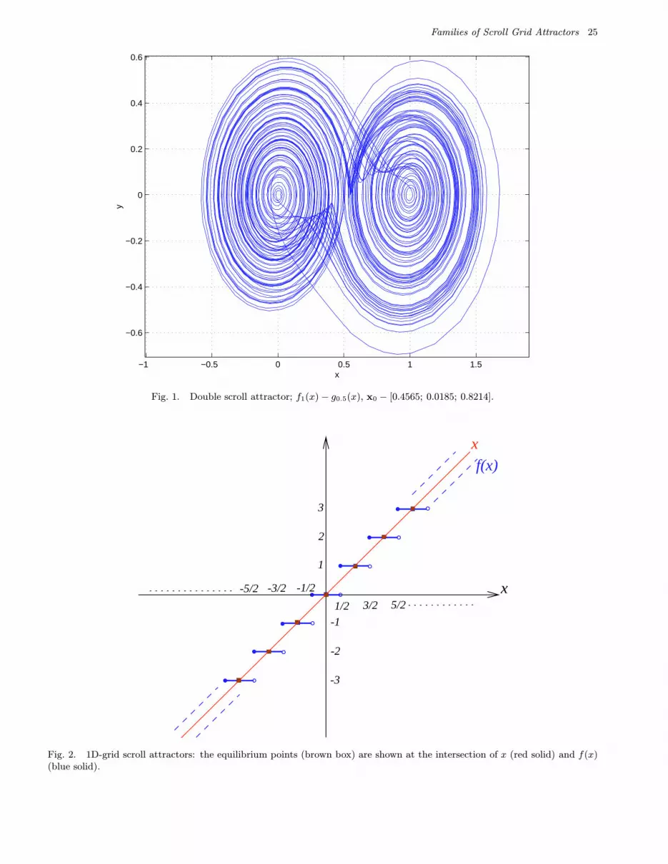
Fig. 1. Double scroll attractor; f1(x)− g0.5(x), x0 − [0.4565; 0.0185; 0.8214].

x3/2 5/21/2

-5/2 -3/2 -1/2

-2

-1

-3

1

2

3

f(x)x

Fig. 2. 1D-grid scroll attractors: the equilibrium points (brown box) are shown at the intersection of x (red solid) and f(x)(blue solid).


given by Yalcın et al. [2000c]. Here, we considera minor modification of the latter model by takingthe nonlinearity

f1(x) =Mx∑i=1

g(−2i+1)

2

(x) +Nx∑i=1

g(2i−1)

2

(x) (3)

where

gθ(ζ) =

1, ζ ≥ θ θ > 0

0, ζ < θ θ > 0

0, ζ ≥ θ θ < 0

−1, ζ < θ θ < 0 .

(4)

A computer simulation for the double scroll attrac-tor is shown in Fig. 1 corresponding to Mx = 0,

Nx = 1 and a = 0.8. A generalization of the systemEq. (1) can be systematically obtained by introduc-ing additional breakpoints in the nonlinearity whereeach breakpoint can be implemented by Eq. (4).Therefore, we call Eq. (4) the core function. Theequilibrium points can be found from the followingset of equations

x = f1(x)

y = 0

z = 0.

The equilibrium points are located at the intersec-tion of the nonlinear function f1(x) and x drawn in

−2 −1.5 −1 −0.5 0 0.5 1 1.5 2−1

−0.8

−0.6

−0.4

−0.2

0

0.2

0.4

0.6

0.8

1

x

y

(a)

−0.5 0 0.5 1 1.5 2 2.5 3 3.5 4 4.5−1

−0.5

0

0.5

1

x

y

(b)

−5 −4 −3 −2 −1 0 1 2 3 4 5 6−1

−0.8

−0.6

−0.4

−0.2

0

0.2

0.4

0.6

0.8

x

y

(c)

Fig. 3. (a) M = 1, N = 1, 3-scroll attractor, x0 = [0.30460; 18970; 1934]; (b) M = 0, N = 4, 5-scroll attractor, x0 =[0.3529; 0.8132; 0.0099]; (c) M = 4, N = 5, 10-scroll attractor, x0 = [0.6721; 0.8381; 0.0196].


−6 −4 −2 0 2 4 6 8 10 12 14−3

−2

−1

0

1

2

3

x

ya=0.1

(a)

−2 −1 0 1 2 3 4 5−0.8

−0.6

−0.4

−0.2

0

0.2

0.4

0.6

0.8

1

1.2

x

y

a=.23

(b)

−1 0 1 2 3 4 5−1.5

−1

−0.5

0

0.5

1

x

y

a=.34

(c)

−1 0 1 2 3 4 5−1

−0.8

−0.6

−0.4

−0.2

0

0.2

0.4

0.6

0.8

1

x

y

a=.37

(d)

−1 0 1 2 3 4 5−1

−0.8

−0.6

−0.4

−0.2

0

0.2

0.4

0.6

0.8

1a=.41

x

y

(e)

−1 0 1 2 3 4 5−1

−0.5

0

0.5

1

1.5

x

y

a=.47

(f)

−1 0 1 2 3 4 5−1

−0.5

0

0.5

1

1.5

x

y

a=.50

(g)

−1 0 1 2 3 4 5−0.8

−0.6

−0.4

−0.2

0

0.2

0.4

0.6

0.8

x

y

a=.61

(h)

−1 0 1 2 3 4 5−0.8

−0.6

−0.4

−0.2

0

0.2

0.4

0.6

0.8

y

x

a=.7

(i)

−1 0 1 2 3 4 5−0.6

−0.4

−0.2

0

0.2

0.4

0.6

0.8

x

y

a=.81

(j)

−0.5 0 0.5 1 1.5 2 2.5 3 3.5 4 4.5−0.5

−0.4

−0.3

−0.2

−0.1

0

0.1

0.2

0.3

0.4

0.5

x

y

a=1

(k)

−0.5 0 0.5 1 1.5 2 2.5 3 3.5 4 4.5−0.3

−0.2

−0.1

0

0.1

0.2

0.3

0.4

x

y

a=2

(l)

Fig. 4. Bifurcations related to 5-scroll attractors with respect to parameter value a: (a) a = 0.1, for five different initialconditions which are close to the equilibrium points; (b) a = 0.23; (c) a = 0.34; (d) a = 0.37; (e) a = 0.41; (f) a = 0.47;(g) a = 0.5; (h) a = 0.61; (i) a = 0.7; (j) a = 0.81, for five different initial conditions which are close to the equilibrium points;(k) a = 1; (1) a = 2.


Fig. 2 for the general case. The set of equilibriumpoints is

Veq =[i; 0; 0]|i = −Mx,−Mx + 1, . . . ,Nx−1,Nx

which are located on the x-axis in state space[Fig. 8(a)]. Due to the location of the equilibriumpoints, this strange attractor family is called 1D-grid scroll attractors. In the attractors, the scrollsare located around the equilibrium points. There-fore, the number of scrolls equals the number ofequilibrium points. The number of scrolls gener-ated from the generalized nonlinearity is equal toMx + Nx + 1. In Fig. 3, 3-, 5- and 10-scroll at-tractors are shown by using the generic model fora = 0.4 and for (Mx = 1, Nx = 1), (Mx = 0,Nx = 4), (Mx = 4, Nx = 5), respectively. Figure 4shows the bifurcation phenomenon with respect tothe parameter value a related to a 5-scroll attractor.

3. 2D-Grid Scroll Attractors

Now we show that it is also possible to increase thenumber of scrolls in the y state variable direction.We start from the same system (1), but with

A =

0 1 0

0 0 1

−a −a −a

, B =

−1 0 0

0 0 0

0 0 a

,

Φ =

f1(y)

0

f2(x)

with

f1(y) =

My∑i=1

g(−2i+1)

2

(y) +

Ny∑i=1

g(2i−1)

2

(y) (5)

and additional nonlinearity

f2(x) =m−1∑i=1

βgpi(x) (6)

where

pi = My + 0.5 + (i− 1)(My +Ny + 1)

β = My +Ny + 1 .

The equilibrium points follow fromx+ y = f2(x)

y = f1(y)

z = 0 .

(7)

The solutions of the second equation of (7) have al-ready been indicated in the previous section, whichwas given by

ueq,y = [−My; . . . ;−1; 0; 1; . . . Ny] .

The points for the x state variable corresponding toeach ueq,y

j are determined in a graphyical way fromthe first equation of (7). The set of equilibriumpoints becomes

Veq = [(i− 1)(My +Ny + 1) + j,−j; 0]

|i = 1, 2, . . . ,m; j = −Ny, . . . ,−1, 0, 1, . . . ,My

It should be noted that the locations of the equilib-rium points are located in the x−y plane [Fig. 8(b)]and the system has a number of m(My + Ny + 1)equilibrium points. For this reason, we will call thisstrange attractor family m × (My + Ny + 1)-scrollgrid attractors. Some resulting 2D-grid scroll at-tractors and their corresponding nonlinearities aregiven by:

• 2 × 2-grid scroll attractor (My = 0, Ny = 1,m = 2) (Fig. 5)

f1(y) = g0.5(y)

f2(x) = 2g0.5(x)

• 2 × 3-grid scroll attractor (My = 0, Ny = 2,m = 2) (Fig. 6)

f1(y) = g0.5(y) + g1.5(y)

f2(x) = 3g0.5(x)

• 3 × 3-grid scroll attractor (My = 0, Ny = 2,m = 3) [Fig. 7(a)]

f1(y) = g0.5(y) + g1.5(y)

f2(x) = 3(g0.5(x) + g3.5(x))

• 4 × 4-grid scroll attractor (My = 0, Ny = 3,m = 4) [Fig. 7(b)]

f1(y) = g0.5(y) + g1.5(y) + g2.5(y)

f2(x) = 4(g0.5(x) + g4.5(x) + g8.5(x))

• 4 × 5-grid scroll attractor (My = 0, Ny = 4,m = 4) [Fig. 7(c)]

f1(y) = g0.5(y) + g1.5(y) + g2.5(y) + g3.5(y)

f2(x) = 5(g0.5(x) + g5.5(x) + g10.5(x))


−2 −1.5 −1 −0.5 0 0.5 1 1.5 2 2.5 3−1

−0.5

0

0.5

1

1.5

2

x

y

(a)

−1 −0.5 0 0.5 1 1.5 2−0.8

−0.6

−0.4

−0.2

0

0.2

0.4

0.6

0.8

y

z

(b)

−2

−1

0

1

2

3

−1

−0.5

0

0.5

1

1.5

2

−1

−0.5

0

0.5

1

yx

z

(c)

Fig. 5. 2 × 2-grid scroll attractor. Projection onto (a) the(x, y) and (b) the (y, z) planes, (c) view on 3D-state space.

−3 −2 −1 0 1 2 3 4−1

−0.5

0

0.5

1

1.5

2

2.5

3

y

x

(a)

−1 −0.5 0 0.5 1 1.5 2 2.5 3−1.5

−1

−0.5

0

0.5

1

1.5

y

z

(b)

−3

−2

−1

0

1

2

3

4−1

−0.50

0.51

1.52

2.53

−2

−1

0

1

2

yx

z

(c)

Fig. 6. 2× 3-grid scroll attractor.


(a)

(b)

(c)

Fig. 7. Projection onto the (x, y) plane of (a) 3×3-, (b) 4×4-and (c) 4× 5-grid scroll attractor.

4. 3D-Grid Scroll Attractors

The following additional nonlinearity f1(z) is intro-duced now to the system (1) with

A =

0 1 0

0 0 1

−a −a −a

, B =

−1 0 0

0 −1 0

0 0 a

,

Φ =

f1(y)

f1(z)

f3(x)

where

f1(z) =Mz∑i=1

g(−2i+1)

2

(z) +Nz∑i=1

g(2i−1)

2

(z) , (8)

and

f3(x) =k−1∑l=1

γgnl(x) (9)

where

nl = ρ+ 0.5 + (l − 1)(ρ+ ς + 1)

γ = ρ+ ς + 1

with

ρ =

∣∣∣∣mini,jueq,y

i + ueq,zj

∣∣∣∣ ,ς =

∣∣∣∣maxi,jueq,y

i + ueq,zj

∣∣∣∣and ueq,y and ueq,z are the vectors for the y andz variables related to the equilibrium points. Theequilibrium points follow from

x+ y + z = f3(x)

y = f1(y)

z = f1(z)

where the points for the y, z variables are given by

ueq,y = [−My; . . . ;−1; 0; 1; . . . ; Ny] ,

ueq,z = [−Mz; . . . ;−1; 0; 1; . . . ;Nz] .

With these nonlinearities the system produces k ×(My+Ny+1)×(Mz +Nz+1)-scroll grid attractors.


All the scrolls are located around the equilibriumpoints which are given

Veq = [(l − 1)(ς + 1 + ρ)− ueq,yi

− ueq,zj ;ueq,y

i ;ueq,zj ]

with i = 1, 2, . . . ,My + Ny + 1, j = 1, 2, . . . ,Mz +Nz + 1 and l = 1, 2, . . . , k. The location of theequilibrium points in 3D is shown in Fig. 8(c).Here, some examples of 3D-grid scroll attractors aregiven:

• 2 × 2 × 2-grid scroll attractor (My = 0, Ny = 1,Mz = 0, Nz = 1, k = 2) (Fig. 9)

f3(x) = 3g0.5(x)

f1(y) = g0.5(y)

f1(z) = g0.5(z)


f3(x) = 3(g0.5(x) + g3.5(x) + g6.5(x))

f1(y) = g0.5(y)

f1(z) = g0.5(z)


f3(x) = 4(g1.5(x) + g5.5(x) + g9.5(x))

f1(y) = g−0.5(y) + g0.5(y)

f1(z) = g0.5(z)

5. Lur’e Representation

The new circuits from which the scroll grid attractorfamilies are generated can be represented as Lur’esystems, i.e. as a linear system interconnected byfeedback to a static nonlinearity that satisfies a sec-tor condition

x = Ax + Bσ(Cx)

with

A =

0 1 0

0 0 1

−a −a −a

, B =

by 0 0

0 bz 0

0 0 a

,

C =

0 1 0

0 0 1

1 0 0

.

y

x

z

0 1 2 3 4-1-2-3-4

(a)

x

y

z

(3,0,0)

(2,1,0)

(1,2,0)

(0,0,0)

(-1,1,0)

(-2,2,0)

(b)

(-2,1,1)

(-1,1,0)

(1,1,1)

(-1,0,1)

(2,0,1)

(3,0,0)

(2,1,0)

(0,0,0)

x

y

z

(c)

Fig. 8. The equilibrium points are located on (a) x axis for1D-grid scroll attractor, (b) (x, y) plane for 2D-grid scroll at-tractor (equilibrium points are shown for 3×3-grid attractor)(c) in a 3D body for 3D-grid scroll attractors (equilibriumpoints are shown for a 2× 2× 2-scroll grid attractor).


−1 −0.5 0 0.5 1 1.5 2−3

−2

−1

0

1

2

3

4

y

x

(a)

−1 −0.5 0 0.5 1 1.5 2−1

−0.5

0

0.5

1

1.5

2

y

z

(b)

−3−2

−10

12

34

−1

−0.5

0

0.5

1

1.5

2−1

−0.5

0

0.5

1

1.5

2

xy

z

(c)

Fig. 9. 2×2×2-grid scroll attractor. Projection onto (a) the(y, x) and (b) the (y, z) planes, (c) view on 3D state space.

−1 −0.5 0 0.5 1 1.5 2−4

−2

0

2

4

6

8

10

y

x

(a)

−1 −0.5 0 0.5 1 1.5 2−1

−0.5

0

0.5

1

1.5

2

y

z

(b)

−4−2

02

46

810

−1

−0.5

0

0.5

1

1.5

2−1

−0.5

0

0.5

1

1.5

2

xy

z

(c)

Fig. 10. 4× 2× 2-grid scroll attractor.


−2 −1.5 −1 −0.5 0 0.5 1 1.5 2−4

−2

0

2

4

6

8

10

12

14

y

x

(a)

−2 −1.5 −1 −0.5 0 0.5 1 1.5 2−1.5

−1

−0.5

0

0.5

1

1.5

2

2.5

y

z

(b)

−5

0

5

10

15

−2

−1

0

1

2−1.5

−1

−0.5

0

0.5

1

1.5

2

2.5

xy

z

(c)

Fig. 11. 4× 3× 2-grid scroll attractor.

One obtains the following for the different cases:

• 1D-scroll grid attractors (n-scroll attractor):by = 0, bz = 0

σ(·) =

0

0

f1(·)

where f1(·) is given by Eq. (3), which belongs tosector [0, 2].

• 2D-scroll grid attractors:by = −1, bz = 0

σ(·) =

f1(·)0

f2(·)

where f2(·) is given by Eq. (6), which belongs tosector [0, (My +Ny + 1)/(My + 0.5)].

• 3D-grid scroll attractors:by = −1, bz = −1

σ(·) =

f1(·)f1(·)f3(·)

where f3(·) is given by Eq. (9), which belongs tosector [0, (ς + ρ+ 1)/(ρ+ 0.5)].

6. Circuit Realizations

In this section, the realizations of some of the 1D-,2D- and 3D-grid scroll attractors discussed aboveare given. For this purpose, a circuit using con-ventional voltage opamps could be employed. How-ever, a number of research results, which illustratethe advantages of current feedback opamps (CFOA)over conventional voltage opamps, have been pre-sented in the literature, e.g. [Toumazou et al., 1990;Fabre, 1993; Toumazou & Lidgey, 1994]. Fromthese works, it is known that CFOA is almost freefrom slew-rate limitations as opposed to voltageopamp. It is capable of operating at much higherfrequencies and offers design flexibility which allowsthe derivation of relatively simpler circuits. Con-sidering these facts, researchers have attempted touse CFOAs in the implementation of chaotic oscil-lators in order to have an improved high-frequencyperformance, e.g. [Senani & Gupta, 1998; Elwakil


VY

C 1R 1

C 1R 1

VX

C 2C 2R

2

R 4C 3C 3

R 1VZ

CFOA

CFOA

CFOA

V

CFOA

R

CFOA

R

V

x1

V

R

cmp

cmpx2

x1

x2

VCC

CCV

V

cmp

RV

cmp

V

V

cmp

V

RV

cmp

Vz1

z2

z2CC

z1CC CC

y1

y2

y2CC

R y1

z1

z2 y2

y1

x2

x1

Fig. 12. Possible circuit diagram realizing the proposed system.

& Kennedy, 1998, 2000]. In the same way, we havealso used a possible CFOA-based circuit in orderto realize and observe some of the scroll grid at-tractors described in the previous sections. Thecircuit we have used for this purpose is given inFig. 12. The CFOAs implemented using AD8441

from Analog Devices and the required nonlineari-ties in Eqs. (5), (8) and (9) are realized using thesubcircuits drawn within the dashed lines. Thecomparators (cmps.) involved in these subcircuitsare of LM311 type comparators. The subcircuitswithin the dashed lines colored in green, red andblue are used to increase the number of scrolls inthe x, y and z state variable directions, respec-tively. Since each of these subcircuits includes two

LM311 comparators, a 3× 3 × 3-grid scroll attrac-tor or 3D-grid scroll attractor can be observed usingthis circuit. Obviously, by appropriately insertingadditional comparators in the corresponding sub-circuit, the number of scrolls can be systematicallyincreased in all directions. Also, by appropriatelyremoving these subcircuits, new circuits allowingthe observation of any 1D- and 2D-grid scroll at-tractors can readily be obtained.

For C1 = C2 = C3 = C, R1 = R, R2 =R4 = R/a, Vx = ax, Vy = ay, Vz = z and us-ing the normalized quantity tn = t/RC, it canbe verified that the circuit realizes the system inEq. (1). Also, as explained above, the nonlineari-ties in Eqs. (5), (8) and (9) are realized using the

1Analog Devices [1990] Linear Products Data Book, Norwood, MA, USA.


subcircuits in red, blue and green, respectively,where the parameters θ of the core functions, gθ(·)in Eq. (4) are adjusted through the controlling volt-ages at the inverting/noninverting inputs of thecomparators. It should be noted that all threestates are available at the buffered output termi-nals of the CFOAs, a property which is expectedto simplify the realizations of various chaotic com-munication systems based on the proposed circuit.Also, the fact that all the capacitors are groundedsimplifies the IC integration of the circuit. In allthe experiments given in this section, CFOAs andLM311 type comparators are supplied under ±15 VDC and the passive component values are taken asC1 = C2 = C3 = 1 nF , R1 = 5.1 kΩ. For allexperiments, different values have been assigned tothe other passive components. Also, the controllingvoltages at the inverting and noninverting inputs ofthe comparators are taken as adjustable.

First, we have implemented a 5-scroll attrac-tor or 1D-grid scroll attractor from the circuit inFig. 12. In order to obtain a 5-scroll attractor inthe x state variable direction, we have removed thesubcircuits in red and blue and added two more

comparators to the subcircuit in green. The passivecomponent values are taken as R2 = R4 = 8 kΩ,Rx1 = Rx2 = Rx3 = Rx4 = 70 kΩ. The observed(Vx, Vy) trajectory is given in Fig. 13(c). Thesepassive component values correspond to a = 0.64.Also, by changing the values of the resistors R2 andR4, the circuit is tested for different values of a, andthe corresponding results are given in Figs. 13(a)–13(d). These results also verify the dynamic behav-ior of the circuit with respect to parameter value a,which was shown on the simulations of Fig. 4.

Second, we have implemented 2×2-, 3×2- and3 × 3-grid scroll attractors from 2D-grid scroll at-tractor family. In order to have a 2×2-grid scroll at-tractor, we have removed the subcircuit in blue, thecomparators cmpx2, cmpy2 and the resistors Rx2,Ry2, from the circuit in Fig. 12. The passive com-ponents values are taken as R2 = R4 = 9.7 kΩ,Rx1 = 37 kΩ, Ry1 = 77 kΩ. The controlling volt-ages, i.e. Vx1, Vy1 are taken identical. The observedphase space corresponding to the (Vx, Vy) trajec-tory is given in Fig. 14. A 3×2-grid scroll attractoris realized by adding a comparator, cmpy2 and aresistor Ry2 to the circuit above which was used to

(a)

Fig. 13. 5-scroll attractor from a 1D-grid scroll attractor. Experimental results shown are for (a) a = 0.26 (R4 = 20 kΩ),(b) a = 0.34 (R4 = 15 kΩ), (c) a = 0.64 (R4 = 8 kΩ), (d) a = 1 (R4 = 5.1 kΩ), (Vx, Vy) trajectory x = 0.5 V/div,y = 0.5 V/div.


(b)

(c)

Fig. 13. (Continued)


(d)


Fig. 14. 2× 2-grid scroll attractor. Experimental result shown is (Vx, Vy) trajectory. x = 0.5 V/div, y = 0.5 V/div.


Fig. 15. 2× 3-grid scroll attractor. Experimental result shown is (Vx, Vy) trajectory. x = 1 V/div, y = 0.5 V/div.

Fig. 16. 3× 3-grid scroll attractor. Experimental result shown in (Vx, Vy) trajectory. x = 1 V/div, y = 0.5 V/div.


(a)

(b)

Fig. 17. 2 × 2 × 2-grid scroll attractor. Experimental results shown are (a) (Vy, Vx) trajectory. x = 1 V/div, y = 2 V/div,(b) (Vz, Vx) trajectory. x = 1 V/div, y = 2 V/div, (c) (Vy, Vz) trajectory. x = 1 V/div, y = 2 V/div.


(c)


realize a 2 × 2-grid scroll attractor. The passivecomponent values are taken as R2 = R4 = 11 kΩ,Rx1 = 27 kΩ, Ry1 = 88 kΩ, Ry2 = 75 kΩ. Thecontrolling voltages Vx1, Vy1 are taken to be iden-tical. The observed (Vx, Vy) trajectory shown inFig. 15 verifies the theory. As a final example ofthe 2D-grid attractor family, we have realized a3 × 3-grid attractor by increasing the number ofcomparators in the subcircuit in green by one. Inthis case, the passive component values are chosenas R2 = R4 = 12 kΩ, Rx1 = 28 kΩ, Rx2 = 30 kΩ,Ry1 = 90 kΩ, Ry2 = 80 kΩ. Again, the measured(Vx, Vy) trajectory is given in Fig. 16.

Finally, a 2 × 2 × 2-grid attractor from the3D-grid attractor family is realized using the cir-cuit in Fig. 12. In order to have a 2 × 2 × 2-gridscroll attractor with My = 0, Ny = 1, Mz = 0,Nz = 1 and k = 2, we have removed the com-parators cmpx2, cmpy2 and cmpz2 in the subcircuitswithin the dashed lines and the passive componentvalues are taken as R2 = R4 = 8.3 kΩ, Rx1 = 19 kΩ,Ry1 = 47 kΩ, Rz1 = 50 kΩ. The controlling volt-ages at the comparator inputs are taken as identi-cal. The experimental results corresponding to the(Vy, Vx), (Vz, Vx) and (Vy, Vz) trajectories are givenin Fig. 17.

7. Conclusions

Since the introduction of Chua’s circuit, severalmulti scroll-based chaotic attractors have been pre-sented in the literature. However, up till now it wasnot possible to generate the scrolls in different di-rections. In this paper, we have shown that it ispossible to create strange attractors whose scrollscan be located in any state variable direction. Fol-lowing the ideas outlined in this paper, the designof new attractors depends on the designer’s imagi-nation, as the presented attractors are just samplesderived from the new proposed family which mightbe further extended in the future. The proposedsystem presented in this work is expected to yieldnew chaotic signal generators which can be usefulin many chaos-based applications.

Acknowledgments

This research work was carried out at the ESAT lab-oratory and the Interdisciplinary Center of NeuralNetworks ICNN of the Katholieke Universiteit Leu-ven, in the framework of the Belgian Programmeon Interuniversity Poles of Attraction, initiatedby the Belgian State, Prime Minister’s Office for


Science, Technology and Culture (IUAP P4-02), theConcerted Action Project MEFISTO of the FlemishCommunity, the FWO project Collective Behaviorand Optimization: an Interdisciplinary Approachand ESPRIT IV 27077 (DICTAM). Johan Suykensis a postdoctoral researcher with the National Fundfor Scientific Research FWO – Flanders.

ReferencesArena, P., Baglio, S., Fortuna, L. & Manganaro, G. [1996]

“Generation of n-double scrolls via cellular neural net-works,” Int. J. Circuit Th. Appl. 24, 241–252.

Chua, L. O., Komuro, M. & Matsumoto, T. [1986] “Thedouble scroll family,” IEEE Trans. Circuits Syst. I33(11), 1072–1118.

Chua, L. O. & Roska, T. [1993] “The CNN paradigm,”IEEE Trans. Circuits Syst. I 40(3), 147–156.

Chua, L. O. [1994] “Chua’s circuit 10 years later,” Int.J. Circuit Th. Appl. 22, 279–305.

Elwakil, A. S. & Kennedy, M. P. [2000] “Improved im-plementation of Chua’s chaotic oscillator using currentfeedback opamp,” IEEE Trans. Circuits Syst. I 47(1),76–79.

Elwakil, A. S., Salama, K. N. & Kennedy, M. P. [2000] “Asystem for chaos generation and its implementation inmonolithic form,” Proc. IEEE Int. Symp. Circuits andSystems (ISCAS 2000) (V), pp. 217–220.

Fabre, A. [1993] “Insensitive voltage-mode and current-mode filters from commercially available trans-impedance op-amps,” IEE Proc. G 140(5), 319–321.

Hasler, M. [1994] “Synchronization principles and appli-cations,” Circuit & Systems: Tutorials IEEE-ISCAS’94, pp. 314–326.

Kapitaniak, T. & Chua, L. O. [1994] “Hyperchaotic at-tractors of unidirectionally-coupled Chua’s circuit,”Int. J. Bifurcation and Chaos 4(2), 477–482.

Kataoka, M. & Saito, T. [2000] “A 4-D chaotic oscil-lator with a hysteresis 2-Port VCCS,” Proc. IEEEInt. Symp. Circuits and Systems (ISCAS 2000) (V),pp. 418–421.

Khalil, H. K. [1993] Nonlinear Systems (MacmillanPublishing Company, NY).

Kolumban, G., Kennedy, M. P. & Chua, L. O. [1998]“The role of synchronization in digital communica-

tions using chaos-Part II: Chaotic modulation of dig-ital communications,” IEEE Trans. Circuits Syst. I45(11), 1129–1140.

Madan, R. N. [1993] Chua’s Circuit: A Paradigm forChaos (World Scientific, Singapore).

Saito, T. [1990] “An approach toward higher dimensionalhysteresis chaos generators,” IEEE Trans. CircuitsSyst. I 37(3), 399–409.

Senani, R. & Gupta, S. S. [1998] “Implementationof Chua’s chaotic circuits using current feedbackopamps,” Electron. Lett. 34(9), 829–830.

Suykens, J. A. K. & Vandewalle, J. [1993] “Generationof n-double scrolls (n = 1, 2, 3, 4, . . .),” IEEE Trans.Circuits Syst. I 40(11), 861–867.

Suykens, J. A. K. & Chua, L. O. [1997] “n-Double scrollhypercubes in 1-D CNNs,” Int. J. Bifurcation andChaos 7(8), 1873–1885.

Suykens, J. A. K., Huang, A. & Chua, L. O. [1997] “Afamily of n-scroll attractors from a generalized Chua’scircuit,” Archiv fur Elektronik und Ubertragungstech-nik (Int. J. Electronics and Communications) 51(3),131–138.

Suykens, J. A. K., Curran, P. F. & Chua, L. O. [1999]“Robust synthesis for master–slave synchronization ofLur’e Systems,” IEEE Trans. Circuits Syst. I 46(7),841–850.

Toumazou, C., Lidgey, F. J. & Haigh, D. Q. [1990] AnalogIC Design: The Current Mode Approach (Peter Pere-grinus, London).

Toumazou, C. & Lidgey, F. J. [1994] “Current feedbackop-amps: A blessing in disguise?” IEEE Circuits De-vices Mag. 10(1), 43–47.

Vidyasagar, M. [1993] Nonlinear Systems Analysis(Prentice-Hall).

Yalcın, M. E., Suykens, J. A. K. & Vandewalle, J. [2000a]“Experimental confirmation of 3- and 5-scroll attrac-tors from a generalized Chua’s circuit,” IEEE Trans.Circuits Syst. I 47(3), 425–429.

Yalcın, M. E., Suykens, J. A. K. & Vandewalle, J. [2000b]“Hyperchaotic n-scroll attractors,” Proc. IEEE Work-shop on Nonlinear Dynamics of Electronic Systems(NDES 2000), pp. 25–28.

Yalcın, M. E., Ozoguz, S., Suykens, J. A. K. &Vandewalle, J. [2000c] “n-Scroll chaos generators: Asimple circuit model,” Electron. Lett. 37(3), 147–148.

families of scroll grid attractors

Documents