International Journal of Bifurcation and Chaos, Vol. 17, No. 9 (2007) 3235–3251c© World Scientific Publishing Company

ON A DYNAMICAL SYSTEM WITHMULTIPLE CHAOTIC ATTRACTORS

XIAODONG LUO and MICHAEL SMALLDepartment of Electronic and Information Engineering,

Hong Kong Polytechnic University, Hong Kong, P. R. China

MARIUS-F. DANCADepartment of Applied Sciences, Avram Iancu University,

Cluj-Napoca, Romania

GUANRONG CHENDepartment of Electronic Engineering, City University of Hong Kong,

Hong Kong, P. R. China

Received May 18, 2006; Revised July 6, 2006

The chaotic behavior of the Rabinovich–Fabrikant system, a model with multiple topologicallydifferent chaotic attractors, is analyzed. Because of the complexity of this system, analyticaland numerical studies of the system are very difficult tasks. Following the investigation of thissystem carried out in [Danca & Chen, 2004], this paper verifies the presence of multiple chaoticattractors in the system. Moreover, the Monte Carlo hypothesis test (or, equivalently, surrogatedata test) is applied to the system for the detection of chaos.

Keywords : Rabinovich–Fabrikant system; multiple attractors; LIL algorithm; chaos detection;Monte Carlo hypothesis test; surrogate data test.

1. Introduction

Chaotic systems with multiple attractors havereceived increasing attention in recent years becauseof their great impact on both theoretical analysisand engineering applications. Studies have revealedthat multiattractors could be considered a source ofunpredictability [Dutta et al., 1999], and they havesome potential applications in, for instance, com-munications [Carroll & Pecora, 1998], mechanicaldynamics [Lowenberg, 1998; Zhou et al., 2001], andecology [Anand & Desrochers, 2004].

There are some, though not too many,lower-dimensional dynamical systems with mul-tiple chaotic attractors. For example, a three-dimensional autonomous quadratic chaotic system,which has five equilibria and could produce twotwo-wing chaotic attractors, is designed and studied

in [Lu et al., 2004]. As another example, recentlyreported in [Qi et al., 2005], a four-dimensionalautonomous cubic system, generated through theso-called “proto-Lorenz systems”, could yield four-wing chaotic attractors. More examples and studiescan be found in [Chua et al., 1986; Han et al., 2005;Liu & Chen, 2004; Lu et al., 2003; Suykens & Van-derwalle, 1993; Yalcin et al., 2001].

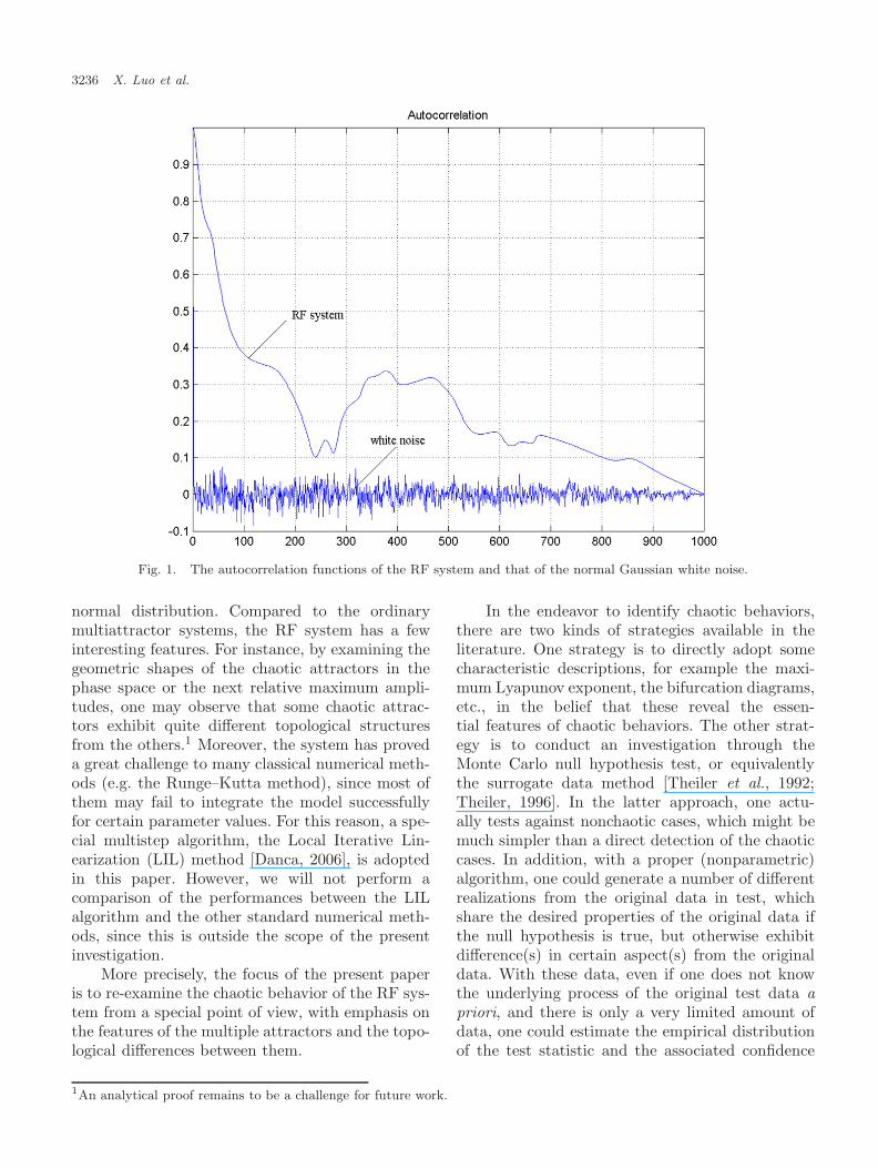
A more specific example with multiple attrac-tors will be further studied in this paper — theRabinovich–Fabrikant system (called the “RF sys-tem” hereafter). This RF system arises from thepractical demand of modeling the stochasticity dueto the modulation instability in a nonequilibriumdissipative medium [Rabinovich & Fabrikant, 1979].As indicated in Fig. 1, a pronounced chaotic behav-ior can be observed from the autocorrelation func-tion of the RF system versus the white noise with

3235

3236 X. Luo et al.

Fig. 1. The autocorrelation functions of the RF system and that of the normal Gaussian white noise.

normal distribution. Compared to the ordinarymultiattractor systems, the RF system has a fewinteresting features. For instance, by examining thegeometric shapes of the chaotic attractors in thephase space or the next relative maximum ampli-tudes, one may observe that some chaotic attrac-tors exhibit quite different topological structuresfrom the others.1 Moreover, the system has proveda great challenge to many classical numerical meth-ods (e.g. the Runge–Kutta method), since most ofthem may fail to integrate the model successfullyfor certain parameter values. For this reason, a spe-cial multistep algorithm, the Local Iterative Lin-earization (LIL) method [Danca, 2006], is adoptedin this paper. However, we will not perform acomparison of the performances between the LILalgorithm and the other standard numerical meth-ods, since this is outside the scope of the presentinvestigation.

More precisely, the focus of the present paperis to re-examine the chaotic behavior of the RF sys-tem from a special point of view, with emphasis onthe features of the multiple attractors and the topo-logical differences between them.

In the endeavor to identify chaotic behaviors,there are two kinds of strategies available in theliterature. One strategy is to directly adopt somecharacteristic descriptions, for example the maxi-mum Lyapunov exponent, the bifurcation diagrams,etc., in the belief that these reveal the essen-tial features of chaotic behaviors. The other strat-egy is to conduct an investigation through theMonte Carlo null hypothesis test, or equivalentlythe surrogate data method [Theiler et al., 1992;Theiler, 1996]. In the latter approach, one actu-ally tests against nonchaotic cases, which might bemuch simpler than a direct detection of the chaoticcases. In addition, with a proper (nonparametric)algorithm, one could generate a number of differentrealizations from the original data in test, whichshare the desired properties of the original data ifthe null hypothesis is true, but otherwise exhibitdifference(s) in certain aspect(s) from the originaldata. With these data, even if one does not knowthe underlying process of the original test data apriori, and there is only a very limited amount ofdata, one could estimate the empirical distributionof the test statistic and the associated confidence

1An analytical proof remains to be a challenge for future work.

On a Dynamical System with Multiple Chaotic Attractors 3237

interval under the null hypothesis, as will be shownlater in the paper.

With the above motivations, in this paper weapply the surrogate data method to detect thechaotic behaviors of the RF system, which providesa good complement to the existing investigationsusing the conventional concepts like the Lyapunovexponent spectrum, histograms, Poincare sections,first return map of the relative maximum, bifurca-tion diagrams, etc. [Danca & Chen, 2004].

The rest of the paper is organized as follows: InSec. 2, a brief introduction is presented to describethe mathematical model of the RF system. A fur-ther investigation of the chaotic behaviors of the RFsystem is carried out in Sec. 3, based on the surro-gate data method, where the multiattractor featureof the RF system will also be discussed. Section 4briefly concludes the investigation of the paper.

2. The Rabinovich–Fabrikant System

The Rabinovich–Fabrikant (RF) system isdescribed by the following equations:

x1 = x2(x3 − 1 + x21) + ax1,

x2 = x1(3x3 + 1 − x21) + ax2,

x3 = −2x3(b + x1x2),(1)

with parameters a, b > 0. This system models thedynamical behavior arising from the modulationinstability in a nonequilibrium dissipative medium[Rabinovich & Fabrikant, 1979].

The RF model (1) has the following five hyper-bolic equilibria points:

X∗(0, 0, 0),

X∗1,2

(±x−,− b

x−, 1 −

(1 − a

b

)x2−

),

X∗3,4

(±x+,− b

x+, 1 −

(1 − a

b

)x2

+

),

with

x± =

√√√√√√√√1 ±

√

1 − ab

(1 − 3a

4b

)

2(

1 − 3a4b

) .

Denote the smooth real-valued function on theright-hand side of model (1) in the form off = ( f1(x1, x2, x3), f2(x1, x2, x3), f3(x1, x2, x3))T .

Then, it is easy to see that the system has the fol-lowing symmetry:

f1(−x1,−x2, x3) = −f1(x1, x2, x3),f2(−x1,−x2, x3) = −f2(x1, x2, x3),

f3(−x1,−x2,−x3) = −f3(x1, x2, x3),

which influences the geometry of the attractors. Inaddition, the divergence of the system is

∇ · f(x1, x2, x3) =3∑

i=1

∂

∂xifi(x1, x2, x3) = 2(a − b),

which implies that the system is dissipative fora < b, since the volume of the system contractsaccording to the Liouville formula.

Notice that the system behavior is very sensi-tive to the parameter b. Therefore, for most casesdiscussed in [Danca & Chen, 2004] the parame-ter a is fixed 0.1, with the parameter b beingin the interval (0.13, 1.3). As supplementary exam-ples, we do consider a few cases with a #= 0.1 andb /∈ (0.13, 1.3). Specifically, the parameters val-ues (a, b) to be re-examined in this work include:{(0.1, 0.2715), (0.1, 0.2876), (0.1, 0.98), (0.1, 1.215),(0.05, 0.06), (−1,−0.2)2}. For more details, see[Danca & Chen, 2004].

3. Chaotic Behaviors of the RFSystem

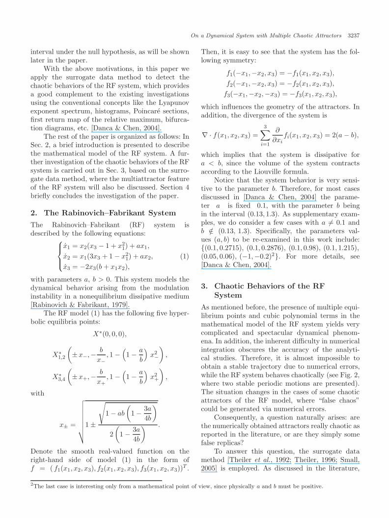
As mentioned before, the presence of multiple equi-librium points and cubic polynomial terms in themathematical model of the RF system yields verycomplicated and spectacular dynamical phenom-ena. In addition, the inherent difficulty in numericalintegration obscures the accuracy of the analyti-cal studies. Therefore, it is almost impossible toobtain a stable trajectory due to numerical errors,while the RF system behaves chaotically (see Fig. 2,where two stable periodic motions are presented).The situation changes in the cases of some chaoticattractors of the RF model, where “false chaos”could be generated via numerical errors.

Consequently, a question naturally arises: arethe numerically obtained attractors really chaotic asreported in the literature, or are they simply somefalse replicas?

To answer this question, the surrogate datamethod [Theiler et al., 1992; Theiler, 1996; Small,2005] is employed. As discussed in the literature,

2The last case is interesting only from a mathematical point of view, since physically a and b must be positive.

3238 X. Luo et al.

Fig. 2. Two periodic motions of period 8 for the case of a = 0.1 and b = 0.05.

the elements that form the framework of a surro-gate test are null hypothesis, surrogate generationalgorithm, discriminating statistic and discriminat-ing criterion. Since, in the present case, the pseudo-periodic time series is either chaotic or periodic butcontaminated with dynamical noise (round errors,for example), the following null hypothesis is formu-lated: The pseudo-periodic time series was gener-ated from a periodic orbit perturbed by uncorrelateddynamical noise, while the alternative hypothesis isthat the time series is chaotic, and the potentialrisk is considered as the false rejection rate, whichwill be analyzed below.

The method for surrogate generation followsthe pseudo-periodic surrogate (PPS) algorithm[Small et al., 2001; Small, 2005]. As a popularchoice, the correlation dimension [Grassberger &Procaccia, 1983] is chosen as the discriminatingstatistic here, while the adopted discriminating cri-terion is extended from the nonparametric methodproposed in [Theiler & Prichard, 1997]. Specifically,the discriminating criterion examines the ranks ofthe statistic values of the original time series andits surrogates (for this reason, we call it ranking cri-terion hereafter). Suppose that the discriminatingstatistic of the original data is T0 and the surro-gate values are {Ti}N

i=1, given N surrogate realiza-tions. Then, one sorts the set {T0, T1, . . . , TN} in

ascending order. Let the rank of T0 be denoted byR0, and the median of the set {1, 2, . . . , N + 1} bedenoted by M . For one-sided tests, if R0 < M , thefalse rejection rate is R0/(N + 1) to reject the nullhypothesis; otherwise, it is (N + 2 − R0)/(N + 1).For two-sided tests, however, if R0 < M then therate is thought to be 2R0/(N + 1) to reject thenull hypothesis; otherwise, it is estimated to be2(N + 2 − R0)/(N + 1).

In the following, we apply the above frame-work to re-examine several chaotic cases reportedin [Danca & Chen, 2004]. In all the tests, the timeseries measured from the first coordinate x1 will beconsidered, and the PPS algorithm will be appliedto produce 100 surrogates. For numerical compu-tation of the correlation dimensions, it is recom-mended to adopt the Gaussian kernel algorithm(GKA) [Diks, 1996; Yu, 2000] because of its effi-ciency and robustness against noise. But, to speedup the calculation, only 2000 data points are usedas the reference points in computation. Therefore,there are some statistical fluctuations even for thesame data set in calculating its correlation dimen-sion. For this reason, the correlation dimension ofthe original time series will be calculated 100 timesto estimate the mean value and the standard devi-ation. For the 100 surrogates, however, they willonly be calculated once for simplicity. These test

On a Dynamical System with Multiple Chaotic Attractors 3239

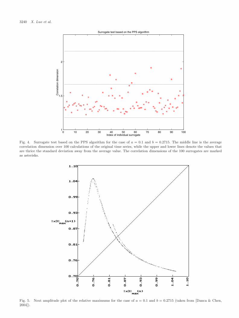
results will be plotted together into the related plots(see, for example, Figs. 4, 7, 10, and so on), wherethe middle lines denote the mean correlation dimen-sions for 100 times calculations of the original timeseries, and the upper and lower lines represent thevalues that are three times the standard deviationaway from the mean correlation value. Finally, thecorrelation dimensions of the 100 surrogates aremarked by the asterisks.

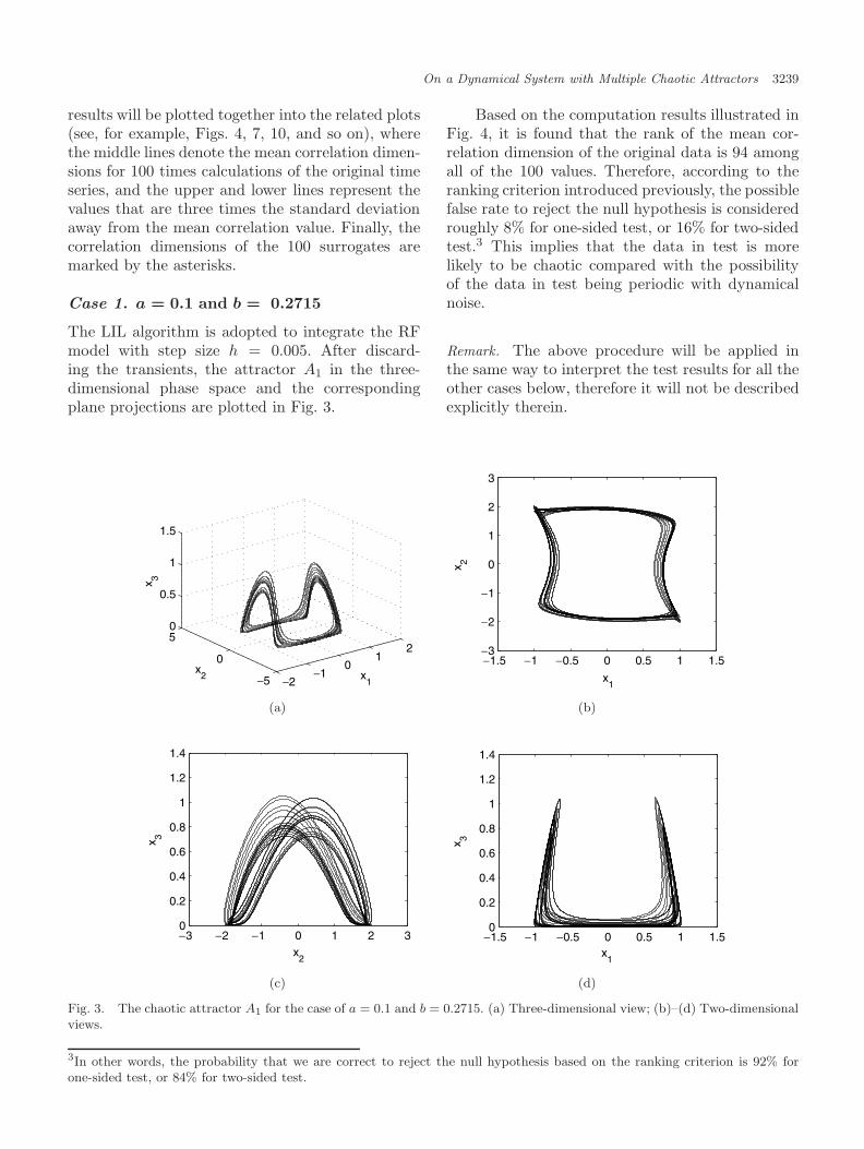
Case 1. a = 0.1 and b = 0.2715

The LIL algorithm is adopted to integrate the RFmodel with step size h = 0.005. After discard-ing the transients, the attractor A1 in the three-dimensional phase space and the correspondingplane projections are plotted in Fig. 3.

Based on the computation results illustrated inFig. 4, it is found that the rank of the mean cor-relation dimension of the original data is 94 amongall of the 100 values. Therefore, according to theranking criterion introduced previously, the possiblefalse rate to reject the null hypothesis is consideredroughly 8% for one-sided test, or 16% for two-sidedtest.3 This implies that the data in test is morelikely to be chaotic compared with the possibilityof the data in test being periodic with dynamicalnoise.

Remark. The above procedure will be applied inthe same way to interpret the test results for all theother cases below, therefore it will not be describedexplicitly therein.

−2−1

01

2

−5

0

50

0.5

1

1.5

x1

x2

x 3

−1.5 −1 −0.5 0 0.5 1 1.5−3

−2

−1

0

1

2

3

x1

x 2

(a) (b)

−3 −2 −1 0 1 2 30

0.2

0.4

0.6

0.8

1

1.2

1.4

x2

x 3

−1.5 −1 −0.5 0 0.5 1 1.50

0.2

0.4

0.6

0.8

1

1.2

1.4

x1

x 3

(c) (d)

Fig. 3. The chaotic attractor A1 for the case of a = 0.1 and b = 0.2715. (a) Three-dimensional view; (b)–(d) Two-dimensionalviews.

3In other words, the probability that we are correct to reject the null hypothesis based on the ranking criterion is 92% forone-sided test, or 84% for two-sided test.

3240 X. Luo et al.

0 10 20 30 40 50 60 70 80 90 1001

1.5

2

Index of individual surrogate

Cor

rela

tion

dim

ensi

on

Surrogate test based on the PPS algorithm

Fig. 4. Surrogate test based on the PPS algorithm for the case of a = 0.1 and b = 0.2715. The middle line is the averagecorrelation dimension over 100 calculations of the original time series, while the upper and lower lines denote the values thatare thrice the standard deviation away from the average value. The correlation dimensions of the 100 surrogates are markedas asterisks.

Fig. 5. Next amplitude plot of the relative maximums for the case of a = 0.1 and b = 0.2715 (taken from [Danca & Chen,2004]).

On a Dynamical System with Multiple Chaotic Attractors 3241

−20

2

−2

0

20

0.5

1

x1

x2

x 3

−2 −1 0 1 2−2

−1

0

1

2

x1

x 2

(a) (b)

−2 −1 0 1 20

0.2

0.4

0.6

0.8

1

x2

x 3

−2 −1 0 1 20

0.2

0.4

0.6

0.8

1

x1

x 3

(c) (d)

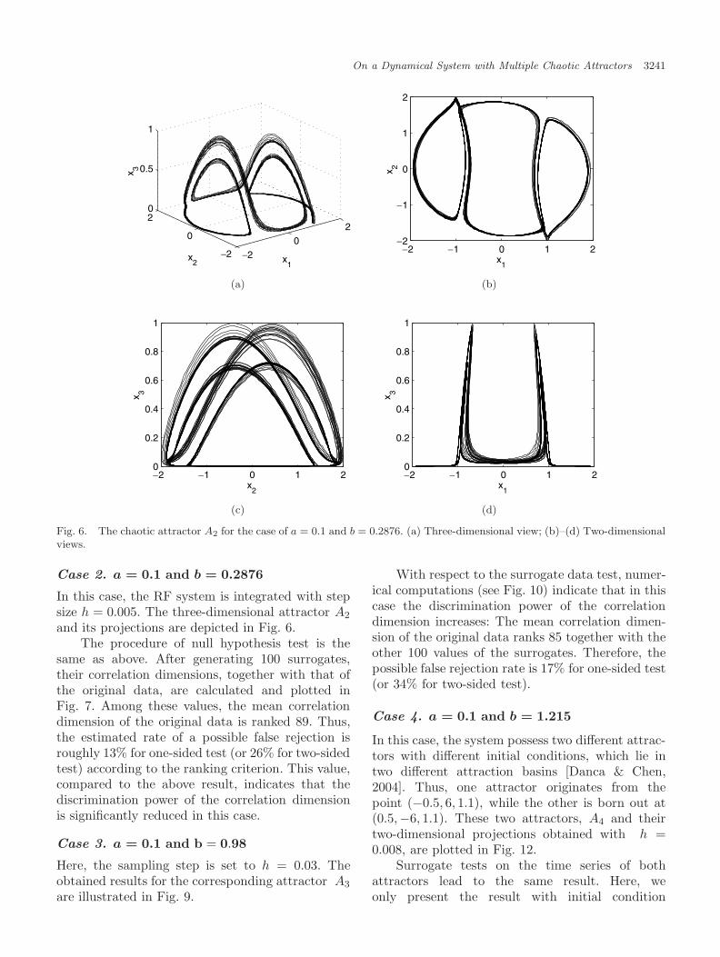
Fig. 6. The chaotic attractor A2 for the case of a = 0.1 and b = 0.2876. (a) Three-dimensional view; (b)–(d) Two-dimensionalviews.

Case 2. a = 0.1 and b = 0.2876

In this case, the RF system is integrated with stepsize h = 0.005. The three-dimensional attractor A2

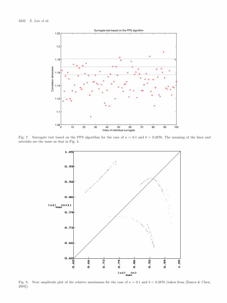
and its projections are depicted in Fig. 6.The procedure of null hypothesis test is the

same as above. After generating 100 surrogates,their correlation dimensions, together with that ofthe original data, are calculated and plotted inFig. 7. Among these values, the mean correlationdimension of the original data is ranked 89. Thus,the estimated rate of a possible false rejection isroughly 13% for one-sided test (or 26% for two-sidedtest) according to the ranking criterion. This value,compared to the above result, indicates that thediscrimination power of the correlation dimensionis significantly reduced in this case.

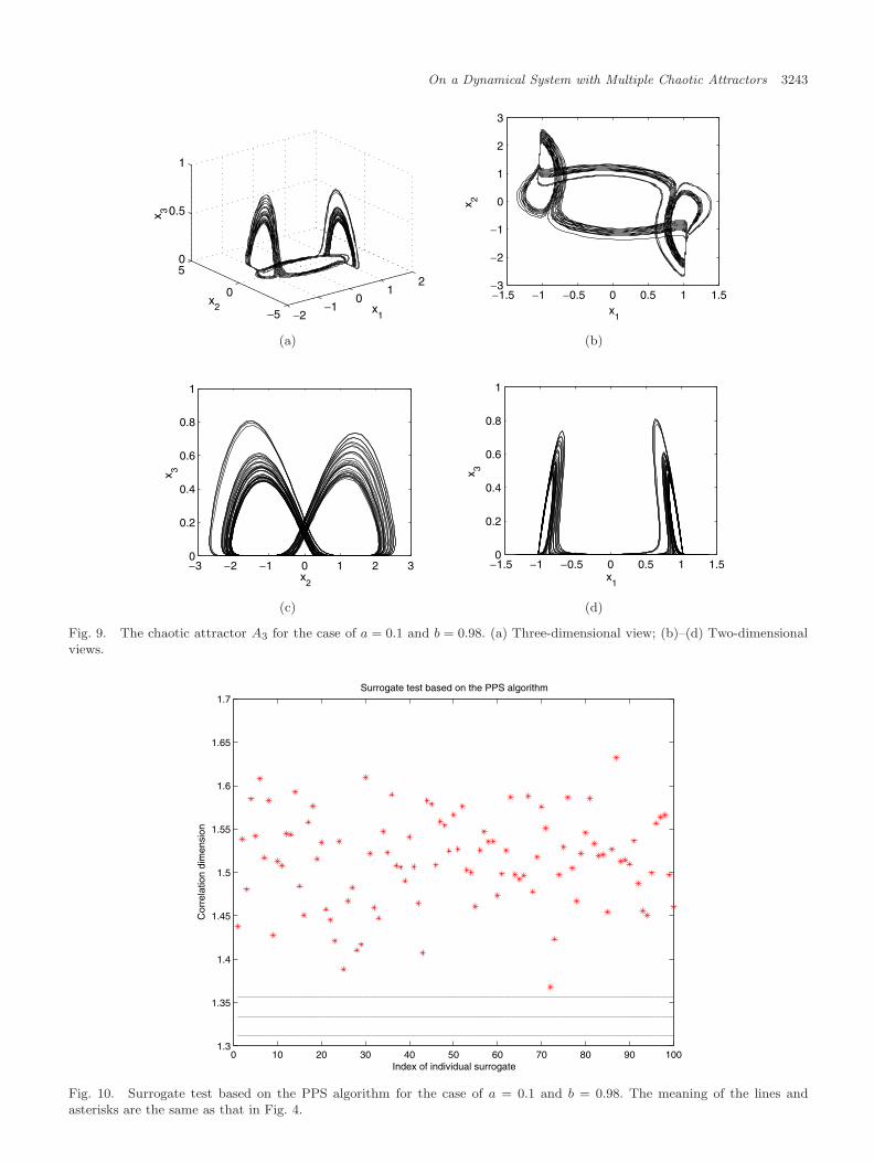
Case 3. a = 0.1 and b = 0.98

Here, the sampling step is set to h = 0.03. Theobtained results for the corresponding attractor A3

are illustrated in Fig. 9.

With respect to the surrogate data test, numer-ical computations (see Fig. 10) indicate that in thiscase the discrimination power of the correlationdimension increases: The mean correlation dimen-sion of the original data ranks 85 together with theother 100 values of the surrogates. Therefore, thepossible false rejection rate is 17% for one-sided test(or 34% for two-sided test).

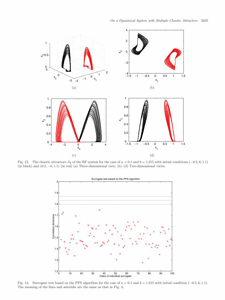
Case 4. a = 0.1 and b = 1.215

In this case, the system possess two different attrac-tors with different initial conditions, which lie intwo different attraction basins [Danca & Chen,2004]. Thus, one attractor originates from thepoint (−0.5, 6, 1.1), while the other is born out at(0.5,−6, 1.1). These two attractors, A4 and theirtwo-dimensional projections obtained with h =0.008, are plotted in Fig. 12.

Surrogate tests on the time series of bothattractors lead to the same result. Here, weonly present the result with initial condition

3242 X. Luo et al.

0 10 20 30 40 50 60 70 80 90 1001.08

1.1

1.12

1.14

1.16

1.18

1.2

1.22

Index of individual surrogate

Cor

rela

tion

dim

ensi

on

Surrogate test based on the PPS algorithm

Fig. 7. Surrogate test based on the PPS algorithm for the case of a = 0.1 and b = 0.2876. The meaning of the lines andasterisks are the same as that in Fig. 4.

Fig. 8. Next amplitude plot of the relative maximums for the case of a = 0.1 and b = 0.2876 (taken from [Danca & Chen,2004]).

On a Dynamical System with Multiple Chaotic Attractors 3243

−2−1

01

2

−5

0

50

0.5

1

x1

x2

x 3

−1.5 −1 −0.5 0 0.5 1 1.5−3

−2

−1

0

1

2

3

x1

x 2

(a) (b)

−3 −2 −1 0 1 2 30

0.2

0.4

0.6

0.8

1

x2

x 3

−1.5 −1 −0.5 0 0.5 1 1.50

0.2

0.4

0.6

0.8

1

x1

x 3

(c) (d)

Fig. 9. The chaotic attractor A3 for the case of a = 0.1 and b = 0.98. (a) Three-dimensional view; (b)–(d) Two-dimensionalviews.

0 10 20 30 40 50 60 70 80 90 1001.3

1.35

1.4

1.45

1.5

1.55

1.6

1.65

1.7

Index of individual surrogate

Cor

rela

tion

dim

ensi

on

Surrogate test based on the PPS algorithm

Fig. 10. Surrogate test based on the PPS algorithm for the case of a = 0.1 and b = 0.98. The meaning of the lines andasterisks are the same as that in Fig. 4.

3244 X. Luo et al.

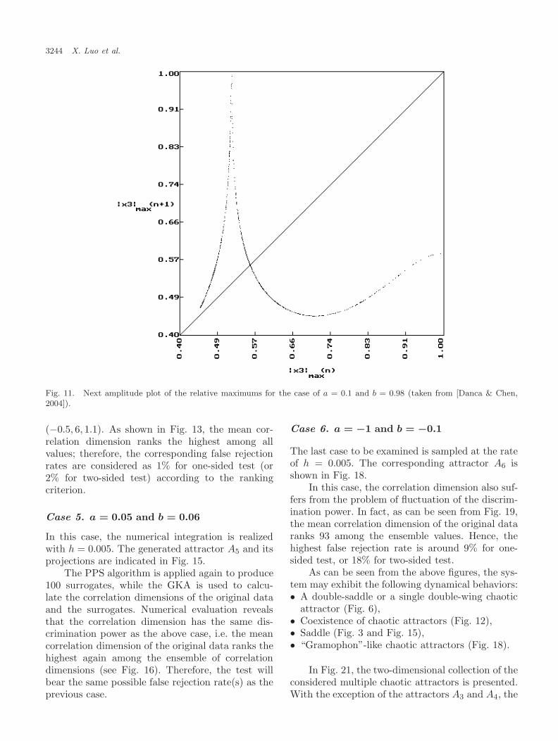
Fig. 11. Next amplitude plot of the relative maximums for the case of a = 0.1 and b = 0.98 (taken from [Danca & Chen,2004]).

(−0.5, 6, 1.1). As shown in Fig. 13, the mean cor-relation dimension ranks the highest among allvalues; therefore, the corresponding false rejectionrates are considered as 1% for one-sided test (or2% for two-sided test) according to the rankingcriterion.

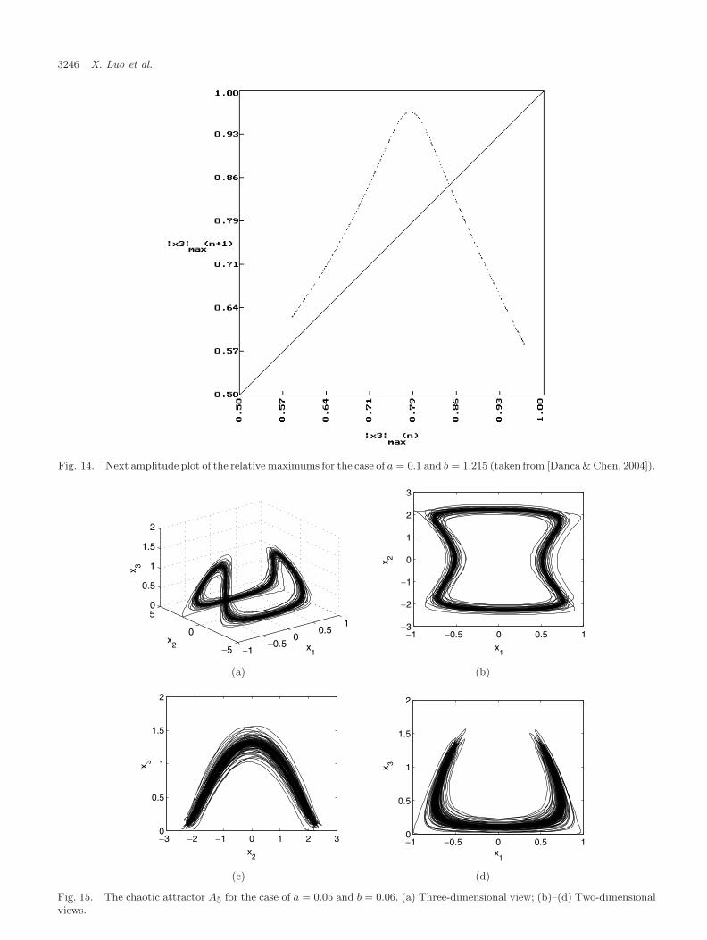
Case 5. a = 0.05 and b = 0.06

In this case, the numerical integration is realizedwith h = 0.005. The generated attractor A5 and itsprojections are indicated in Fig. 15.

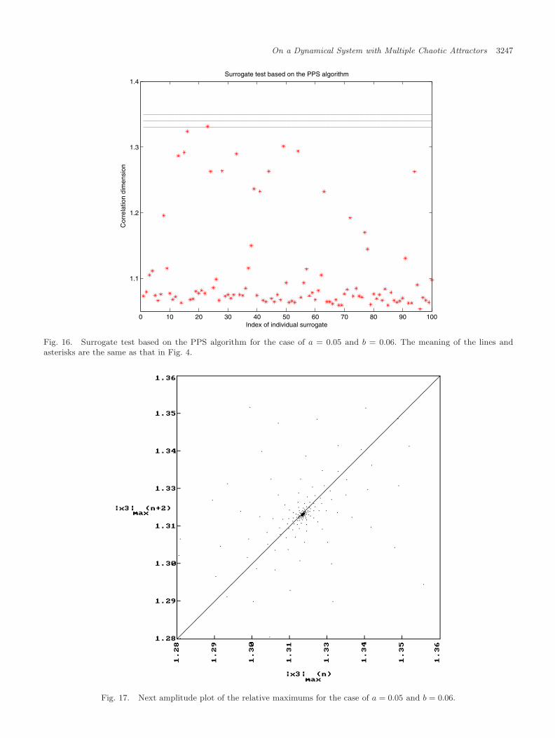
The PPS algorithm is applied again to produce100 surrogates, while the GKA is used to calcu-late the correlation dimensions of the original dataand the surrogates. Numerical evaluation revealsthat the correlation dimension has the same dis-crimination power as the above case, i.e. the meancorrelation dimension of the original data ranks thehighest again among the ensemble of correlationdimensions (see Fig. 16). Therefore, the test willbear the same possible false rejection rate(s) as theprevious case.

Case 6. a = !1 and b = !0.1

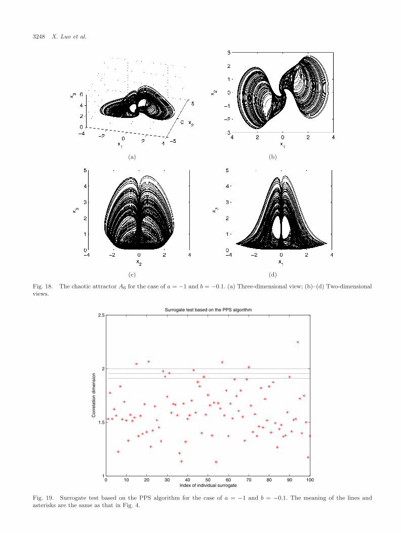
The last case to be examined is sampled at the rateof h = 0.005. The corresponding attractor A6 isshown in Fig. 18.

In this case, the correlation dimension also suf-fers from the problem of fluctuation of the discrim-ination power. In fact, as can be seen from Fig. 19,the mean correlation dimension of the original dataranks 93 among the ensemble values. Hence, thehighest false rejection rate is around 9% for one-sided test, or 18% for two-sided test.

As can be seen from the above figures, the sys-tem may exhibit the following dynamical behaviors:• A double-saddle or a single double-wing chaotic

attractor (Fig. 6),• Coexistence of chaotic attractors (Fig. 12),• Saddle (Fig. 3 and Fig. 15),• “Gramophon”-like chaotic attractors (Fig. 18).

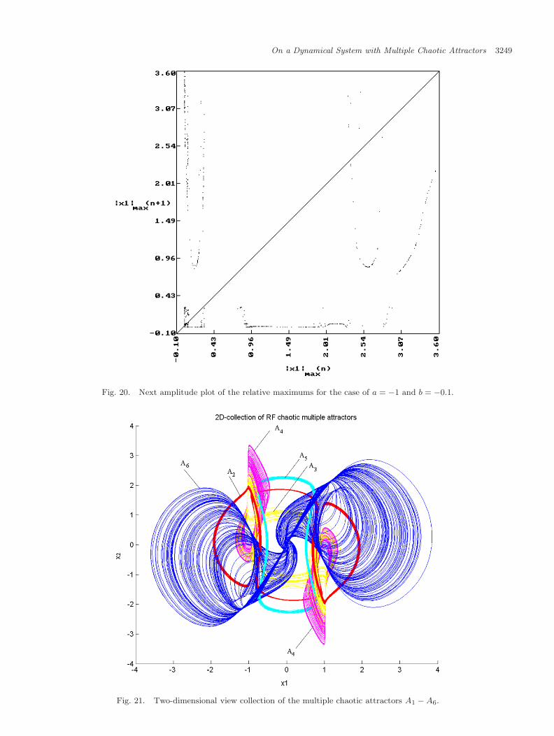
In Fig. 21, the two-dimensional collection of theconsidered multiple chaotic attractors is presented.With the exception of the attractors A3 and A4, the

On a Dynamical System with Multiple Chaotic Attractors 3245

−2−1

0 1

2

−5

0

5 0

0.5

1

x1

x2

x 3

−1.5 −1 −0.5 0 0.5 1 1.5 −4

−2

0

2

4

x1

x 2

(a) (b)

−4 −2 0 2 4 0

0.2

0.4

0.6

0.8

1

x2

x 3

−1.5 −1 −0.5 0 0.5 1 1.5 0

0.2

0.4

0.6

0.8

1

x1

x 3

(c) (d)

Fig. 12. The chaotic attractors A4 of the RF system for the case of a = 0.1 and b = 1.215 with initial conditions (−0.5, 6, 1.1)(in black) and (0.5,−6, 1.1) (in red) (a) Three-dimensional view; (b)–(d) Two-dimensional views.

0 10 20 30 40 50 60 70 80 90 1001.2

1.3

1.4

1.5

1.6

1.7

1.8

1.9

2

Index of individual surrogate

Cor

rela

tion

dim

ensi

on

Surrogate test based on the PPS algorithm

Fig. 13. Surrogate test based on the PPS algorithm for the case of a = 0.1 and b = 1.215 with initial condition (−0.5, 6, 1.1).The meaning of the lines and asterisks are the same as that in Fig. 4.

3246 X. Luo et al.

Fig. 14. Next amplitude plot of the relative maximums for the case of a = 0.1 and b = 1.215 (taken from [Danca & Chen, 2004]).

−1−0.5

00.5

1

−5

0

50

0.5

1

1.5

2

x1

x2

x 3

−1 −0.5 0 0.5 1−3

−2

−1

0

1

2

3

x1

x 2

(a) (b)

−3 −2 −1 0 1 2 30

0.5

1

1.5

2

x2

x 3

−1 −0.5 0 0.5 10

0.5

1

1.5

2

x1

x 3

(c) (d)

Fig. 15. The chaotic attractor A5 for the case of a = 0.05 and b = 0.06. (a) Three-dimensional view; (b)–(d) Two-dimensionalviews.

On a Dynamical System with Multiple Chaotic Attractors 3247

0 10 20 30 40 50 60 70 80 90 100

1.1

1.2

1.3

1.4

Index of individual surrogate

Cor

rela

tion

dim

ensi

on

Surrogate test based on the PPS algorithm

Fig. 16. Surrogate test based on the PPS algorithm for the case of a = 0.05 and b = 0.06. The meaning of the lines andasterisks are the same as that in Fig. 4.

Fig. 17. Next amplitude plot of the relative maximums for the case of a = 0.05 and b = 0.06.

3248 X. Luo et al.

(a) (b)

(c) (d)

Fig. 18. The chaotic attractor A6 for the case of a = −1 and b = −0.1. (a) Three-dimensional view; (b)–(d) Two-dimensionalviews.

0 10 20 30 40 50 60 70 80 90 1001

1.5

2

2.5

Index of individual surrogate

Cor

rela

tion

dim

ensi

on

Surrogate test based on the PPS algorithm

Fig. 19. Surrogate test based on the PPS algorithm for the case of a = −1 and b = −0.1. The meaning of the lines andasterisks are the same as that in Fig. 4.

On a Dynamical System with Multiple Chaotic Attractors 3249

Fig. 20. Next amplitude plot of the relative maximums for the case of a = −1 and b = −0.1.

Fig. 21. Two-dimensional view collection of the multiple chaotic attractors A1 − A6.

3250 X. Luo et al.

rest of the attractors belong to different regions ofthe phase space.

The topological difference between all theseattractors can also be observed from the pro-nounced differences between their first return mapsof the relative maximum amplitude (see Figs. 5,8, 11, 14, 17 and 20). As is well known, thesethin sheets are almost one-dimensional maps, fromwhich chaos can be predicted.

It is interesting to note that usually the mapslike those plotted in Figs. 11 and 14 may pro-duce intermittency. Another intriguing aspect is theresemblance between these maps and those of somewell-known attractors. For example, the first returnmap of the case of a = 0.1 and b = 0.2715 remindsthe first return map of the Belusov–Zhabotinskiireaction [Roux et al., 1982] (the same for their cor-responding chaotic attractors — A4 for RF system),the map of the case of a = 0.1 and b = 0.98 is analo-gous to that of the Lorenz system, while the case ofa = 0.1 and b = 1.215 is reminiscent of the Rosslersystem.

4. Conclusions

In this paper, we have given a brief review ofthe chaotic behavior of the Rabinovich–Fabrikantsystem. As reported in the literature, this par-ticular system has many interesting features. Inthis work, we have illustrated that the systemmay possess multiple topologically different chaoticattractors.

The focus of this paper is two-folded: First, it isto investigate the chaotic behavior of the RF systemthrough the method of Monte Carlo hypothesis test[Small et al., 2001; Small, 2005; Theiler et al., 1992;Theiler, 1996], which could be considered as analternative test strategy to the conventional ones(see [Danca & Chen, 2004]). With this method, wehave examined the hypothesis which assumes thatthe reported multiple attractors are not chaotic.Numerical calculations have indicated that, in allcases, this assumption is not favorable, which (indi-rectly) provides supportive evidence of their chaoticbehavior reported in [Danca & Chen, 2004]. Sec-ond, it is to indicate that some chaotic attrac-tors may appear quite differently from the others,from a topological point of view. This phenomenonhas been illustrated through the phase-space plotsand the first return maps of the relative maximumamplitudes. In summary, we believe that the RFsystem does have multiple chaotic attractors.

Acknowledgments

X. Luo is supported by a direct allocation grant fromthe Hong Kong Polytechnic University; G. R. Chenis supported by the Hong Kong Research GrantsCouncil under the CERG Grant CityU 1114/05E.

References

Anand, M. & Desrochers, R. E. [2004] “Quantificationof restoration success using complex systems conceptsand models,” Restor. Ecol. 12, 117–123.

Carroll, T. L. & Pecora, L. M. [1998] “Using multipleattractor chaotic systems for communication,” Proc.ICECS’1998.

Chen, G. & Ueta, D. [1999] “Yet another chaotic attrac-tor,” Int. J. Bifurcation and Chaos 9, 1465–1466.

Chua, L. O., Komuro, M. & Matsumoto, T. [1986] “Thedouble scroll family,” IEEE Trans. Circuits Syst.-I33, 1072–1118.

Danca, M.-F. & Chen, G. [2004] “Bifurcation and chaosin a complex model of dissipative medium,” Int. J.Bifurcation and Chaos 14, 3409–3447.

Danca, M.-F. [2006] “A multistep algorithm for ODEs,”Dyn. Cont. Discr. Impul. Syst. Series B: Appl. Algor.13, 803–821.

Diks, C. [1996] “Estimating invariants of noisy attrac-tors,” Phys. Rev. E 53, 4263–4266.

Dutta, M., Nusse, H. E., Ott, E. & Yorke, J. A.[1999] “Multiple attractor bifurcations: A sourceof unpredictability in piecewise smooth systems,”arXiv.org/chao-dyn/chao-dyn/9904017.

Grassberger, P. & Procaccia, I. [1983] “Characterizationof strange attractors,” Phys. Rev. Lett. 50, 346–349.

Han, F., Yu, X., Lu, J., Chen, G. & Feng, Y. [2005] “Gen-erating multi-scroll chaotic attractors via a linearsecond-order hysteresis system,” Dyn. Contin. Discr.Impul. Syst. Series B: Appl. Algor. 12, 95–110.

Henson, S. M., Costantino, R. F., Desharnais, R. A.,Cushing, J. M. & Dennis, B. [2002] “Basins of attrac-tion: Population dynamics with two stable 4-cycles,”OIKOS 98, 17–24.

Liu, W. & Chen, G. [2004] “Can a three-dimensionalsmooth autonomous quadratic chaotic system gener-ate a single four-scroll attractor?” Int. J. Bifurcationand Chaos 14, 1395–1403.

Lowenberg,M.H. [1998] “Bifurcation analysis ofmultiple-attractor flight dynamics,” Philos. Trans. Roy. Soc. A:Math. Phys. Engin. Sci. 356, 2297–2319.

Lu, J., Yu, X. & Chen, G. [2003] “Generating chaoticattractors with multiple merged basins of attraction:A switching piecewise-linear control approach,” IEEETrans. Circuits Syst.-I 50, 198–207.

Lu, J., Chen, G. & Cheng, D. [2004] “A new chaotic sys-tem and beyond: The generalized Lorenz-like system,”Int. J. Bifurcation and Chaos 14, 1507–1537.

On a Dynamical System with Multiple Chaotic Attractors 3251

Qi, G., Du, S., Chen, G., Chen, Z. & Yuan, Z. [2005]“On a four-dimensional chaotic system,” Chaos Solit.Fract. 23, 1671–1682.

Rabinovich, M. I. & Fabrikant, A. L. [1979] “Stochasticself-modulation of waves in nonequilibrium media,” J.E. T. P. (Sov.) 77, 617–629.

Roux, J. C., Turner, J. S., McCormick, W. D. &Swinney, H. L. [1982] “Experimental observations ofcomplex dynamics in a chemical reaction,” in Non-linear Problems: Present and Future, eds. Bishop, A.R., Campbell, D. K. & Nicolaenko, B. (Amsterdam,North-Holland).

Small, M., Yu, D. J. & Harrison, R. G. [2001] “A surro-gate test for pseudo-periodic time series data,” Phys.Rev. Lett. 87, 188101.

Small, M. [2005] Applied Nonlinear Time SeriesAnalysis: Applications in Physics, Physiology andFinance (World Scientific, Singapore).

Suykens, J. A. K. & Vandewalle, J. [1993] “Generationof n-double Scrolls (n = 1, 2, 3, 4, . . .),” IEEE Trans.Circuits Syst.-I 40, 861–867.

Theiler, J., Eubank, S., Longtin, A., Gaidrikian, B. &Farmer, J. D. [1992] “Testing for nonlinearity in time

series: The method of surrogate data,” Physica D 58,77–94.

Theiler, J. & Prichard, D. [1996] “Constrained-realization Monte-Carlo method for hypothesis test-ing,” Physica D 94, 221–235.

Theiler, J. & Prichard, D. [1997] “Using ‘surrogate sur-rogate Data’ to calibrate the actual rate of false pos-itives in tests for nonlinearity in time series,” FieldsInst. Commun. 11, 99–112.

Yalcin, M. E., Ozoguz, S., Suykens, J. A. K. & Vande-walle, J. [2001] “n-scroll chaos generators: A simplecircuit model,” Electron. Lett. 37, 147–148.

Yu, D. J., Small, M., Harrison, R. G. & Diks, C.[2000] “Efficient implementation of the Gaussian ker-nel algorithm in estimating invariants and noise levelfrom noisy time series data,” Phys. Rev. E 61,3750–3756.

Zhou, N.-F., Luo, J.-W. & Cai, Y.-J. [2001] “Imple-mentation and simulation of chaotic behavior ofmulti-attractor generated by a physical pendulum,”(in Chinese) J. Zhejiang Univ. 28, 42–45.