Weight Functions Method application on a delta-wing

X-31 configuration

Nicoleta Anton

Ecole de Technologie Supérieure

Montreal, Quebec, Canada

Ruxandra Mihaela Botez

Ecole de Technologie Superieure

Montreal, Quebec, Canada

ruxandra.botez@etsmtl.ca

Abstract— The stability analysis of an aircraft configuration is

studied using a new system stability method called the weight

function method. This new method finds a number of weight

functions that are equal to the number of first-order differential

equations. This method is applied for longitudinal and lateral

motions on a delta-wing aircraft, the X-31, designed to break the

"stall barrier". Aerodynamic coefficients and stability

derivatives obtained using the Digital DATCOM code have been

validated with the experimental Low-Speed Wind tunnel data

obtained using the German–Dutch Wind Tunnel (DNW–NWB).

Handling Qualities Methods are used to validate the method

proposed in this paper.

Keywords- aerodynamics, DATCOM, flight dynamics, root locus,

stability derivatives, wind tunnel

I. INTRODUCTION

Modern fighter aircraft are designed with an unstable

configuration or a marginal stability and control laws are

needed to stabilize the aircraft. A new method for systems

stability analysis, called the Weight Function Method, to

analysis the longitudinal and lateral motions of the X-31.

The X-31 aircraft was designed to achieve the best

performance, flexibility and effectiveness in air combat its

canard configuration gives a better longitudinal

maneuverability. Its aerodynamics contains degrees of non

linearity’s that are representative for a modern fighter aircraft,

that was designed to investigate its behavior at high angles of

attack (-5 to 56 degrees). The mathematical model uses

aerodynamic data obtained from wind tunnel tests and the

results provided by Digital DATCOM code, for subsonic

speeds.

Digital DATCOM code [1], known also as DATCOM+, is

the first implementation of the DATCOM procedures in an

automatic calculations code. The software is a portable

application, directly executable. Input data, consisting of

geometric and aerodynamic parameters of the aircraft and

flight conditions, are introduced through a text file called

"aircraft_name.dcm" whose format is specific to the software.

The DATCOM+ program calculates the static stability, the

high lift and control, and the dynamic derivative

characteristics. This program applies to aircraft flying in the

subsonic, transonic and supersonic regimes, more precisely to

traditional wing–body–tail and canard– equipped aircraft. The

computer program offers a trim option that computes control

deflections and aerodynamic data needed to trim the aircraft in

the subsonic Mach regimes.

II. WEIGHT FUNCTION METHOD DESCRIPTION

In most practical problems, differential equations that

model the behavior of a dynamical system often depend on

more than one parameter. The Lyapunov stability criterion is

based on finding a Lyapunov function. It is not simple and is

not always guaranteed to find a Lyapunov function. The

Lyapunov method is very useful, however, when the

linearization around the point of equilibrium leads to a matrix

of evolution with eigenvalues having zero real parts [2].

The WFM replaces the classical Lyapunov function finding

problem with a method that finds a number of weight

functions equal to the number of the first order differential

equations modeling the system [2, 3]. The difference between

the two methods is that the Lyapunov method finds all

functions simultaneously, while the weight functions method

finds one function at a time, with their total number equal to

the number of the first order differential equations. For this

reason s is found to be more efficient than the Lyapunov

method.

For a better understanding of this method, its basic principle

is defined in the next system of equations (1). The

coefficients a1i, b1i, c1i, d1i, i = 1÷4 contain the stability

derivatives terms. The x1, x2, x3, x4 represent the unknowns of

the system of equations:

1 11 1 12 2 13 3 14 4

2 11 1 12 2 13 3 14 4

3 11 1 12 2 13 3 14 4

4 11 1 12 2 13 3 14 4

f a x a x a x a x

f b x b x b x b x

f c x c x c x c x

f d x d x d x d x

(1)

The total weight function

4

1

k k k

k

W w x f

is defined, in

which w1, w2, w3 and w4 are the weight functions whose sign

should be negative to ensure the aircraft stability. In the

model, the sign of the total function W given by (2) should be

negative to ensure the aircraft stability.

1 1 11 1 12 2 13 3 14 4

2 2 11 1 12 2 13 3 14 4

3 3 11 1 12 2 13 3 14 4

4 4 11 1 12 2 13 3 14 4

W w x a x a x a x a x

w x b x b x b x b x

w x c x c x c x c x

w x d x d x d x d x

(2)

In our paper, three of the four functions wi : w1, w2 and w3

will be positively defined based on the sign of the coefficients

a1i, b1i, c1i, d1i with i = 1÷4. The last one will be constant and

imposed by the author, w4 > 0. If the positive weight functions

will be well defined, then the sign of total function W will be

analyzed in order to identify the stability or instability areas of

the system.

III. APLICATION ON X-31 AIRCRAFT

The X–31 aircraft was designed to break the "stall barrier",

allowing the aircraft to remain under control at very high

angles of attack. The X–31 aircraft employs thrust vectoring

paddles which are placed in the jet exhaust, allowing its

aerodynamic surfaces to maintain their control at very high

angles. For its control, the aircraft has a canard, a vertical tail

with a conventional rudder, and wing Leading–Edge and

Trailing–Edge flaps.

The main part of the X–31 aircraft model is a wing–

fuselage section with eight servo–motors for changing the

canard angles (–700 ≤ δc ≤ 20

0), the wing Leading-Edge

inner/outer flaps (–700 ≤ δLEi ≤ 0

0) /(–40

0 ≤ δLEo ≤ 0

0 ), the

wing Trailing-Edge flaps (–300 ≤ δTE ≤ 30

0) and the rudder (–

300 ≤ δr ≤ 30

0) angles [3]. The X–31 aircraft is capable of

flying at high angles of attack [–50 to 56

0] and at sideslip

angles [–200 to 20

0].

The aircraft geometrical data are: reference wing area of

0.3984 m2, MAC of 0.51818 m, reference wing span of 1.0 m.

In addition its mass is 120 kg at Mach number of 0.18 and sea

level. The variations of aerodynamic coefficients with angle of

attack are used in this analysis were presented as variations of

the angle of attack and they have been estimated using the

Digital DATCOM code [4, 5].

A. Aircraft longitudinal motion analysis

If a longitudinal state vector

T

u V q x 1 2 3 4

Tx x x x is defined along with a

single control term δ (elevator), then the aircraft’s linearized

longitudinal dynamics becomes [6]

long long x A x B (3)

where A is the system matrix and B is the control matrix. The

two pairs of complex conjugate roots of the linearized

longitudinal dynamics correspond to short–period (fast mode)

and phugoid (slow mode).

The non dimensional longitudinal equations of motion (1)

are written, with x1 = u/V, x2 = α, x3 = q and x4,= θ as follows

1 1 2 3 1

2 4 5 6 7 2

3 8 9 10 3

4 11

f a u V a a d

f a u V a a q a d

f a u V a a q d

f a q

(4)

where the coefficients a1 to a11 are determined following (5)

1 2 3 0 4

5 6

7 0 8

9 10

11 1 2 3

, , cos , ,

, ,

sin , ,

, ,

1, , ,

u

u

q

u

u

q

q

X VZga X a a a

V V V Z

V ZZa a

V Z V Z

VZ Mga a VM

V Z V Z

V ZZ Ma M a M M

V Z V Z

X Z Z Ma d d d M

V V Z V Z

(5)

The term (u/V) is then replaced with u . By taking into

account (4) and (5) and knowing the term a7 = 0 (because θ =

0), the final total weight function W becomes:

42 2 2

1 1 2 5 3 10

1

1 2 2 4 2 6 3 9

3 8 1 3

4 11 1 1 2 2 3 3

k k k

k

W w x f w a u w a w a q

u w a w a q w a w a

u w a q w a

w a q w d u w d w d q

(6)

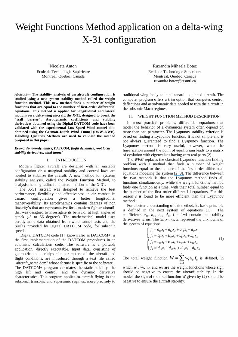
In order to analyze the sign of the total weight function W,

it is needed to analyze the signs of all terms ai, i = 1÷11 and dj,

j = 1÷3. For this reason, the graphs of the variations of

coefficients a1 to a11 and d1 to d3 with angle of attack are

shown in Figure 1, where it can be seen that the coefficients

1 3 6 110, 0, 0, 0a a a a as well as other coefficients have

fluctuant behavior. All three terms dj have an oscillating

behavior.

Figure 1. Coefficients ai and dj variation with the angle of attack

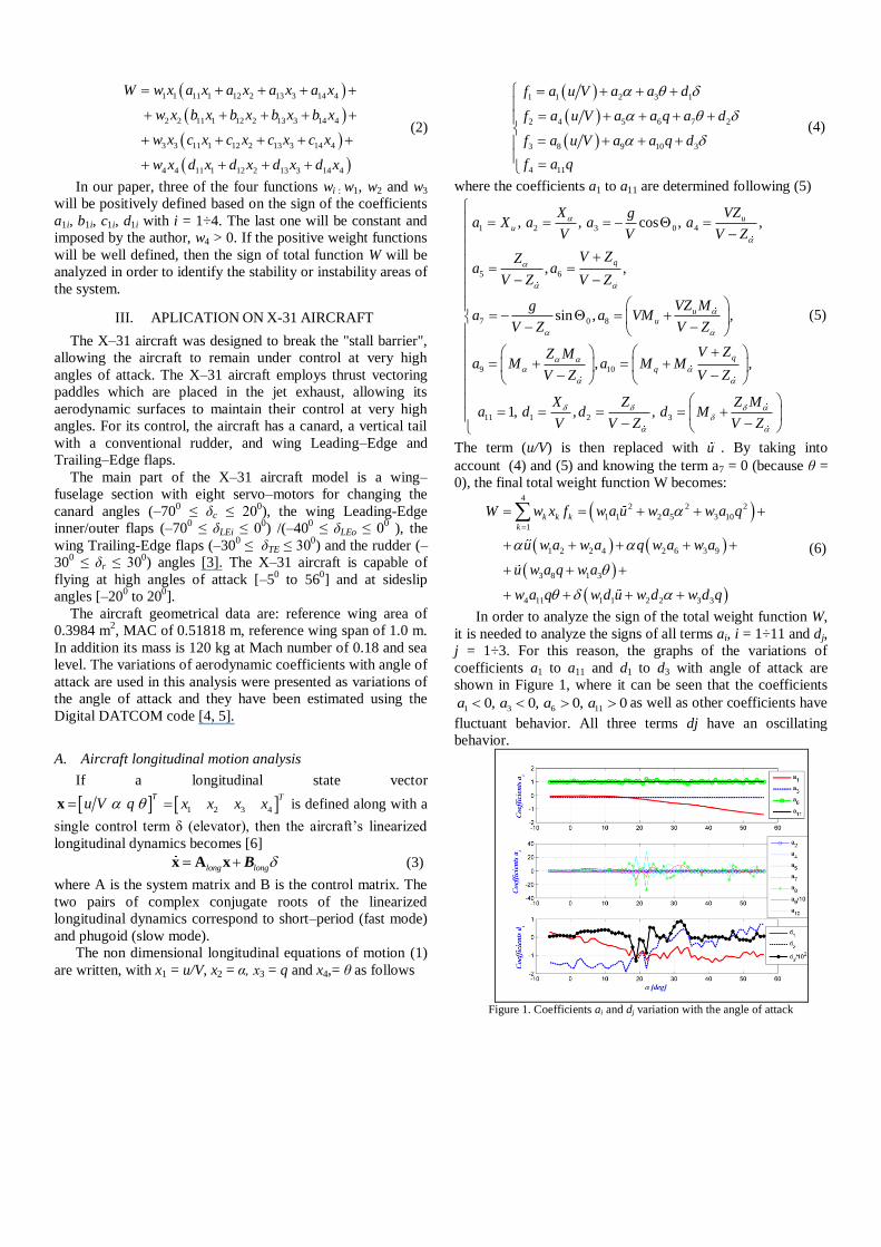
The weight functions are chosen considering the signs of

the coefficients ai, dj and the tested cases for the pitch angles θ

= [–20 to 20]0 and pitch rates q = [–10 to 10]

0/s. The aim of

the WFM is to find 3 positive weighting functions w1, w2 and

w3 presented in Figure 2, based on the coefficients variations

presented in Figure 1. For the flight case configuration

presented in this paper it is considered that the canard angle as

δc = 00 and the flap angle δ = 5

0. The positive weight functions

are defined as:

2

1 1 2 3 1

22

2 4 5 6 2

22

3 8 9 10 3

4 1,100

w u a u a a d

w a u a a q d

w q a u a a q d

w

(7)

and the corresponding final form of the total weight function

W is given by (8).

4

1 1 2 2 3 3 4 4

1

32

1 2 3 1

33

4 5 6 2

33

8 9 10 3 4 11

k k k

k

W w x f w f u w f w f q w f

u a u a a d

a u a a q d

q a u a a q d w q a

(8)

Figure 2. Weight functions chosen for longitudinal dynamics

a)

b)

c)

d)

e)

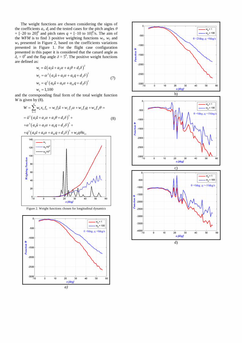
f)

Figure 3. Stability analyses with the weight functions method for different

values of constant w4 as a function of angle of attack

Two positives values for w4 are chosen: 1 and 100. It can

be observed in Figure 3 that the shape of the stability curve

does not change with the values of pitch angle θ and pitch rate

q, probably because the terms multiplying the pitch angle are

small and constant (a3 = 0.1601 and a11 = 1) as seen also on

Figure 1; for this reason, their contributions are quite

insignificant in comparison with the rest of the coefficients.

Under these circumstances, for any considered range of pitch

rates q and pitch angles θ the system remains always stable.

B. Aircraft lateral analysis motion

Next, the non-dimensional lateral–directional equations of

motion are given in (9).

1 2 3 4 1

5 6 7 2

8 9 10 3

11

c c p c c r b

p c c p c r b

r c c p c r b

c p

(9)

where

1 2 3 0 4 1

5 6

7 2

8 9

10 3

, , cos , ,

, ,

,

, ,

,

p r

xz xz

p p

x x

xz xz

r r

x x

xz xz

p p

z z

xz xz

r r

z

YY YY Vgc c c c b

V V V V V

I Ic L N c G L N

I I

I Ic G L N b G L N

I I

I Ic N L c G N L

I I

I Ic G N L b G N L

I I

G

G

11, 1z

c

(10)

The weighting function W can be thus written under the

following form, where x1 = β (sideslip rate), x2 = p (roll rate),

x3 = r (yaw rate), x4 = Φ (bank angle), x5 = δ:

4

1 1 2 4 3 1

1

2 6 5 7 2

3 10 8 9 3 4 11

k k k

k

W w x f w c c p c r c b

w p c p c c r b

w r c r c c p b w c p

(11)

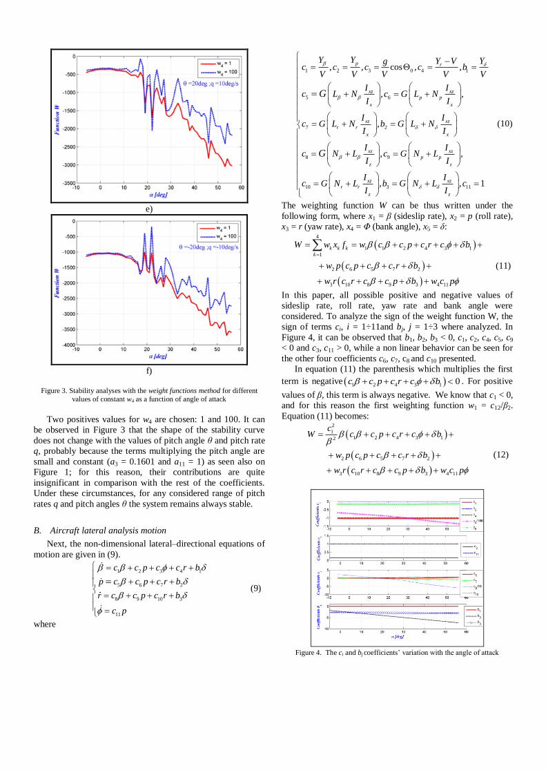
In this paper, all possible positive and negative values of

sideslip rate, roll rate, yaw rate and bank angle were

considered. To analyze the sign of the weight function W, the

sign of terms ci, i = 1÷11and bj, j = 1÷3 where analyzed. In

Figure 4, it can be observed that b1, b2, b3 < 0, c1, c2, c4, c5, c9

< 0 and c3, c11 > 0, while a non linear behavior can be seen for

the other four coefficients c6, c7, c8 and c10 presented.

In equation (11) the parenthesis which multiplies the first

term is negative 1 2 4 3 1 0c c p c r c b . For positive

values of β, this term is always negative. We know that c1 < 0,

and for this reason the first weighting function w1 = c12/β2.

Equation (11) becomes:

2

1

1 2 4 3 12

2 6 5 7 2

3 10 8 9 3 4 11

cW c c p c r c b

w p c p c c r b

w r c r c c p b w c p

(12)

Figure 4. The ci and bj coefficients’ variation with the angle of attack

The parenthesis which multiplies w2p is also

negative 6 5 7 2 0c p c c r b . Based on its sign the

second function w2 are defined

as 22

2 6 5 7 2w p c p c c r b . The total function W is

now given by (13).

2

1

1 2 4 3 12

22

6 5 7 2 6 5 7 2

3 10 8 9 3 4 11

cW c c p c r c b

p c p c c r b p c p c c r b

w r c r c c p b w c p

(13)

At this point it is possible to defined w3 or w4 as a positive

constant. Because c11 > 0, it was chose4 11w c p . The final

form of function W is given by (14).

2

1

1 2 4 3 1

33

6 5 7 2

2

3 10 8 9 3 11

23 11 2 4 3 1

32 2 2 3

11 6 5 7 2

3 10 8 9 3

cW c c p c r c b

p c p c c r b

w r c r c c p b c p

cc c p c r c b

c p p c p c c r b

w r c r c c p b

(14)

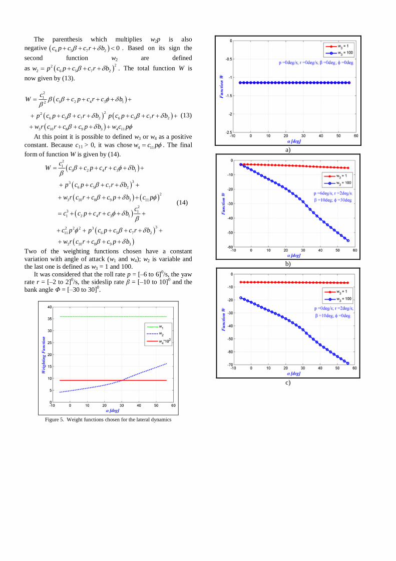
Two of the weighting functions chosen have a constant

variation with angle of attack (w1 and w4); w2 is variable and

the last one is defined as w3 = 1 and 100.

It was considered that the roll rate p = [–6 to 6]0/s, the yaw

rate r = [–2 to 2]0/s, the sideslip rate β = [–10 to 10]

0 and the

bank angle Φ = [–30 to 30]0.

Figure 5. Weight functions chosen for the lateral dynamics

a)

b)

c)

d)

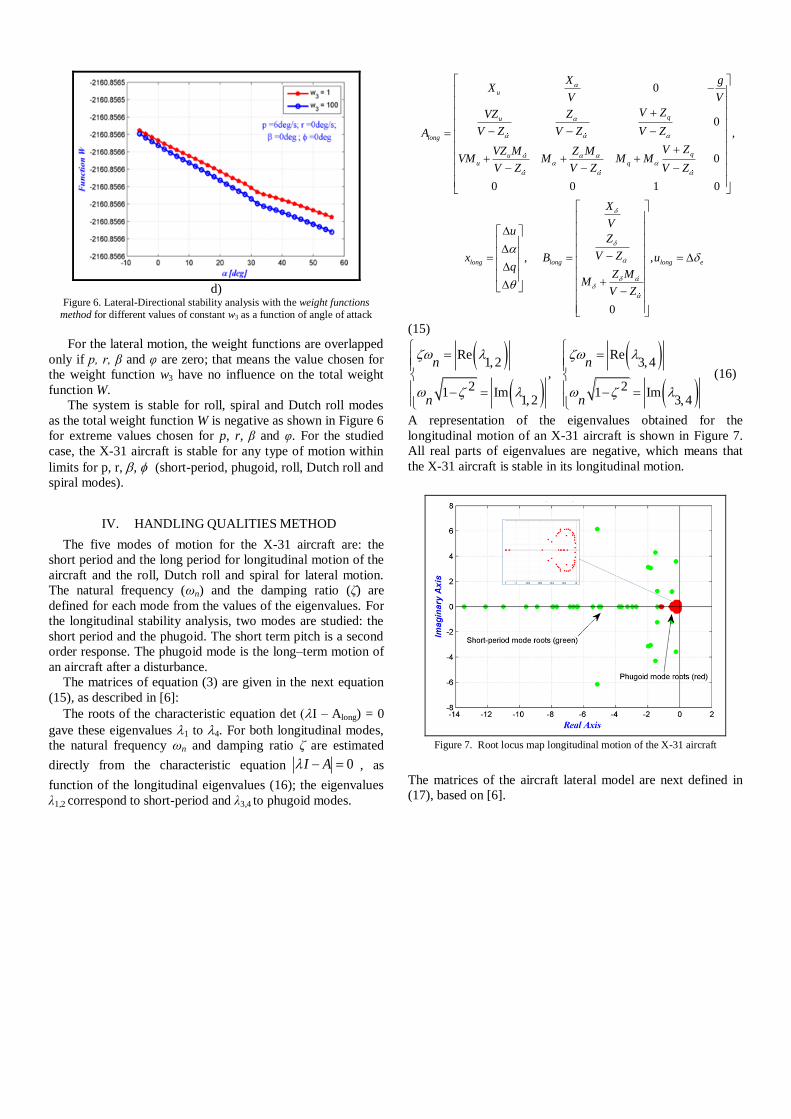
Figure 6. Lateral-Directional stability analysis with the weight functions

method for different values of constant w3 as a function of angle of attack

For the lateral motion, the weight functions are overlapped

only if p, r, β and φ are zero; that means the value chosen for

the weight function w3 have no influence on the total weight

function W.

The system is stable for roll, spiral and Dutch roll modes

as the total weight function W is negative as shown in Figure 6

for extreme values chosen for p, r, β and φ. For the studied

case, the X-31 aircraft is stable for any type of motion within

limits for p, r, , (short-period, phugoid, roll, Dutch roll and

spiral modes).

IV. HANDLING QUALITIES METHOD

The five modes of motion for the X-31 aircraft are: the

short period and the long period for longitudinal motion of the

aircraft and the roll, Dutch roll and spiral for lateral motion.

The natural frequency (ωn) and the damping ratio (ζ) are

defined for each mode from the values of the eigenvalues. For

the longitudinal stability analysis, two modes are studied: the

short period and the phugoid. The short term pitch is a second

order response. The phugoid mode is the long–term motion of

an aircraft after a disturbance.

The matrices of equation (3) are given in the next equation

(15), as described in [6]:

The roots of the characteristic equation det I – Along) = 0

gave these eigenvalues 1 to 4. For both longitudinal modes,

the natural frequency ωn and damping ratio ζ are estimated

directly from the characteristic equation 0I A , as

function of the longitudinal eigenvalues (16); the eigenvalues

λ1,2 correspond to short-period and λ3,4 to phugoid modes.

0

0,

0

0 0 1 0

, ,

0

u

qu

long

quu q

long long long e

X gX

V V

V ZVZ Z

V Z V Z V ZA

V ZVZ M Z MVM M M M

V Z V Z V Z

X

Vu

Z

V Zx B uq

Z MM

V Z

(15)

Re Re1,2 3,4

,2 21 Im 1 Im

1,2 3,4

n n

n n

(16)

A representation of the eigenvalues obtained for the

longitudinal motion of an X-31 aircraft is shown in Figure 7.

All real parts of eigenvalues are negative, which means that

the X-31 aircraft is stable in its longitudinal motion.

Figure 7. Root locus map longitudinal motion of the X-31 aircraft

The matrices of the aircraft lateral model are next defined in

(17), based on [6].

0

0

cos

0,

0

0 1 0 0

,

p r

xz xz xzp p r r

x x xlat

xz xz xzp p r r

z z z

xz

lat lat

YY Y V g

V V V u

I I IL N G L N G L N

I I IA

I I IN L G N L G N L

I I I

Y

V

IG L Np

x Br

G

G

,

0

x lat a

xz

z

I u

IG N L

I

(17)

Three modes are considered in the aircraft lateral motion

modeling:

Spiral mode representing, a convergent or a divergent

motion;

Roll mode representing a fast convergent motion, and

Dutch roll mode representing a light damped oscillatory

motion with a low frequency.

These modes are significant factors mainly in the uniform

cruise flight. For the lateral aircraft motion modelling, two real

roots correspond to roll and spiral modes, and a pair of

complex roots correspond to Dutch roll mode obtained from

the characteristic equation 0latI A .

The rolling motion is generally very much damped and

reaches the steady state in a very short time. An unstable spiral

mode results into a turning flight path. The Dutch roll is a

nuisance mode that appears in the basic roll response to lateral

control and can induce non–controlled and non–desired

motions in roll and yaw modes. These motions can

significantly influence the ability of the pilot to control the

lateral–directional motions with precision.

The eigenvalues for all three motions described above for

X-31 aircraft are represented in Figure 8: blue for Dutch Roll,

red for spiral and green for roll mode.

Results obtained with the weight functions method shown

in Figure 6, have proven that the aircraft is stable in its lateral

motion. Results presented with root locus map presented in

Figure 8 show that the X-31 aircraft has a stable lateral

motion, because all eigenvalues calculated with the root locus

map are situated in the negative plane.

Figure 8. Root locus map for lateral motion

V. CONCLUSIONS

A stability analysis based on the null solutions stability

studies for differential equation systems was presented in this

paper. The main aim was to found the positive weight

functions in order to analyze the X-31 aircraft stability. The

aerodynamics coefficients and their stability derivatives were

determined with Digital DATCOM code. Based on the

aircraft’s aerodynamic model in the WFM, 3 functions were

defined as function of stability derivatives terms, and the last

fourth function was considered positive and chosen to be 1

and 100.

The WFM was applied for longitudinal and lateral motions.

A discussion of results was done for each case, and the

stability was defined and is summarized in the previous

sections. HQM was also applied to validate the aircraft

stability results found with WFM.

X-31 has a stable longitudinal and lateral dynamics. For the

considered altitude and Mach number, the aircraft was found

to be stable, regardless the angle of attack. Both modes tested

here, the slow and the fast, did not induced any oscillations

and/or instabilities.

ACKNOWLEDGMENTS

Thanks are due to Dr. Andreas Schütte from DLR and Dr.

Russell Cummings from the USAF Academy for their

leadership and support in RTO/AVT–161 “Assessment of

Stability and Control Prediction Methods for NATO Air and

Sea Vehicles” and for providing the wind tunnel test data for

the X-31 aircraft.

REFERENCES

[1]. The USAF Stability And Control Digital Datcom, Volume I, “Users

Manual. USAF Technical Report AFFDL-TR-79-3032 (AD A086557) ”,

April 1979.

[2]. Stroe, Ion, “Weight functions method in stability study of vibrations”,

SISOM 2008 and Session of the Commission of Acoustics, Bucharest

29–30 May, 2008.

[3]. Stroe, I., and Parvu, P., “Weight functions method in Stability Study of

Systems”, 79th Annual Meeting of the International Association of

Applied Mathematics and Mechanics (GAMM), Bremen, pp. 10385–

10386, 2009.

[4]. Anton, N., Botez, R.M. and Popescu, D., “Stability derivatives for X-31

delta-wing aircraft validated using wind tunnel test data”, Proceeding of

the Institution of Mechanical Engineers, Vol. 225, Part G, Journal of

Aerospace Engineering, pp 403-416, 2011

[5]. Anton, N., Botez, R.M. and Popescu, D., “ New methodology and code

for Hawker 800XP aircraft stability derivatives calculations from

geometrical data”, The Aeronautical Journal, Vol. 114, No. 1156, Paper

No. 3454, 2010

[6]. Schmidt, L.V., “Introduction to Aircraft Flight Dynamics”, AIAA

Education Series, 1998.

[7]. Hodgkinson, J., “Aircraft Handling Qualities”, AIAA Education Series,

1999.

[8]. Bihrle, W., “A Handling Qualities Theory for Precise Flight Path

Control”, Tech. Rep. AFFDL-TR-65-195, AFRL, Wright Patterson

AFB, OH, June 1965. [9]. Cotting, M. Christoffer.`, “Evolution of flying qualities analysis:

Problems for the new generation of aircraft”, PhD Thesis, Faculty of the

Virginia Polytechnic Institute and State University, Blacksburg,

Virginia, March 2010.

NOMENCLATURE

b wing span

c wing mean aerodynamic chord

CD drag coefficient

CDα drag due to the angle of attack derivative

CDq drag due to the pitch rate derivative

CL lift coefficient

CLα lift due to the angle of attack derivative

CLq lift due to the pitch rate derivative

LC lift due to the angle of attack rate derivative

Cm pitching moment coefficient

Cmα static longitudinal stability moment with respect to the angle of attack derivative

Cmq pitching moment due to the pitch rate derivative

mC pitching moment due to the angle of attack rate derivative

Clp rolling moment due to the roll rate derivative

Clr rolling moment due to the yaw rate derivative

Clβ rolling moment due to the sideslip angle derivative

l

C

rolling moment due to the sideslip angle rate derivative

Cnp yawing moment due to the roll rate derivative

Cnr yawing moment due to the yaw rate derivative

Cnβ yawing moment due to the sideslip angle derivative

Cyp side force due to the roll rate derivative

Cyr side force due to the yaw rate derivative

Cyβ side force due to the sideslip angle derivative

Ix,Iy,Iz moment of inertia about the X, Y and Z body axes, respectively

Ixz product of inertia

Lp rolling moment due to roll rate

2p lp

x

qSb bL C

I V

Lr rolling moment due to yaw rate

2r lr

x

qSb bL C

I V

Lβ rolling moment due to sideslip

l

x

qSbL C

I

Lδ roll control derivative

l

x

qSbL C

I

m aircraft mass

M Mach number

Mq pitching moment due to pitch rate

2q mq

y

qSc cM C

I V

Mu pitching moment increment with increased speed

u mM

y

qScM C

I V

Mα pitching moment due to incidence

2q m

y

qSc cM C

I V

M pitching moment due to rate of change of the incidence

2m

y

qSc cM C

I V

Mδ pitching moment due to flap deflection

m

y

qScM C

I

Np yawing moment due to roll rate

2p np

z

qSb bN C

I V

Nr yawing moment due to yaw rate

2r nr

z

qSb bN C

I V

Nβ yawing moment due to sideslip

n

z

qSbN C

I

Nδ yawing moment due to flap deflection

n

z

qSbN C

I

p, q, r angular rates about the X, Y and Z body axes,

respectively

, ,p q r time rate of change of p, q, r

q dynamic pressure

S wing area

u axial velocity perturbation

u time rate of change of u

V airspeed

Xu drag increment with increased speed 2u D

qSX C

mV

Xα drag due to incidence L D

qSX C C

m

Xδ drag due to flap deflection

D

qSX C

m

Yp side force due to roll rate

2p yp

qS bY C

m V

Yr side force due to yaw rate

2r yr

qS bY C

m V

Yβ side force due to sideslip

y

qSY C

m

Yδ side force control derivative

y

qSY C

m

Zq lift due to pitch rate

2q Lq

qS cZ C

m V

Zu lift due to speed increment

2u L

qSZ C

mV

Zα lift due to incidence

D L

qSZ C C

m

Z lift due to the rate of change of incidence

2L

qS cZ C

m V

Zδ lift due to flap deflection

L

qSZ C

m

α angle of attack

, , time rate of change of α, β, θ

β sideslip angle

δ control deflection

θ pitch angle

ϕ roll angle