specifying the equatorial ionosphere using cindi on c/nofs, cosmic, and data interpolating empirical...

JOURNAL OF GEOPHYSICAL RESEARCH: SPACE PHYSICS, VOL. 118, 1–17, doi:10.1002/jgra.50596, 2013

Specifying the equatorial ionosphere using CINDI on C/NOFS,COSMIC, and data interpolating empiricalorthogonal functionsR. A. Stoneback,1 N. K. Malakar,1 D. J. Lary,1 and R. A. Heelis1

Received 7 March 2013; revised 12 September 2013; accepted 23 September 2013.

[1] Data Interpolating Empirical Orthogonal Functions (DINEOFs) are a data-basedmethod for determining a few orthogonal basis functions that optimally reproduce a givendata set. This technique is applied to meridional drift measurements performed by theCoupled Ion Neutral Dynamics Investigation (CINDI) onboard theCommunication/Navigation Outage Forecasting System (C/NOFS) as well as electrondensity profiles derived from GPS Radio Occulations (RO) performed by theConstellation Observing System for Meteorology, Ionosphere, and Climate (COSMIC).The low densities of the equatorial ionosphere spanning 2009–2010 restricted quality driftmeasurements by CINDI to altitudes near perigee, limiting the local time coverage ofmeasurements. Full local time descriptions may be obtained as perigee moves through alllocal times though this requires a minimum 67 day season. To increase the data coverageof the ionosphere, CINDI data are supplemented with COSMIC GPS RO data. DINEOFsare applied to median meridional drift measurements as well as COSMIC measurementsspanning 2009–2010 and are used to make a best estimate of the equatorial ionosphere atlocations not observed. The scattered distribution of COSMIC profiles as well as thephysical relationship between meridional ion drifts and the distribution of density withaltitude improves the quality of the reconstructions compared to using CINDI alone. TheDINEOF reconstructions demonstrate that the annual anomaly of reduced ionosphericdensities in June compared to December measured by COSMIC is coincident with achange in the meridional ion drifts at the geomagnetic equator measured by CINDI.Citation: Stoneback, R. A., N. K. Malakar, D. J. Lary, and R. A. Heelis (2013), Specifying the equatorial ionosphereusing CINDI on C/NOFS, COSMIC, and data interpolating empirical orthogonal functions, J. Geophys. Res. Space Physics,118, doi:10.1002/jgra.50596.

1. Introduction[2] Data Interpolating Empirical Orthogonal Functions

(DINEOFs) [Beckers and Rixen, 2003] are a data-basedmethod useful for reconstructing missing data in a data setusing an empirical orthogonal function (EOF) basis. An iter-ative EOF decomposition of a sparse data set is performedto determine a limited set of orthogonal basis functions thatoptimally reconstruct the data set. For a given data slice fromthe set, missing values are determined by fitting the deter-mined basis functions to known data. The fitted amplitudesmay then be used along with the basis functions to fill inany gaps in the data slice. No a priori information about thedata set needs to be specified. The technique has typicallybeen applied to satellite data that contain measurement gapsdue to the many challenges in forming a complete satellitedata set.

1W. B. Hanson Center for Space Sciences, Physics Department, Uni-versity of Texas at Dallas, Richardson, Texas, USA.

Corresponding author: R. A. Stoneback, W. B. Hanson Center for SpaceSciences, Physics Department, University of Texas at Dallas, 800 W.Campbell Rd. WT 15, Richardson, TX 75080, USA. ([email protected])

©2013. American Geophysical Union. All Rights Reserved.2169-9380/13/10.1002/jgra.50596

[3] EOFs have seen widespread use in atmospheric sci-ence over several decades (see review by Hannachi et al.[2007]). Similar techniques have been used for the iono-sphere; Sun et al. [1998] used the method of natural orthog-onal components to isolate components of ionosphericcurrents driven directly by substorm processes using a chainof magnetometers. Golovkov et al. [2007] used the samemethod to generate a data-based model of the geomagneticfield in space and time. The model generated a main fieldthat differed from traditional models by less than 10–15 nT.Kim et al. [2012] used a principal component analysis ofSuper Dual Auroral Radar Network data to perform a modalanalysis of polar convection and determine the influence ofthe interplanetary magnetic field upon these modes. A et al.[2012] used global total electron content (TEC) data over1999–2009 and were able to reconstruct 99% of the inputvariance using only four modes.

[4] DINEOFs have been applied to sea surface temper-atures recorded by the Advanced Very High ResolutionRadiometer satellite [Beckers and Rixen, 2003] with mea-surement gaps due to cloud coverage. A more completetreatment follows that also includes a comparison with opti-mal interpolation methods [Alvera-Azcárate et al., 2005].Errors on the order of 1ıC are found for sea surface

1

STONEBACK ET AL.: SPECIFYING THE EQUATORIAL IONOSPHERE

temperatures ranging between 16ıC and 24ıC. TheDINEOF method can also be used to generate an errorestimate for each missing data location along with thereconstruction of missing data [Beckers et al., 2006].

[5] The method is amenable to operating on several scalarquantities at once. Sea surface temperatures, chlorophyll,and wind field measurements were analyzed simultaneouslyby Alvera-Azcárate et al. [2007], enabling a more accuratereconstruction of missing data than when using sea surfacetemperatures alone. Gaps in each of the parameters are filledin by DINEOFs. The performance on long data sets may alsobe improved by applying a filter function on measurementsseparated in time [Alvera-Azcárate et al., 2009], ensuringthat extremely sparse slices of data do not unduly influencethe inferred missing data.

[6] The DINEOF process is applied here to equatorial insitu meridional ion drift measurements made by the Cou-pled Ion Neutral Dynamics Investigation (CINDI) onboardthe Communications/Navigation Outage Forecasting Sys-tem (C/NOFS) satellite. C/NOFS was launched in April2008 into an elliptical orbit with perigee and apogee near450, 850 km, respectively, with a 13ı inclination. CINDImeasures thermal plasma parameters as well as the ion driftin three dimensions [Heelis and Hanson, 1998]. Low iono-spheric densities during the CINDI mission [Heelis et al.,2009; Stoneback et al., 2011] restricted quality drift mea-surements to altitudes near perigee, limiting the daily localtime coverage of ion drifts. The DINEOF process is appliedto the equatorial measurements of ion drift to fill in gapsin data coverage and produce a more complete map ofequatorial ionosphere behavior.

[7] The impact of the low-data coverage upon theDINEOF reconstruction may be exacerbated by the distri-bution of the CINDI data. Perigee takes 67 days to movethrough all local times; thus, high-quality measurements atmidnight are separated from high-quality measurements atnoon by 33 days. This time span between measurements andthe fact that drifts separated by 12 h of local time at a fixedlongitude are infrequently simultaneously observed (due toaltitude restrictions) do not provide a strong constraint on thebasis functions in local time.

[8] To improve the DINEOF reconstruction, electron den-sity profiles obtained from COSMIC GPS Radio Occul-tations (RO) are incorporated into the DINEOF process.COSMIC(Formosat-3)[Cheng et al., 2006; Lin et al., 2007b;Lei et al., 2007a] is a constellation of six microsatelliteslaunched in April 2006, each carrying a GPS RO receiver[Schreiner et al., 2012]. Though in situ measurements fromCINDI move slowly through local time, altitude profilesobtained from RO are scattered in local time. When C/NOFSperigee is located at midnight, daytime measurements of iondrift are unavailable. During this same time period, COS-MIC will make measurements of the daytime ionosphereproviding DINEOFs with more constraints on the state of theionosphere. For ease of computation, the peak in ionosphericdensity, the altitude of the peak density, and a thicknessparameter for the ionosphere are used to characterize theprofiles rather than using the entire profile. These parametersare analyzed along with the CINDI data to produce a map ofthe equatorial ionosphere spanning 2009–2010.

[9] Here an overview of DINEOFs is provided, andthe application to CINDI and COSMIC measurements is

discussed. Results from the method and possible improve-ments in the application of DINEOFs to the equatorialionosphere are also considered.

2. DINEOFs[10] Consider a matrix X of size m!n containing measure-

ments at m different locations in the equatorial ionosphereover n different times. The empirical orthogonal functions(EOFs) that best represent data Xij for i = 1 " " "m andj = 1 " " " n may be obtained by using the Singular ValueDecomposition (SVD) to rewrite this matrix as

X = U†VT (1)

where U is a set of orthogonal spatial basis functions, V isthe amplitude of the basis functions in time, and † is thematrix of singular values. It can be shown that the orthogo-nal basis functions U and V are the best representations ofthe data set X for a given number of modes [Preisendorfer,1988; Beckers and Rixen, 2003]. When the SVD descrip-tion is truncated to the N most significant modes, it providesa data reconstruction X0 that is smoother than the supplieddata in X.

[11] This process may only be applied if data set X is com-plete, a situation not often encountered with satellite data.To overcome this limitation, an iterative EOF analysis isperformed [Beckers and Rixen, 2003]. An initial estimateof the value of the missing data is made by using the spa-tiotemporal mean of the data. This estimate is used for allmissing points, and an EOF analysis of this updated dataset is performed and used to create a reconstructed set, X0.The updated estimates for the missing data produced by theEOF in X0 are used to replace the initial estimate of themissing data in X and the EOF process is repeated, produc-ing a new X0. The process iterates until the basis functionson successive iterations converge, producing both a set offunctions that optimally reproduce the data as well as an esti-mate of all missing data points [Beckers and Rixen, 2003;Alvera-Azcárate et al., 2005].

[12] The number of basis functions that optimally repro-duce X is determined by a cross-validation technique. Aportion of data within X is set aside and treated as miss-ing. The root-mean-square (RMS) difference between theDINEOF reconstruction and the measured data is trackedas the number of basis functions determined via DINEOFsis varied. The reconstruction with the lowest RMS is cho-sen. DINEOFs employ the Lanczos solver [Toumazou andCretaux, 2001] which has the desirable property that only thefirst N modes are actually calculated, minimizing calculationtimes for large data sets [Alvera-Azcárate et al., 2005].

[13] The basis functions determined by the SVD willoptimally reconstruct the data contained in X. As physicaldrivers are not necessarily orthogonal, the basis functionswill not generally isolate single physical drivers per basisfunction. EOF decompositions also tend to share similarcharacteristics [Hannachi et al., 2007]. The lowest modegenerally has wave number 1 and spans the whole domain.The next mode tends to have wave number 2 and will alsobe orthogonal to the first mode regardless of the physics ofthe system under study.

[14] Some techniques have been developed to enhancethe physical interpretation of EOFs and a widely used

2


Mer

idio

nal I

on D

rift (

m/s

)

(a)

Mer

idio

nal I

on D

rift (

m/s

)

(b)

Figure 1. (a) Measurements of meridional ion drift fromCINDI as a function of apex longitude and magneticlocal time over all magnetic latitudes. The median driftfor each bin is reported using measurements over 5 days,spanning DOY 256–260, 2010. (b) DINEOF reconstructionof meridional ion drifts over all longitudes and local times.

technique is known as rotation [Hannachi et al., 2007]. If aconstraint upon the system is available, the constraint couldbe applied to the basis functions to determine a combina-tion of these functions that more closely satisfy the physicalconstraint. The general effectiveness of the method is lim-ited by the need for an objective constraint upon the system.Despite the complications of interpreting the EOF basismodes for physical behaviors, the DINEOF results presentedby Alvera-Azcárate et al. [2005] have identifiable physicalsources in the basis functions. Thus, DINEOFs may be use-ful in increasing the physical understanding of the systemat hand.

[15] The basis function determination involves a calcula-tion of a covariance array, determining how each measure-ment location relates to every other measurement location.Thus, the arrangement of the spatial locations in X is notimportant. Multidimensional measurements of a system in

0 6 12 1830

20

10

0

10

20

30

40

MLT24

Med

ian

Drif

t (m

/s)

Figure 2. Measured and DINEOF reconstructed drifts inthe 285ı apex longitude sector (western pacific) for the sametime period as in Figure 1.

time are treated simply as a one-dimensional array in spacewith measurements in time. This generality allows for anyspatial distribution of measurements and may also be usedto combine measurements of different physical parameters[Alvera-Azcárate et al., 2007]. COSMIC and CINDI datamay be analyzed together simply by putting both data setsinto separate rows in X. Due to the different physical units ofeach measurement parameter (ion drift, peak density, etc.),for each parameter, the spatiotemporal mean over the respec-tive data set is subtracted and then the data is normalized tohave an absolute maximum value of 1.

[16] In addition, parameters that do not have a specificspatial location but are expected to have a common variationwith other parameters in the data set may also be incorpo-rated. For equatorial ionosphere studies, the state of the Sunand the magnetosphere can have a significant impact uponthe state of the ionosphere. The strength of ultraviolet (UV)emissions from the Sun is commonly characterized by usingthe strength of 10.7 cm radio emission as a proxy as it is eas-ily measured from the ground. The impact of UV upon theionosphere varies as a function of local time, location, sea-son as well the state of the Sun in its 11 year solar cycle.The covariance matrices determined in the DINEOF processallows a F10.7 index to influence the reconstruction of thewhole data set where appropriate without having to spec-ify the relation between F10.7 and the ionosphere. Similarly,solar wind parameters, interplanetary magnetic field strengthand orientation, and Kp, Ap, or Dst indices may be used.

0 6 12 1840

20

0

20

40

60

MLT

ObservedPredictedAverage range

Med

ian

Drif

t (m

/s)

24

Figure 3. Measurements of meridional ion drift (blue)spanning 270ı–300ı apex longitude (western Pacific) alongwith average absolute deviations from the median spanning36–40, 2010. The DINEOF reconstruction of drifts at alllocal times is in red.

3


(a) CINDI Meridional Drifts (b) COSMIC Peak Density

(c) COSMIC peak density height (d) COSMIC thickness

Figure 4. CINDI and COSMIC data using 9 day medians and 1 h local time bins.

These parameters may also be included as new rows in X,where each measurement type is modified to have a mean ofzero and an absolute maximum value of 1.

3. Results[17] To apply the methods above to a description of equa-

torial ionosphere dynamics, the median of in situ measure-ments of meridional drift from CINDI over 5 day incrementswas calculated and binned by magnetic local time to producethe data set X for DINEOF analysis. Note that the numberof data days per median does not remain constant through-out this work. The data are restricted to altitudes below550 km subject to an O+ density minimum of 3 ! 103 N/ccand 100 samples per bin are required. A 5 day period wasused to smooth some of day-to-day variability in the iono-sphere and increase data coverage. Though the DINEOFprocess can in principle handle data on a daily basis, therewas insufficient data for 2009/2010 to sufficiently constrainthe DINEOF process and produce reasonable predictions formissing data.

[18] Median drifts measured by CINDI were averagedwith 2 h bins in magnetic local time (MLT), 30ı apex lon-gitude sectors, and drifts over all magnetic latitudes wereallowed. The medians over 2 h time bins were interpolated to1 h bins. With these restrictions, there is less than 50% datacoverage from CINDI measurements. Missing data valuesfor 2009 and 2010 were filled in separately with DINEOFs.

An example of the meridional drifts for day of year (DOY)256–260, 2010, one of the data slices input to the method,is shown in Figure 1a. The basis functions determined byDINEOFs are used to fill in drifts in the remaining localtimes in Figure 1b. Peak upward drifts are found near 10MLT between 0ı and 180ı apex longitude and are found abit earlier in local time between 240ı and 360ı. Three peaksare seen in the upward meridional drifts near 90ı, 180ı,and 270ı, displaying longitudinal variations with a charac-ter similar to tidal patterns in the ionosphere. Huang et al.[2012] report tidal signatures in meridional drift velocitiesfor CINDI data spanning November 2008 through Fall 2009.A wave 4 pattern is seen most strongly in the February–Apriland August–October periods, with peaks near 90ı, 180ı, and270ı and across 360ı, 0ı geographic longitude. Apex andgeographic longitudes differ by about –70ı at the magneticequator; thus, the peaks in Figure 1b are shifted relative toHuang et al. [2012]. With the exception of the peak across90ı geographic longitude (20ı apex longitude) reportedby Huang et al. [2012], similar peaks are reconstructedby DINEOFs.

[19] A slice from the Pacific sector (285ı) in Figure 1bis shown in Figure 2. Weak afternoon drifts are observedwith a peak upward drift after sunset followed by down-ward drifts. The remaining local time sectors are recon-structed using DINEOFs. Upward drifts after midnightare observed, increasing after dawn with a peak near

4




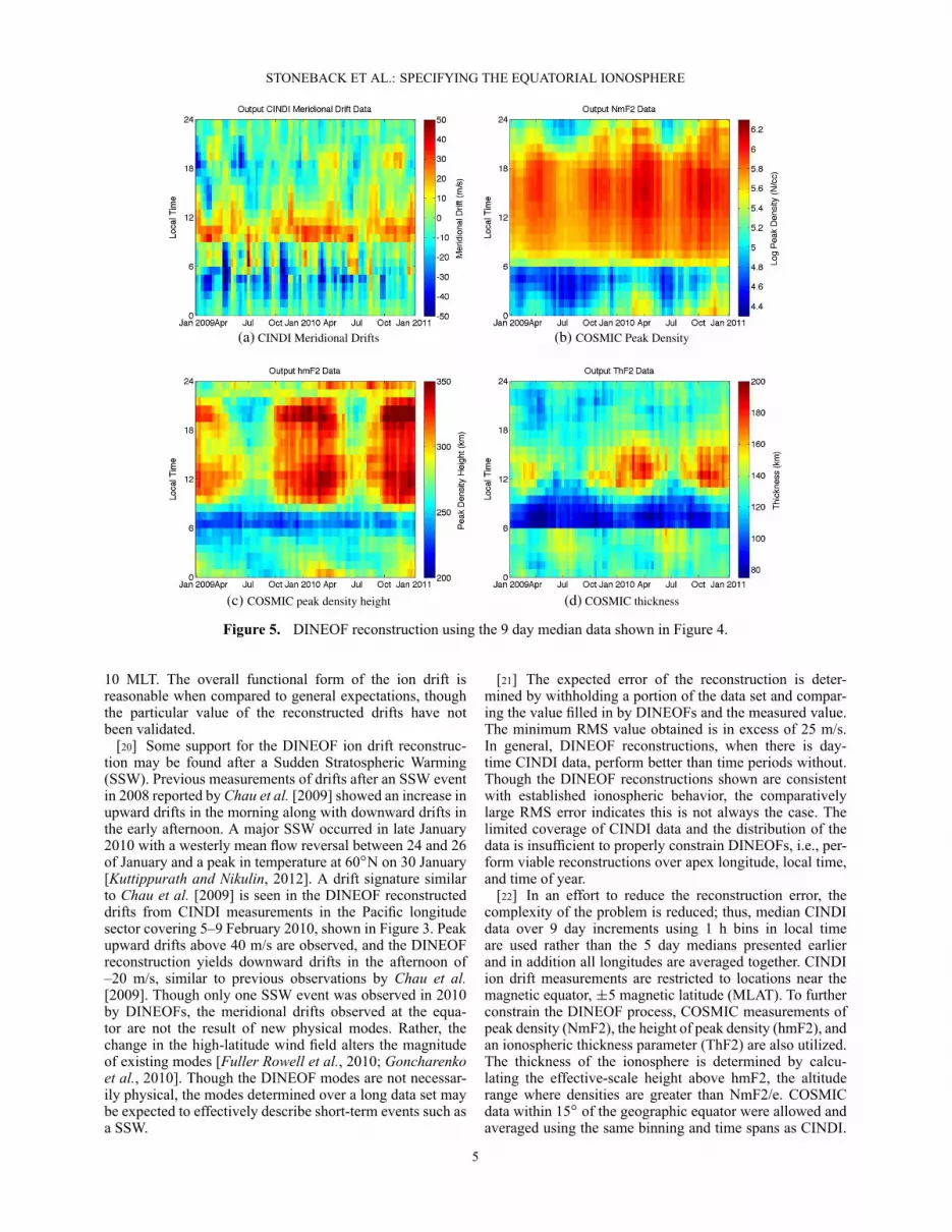
Figure 5. DINEOF reconstruction using the 9 day median data shown in Figure 4.

10 MLT. The overall functional form of the ion drift isreasonable when compared to general expectations, thoughthe particular value of the reconstructed drifts have notbeen validated.

[20] Some support for the DINEOF ion drift reconstruc-tion may be found after a Sudden Stratospheric Warming(SSW). Previous measurements of drifts after an SSW eventin 2008 reported by Chau et al. [2009] showed an increase inupward drifts in the morning along with downward drifts inthe early afternoon. A major SSW occurred in late January2010 with a westerly mean flow reversal between 24 and 26of January and a peak in temperature at 60ıN on 30 January[Kuttippurath and Nikulin, 2012]. A drift signature similarto Chau et al. [2009] is seen in the DINEOF reconstructeddrifts from CINDI measurements in the Pacific longitudesector covering 5–9 February 2010, shown in Figure 3. Peakupward drifts above 40 m/s are observed, and the DINEOFreconstruction yields downward drifts in the afternoon of–20 m/s, similar to previous observations by Chau et al.[2009]. Though only one SSW event was observed in 2010by DINEOFs, the meridional drifts observed at the equa-tor are not the result of new physical modes. Rather, thechange in the high-latitude wind field alters the magnitudeof existing modes [Fuller Rowell et al., 2010; Goncharenkoet al., 2010]. Though the DINEOF modes are not necessar-ily physical, the modes determined over a long data set maybe expected to effectively describe short-term events such asa SSW.

[21] The expected error of the reconstruction is deter-mined by withholding a portion of the data set and compar-ing the value filled in by DINEOFs and the measured value.The minimum RMS value obtained is in excess of 25 m/s.In general, DINEOF reconstructions, when there is day-time CINDI data, perform better than time periods without.Though the DINEOF reconstructions shown are consistentwith established ionospheric behavior, the comparativelylarge RMS error indicates this is not always the case. Thelimited coverage of CINDI data and the distribution of thedata is insufficient to properly constrain DINEOFs, i.e., per-form viable reconstructions over apex longitude, local time,and time of year.

[22] In an effort to reduce the reconstruction error, thecomplexity of the problem is reduced; thus, median CINDIdata over 9 day increments using 1 h bins in local timeare used rather than the 5 day medians presented earlierand in addition all longitudes are averaged together. CINDIion drift measurements are restricted to locations near themagnetic equator,˙5 magnetic latitude (MLAT). To furtherconstrain the DINEOF process, COSMIC measurements ofpeak density (NmF2), the height of peak density (hmF2), andan ionospheric thickness parameter (ThF2) are also utilized.The thickness of the ionosphere is determined by calcu-lating the effective-scale height above hmF2, the altituderange where densities are greater than NmF2/e. COSMICdata within 15ı of the geographic equator were allowed andaveraged using the same binning and time spans as CINDI.

5




Figure 6. Input data using 1 day medians.

A minimum of 5 COSMIC observations per local time isrequired. Generally, there are 5–10 ROs per local time binper day for each reported median.

[23] The raw COSMIC GPS measurements are convertedto electron density profiles by making a set of assump-tions about the ionosphere and using the Abel transform.These assumptions break down when there are large hori-zontal gradients in the ionosphere. Errors are found withinthe E-region as well as at low latitudes. The derived param-eters NmF2 and hmF2 are less affected by these errorsand are generally reliable [Yue et al., 2010]. Profiles arerestricted to derived hmF2 altitudes between 175 and 475km. The profiles provided by COSMIC Data Analysis andArchive Center (CDAAC) may also contain errors due tocycle slips or multipath signals [Hwang et al., 2010]. Thesedistorted profiles are excluded by filtering profiles with sharpdensity gradients.

[24] CINDI and COSMIC inputs are shown in Figure 4.The tracks of CINDI data are a result of measurements lim-ited to local times near perigee and the 67 day movementof perigee through all local times. The COSMIC data aregenerally more complete than CINDI and have a more var-ied distribution. The satellite measurements in Figure 4 aresupplied to DINEOFs along with 9 day means of F10.7and Dst. To encourage the generation of seasonal modes byDINEOFs, a sine and a cosine wave are supplied witha yearly period and maxima at the equinox and solstice,respectively. Sinusoidal functions are chosen due to theperiodicity of seasonal variations that are not effectively

described with a linear day of year number. Both the sine andcosine are functions of day number and when used togetheruniquely index each day of the year while also linking theend of one calendar year with the beginning of the next.The same seasonal waveforms have been used when estimat-ing TEC values using a neural network [Habarulema et al.,2011]. Nine day means of these waveforms are also suppliedto DINEOFs.

[25] The DINEOF reconstructions are shown in Figure 5.Peak upward meridional drifts are typically seen near 10MLT in Figure 5a, though there are some deviations duringthe June solstices with peak upward drifts near dawn. Down-ward drifts are seen before sunset during the June solsticesas well as in January of 2009 and 2010. Strong downwarddrifts are observed after midnight and through dawn in theperiod from January 2009 to July 2010.

[26] The DINEOF reconstructed peak density (NmF2) isshown in Figure 5b. The largest densities are observedduring the equinoxes, with the lowest peak densities dur-ing the June solstices. The reduction in density is consis-tent with the reduced upward drifts through the day anddownward drifts in the afternoon through sunset shownin Figure 5a. Reductions in NmF2 are also observedwith the downward afternoon drifts in January of 2009and 2010.

[27] The peak height (hmF2) is shown in Figure 5c. Thelargest peak heights are found during the December sol-stices, with minima in June. There is also a general increasefrom 2009 to 2010, consistent with increasing F10.7 levels.

6




Figure 7. DINEOF reconstruction of the ionosphere using 1 day medians of CINDI, COSMIC, and therelevant space weather parameters.

[28] The thickness above the density maximum (ThF2)is shown in Figure 5d. In local time, the smallest ThF2 isseen just after dawn and the commencement of photopro-duction. The thickness generally increases through the day,influenced by the meridional ion drift. Upward/downwardmovement of ions during the day is expected to thicken/thinthe ionosphere, as seen in the reconstructions. The maximumdaytime thickness is found during the December solsticeand equinox, coincident with the largest upward meridionaldrifts. At nighttime, the largest thickness is found during theJune solstice. We will show that these increases in thicknessare also coincident with an upward perturbation to ion driftsafter midnight during the June solstice, not clearly visible inFigure 5a due to the color scale.

[29] Figures 6 and 7 contain the input data and DINEOFreconstructions when using median CINDI and related dataon a 1 day basis using 1 h MLT bins. COSMIC has signifi-cantly less coverage than in the 9 day example. Despite thelower data filling factor, the general characteristics of thereconstruction match those in the 9 day medians in Figure 5.Though these global averages of ion drift, NmF2, hmF2,and ThF2 in longitude over equatorial latitudes can not bedirectly confirmed, the similarity of the 1 day reconstruc-tions compared to the 9 day medians supports the DINEOFprocess on this shorter timescale.

[30] In general, seasonal changes of the ionosphere arereflected in all of the ionospheric parameters in Figures 5 and

7. This is to be expected from the DINEOF reconstruction.Each mode determined by DINEOFs spans meridional iondrift, NmF2, hmF2, ThF2, F10.7, Dst, as well as the seasonalsine and cosine inputs. Each mode has a single amplitude ateach time for all parameters; thus, a change in a given modalamplitude to alter the reconstruction for a single parameternecessarily changes the reconstruction of the other quanti-ties. The overall reconstruction provided by DINEOFs thusreflects a best fit of the ionosphere for all supplied measure-ment parameters. While the physical relationship betweenparameters has not been specified, the various parameterswithin a single mode are coupled through covariance in thedata. Note, however, that the action of a physical sourceon the ionosphere could have a DINEOF description spreadacross multiple modes.

[31] The mode with the single largest contribution to thereconstruction is shown in Figure 8 with unit amplitude. Thehorizontal line in each plot is the mean value of the inputdata set when supplied to DINEOFs and should be treatedas an effective zero line when scaling the modal amplitudes.The dominant mode for meridional ion drifts in Figure 8a hasdownward drifts after midnight, with a maximum downwarddrift before dawn. After, dawn drifts increase peaking near10 MLT, only to decrease and become downward shortlyafter noon. A slight prereversal enhancement (PRE) is seenjust after sunset. The downward afternoon drifts in this modeare consistent with the reported downward afternoon drifts

7




Figure 8. Mode with the largest contribution to the DINEOF reconstruction shown in Figure 7 using 1day medians.

obtained using seasonally averaged CINDI data over allmagnetic latitudes observed by C/NOFS [Stoneback et al.,2011], though the results here are restricted to locations nearthe magnetic equator.

[32] The peak density NmF2 is shown in Figure 8b; min-imum densities are seen before dawn, rising quickly afterdawn and throughout the day. Densities decrease after sun-set and fall through the night, as expected for the ionosphere.The peak density height in Figure 8c is similar to themeridional drifts, increasing after dawn with a peak nearnoon. hmF2 falls after noon only to increase after sunset,consistent with the timing of the PRE in the ion drifts.Downward ion drifts are not necessarily inconsistent withthe increase in hmF2 after sunset. The loss of photopro-duction with sunset allows loss processes to exert moreinfluence on the distribution of plasma in the ionosphere.Loss rates decrease with increasing altitude; thus, after sun-set, the lower altitudes of the ionosphere are lost, raising thepeak density height of the ionosphere, though NmF2 itselfis lower.

[33] The ionospheric thickness in Figure 8d has a riseafter sunrise and a decrease though the afternoon. As NmF2and hmF2 fall through the night, the thickness of the iono-sphere increases. Once photoproduction commences withsunrise, a thin ionosphere is found at the location of peakphotoproduction.

[34] The amplitude of the DINEOF modes is shown inFigure 9 while the modes themselves are shown in Figure 10with unit amplitude. Note that a given modal amplitudegoverns the contribution of that mode across all input mea-surement types. The modes are sorted in decreasing order ofimportance in reconstructing the variance of the input CINDIand COSMIC data set. Note that the variance contribution ofeach mode is a product of both the mode and its amplitudein time. The most dominant mode, highlighted in Figure 8,has a nearly constant amplitude over 2 years, interpretedas the average state of the ionosphere. The second modeis largest during the June and December solstices. Duringthe June solstice, downward perturbations in meridional iondrift, NmF2, and hmF2 with an oscillation period of 8 h inlocal time are observed. The perturbation to hmF2 increasesthrough the daytime hours, maximizing after sunset. Thedrift perturbation at this time acts against the PRE; thus, adownward perturbation in hmF2 is expected to counter theincrease in hmF2 in the quasi constant first mode. The scaleheight above hmF2 is generally reduced through the day,with an increase after midnight and before dawn. The oppo-site contribution is generally found during the Decembersolstices.

[35] The third mode has a clear sinusoidal variationwith maxima near equinox. This mode leads to down-ward/upward drift perturbations after sunset through dawn

8


Figure 9. Amplitude of the DINEOF modes over 2009/2010 using 1 day median data.



Figure 10. DINEOF modes determined using data shown in Figure 6 and 1 day medians. While eachDINEOF mode spans all input parameters, only the meridional drift, NmF2, hmF2, and ThF2 results areshown here. The space weather parameter portion of these modes is shown in Figure 11.

9


(a) 10.7cm radio flux (b) Dst index

(c) Equinox (d) Solstice Wave

Figure 11. DINEOF modes determined using data shown in Figure 6. The contribution of these modesto the space weather parameters is detailed. As each mode spans all input parameters, the correspondingvariations in the remaining parameters (NmF2, hmF2, ThF2, meridional ion drift) for these modes areshown in Figure 10.

in the autumn/spring; however, this corresponds with anincrease/decrease in NmF2 during the nighttime hours.NmF2 is primarily driven by solar inputs; thus, a completecorrelation with meridional drifts is not expected. Variationsin hmF2 and ThF2 have similar and consistent waveforms inlocal time.

[36] Modes 4–6 have variations accounting for shorterterm variations in the ionosphere. Mode 5 has a clear peri-odic oscillation in Figure 9 with a period near 30 days fromOctober 2009 to January 2010. Mode 5 also has a meridionaldrift variation with a nonzero average in local time. Theamplitude of this mode in time is periodic; thus, the long-term drift contribution to the ionosphere remains near zero.Mode 6 has downward drifts after dawn and correspondingdecreases in hmF2 and ThF2.

[37] The product of the modal amplitudes in Figure 9 withthe DINEOF modes leads to reconstructions in all parame-ters. For ion drifts, NmF2, hmF2, and ThF2, the DINEOFmodes describe variations over 24 h of local time. For thekey indices, the modes are a single number rather than awaveform in local time. Bar charts detailing the modes forF10.7, Dst, and the seasonal sine and cosine inputs with unitamplitude are shown in Figure 11. The values plotted aredeviations from the mean of each particular input. For F10.7,

mode 2 has the largest component, with decreasing contribu-tions from modes 4, 5, and 6. For Dst, mode 4 has the largestcomponent. Modes 2 and 6 have similar magnitudes, half aslarge as mode 4.

[38] Mode 3 is significantly larger in Figure 11c than theother components and thus will have a dominant contribu-tion to the equinox waveform when all modes have a similaramplitude. The amplitude of mode 3 in time in Figure 9 alsofollows a sinusoidal oscillation, demonstrating that it is thedominant mode in reconstructing the equinox waveform. Forthe solstice variation, mode 2 in Figure 11d is the largest,followed by mode 4. We can see that the amplitude of mode2 is similar to a cosine; however, at the beginning of thedata set where we would expect an absolute maximum, it isnear 0. During this time, mode 4 has an amplitude near 2.So while mode 2 generally accounts for solstitial variationsin the ionosphere, there can be significant contributions tothis seasonal behavior from mode 4. Note that modes 2 and4 also have nonnegligible contributions to the reconstructionof F10.7 and Dst. Thus, variations in the ionosphere withsolstice are spread across more than one mode.

[39] In Figure 12, we can see that DINEOFs have beenable to reproduce the variations in F10.7 cm flux and sea-son fairly well. The input and reconstructed Dst are shown

10


(a) 10.7cm radio flux (b) Dst index

(c) Equinox Wave (d) Solstice Wave

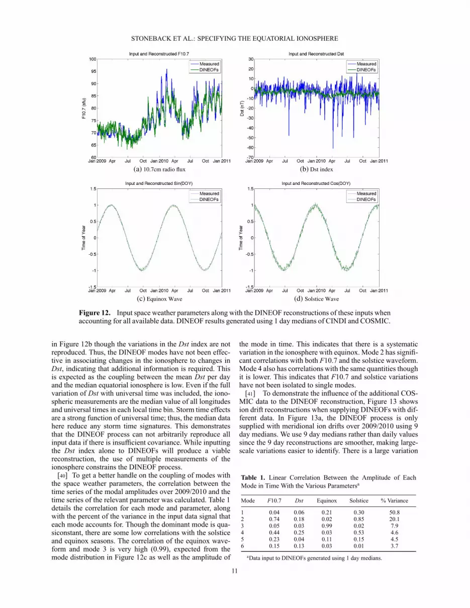
Figure 12. Input space weather parameters along with the DINEOF reconstructions of these inputs whenaccounting for all available data. DINEOF results generated using 1 day medians of CINDI and COSMIC.

in Figure 12b though the variations in the Dst index are notreproduced. Thus, the DINEOF modes have not been effec-tive in associating changes in the ionosphere to changes inDst, indicating that additional information is required. Thisis expected as the coupling between the mean Dst per dayand the median equatorial ionosphere is low. Even if the fullvariation of Dst with universal time was included, the iono-spheric measurements are the median value of all longitudesand universal times in each local time bin. Storm time effectsare a strong function of universal time; thus, the median datahere reduce any storm time signatures. This demonstratesthat the DINEOF process can not arbitrarily reproduce allinput data if there is insufficient covariance. While inputtingthe Dst index alone to DINEOFs will produce a viablereconstruction, the use of multiple measurements of theionosphere constrains the DINEOF process.

[40] To get a better handle on the coupling of modes withthe space weather parameters, the correlation between thetime series of the modal amplitudes over 2009/2010 and thetime series of the relevant parameter was calculated. Table 1details the correlation for each mode and parameter, alongwith the percent of the variance in the input data signal thateach mode accounts for. Though the dominant mode is qua-siconstant, there are some low correlations with the solsticeand equinox seasons. The correlation of the equinox wave-form and mode 3 is very high (0.99), expected from themode distribution in Figure 12c as well as the amplitude of

the mode in time. This indicates that there is a systematicvariation in the ionosphere with equinox. Mode 2 has signifi-cant correlations with both F10.7 and the solstice waveform.Mode 4 also has correlations with the same quantities thoughit is lower. This indicates that F10.7 and solstice variationshave not been isolated to single modes.

[41] To demonstrate the influence of the additional COS-MIC data to the DINEOF reconstruction, Figure 13 showsion drift reconstructions when supplying DINEOFs with dif-ferent data. In Figure 13a, the DINEOF process is onlysupplied with meridional ion drifts over 2009/2010 using 9day medians. We use 9 day medians rather than daily valuessince the 9 day reconstructions are smoother, making large-scale variations easier to identify. There is a large variation

Table 1. Linear Correlation Between the Amplitude of EachMode in Time With the Various Parametersa

Mode F10.7 Dst Equinox Solstice % Variance

1 0.04 0.06 0.21 0.30 50.82 0.74 0.18 0.02 0.85 20.13 0.05 0.03 0.99 0.02 7.94 0.44 0.25 0.03 0.53 4.65 0.23 0.04 0.11 0.15 4.56 0.15 0.13 0.03 0.01 3.7

aData input to DINEOFs generated using 1 day medians.

11


(a) CINDI Meridional Drifts (b) CINDI Drifts along with Space Weather Parameters(SWP)

(c) Drifts with COSMIC peak density, peak density height,and SWP.

(d) Drifts with COSMIC peak density, density height, iono-sphere thickness, and SWP.

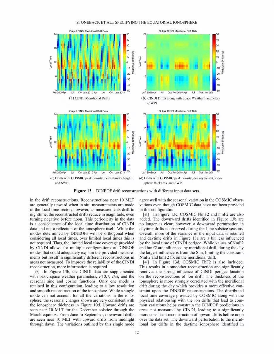
Figure 13. DINEOF drift reconstructions with different input data sets.

in the drift reconstructions. Reconstructions near 10 MLTare generally upward when in situ measurements are madein the local time sector; however, as measurements drift tonighttime, the reconstructed drifts reduce in magnitude, eventurning negative before noon. This periodicity in the datais a consequence of the local time distribution of CINDIdata and not a reflection of the ionosphere itself. While themodes determined by DINEOFs will be orthogonal whenconsidering all local times, over limited local times this isnot required. Thus, the limited local time coverage providedby CINDI allows for multiple configurations of DINEOFmodes that could adequately explain the provided measure-ments but result in significantly different reconstructions inareas not measured. To improve the reliability of the CINDIreconstruction, more information is required.

[42] In Figure 13b, the CINDI data are supplementedwith basic space weather parameters, F10.7, Dst, and theseasonal sine and cosine functions. Only one mode isretained in this configuration, leading to a low resolutionand smooth reconstruction of the ionosphere. While a singlemode can not account for all the variations in the iono-sphere, the seasonal changes shown are very consistent withthe ionosphere thickness in Figure 10d. Upward drifts areseen near 10 MLT for the December solstice through theMarch equinox. From June to September, downward driftsare seen near 10 MLT with upward drifts from midnightthrough dawn. The variations outlined by this single mode

agree well with the seasonal variation in the COSMIC obser-vations even though COSMIC data have not been providedin this configuration.

[43] In Figure 13c, COSMIC NmF2 and hmF2 are alsoadded. The downward drifts identified in Figure 13b areno longer as clear; however, a downward perturbation indaytime drifts is observed during the June solstice seasons.Overall, more of the variance of the input data is retainedand daytime drifts in Figure 13a are a bit less influencedby the local time of CINDI perigee. While values of NmF2and hmF2 are influenced by meridional drift, during the daythe largest influence is from the Sun, limiting the constraintNmF2 and hmF2 fix on the meridional drift.

[44] In Figure 13d, COSMIC ThF2 is also included.This results in a smoother reconstruction and significantlyremoves the strong influence of CINDI perigee locationon the reconstructions of ion drift. The thickness of theionosphere is more strongly correlated with the meridionaldrift during the day which provides a more effective con-straint upon the DINEOF reconstructions. The distributedlocal time coverage provided by COSMIC along with thephysical relationship with the ion drifts that lead to com-mon variations helps constrain the DINEOF predictions inareas not measured by CINDI, leading to a significantlymore consistent reconstruction of upward drifts before noonover the data set. The downward perturbation to the merid-ional ion drifts in the daytime ionosphere identified in

12


Table 2. The Expected Error for Filling in Gaps in the Data Setas Well as the RMS Error Between the DINEOF Fitted Curves andthe Input Dataa

Data Set 1 Day 9 Day 1 Day 9 Day

Parameter Expected Error RMS Error

Ion drift (m/s) 19.9 7.1 8.9 5.4hmF2 (km) 26.1 13.4 16.9 9.2Log NmF2 (cm–3) 0.28 0.16 0.10 0.05ThF2 (km) 39.1 12.5 17.9 7.5F10.7 (sfu) 4.6 2.1 2.7 1.9Dst (nT) 12.7 3.1 7.9 4.5Equinox 0.22 0.15 0.06 0.06Solstice 0.22 0.15 0.03 0.03

aThe expected error is generated by withholding 770 of the input datapoints from the process and comparing the reconstructed values to the mea-sured values. The RMS error is determined by comparing all of the inputdata points to the DINEOF reconstructions.

Figure 13b is still visibly present, though drifts are generallystill upward in the midmorning, consistent with expecta-tions. The upward perturbation to drifts after midnight nearthe June solstices is also still present though the additionalnight time variability makes the signature less clear.

[45] Though a number of details present in input data arenot reproduced by the final reconstruction, the loss of detailis outweighed by the improvement in general characteris-tics. The overall expected error on the normalized data setis 0.146, calculated by the DINEOF process using 770 datapoints treated as missing. Using the normalization constantsfor each measurement parameter, this leads to the expectederrors listed in Table 2. The expected error characterizesDINEOFs ability to estimate values at unobserved locationsusing a sparse data set. The RMS error also listed in Table 2characterizes DINEOFs ability to reproduce measured val-ues in the ionosphere using the modes it has determined. It isdetermined by calculating the RMS error between all inputdata and the reconstructions. Predicting ion drifts in the iono-sphere with DINEOFs has an expected error of 7.1 m/s. Thetarget accuracy for cross-track in situ measurements of iondrift by CINDI is ˙5 m/s, limited by the pointing accuracyof the satellite [Stoneback et al., 2012]. Though the recon-structions are not statistically as good as measurements, onaverage the error is only approximately 2 m/s larger thanmeasurements. A DINEOF reconstruction in locations thathave measurements has an RMS error of 5.4 m/s, close to theuncertainty in the CINDI measurements. This error charac-terizes both the limitations of the DINEOF modes as well asthe deviation caused when making the reconstructions of oneparameter consistent with all other measured parameters.

[46] For daily median, data filling in ion drifts has anerror of 19.9 m/s; thus, the 1 day data are not currently capa-ble of accounting for the full variability of the ionospherein ion drifts. A portion of this error will account for biasesin the input data, more prominent in the 1 day data than thelonger 9 day averages. With a shorter averaging time frame,the results from both COSMIC and CINDI may not fullycharacterize each local time bin over all longitudes and equa-torial latitudes. With only 5–10 ROs per local time bin perday, there will be variations in the longitudes and latitudessampled by COSMIC. Despite these issues, the expectederror for hmF2 is 26.1 km, less than 10% error for hmF2outside of dawn.

4. Discussion[47] The DINEOF process was able to successfully inte-

grate measurements from both COSMIC and CINDI toproduce a reconstruction of the ionosphere. The dominantmodes identified in ion drift, NmF2, and hmF2 are consis-tent with known properties of the ionosphere [Kelley, 2009].While ion drifts are generally positive in the afternoon athigher solar activity levels [Fejer et al., 1991; Kil et al.,2009; Pacheco et al., 2010; Fejer, 2011], the waveformidentified by DINEOFs is clearly consistent with the aver-age ionosphere. Downward afternoon drifts during periodsof low solar activity have been reported using CINDI data[Stoneback et al., 2011], Vector Electric Field Instrument(VEFI) data [Pfaff et al., 2010], as well as ground stationmeasurements [Patra et al., 2012] during the solar minimumperiod of 2009/10.

[48] The inclusion of the seasonal sine and cosine func-tions with the DINEOF process leads to a modal descriptionthat highlights seasonal variations. Changes to the iono-sphere during equinox are captured very well by mode 3.As DINEOFs is purely data based, this demonstrates thatthere are systematic variations in the input data with sea-son. While the fact that seasonal variations in the ionosphereoccur is not new [Burkard, 1951; Liu et al., 2009], it isstill a topic of study [Rishbeth, 2004; Fejer, 2011]. Theisolation of seasonal effects by providing a seasonal inputsuggests that other variations in the ionosphere due to agiven input may be isolated by providing that input to theDINEOF process.

[49] However, simply including an index parameter isnot always sufficient in isolating a response. Solstice vari-ations are not isolated as cleanly due to correlations withthe F10.7 index. Reductions in F10.7 tend to coincide withthe June solstice seasons over the time period consideredeven though each process is completely independent. Thevariation in mean F10.7 is not very large over the timeperiod investigated and only comprises a short fraction ofa solar cycle. A longer data set with larger solar outputvariations would likely result in DINEOF modes that dis-criminate between F10.7 and seasonal variations more effec-tively. The long data set used by A et al. [2012] that spans1999–2009 produced a base mode that is highly correlatedwith F10.7.

[50] Isolating ionospheric changes with the Dst index wasnot as successful as for the other parameters. The data usedhere averaged all longitude sectors together. Thus, for agiven geomagnetic disturbance, measurements at a givenlocal time will involve universal times both before and dur-ing the disturbance, weakening the underlying physical rela-tionship between geomagnetic disturbances and ionosphericeffects. Further, during the analysis period, variations inDst are generally small and measurements are restricted tolow latitudes. The stronger the physical connection betweenmeasurements is expressed in the data, the more effectivethe measurements will be in the DINEOF process. Thus,a strong storm time response with this configuration ofinputs was not expected. There could be additional factorsfor the limited reconstruction of Dst such as time lags oreven physical irrelevance. However, the median averagingof ionospheric data over all longitudes used here fundamen-tally smears any ionospheric response to magnetospheric

13


changes captured by Dst and thus is not well suited for Dstinvestigations. A more complete description of the iono-sphere in longitude as well as the inclusion of additionaldata sets that characterize energy inputs at high latitudes mayproduce a more effective description of disturbance effects.

[51] Though the Dst effects were not isolated, this resultdemonstrates that the inclusion of multiple data sets limitsthe DINEOF process when determining the basis functions.While the DINEOF process is able to reconstruct the Dstindex parameter without issue when provided alone, the con-straints provided by multiple measurement types reduce thespace of possible functions that could be used to reconstructthe data set. In situations where there is a lack of a systematicresponse in a large and varied data set to a given param-eter, the DINEOF process is not expected to effectivelydescribe those variations. Since a complete reconstructionof all inputs is not guaranteed in a varied data set, the suc-cessful isolation of a response to a given input parameterin the DINEOF process suggests that the mode derived isnot arbitrary.

[52] COSMIC data used here were restricted to˙15ı geo-graphic latitude (GLAT). Since the geographic latitude of thegeomagnetic equator varies as a function of longitude, thisintroduces some variance in the COSMIC sampling. Increas-ing the latitudinal width of allowed measurements to ˙20ıdoes not change any of the conclusions generated from themore restricted set. As expected, however, the increased datacoverage does reduce the errors of the DINEOF process.Using geopack-2008, the magnetic latitude of the COSMICmeasurements was generated and the DINEOF process wasapplied to data sets spanning ˙15ı and ˙25ı magnetic lat-itude (MLAT). The DINEOF results for these inputs arequalitatively the same as previous runs. The same changes tohmF2, NmF2, and ThF2 are observed with the June solsticeswhen compared to December. Though the depression inThF2 during the day remains clear, as the latitudinal width ofthe COSMIC data increases, the increase in ThF2 just beforedawn is not as prevalent. The dominant modes for ThF2still show the same behaviors as shown here when usingdata within ˙15ı GLAT, including the predawn increase inThF2. Both the RMS and reconstruction error when using9 day medians and measurements between ˙25ı MLATare less than 5 m/s for meridional ion drifts. The reduc-tion in the meridional ion drift estimations is a result ofthe increased COSMIC coverage as CINDI measurementsremained restricted to ˙5ı MLAT.

[53] The normalization of the input data sets by the max-imum deviation from the mean employed allows for thepossibility of noise in the input data to significantly alter thenormalization and impact the specific covariances calculatedby DINEOFs. While care was taken in producing a cleaninput data set, to ensure the conclusions presented are robust,the more common normalization by the standard deviationwas also utilized. Processing input data by removing themean and normalizing by the standard deviation for eachdifferent measurement type or by using the mean and stan-dard deviation of each input array element in time producedno significant changes in the reconstruction characteristicsof F10.7, Dst, C/NOFS, or COSMIC data. Reconstructionof the seasonal sine and cosine inputs was degraded whennormalizing by the standard deviation compared to usingthe maximum deviation. The cosine mode is still reproduced

though with a larger variance around the input waveform.When normalizing by the maximum value, this equinoc-tial variation is described in a single mode while the use ofthe standard deviation for normalization spreads this varia-tion across multiple DINEOF modes. For the solstice sinewave, only the most general characteristics are reproduced.The solstice waveform has a significant correlation with theF10.7 waveform while also having smaller normalized (bystandard deviation) deviations from the mean. The choice ofa standard deviation normalization makes changes in F10.7more significant while the general correlation of F10.7 andsolstice in time places both of these inputs in competition.Thus, we find that the fidelity in which particular varia-tions in a given data set may be isolated is impacted bynormalization choices but the overall characteristics of thereconstruction are not.

4.1. Future Work[54] DINEOF reconstructions of the ionosphere could be

improved by incorporating ion drift measurements frommultiple platforms. Ion drifts measured by ground stationssuch as the Jicamarca Radar Observatory along with in situsatellite measurements from Defense Meteorological Satel-lite Program (DMSP) and C/NOFS could all be combined.Jicamarca Radar Observatory (JRO) observes a fixed loca-tion at all local times (given sufficient signal) while thepolar orbit of DMSP confines measurements to all longi-tudes and a range of magnetic local times near sunrise andsunset. C/NOFS has an equatorial orbit and makes about15 passes around the globe per day, with quality drift mea-surements restricted by ambient density levels. The differentmeasurement tracks of each platform provide different per-spectives upon the ionosphere and the additional data shouldprovide for more accurate DINEOF reconstructions that alsoaccounts for longitudinal variations.

[55] Ion drift data from each instrument could be com-bined into a single array covering longitude and local timeand analyzed with DINEOFs. At locations with multiplemeasurements, a method of combining the measurementswould need to be used. Alternatively, the measurementsfrom each platform could be treated separately. Adding JROand DMSP measurements to the DINEOF process can beaccomplished by including the data as additional rows indata set X. Since the individual platforms could have a rel-ative bias between the instruments, by separating out eachinstrument, the DINEOF process determines the relativeassociations between the instruments when performing thereconstruction. However, in this configuration, there is a driftreconstruction for each instrument yielding multiple driftpredictions wherever instrument coverage overlaps.

[56] CINDI and COSMIC data may also be combinedto produce a specification of parallel or field-aligned iondrifts. The movement of plasma along the field line has animpact on the relative levels of NmF2 and hmF2 at lati-tudes away from the equator in the Northern and SouthernHemispheres [Burrell et al., 2011]. The physical relationshipbetween the COSMIC measurements away from the equatoras well as the in situ field-aligned drifts and meridional drifts[Burrell et al., 2012] may be exploited to produce a similarreconstruction for these quantities. Given the relationship tothe meridional drifts, it may be possible to incorporate thisadditional information with the model presented here.

14


[57] For the equatorial ionosphere, physical boundaryconditions may also be incorporated into the DINEOF pro-cess to improve reconstructions. The mean meridional driftsover all local times and longitudes are required to be zero tomaintain a curl-free electric field. In principle, this require-ment could be determined from the data alone, providedsufficient data coverage. The requirement of zero meanmeridional drifts can be explicitly incorporated into theDINEOF iterative process by subtracting the mean of allmeridional drifts for each time slice from the DINEOFestimated drifts at missing data locations each iteration.

[58] The curl-free condition of the electric field is alsosatisfied by the tidal components, diurnal, semi-diurnal, etc.that comprise the net electric field and ion drift around theionosphere. Thus, in addition to requiring a zero meridionaldrift for the net reconstructions, a zero meridional drift mayalso be useful as a constraint on the individual DINEOFbasis functions.

[59] The averages presented to DINEOFs have periodicboundary conditions across 0, 24 local time as well as0ı, 360ı longitude. As no a priori information about the datahas been supplied to the DINEOF process, the continuityof the ionosphere across these boundaries is not required.It may be possible to encourage continuity across periodicboundary conditions when data coverage is sparse. The dataset X could be expanded to include measurements at animposed periodic boundary where all measurements at theboundary are treated as missing. As DINEOFs iterate to esti-mate these missing values, the mean of the points on eitherside of the boundary may be substituted for the DINEOFestimated value. With each iteration, continuity is assumedacross the boundary and this assumption influences theDINEOF determined basis functions on the next iteration.The boundary condition will only affect the reconstructeddrifts and basis functions on either side of the boundary ifthere is a significant covariance between these locations. Asthe boundary condition is expressed here as a mean of thesurrounding points, a significant covariance is expected.

[60] These basic properties of the ionosphere may be use-ful as the objective measures needed for EOF rotations[Hannachi et al., 2007]. Both orthogonal and nonorthogo-nal rotations are available that can determine a combinationof modes that best satisfy the requirements. Due to thedifficulties in establishing an offset correction for satellitemeasurements of drifts with no residual, a linear combina-tion of basis functions that minimize the absolute mean ofthe drift modes may be a more useful rotation condition thana zero mean. Though the rotated basis functions are still notguaranteed to isolate physical sources, basis functions thatbest explain a long data set and also satisfy geophysical con-straints upon the ionosphere could reveal additional physicalinformation about the ionosphere.

[61] The upcoming COSMIC II mission offers the possi-bility of a constellation of satellites performing both in situand RO measurements of the ionosphere. With the addi-tional data, we hope to form reconstructions of NmF2 andhmF2 in longitude, latitude, and local time that can be usedwith in situ measurements of ion density to estimate scin-tillation measured on the ground [Basu et al., 1988; Werniket al., 2007; Stoneback et al., 2013]. In situ measurementsof ion density can characterize plasma irregularities aroundthe satellite accurately; however, the largest impact to a radio

signal occurs at the largest absolute density change in theionosphere. Since a satellite will generally not be at thedensity maximum, normalized in situ observations of irreg-ularities may be scaled to the peak ion density assuming that!N/N remains constant along a flux tube if the maximumionospheric density is known. Wernik et al. [2007] use theInternational Reference Ionosphere (IRI) to scale observedirregularities to the peak in ion density, though IRI has onlylimited capability in reproducing the day-to-day variabil-ity of the ionosphere. With complete maps of NmF2 andhmF2 from DINEOFs on a daily basis, in situ density mea-surements may be converted to a more accurate scintillationindex. DINEOFs could be applied again to the in situ scin-tillation and combined with RO estimates of scintillation,as well as ground-based measurements, to produce a modalanalysis of scintillation and provide an estimate for any gapsin the data set.

[62] The DINEOF process may also be useful in predict-ing space weather. Instead of determining basis functionsdescribing the ionosphere over a single day, basis functionsmay be determined that describe the evolution of the iono-sphere over several days [Alvera-Azcárate et al., 2007]. Ifthe DINEOF basis functions span p days, supplying data forq days where q < p will provide a prediction for the remain-ing days. This prediction is generated using basis functionsthat best describe the data set. Thus, a long data set thatincludes the most significant drivers of a system may beeffective at predicting the future state of the system. Giventhat the basis functions derived by DINEOFs best describethe data at hand, a system with sufficient high-quality datacould be capable of accurate predictions. While the DINEOFmodel presented here was not able to relate Dst variationsto changes in the ionosphere, one of the DINEOF modelsdid produce an ionospheric response to a SSW consistentwith previous measurements. Thus, we believe that as ageneral technique, DINEOFs could be useful for predictingshort-term variations in the ionosphere given sufficient mea-surements even if the presented work is not always capableof this achievement.

[63] The future state of the ionosphere significantlydepends upon the space weather inputs to the system. A fullprediction of the ionosphere thus also requires a predictionof these inputs. Without a specification of the future inputs,DINEOF predictions would be based upon the presumptionthat existing trends in solar inputs would continue. This willobviously lead to errors when the actual solar inputs divergefrom predictions. However, as the solar inputs change, thesechanges are reflected in the state of the ionosphere that willtranslate to changes in the DINEOF reconstructions.

5. Conclusion[64] A combination of CINDI and COSMIC data pro-

duced a set of modes that span meridional ion drift,NmF2, hmF2, ThF2, F10.7, Dst, as well as time of year.Reconstructions with DINEOFs increased in accuracy withthe inclusion of these different measurements relative tousing CINDI meridional drifts alone. The different param-eters are coupled via the covariance between parametersand measurement locations in the data set. The most sig-nificant mode identifies a base, generally static ionosphere.This mode follows general expectations for meridional ion

15


drift though drifts are weakly downward in the afternoon.Higher order modes account for seasonal and F10.7 changesthough Dst changes are not well represented. An improvedDINEOF specification of the ionosphere during geomag-netic disturbances might be achieved by including additionalspace weather parameters or data sets.

[65] During the June solstices, the ionosphere departsfrom conditions that dominate the other seasons, reflected inboth COSMIC measurements of NmF2, hmF2, and ThF2 aswell as CINDI measurements of ion drift, validating mea-surements from both platforms. The annual anomaly in iono-spheric density has been reported previously [Berkner andWells, 1938; Rishbeth, 1998, 2004; Zeng et al., 2008; Burnset al., 2012] and reflects an increased NmF2 in Decemberwhen compared to June. The change in the equatorial iono-sphere during the June solstices is consistent with the changein meridional ion drift reported here, though the cause ofthe drift perturbation is not known. Changing the altitude ofthe ionosphere near the equator with meridional ion driftsleads to field-aligned plasma motions called the “fountaineffect” which produces the equitorial ionization anomalycrests. Thus, the reported change in meridional ion drift willalso impact ionospheric densities at latitudes away from themagnetic equator. Though F10.7 cm flux has relative min-ima during the June solstice seasons, the June solstice of2010 has a higher F10.7 flux than January 2009; thus, theseasonal changes to the ionosphere measured by COSMICare not solely due to changes in solar output.

[66] The DINEOF process has a number of advantagesfor studies of the ionosphere. Satellite data are often incom-plete and DINEOFs can provide a best guess at the value ofmissing data locations. DINEOFs can incorporate multipletypes of measurements of the ionosphere, whether from theground or satellite, and can accommodate the different spa-tial characteristics of each instrument. As shown, with theseproperties, DINEOFs can be used to integrate a number ofdifferent ionospheric measurements, provided the measure-ments have an underlying physical relationship, to producea single data-based model of the ionosphere.

[67] Acknowledgments. Work is supported at UT Dallas by NASAgrant NNX10AT029.

[68] Robert Lysak thanks Hee-Jeong Kim and two anonymous review-ers for their assistance in evaluating this paper.

ReferencesA, E., D. Zhang, A. J. Ridley, Z. Xiao, and Y. Hao (2012), A global

model: Empirical orthogonal function analysis of total electron con-tent 1999–2009 data, J. Geophys. Res., 117, A03328, doi:10.1029/2011JA017238.

Alvera-Azcárate, A., A. Barth, and M. Rixen (2005), Reconstruction ofincomplete oceanographic data sets using empirical orthogonal func-tions: Application to the Adriatic Sea surface temperature, Ocean Model.,9, 325–346

Alvera-Azcárate, A., A. Barth, J. M. Beckers, and R. H. Weisberg (2007),Multivariate reconstruction of missing data in sea surface temperature,chlorophyll, and wind satellite fields, J. Geophys. Res., 112, C03008,doi:10.1029/2006JC003660.

Alvera-Azcárate, A., A. Barth, D. Sirjacobs, and J. M. Beckers(2009), Enhancing temporal correlations in EOF expansions for thereconstruction of missing data using DINEOF, Ocean Sci., 5(4),475–485.

Basu, S., S. Basu, E. J. Weber, and W. R. Coley (1988), Case study ofpolar cap scintillation modeling using DE 2 irregularity measurements at800 km, Radio Sci., 23(4), 545–553.

Beckers, J. M., and M. Rixen (2003), EOF calculations and data fillingfrom incomplete oceanographic datasets, J. Atmos. Oceanic Technol., 20,1839–1856.

Beckers, J. M., A. Barth, and A. Alvera-Azcárate (2006), DINEOF recon-struction of clouded images including error maps. Application to theSea-Surface Temperature around Corsican Island, Ocean Sci., 2(2),183–199.

Berkner, L. V., and H. W. Wells (1938), Non-seasonal change of F 2-regionion-density, J. Geophys. Res., 43(1), 15.

Burkard, O. (1951), Die halbjährige Periode derF 2-Schicht-Ionisation,Institut für Meteorologie und Geophysik, 4(1), 391–402.

Burns, A. G., S. C. Solomon, W. Wang, L. Qian, Y. Zhang, and L. J.Paxton (2012), Daytime climatology of ionospheric NmF2 and hmF2from COSMIC data, J. Geophys. Res., 117, A09315, doi:10.1029/2012JA017529.

Burrell, A. G., R. A. Heelis, and R. Stoneback (2011), Latitude andlocal time variations of topside magnetic field-aligned ion drifts at solarminimum, J. Geophys. Res., 116, A11312, doi:10.1029/2011JA016715.

Burrell, A. G., R. A. Heelis, and R. Stoneback (2012), Equato-rial longitude and local time variations of topside magnetic field-aligned ion drifts at solar minimum, J. Geophys. Res., 117, A04304,doi:10.1029/2011JA017264.

Chau, J. L., B. G. Fejer, and L. P. Goncharenko (2009), Quiet variabilityof equatorial E x B drifts during a sudden stratospheric warming event,Geophys. Res. Lett., 36(5), L05101, doi:10.1029/2008GL036785.

Cheng, C.-Z. F., Y.-H. Kuo, R. A. Anthes, and L. Wu (2006), Satelliteconstellation monitors global and space weather, Eos, 87(1), 166–166.

Fejer, B. G. (2011), Low latitude ionospheric electrodynamics, Space Sci.Rev., 158, 145–166.

Fejer, B. G., S. A. Gonzalez, E. R. de Paula, and R. F. Woodman (1991),Average vertical and zonal F region plasma drifts over Jicamarca, J.Geophys. Res., 96(A8), 13,901–13,906.

Fuller Rowell, T., F. Wu, R. Akmaev, T. W. Fang, and E. Araujo-Pradere(2010), A whole atmosphere model simulation of the impact of a suddenstratospheric warming on thermosphere dynamics and electrodynamics,J. Geophys. Res., 115, A00G08, doi:10.1029/2010JA015524.

Golovkov, V. P., T. I. Zvereva, and T. A. Chernova (2007), Space-timemodeling of the main magnetic field by combined methods of sphericalharmonic analysis and natural orthogonal components, Geomag. Aeron.,47, 256–262.

Goncharenko, L. P., J. L. Chau, and H.-L. Liu (2010), Unexpected connec-tions between the stratosphere and ionosphere, Geophys. Res. Lett., 37,L10101, doi:10.1029/2010GL043125.

Habarulema, J. B., L.-A. McKinnell, and B. D. L. Opperman (2011),Regional GPS TEC modeling; Attempted spatial and temporal extrap-olation of TEC using neural networks, J. Geophys. Res., 116, A04314,doi:10.1029/2010JA016269.

Hannachi, A., I. T. Jolliffe, and D. B. Stephenson (2007), Empirical orthog-onal functions and related techniques in atmospheric science: A review,Int. J. Climatol., 27(9), 1119–1152.

Heelis, R. A., and W. Hanson (1998), Measurements of thermal ion driftvelocity and temperature using planar sensors, in Measurement Tech-niques in Space Plasmas: Particles, Geophys. Monogr. Ser., vol. 102,edited by F. Pfaff, E. Borovsky, and T. Young, pp. 61–71, AGU,Washington, D. C.

Heelis, R. A., et al. (2009), Behavior of the O+/H+ transition height duringthe extreme solar minimum of 2008, Geophys. Res. Lett., 36, L00C03,doi:10.1029/2009GL038652.

Huang, C., S. H. Delay, P. A. Roddy, E. K. Sutton, and R. Stoneback (2012),Longitudinal structures in the equatorial ionosphere during deep solarminimum, J. Atmos. Sol. Terr. Phys., 90-91, 156–163.

Hwang, C., T. P. Tseng, T. J. Lin, D. Švehla, and U. Hugentobler(2010), Quality assessment of FORMOSAT-3/COSMIC and GRACEGPS observables: Analysis of multipath, ionospheric delay and phaseresidual in orbit determination, GPS solutions, 14, 121–131.

Kelley, M. C. (2009), The Earth’s Ionosphere: Plasma Physics and Elec-trodynamics, 2nd ed., Elsevier, Boston, Mass.

Kil, H., S.-J. Oh, L. J. Paxton, and T.-W. Fang (2009), High-resolution ver-tical E x B drift model derived from ROCSAT-1 data, J. Geophys. Res.,114, A10314, doi:10.1029/2009JA014324.

Kim, H.-J., L. R. Lyons, J. M. Ruohoniemi, N. A. Frissell, and J. B. Baker(2012), Principal component analysis of polar cap convection, Geophys.Res. Lett., 39, L11105, doi:10.1029/2012GL052083.

Kuttippurath, J., and G. Nikulin (2012), The sudden stratospheric warm-ing of the Arctic winter 2009/2010: Comparison to other recent warmwinters, Atmos. Chem. Phys. Discuss., 12(3), 7243–7271.

Lei, J., et al. (2007a), Comparison of COSMIC ionospheric measurementswith ground-based observations and model predictions: Preliminaryresults, J. Geophys. Res., 112, A07308, doi:10.1029/2006JA012240.

Lin, C. H., C. C. Hsiao, J. Y. Liu, and C. H. Liu (2007b), Longitudinal struc-ture of the equatorial ionosphere: Time evolution of the four-peaked EIAstructure, J. Geophys. Res., 112, A12305, doi:10.1029/2007JA012455.

16


Liu, L., B. Zhao, W. Wan, B. Ning, M.-L. Zhang, and M. He (2009),Seasonal variations of the ionospheric electron densities retrieved fromconstellation observing system for meteorology, ionosphere, and climatemission radio occultation measurements, J. Geophys. Res., 114, A02302,doi:10.1029/2008JA013819.

Pacheco, E. E., R. A. Heelis, and S. Y. Su (2010), Quiet time meridional(vertical) ion drifts at low and middle latitudes observed by ROCSAT-1,J. Geophys. Res., 115, A09308, doi:10.1029/2009JA015108.

Patra, A. K., P. P. Chaitanya, N. Mizutani, Y. Otsuka, T. Yokoyama, and M.Yamamoto (2012), A comparative study of equatorial daytime vertical Ex B drift in the Indian and Indonesian sectors based on 150 km echoes, J.Geophys. Res., 117, A11312, doi:10.1029/2012JA018053.

Pfaff, R., D. Rowland, and H. Freudenreich (2010), Observations of DCelectric fields in the low-latitude ionosphere and their variations withlocal time, longitude, and plasma density during extreme solar minimum,J. Geophys. Res., 115, A12324, doi:10.1029/2010JA016023.

Preisendorfer, R. W. (1988), Principal Component Analysis in Meteorologyand Oceanography, Elsevier, New York.

Rishbeth, H. (1998), How the thermospheric circulation affects the iono-spheric F2-layer, J. Atmos. Sol. Terr. Phys., 60(1), 1385–1402.

Rishbeth, H. (2004), Questions of the equatorial F2-layer and thermosphere,J. Atmos. Sol. Terr. Phys., 66(1), 1669–1674.

Schreiner, W. S., S. V. Sokolovskiy, C. Rocken, and D. C. Hunt (2012),Analysis and validation of GPS/MET radio occultation data in theionosphere, Radio Sci., 34(4), 949–966, doi:10.1029/1999RS900034.

Stoneback, R., R. A. Heelis, A. G. Burrell, W. R. Coley, B. G. Fejer, andE. Pacheco (2011), Observations of quiet time vertical ion drift in the

equatorial ionosphere during the solar minimum period of 2009, J.Geophys. Res., 116, A12327, doi:10.1029/2011JA016712.

Stoneback, R., R. L. Davidson, and R. A. Heelis (2012), Ion drift metercalibration and photoemission correction for the C/NOFS satellite, J.Geophys. Res., 117, A08323, doi:10.1029/2012JA017636.

Stoneback, R. A., R. A. Heelis, R. G. Caton, Y.-J. Su, and K. M.Groves (2013), In situ irregularity identification and scintillation estima-tion using wavelets and CINDI on C/NOFS, Radio Sci., 48, 388–395,doi:10.1002/rds.20050.

Sun, W., W. Y. Xu, and S. I. Akasofu (1998), Mathematical separa-tion of directly driven and unloading components in the ionosphericequivalent currents during substorms, J. Geophys. Res., 103(A6),11,695–11,700.

Toumazou, V., and J. Cretaux (2001), Using a Lanczos eigensolver in thecomputation of empirical orthogonal functions, Mon. Weather Rev., 129(5), 1243–1250.

Wernik, A., L. Alfonsi, and M. Materassi (2007), Scintillation modelingusing in situ data, Radio Sci., 42, RS1002, doi:10.1029/2006RS003512.

Yue, X., W. S. Schreiner, J. Lei, S. V. Sokolovskiy, C. Rocken, D. C. Hunt,and Y.-H. Kuo (2010), Error analysis of Abel retrieved electron den-sity profiles from radio occultation measurements, Ann. Geophys., 28(1),217–222.

Zeng, Z., A. Burns, W. Wang, and J. Lei (2008), Ionospheric annualasymmetry observed by the COSMIC radio occultation measurementsand simulated by the TIEGCM, J. Geophys. Res., 113, A07305,doi:10.1029/2007JA012897.

17

specifying the equatorial ionosphere using cindi on c/nofs, cosmic, and data interpolating empirical...

Documents