spatial heterogeneity of the agricultural sector in economic
TRANSCRIPT

March 2016
METRICS, MODELS AND FORESIGHT FOR EUROPEAN SUSTAINABLE FOOD AND NUTRITION
SECURITY H2020 / SFS-19-2014: Sustainable food and nutrition security through evidence based EU agro-food policy GA no. 633692
Spatial heterogeneity of the agricultural sector in economic models Marcel Adenäuer*, Wolfgang Britz, Andrea Zimmermann
Institute for Food and Resource Economics, University of Bonn Corresponding author: [email protected]
1
Spatial heterogeneity of the agricultural sector in economic models
Marcel Adenäuer*, Wolfgang Britz, Andrea Zimmermann
Institute for Food and Resource Economics, University of Bonn
SUSFANS working paper
March 2016
Abstract
The explicit representation of land use and management is crucial for modeling projections on the impacts of land use changes, climate change as well as policy and market develop-ments. The paper aims at a classification and systematic comparison of key mechanisms with regard to land use in various model applications. It focuses on spatial heterogeneity, which can be understood as the combination and interaction of land and firm heterogenei-ty. Plots typically differ in biophysical conditions like soil properties, slope or local climate. Furthermore, plot size and shape, distance to markets, use of a plot and its management in previous periods can contribute to land heterogeneity. Differences in management across farms adds the aspect of firm heterogeneity. This paper is the first to provide a comprehen-sive and theory-based discussion of approaches to represent spatial and land heterogeneity in economic models and how this representation could be improved. It is empirically demon-strated for a test case on crop yields in Germany that the error which is associated with as-suming average regional potential yields is quite low.
___________
*Corresponding author: [email protected]
The research leading to these results has received funding from the European Union’s H2020 Pro-gramme under Grant Agreement number 633692 (SUSFANS: Metrics, models and foresight for Euro-pean sustainable food and nutrition security). This paper is work in progress; comments are wel-come. The authors only are responsible for any omissions or deficiencies.

2
Introduction
Recent food price spikes and their potential link to biofuel and increased food demand (e.g. Ajanovic,
2011; Gilbert, 2010; Mueller et al., 2011; Piesse and Thirtle, 2009; Zilberman et al., 2012), on-going
land use changes, such as conversion of tropical forest to agricultural land, and their relation to
Green House Gas Emissions (cf. Harvey and Pilgrim, 2011) and discussions around the so-called bioe-
conomy (e.g. Hertel et al., 2013; Sheppard et al., 2011; Zilberman et al., 2013) all have renewed soci-
etal and scientific interest in better understanding how agricultural land use reacts to price and poli-
cy signals.
Consequently, economic models working on quite different scales and being based on different
methodologies were extended in recent years to better deal with land use and management issues.
Prominent examples provide the development of GTAP-AEZ (Lee et al., 2009), the introduction of
land supply curves in GTAP based Computable General Equilibrium (CGE) models (van Meijl et al.,
2006) and multi-commodity models such as ESIM (cf. Shutes et al., 2012) or the global market com-
ponent of CAPRI (Adenauer and Britz, 2012), as well as the evolvement of new modeling systems
such as GLOBIOM (Havlík et al., 2014, Schneider et al., 2011) with a potentially quite high dis-
aggregation of land at global scale. In parallel, supply side models such as the regional programming
models in CAPRI were improved to better capture land use issues (cf. Gocht et al., 2013), while re-
cently developed programming models at the farm scale such as FSSIM (Louhichi et al. 2008) explicit-
ly differentiate soil types. In parallel, duality based estimated farm models were coupled to simulate
interactions in land markets (Buysse et al., 2007). Agent Based Models provide yet another approach
of modeling competition for land (e.g. Magliocca et al., 2011), while post-model disaggregation such
as in Leip et al. (2008) makes use of biophysical information to break down land use related endoge-
nous results to high resolution grids.

3
While long-term results of global economic models have been systematically compared in the so-
called AgMIP initiative (The Agricultural Model Intercomparison and Improvement Project, e.g. von
Lampe et al., 2013), a systematic comparison of key model mechanisms with regard to land use
seems not yet available. The paper therefore aims first at a classification and systematic comparison
of these mechanisms focusing on land heterogeneity. Here, it is useful to distinguish between chang-
es at the intensive margin, i.e. moves on the production function while keeping land use fixed, and
changes at the extensive margin, i.e. changes in the land used. The latter can be accompanied with a
shift of the (aggregate) production function if the average quality of the land added or removed to a
land use activity changes. Here, the empirical part of the paper provides an analysis how important
such shifts of the production potentially are, to help designing appropriate solutions in modeling.
The paper is structured as follows. In section 2, we provide a comprehensive discussion of represent-
ing spatial and land heterogeneity in economic models. Section 3 systematically compares selected
models operating at global scale with regard to the (1) production functions applied, (2) how they are
parameterized, (3) how land use changes are modeled and (4) how land heterogeneity is addressed.
Theoretical and methodological questions of modelling land are addressed in section 4. Based on
these considerations, we analyze how production functions potentially shift if the composition of
land used in selected cropping activities changes in the empirical part of the paper (section 5). This is
exemplarily shown for Germany based on high-resolution spatial data. Finally, we summarize and
conclude.
What are spatial, firm and land heterogeneity?
It might seem astonishing, but the papers which discuss the land use related model extensions typi-
cally refrain from a deeper discussion on their definition of spatial and/or land heterogeneity. In or-
der to ease the comparison of different approaches, we therefore first aim at a clearer conceptual
differentiation between spatial, firm and land heterogeneity when analyzing the supply of agricultur-
4
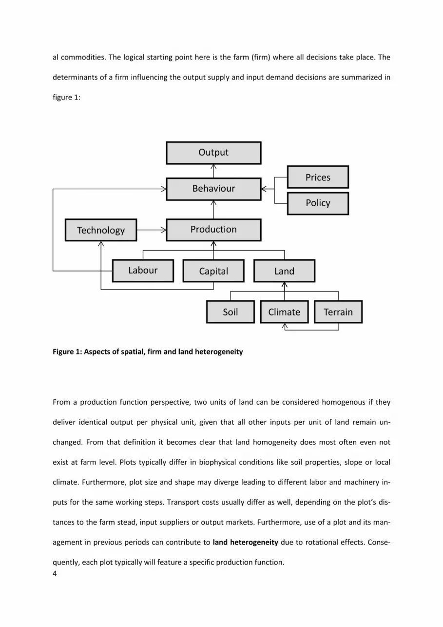
al commodities. The logical starting point here is the farm (firm) where all decisions take place. The
determinants of a firm influencing the output supply and input demand decisions are summarized in
figure 1:
Figure 1: Aspects of spatial, firm and land heterogeneity
From a production function perspective, two units of land can be considered homogenous if they
deliver identical output per physical unit, given that all other inputs per unit of land remain un-
changed. From that definition it becomes clear that land homogeneity does most often even not
exist at farm level. Plots typically differ in biophysical conditions like soil properties, slope or local
climate. Furthermore, plot size and shape may diverge leading to different labor and machinery in-
puts for the same working steps. Transport costs usually differ as well, depending on the plot’s dis-
tances to the farm stead, input suppliers or output markets. Furthermore, use of a plot and its man-
agement in previous periods can contribute to land heterogeneity due to rotational effects. Conse-
quently, each plot typically will feature a specific production function.
Production
Prices
Output
Soil Climate Terrain
Land Capital
Technology
Behaviour
Labour
Policy

5
If we now move to a higher aggregation level as for example a group of farm situated in the same
region, differences in production functions will increase with higher variability in biophysical condi-
tions and other aspects. Additionally, an aggregation in space implies an aggregation over farms as
well, and thus adds the aspect of firm heterogeneity: besides the immobile factor land, firms clearly
differ as well in the other production factors such as labor and capital, both with regard to factor
quantities, proportions and quality. Quasi-fixed capital and knowledge (human capital, managerial
capacity) typically strongly influence the available technology and thus the production function. The
factor human capital is also closely related to an adequate behavioral model of the firm (focus solely
on profits or other aspects of utility such as risk, preferences for specific farm branches, leisure and
environmental externalities). Clearly, the behavioral model and the production functions determine
jointly optimal input demand and output supply in reaction to market and policy signals. Conse-
quently, even identical plots from a bio-physical perspective might deliver a different output at given
input quantities, if the technology of the firms and/or the utility function of the managers operating
these plots differs.
Spatial heterogeneity can hence be understood as the combination and interaction of land and firm
heterogeneity, but has also to take into account spatial differences in market and policy signals.
While for commodities like grains or oilseeds the market signals might be quite similar within a coun-
try, other markets like fruits and vegetables more likely receive market signals that differ spatially.
Policy signals clearly also differ in space since political interventions impacting agricultural land use
can differ even at a high spatial resolution (e.g. zoning laws, protected sites, nitrate vulnerable
zones), more often so at regional level (e.g. to support so-called Less Favoured Areas under the CAP)
and typically between nations. Access to input and outputs markets, transport cost differences and
policy interventions such as border protection also clearly differentiate prices in space and lead to
spatial specialization in agriculture (cf. von Thünen model). Furthermore vertical and horizontal inte-
gration of firms influence firm productivity and thus add to spatial heterogeneity.
6
The challenge for economic modeling is that typically only some of the spatially heterogeneous driv-
ers can be directly observed, others along with the behavioral model and the production functions
can typically only be deducted. Accordingly, a clear separation of land from other spatial heterogene-
ity is hardly possible in empirical applications. These reflections lead to the following viewpoints to
evaluate quantitative modeling approaches with respect to their representation of spatial heteroge-
neity:
(V1) Are attributes of spatial heterogeneity such as soil or climate considered explicitly in the pro-
duction function or only indirectly by calibrating to observed input/output relations?
(V2) Is there a clear separation between land heterogeneity and other factors which are (poten-
tially) spatially differentiated (other production factors, behavioral model, market and policy
signals)?
The next section continues with an overview of some of the existing global economic models cover-
ing the agricultural sector led by these two questions and following the definitions given above.

7
Existing modeling approaches and their representation of heterogeneity
The section provides an overview of a number of global (agro-) economic models focusing on their
representation of land heterogeneity (subsection 3.1). It is rounded off by a section discussing recent
econometric work on representing the intensive margin (subsection 3.2).
Modeling approaches
Many models covering the agricultural sector on a global scale do not cover spatial heterogeneity in a
detailed way. CGE models like GTAP (Hertel, 1997) traditionally do not treat production factors het-
erogeneously below the national level, and often even aggregate over nations to global regions. CGE
models conventionally use a combination of Leontief and CES production functions to model supply
and are typically perfectly calibrated against a benchmark. Criticism that the typical production func-
tion structure is not well suited to model yield and input use changes in agriculture is reflected in the
development of specific nesting structures and primary factor market structures such as in GTAP-AGR
(Keeney and Hertel, 2005).
In order to overcome aggregation bias in global CGE modeling with regard to land use, the GTAP-AEZ
approach (Lee et al. 2009) was developed. It provides a prominent example for the challenges of
higher spatial disaggregation in land in global models, also with regard to data issues. As Social Ac-
counting Matrices (SAMs) are not available at the level of the Agro Environmental Zones (AEZ), but at
least land rents are required for the parameterization of the subnational land demands, GTAP-AEZ
uses actual crop revenues from FAOSTAT in conjunction with a rather simple spatial disaggregation of
crops (Monfreda et al., 2008) to disaggregate land rents at national level (see Lee et al., 2009, page
74). This means that land heterogeneity below the national level is taken into account explicitly, but
other types of spatial heterogeneity are not covered separately. Moreover, only land use is spatially
differentiated, while intermediate inputs and other primary factors are determined for each sector at
the level of nations or aggregates thereof. A change in the composition of land use therefore does
not shift the aggregate production function. The aim of the approach is thus rather to model where

8
land use changes occur at the regional level and to quantify related greenhouse gas (GHG) emissions.
It does inform the overall model on interactions between land quality and the shape of the produc-
tion function. The same holds for GTAP children like MAGNET (www.magnet-model.org) or DART
(Klepper et al., 2003).
Similarly, most Multi-Commodity Models (MCMs) such as OECD’s and FAO’s Aglink-Cosimo model
(OECD and FAO, 2015) capture sub-national spatial heterogeneity implicitly through observed aggre-
gated input/output relations in conjunction with estimated response parameters. MCMs generally do
not use production, but behavioral functions. The yield response to prices in these functions – i.e.
changes in the intensive margin - hence simultaneously captures a move on the production function
and its potential shift.
This also holds for the global multi commodity model in CAPRI (Britz and Witzke, 2014). In contrast,
the supply side for European countries of CAPRI features a high spatial disaggregation of all inputs
and outputs either on NUTS2 regional level or farm types within these regions (Gocht and Britz,
2011). Spatial heterogeneity within those regions is however only captured through the observed
relations of outputs and inputs. Other examples for a sub-national resolution in global MCMs are
given by the FAPRI modeling system which has a module breaking down the US to individual states
(Meyers et al., 2010) and the IMPACT-WATER model (Rosegrant et al., 2005) which features a dis-
aggregation to larger river basins in combination with a distinction between irrigated and rainfed
agriculture.
The GLOBIOM model (Global Biosphere Management Model, www.globiom.org) is a global, recur-
sively dynamic, bottom-up partial equilibrium model of the agricultural, forestry and bio-energy sec-
tor. Its structure is linked to the FASOM model developed by McCarl et. al. (Adams et al., 1996), i.e.
supply is based on Leontief production functions, demand functions are linear and account only for
own price effects and trade is modeled based on minimizing transport costs. The model is fully linear,
and thus potentially subject to over-specialization, and impossible to calibrate exactly against

9
benchmark supply, demand, price and trade data. The demand side of the model is represented
through 30 aggregated world regions while the agricultural and forestry supply is modeled on
0.5°x0.5° Simulation Units differing in biophysical conditions (altitude, slope and soil type), but also
irrigation water availability. The production possibility set on each simulation unit is represented by a
set of Leontief production functions (low/high input, tillage practice, irrigation). For crops, technolo-
gies and yields are generated by the Environmental Policy Integrated (EPIC) Model, a biophysical crop
growth model (Williams, 1995). Due to a lack of global spatially explicit data on the management
practices, factor endowments are estimated at the Simulation Unit level either through biophysical
models or downscaling of national (FAO, IFPRI) datasets. For the land factor, the GLC 2000 land cover
map (JRC) is used. Initial crop areas per management system are based on SPAM data (Spatial Pro-
duction Allocation Model, IFPRI). Different levels of aggregation can be used depending on the geo-
graphic scope of the analysis. For the global version of the model, Simulations Units are aggregated
to a lower spatial resolution, whereas for regional studies (GLOBIOM-EU and GLOBIOM-Brazil) some
countries of interest can be represented in greater spatial and sectoral detail, both on the demand
and the supply side. GLOBIOM is therefore a good example of a model that tries to capture spatial
heterogeneity in a rather detailed way by simulating farmer’s decision on a gridded scale.
However, economic data on other than selected attributes of land heterogeneity globally do not exist
at a high spatial resolution making estimates necessary. GLOBIOM therefore uses a crop growth
model to construct spatially differentiated production feasibility sets. Such a crop growth model can
hence be understood as a production function where (selected) biophysical attributes are explicitly
considered, i.e. the simulated productivity of land depends directly on soil properties and climate1.
However, if such bio-physical models are calibrated against observed yields, other drivers of land
productivity, which might differ in space and are not explicitly considered in the calibration exercise,
1 Bouman et al. (1996) provide a good overview on the history of crop models

10
need to be represented by correction factors, i.e. are not explicitly accounted for (cf. Osborne et al.,
2013). The same principles hold for the FSSIM model (van Ittersum et al., 2008).
A similar approach with regard to the coupling of biophysical and economic models is used in the
global MAgPIE model (Lotze-Campen et al., 2008). MAgPIE can be less clearly categorized compared
to the other modeling systems. One distinct feature of MAgPIE is that food energy demand for 10
food categories is fixed during simulation, driven by trends and income. The model is hence a global
supply side, and not a market model, as there is no market clearing mechanism. Feed demand for
each product is linked with Leontief coefficients to animal output quantities. Consequently, the mod-
el minimizes overall production costs to satisfy given final demand, while costs of trade seem not to
be considered. However, there is no feedback of costs on the demand side. Equally, the export (and
thus implicitly import) quantities for each region are set exogenously. In each grid cell, land, irrigation
water and minimal and maximal rotation shares restrict the crop allocation. Animal production also
requires water, but it remains somewhat unclear what else drives the allocation of animal production
in space. The basic technology is Leontief, but there are terms which allow yield increases at addi-
tional costs, however, these costs are not attributed to specific production factors. Equally, available
crop land can be expanded at additional costs. The model covers 18 crop and 5 livestock categories.
Potential crop yields for each grid cell (three by three degrees) are supplied by the Lund–Potsdam–
Jena dynamic global vegetation model with managed lands (LPJmL, Bondeau et al., 2007). The yield
gap in the first period (relative difference between the potential and observed yield) enters the
model, but the yield gap can be closed by additional costs as mentioned above. These supply grids
are aggregated to 10 global regions on which demand is modeled. The model is run recursively in 10
year time steps; the link between time steps appears to be mostly based on using the cropped land
from the previous time point as the starting endowment. Overall, the supply side of the model pro-
vides a mix of a classical programming approach and endogenous yields. Due to the fixed Leontief

11
feed coefficients, also feed demand is probably more or less fixed with final demand for animal
products being exogenously given.
Table 1. Overview of the representation of land heterogeneity in selected global models
Model name # of spatial units Remarks Explicit soil attributes or based on ob-served input-out relations
Separation between land heterogeneity and other spatially het-erogenous factors
GTAP-AEZ 18 AEZ potentially per country, several AEZ only found if country spans over different climate zones
Disaggregation only for land in produc-tion function
Explicit no
Aglink-Cosimo Indirect no CAPRI, global trade module
77 countries orga-nized in 40 trading blocks
Indirect no
CAPRI supply side, regional version
ca. 280 NUTS2 re-gions for Europe or about 2000 farm types
Indirect no
GLOBIOM Depending on appli-cation
Based on so-called response units at 0.5°x0.5° (between 10x10 to 50x50 km) from which actual supply side units are aggregated
Explicit Partly, by link to crop growth model
MAgPIE Grids 3°x3° Explicit Partly, by link to crop growth model
The strategy of all these models to reflect land heterogeneity is a regional disaggregation of supply at
subnational or even subregional level based on (administrative) units for which data are either readi-
ly available or can be constructed. This approach can improve an economic model not only with re-
gard to land heterogeneity in a narrow sense, but with regard to any spatial differences in, for exam-

12
ple, technology, assets, behavior, market structure or policy instruments. To the extent that the
models used a grid, some allocation model such as SPAM (Spatial Production Allocation Model, Har-
vestCHoice, 2014) is necessary to provide at least a starting allocation ex-post.
The models mentioned above are all templated, i.e. they use structurally identical equations (except
for Aglink-Cosimo). Increasing the spatial resolution does not require changes in the model structure.
Leaving data availability aside, there are still two other major challenges related to such a higher
spatial resolution. The first one is a proper parameterization. Indeed, if the model’s functional forms
and parameterization imply equal relative reactions across all spatial units, little might be won by a
further disaggregation. If that is not the case, the question is if econometric studies are available
which allow for a defendable parameterization of the individual spatial units. GLOBIOM and MAgPIE
partially circumvent that problem by using the functional relations between bio-physical attributes,
input demand and yields embedded in crop growth models, but clearly still struggle with a good rep-
resentation of the difference between the potential and observed yields, and the drivers between
the yield gap. Recent econometric approaches tackling the problem of an interdisciplinary represen-
tation of the yield gap, and thus the intensive margin are summarized in subsection 3.2. The second
challenge is more subtle: agent interactions in spatial units, such as the exchange of feed, nutrients,
machinery and labor between farms, which are implicitly covered at a higher aggregation level by the
parameterization of the model’s equations, might need to be explicitly modeled if the spatial dis-
aggregation is increased. Non-tradables at the level of firm aggregates might need to be considered
as tradable, such that an existing template fitting a more aggregate spatial modeling approach might
no longer be appropriate at finer spatial resolution.
Clearly, a higher disaggregation also has computational consequences, but pure Linear Programming
(LP) models such as GLOBIOM can probably be solved with millions of variables in reasonable time,
while classical CGE and MCM models represented by square systems of equations can probably
solved in larger shocks with some hundreds of thousands of variables and equations. The CAPRI
13
model solved the computational issue of explicit optimizations of its highly detailed supply side by
using iterations between the individually in parallel solved regional or farm type supply models and
its market model based on sequential iteration (Britz, 2008). However there are possibilities to reflect
land heterogeneity even on a higher aggregation through the properties of the factor land. The next
section addresses this issue.
Econometric specification of the intensive margin
For empirically determining a production function based on potential yields and their land heteroge-
neity, statistical-econometric pre-work is required. More particularly, one would have to explicitly
distinguish between biophysical drivers (b) and managerial/economic drivers (m) of actually ob-
served yields already in the econometric setup to obtain the respective parameters for the simula-
tion model. Requiring a good deal of multidisciplinary cooperation between meteorologists, crop
scientists and economists, work on this differentiation has just started. To our knowledge only two
statistical-econometric studies attempt to disentangle the biophysical and economic effects deter-
mining potential and actual yields, respectively: Neumann et al. (2010) and Baldos and Hertel
(2012).2 Both build upon the large strand of economic productivity and efficiency analyses (e.g. Coelli
et al. 2005). In the agricultural economics literature, the efficiency analyses are usually based on pro-
duction function approaches. The overall or activity (e.g. crop) specific production functions are
thereby either represented in terms of a programming (Data Envelopment Analysis – DEA) or of a
statistical-econometric approach (Stochastic Frontier Analysis – SFA). Explained are efficiency
measures or output, respectively, in economic terms. A bridging study between traditional farm effi-
ciency analysis and so-called yield gap analyses is provided by Reidsma et al. (2009) who still focus on
explaining economic output per crop. However, apart from managerial, economic and political fac-
tors, they are the first who also include biophysical determinants – namely, temperature and precipi-
tation - in their analysis. Neumann et al. (2010) and Baldos and Hertel (2012) extend the approach by
2 A tabular overview of the studies mentioned here is given in Table A 1 in the Appendix.

14
specifically targeting at explaining crop yields and yield gaps in physical terms and at global level.
Both take three crops of global relevance into account: wheat, maize, and rice. Neumann et al.
(2010) use a temperature measure, precipitation, Photosynthetically Active Radiation (PAR) and soil
fertility constraints as independent variables explaining regional yield frontiers, which are interpreted
as regional potential yields. The regional deviation from potential yields is explained by managerial
and locational factors such as irrigation and slope and macroeconomic factors such as agricultural
population, market access and market influence. Baldos and Hertel (2012) determine regional fron-
tier yields by temperature, precipitation, soil constraints and slope. Deviations from frontier yields
are explained by population, fertilizer use, irrigation, market accessibility, market influence and insti-
tutional strength. Thus, both studies account for land heterogeneity by considering soil constraints
and climatic conditions. Summarizing, these three articles provide a good foundation for a potential
parameterization of simulation models based on a truly cross-disciplinary econometric approach. A
theoretical example for this is presented as an outlook at the end of the empirical section 5. The next
section addresses the extensive margin in terms of land aggregation issues and the combination of
extensive and intensive margin in terms of ensuring convexity in the simulation models from a theo-
retical perspective.
Modelling land from the micro-economic perspective
Two strands of how land is aggregated in agro-economic modeling can be observed - either linearly,
as a physical land restriction, or non-linearly. Both will be looked at in more detail in subsections 0
and 0, respectively, followed by some considerations of establishing convexity in the decision varia-
bles.

15
Linear aggregation
A linear aggregation of different types of land use u in an (implicit) optimization problem depending
on the amount of each land use l, measured in a physical unit,
(1) ( )
[ ]max
. . uu
l
s t l L l
Π
=∑
implies equal marginal economic returns λ between competing uses u. The linear aggregation typical-
ly uses an area based physical unit such as hectares to define available land. Average returns to land
are not necessary equal to marginal ones for each use u, such that factor/input use for each u per
unit of l can differ across l, or prices respectively policy (dis-) incentive might vary per physical unit of
land used in u. The linear aggregation which implies homogeneity from an economic accounting per-
spective (=equal marginal economic returns) might hence be incompatible with homogeneity from
an environmental (=equal per unit impact, such as GHG emissions) accounting perspective.
However, if the linear aggregation is combined with a constant-return-to-scale (CRS) technology for
each u, marginal and average land productivities become identical. That is the most common solu-
tion found in programming models where Leontief technologies are used. However, it is possible to
differentiate land classes by productivity and restricting the set of activities by class. A simple appli-
cation of such a classification is the distinction between arable and permanent grass lands as found,
for example, in CAPRI (Britz and Witzke, 2014). A more refined approach offers FSSIM (Louhichi et al.,
2010) where land can be broken down to different soil types.
CGE models also typically assume CRS, however usually apply CES production functions. In combina-
tion with a linear aggregation (sector specific land stocks or fully mobile land), this implies that aver-
age and marginal output and input use per physical unit of land are equal in each competing use u. If
a linear aggregation is combined with non-CRS technologies, such as in applications of PMP (Howitt,
1995), marginal and average land productivity typically differ. In PMP, two different strands can be

16
distinguished in that respect: introduction of a dual non-linear cost function while keeping in-
put/output (I/O) coefficients fixed, or introducing explicitly a non-linear technology.
The dual cost function approach with fixed yields implies that the marginal physical productivity of
land remains fixed when acreages change. This implies that farm management is adjusted in such a
way that yields stay constant. However, marginal economic returns to land respond to acreage
changes as marginal production costs are a function of acreages. Fixing yields typically eases envi-
ronmental accounting as emission factors do not need to be updated endogenously. In Howitt’s 1995
original paper on PMP, the non-linearity was introduced by a quadratic yield function which depends
on the acreage of the respective crop, which he attributes to changing land quality (p. 334). That
solution could be alternatively interpreted as a non-CRS technology. Mérel et al. (2011) combine the
PMP approach with a CES production function with decreasing returns to scale.
To sum up: CRS technologies in combination with a linear land aggregator imply that land is a homo-
geneous factor, while a linear land aggregator combined with non-CRS technologies treats land as
heterogeneous as marginal returns to land are not equal to average returns.
Non-linear aggregation
Under the formulation
(2)
( )[ ]
max
. . ( )
l
s t g l L l
Π
= ,
the marginal economic returns per unit of land might differ across the competing uses u in the opti-
mum. That allows calibrating the system against observations where land rents differ by u which is
the case in reality – either due to different biophysical attributes or management decisions that lead
to different economic outputs of the same crop on different plots. Such a solution is found when so-
called “sluggish land mobility” is implemented in CGEs models where typically Constant Elasticity of
Transformation (CET) functions are used (Hertel et al. 2009), but also in the partial equilibrium model

17
PEM (Policy Evaluation Matrix, OECD 2001). The CAPRI supply models use a similar mechanism, how-
ever with a different functional form (Britz and Witzke, 2014) to model substitution between arable
and grassland in its programming models.
As the amounts l for each u enter a production function with unchanged parameters, the non-linear
aggregation transforms the given physical land stock L into units of equal productivity. The unit of l is
hence not equal to the physical unit used to measure L, i.e. ( ) uu
g l l≠∑ . The non-linear aggregation
could hence be understood as a land (or location) quality (or heterogeneity) correction.
The CET function implies that the physical productivity per physical unit of land always decreases if a
certain land use is expanded. This is also assumed in the models of Howitt (1995) with yield functions
decreasing in land and Mérel et al. (2011) who use a non-CRS-CES production function. The use of a
CET land market implies that even if the production function into which the land enters has a CRS-
technology, the overall technology is non-CRS in physical land.
The CET approach seems to be appropriate to reflect land heterogeneity, however the link between
the quality-corrected land and the physical units are not explicit. It is possible to scale the quality-
adjusted land with a constant factor (for each CET nest) to meet the physical land constraint, but
there is no theory that would suggest a constant factor to be the right choice. The constant scaling
factor is illustrated by the case of two crops competing for one hectare.

18
Figure 2: Linear and nonlinear land transformation
In figure 2, the solid black line shows the linear aggregation case. For each additional unit land of
crop B the same amount land of crop A must be reduced. In the nonlinear case one can see that it
becomes more “expensive” to extend crop B the higher its production share is already (dotted grey
line). The linear scaling factor that would result from translating each combination of the productivity
adjusted crops to a physical combination is given by dashed line. The u-shape of this reveals one fea-
ture of the CET approach: the value of each chosen combination of crops A and B decreases when
moving away from the point where physical and value adjusted combinations are equal (in this case
0.5/0.5) implying decreasing total productivity in both directions.
Physical units of land are indeed needed for the calculation of many indicators defined on a per hec-
tare basis and consistent land use reporting. A model should therefore be able clearly to separate the
intensification effect (higher input use per ha) from extensification (expanding land). As already no-
ticed the above discussed approaches implicitly or explicitly assume decreasing returns to scale of
physical land. This effect is a combination of heterogeneous land and adjustments to other input
factors. While there exist arguments for the latter to lead always to decreasing marginal returns to
0.000.100.200.300.400.500.600.700.800.901.001.101.201.301.401.50
0.00 0.10 0.20 0.30 0.40 0.50 0.60 0.70 0.80 0.90 1.00
crop
A
crop Blinear aggregation nonlinear aggregationscaling factor

19
land (expanding land with other production factors not fully adjusting due to other constraining fac-
tors) the expected reactions at the micro level do not guarantee that expanding a certain crop will
happen on a less productive plot than the current ones, one might for example observe that higher
gross margins lead to an expansion of minor crops into more productive land. We can therefore not
pre-determine the direction of the land heterogeneity effect without explicitly modeling each
farmer’s decision through, for example, Agent Based Models (ABM) linked to single farm models (cf.
for example the FarmDyn model, Britz et al., 2014) that differentiate soil type and plot sizes.
Convexity
Solving large-scale economic simulations model typically requires convexity of the underlying optimi-
zation problem in the decision variables. In linear programming models, this convexity is achieved
through a rich definition of constraints that become more costly in terms of model performance
(convergence, model building time, runtime, etc.) the more binding they are – although convexity
here is not smooth but discrete. Nonlinear programming models such as PMP applications are con-
vex in objective functions by adding increasing costs or decreasing yields with extending activity lev-
els (non-CRS technology) and dual formulations in square equation systems build on the assumptions
of existing objective function maxima of the primal model on which they are based as well.
As indicated before, land heterogeneity alone does not guarantee this convexity. Let us assume a
(regional) supply definition:
(3) ( ) ( ), , , ,potr u r u r u r us y l y l i l = = b m l
The supply s of crop u in region r is defined as the physical acreage l of that crop multiplied by the
yield y. This regional yield depends on many variables but can be broken down into two components:
a biophysical component b and one related to management m. The latter is represented by the in-
tensity function i which depends on the actual land allocation (e.g. through rotational effects) as well
as some management factors m like plant protection and fertilizer applications. The biophysical
20
component can be interpreted as the regional potential yield (ypot) which depends on a vector b of
biophysical variables like soil quality, slope, plot size and shape as well as climatic conditions. Howev-
er, this potential yield also depends on the allocation to the respective crop. As the impact of the
different factors on the potential yield is non-linear, an aggregate of plots needs to reflect the com-
position of the aggregate to derive the correct average potential yield. In simulation, one thus needs
to reflect how the plot composition reacts to changes in crop acreages. There exist several definitions
of a potential yield (e.g. van Ittersum et al., 2013). An agronomist will argue that the potential yield is
only dependant on biophysical variables, which is true when focusing on single spots. As soon as we
regard a regional aggregate of such spots, however, those spots need to be weighted somehow to
come up with a regional definition of potential yields. The simplest solution would be to use an un-
weighted average among single spots. In that case even those spots would be included in that aver-
age where a crop is never cultivated, e.g. absolute grass lands in case of arable crops. Consequently,
it is not guaranteed that average regional observed yields are below this potential yield, rendering
such a definition contra-intuitive. A second definition leads to the black line in figure 4. The potential
yield of a certain land allocation would be the one that is achieved when growing a crop always on
the plots with the best attainable yield. This definition disregards, however, the fact that there is
competition between crops among plots where their potential yields might be highly correlated. We
therefore define the regional potential yield as the average at a specific land allocation.
Let a region r consist of 10 plots that may for now be all of the same size (1 ha) and shape but differ
in potential yields for a certain crop. If we then order these plots by potential yields and visualize
them in a bar graph, this would look like the bars in figure 3.

21
Figure 3: Potential yields per plot and region
The average potential yield at regional level of that crop can theoretically vary between the grey line,
where plots are chosen starting with the lowest potential yield and then with the next higher one,
and the black line, where the best plot is chosen first. Accordingly, any possible allocation of crops to
plots will yield average potential yields within that range. The figure already reveals one finding:
F1: the range in which potential yields of a certain crop may vary decreases with increasing
cropping shares.
The question might now be how important this range is in reality. This will be evaluated in the next
section exemplary for Germany.
How important is the spatial distribution of potential yields for simulations
with a regionally aggregated model?
Below, we analyse the importance of the spatial allocation of crops on estimated regional potential
yields based on potential yield data for Germany as an empirical example. Thereby we first explore
0
20
40
60
80
100
120
140
160
1 2 3 4 5 6 7 8 9 10
pote
ntia
l yie
lds
plots potential yields per plot maximal regional potential yield minimal regional potential yield

22
the range that in which the average regional potential yield might fall and narrow this further down
after that using a simple approach for land allocation at higher aggregation level for illustration. The
database and descriptive statistics for the example are described next.
Exemplary data for Germany
The data used for this example is based on data from Leip et al. (2008) that features potential yields
allocated to so-called Homogenous Spatial Mapping Units (HSMU), 1x1 km cluster cells which are
assumed to be uniform in climate and soil. The data set also comprises a consistent down-scaling of
crop acreages from administrative regions to the HSMU level. Potential yields are only available for
eight of these crops (average crop shares on arable lands in Germany are given in brackets3): soft
wheat (25%), barley (15%), maize grain 4%, maize silage 13%, rape seed (12%), sunflower (0.2%),
potatoes (2%) and sugar beet (6%). Together, they account for about 74% of arable land in Germany.
In total, there are about 5.100 HSMUs found in Germany where one or several of the crops are re-
ported as being farmed.
Figure 4 reports the distribution of the potential yields over the HSMUs, without considering the
actual crop allocation as weights. Most of these distributions show a relatively narrow spread, indi-
cating that climatic and other conditions in Germany on spots where the crops are actually grown do
not lead to drastic changes in crop yields. The potential yields vary between 5% (pulses) up to 20%
(rapeseed) around their average value. All non-cereals have however some longer tails with possible
outliers. These might be important especially if low cropping shares are given.
3 The data used for Germany is derived from the database of the CAPRI model (Britz and Witzke, 2014) and represent three year averages around 2008.

23
Figure 4: Distributions of potential crop yields [t/ha] across spatial units
Source: Own illustration based on Leip et al. (2008)
Exploring the possible range of aggregate yield results
Similar as in figure 3 it is possible to generate the minimal and maximal potential yields depending on
the chosen cropping share for the dataset for Germany. In figure 5 this is done for soft wheat. The
outer horizontal lines are thereby computed by choosing HSMUs with the highest/lowest potential
yield first for a given national cropping share which is given on the x-axis. Total area per HSMU is

24
calculated as the sum of land allocated to arable crops as the HSMUs may contain considerable
shares, for example, of forest, permanent grassland or sealed areas. The national arable crop area is
then given as the sum over the HSMUs’ total areas. Figure 5 further gives the minimal, average and
maximal national cropping shares of soft wheat in Germany over the past 30 years. According to this
soft wheat shares varied between 19% and 26% of arable land. We further plot the average potential
yield at the cropping shares from an available dataset for 2008 (10.3 t/ha). The picture reveals, that
the average national potential soft wheat yield in the past 30 years was found in the range between
9.5 and 10.8 t/ha – the minimal and maximal shares at the lowest observed cropping share.
This range of 1.3 t/ha is however further reduced if we apply some plausibility restrictions. So far we
were allowing mono-cropping per HSMU, which is not realistic from an agronomic point of view. We
therefore introduce rotational restrictions per HSMU. For each cereal, we allow only a cropping share
of 50% and restrict all other crops to 1/3 of the arable crop area which led to the green lines. Poten-
tial yields vary here only between 9.7 and 10.65 t/ha.
Figure 6: Range of regional potential yields [t/ha] depending on cropping shares (soft wheat, Ger-
many)
9
9.2
9.4
9.6
9.8
10
10.2
10.4
10.6
10.8
11
regi
onal
pot
entia
l yie
ld
cropping share
minimal cropping share (1990-2010)
average cropping share (1990-2010)
maximal cropping share (1990-2010)
potential yield at 2008 cropping share
maximal potential yield
minimal potential yield
maximal potential yield with rotation
minimal potential yield with rotation

25
In a next step, we assume that observed regional patterns are likely to prevail, if the national crop-
ping shares change. Therefore we introduce the restriction, that cropping shares do not only need to
be met at national, but also at regional level. This implies that an increase of one percent point at
national level is translated to a higher increase in regions, where the observed cropping shares are
already higher compared to regions with lower initial shares. This is done for the NUTS1 and NUTS2
levels in Germany for 7 of the available products (leaving pulses and sunflowers out due to rather
small cropping shares). The results are summarized in figure 6. Clearly, the additional restrictions at
the NUTS levels narrow down the range in which average potential yields may vary depending to the
actual choice of crops per HSMU. In the NUTS2 case, this range amounts to about 400 kg for wheat
and barley, 900 kg for maize, 500 kg for rape, 3 t for potatoes and 2 t for sugar beets and silage
maize. Although these ranges may be deemed important, if we further disaggregated the procedure
to the farm level and apply the same restrictions, the “range of uncertainty” around the average
potential yield would most likely become very small. An endogenous reflection of the dependency of
average potential yields on actual cropping shares might not be necessary, especially when remem-
bering that cropping share changes that sector models typically simulate are in limited ranges as well.

26
Figure 6: Range of regional potential yields [t/ha] depending on cropping shares for seven crops
9
9.2
9.4
9.6
9.8
10
10.2
10.4
10.6
10.8
11
15.0
%15
.9%
16.7
%17
.6%
18.4
%19
.3%
20.1
%21
.0%
21.8
%22
.7%
23.5
%24
.4%
25.2
%26
.1%
26.9
%27
.8%
28.6
%29
.5%
30.3
%31
.2%
regi
onal
pot
entia
l yie
ld
cropping share
soft wheat
8
8.2
8.4
8.6
8.8
9
9.2
9.4
9.6
9.0%
9.9%
10.7
%11
.6%
12.4
%13
.3%
14.1
%15
.0%
15.8
%16
.7%
17.5
%18
.4%
19.2
%20
.1%
20.9
%21
.8%
22.6
%23
.5%
24.3
%25
.2%
regi
onal
pot
entia
l yie
ld
cropping share
barley
7
7.5
8
8.5
9
9.5
10
10.5
11
11.5
0.5%
0.9%
1.4%
1.8%
2.2%
2.6%
3.1%
3.5%
3.9%
4.3%
4.8%
5.2%
5.6%
6.0%
6.5%
6.9%
7.3%
7.7%
8.2%
8.6%
regi
onal
pot
entia
l yie
ld
cropping share
maize
52
54
56
58
60
62
64
66
68
0.5%
1.0%
1.5%
1.9%
2.4%
2.9%
3.4%
3.8%
4.3%
4.8%
5.3%
5.7%
6.2%
6.7%
7.2%
7.6%
8.1%
8.6%
9.1%
9.5%
regi
onal
pot
entia
l yie
ld
cropping share
potatos
60
65
70
75
80
85
0.5%
1.0%
1.5%
1.9%
2.4%
2.9%
3.4%
3.8%
4.3%
4.8%
5.3%
5.7%
6.2%
6.7%
7.2%
7.6%
8.1%
8.6%
9.1%
9.5%
regi
onal
pot
entia
l yie
ld
cropping share
sugar beet
55
57
59
61
63
65
67
69
4.0%
4.8%
5.6%
6.4%
7.2%
8.0%
8.8%
9.6%
10.4
%11
.2%
12.0
%12
.8%
13.6
%14
.4%
15.2
%16
.0%
16.8
%17
.6%
18.4
%19
.2%
regi
onal
pot
entia
l yie
ld
cropping share
silage maize
2
2.5
3
3.5
4
4.5
5
5.5
6
0.5%
1.4%
2.3%
3.1%
4.0%
4.9%
5.8%
6.6%
7.5%
8.4%
9.3%
10.1
%11
.0%
11.9
%12
.8%
13.6
%14
.5%
15.4
%16
.3%
17.1
%
regi
onal
pot
entia
l yie
ld
cropping share
rape

27
Figure 6 reveals two additional finding:
F2: The range in which potential yields of a certain crop may vary decreases when reflecting
crop rotations.
F3: The range further decreases when a national shift in cropping shares are stronger in re-
gions (on farms) where the actual share is higher compared to regions with lower shares.
A simple economic approach for assessing regional potential yields
In a next step, we develop a rather simple approach for allocating land. It assumes, as above, that
potential yields for each crop are given for a set of spatial units u which together cover the land
managed by an (aggregate) agent. The data on potential yields are complemented by information or
assumptions on the relation between the gross margins for each crop per hectare as a function of the
potential yield. In order to ease the analysis, we assume in here that the gross margin gm [€ ha-1] for
each crop i and spatial unit u is simply proportional to the potential yield y [t ha-1], according to a
gross margin multiplier r [€ ha-1 t-1]:
(4) , ,pot
i u i u igm y r=
The reader should note that this assumption does not imply a Leontief technology, as the relation
between allocated inputs hiding behind the crop specific margins and land will change as a linear
function of the potential yield.
In order to allocate the crops spatially, the agents are assumed to optimize the total gross margin
GM, subject to given acreages of the crops, decided elsewhere, and given plot sizes:
(5) ,
, ,,,
,
,
. .
maxi u
poti u i i u
i uha i u
i u ui
i u iu
GM y r ha
ha ha us t
ha ha i
∀
=
= ∀
= ∀
∑
∑∑

28
The optimization model (5) could be part of a decision problem with two interlinked levels where at
the upper level, depending on the mean yield of each crop, total acreages are decided upon, and (5)
depicts the best possible distribution of the crops across the plots. The average yields of the crops
optimized in turn enter the decision problem on the total acreages which constraints the solution.
We use this model to conduct several experiments. As starting point we use the same gross margin
per ha for all crops at average yields, converted to construct the crop specific revenue multiplicator r
by division of the yield average over all spatial unit. That assumption reflects a typical (implicit or
explicit) First Order Condition (FOC) in aggregate simulation models, namely that the marginal re-
turns to land are equal across crops. We term these equal marginal returns to land the “gross mar-
gin” per ha, divided by the average yield of each crop, it must yield the marginal gross margin per
unit of output of each crop produced on the last unit of land. As above, a maximum allowed share of
50% on each spatial unit is assumed for all crops, with the exemption of potatoes and sugar beets,
where 33% is used. We further apply the regional restriction at NUTS2 level as above.
We use a nested experiment design, where at the upper level the aggregate acreages are decided
upon. Here we explore the same range as in figure 7. Each crop is separately moved from the mini-
mum to the maximum of the range and all other crops are scaled linearly to fit the area of each spa-
tial unit u.
For each of these cropping share combinations, we apply the second level of experiments where we
randomly change the gross margin multipliers for the crops r with a factor between zero and unity on
all spatial units. That introduces drastic changes in the competitiveness of crops across the whole
region. The draws are constructed using design of experiments. There will be draws where one crop
is preferred in any units over all crops. Figure 7 illustrates the results of these experiments. It shows
for all 7 crops the highest and lowest values that average potential yields take – which are very close
to those in figure 6, although the minimal values are a bit higher in figure 8 meaning that even for
very low gross margins the crops will not be allocated to the spatial units with the lowest potential

29
yields. We further see the lower and upper quartiles of the resulting distributions as well as their
medians. For all crops it can be observed, that the distribution is skewed to the upper limit, because
the lower grey areas often take more than half of the total shaded areas. In other words:
F4: There is a higher probability that average yields will be found closer to their theoretical
maximum than to the minimum.
If we take only the area between the theoretical maximum and the Q1 quartile into account, in which
75% of all draws can be found, the range of potential yields is further reduced considerably. For
wheat and barley it is reduced to about 100 kg /ha. For maize, 200 kg/ha are left, for sugar beet, the
range for potatoes and silage maize is reduced to 1 t/ha and for rape seed to about 50 kg/ha.
Figure 7 gives the impression that the impact of changes in the spatial allocation of crops on the av-
erage potential yield is not of high relevance in Germany. We need to bear in mind that the reve-
nue/ha distribution from which we drew our experiments was spread very widely - much stronger
than in reality.
It might therefore be valid to reformulate the supply definition equation (3) as follows.
(6) ( ) ( )*, , ,pot
r u r u r r us y l y b l i m l l = =
The regional potential yield is here no longer dependent on the actual land allocation, but the “ob-
served” one l*. This simplifies reality but might be sufficient in large scale modeling. However, the
specification of such a production function still requires some thought, which we carry out in the
next section.

30
Figure 7: Range of regional potential yields [t/ha] depending on cropping shares and relative prof-itability for 7 crops
10
10.1
10.2
10.3
10.4
10.5
10.615
%16
%17
%18
%18
%19
%20
%21
%22
%23
%24
%24
%25
%26
%27
%28
%29
%29
%30
%31
%32
%
regi
onal
pot
entia
l yie
ld
cropping share
soft wheat
8.5
8.6
8.7
8.8
8.9
9
9.1
9.2
9.3
9% 10%
11%
12%
12%
13%
14%
15%
16%
17%
18%
18%
19%
20%
21%
22%
23%
23%
24%
25%
26%
regi
onal
pot
entia
l yie
ld
cropping share
barley
9.59.69.79.89.910
10.110.210.310.410.5
1% 1% 1% 2% 2% 3% 3% 3% 4% 4% 5% 5% 6% 6% 6% 7% 7% 8% 8% 9% 9%
regi
onal
pot
entia
l yie
ld
cropping share
maize
70
70.5
71
71.5
72
72.5
73
73.5
1% 1% 1% 2% 2% 3% 3% 4% 4% 5% 5% 6% 6% 7% 7% 8% 8% 9% 9% 10%
10%
regi
onal
pot
entia
l yie
ld
cropping share
sugar beet
59
59.5
60
60.5
61
61.5
62
62.5
63
63.5
1% 1% 1% 2% 2% 3% 3% 4% 4% 5% 5% 6% 6% 7% 7% 8% 8% 9% 9% 10%
10%
regi
onal
pot
entia
l yie
ld
cropping share
potatos
3.5
3.6
3.7
3.8
3.9
4
4.1
4.2
4.3
1% 1% 2% 3% 4% 5% 6% 7% 8% 8% 9% 10%
11%
12%
13%
14%
15%
15%
16%
17%
18%
regi
onal
pot
entia
l yie
ld
cropping share
rape seed
60
60.2
60.4
60.6
60.8
61
61.2
61.4
61.6
4% 5% 6% 6% 7% 8% 9% 10%
10%
11%
12%
13%
14%
14%
15%
16%
17%
18%
18%
19%
20%
regi
onal
pot
entia
l yie
ld
cropping share
silage maize

31
Parameterizing potential yield and management
For parameterizing equation (3) with fixed l* and for a given region r, we believe that an econometric
Stochastic Frontier Analysis (SFA) following Neumann et al. (2010) is the most suitable approach
since it allows estimating the parameters of the biophysical drivers (b) and the managerial/economic
drivers (m) simultaneously. In the stylised form
(7) ( ) ( ) ( )0 1exp ln exp expj j j jy b v ib b= + × × ,
the output y of crop j, in this case the actual crop yield, would be explained by a deterministic com-
ponent which represents the potential yield ypot in equation (1.3) and is based on biophysical drivers
b and their coefficients β1 (β0 is the coefficient of the constant), a noise effect v, and a term repre-
senting management i in equation (1.3). The management term i can further be parameterized as
(8) j ji mδ=
which is based on managerial and other non-biophysical drivers m and their coefficients δ. Though a
classical Cobb-Douglas production function is shown here for illustrational purposes, other functional
forms might actually be more applicable depending on further theoretical and methodological con-
siderations. Figure 8 depicts the stochastic production frontier. It shows the production frontier
which is ypot and depends on the biophysical drivers. Both positive and negative deviations from the
frontier production can be due to noise effects, whereas systematic negative deviations are due to
non-biophysical factors such as management. Following the literature, those are usually termed “in-
efficiency”4. However, in this context, they should not be termed “inefficiency” anymore, but may
rather be well-founded, for example, due to economic considerations. In this setting, it would be
interpreted as the systematic deviation from frontier yields, i.e. the yield gap.
4 Please note that the “inefficiency” terminology is due to historic reasons. In fact, most researchers in this field would doubt that it represents inefficiency, but would rather be determined by other economically reasonable considerations.

32
Figure 8: Stochastic production frontier
Source: Based on Coelli et al. (2005) and Neumann et al. (2010).
Based on the literature and theoretical considerations, this section presented a general concept how
to derive the parameters for equation (3). The detailed specification of the approach is beyond the
scope of this paper and will be followed up in future research.
Summary and conclusions
Acknowledging that the explicit representation of land use and management is crucial for many
state-of-the-art model applications for predicting the impacts of land use changes, climate change as
well as policy and market developments, we provide definitions of spatial, firm, and land heterogene-
Deterministic frontier
( )0 1exp lnj jy bb b= +
yj (Yield)
bi (Input) bA
yA
Noise effect
“Inefficiency” effect = systematic deviation from frontier yields = yield gap
x
x
x
x
x

33
ity, where spatial heterogeneity is understood as the combination and interaction of both firm and
land heterogeneity and may include additional aspects at a smaller scale of the originally chosen
spatial scope, for example policy and market signals. We show how these are currently tackled in
some global economic modeling systems arguing that recent developments in land use representa-
tions at small scale usually do not explicitly account for their implications for parameterization of and
interaction between the smaller-scale units. We discuss the modeling of land from a micro-economic
perspective, and, based on these findings, explore the importance of the spatial distribution of po-
tential crop yields for simulations with a regionally aggregated model and exemplarily for Germany.
Additionally, an outlook for potential solutions for the parameterization of our approach is given.
The main contribution of the paper to the literature is that it provides the first comprehensive and
theory-based discussion of approaches to represent spatial and land heterogeneity in economic
models and how this representation could be improved. We limit the review of different modeling
approaches of land heterogeneity to a few selected models to illustrate their implications. We
demonstrate for a test case (crop yields in Germany) that the error which is associated with assuming
average regional potential yields independent from the “real” spatial land allocation is quite low.
Consequently it seems a valid strategy to calculate them at fixed land allocation shares. Full verifica-
tion of this at European or global scale is left for future model applications. Also, we just show a basic
illustration of how economic yield functions that take biophysical aspects into account could poten-
tially be parameterized based on transferring applications in the literature to our approach. The re-
finement of the parameterization and its adaptation to our purposes is beyond the scope of this pa-
per and will be discussed in future research.
References
Adams, D.M., Alig, R.J., Callaway, J.M., McCarl, B.A., Winnett, S.M., 1996. The Forest and Agricultural Sector Optimization Model (FASOM): Model Structure and Policy Applications. PNW-RP-495. U.S. Department of Agriculture, Pacific Northwest Research Station. Portland, Oregon, USA.

34
Adenauer, M., Britz, W., 2012. A Land Demand And Supply System With Endogenous Land Prices In The Capri Agricultural Sector Model (52nd Annual Conference, Stuttgart, Germany, Septem-ber 26-28, 2012 No. 137137). German Association of Agricultural Economists (GEWISOLA).
Ajanovic, A., 2011. Biofuels versus food production: Does biofuels production increase food prices? Energy, 5th Dubrovnik Conference on Sustainable Development of Energy, Water & Envi-ronment Systems 36, 2070–2076. doi:10.1016/j.energy.2010.05.019
Baldos, U.L.C., Hertel, T.W., 2012. Economics of global yield gaps: A spatial analysis, in: 2012 Annual Meeting, August 12-14, 2012, Seattle, Washington.
Bondeau, A., Smith, P.C., Zaehle, S., Schaphoff, S., Lucht, W., Cramer, W., Gerten, D., Lotze-Campen, H., Müller, C., Reichstein, M., Smith, B., 2007. Modelling the role of agriculture for the 20th century global terrestrial carbon balance. Global Change Biology 13, 679–706. doi:10.1111/j.1365-2486.2006.01305.x
Bouman, B.A.M., van Keulen, H., van Laar, H.H., Rabbinge, R., 1996. The “School of de Wit” crop growth simulation models: A pedigree and historical overview. Agricultural Systems 52, 171–198. doi:10.1016/0308-521X(96)00011-X
Britz, W., 2008. Automated model linkages: the example of CAPRI. German Journal of Agricultural Economics 57.
Britz, W., Lengers, B., Kuhn, T., Schäfer, D., 2014. A highly detailed template model for dynamic opti-mization of farms.
Britz, W., Witzke, P., 2014. CAPRI model documentation. Bonn, Germany.
Buysse, J., Fernagut, B., Harmignie, O., Frahan, B.H. de, Lauwers, L., Polomé, P., Huylenbroeck, G.V., Meensel, J.V., 2007. Farm-based modelling of the EU sugar reform: impact on Belgian sugar beet suppliers. Eur Rev Agric Econ 34, 21–52. doi:10.1093/erae/jbm001
Coelli, T.J., Rao, D.S.P., O’Donnell, C.J., Battese, G.E., 2005. An Introduction to Efficiency and Produc-tivity Analysis, 2nd edition. ed. Springer, New York.
Gilbert, C.L., 2010. How to Understand High Food Prices. Journal of Agricultural Economics 61, 398–425. doi:10.1111/j.1477-9552.2010.00248.x
Gocht, A., Britz, W., 2011. EU-wide farm type supply models in CAPRI—How to consistently disaggre-gate sector models into farm type models. Journal of Policy Modeling 33, 146–167. doi:10.1016/j.jpolmod.2010.10.006
HarvestCHoice, 2014. Crop Production: SPAM. International Food Policy Research Institute, Washing-ton, DC., and University of Minnesota, St. Paul, MN. Available online at http://harvestchoice.org/node/9716.
Harvey, M., Pilgrim, S., 2011. The new competition for land: Food, energy, and climate change. Food Policy, The challenge of global food sustainability 36, Supplement 1, S40–S51. doi:10.1016/j.foodpol.2010.11.009
Hertel, T., Steinbuks, J., Baldos, U., 2013. Competition for land in the global bioeconomy. Agricultural Economics 44, 129–138. doi:10.1111/agec.12057
Hertel, T.W., 1997. Global Trade Analysis: Modeling and Applications. Cambridge University Press.
Howitt, R.E., 1995. Positive Mathematical Programming. Am. J. Agr. Econ. 77, 329–342. doi:10.2307/1243543
35
Keeney, R., Hertel, T., 2005. GTAP-AGR: A Framework for Assessing the Implications of Multilateral Changes in Agricultural Policies [WWW Document]. GTAP Technical Paper No. 24. URL http://www.gtap.agecon.purdue.edu/resources/res_display.asp?RecordID=1869
Klepper, G., Peterson, S., Springer, K., 2003. DART97: A Description of the Multi-regional, Multi-sectoral Trade Model for the Analysis of Climate Policies. Kiel Working Paper No. 1149. Kiel Institute for World Economics, Kiel, Germany.
Lee, H.-L., Hertel, T.W., Rose, S., Avetisyan, M., 2009. An integrated global land use database for CGE analysis of climate policy options, in: Economic Analysis of Land Use in Global Climate Change Policy.
Leip, A., Marchi, G., Koeble, R., Kempen, M., Britz, W., Li, C., 2008. Linking an economic model for European agriculture with a mechanistic model to estimate nitrogen and carbon losses from arable soils in Europe. Biogeosciences 5, 73–94. doi:10.5194/bg-5-73-2008
Lotze-Campen, H., Müller, C., Bondeau, A., Rost, S., Popp, A., Lucht, W., 2008. Global food demand, productivity growth, and the scarcity of land and water resources: a spatially explicit mathe-matical programming approach. Agricultural Economics 39, 325–338. doi:10.1111/j.1574-0862.2008.00336.x
Louhichi, K., Kanellopoulos, A., Janssen, S., Flichman, G., Blanco, M., Hengsdijk, H., Heckelei, T., Ber-entsen, P., Lansink, A.O., Ittersum, M.V., 2010. FSSIM, a bio-economic farm model for simu-lating the response of EU farming systems to agricultural and environmental policies. Agricul-tural Systems 103, 585–597. doi:10.1016/j.agsy.2010.06.006
Magliocca, N., Safirova, E., McConnell, V., Walls, M., 2011. An economic agent-based model of cou-pled housing and land markets (CHALMS). Computers, Environment and Urban Systems 35, 183–191. doi:10.1016/j.compenvurbsys.2011.01.002
Mérel, P., Simon, L.K., Yi, F., 2011. A Fully Calibrated Generalized Constant-Elasticity-of-Substitution Programming Model of Agricultural Supply. Am. J. Agr. Econ. 93, 936–948. doi:10.1093/ajae/aar029
Meyers, W.H., Westhoff, P., Fabiosa, J., Hayes, D., 2010. The FAPRI Global Modeling System and Out-look Process. Journal of International Agricultural Trade and Development 6, 1–20.
Monfreda, C., Ramankutty, N., Foley, J.A., 2008. Farming the planet: 2. Geographic distribution of crop areas, yields, physiological types, and net primary production in the year 2000. Global Biogeochem. Cycles 22, GB1022. doi:10.1029/2007GB002947
Mueller, S.A., Anderson, J.E., Wallington, T.J., 2011. Impact of biofuel production and other supply and demand factors on food price increases in 2008. Biomass and Bioenergy 35, 1623–1632. doi:10.1016/j.biombioe.2011.01.030
Neumann, K., Verburg, P.H., Stehfest, E., Müller, C., 2010. The yield gap of global grain production: A spatial analysis. Agricultural Systems 103, 316–326. doi:10.1016/j.agsy.2010.02.004
OECD, FAO, 2015. Aglink-Cosimo Model Documentation. A partial equilibrium model of world agricul-tural markets.
Osborne, T., Rose, G., Wheeler, T., 2013. Variation in the global-scale impacts of climate change on crop productivity due to climate model uncertainty and adaptation. Agricultural and Forest Meteorology, Agricultural prediction using climate model ensembles 170, 183–194. doi:10.1016/j.agrformet.2012.07.006

36
Piesse, J., Thirtle, C., 2009. Three bubbles and a panic: An explanatory review of recent food com-modity price events. Food Policy 34, 119–129. doi:10.1016/j.foodpol.2009.01.001
Reidsma, P., Ewert, F., Boogaard, H., Diepen, K. van, 2009. Regional crop modelling in Europe: The impact of climatic conditions and farm characteristics on maize yields. Agricultural Systems 100, 51–60. doi:10.1016/j.agsy.2008.12.009
Rosegrant, M.W., Ringler, C., Msangi, S., Cline, S.A., Sulser, T.B., 2005. International model for policy analysis of agricultural commodities and trade (IMPACT-WATER): Model description. Interna-tional Food Policy Research Institute. Washington, DC, USA.
Schneider, U.A., Havlík, P., Schmid, E., Valin, H., Mosnier, A., Obersteiner, M., Böttcher, H., Skalský, R., Balkovič, J., Sauer, T., Fritz, S., 2011. Impacts of population growth, economic develop-ment, and technical change on global food production and consumption. Agricultural Sys-tems 104, 204–215. doi:10.1016/j.agsy.2010.11.003
Sheppard, A.W., Gillespie, I., Hirsch, M., Begley, C., 2011. Biosecurity and sustainability within the growing global bioeconomy. Current Opinion in Environmental Sustainability 3, 4–10. doi:10.1016/j.cosust.2010.12.011
Shutes, L., Rothe, A., Banse, M., 2012. Factor Markets in Applied Equilibrium Models: The current state and planned extensions towards an improved presentation of factor markets in agricul-ture. Factor Markets Working Paper No. 23, February 2012 (Working Paper).
van Ittersum, M.K., Cassman, K.G., Grassini, P., Wolf, J., Tittonell, P., Hochman, Z., 2013. Yield gap analysis with local to global relevance—A review. Field Crops Research, Crop Yield Gap Anal-ysis – Rationale, Methods and Applications 143, 4–17. doi:10.1016/j.fcr.2012.09.009
von Lampe, M., Willenbockel, D., Calvin, K., Fujimori, S., Hasegawa, T., Havlik, P., Kyle, P., et al., 2013. Why Do Global Long-term Scenarios for Agriculture Differ? An Overview of the AgMIP Global Economic Model Intercomparison. Agricultural Economics.
Williams, J.R., 1995. The EPIC model. 909–1000.
Zilberman, D., Hochman, G., Rajagopal, D., Sexton, S., Timilsina, G., 2012. The Impact of Biofuels on Commodity Food Prices: Assessment of Findings. Am. J. Agr. Econ. aas037. doi:10.1093/ajae/aas037
Zilberman, D., Kim, E., Kirschner, S., Kaplan, S., Reeves, J., 2013. Technology and the future bioecon-omy. Agricultural Economics n/a–n/a. doi:10.1111/agec.12054

37
Appendix
Table A 1. Econometric yield gap studies
Study Focus/aim Crops Regional extent/resolution
Time series
Method Dependent Determinants frontier
Determinants inefficiency
Reidsma et al. (2009)
Climate change adaptation
Cereals, maize, arable crops, other agricultural activities
EU15; national level
1990-2003
SFA, translog distance function (multiple outputs)
Output (€) Fertilizer, crop protection, economic size, irrigated area, land allocation, temperature, precipitation, subsidies, trend
Neumann et al. (2010)
Yield gap analysis
Wheat, maize, rice
Global; 26 regions 2000 SFA, Cobb-Douglas production function
Actual yield Temperature, precipitation, PAR, soil fertility constraints
Irrigation proxy, slope, proxy for agricultural population density, market accessability
Baldos and Hertel (2012)
Yield gap analysis
Wheat, maize, rice
Global; 8 regions 2000 DEA + spatial Durbin-Tobit model
Yield gap = efficiency scores for rainfed and irrigated areas
Precipitation, temperature, terrain constraint, soil constraint, slope
Popultation, fertilizer use, irrigation, market access, proxy for market influence, proxy for institutional strength, spatial weights