Simulating Spiking Neural P systems withoutdelays using GPUs

Francis Cabarle1, Henry Adorna1, Miguel A. Martınez–del–Amor2

1 Algorithms & Complexity LabDepartment of Computer ScienceUniversity of the Philippines DilimanDiliman 1101 Quezon City, PhilippinesE-mail: fccabarle@up.edu.ph, hnadorna@dcs.upd.edu.ph

2 Research Group on Natural ComputingDepartment of Computer Science and Artificial IntelligenceUniversity of SevilleAvda. Reina Mercedes s/n, 41012 Sevilla, SpainE-mail: mdelamor@us.es

Summary. We present in this paper our work regarding simulating a type of P sys-tem known as a spiking neural P system (SNP system) using graphics processing units(GPUs). GPUs, because of their architectural optimization for parallel computations,are well-suited for highly parallelizable problems. Due to the advent of general purposeGPU computing in recent years, GPUs are not limited to graphics and video processingalone, but include computationally intensive scientific and mathematical applications aswell. Moreover P systems, including SNP systems, are inherently and maximally parallelcomputing models whose inspirations are taken from the functioning and dynamics of aliving cell. In particular, SNP systems try to give a modest but formal representation ofa special type of cell known as the neuron and their interactions with one another. Thenature of SNP systems allowed their representation as matrices, which is a crucial stepin simulating them on highly parallel devices such as GPUs. The highly parallel natureof SNP systems necessitate the use of hardware intended for parallel computations. Thesimulation algorithms, design considerations, and implementation are presented. Finally,simulation results, observations, and analyses using an SNP system that generates allnumbers in N - {1} are discussed, as well as recommendations for future work.

Key words: Membrane computing, Parallel computing, GPU computing

1 Introduction

1.1 Parallel computing: Via graphics processing units (GPUs)

The trend for massively parallel computation is moving from the more commonmulti-core CPUs towards GPUs for several significant reasons [13, 14]. One impor-

arX

iv:1

104.

1824

v1 [

cs.D

C]

11

Apr

201

1

2 F. Cabarle, H. Adorna, M. Martınez–del–Amor

tant reason for such a trend in recent years include the low consumption in termsof power of GPUs compared to setting up machines and infrastructure which willutilize multiple CPUs in order to obtain the same level of parallelization and per-formance [15]. Another more important reason is that GPUs are architecturedfor massively parallel computations since unlike most general purpose multicoreCPUs, a large part of the architecture of GPUs are devoted to parallel execu-tion of arithmetic operations, and not on control and caching just like in CPUs[13, 14]. Arithmetic operations are at the heart of many basic operations as wellas scientific computations, and these are performed with larger speedups whendone in parallel as compared to performing them sequentially. In order to per-form these arithmetic operations on the GPU, there is a set of techniques calledGPGPU (General Purpose computations on the GPU) coined by Mark Harris in2002 which allows programmers to do computations on GPUs and not be limitedto just graphics and video processing alone [1].

1.2 Parallel computing: Via Membranes

Membrane computing or its more specific counterpart, a P system, is a Turingcomplete computing model (for several P system variants) that perform computa-tions nondeterministically, exhausting all possible computations at any given time.This type of unconventional model of computation was introduced by GheorghePaun in 1998 and takes inspiration and abstraction, similar to other membersof Natural computing (e.g. DNA/molecular computing, neural networks, quantumcomputing), from nature [6, 7]. Specifically, P systems try to mimic the consti-tution and dynamics of the living cell: the multitude of elements inside it, andtheir interactions within themselves and their environment, or outside the cell’sskin (the cell’s outermost membrane). Before proceeding, it is important to clarifywhat is meant when it is said that nature computes, particularly life or the cell:computation in this case involves reading information from memory from past orpresent stimuli, rewrite and retrieve this data as a stimuli from the environment,process the gathered data and act accordingly due to this processing [2]. Thus, wetry to extend the classical meaning of computation presented by Allan Turing.

SN P systems differ from other types of P systems precisely because theyare mono−membranar and the working alphabet contains only one object type.These characteristics, among others, are meant to capture the workings of a specialtype of cell known as the neuron. Neurons, such as those in the human brain,communicate or ’compute’ by sending indistinct signals more commonly knownas action potential or spikes [3]. Information is then communicated and encodednot by the spikes themselves, since the spikes are unrecognizable from one another,but by (a) the time elapsed between spikes, as well as (b) the number of spikessent/received from one neuron to another, oftentimes under a certain time interval[3].

It has been shown that SN P systems, given their nature, are representable bymatrices [4, 5]. This representation allows design and implementation of an SN Psystem simulator using parallel devices such as GPUs.

Simulating Spiking Neural P systems without delays using GPUs 3

1.3 Simulating SNP systems in GPUs

Since the time P systems were presented, many simulators and software applica-tions have been produced [10]. In terms of High Performance Computing, manyP system simulators have been also designed for clusters of computers [11], forreconfigurable hardware as in FPGAs [12], and even for GPUs [9, 8]. All of theseefforts have shown that parallel architectures are well-suited in performance tosimulate P systems. However, these previous works on hardware are designed tosimulate cell-like P system variants, which are among the first P system variantsto have been introduced. Thus, the efficient simulation of SNP systems is a newchallenge that requires novel attempts.

A matrix representation of SN P systems is quite intuitive and natural dueto their graph-like configurations and properties (as will be further shown in thesucceeding sections such as in subsection 2.1).

On the other hand, linear algebra operations have been efficiently implementedon parallel platforms and devices in the past years. For instance, there is a largenumber of algorithms implementing matrix−matrix and vector −matrix oper-ations on the GPU. These algorithms offer huge performance since dense linearalgebra readily maps to the data-parallel architecture of GPUs [16, 17].

It would thus seem then that a matrix represented SN P system simulatorimplementation on highly parallel computing devices such as GPUs be a naturalconfluence of the earlier points made. The matrix representation of SN P systemsbridges the gap between the theoretical yet still computationally powerful SNP systems and the applicative and more tangible GPUs, via an SN P systemsimulator.

The design and implementation of the simulator, including the algorithmsdeviced, architectural considerations, are then implemented using CUDA. TheCompute Unified Device Architecture (CUDA) programming model, launched byNVIDIA in mid-2007, is a hardware and software architecture for issuing and man-aging computations on their most recent GPU families (G80 family onward), mak-ing the GPU operate as a highly parallel computing device [15]. CUDA program-ming model extends the widely known ANSI C programming language (amongother languages which can interface with CUDA), allowing programmers to easilydesign the code to be executed on the GPU, avoiding the use of low-level graph-ical primitives. CUDA also provides other benefits for the programmer such asabstracted and automated scaling of the parallel executed code.

This paper starts out by introducing and defining the type of SNP systemthat will be simulated. Afterwards the NVIDIA CUDA model and architectureare discussed, baring the scalability and parallelization CUDA offers. Next, thedesign of the simulator, constraints and considerations, as well as the details ofthe algorithms used to realize the SNP system are discussed. The simulation resultsare presented next, as well as observations and analysis of these results. The paperends by providing the conclusions and future work.

The objective of this work is to continue the creation of P system simulators ,in this particular case an SN P system, using highly parallel devices such as GPUs.

4 F. Cabarle, H. Adorna, M. Martınez–del–Amor

Fidelity to the computing model (the type of SNP system in this paper) is a partof this objective.

2 Spiking neural p systems

2.1 Computing with SN P systems

The type of SNP systems focused on by this paper (scope) are those without delaysi.e. those that spike or transmit signals the moment they are able to do so [4, 5].Variants which allow for delays before a neuron produces a spike, are also available[3]. An SNP system without delay is of the form:

Definition 1.Π = (O, σ1, . . . , σm, syn, in, out),

where:

1. O = {a} is the alphabet made up of only one object, the system spike a.2. σ1, . . . , σm are m number of neurons of the form

σi = (ni, Ri), 1 ≤ i ≤ m,

where:a) ni ≥ 0 gives the initial number of as i.e. spikes contained in neuron σib) Ri is a finite set of rules of with two forms:(b-1) E/ac → ap, are known as Spiking rules, where E is a regular expression

over a, and c ≥ 1, such that p ≥ 1 number of spikes are produced,one for each adjacent neuron with σi as the originating neuron andac ∈ L(E).

(b-2) as → λ, are known as Forgetting rules, for s ≥ 1, such that for eachrule E/ac → a of type (b-1) from Ri, a

s /∈ L(E).(b-3) ak → a, a special case of (b-1) where E = ac, k ≥ c.

3. syn = {(i, j) | 1 ≤ i, j ≤ m, i 6= j } are the synapses i.e. connection betweenneurons.

4. in, out ∈ {1, 2, . . . ,m} are the input and output neurons, respectively.

Furthermore, rules of type (b-1) are applied if σi contains k spikes, ak ∈ L(E)and k ≥ c. Using this type of rule uses up or consumes k spikes from the neuron,producing a spike to each of the neurons connected to it via a forward pointingarrow i.e. away from the neuron. In this manner, for rules of type (b-2) if σicontains s spikes, then s spikes are forgotten or removed once the rule is used.

The non-determinism of SN P systems comes with the fact that more thanone rule of the several types are applicable at a given time, given enough spikes.The rule to be used is chosen non-deterministically in the neuron. However, onlyone rule can be applied or used at a given time [3, 4, 5]. The neurons in an SNP system operate in parallel and in unison, under a global clock [3]. For Figure 1

Simulating Spiking Neural P systems without delays using GPUs 5

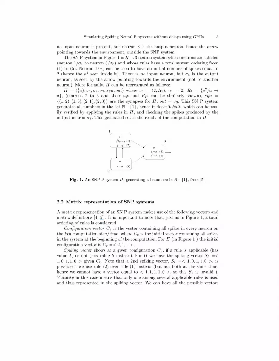
no input neuron is present, but neuron 3 is the output neuron, hence the arrowpointing towards the environment, outside the SNP system.

The SN P system in Figure 1 is Π, a 3 neuron system whose neurons are labeled(neuron 1/σ1 to neuron 3/σ3) and whose rules have a total system ordering from(1) to (5). Neuron 1/σ1 can be seen to have an initial number of spikes equal to2 (hence the a2 seen inside it). There is no input neuron, but σ3 is the outputneuron, as seen by the arrow pointing towards the environment (not to anotherneuron). More formally, Π can be represented as follows:

Π = ({a}, σ1, σ2, σ3, syn, out) where σ1 = (2, R1), n1 = 2, R1 = {a2/a →a}, (neurons 2 to 3 and their nis and Ris can be similarly shown), syn ={(1, 2), (1, 3), (2, 1), (2, 3)} are the synapses for Π, out = σ3. This SN P systemgenerates all numbers in the set N - {1}, hence it doesn’t halt, which can be eas-ily verified by applying the rules in Π, and checking the spikes produced by theoutput neuron σ3. This generated set is the result of the computation in Π.

Fig. 1. An SNP P system Π, generating all numbers in N - {1}, from [5].

2.2 Matrix representation of SNP systems

A matrix representation of an SN P system makes use of the following vectors andmatrix definitions [4, 5] . It is important to note that, just as in Figure 1, a totalordering of rules is considered.

Configuration vector Ck is the vector containing all spikes in every neuron onthe kth computation step/time, where C0 is the initial vector containing all spikesin the system at the beginning of the computation. For Π (in Figure 1 ) the initialconfiguration vector is C0 =< 2, 1, 1 >.

Spiking vector shows at a given configuration Ck, if a rule is applicable (hasvalue 1 ) or not (has value 0 instead). For Π we have the spiking vector Sk =<1, 0, 1, 1, 0 > given C0. Note that a 2nd spiking vector, Sk =< 1, 0, 1, 1, 0 >, ispossible if we use rule (2) over rule (1) instead (but not both at the same time,hence we cannot have a vector equal to < 1, 1, 1, 1, 0 >, so this Sk is invalid ).V alidity in this case means that only one among several applicable rules is usedand thus represented in the spiking vector. We can have all the possible vectors

6 F. Cabarle, H. Adorna, M. Martınez–del–Amor

composed of 0s and 1s with length equal to the number of rules, but have onlysome of them be valid, given by Ψ later at subsection 4.2.

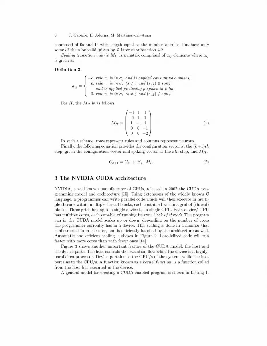
Spiking transition matrix MΠ is a matrix comprised of aij elements where aijis given as

Definition 2.

aij =

−c, rule ri is in σj and is applied consuming c spikes;p, rule ri is in σs (s 6= j and (s, j) ∈ syn)

and is applied producing p spikes in total;0, rule ri is in σs (s 6= j and (s, j) /∈ syn).

For Π, the MΠ is as follows:

MΠ =

−1 1 1−2 1 11 −1 10 0 −10 0 −2

(1)

In such a scheme, rows represent rules and columns represent neurons.Finally, the following equation provides the configuration vector at the (k+1)th

step, given the configuration vector and spiking vector at the kth step, and MΠ :

Ck+1 = Ck + Sk ·MΠ . (2)

3 The NVIDIA CUDA architecture

NVIDIA, a well known manufacturer of GPUs, released in 2007 the CUDA pro-gramming model and architecture [15]. Using extensions of the widely known Clanguage, a programmer can write parallel code which will then execute in multi-ple threads within multiple thread blocks, each contained within a grid of (thread)blocks. These grids belong to a single device i.e. a single GPU. Each device/ GPUhas multiple cores, each capable of running its own block of threads The programrun in the CUDA model scales up or down, depending on the number of coresthe programmer currently has in a device. This scaling is done in a manner thatis abstracted from the user, and is efficiently handled by the architecture as well.Automatic and efficient scaling is shown in Figure 2. Parallelized code will runfaster with more cores than with fewer ones [14].

Figure 3 shows another important feature of the CUDA model: the host andthe device parts. The host controls the execution flow while the device is a highly-parallel co-processor. Device pertains to the GPU/s of the system, while the hostpertains to the CPU/s. A function known as a kernel function, is a function calledfrom the host but executed in the device.

A general model for creating a CUDA enabled program is shown in Listing 1.

Simulating Spiking Neural P systems without delays using GPUs 7

Fig. 2. NVIDIA CUDA automatic scaling, hence more cores result to faster execution,from [14].

Fig. 3. NVIDIA CUDA programming model showing the sequential execution of thehost code alongside the parallel execution of the kernel function on the device side, from[9].

8 F. Cabarle, H. Adorna, M. Martınez–del–Amor

Listing 1. General code flow for CUDA programming written in the CUDA extended Clanguage

1 // a l l o c a t e memory on GPU e . g .2 cudaMalloc ( ( void ∗∗)&dev a , N ∗ s i z e o f ( i n t )3

4 // populate ar rays5 . . .6

7 // copy ar rays from host to dev i ce e . g .8 cudaMemcpy( dev a , a , N ∗ s i z e o f ( i n t ) ,9 cudaMemcpyHostToDevice )

10

11 // c a l l k e rne l (GPU) func t i on e . g .12 add<<<N, 1>>>( dev a , dev b , dev c ) ;13

14 // copy ar rays from dev i ce to host e . g .15 cudaMemcpy( c , dev c , N ∗ s i z e o f ( i n t ) ,16 cudaMemcpyDeviceToHost )17

18 // d i s p l a y r e s u l t s19

20 // f r e e memory e . g .21 cudaFree ( dev a ) ;

Lines 2 and 21, implement CUDA versions of the standard C language functionse.g. the standard C function malloc has the CUDA C function counterpart beingcudaMalloc, and the standard C function free has cudaFree as its CUDA Ccounterpart.

Lines 8 and 15 show a CUDA C specific function, namely cudaMemcpy, which,given an input of pointers ( from Listing 1 host code pointers are single letter vari-ables such as a and c,while device code variable counterparts are prefixed by devsuch as dev a and dev c ) and the size to copy ( as computed by the sizeof func-tion ), moves data from host to device ( parameter cudaMemcpyHostToDevice )or device to host ( parameter cudaMemcpyDeviceToHost).

A kernel function call uses the triple < and > operator, in this case the kernelfunction

add <<< N, 1 >>>(dev a, dev b, dev c).This function adds the values, per element (and each element is associated to

1 thread), of the variables dev a and dev b sent to the device, collected in variabledev c before being sent back to the host/CPU. The variable N in this case allowsthe programmer to specify N number of threads which will execute the add kernelfunction in parallel, with 1 specifying only one block of thread for all N threads.

Simulating Spiking Neural P systems without delays using GPUs 9

3.1 Design considerations for the hardware and software setup

Since the kernel function is executed in parallel in the device, the function needsto have its inputs initially moved from the CPU/host to the device, and then backfrom the device to the host after computation for the results. This movementof data back and forth should be minimized in order to obtain more efficient, interms of time, execution. Implementing an equation such as (2), which involvesmultiplication and addition between vectors and a matrix, can be done in parallelwith the previous considerations in mind. In this case, Ck, Sk, and MΠ are loaded,manipulated, and pre-processed within the host code, before being sent to thekernel function which will perform computations on these function arguments inparallel. To represent Ck, Sk, and MΠ , text files are created to house each input,whereby each element of the vector or matrix is entered in the file in order, fromleft to right, with a blank space in between as a delimiter. The matrix however isentered in row-major ( a linear array of all the elements, rows first, then columns)order format i.e. for the matrix MΠ seen in (1), the row-major order version issimply

− 1, 1, 1,−2, 1, 1, 1,−1, 1, 0, 0,−1, 0, 0,−2 (3)

Row major ordering is a well-known ordering and representation of matrices fortheir linear as well as parallel manipulation in corresponding algorithms [13]. Onceall computations are done for the (k + 1)th configuration, the result of equation(2) are then collected and moved from the device back to the host, where they canonce again be operated on by the host/CPU. It is also important to note that theseoperations in the host/CPU provide logic and control of the data/inputs, whilethe device/GPU provides the arithmetic or computational ’muscle’, the laborioustask of working on multiple data at a given time in parallel, hence the currentdichotomy of the CUDA programming model [9]. The GPU acts as a co-processorof the central processor. This division of labor is observed in Listing 1 .

3.2 Matrix computations and CPU-GPU interactions

Once all 3 initial and necessary inputs are loaded, as is to be expected from equa-tion 2, the device is first instructed to perform multiplication between the spikingvector Sk and the matrix MΠ . To further simplify computations at this point,the vectors are treated and automatically formatted by the host code to appearas single row matrices, since vectors can be considered as such. Multiplication isdone per element (one element is in one thread of the device/GPU), and then theproducts are collected and summed to produce a single element of the resultingvector/single row matrix.

Once multiplication of the Sk and MΠ is done, the result is added to theCk, once again element per element, with each element belonging to one thread,executed at the same time as the others.

For this simulator, the host code consists largely of the programming languagePython, a well-known high- level, object oriented programming (OOP) language.

10 F. Cabarle, H. Adorna, M. Martınez–del–Amor

The reason for using a high-level language such as Python is because the initialinputs, as well as succeeding ones resulting from exhaustively applying the rulesand equation (2) require manipulation of the vector/matrix elements or values asstrings. The strings are then concatenated, checked on (if they conform to theform (b-3) for example) by the host, as well as manipulated in ways which willbe elaborated in the following sections along with the discussion of the algorithmfor producing all possible and valid Sks and Cks given initial conditions. The hostcode/Python part thus implements the logic and control as mentioned earlier,while in it, the device/GPU code which is written in C executes the parallel partsof the simulator for CUDA to be utilized.

4 Simulator design and implementation

The current SNP simulator, which is based on the type of SNP systems withouttime delays, is capable of implementing rules of the form (b-3) i.e. whenever theregular expression E is equivalent to the regular expression ak in that rule. Rulesare entered in the same manner as the earlier mentioned vectors and matrix, asblank space delimited values (from one rule to the other, belonging to the sameneuron) and $ delimited ( from one neuron to the other). Thus for the SNP systemΠ shown earlier, the file r containing the blank space and $ delimited values is asfollows:

2 2 $ 1 $ 1 2 (4)

That is, rule (1) from Figure 1 has the value 2 in the file r (though rule (1)isn’t of the form (b-3) it nevertheless consumes a spike since its regular expressionis of the same regular expression type as the rest of the rules of Π ). Anotherimplementation consideration was the use of lists in Python, since unlike dic-tionaries or tuples, lists in Python are mutable, which is a direct requirement ofthe vector/matrix element manipulation to be performed later on (concatenationmostly). Hence a Ck =< 2, 1, 1 > is represented as [2, 1, 1] in Python. That is, atthe kth configuration of the system, the number of spikes of neuron 1 are givenby accessing the index (starting at zero) of the configuration vector Python listvariable confV ec, in this case if

confV ec = [2, 1, 1] (5)

then confV ec[0] = 2 gives the number of spikes available at that time forneuron 1, confV ec[1] = 1 for neuron 2, and so on. The file r, which contains theordered list of neurons and the rules that comprise each of them, is represented asa list of sub- lists in the Python/host code. For SNP system Π and from (4) wehave the following:

r = [[2, 2], [1], [1, 2]] (6)

Neuron 1’s rules are given by accessing the sub-lists of r (again, starting atindex zero) i.e. rule (1) is given by r[0][0] = 2 and rule (4) is given by r[2][1] = 1.Finally, we have the input file M , which holds the Python list version of (3).

Simulating Spiking Neural P systems without delays using GPUs 11

4.1 Simulation algorithm implementation

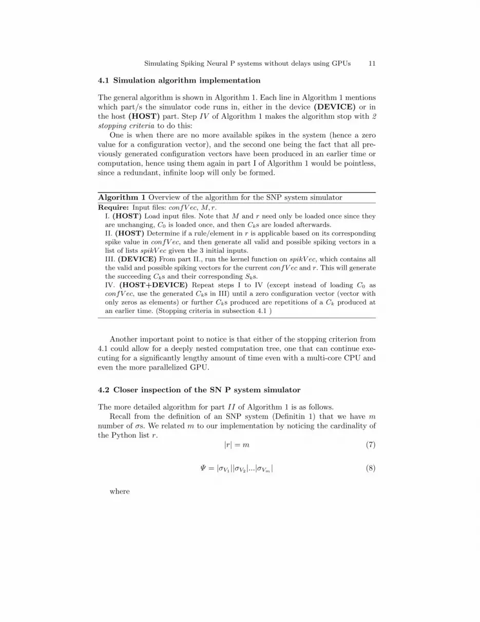
The general algorithm is shown in Algorithm 1. Each line in Algorithm 1 mentionswhich part/s the simulator code runs in, either in the device (DEVICE) or inthe host (HOST) part. Step IV of Algorithm 1 makes the algorithm stop with 2stopping criteria to do this:

One is when there are no more available spikes in the system (hence a zerovalue for a configuration vector), and the second one being the fact that all pre-viously generated configuration vectors have been produced in an earlier time orcomputation, hence using them again in part I of Algorithm 1 would be pointless,since a redundant, infinite loop will only be formed.

Algorithm 1 Overview of the algorithm for the SNP system simulator

Require: Input files: confV ec, M, r.I. (HOST) Load input files. Note that M and r need only be loaded once since theyare unchanging, C0 is loaded once, and then Cks are loaded afterwards.II. (HOST) Determine if a rule/element in r is applicable based on its correspondingspike value in confV ec, and then generate all valid and possible spiking vectors in alist of lists spikV ec given the 3 initial inputs.III. (DEVICE) From part II., run the kernel function on spikV ec, which contains allthe valid and possible spiking vectors for the current confV ec and r. This will generatethe succeeding Cks and their corresponding Sks.IV. (HOST+DEVICE) Repeat steps I to IV (except instead of loading C0 asconfV ec, use the generated Cks in III) until a zero configuration vector (vector withonly zeros as elements) or further Cks produced are repetitions of a Ck produced atan earlier time. (Stopping criteria in subsection 4.1 )

Another important point to notice is that either of the stopping criterion from4.1 could allow for a deeply nested computation tree, one that can continue exe-cuting for a significantly lengthy amount of time even with a multi-core CPU andeven the more parallelized GPU.

4.2 Closer inspection of the SN P system simulator

The more detailed algorithm for part II of Algorithm 1 is as follows.Recall from the definition of an SNP system (Definitin 1) that we have m

number of σs. We related m to our implementation by noticing the cardinality ofthe Python list r.

|r| = m (7)

Ψ = |σV1 ||σV2 |...|σVm | (8)

where

12 F. Cabarle, H. Adorna, M. Martınez–del–Amor

|σVm|

means the total number of rules in the mth neuron which satisfy the regularexpresion E in (b-3). m gives the total number of neurons, while Ψ gives theexpected number of valid and possible Sks which should be produced in a givenconfiguration. We also define ω as both the largest and last integer value in the sub-list (neuron) created in step II of Algorithm 1 and further detailed in Algorithm2, which tells us how many elements of that neuron satisfy E.

During the exposition of the algorithm, the previous Python lists (from theirvector/matrix counterparts in earlier sections) (5) and (6) will be utilized. For partII Algorithm 1 we have a sub-algorithm (Algorithm 2) for generating all valid andpossible spiking vectors given input files M , confV ec, and r.

Algorithm 2 Algorithm further detailing part II in Algorithm 1

II-1. Create a list tmp, a copy of r, marking each element of tmp in increasing order ofN, as long as the element/s satisfy the rule’s regular expression E of a rule (given bylist r ). Elements that don’t satisfy E are marked with 0.

II-2. To generate all possible and valid spiking vectors from tmp, we go through each neu-ron i.e. all elements of tmp, since we know a priori m as well as the number of elementsper neuron which satisfy E. We only need to iterate through each neuron/element oftmp, ω times. (from II-1). We then produce a new list, tmp2, which is made up ofa sub-list of strings from all possible and valid {1,0} strings i.e. spiking vectors perneuron.

II-3. To obtain all possible and valid {1,0} strings (Sks), given that there are multiplestrings to be concatenated ( as in tmp2’s case ), pairing up the neurons first, in order,and then exhaustively distributing every element of the first neuron to the elements ofthe 2nd one in the pair. These paired-distributed strings will be stored in a new list,tmp3.

Algorithm 2 ends once all {1,0} have been paired up to one another. As anillustration of Algorithm 2, consider (5), (6), and (1) as inputs to our SNP systemsimulator. The following details the production of all valid and possible spikingvectors using Algorithm 2.

Initially from II-1 of Algorithm 2, we haver = tmp = [[2, 2], [1], [1, 2]].Proceeding to illustrate II-2 we have the following passes.1st pass: tmp = [[1, 2], [1], [1, 2]]

Remark/s: previously, tmp[0][0] was equal to 2, but now has been changed to 1,since it satisfies E ( configV ec[0] = 2 w/c is equal to 2, the number of spikesconsumed by that rule).Σ

2nd pass: tmp = [[1, 2], [1], [1, 2]]Remark/s: previously tmp[0][1] = 2, which has now been changed (incidentally)to 2 as well, since it’s the 2nd element of σ1 which satisfies E.

3rd pass: tmp = [[1, 2], [1], [1, 2]]Remark/s: 1st (and only) element of neuron 2 which satisfies E.

Simulating Spiking Neural P systems without delays using GPUs 13

4th pass: tmp = [[1, 2], [1], [1, 2]]Remark/s: Same as the 1st pass

5th pass: tmp = [[1, 2], [1], [1, 0]]Remark/s: element tmp[2][1], or the 2nd element/rule of neuron 3 doesn’t satisfyE.

Final result: tmp = [[1, 2], [1], [1, 0]]At this point we have the following, based on the earlier definitions:m = 3 ( 3 neurons in total, one per element/value of confV ec)Ψ = |σV1

||σV2||σV3

| = 2 ∗ 1 ∗ 1 = 2Ψ tells us the number of valid strings of 1 s and 0 s i.e. Sks, which need to be

produced later, for a given Ck which in this case is confvec. There are only 2 validSks/spiking vectors from (5) and the rules given in (6) encoded in the Python listr. These Sks are

< 0, 1, 1, 1, 0 > (9)

< 1, 0, 1, 1, 0 > (10)

In order to produce all Sks in an algorithmic way as is done in Algorithm 2 , it’simportant to notice that first, all possible and valid Sks ( made up of 1 s and 0 s)per σ have to be produced first, which is facilitated by II-1 of Algorithm 2 and itsoutput (the current value of the list tmp ).

Continuing the illustration of II-1, and illustrating II-2 this time, we iterateover neuron 1 twice, since its ω = 2, i.e. neuron 1 has only 2 elements whichsatisfy E, and consequently, it is its 2nd element,

tmp[0][1] = 2.For neuron 1, our first pass along its elements/list is as follows. Its 1st element,tmp[0][0] = 1is the first element to satisfy E, hence it requires a 1 in its place, and 0 in the

others. We therefore produce the string ’10 ’ for it. Next, the 2nd element satisfiesE and it too, deserves a 1, while the rest get 0 s. We produce the string ’01 ’ for it.

The new list, tmp2, collecting the strings produced for neuron 1 thereforebecomes

tmp2 = [[10, 01]]Following these procedures, for neuron 2 we get tmp2 to be as follows:tmp2 = [[10, 01], [1]]Since neuron 2 which has only one element only has 1 possible and valid string,

the string 1. Finally, for neuron 3, we get tmp2 to betmp2 = [[10, 01], [1], [10]]In neuron 3, we iterated over it only once because ω, the number of elements

it has which satisfy E, is equal to 1 only. Observe that the sublisttmp2[0] = [10, 01]is equal to all possible and valid {1,0} strings for neuron 1, given rules in (6)

and the number of spikes in configV ec.Illustrating II-3 of Algorithm 2, given the valid and possible {1,0} strings

(spiking vectors) for neurons 1, 2, and 3 (separated per neuron-column) from (5)

14 F. Cabarle, H. Adorna, M. Martınez–del–Amor

and (6) and from the illustration of II-2, all possible and valid list of {1,0} string/sfor neuron 1: [’10’,’01’], neuron 2: [’1’], and neuron 3: [’10’].

First, pair the strings of neurons 1 and 2, and then distribute them exhaustivelyto the other neuron’s possible and valid strings, concatenating them in the process(since they are considered as strings in Python).

’10’ + ’1’ → ’101’’01’

and’10’’01’ + ’1’ → ’011’now we have to create a new list from tmp2, which will house the concatenations

we’ll be doing. In this case,tmp3 = [101, 011]next, we pair up tmp3 and the possible and valid strings of neuron 3’101’ + ’10’ → ’10110’’011’

and’101’’011’ + ’10’ → ’01110’eventually turning tmp3 intotmp3 = [10110, 01110]The final output of the sub-algorithm for the generation of all valid and possible

spiking vectors is a list,tmp3 = [10110, 01110]As mentioned earlier, Ψ = 2 is the number of valid and possible Sks to be

expected from r, MΠ , and C0 = [2,1,1] in Π. Thus tmp3 is the list of all possibleand valid spiking vectors given (5) and (6) in this illustration. Furthermore, tmp3includes all possible and valid spiking vectors for a given neuron in a given con-figuration of an SN P system with all its rules and synapses (interconnections).Part II-3 is done ( m − 1) times, albeit exhaustively still so, between the twolists/neurons in the pair.

5 Simulation results, observations, and analyses

The SNP system simulator (combination of Python and CUDA C) implements thealgorithms in section 4 earlier. A sample simulation run with the SNP system Πis shown below (most of the output has been truncated due to space constraints )with C0 = [2,1,1]

****SN P system simulation run STARTS here****

Spiking transition Matrix:

...

Rules of the form a^n/a^m -> a or a^n ->a loaded:

Simulating Spiking Neural P systems without delays using GPUs 15

[’2’, ’2’, ’$’, ’1’, ’$’, ’1’, ’2’]

Initial configuration vector: 211

Number of neurons for the SN P system is 3

Neuron 1 rules criterion/criteria and total order

...

tmpList = [[’10’, ’01’], [’1’], [’10’]]

All valid spiking vectors: allValidSpikVec =

[[’10110’, ’01110’]]

All generated Cks are allGenCk =

[’2-1-1’, ’2-1-2’, ’1-1-2’]

End of C0

**

**

**

initial total Ck list is

[’2-1-1’, ’2-1-2’, ’1-1-2’]

Current confVec: 212

All generated Cks are allGenCk =

[’2-1-1’, ’2-1-2’, ’1-1-2’, ’2-1-3’, ’1-1-3’]

**

**

**

Current confVec: 112

All generated Cks are allGenCk =

[’2-1-1’, ’2-1-2’, ’1-1-2’, ’2-1-3’, ’1-1-3’,

’2-0-2’, ’2-0-1’]

**

**

...

Current confVec: 109

All generated Cks are allGenCk = [’2-1-1’, ’2-1-2’,

...

’1-0-7’, ’0-1-9’, ’1-0-8’, ’1-0-9’]

**

**

**

No more Cks to use (infinite loop/s otherwise). Stop.

****SN P system simulation run ENDS here****

16 F. Cabarle, H. Adorna, M. Martınez–del–Amor

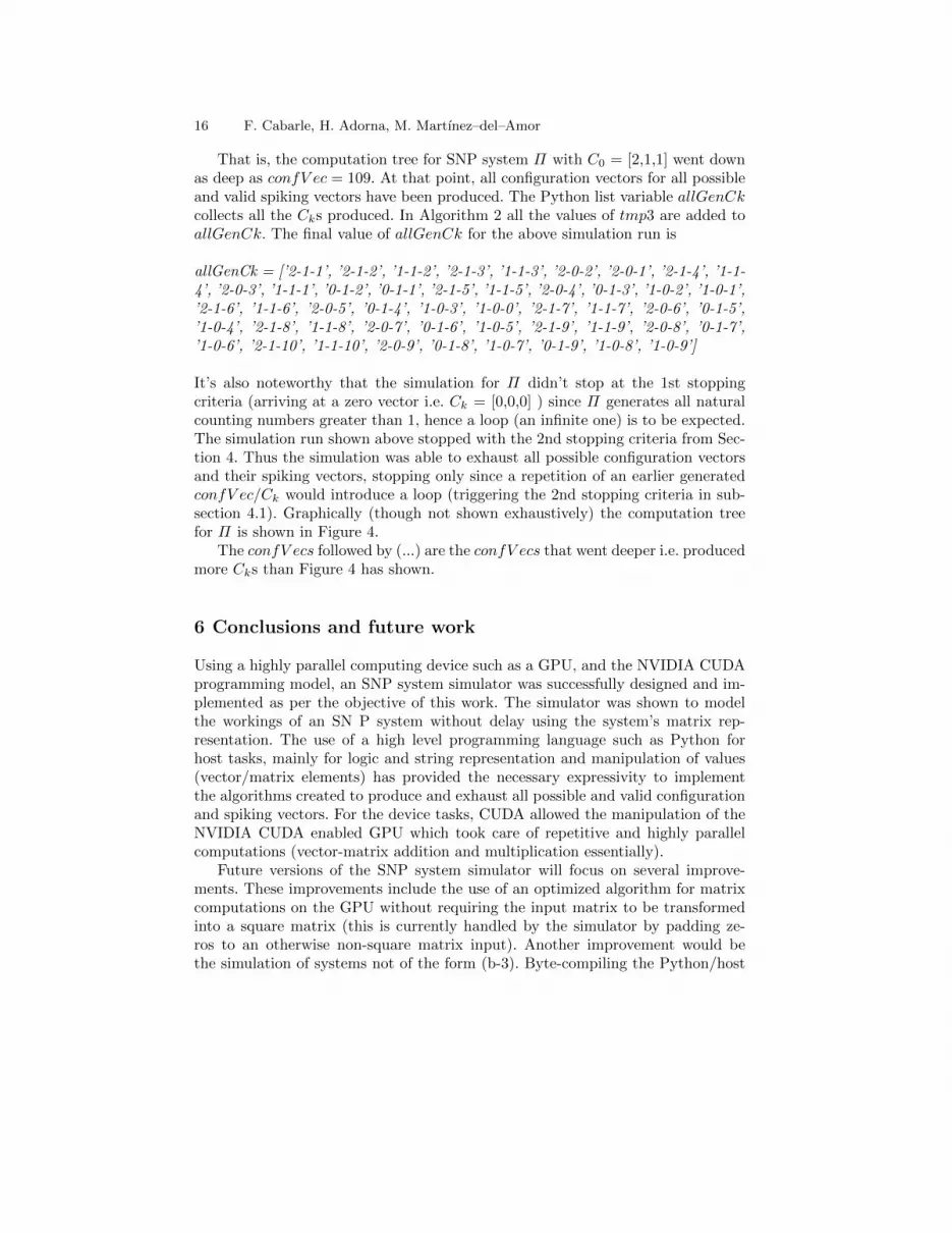
That is, the computation tree for SNP system Π with C0 = [2,1,1] went downas deep as confV ec = 109. At that point, all configuration vectors for all possibleand valid spiking vectors have been produced. The Python list variable allGenCkcollects all the Cks produced. In Algorithm 2 all the values of tmp3 are added toallGenCk. The final value of allGenCk for the above simulation run is

allGenCk = [’2-1-1’, ’2-1-2’, ’1-1-2’, ’2-1-3’, ’1-1-3’, ’2-0-2’, ’2-0-1’, ’2-1-4’, ’1-1-4’, ’2-0-3’, ’1-1-1’, ’0-1-2’, ’0-1-1’, ’2-1-5’, ’1-1-5’, ’2-0-4’, ’0-1-3’, ’1-0-2’, ’1-0-1’,’2-1-6’, ’1-1-6’, ’2-0-5’, ’0-1-4’, ’1-0-3’, ’1-0-0’, ’2-1-7’, ’1-1-7’, ’2-0-6’, ’0-1-5’,’1-0-4’, ’2-1-8’, ’1-1-8’, ’2-0-7’, ’0-1-6’, ’1-0-5’, ’2-1-9’, ’1-1-9’, ’2-0-8’, ’0-1-7’,’1-0-6’, ’2-1-10’, ’1-1-10’, ’2-0-9’, ’0-1-8’, ’1-0-7’, ’0-1-9’, ’1-0-8’, ’1-0-9’]

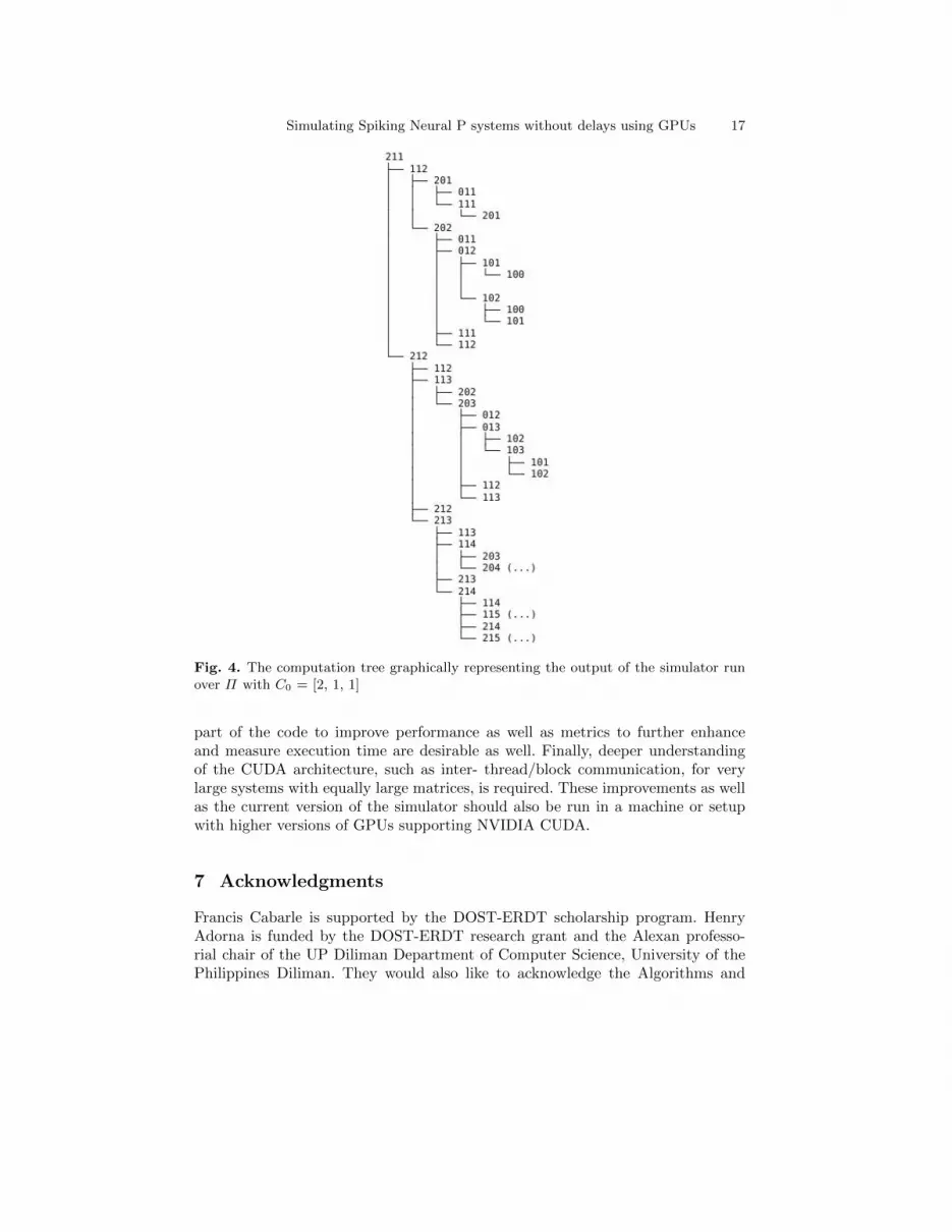
It’s also noteworthy that the simulation for Π didn’t stop at the 1st stoppingcriteria (arriving at a zero vector i.e. Ck = [0,0,0] ) since Π generates all naturalcounting numbers greater than 1, hence a loop (an infinite one) is to be expected.The simulation run shown above stopped with the 2nd stopping criteria from Sec-tion 4. Thus the simulation was able to exhaust all possible configuration vectorsand their spiking vectors, stopping only since a repetition of an earlier generatedconfV ec/Ck would introduce a loop (triggering the 2nd stopping criteria in sub-section 4.1). Graphically (though not shown exhaustively) the computation treefor Π is shown in Figure 4.

The confV ecs followed by (...) are the confV ecs that went deeper i.e. producedmore Cks than Figure 4 has shown.

6 Conclusions and future work

Using a highly parallel computing device such as a GPU, and the NVIDIA CUDAprogramming model, an SNP system simulator was successfully designed and im-plemented as per the objective of this work. The simulator was shown to modelthe workings of an SN P system without delay using the system’s matrix rep-resentation. The use of a high level programming language such as Python forhost tasks, mainly for logic and string representation and manipulation of values(vector/matrix elements) has provided the necessary expressivity to implementthe algorithms created to produce and exhaust all possible and valid configurationand spiking vectors. For the device tasks, CUDA allowed the manipulation of theNVIDIA CUDA enabled GPU which took care of repetitive and highly parallelcomputations (vector-matrix addition and multiplication essentially).

Future versions of the SNP system simulator will focus on several improve-ments. These improvements include the use of an optimized algorithm for matrixcomputations on the GPU without requiring the input matrix to be transformedinto a square matrix (this is currently handled by the simulator by padding ze-ros to an otherwise non-square matrix input). Another improvement would bethe simulation of systems not of the form (b-3). Byte-compiling the Python/host

Simulating Spiking Neural P systems without delays using GPUs 17

Fig. 4. The computation tree graphically representing the output of the simulator runover Π with C0 = [2, 1, 1]

part of the code to improve performance as well as metrics to further enhanceand measure execution time are desirable as well. Finally, deeper understandingof the CUDA architecture, such as inter- thread/block communication, for verylarge systems with equally large matrices, is required. These improvements as wellas the current version of the simulator should also be run in a machine or setupwith higher versions of GPUs supporting NVIDIA CUDA.

7 Acknowledgments

Francis Cabarle is supported by the DOST-ERDT scholarship program. HenryAdorna is funded by the DOST-ERDT research grant and the Alexan professo-rial chair of the UP Diliman Department of Computer Science, University of thePhilippines Diliman. They would also like to acknowledge the Algorithms and

18 F. Cabarle, H. Adorna, M. Martınez–del–Amor

Complexity laboratory for the use of Apple iMacs with NVIDIA CUDA enabledGPUs for this work. Miguel A. Martınez–del–Amor is supported by “Proyecto deExcelencia con Investigador de Reconocida Valıa” of the “Junta de Andalucıa”under grant P08-TIC04200, and the support of the project TIN2009–13192 of the“Ministerio de Educacion y Ciencia” of Spain, both co-financed by FEDER funds.Finally, they would also like to thank the valuable insights of Mr. Neil Ibo.

References

1. M. Harris, “Mapping computational concepts to GPUs”, ACM SIGGRAPH 2005Courses, NY, USA, 2005.

2. M. Gross, “Molecular computation”, Chapter 2 of Non-Standard Computation, (T.Gramss, S. Bornholdt, M. Gross, M. Mitchel, Th. Pellizzari, eds.), Wiley-VCH,Weinheim, 1998.

3. M. Ionescu, Gh. Paun, T. Yokomori, “Spiking Neural P Systems”, Journal Fun-damenta Informaticae , vol. 71, issue 2,3 pp. 279-308, Feb. 2006.

4. X. Zeng, H. Adorna, M. A. Martınez-del-Amor, L. Pan, “When Matrices MeetBrains”, Proceedings of the Eighth Brainstorming Week on Membrane Computing, Sevilla, Spain, Feb. 2010.

5. X. Zeng, H. Adorna, M. A. Martınez-del-Amor, L. Pan, M. Perez-Jimenez, “MatrixRepresentation of Spiking Neural P Systems”, 11th International Conference onMembrane Computing , Jena, Germany, Aug. 2010.

6. Gh. Paun, G. Ciobanu, M. Perez-Jimenez (Eds), “Applications of Membrane Com-puting” , Natural Computing Series, Springer, 2006.

7. P systems resource website. (2011, Jan) [Online]. Available:www.ppage.psystems.eu.

8. J.M. Cecilia, J.M. Garcıa, G.D. Guerrero, M.A. Martınez-del-Amor, I. Perez-Hurtado, M.J. Perez-Jimenez, “Simulating a P system based efficient solution toSAT by using GPUs”, Journal of Logic and Algebraic Programming, Vol 79, issue6, pp. 317-325, Apr. 2010.

9. J.M. Cecilia, J.M. Garcıa, G.D. Guerrero, M.A. Martınez-del-Amor, I. Perez-Hurtado, M.J. Perez-Jimenez, “Simulation of P systems with active membraneson CUDA”, Briefings in Bioinformatics, Vol 11, issue 3, pp. 313-322, Mar. 2010.

10. D. Dıaz, C. Graciani, M.A. Gutierrez, I. Perez-Hurtado, M.J. Perez-Jimenez. Soft-ware for P systems. In Gh. Paun, G. Rozenberg, A. Salomaa (eds.) The OxfordHandbook of Membrane Computing, Oxford University Press, Oxford (U.K.), Chap-ter 17, pp. 437-454, 2009.

11. G. Ciobanu, G. Wenyuan. P Systems Running on a Cluster of Computers. LectureNotes in Computer Science, 2933, 123-139, 2004.

12. V. Nguyen, D. Kearney, G. Gioiosa. A Region-Oriented Hardware Implementationfor Membrane Computing Applications and Its Integration into Reconfig-P. LectureNotes in Computer Science, 5957, 385-409, 2010.

13. D. Kirk, W. Hwu, “Programming Massively Parallel Processors: A Hands On Ap-proach” , 1st ed. MA, USA: Morgan Kaufmann, 2010.

14. NVIDIA corporation, “NVIDIA CUDA C programming guide” , version 3.0, CA,USA: NVIDIA, 2010.

Simulating Spiking Neural P systems without delays using GPUs 19

15. NVIDIA CUDA developers resources page: tools, presentations, whitepapers.(2010, Jan) [Online]. Available: http://developer.nvidia.com/page/home.html

16. V. Volkov, J. Demmel, “Benchmarking GPUs to tune dense linear algebra”, Pro-ceedings of the 2008 ACM/IEEE conference on Supercomputing, NJ, USA, 2008.

17. K. Fatahalian, J. Sugerman, P. Hanrahan, “Understanding the efficiency of GPUalgorithms for matrix-matrix multiplication”, In Proceedings of the ACM SIG-GRAPH/EUROGRAPHICS conference on Graphics hardware (HWWS ’04) ,ACM, NY, USA, pp. 133-137, 2004