delays in claiming social security benefits
TRANSCRIPT

NBER WORKING PAPER SERIES
DELAYS IN CLAIMINGSOCIAL SECURITY BENEFITS
Courtney CoilePeter Diamond
Jonathan GruberAlain Jousten
Working Paper 7318http://www.nber.org/papers/w7318
NATIONAL BUREAU OF ECONOMIC RESEARCH1050 Massachusetts Avenue
Cambridge, MA 02138August 1999
We are grateful to seminar participants at MIT and the NBER for helpful comments. Coile acknowledgesfinancial support from the National Institute on Aging through the National Bureau of Economic Research.Diamond acknowledges financial support from the National Science Foundation. Gruber acknowledgesfinancial support from the National Science Foundation and the National Institute on Aging. Joustenacknowledges financial support from the NBER and from the CREPP. The views expressed herein are thoseof the authors and not necessarily those of the National Bureau of Economic Research.
© 1999 by Courtney Coile, Peter Diamond, Jonathan Gruber, and Alain Jousten. All rights reserved. Short
sections of text, not to exceed two paragraphs, may be quoted without explicit permission provided that fullcredit, including © notice, is given to the source.Delays in Claiming Social Security BenefitsCourtney Coile, Peter Diamond, Jonathan Gruber, and Alain JoustenNBER Working Paper No. 7318August 1999JEL No. H3, H5
ABSTRACT
This paper focuses on Social Security benefit claiming behavior, a take-up decision that has been
ignored in the previous literature. Using financial calculations and simulations based on an expected utility
maximization model, we show that delaying benefit claim for a period of time after retirement is optimal in
a wide variety of cases and that gains from delay may be significant. We find that approximately 10% of
men retiring before their 62nd birthday delay claiming for at least one year after eligibility. We estimate
hazard and probit models using data from the New Beneficiary Data System to test four cross-sectional
predictions. While the data suggest that too few men delay, we find that the pattern of delays by early
retirees is generally consistent with the hypotheses generated by our theoretical model.
Courtney Coile Peter DiamondDepartment of Economics Department of EconomicsMassachusetts Institute of TechnologyMassachusetts Institute of Technology50 Memorial Drive Room E52-344Cambridge, MA 02139 50 Memorial [email protected] Cambridge, MA 02139
Jonathan Gruber Alain JoustenDepartment of Economics COREMassachusetts Institute of Technology 34 Voie du Roman PaysRoom E52-355 1348 Louvain-la-Neuve, Belgium 50 Memorial Drive [email protected], MA 02139and [email protected]
Social Security (SS) is the largest entitlement program in the United States today,
providing income support for retired and disabled workers and their families. The concurrent
growth in this program and decline in the labor force participation of older men has motivated an
extensive literature investigating how SS influences retirement behavior. There is another large
literature investigating the transfers induced by SS across and within cohorts.
One common feature of the work in this area has been the assumption that individuals
claim benefits as soon as they are eligible - either upon retirement, or upon turning age 62 if
retirement is before that age. However, as with other social insurance programs, there is a take-
up decision associated with claiming SS benefits. Individuals need not claim their benefits
immediately upon retirement, or upon turning age 62. By delaying claiming, workers increase the
benefits paid to them and their spouses, through the actuarial adjustment. As we demonstrate
below, it is optimal in a wide variety of cases to delay claiming benefits for a period of time after
eligibility. Moreover, for at least one group, men retiring before their 62nd birthday (the age of
first eligibility for benefits), claiming delays are empirically important: roughly 10% of these
retirees delay claiming for at least one year.
This dynamic take-up consideration suggests that standard computations of both the
retirement incentives of SS and the redistribution through SS may be biased. Moreover, we are
not aware of any in-depth analysis of this take-up behavior. An examination of the extent to
which observed claiming patterns are consistent with rational choice theory may have important
implications for aspects of SS design and reform.
The purpose of our paper is to investigate delays in SS benefits claiming and to explore
their implications. We do so in five steps. First, in Part I, we provide relevant institutional
2
1This discussion applies only to those under age 70; at age 70, benefits are paid out regardlessof retirement.
background on the SS program. We highlight the fact that retirement provides only a necessary,
and not a sufficient, condition for receiving SS benefits.1 We briefly review the SS literature,
emphasizing areas where realistic consideration of claiming behavior can affect analysis.
In Part II, we turn to a theoretical examination of claiming delays. We begin with a
discussion of the benefit rules to explore how worker characteristics such as mortality
expectations, wealth, age difference with spouse, and relative earnings of spouses may influence
claiming delays. Then we use simulations of financial gains from delay to generate cross-sectional
predictions that can be tested in our empirical analysis. We also present simulation results based
on an expected utility maximization model with liquidity constraints, as we recognize that
financial calculations in general understate the incentives to delay relative to the optimization of a
risk averse utility function. This is because SS provides a real annuity valued by risk averse
individuals with an uncertain date of death; individuals buy more of this annuity by delaying, so
delays are more attractive with risk aversion.
Part III presents evidence that claiming delays are empirically relevant. We use data from
the New Beneficiary Data System (NBDS), a survey of SS claimants in the early 1980s. This
survey provides administrative data on work and benefits histories which allows us to form a
relatively precise measure of claiming delays. We highlight the differences in delays by early
retirees, those retired before their 62nd birthday, and later retirees, those retiring after their 62nd
birthday. We confirm our findings using more recent data from the Health and Retirement Survey
(HRS). While we do not attempt to quantify the predicted prevalence of delayed claiming, delay
3
appears to be far less prevalent than the theory predicts.
Nevertheless, in Part IV, we investigate whether the claiming behavior of men in our
sample is consistent with our cross-sectional predictions. We present both hazard and probit
models of delays. We find support for three hypotheses. Specifically, we find that men with
longer life expectancies have longer delays; that delays follow an inverse u-shaped pattern as
wealth increases; and that men with younger spouses have longer delays. On the other hand, we
do not find support for the prediction that single men should have shorter delays. Part V
concludes by summarizing our findings and considering the implications for previous research on
SS and for SS design and reform.
Part I: Background
Institutional Features
Understanding the motivation for our analysis requires a brief overview of how benefits
are determined. Individuals are fully insured for retired worker benefits once they have worked
40 quarters in the covered sector. Benefits are computed as follows: nominal taxable annual
earnings before age 60 are converted into age 60 dollars using a wage index, the 35 highest years
of indexed earnings (indexed before age 60 but not after) are averaged and divided by 12 to
generate the Average Indexed Monthly Earnings (AIME), and a non-linear formula is applied to
the AIME to generate the Primary Insurance Amount (PIA) on which monthly benefits are based.
Fully insured individuals can claim retired worker benefits if they meet two criteria. First,
they must be at least age 62. Second, individuals must pass an earnings test: if their earnings
exceed a ceiling amount, benefits are reduced by 50 cents for each additional dollar of earnings (if
4
2Gruber and Orszag (1999) provide a description of the operation and implications of theearnings test.
3The NRA is scheduled to rise in a series of steps, reaching 67 for workers attaining age 60 inthe year 2022 or later.
4The delayed retirement credit is rising over time, and is scheduled to reach 8% per year forthose attaining age 62 in the year 2005 or later.
age 62-64) or 33 cents for each additional dollar of earnings (if age 65-69). In 1998, this ceiling
was $9,120 of annual earnings for 62-64 year olds, and $14,500 for 65-69 year olds. There is
also a monthly earnings test that individuals may use for one year only, usually the year of
retirement. In 1995, the monthly earnings test ceiling was $760 for 62-64 year olds and $1,208
for 65-69 year olds. In the year that the monthly earnings test is applied, individuals may have
annual earnings above the annual earnings test ceiling but may still receive full benefits for any
months in which they earned less than the monthly earnings test ceiling. Any benefit reduction
from the earnings test is offset by higher benefits upon full retirement, through the actuarial
adjustment.2
Monthly benefits also depend on age at claiming. If individuals claim at the normal
retirement age (NRA) of 65, the monthly benefit equals 100% of the PIA.3 If they claim between
age 62 and age 65, there is an actuarial reduction in the benefit of 5/9% for each month of
claiming before age 65. Thus workers claiming on their 62nd birthdays have a benefit equal to
80% of PIA. If they claim after age 65, there is a delayed retirement credit. For respondents in
the NBDS, the credit was only 1% per year; this is much smaller than the actuarial reduction,
generating a kink at age 65 in the schedule of benefits as a function of age at claiming.4
A key feature of this institutional structure is that retirement need not be concurrent with
5
claiming. For example, if individuals retire at age 62, they need not claim on their 62nd birthday.
As we document below, in many cases total expected discounted benefits are increased by
delaying for some months.
Calculating the advantages of delaying is complicated by the family benefits structure of
SS. Spouses are eligible for dependent spouse benefits and may also be entitled to retired worker
benefits on their own record; however, spouses receive only the larger of the two amounts. The
dependent spouse benefit is 50% of the retired worker’s PIA, can be claimed once the dependent
spouse is 62 and the worker has claimed, and is subject to an actuarial reduction if the dependent
spouse claims before 65. Surviving spouses of retired workers are entitled to a survivor benefit of
100% of the retired worker’s PIA; the benefit can be claimed once the survivor is 60 and may be
reduced depending on the survivor’s age when benefits begins. Also the benefit may be reduced
depending on the worker’s ages at claiming and at death. Claiming the survivor benefit implies
foregoing the survivor’s retired worker or dependent spouse benefit. We return to the question of
how family benefits affect incentives for delays below.
Previous Literature
The concern that this benefits structure might have important implications for retirement
incentives has motivated an enormous literature on the effect of SS on retirement, reviewed in
Hurd (1990) and Diamond and Gruber (1999). The first strand of this literature uses aggregate
information on the labor force behavior of workers at different ages over time to infer the impact
of SS. Hurd (1990) and Ruhm (1995) find a spike in the age pattern of retirement at 62 and show
that this peak has grown over time as SS benefits have increased; Burtless and Moffitt (1984)

6
5An notable exception to this conclusion is the work of Krueger and Pischke (1992), whonoted that the benefit cut for the “notch generation” of the late 1970s and early 1980s was notassociated with any slowdown in the trend towards early retirement.
show that there was no peak before claiming at 62 became an option. There is also a spike in
retirement at age 65, which is consistent with the unfair actuarial adjustment for work beyond age
65. Blau (1994) finds that nearly 25% of the men in the labor force on their 65th birthday retire in
the next quarter; this hazard rate is 2.5 times as large as the rate in surrounding quarters.
The second strand of this literature uses micro-data sets with SS benefit determinants or
ex-post benefit levels to measure the incentives to retire across individuals, then estimates
retirement models as a function of these incentives. This large literature is reviewed at length in
Coile and Gruber (1999). There are a variety of techniques employed in this literature. Earlier
papers modeled retirement status or transitions to retirement as a function of Social Security
benefit levels or the present discounted value of future Social Security entitlements (SS “wealth”,
or SSW). More recent work has considered retirement dynamics as a function of the evolution of
SSW, examining either accruals for an additional year of work, or the entire future evolution of
Social Security (and private pension) wealth with additional years of work. While the techniques
differ across papers, the conclusion of this literature has generally been that Social Security has
large effects on retirement, but that they are small relative to the time trend in male retirement
over the past 40 years.5
This literature, however, suffers from a potential weakness that has thus far been ignored:
the endogeneity of the timing of SS benefits claiming and therefore of the benefit level. The key
independent variable in cross-sectional estimation, SS benefits, may confound potentially
exogenous characteristics which determine benefits, such as lifetime earnings, with the
7
endogenous take-up decision. For example, consider two individuals who retire at the same point
(their 61st birthday) and are identical in every respect except time preference. Impatient
individual B claims benefits at 62, while patient individual A delays until age 65 and receives a
higher benefit. Regression analysis would show that higher SS benefits do not cause earlier
retirement. But in fact these two individuals have the same PIAs and thus face the same menu of
retirement benefit choices. This suggests that by using actual SS benefits received rather than PIA
to model retirement incentives, previous studies may have misstated the incentives.
The literature which has used accrual rates or other measures of the evolution of SSW is
also affected by ignoring the endogenous claiming decision. These measures all assume that
retirement and claiming are on the same date. But if claiming can be delayed, it affects the accrual
rate, leading again to mismeasurement of the key regressor. That is, if claiming is distinct from
retirement, then it limits the impact of additional work on wealth accruals; the major impact is
from delayed claiming, so that it has relatively little implication for work decisions.
Another strand of the literature stresses differential distributional outcomes within and
across generations arising from SS (Hurd and Shoven 1985, Boskin et al. 1987, Steuerle and
Bakija 1994). This literature has found significantly lower net returns for: recent and future
cohorts relative to older cohorts; low earners relative to high earners in previous cohorts; high
earners relative to high earners in current and future cohorts; the short lived relative to the long
lived; and for single men relative to married men. But this literature has also ignored delayed
claiming. The ability to delay claiming increases the redistribution of the system, for example,
from short lived to long lived, as the long lived gain differentially by delaying claiming. SS also
differentially affects those who are liquidity constrained and those who are not.
8
6Our theoretical analysis parallels in some respects that of Mirer (1998), a paper writtensimultaneously with ours. Mirer’s paper also makes the point that it may be optimal in manycontexts to delay claiming. But his theoretical model does not consider the cross-sectionaldeterminants of claiming delay, and his paper does not present any empirical evidence on eitherthe magnitude or determinants of claiming.
A full analysis of the problem of delayed claiming would model jointly the retirement and
the claiming decision. Such a model is beyond the scope of the current effort. Rather, our goal is
threefold: to demonstrate theoretically that delayed claiming is often worthwhile; to document
empirically that delayed claiming is a relevant phenomenon, at least for some classes of retirees;
and to assess whether delays in claiming follow the cross-sectional patterns suggested by theory.
Part II: When is it Optimal to Delay Claiming?
In this section, we illustrate the incentives for claiming delays under the US Social
Security System by presenting two simulation approaches. The first technique is a purely financial
calculation of the expected present discounted values (EPDV) of future net benefit streams for a
single worker and for a married couple. We examine the variation in incentives for claiming
delays among subgroups of the population with different characteristics.
The second technique is expected utility maximization under liquidity constraints. This
technique has the advantage of capturing the value of SS as a real annuity to a risk averse person
with an uncertain date of death. However, due to computational complexity, we calculate the
expected utility maximization model for a single worker only, leaving a full household
optimization model for future work. Before turning to the simulations, we review the benefit
rules to explain how factors such as mortality expectations affect incentives for claiming delays.6
9
7The rules for male and female retired workers are the same; we refer to a male since theempirical work is focused on men. The rules are slightly different with birthdays on the first andsecond days of the month. Benefit levels (whether claimed or not) are adjusted annually to reflectcost-of-living adjustments.
While we use a vocabulary of delays in claiming, our analysis is in fact based on a theory
of claiming, not a theory of delays. That is, retiring one year earlier does not affect the optimal
age of claiming, ceteris paribus, but it does increase the optimal delay by one year, since the delay
is the period of time after retirement and before claiming.
Benefit Rules
Consider a single male who is fully insured for retired worker benefits, has just turned 62,
and has stopped working.7 He could claim benefits immediately and begin receiving a monthly
benefit of .8*PIA. Alternatively, he could delay claiming for some period of time. Consider the
effect of waiting one year and claiming on his 63rd birthday: he forgoes one year of benefits, but
receives a monthly benefit of .867*PIA for the rest of his life, an increase of 8.33%. Thus,
claiming delays involve the sacrifice of current benefits for a higher future benefit level.
To evaluate this tradeoff, he considers his life expectancy and discount rate. A longer
life expectancy creates a stronger incentive to delay because the higher future benefit level is
expected to last longer. A lower discount rate creates a stronger incentive to delay because future
benefits are valued more highly. The operative discount rate, in turn, will depend at least partly
on both wealth levels and bequest motives, in a manner described in more detail below.
The family structure of Social Security benefits is also relevant for the claiming decision.
In general, married workers will have a greater financial incentive to delay than will single

10
workers, since by doing so they not only raise the value of their future benefits, but also their
spouse’s survivor benefits as well. On the other hand, being married lowers the annuity value of
Social Security, since the couple can provide some self-insurance against mortality risk (Kotlikoff
and Spivak, 1981; Brown and Poterba, 1999).
A couple’s claiming delays are also affected by the age difference between the spouses.
Consider a 62 year old husband with a wife who has never worked, making the decision as to
whether to delay claiming for one year. While the change in value of the worker’s benefit does
not depend on the age of his wife, the expected values of both her spouse benefit and her possible
survivor benefit do vary with her age. To see some of the elements that go into the calculation
model, let us contrast the cases where the wife is also 62 and where the wife is 61, considering the
setting where she claims benefits as soon as she can. If the husband delays for a year, then a 62-
year old wife must delay claiming the spouse benefit by a year, while a 61-year old wife is not
affected, since she could not have claimed anyway. Whether this increases or decreases the value
of the spouse benefit depends on whether the actuarial adjustment for the spouse benefit is more
or less than fair; that is, whether the reduced year of dependent benefits receipt of for the 62 year
old wife is more or less than adequately compensated by the actuarial adjustment.
The situation is more complex for the survivor benefit, since the impact of her age on the
expected gain from his delay depends on whether the size of her survivor benefit is affected by his
actuarial reduction or not. That is, the survivor benefit might be reduced because of the age at
which she claims a survivor benefit or because of a limitation based on the age at which he
claimed a benefit. Which of these will control depends on the age at which he dies. If the
husband dies sufficiently late that it is his actuarial reduction that matters for her survivors benefit,
11
8For men with working wives, the ratio of the wife’s PIA to the husband’s PIA will bepotentially relevant. But, as discussed at length in Coile et al. (1997), there is no clear predictionfor the relationship between PIA ratios and claiming delays, so we do not consider that variablehere.
9Deaths may occur on a monthly basis. We use all Social Security rules including futureplanned adjustments as of 1996.
then it is clear that when the wife is younger the delay in his claiming is worth more, since there
are more expected years for which those survivor benefits can be claimed. On the other hand, if
the husband dies sufficiently early that it is the wife’s claiming decision that is dominant, then the
effect of the age difference on the value of delay is ambiguous, since it depends on the size of the
actuarial adjustment in the survivor benefit. In the simulations below, it will generally turn out
that the incentive for delay is larger with a younger wife, since most of the mass of death
probabilities is at older ages. We also note that there are life expectancy difference across women
other than those associated with age and that men whose wives have a higher life expectancy have
a stronger incentive to delay.8
Financial calculations
We begin with financial calculations which measure how the EPDV of SS benefits varies
with months of delay (assuming that the worker is already retired). The EPDV is defined as the
discounted flow of future potential benefits paid to the family. The program we developed first
computes, for every future month at which a family member may be alive, the benefits
corresponding to all possible survival and death patterns in the family, then adjusts them for
survival probabilities and inflation and discounts them back to the base year.9 This computation is
12
10We use the NBDS, a sample of 1980-81 claimants, in the empirical analysis; however, asthere are no relevant rule changes between 1980 and 1992, the simulation results are applicable tothe NBDS population.
11A wife claiming retired worker benefits claims at age 62. A wife claiming dependent spousebenefits claims at the later of age 62 or her husband’s date of claim.
repeated for each possible month of benefit claim by the prime earner. Appendix A provides a
more detailed explanation of these calculations.
We focus on a household whose prime earner is a male born on January 2, 1930 and alive
at age 62. The base year for the simulations is 1992.10 We make the following assumptions in all
cases unless otherwise noted. We assume that the wife was born on January 2, 1932 and that the
couple has no dependents. We assume that this is a one-earner couple, that the husband stops
work before the year containing his 62nd birthday, and that the husband’s wage history
corresponds to the economy-wide median earnings profile for his age cohort from age 20 to age
50 and is constant in real terms thereafter. We assume that the wife claims benefits as soon as
possible.11 Finally, we assume that the household’s discount rate is 3% and that mortality risks
correspond to the Social Security Administration’s sex- and cohort-specific survival tables.
Table 1 presents the EPDV calculations. Column (b) shows the optimal delay in months.
Column © shows the EPDV with no delay, column (d) shows the EPDV at the optimal delay, and
column (e) shows the difference between these two, which is the value of delayed claiming.
Column (g) presents the change in EPDV scaled by PIA. As the monthly retired worker benefit is
equal to the PIA if the worker claims at age 65, the number in column (g) can be loosely
interpreted as the number of additional months of retired worker benefits received in expectation
13
12Of course, this relationship is not exact unless the worker claims at age 65.
over the worker’s lifetime as a result of choosing the optimal delay.12
The first row shows the results for the base case with a one-earner couple. In this case, it
is optimal for the husband to delay claiming by 36 months to age 65. The delay raises the EPDV
of benefits by $6,270, or 651% of PIA. This result and those that follow suggest that optimal
claiming delays are frequently long and that gains from delay are moderate for a one-earner
couple. In the base case, a delay of 36 months would result in an increase of $232 in the couple’s
monthly benefit check, from $1132 to $1364. Figure 1 illustrates the EPDV of benefits as a
function of delay for a one-earner couple in the base case.
The next six rows of Table 1 show the effect of varying the mortality risk, discount rate,
and earnings level. We leave the discussion of these factors to the single worker case; due to a
kink in the actuarial adjustment schedule at age 65, optimal delays in the one-earner couple cases
bunch up at 36 months, making it difficult to see the effect of these factors. The impact of these
factors can be seen in the final column, which shows financial gains from delay; these gains follow
the same pattern discussed below for single workers, and are much more sizeable in every case.
The final one-earner couple cases illustrate the effect of varying the age difference
between the husband and wife. As expected, we find that an increase in the age difference
between the spouses leads to longer delays: the optimal delay is 0 if the wife is 5 years older than
the husband, 12 months if she is 2 years older, 35 months if she is the same age, and 36 months if
she is 2 years (or more) younger (the base case).
Next we examine results for the single worker cases. In general, delays are shorter and
14
13Mortality risk is altered by multiplying the number of deaths per period by a constant: 0.84for low mortality, 1.16 for high mortality. To get a sense of the impact of these multipliers,consider the thought exercise where we start with equal numbers of high and low mortality typesat age 62; with these high an low multipliers we would end up with 53% low mortality types and47% high mortality types at age 70. Note that calculations are for given mortality expectations atage 62 with no later health news.
14The discount rate is 1% in the low discount rate case and 6% in the high discount rate case.
gains from delays are much smaller compared to the one-earner couple cases. This is due to the
fact that with couples, delays raise the survivor benefit and potentially the dependent spouse
benefit; this is consistent with our earlier statement that married men have a stronger incentive to
delay than single men (subject to the noted caveat about intra-family risk sharing). In the single
worker base case, the optimal delay is 10 months and the gain from delay is $202, or 21% of PIA.
The change in the EPDV as delay increases for a single worker in the base case is shown in Figure
2.
The next two rows explore the effect of varying mortality risk.13 As expected, we find
that a longer life expectancy leads to longer delays. With increased mortality risk, the optimal
delay falls to 0 months, while with decreased mortality risk, delay rises to 23 months. The gain
from delay in the low mortality risk case is $1,986, or 206% of PIA.
The next two rows of the table show the effect of varying the discount rate.14 Above we
described how a lower discount rate leads to longer delays. The simulations confirm this: in the
high discount rate case, delay drops to 0 months, while in the low discount rate case, delay rises
to 36 months. The gain from delay in the low discount rate case is $3,007, or 312% of PIA.
The last two rows in the table illustrate the irrelevance of the earnings level for the optimal
delay. The optimal delay is approximately 10 months whether we consider a person at the 10th
15
15We construct earnings histories for the 10th and 90th percentile earnings level by taking therelative position in the last year of earnings (year worker turns 61) to fix the level of the earningsprofile and then copying the shape of the earnings profile from the baseline scenario. Delay wouldbe 10 months in all cases except for rounding in the benefit rules.
16Crawford and Lillien (1981) model the incentive to work longer because of the increasedvalue of a real annuity; they also assume that Social Security is the only way to get a real annuity.
percentile of earnings, at the median, or at the 90th percentile.15 This is because the PIA scales
the expression without changing the shape of the time pattern, apart from rounding.
Expected Utility Maximization
The EPDV results in Tables 1 and 2 show that in many cases it is optimal to delay
claiming and that the gains from delays can be large in some case. However, if individuals are risk
averse, these calculations understate the gains from delays, assuming that real annuities are not
available in the market on comparable terms. SS provides a real annuity valued by risk averse
individuals with an uncertain date of death.16 Individuals are able to purchase more of this real
annuity by delaying, so delays are more attractive under risk aversion.
The question of how to value a marginal annuity is controversial. Bernheim (1987) argues
that only the discount rate, and not survival probabilities, should be used to value a marginal
annuity stream for a risk averse individual with an uncertain life span. However, Bernheim
assumes that annuities are not available on the margin and that there are no bequest motives. In
this paper, we recognize that individuals can vary their annuity holdings on the margin by delaying
social security claiming. In addition, Jousten (1998) shows that for a sufficiently strong (and
linear) bequest motive, the correct way to value a marginal annuity is actuarial valuation, which
16
17We assume that liquidity constraints are in the form of wealth non-negativity constraints.This seems reasonable for this cohort, especially since it is illegal to use SS as collateral for a loan. We do not consider the role of precautionary balances.
18The parameter on the linear utility of bequests term is 5.5 x 10⁻⁵; the justification for thisvalue is discussed further below.
takes into account both survival probabilities and the discount rate.
We present simulations from an expected utility maximization model with liquidity
constraints to show how the inclusion of risk aversion affects the length of optimal delays and the
gains from delay. While liquidity constraints are irrelevant in the financial calculations, since the
timing of benefit receipt does not matter except through the discount rate, liquidity constraints are
key here. In order to purchase more of the real annuity, the individual must delay the onset of the
annuity stream. Assuming that the individual has no other income and cannot borrow against SS,
he must consume from financial wealth during his delay.17 An individual with high wealth will
delay longer, since he can better afford to consume out of wealth during the delay.
For the simulations, we restrict our attention to the case of a single individual. This is
sufficient to illustrate the difference between this model and the financial calculations and avoids
the computational burden of a full household optimization model. We use a CRRA specification
of the instantaneous utility function of consumption. There are three new parameters: the utility
discount rate, the coefficient of relative risk aversion and the initial wealth level. We assume that
the utility discount rate is equal to the market interest rate of 3%. In the base case, we use log
utility, corresponding to a CRRA of one, and financial wealth of $40,000. In some simulations,
we introduce a linear utility of bequests term.18 The full model is presented in Appendix B.
Table 2 presents results using expected utility maximization. Columns (d) and (e) show
17
optimal delays under financial calculation and expected utility maximization. The following three
columns report wealth equivalents at zero delay, the financial optimal delay, and the expected
utility maximizing delay; the wealth equivalent is the amount of wealth an individual requires
today to be made as well off as he is by his entitlement to the stream of SS benefits. The final
column contains the change in wealth equivalent from choosing the expected utility maximizing
delay rather than zero delay divided by the PIA.
We can compare Table 2 to the single worker base case from Table 1. Several pieces of
evidence support our prediction that SS benefits are valued more highly under risk aversion.
First, the optimal delay is longer using expected utility maximization than financial calculation for
any wealth level. Second, for any given delay, the wealth equivalent is higher than the EPDV.
Third, the increase in the wealth equivalent from choosing the expected utility maximizing delay
rather than zero delay is much larger than the increase in EPDV from choosing the financial
optimal delay rather than zero delay.
The first six rows show the effect of varying the wealth level when there is no bequest
motive. The expected utility maximizing delay increases monotonically with wealth: the optimal
delay is 11 months when wealth is $10,000, 27 months when wealth is $40,000, and 36 months
when wealth is $120,000. This is consistent with our explanation that delay is less costly for high
wealth individuals.
But these calculations assume that there is no operative bequest motive. Introducing a
bequest motive changes the results considerably, because the bequest introduces a new means for
high wealth individuals to insure against longer-than-expected longevity. That is, for individuals
18
for whom a linear bequest motive is operative on the margin, there is no valuation of the annuity
aspect of SS, since consumption is never reduced to just SS benefits and variation in bequests
provides length-of-life insurance.
The interesting implications of introducing a bequest motive are shown in the next panel of
Table 2. For the lowest wealth workers, there is no impact of the bequest motive on optimal
delays, since they are sufficiently constrained to be fully consuming their wealth and their Social
Security benefits (although this does lower the gain from delay in wealth equivalent terms). For
the base case workers with $40,000 in wealth, the bequest motive shortens delay from 27 to 18
months. For the high wealth workers, delay is shortened much further, from 36 to 11 months.
This reflects the fact that they no longer value the annuity function of Social Security, as they can
use bequests to insure length of life; as a result, optimal delays with very high wealth are now
quite similar to those in the linear case shown in Table 1. Therefore, if there is an operative
bequest motive, we may observe an inverse u-shaped pattern of claiming delays as wealth rises:
those with medium wealth have longer delays than either those with low or high wealth.
Of course, this is not necessarily the pattern induced by introducing bequests. At a
parameter for the utility of bequests that is much lower than the value we have chosen for our
simulations, the patterns with bequests would look much like that without bequests; likewise, with
a much higher valuation of bequests, individuals would effectively become risk neutral with
respect to Social Security and the pattern would look like the financial calculations shown above.
We have selected the parameter value for this case to illustrate the possibility of a U-shaped
pattern; it is left to the empirical work to demonstrate the empirical relevance of this case.
19
The final row of Table 2 shows that a larger CRRA leads to a longer delay and a larger
wealth equivalent for any given delay. This is because more risk aversion leads to a higher
valuation of the annuity value of delay.
Summary
To recap, our discussion of benefit rules, financial calculations, and utility simulations
suggest several conclusions about claiming delays. First, under a wide variety of circumstances,
delayed claiming is optimal, and the gains can become quite substantial to doing so (particularly
when one considers the annuity value of Social Security benefits). Second, there are some clear
predictions from these simulations about the cross-sectional determinants of delays: the incentive
to delay is stronger if the claimant has a longer life expectancy; married men generally have a
stronger incentive to delay claiming than do single men; the incentive to delay is stronger if the
claimant has a larger positive age difference with his wife; and claiming delays may follow an
increasing or U-shaped pattern in wealth holdings. The next section documents both the
prevalence of claiming delays and the cross-sectional patterns that we observe empirically.
Part III: Empirical Evidence on Claiming Delays
Data
The primary data set for this analysis is the Social Security Administration’s New
Beneficiary Data System (NBDS). The universe for the NBDS is individuals who claimed some
20
19The NBDS sample includes members of the “notch generation” (born 1917-1921) as well asindividuals born prior to this. Members of the notch generation have lower PIAs than identicalindividuals born before them and thus may exhibit different retirement behavior. However, thelevel of the PIA does not affect the optimal claiming delay, as shown in Part II, and this paperfocuses on claiming conditional on retirement; therefore, the presence of “notch babies” in thesample does not bias the analysis.
20The NBDS sample excludes individuals switching from one benefit type to another, so oursample excludes individuals converting from disability benefits to retired worker benefits.
21Because the NBDS is a sample of claimants, it contains representatives from 9 birth cohorts(men ages 62-70 at claim). As a result, our findings are not representative of a given birth cohortunless retirement and claiming behavior are constant across cohorts and cohorts are the same size,but results are representative of average claiming behavior across this set of cohorts.
form of SS benefits between mid-1980 and mid-1981.19 The survey contains administrative data
on annual SS earnings from 1951 to 1991 and dates of benefit receipt matched to 1982 and 1991
survey data on health, wealth, income, and job characteristics. Our sample is all male primary
respondents in the NBDS who claimed retired worker benefits, which is 5,307 men.20
We measure claiming delays in months as the difference between the date of claiming and
the later of the date of retirement and the date of the 62nd birthday. We use two definitions of the
year of retirement: last year with non-zero earnings and last year with earnings above the SS
earnings test cutoff. We define date of claiming as the first month for which benefits were paid, as
this is what determines the actuarial adjustment.
The NBDS is an excellent data source because of its large sample size and administrative
data on claiming and retirement. But there are two potential sample selection problems. First, the
NBDS is a sample of claimants, not a sample from a birth cohort.21 The sample omits men who
die between ages 62 and 70 without having claimed, thus estimates of delays based on the sample
may be biased. However, the share of the population sampled in the NBDS that dies without
21
22Retirement and claiming dates are defined the same way as in the NBDS; we adjust for thepossibility of work in the government sector using industry, as described above (payment of FICAtaxes is not asked in the HRS).
claiming appears to be very small; our calculations comparing NBDS aggregates to Social
Security administrative data suggest that it is less than 1%. Second, the NBDS excludes
individuals who died after claiming and before the interviews in late 1982, another potential
source of bias. However, this does not appear to be a significant problem; only 3% of male
retired workers were ineligible for interview, a group that includes both persons who had died and
persons who were ineligible for other reasons.
One problem with using earnings histories to determine retirement is that individuals who
appear to be retired based on their SS earnings may in fact be working in non-covered
employment. We address this possibility as follows. If an individual’s self-reported last year
worked is later than his 62nd birthday and his job at age 62 is in non-covered employment, we use
his self-reported date of retirement; otherwise, we use the SS earnings history to determine
retirement. Non-covered employment is defined in one of two ways: employment in the federal,
state, or local government sector, or employment for which FICA taxes are not paid.
We confirm some of our findings using the Health and Retirement Survey (HRS), both to
verify that the problems in the NBDS are negligible and to document whether claiming behavior
has changed over time. The HRS is a survey of persons ages 51-61 in 1992 which matches
biennial survey data to administrative data on SS earnings and benefits receipt.22 No HRS
respondents were eligible to claim by 1991, the last year of administrative data, so we use spouses
who reached age 62 by 1991. We do not use this as our primary data due to its small sample size.
22
23We use monthly earnings (annual earnings/12) from the last year worked before theretirement year to estimate months worked in the retirement year, assuming constant wages. Ourresults are similar if we assume instead that everyone retires in July or December.
Results
We divide the NBDS sample into two parts. The “clean” sample is individuals who retired
before the calendar year in which they turn 62. Delays for this group start at the 62nd birthday and
are measured exactly. The “non-clean” sample is individuals who retire in the year in which they
turn 62 or above. Delays for this group begin at retirement and rely on an imputed month of
retirement, since SS earnings data is annual.23 Most of our analysis focuses on the clean sample
because of the difficulty of measuring delays exactly in the non-clean sample. For the HRS, we
do not present results for the non-clean sample, as it has too few additional observations.
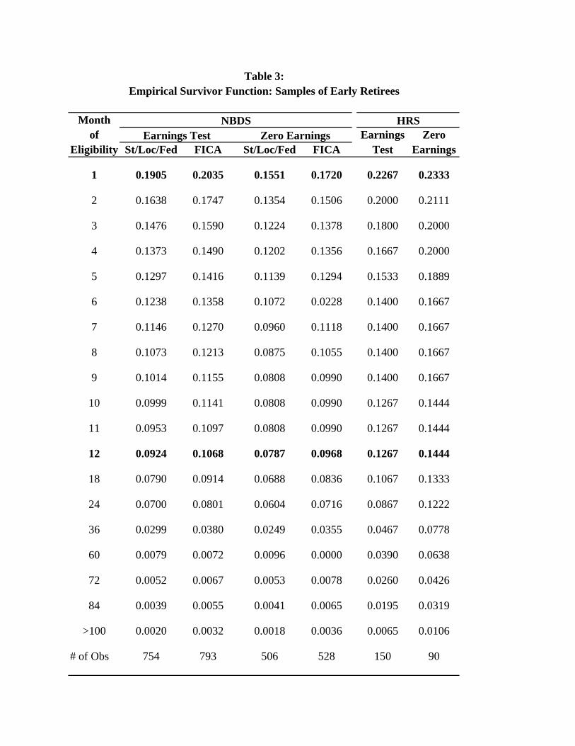
We first examine delays in the clean sample. The empirical survivor function is shown in
Table 3 and Figure 3. Two key features of the pattern of claiming are apparent. First, most
retirees claim immediately: roughly 80% of men claim in the first month of eligibility, at their 62nd
birthday. Second, a significant share of the sample has a long delay: roughly 10% of the sample
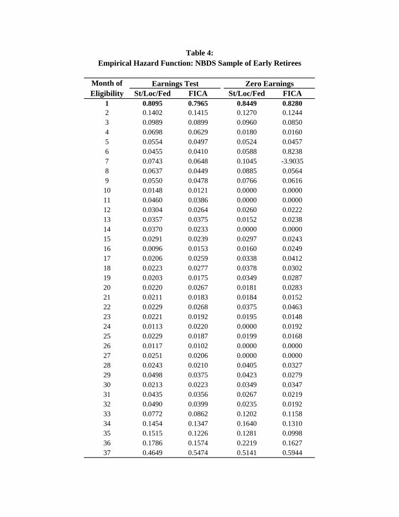
delays for at least one year. The hazard rate, shown in Table 4 and Figure 4, is very high in the
first month, is low for the next three years, and rises again near 36 months (age 65).
These patterns are extremely similar for both definitions of retirement (earnings of zero,
and earnings below the earnings test level), both methods of accounting for non-covered
employment (government, or no FICA earnings), and in both samples (NBDS, or HRS). We
choose as our preferred sample for the remainder of the analysis the NBDS sample that uses the
earnings test definition of retirement and that corrects for government employment, because the
23
24This is the sample used in Figures 3 and 4.
25HRS administrative data ends in December 1991. We assume all member of the sample whoare still delaying in December 1991 claim in January 1992.
earnings test sample is larger and because it seems more plausible that people would know the
sector of their employment than whether they pay FICA taxes.24 The percent delaying at least one
year in the preferred sample is 9.2%, versus 10.7%, 7.9%, and 9.7% in the other NBDS samples.
In the HRS, the percent delaying at least one year is 12.7% in the sample analogous to the
preferred sample. In fact, the true figure in the HRS may be even higher, as we conservatively
assume that all right-censored delays end when our observation period ends, which affects 44% of
the observations.25
Thus, claiming delays are empirically important for early retirees. Nevertheless, the
relatively small amount of delays in aggregate appears to contradict the general applicability of
gains from delayed claiming that we documented in our theoretical discussion. We return to this
point in the conclusion.
For the non-clean sample, the pattern is very different, as shown in Table 5 for the
earnings test sample. There is substantial claiming before retirement, represented by the "-1" row.
This reflects two factors: imperfect imputation of the month of retirement and application of the
monthly earnings test rather than the annual earnings test. Since both factors cannot, by
definition, affect the delay by more than one year, we compare the percentage delaying more than
one year in Table 7 to that in the previous tables. This share is much smaller in the non-clean
sample: it is 5% for those retiring at 62, 7% for those retiring at 63, and negligible for those
retiring at or after 65.
24
There are two explanations for our finding that early retirees delay longer. First, as noted
above, the optimal delay falls with retirement age past the 62nd birthday; the optimal age of
claiming does not vary significantly with the age of retirement, so a later retirement age results in
shorter delays. Second, those who retire early may be wealthier on average and, as we
documented above, optimal delays rise with wealth over some range of wealth. On the other
hand, those who retire earlier may be less healthy on average, which would correspond to shorter
delays. These effect of these covariates will be explored in the next section.
Table 6 presents summary statistics for the sample. We use weighted data to correct for
oversampling of older claimants. The typical respondent in the sample claims benefits in his first
month of benefit eligibility, though the mean claim occurs at 4.5 months due to the skewed nature
of the distribution. The typical respondent has an 83% probability of living to age 70; has $5,600
in financial assets; is married and two years older than his wife; has a 49% chance of having a
pension; is white; and has been retired for four years.
Part IV: Cross-Sectional Analysis
The discussion in Part II suggests a set of cross-sectional patterns in the incentives to
delay. We can verify that delays reflect calculating behavior on behalf of at least some retirees by
confirming the patterns in the data. For the cross-sectional analysis, we use our “preferred”
version of the NBDS clean sample (based on the earnings test definition of retirement and
adjusting for public sector employees) because it provides a precise measure of delays and a
sufficiently large sample of 754 observations.
25
26While we use mortality by age 70, results are similar using mortality by ages 68-74.
In the cross-sectional analysis, we test the four predictions derived in Part II. First, we
consider whether individuals who expect to live longer have longer delays by using data on ex-
post realized mortality by age 70 to proxy for mortality expectations at time of claim. Much of
the literature on modeling the effects of health suggests that objective measures such as this may
be preferable to self-reported measures of health.26
Second, we examine whether claiming delays exhibit a declining or inverse u-shaped
pattern as wealth rises. One difficulty in using NBDS wealth data to estimate the effect of wealth
on delays: the NBDS measures wealth at claiming, while the variable of interest is wealth at age
62. We were unable to obtain data on wealth at age 62, but this should be highly correlated with
wealth at claiming. We use total household net worth as our measure of wealth.
Third, married men should have longer delays than single men. Finally, among married
men, men with a larger (positive) age difference with their wives should have longer delays.
Hazard Model Estimates
The claiming decision is analyzed most naturally in a hazard model framework. A spell in
this context refers to a period of claiming delay, which begins when the individual first becomes
eligible for SS benefits by being both retired and at least 62 and ends when the individual claims.
We assume a proportional hazard specification of the form h(t) = h0(t)*eB1x1+...+BkXk and use non-
parametric estimation of the baseline hazard, h0(t). Importantly, in this hazard framework, a
negative coefficient indicates increased delays, so that for example we would predict a negative
26
coefficient on living to age 70, a positive or U-shaped relationship with wealth, a negative effect
of larger age differences between husband and wife, and a positive effect of being single. To
evaluate the coefficients, we compare them to a benchmark of zero: a coefficient of -.2 means that
a one unit change in the variable leads to a 20% decrease in the baseline hazard, and a lower
baseline hazard results in longer delays.
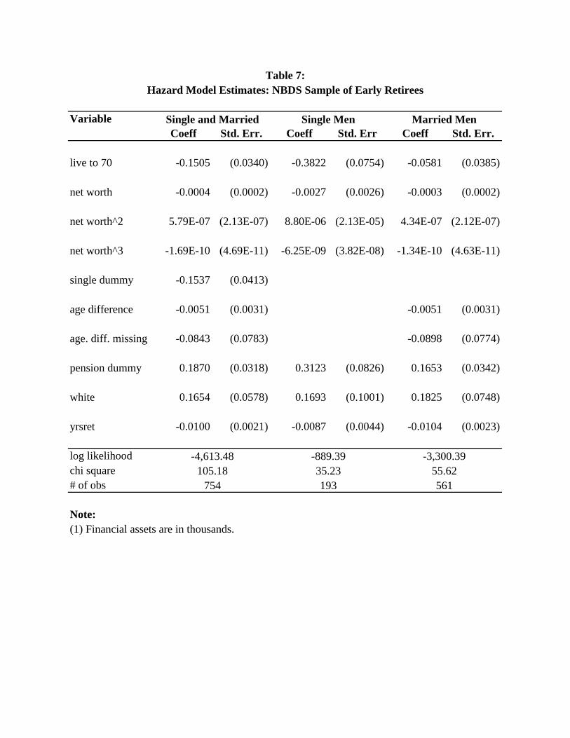
The first column of Table 7 presents our hazard model results for the pooled sample of
married and single men; for the single men, spousal age difference is set to zero, and a dummy for
being single is included in the model. These results provide substantial support for the cross-
sectional predictions of the model. First, we find that mortality prospects (as proxied by living
until age 70) cause a significant delay in claiming; living until age 70 lowers the hazard rate of
claiming by 15.1%, a quite sizeable effect. We also see a U-shaped pattern with respect to wealth
in the hazard rate: more wealth at first delays claiming, then ultimately speeds it up. This
relationship is graphed in Figure 5. We see that for wealth levels below $450,000, additional
wealth causes increases in delays, reflecting the first effect discussed earlier, the increased
valuation of annuities through easing of liquidity constraints. However, for wealth levels beyond
this level, additional wealth causes reductions in delays, as the bequest motive presumably
becomes operative and the value of the marginal annuity falls.
Strikingly, the coefficient on being single is negative, indicating longer delays for single
men. This is very much at odds with the simulations presented above, and there are at least three
explanations. The first is that the annuity provided by Social Security may be worth less to a
married couple because they are better able to self-insure, as argued by Kotlikoff and Spivak

27
(1981), which offsets the increased financial value of delayed claiming through the survivor
benefit. Second, the bequest motive may operate more strongly for married couples than for
single men (one-third of whom are never married), once again reducing the valuation of delayed
claiming on the margin. Finally, there may just be other underlying differences between single and
married claimants that are not captured in our model. We provide some evidence on these
hypotheses below.
The coefficient on the age difference with the spouse is the right sign, with larger age
differences leading to more delay, and it is significant at the 10% level. The estimate shows that
each year of age difference lowers the hazard by approximately 0.5%, so that having a wife that is
4 years younger reduces the hazard by 2% relative to having a wife that is the same age.
The remaining coefficients in the regression are also of interest. We find that, for each
year retired prior to age 62, the hazard is 0.8% lower, so younger retirees have longer delays
beyond age 62. The early retiree population includes two groups, those wealthy enough to afford
early retirement and those who are sick or have poor job prospects. The fact that we find a
significant negative coefficient may indicate that early retirees in our sample are largely drawn
from the well-off group; this is consistent with the fact that persons converting from disability to
SS benefits, who may make up a large fraction of sick and unemployable early retirees, are not in
the sample. Also, the fact that wealth is measured imperfectly, as detailed above, may further
explain why this variable may be picking up a wealth effect. Second, we find that a white
individual has a 19% higher hazard and a shorter delay.
Finally, we find that having a pension leads to a 30% higher hazard and a shorter delay.
28
27Our attempts to test this theory are not entirely successful. First, we find that delays amongmen with private pension plans are similar to delays among men with government pensions,despite the fact that private pension plans are much more likely to be integrated with SS. Second,we use questions about whether the pension rose or fell at age 62, age 65, or at benefit claim; wefind that these factors affect delays as we would expect, but the results are not significant, perhapsdue to the small number of people who report such changes in their pension.
There are two possible explanations for this finding. First, pensions may be integrated with SS
benefits; if pensions decrease automatically at age 62, men with pensions may claim without delay
to maintain a constant income.27 Second, the fact that the sample is selected on retiring prior to
age 62 could affect the result; for example, men with pensions who retire before age 62 could
have higher discount rates and therefore be less likely to delay.
We next separately analyze delays by single and married men. Two interesting features
emerge from this division of the sample. First, the effect of mortality on claiming is much
stronger for single than for married men, with living until age 70 lowering the hazard by almost
40% for single men and by only 6% for married men. Second, while the pattern of wealth effects
is nicely U-shaped for the married sample, as for the overall sample, it is much more variable for
the single sample, first declining, then increasing, then declining again.
Both of these findings are loosely consistent with our explanations for the counterintuitive
finding that single men delay longer. Married men’s delay is less affected by own mortality
prospects since they also depend on spouse mortality and since they are partially insured through
within-family annuitization. In addition, the wealth pattern is less clearly u-shaped for single men
because of a weaker bequest motive; for this population, very high wealth levels lead to longer
delays, as would be consistent with the model without bequests. Of course, these results are not
29
dispositive, and our finding of significantly longer delays for single men deserves further study.
Probit Model Estimates
Our hazard model considers the marginal impact of individual characteristics on delay in
general. But of particular interest is the impact of these characteristics on reasonably long delays,
since these are the cases that are of most relevance for both policy-making and empirical work on
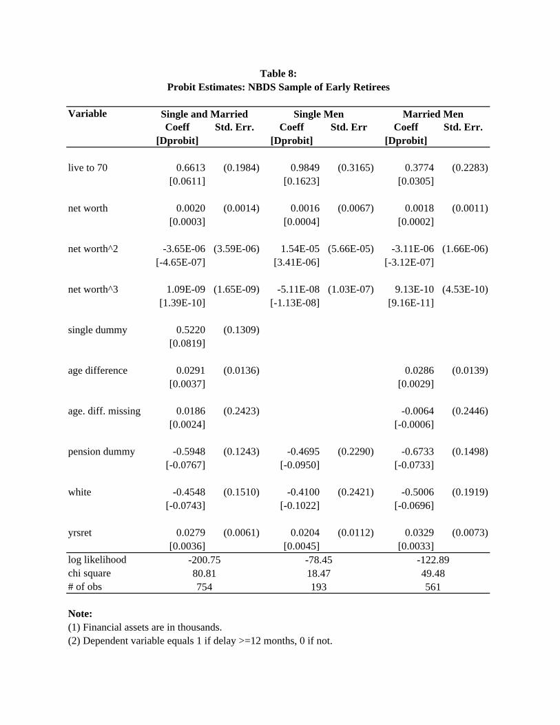
the behavioral impacts of Social Security. We therefore, in Table 8, reestimate our model as a
probit model of the decision to delay claiming at least 12 months. As noted earlier, the mean of
this dependent variable is 9.2%.
Each cell in Table 8 shows the probit coefficient, standard error, and the implied
percentage point change in delays. We expect all coefficients to change signs, as a positive
coefficient in the probit indicates a higher probability of delay. This is precisely what we find.
The mortality coefficient remains large and significant, suggesting that living to age 70 raises the
odds of delay by 6.1% , which is two-thirds of the baseline rate of delay in this sample of 9.3%.
Likewise, we continue to see a U shaped pattern in wealth holdings; in this case, the peak of the
inverse-U shape is at $320,000. But the coefficients on the wealth terms are no longer significant.
On the other hand, the coefficient on the age difference is now much more significant than in the
hazard model, and implies that each year of age difference increases the odds of delaying by 0.37
percentage points, which is 4% of baseline; that is, a man with a wife who is four years younger is
16% more likely to delay one year than is a man with a wife the same age. As in Table 7,
however, we continue to find a wrong-signed coefficient on the dummy for being single, which
30
28For example, in 1996 there were 43.7 million SS beneficiaries (of which 26.9 million wereretired worker beneficiaries), versus 8.1 million UI recipients and 4.5 million AFDC families (or12.6 million AFDC recipients). In 1996, SS benefits paid were $354 billion, compared to UIbenefits of $21 billion and AFDC benefits of $290 billion. All figures are from the 1998 GreenBook, Committee on Ways and Means, U.S. House of Representatives.
29Figures are unpublished data from the Office of the Chief Actuary, Social SecurityAdministration.
now indicates that being single raises the odds of delay by almost 11%. The other coefficients
have similar effects to those found in Table 7.
Thus, our probit estimates confirm the pattern of findings from the hazard model. For
mortality and spousal age difference, the effects are much larger in magnitude than in the hazard
model, suggesting that these factors may play a larger role in the decision to delay claiming for
longer periods of time than to delay for shorter periods. Indeed, if we reestimate these probit
models with a dummy for any delay, as opposed to a dummy for long delays, we get much weaker
results on mortality and spousal age differences.
Part V: Conclusions
While there is a large literature on take-up decisions for programs such as UI and AFDC,
we are not aware of any previous analysis of SS claiming behavior as a take-up decision, despite
the fact that SS dwarfs these programs in terms of annual expenditures and beneficiaries.28 Each
year, roughly one million male and 750,000 female fully insured individuals reach age 62 and face
choices of when to retire and when to claim SS benefits. Thus, understanding of the claiming
decision is important for modeling of the impacts of this program.29 In addition, the SS take-up
decision differs from that for UI or AFDC because it is completely a dynamic decision; the
31
question is not whether to take up benefits, but when.
In this paper, we first use financial calculations and simulations of an expected utility
maximization model to estimate optimal delays and the gains from delay. We find that delays are
optimal in a wide variety of cases and that gains are often significant. In the financial calculations,
gains from delay are around 600% of PIA for married couples in our base case. The simulations
of the expected utility maximization model for a single worker suggest that optimal delays are
longer and that gains from delay may be ten or more times larger when risk aversion is
incorporated.
While we find a much lower prevalence of delay empirically than the theoretical models
suggest, we have nevertheless documented that delays are empirically important for early retirees,
with approximately 10% of those retiring before age 62 delaying at least one year. By contrast,
delays are fairly unimportant for later retirees. Moreover, our hazard, and probit modeling
suggest that delays are largely consistent with the predictions of the theory. In particular, we find
support for three hypotheses: men with longer life expectancies have longer delays; delays follow
an inverse u-shaped pattern as wealth increases; and men with younger spouses have longer
delays. Surprisingly, however, we do not find that married men have longer delays than single
men. Perhaps differences in the claiming estimates across these groups are related to differences
in the ability of these groups to self-insure against mortality risk and in their bequest motives.
Our research has implications for the large literature on SS, in particular the estimation of
retirement responses to SS and the computation of the distributional effects of the program. As
we have discussed, the SS benefit level may be endogenous. Claiming appears to be influenced by

32
factors such as health, wealth, wife’s age, and wife’s earnings which may also affect retirement
propensities. Assuming that individuals claim benefits as soon as they retire overstates the benefit
of continued work, as part of the benefit is available to those who retire by delaying claiming.
Future work on retirement modeling can use our estimated claiming effects to correct their
estimates for delayed claiming.
Researchers studying the distributional effects of the program may also want to estimate
such effects using both the PIA and the actual benefit level; the former shows patterns of
redistribution inherent in the system conditional on everyone claiming at age 65, and comparing
the latter to the former shows to what extent these patterns are altered by claiming behavior. We
feel these issues are particularly relevant now, as the release of the HRS will certainly lead to a
new round of research on Social Security.
However, the simulations suggest that the fraction of early retirees claiming immediately
at age 62 is much too large. Tables 1 and 2 indicate that immediate claiming is only optimal for
those with a much older wife, high mortality risk, or a high discount rate. Thus we suspect that
part of the population simply claims immediately without sufficient consideration of intertemporal
choice issues. This finding of heterogeneity in the SS population has implications for aspects of
SS design and reform. For instance, it may affect the age at which benefits should first be made
available, an issue that has been made more salient by the gradual increase in the NRA from 62 to
67. This finding may also raise concerns about the rationality of the savings decision, which is of
great importance in the debate over SS reform. For all these reasons, we feel that claiming
behavior should be better understood by those interested in Social Security.

References
Bernheim, B. Douglas (1987). “The Economic Effects of Social Security: Towards aReconciliation of Theory and Measurement,” Journal of Public Economics, 33, 273-304.
Blau, David M. (1994). "Labor Force Dynamics of Older Men," Econometrica, 62, 117-156.
Boskin, Michael et al. (1987). "Social Security: A Financial Appraisal Across and WithinGenerations," National Tax Journal, 40, 19-33.
Brown, Jeffrey, and James Poterba (1999). “Joint Life Annuities and Annuity Demand byMarried Couples,” NBER Working Paper #7199.
Burtless, Gary and Robert Moffitt (1984). "The Effect of Social Security Benefits on the LaborSupply of the Aged," in H. Aaron and G. Burtless, eds., Retirement and EconomicBehavior. Washington: Brookings Institution, 135-175.
Coile, Courtney, and Jonathan Gruber (1999). “Social Security and Retirement,” mimeo, MIT.
Coile, Courtney, Peter Diamond, Jonathan Gruber, and Alain Jousten (1997). “Delays in ClaimingSocial Security Benefits,” mimeo, MIT.
Crawford, Vincent P. and David M. Lillien (1981). “Social Security and the Retirement Decision,”Quarterly Journal of Economics, 96, 505-529.
Diamond, Peter A. and Jonathan Gruber (1999). “Social Security and Retirement in the U.S.,” inJonathan Gruber and David Wise, eds., Social Security and Retirement Around the World.Chicago: University of Chicago Press.
Gruber, Jonathan, and Peter Orszag (1999). “What to do About the Social Security EarningsTest?,” Center for Retirement Research at Boston College, Issue in Brief #1.
Hurd, Michael (1990). "Research on the Elderly: Economic Status, Retirement, and Consumptionand Saving," Journal of Economic Literature, 28, 565-637.
Hurd, Michael and John Shoven (1985). "The Distributional Impact of Social Security," in D. Wise,ed., Pensions, Labor, and Individual Choice. Chicago: The University of Chicago Press, 193-221.
Jousten, Alain (1998). “Essays on annuity valuation, bequests, and Social Security” Ph.D.dissertation, MIT.
Kotlikoff, Laurence J. and Avia Spivak (1981). “The Family as an Incomplete Annuities Market,”Journal of Political Economy 89(2):372-391.
Krueger, Alan and Jorn-Steffen Pischke (1992). "The Effect of Social Security on Labor Supply: ACohort Analysis of the Notch Generation," Journal of Labor Economics,10, 412-437.
Mirer, Thad W. (1998). “The Optimal Time to File for Social Security Benefits,” Public FinanceReview, 26, 611-636.
Ruhm, Christopher (1995). "Secular Changes in the Work and Retirement Patterns of Older Men,"Journal of Human Resources, 30, 362-385.
Steuerle, C. Eugene and Jon M. Bakija (1994). Retooling Social Security for the 21st Century: Rightand Wrong Approaches to Reform. Washington, D.C.: Urban Institute Press.
</ref_section>
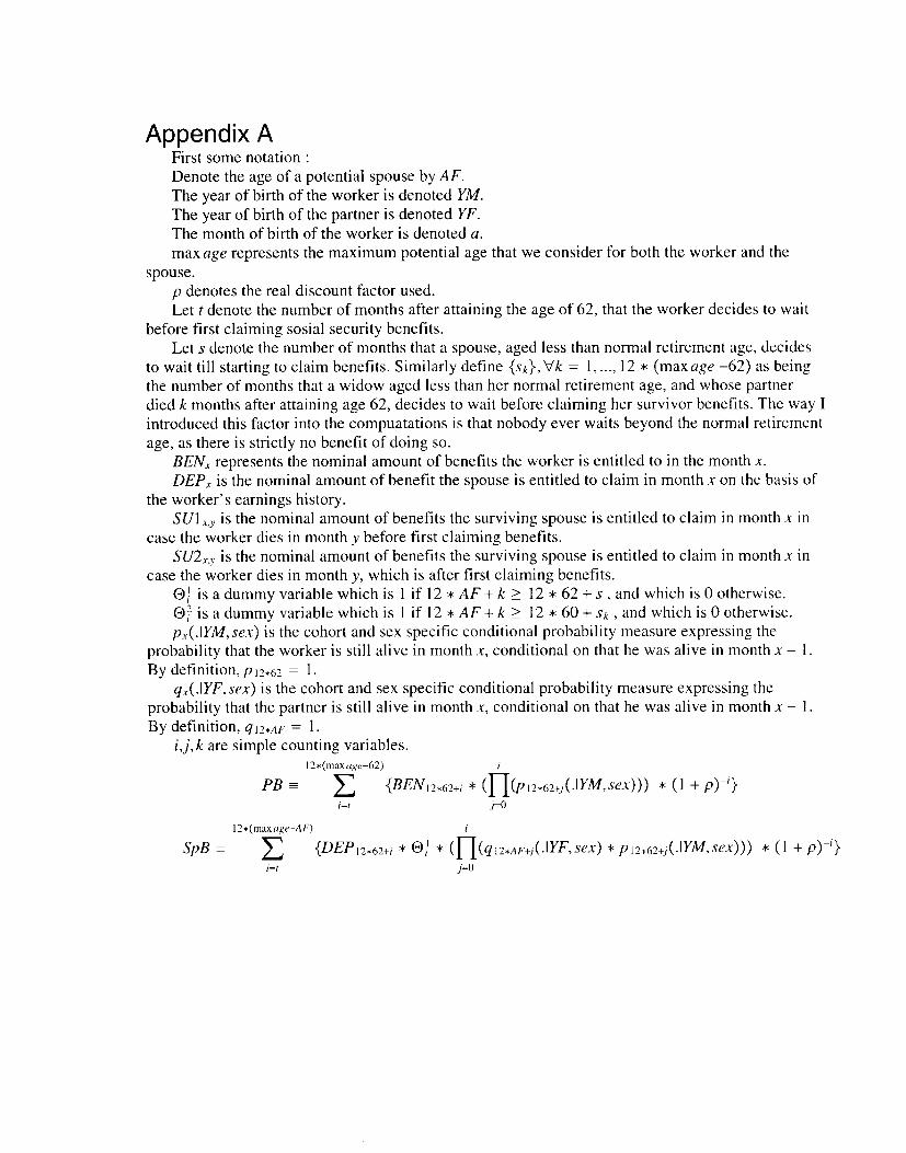
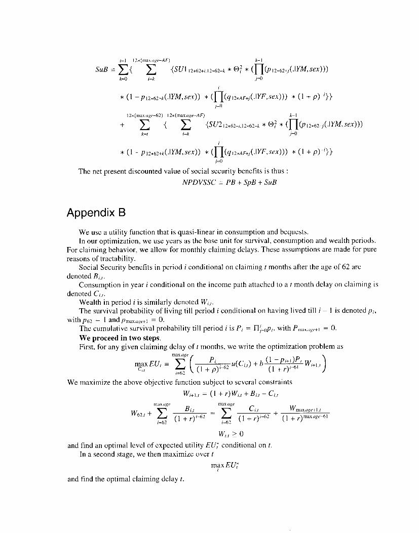
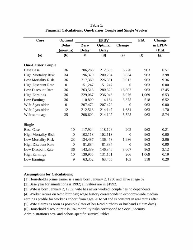
Table 1:Financial Calculations: One-Earner Couple and Single Worker
Case Optimal PIA ChangeDelay Zero Optimal Change in EPDV
(months) Delay Delay / PIA(a) (b) © (d) (e) (f) (g)
One-Earner CoupleBase Case 36 206,268 212,538 6,270 963 6.51High Mortality Risk 34 196,370 200,204 3,834 963 3.98Low Mortality Risk 36 217,369 226,381 9,012 963 9.36High Discount Rate 0 151,247 151,247 0 963 0.00Low Discount Rate 36 263,513 280,320 16,807 963 17.45High Earnings 36 229,067 236,043 6,976 1,069 6.53Low Earnings 36 110,809 114,184 3,375 518 6.52Wife 5 yrs older 0 207,472 207,472 0 963 0.00Wife 2 yrs older 12 212,513 214,147 1,634 963 1.70Wife same age 35 208,602 214,127 5,525 963 5.74
Single Base Case 10 117,924 118,126 202 963 0.21High Mortality Risk 0 102,113 102,113 0 963 0.00Low Mortality Risk 23 134,487 136,473 1,986 963 2.06High Discount Rate 0 81,884 81,884 0 963 0.00Low Discount Rate 36 143,339 146,346 3,007 963 3.12High Earnings 10 130,955 131,161 206 1,069 0.19Low Earnings 9 63,352 63,455 103 518 0.20
Assumptions for Calculations:(1) Household's prime earner is a male born January 2, 1930 and alive at age 62.(2) Base year for simulations is 1992; all values are in $1992.(3) Wife is born January 2, 1932; wife has never worked; couple has no dependents.(4) Worker retires on 62nd birthday; wage history corresponds to economy-wide medianearnings profile for worker's cohort from ages 20 to 50 and is constant in real terms after.(5) Wife claims as soon as possible (later of her 62nd birthday or husband's claim date).(6) Household discount rate is 3%; mortality risks correspond to Social SecurityAdministration's sex- and cohort-specific survival tables.
EPDV
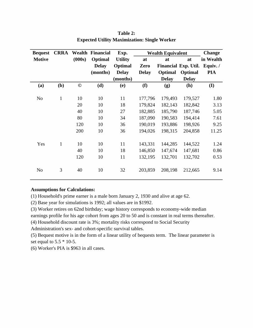
Table 2:Expected Utility Maximization: Single Worker
Bequest CRRA Wealth Financial Exp. ChangeMotive (000s) Optimal Utility at at at in Wealth
Delay Optimal Zero Financial Exp. Util. Equiv. /(months) Delay Delay Optimal Optimal PIA
(months) Delay Delay(a) (b) © (d) (e) (f) (g) (h) (I)
No 1 10 10 11 177,796 179,493 179,527 1.8020 10 18 179,824 182,143 182,842 3.1340 10 27 182,885 185,790 187,746 5.0580 10 34 187,090 190,583 194,414 7.61120 10 36 190,019 193,886 198,926 9.25200 10 36 194,026 198,315 204,858 11.25
Yes 1 10 10 11 143,331 144,285 144,522 1.2440 10 18 146,850 147,674 147,681 0.86120 10 11 132,195 132,701 132,702 0.53
No 3 40 10 32 203,859 208,198 212,665 9.14
Assumptions for Calculations:(1) Household's prime earner is a male born January 2, 1930 and alive at age 62.(2) Base year for simulations is 1992; all values are in $1992.(3) Worker retires on 62nd birthday; wage history corresponds to economy-wide medianearnings profile for his age cohort from ages 20 to 50 and is constant in real terms thereafter.(4) Household discount rate is 3%; mortality risks correspond to Social SecurityAdministration's sex- and cohort-specific survival tables.(5) Bequest motive is in the form of a linear utility of bequests term. The linear parameter isset equal to 5.5 * 10-5.(6) Worker's PIA is $963 in all cases.
Wealth Equivalent
Monthof Earnings Zero
Eligibility St/Loc/Fed FICA St/Loc/Fed FICA Test Earnings
1 0.1905 0.2035 0.1551 0.1720 0.2267 0.2333
2 0.1638 0.1747 0.1354 0.1506 0.2000 0.2111
3 0.1476 0.1590 0.1224 0.1378 0.1800 0.2000
4 0.1373 0.1490 0.1202 0.1356 0.1667 0.2000
5 0.1297 0.1416 0.1139 0.1294 0.1533 0.1889
6 0.1238 0.1358 0.1072 0.0228 0.1400 0.1667
7 0.1146 0.1270 0.0960 0.1118 0.1400 0.1667
8 0.1073 0.1213 0.0875 0.1055 0.1400 0.1667
9 0.1014 0.1155 0.0808 0.0990 0.1400 0.1667
10 0.0999 0.1141 0.0808 0.0990 0.1267 0.1444
11 0.0953 0.1097 0.0808 0.0990 0.1267 0.1444
12 0.0924 0.1068 0.0787 0.0968 0.1267 0.1444
18 0.0790 0.0914 0.0688 0.0836 0.1067 0.1333
24 0.0700 0.0801 0.0604 0.0716 0.0867 0.1222
36 0.0299 0.0380 0.0249 0.0355 0.0467 0.0778
60 0.0079 0.0072 0.0096 0.0000 0.0390 0.0638
72 0.0052 0.0067 0.0053 0.0078 0.0260 0.0426
84 0.0039 0.0055 0.0041 0.0065 0.0195 0.0319
>100 0.0020 0.0032 0.0018 0.0036 0.0065 0.0106
# of Obs 754 793 506 528 150 90
Zero EarningsEarnings Test
Empirical Survivor Function: Samples of Early RetireesTable 3:
HRSNBDS
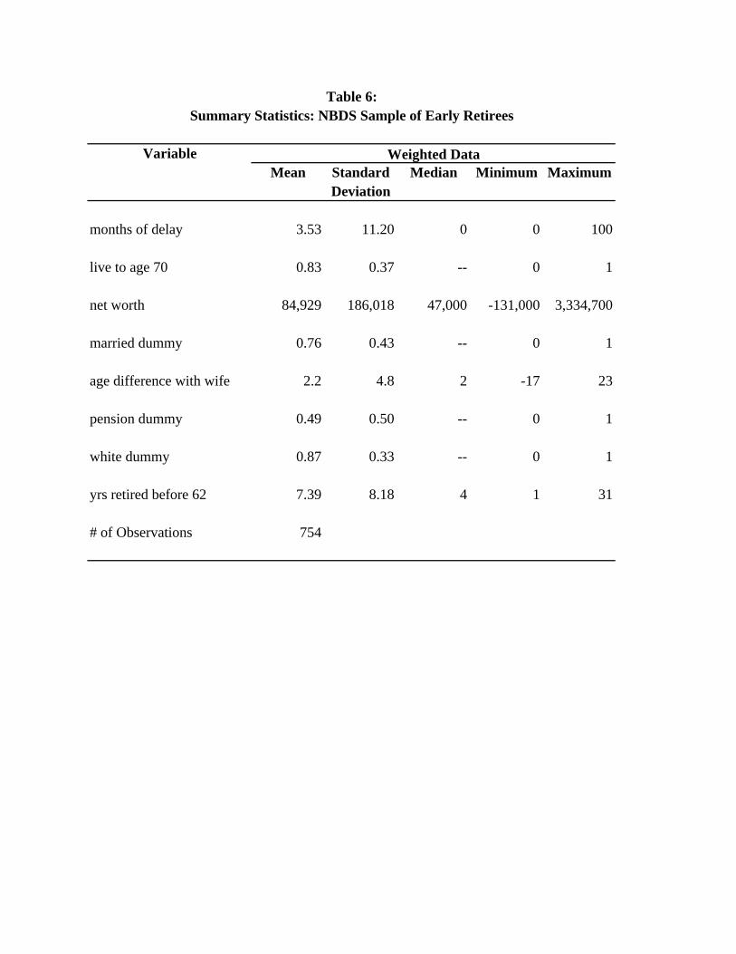
Table 6:Summary Statistics: NBDS Sample of Early Retirees
VariableMean Standard Median Minimum Maximum
Deviation
months of delay 3.53 11.20 0 0 100
live to age 70 0.83 0.37 -- 0 1
net worth 84,929 186,018 47,000 -131,000 3,334,700
married dummy 0.76 0.43 -- 0 1
age difference with wife 2.2 4.8 2 -17 23
pension dummy 0.49 0.50 -- 0 1
white dummy 0.87 0.33 -- 0 1
yrs retired before 62 7.39 8.18 4 1 31
# of Observations 754
Weighted Data
Month ofEligibility St/Loc/Fed FICA St/Loc/Fed FICA
1 0.8095 0.7965 0.8449 0.82802 0.1402 0.1415 0.1270 0.12443 0.0989 0.0899 0.0960 0.08504 0.0698 0.0629 0.0180 0.01605 0.0554 0.0497 0.0524 0.04576 0.0455 0.0410 0.0588 0.82387 0.0743 0.0648 0.1045 -3.90358 0.0637 0.0449 0.0885 0.05649 0.0550 0.0478 0.0766 0.0616
10 0.0148 0.0121 0.0000 0.000011 0.0460 0.0386 0.0000 0.000012 0.0304 0.0264 0.0260 0.022213 0.0357 0.0375 0.0152 0.023814 0.0370 0.0233 0.0000 0.000015 0.0291 0.0239 0.0297 0.024316 0.0096 0.0153 0.0160 0.024917 0.0206 0.0259 0.0338 0.041218 0.0223 0.0277 0.0378 0.030219 0.0203 0.0175 0.0349 0.028720 0.0220 0.0267 0.0181 0.028321 0.0211 0.0183 0.0184 0.015222 0.0229 0.0268 0.0375 0.046323 0.0221 0.0192 0.0195 0.014824 0.0113 0.0220 0.0000 0.019225 0.0229 0.0187 0.0199 0.016826 0.0117 0.0102 0.0000 0.000027 0.0251 0.0206 0.0000 0.000028 0.0243 0.0210 0.0405 0.032729 0.0498 0.0375 0.0423 0.027930 0.0213 0.0223 0.0349 0.034731 0.0435 0.0356 0.0267 0.021932 0.0490 0.0399 0.0235 0.019233 0.0772 0.0862 0.1202 0.115834 0.1454 0.1347 0.1640 0.131035 0.1515 0.1226 0.1281 0.099836 0.1786 0.1574 0.2219 0.162737 0.4649 0.5474 0.5141 0.5944
Earnings Test Zero Earnings
Table 4:Empirical Hazard Function: NBDS Sample of Early Retirees
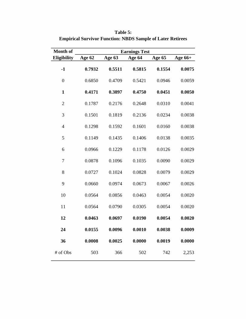
Table 5:Empirical Survivor Function: NBDS Sample of Later Retirees
Month ofEligibility Age 62 Age 63 Age 64 Age 65 Age 66+
-1 0.7932 0.5511 0.5815 0.1554 0.0075
0 0.6850 0.4709 0.5421 0.0946 0.0059
1 0.4171 0.3897 0.4750 0.0451 0.0050
2 0.1787 0.2176 0.2648 0.0310 0.0041
3 0.1501 0.1819 0.2136 0.0234 0.0038
4 0.1298 0.1592 0.1601 0.0160 0.0038
5 0.1149 0.1435 0.1406 0.0138 0.0035
6 0.0966 0.1229 0.1178 0.0126 0.0029
7 0.0878 0.1096 0.1035 0.0090 0.0029
8 0.0727 0.1024 0.0828 0.0079 0.0029
9 0.0660 0.0974 0.0673 0.0067 0.0026
10 0.0564 0.0856 0.0463 0.0054 0.0020
11 0.0564 0.0790 0.0305 0.0054 0.0020
12 0.0463 0.0697 0.0190 0.0054 0.0020
24 0.0155 0.0096 0.0010 0.0038 0.0009
36 0.0008 0.0025 0.0000 0.0019 0.0000
# of Obs 503 366 502 742 2,253
Earnings Test

Table 6:Summary Statistics: NBDS Sample of Early Retirees
VariableMean Standard Median Minimum Maximum
Deviation
months of delay 3.53 11.20 0 0 100
live to age 70 0.83 0.37 -- 0 1
net worth 84,929 186,018 47,000 -131,000 3,334,700
married dummy 0.76 0.43 -- 0 1
age difference with wife 2.2 4.8 2 -17 23
pension dummy 0.49 0.50 -- 0 1
white dummy 0.87 0.33 -- 0 1
yrs retired before 62 7.39 8.18 4 1 31
# of Observations 754
Weighted Data
VariableCoeff Std. Err. Coeff Std. Err Coeff Std. Err.
live to 70 -0.1505 (0.0340) -0.3822 (0.0754) -0.0581 (0.0385)
net worth -0.0004 (0.0002) -0.0027 (0.0026) -0.0003 (0.0002)
net worth^2 5.79E-07 (2.13E-07) 8.80E-06 (2.13E-05) 4.34E-07 (2.12E-07)
net worth^3 -1.69E-10 (4.69E-11) -6.25E-09 (3.82E-08) -1.34E-10 (4.63E-11)
single dummy -0.1537 (0.0413)
age difference -0.0051 (0.0031) -0.0051 (0.0031)
age. diff. missing -0.0843 (0.0783) -0.0898 (0.0774)
pension dummy 0.1870 (0.0318) 0.3123 (0.0826) 0.1653 (0.0342)
white 0.1654 (0.0578) 0.1693 (0.1001) 0.1825 (0.0748)
yrsret -0.0100 (0.0021) -0.0087 (0.0044) -0.0104 (0.0023)
log likelihoodchi square# of obs
Note:(1) Financial assets are in thousands.
105.18754
-889.3935.23193
55.62561
Single Men Married Men
Table 7:Hazard Model Estimates: NBDS Sample of Early Retirees
Single and Married
-3,300.39-4,613.48
VariableCoeff Std. Err. Coeff Std. Err Coeff Std. Err.
[Dprobit] [Dprobit] [Dprobit]
live to 70 0.6613 (0.1984) 0.9849 (0.3165) 0.3774 (0.2283)[0.0611] [0.1623] [0.0305]
net worth 0.0020 (0.0014) 0.0016 (0.0067) 0.0018 (0.0011)[0.0003] [0.0004] [0.0002]
net worth^2 -3.65E-06 (3.59E-06) 1.54E-05 (5.66E-05) -3.11E-06 (1.66E-06)[-4.65E-07] [3.41E-06] [-3.12E-07]
net worth^3 1.09E-09 (1.65E-09) -5.11E-08 (1.03E-07) 9.13E-10 (4.53E-10)[1.39E-10] [-1.13E-08] [9.16E-11]
single dummy 0.5220 (0.1309)[0.0819]
age difference 0.0291 (0.0136) 0.0286 (0.0139)[0.0037] [0.0029]
age. diff. missing 0.0186 (0.2423) -0.0064 (0.2446)[0.0024] [-0.0006]
pension dummy -0.5948 (0.1243) -0.4695 (0.2290) -0.6733 (0.1498)[-0.0767] [-0.0950] [-0.0733]
white -0.4548 (0.1510) -0.4100 (0.2421) -0.5006 (0.1919)[-0.0743] [-0.1022] [-0.0696]
yrsret 0.0279 (0.0061) 0.0204 (0.0112) 0.0329 (0.0073)[0.0036] [0.0045] [0.0033]
log likelihoodchi square# of obs
Note:(1) Financial assets are in thousands.(2) Dependent variable equals 1 if delay >=12 months, 0 if not.
Table 8:Probit Estimates: NBDS Sample of Early Retirees
Single Men Married MenSingle and Married
193 561754
-78.45 -122.89-200.7518.47 49.4880.81
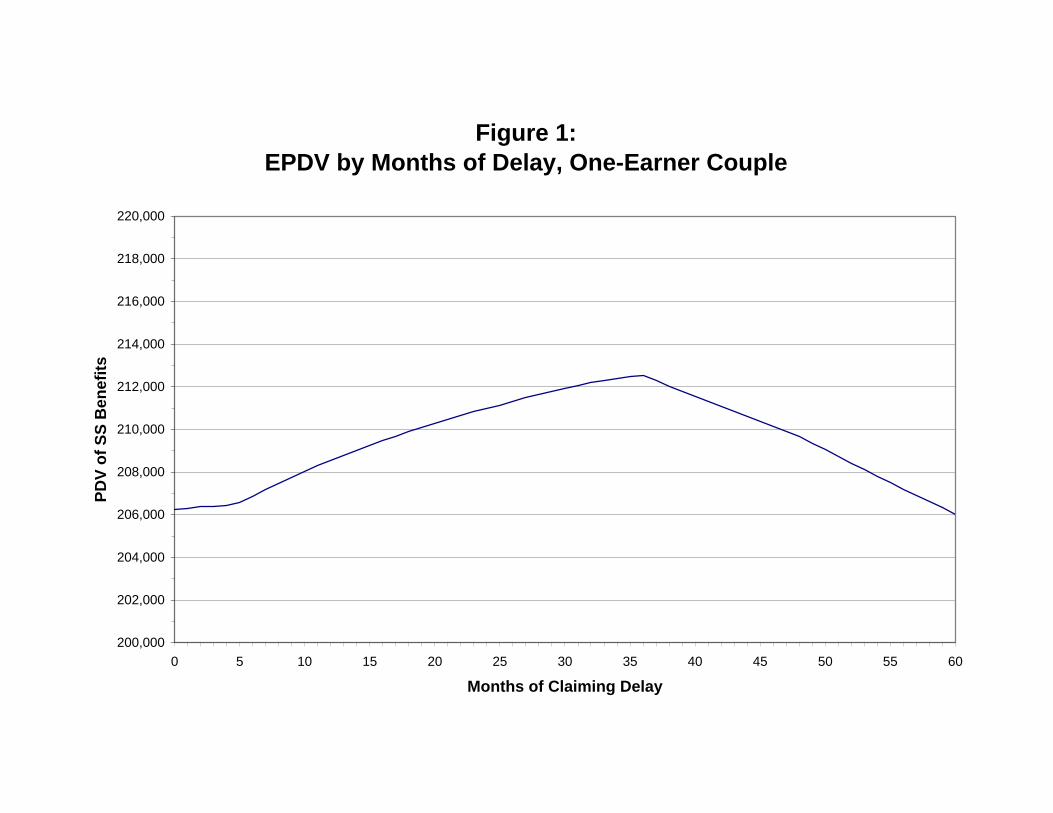
Figure 1: EPDV by Months of Delay, One-Earner Couple
200,000
202,000
204,000
206,000
208,000
210,000
212,000
214,000
216,000
218,000
220,000
0 5 10 15 20 25 30 35 40 45 50 55 60
Months of Claiming Delay
PD
V o
f S
S B
enef
its
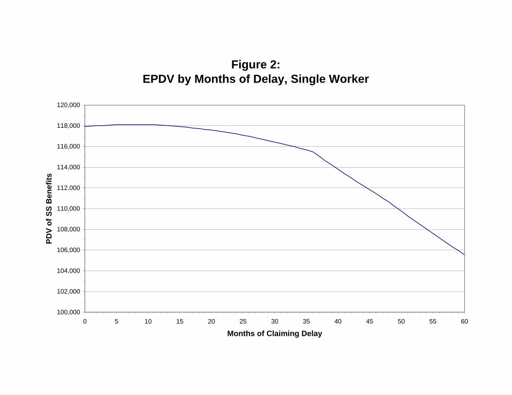
Figure 2: EPDV by Months of Delay, Single Worker
100,000
102,000
104,000
106,000
108,000
110,000
112,000
114,000
116,000
118,000
120,000
0 5 10 15 20 25 30 35 40 45 50 55 60
Months of Claiming Delay
PD
V o
f S
S B
enef
its
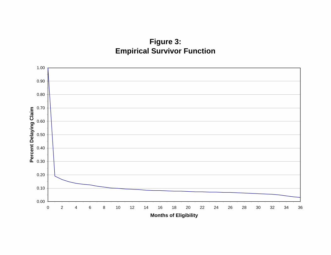
Figure 3: Empirical Survivor Function
0.00
0.10
0.20
0.30
0.40
0.50
0.60
0.70
0.80
0.90
1.00
0 2 4 6 8 10 12 14 16 18 20 22 24 26 28 30 32 34 36
Months of Eligibility
Per
cen
t D
elay
ing
Cla
im

Figure 4:Empirical Hazard Function
0.00
0.10
0.20
0.30
0.40
0.50
0.60
0.70
0.80
0.90
1 3 5 7 9 11 13 15 17 19 21 23 25 27 29 31 33 35
Months of Eligibility
Per
cen
t o
f D
elay
ers
Cla
imin
g E
ach
Mo
nth
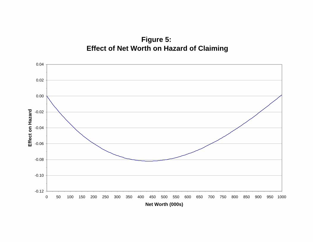
Figure 5: Effect of Net Worth on Hazard of Claiming
-0.12
-0.10
-0.08
-0.06
-0.04
-0.02
0.00
0.02
0.04
0 50 100 150 200 250 300 350 400 450 500 550 600 650 700 750 800 850 900 950 1000
Net Worth (000s)
Eff
ect
on
Haz
ard