Systems & Control Letters 58 (2009) 353–358

Contents lists available at ScienceDirect

Systems & Control Letters

journal homepage: www.elsevier.com/locate/sysconle

Signal-to-noise ratio performance limitations for input disturbance rejection inoutput feedback controlAlejandro J. Rojas ∗ARC Centre of Excellence for Complex Dynamic Systems and Control, The University of Newcastle, Callaghan NSW 2308, Australia

a r t i c l e i n f o

Article history:Received 22 July 2008Received in revised form10 December 2008Accepted 5 January 2009Available online 1 February 2009

Keywords:Signal to noise ratioControl over communication networksPerformance limitationsInput disturbance rejectionStability of linear systems

a b s t r a c t

Communication channels impose a number of obstacles to feedback control. One recent line of researchconsiders the problem of feedback stabilization subject to a constraint on the channel signal-to-noiseratio (SNR). We use the spectral factorization induced by the optimal solution and quantify in closed-form the infimal SNR required for both stabilization and input disturbance rejection for a minimumphase plant with relative degree one and memoryless additive white Gaussian noise (AWGN) channel.Finally we conclude by presenting a closed-form expression of the difference between the infimal AWGNchannel capacity for input disturbance rejection and the infimal AWGN channel capacity required onlyfor stabilizability.

© 2009 Elsevier B.V. All rights reserved.

1. Introduction

Fundamental limitations in control design have been animportant area of research for many years, [1,2]. Recently, thestudy of fundamental limitations has been extended to problemsof control over communication networks, see for example [3,Theorem 4.6], [4], as well as the special issue [5] and the recentsurvey by Nair et al. [6].Communication channels impose additional limitations to

feedback, such as constraints in transmission data rate andbandwidth, and effects of noise and time-delay. One line of recentresearch introduced a framework to study stabilizability of afeedback loop over channels with a signal to noise ratio (SNR)constraint [7,8]. These papers obtained the infimal SNR requiredto stabilize an unstable linear time invariant (LTI) plant overan additive white Gaussian noise (AWGN) channel. A distinctivecharacteristic of the SNR approach is that it is a linear formulation,suited for the analysis of robustness usingwell-developed tools [9].For the case of LTI controllers and minimum phase plant modelswith no time delay, these conditions match those derived in [10]by application of Shannon’s theorem [11, Section 10.3].Different techniques are used in [7,8] depending on whether

stabilization is achieved by state feedback or by output feedback.A common framework for both state and output feedback casesis proposed in [12], where it is shown that both problems can

∗ Tel.: +61 02 4916023.E-mail address: alejandro.rojas@newcastle.edu.au.

0167-6911/$ – see front matter© 2009 Elsevier B.V. All rights reserved.doi:10.1016/j.sysconle.2009.01.001

be solved as a linear quadratic Gaussian (LQG) optimization.Specifically, the optimal control problem arising from the infimalSNR constrained control problem may be posed as an LQGoptimization with weights chosen as in the loop transfer recovery(LTR) technique (see [13–17]). Doing so not only allows a unifiedtreatment of the state and output feedback cases, but also suggestshow performance considerations may be analyzed in addition tostabilization.The first contribution of the present paper is to obtain the

infimal SNR constrained solution in closed-form for stabilizabilityand input disturbance rejection in the case of memoryless AWGNchannels. The second contribution is that by means of the infimalSNR constrained solution we quantify the difference betweenthe infimal channel capacity C for performance and the infimalchannel capacity required for stabilizability only, see [10]. Thisdifference between channel capacities has been identified in [4],based on information theoretic arguments, as a key elementrepresenting a fundamental limitation in control over networkperformance. To the best knowledge of the author the channelcapacity difference imposed by the input disturbance rejection hasnot been quantified in closed-form before.Of the two possible configurations for the location of the

idealized communication channel, we consider the case of anAWGN communication channel over the measurement link. Sucha setting is common in practice and arises, for example, whensensors are far from the controller and have to communicatethrough a communication network.We neglect all pre- and post- signal processing involved in

the communication link, which is then reduced only to the

354 A.J. Rojas / Systems & Control Letters 58 (2009) 353–358

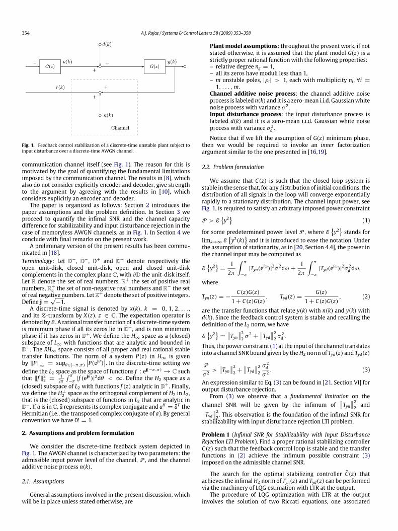
Fig. 1. Feedback control stabilization of a discrete-time unstable plant subject toinput disturbance over a discrete-time AWGN channel.

communication channel itself (see Fig. 1). The reason for this ismotivated by the goal of quantifying the fundamental limitationsimposed by the communication channel. The results in [8], whichalso do not consider explicitly encoder and decoder, give strengthto the argument by agreeing with the results in [10], whichconsiders explicitly an encoder and decoder.The paper is organized as follows: Section 2 introduces the

paper assumptions and the problem definition. In Section 3 weproceed to quantify the infimal SNR and the channel capacitydifference for stabilizability and input disturbance rejection in thecase of memoryless AWGN channels, as in Fig. 1. In Section 4 weconclude with final remarks on the present work.A preliminary version of the present results has been commu-

nicated in [18].Terminology: Let D−, D−, D+ and D+ denote respectively theopen unit-disk, closed unit-disk, open and closed unit-diskcomplements in the complex plane C, with ∂D the unit-disk itself.Let R denote the set of real numbers, R+ the set of positive realnumbers, R+o the set of non-negative real numbers and R− the setof real negative numbers. LetZ+ denote the set of positive integers.Define j =

√−1.

A discrete-time signal is denoted by x(k), k = 0, 1, 2, . . .,and its Z-transform by X(z), z ∈ C. The expectation operator isdenoted by E . A rational transfer function of a discrete-time systemis minimum phase if all its zeros lie in D−, and is non minimumphase if it has zeros in D+. We define the H∞ space as a (closed)subspace of L∞ with functions that are analytic and bounded inD+. The RH∞ space consists of all proper and real rational stabletransfer functions. The norm of a system P(z) in H∞ is givenby ‖P‖

∞= supθ∈[−π,π)

∣∣P(ejθ )∣∣. In the discrete-time setting wedefine the L2 space as the space of functions f : ej[−π,π) → C suchthat ‖f ‖22 =

12π

∫ π−π|f (ejθ )|2dθ < ∞. Define the H2 space as a

(closed) subspace of L2 with functions f (z) analytic in D+. Finally,we define the H⊥2 space as the orthogonal complement of H2 in L2,that is the (closed) subspace of functions in L2 that are analytic inD−. If a is inC, a represents its complex conjugate and aH = aT theHermitian (i.e., the transposed complex conjugate of a). By generalconvention we have 0! = 1.

2. Assumptions and problem formulation

We consider the discrete-time feedback system depicted inFig. 1. The AWGN channel is characterized by two parameters: theadmissible input power level of the channel, P , and the channeladditive noise process n(k).

2.1. Assumptions

General assumptions involved in the present discussion, whichwill be in place unless stated otherwise, are

Plantmodel assumptions: throughout the present work, if notstated otherwise, it is assumed that the plant model G(z) is astrictly proper rational function with the following properties:– relative degree ng = 1,– all its zeros have moduli less than 1,– m unstable poles, |ρi| > 1, each with multiplicity ni, ∀i =1, . . . ,m.

Channel additive noise process: the channel additive noiseprocess is labeled n(k) and it is a zero-mean i.i.d. Gaussianwhitenoise process with variance σ 2.Input disturbance process: the input disturbance process islabeled d(k) and it is a zero-mean i.i.d. Gaussian white noiseprocess with variance σ 2d .

Notice that if we lift the assumption of G(z) minimum phase,then we would be required to invoke an inner factorizationargument similar to the one presented in [16,19].

2.2. Problem formulation

We assume that C(z) is such that the closed loop system isstable in the sense that, for anydistribution of initial conditions, thedistribution of all signals in the loop will converge exponentiallyrapidly to a stationary distribution. The channel input power, seeFig. 1, is required to satisfy an arbitrary imposed power constraint

P > E{y2}

(1)

for some predetermined power level P , where E{y2}stands for

limk→∞ E{y2(k)

}and it is introduced to ease the notation. Under

the assumption of stationarity, as in [20, Section 4.4], the power inthe channel input may be computed as

E{y2}=12π

∫ π

−π

|Tyn(ejω)|2σ 2dω +12π

∫ π

−π

|Tyd(ejω)|2σ 2d dω,

where

Tyn(z) = −C(z)G(z)1+ C(z)G(z)

, Tyd(z) =G(z)

1+ C(z)G(z), (2)

are the transfer functions that relate y(k) with n(k) and y(k) withd(k). Since the feedback control system is stable and recalling thedefinition of the L2 norm, we have

E{y2}=∥∥Tyn∥∥22 σ 2 + ∥∥Tyd∥∥22 σ 2d .

Thus, the power constraint (1) at the input of the channel translatesinto a channel SNR bound given by theH2 norm of Tyn(z) and Tyd(z)

P

σ 2>∥∥Tyn∥∥22 + ∥∥Tyd∥∥22 σ 2dσ 2 . (3)

An expression similar to Eq. (3) can be found in [21, Section VI] foroutput disturbance rejection.From (3) we observe that a fundamental limitation on the

channel SNR will be given by the infimum of∥∥Tyn∥∥22 and∥∥Tyd∥∥22. This observation is the foundation of the infimal SNR for

stabilizability with input disturbance rejection LTI problem.

Problem 1 (Infimal SNR for Stabilizability with Input DisturbanceRejection LTI Problem). Find a proper rational stabilizing controllerC(z) such that the feedback control loop is stable and the transferfunctions in (2) achieve the infimum possible constraint (3)imposed on the admissible channel SNR.

The search for the optimal stabilizing controller C(z) thatachieves the infimalH2 norm of Tyn(z) and Tyd(z) can be performedvia the machinery of LQG estimation with LTR at the output.The procedure of LQG optimization with LTR at the output

involves the solution of two Riccati equations, one associated

A.J. Rojas / Systems & Control Letters 58 (2009) 353–358 355

with the design of the observer and another with the designof the regulator. If we were to perform the full design for theoutput feedback loop we would have to design two pairs ofweightingmatrices, one pair for the observer’s Riccati equation anda second pair for the regulator Riccati equation. The LTR proceduresimplifies the LQG design by pre-assigning the weights for theregulator Riccati equation as a cheap control design.It is well known that as a result of the LQG/LTR approach, for a

minimum phase plant model with relative degree one, the outputfeedback optimal sensitivity function S(z) = 1/(1 + G(z)C(z))recovers the observer’s design. That is, for a minimum phase plantmodel with relative degree one, we are able to recover the designfor the observer at the output. This remark is very useful since asimple spectral factorization analysis can now be applied to obtainthe closed loop characteristic polynomial whenever the infimalcontroller C(z) is in place, see for example [22, Section 6.4.3] andalso [18, Section V].

3. Infimal channel signal to noise ratio for input disturbancerejection

Consider that C(z), the controller that solves Problem 1, isin place. It is possible to verify that such controller will induce aspectral factorization given by

S−1(z)

(m∏i=1

(ρi

zi

)ni)S−T (z−1) = 1+ G(z)

σ 2d

σ 2G(z−1). (4)

From Eq. (4) we have that the plant model G(z), together with σ 2

and σ 2d , will determine S(z). Notice though that the stable polesof G(z) will also play a role in (4), as different from the case ofstabilizability with no input disturbance rejection where only theunstable poles of G(z) played a role (see [22]).We now quantify the infimal SNR required for stabilizability

and input disturbance rejection for the case of memoryless AWGNchannels. To do so we use the spectral factorization result in (4)and specify the plant model to be

G(z) =q(z)p(z)=

q(z)m∏i=1(z − ρi)ni

. (5)

The polynomial q(z) is assumed known,with degree n1+n2+· · ·+nm − 1 and all its solutions are in D−. As we stated before, we areultimately attempting to characterize the particular S(z) that takespart into the infimal SNR for stabilizability with input disturbancerejection LTI solution. Notice that S(z) must contain the m unsta-ble plant poles ρi, including multiplicity, as non minimum phase(NMP) zeros to guarantee the internal stability of the closed loop.Thus, we only have to obtain from (4) the location of the poles ofS(z)

S−1(z)

(m∏i=1

(ρi

zi

)ni)S−T (z−1)

=p(z)p(z−1)+ q(z) σ

2dσ 2q(z−1)

p(z)p(z−1). (6)

From (6)we recognize that the poles of S(z), labeled zi, zi ∈ D− i =1, · · ·m, with multiplicities n1, n2, · · · , nm, are the

∑mi=1 ni Schur’s

solutions of

p(z)p(z−1)+ q(z)σ 2d

σ 2q(z−1) = 0, (7)

a polynomial of degree 2(∑m

i=1 ni). It can be shown that the

other∑mi=1 ni solutions of (7) are the reflections of each zi, that is

1/zi, 1/zi ∈ D+ i = 1, · · ·m. We have then that a characterization

of the optimal S(z) is given by

S(z) =m∏i=1

(z − ρiz − zi

)ni. (8)

We stress that, although we do not have a closed-form for each zi,they can be computed by any of the many currently available al-gorithms for the purpose of finding the solutions of a polynomial,thus for all purposeswe consider themas knownquantities. Finallynotice, also from (7), that as σ 2d → 0, each zi will tend to one of theunstable plant poles mirrored images 1/ρi. By means of (8) we areable to quantify the infimal SNR for stabilizability with input dis-turbance rejection.

Theorem 2 (Infimal SNR for Stabilizability with Input DisturbanceRejection).Assume the plant to be as in (5) and the channelmodel to bea memoryless AWGN channel as in Fig. 1. Then, for the feedback loopto be stabilizable and ensure input disturbance rejection, the channelSNR must satisfy

Pσ 2

>

m∏i=1

(ρi)2ni − 1+

m∏i=1

(ρi)2ni

×

m∑i=1

ni∑l=1

mi,l(l− 1)!

m∑j=1

nj∑p=1

dl−1

dz l−1

(mj,pzp−1

(1− zzj)p

)∣∣∣∣∣z=zi

+σ 2d

σ 2

m∑i=1

ni∑l=1

gi,l(l− 1)!

m∑j=1

nj∑p=1

dl−1

dz l−1

(gj,pzp−1

(1− zzj)p

)∣∣∣∣∣z=zi

,

(9)

where

mi,l =1

(ni − l)!dni−l

dzni−l

m∏j=1(z − 1/ρj)nj

m∏j=1j6=i

(z − zj)nj

∣∣∣∣∣∣∣∣∣∣z=zi

,

gi,l =1

(ni − l)!dni−l

dzni−l(q(z))|z=zi .

(10)

Proof. We proceed by considering the function spaces L2, H2, H⊥2 ,and RH∞, with the stability region given by the open unit diskin the complex plane. Introduce a coprime factorization such thatG(z) = N(z)/M(z), where

N(z) =q(z)

m∏i=1(1− zρi)ni

, M(z) =m∏i=1

(z − ρi1− zρi

)ni,

and the parameterization of all stabilizing controllers (see [23, pp.64–65])

C(z) = (X(z)+M(z)Q (z)) / (Y (z)− N(z)Q (z)),

where X(z) and Y (z) satisfy the Bezout identity, N(z)X(z)+M(z)Y (z) = 1 and Q (z) is the Youla parameter, see for example[24]. From (2) and (3) we have

P

σ 2> ‖Tyn‖22 +

σ 2d

σ2‖Tyd‖22.

Notice that for the infimal solution with input disturbancerejection S(z) is equal to S(z), thus

P

σ 2> ‖NX + NMQ‖22 +

σ 2d

σ2

∥∥∥∥∥∥∥∥q(z)

m∏i=1(z − zi)ni

∥∥∥∥∥∥∥∥2

2

. (11)

356 A.J. Rojas / Systems & Control Letters 58 (2009) 353–358

We start by analyzing the termNX+NMQ which can be factorizedas

‖NX + NMQ‖22 = ‖M−1NX + NQ‖22, (12)

sinceM(z) is all-pass. Introduce now the following decomposition

M−1(z)N(z)X(z) = Γ ⊥(z)+ Γ (z),

where Γ ⊥ is in H⊥2 and Γ is in H2 and replace in (12)

‖NX + NMQ‖22 = ‖Γ⊥‖22 + ‖Γ + NQ‖

22. (13)

The term ‖Γ ⊥‖22 is the infimal SNR for stabilizability with no inputdisturbance rejection which, from applying Theorem III.1 in [8],we know is equal to

∏mi=1(ρi)

2ni − 1. Also directly from (13) wecan observe that the Youla parameter Q (z) achieving the infimalSNR for stabilizabilitywith no input disturbance rejectionwould begiven by−Γ (z)N−1(z), since this choicewould ensure the squaredH2 norm of Γ + NQ to be zero. Therefore we can observe that

‖NX + NMQ‖22 =m∏i=1

(ρi)2ni − 1+ ‖ − NQ + NQ‖22.

Reintroduce now M(z), since it is all-pass, into the squared H2norm term and add and subtract the term N(z)X(z)

‖NX + NMQ‖22 =m∏i=1

(ρi)2ni − 1

+‖ − NMQ + NMQ + NX − NX‖22.

Rearrange terms and recognize T (z) = NX + NMQ and T (z) =NX + NMQ

‖NX + NMQ‖22 =m∏i=1

(ρi)2ni − 1+ ‖T − T‖22.

Since T (z) = 1− S(z) and T (z) = 1− S(z) and S(z) = S(z)|σ 2d=0 =∏mi=1

(z−ρiz−1/ρi

)niwe have

‖NX + NMQ‖22 =m∏i=1

(ρi)2ni − 1

+

∥∥∥∥∥ m∏i=1

(z − ρiz − zi

)ni−

m∏i=1

(z − ρiz − 1/ρi

)ni∥∥∥∥∥2

2

.

By recognizing and extractingM(z)we can claim that

‖NX + NMQ‖22 =m∏i=1

(ρi)2ni − 1+

m∏i=1

(ρi)2ni

×

∥∥∥∥∥∥∥∥m∏i=1(z − 1/ρi)ni −

m∏i=1(z − zi)ni

m∏i=1(z − zi)ni

∥∥∥∥∥∥∥∥2

2

. (14)

Applying partial fraction expansion on the term inside the RHSsquared H2 norm and then invoking the Residue Theorem (see forexample [25, pp. 169–172]) we obtain

‖NX + NMQ‖22 =m∏i=1

(ρi)2ni − 1+

m∏i=1

(ρi)2ni

×

m∑i=1

ni∑l=1

mi,l(l− 1)!

m∑j=1

nj∑p=1

dl−1

dz l−1

(mj,pzp−1

(1− zzj)p

)∣∣∣∣z=zi

, (15)

with mi,l as in (10). Notice that the term∏mi=1(z − zi)

ni in thenumerator of the squared H2 norm in (14) does not contribute tothe residue since it and its derivatives in z are zero at each z = zi.We now focus on the second term in (11), for which applying

partial fraction expansion and then invoking the Residue Theoremgives

σ 2d

σ 2

m∑i=1

ni∑l=1

gi,l(l− 1)!

m∑j=1

nj∑p=1

dl−1

dz l−1

(gj,pzp−1

(1− zzj)p

)∣∣∣∣z=zi

, (16)

with gi,l as in (10). Finally we observe that the result in (15), plusthe result in (16), give the expression in (9) which concludes theproof. �

Theorem 2 quantifies the infimal SNR for stabilizability with inputdisturbance rejection. Notice how if σ 2d = 0, then the last term inthe RHS of (9) vanishes, whilst the second term vanishes as wellsince zi = 1/ρi in (14), and we are left with the infimal LTI SNRfor stabilizability as in [8, Theorem III.1]. Let us introduce a simpleexample in which we can explicitly account for the pole of S(z).

Example 3. Consider the plant to be G(z) = K/(z − ρ), withρ ∈ R+, ρ > 1 and K ∈ R+. From (4) we have that

1+ G(z)σ 2d

σ 2G(z−1) =

z2 +(−ρ − 1

ρ−K2σ 2dρσ 2

)z + 1

(z − ρ)(z − 1

ρ

) ,

therefore z1, the solution for the numerator and pole of S(z), isgiven by

z1 =ρ + 1

ρ+K2σ 2dρσ 2−

√(−ρ − 1

ρ−K2σ 2dρσ 2

)2− 4

2, (17)

the only solution that satisfies z1 ∈ D−. This can be seen to be truefrom the fact that

ρ +1ρ+K 2σ 2dρσ 2

> 2,

as long as ρ ∈ R+, which in turn allows us to claim that z1 < 1.With z1 known, applying Theorem 2 gives

P

σ 2> ρ2 − 1+ ρ2

(z1 − 1/ρ)2

1− z21+σ 2d

σ 2

K 2

1− z21, (18)

from which we observe that as σ 2d → 0, then z1 → 1/ρ and

P

σ 2> ρ2 − 1,

the infimal LTI SNR for stabilizability with no input disturbancerejection result, see for example [8, Theorem III.2].As a comparison with the LQG/LTR approach, consider now the

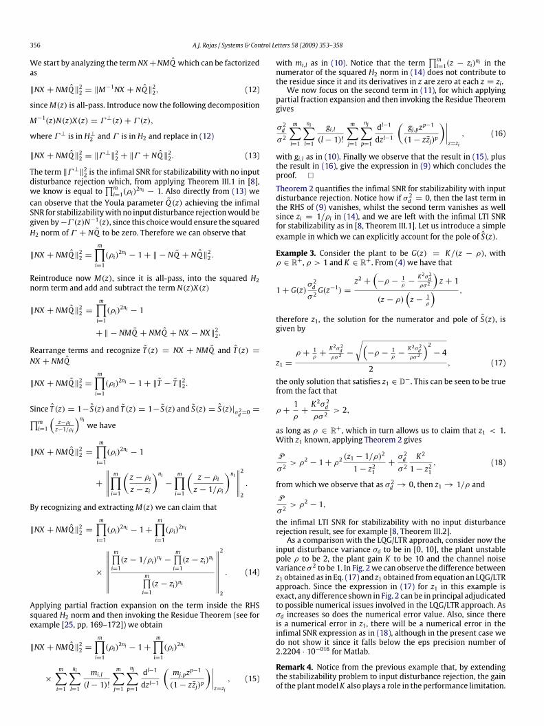
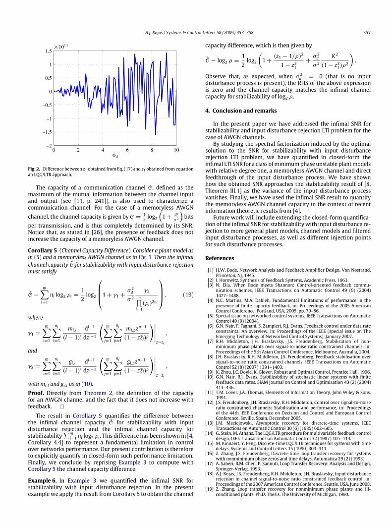
input disturbance variance σd to be in [0, 10], the plant unstablepole ρ to be 2, the plant gain K to be 10 and the channel noisevariance σ 2 to be 1. In Fig. 2we can observe the difference betweenz1 obtained as in Eq. (17) and z1 obtained fromequation an LQG/LTRapproach. Since the expression in (17) for z1 in this example isexact, any difference shown in Fig. 2 can be in principal adjudicatedto possible numerical issues involved in the LQG/LTR approach. Asσd increases so does the numerical error value. Also, since thereis a numerical error in z1, there will be a numerical error in theinfimal SNR expression as in (18), although in the present case wedo not show it since it falls below the eps precision number of2.2204 · 10−016 for Matlab.

Remark 4. Notice from the previous example that, by extendingthe stabilizability problem to input disturbance rejection, the gainof the plantmodelK also plays a role in the performance limitation.

A.J. Rojas / Systems & Control Letters 58 (2009) 353–358 357

Fig. 2. Difference between z1 obtained from Eq. (17) and z1 obtained from equationan LQG/LTR approach.

The capacity of a communication channel C, defined as themaximum of the mutual information between the channel inputand output (see [11, p. 241]), is also used to characterize acommunication channel. For the case of a memoryless AWGNchannel, the channel capacity is given byC = 1

2 log2(1+ P

σ 2

)bits

per transmission, and is thus completely determined by its SNR.Notice that, as stated in [26], the presence of feedback does notincrease the capacity of a memoryless AWGN channel.

Corollary 5 (Channel Capacity Difference). Consider a plant model asin (5) and a memoryless AWGN channel as in Fig. 1. Then the infimalchannel capacity C for stabilizability with input disturbance rejectionmust satisfy

C −m∑i=1

ni log2 ρi =12log2

1+ γ1 + σ 2dσ 2 γ2m∏i=1(ρi)2ni

, (19)

where

γ1 =

m∑i=1

ni∑l=1

mi,l(l− 1)!

dl−1

dz l−1

(m∑j=1

nj∑p=1

mj,pzp−1

(1− zzj)p

)∣∣∣∣∣z=zi

,

and

γ2 =

m∑i=1

ni∑l=1

gi,l(l− 1)!

dl−1

dz l−1

(m∑j=1

nj∑p=1

gj,pzp−1

(1− zzj)p

)∣∣∣∣∣z=zi

,

with mi,l and gi,l as in (10).Proof. Directly from Theorem 2, the definition of the capacityfor an AWGN channel and the fact that it does not increase withfeedback. �

The result in Corollary 5 quantifies the difference betweenthe infimal channel capacity C for stabilizability with inputdisturbance rejection and the infimal channel capacity forstabilizability

∑mi=1 ni log2 ρi. This difference has been shown in [4,

Corollary 4.4] to represent a fundamental limitation in controlover networks performance. Our present contribution is thereforeto explicitly quantify in closed-form such performance limitation.Finally, we conclude by reprising Example 3 to compute withCorollary 5 the channel capacity difference.

Example 6. In Example 3 we quantified the infimal SNR forstabilizability with input disturbance rejection. In the presentexamplewe apply the result from Corollary 5 to obtain the channel

capacity difference, which is then given by

C − log2 ρ =12log2

(1+

(z1 − 1/ρ)2

1− z21+σ 2d

σ 2

K 2

(1− z21)ρ2

).

Observe that, as expected, when σ 2d = 0 (that is no inputdisturbance process is present), the RHS of the above expressionis zero and the channel capacity matches the infimal channelcapacity for stabilizability of log2 ρ.

4. Conclusion and remarks

In the present paper we have addressed the infimal SNR forstabilizability and input disturbance rejection LTI problem for thecase of AWGN channels.By studying the spectral factorization induced by the optimal

solution to the SNR for stabilizability with input disturbancerejection LTI problem, we have quantified in closed-form theinfimal LTI SNR for a class ofminimumphase unstable plantmodelswith relative degree one, a memoryless AWGN channel and directfeedthrough of the input disturbance process. We have shownhow the obtained SNR approaches the stabilizability result of [8,Theorem III.1] as the variance of the input disturbance processvanishes. Finally, we have used the infimal SNR result to quantifythe memoryless AWGN channel capacity in the context of recentinformation theoretic results from [4].Future work will include extending the closed-form quantifica-

tion of the infimal SNR for stabilizabilitywith input disturbance re-jection to more general plant models, channel models and filteredinput disturbance processes, as well as different injection pointsfor such disturbance processes.

References

[1] H.W. Bode, Network Analysis and Feedback Amplifier Design, Von Nostrand,Princeton, NJ, 1945.

[2] I. Horowitz, Synthesis of Feedback Systems, Academic Press, 1963.[3] N. Elia, When Bode meets Shannon: Control-oriented feedback commu-nication schemes, IEEE Transactions on Automatic Control 49 (9) (2004)1477–1488.

[4] N.C. Martins, M.A. Dahleh, Fundamental limitations of performance in thepresence of finite capacity feedback, in: Proceedings of the 2005 AmericanControl Conference, Portland, USA, 2005, pp. 79–86.

[5] Special issue on networked control systems, IEEE Transactions on AutomaticControl 49 (9) (2004).

[6] G.N. Nair, F. Fagnani, S. Zampieri, R.J. Evans, Feedback control under data rateconstraints: An overview, in: Proceedings of the IEEE (special issue on TheEmerging Technology of Networked Control Systems), January 2007.

[7] R.H. Middleton, J.H. Braslavsky, J.S. Freudenberg, Stabilization of non-minimum phase plants over signal-to-noise ratio constrained channels, in:Proceedings of the 5th Asian Control Conference, Melbourne, Australia, 2004.

[8] J.H. Braslavsky, R.H. Middleton, J.S. Freudenberg, Feedback stabilisation oversignal-to-noise ratio constrained channels, IEEE Transactions on AutomaticControl 52 (8) (2007) 1391–1403.

[9] K. Zhou, J.C. Doyle, K. Glover, Robust and Optimal Control, Prentice Hall, 1996.[10] G.N. Nair, R.J. Evans, Stabilizability of stochastic linear systems with finite

feedback data rates, SIAM Journal on Control and Optimization 43 (2) (2004)413–436.

[11] T.M. Cover, J.A. Thomas, Elements of Information Theory, John Wiley & Sons,1991.

[12] J.S. Freudenberg, J.H. Braslavsky, R.H. Middleton, Control over signal-to-noiseratio constrained channels: Stabilization and performance, in: Proceedingsof the 44th IEEE Conference on Decision and Control and European ControlConference, Seville, Spain, December 2005.

[13] J.M. Maciejowski, Asymptotic recovery for discrete-time systems, IEEETransactions on Automatic Control 30 (6) (1985) 602–605.

[14] G. Stein, M. Athans, The LQG/LTR procedure for multivariable feedback controldesign, IEEE Transactions on Automatic Control 32 (1987) 105–114.

[15] M. Kinnaert, Y. Peng, Discrete-time LQG/LTR techniques for systems with timedelays, Systems and Control Letters 15 (1990) 303–311.

[16] Z. Zhang, J.S. Freudenberg, Discrete-time loop transfer recovery for systemswith nonminimum phase zeros and time delays, Automatica 29 (2) (1993).

[17] A. Saberi, B.M. Chen, P. Sannuti, Loop Transfer Recovery: Analysis and Design,Springer-Verlag, 1993.

[18] A.J. Rojas, J.S. Freudenberg, R.H. Middleton, J.H. Braslavsky, Input disturbancerejection in channel signal-to-noise ratio constrained feedback control, in:Proceedings of the 2007American Control Conference, Seattle, USA, June 2008.

[19] Z. Zhang, Loop transfer recovery for nonminimum phase plants and ill-conditioned plants, Ph.D. Thesis, The University of Michigan, 1990.

358 A.J. Rojas / Systems & Control Letters 58 (2009) 353–358

[20] K.J. Åström, Introduction to Stochastic Control Theory, Academic Press, 1970.[21] N. Elia, The information cost of loop shaping over Gaussian channels,

in: Proceedings of the 13th Mediterranean Conference on Control andAutomation, 2005.

[22] A.J. Rojas, Feedback control over signal to noise ratio constrained commu-nication channels, Ph.D. Thesis, The University of Newcastle, NSW 2308,Australia, July 2006. http://www.newcastle.edu.au/service/library/adt/public/adt-NNCU20070316.113249/index.html.

[23] J.C. Doyle, B.A. Francis, A.R. Tannenbaum, Feedback Control Theory, MacmillanPublishing Company, 1992.

[24] M. Vidyasagar, Control System Synthesis: A Factorization Approach,MIT Press,1985.

[25] R.V. Churchill, J.W. Brown, Complex Variables and Applications, 5th ed.,McGraw-Hill International Editions, 1990.

[26] C. Shannon, The zero error capacity of a noisy channel, Institute of RadioEngineers, Transactions on Information Theory IT-2 (1956) S8–S19.