Disturbance Tolerance and Rejection of Linear Systems with ImpreciseKnowledge of Actuator Input Output Characteristics

Haijun Fang Zongli Lin Yacov Shamash

Abstract— In this paper, we study the robustness of linearsystems with respect to the disturbances and the uncertaintiesin the actuator input output characteristics. Disturbances eitherbounded in energy or bounded in magnitude are considered.The actuator input output characteristics are assumed to residein a so-called generalized sector bounded by piecewise linearcurves. Robust bounded state stability of the closed-loop systemis first defined and characterized in terms of linear matrixinequalities (LMIs). Based on this characterization, the eval-uation of the disturbance tolerance and disturbance rejectioncapabilities of the closed-loop system under a given feedbacklaw is formulated into and solved as optimization problems withLMI constraints. The maximal tolerable disturbance is thendetermined by optimizing the disturbance tolerance capabilityof the closed-loop system over the choice of feedback gains.Similarly, the design of feedback gain that maximizes thedisturbance rejection capability of can be carried out by viewingthe feedback gain as an additional free parameter in theoptimization problem for the evaluation of the disturbancerejection capability under a given feedback gain.

I. INTRODUCTION

In this paper, we consider the robustness analysis and statefeedback design for an uncertain nonlinear system,⎧⎨

⎩x = Ax + Bψ(u, t) + Eω,u = Fx,z = Cx,

(1)

where x ∈ Rn is the state, u ∈ R is the control input,ω ∈ Rp is the disturbance, z ∈ Rq is the controlled output ofthe system, and the function ψ(u, t) represents the actuatorinput output characteristics, which is a nonlinear function,such as a saturation like function, and is not precisely known.We also assume that ω belongs to one of the followingtwo classes of disturbances whose energy or magnitudes arebounded by a given number α > 0,

W1α :=

{ω : R+ → Rq :

∫ ∞

0

ωT(t)ω(t)dt ≤ α

},

W2α := {ω : R+ → Rq : ωT(t)ω(t) ≤ α, ∀t ≥ 0} .

The analysis and design of control systems in the presenceof saturation or saturation type nonlinearities and externaldisturbances have been studied by many authors. A smallsample of their works include [1], [2], [4], [5], [7], [9], [10],[11], [12], [13], [14], [15], [16], [18], [19].

More recently, we considered in [3] the situation whereno boundedness assumption is made on the magnitude of

H. Fang and Z. Lin are with Charles L. Brown Department of Electricaland Computer Engineering, University of Virginia, Charlottesville, VA22904-4743, USA. Email: zl5y, hf2r@virginia.edu. Y. Shamash is withCollege of Engineering and Applied Science, State University of New York,Stony Brook, NY 11794-2200, USA. Work supported in part by NSF grantCMS-0324329.

the disturbances and the system initial conditions are notnecessarily zero, and proposed an LMI based approach to theanalysis and design of closed-loop system under linear statefeedback laws. Both the questions of disturbance toleranceand disturbance rejection were addressed. The approachproposed in [3] has also been extended to the output feedbacksetting [20] and the discrete-time setting [18], [19].

The objective of this paper is to revisit the problemsposed in [3] in a broader setting so that robustness to theuncertainties in the actuator input output characteristics canbe addressed simultaneously. This is made possible by ourrecent work on stabilization of linear systems with actuatornonlinearities [6], in which uncertainties in the actuatornonlinearities are assumed to reside in a so-called generalizedsector bounded by two convex or concave curves.

We will first establish sufficient conditions, in terms oflinear matrix inequalities (LMIs), under which trajectoriesof the given system (1) starting from within a boundedset of initial conditions remain bounded. Such a propertyof the system can be called robust bounded state stability.Based on these conditions, we will be able to formulate andsolve the problems of assessing disturbance tolerance anddisturbance rejection capabilities as optimization problemswith LMI constraints. The design of state feedback laws toenhance the disturbance tolerance/rejection capabilities of theclosed-loop system can then be carried out by viewing thestate feedback gain as an additional free parameter in theseoptimization problems.

The disturbance tolerance capability is measured by themaximal energy/magnitude bound α, say α∗, under whichany system trajectory starting from the given bounded setof initial conditions remains bounded. For an α ≤ α∗, thesize of the set of initial conditions from which any trajectoryremains bounded can also effectively indicate the disturbancetolerance capability.

One way to measure the disturbance rejection capability isto estimate the restricted L2 gain over W1

α, or the maximumof the l∞ norm of the output with zero initial conditionover W2

α. As trajectories starting from a given bounded setmay be driven out of the set by tolerable energy boundeddisturbances, but will remain within a larger bounded set,the gap between the two sets is also an indication of thedisturbance rejection capability.

Notation: For a vector F ∈ R1×n, denote L(F ) :={x ∈ Rn : |Fx| ≤ 1}. For a positive definite matrix P ∈Rn×n, and a positive scalar ρ, denote ε(P, ρ) :={x ∈ Rn : xTPx≤ρ}. We use sat(u) to denote the standardsaturation function, i.e., sat(u) = sign(u)min{1, |u|}. Givena set of vectors x1, x2, · · · , xN , we use co{x1, x2, · · · , xN}

Proceedings of the44th IEEE Conference on Decision and Control, andthe European Control Conference 2005Seville, Spain, December 12-15, 2005

ThC17.4

0-7803-9568-9/05/$20.00 ©2005 IEEE 8294

to denote the convex hull of these vectors.

II. ROBUST BOUNDED STATE STABILITY

We will first consider actuator nonlinearities that residein a generalized sector bounded by two concave piecewiselinear functions. The results for generalized sectors whereone or both boundaries are convex can be established in thesame manner.

We will need to recall the following lemma from [5].Lemma 1: Given an F ∈ R1×n and a positive definite

matrix P ∈ Rn×n. Then, for any H ∈ R1×n such that|Hx| ≤ 1, then sat(Fx) ∈ co {Fx, Hx} .

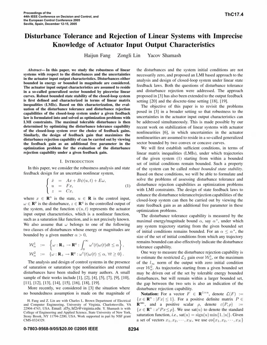
A. Piecewise linear functions with one bend

Consider the system (1) with

ψ(u, t) ∈ co{ψ1(u), ψ2(u)}, (2)

where ψi(u), i ∈ [1, 2], are odd symmetric and

ψi(u) ={

ki0u, if u ∈ [0, bi1],ki1u + ci1, if u ∈ (bi1,∞), (3)

where bi1 = ci1ki0−ki1

> 0, ki0 > ki1, ki0 > 0 (see Fig. 1).

v

ui1b

i1i1 cukv −=

oi1b−

( )uvi

ψ=

i1i1 cukv +=i1i0bk

i1i0bk−

Fig. 1. A concave piecewise linear function with one bend, ψi(u).

Theorem 1: Consider system (1) with ψ(u, t) given by (2)and ω ∈ W1

α. Let the positive definite matrix P ∈ Rn×n begiven.

(a) If there exist H1, H2 ∈ R1×n and a positive number ηsuch that, for i ∈ [1, 2],⎧⎪⎨

⎪⎩(A+ki0BF )TP+P (A+ki0BF )+

1ηPEETP≤0,

(A+BHi)TP +P (A+BHi)+1ηPEETP ≤0,

(4)

and ε(P, 1 + αη) ⊂ L(

Hi−ki1Fci1

), then any trajectory

of the closed-loop system (1) that starts from inside ofε(P, 1) will remain inside of ε(P, 1 + αη).

(b) If there exist H1, H2 ∈ R1×n such that, for i ∈ [1, 2],{(A+ki0BF )TP+P (A+ki0BF )+PEETP ≤ 0,(A+BHi)TP +P (A+BHi)+PEETP ≤ 0,

(5)

and ε(P, α) ⊂ L(

Hi−ki1Fci1

), then the trajectory of

the closed-loop system that starts from the origin willremain inside the ellipsoid ε(P, α).

Theorem 2: Consider system (1) with ψ(u, t) given by (2)and ω ∈ W2

α. Let the positive definite matrix P ∈ Rn×n begiven. If there exist an H ∈ R1×n and a positive number ηsuch that, for i ∈ [1, 2],

⎧⎪⎨⎪⎩

(A+ki0BF )TP+P (A+ki0BF )+1ηPEETP+ηαP ≤ 0,

(A+BHi)TP+P (A+BHi)+1ηPEETP+ηαP ≤ 0,

(6)

and ε(P, α)⊂L(

Hi−ki1Fci1

), then ε(P, α) is an invariant set.

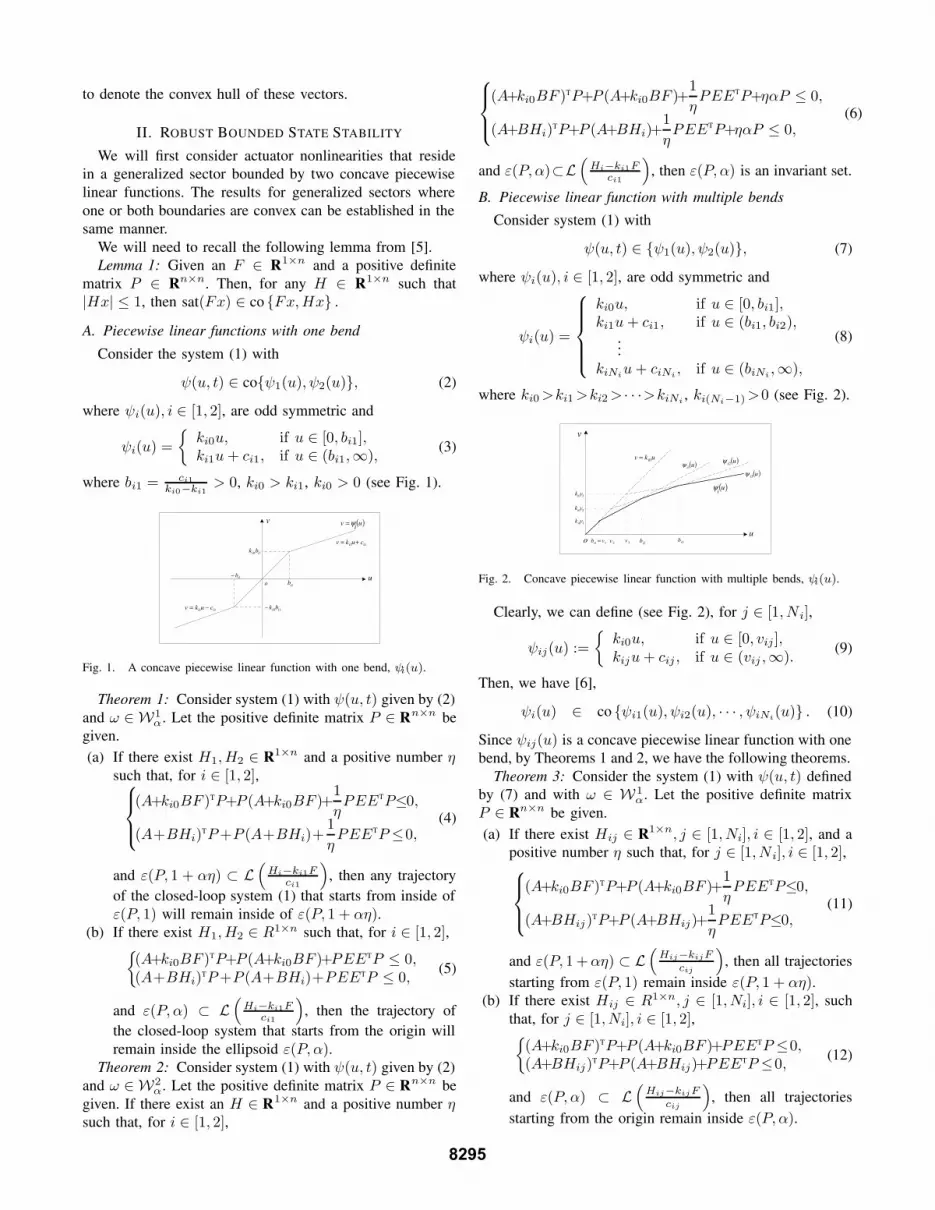
B. Piecewise linear function with multiple bends

Consider system (1) with

ψ(u, t) ∈ {ψ1(u), ψ2(u)}, (7)

where ψi(u), i ∈ [1, 2], are odd symmetric and

ψi(u) =

⎧⎪⎪⎪⎨⎪⎪⎪⎩

ki0u, if u ∈ [0, bi1],ki1u + ci1, if u ∈ (bi1, bi2),

...kiNiu + ciNi , if u ∈ (biNi ,∞),

(8)

where ki0 >ki1 >ki2 > · · ·>kiNi , ki(Ni−1) >0 (see Fig. 2).

o

ukv i0=

1i1 vb = i3b

2i0vk

u

v

( )ui1ψ ( )ui2ψ

( )ui3ψ

i2b

3i0vk( )u

iψ

1i0vk

2v 3v

Fig. 2. Concave piecewise linear function with multiple bends, ψi(u).

Clearly, we can define (see Fig. 2), for j ∈ [1, Ni],

ψij(u) :={

ki0u, if u ∈ [0, vij ],kiju + cij , if u ∈ (vij ,∞). (9)

Then, we have [6],

ψi(u) ∈ co {ψi1(u), ψi2(u), · · · , ψiNi(u)} . (10)

Since ψij(u) is a concave piecewise linear function with onebend, by Theorems 1 and 2, we have the following theorems.

Theorem 3: Consider the system (1) with ψ(u, t) definedby (7) and with ω ∈ W 1

α. Let the positive definite matrixP ∈ Rn×n be given.

(a) If there exist Hij ∈ R1×n, j ∈ [1, Ni], i ∈ [1, 2], and apositive number η such that, for j ∈ [1, Ni], i ∈ [1, 2],⎧⎪⎨⎪⎩

(A+ki0BF )TP+P (A+ki0BF )+1ηPEETP≤0,

(A+BHij)TP+P (A+BHij)+1ηPEETP≤0,

(11)

and ε(P, 1 + αη) ⊂ L(

Hij−kijFcij

), then all trajectories

starting from ε(P, 1) remain inside ε(P, 1 + αη).(b) If there exist Hij ∈ R1×n, j ∈ [1, Ni], i ∈ [1, 2], such

that, for j ∈ [1, Ni], i ∈ [1, 2],{(A+ki0BF )TP+P (A+ki0BF )+PEETP ≤0,(A+BHij)TP+P (A+BHij)+PEETP ≤0,

(12)

and ε(P, α) ⊂ L(

Hij−kijFcij

), then all trajectories

starting from the origin remain inside ε(P, α).

8295

Theorem 4: Consider system (1) with ψ(u, t) defined by(7) and ω ∈ W2

α. Let the positive definite matrix P ∈Rn×n

be given. If there exist Hij ∈R1×n, j∈ [1, Ni],i∈ [1, 2], and apositive number η such that, for j∈ [1, Ni], i∈ [1, 2],⎧⎪⎨⎪⎩(A+ki0BF )TP+P (A+ki0BF )+

1ηPEETP+ηαP≤0,

(A+BHij)TP+P (A+BHij)+1ηPEETP+ηαP≤0,

(13)

and ε(P, α)⊂L(

Hij−kijFcij

), then ε(P, α) is an invariant set.

III. DISTURBANCE TOLERANCE

Consider system (1) under a given feedback gain F witha given set of initial conditions. The disturbance tolerancecapability of the system can be measured by the largest α, sayα∗

F , such that any trajectory of system (1) remains bounded.The maximum level of disturbance that the system (1) cantolerate by an appropriate design of F is then given by α ∗ =supF α∗

F .We will consider system (1) with initial conditions from,

say ε(S, 1), S > 0. We will also consider the case with zeroinitial condition, which will arise in the estimation of therestricted L2 gain.Disturbance tolerance with ω ∈ W1

α and non-zero i.c.By Item (a) of Theorem 3, this problem can be formulatedinto the following optimization problem,

supP>0,η>0,Hij ,j∈[1,Ni],i∈[1,2]

α, (14)

s.t. a) ε(S, 1) ⊂ ε(P, 1),b) Inequalities (11),

c) ε(P, 1 + αη) ⊂ L(

Hij − kijF

cij

).

To transform the optimization problem (14) into an LMIproblem, let α =

√α, Q = P−1, Yij = HijQ, j ∈

[1, Ni], i = [1, 2], and µ = 11+αη ∈ (0, 1). Then constraints

in (14) are equivalent to the following constraints,[S II Q

]≥ 0, (15)

⎧⎪⎪⎪⎪⎪⎪⎪⎪⎨⎪⎪⎪⎪⎪⎪⎪⎪⎩

⎡⎣ Q(A+ki0BF )T+(A+ki0BF )Q αE

αETµ−1µ

I

⎤⎦ ≤ 0,

⎡⎣ QAT+AQ+(BYij)T+BYij αE

αETµ−1µ

I

⎤⎦ ≤ 0,

j ∈ [1, Ni], i ∈ [1, 2],

(16)

⎡⎢⎢⎣

µYij − kijFQ

cij(Yij − kijFQ

cij

)T

Q

⎤⎥⎥⎦ ≥ 0,

j ∈ [1, Ni], i ∈ [1, 2]. (17)

The optimization problem (14) is equivalent tosup

Q>0,µ∈(0,1),Yij ,j∈[1,Ni],i∈[1,2]

α, (18)

s.t. (15), (16), (17).

Obviously, all constraints in (18) are LMIs for a fixed valueof µ. Thus, by sweeping µ over the interval (0, 1), the globalmaximum of α, and thus α∗

F , can be obtained.To find the maximum disturbance tolerance capability α∗,

we will view F as a free parameter. By an additional changeof variable Z = FQ, (16) and (17) become⎧⎪⎪⎪⎪⎪⎪⎪⎪⎨⎪⎪⎪⎪⎪⎪⎪⎪⎩

⎡⎣ QAT+AQ+ki0BZ+ki0(BZ)T αE

αETµ−1µ

I

⎤⎦ ≤ 0,

⎡⎣ QAT+AQ+(BYij)T+BYij αE

αETµ−1µ

I

⎤⎦ ≤ 0,

j ∈ [1, Ni], i ∈ [1, 2],

(19)

⎡⎢⎢⎣

µYij − kijZ

cij(Yij − kijZ

cij

)T

Q

⎤⎥⎥⎦ ≥ 0,

j ∈ [1, Ni], i ∈ [1, 2], (20)

respectively. Hence, we can formulate the problem of findingα∗ into the following LMI problem,

supQ>0,µ∈(0,1),Z,Yij ,j∈[1,Ni],i∈[1,2]

α, (21)

s.t. (15), (19), (20).

Disturbance tolerance with ω ∈ W1α and zero i.c.:

By Theorem 3, Item (b), this problem can be formulated intothe following optimization problem,

supP>0,η>0,Hij ,j∈[1,Ni],i∈[1,2]

α, (22)

s.t. a) Inequalities (12),

b) ε(P, α) ⊂ L(

Hij − kijF

cij

).

By the change of variable, ν = 1α , Q = P−1 and

Yij = HijQ, j ∈ [1, Ni], i ∈ [1, 2], constraint a) in (22)is equivalent to⎧⎨⎩

Q(A + ki0BF )T + (A + ki0BF )Q + EET ≤ 0,QAT + AQ + (BYij)T + BYij + EET ≤ 0,j ∈ [1, Ni], i ∈ [1, 2].

(23)

Constraint b) is equivalent to⎡⎢⎢⎣

νYij − kijFQ

cij(Yij − kijFQ

cij

)T

Q

⎤⎥⎥⎦ ≥ 0,

j ∈ [1, Ni], i ∈ [1, 2]. (24)

Hence the optimization problem (22) is equivalent to thefollowing LMI optimization problem,

infQ>0,Yij ,j∈[1,Ni],i∈[1,2]

ν, (25)

s.t. (23), (24).

With the solution ν∗, the disturbance tolerance capability ofthe system (1) under a given F is then given by α∗

F = 1ν∗ . To

determine the maximum disturbance tolerance α∗, we solvethe optimization problem (25) by an additional change ofvariable Z = FQ.

8296

Disturbance tolerance with ω ∈ W2α:

By Theorem 4, the problem is equivalent to

supP>0,η>0,Hij ,j∈[1,Ni],i∈[1,2]

α, (26)

s.t. a) ε(S, 1) ⊂ ε(P, 1),b) Inequalities (13),

c) ε(P, α) ⊂ L(

Hij − kijF

cij

), j∈[1, Ni], i∈[1, 2].

Let Q = αP−1, Yij = αHijQ, j ∈ [1, Ni], i ∈ [1, 2] andη = ηα, then constraint a) in (26) is equivalent to[

αS αIαI Q

]> 0, (27)

constraint b) is equivalent to⎧⎪⎪⎪⎪⎨⎪⎪⎪⎪⎩

[Q(A+ki0BF )T+(A+ki0BF )Q+ηQ αE

αET −η

]≤ 0,[

QAT+AQ+BYij+(BYij)T+ηQ αEαET −η

]≤ 0,

j ∈ [1, Ni], i ∈ [1, 2],

(28)

and constraint c) is equivalent to⎡⎢⎢⎣

1Yij − kijFQ

cij(Yij − kijFQ

cij

)T

Q

⎤⎥⎥⎦ ≥ 0,

j ∈ [1, Ni], i ∈ [1, 2]. (29)

Hence, the optimization problem (26) can be transformedinto the following optimization problem,

infQ>0,η>0,Yij,j∈[1,Ni],i∈[1,2]

α, (30)

s.t. (27), (28), (29)

in which all constraints are LMIs for a fixed value of η. Theglobal maximum of α, α∗

F , can be obtained by sweeping ηover the interval (0,∞). In the case of zero initial condition,constraint a) in (26) is automatically satisfied and thus canbe left out. As before, α∗ can be determined by solvingthe optimization problem (30) with an additional change ofvariable Z = FQ.Example. Consider the system (1) with

A =[

0.6 −0.80.8 0.6

], B =

[24

], E =

[0.10.1

],

F =[

1.2231 −2.2486], C =

[1 1

].

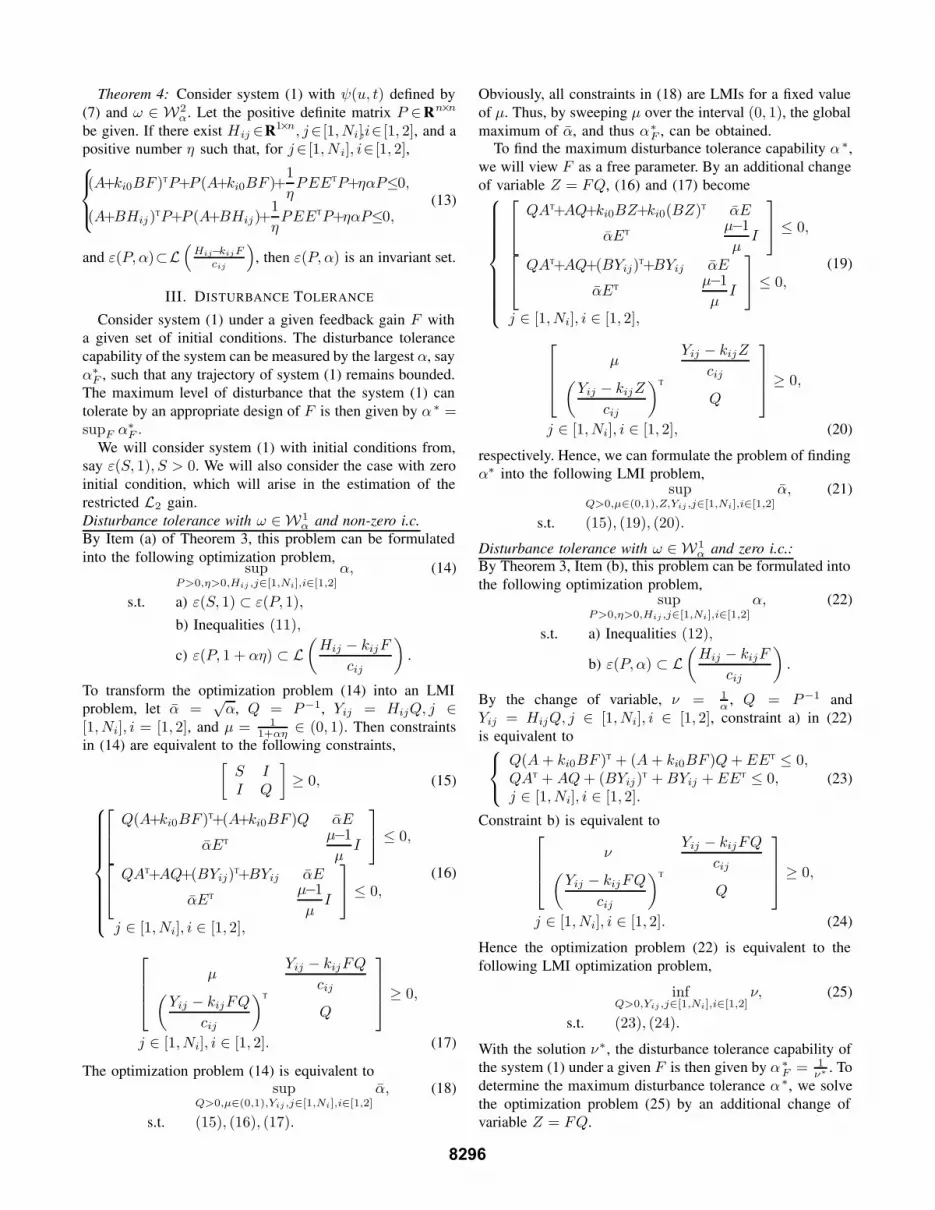
Let ψ(u, t) reside in a generalized sector [6] bounded byψ1(u) = u and ψ2(u) of the form (7) with N = 5and (k20, k21, k22, k23, k24, k25) = (0.7845, 0.3218, 0.1419,0.0622, 0.0243, 0), (c21, c22, c23, c24, c25) = (0.4636,0.8234, 1.0625, 1.2517, 1.4464), (see the solid straight lineand the solid piecewise linear curves in Fig. 3).

Let the set ε(S, 1) be defined by S = I . Then, thedisturbance tolerance capability can be assessed as follows.For ω ∈ W1

α with x(0) ∈ ε(S, 1):• By solving the optimization problem (18), we obtain

α∗F = 543.9380, with η∗

F = 0.36. In this simulation,

−10 −8 −6 −4 −2 0 2 4 6 8 10−2

−1.5

−1

−0.5

0

0.5

1

1.5

2

u

vv=u

v=tan−1(u)

v=ψ2(u)

o

Fig. 3. The generalized sector defined by ψ1(u) and ψ2(u) in the example.

as well as the simulation throughout the paper, we useψ(u, t) = tan−1(u), which resides in the generalizedsector defined by ψ1(u) and ψ2(u).

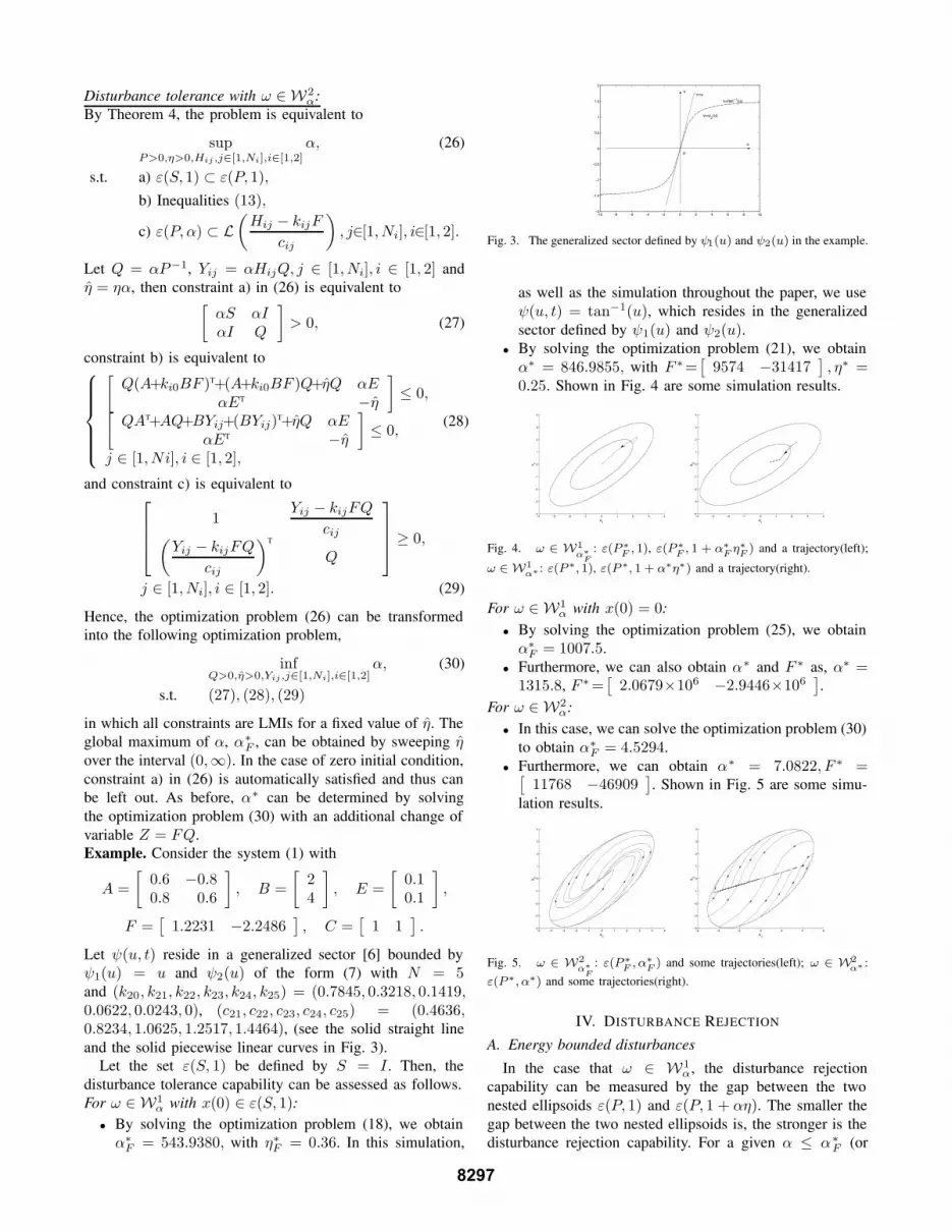
• By solving the optimization problem (21), we obtainα∗ = 846.9855, with F ∗=

[9574 −31417

], η∗ =

0.25. Shown in Fig. 4 are some simulation results.

−4 −3 −2 −1 0 1 2 3 4−4

−3

−2

−1

0

1

2

3

4

x1

x 2

−4 −3 −2 −1 0 1 2 3 4−4

−3

−2

−1

0

1

2

3

4

x1

x 2

Fig. 4. ω ∈ W1α∗

F: ε(P ∗

F , 1), ε(P ∗F , 1 + α∗

F η∗F ) and a trajectory(left);

ω ∈ W1α∗ : ε(P ∗, 1), ε(P ∗, 1 + α∗η∗) and a trajectory(right).

For ω ∈ W1α with x(0) = 0:

• By solving the optimization problem (25), we obtainα∗

F = 1007.5.• Furthermore, we can also obtain α∗ and F ∗ as, α∗ =

1315.8, F ∗=[

2.0679×106 −2.9446×106].

For ω ∈ W2α:

• In this case, we can solve the optimization problem (30)to obtain α∗

F = 4.5294.• Furthermore, we can obtain α∗ = 7.0822, F ∗ =[

11768 −46909]. Shown in Fig. 5 are some simu-

lation results.

−5 −4 −3 −2 −1 0 1 2 3 4 5−4

−3

−2

−1

0

1

2

3

4

x1

x 2

−6 −4 −2 0 2 4 6−4

−3

−2

−1

0

1

2

3

4

x1

x 2

Fig. 5. ω ∈ W2α∗

F: ε(P ∗

F , α∗F ) and some trajectories(left); ω ∈ W2

α∗ :

ε(P ∗, α∗) and some trajectories(right).

IV. DISTURBANCE REJECTION

A. Energy bounded disturbances

In the case that ω ∈ W1α, the disturbance rejection

capability can be measured by the gap between the twonested ellipsoids ε(P, 1) and ε(P, 1 + αη). The smaller thegap between the two nested ellipsoids is, the stronger is thedisturbance rejection capability. For a given α ≤ α∗

F (or

8297

α ≤ α∗), the gap between the two ellipsoids is measuredby the value of η. Another way to assess the disturbancerejection capability is to estimate the restricted L2 gain.The gap between ε(P, 1) and ε(P, 1 + αη):Under a given F , the level of disturbance rejection η ∗

F canbe determined by solving the optimization problem,

infP>0,Hij

η, (31)

s.t. a) ε(S, 1) ⊂ ε(P, 1),b) Inequalities (11),

c) ε(P, 1+αη)⊂L(

Hij − kijF

cij

), j ∈ [1, Ni], i ∈ [1, 2].

Let Q = P−1, η = 1η , and Yij = HijQ, j ∈ [1, Ni], i ∈

[1, 2], then constraint b) in (31) is equivalent to{Q(A + ki0BF )T + (A + ki0BF )Q + ηEET ≤ 0,QAT + AQ + BYij + (BYij)T + ηEET ≤ 0.

(32)

By using Schur complement, constraint c) is equivalent to⎡⎢⎢⎢⎢⎢⎢⎣

Q

(Yij−kijFQ

cij

)T (Yij−kijFQ

cij

)T

Yij−kijFQ

cij1 0

Yij−kijFQ

cij0

η

α

⎤⎥⎥⎥⎥⎥⎥⎦≥ 0,

j ∈ [1, Ni], i ∈ [1, 2]. (33)

Hence problem (31) is equivalent to the LMI problem,

supQ>0,Yij ,j∈[1,Ni],i∈[1,2]

η, (34)

s.t. (15), (32), (33).

The design of feedback gain F to achieve a higher level ofdisturbance rejection η∗ can be carried out by viewing F asan additional free parameter and using an additional changeof variable Z = FQ in the above optimization problem.The restricted L2 gain:

Theorem 5: Consider system (1) with ψ(u, t) defined by(7) and with ω ∈ W1

α. Let F and α ≤ α∗F be given. For

a given γ > 0, if there exist a positive definite matrix P ∈Rn×n and matrices Hij ∈ R1×n, j ∈ [1, Ni], i ∈ [1, 2], suchthat, for j ∈ [1, Ni], i ∈ [1, 2],⎧⎪⎨⎪⎩(A+ki0BF)TP+P (A+ki0BF )+PEETP+

1γ2

CTC≤0,

(A+BHij)TP+P (A+BHij)+PEETP+1γ2

CTC≤0,(35)

and ε(P, α) ⊂ L(

Hij−kijFij

cij

), then, the restricted L2 gain

from ω to z, with x(0) = 0, is less than or equal to γ.By Theorem 5, the problem of determining the restricted

L2 gain, γ∗F , can be formulated into and solved as the

following optimization problem,

infP>0,Hij ,j∈[1,Ni],i∈[1,2]

γ2, (36)

a) Inequalities (35),

b) ε(P, α) ⊂ L(

Hij − kijF

cij

), j ∈ [1, Ni], i ∈ [1, 2].

By the change of variable, Q = P −1 and Yij = HijQ, j ∈[1, Ni], i ∈ [1, 2], and application of the Schur complement,constraint a) in (36) is equivalent to⎧⎪⎪⎪⎪⎪⎪⎪⎪⎨⎪⎪⎪⎪⎪⎪⎪⎪⎩

⎡⎣ Q(A+ki0BF )T+(A+ki0BF )Q E QCT

ET −I 0CQ 0 −γ2I

⎤⎦≤0,

⎡⎣ QAT + AQ + BYij + (BYij)T E QCT

ET −I 0CQ 0 −γ2I

⎤⎦ ≤ 0,

j ∈ [1, Ni], i ∈ [1, 2].(37)

Constrain b) is equivalent to⎡⎢⎢⎣

1α

Yij − kijFQ

cij(Yij − kijFQ

cij

)T

Q

⎤⎥⎥⎦ ≥ 0,

j ∈ [1, Ni], i ∈ [1, 2]. (38)

Then, problem (36) is equivalent to the LMI problem,

infQ>0,Yij ,j∈[1,Ni],i∈[1,2]

γ2, (39)

s.t. (37), (38).

As before, the determination of F that minimizes γ ∗F can

be carried out by viewing F as a free parameter and by usingan additional change of variable Z = FQ. The resultingminimal γ∗

F will be denoted as γ∗.

B. Magnitude bounded disturbances

For system (1) with ω ∈ W2α, we will use the maximum

l∞ norm of the output with zero initial condition to indicatethe disturbance rejection capability.

Theorem 6: Consider system (1) with ψ(u, t) defined by(7) and with ω ∈ W2

α. Let the feedback gain F and α ≤ α∗F

be given. For a given positive constant ζ, the maximum l∞norm of the output of the system (1) is less than or equal to ζif there exist a positive definite matrix P ∈ Rn×n, matricesHij ∈ R1×n, j ∈ [1, Ni], i ∈ [1, 2], and a positive scalar η,such that, for j ∈ [1, Ni], i ∈ [1, 2],⎧⎪⎪⎪⎨⎪⎪⎪⎩

(A+ki0BF )TP+P (A+ki0BF )+1η PEETP+ηαP≤0,

(A+BHij)TP+P (A+BHij)+1ηPEETP+ηαP≤0,

CTC ≤ ζ2

αP ,

(40)

and ε(P, α) ⊂ L(

Hij−kijFcij

).

By Theorem 6, we have the optimization problem,

infP>0,η>0,Hij ,j∈[1,Ni],i∈[1,2]

ζ2, (41)

s.t. a) Inequalities (40),

b) ε(P, α) ⊂ L(

Hij − kijF

cij

).

By the change of variable, Q = P −1 and Yij = HijQ, j ∈[1, Ni], i ∈ [1, 2], the problem (41) is equivalent to

8298

infQ>0,η>0,Yij ,j∈[1,Ni],i∈[1,2]

ζ2, (42)

s.t. a) Q(A+ki0BF )T+(A+ki0BF )Q+1ηEET+ηαQ ≤ 0,

b) QA+ATQ+BYij+(BYij)T+1ηEET+ηαQ ≤ 0,

c) CQCT ≤ ζ2

αI,

d)

⎡⎢⎢⎣

1α

Yij−kijFQ

cij(Yij−kijFQ

cij

)T

Q

⎤⎥⎥⎦ ≥ 0,

j ∈ [1, Ni], i ∈ [1, 2],

where all constraints in (42) are LMIs. The global minimumof ζ can be obtained by sweeping η over the interval (0,∞).We note that a small ζ implies a small invariant set ε(P, α).Thus, the obtained ζ∗

F is a good approximation to the ζ ∗F for

zero initial condition.Once again, the above optimization problem can be easily

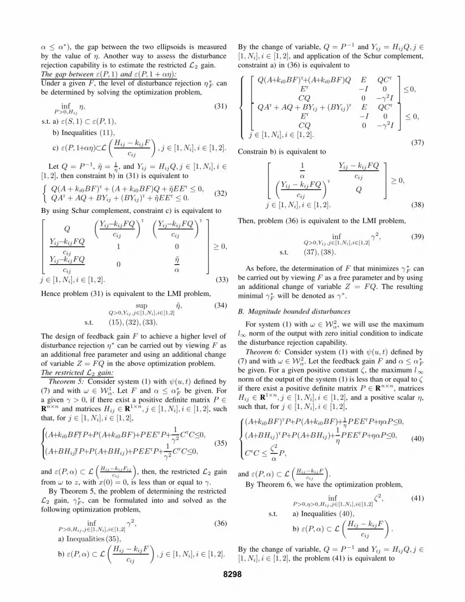
adapted for the design of F . We will denote ζ ∗ = infF ζ∗F .Example (continued).For ω ∈ W1

α:

• We recall from Section III that, for the given F , α∗F =

543.9380. Let α = 200. Solving optimization problem(34), we obtain that η∗

F = 0.0012. Similarly, the level ofdisturbance rejection can be optimized over the choiceof F , leading to η∗ = 9.0190 × 10−4, with F ∗ =[0.7243× 106 −1.2701× 106

]. Shown in Fig. 6 are

some simulation results.

−2.5 −2 −1.5 −1 −0.5 0 0.5 1 1.5 2 2.5−3

−2

−1

0

1

2

3

x1

x 2

−3 −2 −1 0 1 2 3−3

−2

−1

0

1

2

3

x1

x 2

Fig. 6. ω ∈ W1200 : ε(P ∗

F , 1), ε(P ∗F , 1 + 200η∗

F ) and a trajectory(left);ε(P ∗, 1), ε(P ∗, 1 + 200η∗) and a trajectory(right).

0 50 100 150 200 250 300

−0.25

−0.2

−0.15

−0.1

−0.05

0

0.05

0.1

0.15

0.2

0.25

t

z

Fig. 7. ω ∈ W2α: The output of the system (1).

• The restricted L2 gain within W1200 is γ∗

F = 0.1119.By minimizing γ∗

F over the choice of F , we ob-tain, γ∗ = infF γ∗

F = 0.0929, with F ∗ =[2.2018× 106 −1.6670× 106

].

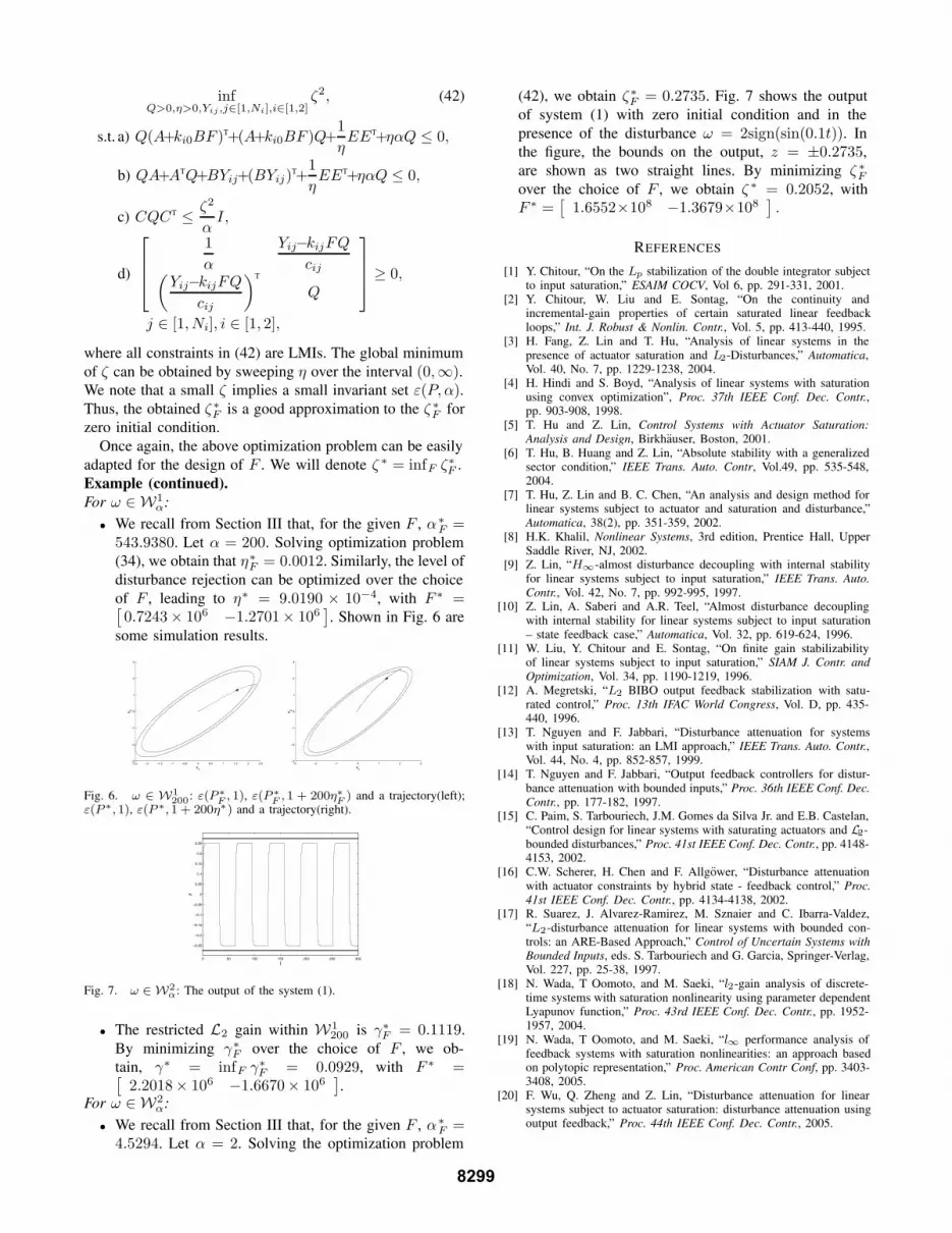
For ω ∈ W2α:

• We recall from Section III that, for the given F , α∗F =

4.5294. Let α = 2. Solving the optimization problem

(42), we obtain ζ∗F = 0.2735. Fig. 7 shows the output

of system (1) with zero initial condition and in thepresence of the disturbance ω = 2sign(sin(0.1t)). Inthe figure, the bounds on the output, z = ±0.2735,are shown as two straight lines. By minimizing ζ ∗

F

over the choice of F , we obtain ζ ∗ = 0.2052, withF ∗ =

[1.6552×108 −1.3679×108

].

REFERENCES

[1] Y. Chitour, “On the Lp stabilization of the double integrator subjectto input saturation,” ESAIM COCV, Vol 6, pp. 291-331, 2001.

[2] Y. Chitour, W. Liu and E. Sontag, “On the continuity andincremental-gain properties of certain saturated linear feedbackloops,” Int. J. Robust & Nonlin. Contr., Vol. 5, pp. 413-440, 1995.

[3] H. Fang, Z. Lin and T. Hu, “Analysis of linear systems in thepresence of actuator saturation and L2-Disturbances,” Automatica,Vol. 40, No. 7, pp. 1229-1238, 2004.

[4] H. Hindi and S. Boyd, “Analysis of linear systems with saturationusing convex optimization”, Proc. 37th IEEE Conf. Dec. Contr.,pp. 903-908, 1998.

[5] T. Hu and Z. Lin, Control Systems with Actuator Saturation:Analysis and Design, Birkhauser, Boston, 2001.

[6] T. Hu, B. Huang and Z. Lin, “Absolute stability with a generalizedsector condition,” IEEE Trans. Auto. Contr, Vol.49, pp. 535-548,2004.

[7] T. Hu, Z. Lin and B. C. Chen, “An analysis and design method forlinear systems subject to actuator and saturation and disturbance,”Automatica, 38(2), pp. 351-359, 2002.

[8] H.K. Khalil, Nonlinear Systems, 3rd edition, Prentice Hall, UpperSaddle River, NJ, 2002.

[9] Z. Lin, “H∞-almost disturbance decoupling with internal stabilityfor linear systems subject to input saturation,” IEEE Trans. Auto.Contr., Vol. 42, No. 7, pp. 992-995, 1997.

[10] Z. Lin, A. Saberi and A.R. Teel, “Almost disturbance decouplingwith internal stability for linear systems subject to input saturation– state feedback case,” Automatica, Vol. 32, pp. 619-624, 1996.

[11] W. Liu, Y. Chitour and E. Sontag, “On finite gain stabilizabilityof linear systems subject to input saturation,” SIAM J. Contr. andOptimization, Vol. 34, pp. 1190-1219, 1996.

[12] A. Megretski, “L2 BIBO output feedback stabilization with satu-rated control,” Proc. 13th IFAC World Congress, Vol. D, pp. 435-440, 1996.

[13] T. Nguyen and F. Jabbari, “Disturbance attenuation for systemswith input saturation: an LMI approach,” IEEE Trans. Auto. Contr.,Vol. 44, No. 4, pp. 852-857, 1999.

[14] T. Nguyen and F. Jabbari, “Output feedback controllers for distur-bance attenuation with bounded inputs,” Proc. 36th IEEE Conf. Dec.Contr., pp. 177-182, 1997.

[15] C. Paim, S. Tarbouriech, J.M. Gomes da Silva Jr. and E.B. Castelan,“Control design for linear systems with saturating actuators and L2-bounded disturbances,” Proc. 41st IEEE Conf. Dec. Contr., pp. 4148-4153, 2002.

[16] C.W. Scherer, H. Chen and F. Allgower, “Disturbance attenuationwith actuator constraints by hybrid state - feedback control,” Proc.41st IEEE Conf. Dec. Contr., pp. 4134-4138, 2002.

[17] R. Suarez, J. Alvarez-Ramirez, M. Sznaier and C. Ibarra-Valdez,“L2-disturbance attenuation for linear systems with bounded con-trols: an ARE-Based Approach,” Control of Uncertain Systems withBounded Inputs, eds. S. Tarbouriech and G. Garcia, Springer-Verlag,Vol. 227, pp. 25-38, 1997.

[18] N. Wada, T Oomoto, and M. Saeki, “l2-gain analysis of discrete-time systems with saturation nonlinearity using parameter dependentLyapunov function,” Proc. 43rd IEEE Conf. Dec. Contr., pp. 1952-1957, 2004.

[19] N. Wada, T Oomoto, and M. Saeki, “l∞ performance analysis offeedback systems with saturation nonlinearities: an approach basedon polytopic representation,” Proc. American Contr Conf, pp. 3403-3408, 2005.

[20] F. Wu, Q. Zheng and Z. Lin, “Disturbance attenuation for linearsystems subject to actuator saturation: disturbance attenuation usingoutput feedback,” Proc. 44th IEEE Conf. Dec. Contr., 2005.

8299