Climate change impact assessment: Uncertainty modeling

with imprecise probability

Subimal Ghosh1 and P. P. Mujumdar2

Received 21 December 2008; revised 11 June 2009; accepted 30 June 2009; published 23 September 2009.

[1] Hydrologic impacts of climate change are usually assessed by downscaling theGeneral Circulation Model (GCM) output of large-scale climate variables to local-scalehydrologic variables. Such an assessment is characterized by uncertainty resulting fromthe ensembles of projections generated with multiple GCMs, which is known asintermodel or GCM uncertainty. Ensemble averaging with the assignment of weights toGCMs based on model evaluation is one of the methods to address such uncertaintyand is used in the present study for regional-scale impact assessment. GCM outputs oflarge-scale climate variables are downscaled to subdivisional-scale monsoon rainfall.Weights are assigned to the GCMs on the basis of model performance and modelconvergence, which are evaluated with the Cumulative Distribution Functions (CDFs)generated from the downscaled GCM output (for both 20th Century [20C3M] and futurescenarios) and observed data. Ensemble averaging approach, with the assignment ofweights to GCMs, is characterized by the uncertainty caused by partial ignorance, whichstems from nonavailability of the outputs of some of the GCMs for a few scenarios(in Intergovernmental Panel on Climate Change [IPCC] data distribution center forAssessment Report 4 [AR4]). This uncertainty is modeled with imprecise probability,i.e., the probability being represented as an interval gray number. Furthermore, the CDFgenerated with one GCM is entirely different from that with another and therefore the useof multiple GCMs results in a band of CDFs. Representing this band of CDFs with asingle valued weighted mean CDF may be misleading. Such a band of CDFs can only berepresented with an envelope that contains all the CDFs generated with a number ofGCMs. Imprecise CDF represents such an envelope, which not only contains the CDFsgenerated with all the available GCMs but also to an extent accounts for the uncertaintyresulting from the missing GCM output. This concept of imprecise probability is alsovalidated in the present study. The imprecise CDFs of monsoon rainfall are derived forthree 30-year time slices, 2020s, 2050s and 2080s, with A1B, A2 and B1 scenarios.The model is demonstrated with the prediction of monsoon rainfall in Orissameteorological subdivision, which shows a possible decreasing trend in the future.

Citation: Ghosh, S., and P. P. Mujumdar (2009), Climate change impact assessment: Uncertainty modeling with imprecise

probability, J. Geophys. Res., 114, D18113, doi:10.1029/2008JD011648.

1. Introduction

[2] Climate change refers to any systematic change in thelong-term statistics of climate elements (such as tempera-ture, pressure, or winds) sustained over several decades orlonger time periods. Water resources are inextricably linkedwith climate, so the prospect of global climate change hasserious implications for water resources and regional devel-opment [Intergovernmental Panel on Climate Change(IPCC), 2001]. Increased evaporation (resulting from higher

temperatures), combined with regional changes in precipi-tation characteristics (e.g., total amount, variability, andfrequency of extremes), has the potential to affect meanrunoff, frequency and intensity of floods and droughts, soilmoisture, and water supplies for irrigation and hydroelectricgeneration. Assessing the impact of climate change onhydrology essentially involves projections of climatic var-iables (e.g., temperature, humidity, mean sea level pressureetc.) at a global scale, downscaling of global-scale climaticvariables to local-scale hydrologic variables and computa-tions of risk of hydrologic extremes in future for waterresources planning and management. Projections of climaticvariables globally can be performed with General Circula-tions Models (GCMs), which provide projections at largespatial scales. Such large-scale climate projections mustthen be downscaled to obtain smaller-scale hydrologicprojections with appropriate linkages between the climate

JOURNAL OF GEOPHYSICAL RESEARCH, VOL. 114, D18113, doi:10.1029/2008JD011648, 2009ClickHere

for

FullArticle

1Department of Civil Engineering, Indian Institute of TechnologyBombay, Mumbai, India.

2Department of Civil Engineering and Divecha Center for ClimateChange, Indian Institute of Science, Bangalore, India.

Copyright 2009 by the American Geophysical Union.0148-0227/09/2008JD011648$09.00

D18113 1 of 17

and hydrologic variables. Climate change impact assess-ment on hydrology, based on statistical downscaling fromGCM output is characterized by uncertainty caused byinadequate information and understanding about the under-lying geophysical process of global change, leading tolimitations in the accuracy of GCMs. This may lead to amismatch between the future projections of GCMs and canalso be termed as GCM uncertainty. It is widely acknowl-edged that disagreements between different GCMs overregional climate change represent significant sources ofuncertainty [Wilby and Harris, 2006]. Downscaled outputof a single GCM represents a single trajectory among anumber of possible realizations derived with various GCMs.Such a single trajectory alone cannot represent a futurehydrologic scenario. Therefore overreliance on a singleGCM could lead to inappropriate planning or adaptationresponses.[3] During the last decade, research on modeling uncer-

tainty in assessment of climate change impact has advancedon several fronts. New and Hulme [2000] presented anapproach to quantify uncertainties associated with climatechange within a probabilistic framework. A hierarchicalimpact model with Bayesian Monte Carlo simulation wasdeveloped for addressing uncertainty about future green-house gas emissions, the climate sensitivity, and limitationsand unpredictability in GCMs. Allen et al. [2000] assessedthe range of warming rates over the coming 50 years that areconsistent with the observed near-surface temperature re-cord as well as with the overall patterns of responsepredicted by several GCMs. Raisanen and Palmer [2001]developed a probabilistic approach to model the inherentuncertainties in the computational representation of climateand the unforced chaotic climate variability and expressedclimate change projections in probabilistic form. In thatstudy, 17 Coupled Model experiments sharing the samegradual increase in atmospheric CO2 were treated as aprobabilistic multimodel ensemble projection of futureclimate. Giorgi and Mearns [2002, 2003] developed aReliability Ensemble Averaging (REA) method for estimat-ing probability of regional climate change exceeding giventhresholds based on ensembles of different model simula-tions. The method takes into account two reliability criteria:the performance of the model in reproducing present-dayclimate (‘‘model performance criterion’’) and the conver-gence of the simulated changes across the models (‘‘modelconvergence criterion’’). The method was applied to a set oftransient experiments for the A2 and B2 IPCC emissionscenarios with 9 different Atmosphere-Ocean General Cir-culation Models (AOGCMs). Weights were assigned to theGCMs on the basis of model performance and modelconvergence which were evaluated on the basis of simulatedglobal mean climate scenarios obtained for 10 regions ofsubcontinental scale. Local-scale projections and temporalvariability of climate variables were not considered in thatstudy. Murphy et al. [2004] reported a systematic attempt todetermine the range of climate change projections consistentwith the uncertainties due intramodel variation, based on a53-member ensemble of model versions constructed byvarying model parameters. They estimated a probabilitydensity function for the sensitivity of climate to a doublingof atmospheric carbon dioxide levels. Tebaldi et al. [2004,2005] presented a Bayesian approach to determine proba-

bility density functions of temperature change, from theoutput of a multimodel ensemble, run under the samescenario of future anthropogenic emissions. A main featureof the method was the formalization of the two criteria ofbias and convergence that the REA method [Giorgi andMearns, 2003] first quantified as a way of assessing modelreliability. Thus the GCMs of the ensemble were combinedin a way that accounts for their performance with respect tocurrent climate and a measure of each model’s agreementwith the majority of the ensemble. For illustration purpose,Tebaldi et al. [2005] considered the output of mean surfacetemperature from nine GCMs, run under the A2 emissionscenario, for winter and summer, aggregated over 22 landregions and into two 30 year averages representative ofcurrent and future climate conditions. Like REA, the studiesby Tebaldi et al. [2004, 2005] also did not consider thetemporal variability of the climate variables and localhydrologic scenarios. More recently, Wilby and Harris[2006] developed a framework for assessing uncertaintiesin climate change impacts in projecting low flow scenariosof River Thames, UK. This model considers the predictionsof the local-scale hydrologic scenario with multiple GCMs.A probabilistic framework is developed for combininginformation from an ensemble of four GCMs, two greenhouse gas emission scenarios, two statistical downscalingtechniques, two hydrologic model structures and two setsof hydrologic model parameters. GCMs are weighted onthe basis of the bias calculated with Impact RelevantClimate Prediction Index (IRCPI). A limitation of the modelis that it does not consider model convergence, which is ameasure of each model’s agreement with the majority of theensemble.[4] Ghosh and Mujumdar [2007] used nonparametric

approach for modeling uncertainty in drought assessmentincorporating climate change. Standardized PrecipitationIndex-12 (SPI-12) has been used as a drought indicator inthat study and computed from GCM projections usingstatistical downscaling and equiprobability transformation.The probability density function of SPI in each year hasbeen computed with nonparametric methods, viz., kerneldensity estimation and orthonormal series method. Themodel assigns equal weights to all the GCMs, which maynot be valid. To assign weights to the GCMs and scenarios,a possibilistic approach for modeling uncertainty has beendeveloped by Mujumdar and Ghosh [2008], where possi-bilities of GCMs and scenarios are computed with theirperformances in the near past (after 1990) under climateforcing. The limitations of these models are as follows.[5] 1. Evaluation of GCMs based on model convergence

is not performed in either of the studies performed by Ghoshand Mujumdar [2007] and Mujumdar and Ghosh [2008].[6] 2. GCM and scenario uncertainty are treated on equal

ground, although the latter is not really an uncertainty in amathematical sense but a control influenced by socioeco-nomic behavior. Hence the analysis should be performedper forcing scenario, to demonstrate the different futurehydrologic conditions the region could expect under variousglobal mitigation policies.[7] 3. Not for all combinations of scenarios and GCMs

outputs are available or, in other words, the IPCC datadistribution center, which is the source of GCM data used inthe study, does not provide outputs for all GCMs with all

D18113 GHOSH AND MUJUMDAR: UNCERTAINTY MODELING

2 of 17

D18113

the scenarios. For example, the output of the GCM, CM 3.0developed by Institute for Numerical Mathematics, Russia,is not available for the A2 scenario. Such missing outputimposes another source of uncertainty, which contributes to‘‘partial ignorance’’ in climate change impact assessment.To date, such uncertainty has not been considered in anyresearch studies on hydroclimatology. Furthermore, theexisting GCMs are few in number. In fact they are a smallfinite set from an infinite space of possible models, whichintroduces a source of uncertainty which should be takencare.[8] Therefore from hydrologic point of view there is a

need to develop an uncertainty model, for climate changeimpact assessment on local-scale hydrology, which evalu-ates GCMs on the basis of Reliability Ensemble Averaging(REA), considers temporal variability of hydrologic vari-able and incorporates uncertainty caused by partial igno-rance. For modeling GCM uncertainty in climate changeimpact assessment, Giorgi and Mearns [2002, 2003] pro-posed Reliability Ensemble Averaging (REA) method. Themethod takes into account two reliability criteria: theperformance of the model in reproducing present-day cli-mate (‘‘model performance criterion’’) and the convergenceof the simulated changes across the models (‘‘model con-vergence criterion’’). The first criterion is based on theability of GCMs to reproduce present-day climate: the betterthe model performance, the higher the reliability of theGCM. The second criterion is based on the convergence ofsimulations by different models for a given forcing scenariofor future. As the observed climate time series is notavailable for future, a factor is used as reliability indicatorof a GCM, which measures the model reliability in terms ofthe deviation of simulations by that GCM from the REAaverage (weighted mean) simulations. High deviationdenotes low model reliability. The philosophy underlyingthe REA approach is to minimize the contribution ofsimulations that either perform poorly in the representationof present-day climate over a region or provide outliersimulations for future with respect to the other models inthe ensemble. In the present study, the deviation of thesimulated variable (Rainfall) with respect to the observed orREA average variable is computed with the deviation ofCDFs. Uncertainty caused by partial ignorance resultingfrom missing GCM output is also modeled. The presentstudy aims to achieve this using the concept of impreciseprobability, i.e., probability expressed as interval graynumber (closed and bounded interval with known lowerand upper bounds but unknown distribution information[Huang et al., 1995]). The flowchart of the model ispresented in Figure 1. GCM outputs of large-scale climatevariables (downloaded for AR4 [Intergovernmental Panelon Climate Change (IPCC), 2007], from IPCC data distri-bution center, http://www.ipcc-data.org) are first down-scaled to subdivisional monsoon rainfall using PrincipalComponent Analysis (PCA) and linear regression. Theunderlying uncertainty is modeled with reliability ensembleaveraging, where weights are assigned to GCMs on thebasis of model performance and model convergence, com-puted with the deviation of simulated CDF from that oftarget (for observed period) and weighted mean CDF (forfuture). Uncertainty caused by missing outputs of GCMs isthen modeled with imprecise probability, where an impre-

cise CDF is fitted to the future rainfall scenario. ImpreciseCDF is fitted with interval regression, which consists of twoparts: least square fitting and determination of optimuminterval. Least square fitting is achieved with the weightedmean CDF and the optimum interval is obtained consideringthe CDFs derived from all available GCMs. The method-ology is then validated and used to model GCM uncertaintyfor Orissa meteorological subdivision under A1B, A2 andB1 scenarios. The following section presents a brief over-view of the data used in the study and the statisticaldownscaling method.

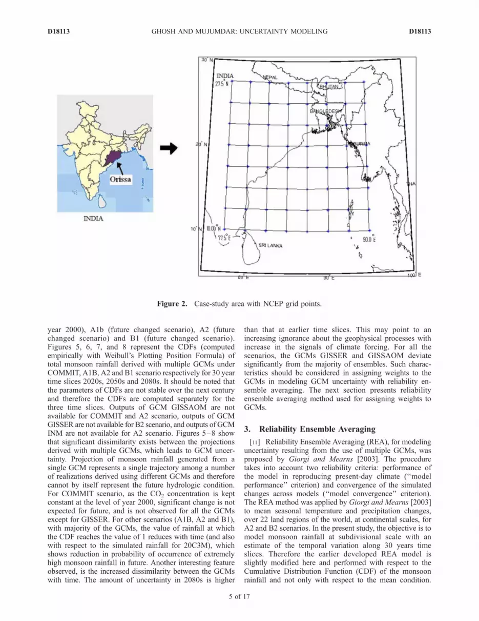
2. Data Extraction and Statistical Downscaling

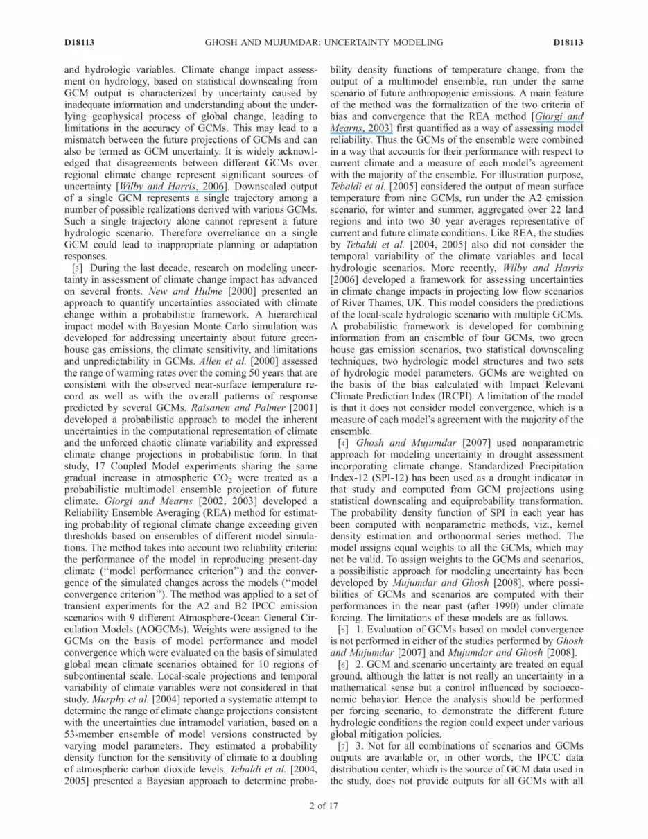
[9] The Orissa meteorological subdivision (Figure 2),located on the eastern coast of India, extends from 17�Nto 22�N in latitude, and 82�E to 87�E in longitude. Themonthly area weighted precipitation data of Orissa meteo-rological subdivision in India, from January 1950 to De-cember 1999, is obtained from Indian Institute of TropicalMeteorology, Pune (http://www.tropmet.res.in). This dataset is used in the downscaling as predictand. The predictorsused for downscaling [Wilby et al., 1999; Wetterhall et al.,2005] should be (1) reliably simulated by GCMs, (2) readilyavailable from archives of GCM outputs, and (3) stronglycorrelated with the surface variables of interest (rainfall inthe present case). Considering these criteria, the predictorsselected for the present study are Mean Sea Level Pressure(MSLP), surface specific humidity, near-surface air temper-ature, zonal wind speed and meridional wind speed. Mon-soon rainfall in Orissa is caused by high temperature in theland area and subsequent generation of low-pressure zone.This results in wind flow with moisture from Bay of Bengalto the land area. This is considered in selection of predictorsfor the downscaling model. Correlation coefficient of thesepredictor variables with monsoon rainfall is also observed tobe high. It has been reported in literature [Wilby et al., 1999;Wetterhall et al., 2005; Wilby and Harris, 2006] that thesevariables can be simulated well at a larger scale by a GCM.In the present study the predictors are selected on the basisof literature. However, a statistical skill test, based onJohnson and Sharma [2009], will add credibility in selec-tion of predictors for downscaling models. Statistical down-scaling (Figure 3) involves development of statisticalrelationship between large-scale climate variables and lo-cal-scale hydrologic variable and use of the statisticalrelationship with the GCM output for future projections.Training (calibration) of the statistical downscaling modelrequires observed climate data. In the absence of adequateobserved climatological data, the data from the NationalCenter for Environmental Prediction/National Center forAtmospheric Research (NCEP/NCAR) reanalysis project[Kalnay et al., 1996] may be used as a proxy to theobserved data. In the present study NCEP/NCAR reanalysisdata is used for calibration of the downscaling model.Monthly average climate variables from January 1950 toDecember 1999 were obtained for a region spanning10.00�N–27.50�N in latitude and 77.50�E–95.00�E inlongitude (constituting 64 grid points) that encapsules thestudy region. Figure 2 shows the NCEP grid points super-posed on the map of Orissa meteorological subdivision. Theoutput (MSLP, surface specific humidity, near-surface air

D18113 GHOSH AND MUJUMDAR: UNCERTAINTY MODELING

3 of 17

D18113

temperature, zonal wind speed, meridional wind speed) ofGCMs are downloaded from IPCC data distribution centerfor AR4 [IPCC, 2007]. The GCMs considered, on the basisof the availability of the output in IPCC Data, are given inTable 1.[10] Five climate variables at 64 grid points are used as

predictors, and hence the dimension of the predictors is 320.Furthermore, predictors at a grid point are expected to behighly correlated with those of neighboring grid points.Therefore direct use of the predictor variables, in statisticalregression, may lead to multicollinearity and may be com-putationally unstable. Principal Component Analysis (PCA)is performed to reduce the dimensionality of the predictorvariables. Principal components obtained from PCA areuncorrelated and therefore can be used directly in theregression. It is observed that first 35 principal componentsrepresent 98% variability of the original data set and henceare used in the study. Standardization [Wilby et al., 2004] isperformed prior to principal component analysis and down-scaling to remove systematic bias in mean and standarddeviation of the GCM simulated climate variables. Principal

components are used as regressors to predict the monthlymonsoon rainfall of Orissa meteorological subdivision inthe linear regression model (equation (1)).

Raint ¼ b0 þXKi¼1

bi � pcit ð1Þ

where, Raint is the monthly monsoon rainfall during montht, b0, . . ., bK are the coefficient of linear regression model, Kis the number of principal components considered, and pcitis the ith principal component at time t, obtained fromstandardized reanalysis data. Two-third of the data set isused in training and rest of the data set is used in testing ofthe model. The training and testing R values (correlationcoefficient between observed and predicted rainfall) areobtained as 0.8540 and 0.7911 respectively. The predictedand observed monsoon rainfalls are presented in Figure 4.The statistical relationship developed is then used on thestandardized output of the GCMs as mentioned in Table 1,with the scenarios 20C3M (20th century forcing), COM-MIT (maintaining CO2 concentration of future as that of

Figure 1. Overview of the proposed model.

D18113 GHOSH AND MUJUMDAR: UNCERTAINTY MODELING

4 of 17

D18113

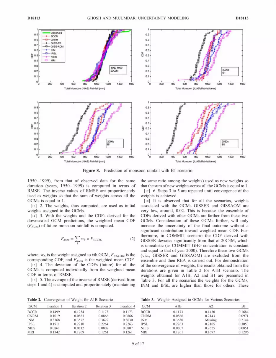
year 2000), A1b (future changed scenario), A2 (futurechanged scenario) and B1 (future changed scenario).Figures 5, 6, 7, and 8 represent the CDFs (computedempirically with Weibull’s Plotting Position Formula) oftotal monsoon rainfall derived with multiple GCMs underCOMMIT, A1B, A2 and B1 scenario respectively for 30 yeartime slices 2020s, 2050s and 2080s. It should be noted thatthe parameters of CDFs are not stable over the next centuryand therefore the CDFs are computed separately for thethree time slices. Outputs of GCM GISSAOM are notavailable for COMMIT and A2 scenario, outputs of GCMGISSER are not available for B2 scenario, and outputs of GCMINM are not available for A2 scenario. Figures 5–8 showthat significant dissimilarity exists between the projectionsderived with multiple GCMs, which leads to GCM uncer-tainty. Projection of monsoon rainfall generated from asingle GCM represents a single trajectory among a numberof realizations derived using different GCMs and thereforecannot by itself represent the future hydrologic condition.For COMMIT scenario, as the CO2 concentration is keptconstant at the level of year 2000, significant change is notexpected for future, and is not observed for all the GCMsexcept for GISSER. For other scenarios (A1B, A2 and B1),with majority of the GCMs, the value of rainfall at whichthe CDF reaches the value of 1 reduces with time (and alsowith respect to the simulated rainfall for 20C3M), whichshows reduction in probability of occurrence of extremelyhigh monsoon rainfall in future. Another interesting featureobserved, is the increased dissimilarity between the GCMswith time. The amount of uncertainty in 2080s is higher

than that at earlier time slices. This may point to anincreasing ignorance about the geophysical processes withincrease in the signals of climate forcing. For all thescenarios, the GCMs GISSER and GISSAOM deviatesignificantly from the majority of ensembles. Such charac-teristics should be considered in assigning weights to theGCMs in modeling GCM uncertainty with reliability en-semble averaging. The next section presents reliabilityensemble averaging method used for assigning weights toGCMs.

3. Reliability Ensemble Averaging

[11] Reliability Ensemble Averaging (REA), for modelinguncertainty resulting from the use of multiple GCMs, wasproposed by Giorgi and Mearns [2003]. The proceduretakes into account two reliability criteria: performance ofthe model in reproducing present-day climate (‘‘modelperformance’’ criterion) and convergence of the simulatedchanges across models (‘‘model convergence’’ criterion).The REA method was applied by Giorgi and Mearns [2003]to mean seasonal temperature and precipitation changes,over 22 land regions of the world, at continental scales, forA2 and B2 scenarios. In the present study, the objective is tomodel monsoon rainfall at subdivisional scale with anestimate of the temporal variation along 30 years timeslices. Therefore the earlier developed REA model isslightly modified here and performed with respect to theCumulative Distribution Function (CDF) of the monsoonrainfall and not only with respect to the mean condition.

Figure 2. Case-study area with NCEP grid points.

D18113 GHOSH AND MUJUMDAR: UNCERTAINTY MODELING

5 of 17

D18113

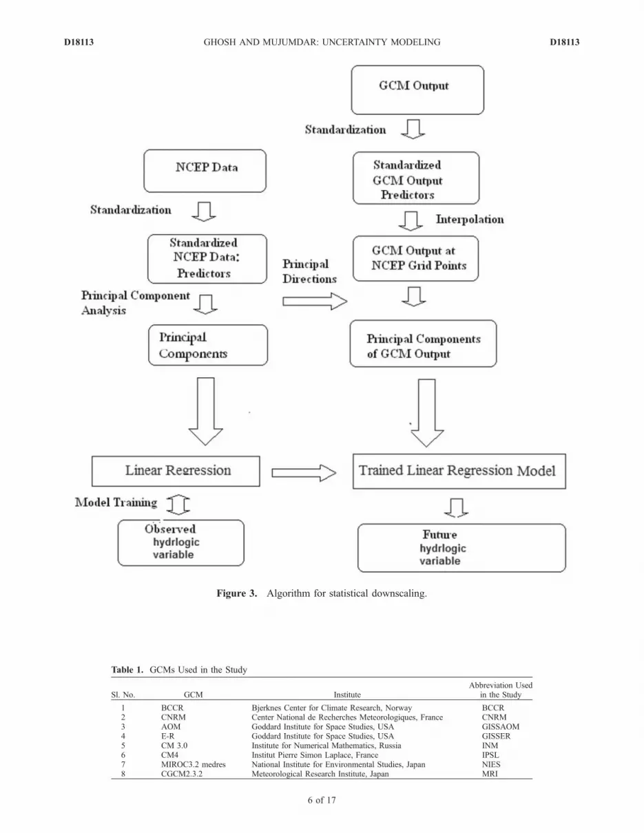
Figure 3. Algorithm for statistical downscaling.

Table 1. GCMs Used in the Study

Sl. No. GCM InstituteAbbreviation Used

in the Study

1 BCCR Bjerknes Center for Climate Research, Norway BCCR2 CNRM Center National de Recherches Meteorologiques, France CNRM3 AOM Goddard Institute for Space Studies, USA GISSAOM4 E-R Goddard Institute for Space Studies, USA GISSER5 CM 3.0 Institute for Numerical Mathematics, Russia INM6 CM4 Institut Pierre Simon Laplace, France IPSL7 MIROC3.2 medres National Institute for Environmental Studies, Japan NIES8 CGCM2.3.2 Meteorological Research Institute, Japan MRI

D18113 GHOSH AND MUJUMDAR: UNCERTAINTY MODELING

6 of 17

D18113

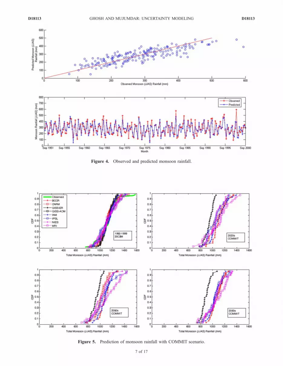
Figure 4. Observed and predicted monsoon rainfall.

Figure 5. Prediction of monsoon rainfall with COMMIT scenario.

D18113 GHOSH AND MUJUMDAR: UNCERTAINTY MODELING

7 of 17

D18113

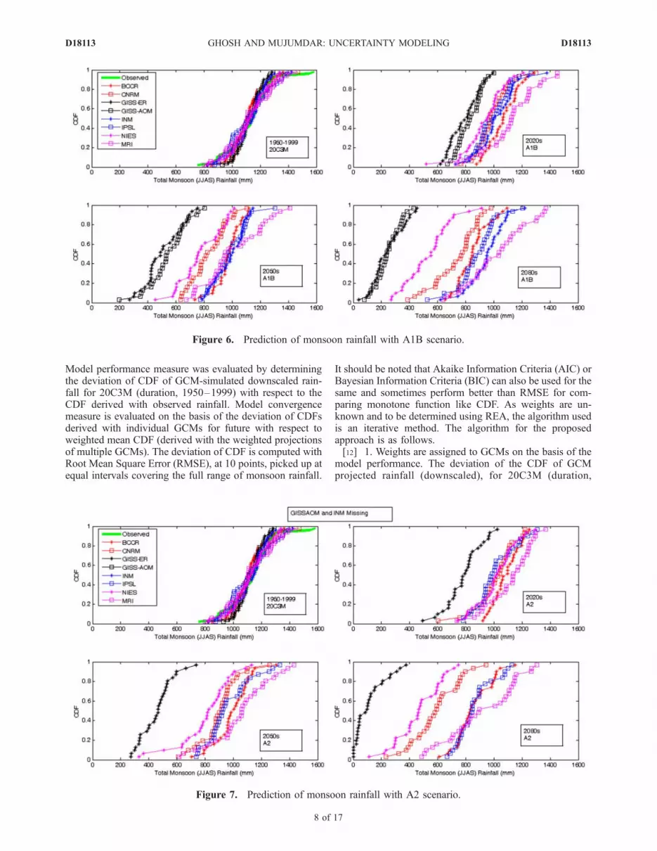
Model performance measure was evaluated by determiningthe deviation of CDF of GCM-simulated downscaled rain-fall for 20C3M (duration, 1950–1999) with respect to theCDF derived with observed rainfall. Model convergencemeasure is evaluated on the basis of the deviation of CDFsderived with individual GCMs for future with respect toweighted mean CDF (derived with the weighted projectionsof multiple GCMs). The deviation of CDF is computed withRoot Mean Square Error (RMSE), at 10 points, picked up atequal intervals covering the full range of monsoon rainfall.

It should be noted that Akaike Information Criteria (AIC) orBayesian Information Criteria (BIC) can also be used for thesame and sometimes perform better than RMSE for com-paring monotone function like CDF. As weights are un-known and to be determined using REA, the algorithm usedis an iterative method. The algorithm for the proposedapproach is as follows.[12] 1. Weights are assigned to GCMs on the basis of the

model performance. The deviation of the CDF of GCMprojected rainfall (downscaled), for 20C3M (duration,

Figure 7. Prediction of monsoon rainfall with A2 scenario.

Figure 6. Prediction of monsoon rainfall with A1B scenario.

D18113 GHOSH AND MUJUMDAR: UNCERTAINTY MODELING

8 of 17

D18113

1950–1999), from that of observed data for the sameduration (years, 1950–1999) is computed in terms ofRMSE. The inverse values of RMSE are proportionatelyused as weights so that the sum of weights across all theGCMs is equal to 1.[13] 2. The weights, thus computed, are used as initial

weights assigned to the GCMs.[14] 3. With the weights and the CDFs derived for the

downscaled GCM predictions, the weighted mean CDF(FXwm) of future monsoon rainfall is computed.

FXwm ¼Xk

wk � FXGCMkð2Þ

where, wK is the weight assigned to kth GCM, FXGCMk is thecorresponding CDF, and FXwm is the weighted mean CDF.[15] 4. The deviation of the CDFs (future) for all the

GCMs is computed individually from the weighted meanCDF in terms of RMSE.[16] 5. The average of the inverse of RMSE (derived from

steps 1 and 4) is computed and proportionately (maintaining

the same ratio among the weights) used as new weights sothat the sum of newweights across all the GCMs is equal to 1.[17] 6. Steps 3 to 5 are repeated until convergence of the

weights is achieved.[18] It is observed that for all the scenarios, weights

associated with the GCMs GISSER and GISSAOM arevery low, around, 0.02. This is because the ensemble ofCDFs derived with other GCMs are farther from these twoGCMs. Consideration of these GCMs further, will onlyincrease the uncertainty of the final outcome without asignificant contribution toward weighted mean CDF. Fur-thermore, in COMMIT scenario the CDF derived withGISSER deviates significantly from that of 20C3M, whichis unrealistic (as COMMIT GHG concentration is constantand equal to that of year 2000). Therefore these two GCMs(viz., GISSER and GISSAOM) are excluded from theensemble and then REA is carried out. For demonstrationof the convergence of weights, the results obtained from theiterations are given in Table 2 for A1B scenario. Theweights obtained for A1B, A2 and B1 are presented inTable 3. For all the scenarios the weights for the GCMs,INM and IPSL are higher than those for others. These

Figure 8. Prediction of monsoon rainfall with B1 scenario.

Table 2. Convergence of Weight for A1B Scenario

GCM Iteration 1 Iteration 2 Iteration 3 Iteration 4

BCCR 0.1499 0.1254 0.1173 0.1173CNRM 0.1019 0.0883 0.0866 0.0866INM 0.3368 0.3572 0.3629 0.3630IPSL 0.1911 0.2210 0.2264 0.2263NIES 0.0861 0.0812 0.0807 0.0807MRI 0.1342 0.1269 0.1261 0.1261

Table 3. Weights Assigned to GCMs for Various Scenarios

GCM A1B A2 B1

BCCR 0.1173 0.1430 0.1684CNRM 0.0866 0.2143 0.0971INM 0.3630 Missing 0.2144IPSL 0.2263 0.2105 0.3053NIES 0.0807 0.2625 0.0851MRI 0.1261 0.1697 0.1296

D18113 GHOSH AND MUJUMDAR: UNCERTAINTY MODELING

9 of 17

D18113

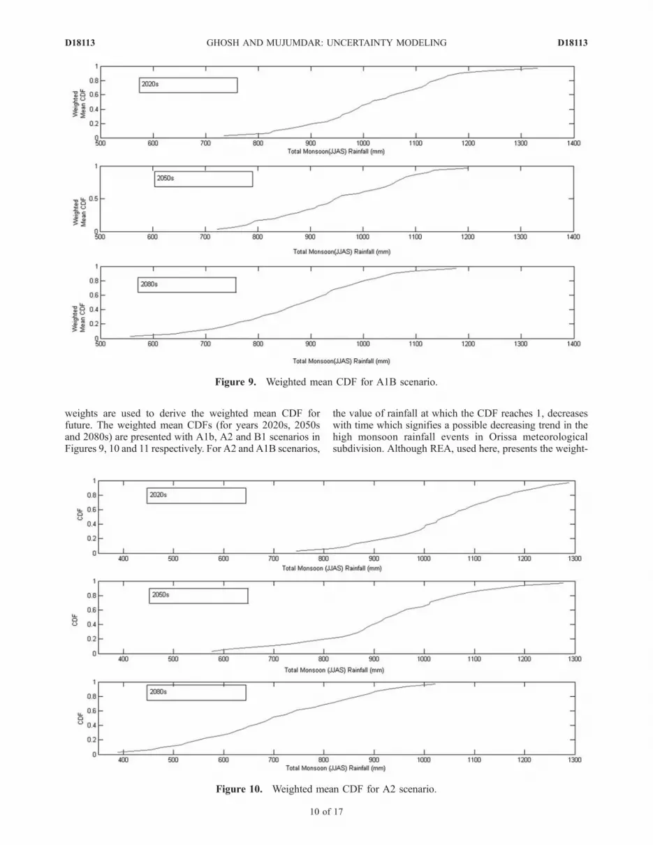
weights are used to derive the weighted mean CDF forfuture. The weighted mean CDFs (for years 2020s, 2050sand 2080s) are presented with A1b, A2 and B1 scenarios inFigures 9, 10 and 11 respectively. For A2 and A1B scenarios,

the value of rainfall at which the CDF reaches 1, decreaseswith time which signifies a possible decreasing trend in thehigh monsoon rainfall events in Orissa meteorologicalsubdivision. Although REA, used here, presents the weight-

Figure 9. Weighted mean CDF for A1B scenario.

Figure 10. Weighted mean CDF for A2 scenario.

D18113 GHOSH AND MUJUMDAR: UNCERTAINTY MODELING

10 of 17

D18113

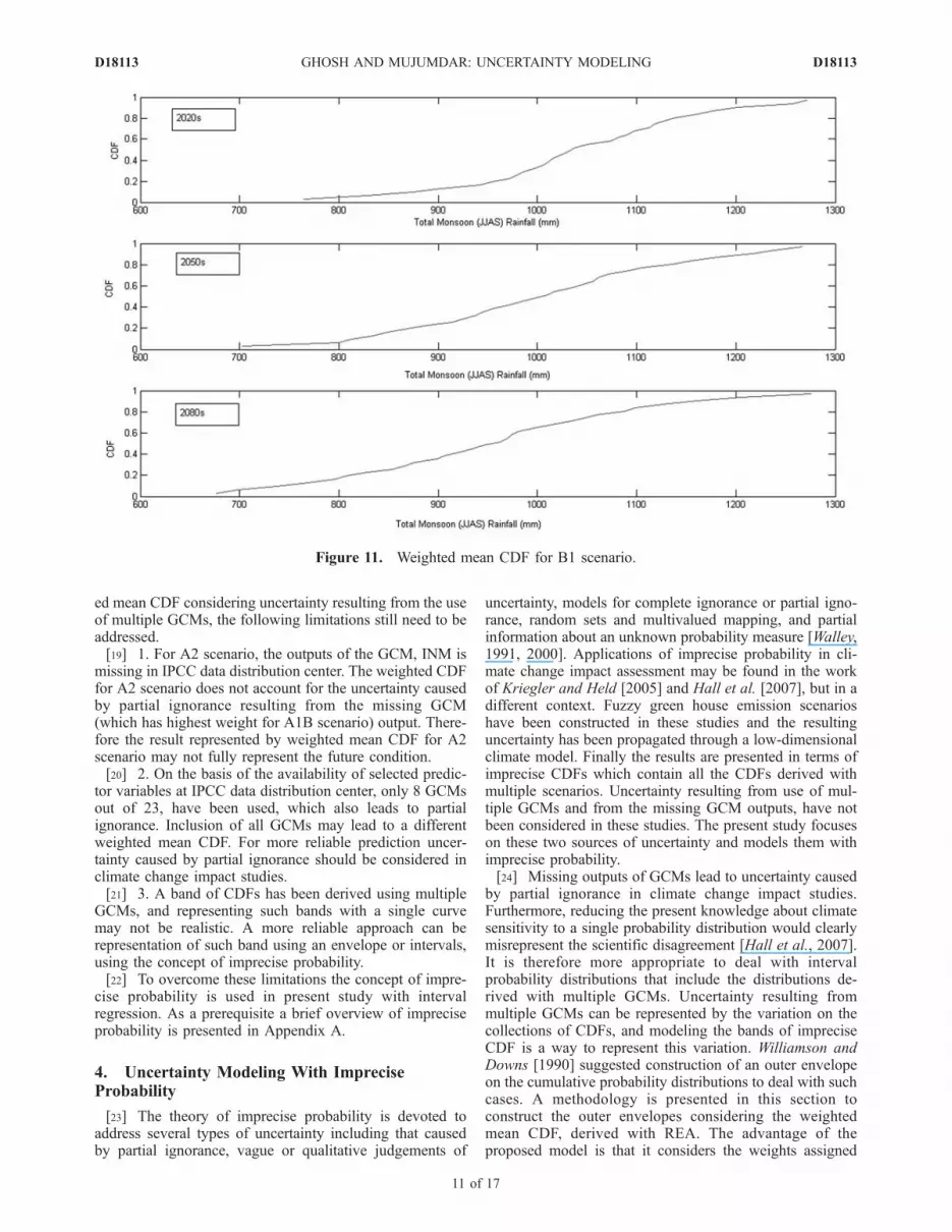
ed mean CDF considering uncertainty resulting from the useof multiple GCMs, the following limitations still need to beaddressed.[19] 1. For A2 scenario, the outputs of the GCM, INM is

missing in IPCC data distribution center. The weighted CDFfor A2 scenario does not account for the uncertainty causedby partial ignorance resulting from the missing GCM(which has highest weight for A1B scenario) output. There-fore the result represented by weighted mean CDF for A2scenario may not fully represent the future condition.[20] 2. On the basis of the availability of selected predic-

tor variables at IPCC data distribution center, only 8 GCMsout of 23, have been used, which also leads to partialignorance. Inclusion of all GCMs may lead to a differentweighted mean CDF. For more reliable prediction uncer-tainty caused by partial ignorance should be considered inclimate change impact studies.[21] 3. A band of CDFs has been derived using multiple

GCMs, and representing such bands with a single curvemay not be realistic. A more reliable approach can berepresentation of such band using an envelope or intervals,using the concept of imprecise probability.[22] To overcome these limitations the concept of impre-

cise probability is used in present study with intervalregression. As a prerequisite a brief overview of impreciseprobability is presented in Appendix A.

4. Uncertainty Modeling With ImpreciseProbability

[23] The theory of imprecise probability is devoted toaddress several types of uncertainty including that causedby partial ignorance, vague or qualitative judgements of

uncertainty, models for complete ignorance or partial igno-rance, random sets and multivalued mapping, and partialinformation about an unknown probability measure [Walley,1991, 2000]. Applications of imprecise probability in cli-mate change impact assessment may be found in the workof Kriegler and Held [2005] and Hall et al. [2007], but in adifferent context. Fuzzy green house emission scenarioshave been constructed in these studies and the resultinguncertainty has been propagated through a low-dimensionalclimate model. Finally the results are presented in terms ofimprecise CDFs which contain all the CDFs derived withmultiple scenarios. Uncertainty resulting from use of mul-tiple GCMs and from the missing GCM outputs, have notbeen considered in these studies. The present study focuseson these two sources of uncertainty and models them withimprecise probability.[24] Missing outputs of GCMs lead to uncertainty caused

by partial ignorance in climate change impact studies.Furthermore, reducing the present knowledge about climatesensitivity to a single probability distribution would clearlymisrepresent the scientific disagreement [Hall et al., 2007].It is therefore more appropriate to deal with intervalprobability distributions that include the distributions de-rived with multiple GCMs. Uncertainty resulting frommultiple GCMs can be represented by the variation on thecollections of CDFs, and modeling the bands of impreciseCDF is a way to represent this variation. Williamson andDowns [1990] suggested construction of an outer envelopeon the cumulative probability distributions to deal with suchcases. A methodology is presented in this section toconstruct the outer envelopes considering the weightedmean CDF, derived with REA. The advantage of theproposed model is that it considers the weights assigned

Figure 11. Weighted mean CDF for B1 scenario.

D18113 GHOSH AND MUJUMDAR: UNCERTAINTY MODELING

11 of 17

D18113

to the GCMs through weighted mean CDF and at the sametime the uncertainty caused by partial ignorance is alsomodeled. The methodology is based on interval regression,which, being highly nonlinear, is solved with nonlinearsearch algorithm, Probabilistic Global Search Laussane(PGSL) [Raphael and Smith, 2003]. The imprecise distri-bution of predicted monsoon rainfall is assumed to beGaussian with mean and standard deviation being intervalgray numbers (closed and bounded interval with knownlower and upper bounds but unknown distribution informa-tion [Huang et al., 1995]). Interval resulting from aninterval regression absorbs the uncertainty lying in theassumption of the type of the fitted curve, and thereforethe uncertainty resulting from the assumption of Gaussiandistribution will be taken care by the interval regression.[25] For computing a normal or Gaussian cumulative

distribution function, the usual procedure is to convert thedata into its standard normal deviate and then use it inderiving the CDF. When the distribution is imprecise, i.e.,mean (m) and standard deviation (s) are both interval graynumbers, denoted by m± and s±, then the original data(monsoon rainfall in the present case) (xi) can be convertedto imprecise standard normal deviate (zi

±) by

z�i ¼ xi � m�

s� ð3Þ

[26] If A± = 1s� and B± = �m�

s� , then equation (3) can bemodified to

z�i ¼ A�xi þ B� ð4Þ

[27] The involvement of lower and upper bounds of A±

and B± in deriving the bounds of zi± depends on the sign of

xi. Here xi denotes rainfall and therefore it is nonnegative(�0). For nonnegative xi, the upper bounds of both A± andB± will result in the upper bound of zi

±, and the lowerbounds of A± and B± will result in lower bound of z±, i.e.

zþi ¼ Aþxi þ Bþ xi � 0 ð5Þ

z�i ¼ A�xi þ B� xi � 0 ð6Þ

[28] The imprecise CDF (FX± (x)) can be computed from

standard normal deviate using

F�X xið Þ ¼ H z�i

� �¼ 1ffiffiffiffiffiffi

2pp

Z z�i

�1e�z2

2 dz ð7Þ

[29] Since the function FX± (xi) increases continuously

with zi±, zi

+ and zi� will be involved in computing FX

+ (xi)and FX

�(xi) respectively. The imprecise Gaussian CDF isfitted to the weighted mean CDF (FXwm) with intervalregression, to account for the uncertainty caused by partialignorance, so that all the CDFs derived with multiple GCMswill lie within the bounds.[30] Interval regression, where a model is assumed to

have interval coefficients, is regarded as the simplestversion of possibilistic regression analysis [Tanaka andLee, 1998]. Tanaka and Lee [1998] developed a model for

interval regression where the objective is to minimize thesquared spread of the estimated output. Hong and Hwang[2005] used support vector machine for interval regressionwhere the objective is to minimize the squared distancebetween the whitened mid value (average of upper andlower bounds of an interval gray number) of the estimatedoutput and the observed output along with the minimizationof the squared spread of the estimated output.[31] The imprecise CDF, FX

± (x), of monsoon rainfall, canbe determined by computing the parameters of the impre-cise normal distribution in terms of A± and B±. The intervalregression used for computing A± and B±, has three objec-tives: (1) to minimize of the squared distance between thewhitened mid value (average of upper and lower bounds ofan interval gray number) of the imprecise CDF to beestimated, and the weighted mean CDF (FXwm(xi)); (2) toaccommodate the CDFs derived with multiple GCMs withinthe bounds of imprecise CDF; and (3) to minimize thesquared spread of the imprecise CDF to be estimated.[32] The following optimization model of interval regres-

sion is developed for fitting the imprecise normal distribu-tion to the monsoon rainfall.

MinimizeXi

FXwm xið Þ � FþX xið Þ þ F�

X xið Þ2

� �2

þXi

Gd F�X xið Þ

� �

ð8Þ

subject to

z�i ¼ A�xi þ B� ð9Þ

F�X xið Þ ¼ H z�i

� �ð10Þ

F�X xið Þ � FXGCMk

xið Þ � FþX xið Þ 8k ð11Þ

A� > 0 ð12Þ

[33] Equation (8) is the objective function of the nonlin-ear optimization model, which comprises of two parts. Thefirst part minimizes the squared distance between thewhitened mid value (average of upper and lower boundsof an interval gray number) of the estimated CDF and theweighted mean CDF computed with REA. The second partminimizes the gray degree of the estimated CDF (Gd(FX

± (xi)))to restrict the spread. gray degree is a measure of uncer-tainty of the output [Huang et al., 1995; Karmakar andMujumdar, 2006], which, for an interval gray number (a±) isdefined by the ratio of its width (a+ � a�) to the whitenedmid value [1

2(a+ + a�)] and is expressed as

Gd a�� �

¼ aþ � a�

12aþ þ a�ð Þ

ð13Þ

[34] By minimizing the gray degree of the estimated CDF,the model minimizes the uncertainty in the regressionoutput. Equations (9) and (10) present the functional rela-tionship between FX

± (xi) and xi. Constraint (11) ensures thatthe CDFs (FXGCMk(xi)) obtained from multiple GCMs willlie in the p-box (details of p-box are in Appendix A) with

D18113 GHOSH AND MUJUMDAR: UNCERTAINTY MODELING

12 of 17

D18113

the bounds FX�(xi) and FX

+ (xi). The subscript i and k denotethe serial number of data and GCM respectively. A± is theinverse of s± which is a positive quantity (constraint (12)).The bounds of A± and B± are the decision variables of theoptimization model. The model is solved for three timeslices 2020s, 2050s and 2080s. As the model is nonlinear,Probabilistic Global Search Laussane (PGSL), a globalsearch algorithm for nonlinear optimization is used. Testson benchmark problems having multiparameter nonlinearobjective function have revealed that PGSL performs betterthan Genetic Algorithm and advanced algorithms for Sim-ulated Annealing [Raphael and Smith, 2003]. The algorithmis based on the assumption that better sets of points aremore likely to be found in the neighborhood of good sets ofpoints and therefore intensifying the search in the regionsthat contain good solutions. Details of the algorithm may befound in the work of Raphael and Smith [2003].[35] The optimization model (equations (8)– (12)) is

solved for three time slices 2020s, 2050s and 2080s, firstwith A1B scenario. The parameters of imprecise CDFs arecomputed from the decision variables of the optimizationmodel and are presented in Table 4. The resulting impreciseCDF is presented in Figure 12. The lower bound CDF doesnot show any significant change with time whereas thevalue, at which the upper bound CDF reaches 1, decreaseswith time. Consideration of imprecise probability helps thewater resources planners to consider both the possible cases,‘‘no change’’ in rainfall and decrease in rainfall correspond-ing to lower and upper envelope of the CDF respectively,whereas REA method does not allow to consider the ‘‘no

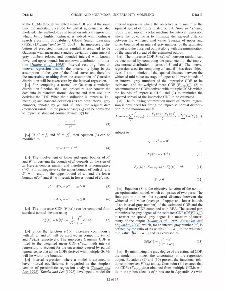
change’’ cases. Because of the ignorance about futurescenario, the ‘‘no change’’ case cannot be ignored and therelies the advantage of using imprecise probability. Constraint(opt4) ensures that the CDFs obtained from multiple GCMswill lie in the p-box, and that is reflected in Figure 12.However, it is not ensured that the missing outputs ofGCMs will also lie within the bounds and therefore it isrequired to validate the model. For validation, the GCM,INM (which is missing for A2 scenario) is not consideredfor A1B scenario, and the analysis is reperformed (REA andsubsequent solving of optimization model) for A1B scenar-io. The imprecise CDFs along with the CDFs for the GCMINM (for years 2020s, 2050s and 2080s) are presented inFigure 13. For 2020s, the CDF derived with INM is wellwithin the bounds of p-box. For 2050s and 2080s, there arefew points which are not within the bounds but almost at theborder of the p-box. The imprecise CDF derived withoutconsidering INM is quite similar to that considering all theGCMs (‘‘no change’’ for lower bound, and decrease inupper bound).[36] The optimization model is also solved for A2 and B1

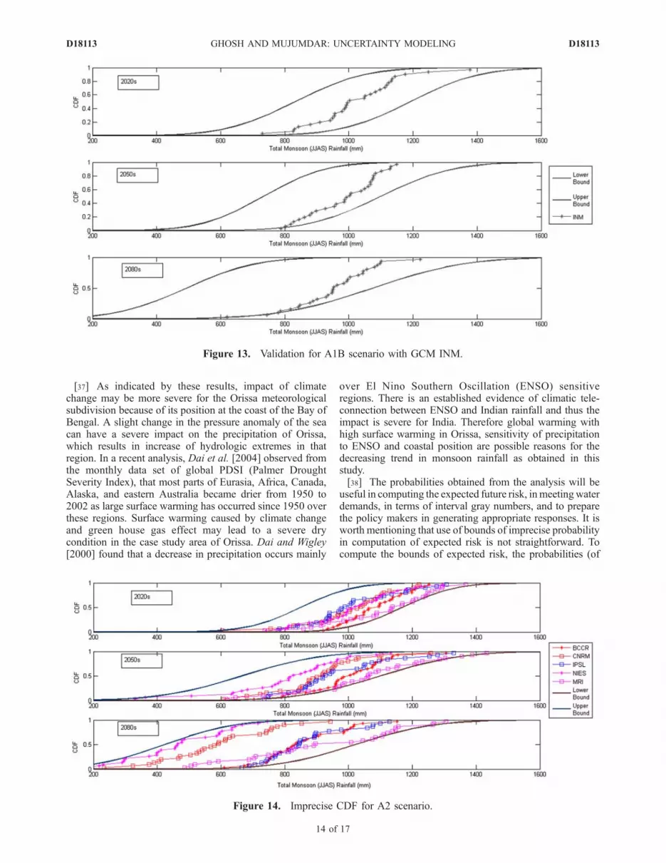
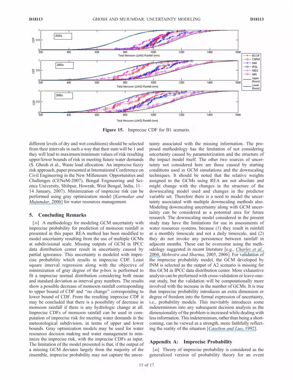
scenarios and the results are presented in Figures 14 and 15respectively. For A2 scenario, the result is quite similar tothat of A1B scenario with ‘‘no change’’ for lower boundCDF and decrease in rainfall corresponding to upper boundCDF. For B1 scenario, the change is not as significant asthat of A1B or A2 scenario. The result shows the possibilityof most significant reduction of monsoon rainfall for A2scenario. The B1 scenario presents the most favorablecondition (with minimum change) among all the scenarios.The results presented in Figures 12–15 indicate that therewill be a reduction in monsoon rainfall for future if at allthere is a change. Earlier study [Ghosh and Mujumdar,2007] on Orissa meteorological subdivision has also pro-jected an extremely dry condition for the case study area.The results obtained from the present study resemble that ofthe earlier study. Climate change impact study [Mujumdarand Ghosh, 2008] on Mahanadi River (at Orissa meteoro-logical subdivision) streamflow has also indicated similardry conditions.

Figure 12. Imprecise CDF for A1B scenario.

Table 4. Parameters of Imprecise CDF for A1B Scenarioa

Parameters 2020s 2050s 2080s

Mean UB 1190.81 1100.52 1082.96LB 832.34 734.26 444.80

Standard deviation UB 169.49 169.49 222.22LB 169.49 151.52 204.08

aUB, upper bound; LB, lower bound.

D18113 GHOSH AND MUJUMDAR: UNCERTAINTY MODELING

13 of 17

D18113

[37] As indicated by these results, impact of climatechange may be more severe for the Orissa meteorologicalsubdivision because of its position at the coast of the Bay ofBengal. A slight change in the pressure anomaly of the seacan have a severe impact on the precipitation of Orissa,which results in increase of hydrologic extremes in thatregion. In a recent analysis, Dai et al. [2004] observed fromthe monthly data set of global PDSI (Palmer DroughtSeverity Index), that most parts of Eurasia, Africa, Canada,Alaska, and eastern Australia became drier from 1950 to2002 as large surface warming has occurred since 1950 overthese regions. Surface warming caused by climate changeand green house gas effect may lead to a severe drycondition in the case study area of Orissa. Dai and Wigley[2000] found that a decrease in precipitation occurs mainly

over El Nino Southern Oscillation (ENSO) sensitiveregions. There is an established evidence of climatic tele-connection between ENSO and Indian rainfall and thus theimpact is severe for India. Therefore global warming withhigh surface warming in Orissa, sensitivity of precipitationto ENSO and coastal position are possible reasons for thedecreasing trend in monsoon rainfall as obtained in thisstudy.[38] The probabilities obtained from the analysis will be

useful in computing the expected future risk, inmeetingwaterdemands, in terms of interval gray numbers, and to preparethe policy makers in generating appropriate responses. It isworth mentioning that use of bounds of imprecise probabilityin computation of expected risk is not straightforward. Tocompute the bounds of expected risk, the probabilities (of

Figure 13. Validation for A1B scenario with GCM INM.

Figure 14. Imprecise CDF for A2 scenario.

D18113 GHOSH AND MUJUMDAR: UNCERTAINTY MODELING

14 of 17

D18113

different levels of dry and wet conditions) should be selectedfrom their intervals in such a way that their sum will be 1 andthey will lead to maximum/minimum values of risk resultingupper/lower bounds of risk in meeting future water demands(S. Ghosh et al., Waste load allocation: An imprecise fuzzyrisk approach, paper presented at International Conference onCivil Engineering in the New Milleneum: Opportunities andChallenges (CENeM-2007), Bengal Engineering and Sci-ence University, Shibpur, Howrah, West Bengal, India, 11–14 January, 2007). Minimization of imprecise risk can beperformed using gray optimization model [Karmakar andMujumdar, 2006] for water resources management.

5. Concluding Remarks

[39] A methodology for modeling GCM uncertainty withimprecise probability for prediction of monsoon rainfall ispresented in this paper. REA method has been modified tomodel uncertainty resulting from the use of multiple GCMsat subdivisional scale. Missing outputs of GCM in IPCCdata distribution center result in uncertainty caused bypartial ignorance. This uncertainty is modeled with impre-cise probability which results in imprecise CDF. Leastsquare interval regression along with the objective ofminimization of gray degree of the p-box is performed tofit a imprecise normal distribution considering both meanand standard deviation as interval gray numbers. The resultsshow a possible decrease of monsoon rainfall correspondingto upper bound of CDF and ‘‘no change’’ corresponding tolower bound of CDF. From the resulting imprecise CDF itmay be concluded that there is a possibility of decrease inmonsoon rainfall if there is any hydrologic change at all.Imprecise CDFs of monsoon rainfall can be used in com-putation of imprecise risk for meeting water demands in themeteorological subdivision, in terms of upper and lowerbounds. Gray optimization models may be used for waterresources decision making and water management to min-imize the imprecise risk, with the imprecise CDFs as input.The limitation of the model presented is that, if the output ofa missing GCM deviates largely from the majority of theensemble, imprecise probability may not capture the uncer-

tainty associated with the missing information. The pro-posed methodology has the limitation of not consideringuncertainty caused by parameterization and the structure ofthe impact model itself. The other two sources of uncer-tainty not considered here are those caused by startingconditions used in GCM simulations and the downscalingtechniques. It should be noted that the relative weightsassigned to the GCMs using REA are not absolute andmight change with the changes in the structure of thedownscaling model used and changes in the predictorvariable set. Therefore there is a need to model the uncer-tainty associated with multiple downscaling methods also.Modeling downscaling uncertainty along with GCM uncer-tainty can be considered as a potential area for futureresearch. The downscaling model considered in the presentstudy may have the limitations for use in assessments ofwater resources systems, because (1) they result in rainfallat a monthly timescale and not a daily timescale, and (2)they do not invoke any persistence between rainfall inadjacent months. These can be overcome using the meth-odology suggested in recent literature [e.g., Charles et al.,2004; Mehrotra and Sharma, 2005, 2006]. For validation ofthe imprecise probability model, the GCM developed byINM is selected as the output of A2 scenario is missing forthis GCM in IPCC data distribution center. More exhaustiveanalysis can be preformedwith cross-validation or leave-one-out study, but the validation will be computationally moreinvolved with the increase in the number of GCMs. It is truethat imprecise probability introduces an extra dimension ordegree of freedom into the formal expression of uncertainty,i.e., probability models. This inevitably introduces someindeterminism into any subsequent decision analysis as thedimensionality of the problem is increased while dealing withless information. This indeterminism, rather than being a short-coming, can be viewed as a strength, more faithfully reflect-ing the reality of the situation [Caselton and Luo, 1992].

Appendix A: Imprecise Probability

[40] Theory of imprecise probability is considered as thegeneralized version of probability theory for an event

Figure 15. Imprecise CDF for B1 scenario.

D18113 GHOSH AND MUJUMDAR: UNCERTAINTY MODELING

15 of 17

D18113

characterized by partial ignorance. It is also considered asthe generalized form of other two uncertainty theories:(1) theory of possibility and necessity measures [Duboisand Prade, 1988], in which the model is characterized byqualitative knowledge and intuitions in the absence ofprecise measurement, and (2) theory of belief and plausi-bility functions following Dempster-Shafer structure[Dempster, 1967; Shafer, 1976; Caselton and Luo, 1992],when evidence is available in terms of sets or intervals andnot as precise values. In the present work, uncertaintycaused by partial ignorance resulting from missing GCMoutputs is modeled with imprecise probability.[41] The essence of imprecise probability is the assign-

ment of ranges of probabilities to events. Therefore uncer-tainty about an event, E, would be expressed by an interval[P�(E), P+(E)], where, 0 � P�(E) � P+(E) � 1. The twobounds P�(E) and P+(E), called respectively, the lower andupper probabilities of E, are chosen so that, given theevidence, one can be reasonably sure that probability of Eis neither less than P�(E) nor greater than P+(E). Thefollowing illustration (following the work of Tonn [2005])is designed to show how imprecise probability can be moreexpressive in the highly uncertain hydrologic data modelingcharacterized with missing information. Let us assume thata hydrologic event has two states 1 and 2 and the data set ofthat event has 100 data points. The probability of hydrologicevent to be in state 1 and 2 are defined by P(1) and P(2),respectively. The following four cases are considered toexplain the concept of imprecise probability.[42] 1. If all the data points lie in state 1, then P(1) = 1

and P(2) = 0, and the probability model is considered to be a‘‘certain or deterministic model’’, which is quite uncommonin hydrology.[43] 2. If 50 data points are in state 1 and rest are in state 2,

then P(1) = 0.5 and P(2) = 0.5, and the probability model isconsidered to be a uncertain (because of randomness) modelwith ‘‘complete knowledge’’.[44] 3. If 40 data points are in state 1, 40 data points are in

state 2, and the rest are missing, then the two extremepossible cases are: (1) 60 data points are in state 1, and 40data points are in state 2, i.e., P(1) = 0.6 and P(2) = 0.4; and(2) 40 data points are in state 1, and 60 data points are instate 2, i.e., P(1) = 0.4 and P(2) = 0.6. From these twopossible cases it can be inferred that P(1) and P(2) can varybetween 0.4 and 0.6, which results in imprecise probabili-ties, probabilities denoted by interval gray numbers. In sucha case, the upper and lower bounds of P(1) will be 0.6 and0.4. Similarly, the bounds of P(2) will also be 0.6 and 0.4.Such a probability model can be categorized as an uncertainmodel with ‘‘partial ignorance’’.[45] 4. If all the data points are missing, then P(1) and

P(2) can vary between 0 and 1 and the upper and lowerbounds of both the probabilities will be 1 and 0. Such a modelis termed as uncertain model with ‘‘complete ignorance’’.[46] Imprecise probability thus addresses uncertainty

caused by partial ignorance with interval gray numbersand the interval between the bounds of the probabilityreflects the incomplete nature of knowledge or partialignorance. It may be noted that the application presentedin this appendix is entirely different from the proposedmethodology of modeling uncertainty because of missingGCM output. For the proposed model imprecise probability

is used to capture to the best possible extent, the missingrealizations of multiple ensemble generated with multipleGCMs.[47] The properties of imprecise probability are as follows.[48] 1. For universal sample set (W) and null set (F) both

the bounds of imprecise probability follow axioms ofprobability.

P� Fð Þ ¼ Pþ Fð Þ ¼ 0 ðA1Þ

P� Wð Þ ¼ Pþ Wð Þ ¼ 1 ðA2Þ

[49] 2. For any event E, both the bounds P�(E) and P+(E)are monotonically increasing, i.e.

E1 E2 ) P� E1ð Þ � P� E2ð Þ ðA3Þ

E1 E2 ) Pþ E1ð Þ � Pþ E2ð Þ ðA4Þ

[50] 3. Bounds of imprecise probability follow propertiesof complementarity, i.e.

P� Eð Þ þ Pþ E0ð Þ ¼ 1 8 E W ðA5Þ

where, E0 is the complement set of E.[51] 4. For two mutually exclusive sets E3 and E4,

imprecise probability follows.

E3 \ E4 ¼ F ) P� E3 [ E4ð Þ � P� E3ð Þ þ P� E4ð Þ ðA6Þ

E3 \ E4 ¼ F ) Pþ E3 [ E4ð Þ � Pþ E3ð Þ þ Pþ E4ð Þ ðA7Þ

where F denotes null set. If E3 and E4 are mutuallyexclusive and exhaustive sets, then, from equations (A6)and (A7)

E3 [ E4 ¼ W ) P� E3ð Þ þ P� E4ð Þ � 1 ðA8Þ

and

E3 [ E4 ¼ W ) Pþ E3ð Þ þ Pþ E4ð Þ � 1 ðA9Þ

Following, equation (A9), for any set E

Pþ Eð Þ þ Pþ E0ð Þ � 1 ðA10Þ

It should be noted that the difference between (P+(E) +P+(E 0)) and 1 reflects the uncertainty caused by incompleteknowledge. If U denotes the total uncertainty, then

Pþ Eð Þ þ Pþ E0ð Þ � 1 ¼ U ðA11Þ

Following equation (A5), equation (A11) can be rewrittenas

Pþ Eð Þ þ 1� P� Eð Þ � 1 ¼ U ) Pþ Eð Þ � P� Eð Þ ¼ U

ðA12Þ

D18113 GHOSH AND MUJUMDAR: UNCERTAINTY MODELING

16 of 17

D18113

Therefore the interval between P�(E) and P+(E) reflects thetotal uncertainty resulting from partial ignorance.[52] A natural model of an imprecise probability measure

is obtained by considering a pair (F�; F+) of CDFs, gener-alizing an interval (C. Baudrit and D. Dubois, Comparingmethods for joint objective and subjective uncertainty prop-agation with an example in a risk assessment, paper presentedat 4th International Symposium on Imprecise Probabilitiesand Their Applications, Pittsburgh, Pa, 20–23 July, 2005).The interval [F�, F+] is called a probability box or p-box.Following equation (A12), the interval between F� and F+

reflects the incomplete nature of knowledge, thus picturingthe extent of what is ignored.

[53] Acknowledgments. We sincerely thank the editor Steve Ghan,and the three anonymous reviewers for reviewing the manuscript andoffering their critical comments to improve the manuscript. Part of thework reported in this paper was funded by IRCC, Indian Institute ofTechnology Bombay, Mumbai, India (project 07IR040).

ReferencesAllen, M. R., P. A. Stott, J. F. B. Mitchell, R. Schnur, and T. L. Delworth(2000), Quantifying the uncertainty in forecasts of anthropogenic climatechange, Nature, 407, 617–620.

Caselton, W. F., and W. Luo (1992), Decision making with impreciseprobabilities: Dempster-Shafer theory and application, Water Resour.Res., 28(12), 3071–3083.

Charles, S. P., B. C. Bates, I. N. Smith, and J. P. Hughes (2004), Statisticaldownscaling of daily precipitation from observed and modelled atmo-spheric fields, Hydrol. Processes, 18(8), 1373–1394.

Dai, A. G., and T. M. L. Wigley (2000), Global patterns of ENSO inducedprecipitation, Geophys. Res. Lett., 27(9), 1283–1286.

Dai, A., K. E. Trenberth, and T. Qian (2004), A global data set of PalmerDrought Severity Index for 1870–2002: Relationship with soil moistureand effects of surface warming, J. Hydrometeorol., 5(6), 1117–1130.

Dempster, A. P. (1967), Upper and lower probabilities induced by a multi-valued mapping, Ann. Math. Stat., 37, 355–374.

Dubois, D., and H. Prade (1988), Possibility Theory, Plenum, New York.Ghosh, S., and P. P. Mujumdar (2007), Nonparametric methods for model-ing GCM and scenario uncertainty in drought assessment, Water Resour.Res., 43, W07405, doi:10.1029/2006WR005351.

Giorgi, F., and L. O. Mearns (2002), Calculation of average, uncertaintyrange, and reliability of regional climate changes from AOGCM simula-tions via the ‘‘Reliability Ensemble Averaging’’ (REA) method, J. Clim.,15(10), 1141–1158.

Giorgi, F., and L. O. Mearns (2003), Probability of regional climate changecalculated using the Reliability Ensemble Averaging (REA) method,Geophys. Res. Lett., 30(12), 1629, doi:10.1029/2003GL017130.

Hall, J., G. Fu, and J. Lawry (2007), Imprecise probabilities of climatechange: aggregation of fuzzy scenarios and model uncertainties, Clim.Change, 81, 265–281.

Hong, D. H., and C. Hwang (2005), Interval regression analysis usingquadratic loss support vector machine, IEEE Trans. Fuzzy Sys., 13(2),229–237.

Huang, G. H., B. W. Baetz, and G. G. Patry (1995), Grey integer program-ming: An application to waste management planning under uncertainty,Eur. J. Oper. Res., 83, 594–620.

Intergovernmental Panel on Climate Change (IPCC) (2001), ClimateChange 2001—The Scientific Basis. Contribution of Working Group Ito the Third Assessment Report of the Intergovernmental Panel on Cli-mate Change, edited by J. T. Houghton et al., Cambridge Univ. Press,Cambridge, U. K.

Intergovernmental Panel on Climate Change (IPCC) (2007), ClimateChange 2007—The Physical Science Basis, Contribution of WorkingGroup I to the Fourth Assessment Report of the Intergovernmental Panelon Climate Change, edited by S. Solomon et al., Cambridge Univ. Press,Cambridge, U. K.

Johnson, F., and A. Sharma (2009), Measurement of GCM skill in predict-ing variables relevant for hydroclimatological assessments, J. Clim.,doi:10.1175/2009JCLI2681.1.

Kalnay, E., et al. (1996), The NCEP/NCAR 40-year reanalysis project, Bull.Am. Meteorol. Soc., 77(3), 437–471.

Karmakar, S., and P. P. Mujumdar (2006), Grey fuzzy optimization modelfor water quality management of a river system, Adv. Water Resour.,29(7), 1088–1105.

Kriegler, E., and H. Held (2005), Utilizing belief functions for the estima-tion of future climate change, Int. J. Approx. Reason., 39(23), 185–209.

Mehrotra, R., and A. Sharma (2005), A nonparametric nonhomogeneoushidden Markov model for downscaling of multisite daily rainfall occur-rences, J. Geophys. Res., 110, D16108, doi:10.1029/2004JD005677.

Mehrotra, R., and A. Sharma (2006), A nonparametric stochastic down-scaling framework for daily rainfall at multiple locations, J. Geophys.Res., 111, D15101, doi:10.1029/2005JD006637.

Mujumdar, P. P., and S. Ghosh (2008), Modeling GCM and scenariouncertainty using a possibilistic approach: Application to the MahanadiRiver, India, Water Resour. Res. , 44 , W06407, doi:10.1029/2007WR006137.

Murphy, J. M., D. M. H. Sexton, D. N. Barnett, G. S. Jones, M. J. Webb,M. Collins, and D. A. Stainforth (2004), Quantification of modellinguncertainties in a large ensemble of climate change simulations, Nature,430, 768–772.

New, M., and M. Hulme (2000), Representing uncertainty in climatechange scenarios: A Monte Carlo approach, Integrated Assessment, 1,203–213.

Raisanen, J., and T. N. Palmer (2001), A probability and decision-modelanalysis of a multimodel ensemble of climate change simulations,J. Clim., 14, 3212–3226.

Raphael, B., and B. Smith (2003), A direct stochastic algorithm for globalsearch, Appl. Math. Comput., 146(3), 729–758.

Shafer, G. (1976), A Mathematical Theory of Evidence, Princeton Univ.Press, Princeton, N. J.

Tanaka, H., and H. Lee (1998), Interval regression analysis by quadraticprogramming approach, IEEE Trans. Fuzzy Sys., 6(4), 473–481.

Tebaldi, C., L. O. Mearns, D. Nychka, and R. L. Smith (2004), Regionalprobabilities of precipitation change: A Bayesian analysis of multimodelsimulations, Geophys. Res. Lett. , 31 , L24213, doi:10.1029/2004GL021276.

Tebaldi, C., R. Smith, D. Nychka, and L. O. Mearns (2005), Quantifyinguncertainty in projections of regional climate change: A Bayesianapproach to the analysis of multi-model ensembles, J. Clim., 18,1524–1540.

Tonn, B. (2005), Imprecise probabilities and scenarios, Futures, 37, 767–775.

Walley, P. (1991), Statistical Reasoning with Imprecise Probabilities, Chap-man and Hall, London, U. K.

Walley, P. (2000), Towards a unified theory of imprecise probability, Int.J. Approx. Reason., 24, 125–148.

Wetterhall, F., S. Halldin, and C. Xu (2005), Statistical precipitation down-scaling in central Sweden with the analogue method, J. Hydrol., 306,174–190.

Wilby, R. L., and I. Harris (2006), A framework for assessing uncertaintiesin climate change impacts: Low-flow scenarios for the River Thames,UK, Water Resour. Res., 42, W02419, doi:10.1029/2005WR004065.

Wilby, R. L., L. E. Hay, and G. H. Leavesly (1999), A comparison ofdownscaled and raw GCM output: implications for climate change sce-narios in the San Juan river basin, Colorado, J. Hydrol., 225, 67–91.

Wilby, R. L., S. P. Charles, E. Zorita, B. Timbal, P. Whetton, and L. O.Mearns (2004), The guidelines for use of climate scenarios developedfrom statistical downscaling methods, Supporting material of the Inter-governmental Panel on Climate Change (IPCC), prepared on behalf ofTask Group on Data and Scenario Support for Impacts and ClimateAnalysis (TGICA). (Available at http://ipccddc.cru.uea.ac.uk/guidelines/StatDownGuide.pdf)

Williamson, R. C., and T. Downs (1990), Probabilistic arithmetic: I. Nu-merical methods for calculating convolutions and dependency bounds,Int. J. Approx. Reason., 4(2), 89–158.

�����������������������S. Ghosh, Department of Civil Engineering, Indian Institute of

Technology Bombay, Powai, Mumbai 400 076, India. (subimal@civil.iitb.ac.in)P. P. Mujumdar, Department of Civil Engineering and Divecha Center for

Climate Change, Indian Institute of Science, Bangalore, Karnataka 560 012,India. (pradeep@civil.iisc.ernet.in)

D18113 GHOSH AND MUJUMDAR: UNCERTAINTY MODELING

17 of 17

D18113