shape reconstruction with uncertainty

Eurographics Italian Chapter Conference (2006)G. Gallo and S. Battiato and F. Stanco (Editors)

Shape Reconstruction with Uncertainty

L. Papaleo†, E. Puppo

Department of Informatics and Computer Science, University of Genova, Italy

AbstractThis paper presents a general Surface Reconstruction framework which encapsulates the uncertainty of the sam-pled data, making no assumption on the shape of the surface to be reconstructed. Starting from the input points(either points clouds or multiple range images), an Estimated Existence Function (EEF) is built which modelsthe space in which the desired surface could exist and, by the extraction of EEF critical points, the surface isreconstructed. The final goal is the development of a generic framework able to adapt the result to different kindsof additional information coming from multiple sensors.

Categories and Subject Descriptors (according to ACM CCS): I.3.3 [Computer Graphics]: Shape Modeling, Uncer-tain data, Multi-sensor Data Fusion

1. Introduction

3D scanning devices are becoming more and more availableand affordable. Thanks to modern acquisition technologies,heterogeneous data can be acquired from multiple acquisi-tion sensors, which often incorporate information about un-certainty of the data sampling process. Surface reconstruc-tion techniques designed over a specific sensor often takeinto account uncertainty during the reconstruction process,but they are limited to work with a single device. On thecontrary, general techniques that can process data comingfrom different sensors usually disregard much part of sensor-specific information, and seldom take into account uncer-tainty.

The basic concept of our approach is uncertainty: lack ofknowledge, which cannot be predicted and may be caused,e.g. from inadequate model etc. In case of multiple acquisi-tion technologies, there are different types of uncertainty:

• Incompleteness: sensors possibly leave something out.• Imprecision: sensors can provide only approximate infor-

mation.• Inconsistency: sensors data may not always agree with

each other.• Ambiguity: data from various sensors may be indistin-

guishable from one another.

† Corresponding author. [email protected]

The goal of our research is to define a flexible techniquethat can deal with data coming from different sensors, whileit fully exploits specific information about uncertainty asso-ciated to each specific sensor. To this aim, we adopt a prob-abilistic approach. We use information attached to data sam-ples to define and generate an Estimated Existence Function(EEF), which represents the probability that the desired sur-face exists in a volume of space. The reconstructed surfaceis then extracted by considering the ridges of our EEF andbuilding a triangle mesh out of them.

Each sample point in the input dataset brings informationabout the surface in its neighborhood. Information availablefor a single point may go from the bare coordinates, to esti-mation of differential properties like surface normal or cur-vature, to more or less elaborate estimation of uncertainty.On the basis of such information, different probability dis-tribution functions may be obtained, which shape the contri-bution of each sampled point to define the EEF in its neigh-borhood. Under the assumption that all samples are indepen-dent, the EEF is built by combining contributions comingfrom the different samples.

In this preliminary work, we analyze a simple scenario:each sample consists just of the coordinates of a point inspace, plus an estimation of uncertainty in the form of ascalar value. Under this assumption, we adopt a Gaussiandistribution to model our EEF. We present some results onboth synthetic and real datasets.

c© The Eurographics Association 2006.

L. Papaleo & E. Puppo / Shape Reconstruction with Uncertainty

2. Related Work

A burst of research has been made during the last decade on3D Reconstruction and several interesting and well-behavedalgorithms have been developed. General solutions shouldnot assume any knowledge of the object shape or topologybut possible approaches may strongly depend on the giventype of input (e.g. point clouds, multiple range images). It isnot simple to propose a significant taxonomy of the existingsurface reconstruction methods: most of them, especially inthe last few years, try to adopt hybrid solutions using differ-ent approaches in the same method. Regardless the under-lying structure of data, approaches can be divided into twogroups [MM98], depending on whether they produce an in-terpolation or an approximation of the input data.The interpolating approaches, in some sense, rely on the ac-curacy of the input and use them as constraints for the con-struction of the final mesh [ACTL02,Att97,AS00,BBCS96,TGLW01, HDD∗92, TC98]. The basic strategy is to use theinput points as the optimal geometric description of thescanned object. In general, a cloud of points with no otherinformation is considered [BBCS96, TGLW01]. In somecases, also point clouds with additional information on theobject structure or proximity of points maybe processed[ACTL02, Att97, AS00]. In addition, the modern scanningtechnologies often return also an estimation of the normal ineach point that can be used [TC98]. In case of approximationmethods, the vertices in the resulting mesh can be differentfrom the original sampled points. The basic strategy is to useinput points as a guide for surface reconstruction. Especiallyfor range data, an approximating rather than an interpolatingmesh is desirable in order to get a result of moderate com-plexity [CM95, CMSR00, CL96, HSIW96, JM02].

Few recent existing approaches try to consider the con-fidence of the sampled data. Schneider analyzed shape un-certainty from a more abstract point of view in [Sch01]. Heidentifies various sources for shape uncertainty and stressesthe importance of additional context information to reducethe uncertainty. Guibas et al. [PMG04] try to describe shapeinformation by combining local estimates using influencefunctions. Part of our work is most closely related to the onepresented by Johnson and Manduchi [JM02]. Both of themuse a probabilistic rule for constructing a probability func-tion. The scope of their work is quite different though, sincethey mainly concentrate on terrains by the use of radar inputdatasets.

3. Problem Definition and proposed approach

From a mathematical point of view, the surface of a 3D ob-ject can be defined as a two-dimensional manifold that iscompact, orientable and connected. Our Surface Reconstruc-tion problem can be formalized as follow:

Given a set of measurements V = {µ1, . . . ,µn} ofan object (environment), coming from different

sensors s1, . . . ,sk and a set of additional informa-tion M = {M1, . . . ,Mn} related to the given mea-surements in V , find a surface S ⊂<3 that approx-imates the observed object.

Each Mi may contain properties related to the measure-ment i (e.g., RGB color of the measurement, geometric prop-erties such as normal vector and local curvature) or measure-ment models (i.e, an error model, a reliability model, and soon).

Our idea is to define a Probability Density Function (PDFfor short) for each measurement µi integrating all the infor-mation present in the Mi. The PDF will indicate the degreeof importance of µi in the reconstruction process of the de-sired surface F . The PDFs related to measurements, supportthe construction of the Estimated Existence Function (EEFfor short) and for building it, we define:

• Ux a suitable neighborhood of a point x with x ∈ <3

• P(µ is x) as the probability that µ measures a point in Ux• P(x ∈ S) as P(S∩Ux 6= ∅)

The probability P that, given a measurement µ, a point x ison the desired surface S of the observed object is

P(x ∈ S|µ) = P(x ∈ S|µ is x) ·P(µ is x)

+ P(x ∈ S|µ is x) ·P(µ is x)

If all the measurements come exactly from the surface, thenthe probability that a given x measures the surface S at x isobviously 1 (maximum of information). If we have a genericpoint x and no measurements on it, we cannot infer anythingon x. In this case, we adopt a conventional probability of 1

2(minimum of information on x). Additionally, we have thatP(µ is x) = 1−P(µ is x) and from the equation above:

P(x ∈ S|µ) = 1 ·P(µ is x)+12· (1−P(µ is x)) (1)

P(x ∈ S|µ) =12· (1+Mµ(x)) (2)

where Mµ is the measurement model related to the measure-ment µ. Equation 2 shows that if the point x falls withinthe measurement model, then the surface probability will begreater than 1

2 but less than 1; otherwise the probability is12 . Also, given µ, the probability P that a point x lies on thesurface S is directly proportional to the value of the mea-surement model Mµ computed on x. Given the input datasetin the form of n independent measurements {µ1, . . . ,µn}, theEstimated Existence Function of a point x in space is theprobability that x lies on the desired surface S:

EEF(x) = Pn(x) = P(x ∈ S|µ1, . . . ,µn) (3)

Using similar reasoning as above, Pn(x) can be derived frommultiple independent measurement models:

EEF(x) = P(x ∈ S|µi is x, all i) ·P(µi is x, all i)

+ P(x ∈ S|µi is x, all i) ·P(µi is x, all i)



using the above formulas we obtain:

EEF(x) = 1−12

P(µi is x, all i) (4)

= 1−12

Πni=1(1−P(µi is x)) (5)

So we have:

P(µi is x) =Z

Ux

Mµ(y),dy (6)

In cases of small Ux for each x, we can approximate the in-tegral as follows:

P(µi is x) =Z

Ux

Mµ(y),dy ∼= Mµ(x)|Ux| ≡ E i(x) (7)

Where |Ux| is the volume of Ux. From equation 5, substitut-ing symbols using equation 7 we can define:

EEF(x) = Pn(x) = 1−12

Πni=1(1−P(µi is x)) (8)

= 1−12

Πni=1(1−E i(x)) (9)

Equation 9 indicates our Estimated Existence Function foreach point in space and how it depends on all the modelsMi ∈ M related to all the measurements µ ∈V .Once we have defined the EEF , we search for the charac-teristic points of the EEF , following the definition of Eberlyet al. of surface ridges on a volume [EGM∗94]. Basically, apoint x is a ridge point of type 3−1 (surface-on-a-volume)if νT

1 (x) ·∇ f (x) = 0 and ki(x) > 0, where νi are the eigen-vector of the negative Hessian matrix of f , ki are the eigen-values, for i = 1,2,3 and ∇ f (x) is the gradient. The pointx is a strong ridge point if also the property k1(x) > |k3(x)|holds. This definition says that a point x ∈<3 is a ridge pointif the component of the gradient in the maximal changing di-rection is zero and the function is more concave than convex.The set of points R that are ridge points of type 3−1 identi-fies the surface S we are searching for.If necessary, we can filter the set R choosing a new setR1 ⊆ R such that the points in R1 are ridge points of type3− 1 where the EEF function value is more than a suitablethreshold θ.

R1{x ∈ <3|x is ridge point and EEF(x) > θ} (10)

3.1. Building the Estimated Existence Function

The definition of the Estimated Existence function is givenin equation 9, under the hypothesis of n independent mea-surements µ, . . . ,µn. The independence of the measurementshelps us in the definition of an incremental rule for the com-putation of the EEF which will speed-up the overall exe-cution of the algorithm. The EEF function can be definedas

EEF(x) = 1−12

Πni=1(1−E i(x)) = 1−

12

f (x)n (11)

where f (x)n = Πni=1(1−E i(x)). So the Estimated Existence

Function EEF(x) depends on a function f n(x) that can be

computed incrementally. In fact:

f n(x) = (1−E i(x)) ·Π(n−1)i=1 (1−E i(x)) (12)

= (1−E i(x)) · f n−1(x) (13)

The function f n(x) depends on f n−1(x), on the E i(x) and,as consequence, on the models Mi(x) given as input for eachmeasurement in V . In this paper, we present as model onlyan error measurement model related to each sampled valuein the form of a Multivariate Normal Distribution (GaussianDistribution).

G(x) = 2πn2 · |Σ|−

12 · e−

12 (x−µ)T Σ−1

x (x−µ) (14)

where Σ is the covariance matrix and µ is the mean vector.At this step of development, we consider only input datasetswhich come with a reliability value related to each measure-ment (in this case we use an isotropic Gaussian) or datasetswith the covariance matrix which will be used in the Gaus-sian Function.The EEF(x) is defined in <3 but for computability prob-lem, we cannot work in the continuum. For this reason,we discretize the space using of a regular grid G with agrid step s interactively defined by the user. Moreover, forefficiency purposes, we can bound the influence space ofeach measurement to a certain domain without computingits contribution to the EEF over all points in <3. Fromprobabilistic and statistical theory [Spa99, SS95], we knowthat, for a Gaussian Distribution in the form of equation 14,at least 99,7% of the non-zero values fall in the interval[µ−3σ,µ+3σ]. So we decided to compute the contributionof a measurement x to the EEF only in such a bounded por-tion of space. For each measurement x the inference spacesx will depend on the 3σx,3σy and 3σz values and can beapproximated as an ellipsoid with principal axes dependingon x,y,z.Out of this inference space, the EEF value of a grid pointwill not depend on the measurement x. At this point of theprocess, we have a regular grid in which all points have therelated EEF value: 1

2 value if the grid point is not fallen inany inference space and EEF(x) if it is fallen on one or moreinference spaces.

4. Compute the Ridge Points

The extraction of the characteristics points of the EEF is afundamental step for the reconstruction of the desired sur-face S. We have implemented two different methods: onemore rigorous (and more elaborated) that follows the formaldefinition of characteristic surface on an approximated vol-ume (condition by equation 10) and the other (the simplestone) that defines if a point is ridge considering the neigh-bours and therefore dicretizing the procedure.

4.1. Ridge surface on a volume

In order to compute the ridge points using the condition inequation 10 we need the first and second order partial deriva-



p

40

30

20

30

41

22

34

p

40

30

20

44

41

22

34

(a) (b)

x

y

z

x

y

z

Figure 1: (a) Point p is a ridge point. It is maximum in thez direction and not minimum in the other two. (b) Point p isnot a ridge. It is maximum in the z direction but minimum inthe x direction.

tives of the EEF . While we compute the EEF value foreach grid point, the derivatives can be computed followingan incremental rule analogous to the one in equation 13. Thepartial derivatives of the EEF function will depend on thepartial derivatives of f n(x). For each measurement x the sys-tem is reading, we are able to incrementally compute theEEF value and the relative first and second order partialderivatives on each influenced grid point. This effectivelyspeeds up the entire process. Once all the partial derivativeshave been computed, we use the condition in equation 10 formarking those grid points that are ridge points of type 3-1.The property of being a ridge of a grid point is an approxima-tion: discretizing the space, we marked a grid point as ridgeindicating that it is near a real ridge of the EEF function. Forthis reason, we added two tolerance values modifiable by theuser: on the one hand, we select a subset of ridge points, fil-tering on the intensity value (EEF value), while on the otherhand, we filter the ridge points by varying the approxima-tion error ε (basically we test if ν1(x)

T∇ f (x) < ε instead ofν1(x)

T∇ f (x) = 0).

4.2. Heuristic Method

As we said before, the heuristic method uses a less rigor-ous but not less effective definition of characteristic points.Considering that the EEF function is defined on a discretedomain, it is possible to study the problem from a practicalpoint of view, as it was done in [JR75, Mar83, MB95, TF78]for the case of terrains. We have extended these techniquesto 3D grids by considering the 6-adjacent neighbors of a gridpoint gi,k, j , i.e. the vertices in the link of gi, j,k connected togi, j,k through an edge [Pap04]. A grid point gi, j,k is a ridge ifit is a local maximum in one direction (x, y, z direction) andnot a minimum in the other two.The formalization of what we have just explained follows:given a grid G and a point gi, j,k ∈ G, it is a characteristicpoint if:

IsMa jor(x,1,0,0) AND (!IsMinor(x,0,1,0))

AND (!IsMinor(x,0,0,1))OR


AND (!IsMinor(x,0,0,1))OR


AND (!IsMinor(x,0,1,0))

Where [1,0,0] is the x direction (Y Z plane), [0,1,0] is they direction (XZ plane), [0,0,1] is the z direction (XY plane)and IsMa jor(· · ·), IsMinor(· · ·) are predicates which returnT RUE if the point is maximum (minimum) in that direc-tion and FALSE otherwise. Figure 1 (a) shows an exampleof ridge condition for a point p, while Figure 1 (b) shows apoint p in the grid which is not a ridge point.

5. Building the mesh

Once all the ridge points have been computed, so that wehave identified in the grid G the points in which the proba-bility to be part of the desired surface is more high, we needto build a final triangular mesh, which approximates the de-sired surface S. Our first idea was to march the cells of thegrid, triangulating each triplet of ridge points. Unfortunately,this simple approach leads to not satisfactory results: mostof the marked ridges are on the desired surface but some ofthem are outliers. In order to filter the set of ridges and toimprove the result, we decided to implement a method thattransfers the information of being a ridge from a vertex toan edge (or more edges) thus achieving sub-voxel precision.This is done with the application of a P-Method (Parabola-Method) which does the following. For each grid point gi, j,kin the grid G and for each principal direction, x,y and z:

1. Take the parabola passing for the EEF values of the gridpoints gi−1, j,k,gi, j,k,gi+1, j,k (for simplicity, the x direc-tion)

2. Take the maximum max with coordinates(xmax,ymax,zmax) of the parabola (if it exists)

3. Consider the projection of this point.

• if it falls in the interval [gi−1, j,k,gi, j,k] mark an inter-section in this edge;

• if it falls in the interval [gi, j,k,gi+1, j,k] mark an inter-section in this edge.

The P-method is a general smoothing approach which worksquite well for large datasets even if some outliers still re-main. In any case, at the end of the procedure, we have theintersections in the edges of our grid and we can launch amodified Marching Cubes procedure that starts directly fromthe intersections instead of the conditions on the vertices ofa cell. This procedure definitely improves the quality of theresults as it is shown in Figure 2.

6. Implementation and Results

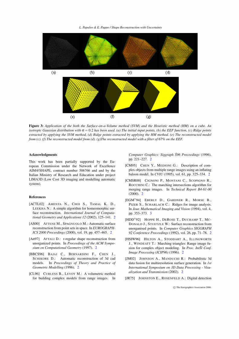
We have tested our method on different datasets [Pap04].The results of our method on a cube with four supersam-pled faces and two subsampled faces is shown in Figure 3.From an input dataset of 4240 points (Figure 3(a)), we built



Figure 2: A teapot: the input dataset (a) shows noisy data especially near the handles. (b) The reconstructed model by extractingthe ridge points via the heuristic method (HM) and with no application of the P-method. The model shows noise. (c) Thereconstructed model by extracting the ridge points via the heuristic method (HM) and with the application of the P-method.Outliers are eliminated and the model correctly represents the input teapot.

a grid G of 80x80x80 grid points. Using an isotropic Gaus-sian distribution with σ = 0.2 we obtained 85245 influencedgrid points with relative EEF values (Figure 3(b)). Suc-cessively, we run the Surface on a Volume method (SVM)obtaining 10245 ridge points (Figure 3(c)) and the Heuris-tic Method (HM) obtaining 13252 ridge points in less time(Figure 3(d)). The meshes obtained by applying a modi-fied Marching Cubes which starts directly from intersectionson edges are showed in Figure 3(e)-(f). Finally Figure 3(g)shows the result of the reconstruction method by the use ofthe heuristic method (HM) with a filter over the EEF valuesof the 67%.

The HM method is sensible to symmetries in the object,but it is much faster than the SVM method and, by the use ofthe filter over the EEF values can reach optimal results onsuch a simple sampled dataset. On the other hand, the SVMmethod, using an isotropic Gaussian distribution, is able toreconstruct those faces that are sufficiently sampled, but it isnot able to recovery the upper face of the cube that is sub-sampled (Figure 3(f)).When dealing with complex input datasets, as in the caseof the Stanford bunny and the dragon, the SVM method be-haves generally better than the HM method, even if the HMmethod does not produce as many outliers as in the case ofsymmetric objects (like the cube above).

Our experiments have shown results which differ by vary-ing some of the modelling parameters we made available inthe implemented interface. In particular, the results dependupon:

• the sampling density of the dataset• the grid resolution• the sigma vector we are using• the filter applied on the EEF values• the approximation error for the ridge condition (only

SVM method)

In Figure 4 we show one of our experiment on the Cybewareball-joint dataset, outlying problems and quality of resultswith different parameters values,

7. Concluding remarks

We have presented a Surface Reconstruction method thatadopts a probabilistic approach and makes explicit use ofuncertainty of input samples. This is a first step in the di-rection of developing a flexible method that can integratedata from different sensors, while exploiting heterogeneousinformation that can be sensor-specific.

The general framework we have presented is based on anEstimated Existence Function (EEF), which is computed in-crementally and indicates the probability that the desired sur-face exists in a particular volume of space. The general ideais that the surface passes through the ridges of such EEF . Wehave implemented a discrete computation of both the EEFand its ridges on a volume grid, and we have used a variantof the Marching Cubes to extract a surface mesh out of suchgrid.

While in this paper we have considered just a simple def-inition of uncertainty, our goal is to integrate more elabo-rate information that often are made available by sensors,such as uncertainty defined by covariance matrices, and es-timation of differential properties of the surface at the sam-pled points. The idea is that the computational frameworkremains unchanged, while just the probability distributionfunction (PDF) is redefined depending on information avail-able. Our current research is aimed at incorporating richerinformation in the definition of a (more elaborate) pdf and,thus, of the EEF . In the design of new PDFs we will alsotake into account the need of handling data with variablesampling density. in fact, we found that the EEF used inthis paper (which is defined upon a Gaussian PDF), is toosensitive to sampling density.

Experiments presented in this paper are just qualitativeand are aimed at exploring the effectiveness of our ap-proach. On the basis of such experiments, the approachseems promising. We have not made, for now, quantitativeevaluations (such as computing the maximal, average andminimal errors in reconstruction). This latter issue will bealso the subject of our future research.



Figure 3: Application of the both the Surface-on-a-Volume method (SVM) and the Heuristic method (HM) on a cube. Anisotropic Gaussian distribution with σ = 0.2 has been used. (a) The initial input points, (b) the EEF function, (c) Ridge pointsextracted by applying the SVM method, (d) Ridge points extracted by applying the HM method. (e) The reconstructed modelfrom (c). (f) The reconstructed model from (d). (g)The reconstructed model with a filter of 67% on the EEF.

Acknowledgments

This work has been partially supported by the Eu-ropean Commission under the Network of ExcellenceAIM@SHAPE, contract number 506766 and and by theItalian Ministry of Research and Education under projectLIMA3D (Low Cost 3D imaging and modelling automaticsystem).

References

[ACTL02] AMENTA N., CHOI S., TAMAL K. D.,LEEKHA N.: A simple algorithm for homeomorphic sur-face reconstruction. International Journal of Computa-tional Geometry and Applications 12 (2002), 125–141. 2

[AS00] ATTENE M., SPAGNUOLO M.: Automatic surfacereconstruction from point sets in space. In EUROGRAPH-ICS 2000 Proceedings (2000), vol. 19, pp. 457–465. 2

[Att97] ATTALI D.: r-regular shape reconstruction fromunorganized points. In Proceedings of the ACM Sympo-sium on Computational Geometry (1997). 2

[BBCS96] BAJAJ C., BERNARDINI F., CHEN J.,SCHIKORE D.: Automatic reconstruction of 3d cadmodels. In Proceedings of Theory and Practice ofGeometric Modelling (1996). 2

[CL96] CURLESS B., LEVOY M.: A volumetric methodfor building complex models from range images. In

Computer Graphics: Siggraph Š96 Proceedings (1996),pp. 221–227. 2

[CM95] CHEN Y., MEDIONI G.: Description of com-plex objects from multiple range images using an inflatingbaloon model. In CVIU (1995), vol. 61, pp. 325–334. 2

[CMSR00] CIGNONI P., MONTANI C., SCOPIGNO R.,ROCCHINI C.: The marching intersections algorithm formerging range images. In Technical Report B4-61-00(2000). 2

[EGM∗94] EBERLY D., GARDNER R., MORSE B.,PIZER S., SCHARLACH C.: Ridges for image analysis.In Jour. Mathematical Imaging and Vision (1994), vol. 4,pp. 353–373. 3

[HDD∗92] HOPPE H., DEROSE T., DUCHAMP T., MC-DONALD J., STUETZLE W.: Surface reconstruction fromunorganised points. In Computer Graphics SIGGRAPH92 Conference Proceedings (1992), vol. 26, pp. 71–78. 2

[HSIW96] HILTON A., STODDART A., ILLINGWORTH

J., WINDEATT T.: Marching triangles: Range image fu-sion for complex object modeling. In Proc. IntŠl Conf.Image Processing (ICIP96) (1996). 2

[JM02] JOHNSON A., MANDUCHI R.: Probabilistic 3ddata fusion for multiresolution surface generation. In 1stInternational Symposium on 3D Data Processing - Visu-alization and Transmission (2002). 2

[JR75] JOHNSTON E., ROSENFELD A.: Digital detection



Figure 4: Three different applications of our method to the cybeware ball-joint dataset: The initial point cloud (a), the computedEEF function (b). Ridge points extracted by applying the Heuristic Method (HM) with no filter on the EEF (c), ridge pointsextracted by applying the Heuristic Method (HM) with 0.5 filter on the EEF values (d) and ridge points extracted by applyingthe Surface-on-a-Volume Method (SVM) with no filter in the EEF (e). The intersections (f-h) and the resulting models (i-m).

of pits, peaks, ridges, and ravines. SMC 5 (July 1975),472–480. 4

[Mar83] MARK D.: Automated detection of drainage net-works from digital elevation models. In AutoCarto IV:Proceedings Sixth International Symposium on ComputerAssisted Cartography (1983), p. 288U298. 4

[MB95] MONGA O., BENAYOUN S.: Using partialderivatives of 3d images to extract typical surface fea-tures. In Computer Vision and Image Understanding(1995), vol. 61, pp. 171–189. 4

[MM98] MENCL R., MÜLLER: Interpolation and approx-imation of surfaces from three dimensional scattered datapoints. In EUROGRAPHICS 98 State of the Art Reports(1998). 2

[Pap04] PAPALEO L.: Surface reconstruction: Online mo-saicing and modeling with uncertainty. In PhD Thesis -Department of Computer Science, University of Genova(2004), vol. DISI-TH-2004-04. 4

[PMG04] PAULY M., MITRA N. J., GUIBAS L.: Uncer-tainty and variability in point cloud surface data. In Sym-posium on Point-Based Graphics (2004), pp. 77–84. 2

[Sch01] SCHNEIDER B.: On the uncertainty of local formof lines and surfaces. In In Cartography and GeographicInformation Science (2001), vol. 28, p. 237U247. 2

[Spa99] SPANOS A.: Probability Theory and Statisti-cal Inference. ISBN-0521424089. Cambridge UniversityPress, 1999. 3

[SS95] SHIRYAEV A., SHIRIAE A.: Probability. ISBN-0387945490. Springer, 1995. 3

[TC98] TEICHMANN M., CAPPS M.: Surface reconstruc-tion with anisotropic density-scaled α-shape. In Proceed-ings in IEEE Visualization (1998), pp. 18–23. 2

[TF78] TORIWAKI J., FUKUMURA T.: Extraction ofstructural information from gray pictures. ComputerGraphics and Image Processing 7 (1978), 30–51. 4

[TGLW01] TAMAL K. D., GIESEN J., LEEKHA N.,WENGER R.: Detecting boundaries for surface recon-struction using co-cones. In Int. J. Computer Graphics& CAD/CAM (2001). 2


shape reconstruction with uncertainty

Documents