Sequential estimation of Spearman rank correlation using Hermite seriesestimators

Michael Stephanoua,∗, Melvin Varughesea,b

aDepartment of Statistical Sciences, University of Cape Town, Cape Town, South AfricabSchool of Mathematics and Statistics, University of Western Australia, Perth, Australia

Abstract

In this article we describe a new Hermite series based sequential estimator for the Spearman rank correlation coeffi-cient and provide algorithms applicable in both the stationary and non-stationary settings. To treat the non-stationarysetting, we introduce a novel, exponentially weighted estimator for the Spearman rank correlation, which allows thelocal nonparametric correlation of a bivariate data stream to be tracked. To the best of our knowledge this is the firstalgorithm to be proposed for estimating a time varying Spearman rank correlation that does not rely on a movingwindow approach. We explore the practical effectiveness of the Hermite series based estimators through real data andsimulation studies demonstrating good practical performance. The simulation studies in particular reveal competitiveperformance compared to an existing algorithm. The potential applications of this work are manifold. The Hermiteseries based Spearman rank correlation estimator can be applied to fast and robust online calculation of correlationwhich may vary over time. Possible machine learning applications include, amongst others, fast feature selection andhierarchical clustering on massive data sets.

Keywords: Hermite series estimators, Incremental estimation, Nonparametric correlation, O(1) update algorithm,Online estimation, Sequential estimation, Spearman correlation coefficient2020 MSC: 62L12, 62G05

1. Introduction

The statistical analysis of streaming data and one-pass analysis of massive data sets has become highly relevantin recent times. These settings necessitate online algorithms that are able to process observations sequentially, whereideally the time taken and memory used do not grow with the number of previous observations, i.e., O(1) updatetime and memory requirements. In the univariate setting, certain statistical properties naturally lend themselves toefficient, sequential calculation such as the mean and variance [5, 22, 37, 38] and higher order moments [4, 24].Similar developments include incremental formulae for cumulants up to fourth order [3, 8]. In addition, algorithmshave been introduced for sequential estimation of probability densities (see Chapters 4 and 5 of [13] and Chapter 7 of[9] for a discussion of recursive kernel estimators and [30] for recursive estimators based on Bernstein polynomials),cumulative probabilities [18, 29, 33] and quantiles [6, 14, 15, 17, 21, 25, 26, 33, 35, 40]. In the context of the statis-tical analysis of bivariate streaming data and one-pass analysis of massive bivariate data sets, certain quantities againeasily extend to online calculation, such as the Pearson product-moment correlation coefficient. By contrast, onlinealgorithms for nonparametric measures of concordance such as the Spearman rank correlation coefficient (SpearmanRho) and Kendall rank correlation coefficient (Kendall Tau) have only recently been proposed [39]. These nonpara-metric correlation measures are suitable for all monotonic relationships and not just linear relationships as in the caseof the Pearson correlation coefficient [10]. In addition, these nonparametric correlation measures are more robust

© 2021. This manuscript version is made available under the CC-BY-NC-ND 4.0 license http://creativecommons.org/licenses/

by-nc-nd/4.0/∗Corresponding author. Email address: michael.stephanou@gmail.com

Preprint submitted to Journal of Multivariate Analysis July 7, 2021

arX

iv:2

012.

0628

7v2

[st

at.M

E]

6 J

ul 2

021

than the Pearson correlation estimator [7]. Applications of nonparametric correlation measures include eliciting re-lationships for financial instruments [2], amongst others. We propose a novel approach to the sequential estimationof the most popular nonparametric correlation measure, Spearman rank correlation, based on bivariate Hermite seriesdensity estimators and Hermite series based cumulative distribution function (CDF) estimators [32, 33]. We leveragea key advantage of these estimators, namely their ability to maintain sequential estimates of the full density and fulldistribution function respectively. The central idea is that we can utilize the Hermite series CDF estimator and thebivariate Hermite series density estimator together with a large sample definition of the Spearman rank correlationestimator to furnish online estimates of the Spearman rank correlation. These estimates can be updated in constant,i.e., O(1) time and require only a small and fixed amount of memory (O(1) memory requirements with respect tonumber of observations). By comparison, the standard estimator of Spearman rank correlation requires first sortingall observations to determine ranks implying an average time complexity of O(n log n) for n observations. In addition,a naıve approach to updating a Spearman rank correlation estimate with a new observation would change all ranks(in general an operation with worse than constant time complexity) and necessitate a recalculation over the historyof previous observations (O(n) time complexity). Our algorithms are useful in the stationary sequential estimationsetting (i.i.d. observations from a bivariate distribution for example) as well as one-pass batch estimation in the set-ting of massive data sets. In the i.i.d. observation case, we are able to provide asymptotic guarantees on the rate ofconvergence in mean of this estimator to the large sample Spearman rank correlation estimate. The Hermite seriesbased Spearman rank correlation estimation algorithm can also be modified to estimate the Spearman rank correla-tion for non-stationary bivariate data streams. To treat the case of sequential estimation in the non-stationary setting,we introduce a novel, exponentially weighted estimator for the Spearman rank correlation, which allows the localnonparametric correlation of a bivariate data stream to be tracked. To the best of our knowledge this is the first algo-rithm to be proposed for estimating a time varying Spearman rank correlation that does not rely on a moving windowapproach. The rest of the article is organized as follows: in Section 2 we review some relevant background on theSpearman rank correlation coefficient. In addition, we briefly review the bivariate Hermite series density estimatorand the Hermite series distribution function estimator. In Section 2.2 we link the Hermite series based density andCDF estimators to the Spearman rank correlation coefficient. In Section 3.1 we present an algorithm for calculatingthe Spearman rank correlation coefficient applicable to the stationary sequential setting. In Section 3.2 we presentan algorithm suitable for non-stationary data streams, based on an exponentially weighted Spearman rank correlationestimator. We provide the rate of convergence in mean of the Hermite series based Spearman rank correlation esti-mator applicable to the stationary setting for i.i.d data streams in Section 4. In Section 5 we investigate the variance(and hence standard error) properties of the exponentially weighted Spearman correlation estimator. In Section 6 wepresent simulation studies which demonstrate the effectiveness of our algorithms in practice both in the stationary andnon-stationary settings. In the stationary setting, we demonstrate that our algorithm is competitive with an existingalgorithm. In addition, we present an application of the non-stationary Spearman correlation estimation algorithm toreal data in the form of streaming forex data in Section 7. We conclude in Section 8. Proofs and further technicaldetails are collected in Appendix A and Appendix B. An R [27] package implementing the algorithms described inthis article is available online [31].

2. Background

2.1. Measures of Correlation

In this article we focus our attention on the most popular measure of nonparametric correlation, namely the Spear-man rank correlation coefficient. Suppose we have a sample of n observations drawn from a continuous bivariateprobability distribution, F(x, y), with probability density function f (x, y), i.e., (xi,yi) ∼ f (x, y). The Spearman rankcorrelation coefficient is defined as the sample Pearson product-moment correlation of the ranks of the observations,(ri,si), i ∈ {1, . . . , n},

R =

∑ni=1(ri − R)(si − S )

(∑n

i=1(ri − R)2 ∑ni=1(si − S )2)1/2

, (1)

where R = (1/n)∑n

i=1 ri and S = (1/n)∑n

i=1 si are the sample means of the ranks. The coefficient R does not di-rectly have a population analog. This is due to the fact that if we assume the marginal distributions of the random

2

variables are continuous, the values which the random variables can take cannot be enumerated and ranked. How-ever, we can define a constant which is a natural estimand as the sample size, n → ∞, namely the grade correlation,ρ(F(1)(X), F(2)(Y)), where F(1)(X), F(2)(Y) are the marginal cumulative distribution functions and ρ(x, y) is the Pearsonproduct-moment correlation. In particular, (1) is a Fisher consistent estimator of the grade correlation. We can alsodefine the grade correlation as the constant for which R is an unbiased estimator in large samples [10],

limn→∞E(R) = ρ(F(1)(X), F(2)(Y)).

The grade correlation can be simplified to (using the exposition in [10]),

ρ(F(1)(X), F(2)(Y)) = 12∫ ∫

(F(1)(x) − 1/2)(F(2)(y) − 1/2) f (x, y)dxdy, (2)

an expression that will be useful in the developments in Section 2.2 below where we define an estimator for thegrade correlation based on Hermite series bivariate density estimators and Hermite series based distribution functionestimators.

2.2. Hermite Series Estimators for Spearman Rank Correlation Estimation

Hermite series estimators for univariate probability density functions have the following form [11, 12, 20, 28, 36]:

fN,n(x) =

N∑k=0

a(n)k hk(x), a(n)

k =1n

n∑i=1

hk(xi), k ∈ {0, . . . ,N}, (3)

where hk =(2kk!√π)− 1

2 e−x22 Hk(x), k ∈ {0, . . . ,N}, are the normalized Hermite functions defined from the Hermite

polynomials, Hk(x) = (−1)kex2(dk/dxk)e−x2

, k ∈ {0, . . . ,N}. The bivariate Hermite series probability density functionestimator is given by:

fN1,N2,n(x, y) =

N1∑k=0

N2∑j=0

A(n)k j hk(x)h j(y), A(n)

k j =1n

n∑i=1

hk(xi)h j(yi), k ∈ {0, . . . ,N1}, j ∈ {0, . . . ,N2}, (4)

where (xi, yi) ∼ f (x, y). Theoretical properties of the univariate Hermite series density estimator easily generalize tothe multivariate case as discussed in [28] and [36]. In [32, 33] the following univariate distribution function estimatorwas studied, based on (3), for densities with support on the full real line:

FN,n(x) =

∫ x

−∞

fN,n(t)dt =

N∑k=0

a(n)k

∫ x

−∞

hk(t)dt. (5)

In the context of online estimation of the Spearman rank correlation coefficient we make use of the expression (2), theHermite series bivariate density function estimator (4) and the univariate Hermite series based distribution functionestimator (5) to define:

RN1,N2,N3,N4 = 12∫ ∫

(F(1)N1

(x) − 1/2)(F(2)N2

(y) − 1/2) fN3N4 (x, y)dxdy. (6)

As discussed in Section 2.1, the grade correlation is that constant for which (1) is an asymptotically unbiased estimator.Given that the online streaming and massive data set scenarios are large sample situations, the above estimator isnatural. Note that in principle, N1, N2, N3 and N4 can all take on distinct values. However, for simplicity of theexplication of the algorithms below (along with certain computational advantages), we set N1 = N2 = N3 = N4 = N,

RN = 12∫ ∫

(F(1)N (x) − 1/2)(F(2)

N (y) − 1/2) fNN(x, y)dxdy. (7)

3

For computational efficiency it is advantageous to phrase the estimator above in terms of linear algebra operations:

RN = 12(a(n)(1))

ᵀWᵀA(n)Wa(n)(2)

− 6(a(n)(1))

ᵀWᵀA(n)z − 6zᵀA(n)Wa(n)(2) + 3zᵀA(n)z, (8)

where the matrix (W)kl =∫ ∞−∞

hk(u)∫ u−∞

hl(v)dvdu and the vector (z)k =∫ ∞−∞

hk(u)du. The vector a(n)(1) is the vector

of coefficients (a(n)(1))k associated with the Hermite series distribution function estimator F(1)

N (x) and a(n)(2) is the vector

of coefficients (a(n)(2))k associated with the Hermite series distribution function estimator F(2)

N (y). The vectors a(n)(1), a

(n)(2)

are as defined in equation (3). Sequential, but ultimately equivalent, versions of these estimators are presented inequations (9) and (10) for stationary data. In the non-stationary case we can utilize exponentially weighted estimatesinstead as per equations (12) and (13). The matrix A(n) is the matrix of coefficients (A(n))kl associated with the Hermiteseries bivariate density function estimator fNN(x, y) as defined in equation (4). A sequential, but equivalent estimatoris provided in (11) for stationary data. An exponentially weighted estimator appropriate to non-stationary data isprovided in equation (14). For all matrices and vectors thus defined, k, l ∈ {0, . . . ,N}. Note that these integralscan be evaluated numerically once and the values stored for rapid calculation. In the next section we utilize thisestimator in order to define algorithms for sequential (online) Spearman rank correlation estimation in both stationaryand non-stationary data settings.

3. Sequential Spearman Rank Correlation Estimation

3.1. Sequential Analysis of Stationary Data

In this section, we propose an algorithm for sequential (online) estimation of the Spearman rank correlation coef-ficient in the setting of stationary data, namely stationary streaming data and massive data sets.

Algorithm 1

1. For each observation from the data stream (xi, yi), where i ∈ {1, . . . , n}, apply the update rules:

a(1)(1) = h(x1), a(i)

(1) =1i

[(i − 1)a(i−1)

(1) + h(xi)], i ∈ {2, . . . , n}, (9)

a(1)(2) = h(y1), a(i)

(2) =1i

[(i − 1)a(i−1)

(2) + h(yi)], i ∈ {2, . . . , n}, (10)

A(1) = h(x1) ⊗ h(y1), A(i) =1i

[(i − 1)A(i−1) + h(xi) ⊗ h(yi)

], i ∈ {2, . . . , n}. (11)

2. Plug the coefficients a(i)(1), a(i)

(2) and A(i) into the expression (8) to obtain an updated online estimate of the Spear-man rank correlation coefficient, RN .

Here h(xi) and h(yi) are the vectors hk(xi), k ∈ {0, . . . ,N} and hl(yi), l ∈ {0, . . . ,N} respectively. For computa-tional efficiency it is advantageous to calculate h(xi) and h(yi) making use of the recurrence relation for the Hermitepolynomials Hk+1(x) = 2xHk(x) − 2kHk−1(x). Note that in the practical application of this algorithm, N is fixed anddoes not depend on the number of observations n. This is different to the setup in Theorem 1, where we show thatthe estimator (6) is consistent in mean for N(n) → ∞, n → ∞ under certain conditions, providing comfort that theestimator is sensible in an asymptotic sense. For fixed N, in the large sample limit where the number of observations,n → ∞, we learn in the proof of Theorem 1 that the asymptotic bound on the MAE of the estimator (6) decreaseswith increasing N. Thus, in the massive data set and streaming scenarios, N would be set as large as possible subjectto computational constraints (larger N implies more costly numerical calculations). Indeed, the simulation studies inSection 6.1 support this assertion. We demonstrate through extensive simulation studies that for the bivariate normaldistribution across a range of correlation parameters, a value of N = 20 is sufficiently large and gives good results.This value can therefore be used as a starting point for similar distributions. The computational cost of updating thecoefficients, a(i)

(1), a(i)(2) and A(i), as above is manifestly constant (O(1)). In addition, since the expression (8) has no

4

explicit dependence on the observations, the time complexity of updating the Spearman correlation coefficient is alsoO(1) with respect to the number of previous observations. Finally, it is clear that the space/memory complexity isO(1) with respect to the number of previous observations since the number of coefficients to be stored and updated isfixed.

3.2. Sequential Analysis of Non-Stationary DataIn this section we describe an algorithm for tracking the Spearman rank correlation coefficient for a dynamically

varying (non-stationary) data stream. To the best of our knowledge the algorithm we present below is the only onlinealgorithm for the Spearman rank correlation coefficient applicable to non-stationary data streams that does not relyon maintaining a moving/sliding window of previous observations. Our approach is based on using an exponentiallyweighted moving average version of the Hermite series coefficients. The parameter λ in the algorithm below con-trols the weighting of new observations (and controls how rapidly the weights of older observations decrease). Thisweighting scheme allows the local nonparametric correlation of a bivariate data stream to be tracked.

Algorithm 2

1. For each observation from the data stream (xi, yi), where i ∈ {1, . . . , n}, apply the update rules:

a(1)(1) = h(x1), a(i)

(1) = (1 − λ)a(i−1)(1) + λh(xi), i ∈ {2, . . . , n}, (12)

a(1)(2) = h(y1), a(i)

(2) = (1 − λ)a(i−1)(2) + λh(yi), i ∈ {2, . . . , n}, (13)

A(1) = h(x1) ⊗ h(y1), A(i) = (1 − λ)A(i−1) + λh(xi) ⊗ h(yi), i ∈ {2, . . . , n}. (14)

2. Plug the coefficients a(i)(1), a(i)

(2) and A(i) into the expression (8) to obtain an updated online estimate of the Spear-man rank correlation coefficient, RN .

Note that in the algorithm above, N, λ are both fixed and do not depend on the number of observations n. Againthe time complexity of updating the coefficients, a(i)

(1), a(i)(2) and A(i), is manifestly constant (O(1)) as is the time and

memory/space complexity of updating the Spearman correlation coefficient.

3.3. Guidance in selecting λ and NIn selecting λ, there are two balancing considerations, namely the responsiveness of the Hermite series based

Spearman correlation estimator to changes in the non-stationary streaming data being analyzed and the variance inthe estimates. We expect that the higher the value of λ, the more responsive the estimator, but that this responsivenesscomes at the cost of increased variance. We can make both of these considerations more concrete. In terms ofresponsiveness of the estimator, λ essentially determines an effective window size for past observations to includein the estimate. This can be understood by noting that the weighting factors of terms comprising the Hermite seriescoefficient estimates decrease geometrically with increasing observation age. Beyond a certain observation age, thecontribution to the estimates become negligible in practice (particularly considering that the individual terms in theHermite series coefficient estimators are bounded). One commonly used relation between simple moving averagesand exponentially weighted moving averages suggests setting λ = 2/(w + 1), where w is the moving window size ofthe simple moving average, to achieve an effective window size of w for the exponentially weighted moving average.This relation is based on equating the average “age”/lag of an observation in the moving window, (w + 1)/2, and theaverage “age”/lag of an observation in the exponentially weighted setting, 1/λ. Using this relation, we see that onepossible definition for the effective window size is w = 2/λ − 1. While there are several possible definitions of theeffective window size, all definitions imply that the larger the value of λ, the smaller the effective window size andthe more responsive the estimator should be to recent changes and vice-versa. In terms of the variance of the Hermiteseries based Spearman correlation estimator, we can make concrete statements in an i.i.d. scenario, as explored inSection 5. This analysis shows that the variance is O(λ) and the standard error is O(λ1/2). Using the results elucidatedin Section 5, we obtain a simple rough guide to select λ based on the standard error one is willing to tolerate, σtol,namely, λ . 2σ2

tol.While these results are based on an i.i.d. scenario and the bivariate normal distribution in particular,we propose that they can be cautiously applied as a rule of thumb even in more general non-stationary scenarios. This

5

simple guide also builds in the fact that given that the value of the Spearman correlation coefficient lies between −1and 1, it is reasonable to assume that a standard error of σtol < 0.2 is desirable. Our results suggest that if one wants tocontrol the standard error at say, σtol = 0.1, then λ . 0.02. This is supported by our simulation studies in Section 6.2and real data analyses in Section 7 where we have found that smaller values of lambda (i.e. 0.002, 0.005, 0.01) givegood results and are sensible starting points. The parameter λ can also be varied over time in principle. Varying λ overtime in a data driven manner is a promising area for future research. In selecting N along with λ one needs to bear inmind that the effective window size may not be large enough to motivate setting a large N value. Indeed, the effectivewindow size does not grow with the number of observations, so the recommendation to set N as large as possiblesubject to computational constraints as discussed in the stationary case (Section 3.1) is no longer appropriate. Wedemonstrate in our simulation studies in Section 6.2 that the performance of the estimator is not critically sensitive tothe choice of N however, and N = 10 or N = 20 should constitute reasonable starting points. In order to perform data-driven selection of the fixed N parameter in stationary scenarios and fixed N, λ parameters in non-stationary scenarioswe recommend a grid search over N and N, λ values respectively minimizing a contemporaneous or predictive errorfunction on an initial sample of the streaming data to be analyzed. This procedure is applied in Section 7 with a lossfunction of predictive MAE to illustrate the approach. With sufficient initial data this grid search would ideally becombined with time-series cross-validation to establish generalizability. Note that in stationary scenarios, N can beselected based on analysis of an initial sample in the knowledge that as n→ ∞, the accuracy will only improve.

4. Mean Absolute Error of Hermite based Estimator

In this section, we present a theorem concerning the asymptotic convergence of the estimator (6) to the gradecorrelation in an i.i.d. setting as the number of observations n→ ∞. In particular, we prove convergence in mean andprovide the rate. While these results do not directly apply to the fixed and finite N1,N2,N3,N4 scenario, they do giveassurances that the asymptotic properties of the estimator (6) are sensible.

Theorem 1. For a sample of n i.i.d. bivariate observations (xi, yi) ∼ f (x, y), assume:

1. f (1)(x) ∈ L2, r1 ≥ 8 derivatives of f (1)(x) exist, (x − d/dx)r1 f (1)(x) ∈ L2 and E|X|4/3 < ∞, where f (1)(x) is theprobability density function associated with the marginal cumulative distribution F(1)(x).

2. f (2)(y) ∈ L2, r2 ≥ 8 derivatives of f (2)(y) exist, (y − d/dy)r2 f (2)(y) ∈ L2 and E|Y |4/3 < ∞, where f (2)(y) is theprobability density function associated with the marginal cumulative distribution F(2)(y).

3. f (x, y) ∈ L2 and (x − ∂x)r3 (y − ∂y)r3 f (x, y) ∈ L2, r3 ≥ 8.4. N1(n) = O(n2/(2r1+1)), N2(n) = O(n2/(2r2+1)) and N3(n) = N4(n) = O(n1/(2r3+1)) as n→ ∞.

For n→ ∞:

E|RN1,N2,N3,N4 − ρ(F(1)(X), F(2)(Y))| =O(n34/12(2r1+1)+34/12(2r2+1)−(r3−2)/(2r3+1)) + O(n34/12(2r1+1)−(r2−2)/(2r2+1))

+ O(n−(r1−2)/(2r1+1)) = o(1) uniformly in x,y.

See Appendix A for the proof of Theorem 1. A few comments are in order. The theorem above only appliesfor r1, r2, r3 fixed and finite as discussed in the proof in Appendix A. What does this imply for densities such asthe normal distribution density? As demonstrated in [32], all derivatives of f (x) exist for the normal density and(x − d/dx)r f (x) ∈ L2 for all finite r ≥ 1. In the context of Theorem 1, this case is directly relevant to the illustrativeexample where f (x, y) is the bivariate normal distribution with ρ = 0. In this case, the first three conditions are clearlysatisfied for all finite r1, r2, r3 ≥ 8. Therefore, for a choice of r1, r2, r3 >> 1, the asymptotic bound on the MAEis approximately O(n−1/2), for sufficiently large N(n) and n. It remains true that the larger the values of N(n) and nthe lower the bound on the MAE. In general, while larger values of r1, r2, r3 improve the asymptotic rate to a point,they affect the size of the coefficients in the asymptotic expansion and larger values of N(n), n may be required beforeMAE << 1. It is also noteworthy that Theorem 1 does not apply to distributions where the mean does not exist or themean is not finite due to the moment conditions described in the first two conditions above.

6

5. Variance of Exponentially Weighted Hermite based Estimator

The estimator introduced in Section 3.2 based on exponentially weighted versions of the Hermite series coefficientsshould be applicable in the general non-stationary scenario. In the general case, we cannot necessarily obtain directtheoretical insights into the bias and variance of the Hermite series based Spearman rank correlation estimator (e.g.useful bounds etc.). We can however get insights into the variance of the estimator introduced in 3.2 in the i.i.d.scenario. In particular we can establish the relationship between the variance of RN and λ for fixed N as n→ ∞.

Theorem 2. For fixed N, fixed 0 < λ < 1 and n→ ∞ we have:

Var(RN) =

(λ

2 − λ

)[

N∑r=0

(g(1)r )2Var(hr(x)) +

N∑s=0

(g(2)s )2Var(hs(y)) +

N∑u,v=0

(g(3)uv )2Var(hu(x)hv(y))

+

N∑r,s=0

g(1)r g(2)

s Cov(hr(x), hs(y)) +

N∑r,u,v=0

g(1)r g(3)

uv Cov(hr(x), hu(x)hv(y))

+

N∑s,u,v=0

g(2)s g(3)

uv Cov(hs(y), hu(x)hv(y))] + o (λ) ,

where

g(1)r =

∂RN

∂(a(1))r|a(1),a(2),A = 12

∑l,m,o

WlrAlmWmo(a(2))o − 6∑l,m

WlrAlmzm,

g(2)s =

∂RN

∂(a(2))s|a(1),a(2),A = 12

∑k,l,m

(a(1))kWlkAlmWms − 6∑k,m

zkAkmWms,

g(3)uv =

∂RN

∂(Auv)|a(1),a(2),A = 12

∑k,o

(a(1))kWukWvo(a(2))o − 6∑

k

(a(1))kWukzv − 6∑

o

zuWvo(a(2))o + 3zuzv.

Thus Var(RN) = O(λ) and the standard error of RN is O(λ1/2).

See Appendix A for a proof of Theorem 2. As is fruitful in settings like bandwidth selection for kernel densityestimation, we can obtain specific results for the normal distribution and use these as a rough guide to the behaviour ofsimilar distributions (e.g. Silverman’s rule of thumb). We begin by restating the result above for the bivariate normaldistribution for n→ ∞ as:

Var(RN) =

[λ

2 − λ

]gN,ρ + o (λ) .

As noted in Section 3.3, the larger the value of λ, the more responsive the estimator will be to changes in thedistribution of the data stream being analyzed. We can utilize the results for the normal distribution to provide a simplerough guide as to how large one can set λ to increase responsiveness whilst staying within a chosen variance “budget”.These results are particularly relevant to non-stationary data streams which switch between different stationary regimesfor example. Roughly speaking, the variance for sufficiently small λ is approximately [λ/(2 − λ)] gN,ρ for distributionssimilar to the bivariate normal distribution with correlation parameter ρ in the i.i.d. scenario. We have evaluated thevalues of gN,ρ numerically and determined that the maximum variance across a range of N, ρ values is approximately[λ/(2 − λ)] (obtained at ρ = 0). Thus, λ should be selected according to, λ . (2σ2

tol)/(1+σtol)2, in order to stay withinthe variance budget defined by σ2

tol. In fact, given that one would reasonably set σtol to a small value, e.g., σtol ≤ 0.2,we can apply:

λ . 2σ2tol,

furnishing a simple rough guide for selecting λ. These results may even be potentially applied in a weakly seriallycorrelated scenario. This is an area for further research.

7

6. Simulation Studies

6.1. Stationary Data

In this section, we evaluate the effectiveness of the proposed sequential Hermite series based Spearman rankcorrelation estimation algorithm and compare to the first and only existing algorithm known to the authors, [39], whichwe will refer to as the count matrix based approach. The count matrix algorithm provides a neat and straightforwardway to approximate the Spearman rank correlation coefficient for streaming data in a sequential manner. In essence,observations are placed in two-dimensional buckets, similar to constructing a two dimensional histogram with fixedcut-points. These cut-points are chosen to be quantiles of the univariate standard normal distribution. Upon the arrivalof a new observation, the appropriate bucket’s count is incremented. The associated matrix of observation countsforms an input to a tied-observation form of the Spearman rank correlation coefficient estimator, phrased in terms oflinear algebra operations for computational efficiency. It is worth briefly noting here that the count matrix algorithmcan only be applied in non-stationary scenarios using a moving window approach, where memory requirements growlinearly with chosen window size. By contrast, the Hermite series based algorithm can be easily extended to the non-stationary scenario (i.e. algorithm 2 in Section 3.2) and has fixed memory requirements irrespective of the “effective”window size implied by the weighting parameter λ. This is a distinct advantage. This implies that even if the accuracyof the algorithms was similar, the Hermite series based approach is still a valuable development.

The simulation study we conduct is as follows, we draw i.i.d. samples from the ubiquitous bivariate normaldistribution for several sample sizes, n, at various values of the correlation parameter, ρ, and compare the accuracyof the sequential Hermite series based Spearman rank correlation estimation algorithm to the count matrix basedalgorithm. We utilize the following parameters for the mean vector and covariance matrix respectively, µ = (0, 0),Σ = (σ2

1, ρσ1σ2; ρσ1σ2, σ22) where σ1 = 1, σ2 = 1. For each sample size n ∈ {104, 5 × 104, 105} and each value of the

correlation parameter, ρ ∈ {−0.75,−0.5,−0.25, 0.25, 0.5, 0.75}, the following steps are repeated m = 103 times for theHermite series based Spearman rank correlation estimation algorithm:

1. Draw n i.i.d. observations, (xi, yi), i ∈ {1, . . . , n} from the bivariate normal distribution with mean vector µ andcorrelation parameter ρ;

2. Iterate through the sample, updating the Hermite series based Spearman rank correlation estimate, RN , in accor-dance with algorithm 1 in Section 3.1. The Spearman rank correlation is then recorded at the last observationin the sample, i = n, for the Hermite series based algorithm;

3. Calculate the exact Spearman correlation coefficient, R, for the sample;4. Calculate the absolute error between the Hermite series based Spearman correlation estimate and the exact

Spearman correlation coefficient.

The MAE between the Hermite series based estimate and the exact Spearman rank correlation coefficient for a par-ticular value of ρ and sample size n is then estimated through MAE(RN) = (1/m)

∑mj=1 |R

( j)N − R( j)|, where j indexes

a particular set of n observations and m = 103 is the number of repeated draws of n observations. The exact samesteps as above are repeated for the count matrix algorithm, where we iterate through each sample, updating the countmatrix based Spearman rank correlation estimate in accordance with algorithm 2 in [39].

In terms of the choice of N for the Hermite series based algorithm, we selected a value consistent with ourconsiderations in Section 3.1. Given that our simulation studies are conducted for large samples, we would expectthat the larger the value of N, the better the accuracy (as long as our samples are sufficiently large). A coarse gridsearch of N values, up to a maximum of N = 20, confirmed that the largest value, N = 20 indeed minimized theaverage estimated MAE across all values of ρ for all sample sizes considered. The maximum value of N for the gridsearch, N = 20, was chosen as a value yielding very good computational performance in our context. We evaluatedtwo choices of cut-points for the count matrix based algorithm, namely c = 20 and c = 30. The choices are motivatedas follows: c = 20 yields a similar number of values to maintain in memory for the count matrix based algorithmas the Hermite series based algorithm with N = 20, i.e., this constitutes a like-for-like comparison. In [39] a rule ofthumb of c = 30 cut-points is suggested for the count matrix based algorithm to give good performance for estimatingthe Spearman correlation coefficient. Larger numbers of cut-points are expected to give even better performance. Welimit the maximum cut-points to 30 however since this already implies storing 961 values for the count matrix versusthe Hermite series algorithm where the maximum number of values to store is 483 for N = 20. It is also worth noting

8

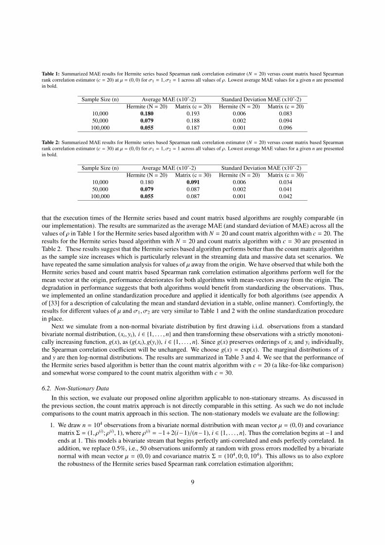
Table 1: Summarized MAE results for Hermite series based Spearman rank correlation estimator (N = 20) versus count matrix based Spearmanrank correlation estimator (c = 20) at µ = (0, 0) for σ1 = 1, σ2 = 1 across all values of ρ. Lowest average MAE values for a given n are presentedin bold.

Sample Size (n) Average MAE (x10ˆ-2) Standard Deviation MAE (x10ˆ-2)Hermite (N = 20) Matrix (c = 20) Hermite (N = 20) Matrix (c = 20)

10,000 0.180 0.193 0.006 0.08350,000 0.079 0.188 0.002 0.094

100,000 0.055 0.187 0.001 0.096

Table 2: Summarized MAE results for Hermite series based Spearman rank correlation estimator (N = 20) versus count matrix based Spearmanrank correlation estimator (c = 30) at µ = (0, 0) for σ1 = 1, σ2 = 1 across all values of ρ. Lowest average MAE values for a given n are presentedin bold.

Sample Size (n) Average MAE (x10ˆ-2) Standard Deviation MAE (x10ˆ-2)Hermite (N = 20) Matrix (c = 30) Hermite (N = 20) Matrix (c = 30)

10,000 0.180 0.091 0.006 0.03450,000 0.079 0.087 0.002 0.041

100,000 0.055 0.087 0.001 0.042

that the execution times of the Hermite series based and count matrix based algorithms are roughly comparable (inour implementation). The results are summarized as the average MAE (and standard deviation of MAE) across all thevalues of ρ in Table 1 for the Hermite series based algorithm with N = 20 and count matrix algorithm with c = 20. Theresults for the Hermite series based algorithm with N = 20 and count matrix algorithm with c = 30 are presented inTable 2. These results suggest that the Hermite series based algorithm performs better than the count matrix algorithmas the sample size increases which is particularly relevant in the streaming data and massive data set scenarios. Wehave repeated the same simulation analysis for values of µ away from the origin. We have observed that while both theHermite series based and count matrix based Spearman rank correlation estimation algorithms perform well for themean vector at the origin, performance deteriorates for both algorithms with mean-vectors away from the origin. Thedegradation in performance suggests that both algorithms would benefit from standardizing the observations. Thus,we implemented an online standardization procedure and applied it identically for both algorithms (see appendix Aof [33] for a description of calculating the mean and standard deviation in a stable, online manner). Comfortingly, theresults for different values of µ and σ1, σ2 are very similar to Table 1 and 2 with the online standardization procedurein place.

Next we simulate from a non-normal bivariate distribution by first drawing i.i.d. observations from a standardbivariate normal distribution, (xi, yi), i ∈ {1, . . . , n} and then transforming these observations with a strictly monotoni-cally increasing function, g(x), as (g(xi), g(yi)), i ∈ {1, . . . , n}. Since g(x) preserves orderings of xi and yi individually,the Spearman correlation coefficient will be unchanged. We choose g(x) = exp(x). The marginal distributions of xand y are then log-normal distributions. The results are summarized in Table 3 and 4. We see that the performance ofthe Hermite series based algorithm is better than the count matrix algorithm with c = 20 (a like-for-like comparison)and somewhat worse compared to the count matrix algorithm with c = 30.

6.2. Non-Stationary Data

In this section, we evaluate our proposed online algorithm applicable to non-stationary streams. As discussed inthe previous section, the count matrix approach is not directly comparable in this setting. As such we do not includecomparisons to the count matrix approach in this section. The non-stationary models we evaluate are the following:

1. We draw n = 104 observations from a bivariate normal distribution with mean vector µ = (0, 0) and covariancematrix Σ = (1, ρ(i); ρ(i), 1), where ρ(i) = −1+2(i−1)/(n−1), i ∈ {1, . . . , n}. Thus the correlation begins at −1 andends at 1. This models a bivariate stream that begins perfectly anti-correlated and ends perfectly correlated. Inaddition, we replace 0.5%, i.e., 50 observations uniformly at random with gross errors modelled by a bivariatenormal with mean vector µ = (0, 0) and covariance matrix Σ = (104, 0; 0, 104). This allows us to also explorethe robustness of the Hermite series based Spearman rank correlation estimation algorithm;

9

Table 3: Summarized MAE results for Hermite series based Spearman rank correlation estimator (N = 20) versus count matrix based Spearmanrank correlation estimator (c = 20) for bivariate normal variables transformed as (g(xi), g(yi)) with g(x) = exp(x), across all values of ρ. Lowestaverage MAE values for a given n are presented in bold.

Sample Size (n) Average MAE (x10ˆ-2) Standard Deviation MAE (x10ˆ-2)Hermite (N = 20) Matrix (c = 20) Hermite (N = 20) Matrix (c = 20)

10,000 0.897 1.072 0.527 0.59250,000 0.812 0.939 0.634 0.547

100,000 0.810 0.909 0.675 0.540

Table 4: Summarized MAE results for Hermite series based Spearman rank correlation estimator (N = 20) versus count matrix based Spearmanrank correlation estimator (c = 30) for bivariate normal variables transformed as (g(xi), g(yi)) with g(x) = exp(x), across all values of ρ. Lowestaverage MAE values for a given n are presented in bold.

Sample Size (n) Average MAE (x10ˆ-2) Standard Deviation MAE (x10ˆ-2)Hermite (N = 20) Matrix (c = 30) Hermite (N = 20) Matrix (c = 30)

10,000 0.897 0.690 0.527 0.36150,000 0.812 0.549 0.634 0.300

100,000 0.810 0.517 0.675 0.289

2. We draw n = 104 observations from a bivariate normal distribution with mean vector µ = (0, 0) and covariancematrix Σ = (1, ρ(i); ρ(i), 1), where ρ(i) = sin(2π(i − 1)/(n − 1)), i ∈ {1, . . . , n}. This models a bivariate streamthat oscillates between correlated and anti-correlated regimes. This could represent the price return innovationsof two financial time series which switch between momentum and mean-reversion regimes for example. Inaddition, we replace 0.5%, i.e., 50 observations uniformly at random with gross errors modelled by a bivariatenormal with mean vector µ = (0, 0), Σ = (104, 0; 0, 104).

In Fig. 1 we plot the evolution of the correlation parameter ρ for the two models described above. To assess the

Fig. 1: Evolution of the correlation parameter ρ of the bivariate normal distribution used for the non-stationary models. Model 1 produces astream of observations with monotonically increasing correlation. Model 2 produces a stream of observations that oscillates between correlatedand anti-correlated regimes.

robustness of the exponentially weighted Hermite series based Spearman rank correlation estimator, we also trans-form the Spearman rank correlation to Pearson’s product-moment correlation (using the Fisher consistent estimator,ρS = 2 sin

((π/6)RN

), applicable to bivariate normal distributions) and compare to an online, exponentially weighted

version of the standard Pearson’s correlation estimator, ρ(x, y)λ, which we define in Appendix B. While the Spearmanrank based estimator for the Pearson’s product-moment correlation is not expected to be as efficient as the standardPearson’s correlation estimator, it allows us to assess robustness and accuracy in a comparable manner. For each ofthe two models, the following steps are repeated:

10

1. Draw n = 104 observations from the model;2. Iterate through the sample, updating the exponentially weighted Hermite series based Spearman rank correlation

estimate in accordance with algorithm 2 in Section 3.2 at each observation, i. Note that we did not apply anonline standardization procedure to the observations. In addition, the Pearson’s correlation is estimated fromthe Hermite series based Spearman rank estimate as ρ(i)

S = 2 sin((π/6)R(i)

N

);

3. Calculate the exact, large sample limit of the Spearman correlation coefficient (i.e. the grade correlation) at eachobservation through R(i) = (6/π) arcsin(ρ(i)/2), where ρ(i) is the exact Pearson’s correlation at each observationgenerated by the model under consideration;

4. Repeat the aforementioned steps m = 103 times and estimate two MAE curves. The first MAE curve tracks theMAE at the ith observation between the Hermite series based Spearman correlation estimate and the exact, largesample limit of the Spearman rank coefficient. The second MAE curve tracks the MAE at the ith observationbetween ρ(i)

S = 2 sin((π/6)R(i)

N

), and the exact Pearson’s correlation. The latter MAE curve is compared to the

MAE performance of an exponentially weighted version of the standard Pearson’s correlation estimator;5. Repeat this procedure at a grid of N and λ values to assess the performance of the Hermite series based esti-

mator for different values of these parameters. Given that the selection of these parameters requires balancingseveral considerations, we assess performance on a grid of parameters to evaluate sensitivity of the results tothe parameter choice. In addition, we seek to determine whether smaller values of λ perform better as discussedin Section 3.3.

The Spearman rank correlation results for model 1 are presented in Fig. 2. Note that the results for model 1 excludingoutliers (omitted for brevity) are very similar to the results with outliers as presented in Fig. 2, providing goodevidence for the robustness of the Hermite series based estimator. The Pearson’s correlation results for model 1 arepresented in Fig. 3. The best results are achieved for λ = 0.005 and the MAE is relatively insensitive to the choice

Fig. 2: Mean absolute error results for the Hermite series based Spearman rank correlation estimator for Model 1 on a grid of N and λ values.These are the parameters controlling the behaviour of the estimator as discussed in Section 3.3. In particular, we evaluate N ∈ {6, 10, 20} andλ ∈ {0.005, 0.01, 0.05}.

of N. It is clear that the Pearson’s correlation derived from the Hermite series based Spearman rank correlationestimator is more accurate and robust than an exponentially weighted version of the standard Pearson’s product-moment correlation estimator. This is to be contrasted with the case without outliers in Fig. 4, where the performanceof the two estimators is very similar. The Spearman rank correlation results for model 2 are presented in Fig. 5.Again the results for model 2 excluding outliers (omitted for brevity) are very similar to the results with outliers aspresented in Fig. 5. The Pearson’s product-moment results for model 2 are presented in Fig. 6. The best results areachieved for λ = 0.01 with higher values of N performing slightly better than lower values (N = 20 yields the bestperformance). The Pearson’s correlation derived from the Hermite series based Spearman rank correlation estimatoris again more accurate and robust than an exponentially weighted version of the standard Pearson’s product-momentcorrelation estimator. The performance of the two estimators is very similar in the case with no outliers as can be seenin Fig. 7.

11

Fig. 3: Mean absolute error results for the Hermite series based Spearman rank correlation estimator transformed to give Pearson’s product-momentcorrelation compared to an exponentially weighted version of the standard Pearson’s product-moment correlation estimator (λ is the same for bothalgorithms).

Fig. 4: Mean absolute error results for the Hermite series based Spearman rank correlation estimator transformed to give Pearson’s product-momentcorrelation compared to an exponentially weighted version of the standard Pearson’s product-moment correlation estimator (λ is the same for bothalgorithms) for model 1 with no outliers.

7. Real Data Example

In this section, we assess the exponentially weighted Hermite series based Spearman rank correlation estimatorapplied to tick-by-tick forex data (sourced from [16]). The association between two currency pairs (EURUSD andGBPUSD in this instance) is expected to vary over time and is thus a good example of a non-stationary setting.

7.1. Data Description

The forex data is sourced from [16] and is comprised of tick-by-tick, top-of-book bid and offer quotes (aggre-gated across several bank liquidity providers) for EURUSD and GBPUSD for April 2019. The mid-price series forEURUSD, p(1)

i , and GBPUSD, p(2)j , are calculated from the bid and offer quotes as follows:

p(1)i = (b(1)

i + a(1)i )/2 i ∈ {1, . . . , n1}, p(2)

j = (b(2)j + a(2)

j )/2 j ∈ {1, . . . , n2},

where a(1), a(2) are EURUSD and GBPUSD offer quotes respectively and b(1), b(2) are EURUSD and GBPUSD bidquotes respectively. These mid-prices are then sampled on a minutely basis using the previous-tick methodology(i.e. the most recent tick in each currency pair is recorded as the price at a given minute), see [1] for example for a

12

Fig. 5: Mean absolute error results for the Hermite series based Spearman rank correlation estimator for Model 2 on a grid of N and λ values.These are the parameters controlling the behaviour of the estimator as discussed in Section 3.3. In particular, we evaluate N ∈ {6, 10, 20} andλ ∈ {0.005, 0.01, 0.05}.

Fig. 6: Mean absolute error results for the Hermite series based Spearman rank correlation estimator transformed to give Pearson’s product-momentcorrelation compared to an exponentially weighted version of the standard Pearson’s product-moment correlation estimator (λ is the same for bothalgorithms).

description of this methodology in the context of other approaches to data synchronization. The mid-price minutelysampled series are thus:

p(1)t(1), . . . , p(1)

t(n), p(2)

t(1), . . . , p(2)

t(n), t(i+1) − t(i) = 1 minute, i ∈ {1, . . . , n},

and we obtain the basis point log returns returns via:

r(1)( j) = 104 log

p(1)t( j+1)

p(1)t( j)

, r(2)( j) = 104 log

p(2)t( j+1)

p(2)t( j)

, j ∈ {1, . . . , n − 1}. (15)

The descriptive statistics of the returns are presented in Table 5. The data presents a mild violation of the assumptionof a continuous bivariate distribution in that some values of basis point log returns are repeated (due to the fact that theminimum increment of quotes, i.e., tick size is 1e-5). Indeed 17.3% of EURUSD log returns and 11% of GBPUSDlog returns are repeated.

7.2. ResultsIn this section, we utilize our R code implementation which has been formalized in the package hermiter [31].

The initial analysis we conduct is as follows: we iterate through the bivariate forex returns data set described above and

13

Fig. 7: Mean absolute error results for the Hermite series based Spearman rank correlation estimator transformed to give Pearson’s product-momentcorrelation compared to an exponentially weighted version of the standard Pearson’s product-moment correlation estimator (λ is the same for bothalgorithms) for model 2 with no outliers..

Table 5: Descriptive statistics of forex basis point log returns calculated as per equation (15) for EURUSD and GBPUSD data for April 2019sourced from [16].

Summary Statistic EURUSD Returns GBPUSD ReturnsCount 30572.00 30572.00Mean 0.00 0.01

Standard Deviation 0.77 1.21Skewness -0.66 0.08Kurtosis 21.06 26.53

Min -17.50 -26.67Max 7.49 21.97

update the exponentially weighted Hermite series based Spearman rank correlation estimator at each minutely returnupdate (r(1)

( j) , r(2)( j) ), j ∈ {1, . . . , n− 1}. These estimates are then compared to exact Spearman rank correlation estimates,

based on a trailing moving window of a certain size. In choosing the appropriate value for the exact Spearman rankcorrelation moving window size, w, we utilize the relation λ = 2/(w + 1) as described in Section 3.3. For analyzingthe forex returns data at an average “age”/lag of approximately two hours, we set λ = 0.01, corresponding to a movingwindow size w = 200. Based on the simulation studies conducted previously, we have seen that the Hermite seriesbased algorithm is reasonably insensitive to the choice of N, we thus chose N = 10 for illustrative purposes. Theresults are presented in Fig. 8.

It is clear that the exponentially weighted Hermite series based Spearman rank correlation estimator and themoving window exact Spearman rank correlation estimator track the association between the currency pairs similarly.Indeed the mean absolute difference between the estimates across all observations is 0.048.

In terms of forecasting ability, we predict the two hour forward realized Spearman rank correlation coefficientformed from observations j + 1, . . . , j + 120, where j ∈ {1000, . . . , (n − 120)}. We have thus assumed approximatelocal stationarity of the data at the time scale of a few hours. The true value of the realized forward Spearman rankcorrelation is compared to the exact Spearman correlation estimate calculated on a trailing moving window, as wellas to the exponentially weighted Hermite series based Spearman correlation estimate, both evaluated at observation jwhere j ∈ {1000, . . . , (n−120)}. The latter estimates are the most recently computed Spearman correlation coefficientsin the exponentially weighted scheme at each observation. To select the best λ,N values for the Hermite series basedestimator and the best w value for the moving window estimator we analyzed forex data for the previous month ofMarch 2019. In particular, we performed a grid-search for λ and N, covering λ ∈ {0.001, 0.002, 0.005, 0.01, 0.05}and N ∈ {6, 8, 10, 20} for the exponentially weighted Hermite series Spearman rank correlation estimator. The bestperforming parameters were selected according to the MAE of the predicted Spearman rank correlation versus therealized forward Spearman rank correlation for the next two hours. These values were λ = 0.002,N = 10, respectively.

14

Fig. 8: Hermite series based exponentially weighted Spearman rank estimator (λ = 0.01) versus moving window exact Spearman correlation(w = 200).

Table 6: Out of sample MAE results for forecasting forward, realized two hour Spearman rank correlation.

Algorithm MAEHermite EW (λ = 0.002) 0.1103

Moving Window (w = 850) 0.1120Constant Estimate 0.1211

Note that we again applied the online standardization procedure that we found advantageous in our simulation studiesin Section 6.1. For the trailing moving window size of the exact Spearman correlation coefficient, we evaluatedw ∈ {50, 100, . . . , 1000}. The best value for the moving window size was w = 850. Even at w = 200 the movingwindow approach was more computationally expensive and slower than the Hermite series based approach. We thusterminated the parameter search at w = 1000. We also evaluated the constant prediction based on the batch estimateformed from calculating the Spearman rank correlation coefficient for the whole March 2019 data set. The out ofsample results for the MAE of the estimates compared to the forward realized Spearman rank correlation coefficientin April 2019 are displayed in Table 6.

The Hermite series based exponentially weighted Spearman estimator is slightly more accurate than the exactSpearman correlation evaluated on a trailing moving window and significantly more accurate than the batch estimateformed from March 2019. The main advantages of the Hermite series based exponentially weighted estimator are asfollows. Firstly, the Hermite series based Spearman rank correlation estimator has O(1) time and memory complexitywith respect to λ. By contrast, the trailing moving window approach grows in time complexity and memory require-ments with moving window size. For large moving window sizes with the usual Spearman correlation estimator, theHermite series based estimator will be significantly faster. As an example, with our implementation in R [31], themoving window estimator (using cor in R) with w = 1000 is roughly 3 times slower than the Hermite series basedalgorithm and this differential increases rapidly with w. Secondly, observations older than a certain threshold do notsharply drop off, but are rather incorporated with decreasing weighting.

8. Conclusion and Perspectives

In this article we have introduced novel, sequential (online) algorithms to estimate the most popular measure ofnonparametric correlation, the Spearman rank correlation coefficient, in both stationary (static) and non-stationary(dynamic) settings. These algorithms are based on bivariate Hermite series density estimators and Hermite seriesbased distribution function estimators. The stationary setting corresponds to bivariate data streams where the Spear-man rank correlation coefficient is constant. This setting also includes the one-pass estimation of the Spearman rankcorrelation for massive data sets. In addition, this algorithm could be applied in decentralized settings where Hermite

15

series based estimates of the Spearman rank correlation, generated on separate portions of a larger dataset, can becombined to form an overall estimate. We have proved that in the i.i.d. setting, the Hermite series based Spearmanrank correlation estimator converges to the grade correlation which is the constant that is unbiasedly estimated bythe standard Spearman rank correlation estimator in large samples. The non-stationary (dynamic) setting correspondsto situations where the Spearman rank correlation of a bivariate data stream is expected to vary over time. In orderto treat these scenarios we have introduced an exponentially weighted version of the Hermite series based Spearmanrank correlation estimator. To the best of our knowledge this is the first algorithm allowing the online tracking of atime varying Spearman rank correlation of a bivariate data stream that does not rely on moving/sliding windows. Wehave derived variance (and standard error) results for the exponentially weighted estimator in the i.i.d. scenario andused these results to provide rule of thumb guidance for the selection of the weighting parameter, λ. The effectivenessof the Hermite series based Spearman rank estimator has been demonstrated in the stationary setting by means of asimulation study which revealed the Hermite series based estimator to be competitive with an existing approach. Wehave also demonstrated the effectiveness of the exponentially weighted Hermite estimator through simulation and realdata studies. We expect our algorithms to be useful in a variety of settings, particularly those where robustness tooutliers and errors is required in addition to fast online calculation of correlation which may vary over time (financialapplications involving high frequency data streams for example). The same approach can also be applied to define aHermite series based Kendall rank correlation estimator. We hope to report on these developments in the near future.

8.1. Future Directions

Some directions for future work include extending and improving the theoretical results presented in this articleand exploring applications in machine learning. For example, in Theorem 1, the regularity conditions on f (x, y)and associated marginal densities imply a fairly high degree of smoothness. It may be possible to weaken theseconditions however, further generalizing the result. In addition, it is possible that a better rate of convergence could bederived. Potential applications in the machine learning domain include, firstly, feature selection on massive datasets.In particular, a univariate filter approach based on our Spearman rank correlation estimator can be applied, which ismore general and robust than the Pearson’s correlation, and could be a more computationally efficient alternative toinformation gain (mutual information). Another potential application pertains to hierarchical clustering on massivedata sets or streaming data. A dissimilarity matrix based on Spearman correlation can be calculated in real time(for streaming data), or in one pass (for massive data sets), leveraging the computational advantages of the Hermiteseries based Spearman rank correlation estimator. This dissimilarity matrix can then be used along with standardagglomerative or divisive hierarchical clustering algorithms. For a reasonably small number of variables this shouldfacilitate real-time hierarchical clustering. This is again a potentially fruitful area for future research.

Acknowledgments

We would like to sincerely thank the referees, the Associate Editor and especially the Editor. The insightful andvery useful comments and suggestions we received greatly helped us to improve this article.

Appendix A. Proofs

In the proof of Theorem 1, we make use of the following two lemmas proved below.

Lemma 1. For the Hermite series based distribution function estimators of the marginal cumulative distributionfunctions F(1)(x) and F(2)(y), we have,

maxx

(|F(1)N (x)|) = O(N17/12), max

y(|F(2)

N (y)|) = O(N17/12).

Proof of Lemma 1: Using (5) and lemma 4 of [32],

|F(1)N (x)| ≤

N∑k=0

|ak |

∫ x

−∞

|hk(t)|dt ≤ u1

N∑k=0

(k + 1)−13 + v1

N∑k=0

(k + 1)5

12 = O(N17/12),

16

where u1 and v1 are positive constants. Note that we have used the fact that maxx |hk(x)| ≤ C(k + 1)−1/12 whereC is a positive constant (implied by Theorem 8.91.3 of [34]) which implies maxx |ak | ≤ C(k + 1)−1/12. Similarlymaxy(|F(2)

N (y)|) = O(N17/12).

Lemma 2. Suppose f (x, y) ∈ L2 and (x − ∂x)r3 (y − ∂y)r3 f (x, y) ∈ L2, r3 > 2 fixed and finite. In addition, supposeE|XY |2/3 < ∞ and that N3(n) = N4(n) = O(n1/(2r3+1)) as n→ ∞, then we have,

E∫| fN3N4 (x, y) − f (x, y)|dxdy = O(n−(r3−2)/(2r3+1)) = o(1) uniformly in x and y,

where fN3N4 (x, y) is the bivariate Hermite series estimator (4).

Proof of Lemma 2: From the inequalities implied by Theorem 8.91.3 of [34], namely,

max|x|≤a

hk(x) ≤ ca(k + 1)−14 , max

|x|≥a|hk(x)|xλ ≤ da(k + 1)s, (A.1)

where ca and da are constants, s = max(λ/2 − 1/12,−1/4), we have:

E(Akl − Akl)2 =1n

Var(hk(x)hl(y)) ≤1n

E[(hk(x))2(hl(y))2

]≤

cn

E(|XY |2/3)(k + 1)−1/2(l + 1)−1/2,

where we have set λ = −1/3 in the inequality (A.1) and c is a positive constant. Note that this is satisfied whenE|X|4/3 < ∞ and E|Y |4/3 < ∞ by the Cauchy-Schwarz inequality. Now using the definition of (4) along with themonotone convergence theorem and the Lyapunov inequality we have,

E∫| fN3N4 (x, y) − f (x, y)|dxdy

≤

N3∑k=0

N4∑l=0

E|Akl − Akl|

∫ ∞

−∞

|hk(x)|dx∫ ∞

−∞

|hl(y)|dy +

∞∑k=N3+1

∞∑l=N4+1

|Akl|

∫ ∞

−∞

|hk(x)|dx∫ ∞

−∞

|hl(y)|dy

≤

N3∑k=0

N4∑l=0

√E|Akl − Akl|

2

∫ ∞

−∞

|hk(x)|dx∫ ∞

−∞

|hl(y)|dy +

∞∑k=N3+1

∞∑l=N4+1

|Akl|

∫ ∞

−∞

|hk(x)|dx∫ ∞

−∞

|hl(y)|dy.

In a similar way to [36], if (x − ∂x)r3 (y − ∂y)r3 f (x, y) ∈ L2, then,

|Akl| ≤ |Bkl|2−r3 (k + 1)−r3/2(l + 1)−r3/2, (A.2)

where Bkl are the bivariate Hermite expansion coefficients of (x − ∂x)r3 (y − ∂y)r3 f (x, y). Note that this result relies onan asymptotic expansion of the Hurwitz zeta function and only applies for r3 fixed and finite (see [23], equation 1.3for the form of the asymptotic expansion). Utilizing the results for the variance of Akl above along with lemma 4 of[32], (A.2) and the Cauchy-Schwarz inequality we have,

E∫| fN3N4 (x, y) − f (x, y)|dxdy = O

N5/43 N5/4

4√

n

+ O(N−r3/2+1

3 N−r3/2+14

).

Now if we set N3(n) = N4(n) = O(n1/(2r3+1)), we obtain:

E∫| fN3N4 (x, y) − f (x, y)|dxdy = O(n−(r3−2)/(2r3+1)).

17

Proof of Theorem 1: We utilize (2) and (6) along with the Cauchy-Schwarz inequality, lemma 1 and Jensen’s in-equality to obtain,

E|RN1,N2,N3,N4 − ρ(F(1)(X), F(2)(Y))|

≤O((N1N2)17/12

)E

∫| fN3N4 (x, y) − f (x, y)|dxdy + O

(N17/12

1

) √E

∫(F(2)

N2(y) − F(2)(y))2 f (y)dy

+ 12

√E

∫(F(1)

N1(x) − F(1)(x))2 f (x)dx + O

(N17/12

1

)E

∫| fN3N4 (x, y) − f (x, y)|dxdy

+ 6

√E

∫(F(1)

N1(x) − F(1)(x))2 f (x)dx + O

(N17/12

2

)E

∫| fN3N4 (x, y) − f (x, y)|dxdy

+ 6

√E

∫(F(2)

N2(y) − F(2)(y))2 f (y)dy + 3E

∫| fN3N4 (x, y) − f (x, y)|dxdy.

Now, given assumptions 1, 2 and 4 (also note that E|X|4/3 < ∞ and E|Y |4/3 < ∞ implies that E|X|2/3 < ∞ andE|Y |2/3 < ∞ by the Lyapunov inequality), Theorem 2 of [32] implies that,

E∫

(F(1)N1

(x) − F(1)(x))2 f (x)dx = O(N−r1+21 ) + O(N5/2

1 /n) = O(n−2(r1−2)/(2r1+1)),

E∫

(F(2)N2

(y) − F(2)(y))2 f (y)dy = O(N−r2+22 ) + O(N5/2

2 /n) = O(n−2(r2−2)/(2r2+1)).

Note that again these results rely on an asymptotic expansion of the Hurwitz zeta function and only apply for r1, r2fixed and finite. Using the above results along with Lemma 2 we have, for n→ ∞:

E|RN1,N2,N3,N4 − ρ(F(1)(X), F(2)(Y))| = O(n34/12(2r1+1)+34/12(2r2+1)−(r3−2)/(2r3+1))

+ O(n34/12(2r1+1)−(r2−2)/(2r2+1)) + O(n−(r1−2)/(2r1+1)).

This implies that if we have r1, r2, r3 ≥ 8:

E|RN1,N2,N3,N4 − ρ(F(1)(X), F(2)(Y))| = o(1).

Proof of Theorem 2: We begin by noting that:

Var((a(1))r) = λ2n−1∑j=0

(1 − λ)2 jVar(hr(xn− j)) + (1 − λ)2nVar(hr(x0)) =

[λ

2 − λ(1 − (1 − λ)2n) + (1 − λ)2n

]Var(hr(x)).

Thus for n → ∞, we have Var((a(1))r) → (λ/(2 − λ))Var(hr(x)) which is O(λ). Similarly, for n → ∞, we have thatVar((a(2))s)), Var((A)uv), cov((a(1))r, (a(2))s), cov((a(1))r, (Auv)), cov((a(2))s, (Auv)) are O(λ). Therefore, all the variancesand covariances above are O(λ). An exact Taylor series expansion of RN implies E(RN) = RN |a(1),a(2),A + O(λ) and

facilitates a convenient reorganisation of the variance expression, E(RN − E(RN)

)2. A straightforward but lengthy

calculation yields the stated result for n→ ∞. Note that this essentially corresponds to the delta method as describedin [19].

Appendix B. Exponentially weighted Pearson’s correlation Estimator

The exponentially weighted version of the standard Pearson’s product-moment correlation estimator is defined as:

X(1)λ = x1, X(i)

λ = λxi + (1 − λ)X(i−1)λ , Y (1)

λ = y1, Y (i)λ = λyi + (1 − λ)Y (i−1)

λ ,

18

V(x)(1)λ = 1, V(x)(i)

λ = λ(xi − X(i)λ )2 + (1 − λ)V(x)(i−1)

λ , V(y)(1)λ = 1, V(y)(i)

λ = λ(yi − Y (i)λ )2 + (1 − λ)V(y)(i−1)

λ ,

C(x, y)(1)λ = 1, C(x, y)(i)

λ = λ(xi − X(i)λ )(yi − Y (i)

λ ) + (1 − λ)C(x, y)(i−1)λ , i ∈ {2, . . . , n},

ρ(x, y)iλ =

C(x, y)(i)λ√

V(x)(i)λ V(y)(i)

λ

.

References

[1] Y. Aıt-Sahalia, J. Fan, D. Xiu, High-frequency covariance estimates with noisy and asynchronous financial data, Journal of the AmericanStatistical Association 105 (2010) 1504–1517.

[2] M. Alanyali, H. S. Moat, T. Preis, Quantifying the relationship between financial news and the stock market, Scientific Reports 3 (2013)3578.

[3] P.-O. Amblard, J.-M. Brossier, Adaptive estimation of the fourth-order cumulant of a white stochastic process, Signal Processing 42 (1995)37–43.

[4] J. Bennett, R. Grout, P. Pebay, D. Roe, D. Thompson, Numerically stable, single-pass, parallel statistics algorithms, in: 2009 IEEE Interna-tional Conference on Cluster Computing and Workshops, IEEE, 2009, pp. 1–8.

[5] T. F. Chan, G. H. Golub, R. J. LeVeque, Updating formulae and a pairwise algorithm for computing sample variances, in: COMPSTAT 19825th Symposium held at Toulouse 1982, Springer, 1982, pp. 30–41.

[6] F. Chen, D. Lambert, J. C. Pinheiro, Incremental quantile estimation for massive tracking, in: Proceedings of the sixth ACM SIGKDDinternational conference on Knowledge discovery and data mining, ACM, 2000, pp. 516–522.

[7] C. Croux, C. Dehon, Influence functions of the spearman and kendall correlation measures, Statistical Methods & Applications 19 (2010)497–515.

[8] D. Dembele, G. Favier, Recursive estimation of fourth-order cumulants with application to identification, Signal Processing 68 (1998) 127–139.

[9] L. Devroye, L. Gyorfi, Nonparametric Density Estimation: the L1 View, volume 119, New York; Toronto: Wiley, 1985.[10] J. D. Gibbons, S. Chakraborti, Nonparametric Statistical Inference, CRC Press, 2010.[11] W. Greblicki, M. Pawlak, Hermite series estimates of a probability density and its derivatives, Journal of Multivariate Analysis 15 (1984)

174–182.[12] W. Greblicki, M. Pawlak, Pointwise consistency of the Hermite series density estimate, Statistics & Probability letters 3 (1985) 65–69.[13] W. Greblicki, M. Pawlak, Nonparametric System Identification, Cambridge University Press Cambridge, 2008.[14] H. L. Hammer, A. Yazidi, H. Rue, A new quantile tracking algorithm using a generalized exponentially weighted average of observations,

Applied Intelligence 49 (2019) 1406–1420.[15] H. L. Hammer, A. Yazidi, H. Rue, Tracking of multiple quantiles in dynamically varying data streams, Pattern Analysis and Applications

(2019) 1–13.[16] Integral, Truefx, https://www.truefx.com/, 2019. Accessed: 2019-05-24.[17] R. Jain, I. Chlamtac, The p 2 algorithm for dynamic calculation of quantiles and histograms without storing observations, Communications

of the ACM 28 (1985) 1076–1085.[18] A. Jmaei, Y. Slaoui, W. Dellagi, Recursive distribution estimator defined by stochastic approximation method using Bernstein polynomials,

Journal of Nonparametric Statistics 29 (2017) 792–805.[19] M. G. Kendall, A. Stuart, J. K. Ord, Kendall’s Advanced Theory of Statistics. v. 1: Distribution theory, London (UK) Griffin, 1987.[20] E. Liebscher, Hermite series estimators for probability densities, Metrika 37 (1990) 321–343.[21] V. Naumov, O. Martikainen, Exponentially weighted simultaneous estimation of several quantiles, World Academy of Science, Engineering

and Technology 8 (2007) 563–568.[22] P. M. Neely, Comparison of several algorithms for computation of means, standard deviations and correlation coefficients, Communications

of the ACM 9 (1966) 496–499.[23] G. Nemes, Error bounds for the asymptotic expansion of the hurwitz zeta function, Proceedings of the Royal Society A: Mathematical,

Physical and Engineering Sciences 473 (2017) 20170363.[24] P. Pebay, T. B. Terriberry, H. Kolla, J. Bennett, Numerically stable, scalable formulas for parallel and online computation of higher-order

multivariate central moments with arbitrary weights, Computational Statistics 31 (2016) 1305–1325.[25] K. E. Raatikainen, Simultaneous estimation of several percentiles, Simulation 49 (1987) 159–163.[26] K. E. Raatikainen, Sequential procedure for simultaneous estimation of several percentiles, Transactions of the Society for Computer Simu-

lation 1 (1990) 21–44.[27] R Core Team, R: A Language and Environment for Statistical Computing, R Foundation for Statistical Computing, Vienna, Austria, 2020.[28] S. C. Schwartz, Estimation of probability density by an orthogonal series, The Annals of Mathematical Statistics 38 (1967) 1261–1265.[29] Y. Slaoui, The stochastic approximation method for estimation of a distribution function, Mathematical Methods of Statistics 23 (2014)

306–325.[30] Y. Slaoui, A. Jmaei, Recursive density estimators based on robbins-monro’s scheme and using bernstein polynomials, Statistics and Its

Interface 12 (2019) 439–455.[31] M. Stephanou, M. Varughese, hermiter, 2020. R package version 2.0.3, https://CRAN.R-project.org/package=hermiter.[32] M. Stephanou, M. Varughese, On the properties of hermite series based distribution function estimators, Metrika 84 (2021) 535–559.[33] M. Stephanou, M. Varughese, I. Macdonald, Sequential quantiles via Hermite series density estimation, Electronic Journal of Statistics 11

(2017) 570–607.

19

[34] G. Szego, Orthogonal Polynomials, American Mathematical Society, Providence, R.I., fourth edition, 1975. American Mathematical Society,Colloquium Publications, Vol. XXIII.

[35] N. Tiwari, P. C. Pandey, A technique with low memory and computational requirements for dynamic tracking of quantiles, Journal of SignalProcessing Systems 91 (2019) 411–422.

[36] G. G. Walter, Properties of Hermite series estimation of probability density, The Annals of Statistics 5 (1977) 1258–1264.[37] B. Welford, Note on a method for calculating corrected sums of squares and products, Technometrics 4 (1962) 419–420.[38] D. West, Updating mean and variance estimates: An improved method, Communications of the ACM 22 (1979) 532–535.[39] W. Xiao, Novel online algorithms for nonparametric correlations with application to analyze sensor data, in: 2019 IEEE International Con-

ference on Big Data, IEEE, 2019, pp. 404–412.[40] A. Yazidi, H. Hammer, Multiplicative update methods for incremental quantile estimation, IEEE Transactions on Cybernetics 49 (2017)

746–756.

20