sentry selection in wireless networks
TRANSCRIPT
Sentry selection in wireless networks
Paul Balister, Bela Bollobas, Amites Sarkar, and Mark Walters
Abstract Let P be a Poisson process of intensity one in the infinite plane R2.We surround each point x of P by the open disc of radius r centred at x.Now let Sn be a fixed disc of area n, and let Cr(Sn) be the set of discswhich intersect Sn. Write Ek
r for the event that Cr(Sn) is a k-cover of Sn,and F k
r for the event that Cr(Sn) may be partitioned into k disjoint singlecovers of Sn. We prove that P(Ek
r \ F kr ) ≤ ck
log n , and that this result is bestpossible. We also give improved estimates for P(Ek
r ). Finally, we study theobstructions to k-partitionability in more detail. As part of this study, weprove a classification theorem for (deterministic) covers of R2 with half-planesthat cannot be partitioned into two single covers.
Paul BalisterDepartment of Mathematical Sciences, University of Memphis, Memphis, TN 38152, USA,e-mail: [email protected] by NSF grant CCF-0728928.
Bela BollobasTrinity College, Cambridge CB2 1TQ, UK, and Department of Mathematical Sciences,University of Memphis, Memphis, TN 38152, USA, e-mail: [email protected] by ARO grant W911NF-06-1-0076, and NSF grants CNS-0721983, CCF-0728928 and DMS-0906634.
Amites SarkarDepartment of Mathematics, Western Washington University, Bellingham, WA 98225,USA, e-mail: [email protected]
Mark WaltersSchool of Mathematical Sciences, Queen Mary, University of London, Mile End Road,London E1 4NS, UK, e-mail: [email protected]
1
2 Paul Balister, Bela Bollobas, Amites Sarkar, and Mark Walters
1 Introduction
Questions involving coverage arise frequently in engineering. Here is a typicalexample. A network of wireless sensors is deployed in a large area (the sensingregion). Each sensor can detect any event occurring within distance r ofitself. If the sensor locations are random (we will model them as points ofa unit intensity Poisson process), how large should r be to ensure that anyevent occurring anywhere in the sensing region will be detected by at leastone sensor? A good way to visualize, and indeed analyze, this problem is toimagine that we place discs of radius r around each sensor. Now we simplyask for the smallest r for which these discs cover the sensing region. A naturalvariant of this problem is to ask for the smallest r for which these discs k-cover the region, i.e., we require each point in the sensing region to be withinrange of at least k sensors. This may be more useful in applications as it givesa degree of tolerance in case of unreliable sensors, or the ability to locate anevent by triangulation. It is worth noting that for fixed k and large sensingregions, k-coverage usually occurs for r only slightly more than that which isnecessary for (single) coverage.
These problems have received much attention [5, 6, 8, 9, 10]. In this paperwe consider a slightly different problem. Suppose that we wish to devise arota system so that each sensor can sleep for most of the time, for example,to extend battery life. A natural way of doing this would be to partition theset of sensors into k groups, and arrange that only the sensors in group `are active in the `th time slot. After k time slots have expired, we repeat theprocess. In order to detect an event occurring anywhere and at any time, it isnecessary that the sensors in each group themselves form a single cover of thesensing region. Thus our question becomes: for fixed k, how large should rbe to ensure that the sensors can be partitioned into k groups, each of whichcovers the sensing region? We call this the problem of sentry selection, sinceeach of the groups is a group of sentries keeping watch over the region whilethe others are sleeping.
For the discs to be partitioned into k single covers (k-partitionability), itis clearly necessary that they k-cover. However, it is important to note that ak-cover of an arbitrary set cannot always be partitioned into k single covers.For instance, let S be the set of all subsets of A = 1, 2, . . . , n of size k.The n sets Si = B ∈ S : i ∈ B, 1 ≤ i ≤ n, form a k-cover of S whichcannot even be partitioned into two single covers if n ≥ 2k−1. This exampleshows that a solution to our problem must make some use of its geometricsetting. Also, even restricting ourselves to discs of equal radii, it is possibleto construct k-covers of the plane that are not d(2k+2)/3e-partitionable (seeSection 9). Thus we shall also make use of the probabilistic setting.
Let us formalize our problem. Consider a Poisson process P of intensityone in the infinite plane. Thus for any bounded measurable region A, thenumber of points in A ∩ P is given by a Poisson random variable with meanequal to the area |A|, and is independent of the number and location of
Sentry selection in wireless networks 3
points of P in any disjoint region. We surround each point x of P by theopen disc Dr(x) of radius r centred at x. Now for definiteness, let the sensingregion Sn be the open disc of area n centred at the origin. (For all the resultsin this paper, it is enough that Sn be an open connected region of area nsuch that boundary ∂Sn is of length O(n1−δ) for some δ > 0 and ∂Sn doesnot intersect any circle ∂Dr(x) in more than a bounded number of points.)Consider the set Cr(Sn) of discs Dr(x), x ∈ P, which intersect Sn. We wishto choose r = r(n) as small as possible so that, with high probability, we maypartition Cr(Sn) into k classes such that each point y ∈ Sn is contained in adisc from each class. Here, and throughout the paper, the phrase “with highprobability”, abbreviated to whp, means “with probability tending to oneas n → ∞”. Note that some of the sensors defining Cr(Sn) may lie outsideof Sn. This slightly unusual method of dealing with the boundary is chosento simplify the analysis of boundary effects, while remaining applicable toreal-life situations.
The basic disc model we are considering was introduced by Gilbert [4]in 1961 in the context of percolation. His subsequent paper [5] on coveragecontains the following important observation. In order for a family of discs ofequal radii to cover a region without boundary, say a large torus, it is not onlynecessary but also sufficient that every intersection of two disc boundaries iscontained in a third disc, provided there is at least one such intersection.Note that the intersection itself is not contained in either of the first twodiscs, since they are open. This fact, and its generalization to k-coverage, hasbeen used in almost all subsequent work on the problem: it enabled Hall [6]to prove sharp results for k-coverage in d dimensions (see below). We use thisobservation in the following general form.
Lemma 1. If S is a bounded open connected planar region, then S is k-covered by Cr(S) provided every intersection point of the boundaries of twodiscs in Cr(S) that lies in S, and every intersection of a boundary of somedisc in Cr(S) with the boundary of S, is k-covered, and at least one suchintersection (of either type) exists.
Proof. Suppose these conditions hold, but that S is not k-covered, and let Rbe a connected component of the subset of S that is not k-covered. Then theboundary ∂R consists only of points from ∂S or from some ∂Dr(x), x ∈ P.However, no intersection point lies in ∂R as these would then fail to be k-covered. Thus each component of ∂R is equal to either a component of ∂Sor the whole of some ∂Dr(x). We may remove Dr(x) from Cr(S) whenever∂R ⊇ ∂Dr(x) without removing or uncovering any intersection points sinceno other disc can intersect Dr(x) without generating an intersection point on∂Dr(x). (Here we use the fact that the discs all have the same radii.) Thuswe may assume ∂R ⊆ ∂S. But in this case any point in R may be joinedto any point in S by a path not meeting ∂R. Thus R = S and there are nointersection points inside S or on the boundary of S.
4 Paul Balister, Bela Bollobas, Amites Sarkar, and Mark Walters
Throughout the paper we will ignore events of probability zero, so that,for instance, we will assume that an intersection of two disc boundaries doesnot lie on the boundary of a third disc.
2 Results
Let n, r ∈ R. For k ∈ N, write Ekr for the event that Cr(Sn) is a k-cover of
Sn, and F kr for the event that Cr(Sn) may be partitioned into k single covers
of Sn. Our main result is the following.
Theorem 1. With r, n ∈ R, k ∈ N,
P(Ekr \ F k
r ) ≤ ck
log n.
In Section 5 we prove this theorem, and in Section 7 we show that thisresult is best possible (up to the value of ck). In Section 6 we prove two hittingtime versions of Theorem 1: if we fix n and slowly increase r, or if we fix r andadd points uniformly at random to a given area, then with high probability, k-partitionability occurs as soon as we have k-coverage. The proofs identify theprincipal obstructions to k-partitionability in a k-cover as certain small non-partitionable k-covered configurations. These configurations involve a smallarea which is covered by k − 2 common discs, but for which the remainingdiscs form a 2-cover which is not 2-partitionable. Since these configurationsare very small, the curvature of the discs forming them is negligible, so thatour obstructions are essentially 2-covers with half-planes which cannot bepartitioned into two single covers. It is therefore of interest to classify suchconfigurations. Such a classification is achieved in Theorem 9, whose proofoccupies Section 8.
For Cr(Sn) to admit a k-partition, it must certainly form a k-cover of Sn.Hall [6] proved the following result, which shows that the area of the sensingregions required for k-coverage is only slightly more than that required forsingle coverage. In particular, we do not need k times the disc area for singlecoverage to ensure k-coverage, as one might naively expect.
Theorem 2 (Hall [6]). Let k ∈ N and let r be given by
πr2 = log n + k log log n + f(n).
Then Cr(Sn) is a k-cover of Sn whp if and only if f(n) →∞ as n →∞.
In Section 4 we strengthen this result by proving the following.
Theorem 3. Fix k ∈ N and let r be given by
πr2 = log n + k log log n + f(n).
Sentry selection in wireless networks 5
ThenP(Ek
r ) = e−e−f(n)+o(1)/(k−1)! + O( 1log n ) as n →∞.
In particular, if f(n) = t is a constant, then P(Ekr ) → e−e−t/(k−1)! as
n → ∞. After proving Theorem 3, we discovered that this corollary can beread out of results of Janson [7].
3 Thinly covered regions
Call a point `-thinly covered (or just thinly covered if ` is clear from thecontext) if it is not `-covered by the discs Dr(x), x ∈ P. An `-thinly coveredregion is a connected component of the set of points in Sn that are `-thinlycovered. Note that if an `-thinly covered region is not (`− 1)-covered then itwill contain several atomic regions, i.e., components of Sn \
⋃x∈P ∂Dr(x).
Let X be the number of intersection points of the boundaries of the discsof Cr(Sn) that lie inside Sn, and let X∂ be the number of intersection pointsof ∂Sn with the boundaries of the discs of Cr(Sn). Write X = X + X∂ forthe total number of intersection points. Let Xk (respectively, X
k , X∂k ) be
the number of intersection points (respectively, interior intersection points,boundary intersection points) that are k-thinly covered. Lemma 1 can nowbe restated as saying that if Xk = 0 and X > 0 then Sn is k-covered.
Lemma 2. Fix k ∈ N and write
πr2 = log n + k log log n + t,
where t = t(n) = o(log n). Then as n →∞,
E(X) = 4πr2n, E(X∂) = n1−Ω(1), P(X = 0) = n−ω(1),
E(Xk) =(4 + o(1))e−t
(k − 1)!and E(X∂
k ) = n−Ω(1).
Proof. A fixed disc boundary ∂Dr(x) with centre x ∈ P intersects twiceeach disc boundary whose centre lies within distance 2r of x. Therefore,the expected number of intersections involving ∂Dr(x) is 8πr2. The densityof intersections in the infinite plane is thus 4πr2 (since each intersection iscounted twice), and so E(X) = 4πr2|Sn| = 4πr2n. For any intersectionpoint u ∈ ∂Sn, there must be a point x ∈ P at distance r from u, so x ∈∂Dr(u). Since each such x gives rise to a bounded number of intersectionpoints u ∈ ∂Sn, and the total area A swept out by ∂Dr(u) as u movesaround ∂Sn is at most 2πr|∂Sn| = O((log n)1/2n1−δ) = n1−Ω(1), we haveE(X∂) = n1−Ω(1). The area A includes all points within distance r of ∂Sn
when the diameter diam(Sn) is greater than 2r, however diam(Sn) = Ω(√
n),so this holds for sufficiently large n. If diam(Sn) = ‖x− y‖ with x, y ∈ ∂Sn,
6 Paul Balister, Bela Bollobas, Amites Sarkar, and Mark Walters
then any line perpendicular and crossing the line segment from x to y mustintersect ∂Sn, and hence intersects A in an interval of length at least 2r. Thus|A| ≥ 2r diam(Sn) and the probability that there is no boundary intersectionpoint is P(Po(|A|) = 0) = e−|A| ≤ e−Ω(r
√n) = n−ω(1). Hence P(X = 0) =
n−ω(1).A fixed intersection u needs at least k other points of P within distance
r to be k-covered. Conditioning on the locations of the point(s) of P givingrise to u does not change the distribution of the remaining points of P. (Thisis a key property of a Poisson process.) Therefore, the probability p that u isnot k-covered may be estimated by
p = P(Po(πr2) < k)
=k−1∑
i=0
e−πr2(πr2)i/i!
= e− log n−k log log n−t(πr2)k−1 1(1−O(k/πr2))(k − 1)!
= (πr2n)−1e−t(πr2/ log n)k 1(1−O(k/πr2))(k − 1)!
= (πr2n)−1e−t 1 + o(1)(k − 1)!
,
where the third line follows by comparison with a geometric series, and thelast line uses the fact that t = o(log n) and hence πr2 = (1 + o(1)) log n.Consequently E(Xk) = (4πr2n + n1−Ω(1))p = (4 + o(1))e−t/(k − 1)! andE(X∂
k ) = n1−Ω(1)p = n−Ω(1) as required.
Note that for πr2 = (1 + o(1)) log n, E(Xk)/E(Xk−1) = 1+o(1)k−1 log n =
Θ(log n), so one would expect many regions to fail to be k-covered beforeany region fails to be (k − 1)-covered.
Next we need a simple lemma bounding the tail of the Poisson distribution.
Lemma 3. Fix c > 0, and set
c− = ce−1−1/c.
ThenP(Po(c− log n) ≥ c log n) = n−1−Ω(1).
Proof. Write k = dc log ne and λ = c− log n. Then, by comparison with ageometric series, the probability can be estimated as
Sentry selection in wireless networks 7
∞∑
l=k
e−λ λl
l! < e−λ 11−(λ/k)
λk
k!
< e−λ 11−(λ/k)
(λek
)k
= 11−(c−/c) nc(log(c−/c)+1)−c−+o(1),
which is n−1−Ω(1) provided
c− < c and c log(c−/c) + c− c− < −1.
However this holds for c− as in the statement of the theorem.
We use this lemma to show that whp the intersections are not too clus-tered.
Lemma 4. If πr2 = (1+o(1)) log n, then with probability 1−n−Ω(1) there areat most 677(log n)2 intersections within distance 2r of any other intersection.
Proof. Fix two points x, y ∈ P (or one point x ∈ P and ∂Sn) giving rise to anintersection u. Conditioning on the locations of x and y, the distribution ofthe remaining points in P is still given by a Poisson process. Any intersectionwithin distance 2r of u is defined by (at most) two points of P, each withindistance 3r of u. By Lemma 3 (with c = 26, which gives c− > 9),
P(Po(9πr2) ≥ 26 log n) = n−1−Ω(1).
By Lemma 2, the expected number of intersection points in (or on the bound-ary of) Sn is 4πr2n+n1−Ω(1) = n1+o(1). It follows that the expected numberof intersection points with more than 26 log n+2 points of P within distance3r is n−Ω(1). Thus with probability 1−n−Ω(1), there is no intersection pointwith more than 26 log n + 2 points of P within distance 3r, and hence nointersection point with more than 677(log n)2 intersections within distance2r (for sufficiently large n).
Typically, most of Sn is very heavily covered by the discs of Cr(Sn).It seems reasonable that these areas are unlikely to cause any obstructionto k-partitionability. Thus most of the work is involved in partitioning thediscs covering lightly covered regions. Fortunately these regions occur in well-separated groups.
Let ` = 3k log log n and define ε by
ε =2` log log n√
log n=
6k(log log n)2√log n
. (1)
Note that ε → 0 as n →∞.On each disc Dr(x) in Cr(Sn) define seven marked points equally spaced
around its boundary ∂Dr(x), say at angles 2πj/7, 0 ≤ j < 7, from the x-axis.
8 Paul Balister, Bela Bollobas, Amites Sarkar, and Mark Walters
For technical reasons we shall need to include these as well as intersectionpoints in the following lemma.
Lemma 5. Assume πr2 = (1 + o(1)) log n, ` = 3k log log n, and ε is de-fined as in (1). Then the expected number of `-thinly covered points thatare intersections or marked points and are within distance 4r + ε of ∂Sn is(log n)−ω(1)E(Xk). The expected number of pairs of `-thinly covered points uand v, each of which are either an intersection point or a marked point, andwith ε ≤ ‖u− v‖ ≤ 4r + 2ε is also (log n)−ω(1)E(Xk).
Proof. The number of intersection and marked points within distance 4r+ε of∂Sn is O(r3|∂Sn|) = n1−Ω(1) and so, as in the proof of Lemma 2, the expectednumber of these that are `-thinly covered is n1−Ω(1)P(Po(πr2) < `). Now
P(Po(πr2) < `) = e−πr2 11−O(`/πr2)
(πr2)`−1
(`−1)!
≤ n−1+o(1)(log n)(3+o(1))k log log n
= n−1+o(1)+(3+o(1))k(log log n)2/ log n,
= n−1+o(1),
where we have used the fact that πr2 = (1+o(1)) log n and ` = o(log n). Thusthe expected number of `-thinly covered intersection or marked points withindistance 4r + ε of ∂Sn is n−Ω(1), which is (log n)−ω(1)E(Xk) by Lemma 2.For the second part note that such pairs (u, v) are defined by (at most) fourpoints x1, . . . , x4 of P, any two of which are at most 6r + 2ε ≤ 7r apart (forlarge n). Now x1 lies within distance r of Sn, so there are Po((1 + o(1))n)choices for x1. Conditioned on the choices of x1, . . . , xi−1, there are at mostPo(49πr2) choices for xi (using once again the fact that conditioning onthe existence of certain points in a Poisson process leaves the remainingpoints occurring with an identical Poisson process distribution). Thus theexpected number of ordered 4-tuples (x1, . . . , x4) of distinct points is boundedby (1 + o(1))n(49πr2)3 = O(n(log n)3). Similarly, the number of ordered 3,2, or 1-tuples is also O(n(log n)3). Since any choice of tuple corresponds to abounded number of choices of pair (u, v), there are on average O(n(log n)3) =O((log n)2E(X)) pairs (u, v) of marked or intersection points with ε ≤ ‖u −v‖ ≤ 4r + 2ε.
For any such pair u, v, we have
|Dr(u) ∪Dr(v)| ≥ πr2 + 2ε√
r2 − (ε/2)2
≥ πr2 + ( 2√π− o(1))ε
√log n
≥ πr2 + 2.2` log log n
for sufficiently large n. Also Dr(u) ∪Dr(v) must contain less than 2` pointsof P. Even conditioned on x1, . . . , x4, the probability of this is at most
Sentry selection in wireless networks 9
P(Po(πr2 + 2.2` log log n) ≤ 2`) ≤ e−πr2−2.2` log log n 11−O(`/πr2)
(πr2)2`
(2`)!
≤ e−πr2 (πr2)k−1
(k−1)! (log n)2`−(k−1)+o(`)−2.2`
≤ P(Po(πr2) < k)(log n)−ω(1)
since ` → ∞ as n → ∞. Since (by the proof of Lemma 2) E(Xk) =E(X)P(Po(πr2) < k), there are on average (log n)−ω(1)E(Xk) such pairs of`-thinly covered intersection or marked points.
Lemma 6. Assume πr2 = (1 + o(1)) log n, ` = 3k log log n, and ε is de-fined as in (1). Then, with probability 1− (log n)−ω(1)E(Xk), there are discsD1, . . . , Dm in Sn, each of radius ε, such that all `-thinly covered regions ofSn lie in
⋃mi=1 Di, and each Di lies at distance at least 4r from the other Djs
and from ∂Sn.
Proof. By Lemma 5, with probability 1 − (log n)−ω(1)E(Xk) there are nothinly covered intersection or marked points u and v of Sn with ε ≤ ‖u −v‖ ≤ 4r + 2ε, and no thinly covered intersection or marked points withindistance 4r + ε of ∂Sn. Assume this holds, and choose inductively a sequenceu1, u2, . . . , um of thinly covered intersection or marked points in Sn withui /∈ ⋃
j<i Dε(uj). This process will terminate (almost surely) with all thinlycovered intersection and marked points in Sn lying in some Di = Dε(ui). Byassumption, ‖ui − uj‖ ≥ ε, so ‖ui − uj‖ ≥ 4r + 2ε for all i 6= j. Hence eachdisc Di is at distance at least 4r from any other disc Dj or ∂Sn. Now considerany thinly covered region R in Sn. The intersection and marked points on theboundary of R are thinly covered. But there are no thinly covered intersectionpoints on ∂Sn. Thus the components of ∂R must each lie either entirely within∂Sn or entirely within the interior of Sn. Consider a component of ∂R thatlies inside Sn. This boundary is formed from arcs of discs. Since any arcbetween marked points on a disc has length less than r − ε (for sufficientlylarge n), no point on this component of ∂R can be at distance more thanr − ε from a thinly covered marked or intersection point. Hence no point onthis component of ∂R can be at distance more than r from some ui. Thus∂R ⊆ D ∪ ∂Sn, where D =
⋃mi=1 Dr(ui). Hence either R ⊆ D or Sn \D ⊆ R.
If we fix two points z1 and z2 arbitrarily, but deterministically, in Sn with‖z1 − z2‖ = 2r, then at most one of these can lie in D, as they cannot bothlie in the same Dr(ui), and Dr(ui) and Dr(uj) are more than 2r apart wheni 6= j. Hence if Sn\D ⊆ R then at least one of z1 and z2 is thinly covered. Butthe probability that at least one of these (deterministically chosen) points isthinly covered is at most 2E(Xk)/E(X) = (log n)−ω(1)E(Xk). Thus we mayassume R ⊆ D. As R is connected, this implies R ⊆ Dr(ui) for some i. Theexternal boundary of R is formed from arcs of discs that curve inwards, sincethe exterior of R is covered more times than the interior. Thus R is containedwithin the convex hull of the intersection points on its boundary, all of whichlie in Di = Dε(ui). Thus R ⊆ Di.
10 Paul Balister, Bela Bollobas, Amites Sarkar, and Mark Walters
Next we shall show that usually, inside each Di, the 3k-thinly coveredregions are covered by k − 1 common discs from Cr(Sn). In fact we shallprove a slightly stronger result. Define r′ by the formula
r′2 = r2 − ε2 = r2 − 36k2(log log n)4
log n, (2)
where ε is defined by (1).
Lemma 7. Fix k and assume πr2 = (1 + o(1)) log n. Then with probability1− O(E(Xk−1)), any set of 3k-thinly covered points of Sn that lie within asingle disc of radius ε are covered by a common set of k−1 discs of Cr′(Sn).
Here, the two families of discs Cr(Sn) and Cr′(Sn) are constructed from thesame underlying instance of P.
Proof. Assume otherwise, but that the conclusion of Lemma 6 holds. As3k ≤ ` (for sufficiently large n), all 3k-thinly covered points lie in one ofthe discs Di of Lemma 6. Since these discs are far apart from each other,we may without loss of generality assume that the single disc of radius εis one of the Di and the set of 3k-thinly covered points is the set R of all3k-thinly covered points in Di. Note that R might not be connected, but Ris bounded by arcs of circles ∂Dr(x), x ∈ P. Since Di \ R is more highlycovered than R, these boundary arcs curve inwards towards R. Thus R iscontained within the convex hull of the 3k-thinly covered intersection pointsin Di. We may therefore assume there are two thinly covered intersectionpoints u and v in R with α = ‖u− v‖ equal to the diameter of R. Thus thereare at most 6k − 2 points of P in Dr(u) ∪Dr(v), and hence at most 6k − 2points in the slightly smaller region A1 = Dr′(u)∪Dr′(v). If R does not havea common (k − 1)-cover from Cr′(Sn), then there are less than k − 1 pointsof P in A2 = Dr′−α(u) ∪Dr′−α(v). For fixed u and v the probability of thisoccurring is at most
p = e−|A2|−|A1\A2|k−2∑
i=0
∑
i+j≤6k−2
|A2|ii!
|A1 \A2|jj!
(even conditioned on the points of P giving rise to u and v). Now A2 ⊆ Dr(u),so |A2| ≤ πr2. Also |A1 \ A2| ≤ 2|Dr′(u) \ Dr′−α(u)| ≤ 4πr′α. Finally, forall α ≤ 2r′, |A2| + |A1 \ A2| = |A1| ≥ πr′2 + πr′α/2 (by concavity of |A1|as a function of α ∈ [0, 2r′]). Thus, setting t = πr′α/2 and recalling thatr′2 = r2 − o(1), we have
Sentry selection in wireless networks 11
p ≤ e−πr2+o(1)−tk−2∑
i=0
∑
i+j≤6k−2
(πr2)i
i!(8t)j
j!
≤(
e−πr2k−2∑
i=0
(πr2)i
i!
)(eo(1)−t
6k−2∑
j=0
(8t)j
j!
).
Fixing u and letting v vary, we have on average (4πr2)(πα2) = (16r2/r′2)t2
choices for the intersection v with t-value less than t, and so (32 + o(1))t dtchoices of v with t-value between t and t + dt. Thus the expected number ofintersections v satisfying the above conditions with a fixed u is at most
(e−πr2
k−2∑
i=0
(πr2)i
i!
)∫ ∞
0
eo(1)−t6k−2∑
j=0
(8t)j
j!(32 + o(1))t dt. (3)
But∫∞0
e−ttj+1dt = (j + 1)! for all j, so the integral above becomes
Ck = (32 + o(1))6k−2∑
j=0
8j(j + 1) = O(k86k), (4)
which is bounded for fixed k, independently of n for large enough n. Sincethe first factor in (3) is just the probability P(Po(πr2) < k−1), the expectednumber of intersections v satisfying the above conditions with a fixed u is atmost Ck P(Po(πr2) < k − 1).
Now letting u vary, we note that the expected number of (ordered) pairs(u, v) satisfying the conditions above is at most Ck times the expectednumber of intersections u that are not (k − 1)-covered, in other words,at most Ck E(Xk−1). In particular, the probability of such a pair exist-ing is O(E(Xk−1)). Adding the probability of failure (log n)−ω(1)E(Xk) =(log n)−ω(1)Θ(log n)E(Xk−1) = o(E(Xk−1)) from Lemma 6 gives the result.
We will also require a lemma of a somewhat more technical nature. Definea bad lune L to be the intersection of two discs from Cr(Sn) with the followingproperties: i) the diameter of L is at most 2ε; ii) L lies at distance at least2ε from ∂Sn; and iii) some point in the interior of L is covered less than ktimes by the discs of Cr′(Sn).
Lemma 8. Assume πr2 = (1 + o(1)) log n. Then the expected number ofk-thinly covered intersection points that lie within distance 2ε of a badlune is at most (log n)−2+o(1)E(Xk). Also, with probability at least 1 −(log n)−2+o(1)E(Xk) there are no bad lunes.
Proof. A lune L satisfying i) and ii) above is defined by two points of Pat distance between 2r and 2
√r2 − ε2 ≥ 2r − 2ε2/r. There are on average
O(ε2n) choices for two such points, and conditioning on their locations doesnot change the distribution of the remaining points. There are no boundary
12 Paul Balister, Bela Bollobas, Amites Sarkar, and Mark Walters
intersection points in D2ε(L) = x : d(x,L) < 2ε as L is at distance atleast 2ε from ∂Sn. The area of D2ε(L) is O(ε2), and so the expected num-ber of interior intersections in D2ε(L) not involving the discs forming L isO(ε2r2) as in the proof of Lemma 2. There are also on average O(εr) in-tersections involving the boundary of the lune. (A full boundary of Dr(x)contains on average 2.π(2r)2 intersection points and the lune consists of twosegments of total length at most about 4ε, so contains on average at mostabout (8πr2)(4ε/2πr) intersection points.) Finally there are 2 intersectionsforming the lune so there are in total on average O(ε2r2 + εr + 2) = O(ε2r2)intersections in D2ε(L).
Suppose we now fix a lune L and an intersection point in D2ε(L). Con-ditioning on this information, the distribution of the remaining points ofP not involved in L or the intersection point is unaffected. Thus if the in-tersection point is not k-covered, there can be at most k − 1 of these re-maining points of P within distance r of the intersection. The probabil-ity of this is just E(X
k)/E(X) = E(Xk)/(4πr2n) by Lemma 2. Conse-
quently, the expected number of k-thinly covered intersections in D2ε(L)is O((ε2n)(ε2r2)E(X
k)/(4πr2n)) = O(ε4E(Xk)). But ε = (log n)−1/2+o(1), so
the expected number of such intersections is at most (log n)−2+o(1)E(Xk).To estimate the expected number of bad lunes we replace r by r′ and Sn by
L and consider coverage and intersection points defined by Cr′(L). Followingthe above argument we see that the expected number of intersection pointsin, or on the boundary of L is O(ε2r′2), even including the two endpointsof L and some intersections outside of L (which, strictly speaking, are nolonger intersection points). If L is not k-covered then one of these pointswill be thinly covered by Lemma 1. (If there are no intersections then Lis k-covered iff one of its endpoints is.) The probability that any one ofthese point is thinly covered is P(Po(πr′2) < k) = (1 + o(1))P(Po(πr2) < k)as r2 = r′2 + o(1) by (2). Thus the expected number of bad lunes is atmost O((ε2n)(ε2r′2)E(X
k)/(4πr2n)) which is at most (log n)−2+o(1)E(Xk) asabove. Hence with probability at least 1 − (log n)−2+o(1)E(Xk) there are nobad lunes.
4 Probability of k-coverage
Proof (Proof of Theorem 3).Write πr2 = log n+k log log n+t and assume for the moment that t = o(log n).By Lemma 2, the average number of k-thinly covered intersection points isE(Xk) = (4+o(1))e−t/(k−1)!. However, these intersection points are clearlynot independent of one another. Indeed, by considering the boundary of ak-thinly covered region of Sn, if one thinly covered intersection exists, thenthere must be at least one other one, and so P(Xk = 1) = 0. Define Yk tobe the number of k-thinly covered regions of Sn other than Sn itself. (If the
Sentry selection in wireless networks 13
whole of Sn is thinly covered, we define Yk to be zero as, for technical reasons,we wish to have at least one intersection point on every thinly covered regioncounted by Yk.) We will show that E(Yk) = (1 + o(1))e−t/(k − 1)! and Yk isgiven by an approximately Poisson distribution. The result will then follow,at least for small t.
To show that Yk has an approximately Poisson distribution, we must showthat the k-thinly covered regions do not occur in clusters (for r in the rangewe are considering). This will follow from the fact that there is usually atmost one k-thinly covered region in any one Di, where the Di are as inLemma 6. This in turn follows from the observation that, within a Di, the discboundaries ∂Dr(x) are almost straight lines, so that the discs Dr(x) behavealmost like half-planes. If they actually were half-planes, Lemma 7 wouldshow that (usually) each Di contains at most one k-thinly covered region.This follows since, having removed the k − 1 half-planes from Lemma 7, theintersection of the complements of the remaining half-planes bordering thenow uncovered region would actually be a single convex polygonal region. Itturns out that for the discs to behave differently, two of them must form abad lune, which we have already shown is extremely unlikely.
Let Y ′k be the number of k-thinly covered regions of Sn that i) do not border
∂Sn, ii) have diameter at most 2ε, and iii) do not contain an intersectionpoint that is at one of the ends of a bad lune. Let X ′
k be the number ofintersection points on the boundary of such a region. Thus any intersectionpoint counted by Xk−X ′
k is either within 2ε of ∂Sn, within 2ε of a bad lune,lies in a thinly covered region of diameter more than 2ε, or lies in the interiorof a thinly covered region. By (the proof of) Lemma 2, the average numberof thinly covered intersection points within 2ε of ∂Sn is O(εn−δE(X
k) +E(X∂
k )) = n−Ω(1)E(Xk). By Lemma 8, the average number of thinly coveredintersection points within 2ε of a bad lune is at most O((log n)−2+o(1)E(Xk)).By Lemma 5, the average number of intersection points that are on theboundary of a thinly covered region with diameter more than 2ε, but notwithin 2ε of ∂Sn, is (log n)−ω(1)E(Xk). (Any such intersection point is atdistance between ε and 2r + ε of at least one other intersection point on theboundary of the same region.) Finally, any intersection point in the interiorof a k-thinly covered region must be (k − 2)-thinly covered, so the expectednumber of these is at most E(Xk−2) = Θ((log n)−2E(Xk)). Hence
E(Xk −X ′k) = O((log n)−2+o(1)E(Xk)). (5)
Since each thinly covered region has at least one intersection on its boundary,Yk − Y ′
k ≤ Xk −X ′k, so E(Yk − Y ′
k) = O((log n)−2+o(1)E(Xk)). Finally, X ′k ≤
Xk ≤ Xk, so E(X
k −X ′k) = O((log n)−2+o(1)E(Xk)) as well.
Pick any internal intersection point u defined by points x, y ∈ P. The eventthat it is thinly covered is independent of the choice of x and y. Moreover,the angle θu between the circles ∂Dr(x) and ∂Dr(y) at u depends only onx and y. As x and y vary, the average value is E(θu | ‖x − y‖ < 2r) = π/2.
14 Paul Balister, Bela Bollobas, Amites Sarkar, and Mark Walters
(Fix x and average over y ∈ D2r(x) to obtain E(θu | ‖x − y‖ < 2r) =(4πr2)−1
∫ 2r
04πx sin−1(x/2r) dx = π/2.) The sum of the external angles of
the intersection points on the boundary of an internal thinly covered regionR is 2π + |∂R|/r, since the boundary arcs all have radius of curvature r andcurve inwards toward R. However, if the diameter of R is less than 2ε, then|∂R| = O(ε) since R is “almost” convex. Now if an intersection u on ∂R iscovered exactly k − 1 times then the exterior angle at u is on average π/2,but if u is covered exactly k−2 times the average exterior angle at u is −π/2.Nonetheless, since E(X ′
k−1) = O(E(X ′k)/ log n), we may write
(2π + O(ε/r))E(Y ′k) = (π
2 + O(1/ log n))E(X ′k)
and thus
E∑
u thin
θu = π2E(Xo
k) = π2E(Xo
k −X ′k) + (2π + o(1))E(Y ′
k).
Hence by Lemma 2 and (5), E(Y ′k) = (1 + o(1))e−t/(k − 1)!.
To prove that Y ′k is approximately Poisson we use the Stein-Chen method.
A simple form of it is given in Theorem 1 of [1], which immediately impliesthe following.
Theorem 4. Let ξ1, ξ2, . . . be a countable collection of independent ran-dom variables and let Z1, Z2, . . . be a countable collection of Bernoulli ran-dom variables where Zi is a function of the values of ξj, j ∈ Si. Sup-pose that
∑i E(Zi) = λ and let b1 =
∑i,j : Si∩Sj 6=∅ E(Zi)E(Zj), b2 =∑
i,j : Si∩Sj 6=∅, i 6=j E(ZiZj) and Z =∑
i Zi. Then for all r,
|P(Z = r)− e−λλr/r! | ≤ 1− e−λ
λ(b1 + b2).
(Theorem 1 in [1] includes another term b3 that bounds dependency whenSi ∩ Sj = ∅, but in our case b3 = 0.)
To make the collection of events countable, divide Sn up into a very finegrid and move all points of P to their nearest grid point. It is clear thatfor fixed r, n, k, we can make the number of thinly covered regions in thisdiscretized version equal to the number of thinly covered regions in the orig-inal with probability arbitrarily close to 1. The random variables ξi recordwhether or not the ith grid point is occupied, and for every conceivable thinlycovered region Ri satisfying i)–iii) above, we introduce a variable Zi indicat-ing whether this thinly covered region exists. The set Si can be taken to bethe set of grid points within distance r + 2ε of Ri. Then E(|Y ′
k − Z|) can bemade arbitrarily small.
We now bound b1 and b2. First consider b1. Fix a potential thinly coveredregion Ri of diameter at most 2ε. Then
∑j : Si∩Sj 6=∅ E(Zj) is bounded by the
expected number of thinly covered intersection points within a disc of radius
Sentry selection in wireless networks 15
2r + 4ε, which is z = O(E(Xk)r2/n) = (log n)−ω(1)E(Z), uniformly in thechoice of Ri. Thus b1 ≤
∑i E(Zi)z = E(Z)z = (log n)−ω(1)E(Z)2. Now con-
sider b2. This counts the expected number of pairs of thinly covered regionssatisfying i)–iii) that lie within distance 2r + 4ε of each other. By Lemma 5,there is a contribution of (log n)−ω(1)E(Xk) to b2 from pairs of regions that arenot contained within a single disc of radius ε. Then by the proof of Lemma 7,there is a contribution of at most O(E(Xk−1)) = O((log n)−1E(Xk)) frompairs of regions that do not share a common (k − 1)-cover from Cr′(Sn),where r′ is defined by (2). (Any such pair gives rise to a pair of thinly cov-ered intersection points u and v with no common (k−1)-cover, and these are(over-) counted in the proof of Lemma 7.) Finally, assume two k-thinly cov-ered regions Ri and Rj have a common (k− 1)-cover by elements of Cr′(Sn)(and hence also by elements of Cr(Sn)). Thus the set of discs of Cr(Sn) cov-ering Ri is the same as the set of discs covering Rj . We shall now show thatif Ri and Rj lie in a disc of radius ε, then at least one of them contains anendpoint of a bad lune, so this pair does not contribute to b2.
Let u ∈ Ri and v ∈ Rj be chosen with ‖u − v‖ minimal. Then at leastone of u or v must be an intersection point, say u. Let Dr(x1) and Dr(x2)be two discs whose boundaries intersect at u. Since these discs do not coverRi, they also do not cover Rj . The regions Rj and Ri must be separated bythe lune formed by Dr(x1) and Dr(x2), since otherwise u would not be theclosest point in Ri to Rj . (Recall that Ri and Rj are contained in a regionof diameter much smaller than r.) In particular, this lune is of diameter atmost 2ε. The point u is k-thinly covered by Cr(Sn) and hence any pointwithin distance r− r′ > 0 of u is k-thinly covered by Cr′(Sn). Thus the luneis bad and Ri contains the endpoint u.
Now b1 = (log n)−ω(1)E(Z)2 and b2 = O((log n)−1E(Z)). Taking r = 0 inTheorem 4 we have
P(Z = 0) = e−λ + O((log n)−1) + (log n)−ω(1)λ,
where λ = E(Z) = (1 + o(1))e−t/(k − 1)!. By (5) and the fact that P(X ′k =
0) = P(Y ′k = 0) is arbitrarily close to P(Z = 0), we have
P(Xk = 0) = e−λ + O((log n)−1) + O((log n)−2+o(1))λ.
Now by Lemma 2 and Lemma 1,
P(k-coverage succeeds) = e−λ + O((log n)−1) + O((log n)−2+o(1))λ + n−ω(1).(6)
For 1/ log n ≤ λ ≤ log log n we have t = o(log n) and so (6) is valid. Butfor this range of λ the last two error terms are dominated by the first andλ = (1 + o(1))e−t/(k − 1)! = e−t+o(1)/(k − 1)!, so
P(k-coverage succeeds) = e−e−t+o(1)/(k−1)! + O((log n)−1). (7)
16 Paul Balister, Bela Bollobas, Amites Sarkar, and Mark Walters
This probability is monotonic in t, and for λ = log log n it is O((log n)−1).Thus (7) holds for all λ ≥ log log n. For λ = 1/ log n, the probability is1−O((log n)−1), so (7) holds for all λ ≤ 1/(log n). Thus (7) holds for all t.
5 k-Partitionability
We turn to our main goal, to prove that if Cr(Sn) forms a k-cover of Sn,then it can almost always be partitioned into k single covers of Sn. We willsuppose that Cr(Sn) forms a k-cover, and colour the discs in Cr(Sn) with kcolours in two steps, the first deterministic and the second random. Our aimis for every region to be covered by discs of every colour; the colour classeswill then form our desired partition.
The discs in Cr(Sn) decompose Sn into regions Ri. A naive random par-titioning runs into trouble with lightly covered regions, which have a goodchance of not being fully covered. Fortunately these regions occur in well-separated groups by Lemma 6.
For the second, random, step of our colouring, we will need the followingform of the Lovasz local lemma.
Lemma 9. Let A1, . . . , An be events in a probability space. Suppose that foreach i, the event Ai is independent of (the σ-algebra generated by) all butat most d other events. Suppose further that P(Ai) ≤ p for all i, and thatpe(d + 1) < 1. Then there is a positive probability that no event Ai occurs.
Proof. See [2].
The following theorem bounds the probability that Cr(Sn) is a non-k-partitionable k-cover in terms of the probability that Cr(Sn) is not a (k−1)-cover.
Let n, r ∈ R. Recall that, for k ∈ N, Ekr is the event that Cr(Sn) is a
k-cover of Sn, and F kr is the event that Cr(Sn) may be partitioned into k
single covers of Sn.
Theorem 5. Let k ∈ N and suppose πr2 = log n + k log log n + o(log log n).Then
P(Ekr \ F k
r ) = O(E(Xk−1)).
Proof. Let B be the event that at least one of the conclusions of Lemma 4,Lemma 6, Lemma 7, or Lemma 8 fails. We shall also include in B someprobability zero events, such as the event that Cr(Sn) is infinite. We shall infact show that Ek
r \ F kr ⊆ B, so that the result follows from the probability
bounds given by these lemmas, namely
P(B) ≤ o((log n)−2) + (log n)−ω(1)E(Xk)
+ O(E(Xk−1)) + (log n)−2+o(1)E(Xk),
Sentry selection in wireless networks 17
which is O(E(Xk−1)) since by Lemma 2, E(Xk) = Θ(log n)E(Xk−1) andE(Xk) = (log n)o(1). Fix a configuration P for which Ek
r holds, but B fails.It is enough to show k-partitionability of the cover Cr(Sn).
Since B fails, we have (by Lemma 6) discs D1, . . . , Dm of radius ε enclosingall the (3k log log n)-thinly covered regions. Recall that, outside
⋃Di, each
point of Sn is covered at least 3k log log n times, and that no Di is withindistance 4r of any of the others. We shall examine the Di one by one. Fora fixed Di, we will colour at most 3k discs intersecting Di with k colours sothat all of Di is covered by a disc of each colour. When we have done thisfor each Di, we will complete the colouring randomly and apply Lemma 9 inconjunction with the conclusion of Lemma 4 to show that each colour class ofthe resulting colouring covers the whole of Sn with positive probability, andhence a good colouring exists. Note that in applying Lemma 9 we are ran-domly colouring a fixed configuration Cr(Sn) (one based on a fixed instanceof P).
Our first task, then, is to k-colour some discs intersecting D = D1 sothat D is covered by a disc of each colour. For each disc Dr(x) of Cr(Sn)intersecting D, we replace Dr(x) by a half-plane H(x) as follows: if ∂Dr(x)intersects D then the boundary of H(x) is the straight line L through theintersection points ∂Dr(x)∩ ∂D and we choose H(x) to lie on the same sideof L as the majority of Dr(x). If Dr(x) ⊇ D, then H(x) is any half-plane thatcovers Dr(x) (and hence D). We also add half-planes surrounding (but notintersecting) D so that the exterior of D is covered as least as many timesas the boundary of D (in particular, at least 3k log log n times). This willrequire the addition of at most a finite number of half-planes since Cr(Sn)(and hence the number of intersections in Sn \ D) is finite. Note that thehalf-planes H(x) still contain the discs Dr′(x) of Cr′(Sn).
We now consider the half-planes as a finite configuration of R2, whichis in fact a (3k log log n)-cover outside of D. The boundaries of these half-planes divide R2 into (sometimes infinite) polygonal regions. We classify thepolygonal regions in R2 into two types: the red regions, those covered at most3k − 1 times, and the green regions, which are covered at least 3k times.
Since B fails, we can assume (Lemma 7) that there are half-planesΠ1, . . . ,Πk−1 each of which covers the entire red region. (Recall that Dr′(x) ⊆H(x) for every Dr(x) intersecting D, and all the red regions are within D. Ifthere are no red regions, then the Πi can be chosen arbitrarily.) If we removethese half-planes, there are two cases.
Case 1. R2 is still covered by the remaining half-planes.Remove Π1, . . . , Πk−1. Since the remaining half-planes cover R2, there is asubset consisting of (at most) three half-planes H(x1), H(x2) and H(x3),which cover R2 (see Lemma 11 below). Hence Dr(x1), Dr(x2) and Dr(x3)cover D.
Case 2. The remaining half-planes do not cover R2.In this case the uncovered region must have been covered at most k − 1times originally, so must lie inside D. The uncovered region is convex, so
18 Paul Balister, Bela Bollobas, Amites Sarkar, and Mark Walters
is a polygonal region P ⊆ D. We convert the half-planes back to discs bydecreasing their radii of curvature from ∞ to r continuously (while keepingthe intersection of their boundaries with D fixed), and stop at the momentD is covered. This will indeed happen, since even if we remove the discs cor-responding to the Πi, which contain the half-planes within D, the remainingdiscs must cover D as D is k-covered. The last point y of D to be coveredlies at the intersection of (almost surely, and if not, then include this eventin B) three discs which correspond to three of our original discs Dr(x1),Dr(x2) and Dr(x3), whose intersection contains y. If Dr(xi), i = 1, 2, 3, donot cover ∂D, but have a common intersection in ∂D then y could not bethe last uncovered point inside D. If two of the Dr(xi) cover disjoint arcs of∂D, then as they intersect in y, these two discs form a lune inside D. Thislune is bad as y is not k-covered by the half-planes and hence not k-coveredby Cr′(Sn). However, no bad lune exists since B fails (Lemma 8). The onlyother possibility is that the Dr(xi) cover ∂D. But then they cover D as eachDr(xi) covers the convex hull of ∂D ∩Dr(xi) and y.
In both case 1 and case 2 we colour the three discs Dr(x1), Dr(x2) andDr(x3) with colour k.
Let A = H(x1),H(x2),H(x3), B = Π1, . . . , Πk−1, and let C be theset of all the half-planes not in A or B. Now all the red regions are coveredby each of the half-planes in B and the green regions are covered at least3k − 3 = 3(k − 1) times by B ∪ C.
Now assume k ≥ 2. The green regions are covered by at least 2(k−1) half-planes from C, and the red regions are covered by Πk−1. Thus C ∪ Πk−1 isa cover of R2. By Lemma 11 we can find a subset of three of these half-planesthat cover R2. Colour these with colour k− 1 and remove them. If Πk−1 wasnot used then move it to the set C. Now |B| = k − 2 and all the red regionsare covered by every half-plane in B, while every green region is covered atleast 3(k−1)−3 = 3(k−2) times by B∪C. Repeating this process we colour3(k − 1) half-planes in total with k − 1 colours so that the whole of R2 iscovered by half-planes of each colour.
Some of our coloured half-planes correspond to some discs of radius r: wecolour these accordingly. (Some of the coloured half-planes may be additionalhalf-planes we added to cover the exterior of D. These may be safely ignoredsince they do not contribute to the coverage of D.) Together with Dr(x1),Dr(x2) and Dr(x3), which receive colour k, we have covered every point ofD with discs of all k colours.
Next we repeat this process for D2, . . . , Dm. At each stage we are colouringdifferent discs from those coloured in previous stages since no disc can inter-sect both Di and Dj for i 6= j. Indeed, no disc coloured in one stage can evenintersect a disc coloured in a different stage, since the distance between discsDi is at least 4r. When we have finished, we will have coloured some of thediscs C ′ ⊆ Cr(Sn), but the level of coverage provided by C ′′ = Cr(Sn) \ C ′
outside the Di is still at least 3k log log n− 3k.
Sentry selection in wireless networks 19
We now colour the discs of C ′′ randomly with k colours, each used withequal probability, and apply Lemma 9. Our “bad” events Au will correspondto the intersection points u outside
⋃i Di: indeed Au will be the event that
u is not covered by discs of all colours. For all u,
P(Au) ≤ k(1− 1
k
)3k log log n−3k ≤ e3k(log n)−3 = p.
Also, Au is independent of Av whenever ‖u− v‖ ≥ 2r, since then no disc cancover both u and v. Since B fails we know (Lemma 4) that, for each u, Au isindependent of all but at most d = 677(log n)2 other Av. Since for sufficientlylarge n
pe(d + 1) ≤ e4k(log n)−3(677(log n)2 + 1) < 1
there is, by Lemma 9, a positive probability that no Au occurs. Hence therequired colouring of C ′′ exists, and we obtain our desired colouring of Cr(Sn)on combining the two colourings above.
Proof (Proof of Theorem 1).Throughout the proof, k will be fixed and all asymptotic notation will be asn → ∞. We shall for simplicity assume Sn is a disc centred at the origin.Write
πr2 = log n + k log log n− log(k − 1)!− log t.
Then by Theorem 3, P(Ekr ) = e−(1+o(1))t + O(1/ log n). If t > 2 log log n
then P(Ekr ) = O(1/ log n) and so the conclusion holds automatically. If t ≤
1/ log n then P(Ekr ) = 1−O(1/ log n). If the conclusion holds for t = 1/ log n
then P(F kr ) = 1 − O(1/ log n). Monotonicity of P(F k
r ) then implies that theconclusion of the theorem holds for all t ≤ 1/ log n. Hence it is enough toprove the result when 1/ log n ≤ t ≤ 2 log log n.
Write
S′n = (x, y) ∈ Sn : y > −ε,T ′n = (x, y) ∈ Sn : y < −ε− 2r,S′′n = (x, y) ∈ Sn : y < ε,T ′′n = (x, y) ∈ Sn : y > ε + 2r,
where ε is defined by (1). Let B be the event that the conclusions of eitherLemma 4, Lemma 6, or Lemma 8 fail in Sn. Coverage events in S′n areindependent from those in T ′n, and similarly for S′′n and T ′′n . Write I ′ forthe event that S′n is k-covered, but that there exist a set of 3k-thinly coveredpoints in S′n within a disc of radius ε that do not have a common (k − 1)-cover by elements of Cr′(Sn). Let E′ be the event that T ′n is k-covered. DefineI ′′ and E′′ analogously. If Ek
r occurs but F kr does not, then by the proof of
Theorem 5, either B occurs, or there is a set of 3k-thinly covered points in Sn
within a disc of radius ε that do not have a common (k−1)-cover by elementsof Cr′(Sn). These points must lie entirely within S′n or entirely within S′′n.
20 Paul Balister, Bela Bollobas, Amites Sarkar, and Mark Walters
Thus if Ekr holds, F k
r fails and B also fails, one of I ′ or I ′′ must occur, andboth E′ and E′′ must occur. Consequently,
P(Ekr \ F k
r ) ≤ P(I ′)P(E′) + P(I ′′)P(E′′) + P(B) = 2P(I ′)P(E′) + P(B). (8)
Now
P(B) ≤ o((log n)−2) + (log n)−ω(1)E(Xk) + (log n)−2+o(1)E(Xk)
≤ (log n)−2+o(1),
as E(Xk) = (4 + o(1))t = O(log log n).Write X ′
k and X ′k−1 for the numbers of intersections in T ′n and S′n respec-
tively that are not covered k and k − 1 times respectively. By Theorem 3(noting that |T ′n| = ( 1
2 + o(1))n)
P(E′) = P(X ′k = 0) + n−ω(1) = e−(1/2+o(1))t + O(1/ log n).
Also, by Lemma 2 we have
E(X ′k−1) = (2 + o(1))t(k − 1)/ log n.
Hence by Lemma 7
P(I ′) = O
(t
log n
). (9)
It follows that
P(Ekr \ F k
r ) ≤ ckte−(1/2+o(1))t
log n+ O(1/ log n) + P(B) ≤ c′k
log n
which completes the proof.
6 Hitting time results
We consider two hitting time variants of Theorem 1. In the first we fix thepoints of the Poisson process in R2, but increase r until k-coverage of Sn
occurs. We show that with high probability, the instant we have k-coveragewe also have k-partitionability. In the second variant we fix r and n andconsider placing points uniformly at random in some large region containingSn (thus effectively increasing the intensity of the Poisson process). We showthat with high probability, the first point added that results in Sn being k-covered by the discs of radius r around these points, also results in this coverbeing k-partitionable. Here “with high probability” means with probabilitytending to 1 as n →∞ in the first case and as n/r2 →∞ in the second. Westart with a useful lemma.
Sentry selection in wireless networks 21
Lemma 10. Suppose πr2 = log n+k log log n+ o(log log n). Then with prob-ability 1 − o(1) (as n → ∞), Cr(Sn) can be partitioned into k − 1 singlecovers A1, . . . ,Ak−1 of Sn, together with a collection Ak of disks that coverall the points of Sn that are k-covered by Cr(Sn). Moreover, we may assumeAk covers ∂Sn.
Proof. By Lemma 2, E(Xk) = o((log n)1/2) and E(Xk−1) = o((log n)−1/2).Following the proof of Lemma 7, we see that with probability at least 1 −o((log n)1/2)E(Xk−1) = 1−o(1) all (0.1 log log n)-thinly covered points withinany single disk of radius ε are covered by a common set of k − 1 discs ofCr′(Sn). Indeed, the only change to the proof of Lemma 7 is in the expression(4) for Ck which is now bounded by O((log log n)80.2 log log n) = o((log n)1/2).Now we follow the proof of Theorem 5. We may assume that the conclusionsof Lemma 4, Lemma 6, and Lemma 8 hold, since the probability that any ofthese fail is o(1). We may also assume from the above that the conclusion ofLemma 7 holds with (0.1 log log n)-thinly covered regions in place of 3k-thinlycovered regions. Finally we may assume that Xk ≤ 0.1 log log n − 3k, sinceonce again this fails with probability o(1).
Fix such a configuration P. Then (by Lemma 6) we have discs D1, . . . , Dm
of radius ε enclosing all the (3k log log n)-thinly covered regions. Recall that,outside
⋃Di, each point of Sn is covered at least 3k log log n times, and that
no Di is within distance 4r of any of the others or of ∂Sn. We shall examinethe Di one by one. For a fixed Di, we will colour at most 0.1 log log n discsintersecting Di with k colours so that all of Di is covered by a disc of eachof the first k − 1 colours, and the discs of colour k cover all the k-coveredregions in Di. When we have done this for each Di, we will complete thecolouring randomly and apply Lemma 9 in conjunction with the conclusionof Lemma 4 to give the required partition.
Our first task, then, is to k-colour some discs intersecting D = D1. Wereplace the discs Dr(x) of Cr(Sn) intersecting D with half-planes H(x) andadd surrounding half-planes as in the proof of Theorem 5. These half-planesdivide R2 into polygonal regions. We classify the polygonal regions in R2 intotwo types: the red regions, those covered less than 0.1 log log n times, and thegreen regions, which are covered at least this many times. As in the proofof Theorem 5, there are half-planes Π1, . . . , Πk−1, each of which covers theentire red region. If we remove these half-planes, there are two cases.
Case 1. R2 is still covered by the remaining half-planes.Remove Π1, . . . , Πk−1. Since the remaining half-planes cover R2, there is asubset consisting of (at most) three half-planes H(x1), H(x2) and H(x3),which cover R2. Hence Dr(x1), Dr(x2) and Dr(x3) cover D, and we colourthese discs with colour k.
Case 2. The remaining half-planes do not cover R2.In this case the uncovered region must have been covered at most k − 1times originally, so must lie inside D. The uncovered region is convex, sois a polygonal region P ⊆ D. We convert the half-planes back to discs bydecreasing their radii of curvature from ∞ to r continuously (while keeping
22 Paul Balister, Bela Bollobas, Amites Sarkar, and Mark Walters
the intersection of their boundaries with D fixed), and stop at the momentwhen either D is covered or when the radius of curvature is r. In the firstcase, the last point y of D to be covered lies at the intersection of (almostsurely) three discs which correspond to three of our original discs Dr(x1),Dr(x2) and Dr(x3), whose intersection contains y. Together, Dr(x1), Dr(x2)and Dr(x3) cover D since there are no bad lunes. We colour these discs withcolour k. In the second case, colour with colour k all discs which boundthe remaining uncovered region (which is exactly the region that was notk-covered originally in D). Once again, the absence of bad lunes implies thatthese discs cover all of D that was originally k-covered. Moreover, since thenumber of intersections that are not k-covered is at most 0.1 log log n − 3k(in the whole of Sn), there can be at most 0.1 log log n − 3k discs borderingregions that are not k-covered (each intersection that is not k-covered meetstwo of these discs, but each such disc has at least two such intersections onits boundary). Thus we have coloured at most 0.1 log log n − 3k discs withcolour k.
The rest of the proof follows that of Theorem 5, except that we need0.1 log log n coverage of the green regions to ensure that we still have 3k − 3coverage after removing the discs coloured with k above. Finally, as all thek-thinly covered regions lie inside
⋃i Di, ∂Sn is k-covered, and so covered
by Ak.
Theorem 6. For any fixed k,
P(r : Cr(Sn) is a k-cover = r : Cr(Sn) is k-partitionable) → 1
as n →∞.
Proof. Choose r0 so that πr20 = log n+k log log n− (log log n)1/2. Then whp,
Cr0(Sn) fails to k-cover (Theorem 3), but does have a partition into k − 1single covers A1(r0), . . . ,Ak−1(r0), and a collection Ak(r0) which covers allthe k-covered regions, including ∂Sn (Lemma 10). Now suppose r is suchthat Cr(Sn) is a k-cover. Then clearly r > r0. Thus each A1(r), . . . ,Ak−1(r)covers Sn, where Ai(r) is the collection of discs of Cr(Sn) corresponding tothe discs Ai(r0) of Cr0(Sn). Suppose there is a point x ∈ Sn which is notcovered by Ak(r). Then no point y within distance r − r0 of x is covered byAk(r0). Since Ak(r0) covers ∂Sn, all points y within distance r − r0 of x liein Sn. But then no such point y is k-covered by Cr0(Sn). In particular, allsuch y are covered by exactly one disc from each Ai(r0), i = 1, . . . , k−1, andhence x can be covered by at most one disc from each Ai(r), i = 1, . . . , k−1.In particular x is not k-covered, a contradiction. Thus Ai(r) covers Sn, andso Cr(Sn) is k-partitionable.
Theorem 7. Fix k, r and Sn. Place points x1, x2, . . . independently and uni-formly at random in the region S′, where S′ is some finite region of the planethat contains every point that is within distance r of Sn. Then with probabilitytending to 1 as n/r2 →∞, the minimum value of N such that Dr(xi)N
i=1
Sentry selection in wireless networks 23
is a k-cover of Sn is equal to the minimum value of N such that Dr(xi)Ni=1
can be partitioned into k single covers of Sn.
Proof. If we choose N = N0 according to a Poisson distribution of meanλ|S′|, then the points x1, . . . , xN0 form a Poisson process in S′ of intensity λ.Choose λ so that
πr2λ = log(λn) + k log log(λn)− (log log(λn))1/2.
We note that for large n/r2, such a λ does exist with λn →∞ as n/r2 →∞.By scaling the plane, we see that this is equivalent to taking a Poissonprocess with intensity 1 and considering coverage of Sλn by discs of ra-dius r
√λ. Thus by Theorem 3, whp, Dr(xi)N0
i=1 fails to k-cover Sn, butdoes have a partition into k − 1 single covers A1, . . . ,Ak−1, and a collectionA′k which covers all the k-covered points in Sn (Lemma 10). Now add discsDr(xN0+1), Dr(xN0+2), . . . , Dr(xN ) to the collection A′k to obtain a collec-tion Ak. If Dr(xi)N
i=1 k-covers any point x ∈ Sn then either Dr(xi)N0i=1 k-
covers x, in which case x is covered by A′k, or Dr(xi)N0i=1 does not k-cover x,
in which case x is covered by only one disc from each of A1, . . . ,Ak−1. Butin this second case, x must be covered by Ak since it is k-covered in total.Thus k-coverage implies Ak covers Sn, so we have a k-partition A1, . . . ,Ak.
7 Sharpness
Note that it is the failure in Lemma 7 which gives rise to the Θ(1/ log n)bound in Theorem 1. Moreover, it can be easily seen that if a common (k −2)-cover were sufficient, then the Θ(1/ log n) bound could be reduced to atleast (log n)−2+o(1). Thus failure of k-partitionability is most likely to occurwith small k-covered configurations which have a common (k−2)-cover. Ournext result shows that Theorem 1 is essentially sharp by exhibiting suchconfigurations that can occur with probability Θ(1/ log n).
Theorem 8. Let n ∈ R, k ∈ N and let πr2 = log n + k log log n. Then
P(Ekr \ F k
r ) ≥ c′klog n
for sufficiently large n and some c′k > 0 independent of n.
Proof. With n, k and r as in the statement of the theorem, we aim to showthat a certain configuration occurs with probability at least c′k
log n . First weshall describe these configurations. Fix ε = 1/r. Let D1, . . . , D6 be six discsof radius ε/10, centred at the vertices of a regular hexagon with radius ε andcentre O (see Figure 1, left). A simple calculation shows that there are half-planes which contain D2, . . . , D6, say, but are at strictly positive distance
24 Paul Balister, Bela Bollobas, Amites Sarkar, and Mark Walters
Fig. 1 Left: C3-configuration used in the proof of Theorem 8. Solid discs are precisely2-covered, but there is no 2-partition. Right: a similar C5-configuration.
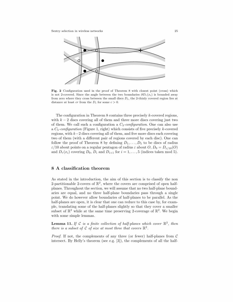
from D1. Thus for n sufficiently large, and hence ε/r sufficiently small, onecan construct six discs Dr(xi), i = 1, . . . , 6, of radius r, such that Dr(xi)contains Di but does not intersect any Dj , j 6= i, when i = 2, 4, 6, and Dr(xi)does not intersect Di, but contains all the Dj , j 6= i, when i = 1, 3, 5. Onecan check (see Figure 2) that the Dr(xi) form a 2-cover of the disc of radiuscr about O for some absolute c > 0. However, D1, D3 and D5 are precisely2-covered by these discs. Suppose that xi ∈ P, but no other point of P lieswithin distance r + 2ε of O. Then the discs are not 2-partitionable, sinceDi is covered only by Dr(xi+2), and Dr(xi+4) (indices mod 6), i = 1, 3, 5,and no 2-colouring of the discs Dr(x1), Dr(x3), Dr(x5) results in D1, D3
and D5 being covered by discs of both colours. It is easy to see that if n issufficiently large then even removing points inside Dr+2ε(O) from P leavesD3r(O) \Dcr(O) k-covered whp. Thus by applying Theorem 3 to the regionSn\D3r(O) we obtain, with probability bounded away from zero, a k-coveredbut not k-partitionable configuration whenever we condition on the event thatP ∩Dr+2ε(O) consists just of the points x1, . . . , x6 plus another k− 2 pointsinside Dr/2(O). It remains to estimate the probability of such a configuration.Clearly, if we do not fix O, then x1 is arbitrary, so we choose x1 to be anypoint of P∩Sn at distance at least r+2ε from ∂Sn (so that our configurationis guaranteed to lie inside Sn). Then x2 is just confined to be within a certaindistance of x1 within a margin of O(r), and hence within a region of areaO(r2). After that, we may assume that the disks D1, . . . , D6 are fixed, so thatthe remaining xi are confined to a region of area O(εr). Thus the probabilityof such a configuration occurring is bounded below by
p = Cnr2(εr)4(r2)k−2e−π(r+2ε)2 .
With ε = 1/r, we obtain p ≥ C ′n(log n)k−1e−πr2= C′
log n , as claimed.
Sentry selection in wireless networks 25
Fig. 2 Configuration used in the proof of Theorem 8 with closest point (cross) whichis not 2-covered. Since the angle between the two boundaries ∂Dr(xi) is bounded awayfrom zero where they cross between the small discs Di, the 2-thinly covered region lies atdistance at least cr from the Di for some c > 0.
The configuration in Theorem 8 contains three precisely k-covered regions,with k − 2 discs covering all of them and three more discs covering just twoof them. We call such a configuration a C3-configuration. One can also usea C5-configuration (Figure 1, right) which consists of five precisely k-coveredregions, with k−2 discs covering all of them, and five more discs each coveringtwo of them (with a different pair of regions covered by each disc). One canfollow the proof of Theorem 8 by defining D1, . . . , D5 to be discs of radiusε/10 about points on a regular pentagon of radius ε about O, D0 = Dε/10(O)and Dr(xi) covering D0, Di and Di+1 for i = 1, . . . , 5 (indices taken mod 5).
8 A classification theorem
As stated in the introduction, the aim of this section is to classify the non2-partitionable 2-covers of R2, where the covers are comprised of open half-planes. Throughout the section, we will assume that no two half-plane bound-aries are equal, and no three half-plane boundaries pass through a singlepoint. We do however allow boundaries of half-planes to be parallel. As thehalf-planes are open, it is clear that one can reduce to this case by, for exam-ple, translating some of the half-planes slightly so that they cover a smallersubset of R2 while at the same time preserving 2-coverage of R2. We beginwith some simple lemmas.
Lemma 11. If C is a finite collection of half-planes which cover R2, thenthere is a subset of C of size at most three that covers R2.
Proof. If not, the complements of any three (or fewer) half-planes from Cintersect. By Helly’s theorem (see e.g. [3]), the complements of all the half-
26 Paul Balister, Bela Bollobas, Amites Sarkar, and Mark Walters
planes from C intersect, contradicting the fact that the original half-planescover R2.
The boundaries of the half-planes form lines which divide R2 into a numberof polygonal (possibly infinite) atomic regions.
Definition 1. A minimal region is an atomic region that is covered bystrictly fewer half-planes than any of its neighbouring regions.
Note that a minimal region may be covered by more half-planes than theleast covered region.
Lemma 12. Suppose C is a finite collection of half-planes which cover R2.Colour some of the half-planes red. If every minimal region is covered by ared half-plane, then the red half-planes cover R2.
Proof. Suppose that A is a non-minimal region that is not covered by a redhalf-plane. One of the regions A′ adjacent to A is covered by a strict subsetof the half-planes covering A, and so is not covered by a red half-plane either.Repeating, and using the fact that A is covered by a finite number of half-planes, we eventually arrive at a minimal region which is not covered by ared half-plane.
Lemma 13. Suppose that the boundary ∂Π of a half-plane Π ∈ C is adjacentto t minimal regions. Then each of these minimal regions is (t− 1)-covered.
Proof. Each of the t minimal regions must lie on the opposite side of ∂Πto Π (since they are minimal). The intersections of (the closures) of theseminimal regions with ∂Π form t disjoint closed intervals I1, . . . , It along ∂Π.Pick one of these intervals Ii. The endpoint(s) of Ii occur where the boundarylines of other half-planes cross ∂Π, Ii itself not being covered by these half-planes. Hence every point in ∂Π \ Ii is covered by one of these half-planes. Inparticular, all the other intervals Ij , j 6= i, are covered by these half-planes.Since two distinct lines can only intersect at a single point, the half-planescorresponding to distinct intervals must be distinct. Thus each interval, andhence its corresponding minimal region, is covered by (at least) (t− 1) half-planes.
Definition 2. A region is precisely k-covered if is is covered by exactly khalf-planes.
Lemma 14. Suppose that C is a 2-cover of R2. Suppose also that the half-planes of C can be 2-coloured so that the precisely 2-covered regions are eachcovered by half-planes of each colour. Then there exists a set of (at most) threehalf-planes Π1,Π2,Π3 ∈ C which covers R2 and such that each precisely 2-covered region is contained in only one of the Πi.
Sentry selection in wireless networks 27
Proof. Let the colours be red and blue, and let the red half-planes beR1, . . . , Rs and the blue half-planes be B1, . . . , Bt. Also, write ri and bj forthe number of precisely 2-covered regions covered by the half-planes Ri andBj respectively. Suppose first that there are at most two red half-planes, R1
and R2 say, with ri > 0. Since removing these half-planes reduces the cover-age of any region by at most two, and all the precisely 2-covered regions arecovered by blue half-planes, the remaining (red and blue) half-planes mustcover R2. Applying Lemma 11 to the remaining half-planes gives the desiredthree (or fewer) half-planes Π1,Π2 and Π3, since all the precisely 2-coveredregions must be covered by either R1 or R2, which are distinct from the Πi,and hence can only be covered by at most one Πi. A similar argument appliesif there are at most two blue half-planes with bj > 0.
Consequently we may assume that there are at least three half-planes ofeach colour, so that s, t ≥ 3, and indeed that at least three of each of the ri
and the bj are positive. Note that no precisely 2-covered region can be coveredby more than one of the Ri, or by more than one of the Bj , by hypothesis,so that
s∑
i=1
ri =t∑
j=1
bj = N,
where N is the number of precisely 2-covered regions. Suppose that at mosttwo of the ri are greater than one. Without loss of generality ri ≤ 1 unlessi = 1 or 2. Now remove R1 and R2. The remaining half-planes still cover R2,so by Lemma 11 we may select three of them which cover R2. Suppose thatthese half-planes are Ri1 , . . . , Rih
and Bj1 , . . . , Bj`where h + ` = 3. Then,
since rir ≤ 1 and there are at least 3 positive bj ,
N ≤h∑
r=1
rir +∑
b=1
bjb≤ h +
∑
b=1
bjb= (3− `) +
∑
b=1
bjb≤
t∑
j=1
bj = N,
so that in fact each precisely 2-covered region is covered exactly once by ourthree half-planes, as required. Hence we may assume that at least three of theri are greater than one, so that in particular there are at least six precisely2-covered regions.
We now claim that there is at most one minimal region M which is coveredmore than twice by C. To see this, fix a precisely 2-covered region A, and letP1 and P2 be the half-planes covering A. For each other minimal region B, Amust lie in at least one of the half-planes forming the boundary of B (since Bis minimal and so R2 \B is covered by these half-planes). Hence all the otherminimal regions lie on the boundary of either P1 or P2. By Lemma 13, atmost three of the precisely 2-covered minimal regions can lie on the boundaryof each Pi. Since there are at least six precisely 2-covered regions, both P1
and P2 are adjacent to at least one precisely 2-covered region. But then byLemma 13 there can be at most three minimal regions lying on each of theboundaries of P1 and P2. Thus there are at most seven minimal regions in
28 Paul Balister, Bela Bollobas, Amites Sarkar, and Mark Walters
total (including A and at most three on each of P1 and P2). Of these at most7 − 6 = 1 can be covered more than twice. Since this region (if it exists) iseither covered by a blue half-plane or a red half-plane, either the blue half-planes or the red half-planes cover all the minimal regions, and hence, byLemma 12, all of R2. Suppose that the red half-planes cover R2, and applyLemma 11. We find three (or fewer) red half-planes covering R2 which satisfyour requirements.
Lemma 15. Suppose C is a finite 2-cover of R2 that is not 2-partitionable.Then the half-planes of C cannot be 2-coloured so that every precisely 2-covered region is covered by half-planes of each colour.
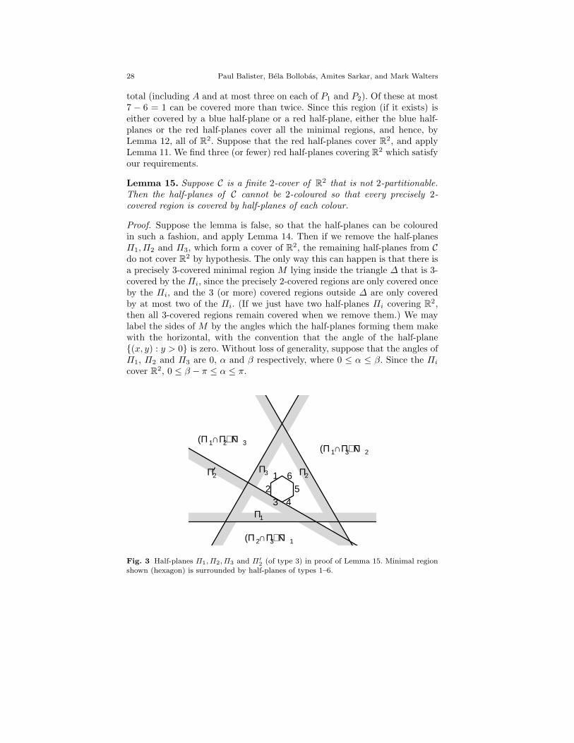
Proof. Suppose the lemma is false, so that the half-planes can be colouredin such a fashion, and apply Lemma 14. Then if we remove the half-planesΠ1, Π2 and Π3, which form a cover of R2, the remaining half-planes from Cdo not cover R2 by hypothesis. The only way this can happen is that there isa precisely 3-covered minimal region M lying inside the triangle ∆ that is 3-covered by the Πi, since the precisely 2-covered regions are only covered onceby the Πi, and the 3 (or more) covered regions outside ∆ are only coveredby at most two of the Πi. (If we just have two half-planes Πi covering R2,then all 3-covered regions remain covered when we remove them.) We maylabel the sides of M by the angles which the half-planes forming them makewith the horizontal, with the convention that the angle of the half-plane(x, y) : y > 0 is zero. Without loss of generality, suppose that the angles ofΠ1, Π2 and Π3 are 0, α and β respectively, where 0 ≤ α ≤ β. Since the Πi
cover R2, 0 ≤ β − π ≤ α ≤ π.
12
3 45
6
Π1
Π2Π3Π2
(Π1∩Π3) Π2
(Π2∩Π3) Π1
(Π1∩Π2) Π3
Fig. 3 Half-planes Π1, Π2, Π3 and Π′2 (of type 3) in proof of Lemma 15. Minimal region
shown (hexagon) is surrounded by half-planes of types 1–6.
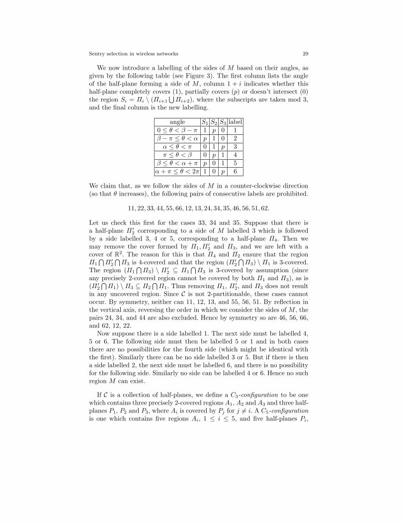
Sentry selection in wireless networks 29
We now introduce a labelling of the sides of M based on their angles, asgiven by the following table (see Figure 3). The first column lists the angleof the half-plane forming a side of M , column 1 + i indicates whether thishalf-plane completely covers (1), partially covers (p) or doesn’t intersect (0)the region Si = Πi \ (Πi+1
⋃Πi+2), where the subscripts are taken mod 3,
and the final column is the new labelling.
angle S1 S2 S3 label0 ≤ θ < β − π 1 p 0 1β − π ≤ θ < α p 1 0 2
α ≤ θ < π 0 1 p 3π ≤ θ < β 0 p 1 4
β ≤ θ < α + π p 0 1 5α + π ≤ θ < 2π 1 0 p 6
We claim that, as we follow the sides of M in a counter-clockwise direction(so that θ increases), the following pairs of consecutive labels are prohibited.
11, 22, 33, 44, 55, 66, 12, 13, 24, 34, 35, 46, 56, 51, 62.
Let us check this first for the cases 33, 34 and 35. Suppose that there isa half-plane Π ′
2 corresponding to a side of M labelled 3 which is followedby a side labelled 3, 4 or 5, corresponding to a half-plane Π4. Then wemay remove the cover formed by Π1,Π
′2 and Π3, and we are left with a
cover of R2. The reason for this is that Π4 and Π2 ensure that the regionΠ1
⋂Π ′
2
⋂Π3 is 4-covered and that the region (Π ′
2
⋂Π3) \Π1 is 3-covered.
The region (Π1
⋂Π3) \ Π ′
2 ⊆ Π1
⋂Π3 is 3-covered by assumption (since
any precisely 2-covered region cannot be covered by both Π1 and Π3), as is(Π ′
2
⋂Π1) \Π3 ⊆ Π2
⋂Π1. Thus removing Π1, Π ′
2, and Π3 does not resultin any uncovered region. Since C is not 2-partitionable, these cases cannotoccur. By symmetry, neither can 11, 12, 13, and 55, 56, 51. By reflection inthe vertical axis, reversing the order in which we consider the sides of M , thepairs 24, 34, and 44 are also excluded. Hence by symmetry so are 46, 56, 66,and 62, 12, 22.
Now suppose there is a side labelled 1. The next side must be labelled 4,5 or 6. The following side must then be labelled 5 or 1 and in both casesthere are no possibilities for the fourth side (which might be identical withthe first). Similarly there can be no side labelled 3 or 5. But if there is thena side labelled 2, the next side must be labelled 6, and there is no possibilityfor the following side. Similarly no side can be labelled 4 or 6. Hence no suchregion M can exist.
If C is a collection of half-planes, we define a C3-configuration to be onewhich contains three precisely 2-covered regions A1, A2 and A3 and three half-planes P1, P2 and P3, where Ai is covered by Pj for j 6= i. A C5-configurationis one which contains five regions Ai, 1 ≤ i ≤ 5, and five half-planes Pi,
30 Paul Balister, Bela Bollobas, Amites Sarkar, and Mark Walters
1 ≤ i ≤ 5, where Ai is covered by Pi and Pi+1, with the subscripts takenmod 5.
Theorem 9. Suppose C is a finite 2-cover of R2 that is not 2-partitionable.Then C contains a C3 or a C5-configuration.
Proof. We define a graph G = (V,E) where the vertices are the half-planes ofC and the edges are the precisely 2-covered regions covered by the half-planescorresponding to their endvertices. This graph is not bipartite, by Lemma 15.Hence it must contain an odd cycle. Suppose first that the vertices of thiscycle correspond to half-planes P1, . . . , Ps, where s is odd and at least seven,and Pi covers the 2-covered regions Ai and Ai+1 (the subscripts taken mods). We observe that any three half-planes from C cannot cover R2 since theycannot even cover the Ai. (The three half-planes include at most three of thePi which between them can cover at most six of the Ai.) Consequently, byLemma 11, C cannot cover R2, a contradiction. Thus G contains a cycle on3 or 5 vertices, corresponding to a C3 or C5-configuration respectively.
9 Deterministic partitionability of k-covers
Theorem 10. Any finite k-cover of R2 by half-planes is dk/2e-partitionable.Conversely, there exists a k-cover of R2 by half-planes which is not d(2k +2)/3e-partitionable.
Proof. A 1-cover or 2-cover is clearly 1-partitionable, so for the first partwe may assume k ≥ 3. We know by Lemma 11 that we can choose threeor fewer half-planes that cover R2. Suppose first that no two half-planescover R2. Choose three half-planes Π1, Π2, Π3 covering R2 with minimaldistance between ∂Π1 and the point of intersection of ∂Π2 and ∂Π3. (Asno two half-planes cover R2, ∂Π2 and ∂Π3 cannot be parallel.) Let ∆ bethe triangle Π1 ∩ Π2 ∩ Π3. Suppose there is a point in ∆ that is preciselyk-covered. Then it must lie in some minimal region M . M consists of apolygonal region whose boundary lies in the interior of ∆ (since no half-plane covering M can have a boundary in common with M). Let p be acorner of M that is closest to ∂Π1. Then the two half-planes Π ′
2 and Π ′3
giving rise to the corner p, together with Π1 cover R2 and p is closer to∂Π1 than ∂Π2 ∩ ∂Π3, contradicting the choice of Π1, Π2,Π3. Thus ∆ is(k + 1)-covered, and removing Π1, Π2, Π3 from the k-cover gives rise to a(k − 2)-cover. If two half-planes Π1, Π2 cover R2, then removing these alsogives rise to a (k− 2)-cover. In either case, by induction on k, the remaininghalf-planes are d(k − 2)/2e-partitionable. Adding the cover Π1, Π2,Π3 orΠ1, Π2 gives a dk/2e-partition as required.
Now consider 2k + 1 half planes all containing the origin, and at anglesthat form all the multiples 2πi/(2k + 1), i = 0, . . . , 2k. Every point in R2 is
Sentry selection in wireless networks 31
covered by at least k of these half-planes, so these half-planes form a k-cover.However, at least three of these half-planes are needed to form any singlecover. Since 3d(2k + 2)/3e ≥ 2k + 2 > 2k + 1, this collection of half-planes isnot d(2k + 2)/3e-partitionable.
Note that the example of failure of d(2k + 2)/3e-partitionability can beextended to covers by discs. Indeed, take an example of this construction andchoose K > 0 so that the half-planes fail to be partitionable even in DK(O).By replacing the half-planes by sufficiently large discs and placing many discsfar from the origin so that every point outside DK(O) is covered, we obtainan example with discs.
References
1. R. Arratia, L. Goldstein and L. Gordon, Two Moments Suffice for Poisson Approxi-mations: The Chen-Stein Method, Ann. Probab. 17 (1989), 9–25.
2. B. Bollobas, Random Graphs, second edition, Cambridge University Press, 2001.3. B. Bollobas, The Art of Mathematics: Coffee Time in Memphis, Cambridge University
Press, 2006.4. E.N. Gilbert, Random plane networks, Journal of the Society for Industrial and Ap-
plied Mathematics 9 (1961), 533–543.5. E.N. Gilbert, The probability of covering a sphere with N circular caps, Biometrika
56 (1965), 323–330.6. P. Hall, On the coverage of k-dimensional space by k-dimensional spheres, Annals of
Probability 13 (1985), 991–1002.7. S. Janson, Random coverings in several dimensions, Acta Mathematica 156 (1986),
83–118.8. S. Kumar, T.H. Lai and J. Balogh, On k-coverage in a mostly sleeping sensor network,
Proceedings of the Tenth International Conference on Mobile Computing Networks(MobiCom 2004).
9. P. Wan and C. Yi, Coverage by randomly deployed wireless sensor networks, IEEETransactions on Information Theory 52 (2006), 2658–2669.
10. H. Zhang and J. Hou, On deriving the upper bound of α-lifetime for large sensornetworks, Proceedings of the Fifth ACM International Symposium on Mobile Ad HocNetwork Computing (MobiHoc 2004).