Citation: Yang, M.; Sun, X.; Jia, F.;

Rushworth, A.; Dong, X.; Zhang, S.;

Fang, Z.; Yang, G.; Liu, B. Sensors

and Sensor Fusion Methodologies for

Indoor Odometry: A Review.

Polymers 2022, 14, 2019. https://

doi.org/10.3390/polym14102019

Academic Editor: Arunas

Ramanavicius

Received: 30 March 2022

Accepted: 11 May 2022

Published: 15 May 2022

Publisher’s Note: MDPI stays neutral

with regard to jurisdictional claims in

published maps and institutional affil-

iations.

Copyright: © 2022 by the authors.

Licensee MDPI, Basel, Switzerland.

This article is an open access article

distributed under the terms and

conditions of the Creative Commons

Attribution (CC BY) license (https://

creativecommons.org/licenses/by/

4.0/).

polymers

Review

Sensors and Sensor Fusion Methodologies for IndoorOdometry: A ReviewMengshen Yang 1,2,3, Xu Sun 1,4,* , Fuhua Jia 1, Adam Rushworth 1,* , Xin Dong 5, Sheng Zhang 6 ,Zaojun Fang 2,3, Guilin Yang 2,3,* and Bingjian Liu 1

1 Department of Mechanical, Materials and Manufacturing Engineering, The Faculty of Science and Engineering,University of Nottingham Ningbo China, Ningbo 315100, China; mengshen.yang@nottingham.edu.cn (M.Y.);fuhua.jia@nottingham.edu.cn (F.J.); bingjian.liu@nottingham.edu.cn (B.L.)

2 Ningbo Institute of Materials Technology and Engineering, Chinese Academy of Sciences,Ningbo 315201, China; fangzaojun@nimte.ac.cn

3 Zhejiang Key Laboratory of Robotics and Intelligent Manufacturing Equipment Technology,Ningbo 315201, China

4 Nottingham Ningbo China Beacons of Excellence Research and Innovation Institute,University of Nottingham Ningbo China, Ningbo 315100, China

5 Department of Mechanical, Materials and Manufacturing Engineering, University of Nottingham,Nottingham NG7 2RD, UK; xin.dong@nottingham.ac.uk

6 Ningbo Research Institute, Zhejiang University, Ningbo 315100, China; szhang1984@zju.edu.cn* Correspondence: xu.sun@nottingham.edu.cn (X.S.); adam.rushworth@nottingham.edu.cn (A.R.);

glyang@nimte.ac.cn (G.Y.)

Abstract: Although Global Navigation Satellite Systems (GNSSs) generally provide adequate accu-racy for outdoor localization, this is not the case for indoor environments, due to signal obstruction.Therefore, a self-contained localization scheme is beneficial under such circumstances. Modernsensors and algorithms endow moving robots with the capability to perceive their environment, andenable the deployment of novel localization schemes, such as odometry, or Simultaneous Localizationand Mapping (SLAM). The former focuses on incremental localization, while the latter stores aninterpretable map of the environment concurrently. In this context, this paper conducts a compre-hensive review of sensor modalities, including Inertial Measurement Units (IMUs), Light Detectionand Ranging (LiDAR), radio detection and ranging (radar), and cameras, as well as applicationsof polymers in these sensors, for indoor odometry. Furthermore, analysis and discussion of thealgorithms and the fusion frameworks for pose estimation and odometry with these sensors areperformed. Therefore, this paper straightens the pathway of indoor odometry from principle toapplication. Finally, some future prospects are discussed.

Keywords: self-contained localization; odometry; SLAM; polymeric sensor; state estimation; sensorfusion; IMU; LiDAR; radar; camera

1. Introduction

Knowing the position of a robot is a requisite condition for conducting tasks such asautonomous navigation, obstacle avoidance, and mobile manipulation. This technologyhas notable economic values, and the global market of indoor Positioning, Localization,and Navigation (PLAN) is expected to reach USD 28.2 billion by 2024 [1]. The socialbenefit of indoor PLAN is also profound, as it may serve as a wayfinder for humans inmetro stations, markets, and airports. In particular, vulnerable people—for instance, theelderly and the visually impaired—may also benefit from this technology. Although GlobalNavigation Satellite Systems (GNSSs) are already a mature solution for precise outdoorlocalization, they may quickly degrade due to satellite coverage fluctuation, multipathreflection, and variation in atmospheric conditions; such degradation is profound in indoorenvironments. To alleviate this effect, several approaches have been proposed, including

Polymers 2022, 14, 2019. https://doi.org/10.3390/polym14102019 https://www.mdpi.com/journal/polymers

Polymers 2022, 14, 2019 2 of 34

magnetic guidance, laser guidance, Wi-Fi, Ultra-Wide Band (UWB), 5G, etc. However, thesemethods require the pre-installation of infrastructure such as beacons, and to change thearrangement of such a system is a tedious task. Thus, a self-contained localization systemis more favorable for agents operating in such indoor environments.

During the past two decades, the self-contained odometry methodologies and Simulta-neous Localization and Mapping (SLAM) technology have developed rapidly and enabledbypassing of the aforementioned problems. Odometry entails deducing the trajectory ofthe moving agent based on readings from observations and, with the initial position andthe path of travel recorded, estimating its current position [2]. Odometry can be regardedas a thread of SLAM, where the aim is to track the position of the robot and to maintain alocal map, while SLAM pursues a globally consistent trajectory and map [3]. Odometryusually serves as the front end of a SLAM system. In this review, onboard sensor systemsas well as the algorithms used for mobile robots’ indoor odometry are our focus.

Materials with novel properties promote the development of odometry technologies.Magnetic materials have been utilized to build compasses for centuries, since the Earth’sgeomagnetic field is able to provide an accurate and reliable reference for orientation. In themodern era, inertial navigation systems built using piezoelectric materials and electro-opticmaterials have emerged. In addition, photoelectric materials and electro-optic materials areapplied in state-of-the-art navigation sensors, including LiDAR and cameras.

Apart from the materials mentioned above, recent advancements in materials andmanufacturing technologies enable polymer-based sensors to be deployed. The first useof polymeric materials in navigation sensors can be traced back to the early 2000s [4].Polymeric materials introduce flexibility to the sensors in terms of both mechanical structureand functionality, and reduce the cost of mass production. Such materials have beenimplemented in odometry sensors such as IMUs and LiDAR. Soft polymeric sensors arealso ideal candidates to be embedded in soft robotics [5]. In this review, the applications ofpolymeric sensors for odometry are also included.

This review paper surveys the literature published in English; the search was mainlyconducted in IEEE Xplore, ScienceDirect, ACM Digital Library, and arXiv. Taking IEEEXplore as an example, the Boolean operators “AND” and “OR” were used for combiningkeywords as well as their synonyms. For polymeric sensors, (“polymeric” OR “polymer”)AND (“accelerometer” OR “gyroscope” OR “LiDAR” OR “Radar”) was used for searchingfor articles; the initial search yielded 407 papers; the papers that explicitly conceptualizedor fabricated a sensor in which polymer materials played a key role—such as an actuator—were retained, while the papers that did not have a major novelty, or concerned the topic ofradar-absorbing materials, were screened. For odometry, (“inertial” OR “IMU” OR “LiDAR”OR “Laser” OR “Radar” OR “visual” OR “vision”) AND (“odometry” OR “localization”OR “SLAM”) was used for searching for publications between 2015 to 2022 within journalsor highly renowned conference proceedings, yielding 7821 papers. Due to the huge amountof results, only papers with more than 50 citations, or papers published after 2020 withmore than 10 citations, were retained at this stage. Among the retained papers, thosepapers using multiple sensors, demonstrating no major novelty in terms of algorithms,focusing mainly on mapping, focused on outdoor environments, or primarily appliedfor mobile phones or pedestrian gait analysis were excluded. For sensor fusion, (“sensorfusion” OR “filter” OR “optimization”) AND (“odometry” OR “localization”) was used forsearching for publications between 2010 and 2022 within renowned journals or conferenceproceedings, yielding 388 papers; those using similar sensor suites and similar fusionframeworks, using inapplicable sensors for indoor mobile robots, or focusing on outdoorenvironments were eliminated. After the preliminary screening, a snowballing search wasconducted with the references from or to the selected papers, to check for additional papers.As a result, a total number of 252 articles was selected for review.

Several reviews have been published on odometry and SLAM. Table 1 summarizesand remarks on some of the representative works from the past five years:

Polymers 2022, 14, 2019 3 of 34

Table 1. Summary of recent reviews on sensors and sensor fusion for SLAM and odometry.

Reference Remarks

Bresson et al. [6] 2017 SLAM in autonomous drivingMohamed et al. [7] 2019 Odometry systems

Huang et al. [8] 2020 Representative LiDAR and visual SLAM systems dictionaryChen et al. [9] 2020

Fayyad et al. [10] 2020 Deep learning for localization and mapping

Yeong et al. [11] 2021 Sensor and sensor calibration methods for robot perceptionEl-Sheimy et al. [1] 2021 Overview of indoor navigation

Taheri et al. [12] 2021 Chronicles of SLAM from 1986–2019Servières et al. [13] 2021 Visual and visual-inertial odometry and SLAM

To the best of our knowledge, existing reviews rarely cover sensing mechanisms,polymer-based sensors, odometry algorithms, and sensor fusion frameworks systematicallyin one paper. A summary table and a highlight of easy-to-use solutions are appended tothe end of each section. This review paper extends previous works from three perspectives:firstly, the operating principles and advancements of sensors for odometry, includingpolymer-based sensors; secondly, a briefing on odometry algorithms and the taxonomyof methods based on their working principles; thirdly, a briefing and taxonomy of sensorfusion techniques for odometry. The paper is organized as follows: Section 2 reviews theoperating principles of sensors for odometry, including IMU, LiDAR, radar, and camera,as well as the corresponding odometry algorithms. A summative table of representativemethods is provided for each sensor. The utilization of polymeric sensors is also presentedaccordingly. Section 3 reviews the sensor fusion methods and their implementation inodometry. Lastly, Sections 4 and 5 present future prospects and conclusions, respectively.

2. Sensors and Sensor-Based Odometry Methods

Sensors are equipped in robotic systems to mimic human sensory systems (e.g., vision,equilibrium, kinesthesia), which provide signals for perception, utilization, and decision.Onboard sensors for mobile robots can be categorized into proprioceptive sensors andexteroceptive sensors, which are sensors for monitoring internal states and the externalenvironment, respectively. Examples of proprioceptive sensors include wheel odometersand IMUs. Examples of exteroceptive sensors include LiDAR, radar, and cameras [14].

Selectivity and sensitivity are two prominent properties of sensors. Sensitivity meansthe lowest power level of the signal as an input from which the sensor can decode infor-mation correctly. Selectivity means the ability to detect and decode signals in the presenceof interfering signals. Advances of materials in device fabrication enable sensors withbetter sensitivity and selectivity to be manufactured. For example, the InGaAs/InP Single-Photon Avalanche Diode (SPAD) can detect the injection of a single photoexcited carrier.SiGe-based radar technology allows high-frequency operation, thus enabling better RFperformances, and even high-resolution imaging is achievable with such sensors [15].

2.1. Wheel Odometer

The word “Odometry” is derived from the odometer, which is a device mounted to awheel to measure the travel distance; it may also be referred to as a wheel encoder. Thereare three types of wheel encoder: the pulsed encoder, single-turn absolute encoder, andmulti-turn absolute encoder. The pulsed encoder is the simplest implementation; it consistsof a Hall sensor with a magnet, or has equally spaced grating to pass or reflect light. It iswidely installed in drive motors for closed-loop control of the motor speed. For example,in the Wheeltec robot, a 500-pulse Hall encoder is used for motor speed feedback. Thesingle-turn absolute encoder has two implementations: The first uses multiple Hall sensorsto determine the absolute rotation angle, and has been used in the Stanford Doggo, whichemploys an AS5047P as the encoder. The second utilizes unequally spaced grating, such asthe Gray code system, in conjunction with a light source and detection system, to determine

Polymers 2022, 14, 2019 4 of 34

the absolute rotation angle. The multi-turn absolute encoder usually consists of severalsingle-turn encoders with a gear set, where the angle and the number of revolutions arerecorded separately.

Several robots, such as TurtleBot and Segway RMP, use encoders for odometry. TheOPS-9 uses two orthogonal wheel encoders, providing planar position information withgood accuracy. Combining learning-based methods with wheel odometers can yield rea-sonably good odometry results. The authors of [16] tested the combination of Gaussianprocesses with neural networks and random variable inference on a publicly available en-coder dataset. A CNN structure was employed for the neural network part, demonstratingbetter trajectory than the physical filters.

2.2. Inertial Measurement Units (IMUs)

The Inertial Measurement Unit (IMU) is a device that is used to estimate the position,velocity, and acceleration of a robot. It is generally composed of a gyroscope, an accelerom-eter, and a magnetometer (optional). Since these devices output the acceleration and theangular rate, other state variables—such as the velocity and the position of the robot—areobtained by integration of the measured data; thus, any drift or bias in the measurement ofacceleration and angular rate will cause accumulation of errors in the estimation of velocityand position. The IMU systems discussed below are of the strapdown type rather than thestable platform (gimbal) type, due to their mechanical simplicity and compactness [17].

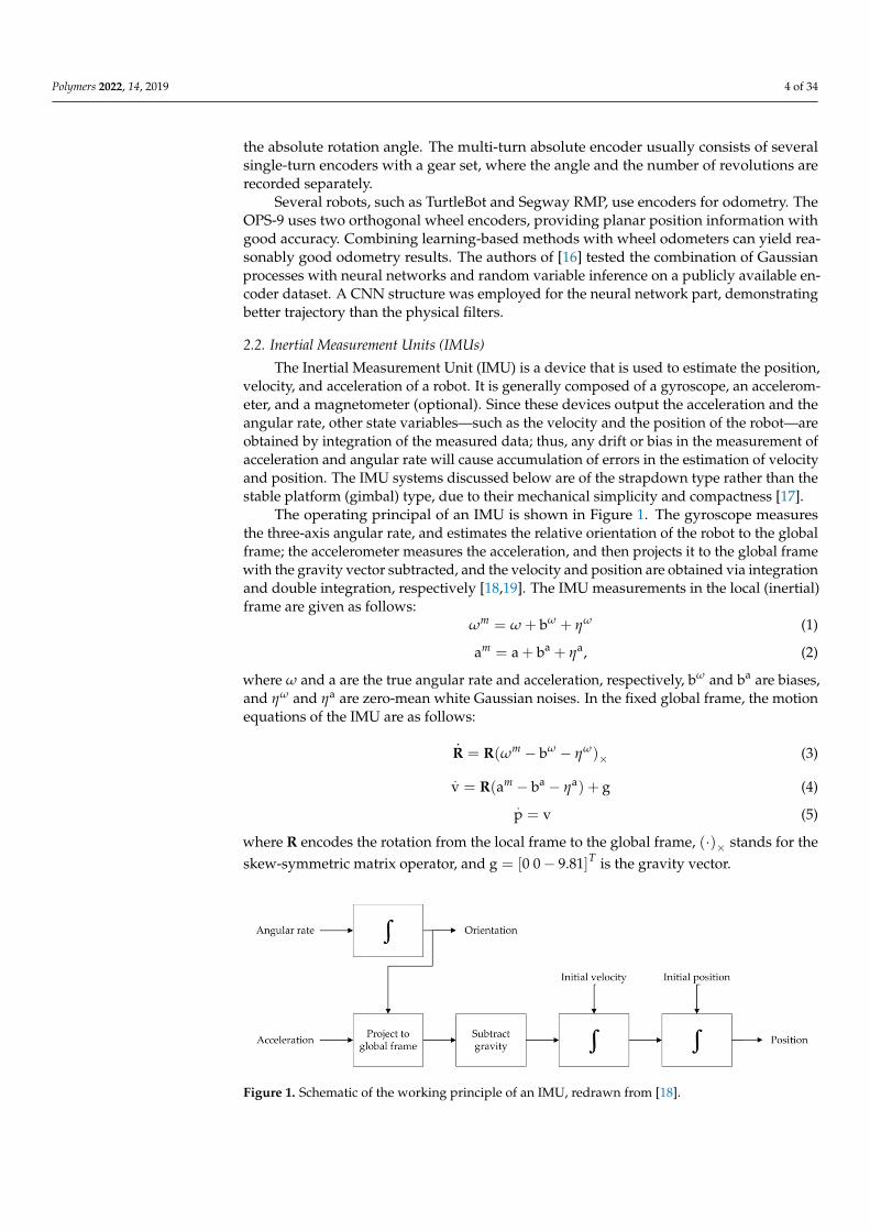
The operating principal of an IMU is shown in Figure 1. The gyroscope measuresthe three-axis angular rate, and estimates the relative orientation of the robot to the globalframe; the accelerometer measures the acceleration, and then projects it to the global framewith the gravity vector subtracted, and the velocity and position are obtained via integrationand double integration, respectively [18,19]. The IMU measurements in the local (inertial)frame are given as follows:

ωm = ω + bω + ηω (1)

am = a + ba + ηa, (2)

where ω and a are the true angular rate and acceleration, respectively, bω and ba are biases,and ηω and ηa are zero-mean white Gaussian noises. In the fixed global frame, the motionequations of the IMU are as follows:

.R = R(ωm − bω − ηω)× (3)

.v = R(am − ba − ηa) + g (4)

.p = v (5)

where R encodes the rotation from the local frame to the global frame, (·)× stands for theskew-symmetric matrix operator, and g = [0 0− 9.81]T is the gravity vector.

Figure 1. Schematic of the working principle of an IMU, redrawn from [18].

Polymers 2022, 14, 2019 5 of 34

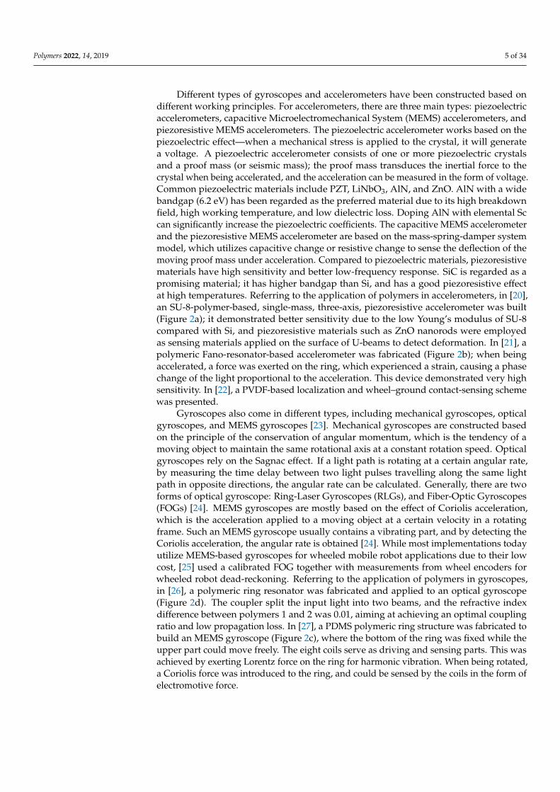
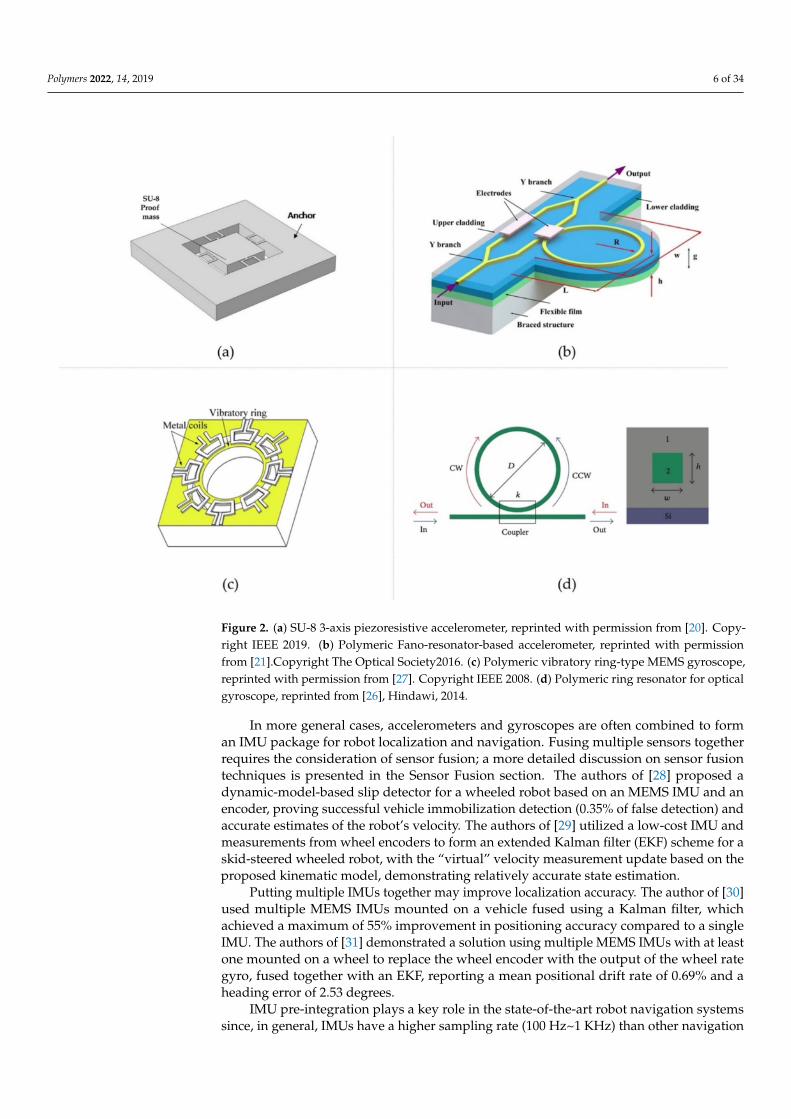
Different types of gyroscopes and accelerometers have been constructed based ondifferent working principles. For accelerometers, there are three main types: piezoelectricaccelerometers, capacitive Microelectromechanical System (MEMS) accelerometers, andpiezoresistive MEMS accelerometers. The piezoelectric accelerometer works based on thepiezoelectric effect—when a mechanical stress is applied to the crystal, it will generatea voltage. A piezoelectric accelerometer consists of one or more piezoelectric crystalsand a proof mass (or seismic mass); the proof mass transduces the inertial force to thecrystal when being accelerated, and the acceleration can be measured in the form of voltage.Common piezoelectric materials include PZT, LiNbO3, AlN, and ZnO. AlN with a widebandgap (6.2 eV) has been regarded as the preferred material due to its high breakdownfield, high working temperature, and low dielectric loss. Doping AlN with elemental Sccan significantly increase the piezoelectric coefficients. The capacitive MEMS accelerometerand the piezoresistive MEMS accelerometer are based on the mass-spring-damper systemmodel, which utilizes capacitive change or resistive change to sense the deflection of themoving proof mass under acceleration. Compared to piezoelectric materials, piezoresistivematerials have high sensitivity and better low-frequency response. SiC is regarded as apromising material; it has higher bandgap than Si, and has a good piezoresistive effectat high temperatures. Referring to the application of polymers in accelerometers, in [20],an SU-8-polymer-based, single-mass, three-axis, piezoresistive accelerometer was built(Figure 2a); it demonstrated better sensitivity due to the low Young’s modulus of SU-8compared with Si, and piezoresistive materials such as ZnO nanorods were employedas sensing materials applied on the surface of U-beams to detect deformation. In [21], apolymeric Fano-resonator-based accelerometer was fabricated (Figure 2b); when beingaccelerated, a force was exerted on the ring, which experienced a strain, causing a phasechange of the light proportional to the acceleration. This device demonstrated very highsensitivity. In [22], a PVDF-based localization and wheel–ground contact-sensing schemewas presented.

Gyroscopes also come in different types, including mechanical gyroscopes, opticalgyroscopes, and MEMS gyroscopes [23]. Mechanical gyroscopes are constructed basedon the principle of the conservation of angular momentum, which is the tendency of amoving object to maintain the same rotational axis at a constant rotation speed. Opticalgyroscopes rely on the Sagnac effect. If a light path is rotating at a certain angular rate,by measuring the time delay between two light pulses travelling along the same lightpath in opposite directions, the angular rate can be calculated. Generally, there are twoforms of optical gyroscope: Ring-Laser Gyroscopes (RLGs), and Fiber-Optic Gyroscopes(FOGs) [24]. MEMS gyroscopes are mostly based on the effect of Coriolis acceleration,which is the acceleration applied to a moving object at a certain velocity in a rotatingframe. Such an MEMS gyroscope usually contains a vibrating part, and by detecting theCoriolis acceleration, the angular rate is obtained [24]. While most implementations todayutilize MEMS-based gyroscopes for wheeled mobile robot applications due to their lowcost, [25] used a calibrated FOG together with measurements from wheel encoders forwheeled robot dead-reckoning. Referring to the application of polymers in gyroscopes,in [26], a polymeric ring resonator was fabricated and applied to an optical gyroscope(Figure 2d). The coupler split the input light into two beams, and the refractive indexdifference between polymers 1 and 2 was 0.01, aiming at achieving an optimal couplingratio and low propagation loss. In [27], a PDMS polymeric ring structure was fabricated tobuild an MEMS gyroscope (Figure 2c), where the bottom of the ring was fixed while theupper part could move freely. The eight coils serve as driving and sensing parts. This wasachieved by exerting Lorentz force on the ring for harmonic vibration. When being rotated,a Coriolis force was introduced to the ring, and could be sensed by the coils in the form ofelectromotive force.

Polymers 2022, 14, 2019 6 of 34

Figure 2. (a) SU-8 3-axis piezoresistive accelerometer, reprinted with permission from [20]. Copy-right IEEE 2019. (b) Polymeric Fano-resonator-based accelerometer, reprinted with permissionfrom [21].Copyright The Optical Society2016. (c) Polymeric vibratory ring-type MEMS gyroscope,reprinted with permission from [27]. Copyright IEEE 2008. (d) Polymeric ring resonator for opticalgyroscope, reprinted from [26], Hindawi, 2014.

In more general cases, accelerometers and gyroscopes are often combined to forman IMU package for robot localization and navigation. Fusing multiple sensors togetherrequires the consideration of sensor fusion; a more detailed discussion on sensor fusiontechniques is presented in the Sensor Fusion section. The authors of [28] proposed adynamic-model-based slip detector for a wheeled robot based on an MEMS IMU and anencoder, proving successful vehicle immobilization detection (0.35% of false detection) andaccurate estimates of the robot’s velocity. The authors of [29] utilized a low-cost IMU andmeasurements from wheel encoders to form an extended Kalman filter (EKF) scheme for askid-steered wheeled robot, with the “virtual” velocity measurement update based on theproposed kinematic model, demonstrating relatively accurate state estimation.

Putting multiple IMUs together may improve localization accuracy. The author of [30]used multiple MEMS IMUs mounted on a vehicle fused using a Kalman filter, whichachieved a maximum of 55% improvement in positioning accuracy compared to a singleIMU. The authors of [31] demonstrated a solution using multiple MEMS IMUs with at leastone mounted on a wheel to replace the wheel encoder with the output of the wheel rategyro, fused together with an EKF, reporting a mean positional drift rate of 0.69% and aheading error of 2.53 degrees.

IMU pre-integration plays a key role in the state-of-the-art robot navigation systemssince, in general, IMUs have a higher sampling rate (100 Hz~1 KHz) than other navigation

Polymers 2022, 14, 2019 7 of 34

sensors; thus, combining serial IMU readings into a single measurement becomes desirable.This method was discussed in [32–34], and is transcribed here as follows:

∆Rij = RTi Rj (6)

∆vij = RTi(vj − vi − g∆tij

)(7)

∆pij = RTi

(pj − pi − vi∆tij −

12

g∆t2ij

). (8)

In terms of currently available solutions, Xsens [35] and Microstrain [36] offer IMUsand development kits for visualization and log data, and can stream odometry data via anROS API. This is also achievable with a low-cost IMU using Arduino [37]. For an in-depthreview of modern inertial navigation systems and commercially available products, pleaserefer to [24,38].

2.3. LiDAR

LiDAR is named after its working principle and function, which is Light Detection andRanging. The authors of [39–42] conducted comprehensive reviews of the principles andapplications of modern LiDAR systems. Based on its working principles, LiDAR can becategorized into Time-of-Flight (ToF) LiDAR and Frequency-Modulated Continuous-Wave(FMCW) LiDAR. ToF LiDAR measures range by comparing the elapsed time between thetransmitted and received signal. It dominates the market due to its simple structure, but itsuffers issues such as interference from sunlight or other LiDAR devices. FMCW LiDARadopts the same principle as FMCW radar—the transmitted laser frequency is modulatedlinearly against the time, and then both the range and the velocity of the observed objectcan be translated from the frequency difference between the transmitted and received laserwave. One notable advantage of FMCW LiDAR is its ability to directly retrieve velocityfrom the measurements.

Based on the laser beam steering mechanism, LiDAR can be further categorized intomechanical LiDAR and solid-state LiDAR. Mechanical steering of the laser beam actuatedby a motor is the most popular solution at present due to its large Field of View (FOV), butit usually results in a very bulky implementation, and is susceptible to distortion causedby motion. Solid-state LiDAR comes in multiple forms, including MEMS LiDAR, FLASHLiDAR, and Optical Phased Array (OPA) LiDAR. Here solid-state refers to a steeringsystem without bulky mechanical moving parts. MEMS LiDAR consists of a micromirrorembedded in a chip, the tilting angle of which is controlled by the electromagnetic force andthe elastic force, resulting in a relatively small FOV (typically 20–50 degrees horizontally).Due to its compact size and low weight, MEMS LiDAR can be used for robotic applications,where size and weight requirements are stringent [43]. Ref. [44] developed and fabricatedan MEMS LiDAR for robotic and autonomous driving applications. The authors of [45]presented an algorithm for such small-FOV solid-state LiDAR odometry, mitigating theproblems of small FOV, irregular scanning pattern, and non-repetitive scanning by linearinterpolation, and demonstrating a trajectory drift of 0.41% and an average rotational errorof 1.1 degrees. FLASH LiDAR operates in a similar way to a camera using a flashlight—a single laser is spread to illuminate the area at once, and a 2D photodiode detectionarray is used to capture the laser’s return. Since the imaging of the scene is performedsimultaneously, movement compensation of the platform is unnecessary. This methodhas been used for pose estimation of space robots, as demonstrated by [46,47]. The maindrawbacks of FLASH LiDAR are its limited detection range (limited laser power for eyeprotection) and relatively narrow FOV. OPA LiDAR controls the optical wavefront bymodulating the speed of light passing through each antenna; ref. [48] presents a realizationand application of such a device.

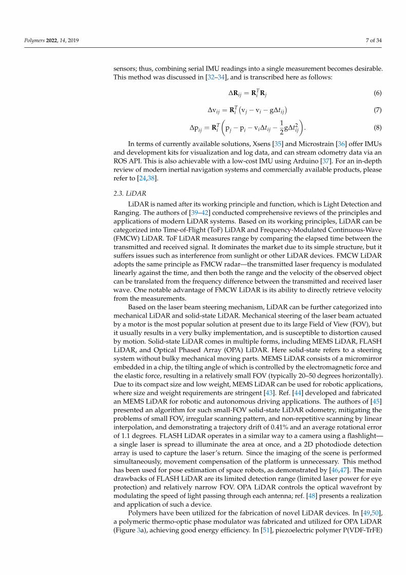
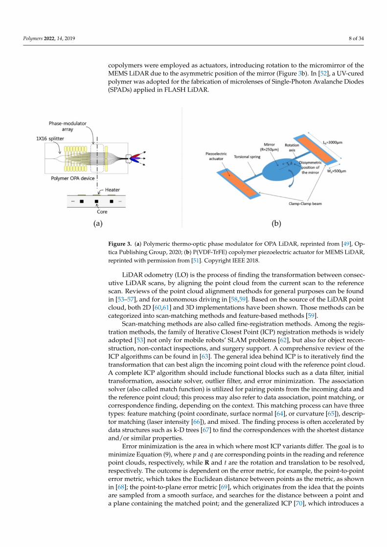
Polymers have been utilized for the fabrication of novel LiDAR devices. In [49,50],a polymeric thermo-optic phase modulator was fabricated and utilized for OPA LiDAR(Figure 3a), achieving good energy efficiency. In [51], piezoelectric polymer P(VDF-TrFE)

Polymers 2022, 14, 2019 8 of 34

copolymers were employed as actuators, introducing rotation to the micromirror of theMEMS LiDAR due to the asymmetric position of the mirror (Figure 3b). In [52], a UV-curedpolymer was adopted for the fabrication of microlenses of Single-Photon Avalanche Diodes(SPADs) applied in FLASH LiDAR.

Figure 3. (a) Polymeric thermo-optic phase modulator for OPA LiDAR, reprinted from [49], Op-tica Publishing Group, 2020; (b) P(VDF-TrFE) copolymer piezoelectric actuator for MEMS LiDAR,reprinted with permission from [51]. Copyright IEEE 2018.

LiDAR odometry (LO) is the process of finding the transformation between consec-utive LiDAR scans, by aligning the point cloud from the current scan to the referencescan. Reviews of the point cloud alignment methods for general purposes can be foundin [53–57], and for autonomous driving in [58,59]. Based on the source of the LiDAR pointcloud, both 2D [60,61] and 3D implementations have been shown. Those methods can becategorized into scan-matching methods and feature-based methods [59].

Scan-matching methods are also called fine-registration methods. Among the regis-tration methods, the family of Iterative Closest Point (ICP) registration methods is widelyadopted [53] not only for mobile robots’ SLAM problems [62], but also for object recon-struction, non-contact inspections, and surgery support. A comprehensive review of theICP algorithms can be found in [63]. The general idea behind ICP is to iteratively find thetransformation that can best align the incoming point cloud with the reference point cloud.A complete ICP algorithm should include functional blocks such as a data filter, initialtransformation, associate solver, outlier filter, and error minimization. The associationsolver (also called match function) is utilized for pairing points from the incoming data andthe reference point cloud; this process may also refer to data association, point matching, orcorrespondence finding, depending on the context. This matching process can have threetypes: feature matching (point coordinate, surface normal [64], or curvature [65]), descrip-tor matching (laser intensity [66]), and mixed. The finding process is often accelerated bydata structures such as k-D trees [67] to find the correspondences with the shortest distanceand/or similar properties.

Error minimization is the area in which where most ICP variants differ. The goal is tominimize Equation (9), where p and q are corresponding points in the reading and referencepoint clouds, respectively, while R and t are the rotation and translation to be resolved,respectively. The outcome is dependent on the error metric, for example, the point-to-pointerror metric, which takes the Euclidean distance between points as the metric, as shownin [68]; the point-to-plane error metric [69], which originates from the idea that the pointsare sampled from a smooth surface, and searches for the distance between a point anda plane containing the matched point; and the generalized ICP [70], which introduces a

Polymers 2022, 14, 2019 9 of 34

probabilistic representation of the points, and can be viewed as a plane-to-plane error metric.LiTAMIN2 [71] introduced an additional K–L divergence that evaluates the difference inthe distribution shape, which can perform well even when the points for registration arerelatively sparse.

(q− (Rp + t))T(q− (Rp + t)) (9)

A major drawback of ICP is that it relies heavily on the initial guess. Therefore,ICP is susceptible to local minima [72]. To address this issue, a global method based onunique features without the need for initial assumption was developed. The authors of [68]proposed a globally optimized ICP that integrates the Branch-and-Bound (BnB) algorithm;the ICP searches the local minima, while the BnB algorithm helps it to jump out of the localminima, and together they converge to the global minima.

Another disadvantage of ICP is that it is a discrete sampling of the environment. Toaddress the effect of uneven LiDAR points, the Normal Distribution Transform (NDT)was introduced for both 2D registration [73] and 3D registration [74]. Instead of usingindividual LiDAR points, the normal distributions give a piecewise smooth Gaussianprobability distribution of the point cloud, thus avoiding the time-consuming nearest-neighbors search and memory-inefficient complete point cloud set storage. The NDT firstequally divides the space occupied by the scan into cells, and then calculates the meanvector q and the covariance matrix C for each cell of the fixed reference scan. The goalis to find the transformation of R and t that can minimize the score function (Equation(10)) using Newton’s optimization method. Since this process iterates over all points in theincoming scan, this is called a Point-to-Distribution (P2D) NDT registration algorithm.

(q− (Rp + t))TC−1(q− (Rp + t)) (10)

If the registration is directly performed on the distribution model of both scans, then itbecomes a Distribution-to-Distribution (D2D) NDT registration algorithm [75]. This methodshares many similarities with generalized ICP in the distance error metric function, butperforms more accurately and faster compared with the generalized ICP and the standardP2D [76]. An NDT histogram of plane orientation is also computed in this method, forbetter initial transformation estimation. However, in some cases it is still susceptible to localminima. The Gaussian Mixture Map (GMM) method [77,78] has similarities with the NDTmethods, since they both maximize the probability of drawing the transformed scan fromthe reference scan, which constructs a Gaussian mixture model over the z-height of the3D LiDAR scan, and then uses a multiresolution Branch-and-Bound search to reach globaloptima. The Coherent Point Drift (CPD) algorithm is also based on the GMM method [79].The Closet Probability and Feature Grid (CPFG)-SLAM [80] is inspired by both ICP andNDT, searching for the nearest-neighbor grid instead of the nearest-neighbor point, andcan achieve a more efficient registration of the point cloud in the off-road scenario.

Other registration methods include the Random Sample Consensus (RANSAC) algorithm-based registration method [81], which randomly chooses minimal points from each scan andthen calculates the transformation, and the transformation with the largest number of inliersis selected and returned. Its time complexity depends on the subset size, the inlier ratio,and the number of data points; thus, its runtime can be prohibitively high in some cases.The Implicit Moving Least-Squares (IMLS) method leverages a novel sampling strategyand an implicit surface matching method, and demonstrates excellent matching accuracy,but is hard to operate in real time [82]. The Surface Element (Surfel) method [83–85] canrepresent a large-scale environment while maintaining dense geometric information at thesame time. MULLS-ICP categorizes points into ground, facade, pillar, and beam, which arethen registered by the multimetric ICP [86].

Feature-based methods extract relevant features from the point clouds, and thenuse them for successive pose estimation. Since these methods only use a selected partof the point cloud, they can be treated as “sparse” methods. Features are the pointswith distinct geometry within a locality [87]. Feature-based methods generally consist of

Polymers 2022, 14, 2019 10 of 34

three main phases: key point detection, feature description, and matching [88]. Summaryand evaluation of the 3D feature descriptors can be found in [87–89]. Several featuredescriptors—including the spinning images (SI) [90], the Fast Point Feature Histograms(FPFHs) [91], the Shape Context (SC) [92,93], and the Signature of Histograms of Orien-tations (SHOT) [94,95]—are applied for point cloud registration and loop-closure detec-tion [60,93,95,96]. According to [97], SHOT is the descriptor that can give the fastest andmost accurate results in the test. Feature descriptor methods are often employed in initialtransformation calculations or loop-closure detection problems.

The state-of-the-art feature-based method LiDAR Odometry And Mapping (LOAM)has held first place in the KITTI odometry benchmark since it was first introduced in [98].LOAM achieves both low drift and low computational complexity by running two algo-rithms in parallel. Feature points are selected as edge points with low smoothness andplanar points with high smoothness, and then the transformation between consecutivescans is found by minimizing the point-to-edge distance for edge points and the point-to-plane distance for planar points, using the Levenberg–Marquardt (L–M) method. Inspiredby LOAM, several methods have been proposed, including LeGO-LOAM [99], which firstsegments the raw point cloud using a range image, and then extracts features via a similarprocess to that used in LOAM, and performs a two-step L–M optimization; that is, [tx, ty,θyaw] are estimated using the edge features, while [tz, θroll , θpitch] are estimated using theplanar features. A summative table of representative LiDAR odometry methods is shownin Table 2.

In terms of currently available solutions, SLAMTEC offers user-friendly software [100]for robotic odometry, mapping, and control, with low-cost LiDAR. Livox offers productsand packages for odometry and mapping. Cartographer is a widely used package forodometry and mapping with LiDAR.

Table 2. Summary of representative LiDAR odometry (LO).

Category Method Loop-ClosureDetection Accuracy 1 Runtime 1

Scan-matching

ICP [70] No Medium HighNDT [76] No Medium HighGMM [77] No Medium -IMLS [82] No High High

MULLS [86] Yes High MediumSurfel-based [83] Yes Medium Medium

DLO [101] No High LowELO [102] No High Low

Feature-based

Feature descriptor [97] No Low HighLOAM [98] No High Medium

LeGO-LOAM [99] No High LowSA-LOAM [103] Yes High Medium

1 Adopted from [58,104].

2.4. Millimeter Wave (MMW) Radar

Radar stands for radio detection and ranging, which is another type of rangefinder. Itis based on the emission and detection of electromagnetic waves in the radio frequencyranging from 3 MHz to 300 GHz (with wavelengths from 100 m to 1 mm). The radarequation (Equation (11)) depicts how the expected received power pr is a function of thetransmitted power pt, the antenna gain G, and the wavelength λ, as well as the RadarCross-Section (RCS) σ and the range r from the target. Compared with its counterpartLiDAR, radar has superior detection performance under extreme weather conditions, sincewaves within this spectrum have weak interaction with dust, fog, rain, and snow. TheMillimeter Wave (MMW) spectrum ranges from 30 GHz to 300 GHz (with wavelengths

Polymers 2022, 14, 2019 11 of 34

from 10 mm to 1 mm), which provides wide bandwidth and narrow beams for sensing,thus allowing finer resolution [105,106].

pr =ptG2λ2σ

(4π)3r4(11)

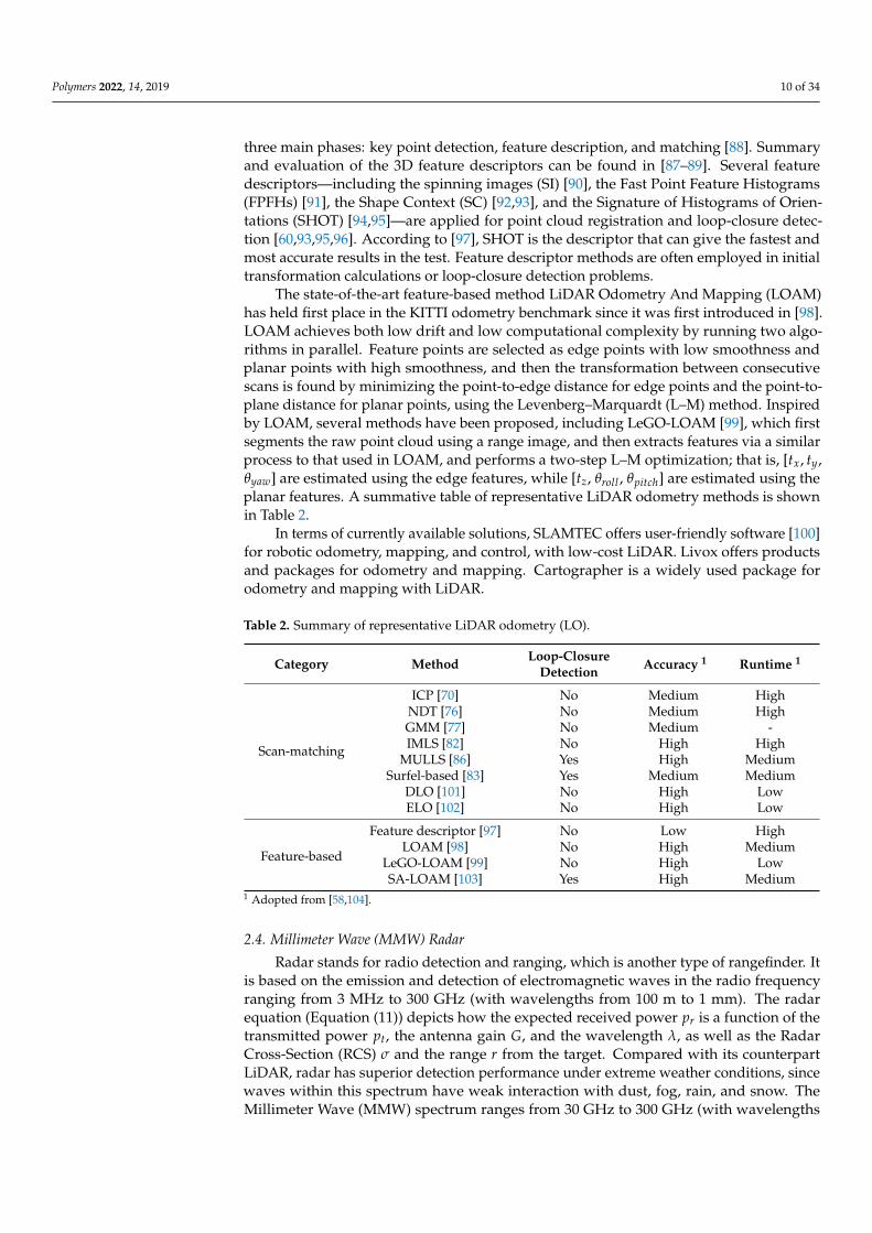
In terms of polymer utilization in radar, Liquid Crystal Polymer (LCP) is regardedas a promising candidate as a substrate for MMW applications due to its flexibility, lowdielectric loss, lower moisture absorption, and ability to withstand temperatures up to300 C [107]. The use of HDPE as a dielectric waveguide for distributed flexible anten-nas for proximity measurement in robotics applications is presented in [108] (Figure 4a).The use of conducting polymers such as polyaniline (PANI), doped with multiwalledcarbon nanotubes, in the fabrication of antennas has demonstrated excellent flexibility andconformality in RF device manufacture [109] (Figure 4b).

Figure 4. (a) HDPE as a dielectric waveguide for distributed radar antennas, reprinted with permis-sion from [108]. Copyright IEEE 2019. (b) PANI/MWCNT fabricated antenna on a Kapton substrate,demonstrating good flexibility; reprinted with permission from [109]. Copyright John Wiley andSons 2018.

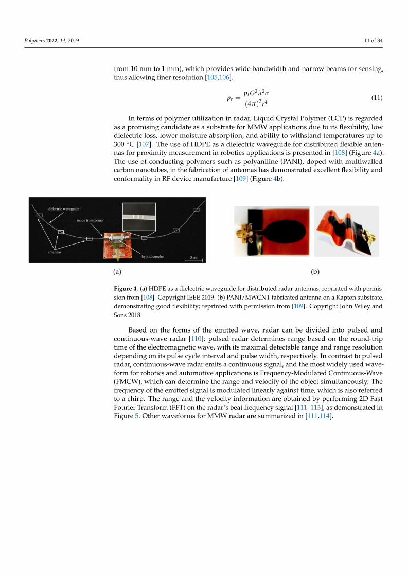
Based on the forms of the emitted wave, radar can be divided into pulsed andcontinuous-wave radar [110]; pulsed radar determines range based on the round-triptime of the electromagnetic wave, with its maximal detectable range and range resolutiondepending on its pulse cycle interval and pulse width, respectively. In contrast to pulsedradar, continuous-wave radar emits a continuous signal, and the most widely used wave-form for robotics and automotive applications is Frequency-Modulated Continuous-Wave(FMCW), which can determine the range and velocity of the object simultaneously. Thefrequency of the emitted signal is modulated linearly against time, which is also referredto a chirp. The range and the velocity information are obtained by performing 2D FastFourier Transform (FFT) on the radar’s beat frequency signal [111–113], as demonstrated inFigure 5. Other waveforms for MMW radar are summarized in [111,114].

Polymers 2022, 14, 2019 12 of 34

Figure 5. 2D FFT of the beat frequency signal, redrawn from [115]. Copyright River Publishers 2017.

The angular location of detection should be discriminated so that the location of theobjects can be resolved. Thanks to the short wavelength of MMW, the aperture size of radarantennas can be made small; hence, many antennas can be densely packed to form an array.With at least two receiver antennas, the Angle of Arrival (AoA) can be calculated from themeasured phase difference at different receivers, which can be performed via 3D FFT [116].A commonly used AoA measurement principle is called Multiple-Input–Multiple-Output(MIMO), which utilizes multiple transmitters and receivers to form an antenna array.Spaced real and virtual receivers can thus calculate the elevation and azimuth angle basedon the phase shift in the corresponding directions. The virtue of a fixed antenna array isthat the examined region is captured instantaneously; hence, no distortion will appeardue to sensor movement and, thus, most automotive radar adopts this configuration. Inaddition to MIMO, the AoA can also be measured by a spinning directive antenna, foreach moment the radar outputs an 1D power–range spectrum for the inspected line ofsight, where the azimuth angle is the radar’s own azimuth angle relative to the fixedcoordinate [115]. In [117,118], a designated spinning radar device called PELICAN wasconstructed and evaluated for mobile robotics applications.

An overview of MMW radar applications in robotics and autonomous vehicles canbe found in [119,120]. Radar-based odometry methods can be classified into direct andindirect methods [121,122]; similar to LO, indirect methods involve feature extractionand association, whereas direct methods forego these procedures. Among the directmethods, in [123], the Fourier–Mellin Transform (FMT) is used for registering radar imagesin sequence, which relies on the translational and rotational properties of the Fouriertransformation [124]. Similarly, FMT is also leveraged in [125], where the rotation andtranslation are calculated in a decoupled fashion, and a local graph optimization process isincluded. Since Doppler radar can measure radial velocity directly, the relative velocityof a stationary target is equal to the inverse sensor velocity. This method is implementedin [126–129], where a RANSAC algorithm is invoked for non-stationary outlier removal.Meanwhile, in [127], the 2D point-to-point ICP is used to obtain finer odometry results.Since Doppler measurement cannot survey rotational ego-motion directly, a hybrid methodis used in [130] for angular rate measurement.

Among the indirect methods, some classical work in SLAM was carried out with theaid of MMW radar, including [131], which incorporated it with a Kalman filter frameworkoperating in an environment with well-separated reflective beacons. The authors of [132]conducted a series of thorough works on mobile robot localization with MMW radar. Intheir work, new feature-extraction algorithms—Target Presence Probability (TPP) and aconfidential model—showed superior performance compared with constant thresholding

Polymers 2022, 14, 2019 13 of 34

and Constant False Alarm Rate (CFAR) [133]. Since radar detection can be impaired byfalse alarms and clutter, feature association may become problematic; thus, the featuremeasurements would be better modeled as Random Finite Sets (RFSs) with arbitrarynumbers of measurements and orders, and incorporated with the RB (Rao–Blackwellized)-PHD (Probability Hypothesis Density) filter [134,135] for map building and odometry.

Some more recent works include [136], which extracts the Binary Annular StatisticsDescriptor (BASD) for feature matching, and then performs graph optimization; and [137],where SURF and M2DP [96] descriptors are computed from radar point clouds for featureassociation and loop-closure detection, respectively; as well as the use of SIFT in [138].Radar measurements are noisy and, thus, may worsen the performance of scan-matchingalgorithms used for LiDAR, such as ICP and NDT; nevertheless, G-ICP [70] showed goodvalidity in [139], where the covariance of each measurement was assigned according toits range; the same can be said of NDT in [140] and GMM in [141], which incorporateddetection clustering algorithms including k-means, DBSCAN, and OPTICS. In [142], RadarCross-Section (RCS) was used as a cue for assisting with feature extraction and CorrelativeScan Matching (CSM). The authors of [143,144] devised a new feature-extraction algorithmfor MMW radar power–range spectra, plus a multipath reflection removal process, andthen performed data association via graph matching.

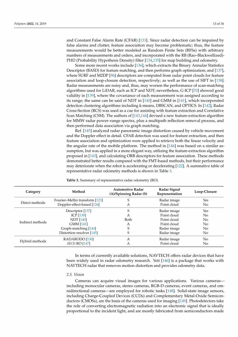
Ref. [145] analyzed radar panoramic image distortion caused by vehicle movementand the Doppler effect in detail. CFAR detection was used for feature extraction, and thenfeature association and optimization were applied to retrieve both the linear velocity andthe angular rate of the mobile platform. The method in [146] was based on a similar as-sumption, but was applied in a more elegant way, utilizing the feature-extraction algorithmproposed in [143], and calculating ORB descriptors for feature association. These methodsdemonstrated better results compared with the FMT-based methods, but their performancemay deteriorate when the robot is accelerating or decelerating [122]. A summative table ofrepresentative radar odometry methods is shown in Table 3.

Table 3. Summary of representative radar odometry (RO).

Category Method Automotive Radar(A)/Spinning Radar (S)

Radar SignalRepresentation Loop-Closure

Direct methodsFourier–Mellin transform [123] S Radar image Yes

Doppler-effect-based [126] A Point cloud No

Indirect methods

Descriptor [137] S Radar image YesICP [139] A Point cloud No

NDT [140] Both Point cloud NoGMM [141] A Point cloud No

Graph-matching [144] S Radar image NoDistortion resolver [145] S Radar image No

Hybrid methods RADARODO [130] A Radar image NoSE(3) RO [147] A Point cloud No

In terms of currently available solutions, NAVTECH offers radar devices that havebeen widely used in radar odometry research. Yeti [146] is a package that works withNAVTECH radar that removes motion distortion and provides odometry data.

2.5. Vision

Cameras can acquire visual images for various applications. Various cameras—including monocular cameras, stereo cameras, RGB-D cameras, event cameras, and om-nidirectional cameras—are employed for robotic tasks [148]. Solid-state image sensors,including Charge-Coupled Devices (CCDs) and Complementary Metal-Oxide Semicon-ductors (CMOSs), are the basis of the cameras used for imaging [149]. Photodetectors takethe role of converting electromagnetic radiation into an electronic signal that is ideallyproportional to the incident light, and are mostly fabricated from semiconductors made

Polymers 2022, 14, 2019 14 of 34

from materials such as Si, GaAs, InSb, InAs, and PbSe. When a photon is absorbed, itcreates a charge-carrier pair, and the movement of charge carriers produces a photocurrentto be detected. Compared with inorganic photodetectors, organic photodetectors exhibitattractive properties such as flexibility, light weight, and semi-transparency. Heterojunctiondiodes based on polymers such as P3HT:PC71BM, PCDTBT:PC71BM, and P3HT:PC61BM asthe photon active layer are fabricated [150]. Organic photodetectors can be classified intoorganic photoconductors, organic photon transistors, organic photomultiplication devices,and organic photodiodes. These organic photodetectors demonstrate utility in imagingsensors [151]. As a recent topic of interest, narrowband photodetectors can be fabricatedfrom materials with narrow bandgaps, exhibiting high selectivity of wavelength [152].

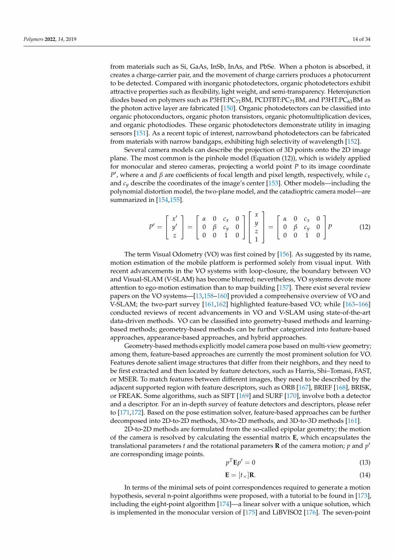
Several camera models can describe the projection of 3D points onto the 2D imageplane. The most common is the pinhole model (Equation (12)), which is widely appliedfor monocular and stereo cameras, projecting a world point P to its image coordinateP′, where α and β are coefficients of focal length and pixel length, respectively, while cxand cy describe the coordinates of the image’s center [153]. Other models—including thepolynomial distortion model, the two-plane model, and the catadioptric camera model—aresummarized in [154,155].

P′ =

x′

y′

z

=

α 0 cx 00 β cy 00 0 1 0

xyz1

=

α 0 cx 00 β cy 00 0 1 0

P (12)

The term Visual Odometry (VO) was first coined by [156]. As suggested by its name,motion estimation of the mobile platform is performed solely from visual input. Withrecent advancements in the VO systems with loop-closure, the boundary between VOand Visual-SLAM (V-SLAM) has become blurred; nevertheless, VO systems devote moreattention to ego-motion estimation than to map building [157]. There exist several reviewpapers on the VO systems—[13,158–160] provided a comprehensive overview of VO andV-SLAM; the two-part survey [161,162] highlighted feature-based VO; while [163–166]conducted reviews of recent advancements in VO and V-SLAM using state-of-the-artdata-driven methods. VO can be classified into geometry-based methods and learning-based methods; geometry-based methods can be further categorized into feature-basedapproaches, appearance-based approaches, and hybrid approaches.

Geometry-based methods explicitly model camera pose based on multi-view geometry;among them, feature-based approaches are currently the most prominent solution for VO.Features denote salient image structures that differ from their neighbors, and they need tobe first extracted and then located by feature detectors, such as Harris, Shi–Tomasi, FAST,or MSER. To match features between different images, they need to be described by theadjacent supported region with feature descriptors, such as ORB [167], BRIEF [168], BRISK,or FREAK. Some algorithms, such as SIFT [169] and SURF [170], involve both a detectorand a descriptor. For an in-depth survey of feature detectors and descriptors, please referto [171,172]. Based on the pose estimation solver, feature-based approaches can be furtherdecomposed into 2D-to-2D methods, 3D-to-2D methods, and 3D-to-3D methods [161].

2D-to-2D methods are formulated from the so-called epipolar geometry; the motionof the camera is resolved by calculating the essential matrix E, which encapsulates thetranslational parameters t and the rotational parameters R of the camera motion; p and p′

are corresponding image points.pTEp′ = 0 (13)

E = [t×]R. (14)

In terms of the minimal sets of point correspondences required to generate a motionhypothesis, several n-point algorithms were proposed, with a tutorial to be found in [173],including the eight-point algorithm [174]—a linear solver with a unique solution, whichis implemented in the monocular version of [175] and LiBVISO2 [176]. The seven-point

Polymers 2022, 14, 2019 15 of 34

algorithm applies the rank-constraint of the essential matrix [177], and is more efficient inthe presence of outliers, but there may exist three solutions, and all three must be tested. Thesix-point algorithm further imposes the trace-constraint of the essential matrix, and mayreturn either a single solution [178] or up to six solutions [179]; the former cannot performin the presence of a planar scene [180]. The six-point algorithm may also serve as a minimalsolver for a partially calibrated camera with unknown focal length [181,182]. If the depthof an object is unknown, only five parameters are calculated for camera motion (two fortranslation and three for rotation); hence, a minimal set of five correspondences is adequate.The five-point algorithm [182–187] solves a multivariate polynomial system and returnsup to 10 solutions; this system can be solved via a Groebner basis [185], hidden variableapproach [182], PolyEig [187], or QuEst [186]. It has the ability to work under planar scenes,and also quadric surfaces [188]. If the rotational angle can be read from other sensors, suchas IMUs, then the four-point algorithm [189] and the three-point algorithm [190,191] canbe used. By imposing the non-holonomic constraint of the ground vehicle, the one-pointalgorithm was proposed in [192]; however, the camera needed to be mounted above therear axis of the vehicle. For cameras moving in a plane, the two-point algorithm wasproposed [193,194]. Note that the above algorithms usually incorporate the RANSACframework, indicating that fewer points lead to faster convergence.

The 3D-to-2D methods aim at recovering camera position and orientation from a set ofcorrespondences between the 3D points and their 2D projections, which is also known asthe Perspective-n-Point (PnP) problem. Several PnP algorithms were summarized in a re-cent review paper [195]. Three points is the minimal set to solve the problem; [196] coveredthe early solutions to the problem, in which the covered solutions suffered from instabilitystemming from the unstable geometric structure [197]. The first complete analytical solutionto the P3P problem was given in [198]. An improved triangulation based method LambdaTwist P3P was proposed in [199]. Ref. [200] directly computed the absolute position andorientation of the camera as a function of image coordinates and their world-frame coordi-nates instead of employing triangulation, and demonstrated better computational efficiency.This was further improved by [201]. Nonetheless, it is desirable to incorporate larger pointsets to bring redundancy and immunity to noise. For more general cases where n > 3, PnPsolutions based on iterative and non-iterative methods have been proposed. Iterative PnPsolutions—including LHM [202] and PPnP [203]—are sensitive to initialization, and mayget stuck in local minima. SQPnP [204] casts PnP as a Quadratically Constrained QuadraticProgram (QCQP) problem, and attains global optima. Among the non-iterative methods,the first efficient algorithm EPnP was presented in [205], which allocates four weightedvirtual control points for the whole set of points to improve efficiency. To improve accuracywhen the point set is small (n ≤ 5), RPnP [206] was proposed, which partitions n pointsinto (n−2) sets, and forms a polynomial system to determine the intermediate rotationalaxis; the rotational angle and translational parameters are retrieved by performing SingularValue Decomposition (SVD) of a linear equation system. This was further refined by theSRPnP algorithm [207]. The Direct-Least-Squares (DLS) method [208] employs a Macaulaymatrix to find all roots of the polynomials parameterized from Carley parameterization,which can guarantee global optima, but suffers from degeneration for any 180 rotation.This issue was circumvented by OPnP [209], which also guarantees global optima usingnon-unit quaternion parameterization.

The 3D-to-3D methods recover transformation based on sets of points with 3D infor-mation, which is similar to the case for LiDAR point cloud registration. Generally, 3D dataacquired with a stereo camera or RGB-D camera are noisier than those acquired by LiDAR;thus, the performance of 3D-to-3D methods is usually inferior to that of the 3D-to-2Dmethods. Similar approaches to those adopted in LiDAR systems—such as ICP [210],NDT [211], and feature registration [91,212]—have been applied for visual odometry, withsurveys and evaluations of their performance to be found in [213,214].

Appearance-based approaches forego the feature-matching step and use the pixelintensities from the consecutive images instead; consequently, they are more robust under

Polymers 2022, 14, 2019 16 of 34

textureless environments. They can be further partitioned into regional-matching-basedand optical-flow-based methods. The regional-matching-based methods recover the trans-formation by minimizing the photometric error function, and have been implemented forstereo cameras [215–218], RGB-D cameras [219], and monocular cameras in dense [220],semi-dense [221], and sparse [222,223] fashion. Optical-flow-based methods retrieve cam-era motion from the point velocity measured on the image plane, as the apparent velocityof a point X ∈ R3 results from the camera linear velocity v and angular velocity ω, where[ω]× stands for the skew-symmetric matrix with the vector ω ∈ R3:

.X = [ω]×X + v (15)

Commonly used algorithms for optical flow field computation include the Lucas–Kanade algorithm and the Horn–Schunck algorithm. Most optical-flow-based methods arederived from the Longuet–Higgins model and Prazdny’s motion field model [224]; for anoverview, please refer to [225].

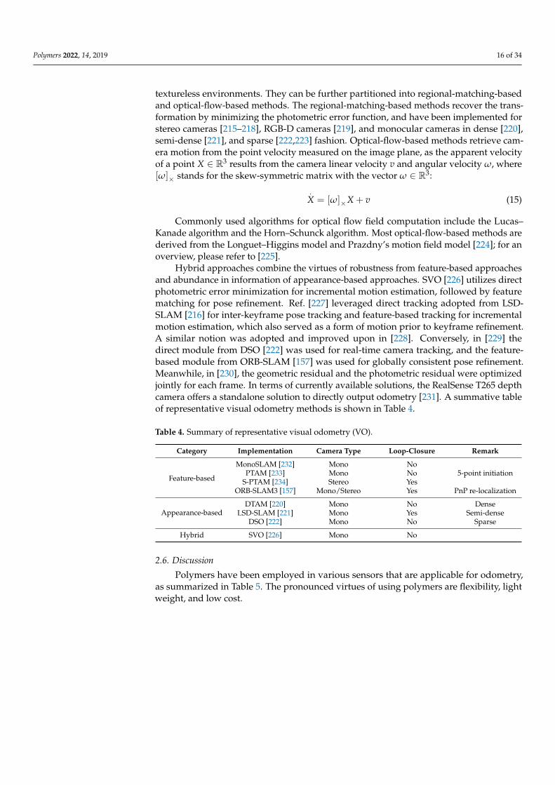
Hybrid approaches combine the virtues of robustness from feature-based approachesand abundance in information of appearance-based approaches. SVO [226] utilizes directphotometric error minimization for incremental motion estimation, followed by featurematching for pose refinement. Ref. [227] leveraged direct tracking adopted from LSD-SLAM [216] for inter-keyframe pose tracking and feature-based tracking for incrementalmotion estimation, which also served as a form of motion prior to keyframe refinement.A similar notion was adopted and improved upon in [228]. Conversely, in [229] thedirect module from DSO [222] was used for real-time camera tracking, and the feature-based module from ORB-SLAM [157] was used for globally consistent pose refinement.Meanwhile, in [230], the geometric residual and the photometric residual were optimizedjointly for each frame. In terms of currently available solutions, the RealSense T265 depthcamera offers a standalone solution to directly output odometry [231]. A summative tableof representative visual odometry methods is shown in Table 4.

Table 4. Summary of representative visual odometry (VO).

Category Implementation Camera Type Loop-Closure Remark

Feature-based

MonoSLAM [232] Mono NoPTAM [233] Mono No 5-point initiation

S-PTAM [234] Stereo YesORB-SLAM3 [157] Mono/Stereo Yes PnP re-localization

Appearance-basedDTAM [220] Mono No Dense

LSD-SLAM [221] Mono Yes Semi-denseDSO [222] Mono No Sparse

Hybrid SVO [226] Mono No

2.6. Discussion

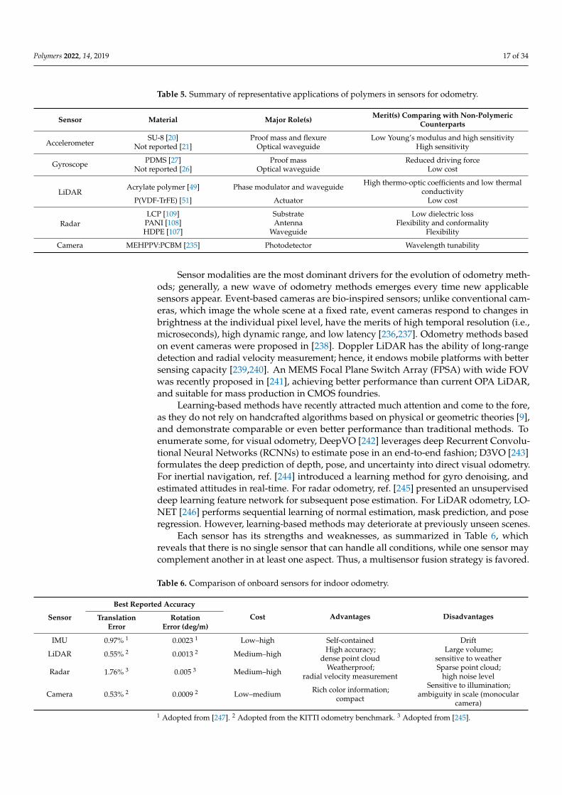
Polymers have been employed in various sensors that are applicable for odometry,as summarized in Table 5. The pronounced virtues of using polymers are flexibility, lightweight, and low cost.

Polymers 2022, 14, 2019 17 of 34

Table 5. Summary of representative applications of polymers in sensors for odometry.

Sensor Material Major Role(s) Merit(s) Comparing with Non-PolymericCounterparts

AccelerometerSU-8 [20] Proof mass and flexure Low Young’s modulus and high sensitivity

Not reported [21] Optical waveguide High sensitivity

Gyroscope PDMS [27] Proof mass Reduced driving forceNot reported [26] Optical waveguide Low cost

LiDARAcrylate polymer [49] Phase modulator and waveguide High thermo-optic coefficients and low thermal

conductivityP(VDF-TrFE) [51] Actuator Low cost

RadarLCP [109] Substrate Low dielectric loss

PANI [108] Antenna Flexibility and conformalityHDPE [107] Waveguide Flexibility

Camera MEHPPV:PCBM [235] Photodetector Wavelength tunability

Sensor modalities are the most dominant drivers for the evolution of odometry meth-ods; generally, a new wave of odometry methods emerges every time new applicablesensors appear. Event-based cameras are bio-inspired sensors; unlike conventional cam-eras, which image the whole scene at a fixed rate, event cameras respond to changes inbrightness at the individual pixel level, have the merits of high temporal resolution (i.e.,microseconds), high dynamic range, and low latency [236,237]. Odometry methods basedon event cameras were proposed in [238]. Doppler LiDAR has the ability of long-rangedetection and radial velocity measurement; hence, it endows mobile platforms with bettersensing capacity [239,240]. An MEMS Focal Plane Switch Array (FPSA) with wide FOVwas recently proposed in [241], achieving better performance than current OPA LiDAR,and suitable for mass production in CMOS foundries.

Learning-based methods have recently attracted much attention and come to the fore,as they do not rely on handcrafted algorithms based on physical or geometric theories [9],and demonstrate comparable or even better performance than traditional methods. Toenumerate some, for visual odometry, DeepVO [242] leverages deep Recurrent Convolu-tional Neural Networks (RCNNs) to estimate pose in an end-to-end fashion; D3VO [243]formulates the deep prediction of depth, pose, and uncertainty into direct visual odometry.For inertial navigation, ref. [244] introduced a learning method for gyro denoising, andestimated attitudes in real-time. For radar odometry, ref. [245] presented an unsuperviseddeep learning feature network for subsequent pose estimation. For LiDAR odometry, LO-NET [246] performs sequential learning of normal estimation, mask prediction, and poseregression. However, learning-based methods may deteriorate at previously unseen scenes.

Each sensor has its strengths and weaknesses, as summarized in Table 6, whichreveals that there is no single sensor that can handle all conditions, while one sensor maycomplement another in at least one aspect. Thus, a multisensor fusion strategy is favored.

Table 6. Comparison of onboard sensors for indoor odometry.

Sensor

Best Reported Accuracy

Cost Advantages DisadvantagesTranslationError

RotationError (deg/m)

IMU 0.97% 1 0.0023 1 Low–high Self-contained Drift

LiDAR 0.55% 2 0.0013 2 Medium–high High accuracy;dense point cloud

Large volume;sensitive to weather

Radar 1.76% 3 0.005 3 Medium–high Weatherproof;radial velocity measurement

Sparse point cloud;high noise level

Camera 0.53% 2 0.0009 2 Low–medium Rich color information;compact

Sensitive to illumination;ambiguity in scale (monocular

camera)

1 Adopted from [247]. 2 Adopted from the KITTI odometry benchmark. 3 Adopted from [245].

Polymers 2022, 14, 2019 18 of 34

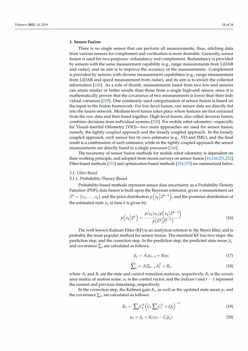
3. Sensor Fusion

There is no single sensor that can perform all measurements; thus, stitching datafrom various sensors for complement and verification is more desirable. Generally, sensorfusion is used for two purposes: redundancy and complement. Redundancy is providedby sensors with the same measurement capability (e.g., range measurements from LiDARand radar), and its aim is to improve the accuracy of the measurements. Complementis provided by sensors with diverse measurement capabilities (e.g., range measurementfrom LiDAR and speed measurement from radar), and its aim is to enrich the collectedinformation [248]. As a rule of thumb, measurements fused from two low-end sensorscan attain similar or better results than those from a single high-end sensor, since it ismathematically proven that the covariance of two measurements is lower than their indi-vidual variances [249]. One commonly used categorization of sensor fusion is based onthe input to the fusion framework: For low-level fusion, raw sensor data are directly fedinto the fusion network. Medium-level fusion takes place where features are first extractedfrom the raw data and then fused together. High-level fusion, also called decision fusion,combines decisions from individual systems [250]. For mobile robot odometry—especiallyfor Visual–Inertial Odometry (VIO)—two main approaches are used for sensor fusion,namely, the tightly coupled approach and the loosely coupled approach. In the looselycoupled approach, each sensor has its own estimator (e.g., VO and IMU), and the finalresult is a combination of each estimator, while in the tightly coupled approach the sensormeasurements are directly fused in a single processor [166].

The taxonomy of sensor fusion methods for mobile robot odometry is dependent ontheir working principle, and adopted from recent surveys on sensor fusion [10,248,251,252].Filter-based methods [253] and optimization-based methods [254,255] are summarized below.

3.1. Filter-Based3.1.1. Probability-Theory-Based

Probability-based methods represent sensor data uncertainty as a Probability DensityFunction (PDF); data fusion is built upon the Bayesian estimator, given a measurement setZk = z1, . . . , zk and the prior distribution p

(xk

∣∣∣Zk−1)

, and the posterior distribution ofthe estimated state xk at time k is given by:

p(

xk

∣∣∣Zk)=

p(zk|xk)p(

xk

∣∣∣Zk−1)

p(Zk∣∣Zk−1

) (16)

The well-known Kalman Filter (KF) is an analytical solution to the Bayes filter, and isprobably the most popular method for sensor fusion. The standard KF has two steps: theprediction step, and the correction step. In the prediction step, the predicted state mean µtand covariance ∑t are calculated as follows:

µt = Atµt−1 + Btut (17)

∑t = AtΣt−1 ATt + Rt, (18)

where At and Bt are the state and control transition matrices, respectively, Rt is the covari-ance matrix of motion noise, ut is the control vector, and the indices t and t − 1 representthe current and previous timestamp, respectively.

In the correction step, the Kalman gain Kt, as well as the updated state mean µt andthe covariance ∑t, are calculated as follows:

Kt = ∑tCTt

(Ct ∑tC

Tt + Qt

)−1(19)

µt = µt + Kt(zt − Ctµt) (20)

Polymers 2022, 14, 2019 19 of 34

∑t = (I − KtCt) ∑t, (21)

where Ct is the measurement matrix, and Qt is the covariance matrix of measurementnoises. For a full derivation of the KF, please refer to [256].

The standard KF requires both the motion and measurement models to be linear;for nonlinear systems, the Extended Kalman Filter (EKF) and Unscented Kalman Filter(UKF) can be adopted, which are based on first- and second-order Taylor expansion ofcurrent estimation, respectively. The EKF has been implemented for Visual–Inertial Odom-etry (VIO) [257], LiDAR–Inertial Odometry (LIO) [258], and Radar–Inertial Odometry(RIO) [128]; an error state space propagation strategy is usually adopted due to its superiorproperties [259]. Inertial measurement serves to propagate the filter state when the measure-ments from the camera or LiDAR are incorporated into the filter update. Variants of the EKF,such as the UKF [260], Multi-State Constraint Kalman Filter (MSCKF) [261,262]—whichincorporates poses of past frames to marginalize features from the state space. IteratedEKF [263], Cubature Kalman Filter (CKF) [264], fuzzy logic KF [265], covariance inter-section KF [266] and invariant EKF based on the Lie group [267], have been proposed inthe literature.

Although widely implemented, the KF and its variants can handle nonlinearity only toa limited degree. Monte Carlo (MC)-simulation-based methods express the underlying statespace as weighted samples, and do not make assumptions of the underlying probabilitydistribution. Markov Chain Monte Carlo (MCMC) and Sequential Monte Carlo (SMC) aretwo types of MC [268]; SMC (also known as Particle Filter) is more frequently seen in robotodometry. Particle Filter (PF) uses a set of particles x[m]

t with index m at time t to resemblethe real state space; the transition of particles takes place according to the state transitionfunction, and then the weight of each sample is calculated as follows:

w[m]t ∝ p

(zt

∣∣∣x[m]t

)(22)

The real trick of PF is the importance sampling step, where the samples are resampledaccording to their weight; this step approximates the posterior distribution of the Bayesfilter [269]. The Rao–Blackwellized Particle Filter (RBPF) is one of the most importantim-plementations of PF for odometry, introduced in [270] and refined in [271]. It is built uponthe Rao–Blackwell theorem, which states the fact that sampling of x1 from the distributionp(x1), and then x2 conditioned on x1 from p(x2), will do no worse than sampling fromtheir joint distribution p(x1, x2). Some notable recent advancements of PF include ParticleSwarm Optimization (PSO)-aided PF [272], entropy-weighted PF [273], Inter-Particle MapSharing (IPMS)-RBPF [274], and a 6D translation–rotation decoupled RBPF with an autoen-coder network to output hypotheses of rotation [275]. The general trend of PF is to eitherreduce the sampling size via a better sampling strategy or simplify the map representation.

3.1.2. Evidential-Reasoning-Based

Evidential-reasoning-based methods rely on the Dempster–Shafer (D–S) theory [276],combining evidence from several sources to prove a certain hypothesis, which can be seenas a generalization of the Bayes theory when ignorance about the hypothesis reaches zero.For a given problem, let X be a finite set of all possible states of the system (also called theFrame of Discernment (FOD)), where the power set 2X represents all possible subsets of X.D–S assigns a mass m(E) to each element E of 2X , representing the proportion of availableevidence that supports the system state x belonging to E, and the mass function has thefollowing properties (∅ stands for empty set):

m(∅) = 0 ∑E∈2X

m(E) = 1 (23)

Using m, the probability interval bel(E) 6 P(E) 6 pl(E) can be obtained, where thelower bound belief is defined as bel(E) = ∑B⊆E m(B) and the upper bound’s plausibility

Polymers 2022, 14, 2019 20 of 34

is defined as pl(E) = ∑B∩E 6= m(B). Evidence from two sources is combined via the D–Scombination rule as follows:

m1 ⊕m2(E) = ∑A∩B=E m1(A)m2(B)1−∑A∩B=∅ m1(A)m2(B)

(24)

The notion of D–S has been deployed for sensor fusion in odometry—as demonstratedin [277,278]—and map building in [279]. Its main advantage is that it requires no priorknowledge of the probability distribution, and has proven utility for systems in which onesensor reading is likely to be unreliable or unavailable during operation.

3.1.3. Random-Finite-Set-Based

Random Finite Set (RFS)-based methods treat the system state as a finite-set-valuedrandom variable instead of a random vector, and the size (cardinality) of the set is alsoa random variable. RFS is deemed to be an ideal extension of the Bayes filter, and hasbeen widely implemented for Multi-Target Tracking (MTT). Propagating the whole RFSProbability Density Function (PDF) is computationally intractable; thus, the first statisticalmoment of RFS—Probability Hypothesis Density (PHD)—is used to construct the PHDfilter, as it is for the Kalman filter (i.e., mean and covariance) [134,280]. With the PHD filter,the target state is modelled as the union (∪) of different RFSs:

Xk = [ ∪ζ∈Xk−1

Sk|k−1(ζ)] ∪ Γk (25)

where Sk|k−1(ζ) represents the surviving targets from time k − 1, and is modelled as aBernoulli RFS, which means that it either survives—with probability PS,k(Xk−1)—to takethe new value Xk, or dies—with probability 1 − PS,k(Xk−1)—into the empty set ∅. Γkrepresents spontaneously born targets at time k, and is modelled as a Poisson RFS withintensity (PHD) γk(·). The observation state is also modelled as the union of different RFSs:

Zk = [ ∪x∈Xk

Θk(x)] ∪ Kk (26)

where Θk(x) represents detected targets, and is modelled as a Bernoulli RFS, which meansthat it is either detected—with probability PD,k(Xk) yielding Zk by the observation functiongk(Zk|Xk)—ormissed—with probability 1− PD,k(Xk)—into the empty set ∅. Kk representsfalse alarms, and is modelled as a Poisson RFS with intensity (PHD) κk(·). The predictionand update equation of the PHD filter are as follows, where Dk is the first moment (i.e.,PHD) of the state RFS:

Dk|k−1(Xk) =∫

PS,k(Xk−1) fk|k−1(Xk|Xk−1)Dk−1(Xk−1)dXk−1 + γk(Xk) (27)

Dk(Xk) = (1− PD,k(Xk))Dk|k−1(Xk) + ∑z∈Zk

PD,k(Xk)gk(zi|Xk)Dk|k−1(Xk)

κk(zi) +∫

PD,kgk(zi|ζ)Dk|k−1(ζ)dζ(28)

The PHD is not a PDF, and is not necessarily integrated into one, integrating thePHD will yield the number of targets in the space [281,282]. The PHD filter is handywhen modelling phenomena such as object block, missing detection, or false alarms. Thus,it has been used for Radar Odometry (RO), since both misdetection and false featureassociation can be commonly encountered in RO [132]. A comparison between PHD filtersand state-of-the-art EKFs [267] was conducted in [283], demonstrating robustness of thePHD filter. A C (Cardinalized)-PHD filter propagates the distribution of the number oftargets (cardinality) in addition to the PHD function; this auxiliary information enableshigher modelling accuracy [284]. Alternatively, a multi-Bernoulli filter was implementedin [285,286].

Polymers 2022, 14, 2019 21 of 34

3.2. Optimization-Based

Optimization-based (smoothing) methods correspond to estimating the full state giventhe whole observations up to current moment. This is the so-called full-SLAM solution. Anintuitive way to achieve this is via the factor graph method, which builds a graph whosevertices encode robot poses and feature locations, with edges encoding the constraintsbetween vertices arising from measurements [255,287]. This is cast into an optimizationproblem that minimizes F(x):

x∗ = argminx

F(x) (29)

F(x) = ∑〈ij〉∈C

e>ij Ωijeij (30)

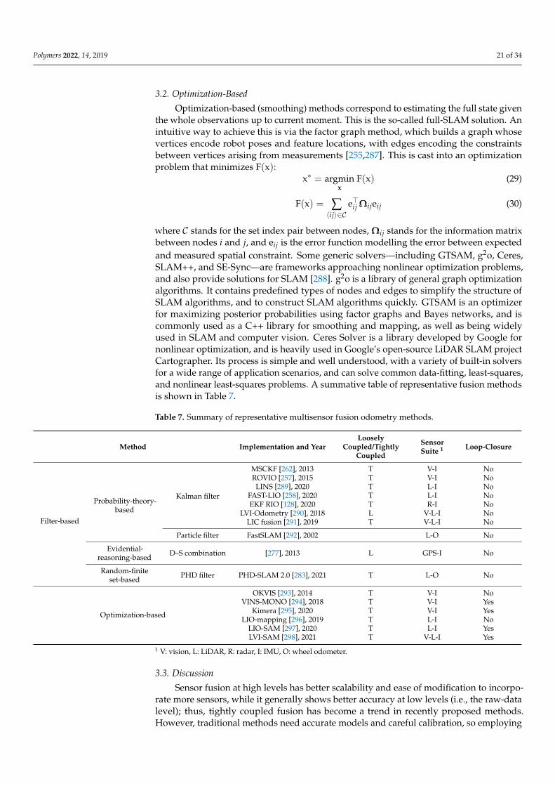
where C stands for the set index pair between nodes, Ωij stands for the information matrixbetween nodes i and j, and eij is the error function modelling the error between expectedand measured spatial constraint. Some generic solvers—including GTSAM, g2o, Ceres,SLAM++, and SE-Sync—are frameworks approaching nonlinear optimization problems,and also provide solutions for SLAM [288]. g2o is a library of general graph optimizationalgorithms. It contains predefined types of nodes and edges to simplify the structure ofSLAM algorithms, and to construct SLAM algorithms quickly. GTSAM is an optimizerfor maximizing posterior probabilities using factor graphs and Bayes networks, and iscommonly used as a C++ library for smoothing and mapping, as well as being widelyused in SLAM and computer vision. Ceres Solver is a library developed by Google fornonlinear optimization, and is heavily used in Google’s open-source LiDAR SLAM projectCartographer. Its process is simple and well understood, with a variety of built-in solversfor a wide range of application scenarios, and can solve common data-fitting, least-squares,and nonlinear least-squares problems. A summative table of representative fusion methodsis shown in Table 7.

Table 7. Summary of representative multisensor fusion odometry methods.

Method Implementation and YearLoosely

Coupled/TightlyCoupled

SensorSuite 1 Loop-Closure

Filter-based

Probability-theory-based

Kalman filter

MSCKF [262], 2013 T V-I NoROVIO [257], 2015 T V-I NoLINS [289], 2020 T L-I No

FAST-LIO [258], 2020 T L-I NoEKF RIO [128], 2020 T R-I No

LVI-Odometry [290], 2018 L V-L-I NoLIC fusion [291], 2019 T V-L-I No

Particle filter FastSLAM [292], 2002 L-O No

Evidential-reasoning-based D–S combination [277], 2013 L GPS-I No

Random-finiteset-based PHD filter PHD-SLAM 2.0 [283], 2021 T L-O No

Optimization-based

OKVIS [293], 2014 T V-I NoVINS-MONO [294], 2018 T V-I Yes

Kimera [295], 2020 T V-I YesLIO-mapping [296], 2019 T L-I No

LIO-SAM [297], 2020 T L-I YesLVI-SAM [298], 2021 T V-L-I Yes

1 V: vision, L: LiDAR, R: radar, I: IMU, O: wheel odometer.

3.3. Discussion

Sensor fusion at high levels has better scalability and ease of modification to incorpo-rate more sensors, while it generally shows better accuracy at low levels (i.e., the raw-datalevel); thus, tightly coupled fusion has become a trend in recently proposed methods.However, traditional methods need accurate models and careful calibration, so employing

Polymers 2022, 14, 2019 22 of 34

machine learning for sensor fusion in odometry has also become an open research topic.In [299], sequences of CNNs were used to extract features and determine pose from acamera and 2D LiDAR. Some learning-based methods, such as VINet and DeepVIO [300],demonstrate comparable or even better performance than traditional methods.

4. Future Prospects4.1. Embedded Sensors for Soft Robots’ State Estimation and Perception

Soft embedded sensors have been employed for soft robots in strain, stress, and tactilesensing [301]. However, soft sensors generally exhibit nonlinearity, hysteresis, and slowresponse. To overcome these issues, multisensor fusion strategies for soft sensors—suchas [302,303]—have been proposed. Recent achievements have also brought soft sensorsand machine learning techniques together for robot kinematic estimation [304].

The need for soft robots to explore unstructured environments is also growing [305].For example, the Visual Odometry (VO) method was used in a soft endoscopic capsulerobot for location tracking [306]. However, current implantations still mostly rely onsolid-state sensors, and employing soft sensors could greatly improve the flexibility andcompatibility of these systems.

4.2. Swarm Odometry

Multiple robots can perform tasks more quickly and are more robust where singleagents may fail [307]. This has been implemented in homogeneous systems, either ina centralized [308] or a decentralized [309] fashion, where multiple drones self-estimatetheir state from onboard sensors, and communicate with the base station or one another.This may also be deployed in a heterogeneous system, where the UAVs and UGVs worktogether. However, the scalability of the system, the relative pose estimation betweenagents, the uncertainty of the relative pose estimation, and the limited communicationrange still challenge such research.

4.3. Accelerating Processing Speed at the Hardware Level

While most current solutions rely on complex and time-consuming operations at thesoftware level, this can be alleviated by using FPGAs (Field-Programmable Gate Arrays) orother dedicated processors [310] to integrate sensors and odometry algorithms at the hard-ware level, which enables odometry estimation at very high rates. This is expected to savecomputational resources and improve the real-time performance of the odometry systems.

5. Conclusions

In this paper, a comprehensive review of odometry methods for indoor navigationis presented, with detailed analysis of the state estimation algorithms for various sensors,including inertial measurement sensors, visual cameras, LiDAR, and radar, with an inves-tigation of the applications of polymeric materials in those sensors. The principles andimplementation of sensor fusion algorithms that have been successively deployed in indoorodometry are also reviewed. Generally, polymers introduce flexibility and compatibilityto the sensors, and reduce the cost of their mass production. They may also serve asembedded solutions that enable novel applications of odometry technology, such as in softendoscopic capsules.

Although mature solutions exist, the improvement of indoor odometry/localizationaccuracy is still an ongoing research topic. It is vital to achieve a sub-centimeter levelfor safe navigation. Prospective research areas within this topic including advanced sen-sor technology, algorithm enhancement, machine intelligence, human–robot interaction,information fusion, and overall performance improvement.

Author Contributions: Writing—original draft preparation, M.Y., X.S., A.R. and F.J.; writing—reviewand editing, X.D., S.Z., G.Y. and B.L.; supervision, X.S., A.R. and G.Y.; funding acquisition, X.S., Z.F.and G.Y. All authors have read and agreed to the published version of the manuscript.

Polymers 2022, 14, 2019 23 of 34

Funding: This research was funded by the National Natural Science Foundation of China, grantnumber 92048201; the Major Program of the Nature Science Foundation of Zhejiang Province, grantnumber LD22E050007; and the Major Special Projects of the Plan “Science and Technology Innovation2025” in Ningbo, grant number 2021Z020.

Institutional Review Board Statement: Not applicable.

Informed Consent Statement: Not applicable.

Data Availability Statement: Not applicable.

Conflicts of Interest: The authors declare no conflict of interest.

References1. El-Sheimy, N.; Li, Y. Indoor navigation: State of the art and future trends. Satell. Navig. 2021, 2, 7. [CrossRef]2. Everett, H. Sensors for Mobile Robots; AK Peters/CRC Press: New York, NY, USA, 1995.3. Civera, J.; Lee, S.H. RGB-D Odometry and SLAM. In RGB-D Image Analysis and Processing; Rosin, P.L., Lai, Y.-K., Shao, L., Liu, Y.,

Eds.; Springer International Publishing: Cham, Switzerland, 2019; pp. 117–144.4. Ashley, P.; Temmen, M.; Diffey, W.; Sanghadasa, M.; Bramson, M.; Lindsay, G.; Guenthner, A. Components for IFOG Based Inertial

Measurement Units Using Active and Passive Polymer Materials; SPIE: Sandiego, CA, USA, 2006; Volume 6314.5. Hellebrekers, T.; Ozutemiz, K.B.; Yin, J.; Majidi, C. Liquid Metal-Microelectronics Integration for a Sensorized Soft Robot Skin. In

Proceedings of the IEEE/RSJ International Conference on Intelligent Robots and Systems (IROS), Madrid, Spain, 1–5 October2018; pp. 5924–5929.

6. Bresson, G.; Alsayed, Z.; Yu, L.; Glaser, S. Simultaneous Localization and Mapping: A Survey of Current Trends in AutonomousDriving. IEEE Trans. Intell. Veh. 2017, 2, 194–220. [CrossRef]

7. Mohamed, S.A.S.; Haghbayan, M.H.; Westerlund, T.; Heikkonen, J.; Tenhunen, H.; PLoSila, J. A Survey on Odometry forAutonomous Navigation Systems. IEEE Access 2019, 7, 97466–97486. [CrossRef]

8. Huang, B.; Zhao, J.; Liu, J. A survey of simultaneous localization and mapping with an envision in 6g wireless networks. arXiv2019, arXiv:1909.05214.

9. Chen, C.; Wang, B.; Lu, C.X.; Trigoni, N.; Markham, A. A survey on deep learning for localization and mapping: Towards the ageof spatial machine intelligence. arXiv 2020, arXiv:2006.12567.

10. Fayyad, J.; Jaradat, M.A.; Gruyer, D.; Najjaran, H. Deep Learning Sensor Fusion for Autonomous Vehicle Perception andLocalization: A Review. Sensors 2020, 20, 4220. [CrossRef]

11. Yeong, D.J.; Velasco-Hernandez, G.; Barry, J.; Walsh, J. Sensor and Sensor Fusion Technology in Autonomous Vehicles: A Review.Sensors 2021, 21, 2140. [CrossRef]

12. Taheri, H.; Xia, Z.C. SLAM; definition and evolution. Eng. Appl. Artif. Intell. 2021, 97, 104032. [CrossRef]13. Servières, M.; Renaudin, V.; Dupuis, A.; Antigny, N. Visual and Visual-Inertial SLAM: State of the Art, Classification, and

Experimental Benchmarking. J. Sens. 2021, 2021, 2054828. [CrossRef]14. Tzafestas, S.G. 4—Mobile Robot Sensors. In Introduction to Mobile Robot Control; Tzafestas, S.G., Ed.; Elsevier: Amsterdam,

The Netherlands, 2014; pp. 101–135.15. Thomas, S.; Froehly, A.; Bredendiek, C.; Herschel, R.; Pohl, N. High Resolution SAR Imaging Using a 240 GHz FMCW Radar

System with Integrated On-Chip Antennas. In Proceedings of the 15th European Conference on Antennas and Propagation(EuCAP), Virtual, 22–26 March 2021; pp. 1–5.

16. Brossard, M.; Bonnabel, S. Learning Wheel Odometry and IMU Errors for Localization. In Proceedings of the InternationalConference on Robotics and Automation (ICRA), Montreal, QC, Canada, 20–24 May 2019; pp. 291–297.

17. Woodman, O.J. An Introduction to Inertial Navigation; University of Cambridge: Cambridge, UK, 2007.18. Siciliano, B.; Khatib, O. Springer Handbook of Robotics; Springer: Berlin/Heidelberg, Germany, 2016.19. Siegwart, R.; Nourbakhsh, I.R.; Scaramuzza, D. Introduction to Autonomous Mobile Robots; MIT Press: Cambridge, MA, USA, 2011.20. Ahmed, A.; Pandit, S.; Patkar, R.; Dixit, P.; Baghini, M.S.; Khlifi, A.; Tounsi, F.; Mezghani, B. Induced-Stress Analysis of SU-8

Polymer Based Single Mass 3-Axis Piezoresistive MEMS Accelerometer. In Proceedings of the 16th International Multi-Conferenceon Systems, Signals & Devices (SSD), Istanbul, Turkey, 21–24 March 2019; pp. 131–136.

21. Wan, F.; Qian, G.; Li, R.; Tang, J.; Zhang, T. High sensitivity optical waveguide accelerometer based on Fano resonance. Appl. Opt.2016, 55, 6644–6648. [CrossRef]

22. Yi, J. A Piezo-Sensor-Based “Smart Tire” System for Mobile Robots and Vehicles. IEEE/ASME Trans. Mechatron. 2008, 13, 95–103.[CrossRef]

23. Passaro, V.M.N.; Cuccovillo, A.; Vaiani, L.; De Carlo, M.; Campanella, C.E. Gyroscope Technology and Applications: A Review inthe Industrial Perspective. Sensors 2017, 17, 2284. [CrossRef] [PubMed]

24. El-Sheimy, N.; Youssef, A. Inertial sensors technologies for navigation applications: State of the art and future trends. Satell.Navig. 2020, 1, 2. [CrossRef]

25. Hakyoung, C.; Ojeda, L.; Borenstein, J. Accurate mobile robot dead-reckoning with a precision-calibrated fiber-optic gyroscope.IEEE Trans. Robot. Autom. 2001, 17, 80–84. [CrossRef]

Polymers 2022, 14, 2019 24 of 34

26. Qian, G.; Tang, J.; Zhang, X.-Y.; Li, R.-Z.; Lu, Y.; Zhang, T. Low-Loss Polymer-Based Ring Resonator for Resonant IntegratedOptical Gyroscopes. J. Nanomater. 2014, 2014, 146510. [CrossRef]

27. Yeh, C.N.; Tsai, J.J.; Shieh, R.J.; Tseng, F.G.; Li, C.J.; Su, Y.C. A vertically supported ring-type mems gyroscope utilizingelectromagnetic actuation and sensing. In Proceedings of the IEEE International Conference on Electron Devices and Solid-StateCircuits, Hong Kong, China, 8–10 December 2008; pp. 1–4.

28. Ward, C.C.; Iagnemma, K. A Dynamic-Model-Based Wheel Slip Detector for Mobile Robots on Outdoor Terrain. IEEE Trans.Robot. 2008, 24, 821–831. [CrossRef]

29. Yi, J.; Wang, H.; Zhang, J.; Song, D.; Jayasuriya, S.; Liu, J. Kinematic Modeling and Analysis of Skid-Steered Mobile RobotsWith Applications to Low-Cost Inertial-Measurement-Unit-Based Motion Estimation. IEEE Trans. Robot. 2009, 25, 1087–1097.[CrossRef]

30. Bancroft, J.B. Multiple IMU integration for vehicular navigation. In Proceedings of the Proceedings of the 22nd InternationalTechnical Meeting of The Satellite Division of the Institute of Navigation (ION GNSS 2009), Savannah, GA, USA, 22–25 September2009; pp. 1828–1840.

31. Wu, Y.; Niu, X.; Kuang, J. A Comparison of Three Measurement Models for the Wheel-mounted MEMS IMU-based DeadReckoning System. arXiv 2020, arXiv:2012.10589. [CrossRef]

32. Lupton, T.; Sukkarieh, S. Visual-Inertial-Aided Navigation for High-Dynamic Motion in Built Environments Without InitialConditions. IEEE Trans. Robot. 2012, 28, 61–76. [CrossRef]

33. Forster, C.; Carlone, L.; Dellaert, F.; Scaramuzza, D. On-Manifold Preintegration for Real-Time Visual—Inertial Odometry. IEEETrans. Robot. 2017, 33, 1–21. [CrossRef]

34. Brossard, M.; Barrau, A.; Chauchat, P.; Bonnabel, S. Associating Uncertainty to Extended Poses for on Lie Group IMU Preintegra-tion With Rotating Earth. IEEE Trans. Robot. 2021, 3, 998–1015. [CrossRef]

35. Quick Start for MTi Development Kit. Available online: https://xsenstechnologies.force.com/knowledgebase/s/article/Quick-start-for-MTi-Development-Kit-1605870241724?language=en_US (accessed on 1 March 2022).

36. ROS (Robot Operating System) Drivers | MicroStrain. Available online: https://www.microstrain.com/software/ros (accessedon 1 March 2022).

37. Mukherjee, A. Visualising 3D Motion of IMU Sensor. Available online: https://create.arduino.cc/projecthub/Aritro/visualising-3d-motion-of-imu-sensor-3933b0?f=1 (accessed on 1 March 2022).

38. Borodacz, K.; Szczepanski, C.; Popowski, S. Review and selection of commercially available IMU for a short time inertialnavigation. Aircr. Eng. Aerosp. Technol. 2022, 94, 45–59. [CrossRef]

39. Behroozpour, B.; Sandborn, P.A.M.; Wu, M.C.; Boser, B.E. Lidar System Architectures and Circuits. IEEE Commun. Mag. 2017, 55,135–142. [CrossRef]

40. Khader, M.; Cherian, S. An Introduction to Automotive LIDAR, Texas Instruments; Technical Report; Taxes Instruments Incorporated:Dallas, TX, USA, 2018.

41. Li, Y.; Ibanez-Guzman, J. Lidar for Autonomous Driving: The Principles, Challenges, and Trends for Automotive Lidar andPerception Systems. IEEE Signal Process Mag. 2020, 37, 50–61. [CrossRef]

42. Royo, S.; Ballesta-Garcia, M. An Overview of Lidar Imaging Systems for Autonomous Vehicles. Appl. Sci. 2019, 9, 4093. [CrossRef]43. Wang, D.; Watkins, C.; Xie, H. MEMS Mirrors for LiDAR: A Review. Micromachines 2020, 11, 456. [CrossRef]44. Yoo, H.W.; Druml, N.; Brunner, D.; Schwarzl, C.; Thurner, T.; Hennecke, M.; Schitter, G. MEMS-based lidar for autonomous

driving. Elektrotechnik Inf. 2018, 135, 408–415. [CrossRef]45. Lin, J.; Zhang, F. Loam livox: A fast, robust, high-precision LiDAR odometry and mapping package for LiDARs of small FoV. In

Proceedings of the IEEE International Conference on Robotics and Automation (ICRA), Paris, France, 31 May–31 August 2020;pp. 3126–3131.

46. Amzajerdian, F.; Pierrottet, D.; Petway, L.B.; Hines, G.D.; Roback, V.E.; Reisse, R.A. Lidar sensors for autonomous landing andhazard avoidance. In Proceedings of the AIAA Space 2013 Conference and Exposition, San Diego, CA, USA, 10–12 September2013; p. 5312.

47. Dietrich, A.B.; McMahon, J.W. Robust Orbit Determination with Flash Lidar Around Small Bodies. J. Guid. Control. Dyn. 2018, 41,2163–2184. [CrossRef]

48. Poulton, C.V.; Byrd, M.J.; Russo, P.; Timurdogan, E.; Khandaker, M.; Vermeulen, D.; Watts, M.R. Long-Range LiDAR andFree-Space Data Communication With High-Performance Optical Phased Arrays. IEEE J. Sel. Top. Quantum Electron. 2019, 25, 1–8.[CrossRef]

49. Kim, S.-M.; Park, T.-H.; Im, C.-S.; Lee, S.-S.; Kim, T.; Oh, M.-C. Temporal response of polymer waveguide beam scanner withthermo-optic phase-modulator array. Opt. Express 2020, 28, 3768–3778. [CrossRef]

50. Im, C.S.; Kim, S.M.; Lee, K.P.; Ju, S.H.; Hong, J.H.; Yoon, S.W.; Kim, T.; Lee, E.S.; Bhandari, B.; Zhou, C.; et al. Hybrid IntegratedSilicon Nitride–Polymer Optical Phased Array For Efficient Light Detection and Ranging. J. Lightw. Technol. 2021, 39, 4402–4409.[CrossRef]

51. Casset, F.; Poncet, P.; Desloges, B.; Santos, F.D.D.; Danel, J.S.; Fanget, S. Resonant Asymmetric Micro-Mirror Using Electro ActivePolymer Actuators. In Proceedings of the IEEE SENSORS, New Delhi, India, 28–31 October 2018; pp. 1–4.

52. Pavia, J.M.; Wolf, M.; Charbon, E. Measurement and modeling of microlenses fabricated on single-photon avalanche diode arraysfor fill factor recovery. Opt. Express 2014, 22, 4202–4213. [CrossRef] [PubMed]

Polymers 2022, 14, 2019 25 of 34

53. Cheng, L.; Chen, S.; Liu, X.; Xu, H.; Wu, Y.; Li, M.; Chen, Y. Registration of Laser Scanning Point Clouds: A Review. Sensors 2018,18, 1641. [CrossRef] [PubMed]

54. Saiti, E.; Theoharis, T. An application independent review of multimodal 3D registration methods. Comput. Graph. 2020, 91,153–178. [CrossRef]

55. Huang, X.; Mei, G.; Zhang, J.; Abbas, R. A comprehensive survey on point cloud registration. arXiv 2021, arXiv:2103.02690.56. Zhu, H.; Guo, B.; Zou, K.; Li, Y.; Yuen, K.-V.; Mihaylova, L.; Leung, H. A Review of Point Set Registration: From Pairwise

Registration to Groupwise Registration. Sensors 2019, 19, 1191. [CrossRef]57. Holz, D.; Ichim, A.E.; Tombari, F.; Rusu, R.B.; Behnke, S. Registration with the Point Cloud Library: A Modular Framework for

Aligning in 3-D. IEEE Robot. Autom. Mag. 2015, 22, 110–124. [CrossRef]58. Jonnavithula, N.; Lyu, Y.; Zhang, Z. LiDAR Odometry Methodologies for Autonomous Driving: A Survey. arXiv 2021,

arXiv:2109.06120.59. Elhousni, M.; Huang, X. A Survey on 3D LiDAR Localization for Autonomous Vehicles. In Proceedings of the IEEE Intelligent

Vehicles Symposium (IV), Las Vegas, NV, USA, 19 October–13 November 2020; pp. 1879–1884.60. Bosse, M.; Zlot, R. Keypoint design and evaluation for place recognition in 2D lidar maps. Rob. Auton. Syst. 2009, 57, 1211–1224.

[CrossRef]61. Wang, D.Z.; Posner, I.; Newman, P. Model-free detection and tracking of dynamic objects with 2D lidar. Int. J. Robot. Res. 2015, 34,

1039–1063. [CrossRef]62. Zou, Q.; Sun, Q.; Chen, L.; Nie, B.; Li, Q. A Comparative Analysis of LiDAR SLAM-Based Indoor Navigation for Autonomous

Vehicles. IEEE Trans. Intell. Transp. Syst. 2021, 1–15. [CrossRef]63. François, P.; Francis, C.; Roland, S. A Review of Point Cloud Registration Algorithms for Mobile Robotics. Found. Trends Robot.

2015, 4, 1–104.64. Münch, D.; Combès, B.; Prima, S. A Modified ICP Algorithm for Normal-Guided Surface Registration; SPIE: Bellingham, WA, USA,

2010; Volume 7623.65. Serafin, J.; Grisetti, G. NICP: Dense normal based point cloud registration. In Proceedings of the IEEE/RSJ International

Conference on Intelligent Robots and Systems (IROS), Hamburg, Germany, 28 September–2 October 2015; pp. 742–749.66. Godin, G.; Rioux, M.; Baribeau, R. Three-Dimensional Registration Using Range and Intensity Information; SPIE: Boston, MA, USA,

1994; Volume 2350.67. Greenspan, M.; Yurick, M. Approximate k-d tree search for efficient ICP. In Proceedings of the Fourth International Conference on

3-D Digital Imaging and Modeling, Banff, AB, Canada, 6–10 October 2003; pp. 442–448.68. Yang, J.; Li, H.; Campbell, D.; Jia, Y. Go-ICP: A Globally Optimal Solution to 3D ICP Point-Set Registration. IEEE Trans. Pattern

Anal. Mach. Intell. 2016, 38, 2241–2254. [CrossRef] [PubMed]69. Park, S.-Y.; Subbarao, M. An accurate and fast point-to-plane registration technique. Pattern Recognit. Lett. 2003, 24, 2967–2976.

[CrossRef]70. Segal, A.; Haehnel, D.; Thrun, S. Generalized-icp. In Proceedings of the Robotics: Science and Systems, Seattle, WA, USA, 28

June–1 July 2009; p. 435.71. Yokozuka, M.; Koide, K.; Oishi, S.; Banno, A. LiTAMIN2: Ultra Light LiDAR-based SLAM using Geometric Approximation

applied with KL-Divergence. arXiv 2021, arXiv:2103.00784.72. Lu, D.L. Vision-Enhanced Lidar Odometry and Mapping; Carnegie Mellon University: Pittsburgh, PA, USA, 2016.73. Biber, P.; Strasser, W. The normal distributions transform: A new approach to laser scan matching. In Proceedings of the

Proceedings IEEE/RSJ International Conference on Intelligent Robots and Systems (IROS 2003) (Cat. No.03CH37453), Las Vegas,NV, USA, 27–31 October 2003; Volume 2743, pp. 2743–2748.

74. Magnusson, M.; Lilienthal, A.; Duckett, T. Scan registration for autonomous mining vehicles using 3D-NDT. J. Field Rob. 2007, 24,803–827. [CrossRef]

75. Stoyanov, T.; Magnusson, M.; Andreasson, H.; Lilienthal, A.J. Fast and accurate scan registration through minimization of thedistance between compact 3D NDT representations. Int. J. Robot. Res. 2012, 31, 1377–1393. [CrossRef]

76. Magnusson, M.; Vaskevicius, N.; Stoyanov, T.; Pathak, K.; Birk, A. Beyond points: Evaluating recent 3D scan-matching algorithms.In Proceedings of the IEEE International Conference on Robotics and Automation (ICRA), Seattle, WA, USA, 26–30 May 2015;pp. 3631–3637.

77. Wolcott, R.W.; Eustice, R.M. Robust LIDAR localization using multiresolution Gaussian mixture maps for autonomous driving.Int. J. Robot. Res. 2017, 36, 292–319. [CrossRef]

78. Eckart, B.; Kim, K.; Kautz, J. Hgmr: Hierarchical gaussian mixtures for adaptive 3d registration. In Proceedings of the EuropeanConference on Computer Vision (ECCV), Munich, Germany, 8–14 September 2018; pp. 705–721.

79. Myronenko, A.; Song, X. Point Set Registration: Coherent Point Drift. IEEE Trans. Pattern Anal. Mach. Intell. 2010, 32, 2262–2275.[CrossRef]

80. Ji, K.; Chen, H.; Di, H.; Gong, J.; Xiong, G.; Qi, J.; Yi, T. CPFG-SLAM:a Robust Simultaneous Localization and Mapping based onLIDAR in Off-Road Environment. In Proceedings of the IEEE Intelligent Vehicles Symposium (IV), Changshu, China, 26–30 June2018; pp. 650–655.

Polymers 2022, 14, 2019 26 of 34

81. Fontanelli, D.; Ricciato, L.; Soatto, S. A Fast RANSAC-Based Registration Algorithm for Accurate Localization in UnknownEnvironments using LIDAR Measurements. In Proceedings of the IEEE International Conference on Automation Science andEngineering, Scottsdale, AZ, USA, 22–25 September 2007; pp. 597–602.

82. Deschaud, J.-E. IMLS-SLAM: Scan-to-model matching based on 3D data. In Proceedings of the IEEE International Conference onRobotics and Automation (ICRA), Brisbane, Australia, 21–16 May 2018; pp. 2480–2485.

83. Behley, J.; Stachniss, C. Efficient Surfel-Based SLAM using 3D Laser Range Data in Urban Environments. In Proceedings of theRobotics: Science and Systems, Pittsburgh, PA, USA, 26–30 June 2018.

84. Quenzel, J.; Behnke, S. Real-time multi-adaptive-resolution-surfel 6D LiDAR odometry using continuous-time trajectory opti-mization. arXiv 2021, arXiv:2105.02010.

85. Droeschel, D.; Schwarz, M.; Behnke, S. Continuous mapping and localization for autonomous navigation in rough terrain using a3D laser scanner. Rob. Auton. Syst. 2017, 88, 104–115. [CrossRef]

86. Pan, Y.; Xiao, P.; He, Y.; Shao, Z.; Li, Z. MULLS: Versatile LiDAR SLAM via Multi-metric Linear Least Square. In Proceedings ofthe IEEE International Conference on Robotics and Automation (ICRA), Hybrid Event, 30 May–5 June 2021; pp. 11633–11640.

87. Kim, H.; Hilton, A. Evaluation of 3D Feature Descriptors for Multi-modal Data Registration. In Proceedings of the InternationalConference on 3D Vision—3DV 2013, Seattle, WA, USA, 29 June–1 July 2013; pp. 119–126.

88. Guo, Y.; Bennamoun, M.; Sohel, F.; Lu, M.; Wan, J. 3D Object Recognition in Cluttered Scenes with Local Surface Features: ASurvey. IEEE Trans. Pattern Anal. Mach. Intell. 2014, 36, 2270–2287. [CrossRef] [PubMed]

89. Alexandre, L.A. 3D descriptors for object and category recognition: A comparative evaluation. In Proceedings of the Workshopon Color-Depth Camera Fusion in Robotics at the IEEE/RSJ International Conference on Intelligent Robots and Systems (IROS),Vilamoura, Portugal, 7–12 October 2012; p. 7.

90. He, Y.; Mei, Y. An efficient registration algorithm based on spin image for LiDAR 3D point cloud models. Neurocomputing 2015,151, 354–363. [CrossRef]

91. Rusu, R.B.; Blodow, N.; Beetz, M. Fast Point Feature Histograms (FPFH) for 3D registration. In Proceedings of the IEEEInternational Conference on Robotics and Automation, Kobe, Japan, 12–17 May 2009; pp. 3212–3217.

92. Tombari, F.; Salti, S.; Stefano, L.D. Unique shape context for 3d data description. In Proceedings of the ACM Workshop on 3DObject Retrieval, Firenze, Italy, 25 October 2010; pp. 57–62.

93. Kim, G.; Kim, A. Scan Context: Egocentric Spatial Descriptor for Place Recognition Within 3D Point Cloud Map. In Proceedings ofthe IEEE/RSJ International Conference on Intelligent Robots and Systems (IROS), Madrid, Spain, 1–5 October 2018; pp. 4802–4809.

94. Tombari, F.; Salti, S.; Di Stefano, L. Unique Signatures of Histograms for Local Surface Description; Springer: Berlin/Heidelberg,Germany, 2010; pp. 356–369.

95. Guo, J.; Borges, P.V.K.; Park, C.; Gawel, A. Local Descriptor for Robust Place Recognition Using LiDAR Intensity. IEEE Rob.Autom. Lett. 2019, 4, 1470–1477. [CrossRef]

96. He, L.; Wang, X.; Zhang, H. M2DP: A novel 3D point cloud descriptor and its application in loop closure detection. InProceedings of the IEEE/RSJ International Conference on Intelligent Robots and Systems (IROS), Daejeon, Korea, 9–14 October2016; pp. 231–237.

97. Skjellaug, E.; Brekke, E.F.; Stahl, A. Feature-Based Laser Odometry for Autonomous Surface Vehicles utilizing the Point CloudLibrary. In Proceedings of the IEEE 23rd International Conference on Information Fusion (FUSION), Virtual, 6–9 July 2020;pp. 1–8.

98. Zhang, J.; Singh, S. LOAM: Lidar Odometry and Mapping in Real-time. In Proceedings of the Robotics: Science and Systems,Berkeley, CA, USA, 12–16 July 2014.

99. Shan, T.; Englot, B. LeGO-LOAM: Lightweight and Ground-Optimized Lidar Odometry and Mapping on Variable Terrain. InProceedings of the IEEE/RSJ International Conference on Intelligent Robots and Systems (IROS), Madrid, Spain, 1–5 October2018; pp. 4758–4765.

100. RoboStudio. Available online: https://www.slamtec.com/en/RoboStudio (accessed on 1 March 2022).101. Chen, K.; Lopez, B.T.; Agha-mohammadi, A.a.; Mehta, A. Direct LiDAR Odometry: Fast Localization With Dense Point Clouds.

IEEE Rob. Autom. Lett. 2022, 7, 2000–2007. [CrossRef]102. Zheng, X.; Zhu, J. Efficient LiDAR Odometry for Autonomous Driving. IEEE Rob. Autom. Lett. 2021, 6, 8458–8465. [CrossRef]103. Li, L.; Kong, X.; Zhao, X.; Li, W.; Wen, F.; Zhang, H.; Liu, Y. SA-LOAM: Semantic-aided LiDAR SLAM with Loop Closure. In Pro-

ceedings of the IEEE International Conference on Robotics and Automation (ICRA), Virtual, 30 May–5 June 2021; pp. 7627–7634.104. Lu, W.; Wan, G.; Zhou, Y.; Fu, X.; Yuan, P.; Song, S. DeepVCP: An End-to-End Deep Neural Network for Point Cloud Registration.

In Proceedings of the IEEE/CVF International Conference on Computer Vision (ICCV), Seoul, Korea, 27 October–2 November2019; pp. 12–21.

105. Berlo, B.v.; Elkelany, A.; Ozcelebi, T.; Meratnia, N. Millimeter Wave Sensing: A Review of Application Pipelines and BuildingBlocks. IEEE Sens. J. 2021, 21, 10332–10368. [CrossRef]

106. Waldschmidt, C.; Hasch, J.; Menzel, W. Automotive Radar—From First Efforts to Future Systems. IEEE J. Microw. 2021, 1, 135–148.[CrossRef]

107. Jilani, S.F.; Munoz, M.O.; Abbasi, Q.H.; Alomainy, A. Millimeter-Wave Liquid Crystal Polymer Based Conformal Antenna Arrayfor 5G Applications. IEEE Antennas Wirel. Propag. Lett. 2019, 18, 84–88. [CrossRef]

Polymers 2022, 14, 2019 27 of 34

108. Geiger, M.; Waldschmidt, C. 160-GHz Radar Proximity Sensor With Distributed and Flexible Antennas for Collaborative Robots.IEEE Access 2019, 7, 14977–14984. [CrossRef]

109. Hamouda, Z.; Wojkiewicz, J.-L.; Pud, A.A.; Kone, L.; Bergheul, S.; Lasri, T. Flexible UWB organic antenna for wearable technologiesapplication. IET Microw. Antennas Propag. 2018, 12, 160–166. [CrossRef]

110. Händel, C.; Konttaniemi, H.; Autioniemi, M. State-of-the-Art Review on Automotive Radars and Passive Radar Reflectors: ArcticChallenge Research Project; Lapland UAS: Rovaniemi, Finland, 2018.

111. Patole, S.M.; Torlak, M.; Wang, D.; Ali, M. Automotive radars: A review of signal processing techniques. IEEE Signal Process Mag.2017, 34, 22–35. [CrossRef]

112. Ramasubramanian, K.; Ginsburg, B. AWR1243 Sensor: Highly Integrated 76–81-GHz Radar Front-End for Emerging ADASApplications. Tex. Instrum. White Pap. 2017. Available online: https://www.ti.com/lit/wp/spyy003/spyy003.pdf?ts=1652435333581&ref_url=https%253A%252F%252Fwww.google.com%252F (accessed on 1 March 2022).

113. Rao, S. Introduction to mmWave sensing: FMCW radars. In Texas Instruments (TI) mmWave Training Series; Texas Instruments:Dallas, TX, USA, 2017; Volume SPYY003, pp. 1–11.

114. Hakobyan, G.; Yang, B. High-Performance Automotive Radar: A Review of Signal Processing Algorithms and ModulationSchemes. IEEE Signal Process Mag. 2019, 36, 32–44. [CrossRef]

115. Meinl, F.; Schubert, E.; Kunert, M.; Blume, H. Real-Time Data Preprocessing for High-Resolution MIMO Radar Sensors. Comput.Sci. 2017, 133, 54916304.

116. Gao, X.; Roy, S.; Xing, G. MIMO-SAR: A Hierarchical High-Resolution Imaging Algorithm for mmWave FMCW Radar inAutonomous Driving. IEEE Trans. Veh. Technol. 2021, 70, 7322–7334. [CrossRef]

117. Rouveure, R.; Faure, P.; Monod, M.-O. PELICAN: Panoramic millimeter-wave radar for perception in mobile robotics applications,Part 1: Principles of FMCW radar and of 2D image construction. Rob. Auton. Syst. 2016, 81, 1–16. [CrossRef]

118. Rouveure, R.; Faure, P.; Monod, M.-O. Description and experimental results of a panoramic K-band radar dedicated to perceptionin mobile robotics applications. J. Field Rob. 2018, 35, 678–704. [CrossRef]

119. Dickmann, J.; Klappstein, J.; Hahn, M.; Appenrodt, N.; Bloecher, H.; Werber, K.; Sailer, A. Automotive radar the key technology forautonomous driving: From detection and ranging to environmental understanding. In Proceedings of the IEEE Radar Conference(RadarConf), Philadelphia, PA, USA, 2–6 May 2016; pp. 1–6.

120. Zhou, T.; Yang, M.; Jiang, K.; Wong, H.; Yang, D. MMW Radar-Based Technologies in Autonomous Driving: A Review. Sensors2020, 20, 7283. [CrossRef]

121. Cen, S. Ego-Motion Estimation and Localization with Millimeter-Wave Scanning Radar; University of Oxford: Oxford, UK, 2019.122. Vivet, D.; Gérossier, F.; Checchin, P.; Trassoudaine, L.; Chapuis, R. Mobile Ground-Based Radar Sensor for Localization and

Mapping: An Evaluation of two Approaches. Int. J. Adv. Rob. Syst. 2013, 10, 307. [CrossRef]123. Checchin, P.; Gérossier, F.; Blanc, C.; Chapuis, R.; Trassoudaine, L. Radar Scan Matching SLAM Using the Fourier-Mellin Transform;

Springer: Berlin/Heidelberg, Germany, 2010; pp. 151–161.124. Reddy, B.S.; Chatterji, B.N. An FFT-based technique for translation, rotation, and scale-invariant image registration. IEEE Trans.

Image Process. 1996, 5, 1266–1271. [CrossRef]125. Park, Y.S.; Shin, Y.S.; Kim, A. PhaRaO: Direct Radar Odometry using Phase Correlation. In Proceedings of the IEEE International

Conference on Robotics and Automation (ICRA), Virtual, 31 May–31 August 2020; pp. 2617–2623.126. Kellner, D.; Barjenbruch, M.; Klappstein, J.; Dickmann, J.; Dietmayer, K. Instantaneous ego-motion estimation using multiple

Doppler radars. In Proceedings of the IEEE International Conference on Robotics and Automation (ICRA), Hong Kong, China, 31May–7 June 2014; pp. 1592–1597.

127. Holder, M.; Hellwig, S.; Winner, H. Real-Time Pose Graph SLAM based on Radar. In Proceedings of the IEEE Intelligent VehiclesSymposium (IV), Paris, France, 9–12 June 2019; pp. 1145–1151.

128. Doer, C.; Trommer, G.F. An EKF Based Approach to Radar Inertial Odometry. In Proceedings of the IEEE International Conferenceon Multisensor Fusion and Integration for Intelligent Systems (MFI), Virtual Conference, 14–16 September 2020; pp. 152–159.

129. Kramer, A.; Stahoviak, C.; Santamaria-Navarro, A.; Agha-mohammadi, A.a.; Heckman, C. Radar-Inertial Ego-Velocity Estimationfor Visually Degraded Environments. In Proceedings of the IEEE International Conference on Robotics and Automation (ICRA),Virtual Conference, 31 May–31 August 2020; pp. 5739–5746.

130. Monaco, C.D.; Brennan, S.N. RADARODO: Ego-Motion Estimation From Doppler and Spatial Data in RADAR Images. IEEETrans. Intell. Veh. 2020, 5, 475–484. [CrossRef]

131. Dissanayake, M.W.M.G.; Newman, P.; Clark, S.; Durrant-Whyte, H.F.; Csorba, M. A solution to the simultaneous localization andmap building (SLAM) problem. IEEE Trans. Robot. Autom. 2001, 17, 229–241. [CrossRef]

132. Adams, M.; Adams, M.D.; Mullane, J.; Jose, E. Robotic Navigation and Mapping with Radar; Artech House: Boston, MA, USA, 2012.133. Mullane, J.; Jose, E.; Adams, M.D.; Wijesoma, W.S. Including probabilistic target detection attributes into map representations.

Rob. Auton. Syst. 2007, 55, 72–85. [CrossRef]134. Adams, M.; Vo, B.; Mahler, R.; Mullane, J. SLAM Gets a PHD: New Concepts in Map Estimation. IEEE Robot. Autom. Mag. 2014,

21, 26–37. [CrossRef]135. Mullane, J.; Vo, B.; Adams, M.D.; Vo, B. A Random-Finite-Set Approach to Bayesian SLAM. IEEE Trans. Robot. 2011, 27, 268–282.

[CrossRef]

Polymers 2022, 14, 2019 28 of 34

136. Schuster, F.; Keller, C.G.; Rapp, M.; Haueis, M.; Curio, C. Landmark based radar SLAM using graph optimization. In Proceedingsof the IEEE 19th International Conference on Intelligent Transportation Systems (ITSC), Rio de Janeiro, Brazil, 1–4 November2016; pp. 2559–2564.

137. Hong, Z.; Petillot, Y.; Wang, S. RadarSLAM: Radar based Large-Scale SLAM in All Weathers. In Proceedings of the IEEE/RSJ Inter-national Conference on Intelligent Robots and Systems (IROS), Las Vegas, NV, USA, 24 October–24 January 2021; pp. 5164–5170.

138. Callmer, J.; Törnqvist, D.; Gustafsson, F.; Svensson, H.; Carlbom, P. Radar SLAM using visual features. EURASIP J. Adv. SignalProcess. 2011, 2011, 71. [CrossRef]

139. Ward, E.; Folkesson, J. Vehicle localization with low cost radar sensors. In Proceedings of the IEEE Intelligent Vehicles Symposium(IV), Gothenburg, Sweden, 19–22 June 2016; pp. 864–870.

140. Kung, P.-C.; Wang, C.-C.; Lin, W.-C. A Normal Distribution Transform-Based Radar Odometry Designed For Scanning andAutomotive Radars. arXiv 2021, arXiv:2103.07908.

141. Rapp, M.; Barjenbruch, M.; Hahn, M.; Dickmann, J.; Dietmayer, K. Probabilistic ego-motion estimation using multiple automotiveradar sensors. Rob. Auton. Syst. 2017, 89, 136–146. [CrossRef]

142. Li, Y.; Liu, Y.; Wang, Y.; Lin, Y.; Shen, W. The Millimeter-Wave Radar SLAM Assisted by the RCS Feature of the Target and IMU.Sensors 2020, 20, 5421. [CrossRef]

143. Cen, S.H.; Newman, P. Precise Ego-Motion Estimation with Millimeter-Wave Radar Under Diverse and Challenging Conditions.In Proceedings of the IEEE International Conference on Robotics and Automation (ICRA), Brisbane, Australia, 21–25 May 2018;pp. 6045–6052.

144. Cen, S.H.; Newman, P. Radar-only ego-motion estimation in difficult settings via graph matching. In Proceedings of theInternational Conference on Robotics and Automation (ICRA), Montreal, QC, Canada, 20–24 May 2019; pp. 298–304.

145. Vivet, D.; Checchin, P.; Chapuis, R. Localization and Mapping Using Only a Rotating FMCW Radar Sensor. Sensors 2013, 13,4527–4552. [CrossRef]

146. Burnett, K.; Schoellig, A.P.; Barfoot, T.D. Do We Need to Compensate for Motion Distortion and Doppler Effects in SpinningRadar Navigation? IEEE Rob. Autom. Lett. 2021, 6, 771–778. [CrossRef]

147. Retan, K.; Loshaj, F.; Heizmann, M. Radar Odometry on SE(3) With Constant Velocity Motion Prior. IEEE Rob. Autom. Lett. 2021,6, 6386–6393. [CrossRef]

148. Zaffar, M.; Ehsan, S.; Stolkin, R.; Maier, K.M. Sensors, SLAM and Long-term Autonomy: A Review. In Proceedings of theNASA/ESA Conference on Adaptive Hardware and Systems (AHS), Edinburgh, UK, 6–9 August 2018; pp. 285–290.

149. Fossum, E.R. The Invention of CMOS Image Sensors: A Camera in Every Pocket. In Proceedings of the Pan Pacific MicroelectronicsSymposium (Pan Pacific), Kapaau, Hawaii, 10–13 February 2020; pp. 1–6.

150. Jansen-van Vuuren, R.D.; Armin, A.; Pandey, A.K.; Burn, P.L.; Meredith, P. Organic Photodiodes: The Future of Full ColorDetection and Image Sensing. Adv. Mater. 2016, 28, 4766–4802. [CrossRef]

151. Zhao, Z.; Xu, C.; Niu, L.; Zhang, X.; Zhang, F. Recent Progress on Broadband Organic Photodetectors and their Applications.Laser Photonics Rev. 2020, 14, 2000262. [CrossRef]

152. Wang, Y.; Kublitski, J.; Xing, S.; Dollinger, F.; Spoltore, D.; Benduhn, J.; Leo, K. Narrowband organic photodetectors—Towardsminiaturized, spectroscopic sensing. Mater. Horiz. 2022, 9, 220–251. [CrossRef]

153. Hata, K.; Savarese, S. CS231A Course Notes 1: Camera Models. 2017. Available online: https://web.stanford.edu/class/cs231a/course_notes/01-camera-models.pdf (accessed on 1 March 2022).

154. Peter, S.; Srikumar, R.; Simone, G.; João, B. Camera Models and Fundamental Concepts Used in Geometric Computer Vision.Found. Trends Comput. Graph. Vis. 2011, 6, 1–183.

155. Corke, P.I.; Khatib, O. Robotics, Vision and Ccontrol: Fundamental Algorithms in MATLAB; Springer: Berlin/Heidelberg, Germany,2011; Volume 73.

156. Nister, D.; Naroditsky, O.; Bergen, J. Visual odometry. In Proceedings of the IEEE Computer Society Conference on ComputerVision and Pattern Recognition, Washington, DC, USA, 27 June–2 July 2004; p. I.

157. Campos, C.; Elvira, R.; Rodríguez, J.J.G.; Montiel, J.M.M.; Tardós, J.D. ORB-SLAM3: An Accurate Open-Source Library for Visual,Visual–Inertial, and Multimap SLAM. IEEE Trans. Robot. 2021, 37, 1874–1890. [CrossRef]

158. Aqel, M.O.A.; Marhaban, M.H.; Saripan, M.I.; Ismail, N.B. Review of visual odometry: Types, approaches, challenges, andapplications. SpringerPlus 2016, 5, 1897. [CrossRef]

159. Poddar, S.; Kottath, R.; Karar, V. Motion Estimation Made Easy: Evolution and Trends in Visual Odometry. In Recent Advances inComputer Vision: Theories and Applications, Hassaballah, M., Hosny, K.M., Eds.; Springer International Publishing: Cham, Switzerland,2019; pp. 305–331.

160. Woo, A.; Fidan, B.; Melek, W.W. Localization for Autonomous Driving. In Handbook of Position Location; Wiley-IEEE Press:Hoboken, NJ, USA, 2018; pp. 1051–1087.

161. Scaramuzza, D.; Fraundorfer, F. Visual Odometry [Tutorial]. IEEE Robot. Autom. Mag. 2011, 18, 80–92. [CrossRef]162. Fraundorfer, F.; Scaramuzza, D. Visual Odometry: Part II: Matching, Robustness, Optimization, and Applications. IEEE Robot.

Autom. Mag. 2012, 19, 78–90. [CrossRef]163. Lim, K.L.; Bräunl, T. A Review of Visual Odometry Methods and Its Applications for Autonomous Driving. arXiv 2020,

arXiv:2009.09193.

Polymers 2022, 14, 2019 29 of 34

164. Li, R.; Wang, S.; Gu, D. Ongoing Evolution of Visual SLAM from Geometry to Deep Learning: Challenges and Opportunities.Cogn. Comput. 2018, 10, 875–889. [CrossRef]

165. Wang, K.; Ma, S.; Chen, J.; Ren, F.; Lu, J. Approaches Challenges and Applications for Deep Visual Odometry Toward toComplicated and Emerging Areas. IEEE Trans. Cogn. Dev. Syst. 2020, 14, 35–49. [CrossRef]

166. Alkendi, Y.; Seneviratne, L.; Zweiri, Y. State of the Art in Vision-Based Localization Techniques for Autonomous NavigationSystems. IEEE Access 2021, 9, 76847–76874. [CrossRef]

167. Rublee, E.; Rabaud, V.; Konolige, K.; Bradski, G. ORB: An efficient alternative to SIFT or SURF. In Proceedings of the InternationalConference on Computer Vision, Barcelona, Spain, 6–13 November 2011; pp. 2564–2571.

168. Calonder, M.; Lepetit, V.; Strecha, C.; Fua, P. BRIEF: Binary Robust Independent Elementary Features; Springer: Berlin/Heidelberg,Germany, 2010; pp. 778–792.

169. Lowe, D.G. Distinctive Image Features from Scale-Invariant Keypoints. Int. J. Comput. Vision 2004, 60, 91–110. [CrossRef]170. Bay, H.; Ess, A.; Tuytelaars, T.; Van Gool, L. Speeded-Up Robust Features (SURF). Comput. Vision Image Underst. 2008, 110, 346–359.

[CrossRef]171. Hassaballah, M.; Abdelmgeid, A.A.; Alshazly, H.A. Image Features Detection, Description and Matching. In Image Feature

Detectors and Descriptors: Foundations and Applications; Awad, A.I., Hassaballah, M., Eds.; Springer International Publishing: Cham,Switzerland, 2016; pp. 11–45.

172. Li, Y.; Wang, S.; Tian, Q.; Ding, X. A survey of recent advances in visual feature detection. Neurocomputing 2015, 149, 736–751.[CrossRef]

173. Pajdla, T. The Art of Solving Minimal Problems. Available online: http://cmp.felk.cvut.cz/minimal-iccv-2015/program.html(accessed on 1 March 2022).

174. Hartley, R.I. In defense of the eight-point algorithm. IEEE Trans. Pattern Anal. Mach. Intell. 1997, 19, 580–593. [CrossRef]175. Hu, G.; Huang, S.; Zhao, L.; Alempijevic, A.; Dissanayake, G. A robust RGB-D SLAM algorithm. In Proceedings of the IEEE/RSJ

International Conference on Intelligent Robots and Systems, Algarve, Portugal, 7–12 October 2012; pp. 1714–1719.176. Geiger, A.; Ziegler, J.; Stiller, C. StereoScan: Dense 3d reconstruction in real-time. In Proceedings of the IEEE Intelligent Vehicles

Symposium (IV), Baden-Baden, Germany, 5–9 June 2011; pp. 963–968.177. Hartley, R.; Zisserman, A. Multiple View Geometry in Computer Vision, 2nd ed.; Cambridge University Press: Cambridge, UK, 2004.178. Philip, J. A Non-Iterative Algorithm for Determining All Essential Matrices Corresponding to Five Point Pairs. Photogramm. Rec.

1996, 15, 589–599. [CrossRef]179. Pizarro, O.; Eustice, R.; Singh, H. Relative Pose Estimation for Instrumented, Calibrated Imaging Platforms; DICTA: Calgary, AB,

Canada, 2003; pp. 601–612.180. Philip, J. Critical Point Configurations of the 5-, 6-, 7-, and 8-Point Algorithms for Relative Orientation; Department of Mathematics,

Royal Institute of Technology: Stockholm, Sweden, 1998.181. Li, H. A Simple Solution to the Six-Point Two-View Focal-Length Problem; Springer: Berlin/Heidelberg, Germany, 2006; pp. 200–213.182. Hartley, R.; Li, H. An Efficient Hidden Variable Approach to Minimal-Case Camera Motion Estimation. IEEE Trans. Pattern Anal.

Mach. Intell. 2012, 34, 2303–2314. [CrossRef]183. Nister, D. An efficient solution to the five-point relative pose problem. IEEE Trans. Pattern Anal. Mach. Intell. 2004, 26, 756–770.

[CrossRef] [PubMed]184. Hongdong, L.; Hartley, R. Five-Point Motion Estimation Made Easy. In Proceedings of the 18th International Conference on

Pattern Recognition (ICPR’06), Washington, DC, USA, 20–24 August 2006; pp. 630–633.185. Stewénius, H.; Engels, C.; Nistér, D. Recent developments on direct relative orientation. ISPRS J. Photogramm. Remote Sens. 2006,

60, 284–294. [CrossRef]186. Fathian, K.; Ramirez-Paredes, J.P.; Doucette, E.A.; Curtis, J.W.; Gans, N.R. QuEst: A Quaternion-Based Approach for Camera

Motion Estimation From Minimal Feature Points. IEEE Rob. Autom. Lett. 2018, 3, 857–864. [CrossRef]187. Kukelova, Z.; Bujnak, M.; Pajdla, T. Polynomial Eigenvalue Solutions to the 5-pt and 6-pt Relative Pose Problems; BMVC: Columbus,

OH, USA, 2008.188. Rodehorst, V.; Heinrichs, M.; Hellwich, O. Evaluation of relative pose estimation methods for multi-camera setups. Int. Arch.

Photogramm. Remote Sens. 2008, XXXVII, 135–140.189. Li, B.; Heng, L.; Lee, G.H.; Pollefeys, M. A 4-point algorithm for relative pose estimation of a calibrated camera with a known

relative rotation angle. In Proceedings of the IEEE/RSJ International Conference on Intelligent Robots and Systems, Tokyo, Japan,3–7 November 2013; pp. 1595–1601.

190. Fraundorfer, F.; Tanskanen, P.; Pollefeys, M. A Minimal Case Solution to the Calibrated Relative Pose Problem for the Case of Two KnownOrientation Angles; Springer: Berlin/Heidelberg, Germany, 2010; pp. 269–282.

191. Ding, Y.; Yang, J.; Kong, H. An efficient solution to the relative pose estimation with a common direction. In Proceedings of theIEEE International Conference on Robotics and Automation (ICRA), Virtual Conference, 31 May–31 August 2020; pp. 11053–11059.

192. Scaramuzza, D. Performance evaluation of 1-point-RANSAC visual odometry. J. Field Rob. 2011, 28, 792–811. [CrossRef]193. Saurer, O.; Vasseur, P.; Boutteau, R.; Demonceaux, C.; Pollefeys, M.; Fraundorfer, F. Homography Based Egomotion Estimation

with a Common Direction. IEEE Trans. Pattern Anal. Mach. Intell. 2017, 39, 327–341. [CrossRef] [PubMed]194. Choi, S.; Kim, J.-H. Fast and reliable minimal relative pose estimation under planar motion. Image Vision Comput. 2018, 69,

103–112. [CrossRef]

Polymers 2022, 14, 2019 30 of 34

195. Pan, S.; Wang, X. A Survey on Perspective-n-Point Problem. In Proceedings of the 40th Chinese Control Conference (CCC),Shanghai, China, 26–28 July 2021; pp. 2396–2401.

196. Haralick, B.M.; Lee, C.-N.; Ottenberg, K.; Nölle, M. Review and analysis of solutions of the three point perspective pose estimationproblem. Int. J. Comput. Vision 1994, 13, 331–356. [CrossRef]

197. Zhang, C.; Hu, Z. Why is the Danger Cylinder Dangerous in the P3P Problem? Acta Autom. Sin. 2006, 32, 504.198. Xiao-Shan, G.; Xiao-Rong, H.; Jianliang, T.; Hang-Fei, C. Complete solution classification for the perspective-three-point problem.

IEEE Trans. Pattern Anal. Mach. Intell. 2003, 25, 930–943. [CrossRef]199. Persson, M.; Nordberg, K. Lambda Twist: An Accurate Fast Robust Perspective Three Point (P3P) Solver; Springer: Cham, Switzerland,

2018; pp. 334–349.200. Kneip, L.; Scaramuzza, D.; Siegwart, R. A novel parametrization of the perspective-three-point problem for a direct computation

of absolute camera position and orientation. In Proceedings of the CVPR, Colorado Springs, CO, USA, 20–25 June 2011;pp. 2969–2976.

201. Ke, T.; Roumeliotis, S.I. An Efficient Algebraic Solution to the Perspective-Three-Point Problem. In Proceedings of the IEEEConference on Computer Vision and Pattern Recognition (CVPR), Honolulu, HI, USA, 21–26 July 2017; pp. 4618–4626.

202. Lu, C.; Hager, G.D.; Mjolsness, E. Fast and globally convergent pose estimation from video images. IEEE Trans. Pattern Anal.Mach. Intell. 2000, 22, 610–622. [CrossRef]

203. Garro, V.; Crosilla, F.; Fusiello, A. Solving the PnP Problem with Anisotropic Orthogonal Procrustes Analysis. In Proceedings ofthe Second International Conference on 3D Imaging Modeling, Processing, Visualization & Transmission, Zurich, Switzerland,13–15 October 2012; pp. 262–269.

204. Terzakis, G.; Lourakis, M. A Consistently Fast and Globally Optimal Solution to the Perspective-n-Point Problem; Springer: Cham,Switzerland, 2020; pp. 478–494.

205. Lepetit, V.; Moreno-Noguer, F.; Fua, P. EPnP: An Accurate O(n) Solution to the PnP Problem. Int. J. Comput. Vision 2008, 81, 155.[CrossRef]

206. Li, S.; Xu, C.; Xie, M. A Robust O(n) Solution to the Perspective-n-Point Problem. IEEE Trans. Pattern Anal. Mach. Intell. 2012, 34,1444–1450. [CrossRef] [PubMed]

207. Wang, P.; Xu, G.; Cheng, Y.; Yu, Q. A simple, robust and fast method for the perspective-n-point Problem. Pattern Recognit. Lett.2018, 108, 31–37. [CrossRef]

208. Hesch, J.A.; Roumeliotis, S.I. A Direct Least-Squares (DLS) method for PnP. In Proceedings of the International Conference onComputer Vision, Barcelona, Spain, 6–3 November 2011; pp. 383–390.

209. Zheng, Y.; Kuang, Y.; Sugimoto, S.; Åström, K.; Okutomi, M. Revisiting the PnP Problem: A Fast, General and Optimal Solution.In Proceedings of the IEEE International Conference on Computer Vision, Sydney, Australia, 1–8 December 2013; pp. 2344–2351.

210. Whelan, T.; Johannsson, H.; Kaess, M.; Leonard, J.J.; McDonald, J. Robust real-time visual odometry for dense RGB-D map-ping. In Proceedings of the IEEE International Conference on Robotics and Automation, Karlsruhe, Germany, 6–10 May 2013;pp. 5724–5731.

211. Andreasson, H.; Stoyanov, T. Real time registration of RGB-D data using local visual features and 3D-NDT registration. InProceedings of the SPME Workshop at Int. Conf. on Robotics and Automation (ICRA), St Paul, MN, USA, 14–19 May 2012.

212. Zeisl, B.; Köser, K.; Pollefeys, M. Automatic Registration of RGB-D Scans via Salient Directions. In Proceedings of the IEEEInternational Conference on Computer Vision, Sydney, Australia, 1–8 December 2013; pp. 2808–2815.

213. Fang, Z.; Scherer, S. Experimental study of odometry estimation methods using RGB-D cameras. In Proceedings of the IEEE/RSJInternational Conference on Intelligent Robots and Systems, Chicago, IL, USA, 14–18 September 2014; pp. 680–687.

214. 214. Vicente, M.-G.; Marcelo, S.-C.; Victor, V.-M.; Jorge, A.-L.; Jose, G.-R.; Miguel, C.; Sergio, O.-E.; Andres, F.-G. A Survey of 3DRigid Registration Methods for RGB-D Cameras. In Advancements in Computer Vision and Image Processing; Jose, G.-R., Ed.; IGIGlobal: Hershey, PA, USA, 2018; pp. 74–98.

215. Comport, A.I.; Malis, E.; Rives, P. Real-time Quadrifocal Visual Odometry. Int. J. Robot. Res. 2010, 29, 245–266. [CrossRef]216. Engel, J.; Stückler, J.; Cremers, D. Large-scale direct SLAM with stereo cameras. In Proceedings of the IEEE/RSJ International

Conference on Intelligent Robots and Systems (IROS), Hamburg, Germany, 28 September–2 October 2015; pp. 1935–1942.217. Wang, Z.; Li, M.; Zhou, D.; Zheng, Z. Direct Sparse Stereo Visual-Inertial Global Odometry. In Proceedings of the IEEE

International Conference on Robotics and Automation (ICRA), Hybrid Event, 30 May–5 June 2021; pp. 14403–14409.218. Liu, W.; Mohta, K.; Loianno, G.; Daniilidis, K.; Kumar, V. Semi-dense visual-inertial odometry and mapping for computationally

constrained platforms. Auton. Robot. 2021, 45, 773–787. [CrossRef]219. Whelan, T.; Salas-Moreno, R.F.; Glocker, B.; Davison, A.J.; Leutenegger, S. ElasticFusion: Real-time dense SLAM and light source

estimation. Int. J. Robot. Res. 2016, 35, 1697–1716. [CrossRef]220. Newcombe, R.A.; Lovegrove, S.J.; Davison, A.J. DTAM: Dense tracking and mapping in real-time. In Proceedings of the

International Conference on Computer Vision, Washington, DC, USA, 6–13 November 2011; pp. 2320–2327.221. Engel, J.; Schöps, T.; Cremers, D. LSD-SLAM: Large-Scale Direct Monocular SLAM; Springer: Cham, Switzerland, 2014; pp. 834–849.222. Engel, J.; Koltun, V.; Cremers, D. Direct Sparse Odometry. IEEE Trans. Pattern Anal. Mach. Intell. 2018, 40, 611–625. [CrossRef]223. Zubizarreta, J.; Aguinaga, I.; Montiel, J.M.M. Direct Sparse Mapping. IEEE Trans. Robot. 2020, 36, 1363–1370. [CrossRef]224. Jaegle, A.; Phillips, S.; Daniilidis, K. Fast, robust, continuous monocular egomotion computation. In Proceedings of the IEEE

International Conference on Robotics and Automation (ICRA), Stockholm, Sweden, 16–21 May 2016; pp. 773–780.

Polymers 2022, 14, 2019 31 of 34

225. Raudies, F.; Neumann, H. A review and evaluation of methods estimating ego-motion. Comput. Vision Image Underst. 2012, 116,606–633. [CrossRef]

226. Forster, C.; Zhang, Z.; Gassner, M.; Werlberger, M.; Scaramuzza, D. SVO: Semidirect Visual Odometry for Monocular andMulticamera Systems. IEEE Trans. Robot. 2017, 33, 249–265. [CrossRef]

227. Krombach, N.; Droeschel, D.; Behnke, S. Combining Feature-Based and Direct Methods for Semi-Dense Real-Time Stereo Visual Odometry;Springer: Cham, Switzerland, 2017; pp. 855–868.

228. Luo, H.; Pape, C.; Reithmeier, E. Hybrid Monocular SLAM Using Double Window Optimization. IEEE Rob. Autom. Lett. 2021, 6,4899–4906. [CrossRef]

229. Lee, S.H.; Civera, J. Loosely-Coupled Semi-Direct Monocular SLAM. IEEE Rob. Autom. Lett. 2019, 4, 399–406. [CrossRef]230. Younes, G.; Asmar, D.; Zelek, J. A Unified Formulation for Visual Odometry*. In Proceedings of the IEEE/RSJ International

Conference on Intelligent Robots and Systems (IROS), The Venetian Macao, Macau, 3–8 November 2019; pp. 6237–6244.231. Introduction to Intel®RealSense™ Visual SLAM and the T265 Tracking Camera. Available online: https://dev.intelrealsense.

com/docs/intel-realsensetm-visual-slam-and-the-t265-tracking-camera (accessed on 1 March 2022).232. Davison, A.J.; Reid, I.D.; Molton, N.D.; Stasse, O. MonoSLAM: Real-Time Single Camera SLAM. IEEE Trans. Pattern Anal. Mach.

Intell. 2007, 29, 1052–1067. [CrossRef] [PubMed]233. Klein, G.; Murray, D. Parallel Tracking and Mapping for Small AR Workspaces. In Proceedings of the 6th IEEE and ACM

International Symposium on Mixed and Augmented Reality, Nara, Japan, 13–16 November 2007; pp. 225–234.234. Pire, T.; Fischer, T.; Castro, G.; De Cristóforis, P.; Civera, J.; Jacobo Berlles, J. S-PTAM: Stereo Parallel Tracking and Mapping. Rob.

Auton. Syst. 2017, 93, 27–42. [CrossRef]235. Ng, T.N.; Wong, W.S.; Chabinyc, M.L.; Sambandan, S.; Street, R.A. Flexible image sensor array with bulk heterojunction organic

photodiode. Appl. Phys. Lett. 2008, 92, 213303. [CrossRef]236. Gallego, G.; Delbrück, T.; Orchard, G.; Bartolozzi, C.; Taba, B.; Censi, A.; Leutenegger, S.; Davison, A.J.; Conradt, J.; Daniilidis, K.;

et al. Event-Based Vision: A Survey. IEEE Trans. Pattern Anal. Mach. Intell. 2022, 44, 154–180. [CrossRef]237. Posch, C.; Serrano-Gotarredona, T.; Linares-Barranco, B.; Delbruck, T. Retinomorphic Event-Based Vision Sensors: Bioinspired

Cameras With Spiking Output. Proc. IEEE 2014, 102, 1470–1484. [CrossRef]238. Zhou, Y.; Gallego, G.; Shen, S. Event-Based Stereo Visual Odometry. IEEE Trans. Robot. 2021, 37, 1433–1450. [CrossRef]239. Martin, A.; Dodane, D.; Leviandier, L.; Dolfi, D.; Naughton, A.; O’Brien, P.; Spuessens, T.; Baets, R.; Lepage, G.; Verheyen, P.; et al.

Photonic Integrated Circuit-Based FMCW Coherent LiDAR. J. Lightw. Technol. 2018, 36, 4640–4645. [CrossRef]240. Crouch, S. Advantages of 3D imaging coherent lidar for autonomous driving applications. In Proceedings of the 19th Coherent

Laser Radar Conference, Okinawa, Japan, 18–21 June 2018; pp. 18–21.241. Zhang, X.; Kwon, K.; Henriksson, J.; Luo, J.; Wu, M.C. A large-scale microelectromechanical-systems-based silicon photonics

LiDAR. Nature 2022, 603, 253–258. [CrossRef] [PubMed]242. Wang, S.; Clark, R.; Wen, H.; Trigoni, N. DeepVO: Towards end-to-end visual odometry with deep Recurrent Convolutional

Neural Networks. In Proceedings of the IEEE International Conference on Robotics and Automation (ICRA), Singapore, 29May–3 June 2017; pp. 2043–2050.

243. Yang, N.; Stumberg, L.v.; Wang, R.; Cremers, D. D3VO: Deep Depth, Deep Pose and Deep Uncertainty for Monocular VisualOdometry. In Proceedings of the IEEE/CVF Conference on Computer Vision and Pattern Recognition (CVPR), Seattle, WA, USA,13–19 June 2020; pp. 1278–1289.

244. Brossard, M.; Bonnabel, S.; Barrau, A. Denoising IMU Gyroscopes With Deep Learning for Open-Loop Attitude Estimation. IEEERob. Autom. Lett. 2020, 5, 4796–4803. [CrossRef]

245. Burnett, K.; Yoon, D.J.; Schoellig, A.P.; Barfoot, T.D. Radar odometry combining probabilistic estimation and unsupervised featurelearning. arXiv 2021, arXiv:2105.14152.

246. Li, Q.; Chen, S.; Wang, C.; Li, X.; Wen, C.; Cheng, M.; Li, J. LO-Net: Deep Real-Time Lidar Odometry. In Proceedings ofthe IEEE/CVF Conference on Computer Vision and Pattern Recognition (CVPR), Long Beach, CA, USA, 15–20 June 2019;pp. 8465–8474.

247. Brossard, M.; Barrau, A.; Bonnabel, S. AI-IMU Dead-Reckoning. IEEE Trans. Intell. Veh. 2020, 5, 585–595. [CrossRef]248. Hu, J.-W.; Zheng, B.-Y.; Wang, C.; Zhao, C.-H.; Hou, X.-L.; Pan, Q.; Xu, Z. A survey on multi-sensor fusion based obstacle detection

for intelligent ground vehicles in off-road environments. Front. Inf. Technol. Electron. Eng. 2020, 21, 675–692. [CrossRef]249. Van Brummelen, J.; O’Brien, M.; Gruyer, D.; Najjaran, H. Autonomous vehicle perception: The technology of today and tomorrow.

Transp. Res. Part C Emerg. Technol. 2018, 89, 384–406. [CrossRef]250. Galar, D.; Kumar, U. Chapter 1—Sensors and Data Acquisition. In eMaintenance; Galar, D., Kumar, U., Eds.; Academic Press:

Cambridge, MA, USA, 2017; pp. 1–72.251. Khaleghi, B.; Khamis, A.; Karray, F.O.; Razavi, S.N. Multisensor data fusion: A review of the state-of-the-art. Inf. Fusion 2013, 14,

28–44. [CrossRef]252. Qu, Y.; Yang, M.; Zhang, J.; Xie, W.; Qiang, B.; Chen, J. An Outline of Multi-Sensor Fusion Methods for Mobile Agents Indoor

Navigation. Sensors 2021, 21, 1605. [CrossRef]253. Ho, T.S.; Fai, Y.C.; Ming, E.S.L. Simultaneous localization and mapping survey based on filtering techniques. In Proceedings of

the 10th Asian Control Conference (ASCC), Sabah, Malaysia, 31 May–3 June 2015; pp. 1–6.

Polymers 2022, 14, 2019 32 of 34

254. Grisetti, G.; Kümmerle, R.; Stachniss, C.; Burgard, W. A Tutorial on Graph-Based SLAM. IEEE Intell. Transp. Syst. Mag. 2010, 2,31–43. [CrossRef]

255. Wu, X.; Xiao, B.; Wu, C.; Guo, Y.; Li, L. Factor graph based navigation and positioning for control system design: A review. Chin.J. Aeronaut. 2021, 35, 25–39. [CrossRef]

256. Thrun, S.; Burgard, W.; Fox, D. Probabilistic Robotics (Intelligent Robotics and Autonomous Agents); MIT Press: Cambridge, MA,USA, 2005.

257. Bloesch, M.; Omari, S.; Hutter, M.; Siegwart, R. Robust visual inertial odometry using a direct EKF-based approach. In Proceedingsof the IEEE/RSJ International Conference on Intelligent Robots and Systems (IROS), Hamburg, Germany, 28 September–2 October2015; pp. 298–304.

258. Xu, W.; Zhang, F. FAST-LIO: A Fast, Robust LiDAR-Inertial Odometry Package by Tightly-Coupled Iterated Kalman Filter. IEEERob. Autom. Lett. 2021, 6, 3317–3324. [CrossRef]

259. Huang, G. Visual-Inertial Navigation: A Concise Review. In Proceedings of the International Conference on Robotics andAutomation (ICRA), Montreal, Canada, 20–24 May 2019; pp. 9572–9582.

260. Brossard, M.; Bonnabel, S.; Barrau, A. Unscented Kalman Filter on Lie Groups for Visual Inertial Odometry. In Proceedings of theIEEE/RSJ International Conference on Intelligent Robots and Systems (IROS), Madrid, Spain, 1–5 October 2018; pp. 649–655.

261. Sun, K.; Mohta, K.; Pfrommer, B.; Watterson, M.; Liu, S.; Mulgaonkar, Y.; Taylor, C.J.; Kumar, V. Robust Stereo Visual InertialOdometry for Fast Autonomous Flight. IEEE Rob. Autom. Lett. 2018, 3, 965–972. [CrossRef]

262. Li, M.; Mourikis, A.I. High-precision, consistent EKF-based visual-inertial odometry. Int. J. Robot. Res. 2013, 32, 690–711.[CrossRef]

263. Bloesch, M.; Burri, M.; Omari, S.; Hutter, M.; Siegwart, R. Iterated extended Kalman filter based visual-inertial odometry usingdirect photometric feedback. Int. J. Robot. Res. 2017, 36, 1053–1072. [CrossRef]

264. Nguyen, T.; Mann, G.K.I.; Vardy, A.; Gosine, R.G. Developing Computationally Efficient Nonlinear Cubature Kalman Filteringfor Visual Inertial Odometry. J. Dyn. Syst. Meas. Contr. 2019, 141, 081012. [CrossRef]

265. Zhu, J.; Tang, Y.; Shao, X.; Xie, Y. Multisensor Fusion Using Fuzzy Inference System for a Visual-IMU-Wheel Odometry. IEEETrans. Instrum. Meas. 2021, 70, 3051999. [CrossRef]

266. Li, L.; Yang, M. Joint Localization Based on Split Covariance Intersection on the Lie Group. IEEE Trans. Robot. 2021, 37, 1508–1524.[CrossRef]

267. Barrau, A.; Bonnabel, S. Invariant Kalman Filtering. Annu. Rev. Control Rob. Auton. Syst. 2018, 1, 237–257. [CrossRef]268. Hartig, F.; Calabrese, J.M.; Reineking, B.; Wiegand, T.; Huth, A. Statistical inference for stochastic simulation models—Theory and

application. Ecol. Lett. 2011, 14, 816–827. [CrossRef]269. Elfring, J.; Torta, E.; van de Molengraft, R. Particle Filters: A Hands-On Tutorial. Sensors 2021, 21, 438. [CrossRef]270. Doucet, A.; Freitas, N.D.; Murphy, K.P.; Russell, S.J. Rao-Blackwellised Particle Filtering for Dynamic Bayesian Networks. In

Proceedings of the 16th Conference on Uncertainty in Artificial Intelligence, San Francisco, CA, USA, 30 June–3 July 2000;pp. 176–183.

271. Grisetti, G.; Stachniss, C.; Burgard, W. Improved Techniques for Grid Mapping With Rao-Blackwellized Particle Filters. IEEETrans. Robot. 2007, 23, 34–46. [CrossRef]

272. Zhang, Q.-B.; Wang, P.; Chen, Z.-H. An improved particle filter for mobile robot localization based on particle swarm optimization.Expert Syst. Appl. 2019, 135, 181–193. [CrossRef]

273. Kim, H.; Liu, B.; Goh, C.Y.; Lee, S.; Myung, H. Robust Vehicle Localization Using Entropy-Weighted Particle Filter-based DataFusion of Vertical and Road Intensity Information for a Large Scale Urban Area. IEEE Rob. Autom. Lett. 2017, 2, 1518–1524.[CrossRef]

274. Jo, H.; Cho, H.M.; Jo, S.; Kim, E. Efficient Grid-Based Rao–Blackwellized Particle Filter SLAM With Interparticle Map Sharing.IEEE/ASME Trans. Mechatron. 2018, 23, 714–724. [CrossRef]

275. Deng, X.; Mousavian, A.; Xiang, Y.; Xia, F.; Bretl, T.; Fox, D. PoseRBPF: A Rao–Blackwellized Particle Filter for 6-D Object PoseTracking. IEEE Trans. Robot. 2021, 37, 1328–1342. [CrossRef]

276. Zadeh, L.A. A Simple View of the Dempster-Shafer Theory of Evidence and Its Implication for the Rule of Combination. AI Mag.1986, 7, 85. [CrossRef]

277. Aggarwal, P.; Bhatt, D.; Devabhaktuni, V.; Bhattacharya, P. Dempster Shafer neural network algorithm for land vehicle navigationapplication. Inf. Sci. 2013, 253, 26–33. [CrossRef]

278. Wang, D.; Xu, X.; Yao, Y.; Zhang, T. Virtual DVL Reconstruction Method for an Integrated Navigation System Based on DS-LSSVMAlgorithm. IEEE Trans. Instrum. Meas. 2021, 70, 3063771. [CrossRef]

279. Steyer, S.; Tanzmeister, G.; Wollherr, D. Grid-Based Environment Estimation Using Evidential Mapping and Particle Tracking.IEEE Trans. Intell. Veh. 2018, 3, 384–396. [CrossRef]

280. Leung, K.Y.K.; Inostroza, F.; Adams, M. Relating Random Vector and Random Finite Set Estimation in Navigation, Mapping, andTracking. IEEE Trans. Signal Process. 2017, 65, 4609–4623. [CrossRef]

281. Mahler, R.P.S. Multitarget Bayes filtering via first-order multitarget moments. IEEE Trans. Aerosp. Electron. Syst. 2003, 39,1152–1178. [CrossRef]

Polymers 2022, 14, 2019 33 of 34

282. Zhang, F.; Stähle, H.; Gaschler, A.; Buckl, C.; Knoll, A. Single camera visual odometry based on Random Finite Set Statistics. InProceedings of the IEEE/RSJ International Conference on Intelligent Robots and Systems, Algarve, Portugal, 7–12 October 2012;pp. 559–566.

283. Gao, L.; Battistelli, G.; Chisci, L. PHD-SLAM 2.0: Efficient SLAM in the Presence of Missdetections and Clutter. IEEE Trans. Robot.2021, 37, 1834–1843. [CrossRef]

284. Nannuru, S.; Blouin, S.; Coates, M.; Rabbat, M. Multisensor CPHD filter. IEEE Trans. Aerosp. Electron. Syst. 2016, 52, 1834–1854.[CrossRef]

285. Fröhle, M.; Lindberg, C.; Granström, K.; Wymeersch, H. Multisensor Poisson Multi-Bernoulli Filter for Joint Target–Sensor StateTracking. IEEE Trans. Intell. Veh. 2019, 4, 609–621. [CrossRef]

286. Li, D.; Hou, C.; Yi, D. Multi-Bernoulli smoother for multi-target tracking. Aerosp. Sci. Technol. 2016, 48, 234–245. [CrossRef]287. Juric, A.; Kendeš, F.; Markovic, I.; Petrovic, I. A Comparison of Graph Optimization Approaches for Pose Estimation in SLAM. In

Proceedings of the 44th International Convention on Information, Communication and Electronic Technology (MIPRO), Opatija,Croatia, 27 September–1 October 2021; pp. 1113–1118.

288. Grisetti, G.; Guadagnino, T.; Aloise, I.; Colosi, M.; Della Corte, B.; Schlegel, D. Least Squares Optimization: From Theory toPractice. Robotics 2020, 9, 51. [CrossRef]

289. Qin, C.; Ye, H.; Pranata, C.E.; Han, J.; Zhang, S.; Liu, M. LINS: A Lidar-Inertial State Estimator for Robust and Efficient Navigation.In Proceedings of the IEEE International Conference on Robotics and Automation (ICRA), Virtual, 31 May–31 August 2020;pp. 8899–8906.

290. Zhang, J.; Singh, S. Laser–visual–inertial odometry and mapping with high robustness and low drift. J. Field Rob. 2018, 35,1242–1264. [CrossRef]

291. Zuo, X.; Geneva, P.; Lee, W.; Liu, Y.; Huang, G. LIC-Fusion: LiDAR-Inertial-Camera Odometry. In Proceedings of the IEEE/RSJInternational Conference on Intelligent Robots and Systems (IROS), Venetian Macao, Macau, 3–8 November 2019; pp. 5848–5854.

292. Montemerlo, M.; Thrun, S.; Roller, D.; Wegbreit, B. FastSLAM 2.0: An improved particle filtering algorithm for simultaneouslocalization and mapping that provably converges. In Proceedings of the 18th international joint conference on Artificialintelligence, Acapulco, Mexico, 9–15 August 2003; pp. 1151–1156.

293. Leutenegger, S.; Lynen, S.; Bosse, M.; Siegwart, R.; Furgale, P. Keyframe-based visual–inertial odometry using nonlinearoptimization. Int. J. Robot. Res. 2015, 34, 314–334. [CrossRef]

294. Qin, T.; Li, P.; Shen, S. VINS-Mono: A Robust and Versatile Monocular Visual-Inertial State Estimator. IEEE Trans. Robot. 2018, 34,1004–1020. [CrossRef]

295. Rosinol, A.; Abate, M.; Chang, Y.; Carlone, L. Kimera: An Open-Source Library for Real-Time Metric-Semantic Localization andMapping. In Proceedings of the IEEE International Conference on Robotics and Automation (ICRA), Virtual Conference, 31May–31 August 2020; pp. 1689–1696.

296. Ye, H.; Chen, Y.; Liu, M. Tightly Coupled 3D Lidar Inertial Odometry and Mapping. In Proceedings of the InternationalConference on Robotics and Automation (ICRA), Montreal, Canada, 20–24 May 2019; pp. 3144–3150.

297. Shan, T.; Englot, B.; Meyers, D.; Wang, W.; Ratti, C.; Rus, D. LIO-SAM: Tightly-coupled Lidar Inertial Odometry via Smoothingand Mapping. In Proceedings of the IEEE/RSJ International Conference on Intelligent Robots and Systems (IROS), Las Vegas, NV,USA, 24 October–24 January 2020; pp. 5135–5142.

298. Shan, T.; Englot, B.; Ratti, C.; Rus, D. LVI-SAM: Tightly-coupled Lidar-Visual-Inertial Odometry via Smoothing and Mapping.In Proceedings of the IEEE International Conference on Robotics and Automation (ICRA), Hybrid Event, 30 May–5 June 2021;pp. 5692–5698.

299. Valente, M.; Joly, C.; Fortelle, A.D.L. Deep Sensor Fusion for Real-Time Odometry Estimation. In Proceedings of the IEEE/RSJInternational Conference on Intelligent Robots and Systems (IROS), Venetian Macao, Macau, 3–8 November 2019; pp. 6679–6685.

300. Han, L.; Lin, Y.; Du, G.; Lian, S. DeepVIO: Self-supervised Deep Learning of Monocular Visual Inertial Odometry using 3DGeometric Constraints. In Proceedings of the IEEE/RSJ International Conference on Intelligent Robots and Systems (IROS),Venetian Macao, Macau, 3–8 November 2019; pp. 6906–6913.

301. Wang, H.; Totaro, M.; Beccai, L. Toward Perceptive Soft Robots: Progress and Challenges. Adv. Sci. 2018, 5, 1800541. [CrossRef]302. Thuruthel, T.G.; Hughes, J.; Georgopoulou, A.; Clemens, F.; Iida, F. Using Redundant and Disjoint Time-Variant Soft Robotic

Sensors for Accurate Static State Estimation. IEEE Rob. Autom. Lett. 2021, 6, 2099–2105. [CrossRef]303. Kim, D.; Park, M.; Park, Y.L. Probabilistic Modeling and Bayesian Filtering for Improved State Estimation for Soft Robots. IEEE

Trans. Robot. 2021, 37, 1728–1741. [CrossRef]304. Thuruthel, T.G.; Shih, B.; Laschi, C.; Tolley, M.T. Soft robot perception using embedded soft sensors and recurrent neural networks.

Sci. Rob. 2019, 4, eaav1488. [CrossRef] [PubMed]305. Drotman, D.; Jadhav, S.; Karimi, M.; Zonia, P.D.; Tolley, M.T. 3D printed soft actuators for a legged robot capable of navigating

unstructured terrain. In Proceedings of the IEEE International Conference on Robotics and Automation (ICRA), Singapore, 29May–3 June 2017; pp. 5532–5538.

306. Turan, M.; Almalioglu, Y.; Araujo, H.; Konukoglu, E.; Sitti, M. Deep EndoVO: A recurrent convolutional neural network (RCNN)based visual odometry approach for endoscopic capsule robots. Neurocomputing 2018, 275, 1861–1870. [CrossRef]

307. Saeedi, S.; Trentini, M.; Seto, M.; Li, H. Multiple-Robot Simultaneous Localization and Mapping: A Review. J. Field Rob. 2016, 33,3–46. [CrossRef]

Polymers 2022, 14, 2019 34 of 34

308. Weinstein, A.; Cho, A.; Loianno, G.; Kumar, V. Visual Inertial Odometry Swarm: An Autonomous Swarm of Vision-BasedQuadrotors. IEEE Rob. Autom. Lett. 2018, 3, 1801–1807. [CrossRef]

309. Xu, H.; Zhang, Y.; Zhou, B.; Wang, L.; Yao, X.; Meng, G.; Shen, S. Omni-swarm: A Decentralized Omnidirectional Visual-Inertial-UWB State Estimation System for Aerial Swarm. arXiv 2021, arXiv:2103.04131.

310. Bose, L.; Chen, J.; Carey, S.J.; Dudek, P.; Mayol-Cuevas, W. Visual Odometry for Pixel Processor Arrays. In Proceedings of theIEEE International Conference on Computer Vision (ICCV), Venice, Italy, 22–29 October 2017; pp. 4614–4622.