appearance-guided monocular omnidirectional visual odometry for outdoor ground vehicles

1015 IEEE TRANSACTIONS ON ROBOTICS, VOL. 24, NO. 5, OCTOBER 2008

Appearance-Guided Monocular Omnidirectional Visual Odometry for Outdoor Ground Vehicles

Davide Scaramuzza, Member, IEEE, and Roland Siegwart, Fellow, IEEE

Abstract—In this paper, we describe a real-time algorithm for computing the ego-motion of a vehicle relative to the road. The algorithm uses as input only those images provided by a single omnidirectional camera mounted on the roof of the vehicle. The front ends of the system are two different trackers. The first one is a homography-based tracker that detects and matches robust scale-invariant features that most likely belong to the ground plane. The second one uses an appearance-based approach and gives high-resolution estimates of the rotation of the vehicle. This planar pose estimation method has been successfully applied to videos from an automotive platform. We give an example of camera trajectory estimated purely from omnidirectional images over a distance of 400 m. For performance evaluation, the estimated path is superimposed onto a satellite image. In the end, we use image mosaicing to obtain a textured 2-D reconstruction of the estimated path.

Index Terms—Appearance, homography, omnidirectional camera, scale-invariant feature transform (SIFT) features, vehicle ego-motion estimation, visual odometry.

I. INTRODUCTION

ACCURATE estimation of the ego-motion of a vehicle relative to the road is a key component for autonomous driv

ing and computer-vision-based driving assistance. Using cameras instead of other sensors for computing ego-motion allows for a simple integration of ego-motion data into other vision-based algorithms, such as obstacle, pedestrian, and lane detection, without the need for calibration between sensors. This reduces maintenance and cost. In the robotics community as

Manuscript received December 14, 2007; revised May 20, 2008. First published September 16, 2008; current version published October 31, 2008. This paper was recommended for publication by Associate Editor J. Neira and Editor L. Parker upon evaluation of reviewer’s comments. This work was supported by the European Commission Division FP6-IST Future and Emerging Technologies under Contract FP6-IST-027140 (BACS).

The authors are with the Autonomous System Laboratory, Swiss Federal Institute of Technology Zurich (ETH), Zurich 8092, Switzerland (e-mail: [email protected]; [email protected]).

This paper has supplementary downloadable multimedia material available at http://ieeexplore.ieee.org provided by the author. The material includes two video files, where description is as follows: The first video, SIFT&path.wmv, contains two video sequences; a video of the image dataset with superimposed SIFT features and a video of the trajectory estimated using the visual odometry algorithm described in the paper. The two video sequences are synchronized. The second video, mosaic&SIFT&path.wmv, is a video sequence of the image mosaicing while it is being built. The image mosaicing is built using inverse perspective mapping of the images of the original dataset. This video is also synchronized with the video sequences of the image dataset and the estimated trajectory. All videos have extension .WMV and can be played with the Windows media player (version 11). The size of all objects contained in the videos is 18.9 MB. Contact [email protected] or [email protected] for further questions about this work.

Color versions of one or more of the figures in this paper are available online at http://ieeexplore.ieee.org.

Digital Object Identifier 10.1109/TRO.2008.2004490

well, effective use of video sensors for obstacle detection and outdoor navigation has been a goal for many years.

Most of the work in estimating robot motion has been produced using stereo cameras, and can be traced back to Moravec’s work [1]. Similar work has been reported elsewhere also (see [2]–[4]). Furthermore, stereo visual odometry has also been successfully used on Mars by the National Aeronautics and Space Administration (NASA) rovers since early 2004 [5]. Nevertheless, visual odometry methods for outdoor applications have also been produced, which use a single camera alone.

The problem of recovering relative camera poses and 3-D structure from a set of 2-D camera images has been largely studied for many years and is known in the computer vision community as “structure from motion” [6]. Very successful results have been obtained over long distances using either perspective or omnidirectional cameras (see [4] and [7]). The authors in [4] deal with the case of a stereo camera, and they also provide a monocular solution implementing a fully structure from motion algorithm that takes advantage of the five-point algorithm and random sample consensus (RANSAC) robust estimation. The authors in [7] provide two approaches for monocular visual odometry based on omnidirectional imagery. In the first approach, they use optical flow computation, while in the second one, full structure from motion.

Closely related to structure from motion is what is known in the robotics community as simultaneous localization and mapping (SLAM), which aims at estimating the motion of the robot while simultaneously building and updating the environment map. SLAM has most often been performed with other sensors than regular cameras; however, in the past years successful results have been obtained using single cameras alone (see [8]–[11]). Recently, the authors in [10] presented a method for mapping large loops with a single hand-held camera. There, the authors extend Davison’s work on visual 3-D-SLAM [9] and build outdoor, closed-loop maps much larger than previously achieved with visual input alone.

In this paper, we do not deal with visual SLAM, rather we concentrate on the development of a vision-based real-time method to estimate the motion of outdoor ground vehicles over long distances. In our approach, we used a single calibrated omnidirectional camera mounted on the roof of the car. We assume that the vehicle undergoes a purely 2-D motion over a predominant flat ground. Furthermore, because we wanted to perform visual odometry in city streets, flat terrains, as well as in motorways where buildings or 3-D structure are not always present, we chose to estimate the motion of the vehicle by tracking the ground plane.

1552-3098/$25.00 © 2008 IEEE

Authorized licensed use limited to: ETH BIBLIOTHEK ZURICH. Downloaded on November 14, 2008 at 10:17 from IEEE Xplore. Restrictions apply.

( )


Ground plane tracking has already been exploited by the robotics community for indoor visual navigation and most works have been produced using standard perspective cameras ([12]–[15]). In these works, the motion of the vehicle is estimated by using the property that the projection of the ground plane into two different camera views is related by a homography.

In this paper, we propose a similar approach for central omnidirectional cameras, but our goal is to estimate the ego-motion of the vehicle in outdoor environments and over long distances. Due to the large field of view (FOV) of the panoramic camera, interesting points from all around the car are extracted and matched from pairs of consecutive frames. Our key points are scale-invariant feature transform (SIFT) features [16], as they proved to work well with omnidirectional pictures also.

Furthermore, we want to extract those key points that belong to the ground plane only. To retain only these points and discard all the rest, we use a RANSAC-based outlier removal, which uses the constraint that coplanar points seen from different views are related by a homographic transformation. The remaining inliers are then used to compute the rotation and translation matrices. To update the motion, we use only the magnitude of the translation because the rotation estimated from features alone gives rise to large drift errors after several hundreds of meters. Conversely, to estimate the rotation angle of the vehicle, we use an appearance-based tracker. We show that by using this second tracker, the drift error stays very low over several hundreds of meters.

The performance of our approach has been evaluated on a real platform. We will show an example of a camera trajectory estimated purely from omnidirectional images over a distance of 400 m. For performance evaluation, the estimated path is superimposed onto a satellite image of the same test environment. Furthermore, we use image mosaicing to obtain a textured 2-D reconstruction of the estimated path.

This paper is organized as follows. Section II describes our homography-based ground plane navigation. Section III evaluates the performance of two different algorithms for tracking the ground plane. Section IV describes the appearance-based tracker. Section V summarizes the steps of the whole visual odometry algorithm. Finally, Section VI presents our experimental results.

II. HOMOGRAPHY-BASED GROUND PLANE NAVIGATION

The motion information that can be extracted by tracking 2-D features is central to our vehicle navigation system. Therefore, we briefly review a method that uses planar constraints and point tracking to compute the motion parameters.

A. Homography and Planar Motion Parameters

Early work on exploiting coplanar relations has been presented by Tsai and Huang [17], Longuet-Higgins [18], and Faugeras and Lustman [19]. The coplanar relation between two different views of the same plane can be summarized as follows. Consider two camera-centered coordinate systems, frame 1 and

frame 2, which are related by a rigid body transformation:

X2 = RX1 + T (1)

where X1 ,X2 ∈ R3 are the coordinates of a scene point relative to camera frames 1 and 2, respectively, and R ∈ SO(3), T ∈R

3 are the rotation and the translation matrices encoding the relative position of the two coordinate systems. Now, assume that X1 lies on the plane defined by

nTX1 = h (2)

where n ∈ R3 is the plane normal and h ∈ R is the distance to the plane. Then, substituting (2) into (1) gives

( TnT ) X2 = R + X1 . (3)

h We call the matrix

H = R + TnT

∈ R3×3 (4)h

the (planar) homography matrix since it denotes a linear transformation from X1 to X2 as

X2 = H X1 . (5)· Note that the matrix H depends on the motion parameters {R,T} as well as the structure parameters {n, h} of the plane.

Now, let x1 , x2 ∈ R3 be the normalized image coordinates of X1 ,X2 on the unit sphere, i.e.

λ1x1 = X1 λ2x2 = X2 (6)

where λ1 , λ2 are the depth factors. Then, from (5), we have

λ2x2 = H λ1x1 (7)· and then, we can write

x2 ∼ H x1 (8)· where ∼ indicates the equality up to a scale factor.

Since (8) is defined up to a scale factor, H has only 8 DOF. This implies that four corresponding feature pairs (no three collinear) are required to linearly determine H. If more than four points are available, then a least-square solution can be searched. The algorithm we used in our implementation to recover H from a set of consistent point correspondences uses the normalized direct linear transformation (DLT) [6].

Observe that because the homography is defined up to a scale, we are able to recover H of the form

HL = λH = λ R + TnT

∈ R3×3 (9)h

for some (unknown) scale factor λ. However, as shown in [28], the scale factor can be computed as

|λ| = σ2(HL ) (10)

where σ2(HL ) ∈ R is the second largest singular value of HL . Once λ is computed, the estimated homography can be normalized, i.e., H = HL /λ.

Finally, observe that (8) also suggests a method to check whether a given set of points are coplanar. Namely, if we can


1017 SCARAMUZZA AND SIEGWART: APPEARANCE-GUIDED MONOCULAR OMNIDIRECTIONAL VISUAL ODOMETRY

Fig. 1. Vehicle used in our experiments equipped with the omnidirectional camera (in the circle). The vertical FOV is indicated by the lines.

select four coplanar corresponding point pairs that are in a sufficiently general configuration, then H can be computed and used to check whether the other points in the scene lie in the same plane. This is actually the principle of our RANSAC-based outlier removal and will be detailed in Section II-F.

B. Omnidirectional Camera Model and Calibration

The model we used in our work is the generalized omnidirectional model proposed in [22]. This model describes the imaging function that maps world points into camera image points by means of an approximated Taylor series expansion whose coefficients are the calibration parameters. We used this model because the calibration is straightforward due to the availability of a Matlab toolbox available on the author’s Web page and because it is also suitable to any central omnidirectional camera, both dioptric and catadioptric. However, it is important to remark that any other calibration method could have been adopted without restriction provided that the camera is central, i.e., it possesses a single effective view point (SVP) [27]. When the SVP property is verified, any calibrated camera, both omnidirectional and perspective, can be represented as a set of optical rays emanating from the SVP to the viewing directions [see (6)]. The length of these optical rays can be chosen up to the user. Depending on the application, the rays can be projected onto the unit sphere [as we mentioned earlier before (6)] or onto a plane (perspective projection). The coordinates of these reprojected rays are usually referred to as normalized image coordinates. When the image coordinates are normalized, (8) is valid for both perspective and omnidirectional cameras.

C. Homography or Euclidean Transformation?

In our experiments, we mounted the omnidirectional camera on the roof of the car (Fig. 1) with the z-axis of the mirror perpendicular to the ground plane (Fig. 2). By fixing the origin of our coordinate system in the center of projection of the omnidirectional camera (Fig. 2), we have that n = [0, 0, −1]T . The

Fig. 2. Omnidirectional camera model. The axis origin coincides with the single view point of the camera–mirror system. The camera axis is considered to be perpendicular to the ground plane.

distance h of the origin to the ground plane can be measured manually.

According to the last considerations, the homography H has the form

TnT

H = R + h

cos θ − sin θ 0 1 t1 0 T

+ t2

0 0 1 h 0 ·

−1 = sin θ cos θ 0 0

cos θ − sin θ −t1 /h

= sin θ cos θ −t2 /h (11) 0 0 1

where θ is the rotation angle of the camera about the z-axis, and t1 and t2 are the elements of T.

Equation (11) describes a Euclidean transformation on the image plane, which is a particular case of homography. The Euclidean transformation has only 3 DOF and allows us a more stable estimation of the motion with respect to the homography (i.e., 8 DOF) when the motion is constrained to be on the ground plane. However, because of the unavoidable vibrations the camera is subjected to during the motion of the vehicle as well as the nonperfect verticality of the camera, the form of H may appear slightly different from (11). Therefore, an 8-DOF homography is more appropriate than a Euclidean transformation to describe the relation between the two views.

In the next section, we will see two methods to decompose the homography to extract R and T: the “Triggs algorithm” and the “Euclidean method.” We will assume that the image coordinates x1 and x2 are matched correctly and satisfy the homography constraint (i.e., coplanarity). In Section II-F, we will explain how to extract these points.

In Section III, we will evaluate the performance of the two approaches when the planar motion constraint and the verticality of the camera are not perfectly satisfied.


{

[ ] [ ]

∑

1018

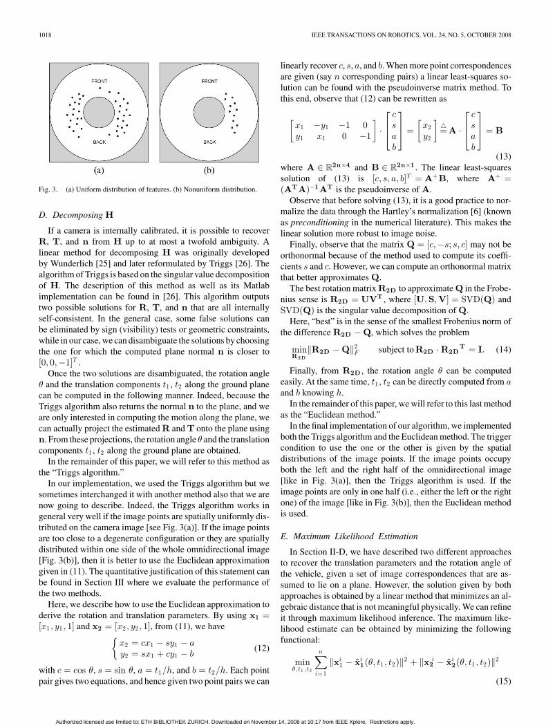
Fig. 3. (a) Uniform distribution of features. (b) Nonuniform distribution.

D. Decomposing H

If a camera is internally calibrated, it is possible to recover R, T, and n from H up to at most a twofold ambiguity. A linear method for decomposing H was originally developed by Wunderlich [25] and later reformulated by Triggs [26]. The algorithm of Triggs is based on the singular value decomposition of H. The description of this method as well as its Matlab implementation can be found in [26]. This algorithm outputs two possible solutions for R, T, and n that are all internally self-consistent. In the general case, some false solutions can be eliminated by sign (visibility) tests or geometric constraints, while in our case, we can disambiguate the solutions by choosing the one for which the computed plane normal n is closer to [0, 0, −1]T .

Once the two solutions are disambiguated, the rotation angle θ and the translation components t1 , t2 along the ground plane can be computed in the following manner. Indeed, because the Triggs algorithm also returns the normal n to the plane, and we are only interested in computing the motion along the plane, we can actually project the estimated R and T onto the plane using n. From these projections, the rotation angle θ and the translation components t1 , t2 along the ground plane are obtained.

In the remainder of this paper, we will refer to this method as the “Triggs algorithm.”

In our implementation, we used the Triggs algorithm but we sometimes interchanged it with another method also that we are now going to describe. Indeed, the Triggs algorithm works in general very well if the image points are spatially uniformly distributed on the camera image [see Fig. 3(a)]. If the image points are too close to a degenerate configuration or they are spatially distributed within one side of the whole omnidirectional image [Fig. 3(b)], then it is better to use the Euclidean approximation given in (11). The quantitative justification of this statement can be found in Section III where we evaluate the performance of the two methods.

Here, we describe how to use the Euclidean approximation to derive the rotation and translation parameters. By using x1 = [x1 , y1 , 1] and x2 = [x2 , y2 , 1], from (11), we have

x2 = cx1 − sy1 − a y2 = sx1 + cy1 − b

(12)

with c = cos θ, s = sin θ, a = t1 /h, and b = t2 /h. Each point pair gives two equations, and hence given two point pairs we can

IEEE TRANSACTIONS ON ROBOTICS, VOL. 24, NO. 5, OCTOBER 2008

linearly recover c, s, a, and b. When more point correspondences are given (say n corresponding pairs) a linear least-squares solution can be found with the pseudoinverse matrix method. To this end, observe that (12) can be rewritten as

c c x1 −y1 −1 0 s s = A = B =

x2 �y1 x1 0 −1

·a y2

· a

b b(13)

where A ∈ R2n×4 and B ∈ R2n×1 . The linear least-squares T = A+ B,solution of (13) is [c, s, a, b] where A+ =

(ATA)−1AT is the pseudoinverse of A. Observe that before solving (13), it is a good practice to nor

malize the data through the Hartley’s normalization [6] (known as preconditioning in the numerical literature). This makes the linear solution more robust to image noise.

Finally, observe that the matrix Q = [c, −s; s, c] may not be orthonormal because of the method used to compute its coefficients s and c. However, we can compute an orthonormal matrix that better approximates Q.

The best rotation matrix R2D to approximate Q in the Frobenius sense is R2D = UVT , where [U, S, V] = SVD(Q) and SVD(Q) is the singular value decomposition of Q.

Here, “best” is in the sense of the smallest Frobenius norm of the difference R2D − Q, which solves the problem

R2D

‖R2D − Q‖2min F subject to R2D R2DT = I. (14)·

Finally, from R2D , the rotation angle θ can be computed easily. At the same time, t1 , t2 can be directly computed from a and b knowing h.

In the remainder of this paper, we will refer to this last method as the “Euclidean method.”

In the final implementation of our algorithm, we implemented both the Triggs algorithm and the Euclidean method. The trigger condition to use the one or the other is given by the spatial distributions of the image points. If the image points occupy both the left and the right half of the omnidirectional image [like in Fig. 3(a)], then the Triggs algorithm is used. If the image points are only in one half (i.e., either the left or the right one) of the image [like in Fig. 3(b)], then the Euclidean method is used.

E. Maximum Likelihood Estimation

In Section II-D, we have described two different approaches to recover the translation parameters and the rotation angle of the vehicle, given a set of image correspondences that are assumed to lie on a plane. However, the solution given by both approaches is obtained by a linear method that minimizes an algebraic distance that is not meaningful physically. We can refine it through maximum likelihood inference. The maximum likelihood estimate can be obtained by minimizing the following functional:

n i i i imin ‖x1 − ˆ x2 (θ, t1 , t2)‖2x1 (θ, t1 , t2)‖2 + ‖x2 − ˆ

θ,t1 ,t2 i=1

(15)


√


with ˆ x2 = Hx1 . If the Triggs algorithm is used, H is defined as in [26], otherwise it is defined as in (11).

To minimize (15), we used the Levenberg–Marquadt algorithm. This algorithm requires an initial guess for θ, t1 , and t2 . As an initial guess, we used the linear solutions provided by

x1 = H−1x2 , ˆ

(13) and (14).

F. Coplanarity Check

The equations given in the previous sections assume that the corresponding image pairs x1 and x2 are correctly matched and that the points lie on the ground plane. Even though in omnidirectional images taken from the roof of the car, the ground plane is predominant, there are also many feature points that come from other objects than just the road, like cars, buildings, trees, guardrails, etc. Furthermore, there are also many unavoidable false matches that are more numerous than those usually output by the SIFT on standard perspective images (about 20%–30% according to [16]) because of the large distortion introduced by the mirror. To discard the outliers, we used the RANSAC paradigm [20]. The RANSAC steps in our case are formally the following.

1) Let A be the set of all image pairs output by SIFT from two consecutive frames. At each iteration, four putative corresponding pairs are randomly selected from A and a homography H is instantiated from these points (four is the minimum number of point pairs required to compute an 8-DOF homography).

2) The instantiated H is used to determine the subset S1 of point pairs in A that are within some error tolerance d. This subset S1 is called consensus set.

3) If the number of members in S1 is greater than some threshold t, which is a function of the expected number of outliers in A, then S1 is used to compute a new H∗.

4) Otherwise, if the number of members in S1 is less than t, then a new subset S2 is randomly selected and the previous process is repeated.

If, after some predetermined number of trials, no consensus set with t or more members is found, then the homography H∗

with the largest consensus set is used. How to the estimate t as a function of the number of outliers can be found in [20].

As an error measure to determine the subset S1 of pairs that are within the error tolerance d, we used the symmetric transfer error

i i i 2erri = ‖x2 − Hxi 1 ‖2 + ‖x1 − H−1x . (16)2 ‖

We reject every pair for which erri > d, where d is computed statistically according to the Huber-type skipped means rule [21], i.e., d = 5.2MAD. MAD stands for median absolute deviation and is defined as

MAD(err) = mediani{|erri − medianj (errj )|}. (17)

Observe that if a prior estimate of the rotation angle is available (consider, for example, that coming from the visual compass of Section IV), then this can be used as a prestage in the first step of RANSAC to constrain the selection of putative matches. This has the effect of speeding up the search of inliers and re

ducing the percentage of outliers. In our implementation, we do this in the following manner: we assume a 3-DOF motion, then the rotation angle can be computed from at least two putative point pairs. If this rotation estimate is consistent (within a certain threshold) with that given by the visual compass, then the two point pairs are retained.

III. TRIGGS VERSUS EUCLID: A PERFORMANCE EVALUATION

In this section, we evaluate the performance of the Triggs and the Euclidean methods under the influence of image noise, point distribution, nonperfectly planar motion, and nonperfectly vertical camera. The analysis is done on simulated data.

In the simulated environment, we used the same omnidirectional camera model of our experiments. Also, the image size was assigned as in the real experiments, namely, 640 × 480 pixels. The self-occlusion of the camera was simulated by removing a circular region of radius Rmin from the center of the omnidirectional image (like in Fig. 11). The length of the camera displacement was chosen equal to the maximum displacement of our real vehicle between two consecutive frames, namely 0.6 m. Also, the camera distance h to the ground plane was assigned as in the real experiments, namely 2 m.

In each simulation trial, we used ten feature points randomly selected from the ground plane. To randomly select these points, we used a uniform probability distribution over the interval [−5, 5] m along both the x- and y-directions. This point interval is consistent to that observed during the experiments. Once the features were selected, we projected them onto the image plane and considered only their pixel coordinates.

Our goal is to characterize the performance of the outputs of the Triggs and Euclidean methods when the planar motion constraint and the verticality of the camera are not perfectly satisfied. The outputs we are interested in are the motion parameters along the ground plane, i.e., the rotation angle θ (here called yaw angle) and the translation length along the ground

2 2plane T| = t1 + t2 , where t1 , t2 are computed as given in |Section II-D. For each simulation experiment, we will give the plots of the absolute errors of θ and T|, respectively. |

As a first study, we characterize the performance of the two algorithms with respect to Gaussian image noise. In the first stage, we consider the ideal case where the camera undergoes pure planar motion and the camera is perfectly vertical. In this experiment, the coordinates of all image points were corrupted by Gaussian noise with mean zero and variance σ. We varied σ from 0 to 2 pixels, and for each value, we ran 1000 independent trials where we computed the motion parameters θ and |T .|The results shown in Fig. 4 are the average of the absolute error. As observed, the error increases linearly with the noise variance. Furthermore, the error given by the Euclidean method is smaller than that given by the Triggs approach. This result was expected because the Euclidean method provides 3-DOF motion estimates that are more robust to image noise when the motion is purely planar and the camera perfectly vertical.

Conversely, when this assumption does not hold, the behavior of the two algorithms can be much different. As an example, consider Fig. 5 to see what happens if the camera does not appear



Fig. 4. Motion estimates versus noise variance [σ (in pixels)]. (a) Yaw angle (in degrees). (b) Translation length (in meters). The case of pure planar motion and camera perfectly vertical is considered.

Fig. 5. Motion estimates versus noise variance [σ (in pixels)]. (a) Yaw angle (in degrees). (b) Translation length (in meters). Camera nonperfectly vertical: pitch = roll = 1.0◦.

perfectly vertical. To generate this plot, we kept the direction of motion still parallel to the ground plane but we slightly changed the orientation (roll and pitch angles) of the camera axis in the second position; in particular, we set roll = pitch = 1.0◦. As observed, for small noise values, the Triggs algorithm performs better than the Euclidean one. Indeed, in the noise-free case, it can compute the exact orientation of the camera, while the Euclidean method cannot. Thus, for small noise values, it performs better than the Euclidean approach. Conversely, when the noise increases, the error on the six motion parameters becomes more relevant, while the error of the Euclidean method stays constant. In the next simulations, we will consider a noise variance of 0.3 pixels.

In Section II-D, we mentioned that we switch between the Triggs and the Euclidean method according to the distribution of the image points (see Fig. 3). The justification of this choice will now be given. First of all, consider that if the scene points are collinear, the homography cannot be computed because the points are in a degenerate configuration. In practice, however, the image points are always corrupted by noise or the scene points are nearly collinear. Thus, in both cases, the homography can be instantiated but, because the data are badly conditioned, the result of the homography decomposition by Triggs would diverge from the correct result. Conversely, the Euclidean transformation is not affected by the collinearity of the scene points. This brought us to the conclusion that if the scene points are nearly collinear (and so the image points lie nearly on a conic), the Euclidean transformation should be used; in all the other

Fig. 6. Motion estimates versus point distribution (Σ (in meters)). Point distribution is computed as point variance along the y-axis. (a) Yaw angle (in degrees). (b) Translation length (in meters). The case of pure planar motion and camera perfectly vertical is considered.

Fig. 7. Motion estimates versus point distribution (Σ (in meters)). Point distribution is computed as point variance along the y-axis. (a) Yaw angle (in degrees). (b) Translation length (in meters). Camera nonperfectly vertical: pitch = roll = 1.0◦

cases, the Triggs algorithm should be adopted. By performing several simulations, we actually found that it is better to use the Euclidean algorithm when the image points lie only on one half of the omnidirectional image (i.e., scene points potentially collinear).

To demonstrate this, we generated our random features along a line parallel to the x-axis and distant 1 m from the camera origin. Then, we perturbed the y-coordinate of the features with Σ meters Gaussian noise. Finally, we projected the features onto the image plane and added 0.3 pixel Gaussian noise. We varied Σ from 0 to 2 m and ran 1000 independent trials. The average values of the absolute error of the motion estimates are shown in Fig. 6. As observed, the Euclidean method performs better than the Triggs for every Σ. However, this experiment was done by again considering pure planar motion and camera perfectly vertical; hence, the Euclidean method has to provide the best result.

Conversely, the effect of a nonperfectly vertical camera (namely, roll = pitch = 1◦) can be seen in Fig. 7 As observed in these plots, the Euclidean method provides more accurate motion estimates than the Triggs method only when Σ < 0.2 m. This means that when Σ = 0.2, most features lie within 3Σ = 0.6 m distance from the line. By increasing further on the inclination of the camera (roll, pitch >1 ◦), we found that this threshold also increases. In practice, the inclination of the camera changes over the time due to jittery motion. This



Fig. 8. Sensitivity of motion estimates to nonplanar motion. The sensitivity is computed as a function of the roll angle of the camera in the second view (pitch = 0, Tz = 0.1 m). (a) Yaw angle (in degrees). (b) Translation length (in meters).

Fig. 9. Sensitivity of motion estimates to the camera axis orientation with respect to the vertical. The sensitivity is computed as a function of the angle between the camera axis and plane normal. (a) Yaw angle (in degrees). (b) Translation length (in meters).

phenomenon motivated our decision of switching the two methods according to the distribution of the image points. Finally, observe that when Σ approaches 0 (i.e., scene points are collinear), the motion estimates by Triggs diverges as expected.

Fig. 8 shows the sensitivity of the motion estimates to non-perfectly planar motion. We added a translation component Tz = 0.1 m along the z-axis and also varied the relative orientation of the camera in the second position. The sensitivity of the motion parameters is computed as a function of the roll angle of the camera in the second position. The roll was varied from 0◦ to 5◦, and for each value, 1000 trials were run. For each run, 0.3 pixel noise was added to corrupt the image points. As observed, the Triggs algorithm always performs better than the Euclidean method, showing to be able to detect violations from the planar motion assumption. We also performed the same experiment by varying the pitch angle and we obtained similar plots.

Finally, Fig. 9 shows the influence of a nonperfectly vertical camera axis on the motion estimates. The motion is still assumed to be parallel to the ground plane. The plot is shown as a function of the angle between the plane normal and the camera axis. This angle was varied from 0◦ to 5◦ and for each value, 1000 trials were run. For each run, 0.3 pixel noise was added to corrupt the image points. As observed, the Triggs algorithm is able to detect deviations of the camera from the verticality.

Fig. 10. Two unwrapped omnidirectional images. For reasons of space, here only one half of the whole 360◦ is shown unwrapped. The central part of the image corresponds to the front view of the vehicle (see Fig. 11). The two frames were taken at different times while the car was translating and turning right. The upper image is taken at time t − 1, the lower image at time t. The red (gray) line is the horizon line. The white box is the search window used in our experiments.

IV. VISUAL COMPASS

In Section II, we described how to use point features to compute the rotation and translation matrices. Unfortunately, when using features to estimate the motion, the resulting rotation is extremely sensitive to systematic errors due to the intrinsic calibration of the camera or the extrinsic calibration between the camera and the ground plane (the last case was studied in Section III). This effect is even more accentuated with omnidirectional cameras due to the large distortion introduced by the mirror. In addition to this, integrating rotational information over time has the major drawback of generally becoming less and less accurate as integration introduces additive errors at each step. An example of camera trajectory recovered only using the feature-based approach described in Section II is depicted in Fig. 13.

To improve the accuracy of the rotation estimation, we used an appearance-based approach. This approach was inspired by a recent work on the use of omnidirectional cameras as visual compass [23]. Directly using the appearance of the world as opposed to extracting features or structure of the world is attractive because methods can be devised that do not need precise calibration steps. Here, we describe how we implemented our visual compass.

For ease of processing, every omnidirectional image is unwrapped into cylindrical panoramas (see Fig. 10). The unwrapping considers only the white region of the omnidirectional image that is depicted in Fig 11. We call these unwrapped versions “appearances.” If the camera is perfectly vertical to the ground, then a pure rotation about its vertical axis will result in a simple column-wise shift of the appearance in the opposite direction. The exact rotation angle could then be retrieved by simply finding the best match between a reference image (before rotation) and a column-wise shift of the successive image (after rotation). The best shift is directly related to the rotation angle undertaken by the camera. In the general motion, translational information is also present. This general case will be discussed later.

The input to our rotation estimation scheme is thus made of appearances that need to be compared. To compare them, we


√ √ ∑ ∑ ∑


Fig. 11. Cylindrical panorama is obtained by unwrapping the white region. The front view is the view pointing to the heading direction of the vehicle. The reduced FOV around the front and back of the camera is demarcated by the two lines.

used different similarity measures. In particular, we have tried cross-correlation, zero-mean normalized cross-correlation, L1norm (Manhattan distance), and an L2-norm (Euclidean distance). The best results were obtained by using the Euclidean distance. A performance comparison with the other metrics is not given in this paper.

The Euclidean distance between two appearances Ii and Ij , with Ij being column-wise shifted (with column wrapping) by α pixels, is

√ h w c

d(Ii, Ij , α) = √ Ii (k, h, l) − Ij (k, h − α, l)|2|k =1 h=1 l=1

(18)

where h × w is the image size and c is the number of color components. In our experiments, we used the red, green, and blue (RGB) color space, thus having three color components per pixel.

Defining αm the best shift that minimizes the distance d(Ii, Ij , αm ) ≤ d(Ii, Ij , α) ∀α ∈ R, then the rotation angle ∆ϑ (in degrees) between Ii and Ij is

360∆ϑ = αm . (19)

w

The width w of the appearance is the width of the omnidirectional image after unwrapping and can be chosen arbitrarily. In our experiments, we used w =360, which means that the angular resolution was 1 pixel/◦. To increase the resolution to 0.1◦, we used cubic spline interpolation with 0.1 pixel precision. We also tried larger image widths, but we did not get any remarkable improvement in the final results. Thus, we used w =360 as the unwrapping can be done in a negligible amount of time. The Euclidean distance between the two images in Fig. 10 as a function of the column-wise shift of the second image is shown in Fig. 12.

The distance minimization in (18) makes sense only when the camera undergoes a pure rotation about its vertical axis, as a rotation corresponds to a horizontal shift in the appearance. In the real case, the vehicle is moving and translational component

Fig. 12. Euclidean distance between the two images in Fig. 10 as a function of the column-wise shift of the second image. The distance is computed according to (18).

is present. However, the “pure rotation” assumption still holds if the camera undergoes small displacements or the distance to the objects (buildings, tree, etc.) is large compared to the displacement. In the other cases, this assumption does not hold for the whole image, but an improvement that can be done over the theoretical method is to only consider parts of the images, namely the front and back part (see Fig. 11). Indeed, the contribution to the optic flow by the motion of the camera is not homogeneous in omnidirectional images; a forward/backward translation mostly contributes in the regions corresponding to the sides of the camera and very little in the parts corresponding to the front and back of the camera, while the rotation contributes equally everywhere.

Because we are interested in extracting the rotation information, only considering the regions of the images corresponding to the front and back of the camera allows us to reduce most of the problems introduced by the translation, in particular sudden changes in appearance (parallax).

According to the last considerations, in our experiments, we used a reduced FOV around the front and back of the camera (Fig. 11). The reduction of the FOV was done on both the horizontal and vertical planes. A reduced horizontal FOV of about 30◦ around the front part is shown by the white window in Fig. 10. Observe that we also reduced the FOV on the vertical plane, in particular under the horizon line. The reason was to reduce the influence of the changes in appearance of the road. The resulting vertical FOV was 50◦ above and 10◦ below the horizon line (the horizon line is indicated in red (gray) in Fig. 10).

The fact of reducing the FOV (especially on the horizontal plane) provided an important improvement over using the whole FOV in terms of stability and sensitivity to prominent features at the sides of the camera. The effect of the size of the horizontal FOV on the estimation of the camera trajectory is depicted in Fig. 14 and will be discussed in Section VI.

V. MOTION ESTIMATION ALGORITHM

As already mentioned, the appearance-based approach provides rotation angle estimates that are more reliable and stable


( )

( )

√


than those output by the pure feature-based approach. Here, we describe how we combined the rotation angle estimates of Section IV with the camera translation estimates of Section II.

In our experiments, the speed of the vehicle ranged between 10 and 20 Km/h, while the images were constantly captured at 10 Hz. This means that the distance covered between two consecutive frames ranged between 0.3 and 0.6 m. For this short distance, the camera configuration (x, y, θ), which contains its 2-D position (x, y) and orientation θ, can be approximated in this way

δθi xi+1 = xi + δρi cos θi + 2

(20) yi+1 = yi + δρi sin θi + δθi 2

θi+1 = θi + δθi

where we use δρ = T h and δθ = ∆ϑ.| |Observe that T is the same translation vector used in

Section II, and thus, |T = t12 + t22 , where t1 and t2 are|computed as described in Section II-D and E. Parameter h is the scale factor (i.e., in our case, this is the height of the camera to the ground plane). The camera rotation angle ∆ϑ is computed as described in Section IV. Observe that we did not use at all the rotation estimates provided by the feature-based method of Section II.

Now, let us resume the steps of our motion estimation scheme, which have been detailed in Sections II and IV. Our omnidirectional visual odometry operates as follows.

1) Acquire two consecutive frames. Consider only the region of the omnidirectional image, which is between Rmin and Rmax (see Fig. 11).

2) Extract and match SIFT features between the two frames. Use the double consistency check to reduce the number of outliers. Then, use the calibrated camera model to normalize the feature coordinates by reprojecting them onto a plane perpendicular to the z-axis and distant 1 from the origin.

3) Unwrap the two images and compare them using the appearance method described in Section IV. In particular, minimize (18), with reduced FOV, to compute the column-wise shift between the appearances and use (19) to compute the rotation angle ∆ϑ.

4) Use RANSAC to reject points that are not coplanar (Section II-F); in particular, use the available rotation estimate ∆ϑ from the visual compass to speed up RANSAC, as explained at the end of Section II-F.

5) Apply the linear algorithm described in Section II-D to estimate R and T from the remaining inliers. In doing this, switch between the Triggs algorithm and the Euclidean method, as described in Section II-D. Then, refine R and T using maximum likelihood estimation (Section II-E).

6) Use δρ = |T h and δθ = ∆ϑ and integrate the motion |using (20).

7) Repeat from step 1.

Fig. 13. Comparison between the camera trajectory recovered thorough two distinct approaches: solid line, the trajectory recovered using the whole algorithm described in this paper (feature and appearance based); dashed line, the trajectory recovered using only the feature-based approach described in Section II.

Fig. 14. Comparison of a camera trajectory recovered by using different FOVs.

Fig. 15. Heading direction θ (in degrees) versus the traveled distance (in meters). The results are shown for different FOVs.



Fig. 16. Estimated path superimposed onto a Google Earth image of the test environment. The scale is shown at the lower left corner.

Fig. 17. Image mosaicing that shows a textured 2-D reconstruction of the estimated path. The two arrows point out the final error at the loop closure (the two pedestrian crossings pointed to by the arrows in reality coincide).

VI. RESULTS

The approach proposed in this paper has been successfully tested on a real vehicle equipped with a central omnidirectional camera. A picture of our vehicle (a Smart) is shown in Fig. 1.

Our omnidirectional camera, composed of a hyperbolic mirror (KAIDAN 360 One VR) and a digital color camera (SONY XCD-SX910, image size 640 × 480 pixels), was installed on the front part of the roof of the vehicle. The frames were grabbed at 10 Hz, and the vehicle speed ranged between 10 and 20 km/h.

The resulting path estimated by our visual odometry algorithm using a 10◦ FOV is shown in Figs. 13, 16, and 17. Our ground truth is a satellite image of the same test environment provided by Google Earth (Fig. 16). The units used in the three figures are meters.

In this experiment, the vehicle was driven along a 400-m-long loop and returned to its starting position (pointed to by the yellow (gray) arrow in Fig. 16). The estimated path is indicated with red (gray) dots in Fig. 16 and is shown superimposed on a satellite



image for comparison. The final error at the loop closure is about 6.5 m for the distance and 5◦ for the orientation. This error is due to the unavoidable visual odometry drift; however, observe that the trajectory is very well estimated until the third 90◦ turn. After this turn, the estimated path deviates smoothly from the expected path instead of continuing straight. After road inspection, we found that this deviation was due to three 0.3-m-tall road humps (indicated by the cyan (gray) circle in Fig. 16) that violate the planar motion assumption.

The content of Fig. 17 is very important as it allows us to evaluate the quality of motion estimation. In this figure, we show a textured top viewed 2-D reconstruction of the whole path. Observe that this image is not a satellite image but is an image mosaicing. Every input image of this mosaic was obtained by an inverse perspective mapping (IPM) of the original omnidirectional image onto an horizontal plane. This inverse mapping is always possible for central cameras, i.e., when a camera has a single effective viewpoint. After being undistorted through IPM, these images were merged together using the 2-D poses estimated by our visual odometry algorithm. The estimated trajectory of the camera is shown superimposed with red (gray) dots. If the reader visually and carefully compares the mosaic (see Fig. 17) with the corresponding satellite image (see Fig. 16), he will recognize in the mosaic the same elements that are present in the satellite image, i.e., trees, white footpaths, pedestrian crossings, roads’ placement, etc. Furthermore, the reader can verify that the location of these elements in the mosaic fits well the location of the same elements in the satellite image.

As mentioned in Section IV, we also evaluated the effect of the reduced horizontal FOV on the final motion estimation. Fig. 14 shows the recovered estimated trajectory respectively using FOV = 10◦, FOV = 20◦, FOV = 30◦, and FOV = 60◦. Observe that the estimation of the trajectory improves as the FOV decreases. Indeed, as mentioned already in Section IV, the fact of reducing the FOV allows us to reduce most of the problems introduced by the translation, like sudden changes in parallax. The best performance in terms of closeness to the ground truth of Fig. 16 is obtained when FOV = 10◦.

In Fig. 15, the effect of the FOV on the estimation of the heading direction is also shown. Also, the best performance is when FOV = 10◦. In this case, in fact 90◦ turns are very well estimated. Furthermore, when FOV = 10◦ the heading direction stays quite constant after each turn, i.e., when the vehicle covers a straight path. Note that when the vehicle returns to its start position, the estimated heading direction is equal to 355◦, which means that the orientation error at the loop closure is 5◦.

Finally, a comparison of the proposed algorithm with the only feature based method of Section II is shown in Fig. 13.

VII. CONCLUSION

In this paper, we described a real-time algorithm for computing the ego-motion of a vehicle relative to the road. The algorithm uses as input only those images provided by a single omnidirectional camera. The front ends of the system are two different trackers. The first one is a feature-based tracker that uses SIFT features and a RANSAC-based outlier removal to

track the key points that most likely belong to the ground plane. The second one uses an appearance-based approach to give high-resolution estimates of the rotation angle of the vehicle. Using the first tracker to compute the vehicle displacement in the heading direction and the second tracker to compute the vehicle rotation proved to give very good visual odometry estimates under planar motion assumption. Furthermore, the performance of the motion estimation given by the proposed method is better than the pure feature-based approach (see Fig. 13).

The proposed algorithm was successfully applied to videos from an automotive platform. We gave an example of a camera trajectory estimated purely from omnidirectional images over a distance of 400 m. The accumulated error after 400 m (i.e., error at the loop closure) was about 6.5 m for the distance and 5◦

for the orientation. For performance evaluation, the estimated path was superimposed onto a satellite image of the same test environment and a textured 2-D reconstruction of the path was built.

ACKNOWLEDGMENT

The authors would like to thank P. Lamon and L. Spinello for their useful help, suggestions, and comments.

REFERENCES

[1] H. Moravec, “Obstacle avoidance and navigation in the real world by a seeing robot rover,” Ph.D. dissertation, Stanford Univ., 1980.

[2] S. Lacroix, A. Mallet, R. Chatila, and L. Gallo, “Rover self localization in planetary-like environments,” in Proc. Int. Symp. Artic. Intell., Robot., Autom. Space (i-SAIRAS), Noordwijk, The Netherlands, 1999, pp. 433– 440.

[3] I. Jung and S. Lacroix, “Simultaneous localization and mapping with stereovision,” in Proc. 11th Int. Symp. Robot. Res., Siena, Italy, 2005.

[4] D. Nister, O. Naroditsky, and J. Bergen, “Visual odometry for ground vehicle applications,” J. Field Robot., vol. 23, no. 1, pp. 3–20, 2006.

[5] M. Maimone, Y. Cheng, and L. Matthies, “Two years of visual odometry on the mars exploration rovers: Field reports,” J. Field Robot., vol. 24, no. 3, pp. 169–186, 2007.

[6] R. Hartley and A. Zisserman, Multiple View Geometry in Computer Vision, 2nd ed. Cambridge, U.K.: Cambridge Univ. Press, 2004, (ISBN: 0521540518).

[7] P. I. Corke, D. Strelow, and S. Singh, “Omnidirectional visual odometry for a planetary rover,” in Proc. IROS, Sep. 28–Oct. 2, 2004, vol. 4, pp. 4007– 4012.

[8] M. C. Deans, “Bearing-Only Localization and Mapping,” Ph.D. dissertation, Carnegie Mellon Univ., 2002.

[9] A. Davison, “Real-time simultaneous localisation and mapping with a single camera,” in Proc. Int. Conf. Comput. Vis., Nice, France, Oct. 13– 16, 2003, vol. 2, pp. 1403–1410.

[10] L. A. Clemente, A. J. Davison, I. Reid, J. Neira, and J. D. Tardos, “Mapping large loops with a single hand-held camera,” in Proc. Conf. Robotics: Sci. Syst., Atlanta, GA, Jun. 27–30, 2007.

[11] T. Lemaire and S. Lacroix, “Slam with panoramic vision,” J. Field Robot., vol. 24, no. 1/2, pp. 91–111, 2007.

[12] H. Wang, K. Yuan, W. Zou, and Q. Zhou, “Visual odometry based on locally planar ground assumption,” in Proc. IEEE Int. Conf. Inf. Acquis., Hong Kong, 2005, pp. 59–64.

[13] Q. Ke and T. Kanade, “Transforming camera geometry to a virtual downward-looking camera: Robust ego-motion estimation and ground-layer detection,” in Proc. CVPR Jun. 18–20, 2003, vol. 1, pp. I-390–I-397.

[14] J. J. Guerrero, R. Martinez-Cantin, and C. Sagues, “Visual map-less navigation based on homographies,” J. Robot. Syst., vol. 22, no. 10, pp. 569– 581, 2005.

[15] B. Liang and N. Pears, “Visual navigation using planar homographies,” in Proc. IEEE ICRA, 2002, vol. 1, pp. 205–210.

[16] D. Lowe, “Distinctive image features from scale-invariant keypoints,” Int. J. Comput. Vis., vol. 20, pp. 91–110, 2003.


1026

[17] R. Tsai and T. Huang, “Estimating three-dimensional motion parameters of a rigid planar patch,” IEEE Trans. Acoust., Speech Signal Process., vol. 29, no. 6, pp. 1147–1152, Dec. 1981.

[18] H. C. Longuet-Higgins, “The reconstruction of a plane surface from two perspective projections,” Proc. R. Soc. Lond. B, Biol. Sci., vol. 277, pp. 399–410, 1986.

[19] O. D. Faugeras and F. Lustman, “Motion and structure from motion in a piecewise planar environment,” Int. J. Pattern Recognit. Artif. Intell., no. 3, pp. 485–508, 1988.

[20] M. A. Fischler and R. C. Bolles, “Random sample consensus: A paradigm for model fitting with applications to image analysis and automated cartography,” Commun. ACM, vol. 24, no. 6, pp. 381–395, 1981.

[21] F. Hampel, “The influence curve and its role in robust estimation,” J. Amer. Stat. Assoc., vol. 69, pp. 383–393, 1974. ·

[22] D. Scaramuzza, A. Martinelli, and R. Siegwart, “A flexible technique for accurate omnidirectional camera calibration and structure from motion,” in Proc. ICVS, Jan. 4–7, 2006, pp. 45–45.

[23] F. Labrosse, “The visual compass: Performance and limitations of an appearance-based method,” J. Field Robot., vol. 23, no. 10, pp. 913–941, 2006.

[24] H. Bay, T. Tuytelaars, and L. Van Gool, “Surf: Speeded up robust features,” in Proc. ECCV, 2006, pp. 404–417.

[25] W. Wunderlich, “Rechnerische Rekonstruktion eines ebenen Objekts aus zwei Photographien,” Geodaesia Universalis (Rinner-Festschrift), vol. 40, pp. 365–377, 1982.

[26] B. Triggs, “Autocalibration from planar scenes,” in Proc. ECCV, 1998, pp. 89–105.

[27] S. Baker and S. Nayar, “A theory of single-viewpoint catadioptric image formation,” Int. J. Comput. Vis., vol. 35, no. 2, pp. 175–196, Nov. 1999.

[28] Y. Ma, S. Soatto, J. Kosecka, and S. Sastry, An Invitation to 3D Vision: From Images to Models. New York: Springer-Verlag, Dec. 2003.

Davide Scaramuzza (M’06) was born in Terni, Italy, in 1980. He received the Graduate degree (summa cum laude and Dignity of Printing) in electronics from the University of Perugia, Perugia, Italy, in 2004 and the Ph.D. degree in computer vision and robotics from the Eidgenossische Technische Hochschule (ETH) Zurich, Zurich, Switzerland, in 2008.

He is currently a Postdoctoral Fellow with the Autonomous System Laboratory, ETH Zurich. He is the author of Omnidirectional Camera Calibration Tool

box for Matlab. His current research interests include omnidirectional vision, computer vision, and robotics.

Dr. Scaramuzza was awarded the Aica-Federcomin Prize, which is the first Italian National Prize for the Best Master Thesis in the field of Information, Communication, and Technology, for the graduation thesis.

IEEE TRANSACTIONS ON ROBOTICS, VOL. 24, NO. 5, OCTOBER 2008

Roland Siegwart (M’90–SM’03–F’08) received the Diploma in mechanical engineering and the Ph.D. degree in mechatronics from the Eidgenossische Technische Hochschule (ETH) Zurich, Zurich, Switzerland, in 1983 and 1989, respectively.

From 1989 to 1990, he was a Postdoctoral Fellow at Stanford University, Stanford, CA. Then, he worked part time as the R&D Director at MECOS Traxler AG. He was also a part-time Lecturer and the Deputy Head of the Institute of Robotics, ETH Zurich, where, since July 2006, he has been a Full

Professor of autonomous systems. In 1996, he was an Associate Professor, and later, a Full Professor for autonomous microsystems and robots at the Ecole Polytechnique Federale de Lausanne (EPFL), Lausanne, Switzerland, where he was a Co-Initiator and the Founding Chairman of the Space Center EPFL and the Vice Dean of the School of Engineering. In 2005, he held visiting positions at the National Aeronautics and Space Administration (NASA) Ames, Moffett Field, CA, and Stanford University. He leads a research group of around 35 people working in the field of robotics, mechatroics, and product design. He is a Coordinator of two large European projects, plays an active role in various rover designs of the European Space Agency, and is a Cofounder of several spin-off companies.

Prof. Siegwart is a member of the Swiss Academy of Engineering Sciences and a Board Member of the European Network of Robotics (EURON). From 2004 to 2005, he was the Vice President for Technical Activities and a Distinguished Lecturer from 2006 to 2007. He is currently an AdCom Member (2007–2009) of the IEEE Robotics and Automation Society.


appearance-guided monocular omnidirectional visual odometry for outdoor ground vehicles

Documents