Sensitivity Analysis of the MM5 Weather ModelUsing Automatic Di�erentiationChristian H. BischofMath. & Comp. Sc. Div.Argonne National LaboratoryArgonne, IL 60439bischof@mcs.anl.gov Gordon D. PuschPhysics DepartmentMichigan State UniversityEast Lansing, MI 48842pusch@mcs.anl.gov Ralf KnoeselMath. & Comp. Sc. Div.Argonne National LaboratoryArgonne, IL 60439knoesel@mcs.anl.govArgonne Preprint MCS-P532-0895AbstractWe present a general method for using automatic di�erentiation to facilitate model sensitivityanalysis. Automatic di�erentiation techniques augment, in a completely mechanical fashion, anexisting code such that it also simultaneously and e�ciently computes derivatives. Our methodallows the sensitivities of the code's outputs to its parameters and inputs to be determinedwith minimal human e�ort by exploiting the relationship between di�erentiation and formalperturbation theory.Employing this method, we performed a sensitivity study of the MM5 code, a mesoscaleweather model jointly developed by Penn State University and the National Center for Atmo-spheric Research, comprising roughly 40,000 lines of Fortran 77 code. Our results show thatAD-computed sensitivities exhibit superior accuracy compared with divided di�erences approx-imations computed from �nite-amplitude perturbations, while consuming comparable or lessCPU time and less human labor. We also comment on a numerically induced precursor wavethat would almost certainly have been undetectable if one used a divided di�erence method.1 IntroductionIn this paper, we present a general approach for automating the sensitivity analysis of a computermodel using automatic di�erentiation. Automatic di�erentiation (AD) techniques augment, in acompletely mechanical fashion, an existing code such that it also simultaneously and e�ciently com-putes derivatives; hence, one may obtain the partial derivatives (also referred to as \sensitivities")of the code's outputs with respect to its parameters and inputs with minimal human e�ort. AnAD tool mechanically generates from an existing code an augmented code that in addition com-putes derivatives by a systematic application of the chain rule to each elementary operation andfunction [18, 14]. Unlike divided di�erence (DD) approximations, AD-computed sensitivities areaccurate to machine precision, whereas DD estimates su�er from an unavoidable tradeo� betweentruncation and cancellation error [12, 17].To demonstrate the utility of our approach, we present two results from a sensitivity study inwhich we used the ADIFOR tool [2, 3, 4] to construct the tangent linear model (TLM) of the MM5�fth generation mesoscale weather model. MM5 is a 3-D limited area (that is, mesoscale and regionalscale) �nite-di�erence weather model. It is capable of both hydrostatic and nonhydrostatic weathersimulation and prediction, and it contains numerous submodels of various microscale and subgrid-scale meteorological processes [13, 10]. MM5 has been developed jointly by the Penn State University(PSU) Meteorology Department and the National Center for Atmospheric Research (NCAR) as acommunity mesoscale model and is continuously being improved by its many users at universitiesand government laboratories. The MM5 code consists of roughly 40,000 lines of Fortran 77 code.The tangent linear model of a system results from linearizing that system about some speci�edreference solution or base [6, 11, 21]. The TLM may also be obtained by applying formal �rst-orderperturbation theory to the system; furthermore, it can be shown that the �rst-order perturbation of1

any prognostic or diagnostic variable may be obtained by evaluating the derivative of that variablewith respect to the perturbation parameter. Therefore, one can generate the TLM of a complex codewith minimal human labor by parameterizing the perturbation of interest, then di�erentiating withrespect to that parameter by using an AD tool. This approach enables one to perform sensitivitystudies on a complex code quickly, easily, and accurately; by contrast, more conventional approachesto sensitivity analysis may require substantial human e�ort to \reverse engineer" and modify thecode, yet achieve less accurate results.The outline of this paper is as follows. In Section 2, we discuss the tangent linear model; wethen show the connection of the TLM to �rst-order perturbation theory and to di�erentiation. InSection 3, we give a brief introduction to automatic di�erentiation and comment on its superiority todivided-di�erence approximations of derivatives. We then show how to easily construct the TLM byusing AD to di�erentiate with respect to a scalar perturbation parameter. In Section 4, we describethe domain and initial conditions used for our unperturbed reference trajectory, and we discussthe physical meaning of our chosen initial perturbation. We then present a dramatic illustration ofthe superior accuracy that may be obtained by using AD-computed sensitivities instead of divided-di�erence approximations. Finally, we discuss one of the phenomena we observed in the TLM outputthat would almost certainly have gone undetected had we used a divided-di�erence approach: anumerically induced \superacoustic" precursor wave.2 The Tangent Linear Model and Di�erentiationWhether presented as a table of results from a set of exploratory runs or formally encapsulatedas a sensitivity coe�cient, most parametric sensitivity studies either are equivalent to or can beembedded in a problem of estimating derivatives. By di�erentiating the output of a model withrespect to its parameters, one can quantify how sensitive or robust the model's predictions arerelative to variations of that parameter, as well as gain insight into how to adjust parameters that arepoorly known. Questions regarding the sensitivity of the model output to more abstract quantitiesinvolving many model variables can also often be rephrased in terms of derivatives, either directly orby embedding the problem of interest into a larger parameterized framework (for example, by usinga continuation [19] or invariant imbedding method [22]). Our approach is an example of this latterapproach: we obtain the TLM evolution of a perturbation in the initial-value data by introducing aparameter that linearly interpolates between the unperturbed and perturbed initial states. We shallshow that formal perturbation theory with respect to the parameter yields the TLM and can beshown to be equivalent to evaluation of the derivative with respect to the interpolating parameter.2.1 An Example of the TLM for Discrete TimeThe tangent linear model describes the linearized evolution of errors or perturbations about thetrajectory of some particular base or reference solution. Its name is derived from the fact that asolution to the TLM always falls somewhere on the instantaneous tangent to the reference solution asboth of them evolve in time [11, 21]. To illustrate the TLM, we consider a discretized-time example.Assume that the vector X(t) describing the state of the system at time t satis�es the simple equationX(tk+1) = H(X(tk)); k = 0; : : : ; f: (1)For the sake of notational simplicity, we shall lump into X not only all the prognostic variables,but also the diagnostic variables and model parameters, and treat X as if it were a single columnvector, rather than a collection of multidimensional arrays. Note also that, while MM5 uses a leapfrogscheme wherein X(tk+1) depends on the state of two preceding time slices, X(tk) andX(tk�1); in (1)we have written that X(tk+1) depends only on X(tk); however this should not be cause for concern.It is always possible to rewrite a second-order di�erence equation �(tk+1) = g(�(tk); �(tk�1)) as two2

�rst-order di�erence equations of the form (1), by regarding the pair (�(tk); �(tk�1)) as a single set ofvariablesX(tk) de�ning the state at tk; and adjoining the trivial equation �(tk) = 1��(tk)+0��(tk�1):Let J(tk) := @X(tk+1)@X(tk) = @H@X ����X=X(tk) (2)denote the n � n Jacobian of H with respect to the state at time step k. Let �X(t) denote thesensitivity of the state X(t) at time t with respect to a perturbation �X(t0) of its initial state X(t0);that is, �X(t) = @X(t)@X(t0) � �X(t0); (3)where \�" denotes vector-matrix multiplication, and �X(t) and �X(t0) should be interpreted ascolumn vectors. Then by (1), (2), (3), and the associativity of the chain-rule,�X(t1) = J(t0) � �X(t0)�X(t2) = J(t1) � �X(t1) = J(t1) � J(t0) � �X(t0)...�X(tk) = J(tk�1) � �X(tk�1) = J(tk�1) � � � � � J(t0) � �X(t0): (4)Note that the sensitivity is propagated by the same chain of Jacobians regardless of the initialperturbation �X(t0): That is, the sensitivity is a linear function of the initial perturbation; however,this function is determined entirely by the unperturbed trajectory, not the perturbed one. In otherwords, the sensitivity is really a property of the trajectory, rather than the perturbation.Let X0(t) be a particular solution of (1), which we shall call the base, or reference trajectory,and let X(t) be a perturbed nonlinear solution that is initially close to X0(t): The tangent linearapproximation XTLM (t) � X(t) relative to the base state X0(t) is de�ned asXTLM (t) := X0(t) + �X(t) = X0(t) + k�1Yi=0 J(ti) � �X(t0); �X(t0) := X(t0)�X0(t0); (5)that is, the TLM solution is a �rst-order Taylor approximation to the perturbed nonlinear solution,expanded about the base state. Because the Jacobian J generalizes the notion of the slope or tangentof a curve to an n-dimensional space, and since the TLM solution is a linear function of �X(t0);it follows that a solution to the TLM always falls somewhere on the instantaneous tangent to thereference solution as both of them evolve in time|hence the term \tangent linear model" [11, 21].Equation (5) represents the general solution of the TLM given an arbitrary �X(t0): The choiceof �X(t0) is at the disposal of the analyst; particular solutions corresponding to speci�c choices of�X(t0) may have particularly simple or useful interpretations. For example, by initializing �Xi(t0) =1, �Xj(t0) = 0 for j 6= i, �X(tf ) can be interpreted as the sensitivity of the �nal state vector X(tf )per unit change in the ith component Xi(t0) of the initial state. For a general choice �X(t0); theinterpretation of �X(tf ) is given by the concept of the directional derivative|the rate of change ofX(tf ) per unit change of X(t0) in the direction of �X(t0):2.2 The TLM and Formal Perturbation TheoryLet us consider a perturbed initial stateX(t0; �; �X(t0)) := X0(t0) + � �X(t0); (6)where we have split the perturbation into two factors|a spatially varying function �X that de-termines its \shape," and a scale factor � parameterizing its amplitude; we use the semicolon to3

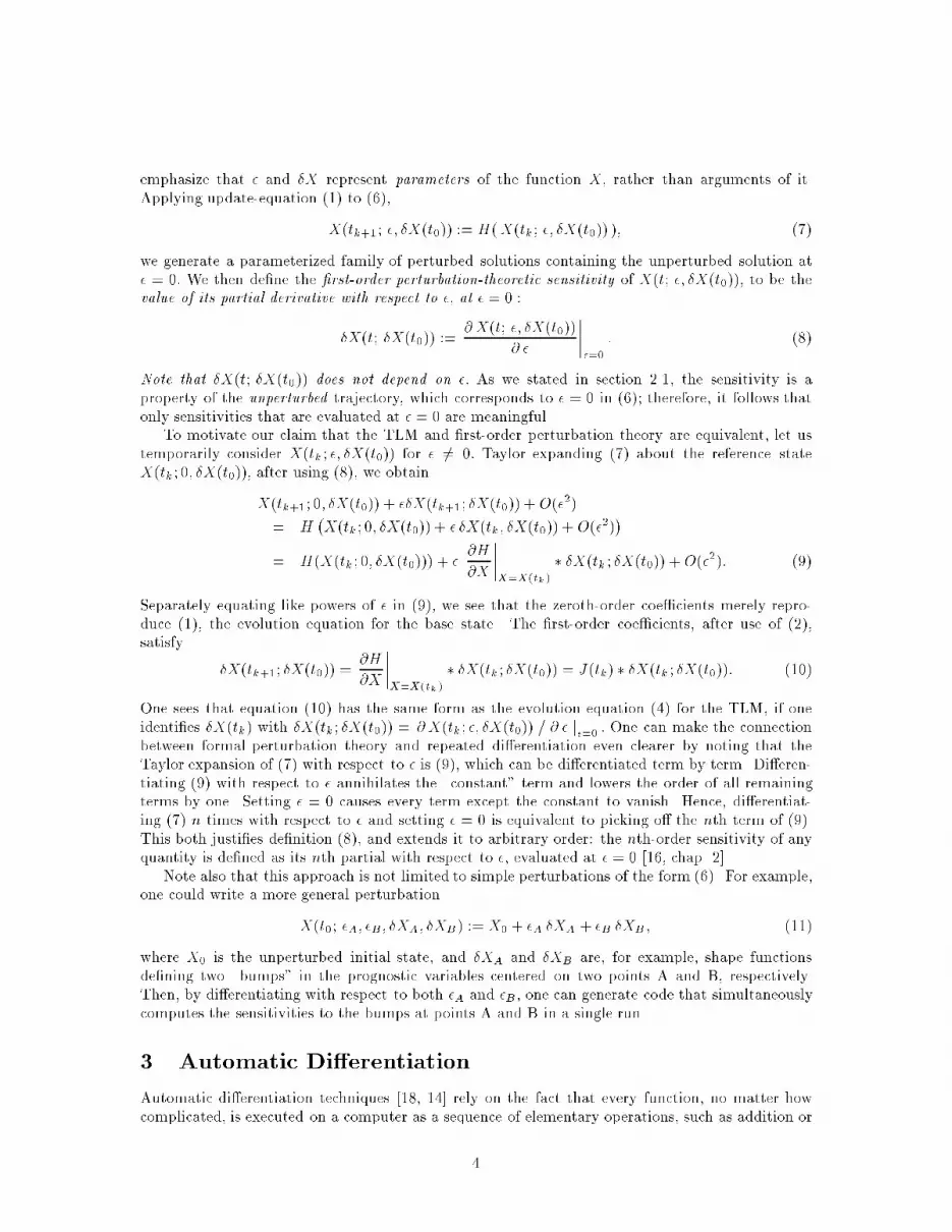
emphasize that � and �X represent parameters of the function X; rather than arguments of it.Applying update-equation (1) to (6),X(tk+1; �; �X(t0)) := H(X(tk; �; �X(t0)) ); (7)we generate a parameterized family of perturbed solutions containing the unperturbed solution at� = 0: We then de�ne the �rst-order perturbation-theoretic sensitivity of X(t; �; �X(t0)); to be thevalue of its partial derivative with respect to �; at � = 0 :�X(t; �X(t0)) := @ X(t; �; �X(t0))@ � �����=0 : (8)Note that �X(t; �X(t0)) does not depend on �: As we stated in section 2.1, the sensitivity is aproperty of the unperturbed trajectory, which corresponds to � = 0 in (6); therefore, it follows thatonly sensitivities that are evaluated at � = 0 are meaningful.To motivate our claim that the TLM and �rst-order perturbation theory are equivalent, let ustemporarily consider X(tk ; �; �X(t0)) for � 6= 0: Taylor expanding (7) about the reference stateX(tk; 0; �X(t0)); after using (8), we obtainX(tk+1; 0; �X(t0)) + ��X(tk+1; �X(t0)) + O(�2)= H �X(tk; 0; �X(t0)) + � �X(tk; �X(t0)) + O(�2)�= H(X(tk; 0; �X(t0))) + � @H@X ����X=X(tk) � �X(tk ; �X(t0)) +O(�2): (9)Separately equating like powers of � in (9), we see that the zeroth-order coe�cients merely repro-duce (1), the evolution equation for the base state. The �rst-order coe�cients, after use of (2),satisfy �X(tk+1; �X(t0)) = @H@X ����X=X(tk ) � �X(tk; �X(t0)) = J(tk) � �X(tk ; �X(t0)): (10)One sees that equation (10) has the same form as the evolution equation (4) for the TLM, if oneidenti�es �X(tk) with �X(tk; �X(t0)) = @ X(tk; �; �X(t0)) = @ � j�=0 : One can make the connectionbetween formal perturbation theory and repeated di�erentiation even clearer by noting that theTaylor expansion of (7) with respect to � is (9), which can be di�erentiated term by term. Di�eren-tiating (9) with respect to � annihilates the \constant" term and lowers the order of all remainingterms by one. Setting � = 0 causes every term except the constant to vanish. Hence, di�erentiat-ing (7) n times with respect to � and setting � = 0 is equivalent to picking o� the nth term of (9).This both justi�es de�nition (8), and extends it to arbitrary order: the nth-order sensitivity of anyquantity is de�ned as its nth partial with respect to �; evaluated at � = 0 [16, chap. 2].Note also that this approach is not limited to simple perturbations of the form (6). For example,one could write a more general perturbationX(t0; �A; �B; �XA; �XB) := X0 + �A �XA + �B �XB ; (11)where X0 is the unperturbed initial state, and �XA and �XB are, for example, shape functionsde�ning two \bumps" in the prognostic variables centered on two points A and B, respectively.Then, by di�erentiating with respect to both �A and �B; one can generate code that simultaneouslycomputes the sensitivities to the bumps at points A and B in a single run.3 Automatic Di�erentiationAutomatic di�erentiation techniques [18, 14] rely on the fact that every function, no matter howcomplicated, is executed on a computer as a sequence of elementary operations, such as addition or4

multiplication, and elementary functions, such as square root or log. By applying the chain rule ofdi�erential calculus, @@tf(g(t))���t=t0 = � @@sf(s)���s=g(t0)� �� @@tg(t)���t=t0� ; (12)to each stage in this sequence of elementary operations, one can compute derivatives of f exactlyand in a completely mechanical fashion. For example, the short code segmenty = sin(x)z = y*x + 5upon being augmented to compute derivatives becomesy = sin(x)@y = cos(x)*@xz = y*x + 5@z = y*@x + x*@y ,where @var is a vector representing the derivatives of var with respect to the independent variable(s).Thus, if x is the scalar independent variable, then @x is equal to 1 and @z represents @z=@x. (Theabove example uses the forward mode of automatic di�erentiation, wherein one propagates thederivatives of intermediate variables with respect to the independent variables; by contrast, in reversemode automatic di�erentiation one propagates the derivatives of dependent variables with respectto the intermediate variables. Reverse mode is related to the adjoint model in the same way thatforward mode is related to the TLM [6].)Several tools have been developed that use automatic di�erentiation to generate derivative codes.A compilation of currently available AD tools can be found on the World-Wide Web at the sitehttp://www.mcs.anl.gov/Projects/autodiff/AD Tools or in [5].We employed the ADIFOR tool in our experiments. ADIFOR (Automatic DI�erentiation ofFORtran) [2, 3, 4] performs automatic di�erentiation of programs written in Fortran 77. Givena collection of Fortran subroutines and a speci�cation of which variables in its parameter listsor common blocks correspond to the \independent" and \dependent" variables for di�erentiation,ADIFOR produces portable Fortran 77 code that allows the computation of the derivatives of thedependent variables with respect to the independent ones.Automatic di�erentiation yields the values of the analytical derivatives, exact to machine pre-cision, without truncation error, and without any adjustable parameters such as step-size to bedetermined. By contrast, to obtain accurate results using a divided di�erence approximation, onemust determine a step size that optimizes the \built-in" tradeo� between minimizing the truncationand the cancellation error|and even if one expends the additional computational e�ort to balancethese two errors, a signi�cant loss of precision will still be incurred [12, 17]. AD yields derivativeswhose accuracy is uniform over the entire simulation domain, and almost always comparable to thatof the function itself at all simulation times; by contrast, a DD step size that is optimal at onepoint or instant may not be optimal elsewhere, since the state variables are both space and timedependent. AD-enhanced code can compute all the desired derivatives in a single run, and thesederivatives are available immediately; by contrast, to compute n divided di�erences, one needs tomake n perturbed runs, plus an additional postprocessing step to compute the di�erences. Finally,AD-enhanced code generated by tools like ADIFOR can achieve all these advantages over divideddi�erences while still only requiring a CPU-time comparable to the total CPU-time that would havebeen consumed by the set of perturbed runs [2, 3].The previous discussion suggests that a simple mechanism for generating the TLM would be touse an AD preprocessor like ADIFOR to compute the perturbation expansion as follows:1. Introduce new variables � and �Xi. 5

2. Modify the code to initialize the ith component of the initial state to Xi(t0) + � �Xi.3. Di�erentiate the resulting code with respect to �.4. Execute the derivative-enhanced code, initializing � to zero, and @� to unity.In accordance with (8), step 4 ensures that the sensitivities are evaluated on the unperturbed ref-erence trajectory and represent derivatives with respect to the amplitude of the perturbation. Thisapproach requires minimal modi�cations to the original code and is ideally suited for automaticdi�erentiation.4 Experimental ResultsTo demonstrate the utility of our methodology, we have analyzed the sensitivity of an MM5 forecastto its initial conditions using a \real world" data set. Below, we describe the simulation domain anddata set used, and the initial perturbation assumed. We then present two results from this study:a dramatic illustration of the superior accuracy that may be obtained by using AD-computed sen-sitivities instead of divided-di�erence approximations, and the observation of a numerical precursorwave that would almost certainly have gone undetected had we used a divided di�erence approach.4.1 Domain, Grid, and Initial ConditionsThe simulation domain is centered on the Korean peninsula. The initial-condition data is de�ned ona 61�61�23 grid; the grid is rectangular and uniform when viewed in stereographic projection fromthe North Pole, and true at 60 degrees north latitude. The mean gridpoint spacing is roughly 101 km;however, as a result of the projection, the local spacing varies signi�cantly over the simulationdomain. The simulation begins at 1994-Nov-12, 1200 UTC; this choice of initial data is representativeof a typical winter day in Southeast Asia. We used a timestep of �ve minutes and terminated therun at 1800 UTC simulation-time, having simulated a total of six hours of weather.4.2 Initializing the PerturbationBy parameterizing our perturbed state-variables as X + � �X and following the prescription ofsection 3, we naturally ensure that the structures of X and �X are identical, and also that a corre-sponding �nite-amplitude perturbation can easily be obtained by simply setting � 6= 0 and runningthe undi�erentiated code. Thus, we can use a single source-code for both the �nite-amplitude-perturbation executable, and as input for sensitivity enhancement by our AD tool. As stated insection 2.1, the choice of the initial-state perturbation �X(t0) is at the disposal of the analyst; ageneral choice will yield a directional derivative, whereas a particular choice may yield a sensitivitywith a particularly simple or useful interpretation.In our study, we were interested in sensitivities of the forecast generated by MM5 with respectto the initial data. Direct di�erentiation of the �nal state with respect to all of the elements of theinitial state would consume a run time on the order of N times the unenhanced code, to yield anN�N sensitivity array, where N is the total number of grid points; however, not only would thisrepresent a prohibitive expenditure of memory and CPU time, but in most practical cases, suchhighly detailed sensitivity information is not needed. By investing some initial consideration intodetermining what one's actual observables are, what sensitivities are actually of interest, and whatlarge scale physical phenomenon might be expected to dominate the model sensitivities, one mayoften reap a substantial savings by a choosing a smaller but \smarter" set of directional derivativesto be computed, instead of exhaustively computing a mathematically complete set. For example, inweather simulation, the physical input data are not the gridded values, but the observations fromthe network of surface meteorological stations|and these are orders of magnitude less numerous6

Figure 1: The Cressman function and its square.than the computational gridpoints. Hence, it is the actual observations one should di�erentiate withrespect to, and therefore one should choose a perturbation representative of how the observationsin uence the initial data on the grid.The initial condition data for MM5 are constructed by a suite of preprocessors [15] by using amodi�ed Cressman objective analysis scheme [9, 1]. Objective analysis is the term meteorologistsuse for any method of interpolating a set of irregularly spaced weather observations onto a regularcomputational grid. Most objective analysis algorithms use some form of spatial proximity-weightingto correct a \�rst guess" initial-data �eld until it agrees with the observations upon interpolatingback to each measurement station (the \�rst guess" data might, for example, be the most recentforecast). The preprocessors also impose various consistency and balance checks on the initial data.In performing our sensitivity study, we chose to perturb the initial temperature, since it impactson every other prognostic variable, yet it is largely decoupled from the consistency and balanceconditions imposed on the pressure and wind; hence we need only simulate the objective analysisprocedure itself. This simulation is straightforward because the modi�ed Cressman update formulasare linear in the observed data [15, 9, 1]; hence, the impact of perturbing a single temperatureobservation will be to perturb the initial conditions at each grid point in the vicinity of the selectedobservation in proportion to the value of its proximity-weighting factor. From the formulae given inthe MM5 preprocessor manual [15], we have determined that a good approximation to this pertur-bation may be obtained by assigning the initial temperature to T +� �T , where T is the unperturbedtemperature �eld, � is the amplitude of the perturbation in degrees Kelvin, and the shape function�T is de�ned as �T := �W (�;R(�)): (13)Here,W (�;R) is the horizontal weighting function, � is the horizontal distance from the perturbationcenter, R(�) is the radius of in uence of the measured datum, and � is the terrain-following verticalcoordinate used by MM5. We de�ne � as� := po(z) � ptopps(x; y) � ptop ; (14)7

where po(z) is the nominal pressure of a stationary equilibrium reference atmosphere at altitude z;ps(x; y) is the nominal pressure of the reference atmosphere at the surface point with horizontalcoordinates (x; y); and ptop is the nominal pressure at the top of the simulation volume; � thereforevaries from unity at the surface, to zero at the top. The horizontal weighting factor W (�;R) waschosen to be the Cressman function, de�ned as [9]W (�;R) :=8<: R2 � �2R2 + �2 ; � < R;0; � � R; (15)which is a bell-shaped function of �=R; Figure 1 shows both W and W 2. The scaling by � inperturbation (13) re ects the fact that a measurement at ground level should have progressively lessin uence on the estimated conditions at increasingly higher altitudes. The radius of in uence R ofthe perturbation also depends linearly on �; as R(�) = R0 [2� �] ; hence R ranges from R0 at thesurface to 2R0 at the top, so that the perturbed volume is shaped like an upside-down truncatedcone. This shape re ects the fact that, while a measurement taken at ground-level should be relevantonly to its immediate neighborhood at the surface, the estimated conditions at high altitude mustbe inferred from many surface observations scattered over a large area. We choose R0 to be threegrid point spacings in our simulation, corresponding to roughly a 300 km radius of in uence.4.3 Comparison of an AD-computed Derivative with a DD Approxima-tionThe results in this section demonstrate the dramatic e�ect automatic di�erentiation can make inobtaining accurate and reliable derivatives. Figures 2 and 3 show the temperature sensitivity ascomputed at time step 12 (60 min) by AD and by DD, respectively. Figure 3 was obtained byusing a second-order forward di�erence approximation to the desired sensitivity (we chose forwardrather than central di�erencing because it allowed us to reuse the data from previous runs whilesearching for the optimum �nite-amplitude perturbation size). After numerous runs, we determinedby trial and error that the optimum step-sizes were near one and two degrees Kelvin; note that theseperturbations are rather large compared with the mean value of the data (on the order of 0.3% and0.6% of the data, respectively), and that they are optimal only in some average sense, since thetemperature data are space dependent.We see that the AD and DD results agree closely in appearance. However, the DD approxi-mation su�ers from substantial loss of accuracy because all but the last three decimal digits of themantissas cancel; this manifests itself in a mottled appearance to the DD frame. Choosing a smalleramplitude perturbation exacerbates this problem. The �gures clearly demonstrate the inadequacy ofdivided di�erences for computing sensitivities of complicated simulations involving many hundredsor thousands of oating-point operations at each grid point per time step.4.4 \Superacoustic" Precursor WaveA weak \precursor" wave was observed to propagate anisotropically and at superacoustic speeds;it was �rst noted through the fact that at the end of the �rst time step, the central 0:39 deg/degpositive peak of the temperature sensitivity was encircled by a shallow negative \moat" of maximumdepth �3:2�10�3 deg/deg, surrounded in turn by a low positive embankment of 2:2�10�3 deg/deg,which fell o� to extremely small values beyond a radius of about 10.5 grid points|that is, nearly sixgrid points larger than the 4.61 grid-point radius of the initial perturbation on this sigma-level. Sincethe speed of sound is only about one grid point per time step, this is at least �ve grid points furtherfrom the perturbation than any disturbance should have had time to travel. During subsequentsteps, the precursor rapidly and anisotropically propagated away from the perturbation|initiallyabout Mach 6, falling asymptotically to about Mach 4. It had a much smaller amplitude than the8

Figure 2: AD-computed 519 mb temperature sensitivity in deg/deg, at t = 60 min: Observe theanisotropic, low-amplitude precursor extending far beyond the 15 grid-point radius to which soundhas had time to propagate (the simulation domain is 61�61 gridpoints), as well as the bipolar,crescent-shaped gravity waves emerging from the central peak. (Contour levels have been chosen bya histogrammic equalization method such that the intervals all occupy approximately equal areas;note the strong nonlinearity of the interval spacing.)9

Figure 3: DD-computed 519 mb temperature sensitivity in deg/deg, at t = 60 min: Observe that,while the bipolar gravity-wave arcs are visible, the precursor is lost in the �nite-precision noise.(Contour levels have also been chosen by histogrammic equalization; note the much more coarselyspaced small-amplitude contour levels used, in comparison with Figure 2.)10

0 10 20 30 40 50 600

10

20

30

40

50

60Time Step at which Precursor Reaches Gridpoint

X Gridpoint Number

Y G

ridpo

int N

umbe

r

Figure 4: First time step for which the temperature-sensitivity becomes nonzero; darker greyscorrespond to later times.11

primary wave and appeared to be strongly damped (it may perhaps behave be more accuratelycharacterized as a \di�usion," rather than a wave). The late-time precursor may be seen in Figure 2as the low-amplitude halo surrounding the central, physical disturbance; at the time of this image,the sensitivities would have been expected to vanish outside the roughly 15-gridpoint radius to whichsound has had time to propagate.The apparent speed of the precursor seems impossible, until one realizes that in nonhydrostaticmode, MM5 performs between two and four microsteps using the semi-implicit acoustic-wave solverSOUND per each \leapfrog" macrostep, and that SOUND couples adjacent grid points together [13, 10].A plot showing the �rst time step for which a nonzero sensitivity value occurs at each grid point(Figure 4) indicates that nonzero values appear on the grid in roughly octagonal regions having ahalf-width and half-height time-sequence of ( 12; 18; 24; 29; 33; 37; 41 ); after time step seven, theleading edge of the precursor reaches the upper right corner of the grid, and we can no longer trackit. Taking four grid points as the radius of the nonzero initial data, we get propagation incrementsof ( 8; 6; 6; 5; 4; 4; 4 ); suggesting that the asymptotic velocity of the precursor is four grid pointsper time step.These observations suggest the hypothesis that, in attempting to account for high-frequencyacoustic modes, SOUND introduces a spurious \superacoustic" computational mode; indeed, oneexpects that because of the adjacent coupling introduced by SOUND, the superacoustic mode shouldpropagate at four grid points per macrostep, independent of the time step size (the larger initialapparent velocity can be understood as a geometric projection e�ect due to the conical shape ofperturbation (13) caused by the �-dependence of R). These features suggest that the precursorrepresents something more nearly akin to a \computational di�usion" than to a true wave.One should expect that both physical and numerically induced precursors may appear in the re-sults of any simulation code. Precursors are an inevitable aspect of dispersive wave propagation [8];the imposition of a discrete space/time mesh for simulation purposes necessarily introduces addi-tional spurious dispersion into the problem, since the discretization length and time scales impose acuto� wavenumber and frequency above which propagation becomes impossible [7, 20]. In addition,since a grid-point is coupled to its neighbors via the \stencil" pattern of the di�erencing scheme, anunphysical \computational wave" will propagate across the grid at one stencil radius per time step.The �rst (or \Sommerfeld") precursor is physical; it characteristically has a rather high frequency onthe order of the reciprocal of some characteristic time associated with the physical properties of themedium, and propagates at velocities on the order of the fastest speed the medium will support|inthis case, the acoustic wave speed, which is far too slow to explain the precursor we observe. How-ever, the semi-implicit method used in SOUND in e�ect couples the nearest four neighbors together,which is precisely what one needs to explain the observed precursor. We conclude that the precursoris probably a computational artifact induced by the semi-implicit microstep algorithm in SOUND.The observation of this precursor provides a remarkable demonstration of the synergy of bothautomatic di�erentiation and suitable visualization techniques: Because of its small amplitude,the precursor almost certainly could not have been observed with a divided-di�erence approach;indeed, one can easily show that except for its innermost radii during the �rst few time steps, theprecursor would have been completely lost to signi�cant-digit cancellation even on a 64-bit machine.By contrast, AD-computed derivatives retain the full accuracy of the original function. Likewise,because of the very large dynamic range in these images, if we had used equally spaced contourintervals instead of histogrammic equalization, the precursor would almost certainly never havebeen noticed.5 ConclusionsWe have shown that, using automatic di�erentiation (AD) tools such as ADIFOR, we can quicklyand easily generate and update sensitivity-enhanced versions of large, complicated codes, such as12

the tangent linear model (TLM) of MM5, a communitymesoscale weather, with little expenditure ofhuman labor. We explained the connection between the TLM and formal perturbation theory andshowed how automatic di�erentiation can be used to assess the e�ect of adding additional observa-tions in the initial temperature �eld of the MM5 mesoscale weather model with little computationale�ort. The inherent accuracy of AD-generated codes allows us to observe low-amplitude sensitivitywaves such as, for example, a numerically induced supersonic precursor. These results show thatautomatic di�erentiation tools, suitably employed, enable the rapid and accurate sensitivity analysisof large computer codes, revealing computational structure that is obscured by the inherent errorsin divided-di�erence approximations of derivatives, and previously detectable only after expendingconsiderable human e�ort in developing accurate derivative codes by hand.AcknowledgmentsWe thank Tom Can�eld, Jimy Dudhia, Georg Grell, Kevin Manning, Lt. Col. Harold Massey, JohnMichalakes, Ravi Nanjundiah, Seon-ki Park, Kathy-Lee Simunich, and David Stau�er for helpfuldiscussions regarding the MM5 code and meteorology, and Peter Campbell and Gerald Marsh fortheir support of this work.This work was supported by the Mathematical, Information, and Computational Sciences Di-vision subprogram of the O�ce of Computational and Technology Research, U. S. Department ofEnergy, under Contract W-31-109-Eng-38.References[1] Stanley G. Benjamin and Nelson L. Seaman. A simple scheme for objective analysis in curved ow. Monthly Weather Review, 113:1184{1198, 1985.[2] Christian Bischof, Alan Carle, George Corliss, Andreas Griewank, and Paul Hovland. ADIFOR:Generating derivative codes from Fortran programs. Scienti�c Programming, 1(1):11{29, 1992.[3] Christian Bischof, Alan Carle, Peyvand Khademi, and Andrew Mauer. The ADIFOR 2.0system for the automatic di�erentiation of Fortran 77 programs, 1994. Preprint MCS-P481-1194, Mathematics and Computer Science Division, Argonne National Laboratory, and CRPC-TR94491, Center for Research on Parallel Computation, Rice University. To appear in IEEEComputational Science & Engineering.[4] Christian Bischof, Alan Carle, Peyvand Khademi, Andrew Mauer, and Paul Hovland. ADIFOR2.0 user's guide. Technical Memorandum ANL/MCS-TM-192, Mathematics and ComputerScience Division, Argonne National Laboratory, 1994. CRPC Technical Report CRPC-95516-S.[5] Christian Bischof and Fred Dilley. A compilation of automatic di�erentiation tools. ACMSIGNUM Newsletter, 30(3):2{20, 1995.[6] Christian H. Bischof. Automatic di�erentiation, tangent linear models and pseudo-adjoints.In Francois-Xavier Le Dimet, editor, High-Performance Computing in the Geosciences, volume462 of Series C: Mathematical and Physical Sciences, pages 59{80, Boston, Mass., 1995. KluwerAcademic Publishers.[7] Leon Brillouin. Wave propagation in periodic structures; electric �lters and crystal lattices. 2ndedition, Dover Publications, New York, 1953.[8] Leon Brillouin. Wave propagation and group velocity, volume 8 of Pure and applied physics.Academic Press, New York, 1960. 13

[9] G. P. Cressman. An operational objective analysis scheme. Monthly Weather Review, 87:293{297, 1959.[10] Jimy Dudhia. A nonhydrostatic version of the Penn State-NCAR mesoscale model: Validationtest and simulation of an Atlantic cyclone and cold front.Monthly Weather Review, 121(5):1493{1513, 1993.[11] Ronald M. Errico, Tomislava Vukicevic, and Kevin Raeder. Examination of the accuracy of atangent linear model. Tellus, 45A(5):462{477, 1993.[12] Phillip E. Gill, Walter Murray, and Margaret H. Wright. Practical Optimization. AcademicPress, London, 1981.[13] G. A. Grell, J. Dudhia, and D. R. Stau�er. A description of the �fth-generation PennState/NCAR mesoscale weather model (MM5). Technical Report NCAR/TN-398+STR,National Center for Atmospheric Research, Boulder, Colorado, June 1994. See alsohttp://www.mmm.ucar.edu/mm5/mm5-home.html.[14] Andreas Griewank. On automatic di�erentiation. In Mathematical Programming: Recent De-velopments and Applications, pages 83{108, Amsterdam, 1989. Kluwer Academic Publishers.[15] Kevin W. Manning and Philip L. Haagenson. Data ingest and objective analysis for thePSU/NCAR modeling system: Programs DATAGRID and RAWINS. Technical ReportNCAR/TN-376+IA, National Center for Atmospheric Research, Boulder, Colorado, October1992.[16] Stephen M. Omohundro. Geometrical Perturbation Theory in Physics. World Scienti�c Pub-lishing, Singapore, 1986.[17] William H. Press and Saul A. Teukolsky. Numerical calculation of derivatives. Computers inPhysics, 5(1):88{89, Jan/Feb 1991.[18] Louis B. Rall. Automatic Di�erentiation: Techniques and Applications, volume 120 of LectureNotes in Computer Science. Springer Verlag, Berlin, 1981.[19] W. C. Rheinboldt. Numerical Analysis of Parametrized Nonlinear Equations. John Wiley andSons, New York, 1986.[20] Robert Vichnevetsky and John B. Bowles. Fourier analysis of numerical approximations ofhyperbolic equations, volume 5 of SIAM Studies in Applied Mathematics. Society for Industrialand Applied Mathematics, Philadelphia, 1982.[21] Tomislava Vukicevic and Ronald M. Errico. Linearization and adjoint of parameterized moistdiabatic processes. Tellus, 45A(5):493{510, 1993.[22] L. T. Watson. Numerical linear algebra aspects of globally convergent homotopy methods.SIAM Reviews, 28:529{545, 1986.14