INTERNATIONAL JOURNAL OF CLIMATOLOGYInt. J. Climatol. 34: 2047–2058 (2014)Published online 24 September 2013 in Wiley Online Library(wileyonlinelibrary.com) DOI: 10.1002/joc.3821

Meteorological conditions on an Arctic ice cap – 8 yearsof automatic weather station data from Austfonna, Svalbard

Thomas V. Schuler,* Thorben Dunse, Torbjørn I. Østby and Jon O. HagenDepartment of Geosciences, University of Oslo, Oslo, Norway

ABSTRACT: Only few reliable records are available covering more than 5 years of meteorological conditions on Arcticglaciers. Here, we report on the operation of an automatic weather station at the Austfonna ice cap, Svalbard, over an 8-yearperiod from 2004 to 2012. Time series of measured and derived quantities are analysed to characterize meteorologicalconditions close to the equilibrium line altitude at ∼400 m.a.s.l. The mean annual temperature is −8.3 ◦C but exhibitslarge variability such that excursions above 0 ◦C occur even during winter. In general, relative air humidity is high andevaluating the wind pattern, we find that moisture is primarily advected from south-easterly directions. Net radiation isdominated by shortwave radiation and, hence, surface albedo plays an important role in the radiation budget. Frequentsummer snowfalls, as observed in 2008, have the ability to maintain a high albedo over much of the ablation season,thereby having large impact on the energy balance as well as on glacier mass balance. Cloudiness is assessed using recordsof incoming longwave radiation. Analyzing the radiation data, we find evidence for the radiation paradox, i.e. an increaseof average net radiation (2004–2012) from −15.7 W m−2 for clear-sky conditions to 7.3 W m−2 during overcast skies.

KEY WORDS automatic weather station; arctic glacier; glacier mass

Received 25 February 2013; Revised 16 July 2013; Accepted 12 August 2013

1. Introduction

Over the past decades, the Arctic has experienced pro-nounced warming and projections of future climateindicate continued warming above the global average(AMAP, 2011). Arctic glaciers loose mass at an increas-ing rate (AMAP, 2011). The associated water volumeaccounts for about one-third of the observed sea-levelrise over the past 50 years (Church et al., 2011) and Arc-tic glaciers are expected to remain important contributorsfor at least the 21st century (Meier et al., 2007; Radicand Hock, 2011). However, uncertainties remain due toa scarcity of direct measurements of glacier mass bal-ance and due to a poor availability of in situ data ofrelevant meteorological quantities, allowing for detailedenergy balance assessments. Recently, meso-scale atmo-spheric models have been employed to fill this gap inknowledge (Claremar et al., 2012), but still require reli-able in situ data for validation. The remoteness of manyArctic glaciers in combination with harsh weather condi-tions complicate continuous acquisition of reliable data.Automatic weather stations (AWS) enable autonomousrecording, still the efforts related to installation and main-tenance are considerable. AWS operate either in com-plete autonomy and transmit the collected data throughtelecommunication or in semi-autonomous mode where

* Correspondence to: T. V. Schuler, Department of Geosciences,University of Oslo, Oslo, Norway. E-mail: t.v.schuler@geo.uio.no

stations are revisited on a regular basis for maintenanceand retrieval of data.

In this article, we present a record spanning 8 yearsacquired from a semi-autonomous AWS located onAustfonna, an Arctic ice cap of approximately 7800 km2.Time series of individual quantities over the period2004–2012 are presented along with an assessment ofdata reliability in light of issues with operation of thestation. On the basis of the obtained data, we characterizemeteorological conditions in the boundary layer above theglacier surface at the location of our AWS.

2. Study site

2.1. Austfonna

Centred at 79◦42′N, 24◦00′E and covering an area ofapproximately 7800 km2 (Moholdt and Kaab, 2012), theAustfonna ice cap occupies most of Nordaustlandet, anisland in the northeastern part of the Svalbard archipelago(Figure 1(a)). Over the past decades, the surface massbalance (SMB) of Austfonna was presumably closeto zero (Pinglot et al., 2001). However, over shortertimescales, SMB exhibits large variations and some yearsfeature negative values (Schuler et al., 2007) whereasduring other years, a gradual build-up towards positivevalues was observed (Dunse et al., 2009). The spatialdistribution of SMB is to a large degree controlled by thecharacteristic, asymmetric pattern of snow accumulationdescribed by Schytt (1964) and Taurisano et al. (2007).

2013 Royal Meteorological Society

2048 T. V. SCHULER et al.

620 640 660 680 700 7208800

8820

8840

8860

8880

8900

8920

East UTM33X (km)

Nor

th U

TM

33X

(km

)

400

500

600

700

600

500

100

200

300

400

500

600AWS-1

AWS-2

(a) (c)

T, RH

SWi, LWi

SWo, LWo

V, ϕ

(b)

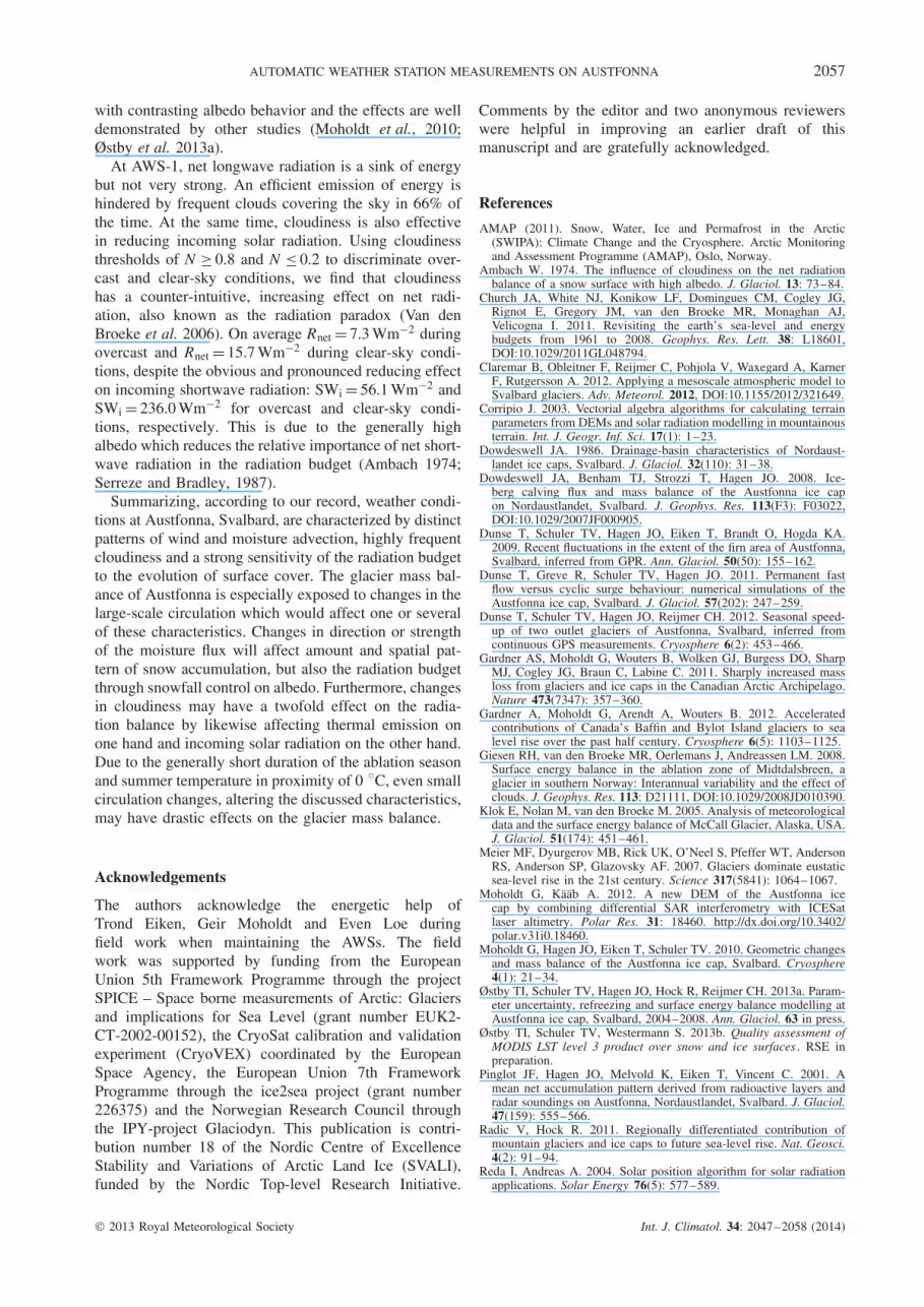
Figure 1. (a) Overview map over Austfonna and the locations of AWS-1 and AWS-2 (triangles). Elevation contours are drawn at intervals of50 m. (b) The location of Austfonna (dark) within the Svalbard archipelago. (c) Photograph of AWS-1 taken in May 2010. Arrows point to the

instruments where the respective quantities are measured.

Nevertheless, the total mass balance of Austfonna is neg-ative due to additional mass loss through iceberg calving(Dowdeswell et al., 2008; Moholdt et al., 2010). Thecalving term comprises both the retreat of the ice marginsas well as the ice flux through the marine margins.

Through iceberg calving and front position changes,a considerable part of the mass loss from Aust-fonna is related to glacier dynamics (Dowdeswell et al.,2008; Moholdt et al., 2010). Feedback mechanisms existbetween surface melting and basal sliding (Schoof, 2010)which may amplify the effect of atmospheric warm-ing on glacier mass balance. Melt-induced seasonal iceflow acceleration is observed at Austfonna (Dunse et al.,2012). Furthermore, it is known that several of the basinsdraining Austfonna have surged in the past (Schytt, 1969;Dowdeswell, 1986; Solheim, 1986) and modeling sug-gests that Austfonna is prone to periodic reorganisationof its velocity structure (Dunse et al., 2011).

2.2. Automatic weather stations

In April 2004, we installed an automatic weather sta-tion (AWS-1) at 22◦25′12′′E, 79◦43′48′′N and 370 m.a.s.l.on Etonbreen, a basin draining ice from the center ofthe ice cap westwards into Wahlenbergfjorden (Figure 1).The location was chosen to measure meteorological con-ditions close to the expected equilibrium line altitudeof glacier mass balance, estimated based on previouswork by Pinglot et al. (2001). Although later observa-tions revealed high interannual variability (Schuler et al.,2007; Dunse et al., 2009; Moholdt et al., 2010), on thelongterm, the mean equilibrium-line at ∼400 m.a.s.l. con-forms to this expectation. According to a recent digitalelevation model (Moholdt and Kaab, 2012), the glaciersurface at AWS-1 has a gentle slope of (<2◦) in a west-ward direction (273◦).

A second, auxiliary station (AWS-2) was installedduring the same period a few kilometers upglacier at

22◦49′48′′E, 79◦46′12′′N and an elevation of 535 m.a.sl.(Figure 1), rendering a more limited dataset. In theremainder of this paper, we will restrict our analysis tothe record from AWS-1. Data from AWS-2 is used tofill gaps in the temperature series caused by occasionalmalfunctioning of AWS-1.

The AWS is mounted on a self-supporting tripod whichwas erected at the actual snow surface in April 2004. Theintention of such a ”floating” station (Klok et al., 2005)is to keep the sensor level constant during the ablationperiod. During the subsequent winter, snow accumulatingon top of the last summer surface reduces the sensorheights relative to the glacier surface. However, as thesite became part of the accumulation area in 2008 and2009, the tripod was partly frozen into solid ice and couldnot be reset to the surface. Therefore, the station wasreinstalled on a new tripod in May 2010, at the same site(Figure 1(b)).

Eight quantities are measured to characterize meteo-rological conditions and provide the data required forcalculating the energy balance (Østby et al., 2013a): airtemperature T , relative humidity RH, wind speed V ,wind direction ϕ and the components of net radiationRnet = SWi + SWo + LWi + LWo, where SWi denotesincoming shortwave radiation, SWo shortwave radiationreflected from the surface, and LWi and LWo representincoming and outgoing longwave radiation. Air tempera-ture is measured using a combined temperature-humidityinstrument (Vaisala HMP45D), housing a PT100 resis-tance thermometer. Relative humidity of air is sensed bythe Humicap device, also incorporated in the HMP45Dwhich, as such, is housed in an EM SS1 radiation shield.Wind speed and direction are measured using a Young05103 wind monitor, a pivot-mounted, helicoid propelleranemometer. The radiation components are monitoredusing a Kipp & Zonen CNR1, consisting of a CM3 pyra-nometer and CG3 pyrgeometer pair that faces upward and

2013 Royal Meteorological Society Int. J. Climatol. 34: 2047–2058 (2014)

AUTOMATIC WEATHER STATION MEASUREMENTS ON AUSTFONNA 2049

Table 1. Overview over instrumentation of AWS-1 specifying sensor type and associated factory uncertainty.

Variable Sensor Accuracy Measurement interval (s)

Air temperature (◦C) Vaisala HMP45D ±0.2 ◦C 120Air temperature (◦C)a Aanderaa 3455 ±0.1 ◦C 3600Humidity (%) Vaisala HMP45D ±2% 120Wind speed (m s−1) Young 05103-5 ±0.3 m s−1 120Wind direction (◦) Young 05103-5 ±2◦ 120Radiation components (Wm−2) Kipp & Zonen CNR1 ±10% of daily total 120

aAWS-2.

a complementary pair that faces downward. The spec-tral ranges of the CM3 and CG3 are 305–2800 nm and5–50 µm, respectively. Further sensor specifications aregiven in Table 1. A Campbell CR10X datalogger is usedto control the measurements conducted at intervals of120 s and store hourly averaged values.

The auxiliary station AWS-2 was mounted on a stakefixed into the ice and therefore, the sensor level abovethe surface changes when snow accumulates or melt orsnow compaction occur. An Aanderaa Sensor ScanningUnit 3010 is used to collect sensor readings and the data isstored on a Aanderaa data storage unit 2990E. The stationwas equipped with left-over instruments from previousactivities and rapid degradation of data quality occurred.We judge only the temperature record being valuable anduse it only to fill occasional gaps in the AWS-1 recordrather than presenting it as an individual dataset. AWS-2became inoperative in 2010.

Since 2004, we have conducted annual field visits,at the end of the accumulation period in April andMay. During these visits, the station is maintained,which involves retrieval of stored data, replacementof exhausted batteries and exchange of sensors wherenecessary. However, a continuous operation of AWS-1 ischallenged by harsh conditions; gaps in the record andobservations made during fieldwork reveal the followinglist of problems:

• Exhausted power supply during the winter 2004–2005caused a continuous gap in the record between 23February and 23 April 2005, subsequent to occasionalloss of data at several occasions in the weeks before.

• In May 2008, the HMP45D was found outside theradiation shield and lying in the snow, the temperaturerecord is therefore strongly dampened with respect tothe one of AWS-2 and judged unreliable. The humiditysensor degraded and showed spurious values. Throughcomparison with the temperature record of AWS-2, theperiod of malfunction was determined to have started5 May 2007. The failure was discovered in May 2008and the sensor was replaced during a summer visit on25 August 2008.

• The downward-looking sensors of the CNR1 wereburied in the snow during parts of the 2009 season.This period is identified in the data by an unusuallylow albedo (<0.5), while the surface was still snow-covered.

• Following what presumably was a visit of the stationby a polar bear on 16 July 2011, the records of theradiation and wind sensors were interrupted. The fail-ure was caused by damage to the cables connectingsensors and datalogger unit. The problem was discov-ered and fixed during the subsequent field visit in May2012.

3. Data treatment

3.1. Quality control

After retrieval of the raw data from the datalogger duringthe annual field visit, the data are processed to convertvoltage readings to calibrated values of the measuredquantities. Furthermore, a quality control procedure isapplied, assigning a quality flag to each individual value.The quality flag QF can take values of 0 or 1, dependingon whether a value is found valid (QF = 1) or missing,unreliable or invalid (QF = 0). In addition, if a correctionor gap filling procedure was applied, the modified valuesare assigned QF = 2.

Since logging of data was interrupted in periods ofinsufficient power supply or when maintenance work wasconducted, the obtained data record is not complete andintervals between adjacent timestamps are not unique.Therefore, in a first step, the entire record was projectedonto a timestamp vector completely covering the obser-vation period at regular intervals of 1 h. The added dataentries are marked by a placeholder to indicate missingvalues, and accordingly QF = 0. Furthermore, the adoptedquality control implements the following scheme whichis described below for each individual variable.

3.1.1. Temperature

Missing values are assigned QF = 0. For the period5 May 2007 until 26 August 2008, for which sensorproblems are known, the quality flag is manually edited(QF = 0). To substitute QF = 0 values, temperature fromAWS-2 is used, accounting for the elevation difference(535–370 m.a.s.l.) by applying an environmental lapserate of 0.0065 Km−1. When data from the auxiliary recordwere available such that the correction could be applied,the flag is set QF = 2.

3.1.2. Relative humidity

Similarly as for temperature, missing values and theperiod 5 May 2007–26 August 2008 are assigned QF = 0.

2013 Royal Meteorological Society Int. J. Climatol. 34: 2047–2058 (2014)

2050 T. V. SCHULER et al.

An auxiliary and reliable record to fill the gaps is notavailable. Inspecting the humidity versus temperaturereveals that the maxima of RH decline with lower tem-perature, symptomatic for the sensor (Humicap) whichrenders RH relative to the saturation vapour pressure ofwater. This leads to a clear cut-off at values below 100%for temperatures below the melting point. Van den Broekeet al. (2004c) describe a correction scheme that involvesa recalculation of relative humidity using the saturationvapor pressure of ice instead of that for water. This pro-cedure is applied to create a secondary RH record havingQF = 2.

3.1.3. Wind speed and direction

We apply a common quality flag to both variables, sinceboth are measured using a single instrument. Further-more, for temporal aggregation, we convert direction andmagnitude into northward and eastward components ofthe wind vector. Riming of the wind sensor is consid-ered a potential issue which may affect the quality ofthe record. Van den Broeke et al. (2004c) detect rimingof their radiation sensor using a scheme based on short-wave radiation. We could not detect similar events basedon our radiation record but do not exclude the possibilitythat the wind sensor was affected but not the radiationsensor. We therefore consider riming or icing obstruct-ing the free motion of the anemometer when recordedwind speed V = 0 m s−1 for three consecutive hours orlonger and hence, QF = 0. Accounting for the low start-ing threshold speed of the sensor (<1 m s−1) and thelow probability of calm conditions at this wind-exposedlocation, this appears a reasonable assumption.

3.1.4. Shortwave radiation

Spurious, negative readings are recorded during polarnight when shortwave radiation is close to zero andare most likely related to small inaccurcies in thesensor calibration. These incidences are replaced by0 Wm−2. Another implausible situation is that incomingshortwave radiation, measured by the upward lookingpyranometer, is smaller than the reflected part, measuredby the downward looking sensor. This situation maybe caused by three different reasons. First, the upwardlooking sensor may be covered by freshly fallen snowwhereas the downward looking one is not. Second,due to its wide field of view, the downward lookingpyranometer receives radiation not only from the glaciersurface but partly also from the sky. Hence, at verylow sun angles above horizon, the downward lookingpyranometer may sense higher radiation than the upwardlooking one. Van den Broeke et al. (2004b) report similarproblems with the same sensor and under comparableconditions in Antarctica. Third, during polar night whenboth, SWi and SWo≈0, small inaccuracies in the sensorcalibrations and random noise in the measurements giverise to SWi < SWo. All instances of SWi < SWo aremarked with QF = 0 and we found that roughly 2/3 ofthese instances are attributed to the last reason. Another

plausibility check is to test whether SWi > I , where Irepresents the potential clear-sky solar radiation whichis directly calculated from solar geometry following(Corripio, 2003; Reda and Andreas, 2004). In casesSWi > I , the actual value of SWi was replaced by that ofI and QF = 2. Apart from these automatically detectedquality issues, we manually modified the quality flagfor periods for which other problems are known buthard to detect automatically. Between 1 June and 16July 2009, at least the downward looking sensor ofthe radiation instrument was buried in snow, noticeablefrom an unusually low albedo. The quality flag over thisperiod was manually set QF = 0. As reported above, theradiation sensor became inoperative on 16 July 2011.

3.1.5. Longwave radiation

The quality control for longwave radiation employs theshortwave record, the sensors of all components arehoused inside the same instrument, and we assume theyall face identical conditions. Obstruction of an upwardlooking sensor by snow leaves a clear signature in theshortwave measurements but is difficult to detect basedon longwave data alone. Hence, we apply the simulta-neous criteria SWi < SWo while the sunangle � > 10◦

and mark those instances QF = 0. The second conditionaccounts for that low sunangles may similarly give rise toSWi < SWo but not affect longwave measurements. Also,the period 1 June to 16 July 2009 is considered unreliableand QF = 0. Similar as with the pyranometer, the pyrge-ometer has a wide field of view and may partly record skyradiation. For a melting glacier surface, the temperaturecannot exceed 0◦C and the associated emitted longwaveradiation is 316 Wm−2. We use this value as an upperbound for the record of outgoing longwave radiation andmark occasional excursions above with QF = 2.

3.2. Derived quantities

3.2.1. Albedo

The ratio of reflected and incoming shortwave radia-tion is termed the albedo α and largely depends onproperties of the surface material. Here, we calculatea broadband albedo over the range of the CM3 sensor(305–2800 nm): α = SWo/SWi. However, albedo valuesare directly affected by errors in the radiation mea-surements associated with low sunangles (poor cosineresponse of the sensor), therefore inducing large diurnalvariations towards the beginning and end of the polarsummer. To remedy these unrealistical variations, wecalculate α only for a 4-h period around solar noonand assume this value valid for the entire 24 h period.To ensure finite values, we additionally require that thesunangle � > 10◦. Applied to AWS-1 data, this pro-cedure yields daily albedo values over the period 21March–22 September, with some variation in betweenyears, depending on data availability. Our values are vir-tually identical to those derived from an ‘accumulated’

2013 Royal Meteorological Society Int. J. Climatol. 34: 2047–2058 (2014)

AUTOMATIC WEATHER STATION MEASUREMENTS ON AUSTFONNA 2051

albedo which is calculated from 24 h averages of the radi-ation components to overcome the same problems (Vanden Broeke et al., 2004b).

3.2.2. Cloud index

Cloud cover exerts a dominating effect on the net long-wave radiation (Van den Broeke et al., 2004a) and wecan use the measured longwave radiation and temperatureto derive a cloudiness index N . For overcast conditions,LWi largely reflects the temperature at the cloud base and,hence, LWi can be approximated by the black-body radia-tion corresponding to measured air temperature T . On theother extreme, for clear-sky conditions, LWi is consider-ably lower than the overcast value for a given air temper-ature. Adopting the procedure by Giesen et al. (2008), wetake the law by Stefan–Boltzmann to describe the upperlimit of LWi for a given air temperature and associate thatwith overcast conditions N = 1. To detect clear-sky con-ditions (N = 0), we fit a second-order polynomial to the5th percentiles of LWi, binned into temperature intervalsof 1 K. On the basis of the assumption that cloudinessincreases linearly between these two limits, intermedi-ate values of LWi are associated with a correspondinglyinterpolated cloudiness.

3.2.3. Moisture flux

We use the available records of RH, T and V to com-pute the near-surface moisture flux M as the productM = qV . Here q = εew/(p − ew) is the specific humid-ity in kg kg−1, ε = 0.622 is the dimensionless ratio ofmolecular weight of water vapor to that of dry air, ew

is the partial pressure of water vapor and p the ambientatmospheric pressure. In absence of pressure measure-ments, we assume p = 975 hPa for the elevation of theAWS (369 m.a.s.l.). The partial pressure of water vaporis determined from RH/100·es, where the saturated vaporpressure es is computed as a function of temperatureusing standard formula.

3.3. Data presentation

To provide an overview over the dataset, hourly valuesof the observation period 24 April 2004–5 May 2012are aggregated in the following quartals: the winterquartal comprises the months December, January andFebruary (denoted DJF), spring comprises March, Apriland May (MAM), summer June, July and August (JJA)and fall September, October and November (SON). Weuse boxplots to visualize aggregated data while at thesame time providing information about the distributionwithin each category bin. In the following figures, foreach quartal, the solid line connects the mean values, thedot represent the median, the upper and lower ends of theblack bars represent the 75 and 25% percentiles and thewhiskers cover about 99% of the values. Annual valuesas well as values representing the observation period areshown in Table 2. Since failures of power supply forthe datalogger and of instruments occurred episodically,

the amount of data available for each quartal varieswith time and is different for the individual variables.Therefore, we also indicate the proportion of QF = 1 andQF = 2 data relative to the potential number of readingsper bin.

4. Analysis of meteorological conditions

4.1. Temperature

Following the procedure described above, the processedtime series of air temperature covers most of the obser-vation period (24 April 2004–5 May 2012). The toppanel in Figure 2 displays the data coverage for each 3-month period within March 2004–May 2012, separatelyfor QF1 and QF2 values. The boxplot in the bottompanel of Figure 2 renders a pronounced annual cycleof quartal mean temperature with minimum mean tem-perature typically occurring either during DJF or MAMand a distinct maximum constricted to JJA. Nevertheless,as indicated by the black boxes and the correspondingwhiskers, temperature variability within each quartal isconsiderable, except for the summer JJA where tem-perature variability is greatly reduced. This behavior ismore clearly depicted in Figure 3 which shows temper-ature aggregated per month over the observation period.Mean temperature and extremes for individual observa-tion years (1 May in the preceding year to 30 April in thefollowing year) are listed in Table 2. Episodically, tem-perature falls below −30 ◦C during winter and hourlyvalues have a minimum of −43.2 ◦C (Table 2) whereastemperatures between −10 ◦C and −20 ◦C prevail dur-ing DJF and MAM. However, temperature excursions toabove 0◦C can occur in each quartal (Figures 2 and 3).The center panels in Figures 2 and 3 show the sums ofpositive degree days calculated from hourly temperatures(PDD = 1/24

∑(max(T ,0))). PDD is generally focused

to the summer quartal JJA (Figure 2) and displays a pro-nounced maximum in July with PDD≈60 Kd on average(Figure 3). However, due to the high variability of tem-perature, PDD>0 Kd in all quartals. The variability ofPDD is indicated by the shaded area in Figure 3 andis largest for September, conformable with the observa-tion that in some years, the melting period extends intoSeptember while in other years it ends in August. PDDsare a good way to compare summer temperature con-ditions between individual years. Temperatures in JJArange from −0.4 ◦C to 1.6 ◦C (Figure 2) and year-to-yearvariations are hardly discernible, however, PDDs revealcharacteristic differences. As such, PDD is minimal dur-ing summer 2008, in agreement with minimal melting(Østby et al., 2013a), positive glacier mass balance mea-sured at AWS-1 for the year 2007–2008 (Moholdt et al.,2010) and lowering of the firn line (Dunse et al., 2009).The maximum quartal PDD is reached in JJA 2009, but2011 exhibits the record PDD for the entire summer dueto T > 0 ◦C persisting until October, indicated by theextraordinarily high PDD in SON 2011.

2013 Royal Meteorological Society Int. J. Climatol. 34: 2047–2058 (2014)

2052 T. V. SCHULER et al.

Table 2. Characteristics of the recorded variables. Values are aggregated for observation years, i.e. from 1st May of the precedingyear until 30th April of the following year. For each variable, the observation period 24 April 2004–5 May 2012 covers a totalof 70 297 entries. In the righthand column, PQF0, PQF1 and PQF2 refer to the percentage of values flagged QF = 0, QF = 1and QF = 2, respectively. RHcorr denotes relative humidity corrected using the method by Van den Broeke et al. (2004c). Italizedvalues refer to periods when the record is incomplete. No values are presented for periods when most of the data were missing.

Unit 2004–2005

2005–2006

2006–2007

2007–2008

2008–2009

2009–2010

2010–2011

2011–2012

2004–2012

T (◦C) Min −37.6 −36.0 −35.3 −35.6 −43.2 −32.9 −40.6 −30.9 0.04 PQF0Mean −9.6 −8.0 −8.8 −9.6 −9.8 −6.5 −8.7 −5.5 −8.3 81.27 PQF1Max 6.3 6.9 8.5 8.2 8.3 7.4 7.8 9.1 18.69 PQF2

RH (%) Min 59.5 43.6 60.5 55.9 36.5 52.1 50.1 18.73 PQF0Mean 88.4 89.0 88.7 87.1 90.7 89.3 92.1 89.5 81.27 PQF1Max 99.0 99.3 99.3 100.0 100.0 100.0 100.0 0 PQF2

RHcorr (%) Min 61.2 45.8 60.5 61.3 39.5 52.1 52.8Mean 92.5 93.6 93.8 94.6 94.3 94.5 95.2 94.1Max 100.0 100.0 100.0 100.0 100.0 100.0 100.0

V (m s−1) Min 0.0 0.0 0.0 0.0 0.0 0.0 0.0 0.0 0.78 PQF0Mean 5.4 6.0 5.0 5.1 4.7 5.1 4.7 5.5 5.2 89.65 PQF1Max 21.9 22.6 22.5 24.7 20.5 20.7 22.6 21.2 9.57 PQF2

SWi (Wm−2) Min 0 0 0 0 0 0 11.50 PQF0Mean 109 99 102 105 108 100 105 78.35 PQF1Max 678 610 718 710 721 607 10.15 PQF2

SWo (Wm−2) Min 0 0 0 0 0 0Mean 82 77 79 84 88 80 84Max 555 494 590 635 574 485

LWi (Wm−2) Min 126 132 122 136 113 132 122 0 PQF0Mean 254 254 253 248 247 260 258 255 84.18 PQF1Max 349 347 336 343 333 355 334 15.82 PQF2

LWo (Wm−2) Min 187 179 173 178 159 188 163Mean 277 275 273 267 268 281 274 274Max 316 316 316 316 316 316 316

MAM JJA SON DJF MAM JJA SON DJF MAM JJA SON DJF MAM JJA SON DJF MAM JJA SON DJF MAM JJA SON DJF MAM JJA SON DJF MAM JJA SON DJF MAM0

0.51

MAM JJA SON DJF MAM JJA SON DJF MAM JJA SON DJF MAM JJA SON DJF MAM JJA SON DJF MAM JJA SON DJF MAM JJA SON DJF MAM JJA SON DJF MAM0

100200

MAM JJA SON DJF MAM JJA SON DJF MAM JJA SON DJF MAM JJA SON DJF MAM JJA SON DJF MAM JJA SON DJF MAM JJA SON DJF MAM JJA SON DJF MAM−40

−30

−20

−10

0

10

2004 2005 2006 2007 2008 2009 2010 2011

(a)

(b)

(c)

PQ

FP

DD

T

Figure 2. The temperature record at AWS-1 over the observation period (24 Apr 2004–5 May 2012), presented per quartal. (a) PQF, theproportions of QF = 1 (black) and QF = 2 (white), relative to the possible number of timestamps. (b) Quartal values of positive degree day sums(PDD) in (Kd). (c) Boxplot of temperature T in (◦C) for each quartal. For each box, the dot represents the median value, the upper and lowerends of the black bars represent the 75 and 25% percentiles and the whiskers cover about 99% of the values. The solid line connects the mean

quartal values.

4.2. Relative humidity

As mentioned in Section 3.1, readings by the Humicapneed to be corrected for a temperature dependency andwe apply the procedure described above. The correctionnot only causes a general increase of RH values but alsoreduces the amplitude of the seasonal variation apparent

in the uncorrected time series (grey line in Figure 4).This suggests that this apparent seasonality is mostly atemperature effect.

In general, relative humidity at AWS-1 is high andvalues rarely fall below 70% (Figure 4) with the hourlyminimum at 39.5% (Table 2). Annual mean values of

2013 Royal Meteorological Society Int. J. Climatol. 34: 2047–2058 (2014)

AUTOMATIC WEATHER STATION MEASUREMENTS ON AUSTFONNA 2053

J F M A M J J A S O N D0

0.51

J F M A M J J A S O N D0

20406080

J F M A M J J A S O N D

−40−30−20−10

010

(a)

(b)

(c)

PQ

FP

DD

T

Figure 3. The seasonal variation of temperature at AWS-1, averaged permonth. (a) PQF, the proportions of QF = 1 (black) and QF = 2 (white),relative to the possible number of timestamps. (b) The annual variationof PDDs in (Kd). (c) Boxplot of temperature T in (◦C) for eachcomplete month of the observation period (May 2004–April 2012).The shaded areas in (b) and (c) indicate the range of the presented

quantities.

RHcorr are high through all years (Table 2), reflectingthat RHcorr > 90% over 82% of the period.

4.3. Wind

Table 2 reveals that characteristics of wind speed V atAWS-1 are comparable for all years. The overall averagewindspeed is 5.2 m s−1, calm situations (V < 0.1 m s−1)rarely occur and hourly values of V reach a max-imum of 24.7 m s−1. However, we have to bear inmind that the recorded wind speed represents the hourlyaverage of measurements conducted every 120 s, andextreme values during the record interval are not stored.Furthermore, the distribution of wind speed is poorlycharacterized by only the mean and the extrema. Infact, it may be more helpful to consider phenomeno-logically relevant thresholds. On the basis of hourly

values, light wind (V < 1 m s−1) occurs approximately6% of the time, strong wind (V > 10 m s−1) prevailsduring about 10%, and storm (V > 15 m s−1) in lessthan 2%.

Wind roses are instructive to characterize the windconditions in terms of wind speed and directionsimultaneously. Figure 5 reveals the existence of twodistinct wind regimes during the entire observationperiod (24 April 2004–5 May 2012). Winds fromthe sector southeast to east prevail in slightly morethan 50% of the period. A second regime with winddirection grouped around the northern sector is measuredin roughly 25% of all occasions. For higher windspeeds, this bimodal distribution becomes even moreapparent.

To investigate seasonal differences in the wind dis-tribution, separate wind roses are produced each for theaccumulation season (September–May) and the ablationseason (June-August). Figure 5 illustrates that higherwind speeds predominantly occur during the accumu-lation season. The proportion of wind coming fromeast is larger during the accumulation season (15.1%)than during the ablation season (6.8%), whereas duringsummer, northern winds occur more often (12.9%) thanduring the accumulation season (8.3%). As expectedfrom the terrain aspect (W) of the location of AWS-1,the enhanced easterly wind during winter may contain akatabatic component.

4.3.1. Moisture flux

Similar wind roses are used to investigate the direc-tional distribution of the near-surface moisture flux.Obviously, the pattern for all values is identical tothat of the wind distribution shown in Figure 5. How-ever, considering the magnitude of the moisture flux,for larger values (M > 20 g kg−1 m s−1) a predomi-nance of south-eastern components is noticeable. In fact,although M > 20 g kg−1 m s−1during 16% of the time,

MAM JJA SON DJF MAM JJA SON DJF MAM JJA SON DJF MAM JJA SON DJF MAM JJA SON DJF MAM JJA SON DJF MAM JJA SON DJF MAM JJA SON DJF MAM0

0.5

1

MAM JJA SON DJF MAM JJA SON DJF MAM JJA SON DJF MAM JJA SON DJF MAM JJA SON DJF MAM JJA SON DJF MAM JJA SON DJF MAM JJA SON DJF MAM50

60

70

80

90

100

2004 2005 2006 2007 2008 2009 2010 2011

(b)

(a)

PQ

FR

H

RHcorr

RHraw

Figure 4. The relative humidity record at AWS-1 over the observation period (24 Apr 2004–5 May 2012), presented per quartal. (a) PQF, theproportions of QF = 1 (black), relative to the possible number of timestamps. (b) Boxplot of RH in (%) for each quartal. Grey colour denotesthe uncorrected RH and black those corrected according to (Van den Broeke et al., 2004c). For each box, the dot represents the median value,the upper and lower ends of the black bars represent the 75 and 25% percentiles and the whiskers cover about 99% of the values. The solid

lines connect mean quartal values.

2013 Royal Meteorological Society Int. J. Climatol. 34: 2047–2058 (2014)

2054 T. V. SCHULER et al.

20%15%

10%5%

< 5 5 – 1010 –15>15

N

S

W E S

N

W E

S

N

W E

< 20> 20

N

S

20%15%

10%5%

W E

(a)

(b)

(c)

(d)

Figure 5. Wind roses of the recorded data of wind speed in (m s−1) and direction (a) for the observation period (24 Apr 2004–5 May 2012), (b) forthe accumulation period (September–May) and (c) for the ablation period (June–August). (d) Wind rose for the moisture flux in g kg−1 m s−1. Inall subplots, the radial distance represents the frequency (%) of wind direction for 16 different direction classes (N, NNE, NE, etc.). Wind speedsare binned into four different classes (<5; 5–10; 10–15; 15 m s−1), moisture flux is shown for values below (light) and above 20 g kg−1 m s−1

(dark).

this class accounts for roughly 50% of the integral ofM over the observation period. This means that in thelower part of the atmosphere, a considerable part ofmoisture is advected to Austfonna from south-easterlydirection.

4.4. Radiation

4.4.1. Shortwave radiation

The location of AWS-1 (79◦43′48′′N) does not receivedirect solar radiation between 21 October and 20 Febru-ary when the sun is continuously below the horizon. Con-versely, between 13 April and 29 August, the sun is con-tinuously above the horizon. Accordingly, the records ofshortwave radiation SWi and SWo display a pronouncedseasonality with a winter period when SWi≈0 Wm−2 anda distinct summer period when diurnal minima are above0 Wm−2, indicative for midnight sun (Figure 6). Due toits passive nature, the reflected shortwave radiation SWo

exhibits an annual variation corresponding to that of SWi

but is displayed in Figure 6 having opposite sign to illus-trate its opposite effect in the surface energy balance. Onaverage, SWi amounts to 153 Wm−2 annually, but hourlyvalues can exceed 700 Wm−2 (Table 2) and display a pro-nounced diurnal cycle, giving rise to the large variabilityduring summer, noticeable in Figures 6 and 7. The netshortwave radiation resulting from SWi − SWo is muchsmaller than SWi/o reflecting that incoming and reflectedshortwave radiation are of similar magnitude. Character-istically, the net shortwave radiation displays an annualmaximum in July, slightly delayed with respect to theJune peak of SWi. This results from the decrease of sur-face albedo over the course of the melting season, whichis specifically addressed below.

4.4.2. Albedo

The procedure to derive daily albedo described above(Section 3.2) ensures a general high data quality byavoiding problematic periods of low sunangle. QF = 2

J F M A M J J A S O N D

−600−400−200

0200400600800

00.5

1(a)

(b)J F M A M J J A S O N D

PQ

FS

W

SWi

SWnetSWo

Figure 6. The seasonal variation of shortwave radiation at AWS-1,averaged per month. (a) PQF, the proportions of QF = 1 (black) andQF = 2 (white), relative to the possible number of timestamps. (b)Boxplot of incoming (red), reflected (blue) and resulting net (black)shortwave radiation SW in (Wm−2) for each complete month of theobservation period (May 2004–April 2012). The shaded areas represent

the range of values for each of the presented quantities.

for shortwave radiation is primarily related to confin-ing SWi ≤ I which mostly occurs during low sunangles.Since these periods are avoided, the occurrence of QF = 2is rare in the albedo time series and its proportion isnot noticeable in Figure 8(a). The boxplot in Figure8(b) illustrates the variation of albedo for each individualsummer season. In all years, maximum values approach1 whereas there is considerable variability in minimumalbedo between years. The coincidence of these minimawith relatively low values of the 25% percentiles confirmsthat, during these years, low albedo values were system-atic rather than resulting from single, spurious values. Thetwo extreme seasons were 2004 and 2008; in 2004 min-imum albedo was as low as 0.4 whereas in 2008, albedodid not fall significantly below 0.7. Figure 9 shows theseasonal evolution of albedo over these 2 years. The highalbedo (>0.8) before mid June in both years is typicalfor a snow-covered surface. With progress of the summerseason 2004, albedo gradually decreased to values below

2013 Royal Meteorological Society Int. J. Climatol. 34: 2047–2058 (2014)

AUTOMATIC WEATHER STATION MEASUREMENTS ON AUSTFONNA 2055

MAM JJA SON DJFMAM JJA SON DJFMAM JJA SON DJFMAM JJA SON DJFMAM JJA SON DJFMAM JJA SON DJFMAM JJA SON DJFMAM JJA SON DJFMAM0

0.5

1

MAM JJA SON DJFMAM JJA SON DJFMAM JJA SON DJFMAM JJA SON DJFMAM JJA SON DJFMAM JJA SON DJFMAM JJA SON DJFMAM JJA SON DJFMAM

−100

−50

0

50

100

150

2004 2005 2006 2007 2008 2009 2010 2011

(a)

(b)P

QF

SW

/Rne

tSWnetRnet

Figure 7. The records of net shortwave SW and net radiation Rnet at AWS-1 over the observation period (24 Apr 2004–5 May 2012), presentedper quartal. (a) PQF, the proportions of QF = 1 (black) and QF = 2 (white), relative to the possible number of timestamps. (b) Boxplots of netshortwave radiation (black) and net radiation (grey) in (Wm−2) for each quartal. For each box, the dot represents the median value, the upperand lower ends of the black bars represent the 75% and 25% percentiles and the whiskers cover about 99% of the values. The lines connect

mean quartal values.

0.4 when the winter snow cover had disappeared and thedarker glacier ice was exposed. A major snowfall duringAugust temporarily reset the albedo to >0.8 quickly fol-lowed by a decrease, before values rose again to >0.8 atthe end of the summer season in September. In contrast,in 2008, albedo started decreasing in June but never fellsignificantly below 0.7 before it was reset by snowfallswhich frequently occurred in that summer. Since Rnet

is an important contributor to the surface energy bal-ance and is largely controlled by net shortwave radiation,variations in albedo have a large impact on the energybalance (Østby et al., 2013a) and therefore on the glaciermass balance. On the basis of annual mass-balance mea-surements, (Moholdt et al., 2010) found large differencesbetween 2004 and 2008, also confirmed by energy bal-ance calculations (Østby et al., 2013a). Furthermore, theincrease of minimum albedo was synchronous to anexpansion of the accumulation area as detected by radarprofiling (Dunse et al., 2009).

4.4.3. Longwave radiation

In general, the quality of longwave radiation mea-surements is high and only few values are discarded(Figure 10). Most of the corrections (QF = 2) occurduring summer when a melting surface confinesLWo=316 Wm−2 and spurious values exceeding thislimit have been reset. Both LWi and LWo are of similarmagnitude, yielding 255 and 274 Wm−2, respectivelyon annual average (Table 2). Also similar for bothcomponents is that seasonality is not well pronouncedbut variability within each monthly bin is considerable(Figure 10). For LWo, the monthly variability is reducedduring summer as a result of the confining conditionthat surface temperature of a melting glacier cannotexceed 0◦C. Monthly aggregated net longwave radiationLWi − LWo is negative throughout, but absolute valuesare within a few 10 Wm−2 from zero and positivehourly values occur each month. The net radiationSWi − SWo + LWi − LWo displayed in grey in Figure 7

2004 2005 2006 2007 2008 2009 2010 20110

0.51

2004 2005 2006 2007 2008 2009 2010 2011

0.3

0.4

0.5

0.6

0.7

0.8

0.91

(a)

(b)P

QF

α

Figure 8. The variation of albedo over the period 2004–2012. Eachseason represents the illuminated period (March–September). (a) PQF,the proportions of QF = 1 (black) and QF = 2 (white), relative to thepossible number of timestamps. (b) Boxplot of albedo α (−) for eachseason. Data covers only part of the season in 2011 (grey). The lineinside the box represents the median value, the upper and lower endsof the box represent the 75% and 25% percentiles and the whiskers

cover about 99% of the values.

is to a large degree controlled by net shortwave radiation(black), conformable with negative and little variable netlongwave radiation.

4.4.4. Cloudiness

Figure 11 illustrates the annual variation of the cloudi-ness index N which exhibits highest values at smallestvariability during winter. On average, N features a dis-tinct minimum during April, but variability is large duringthis month. N is used to identify clear-sky and overcastconditions, based on the thresholds proposed by Giesenet al. (2008) who classified conditions as clear-sky whenN ≤ 0.2 and as overcast when N ≥ 0.8. For the recordfrom AWS-1, overcast skies prevail for 57% of all mea-surements and clear-sky occur during 12% of the period(Figure 11). This scheme is also used to assess the pos-sible impact of undetected cloud cover on the quality

2013 Royal Meteorological Society Int. J. Climatol. 34: 2047–2058 (2014)

2056 T. V. SCHULER et al.

May Jun Jul Aug Sep Oct0.2

0.3

0.4

0.5

0.6

0.7

α

0.8

0.9

1

20042008

Figure 9. The evolution of albedo α (−) over the summer seasons of2004 (solid black) and 2008 (dashed grey).

00.5

1

J F M A M J J A S O N D−400

−300

−200

−100

0

100

200

300

400

(a)

(b)

J F M A M J J A S O N D

PQ

FLW

LWi LWnetLWo

Figure 10. The seasonal variation of longwave radiation at AWS-1,averaged per month. (a) PQF, the proportions of QF = 1 (black) andQF = 2 (white), relative to the possible number of timestamps. (b)Boxplots of hourly incoming (red), emitted (blue) and resulting net(black) longwave radiation LW in (Wm−2) for each complete month

of the observation period (May 2004–April 2012).

of satellite-derived surface temperature data across Aust-fonna (Østby et al., 2013b).

5. Concluding discussion

Meteorological conditions near the equilibrium-line alti-tude of Austfonna, an Arctic ice cap, have beencharacterized using 8 years (May 2004–May 2012) ofdata obtained from an automatic weather station. TheAWS-1 measurements display a distinct annual temper-ature variation with monthly values below 0◦C exceptfor a short period in summer. During summer, tem-perature variability is small (average standard devia-tion in July σ JJA = 2.4◦C) whereas otherwise it is large(σ DJF = 8.1◦C) and excursions above 0◦C occur even dur-ing winter (on average PDDDJF = 0.8 Kd). This is typicalfor the setting of Svalbard at high latitude but temperedby heat advected through the northern branch of the NorthAtlantic ocean current (Walczowski and Piechura, 2011).

0

0.5

1

J F M A M J J A S O N D

0

0.2

0.4

0.6

0.8

1

(a)

(b)

J F M A M J J A S O N D

PQ

FN

Figure 11. The seasonal variation of cloudiness at AWS-1, averagedper month. (a) PQF, the proportions of QF = 1 (black) and QF = 2(white), relative to the possible number of timestamps. (b) Boxplotof hourly cloudiness index N (−) for each complete month of theobservation period (May 2004–April 2012). The background shadingidentifies overcast (dark grey), intermediate (light grey) and clear sky

(white).

Over the observation period, the temperature record dis-plays considerable interannual variability and a cleartrend is not noticeable. We are aware that the pronouncedtemperature variability in conjunction with the limitedlength of the record may obscure statistical significance.Nevertheless, the absence of a clear warming signal isin contrast to findings from the Canadian Arctic where(Gardner et al., 2011, 2012) attributed accelerated glaciermass loss over 2003–2009 to higher summer temper-atures. This difference emphasizes the importance ofregional variability for assessments of sea-level rise con-tributions from Arctic glaciers.

The humidity record further reflects the proximityto maritime conditions exhibiting high values through-out the year. The wind displays a bimodal pattern withmore frequent flow from south-east than from north. Thesouth-easterly dominance is even more prominent forthe moisture flux during periods of enhanced moistureadvection. The asymmetric snow accumulation patternacross Austfonna, described by Taurisano et al. (2007)and Dunse et al. (2009), has been interpreted as a result ofsouth-easterly moisture advection. To our knowledge, thepresented measurements provide the first in situ , meteo-rological evidence for the hypothesized predominance ofsouth-easterly moisture advection, at least in near-surfacelevels of the atmosphere.

The regime of incoming shortwave radiation istypical for the high latitude (79◦43′48′′N) of the site,characterized by polar night from 21 October to 20February and midnight sun conditions between 13 Apriland 29 August. Since shortwave radiation dominatesthe net radiation, albedo plays an important role in theradiation budget. Albedo of a glacier surface evolvesover the course of the summer, thereby reflecting thetransition of the surface from snow to ice. Therefore,the occurrence of summer snowfalls can have dramaticeffects both on the surface energy balance as well ason the glacier mass balance. Our dataset covers years

2013 Royal Meteorological Society Int. J. Climatol. 34: 2047–2058 (2014)

AUTOMATIC WEATHER STATION MEASUREMENTS ON AUSTFONNA 2057

with contrasting albedo behavior and the effects are welldemonstrated by other studies (Moholdt et al., 2010;Østby et al. 2013a).

At AWS-1, net longwave radiation is a sink of energybut not very strong. An efficient emission of energy ishindered by frequent clouds covering the sky in 66% ofthe time. At the same time, cloudiness is also effectivein reducing incoming solar radiation. Using cloudinessthresholds of N ≥ 0.8 and N ≤ 0.2 to discriminate over-cast and clear-sky conditions, we find that cloudinesshas a counter-intuitive, increasing effect on net radi-ation, also known as the radiation paradox (Van denBroeke et al. 2006). On average Rnet = 7.3 Wm−2 duringovercast and Rnet = 15.7 Wm−2 during clear-sky condi-tions, despite the obvious and pronounced reducing effecton incoming shortwave radiation: SWi = 56.1 Wm−2 andSWi = 236.0 Wm−2 for overcast and clear-sky condi-tions, respectively. This is due to the generally highalbedo which reduces the relative importance of net short-wave radiation in the radiation budget (Ambach 1974;Serreze and Bradley, 1987).

Summarizing, according to our record, weather condi-tions at Austfonna, Svalbard, are characterized by distinctpatterns of wind and moisture advection, highly frequentcloudiness and a strong sensitivity of the radiation budgetto the evolution of surface cover. The glacier mass bal-ance of Austfonna is especially exposed to changes in thelarge-scale circulation which would affect one or severalof these characteristics. Changes in direction or strengthof the moisture flux will affect amount and spatial pat-tern of snow accumulation, but also the radiation budgetthrough snowfall control on albedo. Furthermore, changesin cloudiness may have a twofold effect on the radia-tion balance by likewise affecting thermal emission onone hand and incoming solar radiation on the other hand.Due to the generally short duration of the ablation seasonand summer temperature in proximity of 0 ◦C, even smallcirculation changes, altering the discussed characteristics,may have drastic effects on the glacier mass balance.

Acknowledgements

The authors acknowledge the energetic help ofTrond Eiken, Geir Moholdt and Even Loe duringfield work when maintaining the AWSs. The fieldwork was supported by funding from the EuropeanUnion 5th Framework Programme through the projectSPICE – Space borne measurements of Arctic: Glaciersand implications for Sea Level (grant number EUK2-CT-2002-00152), the CryoSat calibration and validationexperiment (CryoVEX) coordinated by the EuropeanSpace Agency, the European Union 7th FrameworkProgramme through the ice2sea project (grant number226375) and the Norwegian Research Council throughthe IPY-project Glaciodyn. This publication is contri-bution number 18 of the Nordic Centre of ExcellenceStability and Variations of Arctic Land Ice (SVALI),funded by the Nordic Top-level Research Initiative.

Comments by the editor and two anonymous reviewerswere helpful in improving an earlier draft of thismanuscript and are gratefully acknowledged.

References

AMAP (2011). Snow, Water, Ice and Permafrost in the Arctic(SWIPA): Climate Change and the Cryosphere. Arctic Monitoringand Assessment Programme (AMAP), Oslo, Norway.

Ambach W. 1974. The influence of cloudiness on the net radiationbalance of a snow surface with high albedo. J. Glaciol. 13: 73–84.

Church JA, White NJ, Konikow LF, Domingues CM, Cogley JG,Rignot E, Gregory JM, van den Broeke MR, Monaghan AJ,Velicogna I. 2011. Revisiting the earth’s sea-level and energybudgets from 1961 to 2008. Geophys. Res. Lett. 38: L18601,DOI:10.1029/2011GL048794.

Claremar B, Obleitner F, Reijmer C, Pohjola V, Waxegard A, KarnerF, Rutgersson A. 2012. Applying a mesoscale atmospheric model toSvalbard glaciers. Adv. Meteorol. 2012, DOI:10.1155/2012/321649.

Corripio J. 2003. Vectorial algebra algorithms for calculating terrainparameters from DEMs and solar radiation modelling in mountainousterrain. Int. J. Geogr. Inf. Sci. 17(1): 1–23.

Dowdeswell JA. 1986. Drainage-basin characteristics of Nordaust-landet ice caps, Svalbard. J. Glaciol. 32(110): 31–38.

Dowdeswell JA, Benham TJ, Strozzi T, Hagen JO. 2008. Ice-berg calving flux and mass balance of the Austfonna ice capon Nordaustlandet, Svalbard. J. Geophys. Res. 113(F3): F03022,DOI:10.1029/2007JF000905.

Dunse T, Schuler TV, Hagen JO, Eiken T, Brandt O, Hogda KA.2009. Recent fluctuations in the extent of the firn area of Austfonna,Svalbard, inferred from GPR. Ann. Glaciol. 50(50): 155–162.

Dunse T, Greve R, Schuler TV, Hagen JO. 2011. Permanent fastflow versus cyclic surge behaviour: numerical simulations of theAustfonna ice cap, Svalbard. J. Glaciol. 57(202): 247–259.

Dunse T, Schuler TV, Hagen JO, Reijmer CH. 2012. Seasonal speed-up of two outlet glaciers of Austfonna, Svalbard, inferred fromcontinuous GPS measurements. Cryosphere 6(2): 453–466.

Gardner AS, Moholdt G, Wouters B, Wolken GJ, Burgess DO, SharpMJ, Cogley JG, Braun C, Labine C. 2011. Sharply increased massloss from glaciers and ice caps in the Canadian Arctic Archipelago.Nature 473(7347): 357–360.

Gardner A, Moholdt G, Arendt A, Wouters B. 2012. Acceleratedcontributions of Canada’s Baffin and Bylot Island glaciers to sealevel rise over the past half century. Cryosphere 6(5): 1103–1125.

Giesen RH, van den Broeke MR, Oerlemans J, Andreassen LM. 2008.Surface energy balance in the ablation zone of Midtdalsbreen, aglacier in southern Norway: Interannual variability and the effect ofclouds. J. Geophys. Res. 113: D21111, DOI:10.1029/2008JD010390.

Klok E, Nolan M, van den Broeke M. 2005. Analysis of meteorologicaldata and the surface energy balance of McCall Glacier, Alaska, USA.J. Glaciol. 51(174): 451–461.

Meier MF, Dyurgerov MB, Rick UK, O’Neel S, Pfeffer WT, AndersonRS, Anderson SP, Glazovsky AF. 2007. Glaciers dominate eustaticsea-level rise in the 21st century. Science 317(5841): 1064–1067.

Moholdt G, Kaab A. 2012. A new DEM of the Austfonna icecap by combining differential SAR interferometry with ICESatlaser altimetry. Polar Res. 31: 18460. http://dx.doi.org/10.3402/polar.v31i0.18460.

Moholdt G, Hagen JO, Eiken T, Schuler TV. 2010. Geometric changesand mass balance of the Austfonna ice cap, Svalbard. Cryosphere4(1): 21–34.

Østby TI, Schuler TV, Hagen JO, Hock R, Reijmer CH. 2013a. Param-eter uncertainty, refreezing and surface energy balance modelling atAustfonna ice cap, Svalbard, 2004–2008. Ann. Glaciol. 63 in press.

Østby TI, Schuler TV, Westermann S. 2013b. Quality assessment ofMODIS LST level 3 product over snow and ice surfaces . RSE inpreparation.

Pinglot JF, Hagen JO, Melvold K, Eiken T, Vincent C. 2001. Amean net accumulation pattern derived from radioactive layers andradar soundings on Austfonna, Nordaustlandet, Svalbard. J. Glaciol.47(159): 555–566.

Radic V, Hock R. 2011. Regionally differentiated contribution ofmountain glaciers and ice caps to future sea-level rise. Nat. Geosci.4(2): 91–94.

Reda I, Andreas A. 2004. Solar position algorithm for solar radiationapplications. Solar Energy 76(5): 577–589.

2013 Royal Meteorological Society Int. J. Climatol. 34: 2047–2058 (2014)

2058 T. V. SCHULER et al.

Schoof C. 2010. Ice-sheet acceleration driven by melt supply variabil-ity. Nature 468(7325): 803–806.

Schuler TV, Loe E, Taurisano A, Eiken T, Hagen JO, Kohler J. 2007.Calibrating a surface mass-balance model for Austfonna ice cap,Svalbard. Ann. Glaciol. 46(1): 241–248.

Schytt V. 1964. Scientific results of the Swedish glaciological expe-dition to Nordaustlandet, Spitzbergen, 1957 and 1958. Geogr. Ann.46(3): 243–281.

Schytt V. 1969. Some comments on glacier surges in eastern Svalbard.Can. J. Earth Sci. 6(4): 867–873.

Serreze M, Bradley R. 1987. Radiation and cloud observations on ahigh arctic plateau ice cap. J. Glaciol. 33(114): 162–168.

Solheim A. 1986. Submarine evidence of glacier surges. Polar Res.4(1): 91–95.

Taurisano A, Schuler T, Hagen J, Eiken T, Loe E, Melvold K, Kohler J.2007. The distribution of snow accumulation across the Austfonna

ice cap, Svalbard: direct measurements and modelling. Polar Res.26(1): 7–13.

Van den Broeke M, Reijmer C, van de Wal R. 2004a. Surface radiationbalance in Antarctica as measured with automatic weather stations.J. Geophys. Res. 109: D09103, DOI:10.1029/2003JD004394.

Van den Broeke M, van As D, Reijmer C, van de Wal R. 2004b. Assess-ing and Improving the Quality of Unattended Radiation Observationsin Antarctica. J. Atmos. Oceanic Technol. 21(9): 1417–1431.

Van den Broeke MR, Reijmer CH, van de Wal RS. 2004c. A study ofthe surface mass balance in Dronning Maud Land, Antarctica, usingautomatic weather stations. J. Glaciol. 50(171): 565–582.

Van den Broeke M, Reijmer C, Van As D, Boot W. 2006. Daily cycle ofthe surface energy balance in Antarctica and the influence of clouds.Int. J. Climatol. 26(12): 1587–1605.

Walczowski W, Piechura J. 2011. Influence of the West SpitsbergenCurrent on the local climate. Int. J. Climatol. 31(7): 1088–1093.

2013 Royal Meteorological Society Int. J. Climatol. 34: 2047–2058 (2014)