seismic vulnerability of reinforced concrete
TRANSCRIPT

ARISTOTLE UNIVERSITY OF THESSALONIKI SCHOOL OF ENGINEERING - DEPARTMENT OF CIVIL ENGINEERING
DIVISION OF GEOTECHNICAL ENGINEERING
STAVROULA D. FOTOPOULOU Civil Engineer, Msc
SEISMIC VULNERABILITY OF REINFORCED CONCRETE
BUILDINGS IN SLIDING SLOPES
DOCTORAL THESIS
THESSALONIKI 2012

STAVROULA D. FOTOPOULOU
SEISMIC VULNERABILITY OF REINFORCED CONCRETE BUILDINGS IN SLIDING SLOPES
DOCTORAL THESIS
Submitted to the Department of Civil Engineering, Division of Geotechnical Engineering,
Laboratory of Soil Mechanics, Foundations & Geotechnical Earthquake Engineering
Date of defence: 23 November, 2012
Examining Committee: Prof. K. Pitilakis, Supervisor Prof. C. Anagnostopoulos, Member of the Advisory Committee Prof. J. Corominas, Member of the Advisory Committee Prof. T. Chatzigogos, Examiner Assist. Prof. A. Anastasiadis, Examiner Assoc. Prof. D. Raptakis, Examiner Lecturer D. Pitilakis, Examiner

© Stavroula D. Fotopoulou © AUTH Seismic vulnerability of reinforced concrete buildings in sliding slopes ISBN
‘Acceptance of this Doctoral Thesis by the Department of Civil Engineering of Aristotle
University Thessaloniki does not imply acceptance of the opinions of the author’ (Law
5343/1932, article 202, par. 2)

To my dear family


ACKNOWLEDGEMENTS
First of all, I owe a warm thank to my supervisor, prof. Kyriazis Pitilakis, for his
continuous scientific guidance and support through the course of this study. He
encouraged me from my first steps while at the same time he entrusted me with large
amounts of independence and initiative. I’m also grateful he offered me the opportunity
to participate in large European research projects he was scientifically in charge of. This
gave me the privilege to meet and collaborate with important researchers in the field of
earthquake and landslide engineering.
I sincerely thank the members of my advisory committee prof. Christos Anagnostopoulos
and prof. Jordi Corominas for their constructive and pointed comments, suggestions and
guidance, which made this work possible and helped me improve it.
I would also like to thank my examiners Prof. T. Chatzigogos, Assist. Prof. A.
Anastasiadis, Assoc. Prof. D. Raptakis and Lecturer D. Pitilakis for taking the time to
review this thesis and for their valuable contributions to it.
The work described in this thesis was financially supported by the European research
projects SafeLand (2009-2012) “Living with landslide risk in Europe: Assessment, effects
of global change, and risk management strategies” and REAKT (2011-2013) “Strategies
and tools of Real Time Earthquake Rick Reduction”. This support is gratefully
acknowledged. The additional one-year fund from AUTH Research committee is also
greatly appreciated.
I would like to express my sincere gratitude to Dr. Alberto Callerio (Studio Geotecnico
Italiano S.r.l.) and Prof. George Athanasopoulos (University of Partas, Civil Engineering
Department), for providing me with valuable inputs for the case histories analysis and for
their critical comments and suggestions on my work.
Special thanks go to my dear friends and colleagues at AUTH: Dr. Sevasti Tegou, Dr.
Sotiris Argyroudis, Sotiria Karapetrou, Grigoris Tsinidis, Anna Karatzetzou, Kostas
Trevlopoulos, Evi Riga, Dr. Jacopo Selva (now in INGV, Italy), Dr. Kalliopi Kakderi,
Anastasia Argyroudi, Dr. Kostas Senetakis, Dr. Maria Manakou, Dimitra Manou, Achileas
Pistolas and many others. This thesis would not have been completed if it weren’t for
their persistent support and help during the past four years.

Finally, I would like to deeply thank my parents, Dimitris and Maria, my sister, Lena, and
my husband, Manolis, for their endless support, encouragement and love throughout my
whole studies. This thesis is dedicated to them.
Stavroula D. Fotopoulou

Research is to see what everybody else has seen, and to think
what nobody else has thought.
Albert Szent-Gyorgyi, 1893-1986, Hungarian Biochemist
Η απαισιοδοξία είναι θέμα διάθεσης. Η αισιοδοξία είναι θέμα θέλησης.
Émile Chartier (Alain), 1868-1951, Γάλλος φιλόσοφος
Η επιστήμη είναι οργανωμένη γνώση. Η σοφία είναι οργανωμένη ζωή.
Εμμάνουελ Καντ, 1724-1804, Γερμανός φιλόσοφος

SUMMARY
Seismically triggered landslides represent one of the most devastating collateral hazards
associated with earthquakes, as they may result in significant direct and indirect losses
to the population and built environment. Predicting the expected degree of damage to
affected built structures subjected to earthquake-induced landslides is thus important for
design, urban planning, and for seismic and landslide risk assessment and mitigation
studies.
Stemming from the general lack of comprehensive methodologies to assess building
vulnerability to slides as well as the inherent uncertainties associated with them, one of
the most significant challenges of the present research is the proposition and
quantification of a new analytical methodology to estimate the physical vulnerability of
reinforced concrete (RC) frame buildings subjected to earthquake triggered slow-moving
slides. According to the suggested method, the damage caused by a slow moving slide on
a single building is attributed to the cumulative permanent (absolute or differential)
displacement and it is concentrated within the unstable or moving area. A RC building
located next to the crown of a potential unstable slope, is subjected to forced differential
displacement and subsequently to structural distress and damage. In terms of numerical
computations, a two-step uncoupled analysis is performed. In the first step, the
differential permanent deformation demand at the building’s foundation level is estimated
using a dynamic non-linear finite difference slope-foundation model. To enhance the
reliability of the dynamic analysis results, the computed permanent displacements at the
slope area are compared with Newmark-type displacement methods. In the second step,
the calculated differential permanent displacements are statically imposed at the
building’s nonlinear finite element model at the foundation level to assess the building’s
response to differing permanent seismic ground displacements. Structural limit states are
defined in terms of threshold values of strains for the reinforced concrete structural
components. Various sets of probabilistic fragility curves are proposed both in terms of
peak ground acceleration (PGA) and permanent ground displacement (PGD) based on the
suggested methodological framework, via an extensive parametric investigation and

sensitivity analysis of various slope geometries, soil properties and distances of the
building with respect to the slope’s crown. Τhe slope inclination in conjunction with the
slope soil material are proved to be the most influential features on the vulnerability of
the building exposed to the seismically induced landslide. The slope height may also
greatly influence the building’s fragility for sand steep slope configurations. The
developed curves might be used by scientists and practitioners for efficient
implementation within a probabilistic risk assessment framework from site specific to
local scales. To gain confidence on the proposed methodological framework and the
respective fragility functions, representative fragility curves developed in this study are
compared with literature ones and recorded building damages from real past events.
Traditionally, the structural vulnerability implicitly refers to the intact, as-built structure
assuming an optimum plan of maintenance. However, structures deteriorate due to
various time-dependent mechanisms after they are put into service, without always
subjected to the necessary interventions during their lifetime. These issues are becoming
even more crucial in presence of natural hazards striking the structure, such as landslides
and/or earthquakes. To bridge this gap, the proposed approach is also extended to
account for the evolution of building vulnerability over time by proposing time-dependent
fragility curves for RC buildings exposed to the earthquake -induced landslide hazard. In
particular, the progressive aging of typical RC buildings due to exposure to aggressive
corrosive environment was investigated by including probabilistic models of corrosion
deterioration of the RC elements within the vulnerability modeling framework. It is shown
that the fragility of the structures may increase over time due to corrosion.

CONTENTS
CONTENTS ................................................................................................ i
List of Figures ......................................................................................... v
List of Tables ..................................................................................... xxvii
Chapter 1 ................................................................................................ 1
Introduction ............................................................................................. 1 1.1 Motivation and objectives of the research ............................................ 1 1.2 Outline of the Thesis ........................................................................ 3 1.3 Evidence of originality of the Thesis .................................................... 6
Chapter 2 ................................................................................................ 9
Landslides triggered by earthquakes ............................................................ 9 2.1 Introduction .................................................................................... 9
2.1.1 Worldwide destructive earthquake induced landslides .................................... 10
2.1.2 Experience from earthquake induced landslides in Greece .............................. 16
2.2 Landslide classification and mechanisms ............................................ 20
2.2.1 General classification of earthquake induced landslides ................................. 20
2.2.2 Parameters affecting seismic slope stability ................................................. 24
2.3 Methods to assess earthquake induced landslide hazards ..................... 30
2.3.1 Likelihood or probability of occurrence of a landslide ..................................... 30
2.3.2 Factor of safety of a slope ......................................................................... 31
2.3.3 Slope displacement along a slip surface ...................................................... 33
2.3.4 Discussion .............................................................................................. 37
Chapter 3 .............................................................................................. 39
Literature review on assessing building vulnerability to landslides .................. 39 3.1 Introduction .................................................................................. 39 3.2 Physical vulnerability to landslides .................................................... 39
3.2.1 Landslide intensity measures ..................................................................... 42
3.2.2 Damage to structures impacted by slow moving slides .................................. 43
3.3 Quantification of physical vulnerability to slides .................................. 47
ii Seismic Vulnerability of Reinforced Concrete Buildings in Sliding Slopes
3.3.1 Fragility functions .................................................................................... 47
3.3.2 Review of quantitative methodologies to assess building vulnerability to slides . 55
Chapter 4 .............................................................................................. 69
Vulnerability assessment methodology ....................................................... 69 4.1 Introduction .................................................................................. 69 4.2 Conception and description of the method ......................................... 69 4.3 Layout- Numerical example ............................................................. 74
4.3.1 Dynamic analysis of the slope .................................................................... 74
4.3.2 Non linear static analysis of the RC structures .............................................. 92
4.4 Fragility functions .......................................................................... 95
4.4.1 Definition of limit states ............................................................................ 95
4.4.2 Construction of the fragility curves ............................................................. 98
4.4.3 Discussion ............................................................................................ 113
Chapter 5 ............................................................................................ 115
Newmark- type displacement methods: Comparison with numerical results .... 115 5.1 Introduction ................................................................................. 115
5.1.1 Analytical Newmark rigid block model ....................................................... 116
5.1.2 Rathje and Antonakos (2011) decoupled model .......................................... 117
5.1.3 Bray and Travasarou (2007) coupled model ............................................... 120
5.2 Comparison between the displacement-based methods and with the numerical approach ................................................................................ 123
5.2.1 Literature review ................................................................................... 123
5.2.2 Implementation of the selected displacement-based predictive models .......... 125
5.2.3 Comparison of displacements estimated by displacement-based methods and
dynamic numerical analyses ..................................................................... 134
Chapter 6 ............................................................................................ 145
Fragility curves for low-rise RC buildings subjected to slow-moving slides ...... 145 6.1 Introduction ................................................................................. 145 6.2 General description of the parametric investigation ............................ 145
6.2.1 Derivation of fragility curves .................................................................... 149
6.2.2 Generalized fragility curves ..................................................................... 167
6.3 Sensitivity analysis ........................................................................ 170
6.3.1 Effect of water table ............................................................................... 170
6.3.2 Effect of strain softening in slope soil material ............................................ 172

CONTENTS iii
6.3.3 Effect of foundation compliance .............................................................. 174
6.3.4 Effect of building geometry .................................................................... 176
6.3.5 Effect of building code design level .......................................................... 181
6.4 Conclusive remarks ....................................................................... 182
Chapter 7 ............................................................................................ 183
Validation of the proposed method ........................................................... 183 7.1 Introduction ................................................................................. 183 7.2 Comparison of the developed fragility curves with literature curves ...... 183
7.2.1 Comparison with empirical curves ............................................................ 184
7.2.2 Comparison with expert judgment curves .................................................. 188
7.2.3 Comparison with numerically derived curves .............................................. 193
7.2.4 Comparison with seismic fragility curves for horizontally layered soil media .... 196
7.3 Application to Kato Achaia slope- western Greece .............................. 204
7.3.1 Introduction .......................................................................................... 204
7.3.2 The Earthquake of 8 June 2008 in Achaia-Ilia, Greece ................................. 204
7.3.3 Slope non-linear dynamic analysis ............................................................ 206
7.3.4 Fragility analysis of the building ............................................................... 212
7.4 Application to buildings in Corniglio village- Italy ............................... 214
7.4.1 Introduction .......................................................................................... 214
7.4.2 Landslide movement and building damage data in Corniglio village ............... 215
7.4.3 Comparison of the observed building damage with the damage predicted by the
proposed and simulated fragility curves ..................................................... 225
7.5 Conclusive remarks ....................................................................... 235
Chapter 8 ............................................................................................ 237
Evolution of building vulnerability over time ............................................... 237 8.1 Introduction ................................................................................. 237 8.2 Environmental deterioration of RC structures .................................... 238
8.2.1 Corrosion of reinforcement ...................................................................... 238
8.2.2 Carbonation-induced corrosion ................................................................ 240
8.2.3 Chloride-induced corrosion ...................................................................... 246
8.3 Application to reference RC buildings ............................................... 253
8.3.1 Numerical modeling of the buildings ......................................................... 253
8.3.2 Quantification of aging probabilistic parameters ......................................... 254
8.3.3 Time-dependent fragility functions ........................................................... 259
8.4 Conclusions .................................................................................. 280

iv Seismic Vulnerability of Reinforced Concrete Buildings in Sliding Slopes
Chapter 9 ............................................................................................ 281
Conclusions-Limitations- Future work ........................................................ 281 9.1 Summary of findings and contributions ............................................ 281 9.2 Limitations and recommendations for future work .............................. 286
References .......................................................................................... 289
Annex A ............................................................................................... 309
Slope Configurations .............................................................................. 309 A.1 Slope geometries used for the parametric analysis ............................. 309
Annex B ............................................................................................... 317
Fragility curves for “low-code” buildings .................................................... 317 B.1 Proposed curves for “low-code” designed RC buildings ........................ 317
Εκτενής Περίληψη ............................................................................... 321
I.1 Εισαγωγή ..................................................................................... 321 I.2 Μεθοδολογία αποτίμησης της τρωτότητας ......................................... 322 I.3 Εμπειρικές μέθοδοι εκτίμησης των μόνιμων μετακινήσεων: Συγκρίσεις με τα αποτελέσματα των μη-γραμμικών, αριθμητικών αναλύσεων .......................... 328 I.4 Καμπύλες τρωτότητας κτιρίων Ο/Σ σε κατολισθαίνοντα πρανή .............. 332 I.5 Αξιολόγηση της προτεινόμενης μεθόδου ........................................... 338 I.6 Εξέλιξη της τρωτότητας των κατασκευών στο χρόνο ........................... 345 I.7 Συμπεράσματα .............................................................................. 349 I.8 Βιβλιογραφικές αναφορές ............................................................... 350

LIST OF FIGURES
Figure 2.1. Non-shaking earthquake fatalities for all deadly earthquakes between
September 1968 and June 2008, with deaths from the 2004 Sumatra event removed
(source: Marano et al., 2010) ................................................................................ 9
Figure 2.2. Las Colinas landslide in El Salvador ..................................................... 10
Figure 2.3. General view of the Higashi Takezawa landslide and the head scarp of past
landslide (Sassa et al., 2005) ............................................................................... 11
Figure 2.4. School building hit by the landslide mass (Sassa, 2005) ......................... 11
Figure 2.5. (a) Damage to houses as a result of ground deformation (b) Differential
settlement of periphery road (c) Slope failure of valley fill (Ohtsuka et al., 2009) ........ 12
Figure 2.6. Damage to the built environment as a result of the 1999 Chi-Chi Taiwan
earthquake induced landslides ............................................................................. 13
Figure 2.7. General view of the Jiufengershan landslide (Dong et al., 2007) .............. 13
Figure 2.8. View to the source of the Hattian Bala rock avalanche (Dana Hill) from the
high point of the dam crest (Dunning et al., 2007). ................................................. 14
Figure 2.9. Oblique aerial view (a) and vertical air photo (b) of the Chengxi landslide in
Beichuan (Yin et al., 2009) .................................................................................. 15
Figure 2.10. Calitri landslide activation in 1980, producing damage: on the Francesco
De Sanctis main street (a), on the Torre street (b), along the landslide scarp at the
Giacomo Matteotti main street (c), on the Garibaldi main street (d) (Martino and
Scarascia Mugnozza, 2005) ................................................................................. 16
Figure 2.11. 3D perspective of a typical earthquake-induced landslide at Eratini Gulf
(Bouckovalas et al., 1995) ................................................................................... 17
Figure 2.12. Rockfalls in Agios Kyprianos (Fokaefs and Papadopoulos, 2007)............ 17
Figure 2.13. Rockfalls due to detachment and possible overturn at the Agios Nikitas
(left); Cars were buried under landslides near the same area (right) .......................... 18
Figure 2.14. Plan (left) and side (right) view of the natural slope landslide at the main
square of Mitata village (Karakostas et al., 2006) ................................................... 19

vi Seismic Vulnerability of Reinforced Concrete Buildings in Sliding Slopes
Figure 2.15. Santomeri village: location of the detached rock block that toppled (left) -
the rock block itself (volume 6 to 7 cubic meters) that caused severe structural damage
at one of the houses of the village (right) (Margaris et al., 2008) .............................. 20
Figure 2.16. Classification of landslides (Modified after Varnes, 1978) ...................... 21
Figure 2.17. Relations between area affected by landslides and earthquake magnitude
(Keefer, 2002) ................................................................................................... 26
Figure 2.18. Maximum epicentral distance as a function of the event magnitude for the
three landslide categories (dashed line: disrupted landslides, dash-double-dot line:
coherent landslides, dotted line: lateral spreads and flows) (Keefer, 1984) ................. 27
Figure 2.19. Relation of landslide concentration to the distance from the fault rupture
zone (a) and to the epicentral distance (b) for landslides in the southern Santa Cruz
Mountains triggered by the 1989 Loma Prieta, California, earthquake (Keefer, 2002) ... 28
Figure 2.20. Pseudostatic slope stability analysis ................................................... 32
Figure 2.21. Newmark Sliding-block analogy ....................................................... 34
Figure 2.22. Decoupled dynamic response/rigid sliding block analysis and fully coupled
analysis (Bray, 2007) .......................................................................................... 35
Figure 3.1. Schematic overview of landslide damage types, related to different landslide
types, elements at risk and the location of the exposed element in relation to the
landslide (Van Westen et al., 2006) ...................................................................... 41
Figure 3.2. Landslide intensity criteria (after Leone et al. 1996) ............................... 43
Figure 3.3. Typical shallow foundation systems - Types and layout .......................... 44
Figure 3.4. Building damage due to a deep sited landslide in Austria (Geological Survey
of Austria) ......................................................................................................... 45
Figure 3.5. (a) Structural damage caused by deep-seated slide at Monteverde on
December 22, 1982. (b) Total damage caused by deep-seated slide at Valderchia on
January 6, 1997. (c) Total damage caused by deep-seated slide at Nuvole di Morra on
December 9, 2005. (d) Functional damage caused by deep-seated slide at Badia and
Podere Cipresso (Orvieto) on December 6, 2004. Open arrows show location of damage,
filled arrows show approximate direction of landslide movement (Galli and Guzzetti,
2007). .............................................................................................................. 46
Figure 3.6. Classification of building damage mechanisms impact by slope instability
triggered by the 2011 Great East Japan Earthquake (Japanese Geotechnical Society,
2011). .............................................................................................................. 46

List of Figures vii
Figure 3.7. Building damage due to differential displacement in Sendai City, Japan
following the 2011 Great East Japan Earthquake (Japanese Geotechnical Society, 2011).
....................................................................................................................... 47
Figure 3.8. Concept of fragility curve ................................................................... 49
Figure 3.9. HAZUS fragility curves derived for buildings for different damage states
(NIBS, 2004) ..................................................................................................... 50
Figure 3.10. Correlation of Damage level to Angular Distortion and Horizontal Extension
Strain (after Boscardin and Cording, 1989) ............................................................ 53
Figure 3.11. Proportion of landslide damage (DL) as a function of landslide area (AL) for
different elements at risk in the Umbria region, central Italy (Galli and Guzzetti, 2007).
....................................................................................................................... 57
Figure 3.12. Kinetic and kinematic intensity models (Uzielli et al., 2008) .................. 61
Figure 3.13. Theoretical changing trend of Vulnerability with Intensity/Resistance (a)
and Intensity (b) (Li et al., 2010) ......................................................................... 62
Figure 3.14. Building vulnerability map in a region of northern Himalaya, India (Das et
al., 2011) .......................................................................................................... 64
Figure 3.15. Fragility curves obtained for a one bay-one storey encasing RC frame
building, considering 4 damage limit states: Slight (LS1), Moderate (LS2), Extensive
(LS3) and Complete (LS4) (Negulescu and Foerster, 2010) ...................................... 65
Figure 4.1. Flowchart for the proposed framework of fragility analysis of RC buildings . 71
Figure 4.2. (a) Slope and foundation configuration used for the numerical modeling (b)
and FLAC 2D dynamic model ................................................................................ 75
Figure 4.3. Specification of FLAC Rayleigh damping parameters for the present study
(ξmin=3%, fmin=3.1 Hz) ........................................................................................ 78
Figure 4.4. Normalized average elastic response spectrum of the input motions in
comparison with the corresponding elastic design spectrum for soil type A (rock)
according to EC8 ................................................................................................ 80
Figure 4.5. Absolute and differential horizontal and vertical displacement time histories
at the closest edge of the assumed building from the slope’ crest (i.e. 3.0 m) considering
stiff and flexible foundations for the building and at the same location in the absence of
any structure for two different input motions (cascia, pacoima) scaled at two PGA levels
(0.3, 0.7 g) (sand slope). .................................................................................... 82
Figure 4.5. (Continued)- Absolute and differential horizontal and vertical displacement
time histories at the closest edge of the assumed building from the slope’ crest (i.e. 3.0

viii Seismic Vulnerability of Reinforced Concrete Buildings in Sliding Slopes
m) considering stiff and flexible foundations for the building and at the same location in
the absence of any structure for two different input motions (cascia, pacoima) scaled at
two PGA levels (0.3, 0.7 g) (sand slope). ............................................................... 83
Figure 4.5. (Continued)- Absolute and differential horizontal and vertical displacement
time histories at the closest edge of the assumed building from the slope’ crest (i.e. 3.0
m) considering stiff and flexible foundations for the building and at the same location in
the absence of any structure for two different input motions (cascia, pacoima) scaled at
two PGA levels (0.3, 0.7 g) (sand slope). ............................................................... 84
Figure 4.6. Absolute and differential horizontal and vertical displacement time histories
at the closest edge of the assumed building from the slope’ crest (i.e. 3.0 m) considering
stiff and flexible foundations for the building and at the same location in the absence of
any structure for two different input motions (cascia, pacoima) scaled at two PGA levels
(0.3, 0.7 g) (clay slope). ..................................................................................... 85
Figure 4.6. (Continued)- Absolute and differential horizontal and vertical displacement
time histories at the closest edge of the assumed building from the slope’ crest (i.e. 3.0
m) considering stiff and flexible foundations for the building and at the same location in
the absence of any structure for two different input motions (cascia, pacoima) scaled at
two PGA levels (0.3, 0.7 g) (clay slope). ................................................................ 86
Figure 4.6. (Continued)- Absolute and differential horizontal and vertical displacement
time histories at the closest edge of the assumed building from the slope’ crest (i.e. 3.0
m) considering stiff and flexible foundations for the building and at the same location in
the absence of any structure for two different input motions (cascia, pacoima) scaled at
two PGA levels (0.3, 0.7 g) (clay slope). ................................................................ 87
Figure 4.7. Regression of differential displacement vector for buildings with flexible (top)
and stiff (bottom) foundation system on the maximum computed permanent ground
displacement (sand slope). .................................................................................. 88
Figure 4.8. Regression of differential displacement vector for buildings with flexible (top)
and stiff (bottom) foundation system on the maximum computed permanent ground
displacement (clay slope). ................................................................................... 89
Figure 4.9. Maximum values of differential displacement vector for buildings with flexible
(top) and stiff (bottom) foundation system (sand slope). ........................................ 90
Figure 4.10. Maximum values of differential displacement vector for buildings with
flexible (top) and stiff (bottom) foundation system (clay slope). ................................ 91
Figure 4.11. Discretisation in fibre modelling of a typical reinforced concrete cross-
section (Seismosoft, Seismostruct 2011) ............................................................... 92

List of Figures ix
Figure 4.12. Single bay-single storey RC frame buildings with flexible (a) and stiff (b)
foundation system and displacement loading pattern considered for the non-linear quasi-
static analysis .................................................................................................... 93
Figure 4.13. Stress-strain models for concrete (a) and steel (b) material .................. 94
Figure 4.14. Deformed shapes for buildings with flexible (a) and stiff (b) foundations . 95
Figure 4.15. Maximum recorded strain as a function of PGA (left) and PGD (right) for
1bay-1story RC frame buildings with stiff and flexible foundation system on top of a sand
slope ................................................................................................................ 97
Figure 4.16. Maximum recorded strain as a function of PGA (left) and PGD (right) for
1bay-1story RC frame buildings with stiff and flexible foundation system on top of a clay
slope ................................................................................................................ 98
Figure 4.17. PGA- ln(εs) (a) and ln(PGD)- ln(εs) (b) relationships for the building with
flexible foundation system resting close to the crest of the sand slope ..................... 101
Figure 4.18. Fragility curves for low rise-RC buildings with flexible foundation system on
sand slope based on the regression analysis method ............................................. 102
Figure 4.19. Fragility curves for low rise-RC buildings with flexible foundation system on
clay slope based on the regression analysis method .............................................. 103
Figure 4.20. Fragility curves for low rise-RC buildings with stiff foundation system on
sand slope based on the regression analysis method ............................................. 104
Figure 4.21. Fragility curves for low rise-RC buildings with stiff foundation system on
clay slope based on the regression analysis method .............................................. 105
Figure 4.22. Fragility curves for low rise-RC buildings with flexible foundation system on
sand slope based on the Maximum likelihood method ............................................ 108
Figure 4.23. Fragility curves for low rise-RC buildings with flexible foundation system on
clay slope based on the Maximum likelihood method ............................................. 109
Figure 4.24. Fragility curves for low rise-RC buildings with stiff foundation system on
sand slope based on the Maximum likelihood method ............................................ 110
Figure 4.25. Fragility curves for low rise-RC buildings with stiff foundation system on
clay slope based on the Maximum likelihood method ............................................. 111
Figure 4.26. Comparison of Fragility curves in terms of PGA (left) and PGD (right)
developed based on the regression Analysis (RA) and the Maximum likelihood (ML)
methods ......................................................................................................... 112
Figure 4.26. (Continued) - Comparison of Fragility curves in terms of PGA (left) and
PGD (right) developed based on the regression Analysis (RA) and the Maximum likelihood
(ML) methods .................................................................................................. 113
x Seismic Vulnerability of Reinforced Concrete Buildings in Sliding Slopes
Figure 5.1. (a) Newmark Sliding-block model (b) Newmark algorithm for seismically-
induced permanent displacements (adapted from Wilson and Keefer, 1983). ............ 116
Figure 5.2. Predicted values of sliding displacement as a function of Ts with ky=0.05(a)
and ky=0.1 (b) for the (PGA, PGV) Rathje and Antonakos (2011) model .................. 120
Figure 5.3. Generic seismic slope displacement problem of height H and initial stiffness
Vs and (b) idealized nonlinear stick with one-way sliding used in Bray and Travasarou
(2007). ........................................................................................................... 121
Figure 5.4. Trends from the Bray and Travasarou (2007) model: (a) probability of
negligible displacements and (b) median displacement estimate for a Mw = 7 strike-slip
earthquake at a distance of 10 km, and (c) seismic displacement as a function of yield
coefficient for several intensities of ground motion (Mw = 7.5) for a sliding block with Ts =
0.3 s (adopted from Bray, 2007) ........................................................................ 123
Figure 5.5. Input acceleration time histories (before scaling) and Fourier spectra ..... 126
Figure 5.6. Newmark displacement versus critical acceleration ratio ky/kmax for different
acceleration time histories (cascia, pacoima) scaled at different levels of PGA (PGA=0.3g,
0.7g) .............................................................................................................. 127
Figure 5.7. Rathje and Antonakos (2011) displacement versus critical acceleration ratio
ky/kmax considering a nearly rigid sliding mass (Ts=0.032 sec) for different acceleration
time histories (Cascia, Pacoima) scaled at different levels of PGA (PGA=0.3g, 0.7g) ... 128
Figure 5.8. Bray and Travasarou (2007) displacement versus critical acceleration ratio
ky/kmax considering a nearly rigid sliding mass (Ts=0.032 sec) for different acceleration
time histories (Cascia, Pacoima)) scaled at different levels of PGA (PGA=0.3g, 0.7g) . 128
Figure 5.9. Comparison of the different predictive models for permanent slope
displacement considering a nearly rigid sliding mass (Ts=0.032 sec) for a certain
earthquake scenario (Cascia scaled at 0.3g) ......................................................... 129
Figure 5.10. Comparison of the different predictive models for permanent slope
displacement considering a nearly rigid sliding mass (Ts=0.032 sec) for a certain
earthquake scenario (Pacoima scaled at 0.3g) ...................................................... 129
Figure 5.11. Comparison of the different predictive models for permanent slope
displacement considering a nearly rigid sliding mass (Ts=0.032 sec) for a certain
earthquake scenario (Cascia scaled at 0.7g) ......................................................... 130
Figure 5.12. Comparison of the different predictive models for permanent slope
displacement considering a nearly rigid sliding mass (Ts=0.032 sec) for a certain
earthquake scenario (Pacoima scaled at 0.7g) ...................................................... 130

List of Figures xi
Figure 5.13. Rathje and Antonakos (2011) displacement versus critical acceleration ratio
ky/kmax considering a deformable sliding mass (Ts=0.16 sec) for different acceleration
time histories (Cascia, Pacoima) scales at different levels of PGA (PGA=0.3g, 0.7g) ... 131
Figure 5.14. Bray and Travasarou (2007) displacement versus critical acceleration ratio
ky/kmax considering a deformable sliding mass (Ts=0.16 sec) for different acceleration
time histories (Cascia, Pacoima) scaled at different levels of PGA (PGA=0.3g, 0.7g) ... 131
Figure 5.15. Comparison of the different predictive models for permanent slope
displacement considering a deformable sliding mass (Ts=0.16 sec) for a certain
earthquake scenario (Cascia scaled at 0.3g) ......................................................... 132
Figure 5.16. Comparison of the different predictive models for permanent slope
displacement considering a deformable sliding mass (Ts=0.16 sec) for a certain
earthquake scenario (Pacoima scaled at 0.3g) ...................................................... 132
Figure 5.17. Comparison of the different predictive models for permanent slope
displacement considering a deformable sliding mass (Ts=0.16 sec) for a certain
earthquake scenario (Cascia scaled at 0.7g) ......................................................... 133
Figure 5.18. Comparison of the different predictive models for permanent slope
displacement considering a deformable sliding mass (Ts=0.16 sec) for a certain
earthquake scenario (Pacoima scaled at 0.7g) ...................................................... 133
Figure 5.19. Slope configuration used for the numerical modeling .......................... 134
Figure 5.20. Difference (%) of the predictive models in the median (or mean)
displacement estimation compared to the corresponding computed numerical
displacements for rock outcropping accelerograms scaled at PGA=0.7g- sand slope
(Ts=0.032sec) ................................................................................................. 137
Figure 5.21. Average difference (%) of the predictive models in the median (or mean)
displacement estimation compared to the corresponding computed numerical
displacements for rock outcropping accelerograms scaled at PGA=0.7g- sand slope
(Ts=0.032sec) ................................................................................................. 138
Figure 5.22. Dispersion (%) of the predictive models in the median (or mean)
displacement estimation in relation to the corresponding computed numerical
displacements for rock outcropping accelerograms scaled at PGA=0.7g- sand slope
(Ts=0.032sec) ................................................................................................. 138
Figure 5.23. Comparison between (a) analytical Newmark’s, (b) Rathje and Antonakos
(2011) and (c) Bray and Travasarou (2007) displacements with the co-seismic horizontal
displacements from the 2D dynamic numerical analyses (sand slope) ...................... 139
Figure 5.24. Difference (%) of the predictive models in the median (or mean)
displacement estimation compared to the corresponding computed numerical

xii Seismic Vulnerability of Reinforced Concrete Buildings in Sliding Slopes
displacements for rock outcropping accelerograms scaled at PGA=0.7g- clay slope
(Ts=0.16sec) ................................................................................................... 141
Figure 5.25. Average difference (%) of the predictive models in the median (or mean)
displacement estimation compared to the corresponding computed numerical
displacements for rock outcropping accelerograms scaled at PGA=0.7g- clay slope
(Ts=0.16sec) ................................................................................................... 141
Figure 5.26. Dispersion (%) of the predictive models in the median (or mean)
displacement estimation in relation to the corresponding computed numerical
displacements for rock outcropping accelerograms scaled at PGA=0.7g- clay slope
(Ts=0.16sec) ................................................................................................... 141
Figure 5.27. Comparison between (a) analytical Newmark’s, (b) Rathje and Antonakos
(2011) and (c) Bray and Travasarou (2007) displacements with the co-seismic horizontal
displacements from the 2D dynamic numerical analyses (clay slope) ....................... 142
Figure 6.1. Parametric model under study .......................................................... 146
Figure 6.2. Upslope (a) and downslope (b) Vs variation with depth for the analyzed soil
profiles (soil classification according to EC8) ......................................................... 148
Figure 6.3. Fragility curves as a function of PGA (left) and PGD (right) derived from the
parametric analysis .......................................................................................... 152
Figure 6.3. (Continued) - Fragility curves as a function of PGA (left) and PGD (right)
derived from the parametric analysis .................................................................. 153
Figure 6.3. (Continued) - Fragility curves as a function of PGA (left) and PGD (right)
derived from the parametric analysis .................................................................. 157
Figure 6.4. Fragility curves for extensity damage as a function of PGA (left) and PGD
(right) when varying slope inclination [β=f (Soil properties) = 15ο, 30ο, 45ο] for sand
slopes ............................................................................................................. 160
Figure 6.5. Fragility curves for slight damage as a function of PGA (left) and PGD (right)
when varying slope inclination [β=f (Soil properties) = 15ο, 30ο, 45ο] for clayey slopes
..................................................................................................................... 160
Figure 6.6. Fragility curves as a function of PGA (left) and PGD (right) when varying
slope height (H= 20, 40m) for sand slopes .......................................................... 161
Figure 6.7. Fragility curves as a function of PGA (left) and PGD (right) when varying
slope height (H= 20, 40m) for clayey slopes ........................................................ 162
Figure 6.8. Fragility curves as a function of PGA (left) and PGD (right) when varying
slope soil properties (sand, clay) for soft soil conditions (slope inclination β=15ο) ...... 163

List of Figures xiii
Figure 6.9. Fragility curves as a function of PGA (left) and PGD (right) when varying
slope soil properties (sand, clay) for relatively stiff soil conditions (slope inclination
β=30ο) ........................................................................................................... 164
Figure 6.10. Fragility curves as a function of PGA (left) and PGD (right) when varying
slope soil properties (sand, clay) for stiff soil conditions (slope inclination β=45ο) ...... 165
Figure 6.11. Fragility curves as a function of PGA (left) and PGD (right) when varying
the distance from the crest (L= 3, 5m) for sand slopes .......................................... 166
Figure 6.12. Fragility curves as a function of PGA (left) and PGD (right) when varying
the distance from the crest (L= 3, 5m) for clayey slopes ........................................ 166
Figure 6.13. Proposed fragility curves as a function of PGA (left) and PGD (right) for
high-code, low-rise RC frame buildings subjected to permanent landslide displacements
..................................................................................................................... 167
Figure 6.13. (Continued)- Proposed fragility curves as a function of PGA (left) and PGD
(right) for high-code, low-rise RC frame buildings subjected to permanent landslide
displacements .................................................................................................. 168
Figure 6.13. (Continued)- Proposed fragility curves as a function of PGA (left) and PGD
(right) for high-code, low-rise RC frame buildings subjected to permanent landslide
displacements .................................................................................................. 169
Figure 6.14. Fragility curves as a function of PGA (left) and PGD (right) when varying
the hydraulic conditions (dry or partially saturated materials) for sand slopes ........... 171
Figure 6.15. Fragility curves as a function of PGA (left) and PGD (right) when varying
the hydraulic conditions (dry or partially saturated materials) for clayey slopes ......... 172
Figure 6.16. Two dimensional behavior of a linear elastic-softening plastic material
(Potts and Zbravkovi, 1999) .............................................................................. 173
Figure 6.17. Idealization of the variation of cohesion, friction and dilation with plastic
shear strain to simulate strain softening soil behavior ............................................ 174
Figure 6.18. Fragility curves as a function of PGA (left) and PGD (right) when
considering (or not) a strain softening material ..................................................... 174
Figure 6.19. Schematic view of the analyzed single bay-single storey RC bare-frame
structures with flexible (left) and stiff (right) foundations ....................................... 175
Figure 6.20. Fragility curves as a function of PGA (left) and PGD (right) when varying
the flexibility of the foundation system for sand slopes .......................................... 175
Figure 6.21. Fragility curves as a function of PGA (left) and PGD (right) when varying
the flexibility of the foundation system for clayey slopes ........................................ 175

xiv Seismic Vulnerability of Reinforced Concrete Buildings in Sliding Slopes
Figure 6.22. Schematic view of the analyzed 1 bay- 2 storeys RC bare frame structures
with flexible (left) and stiff (right) foundations ...................................................... 177
Figure 6.23. Fragility curves as a function of PGA (left) and PGD (right) when
considering a one-storey and a two-storey structure on flexible foundations for sand
slopes ............................................................................................................. 177
Figure 6.24. Fragility curves as a function of PGA (left) and PGD (right) when
considering a one-storey and a two-storey structure on flexible foundations for clayey
slopes ............................................................................................................. 177
Figure 6.25. Fragility curves as a function of PGA (left) and PGD (right) when
considering a one-storey and a two-storey structure on stiff foundations for sand slopes
..................................................................................................................... 178
Figure 6.26. Fragility curves as a function of PGA (left) and PGD (right) when
considering a one-storey and a two-storey structure on flexible foundations for clayey
slopes ............................................................................................................. 178
Figure 6.27. Schematic view of the analyzed 2 bays- 1 storey RC bare frame structures
with flexible (top) and stiff (bottom) foundations .................................................. 179
Figure 6.28. Fragility curves as a function of PGA (left) and PGD (right) when
considering a one-bay and a two-bay structure on flexible foundations for sand slopes 180
Figure 6.29. Fragility curves as a function of PGA (left) and PGD (right) when
considering a one-bay and a two-bay structure on flexible foundations for clay slopes 180
Figure 6.30. Fragility curves as a function of PGA (left) and PGD (right) when
considering a one-bay and a two-bay structure on stiff foundations for sand slopes ... 180
Figure 6.31. Fragility curves as a function of PGA (left) and PGD (right) when
considering a one-bay and a two-bay structure on stiff foundations for clay slopes .... 181
Figure 6.32. Fragility curves as a function of PGA (left) and PGD (right) when varying
the code design level ........................................................................................ 181
Figure 7.1. Comparison of the proposed fragility curves as a function of settlement for
the building on flexible foundation with the corresponding empirical curves provided by
Zhang and Ng (2005) ....................................................................................... 187
Figure 7.2. Comparison of the proposed fragility curves as a function of settlement for
the building on stiff foundation with the corresponding empirical curves provided by
Zhang and Ng (2005) ....................................................................................... 187

List of Figures xv
Figure 7.3. Comparison of the proposed fragility curves as a function of angular
distortion for the building on flexible foundation with the corresponding empirical curves
provided by Zhang and Ng (2005) ...................................................................... 188
Figure 7.4. Comparison of the proposed fragility curves as a function of angular
distortion for the building on stiff foundation with the corresponding empirical curves
provided by Zhang and Ng (2005) ...................................................................... 188
Figure 7.5. Comparison of the proposed fragility curves for extensive and complete
damage as a function of permanent ground displacement (PGD) for the building on
flexible foundation with the corresponding expert judgment curves provided by HAZUS
(NIBS, 2004) ................................................................................................... 190
Figure 7.6. Comparison of the proposed fragility curves for extensive and complete
damage as a function of permanent horizontal ground displacement (PHGD) for the
building on flexible foundation with the corresponding expert judgment curves provided
by HAZUS (NIBS, 2004) for ground failure due to lateral spreading ......................... 191
Figure 7.7. Comparison of the proposed fragility curves for extensive and complete
damage as a function of permanent vertical ground displacement (PVGD) for the building
on flexible foundation with the corresponding expert judgment curves provided by
HAZUS (NIBS, 2004) for ground failure due to settlement ...................................... 191
Figure 7.8. Comparison of the proposed fragility curves for extensive damage as a
function of permanent ground displacement (PGD) for the building on stiff foundation
with the corresponding expert judgment curves provided by HAZUS (NIBS, 2004) ..... 192
Figure 7.9. Comparison of the proposed fragility curves for extensive and complete
damage as a function of permanent horizontal ground displacement (PHGD) for the
building on stiff foundation with the corresponding expert judgment curves provided by
HAZUS (NIBS, 2004) for ground failure due to lateral spreading ............................. 192
Figure 7.10. Comparison of the proposed fragility curves for extensive and complete
damage as a function of permanent vertical ground displacement (PVGD) for the building
on stiff foundation with the corresponding expert judgment curves provided by HAZUS
(NIBS, 2004) for ground failure due to settlement ................................................ 193
Figure 7.11. Comparison of the proposed fragility curves as a function of differential
ground displacement for the building on flexible foundation with the corresponding
analytical curves provided by Negulescu and Foerster (2010) ................................. 195
Figure 7.12. Comparison of the proposed fragility curves as a function of differential
ground displacement for the building on stiff foundation with the corresponding
analytical curves provided by Negulescu and Foerster (2010) ................................. 195

xvi Seismic Vulnerability of Reinforced Concrete Buildings in Sliding Slopes
Figure 7.13. Comparison of the harmonized proposed fragility curves as a function of
PGA for low-rise, seismically designed, RC frame buildings exposed to co-seismic slope
displacements with the corresponding curves provided by Ahmad et al. (2011) for the
same building typologies when subjected to seismic ground shaking ........................ 199
Figure 7.14. Comparison of the harmonized proposed fragility curves as a function of
PGA for low-rise, seismically designed, RC frame buildings exposed to co-seismic slope
displacements with the corresponding curves provided by Borzi et al. (2007) for the same
building typologies when subjected to seismic ground shaking ................................ 199
Figure 7.15. Comparison of the harmonized proposed fragility curves as a function of
PGA for low-rise, seismically designed, RC frame buildings exposed to co-seismic slope
displacements with the corresponding curves provided by Kappos et al. (2003) for the
same building typologies when subjected to seismic ground shaking ........................ 200
Figure 7.16. Comparison of the harmonized proposed fragility curves as a function of
PGA for low-rise, seismically designed, RC frame buildings exposed to co-seismic slope
displacements with the corresponding curves provided by Ozmen et al. (2010) for the
same building typologies when subjected to seismic ground shaking ........................ 200
Figure 7.17. Comparison of the harmonized proposed fragility curves as a function of
PGA for low-rise, seismically designed, RC frame buildings exposed to co-seismic slope
displacements with the corresponding curves provided by Rossetto and Elnashai (2003)
for the same building typologies when subjected to seismic ground shaking .............. 201
Figure 7.18. Comparison of the harmonized proposed fragility curves as a function of
PGA for low-rise, seismically designed, RC frame buildings exposed to co-seismic slope
displacements with the corresponding curves provided by Tsionis et al. (2011) for the
same building typologies when subjected to seismic ground shaking ........................ 201
Figure 7.19. Comparison of the harmonized proposed fragility curves as a function of
PGA for low-rise, seismically designed, RC frame buildings exposed to co-seismic slope
displacements with the corresponding curves provided by Akkar et al. (2005) for the
same building typologies when subjected to seismic ground shaking ........................ 202
Figure 7.20. Comparison of the harmonized proposed fragility curves as a function of
PGA for low-rise, seismically designed, RC frame buildings exposed to co-seismic slope
displacements with the corresponding curves provided by Erberik (2008) for the same
building typologies when subjected to seismic ground shaking ................................ 202
Figure 7.21. Comparison of the harmonized proposed fragility curves as a function of
PGA for low-rise, seismically designed, RC frame buildings exposed to co-seismic slope
displacements with the corresponding curves provided by Nuti et al. (1998) for the same
building typologies when subjected to seismic ground shaking ................................ 203

List of Figures xvii
Figure 7.22. Comparison of the harmonized proposed fragility curves as a function of
PGA for low-rise, seismically designed, RC frame buildings exposed to co-seismic slope
displacements with the corresponding curves provided by Fotopoulou et al. (2012) for the
same building typologies when subjected to seismic ground shaking ........................ 203
Figure 7.23. Fault of the June 8, 2008 sequence (black) (determined by analysis of the
main shock and aftershock distribution) and already mapped faults (red).The red circle
denotes the epicenter of the main shock. Towns affected by the earthquake are denoted
by squares. (Margaris et al., 2010). ................................................................... 205
Figure 7.24. Strong motion stations located near the ruptured fault segment. Distance
of Kato Achaia town from the surface projection of the fault. .................................. 205
Figure 7.25. Geographical distribution of the buildings (black circles) that suffered
severe damage in Kato Achaia ........................................................................... 206
Figure 7.26. Topographic map (original scale 1:5000) of Kato Achaia area and position
of Α-Α’ cross section. ........................................................................................ 207
Figure 7.27. Soil model used for the 2D finite difference dynamic analysis of the Kato-
Achaia slope .................................................................................................... 208
Figure 7.28. 2D FLAC dynamic model adopted for the Kato-Achaia slope ................ 208
Figure 7.29. Shear wave velocity variation with depth for the selected recording
stations. ......................................................................................................... 210
Figure 7.30. Modulus reduction and damping curves of Darendeli (2001) used for the 1D
deconvolution analysis ...................................................................................... 210
Figure 7.31. Input outcropping horizontal accelerations used in the dynamic analysis 211
Figure 7.32. Differential horizontal ground displacements at the building’s foundation
level for low and high excitation level. ................................................................. 212
Figure 7.33. Fragility curves proposed for the specific site and structural characteristics
..................................................................................................................... 214
Figure 7.34. General plan of the area of Corniglio affected by the landslide phenomena
during the years 1995-2000. The indicated displacements (ADG = Absolute Ground
Displacement) are obtained by aerial photo interpretation (“Lama” area) and inclinometer
readings (Village) (Callerio et al., 2007) .............................................................. 216
Figure 7.35. Geotechnical profile B-B (see Fig. 7.34) of the Corniglio case history used
for the analysis ................................................................................................ 217
Figure 7.36. Representative physical damage to buildings in Corniglio village (Callerio et
al., 2007) ........................................................................................................ 218

xviii Seismic Vulnerability of Reinforced Concrete Buildings in Sliding Slopes
Figure 7.37. Location of inclinometers, geodetic and crack measurements on buildings.
Buildings are denoted by red polygons whereas the ones that suffered damages due to
the landslide movement are filled in red. (Callerio et al., 2007) ............................... 219
Figure 7.38. Correlation between absolute ground displacement (from nearby
Inclinometer A3-2), building n. 17 and 18 displacement (from geodetic levelling) and
crack opening (compared to the defined damage levels) as a function of time (Callerio et
al., 2007) ........................................................................................................ 221
Figure 7.39. Correlation between absolute ground displacement (from nearby
Inclinometer A2-2), building n. 23 and 25 displacement (from geodetic levelling) and
crack opening (compared to the defined damage levels) as a function of time (Callerio et
al., 2007) ........................................................................................................ 222
Figure 7.40. Correlation between absolute ground displacement (from nearby
Inclinometer A2-6), building n. 27 displacement (from geodetic levelling) and crack
opening (compared to the defined damage levels) as a function of time (Callerio et al.,
2007) ............................................................................................................. 223
Figure 7.41. Correlation between absolute ground displacement (from nearby
Inclinometer A2-1), building n. 27 displacement (from geodetic levelling) and crack
opening (compared to the defined damage levels) as a function of time (Callerio et al.,
2007) ............................................................................................................. 223
Figure 7.42. Correlation between absolute ground displacement (from nearby
Inclinometers A2-1 and A3-3), building n. 35 displacement (from geodetic levelling) and
crack opening (compared to the defined damage levels) as a function of time (Callerio et
al., 2007) ........................................................................................................ 224
Figure 7.43. Correlation between absolute ground displacement (from nearby
Inclinometers A3-1 and A3-3), building n. 63 displacement (from geodetic levelling) and
crack opening (compared to the defined damage levels) as a function of time (Callerio et
al., 2007) ........................................................................................................ 224
Figure 7.44. Closer view of building with ID 17 and the nearby inclinometer A3-2 within
the Corniglio area. The geodetic and crack monitored points on the buildings are also
shown (in green) .............................................................................................. 225
Figure 7.45. Representative fragility functions derived from the parametric analyses 227
Figure 7.46. Slope configuration adopted for the geotechnical profile B-B .............. 229
Figure 7.47. Simplified 2D FLAC dynamic model adopted for the geotechnical profile B-
B ................................................................................................................... 230
Figure 7.48. Linear 5%-damped acceleration response spectra of the records selected
for numerical analyses. The average and median spectra are also shown. ................ 232

List of Figures xix
Figure 7.49. Differential horizontal (a) and vertical (b) ground displacements at the
building’s foundation level for input accelerograms scaled at 0.15 g ......................... 232
Figure 7.50. Schematic view of the studied building in Corniglio village .................. 233
Figure 7.51. Maximum recorded steel strain as a function of permanent ground
displacement vector at the foundation level for the studied building in Corniglio village
..................................................................................................................... 234
Figure 7.52. Fragility curves for the studied RC frame building in Corniglio village ... 235
Figure 8.1. Structural deterioration due to reinforcement corrosion ........................ 238
Figure 8.2. Schematic illustration of the evolution of the reinforced concrete corrosion
(Tuutti, 1982) .................................................................................................. 239
Figure 8.3. Carbonation in concrete (Beushausen and Alexander, 2010) ................. 240
Figure 8.4. Carbonation induced corrosion (Beushausen and Alexander, 2010) ........ 241
Figure 8.5. Typical chloride profile in concrete (Beushausen and Alexander, 2010) ... 246
Figure 8.6. Chloride induced corrosion of reinforcement (Beushausen and Alexander,
2010) ............................................................................................................. 247
Figure 8.7. Information needed to determine the variables CS and CS,∆x (FIB- CEB Task
Group 5.6, 2006) ............................................................................................. 250
Figure 8.8. Reference analyzed RC frame buildings .............................................. 253
Figure 8.9. Distribution of carbonation induced corrosion initiation time Tini (mean =
36.40years, Standard Deviation = 20.85 years) .................................................... 256
Figure 8.10. Distribution of chloride corrosion initiation time Tini (mean = 2.96 years,
Standard Deviation = 2.16 years) ....................................................................... 256
Figure 8.11. Distribution of normalized time variant area of the reinforcement (a) for
carbonation and (b) chloride induced deterioration ................................................ 258
Figure 8.12. Fragility curves in terms of PGA for different points in time (0, 40, 60 and
90 years), for slight (LS1), moderate (LS2), extensive (LS3) and complete (LS4) limit
states considering carbonation induced corroded buildings on flexible foundations. .... 262
Figure 8.13. Fragility curves in terms of PGD for different points in time (0, 40, 60 and
90 years), for slight (LS1), moderate (LS2), extensive (LS3) and complete (LS4) limit
states considering carbonation induced corroded buildings on flexible foundations. .... 263
Figure 8.14. Time-dependent quadratic fit of median values of PGA for the slight,
moderate, extensive and complete limit states considering carbonation induced corroded
buildings on flexible foundations ......................................................................... 263
xx Seismic Vulnerability of Reinforced Concrete Buildings in Sliding Slopes
Figure 8.14. (Continued) - Time-dependent quadratic fit of median values of PGA for the
slight, moderate, extensive and complete limit states considering carbonation induced
corroded buildings on flexible foundations ............................................................ 264
Figure 8.15. Time-dependent quadratic fit of median values of PGD for the slight,
moderate, extensive and complete limit states considering carbonation induced corroded
buildings on flexible foundations ......................................................................... 264
Figure 8.16. Fragility surfaces as a function of time and PGA for slight, moderate,
extensive and complete limit states (fit: Interpolant) considering carbonation induced
corroded buildings on flexible foundation ............................................................. 265
Figure 8.17. Fragility surfaces as a function of time and PGD for slight, moderate,
extensive and complete limit states (fit: Interpolant) considering carbonation induced
corroded buildings on flexible foundations ............................................................ 265
Figure 8.17. (Continued) - Fragility surfaces as a function of time and PGD for slight,
moderate, extensive and complete limit states (fit: Interpolant) considering carbonation
induced corroded buildings on flexible foundations ................................................ 266
Figure 8.18. Fragility curves in terms of PGA for different points in time (0, 40, 60 and
90 years), for slight (LS1), moderate (LS2), extensive (LS3) and complete (LS4) limit
states considering carbonation induced corroded buildings on stiff foundations. ......... 267
Figure 8.19. Fragility curves in terms of PGD for different points in time (0, 40, 60 and
90 years), for slight (LS1), moderate (LS2) and extensive (LS3) limit states considering
carbonation induced corroded buildings on stiff foundations. ................................... 267
Figure 8.19. (Continued) - Fragility curves in terms of PGD for different points in time
(0, 40, 60 and 90 years), for slight (LS1), moderate (LS2) and extensive (LS3) limit states
considering carbonation induced corroded buildings on stiff foundations. .................. 268
Figure 8.20. Time-dependent quadratic fit of median values of PGA for the slight,
moderate, extensive and complete limit states considering carbonation induced corroded
buildings on stiff foundations ............................................................................. 268
Figure 8.21. Time-dependent quadratic fit of median values of PGD for the slight,
moderate, extensive and complete limit states considering carbonation induced corroded
buildings on stiff foundations ............................................................................. 269
Figure 8.22. Fragility surfaces as a function of time and PGA for slight, moderate,
extensive and complete limit states (fit: Interpolant) considering carbonation induced
corroded buildings on stiff foundations ................................................................ 269
Figure 8.22. (Continued) - Fragility surfaces as a function of time and PGA for slight,
moderate, extensive and complete limit states (fit: Interpolant) considering carbonation
induced corroded buildings on stiff foundations ..................................................... 270

List of Figures xxi
Figure 8.23. Fragility surfaces as a function of time and PGD for slight, moderate,
extensive and complete limit states (fit: Interpolant) considering carbonation induced
corroded buildings on stiff foundations ................................................................ 270
Figure 8.24. Fragility curves in terms of PGA for different points in time (0, 20, 40, 60
and 90 years), for slight (LS1), moderate (LS2), extensive (LS3) and complete (LS4) limit
states considering chloride induced corroded buildings on flexible foundations........... 271
Figure 8.24. (Continued) - Fragility curves in terms of PGA for different points in time
(0, 20, 40, 60 and 90 years), for slight (LS1), moderate (LS2), extensive (LS3) and
complete (LS4) limit states considering chloride induced corroded buildings on flexible
foundations. .................................................................................................... 272
Figure 8.25. Fragility curves in terms of PGD for different points in time (0, 20, 40, 60
and 90 years), for slight (LS1), moderate (LS2), extensive (LS3) and complete (LS4) limit
states considering chloride induced corroded buildings on flexible foundations........... 272
Figure 8.26. Time-dependent quadratic fit of median values of PGA for the slight,
moderate, extensive and complete limit states considering chloride induced corroded
buildings on flexible foundations ......................................................................... 273
Figure 8.27. Time-dependent quadratic fit of median values of PGD for the slight,
moderate, extensive and complete limit states considering chloride induced corroded
buildings on flexible foundations ......................................................................... 273
Figure 8.27. (Continued) - Time-dependent quadratic fit of median values of PGD for
the slight, moderate, extensive and complete limit states considering chloride induced
corroded buildings on flexible foundations ............................................................ 274
Figure 8.28. Fragility surfaces as a function of time and PGA for slight, moderate,
extensive and complete limit states (fit: Interpolant) considering chloride induced
corroded buildings on flexible foundations ............................................................ 274
Figure 8.29. Fragility surfaces as a function of time and PGD for slight, moderate,
extensive and complete limit states (fit: Interpolant) considering chloride induced
corroded buildings on flexible foundations ............................................................ 275
Figure 8.30. Fragility curves in terms of PGA for different points in time (0, 20, 40, 60
and 90 years), for slight (LS1), moderate (LS2), extensive (LS3) and complete (LS4) limit
states considering chloride induced corroded buildings on stiff foundations. .............. 276
Figure 8.31. Fragility curves in terms of PGD for different points in time (0, 20, 40, 60
and 90 years), for slight (LS1), moderate (LS2) and extensive (LS3) limit states
considering chloride induced corroded buildings on stiff foundations. ....................... 277

xxii Seismic Vulnerability of Reinforced Concrete Buildings in Sliding Slopes
Figure 8.32. Time-dependent quadratic fit of median values of PGA for the slight,
moderate, extensive and complete limit states considering chloride induced corroded
buildings on stiff foundations ............................................................................. 277
Figure 8.32. (Continued) - Time-dependent quadratic fit of median values of PGA for the
slight, moderate, extensive and complete limit states considering chloride induced
corroded buildings on stiff foundations ................................................................ 278
Figure 8.33. Time-dependent quadratic fit of median values of PGD for the slight,
moderate, extensive and complete limit states considering chloride induced corroded
buildings on stiff foundations ............................................................................. 278
Figure 8.34. Fragility surfaces as a function of time and PGA for slight, moderate,
extensive and complete limit states (fit: Interpolant) considering chloride induced
corroded buildings on stiff foundations ................................................................ 279
Figure 8.35. Fragility surfaces as a function of time and PGD for slight, moderate,
extensive and complete limit states (fit: Interpolant) considering chloride induced
corroded buildings on stiff foundations ................................................................ 279
Figure 8.35. (Continued) - Fragility surfaces as a function of time and PGD for slight,
moderate, extensive and complete limit states (fit: Interpolant) considering chloride
induced corroded buildings on stiff foundations ..................................................... 280
Figure A.1. Slope geometrical configuration 1- Models 1 to 4 ................................ 310
Figure A.2. Slope geometrical configuration 2- Models 5 to 9 ................................ 311
Figure A.3. Slope geometrical configuration 3- Models 9 to 12 ............................... 312
Figure A.4. Slope geometrical configuration 4- Models 13 to 16 ............................. 313
Figure A.5. Slope geometrical configuration 5- Models 17 to 20 ............................. 314
Figure A.6. Slope geometrical configuration 6- Models 21 to 24 ............................. 315
Figure B.1. Proposed fragility curves as a function of PGA (left) and PGD (right) for low-
code, low-rise RC frame buildings subjected to permanent landslide displacements .... 318
Figure B.1. (Continued) - Proposed fragility curves as a function of PGA (left) and PGD
(right) for low-code, low-rise RC frame buildings subjected to permanent landslide
displacements .................................................................................................. 319

List of Figures xxiii
Σχήμα I.1. ∆ιάγραμμα ροής της προτεινόμενης μεθοδολογίας για την εκτίμηση της
τρωτότητας κτιρίων οπλισμένου σκυροδέματος ..................................................... 323
Σχήμα I.2. Τυπικό δισδιάστατο αριθμητικό προσομοίωμα που χρησιμοποιείται για την
ανελαστική σεισμική ανάλυση ............................................................................. 325
Σχήμα I.3. Αντιπροσωπευτικά πλαισιακά κτίρια Ο/Σ χαμηλού ύψους με εύκαμπτο και
δύσκαμπτο σύστημα θεμελίωσης και περιγραφή της φόρτισης κινηματικού τύπου για τη
διεξαγωγή της μη-γραμμικής, ψευδοστατικής ανάλυσης .......................................... 326
Σχήμα I.4. Μέγιστες τιμές αναπτυχθείσας παραμόρφωσης συναρτήσει της PGA (αριστερά)
και PGD (δεξιά) για ένα πλαισιακό κτίριο Ο/Σ χαμηλού ύψους σχεδιασμένου βάσει
σύγχρονου κανονισμού με εύκαμπτο σύστημα θεμελίωσης, τοποθετημένο εγγύς της
στέψης ενός αμμώδους πρανούς ......................................................................... 327
Σχήμα I.5. Συγκριτική παρουσίαση τυπικών καμπυλών τρωτότητας συναρτήσει της PGA
(αριστερά) και PGD (δεξιά) με βάση την μέθοδο της παλινδρόμησης (RA) και την μέθοδο
της μέγιστης πιθανοφάνειας (ML) ........................................................................ 327
Σχήμα I.6. Συγκριτική παρουσίαση των διαφορετικών μοντέλων για την εκτίμηση των
σεισμικών μετακινήσεων των πρανών θεωρώντας μια άκαμπτη ολισθαίνουσα εδαφική μάζα
(Ts=0.032 sec) ................................................................................................ 329
Σχήμα I.7. Συγκριτική παρουσίαση των διαφορετικών μοντέλων για την εκτίμηση των
σεισμικών μετακινήσεων των πρανών θεωρώντας μια παραμορφώσιμη ολισθαίνουσα
εδαφική μάζα (Ts=0.16 sec) ............................................................................... 329
Σχήμα I.8. Σύγκριση των μετακινήσεων των Newmark’s, Rathje και Antonakos (2011)
και Bray και Travasarou (2007 με τις παραμένουσες σεισμικές μετακινήσεις των μη-
γραμμικών αριθμητικών αναλύσεων για την περίπτωση ενός δύσκαμπτου αμμώδους
πρανούς .......................................................................................................... 330
Σχήμα I.9. Σύγκριση των μετακινήσεων των Newmark’s, Rathje και Antonakos (2011)
και Bray και Travasarou (2007 με τις παραμένουσες σεισμικές μετακινήσεις των μη-
γραμμικών αριθμητικών αναλύσεων για την περίπτωση ενός εύκαμπτου αργιλώδους
πρανούς .......................................................................................................... 331
Σχήμα I.10. Το υπό μελέτη παραμετρικό μοντέλο ................................................. 333
Σχήμα I.11. Προτεινόμενες καμπύλες τρωτότητας συναρτήσει της PGA (αριστερά) και της
PGD (δεξιά) για τυπικά πλαισιακά κτίρια Ο/Σ χαμηλού ύψους σχεδιασμένα με συγχρόνους
κανονισμούς που υπόκεινται σε παραμένουσες εδαφικές μετακινήσεις λόγω πιθανής
κατολίσθησης .................................................................................................. 335
Σχήμα I.12 Καμπύλες τρωτότητας συναρτήσει της PGA (αριστερά) και της PGD (δεξιά)
όταν μεταβάλλεται το επίπεδο του υπόγειου νερού (ξηρά ή μερικώς κορεσμένα εδαφικά
υλικά) ............................................................................................................ 336

xxiv Seismic Vulnerability of Reinforced Concrete Buildings in Sliding Slopes
Σχήμα I.13. Καμπύλες τρωτότητας συναρτήσει της PGA (αριστερά) και της PGD (δεξιά)
για θεωρούμενο (ή όχι) υλικό κατολίσθησης που «χαλαρώνει» με την παραμόρφωση
(strain softening material) ................................................................................. 337
Σχήμα I.14. Καμπύλες τρωτότητας συναρτήσει της PGA (αριστερά) και της PGD (δεξιά)
όταν μεταβάλλεται η ευκαμψία του συστήματος θεμελίωσης .................................... 337
Σχήμα I.15. Καμπύλες τρωτότητας συναρτήσει της PGA (αριστερά) και της PGD (δεξιά)
για μονώροφα και διώροφα πλαισιακά κτίρια Ο/Σ ενός ανοίγματος ........................... 337
Σχήμα I.16. Καμπύλες τρωτότητας συναρτήσει της PGA (αριστερά) και της PGD (δεξιά)
όταν για μονώροφα πλαισιακά κτίρια Ο/Σ ενός και δύο ανοιγμάτων .......................... 338
Σχήμα I.17. Καμπύλες τρωτότητας συναρτήσει της PGA (αριστερά) και της PGD (δεξιά)
όταν μεταβάλλεται το επίπεδο σχεδιασμού της κατασκευής ..................................... 338
Σχήμα I.18. Σύγκριση αντιπροσωπευτικών προτεινόμενων καμπυλών συναρτήσει της
καθίζησης (ολικής κατακόρυφης μετακίνησης) με τις εμπειρικές καμπύλες των Zhang και
Ng (2005) ....................................................................................................... 339
Σχήμα I.19. Σύγκριση αντιπροσωπευτικών προτεινόμενων καμπυλών για εκτενείς βλάβες
και ολική κατάρρευση συναρτήσει της παραμένουσας εδαφικής μετακίνησης (PGD) με τις
καμπύλες του HAZUS (NIBS, 2004) ..................................................................... 339
Σχήμα I.20. Σύγκριση αντιπροσωπευτικών προτεινόμενων καμπυλών συναρτήσει της
διαφορικής μετακίνησης με τις αναλυτικές καμπύλες των Negulescu και Foerster (2010)
..................................................................................................................... 340
Σχήμα I.21. Συσχέτιση των εναρμονισμένων προτεινόμενων καμπυλών τρωτότητας
συναρτήσει της PGA για χαμηλού ύψους, πλαισιακά κτίρια Ο/Σ σχεδιασμένων βάσει
σύγχρονων κανονισμών που εκτίθενται σε παραμένουσες σεισμικές μετακινήσεις λόγω
πιθανής κατολίσθησης με τις αντίστοιχες των Kappos et al. (2003), Tsionis et al. (2011),
Erberik (2008) και Fotopoulou et al. (2012) για τις ίδιες τυπολογίες κτιρίων που
υπόκεινται σε σεισμική ταλάντωση ...................................................................... 341
Σχήμα I.22. Προτεινόμενες καμπύλες τρωτότητας αντιπροσωπευτικές της περιοχής
μελέτης και των χαρακτηριστικών των κατασκευών της περιοχής ............................. 342
Σχήμα I.23. Συσχετίσεις μεταξύ της μόνιμης μετατόπισης του υπό μελέτη κτιρίου από
μετρήσεις γεωδαιτικής χωροστάθμησης (geodetic levelling), της παραμένουσας εδαφικής
μετακίνησης από το κοντινότερο σε σχέση με τη θέση του κτιρίου ινκλινόµετρο καθώς και
των μετρήσεων ανοίγματος των ρωγμών του κτιρίου (συγκρινόμενα με τις οριζόμενες
στάθμες βλάβης) συναρτήσει του χρόνου (Callerio et al., 2007) .............................. 344
Σχήμα I.24. Αντιπροσωπευτικές αναλυτικές καμπύλες τρωτότητας που προέκυψαν από
την παραμετρική διερεύνηση για κλίση πρανούς β=30ο (αριστερά) και β=45ο (δεξιά) .. 344

List of Figures xxv
Σχήμα I.25. Καμπύλες τρωτότητας που προτείνονται για το υπό μελέτη κτίριο στην
περιοχή του Corniglio ........................................................................................ 345
Σχήμα I.26. Μεταβολή της κανονικοποιημένης επιφάνειας του οπλισμού με το χρόνο
λόγω του φαινομένου της διάβρωσης για τα σενάρια (α) της ενανθράκωσης του χάλυβα
και (β) της επίδρασης χλωριόντων ..................................................................... 347
Σχήμα I.27. Χρονικά εξαρτώμενες καμπύλες και επιφάνειες τρωτότητας συναρτήσει του
PGD, για μικρές (LS1), μέτριες (LS2), εκτενείς (LS3) βλάβες και ολική κατάρρευση (LS4),
για ένα τυπικό χαμηλού ύψους πλαισιακό κτίριο Ο/Σ επί εύκαμπτου συστήματος
θεμελίωσης, για το σενάριο της διάβρωσης που σχετίζεται με τη διείσδυση χλωριόντων 348
Σχήμα I.28. Αναπαράσταση της χρονικά εξαρτώμενης διαμέσου (σε όρους PGD) των
καμπυλών με πολυώνυμο 2ου βαθμού για την περίπτωση των μικρών (LS1), μέτριων (LS2),
εκτενών (LS3) βλαβών και για ολική κατάρρευση (LS4), για ένα τυπικό χαμηλού ύψους
πλαισιακό κτίριο Ο/Σ επί εύκαμπτου συστήματος θεμελίωσης, για το σενάριο της
διάβρωσης που σχετίζεται με τη διείσδυση χλωριόντων ........................................... 349

xxvi Seismic Vulnerability of Reinforced Concrete Buildings in Sliding Slopes
LIST OF TABLES
Table 2.1. Detailed list of sites and villages with remarkable ground failures (Pavlides et
al., 2004) .......................................................................................................... 19
Table 2.2. Characteristics of earthquake-induced landslides (Keefer, 2002) ............... 22
Table 2.2. (Continued) - Characteristics of earthquake-induced landslides (Keefer, 2002)
....................................................................................................................... 23
Table 2.3. Geometric characteristics of earthquake-induced landslides (Rodríguez et al.,
1999). .............................................................................................................. 24
Table 2.4. Guidelines for selecting appropriate sliding-block analysis (Jibson, 2011) ... 35
Table 3.1. Damage Criteria based on angular distortion (after Bjerrum, 1963) ........... 51
Table 3.2. Classification of visible damage to walls with particular reference to ease of
repair of plaster and brickwork masonry (after Burland, 1995). ................................. 52
Table 3.3. Structural damage state descriptions for RC frame buildings (Crowley et al.,
2004; Bird et al., 2005) ...................................................................................... 54
Table 3.4. Suggested mean post-yield limit state strains for steel (εs) and concrete (εc)
for poorly confined (poor) and well confined (good) RC frame buildings subject to ground
deformations (Bird et al., 2005) ........................................................................... 54
Table 3.5. Suggested limit states for rigid body settlement and rotation due to
earthquake induced ground deformations (Bird et al., 2005) .................................... 54
Table 3.6. Damage expected from slow-moving slides to urban communities versus
movement rate (Mansour et al., 2011) .................................................................. 55
Table 3.7. Data and their relevant raw and standardized scores (after Papathoma et al.,
2007) ............................................................................................................... 58
Table 3.8. Building value and vulnerability considering exposure to different landslide
types within the Fanhões-Trancão test site (Zêzere et al., 2008) ............................... 59
Table 3.9. Values of susceptibility factor for structural typology (Uzielli et al., 2008) .. 60
Table 3.10. Values of susceptibility factor for state of maintenance (Uzielli et al., 2008)
....................................................................................................................... 60

xxviii Seismic Vulnerability of Reinforced Concrete Buildings in Sliding Slopes
Table 3.11. Possible sets of values for kinetic and kinematic relevance factors for
structures (Uzielli et al., 2008) ............................................................................. 61
Table 3.12. Proposed tentative vulnerabilities at different foundation depths (Li et al.,
2010) ............................................................................................................... 63
Table 3.13. HAZUS Building Damage Relationship to PGD - Shallow Foundations ....... 66
Table 3.14. Existing methods to assess building vulnerability to slides in relation to the
methodological framework adopted ....................................................................... 67
Table 4.1. Soil properties of the analyzed slopes .................................................... 76
Table 4.2. Foundation properties ......................................................................... 79
Table 4.3. Interface properties ............................................................................ 79
Table 4.4. Selected outcropping records used for the dynamic analyses .................... 80
Table 4.5. Structural damage state descriptions for RC frame buildings (Crowley et al.
2004) ............................................................................................................... 96
Table 4.6. Definition of limit states for “low” and “high” code design RC buildings ....... 97
Table 4.7. Parameters of fragility functions for PGA based on the regression analysis
method ........................................................................................................... 101
Table 4.8. Parameters of fragility functions for PGD based on the regression analysis
method ........................................................................................................... 102
Table 4.9. Parameters of fragility functions for PGA based on the Maximum likelihood
method ........................................................................................................... 107
Table 4.10. Parameters of fragility functions for PGD based on the Maximum likelihood
method ........................................................................................................... 107
Table 5.1. Parameters describing the characteristics of the ground motions and the slope
dynamic response used for the analyses .............................................................. 126
Table 5.2. Parameters of the models for rock outcropping accelerograms scaled at
PGA=0.7g- sand slope (Ts=0.032sec) .................................................................. 136
Table 5.3. Comparison of numerical horizontal displacements to analytical Newmark
rigid block method, Rathje and Antonakos (2010) decoupled approach and Bray and
Travasarou (2007) coupled stick-slip displacement method for rock outcropping
accelerograms scaled at PGA=0.7g -sand slope (Ts=0.032sec) ............................... 136
Table 5.4. Difference (%) of the models in the displacement estimation compared to the
corresponding computed numerical displacements for rock outcropping accelerograms
scaled at PGA=0.7g- sand slope (Ts=0.032sec) .................................................... 137

List of Tables xxix
Table 5.5. Parameters of the models for rock outcropping accelerograms scaled at
PGA=0.7g- clay slope (Ts=0.16sec) .................................................................... 140
Table 5.6. Comparison of numerical horizontal displacements to analytical Newmark
rigid block method, Rathje and Antonakos (2011) decoupled approach and Bray and
Travasarou (2007) coupled stick-slip displacement method for rock outcropping
accelerograms scaled at PGA=0.7g- clay slope (Ts=0.16sec) .................................. 140
Table 5.7. Difference (%) of the models in the displacement estimation compared to the
corresponding computed numerical displacements for rock outcropping accelerograms
scaled at PGA=0.7g- clay slope (Ts=0.16sec) ....................................................... 140
Table 6.1. Model features for the parametric analysis ........................................... 150
Table 6.2. Varying soil properties of the analyzed slope configurations .................... 151
Table 6.3. Parameters of fragility functions for all the analyzed models when using PGA
as an intensity measure .................................................................................... 158
Table 6.4. Parameters of fragility functions for all the analyzed models when using PGD
as an intensity measure .................................................................................... 159
Table 6.5. Parameters of the proposed fragility functions using PGA as an intensity
measure ......................................................................................................... 170
Table 6.6. Parameters of the proposed fragility functions using PGD as an intensity
measure ......................................................................................................... 170
Table 7.1. Summary of tolerable and intolerable settlements on buildings considering
different foundation types (adapted from Zhang and Ng, 2005) .............................. 184
Table 7.2. Summary of tolerable and intolerable settlements on buildings considering
different foundation types (adapted from Zhang and Ng, 2005) .............................. 185
Table 7.3. Statistics of intolerable and limiting tolerable settlement and angular
distortion of buildings (adapted from Zhang and Ng, 2005) .................................... 185
Table 7.4. Fragility parameters of the proposed curves in terms of settlement and
angular distortion ............................................................................................. 186
Table 7.5. Suggested log-normally distributed fragility parameters of HAZUS for
shallow/unknown foundations ............................................................................ 189
Table 7.6. Fragility parameters of the proposed curves in terms of PGD, PHGD and PVGD
..................................................................................................................... 190
Table 7.7. Fragility parameters of the numerically derived curves provided by Negulescu
and Foerster (2010) ......................................................................................... 194

xxx Seismic Vulnerability of Reinforced Concrete Buildings in Sliding Slopes
Table 7.8. Fragility parameters of the proposed curves in terms of differential ground
displacement ................................................................................................... 194
Table 7.9. Main parameters of the literature seismic fragility curves used for the
comparison ..................................................................................................... 198
Table 7.10. Fragility parameters of the harmonized proposed fragility curves used for
the comparison (sand soil, flexible foundation) ..................................................... 199
Table 7.11. Soil properties used for the 2D finite difference cross-section ............... 209
Table 7.12. Definition of Limit states for “low-code” RC buildings ........................... 213
Table 7.13. Parameters of the representative fragility functions ............................. 226
Table 7.14. Assumed soil properties for the geotechnical profile B-B ...................... 229
Table 7.15. Ground motion records used in the numerical simulations derived from the
SHARE database .............................................................................................. 231
Table 7.16. Parameters of fragility functions for the studied building in Corniglio village
based on the Maximum likelihood method ............................................................ 234
Table 8.1. Statistical characteristics of parameters affecting the carbonation induced
corrosion deterioration of RC elements ................................................................ 245
Table 8.2. Statistical characteristics of parameters affecting the chloride induced
corrosion deterioration of RC elements ................................................................ 252
Table 8.3. Statistical characteristics of parameters affecting the carbonation induced
corrosion deterioration of RC elements adopted in the present study ....................... 255
Table 8.4. Statistical characteristics of parameters affecting the chloride induced
corrosion deterioration of RC elements adopted in the present study ....................... 255
Table 8.5. Definition of limit states for the buildings at different points in time for the
carbonation induced deterioration scenario .......................................................... 259
Table 8.6. Definition of limit states for the buildings at different points in time for the
chloride induced deterioration scenario ................................................................ 260
Table 8.7. Parameters of fragility functions over time as a function of PGA and PGD for
buildings with flexible foundation system considering carbonation induced reinforcement
corrosion ........................................................................................................ 261
Table 8.8. Percent (%) changes in median PGA/PGD and dispersion β values with aging
for buildings with flexible foundation system considering carbonation induced
reinforcement corrosion .................................................................................... 262

List of Tables xxxi
Table 8.9. Parameters of fragility functions over time as a function of PGA and PGD for
buildings with stiff foundation system considering carbonation induced reinforcement
corrosion ........................................................................................................ 266
Table 8.10. Percent (%) changes in median PGA/PGD and dispersion β values with aging
for buildings with stiff foundation system considering carbonation induced reinforcement
corrosion ........................................................................................................ 266
Table 8.11. Parameters of fragility functions over time as a function of PGA and PGD for
buildings with flexible foundation system considering chloride induced reinforcement
corrosion ........................................................................................................ 271
Table 8.12. Percent (%) changes in median PGA/PGD and dispersion β values with aging
for buildings with flexible foundation system considering chloride induced reinforcement
corrosion ........................................................................................................ 271
Table 8.13. Parameters of fragility functions over time as a function of PGA and PGD for
buildings with stiff foundation system considering chloride induced reinforcement
corrosion ........................................................................................................ 275
Table 8.14. Percent (%) changes in median PGA/PGD and dispersion β values with aging
for buildings with stiff foundation system considering chloride induced reinforcement
corrosion ........................................................................................................ 276
Table B.1. Parameters of the proposed fragility functions using PGA as an intensity
measure ......................................................................................................... 320
Table B.2. Parameters of the proposed fragility functions using PGD as an intensity
measure ......................................................................................................... 320

xxxii Seismic Vulnerability of Reinforced Concrete Buildings in Sliding Slopes

CHAPTER 1
Introduction
1.1 Motivation and objectives of the research
Landslides triggered by earthquakes represent a major threat to the population and the
built environment in most mountainous and hilly regions of the world. Marano et al.
(2010) observed that landslides are both the most abundant and the most deadly
secondary effect of earthquakes, being responsible for 71.1% of the non-shaking deaths.
For instance, the 2008 Wenchuan earthquake in China is estimated to have triggered
more than 15000 landslides of various types covering an area of 50,000 km2, causing
approximately 20,000 fatalities and tremendous economic losses (Yin et al., 2009).
Therefore, there is an increasing requirement for effective evaluation, management and
mitigation of the risk associated with earthquake-induced landslides.
In any landslide risk assessment study, the focus is on the asset, i.e., the element at risk
that may suffer damage from a harmful landslide and not on the single slope or the
mapping unit where landslides can occur. As a consequence, to determine landslide risk
information on slope failures and their expected evolution, which is generally the product
of a hazard or susceptibility assessment study, is necessary but not enough. The
landslide risk estimation also requires information regarding the type, spatial and
temporal distribution and vulnerability of the elements at risk in the study area.
Although Quantitative Risk Assessment (QRA) procedures are well established for
earthquakes and river floods hazards, in the case of landslides, QRA methodologies have
been developed only recently and they are far from being routinely used by the scientific
and technical community. The main reason for this is that several key components of risk
are uncertain and/or difficult to obtain (Corominas and Mavrouli, 2011b). Among them,
the quantitative evaluation of the vulnerability of the exposed elements is affected by a
great deal of uncertainty due to its multifaceted and dynamic nature that constraints its
assessment in an objective way and makes its integration into the risk equation, a
challenge.

2 Seismic Vulnerability of Reinforced Concrete Buildings in Sliding Slopes
In this context, the main goal of this thesis is to propose and quantify an innovative
analytical methodology to assess the vulnerability of reinforced concrete buildings
subjected to earthquake-induced slow-moving slides. Various sets of probabilistic fragility
curves are proposed that might be used by scientists and practitioners for efficient
implementation within a probabilistic risk assessment framework from site specific to
local scales. The method is verified through the comparison of representative suggested
curves with reference literature curves and real event damage data.
Traditionally, seismic and landslide vulnerability assessment studies implicitly refer to the
intact, as-built structure assuming an optimum plan of maintenance. Nevertheless, the
real, dynamic vulnerability modeling of structures due to landslides may be significantly
affected by aging considerations, anthropogenic actions, cumulative damage from past
landslide events and retrofitting measures. To bridge this gap, the proposed approach is
also extended to account for the evolution of building vulnerability over time by
proposing time-dependent fragility curves for RC buildings exposed to earthquake –
induced landslide hazard.
Partial objectives and associated results are summarized as follows:
- Identification of the basic categories in which the earthquake triggered landslides are
classified as well as the key parameters affecting seismic slope stability
- Critical review of methods to assess earthquake induced landslide hazards
- Literature review of existing quantitative methodologies to assess building
vulnerability to slides
- Description on the methods to derive fragility curves, on the selection of appropriate
intensity measures for different landslide types, on the extent and mechanisms of
building damage to slow-moving slides and on the definition of structural and non-
structural damage/limit states
- Proposition and quantification of an innovative procedure to assess the vulnerability
of reinforced concrete (RC) structures due to earthquake induced slow-moving slides
based on an uncoupled numerical modeling approach and adequate statistical
analysis
- Comparison of the computed numerical results derived from the proposed approach,
in terms of permanent horizontal displacement, with Newmark-type displacement-
based methods
- Development of various sets of fragility curves accounting for different building
typologies, slope configurations and soil conditions through an extensive parametric
investigation and sensitivity analysis
CHAPTER 1: Introduction 3
- Validation of the developed method via comparison of the suggested fragility curves
with literature ones derived from different approaches i.e. empirical, expert
judgment and analytical.
- Correlations of representative fragility curves proposed in this research for buildings
located on the top of topographic features subjected to earthquake induced slides to
respective curves for buildings on horizontally layered soil deposits subjected to
ground shaking.
- Reliability assessment of the method through comparison of the developed fragility
functions to the damage data on typical buildings recorded in two real case histories:
Kato Achaia slope in Peloponnese –Greece and the Corniglio village-Italy case study
- Development of more realistic fragility curves for a typical building in Corniglio
village. Validation of the curves through comparison of the predicted damage by the
curves to the corresponding damage observed for the measured level of
displacement.
- Broadening of the developed methodological framework to account for the evolution
trends of building vulnerability to earthquake induced landslide hazard over time-
Proposition of time-dependent fragility functions.
1.2 Outline of the Thesis
This thesis is organized into nine chapters with the following contents:
In the present chapter (Chapter 1) the motivation and main goals that aspire to fulfill
this thesis are presented. The organization of the remaining chapters is following.
In Chapter 2 an overview on landslides triggered by earthquakes is presented. First, a
summary of some of the most pronounced, from an engineering point of view, seismically
induced landslides experienced worldwide and in Greece is provided. Furthermore,
particular effort is devoted in identifying the basic categories in which the earthquake
triggered landslides are classified as well as the key parameters affecting seismic slope
stability. The Chapter ends with the description of different methods to assess
earthquake induced landslide hazards that vary from simplified empirical or semi-
empirical methods (e.g. pseudo-static analyses, Newmark- type displacement models) to
more sophisticated numerical approaches. The importance of estimating the extent of
permanent ground deformation along the sliding surface of the slope that may govern its
serviceability level after an earthquake and cause structural distress and damage to
affected buildings and infrastructures is emphasized.

4 Seismic Vulnerability of Reinforced Concrete Buildings in Sliding Slopes
In Chapter 3 a critical review of existing quantitative methodologies to assess building
vulnerability to slides is presented. Various concepts and aspects of physical vulnerability
to slides are discussed and analyzed regarding the development of fragility curves, the
selection of appropriate intensity measures for different landslide types, the extent and
mechanisms of building damage to slow-moving slides and the definition of structural
and non-structural damage/limit states. The general lack of methods to quantify the
physical vulnerability of structures to slides based on analytical relationships and
numerical analysis is highlighted.
Chapter 4 focuses on the proposition and quantification of an analytical procedure to
assess the vulnerability of reinforced concrete (RC) structures due to earthquake induced
slow-moving slides. Vulnerability is expressed in terms of probabilistic fragility curves,
which describe the probability (Pi) of exceeding each limit state (LSi) of a RC building
located next to the crest of the potentially unstable slope, versus the landslide intensity
measure e.g. peak ground acceleration at the assumed “seismic bedrock” or permanent
ground/foundation displacement at the slope area, allowing for the quantification of
various sources of uncertainty. The proposed methodological framework is described with
a simplified case study. In terms of numerical computations, a two-step uncoupled
analysis is performed. In the first step, the deformation demand, i.e. total and differential
displacements considering the actual weight and stiffness of the building and its
foundation, due to the landslide hazard is assessed using an adequate non-linear finite
difference dynamic slope model. In the second step, the building response to the
statically imposed landslide differential displacement is estimated using a Finite Element
code. Modeling issues and associated assumptions concerning both analysis steps are
addressed in full detail. Two alternative analytical procedures amenable to estimate the
parameters of fragility functions are presented and compared to stress the influence of
epistemic uncertainty on the fragility analysis.
In Chapter 5 three different Newmark-type displacement models are presented and
compared, namely the conventional analytical Newmark rigid block, the Rathje and
Antonakos (2011) decoupled and Bray and Travasarou (2007) coupled model, to assess
their relative predictive capability in estimating the expected slope displacements for
certain earthquake scenarios. Then, to enhance the reliability and robustness of the
computed numerical results derived from the non-linear dynamic analysis (Chapter 4),
they are compared, in terms of permanent horizontal displacements, with the
corresponding predicted displacements from the three Newmark-type models for the
step-like slope configurations and soil conditions presented in Chapter 4 in the absence of
any structure near its crest.

CHAPTER 1: Introduction 5
In Chapter 6 different sets of fragility functions for a variety of RC building typologies,
soil conditions and slope configurations are proposed, based on the analytical method
described in Chapter 4, with potential application from site specific to local/regional
scales. To this aim, an extensive parametric study is performed by considering different
idealized finite slope geometries, soil geological settings and distances of the structure to
the slope’s crest. The effect of the various analyzed features on the structural
performance is investigated, highlighting trends on the building’s behavior to the
permanent co-seismic slope deformations. Generic fragility curves as a function of PGA at
the outcrop and PGD at the slope area that could be used for several practical
applications are then suggested based on the parameters that are proved to most
significantly affect the structure’s vulnerability. Moreover, a sensitivity analysis is
conducted to gain insight into the influential role of various additional parameters,
namely the water table level, the consideration of a strain softening landslide material,
the flexibility of the foundation system, the number of bays and storeys of the building
and the code design level on the structure’s fragility.
Chapter 7 aims at verifying the validity of the proposed methodology (Chapter 4) and of
the respective fragility curves (Chapter 6). It is divided into three main parts. In the first
part, the reliability and accuracy of the proposed methodology (Chapter 4) is assessed
through the comparison of representative proposed fragility curves (Chapter 6) with
corresponding literature curves derived by different approaches (empirical, expert
judgment, analytical). The second part provides approximate correlations between the
fragility curves suggested in this research for RC buildings subjected to co-seismic
permanent slope displacement and literature ones derived for low-rise RC buildings on
horizontally layered soil deposits subjected to ground shaking. Overall, the comparisons
allow gaining further insight into the relative extent of damage and the associated
prevailing damage mechanisms for structures impacted by co-seismic slope deformation
and ground shaking respectively. In the third part, the reliability and applicability of the
proposed methodological framework and the corresponding fragility curves is also
assessed through its application to two real case histories: Kato Achaia slope in
Peloponnese –Greece and the Corniglio village-Italy case study. In particular, the
recorded damage data on typical buildings is compared with the corresponding damage
predicted by the developed fragility functions. In addition, to enhance the effective
implementation of the proposed methodological framework within a probabilistic risk
assessment study, more realistic fragility curves are constructed for a representative
building in Corniglio village based on straightforward numerical computations. The curves
were validated through their direct comparison with the observed building damage data
for the measured level of displacement.

6 Seismic Vulnerability of Reinforced Concrete Buildings in Sliding Slopes
In Chapter 8 the proposed methodological framework (Chapter 4) is extended to
account for the evolution trends of building vulnerability to earthquake induced landslide
hazard over time. In particular, the aging of typical RC buildings is considered by
including probabilistic models of corrosion deterioration of the RC elements within the
vulnerability modeling framework. Two potential adverse corrosion scenarios are
examined: chloride and carbonation induced corrosion of the steel reinforcement. An
application of the proposed methodology to reference low-rise RC buildings exposed to
the combined effect of seismically induced landslide differential displacements and
reinforcement corrosion is provided. Both buildings with stiff and flexible foundation
system standing near the crest of a potentially precarious soil slope are examined. The
method results to the construction of time-dependent fragility curves/surfaces as a
function of PGA at the seismic bedrock or PGD at the slope area for both chloride and
carbonation induced deterioration scenarios.
Chapter 9 summarizes the main findings and contributions of the work.
Recommendations for future research are also provided.
1.3 Evidence of originality of the Thesis
The work’s main originality principally lies in the following points:
- To the author’s knowledge, this is the first time that a comprehensive analytical
method to assess the vulnerability of RC buildings subjected to earthquake
induced slow-moving slides is proposed.
- Furthermore, an unusually extensive set of numerical computations is performed
to estimate vulnerability for a variety of RC building typologies, soil conditions and
slope configurations. These computations provide insight into the influential role
of the various analyzed features on the structure’s fragility.
- It ‘s also the first time that fragility curves for RC buildings exposed to earthquake
induced slow-moving landslides are proposed. Such curves allow for an efficient
quantitative estimation of vulnerability within a probabilistic risk assessment
framework from site specific to local/regional scales.
- The validation of the method and of the corresponding fragility curves with high-
quality, recoded damage and displacement data and the proposition of more
realistic fragility curves for a representative building in Corniglio village, based on
straightforward numerical computations, offer a substantial and original
contribution to scientific research in the quantitative risk assessment field.

CHAPTER 1: Introduction 7
- Finally, the dynamic nature of vulnerability has been traditionally neglected in any
vulnerability assessment study. A major contribution and novelty of the present
work is thus the expansion of the proposed method to account for the evolution of
building‘s vulnerability over time exposed to the combined effect of earthquake –
induced landslide and aging. Preliminary time –dependent fragility curves for
different damage states are analytically evaluated at different points in time,
considering different structural deterioration scenarios.

8 Seismic Vulnerability of Reinforced Concrete Buildings in Sliding Slopes

CHAPTER 2
Landslides triggered by earthquakes
2.1 Introduction
The destructive impact of earthquakes can be greatly enhanced by the induced triggering
of landslides during or after the shaking (Bommer and Rodrıguez, 2002). Strong
earthquakes can potentially trigger landslides that can induce catastrophic losses in
terms of human lives and infrastructure damage. Marano et al. (2010) observed that
landslides are both the most abundant and the most deadly earthquake-induced
secondary effect, being responsible for 71.1% of the non-shaking deaths (see Fig. 2.1).
According to Wen et al. (2004), around 20% of the registered landslides are triggered by
earthquakes. In particular, China is the country characterized by significant casualties
associated to slides triggered by earthquakes (Huang and Li, 2011) and many seismic
active countries around the world present records of slope failures causing tremendous
damages and casualties. Therefore, there is an urgent need for efficient landslide hazard,
vulnerability and risk assessment and management at different scales.
Figure 2.1. Non-shaking earthquake fatalities for all deadly earthquakes between September 1968 and June 2008, with deaths from the 2004 Sumatra event removed (source: Marano et al., 2010)

10 Seismic Vulnerability of Reinforced Concrete Buildings in Sliding Slopes
2.1.1 Worldwide destructive earthquake induced landslides
Earthquake induced landslides have been documented from at least as early as 1789 BC
in China (Hansen and Franks, 1991) and 372 BC in Greece (Seed, 1968). Geographic
Information Systems (GIS) and remote sensing have significantly improved the ability to
map earthquake-induced landslides. Various earthquake triggered slides have been
mapped and analyzed in California, Taiwan, Japan, Italy and elsewhere. With the aid of
the GIS incorporating various models (geotechnical parameters, geology, hydrology,
digital elevation model (DEM), land use, lithology, seismic parameters), analyses of the
landslide susceptibility, hazard and risk in local, regional and national scales have been
performed in a deterministic or probabilistic sense. The implementation of GIS tool in the
landslide susceptibility, hazard and risk zoning at different scales is discussed among
others by Wang et al. (2008), Van Westen et al. (2008), Hasegawa et al. (2009) and
Miles and Keefer (2009).
Some of the most pronounced recently occurred seismically induced landslides worldwide
that present particular interest from an engineering viewpoint are briefly outlined below.
The 13th January 2001 El Salvador earthquake (Mw=7.7) caused widespread damage
to buildings and infrastructure due to ground shaking and earthquake-induced ground
failures, including several large-scale landslides. The most tragic among them and one of
the most destructive landslides ever recorded was the Las Colinas landslide (Fig. 2.2),
occurred on the steep northern flank of the Bálsamo Ridge, involving a total volume of
about 180,000 m3 of stratified volcanic deposits (Crosta et al., 2005). Once triggered, the
landslide developed into a flowslide, traveling northward an abnormally long distance of
about 700 m into the Las Colinas neighborhood of Santa Tecla. It covered hundreds of
residential houses, resulting in about 500 casualties (Konagai et al., 2009).
Figure 2.2. Las Colinas landslide in El Salvador

CHAPTER 2: Landslides triggered by earthquakes 11
The 23th October 2004 Niigata–Ken Chuetsu earthquake (Mw=6.8) in Japan caused
more than 4000 slope failures within the area about 200 km North of the city of Tokyo.
Among the great number of slope failures during the 2004 earthquake, 282 ground
failures exceeded 104 m3 and 10 exceeded 105 m3 in terms of the affected areas. The
Higashi-Takezawa landslide (Fig. 2.3) activated by the earthquake was a large-scale
rapid landslide involved a soil volume of about 1,200,000 m3 (Kokusho and Ishizawa,
2005). The landslide mass filled a valley and stopped a river flow forming a large natural
reservoir. One part of the sliding mass spread across the road and hit a school (Fig. 2.4).
The surprisingly large (100m) and rapid runoff of the soil mass motivated several
researchers (Tsukamoto and Ishihara, 2005; Sassa et al., 2005; Kokusho et al., 2009) to
study the Higashi– Takezawa landslide, providing different interpretations of the sliding
process.
Figure 2.3. General view of the Higashi Takezawa landslide and the head scarp of past landslide
(Sassa et al., 2005)
Figure 2.4. School building hit by the landslide mass (Sassa, 2005)

12 Seismic Vulnerability of Reinforced Concrete Buildings in Sliding Slopes
Except for the destructive impact of the Higashi-Takezawa landslide, many other slope
failures induced significant direct and indirect losses to the built environment as a result
of the 2004 Niigata–Ken Chuetsu earthquake. For instance, a large number of houses
were affected by the slope instability at the Takamachi housing complex in southeast
Nagaoka City triggered by the earthquake. In particular, fill slopes around the complex
underwent significant deformation resulting to extensive ground cracks and to the
complete collapse of four slopes. Ohtsuka et al. (2009) analyzed the correlation among
fill thickness, ground cracks and damage to houses. They found that most of the
damaged houses were distributed throughout the fill area. Moreover, they revealed a
strong correlation between the damage to houses and the observed ground cracks,
indicating that many houses were suffered structural damage due to differential
settlement and lateral deformation. Figure 2.5(a) shows an example of a house that
sustained severe damage due to uneven settlement and lateral displacement of its
foundation system. Figure 2.5(b) illustrates the differential settlement of a periphery
road in the fill area whereas Figure 2.5(c) shows a house at the edge of the main scarp
of a fill slope that suffered significant damage.
Figure 2.5. (a) Damage to houses as a result of ground deformation (b) Differential settlement of
periphery road (c) Slope failure of valley fill (Ohtsuka et al., 2009)
(a) (b)
(c)
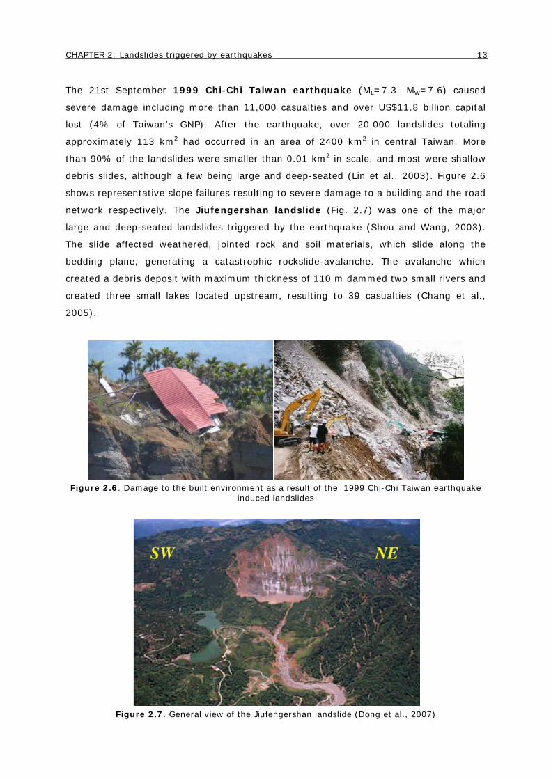
CHAPTER 2: Landslides triggered by earthquakes 13
The 21st September 1999 Chi-Chi Taiwan earthquake (ML=7.3, MW=7.6) caused
severe damage including more than 11,000 casualties and over US$11.8 billion capital
lost (4% of Taiwan’s GNP). After the earthquake, over 20,000 landslides totaling
approximately 113 km2 had occurred in an area of 2400 km2 in central Taiwan. More
than 90% of the landslides were smaller than 0.01 km2 in scale, and most were shallow
debris slides, although a few being large and deep-seated (Lin et al., 2003). Figure 2.6
shows representative slope failures resulting to severe damage to a building and the road
network respectively. The Jiufengershan landslide (Fig. 2.7) was one of the major
large and deep-seated landslides triggered by the earthquake (Shou and Wang, 2003).
The slide affected weathered, jointed rock and soil materials, which slide along the
bedding plane, generating a catastrophic rockslide-avalanche. The avalanche which
created a debris deposit with maximum thickness of 110 m dammed two small rivers and
created three small lakes located upstream, resulting to 39 casualties (Chang et al.,
2005).
Figure 2.6. Damage to the built environment as a result of the 1999 Chi-Chi Taiwan earthquake
induced landslides
Figure 2.7. General view of the Jiufengershan landslide (Dong et al., 2007)

14 Seismic Vulnerability of Reinforced Concrete Buildings in Sliding Slopes
The 8th October 2005 Kashmir earthquake in Pakistan caused severe damage to the
infrastructure and to the landscape including approximately 80,000 fatalities (Schneider,
2008). The earthquake triggered thousands of landslides throughout the region in an
area of 7500 km2, causing approximately 1000 fatalities, destroying roads, and
disrupting communications. These were mainly rock falls and debris falls, although
translational rock and debris slides also occurred (Owen et al., 2008). The largest
landslide associated with the earthquake was the 68×106 m3 Hattian Bala rock
avalanche (Fig. 2.8) that destroyed a village. The reported death toll varies greatly; it is
estimated to be a few hundreds to around 1000 people (Dunning et al., 2007; Schneider,
2008).
Figure 2.8. View to the source of the Hattian Bala rock avalanche (Dana Hill) from the high point
of the dam crest (Dunning et al., 2007).
On May 12th, 2008, the catastrophic Ms 8.0 Wenchuan earthquake occurred in east
Sichuan Province of China, causing more than 69000 casualties and extensive structural
damage to the built environment. It was the strongest earthquake and the most costly
natural disaster recognized to be occurred in China in the past 100 years. The
earthquake triggered more than 15,000 geohazards in the form of earthslides, rockfalls
and debris flows which resulted in about 20,000 deaths. Among the landslides activated
by the earthquake, the Chengxi landslide (Fig. 2.9), which is located at the west side of
the Beichuan County Town, is the most severe one; the landslide was characterized by
its high speed and long runout (considering air-cushion effect) and involved a volume of
around 2 million m3. It buried a large portion of the southwest part of the old Beichuan
resulting to 1,600 fatalities and significant economic losses (Yin et al., 2009).
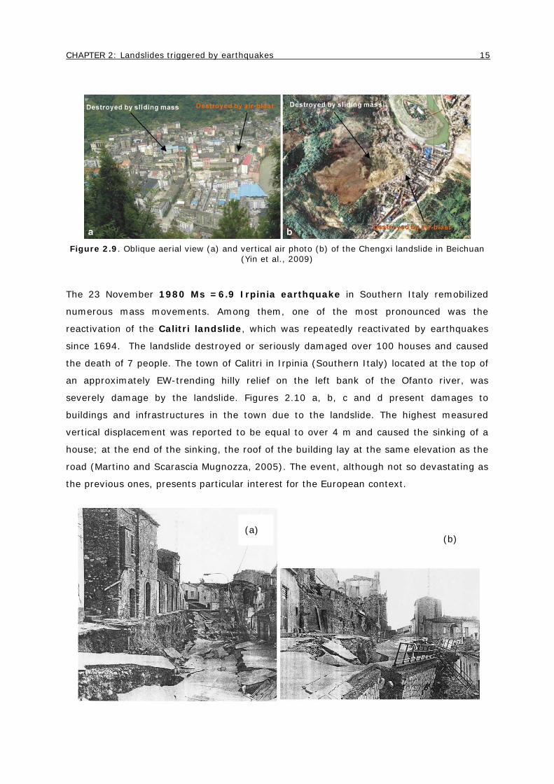
CHAPTER 2: Landslides triggered by earthquakes 15
Figure 2.9. Oblique aerial view (a) and vertical air photo (b) of the Chengxi landslide in Beichuan
(Yin et al., 2009)
The 23 November 1980 Ms =6.9 Irpinia earthquake in Southern Italy remobilized
numerous mass movements. Among them, one of the most pronounced was the
reactivation of the Calitri landslide, which was repeatedly reactivated by earthquakes
since 1694. The landslide destroyed or seriously damaged over 100 houses and caused
the death of 7 people. The town of Calitri in Irpinia (Southern Italy) located at the top of
an approximately EW-trending hilly relief on the left bank of the Ofanto river, was
severely damage by the landslide. Figures 2.10 a, b, c and d present damages to
buildings and infrastructures in the town due to the landslide. The highest measured
vertical displacement was reported to be equal to over 4 m and caused the sinking of a
house; at the end of the sinking, the roof of the building lay at the same elevation as the
road (Martino and Scarascia Mugnozza, 2005). The event, although not so devastating as
the previous ones, presents particular interest for the European context.
(a) (b)

16 Seismic Vulnerability of Reinforced Concrete Buildings in Sliding Slopes
Figure 2.10. Calitri landslide activation in 1980, producing damage: on the Francesco De Sanctis main street (a), on the Torre street (b), along the landslide scarp at the Giacomo Matteotti main
street (c), on the Garibaldi main street (d) (Martino and Scarascia Mugnozza, 2005)
2.1.2 Experience from earthquake induced landslides in Greece
In Europe, there are few and not well documented cases of earthquake induced
landslides. Most of them are concentrated on the Mediterranean region (Greece and
Italy). Papadopoulos and Plessa (2000) compiled a data set of 47 earthquake-induced
landslides occurring in Greece from AD 1650 to 1995 and examined their distribution.
The spatial distribution indicates landslides occurrence almost everywhere in Greece with
the exception of the north Greek mainland, which is likely due to the low occurrence
frequency of large earthquakes. Moreover, they examine the landslide distribution in
relation to various earthquake parameters (earthquake magnitude, epicentral distance)
and compare their result with those obtained by other authors for other seismotectonic
regions of the world (Keefer, 1984; Ambraseys, 1988).
Some examples of landslides triggered by seismic events occurring in Greece over the
last two decades as well as their consequences to the built environment are presented
hereafter.
The June 1995 Aegion earthquake (Ms=6.2) caused significant destruction, including
human losses, structural damage, liquefaction and ground ruptures. The earthquake also
triggered numerous landslides accompanied by debris flows and block rotations (Fig.
2.11). Reconstruction of the pre-earthquake topographic profiles along the main axis of
the landslides indicates that the failure zones extended to a maximum depth of 6 to 10m
within the loose alluvial deposits which cover the seabed. Post-earthquake landslides
occurred for ground slopes as low as 12.0 %, corresponding to a static factor of safety of
2.0. At almost all sites, ground failures were triggered by excess pore pressure build up
in very thin liquefied silty sand layers, with average thickness between 0.24 and 0.36m
(Bouckovalas et al., 1995).
(c) (d)
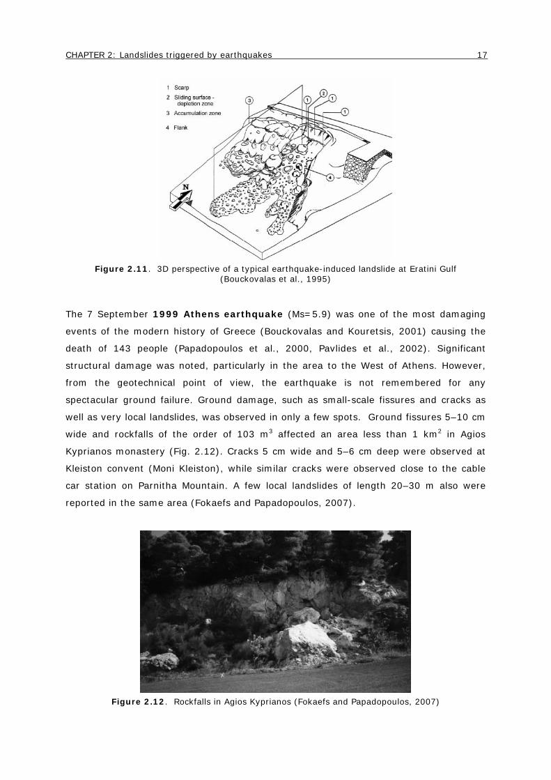
CHAPTER 2: Landslides triggered by earthquakes 17
Figure 2.11. 3D perspective of a typical earthquake-induced landslide at Eratini Gulf
(Bouckovalas et al., 1995)
The 7 September 1999 Athens earthquake (Ms=5.9) was one of the most damaging
events of the modern history of Greece (Bouckovalas and Kouretsis, 2001) causing the
death of 143 people (Papadopoulos et al., 2000, Pavlides et al., 2002). Significant
structural damage was noted, particularly in the area to the West of Athens. However,
from the geotechnical point of view, the earthquake is not remembered for any
spectacular ground failure. Ground damage, such as small-scale fissures and cracks as
well as very local landslides, was observed in only a few spots. Ground fissures 5–10 cm
wide and rockfalls of the order of 103 m3 affected an area less than 1 km2 in Agios
Kyprianos monastery (Fig. 2.12). Cracks 5 cm wide and 5–6 cm deep were observed at
Kleiston convent (Moni Kleiston), while similar cracks were observed close to the cable
car station on Parnitha Mountain. A few local landslides of length 20–30 m also were
reported in the same area (Fokaefs and Papadopoulos, 2007).
Figure 2.12. Rockfalls in Agios Kyprianos (Fokaefs and Papadopoulos, 2007)

18 Seismic Vulnerability of Reinforced Concrete Buildings in Sliding Slopes
The 14 August 2003 Lefkada earthquake (Mw=6.2), due to the very steep morphology
of the region, triggered a large number of landslides; the vast majority of them on the
island road network can be categorized as rock falls, rock slides, and disrupted slides,
with volume ranging from several cm3 to some (5 to 10) m3. Landslides were detected on
both natural and cut slopes, as well as on downstream road embankment slopes. The
slides were mainly observed at the central and northern part of the island, as well as in
the steep western coastal zone along the road joining the town of Lefkada with
Tsoukalades, Agios Nikitas, Kathisma, Kalamitsi, Chortata, Dragano and Komilio (Fig.
2.13). The steep morphology of the west coast, observed at the Ionian Islands, due to
the active tectonism of the area, and the highly fractured rock mass played an important
role in the appearance of such phenomena. The most characteristic rockfalls, with
diameters up to 4 m, were observed along the 6 km long road of Tsoukalades-Agios
Nikitas, which was very close to the epicentral area (EERI, 2003). In Table 2.1 a detailed
list of sites and villages with remarkable ground failures is presented (Pavlides et al.,
2004).
Figure 2.13. Rockfalls due to detachment and possible overturn at the Agios Nikitas (left); Cars
were buried under landslides near the same area (right)
After the 8 January 2006 Kythira earthquake (M=6.9) a number of landslides,
rockfalls and rock slidings were detected on natural slopes, which resulted in cutting off
parts of the road network and caused significant damage (fractures) of the road surface,
and in some cases, local failure of road embankments. The largest landslides and
rockfalls took place at Mitata village and its surroundings. Plan and side view of this
natural slope landslide is shown in Figure 2.14.
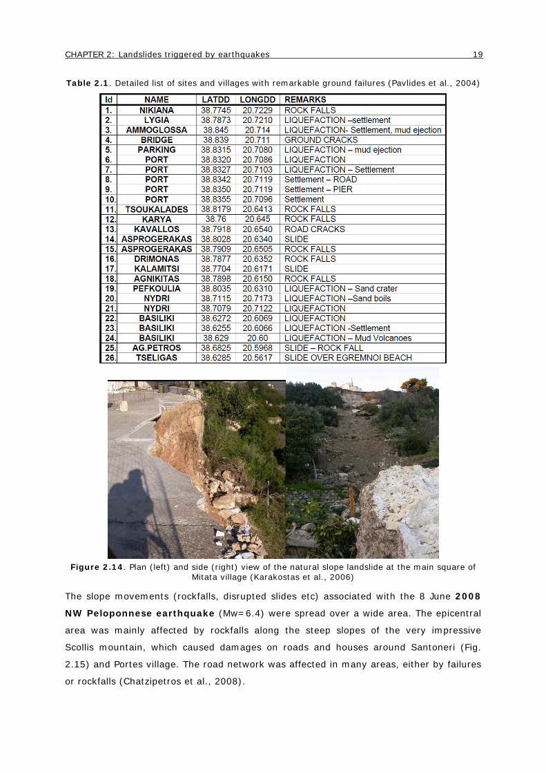
CHAPTER 2: Landslides triggered by earthquakes 19
Table 2.1. Detailed list of sites and villages with remarkable ground failures (Pavlides et al., 2004)
Figure 2.14. Plan (left) and side (right) view of the natural slope landslide at the main square of
Mitata village (Karakostas et al., 2006)
The slope movements (rockfalls, disrupted slides etc) associated with the 8 June 2008
NW Peloponnese earthquake (Mw=6.4) were spread over a wide area. The epicentral
area was mainly affected by rockfalls along the steep slopes of the very impressive
Scollis mountain, which caused damages on roads and houses around Santoneri (Fig.
2.15) and Portes village. The road network was affected in many areas, either by failures
or rockfalls (Chatzipetros et al., 2008).

20 Seismic Vulnerability of Reinforced Concrete Buildings in Sliding Slopes
Figure 2.15. Santomeri village: location of the detached rock block that toppled (left) - the rock
block itself (volume 6 to 7 cubic meters) that caused severe structural damage at one of the houses of the village (right) (Margaris et al., 2008)
2.2 Landslide classification and mechanisms
2.2.1 General classification of earthquake induced landslides
The term “landslide” describes a wide variety of ground processes that result in the
downward and outward movements of slope-forming materials, including rock, soil,
artificial filling, or a combination of these. Landslide classification is a very complex topic
oriented by research purpose. Although the impact of a given landslide type is not
always predictable, the class of landslide does present an indication of the type of
movement and its destructive potential (Glade and Crozier, 2005). Starting from the
work of Varnes (1978), Cruden and Varnes (1996) proposed a taxonomic classification of
landslides which considers, in addition to the movement mechanism at the initial stage of
motion, the material, the state of activity and the rate of movement (Fig. 2.16).
However, they do not distinguish between the different triggering landslide mechanisms.
In a pioneering study, Keefer (1984; 2002), based on the principles and terminology by
Varnes (1978), classified the earthquake triggered landslides into three main categories
on the basis of type of material, landslide movement, degree of internal disruption of the
landslide mass and geologic environment (see Tab. 2.2):
Category I: Disrupted Landslides, which occur fast and at high inclinations (>35°) in
discontinuous rock masses or weakly cemented materials.
Category II: Coherent Landslides either in rock or soil with deep slip weakened surfaces
or with a relatively broad distributed shear zone, reported for inclinations >15°
Category III: Lateral Spreads and flows slides, associated to liquefaction in granular
materials; if residual strengths are lower than static shear stresses, flow slides can
develop at very low inclinations.
Keefer (1984) studied the landslides triggered by 40 historic earthquakes globally with
magnitudes varying from 5.2 to 9.2 and found that the frequency of the seismically

CHAPTER 2: Landslides triggered by earthquakes 21
induced landslides increases with increasing earthquake magnitudes. Three types of
disrupted landslides – i.e. rock falls, disrupted soil slides, and rock slides - were found to
be the most abundant, comprising about 80 percent of the earthquake induced landslides
as reported in Keefer (2002). Rodriguez and co-workers (Rodriguez et al., 1999), after
studying the landslides that occurred after 36 earthquakes worldwide, summarized the
typical geometric characteristics of some of the most common slide categories (Table
2.3) including ranges of depth to the slip surface and the geometry of the slide in terms
of the aspect ratio and the shape of the slip surface.
Figure 2.16. Classification of landslides (Modified after Varnes, 1978)

22 Seismic Vulnerability of Reinforced Concrete Buildings in Sliding Slopes
Table 2.2. Characteristics of earthquake-induced landslides (Keefer, 2002)

CHAPTER 2: Landslides triggered by earthquakes 23
Table 2.2. (Continued) - Characteristics of earthquake-induced landslides (Keefer, 2002)

24 Seismic Vulnerability of Reinforced Concrete Buildings in Sliding Slopes
Table 2.3. Geometric characteristics of earthquake-induced landslides (Rodríguez et al., 1999).
2.2.2 Parameters affecting seismic slope stability
Many factors may influence the seismic stability of slopes and the characteristics of the
landslides induced by earthquakes. Among these, the most important parameters
affecting seismic slope stability are:
physical, mechanical and dynamic properties of the ground;
geometry of the slope
characteristics of shaking primarily related to M, R, PGA, local soil conditions and
topographic effects.
2.2.2.1. Ground Properties
According to Keefer (2002), geomaterials most susceptible to earthquake-induced
landslides are:
(1) Weakly cemented, weathered, sheared, intensely fractured, or closely jointed rocks,
(2) Better-indurated rocks having prominent discontinuities,
(3) Sandy residual or colluvial soils,
(4) Saturated volcanic soils containing sensitive clay,
(5) Loess,
(6) Cemented soils,
(7) Granular deltaic sediments,
(8) Granular flood-plain alluvium, and
(9) Uncompacted, or poorly compacted, granular artificial fill
Data on the involved geomaterials may be derived from previously published documents
such as geologic maps, field reconnaissance survey, laboratory tests and in situ
monitoring.

CHAPTER 2: Landslides triggered by earthquakes 25
Under the influence of earthquake loading, inertial forces and pore pressure build-up may
contribute to increased shear stresses and reduced shear strength along the potential
sliding mass leading to instability and/or permanent deformations. Soils that exhibit
significant reduction of shear strength due to cyclic loading are loose soils and soils with
particles that are weakly bonded into loose structures. Saturated soft cohesionless soils
may liquefy under cyclic loading, lose temporaly all strength, and behave as viscous
fluids.
The presence of pre-existing shear zones and the degree of brittleness is particularly
important in determining the potential of a landslide mass (Hutchinson, 1995).
Considering that the brittleness on preexisting shears is generally low or zero, the
reactivation of landslide movement on such shears is usually slow.
Groundwater when present may play a definite role as well. In Italy, Wasowski et al.
(2002) observed that during the Irpinia earthquake (1980) the change in the
groundwater condition (seismically induced pore-water pressure rise) was a major
controlling parameter in the spatial landslide distribution.
Shear strain softening of soil materials, which can be related in its effectiveness to the
number of (equivalent uniform) excitation cycles N, result to the degradation of the
stiffness and strength properties of the soils: it may be considered as one of the major
causes of most of the slides induced by earthquakes (Ishihara, 1996). If landslide
materials display strain-softening behavior, their kinetic energy can reach catastrophic
proportions and long runout distances (Leroueil et al., 1996). In these materials, a
progressive failure can occur owing to a reduction of strength with increasing strain.
Progressive failure involves non-uniform straining of brittle materials resulting in a
nonuniform mobilisation of the shear strength along the potential slip surface (Bjerrum
1967; Troncone, 2005). General failure of the slope usually takes place before the
residual strength has developed everywhere along the sliding mass. Thus, the average
strength of the mass at failure is less than the peak strength of the soil and greater than
the residual one (Dounias, 1988; Troncone, 2005; Conte et al., 2010; Kourkoulis et al.,
2010).
Knowledge of the effect of rate of displacement on the residual strength is important
when studying the kinematics of a potential sliding mass. Three types of variation of the
fast residual strength with an increasing rate of displacement have been identified (Tika
et al., 1996): (a) neutral rate effect—soils showing a constant residual strength
irrespective of the rate of displacement; (b) negative rate effect—soils showing a
significant drop in strength when sheared at rates higher than a critical value; and (c)
positive rate effect—soils showing an increase in residual strength above the slowly
(static) drained residual value at increasing rates of displacement. Soils with small clay

26 Seismic Vulnerability of Reinforced Concrete Buildings in Sliding Slopes
fractions (sands and soils with PI<10%) have shown neutral rate effect. In soils of
increasing clay fraction (or plasticity), however, negative and positive rate effects have
been observed.
There is a possibility of delayed initiation or reactivation of landslide movement subject
to ground shaking, especially in coherent materials, associated with the potential
reduction of the in situ shear strength and the variation of groundwater conditions. As an
example, this was the case of the Irpinia earthquake occurred in Italy (M= 6.9), where
several large earth flows and other coherent slides began their movement few hours to
few days after the main shock. The post-earthquake movement of these landslides was
inferred to be caused by the increased spring flow and pore-water pressures regime,
associated with the tectonic deformation of the interested area (Keefer, 2002).
A comprehensive overview of the dynamic strength characteristics of granular and
cohesive soils playing a role in the slope seismic stability and related induced
displacements, may be found in Ishihara (1996) and Pitilakis (2010, in Greek).
2.2.2.2. Size of landslides
Expect for the parameters described in Table 2.2, landslide size may be related to the
earthquake magnitude (Fig. 2.17), shaking intensity, and epicentral distance (Keefer,
2002). Hancox et al. (2002) reported that only landslides having volumes < 104 m3
occurred in New Zealand earthquakes with M < 6, whereas landslides having volumes >
108 m3 occurred only in earthquakes with M > 7.5 and intensities of MMI IX or higher.
The size of landslides induced by an earthquake can be also correlated to the relation
between slope aspect and ground shaking intensity during the strong motion phase (Li,
1978 in Wen et al., 2004).
Figure 2.17. Relations between area affected by landslides and earthquake magnitude (Keefer,
2002)

CHAPTER 2: Landslides triggered by earthquakes 27
2.2.2.3. Shaking characteristics
Magnitude
According to Keefer (1984, 2002), the minimum magnitude of an earthquake that would
cause landslides of various types is (see Fig. 2.18):
~4.0 for rock falls, rock slides, soil falls and disrupted soil slides
~4.5 for soil slumps and soil block slides;
~5.0 for soil lateral spreads, rapid soil flows, subaqueous landslides, rock slumps, rock
block slides, and slow earth flows;
~6.0 for rock avalanches; and
~6.5 for soil avalanches.
Modified (generally lower) values were proposed by Rodríguez et al. (1999) for the
earthquake magnitude that can trigger a landslide of various types. These minimum
magnitude thresholds have been empirically derived and as such they are approximate in
nature. However, they are important as they reveal general trends. Smaller earthquake
events can occasionally trigger landslides in correlation with non seismic causes (e.g
intense precipitation). Hence, if a slope is in a marginally stable state, even a weak
earthquake (M<4) can trigger the landslide mass movement. Several examples of low
magnitude induced landslides have been reported in the literature (e.g. Keefer, 1984;
Rodríguez et al., 1999; Papadopoulos and Plessa, 2000).
Figure 2.18. Maximum epicentral distance as a function of the event magnitude for the three
landslide categories (dashed line: disrupted landslides, dash-double-dot line: coherent landslides, dotted line: lateral spreads and flows) (Keefer, 1984)

28 Seismic Vulnerability of Reinforced Concrete Buildings in Sliding Slopes
Epicentral Distance
Keefer (1984) proposed a set of upper bound curves for the maximum distance as a
function of the event magnitude for the three landslide categories (disrupted, coherent,
flows) (Fig. 2.18). Recent studies showed that these curves are appropriate in most
cases, although some outliers were observed for disrupted and coherent type landslides
at moderate to low magnitudes (Delgado et al., 2011).
Statistical analysis of the landslide distribution showed a strong correlation between
landslide concentration, on the one hand, and distance from the epicenter, distance from
the fault rupture, and slope inclination, on the other (Keefer, 2000). Landslide abundance
showed an exponential decrease with increasing distance from the fault-rupture zone
(Fig. 2.19a) but not with increasing epicentral distance (Fig. 2.19b) (Keefer, 2002).
Later studies (e.g. Huang and Li, 2009; Sato and Harp, 2007) also report that the
distribution of earthquake-triggered landslides is more related to the distance from the
surface projection of the fault plane and the surface projection up-dip edge of the fault
rather than the distance from the epicenter.
Figure 2.19. Relation of landslide concentration to the distance from the fault rupture zone (a)
and to the epicentral distance (b) for landslides in the southern Santa Cruz Mountains triggered by the 1989 Loma Prieta, California, earthquake (Keefer, 2002)
Site and Topographic effects
The specific properties and geometrical features of the soil deposits can modify the
characteristics (amplitude, frequency content and duration) of the travelling wave field,
generating extra amplification (aggravation factor in the seismic input characteristics),
attenuation or tensional effects in the ground influencing the deformation and,
eventually, ground failure. Soil nonlinearity, material damping, the impedance contrast
(a) (b)

CHAPTER 2: Landslides triggered by earthquakes 29
between sediments and the underlying bedrock, and the characteristics of incident
wavefield are considered to represent the governing factors for site amplification (Kramer
and Stewart, 2004; Pitilakis, 2004; 2010). A fundamental period of the earthquake close
to the natural period of the site can lead to resonance phenomena and, consequently, to
an amplified energy content of the ground motion. The slope failure potential assumes its
highest values for a combination of a low-frequency seismic input motion together with a
resonance phenomenon in the low-frequency range (Bourdeau et al., 2004; Bourdeau
and Havenith, 2008).
Topographic irregularities can considerably affect the amplitude and frequency content of
ground motions. In the case of hills or slopes this can be related to the triggering forces
acting upon them, since amplified surface accelerations behind the crest may present
larger destabilizing forces, potentially causing higher landslide risk (Paolucci, 2002).
Amplification of both horizontal and vertical ground motion components normally takes
place over a narrow zone near the crest of the slope. This is due, among other factors, to
the diffraction at the surface irregularities and surface wave generation: it can be
observed both in the time domain (as an increase in the maximum observed amplitude
near the crest, with respect to the maximum observed amplitude of the free-field) as well
as in the frequency domain (as a spectral amplification over a narrow band of frequencies
corresponding to wavelengths similar to the horizontal dimension of the slope) (e.g.
Assimaki and Gazetas, 2004; Assimaki et al. 2005; Bouckovalas and Papadimitriou,
2005; Ktenidou, 2010).
While landslides triggered by precipitation are generally distributed uniformly along the
slopes, landslides triggered by earthquakes tend to be clustered near ridge crests and hill
slope toes. Densmore and Hovius (2000) in Peng et al. (2009) attributed this ridge- crest
clustering to topographic effects (as described above), and the clustering at hill slope
toes to dynamic pore-pressure changes in the water-saturated material of lower hill
slopes.
Ashford et al. (1977), Bouckovalas and Papadimitriou (2005), Papadimitriou and
Chaloulos (2010) and Lenti and Martino (2010, 2012), among others, investigated
parametrically the effect of step-like slope topography that may lead to intense
amplification and de-amplification irregularly along the slope, depending on its geometry
and its geological setting as well as on the wavelength of the impinging excitation with
respect to the slope’s height. Bozzano et al. (2008a, 2010) also pointed out the role of
“self-excitation” process due to local seismic amplification resulting from the structural
setting of the stiff bedrock and the pre-existing landslide masses, in the reactivation of
far field pre-existing large landslides. As the authors demonstrated, the frequency
content of the incoming seismic wave field in relation to the geological setting of the
30 Seismic Vulnerability of Reinforced Concrete Buildings in Sliding Slopes
slope is fundamental to the occurrence of this phenomenon. According to Del Gaudio and
Wasowski (2011), amplification in potentially unstable slopes may have a pronounced
directional character causing a re-distribution of shaking energy with maxima oriented
along potential sliding directions. However, more research is needed to identify the
critical factors controlling these phenomena.
2.3 Methods to assess earthquake induced landslide hazards
According to the Association of Professional Engineers and Geoscientists of British
Columbia guidelines (APEGBC, 2010), there are various methods to assess earthquake
induced landslide hazards. These include, but are not limited to, estimating:
The likelihood or probability of occurrence of a landslide,
The factor of safety of a slope,
The slope displacement along a slip surface.
In order for the results of the above estimate to be incorporated in a Quantitative Risk
Assessment (QRA) methodology, they must be combined with an estimate of landslide
run-out distance (for residential development at the bottom of the slope), or an estimate
of where the main scarp of the landslide will intersect the ground (for residential
development on, or at the top of, the slope) (APEGBC, 2010).
2.3.1 Likelihood or probability of occurrence of a landslide
When assessing the probability of a particular slope experiencing landsliding within a
reference period and within a given area, the recognition of the geotechnical, hydro-
geological, topographic conditions that caused the slope to become unstable, and the
mechanisms that triggered the landslide movement is of primary importance. The
triggering variables (e.g. the seismological characteristics) shift the slope from a
marginally stable to an unstable state and thereby initiating failure in an area of given
susceptibility (Dai et al., 2002). They are time-dependent factors that may change over a
very short period of time. The historic frequency of landslides in an area can be
determined to provide realistic estimates of landslide probability of occurrence
throughout a region where landslides have caused a significant amount of damage. The
trigger/landsliding and frequency–magnitude relations that help understanding landslide
probabilities may be derived from landslide inventories. Considering that landslide
inventories are usually incomplete or inaccurate, the use of aerial photographs and/or
satellite images in conjunction with the landslide inventories may give further insight in

CHAPTER 2: Landslides triggered by earthquakes 31
the documentation of the landslide occurrence and the interpretation of the main
landslide triggering processes.
The frequency of seismically induced landslides may be related to the peak ground
acceleration at the site, the magnitude of the earthquake and the distance from the
earthquake epicenter (Fell et al., 2008). Studies by Keefer (1984, 2002), Harp and Jibson
(1996), Rodriguez et al. (1999), Jibson et al. (2000), Papadopoulos and Plessa (2000),
have shown that there is a threshold magnitude, peak ground acceleration and distance
from the earthquake epicenter above which landsliding will occur. This varies for different
landslide types and sizes (see subsection 1.2.2.3). One problem with the characteristics
of the expected ground shaking is that strong-motion stations are not usually widely
distributed in areas where landslides are most likely to occur. Hence, the interpolation of
the available data from the few stations available to grid points in mountainous areas is
difficult and sometimes ineffective.
2.3.2 Factor of safety of a slope
For site-specific slopes, the probability of failure is usually considered as simply the
probability that the factor of safety is less than unity. The factor of safety of a slope may
be defined as the ratio of the shear resistance to the shear stress mobilized. In simple
terms, a FS=1 is assumed when failure occurs and values successively greater than 1
suggest increasing stability and hence lower susceptibility to failure. When an
earthquake occurs, the slope material is subjected to horizontal and vertical acceleration
with reverse cycles. The inertial forces associated with these accelerations may
momentarily reduce the factor of safety below 1.0 by increasing the shear stresses and
possibly decreasing the shear resistance of the material, initiating downslope movement.
If the accelerations are large enough or continue for a long period of time, they may lead
to instability and/or extensive permanent deformations.
There are many different ways to compute the factor of safety of a slope including limit
equilibrium (e.g. Fellenius, Bishop, Janbu, Morgenstern and Price, Spencer, Sarma
methods) and strength reduction method (SRM) (e.g. Dawson and Roth, 1999; Griffiths
and Lane, 1999). For simple homogenous soil slopes, it is found that the results from
these methods are generally in good agreement. The strength reduction method, utilized
in many finite element and finite difference codes (e.g. Plaxis, FLAC 2D, FLAC 3D, Phase
etc.), does not require any pre-definition of the sliding surface. Instead, the failure
surface develops “naturally” based on the selected yield criterion (e.g. Mohr Coulomb,
Hoek-Brown etc.). Nevertheless, the strength reduction method is incapable of
determining other failure surfaces, which may be only slightly less critical than the SRM

32 Seismic Vulnerability of Reinforced Concrete Buildings in Sliding Slopes
solution. It is also sensitive to nonlinear solution algorithms/flow rule for some special
cases (Cheng et al., 2007). For this reason, it is generally advisable to perform both
methods in parallel when dealing with critical problems.
Figure 2.20. Pseudostatic slope stability analysis
In a conventional limit equilibrium slope stability analysis, such as the ordinary method
of slices, simplified Bishop’s method, and simplified Janbu’s method, an additional
horizontal static force is applied to simulate earthquake shaking. Analyses that model the
earthquake as an equivalent static force are commonly referred to as pseudo-static
analyses (Fig. 2.20). For pseudo-static analyses, the horizontal static force is calculated
by multiplying the soil weight by a seismic coefficient, k that represents the earthquake
shaking. Seismic coefficients used in pseudo-static analyses are empirically derived to
represent an equivalent seismic load. The selection of the proper value of the seismic
coefficient is fundamental, as this value controls the inertial forces on the soil masses.
According to Terzaghi (1950), who first introduced the pseudo-static (PS) approach, the
values of the seismic coefficient should be k=0.1 for severe earthquakes, k=0.25 for
violent-destructive earthquakes, and k=0.5 for catastrophic earthquakes. In all cases the
author suggested that the design safety factor with respect to strength, Fs, may be close
to 1.0. In contemporary seismic norms, e.g. Eurocode 8 (EC8 2004), the pseudostatic
slope stability analysis is widely adopted for the design of natural and engineered slopes
due to its simplicity. The selection of a seismic coefficient equal to a specific portion of
the design peak ground acceleration at the site of interest is prescribed depending on the
earthquake magnitude and peak ground acceleration values as well as the acceptable
level of seismic performance of the studied slope. However, a main limitation of the
pseudostatic approach is that it provides only a single numerical threshold below which
no displacement is predicted and above which total, but undefined, failure is predicted.
Moreover, the fact that an equivalent static force models the earthquake does not permit
the actual dynamic response of the structure to be taken into account, and thus, the real
response and stability of the geo-structure cannot be accurately assessed during a
moderate or severe seismic event. Lagaros et al. (2009) recognized that in cases where
the local site conditions play an important role (e.g. sensitive clays, loose saturated silty

CHAPTER 2: Landslides triggered by earthquakes 33
sands), more sophisticated non-linear dynamic analysis procedures should be used.
According to APEGBC (2010) guidelines, pseudostatic analysis can be used for
preliminary analyses and screening procedures and for the evaluation of seismic slope
stability using a slope displacement-based seismic coefficient equivalent to the prescribed
tolerable slope displacement along the slip surface (Bray and Travasarou, 2009).
2.3.3 Slope displacement along a slip surface
It is common practice in geotechnical earthquake engineering to assess the expected
seismic performance of slopes and earth structures by estimating the potential for
seismically induced permanent displacements using one of the available displacement-
based analysis procedures. Considering that (total and/or differential) displacements
ultimately govern the serviceability level of a slope after an earthquake, the use of such
approaches is strongly recommended. Moreover, for a landslide risk assessment study it
is the extent of permanent ground deformation that is the most important parameter,
since the assessment of landslide potential (e.g. probability of landslide occurrence) on
its own is of little relevance if the consequent ground deformations are not expected to
cause distress and damage to buildings and infrastructure. The later represents one of
the most important principles on which this study has been based. Typically, two
different approaches of increased complexity are proposed to assess permanent ground
displacements in case of seismically triggered slides:
Newmark-type displacement methods
Advanced stress- strain dynamic methods
2.3.3.1. Newmark-type displacement methods
Starting from the landmark study of Newmark (Newmark, 1965), the first class includes
simplified or advanced displacement based approaches that generally differ with respect
to the assumptions and idealizations used to represent the mechanism of earthquake-
induced displacement. They are intended for soil slopes and they can be grouped into
three main types (Jibson, 2011): rigid-block, decoupled, and coupled.
The rigid-block model originally proposed by Newmark (1965) treats the potential
landslide block as a rigid mass (no internal deformation) that slides in a perfectly plastic
manner on an inclined plane (Fig. 2.21). The mass experiences no permanent
displacement until the base acceleration exceeds the critical (yield) acceleration of the
block, which is the threshold base acceleration, required to overcome the shear
resistance of the slope and initiate failure; then, the block begins to move downslope.
Cumulative displacements are estimated by double-integrating the parts of an
acceleration-time history that lie above the critical acceleration. The original Newmark

34 Seismic Vulnerability of Reinforced Concrete Buildings in Sliding Slopes
rigid sliding block assumption is employed in many of the available simplified slope
displacement procedures (e.g., Lin and Whitman, 1986; Ambrasseys and Menu, 1988;
Yegian et al. 1991; Jibson, 2007; Saygili and Rathje, 2008 etc.). The dynamic site
response and the sliding block displacements are computed separately in the ‘decoupled’
approach (e.g. Makdisi and Seed, 1978; Bray and Rathje, 1998; Ausilio et al., 2008;
Rathje and Antonakos, 2011) or simultaneously in the ‘coupled’ stick-slip analysis (Rathje
and Bray, 2000; Bray and Travasarou, 2007) (Fig. 2.22). Some of the most commonly
applicable seismic displacement procedures that account for the soil deformability (both
coupled and decoupled) are discussed in Bray (2007). In general, coupled analysis yields
reliable results for slopes of all dynamic stiffness and strength, but, of course, is the most
complex to conduct. Rigid-block analysis is appropriate for analyzing thin, stiff landslides
but yields quite unconvervative results for deep, flexible slopes. The decoupled approach
is generally considered to slightly overestimate displacements compared to the fully
nonlinear, coupled stick-slip analysis. However, it was found non-conservative primarily
for projects undergoing intense, near-fault ground motions (Rathje and Bray, 1999;
2000). Jibson (2011) provides guidelines for selecting the most appropriate sliding-block
analysis based on the Ts/Tm, i.e. the ratio of the fundamental site period (Ts) to the mean
period of the earthquake motion (Tm) (Tab. 2.5). APEGBC (2010), based on the concept
of tolerable slope displacement, proposed the use of Bray and Travasarou (2007)
simplified coupled method for the seismic analysis of soil slopes.
Figure 2.21. Newmark Sliding-block analogy

CHAPTER 2: Landslides triggered by earthquakes 35
The significance of modeled displacements must be judged by their probable effect on a
potential landslide (Jibson, 2011). According to the California Geological Survey’s (2008)
general guidelines, Newmark displacements of 0-15cm are unlikely to correspond to
serious landslide movement and damage; displacements of 15-100cm could be serious
enough to cause serious ground cracking or strength loss and continuing failure; and
displacements greater than 100 cm are very likely to correspond to damaging landslide
Figure 2.22. Decoupled dynamic response/rigid sliding block analysis and fully coupled analysis
(Bray, 2007)
Table 2.4. Guidelines for selecting appropriate sliding-block analysis (Jibson, 2011)
movement, including possible catastrophic failure. However, it is important to note the
fact that the estimated range of seismic induced permanent displacement from semi-
analytical and/or semi-empirical procedures both coupled and uncoupled, should be
considered as an index of the expected seismic performance. Seismic displacement
estimates will always be approximate in nature due to the complexities of the dynamic

36 Seismic Vulnerability of Reinforced Concrete Buildings in Sliding Slopes
response of the soil materials involved and the variability of the earthquake ground
motion (Bray, 2007). Moreover, it‘s worth noticing that the yield coefficient ky is assumed
to be constant during seismic shaking. Thus, Newmark-type approaches should not be
followed when significant strength loss is anticipated in the slope soil material (e.g.
liquefaction) (e.g. Kramer 1996). In the later, a more sophisticated numerical analysis
capable to account for soil nonlinearity is recommended for use.
2.3.3.2. Advanced stress- strain dynamic methods
Advanced stress-deformation analyses based on continuum (finite element (FEM), finite
difference (FDM), boundary element method (BEM)) or discontinuum (e.g. Distinct
Element Method (DEM) and Discontinuous Deformation Analysis (DDA)) formulations
usually incorporating complicated constitutive models, are becoming more and more
attractive, as they can provide approximate solutions to problems which otherwise
cannot be solved by conventional methods e.g. the complex geometry including
topographic and basin effects, material anisotropy and non-linear behavior under seismic
loading, in situ stresses, pore water pressure built-up, progressive failure of slopes due
to strain localization, soil-structure interaction. Numerical methods have been applied to
model the dynamic response of slopes using different constitutive models (e.g. Mohr
Coulomb, strain softening, hysteretic model etc.), boundary conditions and dynamic input
motions (real or synthetic accelerograms, simplified wavelets).
Many investigators implemented continuum FE (e.g. ABAQUS, Opensees, PLAXIS etc.) or
FD (e.g. FLAC 2D, 3D) codes to evaluate the residual ground displacements of soil slopes
using elastic–plastic constitutive models. Martino and Scarascia Mugnozza (2005)
examined the effect of seepage and frequency content of dynamic input motion on the
histories of permanent co-seismic displacements and excess pore pressures of the Calitri
landslide (Southern Italy) by means of the explicit finite difference program FLAC2D.
Siyahi and Arslan (2008) investigated the dynamic behavior and earthquake resistance of
Alibey earth dam (Istanbul, Marmara Region, Turkey) taking into account the effects of
liquefaction and cyclic mobility. They performed displacement-pore pressure coupled FE
analyses using OpenSees (Open System for Earthquake Engineering Simulation)
platform. Marchi et al. (2011) performed a sensitivity analysis on the influence of the
strength, stiffness and damping parameters of the soil on the seismic response (in terms
of permanent displacements) of Las Colinas slope (El Salvador) using the finite element
code PLAXIS. Kourkoulis et al. (2010) used the FE code ABAQUS to estimate the co-
seismic displacements of an idealized slope with strain- softening behavior considering
soil-foundation-interaction. Han and Hart (2010) studied the seismic stability of
reservoir-/earth dam/pore fluid systems and predicted the potential liquefied regions,
earthquake-induced settlement and lateral spreading for a realistic reservoir dam
CHAPTER 2: Landslides triggered by earthquakes 37
experiencing seismic loading using the explicit difference program FLAC2D (Itasca,
2011). Taiebat et al. (2011) estimated the seismic response (in terms of shear strains
and horizontal displacements) of a saturated clay slope based on an advanced modified
isotropic modified Cam-Clay model to account for anisotropy and destructuration. The
model was numerically implemented in the 3D explicit finite-difference program FLAC3D.
Fotopoulou et al. (2011) used the explicit finite difference code FLAC2D to assess the
permanent ground displacement of the Kato-Achaia slope - western Greece as a
consequence of the Ilia-Achaia, Greece 2008 (Mw= 6.4) earthquake, considering the
presence of a structure near the cliff.
To analyze the seismic stability of rock slopes both continuum or discontinuum methods
are possible. An overview of the advantages and disadvantages of these approaches are
presented in Stead et al. (2006). When the seismic stability of rock is controlled by
movement of joint-bounded blocks and/or intact rock deformation then the use of
discontinuum discrete-element codes is generally preferable. The predominant
discontinuum method that has been used to investigate a wide variety of rock slope
failure mechanisms is the distinct-element code UDEC (Itasca, 2004).
The accuracy of advanced numerical methods is highly dependent upon the quality of the
input parameters and the level of model validation performed by the user for similar
applications. One basic limitation is that the parameters required for the definition of the
constitutive models are not easily quantified in the laboratory or in situ. Moreover, due to
their complexity, they are generally more appropriate for specific case studies and not for
a parametric analysis aiming to evaluate the landslide risk at local and regional scale.
Finally, it should be emphasized that numerical modeling is a very powerful tool in the
identification and comprehension of the coupled processes and complex mechanisms
leading to instability of a given slope but it should be combined with engineering
experience and critical judgment in order to yield reliable results.
2.3.4 Discussion
The choice of the most appropriate method to assess earthquake induced landslide
hazard should primarily rely on the scale of the problem, data availability and quality
concerning the geometrical, hydro-geological and the geotechnical characteristics of the
site, the seismic motion parameters and soil dynamic properties (e.g. residual dynamic
shear strength), the criticality of the structure and engineering judgment. A simplified
empirical or semi-empirical method (e.g. pseudo-static analyses, Newmark- type
displacement models) is generally preferable for the landslide hazard assessment in small
scales (e.g. regional scale) while a more sophisticated method (e.g. numerical model) is
usually adopted in large and detailed scales. Within the framework of this research, the

38 Seismic Vulnerability of Reinforced Concrete Buildings in Sliding Slopes
numerical approach is selected as it is reportedly more accurate than any empirical
method and it permits the direct estimation of absolute and/or differential ground
displacements at the slope area, which represent the main cause of damage.

CHAPTER 3
Literature review on assessing building vulnerability to landslides
3.1 Introduction
The present chapter aims at providing a critical review of existing methodologies to
quantify building vulnerability to slides. Various concepts and aspects of physical
vulnerability to slides are discussed and analyzed regarding the development of fragility
curves, the selection of appropriate landslide intensity measures, the extent and
mechanisms of building damage to slides and the definition of structural and non-
structural damage/limit states.
3.2 Physical vulnerability to landslides
Different disciplines use multiple definitions and different conceptual frameworks of the
term of vulnerability. In engineering and natural sciences, physical vulnerability is
commonly expressed as the degree of loss (expressed on a scale of 0: no loss to 1: total
loss) to a given element or set of elements at risk (i.e. buildings and infrastructures),
resulting from the occurrence of a specified hazard of given magnitude. The term of
vulnerability [V], closely related to the consequences of natural hazards, is generally
enclosed in the definition of risk [R] through the following simple formulation (Varnes,
1984):
[R]= [H] x [V] x [E] (3.1)
Where [H]: hazard, [E]: value (or cost) of the element at risk.
However, in many cases the estimation of landslide vulnerability depends on the hazard
evaluation and therefore the vulnerability term should be conditioned on the hazard
term. Thus, the previous relationship can be transformed as follows:
[R]= [H] x [V/H] x [E] (3.2)

40 Seismic Vulnerability of Reinforced Concrete Buildings in Sliding Slopes
Within the context of a landslide risk assessment methodology, physical (technical)
vulnerability comprises a key component that still requires significant research (Leone et
al., 1996; Dai et al., 2002; Cascini et al., 2005; Van Westen et al., 2006; Mavrouli and
Corominas, 2010a and 2010b). The explanation lies in the first place in the scarcity of
available damage data in quantitative terms and the inherent uncertainties associated
with them (Van Westen et al. 2006). The heterogeneity of vulnerable elements to similar
landslide mechanisms, the wide range of processes (e.g. rockfalls, debris flows, earth
slides etc.) and their possible characteristics (e.g. size, shape, velocity, momentum) as
well as the numerous categories of damages and their inherent dynamic nature have also
contributed to the insufficient and somewhat subjective treatment of landslide
vulnerability. Physical vulnerability may be defined as the degree of loss (in terms of
percentage % of structural damage) of the affected built structures subjected to a
landslide event of a given type and intensity. It depends on the structural properties of
the exposed elements (e.g. typology, construction quality, state of maintenance, use
etc), but also on the mechanism and intensity of the landslide processes. An additional
important factor is the geographic location of the exposed elements with respect to the
the landslide area (e.g. within or outside the unstable mass), given the variation of the
soil movement and the consequent interaction with the structures and infrastructures, or
in the case of rock falls, the location and the extent of the rock fall impact on the
exposed elements. For instance, buildings subject to the same landslide event may
experience different vulnerability values owing to their particular different structural
(strength and stiffness) characteristics. Furthermore, buildings having exactly the same
typological and structural properties may suffer less or more damage, determined by the
landslide type and mechanism and their location in relation to the landslide zone. Thus,
they might sufficiently accommodate the impact of a falling block but they cannot avoid
development of tension cracks due to differential displacements produced by a
translational slide (Fell et al, 2008). Figure 3.1 presents a schematic overview of
landslide damage types, related to different types of landslides, elements at risk and the
location of the elements at risk in relation to the landslide (Van Westen et al., 2006).
Physical vulnerability of the exposed elements to the different landslide hazards may be
expressed both in qualitative and quantitative terms. Whether qualitative or quantitative
assessments are more suitable depends on both the desired accuracy of the outcome and
the nature of the problem, and should be compatible with the quality and quantity of
available data (Dai et al., 2002). When sufficient data is available, a quantitative analysis
(QRA) is preferable compared to qualitative, as it allows for a more explicit
characterization of the causes of damage (in terms of permanent deformation, tension
cracks, number of fatalities, monetary values etc.) and offers an improved basis for

CHAPTER 3: Literature review on assessing building vulnerability to landslides 41
communication among the research community, local authorities and emergency
planners (AGS, 2007; Uzielli et al., 2008).
Figure 3.1. Schematic overview of landslide damage types, related to different landslide types,
elements at risk and the location of the exposed element in relation to the landslide (Van Westen et al., 2006)

42 Seismic Vulnerability of Reinforced Concrete Buildings in Sliding Slopes
3.2.1 Landslide intensity measures
According to Hungr (1997) landslide intensity represents a set of spatially distributed
parameters that describe the destructiveness of a landslide. To quantify the landslide
effect on the exposed element, proper intensity parameters should be used that link the
landslide hazard to the response of the exposed element to it. Their selection should be
made with consideration of their predictability, efficiency and sufficiency (Kramer, 2011),
taking also into account the scale of the problem. Intensity measure predictability refers
to the uncertainty with which an IM can be predicted for a given landslide event whereas
intensity measure efficiency refers to the conditional uncertainty in the structural
response given the landslide intensity. Sufficient IM is a measure for which consideration
of additional intensity parameters does not reduce the uncertainty in predicted response.
Intensity (demand) of a given landslide event can be expressed in different ways
depending on the landslide type (slow moving or rapid slide, rockfall, etc.), the relative
position of the exposed element (e.g. uphill, downhill or inside the potential unstable
slope) to the landslide as well as the initial trigger of the landslide event (e.g.
earthquake, intense precipitation, erosion etc.). Commonly used intensity measures are
defined in terms of the absolute or differential displacement, velocity, kinetic energy,
volume of the landslide deposit, impact force, etc. The interaction of the affected
structure with the underlying soil materials may play a definite role as well. For instance,
the uniform (absolute) displacement or tilting may be the optimal intensity measure for a
building on stiff foundations standing near the crest of a potentially unstable slope
whereas the differential displacement is considered more appropriate for a building on
flexible, weak foundations.
Intensity criteria have been proposed by Leone et al. (1996) according to the landslide
type (Fig. 3.2). As shown in Figure 3.2, for certain landslide types (e.g. slides) more than
one intensity parameters are possible based on the particular characteristics of the
problem (e.g building typology, relative location to the slide etc.) and data availability.
Uzielli et al. (2008) proposed a composite intensity parameter accounting for kinetic and
kinematic characteristics of the interaction between the sliding mass and the reference
area. Li et al. (2010) estimated the landslide intensity as a function of dynamic and
geometric intensity factors. Different geometric intensity factors were considered for
structures located within and outside the landslide area. Recommendations for selecting
proper landslide intensity criteria can be found in Corominas and Mavrouli (2011a).

CHAPTER 3: Literature review on assessing building vulnerability to landslides 43
PHENOMENON EFFECT INTENSITY PARAMETER
Slides
Subsidence
Rock falls
Rock avalanche
Debris flow
Catastrophic rock slides (high magnitude rock falls)
Dominant lateral displacement (horizontal and vertical)
Dominant vertical displacement
Lateral stresses
Impacts
Blast
Progressive accumulations
Instantaneous accumulations
Erosion
Depth of the failure surface
Displacements
Differential displacements
Velocity
Stress
Deformations
Kinetic energy
Height of deposits
Contact geometry between hazard and element
Erosion depth or volume
Volume
Figure 3.2. Landslide intensity criteria (after Leone et al. 1996)
3.2.2 Damage to structures impacted by slow moving slides
It is acknowledged that the expected damage of a structure due to the landslide hazard
depends not only on its typology and its specific features but also on the landslide type
and intensity and its relative position to the unstable zone. In the ensuing, the damage
to buildings is described with respect to a basic landslide mechanism, namely slow
moving slide. An extensive description of damage of various elements at risk (buildings,
roads, population) concerning different landslide mechanisms (slow moving slides, debris
flows, rock falls etc) is presented by Corominas and Mavrouli (2011a).
According to Cruden and Varnes (1996) established criteria, slow slides are classified as
extremely slow moving slides (rates 0 to 16 mm/year), very slow moving slides (rates 16
mm/year to 1.6 m/year) and slow-moving slides (rates 1.6 to 160 m/year). While
damage to the built environment resulting from the occurrence of rapid landslides such
as debris flows and rock falls is generally the highest and most severe as it may lead to
the complete destruction of any structure within the affected area, slow-moving slides
also have adverse effects on affected facilities (Mansour et al., 2011; Argyroudis et al.,
2011).

44 Seismic Vulnerability of Reinforced Concrete Buildings in Sliding Slopes
The damage caused by a slow moving slide on a building is mainly attributed to the
cumulative permanent (absolute or differential) displacement and it is concentrated
within the unstable area. For instance, a slow moving slide may produce tension cracks
due to differential displacement to a building that may result to the partial or complete
disruption of the structure’s serviceability and stability. The type of response to
permanent total and differential ground deformation depends primarily on the foundation
type. A structure on a deep foundation compared to shallow foundations often has higher
resistance ability and hence a lower vulnerability (Ragozin and Tikhvinsky, 2000). For
shallow foundations (Fig. 3.3), the distinction is between rigid or flexible/unrestrained
foundation systems. When the foundation system is rigid (e.g. continuous raft
foundation), the building is expected rather to rotate as a rigid body and a failure mainly
attributed to the loss of functionality of the structure is anticipated. In that case, the
building can be rendered uninhabitable by the effect of a landslide without suffering any
significant structural damage to the load-bearing system. On the contrary, when the
foundation system is flexible (e.g. isolated footings), the various modes of differential
deformation produce structural damage (e.g. cracks) to the building members (Bird et al,
2006). The interaction between the structure and the soil is also a key factor as the
influence of the building stiffness is likely to modify its deformation demand compared to
the predicted free field movement (Pitilakis D. et al., 2012). The structural system is a
further crucial parameter that could potentially control the magnitude and distribution of
damage due to the landslide movement. For instance, a bare frame structure would
generally be more affected by the ground displacement than a structure with reinforced
concrete walls supported with stiff floor system. Other typological parameters which
determine the capacity of the building to withstand the landslide deformation demand are
the geometry, material properties, the state of maintenance, code design level,
superstructure details, number of floors etc.
Continuous raft foundationIsolated footings Grade beam footings
Figure 3.3. Typical shallow foundation systems - Types and layout

CHAPTER 3: Literature review on assessing building vulnerability to landslides 45
The extent and type of damage of a structure should also be regarded with respect to the
mechanical properties of the soil beneath its foundation and its relative location to the
potential unstable slope. A ductile failure (usually associated with deep sliding surfaces)
is expected for a slope consisting of clayey material leading to rather homogenous
movements for a building situated next the slope’s crest (within the unstable mass).
Such movements are generally more pertinent to operational and not to structural
damage. On the other hand, a relative brittle failure (associated to shallow sliding
surfaces) is anticipated for a slope consisting of sand or rock materials that could result
to significant differential deformation demand for the building standing at the edge and
consequently to structural distortion and/or tilting.
Figure 3.4 presents various types of damage of different severity for buildings located
within the unstable area of a deep sited landslide in Austria. Similarly, Figure 3.5 (a-d)
illustrates examples of damage to houses including structural cracks and rigid body
deformation caused by mass movements in Umbria. Figure 3.6 presents the main
damage patterns of buildings located on top or within residential unstable slopes
composed by cut and fills triggered by the 2011 Great East Japan Earthquake. Extensive
structural damage was observed on the fill part of slopes (e.g. Fig. 3.7), mainly
attributed to the formation of a soft layer between the original ground and the fill.
Figure 3.4. Building damage due to a deep sited landslide in Austria (Geological Survey of Austria)

46 Seismic Vulnerability of Reinforced Concrete Buildings in Sliding Slopes
Figure 3.5. (a) Structural damage caused by deep-seated slide at Monteverde on December 22, 1982. (b) Total damage caused by deep-seated slide at Valderchia on January 6, 1997. (c) Total damage caused by deep-seated slide at Nuvole di Morra on December 9, 2005. (d) Functional
damage caused by deep-seated slide at Badia and Podere Cipresso (Orvieto) on December 6, 2004. Open arrows show location of damage, filled arrows show approximate direction of landslide
movement (Galli and Guzzetti, 2007).
Figure 3.6. Classification of building damage mechanisms impact by slope instability triggered by
the 2011 Great East Japan Earthquake (Japanese Geotechnical Society, 2011).
(a) (b)
(c) (d)

CHAPTER 3: Literature review on assessing building vulnerability to landslides 47
Figure 3.7. Building damage due to differential displacement in Sendai City, Japan following the
2011 Great East Japan Earthquake (Japanese Geotechnical Society, 2011).
Summarizing, the vulnerability of buildings to slow moving slides may depend on (a) the
hazard level (b) the rate of movement (relative slow to extremely slow moving slides) (c)
the type of materials controlling the movement (d) the triggering mechanism (intense
rainfall, earthquake, erosion, construction activities etc), (e) the specific typological,
strength and geometrical characteristics of the exposed buildings (determining its
capacity), (f) their position and potential interaction in relation to the potential sliding
surface.
3.3 Quantification of physical vulnerability to slides
3.3.1 Fragility functions
The physical vulnerability of elements at risk to landslides may be described through
fragility functions. Fragility curves provide for every element at risk (i.e. building,
infrastructure), the conditional probability for the element to be in or exceed a certain
damage state, under a landslide event of a given type and intensity, taking into account
various sources of uncertainty (both aleatory and epistemic). Fragility relationships are
essential components of quantitative risk assessment (QRA) studies as they allow for the
estimation of risk within a probabilistic performance or consequence-based framework.
However, in contrast to other natural processes such as earthquakes, the use of fragility
curves in landslide vulnerability and risk assessment studies has not received much
attention and remains somewhat primitive. This thesis is intended as a step to bridge this

48 Seismic Vulnerability of Reinforced Concrete Buildings in Sliding Slopes
gap, providing various sets of analytical fragility curves for buildings to earthquake
induced relative slow moving earth slides (see Chapter 6). Figure 3.8 illustrates a
conceptual form of fragility function. Different mathematical procedures for developing
fragility curves have been proposed in the literature (e.g. ATC-13, 1985; Shinozuka et
al., 2000; Cornell et al., 2002; NIBS, 2004; Nielson and DesRoches, 2007; Porter et al.,
2007 etc.). The determination of an appropriate statistical distribution is of major
importance to deal with various sources of uncertainty. A two-parameter lognormal
distribution function is usually adopted due to its simple parametric form to represent a
fragility curve for a predefined damage/limit state (Koutsourelakis, 2010).
The methods used to estimate fragility curves can be classified into four categories –
empirical, engineering judgmental, analytical, and hybrid – based on the scale of the
study area, the availability and quality of input data and the local technology in
construction practice.
Damage observation from previous landslide events are the main source of information
for empirical curves that are generally more realistic compared to the other categories as
they fit real-event data. The most common problem when applying a purely empirical
approach is the unavailability of (sufficient and reliable) statistical data for several
landslide types and intensities. Empirical fragility curves based on damage data survey
on over 300 buildings of various classes were developed by Zhang and Ng (2005) in
terms of limiting building settlement and angular distortion.
Engineering judgmental fragility relationships resort to expert opinion (ATC-13, 1985;
Smith et al., 2012). The reliability of judgment-based curves is questionable due to their
dependence on the individual experience and the number of the experts consulted.
HAZUS (NIBS, 2004) provide fragility curves for extensive/complete building damage due
to ground failure as a function of permanent ground displacement principally based on
expect judgment.
Analytical fragility curves are essentially based on numerical modeling (e.g. Nielson and
DesRoches, 2007; Argyroudis and Pitilakis 2012; Kakderi, 2011; Fotopoulou and Pitilakis,
2012). Analytical fragility relationships offer a higher level of detail compared to the
previous ones. With the expansion of computational power and the development of
reliable analysis tools, the limitations in the analytical derivation of vulnerability curves
are decreasing. A first attempt to derive analytical fragility curves for RC buildings to
differential settlements due to landslides has been made by Negulescu and Foerster
(2010) largely inspired from the work of Bird et al. (2005).
Hybrid relationships attempt to compensate for the scarcity of observational data,
subjectivity of judgmental data and modeling deficiencies of analytical procedures by
combining observed data and analytical estimations (Kappos et al., 2006).

CHAPTER 3: Literature review on assessing building vulnerability to landslides 49
Figure 3.8. Concept of fragility curve
3.3.1.1. Damage states
Damage states express the average level of damages to specific elements at risk
(buildings, lifelines, infrastructures) for different intensity levels. They imply a
relationship between the response of the structure and its capacity to resist that
response. They often describe different fragility curves for slight, moderate, extensive
and complete damage (collapse). Typically multiple damage (or performance) criteria
need to be satisfied. The number of damage states is normally between two and six,
depending on the element at risk (typology, state of maintenance, use etc.) and the
available data. They are defined by a threshold value of the damage index that could be
a limit value of a component strain, joint displacement, inter-story drift, foundation
displacement/rotation or other fragility criteria related to the loss of functionality and/or
stability (Pitilakis et al. 2006a and b). The threshold value for each damage state and
element at risk is commonly defined based on engineering judgment and damage
observations. However, calibration of the adopted limit values with experimental data
and large-scale laboratory tests is certainly desirable to enhance their credibility and
reduce the associated subjectivity and uncertainty. Figure 3.9 presents the form of
IMi
IM1 IM2 IMn

50 Seismic Vulnerability of Reinforced Concrete Buildings in Sliding Slopes
HAZUS (NIBS, 2004) fragility curves to estimate seismic vulnerability of buildings for
different damage states as well as the expected building performance for each damage
state. When considering the impact of a slow moving slide, intensity could be related to
the cumulative (absolute or differential) permanent foundation/ground movement or to
the initial trigger of the landslide (e.g. Peak ground acceleration in case of earthquake
induced landslides).
Figure 3.9. HAZUS fragility curves derived for buildings for different damage states (NIBS, 2004)
Various investigators have proposed different damage criteria for buildings subjected to
ground movements related to slides as well as to other causes such as the dead weight
of the buildings, adjacent excavation and tunneling activities, ground heaving,
liquefaction etc. A review of the proposed damage indicators and the associated damage
states is following.
Over half a century ago, Skempton and MacDonald (1956) based on settlements and
damage observations on buildings due to their own weight suggested a range of limit
values depending on the type of building or foundation, to determine the magnitude of
differential foundation movement that will cause cosmetic, i.e. architectural damage to
structures, or more seriously, structural damage. The damage criterion they used was
the “angular distortion” defined as the ratio of the differential settlements and the
distance between two points after eliminating the influence of the tilt on the building.
Limits were selected empirically at 1/300 for preventing cracks in walls and 1/150 for
avoiding structural damage. These recommendations proved to be in reasonable
agreement with further studies (Burland and Worth, 1974), especially for frame
buildings. Bjerrum (1963) based on the work of Skempton and MacDonald (1956) and

CHAPTER 3: Literature review on assessing building vulnerability to landslides 51
additional empirical data proposed damage criteria for different building types by relating
angular distortion to building’s performance (Tab. 3.1).
Polshin and Tokar (1957) defined limit performance criteria for different types of
buildings which depend on the “slope” (difference of settlement of two adjacent supports
relative to the distance between them), the “relative deflection” (ratio of deflection to the
deflected part length) and the average settlement under the building, based on field
observations on building damage and respective modes of deformation. These criteria
were in accordance with the values proposed by Skempton and MacDonald (1956) and
were also in agreement with the results obtained later by Burland and Worth (1974).
Limit values proposed by Polshin and Tolkar (1957) were incorporated into the 1955
Building Code of the URSS.
Table 3.1. Damage Criteria based on angular distortion (after Bjerrum, 1963)
Angular distortion Damage assessment
1/100 Limit where structural damage is to be feared. Safe limit for flexible brick walls with h/L<0.25. Considerable cracking in panel walls and
brick walls.
1/250 Limit where tilting of high rigid buildings may become visible.
1/300 Limit where difficulties with overhead cranes can be expected.
1/500 Safe limit for buildings where cracking is not permissible.
1/600 Danger limit for frames with diagonals.
1/750 Lower limit for sensitive machinery.
Burland and Worth (1974), based on the results from a number of large scale tests on
masonry panels and walls, showed that, for a given material, the onset of visible cracking
is associated with a well defined value of average tensile strain which is not sensitive to
the mode of deformation. They reported average values of strain at which cracking
becomes evident of 0.05-0.1% for brick and 0.03-0.05% for concrete noting, however,
that these values were much larger than the local tensile strain corresponding to tensile
failure. Burland and Worth (1974) and Burland et al. (1977) applied the concept of
limiting tensile strain to elastic beam theory to study the relation between building
deformation and onset of cracking. Burland et al. (1977) pointed out that the visual
building damage is difficult to quantify due to its subjective nature and thus they
proposed the ease of repair as the key factor to determine the category of damage (Tab.
3.2). The ease of repair was then related to the measure of crack opening.

52 Seismic Vulnerability of Reinforced Concrete Buildings in Sliding Slopes
Boscardin and Cording (1989) complemented Burland and Wroth’s concepts by including
the effect of horizontal strain developing in the ground due to settlements. They noted
that this effect depends on the lateral stiffness of the structure. Based on the results of
their study, they defined categories of damage by developing relationships between the
horizontal strain and the angular distortion (Fig. 3.10).
Table 3.2. Classification of visible damage to walls with particular reference to ease of repair of plaster and brickwork masonry (after Burland, 1995).

CHAPTER 3: Literature review on assessing building vulnerability to landslides 53
Boone (1996) adopted the crack width as an indicator of damage severity to assess the
building damage considering ground deformation pattern, structure design and
geometry, strain superposition and critical strains of building materials. The estimated
damage for a number of examined case histories was found to be in good agreement
with the actual observed building damage.
Figure 3.10. Correlation of Damage level to Angular Distortion and Horizontal Extension Strain
(after Boscardin and Cording, 1989)
Bird et al. (2005; 2006) suggested different damage states for buildings subjected to
seismically induced ground deformations based on the flexibility of the foundation system
(flexible, rigid) and the deformation mode (uniform, differential). Where building
response to ground failure comprised structural damage, damage states were classified
using the same schemes used for structural damage caused by ground shaking (Table
3.3). In that case, limit states were defined in terms of threshold values of steel and
concrete material strain. The first limit state was specified as steel bar yielding whereas
suggested possible mean values for post-yield limit states for steel (εs) and concrete (εc)
material for both poorly confined (poor) and well confined (good) RC frame buildings are
presented in Table 3.4. The damage state of a building subjected to rigid body
deformation was described using empirical solutions, classifying the damage level in
terms of functionality and reparability. Table 3.5 presents the corresponding proposed
rotational and settlement limits for grouping the rigid body response of buildings to
ground failure into similar ranges that coincide with structural damage definitions.
According to the authors these limits should be related to the extent of settlement, the
ease of repair and the repair cost ratio. The authors acknowledge, however, that these
limits involve a considerable degree of uncertainty owning to the lack of available data on
repair methods and costs for settled and rotated buildings.

54 Seismic Vulnerability of Reinforced Concrete Buildings in Sliding Slopes
Table 3.3. Structural damage state descriptions for RC frame buildings (Crowley et al., 2004; Bird et al., 2005)
Structural damage band Description
None to slight Linear elastic response, flexural or shear type
hairline cracks (<1.0 mm) in some members, no yielding in any critical section
Moderate Member flexural strengths achieved, limited
ductility developed, crack widths reach 1.0 mm, initiation of concrete spalling
Extensive Significant repair required to building, wide
flexural or shear cracks, buckling of longitudinal reinforcement may occur
Complete
Repair of building not feasible either physically or economically, demolition after earthquake
required, could be due to shear failure of vertical elements or excessive displacement
Table 3.4. Suggested mean post-yield limit state strains for steel (εs) and concrete (εc) for poorly confined (poor) and well confined (good) RC frame buildings subject to ground deformations (Bird
et al., 2005)
Limit state Poor Buildings Good Buildings
εs εc εs εc
2 0.0125 0.0045 0.0125 0.0045
3 0.0225 0.0075 0.05 0.015
Table 3.5. Suggested limit states for rigid body settlement and rotation due to earthquake induced
ground deformations (Bird et al., 2005)
Damage State
Structural damage
(see Table 3.1 for full description)
Additional description (rigid
body deformation)
Settlement (∆) only
Rotation (θ) only
Slight Hairline cracks only Repairs may be necessary for
aesthetic reasons ∆ ≤ 0.1m θ ≤0.6o 1/100
Moderate Some cracks in load-bearing
elements
Repairable damage, Serviceability and/or functionality affected
0.1m <∆ ≤0.3m 0.6 o < θ≤ 2.3 o 1/100 to 1/25
Extensive
Wide cracks and buckling of longitudinal
reinforcement
Uninhabitable, but repairable 0.3m <∆ ≤1.0m
2.3 o < θ ≤ 4.6 o 1/25 to 1/12.5
Complete
Repair not feasible, shear failures or
excessive displacement
Demolition cheaper than repair.
Structural integrity affected, possible
instability
≥ 1.0m θ ≥ 4.6 o ≥1/12.5

CHAPTER 3: Literature review on assessing building vulnerability to landslides 55
Mansour et al. (2011), based on an extensive literature survey on slow moving slides,
their initial triggers and their impacts, proposed qualitative relations between the
expected extent of damage and the movement rate for urban structures and facilities
(Table 3.6).
Table 3.6. Damage expected from slow-moving slides to urban communities versus movement rate (Mansour et al., 2011)
Movement rate (mm/year) Extent of Damage
0–10 Minor or no damage
10–100
Cracks in streets, footpaths and nearby embankments
General signs of distress like bent trees
House walls disjunction and badly working casings
May cause damage to small dwelling houses
100–300 Cracks are wide to the extent that houses start to suffer a noticeable damage
Rupture of service utilities
300–800 House walls buckling, bending of doors and windows and various damages in houses
800–4,000 Severe damage and failures to slopes or retaining walls supporting buildings
If no warning system is implemented, human losses may occur
>4,000 Complete collapse of buildings
Finally, although not directly associated to damage caused by ground instability (due to
landslides), inter-storey drift limits of a superstructure may provide, in conjunction with
other damageability criteria, an index of the approximate performance of the structure,
in terms of both structural stability and serviceability. Various structural codes and
research provide insight on the relationship between the drift ratio limits and damage
levels for different structural typologies (e.g. SEAOC, 1995; FEMA, 2000; UBC, 1997;
NIBS, 2004; Rossetto and Elnashai, 2003; Ghobarah, 2004 etc.).
3.3.2 Review of quantitative methodologies to assess building vulnerability to
slides
It is recognized that there is a lack of a unified and simple methodological framework to
address the quantification of vulnerability due to different landslide hazards (Glade,
2003). Hollenstein (2005) observed that while there were numerous studies (>1000) on
earthquake and wind (>100) related vulnerability models, there were only a few (<20)
ones for gravitational hazards such as landslides, debris flows, snow avalanches and even
floods. Methodologies are usually classified with regard to the landslide type (slide, debris
flow, rockfall etc.), the element at risk (buildings, roads, lifelines etc.), the scale of

56 Seismic Vulnerability of Reinforced Concrete Buildings in Sliding Slopes
analysis (site specific, local, regional, national) and the methodological framework
adopted (empirical, judgmental/heuristic, analytical). However, focusing in particular on
slides, it is seen that most of the existing methodologies resort to expert judgment and
empirical data providing fixed vulnerability values and hence they are principally
applicable to studies at regional and local scales. Uncertainty (both epistemic and
aleatory) that is inherent in such studies is not properly accounted for. Very few models
are available in the literature to quantify the vulnerability of structures impacted by slides
using analytical relationships and/or numerical simulations with potential application
within a probabilistic framework. Such models may allow to study, in controlled
conditions, the structure‘s behavior under the different landslide schemes considering
various sources of uncertainty.
An overview of the available procedures found in the literature for quantitatively
assessing vulnerability of buildings to slides is provided in the following.
Leone et al. (1996) introduced damage matrices that provide correlation, in terms of
vulnerability, between the exposed elements and the characteristics of landslides.
Structural vulnerability was related to the characteristics of the landslide and the
technical resistance of the building, such as the type, nature, age, etc. The effective
applicability of the method requires statistical analysis of detailed records on landslides
and their consequences on the affected structures. Dai et al. (2002) also proposed the
use of damage matrices due to their flexibility in different situations and reduced
subjectivity.
Heinimann (1999) based on investigation of past landslide events, attributed vulnerability
values to buildings considering different structural typologies and their resistance to
different magnitudes of the landslide processes. However, as Heinimann stated, a major
limitation of the approach is that most of the data have to be assumed.
Few years later, Australian Geological Survey Organization (AGSO 2001) proposed fixed
vulnerability values for buildings subjected to landslides on hill slopes, proximal and
distal debris fans. The capacity of the structure to resist the impact of different landslide
mechanisms is not considered for assessing their vulnerability.
More recently, Galli and Guzzetti (2007) used historical damage data to buildings and
roads caused by slow moving slides and slide-earth flows in Umbria region in central Italy
to establish correlation between the landslide area and the vulnerability to landslides for
the different elements at risk (buildings, major roads, secondary roads). Figure 3.11
presents the derived empirical vulnerability threshold curves for buildings in Umbria
defined as the proportion of landslide damage (DL) to buildings as a function of the
landslide area (AL). The authors observed that the amount of damage generally increases
with increasing landslide area. However, they recognized that this trend is highly non-
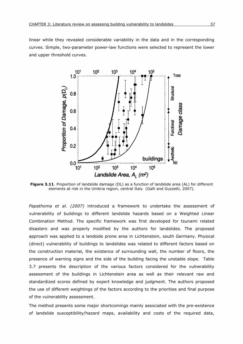
CHAPTER 3: Literature review on assessing building vulnerability to landslides 57
linear while they revealed considerable variability in the data and in the corresponding
curves. Simple, two-parameter power-law functions were selected to represent the lower
and upper threshold curves.
Figure 3.11. Proportion of landslide damage (DL) as a function of landslide area (AL) for different
elements at risk in the Umbria region, central Italy (Galli and Guzzetti, 2007).
Papathoma et al. (2007) introduced a framework to undertake the assessment of
vulnerability of buildings to different landslide hazards based on a Weighted Linear
Combination Method. The specific framework was first developed for tsunami related
disasters and was properly modified by the authors for landslides. The proposed
approach was applied to a landside prone area in Lichtenstein, south Germany. Physical
(direct) vulnerability of buildings to landslides was related to different factors based on
the construction material, the existence of surrounding wall, the number of floors, the
presence of warning signs and the side of the building facing the unstable slope. Table
3.7 presents the description of the various factors considered for the vulnerability
assessment of the buildings in Lichtenstein area as well as their relevant raw and
standardized scores defined by expert knowledge and judgment. The authors proposed
the use of different weightings of the factors according to the priorities and final purpose
of the vulnerability assessment.
The method presents some major shortcomings mainly associated with the pre-existence
of landslide susceptibility/hazard maps, availability and costs of the required data,

58 Seismic Vulnerability of Reinforced Concrete Buildings in Sliding Slopes
weighting of the factors, inclusion of landslide related phenomena etc. The results are
highly sensitive to the weighting of the parameters introducing considerable uncertainties
owning to the subjective manner to which these are assigned. A non-linear regression
sensitivity analysis to determine which attribute influences more the overall vulnerability
of the building is proposed by the authors as a potential future improvement of their
study. Recently, Mousavi et al. (2011) also applied this framework to assess the
vulnerability of buildings exposed to earthquake induced landslides in Emamzadeh Ali
area, Iran by carrying out a detailed investigation of each building in the affected zone.
Table 3.7. Data and their relevant raw and standardized scores (after Papathoma et al., 2007)
Field Description of field Description categories Raw score (code)
Standardised score
Material Material of which the building is made
Concrete 1 0.33
Masonry 2 0.66
Other (poor material such as wood and stone) 3 1
Surround Surrounding walls or
protection especially on the side of the slope
Strong high wall 1 0.33
Medium wall 2 0.66
No/low surrounding wall 3 1
Floors
More than one 1 0.5
One floor 2 1
Warning Presence of warning signs of landslides
Yes 1 0.5
No 2 1
Slope side
Description of the side of the building facing
the slope
Only wall 1 0.33
Small windows 2 0.66
Large windows 3 1
Zêzere et al. (2008) estimated the vulnerability of buildings in a small test site in the
area north of Lisbon (Portugal) under different landslide hazards based on empirical or
historic data, in conjunction with available data on buildings concerning age (state of
maintenance), construction material and function. Vulnerability values (0-1) for the
various building typologies were derived with respect to the different types of landslide
processes (shallow translational slides, translational slides, rotational slides) and
considering their estimated cost of reconstruction (Table 3.8).

CHAPTER 3: Literature review on assessing building vulnerability to landslides 59
Table 3.8. Building value and vulnerability considering exposure to different landslide types within the Fanhões-Trancão test site (Zêzere et al., 2008)
Building type
Value € Vulnerability
m2 Pixel Shallow
translational slides
Translational slides
Rotational slides
Poor traditional masonry buildings 600 15,000 0.5 1 1
Poor adobe stone or taipa buildings 600 15,000 0.5 1 1
Poor other resistant elements (wood, metallic) buildings 600 15,000 0.4 1 1
Usual traditional masonry buildings 1197 29,925 0.5 1 1
Usual reinforced concrete buildings 1197 29,925 0.3 1 1
Luxurious reinforced concrete buildings 2186 54,650 0.3 1 1
Heritage traditional masonry 2217 55,425 0.5 1 1
Remondo et al. (2008) performed a detailed inventory of exposed buildings to the study
area of Bajo Deba in northern Spain to quantitatively assess landslide vulnerability and
risk implemented in a GIS platform. Vulnerability values (0–1) for a given landslide
magnitude scenario were obtained by comparing damages experienced in the past (last
50 years) by each type of building with its actual momentary value. The derived
vulnerability values express the degree of potential monetary loss with respect to the
total value of the element.
Uzielli et al. (2008) developed a method for scenario-based, quantitative estimation of
physical vulnerability of structures to landslides based on expert judgment and empirical
data. Vulnerability is defined quantitatively as a product of the landslide intensity I and
the susceptibility S of vulnerable elements using the following simple relationship:
V= I x S (3.3)
Within their framework, susceptibility of a structure quantifies its capacity to withstand
the landslide action. It was related to two different factors depending on the structure's
typological features and its state of maintenance through an analytical expression. Values
of the partial susceptibility factor for structural type ξSTY were subjectively assigned for
six categories of structures based on the work of Heinimann (1999) (Table 3.9). The
susceptibility factor for state of maintenance ξSMN was expressed as the reduced capacity
of structures in comparison with the “very good” category in which maximum capacity is
expected. The authors proposed indicative values that are given in Table 3.10.

60 Seismic Vulnerability of Reinforced Concrete Buildings in Sliding Slopes
Table 3.9. Values of susceptibility factor for structural typology (Uzielli et al., 2008)
Structural typology Resistance ξSTY
Lightest, simple structures None 1.00 Light structures Very low 0.90 Rock masonry, concrete and timber Low 0.70 Brick masonry, concrete structures Medium 0.50 Reinforced concrete structures High 0.30 Reinforced structures Very high 0.10
Table 3.10. Values of susceptibility factor for state of maintenance (Uzielli et al., 2008)
State of maintenance ξSMN Very poor 0.50 Poor 0.40 Medium 0.25 Good 0.10 Very good 0.00
The landslide intensity was defined accounting for both kinetic (e.g. kinetic energy of the
sliding mass) and kinematic (e.g. displacement) characteristics of the interaction
between the sliding mass and the reference area. The proposed general model for the
intensity of a landslide acting on the element at risk was specified as:
I= kS · [rK· IK+ rM· IM] (3.4)
Where kS = Ai/At (3.5)
kS is the spatial impact ratio; Ai is the area pertaining to the category that is affected by
the landslide; At is the total area pertaining to the category; rK is the kinetic relevance
factor of the category; rM is the kinematic relevance factor of the category; IK is the
kinetic intensity parameter of the category; and IM is the kinematic intensity parameter
of the category. Relevance factors were assumed to be dependent on the characteristics
of the particular landslide event and the expected induced damage to the exposed
element. In any case, they need to comply with the constraint: rK+ rM=1.
The authors acknowledged that the damage caused by a slow moving landslide on a
building is mainly due to the displacement (i.e. kinematic parameter), while kinetic
characteristics could be predominant in case of a rapid movement. In Table 3.11
proposed possible combinations of values for kinetic and kinematic relevance factors are
given for structures for different landslide types (rapid, slow). Figure 3.12 presents the
suggested kinetic and kinematic intensity models for structures (in which C is the velocity
in mm/s of the sliding mass at impact, DG is the absolute displacement in mm of the

CHAPTER 3: Literature review on assessing building vulnerability to landslides 61
ground and DG,t is a threshold value of DG above which complete structural damage or
loss of functionality may be supposed).
Table 3.11. Possible sets of values for kinetic and kinematic relevance factors for structures (Uzielli et al., 2008)
Landslide type rK rM
Rapid 0.90 0.10 Slow 0.15 0.85
Figure 3.12. Kinetic and kinematic intensity models (Uzielli et al., 2008)
The method allows explicit consideration of the uncertainties in the parameters and
models. However, due to its expert-based nature, critical judgment and objective data
should accompany its application. Kaynia et al. (2008) explored the applicability of this
methodology based on the First-Order Second-Moment (FOSM) approach to estimate
landslide risks to the village of Lichtenstein- Unterhausen in Germany. They
acknowledged that the methodology could be improved by inserting more accurate and
precise models and objective data without requiring modification of its general
probabilistic framework.
Li et al. (2010) based on the work of Uzielli et al. (2008) and Kaynia et al. (2008)
suggested a new quantitative model for vulnerability of buildings based on landslide
intensity I and resistance ability R of the structure to withstand the landslide impact.
The proposed model reads:
2
2
2
2
I I2 0.5R R
2 R I IV f(I, R) = 1.0 0.5< 1.0R R
I1.0 1.0R
(3.6)
Figure 3.13 shows the proposed theoretical changing trend of vulnerability as a function
of intensity / resistance (a) and intensity for different resistance values (b).

62 Seismic Vulnerability of Reinforced Concrete Buildings in Sliding Slopes
Figure 3.13. Theoretical changing trend of Vulnerability with Intensity/Resistance (a) and
Intensity (b) (Li et al., 2010)
Landslide intensity was defined as a function of dynamic and geometric intensity factors
depending on the relative location of the structure to the landslide area:
dyn dpt
dyn dfm
I I For structures outside landslide area I =
I I For structures within landslide area (3.7)
where Idyn is the dynamic intensity factor, Idpt is the debris-depth factor (used to evaluate
the elements outside rapid landslide area), and Idfm is the deformation factor (mainly
used to evaluate the structures within the sliding mass of a slow landslide).
The dynamic intensity factor was related to the velocity of the sliding mass. For
stationery elements (e.g. structures) the following expression was proposed:
7
2dyn s 710
0.00 C 5 x10 (mm/s)I = 1 log C 6.30 C 5 x10 (mm/s)
36 (3.8)
The debris-depth factor was estimated in proportion to the debris depth (in meters) at
the location of a building. The later was also correlated to the foundation depth of the
structure based on a previous work (Ragozin and Tikhvinsky, 2000) to allow them to
assign tentative vulnerability values at different foundation depths (see Table 3.12). The
deformation factor for structures is defined as the ratio of DS/DS,T, where DS is the
displacement index of foundation or structure and DS,T is a threshold value of DS above
which complete structural damage or loss of functionality may be expected.
The resistance of the building was related to four different factors, namely the foundation
depth ξsfd, structure type ξsty, maintenance state ξsmn, and height ξsht through the
following expression:
1/4
str sfd sty smn shtR ξ ξ ξ ξ (3.9)

CHAPTER 3: Literature review on assessing building vulnerability to landslides 63
Table 3.12. Proposed tentative vulnerabilities at different foundation depths (Li et al., 2010)
Depth of foundation
(including piles), m
Landslide debris
depth, m Vulnerability
≤2 <2 1.0
>2 <2 0 0.0
Less than a landslide depth 2–10 1.0
10–13 2–10 0.5–1.0
>13 2–10 0.0–0.5
Any >10 1.0
The author recommended values for the last three factors that range from 0.1 (very low
resistance) to 1.5 (very high resistance) whereas they proposed a continuous function
with a minimum of 0.05 and without upper limit for the resistance factor of foundation
depth. Beyond a certain depth, an increase in the foundation depth yielded a marginal
influence on the resistance.
As the previously discussed method proposed by Uzielli et al. (2008), the main limitation
of this method lies again on its expert- based and therefore subjective origin. However,
this approach is generally improved compared to the previous one owning to the
introduction of more refined models and factors concerning both the characterization of
the landslide intensity and the resistance of the structures.
Das et al. (2011) developed a methodology for stochastic landslide vulnerability modeling
and applied it in a region of northern Himalaya, India. A logistic regression method was
adopted for calculating building vulnerability to landslides. This incorporates the
occurrence of landslides as a discrete and dichotomous response variable, and the
locations of the buildings as explanatory variables to generate a conceptually rational
function. The proposed logistic regression model applied to landslide vulnerability of the
buildings was modeled as:
b(i) 1 b(i) 0Pr [V (s)] 1 / (1 exp(α (E (s) α ) (3.10)
where Vb(i)(s) is the spatial vulnerability of the buildings, Eb(i)(s) the maximum unit cost
of the building and coefficients α0 and α1 the intercept and coefficient of a Logit function
obtained from the analysis of damage data from the study area. Equation (3.10)
represents a sigmoid curve and assumes that the property accumulation fits a Logit
curve. Historical records of damage information of buildings were assessed while
generating the vulnerability conditions. Vb(i)(s) values were assessed on the basis of
expected loss considering the maximum building cost for a complete damage condition.

64 Seismic Vulnerability of Reinforced Concrete Buildings in Sliding Slopes
Obtained Pr [Vb(i)(s)] values were then used to generate the building vulnerability map
(Fig. 3.14).
Figure 3.14. Building vulnerability map in a region of northern Himalaya, India (Das et al., 2011)
The authors claim that the proposed stochastic vulnerability framework may form the
basis for a quantitative landslide risk assessment study. However, although the model
offers a comprehensive modeling of uncertainties, a robust building vulnerability
assessment still remains a challenge principally due to the randomness, complexities and
site specific nature of the landslide processes and the particular characteristics of the
vulnerable structures (e.g. typology, age, height, use etc.).
An interesting approach for the quantification of building vulnerability to landslides is
made by Negulescu and Foerster (2010). The authors proposed an analytical
methodology to estimate the vulnerability of RC buildings to differential settlements due
to different landslide hazards. To this aim, a series of 2-dimensional non-linear static
time-history parametric analyses of a reference single bay- single storey structure were
performed in order to identify one or several response parameters (foundation type e.g.
different links, cross-section geometry, reinforcement degree, displacement magnitudes
and displacement inclination angles) that govern the structural behavior when subjected
to differential settlements. The input to the building model was a displacement load
increasing linearly up to a certain value imposed quasi-statically at one of its supports to
simulate the differential displacement demand of the structure impact by a landslide. The
results of the parametric studies revealed that the parameters mostly affecting the
behavior of the frame elements are the displacement magnitude and inclination angle

CHAPTER 3: Literature review on assessing building vulnerability to landslides 65
both related to the landslide deformation demand. Structural damage levels were defined
as a function of the local strain limits of steel and concrete constitutive models.
Preliminary fragility curves were constructed as a function of differential displacement for
an encasing RC frame building (Fig. 3.15).
They authors compare their curves with other empirical ones proposed in the literature
(HAZUS 2003; Zhang and Ng, 2005) and they found relatively good correlations.
However, one must note that the derived curves use a different intensity parameter (i.e.
the differential displacement) compared to the literature curves (HAZUS use the
permanent ground displacement while Zhang and Ng (2005) the absolute settlement at
the foundation level). Considering that, their direct comparison (as performed) involves a
great deal of uncertainty and should be made with caution.
The proposed approach, although is a crucial step in the estimation of landslide
vulnerability performed by means of straightforward analytical simulations, it focuses
solely on the analysis of the building response to assess the settlement induced damage
of buildings. Important factors such as the landslide type and mechanism, the triggering
mechanism, the soil –structure interaction, the relative location of the building to the
potential unstable slope and the corresponding uncertainties associated with them are
not considered in the analysis. The development of analytical fragility curves expressing
building vulnerability to different landslide hazards constitutes also a significant step in
landslide vulnerability research community. However, the use of differential displacement
as an intensity measure generally involves an even greater uncertainty than the
estimation of uniform or average movements (at the foundation level or the sliding
mass) as sufficient field data are often missing.
Figure 3.15. Fragility curves obtained for a one bay-one storey encasing RC frame building,
considering 4 damage limit states: Slight (LS1), Moderate (LS2), Extensive (LS3) and Complete (LS4) (Negulescu and Foerster, 2010)

66 Seismic Vulnerability of Reinforced Concrete Buildings in Sliding Slopes
HAZUS (NIBS 2004) multi-hazard loss estimation methodology is maybe the only
available practical tool to tackle the problem of estimating physical vulnerability of
buildings affected by earthquake triggered landslides. The building damage is estimated
through the use of simplified fragility curves that relate the permanent ground
displacement (PGD) to the probability of exceeding a certain damage state. Different
fragility curves that distinguish between ground failure due to lateral spreading and
ground failure due to ground settlement, and between shallow and deep foundations
were proposed considering one combined Extensive/Complete damage state.
Table 3.13. HAZUS Building Damage Relationship to PGD - Shallow Foundations
P[E or C| PGD] Settlement PGD (cm) Lateral Spread PGD
(cm)
0.10 5.10 30.50
0.5 (median) 25.40 152.40
Table 3.13 presents the HAZUS Building Damage Relationship to PGD for buildings with
shallow foundations (e.g., spread footings). Thus, lateral spread is judged to require
significantly more PGD to effect severe damage than ground settlement. According to
HAZUS methodology, median PGD values given in the table can be used with a lognormal
standard deviation value of βPGD = 1.2 to estimate P [E or C|PGD] for buildings on
shallow foundations or buildings of unknown foundation type.
The aforementioned methodology, which is exclusively based on expert judgment,
involves a high degree of subjectivity and simplification as it does not account various
landslide types and mechanisms, soil type, building typology, stiffness of the foundation
as well as different damage states.
3.3.2.1. Discussion
Table 3.14 summarizes all existing approaches for quantifying building vulnerability to
slides with respect to the methodological framework used (e.g. empirical, engineering
judgemental or analytical). It is seen that almost all methods are classified as empirical
or judgemental while some methods are included in both categories. This may be
attributed to the scarce and discrete historic damage data as well as to the great deal of
randomness, uncertainty and complexity associated with them. Only one purely
analytical model based on numerical simulations is found in the literature (Negulescu and
Foerster, 2010) that involves, however, as discussed previously some basic limitations. It
is noticed that even though some recently developed approaches provide analytical
relationships that allow for implementation within a probabilistic framework (e.g. Li et al.,

CHAPTER 3: Literature review on assessing building vulnerability to landslides 67
2010; Das et al., 2011), their origin is either empirical or heuristic and thus they cannot
be regarded as principally analytical methods.
Table 3.14. Existing methods to assess building vulnerability to slides in relation to the
methodological framework adopted
Methodology to assess vulnerability to slides
Empirical Judgmental/Heuristic Analytical
Galli and Guzzetti (2007) , Zêzere et al. (2008) , Remondo et al.
(2008), Uzielli et al. (2008), Li et al. (2010), Das et al. (2011)
Leone et al. (1996), Heinimann (1999), AGSO 2001, Papathoma et al. (2007), HAZUS (NIBS, 2004),
Uzielli et al. (2008), Li et al. (2010)
Negulescu and Foerster (2010)
Based on the above classification, it is recognized that there is a lack of analytical
methodologies to quantify physical vulnerability of structures to slides. This gap aspires
to bridge this thesis by proposing an analytical methodology for the quantification of the
vulnerability of buildings to relative slow moving slides at site specific/local scales
(Chapter 4). Analytical fragility curves are developed for various buildings typologies
interacting with different landslide materials and slope configurations (Chapter 6).

68 Seismic Vulnerability of Reinforced Concrete Buildings in Sliding Slopes

CHAPTER 4
Vulnerability assessment methodology
4.1 Introduction
In the present chapter an analytical procedure to assess the vulnerability of RC
structures due to earthquake induced landslide displacements is proposed. Part of this
research has recently been published in Landslides scientific journal (Fotopoulou and
Pitilakis, 2012). Vulnerability is described in terms of probabilistic fragility curves, which
describe the probability (Pi) of exceeding each limit state (LSi) of a specific element at
risk (i.e. RC building), on a given slope, versus the given landslide intensity measure,
allowing for the quantification of various sources of uncertainty.
In the following sections, the proposed methodological framework is described with a
simplified case study. In terms of numerical computations, a two-step uncoupled
analysis is performed. In the first step, the deformation demand, i.e. total and differential
displacements considering the actual weight and stiffness of the building and its
foundation, due to the landslide hazard is assessed using an adequate non-linear finite
difference dynamic slope model. In the second step, the building response to the
statically imposed landslide differential displacement is estimated using a Finite Element
code. Modeling issues concerning both analysis steps are described in detail. Finally, two
different analytical procedures to develop fragility functions are presented and applied to
quantitatively evaluate the structural vulnerability in landslide risk analysis of specific RC
building typologies and soil conditions.
4.2 Conception and description of the method
The proposed methodology, largely inspired from earthquake risk analysis, is applicable
for the vulnerability assessment of low-rise RC frame buildings impacted by seismically
induced relative slow moving earth slides. It is based on a comprehensive set of
numerical computations and adequate statistical analysis. In terms of numerical
simulation, a two-step uncoupled analysis is conducted. In the first step, a nonlinear Soil-

70 Seismic Vulnerability of Reinforced Concrete Buildings in Sliding Slopes
Foundation-Interaction analysis is performed using FLAC2D (Itasca, 2008) finite
difference code. Slope dynamic models are subjected to several properly selected ground
motions at their base to estimate the differential permanent displacements at the
building’s foundation level. Soil properties are adequately selected to consider modulus
degradation with shear strains, initial shear stresses and other parameters involved in
the dynamic analysis (Ishihara, 1996; Pitilakis, 2010). Then, the building’s response for
different statically applied ground/foundation differential displacements induced by the
different earthquake time histories with progressively increasing intensities is assessed.
To this aim, the previously computed differential displacements are directly applied as
input quasi-static loads to an appropriate building nonlinear model at the foundation
level. The numerical non-linear static analysis of the building is performed through the
Finite Element code SeismoStruct (Seismosoft, SeismoStruct 2011). It is worth noticing
that the complex issue of combined damages on the building by ground shaking and
ground failure due to landslide is not taken into account in the evaluation of the
building‘s vulnerability, which is assessed only for the effect of the permanent co-seismic
displacement. In other words, it is supposed that the building is properly designed to
resist even severe ground shaking following modern seismic codes and consequently no
initial damage to the building’s structural members (e.g. in terms of stiffness and
strength degradation) is assumed to occur due to ground shaking.
Appropriate limit states are defined in terms of threshold values of building’s material
strain, based on engineering judgment and the associated work of Crowley et al. (2004),
Bird et al. (2005) and Negulescu and Foerster (2010). Different limit strains are adopted
for “low” and “high” code designed structures.
The fragility curves are estimated in terms of peak ground acceleration (PGA) recorded
on rock outcrop or permanent ground displacement (PGD) at the slope area versus the
probability of exceedance of each limit state. The selection of the most appropriate
landslide intensity measure is generally recommended to be made with consideration of
its predictability, efficiency and sufficiency (Kramer, 2011) (see Chapter 3, § 3.2.1). It is
noticed, however, that when the rock outcropping PGA is used as an intensity parameter
the local soil conditions, surface geology, soil and topographic amplification are directly
included in the fragility analysis. Its use is consistent with the modern seismic hazard
assessment methods applied in the most recent approaches (see SHARE,
http://www.share-eu.org/ and OpenQuake, http://openquake.org/). On the other hand,
PGD that is obtained from the response of the landslide to ground shaking is better
correlated to structural deformation and damage. In addition, its use as an intensity
parameter may allow for direct application to non-earthquake related landslide hazards.
Other parameters such as the maximum differential permanent displacement at the

CHAPTER 4: Vulnerability assessment methodology 71
foundation level could potentially be used as measures of the landslide intensity.
However, their accurate estimation generally involves a higher degree of uncertainty.
Thus, their use is justified for site-specific applications on critical structures where
adequate data from field measurements and/or detailed numerical analysis are available.
Figure 4.1. Flowchart for the proposed framework of fragility analysis of RC buildings
Figure 4.1 illustrates the framework of the method. The “capacity” of each building is
defined by the building classification (foundation and superstructure type, and geometry,
material strength), while the “demand” is described in terms of induced permanent
ground deformation (slow moving slide) depending on the landslide type, soil conditions
and the relative location of the building to the potential unstable slope. It is noted that
the soil-foundation relative stiffness may also control in a certain degree the deformation
demand for the building (e.g. for the case of a stiff foundation resting on soft soil
material). Thus, the soil-foundation compliance and the geometric constraints imposed
by the rigidity of the foundation system, as well as its potential slippage and/or
detachment with respect to the underlying soil, may alter the free-field displacement
pattern, modifying the deformation demand for the structure. These two components i.e.
building capacity, deformation demand, can be considered as inputs to the simulation
engine, which is the third major component, providing the methodology for structural
assessment. Structural response data obtained by analyzing the building capacity under
the deformation demand is processed to generate fragility curves. Limit states, which are
determined with respect to the building classification and structural characteristics,
selected empirical criteria and expert judgment, are required at this step. The final step
is the construction of the analytical fragility relationships. Similar flowcharts may be

72 Seismic Vulnerability of Reinforced Concrete Buildings in Sliding Slopes
defined for other triggering mechanisms (intense rainfall, erosion etc.). It is also possible
to construct synthetic flowcharts combining different triggering mechanisms. Further
discussion on the conceptual features of the proposed methodological framework is
highlighted in the following paragraphs. It is noted that some of these features have
already been thoroughly discussed in previous chapters but they are shortly repeated
herein to provide a link with the proposed approach.
The landslide type (rock fall, debris flow, earth slide, etc) is a crucial parameter of the
proposed methodology as landslides of different types and sizes usually require different
and complementary methods to estimate vulnerability. While most devastating damages
to the built environment are probably resulting from the occurrence of rapid landslides
such as debris flows and rock falls, slow-moving slides also have adverse effects to
buildings and lifelines and critical facilities (Mansour et al., 2011; Argyroudis et al.,
2011). The damage caused by a slow moving slide on a single building is mainly
attributed to the cumulative permanent (absolute or differential) displacement and it is
concentrated within the unstable area (see Chapter 3, §3.2.2). A relative slow moving
earth slide that will produce tension cracks due to differential displacement to a RC
building, exposed to the landslide hazard, is considered in this study. Note, however, that
the time scale related to non-earthquake and earthquake induced slow moving slides
studied in this research is different. In particular, the landslide processes associated with
earthquake triggering mechanisms are naturally more rapid as they involve seismic cyclic
loading that may usually last from several seconds to few minutes. Yet, they are
classified herein as “relative slow moving slides” to differentiate them from the
earthquake induced landslides that involve the complete failure of the slope and
displacements of tens of meters.
The characteristics of the earthquake ground motion in terms of amplitude, frequency
content and duration, in relation to the soil dynamic properties and stratigraphy, can
significantly affect the deformation demand for the building. Soil nonlinearity, material
damping, impedance contrast between sediments and underlying bedrock and the
characteristics of incident wavefield are the main governing factors for site
amplification/attenuation (Kramer and Stewart, 2004; Pitilakis, 2010). The slope failure
potential assumes its highest values for a combination of a low-frequency seismic input
motion with a resonance phenomenon in the low-frequency range (Bourdeau et al.,
2004). In general, a fundamental period of the input earthquake close to the natural
period of the site can lead to resonance phenomena and, consequently, to an amplified
energy content of the ground motion (see also Chapter 2, §2.2.2.3 for detailed
description).
CHAPTER 4: Vulnerability assessment methodology 73
The position of the building with respect to the landslide area is also a very important
contributing factor. Topographic effects may alter the amplitude and frequency content of
the ground motions along slopes (Bouckovalas and Papadimitriou, 2005; Ktenidou, 2010)
(see Chapter 2, §2.2.2.3 for details). Moreover, the effect of soil-structure interaction
due to the presence of a structure at a cliff can further modify the seismic response at
the topographic irregularity with respect to the free-field case (i.e. in the absence of any
structure), depending on the soil-structure impedance contrast, the geometry of the
slope and the dynamic characteristics of the building itself (Assimaki and Kausel, 2007;
D. Pitilakis and Tsinaris, 2010). In the current study, RC buildings of different stiffness
characteristics standing near the slope’s crest, where the seismic ground motion due to
topographic effects is generally amplified, are explicitly considered in the analysis.
For a given landslide mechanism and hazard intensity, the typology of the exposed
structure is also a key factor. A building’s geometry and number of floors, material
properties, state of maintenance, code design level, soil conditions and mainly the
foundation and structure details are the critical parameters which determine the capacity
of the building to withstand co-seismic landslide displacements. The response to
permanent total and differential ground deformation depends primarily on the foundation
type (see also Chapter 3, § 3.3.2). A structure on a deep foundation (e.g. piles)
compared to shallow foundations is more resilient and often experiences higher
resistance ability and hence a lower vulnerability. For shallow foundations, a rigid
foundation, i.e. continuous raft foundation is less vulnerable than a flexible one, i.e.
isolated footings. The soil-foundation relative stiffness is also a dominant parameter.
When the foundation system is rigid the building is expected to rotate as a rigid body and
the anticipated damages or failure is mainly attributed to loss of functionality. In this
case, the damage states are defined empirically, as there is limited structural demand to
the members of the building (apart from possible P-∆ effects at larger rotations). On the
contrary, when the foundation system is flexible enough allowing differential movement
of the walls or columns (e.g. isolated footings), the various modes of differential
deformation produce structural damage (e.g. cracks) to the building members (Bird et
al., 2005; 2006).
To derive the vulnerability of a building exposed to seismically induced slow-moving
slides, an analytical procedure analogous to that of the response due to seismic
oscillation is proposed. When building response to ground failure and permanent ground
deformations comprises structural damage, damage states can be classified using the
same schemes used for structural damage caused by ground shaking. Limit states could
be defined in terms of limit value of a component’s strain based on damage observation
from previous earthquake events, the existing knowledge related to earthquake damage

74 Seismic Vulnerability of Reinforced Concrete Buildings in Sliding Slopes
levels, and published tolerances for non-earthquake related foundation deformations
(Crowley et al., 2004; Bird et al., 2005). Different limit strains are assigned based on the
construction quality of the building and code adopted in the design.
In the probabilistic approach proposed herein, several uncertainties are involved with
respect to the capacity of the building, the definition of the limit states and the
deformation demand (differential permanent displacement). The uncertainty in the
permanent displacement capacity is a function of the material properties, geometric
characteristics, and the yield strain of steel and post-yield strain capacities of the steel
bars and concrete. The uncertainty in the demand is associated with the ground motion
estimation and additional uncertainties associated with the landslide type and size, the
relative position of the building in the landslide area, the variability in soil parameters in
space and time during the loading, the stratigraphy and the epistemic uncertainties
associated with the assessment of ground deformations.
4.3 Layout- Numerical example
4.3.1 Dynamic analysis of the slope
The conceptual features of the methodology outlined in the previous section are
described in detail through an idealized, yet realistic, example. The deformation demand
in terms of permanent seismic displacements can be estimated either empirically (e.g.
Newmark type methods) or numerically. The numerical approach applied herein is
selected for two reasons: (a) it is more accurate than any empirical method and (b) it
permits the direct estimation of the differential ground/foundation displacements, which
are the main cause of damage. For completeness reasons, the computed total
permanent displacements for specific slope configurations, material properties and
seismic inputs are compared with different Newmark-type displacement approaches in
Chapter 5, §5.2.3.
4.3.1.1. Numerical model
In order to evaluate the permanent differential ground/foundation displacements
(deformation demand) for the building on a given slope, the dynamic non-linear analyses
are performed using the two dimensional (2D) finite difference code FLAC 6.0 (Itasca,
2008). The 2D dynamic calculation is based on the explicit finite difference scheme to
solve the full equations of motion, using lumped gridpoint masses derived from the real
density of surrounding zones. FLAC2D (Fast Lagrangian Analysis of Continua) has been
widely used by many investigators to study the non-linear dynamic response of slopes

CHAPTER 4: Vulnerability assessment methodology 75
and embankments in plane strain conditions (e.g. Bourdeau et al., 2004; Chugh and
Stark, 2006; Bozzano et al., 2008b; Barani et al., 2010; Fotopoulou et al., 2011; Lenti
and Martino, 2012 etc.) due to its efficiency in modeling nonlinearity, large-strain
problems and physical instability.
Figure 4.2. (a) Slope and foundation configuration used for the numerical modeling (b) and FLAC
2D dynamic model
A schematic representation of the reference finite slope geometrical and geological
features and the corresponding 2D dynamic slope model used to study the irreversible
deformation demand for the building located near its crest is illustrated in Figures 4.2 a
and b respectively. The model has a total length of 300m and width of 100 m, while the
slope height and inclination are 20m and 30o respectively. It contains approximately 9000
four-node quadrilateral elements of various sizes determined by the shear wave
velocities of the medium and the frequency content of the incident motions. Kuhlemeyer
and Lysmer (1973) showed that for accurate representation of wave transmission
through a model, the element size must be smaller than approximately one-tenth to one-
eighth of the wavelength associated with the highest frequency component of the input
(b) A B
(a)

76 Seismic Vulnerability of Reinforced Concrete Buildings in Sliding Slopes
wave. In the present study, the discretization allows for a maximum frequency of at least
10Hz to propagate through the grid without distortion. A finer discretization is adopted in
the slope area, whereas towards the lateral boundaries of the model the mesh is coarser.
The soil materials are modeled using an elastoplastic constitutive model with the Mohr-
Coulomb failure criterion (shear yield) with tension cutoff (tension yield function),
assuming a zero dilatancy non-associated flow rule for shear failure and an associated
rule for tension failure. The use of such simple model within the framework of this study
is justifiable as it allows more clearly identifying the basic parameters that influence the
estimation of the differential displacement demand for the building. Besides, it serves as
a useful reference against which more complex soil behavior may be compared. Soil
strength properties are properly selected to account for the dynamic ground response.
The influence of the initial shear stress in the strength values is directly taken into
account. It is noticed that the sliding surface is not pre‐defined but “emerges” naturally,
following the elastoplastic constitutive law. Two different soil types are selected for the
surface deposits to represent homogenous dry, purely frictional and cohesive materials
corresponding to soil category C of EC8 (CEN-European Committee for Standardization
2003). A stiffer clayey layer (Vs=500 m/sec) is assumed to underlie the surface deposits.
The elastic bedrock (Vs=850 m/sec) lies at 70 m. The mechanical characteristics for the
soil materials and elastic bedrock are presented in Table 4.1.
Table 4.1. Soil properties of the analyzed slopes
Relatively stiff soil
Stiff soil Elastic bedrock sand clay
Dry density (kg/m3) 1800 1800 2000 2300
Young's modulus (KPa) 2.93E+05 2.93E+05 1.30E+06 4.32E+06
Poisson's ratio 0.3 0.3 0.3 0.3
Drained Bulk modulus K (KPa) 2.44E+05 2.44E+05 1.08E+06 3.60E+06
Shear modulus G (KPa) 1.13E+05 1.13E+05 5.00E+05 1.66E+06
Cohesion c (KPa) 0 10 50 -
Friction angle φ (degrees) 36 25.0 27 -
Dilation angle (degrees) 0 0 0 0
P-wave velocity Vp (m/sec) 468 468 935 1590
Shear wave velocity Vs (m/sec) 250 250 500 850
The static factor of safety of the slope is calculated through a limit equilibrium approach
using the Spencer‘s method (Spencer, 1967) as Fs=1.45 for the sand and Fs =1.38 for
the cohesive soil material. The critical failure surfaces during seismic loading cover a

CHAPTER 4: Vulnerability assessment methodology 77
wide range from shallow in the case of surface sand deposits to relatively deep for the
surface clayey materials.
Rayleigh type damping is used in conjunction to the stress-strain constitutive model for
an approximate representation of cyclic energy dissipation. A damping matrix, C, is
used, with components proportional to the mass (M) and stiffness (K) matrices:
C α M β K (4.1)
where
α = the mass-proportional damping constant; and
β = the stiffness-proportional damping constant.
Although Rayleigh damping involves two viscous elements in which the absorbed energy
is dependent on frequency, the frequency-dependent effects can be canceled out over a
restricted range of frequencies with the appropriate choice of parameters.
When irreversible strain accumulation takes place the energy dissipation is intended to be
captured through the yield model. However, while stiffness-proportional damping is
turned off when plastic failure occurs within a FLAC zone, mass proportional damping
remains active. Thus, if excessive failure occurs in a model, the mass proportional term
may inhibit yielding as rigid-body motions that occur during failure modes are
erroneously resisted (Itasca, 2008). In this study, a considerable amount of energy
dissipation is represented by the yield constitutive model considering that extensive
plastic deformation is expected to occur during ground shaking. In this way, the selection
of Rayleigh damping parameters is tend to be less critical to the outcome of the analysis.
Based on the above, a small amount of mass and stiffness -proportional Rayleigh
damping (1 to 3% for the soil materials and 0.5% for the elastic bedrock) is assigned to
account for the energy dissipation during the elastic part of the cyclic response. The
center frequency of the Rayleigh damping (fmin) is selected to lie between the natural
modes of the model, f1= 1.52 Hz and f2=5·f1=7.6 Hz based on common practice (e.g.
Kwok et al., 2007). This range includes the model’s natural frequencies (defined by the
downhill and uphill resonant frequencies respectively) and the predominant frequencies
of the input motions. Figure 4.3 presents the specification of critical damping ratio (for
ξmin=3%) and central (minimum) frequency adopted in this study.
Note that hysteretic damping is an alternative algorithm in FLAC to account for the non-
linear hysteretic soil behavior prior yielding. It is considered conceptually more realistic
as it is based on the implementation of fitted G-γ-D curves that yield different shear
stiffness and damping levels as a function of cyclic strain. However, its use was
abandoned after some preliminary trial investigation as it was found to be performed
outside its expected range of application, resulting to unrealistically high strain

78 Seismic Vulnerability of Reinforced Concrete Buildings in Sliding Slopes
accumulation and to numerical instability, for the large irreversible deformations
anticipated in the analyzed cases.
Figure 4.3. Specification of FLAC Rayleigh damping parameters for the present study (ξmin=3%,
fmin=3.1 Hz)
Free field absorbing boundaries (Cundall et al., 1980) are applied along the lateral
boundaries whereas quiet boundaries (Lysmer and Kuhlemeyer, 1969) are applied along
the bottom of the dynamic model to minimize the effect of artificially reflected waves
(see Fig. 4.2). Free field absorbing boundaries involve the execution of a one-dimensional
free-field calculation in parallel with the main-grid analysis. The coupling of the free-field
grid to the main grid is achieved by viscous dashpots. In this way, plane waves
propagating upward suffer (almost) no distortion at the boundary because the free-field
grid supplies conditions that are identical to those in an infinite model. Quiet (viscous)
boundaries consist of dashpots attached independently in the normal and shear
directions (Lysmer and Kuhlemeyer, 1969). In order to apply quiet boundary conditions
along the same boundary as the dynamic input, the seismic motions must be applied as
stress loads combining with the quiet (absorbing) boundary condition using the following
relationships:
n p n
s s s
σ 2 ρ C vσ 2 ρ C v
(4.2)
where σn and σs are the applied normal and shear stresses, respectively, ρ is the material
density, CP and CS are the P- and S-wave velocities, respectively, and vn and vs are the
input normal and shear particle velocities. The factor of two in Eqs. 4.1 accounts for the
fact that the amplitude of the applied stress waves must be doubled to keep into account
that half the input energy is absorbed by the viscous boundary.

CHAPTER 4: Vulnerability assessment methodology 79
A RC building is assumed to be located 3m away from the slope crest. Two different
shallow foundation systems are considered (Tab. 4.2): isolated footings and a uniform
loaded continuous slab foundation. In the first case, the foundation is simulated with
concentrated loads at the footings’ links. As a consequence, no relative slip and/or
separation between foundation and subsoil are allowed. In the second case, the
foundation system is modeled as a deformable elastic beam connected to the soil
elements’ grid through appropriate interface elements that can approximate the potential
Coulomb sliding and/or tensile separation of the beam. The relative interface movement
is controlled by interface stiffness values in the normal (kn) and tangential directions (ks)
as well as the maximum interface shear resistance between the soil and the foundation.
The interface properties adopted for the present study are presented in Table 4.3. A first
series of analyses is also conducted for the free-field case, i.e. in the absence of any
structure, to assess the influence of Soil-Foundation Interaction in altering the seismic
slope response in the vicinity of the crest.
Table 4.2. Foundation properties
Properties Foundation system
Stiff foundation Flexible foundation
Element beam Width (m) 6
Density (KN/m3) 25 Young's modulus (KPa) 2.90·107 Moment of inertia I (m3) 0.0053
Area (A) (m2) 0.4
Load (KN/m) Uniform distributed q=25KN/m2 Concentrated P=50KN/m
Table 4.3. Interface properties
Properties Surface soil layer
Sand Clay
Normal stiffness kn (KN/m) 2·106 2·106
Shear stiffness ks (KN/m) 1·106 1·106 Cohesion c (KPa) 0.0 7.0
Friction angle φ (degrees) 24 17 Dilation angle (degrees) 0.0 0.0
4.3.1.2. Seismic loading
Prior to the dynamic simulations, a static analysis is carried out to establish the initial
effective stress field throughout the model. The dynamic input motion consists of SV
waves vertically propagating from the base. Seven different earthquake records are

80 Seismic Vulnerability of Reinforced Concrete Buildings in Sliding Slopes
used for the dynamic analyses (Tab. 4.4). They all refer to outcrop conditions as it is
normally proposed in modern seismic codes (i.e. EC8). No specific soil amplification
factors are applied, as this is explicitly taken into consideration through the numerical
analysis. The records are selected to cover a wide range of seismic motions in terms of
the seismotectonic environment, amplitude, frequency content and significant duration.
Figure 4.4 presents the normalized 5%-damped elastic response spectra of the input
motions together with the proposed elastic design spectrum of EC8 (CEN-European
Committee for Standardization 2003) for soil type A (rock).
Table 4.4. Selected outcropping records used for the dynamic analyses
Earthquake Record station Mw R (km) PGA (g) Valnerina, Italy 1979 Cascia 5.9 5.0 0.15 Parnitha, Athens 1999 Kypseli 6.0 10.0 0.12
Montenegro 1979 Hercegnovi Novi 6.9 60.0 0.26 Northridge, California 1994 Pacoima Dam 6.7 19.3 0.41
Campano Lucano, Italy 1980 Sturno 7.2 32.0 0.32 Duzce, Turkey 1999 Mudurno_000 7.2 33.8 0.12
Loma Prieta, California 1989 Gilroy1 6.9 28.6 0.44
Figure 4.4. Normalized average elastic response spectrum of the input motions in comparison with
the corresponding elastic design spectrum for soil type A (rock) according to EC8
Before applying the selected outcropping records (target motions) the appropriate
dynamic loading for the base of the FLAC model needs to be determined. Thus, the time
histories are first subjected to baseline correction and filtering to assure an accurate

CHAPTER 4: Vulnerability assessment methodology 81
representation of wave transmission through the model. In particular, a Butterworth
bandpass 4th order filter type in the frequency range from f1=0.25 Hz to f2=10 Hz and a
linear type baseline correction were applied to all records using Seismosignal computer
software (Seismosoft, Seismosignal 2011). Moreover, due to the compliant base used in
the model the appropriate input excitation corresponds to the upward propagating wave
train that is taken as one-half of the target outcrop motion (Mejia and Dawson, 2006).
Note that the acceleration time histories at the base are integrated to obtain velocities
which are then converted into stress histories using Eq. 4.2. The selected input time
histories are scaled to four levels of peak ground acceleration, namely PGA=0.3, 0.5, 0.7
and 0.9g. This is done in order to assess the building response for a range of ground
differential displacement and to allow the evaluation of fragility curves for different limit
damage states.
4.3.1.3. Results
Numerical computations are carried out in large-strain mode to ensure sufficient accuracy
considering that large deformations are expected to occur.
Figures 4.5 and 4.6 present representative graphs of the maximum absolute (point A in
Fig. 4.2b) and differential (A-B, Fig. 4.2b) horizontal and vertical permanent
displacement time histories at the closest edge of the assumed building from the slope’
crest (i.e. 3 m) considering stiff and flexible foundations for the building and at the same
location in the absence of any structure (free field conditions). A variety of such graphs is
given for both sand and clayey surface slope layers and for two different input motions
(cascia, pacoima) scaled at two PGA levels, namely 0.3 g and 0.7 g. Various trends are
revealed from these comparative plots. A first general observation is that the presence of
a structure next to the slope’s crest may contribute in altering the free field response of
the slope and the corresponding deformation demand for the building. The level of this
differentiation depends primary on the foundation type (flexible, stiff). The building on
flexible foundations seems to follow more closely the free field movement both in terms
of absolute and differential displacement. On the other hand, when the soil-foundation
interaction (building on stiff foundations) is considered, the differential horizontal
displacements at the beam foundation are practically zero and the total (vector)
differential displacement demand for the building is generally decreased due to the
continuity and stiffness of the foundation slab. The displacement patterns are also greatly
influenced by the surface soil conditions (sand, clay). As shown in the figures, for the
sand slope case the building founded on flexible foundations displays larger absolute and
differential displacements compared to the free field conditions and the corresponding
building on continuous stiff foundation. On the contrary, for the clayey slope case, while
the free field absolute movement is generally reduced, the corresponding differential
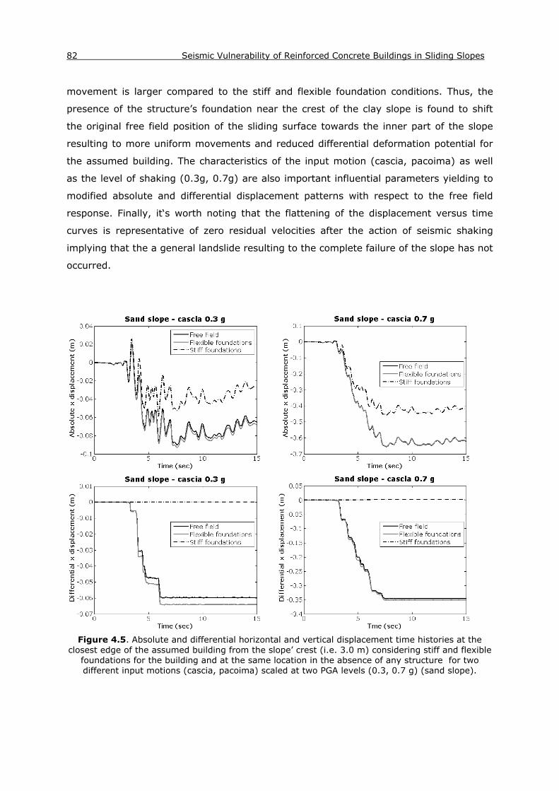
82 Seismic Vulnerability of Reinforced Concrete Buildings in Sliding Slopes
movement is larger compared to the stiff and flexible foundation conditions. Thus, the
presence of the structure’s foundation near the crest of the clay slope is found to shift
the original free field position of the sliding surface towards the inner part of the slope
resulting to more uniform movements and reduced differential deformation potential for
the assumed building. The characteristics of the input motion (cascia, pacoima) as well
as the level of shaking (0.3g, 0.7g) are also important influential parameters yielding to
modified absolute and differential displacement patterns with respect to the free field
response. Finally, it‘s worth noting that the flattening of the displacement versus time
curves is representative of zero residual velocities after the action of seismic shaking
implying that the a general landslide resulting to the complete failure of the slope has not
occurred.
Figure 4.5. Absolute and differential horizontal and vertical displacement time histories at the
closest edge of the assumed building from the slope’ crest (i.e. 3.0 m) considering stiff and flexible foundations for the building and at the same location in the absence of any structure for two different input motions (cascia, pacoima) scaled at two PGA levels (0.3, 0.7 g) (sand slope).

CHAPTER 4: Vulnerability assessment methodology 83
Figure 4.5. (Continued)- Absolute and differential horizontal and vertical displacement time
histories at the closest edge of the assumed building from the slope’ crest (i.e. 3.0 m) considering stiff and flexible foundations for the building and at the same location in the absence of any
structure for two different input motions (cascia, pacoima) scaled at two PGA levels (0.3, 0.7 g) (sand slope).

84 Seismic Vulnerability of Reinforced Concrete Buildings in Sliding Slopes
Figure 4.5. (Continued)- Absolute and differential horizontal and vertical displacement time
histories at the closest edge of the assumed building from the slope’ crest (i.e. 3.0 m) considering stiff and flexible foundations for the building and at the same location in the absence of any
structure for two different input motions (cascia, pacoima) scaled at two PGA levels (0.3, 0.7 g) (sand slope).
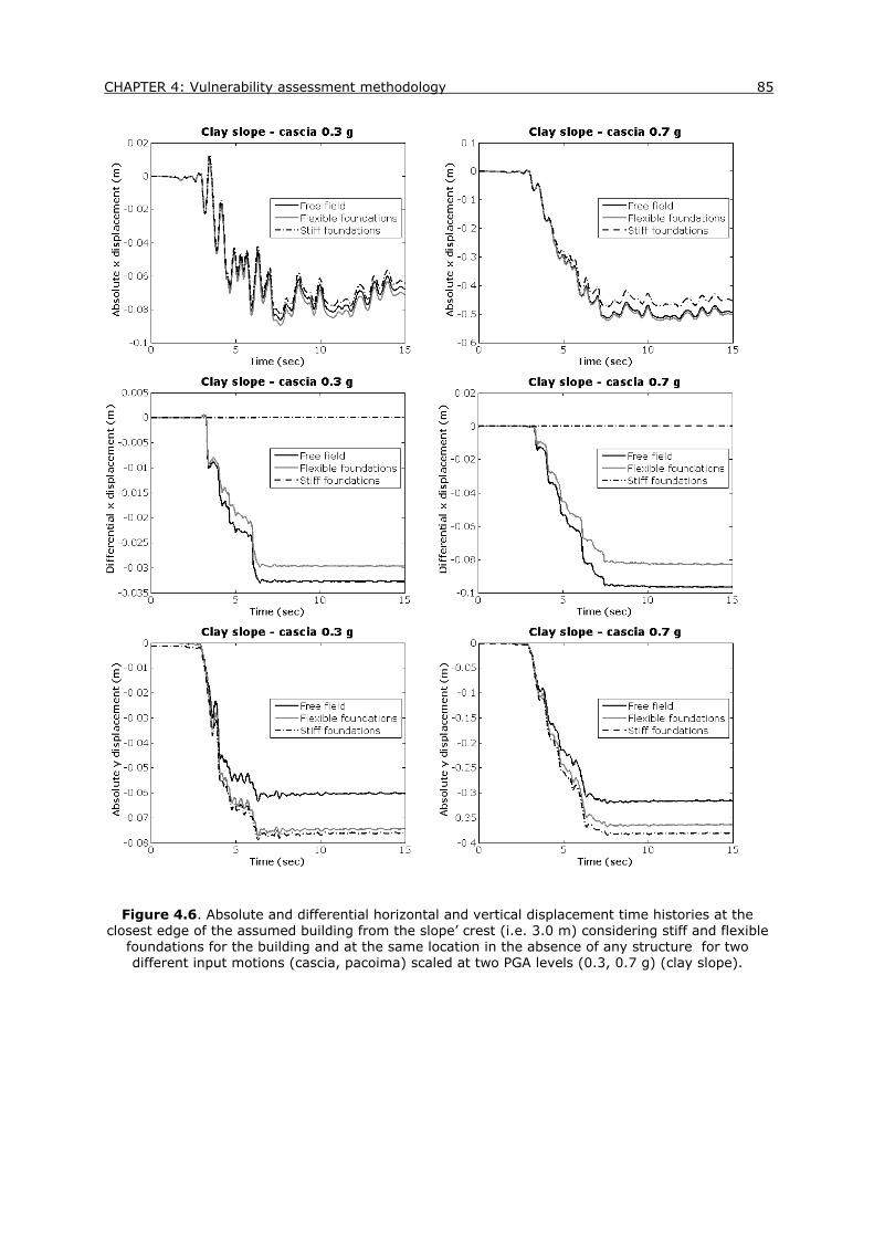
CHAPTER 4: Vulnerability assessment methodology 85
Figure 4.6. Absolute and differential horizontal and vertical displacement time histories at the
closest edge of the assumed building from the slope’ crest (i.e. 3.0 m) considering stiff and flexible foundations for the building and at the same location in the absence of any structure for two different input motions (cascia, pacoima) scaled at two PGA levels (0.3, 0.7 g) (clay slope).

86 Seismic Vulnerability of Reinforced Concrete Buildings in Sliding Slopes
Figure 4.6. (Continued)- Absolute and differential horizontal and vertical displacement time
histories at the closest edge of the assumed building from the slope’ crest (i.e. 3.0 m) considering stiff and flexible foundations for the building and at the same location in the absence of any
structure for two different input motions (cascia, pacoima) scaled at two PGA levels (0.3, 0.7 g) (clay slope).

CHAPTER 4: Vulnerability assessment methodology 87
Figure 4.6. (Continued)- Absolute and differential horizontal and vertical displacement time
histories at the closest edge of the assumed building from the slope’ crest (i.e. 3.0 m) considering stiff and flexible foundations for the building and at the same location in the absence of any
structure for two different input motions (cascia, pacoima) scaled at two PGA levels (0.3, 0.7 g) (clay slope).
Figures 4.7 and 4.8 present the maximum computed values of permanent ground
displacement at the slope area in relation to the corresponding differential displacements
at the foundation level for the different foundation configurations and soil types. A
strong, linear correlation between the two variables is detected in all cases. Thus,
differential deformation can be easily determined by the residual maximum slope
displacement using an appropriate linear expression. While the maximum calculated
slope displacements are found to be of the same order of magnitude for both sand and
clay slopes, the resulting differential displacement for the building is strongly reduced for
slopes consisting of cohesive soil material, implying that in that case the building is
primarily expected to move uniformly as a rigid body rather than to distort differentially.
Figures 4.9 and 4.10 depict the maximum values of differential displacements for the
building with flexible and stiff foundation system founded on sand and clay soil
respectively. It is observed that the specific characteristics (frequency content and
duration) of the seismic ground motions can significantly affect the magnitude of the

88 Seismic Vulnerability of Reinforced Concrete Buildings in Sliding Slopes
computed differential displacement at the foundation level. In particular, for all analyzed
cases, the maximum and minimum differential displacements are estimated when
applying the sturno and gilroy time histories respectively.
Figure 4.7. Regression of differential displacement vector for buildings with flexible (top) and stiff
(bottom) foundation system on the maximum computed permanent ground displacement (sand slope).

CHAPTER 4: Vulnerability assessment methodology 89
Figure 4.8. Regression of differential displacement vector for buildings with flexible (top) and stiff (bottom) foundation system on the maximum computed permanent ground displacement (clay
slope).

90 Seismic Vulnerability of Reinforced Concrete Buildings in Sliding Slopes
Figure 4.9. Maximum values of differential displacement vector for buildings with flexible (top)
and stiff (bottom) foundation system (sand slope).

CHAPTER 4: Vulnerability assessment methodology 91
Figure 4.10. Maximum values of differential displacement vector for buildings with flexible (top)
and stiff (bottom) foundation system (clay slope).

92 Seismic Vulnerability of Reinforced Concrete Buildings in Sliding Slopes
4.3.2 Non linear static analysis of the RC structures
The analysis of the building is conducted using the finite element code SeismoStruct
(Seismosoft, SeismoStruct 2011), which is capable of calculating the large displacements
of space frames under static or dynamic loading, taking into account geometric
nonlinearities and material inelasticity. The code is widely and successfully used in
structural earthquake engineering. Both local (beam-column effect) and global (large
displacements/rotations effects) sources of geometric nonlinearity are automatically
taken into account. Distributed elements are used based on the so-called “fibre
approach” to represent the cross-section inelastic behaviour, where each fibre is
associated with a uni-axial stress-strain relationship (see Fig. 4.11). The sectional stress-
strain state of beam-column elements is then obtained through the numerical integration
of the nonlinear uni-axial stress-strain response of the individual fibres (typically 300-
400) in which the section has been subdivided. In displacement-based (DB) finite
element formulation using nonlinear models, structural elements should be subdivided
into a number of segments (typically 4 to 5) and the delimiting sections follow the
Navier-Bernoulli approximation (plane sections remain plane). In the present analysis,
the frame sections have been discretized into 300 fibres and the structural members, into
4 elements. Nonlinear static time-history analyses are performed for all numerical
simulations. The differential permanent displacement curves, directly extracted from the
FLAC dynamic analysis, are statically imposed at one of the RC frame supports (see Fig.
4.12).
L/2 3 L/2
node B
node A
A
B
GaussSection a
GaussSection a
GaussSection b
RC Section Unconfined Concrete Fibres
Steel FibresConfined Concrete Fibres
Figure 4.11. Discretisation in fibre modelling of a typical reinforced concrete cross-section (Seismosoft, Seismostruct 2011)
The herein studied buildings are single bay-single storey RC bare frame structures with
two foundation types: flexible foundation system (isolated footings) and stiff but not

CHAPTER 4: Vulnerability assessment methodology 93
completely rigid foundation system (continuous uniformly loaded foundation of finite
stiffness characteristics) (Fig. 4.12). The beneficial contribution of masonry infill walls to
the building capacity is not considered in this study. The building’s height and length are
3.0 m and 6.0 m respectively. All columns and beams have rectangular cross sections
(beam: 0.30x 0.50 m, column: 0.40x 0.40m). The structures have been designed
according to the provisions of the Greek Seismic Code (EAK, 2000), for a design
acceleration Ad = 0.36 g, and a behavior factor q = 3.5. The adopted dead and live loads
(g = 1.3 kN/m2 and q = 2 kN/m2) are typical values for residential buildings. The
longitudinal section reinforcement degree used is 1% for the columns and 0.75% for the
beams.
The use of single bay-single storey structures is justified from the observation that the
number of storeys and bays do not seem to comprise crucial parameters in the
determination of the building’s performance subjected to permanent ground
displacements. The latter is also discussed in Bird et al. (2005) and Negulescu and
Foerster (2010) for the vulnerability assessment of RC buildings due to differential
settlements. Hence, one bay-one storey RC structures despite their simplicity are found
to be adequately representative of the performance of real low-rise RC frame buildings.
Figure 4.12. Single bay-single storey RC frame buildings with flexible (a) and stiff (b) foundation system and displacement loading pattern considered for the non-linear quasi-static analysis
The material properties assumed for the structural members of the reference RC
buildings are described below. A uni-axial nonlinear constant confinement model (Fig.
13a) is used for the concrete material (fc=20MPa, ft=2.1MPa, strain at peak stress
0.002mm/mm, confinement factor =1 for unconfined and 1.2 for confined concrete,
specific weight=24KN/m3), assuming a constant confining pressure throughout the entire
stress-strain range (Mander et al., 1988). For the reinforcement, a uni-axial bilinear
stress-strain model with kinematic strain hardening (Fig. 13b) is utilized (fy=400MPa,
E=200GPa, strain hardening parameter μ =0.005, specific weight=78KN/m3). This model
(b) (a) 3m
6m 6m
1 1’ 2 2’

94 Seismic Vulnerability of Reinforced Concrete Buildings in Sliding Slopes
is characterized by easily identifiable calibrating parameters and by its computational
efficiency. Note that only nonlinear models are suitable for the analysis since cracking
and irreversible deformation is expected to govern the behavior of the RC structural
members.
Figure 4.13. Stress-strain models for concrete (a) and steel (b) material
A sensitivity analysis is performed for the reference building cases, which allows for
indentifying the influence of different parameters on the structural response and to
develop a probabilistic framework for the damage estimation. The parameters selected to
vary are the following: yield strength of steel (fy=210, 400, 500 MPa), compressive
(fc=16, 20, 30 MPa) and tensile (ft=2.0, 2.1, 3.0 MPa) strength of concrete,
reinforcement ratio (ρ=0.8%, 1%, 1.2% for columns and ρ=0.55%, 0.75%, 0.95% for
beams) and confinement factor (1.0, 1.2, 1.3). The analyses are conducted for
progressively increasing levels of differential displacements provided by the computed
dynamic stress strain analysis for increasing amplitudes of input acceleration time
histories. For each analysis, the peak response of the structures in terms of maximum
strain is recorded. The yield strength of steel material is proved to be the most influential
factor for both buildings with stiff and flexible foundations resulting to an average
variation on the results of 25% for the stiff and 20% for the flexible foundations.
The deformed shapes of buildings with flexible foundation system are essentially the
same irrespective of the variability in the strength parameters and the level of the
displacement demand in terms of imposed differential ground/foundation deformations,
observation that is in accordance with Bird et al. (2005). The same trend is observed for
the buildings with stiff foundation (Fig. 4.14). In both building typologies, a column
failure mechanism is detected. The reason is that the axial stiffness of the beams is
generally much higher compared to the flexural stiffness of the columns. Moreover, in the
case of buildings with flexible foundations, the applied differential displacement vector is
mainly governed by the horizontal component that governs the deformation mode (Fig.
4.14a). On the contrary, in buildings with stiff foundation system the applied
(b) (a)

CHAPTER 4: Vulnerability assessment methodology 95
displacements are practically vertical (Fig. 4.14b). Thus, the inclination of the applied
differential permanent displacement constitutes a fundamental parameter in determining
the deformed shape of the building when subjected to a permanent displacement at the
foundation level.
Figure 4.14. Deformed shapes for buildings with flexible (a) and stiff (b) foundations
4.4 Fragility functions
Analytical fragility curves are derived for low-rise (single bay- single storey) RC buildings
with varying stiffness of the foundation system founded in the vicinity of a slope
consisting of two different soil materials: a typical sand and a typical clay. Different
methodologies are applied to estimate the parameters of fragility functions, namely the
regression analysis method (e.g. Nielson and DesRoches, 2007; Argyroudis and Pitilakis,
2012) and the maximum likelihood method (e.g. Shinozuka et al., 2000), to investigate
the influence of epistemic uncertainties (stem from lack of knowledge) on the fragility
estimates. The landslide intensity is expressed in terms of peak horizontal ground
acceleration (PGA) at the seismic bedrock that is the initial triggering force of the slow
moving slide or alternatively in terms of permanent ground displacement (PGD) at the
slope area (i.e. a product of PGA). The latter one is generally better correlated to
structural damage and allows for direct comparisons to non-earthquake related landslide
damages to buildings. It is worth noting that the final deformation demand for the
building will be the permanent differential displacements at the foundation level,
irrespective of the intensity measure used in the fragility analysis.
4.4.1 Definition of limit states
The definition of limit states constitutes an important step in the construction of the
fragility curves. The definition and selection of realistic limit damage states are of
paramount importance since these values have a direct effect on the evaluation of the
fragility curve parameters. In this study, a local damage index (DI) describing the steel
and concrete material strains is introduced to identify the building performance in terms
(a) (b)

96 Seismic Vulnerability of Reinforced Concrete Buildings in Sliding Slopes
of damages and to construct the corresponding fragility curves. Within the context of a
fibre-based modelling approach, as implemented in SeismoStruct, material strains
usually constitute the best parameter for identifying the performance state of a given
structure (Seismosoft, SeismoStruct 2011). In all cases analyzed, the steel strain (εs)
yields more critical results. Thus, it was decided to adopt only this parameter as a
damage index. In this way, it is possible to establish a relationship between the
damage index (εs) and the landslide intensity defined in terms of PGA at the seismic
bedrock or PGD at the slope area, for different building typologies and consequently to
assign a median value of PGA or PGD to each limit state.
The next step is the definition of the limit states. Based on the work of Crowley et al.
(2004), Bird et al. (2005; 2006), Negulescu and Foerster (2010) and proper engineering
judgment, 4 limit states (LS1, LS2, LS3, LS4) are defined. Considering that low code RC
buildings are poorly constructed structures characterized by a low level of confinement,
the limit steel strains needed to exceed post yield limit states should have lower values
compared to high code properly constructed buildings. As a consequence, it was decided
to adopt different limit state values to derive exceedance of extensive and complete
damage for low and high code frame RC buildings. A qualitative description of each
damage state for reinforced concrete frames is given in Table 4.5, while the limit state
values finally adopted are presented in Table 4.6. They describe the exceedance of
minor, moderate, extensive and complete damage of the RC building. The first limit
state is specified as steel bar yielding that is the ratio between yield strength and
modulus of elasticity of the steel material. For the rest, mean values of post-yield limit
strains for steel reinforcement and concrete material (for completeness) are suggested,
as shown in Table 4.6.
Table 4.5. Structural damage state descriptions for RC frame buildings (Crowley et al. 2004)
Structural damage band Description
None to slight Linear elastic response, flexural or shear type
hairline cracks (<1.0 mm) in some members, no yielding in any critical section
Moderate Member flexural strengths achieved, limited
ductility developed, crack widths reach 1.0 mm, initiation of concrete spalling
Extensive Significant repair required to building, wide
flexural or shear cracks, buckling of longitudinal reinforcement may occur
Complete
Repair of building not feasible either physically or economically, demolition after earthquake
required, could be due to shear failure of vertical elements or excessive displacement

CHAPTER 4: Vulnerability assessment methodology 97
Table 4.6. Definition of limit states for “low” and “high” code design RC buildings
Limit state Limit strains –low code Limit strains –high code
Steel strain (εs) Concrete strain
(εc) Steel strain (εs)
Concrete strain (εc)
Limit State 1 Steel bar yielding - Steel bar yielding - Limit State 2 0.0125 0.0045 0.0125 0.005 Limit State 3 0.025 0.006 0.04 0.010 Limit State 4 0.045 - 0.06 -
Figures 4.15 and 4.16 present representative plots of damage evolution expressed in
terms of maximum strain as a function of PGA and PGD for low-rise, “high code”
designed RC frame buildings with stiff and flexible foundation system resting close to the
crest of the sand and clay slopes respectively. The corresponding threshold values of
steel strain for each limit state are also shown.
Figure 4.15. Maximum recorded strain as a function of PGA (left) and PGD (right) for 1bay-1story RC frame buildings with stiff and flexible foundation system on top of a sand slope

98 Seismic Vulnerability of Reinforced Concrete Buildings in Sliding Slopes
Figure 4.16. Maximum recorded strain as a function of PGA (left) and PGD (right) for 1bay-1story
RC frame buildings with stiff and flexible foundation system on top of a clay slope
4.4.2 Construction of the fragility curves
To construct the fragility relationships, appropriate cumulative distribution functions have
been generated, in line to previous studies (e.g. Shinozuka et al. 2000; NIBS, 2004;
Pinto, 2007; Nielson and DesRoches, 2007; Koutsourelakis, 2010; Argyroudis and
Pitilakis, 2012 etc.). The probability of exceeding a given limit state LSi, of the structural
damage, for a given intensity measure (IM) is mathematically expressed as a two-
parameter cumulative lognormal distribution function:
1
i i
IMF(IM) InIM
(4.3)
Where:
IM is the intensity measure in terms of PGA at the outcrop or PGD at the slope area
Φ[·] is the standard normal cumulative distribution function,

CHAPTER 4: Vulnerability assessment methodology 99
iIM is the median value of PGA or PGD at which the building reaches the limit state, i,
βi is the standard deviation of the natural logarithm of PGA or PGD for limit state, i.
The median values of peak ground acceleration or permanent ground displacement that
correspond to each limit state can be defined as the values that corresponds to the 50%
probability of exceeding each limit state. The standard deviation values (β) describe the
total variability associated with each fragility curve. The most commonly analyzed
uncertainty sources are associated to the structure‘s capacity and demand and the
definition of damage limit states (e.g. NIBS, 2004; Pinto, 2007). A common β value is
usually adopted for all limit states, assuring the coherence in probability for the different
damage limit states (e.g. Shinozuka et al., 2003).
Two different procedures are applied herein to estimate the fragility parameters (median
and log-standard deviation) given the simulated damage data. The first one, is based on
a regression analysis method (e.g. Nielson and DesRoches, 2007; Argyroudis and
Pitilakis, 2012) whereas the second is based on a purely statistical approach, i.e. the
maximum likelihood method.
4.4.2.1. Regression analysis method
The method is basically based on the establishment of an analytical relationship between
the calculated damage index in terms of maximum steel strain (demand on the structure) and the landslide intensity parameter (PGA or PGD) to assign median iIM for
each limit state. This relationship describes the evolution of damage for an increasing
level of seismic intensity.
According to HAZUS (NIBS, 2004) three primary sources contribute to the total variability
for any given limit state, namely the variability associated with the definition of the limit
state value, the capacity of each structural type and the demand (seismic demand,
landslide type, relative position of the structure to the landslide). The uncertainty in the
definition of limit states (βLS), for all building types and limit states, is assumed to be
equal to 0.4 while the variability of the capacity (βC) is assumed to be 0.3 for “low code”
and 0.25 for “high code” buildings (NIBS, 2004). The third source of uncertainty
associated with the demand (βD), is taken into consideration by calculating the variability
in the results of the numerical simulation (in terms of maximum steel strain). It should
be mentioned that this variability is different for the different intensity measures
considered. Assuming that these three component dispersions are statistically
independent, the total uncertainty (β) is estimated as the root of the sum of the squares
of the component dispersions (NIBS, 2004).
A slightly different procedure is used to assess the fragility parameters when using PGA
and PGD as measures of the landslide intensity, following the work of Kwon and Elnashai
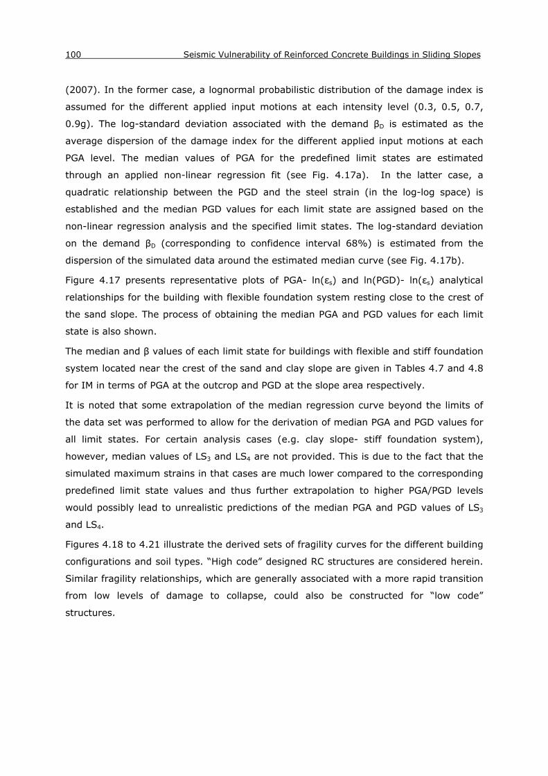
100 Seismic Vulnerability of Reinforced Concrete Buildings in Sliding Slopes
(2007). In the former case, a lognormal probabilistic distribution of the damage index is
assumed for the different applied input motions at each intensity level (0.3, 0.5, 0.7,
0.9g). The log-standard deviation associated with the demand βD is estimated as the
average dispersion of the damage index for the different applied input motions at each
PGA level. The median values of PGA for the predefined limit states are estimated
through an applied non-linear regression fit (see Fig. 4.17a). In the latter case, a
quadratic relationship between the PGD and the steel strain (in the log-log space) is
established and the median PGD values for each limit state are assigned based on the
non-linear regression analysis and the specified limit states. The log-standard deviation
on the demand βD (corresponding to confidence interval 68%) is estimated from the
dispersion of the simulated data around the estimated median curve (see Fig. 4.17b).
Figure 4.17 presents representative plots of PGA- ln(εs) and ln(PGD)- ln(εs) analytical
relationships for the building with flexible foundation system resting close to the crest of
the sand slope. The process of obtaining the median PGA and PGD values for each limit
state is also shown.
The median and β values of each limit state for buildings with flexible and stiff foundation
system located near the crest of the sand and clay slope are given in Tables 4.7 and 4.8
for IM in terms of PGA at the outcrop and PGD at the slope area respectively.
It is noted that some extrapolation of the median regression curve beyond the limits of
the data set was performed to allow for the derivation of median PGA and PGD values for
all limit states. For certain analysis cases (e.g. clay slope- stiff foundation system),
however, median values of LS3 and LS4 are not provided. This is due to the fact that the
simulated maximum strains in that cases are much lower compared to the corresponding
predefined limit state values and thus further extrapolation to higher PGA/PGD levels
would possibly lead to unrealistic predictions of the median PGA and PGD values of LS3
and LS4.
Figures 4.18 to 4.21 illustrate the derived sets of fragility curves for the different building
configurations and soil types. “High code” designed RC structures are considered herein.
Similar fragility relationships, which are generally associated with a more rapid transition
from low levels of damage to collapse, could also be constructed for “low code”
structures.

CHAPTER 4: Vulnerability assessment methodology 101
Figure 4.17. PGA- ln(εs) (a) and ln(PGD)- ln(εs) (b) relationships for the building with flexible
foundation system resting close to the crest of the sand slope
Table 4.7. Parameters of fragility functions for PGA based on the regression analysis method
Soil type Foundation type
Median PGA (g) Dispersion β LS1 (g) LS2 (g) LS3 (g) LS4 (g)
Sand Flexible 0.29 0.36 0.59 0.84 0.81
Stiff 0.31 0.62 1.70 - 0.82
Clay Flexible 0.38 0.83 1.41 1.71 0.82
Stiff 0.53 1.78 - - 0.69
(a)
(b)

102 Seismic Vulnerability of Reinforced Concrete Buildings in Sliding Slopes
Table 4.8. Parameters of fragility functions for PGD based on the regression analysis method
Soil type Foundation type
Median PGD (m) Dispersion β LS1 (m) LS2 (m) LS3 (m) LS4 (m)
Sand Flexible 0.14 0.45 1.06 1.47 0.62
Stiff 0.25 1.07 2.53 3.36 0.55
Clay Flexible 0.25 1.09 2.27 2.87 0.53
Stiff 0.52 3.31 - - 0.55
Figure 4.18. Fragility curves for low rise-RC buildings with flexible foundation system on sand
slope based on the regression analysis method

CHAPTER 4: Vulnerability assessment methodology 103
Figure 4.19. Fragility curves for low rise-RC buildings with flexible foundation system on clay slope
based on the regression analysis method
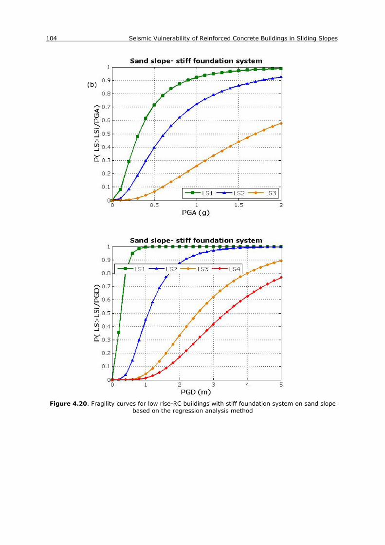
104 Seismic Vulnerability of Reinforced Concrete Buildings in Sliding Slopes
Figure 4.20. Fragility curves for low rise-RC buildings with stiff foundation system on sand slope
based on the regression analysis method
(b)

CHAPTER 4: Vulnerability assessment methodology 105
Figure 4.21. Fragility curves for low rise-RC buildings with stiff foundation system on clay slope
based on the regression analysis method

106 Seismic Vulnerability of Reinforced Concrete Buildings in Sliding Slopes
4.4.2.2. Maximum likelihood method
The Maximum Likelihood (ML) method is a commonly used approach to estimate the log-
normal parameters of the fragility curves (median and log-standard deviation). The
maximum likelihood function gives, among the possible values of the fragility
parameters, the ones that maximize the likelihood of obtaining the simulated dataset.
The likelihood function is expressed as (Shinozuka, 2000):
i iN
y 1 yi i
i 1L = F(IM ) 1 F(IM )
(4.4)
F (.): represents the lognormal fragility distribution for a certain limit state (see Eq. 4.3)
IMi: is the intensity measure in terms of PGA at the outcrop or PGD at the slope area
yi: represents the realization of the Bernouilli random variable Yi with yi = 1 or 0
depending on whether or not the structure sustains the specific state of damage under
the IM equal to IMi and N is the total number of simulations.
The two fragility parameters IM and β (see Eq. 4.3) are computed so as to maximize lnL
(and hence L) satisfying the following equations:
d lnL d lnL 0ddIM
(4.5)
Considering a common β for all limit damage states the likelihood function can be
introduced as (e.g. Shinozuka et al 2003; Argyroudis, 2010):
ijN 4 y
1 2 3 4 j i ji 1 j 0
L IM ,IM ,IM ,IM , = P IM ;E (4.6)
Where
Ej the specified damage state for no damage (j=0), at least slight damage (j=1), at least
moderate damage (j=2), at least extensive damage (j=3) and complete damage (j=4).
yij=1 if the damage state Ej occurs for the i simulation of the structure subject to the landslide intensity iIM and 0 otherwise. The computation is performed numerically using
a standard optimization algorithm.
As already discussed previously, three primary sources of uncertainty contribute to the
total variability:
‐ Uncertainty on the demand that is taken into account from the dispersion of the
recorded damage indices (maximum strain) as a function on the selected IM due
to the variability of the seismic input motion,
‐ Damage state threshold uncertainty that is accounted for by performing, for each starting datum ( ;i jIM E ), a Monte Carlo simulation (sample size N=500). Thus,
one obtains 500 realizations of (IMi, yi) for each damage state (Ej) by comparing

CHAPTER 4: Vulnerability assessment methodology 107
out the observed value for the damage state with randomly sampled thresholds.
The damage state thresholds are sampled from lognormal distributions in
accordance to the pertinent literature (Crowley et al., 2004) with median the
already defined limit state values (see Tab. 4.6) and coefficient of variation equal
to 0.4.
‐ Uncertainty on the capacity properties of the building is taken equal to 0.25 or
0.30 depending on the code design level of the structure (e.g. NIBS, 2004).
The combined variability (β’) associated with the demand and the damage state
threshold is estimated, for each limit state j, from the dispersion of the recorded
maximum strains as a function on the selected IM by randomly sampling from the
damage state thresholds. The best guess values for the parameters ( IM and β’) are
obtained by numerically maximizing the likelihood function L (Eq. 4.5).
The total variability is found from the square root of the sum of the squares (SRSS) of
the uncertainty associated with the demand and damage state threshold (β’) together with the uncertainty in the capacity ( Cβ ) through the following expression:
2 2Cβ= β +β (4.7)
This β-value, which includes also capacity uncertainty, is then put into the likelihood
function (Eq. 3) to estimate the median values IM for each limit state. The obtained
IM and β values represent the parameters of the derived fragility curves.
Table 4.9. Parameters of fragility functions for PGA based on the Maximum likelihood method
Soil type Foundation type
Median PGA (g) Dispersion β LS1 (g) LS2 (g) LS3 (g) LS4 (g)
Sand Flexible 0.22 0.39 0.58 0.81 0.37
Stiff 0.34 0.75 1.12 1.61 0.40
Clay Flexible 0.29 0.61 1.0 1.37 0.39
Stiff 0.45 1.51 - - 0.51
Table 4.10. Parameters of fragility functions for PGD based on the Maximum likelihood method
Soil type Foundation type
Median PGD (m) Dispersion β LS1 (m) LS2 (m) LS3 (m) LS4 (m)
Sand Flexible 0.14 0.37 0.80 1.54 0.42
Stiff 0.25 0.99 2.29 - 0.45
Clay Flexible 0.24 0.96 2.35 - 0.46
Stiff 0.42 3.86 - - 0.74

108 Seismic Vulnerability of Reinforced Concrete Buildings in Sliding Slopes
Figure 4.22. Fragility curves for low rise-RC buildings with flexible foundation system on sand
slope based on the Maximum likelihood method

CHAPTER 4: Vulnerability assessment methodology 109
Figure 4.23. Fragility curves for low rise-RC buildings with flexible foundation system on clay slope
based on the Maximum likelihood method

110 Seismic Vulnerability of Reinforced Concrete Buildings in Sliding Slopes
Figure 4.24. Fragility curves for low rise-RC buildings with stiff foundation system on sand slope
based on the Maximum likelihood method

CHAPTER 4: Vulnerability assessment methodology 111
Figure 4.25. Fragility curves for low rise-RC buildings with stiff foundation system on clay slope
based on the Maximum likelihood method
112 Seismic Vulnerability of Reinforced Concrete Buildings in Sliding Slopes
4.4.2.3. Comparison between the methods
The differences on the fragility curves when applying the two different approaches are
due to the different assumptions adopted in each method and clearly identify the
influence of epistemic uncertainty on the fragility analysis. In particular, the two methods
estimate medians in terms of PGA and PGD that are generally in good agreement. The
estimated β values from the two methods are quite similar when using PGD as a
landslide intensity measure whereas it presents a large dispersion in case that the PGA is
used as an intensity parameter. More specifically, it is shown that the maximum
likelihood method predicts quite smaller log-normal standard deviations. In that sense, it
may be concluded that for the given dataset the maximum likelihood method is more
efficient compared to the regression analysis method when considering PGA as a
measure of the landslide intensity.
Figure 4.26. Comparison of Fragility curves in terms of PGA (left) and PGD (right) developed based on the regression Analysis (RA) and the Maximum likelihood (ML) methods

CHAPTER 4: Vulnerability assessment methodology 113
Figure 4.26. (Continued) - Comparison of Fragility curves in terms of PGA (left) and PGD (right)
developed based on the regression Analysis (RA) and the Maximum likelihood (ML) methods
4.4.3 Discussion
As expected, the building with stiff foundation system would sustain less damage due to
earthquake induced slow moving slides, compared to the same building with the flexible
foundation system. The soil type (dry sand or clay in our case) is also proved to play a
significant role in assessing the building’s vulnerability standing near the crest of
potentially precarious slopes. It is observed that buildings with the same structural and
stiffness characteristics located on slopes of cohesive material behave much better
compared to sandy slopes when subject to differential deformation. More specifically,
among the structures analyzed, the ones with flexible foundations located on sand slopes
present the highest vulnerability whereas the corresponding ones with stiff foundations
located on clay slopes appear to be the least susceptible to damage.
It should be noted that only the structural damage of the building members is considered
in this research. The total damage (structural and non-structural) will be quite different
(certainly larger) in case of the building with the stiff foundation as a considerable
amount of damage may be attributed to the rotation of the whole building as a rigid

114 Seismic Vulnerability of Reinforced Concrete Buildings in Sliding Slopes
body. In the latter, the damage can only be defined using empirical criteria and expert
opinion (Bird et al., 2005). Furthermore, it is worth pointing out that the complex issue
of combined damages due to ground shaking and ground failure is not taken into account
in the evaluation of building‘s vulnerability. Thus, no strength or stiffness degradation to
the building’s structural members due to the effect of ground shaking is assumed to
occur. Neither are aging effects such as concrete or steel corrosion considered in the
present chapter. It is implicitly assumed that the maintenance of the building is
conducted in an optimal manner. A first attempt to include these effects within the
vulnerability assessment framework and to propose time-variant fragility functions is
presented in Chapter 8.
The derived fragility curves are valid only for the specific combination of geometry,
material properties and limit states used herein; their use to other geometric
configurations and site conditions should be made with caution. In order to derive
generic fragility functions for the assessment of the seismic risk and to design
appropriate mitigation measures at building or aggregate scale, an extensive numerical
parametric analysis considering various building typologies, slope configurations and soil
properties should be carried out. Such analysis is presented in Chapter 6.
The reliability and accuracy of the proposed methodology is assessed through the
comparison of the analytically derived fragility curves with literature ones and recorded
building damage data from two real case histories: Kato Achaia slope in Peloponnese –
Greece and Corniglio village-Italy case study (Chapter 7).

CHAPTER 5
Newmark- type displacement methods: Comparison with numerical results
5.1 Introduction
The sliding-block analogy proposed by Newmark (1965) still provides the conceptual
basis on which all displacement-based methods have been developed. Since then,
however, several variations of Newmark's method have been proposed with the aim to
yield more accurate estimates of slope displacement. This has been accomplished by
proposing more efficient ground motion intensity measures (e.g. Crespelllani et al.,
1998; Jibson, 2007; Watson-Lamprey and Abrahamson, 2006; Saygili and Rathje, 2008),
improving the modeling of dynamic resistance of the slope characterized by its yield
coefficient (e.g. see Bray, 2007) and by analyzing the dynamic slope response more
rigorously (e.g. Bray and Travasarou, 2007; Ausilio et al., 2008; Rathje and Antonakos,
2011). In terms of their assumptions to analyze the dynamic slope response,
displacement based methods can be classified into three main types (Jibson, 2011): rigid
block, decoupled and coupled.
A short description of the different types of Newmark-type displacement methods as well
as recommendations for the selection of the most appropriate ones have already been
presented in Chapter 2, § 2.3.3. The focus in this chapter is first on the description of
three different displacement –based models (one of each type): the conventional
analytical Newmark rigid block, the Rathje and Antonakos (2011) decoupled and Bray
and Travasarou (2007) coupled model that have been selected to assess the expected
slope displacements. Then, after providing a short literature review on the reliability
assessment of various displacement based methods for site specific applications, a
comparison of the three Newmark-type procedures is attempted to assess their relative
predictive capability considering various earthquake scenarios and different compliance of
the sliding surface. Finally, the computed FLAC numerical results derived from the non-
linear dynamic analysis (see Chapter 4, §4.3.1), in terms of permanent horizontal

116 Seismic Vulnerability of Reinforced Concrete Buildings in Sliding Slopes
displacements, are compared with the predicted displacements from the three models for
the case of a 30o inclined sand and clayey slope.
5.1.1 Analytical Newmark rigid block model
Ιn his 1965 seminal Rankine Lecture, Newmark (1965) proposed that seismic stability of
earth dams and embankments could be assessed in terms of earthquake-induced
deformations which occur whenever the inertia forces on a potential slide mass are large
enough to overcome the frictional resistance at the “failure” surface. He formulated this
concept by proposing the analogue of a rigid block on inclined plane as a simple way of
analytically obtaining approximate estimates of these deformations.
Newmark (1965) computed rigid block displacements for four earthquake motions and
showed that displacement was a function of yield coefficient (ky), peak ground
acceleration and peak ground velocity.
Figure 5.1. (a) Newmark Sliding-block model (b) Newmark algorithm for seismically-induced
permanent displacements (adapted from Wilson and Keefer, 1983).
The basic assumption of Newmark’s method is that the potential landslide block behaves
as a rigid mass that slides in a perfectly plastic manner on an inclined plane (Fig. 5.1a).
This assumption is reasonable for relatively thin landslides in stiff or brittle materials, but
it introduces significant errors as landslides become thicker and material becomes softer
(Jibson, 2011). Cumulative landslide displacements are estimated by integrating twice
with respect to time the parts of an earthquake acceleration-time history that exceed the
(a) (b)
CHAPTER 5: Newmark-type displacement methods: Comparison with numerical results 117
critical or yield acceleration, ac (ky·g), that is the threshold acceleration required to
overcome basal resistance and initiate sliding. Figure 5.1b presents a schematic
description of the rigorous Newmark Sliding Block procedure (adapted from Wilson and
Keefer, 1983) for estimating permanent co-seismic landslide displacements. The critical
(yield) acceleration may be determined through a pseudostatic analysis or by a simplified
empirical relationship (e.g. Bray, 2007).
Expect for the rigid block key assumption, several other simplifying assumptions were
imposed (see e.g. Newmark, 1965; Makdisi and Seed, 1978; Chang et al., 1984;
Ambraseys and Menu, 1988); these include:
Static and dynamic material shear strengths are taken to be the same
Seismic yield coefficient (ky) is not strain dependent and thus remains constant
during sliding implying that the soil does not undergo significant strength loss as a
result of shaking
The upslope resistance is taken to be infinitely large such that displacements
occur in the downslope direction only
The effects of dynamic pore pressures are neglected
Yield behavior of the material is non-elastic, perfectly-plastic (implied by the use
of ky);
Displacements are assumed to occur along a single, well-defined slip surface
(typically the LEM critical pseudostatic surface);
Accelerations and corresponding inertial forces act in the direction of initial
movement at the center of gravity of the slide mass.
Newmark conventional analytical rigid block method is used in this study to predict
cumulative slope displacements obtained by double integration of the accelerograms
recorded on rock outcrop condition. The freeware software by Jibson and Jibson (2003)
was used for that calculation.
5.1.2 Rathje and Antonakos (2011) decoupled model
Rathje and Antonakos (2011) decoupled model is based on the recent empirical
displacement models of Saygili and Rathje (2008) and Rathje and Saygili (2009) and
thus a brief description of the aforementioned models is first provided.
Saygili and Rathje (2008) presented a suite of empirical predictive models for rigid block
sliding displacements developed using a database of more than 2000 acceleration time
histories with moment magnitudes that range from 5.0 to 7.9 and four values of yield

118 Seismic Vulnerability of Reinforced Concrete Buildings in Sliding Slopes
coefficient. These models consider various single ground motion parameters (PGA, PGV,
Ia, Tm) and vectors of ground motion parameters (e.g. PGA, PGV, Ia, Tm, D5-75, D5-95) to
estimate the sliding displacements with the goal of minimizing the standard deviation in
the displacement prediction. Rathje and Sayligi (2009) slightly modified the single
parameter PGA model of Saygili and Rathje (2008) by adding a term related to
earthquake magnitude.
The authors recommended (among others) the use of the two parameter vector (PGA,
PGV) model due to its ability to significantly reduce the variability in the displacement
prediction. The derived (PGA, PGV) displacement model is given by the following
equation (Saygili and Rathje, 2008):
2 3 4
y y y y
InD
k k k kln D 156 4.58 20.84 44.75 30.50
PGA PGA PGA PGA
0.64ln(PGA) +1.55ln(PGV) + ε σ
(5.1)
Were D=sliding displacement (cm); ky =yield coefficient (g); PGA is the peak ground
acceleration (g); PGV is the peak ground velocity (cm/sec); σInD= standard deviation in
natural log units; and ε= standard normal variate with zero mean and unit standard
deviation.
The standard deviation of the (PGA, PGV) model σInD is a function of ky/PGA is and given
by:
yInD
kσ = 0.41+0.52
PGA
(5.2)
Rathje and Antonakos (2011) presented a unified framework that extends these models
for application to flexible sliding masses following a decoupled approximation. The
decoupled approach estimates the effect of dynamic response of the slide mass on
permanent sliding displacement in a two-step procedure: first, a dynamic response
analysis of the slope is performed assuming no failure surface to estimate the equivalent
acceleration time history within the slide mass and then the resulting time history is
input into a rigid block analysis and the permanent displacements are estimated.
To use the rigid block predictive expressions (Saygili and Rathje, 2008; Rathje and
Sayligi, 2009) for deformable sliding masses appropriate seismic loading parameters
were specified. In particular, for the two vector (PGA, PGV) model, kmax (e.g. peak value
of the average acceleration time history within the sliding mass) was used to replace
PGA and k-velmax (e.g. peak value of the k-vel time history provided by numerical
integration of the k-time history) to replace PGV. The authors presented predictive
models for kmax and k-velmax based on one-dimensional site response analysis of five sites
subjected to 80 input ground motions (Antonakos, 2009). The computed kmax values were

CHAPTER 5: Newmark-type displacement methods: Comparison with numerical results 119
normalized by the input PGA and correlated to Ts/Tm ; the ratio of the fundamental site
period (Ts) to the mean period of the earthquake motion (Tm). The derived model
predicts ln(kmax/PGA) as a function of In(Ts/Tm) and PGA:
For Ts/Tm≥0.1:
2
s s
m mmax
T TIn In
T Tln k / PGA = (0.459 -0.702 PGA) ( 0.228 0.076 PGA)
0.1 0.1
(5.3)
For Ts/Tm<0.1 (nearly rigid conditions):
maxln k / PGA = 0
A similar predictive model was developed for k-velmax /PGV given by:
For Ts/Tm≥0.2:
2
s s
m mmax
T TIn In
T Tln k-vel / PGV = (0.240) ( 0.091 0.171 PGA)
0.2 0.2
(5.4)
For Ts/Tm<0.2:
maxln k-vel / PGV = 0
The standard deviation for these models in natural log units is 0.25.
In addition to the change in seismic loading parameters, the rigid block predictive models
(Saygili and Rathje, 2008; Rathje and Sayligi, 2009) were further modified to account for
the differences in frequency characteristics between acceleration-time histories and k-
time histories. This modification is a function of Ts and increases the predicted
displacement.
The resulting modification to the (PGA, PGV) model to account for flexible sliding is:
For Ts/Tm≤0.5:
flexible PGA,PGV sln D = ln D 1.42 T
For Ts/Tm>0.5: (5.5)
flexible PGA,PGVln D = ln D 0.71
where DPGA,PGV represents the median displacement predicted by the (PGA, PGV) rigid
sliding block model where kmax is used in lieu of PGA and k–velmax is used in lieu of PGV.

120 Seismic Vulnerability of Reinforced Concrete Buildings in Sliding Slopes
A revised linear relationship is used to predict σlnD for flexible sliding masses for the (PGA,
PGV) model:
yInD
max
kσ = 0.40+0.284
k
(5.6)
Figure 5.2 depicts the plots of displacements as a function of Ts for ky=0.05 and 0.1 for
the revised (PGA, PGV) Rathje and Antonakos (2011) model.
Figure 5.2. Predicted values of sliding displacement as a function of Ts with ky=0.05(a) and ky=0.1
(b) for the (PGA, PGV) Rathje and Antonakos (2011) model
It’s worth noting that the (PGA, PGV) model is recommended for use in practice by
Rathje and Antonakos (2011) because of the significant frequency content information
provided by PGV (for rigid sliding) and by k-velmax (for flexible sliding) resulting in the
minimization of the uncertainty in the displacement estimation. Considering that, this
method is used in this study to predict co-seismic slope displacements for different
earthquake scenarios.
5.1.3 Bray and Travasarou (2007) coupled model
Bray and Travasarou (2007) proposed a simplified semi-empirical method to estimate
earthquake deviatoric- induced displacements of rigid and deformable soil slopes.
Displacements were calculated using the nonlinear fully coupled stick-slip deformable
sliding block model proposed by Rathje and Bray (2000) to capture the dynamic

CHAPTER 5: Newmark-type displacement methods: Comparison with numerical results 121
response of an earth-waste structure (Fig. 5.3). In a fully coupled analysis, as proposed
by the authors, the dynamic response of the sliding mass and the permanent
displacement are modeled together so that the effect of plastic sliding displacement on
ground motions is taken into account. Thus, the fully coupled stick-slip deformable sliding
block model offers a conceptual improvement over the decoupled approximation.
Figure 5.3. Generic seismic slope displacement problem of height H and initial stiffness Vs and (b)
idealized nonlinear stick with one-way sliding used in Bray and Travasarou (2007).
The model used is based on an equivalent-linear visco-elastic one dimensional analysis to
allow for the use of a large number ground motions with wide range of properties of the
potential sliding mass. Vucetic and Dobry (1991) shear modulus and damping curves for
PI=30 were used. 688 recorded ground motions from 41 earthquakes with moment
magnitudes (Mw) that range from 5.5 to 7.6, has been used to compute co-seismic
displacements (Travasarou, 2003). The predictive seismic displacement model
parameters include the system’s yield coefficient (ky), its initial fundamental period (Ts),
and the ground motion’s spectral acceleration at a degraded period equal to 1.5Ts. The
slope’s yield coefficient (ky) and initial fundamental period (Ts) were selected to represent
the dynamic strength and stiffness, respectively, of the earth/waste slope in the seismic
displacement model. The seismic displacements were computed for ten values of ky
(0.02-0.4) and eight values of Ts (0 - 2 s) for the entire set of used ground motions. The
slope’s yield coefficient (ky) can be estimated through a psedostatic analysis or by a
simplified expression as a function of the slope geometry, weight and strength (e.g. Bray
et al., 1998). The initial fundamental period of the sliding mass can normally be
estimated using the expression Ts=4H/Vs, where H= average height of the potential
sliding mass, Vs=average shear wave velocity of the sliding mass. A modified expression
should be used in case of a triangular –shaped sliding mass (Bray, 2007). In Bray and
Travasarou (2007), average H varied from 12 to 100m and Vs from 200 to 425m/sec.
The spectral acceleration at a degraded period equal to 1.5 times the initial fundamental
period of the slope, i.e., Sa (1.5Ts), was found to represent (among others) an efficient
122 Seismic Vulnerability of Reinforced Concrete Buildings in Sliding Slopes
measure of the seismic intensity for minimizing the variability of displacement predictions
(Travasarou and Bray, 2003). Note that the model has been developed for Sa (1.5Ts)
values from 0.002 to 2.7 g and should be used within these ranges to provide reasonable
and reliable estimates of the slope displacements. The degraded fundamental period is
considered to capture the overall average stiffness reduction for the earth/waste slopes.
It is also important to notice that the Bray and Travasarou (2007) expressions do not
model the foundation conditions (e.g. rock, stiff soil) that can moderately effect the
computed displacements.
The model separates the probability of “zero” displacement occurring from the
distribution of “non-zero” displacement, so that to exclude from the results values of
calculated displacement <1 cm that are assumed to be of no engineering significance.
The probability of negligible “zero” displacement is estimated as:
y s y a sP(D "0") 1–Φ ( 1.76 3.22 ln(k ) 0.484T ln(k ) 3.52 ln(S (1.5T ))) (5.7)
where P(D=0): probability (as a decimal number) of occurrence of zero displacements;
D-seismic displacement; Φ: standard normal cumulative distribution function; ky: yield
coefficient; Ts: initial fundamental period of the sliding mass in seconds, and Sa(1.5Ts):
the spectral acceleration of the input ground motion at a period of 1.5Ts in terms of g.
The likely amount of nonzero seismic displacement (D) is given by the following
equation:
2y y a s
2a s a s s
ln D 1.10 2.83 ln(k ) 0.333 (ln(k )) 0.566ln(S (1.5T ))
3.04 ln(S (1.5T )) 0.244(ln(S (1.5T ))) 1.50T 0.278(M – 7) ε
(5.8)
where the ky, Ts, and Sa(1.5Ts) are defined as previously for Eq. (5.7), and ε is a
normally distributed random variable with zero mean and standard deviation σ=0.66.
For the nearly Newmark rigid sliding block case (Ts≈0), Eq. (5.8) is transformed as
follows:
2y y
2s
ln D 0.22 2.83 ln(k ) 0.333 (ln(k )) 0.566ln(PGA)
3.04 ln(PGA) 0.244(ln(PGA)) 1.50T 0.278(M – 7) ε
(5.9)
where PGA is the peak ground acceleration of the ground motion (i.e., Sa(Ts=0)).
The model can be implemented rigorously within a fully probabilistic framework for the
estimation of the probability of exceedance of a selected threshold of displacement (d)
for a specified earthquake scenario and slope properties.
The probability of the seismic displacement (D) exceeding a specified displacement
threshold (d) is expressed as:

CHAPTER 5: Newmark-type displacement methods: Comparison with numerical results 123
P(D d) 1 – P(D "0") P(D d / D "0") (5.10)
The term P(D=0) is computed using Eq. (2). The term P (D>d/D>0) may be computed
assuming that the estimated displacements are lognormally distributed as:
ˆlnd lndP(D d / D "0") 1 – P D d / D "0" 1 Φ
σ
(5.11)
where ˆlnd is computed using Eq. (3); σ is the standard deviation of the random error,
which in this case is 0.66; and Φ is the standard normal cumulative distribution function.
Some trends in the estimates from the model are shown in Figure 5.4.
Figure 5.4. Trends from the Bray and Travasarou (2007) model: (a) probability of negligible displacements and (b) median displacement estimate for a Mw = 7 strike-slip earthquake at a distance of 10 km, and (c) seismic displacement as a function of yield coefficient for several
intensities of ground motion (Mw = 7.5) for a sliding block with Ts = 0.3 s (adopted from Bray, 2007)
The Bray and Travasarou (2007) seismic displacement model has shown to predict
reliably the seismic performance observed at 16 earth dams and solid-waste landfills.
The authors also found that the values of predicted displacements were not inconsistent
with other simplified methods. This method is also used in this study to predict sliding
displacements for various earthquake scenarios.
5.2 Comparison between the displacement-based methods and with the numerical approach
5.2.1 Literature review
Several investigators have applied Newmark-type deformation procedures of different
complexity as well as advanced 2D dynamic stress-strain methods to case studies to

124 Seismic Vulnerability of Reinforced Concrete Buildings in Sliding Slopes
compare the results among the different approaches and with the actual field
performance. This comparison allows assessing the reliability of the various methods to
predict the expected co-seismic displacements and to judge their relative degree of
conservativeness.
Wilson and Keefer (1983) applied the Newmark method to a landslide triggered by the
1979 Coyote Creek, California earthquake using a real acceleration time history recorded
at the landslide area and they found that the predicted Newmark landslide displacement
agreed well with the observed displacement.
Chugh and Stark (2006) applied 2D FD dynamic analysis and analytical Newmark rigid
block method to assess the seismically induced slope deformations of the Quaternary
landslide (Qls-18) in California. They found that the obtained permanent displacements
of both methods are in good agreement with the field observations.
Pradel et al. (2005) compared the post earthquake field performance of a pre-existing
coherent landslide reactivated after the Northridge earthquake with the seismic
displacements calculated using the analytical decoupled Newmark approximation as well
as the simplified decoupled empirical relationships suggested by Makdisi and Seed (1978)
and Bray and Rathje (1998). The authors showed that decoupled Newmark- type sliding
block analyses can result in reasonable estimates of the observed displacement.
Bray and Travasarou (2007) confirmed the reliability of their model by providing
estimations of the seismic displacements for 16 earth dams and solid-waste landfills that
are correlated quite well with the observed seismic performance. The authors also found
that the values of predicted displacements are not inconsistent with other simplified
decoupled approaches (Makdisi and Seed, 1978; Bray and Rathje, 1998).
Austilio et al. (2009) evaluated the seismic displacements of the Calitri landslide
(southern Italy) reactivated after the Irpinia earthquake (1980), based on simplified and
analytical decoupled Newmark-type approaches, a 1D stick-slip coupled model (Austilio
et al., 2008) and 2D FD dynamic analyses. They observed that the displacements
predicted by simplified and analytical decoupled procedures for four different soil profiles
seemed to capture the average value of displacement recorded at Calitri after the
earthquake while the 1D coupled method generally yielded more conservative results.
Moreover, they showed that the 2D FD dynamic analysis for the certain case history
predicted the largest displacements, constant for all soil profiles that are comparable with
the maximum observed values.
Strenk (2010) applied a suite of 20 deformation based methods of different categories
(rigid block, decoupled and coupled) to assess their reliability in predicting the observed
seismically-induced displacements at three case studies in California, USA : Calabasas

CHAPTER 5: Newmark-type displacement methods: Comparison with numerical results 125
landslide triggered by the 1994 Northridge earthquake and Ditullio and Upper Laurel
landslides triggered by the 1989 Loma Prieta earthquake. By comparing the median
predictions obtained from each method to the actual measured displacement observed at
each landslide he concluded that no method (or category of methods) is drastically more
accurate than any of the others while he observed an overall tendency for nearly all
deformation-based methods to under-predict the recorded field displacement (73% of
the total number of predictions were reported to be near or below the actual measured
displacement). He proposed the use of more recent simplified rigid-block methods that
are derived using larger ground motion databases and robust mathematical regression
techniques. Moreover, he recommended the use of the analytical-versions over the
simplified versions of all deformation based methods as he recognized that simplified
methods make more assumptions associated with the reduction of the analytical
approach into a simplified mathematical equation or chart that can introduce significant
bias on the computed displacements.
5.2.2 Implementation of the selected displacement-based predictive models
After providing a short literature review on the different displacement based approaches
to site-specific applications, the three different procedures described in section 5.1 are
used to predict the permanent slope deformation: the conventional analytical Newmark
rigid block model (Newmark 1965), the decoupled Rathje and Antonakos (2011) model
and the coupled Bray and Travasarou (2007) sliding block model. The main goal is to
identify the influence of the earthquake characteristics and the dynamic response of the
slope on the magnitude of the residual slope displacements using the aforementioned
predictive models. In this respect, permanent displacements as a function of the critical
acceleration ratio (e.g. ky/kmax or ky/PGA) were computed using the three different
approaches considering different earthquake scenarios and compliance of the sliding
surface. Comparisons between the methods were allowed to be made to assess their
relative degree of conservatism. Mean displacements were calculated using the Newmark
rigid block model whereas median values ±1 standard deviation and median and 16th -
84th percentiles were derived for the decoupled and coupled approximations respectively.
The applied seismic input consists of two real acceleration time histories characterized by
quite different frequency content recorded at rock outcropping conditions (Fig. 5.5).
These are scaled at two different levels of PGA, namely 0.3 and 0.7g. Table 5.1 presents
the parameters describing some basic characteristics of the ground motions and the
flexibility of the potential sliding surface. Moment magnitude values for the Bray and
Travasarou model were approximately taken to be consistent to the level of shaking and

126 Seismic Vulnerability of Reinforced Concrete Buildings in Sliding Slopes
considering the initial shaking characteristics of the given earthquake events. The
displacement were computed for nearly rigid (Ts=0.032sec) and relatively flexible
(Ts=0.16 sec) sliding masses.
The derived (mean or median) permanent displacements for the three different predictive
models and for the different considered earthquake scenarios plotted as a function of the
critical acceleration ratio, PGA (or kmax)/ky, are illustrated in Figures 5.6 to 5.8 and 5.13
to 5.14 for the nearly rigid and relatively flexible sliding surfaces respectively.
Comparative plots between the methods are shown as well (Figs. 5.9-5.12 and 5.15-5.18
for the nearly rigid and relatively flexible sliding surfaces respectively).
Figure 5.5. Input acceleration time histories (before scaling) and Fourier spectra Table 5.1. Parameters describing the characteristics of the ground motions and the slope dynamic
response used for the analyses
Earthquake record name Valnerina 1979-Cascia_L
Northridge 1994-Pacoima Dam_L
Earthquake code cascia pacoima
Moment magnitude 5.9 6.7
Fundamental period of the input motion Tp (sec) 0.23 0.48
Mean Period of the input motions Tm (sec) 0.295 0.507
Scaled outcropping PGA (g) 0.30 0.70 0.30 0.70
PGV (cm/sec) 10.30 30.90 14.60 43.90
Fundamental period of the sliding mass Ts (sec) 0.16 0.032 0.16 0.032
Sa(1.5Ts)/PGA 2.926 1.073 2.257 1.033
Ts/Tm 0.542 0.106 0.316 0.063
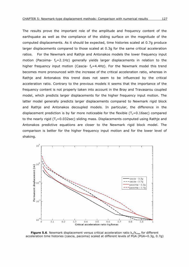
CHAPTER 5: Newmark-type displacement methods: Comparison with numerical results 127
The results prove the important role of the amplitude and frequency content of the
earthquake as well as the compliance of the sliding surface on the magnitude of the
computed displacements. As it should be expected, time histories scaled at 0.7g produce
larger displacements compared to those scaled at 0.3g for the same critical acceleration
ratios. For the Newmark and Rathje and Antonakos models the lower frequency input
motion (Pacoima- fp=2.1Hz) generally yields larger displacements in relation to the
higher frequency input motion (Cascia- fp=4.4Hz). For the Newmark model this trend
becomes more pronounced with the increase of the critical acceleration ratio, whereas in
Rathje and Antonakos this trend does not seem to be influenced by the critical
acceleration ratio. Contrary to the previous models it seems that the importance of the
frequency content is not properly taken into account in the Bray and Travasarou coupled
model, which predicts larger displacements for the higher frequency input motion. The
latter model generally predicts larger displacements compared to Newmark rigid block
and Rathje and Antonakos decoupled models. In particular, the difference in the
displacement prediction is by far more noticeable for the flexible (Ts=0.16sec) compared
to the nearly rigid (Ts=0.032sec) sliding mass. Displacements computed using Rathje and
Antonakos predictive equations are closer to the Newmark rigid block model. The
comparison is better for the higher frequency input motion and for the lower level of
shaking.
Figure 5.6. Newmark displacement versus critical acceleration ratio ky/kmax for different
acceleration time histories (cascia, pacoima) scaled at different levels of PGA (PGA=0.3g, 0.7g)

128 Seismic Vulnerability of Reinforced Concrete Buildings in Sliding Slopes
Figure 5.7. Rathje and Antonakos (2011) displacement versus critical acceleration ratio ky/kmax considering a nearly rigid sliding mass (Ts=0.032 sec) for different acceleration time histories
(Cascia, Pacoima) scaled at different levels of PGA (PGA=0.3g, 0.7g)
Figure 5.8. Bray and Travasarou (2007) displacement versus critical acceleration ratio ky/kmax considering a nearly rigid sliding mass (Ts=0.032 sec) for different acceleration time histories
(Cascia, Pacoima)) scaled at different levels of PGA (PGA=0.3g, 0.7g)

CHAPTER 5: Newmark-type displacement methods: Comparison with numerical results 129
Figure 5.9. Comparison of the different predictive models for permanent slope displacement
considering a nearly rigid sliding mass (Ts=0.032 sec) for a certain earthquake scenario (Cascia scaled at 0.3g)
Figure 5.10. Comparison of the different predictive models for permanent slope displacement
considering a nearly rigid sliding mass (Ts=0.032 sec) for a certain earthquake scenario (Pacoima scaled at 0.3g)

130 Seismic Vulnerability of Reinforced Concrete Buildings in Sliding Slopes
Figure 5.11. Comparison of the different predictive models for permanent slope displacement considering a nearly rigid sliding mass (Ts=0.032 sec) for a certain earthquake scenario (Cascia
scaled at 0.7g)
Figure 5.12. Comparison of the different predictive models for permanent slope displacement
considering a nearly rigid sliding mass (Ts=0.032 sec) for a certain earthquake scenario (Pacoima scaled at 0.7g)

CHAPTER 5: Newmark-type displacement methods: Comparison with numerical results 131
Figure 5.13. Rathje and Antonakos (2011) displacement versus critical acceleration ratio ky/kmax
considering a deformable sliding mass (Ts=0.16 sec) for different acceleration time histories (Cascia, Pacoima) scales at different levels of PGA (PGA=0.3g, 0.7g)
Figure 5.14. Bray and Travasarou (2007) displacement versus critical acceleration ratio ky/kmax
considering a deformable sliding mass (Ts=0.16 sec) for different acceleration time histories (Cascia, Pacoima) scaled at different levels of PGA (PGA=0.3g, 0.7g)

132 Seismic Vulnerability of Reinforced Concrete Buildings in Sliding Slopes
Figure 5.15. Comparison of the different predictive models for permanent slope displacement considering a deformable sliding mass (Ts=0.16 sec) for a certain earthquake scenario (Cascia
scaled at 0.3g)
Figure 5.16. Comparison of the different predictive models for permanent slope displacement
considering a deformable sliding mass (Ts=0.16 sec) for a certain earthquake scenario (Pacoima scaled at 0.3g)

CHAPTER 5: Newmark-type displacement methods: Comparison with numerical results 133
Figure 5.17. Comparison of the different predictive models for permanent slope displacement considering a deformable sliding mass (Ts=0.16 sec) for a certain earthquake scenario (Cascia
scaled at 0.7g)
Figure 5.18. Comparison of the different predictive models for permanent slope displacement
considering a deformable sliding mass (Ts=0.16 sec) for a certain earthquake scenario (Pacoima scaled at 0.7g)

134 Seismic Vulnerability of Reinforced Concrete Buildings in Sliding Slopes
5.2.3 Comparison of displacements estimated by displacement-based
methods and dynamic numerical analyses
In the previous section an application of the selected displacement based approaches
was performed for different earthquake scenarios for both deformable and nearly rigid
sliding surfaces highlighting prevailing trends in the displacement prediction.
In this section, 2 dimensional fully non-linear FLAC numerical results (see Chapter 4) are
compared in terms of permanent horizontal displacement along the unstable slope area,
with the Newmark-type displacement methods. The aim is, on the one hand, to gain
confidence on the results of the numerical analysis and, on the other hand, to assess the
predictive capability of the different displacement based approaches with respect to the
a-priori more accurate numerical analysis. As described above, the conventional
analytical Newmark rigid block model (Newmark 1965), the decoupled Rathje and
Antonakos (2011) model and the coupled Bray and Travasarou (2007) sliding block
model are used for this purpose to calculate permanent displacements of the slide mass.
These are compared with the FLAC permanent horizontal displacements within the sliding
mass derived from the dynamic analysis for the free-field conditions (in the absence of
any structure) for the two idealized step-like slopes analyzed in Chapter 4 (see Fig.
5.19), which characterized by sand and clayey soil materials respectively that overlay a
stiff clayey layer. The elastic bedrock lies at 70 m. The mechanical characteristics for the
soil materials and elastic bedrock have been presented in Chapter 4, Table 4.1. Details
regarding the numerical modeling and the computed permanent FLAC displacements
have already been discussed in Chapter 4 and will not be repeated herein.
Figure 5.19. Slope configuration used for the numerical modeling

CHAPTER 5: Newmark-type displacement methods: Comparison with numerical results 135
The initial fundamental period of the sliding mass (Ts) has been estimated using the
simplified expression: Ts = 4H/Vs, where H is the depth and Vs is the shear wave velocity
of the potential sliding mass. Different depths of the potential sliding surface have been
evaluated for slopes consisting of sand (H=2 m) and clay material (H=10 m) by means of
a LEM pseudostatic analysis.
The horizontal yield coefficient, ky, has been computed via a pseudostatic slope stability
analysis using Spencer method of slides (Spencer, 1967) that satisfied full equilibrium.
The ky values are estimated as 0.16 and 0.15 for the 30o inclined slopes consisting of
sand and clay soil material respectively.
The seismic input applied along the base of the dynamic model consists of a set of 7 real
acceleration time histories from different earthquakes worldwide recorded on rock
outcrop (see Chapter 4, Tab. 4.4). Two of them (Valnerina –Cascia_L, Northridge -
Pacoima Dam_L) have also been used in the previous section to predict permanent slope
deformation using different Newmark-type displacement methods. To obtain the
appropriate inputs for the Newmark-type displacement based methods that include the
effect of soil conditions, and to allow a direct comparison with the numerical results, the
selected acceleration time histories were first propagated up to the depth of the potential
sliding surface through a 1D non-linear site response analysis considering the same soil
properties as in the 2D dynamic analysis. It is noticed that the 1D soil profile is located at
the section that approximately corresponds to the maximum slide mass thickness of the
slope (Section A, see Fig. 5.19). The bottom of the sliding surface is taken be consistent
to the estimated fundamental period of the sliding mass (Ts) that is different for the clay
and sand slopes. It‘s worth noting that the thickness of the landslide mass may also vary
with respect to the characteristics of the earthquake and the level of shaking. This effect,
however, was not taken into account and thus only average predictions of the cumulative
co-seismic displacement can be made.
Tables 5.2 and 5.5 present the computed parameters of the models for outcropping
accelerograms scaled at PGArock=0.7g for the sand (Ts=0.032sec) and clay (Ts=0.16sec)
slopes respectively. Tables 5.3 and 5.6 present the predicted numerical horizontal
displacements together with those calculated using the different Newmark-type
displacement methods for rock outcropping accelerograms scaled at PGA=0.7g for the
hypothesized sand (Ts=0.032 sec) and clay (Ts=0.16 sec) slopes. The error (%) of the
Newmark-type models in the displacement estimation compared to the corresponding
numerical displacement calculation for input accelerograms scaled at PGA=0.7g are
presented in Table 5.4 for sand nearly rigid sliding mass (Ts=0.032 sec) and in Table 5.7
for clay deformable sliding mass (Ts=0.16 sec). Relative different (%) of the models in
the median displacement estimation as well as the corresponding average difference (%)

136 Seismic Vulnerability of Reinforced Concrete Buildings in Sliding Slopes
to the numerical displacement calculation are depicted in Figures 5.20 and 5.21 for the
sand and in Figures 5.24 and 5.25 for the clay slope respectively. The dispersion of the
corresponding difference is presented in Figures 5.22 and 5.26 for the sand and clay
slope respectively. Finally, Figures 5.23 and 5.27 show a direct comparison between
analytical Newmark’s , Bray and Travasarou (2007) and Rathje and Antonakos (2011)
displacements with the maximum horizontal displacements from the 2D dynamic
numerical analyses for rock outcropping accelerograms scaled at different levels of PGA
(0.3g, 0.5g, 0.7g, 0.9g) for sand and clay slopes respectively. The comparisons generally
demonstrate similar trends for the lower and higher levels of shaking.
Table 5.2. Parameters of the models for rock outcropping accelerograms scaled at PGA=0.7g-
sand slope (Ts=0.032sec)
Earthquake code
PGArock (g)
PGA sliding surface
(g)
PGV sliding surface
(cm/sec)
Tm (sec) Ts/Tm
kmax (g) (Eq. 5.3)
k-velmax (cm/sec)
(Eq. 5.4)
Sa(1.5Ts) (g)
cascia 0.70 0.89 61.70 0.42 0.08 0.89 61.70 0.96 kypseli 0.70 0.91 70.60 0.45 0.07 0.91 70.60 1.00
montenegro 0.70 0.75 66.30 0.49 0.07 0.75 66.30 0.81 pacoima 0.70 0.86 72.60 0.56 0.06 0.86 72.60 0.93 sturno 0.70 1.04 91.70 0.55 0.06 1.04 91.70 1.12 duzce 0.70 0.84 60.20 0.41 0.08 0.84 60.20 0.94 gilroy 0.70 0.81 52.10 0.36 0.09 0.81 52.10 0.93
Table 5.3. Comparison of numerical horizontal displacements to analytical Newmark rigid block method, Rathje and Antonakos (2010) decoupled approach and Bray and Travasarou (2007)
coupled stick-slip displacement method for rock outcropping accelerograms scaled at PGA=0.7g -sand slope (Ts=0.032sec)
Earthquake code
Numerical displacement
(m)
Average Newmark
displacement (m)
Rathje and Antonakos displacement (m)
Bray and Travasarou displacement (m)
Median Dflexible
Median -1sd (m)
Median +1sd (m)
Median (m)
84th percentile
(m)
16th percentile
(m)
cascia 0.60 0.64 0.40 0.62 0.25 0.60 0.31 1.16 kypseli 0.50 0.55 0.50 0.78 0.32 0.65 0.34 1.25
montenegro 0.90 0.70 0.37 0.59 0.24 0.42 0.22 0.81 pacoima 0.70 0.53 0.49 0.78 0.31 0.57 0.29 1.09 sturno 1.70 1.38 0.83 1.29 0.53 0.81 0.42 1.55 duzce 1.10 0.94 0.36 0.57 0.23 0.57 0.30 1.10 gilroy 0.20 0.23 0.28 0.44 0.18 0.57 0.29 1.09
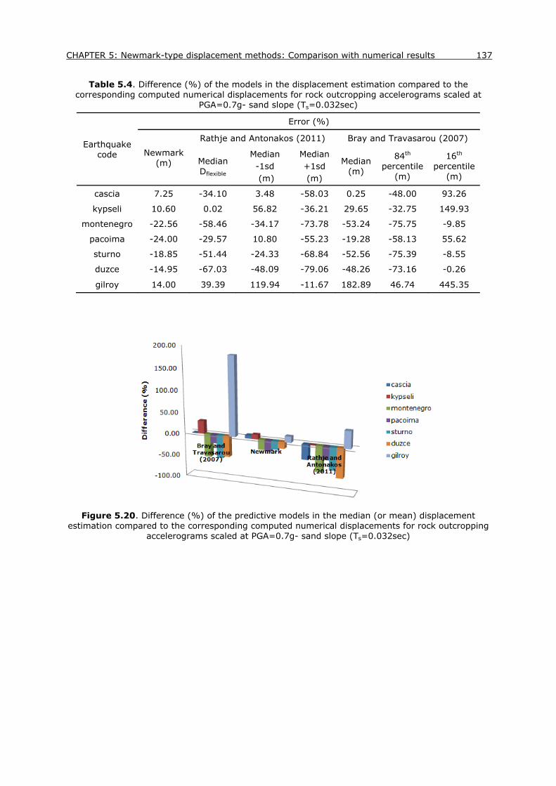
CHAPTER 5: Newmark-type displacement methods: Comparison with numerical results 137
Table 5.4. Difference (%) of the models in the displacement estimation compared to the corresponding computed numerical displacements for rock outcropping accelerograms scaled at
PGA=0.7g- sand slope (Ts=0.032sec)
Earthquake code
Error (%)
Newmark (m)
Rathje and Antonakos (2011) Bray and Travasarou (2007)
Median Dflexible
Median -1sd (m)
Median +1sd (m)
Median (m)
84th percentile
(m)
16th percentile
(m)
cascia 7.25 -34.10 3.48 -58.03 0.25 -48.00 93.26
kypseli 10.60 0.02 56.82 -36.21 29.65 -32.75 149.93
montenegro -22.56 -58.46 -34.17 -73.78 -53.24 -75.75 -9.85
pacoima -24.00 -29.57 10.80 -55.23 -19.28 -58.13 55.62
sturno -18.85 -51.44 -24.33 -68.84 -52.56 -75.39 -8.55
duzce -14.95 -67.03 -48.09 -79.06 -48.26 -73.16 -0.26
gilroy 14.00 39.39 119.94 -11.67 182.89 46.74 445.35
Figure 5.20. Difference (%) of the predictive models in the median (or mean) displacement
estimation compared to the corresponding computed numerical displacements for rock outcropping accelerograms scaled at PGA=0.7g- sand slope (Ts=0.032sec)

138 Seismic Vulnerability of Reinforced Concrete Buildings in Sliding Slopes
Figure 5.21. Average difference (%) of the predictive models in the median (or mean)
displacement estimation compared to the corresponding computed numerical displacements for rock outcropping accelerograms scaled at PGA=0.7g- sand slope (Ts=0.032sec)
Figure 5.22. Dispersion (%) of the predictive models in the median (or mean) displacement
estimation in relation to the corresponding computed numerical displacements for rock outcropping accelerograms scaled at PGA=0.7g- sand slope (Ts=0.032sec)

CHAPTER 5: Newmark-type displacement methods: Comparison with numerical results 139
Figure 5.23. Comparison between (a) analytical Newmark’s, (b) Rathje and Antonakos (2011) and (c) Bray and Travasarou (2007) displacements with the co-seismic horizontal displacements from
the 2D dynamic numerical analyses (sand slope)
(a)
(b)
(c)
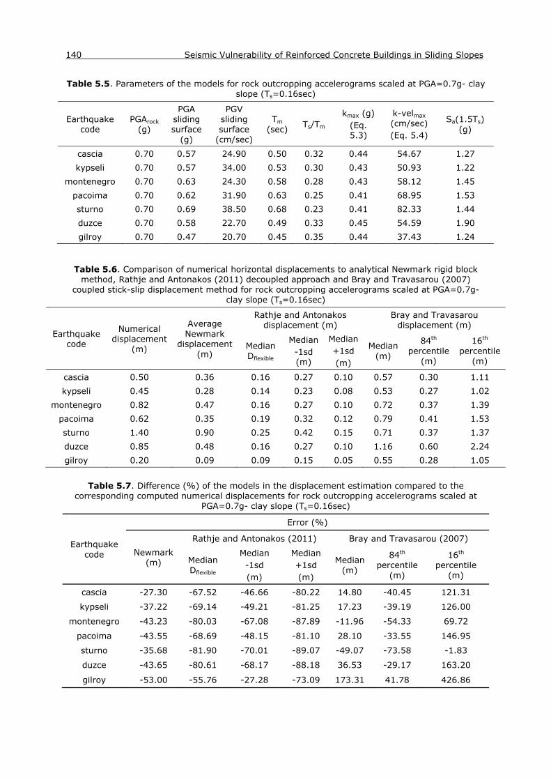
140 Seismic Vulnerability of Reinforced Concrete Buildings in Sliding Slopes
Table 5.5. Parameters of the models for rock outcropping accelerograms scaled at PGA=0.7g- clay slope (Ts=0.16sec)
Earthquake code
PGArock (g)
PGA sliding surface
(g)
PGV sliding surface
(cm/sec)
Tm (sec) Ts/Tm
kmax (g) (Eq. 5.3)
k-velmax (cm/sec) (Eq. 5.4)
Sa(1.5Ts) (g)
cascia 0.70 0.57 24.90 0.50 0.32 0.44 54.67 1.27 kypseli 0.70 0.57 34.00 0.53 0.30 0.43 50.93 1.22
montenegro 0.70 0.63 24.30 0.58 0.28 0.43 58.12 1.45 pacoima 0.70 0.62 31.90 0.63 0.25 0.41 68.95 1.53 sturno 0.70 0.69 38.50 0.68 0.23 0.41 82.33 1.44 duzce 0.70 0.58 22.70 0.49 0.33 0.45 54.59 1.90 gilroy 0.70 0.47 20.70 0.45 0.35 0.44 37.43 1.24
Table 5.6. Comparison of numerical horizontal displacements to analytical Newmark rigid block
method, Rathje and Antonakos (2011) decoupled approach and Bray and Travasarou (2007) coupled stick-slip displacement method for rock outcropping accelerograms scaled at PGA=0.7g-
clay slope (Ts=0.16sec)
Earthquake code
Numerical displacement
(m)
Average Newmark
displacement (m)
Rathje and Antonakos displacement (m)
Bray and Travasarou displacement (m)
Median Dflexible
Median -1sd (m)
Median +1sd (m)
Median (m)
84th percentile
(m)
16th percentile
(m)
cascia 0.50 0.36 0.16 0.27 0.10 0.57 0.30 1.11 kypseli 0.45 0.28 0.14 0.23 0.08 0.53 0.27 1.02
montenegro 0.82 0.47 0.16 0.27 0.10 0.72 0.37 1.39 pacoima 0.62 0.35 0.19 0.32 0.12 0.79 0.41 1.53 sturno 1.40 0.90 0.25 0.42 0.15 0.71 0.37 1.37 duzce 0.85 0.48 0.16 0.27 0.10 1.16 0.60 2.24 gilroy 0.20 0.09 0.09 0.15 0.05 0.55 0.28 1.05
Table 5.7. Difference (%) of the models in the displacement estimation compared to the
corresponding computed numerical displacements for rock outcropping accelerograms scaled at PGA=0.7g- clay slope (Ts=0.16sec)
Earthquake code
Error (%)
Newmark (m)
Rathje and Antonakos (2011) Bray and Travasarou (2007)
Median Dflexible
Median -1sd (m)
Median +1sd (m)
Median (m)
84th percentile
(m)
16th percentile
(m)
cascia -27.30 -67.52 -46.66 -80.22 14.80 -40.45 121.31
kypseli -37.22 -69.14 -49.21 -81.25 17.23 -39.19 126.00
montenegro -43.23 -80.03 -67.08 -87.89 -11.96 -54.33 69.72
pacoima -43.55 -68.69 -48.15 -81.10 28.10 -33.55 146.95
sturno -35.68 -81.90 -70.01 -89.07 -49.07 -73.58 -1.83
duzce -43.65 -80.61 -68.17 -88.18 36.53 -29.17 163.20
gilroy -53.00 -55.76 -27.28 -73.09 173.31 41.78 426.86

CHAPTER 5: Newmark-type displacement methods: Comparison with numerical results 141
Figure 5.24. Difference (%) of the predictive models in the median (or mean) displacement
estimation compared to the corresponding computed numerical displacements for rock outcropping accelerograms scaled at PGA=0.7g- clay slope (Ts=0.16sec)
Figure 5.25. Average difference (%) of the predictive models in the median (or mean)
displacement estimation compared to the corresponding computed numerical displacements for rock outcropping accelerograms scaled at PGA=0.7g- clay slope (Ts=0.16sec)
Figure 5.26. Dispersion (%) of the predictive models in the median (or mean) displacement
estimation in relation to the corresponding computed numerical displacements for rock outcropping accelerograms scaled at PGA=0.7g- clay slope (Ts=0.16sec)

142 Seismic Vulnerability of Reinforced Concrete Buildings in Sliding Slopes
Figure 5.27. Comparison between (a) analytical Newmark’s, (b) Rathje and Antonakos (2011) and (c) Bray and Travasarou (2007) displacements with the co-seismic horizontal displacements from
the 2D dynamic numerical analyses (clay slope)
(a)
(b)
(c)

CHAPTER 5: Newmark-type displacement methods: Comparison with numerical results 143
5.2.3.1. Discussion - Concluding remarks
FLAC displacements generally are not inconsistent with the predicted Newmark-type
displacements enhancing the reliability and robustness of the dynamic analysis results.
All three displacement based models predict displacements that are generally in good
agreement with the FLAC results for the sand stiff slope case. On the contrary, for the
clay more flexible slope the correlation is not so good. In particular, Bray and Travasarou
(2007) model tend to predict generally larger displacements with respect to the dynamic
analysis whereas Newmark rigid block and Rathje and Antonakos (2011) models
underpredict the corresponding displacements.
Among the three methods, Bray and Travasarou model was found to present the
minimum average predictive error (%) in relation to the dynamic analysis for both sand
nearly rigid and clay relatively flexible slope cases. This is in line with the inherent
coupled stick-slip assumption adopted in the method that offers a conceptual
improvement over the rigid block and decoupled approaches for modeling the physical
mechanism of earthquake-induced landslide deformation. However, Bray and Travasarou
model presents a very large dispersion in the median displacement estimation (up to
70% for both sandy and clayey slopes). Thus, the use of Sa(1.5 Ts) seems rather
insufficient to fully describe the characteristics of the seismic loading (i.e. amplitude,
frequency content and duration) for site-specific applications.
Newmark analytical approach shows the minimum dispersion in the displacement
prediction (less than 10-20%) with respect the numerical analysis results compared to
the Bray and Travasarou and Rathje and Antonakos models. This may be justified by the
fact that Newmark analytical method uses the entire time history to characterize the
seismic loading as opposed to the Bray and Travasarou and Rathje and Antonakos
models that use one [Sa(1.5 Ts)] and two (PGA, PGV) intensity parameters respectively.
As such, uncertainties associated to the selection of the ground motion intensity
parameters are limited in the Newmark conventional analytical approach.
Overall, the differences in the displacement prediction between the models are larger for
the more ductile clay slope. Thus, the compliance of the failure surface in relation to the
frequency content of the input earthquake scenarios allows for some bias to be
introduced on the results.
Summarizing, Newmark-type displacement methods display a valuable compromise
between simplistic pseudostatic approaches and sophisticated numerical modeling
techniques in providing a rough estimate of the seismic slope performance. They can be
efficiently implemented in the prediction of earthquake induced landslide displacements
for regional seismic hazard analysis (e.g. Jibson et al., 2000). However, as shown in this
study, their use in site specific problems should be made with caution, acknowledging the

144 Seismic Vulnerability of Reinforced Concrete Buildings in Sliding Slopes
simplified assumptions associated with them. In any case, a stochastic framework to
account for the (generally large) uncertainty in the displacement prediction is
recommended.

CHAPTER 6
Fragility curves for low-rise RC buildings subjected to slow-moving slides
6.1 Introduction
The present chapter, stemming from the general lack of existing fragility curves for
buildings subjected to slow-moving slides (see Chapter 3), aspires to propose different
sets of fragility functions for a variety of RC building typologies, soil conditions and slope
configurations, based on the analytical method described in Chapter 4, with potential
application from site specific to local/regional scales.
To this aim, an extensive parametric study is performed by considering different idealized
slope geometries, soil geological settings and distances of the structure to the slope’s
crest. The effect of the various analyzed features on the structural performance is
investigated, highlighting trends on the building’s behavior to the permanent co-seismic
slope deformations. Generic fragility curves as a function of PGA at the outcrop and PGD
at the slope area that could be used for several practical applications are then suggested
based on the parameters that are proved to most significantly contribute to the
structure’s vulnerability. Moreover, a sensitivity analysis is conducted to stress the
influential role of various additional parameters, namely the water table level, the
consideration of a strain softening landslide material, the flexibility of the foundation
system, the number of bays and storeys of the building and the code design level on the
structure’s fragility. Some of these parameters may, under certain circumstances,
control the structural response to the permanent landslide displacement.
6.2 General description of the parametric investigation
In order to construct an abacus of fragility curves applicable to various RC building
typologies, soil conditions and slope configurations, an extensive parametric investigation
is performed based on the method proposed in Chapter 4. The main parameters selected
to vary are associated to:
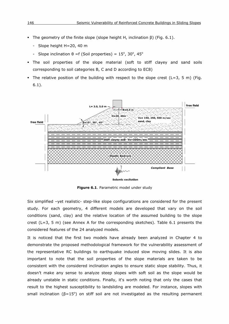
146 Seismic Vulnerability of Reinforced Concrete Buildings in Sliding Slopes
The geometry of the finite slope (slope height H, inclination β) (Fig. 6.1).
- Slope height H=20, 40 m
- Slope inclination θ =f (Soil properties) = 15ο, 30ο, 45ο
The soil properties of the slope material (soft to stiff clayey and sand soils
corresponding to soil categories B, C and D according to EC8)
The relative position of the building with respect to the slope crest (L=3, 5 m) (Fig.
6.1).
Figure 6.1. Parametric model under study
Six simplified –yet realistic- step-like slope configurations are considered for the present
study. For each geometry, 4 different models are developed that vary on the soil
conditions (sand, clay) and the relative location of the assumed building to the slope
crest (L=3, 5 m) (see Annex A for the corresponding sketches). Table 6.1 presents the
considered features of the 24 analyzed models.
It is noticed that the first two models have already been analyzed in Chapter 4 to
demonstrate the proposed methodological framework for the vulnerability assessment of
the representative RC buildings to earthquake induced slow moving slides. It is also
important to note that the soil properties of the slope materials are taken to be
consistent with the considered inclination angles to ensure static slope stability. Thus, it
doesn’t make any sense to analyze steep slopes with soft soil as the slope would be
already unstable in static conditions. Finally, it‘s worth noting that only the cases that
result to the highest susceptibility to landsliding are modeled. For instance, slopes with
small inclination (β=15ο) on stiff soil are not investigated as the resulting permanent

CHAPTER 6: Fragility curves for low-rise RC buildings subjected to slow-moving slides 147
deformation and consequently the building expected damage would be negligible and
thus out of the scope of this study.
Figure 6.2 shows the considered upslope and downslope variation of shear wave velocity
Vs with depth whereas Table 6.2 presents the assumed properties for the soil materials
and the elastic bedrock. As thoroughly presented in Chapter 4, the numerical analysis is
based on an uncoupled approach and involves two consecutive steps. First, the
differential permanent displacements at the building’s foundation level are estimated
using a plane strain FLAC2D (Itasca 2008) finite difference non-linear dynamic slope
model considering the foundation compliance. The seismic input applied along the base of
the dynamic model consists of a suite of 7 real acceleration time histories from different
earthquakes worldwide recorded on rock outcropping conditions and scaled at different
level of PGA i.e. 0.3 g, 0.5g, 0.7g and 0.9g (see Chapter 4, §4.3.1). Some additional
analyses for lower levels of PGA (e.g. 0.1 g) were deemed necessary for certain models
(e.g. model 21) in order to obtain reliable results for all damage states. Then, the
calculated differential displacements are imposed to the Seismostruct (Seismosoft,
SeismoStruct 2011) building model at the foundation level to assess the building’s
response for the different applied landslide displacements induced by the earthquake. A
high code designed single bay-single storey structure with flexible foundation system
located in the vicinity of the slope’s crest (L=3, 5 m) is considered in all analyzed cases
herein. Its geometrical, strength and stiffness characteristics are identical to the ones of
the structure on isolated footings described in Chapter 4, §4.3.2. Limit states are defined
in terms of threshold values of steel and concrete material strain for both “low” and
“high” code designed RC buildings (see Chapter 4, § 4.4.1). The results are presented in
terms of fragility curves as a function of PGA at the outcrop or PGD at the slope area.
Two different methodologies to derive the log-normally distributed parameters of the
fragility functions are presented in Chapter 4, § 4.4.2. These have been found to yield
results that are generally in good agreement and as such they can be equally
implemented to construct the fragility curves.
It ‘s worth noting that the computational demand for the derivation of fragility curves is
very large. Analysis time for the 24 models subjected to the two-step numerical approach
is about 1000 hours on a fast PC (Intel Core i7-2600 CPU, 3.4 GHz, 4.0 GByte of RAM) at
the time of the current study.

148 Seismic Vulnerability of Reinforced Concrete Buildings in Sliding Slopes
Figure 6.2. Upslope (a) and downslope (b) Vs variation with depth for the analyzed soil profiles
(soil classification according to EC8)
(a)
(b)
CHAPTER 6: Fragility curves for low-rise RC buildings subjected to slow-moving slides 149
6.2.1 Derivation of fragility curves
The parametric analysis results to the construction of fragility curves (Figure 6.3) as a
function of PGA at the outcrop and PGD at the slope area for the different investigated
models presented in Table 6.1. The Maximum Likelihood method as described in Chapter
4, section 4.4.2.2 is used herein to estimate the log-normal parameters (median and log-
standard deviation) of the fragility relationships. Tables 6.3 and 6.4 present the derived
median and log-standard deviation for all the analyzed models when using PGA at the
outcrop and PGD at the slope area as a metric of the landslide intensity respectively.
The fragility curves presented below can be used to assess the vulnerability of low-rise,
“high-code” RC buildings on isolated footings subjected to seismically induced slow
moving slides for a variety of slope configurations and site conditions. Similar curves,
generally associated with a more rapid transition from slight damage to collapse could be
derived for “low-code” RC frame structures (see section 6.3.5 and Annex B).
It is noted that PGD refers to the response of the landslide to cyclic loading (and not to
the initial triggering force) that is then correlated to differential permanent displacement
at the foundation level and to structural distortion and damage. Thus, the derived curves
as a function of PGD at the slope area, although initially developed to deal with
earthquake induced landslide displacements, they can also be implemented to buildings
impacted by non-earthquake related slow-moving slides.
It is seen that the structure’s vulnerability may vary significantly with respect to the
various considered features. A first comparison is facilitated by looking at just the
medians of the various analyzed models. Thus, among the analyzed cases, models 23
and 21 would suffer the highest vulnerability whereas models 20 and 18 would sustain
the lowest vulnerability measured in terms of expected median values of PGA and PGD
respectively. The estimated β-values that represent the dispersion of the results are
found to vary from 0.25 to 0.56 and from 0.36 to 0.94 when considering PGA and PGD
respectively as an intensity parameter. To better illustrate the influential role of each
parameter to the building’s expected damage level several comparative plots of fragility
functions are presented in the following subsections.

150 Seismic Vulnerability of Reinforced Concrete Buildings in Sliding Slopes
Table 6.1. Model features for the parametric analysis
Geometry model Slope inclination β (degrees)
Slope height H (m)
V s,30 (m/sec) Soil Distance from the
crest L (m)
Geometry 1 model 1 30 20 250 medium dense sand 3
model 2 30 20 250 relatively stiff clay 3
model 3 30 20 250 medium dense sand 5
model 4 30 20 250 relatively stiff clay 5
Geometry 2 model 5 30 40 250 medium dense sand 3
model 6 30 40 250 relatively stiff clay 3
model 7 30 40 250 medium dense sand 5
model 8 30 40 250 relatively stiff clay 5
Geometry 3 model 9 15 20 150 loose sand 3
model 10 15 20 150 soft clay 3
model 11 15 20 150 loose sand 5
model 12 15 20 150 soft clay 5
Geometry 4 model 13 15 40 150 loose sand 3
model 14 15 40 150 soft clay 3
model 15 15 40 150 loose sand 5
model 16 15 40 150 soft clay 5
Geometry 5 model 17 45 20 500 dense sand 3
model 18 45 20 500 stiff clay 3
model 19 45 20 500 dense sand 5
model 20 45 20 500 stiff clay 5
Geometry 6 model 21 45 40 500 dense sand 3
model 22 45 40 500 stiff clay 3
model 23 45 40 500 dense sand 5
model 24 45 40 500 stiff clay 5

CHAPTER 6: Fragility curves for low-rise RC buildings subjected to slow-moving slides 151
Table 6.2. Varying soil properties of the analyzed slope configurations
Elastic bedrock
Stiff soil Relatively stiff soil Soft soil sand clay sand clay sand clay
Constitutive model Elastic Mohr Coulomb
Mohr Coulomb
Mohr Coulomb Mohr Coulomb Mohr
Coulomb Mohr
Coulomb Dry density (kg/m3) 2300 2000 2000 1800 1800 1700 1700
Young's modulus (KPa) 4.321·106 1.300·106 1.300·106 2.925·105 2.925·105 9.945·104 9.945·104 Poisson's ratio 0.3 0.3 0.3 0.3 0.3 0.3 0.3
Drained Bulk modulus K (KPa) 3.600·106 1.0833·106 1.083·106 2.438·105 2.438·105 8.288·104 8.288·104 Shear modulus G (KPa) 1.662·106 5.0000·105 5.000·105 1.125·105 1.125·105 3.825·104 3.825·104
Cohesion c (KPa) - 10 50 0 10 0 5
Friction angle φ (degrees) - 44 27 36 25 25 15 Hydraulic conductivity (m·sec-1) 5·10-07 1·10-05 1·10-07 1·10-05 1·10-07 1·10-05 1·10-07
P-wave velocity Vp (m/sec) 1590.20 935.41 935.41 467.71 467.71 280.62 280.62 Shear wave velocity Vs (m/sec) 850.00 500.00 500.00 250.00 250.00 150.00 150.00
Max. allowed zone size (m) 8.50 5.00 5.00 2.50 2.50 1.50 1.50 Max. Allowed frequency 10.00 10.00 10.00 10.00 10.00 10.00 10.00

152 Seismic Vulnerability of Reinforced Concrete Buildings in Sliding Slopes
Figure 6.3. Fragility curves as a function of PGA (left) and PGD (right) derived from the parametric
analysis

CHAPTER 6: Fragility curves for low-rise RC buildings subjected to slow-moving slides 153
Figure 6.3. (Continued) - Fragility curves as a function of PGA (left) and PGD (right) derived from
the parametric analysis

154 Seismic Vulnerability of Reinforced Concrete Buildings in Sliding Slopes
Figure 6.3. (Continued) - Fragility curves as a function of PGA (left) and PGD (right) derived from
the parametric analysis

CHAPTER 6: Fragility curves for low-rise RC buildings subjected to slow-moving slides 155
Figure 6.3. (Continued) - Fragility curves as a function of PGA (left) and PGD (right) derived from
the parametric analysis

156 Seismic Vulnerability of Reinforced Concrete Buildings in Sliding Slopes
Figure 6.3. (Continued) - Fragility curves as a function of PGA (left) and PGD (right) derived from
the parametric analysis

CHAPTER 6: Fragility curves for low-rise RC buildings subjected to slow-moving slides 157
Figure 6.3. (Continued) - Fragility curves as a function of PGA (left) and PGD (right) derived from
the parametric analysis

158 Seismic Vulnerability of Reinforced Concrete Buildings in Sliding Slopes
Table 6.3. Parameters of fragility functions for all the analyzed models when using PGA as an intensity measure
Model Median PGA (g)
Dispersion β LS1 (g) LS2 (g) LS3 (g) LS4 (g)
1 0.22 0.39 0.58 0.81 0.37
2 0.34 0.75 1.12 1.61 0.40
3 0.31 0.46 0.74 1.00 0.36
4 0.34 0.75 1.12 1.61 0.40
5 0.17 0.28 0.49 0.74 0.43
6 0.27 0.57 1.03 1.53 0.50
7 0.19 0.41 0.66 0.92 0.38
8 0.21 0.46 0.85 1.23 0.50
9 0.29 0.51 0.84 1.17 0.45
10 0.25 0.63 1.17 2.00 0.51
11 0.35 0.62 0.99 1.43 0.42
12 0.25 0.54 1.03 1.58 0.48
13 0.27 0.51 0.82 1.12 0.44
14 0.24 0.64 1.12 1.59 0.48
15 0.32 0.61 0.97 1.29 0.40
16 0.21 0.51 0.99 1.47 0.52
17 0.23 0.35 0.55 0.81 0.39
18 1.46 - - - 0.25
19 0.26 0.41 0.65 0.90 0.37
20 1.60 - - - 0.38
21 0.12 0.19 0.25 0.30 0.44
22 0.88 1.71 - - 0.56
23 0.04 0.13 0.22 0.38 0.55
24 0.63 1.24 - - 0.55

CHAPTER 6: Fragility curves for low-rise RC buildings subjected to slow-moving slides 159
Table 6.4. Parameters of fragility functions for all the analyzed models when using PGD as an intensity measure
Model Median PGD (m)
Dispersion β LS1 (m) LS2 (m) LS3 (m) LS4 (m)
1 0.14 0.37 0.80 1.54 0.42
2 0.25 0.99 2.29 - 0.45
3 0.26 0.53 1.36 2.30 0.45
4 0.25 0.99 2.29 - 0.45
5 0.19 0.44 0.95 1.66 0.40
6 0.33 0.99 2.20 - 0.39
7 0.26 0.70 1.40 2.50 0.36
8 0.23 0.69 1.68 3.26 0.43
9 0.23 0.58 1.20 2.02 0.38
10 0.30 1.07 2.79 - 0.43
11 0.29 0.78 1.61 2.70 0.37
12 0.29 0.90 2.24 - 0.43
13 0.24 0.63 1.33 2.30 0.39
14 0.32 1.28 3.05 - 0.46
15 0.32 0.85 1.97 3.18 0.39
16 0.30 0.98 2.33
0.45
17 0.09 0.18 0.47 0.91 0.43
18 3.87 - - - 0.94
19 0.08 0.24 0.56 1.01 0.44
20 1.83 - - - 0.72
21 0.04 0.16 0.45 0.67 0.50
22 1.13 3.21 - - 0.51
23 0.14 0.22 0.52 0.99 0.48
24 0.66 1.82 - - 0.56
6.2.1.1. Effect of slope inclination
The influence of the slope inclination to the fragility curves in terms of PGA and PGD are
presented in Figures 6.4 and 6.5 respectively for varying slope inclinations (15ο, 30ο, 45ο)
considering both sand (models 1, 9 and 17) and clayey slopes (models 2, 10 and 18). In
particular, the fragility curves for extensive (Figs. 6.4) and slight (Figs. 6.5) damage are
presented for the sand and clayey slope respectively. As shown in Table 6.1, soft,
relatively stiff and stiff soil materials are considered for the 15o, 30o and 45o slope
configurations respectively that distinguish different mechanical parameters for the sand
and clay slopes (see Table 6.2). The height of the slope for the herein examined models
is 20 m.

160 Seismic Vulnerability of Reinforced Concrete Buildings in Sliding Slopes
It is shown that the slope inclination plays a fundamental role in the fragility analysis of
the building standing next to the slope’s edge. However, it should be regarded in
conjunction to the slope soil properties to obtain meaningful conclusions. Thus, for the
sand slope, the building would suffer more damage as the slope inclination increases.
On the contrary, for the clayey slope, the building is expected to sustain less structural
damage when standing on the 45o inclined slope compared to the gentler ones due to the
stiff cohesive soil conditions assumed for the steep slope configuration.
These trends are generally evident when considering both PGA and PGD as intensity
measures.
Figure 6.4. Fragility curves for extensity damage as a function of PGA (left) and PGD (right) when
varying slope inclination [β=f (Soil properties) = 15ο, 30ο, 45ο] for sand slopes
Figure 6.5. Fragility curves for slight damage as a function of PGA (left) and PGD (right) when
varying slope inclination [β=f (Soil properties) = 15ο, 30ο, 45ο] for clayey slopes
6.2.1.2. Effect of slope height
To demonstrate the influence of the slope height on the vulnerability of the building to
permanent ground displacement due to the landslide impact, comparative plots of

CHAPTER 6: Fragility curves for low-rise RC buildings subjected to slow-moving slides 161
fragility curves as a function of PGA and PGD when varying slope height (H= 20, 40m)
for sand and clayey slopes are presented in Figures 6.6 and 6.7 respectively.
Figure 6.6. Fragility curves as a function of PGA (left) and PGD (right) when varying slope height
(H= 20, 40m) for sand slopes

162 Seismic Vulnerability of Reinforced Concrete Buildings in Sliding Slopes
Figure 6.7. Fragility curves as a function of PGA (left) and PGD (right) when varying slope height
(H= 20, 40m) for clayey slopes
In overall, the slope height can moderately affect the structure’s fragility. Different
trends are revealed depending on the selected intensity measure (PGA or PGD) and the
inclination angle of the analyzed slopes (15o, 30o, 45o). These trends seem to hold
irrespective of the type (sand or clayey) of the slope soil materials involved.
When using PGA as an intensity parameter, it is seen that the vulnerability of the building
increases with the slope height. As it would be normally expected, this increase is more
pronounced for the 45o steep slope configurations (e.g. models 17, 18, 23, 24) whereas
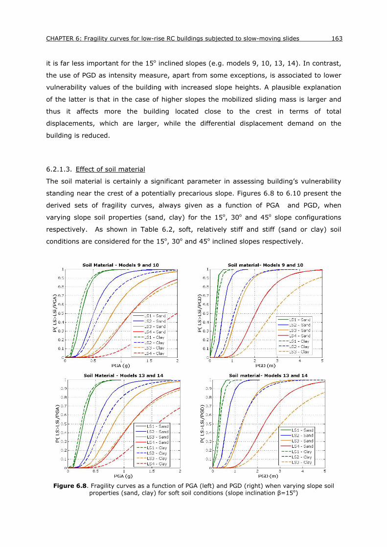
CHAPTER 6: Fragility curves for low-rise RC buildings subjected to slow-moving slides 163
it is far less important for the 15o inclined slopes (e.g. models 9, 10, 13, 14). In contrast,
the use of PGD as intensity measure, apart from some exceptions, is associated to lower
vulnerability values of the building with increased slope heights. A plausible explanation
of the latter is that in the case of higher slopes the mobilized sliding mass is larger and
thus it affects more the building located close to the crest in terms of total
displacements, which are larger, while the differential displacement demand on the
building is reduced.
6.2.1.3. Effect of soil material
The soil material is certainly a significant parameter in assessing building’s vulnerability
standing near the crest of a potentially precarious slope. Figures 6.8 to 6.10 present the
derived sets of fragility curves, always given as a function of PGA and PGD, when
varying slope soil properties (sand, clay) for the 15o, 30o and 45o slope configurations
respectively. As shown in Table 6.2, soft, relatively stiff and stiff (sand or clay) soil
conditions are considered for the 15o, 30o and 45o inclined slopes respectively.
Figure 6.8. Fragility curves as a function of PGA (left) and PGD (right) when varying slope soil
properties (sand, clay) for soft soil conditions (slope inclination β=15ο)

164 Seismic Vulnerability of Reinforced Concrete Buildings in Sliding Slopes
It is observed that slopes consisting of clay material generally demonstrate better
performance compared to sands when subjected to differential permanent ground
displacements, resulting to lower vulnerability levels for the building. This is largely due
to the inherent cohesive behavior of clay soil material that is associated to the formation
of larger and deeper sliding surfaces. Thus, the considered one-bay building located at a
close distance (i.e. 3m) from the slope’s crest would be practically within the sliding mass
and therefore it is primarily expected to move uniformly with the landslide mass rather
than to distort differentially. The above observation is more noticeable as the slope
inclination increases, i.e. for the stiffer clayey soil materials.
Figure 6.9. Fragility curves as a function of PGA (left) and PGD (right) when varying slope soil
properties (sand, clay) for relatively stiff soil conditions (slope inclination β=30ο)

CHAPTER 6: Fragility curves for low-rise RC buildings subjected to slow-moving slides 165
Figure 6.10. Fragility curves as a function of PGA (left) and PGD (right) when varying slope soil
properties (sand, clay) for stiff soil conditions (slope inclination β=45ο)
6.2.1.4. Effect of the foundation location with respect to the slope’s crest
The distance of the assumed building from the crest of the slope may also considerably
influence its vulnerability to the permanent landslide displacement. Figures 6.11 and 6.12
display the derived sets of fragility curves when varying the distance from the crest (L=
3, 5m) for sand and clayey slopes respectively. Different observations can be made
depending on the type of the considered slope soil materials. For sand slopes, the
building is expected to suffer less damage as the distance from the crest increases. On
the contrary, for the clayey slopes, the more distant building from the crest would be
more vulnerable. This differentiation lies again on the nature of the slope soil materials
involved that are associated to the formation of sliding surfaces that may vary for very
small and shallow for sands brittle slopes to large and deep for clayey deformable slopes.
Thus, the assumed one-bay building standing at 3m from the crest of the clayey slope is
basically within the landslide mass and moves rather uniformly as a rigid body whereas
for increasing distances from the crest (5 m) the building shifts (partially) outside the
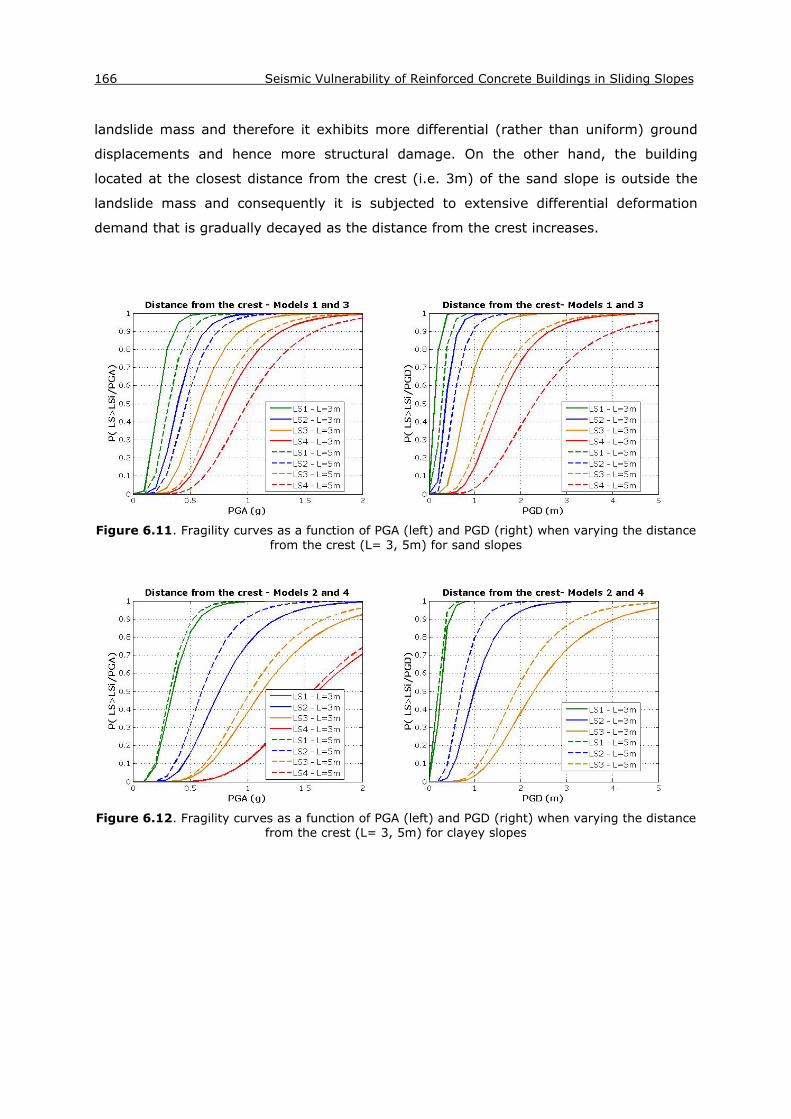
166 Seismic Vulnerability of Reinforced Concrete Buildings in Sliding Slopes
landslide mass and therefore it exhibits more differential (rather than uniform) ground
displacements and hence more structural damage. On the other hand, the building
located at the closest distance from the crest (i.e. 3m) of the sand slope is outside the
landslide mass and consequently it is subjected to extensive differential deformation
demand that is gradually decayed as the distance from the crest increases.
Figure 6.11. Fragility curves as a function of PGA (left) and PGD (right) when varying the distance
from the crest (L= 3, 5m) for sand slopes
Figure 6.12. Fragility curves as a function of PGA (left) and PGD (right) when varying the distance
from the crest (L= 3, 5m) for clayey slopes

CHAPTER 6: Fragility curves for low-rise RC buildings subjected to slow-moving slides 167
6.2.2 Generalized fragility curves
Seven sets of fragility curves both in terms of PGA and PGD (Fig. 6.13) are proposed
herein that could be used for engineering applications based on the main features that
proved to be the most influential in assessing the vulnerability of the building to the
differential permanent deformation due to the landslide hazard. These are principally the
slope inclination and the soil material of the slope that are found to be highly correlated.
The slope height is also proved to be a significant contributor to the building’s fragility for
the steep sand slope configurations. Thus, for the 45o inclined sand slopes fragility curves
are also differentiated with respect to the considered slope height (H=20, 40 m). The
latter curves are probably less accurate than the others as they are based on a smaller
simulated dataset. It is noted that the proposed curves have been constructed
considering the most adverse position of the building with respect to the landslide that
was found to be different for sand and clay slopes. It is also important to note that the
curves presented herein refer to “high-code”, adequately confined RC frame structures.
The corresponding suggested curves accounting for “low-code”, poorly confined frames
are presented in Annex B. Tables 6.5 and 6.6 present the median and dispersions of the
suggested curves when using PGA and PGD as an intensity measure respectively.
Figure 6.13. Proposed fragility curves as a function of PGA (left) and PGD (right) for high-code,
low-rise RC frame buildings subjected to permanent landslide displacements

168 Seismic Vulnerability of Reinforced Concrete Buildings in Sliding Slopes
Figure 6.13. (Continued)- Proposed fragility curves as a function of PGA (left) and PGD (right) for
high-code, low-rise RC frame buildings subjected to permanent landslide displacements

CHAPTER 6: Fragility curves for low-rise RC buildings subjected to slow-moving slides 169
Figure 6.13. (Continued)- Proposed fragility curves as a function of PGA (left) and PGD (right) for
high-code, low-rise RC frame buildings subjected to permanent landslide displacements
As already shown, the building founded upon sand slopes is expected to demonstrate a
greater damaging potential than the respective clayey ones. The corresponding curves
referring to sand slopes are generally shifted to the left compared to clays and they are
associated with a more rapid transition from slight to complete damage limits. These
differences are becoming much more pronounced as the slope inclination increases.
Among the considered cases, the sand steep, high-rise slope and clay steep slope
configurations are producing the most and the least damage respectively on the building.

170 Seismic Vulnerability of Reinforced Concrete Buildings in Sliding Slopes
The dispersion of the suggested curves is found to vary from 0.39 to 0.66 and from 0.40
to 0.50 when considering PGA and PGD respectively as an intensity parameter. As shown
on the tables presented above, the larger β values are expected for the 45o slope
configurations and for clayey soil materials.
Table 6.5. Parameters of the proposed fragility functions using PGA as an intensity measure
Parametric models
Median PGA (g) Dispersion β LS1
(g) LS2 (g)
LS3 (g)
LS4 (g)
sand_β30 0.20 0.34 0.54 0.76 0.40 clay_β30 0.27 0.53 0.93 1.37 0.46 sand_β15 0.28 0.50 0.83 1.17 0.44 clay_β15 0.23 0.54 1.01 1.51 0.50
sand_β45_H20 0.23 0.35 0.55 0.81 0.39 sand_β45_H40 0.12 0.19 0.25 0.30 0.44
clay_β45 1.04 1.77 - - 0.66
Table 6.6. Parameters of the proposed fragility functions using PGD as an intensity measure
Parametric models
Median PGD (m) Dispersion β LS1
(m) LS2 (m)
LS3 (m)
LS4 (m)
sand_β30 0.15 0.39 0.87 1.64 0.43 clay_β30 0.22 0.67 1.70 3.43 0.43 sand_β15 0.24 0.60 1.29 2.19 0.40 clay_β15 0.28 0.94 2.32 - 0.43
sand_β45_H20 0.09 0.18 0.47 0.91 0.43 sand_β45_H40 0.04 0.16 0.45 0.67 0.50
clay_β45 0.77 1.72 - - 0.47
6.3 Sensitivity analysis
Apart from the main parametric investigation, a sensitivity analysis is also conducted to
examine the relative influence of various additional parameters on the structure’s
performance and fragility. In all analyzed cases hereafter we refer to a 30ο inclined and
20m high slope configuration consisting of a relatively stiff upslope soil material
corresponding to soil class C according to EC8 (Vs=250 m/s), to allow for direct
comparison with the already analyzed reference models 1 to 4 (see Table 6.1) .
6.3.1 Effect of water table
The influence of groundwater in altering the slope‘s seismic response and the extent of
ground and foundation irreversible deformation and consequently the expected structural

CHAPTER 6: Fragility curves for low-rise RC buildings subjected to slow-moving slides 171
damage is investigated herein. In particular, two hydraulic conditions are examined: a
first one with no water (dry materials, models 1 and 2) and a second with a water table
level located at 80% of the slope height (saturated materials underneath the water table
and dry materials above). Non-liquefiable upslope soil deposits are considered in this
research as the proposed methodology (Chapter 4) is dealing with slow movements. The
analyzed slope dynamic models (β=30ο, H=20m, Vs=250m/sec) vary only in the
hydrological and soil conditions studied. A single bay-single story bare frame RC building
with flexible foundation system standing 3m from the slope’s crest is considered for all
the analysis cases.
The results are given in terms of fragility functions that account for dry and partially
saturated soil conditions. The corresponding plots of the fragility diagrams are illustrated
in Figures 6.14 and 6.15 for slopes consisting of sand and clay soil materials respectively.
For sand soil conditions, the presence of water results in a slight increase on the total
and differential displacement imposed to the building at the foundation level that causes
a shift of the respective curves to the left (Fig. 6.14). On the contrary, the corresponding
displacement is decreased in case of clayey materials yielding to lower vulnerability levels
(Fig. 6.15). A reasonable explanation could be the following: the presence of
groundwater might potentially reduce the static factor of safety of the slope giving rise to
instability and/or permanent displacement that was found to be more pronounced for
higher permeability values i.e. for the sand soil material (Srivastava et al., 2010). In
addition, its presence is associated with the formation of larger sliding surfaces that, in
relation to the proximity of the structure to the slope’s crest, results to reduced
differential displacements for the specified building (located 3m from the crest) resting
on the clay slope and to slightly increased differential deformation for the building on the
sand slope.
Figure 6.14. Fragility curves as a function of PGA (left) and PGD (right) when varying the
hydraulic conditions (dry or partially saturated materials) for sand slopes

172 Seismic Vulnerability of Reinforced Concrete Buildings in Sliding Slopes
Figure 6.15. Fragility curves as a function of PGA (left) and PGD (right) when varying the
hydraulic conditions (dry or partially saturated materials) for clayey slopes
6.3.2 Effect of strain softening in slope soil material
In all analyses performed so far non-softening slope soil materials are considered.
However, quite often brittle soils in slopes may exhibit a strain softening behavior when
subjected to cyclic loading. In these materials, a progressive failure can occur owing to
the reduction of strength with increasing strain (e.g. Bjerrum, 1967; Dounias, 1988;
Troncone, 2005; Conte et al., 2010; Kourkoulis et al., 2010).
In order to capture such phenomena, a simple elastoplastic constitutive model of the
Mohr-Coulomb type coupled with an isotropic strain-softening rule, able to simulate the
reduction of the strength parameters after the onset of plastic yield, may be used (Fig.
6.16). The use of such models allows for simulating the formation of shear zones in
which strain localized and hence are capable to reproduce a progressive failure process
along a potential rupture surface in slopes. The model requires the specification of peak
and residual strength as a function of the deviatoric plastic strain. A piecewise-linear
variation of strength parameters with plastic shear strain is adopted herein to simulate
the strain softening law (Fig. 6.17). The determination of peak and residual values of
cohesion, friction angle and dilation as well as the yield and failure plastic strains depend
on the soil type and should be based on appropriate laboratory and in situ tests. From a
computational point of view, the adaptation of such a model presents many difficulties
associated with lack of convergence due to numerical/physical instability and mesh
dependency (e.g. Troncone 2005; Conte et al, 2010; Kourkoulis et al., 2010). In the
present study, the proper element size of the slope dynamic model in the slope area was
determined through a parametric analysis to balance between accuracy and
computational efficiency as discussed in Kourkoulis et al. (2010).

CHAPTER 6: Fragility curves for low-rise RC buildings subjected to slow-moving slides 173
Following the calibration procedure discussed in Anastasopoulos et al. (2007) to model
medium dense Fontainebleau sand, the softening behavior of sand soil is determined
utilizing the values for strength and plastic strain given below: φp=39o, ψp=11o, φr=30o,
ψr=0o, yy=2%, yp=13.5%. The derived dynamic model, expect for the considered strain
softening slope material, distinguishes the same features with the analyzed model 1 (see
Table 6.1) to allow for direct comparisons. Figure 6.18 presents the derived sets of
fragility curves as a function of PGA and PGD considering a non-softening (model 1) and
a softening soil material. As we may see, the curves accounting for the slope soil
materials with strain softening behavior are more close together and are generally
associated with increased steepness and higher vulnerability levels. A physical
interpretation of this lies on the inherent softening behavior of the sand soil material,
which is simulated by reducing its friction angle and dilation from peak to residual with
increasing deviatoric shear strain.
More research is needed to analyze strain softening behavior of slopes in different soil
conditions (e.g. a stiff clay) and slope configurations. However, it‘s worth noting that
such analyzes are computationally expensive and therefore they are often warranted only
for site specific applications where detailed information on the soil parameters and strain
thresholds are available from in-situ or laboratory tests.
Figure 6.16. Two dimensional behavior of a linear elastic-softening plastic material (Potts and
Zbravkovi, 1999)

174 Seismic Vulnerability of Reinforced Concrete Buildings in Sliding Slopes
Figure 6.17. Idealization of the variation of cohesion, friction and dilation with plastic shear strain
to simulate strain softening soil behavior
Figure 6.18. Fragility curves as a function of PGA (left) and PGD (right) when considering (or not)
a strain softening material
6.3.3 Effect of foundation compliance
The parametric analyses conducted in section 6.2 refer to a simple single bay-single
storey RC bare frame structure founded on flexible foundation system (e.g. isolated
footings). However, as it has been thoroughly discussed Chapter 4, the stiffness of the
foundation system may considerably modify the deformation demand for the building and
its resistance ability and therefore its vulnerability.
The fragility curves (Figs. 6.20 and 6.21), as developed in Chapter 4, are also presented
herein for the building founded on two different foundation systems (Fig. 6.19), namely
isolated footings (models 1 and 2) and a continuous raft foundation, to stress the
significant role of foundation flexibility in assessing the vulnerability of the building to the
differential permanent displacement due to the landslide hazard. The building is assumed
to be standing 3 m from the crest of a potentially unstable sand and clayey slope. It is

CHAPTER 6: Fragility curves for low-rise RC buildings subjected to slow-moving slides 175
noticed that simulation issues, concerning e.g. the modeling of the foundation system,
have been extensively presented in Chapter 4 and are not repeated herein.
Figure 6.19. Schematic view of the analyzed single bay-single storey RC bare-frame structures
with flexible (left) and stiff (right) foundations
Figure 6.20. Fragility curves as a function of PGA (left) and PGD (right) when varying the
flexibility of the foundation system for sand slopes
Figure 6.21. Fragility curves as a function of PGA (left) and PGD (right) when varying the
flexibility of the foundation system for clayey slopes
Overall, the computed fragility curves display an important reduction on the structure’s
expected damages when a stiff foundation system rather than a flexible one is

176 Seismic Vulnerability of Reinforced Concrete Buildings in Sliding Slopes
considered. This observation is noticeable for both slopes consisting of sand and clay
material. Thus, the fragility curves proposed in 6.2.2 that refer to buildings on flexible
foundation are expected to be always on the safe site. Once the type and relative
stiffness of the foundation system is adequately known (e.g. for site specific applications
and critical structures), the suggested curves for flexible foundations (isolated footings)
could be properly modified to capture the influence of the foundation flexibility on the
structure’s performance and vulnerability.
6.3.4 Effect of building geometry
One-bay one-storey RC frame buildings have been investigated so far. Such simple
structures have been found to adequately capture the performance of the low-rise RC
frame buildings to permanent ground deformations (e.g. Bird et al. 2005; 2006;
Negulescu and Foerster 2010).
However, for the sake of completeness, it was decided to carry out a sensitivity analysis
on the geometry of the building (e.g. number of storeys, number of bays) considering
different foundation systems and slope material properties to identify possible trends in
its vulnerability.
6.3.4.1. Number of storeys
The effect of number of storeys on the expected differential deformation demand for the
building and consequently on its structural response and vulnerability is explored herein
considering different foundation types and slope soil materials. To this aim, 1 bay - 2
storey RC bare frame structures are analyzed (Fig. 6.22) assuming the same slope
dynamic properties (i.e. see models 1 and 2) and typological parameters as for the
respective 1 bay- 1 storey buildings (see Fig. 6.19 for the corresponding sketches).
Worthy of note is the fact that the load applied on the foundation system of the two-
storey frames is doubled with respect to the corresponding load on the one-storey frame
structure resulting to increased slope and foundation deformations.
Figures 6.23 to 6.26 depict the derived sets of fragility curves when considering a one-
storey and a two-storey structure accounting for different foundation systems (flexible,
stiff) and slope soil materials (sand, clay).
In all cases, the two-storey building is expected to sustain more damage compared to
the corresponding one-storey building. This is largely due to the heavier loaded
foundation assumed in the simulation of the two-storey building that gives rise to
increased permanent displacements at the slope area. In this regard, it might deem
necessary to modify the proposed curves in 6.2.2 for weightily loaded structures.
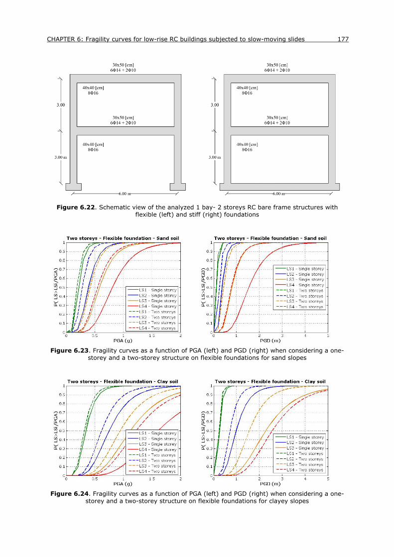
CHAPTER 6: Fragility curves for low-rise RC buildings subjected to slow-moving slides 177
Figure 6.22. Schematic view of the analyzed 1 bay- 2 storeys RC bare frame structures with
flexible (left) and stiff (right) foundations
Figure 6.23. Fragility curves as a function of PGA (left) and PGD (right) when considering a one-
storey and a two-storey structure on flexible foundations for sand slopes
Figure 6.24. Fragility curves as a function of PGA (left) and PGD (right) when considering a one-
storey and a two-storey structure on flexible foundations for clayey slopes

178 Seismic Vulnerability of Reinforced Concrete Buildings in Sliding Slopes
Figure 6.25. Fragility curves as a function of PGA (left) and PGD (right) when considering a one-
storey and a two-storey structure on stiff foundations for sand slopes
Figure 6.26. Fragility curves as a function of PGA (left) and PGD (right) when considering a one-
storey and a two-storey structure on flexible foundations for clayey slopes
6.3.4.2. Number of bays
The number of bays of the considered building is an additional parameter that is selected
to vary in this research. In particular, 2-bay RC bare frames are also studied considering
different foundation systems and slope soil conditions. A schematic view of the analyzed
two-bay structures is illustrated in Figure 6.27.
The performance of these structures is compared with the corresponding performance of
the single-bay frames (see Fig. 6.19) by means of fragility functions considering common
features for the slope dynamic models (model 1 and 2) and the structural typology. The
building is assumed to be located 3m from the crest of the slope. It is noticed that the
surcharge load on the foundation of the two-bay frame that is applied to an extended
zone (determined by the foundation width), may contribute in deviating the path of

CHAPTER 6: Fragility curves for low-rise RC buildings subjected to slow-moving slides 179
excessive shearing deformation and consequently in altering the potential sliding surface
exhibited.
A graphical representation of the fragility relationships is given in Figures 6.28 to 6.31. It
is seen that, for the sand slope case, the two-bay frame would be less vulnerable
compared to the corresponding single-bay frame building. On the contrary, for the clay
slopes, the two-bay frame would suffer more damages than the single-bay one. These
observations hold true irrespective of the foundation typology considered; they are
associated to the relative position of the foundation to the potential sliding surface as
well as to the zone in which the surcharge load is applied. For the slopes consisting of
clayey soil material, the zone of the applied load on the foundation for the two-bay
building would be comparable in dimensions with the potential sliding surface and thus
the building would be partially outside the landslide mass resulting to increased
differential deformation compared to the single-bay case where a rather more uniform
movement of the building is anticipated. On the other hand, for the sand slope materials
this zone is quite larger than the expected possible sliding surface and therefore a
generally reduced differential deformation demand for the building is more likely.
Figure 6.27. Schematic view of the analyzed 2 bays- 1 storey RC bare frame structures with
flexible (top) and stiff (bottom) foundations

180 Seismic Vulnerability of Reinforced Concrete Buildings in Sliding Slopes
Figure 6.28. Fragility curves as a function of PGA (left) and PGD (right) when considering a one-
bay and a two-bay structure on flexible foundations for sand slopes
Figure 6.29. Fragility curves as a function of PGA (left) and PGD (right) when considering a one-
bay and a two-bay structure on flexible foundations for clay slopes
Figure 6.30. Fragility curves as a function of PGA (left) and PGD (right) when considering a one-
bay and a two-bay structure on stiff foundations for sand slopes

CHAPTER 6: Fragility curves for low-rise RC buildings subjected to slow-moving slides 181
Figure 6.31. Fragility curves as a function of PGA (left) and PGD (right) when considering a one-
bay and a two-bay structure on stiff foundations for clay slopes
6.3.5 Effect of building code design level
The code design level is another important parameter in assessing the vulnerability of RC
frame structures to the irreversible landslide displacement. Considering that low-code RC
buildings are poorly constructed structures characterized by a low level of confinement,
the limit steel strains needed to exceed post yield limit states should have lower values
compared to high-code, properly constructed RC buildings. As a consequence, different
limit state values were adopted for exceedance of extensive and complete damage for
low- and high-code frame RC buildings (see Chapter 4, Table 4.6) based on the work of
Crowley et al. (2004), Bird et al. (2005), Negulescu and Foerster (2010) and engineering
judgement. The corresponding fragility functions for the high- and low-code designed
buildings as a function of PGA and PGD assuming the same geometrical and hydro-
geological conditions (model 1) are depicted in Figure 6.32.
Figure 6.32. Fragility curves as a function of PGA (left) and PGD (right) when varying the code
design level

182 Seismic Vulnerability of Reinforced Concrete Buildings in Sliding Slopes
It is observed that for the 1st and 2nd limit states, low- and high-code RC frame buildings
experience quite similar performance. However, when extensive or complete damage to
the building members is anticipated, the deviation in the building performance for low-
and high-code designed buildings is expected to increase resulting to higher vulnerability
levels for low code buildings. This is due to the low levels of attainable limit strains
assumed for low-code building compared to high code, adequately confined structures.
Several portfolios of fragility curves for low-code buildings based on the most crucial
analyzed features are given in Annex B.
6.4 Conclusive remarks
Generic fragility curves both in terms of PGA and PGD have been proposed based on an
extensive parametric investigation and sensitivity analysis of various slope
configurations, soil properties and distances of the building with respect to the slope’s
crown. The features that have proved to affect more drastically the vulnerability of the
building to the differential permanent deformation due to the seismically induced
landslide hazard are the slope inclination in conjunction with the slope soil material. The
slope height has also turned out to significantly influence the building’s fragility for the
steep sand slope configurations. Based on the above observations, seven sets of fragility
curves have been suggested considering the most adverse position of the building with
respect to the landslide that was found to be different for sand and clay slopes.
Several additional parameters, namely the water table level, the consideration of a strain
softening landslide material, the flexibility of the foundation system, the number of bays
and storeys of the building and the code design level, have also been studied for specific
finite slope geometries and soil conditions, to illustrate the relative influence of each one
of them on the structure’s fragility. The influence of each parameter may vary with
respect to the slope soil material (e.g. for the water table) and the foundation compliance
(e.g. for the building geometry). Overall, their effect might potentially control the
structure’s fragility. It is noted, however, that a more in depth analysis of each of the
additional features is generally warranted only for case histories where adequate
quantitative data on the soil properties, slope geometry and building typologies are
available.

CHAPTER 7
Validation of the proposed method
7.1 Introduction
The reliability and accuracy of the proposed methodology (Chapter 4) is assessed
through the comparison of the analytically derived fragility curves with literature curves
and recorded building damage data from two real case histories: Kato Achaia slope in
Peloponnese –Greece and the Corniglio-Italy case study. In addition, in order to increase
the applicability band of the proposed methodological framework, more realistic fragility
curves are suggested for a representative building in Corniglio village.
7.2 Comparison of the developed fragility curves with literature curves
The validity of the developed curves is assessed through their comparison with respective
literature curves derived by different approaches. In particular, fragility curves based on
empirical damage data (Zhang and Ng, 2005), engineering judgement (NIBS, 2004) and
on numerical simulations (Negulescu and Foerster, 2010) are used for that comparison.
Moreover, fragility curves derived for buildings subjected to ground shaking on
horizontally layered soil deposits are used for approximate correlations with the ones
proposed in this study. The purpose of this comparison is twofold: first, to assess the
reliability of the proposed curves (mainly in terms of the order of magnitude) and second
to gain better insight into the relative extent of damage and the associated failure
mechanisms that dominate the structural response and fragility for structures subjected
to ground shaking and co-seismic slope deformation respectively.
Among the developed curves, the ones that are selected for the comparison refer to a
low-rise, high-code RC frame building resting on a shallow foundation of varying stiffness
characteristics (i.e. isolated footings, continuous raft foundation) located next to the
crest (i.e. 3m) of a 30o inclined sand slope (see Chapter 4). These curves generally
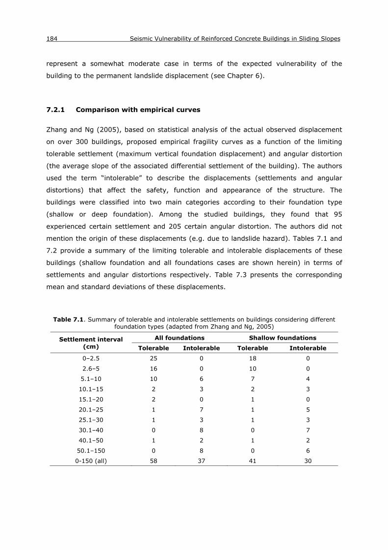
184 Seismic Vulnerability of Reinforced Concrete Buildings in Sliding Slopes
represent a somewhat moderate case in terms of the expected vulnerability of the
building to the permanent landslide displacement (see Chapter 6).
7.2.1 Comparison with empirical curves
Zhang and Ng (2005), based on statistical analysis of the actual observed displacement
on over 300 buildings, proposed empirical fragility curves as a function of the limiting
tolerable settlement (maximum vertical foundation displacement) and angular distortion
(the average slope of the associated differential settlement of the building). The authors
used the term “intolerable” to describe the displacements (settlements and angular
distortions) that affect the safety, function and appearance of the structure. The
buildings were classified into two main categories according to their foundation type
(shallow or deep foundation). Among the studied buildings, they found that 95
experienced certain settlement and 205 certain angular distortion. The authors did not
mention the origin of these displacements (e.g. due to landslide hazard). Tables 7.1 and
7.2 provide a summary of the limiting tolerable and intolerable displacements of these
buildings (shallow foundation and all foundations cases are shown herein) in terms of
settlements and angular distortions respectively. Table 7.3 presents the corresponding
mean and standard deviations of these displacements.
Table 7.1. Summary of tolerable and intolerable settlements on buildings considering different foundation types (adapted from Zhang and Ng, 2005)
Settlement interval (cm)
All foundations Shallow foundations
Tolerable Intolerable Tolerable Intolerable
0–2.5 25 0 18 0
2.6–5 16 0 10 0
5.1–10 10 6 7 4
10.1–15 2 3 2 3
15.1–20 2 0 1 0
20.1–25 1 7 1 5
25.1–30 1 3 1 3
30.1–40 0 8 0 7
40.1–50 1 2 1 2
50.1–150 0 8 0 6
0-150 (all) 58 37 41 30
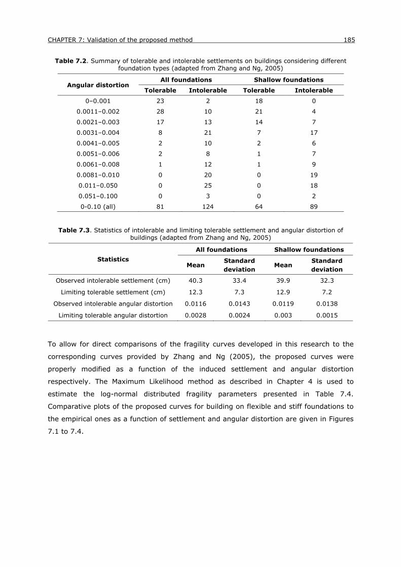
CHAPTER 7: Validation of the proposed method 185
Table 7.2. Summary of tolerable and intolerable settlements on buildings considering different foundation types (adapted from Zhang and Ng, 2005)
Angular distortion All foundations Shallow foundations
Tolerable Intolerable Tolerable Intolerable
0–0.001 23 2 18 0
0.0011–0.002 28 10 21 4
0.0021–0.003 17 13 14 7
0.0031–0.004 8 21 7 17
0.0041–0.005 2 10 2 6
0.0051–0.006 2 8 1 7
0.0061–0.008 1 12 1 9
0.0081–0.010 0 20 0 19
0.011–0.050 0 25 0 18
0.051–0.100 0 3 0 2
0-0.10 (all) 81 124 64 89
Table 7.3. Statistics of intolerable and limiting tolerable settlement and angular distortion of
buildings (adapted from Zhang and Ng, 2005)
Statistics All foundations Shallow foundations
Mean Standard deviation
Mean Standard deviation
Observed intolerable settlement (cm) 40.3 33.4 39.9 32.3
Limiting tolerable settlement (cm) 12.3 7.3 12.9 7.2
Observed intolerable angular distortion 0.0116 0.0143 0.0119 0.0138
Limiting tolerable angular distortion 0.0028 0.0024 0.003 0.0015
To allow for direct comparisons of the fragility curves developed in this research to the
corresponding curves provided by Zhang and Ng (2005), the proposed curves were
properly modified as a function of the induced settlement and angular distortion
respectively. The Maximum Likelihood method as described in Chapter 4 is used to
estimate the log-normal distributed fragility parameters presented in Table 7.4.
Comparative plots of the proposed curves for building on flexible and stiff foundations to
the empirical ones as a function of settlement and angular distortion are given in Figures
7.1 to 7.4.

186 Seismic Vulnerability of Reinforced Concrete Buildings in Sliding Slopes
Table 7.4. Fragility parameters of the proposed curves in terms of settlement and angular distortion
Limit state Flexible foundation Stiff foundation
Settlement (m)
Median
LS1 0.07 0.06
LS2 0.21 0.32
LS3 0.31 0.75
LS4 0.49 1.36
Dispersion β 0.39 0.42
Angular distortion
Median
LS1 0.006 0.007
LS2 0.018 0.029
LS3 0.037 0.061
LS4 0.064 0.100
Dispersion β 0.36 0.37
Overall, the comparison between the curves is judged satisfactory considering the large
uncertainty and variability involved and the fact that the empirically derived curves are
dealing with foundation movements irrespective of their origin (e.g. earthquake induced
landslide hazard) and the superstructure typology.
A good correlation is observed between the empirical curves and the proposed fragility
curves for the building when using Settlement as a metric of the landslide displacement.
A better match is detected for buildings on flexible foundation rather than on stiff ones.
The correlation is not so good when using Angular distortion as an intensity parameter.
In particular, the empirical curves are generally shift to the left predicting quite low
median values of limiting tolerable angular distortion and consequently increased
expected building damage. These low values are probably associated to loss of
functionality (e.g. due to tilting), which is not accounted for in the proposed numerically
derived curves, and not to structural damage to the building members.

CHAPTER 7: Validation of the proposed method 187
Figure 7.1. Comparison of the proposed fragility curves as a function of settlement for the building
on flexible foundation with the corresponding empirical curves provided by Zhang and Ng (2005)
Figure 7.2. Comparison of the proposed fragility curves as a function of settlement for the building
on stiff foundation with the corresponding empirical curves provided by Zhang and Ng (2005)

188 Seismic Vulnerability of Reinforced Concrete Buildings in Sliding Slopes
Figure 7.3. Comparison of the proposed fragility curves as a function of angular distortion for the building on flexible foundation with the corresponding empirical curves provided by Zhang and Ng
(2005)
Figure 7.4. Comparison of the proposed fragility curves as a function of angular distortion for the
building on stiff foundation with the corresponding empirical curves provided by Zhang and Ng (2005)
7.2.2 Comparison with expert judgment curves
HAZUS loss estimation methodology (NIBS, 2004) provided fragility curves for structures
subjected to earthquake-induced ground failure taking into account the expected mode of
failure and the foundation type (see also Chapter 3, § 3.3.2). Separate fragility curves

CHAPTER 7: Validation of the proposed method 189
distinguishing between ground failure due to lateral spreading and ground failure due to
ground settlement, and between shallow and deep foundations were proposed. Only one
combined Extensive/Complete damage state was considered. In essence, according to
HAZUS, buildings were assumed to be either undamaged or severely damaged due to
ground failure. Fragility curves were derived as a function of permanent ground
displacement (PGD) using a form similar to those used to estimate shaking damage.
Engineering judgment was used to develop a set of assumptions, which define building
fragility. Suggested median and lognormal standard deviation values in terms of PGD for
buildings on shallow foundations or buildings of unknown foundation type are given in
Table 7.5. As shown in the table, that lateral spread was judged to require significantly
more PGD to effect severe damage than ground settlement. This is due to the fact that
many buildings in lateral spread areas are generally expected to move with the spread,
but not to be severely damaged until the spread becomes quite significant.
Table 7.5. Suggested log-normally distributed fragility parameters of HAZUS for shallow/unknown foundations
Settlement PGD (m)
Lateral Spread PGD
(m)
Median 0.254 0.1524
Dispersion β 1.2 1.2
The expert judgemental curves provided by HAZUS are compared with the numerically
derived curves for extensive and complete damage for the building on flexible and stiff
foundations (Figs. 7.5 to 7.10). The herein proposed curves are given as a function of the
maximum permanent ground displacement vector (PGD), horizontal permanent ground
displacement (PHGD) and vertical permanent ground displacement (PVGD) at the slope
area, to permit the comparison with both HAZUS curves (Figs. 7.5 and 7.8) and
separately with the curves which account for lateral spreading (principally horizontal
movement) (Figs. 7.6 and 7.9) and settlement (principally vertical movement) (Figs. 7.7
and 7.10) respectively. The log-normal distributed fragility parameters of the proposed
curves in terms of PGD, PHGD and PVGD are presented in Table 7.6.
A good agreement between the proposed curves for the building on flexible foundation
and the respective HAZUS curves is observed, with the latter generally predicting larger
vulnerability values. However, the comparison is not satisfactory when considering a
building on stiff foundations. In particular, HAZUS curves are found to be far more
conservative, highlighting the influential role of foundation stiffness (that is not taken
into account in HAZUS methodology) in modifying (generally reducing) the building
vulnerability to the permanent landslide displacement.

190 Seismic Vulnerability of Reinforced Concrete Buildings in Sliding Slopes
Table 7.6. Fragility parameters of the proposed curves in terms of PGD, PHGD and PVGD
Limit state Flexible foundation Stiff foundation
PGD (m)
Median
LS1 0.14 0.24
LS2 0.37 0.96
LS3 0.80 2.35
LS4 1.54 -
Dispersion β 0.42 0.46
PHGD (m)
Median
LS1 0.12 0.19
LS2 0.31 0.81
LS3 0.67 2.08
LS4 1.35 3.66
Dispersion β 0.46 0.47
PVGD (m)
Median
LS1 0.08 0.13
LS2 0.22 0.49
LS3 0.43 1.15
LS4 0.80 1.88
Dispersion β 0.40 0.40
Figure 7.5. Comparison of the proposed fragility curves for extensive and complete damage as a function of permanent ground displacement (PGD) for the building on flexible foundation with the
corresponding expert judgment curves provided by HAZUS (NIBS, 2004)

CHAPTER 7: Validation of the proposed method 191
Figure 7.6. Comparison of the proposed fragility curves for extensive and complete damage as a
function of permanent horizontal ground displacement (PHGD) for the building on flexible foundation with the corresponding expert judgment curves provided by HAZUS (NIBS, 2004) for
ground failure due to lateral spreading
Figure 7.7. Comparison of the proposed fragility curves for extensive and complete damage as a function of permanent vertical ground displacement (PVGD) for the building on flexible foundation with the corresponding expert judgment curves provided by HAZUS (NIBS, 2004) for ground failure
due to settlement

192 Seismic Vulnerability of Reinforced Concrete Buildings in Sliding Slopes
Figure 7.8. Comparison of the proposed fragility curves for extensive damage as a function of
permanent ground displacement (PGD) for the building on stiff foundation with the corresponding expert judgment curves provided by HAZUS (NIBS, 2004)
Figure 7.9. Comparison of the proposed fragility curves for extensive and complete damage as a function of permanent horizontal ground displacement (PHGD) for the building on stiff foundation
with the corresponding expert judgment curves provided by HAZUS (NIBS, 2004) for ground failure due to lateral spreading
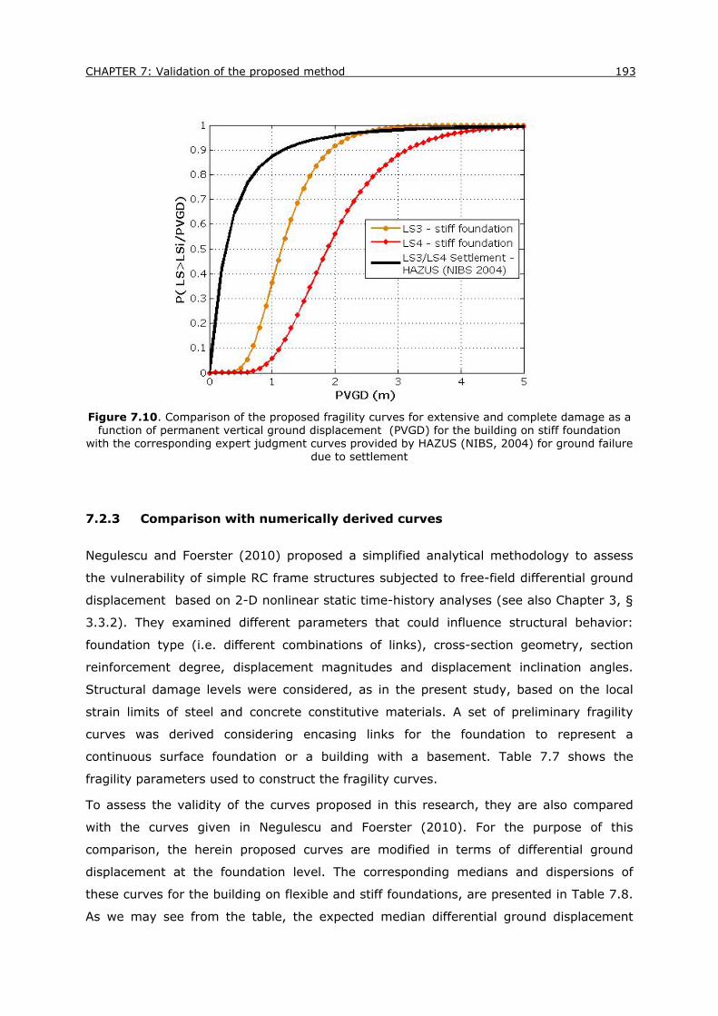
CHAPTER 7: Validation of the proposed method 193
Figure 7.10. Comparison of the proposed fragility curves for extensive and complete damage as a
function of permanent vertical ground displacement (PVGD) for the building on stiff foundation with the corresponding expert judgment curves provided by HAZUS (NIBS, 2004) for ground failure
due to settlement
7.2.3 Comparison with numerically derived curves
Negulescu and Foerster (2010) proposed a simplified analytical methodology to assess
the vulnerability of simple RC frame structures subjected to free-field differential ground
displacement based on 2-D nonlinear static time-history analyses (see also Chapter 3, §
3.3.2). They examined different parameters that could influence structural behavior:
foundation type (i.e. different combinations of links), cross-section geometry, section
reinforcement degree, displacement magnitudes and displacement inclination angles.
Structural damage levels were considered, as in the present study, based on the local
strain limits of steel and concrete constitutive materials. A set of preliminary fragility
curves was derived considering encasing links for the foundation to represent a
continuous surface foundation or a building with a basement. Table 7.7 shows the
fragility parameters used to construct the fragility curves.
To assess the validity of the curves proposed in this research, they are also compared
with the curves given in Negulescu and Foerster (2010). For the purpose of this
comparison, the herein proposed curves are modified in terms of differential ground
displacement at the foundation level. The corresponding medians and dispersions of
these curves for the building on flexible and stiff foundations, are presented in Table 7.8.
As we may see from the table, the expected median differential ground displacement
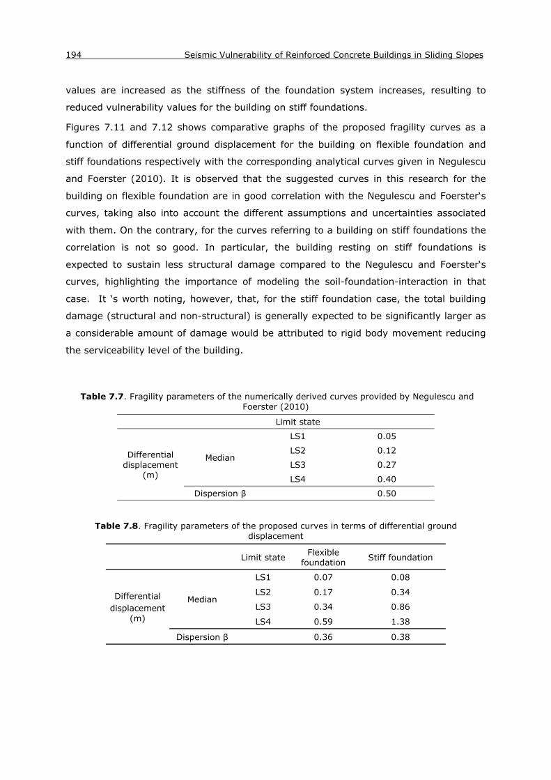
194 Seismic Vulnerability of Reinforced Concrete Buildings in Sliding Slopes
values are increased as the stiffness of the foundation system increases, resulting to
reduced vulnerability values for the building on stiff foundations.
Figures 7.11 and 7.12 shows comparative graphs of the proposed fragility curves as a
function of differential ground displacement for the building on flexible foundation and
stiff foundations respectively with the corresponding analytical curves given in Negulescu
and Foerster (2010). It is observed that the suggested curves in this research for the
building on flexible foundation are in good correlation with the Negulescu and Foerster‘s
curves, taking also into account the different assumptions and uncertainties associated
with them. On the contrary, for the curves referring to a building on stiff foundations the
correlation is not so good. In particular, the building resting on stiff foundations is
expected to sustain less structural damage compared to the Negulescu and Foerster‘s
curves, highlighting the importance of modeling the soil-foundation-interaction in that
case. It ‘s worth noting, however, that, for the stiff foundation case, the total building
damage (structural and non-structural) is generally expected to be significantly larger as
a considerable amount of damage would be attributed to rigid body movement reducing
the serviceability level of the building.
Table 7.7. Fragility parameters of the numerically derived curves provided by Negulescu and Foerster (2010)
Limit state
Differential displacement
(m)
Median
LS1 0.05
LS2 0.12
LS3 0.27
LS4 0.40
Dispersion β 0.50
Table 7.8. Fragility parameters of the proposed curves in terms of differential ground
displacement
Limit state Flexible
foundation Stiff foundation
Differential displacement
(m)
Median
LS1 0.07 0.08
LS2 0.17 0.34
LS3 0.34 0.86
LS4 0.59 1.38
Dispersion β
0.36 0.38

CHAPTER 7: Validation of the proposed method 195
Figure 7.11. Comparison of the proposed fragility curves as a function of differential ground displacement for the building on flexible foundation with the corresponding analytical curves
provided by Negulescu and Foerster (2010)
Figure 7.12. Comparison of the proposed fragility curves as a function of differential ground
displacement for the building on stiff foundation with the corresponding analytical curves provided by Negulescu and Foerster (2010)

196 Seismic Vulnerability of Reinforced Concrete Buildings in Sliding Slopes
7.2.4 Comparison with seismic fragility curves for horizontally layered soil
media
It is also particularly interesting from an engineering viewpoint to compare the fragility
curves proposed in this research for buildings standing near the crest of a slope that are
exposed to co-seismic irreversible slope displacements to the ones for buildings on
horizontally layered soil deposits (without any topographic irregularity) subjected to
cyclic loading due to an earthquake.
To accomplish this, an analytical code developed within the framework of Syner-G
European project is used. The so-called Syner-G Fragility Function Manager (Crowley et
al. 2011- SYNER-G project) is an efficient tool able to store, harmonize and compare
different sets of fragility curves. It is based on the collection of existing fragility functions
and the identification of categories for grouping buildings (taxonomy) and for
harmonizing different intensity measures and limit states. Except for the already
available fragility functions in the code, the recently developed fragility curves by
Fotopoulou et al. (2012) for seismically designed RC frame buildings were stored and
harmonized to permit correlations. It ‘s worth noting that the fragility curves in Syner-G
Fragility Function Manager tool have been constructed for buildings subjected to ground
shaking and not to earthquake induced differential permanent ground displacement, as
proposed in this research, and thus only approximate comparisons, focusing e.g. on the
order of magnitude, are possible.
The selected curves were harmonized both in terms of the intensity measure and the
number of limit states to permit direct comparison. In particular, the harmonization in
terms of the intensity measure was performed using PGA at the outcrop as the target
intensity measure and considering appropriate conversion equations depending on the
initial intensity parameter and the region of interest (see Table 7.9). The harmonization
in terms of limit states is conducted by considering two different limit states, namely
yielding and collapse, based on the reasonable assumption that yielding will almost
always be either the first or the second curve whilst the collapse limit state is usually the
last curve in the set (Crowley et al. 2011- SYNER-G project). Table 7.9 presents the basic
references and assumptions associated with that curves. Table 7.10 presents the
harmonized fragility parameters of the curves proposed in this thesis (see Chapters 4 and
6) referring to low-rise, seismically designed, RC moment-resisting bare frame buildings
on flexible foundations subjected to co-seismic permanent landslide differential
displacement for the yielding and collapse limit states. Comparative plots between the
proposed curves for the yielding and collapse limit states and the harmonized literature
seismic fragility curves are presented in Figures 7.13 to 7.22.

CHAPTER 7: Validation of the proposed method 197
It is shown that for the yielding limit state most of the literature curves predict larger
damages for the building (the curves given by Ozmen et al. (2010) and Rossetto and
Elnashai (2003) represent an exception). This is reasonable considering that the building
is generally expected to suffer some (usually slight) initial damage due to ground shaking
before the onset of the landslide movement. On the contrary, it is observed that for the
collapse limit state most of the literature curves estimate lower vulnerability values for
the building with respect to the ones proposed in this study. Thus, it is implicitly shown
that once the landslide has triggered by the earthquake, it may become the prevailing
damage mechanism resulting to larger damages for the building near collapse.
Overall, the comparisons are judged satisfactory revealing, however, the high aleatory
and epistemic uncertainty associated with the different fragility curves found in the
literature.

198 Seismic Vulnerability of Reinforced Concrete Buildings in Sliding Slopes
Table 7.9. Main parameters of the literature seismic fragility curves used for the comparison
Reference Region of applicability Methodology Intensity measure
Intensity measure type
conversion
Cumulative distribution
function
Ahmad et al. 2011 Euro-Mediterranean
Regions (Greek, Italy, Turkey)
Analytical – Nonlinear Static PGA - Lognormal
Borzi et al. 2007 Italy Analytical – Nonlinear Static PGA - Lognormal
Kappos et al. 2003 Greece Hybrid PGA - Lognormal
Ozmen et al. 2010 Turkey Analytical – Nonlinear Dynamic PGA - Lognormal
Rossetto and Elnashai 2003 Europe Empirical PGA - P=1-exp(-αGMβ)
Tsionis et al. 2011 Euro-Mediterranean Regions
Analytical – Nonlinear Dynamic PGA - Lognormal
Akkar et al. 2005 Turkey Analytical – Nonlinear Dynamic PGV
Bommer and Alarcon 2006 &
IBC 2006 Lognormal
Erberik 2008 Turkey Analytical – Nonlinear Dynamic PGV
Bommer and Alarcon 2006 &
IBC 2006 Lognormal
Nuti et al. 1998 Italy Empirical MCS Scale (Mercalli
– Cancani – Sieberg)
Margottini et al. 1992 Lognormal
Fotopoulou et al. 2012 Euro-Mediterranean Regions
Analytical – Nonlinear Dynamic PGA - Lognormal

CHAPTER 7: Validation of the proposed method 199
Table 7.10. Fragility parameters of the harmonized proposed fragility curves used for the comparison (sand soil, flexible foundation)
PGA (g)
Median Dispersion β
Yielding Collapse
0.22 0.81 0.37
Figure 7.13. Comparison of the harmonized proposed fragility curves as a function of PGA for low-rise, seismically designed, RC frame buildings exposed to co-seismic slope displacements with the
corresponding curves provided by Ahmad et al. (2011) for the same building typologies when subjected to seismic ground shaking
Figure 7.14. Comparison of the harmonized proposed fragility curves as a function of PGA for low-rise, seismically designed, RC frame buildings exposed to co-seismic slope displacements with the
corresponding curves provided by Borzi et al. (2007) for the same building typologies when subjected to seismic ground shaking

200 Seismic Vulnerability of Reinforced Concrete Buildings in Sliding Slopes
Figure 7.15. Comparison of the harmonized proposed fragility curves as a function of PGA for low-rise, seismically designed, RC frame buildings exposed to co-seismic slope displacements with the
corresponding curves provided by Kappos et al. (2003) for the same building typologies when subjected to seismic ground shaking
Figure 7.16. Comparison of the harmonized proposed fragility curves as a function of PGA for low-rise, seismically designed, RC frame buildings exposed to co-seismic slope displacements with the
corresponding curves provided by Ozmen et al. (2010) for the same building typologies when subjected to seismic ground shaking

CHAPTER 7: Validation of the proposed method 201
Figure 7.17. Comparison of the harmonized proposed fragility curves as a function of PGA for low-rise, seismically designed, RC frame buildings exposed to co-seismic slope displacements with the corresponding curves provided by Rossetto and Elnashai (2003) for the same building typologies
when subjected to seismic ground shaking
Figure 7.18. Comparison of the harmonized proposed fragility curves as a function of PGA for low-rise, seismically designed, RC frame buildings exposed to co-seismic slope displacements with the
corresponding curves provided by Tsionis et al. (2011) for the same building typologies when subjected to seismic ground shaking

202 Seismic Vulnerability of Reinforced Concrete Buildings in Sliding Slopes
Figure 7.19. Comparison of the harmonized proposed fragility curves as a function of PGA for low-rise, seismically designed, RC frame buildings exposed to co-seismic slope displacements with the
corresponding curves provided by Akkar et al. (2005) for the same building typologies when subjected to seismic ground shaking
Figure 7.20. Comparison of the harmonized proposed fragility curves as a function of PGA for low-rise, seismically designed, RC frame buildings exposed to co-seismic slope displacements with the corresponding curves provided by Erberik (2008) for the same building typologies when subjected
to seismic ground shaking

CHAPTER 7: Validation of the proposed method 203
Figure 7.21. Comparison of the harmonized proposed fragility curves as a function of PGA for low-rise, seismically designed, RC frame buildings exposed to co-seismic slope displacements with the
corresponding curves provided by Nuti et al. (1998) for the same building typologies when subjected to seismic ground shaking
Figure 7.22. Comparison of the harmonized proposed fragility curves as a function of PGA for low-rise, seismically designed, RC frame buildings exposed to co-seismic slope displacements with the corresponding curves provided by Fotopoulou et al. (2012) for the same building typologies when
subjected to seismic ground shaking
204 Seismic Vulnerability of Reinforced Concrete Buildings in Sliding Slopes
7.3 Application to Kato Achaia slope- western Greece
7.3.1 Introduction
The reliability and applicability of the proposed fragility curves is also explored through
its application to real case histories. More specifically, the approach is implemented to a
reference RC building located in the vicinity of the Kato Achaia slope‘s ridge, where most
of the building damages were observed as a result of the Ilia-Achaia, Greece 2008 (Mw=
6.4) earthquake. The ultimate goal of the analysis is to assess the validity of the
developed fragility curves via comparison with recorded and simulated building damage
data.
7.3.2 The Earthquake of 8 June 2008 in Achaia-Ilia, Greece
On 8 June 2008, an Mw 6.4 strong earthquake occurred in the area of northwest
Peloponnese, western Greece, at a distance of about 17 km southwest of the town of
Patras on a dextral strike slip fault (Fig. 7.23). The main shock was recorded by 27
strong motion instruments at distances ranging approximately from 15 to 350 km from
the surface projection of the fault. Of those 27 stations, six are within a relatively small
region in Patras (Margaris et al., 2010). The event caused considerable structural
damage to buildings and infrastructures. Ground failure was widely observed within
approximately 15 km of the fault, taking the form of landslides (mostly rockfalls),
liquefaction, coastal subsidence, and settlement of fills (Margaris et al., 2008).
The town of Kato Achaia is located approximately 20 km from the epicenter of the main
shock and from the town of Patras (Fig. 7.23). The minimum distance from the surface
projection of the fault was estimated as Rjb = 6 km (Fig. 7.24). The site along the coast
of Kato Achaia was found to suffer extensive ground deformation due to liquefaction.
However, it is not our objective here to study liquefaction phenomena. Preliminary
investigation on Kato Achaia area indicates peak horizontal ground acceleration values on
the order of 0.3g, quite higher than the values recorded in Patras downtown.
An important concentration of severe building damages is observed near the edge of the
cliff that comprises the northern boundary of Kato Achaia town (Fig. 7.25). This is
probably due to simple site amplification in the vicinity of the crest as it is illustrated by
the amplification of the horizontal acceleration and the generation of parasitic vertical
acceleration near the top of the slope (Athanasopoulos G. and Pefani H., personal
communication, 2010). However such models are not considering any effect from
permanent ground displacements due to differential ground movements close to the

CHAPTER 7: Validation of the proposed method 205
slope and the crest. In the present study, the possible presence of both phenomena is
investigated.
Figure 7.23. Fault of the June 8, 2008 sequence (black) (determined by analysis of the main shock and aftershock distribution) and already mapped faults (red).The red circle denotes the
epicenter of the main shock. Towns affected by the earthquake are denoted by squares. (Margaris et al., 2010).
Figure 7.24. Strong motion stations located near the ruptured fault segment. Distance of Kato
Achaia town from the surface projection of the fault.
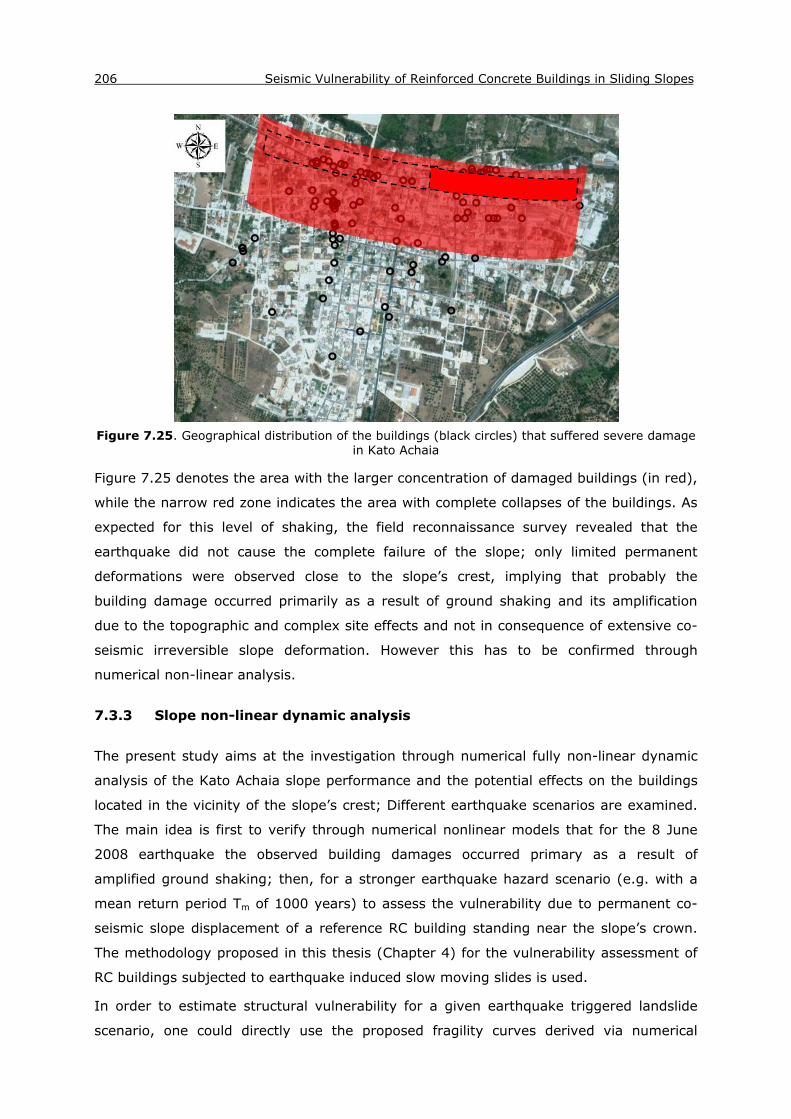
206 Seismic Vulnerability of Reinforced Concrete Buildings in Sliding Slopes
Figure 7.25. Geographical distribution of the buildings (black circles) that suffered severe damage
in Kato Achaia
Figure 7.25 denotes the area with the larger concentration of damaged buildings (in red),
while the narrow red zone indicates the area with complete collapses of the buildings. As
expected for this level of shaking, the field reconnaissance survey revealed that the
earthquake did not cause the complete failure of the slope; only limited permanent
deformations were observed close to the slope’s crest, implying that probably the
building damage occurred primarily as a result of ground shaking and its amplification
due to the topographic and complex site effects and not in consequence of extensive co-
seismic irreversible slope deformation. However this has to be confirmed through
numerical non-linear analysis.
7.3.3 Slope non-linear dynamic analysis
The present study aims at the investigation through numerical fully non-linear dynamic
analysis of the Kato Achaia slope performance and the potential effects on the buildings
located in the vicinity of the slope’s crest; Different earthquake scenarios are examined.
The main idea is first to verify through numerical nonlinear models that for the 8 June
2008 earthquake the observed building damages occurred primary as a result of
amplified ground shaking; then, for a stronger earthquake hazard scenario (e.g. with a
mean return period Tm of 1000 years) to assess the vulnerability due to permanent co-
seismic slope displacement of a reference RC building standing near the slope’s crown.
The methodology proposed in this thesis (Chapter 4) for the vulnerability assessment of
RC buildings subjected to earthquake induced slow moving slides is used.
In order to estimate structural vulnerability for a given earthquake triggered landslide
scenario, one could directly use the proposed fragility curves derived via numerical

CHAPTER 7: Validation of the proposed method 207
parametric analysis (see Chapter 6). These correspond to the simplified geometrical,
geological and structural settings for the slope and the structure. Nevertheless, it was
decided to reproduce the numerical simulation for the real slope geometrical, hydro-
geotechnical, geological and shaking characteristics to check the reliability and
applicability band of the proposed simplified curves.
Figure 7.26 presents the topographic map (original scale 1:5000) of the Kato Achaia area
and the location of the 2 dimensional cross-section Α-Α’ used to conduct the numerical
dynamic analysis. A geotechnical and geophysical investigation has been performed by
the University of Patras (Greece) Civil Engineering Department (UPatras;
http://www.civil.upatras.gr/) in the broader area including geotechnical boreholes, NSPT
tests, Surface Waves tests (using ReΜi, SASW and MASW techniques) and classical
geotechnical laboratory tests on representative and undisturbed soil samples. Based on
the above data provided by the University of Patras, Figure 7.27 presents the simplified
2-dimensional cross-section used for the dynamic analysis together with the (two) sites
of geotechnical boreholes whereas Figure 7.28 presents the corresponding finite
difference grid. The water table is found to be located 30 m below the slope’s crest and
1m above the slope’s toe. The geotechnical surveys reveal 9 different soil layers. The
geotechnical characteristics assigned to each layer are summarized in Table 7.11. It
should be noted that the investigation of the potential for liquefaction is beyond the
scope of this study.
Figure 7.26. Topographic map (original scale 1:5000) of Kato Achaia area and position of Α-Α’
cross section.

208 Seismic Vulnerability of Reinforced Concrete Buildings in Sliding Slopes
Figure 7.27. Soil model used for the 2D finite difference dynamic analysis of the Kato-Achaia slope
Figure 7.28. 2D FLAC dynamic model adopted for the Kato-Achaia slope
In order to establish correlation between the earthquake demand and the permanent
differential displacements for the building, dynamic non-linear analyses were performed
using the computer code FLAC 6.0 (Itasca, 2008). The soil materials are modeled using
an elastoplastic constitutive model with the Mohr-Coulomb failure criterion, assuming a
zero dilatancy non-associated flow rule. The discretization allows for a maximum
frequency of at least 10Hz to propagate through the finite difference grid without
distortion. A small amount of mass- and stiffness-proportional Rayleigh damping is also
applied (0.5-2%), to account for the energy dissipation during the elastic part of the
response and during wave propagation through the site. The center frequency of the

CHAPTER 7: Validation of the proposed method 209
installed Rayleigh damping is selected to lie between the fundamental frequencies of the
input acceleration time histories and the natural modes of the system. The 2D dynamic
model is 800m wide and the elevations of ground surface vary from 160 to 195 m. The
slope’s height and inclination are estimated at 23 m and 28o respectively.
Free field absorbing boundaries are applied along the lateral boundaries while quiet
(viscous) boundaries are used along the bottom of the dynamic model to minimize the
affect of reflected waves. In order to apply a compliant base along the same boundary as
the dynamic input, the seismic motion is modeled as stress loads combining with the
quiet (absorbing) boundary condition.
Table 7.11. Soil properties used for the 2D finite difference cross-section
Material γd (KΝ/m3)
γsat (KΝ/m3)
Poisson's ratio Vs (m/sec) φ
(o) c
(KPa)
Soil 1 (SM-CL) 18 20 0.4 150-250 27 5 Soil 2 (CL) 19 21 0.4 250-450 20 35 Soil 3 (ML) 19 21 0.4 450-550 34 5 Soil 4 (ML) 19 21 0.4 450-550 38 5
Soil 5 (CL-ML) 20 21 0.4 450-550 30 8 Soil 6 (ML) 20 21 0.4 550 24 15
Soil 7 (SM-SC) 20 21 0.4 550 40 8 Soil 8 (OL-CL-OH) 20 21 0.4 550 22 50
Soil 9 (OL-CL) 21 22 0.4 550-1000 28 80
A RC building is assumed to be located 3 m from the slope’s crest. At this (first) stage of
the numerical analysis, the building is modeled only by its foundation with a width of 6m
(uncoupled approach). The combined effect of the soil-structure interaction and of the
topographic irregularity on the dynamic response of the building (e.g. see Pitilakis 2009)
is not taken into account in the analysis. A flexible foundation system (isolated footings)
simulated with concentrated loads (P=50KN/m) at the footings’ links is considered. Thus,
no relative slip between foundation and subsoil is permitted.
Due to the lack of acceleration records within the slope area, two different strong motion
time-histories recorded at the stations PAT3 – (Patra High School) and Pat_Hosp (Patras
Hospital) of the town of Patras were used in the numerical simulations (see Fig. 7.24).
The base motions imposed in the dynamic model were obtained by deconvolution of the
motion recorded in Patras and appropriate scaling for distance. The code Cyberquake
(BRGM Software, 1998) and the profiles of Figure 7.29 were used for this purpose. Site
conditions for the selected stations were made available from previous geotechnical and
geophysical investigations (Athanasopoulos G. and Pefani H., personal communication,

210 Seismic Vulnerability of Reinforced Concrete Buildings in Sliding Slopes
Figure 7.29. Shear wave velocity variation with depth for the selected recording stations.
Figure 7.30. Modulus reduction and damping curves of Darendeli (2001) used for the 1D
deconvolution analysis

CHAPTER 7: Validation of the proposed method 211
2010). Three different sets of G-γ-D curves proposed by Darendeli (2001), which account
for soil plasticity, OCR, and overburden pressure, were used for the deconvolution
analysis (Fig. 7.30). The deconvoluted excitations which were obtained and used as
seismic input are shown in Figure 7.31. Before applied to our Kato Achaia 2D model, they
are subjected to appropriate correction (baseline correction and filtering) to allow for an
accurate representation of wave transmission through the model.
Figure 7.31. Input outcropping horizontal accelerations used in the dynamic analysis
Finally the input accelerograms are scaled for two levels of peak ground acceleration at
the assumed seismic bedrock, namely 0.2 and 0.5g. The low level of excitation is taken
to be consistent with the PGA values reported at the Kato Achaia area during the 2008
Ilia Achaia earthquake (reaching PGA values on the order of 0.3g at the free surface).
The higher excitation level (0.5g) is considered in order to further investigate irreversible
deformation beneath the building’s foundation and finally to assess the vulnerability of
the assumed building due to the differential permanent ground displacement induced by
the landslide. The differential horizontal ground displacements at the foundation level
derived from the 2D finite difference dynamic analysis by applying the PAT3-T and
Pat_hosp-N accelerograms at the assumed seismic bedrock are schematically illustrated
in Figure 7.32 for the two levels of excitation.
In accordance with the field observations carried out after the 2008 Achaia-Ilia
earthquake, relatively small (<10cm) total and differential deformations at the building’s
foundation level are anticipated when applying the outcropping horizontal accelerograms
scaled at 0.2g (Fig. 7.32- left). In contrast, for the stronger earthquake scenario (0.5g),
significant differential permanent displacements (0.4m - 0.6m) are expected (Fig. 7.32-
right).

212 Seismic Vulnerability of Reinforced Concrete Buildings in Sliding Slopes
Figure 7.32. Differential horizontal ground displacements at the building’s foundation level for low
and high excitation level.
7.3.4 Fragility analysis of the building
The analysis of the building is conducted by means of the finite element code
SeismoStruct (Seismosoft, SeismoStruct 2011), which is capable of calculating the large
displacement behavior of space frames under static or dynamic loading, taking into
account both geometric nonlinearities and material inelasticity. Both local (beam-column
effect) and global (large displacements/rotations effects) sources of geometric
nonlinearity are automatically taken into account. The spread of material inelasticity
along the member length and across the section area is represented through the
employment of a fibre-based modeling approach, implicit in the formulation of
SeismoStruct's inelastic beam-column frame elements. Nonlinear static time-history
analyses are performed for all numerical simulations. In particular, the differential
permanent displacement (versus time) curves (Fig. 7.32), directly extracted from the
FLAC dynamic analysis, are imposed as quasi-static loads at one of the RC frame
supports.
The studied building is a “low-code”, single bay-single storey RC bare frame structure,
considering that most of the existing RC buildings found in the area are low rise, old,
poorly constructed structures. The building’s height and length are 3m and 6m
respectively. A uni-axial nonlinear constant confinement model is used for the concrete
material (fc=20MPa, ft=2.1MPa, strain at peak stress 0.002mm/mm, confinement factor
1.2), assuming a constant confining pressure throughout the entire stress-strain range
(Mander et al, 1988). For the reinforcement, a uni-axial bilinear stress-strain model with
kinematic strain hardening is utilized (fy=400MPa, E=200GPa, strain hardening
parameter μ =0.005). All columns and beams have rectangular cross sections (0.40x

CHAPTER 7: Validation of the proposed method 213
0.40m). A low level of steel reinforcement is used (8Φ12) for all the cross sections
considered.
Table 7.12. Definition of Limit states for “low-code” RC buildings
Limit state Steel strain (εs) –low code design
Limit State 1 Steel bar yielding Limit State 2 0.0125 Limit State 3 0.025 Limit State 4 0.045
The building structural response is obtained for the two different levels of excitation by
analyzing the building capacity under the deformation demand (differential displacement
time histories). In order to identify the building performance (damage) state, 4 limit
states (LS1, LS2, LS3, LS4) are defined in terms of allowable values of steel
reinforcement strain, based on the work of Crowley et al. (2004), Bird et al. (2005),
Negulescu and Foerster (2010) and engineering judgment (Table 7.12). This concern
exceedance of minor, moderate, extensive and complete damage of the “low-code”
designed building.
The building’s damage level is finally assessed by comparing the response of the critical
member of the building (in terms of maximum steel bar strain) for the given hazard level
to the specified threshold values for each limit state. As expected, the building will
sustain slight damage (average maximum steel strain at the critical column εs,ave =0.0027
>0.002=Es/fy) due to permanent ground deformation (landslide) for the low level of
input excitation (0.2g), which most probably happened during the earthquake under
consideration. This is in line with the minor permanent slope displacement observed after
the 2008 Achaia-Ilia earthquake. On the contrary, for the strong earthquake scenario
(0.5g), the structure is expected to suffer complete damage (average maximum steel
strain at the critical column εs,ave =0.0545> 0.045), making the repair of the building non
feasible in physical or economical terms.
The fragility curves that are found to be more representative of the geotechnical,
geological, geometrical and structural characteristics of the site and the building (“Low-
code” building- Slope inclination 30o- sand soil), derived via an extensive parametric
analysis (Chapter 6), are depicted in Figure 7.33.

214 Seismic Vulnerability of Reinforced Concrete Buildings in Sliding Slopes
Figure 7.33. Fragility curves proposed for the specific site and structural characteristics
It is observed that the proposed curves predict that the typical building studied herein
would suffer extensive or complete damage (estimated probabilities of being in extensive
and complete damage state 0.34 and 0.29 respectively) for the high seismic hazard
scenario (0.5g) and no or low damage for the low seismic hazard scenario (0.2g)
(estimated probability of being in no damage and slight damage state 0.45 and 0.482
respectively). These observations are in fairly good agreement with the recorded (for the
low hazard scenario) and simulated damages (for both hazard levels) of the typical
building.
7.4 Application to buildings in Corniglio village- Italy
7.4.1 Introduction
Stemming from the valuable set of data (in terms of ground and building landslide
displacement and measured building damage) which were made available and post-
processed for a population of buildings in the village of Corniglio in the North-Western
Italian Appennines (Callerio et al., 2007), the aim of the present study is twofold: first, to
explore the reliability of the fragility curves derived via an extensive parametric
investigation (Chapter 6) through their comparison with the observed damage data for a
representative RC frame building at Coniglio village for the measured level of ground and
building displacement and then, to enhance the applicability of the proposed
methodological framework (Chapter 4), by comparing the more realistic fragility curves

CHAPTER 7: Validation of the proposed method 215
derived for the Corniglio case history through straightforward numerical computations
with the observed building damage data.
7.4.2 Landslide movement and building damage data in Corniglio village
The Corniglio Village is located in the northern part of the Appennines, at an altitude of
about 700 m a.s.l., between the towns of Parma and La Spezia (as shown in Fig. 7.34).
The morphology of the investigated area shows the characteristics features of an
Appennine mountain site, with steep slopes alternating with narrow and deep valleys.
The Corniglio Village area is principally affected by two different slide movements
(Lessloss, 2005): a deep rock block slide (cross section A-A in Fig.7.34) and a surface
rotational landslide (cross section B-B in Fig. 7.34). The geological profile of B-B cross
section, in which this study is focused, is presented in Figure 7.35. Several re-activations
of the landslides have affected Corniglio village damaging buildings, roads and other
infrastructures. The landslide movements are attributed mainly to a decrease of
geomechanical parameters, caused by the weathering process due to intense
precipitations and weak and moderate seismic activity.
The time period of interest in this study lies from September 1994 to December 1999
that was characterized by nearly continuous landslide activity. Through the entire period
considered, the observed displacements reached tens of m on the main slide body, the
so-called “Lama” (see Fig. 7.34), causing heavy damage to all sparse buildings in the
Lama area. In Corniglio Village, the surface ground movements measured by
inclinometers reached typically 20 to 25 cm, resulting to moderate/significant damage to
the buildings located in the old centre of the village. The induced physical damage to the
buildings in Corniglio included cracks in masonry vaults, opening of structural joints,
cracking of retaining walls and in vertical and horizontal structural elements etc. Figure
7.36 illustrates representative observed building damages in Corniglio village. The most
frequent structural typologies of Corniglio buildings, as it can be reasonably assumed on
the basis of the pictures, are low-rise masonry buildings and low-rise RC frame buildings.
A substantial set of instrumental observations has been gathered mainly from the Emilia
Romagna Regional Administration in charge of the monitoring and surveillance activities,
including inclinometer data (monitoring ground movements in free field), geodetic
levelling data on almost every building within the village area for the entire period of
interest and crack aperture measurements in some susceptible to damage buildings.
The inclinometers position, the locations of the geodetic targeted points (and their ID’s)
and, for each building monitored, a letter from A to Z between brackets which indicates

216 Seismic Vulnerability of Reinforced Concrete Buildings in Sliding Slopes
the crack meters installed, are depicted in Figure 7.37. The most damaged buildings are
denoted by red filled polygons.
Figure 7.34. General plan of the area of Corniglio affected by the landslide phenomena during the
years 1995-2000. The indicated displacements (ADG = Absolute Ground Displacement) are obtained by aerial photo interpretation (“Lama” area) and inclinometer readings (Village) (Callerio
et al., 2007)

CHAPTER 7: Validation of the proposed method 217
Figure 7.35. Geotechnical profile B-B (see Fig. 7.34) of the Corniglio case history used for the analysis

218 Seismic Vulnerability of Reinforced Concrete Buildings in Sliding Slopes
Figure 7.36. Representative physical damage to buildings in Corniglio village (Callerio et al., 2007)
Building n. 25
Building n. 17
Building n. 18
Building n. 63

CHAPTER 7: Validation of the proposed method 219
Figure 7.37. Location of inclinometers, geodetic and crack measurements on buildings. Buildings are denoted by red polygons whereas the ones that
suffered damages due to the landslide movement are filled in red. (Callerio et al., 2007)
220 Seismic Vulnerability of Reinforced Concrete Buildings in Sliding Slopes
The processing of the data set was conducted by Callerio et al. (2007), focusing on
establishing a correlation among ground displacement, building movements and damage
induced during sliding so as to provide the basis for a probabilistically sound vulnerability
assessment framework.
The damage levels observed in Corniglio were defined in terms of ease of repair, based
on the scale proposed by Standing et al (1999), identifying 3 damage levels: negligible to
slight, slight to moderate and moderate to severe. The ease of repair was then related to
the measure of cracks opening.
Figures 7.38 to 7.43 display the ground displacement measured by the nearest
inclinometer with respect to the building location, the building movement by geodetic
levelling and the opening of each crack monitored on the structure. All the plots are over
imposed on the damage scale in terms of cracks opening, to assess for each building the
expected damage state. As it can be noticed from the figures, the ground displacement is
not always linearly related to building movement. Moreover, the crack openings, which
depend on various local factors (e.g. direction of crack opening, texture of the walls,
precence of structural reinforcement etc.) are not directly related to ground
displacement. A rather linear relationship between the building movement and crack
opening is detected in some of the cases (i.e. for buildings 17, 23, 25).

CHAPTER 7: Validation of the proposed method 221
Figure 7.38. Correlation between absolute ground displacement (from nearby Inclinometer A3-2), building n. 17 and 18 displacement (from geodetic levelling) and crack opening (compared to the
defined damage levels) as a function of time (Callerio et al., 2007)

222 Seismic Vulnerability of Reinforced Concrete Buildings in Sliding Slopes
Figure 7.39. Correlation between absolute ground displacement (from nearby Inclinometer A2-2), building n. 23 and 25 displacement (from geodetic levelling) and crack opening (compared to the
defined damage levels) as a function of time (Callerio et al., 2007)

CHAPTER 7: Validation of the proposed method 223
Figure 7.40. Correlation between absolute ground displacement (from nearby Inclinometer A2-6), building n. 27 displacement (from geodetic levelling) and crack opening (compared to the defined
damage levels) as a function of time (Callerio et al., 2007)
Figure 7.41. Correlation between absolute ground displacement (from nearby Inclinometer A2-1), building n. 27 displacement (from geodetic levelling) and crack opening (compared to the defined
damage levels) as a function of time (Callerio et al., 2007)

224 Seismic Vulnerability of Reinforced Concrete Buildings in Sliding Slopes
Figure 7.42. Correlation between absolute ground displacement (from nearby Inclinometers A2-1 and A3-3), building n. 35 displacement (from geodetic levelling) and crack opening (compared to
the defined damage levels) as a function of time (Callerio et al., 2007)
Figure 7.43. Correlation between absolute ground displacement (from nearby Inclinometers A3-1 and A3-3), building n. 63 displacement (from geodetic levelling) and crack opening (compared to
the defined damage levels) as a function of time (Callerio et al., 2007)

CHAPTER 7: Validation of the proposed method 225
7.4.3 Comparison of the observed building damage with the damage
predicted by the proposed and simulated fragility curves
The present study is focused on the fragility analysis of building n. 17 due to its proximity
to the inclinometer A3-2, which is installed near the slope crown of the geotechnical
profile B-B of the Corniglio case history (see Fig. 7.35). As shown in Figure 7.38,
building n. 17 is a rather simple two-storey RC frame structure with masonry infill walls.
Figure 7.44 shows a closer view of building n. 17 and of the nearby inclinometer A3-2
within the Corniglio area.
Despite the proximity of building n.18 as well to the inclinometer A3-2 and the fact that
the recorded displacements on both buildings 17 and 18 show more or less the same
trends, building n. 18 is an upper class, well maintained masonry bearing wall structure
with an heavy roof (A. Calerio, personal communication 2012), which is not considered
appropriate for the herein fragility analysis, concentrated on RC buildings.
Other buildings, such as buildings n. 33 (RC frame 3 storey building, now demolished)
and n. 35 (mixed RC frame, masonry structure), could potentially be suitable for this
study. However, these buildings are not directly influenced by the landslide movement of
the B-B cross section.
Figure 7.44. Closer view of building with ID 17 and the nearby inclinometer A3-2 within the
Corniglio area. The geodetic and crack monitored points on the buildings are also shown (in green)
As it was expected, the given data do not exactly fit the proposed curves derived through
the parametric analysis (Chapter 6). In particular, the studied slope configurations do not
match very precisely to the given finite slope geometry and soil geotechnical properties
of Corniglio case history (see Fig. 7.35, geotechnical profile B-B: average slope
inclination≈ 37o, average height ≈43 m). Moreover, first-time failures where the sliding
surface is allowed to be freely developed were analyzed in Chapter 6, as opposed to the
Corniglio case study where a pre-existing landslide has to be simulated. Regarding all
the above, two different approaches of increased complexity for the fragility analysis of
building n. 17 in Corniglio village are presented in the ensuing.
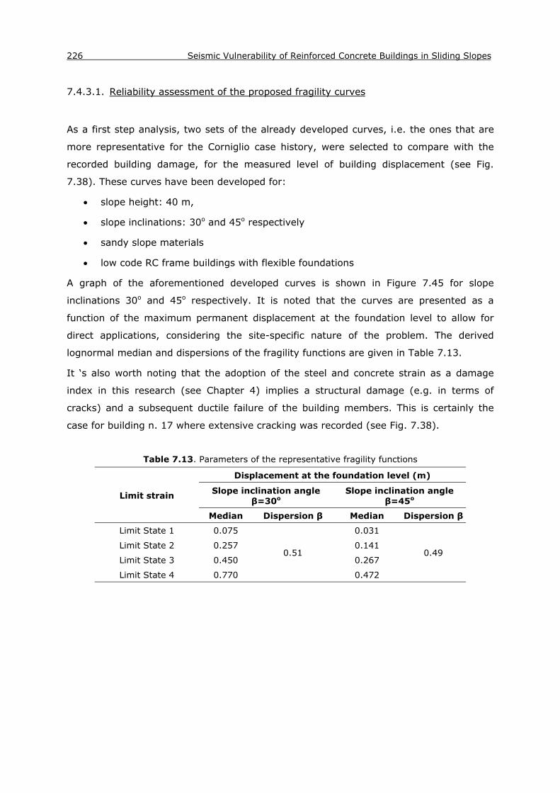
226 Seismic Vulnerability of Reinforced Concrete Buildings in Sliding Slopes
7.4.3.1. Reliability assessment of the proposed fragility curves
As a first step analysis, two sets of the already developed curves, i.e. the ones that are
more representative for the Corniglio case history, were selected to compare with the
recorded building damage, for the measured level of building displacement (see Fig.
7.38). These curves have been developed for:
slope height: 40 m,
slope inclinations: 30o and 45o respectively
sandy slope materials
low code RC frame buildings with flexible foundations
A graph of the aforementioned developed curves is shown in Figure 7.45 for slope
inclinations 30o and 45o respectively. It is noted that the curves are presented as a
function of the maximum permanent displacement at the foundation level to allow for
direct applications, considering the site-specific nature of the problem. The derived
lognormal median and dispersions of the fragility functions are given in Table 7.13.
It ‘s also worth noting that the adoption of the steel and concrete strain as a damage
index in this research (see Chapter 4) implies a structural damage (e.g. in terms of
cracks) and a subsequent ductile failure of the building members. This is certainly the
case for building n. 17 where extensive cracking was recorded (see Fig. 7.38).
Table 7.13. Parameters of the representative fragility functions
Limit strain
Displacement at the foundation level (m)
Slope inclination angle β=30ο
Slope inclination angle β=45ο
Median Dispersion β Median Dispersion β
Limit State 1 0.075
0.51
0.031
0.49 Limit State 2 0.257 0.141
Limit State 3 0.450 0.267
Limit State 4 0.770 0.472

CHAPTER 7: Validation of the proposed method 227
Figure 7.45. Representative fragility functions derived from the parametric analyses
The damages predicted by the curves are compared with the damages observed in
building n. 17 for the recorded level of displacement, i.e. 0.121 m. As shown in Figure
7.38, for this level of displacement, the building would be in “moderate to severe”
damage level according to the damage states proposed in Callerio et al. (2007).

228 Seismic Vulnerability of Reinforced Concrete Buildings in Sliding Slopes
The proposed curves predict “slight to moderate” to “moderate to extensive” damages
that are in relatively good correlation with the corresponding assigned damage levels
based on the field measurements and observations. As it can be easily seen in Figure
7.45, the expected damages when using the curves derived for 45o slope inclinations are
more in line with the observed structural performance. In particular, the estimated
probabilities of exceeding slight and moderate damage are 1.0 and 0.4 respectively for
the curves referring to the 45o inclined slope whereas the corresponding probabilities are
0.84 and 0.08 respectively for the curves referring to the 30o inclined slope.
7.4.3.2. Fragility curves for the Corniglio case study – Comparison with recorded damage
data
Considering the relatively crude approximation that it may be achieved with the
comparisons presented below, a more sophisticated analysis is performed herein
resulting to the development of fragility curves for the Corniglio case history based on
the data provided (e.g. geotechnical profile B-B, inclinometer A3-2 records associated
with building n.17 geodetic and crack measurements). Fragility curves are derived from
the response of the landslide to earthquake shaking that is in our case the differential
displacement at the foundation level. The ultimate goal of the analysis is to get more
reliable correlations between the observed and simulated damage of the building for the
recorded displacement level so as to enhance the reliability and applicability band of the
proposed methodology (Chapter 4).
In terms of numerical computations, a two-step uncoupled analysis is performed based
on the methodological framework described in Chapter 4. The computer codes FLAC2D
7.0 (Itasca, 2011) and SeismoStruct (Seismosoft, SeismoStruct 2011) are used for the
slope-foundation dynamic and structure’s quasi-static analysis respectively.
Taking into account the various uncertainties involved due to lack of a detailed
geotechnical investigation, the simplified finite slope geometry shown in Figure 7.46 is
adopted to simulate the geotechnical profile B-B, characterized by three layers with
different material properties (Soil 1, Soil 2, elastic bedrock) and a pre-existing sliding
surface (Slide). The water table is assumed to lie at the base of the slope (-43m).
The soil materials overlaying the elastic bedrock were defined by the elasto-plastic Mohr
Coulomb constitutive model coupled with the hysteretic damping scheme. In particular,
FLAC 7.0 hysteretic damping formulation was implemented using the “default” model to
account for the nonlinear hysteretic soil behavior prior yielding. The model approximately
fits the damping and shear modulus curves over a reasonable range of strains (e.g. up to
0.2-0.3%) that are expected to occur in the herein dynamic analysis. In particular, the

CHAPTER 7: Validation of the proposed method 229
Seed and Idriss (1970) sand-upper range curves were used for the slide and the upper
soil formation (Soil 1) whereas Sun et al. (1988) clay-upper range curves were used for
Soil 2. A small amount (e.g. 0.2%) of stiffness-proportional Rayleigh damping was also
added to compensate for the low damping demonstrated by the program at small strains.
In addition, for the elastic bedrock materials a constant 0.5% of Rayleigh-type damping
was assigned. The geotechnical properties for the assumed 2D cross-section are
summarized in Table 7.14.
Figure 7.46. Slope configuration adopted for the geotechnical profile B-B
Table 7.14. Assumed soil properties for the geotechnical profile B-B
Soil 1 Slide Soil2 Elastic bedrock
Soil thickness (m) 20 1.0-2.0 93 40 Density ρ (kg/m3) 1800 1700 2000 2300
Young's modulus E (KPa) 2.925E+05 4.420E+04 1.300E+06 4.321E+06 Poisson's ratio v 0.3 0.3 0.3 0.3
Bulk modulus K (KPa) 2.438E+05 3.683E+04 1.083E+06 3.600E+06 Shear modulus G (KPa) 1.125E+05 1.700E+04 5.000E+05 1.662E+06
K + 4G/3 3.900E+05 5.894E+04 1.733E+06 5.761E+06 Cohesion (KPa) 10 8 50 -
Friction angle (degrees) 35 35 30 - P wave velocity Vp (m/sec) 465.48 186.19 930.95 1582.61
Shear wave velocity Vs (m/sec) 250.00 100.00 500.00 850.00 Max. allowed zone size (m) 2.50 1.00 5.00 8.50
Max. Allowed frequency 10.00 10.00 10.00 10.00
Free field absorbing boundaries are applied along the lateral boundaries while quiet
(viscous) boundaries are applied along the bottom of the dynamic model to minimize the
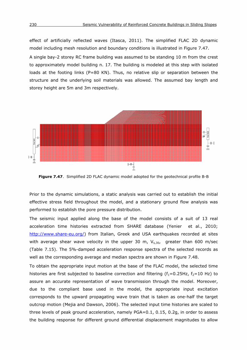
230 Seismic Vulnerability of Reinforced Concrete Buildings in Sliding Slopes
effect of artificially reflected waves (Itasca, 2011). The simplified FLAC 2D dynamic
model including mesh resolution and boundary conditions is illustrated in Figure 7.47.
A single bay-2 storey RC frame building was assumed to be standing 10 m from the crest
to approximately model building n. 17. The building is modeled at this step with isolated
loads at the footing links (P=80 KN). Thus, no relative slip or separation between the
structure and the underlying soil materials was allowed. The assumed bay length and
storey height are 5m and 3m respectively.
Figure 7.47. Simplified 2D FLAC dynamic model adopted for the geotechnical profile B-B
Prior to the dynamic simulations, a static analysis was carried out to establish the initial
effective stress field throughout the model, and a stationary ground flow analysis was
performed to establish the pore pressure distribution.
The seismic input applied along the base of the model consists of a suit of 13 real
acceleration time histories extracted from SHARE database (Yenier et al., 2010;
http://www.share-eu.org/) from Italian, Greek and USA earthquakes recorded at sites
with average shear wave velocity in the upper 30 m, Vs,30, greater than 600 m/sec
(Table 7.15). The 5%-damped acceleration response spectra of the selected records as
well as the corresponding average and median spectra are shown in Figure 7.48.
To obtain the appropriate input motion at the base of the FLAC model, the selected time
histories are first subjected to baseline correction and filtering (f1=0.25Hz, f2=10 Hz) to
assure an accurate representation of wave transmission through the model. Moreover,
due to the compliant base used in the model, the appropriate input excitation
corresponds to the upward propagating wave train that is taken as one-half the target
outcrop motion (Mejia and Dawson, 2006). The selected input time histories are scaled to
three levels of peak ground acceleration, namely PGA=0.1, 0.15, 0.2g, in order to assess
the building response for different ground differential displacement magnitudes to allow

CHAPTER 7: Validation of the proposed method 231
the evaluation of different damage states for the building and at the end to construct the
corresponding fragility curves. It is noted that due to the presence of a pre-existing
sliding surface, the required amplitude of the input excitations able to cause extensive
slope and foundation deformations is largely decreased compared to the corresponding
amplitude considered for the first-time failures in Chapter 4.
Table 7.15. Ground motion records used in the numerical simulations derived from the SHARE
database
Earthquake Name
Earthquake Country Date
Epicetral distance R (km)
Magnitude MW
Station Name
Vs,30 (m/s)
Database Code
Kalamata (Aftershock) Greece 10/6/1987 17 5.36
Kyparrisia-Agriculture
Bank 778 ESMD_126_H1
Ano Liosia Greece 7/9/1999 17 6.04 Athens 4 (Kipseli District)
934 ESMD_335_H1
Kozani (Aftershock) Greece 17/5/1995 16 5.30
Chromio-Community
Building 623 ISESD_1210_H1
Friuli Italy 6/5/1976 21.7 6.40 Tolmezzo-Diga Ambiesta 1030 ITACA_16_H1
Friuli (Aftershock) Italy 15/9/1976 8.5 5.90 Tarcento 901 ITACA_116_H1
Umbria Marche
(Aftershock) Italy 14/10/1997 20 5.60 Norcia 681 ITACA_491_H2
App. Lucano Italy 9/9/1998 6.6 5.60 Lauria Galdo 603 ITACA_613_H2
L Aquila Mainshock Italy 6/4/2009 4.4 6.30
L Aquila - V. Aterno - Colle
Grilli 685 ITACA_857_H2
San Fernando USA 9/2/1971 20.04 6.61 Lake Hughes #12 602 NGA_71_H2
Coyote Lake USA 6/8/1979 4.37 5.74 Gilroy Array #6 663 NGA_150_H2
Morgan Hill USA 24/4/1984 36.34 6.19 Gilroy Array #6 663 NGA_459_H2
Loma Prieta USA 18/10/1989 35.47 6.93 Gilroy Array #6 663 NGA_769_H1
Northridge-01 USA 17/1/1994 25.42 6.69 La - Griffith
Park Observatory
971 NGA_994_H1

232 Seismic Vulnerability of Reinforced Concrete Buildings in Sliding Slopes
Figure 7.48. Linear 5%-damped acceleration response spectra of the records selected for
numerical analyses. The average and median spectra are also shown.
Figures 7.49a and b depict the derived horizontal and vertical differential displacements
time histories respectively at the closest edge of the assumed building from the slope’s
crest (i.e. 10 m) for input accelerograms scaled at 0.15 g. It is observed that the specific
characteristics (frequency content and duration) of the seismic ground motions can
significantly affect the history and the amplitude of the computed differential
displacement demand at the foundation level.
Figure 7.49. Differential horizontal (a) and vertical (b) ground displacements at the building’s
foundation level for input accelerograms scaled at 0.15 g
(a) (b)

CHAPTER 7: Validation of the proposed method 233
Then, a non-linear quasi-static analysis is performed for the studied 1 bay- 2 storey RC
frame building model (Fig. 7.50) by means of the finite element code SeismoStruct
(Seismosoft, SeismoStruct 2011). More specifically, the derived differential displacement
time histories extracted from FLAC dynamic analysis (see Fig. 7.49) were directly applied
as static loads at one of the RC frame supports. The beneficial contribution of masonry
infill walls to the building capacity is not considered in this study.
Figure 7.50. Schematic view of the studied building in Corniglio village
Non-linear fibre-based material properties are assumed for the structural members of the
RC frame building under investigation. More specifically, a uni-axial nonlinear constant
confinement model is used for the concrete material (fc=20MPa, ft=2.1MPa, strain at
peak stress 0.002mm/mm, confinement factor =1 for unconfined and 1.2 for confined
concrete, specific weight=24KN/m3) and a uni-axial bilinear stress-strain model with
kinematic strain hardening is used for the reinforcement (fy=400MPa, E=200GPa, strain
hardening parameter μ =0.005, specific weight=78KN/m3).
Figure 7.51 presents representative plot of damage evolution expressed in terms of
maximum steel strain (damage index) as a function of the maximum permanent ground
displacement vector at the foundation level for the low-rise, “low code” designed RC
frame building. The figure also shows the limit steel strains needed to exceed yield and
post-yield limit states for low-code RC buildings characterized by a low level of
confinement as defined in Chapter 4.

234 Seismic Vulnerability of Reinforced Concrete Buildings in Sliding Slopes
Figure 7.51. Maximum recorded steel strain as a function of permanent ground displacement
vector at the foundation level for the studied building in Corniglio village
Finally, probabilistic fragility curves in terms of permanent displacement vector at the
foundation level for building n. 17 in Corniglio village were derived using the Maximum
likelihood Method (see Chapter 4 for details). Table 7.16 presents the lognormal
parameters of the fragility functions whilst Figure 7.52 depicts the corresponding graphs.
Table 7.16. Parameters of fragility functions for the studied building in Corniglio village based on
the Maximum likelihood method
Permanent displacement at the foundation level (m)
Median (m) Dispersion β
Limit State 1 0.042
0.41 Limit State 2 0.093
Limit State 3 0.168
Limit State 4 0.315

CHAPTER 7: Validation of the proposed method 235
Figure 7.52. Fragility curves for the studied RC frame building in Corniglio village
The simulated fragility curves predict that the building n. 17 studied herein is more likely
to suffer “moderate to extensive damage”, for the measured level of displacement, i.e.
0.121 m. In particular, the estimated probabilities of exceeding moderate and extensive
damage are 0.85 and 0.22 respectively. These observations are in fairly good agreement
with the recorded building damages (see Fig. 7.38), verifying the validity of the derived
curves and finally enforcing the credibility and applicability band of the proposed
methodological framework.
7.5 Conclusive remarks
The validity the proposed method has been verified through the comparison of
representative suggested fragility curves in this thesis with corresponding curves
proposed in the literature derived by different approaches (empirical, expert judgment,
analytical). The comparisons are generally judged satisfactory when considering a low-
rise, high-code RC frame building resting on flexible foundations (e.g. isolated footings)
whereas they are not so good in case of the building on stiff foundations (e.g. continuous
raft foundation). In particular, the proposed curves generally predict lower vulnerability
values for the building on stiff foundations compared to the literature ones. It should be
noticed, however, that only the structural damage (e.g. in terms of cracks) to the
building members could be estimated by the proposed curves even though, for the stiff

236 Seismic Vulnerability of Reinforced Concrete Buildings in Sliding Slopes
foundation case, a considerable amount of damage would be non structural (e.g. rigid
body movement), reducing the serviceability level of the building.
Approximate correlations between the proposed fragility curves in this research for RC
buildings subjected to co-seismic permanent slope displacement and different literature
fragility curves derived for low-rise RC buildings subjected to ground shaking on
horizontally layered soil deposits were also performed. Overall, the comparisons allow
gaining better insight into the relative extent of damage and the associated dominating
failure mechanism for structures subjected to co-seismic slope deformation and ground
shaking respectively. More specifically, for the yielding limit state most of the literature
curves predict larger damages for the building, implying that the building is generally
expected to suffer some initial damage due to ground shaking before the onset of the
landslide movement. For the collapse limit state, on the other hand, most of the
literature curves estimate lower vulnerability values for the building with respect to the
ones proposed in this study. Thus, the landslide, once triggered by the earthquake, may
become the prevailing damage mechanism resulting to greater damages for the building
near collapse.
The reliability and applicability of the proposed methodological framework and the
corresponding fragility curves has been also assessed through its application to two real
case histories: Kato Achaia slope in Peloponnese –Greece and the Corniglio village-Italy
case study. The direct comparison of the recorded damage data on typical buildings with
the corresponding damage predicted by the developed fragility functions proved that the
proposed fragility curves could adequately capture the performance of the representative
RC building affected by the slope co-seismic landslide differential displacement. In
addition, to enhance the effective implementation of the proposed methodological
framework within a probabilistic risk assessment study, more realistic fragility curves
were constructed for a representative building in Corniglio village based on
straightforward numerical computations. The curves were verified through their
comparison with the observed building damage for the measured level of displacement.

CHAPTER 8
Evolution of building vulnerability over time
8.1 Introduction
The assessment of landslide risk depends on the evaluation of landslide hazard and the
vulnerability of exposed structures which both change with time. The real, non-stationary
vulnerability modeling of structures due to landslides may be significantly affected by
various degradation mechanisms such as aging considerations, anthropogenic actions,
cumulative damage from past landslide events and retrofitting measures. Such
mechanisms, however, have been traditionally neglected in vulnerability assessment
studies assuming an optimum plan of maintenance.
With the above in mind, the present work aims at the expansion of the proposed
vulnerability assessment methodology in Chapter 4 to account for the evolution of
building vulnerability over time exposed to earthquake –induced landslide hazard. In
particular, the aging of typical RC buildings is considered in this research by including
probabilistic models of corrosion deterioration of the RC elements within the vulnerability
modeling framework. Two potential adverse corrosion scenarios are examined: chloride
and carbonation induced corrosion of the steel reinforcement.
An application of the proposed methodology to reference low-rise RC buildings exposed
to the combined effect of seismically induced landslide differential displacements and
reinforcement corrosion is provided. Both buildings with stiff and flexible foundation
system standing near the crest of a potentially precarious soil slope are examined. Non
linear static time history analyses of the buildings are performed using a finite element
code. The distribution for the corrosion initiation time is assessed through Monte Carlo
simulation using appropriate probabilistic models for the carbonation and the chloride
induced corrosion. Then, the loss of area of steel over time due to corrosion of the RC
elements is modeled as a reduction in longitudinal reinforcing bar cross-sectional area in
the fiber section model. Time dependent structural limit states are defined in terms of
steel material strain. Fragility curves/surfaces are derived for different points in time as a

238 Seismic Vulnerability of Reinforced Concrete Buildings in Sliding Slopes
function of Peak Ground Acceleration PGA at the seismic bedrock or permanent co-
seismic ground displacement PGD at the slope area for both chloride and carbonation
induced deterioration scenarios.
8.2 Environmental deterioration of RC structures
8.2.1 Corrosion of reinforcement
The strength of the components of any structural system is in general a time dependent
property which may decrease in resistance along the structure’s service life. Potential
reasons for structural strength and stiffness degradation can be attributed to multiple
factors such as corrosion, erosion, other forms of chemical deterioration and fatigue
(Melchers and Frangopol, 2008). Among these, reinforcement corrosion is undoubtedly,
one of the most important causes of deterioration of reinforced concrete in Europe and
worldwide. Corrosion is a complex process that may affect a RC structure in a variety of
ways, including, among others, cover spalling, loss of steel-concrete bond strength and
loss of reinforcement cross sectional area, potentially resulting to the reduction of the
resistance and load bearing capacity of the structure and to the variation of the failure
mechanism from ductile to fragile type (e.g. Saetta et al., 2008; Mohammed et al.,
2011; Yalciner et al., 2012 etc.). Thus, it may affect both the safety and serviceability of
RC structures in relation to their initial as-built state. Figure 8.1 presents typical
structural failures as a result of reinforcement corrosion.
Figure 8.1. Structural deterioration due to reinforcement corrosion

CHAPTER 8: Evolution of building vulnerability over time 239
Theoretically corrosion of the reinforcement should not occur as the reinforcement is
supposedly well protected by the concrete cover and the alkalinity of the last. Non
carbonated concrete has a high alkalinity (pH=13) that is a result of the presence of
sodium, potassium and calcium hydroxides produced during the hydration of the cement.
In this alkaline environment an oxide layer is formed on the steel surface, the so-called
“passive film” that prevents the corrosion of the reinforcement. However, there are
principally two processes that may break down this passive film: the ingress of chlorides
and carbon dioxide (e.g. Zhong et al., 2010).
Figure 8.2. Schematic illustration of the evolution of the reinforced concrete corrosion (Tuutti,
1982)
The amount of structural damage due to corrosion of steel reinforcement as a function of
the age of the structure can be expressed through a bilinear model as schematically
illustrated in Figure 8.2. Deterioration caused by reinforcement corrosion is normally
divided into two main time periods, the initiation period (ti) and the propagation period
(tp). The initiation period is defined as the time until the reinforcement becomes
depassivated either by the presence of chloride salts or by carbonation. As soon as the
concrete at the depth of the reinforcement is carbonated or contains a critical amount of
free chlorides the reinforcement becomes depassivated and corrosion may occur. This
limit state defines the beginning of the propagation period. During the propagation period
the reinforcement is corroding, which may lead to deterioration of the concrete as well.
Expansive corrosion products provoke cracks along the reinforcement, and subsequently,
spalling of the concrete cover may occur. Finally, the loss of cross section of the
reinforcement may lead to reduction of the load bearing capacity.

240 Seismic Vulnerability of Reinforced Concrete Buildings in Sliding Slopes
8.2.2 Carbonation-induced corrosion
8.2.2.1. Mechanism
Concrete carbonation induces a decrease of the pH of the pore solution, which leads to
dissolving the protective layer (Fig. 8.3). Then the corrosion of the reinforcement starts
only if the reinforcing steel has significant electrical potential difference along with the
presence of sufficient moisture and oxygen. Concrete carbonation is a complex physico-
chemical process that develops in two distinct regions: the anode, where the passive
layer is destroyed and the steel dissolved; and the cathode, where hydroxide ions are
formed due to the combination of oxygen, water and the electrons coming from the
anode. It includes the diffusion of CO2 into the gas phase of the concrete pores and its
reaction with the calcium hydroxyl Ca(OH)2. As the high pH of uncarbonated concrete is
mainly due to the presence of Ca(OH)2, it is clear that the consumption of this species
will lead to a pH drop, which can attain a value of 9 when the reaction is completed. In
this environment, the oxide layer that protected the reinforcement bars is attacked and
corrosion starts. In practice, CO2 penetrates into the concrete mass by diffusion from the
surface layer. Thus a carbonation front appears that moves into the structure (Fig. 8.4).
Figure 8.3. Carbonation in concrete (Beushausen and Alexander, 2010)

CHAPTER 8: Evolution of building vulnerability over time 241
Figure 8.4. Carbonation induced corrosion (Beushausen and Alexander, 2010)
8.2.2.2. Probabilistic modeling of carbonation induced corrosion initiation
Probabilistic modeling of corrosion has much to offer with regard to practicality and
reliability as compared with attempts at formulating purely deterministic models.
Ditlevsen (1984) states: “Probabilistic models are almost always superior to deterministic
models of equal level of complexity in the sense that the former have considerable higher
threshold of realism when dealing with phenomena taking place in uncertain
environments”.
Several methods have been proposed to model corrosion due to carbonation (e.g. Sudret
et al. 2007; Peng and Stewart, 2008; Marques and Costa, 2010 etc.). The reliability-
based model for computing the carbonation depth xc proposed by FIB- CEB Task Group
5.6 (2006) is adopted in this study. The model has been developed within the research
project DuraCrete and slightly revised in the research project DARTS, each project was
funded by the European Union. It is based on diffusion as the prevailing transport
mechanism within the concrete (Fick’s 1st law of diffusion) assuming that the diffusion
coefficient for carbon dioxide through the material is a constant material property.
1c e c t ACC ,0 t sx (t ) 2 k k (k R a ) C t W(t ) (8.1)
where
xc(t): carbonation depth at the time t [mm]
t: time [years]

242 Seismic Vulnerability of Reinforced Concrete Buildings in Sliding Slopes
ke: environmental function [-]
kc: execution transfer parameter [-]
kt: regression parameter [-]
RACC,0-1: inverse effective carbonation resistance of concrete [(mm2/years)/(kg/m3)]
at: error term,
CS: CO2-concentration [kg/m3]
W(t): weather function [-]
It is supposed that corrosion immediately starts when carbonation has attained the
rebar. Denoting by a (mm) the concrete cover, the time necessary for corrosion to start,
called corrosion initiation time, is given as:
11 2 w 1
e c t ACC ,0 t s 2 winit 02
2 k k (k R a ) CT t
a
(8.2)
The environmental function ke takes account of the influence of the humidity level on the
diffusion coefficient and hence on the carbonation resistance of the concrete. The
reference climate is T= +20°C/ 65% RH. It can be described by means of Equation 8.3.
cc
c
gfreal
e fref
RH
kRH
1100
1100
(8.3)
where
RHreal: weather nearest station data (daily mean value: 0 % < RH < 100 %)
RHref [%]: constant parameter, value: 65
gc [-]: constant parameter, value: 2.5
fc [-]: constant parameter, value: 5.0
The execution transfer parameter kc takes the influence of curing on the effective
carbonation resistance into account. It can be described by means of Equation 8.4,
derived from Bayesian regression analysis. cb
cc
tk7
(8.4)
kc: execution transfer parameter [-]
bc: exponent of regression [-], normally distributed variable
tc: period of curing [d], constant parameter, value: period of curing
CHAPTER 8: Evolution of building vulnerability over time 243
The inverse carbonation resistance of concrete RACC,0-1 should be quantified using
different direct and indirect testing methods. If no test data is available, literature data
can be used for orientation purposes [Table B1-2, FIB- CEB Task Group 5.6 (2006)].
The factors kt and at have been introduced in order to transform the results gained under
“accelerated carbonation” conditions RACC,0-1 into an inverse carbonation resistance RNAC,0
-1
under “natural carbonation” conditions. NAC t ACC tR k R a1 1
,0 ,0 (8.5)
RACC,0-1: inverse effective carbonation resistance of dry concrete, determined at a certain
point of time t0 on specimens with the accelerated carbonation test ACC
[(mm2/years)/(kg/m3)], normally distributed variable.
RNAC,0-1: inverse effective carbonation resistance of dry concrete (65% RH) determined at
a certain point of time t0 on specimens with the normal carbonation test NAC
[(mm2/years)/(kg/m3)]
kt: regression parameter which considers the influence of test method on the ACC-test [-
],normally distributed variable.
at: error term considering inaccuracies which occur conditionally when using the ACC test
method [(mm2/years)/(kg/m3)], normally distributed variable.
The CO2 concentration of the ambient air represents the direct impact on the concrete
structure. The impact can be described by the following equation:
S S atm S emiC C C, , (8.6)
where
CS: CO2 concentration [kg/m3]
CS,atm.: CO2 concentration of the atmosphere [kg/m3]
CS,emi.: additional CO2 concentration due to emission sources [kg/m3]
For usual structures, Equation 8.6 can be reduced to Equation 8.7:
CS = CS,atm (8.7)
The atmospheric concentration of CO2 can be quantified as a normally distributed
variable (mean= 0.00082, s=0.0001).
The weather function W takes the meso-climatic conditions due to wetting events of the
concrete surface into account.

244 Seismic Vulnerability of Reinforced Concrete Buildings in Sliding Slopes
( )bwSRp ToWwt tW
t t2
0 0
⋅
æ ö æ ö÷ ÷ç ç÷ ÷ç ç÷ ÷ç ç÷ ÷ç çè ø è ø= = (8.8)
t0: time of reference [years]
w: weather exponent [-]
ToW: time of wetness [-], value: to be evaluated from weather station data
Nddays with
ToW rainfall h 2.5 mm per year
365 (8.9)
pSR: probability of driving rain [-],value: depending on the type of structural elements
bw: exponent of regression [-],normally distributed variable
to [years]: constant parameter, value: 0.0767
The statistical quantification of the model parameters is provided in Table 8.1 based on
the FIB- CEB Task Group 5.6 (2006) proposed model. For illustrational purposes, values
for Portland Cement Concrete (PCC) and three different water/cement ratios (namely
w/c=0.4,0.5 and 0.6) are given. Three different corrosion levels (low, medium, high) are
considered in the table based on recent available literature (Marques and Costa, 2010).

CHAPTER 8: Evolution of building vulnerability over time 245
Table 8.1. Statistical characteristics of parameters affecting the carbonation induced corrosion deterioration of RC elements
Water to cement ratio (w/c)
Distribution Reference 0.4 0.5 0.6
Parameters Mean cov Mean cov Mean cov
Cover Depth (mm) a 25.00 0.32 25.00 0.32 25.00 0.32 Lognormal
FIB- CEB Task Group 5.6 (2006)
Rhreal,k (% rel. humidity) 70.00 cov=0.1 , a=40.0, b=100 70.00
cov=0.1 , a=40.0, b=100
70.00 cov=0.1 , a=40.0, b=100
Beta
exponent of regression bc -0.567 0.042 -0.567 0.042 -0.567 0.042 Normal
Inverse carbonation resistance (Racc,01) (mm2/year) / (kg/m3) 3.10E-11 0.15 6.80E-11 0.13 2.30E-10 0.10 Normal
Influence of test method kt 1.25 0.28 1.25 0.28 1.25 0.28 Normal
Error term et (mm2/years) 315.5 0.15 315.5 0.15 315.5 0.15 Normal
Cs, atm (kg/m3) 0.000820 0.12 0.000820 0.12 0.000820 0.12 Normal
Exponent of regression bw 0.446 0.365 0.446 0.365 0.446 0.365 Normal
Rate of Corrosion (rcorr)
mA/cm2
Low corrosion Level 0.1-0.5
0.25
0.1-0.5
0.25
0.1-0.5
0.25 Normal Marques and Costa (2010) Medium corrosion Level 0.5-1 0.5-1 0.5-1
High corrosion Level >1 >1 >1

246 Seismic Vulnerability of Reinforced Concrete Buildings in Sliding Slopes
8.2.3 Chloride-induced corrosion
8.2.3.1. Mechanism
Chloride induced corrosion is reportedly the most serious and widespread deterioration
mechanism of concrete structures, fib (2006). It can be attributed to the ingress of
chloride ions from the concrete surface through the concrete cover to the reinforcing
steel. Once the chlorides have penetrated the concrete cover and reached the surface of
reinforcement, and their concentration exceeds a threshold value, corrosion is initiated
(Figs. 8.5 and 8.6). According to DuraCrete (2000) two exposure environments are of
main concern, namely marine and road environment. Within these, different zones are
identified:
- the atmospheric
- the splash
- the tidal and
- the submerged zone
Chloride-induced corrosion causes extensive damage as the presence of salt and water
creates the right conditions for rapid corrosion rates generating pits and expansive rust.
Figure 8.5. Typical chloride profile in concrete (Beushausen and Alexander, 2010)

CHAPTER 8: Evolution of building vulnerability over time 247
Figure 8.6. Chloride induced corrosion of reinforcement (Beushausen and Alexander, 2010)
8.2.3.2. Probabilistic modeling of chloride induced corrosion initiation
Several models have been proposed to quantify and account for corrosion in the design,
construction, and maintenance of RC structures. A summary of these models can be
found e.g. in DuraCrete (1998). Researchers tend to agree that corrosion phenomena are
subject to severe uncertainties thus necessitating the use of probabilistic models. The
probabilistic model proposed by FIB- CEB Task Group 5.6 (2006) for modeling corrosion
initiation due to chloride ingress is adopted herein. It is based on the limit-state
Equation 8.10, in which the critical chloride concentration Ccrit is compared to the actual
chloride concentration at the depth of the reinforcing steel at a time t C(x = a, t). The
model has been developed within the research project DuraCrete and slightly revised in
the research project DARTS, each project was funded by the European Union.
crit S xapp C
a xC C x a t C C C erfD t. 0 , 0
,
( , ) 12
(8.10)
where
Ccrit.: critical chloride content [wt.-%/c]
C(x,t): content of chlorides in the concrete at a depth x (structure surface: x = 0 m) and
at time t [wt.-%/c]
C0: initial chloride content of the concrete [wt.-%/c]
CS,∆x: chloride content at a depth ∆x and a certain point of time t [wt.-%/c]
x: depth with a corresponding content of chlorides C(x,t) [mm]
a: concrete cover [mm]
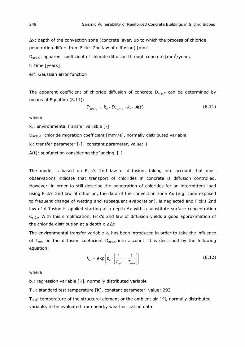
248 Seismic Vulnerability of Reinforced Concrete Buildings in Sliding Slopes
∆x: depth of the convection zone (concrete layer, up to which the process of chloride
penetration differs from Fick’s 2nd law of diffusion) [mm]
Dapp,C: apparent coefficient of chloride diffusion through concrete [mm2/years]
t: time [years]
erf: Gaussian error function
The apparent coefficient of chloride diffusion of concrete Dapp,C can be determined by
means of Equation (8.11):
app C e RCM tD k D k A t, ,0 ( ) (8.11)
where
ke: environmental transfer variable [-]
DRCM,0: chloride migration coefficient [mm2/a], normally distributed variable
kt: transfer parameter [-], constant parameter, value: 1
A(t): subfunction considering the ‘ageing’ [-]
The model is based on Fick’s 2nd law of diffusion, taking into account that most
observations indicate that transport of chlorides in concrete is diffusion controlled.
However, in order to still describe the penetration of chlorides for an intermittent load
using Fick’s 2nd law of diffusion, the data of the convection zone ∆x (e.g. zone exposed
to frequent change of wetting and subsequent evaporation), is neglected and Fick’s 2nd
law of diffusion is applied starting at a depth ∆x with a substitute surface concentration
Cs,∆x. With this simplification, Fick’s 2nd law of diffusion yields a good approximation of
the chloride distribution at a depth x ≥∆x.
The environmental transfer variable ke has been introduced in order to take the influence
of Treal on the diffusion coefficient Dapp,C into account. It is described by the following
equation:
e eref real
k bT T1 1exp
æ öæ ö÷ç ÷ç ÷÷ç= ⋅ -ç ÷÷ç ç ÷÷ç ÷ç è øè ø (8.12)
where
be: regression variable [K], normally distributed variable
Tref: standard test temperature [K], constant parameter, value: 293
Treal: temperature of the structural element or the ambient air [K], normally distributed
variable, to be evaluated from nearby weather station data

CHAPTER 8: Evolution of building vulnerability over time 249
The Chloride Migration Coefficient DRCM,0 is one of the governing parameters for the
description of the material properties in the chloride induced corrosion model. Suitable
data for DRCM,0 may be obtained from literature for different concrete mixtures to be used
as starting variables in service life design or vulnerability assessment calculations [Table
B2-1, FIB- CEB Task Group 5.6 (2006)].
The apparent diffusion coefficient Dapp,C is subject to considerable scatter and tends to
reduce with increasing exposure time. In order to take this into account when modeling
the initiation process, a transfer parameter kt in combination with a so-called ageing
exponent n has been introduced.
ntA t
t0( ) (8.13)
n: ageing exponent [-], beta distributed variable, Table B2-2, FIB- CEB Task Group 5.6
(2006)
t0: reference point of time [years], constant parameter, value: 0.0767
The chloride content in the concrete is not only caused by chloride ingress from the
surface, but can also be due to chloride contaminated aggregates, cements or water used
for the concrete production (initial chloride content C0). In certain circumstances the
chloride content of fine and coarse aggregates and water can be considerable.
The chloride content CS at the concrete surface as well as the substitute surface content
CS,∆x at a depth ∆x are variables that depend on material properties (e.g. type of binder
and the concrete composition) and on geometrical (e.g. geometry of the structural
element and the distance to the chloride source) and environmental (e.g. equivalent
chloride concentration of the ambient solution) conditions. The information needed to
determine CS and CS,∆x is briefly summarized in the flowchart given in Figure 8.7.
Under a continuous chloride impact of constant concentration, the chloride saturation
concentration CS,0 on the concrete surface is reached often in relative short time periods
compared to the service life of the structure (CS,0 = CS). Based on these results, the
conservative simplification that the variable CS is from the beginning constant with time
can be concluded for certain exposure conditions (e. g. for concrete continuously exposed
to sea water).

250 Seismic Vulnerability of Reinforced Concrete Buildings in Sliding Slopes
Figure 8.7. Information needed to determine the variables CS and CS,∆x (FIB- CEB Task Group 5.6,
2006)
In order to quantify the substitute chloride surface concentration CS,∆x , the transfer
function ∆x needs to be determined. For the different types of exposure conditions
(splash, submerged, spray, tidal and atmospheric) ∆x can be quantified based on the
information provided in section B2.2.5.5 of FIB- CEB Task Group 5.6 (2006). Depending
on the exposure condition CS,∆x may be defined as the maximum chloride content Cmax.
In cases when no ∆x develops (e.g. spray zone), Cmax represents the chloride content at
the concrete surface CS.
The critical chloride content Ccrit is the critical chloride concentration that causes
dissolution of the protective passive film around the reinforcement and initiates
corrosion. A beta-distribution with a lower boundary of 0.20 wt.-%/cement, mean value
of 0.60 wt.-%/cement and upper boundary of 2 wt.-%/cement was found to yield a
sufficiently good description of the test results.
Based on Equation (8.10) and assuming that the chloride ion concentration near the
concrete surface is constant, the time till corrosion initiation can be determined as:
CHAPTER 8: Evolution of building vulnerability over time 251
ncrit
init nse t RCM
CaT erfCk k D t
12 12
1
,0 0
14
(8.14)
where
Tinit: the corrosion initiation time (years) and
Cs: the equilibrium chloride concentration at the concrete surface
The statistical quantification of the model parameters describing the corrosion initiation
of the reinforced concrete elements is provided in Table 8.2 based on the FIB- CEB Task
Group 5.6 (2006) proposed model. For illustrational purposes, values for Portland
Cement Concrete (PCC) and three different water/cement ratios (namely w/c=0.4,0.5
and 0.6) are given. The values of surface chloride concentration CS and of the
temperature of the structural element or the ambient air Treal presented in the table are
applicable to structures exposed to atmospheric chloride condition (Choe et al. 2009).
Three different corrosion levels (low, medium, high) are considered in the table based on
available literature (Stewart, 2004).
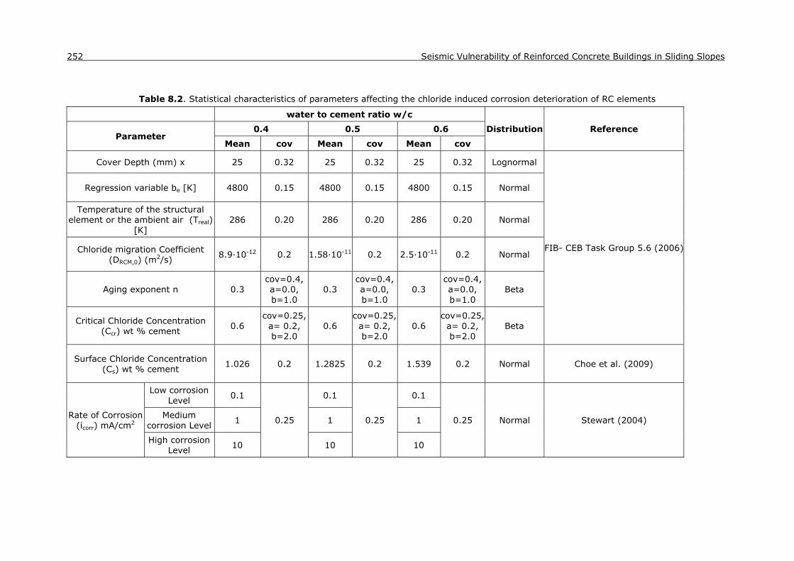
252 Seismic Vulnerability of Reinforced Concrete Buildings in Sliding Slopes
Table 8.2. Statistical characteristics of parameters affecting the chloride induced corrosion deterioration of RC elements
water to cement ratio w/c
Distribution Reference Parameter
0.4 0.5 0.6
Mean cov Mean cov Mean cov
Cover Depth (mm) x 25 0.32 25 0.32 25 0.32 Lognormal
FIB- CEB Task Group 5.6 (2006)
Regression variable be [K] 4800 0.15 4800 0.15 4800 0.15 Normal
Temperature of the structural element or the ambient air (Treal)
[K] 286 0.20 286 0.20 286 0.20 Normal
Chloride migration Coefficient (DRCM,0) (m2/s) 8.9·10-12 0.2 1.58·10-11 0.2 2.5·10-11 0.2 Normal
Aging exponent n 0.3 cov=0.4, a=0.0, b=1.0
0.3 cov=0.4, a=0.0, b=1.0
0.3 cov=0.4, a=0.0, b=1.0
Beta
Critical Chloride Concentration (Ccr) wt % cement 0.6
cov=0.25, a= 0.2, b=2.0
0.6 cov=0.25, a= 0.2, b=2.0
0.6 cov=0.25, a= 0.2, b=2.0
Beta
Surface Chloride Concentration (Cs) wt % cement 1.026 0.2 1.2825 0.2 1.539 0.2 Normal Choe et al. (2009)
Rate of Corrosion (icorr) mA/cm2
Low corrosion Level 0.1
0.25
0.1
0.25
0.1
0.25 Normal Stewart (2004) Medium corrosion Level 1 1 1
High corrosion Level 10 10 10
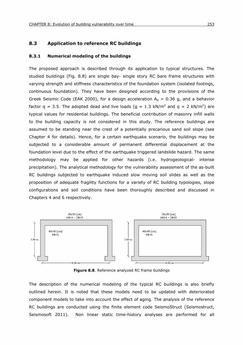
CHAPTER 8: Evolution of building vulnerability over time 253
8.3 Application to reference RC buildings
8.3.1 Numerical modeling of the buildings
The proposed approach is described through its application to typical structures. The
studied buildings (Fig. 8.8) are single bay- single story RC bare frame structures with
varying strength and stiffness characteristics of the foundation system (isolated footings,
continuous foundation). They have been designed according to the provisions of the
Greek Seismic Code (EAK 2000), for a design acceleration Ad = 0.36 g, and a behavior
factor q = 3.5. The adopted dead and live loads (g = 1.3 kN/m2 and q = 2 kN/m2) are
typical values for residential buildings. The beneficial contribution of masonry infill walls
to the building capacity is not considered in this study. The reference buildings are
assumed to be standing near the crest of a potentially precarious sand soil slope (see
Chapter 4 for details). Hence, for a certain earthquake scenario, the buildings may be
subjected to a considerable amount of permanent differential displacement at the
foundation level due to the effect of the earthquake triggered landslide hazard. The same
methodology may be applied for other hazards (i.e. hydrogeological- intense
precipitation). The analytical methodology for the vulnerability assessment of the as-built
RC buildings subjected to earthquake induced slow moving soil slides as well as the
proposition of adequate fragility functions for a variety of RC building typologies, slope
configurations and soil conditions have been thoroughly described and discussed in
Chapters 4 and 6 respectively.
Figure 8.8. Reference analyzed RC frame buildings
The description of the numerical modeling of the typical RC buildings is also briefly
outlined herein. It is noted that these models need to be updated with deteriorated
component models to take into account the effect of aging. The analysis of the reference
RC buildings are conducted using the finite element code SeismoStruct (Seismostruct,
Seismosoft 2011). Non linear static time-history analyses are performed for all

254 Seismic Vulnerability of Reinforced Concrete Buildings in Sliding Slopes
numerical simulations. In this analysis type, the applied loads (displacements) at the
foundation level vary in the pseudo-time domain, according to a load pattern prescribed
as the differential permanent ground displacement (versus time) curves directly
extracted from the seismic 2D dynamic analysis.
The material properties assumed for the members of the RC buildings are a uni-axial
nonlinear constant confinement model for the concrete (fc=20MPa, ft=2.1MPa, strain at
peak stress 0.002mm/mm, confinement factor 1.2) and a uni-axial bilinear stress-strain
model with kinematic strain hardening for the reinforcement (fy=400MPa, E=200GPa,
strain hardening parameter μ =0.005). All columns and beams have rectangular cross
sections (beam: 0.30x 0.50 m, column: 0.40x 0.40m). The initial longitudinal section
reinforcement degree used is 1% for the columns and 0.75% for the beams.
8.3.2 Quantification of aging probabilistic parameters
The present study considers the aging of the typical RC buildings by including
probabilistic models of carbonation and chloride induced corrosion deterioration of the RC
elements within the proposed vulnerability modeling framework. The application of the
fully probabilistic approach to the referred RC structures through a crude Monte Carlo
simulation using the coefficient of variations proposed in FIB- CEB Task Group 5.6 (2006)
was found to require large computational burden for practical problems and to yield to
numerical errors and instability for usual sample sizes (e.g. 100000-500000). Hence, in
an effort to equilibrate the computing efficiency and accuracy, for the probabilistic
modeling of rebar corrosion of a specified RC building, it was decided to adopt the mean
values of the parameters given in Tables 8.1 and 8.2 and to consider lower variability for
the random variables. Tables 8.3 and 8.4 present the statistical characteristics of the
parameters finally adopted for an adverse carbonation and chloride induced corrosion
scenario (w/c=0.6, High corrosion Level) respectively. It should be noted that for the
chloride corrosion scenario, an atmospheric exposure environment is assumed (e.g.
ke=0.67, Choe et al., 2009; 2010).

CHAPTER 8: Evolution of building vulnerability over time 255
Table 8.3. Statistical characteristics of parameters affecting the carbonation induced corrosion deterioration of RC elements adopted in the present study
Parameter Mean COV Distribution
Cover Depth (mm) a 25.00 0.20 Lognormal
Rhreal,k (% rel. humidity) 70.00 cov=0.05, a=40.0, b=100
Beta
Exponent of regression bc -0.567 0.035 Normal Inverse carbonation resistance (Racc,0
-1) (mm2/year) / (kg/m3) 2.30·10-10 0.10 Normal
Influence of test method kt 1.25 0.10 Normal
Error term et (mm2/years) 315.5 0.05 Normal
Cs,atm (kg/m3) 0.000820 0.10 Normal
Exponent of regression bw 0.446 0.10 Normal
Rate of Corrosion (rcorr) mA/cm2 2 0.20 Normal
Table 8.4. Statistical characteristics of parameters affecting the chloride induced corrosion
deterioration of RC elements adopted in the present study
Parameter Mean COV Distribution
Cover Depth (mm) x 25 0.2 Lognormal Environmental tranfer variable ke 0.67 0.1 Normal
Chloride migration Coefficient (DRCM,0) (m2/s) 2.5·10-11 0.1 Normal
Aging exponent n 0.3 cov=0.05, a=0.0, b=1.0 Beta
Critical Chloride Concentration (Ccr) wt % cement 0.6 cov=0.05, a=
0.2, b=2.0 Beta
Surface Chloride Concentration (Cs) wt % cement 1.539 0.1 Normal
Rate of Corrosion (icorr) mA/cm2 10 0.20 Normal
8.3.2.1. Corrosion initiation time
The corrosion initiation time depends on a number of parameters that can vary
considerably for different structures depending on the deterioration mechanism, the
structure location and environmental exposure condition. The distribution for the
corrosion initiation time is assessed through Monte Carlo simulation having a sample size
of 100000, using the equations 8.2 and 8.14 presented below for carbonation and
chloride induced corrosion respectively. A lognormal distribution with mean 36.40 years
and standard deviation of 20.85 years is found to be a good fit to the simulated data for
the carbonation induced corrosion initiation time (Fig. 8.9). Similarly, a lognormal fit with
mean 2.96 years and standard deviation of 2.16 years is adopted for the chloride induced
corrosion initiation time (Fig. 8.10). These distributions will subsequently be used as key

256 Seismic Vulnerability of Reinforced Concrete Buildings in Sliding Slopes
inputs for probabilistic modeling of rebar corrosion due to presence of carbonation and
chloride concentration.
Figure 8.9. Distribution of carbonation induced corrosion initiation time Tini (mean = 36.40years,
Standard Deviation = 20.85 years)
Figure 8.10. Distribution of chloride corrosion initiation time Tini (mean = 2.96 years, Standard
Deviation = 2.16 years)

CHAPTER 8: Evolution of building vulnerability over time 257
8.3.2.2. Time dependent loss of reinforcement
Once the protective passive film around the reinforcement dissolves due to continued
chloride ingress or carbonation, corrosion initiates and the time dependent loss of
reinforcement cross-sectional area can be expressed as (e.g. Ghosh and Padgett, 2010):
2
2
if t T4( )
max ,0 if t T 4
i init
init
n DA t
n D t
(8.15)
where, n is the number of reinforcement bars, Di is the initial diameter of steel
reinforcement, t is the elapsed time in years and D(t) is the reinforcement diameter at
the end of (t-Ti) years , which can be represented as:
i init
i corr init init
DD t
D i t T if t T
( )max[ ( ),0] if t T
(8.16)
If generalized corrosion is considered, the loss of metal due to corrosion is approximately
uniform over the whole surface. In this case, Faraday’s law indicates that a corrosion
current density corresponds to a uniform corrosion penetration of κ = 11, 6μm/year. The
rate of corrosion icorr in this study is considered to be constant on average along the
service life of the structure. Generally, the rate of corrosion due to carbonated concrete
cover is slower compared to chloride-induced corrosion.
The loss of area of steel due to corrosion of the RC elements is modeled as a reduction in
longitudinal reinforcing bar cross sectional area as compared to the elements in the initial
nondegraded state. It is assumed that the corrosion will not affect the mechanical and
material properties of the steel reinforcing bars. Figures 8.11 (a) and (b) show the
probabilistic assessment of the time-dependent area reduction ratio, which is the area of
reinforcing steel at time t, A(t), normalized by the initial area of reinforcement, A(t0) (for
Di= 14 mm, n=6). As expected, the variability in the loss of area of reinforcing steel tends
to increase with time due to the combined effect of the variability of the initial
reinforcement diameter, rate of corrosion and corrosion initiation time.
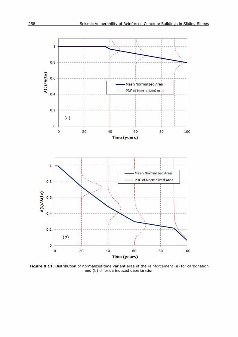
258 Seismic Vulnerability of Reinforced Concrete Buildings in Sliding Slopes
Figure 8.11. Distribution of normalized time variant area of the reinforcement (a) for carbonation
and (b) chloride induced deterioration
(b)
(a)

CHAPTER 8: Evolution of building vulnerability over time 259
8.3.3 Time-dependent fragility functions
In order to identify the building performance at different points in time and to construct
the corresponding time-dependent fragility curves, a time-variant local damage index
(DI) is introduced, describing the steel and concrete material strains. In all cases
analyzed the steel strain (εs) yields more critical results. Thus, it was decided to adopt
only this parameter as a damage index. In this way, it is possible to establish a
relationship between the damage index (εs) and the intensity parameter expressed
in terms of the peak ground acceleration (PGA) values at the seismic bedrock or
permanent ground displacement (PGD) values at the slope area, for different building
typologies and consequently to assign a median value of PGA/PGD to each limit state.
The next step is the definition of the limit states. For RC corroded buildings characterized
by a low level of confinement, the limit steel strains needed to exceed post yield limit
states should have lower values compared to adequately and properly confined
structures (Crowley et al., 2004; Bird et al., 2005). As a consequence, lower limit state
values were assumed to derive exceedance of moderate, extensive and complete
damage for the corroded poorly confined buildings. The time-dependent limit state values
finally adopted for the different limit states for the carbonation and chloride induced
deterioration scenario are presented in Tables 8.5 and 8.6 respectively. Note that for
carbonation induced corrosion the reduction in longitudinal reinforcing bar cross sectional
area is less than 20% in time t=90 years (see Fig. 8.11a). Thus, a minor reduction on
the limit strain values for the corroded structures is assigned as shown in Table 8.5. On
the contrary, larger reduction in the longitudinal reinforcing bar cross sectional area is
expected for the chloride induced corrosion (see Fig. 8.11b) resulting in significantly
reduced values over time for the corresponding limit states.
Table 8.5. Definition of limit states for the buildings at different points in time for the carbonation
induced deterioration scenario
Limit strains
Time (years) Limit State 1 Limit State 2 Limit State 3 Limit State 4
0
Steel bar yielding
0.0125 0.040 0.060 40 0.0125 0.039 0.059 60 0.0117 0.037 0.057 90 0.0115 0.035 0.055

260 Seismic Vulnerability of Reinforced Concrete Buildings in Sliding Slopes
Table 8.6. Definition of limit states for the buildings at different points in time for the chloride induced deterioration scenario
Limit strains
Time (years) Limit State 1 Limit State 2 Limit State 3 Limit State 4
0
Steel bar yielding
0.0125 0.040 0.060 20 0.0115 0.035 0.055 40 0.010 0.025 0.045 60 0.008 0.020 0.035 90 0.008 0.015 0.030
The overall fragility function of the buildings can be mathematically expressed as (e.g.
Ghosh and Padgett, 2010):
In IM In m tP LS IM
t/ Φ
(8.17)
where, IM is the intensity measure of the earthquake induced landslide expressed in
terms of PGA at the “seismic bedrock” or PGD at the slope area, m(t) and β(t) are the
median values (in units of g or m for PGA and PGD respectively) and logarithmic
standard deviations of the structure’s fragility at different points in time along the service
life and LS is the limit state.
The median values of PGA (t) and PGD (t) that correspond to each limit state can be
defined for the threshold values of the aforementioned damage indexes as the values
that correspond to the 50% probability of exceeding each limit state. The time-
dependent median of the buildings fragilities at each limit state can be adequately
represented by a quadratic fit for both deterioration scenarios (see subsections §8.3.1.1
and §8.3.1.1 for the carbonation and chloride induced scenarios respectively). Similar
models have also been adopted to demonstrate the increase in bridge fragility over time
due to corrosion (e.g. Ghosh and Padgett, 2010). Such time-dependent models offer the
advantage of estimating directly the fragility parameters at any point in time for the
given building and corrosion parameters, once the initial non-degraded fragility of the
building is known. The standard deviation values β(t) describe the total variability
associated with each fragility curve for different points in time.
The Maximum Likelihood Method, as described in Chapter 4 (§4.4.2.2), is used herein to
estimate the fragility parameters. The median and standard deviation values adopted are
presented in Tables 8.7 and 8.9 for the carbonation induced corrosion for buildings with
flexible and stiff foundations respectively and in Tables 8.11 and 8.13 for the chloride
induced corrosion of the reinforcement for buildings with flexible and stiff foundations
respectively. Tables 8.8 and 8.10 provide the percent (%) changes in fragility in terms of
median PGA/PGD and dispersion βPGA/ βPGD with aging for the carbonation induced

CHAPTER 8: Evolution of building vulnerability over time 261
corroded buildings with flexible and stiff foundation system respectively while Tables 8.12
and 8.14 present the corresponding changes for the chloride induced corroded buildings.
Fragility curves in terms of PGA (outcrop conditions) and PGD for different limit states
are analytically evaluated at different points in time along the service life of the studied
buildings with flexible and stiff foundation system to assess the time-dependent effect of
corrosion on their vulnerability for the given carbonation (§8.3.1.1) or chloride induced
(§8.3.1.2) deterioration scenario. A 3D illustration of the fragility estimates over time
(fragility surface) is also shown in order to obtain a better view of the evolution of
vulnerability with time.
It is observed that the fragility of the structure generally increases over time due to
corrosion. This increase is much more pronounced for the chloride induced corrosion
scenario and for higher levels of damage. Greater increase in vulnerability is expected for
the chloride induced corroded building with flexible foundation system, resulting to a
maximum reduction of 56% and 78% in the median PGA and PGD predicted values
respectively for the complete limit state after 90 years exposure to chlorides (see Tab.
8.11 and Figs. 8.25 and 8.26). There is also a change in the dispersion over time,
generally indicating increased uncertainty in estimating the median PGA and PGD values.
This trend is more evident for buildings with stiff foundation system subjected to chloride
induced reinforcement corrosion (see Tab. 8.13).
8.3.3.1. Fragility functions for carbonation induced corrosion of reinforcement
Building with flexible foundation system
Table 8.7. Parameters of fragility functions over time as a function of PGA and PGD for buildings
with flexible foundation system considering carbonation induced reinforcement corrosion
PGA (g) PGD (m)
Time (years)
Median PGA (g) Dispersion βPGA
Median PGD (m) Dispersion βPGD LS1 LS2 LS3 LS4 LS1 LS2 LS3 LS4
0 0.22 0.39 0.58 0.81 0.37 0.14 0.37 0.80 1.54 0.42
40 0.22 0.39 0.58 0.81 0.40 0.15 0.37 0.75 1.49 0.47
60 0.22 0.38 0.55 0.78 0.40 0.14 0.36 0.74 1.44 0.48
90 0.21 0.37 0.52 0.75 0.41 0.14 0.35 0.67 1.28 0.46

262 Seismic Vulnerability of Reinforced Concrete Buildings in Sliding Slopes
Table 8.8. Percent (%) changes in median PGA/PGD and dispersion β values with aging for buildings with flexible foundation system considering carbonation induced reinforcement corrosion
Change (%) with aging
Time (years)
Median PGA (g) Dispersion βPGA
Median PGD (m) Dispersion βPGD LS1 LS2 LS3 LS4 LS1 LS2 LS3 LS4
0 0.00 0.00 0.00 0.00 0.00 0.00 0.00 0.00 0.00 0.00
40 0.31 1.14 1.36 -0.32 -8.31 -1.88 -0.37 6.03 2.84 -11.68
60 -0.12 3.93 6.26 3.34 -9.95 -0.13 1.54 7.95 6.26 -14.59
90 3.01 5.85 11.29 7.15 -10.53 4.04 5.79 16.98 16.43 -9.22
Figure 8.12. Fragility curves in terms of PGA for different points in time (0, 40, 60 and 90 years),
for slight (LS1), moderate (LS2), extensive (LS3) and complete (LS4) limit states considering carbonation induced corroded buildings on flexible foundations.

CHAPTER 8: Evolution of building vulnerability over time 263
Figure 8.13. Fragility curves in terms of PGD for different points in time (0, 40, 60 and 90 years),
for slight (LS1), moderate (LS2), extensive (LS3) and complete (LS4) limit states considering carbonation induced corroded buildings on flexible foundations.
Figure 8.14. Time-dependent quadratic fit of median values of PGA for the slight, moderate,
extensive and complete limit states considering carbonation induced corroded buildings on flexible foundations
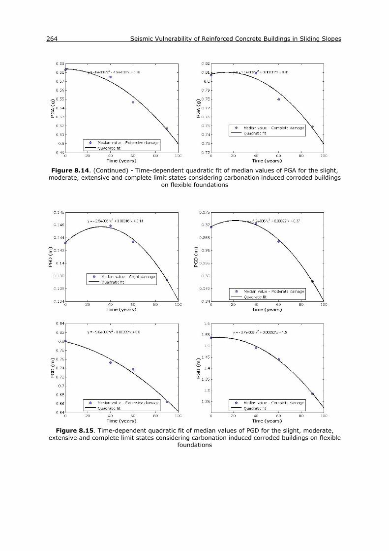
264 Seismic Vulnerability of Reinforced Concrete Buildings in Sliding Slopes
Figure 8.14. (Continued) - Time-dependent quadratic fit of median values of PGA for the slight,
moderate, extensive and complete limit states considering carbonation induced corroded buildings on flexible foundations
Figure 8.15. Time-dependent quadratic fit of median values of PGD for the slight, moderate,
extensive and complete limit states considering carbonation induced corroded buildings on flexible foundations

CHAPTER 8: Evolution of building vulnerability over time 265
Figure 8.16. Fragility surfaces as a function of time and PGA for slight, moderate, extensive and
complete limit states (fit: Interpolant) considering carbonation induced corroded buildings on flexible foundation
Figure 8.17. Fragility surfaces as a function of time and PGD for slight, moderate, extensive and
complete limit states (fit: Interpolant) considering carbonation induced corroded buildings on flexible foundations

266 Seismic Vulnerability of Reinforced Concrete Buildings in Sliding Slopes
Figure 8.17. (Continued) - Fragility surfaces as a function of time and PGD for slight, moderate, extensive and complete limit states (fit: Interpolant) considering carbonation induced corroded
buildings on flexible foundations
Building with stiff foundation system
Table 8.9. Parameters of fragility functions over time as a function of PGA and PGD for buildings
with stiff foundation system considering carbonation induced reinforcement corrosion
PGA (g) PGD (m)
Time (years)
Median PGA (g) Dispersion βPGA
Median PGD (m) Dispersion βPGD LS1 LS2 LS3 LS4 LS1 LS2 LS3
0 0.29 0.61 1.01 1.37 0.37 0.24 0.96 2.35 0.42
40 0.29 0.63 1.01 1.36 0.41 0.23 0.92 2.35 0.46
60 0.29 0.61 1.00 1.36 0.42 0.23 0.91 2.20 0.48
90 0.29 0.59 0.99 1.36 0.41 0.23 0.91 2.20 0.48
Table 8.10. Percent (%) changes in median PGA/PGD and dispersion β values with aging for
buildings with stiff foundation system considering carbonation induced reinforcement corrosion
Change (%) with aging
Time (years)
Median PGA (g) Dispersion βPGA
Median PGD (m) Dispersion βPGD LS1 LS2 LS3 LS4 LS1 LS2 LS3
0 0.00 0.00 0.00 0.00 0.00 0.00 0.00 0.00 0.00
40 -0.08 -3.40 -0.20 0.87 -11.16 2.31 4.46 0.26 -11.17
60 1.04 0.67 1.17 0.78 -13.49 4.43 5.05 6.71 -13.89
90 1.58 2.89 2.08 0.98 -11.96 4.43 5.05 6.71 -13.89

CHAPTER 8: Evolution of building vulnerability over time 267
Figure 8.18. Fragility curves in terms of PGA for different points in time (0, 40, 60 and 90 years),
for slight (LS1), moderate (LS2), extensive (LS3) and complete (LS4) limit states considering carbonation induced corroded buildings on stiff foundations.
Figure 8.19. Fragility curves in terms of PGD for different points in time (0, 40, 60 and 90 years),
for slight (LS1), moderate (LS2) and extensive (LS3) limit states considering carbonation induced corroded buildings on stiff foundations.
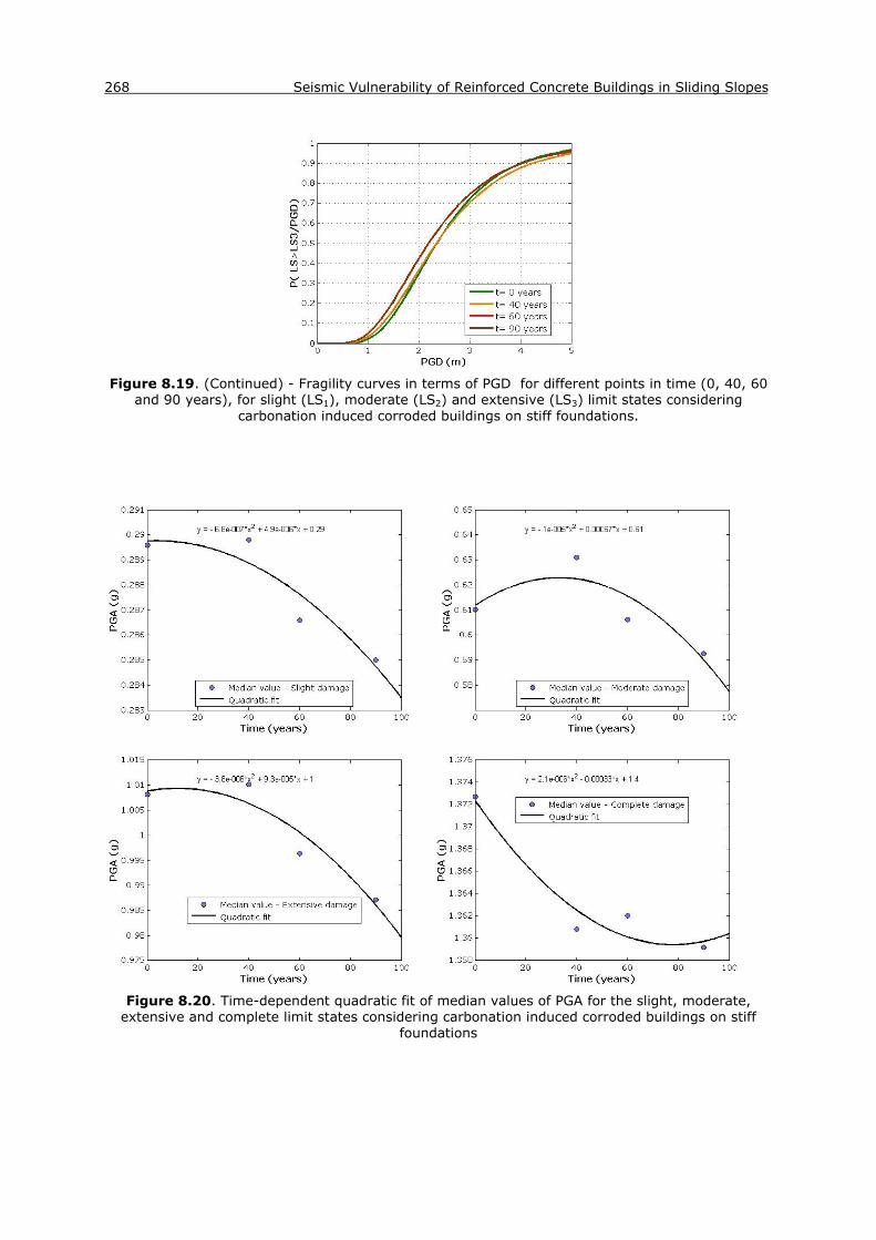
268 Seismic Vulnerability of Reinforced Concrete Buildings in Sliding Slopes
Figure 8.19. (Continued) - Fragility curves in terms of PGD for different points in time (0, 40, 60
and 90 years), for slight (LS1), moderate (LS2) and extensive (LS3) limit states considering carbonation induced corroded buildings on stiff foundations.
Figure 8.20. Time-dependent quadratic fit of median values of PGA for the slight, moderate,
extensive and complete limit states considering carbonation induced corroded buildings on stiff foundations

CHAPTER 8: Evolution of building vulnerability over time 269
Figure 8.21. Time-dependent quadratic fit of median values of PGD for the slight, moderate,
extensive and complete limit states considering carbonation induced corroded buildings on stiff foundations
Figure 8.22. Fragility surfaces as a function of time and PGA for slight, moderate, extensive and complete limit states (fit: Interpolant) considering carbonation induced corroded buildings on stiff
foundations

270 Seismic Vulnerability of Reinforced Concrete Buildings in Sliding Slopes
Figure 8.22. (Continued) - Fragility surfaces as a function of time and PGA for slight, moderate, extensive and complete limit states (fit: Interpolant) considering carbonation induced corroded
buildings on stiff foundations
Figure 8.23. Fragility surfaces as a function of time and PGD for slight, moderate, extensive and complete limit states (fit: Interpolant) considering carbonation induced corroded buildings on stiff
foundations

CHAPTER 8: Evolution of building vulnerability over time 271
8.3.3.2. Fragility functions for chloride induced corrosion of reinforcement
Building with flexible foundation system
Table 8.11. Parameters of fragility functions over time as a function of PGA and PGD for buildings
with flexible foundation system considering chloride induced reinforcement corrosion
PGA (g) PGD (m)
Time (years)
Median PGA (g) Dispersion βPGA
Median PGD (m) Dispersion βPGD LS1 LS2 LS3 LS4 LS1 LS2 LS3 LS4
0 0.22 0.39 0.58 0.81 0.37 0.14 0.37 0.80 1.54 0.42
20 0.20 0.38 0.54 0.73 0.39 0.12 0.37 0.70 1.31 0.47
40 0.18 0.36 0.48 0.71 0.40 0.11 0.33 0.58 1.18 0.45
60 0.17 0.31 0.40 0.55 0.41 0.07 0.25 0.41 0.81 0.50
90 0.12 0.19 0.25 0.36 0.38 0.07 0.13 0.24 0.34 0.48
Table 8.12. Percent (%) changes in median PGA/PGD and dispersion β values with aging for buildings with flexible foundation system considering chloride induced reinforcement corrosion
Change (%) with aging
Time (years)
Median PGA (g) Dispersion βPGA
Median PGD (m) Dispersion βPGD LS1 LS2 LS3 LS4 LS1 LS2 LS3 LS4
0 0.00 0.00 0.00 0.00 0.00 0.00 0.00 0.00 0.00 0.00
20 8.02 2.62 8.21 9.75 -7.23 12.96 0.72 12.10 14.48 -11.64
40 17.49 8.39 18.08 12.43 -9.91 24.87 10.77 27.73 23.05 -8.25
60 23.89 21.58 31.13 31.33 -10.24 49.04 32.22 48.94 47.54 -19.44
90 43.53 52.14 56.47 55.75 -2.06 53.25 64.79 69.95 77.62 -15.90
Figure 8.24. Fragility curves in terms of PGA for different points in time (0, 20, 40, 60 and 90
years), for slight (LS1), moderate (LS2), extensive (LS3) and complete (LS4) limit states considering chloride induced corroded buildings on flexible foundations.

272 Seismic Vulnerability of Reinforced Concrete Buildings in Sliding Slopes
Figure 8.24. (Continued) - Fragility curves in terms of PGA for different points in time (0, 20, 40, 60 and 90 years), for slight (LS1), moderate (LS2), extensive (LS3) and complete (LS4) limit states
considering chloride induced corroded buildings on flexible foundations.
Figure 8.25. Fragility curves in terms of PGD for different points in time (0, 20, 40, 60 and 90
years), for slight (LS1), moderate (LS2), extensive (LS3) and complete (LS4) limit states considering chloride induced corroded buildings on flexible foundations.

CHAPTER 8: Evolution of building vulnerability over time 273
Figure 8.26. Time-dependent quadratic fit of median values of PGA for the slight, moderate, extensive and complete limit states considering chloride induced corroded buildings on flexible
foundations
Figure 8.27. Time-dependent quadratic fit of median values of PGD for the slight, moderate, extensive and complete limit states considering chloride induced corroded buildings on flexible
foundations

274 Seismic Vulnerability of Reinforced Concrete Buildings in Sliding Slopes
Figure 8.27. (Continued) - Time-dependent quadratic fit of median values of PGD for the slight, moderate, extensive and complete limit states considering chloride induced corroded buildings on
flexible foundations
Figure 8.28. Fragility surfaces as a function of time and PGA for slight, moderate, extensive and complete limit states (fit: Interpolant) considering chloride induced corroded buildings on flexible
foundations

CHAPTER 8: Evolution of building vulnerability over time 275
Figure 8.29. Fragility surfaces as a function of time and PGD for slight, moderate, extensive and complete limit states (fit: Interpolant) considering chloride induced corroded buildings on flexible
foundations
Building with stiff foundation system
Table 8.13. Parameters of fragility functions over time as a function of PGA and PGD for buildings
with stiff foundation system considering chloride induced reinforcement corrosion
PGA (g) PGD (m)
Time (years)
Median PGA (g) Dispersion βPGA
Median PGD (m) Dispersion βPGD LS1 LS2 LS3 LS4 LS1 LS2 LS3
0 0.29 0.61 1.01 1.37 0.39 0.24 0.96 2.35 0.46
20 0.27 0.59 0.98 1.32 0.42 0.23 0.87 2.13 0.46
40 0.27 0.53 0.87 1.21 0.42 0.22 0.75 1.72 0.47
60 0.25 0.47 0.77 1.06 0.42 0.17 0.56 1.39 0.53
90 0.20 0.40 0.71 1.02 0.44 0.11 0.40 1.15 0.71
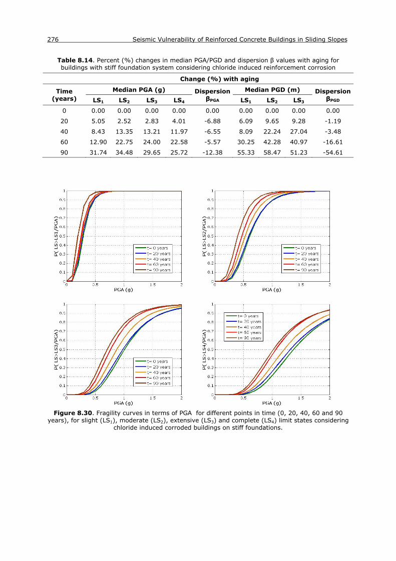
276 Seismic Vulnerability of Reinforced Concrete Buildings in Sliding Slopes
Table 8.14. Percent (%) changes in median PGA/PGD and dispersion β values with aging for buildings with stiff foundation system considering chloride induced reinforcement corrosion
Change (%) with aging
Time (years)
Median PGA (g) Dispersion βPGA
Median PGD (m) Dispersion βPGD LS1 LS2 LS3 LS4 LS1 LS2 LS3
0 0.00 0.00 0.00 0.00 0.00 0.00 0.00 0.00 0.00
20 5.05 2.52 2.83 4.01 -6.88 6.09 9.65 9.28 -1.19
40 8.43 13.35 13.21 11.97 -6.55 8.09 22.24 27.04 -3.48
60 12.90 22.75 24.00 22.58 -5.57 30.25 42.28 40.97 -16.61
90 31.74 34.48 29.65 25.72 -12.38 55.33 58.47 51.23 -54.61
Figure 8.30. Fragility curves in terms of PGA for different points in time (0, 20, 40, 60 and 90
years), for slight (LS1), moderate (LS2), extensive (LS3) and complete (LS4) limit states considering chloride induced corroded buildings on stiff foundations.

CHAPTER 8: Evolution of building vulnerability over time 277
Figure 8.31. Fragility curves in terms of PGD for different points in time (0, 20, 40, 60 and 90
years), for slight (LS1), moderate (LS2) and extensive (LS3) limit states considering chloride induced corroded buildings on stiff foundations.
Figure 8.32. Time-dependent quadratic fit of median values of PGA for the slight, moderate, extensive and complete limit states considering chloride induced corroded buildings on stiff
foundations

278 Seismic Vulnerability of Reinforced Concrete Buildings in Sliding Slopes
Figure 8.32. (Continued) - Time-dependent quadratic fit of median values of PGA for the slight, moderate, extensive and complete limit states considering chloride induced corroded buildings on
stiff foundations
Figure 8.33. Time-dependent quadratic fit of median values of PGD for the slight, moderate, extensive and complete limit states considering chloride induced corroded buildings on stiff
foundations

CHAPTER 8: Evolution of building vulnerability over time 279
Figure 8.34. Fragility surfaces as a function of time and PGA for slight, moderate, extensive and
complete limit states (fit: Interpolant) considering chloride induced corroded buildings on stiff foundations
Figure 8.35. Fragility surfaces as a function of time and PGD for slight, moderate, extensive and
complete limit states (fit: Interpolant) considering chloride induced corroded buildings on stiff foundations

280 Seismic Vulnerability of Reinforced Concrete Buildings in Sliding Slopes
Figure 8.35. (Continued) - Fragility surfaces as a function of time and PGD for slight, moderate,
extensive and complete limit states (fit: Interpolant) considering chloride induced corroded buildings on stiff foundations
8.4 Conclusions
An extension of the proposed vulnerability assessment framework to account for the
time-dependent fragility analysis of corroded RC buildings impacted by co-seismic
permanent landslide displacements has been presented. Two potential adverse corrosion
scenarios are examined: chloride and carbonation induced corrosion of the steel
reinforcement. The methodology is applied to reference low-rise RC frame buildings with
varying strength and stiffness of the foundation system that are subjected to the
combined effects of reinforcement corrosion and earthquake triggered landslide
displacements. Fragility curves in terms of PGA (outcrop conditions) and PGD for different
limit states are analytically evaluated at different points in time (0, 20, 40, 60, 90 years)
to assess the time-dependent effect of corrosion on their vulnerability for the given
carbonation or chloride induced deterioration scenario. It is observed that the fragility of
the structures generally increases over time due to corrosion. This increase is more
pronounced for the chloride induced corroded RC buildings founded on isolated footings.
Future work should aim at the validation of the proposed time-dependent model through
comparison of the computed damages to experimental results and/or empirical data.
Significant effort should also be devoted in the more refined definition of the time-
dependent performance indicators and the corresponding limit states. Moreover, further
research is needed to address time-dependent fragility of additional building types and
geometries, different triggering mechanisms of the potential landslide mass (e.g. intense
precipitation) and different hazard (e.g. earthquakes) as well as deterioration
mechanisms.

CHAPTER 9
Conclusions-Limitations- Future work
9.1 Summary of findings and contributions
An efficient quantitative risk assessment (QRA) tool that allows for establishing risk
management strategies and emergency planning in a cost-effective manner, requires the
quantification of both hazard and vulnerability of the elements at risk. However, most of
the existing risk assessment studies do not focus on assessing physical vulnerability to
landslides comprehensively. Instead, they often provide empirical or expect judgment-
based vulnerability values depending on the landslide type and the element at risk (e.g.
Dai et al. 2002). This is principally due to its complex, dynamic and multidimensional
nature and to the lack of reliable damage data from previous landslide events, which
makes its quantitative evaluation within a risk assessment study an intrinsically difficult
task. A better understanding on the type and extent of damage to various elements at
risk (buildings, roads, population) produced by different landslide mechanisms (slow
moving slides, debris flows, rock falls etc) is therefore essential to reduce the great deal
of uncertainty associated with the landslide vulnerability modeling. The probabilistic
treatment of these uncertainties through the use of the co-called fragility (or
vulnerability) curves is also a further step towards the efficient integration of the physical
vulnerability component into a QRA study.
Stemming from the general lack of methodologies to assess building vulnerability to
slides (see Chapter 3), one of the most significant contributions of the present research
was the proposition and quantification of an analytical methodology to estimate physical
vulnerability of RC frame buildings subjected to earthquake triggered slow-moving slides
(Chapter 4). Vulnerability was defined through probabilistic fragility curves which allow
for direct implementation within a probabilistic risk assessment framework.
According to the suggested method, the damage caused by a slow-moving slide on a
single building was attributed to the cumulative permanent (absolute or differential)
displacement concentrated within the unstable or moving area. A low-rise RC frame

282 Seismic Vulnerability of Reinforced Concrete Buildings in Sliding Slopes
building located next to the crown of a potential unstable slope was considered subjected
to forced differential displacement due to the earthquake triggered landslide and
subsequently to structural distress and damage. The numerical analysis involved two
consecutive steps and described through an idealized, yet realistic, example.
In the first step, the total and differential permanent displacements were estimated
considering the actual stiffness and weight of the building and its foundation, using a
non-linear finite difference dynamic finite slope model. A suite of seven gradually
increasing acceleration time histories recorded on rock outcrop were applied at the base
of the model to cover a wide range of seismic motions in terms of amplitude, frequency
content and significant duration in order to provide the necessary response quantity
statistics. The analyses were performed for single bay-single storey RC frame buildings
on stiff and flexible foundations considering both sand and clayey surface slope layers.
Additional analyses were also conducted for the free field case i.e. in the absence of any
structure in the vicinity of the crest. It was shown that the presence of a structure next
to the slope’s crest may contribute in altering the free field response of the slope and the
corresponding deformation demand for the building. The level of this differentiation
varies with respect to the foundation type (flexible, stiff), the surface soil conditions
(sand, clay) and the characteristics of the seismic motion.
The computed permanent displacements for the free field case at the slope area were
validated through comparison with simplified Newmark-type displacement methods in
Chapter 5. Three different displacement-based procedures were used to predict the
permanent slope deformation: the conventional analytical Newmark rigid block model
(Newmark 1965), the decoupled Rathje and Antonakos (2011) model and the coupled
Bray and Travasarou (2007) sliding block model. Comparisons between the Newmark-
type models were also conducted to demonstrate their relative degree of conservatism
for different earthquake scenarios and compliance of the sliding surface. It was shown
that Bray and Travasarou (2007) coupled model generally predicted larger displacements
compared to conventional analytical Newmark rigid block and Rathje and Antonakos
decoupled model. The difference in the displacement prediction was more pronounced for
the considered flexible sliding masses.
It is concluded that permanent horizontal displacements along the unstable slope area
derived by the proposed numerical approach were not inconsistent with the predicted
Newmark-type displacements enhancing the reliability and robustness of the dynamic
analysis results. More specifically, all three displacement-based models predicted
displacements that were generally compatible with the numerical results for the sand stiff
slope case. On the contrary, for the clay more flexible slope the correlation was not so
good. In particular, Bray and Travasarou (2007) model predicted larger displacements

CHAPTER 9: Conclusions- Limitations- Future work 283
with respect to the dynamic analysis whereas Newmark rigid block and Rathje and
Antonakos (2011) models underestimated the corresponding displacements. Among the
three methods, Bray and Travasarou model was found to present the minimum average
predictive error (%) in relation to the dynamic analysis whilst Newmark analytical
approach showed the minimum dispersion of that error for both sand nearly rigid and
clay relatively flexible slope cases. Overall, the differences in the displacement prediction
between the models were larger for the more ductile clay slope. Thus, the compliance of
the failure surface in relation to the frequency content of the input earthquake scenarios
probably allowed for some bias to be introduced on the results.
In the second step, non-linear static time history analyses of the selected buildings were
performed to assess the building’s response to the permanent ground deformation
induced by the landslide. The analyses were conducted for progressively increasing levels
of differential displacements provided by the computed dynamic stress strain analysis for
increasing amplitudes of input acceleration time histories. The derived differential
displacements at the foundation level were imposed quasi-statically at one of the RC
building supports (footings). The applied differential displacement vector was found to be
principally governed by the horizontal component that controlled the deformation mode
in buildings with flexible foundations whereas the corresponding displacements were
practically vertical in buildings with stiff foundation system. Structural response data in
terms of maximum material strain were then statistically correlated to the landslide
intensity parameters to estimate structure’s performance and fragility.
Damage limit states were defined with respect to the building classification and its
structural characteristics in terms of threshold values of building’s material strain based
on the work of Crowley et al. (2004), Bird et al. (2005; 2006), Negulescu and Foerster
(2010) and proper engineering judgment. Vulnerability was finally assessed through
probabilistic fragility (or vulnerability) curves, which describe the probability of exceeding
a certain limit state of the building exposed to the landslide hazard given the measure of
the landslide intensity. The landslide intensity was expressed both in terms of peak
horizontal ground acceleration (PGA) at the seismic bedrock (i.e the initial triggering
force of the slow-moving slide) and permanent ground displacement (PGD) at the slope
area (i.e. a product of PGA). The latter one was generally better correlated to structural
deformation and damage and allowed for direct comparisons to non-earthquake related
landslide damages to buildings.
Two different procedures were presented and applied to estimate the log-normally
distributed fragility parameters (median and log-standard deviation) given the simulated
damage data. The first one, was based on a regression analysis method (e.g. Nielson and
DesRoches, 2007; Argyroudis and Pitilakis, 2012) whereas the second was based on a

284 Seismic Vulnerability of Reinforced Concrete Buildings in Sliding Slopes
purely statistical approach, i.e. the maximum likelihood method (e.g. Shinozuka et al.,
2000; 2003). Various sources of uncertainty associated with the building capacity, the
deformation demand and the definition of limit states were explicitly taken into account
in the fragility analysis. The differences on the fragility curves when applying the two
different approaches were due to the different assumptions adopted in each method and
evidently displayed the influence of epistemic uncertainty on the fragility analysis. For
the simulated dataset the maximum likelihood method was found to be more efficient
(predicting lower log-standard deviation values) compared to the regression analysis
method when considering PGA as an intensity parameter.
The derived fragility functions revealed that the foundation compliance and the slope soil
type may greatly influence the structural response and damage. In particular, among the
structures analyzed, the ones with flexible foundations located on sand slopes were the
most vulnerable whereas the corresponding ones with stiff foundations located on clay
slopes appeared to be the least susceptible to damage.
An abacus of fragility curves both in terms of PGA and PGD were developed in Chapter 6
based on the suggested methodological framework via an extensive parametric
investigation and sensitivity analysis of various slope geometries, soil properties and
distances of the building with respect to the slope’s crown. It is concluded that slope
inclination in conjunction with the slope soil material were among the most influential
features on the physical vulnerability of the building exposed to the seismically induced
landslide. The slope height was also proved to greatly influence the building’s fragility for
the steep sand slope configurations. The above observations resulted to the proposition
of seven sets of generalized fragility curves, considering the most unfavorable position of
the building with respect to the slope’s crest that was found to be different for sand and
clay slopes.
To get further insight into the building‘s vulnerability to the permanent differential
displacement due to landslide hazard several additional parameters were also studied.
These included the water table level, the consideration of a strain softening landslide
material, the flexibility of the foundation system, the number of bays and storeys of the
building and the code design level. It was shown that the influence of each parameter
may vary with respect to the slope soil material (e.g. for the water table) and the
foundation compliance (e.g. for the building geometry). Overall, it was observed that
their impact might be, under certain circumstances, crucial to the structure’s fragility.

CHAPTER 9: Conclusions- Limitations- Future work 285
To gain confidence on the proposed methodological framework, representative developed
fragility curves were compared with literature ones and recorded building damages from
real past events in Chapter 7.
The validity the proposed method was first assessed through the comparison of
representative suggested fragility curves with corresponding literature ones based on
empirical damage data (Zhang and Ng, 2005), engineering judgement (NIBS, 2004) and
on numerical simulations (Negulescu and Foerster, 2010). Taking into account the
different assumptions associated with the proposed and the literature curves, the
comparisons showed that the proposed curves were generally in good agreement with
the literature ones for the case of the typical studied building on flexible foundations. On
the contrary, it was found that the proposed curves underestimated the structure’s
fragility with respect to the literature ones for the corresponding building on stiff
foundations.
Typical proposed fragility curves for low-rise RC buildings subjected to co-seismic
permanent slope displacement were also correlated to fragility curves provided by
various investigators for low-rise RC buildings subjected to ground shaking lying on an
horizontally layered soil stratum. Overall, the comparisons allowed seeking an
understanding of the relative extent of damage and the associated dominating failure
mechanism for structures subjected to co-seismic slope deformation and ground shaking
respectively. They revealed, however, the high aleatory and epistemic uncertainty
associated with the different fragility curves found in the literature.
The proposed methodological framework and the corresponding fragility curves were also
validated through its application to two real case histories: Kato Achaia slope in
Peloponnese –Greece and the Corniglio village-Italy case study. The direct comparison of
the recorded damage data on typical buildings with the corresponding damage predicted
by the developed fragility functions proved that the proposed fragility curves could
adequately capture the performance of the representative building affected by the slope
co-seismic landslide differential displacement. In addition, to enhance the effective
implementation of the proposed methodological framework within a probabilistic risk
assessment study, more realistic fragility curves were developed for a representative
building in Corniglio village based on numerical simulations. The reliability of the curves
was verified through their comparison with the observed building damage data for the
measured level of displacement.
Traditionally, the structural vulnerability implicitly refers to the intact, as-built structure
assuming an optimum plan of maintenance. However, structures deteriorate due to
various time-dependent mechanisms after they are put into service, without always
subjected to the necessary interventions during their lifetime. These issues are becoming

286 Seismic Vulnerability of Reinforced Concrete Buildings in Sliding Slopes
even more crucial in presence of natural hazards striking the structure, such as landslides
and/or earthquakes. A major contribution of the present research was thus the expansion
of the proposed method to account for the changing patterns of building‘s vulnerability
over time exposed to earthquake –induced landslide hazard (Chapter 8). In particular,
the progressive aging of typical RC buildings due to exposure to aggressive corrosive
environment was investigated by including probabilistic models of corrosion deterioration
of the RC elements within the vulnerability modeling framework. Two potential corrosion
scenarios were examined: chloride and carbonation induced corrosion of the steel
reinforcement. The proposed methodology was applied to reference low-rise RC frame
buildings with varying strength and stiffness of the foundation system that are subjected
to the combined effects of reinforcement corrosion and earthquake triggered landslide
displacements. Time –dependent fragility curves in terms of PGA (outcrop conditions)
and PGD for different damage states were analytically evaluated at different points in
time (0, 20, 40, 60, 90 years) for the given carbonation or chloride induced deterioration
scenario. It was shown that the fragility of the structures may increase over time due to
corrosion. This increase was more evident for the chloride induced corroded RC buildings
founded on flexible foundations.
9.2 Limitations and recommendations for future work
The work in the present study distinguishes certain limitations and should be extended
through additional research in the following areas:
- The proposed vulnerability assessment method and the corresponding fragility
curves are appropriate for predicting the structural damage of the building
members implying a ductile failure of the structure. However, the total damage
(structural and non-structural) will be quite different (certainly larger) in case of
the building with the stiff foundation as a considerable amount of damage may be
attributed to the rotation of the whole building as a rigid body. In the latter, the
damage can only be defined using empirical criteria and proper engineering
judgment (Bird et al., 2005).
- The complex issue of combined damages due to ground shaking and ground
failure is not taken into account in the evaluation of building‘s vulnerability that is
assessed only for the co-seismic permanent slope differential displacement. Thus,
no strength or stiffness degradation to the building’s structural members due to
the effect of ground shaking is assumed to occur. Future work should be therefore
oriented towards the study of the vulnerability of a typical building standing next

CHAPTER 9: Conclusions- Limitations- Future work 287
to the cliff exposed to the coupled effect of ground shaking and permanent ground
deformation due to landslide.
- It is also suggested to increase the applicability band of the proposed
methodological framework through the development of supplementary fragility
curves for other structural typologies (e.g. for high-rise RC buildings), slope
configurations and soil conditions. Various additional features such as the water
table level should also be addressed more in depth.
- In addition, future research should aim at the validation of the proposed time-
dependent vulnerability model via comparison of the damages predicted by the
curves to experimental results and/or empirical data.
- Significant effort should also be devoted in the more refined definition of the time-
dependent performance indicators and states. This is a very important and
challenging issue which has not received much attention until very recently
(REAKT, http://www.reaktproject.eu/)
- Finally, further research is needed to address time-dependent fragility of
additional building types and geometries, different triggering mechanisms of the
potential landslide mass (e.g. intense precipitation) as well as deterioration
mechanisms.

288 Seismic Vulnerability of Reinforced Concrete Buildings in Sliding Slopes

REFERENCES
AGSO (2001). “Natural hazards and the risk they pose to South-East Queenland”. AGSO-
Geoscience Australia. Digital report on CD-ROM. 389 Pages.
AGS (2007). “Guideline for landslide susceptibility, hazard and risk zoning for land use
management”. Australian geomechanics society landslide taskforce landslide zoning
working group. Australian Geomechanics 42 (1), 13–36.
Ahmad N., Crowley H., Pinho R. (2011). “Analytical fragility functions for reinforced
concrete and masonry buildings and buildings aggregates of Euro-Mediterranean
regions – UPAV methodology”. Internal Report, Syner-G Project 2009/2012.
Akkar S., Sucuoglu H., Yakut A. (2005). “Displacement-based fragility functions for low-
and mid-rise ordinary concrete buildings”. Earthquake Spectra 21(4), 901-927.
Ambraseys N.N. (1988). “Engineering seismology”. Int. J. Earthquake Eng. Struct. Dyn.
17, 1–105.
Ambraseys N.N., Menu J.M. (1988). “Earthquake-induced ground displacements”. J.
Earthquake Eng. 16, 985–1006.
Anastasopoulos I., Gazetas G., Bransby M.F., Davies M.C.R., El Nahas A. (2007). "Fault
rupture propagation through sand: Finite element analysis and validation through
centrifuge experiments". Journal of Geotechnical and Geoenvironmental Engineering
133(8), 943‐958.
Antonakos G. (2009). "Models of dynamic response and decoupled displacements of
earth slopes during earthquakes". M.S. Thesis, University of Texas at Austin, Austin,
TX.
Argyroudis S. (2010). “Contribution to seismic vulnerability and risk of transportation
networks in urban environment”. PhD Thesis (in Greek), Dept. of Civil Engineering,
Aristotle University of Thessaloniki, Greece.
Argyroudis S., Fotopoulou S., Pitilakis K. (2011). “Semi-empirical assessment of road
vulnerability to seismically induced slides”. 2nd World Landslide Forum, 3-8 October.
Argyroudis S., Pitilakis K. (2012). “Seismic fragility curves of shallow tunnels in alluvial
deposits”. Soil Dynamics and Earthquake Engineering 35, 1-12.
Ashford S.A., Sitar N., Lysmer J., Deng N., (1997). “Topographic effects on the seismic
response of steep slopes”. Bulletin of the Seismological Society of America 87, 701–
709.

290 Seismic Vulnerability of Reinforced Concrete Buildings in Sliding Slopes
Assimaki D., Gazetas G. (2004). “Soil and topographic amplification on canyon banks and
the 1999 Athens earthquake”. Journal of Earthquake Engineering 8(1), 1–43.
Assimaki D., Kausel E., Gazetas G. (2005). ”Wave propagation and soil–structure
interaction on a cliff crest during the 1999 Athens Earthquake”. Soil Dynamics and
Earthquake Engineering 25(7-10), 513-527.
Assimaki D., Kausel E. (2007). “Modified topographic amplification factors for a single-
faced slope due to kinematic soil-structure interaction”. Journal of Geotechnical and
Geoenvironmental Engineering 133, 1414–1431.
Association of Professional Engineers and Geoscientists of British Columbia (APEGBC)
(2010). “Guidelines for legislated landslide assessments for proposed residential
developments in BC”. May 2010.
ATC-13 (1985). “Earthquake damage evaluation data for California”. Applied Technology
Council, Redwood City.
Ausilio E., Costanzo A., Silvestri F., Tropeano G. (2008). “Prediction of seismic slope
displacements by dynamic stick-slip analyses”. Seismic Engineering International
Conference(MERCEA’08), Reggio Calabria and Messina, Italy, July 8–11.
Ausilio E., Costanzo A., Tropeano G., Silvestri F. (2009). “Evaluation of seismic
displacements of a natural slope by simplified methods and dynamic analyses”.
Performance-Based Design in Earthquake Geotechnical Engineering – Kokusho,
Tsukamoto & Yoshimine (eds)Taylor & Francis Group, London, ISBN 978-0-415-
55614-9.
Barani S., Bazzurro P., Pelli F. (2010). “A probabilistic method for the prediction of
earthquake induced slope displacements”. Proceedings of 5th International
Conference on recent advances in Geotechnical Earthquake Engineering and Soil
dynamics and Symposium in Honor of professor I. M. Idriss, San Diego, May 24-29.
Beushausen H., Alexander M. (2010). “Concrete deterioration: causes, mechanisms,
prevention”. Concrete Technology for Structural Engineers, Workshop, May 2010.
Bird J.F., Crowley H., Pinho R., Bommer J.J. (2005). “Assessment of building response to
liquefaction induced differential ground deformation”. Bul of the New Zealand Society
for Earthquake Engineering 38(4), 215-234.
Bird J.F., Bommer J.J., Crowley H., Pinho R. (2006). “Modelling liquefaction-induced
building damage in earthquake loss estimation”. Soil dynamics and Earthquake
Engineering 26 (1), 15-30.
Bjerrum L. (1967). “Progressive failure in slopes of overconsolidated plastic clays and
clay shales”. J Mech Found Eng Div ASCE 93(5), 1–49.
REFERENCES 291
Bjerrum L. (1963). “Allowable settlement of structures”. Proceedings of the 3rd European
Conf. on Soil Mech. and Found. Engng, Wiesbaden, 2, Brighton, England, 135–137.
Bommer J., Rodriguez C. (2002). “Earthquake-induced landslides in Central America”.
Engineering Geology 63(3-4), 189-220.
Bommer J.J., Alarcon J.E. (2006). “The prediction and use of peak ground velocity”.
Journal of Earthquake Engineering 10(1), 1-31.
Boone S.J. (1996). “Ground-movement-related building damage”. J. Geotech. Eng.-
ASCE, 122(11), 886–896.
Borzi B., Pinho R., Crowley H. (2007). “SP-BELA: un metodo meccanico per la definizione
della vulnerabilità basato su analisi pushover semplificate”. ANIDIS, Pisa, 2007 (in
italian).
Boscardin M.D., Cording E.G. (1989). “Building response to excavation induced
settlement”. J. Geotech. Eng.-ASCE 115, 1–21.
Bouckovalas G.D., Gazetas G., Papadimitriou A.G. (1995). "Geotechnical aspects of the
1995 Aegion (Greece) earthquake". National Technical University of Athens, Greece.
Bouckovalas G.D., Kouretzis, G. (2001). “Review of soil and topography effects in the
September 7,1999 Athens (Greece) earthquake”. Proc. Forth International Conference
on Recent Advances in Geotechnical Earthquake Engineering and Soil Dynamics and
Symposium in Honor of Professor W.D. Liam Finn (S. Diego – California, 26-
31/05/2001).
Bouckovalas G.D., Papadimitriou A.G. (2005). "Numerical evaluation of slope topography
effects on seismic ground motion". Soil Dynamics and Earthquake Engineering 25(7-
10), 547-558.
Bourdeau C., Havenith H.B., Fleurisson J.A., Grandjean, A.G. (2004). “Numerical
modelling of seismic slope stability”. Engineering Geology for Infrastructure Planning
in Europe, Springer Berlin / Heidelberg 104, 671-684.
Bourdeau C., Havenith H.B. (2008). "Site effects modelling applied to the slope affected
by the Suusamyr earthquake (Kyrgyzstan, 1992)". Engineering Geology 97(3-4), 126-
145.
Bozzano F., Lenti L., Martino S., Paciello A., Scarascia Mugnozza G. (2008a). “Self-
excitation process due to local seismic amplification responsible for the 31st October
2002 reactivation of the Salcito landslide (Italy)”. J Geophys Res 113.
Bozzano F., Bretschneider A., Martino S. (2008b). “Stress–strain history from the
geological evolution of the Orvieto and Radicofani cliff slopes (Italy)”. Landslides 5(4),
351-366.

292 Seismic Vulnerability of Reinforced Concrete Buildings in Sliding Slopes
Bozzano F., Lenti L., Martino S., Paciello A., Scarascia Mugnozza G. (2010). “Evidences of
landslide earthquake triggering due to self-excitation process”. International Journal
of Earth Sciences 100(4), 861-879.
Bray J.D., Rathje E.M., Augello A.J., Merry S.M. (1998). “Simplified seismic design
procedures for geosynthetic-lined, solid waste landfills”. Geosynthet. Int. 5(1–2),
203–235.
Bray J.D., Rathje E.R. (1998). “Earthquake-induced displacements of solid-waste
landfills”. Journal of Geotechnical and Geoenvironmental Engineering, ACE 124(3),
242–253.
Bray J.D., Travasarou, T. (2007). “Simplified procedure for estimating
earthquake-induced deviatoric slope displacements”. Journal of Geotechnical and
Geoenvironmental Engineering, ASCE, 133(4), 381-392.
Bray J.D. (2007). “Simplified seismic slope displacement procedures”. Earthquake
geotechnical engineering. K. D. Pitilakis Editor, 2007 Springer.
Bray J.D., Travasarou T. (2009). "Pseudostatic coefficient for use in simplified seismic
slope stability evaluation". Journal of Geotechnical Engineering ASCE 135(9), 1336-
1340.
BRGM (French Geological Survey) Software (1998). Cyberquake, version 1.1. User’s
guide.
Burland J.B., Broms B.B., De Mello V.F.B. (1977). “Behaviour of foundations and
structures”. SOA Report. Proc. 9th Int. Conf. SMFE, Tokyo, Vol. 2; pp 495-546.
Burland J.B. (1995). “Assessment of risk of damage to buildings due to tunneling and
excavations”. Invited special lecture, in: Proc. 1st Int. Conf. Earthquake Geotechnical
Engineering, IS-Tokyo’95, pp. 1189-1201.
Burland, J. B. Wroth C. P. (1974). “Settlement of buildings and associated damage”.
Proceedings of the Conference on Settlement of Structures – Session V, Cambridge,
England, pp. 611–654.
California Geological Survey (2008). “Guidelines for evaluating and mitigating seismic
hazards in California”. California Geological Survey Special Publication 117A, 98 pp.
Callerio A., Faccioli E., Kaynia A. (2007). Deliverable 121: Landslide risk assessment
methods and applications (III) – Application to real active landslides – Phase II
(68pp). LESSLOSS integrated project: Risk Mitigation for Earthquake and Landslides,
Sub-Project 4 – Landslide risk scenarios and loss modelling.
REFERENCES 293
Cascini L., Bonnard Ch., Corominas J., Jibson R., Montero-Olarte J. (2005). “Landslide
hazard and risk zoning for urban planning and development”. In: Hungr, O., Fell, R.,
Couture, R., Eberthardt, E. (Eds.), Landslide Risk Management. Taylor and Francis.
CEB-FIB Task Group 5.6 (2006). “Model code for service life design”. Bulletin 31,
fédération internationale du béton (fib).
CEN-European Committee for Standardization (2003). p.rENV 1998-1 – Eurocode 8:
Design of structures for earthquake resistance. Part 1: General rules, seismic actions
and rules for buildings, Draft No. 4, Brussels, Belgium.
Chang C.J., Chen W.F., Yao J.T.P., (1984). “Seismic displacements in slopes by limit
analysis”. Journal of Geotechnical Engineering 110, 860–874.
Chang K.J., Taboada A., Chan Y.C. (2005). "Geological and morphological study of the
Jiufengershan landslide triggered by the Chi-Chi Taiwan earthquake". Geomorphology
71(3-4), 293-309.
Chatzipetros A., Valcaniotis S., Papathanassiou G., Sboras S., Neofotistos P., Mavrodis
P., Paulidis S. (2008). “Quick report on the surface effects of the June 8, 2008 NW
Peloponnese earthquake”. Aristotle University of Thessaloniki, Greece.
Cheng Y. M., Lansivaara T., Wei W.B. (2007). "Two-dimensional slope stability analysis
by limit equilibrium and strength reduction methods”. Computers and Geotechnics
34(3), 137-150.
Choe D.E., Gardoni P., Rosowsky D., Haukaas T. (2009). “Seismic fragility estimates for
reinforced concrete bridges subject to corrosion”. Structural Safety 31, 275–283.
Choe D.E., Gardoni P., Rosowsky D. (2010). “Fragility increment functions for
deteriorating reinforced concrete bridge columns”. Journal of Engineering Mechanics
136(8), 969-978.
Chugh A.K., Stark T.D. (2006). “Permanent seismic deformation analysis of a landslide”.
Landslides 3(1), 2-12.
Conte E., Silvestri F., Troncone A. (2010)."Stability analysis of slopes in soils with strain-
softening behavior". Computers and Geotechnics 37(5), 710-722.
Cornell C.A., Jalayer F., Hamburger R.O., Foutch D.A. (2002). “Probabilistic basis for
2000 SAC federal emergency management agency steel moment frame guidelines”.
Journal of Structural Engineering 128, 526-533.
Corominas J., Mavrouli O. (Eds.) (2011a). Deliverable 2.4: Guidelines for landslide
susceptibility, hazard and risk assessment and zoning. Work Package 2.1 –
Harmonization and development of procedures for quantifying landslide hazard.

294 Seismic Vulnerability of Reinforced Concrete Buildings in Sliding Slopes
SafeLand: Seventh Framework Programme for research and technological
development (FP7) of the European Commission.
Corominas J., Mavrouli O. (Eds.) (2011b). Deliverable 2.11: QRA case studies at selected
"hotspots". Synthesis of critical issues. Work Package 2.3 – Development of
procedures for QRA at regional scale and European scale. SafeLand: Seventh
Framework Programme for research and technological development (FP7) of the
European Commission.
Crespellani T., Madiai C., Vannucchi G. (1998). “Earthquake destructiveness potential
factor and slope stability”. Geotechnique 48(3), 411–420.
Crosta G.B., Imposimato S., Roddeman D., Chiesa S., Moia F. (2005). "Small fast-
moving flow-like landslides in volcanic deposits: The 2001 Las Colinas Landslide (El
Salvador)". Engineering Geology 79(3-4), 185-214.
Crowley H., Pinho R., Bommer J.J. (2004). “A probabilistic displacement-based
vulnerability assessment procedure for earthquake loss estimation”. Bulletin of
Earthquake Engineering 2(2),173-219.
Crowley et al. (2011). D3.1 - Fragility functions for common RC building types in Europe,
in SYNER-G: Systemic Seismic Vulnerability and Risk Analysis for Buildings, Lifeline
Networks and Infrastructures Safety Gain, WP3 – Fragility Functions of Elements at
Risk.
Cruden D.M., Varnes D.J. (1996). “Landslides types and processes”. In: Turner A.K. and
Schuster R.L. (Eds.) Landslides: investigation and mitigation. Transportation Research
Board Special Report 247. National Academy Press, Washington, DC, pp. 36–72.
Cundall P.A., Hansteen H., Lacasse S., Selnes P.B. (1980). “NESSI – soil structure
interaction programme for dynamic and static problems”. Report 51508-9, December,
Norwegian Geotechnical Institute.
Dai F.C., Lee C.F., Ngai Y.Y. (2002). "Landslide risk assessment and management: an
overview”. Engineering Geology 64(1), 65-87.
Darendeli M. (2001). “Development of a new family of normalized modulus reduction and
material damping curves”. Ph.D. Dissertation, Univ. of Texas.
DARTS (2004). “Durable and reliable tunnel structures: Deterioration modelling”.
European Commission, Growths 2000, Contract G1RD-CT-2000-00467, Project GrD1-
25633.
Das I., Kumar G., Stein A., Bagchi A., Dadhwal V.K. (2011). “Stochastic landslide
vulnerability modeling in space and time in a part of the northern Himalayas, India”.
Environmental Monitoring and Assessment 178, 25–37.

REFERENCES 295
Dawson E.M., Roth W.H. (1999). “Slope stability analysis with FLAC”, in FLAC and
Numerical Modeling in Geomechanics, Proceedings of the International FLAC
Symposium on Numerical Modeling in Geomechanics, Minneapolis, Minnesota,
September 1999, pp. 3-9.
Del Gaudio V., Wasowski J. (2011). “Advances and problems in understanding the
seismic response of potentially unstable slopes”. Engineering Geology 122(1-2), 73-
83.
Delgado, J., Garrido, J., López-Casado, C., Martino, S., Peláez, J. A. (2011). On far field
occurrence of seismically induced landslides. Engineering Geology 123(3), 204-213.
Densmore A.L., Hovius N., (2000). “Topographic fingerprints of bedrock landslides”.
Geology 28 (4), 371–374.
Ditlevsen O. (1984). “Probabilistic thinking: an imperative in engineering modeling”.
Danmarks Tekniske Hojskole, Lyngby, 1-23.
Dong J.J., Lee W.R., Lin M.L., Huang A.B., Lee Y.L. (2007). “Effects of seismic anisotropy
and geological characteristics on the kinematics of the neighboring Jiufengershan and
Hungtsaiping landslides during Chi-Chi earthquake”. Tectonophysics 466(3-4), 438-
457.
Dounias G.T., Potts D.M., Vaughan P.R. (1988). “Finite element analysis of progressive
failure: two case studies”. Comput. Geotech. 6, 155–175.
Dunning S., Mitchell W., Rosser N., Petley D. (2007). “The Hattian Bala rock avalanche
and associated landslides triggered by the Kashmir Earthquake of 8 October 2005”.
Engineering Geology 93(3-4), 130-144.
DuraCrete (2000). “Probabilistic performance based durability design of concrete
structures: Statistical quantification of the variables in the limit state functions”.
Report No.: BE 95-1347, pp. 62-63.
EAK2000 (2000). Greek Seismic Code, Organization of seismic planning and protection.
EC8 2004. Eurocode 8: Design of structures for earthquake resistance, Part 5:
Foundations, retaining structures and geotechnical aspects. CEN-ENV, Brussels.
EERI (2003). Special Earthquake Report. “Learning from earthquakes: Preliminary
observations on the August 14, 2003, Lefkada island (Western Greece) earthquake”.
November 2003.
Erberik M.A. (2008). “Fragility-based assessment of typical mid-rise and low-rise RC
buildings in Turkey”. Engineering Structures 30(5), 1360-1374.
Federal Emergency Management Agency (FEMA), 2000. Prestandard and commentary for
the seismic rehabilitation of buildings (FEMA 356), ASCE, Washington, DC.

296 Seismic Vulnerability of Reinforced Concrete Buildings in Sliding Slopes
Fell R., Bonnard C., Cascini L., Leroi E., Savage W. (2008). "Guidelines for landslide
susceptibility, hazard and risk zoning for land-use planning". Engineering Geology
102, 99–111.
Fokaefs A., Papadopoulos G. (2007). “Testing the new INQUA intensity scale in Greek
earthquakes”. Quaternary International 173–174, 15–22.
Fotopoulou S., Anastasiadis A., Pitilakis K. (2011). “Building vulnerability to the 2008
Ilia- Achaia earthquake induced slides”. 2nd World Landslide Forum, 3-8 October.
Fotopoulou S., Karapetrou S., Pitilakis K. (2012). “Seismic vulnerability of RC buildings
considering SSI and aging effects”. 15th World Conference on Earthquake
Engineering, Lisbon, Portugal, 24-28 September.
Fotopoulou S., Pitilakis K. (2012). “Vulnerability assessment of reinforced concrete
buildings subjected to seismically triggered slow-moving earth slides”. Landslides
(DOI: 10.1007/s10346-012-0345-5).
Galli M., Guzzetti F. (2007). “Vulnerability to landslides in Umbria, central Italy”.
Environmental Management 40, 649–664.
Ghobarah A. (2004). “On drift limits with different damage levels”. Proceeding of
International Workshop on Performance-based seismic design concepts and
implementation, Bled, Slovenia, June 28th – July 1rd.
Ghosh J., Padgett J.E., (2010). “Aging Considerations in the Development of Time-
Dependent Seismic Fragility Curves”. Journal of Structural Engineering 136(12),
1497-1511.
Glade T. (2003). “Vulnerability assessment in landslide risk analysis”. Beitr
Erdsystemforschung 134(2), 123–146.
Glade T., Crozier M.J. (2005). “The nature of landslide hazard and impact”. In: Glade T,
Anderson MG, Crozier MJ (eds) Landslide hazard and risk. Wiley, Chichester, pp 43–
74.
Griffiths D.V., Lane P.A. (1999). "Slope stability analysis by finite elements".
Geotechnique 49(3), 387-403.
Han Y., Hart R. (2010). “Seismic analysis of the reservoir-earth dam-pore fluid system
using an integrated numerical approach”. Proceedings of 5th International Conference
on recent advances in Geotechnical Earthquake Engineering and Soil dynamics and
Symposium in Honor of professor I. M. Idriss, San Diego, May 24-29.
Hancox G.T., Perrin N.D., Dellow G.D. (2002). “Recent studies of historical earthquake-
induced landsliding, ground damage, and MM intensity in New Zealand”. Bulletin of
the New Zealand Society for Earthquake Engineering 35(2), 59–94.

REFERENCES 297
Hansen A., Franks C.A.M. (1991). “Characterisation and mapping of earthquake triggered
landslides for seismic zonation”. Proceedings of the Fourth International Conference
on Seismic Zonation, Stanford, California, vol. 1, pp. 149–195.
Harp E.L., Jibson R.W. (1996). “Landslides triggered by the 1994 Northridge, California
earthquake”. Bulletin of the Seismological Society of America 86 (1B), S319–S332.
Hasegawa S., Dahal R. K., Nishimura T., Nonomura A., Yamanaka M. (2009). "DEM-
based analysis of earthquake-induced shallow landslide susceptibility". Geotechnical
and Geological Engineering 27(3), 419-430.
Heinimann H.R. (1999). “Risikoanalyse bei gravitativen Naturgefahren - Fallbeispiele und
Daten”. Umwelt-Materialen 107/I, Bern.
Hollenstein K. (2005). “Reconsidering the risk assessment concept: Standardizing the
impact description as a building block for vulnerability assessment”. Nat. Hazards
Earth Syst. Sci. 5, 301–307.
Huang R., Li W. (2009). “Analysis of the geo-hazards triggered by the 12 May 2008
Wenchuan Earthquake, China”. Bulletin of Engineering Geology and the Environment
68(3), 363-371.
Huang R., Li W. (2011). “Formation, distribution and risk control of landslides in China”.
Journal of Rock Mechanics and Geotechnical Engineering 3 (2), 97–116.
Hungr O. (1997). “Some methods of landslide hazard intensity mapping”. In D. Cruden
& R. Fell (editors). Landslide risk assessment. A.A. Balkema, Rotterdam. pp. 215-226
Hutchinson J.N. (1995). Keynote paper: “landslide hazard assessment”. In: Bell, D.H.
(Ed.), Landslides. Balkema, Rotterdam, pp. 1805– 1841.
International Code Council (2006). 2006 International Building Code (IBC-2006), United
States.
Ishihara K., (1996). “Soil behaviour in earthquake geotechnics”. Clarendon, London, 350
pp.
Itasca Consulting Group (2008). Inc. FLAC (Fast Lagrangian Analysis of Continua), ver.
6.0. Itasca Consulting Group, Inc., Minneapolis.
Itasca Consulting Group (2011). Inc. FLAC (Fast Lagrangian Analysis of Continua), ver.
7.0. Itasca Consulting Group, Inc., Minneapolis.
Itasca Consulting Group, Inc. (2004). UDEC, Universal Distinct Element Code, Ver. 4.0,
Itasca Consulting Group, Inc., Minneapolis.
Japanese Geotechnical Society (2011). “Geo-Hazards during earthquake and mitigation
measures – Lessons and recommendations from the 2011 Great East Japan
Earthquake”.

298 Seismic Vulnerability of Reinforced Concrete Buildings in Sliding Slopes
Jibson R.W. (2000). “A method for producing digital probabilistic seismic landslide hazard
maps”. Engineering Geology 58(3-4), 271-289.
Jibson R.W. (2007). “Regression models for estimating co seismic land- slide
displacement”. Eng. Geol. (Amsterdam) 91, 209–218.
Jibson R.W. (2011). “Methods for assessing the stability of slopes during earthquakes—A
retrospective”. Engineering Geology 122(1-1), 43-50.
Kakderi K. (2011). “Seismic vulnerability assessment and seismic risk management of
complex transportation networks”. Application to port facilities. PhD Thesis (in Greek),
Dept. of Civil Engineering, Aristotle University of Thessaloniki, Greece.
Kappos A. Panagiotopoulos C., Panagopoulos G., Papadopoulos El. (2003). WP4 –
Reinforced concrete buildings (Level 1 and Level 2 analysis). RISK-UE.
Kappos A.J., Panagopoulos G., Panagiotopoulos Ch., Penelis Gr. (2006). “A hybrid
method for the vulnerability assessment of R/C and URM buildings”. Bull. of
Earthquake Engineering 4(4), 391-413.
Karakostas Ch., Makarios T., Lekidis V., Salonikios T., Sous I., Makra K, Anastasiadis A.,
Klimis N., Dimitriou P., Margaris B., Papaioannou Ch., Theodulidis N. and Savvaidis
A., (2006). “The Kythira (Greece) earthquake of January 8, 2006: Preliminary report
on strong motion data, geotechnical and structural damage”. EERI Learning from
Earthquakes report.
Kaynia A., Papathoma-Köhle M., Neuhaeuser B., Ratzinger K., Wenzel H., Medina-Cetina
Z. (2008). “Probabilistic assessment of vulnerability to landslide: Application to the
village of Lichtenstein, Baden‐Württemberg, Germany”. Engineering Geology 101, 33-
48.
Keefer D.K. (1984). “Landslides caused by earthquakes”. Geological Society of America
Bulletin 95, 406- 421.
Keefer D.K., (2000). “Statistical analysis of an earthquake-induced landslide distribution
– The 1989 Loma Prieta, California event”. Engineering Geology 58, 231-249.
Keefer D.K. (2002). “Investigating landslides caused by earthquakes – A historical
review”. Surveys in Geophysics 23, 473-510.
Kokusho T., Ishizawa T. (2005). “Energy approach to slope failures and a case study
during 2004 Niigata–ken Chuetsu earthquake”. Proceedings of Geotechnical
Earthquake Engineering Satellite Conference Osaka, Japan, ISSMGE, 255-262.
Kokusho T., Ishizawa T., Hara T. (2009). “Slope failures during the 2004 Niigataken
Chuetsu earthquake in Japan”. Earthquake geotechnical case histories for

REFERENCES 299
performance-based design – Kokusho (ed), 2009 Taylor & Francis Group, London,
ISBN 978-0-415-80484-4.
Konagai K., Orense R.P., Johansson J., (2009). “Las Colinas landslide caused by the 2001
El Salvador Earthquake”. Earthquake geotechnical case histories for performance-
based design –Kokusho (ed), 2009 Taylor & Francis Group, London, ISBN 978-0-415-
80484-4.
Kourkoulis R., Anastasopoulos I., Gelagoti F., Gazetas G. (2010). "Interaction of
foundation-structure systems with seismically precarious slopes: Numerical analysis
with strain softening constitutive model". Soil Dynamics and Earthquake Engineering
30, 1430-1445.
Koutsourelakis P.S. (2010). “Assessing structural vulnerability against earthquakes using
multi-dimensional fragility surfaces: A Bayesian framework”. Probabilistic Engineering
Mechanics 25, 49-60.
Kramer S.L. (1996). “Geotechnical earthquake engineering”. Prentice Hall, Upper Saddle
River, New Jersey, USA.
Kramer S.L., Stewart J.P. (2004). “Geotechnical aspects of seismic hazards”. In:
Earthquake Engineering: from engineering seismology to performance-based
engineering, Y. Bozorgnia, V. Bertero (Eds.), CRC Press, Chapter 4, 85 pp.
Kramer S.L. (2011). “Performance-based earthquake design in geotechnical engineering
practice”. State-of-the art lecture, 5th International Conference on Earthquake
Geotechnical Engineering, Santiago, Chile.
Ktenidou O.-J. (2010). “Theoretical and instrumental study of site and topographic
effects on strong ground motion in Aegion”. Ph.D. thesis, Aristotle University
Thessaloniki, Greece.
Kwok A.O., Stewart J.P., Hashash Y.M.A., Matasovic N., Pyke R., Wang Z., Yang Z.
(2007). “Use of exact solutions of wave propagation problems to guide
implementation of nonlinear seismic ground response analysis procedures”. J.
Geotech. & Geoenv. Engrg. 133 (11), 1385-1398.
Kwon, O.-S. and Elnashai, A. S. (2007). “Probabilistic seismic assessment of structure
foundation and soil interacting systems”. NSEL Report Series, Report No. NSEL-004,
Newmark Structural Engineering Laboratory, Department of Civil and Environmental
Engineering, University of Illinois at Urbana-Champaign, Urbana, Illinois, USA.
Lagaros N.D., Tsompanakis Y., Psarropoulos P.N., Georgopoulos E.C. (2009).
"Computationally efficient seismic fragility analysis of geostructures". Computers &
Structures 87(19-20), 1195-1203.

300 Seismic Vulnerability of Reinforced Concrete Buildings in Sliding Slopes
Lenti L., Martino S. (2010). “The LEMA_DES approach for deriving dynamic equivalent
signals: numerical modeling of input-slope interaction”. Proc. 14ECEE Ohrid
(Macedonia), pp. 1–9.
Lenti L., Martino S., (2012). “The interaction of seismic waves with step-like slopes and
its influence on landslide movements”. Engineering Geology 126, pp. 19–36.
Leone F., Aste J.P., Leroi E. (1996). “Vulnerability assessment of elements exposed to
mass moving: working towards a better risk perception”. In K. Senneset (Ed.),
Landslides, Balkema, Rotterdam. pp. 263-269.
Leroueil S., Locat J., Vaunat J., Picarelli L., Lee H., Faure R. (1996). “Geotechnical
characterization of slope movements”. In: Senneset, K. (Ed.), Landslides. Balkema,
Rotterdam, pp. 53–74.
Lessloss (2005). “The Corniglio landslide (Parma - Italy): Geological data”. Studio
Geotecnico Italiano, 28 April, Milan, 2005.
Li T.C., (1978). “Relation between earthquakes and landslides and prediction on
earthquake induced landslides”. (in Chinese). In: Chengdu Institute of Geography
(ed) Earthquakes and landslides, pp 1–22.
Li Z., Nadim F., Huang H., Uzielli, M., Lacasse, S. (2010). “Quantitative vulnerability
estimation for scenario-based landslide hazards”. Landslides 7(2), 125-134.
Lin J.S., Whitman R. (1986). “Earthquake induced displacements of sliding blocks”. J.
Geotech. Engrg. 112(1), 44–59.
Lin C.W., Shieh C.L., Yuan B.D., Shieh Y.C., Liu S.H., Lee S.Y. (2003). “Impact of Chi-Chi
earthquake on the occurrence of landslides and debris flows: example from the
Chenyulan River watershed, Nantou, Taiwan”. Engineering Geology 71, 49–61.
Lysmer J., Kuhlemeyer R.L. (1969). “Finite dynamic model for infinite media”. Journal of
Engineering Mechanics 95, 859–877.
Makdisi F., Seed H., (1978). “Simplified procedure for estimating dam and embankment
earthquake induced deformations”. Journal of Geotechnical Engineering 104(7), 849–
867.
Mander J.B., Priestley M.J.N., Park R. (1988). “Theoretical stress-strain model for
confined concrete”. Journal of Structural Engineering 114(8), 1804-1826.
Mansour M.F., Morgenstern N.I., Martin C.D. (2011). “Expected damage from
displacement of slow-moving slides”. Landslides 8(1), 117–131.
Marano K.D., Wald D. J., Allen T.I. (2010). “Global earthquake casualties due to
secondary effects: a quantitative analysis for improving rapid loss analyses”. Nat
Hazards 52, 319–328.

REFERENCES 301
Marchi F., Kaynia A., Gottardi G., Nadim F. (2011). “Role of numerical model and
parameter variability on seismic response of slopes : the case of Las Colinas
landslide”. 5th International Conference on Earthquake Geotechnical Engineering
January 2011, 10-13 Santiago, Chile.
Margaris B., Papaioannou C., Theodoulidis N., Savvaidis A., Klimis N., Makra K.,
Karakostas C., Lekidis V., Makarios T., Salonikios T., Demosthenus M.,
Athanasopoulos G., Mylonakis G., Papantonopoulos C., Efthymiadou V., Kloukinas P.,
Ordonez I., Vlachakis V., Stewart J.P. (2008). “Preliminary report on the principal
seismological and engineering aspects of the Mw=6.5 Achaia-Ilia (Greece) earthquake
on 8 June 2008”. GEER Association Report No. GEER-013,
http://research.eerc.berkeley.edu/projects/GEER/ Post_EQ_Reports.html (last
accessed October 2008).
Margaris B., Athanasopoulos G., Mylonakis G., Papaioannou C., Klimis N., Theodoulidis
N., Savvaidis A., Efthymiadou V., Stewart J.P. (2010). “Μw=6.4 Achaia-Elia (Greece)
earthquake on 8 June 2008: Source characteristics, ground motions, and ground
failure”. Earthquake Spectra. 26(2), 399- 424.
Margottini C., Molin D., Serva L. (1992). “Intensity versus ground motion: A new
approach using Italian data”. Engineering Geology 33, 45-58.
Marques P.F., Costa A. (2010). “Service life of RC structures: Carbonation induced
corrosion. Prescriptive vs. performance-based methodologies”. Construction and
Building Materials 24, 258–265.
Martino S., Scarascia Mugnozza G. (2005). “The role of the seismic trigger in the Calitri
landslide (Italy): historical reconstruction and dynamic analysis”. Soil Dynamics and
Earthquake Engineering 25(12), 933-950.
Mavrouli O., Corominas J. (2010a). “Vulnerability of simple reinforced concrete buildings
in front of the rockfall impact”. Landslides 7 (2), 169-180.
Mavrouli O., Corominas J. (2010b). “Rockfall vulnerability assessment for reinforced
concrete buildings”. Nat Hazards Earth Syst Sci 10, 2055-2066.
Mejia L.H., Dawson E.M. (2006). “Earthquake deconvolution for FLAC”. Proc. 4th
International FLAC Symposium, Madrid, Spain, 211-219.
Miles S.B., Keefer D.K. (2009). “Evaluation of CAMEL-comprehensive areal model of
earthquake-induced landslides”. Engineering Geology 104(1-2), 1-15.
Mohammed A.M., Almansour H.H., Martín-Pérez B. (2011). “Combined effect of
reinforcement corrosion and seismic loads on RC bridge columns : modeling”. 2nd
International Engineering Mechanics and Materials Specialty Conference, Ottawa,
Ontario, June 14-17, 2011, pp. 1-10.

302 Seismic Vulnerability of Reinforced Concrete Buildings in Sliding Slopes
Mousavi M.S., Omidvar B., Ghazban F., Feyzi R. (2011). “Quantitative risk analysis for
earthquake-induced landslides—Emamzadeh Ali, Iran”. Engineering Geology 122,
191–203.
National Institute of Building Sciences (2004). Direct physical damage—general building
stock. HAZUS-MH Technical manual, Chapter 5. Federal Emergency Management
Agency, Washington, D.C.
Negulescu C., Foerster E. (2010). “Parametric studies and quantitative assessment of the
vulnerability of a RC frame building exposed to differential settlements”. Natural
Hazards and Earth System Sciences 10, 1781-1792.
Newmark N.M., (1965). “Effects of earthquakes on dams and embankments”.
Geotechnique 15 (2), 139–159.
Nielson B.G., DesRoches R. (2007). “Analytical seismic fragility curves for typical bridges
in the central and southeastern United States”. Earthquake Spectra 23(3), 615.
Nuti C., Vanzi I., Santini S. (1998). “Seismic risk of Italian hospitals”, 11th European
Conference on Earthquake Engineering.
Ohtsuka S., Isobe K., Takahara T. (2009). “Consideration on fill slope failure in
Takamachi developed residential land in 2004 Niigata Chuetsu Earthquake”. Proc. of
International Conference on Performance- Based Design in Earthquake Geotechnical
Engineering – from case history to practice (IS-Tokyo 2009).
Owen L.A., Kamp U., Khattak G.A., Harp E.L., Keefer D.K., Baueret M.A. (2008).
"Landslides triggered by the 8 October 2005 Kashmir earthquake". Geomorphology
94(1-2), 1-9.
Ozmen H.B., Inel M., Meral E., Bucakli M. (2010). “Vulnerability of low and mid-rise
reinforced concrete buildings in Turkey”. 14ECEE, Ohrid.
Paolucci R. (2002). “Amplification of earthquake ground motion by steep topographic
irregularities”. Earthquake Engineering and Structural Dynamics 31 (10), 1831–1853.
Papadimitriou A.G., Chaloulos Y., 2010. “Aggravation of the peak seismic acceleration in
the vicinity of 2D hills, canyons and slopes”. Proc. Fifth International Conference on
Recent Advances in Geotechnical Earthquake Engineering and Soil Dynamics (S.
Diego – California, 24-29/05/2010). Paper n°3-26a, pp. 1–12.
Papadopoulos G.A., Plessa A. (2000). "Magnitude-distance relations for earthquake-
induced landslides in Greece". Engineering Geology 58(3-4), 377-386.
Papadopoulos G.A., Drakatos G., Papanastassiou D., Kalogeras I., Stavrakakis G. (2000).
“Preliminary results about the catastrophic earthquake of 7 September 1999 in
Athens, Greece”. Seismological Research Letters 71, 318–329.

REFERENCES 303
Papathoma K., Neuhauser B., Ratzinger K., Wenzel H., Dominey-Howes D. (2007).
“Elements at risk as a framework for assessing the vulnerability of communities to
landslides”. Natural Hazards and Earth System Sciences 7, 765–779.
Pavlides S.B., Papadopoulos G.A., Ganas A., Papathanassiou G., Karastathis V.,
Keramydas D., Fokaefs A. (2004). “The 14 August 2003 Lefkada (Ionian Sea)
earthquake”. Proceedings of the 5th International Symposium on Eastern
Mediterranean Geology, Thessaloniki, Greece.
Pavlides S.B., Papadopoulos G.A., Ganas A. (2002). “The fault that caused the Athens
September 1999 Ms ¼ 5.9 earthquake: field observations”. Natural Hazards 27, 61–
84.
Peng J., Stewart M.G. (2008). “Carbonation-induced corrosion damage and structural
safety for concrete structures under enhanced greenhouse conditions”. Research
Report No. 270.11.2008.
Peng W.F., Wang C.L., Chen S.T., Lee S.T. (2009). “Incorporating the effects of
topographic amplification and sliding areas in the modeling of earthquake-induced
landslide hazards, using the cumulative displacement method”. Computers and
Geosciences 35(5), 946-966.
Pinto P.E. (editor) (2007). “Probabilistic methods for seismic assessment of existing
structures”. LESSLOSS Report No. 2007/06, Istituto Universitario di Studi Superiori di
Pavia, IUSS Press, ISBN: 978-88-6198-010-5.
Pitilakis D. (2009). “Topographic irregularities and soil- foundation- structure
interaction”. Proceedings of 3rd Greece- Japan Workshop: Seismic Design,
Observation, and Retrofit of Foundations. 22‐23 September 2009. Santorini Greece.
Pitilakis D., Tsinaris A. (2010). “Soil-foundation-structure interaction close to natural
slopes and topographic irregularities (In Greek)”. In: Proc of the 6th National
Conference of Geotechnical Engineering, Volos, Greece.
Pitilakis D., Moderessi-Farahmand-Razavi A., Clouteau D. (2012). “Equivalent-linear
dynamic impedance functions of surface foundations”. Journal of Geotechnical and
Geoenvironmental Engineering (accepted for publication).
Pitilakis K.D. (2004). "Chapter 5: Site effects. Recent advances in earthquake
geotechnical engineering & microzonation (A. Ansal, ed.). Kluwer Publications.
Pitilakis K., Alexoudi M., Argyroudis S., Monge O., Martin C. (2006a). “Vulnerability and
risk assessment of lifelines". Assessing and Managing Earthquake Risk 2, 185-211.
Pitilakis K., Alexoudi M., Argyroudis S., Monge O., Martin C. (2006b). “Earthquake risk
assessment of lifelines”. Bulletin of Earthquake Engineering 4(4), 365-390.
304 Seismic Vulnerability of Reinforced Concrete Buildings in Sliding Slopes
Pitilakis K.D. (2010). “Geotechnical earthquake engineering”. Ziti publication (in Greek).
Polshin D.E., Tokar R.A. (1957). “Maximum allowable non-uniform settlement of
structures”. Proc. 4th Int. Conference Soil Mechanics and Foundation Engineering,
London, Butterworths Scientific Publications, 402–405.
Porter K., Eeri M., Kennedy R., Bachman R. (2007). “Creating fragility functions for
performance-based earthquake engineering”. Background and objectives. Engineering
23(2), 471-489.
Potts D.M., Zdravkovi L. (1999). “Finite element analysis in geotechnical engineering:
theory”. Telford.
Pradel D., Smith P.M., Stewart J.P., Raad G. (2005). “Case history of landslide movement
during the Northridge earthquake”. Journal of Geotechnical and Geoenvironmental
Engineering 131(11), 1360 –1369.
Ragozin A.L., Tikhvinsky I.O. (2000). “Landslide hazard, vulnerability and risk
assessment”. In: Bromhead E, Dixon N, Ibsen ML (eds) Proceedings of the 8th
International Symposium on Landslides, Cardiff, pp 1257–1262.
Rathje E.M., Bray J.D. (1999). “An examination of simplified earthquake-induced
displacement procedures for earth structures”. Canadian Geotechnical Journal 36, 72–
87.
Rathje E.M., Bray J.D. (2000). “Nonlinear coupled seismic sliding analysis of earth
structures”. Journal of Geotechnical and Geoenvironmental Engineering 126(11),
1002–1014.
Rathje E.M., Saygili G. (2009). “Probabilistic assessment of earthquake-induced sliding
displacements of natural slopes”. Bull. of the New Zealand Society for Earthquake
Engineering 42 (1), 18–27.
Rathje E.M., Antonakos G. (2011). “A unified model for predicting earthquake-induced
sliding displacements of rigid and flexible slopes”. Engineering Geology 122(1-2), 51-
60.
Remondo J., Bonachea J., Cendrero A. (2008). “Quantitative landslide risk assessment
and mapping on the basis of recent occurrences”. Geomorphology 94, 496-507.
Rodriguez C.E., Bommer J.J., Chandler R.J. (1999). “Earthquake-induced landslides:
1980-1997”. Soil Dynamics and Earthquake Engineering 18, 325-246.
Rossetto T., Elnashai A. (2003). “Derivation of vulnerability functions for European-type
RC structures based on observational data”. Engineering Structures 25(10), 1241-
1263.

REFERENCES 305
Saetta A., Simioni P., Berto L., Vitaliani R. (2008). “Seismic response of corroded r.c.
structures”. International fib Symposium 2008, May 19th - 22nd, Amsterdam, the
Netherlands.
Sassa K. (2005). “Landslide disasters triggered by the 2004 Mid-Niigata Prefecture
earthquake in Japan”. Landslides 2(2), 135-142.
Sassa K., Fukuoka H., Wang F., Wang G. (2005). “Dynamic properties of earthquake-
induced large-scale rapid landslides within past landslide masses”. Landslides 2(2),
125-134.
Sato H.P., Harp E.L. (2007). “Interpretation of landslide distribution triggered by the
2005 Northern Pakistan earthquake using SPOT 5 imagery”. Landslides 4(2), 113-
122.
Saygili G., Rathje E.M. (2008). “Empirical Predictive Models for Earthquake-Induced
Sliding Displacements of Slopes”. Journal of Geotechnical and Geoenvironmental
Engineering, 134(6), 790.
Schneider J.F. (2008). “Seismically reactivated Hattian slide in Kashmir, Northern
Pakistan”. Journal of Seismology 13(3), 387-398.
SEAOC (1995). “Vision 2000: performance based seismic engineering of buildings:
conceptual framework”. Structural Engineers Association of California, Sacramento.
Seed H.B. (1968). “Landslides During Earthquakes Due to Soil Liquefaction”. American
Society of Landslides for Seismic Zonation, Proceedings of the Fourth International
Conference on Seismic Zonation Stanford, California, vol. 1, pp. 149–195.
Seed H.B., Idriss I.M. (1970). “Soil moduli and damping factors for dynamic response
analyses”. Univ. of California, Berkeley, California, Report No. EERC 70-10.
SeismoSoft, SeismoSignal (2011). A computer program for signal processing of strong-
motion data. Available from URL: www.seismosoft.com.
SeismoSoft, SeismoStruct (2011). A computer program for static and dynamic nonlinear
analysis of framed structures. Available from URL: www.seismosoft.com.
Shinozuka M., Feng M.Q., Lee J., Naganuma T. (2000). “Statistical analysis of fragility
curves”. J. Eng. Mech.-ASCE 126(12), 1224–1231.
Shinozuka M., Feng M.Q., Kim H.K., Uzawa T., Ueda T. (2003). “Statistical analysis of
fragility curves”. Technical Report MCEER-03-0002, State University of New York,
Buffalo.
Shou K.J., Wang C.F. (2003). "Analysis of the Chiufengershan landslide triggered by the
1999 Chi-Chi earthquake in Taiwan". Engineering Geology 68(3-4), 237-250.
306 Seismic Vulnerability of Reinforced Concrete Buildings in Sliding Slopes
Siyahi B., Arslan H. (2008). “Nonlinear dynamic finite element simulation of Alibey earth
dam”. Environmental Geology 54(1), 77-85.
Skempton A.W., MacDonald D.H. (1956). “Allowable settlement of buildings”. P. I. Civil
Eng., 5, Part III, 727–768.
Smith J.T., Winter M.G., Fotopoulou S., Pitilakis K., Mavrouli O.-C., Corominas J.,
Agryroudis S. (2012). “The physical vulnerability of roads to debris flow: an expert
judgement approach”. 11th International & 2nd North American Symposium on
Landslides, 3-8 June, Banff, Alberta, Canada.
Spencer E. (1967). “A method of analysis of the stability of embankments assuming
parallel inter-slice forces”. Geotechnique 17(1), 11-26.
Srivastava A., Babu S., Haldar S. (2010). “Influence of spatial variability of permeability
property on steady state seepage flow and slope stability analysis”. Engineering
Geology 110, 93–101.
Standing J.R., Addenbrooke T.I. Burland J.B. (1999). “The assessment and building
response to tunneling, risk of damage and structural monitoring”. Proc. of
International Congress on Urban Heritage and Building Maintenance: Foundations,
L.G.W. Verhoef ed., Delft University of Technology.
Stead D., Eberhardt E., Coggan J. (2006). “Developments in the characterization of
complex rock slope deformation and failure using numerical modelling techniques”.
Engineering Geology 83(1-3), 217-235.
Stewart M. (2004). “Spatial variability of pitting corrosion and its influence on structural
fragility and reliability of RC beams in flexure”. Structural Safety 26, 453–470.
Strenk (2010). “Evaluation of analytical procedures for estimating seismically induced
permanent deformations in slopes”. PhD thesis, Drexel University.
Sudret B., Defaux, G., Pendola, M. (2007). “Stochastic evaluation of the damage length
in RC beams submitted to corrosion of reinforcing steel”. Civil Engineering and
Environmental Systems 24(2), 165–178.
Sun J.I., Golesorkhi R., Seed H.B. (1988). “Dynamic moduli and damping ratios for
cohesive soils”. Earthquake Engineering Research Center, University of California,
Berkeley, Report No. UCB/EERC-88/15, p. 42.
Taiebat M., Kaynia A., Dafalias Y.F. (2011). “Application of an anisotropic constitutive
model for structured clay to seismic slope stability”. Journal of Geotechnical and
Geoenvironmental Engineering 137(5), 492-504.
Terzaghi K. (1950). “Mechanics of landslides”. Engineering geology (Berkley) volume.
Geological Society of America.

REFERENCES 307
Tika T.E., Vaughan P.R., Lemos L.J. (1996). “Fast shearing of pre-existing shear zone in
soil”. Geotechnique 46(2), p.97–233.
Travasarou T., Bray J.D. (2003). “Optimal ground motion intensity measures for
assessment of seismic slope displacements”. 2003 Pacific Conf. on Earthquake
Engineering, Christchurch, New Zealand.
Travasarou T. (2003). “Optimal ground motion intensity measures for probabilistic
assessment of seismic slope displacements”. Ph.D. Dissertation, U.C. Berkeley.
Troncone A. (2005). “Numerical analysis of a landslide in soils with strain-softening
behavior”. Geotechnique 55(8), 585–96.
Tsionis G., Papailia A., Fardis M.N. (2011). “Analytical fragility functions for reinforced
concrete buildings and buildings aggregates of Euro-Mediterranean regions – UPAT
methodology”. Internal Report, Syner-G Project 2009/2012.
Tsukamoto Y., Ishihara K., (2005). “Residual strength of soils involved in earthquake–
induced landslides”. Proceedings of Geotechnical Earthquake Engineering Satellite
Conference, Osaka, Japan, 10 September 2005, Performance Based Design in
Earthquake Geotechnical Engineering: Concepts and Research, ISSMGE, pp. 117-123.
Tuutti K. (1982). “Corrosion of steel in Concrete”. Report no 4, Swedish Cement and
Concrete research Institute, Stockholm, Sweden.
UBC-97 (1997). Uniform Building Code. International conference of building officials,
Vol.2.
Uzielli M., Nadim F., Lacasse S., Kaynia A.M. (2008). “A conceptual framework for
quantitative estimation of physical vulnerability to landslides”. Eng. Geol. 102, 251–
256.
Van Westen C.J., Van Asch T.W.J., Soeters R. (2006). “Landslide hazard and risk
zonation—why is it still so difficult?”. Bull Eng Geol Env 65, 167–184.
Van Westen C.J., Castellanos E., Kuriakose S.L. (2008). "Spatial data for landslide
susceptibility, hazard and vulnerability assessment: An overview". Engineering
Geology 102(3-4), 112-131.
Varnes D.J. (1978). “Slope movement types and processes”. In: R.L. Schuster and R.J.
Krizek, Editors, Landslide Analysis and Control Special Report 176, Transportation
Research Board, N.R.C., National Academy of Sciences, Washington, DC , pp. 11–33
Chapter 2.
Varnes D.J. (1984). “Landslides hazard zonation: A review of principles and practice”.
UNESCO, Paris.

308 Seismic Vulnerability of Reinforced Concrete Buildings in Sliding Slopes
Vucetic M., Dobry R. (1991). “Effect of soil plasticity on cyclic response”. J. Geotech.
Engrg. 117(1), 89–107.
Wang H., Wang G., Wang F., Sassa K., Chen Y. (2008). "Probabilistic modeling of
seismically triggered landslides using Monte Carlo simulations". Landslides 5(4), 387-
395.
Wasowski J., Del Gaudio V., Pierri P., Capolongo D. (2002). “Factors controlling seismic
susceptibility of the Sele valley slopes: the case of the 1980 Irpinia earthquake re-
examined”. Surveys in Geophysics 23, 563-593.
Watson-Lamprey J., Abrahamson N. (2006). “Selection of ground motion time series and
limits on scaling”. Soil Dyn. Earthquake Eng. 26(5), 477–482.
Wen B., Wang S., Wang E., Zhang J. (2004). “Characteristics of rapid giant landslides in
China”. Landslides 1(4), 247-261.
Wilson R.C., Keefer D.K. (1983). “Dynamic analysis of a slope failure from the 6 August
1979 Coyote Lake, California, earthquake”. Bulletin of Seismological Society of
America 73, 863–877.
Yalciner H., Sensoy S., Eren O. (2012). “Time-dependent seismic performance
assessment of a single-degree-of-freedom frame subject to corrosion”. Engineering
Failure Analysis 19, 109–122.
Yegian M., Marciano E., Ghahraman V. (1991). “Seismic risk analysis for earth dams”. J.
Geotech. Engrg. 117(1), 18–34.
Yenier E., Sandikkaya M.A., Akkar S. (2010). Report on the fundamental features of the
extended strong motion databank prepared for the SHARE project (v1.0).
Yin Y., Wang F., Sun P. (2009). "Landslide hazards triggered by the 2008 Wenchuan
earthquake, Sichuan, China". Landslides 6(2), 139-152.
Zêzere J.L., Garcia R.A.C., Oliveira S.C., Reis E. (2008). “Probabilistic landslide risk
analysis considering direct costs in the area north of Lisbon (Portugal)”.
Geomorphology 94, 467–495.
Zhang L.M., Ng A.M.Y. (2005). “Probabilistic limiting tolerable displacements for
serviceability limit state design of foundations”. Geotechnique 55(2), 151–161.
Zhong J., Gardoni P., Rosowsky D. (2010). “Stiffness degradation and time to cracking of
cover concrete in reinforced concrete structures subject to corrosion”. Journal of
Engineering Mechanics 136(2), 209-219.

ANNEX A
Slope Configurations
A.1 Slope geometries used for the parametric analysis
The main slope configurations used for the parametric analysis (Chapter 6) are
schematically illustrated in Figures A.1 to A.6. For each geometry four different models
are investigated by varying the relative location of the building to the crest and the soil
geological settings.

310 Seismic Vulnerability of Reinforced Concrete Buildings in Sliding Slopes
Figure A.1. Slope geometrical configuration 1- Models 1 to 4
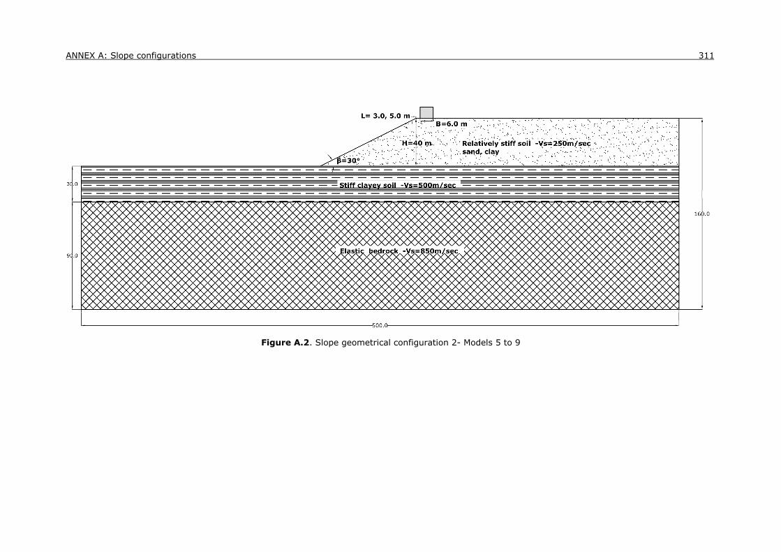
ANNEX A: Slope configurations 311
Figure A.2. Slope geometrical configuration 2- Models 5 to 9

312 Seismic Vulnerability of Reinforced Concrete Buildings in Sliding Slopes
Figure A.3. Slope geometrical configuration 3- Models 9 to 12

ANNEX A: Slope configurations 313
Figure A.4. Slope geometrical configuration 4- Models 13 to 16
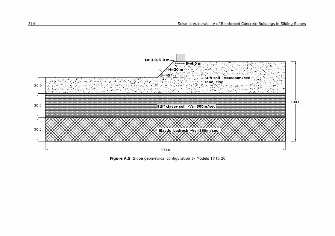
314 Seismic Vulnerability of Reinforced Concrete Buildings in Sliding Slopes
Figure A.5. Slope geometrical configuration 5- Models 17 to 20

ANNEX A: Slope configurations 315
Figure A.6. Slope geometrical configuration 6- Models 21 to 24

316 Seismic Vulnerability of Reinforced Concrete Buildings in Sliding Slopes

ANNEX B
Fragility curves for “low-code” buildings
B.1 Proposed curves for “low-code” designed RC buildings
The suggested fragility curves for low-code designed, RC bare frame structures,
characterized of a low level of confinement are presented herein (Fig. B.1) based on the
analyzed features that proved to be the most influential in assessing the vulnerability of
the building to the permanent landslide displacement (see Chapter 6). It is noted that
lower limit state values were adopted for “low-code” frame RC building for the
exceedance of extensive and complete damages (see Chapter 4, Table 4.6 and Chapter
6, § 6.3.5). Tables B.1 and B.2 present the median and dispersions of the suggested
curves when using PGA and PGD as an intensity measure respectively. As expected, the
suggested curves for “low-code” buildings are associated to lower median values of PGA
and PGD for the exceedance of each limit state and to larger dispersion (represented by
the β values) around the median estimates compared to the “high-code” buildings (see
Chapter 6, § 6.2.2).
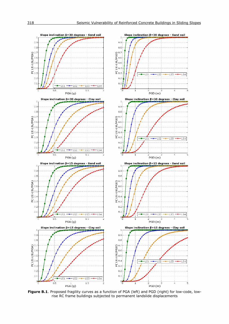
318 Seismic Vulnerability of Reinforced Concrete Buildings in Sliding Slopes
Figure B.1. Proposed fragility curves as a function of PGA (left) and PGD (right) for low-code, low-
rise RC frame buildings subjected to permanent landslide displacements

ANNEX B: Fragility curves for “low-code” buildings 319
Figure B.1. (Continued) - Proposed fragility curves as a function of PGA (left) and PGD (right) for
low-code, low-rise RC frame buildings subjected to permanent landslide displacements

320 Seismic Vulnerability of Reinforced Concrete Buildings in Sliding Slopes
Table B.1. Parameters of the proposed fragility functions using PGA as an intensity measure
Parametric models
Median PGA (g) Dispersion β
LS1 (g) LS2 (g) LS3 (g) LS4 (g)
sand_β30 0.19 0.32 0.43 0.64 0.43
clay_β30 0.25 0.51 0.77 1.12 0.49
sand_β15 0.27 0.49 0.68 0.98 0.47
clay_β15 0.22 0.52 0.83 1.22 0.52
sand_β45_h20 0.23 0.34 0.45 0.67 0.41
sand_β45_h40 0.15 0.17 0.20 0.25 0.36
clay_β45 1.04 1.76 - - 0.66
Table B.2. Parameters of the proposed fragility functions using PGD as an intensity measure
Parametric models
Median PGD (m) Dispersion β
LS1 (m) LS2 (m) LS3 (m) LS4 (m)
sand_β30 0.15 0.38 0.62 1.20 0.45
clay_β30 0.22 0.66 1.23 2.34 0.43
sand_β15 0.22 0.56 0.95 1.71 0.43
clay_β15 0.28 0.90 1.77 3.11 0.46
sand_β45_h20 0.07 0.17 0.31 0.64 0.47
sand_β45_h40 0.04 0.14 0.18 0.25 0.50
clay_β45 0.77 1.75 3.21 - 0.54

ΕΚΤΕΝΗΣ ΠΕΡΙΛΗΨΗ
I.1 Εισαγωγή
Οι κατολισθήσεις που προκαλούνται από σεισμό αποτελούν μια κύριας μορφής απειλή για
τον πληθυσμό και το δομημένο περιβάλλον στις περισσότερες ορεινές και ημιορεινές
περιοχές του κόσμου. Οι Marano et al. (2010) παρατήρησαν ότι οι κατολισθήσεις
αποτελούν την πιο διαδεδομένη και συνάμα την πιο φονική δευτερεύουσα συνέπεια των
σεισμών καθώς θεωρούνται υπεύθυνες για το 71.1% των θανάτων από έμμεσες αιτίες
πέραν της σεισμικής ταλάντωσης. Για παράδειγμα, ο ισχυρός σεισμός (Ms=8.0) που έλαβε
χώρα στο Wenchuan της Κίνας στις 12 Μαΐου 2008 υπολογίζεται ότι ενεργοποίησε
περισσότερες από 15000 κατολισθήσεις διαφόρων τύπων που κάλυπταν μια περιοχή
50000 km2, προκαλώντας το θάνατο περίπου 20000 ανθρώπων και τεράστιες οικονομικές
απώλειες (Yin et al., 2009). Υπάρχει επομένως μια αυξανόμενη απαίτηση από την κοινωνία
και τους εμπλεκόμενους φορείς για την αποτελεσματική διαχείριση και μείωση της
διακινδύνευσης που συνδέεται με τις σεισμικώς προκαλούμενες κατολισθήσεις.
Παρότι οι μέθοδοι ποσοτικής αποτίμησης της διακινδύνευσης είναι αρκετά διαδεδομένες
για φυσικούς κινδύνους όπως οι σεισμοί και οι πλημμύρες, στην περίπτωση των
κατολισθήσεων, οι μεθοδολογίες ποσοτικής αποτίμησης της διακινδύνευσης δεν έχουν
αναπτυχθεί παρά μόνο πολύ πρόσφατα και δεν έχουν εφαρμοστεί ενδελεχώς από την
επιστημονική κοινότητα και τους αρμόδιους φορείς. Το γεγονός αυτό μπορεί να αποδοθεί
στο ότι διάφορες κρίσιμες συνιστώσες της διακινδύνευσης εμπεριέχουν σημαντικές
αβεβαιότητες που καθιστούν δύσκολη την εκτίμησή τους (Corominas και Mavrouli,
2011b). Μεταξύ των συνιστωσών αυτών, η αποτίμηση της τρωτότητας των υπό
διακινδύνευση στοιχείων επηρεάζεται από ποικίλες αβεβαιότητες, λόγω της πολυδιάστατης
και δυναμικής της φύσης, που δυσχεραίνουν τον αντικειμενικό προσδιορισμό της και
καθιστούν προβληματική την ενσωμάτωση της στην εξίσωση της διακινδύνευσης.
Λαμβάνοντας υπόψη τα παραπάνω, κύριος στόχος της διδακτορικής διατριβής αποτελεί η
πρόταση και ποσοτικοποίηση μιας αναλυτικής μεθοδολογίας για την αποτίμηση της
τρωτότητας κτιρίων οπλισμένου σκυροδέματος (Ο/Σ) πλησίον σεισμικώς ασταθών

322 Σεισμική Τρωτότητα Κτιρίων Οπλισμένου Σκυροδέματος σε Κατολισθαίνοντα Πρανή
πρανών. Η αξιοπιστία του αριθμητικού προσομοιώματος επαληθεύεται μέσω της σύγκρισης
των μετακινήσεων στην περιοχή του πρανούς που εξάγονται από τις αριθμητικές
αναλύσεις με τις αντίστοιχες μετακινήσεις που υπολογίζονται από εμπειρικές μεθόδους
εκτίμησης των μετακινήσεων τύπου Newmark. Στο πλαίσιο της διατριβής προτείνονται
καμπύλες τρωτότητας για διάφορους τύπους κατασκευής, εδαφικές συνθήκες και
γεωμετρίες πρανούς καθώς και αποστάσεις της θεωρούμενης κατασκευής από την πιθανή
κατολίσθηση, οι οποίες μπορούν να βρουν άμεση εφαρμογή σε ένα πιθανοτικό πλαίσιο
εκτίμησης της διακινδύνευσης λόγω των κατολισθήσεων. Η μεθοδολογία επιβεβαιώνεται
μέσω της σύγκρισης αντιπροσωπευτικών αναπτυσσόμενων καμπυλών με σχετικές
καμπύλες της βιβλιογραφίας και δεδομένα από βλάβες σε κτίρια λόγω κατολισθητικών
φαινομένων στην Ελλάδα και την Ιταλία.
Παραδοσιακά, οι μελέτες αποτίμησης της τρωτότητας των κατασκευών λόγω
κατολισθήσεων αλλά και άλλων φυσικών αιτιών αναφέρονται στην αρχική κατασκευή
υποθέτοντας ότι αυτή υποβάλλεται σε μια ιδανική, συνεχή πρακτική συντήρησης. Παρόλα
αυτά, η πραγματική, δυναμική τρωτότητα των κτιρίων μπορεί να επηρεαστεί σημαντικά
από φαινόμενα γήρανσης των υλικών, ανθρωπογενείς δράσεις καθώς και τη
συσσωρευτική βλάβη από προηγούμενες κατολισθήσεις ή άλλους φυσικούς κινδύνους.
Για να γεφυρωθεί αυτό το κενό, η προτεινόμενη προσέγγιση επεκτείνεται ώστε να λάβει
υπόψη της την εξέλιξη της τρωτότητας των κατασκευών στο χρόνο, προτείνοντας χρονικά
εξαρτώμενες καμπύλες τρωτότητας για κτίρια Ο/Σ που εκτίθενται σε σεισμικώς
προκαλούμενες κατολισθήσεις.
I.2 Μεθοδολογία αποτίμησης της τρωτότητας
Η διδακτορική διατριβή επικεντρώνεται στην πρόταση και ποσοτικοποίηση μιας καινοτόμου
προσέγγισης για την αποτίμηση της τρωτότητας κτιρίων Ο/Σ που υπόκεινται σε σεισμικώς
προκαλούμενες, σχετικά αργές, εδαφικές ολισθήσεις. Η τρωτότητα εκφράζεται μέσω
αθροιστικών λογαριθμοκανονικών συναρτήσεων τρωτότητας που περιγράφουν την
πιθανότητα υπέρβασης της κάθε οριζόμενης στάθμης βλάβης συναρτήσει μιας ή
περισσοτέρων παραμέτρων που χαρακτηρίζουν την ένταση της πιθανής κατολίσθησης.
Το Σχήμα Ι.1 απεικονίζει το γενικό πλαίσιο της προτεινόμενης μεθοδολογίας. Η
«ικανότητα» της κατασκευής ορίζεται από την τυπολογία του κτιρίου (τύπος θεμελίωσης
και ανωδομής, γεωμετρία, αντοχή υλικών), ενώ η «απαίτηση» περιγράφεται από τη
μόνιμη εδαφική παραμόρφωση, η οποία εξαρτάται από τον τύπο της κατολίσθησης (π.χ.
αργή εδαφική ολίσθηση), τις εδαφικές συνθήκες και τη σχετική θέση του κτιρίου ως προς
την πιθανή ολισθαίνουσα εδαφική μάζα. Σημειώνεται επίσης ότι η σχετική δυσκαμψία
εδάφους-θεμελίωσης-ανωδομής μπορεί να επηρεάσει σημαντικά την απαίτηση

Εκτενής Περίληψη 323
παραμόρφωσης για την κατασκευή. Οι δύο αυτές συνιστώσες (ικανότητα της κατασκευής
και απαίτηση παραμόρφωσης) συνδυάζονται κατάλληλα ώστε να προκύψει η μεθοδολογία
εκτίμησης της απόκρισης, η οποία αποτελεί την τρίτη κύρια συνιστώσα. Τα δεδομένα της
απόκρισης σε επίπεδο παραμορφώσεων χρησιμοποιούνται στη συνέχεια για την ανάπτυξη
των καμπυλών τρωτότητας. Είναι επίσης απαραίτητο να καθοριστούν οριακές στάθμες
βλάβης με βάση την τυπολογία και τα δομικά χαρακτηριστικά της κατασκευής, εμπειρικά
κριτήρια και την έμπειρη κρίση των ειδικών ώστε να είναι δυνατή η ανάπτυξη καμπυλών
τρωτότητας για διαφορετικές στάθμες βλάβης. Τέλος, ακολουθεί η μεθοδολογία
ανάπτυξης των πιθανοτικών συναρτήσεων τρωτότητας.
Σχήμα I.1. ∆ιάγραμμα ροής της προτεινόμενης μεθοδολογίας για την εκτίμηση της τρωτότητας
κτιρίων οπλισμένου σκυροδέματος
Στις επόμενες παραγράφους ακολουθεί μια πιο λεπτομερής περιγραφή των θεμελιωδών
χαρακτηριστικών της προτεινόμενης μεθοδολογίας.
Ο τύπος της κατολίσθησης (καταπτώσεις βράχου, ροή φερτών, εδαφική ολίσθηση κτλ.)
αποτελεί μια κρίσιμη παράμετρο της μεθοδολογίας, δεδομένου ότι κατολισθήσεις
διαφορετικού τύπου και μεγέθους, απαιτούν συνήθως διαφορετικές και συμπληρωματικές
μεθόδους για την εκτίμηση της τρωτότητας των υπό διακινδύνευση στοιχείων. Η βλάβη
που προκαλείται από μια αργή εδαφική ολίσθηση σε ένα τυπικό κτίριο μπορεί να αποδοθεί
κατά κύριο λόγο στην συσσωρευτική μόνιμη (ολική ή διαφορική) εδαφική μετακίνηση και
εστιάζεται εντός της ασταθούς περιοχής του πρανούς (Mansour et al., 2011). Στην
παρούσα εργασία μελετάται μια σχετικά αργή εδαφική ολίσθηση που παράγει καμπτικές
ρηγματώσεις λόγω της διαφορικής μετακίνησης σε ένα κτίριο Ο/Σ που υπόκειται στον
κίνδυνο κατολίσθησης.

324 Σεισμική Τρωτότητα Κτιρίων Οπλισμένου Σκυροδέματος σε Κατολισθαίνοντα Πρανή
Τα χαρακτηριστικά του σεισμού (πλάτος, συχνοτικό περιεχόμενο και διάρκεια) σε σχέση τα
δυναμικά χαρακτηριστικά του εδάφους και τη στρωματογραφία μπορούν να επηρεάσουν
σημαντικά την απαίτηση παραμόρφωσης της κατασκευής. Η μη-γραμμικότητα του
εδάφους, η ικανότητα απόσβεσης του υλικού, η σχετική δυσκαμψία των εδαφικών
αποθέσεων και του υποκείμενου υποβάθρου αποτελούν τους κύριους παράγοντες για
ενίσχυση ή απομείωση της σεισμικής κίνησης (Kramer και Stewart, 2004; Pitilakis, 2010).
Η πιθανότητα αστοχίας του πρανούς είναι γενικά μεγαλύτερη για χαμηλόσυχνους
σεισμικούς κραδασμούς συνδυαζόμενους με φαινόμενα συντονισμού σε χαμηλές
συχνότητες (Bourdeau et al., 2004).
Η θέση της κατασκευής σε σχέση με την κατολίσθηση είναι επίσης ένας καθοριστικός
παράγοντας. Η επίδραση της τοπογραφίας μπορεί να μεταβάλλει το πλάτος και το
συχνοτικό περιεχόμενο των ασκούμενων σεισμικών διεγέρσεων (Bouckovalas and
Papadimitriou, 2005; Ktenidou, 2010). Επιπλέον, η αλληλεπίδραση εδάφους-κατασκευής
λόγω της παρουσίας της κατασκευής κοντά στη στέψη του πρανούς μπορεί να συμβάλλει
περαιτέρω στη μεταβολή της σεισμική απόκρισης πλησίον αυτού σε σχέση με την
περίπτωση του ελευθέρου πεδίου (Assimaki and Kausel, 2007; D. Pitilakis and Tsinaris,
2010). Στην παρούσα εργασία μελετούνται κτίρια Ο/Σ διαφορετικής δυσκαμψίας
τοποθετημένα κοντά στη στέψη του πρανούς, όπου η τοπογραφική επιρροή είναι γενικά
ενισχυμένη.
Η τυπολογία της κατασκευής (π.χ. γεωμετρία, αριθμός των ορόφων, ιδιότητες των
υλικών, το επίπεδο σχεδιασμού, τα χαρακτηριστικά της θεμελίωσης κλπ.) αποτελεί επίσης
ένα βασικό παράγοντα. Η απόκριση στην διαφορική (και ολική) μόνιμη εδαφική
μετακίνηση εξαρτάται πρωτίστως από τον τύπο της θεμελίωσης. Ένα κτίριο θεμελιωμένο
σε πασσάλους είναι γενικά λιγότερο τρωτό σε σχέση με ένα κτίριο σε μια επιφανειακή
θεμελίωση. Αναφορικά με τα επιφανειακά συστήματα θεμελίωσης, μια άκαμπτη θεμελίωση
(π.χ. μια γενική κοιτόστρωση) παρουσιάζει μειωμένη τρωτότητα σε σχέση με μια εύκαμπτη
(π.χ. μεμονωμένα πέδιλα). Όταν το σύστημα θεμελίωσης είναι άκαμπτο, το κτίριο
αναμένεται να στραφεί ως στερεό σώμα και οι αναμενόμενες βλάβες μπορούν να
αποδοθούν κυρίως σε απώλεια λειτουργικότητας. Οι στάθμες βλαβών ορίζονται εμπειρικά,
καθότι υπάρχει περιορισμένη απαίτηση δομικής βλάβης στα μέλη του κτιρίου. Αντιθέτως,
όταν το σύστημα θεμελίωσης είναι εύκαμπτο, η διαφορική μετακίνηση λόγω της
κατολισθαίνουσας εδαφικής μάζας μπορεί να προκαλέσει δομική βλάβη στην κατασκευή
(Bird et al., 2005; 2006). Οι στάθμες βλάβης μπορούν να κατηγοριοποιηθούν στην
περίπτωση αυτή με τρόπο ανάλογο των σταθμών που χαρακτηρίζουν τις δομικές βλάβες,
που οφείλονται σε σεισμική ταλάντωση.
Η μεθοδολογία εκτίμησης της απόκρισης περιλαμβάνει δύο βήματα από πλευράς
αριθμητικών αναλύσεων. Αρχικά, πραγματοποιείται ανελαστική σεισμική ανάλυση του

Εκτενής Περίληψη 325
συστήματος πρανούς - θεμελίωσης κάνοντας μια απλοποιημένη θεώρηση για την
ανωδομή, χρησιμοποιώντας τον κώδικα πεπερασμένων διαφορών FLAC2D (Itasca, 2008).
Το έδαφος (αμμώδες ή αργιλικό) υπακούει σε ελαστοπλαστικό καταστατικό νόμο
συμπεριφοράς με κριτήριο αστοχίας Mohr-Coulomb ενώ το «σεισμικό υπόβαθρο»
ακολουθεί το νόμο της γραμμικής ελαστικότητας. Η προσομοίωση γίνεται με 4κόμβα
στοιχεία επίπεδης παραμόρφωσης. Η διακριτοποίηση επιτρέπει τη διάδοση των σεισμικών
κυμάτων έως τη συχνότητα των 10 Hz. Για την ελαχιστοποίηση των ανακλάσεων των
κυμάτων στα πλευρικά όρια και στη βάση του προσομοιώματος χρησιμοποιούνται
κατάλληλες συνοριακές συνθήκες «ελευθέρου πεδίου» (free field) και «διαφανών ορίων»
(quiet boundaries) αντιστοίχως.
Η προσομοίωση της θεωρούμενης κατασκευής οπλισμένου σκυροδέματος πλησίον της
στέψης του πρανούς εξαρτάται από τη δυσκαμψία της θεμελίωσης. Εξετάζονται δύο
περιπτώσεις:
- μία εύκαμπτη θεμελίωση (π.χ. περίπτωση μεμονωμένων πεδίλων) όπου η προσομοίωση
του συστήματος θεμελίωσης - ανωδομής επιτυγχάνεται μέσω της θεώρησης
συγκεντρωμένων φορτίσεων στις απολήξεις των θεωρούμενων στύλων και
- μία δύσκαμπτη θεμελίωση που η προσομοίωση επιτυγχάνεται μέσω μιας συνεχούς
παραμορφώσιμης ελαστικής δοκού υποβαλλόμενη σε ομοιόμορφα κατανεμημένη φόρτιση
που συνδέεται με το υποκείμενο έδαφος με χρήση κατάλληλων στοιχείων διεπιφάνειας.
Ένα τυπικό δισδιάστατο αριθμητικό προσομοίωμα δίδεται στο Σχήμα Ι.2. Κατάλληλα
διορθωμένες, κλιμακούμενες σεισμικές διεγέρσεις ποικίλων χαρακτηριστικών (συχνοτικού
περιεχομένου και διάρκειας) που έχουν καταγραφεί σε επιφανειακή εμφάνιση βράχου,
εισάγονται στη βάση του αριθμητικού προσομοιώματος. Αποτέλεσμα της ανάλυσης
αποτελεί η εκτίμηση της απαίτησης μόνιμης διαφορικής μετακίνησης στην κατασκευή, στο
επίπεδο της θεμελίωσης, λόγω της σεισμικώς ασταθούς εδαφικής μάζας.
Σχήμα I.2. Τυπικό δισδιάστατο αριθμητικό προσομοίωμα που χρησιμοποιείται για την ανελαστική
σεισμική ανάλυση
A B

326 Σεισμική Τρωτότητα Κτιρίων Οπλισμένου Σκυροδέματος σε Κατολισθαίνοντα Πρανή
Στη συνέχεια, η προαναφερθείσα απαίτηση διαφορικής μετακίνησης συναρτήσει του
χρόνου εισάγεται στη βάση ενός μη-γραμμικού προσομοιώματος της κατασκευής ως
καταναγκασμός, ώστε να εκτιμηθεί η αναμενόμενη απόκρισή της. ∆ιερευνώνται επαρκώς
αντιπροσωπευτικά πλαισιακά κτίρια Ο/Σ χαμηλού ύψους χωρίς τοιχοπληρώσεις με
εύκαμπτο και δύσκαμπτο σύστημα θεμελίωσης, για την ανάλυση των οποίων
χρησιμοποιείται το πρόγραμμα πεπερασμένων στοιχείων Seismostruct (Seismostruct,
Seismosoft 2011) (Σχ. Ι.3). Συγκεκριμένα, η ανάλυση που πραγματοποιείται είναι
ψευδοστατική θεωρώντας ανελαστική τη συμπεριφορά των υλικών της κατασκευής υπό τη
μορφή ινών (fibers). Για κάθε ανάλυση, εξάγεται τελικά η μέγιστη απόκριση της
κατασκευής σε επίπεδο τοπικής παραμόρφωσης (που αποτελεί και το δείκτη βλάβης).
Αξίζει να σημειωθεί ότι η συγκεκριμένη μέθοδος στηρίζεται στην υπόθεση ότι οι βλάβες
στην κατασκευή είναι αποτέλεσμα μόνο της εδαφικής αστοχίας και όχι συνδυασμός αυτής
με την εδαφική ανακυκλική φόρτιση. Έτσι, η κατασκευή δεν υποβάλλεται σε κάποια
αρχική απομείωση της αντοχής ή της δυσκαμψίας της λόγω της επίδρασης της εδαφικής
ταλάντωσης.
Σχήμα I.3. Αντιπροσωπευτικά πλαισιακά κτίρια Ο/Σ χαμηλού ύψους με εύκαμπτο και δύσκαμπτο σύστημα θεμελίωσης και περιγραφή της φόρτισης κινηματικού τύπου για τη διεξαγωγή της μη-
γραμμικής, ψευδοστατικής ανάλυσης
Οι οριακές στάθμες βλάβης για μικρές (Limit state 1), μέτριες (Limit state 2), εκτενείς
(Limit state 3) βλάβες και ολική κατάρρευση (Limit state 4) ορίζονται με βάση οριακές
τιμές παραμορφώσεων των υλικών του Ο/Σ (Crowley et al., 2004; Bird et al., 2005),
ανάλογα με την ποιότητα και τα χαρακτηριστικά της κατασκευής. Στο Σχήμα Ι.4
παρουσιάζονται τυπικά διαγράμματα εξέλιξης της βλάβης σε όρους μέγιστης
παραμόρφωσης συναρτήσει της μέγιστης εδαφικής επιτάχυνσης (PGA) και της μόνιμης
εδαφικής μετακίνησης (PGD) αντιστοίχως για ένα πλαισιακό κτίριο Ο/Σ χαμηλού ύψους
σχεδιασμένου βάσει σύγχρονου κανονισμού (EAK, 2000) με εύκαμπτο σύστημα
θεμελίωσης, τοποθετημένο πλησίον της στέψης ενός αμμώδους εν δυνάμει ασταθούς
πρανούς. Στο σχήμα απεικονίζονται επίσης οι οριακές τιμές της παραμόρφωσης του
χάλυβα του οπλισμού για κάθε στάθμη βλάβης. Τέλος, οι καμπύλες τρωτότητας
συναρτήσει της μέγιστης εδαφικής επιτάχυνσης στο βράχο (PGA) ή της παραμένουσας
3m
6m 6m
1 1’ 2 2’

Εκτενής Περίληψη 327
εδαφικής μετακίνησης (PGD) για τις διάφορες στάθμες βλάβης, παράγονται μετά από
κατάλληλη μέθοδο στατιστικής επεξεργασίας της απόκρισης (σε επίπεδο τοπικών
παραμορφώσεων), σε σχέση με την παράμετρο της έντασης της κατολίσθησης (PGA ή
PGD) και τις οριζόμενες στάθμες βλάβης. Στην πιθανοτική προσέγγιση που προτείνεται,
λαμβάνονται υπόψη διάφορες αβεβαιότητες που σχετίζονται με την ικανότητα της
κατασκευής, τον ορισμό των σταθμών βλάβης και την απαίτηση παραμόρφωσης.
Σχήμα I.4. Μέγιστες τιμές αναπτυχθείσας παραμόρφωσης συναρτήσει της PGA (αριστερά) και PGD (δεξιά) για ένα πλαισιακό κτίριο Ο/Σ χαμηλού ύψους σχεδιασμένου βάσει σύγχρονου κανονισμού με
εύκαμπτο σύστημα θεμελίωσης, τοποθετημένο εγγύς της στέψης ενός αμμώδους πρανούς
∆ύο διαφορετικές μέθοδοι εφαρμόζονται για τον προσδιορισμό των λογαριθμοκανονικών
παραμέτρων (διάμεσος και διασπορά) των καμπυλών τρωτότητας ώστε να διερευνηθεί η
επιρροή της επιστημικής (epistemic) αβεβαιότητας στην εκτίμηση της τρωτότητας. Αυτές
βασίζονται στη μέθοδο της παλινδρόμησης (regression analysis method) (e.g. Nielson και
DesRoches, 2007; Argyroudis και Pitilakis, 2012) και στη μέθοδο της μέγιστης
πιθανοφάνειας (maximum likelihood method) (e.g. Shinozuka et al., 2000; 2003).
Σχήμα I.5. Συγκριτική παρουσίαση τυπικών καμπυλών τρωτότητας συναρτήσει της PGA (αριστερά)
και PGD (δεξιά) με βάση την μέθοδο της παλινδρόμησης (RA) και την μέθοδο της μέγιστης πιθανοφάνειας (ML)

328 Σεισμική Τρωτότητα Κτιρίων Οπλισμένου Σκυροδέματος σε Κατολισθαίνοντα Πρανή
Στο σχήμα Ι.5 δίδονται τυπικές καμπύλες τρωτότητας συναρτήσει της PGA (αριστερά) και
PGD (δεξιά) με βάση την μέθοδο της παλινδρόμησης (RA) και την μέθοδο της μέγιστης
πιθανοφάνειας (ML). Οι δύο μέθοδοι εκτιμούν διάμεσες τιμές σε όρους PGA και PGD που
βρίσκονται γενικά σε αρκετά καλή συμφωνία. Οι υπολογισθείσες τιμές της διασποράς β
είναι συμβατές στις δύο μεθόδους όταν χρησιμοποιείται η PGD ως παράμετρος της έντασης
της κατολίσθησης, ενώ είναι αρκετά διαφορετική όταν χρησιμοποιείται η PGA. Πιο
συγκεκριμένα, διαπιστώνεται ότι η μέθοδος της μέγιστης πιθανοφάνειας εκτιμά σε γενικές
γραμμές μικρότερη διασπορά β για το ίδιο δείγμα δεδομένων που προέκυψε από την
αριθμητική ανάλυση.
I.3 Εμπειρικές μέθοδοι εκτίμησης των μόνιμων μετακινήσεων: Συγκρίσεις με τα αποτελέσματα των μη-γραμμικών, αριθμητικών αναλύσεων
Σε μια μελέτη αποτίμησης της διακινδύνευσης λόγω πιθανής κατολίσθησης, η έκταση των
παραμενουσών εδαφικών μετακινήσεων και όχι απλώς η εκτίμηση της πιθανότητας
εμφάνισης της κατολίσθησης αποτελεί τον πρωταρχικό παράγοντα που ενδέχεται να
οδηγήσει σε καταπόνηση και πιθανή βλάβη σε κτίρια και υποδομές. Στην παρούσα
ενότητα αρχικά παρουσιάζονται και συγκρίνονται τρεις διαφορετικές εμπειρικές μέθοδοι
εκτίμησης των μόνιμων σεισμικών μετατοπίσεων των φυσικών πρανών: το συμβατικό
αναλυτικό μοντέλο άκαμπτου στερεού σώματος (rigid block) του Newmark (1965), το
ασύζευκτο (decoupled) μοντέλο των Rathje και Antonakos (2011) και το συζευγμένο
(coupled) μοντέλο των Bray και Travasarou (2007), έτσι ώστε να εκτιμηθεί η σχετική
ικανότητά τους να προβλέπουν τις αναμενόμενες σεισμικές μετακινήσεις των πρανών για
διαφορετικά σεισμικά σενάρια.
Τα αποτελέσματα επιδεικνύουν τον πολύ σημαντικό ρόλο του πλάτους και του συχνοτικού
περιεχομένου του σεισμού καθώς και της ενδοσιμότητας της επιφάνειας ολίσθησης στην
εκτίμηση των μετακινήσεων. Το μοντέλο των Bray και Travasarou εκτιμά μεγαλύτερες
μετακινήσεις σε σχέση με αυτά του Newmark και των Rathje και Antonakos.
Συγκεκριμένα, η διαφοροποίηση στην προβλεπόμενη μετακίνηση είναι πιο εμφανής για
την περίπτωση της σχετικά εύκαμπτης (Ts=0.16sec) συγκρινόμενη με την σχεδόν άκαμπτη
(Ts=0.032sec) ολισθαίνουσα εδαφική μάζα. Οι μετακινήσεις που υπολογίζονται
χρησιμοποιώντας τις σχέσεις των Rathje και Antonakos είναι περισσότερο συμβατές με
αυτές του Newmark ιδιαίτερα στην περίπτωση ενός χαμηλού πλάτους, υψίσυχνου
σεισμικού κραδασμού. Στα Σχήματα Ι.6 και Ι.7 παρουσιάζονται ενδεικτικά συγκριτικά
διαγράμματα όπου εκτιμώνται οι παραμένουσες σεισμικές μετακινήσεις των πρανών με τις
τρεις μεθόδους για διάφορες τιμές του λόγου της κρίσιμης (ky) προς τη μέγιστη

Εκτενής Περίληψη 329
επιτάχυνση (kmax), για ένα δεδομένο σεισμικό σενάριο (σεισμός «Pacoima» κλιμακούμενος
στα 0.7g), για την περίπτωση μιας παραμορφώσιμης (Ts=0.16sec) και μιας άκαμπτης
(Ts=0.032sec) ολισθαίνουσας εδαφικής μάζας αντιστοίχως.
Σχήμα I.6. Συγκριτική παρουσίαση των διαφορετικών μοντέλων για την εκτίμηση των σεισμικών μετακινήσεων των πρανών θεωρώντας μια άκαμπτη ολισθαίνουσα εδαφική μάζα (Ts=0.032 sec)
Σχήμα I.7. Συγκριτική παρουσίαση των διαφορετικών μοντέλων για την εκτίμηση των σεισμικών μετακινήσεων των πρανών θεωρώντας μια παραμορφώσιμη ολισθαίνουσα εδαφική μάζα (Ts=0.16
sec)

330 Σεισμική Τρωτότητα Κτιρίων Οπλισμένου Σκυροδέματος σε Κατολισθαίνοντα Πρανή
Σχήμα I.8. Σύγκριση των μετακινήσεων των Newmark’s, Rathje και Antonakos (2011) και Bray και
Travasarou (2007 με τις παραμένουσες σεισμικές μετακινήσεις των μη-γραμμικών αριθμητικών αναλύσεων για την περίπτωση ενός δύσκαμπτου αμμώδους πρανούς

Εκτενής Περίληψη 331
Σχήμα I.9. Σύγκριση των μετακινήσεων των Newmark’s, Rathje και Antonakos (2011) και Bray και
Travasarou (2007 με τις παραμένουσες σεισμικές μετακινήσεις των μη-γραμμικών αριθμητικών αναλύσεων για την περίπτωση ενός εύκαμπτου αργιλώδους πρανούς

332 Σεισμική Τρωτότητα Κτιρίων Οπλισμένου Σκυροδέματος σε Κατολισθαίνοντα Πρανή
Επιπλέον, οι μετακινήσεις στην περιοχή του πρανούς για συνθήκες ελεύθερου πεδίου
(δηλ. χωρίς την παρουσία κάποιας κατασκευής στην κορυφή του) που προέκυψαν από τις
μη-γραμμικές, αριθμητικές αναλύσεις στην προηγούμενη ενότητα συγκρίνονται με τις
αντίστοιχες μετακινήσεις που υπολογίζονται από τα τρία εμπειρικά μοντέλα τύπου
Newmark ώστε να ελεγχθεί η αξιοπιστία των αριθμητικών προσομοιωμάτων αλλά και να
αξιολογηθεί η ικανότητα των τριών μοντέλων να εκτιμούν μόνιμες μετατοπίσεις πρανών
σε σχέση με την αριθμητική ανάλυση. Τα αποτελέσματα των αριθμητικών αναλύσεων,
εξαγόμενα σε όρους μόνιμων οριζόντιων μετακινήσεων στην θεωρούμενη επιφάνεια
ολίσθησης, βρίσκονται γενικά σε καλή συμφωνία με αυτά των τριών εμπειρικών μοντέλων
για την περίπτωση του εξετασθέντος αμμώδους πρανούς (Σχ. Ι.8). Αντιθέτως, η συσχέτιση
δεν είναι ικανοποιητική για την περίπτωση του μελετηθέντος πιο εύκαμπτου πρανούς σε
αργιλικό έδαφος (Σχ. Ι.9). Ειδικότερα, το μοντέλο των Bray και Travasarou (2007) τείνει
να προβλέπει μεγαλύτερες τιμές μετακινήσεων σε σχέση με αυτές της αριθμητικής
ανάλυσης ενώ τα μοντέλα του Newmark και των Rathje και Antonakos (2011)
υποεκτιμούν τις αντίστοιχες μετακινήσεις. Μεταξύ των τριών μοντέλων, αυτό των Bray και
Travasarou παρουσιάζει το ελάχιστο μέσο σφάλμα στην εκτίμηση των μετακινήσεων σε
σχέση με τα αποτελέσματα της αριθμητικής ανάλυσης και για τις δύο περιπτώσεις
εδαφικών πρανών (σε αμμώδες και αργιλικό έδαφος). Η αναλυτική προσέγγιση του
Newmark επιδεικνύει ωστόσο την μικρότερη διασπορά στις τιμές των μετακινήσεων
συγκρινόμενη με τις μεθόδους των Bray και Travasarou και των Rathje και Antonakos.
Συνολικά, η διαφοροποίηση στην εκτίμηση των μετακινήσεων είναι μεγαλύτερη για τη πιο
εύκαμπτη ολισθαίνουσα μάζα αποτελούμενη από αργιλικό έδαφος.
I.4 Καμπύλες τρωτότητας κτιρίων Ο/Σ σε κατολισθαίνοντα πρανή
Κύριος στόχος της παρούσας ενότητας αποτελεί η πρόταση γενικευμένων καμπυλών
τρωτότητας για χαμηλού ύψους, πλαισιακά κτίρια Ο/Σ, τοποθετημένα πλησίον της στέψης
σεισμικώς ασταθών πρανών σύμφωνα με τη μεθοδολογία που αναπτύχθηκε στην Ενότητα
Ι.2. Οι καμπύλες αυτές μπορούν να έχουν εφαρμογή στην εκτίμηση της σεισμικής
τρωτότητας και της σεισμικής διακινδύνευσης κτιρίων Ο/Σ σε κατολισθαίνοντα πρανή σε
διάφορες μελέτες περίπτωσης για διάφορες κλίμακες.
Εξετάζονται μονώροφα πλαισιακά κτίρια Ο/Σ θεμελιωμένα σε διαφορετικά εδάφη
(αμμώδη, αργιλικά), για διάφορες κλίσεις (15ο, 30ο, 45ο) και ύψη (20m, 40m) πρανούς
καθώς και αποστάσεις της κατασκευής από τη στέψη (3m, 5m) ώστε να διαπιστωθεί η
επιρροή των διάφορων παραμέτρων στην απόκριση και τελικά στην τρωτότητα της
κατασκευής. Στο Σχήμα Ι.10 παρουσιάζεται ένα σκαρίφημα του βασικού παραμετρικού
μοντέλου. Σημειώνεται ότι οι ιδιότητες των εδαφών που εξετάστηκαν είναι συμβατές με τις

Εκτενής Περίληψη 333
θεωρούμενες κλίσεις του πρανών ώστε να διασφαλίζεται η ευστάθειά τους υπό στατικές
συνθήκες. Πρέπει επίσης να τονιστεί ότι μελετώνται μόνο οι περιπτώσεις που οδηγούν
στην υψηλότερη επιδεκτικότητα των πρανών σε κατολίσθηση. Για παράδειγμα, πρανή με
ήπιες κλίσεις (β=15ο) σε σκληρό έδαφος δεν αναλύονται καθώς η προκύπτουσα
παραμένουσα παραμόρφωση και επομένως η αναμενόμενη δομική βλάβη θα ήταν
αμελητέα και άρα εκτός του πεδίου μελέτης της παρούσας διατριβής. Τα 24 μοντέλα που
τελικά προκύπτουν υποβάλλονται σε μια σειρά αριθμητικών αναλύσεων δύο βημάτων
(συνολικά περίπου 1350 αναλύσεις) με βάση την προτεινόμενη μεθοδολογία. Αποτέλεσμα
των αναλύσεων αποτελεί η αναμενόμενη απόκριση της κατασκευής λόγω της πιθανής
κατολίσθησης και τελικά η τρωτότητά της για τις προκαθορισμένες στάθμες βλάβης.
Σχήμα I.10. Το υπό μελέτη παραμετρικό μοντέλο
Με βάση τα αποτελέσματα της εκτενούς παραμετρικής διερεύνησης, προτείνονται τελικά
επτά σετ καμπυλών τρωτότητας εξαρτώμενα από τις παραμέτρους που συμβάλλουν
περισσότερο στον εκτιμώμενο βαθμό βλάβης της κατασκευής. Ύστερα από μια ανάλυση
ευαισθησίας των αποτελεσμάτων προκύπτει ότι οι παράμετροι αυτές είναι η κλίση και το
εδαφικό υλικό του πρανούς, τα οποία βρέθηκαν να είναι εντόνως αλληλοσυσχετιζόμενα.
Το ύψος του πρανούς αποδεικνύεται επίσης μια σημαντική παράμετρος που συμβάλλει
καθοριστικά στην τρωτότητα της κατασκευής για την περίπτωση απότομων αμμωδών
πρανών. Έτσι, προτείνονται επιπλέον διαφορετικές καμπύλες τρωτότητας για αμμώδη
πρανή 45ο ανάλογα με το ύψος τους. Σημειώνεται ότι οι προτεινόμενες καμπύλες
κατασκευάζονται για την πιο δυσμενή θέση του κτιρίου ως προς την κατολίσθηση, η οποία
είναι διαφορετική για την περίπτωση των αμμωδών και των αργιλωδών πρανών. Στο
σχήμα Ι.11 δίδονται σχηματικά οι προτεινόμενες καμπύλες συναρτήσει της μέγιστης
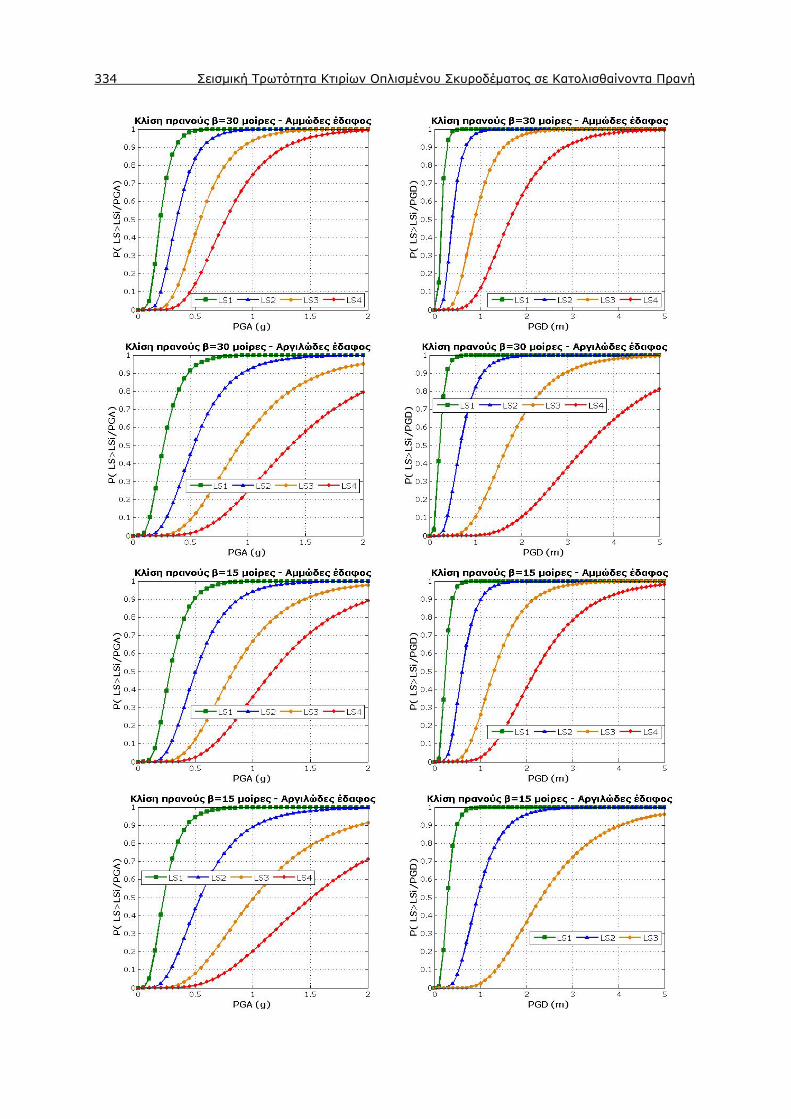
334 Σεισμική Τρωτότητα Κτιρίων Οπλισμένου Σκυροδέματος σε Κατολισθαίνοντα Πρανή

Εκτενής Περίληψη 335
Σχήμα I.11. Προτεινόμενες καμπύλες τρωτότητας συναρτήσει της PGA (αριστερά) και της PGD
(δεξιά) για τυπικά πλαισιακά κτίρια Ο/Σ χαμηλού ύψους σχεδιασμένα με συγχρόνους κανονισμούς που υπόκεινται σε παραμένουσες εδαφικές μετακινήσεις λόγω πιθανής κατολίσθησης
εδαφικής επιτάχυνσης (PGA) και της παραμένουσας εδαφικής μετακίνησης (PGD) για την
περίπτωση ενός τυπικού πλαισιακού κτιρίου Ο/Σ χαμηλού ύψους, επαρκώς οπλισμένου και
σχεδιασμένο με σύγχρονους κανονισμούς (π.χ. ΕΑΚ, 2000). Αντίστοιχες καμπύλες
προτείνονται και για σχετικά κτίρια σχεδιασμένα με παλαιότερους κανονισμούς.
Το κτίριο που θεμελιώνεται σε αμμώδη πρανή αναμένεται να επιδείξει μεγαλύτερο βαθμό
βλάβης σε σχέση με το αντίστοιχο σε αργιλώδη πρανή. Έτσι, οι καμπύλες τρωτότητας που
αναφέρονται σε αμμώδη σε σύγκριση με τις αντίστοιχες για αργιλώδη πρανή είναι γενικά
μετατοπισμένες προς τα αριστερά και ταυτόχρονα είναι συνυφασμένες με μια πιο γρήγορη

336 Σεισμική Τρωτότητα Κτιρίων Οπλισμένου Σκυροδέματος σε Κατολισθαίνοντα Πρανή
μετάβαση από τη στάθμη βλάβης που περιγράφει τις μικρές βλάβες προς αυτή που
σχετίζεται με την ολική κατάρρευση. Οι διαφορές αυτές γίνονται εμφανέστερες καθώς η
κλίση του πρανούς αυξάνει. Μεταξύ των περιπτώσεων που εξετάζονται, το 45ο αμμώδες
πρανές μεγαλύτερου ύψους και το 45ο αργιλώδες πρανές προκαλούν τις μεγαλύτερες και
μικρότερες βλάβες αντιστοίχως στην κατασκευή. Η διασπορά β των καμπυλών κυμαίνεται
από 0.39 έως 0.66 και από 0.40 έως 0.50 όταν θεωρείται η PGA και η PGD αντιστοίχως ως
μέτρο της έντασης της κατολίσθησης. Οι μεγαλύτερες τιμές της διασποράς β αναμένονται
για τα πρανή με απότομη κλίση (45o) και για τα αργιλικά εδάφη.
Επιπροσθέτως, εξετάστηκαν κάποιες επιπλέον παράμετροι όπως το επίπεδο του υπόγειου
νερού, η θεώρηση υλικού κατολίσθησης που «χαλαρώνει» με την παραμόρφωση (strain
softening material), η ενδοσιμότητα του συστήματος θεμελίωσης, η γεωμετρία της
κατασκευής (ο αριθμός των ορόφων και των ανοιγμάτων) και το επίπεδο του σχεδιασμού
της, με σκοπό να διερευνηθεί η σχετική επίδραση καθεμίας από αυτές στην τρωτότητα της
κατασκευής. Η επιρροή της κάθε παραμέτρου μπορεί να διαφοροποιείται σε σχέση με το
εδαφικό υλικό του πρανούς (π.χ. για την περίπτωση της θεώρησης υπόγειου νερού) και με
την ενδοσιμότητα της θεμελίωσης (π.χ. για την περίπτωση όπου μεταβάλλεται η
γεωμετρία της κατασκευής). Συνολικά, η επίδρασή τους μπορεί κάτω υπό ορισμένες
συνθήκες να είναι καθοριστική για τον προβλεπόμενο βαθμό βλάβης της κατασκευής.
Σημειώνεται, ωστόσο, ότι μια πιο διεξοδική ανάλυση καθεμιάς εκ των ανωτέρω
παραμέτρων δικαιολογείται μόνο σε συγκεκριμένες μελέτες περίπτωσης όπου είναι
διαθέσιμα επαρκή στοιχεία για τις ιδιότητες του εδάφους, τη γεωμετρία του πρανούς και
την τυπολογία και τα υλικά των υπό διακινδύνευση κατασκευών. Στα Σχήματα Ι.12 έως
Ι.17 δίνονται κάποια συγκριτικά αντιπροσωπευτικά αποτελέσματα υπό μορφή καμπυλών
τρωτότητας όπου περιγράφεται η σχετική επιρροή της κάθε παραμέτρου για κατασκευές
θεμελιωμένες σε αμμώδες έδαφος.
Σχήμα I.12 Καμπύλες τρωτότητας συναρτήσει της PGA (αριστερά) και της PGD (δεξιά) όταν μεταβάλλεται το επίπεδο του υπόγειου νερού (ξηρά ή μερικώς κορεσμένα εδαφικά υλικά)

Εκτενής Περίληψη 337
Σχήμα I.13. Καμπύλες τρωτότητας συναρτήσει της PGA (αριστερά) και της PGD (δεξιά) για
θεωρούμενο (ή όχι) υλικό κατολίσθησης που «χαλαρώνει» με την παραμόρφωση (strain softening material)
Σχήμα I.14. Καμπύλες τρωτότητας συναρτήσει της PGA (αριστερά) και της PGD (δεξιά) όταν
μεταβάλλεται η ευκαμψία του συστήματος θεμελίωσης
Σχήμα I.15. Καμπύλες τρωτότητας συναρτήσει της PGA (αριστερά) και της PGD (δεξιά) για
μονώροφα και διώροφα πλαισιακά κτίρια Ο/Σ ενός ανοίγματος

338 Σεισμική Τρωτότητα Κτιρίων Οπλισμένου Σκυροδέματος σε Κατολισθαίνοντα Πρανή
Σχήμα I.16. Καμπύλες τρωτότητας συναρτήσει της PGA (αριστερά) και της PGD (δεξιά) όταν για
μονώροφα πλαισιακά κτίρια Ο/Σ ενός και δύο ανοιγμάτων
Σχήμα I.17. Καμπύλες τρωτότητας συναρτήσει της PGA (αριστερά) και της PGD (δεξιά) όταν
μεταβάλλεται το επίπεδο σχεδιασμού της κατασκευής
I.5 Αξιολόγηση της προτεινόμενης μεθόδου
Η συγκεκριμένη ενότητα στοχεύει στην επαλήθευση της αξιοπιστίας της προτεινόμενης
μεθοδολογίας και των σχετικών καμπυλών τρωτότητας.
Αρχικά η εγκυρότητα της μεθόδου εκτιμάται μέσω της σύγκρισης αντιπροσωπευτικών
αναπτυχθέντων καμπυλών τρωτότητας για τυπικά πλαισιακά κτίρια Ο/Σ χαμηλού ύψους
επί εύκαμπτης θεμελίωσης με αντίστοιχες καμπύλες της βιβλιογραφίας που προέκυψαν
από διαφορετικές προσεγγίσεις. Ειδικότερα, καμπύλες τρωτότητας κτιρίων που βασίζονται
σε εμπειρικά δεδομένα βλαβών (Zhang και Ng, 2005), την έμπειρη κρίση των ειδικών
(NIBS, 2004) και σε αριθμητικές αναλύσεις (Negulescu και Foerster, 2010)
χρησιμοποιήθηκαν γι’ αυτή τη σύγκριση. Στα Σχήματα Ι.18 έως Ι.20 δίνονται κάποιες
χαρακτηριστικές συγκρίσεις των προτεινόμενων καμπυλών τρωτότητας με τις αντίστοιχες
καμπύλες των Zhang και Ng (2005), του HAZUS (NIBS, 2004) και των Negulescu και
Foerster (2010). Πρέπει να σημειωθεί ότι οι προτεινόμενες καμπύλες που

Εκτενής Περίληψη 339
χρησιμοποιούνται για τις συγκρίσεις αντιστοιχούν σε μια μέση περίπτωση αναφορικά με τις
αναμενόμενες βλάβες στην κατασκευή (για κλίση πρανούς 30ο και αμμώδες έδαφος). Οι
συγκρίσεις κρίνονται γενικά ικανοποιητικές δεδομένου των διαφορετικών υποθέσεων που
σχετίζονται με τις προτεινόμενες καμπύλες και αυτές της βιβλιογραφίας.
Σχήμα I.18. Σύγκριση αντιπροσωπευτικών προτεινόμενων καμπυλών συναρτήσει της καθίζησης
(ολικής κατακόρυφης μετακίνησης) με τις εμπειρικές καμπύλες των Zhang και Ng (2005)
Σχήμα I.19. Σύγκριση αντιπροσωπευτικών προτεινόμενων καμπυλών για εκτενείς βλάβες και ολική κατάρρευση συναρτήσει της παραμένουσας εδαφικής μετακίνησης (PGD) με τις καμπύλες του
HAZUS (NIBS, 2004)

340 Σεισμική Τρωτότητα Κτιρίων Οπλισμένου Σκυροδέματος σε Κατολισθαίνοντα Πρανή
Σχήμα I.20. Σύγκριση αντιπροσωπευτικών προτεινόμενων καμπυλών συναρτήσει της διαφορικής
μετακίνησης με τις αναλυτικές καμπύλες των Negulescu και Foerster (2010)
Ιδιαίτερο ενδιαφέρον παρουσιάζει επίσης η συσχέτιση των καμπυλών που προτείνονται
στην συγκεκριμένη έρευνα για χαμηλού ύψους, πλαισιακά κτίρια Ο/Σ πλησίον της στέψης
πρανών που εκτίθενται σε παραμένουσες σεισμικές μετακινήσεις λόγω πιθανής
κατολίσθησης, με αντίστοιχες καμπύλες της βιβλιογραφίας για τις ίδιες τυπολογίες κτιρίων
σε οριζόντια στρωματοποιημένες εδαφικές αποθέσεις (χωρίς την ύπαρξη οποιασδήποτε
τοπογραφικής έξαρσης) που υποβάλλονται σε ανακυκλική φόρτιση λόγω ενός σεισμού.
Η εναρμόνιση όλων των καμπυλών ως προς το μέτρο της έντασης και τον αριθμό των
σταθμών βλαβών αποτελεί απαραίτητη προϋπόθεση για να καταστεί δυνατή η
προσεγγιστική σύγκριση των προτεινόμενων καμπυλών με αυτές της βιβλιογραφίας. Αυτή
επιτυγχάνεται μέσω του εργαλείου Syner-G Fragility Function Manager (Crowley et al.
2011- SYNER-G project) που επιτρέπει την αποθήκευση, εναρμόνιση και σύγκριση
διαφορετικών καμπυλών τρωτότητας. Συγκεκριμένα, η εναρμόνιση ως προς την ένταση
επιτελείται θεωρώντας την μέγιστη εδαφική επιτάχυνση (PGA) στην επιφανειακή εμφάνιση
βράχου ως μέτρο της έντασης και υιοθετώντας κατάλληλες σχέσης μετατροπής των
αρχικών παραμέτρων έντασης σε PGA. Η εναρμόνιση ως προς τις στάθμες βλάβης
διεξάγεται για δύο στάθμες βλαβών, αυτές που αντιστοιχούν στη διαρροή και στην ολική
κατάρρευση της κατασκευής. Κάποια τυπικά συγκριτικά διαγράμματα των εναρμονισμένων
προτεινόμενων καμπυλών με τις αντίστοιχες σεισμικές καμπύλες τρωτότητας της
βιβλιογραφίας παρατίθενται στο Σχήμα Ι.21.
∆ιαπιστώνεται ότι για τη στάθμη βλάβης που αντιστοιχεί στη διαρροή οι περισσότερες εκ
των καμπυλών τρωτότητας της βιβλιογραφίας προβλέπουν μεγαλύτερες βλάβες για την

Εκτενής Περίληψη 341
κατασκευή σε σχέση με τις προτεινόμενες. Αυτό φαίνεται λογικό λαμβάνοντας υπόψη ότι η
κατασκευή ενδέχεται γενικά να αναπτύξει κάποιες αρχικές (συνήθως μικρές) βλάβες λόγω
της σεισμικής ταλάντωσης πριν την έναρξη της κατολίσθησης. Αντιθέτως, για την στάθμη
βλάβης που αντιστοιχεί στην ολική κατάρρευση οι περισσότερες από τις καμπύλες της
βιβλιογραφίας εκτιμούν μικρότερες βλάβες σε σχέση με τις προτεινόμενες. Έτσι, μετά την
σεισμική ενεργοποίηση της κατολίσθησης, αυτή μπορεί, υπό προϋποθέσεις, να μετατραπεί
στον κύριο μηχανισμό αστοχίας, οδηγώντας σε μεγαλύτερες βλάβες της κατασκευής κοντά
στην κατάρρευση.
Συνολικά, οι προσεγγιστικές αυτές συγκρίσεις θεωρούνται αρκετά ικανοποιητικές.
Φανερώνουν, ωστόσο, τη μεγάλη αβεβαιότητα που σχετίζεται με τις διαφορετικές
καμπύλες τρωτότητας που συναντώνται στη βιβλιογραφία.
Σχήμα I.21. Συσχέτιση των εναρμονισμένων προτεινόμενων καμπυλών τρωτότητας συναρτήσει της
PGA για χαμηλού ύψους, πλαισιακά κτίρια Ο/Σ σχεδιασμένων βάσει σύγχρονων κανονισμών που εκτίθενται σε παραμένουσες σεισμικές μετακινήσεις λόγω πιθανής κατολίσθησης με τις αντίστοιχες των Kappos et al. (2003), Tsionis et al. (2011), Erberik (2008) και Fotopoulou et al. (2012) για τις
ίδιες τυπολογίες κτιρίων που υπόκεινται σε σεισμική ταλάντωση
Η αξιοπιστία της προτεινόμενης αναλυτικής προσέγγισης και των αντίστοιχων καμπυλών
τρωτότητας εκτιμάται επίσης μέσω της εφαρμογής της σε δύο περιπτώσεις πραγματικών
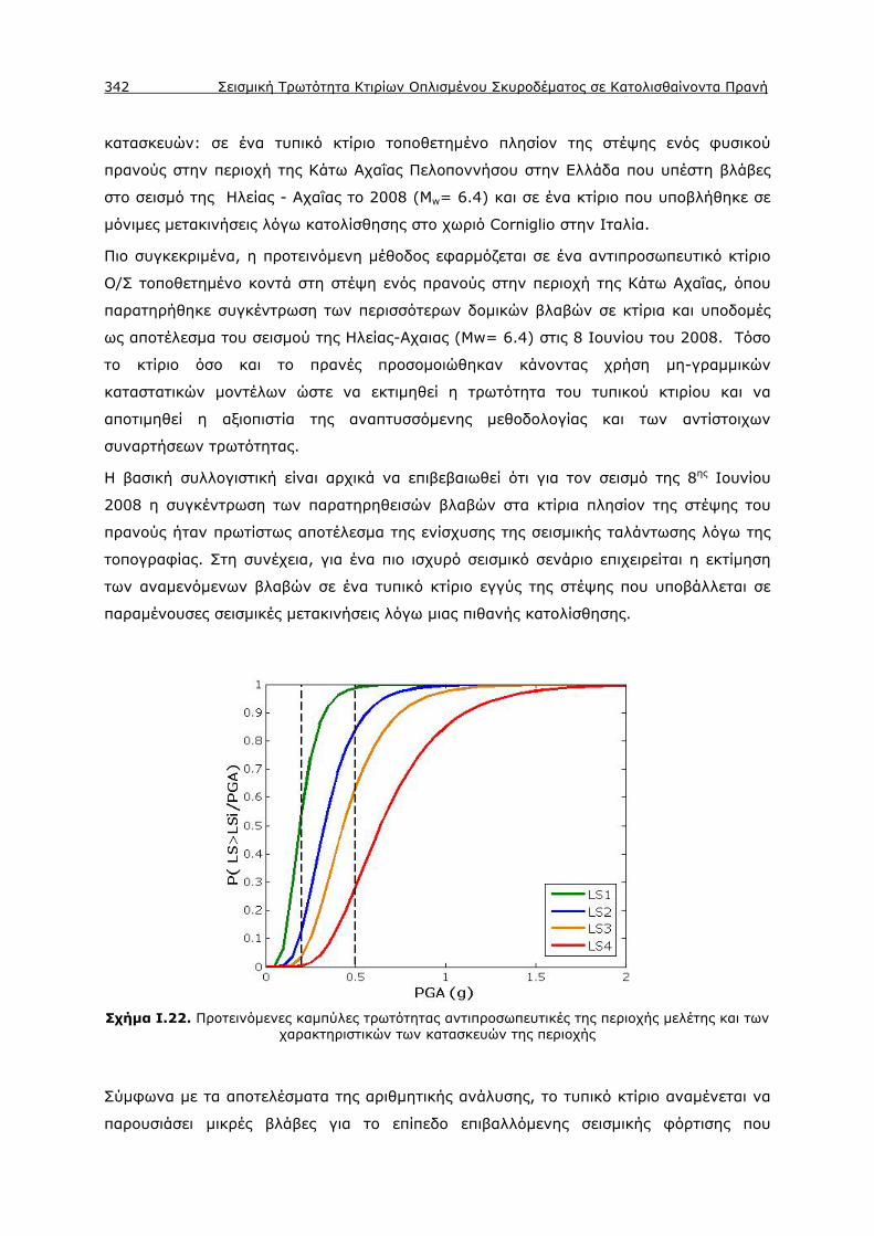
342 Σεισμική Τρωτότητα Κτιρίων Οπλισμένου Σκυροδέματος σε Κατολισθαίνοντα Πρανή
κατασκευών: σε ένα τυπικό κτίριο τοποθετημένο πλησίον της στέψης ενός φυσικού
πρανούς στην περιοχή της Κάτω Αχαΐας Πελοποννήσου στην Ελλάδα που υπέστη βλάβες
στο σεισμό της Ηλείας - Αχαΐας το 2008 (Mw= 6.4) και σε ένα κτίριο που υποβλήθηκε σε
μόνιμες μετακινήσεις λόγω κατολίσθησης στο χωριό Corniglio στην Ιταλία.
Πιο συγκεκριμένα, η προτεινόμενη μέθοδος εφαρμόζεται σε ένα αντιπροσωπευτικό κτίριο
Ο/Σ τοποθετημένο κοντά στη στέψη ενός πρανούς στην περιοχή της Κάτω Αχαΐας, όπου
παρατηρήθηκε συγκέντρωση των περισσότερων δομικών βλαβών σε κτίρια και υποδομές
ως αποτέλεσμα του σεισμού της Ηλείας-Αχαιας (Mw= 6.4) στις 8 Ιουνίου του 2008. Τόσο
το κτίριο όσο και το πρανές προσομοιώθηκαν κάνοντας χρήση μη-γραμμικών
καταστατικών μοντέλων ώστε να εκτιμηθεί η τρωτότητα του τυπικού κτιρίου και να
αποτιμηθεί η αξιοπιστία της αναπτυσσόμενης μεθοδολογίας και των αντίστοιχων
συναρτήσεων τρωτότητας.
Η βασική συλλογιστική είναι αρχικά να επιβεβαιωθεί ότι για τον σεισμό της 8ης Ιουνίου
2008 η συγκέντρωση των παρατηρηθεισών βλαβών στα κτίρια πλησίον της στέψης του
πρανούς ήταν πρωτίστως αποτέλεσμα της ενίσχυσης της σεισμικής ταλάντωσης λόγω της
τοπογραφίας. Στη συνέχεια, για ένα πιο ισχυρό σεισμικό σενάριο επιχειρείται η εκτίμηση
των αναμενόμενων βλαβών σε ένα τυπικό κτίριο εγγύς της στέψης που υποβάλλεται σε
παραμένουσες σεισμικές μετακινήσεις λόγω μιας πιθανής κατολίσθησης.
Σχήμα I.22. Προτεινόμενες καμπύλες τρωτότητας αντιπροσωπευτικές της περιοχής μελέτης και των
χαρακτηριστικών των κατασκευών της περιοχής
Σύμφωνα με τα αποτελέσματα της αριθμητικής ανάλυσης, το τυπικό κτίριο αναμένεται να
παρουσιάσει μικρές βλάβες για το επίπεδο επιβαλλόμενης σεισμικής φόρτισης που

Εκτενής Περίληψη 343
αντιστοιχεί κατά προσέγγιση στον κύριο σεισμό της 8ης Ιουνίου 2008 (PGArock=0.2g), οι
οποίες βρίσκονται σε συμφωνία με τις παρατηρηθείσες, ενώ αναμένεται να υποστεί ολική
κατάρρευση για το ισχυρότερο σεισμικό σενάριο (PGArock=0.5g). Η άμεση σύγκριση των
βλαβών που προέκυψαν από την ανάλυση με τις αντίστοιχες βλάβες που προβλέπουν οι
προτεινόμενες αντιπροσωπευτικές καμπύλες τρωτότητας (βλ. Σχ. Ι. 22) πιστοποιεί ότι οι
καμπύλες που προτείνονται στη συγκεκριμένη διατριβή μπορούν να προβλέψουν επαρκώς
την αναμενόμενη επίδοση αντιπροσωπευτικών κατασκευών Ο/Σ που εκτίθενται σε μόνιμες
σεισμικές διαφορικές μετακινήσεις λόγω κατολίσθησης.
Ο στόχος της εφαρμογής της προτεινόμενης μεθοδολογίας σε ένα αντιπροσωπευτικό
κτίριο στο χωριό Corniglio της Ιταλίας, το οποίο υπέστη μόνιμες μετακινήσεις λόγω της
συνεχούς κατολισθηστικής δραστηριότητας στην περιοχή, είναι διττός: πρώτον, να
διερευνήσει την αξιοπιστία των καμπυλών τρωτότητας που αναπτύχθηκαν στην παρούσα
διατριβή μέσω της σύγκρισης τους με την παρατηρηθείσα βλάβη στο κτίριο για το
συγκεκριμένο επίπεδο μετακίνησης του εδάφους και της κατασκευής και δεύτερον, να
επεκτείνει την εφαρμοσιμότητα της νέας προσέγγισης, προτείνοντας πιο ρεαλιστικές
καμπύλες τρωτότητας για το υπό μελέτη κτίριο μέσω προηγμένων αριθμητικών
αναλύσεων.
Ένας πολύτιμος όγκος δεδομένων (σε όρους παραμενουσών εδαφικών μετακινήσεων και
μόνιμων μετατοπίσεων κτιρίων καθώς και καταγραφουσών βλαβών των κτιρίων λόγω της
κατολίσθησης) κατέστη διαθέσιμος και επεξεργάστηκε (Callerio et al., 2007) για ένα
πλήθος κτιρίων στο χωριό Corniglio, που τοποθετείται νοτιοδυτικά των Ιταλικών
Appennines. Το Σχήμα Ι.23 απεικονίζει τυπικούς συσχετισμούς μεταξύ της μόνιμης
μετατόπισης του υπό μελέτη κτιρίου από μετρήσεις γεωδαιτικής χωροστάθμησης (geodetic
levelling), της παραμένουσας εδαφικής μετακίνησης από το κοντινότερο σε σχέση με τη
θέση του κτιρίου ινκλινόµετρο καθώς και των μετρήσεων ανοίγματος των ρωγμών του
κτιρίου. Στο σχήμα δίδεται επίσης η οριζόμενη κλίμακα εκτίμησης της βλάβης (συναρτήσει
του ανοίγματος των ρωγμών), που επιτρέπει την αποτίμηση της αναμενόμενης βλάβης
στην κατασκευή.
Αρχικά, επιλέχθηκαν δύο σετ καμπυλών τρωτότητας αντιπροσωπευτικών της περιοχής
μελέτης που προέκυψαν από την παραμετρική διερεύνηση στην προηγούμενη ενότητα
(Σχ. Ι.24). Αυτά συγκρίθηκαν με την παρατηρηθείσα βλάβη στο κτίριο, η οποία
εκτιμήθηκε από «μέτρια έως σοβαρή» για το μετρηθέν επίπεδο μετακίνησης του κτιρίου
(0,121 μ) (βλ. Σχ. Ι.23). Για το ίδιο επίπεδο μετακίνησης οι προτεινόμενες καμπύλες
προβλέπουν «μικρές έως μέτριες» και «μέτριες έως εκτενείς» βλάβες που βρίσκονται σε
σχετικά καλή συμφωνία με τις αντίστοιχες στάθμες βλάβης που ορίστηκαν με βάση την
ενόργανη παρακολούθηση και την επί τόπου παρατήρηση. Σημειώνεται ότι οι

344 Σεισμική Τρωτότητα Κτιρίων Οπλισμένου Σκυροδέματος σε Κατολισθαίνοντα Πρανή
αναμενόμενες βλάβες που προκύπτουν από τις προτεινόμενες αντιπροσωπευτικές
καμπύλες για κλίση πρανούς 45o είναι περισσότερο συμβατές με τις παρατηρηθείσες.
Σχήμα I.23. Συσχετίσεις μεταξύ της μόνιμης μετατόπισης του υπό μελέτη κτιρίου από μετρήσεις γεωδαιτικής χωροστάθμησης (geodetic levelling), της παραμένουσας εδαφικής μετακίνησης από το κοντινότερο σε σχέση με τη θέση του κτιρίου ινκλινόµετρο καθώς και των μετρήσεων ανοίγματος των ρωγμών του κτιρίου (συγκρινόμενα με τις οριζόμενες στάθμες βλάβης) συναρτήσει του χρόνου
(Callerio et al., 2007)
Σχήμα I.24. Αντιπροσωπευτικές αναλυτικές καμπύλες τρωτότητας που προέκυψαν από την παραμετρική διερεύνηση για κλίση πρανούς β=30ο (αριστερά) και β=45ο (δεξιά)

Εκτενής Περίληψη 345
Στη συνέχεια, προκειμένου να επεκταθεί το εύρος εφαρμογής της προτεινόμενης
μεθοδολογίας, αναπτύχθηκαν περισσότερο ρεαλιστικές, αναλυτικές καμπύλες τρωτότητας
για το υπό μελέτη κτίριο στο χωριό Corniglio μέσω μη-γραμμικών αριθμητικών
αναλύσεων, με βάση τα διαθέσιμα δεδομένα της περιοχής (δυσδιάστατη γεωτεχνική τομή
της περιοχής, καταγραφές του ινκλινόμετρου A3-2 που βρίσκεται πλησίον του υπό μελέτη
κτιρίου, μετρήσεις μετατοπίσεων και ρωγμών στο κτίριο). Οι καμπύλες τρωτότητας που
προτείνονται για το υπό μελέτη κτίριο (Σχ. Ι.25) εκτιμούν ότι αυτό αναμένεται να υποστεί
«μέτριες έως εκτενείς» βλάβες για το μετρηθέν επίπεδο μετακίνησης. Αυτές βρίσκονται σε
πολύ καλή συμφωνία με τις βλάβες που προέκυψαν από τις ενόργανες καταγραφές και
την επί τόπου έρευνα, επιβεβαιώνοντας την εγκυρότητα της προτεινόμενης μεθοδολογίας
και των αντίστοιχων καμπυλών για τη συγκεκριμένη εφαρμογή.
Σχήμα I.25. Καμπύλες τρωτότητας που προτείνονται για το υπό μελέτη κτίριο στην περιοχή του Corniglio
I.6 Εξέλιξη της τρωτότητας των κατασκευών στο χρόνο
Οι περισσότερες μέθοδοι αποτίμησης θεωρούν τη φυσική τρωτότητα ως «αμετάβλητη» στο
χρόνο. Ωστόσο, η πραγματική, δυναμική τρωτότητα των κατασκευών μπορεί να
μεταβάλλεται στο χρόνο, επηρεαζόμενη από φαινόμενα γήρανσης των υλικών,
ανθρωπογενείς δράσεις και συσσωρευτική βλάβη από προηγούμενες κατολισθήσεις ή
άλλους φυσικούς κινδύνους. Παρά τις προσπάθειες κάποιων ερευνητών να συμπεριλάβουν
τον χρόνο ως μια βασική συνιστώσα της τρωτότητας, η χρήση χρονικά εξαρτώμενων
συναρτήσεων τρωτότητας δεν είναι αρκετά διαδεδομένη έως σήμερα.

346 Σεισμική Τρωτότητα Κτιρίων Οπλισμένου Σκυροδέματος σε Κατολισθαίνοντα Πρανή
Η παρούσα διατριβή φιλοδοξεί να καλύψει εν μέρει αυτό το κενό, επεκτείνοντας την
προτεινόμενη προσέγγιση ώστε να λάβει υπόψη της την εξέλιξη της τρωτότητας των
κτιρίων στο χρόνο. Συγκεκριμένα, η γήρανση των υλικών κτιρίων Ο/Σ λαμβάνεται υπόψη
υιοθετώντας χρονικώς εξαρτώμενα, πιθανοτικά μοντέλα διάβρωσης του χάλυβα του
οπλισμού στο μεθοδολογικό πλαίσιο αποτίμησης της τρωτότητας. Εξετάζονται δύο
δυσμενή σενάρια διάβρωσης που σχετίζονται με την ενανθράκωση του χάλυβα του
οπλισμού και τη διείσδυση χλωριόντων της ατμόσφαιρας. Η μεθοδολογία εφαρμόζεται σε
τυπικά πλαισιακά κτίρια Ο/Σ χαμηλού ύψους, που εκτίθενται στη συνδυασμένη δράση της
παραμένουσας σεισμικής διαφορικής μετακίνησης λόγω της κατολίσθησης και της
διάβρωσης του οπλισμού. Εξετάζονται κτίρια με εύκαμπτο και δύσκαμπτο σύστημα
θεμελίωσης, τοποθετημένα εγγύς της στέψης σεισμικώς εν δυνάμει ασταθών πρανών. Η
ανάλυση που πραγματοποιείται είναι ψευδοστατική θεωρώντας ανελαστική τη
συμπεριφορά των υλικών της κατασκευής υπό τη μορφή ινών (fibers). Η διαφορική
μετακίνηση λόγω της κατολίσθησης συναρτήσει του χρόνου εισάγεται στη βάση του
προσομοιώματος της κατασκευής ως φόρτιση κινηματικού τύπου.
Η κατανομή του χρόνου έναρξης της διάβρωσης εκτιμάται μέσω προσομοίωσης Monte
Carlo κάνοντας χρήση κατάλληλων πιθανοκρατικών μοντέλων για τα δύο μελετηθέντα
σενάρια διάβρωσης. Στη συνέχεια, η απώλεια της επιφάνειας του χάλυβα στο χρόνο λόγω
της διάβρωσης προσομοιώνεται μέσω της απομείωσης της ενεργού διατομής των ράβδων
του οπλισμού. Το Σχήμα Ι.26 απεικονίζει την πιθανοτική εκτίμηση της χρονικά-
εξαρτώμενης απομειωμένης επιφάνειας διάβρωσης των ράβδων του οπλισμού στο χρόνο t,
A(t), κανονικοποιημένης ως προς την αρχική επιφάνεια του οπλισμού, A(t0), για τα δύο
σενάρια διάβρωσης που μελετώνται. Όπως αναμένονταν, η αβεβαιότητα στην εκτίμηση
της απώλειας της επιφάνειας του οπλισμού τείνει να αυξάνει στο χρόνο, εξαρτώμενη από
τη συζευγμένη αβεβαιότητα στην αρχική διάμετρο των ράβδων του οπλισμού, στο ρυθμό
της διάβρωσης και στο χρόνο έναρξης της διάβρωσης.
Οι στάθμες βλάβης ορίζονται συναρτήσει οριακών τιμών τοπικών παραμορφώσεων του
χάλυβα, οι οποίες επίσης μεταβάλλονται στο χρόνο.
Η προτεινόμενη προσέγγιση καταλήγει στην ανάπτυξη χρονικά εξαρτώμενων
λογαριθμοκανονικών καμπυλών και επιφανειών τρωτότητας συναρτήσει της PGA ή της
PGD για κτίρια οπλισμένου σκυροδέματος, που εκτίθενται σε σεισμικώς προκαλούμενες
κατολισθήσεις για τα δύο διαφορετικά σενάρια διάβρωσης (λόγω ενανθράκωσης του
χάλυβα και λόγω διείσδυσης χλωριόντων). Στο Σχήματα Ι.27 δίνονται τυπικά
αποτελέσματα υπό μορφή χρονικά μεταβαλλόμενων καμπυλών και επιφανειών
τρωτότητας συναρτήσει της PGD για την περίπτωση του κτιρίου που εδράζεται σε
εύκαμπτο σύστημα θεμελίωσης, για το σενάριο της διάβρωσης που σχετίζεται με τη
διείσδυση χλωριόντων.

Εκτενής Περίληψη 347
Σχήμα I.26. Μεταβολή της κανονικοποιημένης επιφάνειας του οπλισμού με το χρόνο λόγω του φαινομένου της διάβρωσης για τα σενάρια (α) της ενανθράκωσης του χάλυβα και (β) της
επίδρασης χλωριόντων
Όπως φαίνεται στο Σχήμα Ι.29, η χρονικά εξαρτώμενη διάμεσος των καμπυλών μπορεί να
αναπαρασταθεί επαρκώς με μια πολυωνυμική συνάρτηση 2ου βαθμού. Τέτοια μοντέλα
προσφέρουν το πλεονέκτημα της άμεσης εκτίμησης των διαμέσων των καμπυλών για το
δεδομένο κτίριο και για το συγκεκριμένο σενάριο διάβρωσης για οποιαδήποτε στιγμή στο
χρόνο, εφόσον είναι γνωστή η τρωτότητα της κατασκευής στην αρχική της κατάσταση.
Παρατηρείται ότι η τρωτότητα των κατασκευών αυξάνει στο χρόνο λόγω της διάβρωσης.
Αυτή η αύξηση είναι περισσότερο εμφανής για την περίπτωση των κτιρίων Ο/Σ επί
εύκαμπτης θεμελίωσης που επηρεάζονται από φαινόμενα διάβρωσης λόγω της διείσδυσης
χλωριόντων.
(α)
(β)

348 Σεισμική Τρωτότητα Κτιρίων Οπλισμένου Σκυροδέματος σε Κατολισθαίνοντα Πρανή
Σχήμα I.27. Χρονικά εξαρτώμενες καμπύλες και επιφάνειες τρωτότητας συναρτήσει του PGD, για μικρές (LS1), μέτριες (LS2), εκτενείς (LS3) βλάβες και ολική κατάρρευση (LS4), για ένα τυπικό χαμηλού ύψους πλαισιακό κτίριο Ο/Σ επί εύκαμπτου συστήματος θεμελίωσης, για το σενάριο της
διάβρωσης που σχετίζεται με τη διείσδυση χλωριόντων

Εκτενής Περίληψη 349
Σχήμα I.28. Αναπαράσταση της χρονικά εξαρτώμενης διαμέσου (σε όρους PGD) των καμπυλών με πολυώνυμο 2ου βαθμού για την περίπτωση των μικρών (LS1), μέτριων (LS2), εκτενών (LS3) βλαβών και για ολική κατάρρευση (LS4), για ένα τυπικό χαμηλού ύψους πλαισιακό κτίριο Ο/Σ επί εύκαμπτου συστήματος θεμελίωσης, για το σενάριο της διάβρωσης που σχετίζεται με τη διείσδυση χλωριόντων
I.7 Συμπεράσματα
Οι καταστρεπτικές συνέπειες των κατολισθήσεων που προκαλούνται από σεισμό σε κτίρια
και υποδομές αλλά και σε ανθρώπινες ζωές, καθιστούν επιτακτική την ανάγκη ανάπτυξης
νέων μεθόδων και πρακτικών για την αποτελεσματική αποτίμηση και μείωση της
διακινδύνευσης. Ωστόσο, η ποσοτική εκτίμηση της διακινδύνευσης των διαφόρων τύπων
κατολισθήσεων εμπεριέχει πλήθος αβεβαιοτήτων που παρεμποδίζουν τον αντικειμενικό
προσδιορισμό της. Ένας πρωταρχικός παράγοντας αβεβαιότητας συνδέεται με την
αποτίμηση της τρωτότητας των κατασκευών που υπόκεινται στον κίνδυνο κατολίσθησης
λόγω της δυναμικής και πολυδιάστατης φύσης της αλλά και της γενικότερης έλλειψης
αξιόπιστων στατιστικών στοιχείων βλαβών σε κτίρια και υποδομές λόγω των διαφόρων
μηχανισμών κατολίσθησης. Σε αυτό το πλαίσιο, ένα εκ των βασικών επιτευγμάτων της
συγκεκριμένης διδακτορικής διατριβής, αποτελεί η πρόταση μιας καινοτόμου αναλυτικής
μεθοδολογίας για την αποτίμηση της τρωτότητας κτιρίων οπλισμένου σκυροδέματος
πλησίον σεισμικώς ασταθών πρανών. Η αξιοπιστία του αριθμητικού προσομοιώματος

350 Σεισμική Τρωτότητα Κτιρίων Οπλισμένου Σκυροδέματος σε Κατολισθαίνοντα Πρανή
επιβεβαιώθηκε μέσω της σύγκρισης των μετακινήσεων στην περιοχή του πρανούς, που
εξήχθησαν από τις αριθμητικές αναλύσεις με τις αντίστοιχες μετακινήσεις που
υπολογίστηκαν από εμπειρικές μεθόδους εκτίμησης των μετακινήσεων τύπου Newmark.
Στο πλαίσιο της διατριβής, προτείνονται καμπύλες τρωτότητας για διάφορους τύπους
κατασκευής, εδαφικές συνθήκες και γεωμετρίες πρανούς καθώς και αποστάσεις της
θεωρούμενης κατασκευής από την πιθανή κατολίσθηση μέσω μιας εκτενούς παραμετρικής
διερεύνησης, οι οποίες μπορούν να βρουν άμεση εφαρμογή σε ένα πιθανοτικό πλαίσιο
εκτίμησης της διακινδύνευσης λόγω των κατολισθήσεων. Η αξιοπιστία της προτεινόμενης
μεθοδολογίας επαληθεύτηκε μέσω της σύγκρισης των αναπτυσσόμενων καμπυλών με
σχετικές καμπύλες της βιβλιογραφίας και δεδομένα από βλάβες σε κτίρια λόγω
κατολισθητικών φαινομένων στην Ελλάδα και την Ιταλία. Τέλος, σημαντική είναι η
συμβολή της διδακτορικής διατριβής στη μελέτη του χρόνου ως βασικής συνιστώσας της
τρωτότητας των κατασκευών. Συγκεκριμένα, η προτεινόμενη προσέγγιση επεκτάθηκε
ώστε να λάβει υπόψη της την εξέλιξη της τρωτότητας των κατασκευών στο χρόνο,
προτείνοντας χρονικά εξαρτώμενες καμπύλες και επιφάνειες τρωτότητας για κτίρια
οπλισμένου σκυροδέματος που εκτίθενται σε κατολισθήσεις προκαλούμενων από σεισμό.
I.8 Βιβλιογραφικές αναφορές
Argyroudis S., Pitilakis K. (2012). “Seismic fragility curves of shallow tunnels in alluvial
deposits”. Soil Dynamics and Earthquake Engineering 35, 1-12.
Assimaki D., Kausel E. (2007). “Modified topographic amplification factors for a single-
faced slope due to kinematic soil-structure interaction”. J of Geotechnical and
Geoenvironmental Engineering 133, 1414–1431.
Bird J.F., Crowley H., Pinho R., Bommer J.J. (2005). “Assessment of building response to
liquefaction induced differential ground deformation”. Bul of the New Zealand Society
for Earthquake Engineering 38(4), 215-234.
Bird J.F., Bommer J.J., Crowley H., Pinho R. (2006). “Modelling liquefaction-induced
building damage in earthquake loss estimation”. Soil dynamics and Earthquake
Engineering 26(1), 15-30.
Bouckovalas G.D., Papadimitriou A.G. (2005). "Numerical evaluation of slope topography
effects on seismic ground motion". Soil Dynamics and Earthquake Engineering 25(7-
10), 547-558.
Bourdeau C., Havenith H.-B., Fleurisson J.-A., Grandjean, A.G. (2004). "Numerical
modelling of seismic slope stability”. Engineering Geology for Infrastructure Planning
in Europe, Springer Berlin / Heidelberg 104, 671-684.

Εκτενής Περίληψη 351
Bray J.D., Travasarou, T. (2007). “Simplified procedure for estimating
earthquake-induced deviatoric slope displacements”. Journal of Geotechnical and
Geoenvironmental Engineering 133(4), 381-392.
Callerio A., Faccioli E., Kaynia A. (2007). Deliverable 121: Landslide risk assessment
methods and applications (III) – Application to real active landslides – Phase II
(68pp), LESSLOSS integrated project: Risk Mitigation for Earthquake and Landslides,
Sub-Project 4 – Landslide risk scenarios and loss modelling.
Corominas J. Mavrouli O. (Eds.) (2011b). Deliverable 2.11: QRA case studies at selected
"hotspots". Synthesis of critical issues. Work Package 2.3 – Development of
procedures for QRA at regional scale and European scale. SafeLand: Seventh
Framework Programme for research and technological development (FP7) of the
European Commission.
Crowley H., Pinho R., Bommer J.J. (2004). “A probabilistic displacement-based
vulnerability assessment procedure for earthquake loss estimation”. Bulletin of
Earthquake Engineering 2(2),173-219.
Crowley et al. (2011). D3.1 - Fragility functions for common RC building types in Europe,
in SYNER-G: Systemic Seismic Vulnerability and Risk Analysis for Buildings, Lifeline
Networks and Infrastructures Safety Gain, WP3 – Fragility Functions of Elements at
Risk.
EAK2000 (2000). Greek Seismic Code, Organization of seismic planning and protection.
Erberik M.A. (2008). “Fragility-based assessment of typical mid-rise and low-rise RC
buildings in Turkey”. Engineering Structures 30(5), 1360-1374.
Fotopoulou S., Karapetrou S., Pitilakis K. (2012). “Seismic vulnerability of RC buildings
considering SSI and aging effects”. 15th World Conference on Earthquake
Engineering, Lisbon, Portugal, 24-28 September.
Ishihara K. (1996). “Soil behaviour in earthquake geotechnics”. Clarendon, London, 350
pp.
Itasca Consulting Group (2008). Inc. FLAC (Fast Lagrangian Analysis of Continua), ver.
6.0. Itasca Consulting Group, Inc., Minneapolis.
Kappos A. Panagiotopoulos C., Panagopoulos G., Papadopoulos El. WP4 – Reinforced
concrete buildings (Level 1 and Level 2 analysis). RISK-UE, 2003.
Kramer S.L., Stewart J.P. (2004). “Geotechnical aspects of seismic hazards”. In:
Earthquake Engineering: from Engineering Seismology to Performance-Based
Engineering, Y. Bozorgnia, V. Bertero (Eds.), CRC Press, Chapter 4, 85 pp.
Ktenidou O.J. (2010). “Theoretical and instrumental study of site and topographic effects
on strong ground motion in Aegion”. Ph.D. thesis, Aristotle University Thessaloniki,
Greece.

352 Σεισμική Τρωτότητα Κτιρίων Οπλισμένου Σκυροδέματος σε Κατολισθαίνοντα Πρανή
Mansour M.F., Morgenstern N.I., Martin C.D. (2011). “Expected damage from
displacement of slow-moving slides”. Landslides 8(1), 117–131.
Marano K.D., Wald D.J., Allen T.I. (2010). “Global earthquake casualties due to
secondary effects: a quantitative analysis for improving rapid loss analyses”. Nat
Hazards 52, 319–328.
National Institute of Building Sciences (2004). Direct physical damage—general building
stock. HAZUS-MH Technical manual, Chapter 5. Federal Emergency Management
Agency, Washington, D.C.
Negulescu C., Foerster E. (2010). “Parametric studies and quantitative assessment of the
vulnerability of a RC frame building exposed to differential settlements”. Natural
Hazards and Earth System Sciences 10, 1781-1792.
Newmark N.M. (1965). “Effects of earthquakes on dams and embankments”.
Geotechnique 15 (2), 139–159.
Nielson B.G., DesRoches R. (2007). “Analytical seismic fragility curves for typical bridges
in the central and southeastern United States”. Earthquake Spectra 23(3), 615.
Pitilakis D., Tsinaris A. (2010). “Soil-foundation-structure interaction close to natural
slopes and topographic irregularities (In Greek)”. In: Proc of the 6th National
Conference of Geotechnical Engineering, Volos, Greece.
Pitilakis K.D. (2010). “Geotechnical earthquake engineering”. Ziti publication (in Greek).
Rathje E.M., Antonakos G. (2011). “A unified model for predicting earthquake-induced
sliding displacements of rigid and flexible slopes”. Engineering Geology 122(1-2), 51-
60.
SeismoSoft, SeismoStruct (2011). A computer program for static and dynamic nonlinear
analysis of framed structures. Available from URL: www.seismosoft.com.
Shinozuka M., Feng M. Q., Lee J., Naganuma T. (2000). “Statistical analysis of fragility
curves”. J. Eng. Mech.-ASCE, 126(12), 1224– 1231.
Shinozuka M., Feng M.Q., Kim H.K., Uzawa T., Ueda T. (2003). “Statistical analysis of
fragility curves”. Technical Report MCEER-03-0002, State University of New York,
Buffalo.
Tsionis G., Papailia A., Fardis M.N. (2011). “Analytical fragility functions for reinforced
concrete buildings and buildings aggregates of Euro-Mediterranean regions – UPAT
methodology”. Internal Report, Syner-G Project 2009/2012.
Yin Y., Wang F., Sun P. (2009). "Landslide hazards triggered by the 2008 Wenchuan
earthquake, Sichuan, China". Landslides 6(2), 139-152.
Zhang L.M., Ng A.M.Y. (2005). “Probabilistic limiting tolerable displacements for
serviceability limit state design of foundations”. Geotechnique 55(2), 151–161.