Research Collection

Report

Reinforced concrete slabs - compatibility limit design

Author(s): Monotti, Mario Nicola

Publication Date: 2004

Permanent Link: https://doi.org/10.3929/ethz-a-004847225

Rights / License: In Copyright - Non-Commercial Use Permitted

This page was generated automatically upon download from the ETH Zurich Research Collection. For moreinformation please consult the Terms of use.

ETH Library

Reinforced Concrete Slabs – Compatibility Limit Design

Mario Nicola Monotti

Institute of Structural Engineering Swiss Federal Institute of Technology Zurich

Zurich August 2004

Preface

Stahlbetonplatten gehören zu den klassischen Anwendungsgebieten der Theorie starr-ideal plastischer Körper. Diese um 1950 von Prager, Drucker, Hill und anderen formulierte Theorie, die sich in ihrer Anwendung nach dem unteren und oberen Grenzwertsatz in eine statische und eine kinematische Methode aufteilt, erfuhr in den 1960er Jahren in Bezug auf Plattenprobleme ausgedehnte Darstel-lungen, namentlich durch Wood, Massonnet und Save, Nielsen, Sawczuk und Jaeger, Wolfensberger, Kemp, Morley und weitere Autoren. Die 1921 von Ingerslev eingeführte und ab 1931 von Johansen vorangetriebene Fliessgelenklinientheorie wurde als An-wendung der kinematischen Methode erkannt. Schwierigkeiten ergaben sich allerdings bei der Interpretation der von Johansen einge-führten Knotenkräfte, und zudem wurden Fälle entdeckt, bei denen sich das Versagen nicht mit Fliessgelenklinien beschreiben lässt. Das erste Problem wurde durch die Einsicht in die Äquivalenz von Drillmomenten und Randquerkräften sowie die Möglichkeit von Sprüngen der Drillmomente an Diskontinui-tätslinien teilweise gelöst. Die Lösung des zweiten Problems bestand in der Einführung von Fliesszonen, in denen sowohl die untere als auch die obere Bewehrung fliesst. Analog zur Betrachtung des Kraftflusses in Stahlbeton-Stabtragwerken mit Fachwerk-modellen und Spannungsfeldern wurden am Institut für Baustatik und Konstruktion der ETH Zürich in den 1990er Jahren auf dem unteren Grenzwertsatz beruhende Methoden zur Betrachtung des Kraftflusses in Stahl-betonplatten entwickelt. Liefern bei Stabtrag-werken die Querkräfte den Schlüssel zum Verständnis des Kraftflusses, so sind dies im Innern und am Rand von Platten die Haupt-querkräfte sowie entlang von Diskontinuitäts-linien übertragene Querkräfte. Herrn Monottis Arbeit ist vor diesem Hintergrund zu sehen. Sie führt einerseits zu einer Klärung der Rolle von Knotenkräften;

Reinforced concrete slabs belong to the classical fields of application of the theory of rigid-perfectly plastic bodies. Established around 1950 by Prager, Drucker, Hill, and others, this theory, which can be used in the form of the static or the kinematic method, was extensively applied to slab problems in the 1960’s, in particular by Wood, Massonnet and Save, Nielsen, Sawczuk and Jaeger, Wolfensberger, Kemp, Morley, and others. The yield line theory, introduced by Ingerslev in 1921 and developed by Johansen from 1931 onwards, was recognised to be an application of the kinematic method. However, the interpretation of the nodal forces introduced by Johansen led to difficul-ties and cases were discovered where failure cannot be described by yield line mecha-nisms. The first problem was partially solved by the recognition of the equivalency of twisting moments and edge shear forces as well as the possibility of jumps in the twisting moments along discontinuity lines. The solution of the second problem consisted in introducing yield regions within which both the bottom and the top reinforcements are yielding. Similar to the consideration of the force flow within reinforced concrete beams and frames by means of truss models and stress fields, methods based on the lower-bound theorem of the theory of plasticity were developed at the Institute of Structural Engineering of the ETH during the 1990’s to follow the force flow within reinforced concrete slabs. While for beams and frames, the shear forces provide the key to under-standing the force flow, principal shear forces and shear forces transferred along dis-continuity lines play the same role in the interior and at the edges of slabs. Mr. Monotti’s work should be regarded within this context. On the one hand it clarifies the meaning of nodal forces; they correspond either to jumps in the twisting

diese entsprechen entweder Drillmomenten-sprüngen oder Singularitäten der Haupt-querkräfte. Andererseits stellen seine neu entwickelten Spannungsfelder eine beträcht-liche Bereicherung der Bibliothek vorhande-ner Ansätze dar. Schliesslich belebt sein Konzept der Verträglichkeitsmethode die weitgehend erstarrte Diskussion über die Bemessungsmethoden von Stahlbetonplatten; wie die Kapazitätsbemessung liegt dieses Konzept den Bedürfnissen der praktischen Anwendung nahe und umgeht die bisher in ihrer Bedeutung etwas überbewerteten theoretischen Schwierigkeiten.

moments or to discontinuities of the principal shear forces. On the other hand his newly developed stress fields represent a significant extension of the library of known solutions. Finally, the concept of the so-called compati-bility limit design method provides a new impulse to the rather rigidified discussion of reinforced concrete slab design methods; similar to the capacity design method this concept is suitable for practical applications and it bypasses the theoretical difficulties that have perhaps so far been somewhat overrated in their significance.

Zurich, August 2004 Prof. Dr. Peter Marti

Summary

Based on the theory of plasticity this thesis develops a new design procedure for reinforced concrete slabs – the compatibility limit design method. The basic idea of this method is to extend the typical design procedure for reinforced concrete beams and frames to slabs. For beams and frames, the failure mechanisms indicate the global force flow because the plastic hinges coincide with the points of zero shear force; the force flow within the beam or frame segments defined by the points of zero shear force can be visualised using truss models or corresponding stress fields and the segments’ detailing can be completed accordingly. For slabs, static and kinematic considerations are normally applied in an unrelated way and hence, the potential offered by the theory of plasticity is not fully utilised; by considering yield line mechanisms and developing matching stress fields for slab segments defined by the yield lines the compatibility limit design method attempts to overcome this situation.

After the introduction (Chapter 1) and a presentation of the fundamentals of the theory of rigid-perfectly plastic bodies and its application to reinforced concrete (Chapter 2) Chapter 3 to 5 present the static, limit analysis and kinematic considerations underlying the compatibility limit design method whose application is illustrated in Chapter 6 by means of a practical example. Chapter 7 contains a summary, conclusions and recommendations for future studies.

The static considerations concentrate on the load transfer mechanisms in slabs and their boundary conditions. Distributed and concentrated load transfer are differentiated. Distributed load transfer is described by the generalised strip method, using general curved rather than straight orthogonal beams. Concentrated load transfer occurs in strong bands or along shear lines. Together with a set of stress fields describing a certain distributed load transfer within individual slab segments strong bands and shear lines are the basic tools of a stress field approach for slabs similar to that used for beams and frames.

The limit analysis considerations are based on a discussion of compatible states of stress and deformation using the yield condition and the associated flow rule for orthogonally reinforced concrete slabs. From a kinematic point of view, rigid parts, yield lines and yield regions are differentiated. It is proposed to bypass the difficulties associated with yield regions by introducing an approximate limit analysis, corresponding to enforcing yield line mechanisms of unique sign; similar to the capacity design method used in earthquake engineering this can be ensured by some local strengthening of the reinforcement.

The kinematic considerations illustrate the application of the work method and the equilibrium method to yield line mechanisms. It is shown that the two methods are equivalent if they are associated to a unique statical problem.

The practical application of the compatibility limit design method requires some preliminary assumptions about the resistance distribution in the slab. Based on an intuitively assumed yield line mechanism the required global resistances can be quantified and optimised. In a second step, the stress field approach is employed to study the force flow within and between the individual slab segments and to detect any local resistance deficits.

Zusammenfassung

Auf der Grundlage der Plastizitätstheorie wird eine neue Bemessungsmethode für Stahlbeton-platten entwickelt – die Verträglichkeitsmethode. Die Grundidee dieser Methode besteht darin, die für Stabtragwerke übliche Bemessungsmethode auf Platten zu übertragen. Die Bruchmechanismen von Stabtragwerken zeigen den Kraftfluss im Grossen an, weil die plastischen Gelenke den Querkraftnullpunkten entsprechen; der Kraftfluss im Kleinen, im Inneren der durch die Querkraftnullpunkte begrenzten Elemente, kann mit Fachwerkmodellen oder entsprechenden Spannungsfeldern untersucht werden, was eine passende konstruktive Durchbildung ermöglicht. Bei der Bemessung von Platten werden üblicherweise statische und kinematische Betrachtungen angestellt, die in keinem direkten Zusammenhang stehen, und das Potential der Plastizitätstheorie wird nicht ausgeschöpft; mit der Verträglichkeitsmethode wird versucht, diese unbefriedigende Situation zu überwinden, indem ausgehend von angenommenen Fliessgelenklinienmechanismen entsprechende verträgliche Spannungsfelder in den einzelnen durch die Fliessgelenklinien definierten Plattenteilen entwickelt werden. Nach der Einleitung (Kapitel 1) und einer Zusammenstellung der Grundlagen der Theorie starr- ideal plastischer Körper sowie deren Anwendung auf Stahlbeton (Kapitel 2) enthalten die Kapitel 3 bis 5 die hinter der Verträglichkeitsmethode stehenden statischen, grenztragfähigkeits-theoretischen und kinematischen Betrachtungen. Die Anwendung der Verträglichkeitsmethode wird im Kapitel 6 anhand eines praktischen Beispiels illustriert, und Kapitel 7 enthält eine Zusammenfassung, Schlussfolgerungen sowie Empfehlungen für weiterfürende Studien.

Im Zentrum der statischen Betrachtungen stehen der Kraftfluss in Platten sowie die entsprechenden Randbedingungen. Dabei wird zwischen einer Lastabtragung über verteilte und konzentrierte Querkräfte unterschieden. Die Lastabtragung über verteilte Querkräfte wird mit der verallgemeinerte Streifenmethode untersucht, die allgemein gekrümmte statt gerade orthogonale Koordinaten verwendet. Konzentrierte Querkräfte treten in versteckten Balken und Schublinien auf. Zusammen mit einer Familie von Spannungsfeldern zur Beschreibung der Lastabtragung in Plattenteilen über verteilte Querkräfte ermöglichen versteckte Balken und Schublinien eine Spannungsfeldanalyse von Platten ähnlich jener von Stabtragwerken. Die grenztragfähigkeitstheoretischen Betrachtungen beziehen sich auf verträgliche Spannungs- und Verformungszustände unter Zugrundelegung der Fliessbedingung und des zugeordneten Fliessgesetzes für orthogonal bewehrte Stahlbetonplatten. Kinematisch werden starre Plattenteile, Fliessgelenklinien und Fliesszonen unterschieden. Um die mit Fliesszonen verbundenen Schwierigkeiten zu umgehen wird vorgeschlagen, eine approximative Grenztragfähigkeitsanalyse einzuführen, derart, dass nur positive oder negative Fliess-gelenklinien auftreten; ähnlich wie bei der Kapazitätsbemessung im Erdbebeningenieurwesen wird das Auftreten solcher Mechanismen durch örtliche Bewehrungsverstärkungen erzwungen.

Die kinematischen Betrachtungen sind der Anwendung der sogenanten Energie- und Grenzgleichgewichtsmethoden auf Fliessgelenklinien gewidmet. Es wird gezeigt, dass die beiden Methoden äquivalent sind, wenn sie derselben statischen Problemstellung entsprechen. Die praktische Anwendung der Verträglichkeitsmethode setzt einige Annahmen über die Widerstandsverteilung in der Platte voraus. Von einem intuitiv angenommenen Fliess-gelenklinienmechanismus ausgehend können die notwendigen Widerstände bestimmt und optimiert werden. In einem zweiten Schritt können dann allfällige lokale Widerstandsdefizite durch Anwendung der Spannungsfeldanalyse endeckt und behoben werden.

Table of contents

1 Introduction 1 1.1 Defining the problem 1 1.2 Overview 2 1.3 Assumptions and limitations 4

2 Theory of plasticity 5 2.1 General 5 2.2 Rigid-perfectly plastic behaviour 5 2.3 Reinforced concrete 6 2.4 Yield condition and flow rule 8 2.5 Theorems of limit analysis 10 2.6 Limit analysis and design methods 11

3 Static method 13 3.1 General 13 3.2 Internal forces 13

3.2.1 Definition of internal forces 14 3.2.2 Stress field definition 14

3.3 Equilibrium 16 3.2.1 Orthogonal curvilinear coordinates 16 3.2.2 Sign convention 17 3.2.3 Equilibrium conditions 17

3.4 Load transfer 18 3.4.1 Distributed load transfer 18 3.4.2 Concentrated load transfer 20 3.4.3 Remarks 20

3.5 Boundary conditions 20 3.6 Lower-bound method 22

3.6.1 Generalised strip method 23 3.6.2 Elasticity 23 3.6.3 Strip method 24 3.6.4 Hencky-Prandtl solutions 25 3.6.5 General stress fields 25 3.6.6 Superposition principle 31 3.6.7 Stress field approach for slabs 33

3.7 Examples 34 3.7.1 Simply supported rectangular slab 34 3.7.2 Triangular slab with a free edge 38

3.8 Conclusions 40

4 Limit analysis 41 4.1 General 41 4.2 Yield condition and flow rule 41

4.2.1 Limit states 42 4.2.2 Yield condition 43 4.2.3 Flow rule 46 4.2.4 Discussion 48

4.3 Approximate limit analysis 49 4.4 Example application 50 4.5 Conclusions 51

5 Kinematic method 53 5.1 General 53 5.2 Failure mechanisms and limit analysis 54 5.3 Upper-bound method 55

5.3.1 Work method 55 5.3.2 Equilibrium method 59

5.4 Discussion 67 5.5 Conclusions 69

6 Compatibility limit design 71 6.1 General 71 6.2 Example application 71

6.2.1 Problem statement 72 6.2.2 Assumptions 72 6.2.3 Detailing 73 6.2.4 Kinematical analysis 74 6.2.5 Statical analysis 74 6.2.6 Reinforcement dimensioning 77

6.3 Discussion 78 6.4 Conclusions 80

7 Summary and conclusions 81 7.1 Summary 81 7.2 Conclusions 82 7.3 Recommendations for future studies 83

References 85

Notation 89

1

1 Introduction

1.1 Defining the problem

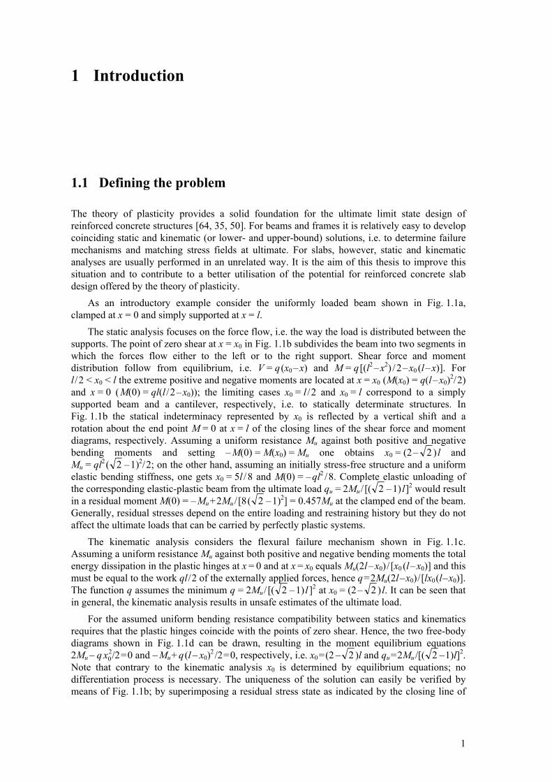
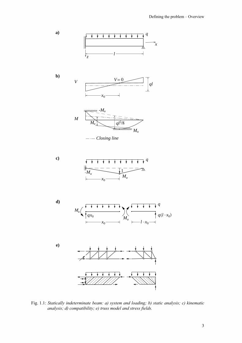
The theory of plasticity provides a solid foundation for the ultimate limit state design of reinforced concrete structures [64, 35, 50]. For beams and frames it is relatively easy to develop coinciding static and kinematic (or lower- and upper-bound) solutions, i.e. to determine failure mechanisms and matching stress fields at ultimate. For slabs, however, static and kinematic analyses are usually performed in an unrelated way. It is the aim of this thesis to improve this situation and to contribute to a better utilisation of the potential for reinforced concrete slab design offered by the theory of plasticity. As an introductory example consider the uniformly loaded beam shown in Fig. 1.1a, clamped at x = 0 and simply supported at x = l. The static analysis focuses on the force flow, i.e. the way the load is distributed between the supports. The point of zero shear at x = x0 in Fig. 1.1b subdivides the beam into two segments in which the forces flow either to the left or to the right support. Shear force and moment distribution follow from equilibrium, i.e. V = q (x0 – x) and M = q [(l2

– x2) / 2 – x0 (l – x)]. For l / 2 < x0 < l the extreme positive and negative moments are located at x = x0 (M(x0) = q(l – x0)2/ 2) and x = 0 ( M(0) = ql(l / 2 – x0)); the limiting cases x0 = l / 2 and x0 = l correspond to a simply supported beam and a cantilever, respectively, i.e. to statically determinate structures. In Fig. 1.1b the statical indeterminacy represented by x0 is reflected by a vertical shift and a rotation about the end point M = 0 at x = l of the closing lines of the shear force and moment diagrams, respectively. Assuming a uniform resistance Mu against both positive and negative bending moments and setting – M(0) = M(x0) = Mu one obtains x0 = (2 – 2 ) l and Mu = ql2

( 2 – 1)2/ 2; on the other hand, assuming an initially stress-free structure and a uniform elastic bending stiffness, one gets x0 = 5l / 8 and M(0) = – ql2

/ 8. Complete elastic unloading of the corresponding elastic-plastic beam from the ultimate load qu = 2Mu / [( 2 – 1) l ]2 would result in a residual moment M(0) = – Mu + 2Mu / [8 ( 2 – 1)2] = 0.457Mu at the clamped end of the beam. Generally, residual stresses depend on the entire loading and restraining history but they do not affect the ultimate loads that can be carried by perfectly plastic systems.

The kinematic analysis considers the flexural failure mechanism shown in Fig. 1.1c. Assuming a uniform resistance Mu against both positive and negative bending moments the total energy dissipation in the plastic hinges at x = 0 and at x = x0 equals Mu(2l – x0) / [x0 (l – x0)] and this must be equal to the work ql / 2 of the externally applied forces, hence q = 2Mu(2l – x0) / [lx0 (l – x0)]. The function q assumes the minimum q = 2Mu / [( 2 – 1) l ]2 at x0 = (2 – 2 ) l. It can be seen that in general, the kinematic analysis results in unsafe estimates of the ultimate load.

For the assumed uniform bending resistance compatibility between statics and kinematics requires that the plastic hinges coincide with the points of zero shear. Hence, the two free-body diagrams shown in Fig. 1.1d can be drawn, resulting in the moment equilibrium equations 2Mu – q 2

0x /2 = 0 and – Mu + q (l – x0)2 /2 = 0, respectively, i.e. x0 = (2 – 2 )l and qu = 2Mu /[( 2 – 1)l]2.

Note that contrary to the kinematic analysis x0 is determined by equilibrium equations; no differentiation process is necessary. The uniqueness of the solution can easily be verified by means of Fig. 1.1b; by superimposing a residual stress state as indicated by the closing line of

Introduction

2

the moment diagram the yield condition for the positive bending moments would be violated; similar arguments apply for the negative moments with a closing line rotation in the opposite direction.

It can be seen that based on compatibility considerations the static and the kinematic analyses are combined and made more efficient. Thus, the ultimate limit state design may start from failure mechanism considerations indicating the global force flow and the required main resistances, followed by a detailed analysis and design of the beam segments between the points of zero shear force, typically based on truss models and corresponding stress fields as shown in Fig. 1.1e.

Reinforced concrete slabs are frequently designed using moments determined according to the theory of elastic plates or Hillerborg’s strip method. Alternatively, yield line mechanisms and approximate design procedures such as the equivalent frame method are applied. Generally, the different methods are used independently of each other and their results may show considerable discrepancies. Insufficient flexibility of the static as well as the kinematic approaches is the reason for this incompatibility. By removing these limitations this thesis attempts to extend the compatibility limit design considerations from reinforced concrete beams and frames to reinforced concrete slabs.

1.2 Overview

Chapter 2 introduces the fundamentals of the theory of rigid-perfectly plastic bodies. Yield condition and associated flow rule are presented in a general form and the theorems of limit analysis are formulated based on the principles of virtual work and maximum energy dissipation. A discussion on the applicability of limit analysis and design procedures to reinforced concrete structures completes this chapter.

Chapters 3 to 5 present the static method, limit analysis and the kinematic method, introducing basic tools, developing methods of analysis and illustrating their application by means of two examples. Chapter 3 concentrates on the load transfer mechanisms in slabs and their boundary conditions. Different lower-bound methods are identified as particular forms of load transfer. In order to obtain the necessary flexibility for compatibility limit designs stress fields for slab segments characterised by distributed load transfer are developed. Together with shear lines and strong bands such stress fields are the basic tools of a stress field approach for slabs similar to that used for beams and frames.

Chapter 4 discusses compatible states of stress and deformation based on the yield condition and the associated flow rule for orthogonally reinforced concrete slabs. From a kinematic point of view, rigid parts, yield lines and yield regions are differentiated. Since yield regions are difficult to deal with it is proposed to introduce an approximate limit analysis, corresponding to enforcing yield line mechanisms of unique sign; similar to the capacity design method used in earthquake engineering this is ensured by some local strengthening of the reinforcement.

Chapter 5 presents the basic principles of yield line analysis and illustrates the application of the work method and of the equilibrium method. The relationships between the two methods are discussed and it is shown that the equilibrium method can be interpreted as an expression of compatibility limit design considerations (for a suitably defined approximate limit analysis problem) similar to those underlying Fig. 1.1d.

Defining the problem – Overview

3

Fig. 1.1: Statically indeterminate beam: a) system and loading; b) static analysis; c) kinematic analysis; d) compatibility; e) truss model and stress fields.

a)

l

q

V

M

ql

ql /82

Mu

-Mu

b)

c)

e)

Mu

Closing line

x

z

x

V = 0

0

q

Mu

Mu

x0

1

d) q

x0 x0l

Muqx0 q x0l( )

Mu

Introduction

4

Chapter 6 demonstrates the application of the compatibility limit design method by means of a practical example, highlighting the importance of detailing considerations and providing comparisons with previously derived solutions.

Chapter 7 contains a summary, conclusions and recommendations for future studies.

1.3 Assumptions and limitations

It is assumed that the load-deformation response of reinforced concrete can be idealised as rigid-perfectly plastic. This requires a sufficiently ductile and appropriately anchored, distributed and detailed reinforcement as well as adequate concrete cross-sections [64, 35].

Membrane action is neglected. While the flow of distributed and concentrated shear forces is analysed in detail the associated dimensioning and detailing is based on established procedures [33].

5

2 Theory of plasticity

2.1 General

The central task of structural engineers is the design of safe and economical structures. Safety not only implies resistance to external actions, but also ductility and robustness. Collapse should be preceded by perceivable deformations and in the case of failure, damage should not extend to the whole structure. Load resistance and ductility are simplified and summarised in the form of rigid-plastic behaviour on the basis of the theory of plasticity. Corresponding limit analysis methods have been applied for a long time, implicitly or explicitly, to solve engineering problems.

Only in the 1950’s the theory of plasticity was established on a sound basis, deviating radically in its approach from that of the theory of elasticity. By considering the elastic-plastic behaviour the transition between the two theories was smoothened [53, 37]; however, the complexity of elastic-plastic analyses and the problems related to the identification of the real state of stress in a structure meant the results were largely of academic interest. In practice the theories of elasticity and plasticity are used independently and with different purposes: serviceability limit states are checked based on the theory of elasticity whereas ultimate limit state checks and design are based on the theory of plasticity.

The present chapter gives a brief summary of the theory of plasticity, focusing on a rigid-perfectly plastic material behaviour. Starting from one-dimensional problems (Chapter 2.2) the analysis is extended to general systems (Chapter 2.4). The theorems of limit analysis (Chapter 2.5) are the basis of corresponding limit analysis and design methods (Chapter 2.6). A comparison of reinforced concrete behaviour – limited to one-dimensional problems – with the rigid-perfectly plastic model (Chapter 2.3) completes the discussion.

2.2 Rigid-perfectly plastic behaviour

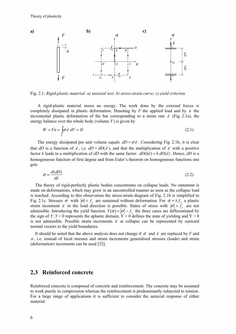
In its basic and simplest form, the theory of plasticity assumes a rigid-perfectly plastic material behaviour. The uniaxial test shown in Fig. 2.1a is examined by considering the stress-strain curve depicted in Fig. 2.1b. The load is increased starting from point O, i.e. from a virgin state. Up to the yield point σ = fy no deformations occur (OA). Once A is reached arbitrary deformations in the load direction are possible without any change in stress; the stress-strain curve extends toward D. At B the bar is unloaded. The stress-strain point moves parallel to OA to point C; the strain ε, i.e. the plastic deformation of the bar, remains constant. Continuing the experiment in the compression direction, a negative deformation occurs as soon as the yield stress σ = – fy is reached (point E ); for the sake of simplicity, the yield stresses in tension and compression are assumed to be of equal magnitude. In the second plastic phase the stress-strain point moves along EFI. Again, the opposite yield stress may be reached by reversing the load direction. For example, starting from G, the curve GHJD is obtained.

Theory of plasticity

6

Fig. 2.1: Rigid-plastic material: a) uniaxial test; b) stress-strain curve; c) yield criterion. A rigid-plastic material stores no energy. The work done by the external forces is completely dissipated in plastic deformation. Denoting by F the applied load and by u& the incremental plastic deformation of the bar corresponding to a strain rate ε& (Fig. 2.1a), the energy balance over the whole body (volume V ) is given by

∫ ===V

DdVuFW εσ && (2.1)

The energy dissipated per unit volume equals εσ &=dD . Considering Fig. 2.1b, it is clear that dD is a function of ε& , i.e. dD = dD(ε& ), and that the multiplication of ε& with a positive factor k leads to a multiplication of dD with the same factor: )()( εε && dDkkdD = . Hence, dD is a homogeneous function of first degree and from Euler’s theorem on homogeneous functions one gets

ε

σ&d

dDd )(= (2.2)

The theory of rigid-perfectly plastic bodies concentrates on collapse loads. No statement is made on deformations, which may grow in an uncontrolled manner as soon as the collapse load is reached. According to this observation the stress-strain diagram of Fig. 2.1b is simplified to Fig. 2.1c. Stresses σ with yf<σ are sustained without deformation. For yf±=σ a plastic strain increment ε& in the load direction is possible. States of stress with yf>σ are not admissible. Introducing the yield function yfY −= σσ )( the three cases are differentiated by the sign of Y: Y < 0 represents the aplastic domain, Y = 0 defines the state of yielding and Y > 0 is not admissible. Possible strain increments ε& at collapse can be represented by outward normal vectors to the yield boundaries. It should be noted that the above analysis does not change if σ and ε& are replaced by F and u& , i.e. instead of local stresses and strain increments generalised stresses (loads) and strain (deformation) increments can be used [32].

2.3 Reinforced concrete

Reinforced concrete is composed of concrete and reinforcement. The concrete may be assumed to work purely in compression whereas the reinforcement is predominantly subjected to tension. For a large range of applications it is sufficient to consider the uniaxial response of either material.

a)

ε

σ b) c)

O

D

FG

σ

O

A B

C

EI

H

J y

ε

F

F

uf

yfyf

yf

Rigid-perfectly plastic behaviour – Reinforced concrete

7

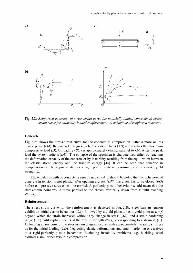
Fig. 2.2: Reinforced concrete: a) stress-strain curve for uniaxially loaded concrete; b) stress-strain curve for uniaxially loaded reinforcement; c) behaviour of reinforced concrete.

Concrete Fig. 2.2a shows the stress-strain curve for the concrete in compression. After a more or less elastic phase (OA), the concrete progressively loses its stiffness (AD) and reaches the maximum compressive load (D). Unloading (BC ) is approximately elastic, parallel to OA. After the peak load the system softens (DE ). The collapse of the specimen is characterised either by reaching the deformation capacity of the concrete or by instability resulting from the equilibrium between the elastic stored energy and the fracture energy [44]. It can be seen that concrete in compression can be approximated as a rigid plastic material, assuming a conservative yield strength fc. The tensile strength of concrete is usually neglected. It should be noted that the behaviour of concrete in tension is not plastic; after opening a crack (OF ) this crack has to be closed (FO) before compressive stresses can be carried. A perfectly plastic behaviour would mean that the stress-strain point would move parallel to the σ-axis, vertically down from F until reaching σ = – fc.

Reinforcement The stress-strain curve for the reinforcement is depicted in Fig. 2.2b. Steel bars in tension exhibit an initial elastic behaviour (OA), followed by a yield plateau, i.e. a yield point at σ = fy beyond which the strain increases without any change in stress (AB), and a strain-hardening range (BE ) until rupture occurs at the tensile strength σ = fu, corresponding to a strain εu (E ). Unloading at any point of the stress-strain diagram occurs with approximately the same stiffness as for the initial loading (CD). Neglecting elastic deformations and strain-hardening one arrives at a rigid-perfectly plastic behaviour. Excluding instability problems, e.g. buckling, steel exhibits a similar behaviour in compression.

a)

F

u

Fy

c

b

a

c)

ε

σ

fc

O F

A

B

C

D

E

ε

σ

fy

fu

O

A B

C

D

E

b)

F

ul

d

b

As

εu

εu

O

A

B

C

D

...

. .

. ..

. .. ..

. ... .

. .. .

. ... . .

. . .. . . . .. .. .. . .. . . . . . . . . . . . . . . .. . .. . . .... ..

12

3

Fcr .....

Theory of plasticity

8

Reinforced concrete The behaviour of reinforced concrete is considered for the example of a simply supported beam subjected to a concentrated load F in the middle of the span l (Fig. 2.2c). The beam has a rectangular cross-section with effective depth d and width b. The reinforcement’s cross-sectional area As is constant over the whole length, and corresponds to a reinforcement ratio ρ = As / (bd ). The load F as well as the associated deflection u are considered as generalised load and deformation, respectively. Alternatively, the bending moment and the rotation at midspan may be chosen as generalised stress and strain, respectively. Under monotonous loading from zero the beam first behaves as a homogeneous, linearly elastic member (OA). At point A the specimen cracks (cracking load F = Fcr). This produces a permanent change in the structure. Moving towards B the beam still behaves approximately elastically, but with a reduced stiffness (cracked behaviour). Upon yielding of the reinforcement (B) the specimen exhibits a behaviour which may be considered as a plastic plateau, F = Fy (BCD). Up to the peak load (C) the hardening of the reinforcing steel compensates the softening of the concrete. At D the concrete reaches its ultimate strain and the beam collapses. The behaviour described above corresponds to the case of a moderately reinforced concrete beam (ρ ≈ 0.5%). Increasing the reinforcement ratio ρ the ultimate load increases, but the ductility of the beam decreases. Curve a depicts the load-deformation curve corresponding to balanced failure; yielding of the reinforcement occurs together with rupture of the concrete. In this curve the phase BCD disappears. Conversely, reducing the reinforcement ratio, the ductility increases and the ultimate load decreases. Curve b depicts the situation for a beam containing minimum reinforcement (ρ ≈ 0.15%); the loads at cracking and yielding (points A and B) coincide and BCD reflects the reinforcement behaviour. Any further reduction of the reinforcement ratio would lead to a brittle failure as soon as the cracking load would be reached (curve c). The following derives from the above considerations: • The behaviour of reinforced concrete can be characterised by an elastic uncracked (line 1), an

elastic cracked (line 2) and a plastic range (line 3). • The plastic behaviour of reinforced concrete is strongly influenced by the reinforcement

ratio. A ductile failure results for low and moderate reinforcement ratios for which the concrete crushes while the steel is yielding.

• The deformation capacity of reinforced concrete elements depends on the ductility of the reinforcement (for low and moderate reinforcement ratios) as well as on the ultimate concrete strain (for high reinforcement ratios); whereas the latter can be improved by detailing measures (e.g. by confinement) sufficient ductility properties of the reinforcement are of utmost importance for the soundness of concrete structures.

2.4 Yield condition and flow rule

The plasticity considerations described above are generalised in the following to an n-dimensional problem. Generalised stresses σ1, σ2,…, σn and associated generalised strain increments 1ε& , 2ε& ,…, nε& of a structure are considered [32]. The values of iε& are zero while the system remains rigid. Finite values of iε& correspond to an arbitrary collapse state.

Reinforced concrete – Yield condition and flow rule

9

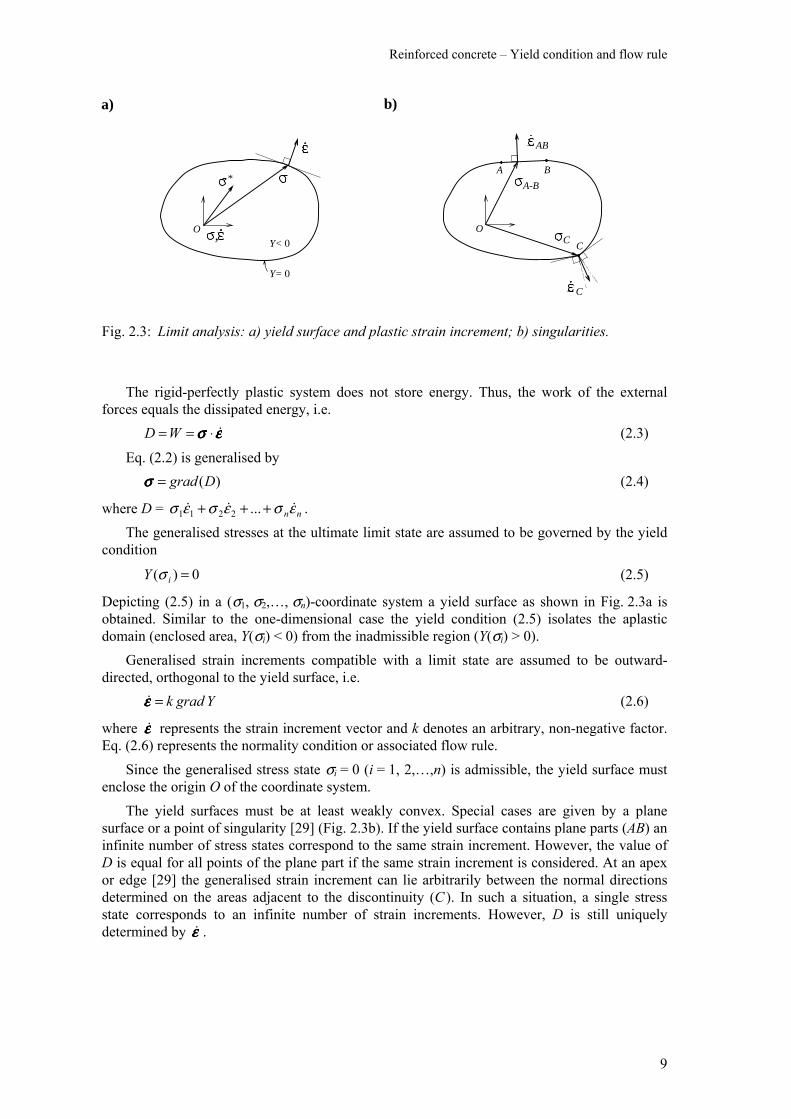
Fig. 2.3: Limit analysis: a) yield surface and plastic strain increment; b) singularities.

The rigid-perfectly plastic system does not store energy. Thus, the work of the external forces equals the dissipated energy, i.e. εεεεσσσσ &⋅== WD (2.3)

Eq. (2.2) is generalised by )(Dgrad=σσσσ (2.4)

where D = nnεσεσεσ &&& +++ ...2211 . The generalised stresses at the ultimate limit state are assumed to be governed by the yield condition

0)( =iY σ (2.5)

Depicting (2.5) in a (σ1, σ2,…, σn)-coordinate system a yield surface as shown in Fig. 2.3a is obtained. Similar to the one-dimensional case the yield condition (2.5) isolates the aplastic domain (enclosed area, Y(σi) < 0) from the inadmissible region (Y(σi) > 0). Generalised strain increments compatible with a limit state are assumed to be outward-directed, orthogonal to the yield surface, i.e. Ygradk=εεεε& (2.6)

where εεεε& represents the strain increment vector and k denotes an arbitrary, non-negative factor. Eq. (2.6) represents the normality condition or associated flow rule. Since the generalised stress state σi = 0 (i = 1, 2,…,n) is admissible, the yield surface must enclose the origin O of the coordinate system. The yield surfaces must be at least weakly convex. Special cases are given by a plane surface or a point of singularity [29] (Fig. 2.3b). If the yield surface contains plane parts (AB) an infinite number of stress states correspond to the same strain increment. However, the value of D is equal for all points of the plane part if the same strain increment is considered. At an apex or edge [29] the generalised strain increment can lie arbitrarily between the normal directions determined on the areas adjacent to the discontinuity (C ). In such a situation, a single stress state corresponds to an infinite number of strain increments. However, D is still uniquely determined by εεεε& .

a) b)

O

*

Y<

Y=

O

A B

C0

0

AB

C

C

A-B

,

Theory of plasticity

10

2.5 Theorems of limit analysis

The theorems of limits analysis result from the application of the principle of virtual work to a rigid-perfectly plastic system, whose behaviour is summarised by the principle of maximum energy dissipation.

The theorems of limit analysis are credited to Gvozdev [13], Hill [17], Drucker, Greenberg and Prager [6, 7] and Sayir and Ziegler [60].

Principle of virtual work In an arbitrary mechanical system, the total work of the internal and external forces (including any internal and external reactions as well as inertial forces) disappears for any admissible virtual motion. For static systems one gets εεεεσσσσ && ⋅=⋅uF (2.7)

where F and σσσσ denote an equilibrium set of external and internal forces (generalised loads and stresses), respectively, and u& and εεεε& denote an arbitrary associated compatibility set of external and internal displacement increments (generalised deformation and strain increments), respectively.

Principle of maximum energy dissipation The stresses corresponding to given strain increments assume such values that the dissipation becomes a maximum [65], i.e.

0)( ≥⋅− εεεεσσσσσσσσ &* (2.8)

where σσσσ is the actual generalised stress state at the yield surface corresponding to εεεε& and σσσσ* is any generalised stress at or within the yield surface (Fig. 2.3a). Eq. (2.8) is trivially verified with the help of Fig. 2.3a, where the associated flow rule is assumed to be valid. Alternatively, the principle of maximum energy dissipation may be postulated and the associated flow rule follows from it [32].

Theorems of limit analysis Excluding instability problems and combining the principle of virtual work with the principle of maximum energy dissipation the following theorems are obtained: Lower-bound theorem: any load Fs corresponding to a statically admissible state of stress everywhere at or below yield is not higher than the ultimate load Fu. Upper-bound theorem: any load Fk resulting from considering a kinematically admissible state of deformation, setting the work done by the external forces equal to the internal energy dissipation, is not lower than the ultimate load Fu. Compatibility theorem: any load for which a complete solution, i.e. a statically admissible state of stress everywhere at or below yield and a compatible, kinematically admissible state of deformation can be found, is equal to the ultimate load. A state of stress is statically admissible if it fulfils the equilibrium and static boundary conditions. A state of deformation is kinematically admissible if it fulfils the kinematic relations and boundary conditions. A state of stress and a state of deformation are compatible if they are related via the associated flow rule (2.6). In a complete solution, the states of stress and deformation only have to be compatible in the sense stated above.

Theorem of limit analysis – Limit analysis and design methods

11

2.6 Limit analysis and design methods

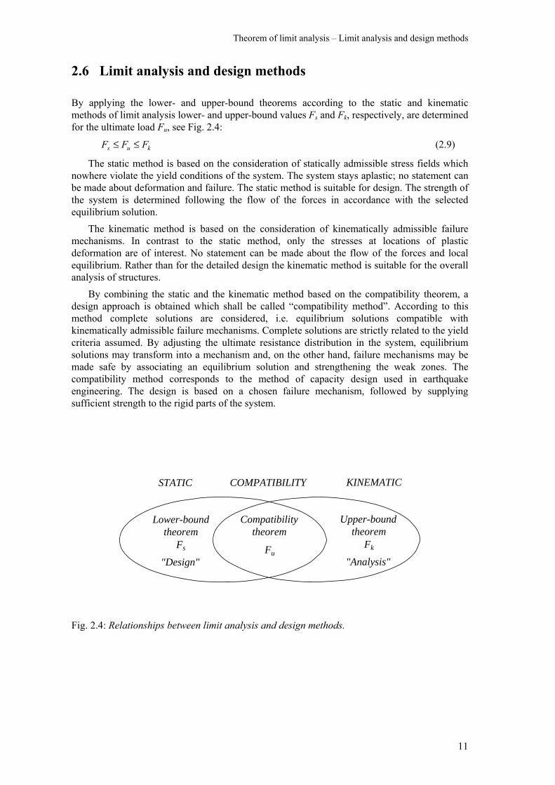
By applying the lower- and upper-bound theorems according to the static and kinematic methods of limit analysis lower- and upper-bound values Fs and Fk, respectively, are determined for the ultimate load Fu, see Fig. 2.4:

kus FFF ≤≤ (2.9)

The static method is based on the consideration of statically admissible stress fields which nowhere violate the yield conditions of the system. The system stays aplastic; no statement can be made about deformation and failure. The static method is suitable for design. The strength of the system is determined following the flow of the forces in accordance with the selected equilibrium solution. The kinematic method is based on the consideration of kinematically admissible failure mechanisms. In contrast to the static method, only the stresses at locations of plastic deformation are of interest. No statement can be made about the flow of the forces and local equilibrium. Rather than for the detailed design the kinematic method is suitable for the overall analysis of structures. By combining the static and the kinematic method based on the compatibility theorem, a design approach is obtained which shall be called “compatibility method”. According to this method complete solutions are considered, i.e. equilibrium solutions compatible with kinematically admissible failure mechanisms. Complete solutions are strictly related to the yield criteria assumed. By adjusting the ultimate resistance distribution in the system, equilibrium solutions may transform into a mechanism and, on the other hand, failure mechanisms may be made safe by associating an equilibrium solution and strengthening the weak zones. The compatibility method corresponds to the method of capacity design used in earthquake engineering. The design is based on a chosen failure mechanism, followed by supplying sufficient strength to the rigid parts of the system.

Fig. 2.4: Relationships between limit analysis and design methods.

Compatibilitytheorem

Lower-boundtheorem

Upper-boundtheorem

Fs

STATIC KINEMATIC COMPATIBILITY

FuFk

"Design" "Analysis"

12

13

3 Static method

3.1 General

The lower-bound method for reinforced concrete beams [34] is based on truss models (strut and tie models) or – in a continuum form – on stress fields. Dimensioning and detailing are performed following the flow of the shear forces, considering truss models or associated stress fields which describe the beam’s structural behaviour.

Reinforced concrete slabs are designed on the basis of an elastic analysis, the strip method or, where available, a limit analysis solution. Each of these methods corresponds to a particular application of the equilibrium conditions. The elastic analysis relates the stresses to the strains and deflections by means of Hooke’s law and Kirchhoff’s hypothesis; the equilibrium and the boundary conditions evolve into a differential problem focused on the deflection function. In its common form, the strip method reduces the slab to an orthogonal set of beams; this corresponds to neglecting twisting moments in the equilibrium conditions. In limit analysis solutions the equilibrium conditions are combined with the failure conditions according to a fixed reinforcement distribution, i.e. the corresponding yield criteria and the associated flow rule (Chapter 4); the known solutions are restricted to a few simple cases.

Basically, beams are special cases of slabs. However, when comparing the design methods for beams and slabs, no direct link is recognised. The analyses concentrate on two different tasks: the load transfer for beams, and the consequences of the load transfer, i.e. the moments, for slabs. The lower-bound procedure for beams is more flexible and precise. Slab design methods are an application of equilibrium considerations, but they do not match beam design methods in their depth of modelling the structural behaviour.

The goal of the static or lower-bound method presented in the following is to provide the foundation for a consistent design of reinforced concrete slabs analogous to that of beams. The analysis focuses on the load transfer, whereby two types of loads are distinguished – distributed and concentrated. Distributed load transfer is governed by the generalised strip method, i.e. a continuous truss model within and at the top and bottom surfaces of the slab, defined by the principal shear and by the principal moment trajectories, respectively. Concentrated load transfer corresponds to statical discontinuity lines. Finally, the stress field approach for beams is extended to slabs, i.e. stress fields according to the generalised strip method and discontinuity lines are put together like pieces of a puzzle to allow for the load transfer from the interior of a slab to its supports.

3.2 Internal forces

The static analysis of slabs is performed with generalised stresses, i.e. stress resultants on vertical strips of unit width. The definition of internal forces in arbitrary sections (Chapter 3.2.1) is followed by the associated stress field definition (Chapter 3.2.2).

Static method

14

3.2.1 Definition of internal forces

A slab is a thin structural member bounded by two parallel planes, loaded perpendicularly to the planes. The right-handed Cartesian coordinate system O(x,y,z), O being an arbitrary point on the middle surface and z being vertical downwards, is introduced as the global system of reference.

The plane vector n in P, Fig. 3.1a, defines a vertical strip section, where the direction n is normal and outwards to the strip considered. This direction and the directions t and z constitute the local coordinate system P(n,t,z). At any point of the strip, e.g. at z = z0 according to Fig. 3.1a, a normal stress σn and shear stresses τtn and τzn are acting. These stresses are positive in the (positive) n-, t- and z-directions, respectively.

The internal forces and moments are obtained by integrating the stresses over the vertical strip for a unit length in the t-direction and for – h / 2 < z < h / 2, h being the slab thickness. They are composed of the membrane forces, i.e. the axial force nn and the in-plane shear force ntn (neglected in the following, see Chapter 1.3)

∫−

=2/

2/

h

hnn dzn σ ; ∫

−

=2/

2/

h

htntn dzn τ [kN / m] (3.1)

the shear force

∫−

=2/

2/

h

hznn dzv τ [kN / m] (3.2)

and the bending and twisting moments

∫−

=2/

2/

h

hnn dzzm σ ; ∫

−

=2/

2/

h

htntn dzzm τ [kN] (3.3)

The internal forces and moments are indexed as the stress components: the first index represents the direction of the stress and the second represents the section (normal vector) considered. For coincidental stress and section directions only one index is used. Fig. 3.1b represents the positive generalised stresses in P.

3.2.2 Stress field definition

Introducing generalised stresses, the stress state of the slab is defined by a plane shear vector and a 2x2 moment tensor. Two different sections n1 and n2 in P with internal forces vn1, mn1, mtn1 and vn2, mn2, mtn2 are considered. An arbitrary section n3 may be resolved into the sections n1 and n2. Starting from a unit strip length n3, the internal forces in this direction result from the sum of the forces on the projected strips in the directions n1 and n2 (Fig. 3.1c). The shear force vn3 is determined by

)cos(

)cos(cos

)cos(

120

1302

0

13013 ϕϕ

ϕϕϕ

ϕϕ−

−=−= nnn

vvv (3.4)

where

12

121

20 sin

1)cos(tanϕ

ϕϕ −=n

n

vv (3.5)

The moments mn3 and mtn3 are given by

1311313 2sin2cos)( ϕϕ tncncn mmmmm +−+=

1311313 2cos2sin)( ϕϕ tncntn mmmm +−−= (3.6)

Internal forces

15

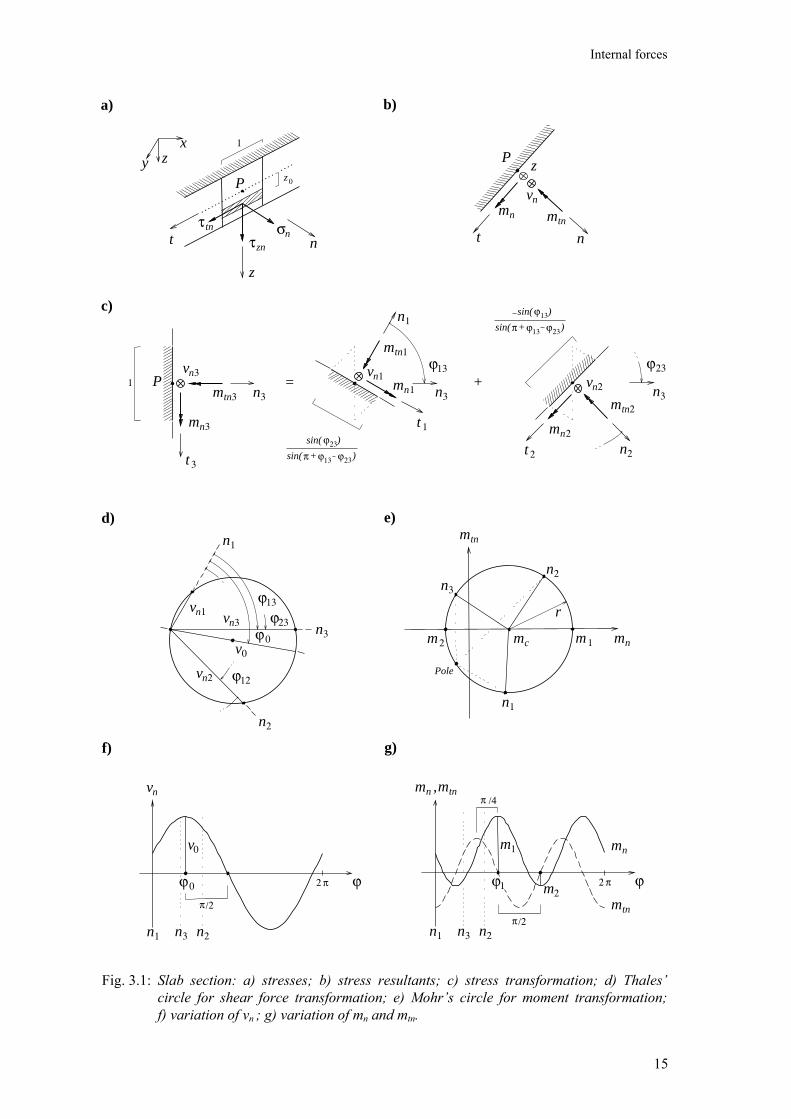
Fig. 3.1: Slab section: a) stresses; b) stress resultants; c) stress transformation; d) Thales’ circle for shear force transformation; e) Mohr’s circle for moment transformation; f) variation of vn ; g) variation of mn and mtn.

a) b)

σt

z

n

τ

z

v

τ

mm

1

P. . .

. . .. . .

. . .. . .

.

. . .. . .

. . ..

tn

znn

z0

zx

y P

nttn

n

n

c)

v

m

mP

n

t

n

n3

3

3

31

vm

m

n

t

nn1

1

1

1

v

m

mnt

tn

n

n2

2

2

2 2

n3 n3

ϕ13

.

ϕ23

.

= +

sin( )ϕ23

sin( + )ϕ13π ϕ23

sin( )ϕ13

sin( + )ϕ13π ϕ23

d) e)

..

..

vn1

v0

vn2

vn3

ϕ13

ϕ0

ϕ12

ϕ23

1

2

mn

mtn

1

2

mc

Pole

m1m2

r

ϕπ/2

ϕ0

v0

vn

31

ϕ

π/2

ϕ1

m1

m ,n

31

mtn

f) g)

π2

m n

mtn

m2

π /4

n3

n

n

n

n

n3

n 2n n n 2nn

π2

tn3

tn1

Static method

16

where

−−++=

12

22

21

2121

nn

tntnnnc mm

mmmmm (3.7)

and ϕij indicates the clockwise angle between the directions i and j. For the case ϕ12 = π / 2, i.e. orthogonal n1 and n2, Eqs. (3.4) to (3.7) reduce to

1321313 sincos ϕϕ nnn vvv += (3.8)

131132

2132

13 2sinsincos ϕϕϕ tnnnn mmmm ++=

1311313123 2coscossin)( ϕϕϕ tnnntn mmmm +−= (3.9)

Figs. 3.1d and 3.1e represent (3.4) and (3.6) graphically. When denoting by vn one side length of a right angled triangle, Eq. (3.4) indicates that different shear forces correspond to the same base, i.e. the Thales’ circle diameter. This extreme shear is called the principal shear v0, while its direction ϕ0 is the principal shear direction [33]. Orthogonal to ϕ0, the circle tangent determines v0 = 0. Eq. (3.6) is the parametric equation of a circle in the (mn,mtn)-space with the angle ϕ13 (or 2ϕ13) as parameter. The circle is centred at C(mc,0) and has the radius

2/121

21 ))(( tncn mmmr +−= . The moments in the direction n3 are obtained by clockwise rotation

of the radius in (mn1,mtn1) by the angle 2ϕ13. This graphical method is attributed to Mohr [39]. The extreme values of the bending moment, i.e. the principal moments, result for mnt = 0 and are given by m1 = mc + r and m2 = mc – r. The corresponding directions, i.e. the principal directions, are indicated by ϕ1 and ϕ2 ( = ϕ1 + π / 2), respectively. The twisting moment has a maximum in the directions ϕ1 + π / 4 and ϕ1 + 3π / 4; mtn reaches the values r± and is accompanied by the bending moment mn = mc. Figures 1f and 1g show the variation of the internal forces for πϕ 20 13 ≤≤ . The variation of vn is harmonic with amplitude v0 in the direction ϕ0 and with period 2π, see Fig. 3.1f. The variation of mn is harmonic between m1 in the direction ϕ1 and m2 in the direction ϕ1 + π / 2 with a period of π. Finally, the variation of mtn has an amplitude (m1 + m2) / 2 and follows the mn-curve with a phase difference of π / 4, see Fig.3.1g. Any stress field is defined by five quantities. By selecting the principal sections, these are distinguished by the statical values v0, m1, m2, and the geometrical values ϕ0, ϕ1.

3.3 Equilibrium

The equilibrium conditions result from the comparison of the internal forces at two neighbouring points, considering the effect of external loads, Chapter 3.3.3. Therefore, the internal forces have to be defined with respect to a fixed system of reference, Chapter 3.3.2. This is chosen in a general form using orthogonal curvilinear trajectories, Chapter 3.3.1.

3.3.1 Orthogonal curvilinear coordinates

A point P of a slab is defined in Cartesian coordinates by the intersection of the lines x = xP and y = yP. These lines also define the y- and x-axes in P, which are positive in the increasing yP- and xP-direction. Similarly, a slab point in curvilinear coordinates is defined by the intersection of the curves u = uP and v = vP, where u and v are functions of x and y:

Internal forces – Equilibrium

17

),(;),( yxvvyxuu == (3.10)

The curvilinear axes u and v in P are the curves v(x,y) = vP = const, and u(x,y) = uP = const, positive in the increasing vP- and uP-direction, respectively. The orthogonality requirement for the curvilinear coordinates is given by 0=∇⋅∇ vu (3.11)

where )/,/( yx ∂∂∂∂≡∇ . The u- and v-axis directions in P are specified introducing the unit vectors n and t tangential to the u- and v-coordinates; P(n,t,z) constitutes a right-handed rectangular coordinate system. With respect to O(x,y,z), the orientation of P(n,t,z) is indicated by the clockwise angle φ between x and n. In contrast to the Cartesian axes, curvilinear axes do not express a fixed length and a fixed direction. A change du (dv) corresponds to an arc element length measured along the coordinate line u (v) of duAdS uu = ( dvAdS vv = ) with

22

2

∂∂+

∂∂=

uy

uxAu (

222

∂∂+

∂∂=

vy

vxAv ) (3.12)

Starting from the angle φ, given by

vA

yuA

x

vu ∂∂=

∂∂=φcos ;

vAx

uAy

vu ∂∂−=

∂∂=φsin (3.13)

a change du (dv) results in an n-direction variation of

duvA

Adv

u

∂∂−=φ ( dv

uAAdu

v

∂∂=φ ) (3.14)

Combining (3.12) with (3.14) one obtains the radii of curvature of the curvilinear axes u and v

vAA

AuA vu

u

uu ∂∂=

∂∂−= φ

ρ1 ;

uAAA

vA vu

v

vv ∂∂=

∂∂= φ

ρ1 (3.15)

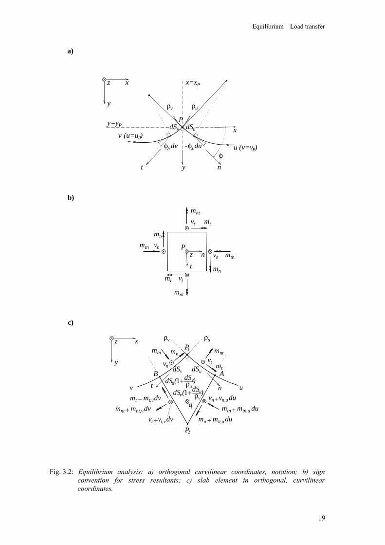
The notation introduced is summarised in Fig. 3.2a.

3.3.2 Sign convention

Previously, the internal forces and moments have been related to a local coordinate system of the cross-section considered and the stress field at a point has been established from the stress resultants on two different cross-sections. Equilibrium considerations require the definition of internal forces corresponding to a fixed system of reference. Referring to the system (n,t,z) in P, the sign convention assumed is defined in Fig. 3.2b. Shear forces are positive if related to positive shear stresses in the z-direction and the moments are positive if related to positive (negative) stresses in the slab portion z > 0 (z < 0). On the sections with negative n- and t-directions, internal forces are in equilibrium with those in the positive one. Note that the symmetry of the stress tensor (i.e. rotational equilibrium) leads to mtn = mnt.

3.3.3 Equilibrium conditions

In a curvilinear coordinate system (3.10) the stress field at the point P1(uP1,vP1) is compared with that at the neighbouring point P2(uP1 + du, vP1 + dv). The shear forces vn and vt, the bending moments mn and mt, and the twisting moments mtn and mnt act on the n- and t-sections in P1.

Static method

18

Moving an increment dSu along the u-axis, the n-direction rotates by (3.141) and the internal forces and moments are

duvv unn ,+ ; dumm unn ,+ ; dumm utntn ,+ (3.16)

Similarly, moving an increment dSv along the v-axis, the t-direction rotates by (3.142) and the internal forces and moments are

dvvv vtt ,+ ; dvmm vtt ,+ ; dvmm vntnt ,+ (3.17)

A comma preceding an index indicates partial derivation with respect to the coordinate given as index. The relations (3.16) and (3.17) define the stress field in P2. With reference to Fig. 3.2c the slab element P1AP2B is considered. Assuming that the stress in P1 and P2 does not change on the sides P1A, P1B and P2A, P2B, the following equilibrium conditions can be formulated:

0,, =++++ qvvvvv

ntSvtSun

uρρ

ntnv

tnntu

SvntSun vmmmmmm =−++++ )(1)(1,, ρρ

(3.18)

tnttnv

ntu

SvtSutn vmmmmmm =++−++ )(1)(1,, ρρ

Eqs. (3.18) are the equilibrium conditions in curvilinear coordinates. The three equations may be combined by inserting (3.182) and (3.183) into (3.181). In Cartesian and in polar coordinates, the equilibrium conditions result as special cases of (3.18) when considering u = x, v = y , 1 / ρu = 1 / ρv = 0, and u2 = r2 = x2

+ y2, v = ϕ = tan–1( y / x ), 1 / ρu = 0, ρv = r , respectively.

3.4 Load transfer

Shear in slabs may arise in distributed [33] or concentrated form [4]. These two load transfer modes are at the centre of the following analysis. In both cases, the requirements for the load transfer are derived by considering the internal flow of forces in an infinitesimal region.

3.4.1 Distributed load transfer

As stated in Chapter 3.2.2, the shear forces vn and vt correspond to the principal shear force 5.022

0 )( tn vvv += being transferred in the direction )/(tan 10 nt vv−=ϕ to the n-axis, see Fig. 3.1d.

Denoting the principal shear trajectory by us, it can be seen that along the length SudS a moment

increment

sudSvm 0=∆ (3.19)

is required for equilibrium (Fig. 3.3a). As in a beam, moments are subordinated to the shear. Eq. (3.182) in the us-vs-system of reference states that the moment change results from the incremental values

sunm , and svntm , or from the trajectory geometry

Sutnnt mm ρ/)( + and Svtn mm ρ/)( − , see Chapter 3.6.

Equilibrium – Load transfer

19

Fig. 3.2: Equilibrium analysis: a) orthogonal curvilinear coordinates, notation; b) sign convention for stress resultants; c) slab element in orthogonal, curvilinear coordinates.

v nt

q

u

x

nt

v (u=u )

uρvρ

P

φφ,u

.

Pn

t

z v mtnn

mn

v

mnt

tmt

vmtn n

mn

v

mnt

t mt

a)

b)

c)

. .

x

y

z uρvρ

v

mtn

n

mn mn,u du+

vn,u du+mtn,u du+

v

mtn

n

mn

vmnt

tmt

mnt mnt,vdv+vt vt,vdv+

mt mt,vdv+

y

z

dSv dSu

1dS ( )vdSu

vρ+

1dS ( )udSv

uρ+

dSudSv

duφ,vdvP

u (v=v )P

x

y

x=x P

y=y P

P1

P2

AB

Static method

20

3.4.2 Concentrated load transfer

Assuming a concentrated shear force V being transferred within a narrow zone S of width ts between the slab regions A and B, Fig. 3.3b depicts a part of the shear trajectory as a free body diagram. The internal forces (3.2) and (3.3) act between the shear strip and the adjacent slab segments, A and B. Within the strip, the shear force V is accompanied by a concentrated bending moment M and a strip-specific line load q . Equilibrium requires that

0, =++− qvvV Bn

Ant (3.20)

VmmM Btn

Atnt =+−, (3.21)

Mmm SBn

An =− ρ)( (3.22)

Equation (3.21) allows for both shear line action and strong band action. A shear line results in the case ts = 0, thus M = 0; concentrated shear forces are transferred thanks to a jump in the twisting moments; some vertical reinforcement is required to provide the shear resistance. A strong band results if B

tnAtn mm = . The strip ts has to be extra reinforced to resist the moment M.

Both load transfer modes may be exploited to transfer the shear forces from a slab segment A to an adjacent segment B. Setting V, q , M and ts equal to zero, the equations (3.20) to (3.22) reduce to the continuity requirements for the stress fields in the slab segments A and B. The concentrated shear transfer equations define in a general form the statical discontinuity in slabs: adjacent stress fields have to provide continuity in the load transfer and in the moments.

3.4.3 Remarks

Distributed load transfer is inherently included in the equilibrium considerations of slabs. In comparison to (3.18), Eq. (3.19) shows the essential structural behaviour; it plays a central role in the development of continuous stress fields (Chapter 3.6.1). Concentrated load transfer along lines of statical discontinuity represents a fundamental tool of plastic analysis (Chapter 3.6.7). In the past, stress fields for slabs were first developed based on the theory of elasticity [28]. Since elastic solutions correspond to a distributed load transfer (Chapter 3.6.2) discontinuities occur only at slab boundaries (Chapter 3.5). Plastic solutions are based on both load transfer modes, i.e. lines of discontinuity may also arise within the slab. Johansen [21] first postulated the existence of internal shear zones. Hillerborg [18] mentioned that discontinuity in the twisting moments generates a shear flow, but he considered only load transfer in strong bands. The research on nodal forces in the 1960’s (Chapter 5.3.2) recognised the importance of shear zones without further developing them. Clyde [4] suggested that nodal forces are real forces, identifying them as concentrated shear forces. Stress fields which included statical discontinuities were developed by Rozvany [56], Morley [42, 43], Clyde [5], Fox [9, 10] and Marti [36]. Recently, Meyboom and Marti [38] completed an analytical study with an experimental verification of the static discontinuity behaviour.

3.5 Boundary conditions

Slab boundaries are statical discontinuities of the stress field. The statical requirements at slab edges are an expression of a concentrated load transfer. S is a narrow boundary strip and the forces with upper index B correspond to the reactions.

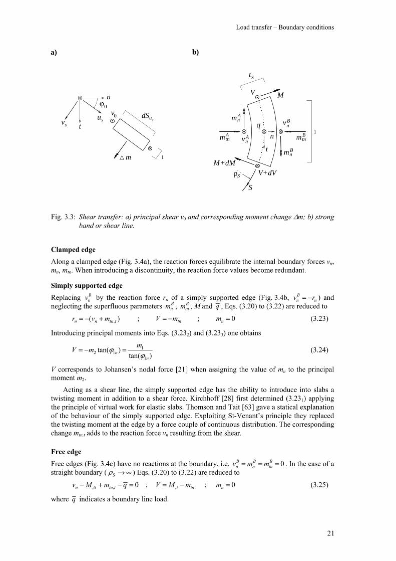
Load transfer – Boundary conditions

21

Fig. 3.3: Shear transfer: a) principal shear v0 and corresponding moment change ∆m; b) strong

band or shear line.

Clamped edge Along a clamped edge (Fig. 3.4a), the reaction forces equilibrate the internal boundary forces vn, mn, mtn. When introducing a discontinuity, the reaction force values become redundant.

Simply supported edge Replacing B

nv by the reaction force rn of a simply supported edge (Fig. 3.4b, nBn rv −= ) and

neglecting the superfluous parameters Bnm , B

tnm , M and q , Eqs. (3.20) to (3.22) are reduced to

)( ,ttnnn mvr +−= ; tnmV −= ; 0=nm (3.23)

Introducing principal moments into Eqs. (3.232) and (3.233) one obtains

)tan(

)tan(1

112

nn

mmVϕ

ϕ =−= (3.24)

V corresponds to Johansen’s nodal force [21] when assigning the value of mu to the principal moment m2. Acting as a shear line, the simply supported edge has the ability to introduce into slabs a twisting moment in addition to a shear force. Kirchhoff [28] first determined (3.231) applying the principle of virtual work for elastic slabs. Thomson and Tait [63] gave a statical explanation of the behaviour of the simply supported edge. Exploiting St-Venant’s principle they replaced the twisting moment at the edge by a force couple of continuous distribution. The corresponding change mtn,t adds to the reaction force vn resulting from the shear.

Free edge Free edges (Fig. 3.4c) have no reactions at the boundary, i.e. 0=== B

tnBn

Bn mmv . In the case of a

straight boundary ( ∞→Sρ ) Eqs. (3.20) to (3.22) are reduced to

0,, =−+− qmMv ttnttn ; tnt mMV −= , ; 0=nm (3.25)

where q indicates a boundary line load.

S

mtnA

mnA

q vnB

mnB

mtnBn

V

M+

vnA

t

dMV+dV

M

t

1

m

vus

ϕ0

1

S

0 dSu

n

ts

a) b)

Sρ

vs

Static method

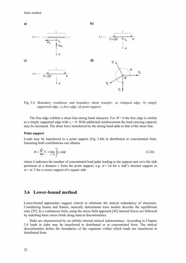
22

Fig. 3.4: Boundary conditions and boundary shear transfer: a) clamped edge; b) simply supported edge; c) free edge; d) point support.

The free edge exhibits a shear line-strong band character. For M = 0 the free edge is similar to a simply supported edge with rn = 0. With additional reinforcement the load carrying capacity may be increased. The shear force transferred by the strong band adds to that of the shear line.

Point support Loads may be transferred to a point support (Fig. 3.4d) in distributed or concentrated form. Summing both contributions one obtains

∫∑ →+=

α

ϕ0

0lim rdvVR rr

k

ii (3.26)

where k indicates the number of concentrated load paths leading to the support and rα is the slab perimeter at a distance r from the point support, e.g. α = 2π for a slab’s internal support or α = π / 2 for a corner support of a square slab.

3.6 Lower-bound method

Lower-bound approaches suggest criteria to eliminate the statical redundancy of structures. Considering beams and frames, statically determinate truss models describe the equilibrium state [55]. In a continuous form, using the stress field approach [45] internal forces are followed by matching basic stress fields along statical discontinuities. Slabs are characterised by an infinite internal statical indeterminacy. According to Chapter 3.4 loads in slabs may be transferred in distributed or in concentrated form. The statical discontinuities define the boundaries of the segments within which loads are transferred in distributed form.

n

1

r

n

t

n

mtn

mn

R

α

V1

V2

Vi

Vk

VV+dV

a) b)

c) d)

1

rt

n

n

VV+dV

1

t

Boundary conditions – Lower-bound method

23

Starting by considering the distributed load transfer, a statically determinate continuous truss model adequate for slab analysis is defined with the principal shear force and the principal moment trajectories. The shear field is determined with vertical equilibrium in the principal shear force direction. Similarly, the moment field is obtained by formulating equilibrium in the principal moment directions. Including curvilinear principal moment trajectories, the procedure becomes an extension of Hillerborg’s strip method [18], in which the principal moment sections are limited to Cartesian coordinates, hence the designation generalised strip method. On the basis of the new method, the lower-bound analysis of slabs is reviewed in Chapters 3.6.2 to 3.6.6, distinguishing an elastic approach, Hillerborg’s method and the Hencky-Prandtl solutions. Finally, the analysis of curvilinear trajectories on conical sections, together with the superposition principle, leads to known limit analysis solutions. Similar to the stress field approach for beams, a stress field approach for slabs is developed fitting the continuous stress fields into the slab with connections along lines of discontinuity.

3.6.1 Generalised strip method

The generalised strip method results from a direct application of the distributed load transfer requirements, cf. Chapter 3.4.1. Establishing equilibrium with respect to chosen principal shear and moment trajectories, loads are firstly integrated to shear forces and secondly to moments.

Shear field In the orthogonal curvilinear coordinate system us, vs, with us corresponding to the principal shear trajectory, Eq. (3.181) is reduced to

00,0 =++ qvv

s

sv

Su ρ (3.27)

Assuming a certain shear flow, i.e. the geometry of the shear field, Eq. (3.27) can be integrated. The boundary conditions of the shear problem require one value of v0 along each trajectory us. Note that arbitrary load distributions are included in the analysis by considering q as a function q(us,vs). Concentrated loads correspond to the homogeneous problem q = 0.

Moment field Introducing the principal moments m1 and m2 with their trajectories um and vm, Eqs. (3.182) and (3.183) are reduced to

m

m

mm

m

m tu

Svnv

Su vmmmvmmm =−+=−+ )(1;)(112,221,1 ρρ

(3.28)

The shear force components mnv and

mtv of the shear field in the directions um and vm, respectively, are determined according to Eq. (3.8). Eqs. (3.28) generally involve a complex analysis and do not always lead to an explicit solution; additionally, agreement with the slab’s boundary conditions is not always possible.

3.6.2 Elasticity

Most engineers design slabs according to elastic solutions. Basically, elastic solutions are not simple to apply. However, a quick procedure results from the use of FE-software. In the following, the generalised strip method is exploited to extend the elastic analysis of beams to slabs. Elasticity theory is based on Hooke’s law: “ut tension sic vis” (the extension is proportional to the force): Eσε = , where E is the modulus of elasticity of the material. During bending,

Static method

24

vertical cross-sections remain plane, so that they undergo only a rotation with respect to the neutral axis (Bernoulli’s hypothesis); zχε = . The elongation of each fibre is proportional to the distance z from the neutral axis. The proportionality constant is the curvature χ of the deflection curve w. For small deflections in comparison to the span of the beam one gets χ = uuw,− , u being the bending direction. The bending moment results by integrating the normal stresses acting on a cross-section, i.e. uuEIwM ,−= where EI is the flexural rigidity of the beam. By introducing considerations of equilibrium – uMV ,= and uVq ,−= – elastic beams are described by the equation )/(, EIqw uuuu = . In a two-dimensional continuum the elastic stress-strain relation is given by ε1 = (σ1 – νσ2) / E and ε2 = (σ2 – νσ1) / E, where ν denotes Poisson’s ratio. For a slab, assuming Bernoulli’s hypothesis along the principal curvature trajectories u and v of the deflection function w, the principal curvatures are given by uuw,1 −=χ and vvw,2 −=χ . Principal moments result by integrating the stresses in unit vertical strips in u- and v-direction: uuDwm ,1 −= and

vvDwm ,2 −= , respectively, D = Eh3 / [12 (1 – ν2)] being the flexural rigidity of the slab.

Introducing m1 and m2 into (3.28) and substituting the resulting shear components in Eq. (3.181), the elastic slab analysis simplifies to Dqw /=∆∆ . Summarising, the generalised strip method extends the elastic analysis of beams to slabs by considering the principal curvature trajectories of the deflection function w as elastic beams. Within the whole slab loads are transferred in distributed form since the basic principal trajectories extend over the whole slab to the supports.

3.6.3 Strip method

Hillerborg’s method is based on the Cartesian system defined by the coordinates x and y. The analysis starts by dividing the load into single portions referred to the coordinate directions

),(),(),( yxqyxqyxq yx += (3.29)

The shear field is defined by the components vx and vy. These result by integrating the respective load portion as in a beam, i.e.

)(),( yCdxyxqv sxxx +−= ∫ ; )(),( xCdyyxqv syyy +−= ∫ (3.30)

Eqs. (3.30) are additionally integrated to give the moment functions

)()(),(2

yCyCxdxyxqm mxsxxx ++−= ∫ ∫

)()(),(2

xCxCydyyxqm mysyyy ++−= ∫ ∫ (3.31)

Hillerborg’s method reduces the slab to two sets of beams at right angles to each other. Each coordinate line (x = xP or y = yP) defines a beam. According to (3.30) and (3.31), on each beam a shear integration constant, Cxs(yP) or Cys(xP), and a moment integration constant, Cxm(yP) or Cym(xP), are available to fulfil the boundary conditions. Concerning the shear field analysis, the load split (3.29) proposed by Hillerborg is equivalent to the selection of the principal shear trajectories adopted in the generalised strip method. Despite some analytical difficulties in the solution of (3.27) compared to (3.30), the shear field analysis of the generalised strip method has the advantage of a deliberate choice of the load path throughout the slab. In addition, the principal shear force allows a better control against shear failure than the shear components. The main difference between Hillerborg’s method and the generalised strip method concerns the moment field analysis. In Hillerborg’s method principal moment trajectories are fixed in the Cartesian directions. By contrast, the generalised strip method allows a free choice. With straight principal moment directions, the geometrical load-carrying capacity resulting from curved principal sections (i.e. (m1 – m2) / ρv,

Lower-bound method

25

(m2 – m1) / ρu, cf. Eqs. (3.28)) disappears. Such geometrical contributions fill the gap between the lower-bound solutions of the strip method and the complete solutions of slab limit analysis.

3.6.4 Hencky-Prandtl solutions

In contrast to the strip method, where the geometrical load transfer contribution is neglected (1 / ρx = 1 / ρy = 0), the following analysis involves a load transfer with constant principal moments

.1 constmmu == ; .2 constmmv == (3.32)

In an unknown net of principal moment trajectories Eqs. (3.28) are given by

mm vn mv ρ/∆= ;

mm ut mv ρ/∆−= (3.33)

where 21 mmm −=∆ . In the same system of reference, Eq. (3.181) together with (3.14) and (3.15) result in the equilibrium condition

02 , =+∆ qmmmSvSuφ (3.34)

where the function φ (um,vm) defines the moment net (Chapter 3.3.1), completing the stress field of the slab. The boundary conditions of (3.34) have to determine the orientation of the principal moments at the boundary.

In the special case q = 0 Eq. (3.34) is similar to the equations of the plane strain problem [9, 14, 15, 16, 3]. The inhomogeneous problem requires a much more complex analysis [10]. Note that for m1 = m2, hence 0=∆m , the slab cannot carry any loads, and that q is proportional to m∆ .

3.6.5 General stress fields

The possibility of freely choosing principal trajectories, established in mathematical form by the generalised strip method, relates the slab analysis to a flow field theory and its applications, similar to electric flow fields, magnetic fields, water flow, membrane deflection [31, 57], natural shapes of shells [54], Chladni-plates, etc. The mathematical complexity of the solution of the generalised strip method equations as well as the restrictions imposed by the boundary conditions hinder the development of stress fields with curvilinear principal shear and moment trajectories. In this context a stress field library is introduced as an intermediate step between the basic equations and the practical statical analysis of slabs. Families of curvilinear coordinates, load distributions and boundary conditions lead to a systematic approach in the equilibrium analysis of slabs. In the following, the basic steps of the generalised strip method are applied for the analysis of curvilinear coordinates given by conical sections for the case of a uniform load distribution.

Curvilinear coordinates and geometrical parameters Consider the family of curvilinear coordinates

22),( kyxyxu += ; klxyyxv −= )/(),( (3.35)

represented in Fig. 3.5a as functions of the parameter k, l denoting a reference length. The curves (3.35) fulfil the orthogonality condition (3.11). According to (3.12) and (3.15) the infinitesimal arc length and the radii of curvature of the curvilinear axes are given by

Static method

26

222 ykx

dykydxxdsu+

+= ; 222 ykx

dyxdxkydsv+

+−= (3.36)

and

2/3222 )()1(1ykx

xykk

u +−=

ρ ; 2/3222

22

)()(1

ykxkyxk

v ++=

ρ (3.37)

respectively.

Shear field For a load path along the u-coordinate with parameters ks (denoted by us) and for a uniform load distribution q, Eq. (3.27) reduces to

( ) ( ) 0222222

22

0,0,0 =+++

+++ ykxqykxykxkvvykvx s

s

ssysx (3.38)

Starting from the point P(xP,yP) and moving along the characteristics of the shear problem, i.e. the curve sk

P lxvxy )/()( = with vP = v (xP,yP), (3.38) simplifies to

( ) 0)/()/()/( 22222222

222

0,0 =+++++ s

s

sk

PskPs

kPss

x lxvkxqlxvkxlxvkxkvvx (3.39)

Note that ( )dxvxykvdv ysx ,0,00 )/(+= . Solving Eq. (3.39), the shear field is given by

( )

−=−+=

−≠

+−

+=

+

)1(ln

)1(1

220

1222

0

ss

ss

k

ss

kxqCyxv

kk

qxlCykxv

s

(3.40)

To obtain (3.40), vP was replaced by sklxy −)/( after integration. The integration constant Cs is a function of vP, i.e. Cs = Cs(vP). The shear force value on a point of each characteristic may be arbitrary. For instance, requiring 00 vv = at xx = for 1−≠sk , one obtains

++

+

=

−+

1

2/1

2

2222

0

1

ss

k

s kq

xxykxv

lxC

s

(3.41)

At (x,y) = (0,0), Eq. (3.41) remains valid only if the shear force disappears (i.e. 0=sC ). At this characteristic intersection point different shear forces correspond to a load concentration, hence a shear field singularity (see Eq. 3.26). A similar analysis may also be formulated for a load path along the v-coordinate. Note that a load transfer along closed trajectories (such as for positive ks, see Fig. 3.5a) is possible only if they meet a support.

Moment field The following analysis aims at developing a moment field in agreement with the shear field determined above, having principal moment sections in the direction of the curvilinear coordinates (3.35) with k = km. Applying Eq. (3.8), Eq. (3.40) is split into the principal moment sections:

( )

−≠

+−

+

−=

+−

+

+=

+

+

)1(

1

11

222

1

222

22

s

s

k

sm

mst

s

k

sm

msn

k

kq

xlC

ykx

kkxyv

kq

xlC

ykx

ykkxv

s

m

s

m

(3.421)

Lower-bound method

27

( )

( ) ( )

−=−

+

+−=

−+

−=

)1(ln1

ln

222

222

22

s

sm

mt

sm

mn

kxqC

ykx

kxyv

xqCykx

ykxv

m

m

(3.422)

Inserting (3.421) into (3.28), one obtains

( ) ( )( ) ( )

( ) ( ) ( ) ( )

+−

−=−

+−++−

+−

+=−

++++

+

+

11

11

12222,2,2

122

21222

22

,1,1

s

k

smsm

mmyxm

s

k

smsm

mmymx

kq

xlCkkxymm

ykxxykkmxmyk

kq

xlCykkxmm

ykxykxkmykmx

s

s

(3.43)

and, similarly, for (3.422)

( ) ( )( ) ( )( )

( ) ( ) ( ) ( ) ( )

−+−=−+

−−+−

−−=−+

+++

xqCkxymmykx

xykkmxmyk

xqCykxmmykx

ykxkmykmx

smm

mmyxm

smm

mmymx

ln11

ln

12222,2,2

2221222

22

,1,1

(3.44)

Eqs. (3.43) and (3.44) are the moment equilibrium requirements in curvilinear coordinates resulting from a shear flow in the direction us (ks) and a principal moment section in the directions um (km) and vm (km). Since both moments m1 and m2 are involved in the equilibrium conditions with characteristics um and vm, the analysis cannot be reduced to a one-dimensional problem and a general solution cannot be formulated. Next, some particular solutions of (3.43) are presented.

Rectangular slab segment Assuming m2 = 0 the equation system (3.43) becomes similar to the differential shear problem (3.38). In a more general form, m2 is set equal to a constant value m. Excluding the cases km = 0 and km = 1, which are analysed separately in the following sections, (3.432) is solved with respect to m1:

{ }1,01)1(

))(( 1222

1 ∉

+−

−−+−=

+

ms

k

smm

msm kk

qxlC

kkkkykxmm

s

(3.45)

Inserting (3.45) into (3.431), one obtains

[ ] 0)1()(

1)22(

)1(

,,

1

12

222

=

+−+

−−

−

+−

−−+

−+

+

+

ssysmxs

k

ms

s

k

ssmsmmmm

m

CkCykCxxlkk

kq

xlCkkkkk

kkykx

s

s

(3.46)

For Cs = 0, Eq. (3.46) is always fulfilled if 022 2 =−−+ ssmmm kkkkk . This corresponds to a shear distribution with parameter ks combined with principal moment sections with parameters

++±−= 1141

41 2

sssm kkkk (3.47)

see Fig. 3.5b. The principal moments on the trajectories um(km) and vm(km) are given by

12 2

222

1 +++−=

mm

m

kkykxqmm ; mm =2 (3.48)

Static method

28

Exploiting Eqs. (3.9) the moment distribution is referred to Cartesian coordinates, i.e.

12

;12

;12 22

22

2

2

++−=

++−=

++−=

mm

mxy

mm

my

mmx kk

xykqmkkykqmm

kkxqmm (3.49)

Assuming a boundary along the lines x = a or y = b, (3.23) leads to the boundary forces

)1(

)1()( 2 +++−=−=

mm

maa kk

kqarq ; )1()1()( 2 ++

+−=−=mm

mmbb kk

kqbkrq (3.50)

and the boundary moments

12 2

2

++−=

mma kk

aqmm ; 12 2

22

++−=

mm

mb kk

bkqmm (3.51)

The shear forces transferred along such boundaries are given by

12 2 ++

=mm

ma kk

yakqV ; 12 2 ++

=mm

mb kk

xbkqV (3.52)

According to Fig. 3.5c the conditions (3.50) to (3.52) for 2/lka m±= and 2/lb ±= describe the boundary conditions of a uniformly loaded rectangular slab segment. Setting mn = 0 at the boundaries, (3.51) corresponds to ])1(8[/ 222 ++= mmm kklqkm , while the line loads

)/()1(4 lkkmq mma +−= and )/()1(4 lkkmq mmb +−= act at 2/lkx m±= and 2/ly ±= , respectively. According to (3.52) the boundaries act as shear lines transferring to each slab corner

mm kmkF /2= . The boundary loads q are equivalent to the reactions qrn −= , see Eq. (3.50). Different boundary moments can be obtained by moving the system of reference in the plane of the slab.

The strip method (km = 0) For km = 0, um and vm coincide with the Cartesian coordinates x and y and Eq. (3.43) reduces to the familiar expressions vx = mx,x and vy = my,y of the strip method, with

1+

−=s

x kxqv ;

1+−=

s

sy k

ykqv (3.53)

In (3.43) Cs has been tacitly set equal to zero, i.e. the shear forces disappear at the origin of the Cartesian coordinates. By comparing (3.40) and (3.53) it follows that a constant value of qx and qy in (3.29) corresponds to a principal shear distribution in the direction us with ks = (q – qx) / qx = qy / (q – qy). In conclusion, the line km = 0 in the ks-km-diagram (Fig. 3.5b) represents the strip method solution corresponding to a split of the external load into constant portions.

Polar trajectories (km = 1) Considering km = 1 and m2 = m = constant in (3.432), the moment equilibrium in the tangential direction is trivially satisfied only if combined with a load distribution with ks = 1. This statement agrees with (3.19), where principal trajectories aligned with the polar coordinates and a constant moment distribution on the tangential section produce a moment change in the tangential direction only, i.e. a radial shear transfer. The analysis is performed by introducing polar coordinates, r2 = x2

+ y2; tanϕ = y / x. Thereby, the characteristic y(x) = vP x / l through P(xP,yP) with vP = v(xP,yP) corresponds to the radial line ϕ = ϕP = tan–1(vP / l ). Integrating (3.431) for km = ks = 1 on ϕ = ϕP one obtains

mr

ClCqrm msr +++−=

ϕϕ coscos6 2

22

; mm =ϕ (3.54)

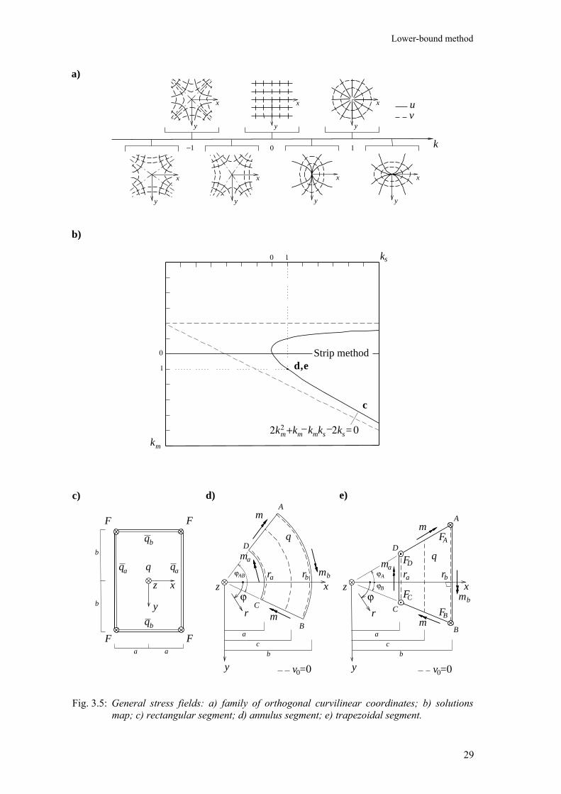
Lower-bound method

29

Fig. 3.5: General stress fields: a) family of orthogonal curvilinear coordinates; b) solutions map; c) rectangular segment; d) annulus segment; e) trapezoidal segment.

−1 0 1 k

v u x

y

a)

k0

k

0

m

s1

1

b)

c)

d

c

x

y

z

q

qb

F

F F

F

qa

0=km22 km+ km

_ ks ks_2

d)

a

b

b

a

qa

qb

D

ϕB

A

B

C

ϕA

b

ca

x

y

zm

rb

FB

FA

b

mra

FC

aFD

r

ϕ

m

m

e)

q

ϕAB

b

ca

x

y

zmb

ma

r

ϕ

q

Strip methode,

A

B

C

D

rbra

m

m

x

y

x

y

x

y

x

y

x

y

x

y

v 0=0v 0=0

Static method

30

The integration constants Cs and Cm are functions of ϕP: Cs = Cs(ϕP), Cm = Cm(ϕP). Since the shear and moment characteristics coincide, Cs is a constant in the shear-moment integration. Polar trajectories emulate the previous case of the strip method, where each coordinate line ϕP = const is an independent strip and two integration constants are available to fulfil the boundary conditions. The coordinate centre is a singularity point of the shear as well as the moment field; the values of the shear force and of the radial principal moments at this point determine a symmetrical stress field distribution. In order to provide an efficient load transfer, the geometrical load transfer rate ( rm/− ) has to improve the radial shear flow, i.e. shear flow in positive (negative) r-direction requires m > 0 (m < 0). In the following, the stress field of an annulus and a trapezoidal segment are explained as examples of the polar stress field family.

a) Annulus segment Consider the annulus segment ABCD depicted in Fig. 3.5d. The geometry of the segment is defined by the internal and the external supported boundary r = a and r = b, respectively, and the arbitrary apex angle ϕAB. The segment is subjected to a uniformly distributed load q. For the boundary moments mr( r = a ) = ma, mr( r = b ) = mb and mϕ = m, the shear field (Eq. (3.40) with ks = 1) and the moment field (Eqs. (3.54)) simplify to

−= r

rcqv

2

0 2 (3.55)

( ) mbammbaq

rabcqqrm ba

r +

−−++−+−=

626

22

; mm =ϕ (3.56)

where

( ) ( ) ( )

−+−−−

−= ba mmbmmabaq

baqc 332

6)(2 (3.57)

Starting from r = c, the load on the segment area cra ≤≤ is restricted by the reaction ra = q (c2– a2) / (2a) at the support CD and the load on the segment area brc ≤≤ is restricted by the reaction rb = q (b2

– c2 ) / (2b) at the support AB. Note that Eqs. (3.23) reduce to ra = – v0( r = a),

and rb = – v0 ( r = b ), respectively, AB and CD being principal moment trajectories. For a = 0 the annulus segment is transformed into a circular sector. At r = 0, Eq. (3.55) is indeterminate and the reaction ra degenerates to a concentrated support force of intensity Ra = q c2ϕΑΒ / 2. This singularity disappears if c = 0, or, equivalently, if m = qb2

/ 6 + mb.

b) Trapezoidal segment Consider the trapezoidal segment ABCD depicted in Fig. 3.5e, having bases CD and AB at x = a and x = b (0 < a < b), respectively, and oblique sides AD and BC at angles ϕA and ϕB from the x-axis. The segment is subjected to a uniformly distributed load q. It is supported along the bases AB and CD and free along AD and BC. In addition, the bending moments m, ma and mb act on the sides AD and BC, CD and AB, respectively. The stress field of the segment is obtained by adjusting Eq. (3.40) to ks = 1, and Eqs. (3.54) to the boundary conditions mx( x = a ) = ma and mx( x = b ) = mb:

−= r

rcqv

ϕ2

2

0 cos2 (3.58)

( ) mbammbaq

rabcqqrm ba

r +

−−++−+−=

6coscos26 32

22

ϕϕ ; mm =ϕ (3.59)

with

( ) ( ) ( )

−+−−−

−= ba mmbmmabaq

baqc 332

6)(2 (3.60)

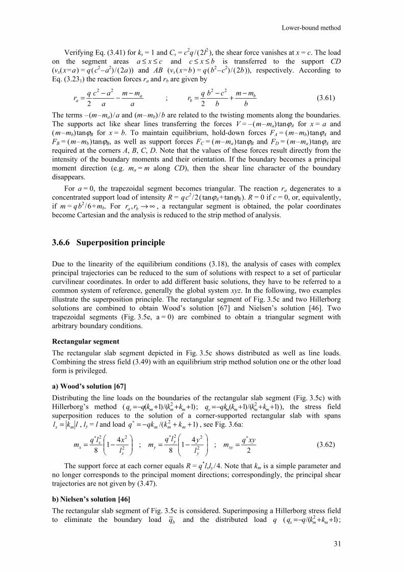
Lower-bound method

31

Verifying Eq. (3.41) for ks = 1 and Cs = c2q / ( 2l2 ), the shear force vanishes at x = c. The load

on the segment areas cxa ≤≤ and bxc ≤≤ is transferred to the support CD (vx( x = a ) = q ( c2

– a2) / ( 2a )) and AB (vx ( x = b ) = q ( b2 – c2) / ( 2b )), respectively. According to

Eq. (3.231) the reaction forces ra and rb are given by

a

mma

acqr aa

−−−=22

2 ;

bmm

bcbqr b

b−+−=

22

2 (3.61)

The terms – (m – ma) / a and (m – mb) / b are related to the twisting moments along the boundaries. The supports act like shear lines transferring the forces V = – ( m – ma) tanϕA for x = a and ( m – mb) tanϕB for x = b. To maintain equilibrium, hold-down forces FA = ( m – mb) tanϕA and FB = ( m – mb ) tanϕB, as well as support forces FC = ( m – ma ) tanϕB and FD = ( m – ma ) tanϕA are required at the corners A, B, C, D. Note that the values of these forces result directly from the intensity of the boundary moments and their orientation. If the boundary becomes a principal moment direction (e.g. ma = m along CD), then the shear line character of the boundary disappears. For a = 0, the trapezoidal segment becomes triangular. The reaction ra degenerates to a concentrated support load of intensity R = q c2

/ 2 ( tanϕA + tanϕB ). R = 0 if c = 0, or, equivalently, if m = q b2

/ 6 + mb. For ∞→ba rr , , a rectangular segment is obtained, the polar coordinates become Cartesian and the analysis is reduced to the strip method of analysis.

3.6.6 Superposition principle

Due to the linearity of the equilibrium conditions (3.18), the analysis of cases with complex principal trajectories can be reduced to the sum of solutions with respect to a set of particular curvilinear coordinates. In order to add different basic solutions, they have to be referred to a common system of reference, generally the global system xyz. In the following, two examples illustrate the superposition principle. The rectangular segment of Fig. 3.5c and two Hillerborg solutions are combined to obtain Wood’s solution [67] and Nielsen’s solution [46]. Two trapezoidal segments (Fig. 3.5e, a = 0) are combined to obtain a triangular segment with arbitrary boundary conditions.

Rectangular segment The rectangular slab segment depicted in Fig. 3.5c shows distributed as well as line loads. Combining the stress field (3.49) with an equilibrium strip method solution one or the other load form is privileged.

a) Wood’s solution [67] Distributing the line loads on the boundaries of the rectangular slab segment (Fig. 3.5c) with Hillerborg’s method ( )1/()1( 2 +++−= mmmx kkkqq ; )1/()1( 2 +++−= mmmmy kkkqkq ), the stress field superposition reduces to the solution of a corner-supported rectangular slab with spans

lkl mx = , ly = l and load )1/( 2 ++−=∗mmm kkqkq , see Fig. 3.6a:

2

;418

;418 2

22

2

22 xyqmlylq

mlxlqm xy

y

yy

x

xx

∗∗∗

=

−=

−= (3.62)

The support force at each corner equals R = q*lxly / 4. Note that km is a simple parameter and no longer corresponds to the principal moment directions; correspondingly, the principal shear trajectories are not given by (3.47).

b) Nielsen’s solution [46] The rectangular slab segment of Fig. 3.5c is considered. Superimposing a Hillerborg stress field to eliminate the boundary load bq and the distributed load q ( )1/( 2 ++−= mmx kkqq ;

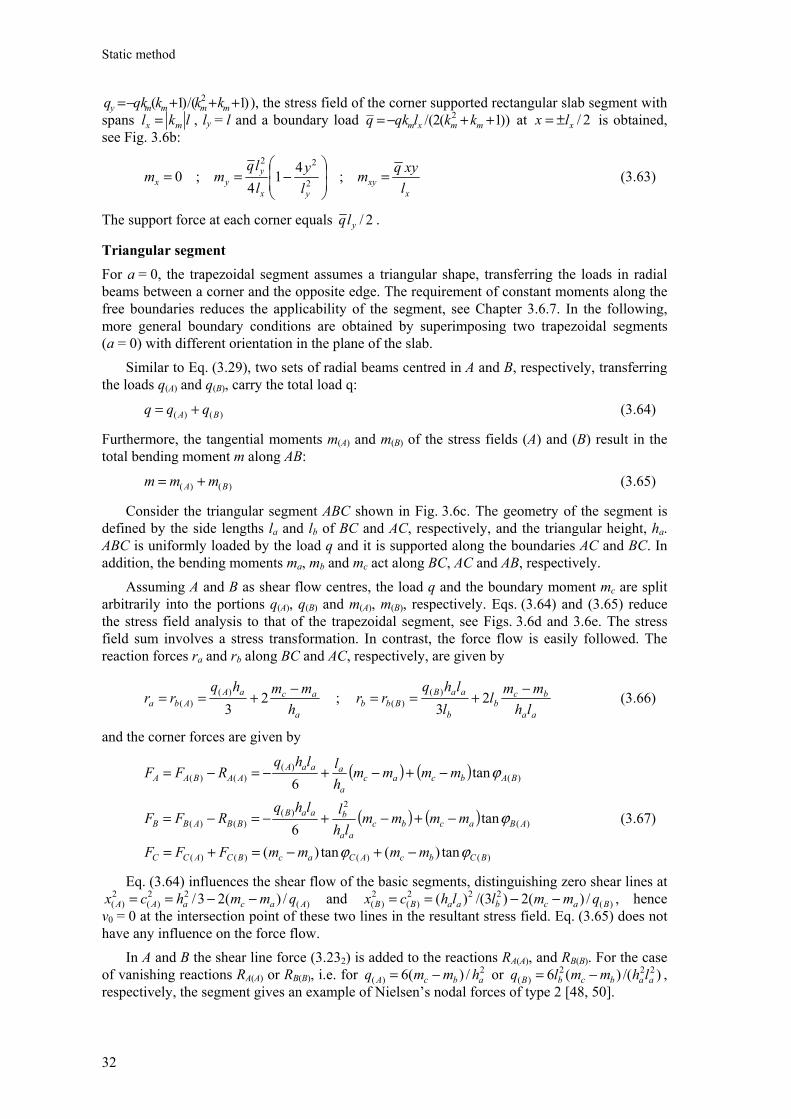
Static method

32

)1/()1( 2 +++−= mmmmy kkkqkq ), the stress field of the corner supported rectangular slab segment with spans lkl mx = , ly = l and a boundary load ))1(2/( 2 ++−= mmxm kklqkq at 2/xlx ±= is obtained, see Fig. 3.6b:

x

xyyx

yyx l

xyqmly

llq

mm =

−== ;41

4;0 2

22

(3.63)

The support force at each corner equals 2/ylq .

Triangular segment For a = 0, the trapezoidal segment assumes a triangular shape, transferring the loads in radial beams between a corner and the opposite edge. The requirement of constant moments along the free boundaries reduces the applicability of the segment, see Chapter 3.6.7. In the following, more general boundary conditions are obtained by superimposing two trapezoidal segments (a = 0) with different orientation in the plane of the slab.

Similar to Eq. (3.29), two sets of radial beams centred in A and B, respectively, transferring the loads q(A) and q(B), carry the total load q:

)()( BA qqq += (3.64)

Furthermore, the tangential moments m(A) and m(B) of the stress fields (A) and (B) result in the total bending moment m along AB:

)()( BA mmm += (3.65)

Consider the triangular segment ABC shown in Fig. 3.6c. The geometry of the segment is defined by the side lengths la and lb of BC and AC, respectively, and the triangular height, ha. ABC is uniformly loaded by the load q and it is supported along the boundaries AC and BC. In addition, the bending moments ma, mb and mc act along BC, AC and AB, respectively.

Assuming A and B as shear flow centres, the load q and the boundary moment mc are split arbitrarily into the portions q(A), q(B) and m(A), m(B), respectively. Eqs. (3.64) and (3.65) reduce the stress field analysis to that of the trapezoidal segment, see Figs. 3.6d and 3.6e. The stress field sum involves a stress transformation. In contrast, the force flow is easily followed. The reaction forces ra and rb along BC and AC, respectively, are given by

aa

bcb

b

aaBBbb

a

acaAAba lh

mmll

lhqrr

hmmhq

rr −+==−+== 23

;23

)()(

)()( (3.66)

and the corner forces are given by

( ) ( )

( ) ( )

)()()()(

)(

2)(

)()(

)()(

)()(

tan)(tan)(

tan6

tan6

BCbcACacBCACC

ABacbcaa

baaBBBABB

BAbcaca

aaaAAABAA

mmmmFFF

mmmmlh

llhqRFF

mmmmhllhq

RFF

ϕϕ

ϕ

ϕ

−+−=+=

−+−+−=−=

−+−+−=−=

(3.67)

Eq. (3.64) influences the shear flow of the basic segments, distinguishing zero shear lines at )(

22)(

2)( /)(23/ AacaAA qmmhcx −−== and )(

222)(

2)( /)(2)3/()( BacbaaBB qmmllhcx −−== , hence

v0 = 0 at the intersection point of these two lines in the resultant stress field. Eq. (3.65) does not have any influence on the force flow. In A and B the shear line force (3.232) is added to the reactions RA(A), and RB(B). For the case of vanishing reactions RA(A) or RB(B), i.e. for 2

)( /)(6 abcA hmmq −= or )/()(6 222)( aabcbB lhmmlq −= ,

respectively, the segment gives an example of Nielsen’s nodal forces of type 2 [48, 50].

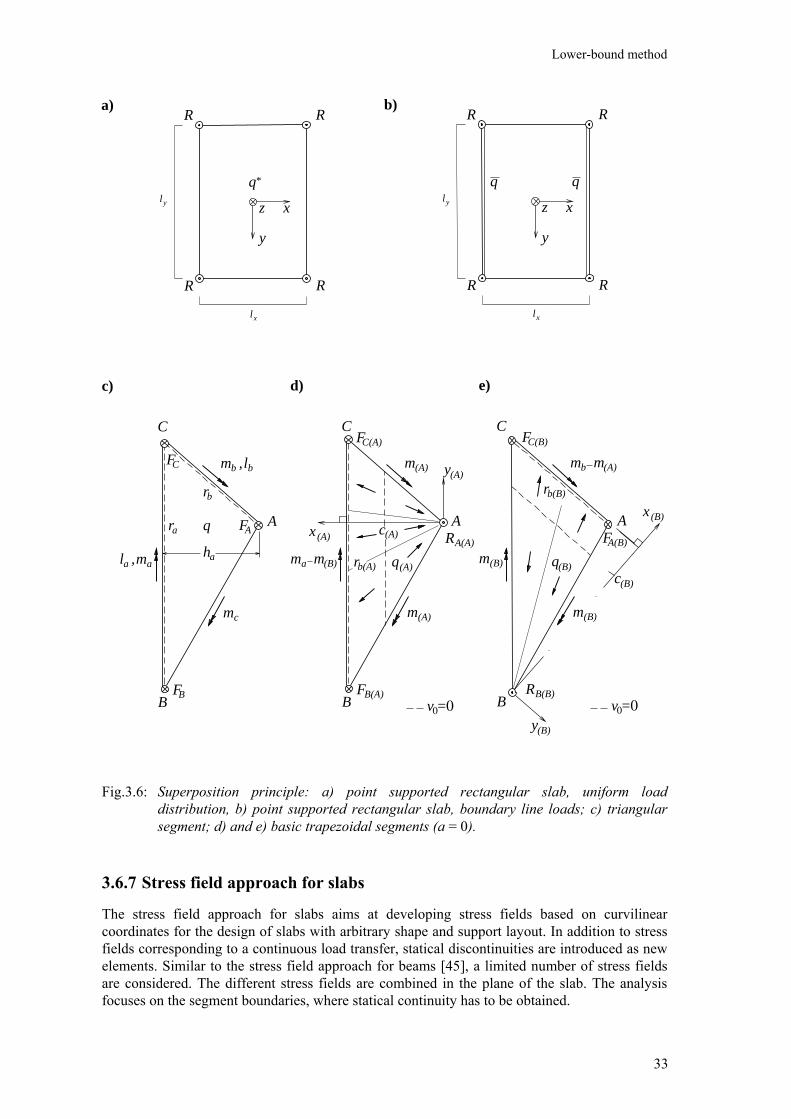
Lower-bound method

33

Fig.3.6: Superposition principle: a) point supported rectangular slab, uniform load distribution, b) point supported rectangular slab, boundary line loads; c) triangular segment; d) and e) basic trapezoidal segments (a = 0).

3.6.7 Stress field approach for slabs

The stress field approach for slabs aims at developing stress fields based on curvilinear coordinates for the design of slabs with arbitrary shape and support layout. In addition to stress fields corresponding to a continuous load transfer, statical discontinuities are introduced as new elements. Similar to the stress field approach for beams [45], a limited number of stress fields are considered. The different stress fields are combined in the plane of the slab. The analysis focuses on the segment boundaries, where statical continuity has to be obtained.

c) d) e)

q

ha

a) b)

x

y

z

q

R

xl

RR

R

x

y

z

R

RR

R

q q

C

A

B

mal ,a

m

lb

c

m ,b

qm a

m(A)

m (A)

m(B)

m(B)

bFC

FA

FB

rb

ra

(A)m (B)

m m (A)

q(B)rb(A)

FB(A)

FC(A)

RA(A)

rb(B)

x(B)

y(B)

y(A)

x(A) c(A)

c(B)

v 0=0RB(B)

FC(B)

FA(B)

yl

xl

yl

*

v 0=0

C

A

B

C

A

B

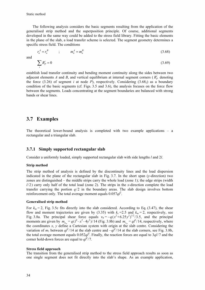
Static method

34

The following analysis considers the basic segments resulting from the application of the generalised strip method and the superposition principle. Of course, additional segments developed in the same way could be added to the stress field library. Fitting the basic elements in the plane of the slab, a load transfer scheme is selected. The segment geometry determines a specific stress field. The conditions

Bn

An rr = ; B

nAn mm = (3.68)

and ∑ =

i

iPR 0 (3.69)

establish load transfer continuity and bending moment continuity along the sides between two adjacent elements A and B, and vertical equilibrium at internal segment corners ( i

PR denoting the force (3.26) of segment i at node P), respectively. Considering (3.682) as a boundary condition of the basic segments (cf. Figs. 3.5 and 3.6), the analysis focuses on the force flow between the segments. Loads concentrating at the segment boundaries are balanced with strong bands or shear lines.

3.7 Examples

The theoretical lower-bound analysis is completed with two example applications – a rectangular and a triangular slab.

3.7.1 Simply supported rectangular slab

Consider a uniformly loaded, simply supported rectangular slab with side lengths l and 2l.

Strip method The strip method of analysis is defined by the discontinuity lines and the load dispersion indicated in the plane of the rectangular slab in Fig. 3.7. In the short span (y-direction) two zones are distinguished – the middle strips carry the whole load (zone 1); the edge strips (width l / 2 ) carry only half of the total load (zone 2). The strips in the x-direction complete the load transfer carrying the portion q / 2 in the boundary areas. The slab design involves bottom reinforcement only. The total average moment equals 0.057ql2.

Generalised strip method For km = 2, Fig. 3.5c fits directly into the slab considered. According to Eq. (3.47), the shear flow and moment trajectories are given by (3.35) with ks =2.5 and km = 2, respectively, see Fig. 3.8a. The principal shear force equals v0 = – q ( x2

+ 6.25 y2 )1/2

/ 3.5, and the principal moments are given by

mum = q ( l2 – x2

– 4y2 ) / 14 (Fig. 3.8b) and

mvm = ql2 / 14, respectively, where

the coordinates x, y define a Cartesian system with origin at the slab centre. Considering the variation of m1 between ql2

/ 14 at the slab centre and – ql2 / 14 at the slab corners, see Fig. 3.8b,

the total average moment equals 0.052ql2. Finally, the reaction forces are equal to 3ql / 7 and the corner hold-down forces are equal to ql2

/ 7.

Stress field approachThe transition from the generalised strip method to the stress field approach results as soon as one single segment does not fit directly into the slab’s shape. As an example application,

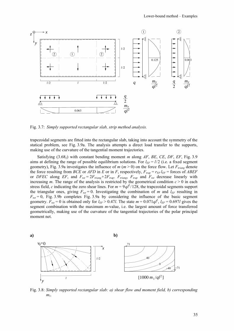
Lower-bound method – Examples

35

Fig. 3.7: Simply supported rectangular slab, strip method analysis.

trapezoidal segments are fitted into the rectangular slab, taking into account the symmetry of the statical problem, see Fig. 3.9a. The analysis attempts a direct load transfer to the supports, making use of the curvature of the tangential moment trajectories. Satisfying (3.682) with constant bending moment m along AF, BE, CE, DF, EF, Fig. 3.9 aims at defining the range of possible equilibrium solutions. For lEF = l / 2 (i.e. a fixed segment geometry), Fig. 3.9a investigates the influence of m (m > 0) on the force flow. Let Ftriang denote the force resulting from BCE or AFD in E or in F, respectively, Ftrap = rEF lEF = forces of ABEF or DFEC along EF, and Ftot = 2Ftriang + 2Ftrap. Ftriang, Ftrap and Ftot decrease linearly with increasing m. The range of the analysis is restricted by the geometrical condition c > 0 in each stress field, c indicating the zero shear lines. For m = 9 ql2

/ 128, the trapezoidal segments support the triangular ones, giving Ftot = 0. Investigating the combination of m and lEF resulting in Ftot = 0, Fig. 3.9b completes Fig. 3.9a by considering the influence of the basic segment geometry. Ftot = 0 is obtained only for lEF > 0.47l. The state m = 0.071ql2, lEF = 0.697l gives the segment combination with the maximum m-value, i.e. the largest amount of force transferred geometrically, making use of the curvature of the tangential trajectories of the polar principal moment net.

Fig. 3.8: Simply supported rectangular slab: a) shear flow and moment field, b) corresponding m1.

a)

x

y

b)

v 0=0

l [1000 m /ql2 ]1

0

40

−40

71

−71

l /2

0.125

q

12 2

x0.063

0.063

x

y

l /2

l /2

l /2 l /2l

z1 2

2q

ql2m

y

ql2m y

ql2m

2q

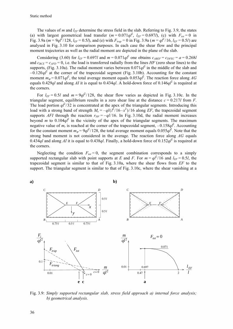
Static method

36

The values of m and lEF determine the stress field in the slab. Referring to Fig. 3.9, the states (a) with largest geometrical load transfer (m = 0.071ql2, lEF = 0.697l), (c) with Ftot = 0 in Fig. 3.9a (m = 9ql2

/ 128, lEF = 0.5l), and (e) with Ftrap = 0 in Fig. 3.9a ( m = ql2 / 16, lEF = 0.5l ) are

analysed in Fig. 3.10 for comparison purposes. In each case the shear flow and the principal moment trajectories as well as the radial moment are depicted in the plane of the slab.

Considering (3.60) for lEF = 0.697l and m = 0.071ql2 one obtains cABEF = cDFEC = a = 0.268l and cBCE = cAFD = 0, i.e. the load is transferred radially from the lines HF (zero shear lines) to the supports, (Fig. 3.10a). The radial moment varies between 0.071ql2 in the middle of the slab and – 0.120 ql2 at the corner of the trapezoidal segment (Fig. 3.10b). Accounting for the constant moment mϕ = 0.071ql2, the total average moment equals 0.053ql2. The reaction force along AG equals 0.429ql and along AI it is equal to 0.434ql. A hold-down force of 0.146ql2 is required at the corners.

For lEF = 0.5l and m = 9ql2 / 128, the shear flow varies as depicted in Fig. 3.10c. In the

triangular segment, equilibrium results in a zero shear line at the distance c = 0.217l from F. The load portion ql2

/ 32 is concentrated at the apex of the triangular segments. Introducing this load with a strong band of strength Mx = – ql ( l2

/ 16 – x2 ) / 16 along EF, the trapezoidal segment

supports AFI through the reaction rHF = – ql / 16. In Fig. 3.10d, the radial moment increases beyond m to 0.104ql2 in the vicinity of the apex of the triangular segments. The maximum negative value of mr is reached at the corner of the trapezoidal segment, – 0.158ql2. Accounting for the constant moment mϕ = 9ql2

/ 128, the total average moment equals 0.055ql2. Note that the strong band moment is not considered in the average. The reaction force along AG equals 0.434ql and along AI it is equal to 0.438ql. Finally, a hold-down force of 0.152ql2 is required at the corners.

Neglecting the condition Ftot = 0, the segment combination corresponds to a simply supported rectangular slab with point supports at E and F. For m = ql2

/ 16 and lEF = 0.5l, the trapezoidal segment is similar to that of Fig. 3.10a, where the shear flows from EF to the support. The triangular segment is similar to that of Fig. 3.10c, where the shear vanishing at a

Fig. 3.9: Simply supported rectangular slab, stress field approach a) internal force analysis; b) geometrical analysis.

0.1

0.01

D

A

C

B

FE

l0.5

0.75 l0.5

mql2

Fi

ql2Ftot

ql2

2c= 0c= 0

Ftot

Ftriang

Ftrap

= 0m

0.01

0.47

0.071

0.697

llEF

a) b)

ace

l

l0.5

0.75 l

D

A

C

B

FE

x

y

Examples

37

Fig. 3.10: Particular solutions: a) shear flow and moment field for lEF = 0.697l and m = 0.071ql2, b) corresponding mr; c) shear flow and moment field for lEF = 0.5l and m = 9ql2

/ 128, d) corresponding mr; e) shear flow and moment field for lEF = 0.5l and m = ql2

/ 16, f) corresponding mr; g) transfer of RF: shear lines FL; h) additional moment distribution.

a)

I

A

H

G

l0.5

l0.349 l0.651

c)

l0.25 l0.533

e)

v 0=0

l0.25 0.5

l0.217

F71

0

40

r /8=HF qlRF=ql2/32

v 0=0

l0.25

2

L

RF=ql2/24

RF

v 0=0

v 0=0 RF =ql2/24

l0.25 l075d d

0

4080

I

A

H

G

I

A

H

G

I

A

H

G

l

0−40 −80

40

0

4080

0−40 −80

40

0−40 −80

40

x

x

x

y

y

y

y

M

m x= dRF

l

m y= lRF

d4

−141

−28

70

63 108

104

71

−158

−31

120

−42

b)

d)

f)

h)g)

[1000 mr /ql2 ]

[1000 mr /ql2 ]

[1000 mr /ql2 ]

x

F

F

F

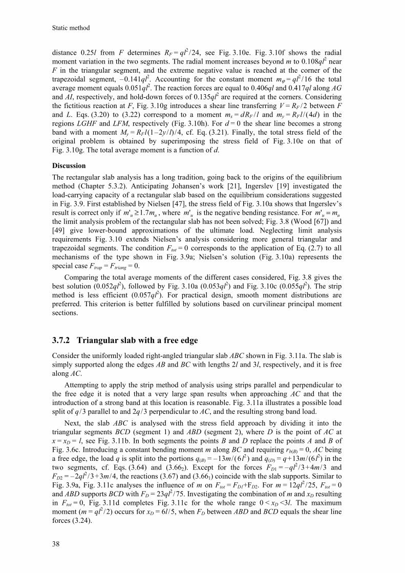
Static method

38

distance 0.25l from F determines RF = ql2 / 24, see Fig. 3.10e. Fig. 3.10f shows the radial

moment variation in the two segments. The radial moment increases beyond m to 0.108ql2 near F in the triangular segment, and the extreme negative value is reached at the corner of the trapezoidal segment, – 0.141ql2. Accounting for the constant moment mϕ = ql2

/ 16 the total average moment equals 0.051ql2. The reaction forces are equal to 0.406ql and 0.417ql along AG and AI, respectively, and hold-down forces of 0.135ql2 are required at the corners. Considering the fictitious reaction at F, Fig. 3.10g introduces a shear line transferring V = RF / 2 between F and L. Eqs. (3.20) to (3.22) correspond to a moment mx = d RF / l and my = RF l / ( 4d ) in the regions LGHF and LFM, respectively (Fig. 3.10h). For d = 0 the shear line becomes a strong band with a moment My = RF l (1 – 2y / l) / 4, cf. Eq. (3.21). Finally, the total stress field of the original problem is obtained by superimposing the stress field of Fig. 3.10e on that of Fig. 3.10g. The total average moment is a function of d.

Discussion The rectangular slab analysis has a long tradition, going back to the origins of the equilibrium method (Chapter 5.3.2). Anticipating Johansen’s work [21], Ingerslev [19] investigated the load-carrying capacity of a rectangular slab based on the equilibrium considerations suggested in Fig. 3.9. First established by Nielsen [47], the stress field of Fig. 3.10a shows that Ingerslev’s result is correct only if uu mm 7.1' ≥ , where um' is the negative bending resistance. For uu mm =' the limit analysis problem of the rectangular slab has not been solved; Fig. 3.8 (Wood [67]) and [49] give lower-bound approximations of the ultimate load. Neglecting limit analysis requirements Fig. 3.10 extends Nielsen’s analysis considering more general triangular and trapezoidal segments. The condition Ftot = 0 corresponds to the application of Eq. (2.7) to all mechanisms of the type shown in Fig. 3.9a; Nielsen’s solution (Fig. 3.10a) represents the special case Ftrap = Ftriang = 0. Comparing the total average moments of the different cases considered, Fig. 3.8 gives the best solution (0.052ql2), followed by Fig. 3.10a (0.053ql2) and Fig. 3.10c (0.055ql2). The strip method is less efficient (0.057ql2). For practical design, smooth moment distributions are preferred. This criterion is better fulfilled by solutions based on curvilinear principal moment sections.

3.7.2 Triangular slab with a free edge

Consider the uniformly loaded right-angled triangular slab ABC shown in Fig. 3.11a. The slab is simply supported along the edges AB and BC with lengths 2l and 3l, respectively, and it is free along AC. Attempting to apply the strip method of analysis using strips parallel and perpendicular to the free edge it is noted that a very large span results when approaching AC and that the introduction of a strong band at this location is reasonable. Fig. 3.11a illustrates a possible load split of q / 3 parallel to and 2q / 3 perpendicular to AC, and the resulting strong band load. Next, the slab ABC is analysed with the stress field approach by dividing it into the triangular segments BCD (segment 1) and ABD (segment 2), where D is the point of AC at x = xD = l, see Fig. 3.11b. In both segments the points B and D replace the points A and B of Fig. 3.6c. Introducing a constant bending moment m along BC and requiring rb(B) = 0, AC being a free edge, the load q is split into the portions q(B) = – 13m / ( 6 l2

) and q(D) = q + 13m / (6 l2) in the two segments, cf. Eqs. (3.64) and (3.662). Except for the forces FD1 = – ql2

/ 3 + 4m / 3 and FD2 = – 2ql2

/ 3 + 3m / 4, the reactions (3.67) and (3.661) coincide with the slab supports. Similar to Fig. 3.9a, Fig. 3.11c analyses the influence of m on Ftot = FD1+FD2. For m = 12ql2

/ 25, Ftot = 0 and ABD supports BCD with FD = 23ql2

/ 75. Investigating the combination of m and xD resulting in Ftot = 0, Fig. 3.11d completes Fig. 3.11c for the whole range 0 < xD <3l. The maximum moment (m = ql2

/ 2) occurs for xD = 6l / 5, when FD between ABD and BCD equals the shear line forces (3.24).

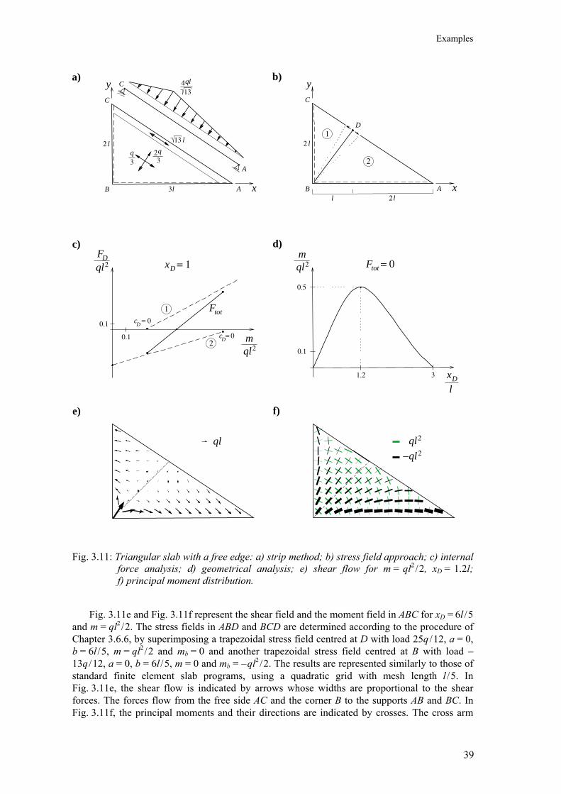
Examples

39

Fig. 3.11: Triangular slab with a free edge: a) strip method; b) stress field approach; c) internal force analysis; d) geometrical analysis; e) shear flow for m = ql2

/ 2, xD = 1.2l; f) principal moment distribution.

Fig. 3.11e and Fig. 3.11f represent the shear field and the moment field in ABC for xD = 6l / 5 and m = ql2

/ 2. The stress fields in ABD and BCD are determined according to the procedure of Chapter 3.6.6, by superimposing a trapezoidal stress field centred at D with load 25q / 12, a = 0, b = 6l / 5, m = ql2

/ 2 and mb = 0 and another trapezoidal stress field centred at B with load –13q / 12, a = 0, b = 6l / 5, m = 0 and mb = – ql2

/ 2. The results are represented similarly to those of standard finite element slab programs, using a quadratic grid with mesh length l / 5. In Fig. 3.11e, the shear flow is indicated by arrows whose widths are proportional to the shear forces. The forces flow from the free side AC and the corner B to the supports AB and BC. In Fig. 3.11f, the principal moments and their directions are indicated by crosses. The cross arm

0.1

0.1

A

C

B

mql2

FD

ql2 Ftotql2

3

c = 0

= 0m

0.1

lxD

a) b)

l2

x

y

l3 A

C

B

l2

x

y

D

2 ll

1

23q

3q2

A

C13ql4

D

c =D

0

xD = 1

1.2

0.5

c) d)

e) f)

ql ql2

ql2−

2

1 Ftot

13 l

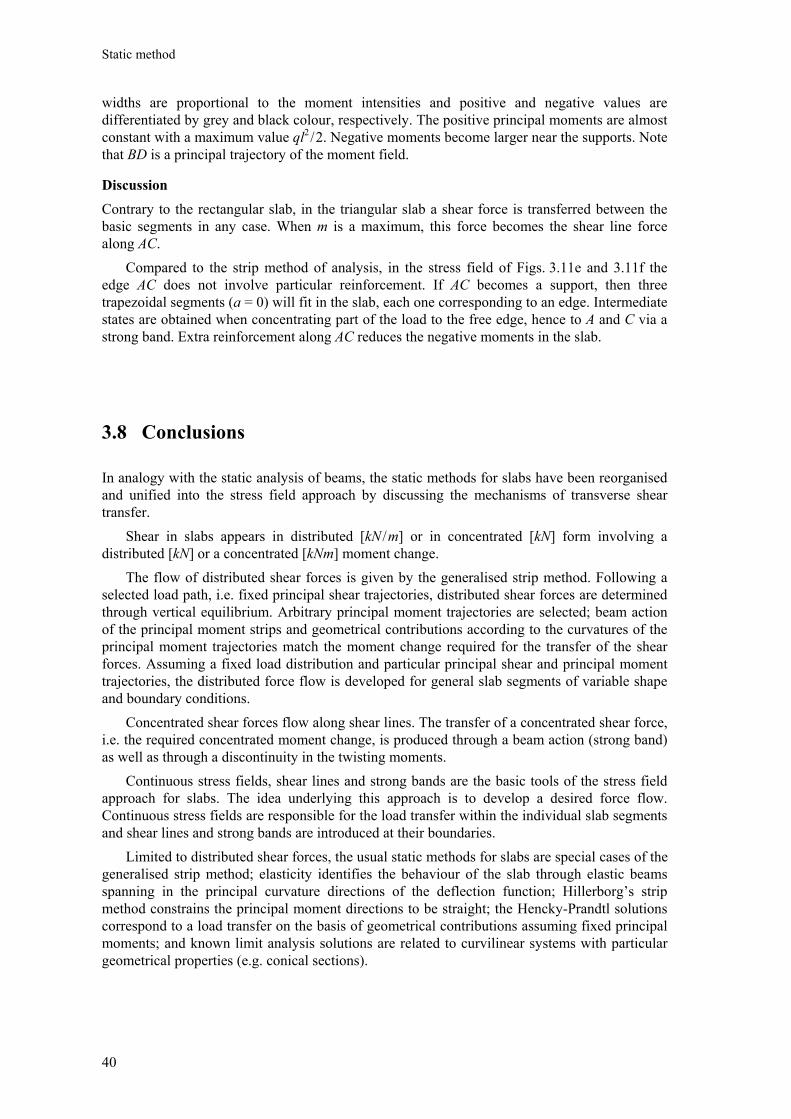
Static method

40

widths are proportional to the moment intensities and positive and negative values are differentiated by grey and black colour, respectively. The positive principal moments are almost constant with a maximum value ql2

/ 2. Negative moments become larger near the supports. Note that BD is a principal trajectory of the moment field.

Discussion

Contrary to the rectangular slab, in the triangular slab a shear force is transferred between the basic segments in any case. When m is a maximum, this force becomes the shear line force along AC.

Compared to the strip method of analysis, in the stress field of Figs. 3.11e and 3.11f the edge AC does not involve particular reinforcement. If AC becomes a support, then three trapezoidal segments (a = 0) will fit in the slab, each one corresponding to an edge. Intermediate states are obtained when concentrating part of the load to the free edge, hence to A and C via a strong band. Extra reinforcement along AC reduces the negative moments in the slab.

3.8 Conclusions

In analogy with the static analysis of beams, the static methods for slabs have been reorganised and unified into the stress field approach by discussing the mechanisms of transverse shear transfer.

Shear in slabs appears in distributed [kN / m] or in concentrated [kN] form involving a distributed [kN] or a concentrated [kNm] moment change. The flow of distributed shear forces is given by the generalised strip method. Following a selected load path, i.e. fixed principal shear trajectories, distributed shear forces are determined through vertical equilibrium. Arbitrary principal moment trajectories are selected; beam action of the principal moment strips and geometrical contributions according to the curvatures of the principal moment trajectories match the moment change required for the transfer of the shear forces. Assuming a fixed load distribution and particular principal shear and principal moment trajectories, the distributed force flow is developed for general slab segments of variable shape and boundary conditions.

Concentrated shear forces flow along shear lines. The transfer of a concentrated shear force, i.e. the required concentrated moment change, is produced through a beam action (strong band) as well as through a discontinuity in the twisting moments. Continuous stress fields, shear lines and strong bands are the basic tools of the stress field approach for slabs. The idea underlying this approach is to develop a desired force flow. Continuous stress fields are responsible for the load transfer within the individual slab segments and shear lines and strong bands are introduced at their boundaries. Limited to distributed shear forces, the usual static methods for slabs are special cases of the generalised strip method; elasticity identifies the behaviour of the slab through elastic beams spanning in the principal curvature directions of the deflection function; Hillerborg’s strip method constrains the principal moment directions to be straight; the Hencky-Prandtl solutions correspond to a load transfer on the basis of geometrical contributions assuming fixed principal moments; and known limit analysis solutions are related to curvilinear systems with particular geometrical properties (e.g. conical sections).

41

4 Limit analysis

4.1 General

The first attempts at a slab limit analysis date back to the 1920’s and 1930’s [19, 21]. Supported by experimental observations, it was assumed that slabs fail along yield lines. The limit analysis consisted in determining the most critical yield line layout (see Chapter 5.3). Attempts to solve the slab limit analysis problem on the basis of the theory of plasticity (see Chapter 2.6) followed in the 1960’s. The plasticity approaches started from the analysis of the limit states following the yielding of the reinforcement. In the lower-bound analysis, the yield condition found direct application for the design of the reinforcement [66]. The upper-bound analysis based on the flow rule was found to be more general than the yield line theory [37, 47, 26]. However, the kinematical research was essentially focused on a review of Johansen’s theory [21]. The newly found failure modes did not correspond to the yield line theory and the limit analysis problem could be completely solved only for some particular cases. This raised doubts about the existence of complete solutions [8, 69] until the 1970’s, when Fox [9, 10] showed that rather simple loading problems may involve complex solutions. Parallel to this development, the limit analysis of slabs split into clear upper- and lower-bound approaches.

This chapter summarises the fundamentals of slab limit analysis. Based on work by Save [58] and Kemp [26], the following analysis starts from a statical yield condition and it uses the flow rule to deduce how yield will occur. The yield surface is used to define the basic elements of slab limit analysis and to illustrate the difficulty to determine matching upper- and lower-bound analyses. These difficulties are mitigated by simplifying the limit analysis to a consistent theory in agreement with a slab collapse involving yield line mechanisms. Simplified complete solutions provide the basis for a new slab design method – the compatibility limit design method (see Chapter 6).

The following discussion is limited to homogeneous orthotropic slabs reinforced in the x- and y-directions in both the top and bottom layers. However, the outlined procedure is valid for an arbitrary reinforcement layout.

4.2 Yield condition and flow rule

For low reinforcement ratios, the slab’s ultimate resistance depends primarily on the strength of the reinforcement (Chapter 4.2.1). The yield condition describes all stress states for which the reinforcement is yielding (Chapter 4.2.2). The transition from statics to kinematics is provided by the flow rule (Chapter 4.2.3). Corresponding parameters of the generalised stresses mx, my, mxy are the generalised strains xχ& , yχ& , 2 xyχ& . Slabs may collapse along yield lines or at yield points; the two cases are characterised by statical and kinematical redundancies, respectively (Chapter 4.2.4).

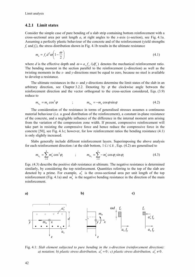
Limit analysis

42

4.2.1 Limit states

Consider the simple case of pure bending of a slab strip containing bottom reinforcement with a cross-sectional area per unit length as at right angles to the x-axis (x-section), see Fig. 4.1a. Assuming a perfectly plastic behaviour of the concrete and of the reinforcement (yield strengths fc and fy), the stress distribution shown in Fig. 4.1b results in the ultimate resistance

−=

212 ωωdfm cu (4.1)

where d is the effective depth and )/( cys dffa=ω denotes the mechanical reinforcement ratio. The bending moment in the section parallel to the reinforcement (y-direction) as well as the twisting moments in the x- and y-directions must be equal to zero, because no steel is available to develop a resistance. The ultimate resistances in the x- and y-directions determine the limit states of the slab in an arbitrary direction, see Chapter 3.2.2. Denoting by ϕ the clockwise angle between the reinforcement direction and the vector orthogonal to the cross-section considered, Eqs. (3.9) reduce to

ϕ2cosun mmu

= ; ϕϕ sincosutn mmu

−= (4.2)

The consideration of the resistance in terms of generalised stresses assumes a continuous material behaviour (i.e. a good distribution of the reinforcement), a constant in-plane resistance of the concrete, and a negligible influence of the difference in the internal moment arm arising from the variation of the compression zone width. If present, compressive reinforcement will take part in resisting the compressive force and hence reduce the compressive force in the concrete [50], see Fig. 4.1c; however, for low reinforcement ratios the bending resistance (4.1) is only slightly increased.

Slabs generally include different reinforcement layers. Superimposing the above analysis for each reinforcement direction i at the slab bottom, ki ≤≤1 , Eqs. (4.2) are generalised to

∑=

=k

ii

iun mm

u1

2cos ϕ ; i

k

ii

iutn mm

uϕϕ sincos

1∑

=

−= (4.3)

Eqs. (4.3) describe the positive slab resistance at ultimate. The negative resistance is determined similarly, by considering the top reinforcement. Quantities referring to the top of the slab are denoted by a prime. For example, sa′ is the cross-sectional area per unit length of the top reinforcement (Fig. 4.1a) and um′ is the negative bending resistance in the direction of the main reinforcement.

Fig. 4.1: Slab element subjected to pure bending in the x-direction (reinforcement direction): a) notation; b) plastic stress distribution, 0=′sa ; c) plastic stress distribution, 0≠′sa .

d

ω

a) c)

. . . ... x

z

y

as

mu

1

mu

as fy

fcd

z

x

as fy

fc

a’s fy

b)

a’s

y

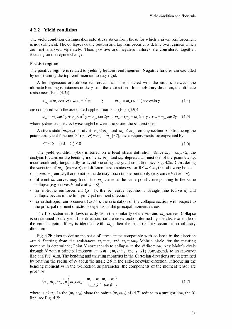
Yield condition and flow rule

43

4.2.2 Yield condition

The yield condition distinguishes safe stress states from those for which a given reinforcement is not sufficient. The collapses of the bottom and top reinforcements define two regimes which are first analysed separately. Then, positive and negative failures are considered together, focusing on the regime change.

Positive regime The positive regime is related to yielding bottom reinforcement. Negative failures are excluded by constraining the top reinforcement to stay rigid. A homogeneous orthotropic reinforced slab is considered with the ratio µ between the ultimate bending resistances in the y- and the x-directions. In an arbitrary direction, the ultimate resistances (Eqs. (4.3))

ϕµϕ 22 sicos nmmm uunu+= ; ϕϕµ sincos)1( −= utn mm

u (4.4)

are compared with the associated applied moments (Eqs. (3.9)) ϕϕϕ 2sinsincos 22

yxyxn mmmm ++= ; ϕϕϕ 2coscossin)( yxxytn mmmm +−= (4.5) where ϕ denotes the clockwise angle between the x- and the n-directions. A stress state (mn,mtn) is safe if

unn mm ≤ and utntn mm ≤ on any section n. Introducing the

parametric yield function unnn mmmY −=+ ),( ϕ [37], these requirements are expressed by

0≤+Y and 0, ≤+ϕY (4.6)

The yield condition (4.6) is based on a local stress definition. Since mtn = mn,ϕ / 2, the analysis focuses on the bending moment.

unm and mn, depicted as functions of the parameter ϕ, must touch only tangentially to avoid violating the yield condition, see Fig. 4.2a. Considering the variation of

unm (curve a) and different stress states mn for πϕ ≤≤0 , the following holds: • curves

unm and mn that do not coincide may touch in one point only (e.g. curve b at ϕ = ϑ); • different mn-curves may touch the

unm -curve at the same point corresponding to the same collapse (e.g. curves b and c at ϕ = ϑ);

• for isotropic reinforcement (µ = 1), the unm -curve becomes a straight line (curve d) and

collapse occurs in the first principal moment direction; • for orthotropic reinforcement ( 1≠µ ), the orientation of the collapse section with respect to

the principal moment directions depends on the principal moment values. The first statement follows directly from the similarity of the mn- and

unm -curves. Collapse is constrained to the yield-line direction, i.e the cross-section defined by the abscissa angle of the contact point. If mn is identical with

unm , then the collapse may occur in an arbitrary direction. Fig. 4.2b aims to define the set c of stress states compatible with collapse in the direction ϕ = ϑ. Starting from the resistances mx = mu and my = µmu Mohr’s circle for the resisting moments is determined; Point N corresponds to collapse in the ϑ-direction. Any Mohr’s circle through N with a principal moment umm ≤1 ( 21 mm ≥ and 1≤µ ) corresponds to an mn-curve like c in Fig. 4.2a. The bending and twisting moments in the Cartesian directions are determined by rotating the radius of N about the angle 2ϑ in the anti-clockwise direction. Introducing the bending moment m in the x-direction as parameter, the components of the moment tensor are given by

( )

−−−=

ϑϑµ

tan,

tan,,, 2

mmmmmmmmm uuuxyyx (4.7)

where umm ≤ . In the (mn,mtn)-plane the points (mx,myx) of (4.7) reduce to a straight line, the X-line, see Fig. 4.2b.

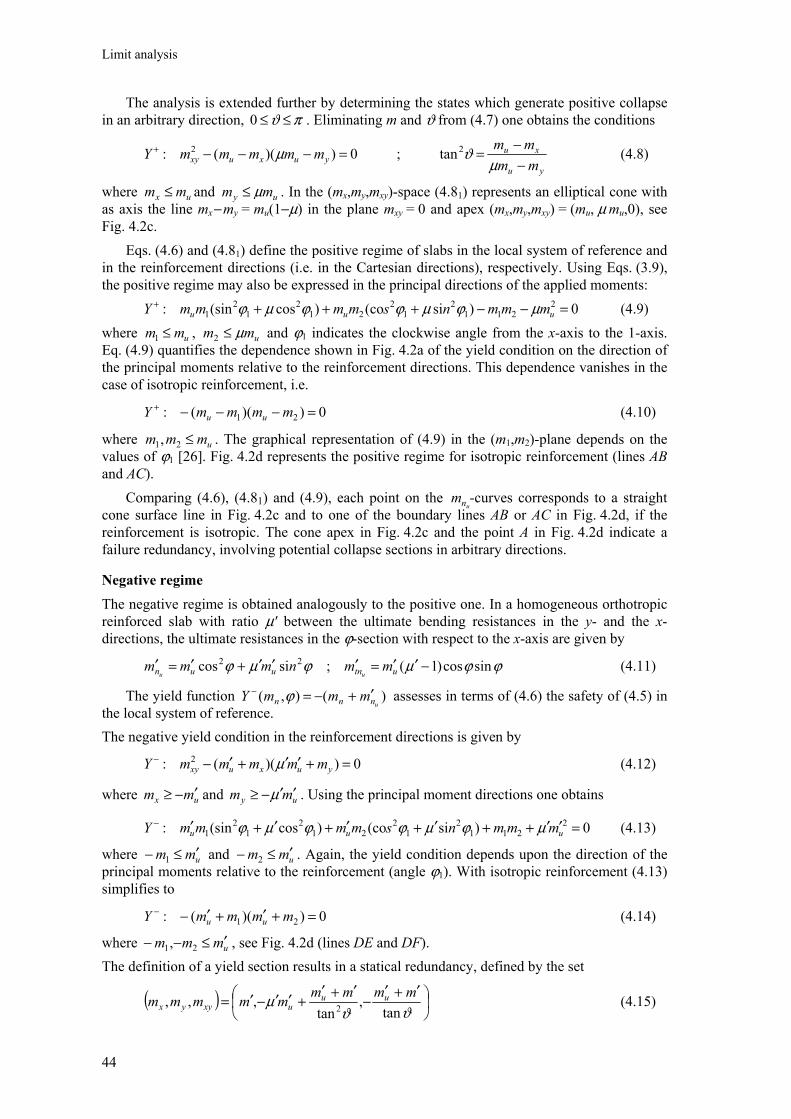
Limit analysis

44

The analysis is extended further by determining the states which generate positive collapse in an arbitrary direction, πϑ ≤≤0 . Eliminating m and ϑ from (4.7) one obtains the conditions

0))((: 2 =−−−+yuxuxy mmmmmY µ ;

yu

xu

mmmm

−−=

µϑ2tan (4.8)

where ux mm ≤ and uy mm µ≤ . In the (mx,my,mxy)-space (4.81) represents an elliptical cone with as axis the line mx − my = mu(1−µ) in the plane mxy = 0 and apex (mx,my,mxy) = (mu, µ mu,0), see Fig. 4.2c. Eqs. (4.6) and (4.81) define the positive regime of slabs in the local system of reference and in the reinforcement directions (i.e. in the Cartesian directions), respectively. Using Eqs. (3.9), the positive regime may also be expressed in the principal directions of the applied moments: 0)si(co)cos(sin: 2

2112

12

212

12

1 =−−++++uuu mmmnsmmmmY µϕµϕϕµϕ (4.9)

where umm ≤1 , umm µ≤2 and ϕ1 indicates the clockwise angle from the x-axis to the 1-axis. Eq. (4.9) quantifies the dependence shown in Fig. 4.2a of the yield condition on the direction of the principal moments relative to the reinforcement directions. This dependence vanishes in the case of isotropic reinforcement, i.e.

0))((: 21 =−−−+ mmmmY uu (4.10)

where ummm ≤21, . The graphical representation of (4.9) in the (m1,m2)-plane depends on the values of ϕ1 [26]. Fig. 4.2d represents the positive regime for isotropic reinforcement (lines AB and AC). Comparing (4.6), (4.81) and (4.9), each point on the

unm -curves corresponds to a straight cone surface line in Fig. 4.2c and to one of the boundary lines AB or AC in Fig. 4.2d, if the reinforcement is isotropic. The cone apex in Fig. 4.2c and the point A in Fig. 4.2d indicate a failure redundancy, involving potential collapse sections in arbitrary directions.

Negative regime The negative regime is obtained analogously to the positive one. In a homogeneous orthotropic reinforced slab with ratio µ′ between the ultimate bending resistances in the y- and the x-directions, the ultimate resistances in the ϕ-section with respect to the x-axis are given by

ϕϕµϕµϕ sincos)1(;sicos 22 −′′=′′′+′=′ utnuun mmnmmmuu

(4.11)

The yield function )(),(unnn mmmY ′+−=− ϕ assesses in terms of (4.6) the safety of (4.5) in

the local system of reference. The negative yield condition in the reinforcement directions is given by

0))((: 2 =+′′+′−−yuxuxy mmmmmY µ (4.12)

where ux mm ′−≥ and uy mm ′′−≥ µ . Using the principal moment directions one obtains

0)si(co)cos(sin: 2211

21

221

21

21 =′′++′+′+′+′−

uuu mmmnsmmmmY µϕµϕϕµϕ (4.13)

where umm ′≤− 1 and umm ′≤− 2 . Again, the yield condition depends upon the direction of the principal moments relative to the reinforcement (angle ϕ1). With isotropic reinforcement (4.13) simplifies to

0))((: 21 =+′+′−− mmmmY uu (4.14)

where ummm ′≤−− 21, , see Fig. 4.2d (lines DE and DF). The definition of a yield section results in a statical redundancy, defined by the set

( )

′+′

−′+′

+′′−′=ϑϑ

µtan

,tan

,,, 2mmmmmmmmm uu

uxyyx (4.15)

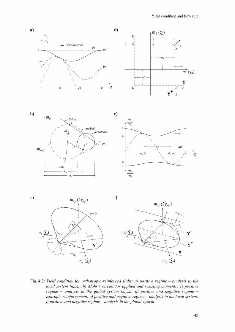
Yield condition and flow rule

45

Fig. 4.2: Yield condition for orthotropic reinforced slabs: a) positive regime – analysis in the local system (n,t,z); b) Mohr’s circles for applied and resisting moments; c) positive regime – analysis in the global system (x,y,z); d) positive and negative regime –isotropic reinforcement; e) positive and negative regime – analysis in the local system; f) positive and negative regime – analysis in the global system.

a) d)

b) e)

mn

mtn

m

muµ

resistance

X

Y

mnu

mtnu

XY

ϑ2

X-line

N

applied

f)c)

χ.

mu

mµ

ϕ = ϑ

Y+

mxy

my

mx

(2χ )xy

.

(χ )y

(χ )x.

Y+

.

Y-

π

ϕ = ϑ

ϑ

m’umn

’

ϑ1 2

∆ϑ

mu

ϕ

mn

1

µ

π

1µ

ϕ1

∆m

ϕ2

m

m

1

2

HD

G

A

mu

m’u

B

F

C

E

Y+

Y-

(χ ).

(χ ).

1

2

u

1

ϕ = ϑ2

my (χ )y.

mx(χ )x.

mxy (2χ )xy

.

12

mu

ϕ0 ϑ

mn

1

µ

Yield-direction

a)

b)

d)

. .. .

.. .

. ..

..

c) π

. .. .

. .. . . . . . . . . . . .. .................

...

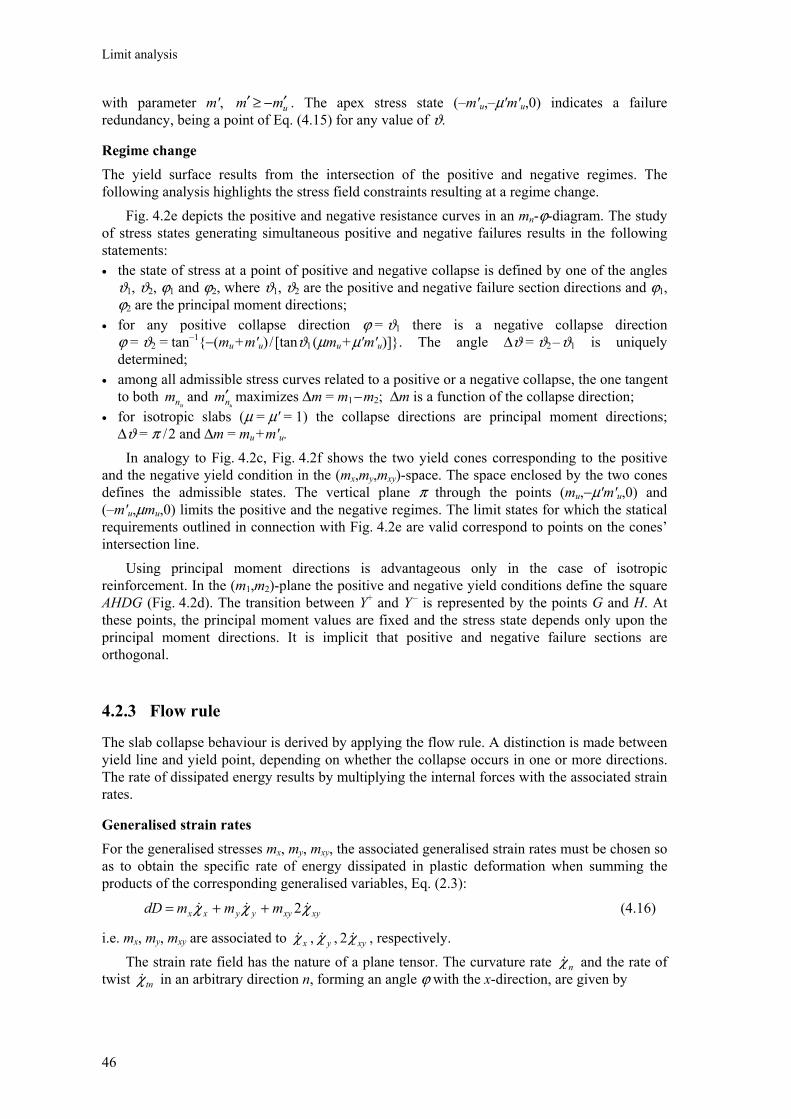
Limit analysis

46

with parameter m', umm ′−≥′ . The apex stress state (–m'u,–µ'm'u,0) indicates a failure redundancy, being a point of Eq. (4.15) for any value of ϑ.

Regime change The yield surface results from the intersection of the positive and negative regimes. The following analysis highlights the stress field constraints resulting at a regime change.

Fig. 4.2e depicts the positive and negative resistance curves in an mn-ϕ-diagram. The study of stress states generating simultaneous positive and negative failures results in the following statements: • the state of stress at a point of positive and negative collapse is defined by one of the angles

ϑ1, ϑ2, ϕ1 and ϕ2, where ϑ1, ϑ2 are the positive and negative failure section directions and ϕ1, ϕ2 are the principal moment directions;

• for any positive collapse direction ϕ = ϑ1 there is a negative collapse direction ϕ = ϑ2 = tan–1{−(mu + m′u) / [tanϑ1 (µmu + µ′m′u)]}. The angle ∆ϑ = ϑ2 – ϑ1 is uniquely determined;

• among all admissible stress curves related to a positive or a negative collapse, the one tangent to both

unm and unm′ maximizes ∆m = m1 − m2; ∆m is a function of the collapse direction;

• for isotropic slabs (µ = µ′ = 1) the collapse directions are principal moment directions; ∆ϑ = π / 2 and ∆m = mu + m′u.

In analogy to Fig. 4.2c, Fig. 4.2f shows the two yield cones corresponding to the positive and the negative yield condition in the (mx,my,mxy)-space. The space enclosed by the two cones defines the admissible states. The vertical plane π through the points (mu,−µ′m′u,0) and (–m′u,µmu,0) limits the positive and the negative regimes. The limit states for which the statical requirements outlined in connection with Fig. 4.2e are valid correspond to points on the cones’ intersection line.

Using principal moment directions is advantageous only in the case of isotropic reinforcement. In the (m1,m2)-plane the positive and negative yield conditions define the square AHDG (Fig. 4.2d). The transition between Y+ and Y

– is represented by the points G and H. At these points, the principal moment values are fixed and the stress state depends only upon the principal moment directions. It is implicit that positive and negative failure sections are orthogonal.

4.2.3 Flow rule

The slab collapse behaviour is derived by applying the flow rule. A distinction is made between yield line and yield point, depending on whether the collapse occurs in one or more directions. The rate of dissipated energy results by multiplying the internal forces with the associated strain rates.

Generalised strain rates For the generalised stresses mx, my, mxy, the associated generalised strain rates must be chosen so as to obtain the specific rate of energy dissipated in plastic deformation when summing the products of the corresponding generalised variables, Eq. (2.3):

xyxyyyxx mmmdD χχχ &&& 2++= (4.16)

i.e. mx, my, mxy are associated to xχ& , yχ& , xyχ&2 , respectively. The strain rate field has the nature of a plane tensor. The curvature rate nχ& and the rate of twist tnχ& in an arbitrary direction n, forming an angle ϕ with the x-direction, are given by

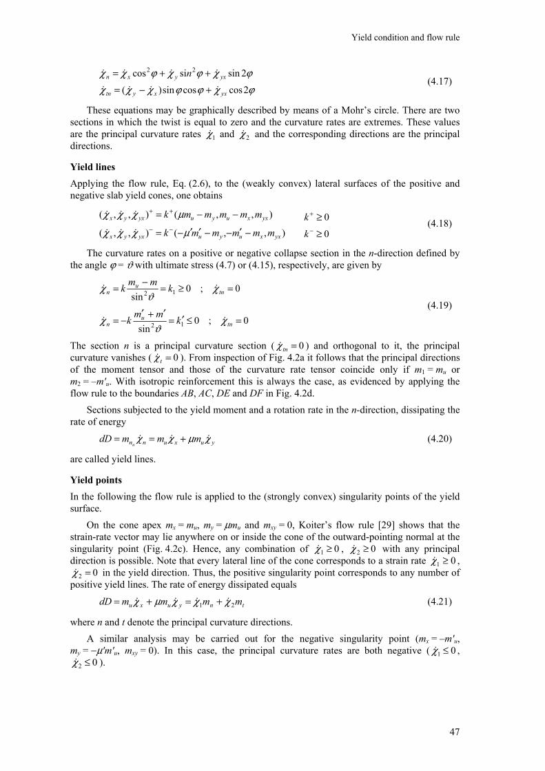
Yield condition and flow rule

47

ϕχϕϕχχχϕχϕχϕχχ2coscossin)(

2sinsicos 22

yxxytn

yxyxn n&&&&

&&&&

+−=

++= (4.17)

These equations may be graphically described by means of a Mohr’s circle. There are two sections in which the twist is equal to zero and the curvature rates are extremes. These values are the principal curvature rates 1χ& and 2χ& and the corresponding directions are the principal directions.

Yield lines Applying the flow rule, Eq. (2.6), to the (weakly convex) lateral surfaces of the positive and negative slab yield cones, one obtains

),,(),,(

),,(),,(

yxxuyuyxyx

yxxuyuyxyx

mmmmmk

mmmmmk

−′−−′′−=

−−=−−

++

µχχχ

µχχχ

&&&

&&&

0

0

≥

≥−

+

k

k (4.18)

The curvature rates on a positive or negative collapse section in the n-direction defined by the angle ϕ = ϑ with ultimate stress (4.7) or (4.15), respectively, are given by

0;0sin 12 =≥=−= tn

un kmmk χ

ϑχ &&

0;0sin 12 =≤′=

′+′−= tn

un kmmk χ

ϑχ &&

(4.19)

The section n is a principal curvature section ( 0=tnχ& ) and orthogonal to it, the principal curvature vanishes ( 0=tχ& ). From inspection of Fig. 4.2a it follows that the principal directions of the moment tensor and those of the curvature rate tensor coincide only if m1 = mu or m2 = –m′u. With isotropic reinforcement this is always the case, as evidenced by applying the flow rule to the boundaries AB, AC, DE and DF in Fig. 4.2d. Sections subjected to the yield moment and a rotation rate in the n-direction, dissipating the rate of energy

yuxunn mmmdDu

χµχχ &&& +== (4.20)

are called yield lines.

Yield pointsIn the following the flow rule is applied to the (strongly convex) singularity points of the yield surface. On the cone apex mx = mu, my = µmu and mxy = 0, Koiter’s flow rule [29] shows that the strain-rate vector may lie anywhere on or inside the cone of the outward-pointing normal at the singularity point (Fig. 4.2c). Hence, any combination of 01 ≥χ& , 02 ≥χ& with any principal direction is possible. Note that every lateral line of the cone corresponds to a strain rate 01 ≥χ& ,

02 =χ& in the yield direction. Thus, the positive singularity point corresponds to any number of positive yield lines. The rate of energy dissipated equals

tnyuxu mmmmdD 21 χχχµχ &&&& +=+= (4.21)

where n and t denote the principal curvature directions. A similar analysis may be carried out for the negative singularity point (mx = –m′u, my = −µ′m′u, mxy = 0). In this case, the principal curvature rates are both negative ( 01 ≤χ& ,

02 ≤χ& ).

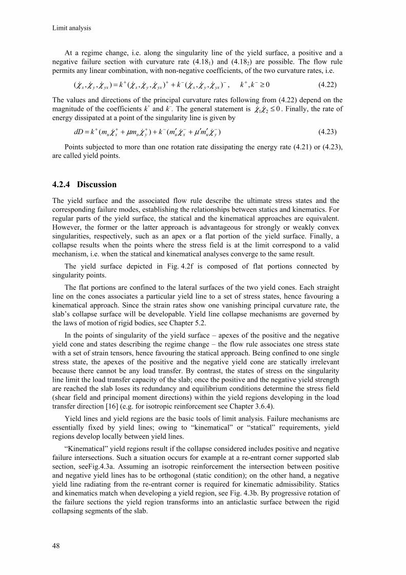
Limit analysis

48

At a regime change, i.e. along the singularity line of the yield surface, a positive and a negative failure section with curvature rate (4.181) and (4.182) are possible. The flow rule permits any linear combination, with non-negative coefficients, of the two curvature rates, i.e.

−−++ += ),,(),,(),,( yxyxyxyxyxyx kk χχχχχχχχχ &&&&&&&&& , 0, ≥−+ kk (4.22)

The values and directions of the principal curvature rates following from (4.22) depend on the magnitude of the coefficients k+ and k–. The general statement is 021 ≤χχ && . Finally, the rate of energy dissipated at a point of the singularity line is given by

)()( −−−+++ ′′+′++= yuxuyuxu mmkmmkdD χµχχµχ &&&& (4.23)

Points subjected to more than one rotation rate dissipating the energy rate (4.21) or (4.23), are called yield points.

4.2.4 Discussion

The yield surface and the associated flow rule describe the ultimate stress states and the corresponding failure modes, establishing the relationships between statics and kinematics. For regular parts of the yield surface, the statical and the kinematical approaches are equivalent. However, the former or the latter approach is advantageous for strongly or weakly convex singularities, respectively, such as an apex or a flat portion of the yield surface. Finally, a collapse results when the points where the stress field is at the limit correspond to a valid mechanism, i.e. when the statical and kinematical analyses converge to the same result. The yield surface depicted in Fig. 4.2f is composed of flat portions connected by singularity points.

The flat portions are confined to the lateral surfaces of the two yield cones. Each straight line on the cones associates a particular yield line to a set of stress states, hence favouring a kinematical approach. Since the strain rates show one vanishing principal curvature rate, the slab’s collapse surface will be developable. Yield line collapse mechanisms are governed by the laws of motion of rigid bodies, see Chapter 5.2.

In the points of singularity of the yield surface – apexes of the positive and the negative yield cone and states describing the regime change – the flow rule associates one stress state with a set of strain tensors, hence favouring the statical approach. Being confined to one single stress state, the apexes of the positive and the negative yield cone are statically irrelevant because there cannot be any load transfer. By contrast, the states of stress on the singularity line limit the load transfer capacity of the slab; once the positive and the negative yield strength are reached the slab loses its redundancy and equilibrium conditions determine the stress field (shear field and principal moment directions) within the yield regions developing in the load transfer direction [16] (e.g. for isotropic reinforcement see Chapter 3.6.4).

Yield lines and yield regions are the basic tools of limit analysis. Failure mechanisms are essentially fixed by yield lines; owing to “kinematical” or “statical” requirements, yield regions develop locally between yield lines. “Kinematical” yield regions result if the collapse considered includes positive and negative failure intersections. Such a situation occurs for example at a re-entrant corner supported slab section, seeFig.4.3a. Assuming an isotropic reinforcement the intersection between positive and negative yield lines has to be orthogonal (static condition); on the other hand, a negative yield line radiating from the re-entrant corner is required for kinematic admissibility. Statics and kinematics match when developing a yield region, see Fig. 4.3b. By progressive rotation of the failure sections the yield region transforms into an anticlastic surface between the rigid collapsing segments of the slab.

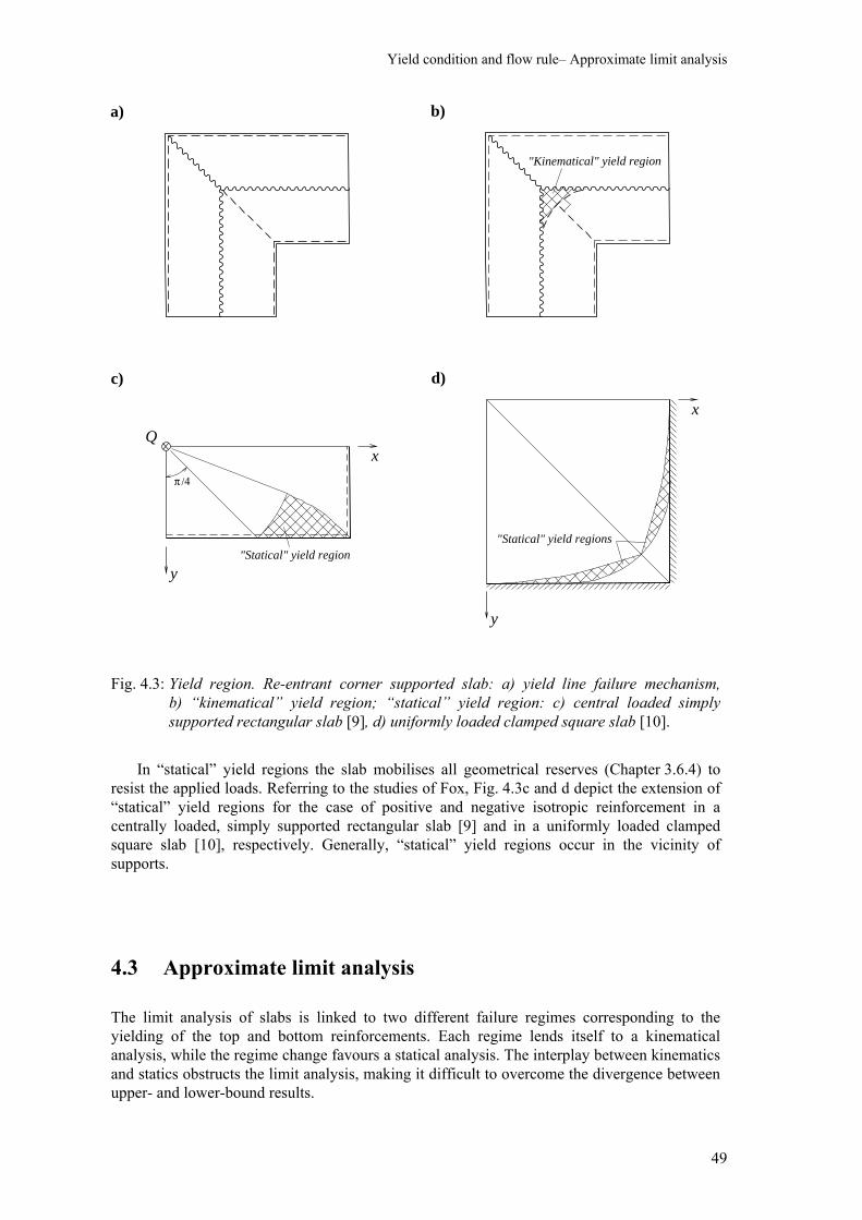
Yield condition and flow rule– Approximate limit analysis

49

Fig. 4.3: Yield region. Re-entrant corner supported slab: a) yield line failure mechanism, b) “kinematical” yield region; “statical” yield region: c) central loaded simply supported rectangular slab [9], d) uniformly loaded clamped square slab [10].

In “statical” yield regions the slab mobilises all geometrical reserves (Chapter 3.6.4) to resist the applied loads. Referring to the studies of Fox, Fig. 4.3c and d depict the extension of “statical” yield regions for the case of positive and negative isotropic reinforcement in a centrally loaded, simply supported rectangular slab [9] and in a uniformly loaded clamped square slab [10], respectively. Generally, “statical” yield regions occur in the vicinity of supports.

4.3 Approximate limit analysis

The limit analysis of slabs is linked to two different failure regimes corresponding to the yielding of the top and bottom reinforcements. Each regime lends itself to a kinematical analysis, while the regime change favours a statical analysis. The interplay between kinematics and statics obstructs the limit analysis, making it difficult to overcome the divergence between upper- and lower-bound results.

a) b)

"Kinematical" yield region

c) d)

x

y

Q

"Statical" yield region

/4π

x

y

"Statical" yield regions

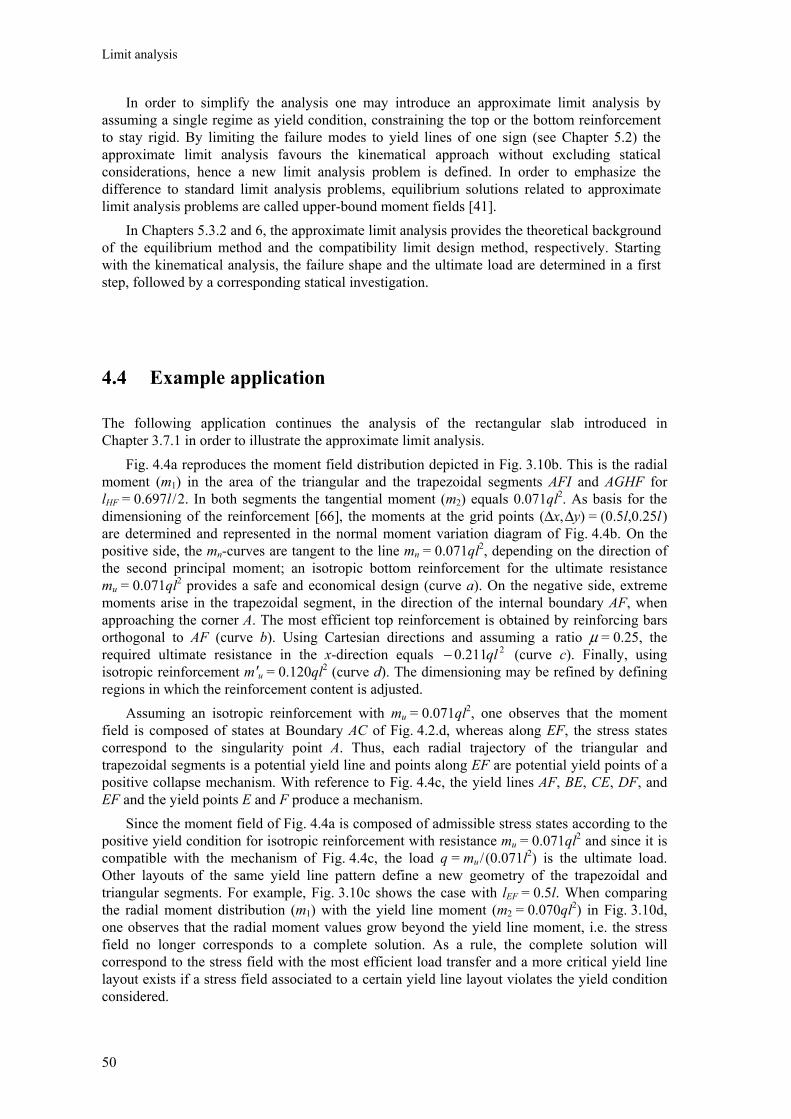
Limit analysis

50

In order to simplify the analysis one may introduce an approximate limit analysis by assuming a single regime as yield condition, constraining the top or the bottom reinforcement to stay rigid. By limiting the failure modes to yield lines of one sign (see Chapter 5.2) the approximate limit analysis favours the kinematical approach without excluding statical considerations, hence a new limit analysis problem is defined. In order to emphasize the difference to standard limit analysis problems, equilibrium solutions related to approximate limit analysis problems are called upper-bound moment fields [41]. In Chapters 5.3.2 and 6, the approximate limit analysis provides the theoretical background of the equilibrium method and the compatibility limit design method, respectively. Starting with the kinematical analysis, the failure shape and the ultimate load are determined in a first step, followed by a corresponding statical investigation.

4.4 Example application

The following application continues the analysis of the rectangular slab introduced in Chapter 3.7.1 in order to illustrate the approximate limit analysis.

Fig. 4.4a reproduces the moment field distribution depicted in Fig. 3.10b. This is the radial moment (m1) in the area of the triangular and the trapezoidal segments AFI and AGHF for lHF = 0.697l / 2. In both segments the tangential moment (m2) equals 0.071ql2. As basis for the dimensioning of the reinforcement [66], the moments at the grid points (∆x, ∆y) = (0.5l,0.25l ) are determined and represented in the normal moment variation diagram of Fig. 4.4b. On the positive side, the mn-curves are tangent to the line mn = 0.071ql2, depending on the direction of the second principal moment; an isotropic bottom reinforcement for the ultimate resistance mu = 0.071ql2 provides a safe and economical design (curve a). On the negative side, extreme moments arise in the trapezoidal segment, in the direction of the internal boundary AF, when approaching the corner A. The most efficient top reinforcement is obtained by reinforcing bars orthogonal to AF (curve b). Using Cartesian directions and assuming a ratio µ = 0.25, the required ultimate resistance in the x-direction equals 2211.0 ql− (curve c). Finally, using isotropic reinforcement m′u = 0.120ql2 (curve d). The dimensioning may be refined by defining regions in which the reinforcement content is adjusted. Assuming an isotropic reinforcement with mu = 0.071ql2, one observes that the moment field is composed of states at Boundary AC of Fig. 4.2.d, whereas along EF, the stress states correspond to the singularity point A. Thus, each radial trajectory of the triangular and trapezoidal segments is a potential yield line and points along EF are potential yield points of a positive collapse mechanism. With reference to Fig. 4.4c, the yield lines AF, BE, CE, DF, and EF and the yield points E and F produce a mechanism.

Since the moment field of Fig. 4.4a is composed of admissible stress states according to the positive yield condition for isotropic reinforcement with resistance mu = 0.071ql2 and since it is compatible with the mechanism of Fig. 4.4c, the load q = mu / (0.071l2) is the ultimate load. Other layouts of the same yield line pattern define a new geometry of the trapezoidal and triangular segments. For example, Fig. 3.10c shows the case with lEF = 0.5l. When comparing the radial moment distribution (m1) with the yield line moment (m2 = 0.070ql2) in Fig. 3.10d, one observes that the radial moment values grow beyond the yield line moment, i.e. the stress field no longer corresponds to a complete solution. As a rule, the complete solution will correspond to the stress field with the most efficient load transfer and a more critical yield line layout exists if a stress field associated to a certain yield line layout violates the yield condition considered.

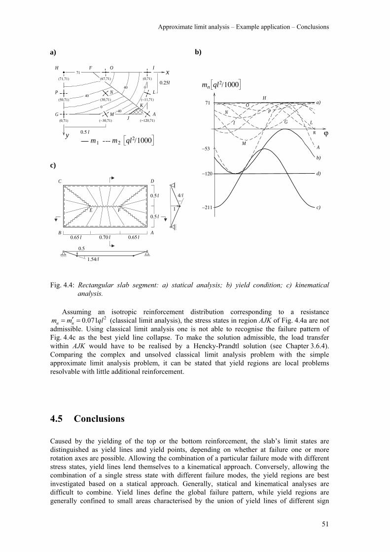
Approximate limit analysis – Example application – Conclusions

51

Fig. 4.4: Rectangular slab segment: a) statical analysis; b) yield condition; c) kinematical analysis.

Assuming an isotropic reinforcement distribution corresponding to a resistance 2071.0 qlmm uu =′= (classical limit analysis), the stress states in region AJK of Fig. 4.4a are not

admissible. Using classical limit analysis one is not able to recognise the failure pattern of Fig. 4.4c as the best yield line collapse. To make the solution admissible, the load transfer within AJK would have to be realised by a Hencky-Prandtl solution (see Chapter 3.6.4). Comparing the complex and unsolved classical limit analysis problem with the simple approximate limit analysis problem, it can be stated that yield regions are local problems resolvable with little additional reinforcement.

4.5 Conclusions

Caused by the yielding of the top or the bottom reinforcement, the slab’s limit states are distinguished as yield lines and yield points, depending on whether at failure one or more rotation axes are possible. Allowing the combination of a particular failure mode with different stress states, yield lines lend themselves to a kinematical approach. Conversely, allowing the combination of a single stress state with different failure modes, the yield regions are best investigated based on a statical approach. Generally, statical and kinematical analyses are difficult to combine. Yield lines define the global failure pattern, while yield regions are generally confined to small areas characterised by the union of yield lines of different sign

a)

ϕ

m n

π

−211

−120

−53

71

b)

c)

d)

b)

c)

1

0.5

4/l

1.54/l

l0.5

0.65 l0.70l

l0.5

0.65 l

l0.25

l0.5

x

y

(71,71) (67,71) (0,71)

(50,71) (30,71) (−11,71)

(0,71) (−120,71)

1000m /ql21 m2

(−30,71)

71

040

0−40

40

H F I

G A

AB

C D

E F

a)

J

K

LP

O

N

M

H

I G

A

L

PO

N

M

1000/ql2

Limit analysis

52

(“kinematical” requirement) or by a mobilisation of all statical reserves (“statical” requirement). Due to its complexity, standard limit analysis of slabs is of little practical interest.

To overcome the difficulties of standard limit analysis, it is suggested to select a single failure regime as the governing yield condition, i.e. to prevent yielding in one reinforcement layer by means of some extra reinforcement; yield line failures are limited to one sign. Supplementing the kinematical study by statical considerations and thus establishing compatibility, the approximate limit analysis problem is completely solved and the extra reinforcement is quantified. Consistent with the theory of plasticity and simpler than standard limit analysis, the approximate limit analysis forms the basis of a review of Johansen’s equilibrium method (Chapter 5.3.2) and of a new design method – the compatibility limit design method (Chapter 6).

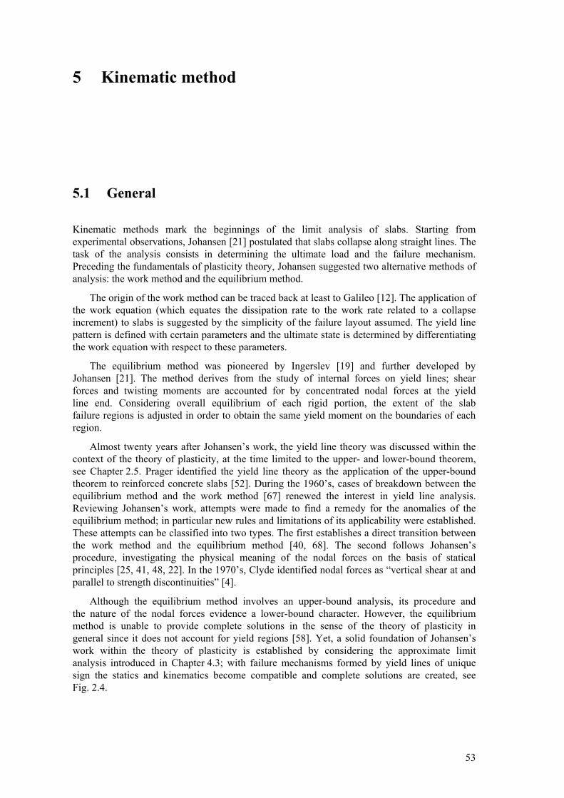
53

5 Kinematic method

5.1 General

Kinematic methods mark the beginnings of the limit analysis of slabs. Starting from experimental observations, Johansen [21] postulated that slabs collapse along straight lines. The task of the analysis consists in determining the ultimate load and the failure mechanism. Preceding the fundamentals of plasticity theory, Johansen suggested two alternative methods of analysis: the work method and the equilibrium method.

The origin of the work method can be traced back at least to Galileo [12]. The application of the work equation (which equates the dissipation rate to the work rate related to a collapse increment) to slabs is suggested by the simplicity of the failure layout assumed. The yield line pattern is defined with certain parameters and the ultimate state is determined by differentiating the work equation with respect to these parameters.

The equilibrium method was pioneered by Ingerslev [19] and further developed by Johansen [21]. The method derives from the study of internal forces on yield lines; shear forces and twisting moments are accounted for by concentrated nodal forces at the yield line end. Considering overall equilibrium of each rigid portion, the extent of the slab failure regions is adjusted in order to obtain the same yield moment on the boundaries of each region.

Almost twenty years after Johansen’s work, the yield line theory was discussed within the context of the theory of plasticity, at the time limited to the upper- and lower-bound theorem, see Chapter 2.5. Prager identified the yield line theory as the application of the upper-bound theorem to reinforced concrete slabs [52]. During the 1960’s, cases of breakdown between the equilibrium method and the work method [67] renewed the interest in yield line analysis. Reviewing Johansen’s work, attempts were made to find a remedy for the anomalies of the equilibrium method; in particular new rules and limitations of its applicability were established. These attempts can be classified into two types. The first establishes a direct transition between the work method and the equilibrium method [40, 68]. The second follows Johansen’s procedure, investigating the physical meaning of the nodal forces on the basis of statical principles [25, 41, 48, 22]. In the 1970’s, Clyde identified nodal forces as “vertical shear at and parallel to strength discontinuities” [4].

Although the equilibrium method involves an upper-bound analysis, its procedure and the nature of the nodal forces evidence a lower-bound character. However, the equilibrium method is unable to provide complete solutions in the sense of the theory of plasticity in general since it does not account for yield regions [58]. Yet, a solid foundation of Johansen’s work within the theory of plasticity is established by considering the approximate limit analysis introduced in Chapter 4.3; with failure mechanisms formed by yield lines of unique sign the statics and kinematics become compatible and complete solutions are created, see Fig. 2.4.

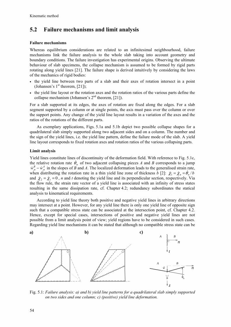
Kinematic method

54

5.2 Failure mechanisms and limit analysis

Failure mechanisms Whereas equilibrium considerations are related to an infinitesimal neighbourhood, failure mechanisms link the failure analysis to the whole slab taking into account geometry and boundary conditions. The failure investigation has experimental origins. Observing the ultimate behaviour of slab specimens, the collapse mechanism is assumed to be formed by rigid parts rotating along yield lines [21]. The failure shape is derived intuitively by considering the laws of the mechanics of rigid bodies: • the yield line between two parts of a slab and their axes of rotation intersect in a point

(Johansen’s 1st theorem, [21]); • the yield line layout or the rotation axes and the rotation ratios of the various parts define the

collapse mechanism (Johansen’s 2nd theorem, [21]). For a slab supported at its edges, the axes of rotation are fixed along the edges. For a slab segment supported by a column or at single points, the axis must pass over the column or over the support points. Any change of the yield line layout results in a variation of the axes and the ratios of the rotations of the different parts. As exemplary applications, Figs. 5.1a and 5.1b depict two possible collapse shapes for a quadrilateral slab simply supported along two adjacent sides and on a column. The number and the sign of the yield lines, i.e. the yield line pattern, define the failure mode of the slab. A yield line layout corresponds to fixed rotation axes and rotation ratios of the various collapsing parts.

Limit analysis Yield lines constitute lines of discontinuity of the deformation field. With reference to Fig. 5.1c, the relative rotation rate nθ& of two adjacent collapsing pieces A and B corresponds to a jump

An

Bn ww ,, && − in the slopes of B and A. The localized deformation leads to the generalised strain rate,

when distributing the rotation rate in a thin yield line zone of thickness b [2]: bnn /1 θχχ &&& == and 02 == tχχ && , n and t denoting the yield line and its perpendicular section, respectively. Via the flow rule, the strain rate vector of a yield line is associated with an infinity of stress states resulting in the same dissipation rate, cf. Chapter 4.2; redundancy subordinates the statical analysis to kinematical requirements. According to yield line theory both positive and negative yield lines in arbitrary directions may intersect at a point. However, for any yield line there is only one yield line of opposite sign such that a compatible stress state can be associated at the intersection point, cf. Chapter 4.2. Hence, except for special cases, intersections of positive and negative yield lines are not possible from a limit analysis point of view; yield regions have to be considered in such cases. Regarding yield line mechanisms it can be stated that although no compatible stress state can be

Fig. 5.1: Failure analysis: a) and b) yield line patterns for a quadrilateral slab simply supported on two sides and one column; c) (positive) yield line deformation.

a) b) c)

nA B

θ.

b n

n

t

A B

z

w.

Failure mechanisms and limit analysis – Upper-bound method

55

associated to positive and negative yield line intersections in general the work equation remains unaffected since the integration width and hence the dissipation at the intersection point vanishes.

Starting from yield line considerations and establishing compatibility with the statical analysis, the approximate limit analysis (see Chapter 4.3) restricts yield line mechanisms to be formed by yield lines of unique sign. There are exceptions to this rule, i.e. yield lines which may be replaced by a boundary condition (e.g. along clamped edges) or which act like a support (e.g. rotation axis over the column in Fig. 5.1b).

5.3 Upper-bound method

In plasticity theory, the kinematical analysis is governed by the upper-bound theorem and complete solutions may be singled out with a statical analysis by applying the compatibility theorem (see Fig. 2.4). In reinforced concrete slabs, the application of the upper-bound theorem to yield line failures leads to the work method. Considering approximate limit analysis problems, the application of the compatibility theorem corresponds to applying the equilibrium method.

5.3.1 Work method

In a failure mechanism, the work produced by the external load q on a deflection w is given by

∫∫=surface

dAwqW (5.1)

while the energy dissipation equals

MdDlinesyield

⋅= ∫θθθθ (5.2)

where θθθθ and dM indicate the rotation vector and the moment vector on an infinitesimal yield line portion, respectively.

In the case of yield line failures (see Chapter 5.2), Eq. (5.2) may be evaluated by means of the normal method or the component vector method [23]. The normal method focuses on the analysis of single yield lines determining the energy dissipation nnn lm

uθ , where nθ ,

unm and ln are the yield line rotation, the ultimate bending moment and the yield line length, respectively. The component vector method focuses on the analysis of the collapsing pieces, making use of the invariance of the rotation rate. Referring to the global system of reference xy defined by the reinforcement and to the ratio µ between the ultimate bending moments in x- and y-direction, the energy dissipated along the boundary of a collapsing piece equals yuyxux lmlm µθθ + . The parameters xθ , yθ , um , umµ and lx, ly designate the yield line rotation components, the yield moments and the projection lengths of the boundary yield lines of the piece considered, all in the x- and y-directions, respectively. The total dissipation is obtained by summing the dissipation of each yield line or of each collapsing piece, respectively.

The approximation of the ultimate load (limit analysis) or the estimation of the required amount of reinforcement (limit design) follows by equating Eq. (5.1) to Eq. (5.2).

For a fixed yield line pattern, the most critical failure mechanism is determined by defining the yield line pattern with certain parameters and looking for the maximum ratio W / D.

Kinematic method

56

Examples In the following the work method is applied to four examples. Starting with the analysis of an isotropically reinforced slab, the application is extended to the case of orthotropic reinforcement. The last two examples investigate the reliability of the work method by comparing different upper-bound studies.

a) Rectangular slab Consider the uniformly loaded simply supported rectangular slab with side lengths l and 2l introduced in Chapter 3.7.1. For a given load intensity q, the work method is applied to estimate the required plastic moment mu (isotropic reinforcement). Fig. 5.2a depicts the failure mechanism on the basis of the upper-bound analysis. The collapse shape divides the slab into two trapezoidal ( ABEF, CDEF ) and two triangular ( AFD, BCE ) segments. Since the axes of rotation of the trapezoidal segments do not meet, the central fracture line EF is parallel to the edges AB and CD. Considering the symmetry in the geometry, the load and the resistance distribution, the yield line layout is defined by a single parameter, for instance the length x of the line EF. Assuming a unit deflection of line EF (see Fig. 4.4c), the work produced by the external loads at failure equals ]2/3/)2[( lxlxlq +− . During the collapse, the fracture lines EF and AF (or, equivalently, BE, CE and DF) rotate by θEF = 4 / l and )]2(/[])2([ 22 xlllxll AFAF −−+=θ , respectively, where =2

AFl (5l2 – 4lx + x2

) / 4. Summing the contributions of each yield line, i.e. AFuAFEFuEF lmlm θθ 4+ , the normal method leads to a total dissipation of )]2/(48[ xllmu −+ . Alternatively, the energy dissipation may be determined with the component vector method. Due to symmetry, only the pieces ABEF and AFD are considered. The trapezoidal and the triangular segments rotate by 2 / l and 2 / (2l – x) respectively. The ultimate bending moments at the sections BE-EF-FA and AF-FD have the resultants 2mul and mul in the directions BA and AD, respectively. Hence, the dissipated energy equals 2(θABEF MABEF + θAFD MAFD ) = mu [8 + 4l / (2l – x)]. Equating the external work to the total dissipation, one obtains mu / ql2 = (4 + x / l) (2 – x / l) / / [24 (5 – 2x / l )]. Fig. 5.2a depicts the variation of mu / ql2 as a function of x / l. The most critical mechanism results for x = 0.697l, where mu = 0.071ql2.

b) Triangular slab with one free edge Consider the triangular slab ABC simply supported along the edges AB and BC and free along AC subjected to a uniformly distributed load q, see Fig. 5.2b. The edges AB and BC have lengths of 3l and 2l, respectively. The following analysis aims at determining the ratio µ between the ultimate bending moments in the y- and the x-direction, so as to obtain the highest load carrying capacity for a fixed reinforcement amount. The kinematical study is performed with a single positive yield line radiating from B. The yield line pattern is defined by the distance x of point D from the boundary BC, see Fig. 5.2b. When D undergoes a unit deflection, the work of the external load equals ql2. During collapse the yield line BD rotates by θBD = [4 (3l – x )2

+ 9x2] / [6x (3l – x) lBD], where 9/)3(4 222 xlxlBD −+= . According to Eq. (4.41) the bending resistance in the failure section equals

2222 /)9/()26( BDuBDun lxmlxlmmu

µ+−= , where mu denotes the bending resistance in the x- direction. The dissipation of energy obtained with the normal method is given by

)]26/(3)3/()3(2[ xlxxxlmlm uBDnBD u−+−= µθ . Note that the twisting moment

)3/()3(2)1( 2BDutn lxlxmm

u−−= µ acting together with

unm on the failure section does not dissipate energy. The same results may be obtained with the component vector method. The yield line rotation vectors of ABD and BCD are given by )0,)26/(3( xlABD −=θ and

)/1,0( xBCD =θ , respectively. The moment resultant on section BD of segment ABD is )3/)3(2,( xlmxm uuABD −−= µM and that of segment BCD is the reaction vector ABDM− .

Finally, θθθθABD·MABD + θθθθBCD·MBCD leads to the same energy dissipation.

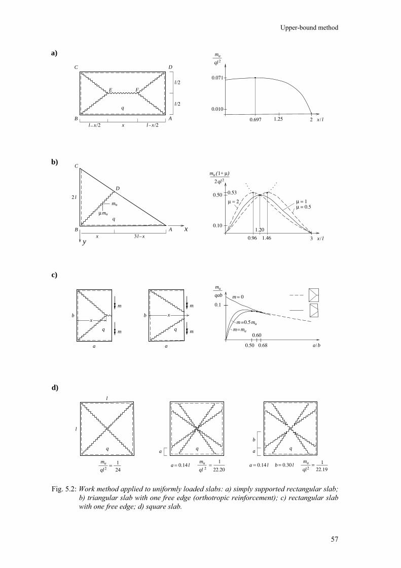
Upper-bound method

57

Fig. 5.2: Work method applied to uniformly loaded slabs: a) simply supported rectangular slab; b) triangular slab with one free edge (orthotropic reinforcement); c) rectangular slab with one free edge; d) square slab.

D

A

C

B

FE

/2 x

a)

l

l

2

0.010

0.697

A

C

B

l2

D

3 l

b)

c)

d)

0.071

x /2l x

/2

l/2

mu

mu

x x

/ lx

3

0.101.20

0.50 0.53

1.460.96

= 1µ= 0.5µ

= 2µ

q

q

ql2

ql2

m

/ lx

1.25

µ

x

y

u

12

m ( + )u µ

.... . . . . . . . . ...

ql2=

ql 2=a = 0.14 l

ql2b = 0.30 la = 0.14 l

a a

b

24 1

22.19 1=

22.20 1

l

l

q q q

mumu mu

a

b

q

a

b

qm

m

xx

m

m 0.1

0.50 / ba

qab

mu

0.60

0.68

= 0

0.5= mm u

mum=

m

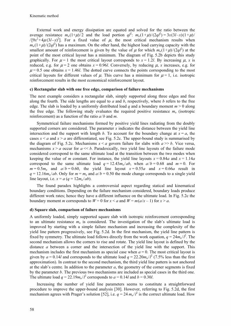
Kinematic method

58

External work and energy dissipation are equated and solved for the ratio between the average resistance mu (1+µ) / 2 and the load portion ql2: mu (1 + µ) / (2ql2) = 3x (3l – x) (1 + µ) / / [9x2

+ 4µ (3l – x)2]. For a fixed value of µ, the most critical mechanism results when mu (1 + µ) / (2ql2) has a maximum. On the other hand, the highest load carrying capacity with the smallest amount of reinforcement is given by the value of µ for which mu (1 + µ) / (2ql2) at the point of the most critical layout has a minimum. The diagram of Fig. 5.2b depicts this study graphically. For µ = 1 the most critical layout corresponds to x = 1.2l. By increasing µ, x is reduced, e.g. for µ = 2 one obtains x = 0.96l. Conversely, by reducing µ, x increases, e.g. for µ = 0.5 one obtains x = 1.46l. The dotted curve connects the points corresponding to the most critical layouts for different values of µ. This curve has a minimum for µ = 1, i.e. isotropic reinforcement results in the most economical reinforcement layout.

c) Rectangular slab with one free edge, comparison of failure mechanisms The next example considers a rectangular slab, simply supported along three edges and free along the fourth. The side lengths are equal to a and b, respectively, where b refers to the free edge. The slab is loaded by a uniformly distributed load q and a boundary moment m > 0 along the free edge. The following study evaluates the required positive resistance mu (isotropic reinforcement) as a function of the ratio a / b and m. Symmetrical failure mechanisms formed by positive yield lines radiating from the doubly supported corners are considered. The parameter x indicates the distance between the yield line intersection and the support with length b. To account for the boundary change at x = a, the cases x < a and x > a are differentiated, see Fig. 5.2c. The upper-bound study is summarised by the diagram of Fig. 5.2c. Mechanisms x < a govern failure for slabs with a >> b. Vice versa, mechanisms x > a occur for a << b. Paradoxically, two yield line layouts of the failure mode considered correspond to the same ultimate load at the transition between the two modes when keeping the value of m constant. For instance, the yield line layouts x = 0.84a and x = 1.14a correspond to the same ultimate load q = 12.43mu / ab, when a / b = 0.68 and m = 0. For m = 0.5mu and a / b = 0.60, the yield line layout x = 0.55a and x = 0.66a result in q = 12.16mu / ab. Only for m = mu and a / b = 0.50 the mode change corresponds to a single yield line layout, i.e. x = a (q = 12mu / ab). The found paradox highlights a controversial aspect regarding statical and kinematical boundary conditions. Depending on the failure mechanism considered, boundary loads produce different work rates; hence they have a different influence on the ultimate load. In Fig. 5.2c the boundary moment m corresponds to W = 0 for x < a and W = m (a /x – 1) for x > a.

d) Square slab, comparison of failure mechanisms A uniformly loaded, simply supported square slab with isotropic reinforcement corresponding to an ultimate resistance mu is considered. The investigation of the slab’s ultimate load is improved by starting with a simple failure mechanism and increasing the complexity of the yield line pattern progressively, see Fig. 5.2d. In the first mechanism, the yield line pattern is fixed by symmetry. The ultimate load follows directly from the work equation, q = 24mu / l2. The second mechanism allows the corners to rise and rotate. The yield line layout is defined by the distance a between a corner and the intersection of the yield line with the support. This mechanism includes the first mechanism as special case when a = 0. The most critical layout is given by a = 0.14l and corresponds to the ultimate load q = 22.20mu / l2 (7.5% less than the first approximation). In contrast to the second mechanism, the third yield line pattern is not anchored at the slab’s centre. In addition to the parameter a, the geometry of the corner segments is fixed by the parameter b. The previous two mechanisms are included as special cases in the third one. The ultimate load q = 22.19mu / l2 corresponds to a = 0.14l and b = 0.30l.

Increasing the number of yield line parameters seems to constitute a straightforward procedure to improve the upper-bound analysis [30]. However, referring to Fig. 5.2d, the first mechanism agrees with Prager’s solution [52], i.e. q = 24 mu / l2 is the correct ultimate load. How

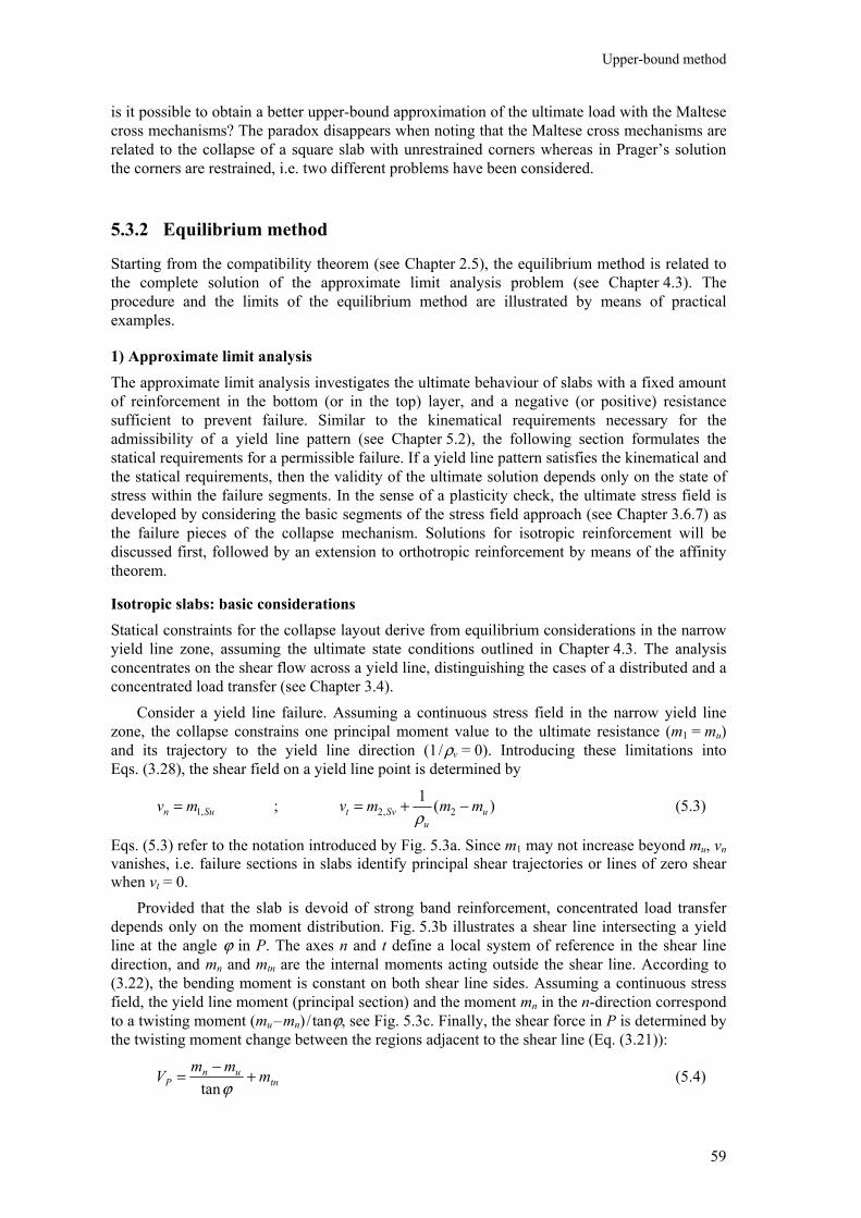
Upper-bound method

59

is it possible to obtain a better upper-bound approximation of the ultimate load with the Maltese cross mechanisms? The paradox disappears when noting that the Maltese cross mechanisms are related to the collapse of a square slab with unrestrained corners whereas in Prager’s solution the corners are restrained, i.e. two different problems have been considered.

5.3.2 Equilibrium method

Starting from the compatibility theorem (see Chapter 2.5), the equilibrium method is related to the complete solution of the approximate limit analysis problem (see Chapter 4.3). The procedure and the limits of the equilibrium method are illustrated by means of practical examples.

1) Approximate limit analysis The approximate limit analysis investigates the ultimate behaviour of slabs with a fixed amount of reinforcement in the bottom (or in the top) layer, and a negative (or positive) resistance sufficient to prevent failure. Similar to the kinematical requirements necessary for the admissibility of a yield line pattern (see Chapter 5.2), the following section formulates the statical requirements for a permissible failure. If a yield line pattern satisfies the kinematical and the statical requirements, then the validity of the ultimate solution depends only on the state of stress within the failure segments. In the sense of a plasticity check, the ultimate stress field is developed by considering the basic segments of the stress field approach (see Chapter 3.6.7) as the failure pieces of the collapse mechanism. Solutions for isotropic reinforcement will be discussed first, followed by an extension to orthotropic reinforcement by means of the affinity theorem.

Isotropic slabs: basic considerations Statical constraints for the collapse layout derive from equilibrium considerations in the narrow yield line zone, assuming the ultimate state conditions outlined in Chapter 4.3. The analysis concentrates on the shear flow across a yield line, distinguishing the cases of a distributed and a concentrated load transfer (see Chapter 3.4). Consider a yield line failure. Assuming a continuous stress field in the narrow yield line zone, the collapse constrains one principal moment value to the ultimate resistance (m1 = mu) and its trajectory to the yield line direction (1 / ρv = 0). Introducing these limitations into Eqs. (3.28), the shear field on a yield line point is determined by

Sun mv ,1= ; )(12,2 u

uSvt mmmv −+=

ρ (5.3)

Eqs. (5.3) refer to the notation introduced by Fig. 5.3a. Since m1 may not increase beyond mu, vn vanishes, i.e. failure sections in slabs identify principal shear trajectories or lines of zero shear when vt = 0. Provided that the slab is devoid of strong band reinforcement, concentrated load transfer depends only on the moment distribution. Fig. 5.3b illustrates a shear line intersecting a yield line at the angle ϕ in P. The axes n and t define a local system of reference in the shear line direction, and mn and mtn are the internal moments acting outside the shear line. According to (3.22), the bending moment is constant on both shear line sides. Assuming a continuous stress field, the yield line moment (principal section) and the moment mn in the n-direction correspond to a twisting moment (mu – mn) / tanϕ, see Fig. 5.3c. Finally, the shear force in P is determined by the twisting moment change between the regions adjacent to the shear line (Eq. (3.21)):

tnun

P mmmV +−=ϕtan

(5.4)

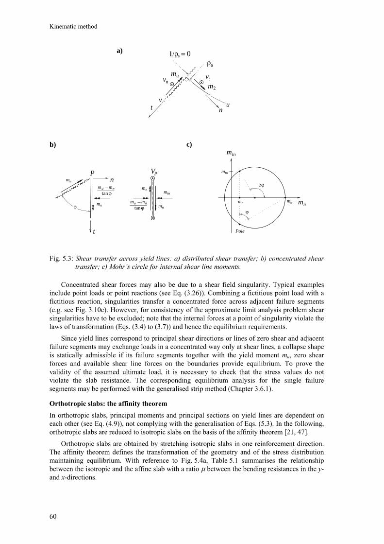
Kinematic method

60

Fig. 5.3: Shear transfer across yield lines: a) distributed shear transfer; b) concentrated shear transfer; c) Mohr’s circle for internal shear line moments.

Concentrated shear forces may also be due to a shear field singularity. Typical examples include point loads or point reactions (see Eq. (3.26)). Combining a fictitious point load with a fictitious reaction, singularities transfer a concentrated force across adjacent failure segments (e.g. see Fig. 3.10c). However, for consistency of the approximate limit analysis problem shear singularities have to be excluded; note that the internal forces at a point of singularity violate the laws of transformation (Eqs. (3.4) to (3.7)) and hence the equilibrium requirements.

Since yield lines correspond to principal shear directions or lines of zero shear and adjacent failure segments may exchange loads in a concentrated way only at shear lines, a collapse shape is statically admissible if its failure segments together with the yield moment mu, zero shear forces and available shear line forces on the boundaries provide equilibrium. To prove the validity of the assumed ultimate load, it is necessary to check that the stress values do not violate the slab resistance. The corresponding equilibrium analysis for the single failure segments may be performed with the generalised strip method (Chapter 3.6.1).

Orthotropic slabs: the affinity theorem In orthotropic slabs, principal moments and principal sections on yield lines are dependent on each other (see Eq. (4.9)), not complying with the generalisation of Eqs. (5.3). In the following, orthotropic slabs are reduced to isotropic slabs on the basis of the affinity theorem [21, 47]. Orthotropic slabs are obtained by stretching isotropic slabs in one reinforcement direction. The affinity theorem defines the transformation of the geometry and of the stress distribution maintaining equilibrium. With reference to Fig. 5.4a, Table 5.1 summarises the relationship between the isotropic and the affine slab with a ratio µ between the bending resistances in the y- and x-directions.

b)

mn

mtn

Pole

P

ϕ

VPn

t

ϕ2

ϕ

mumn

mtn

v

nt u

uρvρ

vn

mu vt

m2

1/ = 0a)

m u mn

tanϕ

mtn

mn

mn

mu

mn

m u mn

tanϕ

c)

Upper-bound method

61

Consider an isotropic slab. Fig. 5.4b (left) depicts a yield line enclosing the angle α with the x-axis. On the yield line section, the stress resultants v1 = 0, v2, m1 = mu and m2 (see Fig. 5.3a) correspond to the shear vector (vx,vy) = (v2sinα , –v2cosα) and the moment vector (mx,my,myx) = (musin2α + m2cos2α , mucos2α + m2sin2α , (mu–m2) sinα cosα) in Cartesian directions. Stretching the slab according to the coefficient µ, the yield line slope in the x-y-plane becomes

αµ tan , and the affine stress resultants are ),( yx vv µ and ),,( yxyx mmm µµ , see Table 5.1. On the yield line section of the orthotropic slab the stress resultants are obtained from considering the equilibrium of an infinitesimal triangular element generated by the Cartesian axes and a yield line portion of unit length, see Fig. 5.4b (right):

ϕϕµϕµϕ sincos)1(;)sin(cos;0 22 −=+== utnunn mmmmvuu

(5.5)

where αµαµϕ 2tan1/tancos += , αµϕ 2tan1/1sin += and (n,t) denotes the system of reference of the yield line section in the orthotropic slab. Similar to isotropic slabs, the shear force on yield line sections of orthotropic slabs vanishes (see Eq. (5.51)), whereas the internal moments are the yield moments (see Eqs. (4.4)). In analogy to Fig. 5.3b, Fig. 5.4c aims at determining the shear line forces in the case of orthotropic reinforcement. Consider a yield line - shear line intersection with the angle ϕ. Introducing the systems of reference n, t and n′, t′ in the yield line and the shear line directions, respectively, the yield moments and the shear line moments are fixed by (

unm ,utnm ) and

(mn′, mt′n′). By means of a Mohr’s circle analysis, the twisting moment within the shear line is found to be

uu tnnn mmm −− ϕtan/)( ' . Thus, the twisting moment change between the regions adjacent to the shear line determines the shear line force

nttnnn

P mmmm

Vu

u′′

′ ++−

=ϕtan

(5.6)

As in isotropic slabs, the statical admissibility of the yield line pattern in the case of orthotropic reinforcement is established by Eqs. (5.5) and (5.6) by verifying the equilibrium of the failure segments. The stress field associated to the failure mechanism is best obtained by the affinity theorem, since in contrast to orthotropic reinforcement the yield line pattern for an isotropic slab suggests the principal moment trajectories. Note that the affine transformation also applies to the principal shear trajectories, but not to the principal moment trajectories.

2) The equilibrium method The equilibrium method suggests a statical approach for the estimation of the slab’s ultimate load according to failure modes which differ from the optimum mode. Stress fields satisfying equilibrium and compatibility with the failure mechanism considered replace the differentiation process of the work method. The following discussion concentrates on isotropic slabs; orthotropic problems can be treated by applying the affinity theorem.

Isotropic slab Orthotropic slab

Geometry: - length ),( yx ),( yx µ

- slope αtan αµ tan

Loads: - distributed load q q

- line load q )2sin2/(cos αµαµ +q

- point load Q Qµ

Stress resultants: - shear force ),( yvxv ),( yvxv µ

- moment ),,( yxmymxm ),,( yxmymxm µµ

Table 5.1: Affinity theorem: transformation laws.

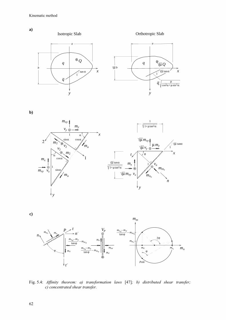
Kinematic method

62

Fig. 5.4: Affinity theorem: a) transformation laws [47]; b) distributed shear transfer;

c) concentrated shear transfer.

y

x

y

x

a)

a

b

Qq

q

Qq µ

Isotropic Slab Orthotropic Slab

αtan

q

tanαµ

a

bµ

x

y

1

2

1

1

mu

muαtan

α

1

x

y

t

n

m

m

my

mxy

vy

m

xy vx

x

m2

2

vv2

2

α

my

mxy

vy

m

mxy vx

x

m

mtn

vnµ

1 µ tan α2+

tanα

1 µ tan α2+

1

sinα

µ µµ

µ

µ

b)

µµsin α2+

cosα

sinα cosα

ϕ

c)

mn

mtn

Pole

P

ϕ

VPn

t

ϕ2

ϕmm

t

n

nu

mtnu

nu

u

nm nu mn

tanϕmtnu

m nu mn

tanϕmtnu

mn

mtn

mnm nu mn

tanϕmtnu

mn

mnumtnu

cos α2

1 1

1

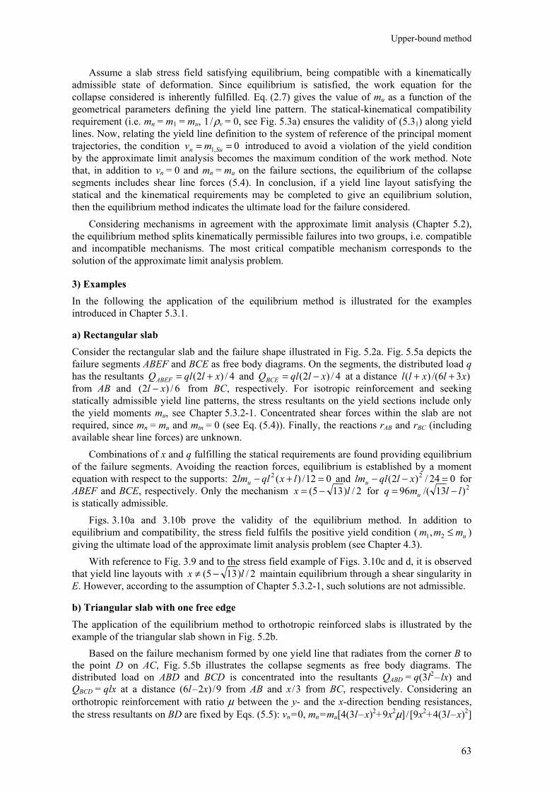
Upper-bound method

63

Assume a slab stress field satisfying equilibrium, being compatible with a kinematically admissible state of deformation. Since equilibrium is satisfied, the work equation for the collapse considered is inherently fulfilled. Eq. (2.7) gives the value of mu as a function of the geometrical parameters defining the yield line pattern. The statical-kinematical compatibility requirement (i.e. mn = m1 = mu, 1 / ρv = 0, see Fig. 5.3a) ensures the validity of (5.31) along yield lines. Now, relating the yield line definition to the system of reference of the principal moment trajectories, the condition 0,1 == Sun mv introduced to avoid a violation of the yield condition by the approximate limit analysis becomes the maximum condition of the work method. Note that, in addition to vn = 0 and mn = mu on the failure sections, the equilibrium of the collapse segments includes shear line forces (5.4). In conclusion, if a yield line layout satisfying the statical and the kinematical requirements may be completed to give an equilibrium solution, then the equilibrium method indicates the ultimate load for the failure considered.

Considering mechanisms in agreement with the approximate limit analysis (Chapter 5.2), the equilibrium method splits kinematically permissible failures into two groups, i.e. compatible and incompatible mechanisms. The most critical compatible mechanism corresponds to the solution of the approximate limit analysis problem.

3) Examples In the following the application of the equilibrium method is illustrated for the examples introduced in Chapter 5.3.1.

a) Rectangular slab Consider the rectangular slab and the failure shape illustrated in Fig. 5.2a. Fig. 5.5a depicts the failure segments ABEF and BCE as free body diagrams. On the segments, the distributed load q has the resultants 4/)2( xlqlQABEF += and 4/)2( xlqlQBCE −= at a distance )36/()( xlxll ++ from AB and 6/)2( xl − from BC, respectively. For isotropic reinforcement and seeking statically admissible yield line patterns, the stress resultants on the yield sections include only the yield moments mu, see Chapter 5.3.2-1. Concentrated shear forces within the slab are not required, since mn = mu and mtn = 0 (see Eq. (5.4)). Finally, the reactions rAB and rBC (including available shear line forces) are unknown.

Combinations of x and q fulfilling the statical requirements are found providing equilibrium of the failure segments. Avoiding the reaction forces, equilibrium is established by a moment equation with respect to the supports: 012/)(2 2 =+− lxqllmu and 024/)2( 2 =−− xlqllmu for ABEF and BCE, respectively. Only the mechanism 2/)135( lx −= for 2)13/(96 llmq u −= is statically admissible.

Figs. 3.10a and 3.10b prove the validity of the equilibrium method. In addition to equilibrium and compatibility, the stress field fulfils the positive yield condition ( ummm ≤21, ) giving the ultimate load of the approximate limit analysis problem (see Chapter 4.3).

With reference to Fig. 3.9 and to the stress field example of Figs. 3.10c and d, it is observed that yield line layouts with 2/)135( lx −≠ maintain equilibrium through a shear singularity in E. However, according to the assumption of Chapter 5.3.2-1, such solutions are not admissible.

b) Triangular slab with one free edge The application of the equilibrium method to orthotropic reinforced slabs is illustrated by the example of the triangular slab shown in Fig. 5.2b. Based on the failure mechanism formed by one yield line that radiates from the corner B to the point D on AC, Fig. 5.5b illustrates the collapse segments as free body diagrams. The distributed load on ABD and BCD is concentrated into the resultants QABD = q(3l2

– lx) and QBCD = qlx at a distance (6l – 2x) / 9 from AB and x / 3 from BC, respectively. Considering an orthotropic reinforcement with ratio µ between the y- and the x-direction bending resistances, the stress resultants on BD are fixed by Eqs. (5.5): vn = 0, mn = mu[4(3l – x)2+ 9x2µ] / [9x2+ 4(3l – x)2]

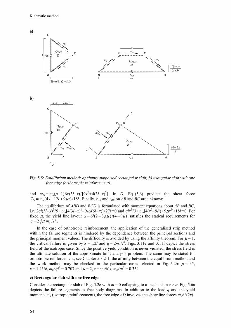
Kinematic method

64

Fig. 5.5: Equilibrium method: a) simply supported rectangular slab; b) triangular slab with one free edge (orthotropic reinforcement).

and mtn = mu(µ – 1) 6x (3l – x) / [9x2 + 4(3l – x)2]. In D, Eq. (5.6) predicts the shear force

lxlxmV uD 18/)9124( µ+−= . Finally, rAB and rBC on AB and BC are unknown.

The equilibrium of ABD and BCD is formulated with moment equations about AB and BC, i.e. 2ql(3l – x)2

/ 9 + mu[4(3l – x)2 – 9µx(6l – x)] / 27l = 0 and qlx2

/ 3 + mu[4(x2 – 9l2) + 9µx2] / 18l = 0. For

fixed µ, the yield line layout )94/()32(6 µµ −−= lx satisfies the statical requirements for 2/2 lmq uµ= .

In the case of orthotropic reinforcement, the application of the generalised strip method within the failure segments is hindered by the dependence between the principal sections and the principal moment values. The difficulty is avoided by using the affinity theorem. For µ = 1, the critical failure is given by x = 1.2l and q = 2mu / l2. Figs. 3.11e and 3.11f depict the stress field of the isotropic case. Since the positive yield condition is never violated, the stress field is the ultimate solution of the approximate limit analysis problem. The same may be stated for orthotropic reinforcement, see Chapter 5.3.2-1; the affinity between the equilibrium method and the work method may be checked in the particular cases selected in Fig. 5.2b: µ = 0.5, x = 1.456l, mu / ql2 = 0.707 and µ = 2, x = 0.961l, mu / ql2 = 0.354.

c) Rectangular slab with one free edge Consider the rectangular slab of Fig. 5.2c with m = 0 collapsing to a mechanism x > a. Fig. 5.6a depicts the failure segments as free body diagrams. In addition to the load q and the yield moments mu (isotropic reinforcement), the free edge AD involves the shear line forces mub / (2x)

b)

QBCD

D

VD

mn

B x

y

C

x /3

rBC

DVD

t

B

n

QABD

A

6 l x

92

rAB

a)

u mtnu

mnumtnu

mu

B A

E F

QABEF

rAB

( + )l x

3l

+ l x6

mumu

l2

x

B

C

EQBCE

rBC

mu

mu

( )/6l x2 ( )/3l x2

l

x /32

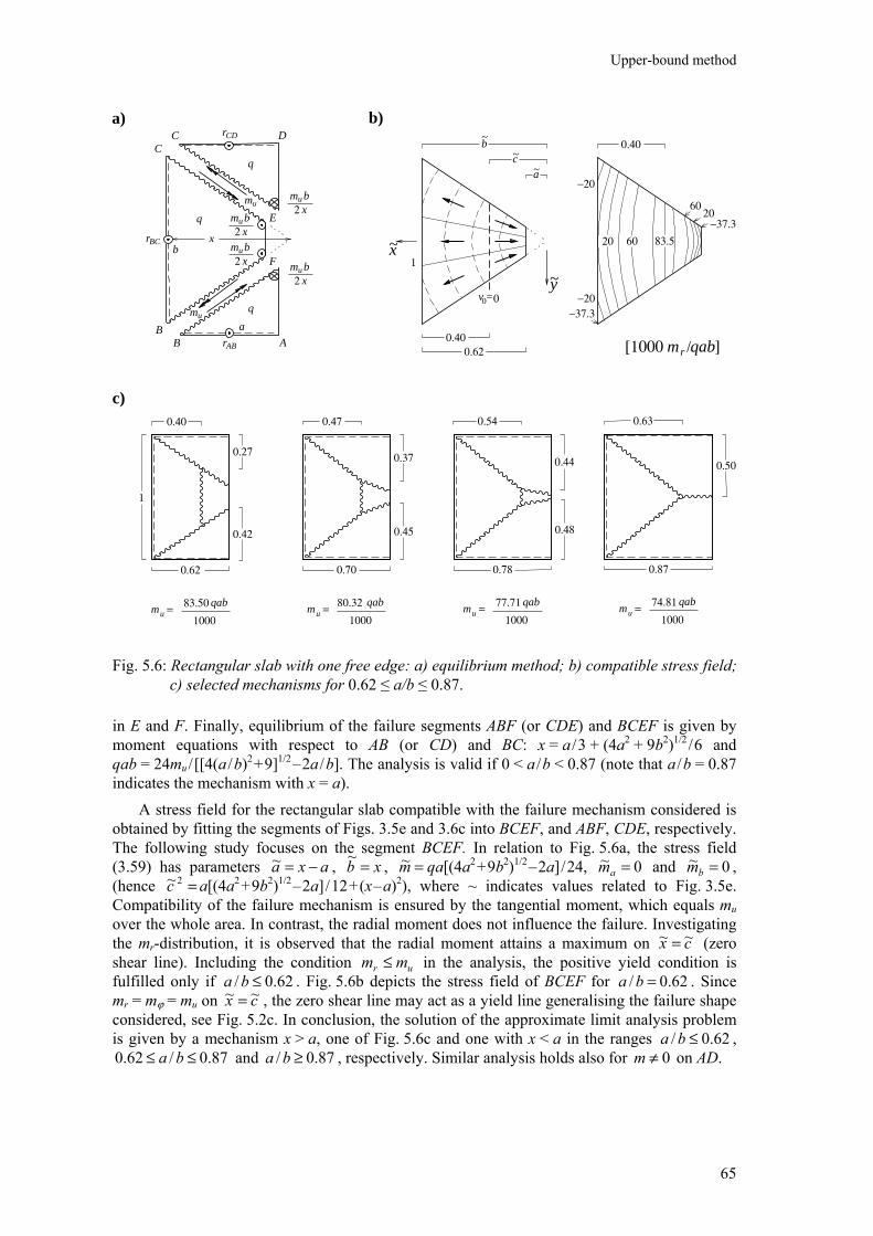
Upper-bound method

65

Fig. 5.6: Rectangular slab with one free edge: a) equilibrium method; b) compatible stress field; c) selected mechanisms for 0.62 ≤ a/b ≤ 0.87.

in E and F. Finally, equilibrium of the failure segments ABF (or CDE) and BCEF is given by moment equations with respect to AB (or CD) and BC: x = a / 3 + (4a2 + 9b2)1/2

/ 6 and qab = 24mu / [[4(a / b)2

+ 9]1/2 – 2a / b]. The analysis is valid if 0 < a / b < 0.87 (note that a / b = 0.87

indicates the mechanism with x = a). A stress field for the rectangular slab compatible with the failure mechanism considered is obtained by fitting the segments of Figs. 3.5e and 3.6c into BCEF, and ABF, CDE, respectively. The following study focuses on the segment BCEF. In relation to Fig. 5.6a, the stress field (3.59) has parameters axa −=~ , xb =~ , =m~ qa[(4a2

+ 9b2)1/2 – 2a] / 24, 0~ =am and 0~ =bm ,

(hence =2~c a[(4a2 + 9b2)1/2

– 2a] / 12 + (x – a)2), where ~ indicates values related to Fig. 3.5e. Compatibility of the failure mechanism is ensured by the tangential moment, which equals mu over the whole area. In contrast, the radial moment does not influence the failure. Investigating the mr-distribution, it is observed that the radial moment attains a maximum on cx ~~ = (zero shear line). Including the condition ur mm ≤ in the analysis, the positive yield condition is fulfilled only if 62.0/ ≤ba . Fig. 5.6b depicts the stress field of BCEF for 62.0/ =ba . Since mr = mϕ = mu on cx ~~ = , the zero shear line may act as a yield line generalising the failure shape considered, see Fig. 5.2c. In conclusion, the solution of the approximate limit analysis problem is given by a mechanism x > a, one of Fig. 5.6c and one with x < a in the ranges 62.0/ ≤ba ,

87.0/62.0 ≤≤ ba and 87.0/ ≥ba , respectively. Similar analysis holds also for 0≠m on AD.

1

0.62 0.70 0.78 0.87

0.42 0.45 0.48

0.500.27

0.40

0.37 0.44

0.47 0.54 0.63

v 0=0

0.40

1

0.62 [1000 mr /qab]

83.56020

−20

−20

6020

−37.3

−37.3

bx

a

q

q

q

mu

mu

mu bx2

mu bx2

mu bx2

mu bx2

a) b)

c)

0.40

rBC

ABB

CC D

E

F

rAB

rCD

mu 83.50 qab=

1000mu

80.32 qab=1000

mu 77.71 qab=

1000mu

74.81 qab=1000

y

x

b~

c~

a~

~

~

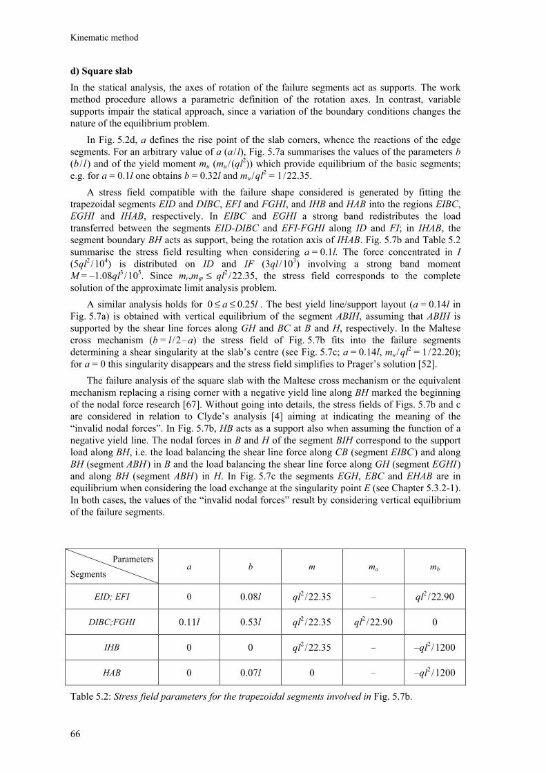
Kinematic method

66

d) Square slab In the statical analysis, the axes of rotation of the failure segments act as supports. The work method procedure allows a parametric definition of the rotation axes. In contrast, variable supports impair the statical approach, since a variation of the boundary conditions changes the nature of the equilibrium problem. In Fig. 5.2d, a defines the rise point of the slab corners, whence the reactions of the edge segments. For an arbitrary value of a (a / l), Fig. 5.7a summarises the values of the parameters b (b / l ) and of the yield moment mu (mu / (ql2)) which provide equilibrium of the basic segments; e.g. for a = 0.1l one obtains b = 0.32l and mu / ql2 = 1 / 22.35. A stress field compatible with the failure shape considered is generated by fitting the trapezoidal segments EID and DIBC, EFI and FGHI, and IHB and HAB into the regions EIBC, EGHI and IHAB, respectively. In EIBC and EGHI a strong band redistributes the load transferred between the segments EID-DIBC and EFI-FGHI along ID and FI; in IHAB, the segment boundary BH acts as support, being the rotation axis of IHAB. Fig. 5.7b and Table 5.2 summarise the stress field resulting when considering a = 0.1l. The force concentrated in I (5ql2

/ 104) is distributed on ID and IF (3ql / 103) involving a strong band moment M = –1.08ql3

/ 105. Since mr,mϕ ≤ ql2 / 22.35, the stress field corresponds to the complete

solution of the approximate limit analysis problem. A similar analysis holds for la 25.00 ≤≤ . The best yield line/support layout (a = 0.14l in Fig. 5.7a) is obtained with vertical equilibrium of the segment ABIH, assuming that ABIH is supported by the shear line forces along GH and BC at B and H, respectively. In the Maltese cross mechanism (b = l / 2 – a) the stress field of Fig. 5.7b fits into the failure segments determining a shear singularity at the slab’s centre (see Fig. 5.7c; a = 0.14l, mu / ql2 = 1 / 22.20); for a = 0 this singularity disappears and the stress field simplifies to Prager’s solution [52]. The failure analysis of the square slab with the Maltese cross mechanism or the equivalent mechanism replacing a rising corner with a negative yield line along BH marked the beginning of the nodal force research [67]. Without going into details, the stress fields of Figs. 5.7b and c are considered in relation to Clyde’s analysis [4] aiming at indicating the meaning of the “invalid nodal forces”. In Fig. 5.7b, HB acts as a support also when assuming the function of a negative yield line. The nodal forces in B and H of the segment BIH correspond to the support load along BH, i.e. the load balancing the shear line force along CB (segment EIBC ) and along BH (segment ABH ) in B and the load balancing the shear line force along GH (segment EGHI ) and along BH (segment ABH ) in H. In Fig. 5.7c the segments EGH, EBC and EHAB are in equilibrium when considering the load exchange at the singularity point E (see Chapter 5.3.2-1). In both cases, the values of the “invalid nodal forces” result by considering vertical equilibrium of the failure segments.

Parameters Segments

a b m ma mb

EID; EFI 0 0.08l ql2 / 22.35 – ql2

/ 22.90

DIBC;FGHI 0.11l 0.53l ql2 / 22.35 ql2

/ 22.90 0

IHB 0 0 ql2 / 22.35 – –ql2

/ 1200

HAB 0 0.07l 0 – –ql2 / 1200

Table 5.2: Stress field parameters for the trapezoidal segments involved in Fig. 5.7b.

Upper-bound method – Discussion

67

Fig. 5.7: Square slab: a) equilibrium analysis; b) example of compatible stress field (a = 0.10l, b = 0.32l, mu = ql2

/ 22.35); c) stress field for the Maltese cross mechanism (a = 0.14l, mu = ql2

/ 22.20).

5.4 Discussion

As an application of the compatibility theorem, the equilibrium method lies between the kinematical and statical methods (see Fig. 2.4). Since compatibility refers to an extension of the yield surface, the equilibrium method clearly constitutes an upper-bound method. Through equilibrium, the failure analysis matches a complete structural analysis. Defining the limits of applicability of the equilibrium method, the following considerations aim at illustrating the advantages of compatibility.

a)

0.25

0.25

0.32

a

b

0.0447

ql2mu

x

0.25 a

0.040

0.14/ l / l

b)

c)

l0.36 l0.14y

[1000 mr /ql2 ]

v 0=0

= −1.62mn0

40

60.06

0

−23.40

0

040

40+ 8

+ 8

/ l

x

l0.32 l0.10y

l0.08 [1000 mr /ql2 ]

0

40

0

44.74 = 43.67mn

= −0.83mn

40

0

25.96

40

0

ABC

H

E

D

F G

I

ABC

H

D,E,F,I G

0.10 0.10

0.045

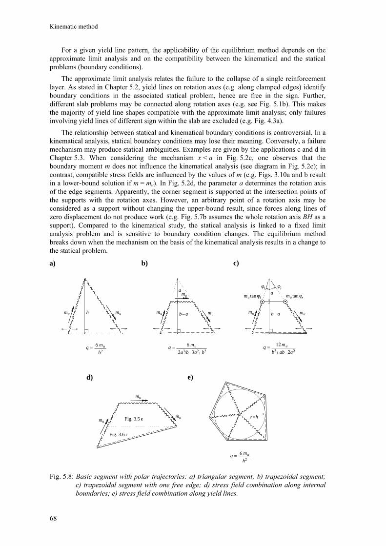
Kinematic method

68

For a given yield line pattern, the applicability of the equilibrium method depends on the approximate limit analysis and on the compatibility between the kinematical and the statical problems (boundary conditions). The approximate limit analysis relates the failure to the collapse of a single reinforcement layer. As stated in Chapter 5.2, yield lines on rotation axes (e.g. along clamped edges) identify boundary conditions in the associated statical problem, hence are free in the sign. Further, different slab problems may be connected along rotation axes (e.g. see Fig. 5.1b). This makes the majority of yield line shapes compatible with the approximate limit analysis; only failures involving yield lines of different sign within the slab are excluded (e.g. Fig. 4.3a). The relationship between statical and kinematical boundary conditions is controversial. In a kinematical analysis, statical boundary conditions may lose their meaning. Conversely, a failure mechanism may produce statical ambiguities. Examples are given by the applications c and d in Chapter 5.3. When considering the mechanism x < a in Fig. 5.2c, one observes that the boundary moment m does not influence the kinematical analysis (see diagram in Fig. 5.2c); in contrast, compatible stress fields are influenced by the values of m (e.g. Figs. 3.10a and b result in a lower-bound solution if m = mu). In Fig. 5.2d, the parameter a determines the rotation axis of the edge segments. Apparently, the corner segment is supported at the intersection points of the supports with the rotation axes. However, an arbitrary point of a rotation axis may be considered as a support without changing the upper-bound result, since forces along lines of zero displacement do not produce work (e.g. Fig. 5.7b assumes the whole rotation axis BH as a support). Compared to the kinematical study, the statical analysis is linked to a fixed limit analysis problem and is sensitive to boundary condition changes. The equilibrium method breaks down when the mechanism on the basis of the kinematical analysis results in a change to the statical problem.

Fig. 5.8: Basic segment with polar trajectories: a) triangular segment; b) trapezoidal segment; c) trapezoidal segment with one free edge; d) stress field combination along internal boundaries; e) stress field combination along yield lines.

mu muh

a) b) c)

d) e)

mu mu

mua

b a

=qmu6=

3q

a2 /b 2a3 2b+

mu mu

a

b a

mu12=2

qb a2ab+ 2

ϕl ϕr

tanmu ϕrtanmu ϕl

r=h

mu6=2

qh

Fig. 3.6

Fig. 3.5 e

c

mu

mu

mu

mu62h

Discussion – Conclusions

69

The equilibrium method involves a “kinematical” and a “statical” study complementary to each other. The more the two analyses are performed simultaneously, the better the equilibrium method. As with the work method, the “kinematical” analysis determines the collapse mechanism and the ultimate load of the slab. The equilibrium of the failure segments replaces the differential procedure of the work method with a simpler calculation and gives additional information about the force flow in the slab. Along yield lines, the ultimate moments and the shear forces on failure sections isolate the individual collapse segments as single problems. Considering the failure segments as basic elements of the stress field approach, the “statical” analysis leads to a compatible equilibrium solution. The slab stress field goes beyond the requirements of the work method. Its determination outlines the slab’s structural behaviour, proving the consistency of the failure analysis (statical boundary conditions of the problem), improving the investigation of the most critical failures (complete solution of the approximate limit analysis problem) and giving information about the actual failure of the slab (development of plastic regions). Examples of these considerations are given in the above applications: comparing Fig. 5.2d with Fig. 5.7b, the slab’s boundary conditions are not clear; in Fig. 5.6c the equilibrium method suggests the ultimate failure; referring to the standard limit analysis problem (mu = m′u), the stress fields of Figs. 3.10a, 3.10b and 3.11e, 3.11f define the extension of yield regions in the slab’s corners. Combining the kinematical and the statical approaches the procedure of the equilibrium method is facilitated. Figs. 5.8a to c give information on the ultimate load of failure elements resulting from the trapezoidal segment introduced in Fig. 3.5e. Referring to the stress field approach, different segments may be connected along internal boundaries or along yield lines. The former case leads to failure segments with complex boundaries (e.g. see Fig. 5.8d) or to the detection of new yield lines within a single failure segment (e.g. see Fig. 5.6c, the trapezoidal segment of Fig. 5.8c constitutes a new yield line if 63 ab (a + b) – (4a2

+ ab + b2)3/2 < 0). In the latter case different segments with known statical conditions are combined along yield lines (e.g. several segments of Fig. 5.8a correspond to a uniformly loaded slab simply supported along boundaries tangent to the circle r = h [21, 59], see Fig. 5.8e).

5.5 Conclusions

Fig. 5.9 reviews the kinematical analysis of slabs outlined in this chapter. The upper-bound analysis is restricted to yield line failures. Such failure modes are in good agreement with experiments, involve only few geometrical parameters, and correspond to an approximate limit analysis problem if only positive or negative failures are enforced (see Chapter 4.3). Compared to Fig. 2.4, the upper-bound theorem is replaced by the work method and the compatibility theorem by the equilibrium method. The best yield line pattern of the approximate limit analysis problem is found in the complete solution group. The equilibrium method singles out the most critical yield line pattern of collapse mechanisms which agree with an approximate limit analysis and correspond to a fixed statical problem. The work method applies to arbitrary failure modes. The compatibility theorem provides a solid foundation for Johansen’s equilibrium method, removing the paradoxes related to the nodal forces. By means of the approximate limit analysis the relation between the lower- and the upper-bound analyses is simplified. The equilibrium method improves the global analysis of the work method; by substituting kinematical by statical boundaries it provides a better understanding of the slab’s behaviour. The kinematical analysis favours a global consideration of the force flow before concentrating on local equilibrium. As

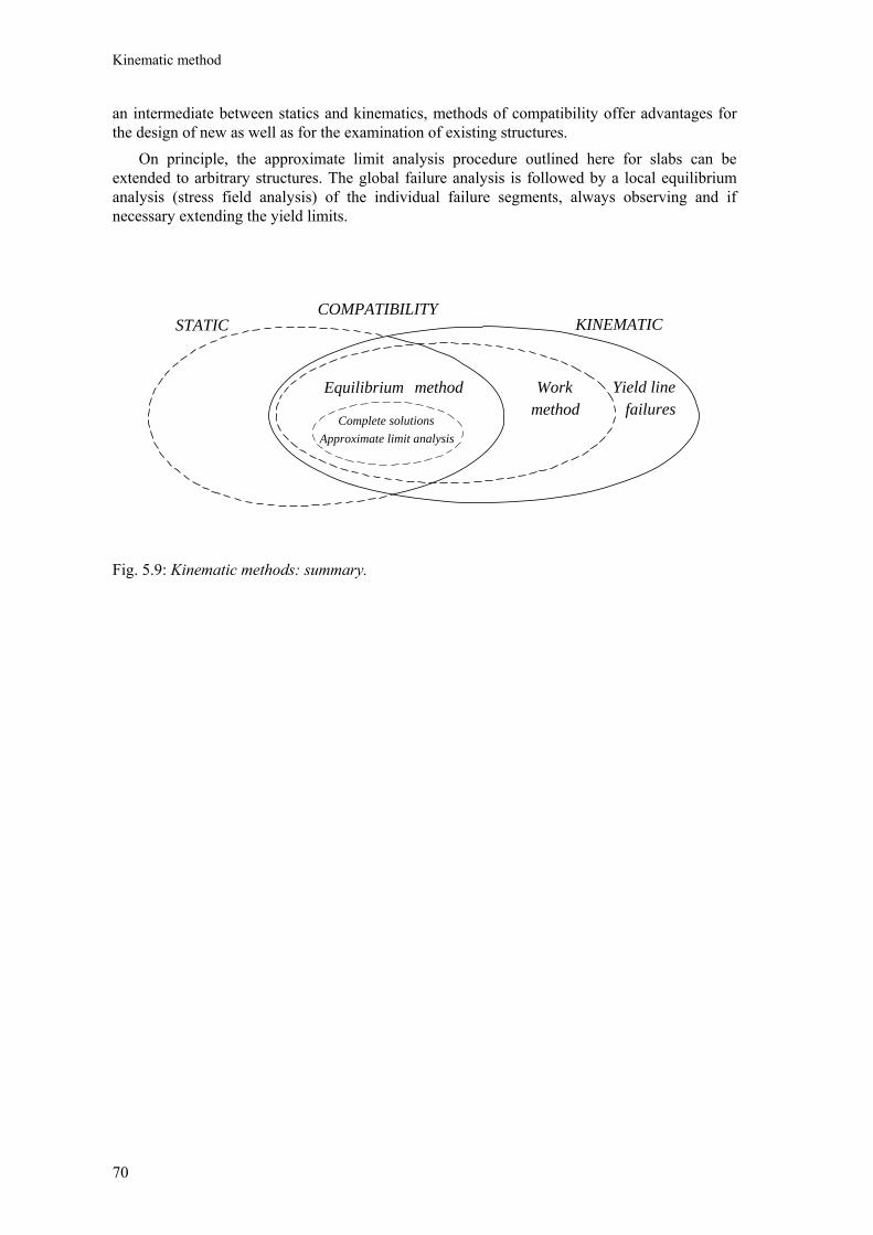
Kinematic method

70

an intermediate between statics and kinematics, methods of compatibility offer advantages for the design of new as well as for the examination of existing structures. On principle, the approximate limit analysis procedure outlined here for slabs can be extended to arbitrary structures. The global failure analysis is followed by a local equilibrium analysis (stress field analysis) of the individual failure segments, always observing and if necessary extending the yield limits.

Fig. 5.9: Kinematic methods: summary.

STATIC KINEMATIC COMPATIBILITY

Approximate limit analysis

Equilibrium method Workmethod

Complete solutions

Yield line failures

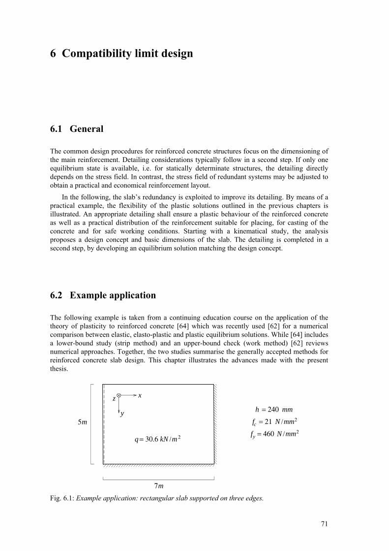
71

6 Compatibility limit design

6.1 General

The common design procedures for reinforced concrete structures focus on the dimensioning of the main reinforcement. Detailing considerations typically follow in a second step. If only one equilibrium state is available, i.e. for statically determinate structures, the detailing directly depends on the stress field. In contrast, the stress field of redundant systems may be adjusted to obtain a practical and economical reinforcement layout.

In the following, the slab’s redundancy is exploited to improve its detailing. By means of a practical example, the flexibility of the plastic solutions outlined in the previous chapters is illustrated. An appropriate detailing shall ensure a plastic behaviour of the reinforced concrete as well as a practical distribution of the reinforcement suitable for placing, for casting of the concrete and for safe working conditions. Starting with a kinematical study, the analysis proposes a design concept and basic dimensions of the slab. The detailing is completed in a second step, by developing an equilibrium solution matching the design concept.

6.2 Example application

The following example is taken from a continuing education course on the application of the theory of plasticity to reinforced concrete [64] which was recently used [62] for a numerical comparison between elastic, elasto-plastic and plastic equilibrium solutions. While [64] includes a lower-bound study (strip method) and an upper-bound check (work method) [62] reviews numerical approaches. Together, the two studies summarise the generally accepted methods for reinforced concrete slab design. This chapter illustrates the advances made with the present thesis.

Fig. 6.1: Example application: rectangular slab supported on three edges.

7m

5m

q = 30.6 kN m/ 2

x

y

z

fc = 21 N mm

fy = 460

h = 240 mm

/ 2

N mm/ 2

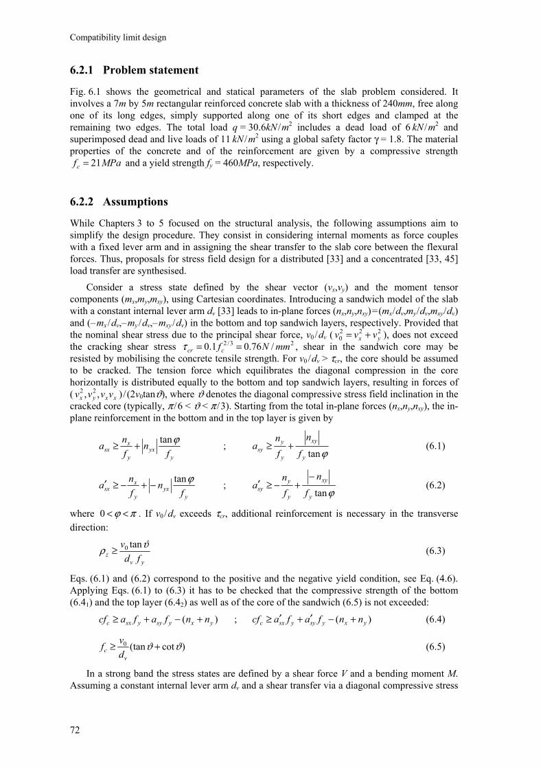
Compatibility limit design

72

6.2.1 Problem statement

Fig. 6.1 shows the geometrical and statical parameters of the slab problem considered. It involves a 7m by 5m rectangular reinforced concrete slab with a thickness of 240mm, free along one of its long edges, simply supported along one of its short edges and clamped at the remaining two edges. The total load q = 30.6kN / m2 includes a dead load of 6 kN / m2 and superimposed dead and live loads of 11 kN / m2 using a global safety factor γ = 1.8. The material properties of the concrete and of the reinforcement are given by a compressive strength

MPafc 21= and a yield strength fy = 460MPa, respectively.

6.2.2 Assumptions

While Chapters 3 to 5 focused on the structural analysis, the following assumptions aim to simplify the design procedure. They consist in considering internal moments as force couples with a fixed lever arm and in assigning the shear transfer to the slab core between the flexural forces. Thus, proposals for stress field design for a distributed [33] and a concentrated [33, 45] load transfer are synthesised. Consider a stress state defined by the shear vector (vx,vy) and the moment tensor components (mx,my,mxy), using Cartesian coordinates. Introducing a sandwich model of the slab with a constant internal lever arm dv [33] leads to in-plane forces (nx,ny,nxy) = (mx / dv,my / dv,mxy / dv) and (– mx / dv,– my / dv,– mxy / dv) in the bottom and top sandwich layers, respectively. Provided that the nominal shear stress due to the principal shear force, v0 / dv ( 222

0 yx vvv += ), does not exceed the cracking shear stress 23/2 /76.01.0 mmNfccr ==τ , shear in the sandwich core may be resisted by mobilising the concrete tensile strength. For v0 / dv > τcr, the core should be assumed to be cracked. The tension force which equilibrates the diagonal compression in the core horizontally is distributed equally to the bottom and top sandwich layers, resulting in forces of ( xxyx vvvv ,, 22 ) / (2v0tanϑ), where ϑ denotes the diagonal compressive stress field inclination in the cracked core (typically, π / 6 < ϑ < π / 3). Starting from the total in-plane forces (nx,ny,nxy), the in-plane reinforcement in the bottom and in the top layer is given by

y

yxy

xsx f

nfna ϕtan+≥ ;

ϕtany

xy

y

ysy f

nfn

a +≥ (6.1)

y

yxy

xsx f

nfna ϕtan−+−≥′ ;

ϕtany

xy

y

ysy f

nfn

a−

+−≥′ (6.2)

where πϕ <<0 . If v0 / dv exceeds τcr, additional reinforcement is necessary in the transverse direction:

yv

z fdv ϑρ tan0≥ (6.3)

Eqs. (6.1) and (6.2) correspond to the positive and the negative yield condition, see Eq. (4.6). Applying Eqs. (6.1) to (6.3) it has to be checked that the compressive strength of the bottom (6.41) and the top layer (6.42) as well as of the core of the sandwich (6.5) is not exceeded:

)( yxysyysxc nnfafacf +−+≥ ; )( yxysyysxc nnfafacf +−′+′≥ (6.4)

)cot(tan0 ϑϑ +≥v

c dvf (6.5)

In a strong band the stress states are defined by a shear force V and a bending moment M. Assuming a constant internal lever arm dv and a shear transfer via a diagonal compressive stress

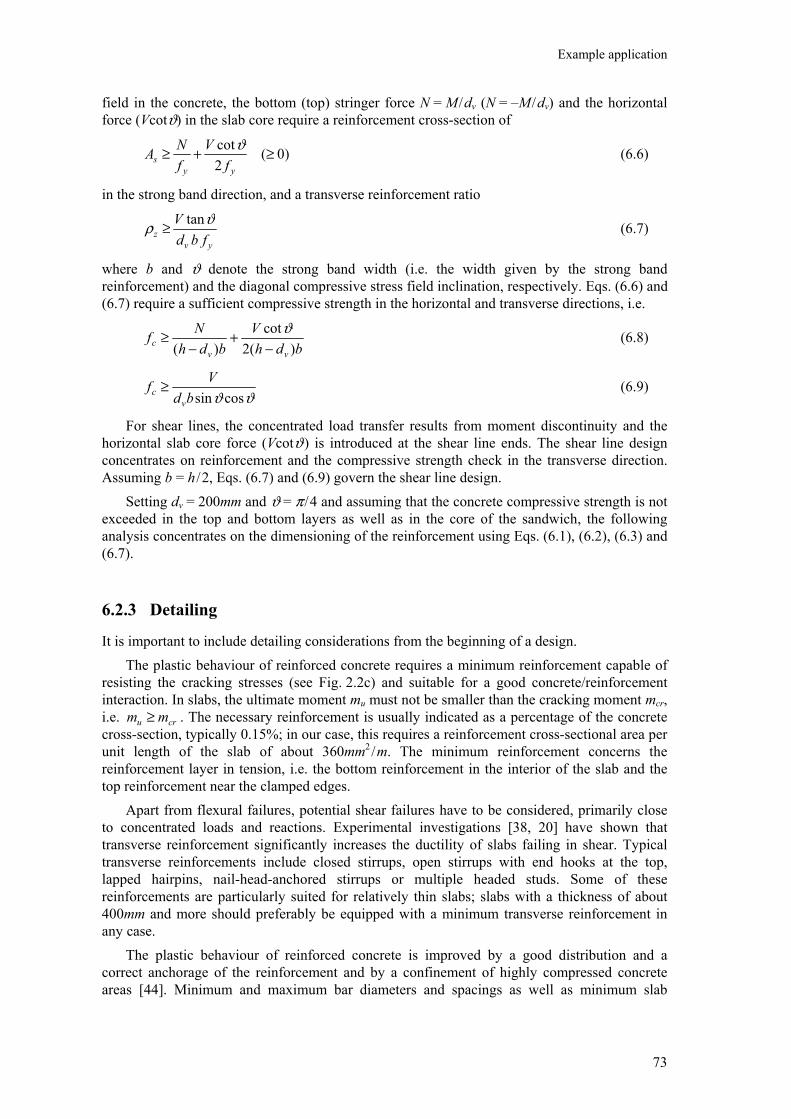
Example application

73

field in the concrete, the bottom (top) stringer force N = M / dv (N = –M / dv) and the horizontal force (Vcotϑ) in the slab core require a reinforcement cross-section of

)0(2cot ≥+≥

yys f

VfNA ϑ (6.6)

in the strong band direction, and a transverse reinforcement ratio

yv

z fbdV ϑρ tan≥ (6.7)

where b and ϑ denote the strong band width (i.e. the width given by the strong band reinforcement) and the diagonal compressive stress field inclination, respectively. Eqs. (6.6) and (6.7) require a sufficient compressive strength in the horizontal and transverse directions, i.e.

bdh

Vbdh

Nfvv

c )(2cot

)( −+

−≥ ϑ (6.8)

ϑϑ cossinbd

Vfv

c ≥ (6.9)

For shear lines, the concentrated load transfer results from moment discontinuity and the horizontal slab core force (Vcotϑ ) is introduced at the shear line ends. The shear line design concentrates on reinforcement and the compressive strength check in the transverse direction. Assuming b = h / 2, Eqs. (6.7) and (6.9) govern the shear line design.

Setting dv = 200mm and ϑ = π / 4 and assuming that the concrete compressive strength is not exceeded in the top and bottom layers as well as in the core of the sandwich, the following analysis concentrates on the dimensioning of the reinforcement using Eqs. (6.1), (6.2), (6.3) and (6.7).

6.2.3 Detailing

It is important to include detailing considerations from the beginning of a design.

The plastic behaviour of reinforced concrete requires a minimum reinforcement capable of resisting the cracking stresses (see Fig. 2.2c) and suitable for a good concrete/reinforcement interaction. In slabs, the ultimate moment mu must not be smaller than the cracking moment mcr, i.e. cru mm ≥ . The necessary reinforcement is usually indicated as a percentage of the concrete cross-section, typically 0.15%; in our case, this requires a reinforcement cross-sectional area per unit length of the slab of about 360mm2

/ m. The minimum reinforcement concerns the reinforcement layer in tension, i.e. the bottom reinforcement in the interior of the slab and the top reinforcement near the clamped edges. Apart from flexural failures, potential shear failures have to be considered, primarily close to concentrated loads and reactions. Experimental investigations [38, 20] have shown that transverse reinforcement significantly increases the ductility of slabs failing in shear. Typical transverse reinforcements include closed stirrups, open stirrups with end hooks at the top, lapped hairpins, nail-head-anchored stirrups or multiple headed studs. Some of these reinforcements are particularly suited for relatively thin slabs; slabs with a thickness of about 400mm and more should preferably be equipped with a minimum transverse reinforcement in any case.

The plastic behaviour of reinforced concrete is improved by a good distribution and a correct anchorage of the reinforcement and by a confinement of highly compressed concrete areas [44]. Minimum and maximum bar diameters and spacings as well as minimum slab

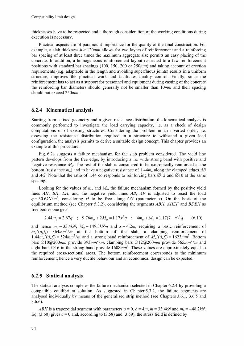
Compatibility limit design

74

thicknesses have to be respected and a thorough consideration of the working conditions during execution is necessary.

Practical aspects are of paramount importance for the quality of the final construction. For example, a slab thickness h > 120mm allows for two layers of reinforcement and a reinforcing bar spacing of at least three times the maximum aggregate size permits an easy placing of the concrete. In addition, a homogeneous reinforcement layout restricted to a few reinforcement positions with standard bar spacings (100, 150, 200 or 250mm) and taking account of erection requirements (e.g. adaptable in the length and avoiding superfluous joints) results in a uniform structure, improves the practical work and facilitates quality control. Finally, since the reinforcement has to act as a support for personnel and equipment during casting of the concrete the reinforcing bar diameters should generally not be smaller than 10mm and their spacing should not exceed 250mm.

6.2.4 Kinematical analysis

Starting from a fixed geometry and a given resistance distribution, the kinematical analysis is commonly performed to investigate the load carrying capacity, i.e. as a check of design computations or of existing structures. Considering the problem in an inverted order, i.e. assessing the resistance distribution required in a structure to withstand a given load configuration, the analysis permits to derive a suitable design concept. This chapter provides an example of this procedure. Fig. 6.2a suggests a failure mechanism for the slab problem considered. The yield line pattern develops from the free edge, by introducing a 1m wide strong band with positive and negative resistance Mu. The rest of the slab is considered to be isotropically reinforced at the bottom (resistance mu) and to have a negative resistance of 1.44mu along the clamped edges AB and AG. Note that the ratio of 1.44 corresponds to reinforcing bars ∅12 and ∅10 at the same spacing.

Looking for the values of mu and Mu, the failure mechanism formed by the positive yield lines AH, BH, EH, and the negative yield lines AB, AF is adjusted to resist the load q = 30.6kN / m2, considering H to be free along CG (parameter x). On the basis of the equilibrium method (see Chapter 5.3.2), considering the segments ABH, AHEF and BDEH as free bodies one gets

qxMmqxMmqm uuuuu22 )7(17.14;17.1276.9;67.244.2 −=+=+= (6.10)

and hence mu = 33.4kN, Mu = 149.3kNm and x = 4.2m, requiring a basic reinforcement of mu / (dv fy) = 364mm2

/ m at the bottom of the slab, a clamping reinforcement of 1.44mu / (dv fy) = 524mm2

/ m and a strong band reinforcement of Mu / (dv fy) = 1623mm2. Bottom bars ∅10@200mm provide 393mm2

/ m, clamping bars ∅12@200mm provide 565mm2 / m and

eight bars ∅16 in the strong band provide 1608mm2. These values are approximately equal to the required cross-sectional areas. The bottom reinforcement corresponds to the minimum reinforcement; hence a very ductile behaviour and an economical design can be expected.

6.2.5 Statical analysis

The statical analysis completes the failure mechanism selected in Chapter 6.2.4 by providing a compatible equilibrium solution. As suggested in Chapter 5.3.2, the failure segments are analysed individually by means of the generalised strip method (see Chapters 3.6.1, 3.6.5 and 3.6.6).

ABH is a trapezoidal segment with parameters a = 0, b = 4m, m = 33.4kN and mb = – 48.2kN. Eq. (3.60) gives c = 0 and, according to (3.58) and (3.59), the stress field is defined by

Example application

75

Fig. 6.2: Structural analysis: a) kinematical analysis; b) shear field and shear line forces; c) moment field.

a)

b)

c)

33.4 − 48.2

100 kN/m v 0=0

149.3

1m

x

M

−1.44

M

AB

FD

GC

21.133.2

H

87.2

133.992.3123.6

69.3

95.1

41.0

69.2

33.4/−115.5

0.1/−133.3

31.1/−79.8

33.4/−70.8

23.4/−132.3

40.2/−2.2 47.2/−10.1146.2/1.0

E

V 57.4

85.4

78.047.5

AB

VCG

VBC VAG

G

C

A

B

B

C

A

G

kN

kN

kN

kN

kN

kN

u u

mu

mu

−1.44 mu

[ ]

kN[ ]

Compatibility limit design

76

44.33;10.544.33;30.15 20 =−=−= ϕmrmrv r (6.11)

where r and ϕ are polar coordinates centred at H. In addition to the reactions rAB = 81.6kN / m and mAB = – 48.2kN, the edge AB acts as a shear line, transferring the forces 85.4kN and 57.4kN in A and B, respectively.

BDEH and AHEF are divided along CG into the segments BCH, AHG and CDEH, GHEF, respectively. BCH and AHG follow the analysis suggested by Figs. 3.6c to 3.6e, while CDFG is considered with the strip method of analysis (see Chapter 3.6.3). Assuming constant bending moments and shear forces between the segments BCH and CDEH, and AHG and GHEF, respectively, the internal forces along CG are determined proving equilibrium of the different segments. From the moment equation of BCH (AHG) with respect to BC (AG) it follows that vCH = 7.06kN / m (vGH = 3.51kN / m). Distributing vCH (vGH) on CDEH (GHEF) as cantilever load of the slab strip in the y-direction (i.e. qy CDEH = –7.1kN / m2, qy GHEF = –3.5kN / m2), moment equilibrium of CDEH (GHEF ) with respect to CG requires mCH = 3.5kN (mGH = 1.8kN).

In BCH, the stress field is defined by the superposition of

)cos

81.0(26.18 20 rr

v −=ϕ

; 44.33cos

82.1409.6 22 ++−=

ϕrmr ; 44.33=ϕm (6.12)

and

)cos

43.15(96.2 20 rr

v −−=ϕ

; ϕ2

2

cos71.4599.0 −= rmr ; 0=ϕm (6.13)

Eqs. (6.12) and (6.13) refer to a polar system of coordinates centred at H (ϕ = 0 for HC) and at B (ϕ = 0 for BC ), respectively. The stress field (6.12) gives the reaction forces rBC = 58.0kN / m and RH = 21.1kN as well as the shear line force FB = 47.5kN. Similarly, Eq. (6.13) corresponds to rCH = 7.1kN / m, RB = –32.2kN and FH = 21.1kN. Note that RH and FH add to zero, while rCH corresponds to the load exchange between BCH and CDEH. The negative sign of RB indicates a downward force in B.

In AHG, the stress field is defined by the superposition of

)cos

74.1(92.19 20 rr

v −=ϕ

; 44.33cos

67.3464.6 22 ++−=

ϕrmr ; 44.33=ϕm (6.14)

and

)cos

19.12(62.4 20 rr

v −−=ϕ

; ϕ2

2

cos35.5654.1 −= rmr ; 0=ϕm (6.15)

Eqs. (6.14) and (6.15) refer to a polar system of coordinates centred at H (ϕ = 0 for HG) and at A (ϕ = 0 for AG ), respectively. The stress field (6.14) gives the reaction forces rAG = 94.6kN / m and RH = 33.2kN as well as the shear line force FA = 78.0kN. Similarly, (6.15) corresponds to rGH = 3.5kN / m, RA = –58.9kN and FH = 33.2kN. Again, RH and FH add to zero, while rGH corresponds to the load exchange between AHG and GHEF. The negative sign of RA indicates a downward force in A.

The stress field of CDFG is developed with the strip method of analysis, by considering the load partition qx = 37.7kN / m2 and qy = –7.1kN / m2 in CDEH, and qx = 34.1kN / m2 and qy = –3.5kN / m2 in GHEF. Strips are clamped at FG and simply supported at CD in the x-direction, while they act as cantilevers in the y-direction. Centring the global system of reference at D, the stress field in CDFG is given by

CDEH: )53.3,83.1805.106(),(;)06.7,66.3705.106(),( 22 yxxmmyxvv yxyx −=−−= (6.16)

GHEF: )76.1,06.1705.9607.14(),(;)51.3,11.3405.96(),( 22 yxxmmyxvv yxyx −+=−−= (6.17)

Example application

77

Finally, the reaction forces along CD and FG are equal to rCD = 106.1kN / m and rFG = 142.7kN / m.

Summing up the edge reactions and the corner forces one obtains 106.1kN + 142.7kN + + 4m·(58.0 + 94.6)kN/m + 7m·81.6kN/m – (47.5 + 32.2 + 85.4)kN – (78.0 + 58.9 + 57.4)kN = 1071kN = = 5m·7m·30.6kN / m2, i.e. vertical equilibrium is provided. Figs. 6.2b and 6.2c summarise the results of the statical analysis, showing the extreme stress values. The solution is compatible with the mechanism of Fig. 6.2a. Since the positive moments increase beyond 33.4kN around H, the slab considered (with unchanged resistance distribution) would probably collapse with a different mechanism.

6.2.6 Reinforcement dimensioning

Starting from the basic reinforcement layout selected with the aid of the kinematical analysis, the slab resistances are locally increased to cover the stress states derived by the statical analysis. Detailing considerations lead to a certain smoothing of the theoretical reinforcement distribution. The reinforcement arrangement, including the reinforcement placing, is given in Fig. 6.3; note that the bar numbers follow the placing sequence. The following section describes its development.

Bending reinforcement The basic reinforcement includes an isotropic mesh ∅10@200 at the bottom of the slab, a 1m wide strong band with 8∅16 along the free edge, and a clamping reinforcement ∅12@200 and 8∅16 along AB, AG and GF, respectively (see Chapter 6.2.4). These reinforcements are provided by positions 1 and 4 at the slab bottom, 2 at the strong band, and 8, 13 and 6 at the clamped edges.

At the bottom of the slab the basic reinforcement extends over the whole length; it starts at the clamped edges and is bent up and back into the slab at the simply supported and the free edge. The straight end over the clamped edge ensures a good anchorage and the bending up at the other end enables the reinforcement to function as shear line reinforcement (along the simply supported edge), concrete confinement (along the free edge) and as splice and support for the top reinforcement. Close to H position 4 is replaced by 3 (∅12@200) to resist stresses beyond 33.4kN (see Fig. 6.2c).

The strong band reinforcement (position 2) follows the detailing of positions 3 and 4 at the bottom of the slab. The required negative bending resistance is ensured by position 6; spliced with the wall reinforcement along FG, position 6 extends into the slab to cover the negative strong band moment, accounting for a development length of 40∅. Required for shear line reinforcement along CG, position 7 together with the bends of position 1 improves the plastic behaviour of the strong band by concrete confinement.

Similar to position 6, positions 8 and 13 provide the necessary negative resistance determined by the kinematical study along GA and AB, respectively.

Considering the reinforcement positions 1, 2, 3, 4, 6, 7, 8 and 13, the slab resistances are compared to the stress field developed in Chapter 6.2.5; weak regions are strengthened by adequate extra reinforcement, paying attention to detailing aspects. Corresponding to the clamping of the edges AB and AF and the twisting moment introduced by the simply supported edge BD, Fig. 6.2c reveals negative moments extending far into the slab. Hence, the basic reinforcement is completed with positions 5 (∅10@200) and 11 (∅10@200) and 12 (∅12@200) in the x- and y-directions, respectively. Spliced with the top part of position 1 along DF, with the top parts of positions 2, 3 and 4 along BD and with the wall reinforcement along the clamped edges, the top reinforcement generates a robust 200 / 200mm mesh, suitable for the casting of the concrete.

Compatibility limit design

78

The basic reinforcement is sufficient for almost all stress states in the slab. Around A and B, positions 9, 14 and 10 are added to resist the locally high negative moments. This extra reinforcement fits between the basic one, reducing the mesh spacing to 100 / 100mm.

Shear reinforcement While the kinematical analysis indicates the global shear flow, shear forces are determined in detail by the statical analysis. This is summarised in Fig. 6.2b.

Up to mkNv /15276.02000 =⋅≤ the core of the slab can be assumed to be uncracked and no transverse reinforcement is required. Fig. 6.2b shows that indeed no transverse reinforcement is required.

With 1m width, the strong band along the free edge is designed like a slab. Since the core is uncracked (see Fig. 6.2b), transverse reinforcement is not necessary. As previously suggested, a confinement of the strong band by means of positions 1 and 7 is recommended for an improved plastic behaviour.

Making a conservative assumption about the shear line width (b = h / 2 = 120mm), transverse reinforcement is required for a shear line force in excess of 18.2kN. It can be seen from Fig. 6.2b that all the shear lines have to be reinforced. The required reinforcement along the edges AG (Vmax = 78.2kN ) and AB (Vmax = 85.4kN ) could for example be realised with vertical hairpins ∅12@200mm spliced with the wall reinforcement. Along BC (Vmax = 47.5kN ), the resistance provided by the bent up bottom reinforcement (36.2kN ) has to be complemented with some additional horizontal hairpins, at least in the region around B. Along CG (Vmax = 33.2kN ), position 6 (∅10@200mm) is sufficient for resisting the shear forces. Note that according to Eq. (6.7) transverse reinforcements ∅10 and ∅12 spaced at 200mm provide shear resistances of 36.2kN and 52.1kN, respectively.

Remarks By applying an approximate limit analysis as outlined in Chapter 4.3, any reinforcement deficit is generally constrained to one sandwich cover. Completing the reinforcement layout intuitively, the local considerations suggested in Chapter 6.2.2 reduce to a simple check represented graphically in Fig. 4.4b.

The reinforcement arrangement shown in Fig. 6.3 involves a reinforcement content of about 90kg / m3 of concrete.

6.3 Discussion

As the positive yield condition is violated in the area around H adjacent to the strong band (see Fig. 6.2c), the failure mechanism selected is not the most critical one. Presumably, the slab considered (i.e. with the same reinforcement layout) would collapse as shown in Fig. 5.6c. The complete solution of the approximate limit analysis problem would consider the basic reinforcement required by the kinematical analysis, and provide some local strengthening to eliminate the reinforcement insufficiency. Of course, the limit analysis problem changes by varying the assumed reinforcement distribution. For instance, an edge beam along DF would improve the failure pattern of Fig. 5.2a. Generally, the development of a complete solution of the approximate limit analysis problem is only of academic interest; the possible reduction in reinforcement is negligible compared to the additional work involved. It can be stated that any failure shape which identifies a kinematical optimum corresponds to a good design concept. On the other hand, failure shapes that do not correspond to a

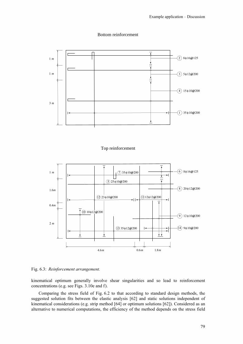
Example application – Discussion

79

Fig. 6.3: Reinforcement arrangement.

kinematical optimum generally involve shear singularities and so lead to reinforcement concentrations (e.g. see Figs. 3.10e and f ).

Comparing the stress field of Fig. 6.2 to that according to standard design methods, the suggested solution fits between the elastic analysis [62] and static solutions independent of kinematical considerations (e.g. strip method [64] or optimum solutions [62]). Considered as an alternative to numerical computations, the efficiency of the method depends on the stress field

Top reinforcement

35φ12 200

12

20 φ12 200

3 m

1 m

1 m

Bottom reinforcement

2 m

1 m

1.6m

0.4m

4.6m 0.6m 1.8m

8

13

35 φ10 2001

8φ16 1252

5φ12 2003

4 15 φ10 200

23φ10 20012 φ12 20011

25φ10 2005

10φ12 2001012 φ10 2009

14 9φ10 200

35φ10 2007 8 16 1256 φ

@

@

@

@

@

@

@

@@

@

@

@

@

@

Compatibility limit design

80

library given in Chapter 3. Some difficulties occur in the reinforcement design, since a stress field with variable principal moment trajectories (i.e. including the effect of the twisting moments) does not match with a fixed reinforcement layout.

The amount of reinforcement involved in the reinforcement arrangement of Fig. 6.3 is comparable with that according to elastic computations (81kg / m3) but it is considerably higher than that according to minimum reinforcement solutions (41kg / m3), see [62]. However, computer analyses generally concentrate on the dimensioning of the main reinforcement and neglect the reinforcement detailing which is left to the engineer’s experience. In contrast, the procedure outlined here integrates detailing and dimensioning aspects, resulting in a practical and detailed design.

6.4 Conclusions

In the example application considered, the individual plastic analysis components discussed in the previous chapters are combined, leading from a design concept to a detailed structural design consistent with detailing requirements.

The development of the design concept requires a simple analysis of global character capable of establishing the force flow. The procedure involves some preliminary assumptions (such as the resistance distribution in the slab, the strong band positions and the clamping ratios) on the basis of an assumed failure mechanism. By means of the kinematical analysis, the intuitively assumed mechanism is optimised and the required resistances are quantified. The failure mechanism also indicates the force flow from the slab to the adjacent structural members which may be designed simultaneously (see Chapter 5.3.2), and the required resistances permit to select suitable combinations of slab thicknesses and basic reinforcement contents. The detailed structural design involves the analysis of the force flow within the slab and the determination of the required local resistances. The statical redundancy of a slab permits the development of stress fields compatible with the assumed failure mechanism. The validity of the preliminary kinematical analysis is maintained and the approximate limit analysis considerations integrate optimum design criteria.

By adjusting the slab design to a selected failure mechanism, the present procedure may be called a compatibility limit design method. Compared to pure lower-bound approaches such as the strip method or statically admissible moment fields, the compatibility limit design method integrates considerations of ultimate state deformations. Similar to an elastic analysis which is suitable for serviceability verification, the compatibility limit design method could be developed further to enable a check of the deformations involved in the plastic analysis, extending current research on tension elements and beams to slabs [61, 24]. As a word of caution, however, the advantage of the simple computations, essentially established by the stress field library, is diminished by the difficulty involved in dimensioning and detailing the reinforcement; some new research is certainly needed in this respect. Still, although being far from a complete development the compatibility limit design method illustrates nicely the great flexibility and power of plastic analysis when applied to reinforced concrete.

81

7 Summary and conclusions

7.1 Summary

This thesis deals with the application of the theory of plasticity to reinforced concrete slabs. After the introduction (Chapter 1) and a presentation of the fundamentals of the theory of plasticity (Chapter 2) it concentrates on the static method (Chapter 3), limit analysis (Chapter 4) and the kinematic method (Chapter 5), step by step developing a new design procedure – the compatibility limit design method – whose application is illustrated by means of a practical example (Chapter 6). The basic idea of the compatibility limit design method is to extend the typical design procedure for reinforced concrete beams and frames to reinforced concrete slabs. For beams and frames, the failure mechanisms indicate the global force flow because the plastic hinges identify the zero shear points. The force flow within the individual beam or frame segments defined by the zero shear points can then be visualised using truss models or corresponding stress fields and the segments’ detailing can be completed accordingly. For slabs, the static and the kinematic method are normally applied in an unrelated way and thus, the potential offered by the theory of plasticity is not fully exploited. By considering yield line mechanisms and developing matching stress fields for the individual slab segments defined by the yield lines the compatibility limit design method attempts to overcome this unsatisfactory situation. The presentation of the static method in Chapter 3 concentrates on the load transfer mechanisms in slabs, differentiating between distributed and concentrated load transfer. Distributed load transfer within slab segments is described by the generalised strip method, using general curved rather than straight orthogonal beams. In addition to the normal beam action with moment increments corresponding to the shear forces, this allows to recognise a geometrical load transfer mechanism due to the curvature of the beams. Depending on the selected beam geometry the statical redundancy of the slabs is replaced by geometrical parameters. While solutions according to the theory of elastic plates refer to beams in the principal curvature directions of the deflection function Hillerborg’s strip method involves straight beams, preventing geometrical load transfer. On the other hand, assuming constant principal moments and a pure geometrical load transfer, Hencky-Prandtl solutions are obtained. Stress fields of complete limit analysis solutions are related to particular curvilinear trajectories; the case of polar trajectories is of considerable practical interest and is presented in detail. Finally, it is demonstrated how stress fields can be adapted to different boundary conditions and how they can be superimposed. Concentrated load transfer occurs via bending moment concentrations in strong bands or due to twisting moment discontinuities along shear lines; generally, strong band and shear line action may be combined along certain trajectories.

The discussion of limit analysis in Chapter 4 is based on a thorough evaluation of stress states and the associated strain rates satisfying the yield condition of orthogonally reinforced concrete slabs and associated flow rule. In the space of the bending and twisting moments with respect to the reinforcement directions this yield condition corresponds to a yield surface consisting of two intersecting elliptical cones, corresponding to positive and negative yield line failures with yielding bottom and top reinforcement, respectively. Stress points within the yield surface correspond to rigid states. Stress points on the cone surfaces correspond to uniaxial

Summary and conclusions

82

curvature rates and hence yield lines; since all points of a straight cone surface line are associated with the same strain rates a kinematic approach is advantageous. Stress points on the elliptical intersection line of the two cones correspond to combinations of positive and negative curvature rates in two distinct directions; yield regions rather than yield lines develop under such circumstances in general and a static approach is advantageous. The stress states corresponding to the two cone apexes are compatible with arbitrary positive or negative curvature rates, respectively. Stress points outside the yield surface are not admissible. The existence of yield regions makes limit analysis solutions quite cumbersome in general. A very effective simplification is obtained by keeping either the top or the bottom reinforcement rigid. With such an approximate limit analysis which corresponds to the capacity design method used in earthquake engineering, yield regions disappear and complete solutions with compatible stress and strain rate fields can be developed.

The presentation of the kinematic method in Chapter 5 starts from a brief review of past research. In particular, the development of the work method and the equilibrium method as well as the nodal force debate of the 1960’s are discussed. Then, the basic principles of yield line analysis are introduced and the application of the work method and of the equilibrium method is illustrated by means of four examples. It is shown that the equilibrium method can be interpreted as an application of the compatibility theorem to a suitably defined approximate limit analysis problem and that the work method and the equilibrium method are equivalent if they are associated to a unique statical problem. In Chapter 6, the application of the compatibility limit design method is illustrated by a practical example. Starting from some preliminary assumptions about the resistance distribution in the slab an intuitively assumed yield line mechanism is optimised and the required global resistances are quantified. In a second step, the force flow within and between the individual slab segments is studied based on the stress field approach developed in Chapter 3 in order to detect any local resistance deficits. The importance of detailing considerations is emphasised and comparisons with previously derived solutions are made.

7.2 Conclusions

Similar to beams and frames the shear forces provide the key to understanding the force flow in slabs. Distributed and concentrated shear force transfer have to be differentiated. Distributed load transfer can be described by the generalised strip method, using curved orthogonal coordinates, allowing for the development of general stress fields. Concentrated load transfer can be realised by strong bands and shear lines.

The investigation of the yield surface using the associated flow rule allows to determine compatible states of stress and deformation. It can be recognised that a kinematic (static) analysis is best suited for the weakly (strongly) convex parts of the yield surface corresponding to yield lines (yield regions). By strengthening the top (bottom) reinforcement failure mechanisms are restricted to positive (negative) yield lines and the associated approximate limit analysis problem is simplified such that a complete solution can be developed.

Being based on an approximate limit analysis the compatibility limit design method for reinforced concrete slabs is similar to the typical design procedure for reinforced concrete beams and frames. It integrates kinematical, statical and detailing considerations and permits a practical and economical design with modest computational effort.

Summary – Conclusions – Recommendations for future studies

83

7.3 Recommendations for future studies

The stress field library should be extended regarding load distribution, principal trajectories, segment shapes and boundary conditions. Considering the basic segments as macro finite elements a numerical implementation would greatly facilitate the application of the compatibility limit design method. The analysis presented here should be extended to skew reinforcement. By making use of geometrical load transfer mechanisms stress fields corresponding to high reinforcement contents in the rigid layer could be improved and the discrepancy between approximate and classical complete limit analysis solutions could be reduced.

In line with previous work on one- and two-dimensional reinforced concrete elements [35, 61, 1, 11, 27, 51, 24] recent research investigated the shear transfer mechanisms and the deformation capacity of reinforced concrete slabs [38, 20]. This research should be combined with the static and kinematic considerations outlined here.

84

85

References

[1] Alvarez, M., Einfluss des Verbundverhalten auf das Verformungsvermögen von Stahlbeton, Institut für Baustatik und Konstruktion, ETH Zürich, IBK Bericht Nr. 236, Birkhäuser Verlag, Basel, 1998, 182 pp.

[2] Braestrup, M.W., Yield lines in discs, plates and shells, Structural Research Laboratory, Technical University of Denmark, Copenhagen, Report No. R 14, 1970, 54 pp.

[3] Carathéodory, C., Schmidt, E.,“Über die Hencky-Prandtlschen Kurven”, Zeitschrift für Angewandte Mathematik und Mechanik, Vol. 3, 1923, pp. 468-475.

[4] Clyde, D.H., “Nodal forces as real forces”, IABSE Colloquium on Plasticity in Reinforced Concrete, IABSE Final report, Copenhagen, Vol. 29, 1979, pp. 159-166.

[5] Clyde, D.H., “Lower-bound moment field – A new approach”, personal correspondence between P. Marti and D.H. Clyde, Apr. 24, 1997, 9 pp.

[6] Drucker, D.C., Greenberg, H.J., Prager, W., “The safety factor of an elastic-plastic body in plane strain”, Journal of Applied Mechanics, ASME, Vol. 18, 1951, pp. 371-378.

[7] Drucker, D.C., Greenberg, H.J., Prager, W., “Extended limit design theorems for continuous media”, Quarterly Journal of Applied Mathematics, Vol. 9, 1952, pp. 381-389.

[8] Fox, E.N., “The existence of exact solutions in limit analysis for homogeneous isotropic plates of rigid perfectly-plastic material”, Engineering plasticity, (Editors: J. Heyman and F.A. Leckie) Cambridge University Press, 1968, pp.147-181.

[9] Fox, E.N., “Limit analysis for plates: a simple loading problem involving a complex exact solution”, Philosophical Transactions of the Royal Society, London, Vol. 272, Series A, 1972, pp. 463-492.

[10] Fox, E.N., “Limit analysis for plates: the exact solution for a clamped square plate of isotropic homogeneous material obeying the square yield criterion and loaded by uniform pressure”, Philosophical Transactions of the Royal Society, London, Vol. 277, Series A, 1974, pp. 121-155.

[11] Fürst, A., Vorgespannte Betonzugglieder im Brückenbau, Institut für Baustatik und Konstruktion, ETH Zürich, IBK Bericht Nr. 267, Birkhäuser Verlag, Basel, 2001, 124 pp.

[12] Galileo, G., Discorsi e dimostrazioni matematiche interno a due nuove scienze attente alla meccanica e ai movimenti locali, Leyden, Elsevirs, 1638.

[13] Gvozdev, A.A., “The determination of the value of the collapse load for statically indeterminate systems undergoing plastic deformations”, International Journal of Mechanical Sciences, Vol. 1, 1960, pp. 322-335.

[14] Hencky, H., “Über einige statisch bestimmte Fälle des Gleichgewichts in plastischen Körpern”, Zeitschrift für Angewandte Mathematik und Mechanik, Vol. 3, 1923, pp. 241-251.

[15] Hencky, H., “Zur Theorie plastischer Deformationen und der hierdurch im Material hervorgerufenen Nebenspannungen”, Zeitschrift für Angewandte Mathematik und Mechanik, Vol. 4, 1924, pp. 323-334.

[16] Hill, R., The mathematical theory of plasticity, Oxford, Clarendon Press, 1950, 356 pp.

86

[17] Hill, R., “On the state of stress in a plastic-rigid body at the yield point”, The Philosophical Magazine, Vol. 42, 1951, pp. 868-875.

[18] Hillerborg, A., Strip method of design, Viewpoint, London, 1975, 256 pp. [19] Ingerslev, Å., “The strength of rectangular slabs”, Journal of the Institution of Civil

Engineers, Vol. 1, No. 1, Jan. 1923, pp. 3-14.

[20] Jaeger, T., “Shear strength and deformation capacity of reinforced concrete slabs”, Sonderpublikation, 4th International Ph.D. Symposium in Civil Engineering, Technische Universität München, Universität der Bundeswehr München, Springer VDI-Verlag, Düsseldorf, Vol. 1, Sept. 19-21, 2002, pp. 280-296.

[21] Johansen, K.W., Yield-line theory, Cement and Concrete Association, London, 1962, 181 pp.

[22] Jones, L.L., “The use of nodal force in the yield-line analysis”, Magazine of Concrete Research, Special Publication, May 1965, pp. 63-74.

[23] Jones, L.L., Wood, R.H., Yield-line analysis of slabs, Thames and Hudson, London, 1967, 405 pp.

[24] Kaufmann, W., Strength and deformations of structural concrete subjected to in-plane shear and normal forces, Institut für Baustatik und Konstruktion, ETH Zürich, IBK Bericht Nr. 234, Birkhäuser Verlag, Basel, 1998, 147 pp.

[25] Kemp, K.O., “The evaluation of nodal and edge forces in the yield line theory”, Magazine of Concrete Research, Special Publication, May 1965, pp. 3-12.

[26] Kemp, K.O., “The yield criterion for orthotropically reinforced concrete slabs”, International Journal of Mechanical Sciences, Vol.7, No. 11, Nov. 1965, pp. 737-746.

[27] Kenel, A., Biegetragverhalten und Mindestbewehrung von Stahlbetonbauteilen, Institut für Baustatik und Konstruktion, ETH Zürich, IBK Bericht Nr. 277, Birkhäuser Verlag, Basel, 2002, 114 pp.

[28] Kirchhoff, G.R., “Über das Gleichgewicht und die Bewegung einer elastischen Scheibe”, A. L. Crelle’s Journal für die reine und angewandte Mathematik, Berlin, Vol. 40, No.1, 1850, pp. 51-88.

[29] Koiter, W.T., “Stress-strain relations, uniqueness and variational theorems for elastic-plastic materials with a singular yield surface”, Quarterly Journal of Applied Mathematics, Vol. 11, 1953, pp. 350-354.

[30] Mansfield, E.H., “An analysis of slabs supported along all edges”, Concrete and Constructional Engineering, Vol. 55, No. 9, 1960, pp. 333-340.

[31] Marcus, H., Die Theorie elastischer Gewebe und ihre Anwendung auf die Berechnung biegsamer Platten, Julius Springer, Berlin, 2. Auflage, 1932, 368 pp.

[32] Marti, P., Zur plastischen Berechnung von Stahlbeton, Institut für Baustatik und Konstruktion, ETH Zürich, IBK Bericht Nr. 104, Birkhäuser Verlag, Basel, 1980, 176 pp.

[33] Marti, P., “Design of concrete slabs for transverse shear”, ACI Structural Journal, Vol. 87, No.2, 1990, pp.180-190.

[34] Marti, P., “How to treat shear in structural concrete”, ACI Structural Journal, Vol. 96, No.3, 1999, pp.408-414.

[35] Marti, P., Alvarez, M., Kaufmann, W., Sigrist, V., Tragverhalten von Stahlbeton, Institut für Baustatik und Konstruktion, ETH Zürich, IBK Publikation SP-008, Birkhäuser Verlag, Basel, 1999, 301 pp.

87

[36] Marti, P., “Kraftfluss in Stahlbetonplatten”, Beton- und Stahlbetonbau, Vol. 98, Heft 2, Feb. 2003, pp. 85-93.

[37] Massonnet, C., Save, M. A., Calcul plastique des constructions, Centre Belgo-Luxembourgeois d’Information de l’Acier, Brussels, Belgium, 1961, 473 pp.

[38] Meyboom, J., Marti, P., Experimental investigation of shear diaphragms in reinforced concrete slabs, Institut für Baustatik und Konstruktion, ETH Zürich, IBK Bericht Nr. 243, Birkhäuser Verlag, Basel, 2001, 165 pp.

[39] Mohr, O., “Über die Darstellung des Spannungszustandesund des Deformations-zustandes eines Körperelementes und über die Anwendung derselben in der Festigkeitslehre”, Der Civilingenieur, Band XXVIII, 1882, pp. 113-156.

[40] Møllmann, H., On the nodal forces of the yield line theory, Bygningsstatiske Meddelelser, Vol. 36, 1965, 24 pp.

[41] Morley, C.T., “Equilibrium methods for least upper bound of rigid-plastic plates”, Magazine of Concrete Research, Special Publication, May 1965, pp.13-24.

[42] Morley, C.T., “Equilibrium design solutions for torsionless grillages or Hillerborg slabs under concentrated loads”, Proceeding of the Institution of Civil Engineers, Vol. 81, Part. 2, Sept. 1986, pp. 447-460.

[43] Morley, C.T., “Local couple transfer to a torsionless grillage”, International Journal of Mechanical Science, Vol. 37, No. 10, 1995, pp. 1067-1078.

[44] Muttoni, A., Die Anwendbarkeit der Plastizitätstheorie in der Bemessung von Stahlbeton, Institut für Baustatik und Konstruktion, ETH Zürich, IBK Bericht Nr. 176, Birkhäuser Verlag, Basel, 1990, 158 pp.

[45] Muttoni, A., Schwartz, J., Thürlimann, B., Bemessung von Betontragwerken mit Spannungsfeldern, Birkhäuser Verlag, Basel, 1996, 145 pp.

[46] Nielsen, M.P., “Exact solutions in the plastic plate theory”, Bygningsstat. Medd.,Vol. 34, No. 1, 1963, pp. 1-28.

[47] Nielsen, M.P., Limit analysis of reinforced concrete slabs, Copenhagen, Acta Polytechnica Scandinavica, Civil Engineering and Building Construction Series, No. 26, 1964, 167 pp.

[48] Nielsen, M.P., “A new nodal-force theory”, Magazine of Concrete Research, Special Publication, May 1965, pp. 25-30.

[49] Nielsen, M.P., Bach, J., “A class of lower-bound solutions for rectangular slabs”, Bygnigngsstat. Medd., Vol. 50, No. 3, 1979, pp. 43-58.

[50] Nielsen, P.M., Limit analysis and concrete plasticity, Prentice-Hall Series in Civil Engineering, Englewood Cliffs, New Jersey, 1984, 420 pp.

[51] Pfyl, T., Tragverhalten von Stahlfaserbeton, Institut für Baustatik und Konstruktion, ETH Zürich, IBK Bericht Nr. 277, Birkhäuser Verlag, Basel, 2003, 139 pp.

[52] Prager, W., “General theory of limit design”, Proceedings of the Eighth International Congress on Applied Mechanics, Istanbul 1952, Istanbul, 1956, Vol. 2, pp. 65-72.

[53] Prager, W., An introduction to plasticity, Addison-Wesley Publishing Company, Inc., Reading, Massachusetts U.S.A., 1959, 148 pp.

[54] Ramm, E., Schunck, E., Heinz Isler, Schalen, 3. Auflage, Hrsg. Gesellschaft für Ingenieurbaukunst, 2002, 111 pp.

[55] Ritter, W., “Die Bauweise Hennebique”, Schweizerische Bauzeitung, Vol. 17, Feb. 1899, pp. 41-43, 49-52 and 59-61.

[56] Rozvany, G.I.N., Optimal design of flexural systems, Pergamon, Oxford, 1976, 246 pp.

88

[57] Saether, K., “Flat plates with irregular column layouts – Analysis”, Journal of Structural Engineering, ASCE, Vol. 120, No. ST5, May 1994, pp. 1563-1579.

[58] Save, M., “A consistent limit-analysis theory for reinforced concrete slabs”, Magazine of Concrete Research, Vol.19, No. 58, Mar. 1967, pp.3-12.

[59] Sawczuk, A.T., Jaeger, T., Grenztragfähigkeits-Theorie der Platten, Springer-Verlag, Berlin/Göttingen/Heidelberg, 1963, 522 pp.

[60] Sayir, M., Ziegler, H., “Der Verträglichkeitssatz der Plastizitätstheorie und seine Anwendung auf räumlich unstetige Felder”, Zeitschrift für Angewandte Mathematik und Mechanik, Vol. 20, 1969, pp. 79-93.

[61] Sigrist, V., Zum Verformungsvermögen von Stahlbetonträgern, Institut für Baustatik und Konstruktion, ETH Zürich, IBK Bericht Nr. 210, Birkhäuser Verlag, Basel, 1995, 159 pp.

[62] Steffen, P., Elastoplastische Dimensionierung von Stahlbetonplatten mittels Finiter Bemessungselemente und Linearer Optimierung, ETH Zürich, IBK Bericht Nr. 220, 1996, 153pp.

[63] Thomson, W., Tait, P.G., “Treatise on natural philosophy”, Vol. I, Part II, No. 645-648, New Edition, Cambridge University Press, 1883, pp. 188-193.

[64] Thürlimann, B., Marti, P., Pralong, J., Ritz, P., Zimmerli, B., Anwendung der Plastizitätstheorie auf Stahlbeton, Übungsbeispiele zum Fortbildungskurs für Bauingenieure, Institut für Baustatik und Konstruktion, ETH Zürich, 1984, 112pp.

[65] Von Mises, R., “Mechanik der plastischen Formänderung von Kristallen”, Zeitschrift für angewandte Mathematik und Mechanik, Vol. 8, 1928, pp. 161-185.

[66] Wolfensberger, R., Traglast und optimale Bemessung von Platten, Wildegg, Technische Forschungs- und Beratungstelle der Zementindustrie, 1964, 119 pp.

[67] Wood, R.H., Plastic and elastic design of slabs and plates, Thames and Hudson, London, 1961, 344 pp.

[68] Wood, R.H., “New techniques in nodal forces theory of slabs”, Magazine of Concrete Research, Special Publication, May 1965, pp.31-62.

[69] Wood, R.H., “A partial failure of limit analysis for slabs, and the consequence for future research”, Magazine of Concrete Research, Vol.21, No. 67, Jun. 1969, pp.79-90.

89

Notation

General x, y, z global coordinates n, t, z local coordinates r, ϕ polar coordinates u, v curvilinear coordinates Au, Av metric of u and v dS arc element length ρ radius of curvature, reinforcement ratio C integration constant k positive factor, parameter i, j number in a series A, B,… point, state P point α, β,... angle π plane γ safety factor l span, length b width d effective depth V volume W work D dissipation Y yield function F load F load vector Fs lower-bound load Fk upper-bound load Fu ultimate load σ (generalised) stress σσσσ (generalised) stress vector σσσσ∗∗∗∗ (generalised) admissible stress vector fy yield strength fu tensile strength fc compressive strength τcr cracking shear stress u deformation, elongation u deformation vector ε (generalised) strain

Beam q distributed load V shear force M bending moment I moment of inertia E modulus of elasticity Mu ultimate moment As cross-sectional area of reinforcement

Slab x geometrical variable a, b,... length, coordinate la, lb, ha geometrical parameter h thickness dv internal moment arm tS shear line width ϕ, ϕij clockwise angle (from i to j) φ clockwise angle (from x- to n-axis) Q point load q line load q distributed load σn, τtn, τzn stress components nn, ntn membrane forces vn shear force v0 principal shear force ϕ0 principal shear direction mn, mtn bending and twisting moment m1, m2 principal moments ϕ1, ϕ2 principal moment directions m constant moment value V concentrated shear force M strong band moment S shear line trajectory rn reaction force R point reaction w deflection function ν Poisson’s ratio D flexural rigidity µ resistance ratio

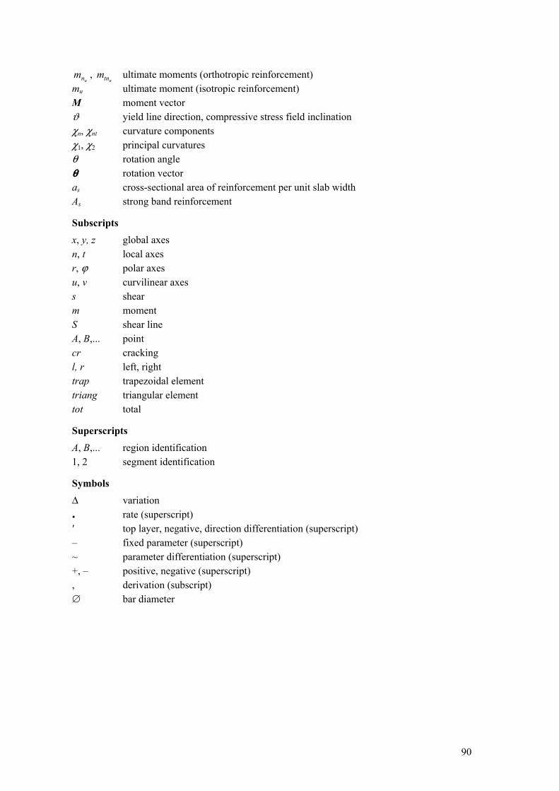
90

unm , utnm ultimate moments (orthotropic reinforcement)

mu ultimate moment (isotropic reinforcement) M moment vector ϑ yield line direction, compressive stress field inclination χn, χnt curvature components χ1, χ2 principal curvatures θ rotation angle θθθθ rotation vector as cross-sectional area of reinforcement per unit slab width As strong band reinforcement

Subscripts x, y, z global axes n, t local axes r, ϕ polar axes u, v curvilinear axes s shear m moment S shear line A, B,... point cr cracking l, r left, right trap trapezoidal element triang triangular element tot total

Superscripts A, B,... region identification 1, 2 segment identification

Symbols ∆ variation . rate (superscript) ′ top layer, negative, direction differentiation (superscript) – fixed parameter (superscript) ~ parameter differentiation (superscript) +, – positive, negative (superscript) , derivation (subscript) ∅ bar diameter