COMPDYN 2009ECCOMAS Thematic Conference on

Computational Methods in Structural Dynamics and Earthquake EngineeringM. Papadrakakis, N.D. Lagaros, M. Fragiadakis (eds.)

Rhodes, Greece, 22-24 June 2009

INTRODUCTION OF FRAGILIY SURFACES FOR A MOREACCURATE MODELING OF THE SEISMIC VULNERABILITY OF

REINFORCED CONCRETE STRUCTURES

Pierre Gehl1, Dariush Seyedi1, John Douglas1 and Mahmoud Khiar1

1BRGM - ARN3, avenue Claude Guillemin

BP 36009 - 45060 ORLEANS Cedex 2e-mail: p.gehl@brgm.fr

Keywords: Reinforced concrete building, fragility curve, fragility surface, non-linear time-history analysis, vulnerability assessment, strong-motion parameters.

Abstract. Earthquake shaking represents complex loading to a structure. It cannot be accu-rately characterized by a single parameter such as peak ground acceleration. The goal of thiswork is to compare the role of various strong-motion parameters on the induced damage in thestructure using numerical calculations. The most influential parameters are then used to buildmulti-variable fragility functions, in order to reduce some of the uncertainty inherent in the re-sponse to seismic loading.To this end, a robust structural model of an eight-story reinforced concrete building on whichdynamic calculations can be performed at an acceptable cost is used. In the model, all el-ements have a linear behaviour, except the ends of each column and each beam to which anonlinear behaviour based on damage mechanics and plasticity type (plastic-hinges model) isassigned [1]. Several hundred nonlinear dynamic analyses are carried out on the structure andthe damage levels are identified using the inter-story drift ratio, which can be linked to standarddamage scales.The spectral displacements, SDs, at the first two modal periods T1 and T2 are used to repre-sent the seismic loading as the most useful parameters reflecting the structure´s response [1].Each pair of points [SD(T1), SD(T2)] is associated with a probability of exceeding a givendamage level. This probability P is evaluated by considering the damage levels attained byother points located in its neighbourhood. A scalar parameter R = f [SD(T1), SD(T2)] isthen built up and we can construct an analytic equation for the fragility curve P = g(R) =g(f [SD(T1), SD(T2)]).This results in an equation for a fragility surface that offers a more complete and accurate viewof the structure´s vulnerability. A comparison between different profiles obtained by the gener-ated fragility surfaces and conventional fragility curves shows the significant role of the secondparameter in accurately estimating the probability of damage.Such fragility surfaces can be implemented within earthquake risk evaluation tools and theyshould provide more precise damage estimations. It is expected that this procedure can lead tomore accurate land-planning and retrofitting policies for risk mitigation.

1

hal-0

0560

523,

ver

sion

1 -

28 J

an 2

011

Author manuscript, published in "COMPDYN 2009 - ECCOMAS Thematic Conference on Computational Methods in StructuralDynamics and Earthquake Engineering, Greece (2009)"

Pierre Gehl, Dariush Seyedi, John Douglas and Mahmoud Khiar

1 INTRODUCTION

A variety of vulnerability analysis procedures have been followed in the past, ranging fromthe analysis of equivalent single-degree-of-freedom systems [3], adaptive pushover analysis ofmultistory models [2] to nonlinear time-history analyses of 3D models of RC structures [4]. Thechoices made for the analysis method, structural idealization, seismic hazard characterizationand damage models strongly influence the derived curves and have been seen to cause signifi-cant discrepancies in seismic risk assessments made by different groups for the same location,structure type and seismicity [5].

The classical procedures are based on the study of simplified substitute structures that arenot capable of accounting for the load redistribution inside structures due to local nonlineari-ties. The objective of damage assessment is to evaluate expected losses based on sufficientlydetailed analyses and the evaluation of the vulnerability characteristics at a given level of earth-quake ground motions. The conditional probability that a particular building will reach a certaindamage state should be determined using a fragility model. It consists of a suite of fragilityfunctions defining the conditional probability of reaching or exceeding a certain damage state.

Earthquake shaking applies complex loading to a structure, which cannot be accurately char-acterized by a single parameter (e.g. peak ground acceleration, PGA, or macroseismic inten-sity). However, in current vulnerability assessment methods, fragility curves are often devel-oped by using a single parameter to relate the level of shaking to the expected damage. Thisstandard method to develop fragility curves neglects the variability in the estimated damagecaused by the use of a single ground-motion parameter, which means that this uncertainty can-not properly be propagated to subsequent parts of the risk analysis nor can the importance ofthis variability be assessed.

The main objective of the ANR-funded VEDA (Seismic vulnerability of structures: A dam-age mechanics approach) project is to improve the existing methods of vulnerability evaluationby introducing the fragility surface concept for current reinforced concrete structures. In thisapproach, the shaking is characterized by two intensity measure (IM) parameters. The selectedIM parameters should ideally be poorly correlated for efficient characterization of the shaking.On the contrary, the structural damage must be correlated to the selected parameters. It is ex-pected that an increase from one to two IM parameters will lead to a significant reduction in thescatter in the fragility curve, which when using more than one parameter is a surface.

The damage level of a typical reinforced concrete structure is evaluated by the use of nonlin-ear numerical calculations. By considering the parts of the structure that would suffer significantdamage during strong ground motions (plastic hinges), an adequate 3D nonlinear robust-yet-simplified finite element model is created to allow numerous computations. The maximuminter-story drift ratio is used to define the damage level of the studied structure. Such a studycan help find a small number of ground-motion parameters that lead to, when used together tocharacterize the shaking, the smallest scatter in the estimated damage. Fragility surfaces arethen proposed for the studied structure.

2 MODEL DEFINITION AND DAMAGE ANALYSIS

2.1 Structural model

The main goal of vulnerability assessment methods is to estimate the seismic response ofexisting buildings. For this purpose we have used a structural model described in Seyedi et al.[1]. This is an eight-storey regular frame reinforced concrete (RC) structure. The structuralsystem of the building mainly consists of parallel shear walls in the Y direction, and an RC

2

hal-0

0560

523,

ver

sion

1 -

28 J

an 2

011

Pierre Gehl, Dariush Seyedi, John Douglas and Mahmoud Khiar

beam-columns frame in the X direction.In the framework of the VEDA project, this building was meshed by NECS, using shells to

represent slabs and walls, and linear beam elements for beams and columns. The damagingprocess is modelled thanks to plastic hinges located at the extremities of each beam and column[1].

The earthquake is applied to the structure in the X direction as an acceleration time-history.Only one horizontal component was used for each analysis. Calculations were carried out withCode Aster [6] finite element program, using the Newton-Raphson implicit algorithm.

2.2 Nonlinear time-history analysis

In this paper it is assumed that the analyzed structure is located in the French Antilles(Guadeloupe and Martinique), which is a region affected by both crustal and subduction (in-terface: shallow-dipping thrust events and intraslab: deep, generally normal-faulting, events)earthquakes. Therefore, a set of strong-motion records were compiled that is consistent withthe seismicity of this region. A magnitude-distance-earthquake-type filter is applied to a largedatabase of strong-motion records from various regions of the world (mainly the Mediterraneanregion, the Middle East, western North America, central America, Japan and Taiwan) to ex-clude records from magnitudes and distances that are not possible for the French Antilles. Alsorecords from small earthquakes and great distances were excluded since such weak motionswill not lead to significant damage for the structure analyzed here.

This led to a selection of 169 natural accelerograms that could potentially be used as inputto the structural modelling to construct the fragility surfaces. However, since the whole rangeof possible motions is not covered by the selected accelerograms it was decided to augment theinput time-history dataset with records simulated using the non-stationary stochastic methodof Pousse et al. [7], which is an extension of the procedure of Sabetta and Pugliese [8]. Thisresulted in the generation of 571 exploitable synthetic accelerograms.

In total, we used 740 strong-motion records (571 synthetic ones and 169 natural ones) asinput to time-history analyses. An extra advantage of using these simulated ground motionsover the natural accelerograms is that the structural modeling was faster due to the generallyshorter length of the records.

2.3 Results

As explained in previous section, 740 non-linear time-history analyses were performed onthe structural model and, for each simulation, the highest inter-storey drift ratio (ISDR) wasextracted as the structure response to the seismic input.

An advantage of using the ISDR to evaluate the damage level of a building is that this vari-able is fairly intuitive and was widely used in previous studies. Based on thousands of obser-vations Rossetto and Elnashai [9] developed empirical functions that correlate the ISDR andthe damage level for different types of European RC buildings. Depending on the type of RCstructure, relationships between the ISDR and an homogenized reinforced concrete damage in-dex (DIHRC) are proposed. Given the model of the studied structure, it was decided to use therelation for non-ductile moment-resisting frames to estimate the damage index of the structure(see Equation 1), this relationship also has the advantage of presenting a satisfactory correlationcoefficient (R2 = 0.991):

DIHRC = 34.89 ln(ISDR) + 39.39 (1)

3

hal-0

0560

523,

ver

sion

1 -

28 J

an 2

011

Pierre Gehl, Dariush Seyedi, John Douglas and Mahmoud Khiar

DIHRC can then be converted to the EMS-98 damage scale [10]: the correlation betweenDIHRC and EMS-98 damage level is shown in Table 1.

DIHRC value EMS-98 damage levelDIHRC < 0 D0

0 ≤ DIHRC < 30 D130 ≤ DIHRC < 50 D250 ≤ DIHRC < 70 D370 ≤ DIHRC < 100 D4

100 ≤ DIHRC D5

Table 1: Correlation between the damage index DIHRC and the EMS-98 damage level [9].

With the ISDR values obtained from the 740 simulations, the objective is now to find twoground-motion parameters that have the most influence on the building’s response, in order tobuild fragility surfaces. Orthogonal parameters are sought that characterize different aspects ofthe shaking, e.g. the amplitude, frequency content and duration, so that the fewest number ofparameters is needed. Problems associated with the choice of parameters for ground motion anddamage characterization can be identified in almost all existing vulnerability relationships [9].The parameter chosen to represent ground motion in the construction of vulnerability curvesmust be both representative of the damage potential of earthquakes and easily quantifiable fromknowledge of the earthquake characteristics.

In this study, we selected several strong-motion intensity parameters that can be well esti-mated through GMPEs and that are likely to have a strong influence on the building response.Table 2 presents the linear equations connecting the inter-storey drift ratio and the investigatedstrong-motion intensity parameters, x.

This study led to the choice of the spectral displacement as a useful variable for constructingthe fragility surfaces (see Table 2). The choice of the periods at which the spectral displacementwas examined was guided by eigenvalue analysis of the modeled building. The two main eigen-periods along the X direction (the direction where the seismic input is applied) were found tobe 1.26 and 0.41s respectively and, hence, SDs at these two periods were chosen as the strong-motion IM parameters.

A quick look at the distribution of selected time-histories in SD(1.26s)–SD(0.41s) space(see Figure 1) reveals that the two selected parameters seem strongly correlated. Neverthelessthese two parameters are sufficiently uncorrelated (correlation coefficient of 0.83) to be used tobuild a fragility surface, e.g. for a SD(1.26s) of 0.01 m Figure 1 shows that SD(0.41s) canrange between roughly 6.10−4 m and 0.02 m. Only some extreme situations (i.e. low SD(1.26s)and very high SD(0.41s) and vice versa) are not represented: these situations are not, in fact,realistic for earthquake shaking.

3 DEVELOPMENT OF FRAGILITY SURFACES

3.1 Conventional fragility curves

A first step, before tackling the issue of fragility surfaces, was to develop conventionalfragility curves, based on only one IM parameter. Shinozuka et al. [11] [12] developed ananalytical function that expresses the fragility curve in the form of a two-parameter lognormaldistribution function (Equation 2).

4

hal-0

0560

523,

ver

sion

1 -

28 J

an 2

011

Pierre Gehl, Dariush Seyedi, John Douglas and Mahmoud Khiar

Parameter Description Equation CorrelationcoefficientR2

SD(1.26s) Spectral displacement at the periodof the first mode

5.6025x− 0.025 0.837

SD(0.41s) Spectral displacement at the periodof the second mode

20.99x− 0.0084 0.650

PGA Peak ground acceleration 0.1239x + 0.0213 0.578AI Arias intensity 0.1506x + 0.1479 0.565AUD Absolute uniform duration (based

on a threshold of 0.03g)0.0834x + 0.0454 0.532

RSD Relative significant duration (basedon the interval between 5 and 95%Arias intensity)

−0.0025x + 0.3045 0.305

RUD Uniform relative duration (based ona threshold of 10% PGA)

−0.0027x + 0.2972 0.003

NC Equivalent number of effective cy-cles (Rainflow method)

0.0191x + 17.784 0.000

Table 2: Correlation between various strong-motion parameters (x) and the building inter-story drift ratio (ISDR).Equation reported is derived through linear regression.

F (x) = φ

(ln(x)− ln(α)

β

)(2)

where x represents the strong motion parameter (e.g. the spectral displacement), and F thestandardized normal distribution function. The two parameters α and β represent the medianand the lognormal standard deviation respectively and are computed so as to maximize thelikelihood function [11] [12], given by Equation 3.

M =N∏

k=0

[F (xk)]yk [1− F (xk)]

1−yk (3)

where N is the total number of simulations, xk the spectral displacement of the k-th accelero-gram, and yk is equal to 1 or 0, whether the structure has reached the given damage state or not(realization from a Bernoulli experiment). For both of the studied IM parameters (SD(1.26s)and SD(0.41s)), we developed four fragility curves corresponding to the four damage levelsfor the studied structure. Figure 2 and Table 3 present the results for SD(1.26s) as the singleIM parameter.

3.2 Development of fragility surfaces using the ‘neighbourhood’ method

The following procedure has been developed to construct the fragility surfaces. For thetwo chosen strong-motion intensity parameters (here SD(1.26s) and SD(0.41s), being the firstand second natural periods of the building), we build a x–y space containing 740 points ofcoordinates (xi, yi), x and y representing the two IM parameters. This space is associated withthe following norm, between points A(x1, y1) and B(x2, y2):

5

hal-0

0560

523,

ver

sion

1 -

28 J

an 2

011

Pierre Gehl, Dariush Seyedi, John Douglas and Mahmoud Khiar

Figure 1: Distribution of selected time-histories in SD(1.26s)–SD(0.41s) space. The crosses (and the greytriangles) represent the synthetic (and the real) accelerograms respectively.

d(A, B) =

√√√√√[ ln(x1

x2)

ln(xmax

xmin)

]2

+

ln(y1

y2)

ln(ymax

ymin)

2

(4)

It was chosen to introduce a logarithm scale because the use of a conventional Euclidiannorm was not adapted to the range of values (several powers of ten) spanned by SD(1.26s) andSD(0.41s). To avoid bias due to differently-scaled parameters this norm was also normalizedby the amplitude (xmax − xmin) of each parameter.

For each of the 740 points we defined a neighbourhood V of radius d, where we can evaluatethe probability to reach or exceed the damage state Dk:

P (D > Dk) =NV,k

NV,tot

(5)

In Equation 5, NV,tot is the total population in the neighbourhood V and NV,k denotes thenumber of points for which the damage state reaches or exceeds Dk. However, not all the points

6

hal-0

0560

523,

ver

sion

1 -

28 J

an 2

011

Pierre Gehl, Dariush Seyedi, John Douglas and Mahmoud Khiar

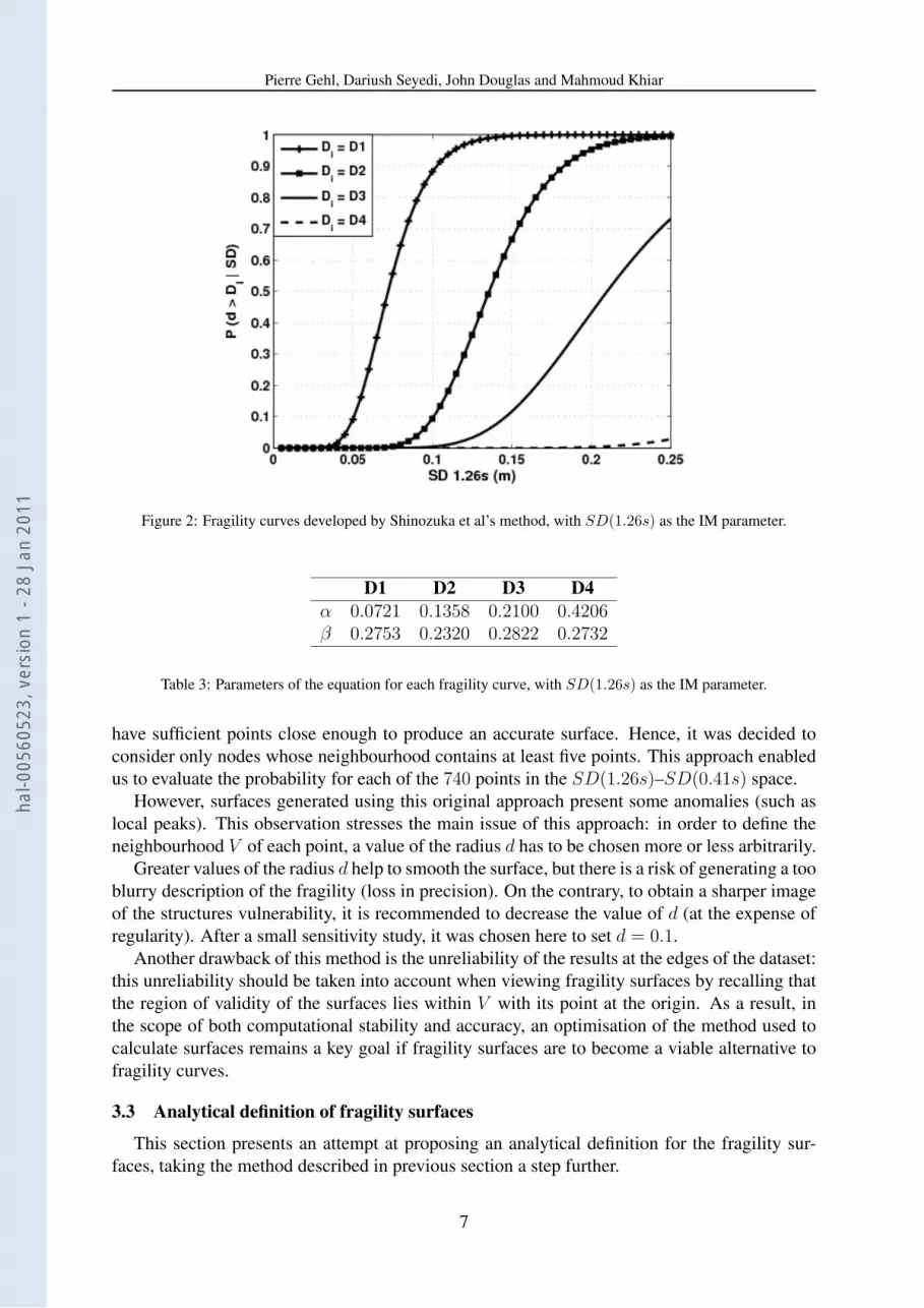
Figure 2: Fragility curves developed by Shinozuka et al’s method, with SD(1.26s) as the IM parameter.

D1 D2 D3 D4α 0.0721 0.1358 0.2100 0.4206β 0.2753 0.2320 0.2822 0.2732

Table 3: Parameters of the equation for each fragility curve, with SD(1.26s) as the IM parameter.

have sufficient points close enough to produce an accurate surface. Hence, it was decided toconsider only nodes whose neighbourhood contains at least five points. This approach enabledus to evaluate the probability for each of the 740 points in the SD(1.26s)–SD(0.41s) space.

However, surfaces generated using this original approach present some anomalies (such aslocal peaks). This observation stresses the main issue of this approach: in order to define theneighbourhood V of each point, a value of the radius d has to be chosen more or less arbitrarily.

Greater values of the radius d help to smooth the surface, but there is a risk of generating a tooblurry description of the fragility (loss in precision). On the contrary, to obtain a sharper imageof the structures vulnerability, it is recommended to decrease the value of d (at the expense ofregularity). After a small sensitivity study, it was chosen here to set d = 0.1.

Another drawback of this method is the unreliability of the results at the edges of the dataset:this unreliability should be taken into account when viewing fragility surfaces by recalling thatthe region of validity of the surfaces lies within V with its point at the origin. As a result, inthe scope of both computational stability and accuracy, an optimisation of the method used tocalculate surfaces remains a key goal if fragility surfaces are to become a viable alternative tofragility curves.

3.3 Analytical definition of fragility surfaces

This section presents an attempt at proposing an analytical definition for the fragility sur-faces, taking the method described in previous section a step further.

7

hal-0

0560

523,

ver

sion

1 -

28 J

an 2

011

Pierre Gehl, Dariush Seyedi, John Douglas and Mahmoud Khiar

The 740 probability values for reaching or exceeding damage state D1, evaluated in theprevious section, were plotted on a 2D-graph, as a function of one parameter only (SD(1.26s)or SD(0.41s)). The two plots are presented in Figure 3: as expected, the graphs show greatscatter, proving once again the need for a second parameter to give a better description of thestructure vulnerability.

Figure 3: Fragility curves for the damage level D1, based on parameters SD(1.26s) and SD(0.41s), generatedwith the points used for the development of fragility surfaces presented in previous section.

An analysis of the fragility surfaces presented previously made us think that a hybrid parame-ter (such as the logarithmic distance between a point A of the SD(1.26s)–SD(0.41s) space andthe origin (10−4, 10−4)) could be a good candidate for building vector-based fragility curves:

R[SD(1.26s), SD(0.41s)] =

√ln2(

SD(1.26s)

10−4) + ln2(

SD(0.41s)

10−4) (6)

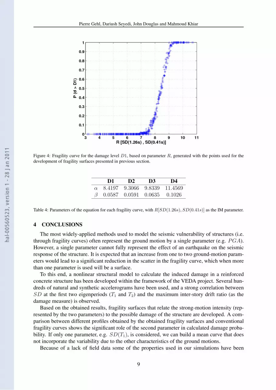
Each of the 740 points are associated with this new variable R, and the probability of reachingor exceeding damage state D1 with R on the abscissa is plotted (see Figure 4).

Figure 4 clearly shows the reduction in the scatter of the probability data: the plotted pointsdirectly take the shape of a normal distribution cumulative function. It is then possible to fit thepoints by a analytical function, depending on the variable R (hence it is a function of the twovariables SD(1.26s) and SD(0.41s)), and defined by Equation 7:

Pk(d > Dk|R) = 0.5

[1 + erf

(ln(R)− ln(αk)

βk

√2

)](7)

The same procedure is applied to damage states D2, D3 and D4, and Table 4 sums up theparameters of Equation 7, for all damage states.

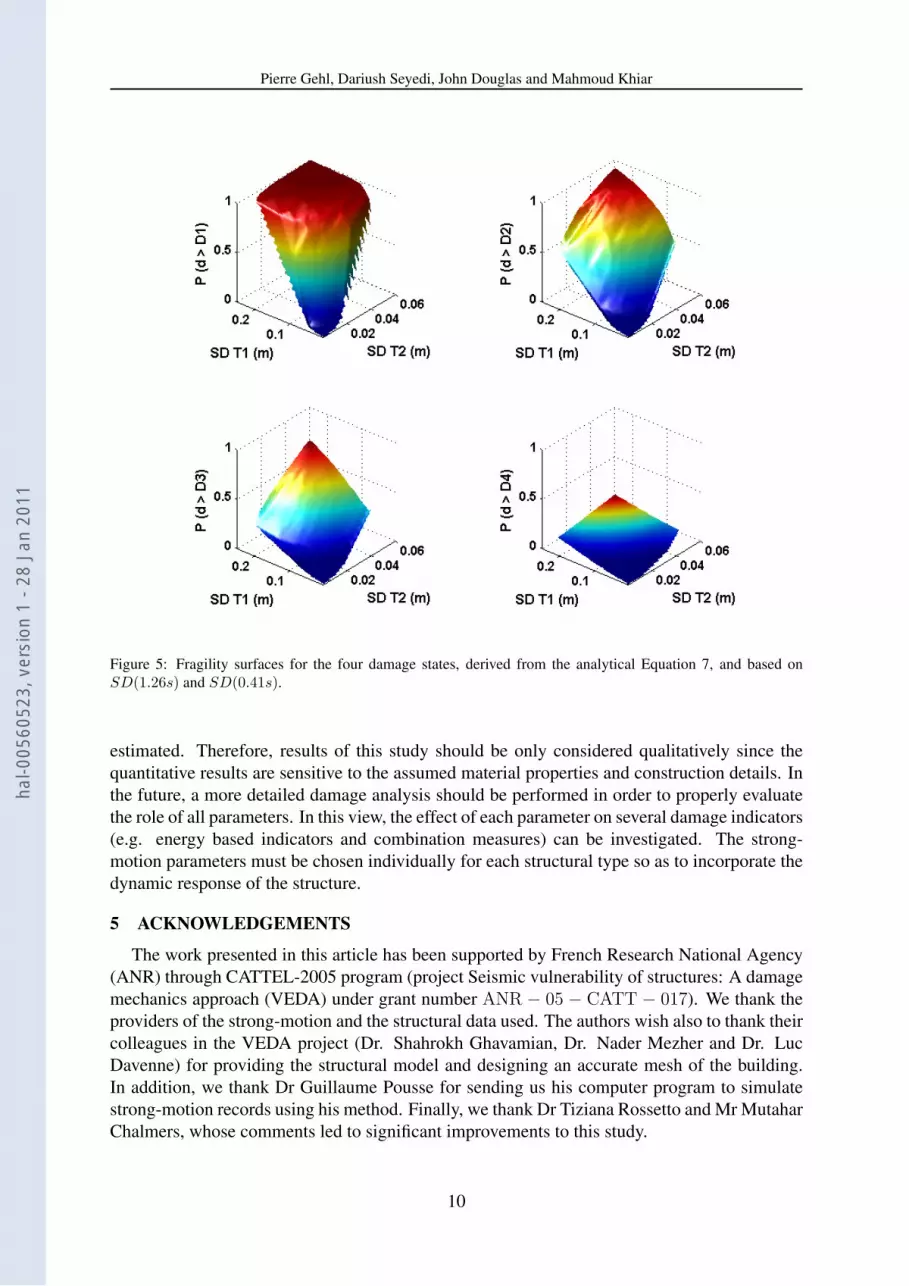
Thanks to Equation 7, we now have the equation of a surface, linking the probability to thetwo desired parameters SD(1.26s) and SD(0.41s). The four analytical fragility surfaces for alldamage states are displayed in Figure 5.

The analytical expression enables users of fragility surfaces to properly exploit the vulnera-bility data (the input of SD(1.26s) and SD(0.41s) parameters returns a calculated probabilityvalue).

8

hal-0

0560

523,

ver

sion

1 -

28 J

an 2

011

Pierre Gehl, Dariush Seyedi, John Douglas and Mahmoud Khiar

Figure 4: Fragility curve for the damage level D1, based on parameter R, generated with the points used for thedevelopment of fragility surfaces presented in previous section.

D1 D2 D3 D4α 8.4197 9.3066 9.8339 11.4569β 0.0587 0.0591 0.0635 0.1026

Table 4: Parameters of the equation for each fragility curve, with R[SD(1.26s), SD(0.41s)] as the IM parameter.

4 CONCLUSIONS

The most widely-applied methods used to model the seismic vulnerability of structures (i.e.through fragility curves) often represent the ground motion by a single parameter (e.g. PGA).However, a single parameter cannot fully represent the effect of an earthquake on the seismicresponse of the structure. It is expected that an increase from one to two ground-motion param-eters would lead to a significant reduction in the scatter in the fragility curve, which when morethan one parameter is used will be a surface.

To this end, a nonlinear structural model to calculate the induced damage in a reinforcedconcrete structure has been developed within the framework of the VEDA project. Several hun-dreds of natural and synthetic accelerograms have been used, and a strong correlation betweenSD at the first two eigenperiods (T1 and T2) and the maximum inter-story drift ratio (as thedamage measure) is observed.

Based on the obtained results, fragility surfaces that relate the strong-motion intensity (rep-resented by the two parameters) to the possible damage of the structure are developed. A com-parison between different profiles obtained by the obtained fragility surfaces and conventionalfragility curves shows the significant role of the second parameter in calculated damage proba-bility. If only one parameter, e.g. SD(T1), is considered, we can build a mean curve that doesnot incorporate the variability due to the other characteristics of the ground motions.

Because of a lack of field data some of the properties used in our simulations have been

9

hal-0

0560

523,

ver

sion

1 -

28 J

an 2

011

Pierre Gehl, Dariush Seyedi, John Douglas and Mahmoud Khiar

Figure 5: Fragility surfaces for the four damage states, derived from the analytical Equation 7, and based onSD(1.26s) and SD(0.41s).

estimated. Therefore, results of this study should be only considered qualitatively since thequantitative results are sensitive to the assumed material properties and construction details. Inthe future, a more detailed damage analysis should be performed in order to properly evaluatethe role of all parameters. In this view, the effect of each parameter on several damage indicators(e.g. energy based indicators and combination measures) can be investigated. The strong-motion parameters must be chosen individually for each structural type so as to incorporate thedynamic response of the structure.

5 ACKNOWLEDGEMENTS

The work presented in this article has been supported by French Research National Agency(ANR) through CATTEL-2005 program (project Seismic vulnerability of structures: A damagemechanics approach (VEDA) under grant number ANR − 05 − CATT − 017). We thank theproviders of the strong-motion and the structural data used. The authors wish also to thank theircolleagues in the VEDA project (Dr. Shahrokh Ghavamian, Dr. Nader Mezher and Dr. LucDavenne) for providing the structural model and designing an accurate mesh of the building.In addition, we thank Dr Guillaume Pousse for sending us his computer program to simulatestrong-motion records using his method. Finally, we thank Dr Tiziana Rossetto and Mr MutaharChalmers, whose comments led to significant improvements to this study.

10

hal-0

0560

523,

ver

sion

1 -

28 J

an 2

011

Pierre Gehl, Dariush Seyedi, John Douglas and Mahmoud Khiar

REFERENCES

[1] D. Seyedi, P. Gehl, J. Douglas, L. Davenne, N. Mezher, S. Ghavamian, Development ofseismic fragility surfaces for reinforced concrete buildings by means of nonlinear time-history analysis. Earthquake Engineering and Structural Dynamics, under revision.

[2] T. Rossetto, A. Elnashai, A new analytical procedure for the derivation of displacement-based vulnerability curves for populations of RC structures. Engineering Structures, 27,397–409, 2005.

[3] K. Mosalam, G. Ayala, R. White, C. Roth, Seismic fragility of LRC frames with and with-out masonry infill walls. Journal of Earthquake Engineering, 1, 683–719, 1997.

[4] A. Singhal, A. Kiremidjian, A method for earthquake motion damage relationships withapplication to reinforced concrete frames. Research Report NCEER-97-0008 State Uni-versity of New York at Buffalo: National Center for Earthquake Engineering, 1997.

[5] M. Priestley, Displacement-based approaches to rational limit states design of new struc-tures. 11th European Conference on Earthquake Engineering, Rotterdam, AA Balkema,1998.

[6] Code Aster, Code d’Analyses des Structures et Thermomecanique pour Etudes etRecherches. www.code-aster.org EDF R&D, 2008.

[7] G. Pousse, L.F. Bonilla, F. Cotton, L. Margerin, Non stationary stochastic simulation ofstrong ground motion time histories including natural variability: Application to the K-net Japanese database. Bulletin of Seismological Society of America, 96(6), 2103–2117,2006.

[8] F. Sabetta, A. Pugliese, Estimation of response spectra and simulation of nonstationaryearthquake ground motions. Bulletin of Seismological Society of America, 86(2), 337–352, 1996.

[9] T. Rossetto, A. Elnashai, Derivation of vulnerability functions for European-type RCstructures based on observational data. Engineering Structures, 25, 1241–1263, 2003.

[10] European Council, European Macroseismic Scale 1998 (EMS-98). Cahier du Centre Eu-ropen de Godynamique et de Sismologie, G. Grnthal (Eds.), 15, 1998.

[11] M. Shinozuka, Statistical analysis of bridge fragility curves. US - Italy Workshop on Pro-tective Systems for Bridges, New-York, April 26-28, 1998.

[12] M. Shinozuka, Q. Feng, J. Lee, T. Naganuma, Statistical analysis of fragility curves. Jour-nal of Engineering Mechanics, ASCE, 126(12), 1224–1231, 2000.

11

hal-0

0560

523,

ver

sion

1 -

28 J

an 2

011