SEISMIC DESIGN GUIDE FOR MASONRY BUILDINGS

Canadian Concrete Masonry Producers Association

Second Edition

2018

Donald AndersonSvetlana Brzev

DISCLAIMER While the authors have tried to be as accurate as possible, they cannot be held responsible for the designs of others that might be based on the material presented in this document. The material included in this document is intended for the use of design professionals who are competent to evaluate the significance and limitations of its contents and recommendations and able to accept responsibility for its application. The authors, and the Canadian Concrete Masonry Producers Association, disclaim any and all responsibility for the applications of the stated principles and for the accuracy of any of the material included in the document. AUTHORS Don Anderson, Ph.D., P.Eng. Professor Emeritus Department of Civil Engineering University of British Columbia Vancouver, BC, Canada

Svetlana Brzev, Ph.D., P.Eng., FEC Adjunct Professor Department of Civil Engineering University of British Columbia Vancouver, BC, Canada

TECHNICAL EDITOR Bill McEwen, P.Eng., LEED AP, Retired Executive Director, Masonry Institute of BC GRAPHIC DESIGN Natalia Leposavic, M.Arch. COVER PAGE Photo credit: Bill McEwen, P.Eng. Graphic design: Prithul Saha, M.Arch. COPYRIGHT Canadian Concrete Masonry Producers Association, 2018 Canadian Concrete Masonry Producers Association P.O. Box 54503, 1771 Avenue Road Toronto, ON M5M 4N5 Tel: (416) 495-7497 Fax: (416) 495-8939 Email: information@ccmpa.ca Web site: www.ccmpa.ca The Canadian Concrete Masonry Producers Association (CCMPA) is a non-profit association whose mission is to support and advance the common interests of its members in the manufacture, marketing, research, and application of concrete masonry products and structures. It represents the interests of Region 6 of the National Concrete Masonry Association (NCMA).

i

Contents Summary

Chapter 1 NBC 2015 Seismic Provisions

Objective: to provide background on seismic response of structures

and seismic analysis methods and explain key NBC 2015 seismic

provisions of relevance for masonry design

DETAILED NBC

SEISMIC

PROVISIONS

Chapter 2 Seismic Design of Masonry Walls to CSA S304-14

Objective: to provide background and commentary for CSA S304-14

seismic design provisions related to reinforced concrete masonry walls,

and discuss the revisions in CSA S304-14 seismic design requirements

with regard to the 2004 edition

DETAILED

MASONRY

DESIGN

PROVISIONS

Chapter 3 Design Examples

Objective: to provide illustrative design examples of seismic load

calculation and distribution of forces to members according to NBCC

2015, and the seismic design of loadbearing and nonloadbearing

masonry elements according to CSA S304-14

DESIGN

EXAMPLES

Appendix A Response of Structures to Earthquakes

Appendix B Research Studies and Code Background Relevant to Masonry Design

Appendix C Relevant Design Background

Appendix D Design Aids

Appendix E Notation

ii

Table of Contents 1 SEISMIC DESIGN PROVISIONS OF THE NATIONAL BUILDING CODE OF CANADA 2015 1-2 1.1 Introduction 1-2 1.2 Design and Performance Objectives 1-3 1.3 Seismic Hazard 1-4 1.4 Effect of Site Soil Conditions 1-6 1.5 Methods of Analysis 1-12 1.6 Base Shear Calculations- Equivalent Static Analysis Procedure 1-12 1.7 Force Reduction Factors 1-15 1.8 Higher Mode Effects 1-17 1.9 Vertical Distribution of Seismic Forces 1-19 1.10 Overturning Moments 1-20 1.11 Torsion 1-21 1.11.1 Torsional effects 1-21 1.11.2 Torsional sensitivity 1-23 1.11.3 Determination of torsional forces 1-25 1.11.4 Flexible diaphragms 1-27 1.12 Configuration Issues: Irregularities and Restrictions 1-30 1.12.1 Irregularities 1-30 1.12.2 Restrictions 1-34 1.13 Deflections and Drift Limits 1-35 1.14 Dynamic Analysis Method 1-36 1.15 Soil-Structure Interaction 1-37 1.16 A Comparison of NBC 2005 and NBC 2015 Seismic Design Provisions 1-38 2 SEISMIC DESIGN OF MASONRY WALLS TO CSA S304-14 2-2 2.1 Introduction 2-2 2.2 Masonry Walls – Basic Concepts 2-2 2.3 Reinforced Masonry Shear Walls Under In-Plane Seismic Loading 2-8 2.3.1 Behaviour and Failure Mechanisms 2-8 2.3.2 Shear/Diagonal Tension Resistance 2-10 2.3.3 Sliding Shear Resistance 2-18 2.3.4 In-Plane Flexural Resistance Due to Combined Axial Load and Bending 2-20 2.4 Reinforced Masonry Walls Under Out-of-Plane Seismic Loading 2-20 2.4.1 Background 2-20 2.4.2 Out-of-Plane Shear Resistance 2-21 2.4.3 Out-of-Plane Sliding Shear Resistance 2-22 2.4.4 Out-of-Plane Section Resistance Due to Combined Axial Load and Bending 2-22 2.5 General Seismic Design Provisions for Reinforced Masonry Shear Walls 2-23 2.5.1 Capacity Design Approach 2-23

iii

2.5.2 Ductile Seismic Response 2-27 2.5.3 Structural Regularity 2-28 2.5.4 Analysis Assumptions – Effective Section Properties 2-28 2.5.5 Redistribution of design moments from elastic analysis 2-30 2.5.6 Minor shear walls as a part of the SFRS 2-30 2.6 CSA S304-14 Seismic Design Requirements 2-30 2.6.1 Classes of reinforced masonry shear walls 2-30 2.6.2 Plastic hinge region 2-32 2.6.3 Ductility check 2-34 2.6.4 Wall height-to-thickness ratio restrictions 2-40 2.6.5 Minimum Required Factored Shear Resistance 2-45 2.6.6 Shear/diagonal tension resistance – seismic design requirements 2-46 2.6.7 Sliding shear resistance – seismic design requirements 2-48 2.6.8 Boundary elements in Moderately Ductile and Ductile shear walls 2-49 2.6.9 Seismic reinforcement requirements for masonry shear walls 2-59 2.6.10 Minimum reinforcement requirements for Moderately Ductile

Squat shear walls 2-68 2.6.11 Summary of Seismic Design Requirements for Reinforced Masonry Walls 2-71 2.6.12 Comparison of the Seismic Design and Detailing Requirements for Reinforced Masonry Walls in CSA S304-14 and CSA S304.1-04 2-73 2.7 Special Topics 2-75 2.7.1 Unreinforced Masonry Shear Walls 2-75 2.7.2 Masonry Infill Walls 2-80 2.7.3 Stack Pattern Walls 2-88 2.7.4 Nonloadbearing Walls 2-93 2.7.5 Flanged shear walls 2-94 2.7.6 Wall-to-Diaphragm Anchorage 2-96 2.7.7 Masonry Veneers and their Connections 2-97 2.7.8 Constructability Issues 2-100 3 DESIGN EXAMPLES 1 Seismic load calculation for a low-rise masonry building to NBC 2015 3-2 2 Seismic load calculation for a medium-rise masonry building to NBC 2015 3-9 3 Seismic load distribution in a masonry building considering both rigid and flexible diaphragm alternatives 3-24 4a Minimum seismic reinforcement for a squat masonry shear wall 3-37 4b Seismic design of a squat shear wall of Conventional Construction 3-41 4c Seismic design of a Moderately Ductile squat shear wall 3-47 5a Seismic design of a Moderately Ductile flexural shear wall 3-57 5b Seismic design of a Ductile shear wall with rectangular cross-section 3-68

iv

5c Seismic design of a Ductile shear wall with boundary elements 3-79 6a Design of a loadbearing wall for out-of-plane seismic effects 3-92 6b Design of a nonloadbearing wall for out-of-plane seismic effects 3-99 7 Seismic design of masonry veneer ties 3-104 8 Seismic design of a masonry infill wall 3-106 REFERENCES

APPENDICES A. RESPONSE OF STRUCTURES TO EARTHQUAKES A-2 A.1. Elastic Response A-2 A.2. Inelastic Response A-6 A.3. Ductility A-7 A.4. A Primer on Modal Dynamic Analysis Procedure A-8 A.4.1. Multi-degree-of-freedom systems A-8 A.4.2. Seismic analysis methods A-9 A.4.3. Modal analysis procedure: an example A-10 A.4.4. Comparison of static and modal analysis results A-14 B RESEARCH STUDIES AND CODE BACKGROUND RELEVANT TO MASONRY DESIGN B-2 B.1 Shear/Diagonal Tension Resistance B-2 B.2 Sliding Shear Resistance B-8 B.3 Ductile Seismic Response of Reinforced Masonry Shear Walls B-12 B.5 Wall Height-to-Thickness Ratio Restrictions B-16 C RELEVANT DESIGN BACKGROUND C-2 C.1 Design for Combined Axial Load and Flexure C-2 C.1.1 Reinforced Masonry Walls Under In-Plane Seismic Loading C-2 C.1.2 Reinforced Masonry Walls Under Out-of-Plane Seismic Loading C-9 C.2 Wall Intersections and Flanged Shear Walls C-15 C.2.1 Effective Flange Width C-15 C.2.2 Types of Intersections C-16 C.2.3 Shear Resistance at the Intersections C-18

v

C.3 Wall Stiffness Calculations C-22 C.3.1 Lateral Load Distribution C-22 C.3.2 Wall Stiffness: Cantilever and Fixed-End Model C-23 C.3.3 Approximate Method for Force Distribution in Masonry Shear Walls C-24 C.3.4 Advanced Design Approaches for Reinforced Masonry Shear Walls with Openings C-27 C.3.5 The Effect of Cracking on Wall Stiffness C-32 D DESIGN AIDS D-2 Table D-1. Properties of Concrete Masonry Walls (per metre or foot length) D-2 Table D-2. wlc ratio, yf = 400 MPa D-3

Figure D-1. wlc ratio, yf = 400 MPa D-4

Table D-3. Wall Stiffness Values tEK m * D-5

E NOTATION

vi

FOREWORD This is the second edition of the “Seismic Design Guide for Masonry Buildings”. It supercedes the first edition published in 2009. This Guide is based on the 2015 edition of the National Building Code of Canada (NBCC) and the 2014 edition of CSA S304, “Design of Masonry Structures”. The major changes found in this second edition are described by its authors in the Guide Preface. The Guide describes the behaviour of masonry under seismic loading, explains and rationalizes the basis of the seismic design requirements within the NBCC and S304, and provides guidance and assistance to masonry designers on their interpretation and use. It describes and details the appropriate methods for seismic design and analysis, and demonstrates their use by many illustrative design examples. The Guide necessarily recognizes the high standard of quality control present in modern masonry structures and the advanced methods used in the structural design of masonry. As with the first edition, the format and content of the second edition of the Guide have been specifically developed to address the needs of the practicing structural engineer designing low-, mid-, and high-rise masonry buildings and their elements. The first edition also served as an excellent reference guide for academics and instructors. Although it is written for the Canadian environment, the Seismic Design Guide has been extremely popular with international designers. There is no similar or comparable guide for the seismic design of masonry in Canada, and no more comprehensive guide for masonry internationally. The Canadian Concrete Masonry Producers Association (CCMPA) is pleased to sponsor and publish the second edition of the Seismic Design Guide. It is co-authored by Drs. Anderson and Brzev, two authorities in seismic behaviour and design of masonry, and also the co-authors of the first edition of the Guide. The CCMPA gratefully acknowledges the commitment by these authors, and their dedication to masonry education and research. We recognize the past and on-going work by Dr. Anderson, Professor Emeritus, University of British Columbia, who has spearheaded and coordinated the requirements for masonry seismic design through his research, and by his work on the many past editions of the National Building Code and CSA S304. Until very recently, Dr. Anderson served as a member of the Standing Committee on Earthquake Design (SCED). Dr. Anderson’s liaison between the Technical Committee for CSA S304 and SCED (and its predecessor CANCEE) has been eminently important for developing the seismic requirements in the S304 standard and for harmonizing its requirements with those of the NBCC. Dr. Brzev is Adjunct Professor of the University of British Columbia, and also Visiting Professor in The Faculty of Civil Engineering, Indian Institute of Technology Gandhinagar. She brings to this Guide, her vast international experience and understanding of behaviour and design of concrete and masonry elements and structures, and earthquake engineering. Dr. Brzev undertakes research and authors seismic research papers, practices professional engineering in British Columbia, and is co-author of “Reinforced Concrete Design, A Practical Approach”. She serves as a member of the Technical Committe on CSA S304. We are also grateful to the editiorial work on this Guide by Mr. Bill McEwen, P.Eng., LEED, retired Executive Director of the Masonry Institute of British Columbia. The development of both editions of the Seismic Design Guide has been sponsored by the Canadian Concrete Masonry Producers Association (CCMPA), a non-profit

vii

association. The CCMPA provides a united voice for the producers of concrete masonry products Canada-wide. Our member firms are engaged in the manufacture of concrete block and concrete brick masonry units used for loadbearing and nonloadbearing applications, and as veneers. The CCMPA also represents Canadian interests within the National Concrete Masonry Association, a U.S.-based international association of concrete masonry producers. The CCMPA supports the educational work of Canadian universities and other educational institutions, and the education of the masonry design professional, practitioner and student, both formally and informally. It sponsors masonry research at many universities in Canada including British Columbia, Alberta, Calgary, Saskatchewan, Manitoba, Waterloo, Windsor, McMaster, Carleton, McGill, Concordia, and Dalhousie. The development and publication of this Guide is part of its continuing commitment to education. The CCMPA is intimately involved in the development and maintenance of CSA masonry and masonry-related standards. These standards serve as the basis for manufacturing and specifying concrete masonry materials and products, product and assembly testing, and the structural design and construction of masonry elements. The CCMPA provides input to the development of the National Building Code of Canada and the National Energy Code for Buildings. The CCMPA continually develops and disseminates information and design tools needed by designers to deliver state-of-the-art, safe and serviceable, durable, and cost-effective masonry elements and structures. This Guide was developed on the basis of the Limit States Design method of CSA Standard S304-14. The references to this standard in this Guide neither duplicate nor replace this standard. Therefore, it is recommended that the user of this Guide obtain a copy of CSA S304-14, “ Design of Masonry Structures” developed and published by the Canadian Standards Association (www.csa.ca). This Guide has given rise to a new generation of masonry buildings and to their proliferation. Gary R. Sturgeon, B.Eng., MSc. P.Eng. Technical Services Engineer The Canadian Concrete Masonry Producers Association (CCMPA)

viii

PREFACE This Guide is intended to assist practicing structural engineers in designing masonry buildings for seismic load effects according to the National Building Code of Canada 2015 (NBC 2015) and the CSA S304-14 masonry design standard. The Guide includes commentary comments that explain the underlying theoretical background and rationale for these seismic provisions. Changes in the seismic design provisions contained in Part 4 of the NBC 2015 and CSA S304-14, and their impact on masonry design and construction are discussed. This is a second edition of the Guide. The first edition, published in 2009, has served as a useful reference for engineers and academics in Canada. Major changes in the second edition are summarized below: Chapter 1 has been revised to address changes in the NBC 2015 (NBC 2005 had

been referenced in the first edition). Section 1.4 from the first edition has been moved to Appendix A.

Chapter 2 has been substantially revised to address changes in the CSA S304-14 (CSA S304.1-04 had been referenced in the first edition). Sections 2.5 to 2.7 have undergone major changes.

Chapter 3 from the first edition has been removed. New Chapter 3 (previously Chapter 4) contains design examples which have been

prepared according to NBC 2015 and CSA S304-14. Most examples existed in the first edition, but have been updated. New Example 5c was developed to illustrate the design of Ductile reinforced masonry shear walls with boundary elements.

Appendix A has been changed. Previous content has been removed and it now contains Section 1.4 from the first edition of the Guide.

Appendices B, C, D, and E have been updated. This is a comprehensive state-of-the-art guide on the seismic design and construction of masonry structural elements for low- to mid-rise structures, such as warehouses, industrial buildings, schools, commercial buildings, and residential/hotel structures. It is restricted to masonry structures designed and constructed using concrete block units. Consideration of the slenderness effects in tall masonry walls is beyond the scope of this Guide. The material is presented in a simple and user-friendly manner. It facilitates the application of seismic design provisions and cross-referencing of code clauses for designers. The Guide has been developed in a modular form, with the content divided into three chapters, each of which can be used in a stand-alone manner. The appendices contain useful resources such as design procedures and research background for some of the design provisions. For easy reference, relevant code clauses are identified by framed boxes wherever appropriate. Chapter 1 provides a review of the general seismic design provisions contained in Part 4 of NBC 2015, including seismic hazard levels, and the equivalent static force procedure. It discusses key design parameters such as irregularities, torsion, height limitations, and the ductility and overstrength factors for masonry structures. Additionally, an introduction to the dynamic analysis of structures to assist in understanding pertinent code provisions has been included in Appendix A.

ix

Chapter 2 provides an overview of seismic design requirements for reinforced masonry walls. Relevant CSA S304-14 design requirements are presented, along with related commentary that provides detailed explanations of the code provisions. Topics include reinforced masonry shear walls subjected to in-plane and out-of-plane seismic loads, and a detailed discussion of the CSA S304-14 seismic design requirements. A few special topics such as masonry infill walls, stack pattern walls, masonry veneers, and construction-related issues are also included. Changes in CSA S304-14 seismic design requirements from the previous CSAS304.1-04 (2004) edition are identified and discussed, along with their design implications. Appendix B contains resources related to the Chapter 2 content, including findings of research studies and foreign code provisions related to the seismic design of masonry structures. Chapter 3 provides illustrative design examples of the seismic load calculations and distribution of forces to members according to NBC 2015, and the design of loadbearing and nonloadbearing masonry elements according to CSA S304-14. The layout of masonry buildings and the mechanical properties of their components in the examples are chosen to reflect situations often encountered in design practice, particularly as they relate to torsionally unsymmetric buildings. These examples are laid out in a step-by-step manner, with ample explanations and appropriate illustrations provided to clarify the design process. Appendix C provides relevant background information for the design examples, including an extensive discussion of in-plane wall stiffness. Appendix D contains design aids used in the Chapter 3 examples. Appendix E lists the notations used in the document. A list of key references, useful for supplementary reading for those interested in pursuing the subject further, is also included.

Svetlana Brzev and Don Anderson

x

ACKNOWLEDGMENTS It would not be possible to develop and finalize a document of this size without the support and assistance provided by several individuals and organizations. The authors are grateful to the Canadian Concrete Masonry Producers Association (CCMPA) for giving them the opportunity to undertake this project. The authors gratefully acknowledge Bill McEwen, P.Eng., retired Executive Director of the Masonry Institute of BC, for providing valuable review comments, guidance and encouragement during the development of both editions of the Guide. Bill shared some of his practical field insights in the Constructability Issues section of the guide. The authors are grateful to Doug Birch, P.Eng., Struct.Eng. of Krahn Engineering, Vancouver, for performing a technical review of the design examples included in the Second Edition of the Guide. The authors are indebted to Gary Sturgeon, P.Eng., former Director of Technical Services, CCMPA for spearheading the original development of this Guide and for the guidance and comments he provided. The authors acknowledge Dr. Jose Centeno of Glotman Simpson, Vancouver (a former Ph.D. student at the Civil Engineering Department, UBC), for contributing his research findings related to the sliding shear resistance of reinforced masonry shear walls which has been included in Appendix B of the Guide. The authors also acknowledge Brook Robazza, M.A.Sc., Ph.D. candidate at the Civil Engineering Department, UBC, for contributing to the research background on out-of-plane instability in reinforced masonry shear walls (Appendix B). The authors would like to thank Natalia Leposavic, M.Arch. of BCIT, Vancouver, for preparing the excellent drawings included in this document, and Prithul Saha, M.Arch. of New Delhi, India for developing the cover page. The authors gratefully acknowledge assistance of Dr. T.S. Kumbar, Librarian at the Indian Institute of Technology Gandhinagar, India and the Library staff for providing access to numerous research publications. CREDITS The authors and the Canadian Concrete Masonry Producers Association acknowledge the following organizations and individuals who have kindly given permission to reproduce the copyright material presented in this publication: National Research Council, Masonry Institute of BC, The Masonry Society, American Concrete Institute, Earthquake Engineering Research Institute, American Society of Civil Engineers, New Zealand Standards, New Zealand Concrete Masonry Association Inc., Federal Emergency Management Agency, Imperial College Press, Bill McEwen, Michael Hatzinikolas and Yasser Korany.

9/1/2018 1-1

TABLE OF CONTENTS – CHAPTER 1

1 SEISMIC DESIGN PROVISIONS OF THE NATIONAL BUILDING CODE OF CANADA 2015 ........................................................................................................................................ 1-2

1.1 Introduction .................................................................................................................................. 1-2

1.2 Design and Performance Objectives ......................................................................................... 1-3

1.3 Seismic Hazard ............................................................................................................................. 1-4

1.4 Effect of Site Soil Conditions ...................................................................................................... 1-6

1.5 Methods of Analysis .................................................................................................................. 1-12

1.6 Base Shear Calculations- Equivalent Static Analysis Procedure ......................................... 1-12

1.7 Force Reduction Factors dR and oR ..................................................................................... 1-15

1.8 Higher Mode Effects ( vM factor) ............................................................................................. 1-17

1.9 Vertical Distribution of Seismic Forces ................................................................................... 1-19

1.10 Overturning Moments ( J factor) ............................................................................................. 1-20

1.11 Torsion ........................................................................................................................................ 1-21 1.11.1 Torsional effects ................................................................................................................... 1-21 1.11.2 Torsional sensitivity .............................................................................................................. 1-23 1.11.3 Determination of torsional forces ......................................................................................... 1-25 1.11.4 Flexible diaphragms ............................................................................................................. 1-27

1.12 Configuration Issues: Irregularities and Restrictions ............................................................ 1-30 1.12.1 Irregularities .......................................................................................................................... 1-30 1.12.2 Restrictions ........................................................................................................................... 1-34

1.13 Deflections and Drift Limits ...................................................................................................... 1-35

1.14 Dynamic Analysis Method ......................................................................................................... 1-36

1.15 Soil-Structure Interaction .......................................................................................................... 1-37

1.16 A Comparison of NBC 2005 and NBC 2015 Seismic Design Provisions .............................. 1-38

9/1/2018 1-2

1 Seismic Design Provisions of the National Building Code of Canada 2015

1.1 Introduction This chapter provides a review of the seismic design provisions in the 2015 National Building Code of Canada (NBC 2015) as they pertain to masonry. Reference will be made here to NBC 2005 where appropriate to point out changes. Appendix A contains an introduction to the dynamic analysis of structures to assist in understanding the NBC provisions. The original edition of this guideline (Anderson and Brzev, 2009) was produced to address the many fundamental changes in how seismic risk was evaluated between NBC 2005 and CSA S304.1-04, and their previous versions. The seismic response of a building structure depends on several factors, such as the structural system and its dynamic characteristics, the building materials and design details, and most importantly, the expected earthquake ground motion at the site. The expected ground motion, termed the seismic hazard, can be estimated using probabilistic methods, or be based on deterministic means if there is an adequate history of large earthquakes on identifiable faults in the region of the site. Canada generally uses a probabilistic method to assess the seismic hazard, and over the years, the probability has been decreasing, from roughly a 40% chance (probability) of being exceeded in 50 years in the 1970s (corresponding to 1/100 per annum probability, also termed the 100-year earthquake), to a 10% in 50-year probability in the 1980s (the 475-year earthquake), to finally a 2% in 50-year probability (the 2475-year earthquake) used for NBC 2015. The change was made so that the risk of building failure in eastern and western Canada would be roughly the same (Adams and Atkinson, 2003), as well as to explicitly recognize that an acceptable probability of severe building damage in North America from seismic activity is about 2% in 50 years. Despite the large changes over the years in the probability level for the seismic hazard determination, the seismic design forces have not changed appreciably because other multiplier factors in the NBC design equations have changed to compensate for these higher hazard values. Thus, while the code seismic design hazard has been rising over the years, the average seismic risk of failure of buildings designed according to the code has not changed greatly, although there can be substantial changes for certain buildings in certain cases. Seismic design of masonry structures became an issue following the 1933 Long Beach, California earthquake in which school buildings suffered damage that would have been fatal to students had the earthquake occurred during school hours. At that time, a seismic lateral load equal to the product of a seismic coefficient and the structure weight had to be considered in those areas of California known to be seismically active. Strong motion instruments that could measure the peak ground acceleration or displacement were developed around that time, and in fact, the first strong motion accelerogram was recorded during the 1933 Long Beach earthquake. However, in this era the most widely used strong ground motion acceleration record was measured at El Centro during the 1940 Imperial Valley earthquake in southern California. The 1940 El Centro record became famous and is still used by many researchers studying the effect of earthquakes on structures. However, today there are thousands of records to use, and the choice of how many and which ones to consider, and whether to scale the records or modify them somewhat to match the design spectrum is a major consideration in any seismic risk analysis.

9/1/2018 1-3

With the availability of ground motion acceleration records (also known as acceleration time history records), it was possible to determine the response of simple structures modelled as single degree of freedom systems. After computers became available in the 1960s it was possible to develop more complex models for analysing the response of larger structures. The availability of computers has also had a huge impact on the ability to predict the ground motion hazard at a site, and in particular, on probabilistic predictions of hazard on which the NBC seismic hazard model is based. They also enhanced the ability of engineers to analyse structures both for linear and nonlinear response.

1.2 Design and Performance Objectives For many years, seismic design philosophy has been founded on the understanding that it would be too expensive to design most structures to remain elastic under the forces that the earthquake ground motion creates. Accordingly, most modern building codes allow structures to be designed for forces lower than the elastic forces, with the result that such structures may suffer inelastic strains and be damaged in an earthquake, but they should not collapse, and the occupants should be able to safely evacuate the building. The past and present NBC editions follow this philosophy, and allow for lateral design forces smaller than the elastic forces, but they also impose detailing requirements so that the inelastic response remains ductile and a brittle failure is prevented, even for larger than expected events. Research studies have shown that for most structures the lateral displacements or drifts are about the same, irrespective of whether the structure remains elastic or is allowed to yield and experience inelastic (plastic) deformations. This is known as the equal displacement rule, and it will be discussed later in this chapter as it forms the basis for many of the code provisions. A comparison of building designs performed according to the NBC 2005 and the NBC 2015 will show an increase in design level forces in some areas of Canada, and a decreased level in others. However, it is expected that the overall difference between these designs is not significant. The NBC 2015 approach to seismic design follows that of previous editions, but its probability seismic hazard has been determined at many more periods, including periods as long as 10 seconds. Previously the hazard for periods longer than 2 or 4 seconds was based on a conservative empirical decay relation. Thus, the probability of severe damage or near collapse remains about 1/2475 per annum, or about 2% in the predicted 50-year life span of the structure, but hopefully with the NBC 2015 spectral values some designs will be more economical. Work on new model codes around the world is leading to what is described as “Performance Based Design”, a concept that is already being applied by some designers working with private or public owners who have concerns that building damage will have an adverse effect on their ability to maintain their business or operations. NBC 2015 only addresses one performance level, that of collapse prevention and life safety, and is essentially mute on serviceability after smaller seismic events that are expected to occur more frequently. Performance based design attempts to minimize the cost of earthquake losses by weighing the costs of repair and lost business against an increased cost of construction. But this usually requires a nonlinear analysis utilizing many earthquake records.

9/1/2018 1-4

1.3 Seismic Hazard

4.1.8.4.(1) The NBC 2015 seismic hazard is based on a 2% in 50 years probability (corresponding to 1/2475 per annum), and it is represented by the 5% damped spectral response acceleration,

)(TSa, as was the NBC 2005, but the values have changed to reflect new information on the

hazard and on spectral values. The response spectrum for each period has the same probability of exceedance, and as such is termed a Uniform Hazard Spectrum, or UHS. For a specified location NBC 2015 gives the UHS values at nine periods and approximates with straight lines to construct a spectrum, )(TSa , which is termed the hazard spectrum. For many locations in the country, these values are specified in Table C-3, Appendix C to the NBC 2015, along with the peak ground acceleration (PGA) and peak ground velocity (PGV). For other Canadian locations, it is possible to find the values online at: http://www.earthquakescanada.nrcan.gc.ca/hazard-alea/interpolat/index-en.php by entering the coordinates (latitude and longitude) of the location. The program does not directly calculate the )(TSa values, but instead, interpolates them from the known values at several surrounding locations. For detailed information on the models used as the basis for the NBC 2015 seismic hazard provisions, the reader is referred to Adams et al. (2015), Halchuk et al. (2014), and Atkinson and Adams (2013).

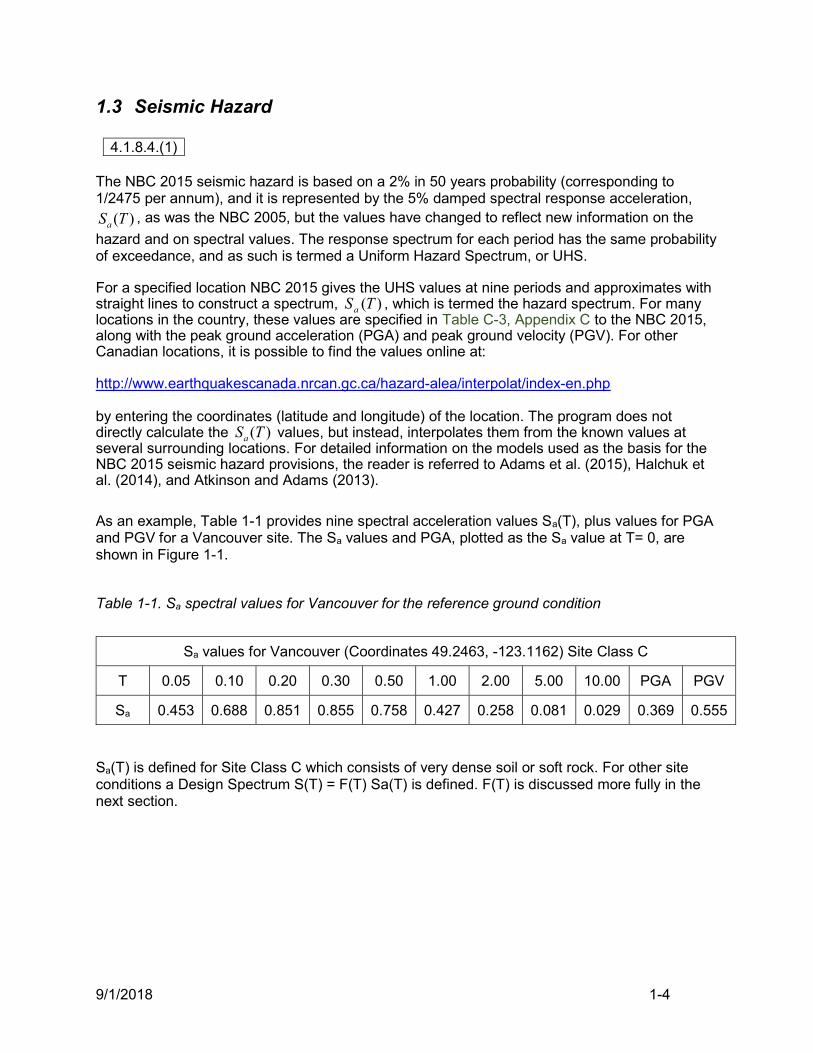
As an example, Table 1-1 provides nine spectral acceleration values Sa(T), plus values for PGA and PGV for a Vancouver site. The Sa values and PGA, plotted as the Sa value at T= 0, are shown in Figure 1-1.

Table 1-1. Sa spectral values for Vancouver for the reference ground condition

Sa values for Vancouver (Coordinates 49.2463, -123.1162) Site Class C

T 0.05 0.10 0.20 0.30 0.50 1.00 2.00 5.00 10.00 PGA PGV

Sa 0.453 0.688 0.851 0.855 0.758 0.427 0.258 0.081 0.029 0.369 0.555

Sa(T) is defined for Site Class C which consists of very dense soil or soft rock. For other site conditions a Design Spectrum S(T) = F(T) Sa(T) is defined. F(T) is discussed more fully in the next section.

9/1/2018 1-5

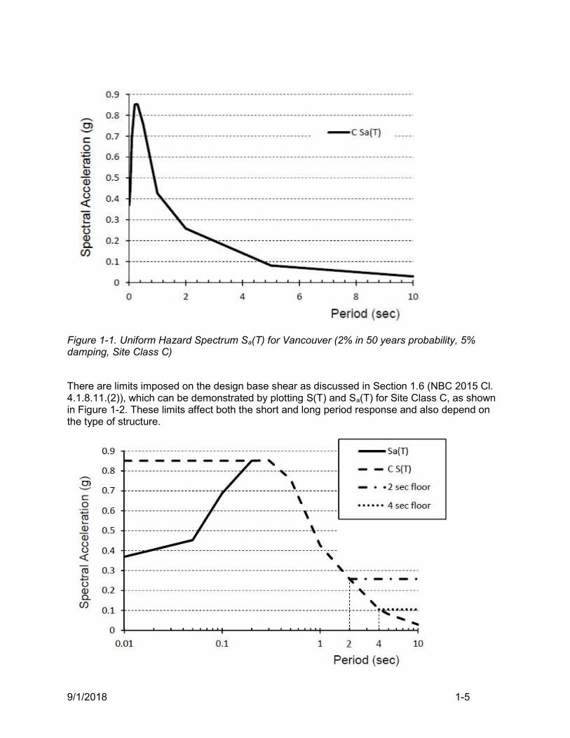
Figure 1-1. Uniform Hazard Spectrum Sa(T) for Vancouver (2% in 50 years probability, 5% damping, Site Class C)

There are limits imposed on the design base shear as discussed in Section 1.6 (NBC 2015 Cl. 4.1.8.11.(2)), which can be demonstrated by plotting S(T) and Sa(T) for Site Class C, as shown in Figure 1-2. These limits affect both the short and long period response and also depend on the type of structure.

9/1/2018 1-6

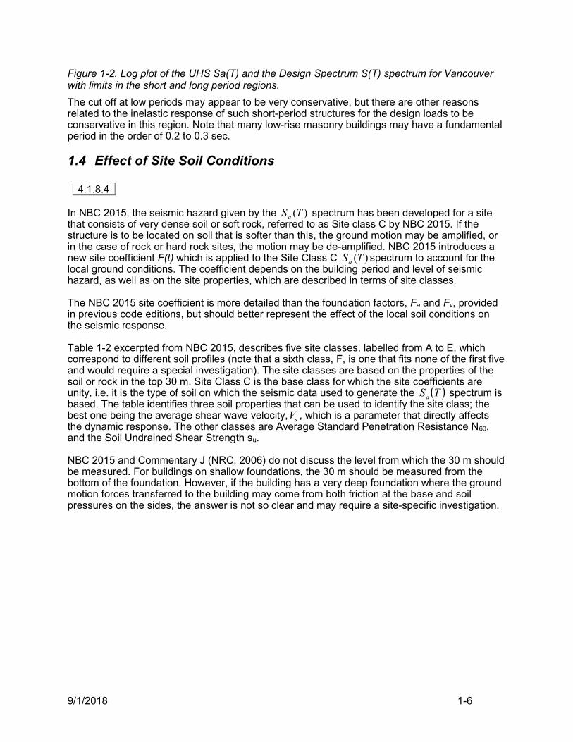
Figure 1-2. Log plot of the UHS Sa(T) and the Design Spectrum S(T) spectrum for Vancouver with limits in the short and long period regions.

The cut off at low periods may appear to be very conservative, but there are other reasons related to the inelastic response of such short-period structures for the design loads to be conservative in this region. Note that many low-rise masonry buildings may have a fundamental period in the order of 0.2 to 0.3 sec.

1.4 Effect of Site Soil Conditions

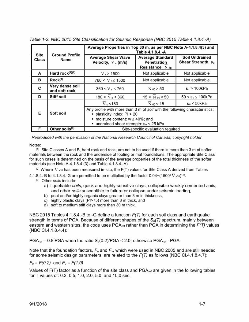
4.1.8.4 In NBC 2015, the seismic hazard given by the )(TSa spectrum has been developed for a site that consists of very dense soil or soft rock, referred to as Site class C by NBC 2015. If the structure is to be located on soil that is softer than this, the ground motion may be amplified, or in the case of rock or hard rock sites, the motion may be de-amplified. NBC 2015 introduces a new site coefficient F(t) which is applied to the Site Class C )(TSa spectrum to account for the local ground conditions. The coefficient depends on the building period and level of seismic hazard, as well as on the site properties, which are described in terms of site classes. The NBC 2015 site coefficient is more detailed than the foundation factors, Fa and Fv, provided in previous code editions, but should better represent the effect of the local soil conditions on the seismic response. Table 1-2 excerpted from NBC 2015, describes five site classes, labelled from A to E, which correspond to different soil profiles (note that a sixth class, F, is one that fits none of the first five and would require a special investigation). The site classes are based on the properties of the soil or rock in the top 30 m. Site Class C is the base class for which the site coefficients are unity, i.e. it is the type of soil on which the seismic data used to generate the TSa spectrum is based. The table identifies three soil properties that can be used to identify the site class; the best one being the average shear wave velocity, sV , which is a parameter that directly affects the dynamic response. The other classes are Average Standard Penetration Resistance N60, and the Soil Undrained Shear Strength su. NBC 2015 and Commentary J (NRC, 2006) do not discuss the level from which the 30 m should be measured. For buildings on shallow foundations, the 30 m should be measured from the bottom of the foundation. However, if the building has a very deep foundation where the ground motion forces transferred to the building may come from both friction at the base and soil pressures on the sides, the answer is not so clear and may require a site-specific investigation.

9/1/2018 1-7

Table 1-2. NBC 2015 Site Classification for Seismic Response (NBC 2015 Table 4.1.8.4.-A)

Site Class

Ground Profile Name

Average Properties in Top 30 m, as per NBC Note A-4.1.8.4(3) and Table 4.1.8.4.-A

Average Shear Wave Velocity, V s (m/s)

Average Standard Penetration

Resistance, N 60

Soil Undrained Shear Strength, su

A Hard rock(1)(2) V s > 1500 Not applicable Not applicable

B Rock(1) 760 < V s 1500 Not applicable Not applicable

C Very dense soil and soft rock 360 < V s < 760 N 60 > 50 su > 100kPa

D Stiff soil 180 < V s < 360 15 < N 60 < 50 50 < su 100kPa

E Soft soil

V s <180 N 60 < 15 su < 50kPa

Any profile with more than 3 m of soil with the following characteristics: plasticity index: PI > 20 moisture content: w 40%; and undrained shear strength: su < 25 kPa

F Other soils(3) Site-specific evaluation required

Reproduced with the permission of the National Research Council of Canada, copyright holder

Notes: (1) Site Classes A and B, hard rock and rock, are not to be used if there is more than 3 m of softer materials between the rock and the underside of footing or mat foundations. The appropriate Site Class for such cases is determined on the basis of the average properties of the total thickness of the softer materials (see Note A-4.1.8.4.(3) and Table 4.1.8.4.-A)

(2) Where V s30 has been measured in-situ, the F(T) values for Site Class A derived from Tables

4.1.8.4.-B to 4.1.8.4.-G are permitted to be multiplied by the factor 0.04+(1500/ V s30)1/2. (3) Other soils include:

a) liquefiable soils, quick and highly sensitive clays, collapsible weakly cemented soils, and other soils susceptible to failure or collapse under seismic loading,

b) peat and/or highly organic clays greater than 3 m in thickness, c) highly plastic clays (PI>75) more than 8 m thick, and d) soft to medium stiff clays more than 30 m thick.

NBC 2015 Tables 4.1.8.4.-B to -G define a function F(T) for each soil class and earthquake strength in terms of PGA. Because of different shapes of the Sa(T) spectrum, mainly between eastern and western sites, the code uses PGAref rather than PGA in determining the F(T) values (NBC Cl.4.1.8.4.4): PGAref = 0.8*PGA when the ratio Sa(0.2)/PGA < 2.0, otherwise PGAref =PGA. Note that the foundation factors, Fa and Fv, which were used in NBC 2005 and are still needed for some seismic design parameters, are related to the F(T) as follows (NBC Cl.4.1.8.4.7):

Fa = F(0.2) and Fv = F(1.0)

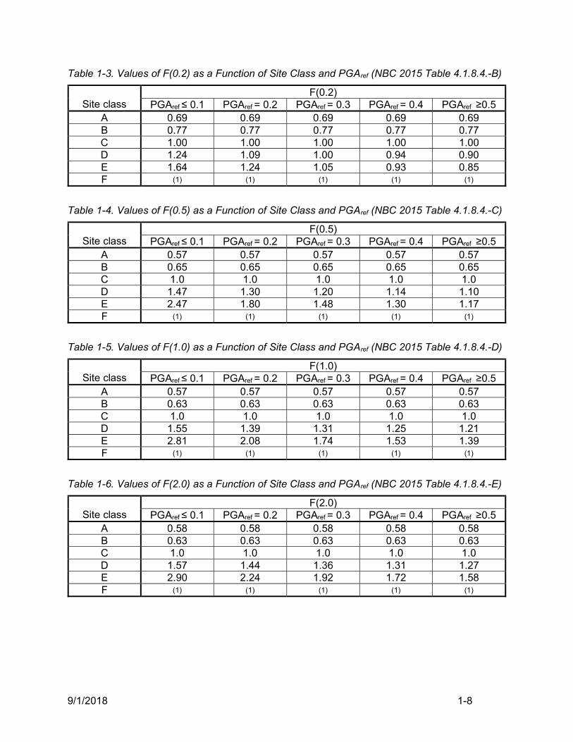
Values of F(T) factor as a function of the site class and PGAref are given in the following tables for T values of: 0.2, 0.5, 1.0, 2.0, 5.0, and 10.0 sec.

9/1/2018 1-8

Table 1-3. Values of F(0.2) as a Function of Site Class and PGAref (NBC 2015 Table 4.1.8.4.-B)

Site class

F(0.2) PGAref ≤ 0.1 PGAref = 0.2 PGAref = 0.3 PGAref = 0.4 PGAref ≥0.5

A 0.69 0.69 0.69 0.69 0.69 B 0.77 0.77 0.77 0.77 0.77 C 1.00 1.00 1.00 1.00 1.00 D 1.24 1.09 1.00 0.94 0.90 E 1.64 1.24 1.05 0.93 0.85 F (1) (1) (1) (1) (1)

Table 1-4. Values of F(0.5) as a Function of Site Class and PGAref (NBC 2015 Table 4.1.8.4.-C)

Site class

F(0.5) PGAref ≤ 0.1 PGAref = 0.2 PGAref = 0.3 PGAref = 0.4 PGAref ≥0.5

A 0.57 0.57 0.57 0.57 0.57 B 0.65 0.65 0.65 0.65 0.65 C 1.0 1.0 1.0 1.0 1.0 D 1.47 1.30 1.20 1.14 1.10 E 2.47 1.80 1.48 1.30 1.17 F (1) (1) (1) (1) (1)

Table 1-5. Values of F(1.0) as a Function of Site Class and PGAref (NBC 2015 Table 4.1.8.4.-D)

Site class

F(1.0) PGAref ≤ 0.1 PGAref = 0.2 PGAref = 0.3 PGAref = 0.4 PGAref ≥0.5

A 0.57 0.57 0.57 0.57 0.57 B 0.63 0.63 0.63 0.63 0.63 C 1.0 1.0 1.0 1.0 1.0 D 1.55 1.39 1.31 1.25 1.21 E 2.81 2.08 1.74 1.53 1.39 F (1) (1) (1) (1) (1)

Table 1-6. Values of F(2.0) as a Function of Site Class and PGAref (NBC 2015 Table 4.1.8.4.-E)

Site class

F(2.0) PGAref ≤ 0.1 PGAref = 0.2 PGAref = 0.3 PGAref = 0.4 PGAref ≥0.5

A 0.58 0.58 0.58 0.58 0.58 B 0.63 0.63 0.63 0.63 0.63 C 1.0 1.0 1.0 1.0 1.0 D 1.57 1.44 1.36 1.31 1.27 E 2.90 2.24 1.92 1.72 1.58 F (1) (1) (1) (1) (1)

9/1/2018 1-9

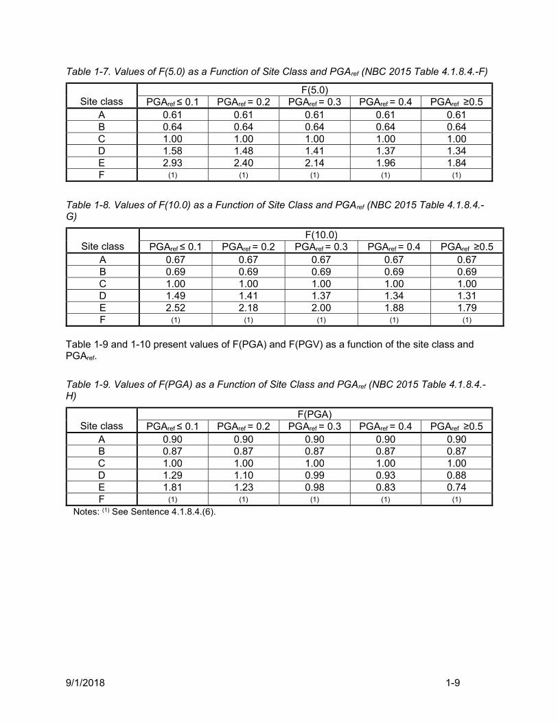
Table 1-7. Values of F(5.0) as a Function of Site Class and PGAref (NBC 2015 Table 4.1.8.4.-F)

Site class

F(5.0) PGAref ≤ 0.1 PGAref = 0.2 PGAref = 0.3 PGAref = 0.4 PGAref ≥0.5

A 0.61 0.61 0.61 0.61 0.61 B 0.64 0.64 0.64 0.64 0.64 C 1.00 1.00 1.00 1.00 1.00 D 1.58 1.48 1.41 1.37 1.34 E 2.93 2.40 2.14 1.96 1.84 F (1) (1) (1) (1) (1)

Table 1-8. Values of F(10.0) as a Function of Site Class and PGAref (NBC 2015 Table 4.1.8.4.-G)

Site class

F(10.0) PGAref ≤ 0.1 PGAref = 0.2 PGAref = 0.3 PGAref = 0.4 PGAref ≥0.5

A 0.67 0.67 0.67 0.67 0.67 B 0.69 0.69 0.69 0.69 0.69 C 1.00 1.00 1.00 1.00 1.00 D 1.49 1.41 1.37 1.34 1.31 E 2.52 2.18 2.00 1.88 1.79 F (1) (1) (1) (1) (1)

Table 1-9 and 1-10 present values of F(PGA) and F(PGV) as a function of the site class and PGAref.

Table 1-9. Values of F(PGA) as a Function of Site Class and PGAref (NBC 2015 Table 4.1.8.4.-H)

Site class

F(PGA) PGAref ≤ 0.1 PGAref = 0.2 PGAref = 0.3 PGAref = 0.4 PGAref ≥0.5

A 0.90 0.90 0.90 0.90 0.90 B 0.87 0.87 0.87 0.87 0.87 C 1.00 1.00 1.00 1.00 1.00 D 1.29 1.10 0.99 0.93 0.88 E 1.81 1.23 0.98 0.83 0.74 F (1) (1) (1) (1) (1)

Notes: (1) See Sentence 4.1.8.4.(6).

9/1/2018 1-10

Table 1-10. Values of F(PGV) as a Function of Site Class and PGAref (NBC 2015 Table 4.1.8.4.-I)

Site class

F(PGV) PGAref ≤ 0.1 PGAref = 0.2 PGAref = 0.3 PGAref = 0.4 PGAref ≥0.5

A 0.62 0.62 0.62 0.62 0.62 B 0.67 0.67 0.67 0.67 0.67 C 1.00 1.00 1.00 1.00 1.00 D 1.47 1.30 1.20 1.14 1.10 E 2.47 1.80 1.48 1.30 1.17 F (1) (1) (1) (1) (1)

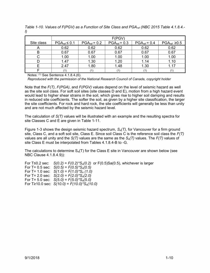
Notes: (1) See Sentence 4.1.8.4.(6). Reproduced with the permission of the National Research Council of Canada, copyright holder Note that the F(T), F(PGA), and F(PGV) values depend on the level of seismic hazard as well as the site soil class. For soft soil sites (site classes D and E), motion from a high hazard event would lead to higher shear strains in the soil, which gives rise to higher soil damping and results in reduced site coefficients. The softer the soil, as given by a higher site classification, the larger the site coefficients. For rock and hard rock, the site coefficients will generally be less than unity and are not much affected by the seismic hazard level. The calculation of S(T) values will be illustrated with an example and the resulting spectra for site Classes C and E are given in Table 1-11. Figure 1-3 shows the design seismic hazard spectrum, Sa(T), for Vancouver for a firm ground site, Class C, and a soft soil site, Class E. Since soil Class C is the reference soil class the F(T) values are all unity and the S(T) values are the same as the Sa(T) values. The F(T) values of site Class E must be interpolated from Tables 4.1.8.4-B to -G. The calculations to determine Sa(T) for the Class E site in Vancouver are shown below (see NBC Clause 4.1.8.4.9)): For T≤0.2 sec: S(0.2) = F(0.2)*Sa(0.2) or F(0.5)Sa(0.5), whichever is larger For T= 0.5 sec: S(0.5) = F(0.5)*Sa(0.5) For T= 1.0 sec: S(1.0) = F(1.0)*Sa (1.0) For T= 2.0 sec: S(2.0) = F(2.0)*Sa(2.0) For T= 5.0 sec: S(5.0) = F(5.0)*Sa(5.0) For T≥10.0 sec: S(10.0) = F(10.0)*Sa(10.0)

9/1/2018 1-11

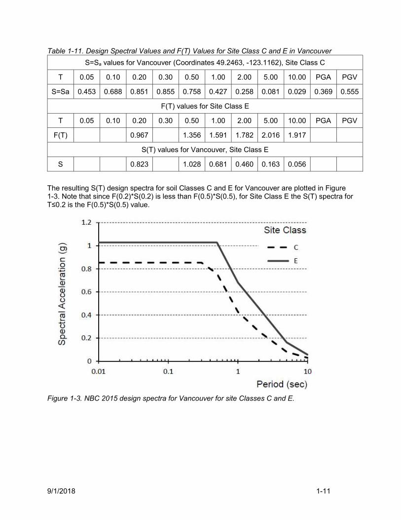
Table 1-11. Design Spectral Values and F(T) Values for Site Class C and E in Vancouver

S=Sa values for Vancouver (Coordinates 49.2463, -123.1162), Site Class C

T 0.05 0.10 0.20 0.30 0.50 1.00 2.00 5.00 10.00 PGA PGV

S=Sa 0.453 0.688 0.851 0.855 0.758 0.427 0.258 0.081 0.029 0.369 0.555

F(T) values for Site Class E

T 0.05 0.10 0.20 0.30 0.50 1.00 2.00 5.00 10.00 PGA PGV

F(T) 0.967 1.356 1.591 1.782 2.016 1.917

S(T) values for Vancouver, Site Class E

S 0.823 1.028 0.681 0.460 0.163 0.056

The resulting S(T) design spectra for soil Classes C and E for Vancouver are plotted in Figure 1-3. Note that since F(0.2)*S(0.2) is less than F(0.5)*S(0.5), for Site Class E the S(T) spectra for T≤0.2 is the F(0.5)*S(0.5) value.

Figure 1-3. NBC 2015 design spectra for Vancouver for site Classes C and E.

9/1/2018 1-12

1.5 Methods of Analysis

4.1.8.7 NBC 2015 prescribes two methods of calculating the design base shear for a structure. The dynamic method is the default method, but the equivalent static method can be used if the structure meets any of the following criteria: (a) is located in a region of low seismic activity where 35.02.0 aaE SFI ( EI is the earthquake importance factor of the structure as defined in Clause 4.1.8.5.(1)), or (b) is a regular structure less than 60 m in height with period, aT , less than 2 seconds in either direction ( aT is defined as the fundamental lateral period of vibration of the structure in the direction under consideration, as defined in Clause 4.1.8.11.(3)), or (c) is an irregular structure, but does not have Type 7 or Type 9 irregularity, and is less than 20 m in height with period, aT , less than 0.5 seconds in either direction. The equivalent static method will be described in this section because it likely can be used on the majority of masonry buildings given the above criteria, and notwithstanding, if the dynamic method is used, it must be calibrated back to the base shear determined from the equivalent static analysis procedure. Basic concepts of the modal dynamic analysis method are presented in Appendix A, and further discussion is offered in Section 1.14.

1.6 Base Shear Calculations- Equivalent Static Analysis Procedure

4.1.8.11 The lateral earthquake forces used for design are specified in the NBC 2015, and are based on the maximum (design) base shear

eV of the structure as given by Clause 4.1.8.11, and is the base shear if the structure were to remain elastic. Design base shear,V , is equal to

eV reduced by the force reduction factors, dR and oR , (related to ductility and overstrength, respectively; discussed in Section 1.7), and increased by the importance factor EI (see Table 1-12 for a description of parameters used in these relations), thus;

od

Ee

RR

IVV

where WMTSV vae , represents the elastic base shear, vM is a multiplier that accounts for

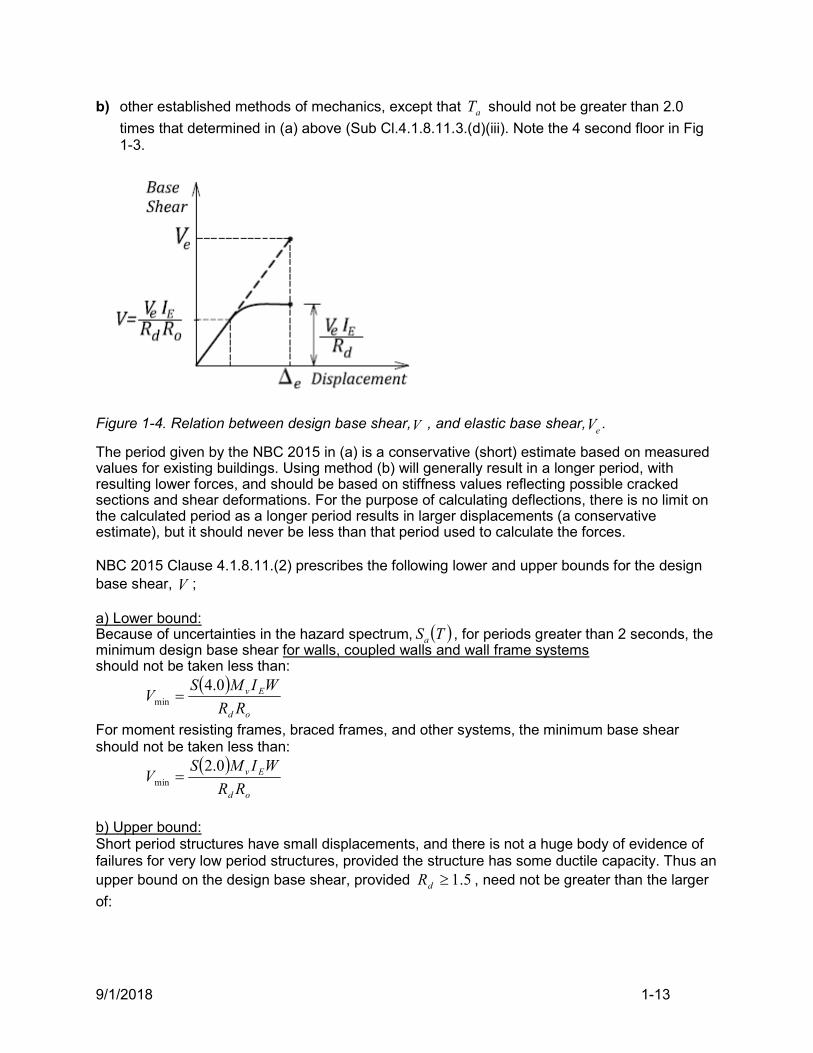
higher mode shears, and W is the dead load attached to the SFRS, as defined in Table 1-12. The relationship between

eV and V is shown in Figure 1-4. Note that the actual strength of the

structure is greater than the design strength because of the overstrength factor Ro.

aT denotes the fundamental period of vibration of the building or structure in seconds in the

direction under consideration. The fundamental period of wall structures is given in the NBC 2015 by:

a) 4305.0 na hT , where nh is the height of the building in metres (Cl.4.1.8.11.3.(c)), or

9/1/2018 1-13

b) other established methods of mechanics, except that aT should not be greater than 2.0

times that determined in (a) above (Sub Cl.4.1.8.11.3.(d)(iii). Note the 4 second floor in Fig 1-3.

Figure 1-4. Relation between design base shear,V , and elastic base shear,eV .

The period given by the NBC 2015 in (a) is a conservative (short) estimate based on measured values for existing buildings. Using method (b) will generally result in a longer period, with resulting lower forces, and should be based on stiffness values reflecting possible cracked sections and shear deformations. For the purpose of calculating deflections, there is no limit on the calculated period as a longer period results in larger displacements (a conservative estimate), but it should never be less than that period used to calculate the forces. NBC 2015 Clause 4.1.8.11.(2) prescribes the following lower and upper bounds for the design base shear, V ; a) Lower bound: Because of uncertainties in the hazard spectrum, TSa , for periods greater than 2 seconds, the minimum design base shear for walls, coupled walls and wall frame systems should not be taken less than:

od

Ev

RR

WIMSV

0.4min

For moment resisting frames, braced frames, and other systems, the minimum base shear should not be taken less than:

od

Ev

RR

WIMSV

0.2min

b) Upper bound: Short period structures have small displacements, and there is not a huge body of evidence of failures for very low period structures, provided the structure has some ductile capacity. Thus an upper bound on the design base shear, provided 5.1dR , need not be greater than the larger

of:

9/1/2018 1-14

od

E

RR

WISV

3

2.02max and

od

E

RR

WISV )5.0(max

vM is not included in the above equations as 1vM for short periods.

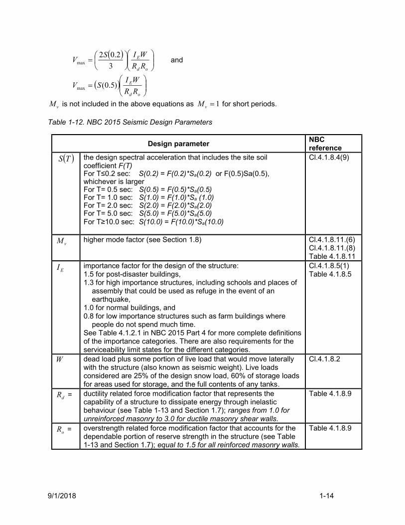
Table 1-12. NBC 2015 Seismic Design Parameters

Design parameter NBC reference

TS the design spectral acceleration that includes the site soil coefficient F(T) For T≤0.2 sec: S(0.2) = F(0.2)*Sa(0.2) or F(0.5)Sa(0.5), whichever is larger For T= 0.5 sec: S(0.5) = F(0.5)*Sa(0.5) For T= 1.0 sec: S(1.0) = F(1.0)*Sa (1.0) For T= 2.0 sec: S(2.0) = F(2.0)*Sa(2.0) For T= 5.0 sec: S(5.0) = F(5.0)*Sa(5.0) For T≥10.0 sec: S(10.0) = F(10.0)*Sa(10.0)

Cl.4.1.8.4(9)

vM higher mode factor (see Section 1.8) Cl.4.1.8.11.(6) Cl.4.1.8.11.(8) Table 4.1.8.11

EI importance factor for the design of the structure: 1.5 for post-disaster buildings, 1.3 for high importance structures, including schools and places of

assembly that could be used as refuge in the event of an earthquake,

1.0 for normal buildings, and 0.8 for low importance structures such as farm buildings where

people do not spend much time. See Table 4.1.2.1 in NBC 2015 Part 4 for more complete definitions of the importance categories. There are also requirements for the serviceability limit states for the different categories.

Cl.4.1.8.5(1) Table 4.1.8.5

W

dead load plus some portion of live load that would move laterally with the structure (also known as seismic weight). Live loads considered are 25% of the design snow load, 60% of storage loads for areas used for storage, and the full contents of any tanks.

Cl.4.1.8.2

dR = ductility related force modification factor that represents the capability of a structure to dissipate energy through inelastic behaviour (see Table 1-13 and Section 1.7); ranges from 1.0 for unreinforced masonry to 3.0 for ductile masonry shear walls.

Table 4.1.8.9

oR = overstrength related force modification factor that accounts for the dependable portion of reserve strength in the structure (see Table 1-13 and Section 1.7); equal to 1.5 for all reinforced masonry walls.

Table 4.1.8.9

9/1/2018 1-15

Note that the design base shear force,V , corresponds to the design force at the ultimate limit state, where the structure is assumed to be at the point of collapse. Consequently, seismic loads are designed with a load factor value of 1.0 when used in combination with other loads (e.g. dead and live loads; see Table 4.1.3.2.-A, NBC 2015). It is also useful to recall that while V represents the design base shear, individual members are designed using factored resistances, R , and since the nominal resistance, R , is greater than the factored resistance, the actual base shear capacity will be approximately equal to

oVR , as shown in Figure 1-4.

1.7 Force Reduction Factors dR and oR

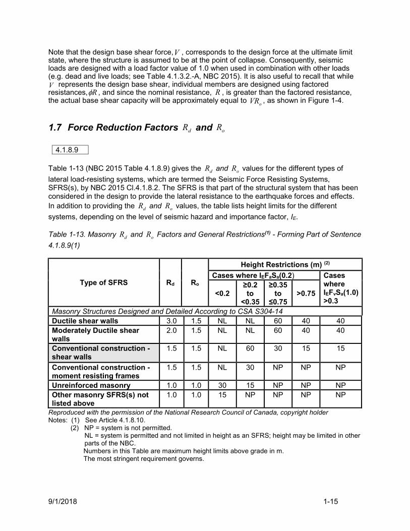
4.1.8.9 Table 1-13 (NBC 2015 Table 4.1.8.9) gives the dR and oR values for the different types of

lateral load-resisting systems, which are termed the Seismic Force Resisting Systems, SFRS(s), by NBC 2015 Cl.4.1.8.2. The SFRS is that part of the structural system that has been considered in the design to provide the lateral resistance to the earthquake forces and effects. In addition to providing the dR and oR values, the table lists height limits for the different

systems, depending on the level of seismic hazard and importance factor, IE. Table 1-13. Masonry dR and oR Factors and General Restrictions(1) - Forming Part of Sentence

4.1.8.9(1)

Type of SFRS Rd Ro

Height Restrictions (m) (2)

Cases where IEFaSa(0.2) Cases where IEFvSa(1.0) >0.3

<0.2 ≥0.2 to

<0.35

≥0.35 to

≤0.75 >0.75

Masonry Structures Designed and Detailed According to CSA S304-14 Ductile shear walls 3.0 1.5 NL NL 60 40 40 Moderately Ductile shear walls

2.0 1.5 NL NL 60 40 40

Conventional construction -shear walls

1.5 1.5

NL

60

30

15 15

Conventional construction -moment resisting frames

1.5 1.5 NL 30 NP NP NP

Unreinforced masonry 1.0 1.0 30 15 NP NP NP Other masonry SFRS(s) not listed above

1.0 1.0 15 NP NP NP NP

Reproduced with the permission of the National Research Council of Canada, copyright holder Notes: (1) See Article 4.1.8.10. (2) NP = system is not permitted.

NL = system is permitted and not limited in height as an SFRS; height may be limited in other parts of the NBC.

Numbers in this Table are maximum height limits above grade in m. The most stringent requirement governs.

9/1/2018 1-16

Commentary

NBC 2015 Table 4.1.8.9 identifies the following five SFRS(s) related to masonry construction:

1. Ductile shear walls (new SFRS introduced in NBC 2015) 2. Moderately Ductile shear walls 3. Conventional construction: shear walls and moment resisting frames 4. Unreinforced masonry 5. Other undefined masonry SFRS(s)

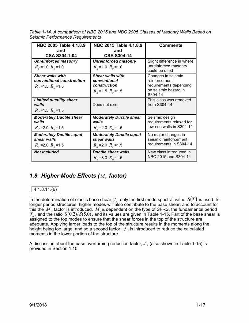
Note that Ductile shear walls are assigned the highest dR value of 3.0, leading to the lowest design forces for masonry structures. The detailing requirements, given in CSA S304 -14, are the most restrictive of all the masonry shear wall types. However, the height limitations imposed by the NBC 2015 are the most liberal, allowing structures up to 60 m in height (approximately 20 storeys) in moderately high seismic regions, and up to 40 m in higher seismic regions. Moderately Ductile shear walls, dR = 2.0, have the same height restrictions as Ductile shear walls. They have less restrictive detailing requirements, but have to be designed for larger forces, generally resulting in a stiffer structure with less ductility demand. Moderately ductile shear walls are required for masonry SFRS(s) used in post-disaster buildings, due to the NBC requirement for an dR = 2.0 for these structures. Moderately Ductile squat shear walls, those with a height-to-length ratio less than 1, are a separate class of Moderately ductile shear wall. They are allowed higher shear resistance, and less restrictive requirements on the height-to-thickness ratio, when compared to regular Moderately Ductile shear walls. Conventional construction shear walls and moment-resisting frames both have Rd=1.5, with more onerous height restrictions, but less stringent detailing requirements than Moderately Ductile walls. Masonry moment-resisting frames are limited to low seismic regions and are not discussed in CSA S304-14. Conventional construction is the most common type of shear wall used in typical masonry structures. Unreinforced masonry construction is only allowed where 35.02.0 aaE SFI . It is limited to a height of 15 or 30 m depending on the level of seismic hazard. Unreinforced masonry does not have a good record in past earthquakes, and is assigned 0.1 od RR values, as there is usually no ductility and brittle failures are a possibility. The oR factor in NBC 2015 is an overstrength factor to account for the real resistance capacity of the structure when compared to the factored design resistance. It is made up of 3 components: i) 2.118.1/1 , ii) a factor that accounts for the expected yield strength of the reinforcement being above the specified yield strength, and iii) a factor of about 1.1 that recognizes that because of restrictions on possible core locations for the reinforcement in modular masonry walls, the amount of reinforcement is in most cases larger than required. This results in an 5.1oR after some rounding of the factors (Mitchell et al., 2003). A comparison of masonry wall classes contained in NBC 2015 and NBC 2005 is presented in Table 1-14. The class Limited ductility shear walls no longer exists in NBC 2015, and a new class (Ductile shear walls) has been introduced.

9/1/2018 1-17

Table 1-14. A comparison of NBC 2015 and NBC 2005 Classes of Masonry Walls Based on Seismic Performance Requirements

NBC 2005 Table 4.1.8.9 and

CSA S304.1-04

NBC 2015 Table 4.1.8.9 and

CSA S304-14

Comments

Unreinforced masonry

dR =1.0 oR =1.0 Unreinforced masonry

dR =1.0 oR =1.0 Slight difference in where unreinforced masonry could be used

Shear walls with conventional construction

dR =1.5 oR =1.5

Shear walls with conventional construction

dR =1.5 oR =1.5

Changes in seismic reinforcement requirements depending on seismic hazard in S304-14

Limited ductility shear walls

dR =1.5 oR =1.5

Does not exist

This class was removed from S304-14

Moderately Ductile shear walls

dR =2.0 oR =1.5

Moderately Ductile shear walls

dR =2.0 oR =1.5

Seismic design requirements relaxed for low-rise walls in S304-14

Moderately Ductile squat shear walls

dR =2.0 oR =1.5

Moderately Ductile squat shear walls

dR =2.0 oR =1.5

No major changes in seismic reinforcement requirements in S304-14

Not included Ductile shear walls

dR =3.0 oR =1.5

New class introduced in NBC 2015 and S304-14

1.8 Higher Mode Effects ( vM factor)

4.1.8.11.(6) In the determination of elastic base shear,

eV , only the first mode spectral value TS is used. In longer period structures, higher modes will also contribute to the base shear, and to account for this the vM factor is introduced. vM is dependent on the type of SFRS, the fundamental period

aT , and the ratio )0.5()2.0( SS , and its values are given in Table 1-15. Part of the base shear is assigned to the top modes to ensure that the shear forces in the top of the structure are adequate. Applying larger loads to the top of the structure results in the moments along the height being too large, and so a second factor, J , is introduced to reduce the calculated moments in the lower portion of the structure. A discussion about the base overturning reduction factor, J , (also shown in Table 1-15) is provided in Section 1.10.

9/1/2018 1-18

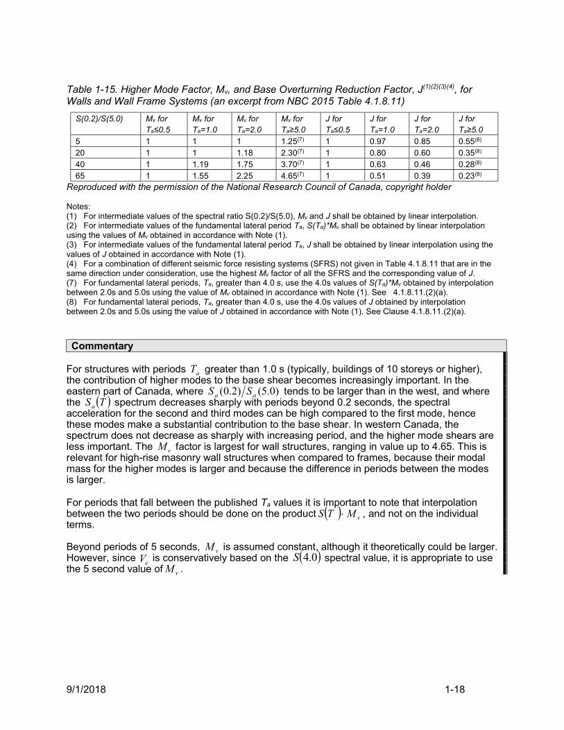
Table 1-15. Higher Mode Factor, Mv, and Base Overturning Reduction Factor, J(1)(2)(3)(4), for Walls and Wall Frame Systems (an excerpt from NBC 2015 Table 4.1.8.11)

S(0.2)/S(5.0) Mv for Ta≤0.5

Mv for Ta=1.0

Mv for Ta=2.0

Mv for Ta≥5.0

J for Ta≤0.5

J for Ta=1.0

J for Ta=2.0

J for Ta≥5.0

5 1 1 1 1.25(7) 1 0.97 0.85 0.55(8) 20 1 1 1.18 2.30(7) 1 0.80 0.60 0.35(8) 40 1 1.19 1.75 3.70(7) 1 0.63 0.46 0.28(8) 65 1 1.55 2.25 4.65(7) 1 0.51 0.39 0.23(8)

Reproduced with the permission of the National Research Council of Canada, copyright holder Notes: (1) For intermediate values of the spectral ratio S(0.2)/S(5.0), Mv and J shall be obtained by linear interpolation. (2) For intermediate values of the fundamental lateral period Ta, S(Ta)*Mv shall be obtained by linear interpolation using the values of Mv obtained in accordance with Note (1). (3) For intermediate values of the fundamental lateral period Ta, J shall be obtained by linear interpolation using the values of J obtained in accordance with Note (1). (4) For a combination of different seismic force resisting systems (SFRS) not given in Table 4.1.8.11 that are in the same direction under consideration, use the highest Mv factor of all the SFRS and the corresponding value of J. (7) For fundamental lateral periods, Ta, greater than 4.0 s, use the 4.0s values of S(Ta)*Mv obtained by interpolation between 2.0s and 5.0s using the value of Mv obtained in accordance with Note (1). See 4.1.8.11.(2)(a). (8) For fundamental lateral periods, Ta, greater than 4.0 s, use the 4.0s values of J obtained by interpolation between 2.0s and 5.0s using the value of J obtained in accordance with Note (1). See Clause 4.1.8.11.(2)(a). Commentary

For structures with periods aT greater than 1.0 s (typically, buildings of 10 storeys or higher), the contribution of higher modes to the base shear becomes increasingly important. In the eastern part of Canada, where )0.5()2.0( aa SS tends to be larger than in the west, and where the TSa spectrum decreases sharply with periods beyond 0.2 seconds, the spectral acceleration for the second and third modes can be high compared to the first mode, hence these modes make a substantial contribution to the base shear. In western Canada, the spectrum does not decrease as sharply with increasing period, and the higher mode shears are less important. The vM factor is largest for wall structures, ranging in value up to 4.65. This is relevant for high-rise masonry wall structures when compared to frames, because their modal mass for the higher modes is larger and because the difference in periods between the modes is larger. For periods that fall between the published Ta values it is important to note that interpolation between the two periods should be done on the product vMTS , and not on the individual terms. Beyond periods of 5 seconds, vM is assumed constant, although it theoretically could be larger. However, since

eV is conservatively based on the 0.4S spectral value, it is appropriate to use the 5 second value of vM .

9/1/2018 1-19

1.9 Vertical Distribution of Seismic Forces

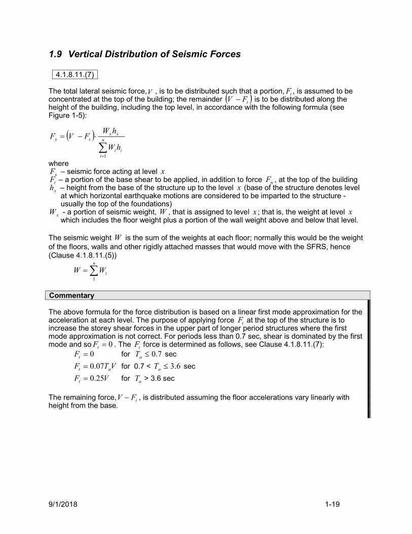
4.1.8.11.(7) The total lateral seismic force,V , is to be distributed such that a portion, tF , is assumed to be concentrated at the top of the building; the remainder tFV is to be distributed along the height of the building, including the top level, in accordance with the following formula (see Figure 1-5):

where xF – seismic force acting at level x tF – a portion of the base shear to be applied, in addition to force nF , at the top of the building xh – height from the base of the structure up to the level x (base of the structure denotes level

at which horizontal earthquake motions are considered to be imparted to the structure - usually the top of the foundations)

xW - a portion of seismic weight, W , that is assigned to level x ; that is, the weight at level x which includes the floor weight plus a portion of the wall weight above and below that level.

The seismic weight W is the sum of the weights at each floor; normally this would be the weight of the floors, walls and other rigidly attached masses that would move with the SFRS, hence (Clause 4.1.8.11.(5))

n

iWW1

Commentary The above formula for the force distribution is based on a linear first mode approximation for the acceleration at each level. The purpose of applying force tF at the top of the structure is to increase the storey shear forces in the upper part of longer period structures where the first mode approximation is not correct. For periods less than 0.7 sec, shear is dominated by the first mode and so 0tF . The tF force is determined as follows, see Clause 4.1.8.11.(7):

0tF for 7.0aT sec

VTF at 07.0 for 0.7 < 6.3aT sec

VFt 25.0 for aT > 3.6 sec

The remaining force, tFV , is distributed assuming the floor accelerations vary linearly with height from the base.

n

iii

xxtx

hW

hWFVF

1

9/1/2018 1-20

Figure 1-5. Vertical force distribution.

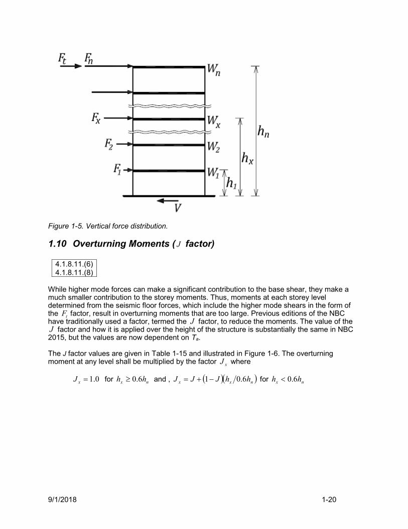
1.10 Overturning Moments ( J factor)

4.1.8.11.(6) 4.1.8.11.(8)

While higher mode forces can make a significant contribution to the base shear, they make a much smaller contribution to the storey moments. Thus, moments at each storey level determined from the seismic floor forces, which include the higher mode shears in the form of the tF factor, result in overturning moments that are too large. Previous editions of the NBC have traditionally used a factor, termed the J factor, to reduce the moments. The value of the J factor and how it is applied over the height of the structure is substantially the same in NBC 2015, but the values are now dependent on Ta. The J factor values are given in Table 1-15 and illustrated in Figure 1-6. The overturning moment at any level shall be multiplied by the factor xJ where

0.1xJ for nx hh 6.0 and , nxx hhJJJ 6.01 for nx hh 6.0

9/1/2018 1-21

.

Figure 1-6. Distribution of the xJ factor over the building height.

Commentary

How the J factor and reduced overturning moments are incorporated into a structural analysis is not always straightforward, and it depends on the structural system. For shear wall structures, the overturning moments can be calculated using the floor forces from the lateral force distribution, and then reduced by the xJ factor at each level to give the design overturning moments. Without applying the J factor, the wall moment capacity would be too high, leading to higher shears when the structure yields, and could result in a shear failure. For frames, the beam shears and moments and axial loads, resulting from applying the code lateral seismic forces at each floor level, will be too large; but the column shears would not increase. This would essentially result in higher axial loads in the columns, but not increase the shear demand on the structure, and so would be conservative in that the columns would be stronger than necessary, especially in the lower levels. The J factor for frames is usually small, and it is believed that many designers ignore it as it is conservative to do so.

1.11 Torsion

1.11.1 Torsional effects

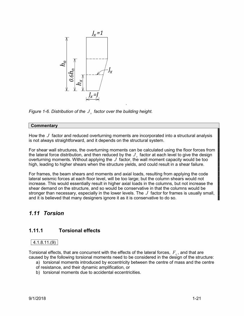
4.1.8.11.(9) Torsional effects, that are concurrent with the effects of the lateral forces, xF , and that are caused by the following torsional moments need to be considered in the design of the structure:

a) torsional moments introduced by eccentricity between the centre of mass and the centre of resistance, and their dynamic amplification, or b) torsional moments due to accidental eccentricities.

9/1/2018 1-22

In determining the torsional forces on members, the stiffness of the diaphragms is important. The discussion in Sections 1.11.1 to 1.11.3 considers rigid diaphragms only, while flexible diaphragms are discussed in Section 1.11.4. Commentary

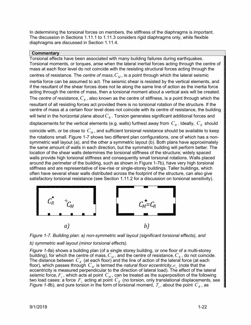
Torsional effects have been associated with many building failures during earthquakes. Torsional moments, or torques, arise when the lateral inertial forces acting through the centre of mass at each floor level do not coincide with the resisting structural forces acting through the centres of resistance. The centre of mass, MC , is a point through which the lateral seismic inertia force can be assumed to act. The seismic shear is resisted by the vertical elements, and if the resultant of the shear forces does not lie along the same line of action as the inertia force acting through the centre of mass, then a torsional moment about a vertical axis will be created. The centre of resistance, RC , also known as the centre of stiffness, is a point through which the resultant of all resisting forces act provided there is no torsional rotation of the structure. If the centre of mass at a certain floor level does not coincide with its centre of resistance, the building will twist in the horizontal plane about RC . Torsion generates significant additional forces and

displacements for the vertical elements (e.g. walls) furthest away from RC . Ideally, RC should

coincide with, or be close to MC , and sufficient torsional resistance should be available to keep the rotations small. Figure 1-7 shows two different plan configurations, one of which has a non-symmetric wall layout (a), and the other a symmetric layout (b). Both plans have approximately the same amount of walls in each direction, but the symmetric building will perform better. The location of the shear walls determines the torsional stiffness of the structure; widely spaced walls provide high torsional stiffness and consequently small torsional rotations. Walls placed around the perimeter of the building, such as shown in Figure 1-7b), have very high torsional stiffness and are representative of low-rise or single-storey buildings. Taller buildings, which often have several shear walls distributed across the footprint of the structure, can also give satisfactory torsional resistance (see Section 1.11.2 for a discussion on torsional sensitivity).

Figure 1-7. Building plan: a) non-symmetric wall layout (significant torsional effects), and

b) symmetric wall layout (minor torsional effects).

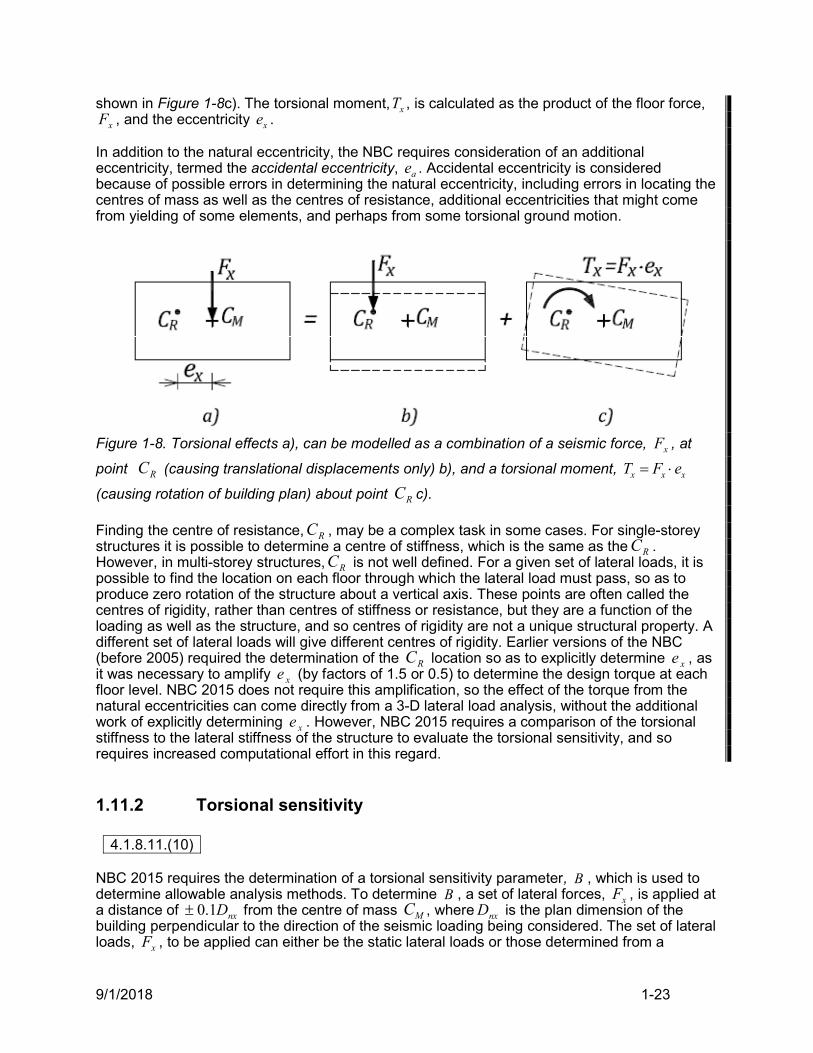
Figure 1-8a) shows a building plan (of a single storey building, or one floor of a multi-storey building), for which the centre of mass, MC , and the centre of resistance, RC , do not coincide. The distance between RC (at each floor) and the line of action of the lateral force (at each floor), which passes through MC is termed the natural floor eccentricity, xe (note that the eccentricity is measured perpendicular to the direction of lateral load). The effect of the lateral seismic force, xF , which acts at point MC , can be treated as the superposition of the following two load cases: a force xF acting at point RC (no torsion, only translational displacements, see Figure 1-8b), and pure torsion in the form of torsional moment, xT , about the point RC , as

9/1/2018 1-23

shown in Figure 1-8c). The torsional moment, xT , is calculated as the product of the floor force, xF , and the eccentricity xe .

In addition to the natural eccentricity, the NBC requires consideration of an additional eccentricity, termed the accidental eccentricity, ae . Accidental eccentricity is considered because of possible errors in determining the natural eccentricity, including errors in locating the centres of mass as well as the centres of resistance, additional eccentricities that might come from yielding of some elements, and perhaps from some torsional ground motion.

Figure 1-8. Torsional effects a), can be modelled as a combination of a seismic force, xF , at

point RC (causing translational displacements only) b), and a torsional moment, x x xT F e

(causing rotation of building plan) about point RC c). Finding the centre of resistance, RC , may be a complex task in some cases. For single-storey structures it is possible to determine a centre of stiffness, which is the same as the RC . However, in multi-storey structures, RC is not well defined. For a given set of lateral loads, it is possible to find the location on each floor through which the lateral load must pass, so as to produce zero rotation of the structure about a vertical axis. These points are often called the centres of rigidity, rather than centres of stiffness or resistance, but they are a function of the loading as well as the structure, and so centres of rigidity are not a unique structural property. A different set of lateral loads will give different centres of rigidity. Earlier versions of the NBC (before 2005) required the determination of the RC location so as to explicitly determine xe , as it was necessary to amplify xe (by factors of 1.5 or 0.5) to determine the design torque at each floor level. NBC 2015 does not require this amplification, so the effect of the torque from the natural eccentricities can come directly from a 3-D lateral load analysis, without the additional work of explicitly determining xe . However, NBC 2015 requires a comparison of the torsional stiffness to the lateral stiffness of the structure to evaluate the torsional sensitivity, and so requires increased computational effort in this regard.

1.11.2 Torsional sensitivity

4.1.8.11.(10) NBC 2015 requires the determination of a torsional sensitivity parameter, B , which is used to determine allowable analysis methods. To determine B , a set of lateral forces, xF , is applied at a distance of nxD1.0 from the centre of mass MC , where nxD is the plan dimension of the building perpendicular to the direction of the seismic loading being considered. The set of lateral loads, xF , to be applied can either be the static lateral loads or those determined from a

9/1/2018 1-24

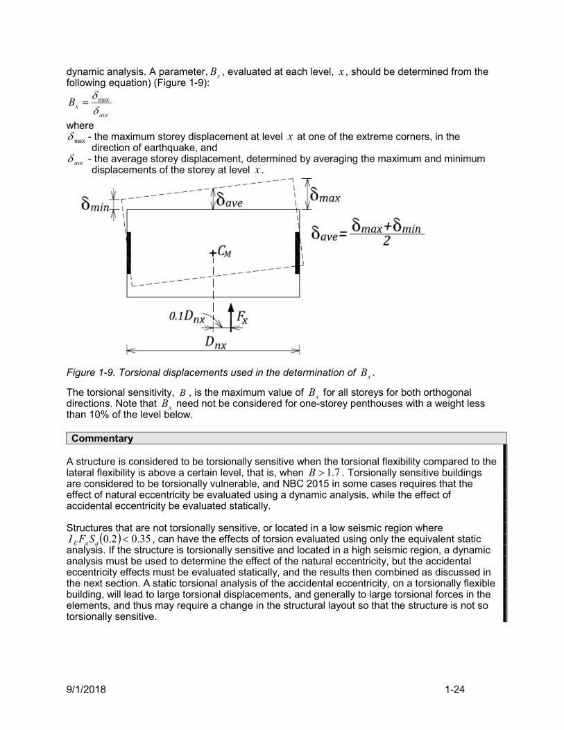
dynamic analysis. A parameter, xB , evaluated at each level, x , should be determined from the following equation) (Figure 1-9):

avexB

max

where max - the maximum storey displacement at level x at one of the extreme corners, in the

direction of earthquake, and ave - the average storey displacement, determined by averaging the maximum and minimum

displacements of the storey at level x .

Figure 1-9. Torsional displacements used in the determination of xB .

The torsional sensitivity, B , is the maximum value of xB for all storeys for both orthogonal directions. Note that xB need not be considered for one-storey penthouses with a weight less than 10% of the level below. Commentary

A structure is considered to be torsionally sensitive when the torsional flexibility compared to the lateral flexibility is above a certain level, that is, when 7.1B . Torsionally sensitive buildings are considered to be torsionally vulnerable, and NBC 2015 in some cases requires that the effect of natural eccentricity be evaluated using a dynamic analysis, while the effect of accidental eccentricity be evaluated statically. Structures that are not torsionally sensitive, or located in a low seismic region where

35.02.0 aaE SFI , can have the effects of torsion evaluated using only the equivalent static analysis. If the structure is torsionally sensitive and located in a high seismic region, a dynamic analysis must be used to determine the effect of the natural eccentricity, but the accidental eccentricity effects must be evaluated statically, and the results then combined as discussed in the next section. A static torsional analysis of the accidental eccentricity, on a torsionally flexible building, will lead to large torsional displacements, and generally to large torsional forces in the elements, and thus may require a change in the structural layout so that the structure is not so torsionally sensitive.

9/1/2018 1-25

1.11.3 Determination of torsional forces

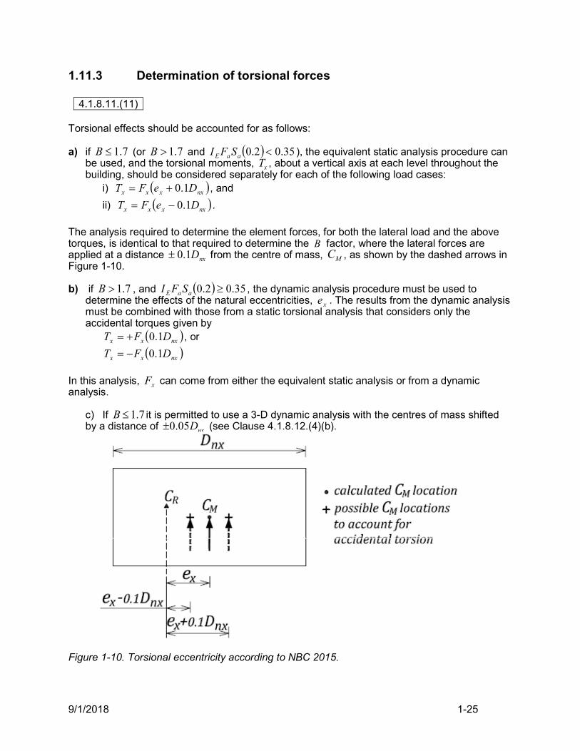
4.1.8.11.(11) Torsional effects should be accounted for as follows: a) if 7.1B (or 7.1B and 35.02.0 aaE SFI ), the equivalent static analysis procedure can

be used, and the torsional moments, xT , about a vertical axis at each level throughout the building, should be considered separately for each of the following load cases:

i) nxxxx DeFT 1.0 , and

ii) nxxxx DeFT 1.0 .

The analysis required to determine the element forces, for both the lateral load and the above torques, is identical to that required to determine the B factor, where the lateral forces are applied at a distance nxD1.0 from the centre of mass, MC , as shown by the dashed arrows in Figure 1-10. b) if 7.1B , and 35.02.0 aaE SFI , the dynamic analysis procedure must be used to

determine the effects of the natural eccentricities, xe . The results from the dynamic analysis must be combined with those from a static torsional analysis that considers only the accidental torques given by

nxxx DFT 1.0 , or

nxxx DFT 1.0

In this analysis, xF can come from either the equivalent static analysis or from a dynamic analysis.

c) If 1.7B it is permitted to use a 3-D dynamic analysis with the centres of mass shifted by a distance of 0.05 nxD (see Clause 4.1.8.12.(4)(b).

Figure 1-10. Torsional eccentricity according to NBC 2015.

9/1/2018 1-26

Commentary When results from a dynamic analysis are combined with accidental torques that use the lateral forces xF from the equivalent static procedure, the designer should ensure that the analysis is done in a consistent manner, that is, by using either the elastic forces or the reduced design forces (elastic forces modified by odE RRI ). The final force results should be given in terms of the reduced design forces, while the displacements should correspond to the elastic displacements. If the structure is torsionally sensitive, 7.1B , and if 35.02.0 aaE SFI , then the member forces and displacements from the accidental eccentricity must be evaluated statically by applying a set of torques to each floor of nxx DF 1.0 . The set of lateral forces, xF , can come from either a static or a dynamic analysis. NBC 2015 is mute on whether the set of lateral static forces should be scaled to match the dynamic base shear (if the dynamic base shear is larger than the static value), and whether the dynamic set should correspond to the set determined with the floor rotations restrained or not restrained (see Section 1.14). It is suggested here that if a set of static forces is used, they should (if necessary) be scaled up to match the base shear from the rotationally restrained dynamic analysis. The static approach to determine member forces and displacements from the accidental eccentricity is illustrated in Figure 1-11. If the static forces are to be used, then the following steps need to be followed:

1. The forces xF are determined using the equivalent static method.

2. Torsional moments at each level are found using the following equations nxxx DFT 1.0 , or nxxx DFT 1.0 .

3. Displacements and forces due to torsional effects are determined, and combined with the results from the dynamic analysis. Note that, in buildings with larger periods, tF will cause large rotations and displacements, and the results will probably be conservative.

Figure 1-11. Static approach to determine the accidental eccentricity effects (Anderson, 2006).

If a dynamic set of floor forces, xF , are to be used, they should be scaled, if necessary (as discussed in Section 1.14), to be equal to the design base shear. For the determination of the storey torques, the force Fx at each floor can be determined from the dynamic analysis by taking the difference in the total shear in the storeys above and below the floor in question. These floor forces are not necessarily the correct floor forces (as discussed in Section A.4.3), however the sum of these forces equals the design base shear and they provide a reasonable set of lateral

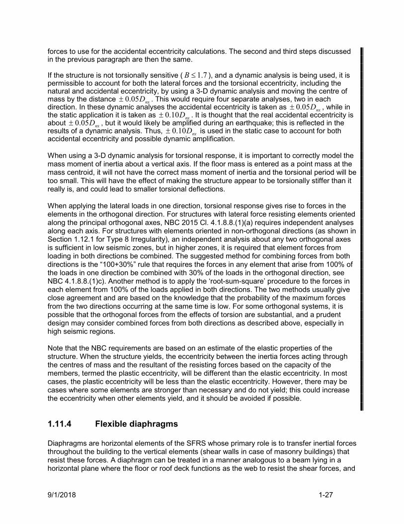
9/1/2018 1-27

forces to use for the accidental eccentricity calculations. The second and third steps discussed in the previous paragraph are then the same. If the structure is not torsionally sensitive ( 7.1B ), and a dynamic analysis is being used, it is permissible to account for both the lateral forces and the torsional eccentricity, including the natural and accidental eccentricity, by using a 3-D dynamic analysis and moving the centre of mass by the distance nxD05.0 . This would require four separate analyses, two in each direction. In these dynamic analyses the accidental eccentricity is taken as nxD05.0 , while in the static application it is taken as nxD10.0 . It is thought that the real accidental eccentricity is about nxD05.0 , but it would likely be amplified during an earthquake; this is reflected in the results of a dynamic analysis. Thus, nxD10.0 is used in the static case to account for both accidental eccentricity and possible dynamic amplification. When using a 3-D dynamic analysis for torsional response, it is important to correctly model the mass moment of inertia about a vertical axis. If the floor mass is entered as a point mass at the mass centroid, it will not have the correct mass moment of inertia and the torsional period will be too small. This will have the effect of making the structure appear to be torsionally stiffer than it really is, and could lead to smaller torsional deflections. When applying the lateral loads in one direction, torsional response gives rise to forces in the elements in the orthogonal direction. For structures with lateral force resisting elements oriented along the principal orthogonal axes, NBC 2015 Cl. 4.1.8.8.(1)(a) requires independent analyses along each axis. For structures with elements oriented in non-orthogonal directions (as shown in Section 1.12.1 for Type 8 Irregularity), an independent analysis about any two orthogonal axes is sufficient in low seismic zones, but in higher zones, it is required that element forces from loading in both directions be combined. The suggested method for combining forces from both directions is the “100+30%” rule that requires the forces in any element that arise from 100% of the loads in one direction be combined with 30% of the loads in the orthogonal direction, see NBC 4.1.8.8.(1)c). Another method is to apply the ‘root-sum-square’ procedure to the forces in each element from 100% of the loads applied in both directions. The two methods usually give close agreement and are based on the knowledge that the probability of the maximum forces from the two directions occurring at the same time is low. For some orthogonal systems, it is possible that the orthogonal forces from the effects of torsion are substantial, and a prudent design may consider combined forces from both directions as described above, especially in high seismic regions. Note that the NBC requirements are based on an estimate of the elastic properties of the structure. When the structure yields, the eccentricity between the inertia forces acting through the centres of mass and the resultant of the resisting forces based on the capacity of the members, termed the plastic eccentricity, will be different than the elastic eccentricity. In most cases, the plastic eccentricity will be less than the elastic eccentricity. However, there may be cases where some elements are stronger than necessary and do not yield; this could increase the eccentricity when other elements yield, and it should be avoided if possible.

1.11.4 Flexible diaphragms Diaphragms are horizontal elements of the SFRS whose primary role is to transfer inertial forces throughout the building to the vertical elements (shear walls in case of masonry buildings) that resist these forces. A diaphragm can be treated in a manner analogous to a beam lying in a horizontal plane where the floor or roof deck functions as the web to resist the shear forces, and

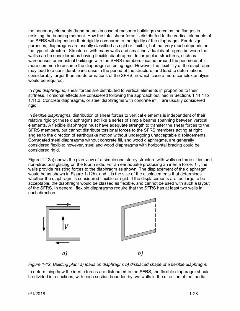
9/1/2018 1-28

the boundary elements (bond beams in case of masonry buildings) serve as the flanges in resisting the bending moment. How the total shear force is distributed to the vertical elements of the SFRS will depend on their rigidity compared to the rigidity of the diaphragm. For design purposes, diaphragms are usually classified as rigid or flexible, but that very much depends on the type of structure. Structures with many walls and small individual diaphragms between the walls can be considered as having flexible diaphragms. In large plan structures, such as warehouses or industrial buildings with the SFRS members located around the perimeter, it is more common to assume the diaphragm as being rigid. However the flexibility of the diaphragm may lead to a considerable increase in the period of the structure, and lead to deformations considerably larger than the deformations of the SFRS, in which case a more complex analysis would be required. In rigid diaphragms, shear forces are distributed to vertical elements in proportion to their stiffness. Torsional effects are considered following the approach outlined in Sections 1.11.1 to 1.11.3. Concrete diaphragms, or steel diaphragms with concrete infill, are usually considered rigid. In flexible diaphragms, distribution of shear forces to vertical elements is independent of their relative rigidity; these diaphragms act like a series of simple beams spanning between vertical elements. A flexible diaphragm must have adequate strength to transfer the shear forces to the SFRS members, but cannot distribute torsional forces to the SFRS members acting at right angles to the direction of earthquake motion without undergoing unacceptable displacements. Corrugated steel diaphragms without concrete fill, and wood diaphragms, are generally considered flexible; however, steel and wood diaphragms with horizontal bracing could be considered rigid. Figure 1-12a) shows the plan view of a simple one storey structure with walls on three sides and non-structural glazing on the fourth side. For an earthquake producing an inertia force, V , the walls provide resisting forces to the diaphragm as shown. The displacement of the diaphragm would be as shown in Figure 1-12b), and it is the size of the displacements that determines whether the diaphragm is considered flexible or rigid. If the displacements are too large to be acceptable, the diaphragm would be classed as flexible, and cannot be used with such a layout of the SFRS. In general, flexible diaphragms require that the SFRS has at least two walls in each direction.

Figure 1-12. Building plan: a) loads on diaphragm; b) displaced shape of a flexible diaphragm.

In determining how the inertia forces are distributed to the SFRS, the flexible diaphragm should be divided into sections, with each section bounded by two walls in the direction of the inertia

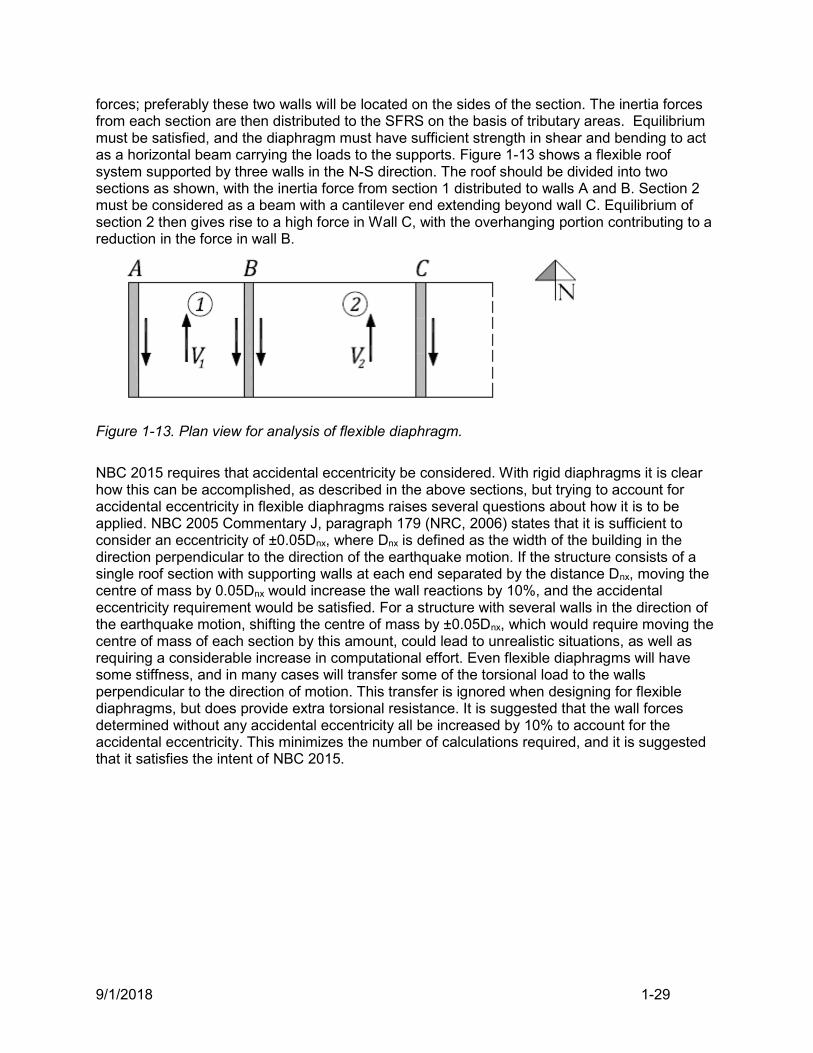
9/1/2018 1-29

forces; preferably these two walls will be located on the sides of the section. The inertia forces from each section are then distributed to the SFRS on the basis of tributary areas. Equilibrium must be satisfied, and the diaphragm must have sufficient strength in shear and bending to act as a horizontal beam carrying the loads to the supports. Figure 1-13 shows a flexible roof system supported by three walls in the N-S direction. The roof should be divided into two sections as shown, with the inertia force from section 1 distributed to walls A and B. Section 2 must be considered as a beam with a cantilever end extending beyond wall C. Equilibrium of section 2 then gives rise to a high force in Wall C, with the overhanging portion contributing to a reduction in the force in wall B.

Figure 1-13. Plan view for analysis of flexible diaphragm.

NBC 2015 requires that accidental eccentricity be considered. With rigid diaphragms it is clear how this can be accomplished, as described in the above sections, but trying to account for accidental eccentricity in flexible diaphragms raises several questions about how it is to be applied. NBC 2005 Commentary J, paragraph 179 (NRC, 2006) states that it is sufficient to consider an eccentricity of ±0.05Dnx, where Dnx is defined as the width of the building in the direction perpendicular to the direction of the earthquake motion. If the structure consists of a single roof section with supporting walls at each end separated by the distance Dnx, moving the centre of mass by 0.05Dnx would increase the wall reactions by 10%, and the accidental eccentricity requirement would be satisfied. For a structure with several walls in the direction of the earthquake motion, shifting the centre of mass by ±0.05Dnx, which would require moving the centre of mass of each section by this amount, could lead to unrealistic situations, as well as requiring a considerable increase in computational effort. Even flexible diaphragms will have some stiffness, and in many cases will transfer some of the torsional load to the walls perpendicular to the direction of motion. This transfer is ignored when designing for flexible diaphragms, but does provide extra torsional resistance. It is suggested that the wall forces determined without any accidental eccentricity all be increased by 10% to account for the accidental eccentricity. This minimizes the number of calculations required, and it is suggested that it satisfies the intent of NBC 2015.

9/1/2018 1-30

1.12 Configuration Issues: Irregularities and Restrictions

1.12.1 Irregularities

4.1.8.6 Table 1-16 (same as NBC 2015 Table 4.1.8.6) lists the nine types of irregularity, and the notes to the table refer to the relevant code clauses that consider the irregularity. If a structure has none of the listed irregularities it is considered to be a regular structure. A trigger for the NBC 2015 irregularity provisions (Cl.4.1.8.6) is the presence of one of nine types of irregularity in combination with the higher seismic hazard index, that is, 35.02.0 aaE SFI . In NBC 2015 there is a new structural irregularity, Type 9, on ‘gravity-induced lateral demand’ which covers cases where gravity loads could cause the building to yield in one direction only and creates larger displacements than a regular building would undergo. Irregularities are used to trigger restrictions and special requirements, some of which are more restrictive than those in previous codes. See NBC Section 4.1.8.10 for additional restrictive clauses covering structural irregularities.

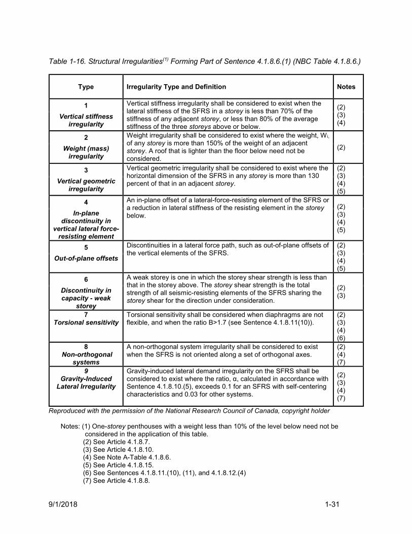
9/1/2018 1-31

Table 1-16. Structural Irregularities(1) Forming Part of Sentence 4.1.8.6.(1) (NBC Table 4.1.8.6.)

Type

Irregularity Type and Definition Notes

1 Vertical stiffness irregularity shall be considered to exist when the lateral stiffness of the SFRS in a storey is less than 70% of the stiffness of any adjacent storey, or less than 80% of the average stiffness of the three storeys above or below.

(2) (3) (4)

Vertical stiffness irregularity

2 Weight irregularity shall be considered to exist where the weight, W i,

of any storey is more than 150% of the weight of an adjacent storey. A roof that is lighter than the floor below need not be considered.

(2) Weight (mass) irregularity

3 Vertical geometric irregularity shall be considered to exist where the horizontal dimension of the SFRS in any storey is more than 130 percent of that in an adjacent storey.

(2) (3) (4) (5)

Vertical geometric irregularity

4 An in-plane offset of a lateral-force-resisting element of the SFRS or a reduction in lateral stiffness of the resisting element in the storey below.

(2) (3) (4) (5)

In-plane discontinuity in

vertical lateral force-resisting element

5 Discontinuities in a lateral force path, such as out-of-plane offsets of the vertical elements of the SFRS.

(2) (3) (4) (5)

Out-of-plane offsets

6 A weak storey is one in which the storey shear strength is less than that in the storey above. The storey shear strength is the total strength of all seismic-resisting elements of the SFRS sharing the storey shear for the direction under consideration.

(2) (3)

Discontinuity in capacity - weak

storey 7

Torsional sensitivity Torsional sensitivity shall be considered when diaphragms are not flexible, and when the ratio B>1.7 (see Sentence 4.1.8.11(10)).

(2) (3) (4) (6)

8 Non-orthogonal

systems

A non-orthogonal system irregularity shall be considered to exist when the SFRS is not oriented along a set of orthogonal axes.

(2) (4) (7)

9 Gravity-Induced

Lateral Irregularity

Gravity-induced lateral demand irregularity on the SFRS shall be considered to exist where the ratio, α, calculated in accordance with Sentence 4.1.8.10.(5), exceeds 0.1 for an SFRS with self-centering characteristics and 0.03 for other systems.

(2) (3) (4) (7)

Reproduced with the permission of the National Research Council of Canada, copyright holder Notes: (1) One-storey penthouses with a weight less than 10% of the level below need not be

considered in the application of this table. (2) See Article 4.1.8.7. (3) See Article 4.1.8.10. (4) See Note A-Table 4.1.8.6. (5) See Article 4.1.8.15. (6) See Sentences 4.1.8.11.(10), (11), and 4.1.8.12.(4) (7) See Article 4.1.8.8.

9/1/2018 1-32

Commentary

The equivalent static analysis procedure is based on a regular distribution of stiffness and mass in a structure. It becomes less accurate as the structure varies from this assumption. Historically, regular buildings have performed better in earthquakes than have irregular buildings. Layouts prone to damage are: torsionally eccentric ones, “in” and “out” of plane offsets of the lateral system, and buildings with a weak storey (Tremblay and DeVall, 2006). For more details on building configuration issues refer to Chapter 6 of Naeim (2001). Figure 1-14 illustrates the NBC 2015 irregularity types. Note that Types 1 to 6 are vertical (elevation) irregularities, while Types 7, 8 and 9 are horizontal (plan) irregularities. According to NBC 2015 Clause 4.1.8.7, the structure is considered to be “regular” if it has none of the nine types of irregularity, otherwise it is deemed to be “irregular”. The default method of analysis is the dynamic method, but the equivalent static method may be used if any of the following conditions are satisfied:

a) the seismic hazard index 35.02.0 aaE SFI , or b) the structure is regular, less than 60 m in height, and has a period T < 0.5 seconds in

either direction, or c) the structure is irregular, but does not have Type 7 or 9 irregularity, and is less than 20

m in height with period T < 0.5 seconds in either direction. For single-storey structures such as warehouses and other low-rise masonry buildings, only irregularity Types 7 and 8 might apply, and these would not likely prevent the use of the equivalent static method. Type 8 irregularity concerns SFRS(s) which are not oriented along a set of orthogonal axes. The structures with this type of irregularity may require more complex seismic analysis in which seismic loads in two orthogonal directions would need to be considered concurrently. According to Clause 4.1.8.8.(1)(b), where the components of the SFRS are not oriented along a set of orthogonal axes, and the structure is in a low seismic zone ( 35.02.0 aaE SFI ), then independent analysis about any two orthogonal axes is permitted. However, where the components of the SFRS are not oriented along a set of orthogonal axes, and the structure is in a medium or high seismic zone ( 35.02.0 aaE SFI ), then the analysis of the structure can be done independently about any two orthogonal axes for 100% of the prescribed earthquake loads in one direction concurrently with 30% of the prescribed earthquake loads acting in the perpendicular direction (see Clause 4.1.8.8.(1)(c). This is so-called “100+30%” rule discussed in Section 1.11.3.

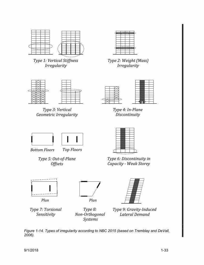
9/1/2018 1-33

Figure 1-14. Types of irregularity according to NBC 2015 (based on Tremblay and DeVall, 2006).

9/1/2018 1-34

1.12.2 Restrictions

4.1.8.10. Restrictions in NBC 2015 are based on (i) the natural period or height of the building, (ii) whether the building is in a “high” or “low” seismic zone, (iii) irregularities, and (iv) the importance category of the building. These restrictions are outlined below:

1. Except as required by Clause 4.1.8.10.(2)(b), structures with Type 6 irregularity, Discontinuity in Capacity – Weak Storey, are not permitted unless 20.02.0 aaE SFI and the forces used for design of the SFRS are multiplied by odRR .

2. Post-disaster buildings shall a) not have any irregularities conforming to Types 1, 3, 4, 5, 7 and 9 as described in

Table 4.1.8.6, in cases where 35.02.0 aaE SFI , b) not have a Type 6 irregularity as described in Table 4.1.8.6, and c) have an SFRS with an 0.2dR . d) have no storey with a lateral stiffness that is less than that of the storey above it.

3. For buildings having fundamental lateral periods 1.0aT s , and where 1.0 0.25E v aI F S , shear walls that are other than wood-based forming part of the

SFRS shall be continuous from their top to the foundation and shall not have irregularities of Type 4 or 5 as described in Table 4.1.8.6.

4. Wood construction, see 4.1.8.9 and Note A-4.1.8.10.(4). 5., 6., and 7. Only apply to Irregularity Type 9.

Refer to Section 1.12.1 and Table 1-16 for the list of irregularities identified by NBC 2015. Commentary

An important restriction for masonry construction concerns post-disaster structures. In other than low seismic regions the structure cannot have irregularity Types 1, 3, 4, 5, or 7; and must have an 0.2dR . Thus masonry post-disaster structures must be designed with Moderately Ductile or Ductile shear walls, and except in low seismic regions (where 35.02.0 aaE SFI ) the above noted irregularity types should be avoided. Irregularity Type 6, Discontinuity in Capacity-Weak Storey, is an important restriction for multi-storey structures, and cannot be present at all in post-disaster structures. For structures with this type of irregularity, the forces used in the design of the SFRS, except in very low seismic areas, must be multiplied by odRR , which implies that the members must remain elastic. This type of irregularity is considered very dangerous, as in past earthquakes many structures with weak storeys have had a total collapse of that storey which has resulted in many deaths. This type of seismic response has often been reported in reinforced concrete frame structures with masonry infill walls which contain more infills in the storeys above the ground floor, leaving the first storey as a weak storey.

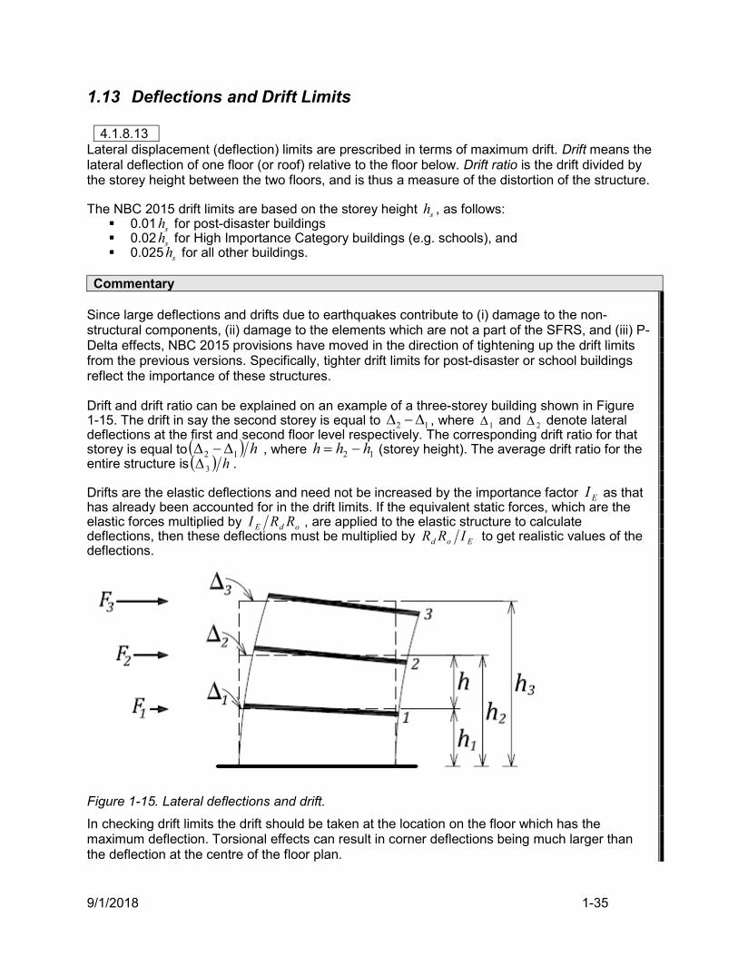
9/1/2018 1-35

1.13 Deflections and Drift Limits

4.1.8.13 Lateral displacement (deflection) limits are prescribed in terms of maximum drift. Drift means the lateral deflection of one floor (or roof) relative to the floor below. Drift ratio is the drift divided by the storey height between the two floors, and is thus a measure of the distortion of the structure. The NBC 2015 drift limits are based on the storey height sh , as follows:

0.01 sh for post-disaster buildings 0.02 sh for High Importance Category buildings (e.g. schools), and 0.025 sh for all other buildings.

Commentary

Since large deflections and drifts due to earthquakes contribute to (i) damage to the non-structural components, (ii) damage to the elements which are not a part of the SFRS, and (iii) P-Delta effects, NBC 2015 provisions have moved in the direction of tightening up the drift limits from the previous versions. Specifically, tighter drift limits for post-disaster or school buildings reflect the importance of these structures. Drift and drift ratio can be explained on an example of a three-storey building shown in Figure 1-15. The drift in say the second storey is equal to 12 , where 1 and 2 denote lateral deflections at the first and second floor level respectively. The corresponding drift ratio for that storey is equal to h12 , where 12 hhh (storey height). The average drift ratio for the entire structure is h3 . Drifts are the elastic deflections and need not be increased by the importance factor EI as that has already been accounted for in the drift limits. If the equivalent static forces, which are the elastic forces multiplied by odE RRI , are applied to the elastic structure to calculate deflections, then these deflections must be multiplied by Eod IRR to get realistic values of the deflections.

Figure 1-15. Lateral deflections and drift.

In checking drift limits the drift should be taken at the location on the floor which has the maximum deflection. Torsional effects can result in corner deflections being much larger than the deflection at the centre of the floor plan.

9/1/2018 1-36

Since deflections increase with an increase in the period T , the stiffness used in calculating the deflections should reflect a softening of the structure (before yielding occurs) that might come from cracking of the masonry. The stiffness for squat shear walls should be determined taking into account shear deformation. If the period T determined per NBC provisions (see Section 1.6) is used to determine the seismic forces, the stiffness of the structure used in calculating the deflections should be such that the calculated period would not be less than the NBC period. Many masonry structures are very stiff and the deflections will be well below the code limits, and so displacement calculations will not be critical in many cases. Drift limits are imposed so that members of the SFRS will not be subjected to large lateral displacements that might degrade their ability to resist the seismic loads, but also to ensure that members that are not part of the SFRS, such as columns that support gravity load only, should not fail during the earthquake. The seismic portion of the code is mute on drift limits for serviceability, however the designer can estimate the structural deflections at different hazard levels, since displacements are roughly proportional to the level of hazard. For example, the drift at an exceedance probability of 1/475 per annum would be about half of that for the 1/2475 per annum design drift because the 1/475 per annum hazard is roughly half the 1/2475 per annum hazard.

1.14 Dynamic Analysis Method

4.1.8.12 In NBC 2015 the default analysis method is the dynamic method. For many structures, even though the equivalent static analysis method could be used according to NBC seismic provisions, dynamic analysis may be used for other reasons. The purpose of this section is not to explain how to use dynamic analysis software, but to give some guidance on scaling or comparing the dynamic results with the results from the static method. The base shear from a dynamic analysis, determined using the site design spectrum S(T), will give the dynamic elastic base shear, eV . Since the static analysis method is allowed to reduce the design base shear for short periods, see 4.1.8.11(2)(d), while the dynamic analysis method uses the design spectrum S(T), it is permitted to reduce the dynamic analysis results by the factors 2S(0.2)/3S(Ta) or S(0.5)/S(Ta) whichever is larger but ≤1.0, to give Ved for Site Classes A to D (NBC 2015 Sec 4.1.8.12(6)). NBC 2015 requires that for regular buildings if the base shear from the dynamic method is less than 0.8 times the base shear from the static method, then the dynamic results should be scaled to give 0.8 of the static base shear. If the structure is deemed to be irregular, then the dynamic results should be scaled to 100% of the static results. In essence this means that the dynamic results cannot be less than the static results (or 80% of the static results for regular structures), but if they are larger they should not be reduced to the static values. If the building is very eccentric, a 3-D dynamic analysis will produce a low total base shear. In that case, it would be very conservative to require that these low base shears be scaled to the static base shear, since the static method of determining the base shear V does not consider torsional motion. To make a fair comparison between the static and dynamic results the suggestion is to perform a dynamic analysis with the rotation of the structure restrained about a

9/1/2018 1-37

vertical axis, and then compare the resulting base shear to the static value to determine the amount of scaling required, if any. Scaling, if necessary, should be applied to the member forces determined from the full 3-D dynamic analysis multiplied by odE RRI to give the design member forces. The design displacements are the elastic displacements given by the dynamic analysis, and scaled if necessary. To these design forces and displacements must be added the forces and displacements from accidental torsion.

1.15 Soil-Structure Interaction For large structures located on soft soil sites the deformation of the soil may have an appreciable influence on the response of the structure. The most common type of soil-structure interaction is based on the flexibility of the soil, which is usually represented by a lateral spring between the foundation and the point where the seismic motion is input, and with a rotational spring at the base of flexural walls. There is a second type of soil-structure interaction, termed the kinematic interaction, which only applies to structures with a very large plan area or a deep foundation, and which will not be discussed further here. The effect of introducing springs between the point of input motion and the foundation is to increase the period of the structure, which usually reduces the seismic forces but increases the deflections. In the case of a wall structure, the increased deflections may not increase the deformation of the wall since they would arise from displacements and rotations of the foundation, but the rotations would increase the interstorey drifts which would have an influence on other parts of the structure. For masonry structures, soil-structure interaction will likely only have an influence for slender wall structures with individual footings, where rotation of the footing would have a large effect on the wall displacement. The determination of the soil stiffness should be left to an experienced geotechnical engineer, but it should be recognized that the precision at which the soil stiffness can be estimated is quite low. It is common to consider quite wide upper and lower bounds on the estimated stiffness of the soil springs.

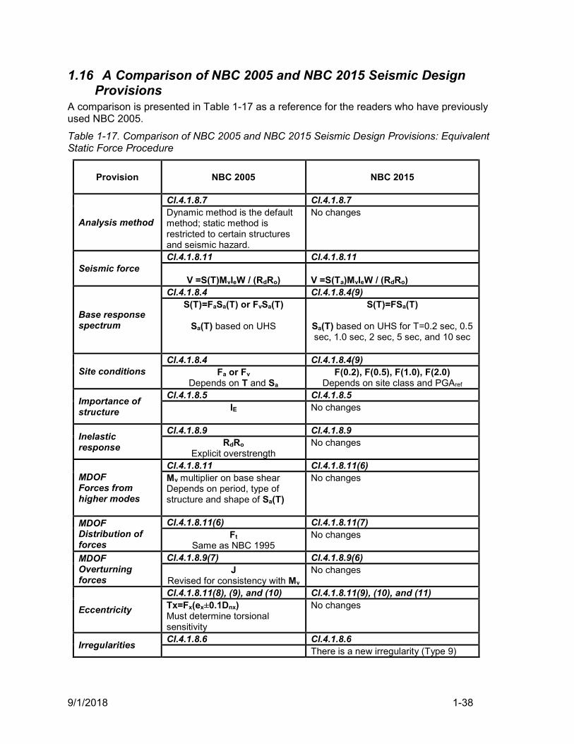
9/1/2018 1-38

1.16 A Comparison of NBC 2005 and NBC 2015 Seismic Design Provisions

A comparison is presented in Table 1-17 as a reference for the readers who have previously used NBC 2005.

Table 1-17. Comparison of NBC 2005 and NBC 2015 Seismic Design Provisions: Equivalent Static Force Procedure

Provision

NBC 2005

NBC 2015

Analysis method

Cl.4.1.8.7 Cl.4.1.8.7 Dynamic method is the default method; static method is restricted to certain structures and seismic hazard.

No changes

Seismic force Cl.4.1.8.11 Cl.4.1.8.11

V =S(T)MvIeW / (RdRo)

V =S(Ta)MvIeW / (RdRo)

Base response spectrum

Cl.4.1.8.4 Cl.4.1.8.4(9) S(T)=FaSa(T) or FvSa(T)

Sa(T) based on UHS

S(T)=FSa(T)

Sa(T) based on UHS for T=0.2 sec, 0.5 sec, 1.0 sec, 2 sec, 5 sec, and 10 sec

Site conditions Cl.4.1.8.4 Cl.4.1.8.4(9)

Fa or Fv

Depends on T and Sa

F(0.2), F(0.5), F(1.0), F(2.0) Depends on site class and PGAref

Importance of structure

Cl.4.1.8.5 Cl.4.1.8.5 IE

No changes

Inelastic response

Cl.4.1.8.9 Cl.4.1.8.9 RdRo

Explicit overstrength No changes

MDOF Forces from higher modes

Cl.4.1.8.11 Cl.4.1.8.11(6) Mv multiplier on base shear Depends on period, type of structure and shape of Sa(T)

No changes

MDOF Distribution of forces

Cl.4.1.8.11(6) Cl.4.1.8.11(7) Ft

Same as NBC 1995 No changes

MDOF Overturning forces

Cl.4.1.8.9(7) Cl.4.1.8.9(6) J

Revised for consistency with Mv No changes

Eccentricity

Cl.4.1.8.11(8), (9), and (10) Cl.4.1.8.11(9), (10), and (11) Tx=Fx(ex±0.1Dnx) Must determine torsional sensitivity

No changes

Irregularities Cl.4.1.8.6 Cl.4.1.8.6 There is a new irregularity (Type 9)

9/1/2018 2-1

TABLE OF CONTENTS – CHAPTER 2

2 SEISMIC DESIGN OF MASONRY WALLS TO CSA S304-14 2-2

2.1 Introduction 2-2

2.2 Masonry Walls – Basic Concepts 2-2

2.3 Reinforced Masonry Shear Walls Under In-Plane Seismic Loading 2-8 2.3.1 Behaviour and Failure Mechanisms 2-8 2.3.2 Shear/Diagonal Tension Resistance 2-10 2.3.3 Sliding Shear Resistance 2-18 2.3.4 In-Plane Flexural Resistance Due to Combined Axial Load and Bending 2-20

2.4 Reinforced Masonry Walls Under Out-of-Plane Seismic Loading 2-20 2.4.1 Background 2-20 2.4.2 Out-of-Plane Shear Resistance 2-21 2.4.3 Out-of-Plane Sliding Shear Resistance 2-22 2.4.4 Out-of-Plane Section Resistance Due to Combined Axial Load and Bending 2-22

2.5 General Seismic Design Provisions for Reinforced Masonry Shear Walls 2-23 2.5.1 Capacity Design Approach 2-23 2.5.2 Ductile Seismic Response 2-27 2.5.3 Structural Regularity 2-28 2.5.4 Analysis Assumptions – Effective Section Properties 2-28 2.5.5 Redistribution of design moments from elastic analysis 2-30 2.5.6 Minor shear walls as a part of the SFRS 2-30

2.6 CSA S304-14 Seismic Design Requirements 2-30 2.6.1 Classes of reinforced masonry shear walls 2-30 2.6.2 Plastic hinge region 2-32 2.6.3 Ductility check 2-34 2.6.4 Wall height-to-thickness ratio restrictions 2-40 2.6.5 Minimum Required Factored Shear Resistance 2-45 2.6.6 Shear/diagonal tension resistance – seismic design requirements 2-46 2.6.7 Sliding shear resistance – seismic design requirements 2-48 2.6.8 Boundary elements in Moderately Ductile and Ductile shear walls 2-49 2.6.9 Seismic reinforcement requirements for masonry shear walls 2-59 2.6.10 Minimum reinforcement requirements for Moderately Ductile Squat shear walls 2-68 2.6.11 Summary of Seismic Design Requirements for Reinforced Masonry Walls 2-71 2.6.12 Comparison of the Seismic Design and Detailing Requirements for Reinforced Masonry Walls in CSA S304-14 and CSA S304.1-04 2-73

2.7 Special Topics 2-75 2.7.1 Unreinforced Masonry Shear Walls 2-75 2.7.2 Masonry Infill Walls 2-80 2.7.3 Stack Pattern Walls 2-88 2.7.4 Nonloadbearing Walls 2-93 2.7.5 Flanged shear walls 2-94 2.7.6 Wall-to-Diaphragm Anchorage 2-96 2.7.7 Masonry Veneers and their Connections 2-97 2.7.8 Constructability Issues 2-100

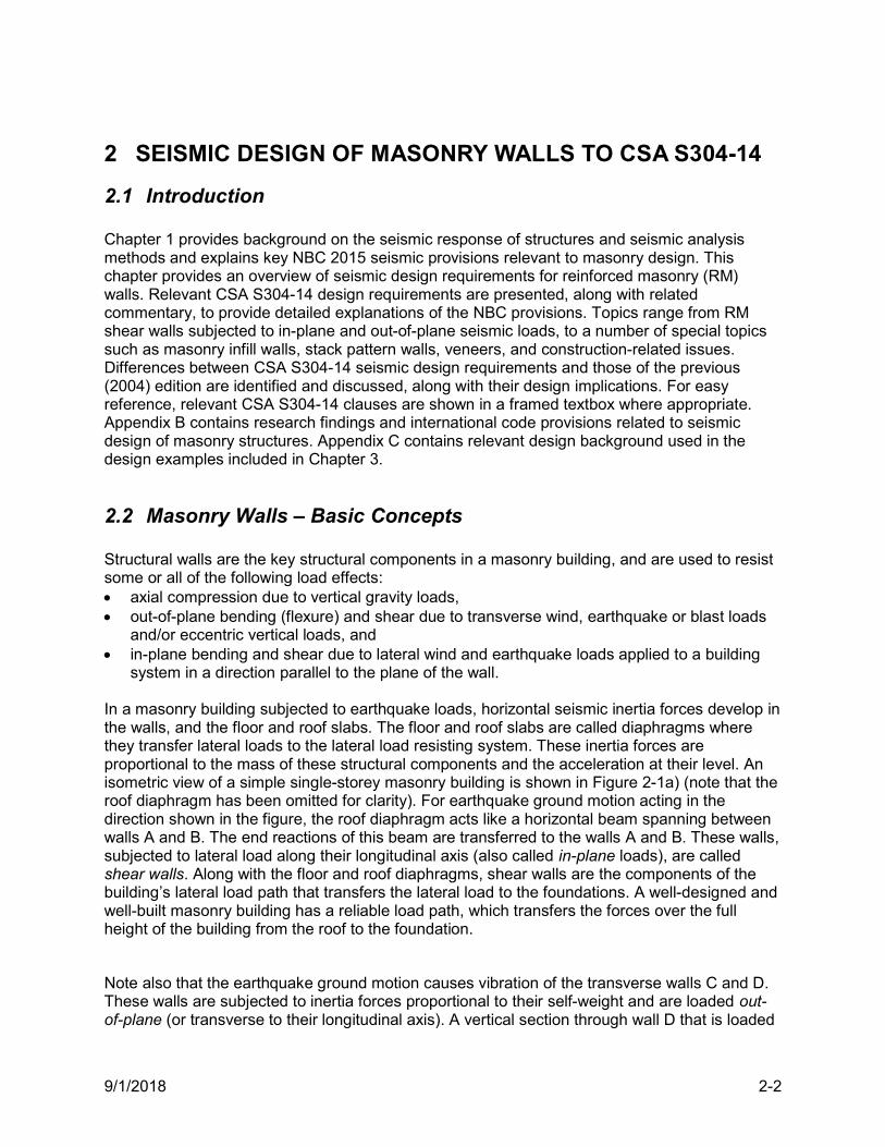
9/1/2018 2-2

2 SEISMIC DESIGN OF MASONRY WALLS TO CSA S304-14

2.1 Introduction Chapter 1 provides background on the seismic response of structures and seismic analysis methods and explains key NBC 2015 seismic provisions relevant to masonry design. This chapter provides an overview of seismic design requirements for reinforced masonry (RM) walls. Relevant CSA S304-14 design requirements are presented, along with related commentary, to provide detailed explanations of the NBC provisions. Topics range from RM shear walls subjected to in-plane and out-of-plane seismic loads, to a number of special topics such as masonry infill walls, stack pattern walls, veneers, and construction-related issues. Differences between CSA S304-14 seismic design requirements and those of the previous (2004) edition are identified and discussed, along with their design implications. For easy reference, relevant CSA S304-14 clauses are shown in a framed textbox where appropriate. Appendix B contains research findings and international code provisions related to seismic design of masonry structures. Appendix C contains relevant design background used in the design examples included in Chapter 3.

2.2 Masonry Walls – Basic Concepts Structural walls are the key structural components in a masonry building, and are used to resist some or all of the following load effects: axial compression due to vertical gravity loads, out-of-plane bending (flexure) and shear due to transverse wind, earthquake or blast loads

and/or eccentric vertical loads, and in-plane bending and shear due to lateral wind and earthquake loads applied to a building

system in a direction parallel to the plane of the wall. In a masonry building subjected to earthquake loads, horizontal seismic inertia forces develop in the walls, and the floor and roof slabs. The floor and roof slabs are called diaphragms where they transfer lateral loads to the lateral load resisting system. These inertia forces are proportional to the mass of these structural components and the acceleration at their level. An isometric view of a simple single-storey masonry building is shown in Figure 2-1a) (note that the roof diaphragm has been omitted for clarity). For earthquake ground motion acting in the direction shown in the figure, the roof diaphragm acts like a horizontal beam spanning between walls A and B. The end reactions of this beam are transferred to the walls A and B. These walls, subjected to lateral load along their longitudinal axis (also called in-plane loads), are called shear walls. Along with the floor and roof diaphragms, shear walls are the components of the building’s lateral load path that transfers the lateral load to the foundations. A well-designed and well-built masonry building has a reliable load path, which transfers the forces over the full height of the building from the roof to the foundation.

Note also that the earthquake ground motion causes vibration of the transverse walls C and D. These walls are subjected to inertia forces proportional to their self-weight and are loaded out-of-plane (or transverse to their longitudinal axis). A vertical section through wall D that is loaded

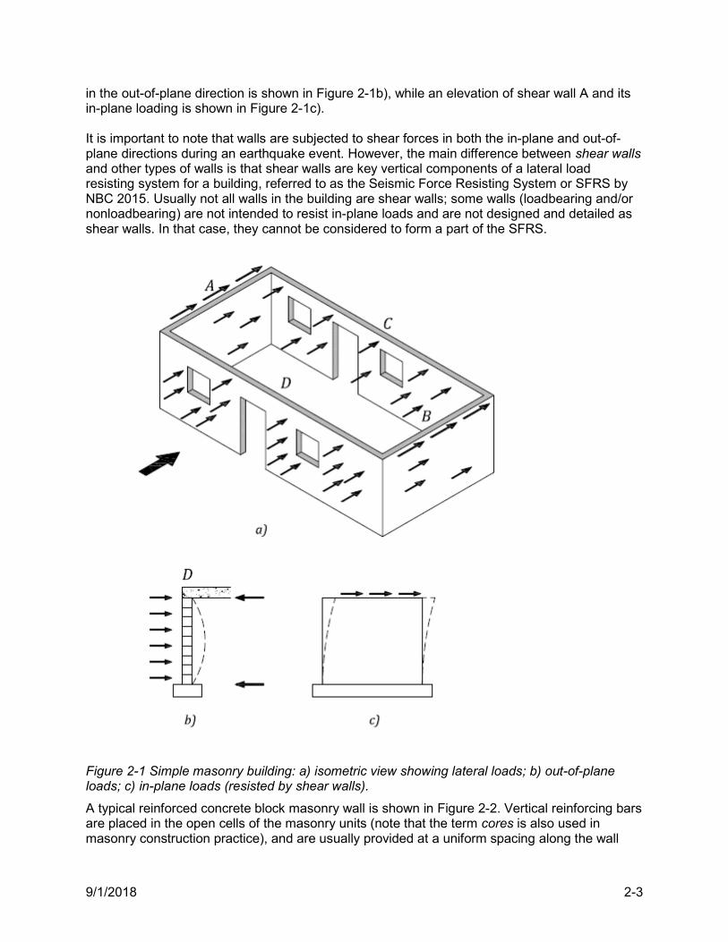
9/1/2018 2-3

in the out-of-plane direction is shown in Figure 2-1b), while an elevation of shear wall A and its in-plane loading is shown in Figure 2-1c). It is important to note that walls are subjected to shear forces in both the in-plane and out-of-plane directions during an earthquake event. However, the main difference between shear walls and other types of walls is that shear walls are key vertical components of a lateral load resisting system for a building, referred to as the Seismic Force Resisting System or SFRS by NBC 2015. Usually not all walls in the building are shear walls; some walls (loadbearing and/or nonloadbearing) are not intended to resist in-plane loads and are not designed and detailed as shear walls. In that case, they cannot be considered to form a part of the SFRS.

Figure 2-1 Simple masonry building: a) isometric view showing lateral loads; b) out-of-plane loads; c) in-plane loads (resisted by shear walls).

A typical reinforced concrete block masonry wall is shown in Figure 2-2. Vertical reinforcing bars are placed in the open cells of the masonry units (note that the term cores is also used in masonry construction practice), and are usually provided at a uniform spacing along the wall

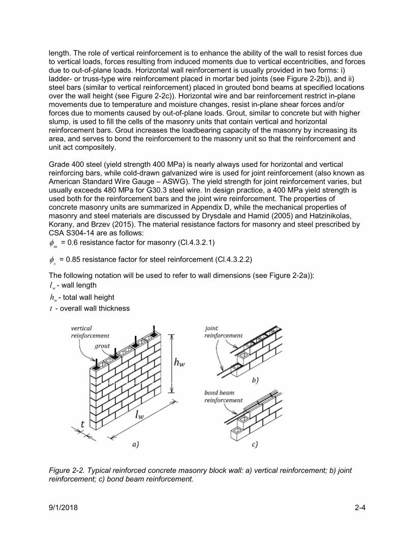
9/1/2018 2-4

length. The role of vertical reinforcement is to enhance the ability of the wall to resist forces due to vertical loads, forces resulting from induced moments due to vertical eccentricities, and forces due to out-of-plane loads. Horizontal wall reinforcement is usually provided in two forms: i) ladder- or truss-type wire reinforcement placed in mortar bed joints (see Figure 2-2b)), and ii) steel bars (similar to vertical reinforcement) placed in grouted bond beams at specified locations over the wall height (see Figure 2-2c)). Horizontal wire and bar reinforcement restrict in-plane movements due to temperature and moisture changes, resist in-plane shear forces and/or forces due to moments caused by out-of-plane loads. Grout, similar to concrete but with higher slump, is used to fill the cells of the masonry units that contain vertical and horizontal reinforcement bars. Grout increases the loadbearing capacity of the masonry by increasing its area, and serves to bond the reinforcement to the masonry unit so that the reinforcement and unit act compositely. Grade 400 steel (yield strength 400 MPa) is nearly always used for horizontal and vertical reinforcing bars, while cold-drawn galvanized wire is used for joint reinforcement (also known as American Standard Wire Gauge – ASWG). The yield strength for joint reinforcement varies, but usually exceeds 480 MPa for G30.3 steel wire. In design practice, a 400 MPa yield strength is used both for the reinforcement bars and the joint wire reinforcement. The properties of concrete masonry units are summarized in Appendix D, while the mechanical properties of masonry and steel materials are discussed by Drysdale and Hamid (2005) and Hatzinikolas, Korany, and Brzev (2015). The material resistance factors for masonry and steel prescribed by CSA S304-14 are as follows:

m = 0.6 resistance factor for masonry (Cl.4.3.2.1)

s = 0.85 resistance factor for steel reinforcement (Cl.4.3.2.2)

The following notation will be used to refer to wall dimensions (see Figure 2-2a)):

wl - wall length

wh - total wall height

t - overall wall thickness

Figure 2-2. Typical reinforced concrete masonry block wall: a) vertical reinforcement; b) joint reinforcement; c) bond beam reinforcement.

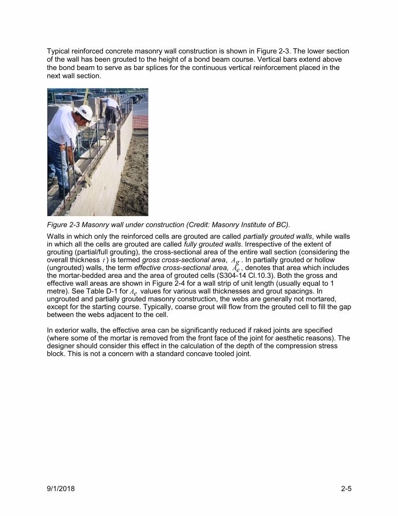
9/1/2018 2-5

Typical reinforced concrete masonry wall construction is shown in Figure 2-3. The lower section of the wall has been grouted to the height of a bond beam course. Vertical bars extend above the bond beam to serve as bar splices for the continuous vertical reinforcement placed in the next wall section.

Figure 2-3 Masonry wall under construction (Credit: Masonry Institute of BC).

Walls in which only the reinforced cells are grouted are called partially grouted walls, while walls in which all the cells are grouted are called fully grouted walls. Irrespective of the extent of grouting (partial/full grouting), the cross-sectional area of the entire wall section (considering the overall thickness t ) is termed gross cross-sectional area, gA . In partially grouted or hollow (ungrouted) walls, the term effective cross-sectional area, eA , denotes that area which includes the mortar-bedded area and the area of grouted cells (S304-14 Cl.10.3). Both the gross and effective wall areas are shown in Figure 2-4 for a wall strip of unit length (usually equal to 1 metre). See Table D-1 for eA values for various wall thicknesses and grout spacings. In ungrouted and partially grouted masonry construction, the webs are generally not mortared, except for the starting course. Typically, coarse grout will flow from the grouted cell to fill the gap between the webs adjacent to the cell. In exterior walls, the effective area can be significantly reduced if raked joints are specified (where some of the mortar is removed from the front face of the joint for aesthetic reasons). The designer should consider this effect in the calculation of the depth of the compression stress block. This is not a concern with a standard concave tooled joint.

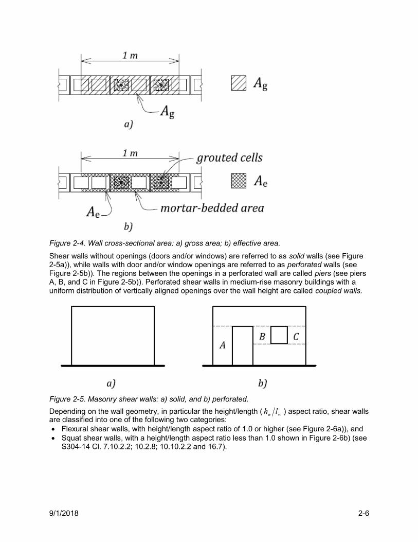
9/1/2018 2-6

Figure 2-4. Wall cross-sectional area: a) gross area; b) effective area.

Shear walls without openings (doors and/or windows) are referred to as solid walls (see Figure 2-5a)), while walls with door and/or window openings are referred to as perforated walls (see Figure 2-5b)). The regions between the openings in a perforated wall are called piers (see piers A, B, and C in Figure 2-5b)). Perforated shear walls in medium-rise masonry buildings with a uniform distribution of vertically aligned openings over the wall height are called coupled walls.

Figure 2-5. Masonry shear walls: a) solid, and b) perforated.

Depending on the wall geometry, in particular the height/length ( ww lh ) aspect ratio, shear walls are classified into one of the following two categories: Flexural shear walls, with height/length aspect ratio of 1.0 or higher (see Figure 2-6a)), and Squat shear walls, with a height/length aspect ratio less than 1.0 shown in Figure 2-6b) (see

S304-14 Cl. 7.10.2.2; 10.2.8; 10.10.2.2 and 16.7).

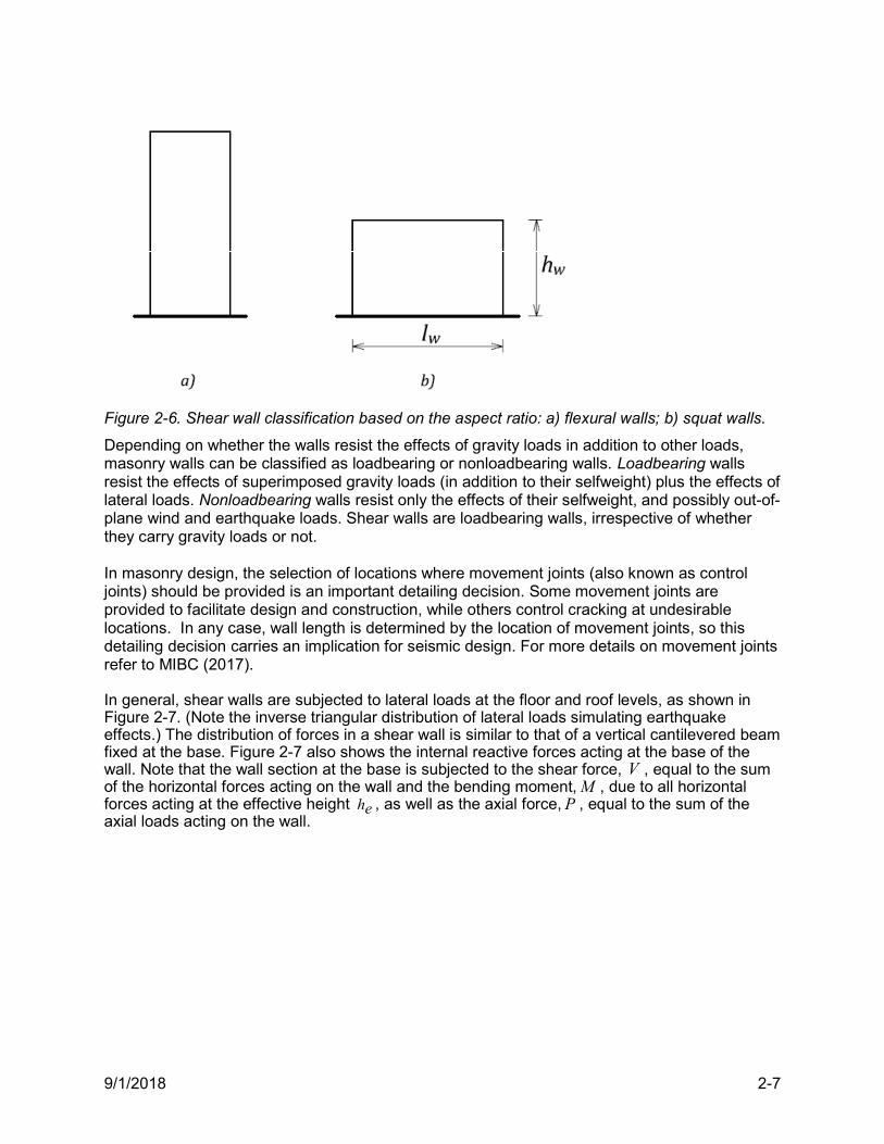
9/1/2018 2-7

Figure 2-6. Shear wall classification based on the aspect ratio: a) flexural walls; b) squat walls.

Depending on whether the walls resist the effects of gravity loads in addition to other loads, masonry walls can be classified as loadbearing or nonloadbearing walls. Loadbearing walls resist the effects of superimposed gravity loads (in addition to their selfweight) plus the effects of lateral loads. Nonloadbearing walls resist only the effects of their selfweight, and possibly out-of-plane wind and earthquake loads. Shear walls are loadbearing walls, irrespective of whether they carry gravity loads or not. In masonry design, the selection of locations where movement joints (also known as control joints) should be provided is an important detailing decision. Some movement joints are provided to facilitate design and construction, while others control cracking at undesirable locations. In any case, wall length is determined by the location of movement joints, so this detailing decision carries an implication for seismic design. For more details on movement joints refer to MIBC (2017). In general, shear walls are subjected to lateral loads at the floor and roof levels, as shown in Figure 2-7. (Note the inverse triangular distribution of lateral loads simulating earthquake effects.) The distribution of forces in a shear wall is similar to that of a vertical cantilevered beam fixed at the base. Figure 2-7 also shows the internal reactive forces acting at the base of the wall. Note that the wall section at the base is subjected to the shear force, V , equal to the sum of the horizontal forces acting on the wall and the bending moment,M , due to all horizontal forces acting at the effective height eh , as well as the axial force, P , equal to the sum of the axial loads acting on the wall.

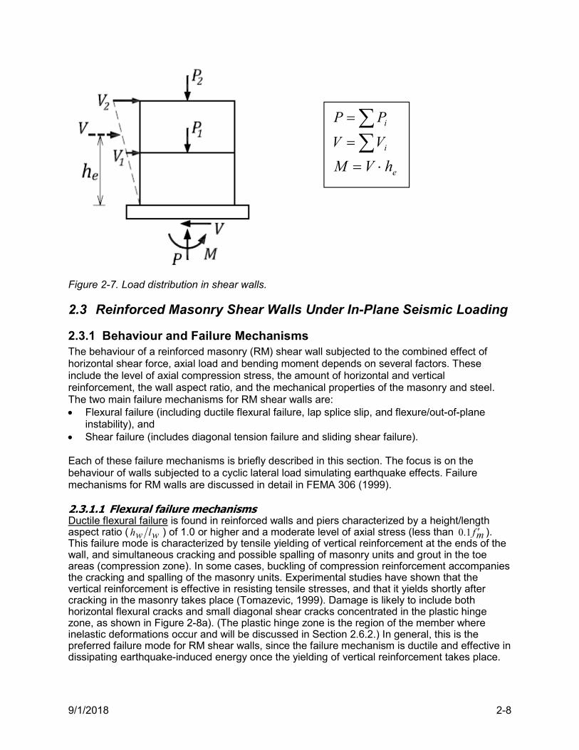
9/1/2018 2-8

Figure 2-7. Load distribution in shear walls.

2.3 Reinforced Masonry Shear Walls Under In-Plane Seismic Loading

2.3.1 Behaviour and Failure Mechanisms The behaviour of a reinforced masonry (RM) shear wall subjected to the combined effect of horizontal shear force, axial load and bending moment depends on several factors. These include the level of axial compression stress, the amount of horizontal and vertical reinforcement, the wall aspect ratio, and the mechanical properties of the masonry and steel. The two main failure mechanisms for RM shear walls are: Flexural failure (including ductile flexural failure, lap splice slip, and flexure/out-of-plane

instability), and Shear failure (includes diagonal tension failure and sliding shear failure). Each of these failure mechanisms is briefly described in this section. The focus is on the behaviour of walls subjected to a cyclic lateral load simulating earthquake effects. Failure mechanisms for RM walls are discussed in detail in FEMA 306 (1999). 2.3.1.1 Flexural failure mechanisms Ductile flexural failure is found in reinforced walls and piers characterized by a height/length aspect ratio ( wlwh ) of 1.0 or higher and a moderate level of axial stress (less than mf 1.0 ). This failure mode is characterized by tensile yielding of vertical reinforcement at the ends of the wall, and simultaneous cracking and possible spalling of masonry units and grout in the toe areas (compression zone). In some cases, buckling of compression reinforcement accompanies the cracking and spalling of the masonry units. Experimental studies have shown that the vertical reinforcement is effective in resisting tensile stresses, and that it yields shortly after cracking in the masonry takes place (Tomazevic, 1999). Damage is likely to include both horizontal flexural cracks and small diagonal shear cracks concentrated in the plastic hinge zone, as shown in Figure 2-8a). (The plastic hinge zone is the region of the member where inelastic deformations occur and will be discussed in Section 2.6.2.) In general, this is the preferred failure mode for RM shear walls, since the failure mechanism is ductile and effective in dissipating earthquake-induced energy once the yielding of vertical reinforcement takes place.

iPP

iVV

ehVM

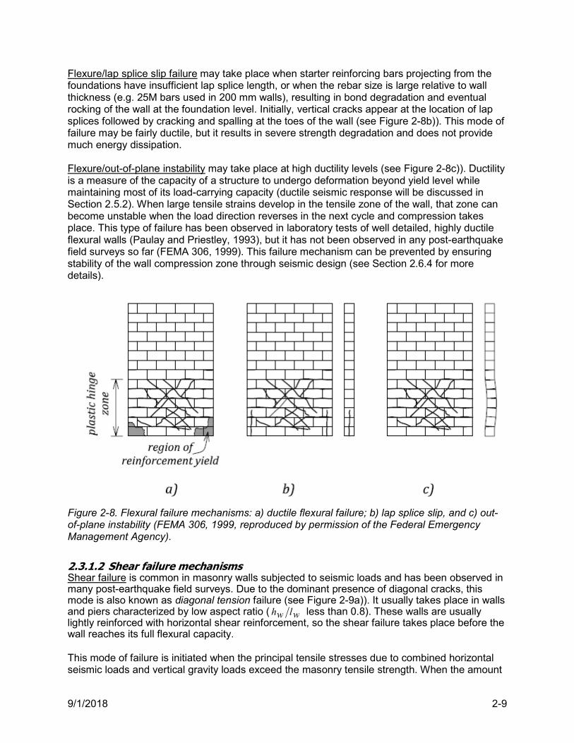
9/1/2018 2-9

Flexure/lap splice slip failure may take place when starter reinforcing bars projecting from the foundations have insufficient lap splice length, or when the rebar size is large relative to wall thickness (e.g. 25M bars used in 200 mm walls), resulting in bond degradation and eventual rocking of the wall at the foundation level. Initially, vertical cracks appear at the location of lap splices followed by cracking and spalling at the toes of the wall (see Figure 2-8b)). This mode of failure may be fairly ductile, but it results in severe strength degradation and does not provide much energy dissipation. Flexure/out-of-plane instability may take place at high ductility levels (see Figure 2-8c)). Ductility is a measure of the capacity of a structure to undergo deformation beyond yield level while maintaining most of its load-carrying capacity (ductile seismic response will be discussed in Section 2.5.2). When large tensile strains develop in the tensile zone of the wall, that zone can become unstable when the load direction reverses in the next cycle and compression takes place. This type of failure has been observed in laboratory tests of well detailed, highly ductile flexural walls (Paulay and Priestley, 1993), but it has not been observed in any post-earthquake field surveys so far (FEMA 306, 1999). This failure mechanism can be prevented by ensuring stability of the wall compression zone through seismic design (see Section 2.6.4 for more details).

Figure 2-8. Flexural failure mechanisms: a) ductile flexural failure; b) lap splice slip, and c) out-of-plane instability (FEMA 306, 1999, reproduced by permission of the Federal Emergency Management Agency).

2.3.1.2 Shear failure mechanisms Shear failure is common in masonry walls subjected to seismic loads and has been observed in many post-earthquake field surveys. Due to the dominant presence of diagonal cracks, this mode is also known as diagonal tension failure (see Figure 2-9a)). It usually takes place in walls and piers characterized by low aspect ratio ( wlwh less than 0.8). These walls are usually lightly reinforced with horizontal shear reinforcement, so the shear failure takes place before the wall reaches its full flexural capacity. This mode of failure is initiated when the principal tensile stresses due to combined horizontal seismic loads and vertical gravity loads exceed the masonry tensile strength. When the amount

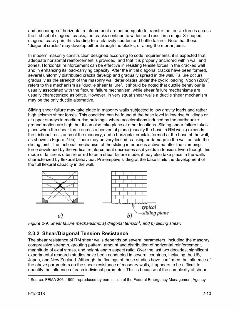
9/1/2018 2-10

and anchorage of horizontal reinforcement are not adequate to transfer the tensile forces across the first set of diagonal cracks, the cracks continue to widen and result in a major X-shaped diagonal crack pair, thus leading to a relatively sudden and brittle failure. Note that these “diagonal cracks” may develop either through the blocks, or along the mortar joints. In modern masonry construction designed according to code requirements, it is expected that adequate horizontal reinforcement is provided, and that it is properly anchored within wall end zones. Horizontal reinforcement can be effective in resisting tensile forces in the cracked wall and in enhancing its load-carrying capacity. After the initial diagonal cracks have been formed, several uniformly distributed cracks develop and gradually spread in the wall. Failure occurs gradually as the strength of the masonry wall deteriorates under the cyclic loading. Voon (2007) refers to this mechanism as “ductile shear failure”. It should be noted that ductile behaviour is usually associated with the flexural failure mechanism, while shear failure mechanisms are usually characterized as brittle. However, in very squat shear walls a ductile shear mechanism may be the only ductile alternative. Sliding shear failure may take place in masonry walls subjected to low gravity loads and rather high seismic shear forces. This condition can be found at the base level in low-rise buildings or at upper storeys in medium-rise buildings, where accelerations induced by the earthquake ground motion are high, but it can also take place at other locations. Sliding shear failure takes place when the shear force across a horizontal plane (usually the base in RM walls) exceeds the frictional resistance of the masonry, and a horizontal crack is formed at the base of the wall, as shown in Figure 2-9b). There may be very limited cracking or damage in the wall outside the sliding joint. The frictional mechanism at the sliding interface is activated after the clamping force developed by the vertical reinforcement decreases as it yields in tension. Even though this mode of failure is often referred to as a shear failure mode, it may also take place in the walls characterized by flexural behaviour. Pre-emptive sliding at the base limits the development of the full flexural capacity in the wall.

Figure 2-9. Shear failure mechanisms: a) diagonal tension1, and b) sliding shear.

2.3.2 Shear/Diagonal Tension Resistance The shear resistance of RM shear walls depends on several parameters, including the masonry compressive strength, grouting pattern, amount and distribution of horizontal reinforcement, magnitude of axial stress, and height/length aspect ratio. Over the last two decades, significant experimental research studies have been conducted in several countries, including the US, Japan, and New Zealand. Although the findings of these studies have confirmed the influence of the above parameters on the shear resistance of masonry walls, it appears to be difficult to quantify the influence of each individual parameter. This is because of the complexity of shear 1 Source: FEMA 306, 1999, reproduced by permission of the Federal Emergency Management Agency

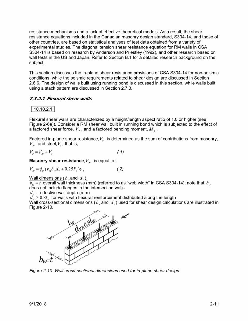
9/1/2018 2-11

resistance mechanisms and a lack of effective theoretical models. As a result, the shear resistance equations included in the Canadian masonry design standard, S304-14, and those of other countries, are based on statistical analyses of test data obtained from a variety of experimental studies. The diagonal tension shear resistance equation for RM walls in CSA S304-14 is based on research by Anderson and Priestley (1992), and other research based on wall tests in the US and Japan. Refer to Section B.1 for a detailed research background on the subject. This section discusses the in-plane shear resistance provisions of CSA S304-14 for non-seismic conditions, while the seismic requirements related to shear design are discussed in Section 2.6.6. The design of walls built using running bond is discussed in this section, while walls built using a stack pattern are discussed in Section 2.7.3. 2.3.2.1 Flexural shear walls

10.10.2.1 Flexural shear walls are characterized by a height/length aspect ratio of 1.0 or higher (see Figure 2-6a)). Consider a RM shear wall built in running bond which is subjected to the effect of a factored shear force, fV , and a factored bending moment, fM . Factored in-plane shear resistance, rV , is determined as the sum of contributions from masonry,

mV , and steel, sV , that is,

smr VVV ( 1)

Masonry shear resistance, mV , is equal to:

gdvwmmm PdbvV )25.0( ( 2)

Wall dimensions ( wb and vd ): tbw overall wall thickness (mm) (referred to as “web width” in CSA S304-14); note that wb

does not include flanges in the intersection walls vd = effective wall depth (mm)

wv ld 8.0 for walls with flexural reinforcement distributed along the length Wall cross-sectional dimensions ( wb and vd ) used for shear design calculations are illustrated in Figure 2-10.

Figure 2-10. Wall cross-sectional dimensions used for in-plane shear design.

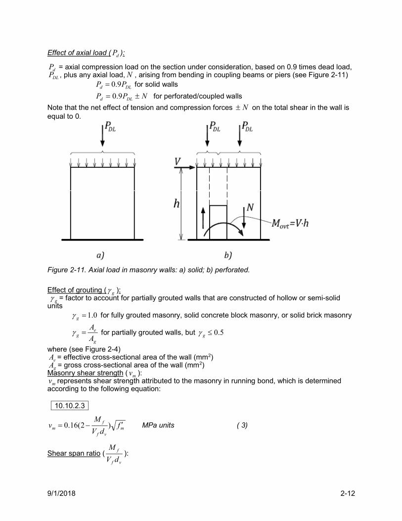
9/1/2018 2-12

Effect of axial load ( dP ):

dP = axial compression load on the section under consideration, based on 0.9 times dead load, DLP , plus any axial load, N , arising from bending in coupling beams or piers (see Figure 2-11)

DLd PP 9.0 for solid walls

NPP DLd 9.0 for perforated/coupled walls

Note that the net effect of tension and compression forces N on the total shear in the wall is equal to 0.

Figure 2-11. Axial load in masonry walls: a) solid; b) perforated.

Effect of grouting ( g ): g = factor to account for partially grouted walls that are constructed of hollow or semi-solid units 0.1g for fully grouted masonry, solid concrete block masonry, or solid brick masonry

g

eg A

A for partially grouted walls, but 5.0g

where (see Figure 2-4) eA = effective cross-sectional area of the wall (mm2) gA = gross cross-sectional area of the wall (mm2)

Masonry shear strength ( mv ): mv represents shear strength attributed to the masonry in running bond, which is determined

according to the following equation:

10.10.2.3

mvf

fm f

dV

Mv )2(16.0 MPa units ( 3)

Shear span ratio (vf

f

dV

M):

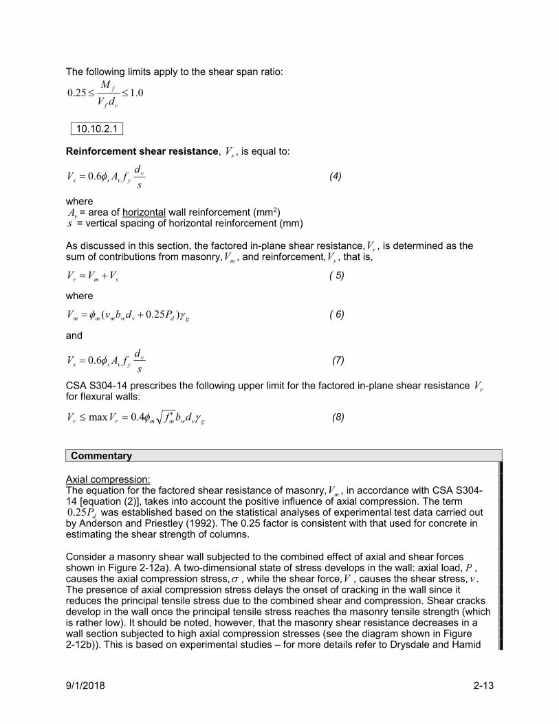
9/1/2018 2-13

The following limits apply to the shear span ratio:

0.125.0 vf

f

dV

M

10.10.2.1

Reinforcement shear resistance, sV , is equal to:

s

dfAV vyvss 6.0 (4)

where vA = area of horizontal wall reinforcement (mm2)

s = vertical spacing of horizontal reinforcement (mm) As discussed in this section, the factored in-plane shear resistance, rV , is determined as the sum of contributions from masonry, mV , and reinforcement, sV , that is,

smr VVV ( 5)

where

gdvwmmm PdbvV )25.0( ( 6)

and

s

dfAV vyvss 6.0 (7)

CSA S304-14 prescribes the following upper limit for the factored in-plane shear resistance rV for flexural walls:

gvwmmrr dbfVV 4.0max (8)

Commentary Axial compression: The equation for the factored shear resistance of masonry, mV , in accordance with CSA S304-14 [equation (2)], takes into account the positive influence of axial compression. The term

dP25.0 was established based on the statistical analyses of experimental test data carried out by Anderson and Priestley (1992). The 0.25 factor is consistent with that used for concrete in estimating the shear strength of columns. Consider a masonry shear wall subjected to the combined effect of axial and shear forces shown in Figure 2-12a). A two-dimensional state of stress develops in the wall: axial load, P , causes the axial compression stress, , while the shear force,V , causes the shear stress, v . The presence of axial compression stress delays the onset of cracking in the wall since it reduces the principal tensile stress due to the combined shear and compression. Shear cracks develop in the wall once the principal tensile stress reaches the masonry tensile strength (which is rather low). It should be noted, however, that the masonry shear resistance decreases in a wall section subjected to high axial compression stresses (see the diagram shown in Figure 2-12b)). This is based on experimental studies – for more details refer to Drysdale and Hamid

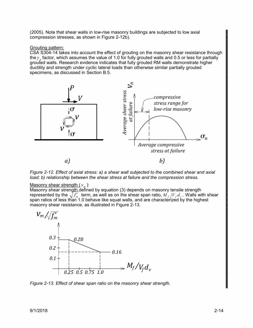
9/1/2018 2-14

(2005). Note that shear walls in low-rise masonry buildings are subjected to low axial compression stresses, as shown in Figure 2-12b). Grouting pattern: CSA S304-14 takes into account the effect of grouting on the masonry shear resistance through the g factor, which assumes the value of 1.0 for fully grouted walls and 0.5 or less for partially grouted walls. Research evidence indicates that fully grouted RM walls demonstrate higher ductility and strength under cyclic lateral loads than otherwise similar partially grouted specimens, as discussed in Section B.5.

Figure 2-12. Effect of axial stress: a) a shear wall subjected to the combined shear and axial load; b) relationship between the shear stress at failure and the compression stress.

Masonry shear strength ( mv ): Masonry shear strength defined by equation (3) depends on masonry tensile strength represented by the mf term, as well as on the shear span ratio, vff dVM . Walls with shear span ratios of less than 1.0 behave like squat walls, and are characterized by the highest masonry shear resistance, as illustrated in Figure 2-13.

Figure 2-13. Effect of shear span ratio on the masonry shear strength.

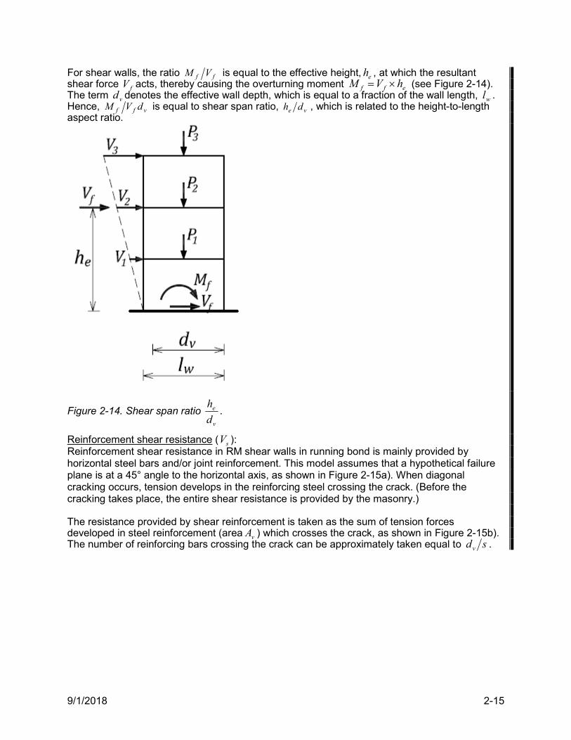
9/1/2018 2-15

For shear walls, the ratio ff VM is equal to the effective height, eh , at which the resultant shear force fV acts, thereby causing the overturning moment eff hVM (see Figure 2-14). The term vd denotes the effective wall depth, which is equal to a fraction of the wall length, wl . Hence, vff dVM is equal to shear span ratio, ve dh , which is related to the height-to-length aspect ratio.

Figure 2-14. Shear span ratio v

e

d

h.

Reinforcement shear resistance ( sV ): Reinforcement shear resistance in RM shear walls in running bond is mainly provided by horizontal steel bars and/or joint reinforcement. This model assumes that a hypothetical failure plane is at a 45° angle to the horizontal axis, as shown in Figure 2-15a). When diagonal cracking occurs, tension develops in the reinforcing steel crossing the crack. (Before the cracking takes place, the entire shear resistance is provided by the masonry.) The resistance provided by shear reinforcement is taken as the sum of tension forces developed in steel reinforcement (area vA ) which crosses the crack, as shown in Figure 2-15b). The number of reinforcing bars crossing the crack can be approximately taken equal to sdv .

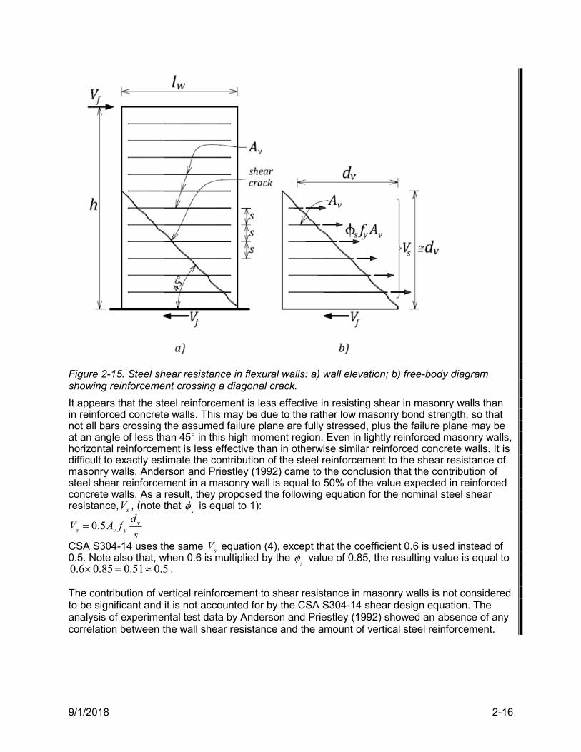
9/1/2018 2-16

Figure 2-15. Steel shear resistance in flexural walls: a) wall elevation; b) free-body diagram showing reinforcement crossing a diagonal crack.

It appears that the steel reinforcement is less effective in resisting shear in masonry walls than in reinforced concrete walls. This may be due to the rather low masonry bond strength, so that not all bars crossing the assumed failure plane are fully stressed, plus the failure plane may be at an angle of less than 45° in this high moment region. Even in lightly reinforced masonry walls, horizontal reinforcement is less effective than in otherwise similar reinforced concrete walls. It is difficult to exactly estimate the contribution of the steel reinforcement to the shear resistance of masonry walls. Anderson and Priestley (1992) came to the conclusion that the contribution of steel shear reinforcement in a masonry wall is equal to 50% of the value expected in reinforced concrete walls. As a result, they proposed the following equation for the nominal steel shear resistance, sV , (note that

s is equal to 1):

s

dfAV vyvs 5.0

CSA S304-14 uses the same sV equation (4), except that the coefficient 0.6 is used instead of 0.5. Note also that, when 0.6 is multiplied by the

s value of 0.85, the resulting value is equal to

5.051.085.06.0 . The contribution of vertical reinforcement to shear resistance in masonry walls is not considered to be significant and it is not accounted for by the CSA S304-14 shear design equation. The analysis of experimental test data by Anderson and Priestley (1992) showed an absence of any correlation between the wall shear resistance and the amount of vertical steel reinforcement.

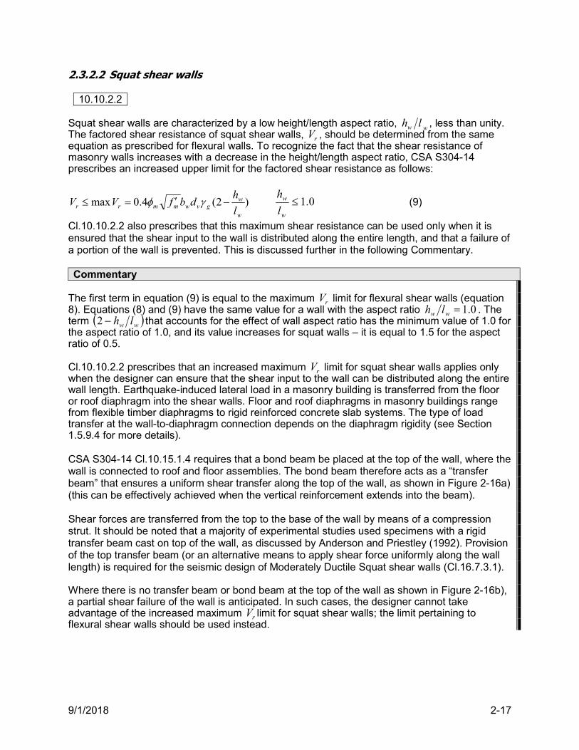
9/1/2018 2-17

2.3.2.2 Squat shear walls

10.10.2.2 Squat shear walls are characterized by a low height/length aspect ratio, ww lh , less than unity. The factored shear resistance of squat shear walls, rV , should be determined from the same equation as prescribed for flexural walls. To recognize the fact that the shear resistance of masonry walls increases with a decrease in the height/length aspect ratio, CSA S304-14 prescribes an increased upper limit for the factored shear resistance as follows:

)2(4.0maxw

wgvwmmrr l

hdbfVV 0.1

w

w

l

h (9)

Cl.10.10.2.2 also prescribes that this maximum shear resistance can be used only when it is ensured that the shear input to the wall is distributed along the entire length, and that a failure of a portion of the wall is prevented. This is discussed further in the following Commentary. Commentary

The first term in equation (9) is equal to the maximum rV limit for flexural shear walls (equation 8). Equations (8) and (9) have the same value for a wall with the aspect ratio 0.1ww lh . The term ww lh2 that accounts for the effect of wall aspect ratio has the minimum value of 1.0 for the aspect ratio of 1.0, and its value increases for squat walls – it is equal to 1.5 for the aspect ratio of 0.5. Cl.10.10.2.2 prescribes that an increased maximum rV limit for squat shear walls applies only when the designer can ensure that the shear input to the wall can be distributed along the entire wall length. Earthquake-induced lateral load in a masonry building is transferred from the floor or roof diaphragm into the shear walls. Floor and roof diaphragms in masonry buildings range from flexible timber diaphragms to rigid reinforced concrete slab systems. The type of load transfer at the wall-to-diaphragm connection depends on the diaphragm rigidity (see Section 1.5.9.4 for more details). CSA S304-14 Cl.10.15.1.4 requires that a bond beam be placed at the top of the wall, where the wall is connected to roof and floor assemblies. The bond beam therefore acts as a “transfer beam” that ensures a uniform shear transfer along the top of the wall, as shown in Figure 2-16a) (this can be effectively achieved when the vertical reinforcement extends into the beam). Shear forces are transferred from the top to the base of the wall by means of a compression strut. It should be noted that a majority of experimental studies used specimens with a rigid transfer beam cast on top of the wall, as discussed by Anderson and Priestley (1992). Provision of the top transfer beam (or an alternative means to apply shear force uniformly along the wall length) is required for the seismic design of Moderately Ductile Squat shear walls (Cl.16.7.3.1). Where there is no transfer beam or bond beam at the top of the wall as shown in Figure 2-16b), a partial shear failure of the wall is anticipated. In such cases, the designer cannot take advantage of the increased maximum rV limit for squat shear walls; the limit pertaining to flexural shear walls should be used instead.

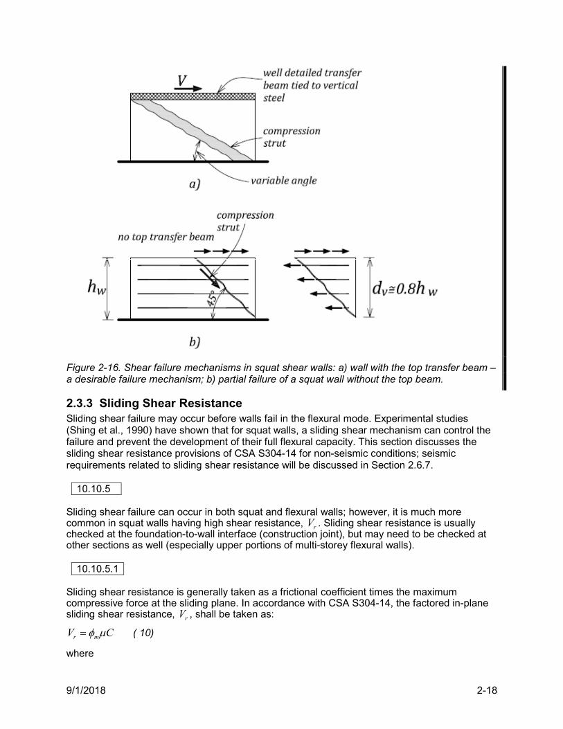
9/1/2018 2-18

Figure 2-16. Shear failure mechanisms in squat shear walls: a) wall with the top transfer beam – a desirable failure mechanism; b) partial failure of a squat wall without the top beam.

2.3.3 Sliding Shear Resistance Sliding shear failure may occur before walls fail in the flexural mode. Experimental studies (Shing et al., 1990) have shown that for squat walls, a sliding shear mechanism can control the failure and prevent the development of their full flexural capacity. This section discusses the sliding shear resistance provisions of CSA S304-14 for non-seismic conditions; seismic requirements related to sliding shear resistance will be discussed in Section 2.6.7.

10.10.5 Sliding shear failure can occur in both squat and flexural walls; however, it is much more common in squat walls having high shear resistance, rV . Sliding shear resistance is usually checked at the foundation-to-wall interface (construction joint), but may need to be checked at other sections as well (especially upper portions of multi-storey flexural walls).

10.10.5.1 Sliding shear resistance is generally taken as a frictional coefficient times the maximum compressive force at the sliding plane. In accordance with CSA S304-14, the factored in-plane sliding shear resistance, rV , shall be taken as:

CV mr ( 10)

where

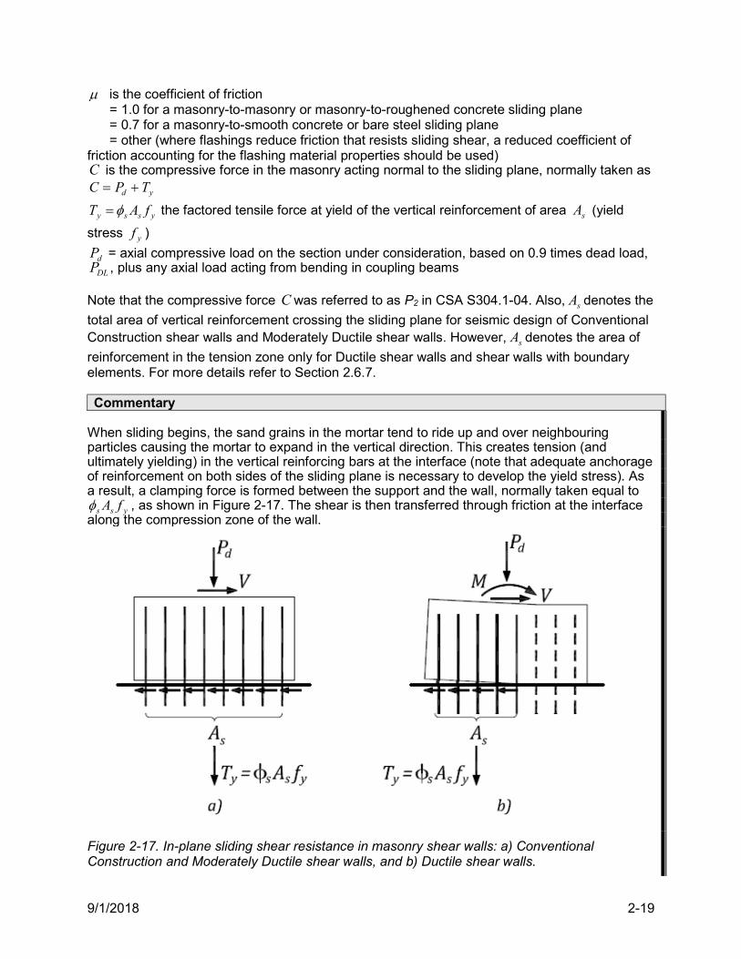
9/1/2018 2-19

is the coefficient of friction = 1.0 for a masonry-to-masonry or masonry-to-roughened concrete sliding plane = 0.7 for a masonry-to-smooth concrete or bare steel sliding plane = other (where flashings reduce friction that resists sliding shear, a reduced coefficient of friction accounting for the flashing material properties should be used) C is the compressive force in the masonry acting normal to the sliding plane, normally taken as

yd TPC

yssy fAT the factored tensile force at yield of the vertical reinforcement of area sA (yield

stress yf )

dP = axial compressive load on the section under consideration, based on 0.9 times dead load, DLP , plus any axial load acting from bending in coupling beams

Note that the compressive force C was referred to as P2 in CSA S304.1-04. Also, sA denotes the

total area of vertical reinforcement crossing the sliding plane for seismic design of Conventional Construction shear walls and Moderately Ductile shear walls. However, sA denotes the area of

reinforcement in the tension zone only for Ductile shear walls and shear walls with boundary elements. For more details refer to Section 2.6.7. Commentary

When sliding begins, the sand grains in the mortar tend to ride up and over neighbouring particles causing the mortar to expand in the vertical direction. This creates tension (and ultimately yielding) in the vertical reinforcing bars at the interface (note that adequate anchorage of reinforcement on both sides of the sliding plane is necessary to develop the yield stress). As a result, a clamping force is formed between the support and the wall, normally taken equal to

yss fA , as shown in Figure 2-17. The shear is then transferred through friction at the interface along the compression zone of the wall.

Figure 2-17. In-plane sliding shear resistance in masonry shear walls: a) Conventional Construction and Moderately Ductile shear walls, and b) Ductile shear walls.

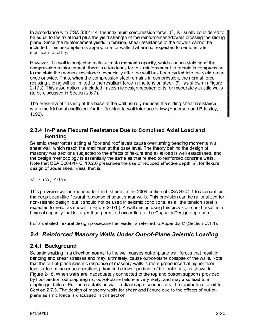
9/1/2018 2-20

In accordance with CSA S304-14, the maximum compression force, C , is usually considered to be equal to the axial load plus the yield strength of the reinforcement/dowels crossing the sliding plane. Since the reinforcement yields in tension, shear resistance of the dowels cannot be included. This assumption is appropriate for walls that are not expected to demonstrate significant ductility. However, if a wall is subjected to its ultimate moment capacity, which causes yielding of the compression reinforcement, there is a tendency for this reinforcement to remain in compression to maintain the moment resistance, especially after the wall has been cycled into the yield range once or twice. Thus, when the compression steel remains in compression, the normal force resisting sliding will be limited to the resultant force in the tension steel, yT , as shown in Figure 2-17b). This assumption is included in seismic design requirements for moderately ductile walls (to be discussed in Section 2.6.7). The presence of flashing at the base of the wall usually reduces the sliding shear resistance when the frictional coefficient for the flashing-to-wall interface is low (Anderson and Priestley, 1992).

2.3.4 In-Plane Flexural Resistance Due to Combined Axial Load and Bending

Seismic shear forces acting at floor and roof levels cause overturning bending moments in a shear wall, which reach the maximum at the base level. The theory behind the design of masonry wall sections subjected to the effects of flexure and axial load is well established, and the design methodology is essentially the same as that related to reinforced concrete walls. Note that CSA S304-14 Cl.10.2.8 prescribes the use of reduced effective depth, d , for flexural design of squat shear walls, that is:

hld w 7.067.0

This provision was introduced for the first time in the 2004 edition of CSA S304.1 to account for the deep beam-like flexural response of squat shear walls. This provision can be rationalized for non-seismic design, but it should not be used in seismic conditions, as all the tension steel is expected to yield, as shown in Figure 2-17b). A wall design using this provision could result in a flexural capacity that is larger than permitted according to the Capacity Design approach. For a detailed flexural design procedure the reader is referred to Appendix C (Section C.1.1).

2.4 Reinforced Masonry Walls Under Out-of-Plane Seismic Loading

2.4.1 Background Seismic shaking in a direction normal to the wall causes out-of-plane wall forces that result in bending and shear stresses and may, ultimately, cause out-of-plane collapse of the walls. Note that the out-of-plane seismic response of masonry walls is more pronounced at higher floor levels (due to larger accelerations) than in the lower portions of the buildings, as shown in Figure 2-18. When walls are inadequately connected to the top and bottom supports provided by floor and/or roof diaphragms, out-of-plane failure is very likely, and may also lead to a diaphragm failure. For more details on wall-to-diaphragm connections, the reader is referred to Section 2.7.6. The design of masonry walls for shear and flexure due to the effects of out-of- plane seismic loads is discussed in this section.

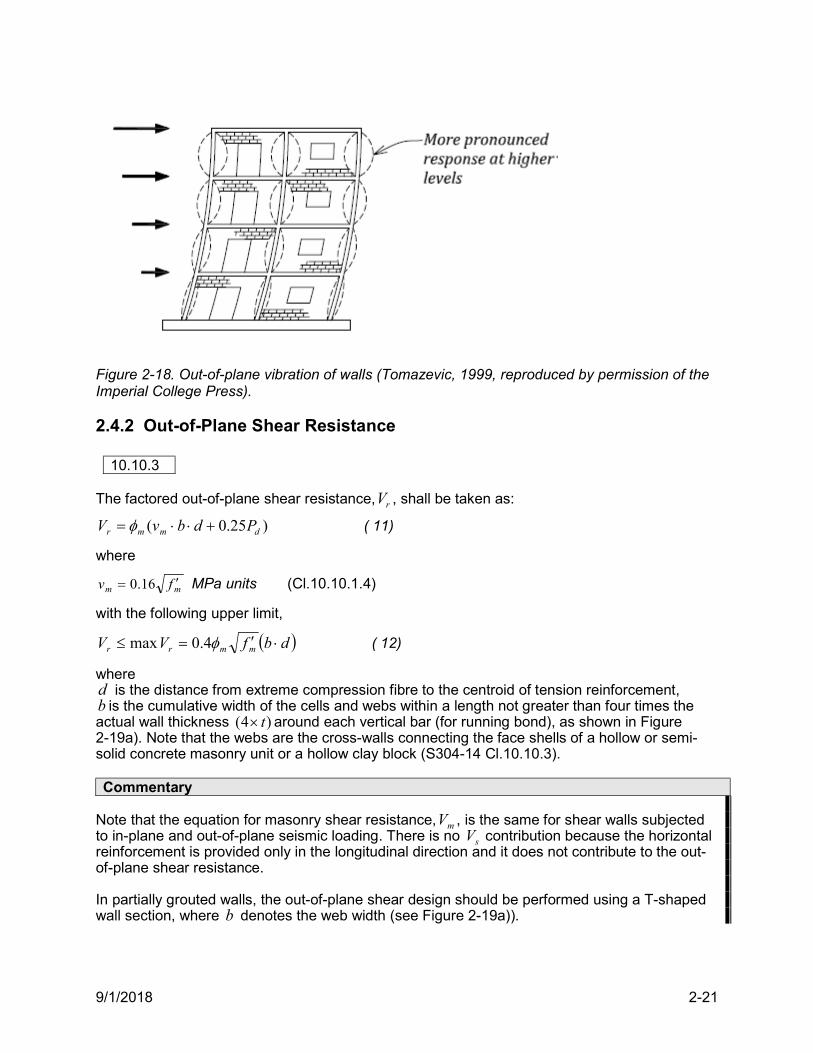
9/1/2018 2-21

Figure 2-18. Out-of-plane vibration of walls (Tomazevic, 1999, reproduced by permission of the Imperial College Press).

2.4.2 Out-of-Plane Shear Resistance

10.10.3 The factored out-of-plane shear resistance, rV , shall be taken as:

)25.0( dmmr PdbvV ( 11)

where

mm fv 16.0 MPa units (Cl.10.10.1.4)

with the following upper limit,

dbfVV mmrr 4.0max ( 12)

where d is the distance from extreme compression fibre to the centroid of tension reinforcement, b is the cumulative width of the cells and webs within a length not greater than four times the actual wall thickness )4( t around each vertical bar (for running bond), as shown in Figure 2-19a). Note that the webs are the cross-walls connecting the face shells of a hollow or semi-solid concrete masonry unit or a hollow clay block (S304-14 Cl.10.10.3). Commentary

Note that the equation for masonry shear resistance, mV , is the same for shear walls subjected to in-plane and out-of-plane seismic loading. There is no sV contribution because the horizontal reinforcement is provided only in the longitudinal direction and it does not contribute to the out-of-plane shear resistance. In partially grouted walls, the out-of-plane shear design should be performed using a T-shaped wall section, where b denotes the web width (see Figure 2-19a)).

9/1/2018 2-22

Figure 2-19. Effective width, b , for out-of-plane seismic effects: a) shear, and b) flexure.

2.4.3 Out-of-Plane Sliding Shear Resistance

10.10.5.2 The factored out-of-plane sliding shear resistance, rV , is calculated from the following equation using the shear friction concept:

CV mr ( 13)

where = the coefficient of friction (same as for the in-plane sliding shear resistance)

C = compressive force in the masonry acting normal to the sliding plane, taken as

yd TPC

yT = the factored tensile force at yield of the vertical reinforcement detailed to develop yield strength. In determining the out-of-plane sliding shear resistance, the entire vertical reinforcement should be taken into account in determining the factored tensile yield force, yT , irrespective of the wall class and the associated ductility level. For more details refer to the discussion on the sliding shear resistance of shear walls under in-plane seismic loading (Section 2.3.3).

2.4.4 Out-of-Plane Section Resistance Due to Combined Axial Load and Bending

Masonry walls subjected to out-of-plane seismic loading need to be designed for the combined effects of bending and axial gravity loads. For flexural design purposes, wall strips of predefined width b (S304-14 Cl.10.6.1) are treated as beams spanning between the lateral supports. When the walls span in the vertical direction, floor and/or roof diaphragms provide lateral supports. Walls can also span horizontally, in which case lateral supports need be provided by cross walls or pilasters. For detailed design procedures, the reader is referred to Section C.1.2 in Appendix C. It should be noted that, for the purpose of out-of-plane seismic design, the maximum permitted compressive strain in the masonry is equal to 0.003 (note that this is an arbitrary value set for the purpose of the analysis). CSA S304-14 does not require a ductility check, because the mechanism of failure is different for the in-plane and out-of-plane seismic resistance, and the wall is not expected to undergo significant rotations at the locations

9/1/2018 2-23

of maximum bending moments. Very large curvatures would be required to cause compression failure of the masonry, corresponding to a high strain gradient over a very small length (equal to the wall thickness). Consequently, there is no need to use the reduced compressive strain limit of 0.0025 for this load condition.

10.6.1 For the case of out-of-plane bending, the effective compression zone width,b , used with each vertical bar in the design of walls with vertical reinforcement shall be taken as the lesser of (see Figure 2-19b))

a) spacing between vertical bars s , or b) four times the actual wall thickness )4( t

Note that the discussion on out-of-plane stability issues is outside the scope of this document and it is covered elsewhere (see Drysdale and Hamid, 2005).

2.5 General Seismic Design Provisions for Reinforced Masonry Shear Walls

2.5.1 Capacity Design Approach

16.3.1 CSA S304-14 Cl.16.3.1, references capacity design principles where inelastic deformations are expected to occur in chosen energy-dissipating components of the SFRS, which are designed and detailed accordingly. All other load-bearing components are designed and detailed to have sufficient strength to ensure that the chosen means of energy-dissipation can be maintained. The NBC 2015 requires that all elements not considered part of the SFRS have the capacity to undergo the earthquake induced deformations, and that stiff elements, such as nonloadbearing walls and partitions, behave elastically or are separated from the SFRS. Every structure or structural component has several possible modes of failure, some of which are ductile, while others are brittle. The satisfactory seismic response of structures requires that brittle failure modes be avoided. This is accomplished through the application of a capacity design approach, which has been used for seismic design of reinforced concrete structures since the 1970’s (Park and Paulay, 1975). The objective of the capacity design approach is to force the structure to yield in a ductile manner without failing at the expected displacements (including other components of the structure, such as columns). At the same time, the rest of the structure needs to remain strong enough, say in shear, or flexible enough not to fail under gravity loads at these displacements. This concept can be explained by using the example of a chain shown in Figure 2-20, which is composed of both brittle and ductile links. When subjected to force, F , if the brittle link is the weakest, the chain will fail suddenly without significant deformation (see Figure 2-20a)). If a ductile link is the weakest, the chain will show significant deformation before failure, and may not fail or break if the deformation is not too great (see Figure 2-20b)). The structural designer is responsible for ensuring that the structure experiences a desirable ductile response when exposed to the design earthquake, that is, an earthquake of the expected intensity for the specific building site location.

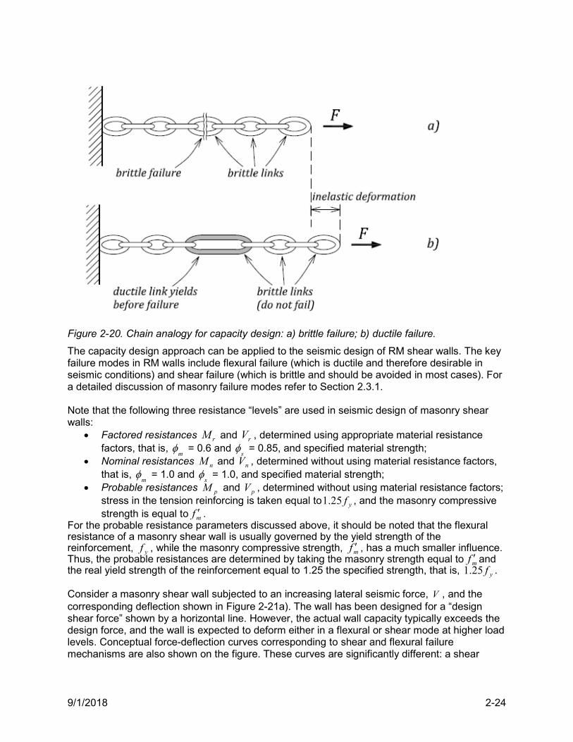
9/1/2018 2-24

Figure 2-20. Chain analogy for capacity design: a) brittle failure; b) ductile failure.

The capacity design approach can be applied to the seismic design of RM shear walls. The key failure modes in RM walls include flexural failure (which is ductile and therefore desirable in seismic conditions) and shear failure (which is brittle and should be avoided in most cases). For a detailed discussion of masonry failure modes refer to Section 2.3.1. Note that the following three resistance “levels” are used in seismic design of masonry shear walls:

Factored resistances rM and rV , determined using appropriate material resistance factors, that is,

m = 0.6 and

s = 0.85, and specified material strength;

Nominal resistances nM and nV , determined without using material resistance factors, that is,

m = 1.0 and

s = 1.0, and specified material strength;

Probable resistances pM and pV , determined without using material resistance factors; stress in the tension reinforcing is taken equal to yf25.1 , and the masonry compressive strength is equal to mf .

For the probable resistance parameters discussed above, it should be noted that the flexural resistance of a masonry shear wall is usually governed by the yield strength of the reinforcement, yf , while the masonry compressive strength, mf , has a much smaller influence. Thus, the probable resistances are determined by taking the masonry strength equal to mf and the real yield strength of the reinforcement equal to 1.25 the specified strength, that is, yf25.1 . Consider a masonry shear wall subjected to an increasing lateral seismic force, V , and the corresponding deflection shown in Figure 2-21a). The wall has been designed for a “design shear force” shown by a horizontal line. However, the actual wall capacity typically exceeds the design force, and the wall is expected to deform either in a flexural or shear mode at higher load levels. Conceptual force-deflection curves corresponding to shear and flexural failure mechanisms are also shown on the figure. These curves are significantly different: a shear

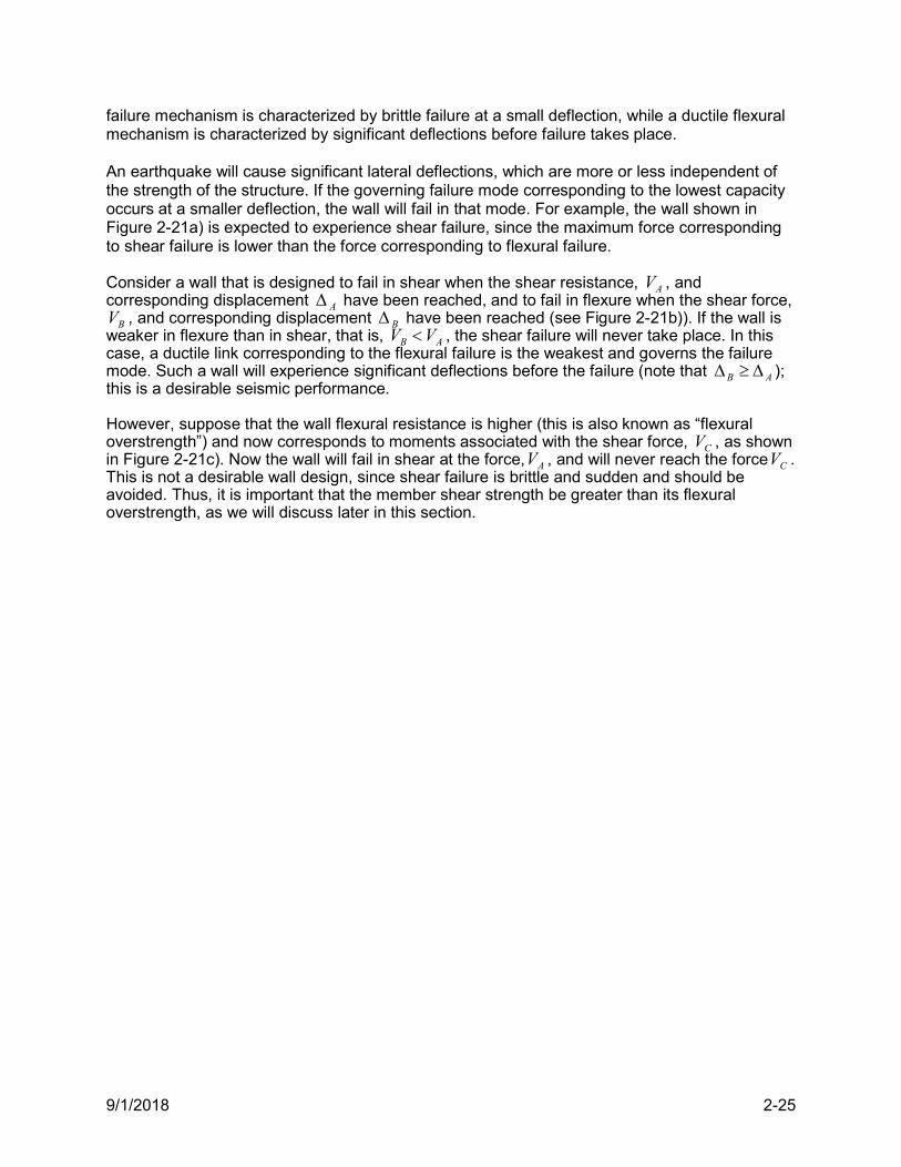
9/1/2018 2-25

failure mechanism is characterized by brittle failure at a small deflection, while a ductile flexural mechanism is characterized by significant deflections before failure takes place. An earthquake will cause significant lateral deflections, which are more or less independent of the strength of the structure. If the governing failure mode corresponding to the lowest capacity occurs at a smaller deflection, the wall will fail in that mode. For example, the wall shown in Figure 2-21a) is expected to experience shear failure, since the maximum force corresponding to shear failure is lower than the force corresponding to flexural failure. Consider a wall that is designed to fail in shear when the shear resistance, AV , and corresponding displacement A have been reached, and to fail in flexure when the shear force,

BV , and corresponding displacement B have been reached (see Figure 2-21b)). If the wall is weaker in flexure than in shear, that is, AB VV , the shear failure will never take place. In this case, a ductile link corresponding to the flexural failure is the weakest and governs the failure mode. Such a wall will experience significant deflections before the failure (note that AB ); this is a desirable seismic performance. However, suppose that the wall flexural resistance is higher (this is also known as “flexural overstrength”) and now corresponds to moments associated with the shear force, CV , as shown in Figure 2-21c). Now the wall will fail in shear at the force, AV , and will never reach the force CV . This is not a desirable wall design, since shear failure is brittle and sudden and should be avoided. Thus, it is important that the member shear strength be greater than its flexural overstrength, as we will discuss later in this section.

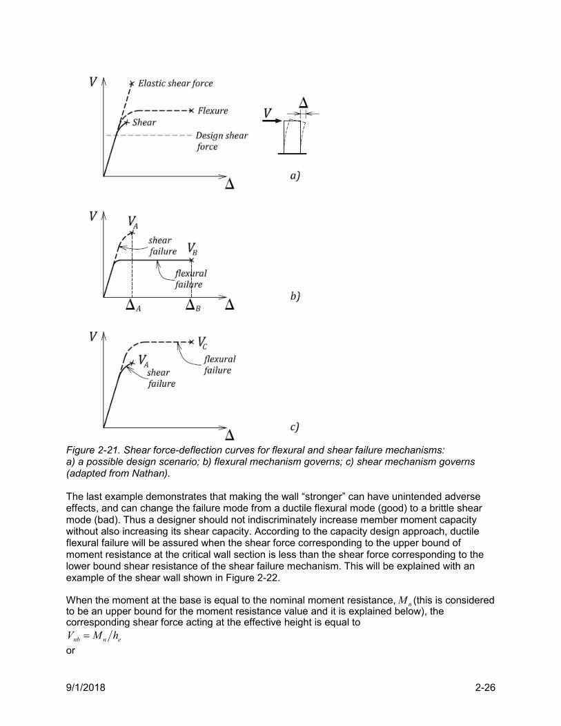
9/1/2018 2-26

Figure 2-21. Shear force-deflection curves for flexural and shear failure mechanisms: a) a possible design scenario; b) flexural mechanism governs; c) shear mechanism governs (adapted from Nathan). The last example demonstrates that making the wall “stronger” can have unintended adverse effects, and can change the failure mode from a ductile flexural mode (good) to a brittle shear mode (bad). Thus a designer should not indiscriminately increase member moment capacity without also increasing its shear capacity. According to the capacity design approach, ductile flexural failure will be assured when the shear force corresponding to the upper bound of moment resistance at the critical wall section is less than the shear force corresponding to the lower bound shear resistance of the shear failure mechanism. This will be explained with an example of the shear wall shown in Figure 2-22. When the moment at the base is equal to the nominal moment resistance, nM (this is considered to be an upper bound for the moment resistance value and it is explained below), the corresponding shear force acting at the effective height is equal to

ennb hMV

or

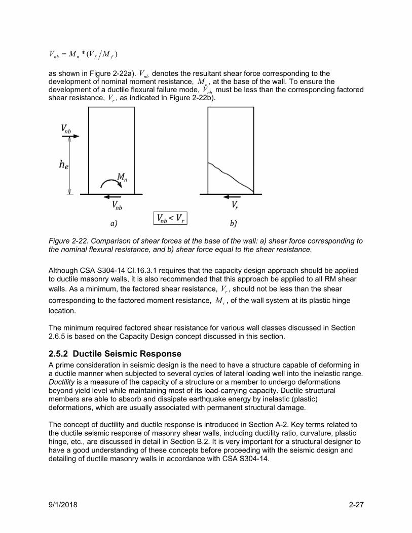
9/1/2018 2-27

)(* ffnnb MVMV

as shown in Figure 2-22a). nbV denotes the resultant shear force corresponding to the development of nominal moment resistance, nM , at the base of the wall. To ensure the development of a ductile flexural failure mode, nbV must be less than the corresponding factored shear resistance, rV , as indicated in Figure 2-22b).

Figure 2-22. Comparison of shear forces at the base of the wall: a) shear force corresponding to the nominal flexural resistance, and b) shear force equal to the shear resistance.

Although CSA S304-14 Cl.16.3.1 requires that the capacity design approach should be applied to ductile masonry walls, it is also recommended that this approach be applied to all RM shear walls. As a minimum, the factored shear resistance, rV , should not be less than the shear

corresponding to the factored moment resistance, rM , of the wall system at its plastic hinge location. The minimum required factored shear resistance for various wall classes discussed in Section 2.6.5 is based on the Capacity Design concept discussed in this section.

2.5.2 Ductile Seismic Response A prime consideration in seismic design is the need to have a structure capable of deforming in a ductile manner when subjected to several cycles of lateral loading well into the inelastic range. Ductility is a measure of the capacity of a structure or a member to undergo deformations beyond yield level while maintaining most of its load-carrying capacity. Ductile structural members are able to absorb and dissipate earthquake energy by inelastic (plastic) deformations, which are usually associated with permanent structural damage. The concept of ductility and ductile response is introduced in Section A-2. Key terms related to the ductile seismic response of masonry shear walls, including ductility ratio, curvature, plastic hinge, etc., are discussed in detail in Section B.2. It is very important for a structural designer to have a good understanding of these concepts before proceeding with the seismic design and detailing of ductile masonry walls in accordance with CSA S304-14.

9/1/2018 2-28

2.5.3 Structural Regularity 16.3.2

Combinations of SFRSs acting in the same direction may be used, provided that each system continues over the full building height. When SFRSs are not continuous over the building height or change type over the building height, when elements from two or more SFRS types are combined to create a hybrid system, or when a significant irregularity exists, an inelastic analysis such as a static pushover or dynamic analysis shall be performed to: a) verify the compatibility of the systems; b) confirm the assumed energy-dissipating mechanisms; c) show that the inelastic rotational demands are less than the inelastic rotational capacities; and d) account for redistribution of forces. Note: The inelastic analysis may be waived if the performance of the system has been previously verified by experimental evidence or analysis. Systems requiring inelastic analysis shall be treated as alternative solutions under the NBC. Commentary

This provision is intended to ensure a satisfactory seismic performance of structures with more than one SFRS, also known as “hybrid systems”. In the case of masonry structures, this may refer to different masonry SFRSs, e.g. RM walls characterized by different ductility levels (a mix of Moderately Ductile and Ductile walls), or a combination of wall and frame systems. For example, the design of open storefront buildings with walls on three sides and non-structural glazing on the fourth side (see Figure 1-12) may require the use of framed SFRS on the open side of the building. It is required to ensure compatibility of these SFRSs in terms of lateral displacements/drifts (S304-14 Cl.16.3.2). Also, internal forces in the frame and wall members must be redistributed based on the calculations.

2.5.4 Analysis Assumptions – Effective Section Properties 16.3.3

In lieu of a more accurate method for determining effective cross-sectional properties, the design seismic force and deformations of a SFRS may be calculated based on reduced section properties to account for nonlinear behavior. These effective cross-sectional properties should be used to determine forces and deflections in shear walls subjected to seismic effects. The SFRS components’ gross cross-sectional properties shall be modified according to the following:

mgsge fAPII '3.0 where gecr III

mgsge fAPAA '3.0 where gecr AAA

where sP is factored axial force due to dead and live loads determined at the base of the wall for

the seismic load combinations. For all shear walls in the main SFRS, an average value of mgs fAP ' may be used. Note that gecr III ,, denote the moments of inertia of cracked,

effective, and gross cross-sections of a masonry shear wall, respectively. Also, gecr AAA ,,

denote the cross-sectional areas of cracked, effective, and gross cross-sections of a masonry shear wall, respectively.

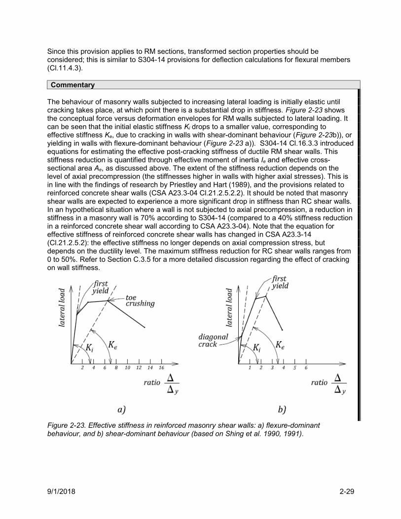
9/1/2018 2-29

Since this provision applies to RM sections, transformed section properties should be considered; this is similar to S304-14 provisions for deflection calculations for flexural members (Cl.11.4.3). Commentary

The behaviour of masonry walls subjected to increasing lateral loading is initially elastic until cracking takes place, at which point there is a substantial drop in stiffness. Figure 2-23 shows the conceptual force versus deformation envelopes for RM walls subjected to lateral loading. It can be seen that the initial elastic stiffness Ki drops to a smaller value, corresponding to effective stiffness Ke, due to cracking in walls with shear-dominant behaviour (Figure 2-23b)), or yielding in walls with flexure-dominant behaviour (Figure 2-23 a)). S304-14 Cl.16.3.3 introduced equations for estimating the effective post-cracking stiffness of ductile RM shear walls. This stiffness reduction is quantified through effective moment of inertia Ie and effective cross-sectional area Ae, as discussed above. The extent of the stiffness reduction depends on the level of axial precompression (the stiffnesses higher in walls with higher axial stresses). This is in line with the findings of research by Priestley and Hart (1989), and the provisions related to reinforced concrete shear walls (CSA A23.3-04 Cl.21.2.5.2.2). It should be noted that masonry shear walls are expected to experience a more significant drop in stiffness than RC shear walls. In an hypothetical situation where a wall is not subjected to axial precompression, a reduction in stiffness in a masonry wall is 70% according to S304-14 (compared to a 40% stiffness reduction in a reinforced concrete shear wall according to CSA A23.3-04). Note that the equation for effective stiffness of reinforced concrete shear walls has changed in CSA A23.3-14 (Cl.21.2.5.2): the effective stiffness no longer depends on axial compression stress, but depends on the ductility level. The maximum stiffness reduction for RC shear walls ranges from 0 to 50%. Refer to Section C.3.5 for a more detailed discussion regarding the effect of cracking on wall stiffness.

Figure 2-23. Effective stiffness in reinforced masonry shear walls: a) flexure-dominant behaviour, and b) shear-dominant behaviour (based on Shing et al. 1990, 1991).

9/1/2018 2-30

2.5.5 Redistribution of design moments from elastic analysis 16.6.3

The redistribution of design moments obtained from elastic analysis, using the effective cross-sectional properties specified in Cl.16.3.3 (see Section 2.5.4), may be used where it can be demonstrated that the ductility capacities of affected components are not exceeded. Note: inelastic redistribution of moments may result in reduced maximum moment resistance requirements.

2.5.6 Minor shear walls as a part of the SFRS 16.3.4

Masonry shear walls designed according to S304-14 seismic provisions should be designed to provide the required ductility under the action of the specified factored loads (Cl.16.3.4.1). Cl.16.3.4.2 addresses the requirements for minor shear walls in masonry buildings. It states that when it can be shown through analysis that the stiffest masonry shear walls attract 90% or more of the design seismic force on the building, such walls can be designated as the main SFRS and shall then be designed for 100% of the design seismic force. Walls not considered to be part of the main SFRS shall be designed to behave elastically or to have sufficient non-linear capacity to support their gravity loads while undergoing deformations compatible with those of the main SFRS. Any masonry shear wall with sufficient stiffness to attract 2.5% or more of the design seismic force or 50% of the average shear wall force in themain SFRS shall be included in the main SFRS. Minor shear walls may be included in the main SFRS.

2.6 CSA S304-14 Seismic Design Requirements

2.6.1 Classes of reinforced masonry shear walls Table 4.1.8.9 of NBC 2015 identifies the following five classes of masonry walls based on their expected seismic performance quantified by means of the ductility-related force modification factor, dR (see also Section 1.7):

1. Unreinforced Masonry and other masonry structural systems not listed below ( 0.1dR ) 2. Conventional Construction shear walls ( 5.1dR ) 3. Moderately Ductile shear walls ( 0.2dR ) 4. Moderately Ductile Squat shear walls ( 0.2dR ) 5. Ductile shear walls ( 0.3dR ) – note that this is a new class.

Classes 3, 4, and 5 are referred to as “ductile shear walls”. The same value of overstrength factor, oR , of 1.5 is prescribed for all the above listed wall classes, except for unreinforced masonry where oR is equal to 1.0. CSA S304-14 Clause 16 outlines the seismic design provisions for masonry shear walls. Note that these provisions have been substantially revised compared to the S304.1-04 provisions. Note that class “limited ductility shear walls” (S304.1-04, Cl.10.16.4) no longer exists.

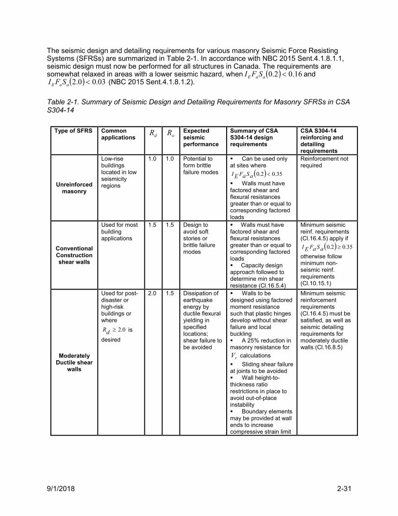
9/1/2018 2-31

The seismic design and detailing requirements for various masonry Seismic Force Resisting Systems (SFRSs) are summarized in Table 2-1. In accordance with NBC 2015 Sent.4.1.8.1.1, seismic design must now be performed for all structures in Canada. The requirements are somewhat relaxed in areas with a lower seismic hazard, when 16.02.0 aaE SFI and

03.00.2 aaE SFI (NBC 2015 Sent.4.1.8.1.2).

Table 2-1. Summary of Seismic Design and Detailing Requirements for Masonry SFRSs in CSA S304-14

Type of SFRS Common

applications dR oR Expected seismic performance

Summary of CSA S304-14 design requirements

CSA S304-14 reinforcing and detailing requirements

Unreinforced masonry

Low-rise buildings located in low seismicity regions

1.0 1.0 Potential to form brittle failure modes

Can be used only at sites where

35.02.0 aSaFEI

Walls must have factored shear and flexural resistances greater than or equal to corresponding factored loads

Reinforcement not required

Conventional Construction shear walls

Used for most building applications

1.5 1.5 Design to avoid soft stories or brittle failure modes

Walls must have factored shear and flexural resistances greater than or equal to corresponding factored loads Capacity design approach followed to determine min shear resistance (Cl.16.5.4)

Minimum seismic reinf. requirements (Cl.16.4.5) apply if

35.02.0 aSaFEI

otherwise follow minimum non-seismic reinf. requirements (Cl.10.15.1)

Moderately Ductile shear

walls

Used for post-disaster or high-risk buildings or where

0.2dR is

desired

2.0 1.5 Dissipation of earthquake energy by ductile flexural yielding in specified locations; shear failure to be avoided

Walls to be designed using factored moment resistance such that plastic hinges develop without shear failure and local buckling A 25% reduction in masonry resistance for

rV calculations

Sliding shear failure at joints to be avoided Wall height-to-thickness ratio restrictions in place to avoid out-of-place instability Boundary elements may be provided at wall ends to increase compressive strain limit

Minimum seismic reinforcement requirements (Cl.16.4.5) must be satisfied, as well as seismic detailing requirements for moderately ductile walls (Cl.16.8.5)

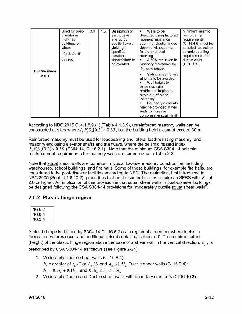
9/1/2018 2-32

Ductile shear walls

Used for post-disaster or high-risk buildings or where

0.2dR is

desired

3.0 1.5 Dissipation of earthquake energy by ductile flexural yielding in specified locations; shear failure to be avoided

Walls to be designed using factored moment resistance such that plastic hinges develop without shear failure and local buckling A 50% reduction in masonry resistance for

rV calculations

Sliding shear failure at joints to be avoided Wall height-to-thickness ratio restrictions in place to avoid out-of-place instability Boundary elements may be provided at wall ends to increase compressive strain limit

Minimum seismic reinforcement requirements (Cl.16.4.5) must be satisfied, as well as seismic detailing requirements for ductile walls (Cl.16.9.5)

According to NBC 2015 Cl.4.1.8.9.(1) (Table 4.1.8.9), unreinforced masonry walls can be constructed at sites where 35.02.0 asE SFI , but the building height cannot exceed 30 m. Reinforced masonry must be used for loadbearing and lateral load-resisting masonry, and masonry enclosing elevator shafts and stairways, where the seismic hazard index

35.02.0 aaE SFI (S304-14, Cl.16.2.1). Note that the minimum CSA S304-14 seismic reinforcement requirements for masonry walls are summarized in Table 2-3. Note that squat shear walls are common in typical low-rise masonry construction, including warehouses, school buildings, and fire halls. Some of these buildings, for example fire halls, are considered to be post-disaster facilities according to NBC. The restriction, first introduced in NBC 2005 (Sent. 4.1.8.10.2), prescribes that post-disaster facilities require an SFRS with dR of 2.0 or higher. An implication of this provision is that squat shear walls in post-disaster buildings be designed following the CSA S304-14 provisions for “moderately ductile squat shear walls”.

2.6.2 Plastic hinge region

16.6.2 16.8.4 16.9.4

A plastic hinge is defined by S304-14 Cl. 16.6.2 as “a region of a member where inelastic flexural curvatures occur and additional seismic detailing is required”. The required extent (height) of the plastic hinge region above the base of a shear wall in the vertical direction, ph , is

prescribed by CSA S304-14 as follows (see Figure 2-24):

1. Moderately Ductile shear walls (Cl.16.8.4):

ph = greater of 2/wl or 6/wh and 1.5p wh l Ductile shear walls (Cl.16.9.4):

0.5 0.1p w wh l h and 0.8 1.5w p wl h l

2. Moderately Ductile and Ductile shear walls with boundary elements (Cl.16.10.3):

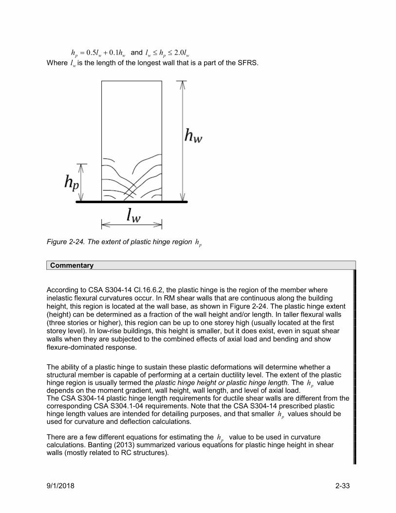
9/1/2018 2-33

0.5 0.1p w wh l h and 2.0w p wl h l

Where wl is the length of the longest wall that is a part of the SFRS.

Figure 2-24. The extent of plastic hinge region ph

Commentary

According to CSA S304-14 Cl.16.6.2, the plastic hinge is the region of the member where inelastic flexural curvatures occur. In RM shear walls that are continuous along the building height, this region is located at the wall base, as shown in Figure 2-24. The plastic hinge extent (height) can be determined as a fraction of the wall height and/or length. In taller flexural walls (three stories or higher), this region can be up to one storey high (usually located at the first storey level). In low-rise buildings, this height is smaller, but it does exist, even in squat shear walls when they are subjected to the combined effects of axial load and bending and show flexure-dominated response.

The ability of a plastic hinge to sustain these plastic deformations will determine whether a structural member is capable of performing at a certain ductility level. The extent of the plastic hinge region is usually termed the plastic hinge height or plastic hinge length. The ph value depends on the moment gradient, wall height, wall length, and level of axial load. The CSA S304-14 plastic hinge length requirements for ductile shear walls are different from the corresponding CSA S304.1-04 requirements. Note that the CSA S304-14 prescribed plastic hinge length values are intended for detailing purposes, and that smaller ph values should be used for curvature and deflection calculations. There are a few different equations for estimating the ph value to be used in curvature calculations. Banting (2013) summarized various equations for plastic hinge height in shear walls (mostly related to RC structures).

9/1/2018 2-34

The findings of an experimental research study by Shing et al. (1990) showed that the plastic hinge height in RM shear walls is in the order of 6/wh . Banting and El-Dakhakhni (2014) studied plastic hinge heights in RM shear walls with boundary elements, and concluded that ph depends on a combination of parameters, including wall length and height, and height/length

ww lh / aspect ratio. The plastic hinge height ranged from 50 to 100% of the wall length wl . The results of the study showed that the plastic hinge height for the test specimens depended more on the ww lh / ratio than on the wall length. For example, the specimen with the highest ww lh / of 3.23 had the largest plastic hinge height equal to wl . The CSA S304-14 plastic hinge height provisions are in line with the research findings and codes in other countries. For example, in the New Zealand Masonry Standard NZS 4230:2004 (SANZ, 2004), Cl. 7.4.3 prescribes the plastic hinge height to be the greater of wl , 6/wh , or 600 mm. The design and detailing of reinforcement within the plastic hinge regions of ductile masonry shear walls is critical, and is discussed in the following sections. These regions are usually heavily reinforced, and it is critical to ensure proper anchorage of reinforcement. Open-end blocks or H-blocks may simplify reinforcing and grouting in these regions. The plastic hinge regions of ductile masonry walls must be fully grouted. Observations from past damaging earthquakes (e.g. 1994 Northridge, California earthquake and the 2011 Christchurch, New Zealand earthquakes) that caused damage to RM walls have shown that the quality of grout placement, and the bond of the grout to the masonry units and reinforcement have a strong influence on the performance of RM structures. Reinforced block walls with large voids around reinforcing bars suffered severe damage in the 1994 Northridge, California earthquake (TMS, 1994). Many RM buildings were exposed to the 2011 Christchurch, New Zealand earthquake. Most of them performed well, considering the shaking intensity and the damage to other building typologies (including RC buildings). It was observed that RM walls with incomplete grouting at the base suffered more extensive damage, see Centeno, Ventura, and Ingham (2014); Dizhur et al. (2011). Experimental studies have also confirmed the effect of grouting quality on the simulated seismic response of RM shear walls. Incomplete grouting at the toes of a RM shear wall specimen designed for ductile flexural response resulted in a reduced ductility capacity, and led to its premature failure (compared to other similar specimens), based on the experimental study by Robazza et al. (2015; 2017). Complete grouting in plastic hinge zones of ductile RM shear walls is a must for their satisfactory seismic performance.

2.6.3 Ductility check

16.8.7 16.8.8 16.9.7

CSA S304-14 prescribes the following simplified ductility requirements for RM shear walls:

1. The neutral axis depth/wall length ratio, wlc , should be within the following limits:

a) For Moderately Ductile shear walls (Cl.16.8.7): 15.0wlc when 0.5ww lh and the drift ratio 01.01 odf RR (provided that

400yf MPa)

b) For Ductile shear walls (Cl.16.9.7):

9/1/2018 2-35

125.0wlc when 0.5ww lh and the drift ratio 01.01 odf RR (provided that

400yf MPa)

2. When these requirements are not satisfied, a detailed ductility verification needs to be performed according to Cl.16.8.

The objective of the ductility check is to confirm that the plastic hinge’s rotational capacity, ic, exceeds inelastic rotational demand due to seismic loading, id (Cl.16.8.8.1).

idic ( 14)

The approach for ductility verification is illustrated in Figure 2-25, which shows the displacement and curvature distribution in a ductile shear wall. The bending moment distribution is shown in Figure 2-25b), with the curvature distribution shown in Figure 2-25c). Elastic curvature corresponds to the onset of yielding in vertical reinforcement, y , while plastic curvature,

u y , corresponds to plastic deformations within the plastic hinge height, ph . Curvature

ductility for this wall is equal to the ratio of total curvature and the curvature at the onset of yield, that is, u y . Note that S304-14 does not require calculation of curvature ductility, however

curvatures are used to determine the plastic hinge rotational capacity (ic). This is done by integrating the plastic curvature over the plastic hinge height ph (assumed to be equal to lw/2)

(Cl.16.8.8.3), that is,

ic u y ph or

( 0.002) 0.0252

mu wic

l

c

(15)

Note that the first term in the above equation denotes total rotation at the ultimate, while the second term denotes yield rotation (which is taken as 0.004 wl ).

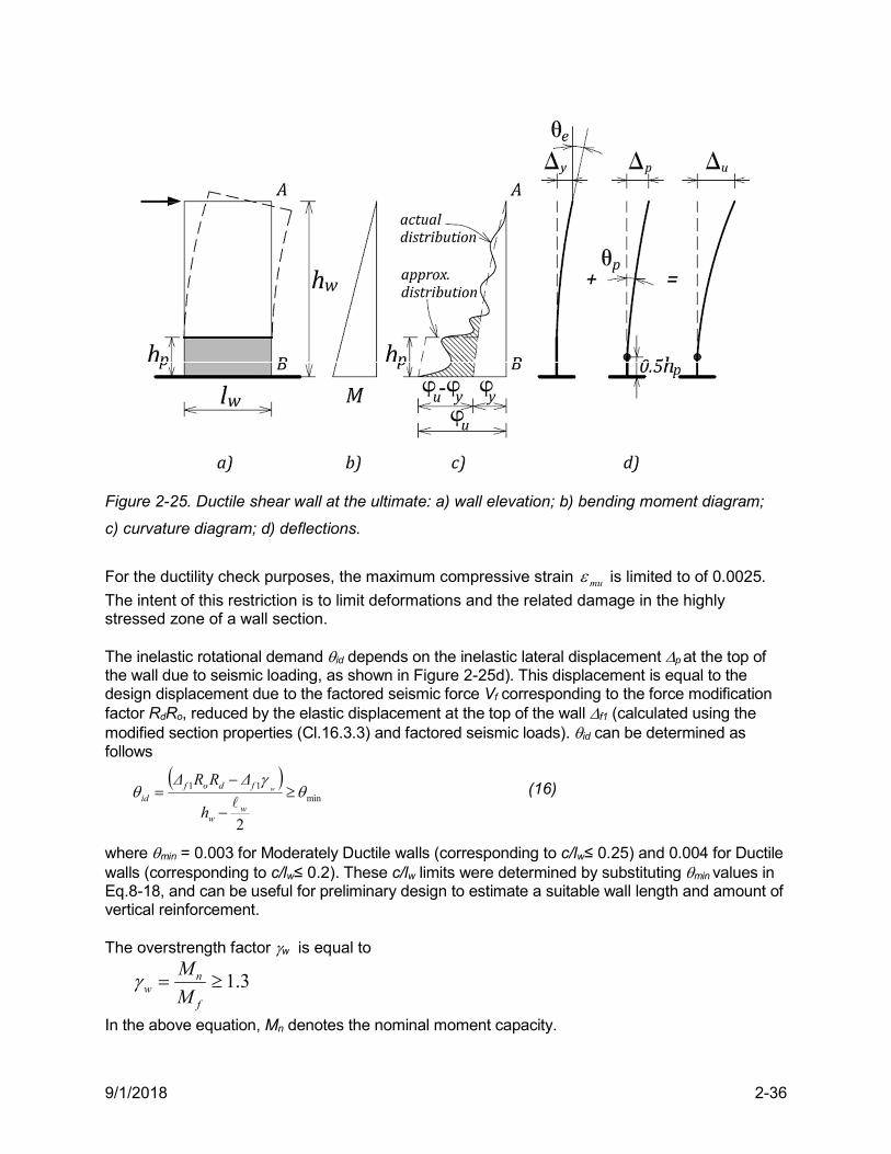
9/1/2018 2-36

Figure 2-25. Ductile shear wall at the ultimate: a) wall elevation; b) bending moment diagram;

c) curvature diagram; d) deflections.

For the ductility check purposes, the maximum compressive strain mu is limited to of 0.0025.

The intent of this restriction is to limit deformations and the related damage in the highly stressed zone of a wall section. The inelastic rotational demand id depends on the inelastic lateral displacement p at the top of the wall due to seismic loading, as shown in Figure 2-25d). This displacement is equal to the design displacement due to the factored seismic force Vf corresponding to the force modification factor RdRo, reduced by the elastic displacement at the top of the wall f1 (calculated using the modified section properties (Cl.16.3.3) and factored seismic loads). id can be determined as follows

min

11

2

ww

fdofid

h

ΔRRΔw

(16)

where min = 0.003 for Moderately Ductile walls (corresponding to c/lw≤ 0.25) and 0.004 for Ductile walls (corresponding to c/lw≤ 0.2). These c/lw limits were determined by substituting min values in Eq.8-18, and can be useful for preliminary design to estimate a suitable wall length and amount of vertical reinforcement.

The overstrength factor w is equal to

3.1f

nw M

M

In the above equation, Mn denotes the nominal moment capacity.

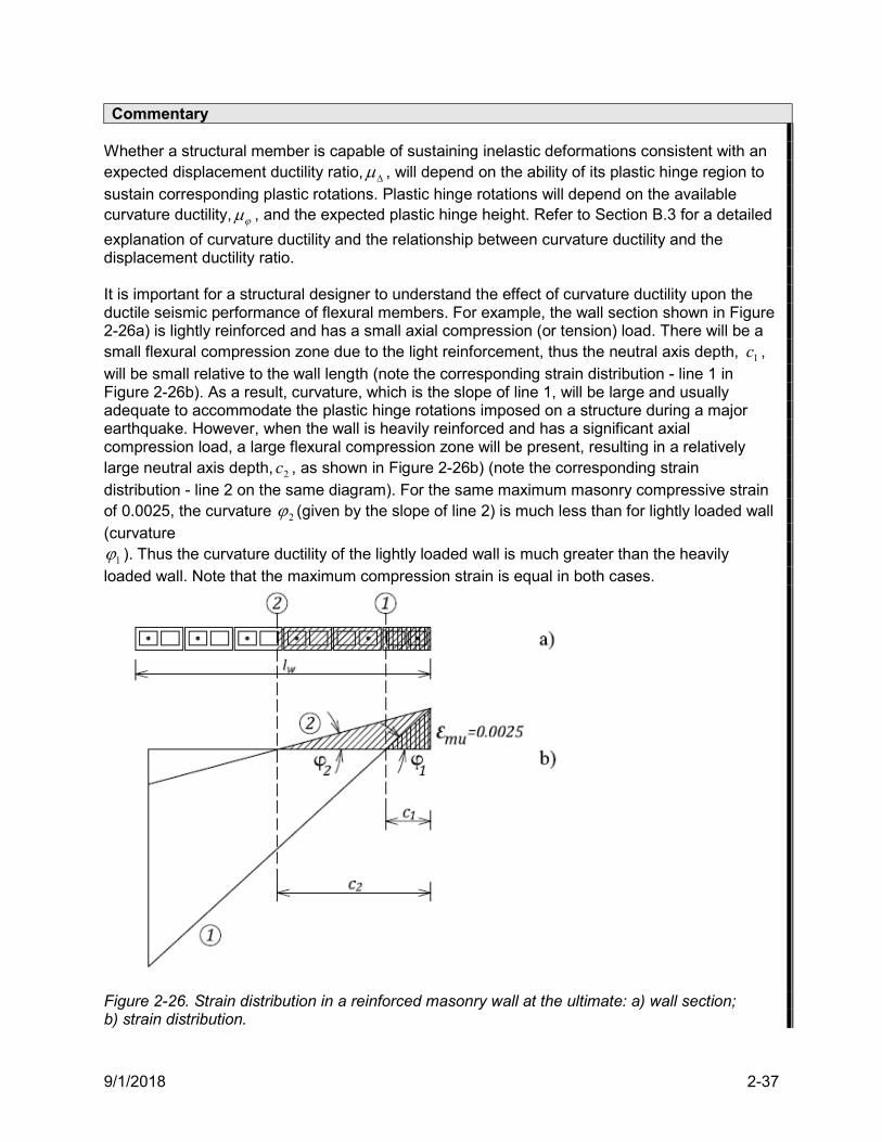
9/1/2018 2-37

Commentary Whether a structural member is capable of sustaining inelastic deformations consistent with an expected displacement ductility ratio, , will depend on the ability of its plastic hinge region to sustain corresponding plastic rotations. Plastic hinge rotations will depend on the available curvature ductility, , and the expected plastic hinge height. Refer to Section B.3 for a detailed

explanation of curvature ductility and the relationship between curvature ductility and the displacement ductility ratio. It is important for a structural designer to understand the effect of curvature ductility upon the ductile seismic performance of flexural members. For example, the wall section shown in Figure 2-26a) is lightly reinforced and has a small axial compression (or tension) load. There will be a small flexural compression zone due to the light reinforcement, thus the neutral axis depth, 1c , will be small relative to the wall length (note the corresponding strain distribution - line 1 in Figure 2-26b). As a result, curvature, which is the slope of line 1, will be large and usually adequate to accommodate the plastic hinge rotations imposed on a structure during a major earthquake. However, when the wall is heavily reinforced and has a significant axial compression load, a large flexural compression zone will be present, resulting in a relatively large neutral axis depth, 2c , as shown in Figure 2-26b) (note the corresponding strain distribution - line 2 on the same diagram). For the same maximum masonry compressive strain of 0.0025, the curvature 2 (given by the slope of line 2) is much less than for lightly loaded wall (curvature

1 ). Thus the curvature ductility of the lightly loaded wall is much greater than the heavily loaded wall. Note that the maximum compression strain is equal in both cases.

Figure 2-26. Strain distribution in a reinforced masonry wall at the ultimate: a) wall section; b) strain distribution.

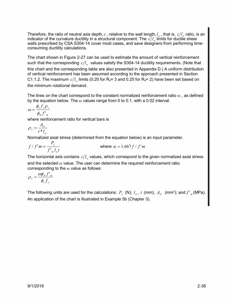
9/1/2018 2-38

Therefore, the ratio of neutral axis depth, c , relative to the wall length, wl , that is, wlc ratio, is an indicator of the curvature ductility in a structural component. The wlc limits for ductile shear walls prescribed by CSA S304-14 cover most cases, and save designers from performing time-consuming ductility calculations. The chart shown in Figure 2-27 can be used to estimate the amount of vertical reinforcement such that the corresponding wlc values satisfy the S304-14 ductility requirements. (Note that

this chart and the corresponding table are also presented in Appendix D.) A uniform distribution of vertical reinforcement has been assumed according to the approach presented in Section C1.1.2. The maximum wlc limits (0.20 for Rd= 3 and 0.25 for Rd= 2) have been set based on

the minimum rotational demand. The lines on the chart correspond to the constant normalized reinforcement ratio , as defined by the equation below. The values range from 0 to 0.1, with a 0.02 interval.

mm

vys

f

f

'

where reinforcement ratio for vertical bars is

w

vtv lt

A

*

Normalized axial stress (determined from the equation below) is an input parameter.

tlf

Pmff

wm

f

''/ where mff '/667.1

The horizontal axis contains wlc values, which correspond to the given normalized axial stress

and the selected value. The user can determine the required reinforcement ratio corresponding to the value as follows:

ys

mmv f

f

'

The following units are used for the calculations: fP (N); wl , t (mm); vtA (mm2); and mf ' (MPa).

An application of the chart is illustrated in Example 5b (Chapter 3).

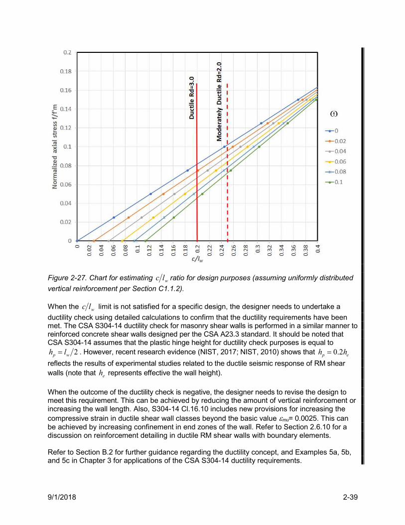
9/1/2018 2-39

Figure 2-27. Chart for estimating wlc ratio for design purposes (assuming uniformly distributed

vertical reinforcement per Section C1.1.2). When the wlc limit is not satisfied for a specific design, the designer needs to undertake a

ductility check using detailed calculations to confirm that the ductility requirements have been met. The CSA S304-14 ductility check for masonry shear walls is performed in a similar manner to reinforced concrete shear walls designed per the CSA A23.3 standard. It should be noted that CSA S304-14 assumes that the plastic hinge height for ductility check purposes is equal to

2p wh l . However, recent research evidence (NIST, 2017; NIST, 2010) shows that 0.2p eh hreflects the results of experimental studies related to the ductile seismic response of RM shear walls (note that eh represents effective the wall height).

When the outcome of the ductility check is negative, the designer needs to revise the design to meet this requirement. This can be achieved by reducing the amount of vertical reinforcement or increasing the wall length. Also, S304-14 Cl.16.10 includes new provisions for increasing the compressive strain in ductile shear wall classes beyond the basic value mu= 0.0025. This can be achieved by increasing confinement in end zones of the wall. Refer to Section 2.6.10 for a discussion on reinforcement detailing in ductile RM shear walls with boundary elements. Refer to Section B.2 for further guidance regarding the ductility concept, and Examples 5a, 5b, and 5c in Chapter 3 for applications of the CSA S304-14 ductility requirements.

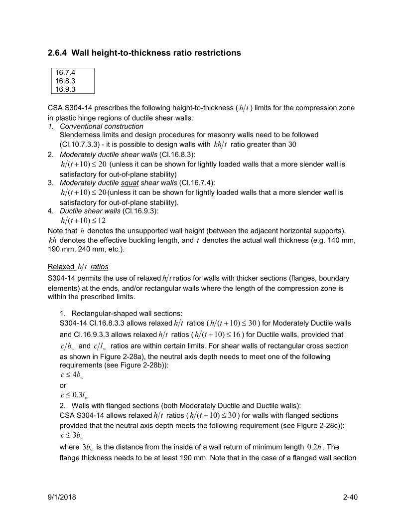
9/1/2018 2-40

2.6.4 Wall height-to-thickness ratio restrictions

16.7.4 16.8.3 16.9.3

CSA S304-14 prescribes the following height-to-thickness ( th ) limits for the compression zone in plastic hinge regions of ductile shear walls: 1. Conventional construction

Slenderness limits and design procedures for masonry walls need to be followed (Cl.10.7.3.3) - it is possible to design walls with tkh ratio greater than 30

2. Moderately ductile shear walls (Cl.16.8.3): 20)10( th (unless it can be shown for lightly loaded walls that a more slender wall is

satisfactory for out-of-plane stability) 3. Moderately ductile squat shear walls (Cl.16.7.4):

20)10( th (unless it can be shown for lightly loaded walls that a more slender wall is satisfactory for out-of-plane stability).

4. Ductile shear walls (Cl.16.9.3): 12)10( th

Note that h denotes the unsupported wall height (between the adjacent horizontal supports), kh denotes the effective buckling length, and t denotes the actual wall thickness (e.g. 140 mm, 190 mm, 240 mm, etc.). Relaxed th ratios

S304-14 permits the use of relaxed th ratios for walls with thicker sections (flanges, boundary elements) at the ends, and/or rectangular walls where the length of the compression zone is within the prescribed limits.

1. Rectangular-shaped wall sections: S304-14 Cl.16.8.3.3 allows relaxed th ratios ( 30)10( th ) for Moderately Ductile walls

and Cl.16.9.3.3 allows relaxed th ratios ( 16)10( th ) for Ductile walls, provided that

wbc and wlc ratios are within certain limits. For shear walls of rectangular cross section

as shown in Figure 2-28a), the neutral axis depth needs to meet one of the following requirements (see Figure 2-28b)):

wbc 4

or

wlc 3.0

2. Walls with flanged sections (both Moderately Ductile and Ductile walls): CSA S304-14 allows relaxed th ratios ( 30)10( th ) for walls with flanged sections provided that the neutral axis depth meets the following requirement (see Figure 2-28c)):

wbc 3

where wb3 is the distance from the inside of a wall return of minimum length h2.0 . The

flange thickness needs to be at least 190 mm. Note that in the case of a flanged wall section

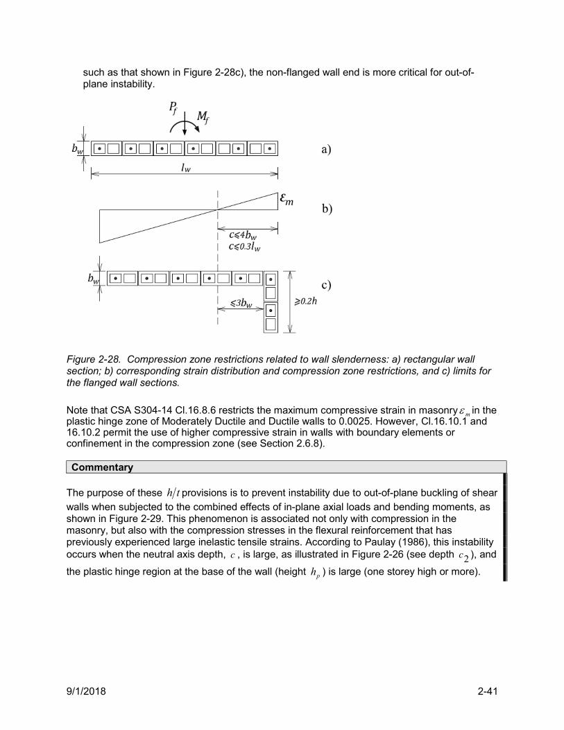
9/1/2018 2-41

such as that shown in Figure 2-28c), the non-flanged wall end is more critical for out-of-plane instability.

Figure 2-28. Compression zone restrictions related to wall slenderness: a) rectangular wall section; b) corresponding strain distribution and compression zone restrictions, and c) limits for the flanged wall sections.

Note that CSA S304-14 Cl.16.8.6 restricts the maximum compressive strain in masonry m in the plastic hinge zone of Moderately Ductile and Ductile walls to 0.0025. However, Cl.16.10.1 and 16.10.2 permit the use of higher compressive strain in walls with boundary elements or confinement in the compression zone (see Section 2.6.8). Commentary

The purpose of these th provisions is to prevent instability due to out-of-plane buckling of shear walls when subjected to the combined effects of in-plane axial loads and bending moments, as shown in Figure 2-29. This phenomenon is associated not only with compression in the masonry, but also with the compression stresses in the flexural reinforcement that has previously experienced large inelastic tensile strains. According to Paulay (1986), this instability occurs when the neutral axis depth, c , is large, as illustrated in Figure 2-26 (see depth 2c ), and

the plastic hinge region at the base of the wall (height ph ) is large (one storey high or more).

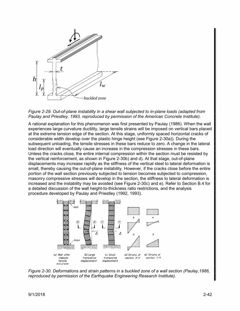
9/1/2018 2-42

Figure 2-29. Out-of-plane instability in a shear wall subjected to in-plane loads (adapted from Paulay and Priestley, 1993, reproduced by permission of the American Concrete Institute).

A rational explanation for this phenomenon was first presented by Paulay (1986). When the wall experiences large curvature ductility, large tensile strains will be imposed on vertical bars placed at the extreme tension edge of the section. At this stage, uniformly spaced horizontal cracks of considerable width develop over the plastic hinge height (see Figure 2-30a)). During the subsequent unloading, the tensile stresses in these bars reduce to zero. A change in the lateral load direction will eventually cause an increase in the compression stresses in these bars. Unless the cracks close, the entire internal compression within the section must be resisted by the vertical reinforcement, as shown in Figure 2-30b) and d). At that stage, out-of-plane displacements may increase rapidly as the stiffness of the vertical steel to lateral deformation is small, thereby causing the out-of-plane instability. However, if the cracks close before the entire portion of the wall section previously subjected to tension becomes subjected to compression, masonry compressive stresses will develop in the section, the stiffness to lateral deformation is increased and the instability may be avoided (see Figure 2-30c) and e). Refer to Section B.4 for a detailed discussion of the wall height-to-thickness ratio restrictions, and the analysis procedure developed by Paulay and Priestley (1992, 1993).

Figure 2-30. Deformations and strain patterns in a buckled zone of a wall section (Paulay,1986, reproduced by permission of the Earthquake Engineering Research Institute).

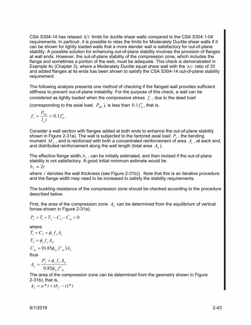
9/1/2018 2-43

CSA S304-14 has relaxed th limits for ductile shear walls compared to the CSA S304.1-04 requirements. In particulr, it is possible to relax the limits for Moderately Ductile shear walls if it can be shown for lightly loaded walls that a more slender wall is satisfactory for out-of-plane stability. A possible solution for enhancing out-of-plane stability involves the provision of flanges at wall ends. However, the out-of-plane stability of the compression zone, which includes the flange and sometimes a portion of the web, must be adequate. This check is demonstrated in Example 4c (Chapter 3), where a Moderately Ductile squat shear wall with the th ratio of 33 and added flanges at its ends has been shown to satisfy the CSA S304-14 out-of-plane stability requirement. The following analysis presents one method of checking if the flanged wall provides sufficient stiffness to prevent out-of-plane instability. For the purpose of this check, a wall can be considered as lightly loaded when the compressive stress cf , due to the dead load

(corresponding to the axial load, DLP ), is less than mf 1.0 , that is,

mw

DLc f

tl

Pf 1.0 .

Consider a wall section with flanges added at both ends to enhance the out-of-plane stability shown in Figure 2-31a). The wall is subjected to the factored axial load fP , the bending moment fM , and is reinforced with both a concentrated reinforcement of area cA , at each end, and distributed reinforcement along the wall length (total area dA ). The effective flange width, fb , can be initially estimated, and then revised if the out-of-plane stability is not satisfactory. A good initial minimum estimate would be

tb f 2

where t denotes the wall thickness (see Figure 2-31b)). Note that this is an iterative procedure and the flange width may need to be increased to satisfy the stability requirements. The buckling resistance of the compression zone should be checked according to the procedure described below. First, the area of the compression zone LA can be determined from the equilibrium of vertical forces shown in Figure 2-31a):

0321 mf CCTTP

where

cys AfCT 31

dys AfT 2

Lmmm AfC '85.0

thus

mm

dysfL f

AfPA

'85.0

The area of the compression zone can be determined from the geometry shown in Figure 2-31b), that is,

ttbtaA fL *)(*

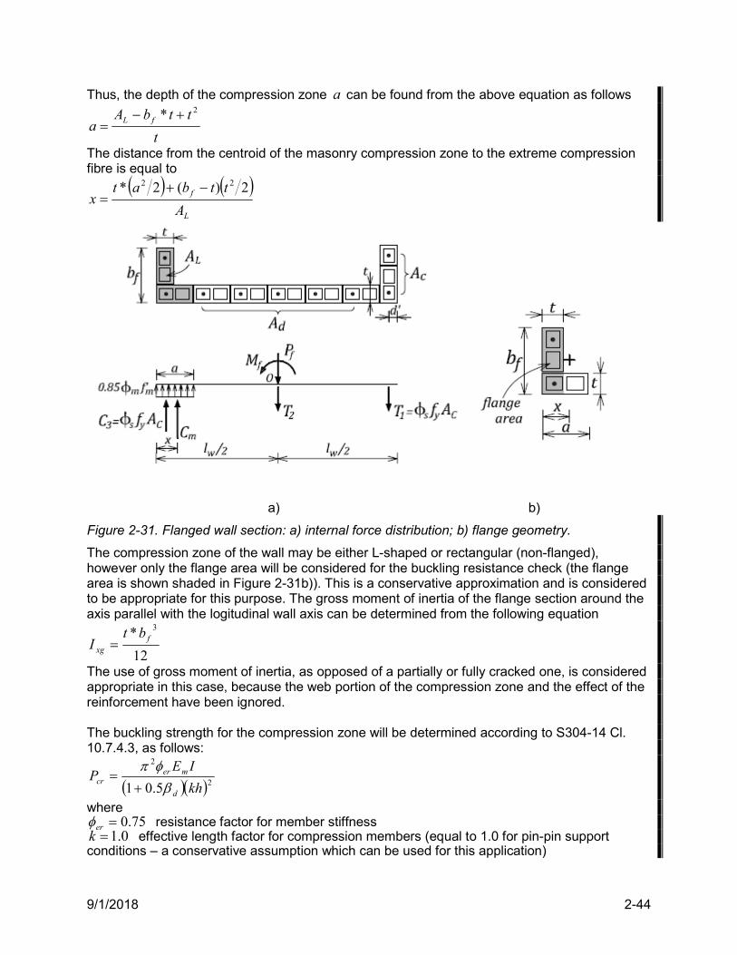
9/1/2018 2-44

Thus, the depth of the compression zone a can be found from the above equation as follows

t

ttbAa fL

2*

The distance from the centroid of the masonry compression zone to the extreme compression fibre is equal to

L

f

A

ttbatx

2)(2* 22

a) b)

Figure 2-31. Flanged wall section: a) internal force distribution; b) flange geometry.

The compression zone of the wall may be either L-shaped or rectangular (non-flanged), however only the flange area will be considered for the buckling resistance check (the flange area is shown shaded in Figure 2-31b)). This is a conservative approximation and is considered to be appropriate for this purpose. The gross moment of inertia of the flange section around the axis parallel with the logitudinal wall axis can be determined from the following equation

12

* 3f

xg

btI

The use of gross moment of inertia, as opposed of a partially or fully cracked one, is considered appropriate in this case, because the web portion of the compression zone and the effect of the reinforcement have been ignored. The buckling strength for the compression zone will be determined according to S304-14 Cl. 10.7.4.3, as follows:

22

5.01 kh

IEP

d

mercr

where 75.0er resistance factor for member stiffness

0.1k effective length factor for compression members (equal to 1.0 for pin-pin support conditions – a conservative assumption which can be used for this application)

9/1/2018 2-45

0d ratio of factored dead load moment to total factored moment (equal to 0 when 100% live load is assumed)

mE - modulus of elasticity for masonry The resultant compression force, including the concrete and steel component, can be determined as follows:

cysmfb AfCP

The out-of-plane buckling resistance is considered to be adequate when

crfb PP

This check gives conservative results, as shown in Example 5b in Chapter 3.

2.6.5 Minimum Required Factored Shear Resistance

16.5.4 16.7.3.2 16.8.9.2 16.9.8.3 16.10.4.3

The S304-14 minimum factored shear resistance requirements are based on the Capacity Design approach, which was discussed in Section 2.5.1. For the design of RM shear walls, the factored shear resistance,

rV , should be greater than the shear due to effects of factored loads, but not less than the smaller of 1. the shear corresponding to the development of moment resistance, as follows:

a. the shear corresponding to the development of factored moment resistance, rM , of

the wall system at its plastic hinge location for Conventional Construction (Cl.16.5.4) or Moderately Ductile Squat (Cl.16.7.3.2) shear walls,

b. the shear corresponding to the development of nominal moment capacity, nM , for

Moderately Ductile shear walls (Cl.16.8.9.2),

c. the shear corresponding to the development of probable moment capacity, pM , for

Ductile shear walls (Cl.16.9.8.3) and walls with boundary elements (Cl.16.10.4.3), and

2. the shear corresponding to the lateral seismic load (base shear) where earthquake effects were calculated using RdRo=1.3.

It is also important that other structural members which are not a part of the SFRS are able to undergo the same lateral displacements as the SFRS members without experiencing brittle failure.

9/1/2018 2-46

2.6.6 Shear/diagonal tension resistance – seismic design requirements

10.10.2 16.8.9.1 16.9.8.1 16.10.4.1

The CSA S304-14 general design provisions for shear (diagonal tension) resistance contained in Cl.10.10.2 were discussed in Section 2.3.2. Special seismic design provisions for the plastic hinge zone of the walls are as follows:

1. Conventional construction shear walls (Cl.10.10.2):

smr VVV

(the same equation used for the non-seismic design) 2. Moderately Ductile Squat shear walls (Cl.10.10.2):

smr VVV

(the same equation used for the non-seismic design of squat shear walls) 3. Moderately Ductile shear walls (Cl.16.8.9.1):

smr VVV 75.0

(a 25% reduction in the masonry shear resistance) 4. Ductile shear walls (Cl.16.9.8.1):

smr VVV 5.0

(a 50% reduction in the masonry shear resistance) 5. Moderately ductile and ductile shear walls with boundary elements (Cl.16.10.4.1):

smmur VVV ))2(0025.0(

(the masonry and axial compressive load contributions to shear capacity are reduced to account for the effects of damage expected at higher ductility)

For Moderately Ductile Squat shear walls, Cl.16.7.3.1 requires that the shear force be applied along the entire wall length, and not concentrated near one end. The purpose of this provision is to ensure that a top transfer beam, or an alternative provision (bond beam provided at the top of the wall), will enable the development of the desirable shear failure mechanism shown in Figure 2-16a), and prevent the partial shear failure shown in Figure 2-16b). Shear failure mechanisms for squat shear walls are discussed in Section 2.3.2.2. Commentary

Tests have shown that shear walls that fail in shear have a very poor cyclic response and demonstrate a sudden loss of strength. Also, walls that initially yield in flexure may fail in shear after several large inelastic cycles, with a resulting rapid strength degradation. Therefore, the shear steel (horizontal reinforcement) is usually designed to carry the entire shear load in the plastic hinge region of a wall (Anderson and Priestley, 1992). Seismic design provisions for ductile reinforced concrete shear walls (CSA A23.3 Cl.21.6.9) completely neglect the concrete contribution to the wall shear resistance in the plastic hinge zone. CSA S304-14 provisions permit the use of the entire masonry shear resistance for all wall classes, except for moderately ductile and ductile wall classes, where 75 and 50% of the

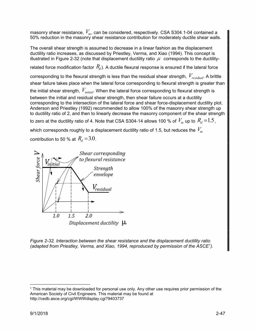
9/1/2018 2-47

masonry shear resistance, mV , can be considered, respectively. CSA S304.1-04 contained a 50% reduction in the masonry shear resistance contribution for moderately ductile shear walls. The overall shear strength is assumed to decrease in a linear fashion as the displacement ductility ratio increases, as discussed by Priestley, Verma, and Xiao (1994). This concept is illustrated in Figure 2-32 (note that displacement ductility ratio corresponds to the ductility-

related force modification factor dR ). A ductile flexural response is ensured if the lateral force

corresponding to the flexural strength is less than the residual shear strength, residualV . A brittle

shear failure takes place when the lateral force corresponding to flexural strength is greater than

the initial shear strength, initialV . When the lateral force corresponding to flexural strength is

between the initial and residual shear strength, then shear failure occurs at a ductility corresponding to the intersection of the lateral force and shear force-displacement ductility plot. Anderson and Priestley (1992) recommended to allow 100% of the masonry shear strength up to ductility ratio of 2, and then to linearly decrease the masonry component of the shear strength

to zero at the ductility ratio of 4. Note that CSA S304-14 allows 100 % of mV up to 5.1dR ,

which corresponds roughly to a displacement ductility ratio of 1.5, but reduces the mV

contribution to 50 % at 0.3dR .

Figure 2-32. Interaction between the shear resistance and the displacement ductility ratio (adapted from Priestley, Verma, and Xiao, 1994, reproduced by permission of the ASCE1).

1 This material may be downloaded for personal use only. Any other use requires prior permission of the American Society of Civil Engineers. This material may be found at http://cedb.asce.org/cgi/WWWdisplay.cgi?9403737

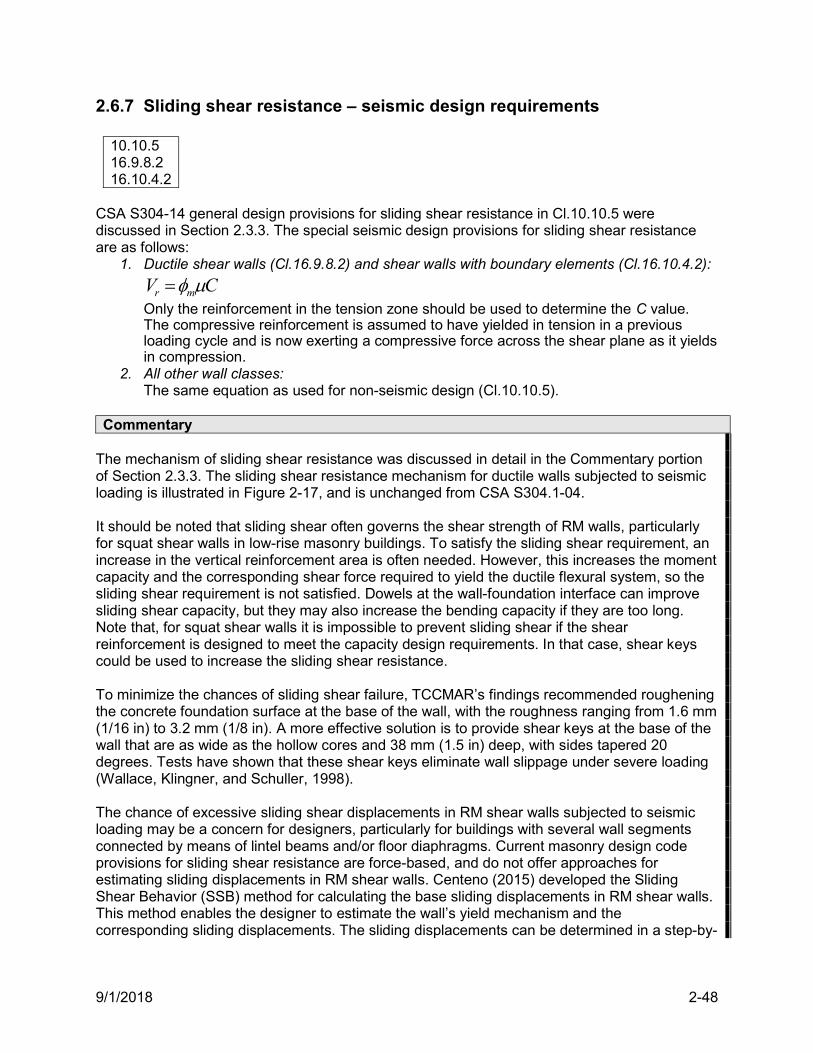
9/1/2018 2-48

2.6.7 Sliding shear resistance – seismic design requirements

10.10.5 16.9.8.2 16.10.4.2

CSA S304-14 general design provisions for sliding shear resistance in Cl.10.10.5 were discussed in Section 2.3.3. The special seismic design provisions for sliding shear resistance are as follows:

1. Ductile shear walls (Cl.16.9.8.2) and shear walls with boundary elements (Cl.16.10.4.2):

CV mr

Only the reinforcement in the tension zone should be used to determine the C value. The compressive reinforcement is assumed to have yielded in tension in a previous loading cycle and is now exerting a compressive force across the shear plane as it yields in compression.

2. All other wall classes: The same equation as used for non-seismic design (Cl.10.10.5).

Commentary

The mechanism of sliding shear resistance was discussed in detail in the Commentary portion of Section 2.3.3. The sliding shear resistance mechanism for ductile walls subjected to seismic loading is illustrated in Figure 2-17, and is unchanged from CSA S304.1-04. It should be noted that sliding shear often governs the shear strength of RM walls, particularly for squat shear walls in low-rise masonry buildings. To satisfy the sliding shear requirement, an increase in the vertical reinforcement area is often needed. However, this increases the moment capacity and the corresponding shear force required to yield the ductile flexural system, so the sliding shear requirement is not satisfied. Dowels at the wall-foundation interface can improve sliding shear capacity, but they may also increase the bending capacity if they are too long. Note that, for squat shear walls it is impossible to prevent sliding shear if the shear reinforcement is designed to meet the capacity design requirements. In that case, shear keys could be used to increase the sliding shear resistance. To minimize the chances of sliding shear failure, TCCMAR’s findings recommended roughening the concrete foundation surface at the base of the wall, with the roughness ranging from 1.6 mm (1/16 in) to 3.2 mm (1/8 in). A more effective solution is to provide shear keys at the base of the wall that are as wide as the hollow cores and 38 mm (1.5 in) deep, with sides tapered 20 degrees. Tests have shown that these shear keys eliminate wall slippage under severe loading (Wallace, Klingner, and Schuller, 1998). The chance of excessive sliding shear displacements in RM shear walls subjected to seismic loading may be a concern for designers, particularly for buildings with several wall segments connected by means of lintel beams and/or floor diaphragms. Current masonry design code provisions for sliding shear resistance are force-based, and do not offer approaches for estimating sliding displacements in RM shear walls. Centeno (2015) developed the Sliding Shear Behavior (SSB) method for calculating the base sliding displacements in RM shear walls. This method enables the designer to estimate the wall’s yield mechanism and the corresponding sliding displacements. The sliding displacements can be determined in a step-by-

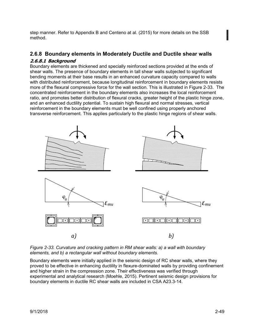
9/1/2018 2-49

step manner. Refer to Appendix B and Centeno at al. (2015) for more details on the SSB method.

2.6.8 Boundary elements in Moderately Ductile and Ductile shear walls 2.6.8.1 Background Boundary elements are thickened and specially reinforced sections provided at the ends of shear walls. The presence of boundary elements in tall shear walls subjected to significant bending moments at their base results in an enhanced curvature capacity compared to walls with distributed reinforcement, because longitudinal reinforcement in boundary elements resists more of the flexural compressive force for the wall section. This is illustrated in Figure 2-33. The concentrated reinforcement in the boundary elements also increases the local reinforcement ratio, and promotes better distribution of flexural cracks, greater height of the plastic hinge zone, and an enhanced ductility potential. To sustain high flexural and normal stresses, vertical reinforcement in the boundary elements must be well confined using properly anchored transverse reinforcement. This applies particularly to the plastic hinge regions of shear walls.

Figure 2-33. Curvature and cracking pattern in RM shear walls: a) a wall with boundary elements, and b) a rectangular wall without boundary elements.

Boundary elements were initially applied in the seismic design of RC shear walls, where they proved to be effective in enhancing ductility in flexure-dominated walls by providing confinement and higher strain in the compression zone. Their effectiveness was verified through experimental and analytical research (Moehle, 2015). Pertinent seismic design provisions for boundary elements in ductile RC shear walls are included in CSA A23.3-14.

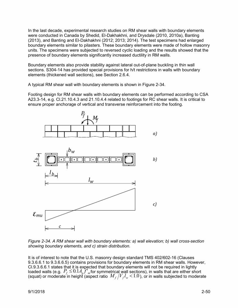
9/1/2018 2-50

In the last decade, experimental research studies on RM shear walls with boundary elements were conducted in Canada by Shedid, El-Dakhakhni, and Drysdale (2010, 2010a), Banting (2013), and Banting and El-Dakhakhni (2012; 2013; 2014). The test specimens had enlarged boundary elements similar to pilasters. These boundary elements were made of hollow masonry units. The specimens were subjected to reversed cyclic loading and the results showed that the presence of boundary elements significantly increased ductility in RM walls. Boundary elements also provide stability against lateral out-of-plane buckling in thin wall sections. S304-14 has provided special provisions for h/t restrictions in walls with boundary elements (thickened wall sections), see Section 2.6.4. A typical RM shear wall with boundary elements is shown in Figure 2-34. Footing design for RM shear walls with boundary elements can be performed according to CSA A23.3-14, e.g. Cl.21.10.4.3 and 21.10.4.4 related to footings for RC shear walls. It is critical to ensure proper anchorage of vertical and transverse reinforcement into the footing.

Figure 2-34. A RM shear wall with boundary elements: a) wall elevation; b) wall cross-section showing boundary elements, and c) strain distribution.

It is of interest to note that the U.S. masonry design standard TMS 402/602-16 (Clauses 9.3.6.6.1 to 9.3.6.6.5) contains provisions for boundary elements in RM shear walls. However, Cl.9.3.6.6.1 states that it is expected that boundary elements will not be required in lightly loaded walls (e.g. mgf fAP '1.0 for symmetrical wall sections), in walls that are either short (squat) or moderate in height (aspect ratio 0.1wff lVM ), or in walls subjected to moderate

9/1/2018 2-51

shear stresses. It is expected that most masonry shear walls in low- to medium-rise buildings would not develop high enough compressive strains to warrant special confinement. According to the TMS 402/602-16 standard, boundary elements may be required in RM shear walls with flexure-dominant behaviour when the wlc ratio exceeds a certain limit. The purpose of this check is to limit the ultimate curvature in the plastic hinge region of the wall (similar to the S304-14 ductility check procedure discussed in Section 2.6.3). TMS 402 also provides a stress-based check for boundary elements, i.e. it provides compressive stress limit (0.2 mf ' ) beyond which boundary elements need to be provided in the compression zone. According to the same check, the boundary element may be discontinued when the calculated compressive stress is less than 0.15 mf ' . When special boundary elements are used, TMS 402 requires that testing be done to verify that the provided detailing is capable of developing the required compressive strain capacity. As an alternative to boundary elements, the New Zealand masonry standard NZS 4230:2004 Cl.7.4.6.5 prescribes the use of horizontal confining plates in ductile RM walls. These thin perforated metal plates (made either of stainless steel or galvanized steel) are placed in mortar bed joints in the compression zone of rectangular walls. The confining plates are effective in increasing the maximum masonry compressive strain in plastic hinge regions up to 0.008 (this value is same as prescribed by CSA S304-14 for shear walls with boundary elements). The provision of confining plates in the New Zealand masonry standard is based on research by Priestley (1981) and Priestley and Elder (1983). 2.6.8.2 When are boundary elements required

16.6.4 16.10

S304-14 Cl.16.10.1 prescribes the use of boundary elements in RM shear walls for the first time. Boundary elements should be provided when the ductility requirements of Cl. 16.8.8 or

16.9.7 are not satisfied assuming a masonry compression strain limit mu of 0.0025. When

boundary elements are used, the maximum compressive strain mu can be higher than 0.0025,

but it should not exceed 0.008. S304-14 Cl.16.6.4 states that tests should be performed to verify

the ductility and strain capacities of the wall when the compressive strain limit mu of 0.0025 is

exceeded. Commentary

S304-14 does not provide guidance on how to calculate the maximum compressive strain in boundary elements. For seismic design purposes, the maximum required compressive strain

mu in boundary elements can be calculated from the S304-14 ductility requirements

(Cl.16.8.8). The calculated strain value should be used for detailing transverse reinforcement in boundary elements, according to the equations presented in Section 2.6.8.5. Priestley (1981) proposed stress-strain equations for unconfined and confined block masonry based on his research study that focused on the use of steel confining plates for enhancing maximum compressive strain in RM walls. The proposed equations take into account the

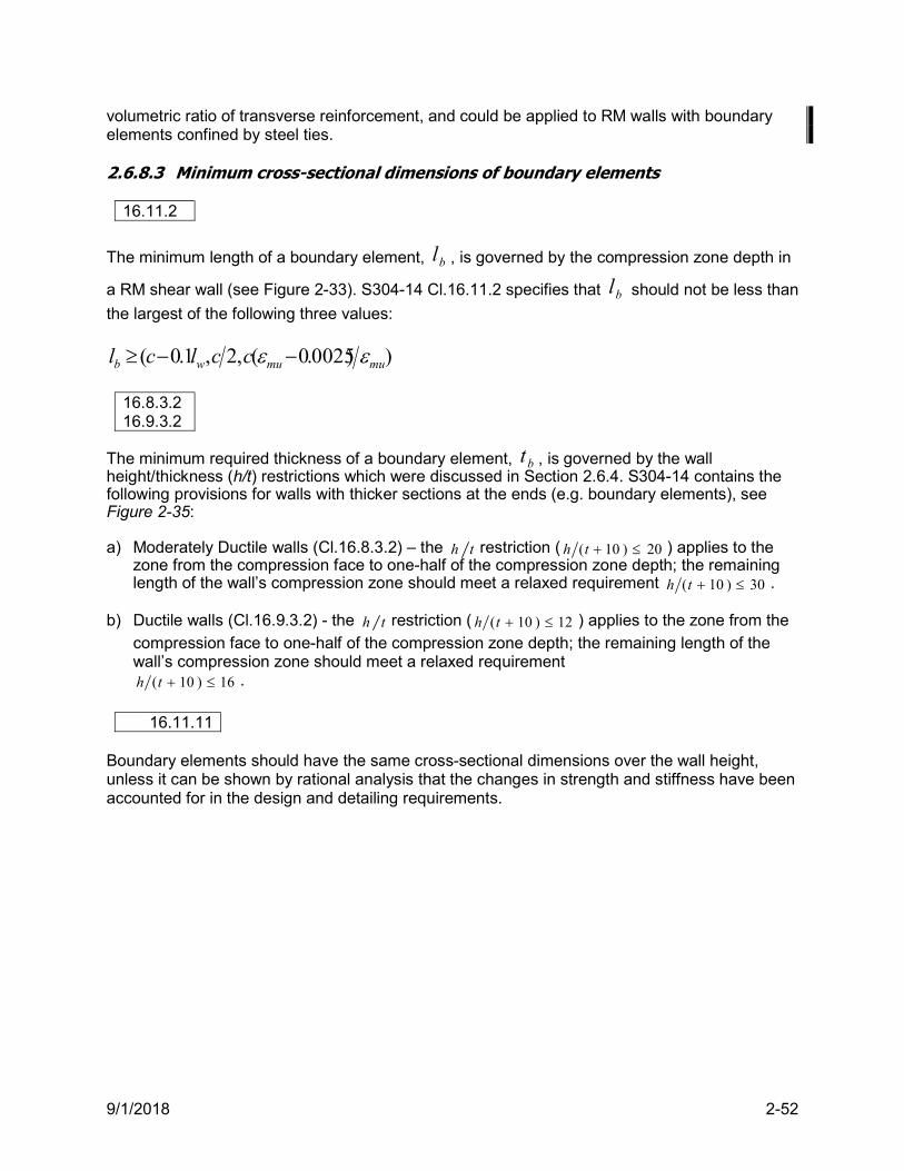
9/1/2018 2-52

volumetric ratio of transverse reinforcement, and could be applied to RM walls with boundary elements confined by steel ties. 2.6.8.3 Minimum cross-sectional dimensions of boundary elements

16.11.2

The minimum length of a boundary element, bl , is governed by the compression zone depth in

a RM shear wall (see Figure 2-33). S304-14 Cl.16.11.2 specifies that bl should not be less than

the largest of the following three values:

))0025.0(,2,1.0( mumuwb cclcl

16.8.3.2 16.9.3.2

The minimum required thickness of a boundary element, bt , is governed by the wall height/thickness (h/t) restrictions which were discussed in Section 2.6.4. S304-14 contains the following provisions for walls with thicker sections at the ends (e.g. boundary elements), see Figure 2-35: a) Moderately Ductile walls (Cl.16.8.3.2) – the th restriction ( 20)10( th ) applies to the

zone from the compression face to one-half of the compression zone depth; the remaining length of the wall’s compression zone should meet a relaxed requirement 30)10( th .

b) Ductile walls (Cl.16.9.3.2) - the th restriction ( 12)10( th ) applies to the zone from the

compression face to one-half of the compression zone depth; the remaining length of the wall’s compression zone should meet a relaxed requirement

16)10( th .

16.11.11 Boundary elements should have the same cross-sectional dimensions over the wall height, unless it can be shown by rational analysis that the changes in strength and stiffness have been accounted for in the design and detailing requirements.

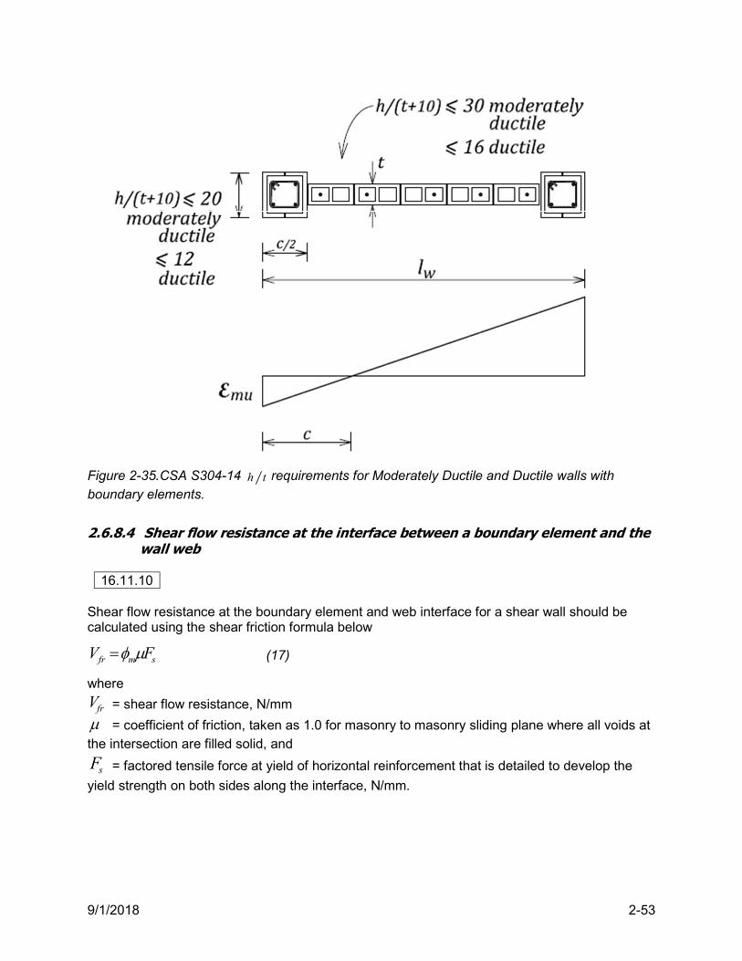
9/1/2018 2-53

Figure 2-35.CSA S304-14 th requirements for Moderately Ductile and Ductile walls with boundary elements.

2.6.8.4 Shear flow resistance at the interface between a boundary element and the

wall web

16.11.10 Shear flow resistance at the boundary element and web interface for a shear wall should be calculated using the shear friction formula below

smfr FV (17)

where

frV = shear flow resistance, N/mm

= coefficient of friction, taken as 1.0 for masonry to masonry sliding plane where all voids at the intersection are filled solid, and

sF = factored tensile force at yield of horizontal reinforcement that is detailed to develop the

yield strength on both sides along the interface, N/mm.

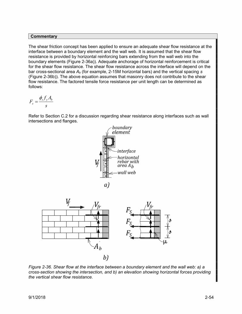
9/1/2018 2-54

Commentary

The shear friction concept has been applied to ensure an adequate shear flow resistance at the interface between a boundary element and the wall web. It is assumed that the shear flow resistance is provided by horizontal reinforcing bars extending from the wall web into the boundary elements (Figure 2-36a)). Adequate anchorage of horizontal reinforcement is critical for the shear flow resistance. The shear flow resistance across the interface will depend on the bar cross-sectional area Ab (for example, 2-15M horizontal bars) and the vertical spacing s (Figure 2-36b)). The above equation assumes that masonry does not contribute to the shear flow resistance. The factored tensile force resistance per unit length can be determined as follows:

s

AfF byss

Refer to Section C.2 for a discussion regarding shear resistance along interfaces such as wall intersections and flanges.

Figure 2-36. Shear flow at the interface between a boundary element and the wall web: a) a cross-section showing the intersection, and b) an elevation showing horizontal forces providing the vertical shear flow resistance.

9/1/2018 2-55

2.6.8.5 Reinforcement detailing requirements for boundary elements and

compression reinforcement in Moderately Ductile and Ductile walls

16.6.5 16.11.5 16.11.6

S304-14 Cl.16.11 outlines the provisions for seismic detailing of reinforcement in boundary elements, but S304-14 Cl.16.6.5 stipulates that the same reinforcement detailing requirements should be followed while detailing compression reinforcement zones in Moderately Ductile and Ductile shear walls. Boundary elements are reinforced with vertical reinforcing bars and transverse reinforcement in the form of ties (hoops), as shown in Figure 2-37a). The ties are in the form of regular ties (outside the plastic hinge zone) and buckling prevention ties (within the plastic hinge zone), see Figure 2-37b). Buckling prevention ties are intended to prevent buckling of the longitudinal reinforcement under reversed cyclic loading. In order to ensure proper confinement, intermediate vertical reinforcing bars should be provided not more than 150 mm spacing away from a laterally supported bar. Seismic cross ties may be also provided to support vertical reinforcing bars, if required. A seismic cross tie (S304-14 Cl.16.11.5) is a reinforcing bar with a 90° hook at one end and a 135° hook at the other end (Figure 2-37b)). The seismic cross ties shall engage vertical reinforcing bars at each end, and where successive ties engage the same vertical reinforcing bar the 90° hook shall be alternated end for end. These ties are not required in boundary elements with 4 vertical bars because each bar is already supported by means of closed ties. Detailing of seismic cross ties requires that a 90° hook has min 6 bar diameter extension at one end, and a 135° hook should be anchored into the confined core with minimum extension of the lesser of 6 bar diameters or 100 mm at the other end.

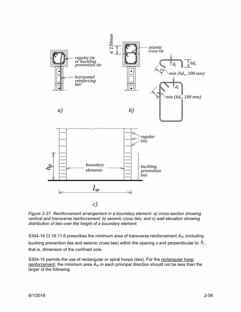
9/1/2018 2-56

Figure 2-37. Reinforcement arrangement in a boundary element: a) cross-section showing vertical and transverse reinforcement; b) seismic cross ties, and c) wall elevation showing distribution of ties over the height of a boundary element.

S304-14 Cl.16.11.6 prescribes the minimum area of transverse reinforcement Ash (including

buckling prevention ties and seismic cross ties) within the spacing s and perpendicular to ch ,

that is, dimension of the confined core. S304-14 permits the use of rectangular or spiral hoops (ties). For the rectangular hoop reinforcement, the minimum area Ash in each principal direction should not be less than the larger of the following:

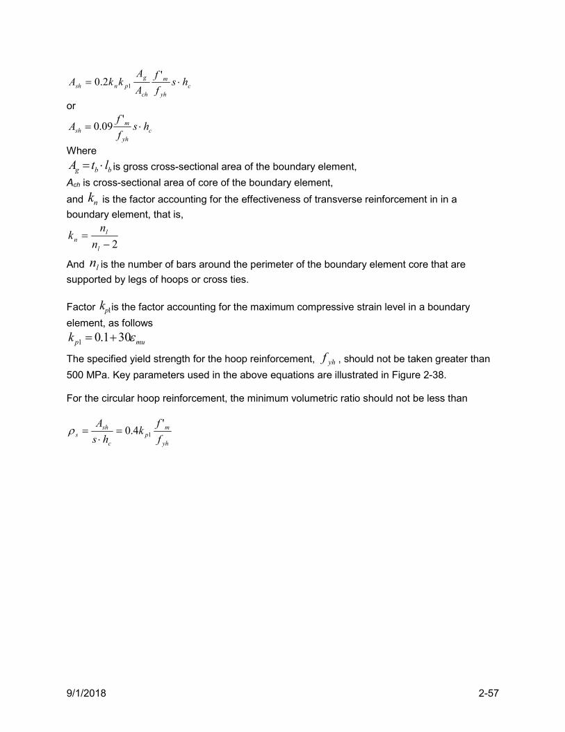
9/1/2018 2-57

cyh

m

ch

gpnsh hs

f

f

A

AkkA

'2.0 1

or

cyh

msh hs

f

fA

'09.0

Where

bbg ltA is gross cross-sectional area of the boundary element,

Ach is cross-sectional area of core of the boundary element,

and nk is the factor accounting for the effectiveness of transverse reinforcement in in a

boundary element, that is,

2

l

ln n

nk

And ln is the number of bars around the perimeter of the boundary element core that are

supported by legs of hoops or cross ties.

Factor 1pk is the factor accounting for the maximum compressive strain level in a boundary

element, as follows

mupk 301.01

The specified yield strength for the hoop reinforcement, yhf , should not be taken greater than

500 MPa. Key parameters used in the above equations are illustrated in Figure 2-38. For the circular hoop reinforcement, the minimum volumetric ratio should not be less than

yh

mp

c

shs f

fk

hs

A '4.0 1

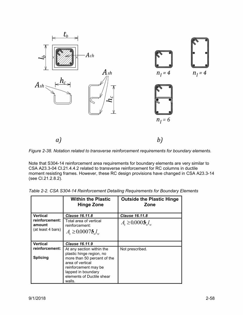
9/1/2018 2-58

Figure 2-38. Notation related to transverse reinforcement requirements for boundary elements.

Note that S304-14 reinforcement area requirements for boundary elements are very similar to CSA A23.3-04 Cl.21.4.4.2 related to transverse reinforcement for RC columns in ductile moment resisting frames. However, these RC design provisions have changed in CSA A23.3-14 (see Cl.21.2.8.2).

Table 2-2. CSA S304-14 Reinforcement Detailing Requirements for Boundary Elements

Within the Plastic Hinge Zone

Outside the Plastic Hinge Zone

Vertical reinforcement: amount (at least 4 bars)

Clause 16.11.8 Clause 16.11.8 Total area of vertical reinforcement:

wws lbA 00075.0

wws lbA 0005.0

Vertical reinforcement: Splicing

Clause 16.11.9 At any section within the plastic hinge region, no more than 50 percent of the area of vertical reinforcement may be lapped in boundary elements of Ductile shear walls.

Not prescribed.

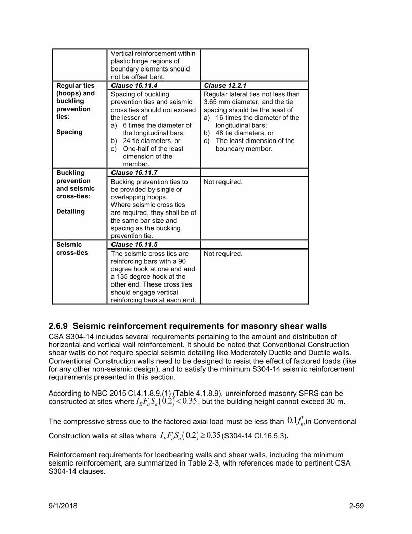
9/1/2018 2-59

Vertical reinforcement within plastic hinge regions of boundary elements should not be offset bent.

Regular ties (hoops) and buckling prevention ties: Spacing

Clause 16.11.4 Clause 12.2.1 Spacing of buckling prevention ties and seismic cross ties should not exceed the lesser of a) 6 times the diameter of

the longitudinal bars; b) 24 tie diameters, or c) One-half of the least

dimension of the member.

Regular lateral ties not less than 3.65 mm diameter, and the tie spacing should be the least of a) 16 times the diameter of the

longitudinal bars; b) 48 tie diameters, or c) The least dimension of the

boundary member.

Buckling prevention and seismic cross-ties: Detailing

Clause 16.11.7 Bucking prevention ties to be provided by single or overlapping hoops. Where seismic cross ties are required, they shall be of the same bar size and spacing as the buckling prevention tie.

Not required.

Seismic cross-ties

Clause 16.11.5 The seismic cross ties are reinforcing bars with a 90 degree hook at one end and a 135 degree hook at the other end. These cross ties should engage vertical reinforcing bars at each end.

Not required.

2.6.9 Seismic reinforcement requirements for masonry shear walls CSA S304-14 includes several requirements pertaining to the amount and distribution of horizontal and vertical wall reinforcement. It should be noted that Conventional Construction shear walls do not require special seismic detailing like Moderately Ductile and Ductile walls. Conventional Construction walls need to be designed to resist the effect of factored loads (like for any other non-seismic design), and to satisfy the minimum S304-14 seismic reinforcement requirements presented in this section. According to NBC 2015 Cl.4.1.8.9.(1) (Table 4.1.8.9), unreinforced masonry SFRS can be constructed at sites where 0.2 0.35E a aI F S , but the building height cannot exceed 30 m.

The compressive stress due to the factored axial load must be less than mf 1.0 in Conventional

Construction walls at sites where 0.2 0.35E a aI F S (S304-14 Cl.16.5.3).

Reinforcement requirements for loadbearing walls and shear walls, including the minimum seismic reinforcement, are summarized in Table 2-3, with references made to pertinent CSA S304-14 clauses.

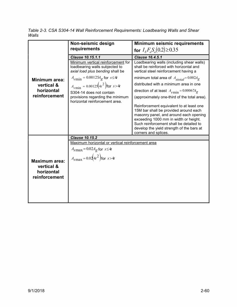
9/1/2018 2-60

Table 2-3. CSA S304-14 Wall Reinforcement Requirements: Loadbearing Walls and Shear Walls

Minimum area: vertical & horizontal

reinforcement

Non-seismic design requirements

Minimum seismic requirements

for 35.02.0 aaE SFI

Clause 10.15.1.1 Clause 16.4.5.1 Minimum vertical reinforcement for loadbearing walls subjected to axial load plus bending shall be

gAvA 00125.0min for ts 4

2400125.0min tvA for ts 4

S304-14 does not contain provisions regarding the minimum horizontal reinforcement area.

Loadbearing walls (including shear walls) shall be reinforced with horizontal and vertical steel reinforcement having a

minimum total area of gAstotalA 002.0

distributed with a minimum area in one

direction of at least gAvA 00067.0min

(approximately one-third of the total area). Reinforcement equivalent to at least one 15M bar shall be provided around each masonry panel, and around each opening exceeding 1000 mm in width or height. Such reinforcement shall be detailed to develop the yield strength of the bars at corners and splices.

Maximum area: vertical & horizontal

reinforcement

Clause 10.15.2 Maximum horizontal or vertical reinforcement area

gAsA 02.0max for ts 4

2402.0max tsA for ts 4

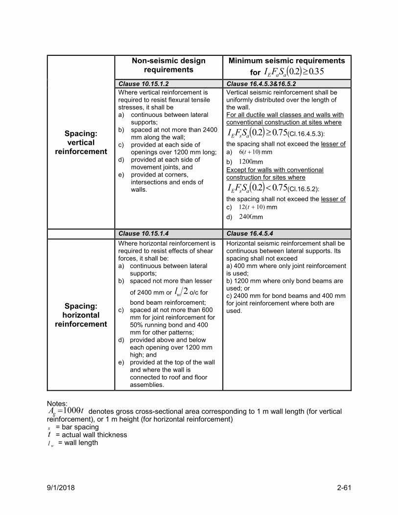
9/1/2018 2-61

Spacing: vertical

reinforcement

Non-seismic design requirements

Minimum seismic requirements

for 35.02.0 aaE SFI

Clause 10.15.1.2 Clause 16.4.5.3&16.5.2 Where vertical reinforcement is required to resist flexural tensile stresses, it shall be a) continuous between lateral

supports; b) spaced at not more than 2400

mm along the wall; c) provided at each side of

openings over 1200 mm long; d) provided at each side of

movement joints, and e) provided at corners,

intersections and ends of walls.

Vertical seismic reinforcement shall be uniformly distributed over the length of the wall. For all ductile wall classes and walls with conventional construction at sites where

75.02.0 asE SFI (Cl.16.4.5.3):

the spacing shall not exceed the lesser of a) )10(6 t mm

b) 1200mm Except for walls with conventional construction for sites where

75.02.0 asE SFI (Cl.16.5.2):

the spacing shall not exceed the lesser of c) )10(12 t mm

d) 2400mm

Clause 10.15.1.4 Clause 16.4.5.4

Spacing: horizontal

reinforcement

Where horizontal reinforcement is required to resist effects of shear forces, it shall be: a) continuous between lateral

supports; b) spaced not more than lesser

of 2400 mm or 2wl o/c for

bond beam reinforcement; c) spaced at not more than 600

mm for joint reinforcement for 50% running bond and 400 mm for other patterns;

d) provided above and below each opening over 1200 mm high; and

e) provided at the top of the wall and where the wall is connected to roof and floor assemblies.

Horizontal seismic reinforcement shall be continuous between lateral supports. Its spacing shall not exceed a) 400 mm where only joint reinforcement is used; b) 1200 mm where only bond beams are used; or c) 2400 mm for bond beams and 400 mm for joint reinforcement where both are used.

Notes:

tAg 1000 denotes gross cross-sectional area corresponding to 1 m wall length (for vertical reinforcement), or 1 m height (for horizontal reinforcement) s = bar spacing t = actual wall thickness wl = wall length

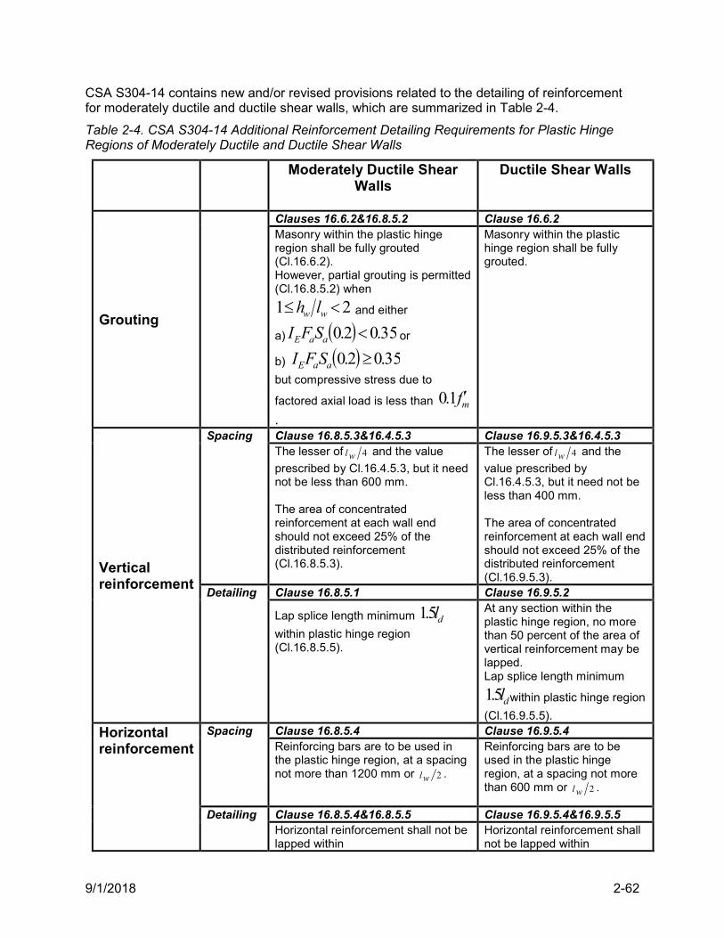
9/1/2018 2-62

CSA S304-14 contains new and/or revised provisions related to the detailing of reinforcement for moderately ductile and ductile shear walls, which are summarized in Table 2-4.

Table 2-4. CSA S304-14 Additional Reinforcement Detailing Requirements for Plastic Hinge Regions of Moderately Ductile and Ductile Shear Walls

Moderately Ductile Shear Walls

Ductile Shear Walls

Grouting

Clauses 16.6.2&16.8.5.2 Clause 16.6.2 Masonry within the plastic hinge region shall be fully grouted (Cl.16.6.2). However, partial grouting is permitted (Cl.16.8.5.2) when

21 ww lh and either

a) 35.02.0 aaE SFI or

b) 35.02.0 aaE SFI but compressive stress due to

factored axial load is less than mf 1.0.

Masonry within the plastic hinge region shall be fully grouted.

Vertical reinforcement

Spacing Clause 16.8.5.3&16.4.5.3 Clause 16.9.5.3&16.4.5.3 The lesser of 4wl and the value

prescribed by Cl.16.4.5.3, but it need not be less than 600 mm. The area of concentrated reinforcement at each wall end should not exceed 25% of the distributed reinforcement (Cl.16.8.5.3).

The lesser of 4wl and the

value prescribed by Cl.16.4.5.3, but it need not be less than 400 mm. The area of concentrated reinforcement at each wall end should not exceed 25% of the distributed reinforcement (Cl.16.9.5.3).

Detailing

Clause 16.8.5.1 Clause 16.9.5.2

Lap splice length minimum dl5.1within plastic hinge region (Cl.16.8.5.5).

At any section within the plastic hinge region, no more than 50 percent of the area of vertical reinforcement may be lapped. Lap splice length minimum

dl5.1 within plastic hinge region

(Cl.16.9.5.5).

Horizontal reinforcement

Spacing Clause 16.8.5.4 Clause 16.9.5.4 Reinforcing bars are to be used in the plastic hinge region, at a spacing not more than 1200 mm or 2wl .

Reinforcing bars are to be used in the plastic hinge region, at a spacing not more than 600 mm or 2wl .

Detailing Clause 16.8.5.4&16.8.5.5 Clause 16.9.5.4&16.9.5.5 Horizontal reinforcement shall not be lapped within

Horizontal reinforcement shall not be lapped within

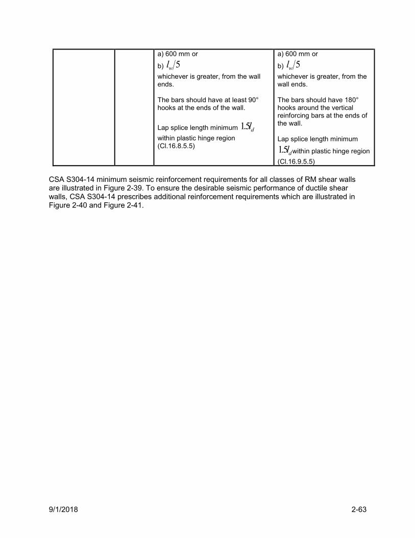
9/1/2018 2-63

a) 600 mm or

b) 5wl

whichever is greater, from the wall ends. The bars should have at least 90° hooks at the ends of the wall.

Lap splice length minimum dl5.1within plastic hinge region (Cl.16.8.5.5)

a) 600 mm or

b) 5wl

whichever is greater, from the wall ends. The bars should have 180° hooks around the vertical reinforcing bars at the ends of the wall. Lap splice length minimum

dl5.1 within plastic hinge region

(Cl.16.9.5.5)

CSA S304-14 minimum seismic reinforcement requirements for all classes of RM shear walls are illustrated in Figure 2-39. To ensure the desirable seismic performance of ductile shear walls, CSA S304-14 prescribes additional reinforcement requirements which are illustrated in Figure 2-40 and Figure 2-41.

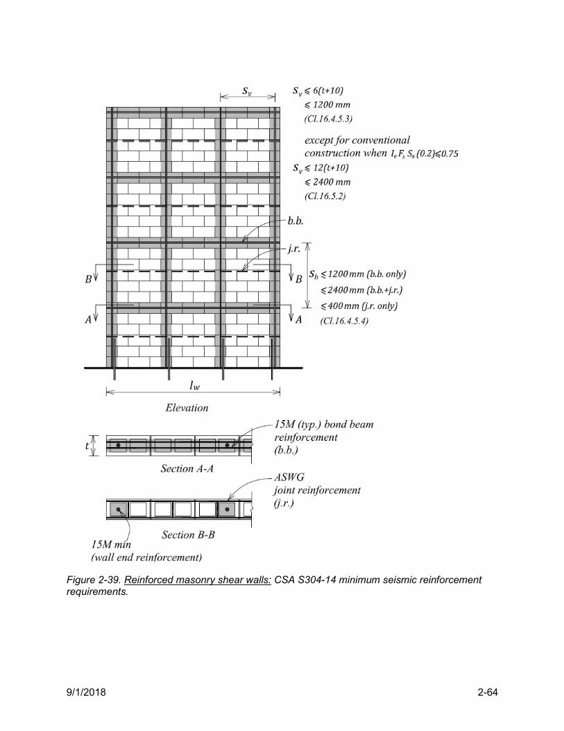
9/1/2018 2-64

Figure 2-39. Reinforced masonry shear walls: CSA S304-14 minimum seismic reinforcement requirements.

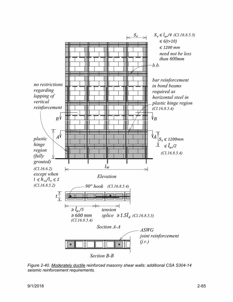
9/1/2018 2-65

Figure 2-40. Moderately ductile reinforced masonry shear walls: additional CSA S304-14 seismic reinforcement requirements.

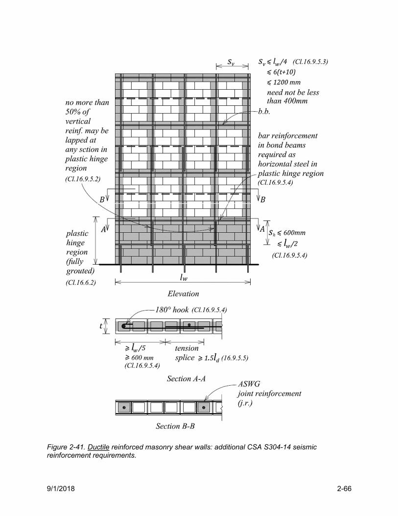
9/1/2018 2-66

Figure 2-41. Ductile reinforced masonry shear walls: additional CSA S304-14 seismic reinforcement requirements.

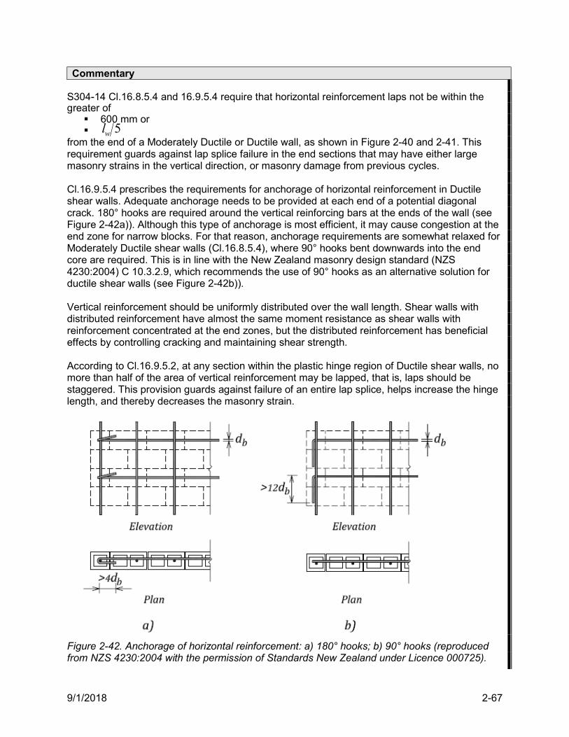
9/1/2018 2-67

Commentary S304-14 Cl.16.8.5.4 and 16.9.5.4 require that horizontal reinforcement laps not be within the greater of

600 mm or 5wl

from the end of a Moderately Ductile or Ductile wall, as shown in Figure 2-40 and 2-41. This requirement guards against lap splice failure in the end sections that may have either large masonry strains in the vertical direction, or masonry damage from previous cycles. Cl.16.9.5.4 prescribes the requirements for anchorage of horizontal reinforcement in Ductile shear walls. Adequate anchorage needs to be provided at each end of a potential diagonal crack. 180° hooks are required around the vertical reinforcing bars at the ends of the wall (see Figure 2-42a)). Although this type of anchorage is most efficient, it may cause congestion at the end zone for narrow blocks. For that reason, anchorage requirements are somewhat relaxed for Moderately Ductile shear walls (Cl.16.8.5.4), where 90° hooks bent downwards into the end core are required. This is in line with the New Zealand masonry design standard (NZS 4230:2004) C 10.3.2.9, which recommends the use of 90° hooks as an alternative solution for ductile shear walls (see Figure 2-42b)). Vertical reinforcement should be uniformly distributed over the wall length. Shear walls with distributed reinforcement have almost the same moment resistance as shear walls with reinforcement concentrated at the end zones, but the distributed reinforcement has beneficial effects by controlling cracking and maintaining shear strength. According to Cl.16.9.5.2, at any section within the plastic hinge region of Ductile shear walls, no more than half of the area of vertical reinforcement may be lapped, that is, laps should be staggered. This provision guards against failure of an entire lap splice, helps increase the hinge length, and thereby decreases the masonry strain.

Figure 2-42. Anchorage of horizontal reinforcement: a) 180° hooks; b) 90° hooks (reproduced from NZS 4230:2004 with the permission of Standards New Zealand under Licence 000725).

9/1/2018 2-68

CSA S304.1-04 and S304-14 seismic reinforcement requirements – a comparison Most of the S304-14 seismic requirements for shear wall reinforcement existed in the 2004 edition of the standard (S304.1-04). A comparison is summarized below. 1. S304.1-04 contained the minimum seismic requirements related to reinforcement area in

RM shear walls. These requirements remain mostly unchanged in S304-14, however, reinforcement spacing requirements have been somewhat expanded. General spacing requirements for vertical reinforcement are stated in Cl.16.4.5.3. However, where, 75.02.0 asE SFI , Cl.16.5.2 allows the vertical reinforcement spacing for Conventional Construction shear walls, to be relaxed to 12(t+10) mm or 2400 mm. This amounts to twice the spacing permitted for ductile classes and walls with conventional construction at sites with higher seismic hazard index values.

2. S304.1-04 Cl.10.16.5.4.2 required 180° end hooks for horizontal reinforcement bars in the plastic hinge region of Moderately Ductile shear walls. However, S304-14 Cl.16.8.5.4 permits the use of 90° end hooks for horizontal reinforcement in Moderately Ductile shear walls; this is a relaxed provision. However, 180° end hooks are required for horizontal reinforcement in the new Ductile shear wall category (S304-14 Cl.16.9.5.4).

3. S304.1-04 10.16.4.1.3 required full grouting in Moderately Ductile shear wall plastic hinge zones. S304-14 Cl.16.8.5.2 permits partial grouting in Moderately Ductile shear walls with a

low aspect ratio ( 21 ww lh ), either where 35.02.0 aaE SFI , or where

35.02.0 aaE SFI , but the compressive stress due to the factored axial load is less than

mf 1.0 .

4. S304.1-04 Cl.10.16.5.4.1 restricted the lapping of vertical reinforcement in plastic hinge zones of Moderately Ductile shear walls; this restriction is not included in S304-14, but the same restriction now applies to Ductile shear walls (S304-14 Cl.16.9.5.2).

2.6.10 Minimum reinforcement requirements for Moderately Ductile Squat shear walls

16.7.5

CSA S304-14 prescribes the following requirements for the minimum amount of reinforcement in Moderately Ductile Squat shear walls:

Horizontal reinforcement ratio h :

ywwsfh fhbV

Relationship between horizontal ( h ) and vertical ( v ) reinforcement ratios:

ywwsshv flbP

Commentary

The seismic design requirements for Moderately Ductile Squat shear walls were introduced in the 2004 edition of S304.1. In general, the squat wall requirements are more relaxed than those pertaining to Moderately Ductile flexural shear walls, because shear failure in squat shear walls is not as critical as in taller flexural walls, and can provide some ductility. Thus the design and

9/1/2018 2-69

detailing requirements related to the flexural failure mechanism (e.g. ductility check) are not required for squat walls. The reinforcement requirements in Cl.16.7.5 have been derived from the mechanism of a squat shear wall failing in the shear-critical mode shown in Figure 2-43a). Consider a squat shear wall subjected to the combined effect of factored shear force, fV , and the seismic axial force, sP (due to gravity and live loads using earthquake load factors). The effect of these forces can be presented in the form of distributed shear stress, fv , and distributed axial stress, fp , as follows

ww

ff lb

Vv

(18)

and

ww

sf lb

Pp

(19)

The wall is reinforced with horizontal and vertical reinforcement, where the reinforcement ratios h for horizontal reinforcement, and v for vertical reinforcement, are given by

ww

vv lb

A

and

ww

hh hb

A

where

tbw overall wall thickness (referred to as “web width” in CSA S304-14)

wl = wall length

wh = wall height

If the yield stress of the reinforcement is given by yf , the factored unit capacity of the reinforcement in the two directions is yhs f and yvs f (see Figure 2-43c) and d)). Once the shear force in the wall reaches a certain level, inclined shear cracks develop in the wall at a 45 angle to the horizontal axis, as shown in Figure 2-43b) (note that this is an idealized model and that the angle may be different from 45). The areas of masonry between these inclined cracks act as compression struts. Consider a typical unit length strut shown in Figure 2-43c). This strut remains in equilibrium only if there is enough force in the vertical reinforcement to satisfy moment equilibrium about the base. Note that the force in both the vertical and horizontal bars that pass through the strut do not create any net force on the strut. The equilibrium of forces in the strut requires that

fyvsf vfp

When the fp and fv expressions are substituted into the above equation, the resulting

relationship between the horizontal and vertical reinforcement (same as Cl. 16.7.5) is as follows

ywws

shv flb

P

(20)

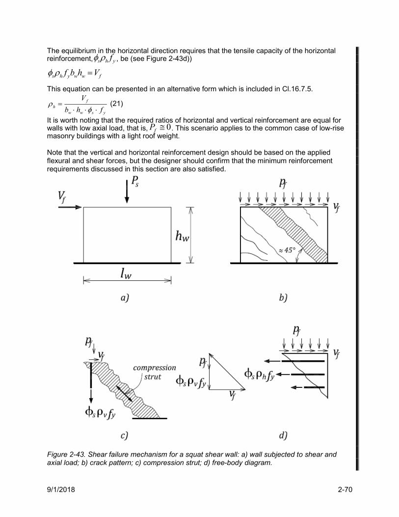
9/1/2018 2-70

The equilibrium in the horizontal direction requires that the tensile capacity of the horizontal reinforcement, yhs f , be (see Figure 2-43d))

fwwyhs Vhbf

This equation can be presented in an alternative form which is included in Cl.16.7.5.

ysww

fh fhb

V

(21)

It is worth noting that the required ratios of horizontal and vertical reinforcement are equal for walls with low axial load, that is, 0fP . This scenario applies to the common case of low-rise masonry buildings with a light roof weight. Note that the vertical and horizontal reinforcement design should be based on the applied flexural and shear forces, but the designer should confirm that the minimum reinforcement requirements discussed in this section are also satisfied.

Figure 2-43. Shear failure mechanism for a squat shear wall: a) wall subjected to shear and axial load; b) crack pattern; c) compression strut; d) free-body diagram.

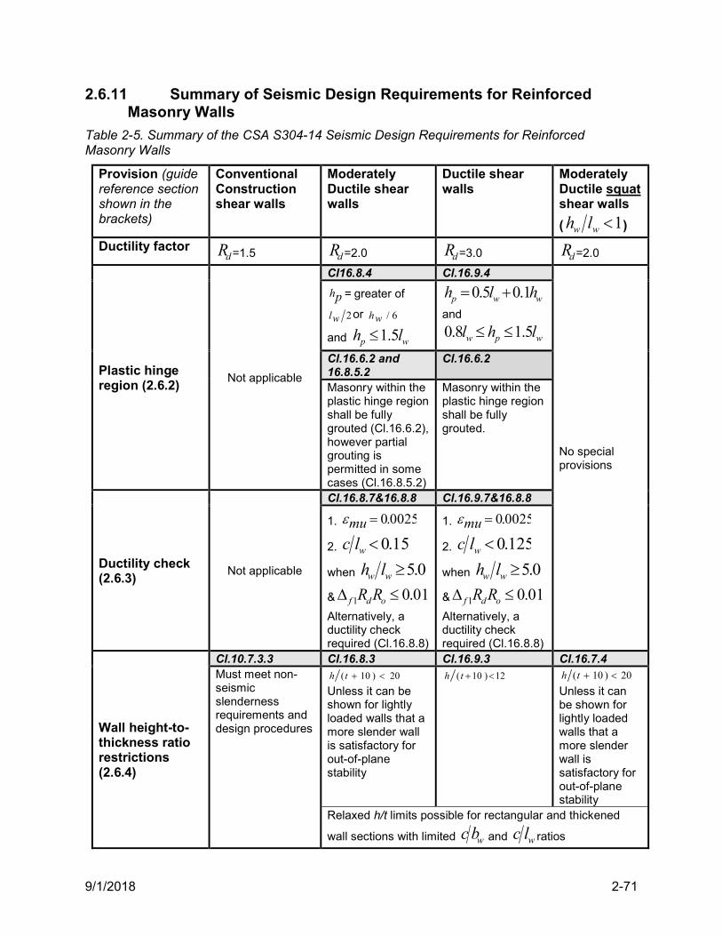
9/1/2018 2-71

2.6.11 Summary of Seismic Design Requirements for Reinforced Masonry Walls

Table 2-5. Summary of the CSA S304-14 Seismic Design Requirements for Reinforced Masonry Walls

Provision (guide reference section shown in the brackets)

Conventional Construction shear walls

Moderately Ductile shear walls

Ductile shear walls

Moderately Ductile squat shear walls

( 1ww lh )

Ductility factor dR =1.5 dR =2.0 dR =3.0 dR =2.0

Plastic hinge region (2.6.2)

Not applicable

Cl16.8.4 Cl.16.9.4

No special provisions

hp = greater of

2wl or 6/wh

and 1.5p wh l

0.5 0.1p w wh l h

and

0.8 1.5w p wl h l

Cl.16.6.2 and 16.8.5.2

Cl.16.6.2

Masonry within the plastic hinge region shall be fully grouted (Cl.16.6.2), however partial grouting is permitted in some cases (Cl.16.8.5.2)

Masonry within the plastic hinge region shall be fully grouted.

Ductility check (2.6.3)

Not applicable

Cl.16.8.7&16.8.8 Cl.16.9.7&16.8.8

1. 0025.0mu

2. 15.0wlc

when 0.5ww lh

& 01.01 odf RR

Alternatively, a ductility check required (Cl.16.8.8)

1. 0025.0mu

2. 125.0wlc

when 0.5ww lh

& 01.01 odf RR

Alternatively, a ductility check required (Cl.16.8.8)

Wall height-to-thickness ratio restrictions (2.6.4)

Cl.10.7.3.3 Cl.16.8.3 Cl.16.9.3 Cl.16.7.4 Must meet non-seismic slenderness requirements and design procedures

20)10( th

Unless it can be shown for lightly loaded walls that a more slender wall is satisfactory for out-of-plane stability

12)10( th 20)10( th

Unless it can be shown for lightly loaded walls that a more slender wall is satisfactory for out-of-plane stability

Relaxed h/t limits possible for rectangular and thickened

wall sections with limited wbc and wlc ratios

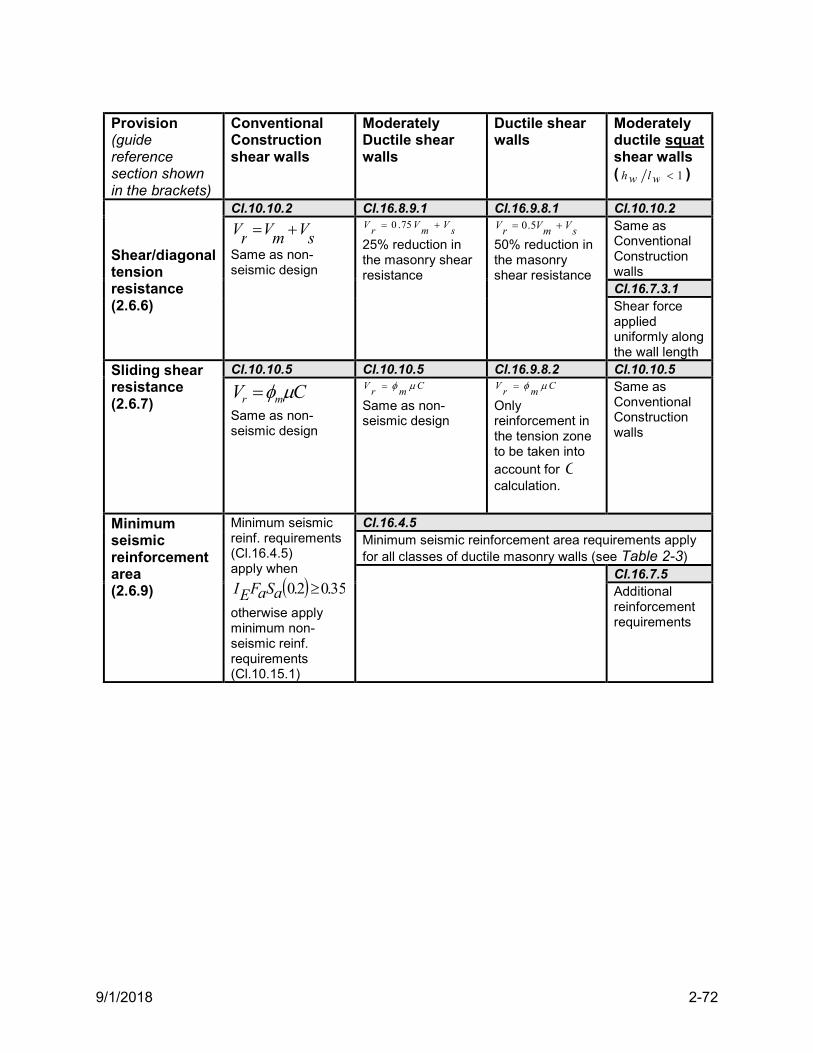
9/1/2018 2-72

Provision (guide reference section shown in the brackets)

Conventional Construction shear walls

Moderately Ductile shear walls

Ductile shear walls

Moderately ductile squat shear walls ( 1wlwh )

Shear/diagonal tension resistance (2.6.6)

Cl.10.10.2 Cl.16.8.9.1 Cl.16.9.8.1 Cl.10.10.2

sVmVrV

Same as non-seismic design

sV

mV

rV 75.0

25% reduction in the masonry shear resistance

sVmVrV 5.0

50% reduction in the masonry shear resistance

Same as Conventional Construction walls Cl.16.7.3.1 Shear force applied uniformly along the wall length

Sliding shear resistance (2.6.7)

Cl.10.10.5 Cl.10.10.5 Cl.16.9.8.2 Cl.10.10.5

CV mr

Same as non-seismic design

Cmr

V

Same as non-seismic design

Cmr

V

Only reinforcement in the tension zone to be taken into account for C calculation.

Same as Conventional Construction walls

Minimum seismic reinforcement area (2.6.9)

Minimum seismic reinf. requirements (Cl.16.4.5) apply when

35.02.0 aSaFEI

otherwise apply minimum non-seismic reinf. requirements (Cl.10.15.1)

Cl.16.4.5 Minimum seismic reinforcement area requirements apply for all classes of ductile masonry walls (see Table 2-3)

Cl.16.7.5 Additional reinforcement requirements

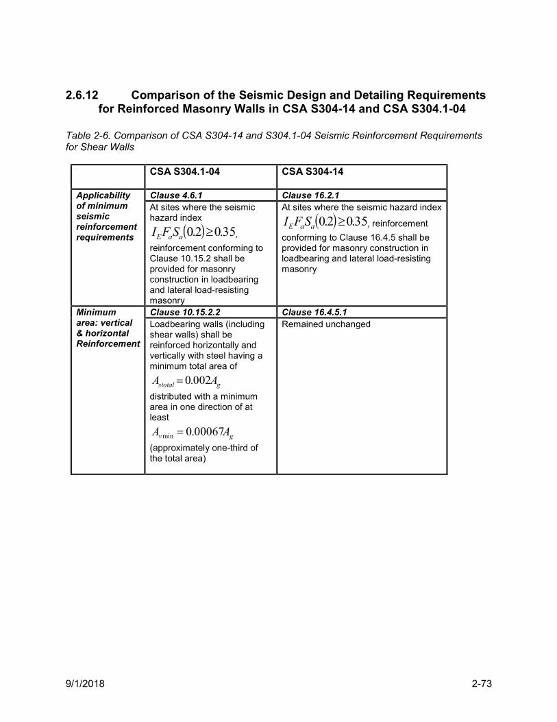
9/1/2018 2-73

2.6.12 Comparison of the Seismic Design and Detailing Requirements for Reinforced Masonry Walls in CSA S304-14 and CSA S304.1-04

Table 2-6. Comparison of CSA S304-14 and S304.1-04 Seismic Reinforcement Requirements for Shear Walls

CSA S304.1-04

CSA S304-14

Applicability of minimum seismic reinforcement requirements

Clause 4.6.1 Clause 16.2.1 At sites where the seismic hazard index

35.02.0 aaE SFI ,

reinforcement conforming to Clause 10.15.2 shall be provided for masonry construction in loadbearing and lateral load-resisting masonry

At sites where the seismic hazard index

35.02.0 aaE SFI , reinforcement

conforming to Clause 16.4.5 shall be provided for masonry construction in loadbearing and lateral load-resisting masonry

Minimum area: vertical & horizontal Reinforcement

Clause 10.15.2.2 Clause 16.4.5.1 Loadbearing walls (including shear walls) shall be reinforced horizontally and vertically with steel having a minimum total area of

gstotal AA 002.0

distributed with a minimum area in one direction of at least

gv AA 00067.0min (approximately one-third of the total area)

Remained unchanged

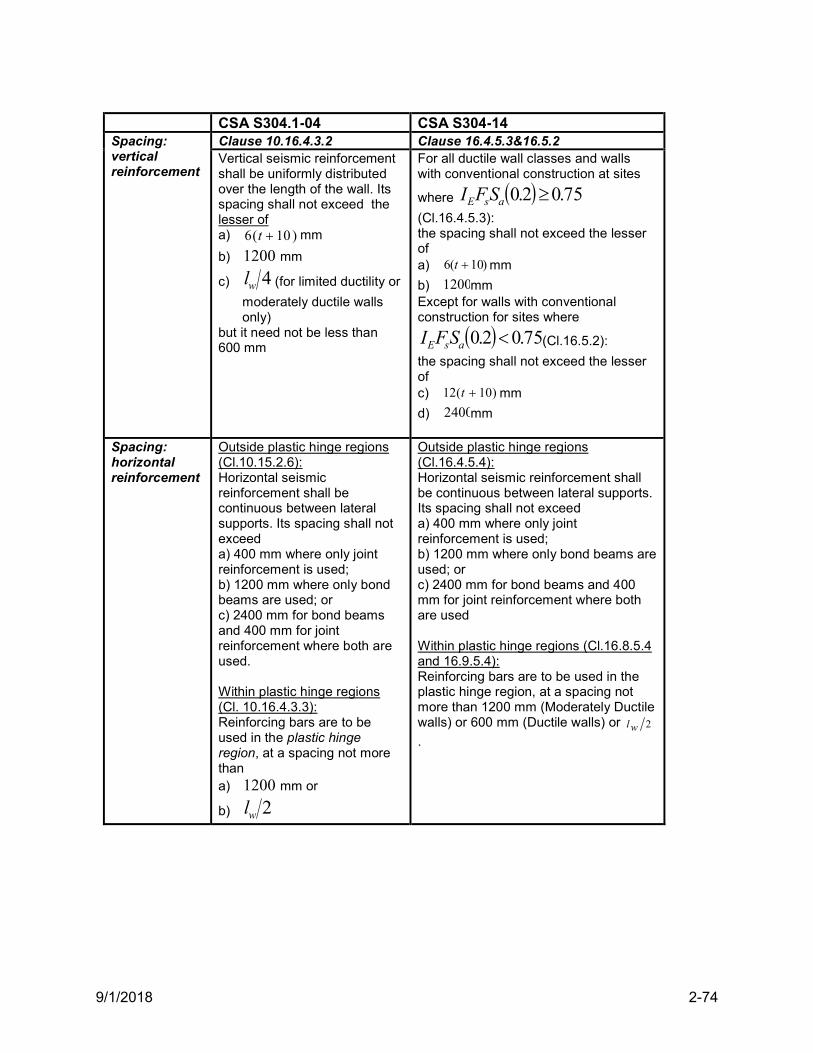
9/1/2018 2-74

CSA S304.1-04 CSA S304-14 Spacing: vertical reinforcement

Clause 10.16.4.3.2 Clause 16.4.5.3&16.5.2 Vertical seismic reinforcement shall be uniformly distributed over the length of the wall. Its spacing shall not exceed the lesser of a) )10(6 t mm

b) 1200 mm

c) 4wl (for limited ductility or

moderately ductile walls only)

but it need not be less than 600 mm

For all ductile wall classes and walls with conventional construction at sites

where 75.02.0 asE SFI(Cl.16.4.5.3): the spacing shall not exceed the lesser of a) )10(6 t mm

b) 1200mm Except for walls with conventional construction for sites where

75.02.0 asE SFI (Cl.16.5.2):

the spacing shall not exceed the lesser of c) )10(12 t mm

d) 2400mm

Spacing: horizontal reinforcement

Outside plastic hinge regions (Cl.10.15.2.6): Horizontal seismic reinforcement shall be continuous between lateral supports. Its spacing shall not exceed a) 400 mm where only joint reinforcement is used; b) 1200 mm where only bond beams are used; or c) 2400 mm for bond beams and 400 mm for joint reinforcement where both are used. Within plastic hinge regions (Cl. 10.16.4.3.3): Reinforcing bars are to be used in the plastic hinge region, at a spacing not more than a) 1200 mm or

b) 2wl

Outside plastic hinge regions (Cl.16.4.5.4): Horizontal seismic reinforcement shall be continuous between lateral supports. Its spacing shall not exceed a) 400 mm where only joint reinforcement is used; b) 1200 mm where only bond beams are used; or c) 2400 mm for bond beams and 400 mm for joint reinforcement where both are used Within plastic hinge regions (Cl.16.8.5.4 and 16.9.5.4): Reinforcing bars are to be used in the plastic hinge region, at a spacing not more than 1200 mm (Moderately Ductile walls) or 600 mm (Ductile walls) or 2wl

.

9/1/2018 2-75

2.7 Special Topics

2.7.1 Unreinforced Masonry Shear Walls According to NBC 2015 Cl.4.1.8.9.(1) (Table 4.1.8.9) and S304-14 Cl. 16.2.1, unreinforced

masonry SFRS can be constructed at sites where 35.02.0 asE SFI .

According to S304-14 Cl.16.2.2, unreinforced shear walls shall not be combined with shear walls designed as reinforced shear walls in a SFRS where shear walls share the lateral load as a function of wall rigidity. S304-14 seismic design provisions for unreinforced masonry shear walls are presented in this section. 2.7.1.1 Shear/diagonal tension resistance (in-plane and out-of-plane)

7.10.1 7.10.2 7.10.3

The design provisions for factored in-plane and out-of-plane diagonal tension shear resistance,

rV , for unreinforced masonry shear walls are the same as those for RM walls, except that there is no steel contribution term ( 0sV ). The background for these provisions is discussed in detail in Sections 2.3.2 and 2.4.2. Commentary

Diagonal tension is a brittle failure mode, characterized by the development of a major diagonal crack that forms when the masonry tensile resistance has been reached (see Section 2.3.1.2). This is an undesirable failure mechanism and should be avoided, preferably by providing horizontal reinforcement in masonry walls loaded in-plane and located in regions where

35.02.0 aaE SFI . 2.7.1.2 Sliding shear resistance (in-plane and out-of-plane)

7.10.5.1 7.10.5.2

Design provisions for in-plane and out-of-plane sliding shear resistance for unreinforced masonry walls are somewhat different from those for RM, in that both bed-joint sliding masonry resistance and the frictional resistance are considered. Note that in RM walls only frictional resistance is considered, as discussed in Section 2.3.3. The in-plane sliding shear resistance,

rV , along bed joints between courses of masonry, also known as bed-joint sliding resistance, is given in Cl.7.10.5.1 as

116.0 PAfV mucmmr

where = the coefficient of friction

= 1.0 for a masonry-to-masonry or masonry-to-roughened concrete sliding plane

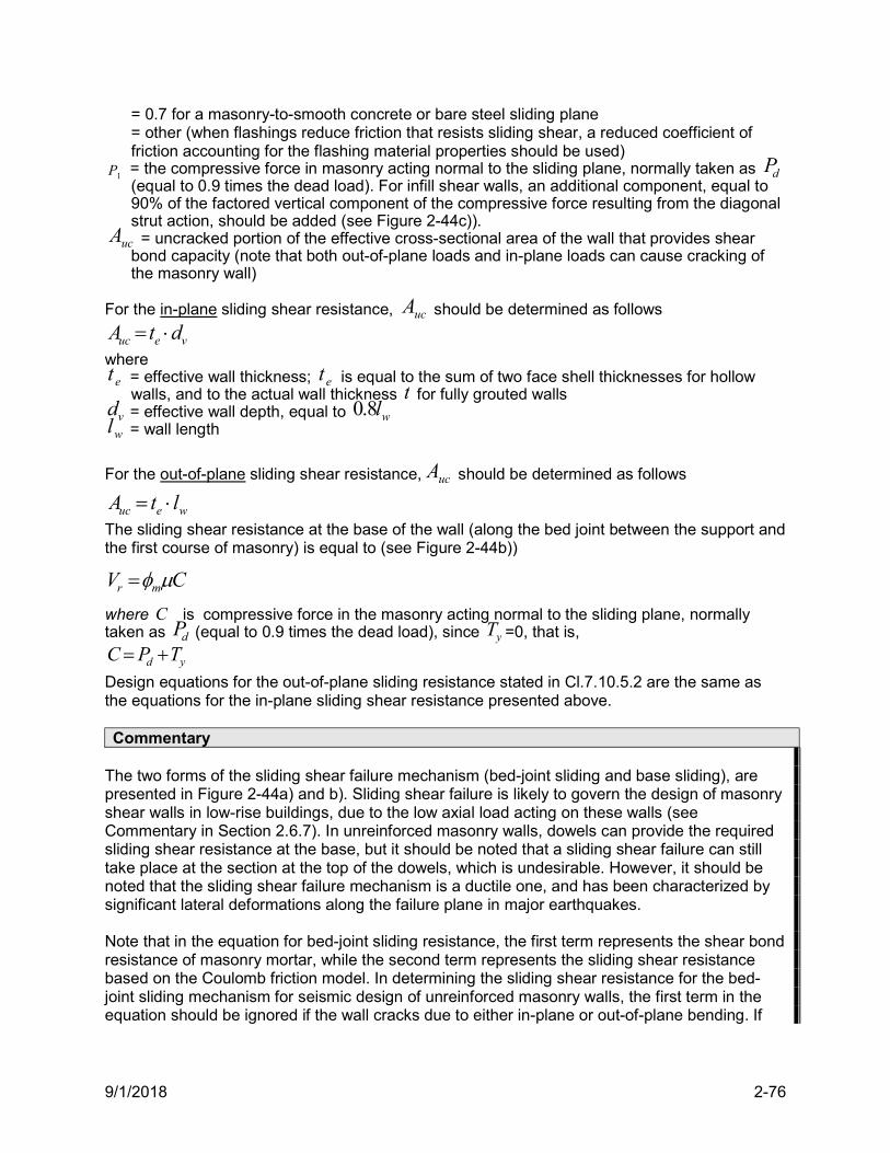
9/1/2018 2-76

= 0.7 for a masonry-to-smooth concrete or bare steel sliding plane = other (when flashings reduce friction that resists sliding shear, a reduced coefficient of friction accounting for the flashing material properties should be used)

1P = the compressive force in masonry acting normal to the sliding plane, normally taken as dP (equal to 0.9 times the dead load). For infill shear walls, an additional component, equal to 90% of the factored vertical component of the compressive force resulting from the diagonal strut action, should be added (see Figure 2-44c)).

ucA = uncracked portion of the effective cross-sectional area of the wall that provides shear bond capacity (note that both out-of-plane loads and in-plane loads can cause cracking of the masonry wall)

For the in-plane sliding shear resistance, ucA should be determined as follows

veuc dtA

where et = effective wall thickness; et is equal to the sum of two face shell thicknesses for hollow

walls, and to the actual wall thickness t for fully grouted walls vd = effective wall depth, equal to wl8.0 wl = wall length

For the out-of-plane sliding shear resistance, ucA should be determined as follows

weuc ltA

The sliding shear resistance at the base of the wall (along the bed joint between the support and the first course of masonry) is equal to (see Figure 2-44b))

CV mr

where C is compressive force in the masonry acting normal to the sliding plane, normally taken as dP (equal to 0.9 times the dead load), since yT =0, that is,

yd TPC

Design equations for the out-of-plane sliding resistance stated in Cl.7.10.5.2 are the same as the equations for the in-plane sliding shear resistance presented above. Commentary

The two forms of the sliding shear failure mechanism (bed-joint sliding and base sliding), are presented in Figure 2-44a) and b). Sliding shear failure is likely to govern the design of masonry shear walls in low-rise buildings, due to the low axial load acting on these walls (see Commentary in Section 2.6.7). In unreinforced masonry walls, dowels can provide the required sliding shear resistance at the base, but it should be noted that a sliding shear failure can still take place at the section at the top of the dowels, which is undesirable. However, it should be noted that the sliding shear failure mechanism is a ductile one, and has been characterized by significant lateral deformations along the failure plane in major earthquakes. Note that in the equation for bed-joint sliding resistance, the first term represents the shear bond resistance of masonry mortar, while the second term represents the sliding shear resistance based on the Coulomb friction model. In determining the sliding shear resistance for the bed-joint sliding mechanism for seismic design of unreinforced masonry walls, the first term in the equation should be ignored if the wall cracks due to either in-plane or out-of-plane bending. If

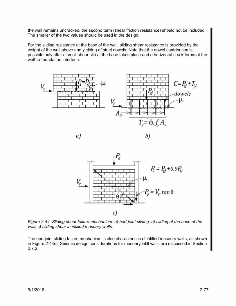
9/1/2018 2-77

the wall remains uncracked, the second term (shear friction resistance) should not be included. The smaller of the two values should be used in the design. For the sliding resistance at the base of the wall, sliding shear resistance is provided by the weight of the wall above and yielding of steel dowels. Note that the dowel contribution is possible only after a small shear slip at the base takes place and a horizontal crack forms at the wall-to-foundation interface.

Figure 2-44. Sliding shear failure mechanism: a) bed-joint sliding; b) sliding at the base of the wall; c) sliding shear in infilled masonry walls.

The bed-joint sliding failure mechanism is also characteristic of infilled masonry walls, as shown in Figure 2-44c). Seismic design considerations for masonry infill walls are discussed in Section 2.7.2.

9/1/2018 2-78

2.7.1.3 Flexural resistance due to combined axial load and bending

7.2 A masonry wall of length, wl , and thickness, t , subjected to factored axial load, fP , and factored bending moment, fM , has an eccentricity, e, equal to

f

f

P

Me

According to Cl.7.2.3, unreinforced masonry walls should be designed to remain uncracked when

wle 33.0 for in-plane bending, or

te 33.0 for out-of-plane bending, but the maximum stresses must not exceed tm f for tension and mm f 6.0 for compression (Cl.7.2.4), where tf is the flexural tensile strength of masonry (see Table 5 of CSA S304-14). The maximum stresses at the wall ends can be calculated as follows:

mme

f

e

fc f

S

M

A

Pf 6.0max

and

tme

f

e

ft f

S

M

A

Pf max

where fP and fM are the factored axial load and the factored bending moment acting on the wall

section

wee ltA effective cross-sectional area of masonry

et = effective wall thickness equal to the sum of two face shell thicknesses for hollow walls, and to the actual wall thickness t for fully grouted walls

6

2we

e

ltS

section modulus of effective wall cross-sectional area

An unreinforced masonry wall should be designed assuming cracked sections (Cl.7.2.1) when eccentricity about either major or minor wall axis is less than

lime , where

lime = 0.33 times the dimension of the section perpendicular to the axis about which moments are being computed for rectangular walls and columns, or

0.5 times the distance from the centroid of the section to the extreme compression fibre in the direction of bending for non-rectangular walls and columns. An equivalent rectangular stress block per Cl.10.2.6 should be used for the design. The centroid of the compression zone must coincide with the load eccentricity,e, as shown in Figure 2-45b), and the compression capacity,

rP , can then be determined from the following equation:

22

85.0

el

tfP wemmr

note that rP must be greater than fP .

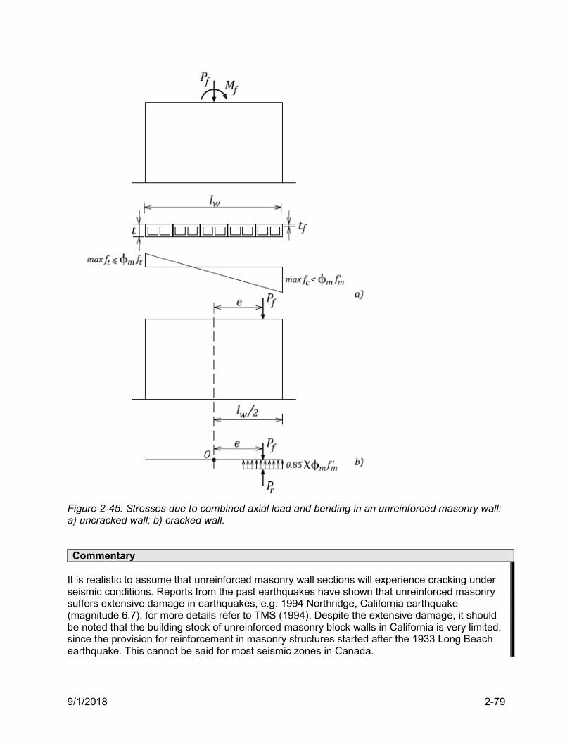
9/1/2018 2-79

Figure 2-45. Stresses due to combined axial load and bending in an unreinforced masonry wall: a) uncracked wall; b) cracked wall.

Commentary It is realistic to assume that unreinforced masonry wall sections will experience cracking under seismic conditions. Reports from the past earthquakes have shown that unreinforced masonry suffers extensive damage in earthquakes, e.g. 1994 Northridge, California earthquake (magnitude 6.7); for more details refer to TMS (1994). Despite the extensive damage, it should be noted that the building stock of unreinforced masonry block walls in California is very limited, since the provision for reinforcement in masonry structures started after the 1933 Long Beach earthquake. This cannot be said for most seismic zones in Canada.

9/1/2018 2-80

2.7.2 Masonry Infill Walls

7.13 10.12

Infill walls are masonry wall panels enclosed by reinforced concrete or steel frame members on all four sides. Infill walls are not listed as a wall class in NBC 2015, and therefore fall under the classification of “other masonry SFRS(s)”. They are only allowed in low seismic regions where

20.02.0 aaE SFI , and have 0.1 od RR and a height limitation of 15 m.

CSA S304-14 design provisions for masonry infill walls, introduced for the first time in the 2004 edition of the code, are summarized below. General design requirements

1. Masonry infill walls are treated as shear walls and should be designed to resist all in-plane and out-of-plane loads (Cl.7.13.1).

2. Masonry infill walls should be designed to resist any vertical loads transferred to them by the frame (Cl.7.13.2.4).

3. The increased stiffness of lateral load-resisting elements that consist of masonry infill shear walls working with the surrounding frame, should be taken into account when distributing the applied loads to these elements (Cl.7.13.2.5).

4. When a diagonal strut is used to model the infill shear wall according to Cl.7.13.3, an infill frame can be designed using a truss model (see the note to Cl.7.13.2.5).

Design approaches for masonry infill walls CSA S304-14 offers three possible design and construction approaches for infill walls:

1. Participating infill (diagonal strut approach) – when there are no openings or gaps between the masonry infill and the surrounding frame, but the infill is not tied or bonded to the frame, the infill should be modelled as a diagonal strut according to Cl.7.13.3. Where openings or gaps exist, the designer must show through experimental testing or special investigations that the diagonal strut action can be formed and all other structural requirements for the infill shear walls can be developed (Cl.7.13.2.3).

2. Frame and infill composite action – when the infill shear wall is tied and bonded to the frame to create a composite shear wall, where the infill forms the web and the columns of the frame form the flanges of the shear wall (Cl.7.13.2.2).

3. Isolated infill - it is also possible to design an isolated infill panel (a note to Cl.7.13.1 and Cl.7.13.2.3), which is separated from the frame structure by a gap created by vertical movement joints along the ends and a horizontal movement joint under the floor above or beam. In that case, masonry infill is a nonloadbearing wall and cannot be treated as a shear wall. Restraints must be provided at the top of the wall to ensure stability for out-of-plane seismic forces.

Diagonal strut model For structural design purposes, infill walls should be modelled as diagonal struts, as shown in Figure 2-46 (Cl.7.13.2.1). The key properties of the diagonal strut model are summarized below. Diagonal strut width w should be determined as follows (Cl.7.13.3.3):

22Lhw

where

9/1/2018 2-81

41

2sin

4

2

em

cfh tE

hIE

and

41

2sin

4

em

bfL tE

lIE

h = vertical contact length between the frame and the diagonal strut

L = horizontal contact length between the frame and the diagonal strut

mE , fE = moduli of elasticity of the masonry wall and frame material, respectively

h, l = height and length of the infill wall, respectively 2 2

dl h l length of the diagonal

et = sum of the thickness of the two face shells for hollow or semi-solid block units and the

thickness of the wall for solid or fully grouted hollow or semi-solid block units

cI , bI = moments of inertia of the column and the beam of the frame respectively

= angle of diagonal strut measured from the horizontal, where

l

htan

Effective diagonal strut width, ew , to be used for the strength calculations should be taken as (Cl.7.13.3.4)

2wwe

or

4e dw l

whichever is the least. The design length of the diagonal strut, sl , should be equal to (Cl.7.13.3.5)

2s dl l w

Depending on the strut end conditions (fixed or pinned), an effective length can be calculated by multiplying the design length by the effective length factor for compression members,k (see Annex B to CSA S304-14). The design length for the diagonal strut in reinforced infill walls should be determined as the smallest of the following (Cl.10.12.3): design length sl as defined above, or infill wall height h or length l , when minimum reinforcement and lateral anchorage are provided for the span in that direction. In-plane resistance of masonry infill walls According to CSA S304-14, masonry infills should be designed considering the following failure mechanisms: Compression or buckling failure in diagonal strut, and In-plane shear failure of the masonry infill. Diagonal strut – compression resistance (Cl.7.13.3.4.3)

9/1/2018 2-82

The compression strength of the diagonal strut, rP , is equal to the compression strength of the masonry times the effective cross-sectional area, that is,

emmr AfP 85.0

where

eee twA *

Note that the masonry compressive strength should be reduced by 5.0 (corresponding to the masonry strength for compression normal to the head joints). The concept of effective cross-sectional area is addressed by S304-14 Cl.7.3 (unreinforced masonry walls) and Cl.10.3 (RM walls). Diagonal strut – buckling resistance

In determining the compression resistance, rP , slenderness effects should be included in accordance with Cl.7.7.5. The designer should ensure that the horizontal component of the diagonal strut compression

resistance, hP , is larger than the factored shear load, fV , acting on the infill (see Figure 2-46c)).

Bed-joint sliding shear resistance of infill walls (Cl.7.13.3.1 for unreinforced infills and Cl.10.12.4 for reinforced infills) Bed-joint sliding resistance is the key in-plane shear resistance mechanism characteristic, both for unreinforced and reinforced infill walls (Cl.7.10.4). See Section 2.7.1.2 for a discussion on the bed-joint sliding mechanism. Infill shear walls should be designed so that a bed-joint sliding shear failure is prevented (Cl.7.13.3.1). This failure mechanism can lead to a knee-braced condition that could cause a premature failure of the column in the surrounding frame, as shown in Figure 2-49a). CSA S304-14 Cl.10.12.4 states that the RM infills need to be designed to resist all applied shear loads in accordance with Cl.10.10.1, as they relate to the diagonal tension shear resistance discussed in Section 2.3.2 of this guide. However, it should be noted that the shear resistance corresponding to the diagonal tension cracking does not represent the limited or ultimate load condition for infill walls (see the discussion in the commentary part of this section). Sliding shear resistance of infill walls (Cl.7.13.3.2 for unreinforced infills and Cl.10.12.5 for reinforced infills) Infill shear walls should be designed for sliding shear according to Section 2.3.3, but the vertical

component of the diagonal strut compression resistance, vP , must be considered in determining

the sliding shear resistance, as shown in Figure 2-44c). Effective diagonal strut stiffness S304-14 contains a new provision regarding the effective stiffness of diagonal strut. The effective stiffness should be calculated as

s

meeffsteff l

EtwK

9/1/2018 2-83

Where sl is the strut length and st is the factor to account for the reduction in stiffness, taken as

0.5. Reinforcement Reinforcement is required to resist tensile and shear stresses in infills (Cl.10.12.2). The minimum reinforcement requirements stated in Cl.10.15 should be followed. Effect of masonry infill on frame members (Cl.7.13.3.2) Adjacent frame members and their connections should be designed to resist additional shear forces resulting from the diagonal strut action (see Note 3 to Cl.7.13.3.2). Commentary

The infilling of frames is associated with the construction of medium- and high-rise steel and reinforced concrete (RC) buildings, where the frames carry gravity and lateral loads, and the infills provide the building envelope and internal partitions. Historically, the frames have been engineered according to the state of the knowledge of the time, with the infill panels considered to be “nonstructural” elements (FEMA 306, 1999). However, recent damaging earthquakes in several countries (e.g. the 1999 Kocaeli earthquake in Turkey, the 2001 Bhuj earthquake in India, the 2001 Chi earthquake in Taiwan, the 2003 Boumerdes earthquake in Algeria, etc.) revealed significant deficiencies and poor seismic performance of RC frame buildings with masonry infills, thereby causing significant human and economic losses (Murty, Brzev, et al. 2006). The introduction of infills into frames changes the lateral-load transfer mechanism of the structure from a predominantly frame action to a predominantly truss action, as shown on Figure 2-37 (Kaushik, Rai, and Jain, 2006). Masonry infills in RC or steel frame buildings are usually modelled as diagonal compression struts, so an infilled frame can be modelled as a braced frame with pin connections at beam-column joints. It should be recognized that the seismic response of infilled frames is very complex. At a low level of seismic loads, the infill panels are uncracked and often cause a significant increase in the stiffness of the entire structure. In some cases, the stiffness of a RC frame with infills may be in the order of 20 times larger than that of the bare frame. At that stage, infills usually attract most of the lateral forces, but as the load increases, the infills crack and their stiffness drops. As a result, the stiffness of an infilled frame progressively decreases in each subsequent loading cycle, and more of the load is transferred to the frame. For that reason, the frames must have sufficient strength to avoid the collapse of the structure (Kaushik, Rai, and Jain, 2006). CSA S304-14 requires that masonry infills should be able to resist the lateral seismic loads without any assistance from the frames (Cl.7.13.3.1). To safeguard frames from being designed for very low seismic forces, some building codes require that the frame alone be designed to independently resist at least 25% of the design seismic forces, in addition to the forces caused by gravity loads. CSA S304-14 Cl.7.13.3.2 (Note 3) states that the frame members and their connections should be designed to resist additional shear forces introduced by the diagonal strut action. For example, the columns will have to resist a shear force equal to the horizontal component of the diagonal strut compression resistance, hP (see Figure 2-46c)).

9/1/2018 2-84

The following two analytical models can be considered in the design of infilled frames (see Figure 2-47):

i) uncracked braced frame with diagonal struts; this model results in a high stiffness (corresponding to a short period) and small lateral deflections, and

ii) bare frame with cracked frame members (assuming failed infills); this model results in a low stiffness (corresponding to a long period) and large deflections.

It should be noted that the first model will give the maximum design forces, while the second one will give the maximum lateral deflections. The designer needs to consider both models in the analysis and use the most critical values for the design. Problems associated with seismic performance of infilled frame structures arise from discontinuities of infills along the building height, and the resulting vertical stiffness discontinuity (see the discussion on irregularities in Section 1.12.1). In such infilled frames, there is a high level of forces to be resisted by the frame components. In some cases, discontinuity of infills at the ground floor level results in a soft storey mechanism, which has caused the collapse of several buildings in past earthquakes (see Figure 2-48). In developing countries, construction quality combined with inadequate detailing of RC frame components may occur, which leads to a non-ductile seismic response of these structures.

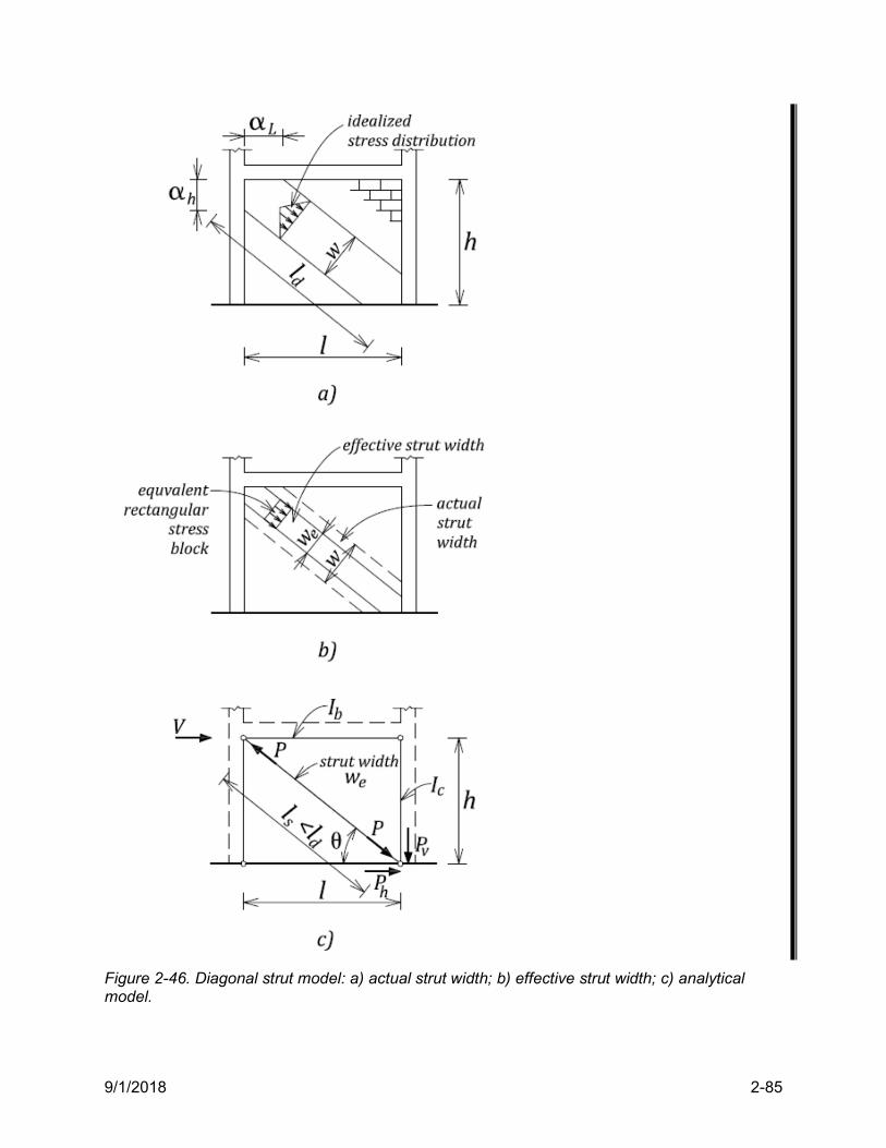
9/1/2018 2-85

Figure 2-46. Diagonal strut model: a) actual strut width; b) effective strut width; c) analytical model.

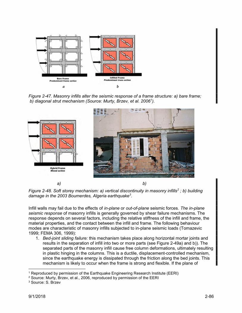
9/1/2018 2-86

Figure 2-47. Masonry infills alter the seismic response of a frame structure: a) bare frame; b) diagonal strut mechanism (Source: Murty, Brzev, et al. 20061).

a) b)

Figure 2-48. Soft storey mechanism: a) vertical discontinuity in masonry infills2 ; b) building damage in the 2003 Boumerdes, Algeria earthquake3.

Infill walls may fail due to the effects of in-plane or out-of-plane seismic forces. The in-plane seismic response of masonry infills is generally governed by shear failure mechanisms. The response depends on several factors, including the relative stiffness of the infill and frame, the material properties, and the contact between the infill and frame. The following behaviour modes are characteristic of masonry infills subjected to in-plane seismic loads (Tomazevic 1999; FEMA 306, 1999):

1. Bed-joint sliding failure: this mechanism takes place along horizontal mortar joints and results in the separation of infill into two or more parts (see Figure 2-49a) and b)). The separated parts of the masonry infill cause free column deformations, ultimately resulting in plastic hinging in the columns. This is a ductile, displacement-controlled mechanism, since the earthquake energy is dissipated through the friction along the bed joints. This mechanism is likely to occur when the frame is strong and flexible. If the plane of

1 Reproduced by permission of the Earthquake Engineering Research Institute (EERI) 2 Source: Murty, Brzev, et al., 2006, reproduced by permission of the EERI 3 Source: S. Brzev

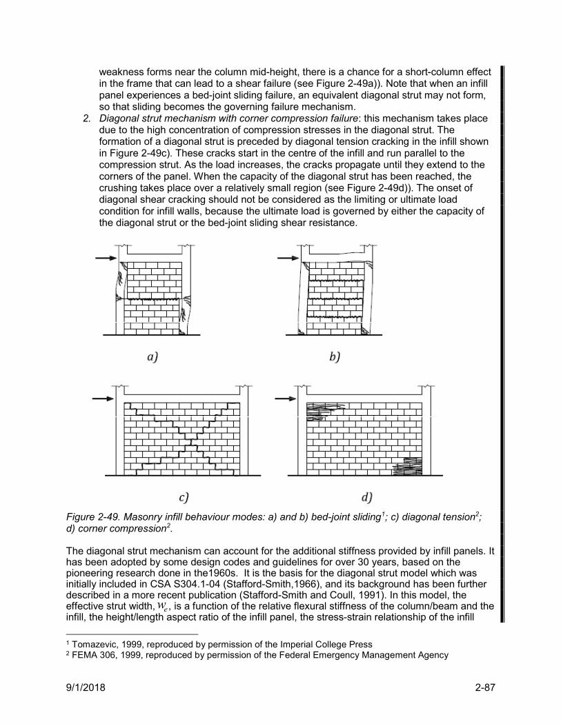
9/1/2018 2-87

weakness forms near the column mid-height, there is a chance for a short-column effect in the frame that can lead to a shear failure (see Figure 2-49a)). Note that when an infill panel experiences a bed-joint sliding failure, an equivalent diagonal strut may not form, so that sliding becomes the governing failure mechanism.

2. Diagonal strut mechanism with corner compression failure: this mechanism takes place due to the high concentration of compression stresses in the diagonal strut. The formation of a diagonal strut is preceded by diagonal tension cracking in the infill shown in Figure 2-49c). These cracks start in the centre of the infill and run parallel to the compression strut. As the load increases, the cracks propagate until they extend to the corners of the panel. When the capacity of the diagonal strut has been reached, the crushing takes place over a relatively small region (see Figure 2-49d)). The onset of diagonal shear cracking should not be considered as the limiting or ultimate load condition for infill walls, because the ultimate load is governed by either the capacity of the diagonal strut or the bed-joint sliding shear resistance.

Figure 2-49. Masonry infill behaviour modes: a) and b) bed-joint sliding1; c) diagonal tension2; d) corner compression2. The diagonal strut mechanism can account for the additional stiffness provided by infill panels. It has been adopted by some design codes and guidelines for over 30 years, based on the pioneering research done in the1960s. It is the basis for the diagonal strut model which was initially included in CSA S304.1-04 (Stafford-Smith,1966), and its background has been further described in a more recent publication (Stafford-Smith and Coull, 1991). In this model, the effective strut width, ew , is a function of the relative flexural stiffness of the column/beam and the infill, the height/length aspect ratio of the infill panel, the stress-strain relationship of the infill

1 Tomazevic, 1999, reproduced by permission of the Imperial College Press 2 FEMA 306, 1999, reproduced by permission of the Federal Emergency Management Agency

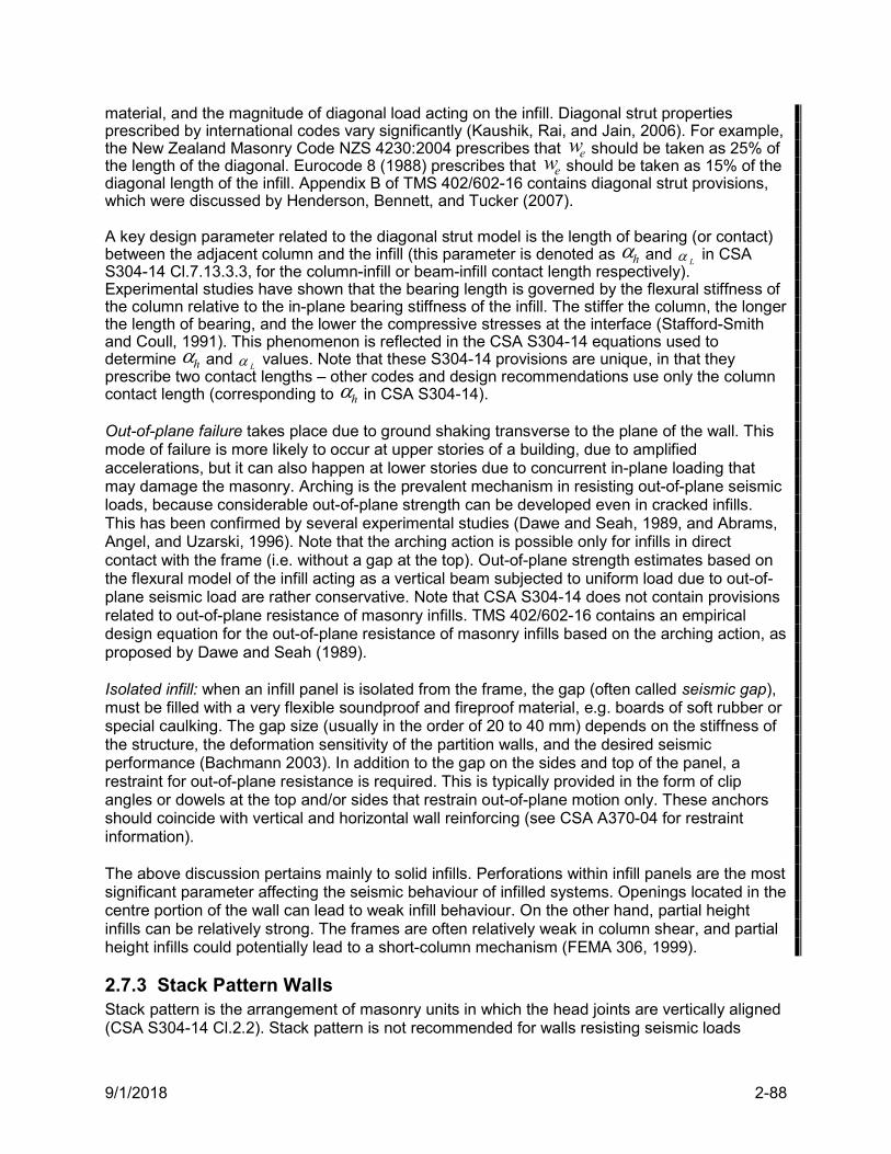
9/1/2018 2-88

material, and the magnitude of diagonal load acting on the infill. Diagonal strut properties prescribed by international codes vary significantly (Kaushik, Rai, and Jain, 2006). For example, the New Zealand Masonry Code NZS 4230:2004 prescribes that ew should be taken as 25% of the length of the diagonal. Eurocode 8 (1988) prescribes that ew should be taken as 15% of the diagonal length of the infill. Appendix B of TMS 402/602-16 contains diagonal strut provisions, which were discussed by Henderson, Bennett, and Tucker (2007). A key design parameter related to the diagonal strut model is the length of bearing (or contact) between the adjacent column and the infill (this parameter is denoted as h and

L in CSA S304-14 Cl.7.13.3.3, for the column-infill or beam-infill contact length respectively). Experimental studies have shown that the bearing length is governed by the flexural stiffness of the column relative to the in-plane bearing stiffness of the infill. The stiffer the column, the longer the length of bearing, and the lower the compressive stresses at the interface (Stafford-Smith and Coull, 1991). This phenomenon is reflected in the CSA S304-14 equations used to determine h and

L values. Note that these S304-14 provisions are unique, in that they prescribe two contact lengths – other codes and design recommendations use only the column contact length (corresponding to h in CSA S304-14). Out-of-plane failure takes place due to ground shaking transverse to the plane of the wall. This mode of failure is more likely to occur at upper stories of a building, due to amplified accelerations, but it can also happen at lower stories due to concurrent in-plane loading that may damage the masonry. Arching is the prevalent mechanism in resisting out-of-plane seismic loads, because considerable out-of-plane strength can be developed even in cracked infills. This has been confirmed by several experimental studies (Dawe and Seah, 1989, and Abrams, Angel, and Uzarski, 1996). Note that the arching action is possible only for infills in direct contact with the frame (i.e. without a gap at the top). Out-of-plane strength estimates based on the flexural model of the infill acting as a vertical beam subjected to uniform load due to out-of-plane seismic load are rather conservative. Note that CSA S304-14 does not contain provisions related to out-of-plane resistance of masonry infills. TMS 402/602-16 contains an empirical design equation for the out-of-plane resistance of masonry infills based on the arching action, as proposed by Dawe and Seah (1989). Isolated infill: when an infill panel is isolated from the frame, the gap (often called seismic gap), must be filled with a very flexible soundproof and fireproof material, e.g. boards of soft rubber or special caulking. The gap size (usually in the order of 20 to 40 mm) depends on the stiffness of the structure, the deformation sensitivity of the partition walls, and the desired seismic performance (Bachmann 2003). In addition to the gap on the sides and top of the panel, a restraint for out-of-plane resistance is required. This is typically provided in the form of clip angles or dowels at the top and/or sides that restrain out-of-plane motion only. These anchors should coincide with vertical and horizontal wall reinforcing (see CSA A370-04 for restraint information). The above discussion pertains mainly to solid infills. Perforations within infill panels are the most significant parameter affecting the seismic behaviour of infilled systems. Openings located in the centre portion of the wall can lead to weak infill behaviour. On the other hand, partial height infills can be relatively strong. The frames are often relatively weak in column shear, and partial height infills could potentially lead to a short-column mechanism (FEMA 306, 1999).

2.7.3 Stack Pattern Walls Stack pattern is the arrangement of masonry units in which the head joints are vertically aligned (CSA S304-14 Cl.2.2). Stack pattern is not recommended for walls resisting seismic loads

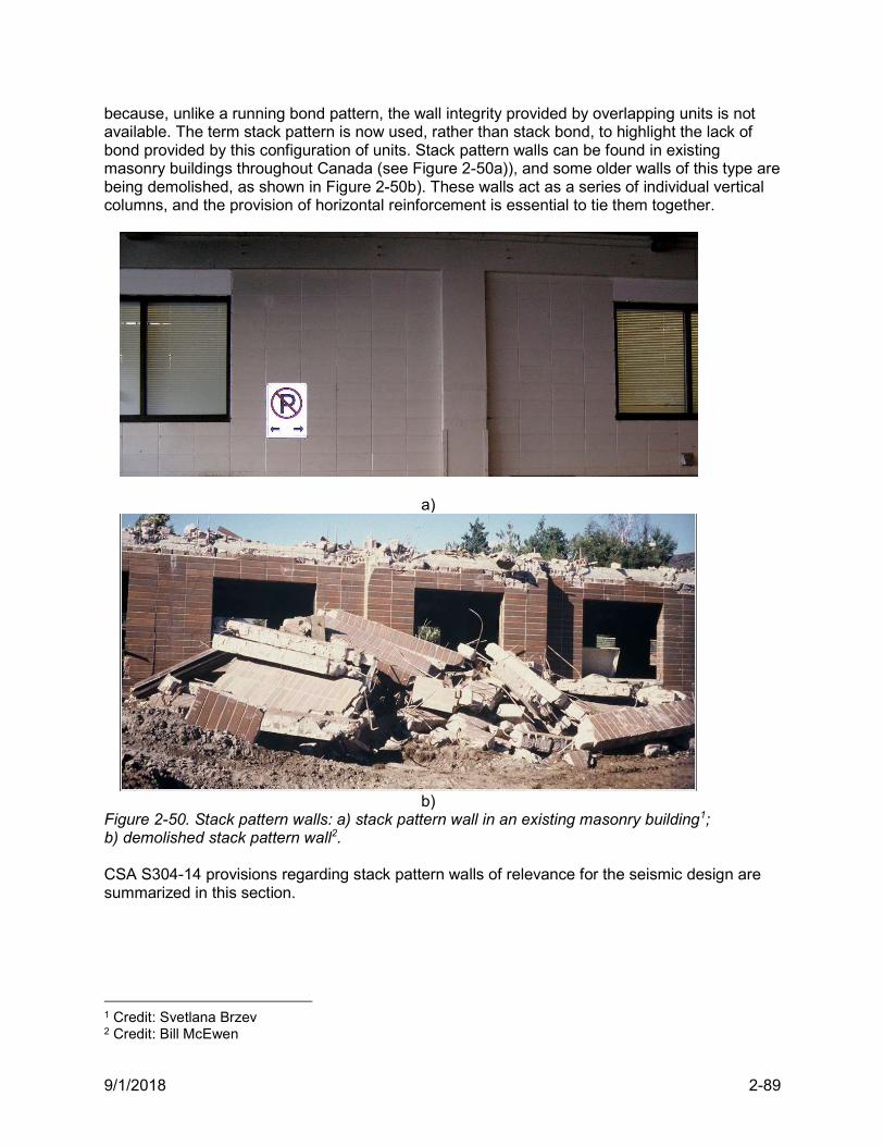
9/1/2018 2-89

because, unlike a running bond pattern, the wall integrity provided by overlapping units is not available. The term stack pattern is now used, rather than stack bond, to highlight the lack of bond provided by this configuration of units. Stack pattern walls can be found in existing masonry buildings throughout Canada (see Figure 2-50a)), and some older walls of this type are being demolished, as shown in Figure 2-50b). These walls act as a series of individual vertical columns, and the provision of horizontal reinforcement is essential to tie them together.

a)

b)

Figure 2-50. Stack pattern walls: a) stack pattern wall in an existing masonry building1; b) demolished stack pattern wall2. CSA S304-14 provisions regarding stack pattern walls of relevance for the seismic design are summarized in this section.

1 Credit: Svetlana Brzev 2 Credit: Bill McEwen

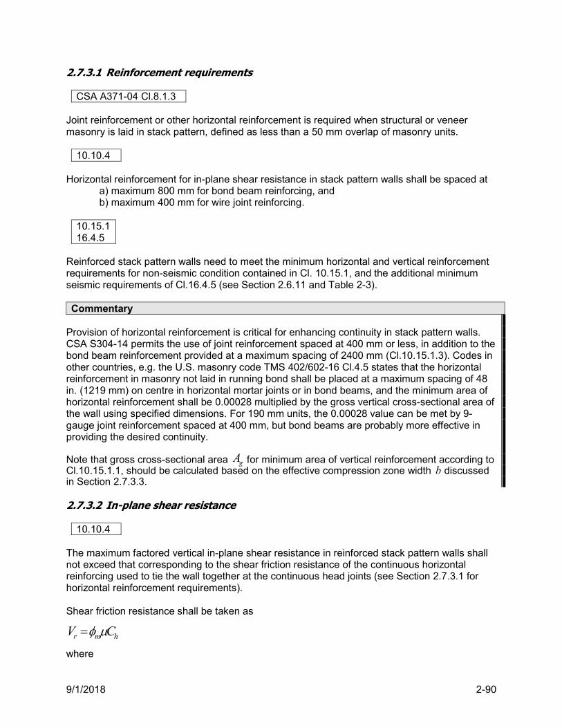
9/1/2018 2-90

2.7.3.1 Reinforcement requirements

CSA A371-04 Cl.8.1.3 Joint reinforcement or other horizontal reinforcement is required when structural or veneer masonry is laid in stack pattern, defined as less than a 50 mm overlap of masonry units.

10.10.4 Horizontal reinforcement for in-plane shear resistance in stack pattern walls shall be spaced at

a) maximum 800 mm for bond beam reinforcing, and b) maximum 400 mm for wire joint reinforcing.

10.15.1 16.4.5

Reinforced stack pattern walls need to meet the minimum horizontal and vertical reinforcement requirements for non-seismic condition contained in Cl. 10.15.1, and the additional minimum seismic requirements of Cl.16.4.5 (see Section 2.6.11 and Table 2-3). Commentary

Provision of horizontal reinforcement is critical for enhancing continuity in stack pattern walls. CSA S304-14 permits the use of joint reinforcement spaced at 400 mm or less, in addition to the bond beam reinforcement provided at a maximum spacing of 2400 mm (Cl.10.15.1.3). Codes in other countries, e.g. the U.S. masonry code TMS 402/602-16 Cl.4.5 states that the horizontal reinforcement in masonry not laid in running bond shall be placed at a maximum spacing of 48 in. (1219 mm) on centre in horizontal mortar joints or in bond beams, and the minimum area of horizontal reinforcement shall be 0.00028 multiplied by the gross vertical cross-sectional area of the wall using specified dimensions. For 190 mm units, the 0.00028 value can be met by 9-gauge joint reinforcement spaced at 400 mm, but bond beams are probably more effective in providing the desired continuity. Note that gross cross-sectional area gA for minimum area of vertical reinforcement according to Cl.10.15.1.1, should be calculated based on the effective compression zone width b discussed in Section 2.7.3.3. 2.7.3.2 In-plane shear resistance

10.10.4 The maximum factored vertical in-plane shear resistance in reinforced stack pattern walls shall not exceed that corresponding to the shear friction resistance of the continuous horizontal reinforcing used to tie the wall together at the continuous head joints (see Section 2.7.3.1 for horizontal reinforcement requirements). Shear friction resistance shall be taken as

hmr CV

where

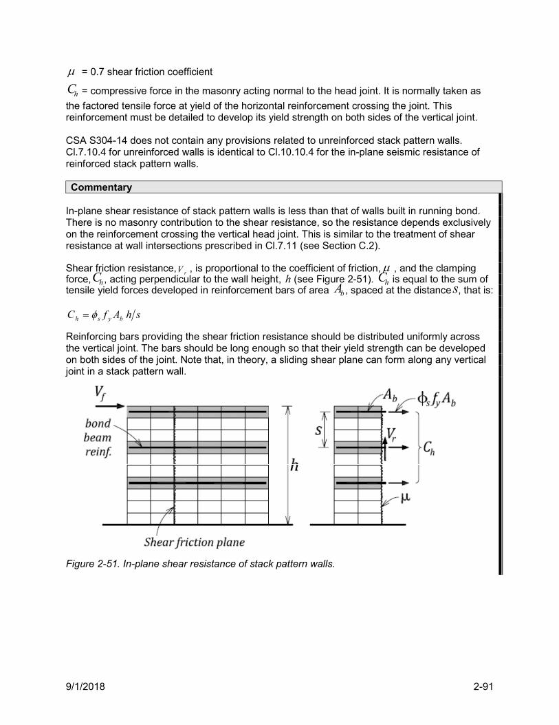
9/1/2018 2-91

= 0.7 shear friction coefficient

hC = compressive force in the masonry acting normal to the head joint. It is normally taken as

the factored tensile force at yield of the horizontal reinforcement crossing the joint. This reinforcement must be detailed to develop its yield strength on both sides of the vertical joint. CSA S304-14 does not contain any provisions related to unreinforced stack pattern walls. Cl.7.10.4 for unreinforced walls is identical to Cl.10.10.4 for the in-plane seismic resistance of reinforced stack pattern walls. Commentary

In-plane shear resistance of stack pattern walls is less than that of walls built in running bond. There is no masonry contribution to the shear resistance, so the resistance depends exclusively on the reinforcement crossing the vertical head joint. This is similar to the treatment of shear resistance at wall intersections prescribed in Cl.7.11 (see Section C.2). Shear friction resistance,

rV , is proportional to the coefficient of friction, , and the clamping force, hC , acting perpendicular to the wall height, h (see Figure 2-51). hC is equal to the sum of tensile yield forces developed in reinforcement bars of area bA , spaced at the distances, that is:

Reinforcing bars providing the shear friction resistance should be distributed uniformly across the vertical joint. The bars should be long enough so that their yield strength can be developed on both sides of the joint. Note that, in theory, a sliding shear plane can form along any vertical joint in a stack pattern wall.

Figure 2-51. In-plane shear resistance of stack pattern walls.

shAfC bysh

9/1/2018 2-92

2.7.3.3 Out-of-plane shear resistance

10.10.3 The out-of-plane shear resistance of stack pattern walls is determined according to the same provisions for walls built in running bond (see Section 2.4.3). Note that for the purpose of shear resistance calculations, b includes the width of the cell and webs at a vertical bar within the length of the reinforced unit. Commentary

Unless horizontal reinforcement is provided in sufficient amount (size and spacing), the out-of-plane shear resistance of stack pattern walls is similar to that of a series of isolated vertical columns. In Figure 2-52 some stacks are not reinforced with vertical bars and so it is important to have adequate horizontal reinforcement to tie the stacks together. 2.7.3.4 Design for the combined axial load and flexure The design approach for reinforced stack pattern walls for combined axial load and flexure is similar to that presented in Sections 2.3.4 and 2.4.4 for running bond. In determining the out-of-plane flexural resistance, the flexural tensile strength tf should be taken equal to zero for tensile resistance parallel to bed joints (S304-14 Cl.5.2.1). Also, the effective compression zone width b should be taken according to Cl.10.6.1.

10.6.1 For the case of out-of-plane loading (or “minor axis bending” as referred to in S304-14), the effective compression zone width,b, used with each vertical bar in the design of stack pattern walls with vertical reinforcement shall be taken as the lesser of a) spacing between vertical bars,s, or b) the length of the reinforced unit. Figure 2-52 shows a portion of a reinforced stack pattern wall. In this example, the length of the reinforced units is less than the spacing between bars and so the compression zone width,b, to be used with such bar is equal to the block length.

Figure 2-52. Effective compression zone width b for out-of-plane seismic effects in stack pattern walls.

9/1/2018 2-93

Commentary The seismic performance of stack pattern walls without closely spaced horizontal reinforcement has been much less satisfactory than for walls constructed in running bond. The presence of horizontal reinforcement is critical for tying together vertical columns formed by stacked blocks (NZS 4230:2004). Unreinforced stack pattern walls located in regions with moderate to high seismic risk are considered to be vulnerable to seismic effects and should be either retrofitted or demolished. It is suggested that unreinforced stack pattern walls not be used in seismic regions.

2.7.4 Nonloadbearing Walls Nonloadbearing walls resist the effects of their own dead load and any out-of-plane wind and earthquake loads. This includes partitions and exterior walls that do not support floors and roofs (S304-14 Cl.2.2). However, walls that do not support floors and roofs, but resist the in-plane forces from wind and earthquake loads are considered loadbearing shear walls (see Section 2.5.4.7 for a detailed discussion on seismic reinforcement requirements for shear walls).

16.2.1 16.2.3

With the exception noted below, nonloadbearing walls, including masonry enclosing elevator shafts and stairways must be reinforced at sites where 35.02.0 aaE SFI (Cl.16.2.1). Although not recommended by the authors, unreinforced masonry partitions can be designed for sites where 75.02.0 aaE SFI , provided that they a) have a mass less than or equal to 200 kg/m2, b) have a height less than or equal to 3 m, and c) are laterally supported at the top and bottom. Unreinforced masonry partitions that do not exceed 3 m in height and are not laterally supported at the top may be designed to span horizontally between vertical elements providing lateral support.

16.4.5 Minimum seismic reinforcement requirements for nonloadbearing walls are summarized below:

1. If 35.02.0 aaE SFI

Minimum seismic reinforcement is not required per CSA S304-14.

2. If 75.02.035.0 aaE SFI (Cl.16.4.5.2a)

Nonloadbearing walls shall be reinforced in one or more directions with reinforcing steel having a minimum total area of

gstotal AA 0005.0 The area should be taken perpendicular to the direction of the reinforcement considered. The reinforcement may be placed in one direction, provided that it is located to reinforce the wall adequately against lateral loads and that it spans between lateral supports.

3. If 75.02.0 aaE SFI (Cl.16.4.5.2b)

Nonloadbearing walls shall be reinforced horizontally and vertically with steel having a minimum total area of

gstotal AA 001.0 distributed with a minimum area in one direction of at least

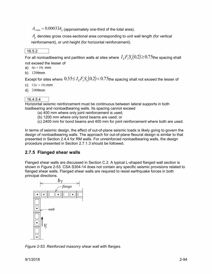
9/1/2018 2-94

gv AA 00033.0min (approximately one-third of the total area).

gA denotes gross cross-sectional area corresponding to unit wall length (for vertical

reinforcement), or unit height (for horizontal reinforcement). 16.5.2

For all nonloadbearing and partition walls at sites where 75.02.0 asE SFI the spacing shall

not exceed the lesser of a) )10(6 t mm b) 1200mm

Except for sites where 75.02.035.0 asE SFI the spacing shall not exceed the lesser of

c) )10(12 t mm d) 2400mm 16.4.5.4

Horizontal seismic reinforcement must be continuous between lateral supports in both loadbearing and nonloadbearing walls. Its spacing cannot exceed

(a) 400 mm where only joint reinforcement is used; (b) 1200 mm where only bond beams are used; or (c) 2400 mm for bond beams and 400 mm for joint reinforcement where both are used.

In terms of seismic design, the effect of out-of-plane seismic loads is likely going to govern the design of nonloadbearing walls. The approach for out-of-plane flexural design is similar to that presented in Section 2.4.4 for RM walls. For unreinforced nonloadbearing walls, the design procedure presented in Section 2.7.1.3 should be followed.

2.7.5 Flanged shear walls Flanged shear walls are discussed in Section C.2. A typical L-shaped flanged wall section is shown in Figure 2-53. CSA S304-14 does not contain any specific seismic provisions related to flanged shear walls. Flanged shear walls are required to resist earthquake forces in both principal directions.

Figure 2-53. Reinforced masonry shear wall with flanges.

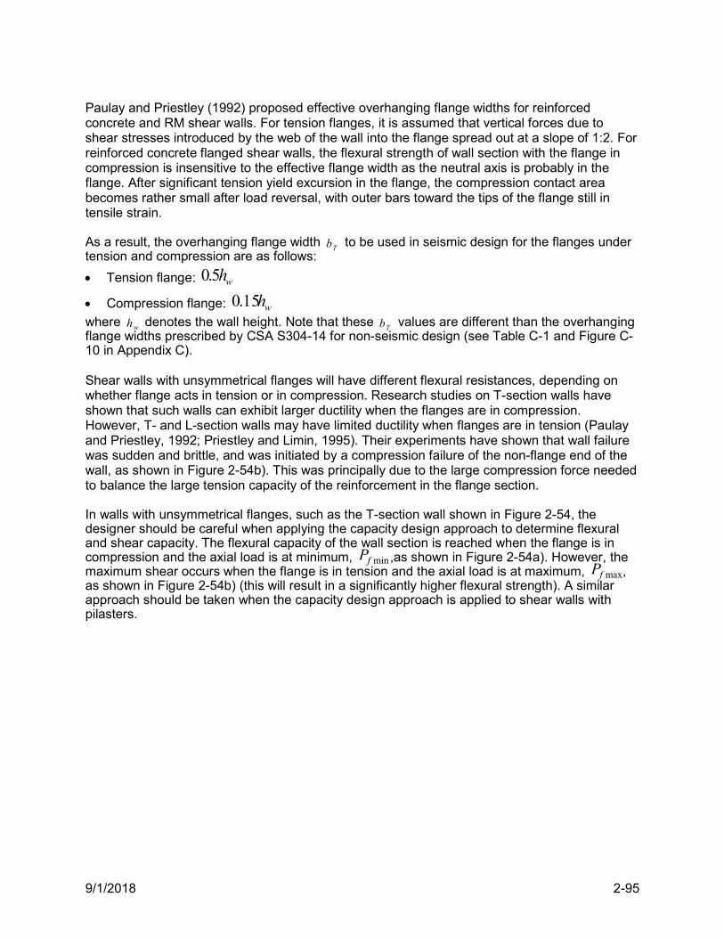
9/1/2018 2-95

Paulay and Priestley (1992) proposed effective overhanging flange widths for reinforced concrete and RM shear walls. For tension flanges, it is assumed that vertical forces due to shear stresses introduced by the web of the wall into the flange spread out at a slope of 1:2. For reinforced concrete flanged shear walls, the flexural strength of wall section with the flange in compression is insensitive to the effective flange width as the neutral axis is probably in the flange. After significant tension yield excursion in the flange, the compression contact area becomes rather small after load reversal, with outer bars toward the tips of the flange still in tensile strain. As a result, the overhanging flange width

Tb to be used in seismic design for the flanges under tension and compression are as follows:

Tension flange: wh5.0

Compression flange: wh15.0

where wh denotes the wall height. Note that these Tb values are different than the overhanging

flange widths prescribed by CSA S304-14 for non-seismic design (see Table C-1 and Figure C-10 in Appendix C). Shear walls with unsymmetrical flanges will have different flexural resistances, depending on whether flange acts in tension or in compression. Research studies on T-section walls have shown that such walls can exhibit larger ductility when the flanges are in compression. However, T- and L-section walls may have limited ductility when flanges are in tension (Paulay and Priestley, 1992; Priestley and Limin, 1995). Their experiments have shown that wall failure was sudden and brittle, and was initiated by a compression failure of the non-flange end of the wall, as shown in Figure 2-54b). This was principally due to the large compression force needed to balance the large tension capacity of the reinforcement in the flange section. In walls with unsymmetrical flanges, such as the T-section wall shown in Figure 2-54, the designer should be careful when applying the capacity design approach to determine flexural and shear capacity. The flexural capacity of the wall section is reached when the flange is in compression and the axial load is at minimum, minfP ,as shown in Figure 2-54a). However, the maximum shear occurs when the flange is in tension and the axial load is at maximum, maxfP , as shown in Figure 2-54b) (this will result in a significantly higher flexural strength). A similar approach should be taken when the capacity design approach is applied to shear walls with pilasters.

9/1/2018 2-96

Figure 2-54. T-section flanged shear wall: a) flexural design scenario: web in tension; b) shear design scenario: web in compression.

S304-14 design provisions related to shear transfer at wall intersections (including flanged walls) are discussed in Section C.2.

2.7.6 Wall-to-Diaphragm Anchorage

CSA A370-14 Masonry shear walls must be adequately anchored to floor and roof diaphragms in accordance with CSA S304-14. (CSA A370-14 Cl. 7.2.2) Anchors connecting masonry walls in general to their lateral supports must be designed to resist specified loads. The maximum anchor spacing between walls and horizontal lateral supports typically should not exceed ten times the nominal wall thickness (t+10 mm) (Cl.7.2.1). Anchors must be fully embedded in reinforced bond beams or reinforced vertical cells. When the unfactored load applied normal to a wall is greater than 0.24 kPa, the ultimate strength of a wall anchor must not be less than 1,600 N (Cl.8.2.1). Commentary

Anchorage is one of the most important and, in many cases, the most vulnerable component of existing masonry buildings exposed to earthquake effects. Many failures of masonry buildings result from a wall-diaphragm failure, that allows an out-of-plane wall failure, followed by a diaphragm failure.

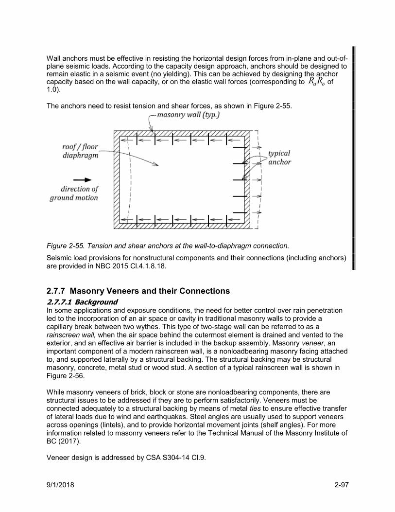
9/1/2018 2-97

Wall anchors must be effective in resisting the horizontal design forces from in-plane and out-of- plane seismic loads. According to the capacity design approach, anchors should be designed to remain elastic in a seismic event (no yielding). This can be achieved by designing the anchor capacity based on the wall capacity, or on the elastic wall forces (corresponding to odRR of 1.0). The anchors need to resist tension and shear forces, as shown in Figure 2-55.

Figure 2-55. Tension and shear anchors at the wall-to-diaphragm connection.

Seismic load provisions for nonstructural components and their connections (including anchors) are provided in NBC 2015 Cl.4.1.8.18.

2.7.7 Masonry Veneers and their Connections 2.7.7.1 Background In some applications and exposure conditions, the need for better control over rain penetration led to the incorporation of an air space or cavity in traditional masonry walls to provide a capillary break between two wythes. This type of two-stage wall can be referred to as a rainscreen wall, when the air space behind the outermost element is drained and vented to the exterior, and an effective air barrier is included in the backup assembly. Masonry veneer, an important component of a modern rainscreen wall, is a nonloadbearing masonry facing attached to, and supported laterally by a structural backing. The structural backing may be structural masonry, concrete, metal stud or wood stud. A section of a typical rainscreen wall is shown in Figure 2-56. While masonry veneers of brick, block or stone are nonloadbearing components, there are structural issues to be addressed if they are to perform satisfactorily. Veneers must be connected adequately to a structural backing by means of metal ties to ensure effective transfer of lateral loads due to wind and earthquakes. Steel angles are usually used to support veneers across openings (lintels), and to provide horizontal movement joints (shelf angles). For more information related to masonry veneers refer to the Technical Manual of the Masonry Institute of BC (2017). Veneer design is addressed by CSA S304-14 Cl.9.

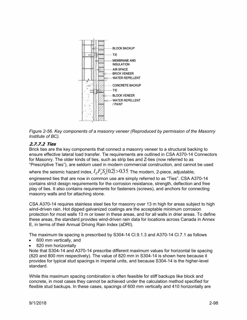
9/1/2018 2-98

Figure 2-56. Key components of a masonry veneer (Reproduced by permission of the Masonry Institute of BC).

2.7.7.2 Ties Brick ties are the key components that connect a masonry veneer to a structural backing to ensure effective lateral load transfer. Tie requirements are outlined in CSA A370-14 Connectors for Masonry. The older kinds of ties, such as strip ties and Z-ties (now referred to as “Prescriptive Ties“), are seldom used in modern commercial construction, and cannot be used

where the seismic hazard index, 35.02.0 aaE SFI . The modern, 2-piece, adjustable,

engineered ties that are now in common use are simply referred to as “Ties”. CSA A370-14 contains strict design requirements for the corrosion resistance, strength, deflection and free play of ties. It also contains requirements for fasteners (screws), and anchors for connecting masonry walls and for attaching stone. CSA A370-14 requires stainless steel ties for masonry over 13 m high for areas subject to high wind-driven rain. Hot dipped galvanized coatings are the acceptable minimum corrosion protection for most walls 13 m or lower in these areas, and for all walls in drier areas. To define these areas, the standard provides wind-driven rain data for locations across Canada in Annex E, in terms of their Annual Driving Rain Index (aDRI). The maximum tie spacing is prescribed by S304-14 Cl.9.1.3 and A370-14 Cl.7.1 as follows 600 mm vertically, and 820 mm horizontally Note that S304-14 and A370-14 prescribe different maximum values for horizontal tie spacing (820 and 800 mm respectively). The value of 820 mm in S304-14 is shown here because it provides for typical stud spacings in imperial units, and because S304-14 is the higher-level standard. While this maximum spacing combination is often feasible for stiff backups like block and concrete, in most cases they cannot be achieved under the calculation method specified for flexible stud backups. In these cases, spacings of 600 mm vertically and 410 horizontally are

9/1/2018 2-99

common. In addition to the general tie spacing, ties must also be located within 300 mm of jambs and tops of walls, and within 400 mm of the base of walls. The wind load lateral deflection limit for flexible stud backups supporting masonry veneer is span/360. The factored resistance of a tie (

rP ) is addressed by A370-14 Cl.9.4.2.1.2, and can be determined as a function of the ultimate tie strength ultP from the following equation

ultr PP *

where is the the resistance factor, which can assume the following values = 0.9 for tie material strength

= 0.6 for embedment failure, failure of fasteners, or buckling failure of the connection. 2.7.7.3 Seismic load provisions for ties Seismic load provisions for ties apply in areas in which the seismic hazard index 35.02.0 aaE SFI , and for all post-disaster buildings (NBC 2015 Cl.4.1.8.18.2). Ties are designed to resist the lateral wind and seismic loads acting perpendicular to the veneer surface, based on the tributary tie area. Note that in many cases, wind loads may govern, even in higher seismic areas. Seismic lateral loads on ties are determined from the provisions for elements and components of buildings and their connections (NBC 2015 Cl. 4.1.8.18). The

seismic tie load pV is determined from the following equation:

ppEaap WSISFV 2.03.0

where

2.0aS = 5 % damped spectral response acceleration for a 0.2 sec period (depends on the

site location; values for various locations in Canada from NBC 2015 Appendix C)

aF = foundation factor, which is a function of site class (soil type) and )2.0(aS (NBC 2015

4.1.8.4(7))

EI = building importance factor equal to1.0, except 1.3 for schools and community centres, and 1.5 for post-disaster buildings (NBC 2015 4.1.8.5)

pS = horizontal force factor for part or portion of a building and its anchorage (see NBC

2015, Table 4.1.8.18, Case 8)

pxrpp RAACS (where 0.47.0 pS )

pC = seismic coefficient for a particular nonstructural component (equal to 1.0 for ties)

rA = response amplification factor to account for the type of attachment (equal to 1.0 for ties)

nxx hhA 21 amplification factor to account for variation of response with the height of the

building (maximum 3.0 for the worst case at top of wall for ties). Note that 3xA is the

worst case for a tall building that may have higher mode contribution to accelerations in the

top part of the building; thus 3xA would be used for the entire top floor. For a single-

storey building this doesn’t make much sense. However, the accelerations will be higher at the top of a wall where the capacity is reduced because of low vertical load on the bricks, so

9/1/2018 2-100

3xA may be reasonable for the top row of ties. This could be reduced in the lower part of

the wall, but for construction simplicity it would generally be better to maintain one spacing on most projects. This could depend on the relative amounts of masonry veneer on the upper and lower portions of the walls.

pR = element or component response modification factor that accounts for ductility (equal to

1.5 for ties).

So, the pS value for tie design is

0.25.10.30.10.1 pS

pW = tributary weight for a specific tie, equal to the unit weight of the veneer masonry

(typically taken as 1.8 kN/m2 for brick and cored block) times the tributary area (equal to the product of tie spacing for each direction).

The tie design load depends on the type of veneer backup (rigid/flexible), as per S304-14 Cl.9.1.3.3:

For rigid backups (e.g. concrete block walls), the tie force is equal to the seismic load pV corresponding to the tributary area weight pW .

For flexible backups (e.g. steel or wood stud walls), a tie must resist 40% of the tributary lateral load on a vertical line of ties. However, a tie must also be able to resist the load from double the tributary area on the tie.

Factored tie capacities

rV are normally provided by test data from the manufacturers. The tie capacity is considered to be adequate provided that

rp VV

If this is not a case, the tributary area and resulting tie spacing can be reduced until the above requirement is satisfied, or a stronger tie can be considered. In many cases, the design will begin with a given tie strength, with the resulting spacing calculated and assessed (see design Example 7 in Chapter 3).

2.7.8 Constructability Issues Most of the information provided in this section has been adapted from the Technical Manual prepared by the Masonry Institute of BC (2017). The requirements for masonry construction are contained in CSA A371-14 Masonry Construction for Buildings. This standard provides direction to masonry contractors and masonry designers on the proper procedures for the erection of masonry walls 2.7.8.1 Reinforcement RM is basically another form of reinforced concrete construction. However, reinforcing and grouting details should consider the cell configuration of the masonry units. Care should be taken to disperse the rebar throughout the wall, and to avoid congestion in individual vertical cells. The cell size of the masonry units will dictate the size and number of bars that can be effectively grouted. A reinforcement arrangement, such as the one shown in Figure 2-57, is unsuitable and should be avoided. Typical RM makes use of 15M or 20M bars. Units of 150 and 200 mm nominal width should not contain more than one vertical bar per cell (2 bars at splices). 25M bars are occasionally used, but are more difficult to handle and require long laps. Vertical

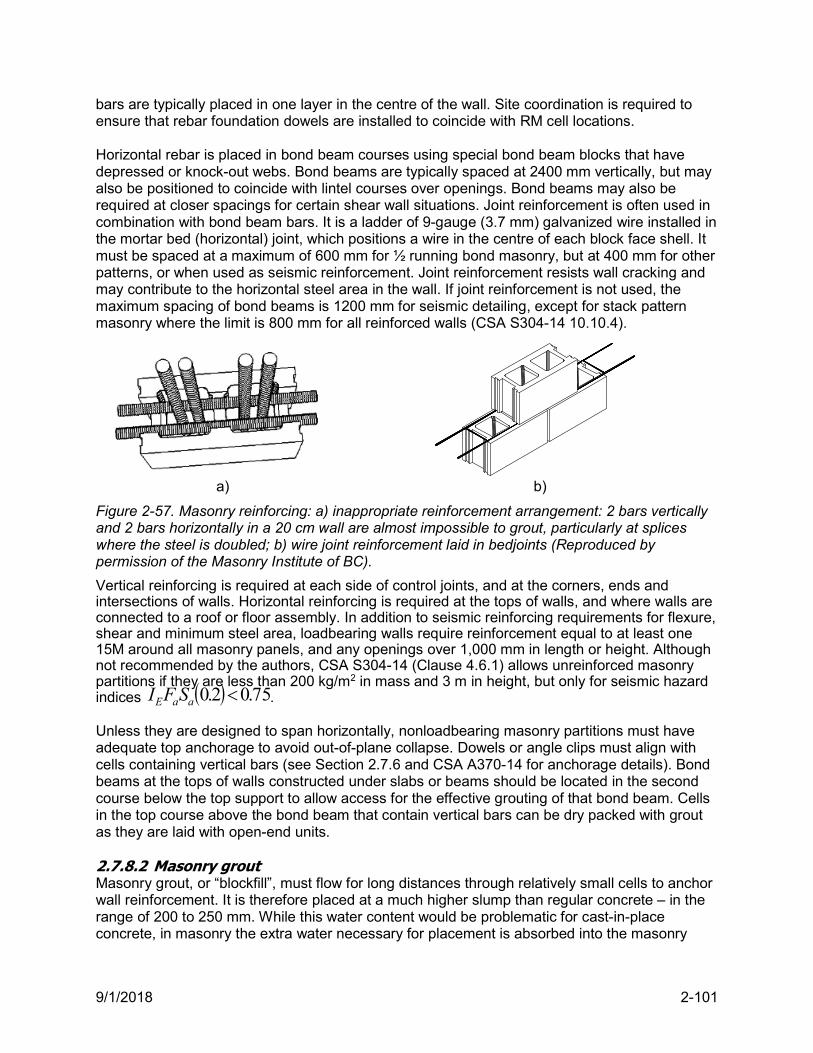
9/1/2018 2-101

bars are typically placed in one layer in the centre of the wall. Site coordination is required to ensure that rebar foundation dowels are installed to coincide with RM cell locations. Horizontal rebar is placed in bond beam courses using special bond beam blocks that have depressed or knock-out webs. Bond beams are typically spaced at 2400 mm vertically, but may also be positioned to coincide with lintel courses over openings. Bond beams may also be required at closer spacings for certain shear wall situations. Joint reinforcement is often used in combination with bond beam bars. It is a ladder of 9-gauge (3.7 mm) galvanized wire installed in the mortar bed (horizontal) joint, which positions a wire in the centre of each block face shell. It must be spaced at a maximum of 600 mm for ½ running bond masonry, but at 400 mm for other patterns, or when used as seismic reinforcement. Joint reinforcement resists wall cracking and may contribute to the horizontal steel area in the wall. If joint reinforcement is not used, the maximum spacing of bond beams is 1200 mm for seismic detailing, except for stack pattern masonry where the limit is 800 mm for all reinforced walls (CSA S304-14 10.10.4).

a) b)

Figure 2-57. Masonry reinforcing: a) inappropriate reinforcement arrangement: 2 bars vertically and 2 bars horizontally in a 20 cm wall are almost impossible to grout, particularly at splices where the steel is doubled; b) wire joint reinforcement laid in bedjoints (Reproduced by permission of the Masonry Institute of BC).

Vertical reinforcing is required at each side of control joints, and at the corners, ends and intersections of walls. Horizontal reinforcing is required at the tops of walls, and where walls are connected to a roof or floor assembly. In addition to seismic reinforcing requirements for flexure, shear and minimum steel area, loadbearing walls require reinforcement equal to at least one 15M around all masonry panels, and any openings over 1,000 mm in length or height. Although not recommended by the authors, CSA S304-14 (Clause 4.6.1) allows unreinforced masonry partitions if they are less than 200 kg/m2 in mass and 3 m in height, but only for seismic hazard indices 75.02.0 aaE SFI . Unless they are designed to span horizontally, nonloadbearing masonry partitions must have adequate top anchorage to avoid out-of-plane collapse. Dowels or angle clips must align with cells containing vertical bars (see Section 2.7.6 and CSA A370-14 for anchorage details). Bond beams at the tops of walls constructed under slabs or beams should be located in the second course below the top support to allow access for the effective grouting of that bond beam. Cells in the top course above the bond beam that contain vertical bars can be dry packed with grout as they are laid with open-end units. 2.7.8.2 Masonry grout Masonry grout, or “blockfill”, must flow for long distances through relatively small cells to anchor wall reinforcement. It is therefore placed at a much higher slump than regular concrete – in the range of 200 to 250 mm. While this water content would be problematic for cast-in-place concrete, in masonry the extra water necessary for placement is absorbed into the masonry

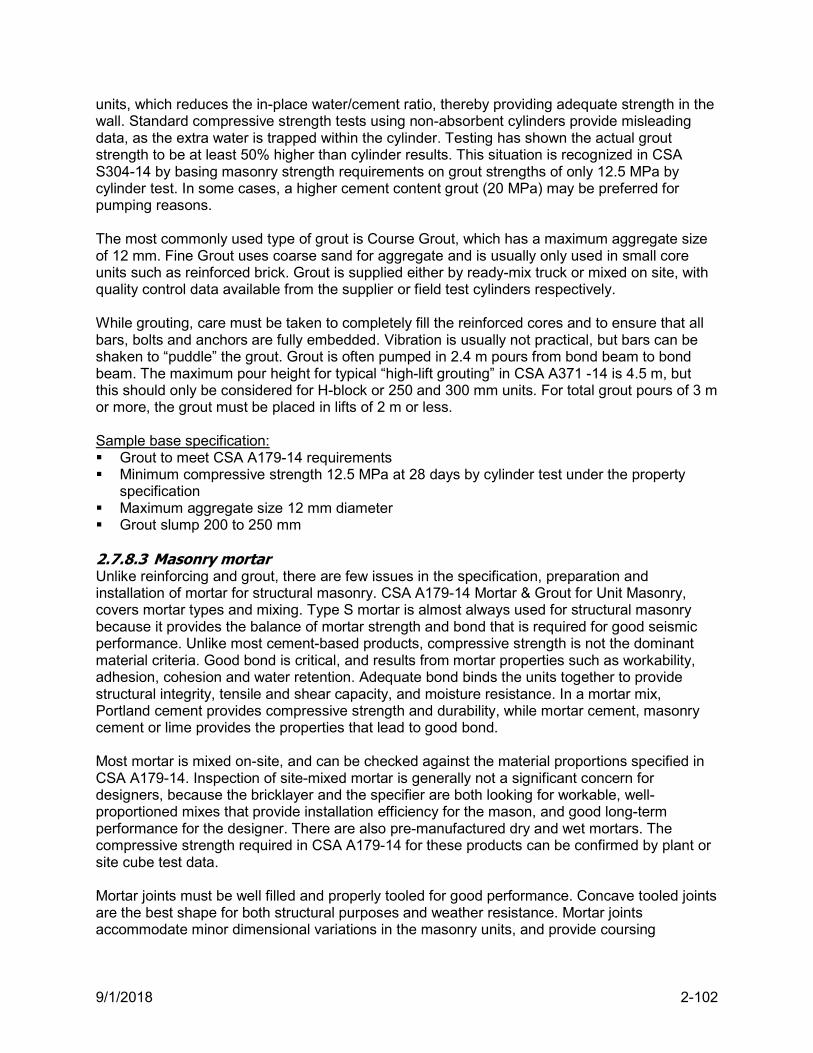
9/1/2018 2-102

units, which reduces the in-place water/cement ratio, thereby providing adequate strength in the wall. Standard compressive strength tests using non-absorbent cylinders provide misleading data, as the extra water is trapped within the cylinder. Testing has shown the actual grout strength to be at least 50% higher than cylinder results. This situation is recognized in CSA S304-14 by basing masonry strength requirements on grout strengths of only 12.5 MPa by cylinder test. In some cases, a higher cement content grout (20 MPa) may be preferred for pumping reasons. The most commonly used type of grout is Course Grout, which has a maximum aggregate size of 12 mm. Fine Grout uses coarse sand for aggregate and is usually only used in small core units such as reinforced brick. Grout is supplied either by ready-mix truck or mixed on site, with quality control data available from the supplier or field test cylinders respectively. While grouting, care must be taken to completely fill the reinforced cores and to ensure that all bars, bolts and anchors are fully embedded. Vibration is usually not practical, but bars can be shaken to “puddle” the grout. Grout is often pumped in 2.4 m pours from bond beam to bond beam. The maximum pour height for typical “high-lift grouting” in CSA A371 -14 is 4.5 m, but this should only be considered for H-block or 250 and 300 mm units. For total grout pours of 3 m or more, the grout must be placed in lifts of 2 m or less. Sample base specification: Grout to meet CSA A179-14 requirements Minimum compressive strength 12.5 MPa at 28 days by cylinder test under the property

specification Maximum aggregate size 12 mm diameter Grout slump 200 to 250 mm 2.7.8.3 Masonry mortar Unlike reinforcing and grout, there are few issues in the specification, preparation and installation of mortar for structural masonry. CSA A179-14 Mortar & Grout for Unit Masonry, covers mortar types and mixing. Type S mortar is almost always used for structural masonry because it provides the balance of mortar strength and bond that is required for good seismic performance. Unlike most cement-based products, compressive strength is not the dominant material criteria. Good bond is critical, and results from mortar properties such as workability, adhesion, cohesion and water retention. Adequate bond binds the units together to provide structural integrity, tensile and shear capacity, and moisture resistance. In a mortar mix, Portland cement provides compressive strength and durability, while mortar cement, masonry cement or lime provides the properties that lead to good bond. Most mortar is mixed on-site, and can be checked against the material proportions specified in CSA A179-14. Inspection of site-mixed mortar is generally not a significant concern for designers, because the bricklayer and the specifier are both looking for workable, well-proportioned mixes that provide installation efficiency for the mason, and good long-term performance for the designer. There are also pre-manufactured dry and wet mortars. The compressive strength required in CSA A179-14 for these products can be confirmed by plant or site cube test data. Mortar joints must be well filled and properly tooled for good performance. Concave tooled joints are the best shape for both structural purposes and weather resistance. Mortar joints accommodate minor dimensional variations in the masonry units, and provide coursing

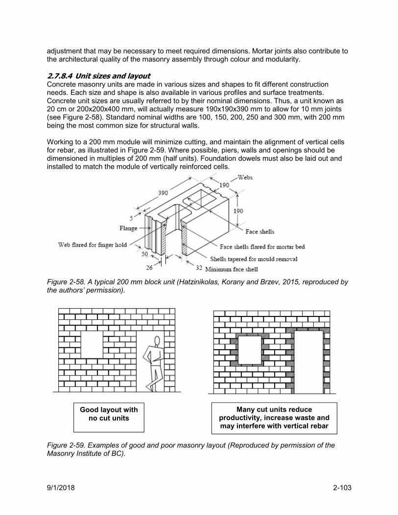
9/1/2018 2-103

adjustment that may be necessary to meet required dimensions. Mortar joints also contribute to the architectural quality of the masonry assembly through colour and modularity. 2.7.8.4 Unit sizes and layout Concrete masonry units are made in various sizes and shapes to fit different construction needs. Each size and shape is also available in various profiles and surface treatments. Concrete unit sizes are usually referred to by their nominal dimensions. Thus, a unit known as 20 cm or 200x200x400 mm, will actually measure 190x190x390 mm to allow for 10 mm joints (see Figure 2-58). Standard nominal widths are 100, 150, 200, 250 and 300 mm, with 200 mm being the most common size for structural walls. Working to a 200 mm module will minimize cutting, and maintain the alignment of vertical cells for rebar, as illustrated in Figure 2-59. Where possible, piers, walls and openings should be dimensioned in multiples of 200 mm (half units). Foundation dowels must also be laid out and installed to match the module of vertically reinforced cells.

Figure 2-58. A typical 200 mm block unit (Hatzinikolas, Korany and Brzev, 2015, reproduced by the authors’ permission).

Figure 2-59. Examples of good and poor masonry layout (Reproduced by permission of the Masonry Institute of BC).

Good layout with no cut units

Many cut units reduce productivity, increase waste and may interfere with vertical rebar

9/1/2018 2-104

2.7.8.5 Other construction issues In “high-lift grouting” (over 1.5 m), clean-out/inspection holes at the base of the reinforced cells may facilitate the removal of excessive mortar droppings and, more importantly, can confirm that grout has reached the bottom of the core. Clause 8.2.3.2.2 of CSA A371-14 allows the common practice of waiving the requirement for clean-out/inspection holes by the designer, when the masonry contractor has demonstrated acceptable performance, or where the walls are not structurally critical. In some cases, the designer may require the initial walls to have clean-outs, pending demonstrated performance, and then waive them for the remaining walls. Vertical movement joints in RM walls are required to accommodate thermal and moisture movements, and possible foundation settlement. They are typically specified at a maximum spacing of 15 m.

9/1/2018 3-1

TABLE OF CONTENTS – CHAPTER 3

3 DESIGN EXAMPLES 1 Seismic load calculation for a low-rise masonry building to NBC 2015 3-2

2 Seismic load calculation for a medium-rise masonry building to NBC 2015 3-9

3 Seismic load distribution in a masonry building considering both rigid and flexible

diaphragm alternatives

3-24

4a Minimum seismic reinforcement for a squat masonry shear wall 3-37

4b Seismic design of a squat shear wall of Conventional Construction 3-41

4c Seismic design of a Moderately Ductile squat shear wall 3-47

5a Seismic design of a Moderately Ductile flexural shear wall 3-57

5b Seismic design of a Ductile shear wall with rectangular cross-section 3-68

5c Seismic design of a Ductile shear wall with boundary elements 3-79

6a Design of a loadbearing wall for out-of-plane seismic effects 3-92

6b Design of a nonloadbearing wall for out-of-plane seismic effects 3-99

7 Seismic design of masonry veneer ties 3-104

8 Seismic design of a masonry infill wall 3-106

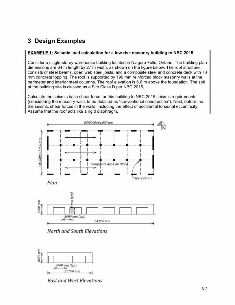
9/1/2018 3-2

3 Design Examples EXAMPLE 1: Seismic load calculation for a low-rise masonry building to NBC 2015 Consider a single-storey warehouse building located in Niagara Falls, Ontario. The building plan dimensions are 64 m length by 27 m width, as shown on the figure below. The roof structure consists of steel beams, open web steel joists, and a composite steel and concrete deck with 70 mm concrete topping. The roof is supported by 190 mm reinforced block masonry walls at the perimeter and interior steel columns. The roof elevation is 6.6 m above the foundation. The soil at the building site is classed as a Site Class D per NBC 2015. Calculate the seismic base shear force for this building to NBC 2015 seismic requirements (considering the masonry walls to be detailed as “conventional construction”). Next, determine the seismic shear forces in the walls, including the effect of accidental torsional eccentricity. Assume that the roof acts like a rigid diaphragm.

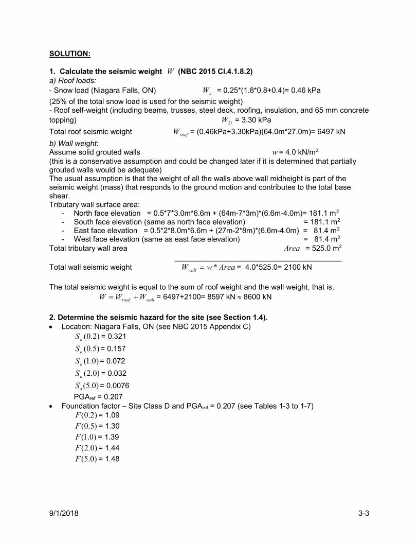
9/1/2018 3-3

SOLUTION: 1. Calculate the seismic weight W (NBC 2015 Cl.4.1.8.2) a) Roof loads: - Snow load (Niagara Falls, ON) sW = 0.25*(1.8*0.8+0.4)= 0.46 kPa

(25% of the total snow load is used for the seismic weight) - Roof self-weight (including beams, trusses, steel deck, roofing, insulation, and 65 mm concrete topping) DW = 3.30 kPa

Total roof seismic weight roofW = (0.46kPa+3.30kPa)(64.0m*27.0m)= 6497 kN

b) Wall weight: Assume solid grouted walls w = 4.0 kN/m2 (this is a conservative assumption and could be changed later if it is determined that partially grouted walls would be adequate) The usual assumption is that the weight of all the walls above wall midheight is part of the seismic weight (mass) that responds to the ground motion and contributes to the total base shear. Tributary wall surface area:

- North face elevation = 0.5*7*3.0m*6.6m + (64m-7*3m)*(6.6m-4.0m)= 181.1 m2 - South face elevation (same as north face elevation) = 181.1 m2 - East face elevation = 0.5*2*8.0m*6.6m + (27m-2*8m)*(6.6m-4.0m) = 81.4 m2 - West face elevation (same as east face elevation) = 81.4 m2

Total tributary wall area Area = 525.0 m2 ________________________________________ Total wall seismic weight AreawWwall * = 4.0*525.0= 2100 kN

The total seismic weight is equal to the sum of roof weight and the wall weight, that is,

wallroof WWW = 6497+2100= 8597 kN 8600 kN

2. Determine the seismic hazard for the site (see Section 1.4). Location: Niagara Falls, ON (see NBC 2015 Appendix C)

)2.0(aS = 0.321

)5.0(aS = 0.157

)0.1(aS = 0.072

)0.2(aS = 0.032

(5.0)aS = 0.0076

PGAref = 0.207 Foundation factor – Site Class D and PGAref = 0.207 (see Tables 1-3 to 1-7)

(0.2)F = 1.09

(0.5)F = 1.30

(1.0)F = 1.39

(2.0)F = 1.44

(5.0)F = 1.48

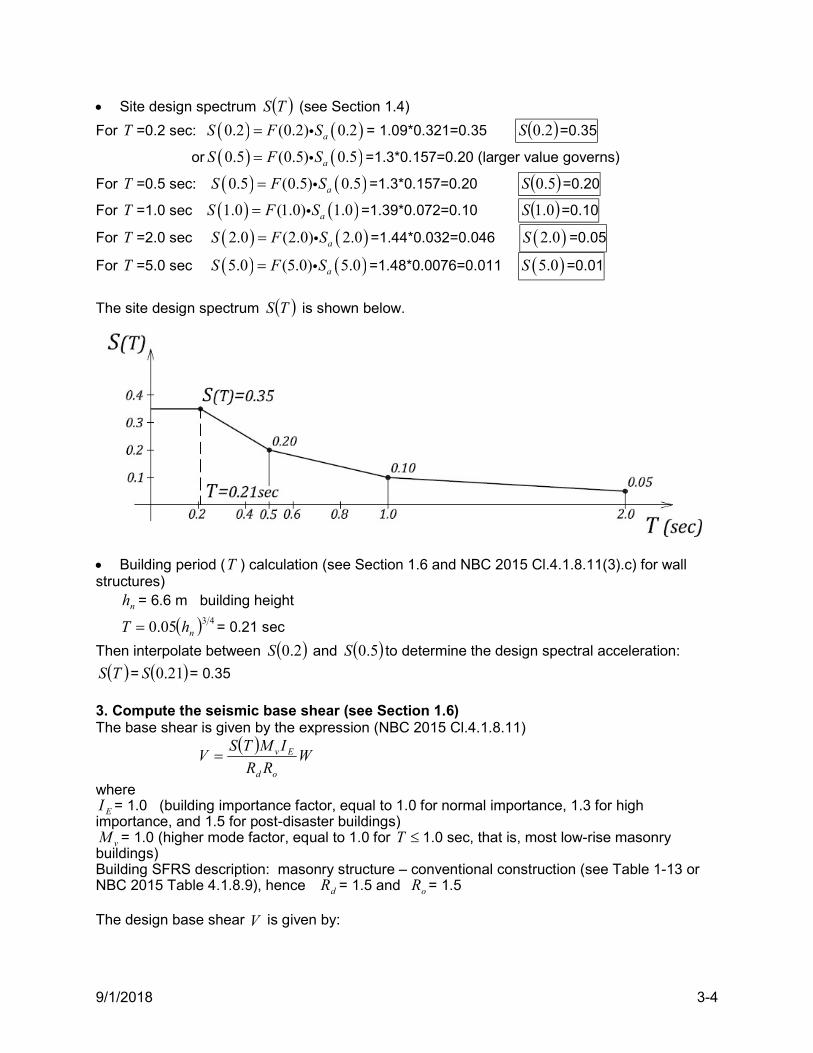
9/1/2018 3-4

Site design spectrum TS (see Section 1.4)

For T =0.2 sec: 0.2 (0.2) 0.2aS F S = 1.09*0.321=0.35 2.0S =0.35

or 0.5 (0.5) 0.5aS F S =1.3*0.157=0.20 (larger value governs)

For T =0.5 sec: 0.5 (0.5) 0.5aS F S =1.3*0.157=0.20 5.0S =0.20

For T =1.0 sec 1.0 (1.0) 1.0aS F S =1.39*0.072=0.10 0.1S =0.10

For T =2.0 sec 2.0 (2.0) 2.0aS F S =1.44*0.032=0.046 2.0S =0.05

For T =5.0 sec 5.0 (5.0) 5.0aS F S =1.48*0.0076=0.011 5.0S =0.01

The site design spectrum TS is shown below.

Building period (T ) calculation (see Section 1.6 and NBC 2015 Cl.4.1.8.11(3).c) for wall structures)

nh = 6.6 m building height

4305.0 nhT = 0.21 sec

Then interpolate between 2.0S and 5.0S to determine the design spectral acceleration:

TS = 21.0S = 0.35 3. Compute the seismic base shear (see Section 1.6) The base shear is given by the expression (NBC 2015 Cl.4.1.8.11)

WRR

IMTSV

od

Ev

where EI = 1.0 (building importance factor, equal to 1.0 for normal importance, 1.3 for high

importance, and 1.5 for post-disaster buildings) vM = 1.0 (higher mode factor, equal to 1.0 for T 1.0 sec, that is, most low-rise masonry

buildings) Building SFRS description: masonry structure – conventional construction (see Table 1-13 or NBC 2015 Table 4.1.8.9), hence dR = 1.5 and oR = 1.5 The design base shear V is given by:

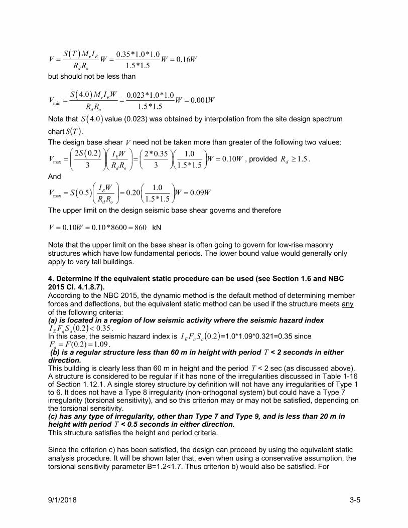
9/1/2018 3-5

0.35*1.0*1.00.16

1.5*1.5v E

d o

S T M IV W W W

R R

but should not be less than

min

4.0 0.023*1.0*1.00.001

1.5*1.5v E

d o

S M I WV W W

R R

Note that 4.0S value (0.023) was obtained by interpolation from the site design spectrum

chart TS .

The design base shear V need not be taken more than greater of the following two values:

max

2 0.2 2*0.35 1.00.10

3 3 1.5*1.5E

d o

S I WV W W

R R

, provided 5.1dR .

And

max

1.00.5 0.20 0.09

1.5*1.5E

d o

I WV S W W

R R

The upper limit on the design seismic base shear governs and therefore

0.10 0.10*8600 860V W kN Note that the upper limit on the base shear is often going to govern for low-rise masonry structures which have low fundamental periods. The lower bound value would generally only apply to very tall buildings. 4. Determine if the equivalent static procedure can be used (see Section 1.6 and NBC 2015 Cl. 4.1.8.7). According to the NBC 2015, the dynamic method is the default method of determining member forces and deflections, but the equivalent static method can be used if the structure meets any of the following criteria: (a) is located in a region of low seismic activity where the seismic hazard index

35.02.0 aaE SFI . In this case, the seismic hazard index is 2.0aaE SFI =1.0*1.09*0.321=0.35 since

(0.2) 1.09aF F . (b) is a regular structure less than 60 m in height with period T < 2 seconds in either direction. This building is clearly less than 60 m in height and the period T < 2 sec (as discussed above). A structure is considered to be regular if it has none of the irregularities discussed in Table 1-16 of Section 1.12.1. A single storey structure by definition will not have any irregularities of Type 1 to 6. It does not have a Type 8 irregularity (non-orthogonal system) but could have a Type 7 irregularity (torsional sensitivity), and so this criterion may or may not be satisfied, depending on the torsional sensitivity. (c) has any type of irregularity, other than Type 7 and Type 9, and is less than 20 m in height with period T < 0.5 seconds in either direction. This structure satisfies the height and period criteria. Since the criterion c) has been satisfied, the design can proceed by using the equivalent static analysis procedure. It will be shown later that, even when using a conservative assumption, the torsional sensitivity parameter B=1.2<1.7. Thus criterion b) would also be satisfied. For

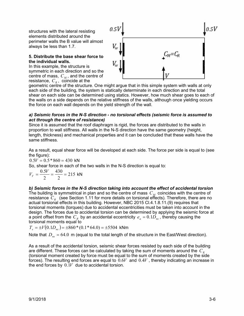
9/1/2018 3-6

structures with the lateral resisting elements distributed around the perimeter walls the B value will almost always be less than 1.7. 5. Distribute the base shear force to the individual walls. In this example, the structure is symmetric in each direction and so the centre of mass, MC , and the centre of resistance, RC , coincide at the geometric centre of the structure. One might argue that in this simple system with walls at only each side of the building, the system is statically determinate in each direction and the total shear on each side can be determined using statics. However, how much shear goes to each of the walls on a side depends on the relative stiffness of the walls, although once yielding occurs the force on each wall depends on the yield strength of the wall. a) Seismic forces in the N-S direction - no torsional effects (seismic force is assumed to act through the centre of resistance) Since it is assumed that the roof diaphragm is rigid, the forces are distributed to the walls in proportion to wall stiffness. All walls in the N-S direction have the same geometry (height, length, thickness) and mechanical properties and it can be concluded that these walls have the same stiffness. As a result, equal shear force will be developed at each side. The force per side is equal to (see the figure):

430860*5.05.0 V kN So, shear force in each of the two walls in the N-S direction is equal to:

2152

430

2

5.0

VVV kN

b) Seismic forces in the N-S direction taking into account the effect of accidental torsion The building is symmetrical in plan and so the centre of mass MC coincides with the centre of resistance RC (see Section 1.11 for more details on torsional effects). Therefore, there are no actual torsional effects in this building. However, NBC 2015 Cl.4.1.8.11.(9) requires that torsional moments (torques) due to accidental eccentricities must be taken into account in the design. The forces due to accidental torsion can be determined by applying the seismic force at a point offset from the RC by an accidental eccentricity nxa De 1.0 , thereby causing the torsional moments equal to

5504)0.64*1.0(*8601.0 nxx DVT kNm

Note that 0.64nxD m (equal to the total length of the structure in the East/West direction).

As a result of the accidental torsion, seismic shear forces resisted by each side of the building are different. These forces can be calculated by taking the sum of moments around the RC (torsional moment created by force must be equal to the sum of moments created by the side forces). The resulting end forces are equal to V6.0 and V4.0 , thereby indicating an increase in the end forces by V1.0 due to accidental torsion.

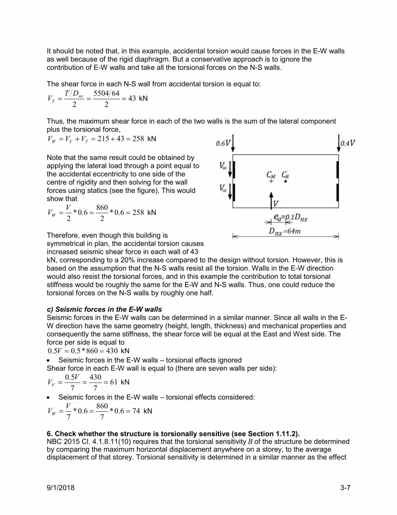
9/1/2018 3-7

It should be noted that, in this example, accidental torsion would cause forces in the E-W walls as well because of the rigid diaphragm. But a conservative approach is to ignore the contribution of E-W walls and take all the torsional forces on the N-S walls. The shear force in each N-S wall from accidental torsion is equal to:

432

645504

2 nx

T

DTV kN

Thus, the maximum shear force in each of the two walls is the sum of the lateral component plus the torsional force,

25843215 TVW VVV kN

Note that the same result could be obtained by applying the lateral load through a point equal to the accidental eccentricity to one side of the centre of rigidity and then solving for the wall forces using statics (see the figure). This would show that

2586.0*2

8606.0*

2

VVW kN

Therefore, even though this building is symmetrical in plan, the accidental torsion causes increased seismic shear force in each wall of 43 kN, corresponding to a 20% increase compared to the design without torsion. However, this is based on the assumption that the N-S walls resist all the torsion. Walls in the E-W direction would also resist the torsional forces, and in this example the contribution to total torsional stiffness would be roughly the same for the E-W and N-S walls. Thus, one could reduce the torsional forces on the N-S walls by roughly one half. c) Seismic forces in the E-W walls Seismic forces in the E-W walls can be determined in a similar manner. Since all walls in the E-W direction have the same geometry (height, length, thickness) and mechanical properties and consequently the same stiffness, the shear force will be equal at the East and West side. The force per side is equal to

430860*5.05.0 V kN Seismic forces in the E-W walls – torsional effects ignored Shear force in each E-W wall is equal to (there are seven walls per side):

617

430

7

5.0

VVV kN

Seismic forces in the E-W walls – torsional effects considered:

746.0*7

8606.0*

7

VVW kN

6. Check whether the structure is torsionally sensitive (see Section 1.11.2). NBC 2015 Cl. 4.1.8.11(10) requires that the torsional sensitivity B of the structure be determined by comparing the maximum horizontal displacement anywhere on a storey, to the average displacement of that storey. Torsional sensitivity is determined in a similar manner as the effect

9/1/2018 3-8

of accidental torsion, that is, by applying a set of a set of lateral forces at a distance of nxD1.0 from the centre of mass MC . In case of a rigid diaphragm, displacements are proportional to the forces developed in the walls. Therefore, B can be determined by comparing the forces at the sides of the building with/without the effect of accidental torsion. The maximum displacement would be proportional to 0.6V, while the displacement on the other side would be proportional to 0.4V. Thus, the average displacement is proportional to 0.5V. Thus

2.15.0

6.0

V

VB

Since B < 1.7, this building is not torsionally sensitive and the equivalent static analysis would have also been allowed under criterion b) as discussed in step 4 above. 7. Discussion It was assumed at the beginning of this example that the roof structure can be modeled like a rigid diaphragm. If this roof was modeled like a flexible diaphragm, the shear forces in each N-S wall would be equal to 0.5V. From a reliability point of view, it does not seem quite right that the forces are smaller for a flexible diaphragm than a rigid one - it should be the other way around. On the other hand, the flexible diaphragm may have a longer period and the forces would be smaller (see Example 3 for a detailed discussion on rigid and flexible diaphragm models).

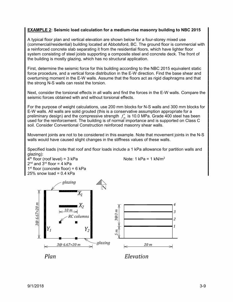
9/1/2018 3-9

EXAMPLE 2: Seismic load calculation for a medium-rise masonry building to NBC 2015 A typical floor plan and vertical elevation are shown below for a four-storey mixed use (commercial/residential) building located at Abbotsford, BC. The ground floor is commercial with a reinforced concrete slab separating it from the residential floors, which have lighter floor system consisting of steel joists supporting a composite steel and concrete deck. The front of the building is mostly glazing, which has no structural application. First, determine the seismic force for this building according to the NBC 2015 equivalent static force procedure, and a vertical force distribution in the E-W direction. Find the base shear and overturning moment in the E-W walls. Assume that the floors act as rigid diaphragms and that the strong N-S walls can resist the torsion. Next, consider the torsional effects in all walls and find the forces in the E-W walls. Compare the seismic forces obtained with and without torsional effects. For the purpose of weight calculations, use 200 mm blocks for N-S walls and 300 mm blocks for E-W walls. All walls are solid grouted (this is a conservative assumption appropriate for a preliminary design) and the compressive strength mf is 10.0 MPa. Grade 400 steel has been used for the reinforcement. The building is of normal importance and is supported on Class C soil. Consider Conventional Construction reinforced masonry shear walls. Movement joints are not to be considered in this example. Note that movement joints in the N-S walls would have caused slight changes in the stiffness values of these walls. Specified loads (note that roof and floor loads include a 1 kPa allowance for partition walls and glazing): 4th floor (roof level) = 3 kPa Note: 1 kPa = 1 kN/m2 2nd and 3rd floor = 4 kPa 1st floor (concrete floor) = 6 kPa 25% snow load = 0.4 kPa

9/1/2018 3-10

SOLUTION: 1. Design assumptions Rigid diaphragm All walls are solid grouted 2. Calculate the seismic weight W (see NBC 2015 Cl.4.1.8.2) Wall weight: N-S walls - 200 mm thick w = 4.18 kPa E-W walls – 300 mm thick w = 6.38 kPa Note that, for the purpose of seismic weight calculations, the length of a N-S wall is 20 m, while the length of an E-W wall is 10.0 m. Seismic weight 1W :

kNmmkPamkPamkPamm

W 357920*200.60.10*2*38.620*2*18.42

0.3

2

0.51

Seismic weight 2W :

kNmmkPamkPamkPamm

W 248420*200.40.10*2*38.620*2*18.42

0.3

2

0.32

Seismic weight 3W (same as 2W ) :

kNW 24843

Seismic weight 4W :

kNmmkPakPamkPamkPam

W 180220*204.00.30.10*2*38.620*2*18.42

0.34

Note that the seismic weight for each floor level is the sum of the wall weights and the floor weight. 25% snow load was included in the roof weight calculation. One-half of the wall height (below and above a certain floor level) was considered in the wall area calculations. The total seismic weight is equal to

kNWWWWW 1035018022484248435794321

3. Calculate the seismic base shear force (see Section 1.6). a) Find seismic design parameters used to determine seismic base shear. Location: Abbotsford, BC (see NBC 2015 Appendix C)

)2.0(aS = 0.701

)5.0(aS = 0.597

)0.1(aS = 0.350

)0.2(aS = 0.215

(5.0)aS = 0.071

PGAref = 0.306 Foundation factor – Site Class C and PGAref = 0.306 (see Tables 1-3 to 1-7)

(0.2)F = (0.5)F = (1.0)F = (2.0)F = (5.0)F = 1.0

Site design spectrum TS (see Section 1.4)

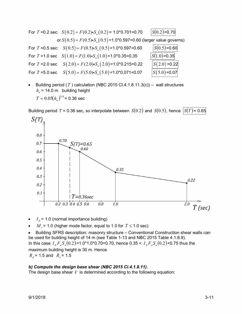
9/1/2018 3-11

For T =0.2 sec: 0.2 (0.2) 0.2aS F S = 1.0*0.701=0.70 2.0S =0.70

or 0.5 (0.5) 0.5aS F S =1.0*0.597=0.60 (larger value governs)

For T =0.5 sec: 0.5 (0.5) 0.5aS F S =1.0*0.597=0.60 5.0S =0.60

For T =1.0 sec 1.0 (1.0) 1.0aS F S =1.0*0.35=0.35 0.1S =0.35

For T =2.0 sec 2.0 (2.0) 2.0aS F S =1.0*0.215=0.22 2.0S =0.22

For T =5.0 sec 5.0 (5.0) 5.0aS F S =1.0*0.071=0.07 5.0S =0.07

Building period (T ) calculation (NBC 2015 Cl.4.1.8.11.3(c)) – wall structures

nh = 14.0 m building height

4305.0 nhT = 0.36 sec

Building period T = 0.36 sec, so interpolate between 2.0S and 5.0S , hence TS = 0.65

EI = 1.0 (normal importance building)

vM = 1.0 (higher mode factor, equal to 1.0 for T 1.0 sec)

Building SFRS description: masonry structure – Conventional Construction shear walls can be used for building height of 14 m (see Table 1-13 and NBC 2015 Table 4.1.8.9). In this case 2.0aaE SFI =1.0*1.0*0.70=0.70, hence 0.35 < 2.0aaE SFI <0.75 thus the

maximum building height is 30 m. Hence

dR = 1.5 and oR = 1.5

b) Compute the design base shear (NBC 2015 Cl.4.1.8.11). The design base shear V is determined according to the following equation:

9/1/2018 3-12

0.70*1.0*1.00.31

1.5*1.5v E

d o

S T M IV W W W

R R

but should not be less than

min

4.0 0.12*1.0*1.00.05

1.5*1.5v E

d o

S M I WV W W

R R

Note that 4.0S value (0.15) was obtained by interpolation from the site design spectrum

chart TS .

The design base shear V need not be taken more than greater of the following two values:

max

2 0.2 2*0.70 1.00.21

3 3 1.5*1.5E

d o

S I WV W W

R R

, provided 5.1dR .

and

max

1.00.5 0.60 0.27

1.5*1.5E

d o

I WV S W W

R R

- this value governs

Therefore, the design seismic base shear is equal to

0.27 0.27*10350 2900V W kN 4. Determine whether the equivalent static procedure can be used (see Section 1.5 and NBC 2015 Cl. 4.1.8.7). According to the NBC 2015, the dynamic method is the default method, but the equivalent static method can be used if the structure meets any of the following criteria: (a) is located in a region of low seismic activity where 35.02.0 aaE SFI ,

In this case, the seismic hazard index is 2.0aaE SFI =1.0*1.0*0.70=0.70 > 0.35 and so this criterion is not satisfied. Note that (0.2) 1.0aF F . (b) is a regular structure less than 60 m in height with period T < 2 seconds in either direction, This building is clearly less than 60 m in height and the period T < 2 sec (as discussed above). To confirm that this structure is regular, the designer needs to review the irregularities discussed in Section 1.12.1. It can be concluded that this building does not have any of the irregularity types identified by NBC 2015 and so this criterion is satisfied. (c) has any type of irregularity (other than Type 7 or Type 9 that requires the dynamic method if B >1.7), but is less than 20 m in height with period T < 0.5 seconds in either direction This is an irregular structure, but it is less than 20 m in height and the period is less than 0.5 sec. The torsional sensitivity B should be checked to confirm that B < 1.7 (see Section 1.11.2). Since the criterion b) has been satisfied, the design can proceed by using the equivalent static analysis procedure. 5. Seismic force distribution over the building height (see Section 1.9). According to NBC 2015 Cl. 4.1.8.11.(7), the total lateral seismic force, V , is to be distributed over the building height in accordance with the following formula (see Figure 1-5):

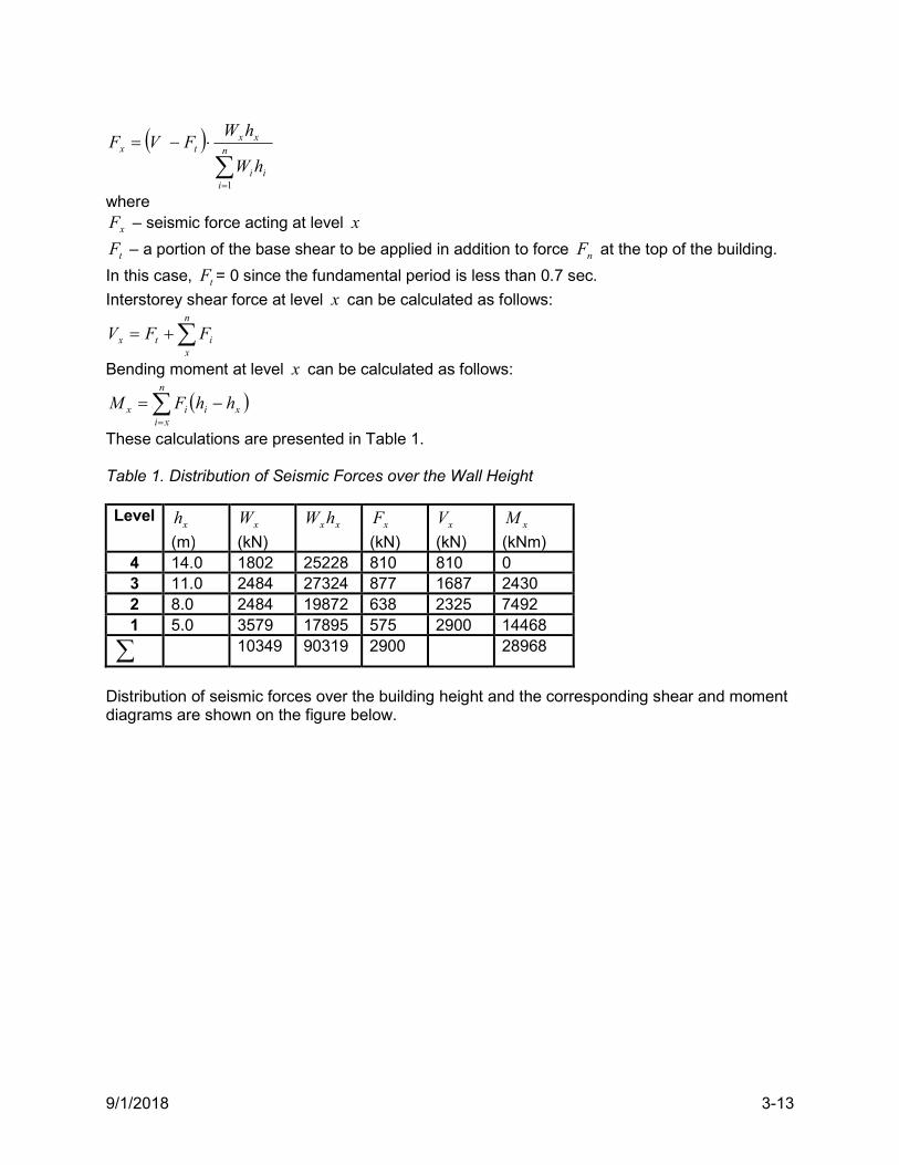
9/1/2018 3-13

where

xF – seismic force acting at level x

tF – a portion of the base shear to be applied in addition to force nF at the top of the building.

In this case, tF = 0 since the fundamental period is less than 0.7 sec.

Interstorey shear force at level x can be calculated as follows:

n

xitx FFV

Bending moment at level x can be calculated as follows:

n

xixiix hhFM

These calculations are presented in Table 1. Table 1. Distribution of Seismic Forces over the Wall Height Level

xh

(m) xW

(kN) xxhW xF

(kN) xV

(kN) xM

(kNm) 4 14.0 1802 25228 810 810 0 3 11.0 2484 27324 877 1687 2430 2 8.0 2484 19872 638 2325 7492 1 5.0 3579 17895 575 2900 14468

10349 90319 2900 28968

Distribution of seismic forces over the building height and the corresponding shear and moment diagrams are shown on the figure below.

n

iii

xxtx

hW

hWFVF

1

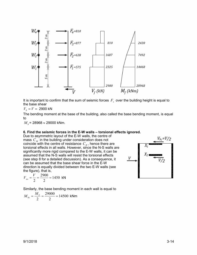
9/1/2018 3-14

It is important to confirm that the sum of seismic forces xF over the building height is equal to the base shear

VVb 2900 kN

The bending moment at the base of the building, also called the base bending moment, is equal to

bM = 28968 29000 kNm.

6. Find the seismic forces in the E-W walls – torsional effects ignored. Due to asymmetric layout of the E-W walls, the centre of mass MC in the building under consideration does not coincide with the centre of resistance RC , hence there are torsional effects in all walls. However, since the N-S walls are significantly more rigid compared to the E-W walls, it can be assumed that the N-S walls will resist the torsional effects (see step 8 for a detailed discussion). As a consequence, it can be assumed that the base shear force in the E-W direction is equally divided between the two E-W walls (see the figure), that is,

14502

2900

2

VVxo kN

Similarly, the base bending moment in each wall is equal to

145002

29000

2 b

bx

MM kNm

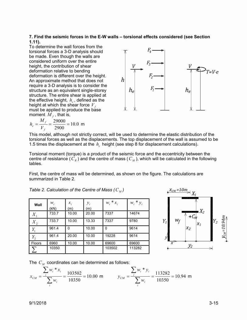
9/1/2018 3-15

7. Find the seismic forces in the E-W walls – torsional effects considered (see Section 1.11). To determine the wall forces from the torsional forces a 3-D analysis should be made. Even though the walls are considered uniform over the entire height, the contribution of shear deformation relative to bending deformation is different over the height. An approximate method that does not require a 3-D analysis is to consider the structure as an equivalent single-storey structure. The entire shear is applied at the effective height, eh , defined as the height at which the shear force fV must be applied to produce the base moment fM , that is,

0.102900

29000

f

fe V

Mh m

This model, although not strictly correct, will be used to determine the elastic distribution of the torsional forces as well as the displacements. The top displacement of the wall is assumed to be 1.5 times the displacement at the eh height (see step 8 for displacement calculations). Torsional moment (torque) is a product of the seismic force and the eccentricity between the centre of resistance ( RC ) and the centre of mass ( MC ), which will be calculated in the following tables. First, the centre of mass will be determined, as shown on the figure. The calculations are summarized in Table 2. Table 2. Calculation of the Centre of Mass ( MC )

Wall iw

(kN) ix

(m) iy

(m) ii xw * ii yw *

1X 733.7 10.00 20.00 7337 14674

2X 733.7 10.00 13.33 7337 9780

1Y 961.4 0 10.00 0 9614

2Y 961.4 20.00 10.00 19228 9614

Floors 6960 10.00 10.00 69600 69600

10350 103502 113282

The MC coordinates can be determined as follows:

00.1010350

103502*

ii

iii

CM w

xwx m 94.10

10350

113282*

ii

iii

CM w

ywy m

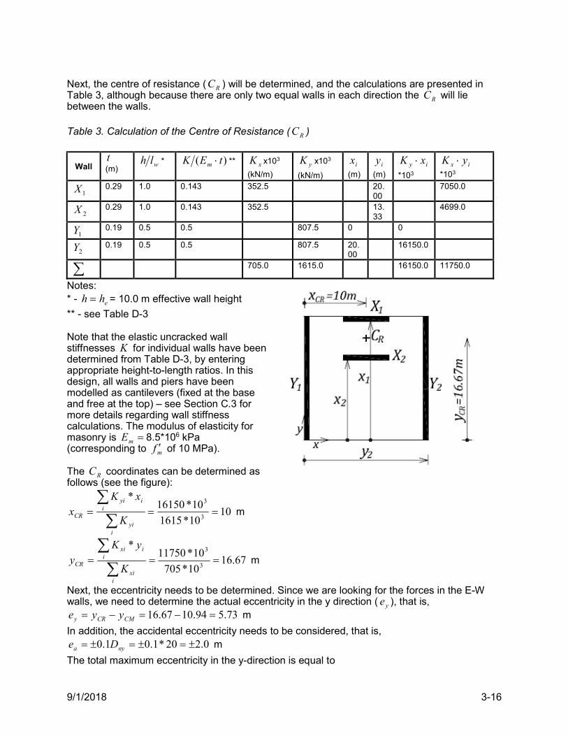
9/1/2018 3-16

Next, the centre of resistance ( RC ) will be determined, and the calculations are presented in Table 3, although because there are only two equal walls in each direction the RC will lie between the walls. Table 3. Calculation of the Centre of Resistance ( RC )

Wall t (m)

wlh * )( tEK m ** xK x103

(kN/m) yK x103

(kN/m) ix

(m) iy

(m) iy xK

*103 ix yK

*103

1X 0.29 1.0 0.143 352.5 20.00

7050.0

2X 0.29 1.0 0.143 352.5 13.33

4699.0

1Y 0.19 0.5 0.5 807.5 0 0

2Y 0.19 0.5 0.5 807.5 20.00

16150.0

705.0 1615.0 16150.0 11750.0

Notes: * - ehh = 10.0 m effective wall height

** - see Table D-3 Note that the elastic uncracked wall stiffnesses K for individual walls have been determined from Table D-3, by entering appropriate height-to-length ratios. In this design, all walls and piers have been modelled as cantilevers (fixed at the base and free at the top) – see Section C.3 for more details regarding wall stiffness calculations. The modulus of elasticity for masonry is mE 8.5*106 kPa (corresponding to mf of 10 MPa). The RC coordinates can be determined as follows (see the figure):

1010*1615

10*16150*

3

3

iyi

iiyi

CR K

xKx m

67.1610*705

10*11750*

3

3

ixi

iixi

CR K

yKy m

Next, the eccentricity needs to be determined. Since we are looking for the forces in the E-W walls, we need to determine the actual eccentricity in the y direction ( ye ), that is,

73.594.1067.16 CMCRy yye m

In addition, the accidental eccentricity needs to be considered, that is, 0.220*1.01.0 nya De m

The total maximum eccentricity in the y-direction is equal to

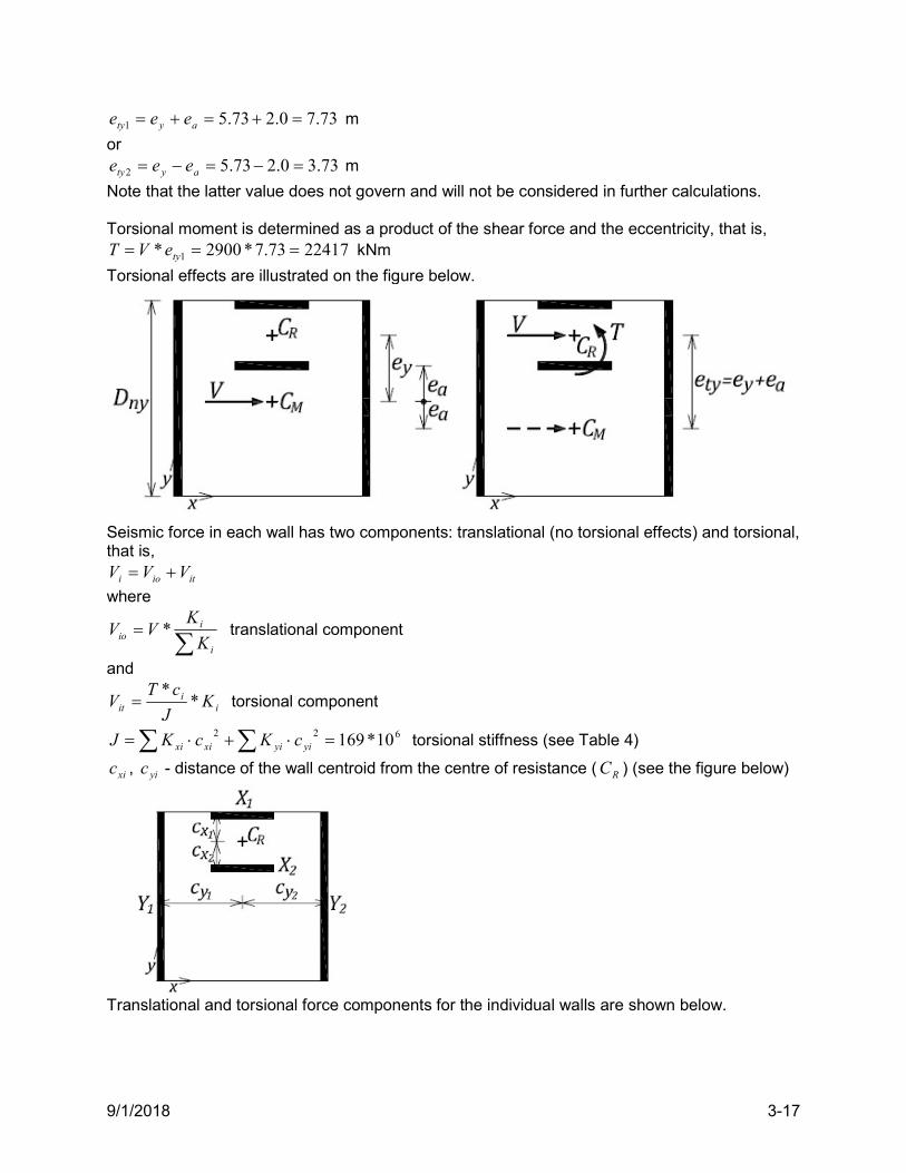
9/1/2018 3-17

73.70.273.51 ayty eee m

or 73.30.273.52 ayty eee m

Note that the latter value does not govern and will not be considered in further calculations. Torsional moment is determined as a product of the shear force and the eccentricity, that is,

2241773.7*2900* 1 tyeVT kNm

Torsional effects are illustrated on the figure below.

Seismic force in each wall has two components: translational (no torsional effects) and torsional, that is,

itioi VVV

where

i

iio K

KVV * translational component

and

ii

it KJ

cTV *

* torsional component

622 10*169 yiyixixi cKcKJ torsional stiffness (see Table 4)

xic , yic - distance of the wall centroid from the centre of resistance ( RC ) (see the figure below)

Translational and torsional force components for the individual walls are shown below.

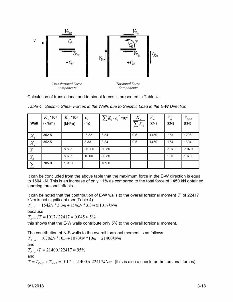
9/1/2018 3-18

Calculation of translational and torsional forces is presented in Table 4. Table 4. Seismic Shear Forces in the Walls due to Seismic Load in the E-W Direction

Wall xK *103

(kN/m) yK *103

(kN/m) ic

(m)

2ii cK *106

x

x

K

K

xoV

(kN) xtV

(kN) totalV

(kN)

1X 352.5 -3.33 3.84 0.5 1450 -154 1296

2X 352.5 3.33 3.84 0.5 1450 154 1604

1Y 807.5 -10.00 80.80 -1070 -1070

2Y 807.5 10.00 80.80 1070 1070

705.0 1615.0 169.0

It can be concluded from the above table that the maximum force in the E-W direction is equal to 1604 kN. This is an increase of only 11% as compared to the total force of 1450 kN obtained ignoring torsional effects. It can be noted that the contribution of E-W walls to the overall torsional moment T of 22417 kNm is not significant (see Table 4).

kNmmkNmkNT WE 10173.3*1543.3*154

because %5045.022417/1017 TT WE

this shows that the E-W walls contribute only 5% to the overall torsional moment. The contribution of N-S walls to the overall torsional moment is as follows:

kNmmkNmkNT SN 2140010*107010*1070

and %9522417/21400 TT SN

and kNmTTT SNWE 22417214001017 (this is also a check for the torsional forces)

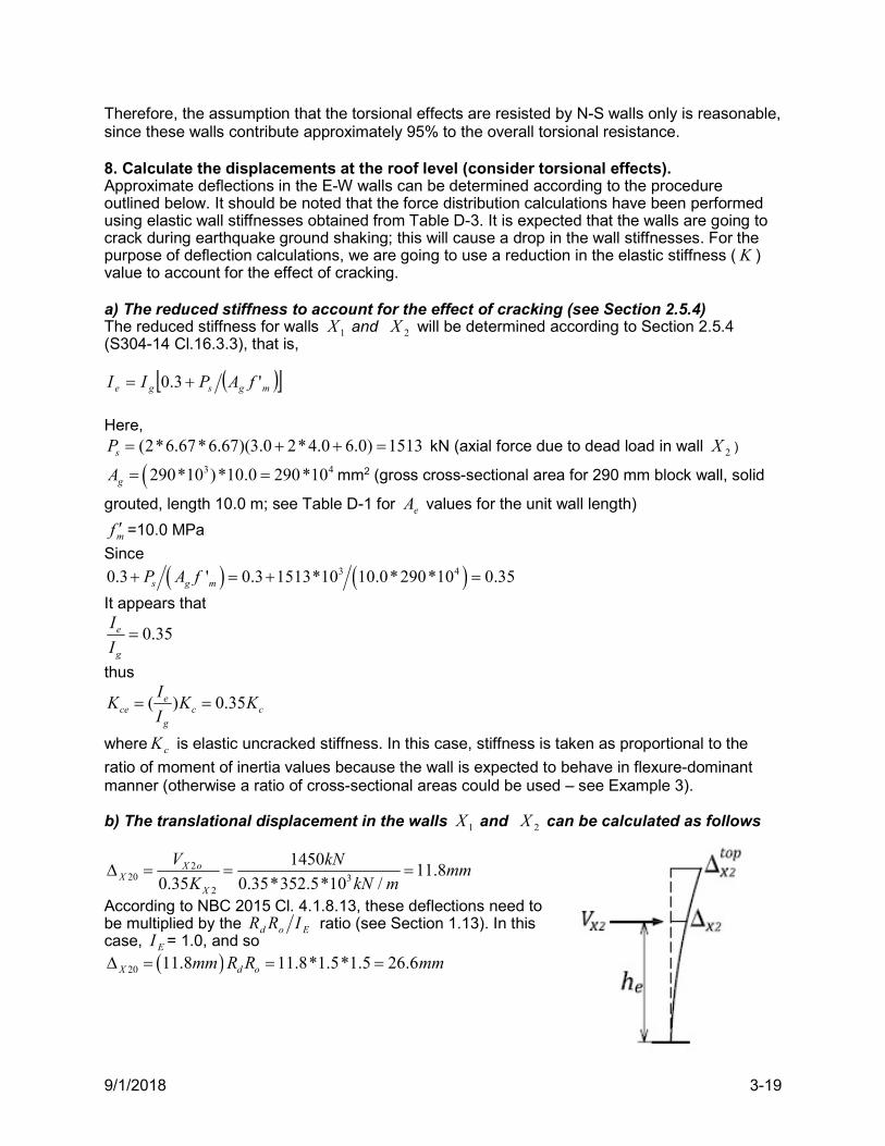
9/1/2018 3-19

Therefore, the assumption that the torsional effects are resisted by N-S walls only is reasonable, since these walls contribute approximately 95% to the overall torsional resistance. 8. Calculate the displacements at the roof level (consider torsional effects). Approximate deflections in the E-W walls can be determined according to the procedure outlined below. It should be noted that the force distribution calculations have been performed using elastic wall stiffnesses obtained from Table D-3. It is expected that the walls are going to crack during earthquake ground shaking; this will cause a drop in the wall stiffnesses. For the purpose of deflection calculations, we are going to use a reduction in the elastic stiffness ( K ) value to account for the effect of cracking. a) The reduced stiffness to account for the effect of cracking (see Section 2.5.4) The reduced stiffness for walls 1X and 2X will be determined according to Section 2.5.4 (S304-14 Cl.16.3.3), that is,

mgsge fAPII '3.0

Here,

(2*6.67*6.67)(3.0 2*4.0 6.0) 1513sP kN (axial force due to dead load in wall 2X )

3 4290*10 )*10.0 290*10gA mm2 (gross cross-sectional area for 290 mm block wall, solid

grouted, length 10.0 m; see Table D-1 for eA values for the unit wall length)

mf =10.0 MPa

Since

3 40.3 ' 0.3 1513*10 10.0*290*10 0.35s g mP A f

It appears that

0.35e

g

I

I

thus

( ) 0.35ece c c

g

IK K K

I

where cK is elastic uncracked stiffness. In this case, stiffness is taken as proportional to the

ratio of moment of inertia values because the wall is expected to behave in flexure-dominant manner (otherwise a ratio of cross-sectional areas could be used – see Example 3). b) The translational displacement in the walls 1X and 2X can be calculated as follows

220 3

2

145011.8

0.35 0.35*352.5*10 /X o

XX

V kNmm

K kN m

According to NBC 2015 Cl. 4.1.8.13, these deflections need to be multiplied by the Eod IRR ratio (see Section 1.13). In this case, EI = 1.0, and so

20 11.8 11.8*1.5*1.5 26.6X d omm R R mm

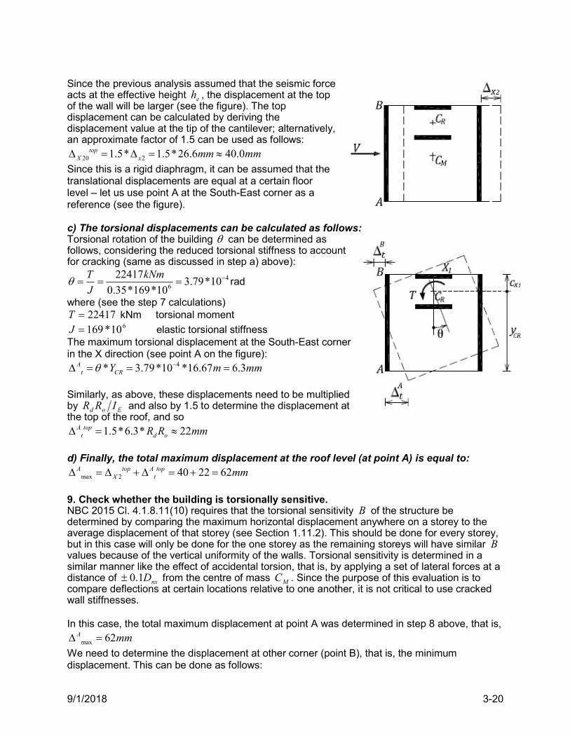
9/1/2018 3-20

Since the previous analysis assumed that the seismic force acts at the effective height eh , the displacement at the top of the wall will be larger (see the figure). The top displacement can be calculated by deriving the displacement value at the tip of the cantilever; alternatively, an approximate factor of 1.5 can be used as follows:

20 21.5* 1.5*26.6 40.0topX x mm mm

Since this is a rigid diaphragm, it can be assumed that the translational displacements are equal at a certain floor level – let us use point A at the South-East corner as a reference (see the figure). c) The torsional displacements can be calculated as follows: Torsional rotation of the building can be determined as follows, considering the reduced torsional stiffness to account for cracking (same as discussed in step a) above):

46

224173.79*10

0.35*169*10

T kNm

J rad

where (see the step 7 calculations) 22417T kNm torsional moment

610*169J elastic torsional stiffness The maximum torsional displacement at the South-East corner in the X direction (see point A on the figure):

4* 3.79*10 *16.67 6.3At CRY m mm

Similarly, as above, these displacements need to be multiplied by Eod IRR and also by 1.5 to determine the displacement at the top of the roof, and so

1.5*6.3* 22A topt d oR R mm

d) Finally, the total maximum displacement at the roof level (at point A) is equal to:

max 2 40 22 62A top A topX t mm

9. Check whether the building is torsionally sensitive. NBC 2015 Cl. 4.1.8.11(10) requires that the torsional sensitivity B of the structure be determined by comparing the maximum horizontal displacement anywhere on a storey to the average displacement of that storey (see Section 1.11.2). This should be done for every storey, but in this case will only be done for the one storey as the remaining storeys will have similar B values because of the vertical uniformity of the walls. Torsional sensitivity is determined in a similar manner like the effect of accidental torsion, that is, by applying a set of lateral forces at a distance of nxD1.0 from the centre of mass MC . Since the purpose of this evaluation is to compare deflections at certain locations relative to one another, it is not critical to use cracked wall stiffnesses. In this case, the total maximum displacement at point A was determined in step 8 above, that is,

max 62A mm

We need to determine the displacement at other corner (point B), that is, the minimum displacement. This can be done as follows:

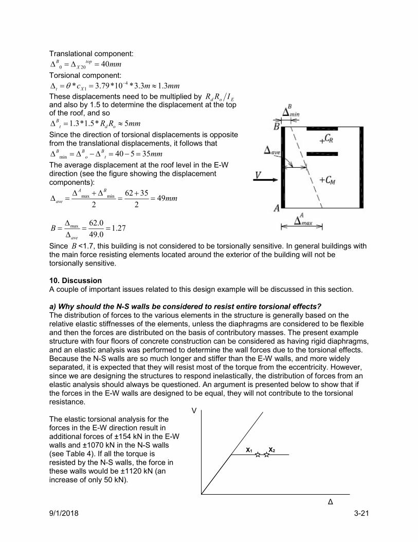
9/1/2018 3-21

Translational component:

0 20 40B topX mm

Torsional component: 4

1* 3.79*10 *3.3 1.3t Xc m mm

These displacements need to be multiplied by Eod IRR and also by 1.5 to determine the displacement at the top of the roof, and so

1.3*1.5* 5Bt d oR R mm

Since the direction of torsional displacements is opposite from the translational displacements, it follows that

min 40 5 35B B Bo t mm

The average displacement at the roof level in the E-W direction (see the figure showing the displacement components):

max min 62 3549

2 2

A B

ave mm

max 62.01.27

49.0ave

B

Since B <1.7, this building is not considered to be torsionally sensitive. In general buildings with the main force resisting elements located around the exterior of the building will not be torsionally sensitive. 10. Discussion A couple of important issues related to this design example will be discussed in this section. a) Why should the N-S walls be considered to resist entire torsional effects? The distribution of forces to the various elements in the structure is generally based on the relative elastic stiffnesses of the elements, unless the diaphragms are considered to be flexible and then the forces are distributed on the basis of contributory masses. The present example structure with four floors of concrete construction can be considered as having rigid diaphragms, and an elastic analysis was performed to determine the wall forces due to the torsional effects. Because the N-S walls are so much longer and stiffer than the E-W walls, and more widely separated, it is expected that they will resist most of the torque from the eccentricity. However, since we are designing the structures to respond inelastically, the distribution of forces from an elastic analysis should always be questioned. An argument is presented below to show that if the forces in the E-W walls are designed to be equal, they will not contribute to the torsional resistance. The elastic torsional analysis for the forces in the E-W direction result in additional forces of ±154 kN in the E-W walls and ±1070 kN in the N-S walls (see Table 4). If all the torque is resisted by the N-S walls, the force in these walls would be ±1120 kN (an increase of only 50 kN).

Δ

V

X1 X2

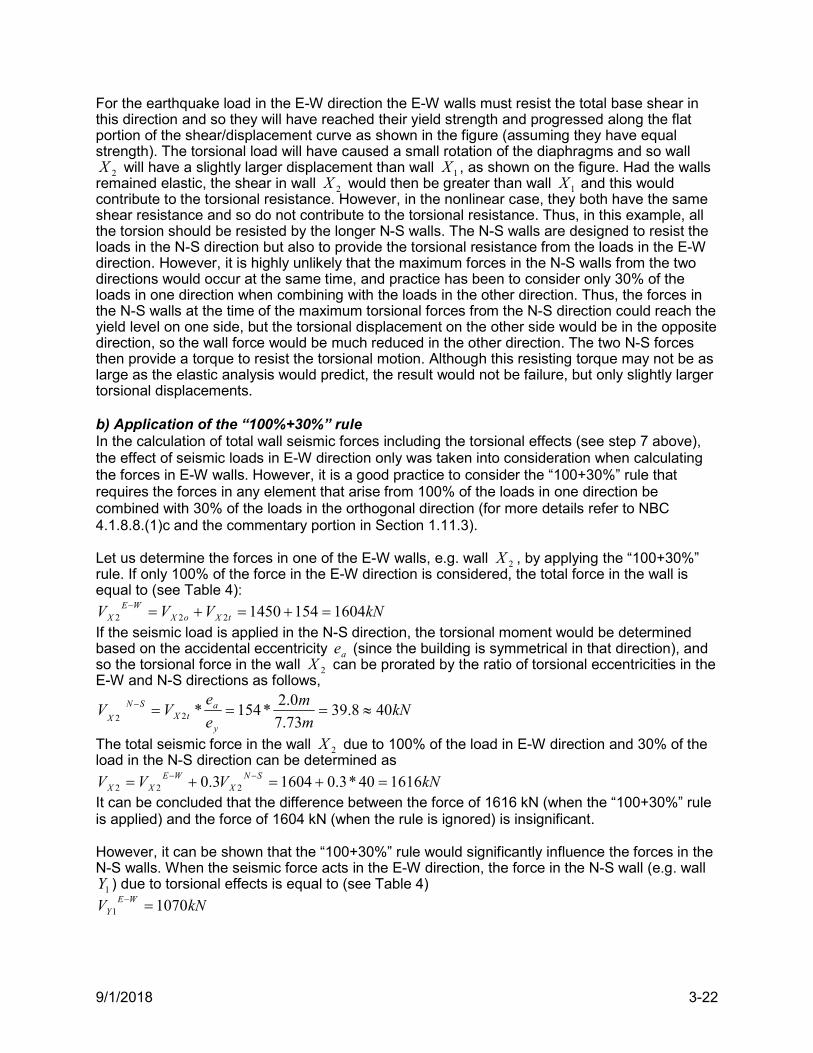
9/1/2018 3-22

For the earthquake load in the E-W direction the E-W walls must resist the total base shear in this direction and so they will have reached their yield strength and progressed along the flat portion of the shear/displacement curve as shown in the figure (assuming they have equal strength). The torsional load will have caused a small rotation of the diaphragms and so wall

2X will have a slightly larger displacement than wall 1X , as shown on the figure. Had the walls remained elastic, the shear in wall 2X would then be greater than wall 1X and this would contribute to the torsional resistance. However, in the nonlinear case, they both have the same shear resistance and so do not contribute to the torsional resistance. Thus, in this example, all the torsion should be resisted by the longer N-S walls. The N-S walls are designed to resist the loads in the N-S direction but also to provide the torsional resistance from the loads in the E-W direction. However, it is highly unlikely that the maximum forces in the N-S walls from the two directions would occur at the same time, and practice has been to consider only 30% of the loads in one direction when combining with the loads in the other direction. Thus, the forces in the N-S walls at the time of the maximum torsional forces from the N-S direction could reach the yield level on one side, but the torsional displacement on the other side would be in the opposite direction, so the wall force would be much reduced in the other direction. The two N-S forces then provide a torque to resist the torsional motion. Although this resisting torque may not be as large as the elastic analysis would predict, the result would not be failure, but only slightly larger torsional displacements. b) Application of the “100%+30%” rule In the calculation of total wall seismic forces including the torsional effects (see step 7 above), the effect of seismic loads in E-W direction only was taken into consideration when calculating the forces in E-W walls. However, it is a good practice to consider the “100+30%” rule that requires the forces in any element that arise from 100% of the loads in one direction be combined with 30% of the loads in the orthogonal direction (for more details refer to NBC 4.1.8.8.(1)c and the commentary portion in Section 1.11.3). Let us determine the forces in one of the E-W walls, e.g. wall 2X , by applying the “100+30%” rule. If only 100% of the force in the E-W direction is considered, the total force in the wall is equal to (see Table 4):

kNVVV tXoXWE

X 16041541450222

If the seismic load is applied in the N-S direction, the torsional moment would be determined based on the accidental eccentricity ae (since the building is symmetrical in that direction), and so the torsional force in the wall 2X can be prorated by the ratio of torsional eccentricities in the E-W and N-S directions as follows,

kNm

m

e

eVV

y

atX

SN

X408.39

73.7

0.2*154*22

The total seismic force in the wall 2X due to 100% of the load in E-W direction and 30% of the load in the N-S direction can be determined as

kNVVV SNX

WEXX 161640*3.016043.0 222

It can be concluded that the difference between the force of 1616 kN (when the “100+30%” rule is applied) and the force of 1604 kN (when the rule is ignored) is insignificant. However, it can be shown that the “100+30%” rule would significantly influence the forces in the N-S walls. When the seismic force acts in the E-W direction, the force in the N-S wall (e.g. wall

1Y ) due to torsional effects is equal to (see Table 4)

kNV WEY 10701

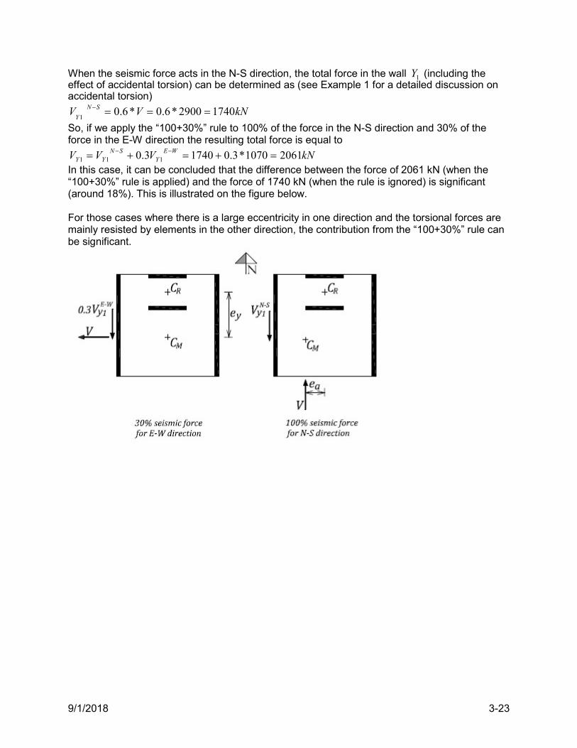
9/1/2018 3-23

When the seismic force acts in the N-S direction, the total force in the wall 1Y (including the effect of accidental torsion) can be determined as (see Example 1 for a detailed discussion on accidental torsion)

kNVV SN

Y17402900*6.0*6.0

1

So, if we apply the “100+30%” rule to 100% of the force in the N-S direction and 30% of the force in the E-W direction the resulting total force is equal to

kNVVV WEY

SNYY 20611070*3.017403.0 111

In this case, it can be concluded that the difference between the force of 2061 kN (when the “100+30%” rule is applied) and the force of 1740 kN (when the rule is ignored) is significant (around 18%). This is illustrated on the figure below. For those cases where there is a large eccentricity in one direction and the torsional forces are mainly resisted by elements in the other direction, the contribution from the “100+30%” rule can be significant.

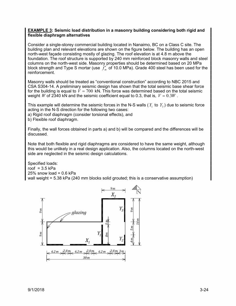
9/1/2018 3-24

EXAMPLE 3: Seismic load distribution in a masonry building considering both rigid and flexible diaphragm alternatives Consider a single-storey commercial building located in Nanaimo, BC on a Class C site. The building plan and relevant elevations are shown on the figure below. The building has an open north-west façade consisting mostly of glazing. The roof elevation is at 4.8 m above the foundation. The roof structure is supported by 240 mm reinforced block masonry walls and steel columns on the north-west side. Masonry properties should be determined based on 20 MPa block strength and Type S mortar (use mf of 10.0 MPa). Grade 400 steel has been used for the reinforcement. Masonry walls should be treated as “conventional construction” according to NBC 2015 and CSA S304-14. A preliminary seismic design has shown that the total seismic base shear force for the building is equal to 700V kN. This force was determined based on the total seismic weight W of 2340 kN and the seismic coefficient equal to 0.3, that is, WV 3.0 . This example will determine the seismic forces in the N-S walls ( 1Y to 3Y ) due to seismic force acting in the N-S direction for the following two cases: a) Rigid roof diaphragm (consider torsional effects), and b) Flexible roof diaphragm. Finally, the wall forces obtained in parts a) and b) will be compared and the differences will be discussed. Note that both flexible and rigid diaphragms are considered to have the same weight, although this would be unlikely in a real design application. Also, the columns located on the north-west side are neglected in the seismic design calculations. Specified loads: roof = 3.5 kPa 25% snow load = 0.6 kPa wall weight = 5.38 kPa (240 mm blocks solid grouted; this is a conservative assumption)

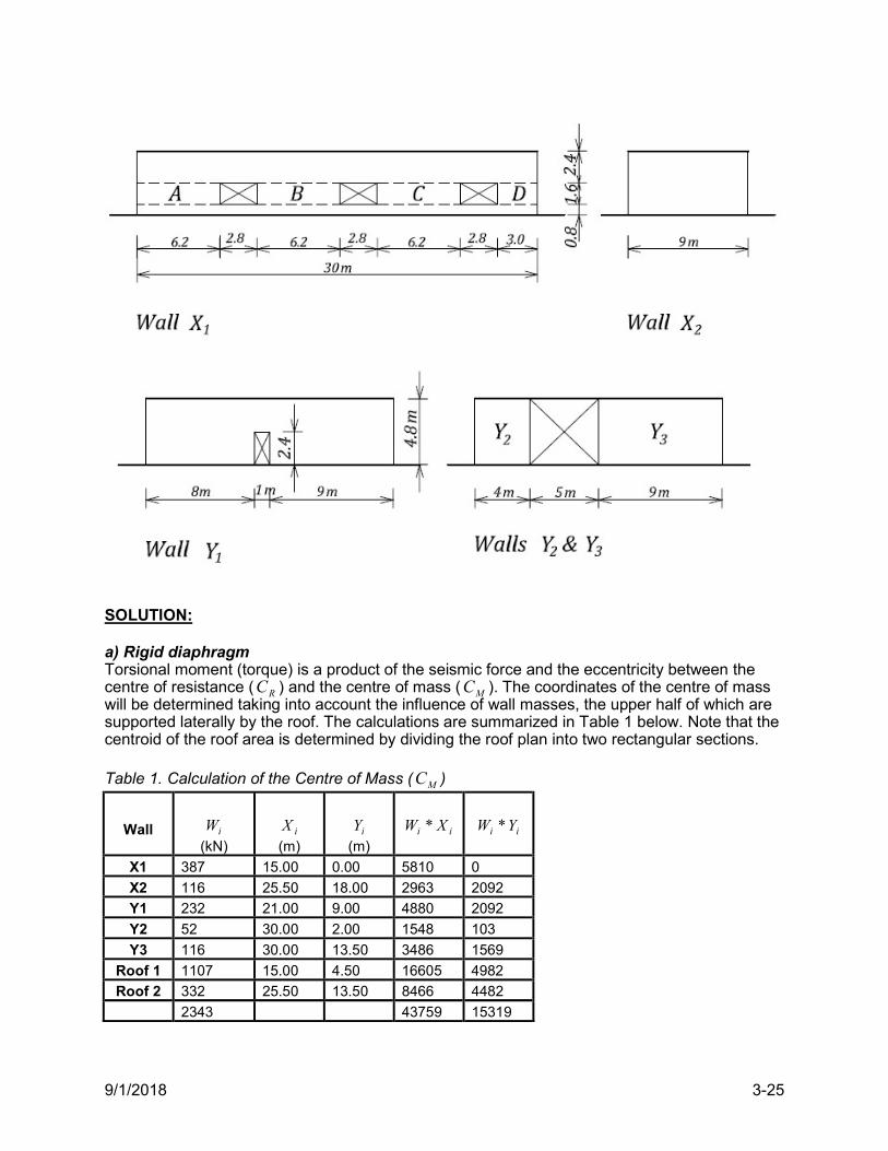
9/1/2018 3-25

SOLUTION: a) Rigid diaphragm Torsional moment (torque) is a product of the seismic force and the eccentricity between the centre of resistance ( RC ) and the centre of mass ( MC ). The coordinates of the centre of mass will be determined taking into account the influence of wall masses, the upper half of which are supported laterally by the roof. The calculations are summarized in Table 1 below. Note that the centroid of the roof area is determined by dividing the roof plan into two rectangular sections. Table 1. Calculation of the Centre of Mass ( MC )

Wall

iW

(kN) iX

(m) iY

(m) ii XW *

ii YW *

X1 387 15.00 0.00 5810 0

X2 116 25.50 18.00 2963 2092

Y1 232 21.00 9.00 4880 2092

Y2 52 30.00 2.00 1548 103

Y3 116 30.00 13.50 3486 1569

Roof 1 1107 15.00 4.50 16605 4982

Roof 2 332 25.50 13.50 8466 4482

2343 43759 15319

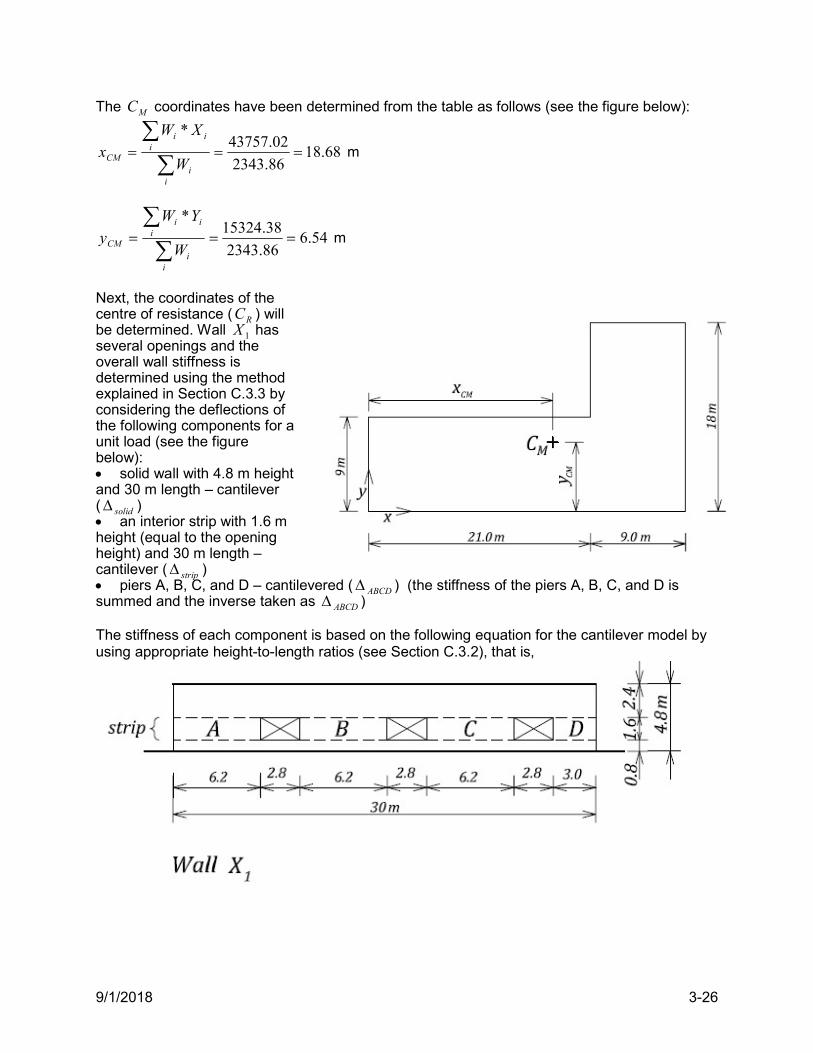
9/1/2018 3-26

The MC coordinates have been determined from the table as follows (see the figure below):

68.1886.2343

02.43757*

ii

iii

CM W

XWx m

54.686.2343

38.15324*

ii

iii

CM W

YWy m

Next, the coordinates of the centre of resistance ( RC ) will be determined. Wall 1X has several openings and the overall wall stiffness is determined using the method explained in Section C.3.3 by considering the deflections of the following components for a unit load (see the figure below): solid wall with 4.8 m height and 30 m length – cantilever ( solid ) an interior strip with 1.6 m height (equal to the opening height) and 30 m length – cantilever ( strip ) piers A, B, C, and D – cantilevered ( ABCD ) (the stiffness of the piers A, B, C, and D is summed and the inverse taken as ABCD ) The stiffness of each component is based on the following equation for the cantilever model by using appropriate height-to-length ratios (see Section C.3.2), that is,

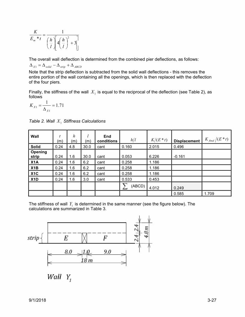
9/1/2018 3-27

34

1

* 2

l

h

l

htE

K

m

The overall wall deflection is determined from the combined pier deflections, as follows:

ABCDstripsolidX 1

Note that the strip deflection is subtracted from the solid wall deflections - this removes the entire portion of the wall containing all the openings, which is then replaced with the deflection of the four piers. Finally, the stiffness of the wall 1X is equal to the reciprocal of the deflection (see Table 2), as follows

71.11

11

XXK

Table 2. Wall 1X Stiffness Calculations

Wall

t (m)

h (m)

l (m)

End conditions lh )*( tEK Displacement )*( tEK final

Solid 0.24 4.8 30.0 cant 0.160 2.015 0.496 Opening strip 0.24 1.6 30.0 cant 0.053 6.226 -0.161

X1A 0.24 1.6 6.2 cant 0.258 1.186

X1B 0.24 1.6 6.2 cant 0.258 1.186

X1C 0.24 1.6 6.2 cant 0.258 1.186

X1D 0.24 1.6 3.0 cant 0.533 0.453

(ABCD) 4.012 0.249

0.585 1.709

The stiffness of wall 1Y is determined in the same manner (see the figure below). The calculations are summarized in Table 3.

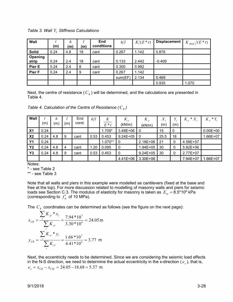
9/1/2018 3-28

Table 3. Wall 1Y Stiffness Calculations Wall

t (m)

h (m)

l (m)

End conditions

lh )*( tEK Displacement )*( tEK final

Solid 0.24 4.8 18 cant 0.267 1.142 0.876 Opening strip 0.24 2.4 18 cant 0.133 2.442 -0.409

Pier E 0.24 2.4 8 cant 0.300 0.992

Pier F 0.24 2.4 9 cant 0.267 1.142

sum(EF) 2.134 0.469

0.935 1.070 Next, the centre of resistance ( RC ) will be determined, and the calculations are presented in Table 4. Table 4. Calculation of the Centre of Resistance ( RC ) Wall

t

(m) h

(m) l

(m) End

cond. lh

tE

K

* xK

(kN/m) yK

(kN/m) iX

(m) iY

(m) iy XK * ix YK *

X1 0.24 1.709* 3.49E+06 0 15 0 0.00E+00

X2 0.24 4.8 9 cant 0.53 0.453 9.24E+05 0 25.5 18 1.66E+07

Y1 0.24 1.070** 0 2.18E+06 21 0 4.58E+07

Y2 0.24 4.8 4 cant 1.20 0.095 0 1.94E+05 30 0 5.82E+06

Y3 0.24 4.8 9 cant 0.53 0.453 0 9.24E+05 30 0 2.77E+07

4.41E+06 3.30E+06 7.94E+07 1.66E+07

Notes: * - see Table 2 ** - see Table 3 Note that all walls and piers in this example were modelled as cantilevers (fixed at the base and free at the top). For more discussion related to modelling of masonry walls and piers for seismic loads see Section C.3. The modulus of elasticity for masonry is taken as mE 8.5*106 kPa (corresponding to mf of 10 MPa). The RC coordinates can be determined as follows (see the figure on the next page):

05.2410*30.3

10*94.7*

6

7

iyi

iiyi

CR K

xKx m

77.310*41.4

10*66.1*

6

7

ixi

iixi

CR K

yKy m

Next, the eccentricity needs to be determined. Since we are considering the seismic load effects in the N-S direction, we need to determine the actual eccentricity in the x-direction ( xe ), that is,

37.568.1805.24 CMCRx xxe m

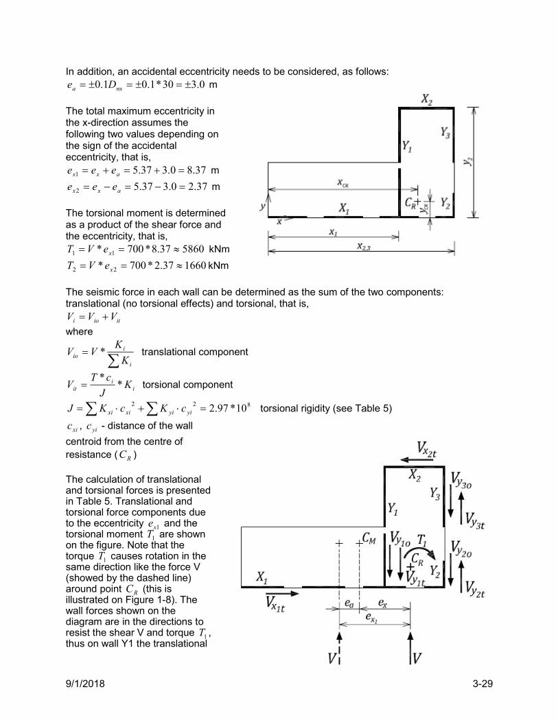
9/1/2018 3-29

In addition, an accidental eccentricity needs to be considered, as follows: 0.330*1.01.0 nxa De m

The total maximum eccentricity in the x-direction assumes the following two values depending on the sign of the accidental eccentricity, that is,

37.80.337.51 axx eee m

37.20.337.52 axx eee m

The torsional moment is determined as a product of the shear force and the eccentricity, that is,

586037.8*700* 11 xeVT kNm

166037.2*700* 22 xeVT kNm

The seismic force in each wall can be determined as the sum of the two components: translational (no torsional effects) and torsional, that is,

itioi VVV

where

i

iio K

KVV * translational component

ii

it KJ

cTV *

* torsional component

822 10*97.2 yiyixixi cKcKJ torsional rigidity (see Table 5)

xic , yic - distance of the wall

centroid from the centre of resistance ( RC ) The calculation of translational and torsional forces is presented in Table 5. Translational and torsional force components due to the eccentricity 1xe and the torsional moment 1T are shown on the figure. Note that the torque 1T causes rotation in the same direction like the force V (showed by the dashed line) around point RC (this is illustrated on Figure 1-8). The wall forces shown on the diagram are in the directions to resist the shear V and torque 1T , thus on wall Y1 the translational

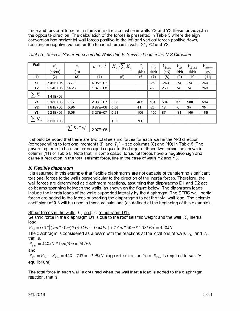
9/1/2018 3-30

force and torsional force act in the same direction, while in walls Y2 and Y3 these forces act in the opposite direction. The calculation of the forces is presented in Table 5 where the sign convention has horizontal wall forces positive to the left and vertical forces positive down, resulting in negative values for the torsional forces in walls X1, Y2 and Y3. Table 5. Seismic Shear Forces in the Walls due to Seismic Load in the N-S Direction

Wall iK

(kN/m) ic

(m)

2* ii cK yy KK oV

(kN) tV1

(kN) totalV1

(kN) tV2

(kN) totalV2

(kN) governV

(kN) (1) (2) (3) (4) (5) (6) (7) (8) (9) (10) (11)

X1 3.49E+06 -3.77 4.96E+07 -260 -260 -74 -74 260

X2 9.24E+05 14.23 1.87E+08 260 260 74 74 260

xK 4.41E+06

Y1 2.18E+06 3.05 2.03E+07 0.66 463 131 594 37 500 594

Y2 1.94E+05 -5.95 6.87E+06 0.06 41 -23 18 -6 35 35

Y3 9.24E+05 -5.95 3.27E+07 0.28 196 -109 87 -31 165 165

yK 3.30E+06 1.00 700

2* ii cK

2.97E+08

It should be noted that there are two total seismic forces for each wall in the N-S direction (corresponding to torsional moments 1T and 2T ) – see columns (8) and (10) in Table 5. The governing force to be used for design is equal to the larger of these two forces, as shown in column (11) of Table 5. Note that, in some cases, torsional forces have a negative sign and cause a reduction in the total seismic force, like in the case of walls Y2 and Y3. b) Flexible diaphragm It is assumed in this example that flexible diaphragms are not capable of transferring significant torsional forces to the walls perpendicular to the direction of the inertia forces. Therefore, the wall forces are determined as diaphragm reactions, assuming that diaphragms D1 and D2 act as beams spanning between the walls, as shown on the figure below. The diaphragm loads include the inertia loads of the walls supported laterally by the diaphragm. The SFRS wall inertia forces are added to the forces supporting the diaphragms to get the total wall load. The seismic coefficient of 0.3 will be used in these calculations (as defined at the beginning of this example). Shear forces in the walls aY1 and 2Y (diaphragm D1): Seismic force in the diaphragm D1 is due to the roof seismic weight and the wall 1X inertia load:

kNkPammkPakPammVD 44838.5*30*4.2)6.05.3(*)30*9(*3.01 The diaphragm is considered as a beam with the reactions at the locations of walls aY1 and 2Y , that is,

kNmmkNR aY 747915*4481

and kNRVR aYDY 299747448112 (opposite direction from aYR 1 is required to satisfy

equilibrium) The total force in each wall is obtained when the wall inertia load is added to the diaphragm reaction, that is,

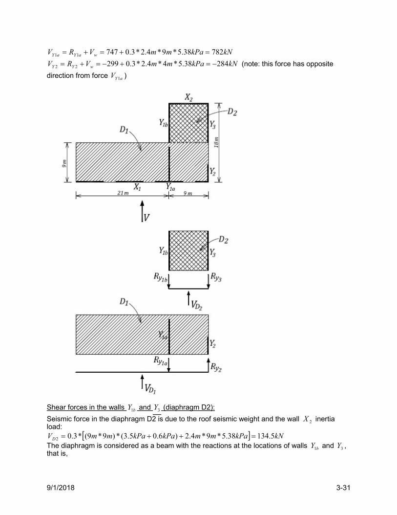
9/1/2018 3-31

kNkPammVRV waYaY 78238.5*9*4.2*3.074711

kNkPammVRV wYY 28438.5*4*4.2*3.029922 (note: this force has opposite

direction from force aYV 1 )

Shear forces in the walls bY1 and 3Y (diaphragm D2):

Seismic force in the diaphragm D2 is due to the roof seismic weight and the wall 2X inertia load:

kNkPammkPakPammVD 5.13438.5*9*4.2)6.05.3(*)9*9(*3.02 The diaphragm is considered as a beam with the reactions at the locations of walls bY1 and 3Y , that is,

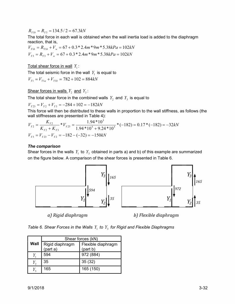
9/1/2018 3-32

kNRR YbY 3.672/5.13431

The total force in each wall is obtained when the wall inertia load is added to the diaphragm reaction, that is,

kNkPammVRV wbYbY 10238.5*9*4.2*3.06711

kNkPammVRV wYY 10238.5*9*4.2*3.06733

Total shear force in wall 1Y :

The total seismic force in the wall 1Y is equal to

kNVVV bYaYY 884102782111

Shear forces in walls 2Y and 3Y :

The total shear force in the combined walls 2Y and 3Y is equal to

kNVVV YYY 1821022843223

This force will then be distributed to these walls in proportion to the wall stiffness, as follows (the wall stiffnesses are presented in Table 4):

kNVKK

KV Y

YY

YY 32)182(*17.0)182(*

10*24.910*94.1

10*94.1*

55

5

2332

22

kNVVV YYY 150)32(1822233

The comparison Shear forces in the walls 1Y to 3Y obtained in parts a) and b) of this example are summarized

on the figure below. A comparison of the shear forces is presented in Table 6.

Table 6. Shear Forces in the Walls 1Y to 3Y for Rigid and Flexible Diaphragms

Wall Shear forces (kN)

Rigid diaphragm (part a)

Flexible diaphragm (part b)

1Y 594 972 (884)

2Y 35 35 (32)

3Y 165 165 (150)

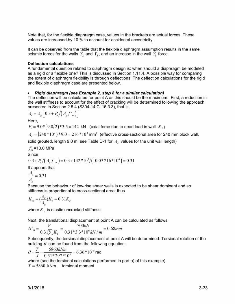
9/1/2018 3-33

Note that, for the flexible diaphragm case, values in the brackets are actual forces. These values are increased by 10 % to account for accidental eccentricity. It can be observed from the table that the flexible diaphragm assumption results in the same seismic forces for the walls 2Y and 3Y , and an increase in the wall 1Y force. Deflection calculations A fundamental question related to diaphragm design is: when should a diaphragm be modeled as a rigid or a flexible one? This is discussed in Section 1.11.4. A possible way for comparing the extent of diaphragm flexibility is through deflections. The deflection calculations for the rigid and flexible diaphragm case are presented below. Rigid diaphragm (see Example 2, step 8 for a similar calculation) The deflection will be calculated for point A as this should be the maximum. First, a reduction in the wall stiffness to account for the effect of cracking will be determined following the approach presented in Section 2.5.4 (S304-14 Cl.16.3.3), that is,

0.3 'e g s g mA A P A f

Here,

9.0* 9.0 2 *3.5 142sP kN (axial force due to dead load in wall 2X )

43 10*2160.9*)10*240 eA mm2 (effective cross-sectional area for 240 mm block wall,

solid grouted, length 9.0 m; see Table D-1 for eA values for the unit wall length)

mf =10.0 MPa

Since

3 40.3 ' 0.3 142*10 10.0*216*10 0.31s g mP A f

It appears that

0.31e

g

A

A

Because the behaviour of low-rise shear walls is expected to be shear dominant and so stiffness is proportional to cross-sectional area; thus

( ) 0.31ece c c

g

AK K K

A

where cK is elastic uncracked stiffness

Next, the translational displacement at point A can be calculated as follows:

0 6

7000.68

0.31 0.31*3.3*10 /A

Y

V kNmm

K kN m

Subsequently, the torsional displacement at point A will be determined. Torsional rotation of the building can be found from the following equation:

56

58606.36*10

0.31*297*10

T kNm

J rad

where (see the torsional calculations performed in part a) of this example) 5860T kNm torsional moment

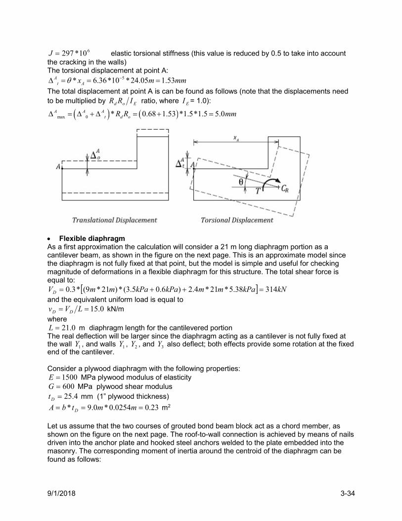
9/1/2018 3-34

610*297J elastic torsional stiffness (this value is reduced by 0.5 to take into account the cracking in the walls) The torsional displacement at point A:

5* 6.36*10 *24.05 1.53At Ax m mm

The total displacement at point A is can be found as follows (note that the displacements need to be multiplied by Eod IRR ratio, where EI = 1.0):

max 0 * 0.68 1.53 *1.5*1.5 5.0A A At d oR R mm

Flexible diaphragm As a first approximation the calculation will consider a 21 m long diaphragm portion as a cantilever beam, as shown in the figure on the next page. This is an approximate model since the diaphragm is not fully fixed at that point, but the model is simple and useful for checking magnitude of deformations in a flexible diaphragm for this structure. The total shear force is equal to:

kNkPammkPakPammVD 31438.5*21*4.2)6.05.3(*)21*9(*3.0 and the equivalent uniform load is equal to

0.15 LVv DD kN/m where

0.21L m diaphragm length for the cantilevered portion The real deflection will be larger since the diaphragm acting as a cantilever is not fully fixed at the wall 1Y , and walls 1Y , 2Y , and 3Y also deflect; both effects provide some rotation at the fixed end of the cantilever. Consider a plywood diaphragm with the following properties:

1500E MPa plywood modulus of elasticity 600G MPa plywood shear modulus

4.25Dt mm (1” plywood thickness)

23.00254.0*0.9* mmtbA D m2 Let us assume that the two courses of grouted bond beam block act as a chord member, as shown on the figure on the next page. The roof-to-wall connection is achieved by means of nails driven into the anchor plate and hooked steel anchors welded to the plate embedded into the masonry. The corresponding moment of inertia around the centroid of the diaphragm can be found as follows:

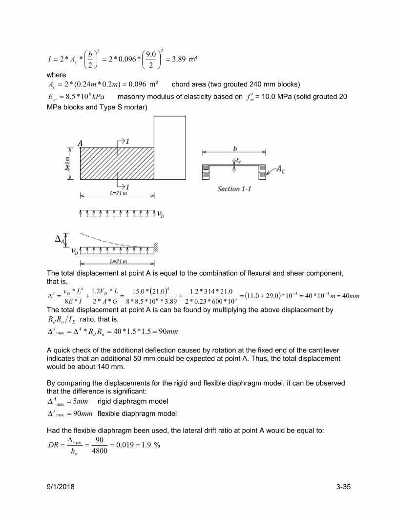
9/1/2018 3-35

89.32

0.9*096.0*2

2**2

22

b

AI c m4

where 096.0)2.0*24.0(*2 mmAc m2 chord area (two grouted 240 mm blocks)

kPaEm610*5.8 masonry modulus of elasticity based on mf = 10.0 MPa (solid grouted 20

MPa blocks and Type S mortar)

The total displacement at point A is equal to the combination of flexural and shear component, that is,

mmmGA

LV

IE

Lv DDA 4010*4010*0.290.1110*600*23.0*2

0.21*314*2.1

89.3*10*5.8*8

0.21*0.15

**2

*2.1

*8

* 33

36

44

The total displacement at point A is can be found by multiplying the above displacement by

Eod IRR ratio, that is,

mmRR odAA 905.1*5.1*40*max

A quick check of the additional deflection caused by rotation at the fixed end of the cantilever indicates that an additional 50 mm could be expected at point A. Thus, the total displacement would be about 140 mm. By comparing the displacements for the rigid and flexible diaphragm model, it can be observed that the difference is significant:

max 5A mm rigid diaphragm model

mmA 90max flexible diaphragm model Had the flexible diaphragm been used, the lateral drift ratio at point A would be equal to:

9.1019.04800

90max

wh

DR %

9/1/2018 3-36

The drift is within the NBC 2015 limit of 2.5% (see Section 1.13); however, a flexible diaphragm would not be an ideal solution for this design – a rigid diaphragm would be the preferred solution. Discussion In this example, seismic forces were determined for the N-S walls due to seismic load acting in the N-S direction. It should be noted, however, that there is a significant eccentricity causing torsional effects in the E-W walls due to seismic load acting in the E-W direction – these calculations were not included in this example.

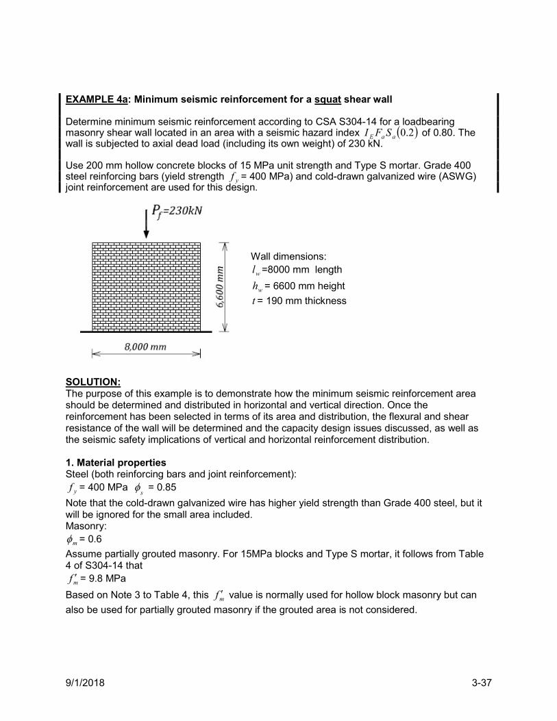
9/1/2018 3-37

EXAMPLE 4a: Minimum seismic reinforcement for a squat shear wall Determine minimum seismic reinforcement according to CSA S304-14 for a loadbearing masonry shear wall located in an area with a seismic hazard index 2.0aaE SFI of 0.80. The wall is subjected to axial dead load (including its own weight) of 230 kN. Use 200 mm hollow concrete blocks of 15 MPa unit strength and Type S mortar. Grade 400 steel reinforcing bars (yield strength yf = 400 MPa) and cold-drawn galvanized wire (ASWG) joint reinforcement are used for this design.

Wall dimensions:

wl =8000 mm length

wh = 6600 mm height

t = 190 mm thickness

SOLUTION: The purpose of this example is to demonstrate how the minimum seismic reinforcement area should be determined and distributed in horizontal and vertical direction. Once the reinforcement has been selected in terms of its area and distribution, the flexural and shear resistance of the wall will be determined and the capacity design issues discussed, as well as the seismic safety implications of vertical and horizontal reinforcement distribution. 1. Material properties Steel (both reinforcing bars and joint reinforcement):

yf = 400 MPa s

= 0.85

Note that the cold-drawn galvanized wire has higher yield strength than Grade 400 steel, but it will be ignored for the small area included. Masonry:

m = 0.6

Assume partially grouted masonry. For 15MPa blocks and Type S mortar, it follows from Table 4 of S304-14 that

mf = 9.8 MPa

Based on Note 3 to Table 4, this mf value is normally used for hollow block masonry but can

also be used for partially grouted masonry if the grouted area is not considered.

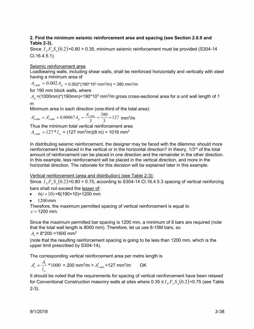
9/1/2018 3-38

2. Find the minimum seismic reinforcement area and spacing (see Section 2.6.9 and Table 2-3). Since 2.0aaE SFI =0.80 > 0.35, minimum seismic reinforcement must be provided (S304-14

Cl.16.4.5.1). Seismic reinforcement area Loadbearing walls, including shear walls, shall be reinforced horizontally and vertically with steel having a minimum area of

gs AA 002.0min = 0.002*(190*103 mm2/m) = 380 mm2/m

for 190 mm block walls, where

gA =(1000mm)*(190mm)=190*103 mm2/m gross cross-sectional area for a unit wall length of 1

m Minimum area in each direction (one-third of the total area):

1273

380

300067.0 min

minmin sgvh

AAAA mm2/m

Thus the minimum total vertical reinforcement area

wv lA *127min = (127 mm2/m)(8 m) = 1016 mm2

In distributing seismic reinforcement, the designer may be faced with the dilemma: should more reinforcement be placed in the vertical or in the horizontal direction? In theory, 1/3rd of the total amount of reinforcement can be placed in one direction and the remainder in the other direction. In this example, less reinforcement will be placed in the vertical direction, and more in the horizontal direction. The rationale for this decision will be explained later in this example. Vertical reinforcement (area and distribution) (see Table 2-3): Since 2.0aaE SFI =0.80 > 0.75, according to S304-14 Cl.16.4.5.3 spacing of vertical reinforcing

bars shall not exceed the lesser of: )10(6 t =6(190+10)=1200 mm

1200mm Therefore, the maximum permitted spacing of vertical reinforcement is equal to s 1200 mm.

Since the maximum permitted bar spacing is 1200 mm, a minimum of 8 bars are required (note that the total wall length is 8000 mm). Therefore, let us use 8-15M bars, so

vA = 8*200 =1600 mm2

(note that the resulting reinforcement spacing is going to be less than 1200 mm, which is the upper limit prescribed by S304-14). The corresponding vertical reinforcement area per metre length is

1000*w

vv l

AA = 200 mm2/m > minvA =127 mm2/m OK

It should be noted that the requirements for spacing of vertical reinforcement have been relaxed for Conventional Construction masonry walls at sites where 0.35 ≤ 2.0aaE SFI <0.75 (see Table

2-3).

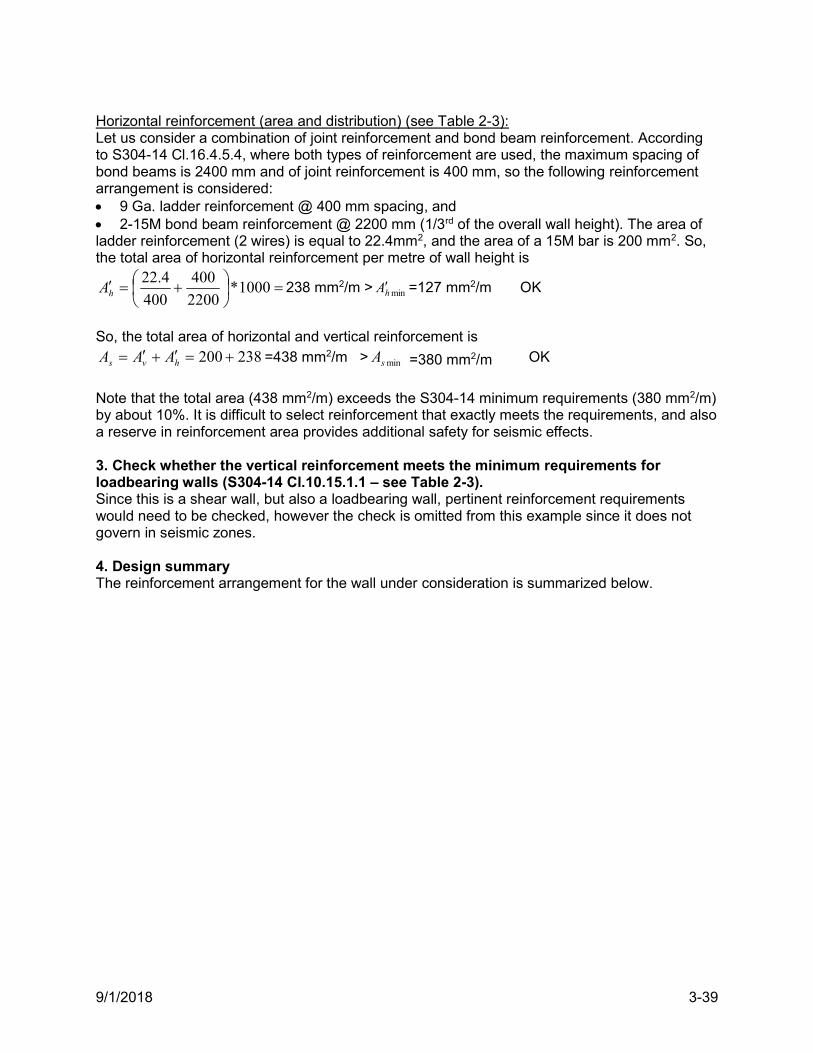
9/1/2018 3-39

Horizontal reinforcement (area and distribution) (see Table 2-3): Let us consider a combination of joint reinforcement and bond beam reinforcement. According to S304-14 Cl.16.4.5.4, where both types of reinforcement are used, the maximum spacing of bond beams is 2400 mm and of joint reinforcement is 400 mm, so the following reinforcement arrangement is considered: 9 Ga. ladder reinforcement @ 400 mm spacing, and 2-15M bond beam reinforcement @ 2200 mm (1/3rd of the overall wall height). The area of ladder reinforcement (2 wires) is equal to 22.4mm2, and the area of a 15M bar is 200 mm2. So, the total area of horizontal reinforcement per metre of wall height is

1000*

2200

400

400

4.22hA 238 mm2/m > minhA =127 mm2/m OK

So, the total area of horizontal and vertical reinforcement is

238200 hvs AAA =438 mm2/m > minsA =380 mm2/m OK

Note that the total area (438 mm2/m) exceeds the S304-14 minimum requirements (380 mm2/m) by about 10%. It is difficult to select reinforcement that exactly meets the requirements, and also a reserve in reinforcement area provides additional safety for seismic effects. 3. Check whether the vertical reinforcement meets the minimum requirements for loadbearing walls (S304-14 Cl.10.15.1.1 – see Table 2-3). Since this is a shear wall, but also a loadbearing wall, pertinent reinforcement requirements would need to be checked, however the check is omitted from this example since it does not govern in seismic zones. 4. Design summary The reinforcement arrangement for the wall under consideration is summarized below.

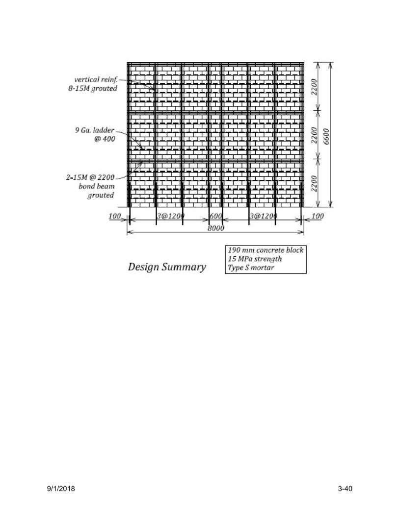
9/1/2018 3-40

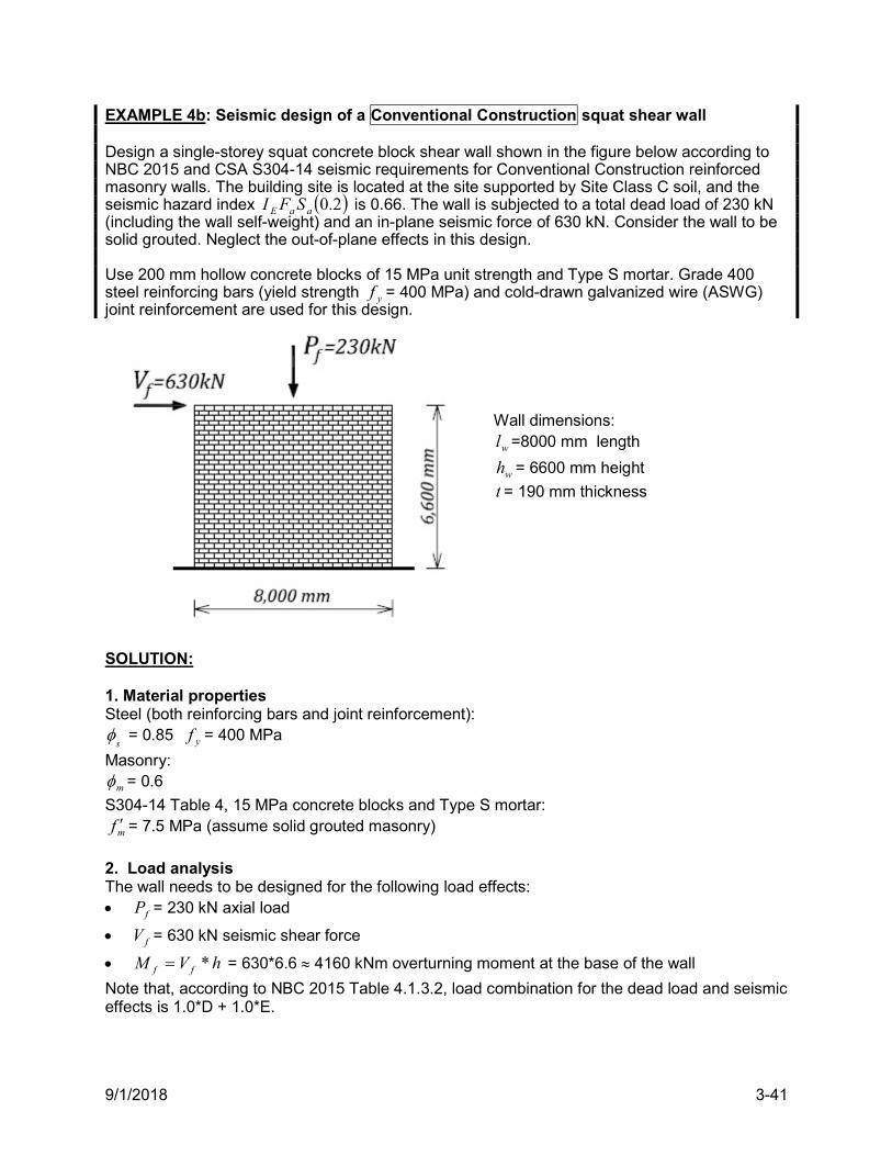
9/1/2018 3-41

EXAMPLE 4b: Seismic design of a Conventional Construction squat shear wall Design a single-storey squat concrete block shear wall shown in the figure below according to NBC 2015 and CSA S304-14 seismic requirements for Conventional Construction reinforced masonry walls. The building site is located at the site supported by Site Class C soil, and the seismic hazard index 2.0aaE SFI is 0.66. The wall is subjected to a total dead load of 230 kN (including the wall self-weight) and an in-plane seismic force of 630 kN. Consider the wall to be solid grouted. Neglect the out-of-plane effects in this design. Use 200 mm hollow concrete blocks of 15 MPa unit strength and Type S mortar. Grade 400 steel reinforcing bars (yield strength yf = 400 MPa) and cold-drawn galvanized wire (ASWG) joint reinforcement are used for this design.

Wall dimensions:

wl =8000 mm length

wh = 6600 mm height

t = 190 mm thickness

SOLUTION: 1. Material properties Steel (both reinforcing bars and joint reinforcement):

s = 0.85 yf = 400 MPa

Masonry:

m = 0.6

S304-14 Table 4, 15 MPa concrete blocks and Type S mortar:

mf = 7.5 MPa (assume solid grouted masonry)

2. Load analysis The wall needs to be designed for the following load effects: fP = 230 kN axial load

fV = 630 kN seismic shear force

hVM ff * = 630*6.6 4160 kNm overturning moment at the base of the wall

Note that, according to NBC 2015 Table 4.1.3.2, load combination for the dead load and seismic effects is 1.0*D + 1.0*E.

9/1/2018 3-42

3. Minimum CSA S304-14 seismic reinforcement (see Section 2.6.9 and Table 2-3) Since 2.0aaE SFI = 0.66 > 0.35, minimum seismic reinforcement is required (S304-14 Cl.16.4.5.1). See Example 4a for a detailed calculation of the S304-14 minimum seismic reinforcement. 4. Design for the combined axial load and flexure A design for the combined effects of axial load and flexure will be performed using two different procedures: i) by considering uniformly distributed vertical reinforcement, and ii) by considering concentrated and distributed reinforcement. Distributed wall reinforcement (see Section C.1.1.2) This procedure assumes uniformly distributed vertical reinforcement over the wall length. The total vertical reinforcement area can be estimated, and the estimate can be revised until the moment resistance value is sufficiently large. After a few trial estimates, the total area of vertical reinforcement was determined as

vtA = 3200 mm2 > 1016 mm2 (minimum seismic reinforcement) - OK

Try 16-15M bars for vertical reinforcement. The wall is subjected to axial load

fP = 230 kN

The approximate moment resistance for the wall section is given by: 85.01 8.01

159.0190*8000*5.7*6.0

3200*400*85.0

'

tlf

Af

wmm

vtys

034.0190*8000*5.7*6.0

10*230

'

3

tlf

P

wmm

f

154780008.0*85.0159.0*2

034.0159.0

2 11

wlc

mm

8000

15441

3200*400*85.0

10*2301

1000

8000*3200*

1000

400*85.0*5.0115.0

3

wvtys

fwvtysr l

c

Af

PlAfM

4253rM kNm > 4160fM kNm OK

Distributed and concentrated wall reinforcement (see Section C.1.1.1) This procedure assumes the same total reinforcement area, but the concentrated reinforcement is provided at the wall ends, and the remaining reinforcement is distributed over the wall length.

vtA = 3200 mm2

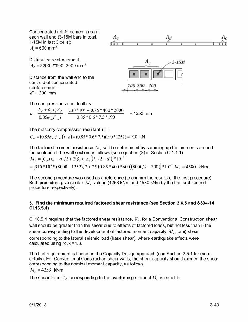
9/1/2018 3-43

Concentrated reinforcement area at each wall end (3-15M bars in total, 1-15M in last 3 cells):

cA = 600 mm2

Distributed reinforcement

dA 3200-2*600=2000 mm2

Distance from the wall end to the centroid of concentrated reinforcement

300d mm The compression zone depth a :

190*5.7*6.0*85.0

2000*400*85.010*230

'85.0

3

tf

AfPa

mm

dysf

= 1252 mm

The masonry compression resultant rC :

910)1252*190)(5.7*6.0*85.0('85.0 atfC mmm kN The factored moment resistance rM will be determined by summing up the moments around the centroid of the wall section as follows (see equation (3) in Section C.1.1.1)

610*'222)( dlAfalCM wcyswmr

63 10*30028000600*400*85.0*22)12528000(*10*910 4580rM kNm The second procedure was used as a reference (to confirm the results of the first procedure). Both procedure give similar rM values (4253 kNm and 4580 kNm by the first and second procedure respectively). 5. Find the minimum required factored shear resistance (see Section 2.6.5 and S304-14 Cl.16.5.4) Cl.16.5.4 requires that the factored shear resistance, rV , for a Conventional Construction shear wall should be greater than the shear due to effects of factored loads, but not less than i) the shear corresponding to the development of factored moment capacity, rM , or ii) shear

corresponding to the lateral seismic load (base shear), where earthquake effects were calculated using RdRo=1.3. The first requirement is based on the Capacity Design approach (see Section 2.5.1 for more details). For Conventional Construction shear walls, the shear capacity should exceed the shear corresponding to the nominal moment capacity, as follows

4253rM kNm

The shear force rbV corresponding to the overturning moment rM is equal to

9/1/2018 3-44

4253

6.6r

rb

MV

h 645 kN

The second requirement gives an “almost elastic” factored base shear force for the wall, which is equal to

630 1.5 1.51090

1.3 1.3f d o

fe

V R RV

kN

The smaller of these two values should be used, hence

645rdV kN

6. Find the diagonal tension shear resistance (see Section 2.3.2 and S304-14 Cl.10.10.2.1). Masonry shear resistance ( mV ):

190wb mm overall wall thickness

64008.0 wv ld mm effective wall depth

0.1g solid grouted wall

fd PP 9.0 = 207 kN

mvf

fm f

dV

Mv )2(16.0 = 0.44 MPa

4.6*630

4160

vf

f

dV

M= 1.03 1.0

gdvwmmm PdbvV )25.0( = 0.6(0.44*190*6400+0.25*207*103)*1.0 = 352 kN

Steel shear resistance sV (2-15M bond beam reinforcement at 1200 mm spacing):

1200

6400*400*

1000

400*85.0*6.06.0

s

dfAV vyvss = 435 kN

Total shear resistance 787435352 smr VVV kN

The factored shear resistance exceeds the minimum required factored shear resistance, that is, 787rV kN > 645rdV kN OK

This is a squat shear wall because 0.1825.08000

6600

w

w

l

h. Maximum shear allowed on the

section is (S304-14 Cl.10.10.2.1)

939)2(4.0max w

wgvwmmr l

hdbfV kN

Since

rr VV max OK Note that a solid grouted wall is required, that is, 0.1g . A partially grouted wall would have

5.0g , so its shear capacity would not be adequate for this design.

9/1/2018 3-45

7. Sliding shear resistance (see Section 2.3.3) The factored in-plane sliding shear resistance rV is determined as follows. = 1.0 for a masonry-to-masonry or masonry-to-roughened concrete sliding plane

sA = 3200 mm2 total area of vertical wall reinforcement

yssy fAT = 0.85*3200*400 = 1088 kN

dP = 207 kN

yd TPP 2 = 207+1088 = 1295 kN

2PV mr = 0.6*1.0*1295=777 kN

777rV kN > 645rdV kN OK

8. Design summary The reinforcement arrangement for the wall under consideration is shown in the figure below. Note that the wall is solidly grouted. A bond beam (transfer beam) is provided atop the wall to ensure uniform shear transfer along the entire length (see Section 2.3.2.2).

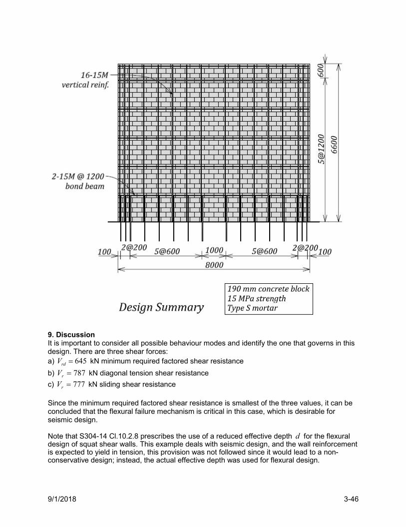
9/1/2018 3-46

9. Discussion It is important to consider all possible behaviour modes and identify the one that governs in this design. There are three shear forces: a) 645rdV kN minimum required factored shear resistance

b) 787rV kN diagonal tension shear resistance

c) 777rV kN sliding shear resistance Since the minimum required factored shear resistance is smallest of the three values, it can be concluded that the flexural failure mechanism is critical in this case, which is desirable for seismic design. Note that S304-14 Cl.10.2.8 prescribes the use of a reduced effective depth d for the flexural design of squat shear walls. This example deals with seismic design, and the wall reinforcement is expected to yield in tension, this provision was not followed since it would lead to a non-conservative design; instead, the actual effective depth was used for flexural design.

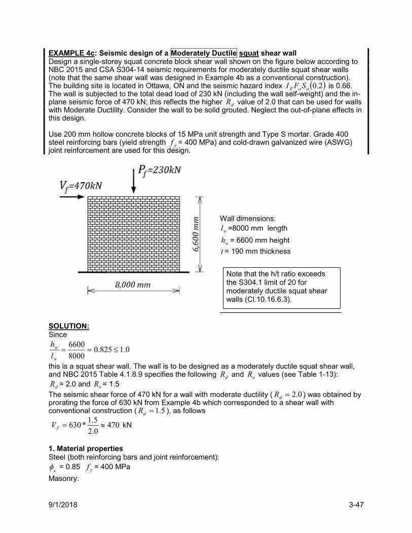
9/1/2018 3-47

EXAMPLE 4c: Seismic design of a Moderately Ductile squat shear wall Design a single-storey squat concrete block shear wall shown on the figure below according to NBC 2015 and CSA S304-14 seismic requirements for moderately ductile squat shear walls (note that the same shear wall was designed in Example 4b as a conventional construction). The building site is located in Ottawa, ON and the seismic hazard index 2.0aaE SFI is 0.66. The wall is subjected to the total dead load of 230 kN (including the wall self-weight) and the in-plane seismic force of 470 kN; this reflects the higher dR value of 2.0 that can be used for walls with Moderate Ductility. Consider the wall to be solid grouted. Neglect the out-of-plane effects in this design. Use 200 mm hollow concrete blocks of 15 MPa unit strength and Type S mortar. Grade 400 steel reinforcing bars (yield strength yf = 400 MPa) and cold-drawn galvanized wire (ASWG) joint reinforcement are used for this design.

Wall dimensions:

wl =8000 mm length

wh = 6600 mm height

t = 190 mm thickness

SOLUTION: Since

0.1825.08000

6600

w

w

l

h

this is a squat shear wall. The wall is to be designed as a moderately ductile squat shear wall, and NBC 2015 Table 4.1.8.9 specifies the following dR and oR values (see Table 1-13):

dR = 2.0 and oR = 1.5

The seismic shear force of 470 kN for a wall with moderate ductility ( 0.2dR ) was obtained by prorating the force of 630 kN from Example 4b which corresponded to a shear wall with conventional construction ( 5.1dR ), as follows

4700.2

5.1*630 fV kN

1. Material properties Steel (both reinforcing bars and joint reinforcement):

s = 0.85 yf = 400 MPa

Masonry:

Note that the h/t ratio exceeds the S304.1 limit of 20 for moderately ductile squat shear walls (Cl.10.16.6.3).

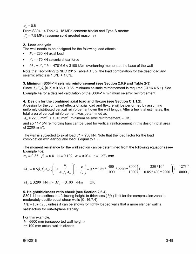
9/1/2018 3-48

m = 0.6

From S304-14 Table 4, 15 MPa concrete blocks and Type S mortar:

mf = 7.5 MPa (assume solid grouted masonry)

2. Load analysis The wall needs to be designed for the following load effects: fP = 230 kN axial load

fV = 470 kN seismic shear force

hVM ff * = 470*6.6 3100 kNm overturning moment at the base of the wall

Note that, according to NBC 2015 Table 4.1.3.2, the load combination for the dead load and seismic effects is 1.0*D + 1.0*E. 3. Minimum S304-14 seismic reinforcement (see Section 2.6.9 and Table 2-3) Since 2.0aaE SFI = 0.66 > 0.35, minimum seismic reinforcement is required (Cl.16.4.5.1). See

Example 4a for a detailed calculation of the S304-14 minimum seismic reinforcement. 4. Design for the combined axial load and flexure (see Section C.1.1.2). A design for the combined effects of axial load and flexure will be performed by assuming uniformly distributed vertical reinforcement over the wall length. After a few trial estimates, the total area of vertical reinforcement was determined as

vtA = 2200 mm2 > 1016 mm2 (minimum seismic reinforcement) - OK

and so 11-15M reinforcing bars can be used for vertical reinforcement in this design (total area of 2200 mm2). The wall is subjected to axial load fP = 230 kN. Note that the load factor for the load combination with earthquake load is equal to 1.0. The moment resistance for the wall section can be determined from the following equations (see Example 4b):

85.01 8.01 109.0 034.0 1273c mm

8000

12731

2200*400*85.0

10*2301

1000

8000*2200*

1000

400*85.0*5.0115.0

3

wvtys

fwvtysr l

c

Af

PlAfM

3290rM kNm > 3100fM kNm OK

5. Height/thickness ratio check (see Section 2.6.4) S304-14 prescribes the following height-to-thickness ( th ) limit for the compression zone in moderately ductile squat shear walls (Cl.16.7.4):

20)10( th , unless it can be shown for lightly loaded walls that a more slender wall is satisfactory for out-of-plane stability. For this example, h = 6600 mm (unsupported wall height) t = 190 mm actual wall thickness

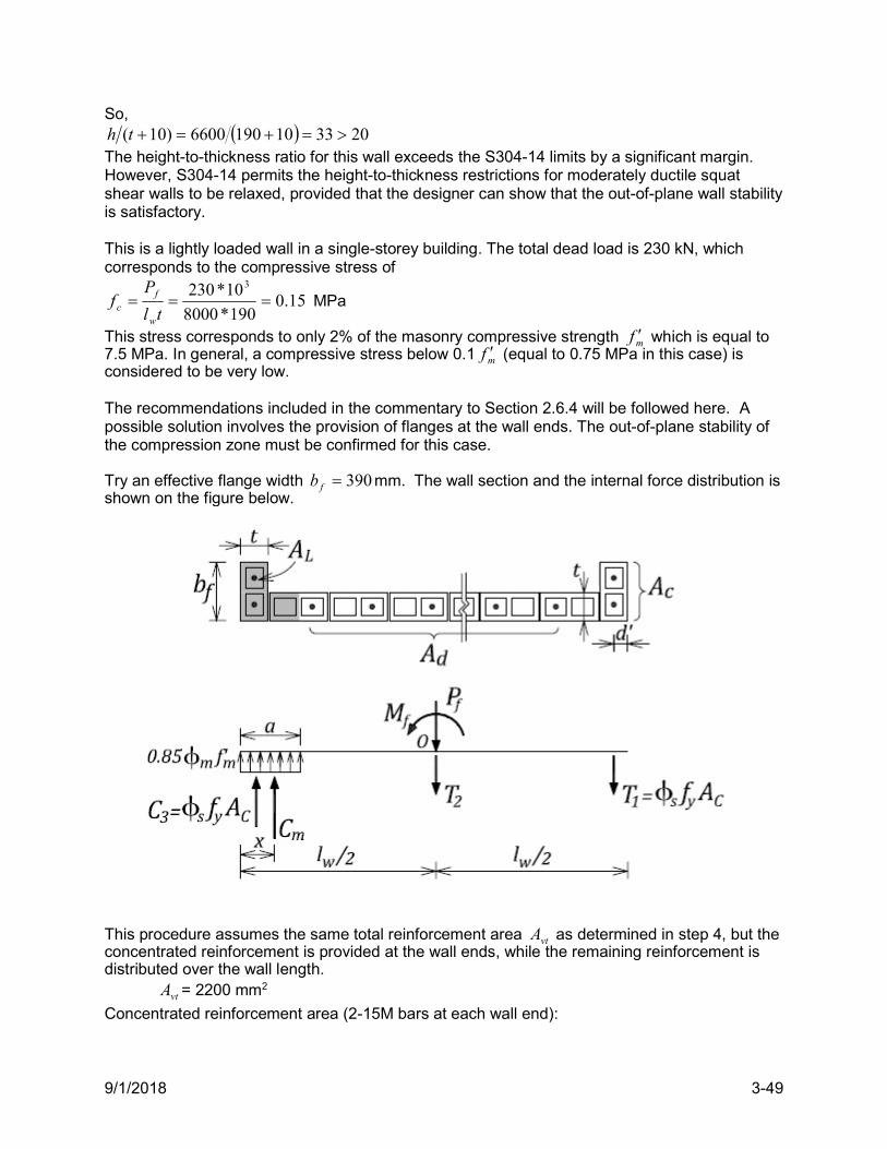
9/1/2018 3-49

So, 2033101906600)10( th

The height-to-thickness ratio for this wall exceeds the S304-14 limits by a significant margin. However, S304-14 permits the height-to-thickness restrictions for moderately ductile squat shear walls to be relaxed, provided that the designer can show that the out-of-plane wall stability is satisfactory. This is a lightly loaded wall in a single-storey building. The total dead load is 230 kN, which corresponds to the compressive stress of

15.0190*8000

10*230 3

tl

Pf

w

fc MPa

This stress corresponds to only 2% of the masonry compressive strength mf which is equal to 7.5 MPa. In general, a compressive stress below 0.1 mf (equal to 0.75 MPa in this case) is considered to be very low. The recommendations included in the commentary to Section 2.6.4 will be followed here. A possible solution involves the provision of flanges at the wall ends. The out-of-plane stability of the compression zone must be confirmed for this case. Try an effective flange width 390fb mm. The wall section and the internal force distribution is shown on the figure below.

This procedure assumes the same total reinforcement area vtA as determined in step 4, but the concentrated reinforcement is provided at the wall ends, while the remaining reinforcement is distributed over the wall length.

vtA = 2200 mm2

Concentrated reinforcement area (2-15M bars at each wall end):

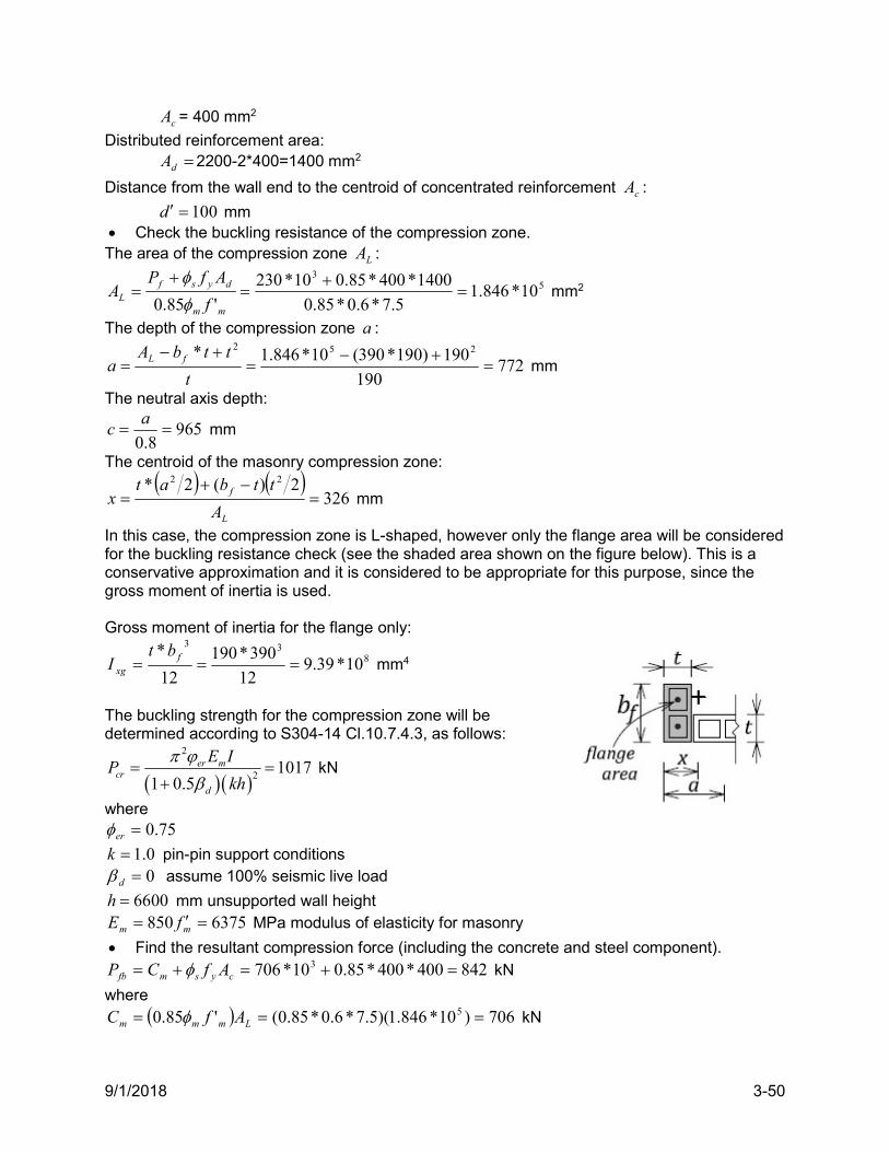
9/1/2018 3-50

cA = 400 mm2

Distributed reinforcement area: dA 2200-2*400=1400 mm2

Distance from the wall end to the centroid of concentrated reinforcement cA :

100d mm Check the buckling resistance of the compression zone. The area of the compression zone LA :

53

10*846.15.7*6.0*85.0

1400*400*85.010*230

'85.0

mm

dysfL f

AfPA

mm2

The depth of the compression zone a :

772190

190)190*390(10*846.1* 252

t

ttbAa fL

mm

The neutral axis depth:

9658.0

ac mm

The centroid of the masonry compression zone:

326

2)(2* 22

L

f

A

ttbatx mm

In this case, the compression zone is L-shaped, however only the flange area will be considered for the buckling resistance check (see the shaded area shown on the figure below). This is a conservative approximation and it is considered to be appropriate for this purpose, since the gross moment of inertia is used. Gross moment of inertia for the flange only:

833

10*39.912

390*190

12

* f

xg

btI mm4

The buckling strength for the compression zone will be determined according to S304-14 Cl.10.7.4.3, as follows:

2

2 10171 0.5

er mcr

d

E IP

kh

kN

where 75.0er

0.1k pin-pin support conditions 0d assume 100% seismic live load

6600h mm unsupported wall height 6375850 mm fE MPa modulus of elasticity for masonry

Find the resultant compression force (including the concrete and steel component). 842400*400*85.010*706 3 cysmfb AfCP kN

where 706)10*846.1)(5.7*6.0*85.0('85.0 5 Lmmm AfC kN

9/1/2018 3-51

Confirm that the out-of-plane buckling resistance is adequate. Since

842fbP kN < 1017crP kN

it can be concluded that the out-of-plane buckling resistance is adequate and so the flanged section can be used for this design. This is in compliance with S304-14 Cl.16.7.4, despite the fact that the th ratio for this wall is 33, which exceeds the S304-14-prescribed limit of 20. 4a. Design the flanged section for the combined axial load and flexure – consider distributed and concentrated wall reinforcement (see Section C.1.1.1). The key design parameters for this calculation were determined in step 5 above. The factored moment resistance rM will be determined by summing up the moments around the centroid of the wall section as follows

)10028000(*400*400*85.0*2)32628000(*10*706)2(22 3 dlAfxlCM wcyswmr

365510*3655 6 NmmM r kNm Since

3655rM kNm > 3100fM kNm OK

6. Find the minimum required factored shear resistance (see Section 2.6.5 and S304-14 Cl.16.7.3.2) Cl.16.7.3.2 requires that the factored shear resistance, rV , for a Moderately Ductile squat shear wall should be greater than the shear due to effects of factored loads, but not less than i) the shear corresponding to the development of factored moment resistance, rM , or ii) shear

corresponding to the lateral seismic load (base shear), where earthquake effects were calculated using RdRo=1.3. The first requirement is based on the Capacity Design approach (see Section 2.5.1 for more details). For Moderately Ductile shear walls, the shear capacity should exceed the shear corresponding to the factored moment resistance. In this case, the factored moment resistance is equal to

3655rM kNm

The shear force at the top of the wall that would cause an overturning moment equal to rM is

3655

6.6r

rbw

MV

h 554 kN

The second requirement gives an “almost elastic” factored base shear force for the wall, which is equal to

470 2.0 1.51085

1.3 1.3f d o

fe

V R RV

kN

The smaller of these two values should be used, hence 554rdV kN

7. The diagonal tension shear resistance (see Section 2.3.2 and S304-14 Cl.10.10.2.1) Masonry shear resistance ( mV ):

190wb mm overall wall thickness

64008.0 wv ld mm effective wall depth

9/1/2018 3-52

0.1g solid grouted wall

fd PP 9.0 = 207 kN

mvf

fm f

dV

Mv )2(16.0 = 0.44 MPa

4.6*470

3100

vf

f

dV

M= 1.03 1.0

gdvwmmm PdbvV )25.0( = 0.6(0.44*190*6400+0.25*207*103)*1.0 = 352 kN

Steel shear resistance sV :

Assume 2-15M bond beam reinforcement at 1200 mm spacing, so 400vA mm2

1200s mm Horizontal reinforcement area per metre:

3331000*1200

4001000*

s

AA vh mm2/m

1200

6400*400*

1000

400*85.0*6.06.0

s

dfAV vyvss = 435 kN

Total diagonal shear resistance 787435352 smr VVV kN

The factored shear resistance exceeds the minimum required factored shear resistance, that is, 787rV kN > 554rdV kN OK

Maximum shear allowed on the section is (S304-14 Cl.10.10.2.2)

939)2(4.0max w

wgvwmmr l

hdbfV kN

Since

rr VV max OK Note that S304-14 Cl.16.7.3.1 requires that the method by which the shear force is applied to the wall shall be capable of applying shear force uniformly over the wall length. This can be achieved by providing a continuous bond beam at the top of the wall, as discussed in Section 2.3.2.2 (see Figure 2-16). 8. Sliding shear resistance (see Section 2.3.3) The factored in-plane sliding shear resistance rV is determined as follows. = 1.0 for a masonry-to-masonry or masonry-to-roughened concrete sliding plane

sA = 2200 mm2 total area of vertical wall reinforcement

yssy fAT = 0.85*2200*400 = 748 kN

dP = 207 kN

yd TPP 2 = 207+748 = 955 kN

2PV mr = 0.6*1.0*955 = 573 kN

9/1/2018 3-53

573rV kN > 554rdV kN OK

Note that 573rV kN < 787rV kN for diagonal tension (this indicates that the sliding shear

resistance governs over the diagonal tension shear resistance). 9. Minimum reinforcement requirements for Moderately Ductile squat shear walls (see Section 2.6.10) S304-14 Cl.16.7.5 prescribes the following requirements for the amount of reinforcement in Moderately Ductile squat shear walls: Horizontal reinforcement ratio h

h should be greater than the minimum value set by S304-14 Cl.16.7.5: 3

3min

470*101.10*10

190*6600*0.85*400f

hw w s y

V

b h f

and the value determined in accordance with Cl.10.10.2 based on the shear resistance requirements

321311.70*10

* 190*6600h

hshearw w

A

b h

where hA is the total area of horizontal reinforcement along the wall height, that is,

333 6.4 2131h h vA A d mm2

where

333hA mm2/m (see step 6)

In this case,

minh =1.10*10-3 < hshear =1.70*10-3

This indicates that the S304-14 shear resistance requirement governs. The amount of horizontal reinforcement (2-15M bond beam reinforcement bar at 1200 mm spacing) is adequate. Vertical reinforcement ratio v

Minimum minv value set by S304-14 Cl.16.7.5: 3

3min min

230*101.10*10

0.85*190*8000*400s

v hs w w y

P

b l f

0.65*10-3

where 230s fP P kN. Actual vertical reinforcement ratio vflex based on the flexural design

requirements (see step 4):

310*447.1190*8000

2200

*

tl

A

w

vtvflex

Since

vflex = 1.447*10-3 > minv = 0.65*10-3

It appears that the amount of vertical reinforcement determined based on the flexural design requirements (11-15M) governs. It can be concluded that the minimum S304-14 reinforcement requirements for Moderately Ductile shear walls have been satisfied.

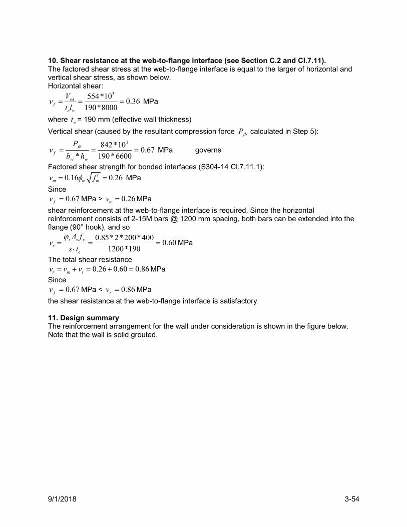
9/1/2018 3-54

10. Shear resistance at the web-to-flange interface (see Section C.2 and Cl.7.11). The factored shear stress at the web-to-flange interface is equal to the larger of horizontal and vertical shear stress, as shown below. Horizontal shear:

3554*100.36

190*8000rd

fe w

Vv

t l MPa

where et = 190 mm (effective wall thickness)

Vertical shear (caused by the resultant compression force fbP calculated in Step 5):

67.06600*190

10*842

*

3

ww

fbf hb

Pv MPa governs

Factored shear strength for bonded interfaces (S304-14 Cl.7.11.1):

0.16 0.26m m mv f MPa

Since 67.0fv MPa > 0.26mv MPa

shear reinforcement at the web-to-flange interface is required. Since the horizontal reinforcement consists of 2-15M bars @ 1200 mm spacing, both bars can be extended into the flange (90° hook), and so

0.85*2*200*4000.60

1200*190s s y

se

A fv

s t

MPa

The total shear resistance 0.26 0.60 0.86r m sv v v MPa

Since 67.0fv MPa < 86.0rv MPa

the shear resistance at the web-to-flange interface is satisfactory. 11. Design summary The reinforcement arrangement for the wall under consideration is shown in the figure below. Note that the wall is solid grouted.

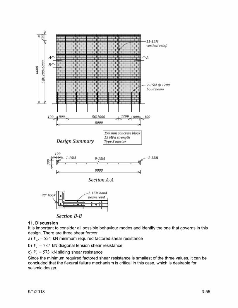
9/1/2018 3-55

11. Discussion It is important to consider all possible behaviour modes and identify the one that governs in this design. There are three shear forces: a) 554rdV kN minimum required factored shear resistance

b) 787rV kN diagonal tension shear resistance

c) 573rV kN sliding shear resistance Since the minimum required factored shear resistance is smallest of the three values, it can be concluded that the flexural failure mechanism is critical in this case, which is desirable for seismic design.

9/1/2018 3-56

Note that S304-14 Cl.10.2.8 prescribes the use of reduced effective depth d for flexural design of squat shear walls. Since this example deals with seismic design and essentially all the wall reinforcement is expected to yield in tension, this provision was not used as it is expected to result in additional vertical reinforcement, which would increase the moment capacity and possibly lead to a more brittle diagonal shear failure. Note that the S304-14 ductility check is not prescribed for Moderately Ductile squat shear walls. This example shows that an addition of flanges can be effective in preventing the out-of-plane buckling of Moderately Ductile squat shear walls. This is in compliance with S304-14 Cl.16.7.4, despite the fact that the th ratio for this wall is 33, which exceeds the S304-14-prescribed limit of 20. The last two examples provide an opportunity for comparing the total amount of vertical reinforcement required for a squat shear wall of conventional construction (Example 4b) and a moderately ductile squat shear wall (this example). It is noted that the moderately ductile wall has less vertical reinforcement (11-15M bars) than a similar wall of conventional construction (16-15M bars); this reduction amounts to approximately 30%.

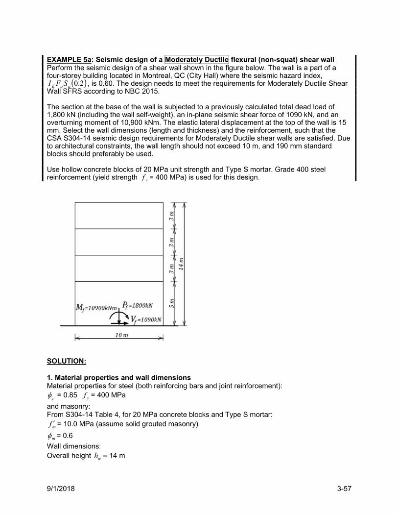
9/1/2018 3-57

EXAMPLE 5a: Seismic design of a Moderately Ductile flexural (non-squat) shear wall Perform the seismic design of a shear wall shown in the figure below. The wall is a part of a four-storey building located in Montreal, QC (City Hall) where the seismic hazard index,

2.0aaE SFI , is 0.60. The design needs to meet the requirements for Moderately Ductile Shear Wall SFRS according to NBC 2015. The section at the base of the wall is subjected to a previously calculated total dead load of 1,800 kN (including the wall self-weight), an in-plane seismic shear force of 1090 kN, and an overturning moment of 10,900 kNm. The elastic lateral displacement at the top of the wall is 15 mm. Select the wall dimensions (length and thickness) and the reinforcement, such that the CSA S304-14 seismic design requirements for Moderately Ductile shear walls are satisfied. Due to architectural constraints, the wall length should not exceed 10 m, and 190 mm standard blocks should preferably be used. Use hollow concrete blocks of 20 MPa unit strength and Type S mortar. Grade 400 steel reinforcement (yield strength yf = 400 MPa) is used for this design.

SOLUTION: 1. Material properties and wall dimensions Material properties for steel (both reinforcing bars and joint reinforcement):

s = 0.85 yf = 400 MPa

and masonry: From S304-14 Table 4, for 20 MPa concrete blocks and Type S mortar:

mf = 10.0 MPa (assume solid grouted masonry)

m = 0.6

Wall dimensions: Overall height wh 14 m

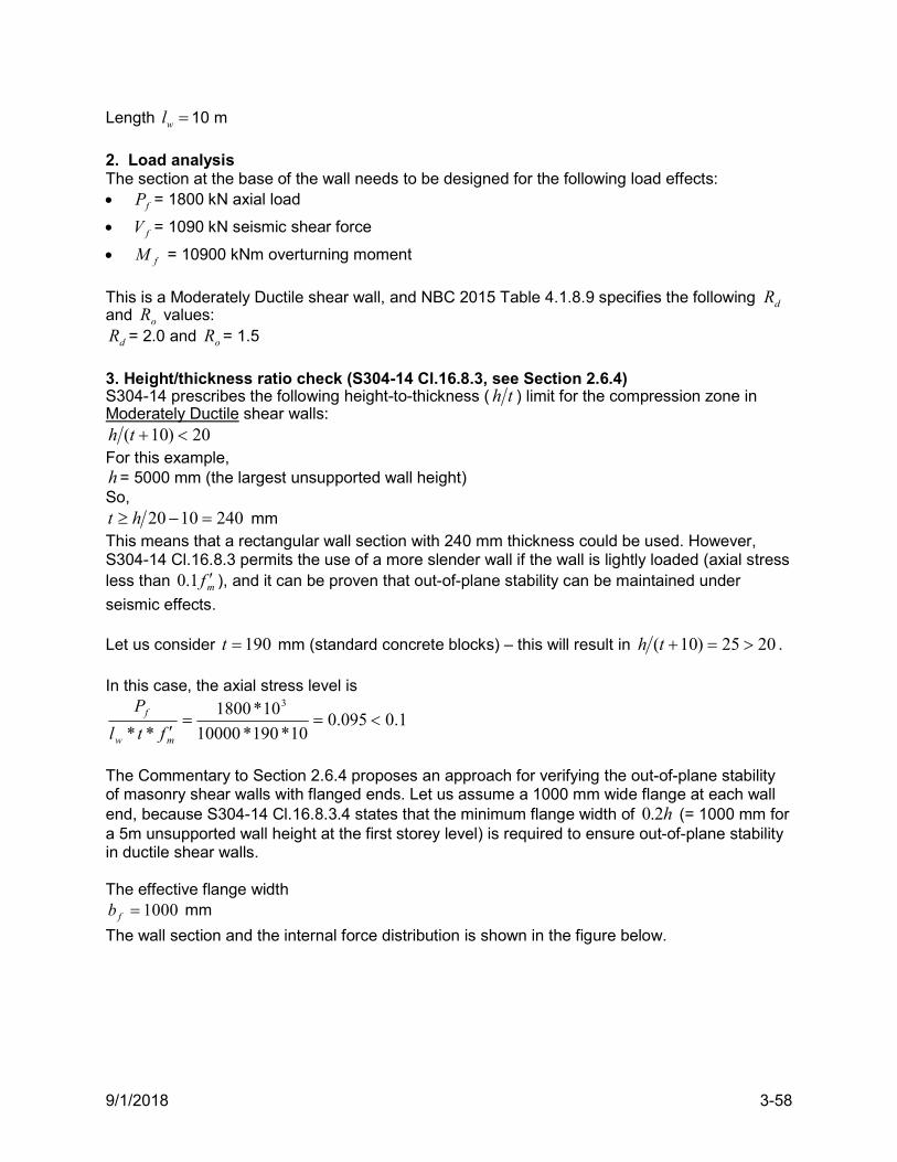
9/1/2018 3-58

Length wl 10 m

2. Load analysis The section at the base of the wall needs to be designed for the following load effects: fP = 1800 kN axial load

fV = 1090 kN seismic shear force

fM = 10900 kNm overturning moment

This is a Moderately Ductile shear wall, and NBC 2015 Table 4.1.8.9 specifies the following dR and oR values:

dR = 2.0 and oR = 1.5

3. Height/thickness ratio check (S304-14 Cl.16.8.3, see Section 2.6.4) S304-14 prescribes the following height-to-thickness ( th ) limit for the compression zone in Moderately Ductile shear walls:

20)10( th For this example, h= 5000 mm (the largest unsupported wall height) So,

2401020 ht mm This means that a rectangular wall section with 240 mm thickness could be used. However, S304-14 Cl.16.8.3 permits the use of a more slender wall if the wall is lightly loaded (axial stress less than mf 1.0 ), and it can be proven that out-of-plane stability can be maintained under

seismic effects. Let us consider 190t mm (standard concrete blocks) – this will result in 2025)10( th . In this case, the axial stress level is

1.0095.010*190*10000

10*1800

**

3

mw

f

ftl

P

The Commentary to Section 2.6.4 proposes an approach for verifying the out-of-plane stability of masonry shear walls with flanged ends. Let us assume a 1000 mm wide flange at each wall end, because S304-14 Cl.16.8.3.4 states that the minimum flange width of h2.0 (= 1000 mm for a 5m unsupported wall height at the first storey level) is required to ensure out-of-plane stability in ductile shear walls. The effective flange width

1000fb mm

The wall section and the internal force distribution is shown in the figure below.

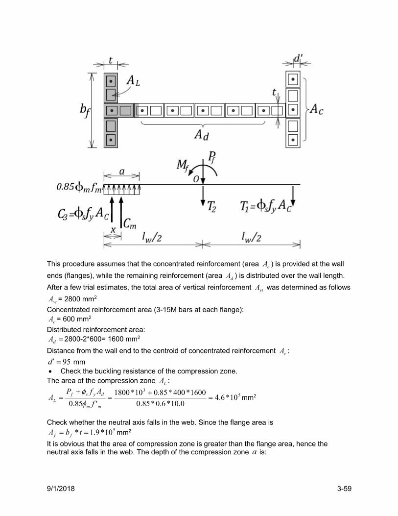
9/1/2018 3-59

This procedure assumes that the concentrated reinforcement (area cA ) is provided at the wall

ends (flanges), while the remaining reinforcement (area dA ) is distributed over the wall length.

After a few trial estimates, the total area of vertical reinforcement vtA was determined as follows

vtA = 2800 mm2

Concentrated reinforcement area (3-15M bars at each flange):

cA = 600 mm2

Distributed reinforcement area: dA 2800-2*600= 1600 mm2

Distance from the wall end to the centroid of concentrated reinforcement cA :

95d mm Check the buckling resistance of the compression zone. The area of the compression zone LA :

53

10*6.40.10*6.0*85.0

1600*400*85.010*1800

'85.0

mm

dysfL f

AfPA

mm2

Check whether the neutral axis falls in the web. Since the flange area is

510*9.1* tbA ff mm2

It is obvious that the area of compression zone is greater than the flange area, hence the neutral axis falls in the web. The depth of the compression zone a is:

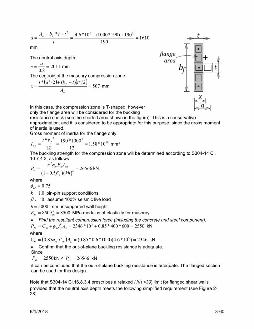
9/1/2018 3-60

1610190

190)190*1000(10*6.4* 252

t

ttbAa fL

mm The neutral axis depth:

20118.0

ac mm

The centroid of the masonry compression zone:

567

2)(2* 22

L

f

A

ttbatx mm

In this case, the compression zone is T-shaped, however only the flange area will be considered for the buckling resistance check (see the shaded area shown in the figure). This is a conservative approximation, and it is considered to be appropriate for this purpose, since the gross moment of inertia is used. Gross moment of inertia for the flange only:

1033

10*58.112

1000*190

12

* f

xg

btI mm4

The buckling strength for the compression zone will be determined according to S304-14 Cl. 10.7.4.3, as follows:

2

2 265661 0.5

er m xgcr

d

E IP

kh

kN

where 75.0er

0.1k pin-pin support conditions 0d assume 100% seismic live load

5000h mm unsupported wall height 8500850 mm fE MPa modulus of elasticity for masonry

Find the resultant compression force (including the concrete and steel component). 2550600*400*85.010*2346 3 cysmfb AfCP kN

where

2346)10*6.4)(0.10*6.0*85.0('85.0 5 Lmmm AfC kN

Confirm that the out-of-plane buckling resistance is adequate. Since

2550fbP kN < 26566crP kN

it can be concluded that the out-of-plane buckling resistance is adequate. The flanged section can be used for this design. Note that S304-14 Cl.16.8.3.4 prescribes a relaxed ( th <30) limit for flanged shear walls provided that the neutral axis depth meets the following simplified requirement (see Figure 2-28):

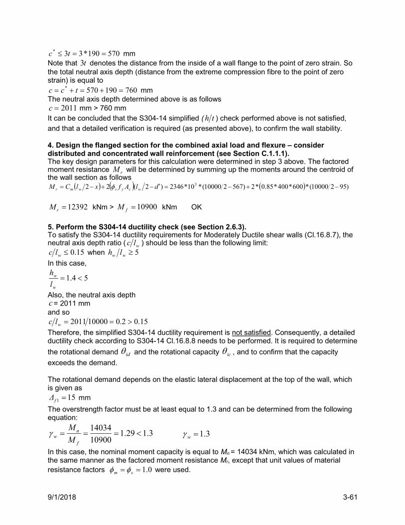
9/1/2018 3-61

570190*33* tc mm Note that t3 denotes the distance from the inside of a wall flange to the point of zero strain. So the total neutral axis depth (distance from the extreme compression fibre to the point of zero strain) is equal to

760190570* tcc mm The neutral axis depth determined above is as follows

2011c mm > 760 mm It can be concluded that the S304-14 simplified ( th ) check performed above is not satisfied, and that a detailed verification is required (as presented above), to confirm the wall stability. 4. Design the flanged section for the combined axial load and flexure – consider distributed and concentrated wall reinforcement (see Section C.1.1.1). The key design parameters for this calculation were determined in step 3 above. The factored moment resistance rM will be determined by summing up the moments around the centroid of the wall section as follows

)95210000(*600*400*85.0*2)567210000(*10*2346)2(22 3 dlAfxlCM wcyswmr

12392rM kNm > 10900fM kNm OK

5. Perform the S304-14 ductility check (see Section 2.6.3). To satisfy the S304-14 ductility requirements for Moderately Ductile shear walls (Cl.16.8.7), the neutral axis depth ratio ( wlc ) should be less than the following limit:

15.0wlc when 5ww lh

In this case,

54.1 w

w

l

h

Also, the neutral axis depth c= 2011 mm and so

15.02.0100002011 wlc

Therefore, the simplified S304-14 ductility requirement is not satisfied. Consequently, a detailed ductility check according to S304-14 Cl.16.8.8 needs to be performed. It is required to determine

the rotational demand id and the rotational capacity ic , and to confirm that the capacity

exceeds the demand. The rotational demand depends on the elastic lateral displacement at the top of the wall, which is given as

151 fΔ mm

The overstrength factor must be at least equal to 1.3 and can be determined from the following equation:

3.129.110900

14034

f

nw M

M 3.1w

In this case, the nominal moment capacity is equal to Mn = 14034 kNm, which was calculated in the same manner as the factored moment resistance Mr, except that unit values of material resistance factors 0.1 sm were used.

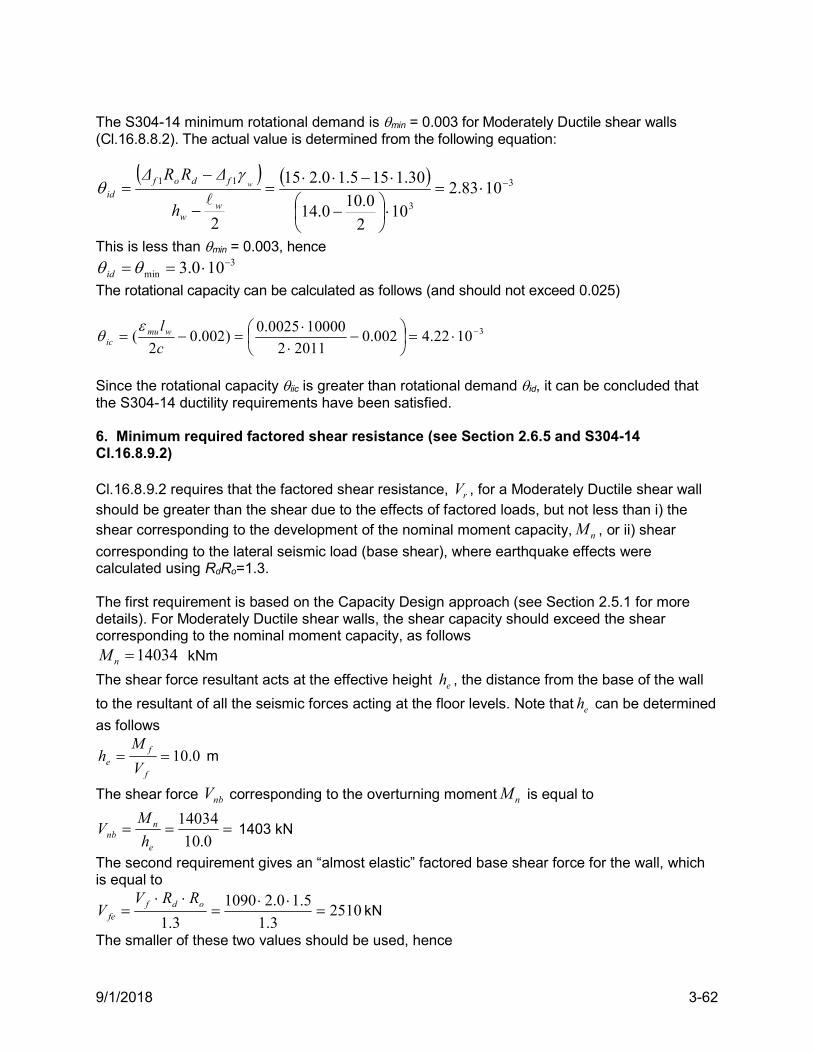
9/1/2018 3-62

The S304-14 minimum rotational demand is min = 0.003 for Moderately Ductile shear walls (Cl.16.8.8.2). The actual value is determined from the following equation:

3

3

11 1083.2

102

0.100.14

30.1155.10.215

2

ww

fdofid

h

ΔRRΔw

This is less than min = 0.003, hence 3

min 100.3 id

The rotational capacity can be calculated as follows (and should not exceed 0.025)

31022.4002.020112

100000025.0)002.0

2(

c

lwmuic

Since the rotational capacity iic is greater than rotational demand id, it can be concluded that the S304-14 ductility requirements have been satisfied. 6. Minimum required factored shear resistance (see Section 2.6.5 and S304-14 Cl.16.8.9.2) Cl.16.8.9.2 requires that the factored shear resistance, rV , for a Moderately Ductile shear wall should be greater than the shear due to the effects of factored loads, but not less than i) the shear corresponding to the development of the nominal moment capacity, nM , or ii) shear

corresponding to the lateral seismic load (base shear), where earthquake effects were calculated using RdRo=1.3. The first requirement is based on the Capacity Design approach (see Section 2.5.1 for more details). For Moderately Ductile shear walls, the shear capacity should exceed the shear corresponding to the nominal moment capacity, as follows

14034nM kNm

The shear force resultant acts at the effective height eh , the distance from the base of the wall

to the resultant of all the seismic forces acting at the floor levels. Note that eh can be determined

as follows

0.10f

fe V

Mh m

The shear force nbV corresponding to the overturning moment nM is equal to

0.10

14034

e

nnb h

MV 1403 kN

The second requirement gives an “almost elastic” factored base shear force for the wall, which is equal to

25103.1

5.10.21090

3.1

odf

fe

RRVV kN

The smaller of these two values should be used, hence

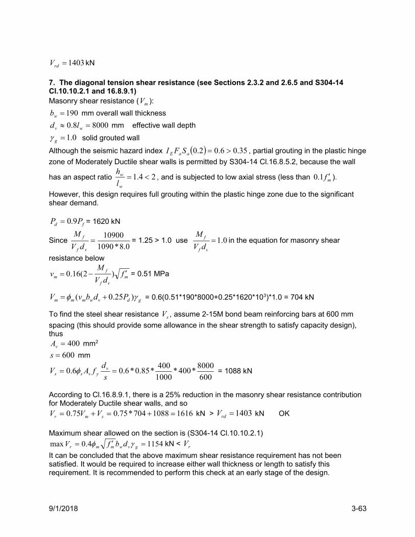
9/1/2018 3-63

1403rdV kN

7. The diagonal tension shear resistance (see Sections 2.3.2 and 2.6.5 and S304-14 Cl.10.10.2.1 and 16.8.9.1) Masonry shear resistance ( mV ):

190wb mm overall wall thickness

80008.0 wv ld mm effective wall depth

0.1g solid grouted wall

Although the seismic hazard index 35.06.02.0 aaE SFI , partial grouting in the plastic hinge

zone of Moderately Ductile shear walls is permitted by S304-14 Cl.16.8.5.2, because the wall

has an aspect ratio 24.1 w

w

l

h, and is subjected to low axial stress (less than mf 1.0 ).

However, this design requires full grouting within the plastic hinge zone due to the significant shear demand.

fd PP 9.0 = 1620 kN

Since 0.8*1090

10900

vf

f

dV

M= 1.25 > 1.0 use 1.0f

f v

M

V d in the equation for masonry shear

resistance below

mvf

fm f

dV

Mv )2(16.0 = 0.51 MPa

gdvwmmm PdbvV )25.0( = 0.6(0.51*190*8000+0.25*1620*103)*1.0 = 704 kN

To find the steel shear resistance sV , assume 2-15M bond beam reinforcing bars at 600 mm

spacing (this should provide some allowance in the shear strength to satisfy capacity design), thus

400vA mm2

600s mm

600

8000*400*

1000

400*85.0*6.06.0

s

dfAV vyvss = 1088 kN

According to Cl.16.8.9.1, there is a 25% reduction in the masonry shear resistance contribution for Moderately Ductile shear walls, and so

16161088704*75.075.0 smr VVV kN > 1403rdV kN OK

Maximum shear allowed on the section is (S304-14 Cl.10.10.2.1)

11544.0max gvwmmr dbfV kN < rV

It can be concluded that the above maximum shear resistance requirement has not been satisfied. It would be required to increase either wall thickness or length to satisfy this requirement. It is recommended to perform this check at an early stage of the design.

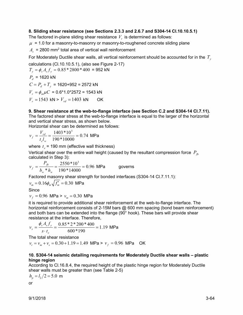
9/1/2018 3-64

8. Sliding shear resistance (see Sections 2.3.3 and 2.6.7 and S304-14 Cl.10.10.5.1) The factored in-plane sliding shear resistance rV is determined as follows:

= 1.0 for a masonry-to-masonry or masonry-to-roughened concrete sliding plane

sA = 2800 mm2 total area of vertical wall reinforcement

For Moderately Ductile shear walls, all vertical reinforcement should be accounted for in the yT

calculations (Cl.10.10.5.1), (also see Figure 2-17) 400*2800*85.0 yssy fAT = 952 kN

dP = 1620 kN

yd TPC = 1620+952 = 2572 kN

CV mr = 0.6*1.0*2572 = 1543 kN

1543rV kN > 1403rdV kN OK

9. Shear resistance at the web-to-flange interface (see Section C.2 and S304-14 Cl.7.11). The factored shear stress at the web-to-flange interface is equal to the larger of the horizontal and vertical shear stress, as shown below. Horizontal shear can be determined as follows:

74.010000*190

10*1403 3

we

rdf lt

Vv MPa

where et = 190 mm (effective wall thickness)

Vertical shear over the entire wall height (caused by the resultant compression force fbP calculated in Step 3):

96.014000*190

10*2550

*

3

ww

fbf hb

Pv MPa governs

Factored masonry shear strength for bonded interfaces (S304-14 Cl.7.11.1):

0.16 0.30m m mv f MPa

Since 96.0fv MPa > 0.30mv MPa

it is required to provide additional shear reinforcement at the web-to-flange interface. The horizontal reinforcement consists of 2-15M bars @ 600 mm spacing (bond beam reinforcement) and both bars can be extended into the flange (90° hook). These bars will provide shear resistance at the interface. Therefore,

19.1190*600

400*200*2*85.0

e

ysss ts

fAv

MPa

The total shear resistance 0.30 1.19 1.49r m sv v v MPa > 96.0fv MPa OK

10. S304-14 seismic detailing requirements for Moderately Ductile shear walls – plastic hinge region According to Cl.16.8.4, the required height of the plastic hinge region for Moderately Ductile shear walls must be greater than (see Table 2-5)

2 2 5.0ph l m

or

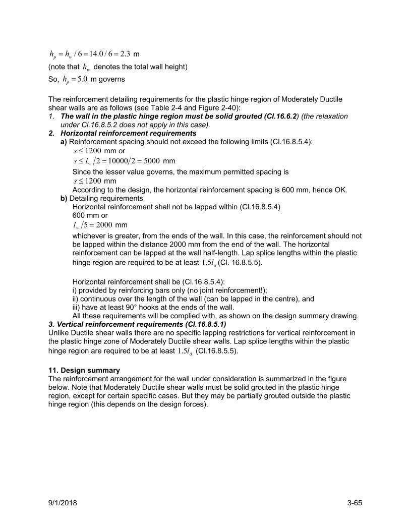
9/1/2018 3-65

/ 6 14.0 / 6 2.3p wh h m

(note that wh denotes the total wall height)

So, 5.0ph m governs

The reinforcement detailing requirements for the plastic hinge region of Moderately Ductile shear walls are as follows (see Table 2-4 and Figure 2-40): 1. The wall in the plastic hinge region must be solid grouted (Cl.16.6.2) (the relaxation

under Cl.16.8.5.2 does not apply in this case). 2. Horizontal reinforcement requirements

a) Reinforcement spacing should not exceed the following limits (Cl.16.8.5.4): 1200s mm or

50002100002 wls mm

Since the lesser value governs, the maximum permitted spacing is 1200s mm

According to the design, the horizontal reinforcement spacing is 600 mm, hence OK. b) Detailing requirements

Horizontal reinforcement shall not be lapped within (Cl.16.8.5.4) 600 mm or

20005 wl mm

whichever is greater, from the ends of the wall. In this case, the reinforcement should not be lapped within the distance 2000 mm from the end of the wall. The horizontal reinforcement can be lapped at the wall half-length. Lap splice lengths within the plastic hinge region are required to be at least dl5.1 (Cl. 16.8.5.5).

Horizontal reinforcement shall be (Cl.16.8.5.4): i) provided by reinforcing bars only (no joint reinforcement!); ii) continuous over the length of the wall (can be lapped in the centre), and iii) have at least 90° hooks at the ends of the wall. All these requirements will be complied with, as shown on the design summary drawing.

3. Vertical reinforcement requirements (Cl.16.8.5.1) Unlike Ductile shear walls there are no specific lapping restrictions for vertical reinforcement in the plastic hinge zone of Moderately Ductile shear walls. Lap splice lengths within the plastic hinge region are required to be at least dl5.1 (Cl.16.8.5.5).

11. Design summary The reinforcement arrangement for the wall under consideration is summarized in the figure below. Note that Moderately Ductile shear walls must be solid grouted in the plastic hinge region, except for certain specific cases. But they may be partially grouted outside the plastic hinge region (this depends on the design forces).

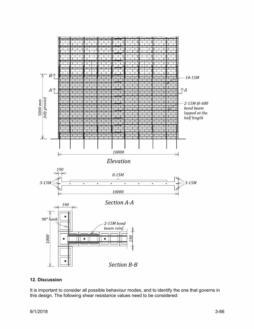
9/1/2018 3-66

12. Discussion It is important to consider all possible behaviour modes, and to identify the one that governs in this design. The following shear resistance values need to be considered:

9/1/2018 3-67

1. 1616rV kN diagonal tension shear resistance

2. 1543rV kN sliding shear resistance

3. 1403rdV kN minimum required shear resistance to achieve ductile flexural behaviour

It can be concluded that the minimum required shear force corresponding to the flexural failure mechanism is the smallest, so the flexural failure mechanism governs in this case, which is a requirement for the Capacity Design approach for Moderately Ductile shear walls.

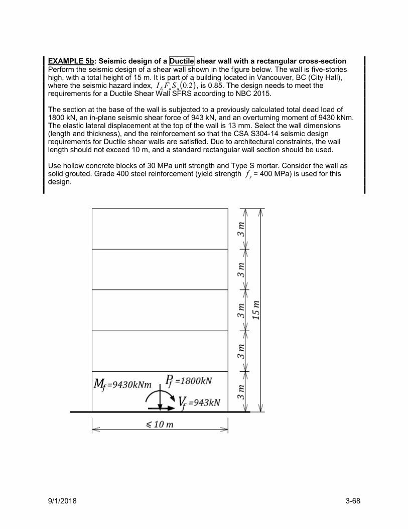
9/1/2018 3-68

EXAMPLE 5b: Seismic design of a Ductile shear wall with a rectangular cross-section Perform the seismic design of a shear wall shown in the figure below. The wall is five-stories high, with a total height of 15 m. It is part of a building located in Vancouver, BC (City Hall), where the seismic hazard index, 2.0aaE SFI , is 0.85. The design needs to meet the requirements for a Ductile Shear Wall SFRS according to NBC 2015. The section at the base of the wall is subjected to a previously calculated total dead load of 1800 kN, an in-plane seismic shear force of 943 kN, and an overturning moment of 9430 kNm. The elastic lateral displacement at the top of the wall is 13 mm. Select the wall dimensions (length and thickness), and the reinforcement so that the CSA S304-14 seismic design requirements for Ductile shear walls are satisfied. Due to architectural constraints, the wall length should not exceed 10 m, and a standard rectangular wall section should be used. Use hollow concrete blocks of 30 MPa unit strength and Type S mortar. Consider the wall as solid grouted. Grade 400 steel reinforcement (yield strength yf = 400 MPa) is used for this design.

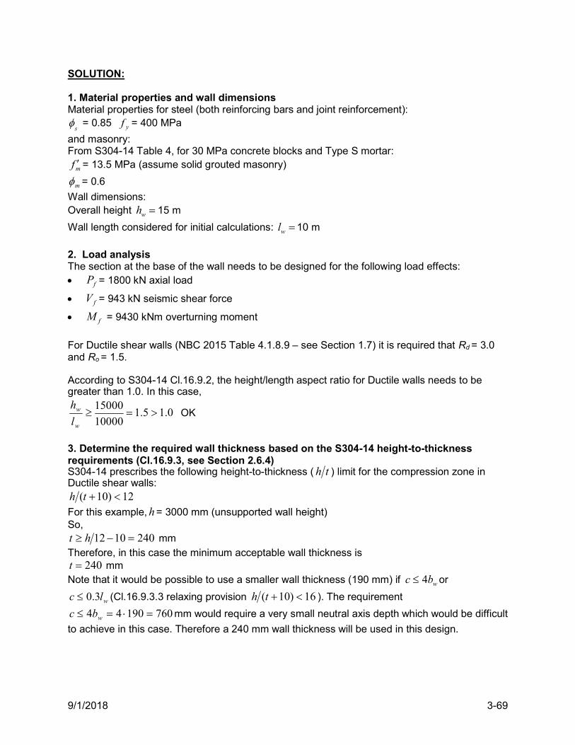
9/1/2018 3-69

SOLUTION: 1. Material properties and wall dimensions Material properties for steel (both reinforcing bars and joint reinforcement):

s = 0.85 yf = 400 MPa

and masonry: From S304-14 Table 4, for 30 MPa concrete blocks and Type S mortar:

mf = 13.5 MPa (assume solid grouted masonry)

m = 0.6

Wall dimensions: Overall height wh 15 m

Wall length considered for initial calculations: wl 10 m

2. Load analysis The section at the base of the wall needs to be designed for the following load effects: fP = 1800 kN axial load

fV = 943 kN seismic shear force

fM = 9430 kNm overturning moment

For Ductile shear walls (NBC 2015 Table 4.1.8.9 – see Section 1.7) it is required that Rd = 3.0 and Ro = 1.5. According to S304-14 Cl.16.9.2, the height/length aspect ratio for Ductile walls needs to be greater than 1.0. In this case,

0.15.110000

15000

w

w

l

h OK

3. Determine the required wall thickness based on the S304-14 height-to-thickness requirements (Cl.16.9.3, see Section 2.6.4) S304-14 prescribes the following height-to-thickness ( th ) limit for the compression zone in Ductile shear walls:

12)10( th

For this example, h= 3000 mm (unsupported wall height) So,

2401012 ht mm Therefore, in this case the minimum acceptable wall thickness is

240t mm Note that it would be possible to use a smaller wall thickness (190 mm) if wbc 4 or

wlc 3.0 (Cl.16.9.3.3 relaxing provision 16)10( th ). The requirement

76019044 wbc mm would require a very small neutral axis depth which would be difficult

to achieve in this case. Therefore a 240 mm wall thickness will be used in this design.

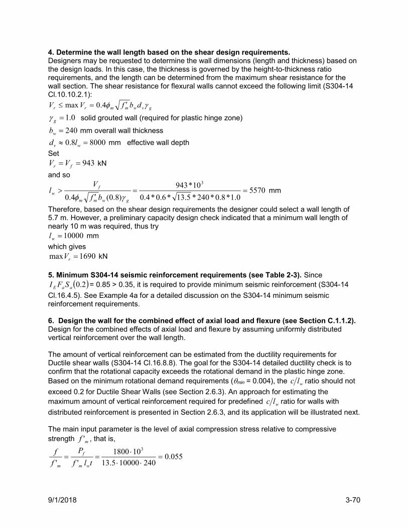
9/1/2018 3-70

4. Determine the wall length based on the shear design requirements. Designers may be requested to determine the wall dimensions (length and thickness) based on the design loads. In this case, the thickness is governed by the height-to-thickness ratio requirements, and the length can be determined from the maximum shear resistance for the wall section. The shear resistance for flexural walls cannot exceed the following limit (S304-14 Cl.10.10.2.1):

gvwmmrr dbfVV 4.0max

0.1g solid grouted wall (required for plastic hinge zone)

240wb mm overall wall thickness

80008.0 wv ld mm effective wall depth

Set 943 fr VV kN

and so

55700.1*8.0*240*5.13*6.0*4.0

10*943

)8.0(4.0

3

gwmm

fw

bf

Vl

mm

Therefore, based on the shear design requirements the designer could select a wall length of 5.7 m. However, a preliminary capacity design check indicated that a minimum wall length of nearly 10 m was required, thus try

10000wl mm

which gives 1690max rV kN

5. Minimum S304-14 seismic reinforcement requirements (see Table 2-3). Since

2.0aaE SFI = 0.85 > 0.35, it is required to provide minimum seismic reinforcement (S304-14

Cl.16.4.5). See Example 4a for a detailed discussion on the S304-14 minimum seismic reinforcement requirements. 6. Design the wall for the combined effect of axial load and flexure (see Section C.1.1.2). Design for the combined effects of axial load and flexure by assuming uniformly distributed vertical reinforcement over the wall length. The amount of vertical reinforcement can be estimated from the ductility requirements for Ductile shear walls (S304-14 Cl.16.8.8). The goal for the S304-14 detailed ductility check is to confirm that the rotational capacity exceeds the rotational demand in the plastic hinge zone. Based on the minimum rotational demand requirements (min = 0.004), the wlc ratio should not

exceed 0.2 for Ductile Shear Walls (see Section 2.6.3). An approach for estimating the maximum amount of vertical reinforcement required for predefined wlc ratio for walls with

distributed reinforcement is presented in Section 2.6.3, and its application will be illustrated next. The main input parameter is the level of axial compression stress relative to compressive strength mf ' , that is,

055.0240100005.13

101800

''

3

tlf

P

f

f

wm

f

m

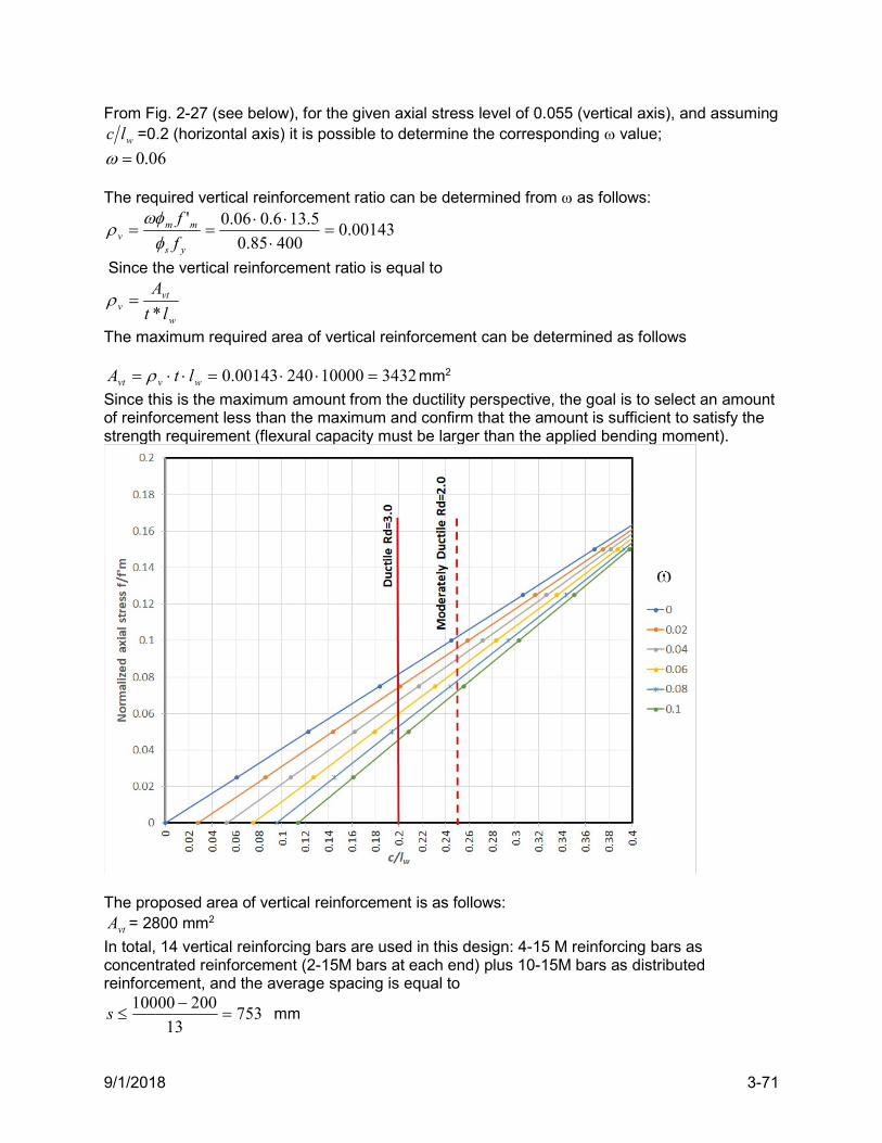
9/1/2018 3-71

From Fig. 2-27 (see below), for the given axial stress level of 0.055 (vertical axis), and assuming

wlc =0.2 (horizontal axis) it is possible to determine the corresponding value;

06.0 The required vertical reinforcement ratio can be determined from as follows:

00143.040085.0

5.136.006.0'

ys

mmv f

f

Since the vertical reinforcement ratio is equal to

w

vtv lt

A

*

The maximum required area of vertical reinforcement can be determined as follows

34321000024000143.0 wvvt ltA mm2

Since this is the maximum amount from the ductility perspective, the goal is to select an amount of reinforcement less than the maximum and confirm that the amount is sufficient to satisfy the strength requirement (flexural capacity must be larger than the applied bending moment).

The proposed area of vertical reinforcement is as follows:

vtA = 2800 mm2

In total, 14 vertical reinforcing bars are used in this design: 4-15 M reinforcing bars as concentrated reinforcement (2-15M bars at each end) plus 10-15M bars as distributed reinforcement, and the average spacing is equal to

75313

20010000

s mm

9/1/2018 3-72

Since 2-15M bars are concentrated at each end, the amount of concentrated reinforcement is

cA = 400 mm2

And the amount of distributed reinforcement is cvtd AAA 2 2000 mm2

For Ductile shear walls, S304-14 Cl.16.9.5.3 notes that the amount of concentrated reinforcement at each wall end should not exceed 25% of the distributed reinforcement. Since

2.02000400 dc AA < 0.25 OK

It is also required to check the maximum reinforcement area per S304-14 Cl.10.15.2 (see Table 2-3). Since mms 753 < 960240*44 t mm

4800)10*240(02.002.0 3max gs AA mm2/m

This is significantly larger than the estimated area of vertical reinforcement. The wall is subjected to axial load fP = 1800 kN. The moment resistance for the wall section can be determined from the following equations (see Section C.1.1.2):

85.01 8.01 05.0 09.0 1820c mm

10000

18201

2800*400*85.0

10*18001

1000

10000*2800*

1000

400*85.0*5.0115.0

3

wvtys

f

wvtysr l

c

Af

PlAfM

11300rM kNm > 9430fM kNm OK

Note that 2.018.0100001820 wlc

Therefore, the S304-14 minimum rotational demand requirement for Ductile shear walls is satisfied. 7. Perform the S304-14 ductility check (see Section 2.6.3). To satisfy the S304-14 ductility requirements for Ductile shear walls (Cl.16.9.7), the neutral axis depth ratio ( wlc ), should be less than the following limit:

125.0wlc when 5ww lh

In this case,

55.1 w

w

l

hAlso, the neutral axis depth

c= 1820 mm and so

125.018.0100001820 wlc

Therefore, the simplified S304-14 ductility requirement is not satisfied. Consequently, a detailed ductility check according to S304-14 Cl.16.8.8 needs to be performed. It is required to determine

the rotational demand id and the rotational capacity ic , and to confirm that the capacity

exceeds the demand. The rotational demand depends on the elastic lateral displacement at the top of the wall, which is given as

131 fΔ mm

9/1/2018 3-73

The overstrength factor must be at least equal to 1.3, and can be determined from the following equation:

36.19430

12800

f

nw M

M

In this case, the nominal moment capacity is equal to Mn = 12,800 kNm, which was calculated in the same manner as the factored moment resistance Mr, except that unit values of material resistance factors 0.1 sm were used.

The S304-14 minimum rotational demand is min = 0.004 for Ductile shear walls. The actual value is determined from the following equation:

3

3

11 1008.4

102

0.100.15

36.1135.10.313

2

ww

fdofid

h

ΔRRΔw

This is greater than min = 0.004, so the actual rotational demand will be used. The rotational capacity can be calculated as follows (and should not exceed 0.025)

31087.4002.018202

100000025.0)002.0

2(

c

lwmuic

Since the rotational capacity iic is greater than rotational demand id, it can be concluded that the S304-14 ductility requirements have been satisfied. 8. Minimum required factored shear resistance (see Section 2.6.5 and S304-14 Cl.16.9.8.3) Cl.16.9.8.3 requires that the factored shear resistance, rV , should be greater than the shear due to effects of factored loads, but not less than i) the shear corresponding to the development of probable moment capacity, pM , or ii) the shear corresponding to the lateral seismic load (base

shear), where earthquake effects were calculated using RdRo=1.3. The first requirement is based on the Capacity Design approach (see Section 2.5.1 for more details). For Ductile shear walls, the shear capacity should exceed the shear corresponding to the probable moment capacity, as follows

13900pM kNm

The shear force resultant acts at the effective height eh , that is, the distance from the base of

the wall to the resultant of all seismic forces acting at the floor levels. Note that eh can be

determined as follows

0.10f

fe V

Mh m

The shear force pbV corresponding to the overturning moment pM is equal to

0.10

13900

e

ppb h

MV 1390 kN

9/1/2018 3-74

The second requirement gives an “almost elastic” factored base shear force for the wall, which is equal to

32643.1

5.10.3943

3.1

odf

fe

RRVV kN

The smaller of these two values should be used, hence 1390rdV kN

9. Diagonal tension shear resistance (see Sections 2.3.2 and 2.6.5 and S304-14 Cl.10.10.2.1 and Cl.16.9.8.1) Masonry shear resistance ( mV ):

240wb mm overall wall thickness

80008.0 wv ld mm effective wall depth

0.1g solid grouted wall

fd PP 9.0 = 1620 kN

Since

0.8*943

9430

vf

f

dV

M= 1.25 > 1.0 use 0.1

vf

f

dV

M in the equation for masonry shear resistance

below

mvf

fm f

dV

Mv )2(16.0 = 0.59 MPa

gdvwmmm PdbvV )25.0( = 0.6(0.59*240*8000+0.25*1620*103)*1.0 = 920 kN

The required steel shear resistance can be found from the following equation (see Section 2.6.5 and S304-14 Cl.16.9.8.1) (note 50% reduction of Vm)

rdsmr VVVV 5.0

hence 9309205.013905.0 mrds VVV kN

The required amount of reinforcement can be found from the following equation

57.08000*400*85.0*6.0

10*930

6.0

3

vys

sv

df

V

s

A

Try 2-15M bond beam reinforcing bars at 600 mm spacing ( 400vA mm2 and 600s mm):

67.0600

400

s

Av > 0.57 OK

Steel shear resistance sV :

600

8000*400*

1000

400*85.0*6.06.0

s

dfAV vyvss = 1088 kN

Total diagonal shear resistance: 0.5 0.5 920 1088 1548r m sV V V kN > 1390rdV kN OK

Maximum shear allowed on the section is (S304-14 Cl.10.10.2.1)

16904.0max gvwmmr dbfV kN

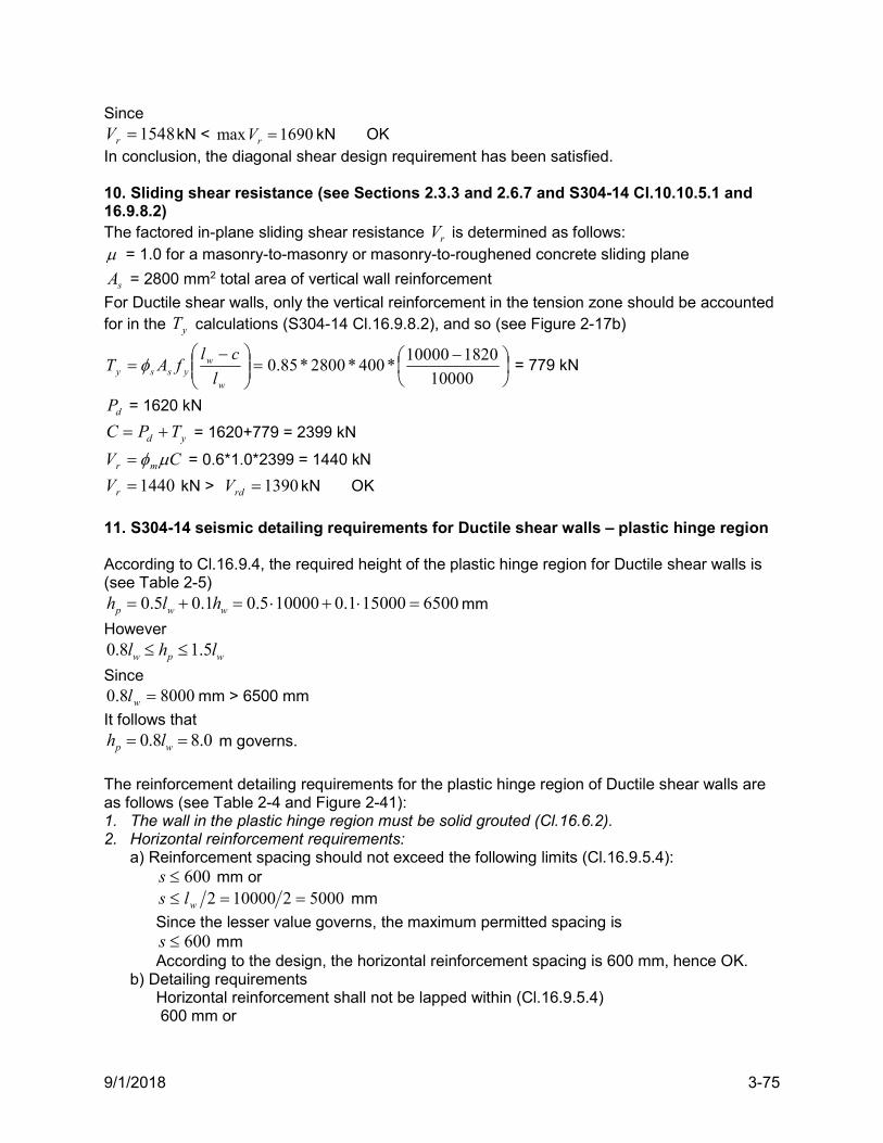
9/1/2018 3-75

Since 1548rV kN < 1690max rV kN OK

In conclusion, the diagonal shear design requirement has been satisfied. 10. Sliding shear resistance (see Sections 2.3.3 and 2.6.7 and S304-14 Cl.10.10.5.1 and 16.9.8.2) The factored in-plane sliding shear resistance rV is determined as follows: = 1.0 for a masonry-to-masonry or masonry-to-roughened concrete sliding plane

sA = 2800 mm2 total area of vertical wall reinforcement

For Ductile shear walls, only the vertical reinforcement in the tension zone should be accounted for in the yT calculations (S304-14 Cl.16.9.8.2), and so (see Figure 2-17b)

10000

182010000*400*2800*85.0

w

wyssy l

clfAT = 779 kN

dP = 1620 kN

yd TPC = 1620+779 = 2399 kN

CV mr = 0.6*1.0*2399 = 1440 kN

1440rV kN > 1390rdV kN OK

11. S304-14 seismic detailing requirements for Ductile shear walls – plastic hinge region According to Cl.16.9.4, the required height of the plastic hinge region for Ductile shear walls is (see Table 2-5)

0.5 0.1 0.5 10000 0.1 15000 6500p w wh l h mm

However 0.8 1.5w p wl h l

Since 80008.0 wl mm > 6500 mm

It follows that 0.8 8.0p wh l m governs.

The reinforcement detailing requirements for the plastic hinge region of Ductile shear walls are as follows (see Table 2-4 and Figure 2-41): 1. The wall in the plastic hinge region must be solid grouted (Cl.16.6.2). 2. Horizontal reinforcement requirements:

a) Reinforcement spacing should not exceed the following limits (Cl.16.9.5.4): 600s mm or

50002100002 wls mm

Since the lesser value governs, the maximum permitted spacing is 600s mm

According to the design, the horizontal reinforcement spacing is 600 mm, hence OK. b) Detailing requirements

Horizontal reinforcement shall not be lapped within (Cl.16.9.5.4) 600 mm or

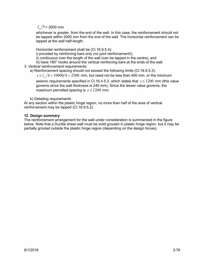
9/1/2018 3-76

5wl = 2000 mm

whichever is greater, from the end of the wall. In this case, the reinforcement should not be lapped within 2000 mm from the end of the wall. The horizontal reinforcement can be lapped at the wall half-length. Horizontal reinforcement shall be (Cl.16.9.5.4): i) provided by reinforcing bars only (no joint reinforcement!); ii) continuous over the length of the wall (can be lapped in the centre), and iii) have 180° hooks around the vertical reinforcing bars at the ends of the wall.

3. Vertical reinforcement requirements: a) Reinforcement spacing should not exceed the following limits (Cl.16.9.5.3):

25004100004 wls mm, but need not be less than 400 mm, or the minimum

seismic requirements specified in Cl.16.4.5.3, which states that 1200s mm (this value governs since the wall thickness is 240 mm). Since the lesser value governs, the maximum permitted spacing is 1200s mm.

b) Detailing requirements At any section within the plastic hinge region, no more than half of the area of vertical reinforcement may be lapped (Cl.16.9.5.2). 12. Design summary The reinforcement arrangement for the wall under consideration is summarized in the figure below. Note that a Ductile shear wall must be solid grouted in plastic hinge region, but it may be partially grouted outside the plastic hinge region (depending on the design forces).

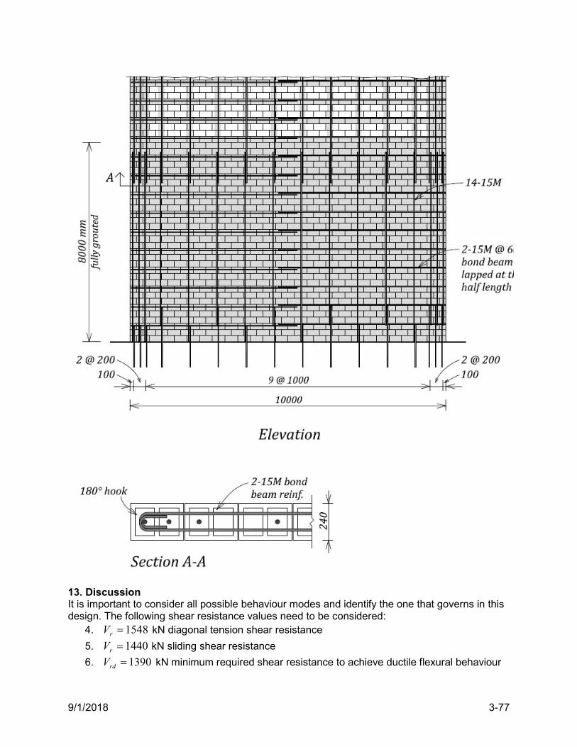
9/1/2018 3-77

13. Discussion It is important to consider all possible behaviour modes and identify the one that governs in this design. The following shear resistance values need to be considered:

4. 1548rV kN diagonal tension shear resistance

5. 1440rV kN sliding shear resistance

6. 1390rdV kN minimum required shear resistance to achieve ductile flexural behaviour

9/1/2018 3-78

It can be concluded that the minimum required shear force corresponding to the flexural failure mechanism is the smallest (1390 kN), so it governs in this case, which is a requirement for the Capacity Design approach for Ductile RM shear walls.

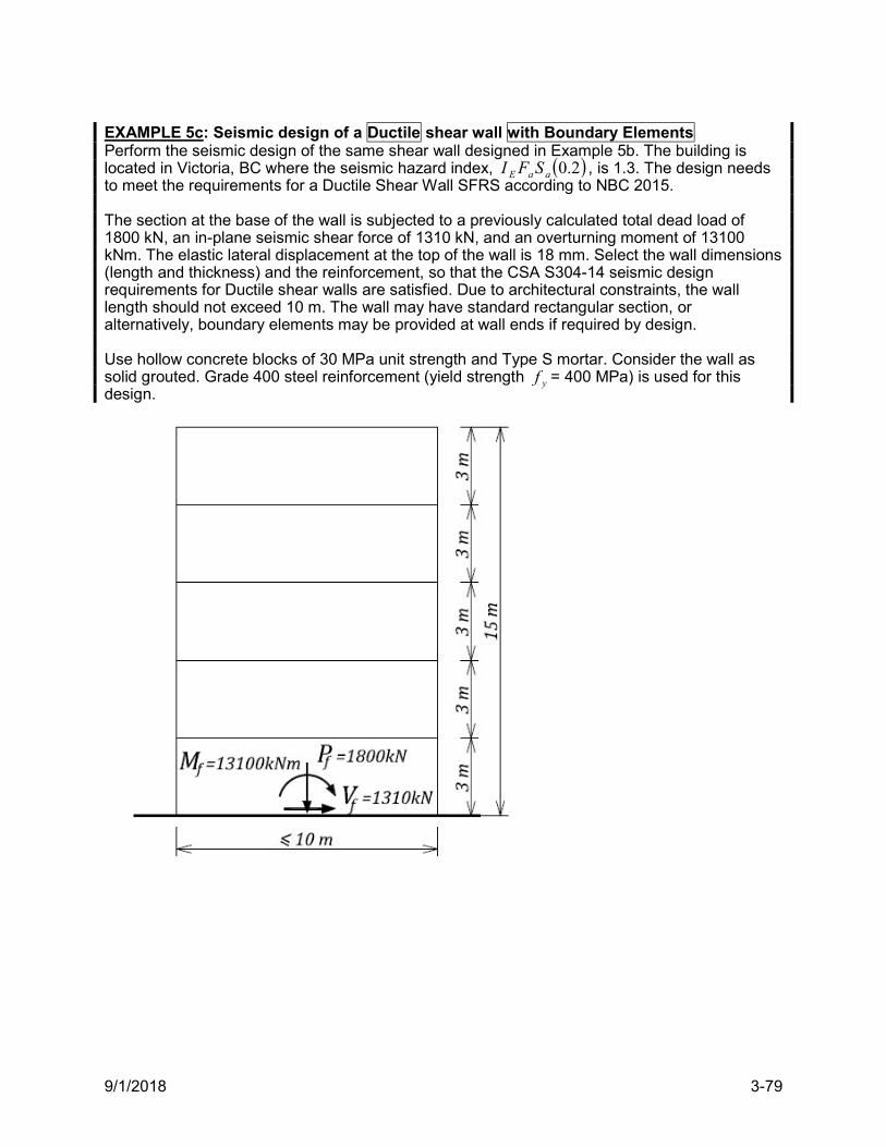
9/1/2018 3-79

EXAMPLE 5c: Seismic design of a Ductile shear wall with Boundary Elements Perform the seismic design of the same shear wall designed in Example 5b. The building is located in Victoria, BC where the seismic hazard index, 2.0aaE SFI , is 1.3. The design needs to meet the requirements for a Ductile Shear Wall SFRS according to NBC 2015. The section at the base of the wall is subjected to a previously calculated total dead load of 1800 kN, an in-plane seismic shear force of 1310 kN, and an overturning moment of 13100 kNm. The elastic lateral displacement at the top of the wall is 18 mm. Select the wall dimensions (length and thickness) and the reinforcement, so that the CSA S304-14 seismic design requirements for Ductile shear walls are satisfied. Due to architectural constraints, the wall length should not exceed 10 m. The wall may have standard rectangular section, or alternatively, boundary elements may be provided at wall ends if required by design. Use hollow concrete blocks of 30 MPa unit strength and Type S mortar. Consider the wall as solid grouted. Grade 400 steel reinforcement (yield strength yf = 400 MPa) is used for this design.

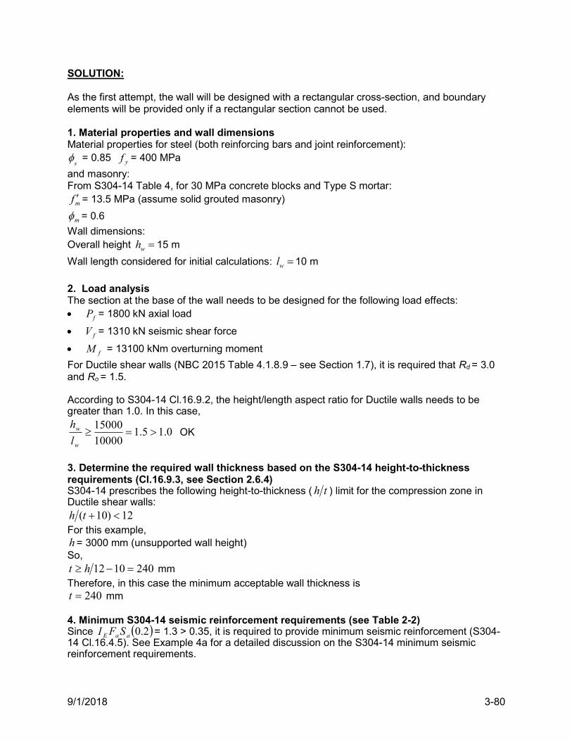
9/1/2018 3-80

SOLUTION: As the first attempt, the wall will be designed with a rectangular cross-section, and boundary elements will be provided only if a rectangular section cannot be used. 1. Material properties and wall dimensions Material properties for steel (both reinforcing bars and joint reinforcement):

s = 0.85 yf = 400 MPa

and masonry: From S304-14 Table 4, for 30 MPa concrete blocks and Type S mortar:

mf = 13.5 MPa (assume solid grouted masonry)

m = 0.6

Wall dimensions: Overall height wh 15 m

Wall length considered for initial calculations: wl 10 m

2. Load analysis The section at the base of the wall needs to be designed for the following load effects: fP = 1800 kN axial load

fV = 1310 kN seismic shear force

fM = 13100 kNm overturning moment

For Ductile shear walls (NBC 2015 Table 4.1.8.9 – see Section 1.7), it is required that Rd = 3.0 and Ro = 1.5. According to S304-14 Cl.16.9.2, the height/length aspect ratio for Ductile walls needs to be greater than 1.0. In this case,

0.15.110000

15000

w

w

l

h OK

3. Determine the required wall thickness based on the S304-14 height-to-thickness requirements (Cl.16.9.3, see Section 2.6.4) S304-14 prescribes the following height-to-thickness ( th ) limit for the compression zone in Ductile shear walls:

12)10( th For this example, h= 3000 mm (unsupported wall height) So,

2401012 ht mm Therefore, in this case the minimum acceptable wall thickness is

240t mm 4. Minimum S304-14 seismic reinforcement requirements (see Table 2-2) Since 2.0aaE SFI = 1.3 > 0.35, it is required to provide minimum seismic reinforcement (S304-14 Cl.16.4.5). See Example 4a for a detailed discussion on the S304-14 minimum seismic reinforcement requirements.

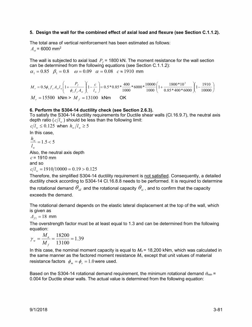
9/1/2018 3-81

5. Design the wall for the combined effect of axial load and flexure (see Section C.1.1.2). The total area of vertical reinforcement has been estimated as follows:

vtA = 6000 mm2

The wall is subjected to axial load fP = 1800 kN. The moment resistance for the wall section can be determined from the following equations (see Section C.1.1.2):

85.01 8.01 09.0 08.0 1910c mm

10000

19101

6000*400*85.0

10*18001

1000

10000*6000*

1000

400*85.0*5.0115.0

3

wvtys

f

wvtysr l

c

Af

PlAfM

15500rM kNm > 13100fM kNm OK

6. Perform the S304-14 ductility check (see Section 2.6.3). To satisfy the S304-14 ductility requirements for Ductile shear walls (Cl.16.9.7), the neutral axis depth ratio ( wlc ) should be less than the following limit:

125.0wlc when 5ww lh

In this case,

55.1 w

w

l

h

Also, the neutral axis depth c= 1910 mm and so

125.019.0100001910 wlc

Therefore, the simplified S304-14 ductility requirement is not satisfied. Consequently, a detailed ductility check according to S304-14 Cl.16.8.8 needs to be performed. It is required to determine

the rotational demand id and the rotational capacity ic , and to confirm that the capacity

exceeds the demand. The rotational demand depends on the elastic lateral displacement at the top of the wall, which is given as

181 fΔ mm

The overstrength factor must be at least equal to 1.3 and can be determined from the following equation:

39.113100

18200

f

nw M

M

In this case, the nominal moment capacity is equal to Mn = 18,200 kNm, which was calculated in the same manner as the factored moment resistance Mr, except that unit values of material resistance factors 0.1 sm were used.

Based on the S304-14 rotational demand requirement, the minimum rotational demand min = 0.004 for Ductile shear walls. The actual value is determined from the following equation:

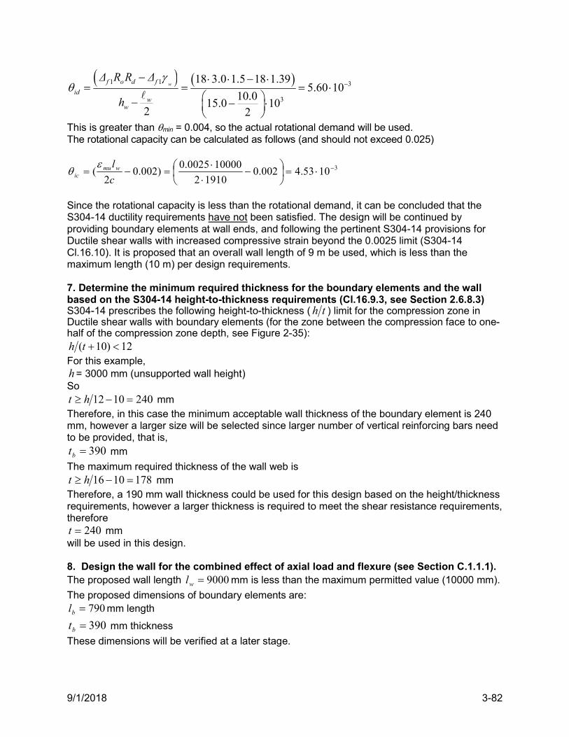
9/1/2018 3-82

1 1 3

3

18 3.0 1.5 18 1.395.60 10

10.015.0 10

2 2

wf o d f

idw

w

Δ R R Δ

h

This is greater than min = 0.004, so the actual rotational demand will be used. The rotational capacity can be calculated as follows (and should not exceed 0.025)

31053.4002.019102

100000025.0)002.0

2(

c

lwmuic

Since the rotational capacity is less than the rotational demand, it can be concluded that the S304-14 ductility requirements have not been satisfied. The design will be continued by providing boundary elements at wall ends, and following the pertinent S304-14 provisions for Ductile shear walls with increased compressive strain beyond the 0.0025 limit (S304-14 Cl.16.10). It is proposed that an overall wall length of 9 m be used, which is less than the maximum length (10 m) per design requirements. 7. Determine the minimum required thickness for the boundary elements and the wall based on the S304-14 height-to-thickness requirements (Cl.16.9.3, see Section 2.6.8.3) S304-14 prescribes the following height-to-thickness ( th ) limit for the compression zone in Ductile shear walls with boundary elements (for the zone between the compression face to one-half of the compression zone depth, see Figure 2-35):

12)10( th For this example, h= 3000 mm (unsupported wall height) So

2401012 ht mm Therefore, in this case the minimum acceptable wall thickness of the boundary element is 240 mm, however a larger size will be selected since larger number of vertical reinforcing bars need to be provided, that is,

390bt mm

The maximum required thickness of the wall web is 1781016 ht mm

Therefore, a 190 mm wall thickness could be used for this design based on the height/thickness requirements, however a larger thickness is required to meet the shear resistance requirements, therefore

240t mm will be used in this design. 8. Design the wall for the combined effect of axial load and flexure (see Section C.1.1.1). The proposed wall length 9000wl mm is less than the maximum permitted value (10000 mm).

The proposed dimensions of boundary elements are: 790bl mm length

390bt mm thickness

These dimensions will be verified at a later stage.

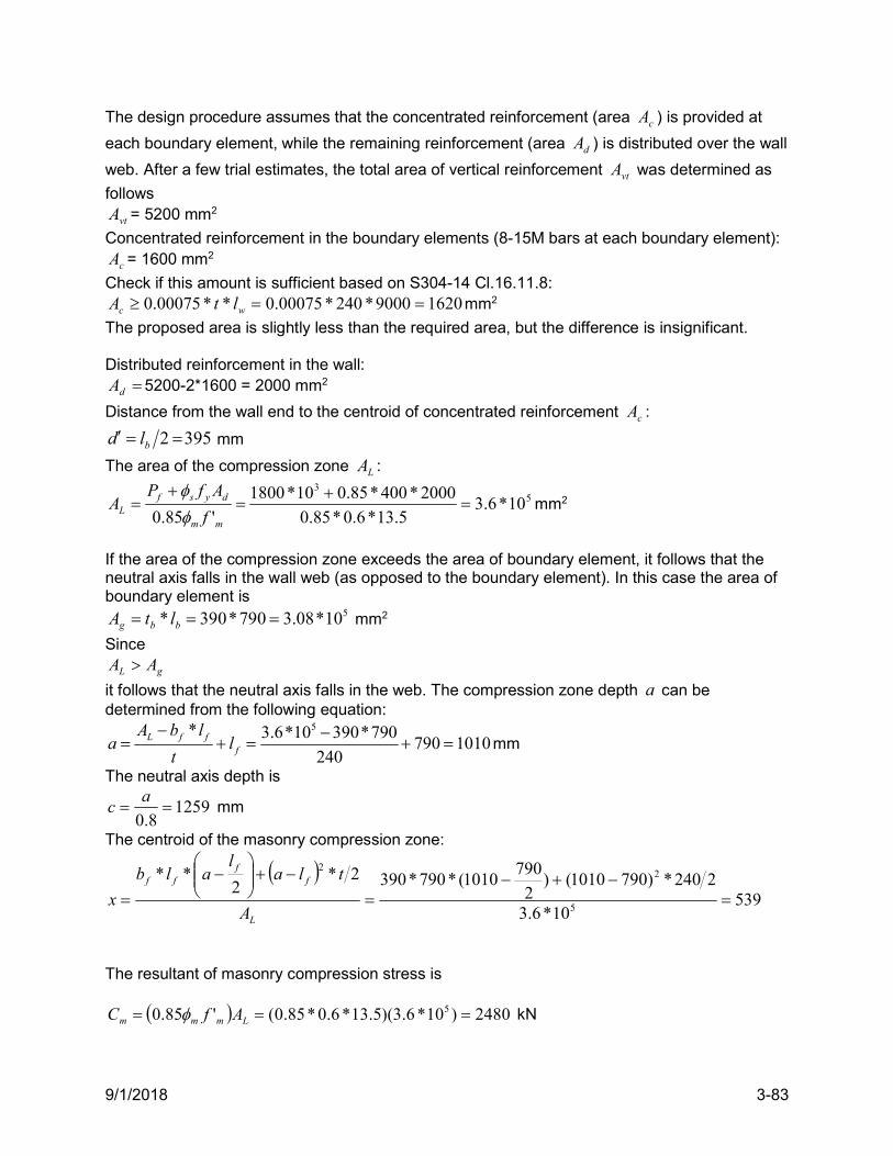
9/1/2018 3-83

The design procedure assumes that the concentrated reinforcement (area cA ) is provided at

each boundary element, while the remaining reinforcement (area dA ) is distributed over the wall

web. After a few trial estimates, the total area of vertical reinforcement vtA was determined as

follows

vtA = 5200 mm2

Concentrated reinforcement in the boundary elements (8-15M bars at each boundary element):

cA = 1600 mm2

Check if this amount is sufficient based on S304-14 Cl.16.11.8: 16209000*240*00075.0**00075.0 wc ltA mm2

The proposed area is slightly less than the required area, but the difference is insignificant. Distributed reinforcement in the wall:

dA 5200-2*1600 = 2000 mm2

Distance from the wall end to the centroid of concentrated reinforcement cA :

3952 bld mm

The area of the compression zone LA :

53

10*6.35.13*6.0*85.0

2000*400*85.010*1800

'85.0

mm

dysfL f

AfPA

mm2

If the area of the compression zone exceeds the area of boundary element, it follows that the neutral axis falls in the wall web (as opposed to the boundary element). In this case the area of boundary element is

510*08.3790*390* bbg ltA mm2

Since

gL AA

it follows that the neutral axis falls in the web. The compression zone depth a can be determined from the following equation:

5* 3.6*10 390*790790 1010

240L f f

f

A b la l

t

mm

The neutral axis depth is

12598.0

ac mm

The centroid of the masonry compression zone:

539

10*6.3

2240*)7901010()2

7901010(*790*3902*

2**

5

22

L

ff

ff

A

tlal

alb

x

The resultant of masonry compression stress is

2480)10*6.3)(5.13*6.0*85.0('85.0 5 Lmmm AfC kN

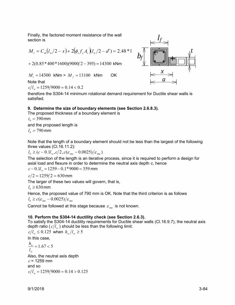
9/1/2018 3-84

Finally, the factored moment resistance of the wall section is

)53929000(10*48.2)2(22 6dlAfxlCM wcyswmr

14300)39529000)(1600*400*85.0(2 kNm

14300rM kNm > 13100fM kNm OK

Note that 2.014.090001259 wlc

therefore the S304-14 minimum rotational demand requirement for Ductile shear walls is satisfied. 9. Determine the size of boundary elements (see Section 2.6.8.3). The proposed thickness of a boundary element is

390bt mm

and the proposed length is 790bl mm

Note that the length of a boundary element should not be less than the largest of the following three values (Cl.16.11.2):

))0025.0(,2,1.0( mumuwb cclcl

The selection of the length is an iterative process, since it is required to perform a design for axial load and flexure in order to determine the neutral axis depth c, hence

3599000*1.012591.0 wlc mm

630212592 c mm The larger of these two values will govern, that is,

630bl mm

Hence, the proposed value of 790 mm is OK. Note that the third criterion is as follows

mumub cl )0025.0(

Cannot be followed at this stage because mu is not known.

10. Perform the S304-14 ductility check (see Section 2.6.3). To satisfy the S304-14 ductility requirements for Ductile shear walls (Cl.16.9.7), the neutral axis depth ratio ( wlc ) should be less than the following limit:

125.0wlc when 5ww lh

In this case,

567.1 w

w

l

h

Also, the neutral axis depth c= 1259 mm and so

125.014.090001259 wlc

9/1/2018 3-85

Therefore, the simplified S304-14 ductility requirement is not satisfied. Consequently, a detailed ductility check according to S304-14 Cl.16.8.8 needs to be performed. It is required to determine

the rotational demand id and the rotational capacity ic , and to confirm that the capacity

exceeds the demand. The rotational demand depends on the elastic lateral displacement at the top of the wall, which is given as

181 fΔ mm

The overstrength factor must be at least equal to 1.3 and can be determined from the following equation:

3.127.113100

16600

f

nw M

M

Hence, 3.1w

In this case, the nominal moment capacity is equal to Mn = 16,600 kNm, which was calculated in the same manner as the factored moment resistance Mr, except that unit values of material resistance factors 0.1 sm were used.

The S304-14 minimum rotational demand is min = 0.004 for Ductile shear walls. The actual value is determined from the following equation:

3

3

11 1049.510

2

0.90.15

30.1185.10.318

2

ww

fdofid

h

ΔRRΔw

This is greater than min = 0.004, so the actual rotational demand will be used. The required maximum compressive strain value can be determined from the following equation (see Section 2.6.8.2)

0021.09000

1259*2)002.010*49.5(

2002.0 3

widmu l

c

Note that

mumub cl )0025.0(

However, this criterion cannot be applied since mu is less than 0.0025.

11. Minimum required factored shear resistance (see Section 2.6.5 and S304-14 Cl.16.10.4.3) Cl.16.10.4.3 requires that the factored shear resistance, rV , should be greater than the shear due to the effects of factored loads, but not less than i) the shear corresponding to the development of probable moment capacity, pM , or ii) the shear corresponding to the lateral

seismic load (base shear), where earthquake effects were calculated using RdRo = 1.3.

9/1/2018 3-86

The first requirement is based on the Capacity Design approach (see Section 2.5.1 for more details). For Ductile shear walls, the shear capacity should exceed the shear corresponding to the probable moment capacity, as follows

18600pM kNm

The shear force resultant acts at the effective height eh , that is, the distance from the base of

the wall to the resultant of all seismic forces acting at the floor levels. Note that eh can be

determined as follows

0.10f

fe V

Mh m

The shear force pbV corresponding to the overturning moment pM is equal to

0.10

18600

e

ppb h

MV 1860 kN

The second requirement gives an “almost elastic” factored base shear force for the wall, which is equal to

1310 3.0 1.54535

1,.3 1.3f d o

fe

V R RV

kN

The smaller of these two values should be used, hence 1860rdV kN

12. Diagonal tension shear resistance (see Section 2.6.5 and S304-14 Cl.10.10.2.1) Masonry shear resistance ( mV ):

240wb mm overall wall thickness

72008.0 wv ld mm effective wall depth

0.1g solid grouted wall

fd PP 9.0 = 1620 kN

mvf

fm f

dV

Mv )2(16.0 = 0.59 MPa

Since

2.7*1310

13100

vf

f

dV

M= 1.39 > 1.0

use 0.1vf

f

dV

M

gdvwmmm PdbvV )25.0( = 0.6(0.59*240*7200+0.25*1620*103)*1.0 = 852 kN

The required steel shear resistance can be found from the following equation (see Section 2.6.5 and S304-14 Cl.16.10.4.1)

rdsmmur VVVV ))2(0025.0(

Since 59.0)0021.0*2(0025.0)2(0025.0 mu

Then

9/1/2018 3-87

1357852*59.0186059.0 mrds VVV kN

The required amount of reinforcement can be found from the following equation

92.07200*400*85.0*6.0

10*1357

6.0

3

vys

sv

df

V

s

A

Try 2-20M bond beam reinforcing bars at 600 mm spacing ( 600vA mm2 and 600s mm):

0.1600

600

s

Av > 0.92 OK

Steel shear resistance sV :

600

7200*600*

1000

400*85.0*6.06.0

s

dfAV vyvss = 1470 kN

Total diagonal shear resistance: 1973147085259.059.0 smr VVV kN > 1860rdV kN OK

Maximum shear allowed on the section is (S304-14 Cl.10.10.2.1)

15204.0max gvwmmr dbfV kN

Since 1973rV kN > 1520max rV kN

the above maximum shear resistance requirement has not been satisfied. It would be required to increase either wall thickness or length to satisfy this requirement. It is recommended to perform this check at an early stage of the design. 13. Sliding shear resistance (see Sections 2.3.3 and 2.6.7, and S304-14 Cl.10.10.5.1 and 16.10.4.2) The factored in-plane sliding shear resistance rV is determined as follows: = 1.0 for a masonry-to-masonry or masonry-to-roughened concrete sliding plane

sA = 5200 mm2 total area of vertical wall reinforcement

For Ductile shear walls, only the vertical reinforcement in the tension zone should be accounted for in the yT calculations (S304-14 Cl.16.10.4.2), (also see Figure 2-17b)

9000

12599000*400*5200*85.0

w

wyssy l

clfAT = 1520 kN

dP = 1620 kN

yd TPC = 1620+1520 = 3140 kN

CV mr = 0.6*1.0*3140 = 1884 kN

1884rV kN > 1860rdV kN OK

14. Shear at the interface (see Section 2.6.8.4 and S304-14 Cl.16.11.10) It is required to check whether the horizontal wall reinforcement is sufficient to resist the vertical shear stresses at the boundary element interface. The shear flow demand is based on the design shear force transferred over the storey height, that is,

6200.3

1860

h

VV rdsf kN/m

The shear flow resistance is as follows (Cl.16.11.10)

9/1/2018 3-88

smfr FV

The resistance provided by horizontal reinforcement (2-20M bars at 600 mm spacing) is as follows

204340*0.1*6.0 smfr FV kN/m

Where 340600600*400*85.0 sAfF vyss kN/m

is the shear flow resistance provided by the horizontal reinforcement. Since

sffr VV

it follows that additional horizontal reinforcement is required to satisfy the requirement. Let us assume that 2-20M bars (total area 600 mm2) will be provided at 200 mm spacing throughout the wall height at the first-floor level, that is,

1020200600*400*85.0 sAfF vyss kN/m

6121020*0.1*6.0 smfr FV kN/m

This shear flow resistance approximately satisfies the shear flow demand. The difference (620-612=8 kN/m) is 1% of the total demand, which is insignificant. 15. Detailing of boundary elements (see Section 2.6.8.5 and S304-14 Cl.16.11) 1) Regular ties and buckling prevention ties within the plastic hinge zone

Dimensions of a boundary element:

790bl mm length

390bt mm thickness 510*08.3390*790* bbg tlA mm2

For the rectangular hoop reinforcement, the minimum area Ash in each principal direction should not be less than the larger of the following (S304-14 Cl.16.11.6):

cyh

m

ch

gpnsh hs

f

f

A

AkkA

'2.0 1

or

cyh

msh hs

f

fA

'09.0

where

33.128

8

2

l

ln n

nk

8ln number of supported bars around the perimeter of a boundary element

163.00021.0*301.0301.01 mupk 510*0.2690*290 chA mm2

is the area of the confined core and 690ch mm is the larger dimension of the confined core

(the dimension in other direction is 290 mm) The maximum spacing of buckling prevention ties within the plastic hinge zone should not exceed the lesser of (S304-14 Cl.16.11.4)

9/1/2018 3-89

)2,24,6( btieb tdds

Where db is longitudinal bar diameter, and dtie is the tie diameter, hence 9015*66 bd mm

24010*2424 tied mm

19523902 bt mm

Hence, 90s mm governs

Assume 80s mm

The required area of tie reinforcement in boundary elements should be at least equal to the larger of

124690*80*400

5.13

10*0.2

10*08.3*163.0*33.1*2.0

'2.0

5

5

1 cyh

m

ch

gpnsh hs

f

f

A

AkkA mm2

or

168690*80*400

5.1309.0

'09.0 c

yh

msh hs

f

fA mm2

Hence 168shA mm2 governs

This area of reinforcement can be achieved through 3-10M bars (total area 300 mm2): two bars are a part of a regular tie enclosing the boundary element, plus a cross tie supporting intermediate bars. 2) Regular ties and buckling prevention ties outside the plastic hinge zone

The maximum spacing of buckling prevention ties outside the plastic hinge zone should not exceed the lesser of (S304-14 Cl.12.2.1)

),48,16( btieb tdds

Where db is longitudinal bar diameter, and dtie is the tie diameter, hence 24015*1616 bd mm

48010*4848 tied mm

390bt mm

Hence, 240s mm governs

Assume 240s mm

3) Vertical reinforcement: detailing At any section within the plastic hinge region, no more than half of the area of vertical reinforcement may be lapped (S304-14 Cl.16.11.9). 16. The S304-14 seismic detailing requirements for Ductile shear walls – plastic hinge region According to Cl.16.10.3, the required height of the plastic hinge region for Ductile shear walls is (see Table 2-5)

9/1/2018 3-90

0.5 0.1 0.5 9000 0.1 15000 6000p w wh l h mm

However 2.0w p wl h l

Since 9000wl mm > 6000 mm

It follows that 9.0p wh l m governs.

The reinforcement detailing requirements for the plastic hinge region of Ductile shear walls are as follows (see Table 2-4 and Figure 2-41): 1. The wall in the plastic hinge region must be solid grouted (Cl.16.6.2). 2. Horizontal reinforcement requirements:

a) Reinforcement spacing should not exceed the following limits (Cl.16.9.5.4): 600s mm or

4500290002 wls mm

Since the lesser value governs, the maximum permitted spacing is 600s mm

According to the design, the horizontal reinforcement spacing is 600 mm, hence OK. b) Detailing requirements

Horizontal reinforcement shall not be lapped within (Cl.16.9.5.4) 600 mm or 5wl = 1800 mm

whichever is greater, from the end of the wall. In this case, the reinforcement should not be lapped within the distance 1800 mm from the end of the wall. The horizontal reinforcement can be lapped at the wall half-length. Horizontal reinforcement shall be (Cl.16.9.5.4): i) provided by reinforcing bars only (no joint reinforcement!); ii) continuous over the length of the wall (can be lapped in the centre), and iii) have 180° hooks around the vertical reinforcing bars at the ends of the wall.

3. Vertical reinforcement requirements: a) Reinforcement spacing should not exceed the following limits (Cl.16.9.5.3):

2250490004 wls mm, but need not be less than 400 mm

or the minimum seismic requirements specified in Cl.16.4.5.3, which states that 1200s mm (this value governs since the wall thickness is 240 mm).

Since the lesser value governs, the maximum permitted spacing is 1200s mm. b) Detailing requirements

At any section within the plastic hinge region, no more than half of the area of vertical reinforcement may be lapped (Cl.16.9.5.2). 17. Design summary The reinforcement arrangement for the wall under consideration is summarized in the figure below. Note that a Ductile shear wall must be solid grouted in plastic hinge region, but it may be partially grouted outside the plastic hinge region (depending on the design forces).

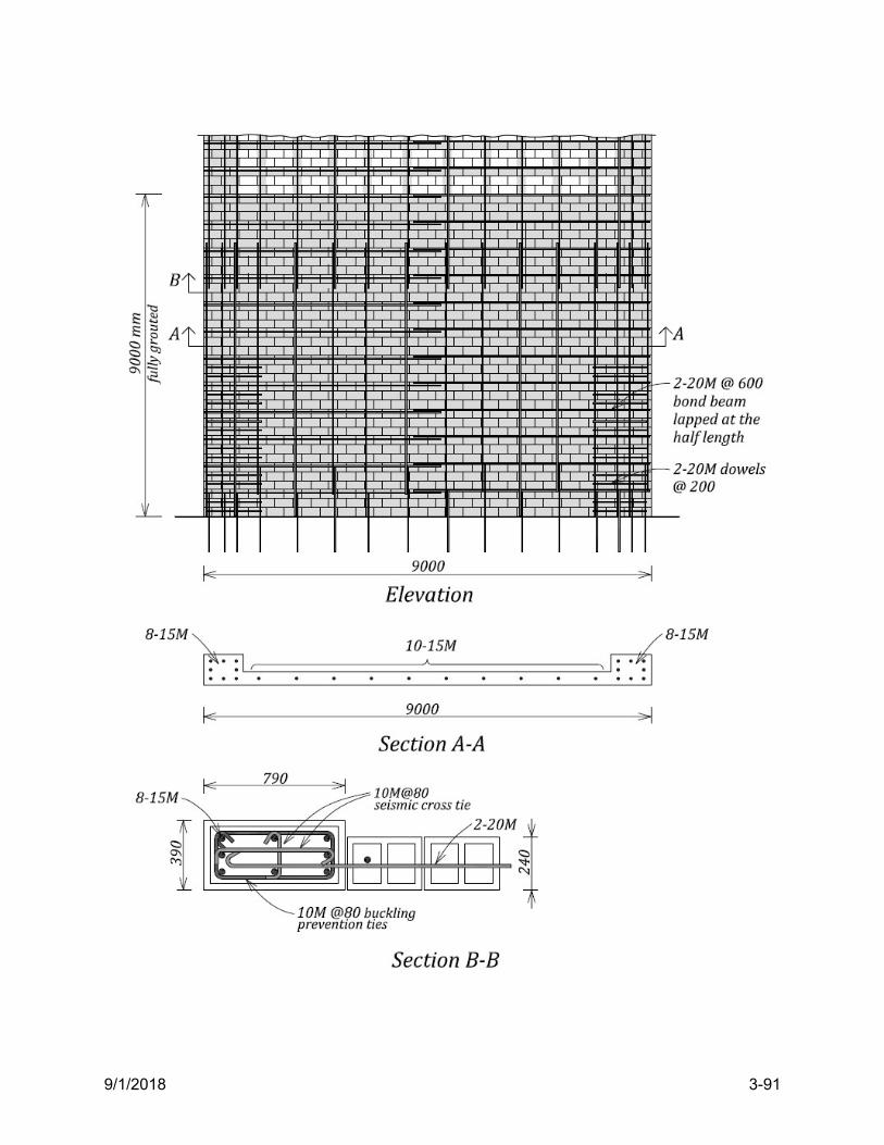
9/1/2018 3-91

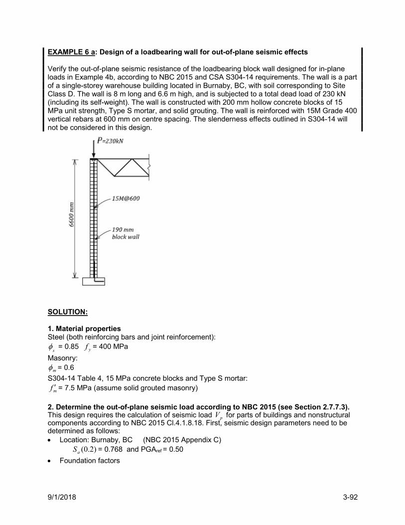
9/1/2018 3-92

EXAMPLE 6 a: Design of a loadbearing wall for out-of-plane seismic effects Verify the out-of-plane seismic resistance of the loadbearing block wall designed for in-plane loads in Example 4b, according to NBC 2015 and CSA S304-14 requirements. The wall is a part of a single-storey warehouse building located in Burnaby, BC, with soil corresponding to Site Class D. The wall is 8 m long and 6.6 m high, and is subjected to a total dead load of 230 kN (including its self-weight). The wall is constructed with 200 mm hollow concrete blocks of 15 MPa unit strength, Type S mortar, and solid grouting. The wall is reinforced with 15M Grade 400 vertical rebars at 600 mm on centre spacing. The slenderness effects outlined in S304-14 will not be considered in this design.

SOLUTION: 1. Material properties Steel (both reinforcing bars and joint reinforcement):

s = 0.85 yf = 400 MPa

Masonry:

m = 0.6

S304-14 Table 4, 15 MPa concrete blocks and Type S mortar:

mf = 7.5 MPa (assume solid grouted masonry)

2. Determine the out-of-plane seismic load according to NBC 2015 (see Section 2.7.7.3). This design requires the calculation of seismic load pV for parts of buildings and nonstructural components according to NBC 2015 Cl.4.1.8.18. First, seismic design parameters need to be determined as follows: Location: Burnaby, BC (NBC 2015 Appendix C)

)2.0(aS = 0.768 and PGAref = 0.50

Foundation factors

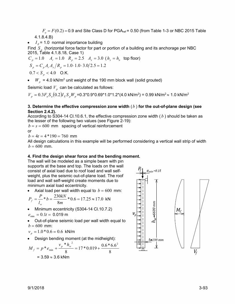
9/1/2018 3-93

(0.2)aF F 0.9 and Site Class D for PGAref = 0.50 (from Table 1-3 or NBC 2015 Table

4.1.8.4.B) EI = 1.0 normal importance building Find pS (horizontal force factor for part or portion of a building and its anchorage per NBC 2015, Table 4.1.8.18, Case 1)

0.1pC 0.1rA 5.2pR 0.3xA ( nx hh top floor)

2.15.20.30.10.1 pxrpp RAACS

0.47.0 pS O.K.

pW = 4.0 kN/m2 unit weight of the 190 mm block wall (solid grouted)

Seismic load pV can be calculated as follows:

ppEaap WSISFV 2.03.0 =0.3*0.9*0.69*1.0*1.2*(4.0 kN/m2) = 0.99 kN/m2 1.0 kN/m2

3. Determine the effective compression zone width (b ) for the out-of-plane design (see Section 2.4.2). According to S304-14 Cl.10.6.1, the effective compression zone width (b ) should be taken as the lesser of the following two values (see Figure 2-19):

600 sb mm spacing of vertical reinforcement or

760190*44 tb mm All design calculations in this example will be performed considering a vertical wall strip of width

600b mm. 4. Find the design shear force and the bending moment. The wall will be modeled as a simple beam with pin supports at the base and top. The loads on the wall consist of axial load due to roof load and wall self-weight, plus the seismic out-of-plane load. The roof load and wall self-weight create moments due to minimum axial load eccentricity. Axial load per wall width equal to 600b mm:

0.1725.176.0*8

230*

m

kNb

l

PP

wf kN

Minimum eccentricity (S304-14 Cl.10.7.2) te 1.0min 0.019 m

Out-of-plane seismic load per wall width equal to 600b mm:

6.06.0*0.1 pv kN/m

Design bending moment (at the midheight):

8

6.6*6.0019.0*17

8

**

22

min wpf

hvepM

= 3.59 3.6 kNm

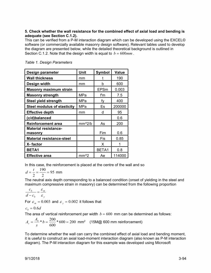
9/1/2018 3-94

5. Check whether the wall resistance for the combined effect of axial load and bending is adequate (see Section C.1.2). This can be verified from a P-M interaction diagram which can be developed using the EXCEL© software (or commercially available masonry design software). Relevant tables used to develop the diagram are presented below, while the detailed theoretical background is outlined in Section C.1.2. Note that the design width is equal to mmb 600 . Table 1. Design Parameters

Design parameter Unit Symbol Value

Wall thickness mm t 190

Design width mm b 600

Masonry maximum strain EPSm 0.003

Masonry strength MPa f'm 7.5

Steel yield strength MPa fy 400

Steel modulus of elasticity MPa Es 200000

Effective depth mm d 95

(c/d)balanced 0.6

Reinforcement area mm^2/b As 200 Material resistance-masonry Fim 0.6

Material resistance-steel Fis 0.85

X- factor X 1

BETA1 BETA1 0.8

Effective area mm^2 Ae 114000 In this case, the reinforcement is placed at the centre of the wall and so

952

190

2

td mm

The neutral axis depth corresponding to a balanced condition (onset of yielding in the steel and maximum compressive strain in masonry) can be determined from the following proportion

y

m

b

b

cd

c

For 003.0m and 002.0y it follows that

dcb 6.0

The area of vertical reinforcement per width 600b mm can be determined as follows:

200600*600

200* b

s

AA bs mm2 (15M@ 600 mm reinforcement)

To determine whether the wall can carry the combined effect of axial load and bending moment, it is useful to construct an axial load-moment interaction diagram (also known as P-M interaction diagram). The P-M interaction diagram for this example was developed using Microsoft

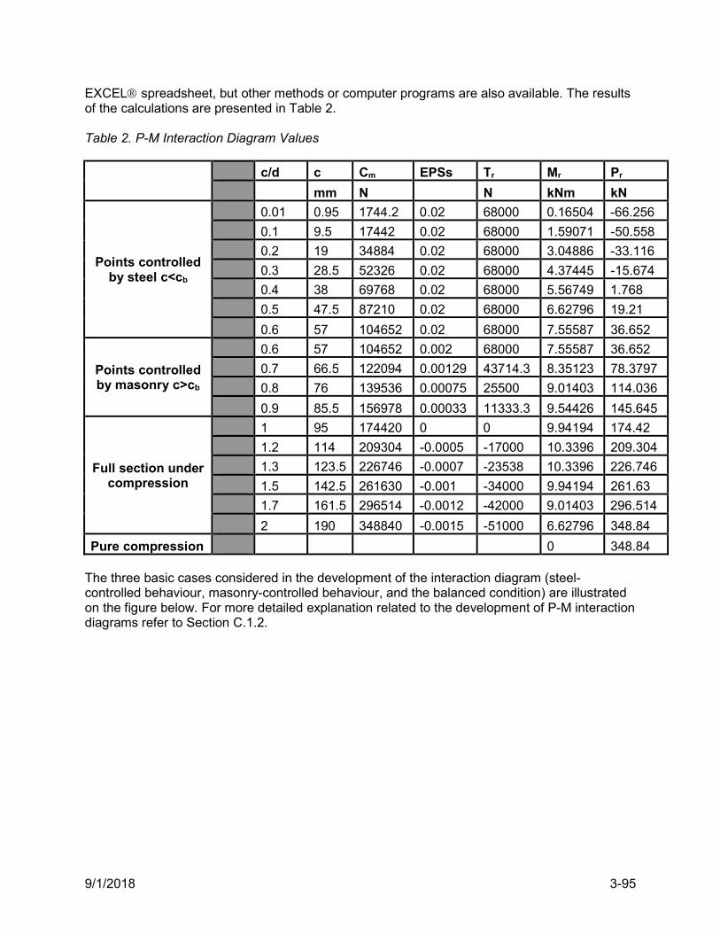
9/1/2018 3-95

EXCEL spreadsheet, but other methods or computer programs are also available. The results of the calculations are presented in Table 2. Table 2. P-M Interaction Diagram Values

c/d c Cm EPSs Tr Mr Pr

mm N N kNm kN

Points controlled by steel c<cb

0.01 0.95 1744.2 0.02 68000 0.16504 -66.256

0.1 9.5 17442 0.02 68000 1.59071 -50.558

0.2 19 34884 0.02 68000 3.04886 -33.116

0.3 28.5 52326 0.02 68000 4.37445 -15.674

0.4 38 69768 0.02 68000 5.56749 1.768

0.5 47.5 87210 0.02 68000 6.62796 19.21

0.6 57 104652 0.02 68000 7.55587 36.652

Points controlled by masonry c>cb

0.6 57 104652 0.002 68000 7.55587 36.652

0.7 66.5 122094 0.00129 43714.3 8.35123 78.3797

0.8 76 139536 0.00075 25500 9.01403 114.036

0.9 85.5 156978 0.00033 11333.3 9.54426 145.645

Full section under compression

1 95 174420 0 0 9.94194 174.42

1.2 114 209304 -0.0005 -17000 10.3396 209.304

1.3 123.5 226746 -0.0007 -23538 10.3396 226.746

1.5 142.5 261630 -0.001 -34000 9.94194 261.63

1.7 161.5 296514 -0.0012 -42000 9.01403 296.514

2 190 348840 -0.0015 -51000 6.62796 348.84

Pure compression 0 348.84 The three basic cases considered in the development of the interaction diagram (steel-controlled behaviour, masonry-controlled behaviour, and the balanced condition) are illustrated on the figure below. For more detailed explanation related to the development of P-M interaction diagrams refer to Section C.1.2.

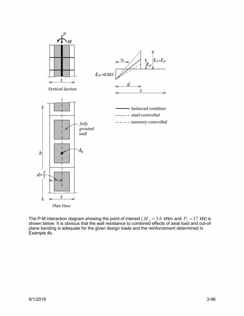
9/1/2018 3-96

The P-M interaction diagram showing the point of interest ( 6.3fM kNm and 17fP kN) is shown below. It is obvious that the wall resistance to combined effects of axial load and out-of-plane bending is adequate for the given design loads and the reinforcement determined in Example 4b.

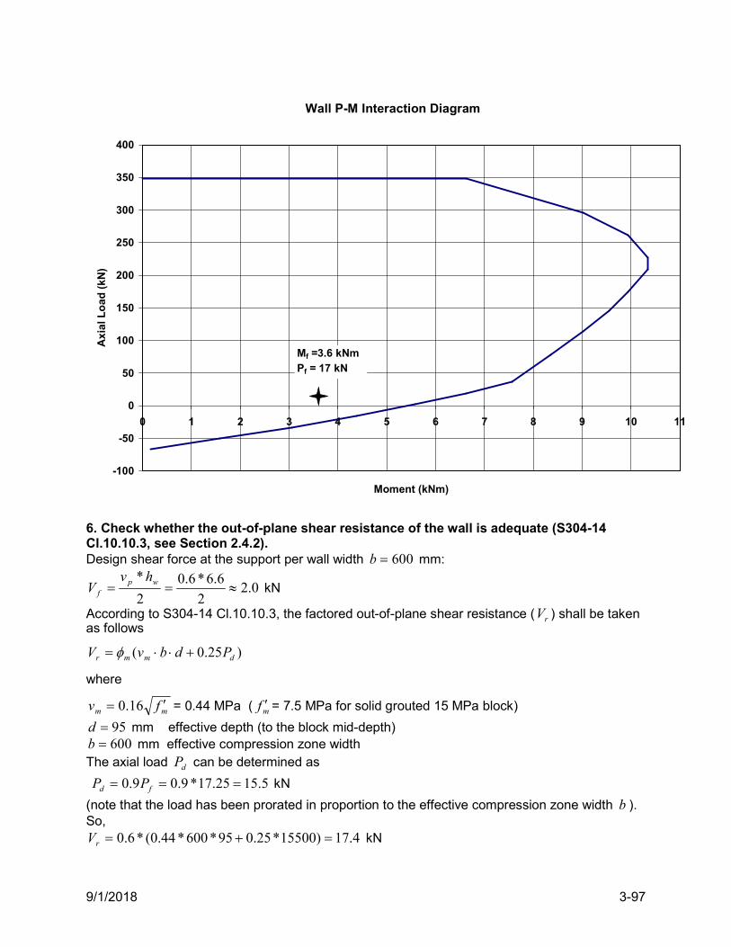
9/1/2018 3-97

Wall P-M Interaction Diagram

-100

-50

0

50

100

150

200

250

300

350

400

0 1 2 3 4 5 6 7 8 9 10 11

Moment (kNm)

Ax

ial

Lo

ad

(k

N)

Mf =3.6 kNm

Pf = 17 kN

6. Check whether the out-of-plane shear resistance of the wall is adequate (S304-14 Cl.10.10.3, see Section 2.4.2). Design shear force at the support per wall width 600b mm:

0.22

6.6*6.0

2

* wp

f

hvV kN

According to S304-14 Cl.10.10.3, the factored out-of-plane shear resistance ( rV ) shall be taken as follows

)25.0( dmmr PdbvV

where

mm fv 16.0 = 0.44 MPa ( mf = 7.5 MPa for solid grouted 15 MPa block)

95d mm effective depth (to the block mid-depth) 600b mm effective compression zone width

The axial load dP can be determined as

5.1525.17*9.09.0 fd PP kN

(note that the load has been prorated in proportion to the effective compression zone width b ). So,

4.17)15500*25.095*600*44.0(*6.0 rV kN

9/1/2018 3-98

Since 0.2fV kN < 4.17rV kN OK

Maximum shear allowed on the section is

5.37)95*600(*5.7*6.0*4.0*4.0max dbfV mmr kN OK

7. Check the sliding shear resistance (see Section 2.4.3). The factored out-of-plane sliding shear resistance rV is determined according to S304-14 Cl.10.10.5.2, as follows: = 1.0 for a masonry-to-masonry or masonry-to-roughened concrete sliding plane

sA = 200 mm2 area of vertical reinforcement per wall width 600b mm

yssy fAT = 0.85*200*400 = 68 kN

5.159.0 fd PP kN

yd TPP 2 = 15.5+68 = 83.5 kN

2PV mr = 0.6*1.0*83.5= 50.0 kN

0.50rV kN > 0.2fV kN OK

Note that the sliding shear resistance does not govern in this case, however this mechanism often governs the in-plane shear resistance. 8. Conclusion It can be concluded that the out-of-plane seismic resistance for this wall is satisfactory. This wall seems to be overdesigned for the out-of-plane resistance because the in-plane seismic design governs (this is a common scenario in design practice).

9/1/2018 3-99

EXAMPLE 6 b: Design of a nonloadbearing wall for out-of-plane seismic effects Consider the same masonry wall discussed in Example 6a, but in this example treat is as a nonloadbearing wall. The wall is 8 m long and 6.6 m high and is constructed using 200 mm hollow concrete blocks of 15 MPa unit strength and Type S mortar. Verify the out-of-plane seismic resistance of the wall according to NBC 2015 and CSA S304-14 seismic requirements. Consider the following two cases: a) unreinforced wall, and b) reinforced partially grouted wall (use Grade 400 steel reinforcement for this design). Use the seismic load determined in Example 6a, that is, 0.1pv kN/m2.

SOLUTION: Material properties Steel (both reinforcing bars and joint reinforcement):

s = 0.85 yf = 400 MPa

Masonry:

m = 0.6

Compression resistance (S304-14 Table 4, 15 MPa concrete blocks and Type S mortar):

mf = 9.8 MPa (ungrouted, or partially grouted ignoring grout area)

Tension resistance normal to bed joint (S304-14 Table 5):

tf = 0.4 MPa (ungrouted)

Find the design shear force and the bending moment. The wall will be modeled as a simple beam with pin supports at the base and the top. The wall height is 6.6wh m. A unit wall strip (width 1000b mm) will be considered for this design. The forces on the wall consist of the axial load due to the wall self-weight and the bending moment due to seismic out-of-plane load (NBC 2015 load combination 1xD+1xE). Factored axial load per width b of 1.0 m: wall weight w = 2.46 kN/m2 (ungrouted 190 mm block wall)

1.80.1*2

6.6*)46.2(*

2* bh

wP wf kN/m

Out-of-plane seismic load per width b of 1.0 m: 0.1pv kN/m

Factored bending moment (at the midheight):

5.58

6.6*0.1

8

* 22

wpf

hvM kNm/m

Factored shear force (at the support):

3.32

6.6*0.1

2

* wp

f

hvV kN/m

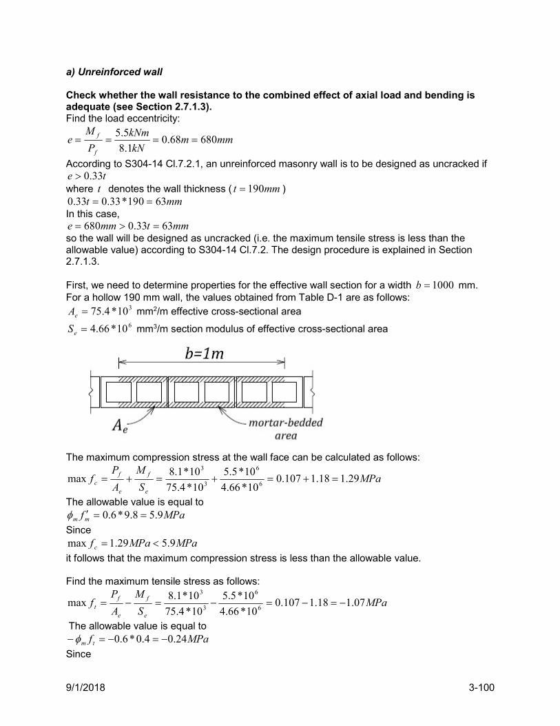
9/1/2018 3-100

a) Unreinforced wall Check whether the wall resistance to the combined effect of axial load and bending is adequate (see Section 2.7.1.3). Find the load eccentricity:

mmmkN

kNm

P

Me

f

f 68068.01.8

5.5

According to S304-14 Cl.7.2.1, an unreinforced masonry wall is to be designed as uncracked if te 33.0

where t denotes the wall thickness ( mmt 190 ) mmt 63190*33.033.0

In this case, mmtmme 6333.0680

so the wall will be designed as uncracked (i.e. the maximum tensile stress is less than the allowable value) according to S304-14 Cl.7.2. The design procedure is explained in Section 2.7.1.3. First, we need to determine properties for the effective wall section for a width 1000b mm. For a hollow 190 mm wall, the values obtained from Table D-1 are as follows:

310*4.75eA mm2/m effective cross-sectional area 610*66.4eS mm3/m section modulus of effective cross-sectional area

The maximum compression stress at the wall face can be calculated as follows:

MPaS

M

A

Pf

e

f

e

fc 29.118.1107.0

10*66.4

10*5.5

10*4.75

10*1.8max

6

6

3

3

The allowable value is equal to MPafmm 9.58.9*6.0

Since MPaMPaf c 9.529.1max

it follows that the maximum compression stress is less than the allowable value. Find the maximum tensile stress as follows:

MPaS

M

A

Pf

e

f

e

ft 07.118.1107.0

10*66.4

10*5.5

10*4.75

10*1.8max

6

6

3

3

The allowable value is equal to MPaf tm 24.04.0*6.0

Since

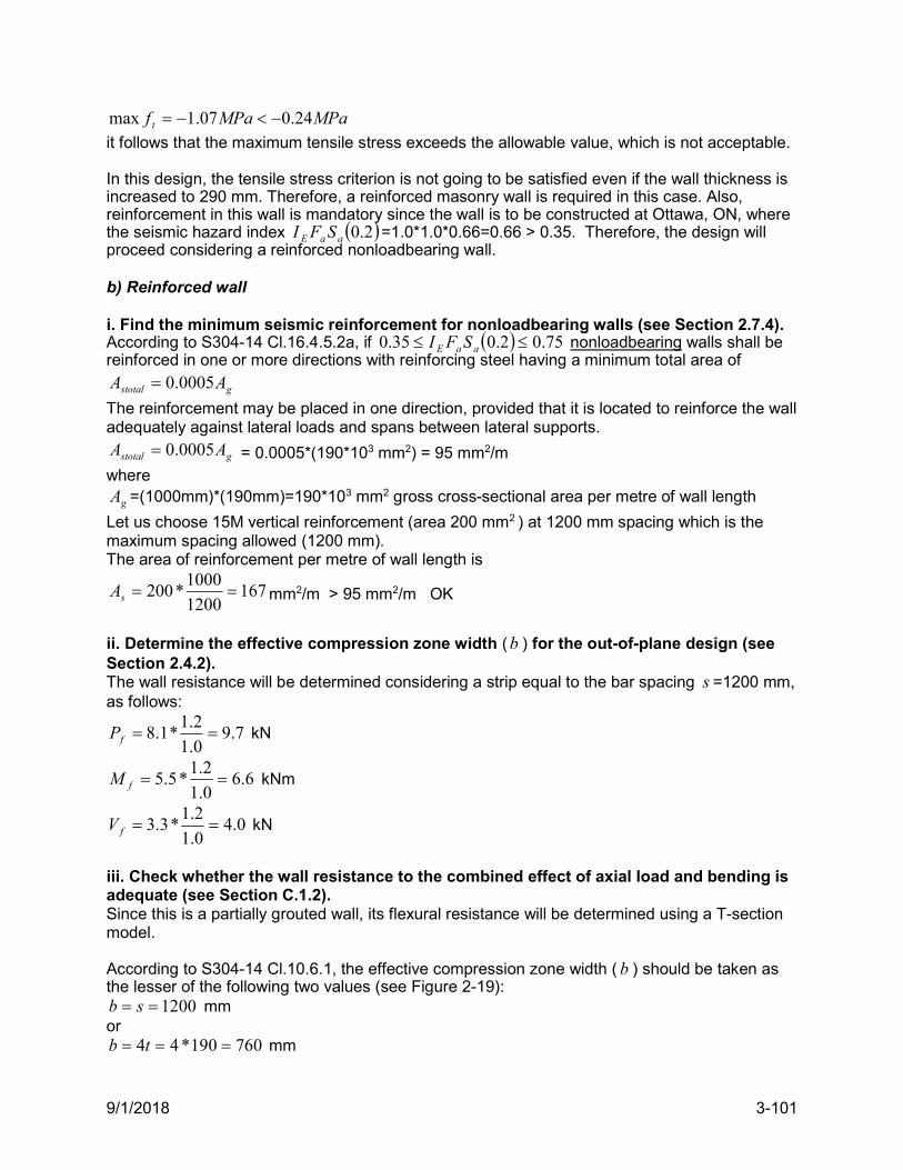
9/1/2018 3-101

MPaMPaf t 24.007.1max

it follows that the maximum tensile stress exceeds the allowable value, which is not acceptable. In this design, the tensile stress criterion is not going to be satisfied even if the wall thickness is increased to 290 mm. Therefore, a reinforced masonry wall is required in this case. Also, reinforcement in this wall is mandatory since the wall is to be constructed at Ottawa, ON, where the seismic hazard index 2.0aaE SFI =1.0*1.0*0.66=0.66 > 0.35. Therefore, the design will proceed considering a reinforced nonloadbearing wall. b) Reinforced wall i. Find the minimum seismic reinforcement for nonloadbearing walls (see Section 2.7.4). According to S304-14 Cl.16.4.5.2a, if 75.02.035.0 aaE SFI nonloadbearing walls shall be reinforced in one or more directions with reinforcing steel having a minimum total area of

gstotal AA 0005.0 The reinforcement may be placed in one direction, provided that it is located to reinforce the wall adequately against lateral loads and spans between lateral supports.

gstotal AA 0005.0 = 0.0005*(190*103 mm2) = 95 mm2/m where

gA =(1000mm)*(190mm)=190*103 mm2 gross cross-sectional area per metre of wall length

Let us choose 15M vertical reinforcement (area 200 mm2 ) at 1200 mm spacing which is the maximum spacing allowed (1200 mm).

The area of reinforcement per metre of wall length is

1671200

1000*200 sA mm2/m > 95 mm2/m OK

ii. Determine the effective compression zone width (b ) for the out-of-plane design (see Section 2.4.2). The wall resistance will be determined considering a strip equal to the bar spacing s =1200 mm, as follows:

7.90.1

2.1*1.8 fP kN

6.60.1

2.1*5.5 fM kNm

0.40.1

2.1*3.3 fV kN

iii. Check whether the wall resistance to the combined effect of axial load and bending is adequate (see Section C.1.2). Since this is a partially grouted wall, its flexural resistance will be determined using a T-section model. According to S304-14 Cl.10.6.1, the effective compression zone width (b ) should be taken as the lesser of the following two values (see Figure 2-19):

1200 sb mm or

760190*44 tb mm

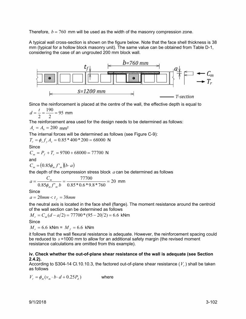
9/1/2018 3-102

Therefore, 760b mm will be used as the width of the masonry compression zone. A typical wall cross-section is shown on the figure below. Note that the face shell thickness is 38 mm (typical for a hollow block masonry unit). The same value can be obtained from Table D-1, considering the case of an ungrouted 200 mm block wall.

Since the reinforcement is placed at the centre of the wall, the effective depth is equal to

952

190

2

td mm

The reinforcement area used for the design needs to be determined as follows: 200 bs AA mm2

The internal forces will be determined as follows (see Figure C-9): 68000200*400*85.0 sysr AfT N

Since 77700680009700 rfm TPC N

and abfC mmm '85.0

the depth of the compression stress block a can be determined as follows

20760*8.9*6.0*85.0

77700

'85.0

bf

Ca

mm

m

mm

Since mmtmma f 3820

the neutral axis is located in the face shell (flange). The moment resistance around the centroid of the wall section can be determined as follows

6.6)22095(*77700)2( adCM mr kNm

Since 6.6rM kNm = 6.6fM kNm

it follows that the wall flexural resistance is adequate. However, the reinforcement spacing could be reduced to s =1000 mm to allow for an additional safety margin (the revised moment resistance calculations are omitted from this example). iv. Check whether the out-of-plane shear resistance of the wall is adequate (see Section 2.4.2). According to S304-14 Cl.10.10.3, the factored out-of-plane shear resistance ( rV ) shall be taken as follows

)25.0( dmmr PdbvV where

9/1/2018 3-103

mm fv 16.0 = 0.50 MPa

95d mm effective depth 200b mm web width - equal to the grouted cell width (156 mm) plus the thickness of the

adjacent webs (26 mm each) The axial load dP can be determined as

7.87.9*9.09.0 fd PP kN

Thus, 0.7)8700*25.095*200*50.0(*6.0 rV kN

Since 0.4fV kN < 0.7rV kN OK

Maximum shear allowed on the section is

3.14)95*200(*8.9*6.0*4.0*4.0max dbfV mmr kN OK

v. Check the sliding shear resistance (see Section 2.4.3). The factored in-plane sliding shear resistance rV is determined according to S304-14 Cl.10.10.5.2, as follows: = 1.0 for a masonry-to-masonry or masonry-to-roughened concrete sliding plane

sA = 200 mm2 area of vertical reinforcement at 1.2 m spacing

yssy fAT = 0.85*200*400 = 68.0 kN

dP = 8.7 kN

yd TPP 2 = 8.7+68.0 = 76.7 kN

2PV mr = 0.6*1.0*76.7 = 46.0 kN

0.46rV kN > 0.4fV kN OK

vi. Conclusion It can be concluded that the out-of-plane seismic resistance of this nonloadbearing wall is satisfactory. It should be noted that the flexural resistance governs in this design. The required amount of vertical reinforcement (15M@1200 mm) corresponds to the following area per metre length

1671000

* s

AA bs mm2

which is significantly larger than the minimum seismic reinforcement prescribed by S304-14, that is, 95stotalA mm2/m. Note that 15M@1200 mm is also the minimum vertical reinforcement that meets the minimum spacing requirements using typical15M bars. Also, since horizontal reinforcement does not contribute to out-of-plane wall resistance, it was not considered in this example. However, provision of 9 Ga. horizontal ladder reinforcement at 400 mm spacing could be considered to improve the overall seismic performance of the wall. It should be noted that, in exterior walls the mortar-bedded joints could be significantly affected by the presence of aesthetic joint finishes characterized by deeper grooves (e.g. raked joints); some of the grooves are up to 10 mm deep. The designer should consider this effect in the calculation of the compression zone depth.

9/1/2018 3-104

EXAMPLE 7: Seismic design of masonry veneer ties Perform the seismic design for tie connections for a 4.8 m high concrete block veneer wall in a school gymnasium in Montréal, Quebec. The building is founded on Site Class C. The design should be performed to the requirements of NBC 2015, CSA S304-14, and CSA A370-14. Consider the following two types of the veneer backup: a) Concrete block wall (a rigid backup), and b) Steel stud wall with 400 mm steel stud spacing (a flexible backup). c) Evaluate the minimum tie strength requirements for the rigid and flexible backup. SOLUTION: This design problem requires the calculation of seismic load pV for nonstructural elements according to NBC 2015 Cl.4.1.8.18 (for more details see Section 2.7.7.3). Note that the wind load could govern in a tie design for many site locations in Canada, however wind load calculations were omitted for this seismic design example. First, seismic design parameters need to be determined as follows: Location: Montréal (City Hall), Quebec (NBC 2015 Appendix C)

)2.0(aS = 0.595 and PGAref = 0.379

Foundation factor (0.2)aF F 1.0 and Site Class C for PGAref = 0.379 (from Table 1-3 or NBC 2015

Table 4.1.8.4.B) EI = 1.3 school (high importance building) At this point, it would be appropriate to check whether the seismic design of ties is required for this design. According to NBC 2015 Cl.4.1.8.18.2, seismic design of ties is required when the seismic hazard index 35.02.0 aaE SFI (and also for post-disaster buildings in lower seismic regions). In this case,

2.0aaE SFI = 1.3*0.88*0.69=0.79 0.35

Therefore, seismic design is required. Find pS (horizontal force factor for part or portion of a building and its anchorage per NBC

2015, Table 4.1.8.18, Case 8) 0.25.10.30.10.1 pxrpp RAACS

where 0.321 nxx hhA for top of wall worst case

Since 0.47.0 pS O.K.

pW = 1.8 kN/m2 unit weight of the veneer masonry (concrete blocks)

Seismic load pV can be calculated as follows:

ppEaap WSISFV 2.03.0 =0.3*1.0*0.595*1.3*2.0*(1.8 kN/m2) =0.85 kN/m2

Note that the above load is determined per m2 of the wall surface area. a) Concrete block backup (rigid) Assume the maximum tie spacing permitted according to S304-14 Cl.9.1.3 of 600 mm vertically and 820 mm horizontally (see Section 2.7.7.2), resulting in a tributary tie area for a concrete backup wall of

9/1/2018 3-105

A = 0.82*0.60 = 0.49 m2 The required factored tie capacity should exceed the factored tie load, that is,

AVV pf * = (0.85 kN/m2)*(0.49 m2) = 0.42 kN

Alternatively, for a given tie capacity, a tie spacing could be determined based on the maximum tributary area calculated from pV and the factored tie capacity fV , that is,

pf VVA

b) Steel stud backup (flexible) Since the steel stud is a flexible backup, a tie must be able to resist 40% of the tributary lateral load on a vertical line of ties (S304-14 Cl.9.1.3.3, see Section 2.7.7.3):

tpf AVV **4.0 = 0.4*(0.85 kN/m2)*(1.92m2) = 0.65 kN

where tA = 0.4m*4.8m = 1.92 m2 is tributary area on a vertical line of ties based on a probable

0.4 m horizontal tie spacing, and 4.8 m wall height According to the same S304-14 clause, the tie must also be able to resist a load corresponding to double the tributary area on a tie, that is,

AVV pf **2 = 2*(0.85 kN/m2)*(0.4m*0.6m) = 0.41 kN

Note that the tributary area was based on a 0.4 m stud spacing, and the maximum vertical tie spacing of 0.6 m prescribed by S304-14 Cl.9.1.3.1. In conclusion, the tie design load for the flexible veneer backup is fV = 0.65 kN.

c) Minimum strength requirements CSA A370-14 Cl.8.1 prescribes minimum ultimate tensile/compressive tie strength of 1 kN. In order to obtain the ultimate tie strength, the factored strength needs to be divided by the resistance factor . According to CSA A370-14 Cl.9.4.2.1.2, the resistance factor is 0.9 for tie material strength, or 0.6 for embedment failure, failure of fasteners, or buckling failure of the connection. It is conservative to use lower resistance factor in determining the ultimate tie strength ultV . For the steel stud backup:

fr VV 0.65 kN

thus the ultimate strength can be determined as follows

08.16.0

65.0

r

ult

VV kN

This value is slightly higher than the minimum of 1 kN prescribed by CSA A370-04 and governs. For the concrete block backup:

fr VV 0.42 kN

thus the ultimate strength can be determined as follows

7.06.0

42.0

r

ult

VV kN

This value is less than the minimum of 1 kN, so the minimum requirement governs.

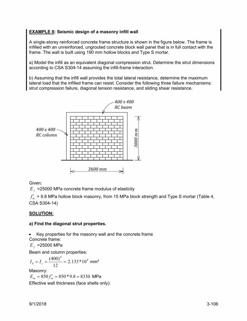
9/1/2018 3-106

EXAMPLE 8: Seismic design of a masonry infill wall A single-storey reinforced concrete frame structure is shown in the figure below. The frame is infilled with an unreinforced, ungrouted concrete block wall panel that is in full contact with the frame. The wall is built using 190 mm hollow blocks and Type S mortar. a) Model the infill as an equivalent diagonal compression strut. Determine the strut dimensions according to CSA S304-14 assuming the infill-frame interaction. b) Assuming that the infill wall provides the total lateral resistance, determine the maximum lateral load that the infilled frame can resist. Consider the following three failure mechanisms: strut compression failure, diagonal tension resistance, and sliding shear resistance.

Given:

fE =25000 MPa concrete frame modulus of elasticity

mf = 9.8 MPa hollow block masonry, from 15 MPa block strength and Type S mortar (Table 4,

CSA S304-14) SOLUTION: a) Find the diagonal strut properties. Key properties for the masonry wall and the concrete frame Concrete frame:

fE =25000 MPa

Beam and column properties:

94

10*133.212

)400( cb II mm4

Masonry: 83308.9*850850 mm fE MPa

Effective wall thickness (face shells only):

9/1/2018 3-107

75et mm (Table D-1, 200 mm hollow block wall)

Diagonal strut geometry (see Section 2.7.2 and S304-14 Cl.7.13) 3000h mm 3600l mm

Find (angle of diagonal strut measured from the horizontal):

833.03600

3000)tan(

l

h 8.39

Length of the diagonal: 2 2 2 23000 3600 4686dl h l mm

Find the strut width (see Figure 2-46):

15878.39*2sin*75*8330

3000*10*133.2*25000*4

22sin

4

2

41

941

em

cfh tE

hIE

33228.39*2sin*75*8330

3600*10*133.2*25000*4

2sin

4 41

941

em

bfL tE

lIE

Strut width:

368233221587 2222 Lhw mm

Effective diagonal strut width ew for the compressive resistance calculation should be taken as the least of (Cl.7.13.3.3)

1841236822 wwe mm

or 4 4686 4 1172e dw l mm

thus 11701172 ew mm

The design length of the diagonal strut sl should be equal to (Cl.7.13.3.4.4)

2 4686 3682 2 2845s dl l w mm

b) Determine the maximum lateral load which the infilled frame can resist assuming that the infill wall provides the total lateral resistance. Diagonal strut: compression resistance (Cl.7.13.3.4.3 and Section 2.7.2) The compression strength of the diagonal strut maxrP is equal to the compression strength of masonry times the effective cross-sectional area, that is,

emmr AfP 85.0max

where

m = 0.6

5.0 the masonry compressive strength parallel to bed joints

877501170*75* eee wtA mm2 the effective cross-sectional area

3.21987750*8.9*6.0*5.0*85.0max rP kN

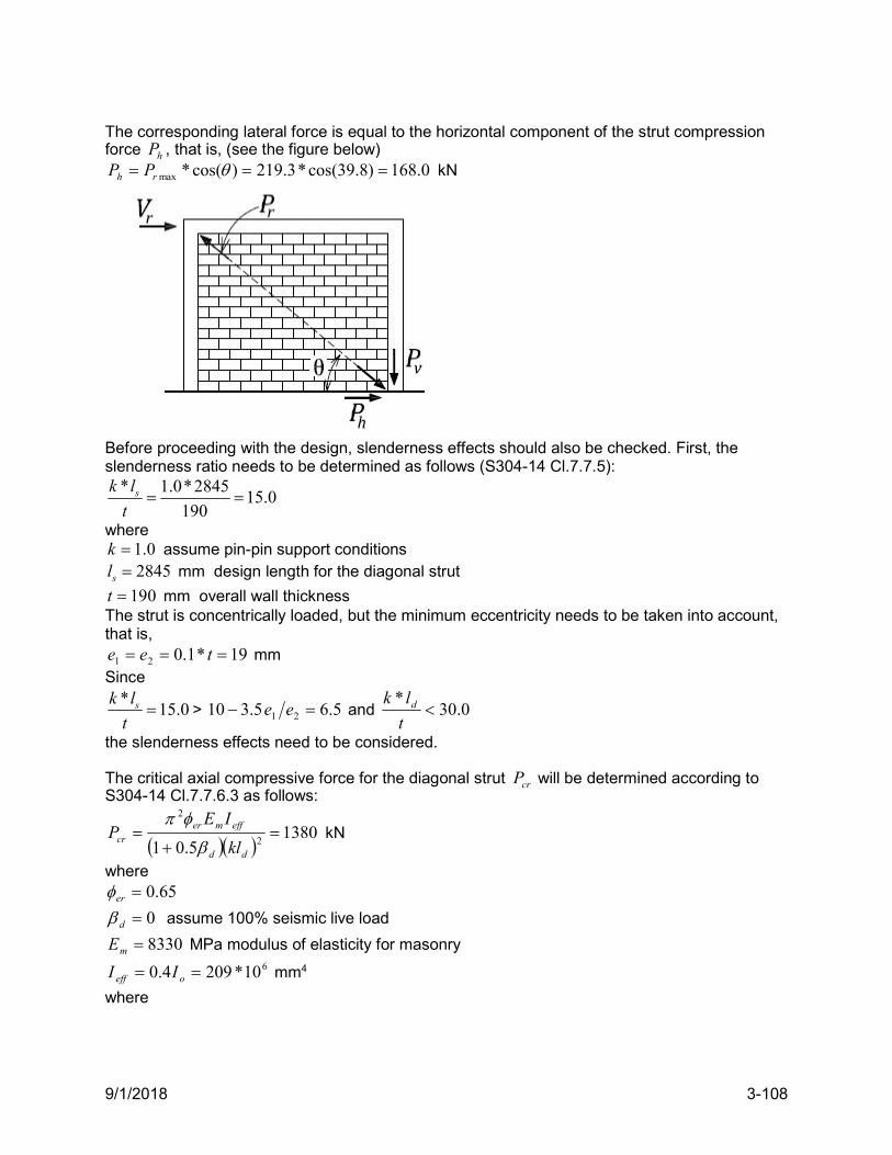
9/1/2018 3-108

The corresponding lateral force is equal to the horizontal component of the strut compression force hP , that is, (see the figure below)

0.168)8.39cos(*3.219)cos(*max rh PP kN

Before proceeding with the design, slenderness effects should also be checked. First, the slenderness ratio needs to be determined as follows (S304-14 Cl.7.7.5): * 1.0*2845

15.0190

sk l

t

where 0.1k assume pin-pin support conditions

2845sl mm design length for the diagonal strut

190t mm overall wall thickness The strut is concentrically loaded, but the minimum eccentricity needs to be taken into account, that is,

19*1.021 tee mm Since *

15.0sk l

t > 5.65.310 21 ee and 0.30

*

t

lk d

the slenderness effects need to be considered. The critical axial compressive force for the diagonal strut crP will be determined according to S304-14 Cl.7.7.6.3 as follows:

1380

5.01 2

2

dd

effmercr

kl

IEP

kN

where 65.0er

0d assume 100% seismic live load

8330mE MPa modulus of elasticity for masonry 610*2094.0 oeff II mm4

where

9/1/2018 3-109

633

10*52212

)4.75190(190*1170

oI mm4 moment of inertia of the effective cross-

sectional area based on the effective diagonal strut width 1170ew mm and the effective wall

thickness 4.75et mm (face shells only).

Since

3.219max rP kN < 1380crP kN

it follows that compression failure governs over buckling failure. The diagonal tension shear resistance (see Section 2.3.2 and S304-14 Cl.10.10.2). Find the masonry shear resistance ( mV ):

190wb mm overall wall thickness

28808.0 wv ld mm effective wall depth

5.0g ungrouted wall

0dP (ignore self-weight)

mm fv 16.0 = 0.5 MPa

gdvwmmm PdbvV )25.0( = 0.6(0.5*190*2880+0)*0.5 82.0 kN

This is a squat shear wall because 0.183.03600

3000

w

w

l

h. In this case, there is no need to find

the maximum permitted shear resistance per S304-14 Cl.10.10.2.1 rVmax because it is not going to control for an unreinforced wall without gravity load. Sliding shear resistance (see Section 2.7.1 and Cl.7.10.5)

116.0 PAfV mucmmrs

The factored in-plane sliding shear resistance rV is determined as follows. = 1.0 for a masonry-to-masonry or masonry-to-roughened concrete sliding plane

2160002880*75 veuc dtA mm2 uncracked portion of the effective wall cross-sectional

area The compressive force in masonry acting normal to the sliding plane is normally taken as dP plus an additional component, equal to 90% of the factored vertical component of the compressive force resulting from the diagonal strut action vP (see the figure on the previous page).

vd PPP *9.01

where )tan(* rsv VP

thus )tan(*9.001 rsVP

The sliding shear resistance can be determined from the following equation

))tan(*9.0(16.0 rsmucmmrs VAfV

or

9/1/2018 3-110

0.118)8.39tan(*9.0*0.1*6.01

216000*8.9*6.0*16.0

)tan(*9.0**1

16.0

m

ucmmrs

AfV kN

Discussion It is important to consider all possible behaviour modes and identify the one that governs in this design. The following three lateral forces should be considered: a) 168hP kN shear force corresponding to the strut compression failure

b) 82mV kN diagonal tension shear resistance

c) 118rsV kN sliding shear resistance

It could be concluded that the diagonal tension shear resistance governs, however once diagonal tension cracking takes place, the strut mechanism forms. Therefore, the maximum shear force developed in an infill wall corresponds either to the strut compression resistance or the sliding shear resistance (see the discussion in Section 2.7.2). In this case, sliding shear resistance governs and so 118max rsr VV kN. It should be noted that the maximum shear force developed in the infill maxrV will be transferred to the adjacent reinforced concrete columns, which need to be designed for shear. This is not the scope of the masonry design, however the designer should always consider the entire lateral load path and the force transfer between the structural components.

9/1/2018 R-1

References

Abrams,D.P. (2000). A Set of Classnotes for a Course in Masonry Structures, Third Edition, The Masonry Society, Boulder, CO, USA.

Abrams,D.P., Angel,R., and Uzarski,J. (1996). Out-of-Plane Strength of Unreinforced Masonry Infill Panels, Earthquake Spectra, 12(4): 825-844.

Atkinson,G.M. and Adams, J. (2013). Ground Motion Prediction Equations for Application to the 2015 Canadian National Seismic Hazard Maps, Canadian Journal of Civil Engineering, 40: 988-998.

Adams, J., Halchuk, S., Allen, T.I., and Rogers, G.C. (2015). Fifth Generation Seismic Hazard Model for Canada: Grid Values of Mean Hazard to be used with the 2015 National Building Code of Canada, Geological Survey of Canada, Open File 7893, 26 pp.

Anderson,D., and Brzev,S. (2009). Seismic Design Guide for Masonry Buildings, First Edition, Canadian Concrete Masonry Producers Association, Toronto, Ontario, 317 pp. (free download available at www.ccmpa.ca).

Anderson,D.L. (2006). Dynamic Analysis, Lecture Notes, Understanding Seismic Load Provisions for Buildings in the National Building Code of Canada 2005, Vancouver Structural Engineers Group Society, Vancouver, BC, Canada.

Anderson, D.L. (2006a). CSA S304.1 and NBCC Seismic Design Provisions for Masonry Structures, Lecture Notes, Course E1 Masonry Design of Buildings, Certificate Program in Structural Engineering, Vancouver Structural Engineers Group Society and the UBC Department of Civil Engineering, Vancouver, BC, Canada (unpublished).

Anderson, D.L., and Priestley, M.J.N. (1992). In Plane Shear Strength of Masonry Walls, Proceedings, The Sixth Canadian Masonry Symposium, Department of Civil Engineering, University of Saskatchewan, Saskatoon, SK, Canada, 2: 223-234.

Amrhein,J.E., Anderson,J.C., and Robles,V.M. (1985). Mexico Earthquakes - September 1985, The Masonry Society Journal, 4(2): G12-G17.

Azimikor, N., Brzev, S., Elwood, K., Anderson, D.L., and McEwen,W. (2017). Out-Of-Plane Instability of Reinforced Masonry Uniaxial Specimens Under Reversed Cyclic Axial Loading, Canadian Journal of Civil Engineering, 44: 367–376.

Azimikor, N. (2012). Out-of-Plane Stability of Reinforced Masonry Shear Walls Under Seismic Loading: Cyclic Uniaxial Tests, A Thesis Submitted in Partial Fulfilment of the Requirements for the Degree of Master of Applied Science in the Faculty of Graduate Studies (Civil Engineering), The University of British Columbia, 180 pp.

Azimikor, N., Robazza, B.R., Elwood, K.J., Anderson, D.L., and Brzev, S. (2012). An Experimental Study on the Out-of-Plane Stability of Reinforced Masonry Shear Walls under In-Plane Reversed Cyclic Loads, Proceedings of the 15th World Conference of Earthquake Engineering. Lisbon, Portugal.

Azimikor, N., Brzev, S., Elwood, K., and Anderson, D. (2011). Out-of-Plane Stability of Reinforced Masonry Shear Walls, Proceedings of the 11th North American Masonry Conference, Minneapolis, MN, USA.

Bachmann,H. (2003). Seismic Conceptual Design of Buildings – Basic Principles for Engineers, Architects, Building Owners, and Authorities, Swiss Federal Office for Water and Geology, Swiss Agency for Development and Cooperation, Switzerland. (free download http://www.preventionweb.net/english/professional/publications/v.php?id=687)

Banting,B.R., and El-Dakhakhni,W.W. (2012). Force- and Displacement-Based Seismic Performance Parameters for Reinforced Masonry Structural Walls with Boundary Elements, ASCE Journal of Structural Engineering, 138(12): 1477-1491.

9/1/2018 R-2

Banting, B.R. (2013). Seismic Performance Quantification of Concrete Block Masonry Structural Walls with Confined Boundary Elements and Development of the Normal Strain-Adjusted Shear Strength Expression (NSSSE), a Thesis Submitted to the School of Graduate Studies in Partial Fulfilment of the Requirements for the Degree of Doctor of Philosophy, McMaster University, Hamilton, ON, Canada.

Banting,B.R., and El-Dakhakhni,W.W. (2013). Seismic Performance Quantification of Reinforced Masonry Structural Walls with Boundary Elements, ASCE Journal of Structural Engineering, 140(5).

Banting, B. R. and El-Dakhakhni, W. W. (2014). Seismic Design Parameters for Special Masonry Structural Walls Detailed with Confined Boundary Elements, ASCE Journal of Structural Engineering, 140 (10).

Bentz, E. C., Vecchio, F. J. and Collins, M. P. (2006). Simplified Modified Compression Field Theory for Calculating Shear Strength of Reinforced Concrete Elements, ACI Journal, 103(4): 614-624.

Brzev, S. and Pao, J. (2016). Reinforced Concrete Design – A Practical Approach, Third Edition, Pearson Education, Inc., New York, USA.

Brzev, S. (2011). Review of Experimental Studies on Seismic Response of Partially Grouted Reinforced Masonry Shear Walls Subjected to Reversed Cyclic Loading, British Columbia Institute of Technology, Vancouver, BC, Canada (unpublished report).

Cardenas, A.E., and Magura, D.D. (1973). Strength of High-Rise Shear Walls — Rectangular Cross Section, Response of Multistory Concrete Structures to Lateral Forces, ACI Publication SP-36, American Concrete Institute, Detroit, pp. 119–150.

Centeno, J. (2015). Sliding Displacements in Reinforced Masonry Walls Subjected to In-Plane Lateral Loads, a Thesis Submitted to the School of Graduate Studies in Partial Fulfilment of the Requirements for the Degree of Doctor of Philosophy, University of British Columbia, Vancouver, BC, Canada.

Centeno,J., Ventura,C., Brzev,S., and Anderson,D. (2015). Estimating Sliding Shear Displacements in Reinforced Masonry Shear Walls, Proceedings of the 11th Canadian Conference on Earthquake Engineering, Victoria, BC, Canada.

Centeno,J., Ventura,C., and Ingham,J. (2014). Seismic Performance of a Six-Story Reinforced Concrete Masonry Building during the Canterbury Earthquake Sequence, Earthquake Spectra, 30(1): 363–381.

Chai, Y.H. and Elayer, D.T. (1999). Lateral Stability of Reinforced Concrete Columns under Axial Reversed Cyclic Tension and Compression, ACI Structural Journal, 96: 780-789.

Chen, S. J., Hidalgo, P. A., Mayes, R. L., Clough, R. W., and McNiven, H. D. (1978). Cyclic Loading Tests of Masonry Single Piers, Volume 2- Height to Width Ratio of 1.0, UCB/EERC-78/28, University of California, Berkeley, CA, USA.

Chopra, A.K. (2012). Dynamics of Structures: Theory and Applications to Earthquake Engineering, 4th Edition, Prentice Hall Inc., Upper Saddle River, NJ, USA.

Corley, W.G. (1966). Rotational Capacity of Reinforced Concrete Beams, Journal of the Structural Division, ASCE, 92(ST10): 121-146.

CSA A23.3-04 (2004). Design of Concrete Structures, Canadian Standards Association, Mississauga, ON, Canada.

CSA A370-14 (2014). Connectors for Masonry, Canadian Standards Association, Mississauga, ON, Canada.

CSA A371-14 (2014). Masonry Construction for Buildings, Canadian Standards Association, Mississauga, ON, Canada.

CSA S304-14 (2014). Design of Masonry Structures, Canadian Standards Association, Mississauga, ON, Canada.

9/1/2018 R-3

CSA S304.1-04 (2004). Masonry Design for Buildings (Limit States Design), Canadian Standards Association, Mississauga, ON, Canada.

Davis, C.L., McLean, D.I., and Ingham, J.M. (2010). Evaluation of Design Provisions for In-Plane Shear in Masonry Walls, The Masonry Society Journal, 28(2): 41-59.

Dawe,J.L., and Seah,C.K. (1989). Out-of-Plane Resistance of Concrete Masonry Infilled Panels, Canadian Journal of Civil Engineering, 16: 854-864.

DeVall, R. (2003). Background Information for Some of the Proposed Earthquake Design Provisions for the 2005 edition of the National Building Code of Canada. Canadian Journal of Civil Engineering, 30: 279-286.

Dizhur, D., et al. (2011). Performance of Masonry Buildings and Churches in the 22 February 2011 Christchurch Earthquake, Bulletin of the New Zealand Society for Earthquake Engineering, 44: 279–296.

Drysdale, R.G., and Hamid, A.A. (2005). Masonry Structures: Behaviour and Design, Canadian Edition, Canada Masonry Design Centre, Mississauga, Ontario.

Elmapruk,J.H. (2010). Shear Strength of Partially Grouted Squat Masonry Shear Walls, Masters Thesis, Department of Civil and Environmental Engineering, Washington State University, Spokane, WA.

El-Dakhakhni,W.W. (2014). Resilient Reinforced Concrete Block Shear Wall Systems for the Next-Generation of Seismic Codes, Proceedings of the 9th International Masonry Conference, Guimarães, Portugal.

El-Dakhakhni, W. W., Banting, B. R., and Miller, S. C. (2013). Seismic Performance Parameter Quantification of Shear-Critical Reinforced Concrete Masonry Squat Walls, ASCE Journal of Structural Engineering, 139(6):957–973.

El-Dakhakhni, W., and Ashour, A. (2017). Seismic Response of Reinforced-Concrete Masonry Shear-Wall Components and Systems: State of the Art, ASCE Journal of Structural Engineering, 143(9):03117001.

Elshafie,H., Hamid,A., and Nasr, E. (2002). Strength and Stiffness of Masonry Shear Walls with Openings, The Masonry Society Journal, 20(1): 49-60.

Elwood, K.J. (2013). Performance of Concrete Buildings in the 22 February 2011 Christchurch Earthquake and Implications for Canadian Codes, Canadian Journal of Civil Engineering, DOI: 10.1139/cjce-2011-0564.

FEMA 306 (1999). Evaluation of Earthquake Damaged Concrete and Masonry Wall Buildings- Basic Procedures Manual (FEMA 306), Federal Emergency Management Agency, Washington, D.C., USA.

FEMA 307 (1999). Evaluation of Earthquake Damaged Concrete and Masonry Wall Buildings-Technical Resources (FEMA 307), Federal Emergency Management Agency, Washington, D.C., USA.

FEMA 99 (1995). A Nontechnical Explanation of the 1994 NEHRP Recommended Provisions, Federal Emergency Management Agency, Washington, D.C., USA.

Ferguson, P.M., Breen,J.E., and Jirsa.,J.O. (1988). Reinforced Concrete Fundamentals, 5th Edition, John Wiley&Sons, New York, USA.

Halchuk, S; Allen, T I; Adams, J; Rogers, G C. (2014). Fifth Generation Seismic Hazard Model Input Files as Proposed to Produce Values for the 2015 National Building Code of Canada, Geological Survey of Canada, Open File 7576, 18 pp.

Hatzinikolas, M.A., Korany, Y., and Brzev, S. (2015). Masonry Design for Engineers and Architects, Fourth Edition, Canadian Masonry Publications, Edmonton, AB, Canada.

Henderson, R.C., Bennett, R., and Tucker, C.J. (2007). Development of Code-Appropriate Methods for Predicting the Capacity of Masonry Infilled Frames Subjected to

9/1/2018 R-4

In-Plane Forces, Final Report Submitted to the National Concrete Masonry Association, USA.

Herrick, C.K. (2014). An Analysis of Local Out-of-Plane Buckling of Ductile Reinforced Structural Walls Due to In-Plane Loading, a Thesis submitted to the Graduate Faculty in partial fulfilment of the requirements for the degree of Master of Science, North Carolina State University, Raleigh, NC, USA, 248 pp.

Ibrahim, K., and Suter, G. (1999). Ductility of Concrete Masonry Shear Walls Subjected to Cyclic Loading, Proceedings of the 8th North American Masonry Conference, The Masonry Society, Longmont, CO, USA.

Ingham,J.M., Davidson,B.J., Brammer,D.R., and Voon, K.C. (2001). Testing and Codification of Partially Grout-Filled Nominally Reinforced Concrete Masonry Subjected to In-Plane Cyclic Loads, The Masonry Society Journal, 19(1): 83-96.

Kaushik,H.B., Rai,D.C., and Jain,S.K. (2006). Code Approaches to Seismic Design of Masonry-Infilled Reinforced Concrete Frames: A State-of-the-Art Review, Earthquake Spectra, 22(4): 961-983.

Kingsley,G.R., Shing,P.B., and Gangel,T. (2014). Seismic Design of Special Reinforced Masonry Shear Walls: A Guide for Practicing Engineers, NIST GCR 14-917-31, prepared by the Applied Technology Council for the National Institute of Standards and Technology, Gaithersburg, MD, USA.

Klingner,R.E. (2010). Masonry Structural Design, McGraw Hill, New York, USALeiva,G., and Klingner,R.E. (1994). Behavior and Design of Multi-Story Masonry Walls Under In-Plane Seismic Loading, The Masonry Society Journal, 13(1): 15-24.

Leiva,G., Merryman,M., and Klingner,R.E. (1990). Design Philosophies For Two-Story Concrete Masonry Walls with Door and Window Openings, Proceedings of the Fifth North American Masonry Conference, University of Illinois at Urbana-Champaign, pp. 287-295.

Matsumura, A. (1987). Shear Strength of Reinforced Hollow Unit Masonry Walls, Proceedings of the 4th North American Masonry Conference, Los Angeles, CA, USA, Paper No. 50.

MacGregor, J.G., and Bartlett, F.M. (2000). Reinforced Concrete – Mechanics and Design, First Canadian Edition, Prentice Hall Canada Inc., Scarborough, ON, Canada.

Maleki, M. (2008). Behaviour of Partially Grouted Reinforced Masonry Shear Walls under Cyclic Reversed Loading, A thesis submitted to the School of Graduate Studies in partial fulfillment of the requirements for the degree of Doctor of Philosophy, McMaster University, Hamilton, ON, Canada.

Maleki, M., Drysdale,R.G., Hamid,A.A., and El-Damatty,A.A. (2009). Behaviour of Partially Grouted Reinforced Masonry Shear Walls - Experimental Study, Proceedings of the 11th Canadian Masonry Symposium, Toronto, ON, Canada.

MIBC (2017). Masonry Technical Manual, Masonry Institute of British Columbia, 140 pp. (free download available at www.masonrybc.org)

Minaie, E., Mota, M., Moon, F.M. and Hamid, A.A. (2010). In-Plane Behavior of Partially Grouted Reinforced Concrete Masonry Shear Walls, ASCE Journal of Structural Engineering, 136(7): 1089-1097.

Mitchell, D., et al. (2003). Seismic Force Modification Factors for the Proposed 2005 Edition of the National Building Code of Canada, Canadian Journal of Civil Engineering, 30: 308-327.

Moehle, J. (2015). Seismic Design of Reinforced Concrete Buildings, McGraw -Hill Education, New York, USA.

Murty, C.V.R, Brzev, S., Faison, H., Comartin, C.D., and Irfanoglu, A. (2006). At Risk: The Seismic Performance of Reinforced Concrete Frame Buildings with Masonry

9/1/2018 R-5

Infill Walls, Earthquake Engineering Research Institute, Publication No. WHE-2006-03, First Edition, 70 pp. (free download available at www.world-housing.net)

Murty, C.V.R. (2005). IITK-BMPTC Earthquake Tips – Learning Earthquake Design and Construction. National Information Center of Earthquake Engineering, IIT Kanpur, India. (free download available at http://www.nicee.org/EQTips.php)

Naeim, F. (2001). The Seismic Design Handbook, Second Edition, Kluwer Academic Publisher, USA.

Nathan, N.D. Philosophy of Seismic Design, Department of Civil Engineering, University of British Columbia, Vancouver, Canada, 93 pp.

NIST (2017). Recommended Modeling Parameters and Acceptance Criteria for Nonlinear Analysis in Support of Seismic Evaluation, Retrofit, and Design, NIST GCR 17-917-45, prepared by the NEHRP Consultants Joint Venture, a partnership of the Applied Technology Council and the Consortium of Universities for Research in Earthquake Engineering for the National Institute of Standards and Technology, Gaithersburg, MD, USA.

NIST (2010). Evaluation of the FEMA P-695 Methodology for Quantification of Building Seismic Performance Factors, NIST GCR 10-917-8, prepared by the NEHRP Consultants Joint Venture, a partnership of the Applied Technology Council and the Consortium of Universities for Research in Earthquake Engineering for the National Institute of Standards and Technology, Gaithersburg, MD, USA.

Nolph, S.M. (2010). In-Plane Shear Performance of Partially Grouted Masonry Shear Walls, Masters Thesis, Department of Civil and Environmental Engineering, Washington State University, Spokane, WA, USA.

Nolph, S.M. and ElGawady, M.A. (2012). Static Cyclic Response of Partially Grouted Masonry Shear Walls, ASCE Journal of Structural Engineering, 138(7): 864-879.

NRC (2017). User’s Guide – NBC 2015 Structural Commentaries (Part 4 of Division B), Canadian Commission on Building and Fire Codes, National Research Council Canada, Ottawa, ON, Canada.

NRC (2015). National Building Code of Canada 2015, National Research Council, Ottawa, ON, Canada.

NZCMA (2004). User’s Guide to NZS 4230:2004 Design of Reinforced Concrete Masonry Structures, New Zealand Concrete Masonry Association Inc., Wellington, New Zealand, pp. 83 (http://www.cca.org.nz/shop/downloads/NZS4230UserGuide.pdf).

NZS 4230:2004 (2004). Design of Reinforced Concrete Masonry Structures, Standards Association of New Zealand, Wellington, New Zealand.

Okamoto, S., et al. (1987). Seismic Capacity of Reinforced Masonry Walls and Beams. Proceedings of the 18th Joint Meeting of the US-Japan Cooperative Program in Natural Resource Panel on Wind and Seismic Effects, NBSIR 87-3540, National Institute of Standards and Technology, Gaithersburg, pp. 307-319.

Park, R. and Paulay, T. (1975). Reinforced Concrete Structures, John Wiley & Sons, Inc, 769 pp.

Paulay, T. (1986) The Design of Ductile Reinforced Concrete Structural Walls for Earthquake Resistance, Earthquake Spectra, 2(4): 783-823.

Paulay, T. and Priestley, M.J.N. (1992). Seismic Design of Concrete and Masonry Buildings, John Wiley and Sons, Inc., New York, USA, 744 pp.

Paulay, T. and Priestley, M.J.N. (1993). Stability of Ductile Structural Walls, ACI Structural Journal, 90(4): 385-392.

Priestley, M.J.N., Verma,R, and Xiao,Y. (1994). Seismic Shear Strength of Reinforced Concrete Columns, ASCE, Journal of Structural Engineering, 120(8): 2310-2329.

9/1/2018 R-6

Priestley, M.J.N. and Limin, H. (1990). Seismic Response of T-Section Masonry Shear Walls, Proceedings of the Fifth North American Masonry Conference, University of Illinois at Urbana-Champaign, pp.359-372.

Priestley,M.J.N., and Hart,G. (1989). Design Recommendations for the Period of Vibration of Masonry Wall Buildings, Structural Systems Research Project, Department of Applied Mechanics and Engineering Sciences, Univeristy of California, San Diego and Department of Civil Engineering, University of California, Los Angeles, Report SSRP-89/05, 46 pp.

Priestley, M. J. N. and Elder, D. M. (1983). Stress-Strain Curves for Unconfined and Confined Concrete Masonry, ACI Journal, 80(3):192-201.

Priestley, M.J.N. (1981). Ductility of Confined and Unconfined Concrete Masonry Shear Walls, The Masonry Society Journal, 1(2): T28-T39.

Robazza,B.R., Brzev,S., Yang,T.Y., Elwood, K.J., Anderson, D.L., and McEwen,W. (2018). Seismic Behaviour of Slender Reinforced Masonry Shear Walls under In-Plane Loading: An Experimental Investigation, ASCE Journal of Structural Engineering, 144(3): 04018008.

Robazza,B.R., Brzev,S., Yang,T.Y., Elwood, K.J., Anderson, D.L., and McEwen,W. (2017a). A Study on the Out-of-Plane Stability of Ductile Reinforced Masonry Shear Walls Subjected to in-Plane Reversed Cyclic Loading, The Masonry Society Journal, 35(1): 73-82.

Robazza,B.R., Brzev,S., Yang,T.Y., Elwood, K.J., Anderson, D.L., and McEwen,W. (2017b). Effects of Flanged Boundary Elements on the Response of Slender Reinforced Masonry Shear Walls: An Experimental Study, Proceedings of the 13th Canadian Masonry Symposium, Halifax, NS, Canada.

Robazza, B.R. (2013). Out-of-Plane Stability of Reinforced Masonry Shear Walls under Seismic Loading: In-Plane Reversed Cyclic Testing, A Thesis Submitted in Partial Fulfilment of the Requirements for the Degree of Master of Applied Science in the Faculty of Graduate Studies (Civil Engineering), The University of British Columbia, 168 pp.

Sarhat, S.R. and Sherwood, E.G. (2010). Effective Shear Design of Reinforced Masonry Beams, The Masonry Society Journal, 28(2):27-39.

Sarhat, S.R. and Sherwood, E.G. (2013). The Strain Effect in Reinforced Masonry Structures, Proceedings of the 12th Canadian Masonry Symposium, Vancouver, BC, Canada.

Schultz, A.E. (1996). Seismic Performance of Partially-Grouted Masonry Shear Walls, Proceedings of the 11th World Conference on Earthquake Engineering, CD-Rom Paper No. 1221, Acapulco, Mexico.

Seif ElDin, H. M., and Galal, K. (2017). In-Plane Seismic Performance of Fully Grouted Reinforced Masonry Shear Walls, ASCE Journal of Structural Engineering, 143 (7): 04017054.

Seif ElDin, H. M., and Galal, K. (2016a). Effect of Horizontal Reinforcement Anchorage End Detail on Seismic Performance of Reinforced Masonry Shear Walls, Proceedings of the Resilient Infrastructure Conference, Canadian Society for Civil Engineering, London, ON, Canada.

Seif ElDin, H. M., and Galal, K. (2016b). Effect of Shear Span to Depth Ratio on Seismic Performance of Reinforced Masonry Shear Walls, Proceedings of the Resilient Infrastructure Conference, Canadian Society for Civil Engineering, London, ON, Canada.

Seif ElDin, H. M., and Galal, K. (2015a). Survey of Design Equations for the In-Plane Shear Capacity of Reinforced Masonry Shear Walls, Proceedings of the 12th North American Masonry Conference, The Masonry Society, Longmont, CO, USA.

9/1/2018 R-7

Seif ElDin, H. M., and Galal, K. (2015b). In-Plane Shear Behavior of Fully Grouted Reinforced Masonry Shear Walls, Proceedings of the 12th North American Masonry Conference, The Masonry Society, Longmont, CO, USA.

Shedid,M.T., El-Dakhakhni,W.W., and Drysdale,R.G. (2010). Characteristics of Rectangular, Flanged, and End-Confined Reinforced Concrete Masonry Shear Walls for Seismic Design, ASCE Journal of Structural Engineering, 136 (12):1471-1482.

Shedid, M. T., El-Dakhakhni, W. W., and Drysdale, R. G. (2010a). Alternative strategies to enhance the seismic performance of reinforced concrete-block shear wall systems. ASCE Journal of Structural Engineering, 136(6): 676-689.

Shing, P.B., Schuller, M., Klamerus,E., Hoskere,V.S., and Noland,J.L. (1989). Design and Analysis of Reinforced Masonry Shear Walls, Proceedings, The Fifth Canadian Masonry Symposium, Department of Civil Engineering, University of British Columbia, Vancouver, BC, Canada, 2: 291-300.

Shing, P., Noland, J., Klamerus, E., and Spaeh, H. (1989a). Inelastic Behavior of Concrete Masonry Shear Walls, ASCE Journal of Structural Engineering, 115(9): 2204-2225.

Shing, P.B., Schuller, M., and Hoskere, V. S. (1990). In-Plane Resistance of Reinforced Masonry Shear Walls, ASCE Journal of Structural Engineering, 116(3): 619-640.

Shing, P.B. et al. (1990a). Flexural and Shear Response of Reinforced Masonry Walls, ACI Structural Journal, 87(6): 646-656.

Shing, P.B., Schuller, M., and Hoskere, V. S. (1990b). Strength and Ductility of Reinforced Masonry Shear Walls, Proceedings of the 5th North America Masonry Conference, University of Illinois, Urbana-Champaign, pp. 309-320.

Shing,P., Noland,J., Spaeh,E., Klamerus,E., and Schuler, M. (1991). Response of Single-Story Reinforced Masonry Shear Walls to In-Plane Lateral Loads, U.S.-Japan Coordinated Program for Masonry Building Research, Report No. 3.1(a)-2, Department of Civil and Architectural Engineering, University of Colorado Boulder, CO, USA.

Stafford Smith, B. and Coull, A., (1991). Tall Building Structures: Analysis and Design, John Wiley&Sons, Inc., Canada, 537 pp.

Stafford-Smith, B. (1966). Behaviour of Square Infilled Frames, Journal of the Structural Division, Proceedings of ASCE, 92(ST1): 381-403.

Sveinsson, B. I., McNiven, H. D., and Sucuoglu, H. (1985). Cyclic Loading Tests of Masonry Piers – Volume 4: Additional Tests with Height to Width Ratio of 1, Report No. UCB/EERC-85-15, Earthquake Engineering Research Center, University of California Berkeley, CA, USA.

Taly, N. (2010). Design of Reinforced Concrete Structures, Second Edition, McGraw Hill, New York, USA.

TMS 402/602-16 (2016). Building Code Requirements & Specification for Masonry Structures, The Masonry Society, Boulder, CO, USA.

TMS (1994). Performance of Masonry Structures in the Northridge, California Earthquake of january 17, 1994. The Masonry Society, Boulder, Colorado, 100 pp.

Tomazevic, M. (1999). Earthquake-Resistant Design of Masonry Buildings. Imperial College Press, London, U.K.

Trembley, R., and DeVall, R. (2006). Analysis Requirements and Structural Irregularities NBCC 2005, Lecture Notes, Understanding Seismic Load Provisions for Buildings in the National Building Code of Canada 2005, Vancouver Structural Engineers Group Society, Vancouver, BC, Canada.

Vecchio, F. J., and Collins, M.P. (1986). The Modified Compression-Field Theory for Reinforced Concrete Elements Subjected to Shear, ACI Journal, 83(2): 219–231.

Voon, K., and Ingham, J. (2007). Design Expression for the In-Plane Shear

9/1/2018 R-8

Strength of Reinforced Concrete Masonry, ASCE Journal of Structural Engineering, 133(5): 706–713.

Voon, K.C. (2007a). In-Plane Seismic Design of Concrete Masonry Structures, A thesis submitted in partial fulfillment of the requirements for the degree of Doctor of Philosophy in Civil and Environmental Engineering, the University of Auckland, New Zealand.

Voon, K.C., and Ingham,J.M. (2006). Experimental In-Plane Shear Strength Investigation of Reinforced Concrete Masonry Walls, ASCE Journal of Structural Engineering, 132(3): 400-408.

Wallace,M.A., Klingner,R.E., and Schuller,M.P. (1998). What TCCMAR Taught Us, Masonry Construction, October 1998, pp.523-529.

Westenenk, B., de la Llera, J., Besa, J.J., Junemann, R., Moehle, J., Luders, C., Inaudi, J. A., Elwood, K.J., Hwang, S.J., (2012). Response of Reinforced Concrete Buildings in Concepcion during the Maule Earthquake, Earthquake Spectra, 28(S1): S257-S280.

9/1/2018 A-1

TABLE OF CONTENTS – APPENDIX A

A. RESPONSE OF STRUCTURES TO EARTHQUAKES ................................................ A-2

A.1. Elastic Response ........................................................................................................................ A-2

A.2. Inelastic Response ...................................................................................................................... A-6

A.3. Ductility ........................................................................................................................................ A-7

A.4. A Primer on Modal Dynamic Analysis Procedure.................................................................... A-8 A.4.1. Multi-degree-of-freedom systems ......................................................................................... A-8 A.4.2. Seismic analysis methods ..................................................................................................... A-9 A.4.3. Modal analysis procedure: an example .............................................................................. A-10 A.4.4. Comparison of static and modal analysis results ................................................................ A-14

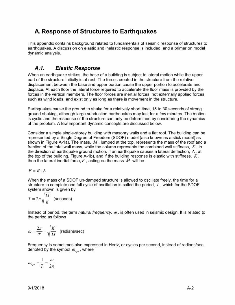
9/1/2018 A-2

A. Response of Structures to Earthquakes This appendix contains background related to fundamentals of seismic response of structures to earthquakes. A discussion on elastic and inelastic response is included, and a primer on modal dynamic analysis.

A.1. Elastic Response When an earthquake strikes, the base of a building is subject to lateral motion while the upper part of the structure initially is at rest. The forces created in the structure from the relative displacement between the base and upper portion cause the upper portion to accelerate and displace. At each floor the lateral force required to accelerate the floor mass is provided by the forces in the vertical members. The floor forces are inertial forces, not externally applied forces such as wind loads, and exist only as long as there is movement in the structure. Earthquakes cause the ground to shake for a relatively short time, 15 to 30 seconds of strong ground shaking, although large subduction earthquakes may last for a few minutes. The motion is cyclic and the response of the structure can only be determined by considering the dynamics of the problem. A few important dynamic concepts are discussed below. Consider a simple single-storey building with masonry walls and a flat roof. The building can be represented by a Single Degree of Freedom (SDOF) model (also known as a stick model) as shown in Figure A-1a). The mass, M , lumped at the top, represents the mass of the roof and a fraction of the total wall mass, while the column represents the combined wall stiffness, K , in the direction of earthquake ground motion. If an earthquake causes a lateral deflection, , at the top of the building, Figure A-1b), and if the building response is elastic with stiffness, K , then the lateral inertial force, F , acting on the mass M will be

KF When the mass of a SDOF un-damped structure is allowed to oscillate freely, the time for a structure to complete one full cycle of oscillation is called the period, T , which for the SDOF system shown is given by

K

MT 2 (seconds)

Instead of period, the term natural frequency, , is often used in seismic design. It is related to the period as follows

M

K

T

2 (radians/sec)

Frequency is sometimes also expressed in Hertz, or cycles per second, instead of radians/sec, denoted by the symbol cps , where

2

1

Tcps

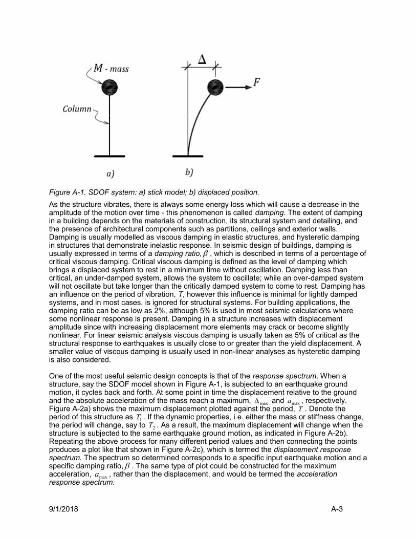
9/1/2018 A-3

Figure A-1. SDOF system: a) stick model; b) displaced position.

As the structure vibrates, there is always some energy loss which will cause a decrease in the amplitude of the motion over time - this phenomenon is called damping. The extent of damping in a building depends on the materials of construction, its structural system and detailing, and the presence of architectural components such as partitions, ceilings and exterior walls. Damping is usually modelled as viscous damping in elastic structures, and hysteretic damping in structures that demonstrate inelastic response. In seismic design of buildings, damping is usually expressed in terms of a damping ratio, , which is described in terms of a percentage of critical viscous damping. Critical viscous damping is defined as the level of damping which brings a displaced system to rest in a minimum time without oscillation. Damping less than critical, an under-damped system, allows the system to oscillate; while an over-damped system will not oscillate but take longer than the critically damped system to come to rest. Damping has an influence on the period of vibration, T, however this influence is minimal for lightly damped systems, and in most cases, is ignored for structural systems. For building applications, the damping ratio can be as low as 2%, although 5% is used in most seismic calculations where some nonlinear response is present. Damping in a structure increases with displacement amplitude since with increasing displacement more elements may crack or become slightly nonlinear. For linear seismic analysis viscous damping is usually taken as 5% of critical as the structural response to earthquakes is usually close to or greater than the yield displacement. A smaller value of viscous damping is usually used in non-linear analyses as hysteretic damping is also considered. One of the most useful seismic design concepts is that of the response spectrum. When a structure, say the SDOF model shown in Figure A-1, is subjected to an earthquake ground motion, it cycles back and forth. At some point in time the displacement relative to the ground and the absolute acceleration of the mass reach a maximum, max and maxa , respectively. Figure A-2a) shows the maximum displacement plotted against the period, T . Denote the period of this structure as 1T . If the dynamic properties, i.e. either the mass or stiffness change, the period will change, say to 2T . As a result, the maximum displacement will change when the structure is subjected to the same earthquake ground motion, as indicated in Figure A-2b). Repeating the above process for many different period values and then connecting the points produces a plot like that shown in Figure A-2c), which is termed the displacement response spectrum. The spectrum so determined corresponds to a specific input earthquake motion and a specific damping ratio, . The same type of plot could be constructed for the maximum acceleration, maxa , rather than the displacement, and would be termed the acceleration response spectrum.

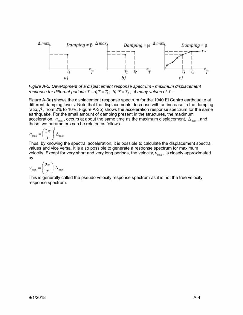
9/1/2018 A-4

Figure A-2. Development of a displacement response spectrum - maximum displacement response for different periods T : a) 1TT ; b) 2TT ; c) many values of T .

Figure A-3a) shows the displacement response spectrum for the 1940 El Centro earthquake at different damping levels. Note that the displacements decrease with an increase in the damping ratio, , from 2% to 10%. Figure A-3b) shows the acceleration response spectrum for the same earthquake. For the small amount of damping present in the structures, the maximum acceleration, maxa , occurs at about the same time as the maximum displacement, max , and these two parameters can be related as follows

max

2

max

2

T

a

Thus, by knowing the spectral acceleration, it is possible to calculate the displacement spectral values and vice versa. It is also possible to generate a response spectrum for maximum velocity. Except for very short and very long periods, the velocity, maxv , is closely approximated by

maxmax

2

T

v

This is generally called the pseudo velocity response spectrum as it is not the true velocity response spectrum.

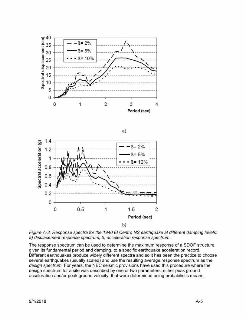
9/1/2018 A-5

a)

b)

Figure A-3. Response spectra for the 1940 El Centro NS earthquake at different damping levels: a) displacement response spectrum; b) acceleration response spectrum.

The response spectrum can be used to determine the maximum response of a SDOF structure, given its fundamental period and damping, to a specific earthquake acceleration record. Different earthquakes produce widely different spectra and so it has been the practice to choose several earthquakes (usually scaled) and use the resulting average response spectrum as the design spectrum. For years, the NBC seismic provisions have used this procedure where the design spectrum for a site was described by one or two parameters, either peak ground acceleration and/or peak ground velocity, that were determined using probabilistic means.

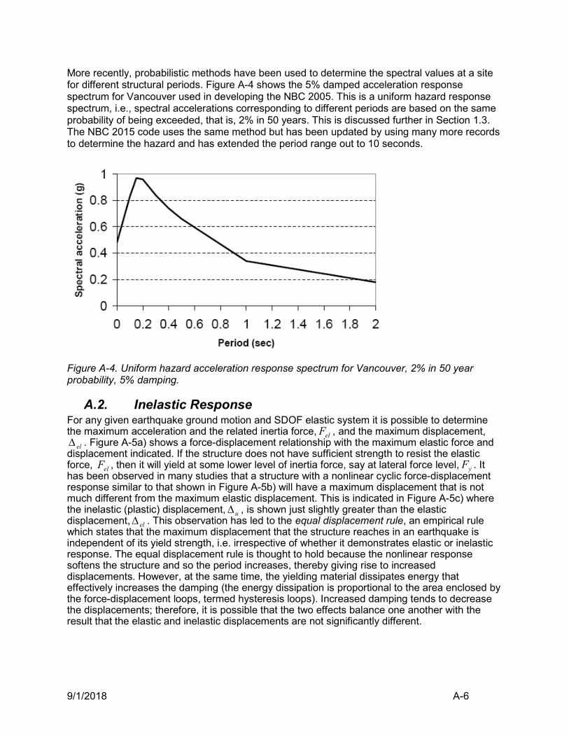
9/1/2018 A-6

More recently, probabilistic methods have been used to determine the spectral values at a site for different structural periods. Figure A-4 shows the 5% damped acceleration response spectrum for Vancouver used in developing the NBC 2005. This is a uniform hazard response spectrum, i.e., spectral accelerations corresponding to different periods are based on the same probability of being exceeded, that is, 2% in 50 years. This is discussed further in Section 1.3. The NBC 2015 code uses the same method but has been updated by using many more records to determine the hazard and has extended the period range out to 10 seconds.

Figure A-4. Uniform hazard acceleration response spectrum for Vancouver, 2% in 50 year probability, 5% damping.

A.2. Inelastic Response For any given earthquake ground motion and SDOF elastic system it is possible to determine the maximum acceleration and the related inertia force, elF , and the maximum displacement,

el . Figure A-5a) shows a force-displacement relationship with the maximum elastic force and displacement indicated. If the structure does not have sufficient strength to resist the elastic force, elF , then it will yield at some lower level of inertia force, say at lateral force level, yF . It has been observed in many studies that a structure with a nonlinear cyclic force-displacement response similar to that shown in Figure A-5b) will have a maximum displacement that is not much different from the maximum elastic displacement. This is indicated in Figure A-5c) where the inelastic (plastic) displacement, u , is shown just slightly greater than the elastic displacement, el . This observation has led to the equal displacement rule, an empirical rule which states that the maximum displacement that the structure reaches in an earthquake is independent of its yield strength, i.e. irrespective of whether it demonstrates elastic or inelastic response. The equal displacement rule is thought to hold because the nonlinear response softens the structure and so the period increases, thereby giving rise to increased displacements. However, at the same time, the yielding material dissipates energy that effectively increases the damping (the energy dissipation is proportional to the area enclosed by the force-displacement loops, termed hysteresis loops). Increased damping tends to decrease the displacements; therefore, it is possible that the two effects balance one another with the result that the elastic and inelastic displacements are not significantly different.

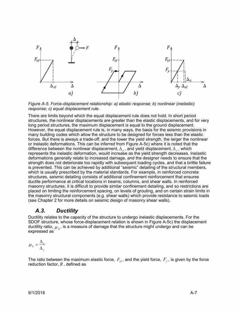
9/1/2018 A-7

Figure A-5. Force-displacement relationship: a) elastic response; b) nonlinear (inelastic) response; c) equal displacement rule.

There are limits beyond which the equal displacement rule does not hold. In short period structures, the nonlinear displacements are greater than the elastic displacements, and for very long period structures, the maximum displacement is equal to the ground displacement. However, the equal displacement rule is, in many ways, the basis for the seismic provisions in many building codes which allow the structure to be designed for forces less than the elastic forces. But there is always a trade-off, and the lower the yield strength, the larger the nonlinear or inelastic deformations. This can be inferred from Figure A-5c) where it is noted that the difference between the nonlinear displacement, u , and yield displacement, y , which represents the inelastic deformation, would increase as the yield strength decreases. Inelastic deformations generally relate to increased damage, and the designer needs to ensure that the strength does not deteriorate too rapidly with subsequent loading cycles, and that a brittle failure is prevented. This can be achieved by additional “seismic” detailing of the structural members, which is usually prescribed by the material standards. For example, in reinforced concrete structures, seismic detailing consists of additional confinement reinforcement that ensures ductile performance at critical locations in beams, columns, and shear walls. In reinforced masonry structures, it is difficult to provide similar confinement detailing, and so restrictions are placed on limiting the reinforcement spacing, on levels of grouting, and on certain strain limits in the masonry structural components (e.g. shear walls) which provide resistance to seismic loads (see Chapter 2 for more details on seismic design of masonry shear walls).

A.3. Ductility Ductility relates to the capacity of the structure to undergo inelastic displacements. For the SDOF structure, whose force-displacement relation is shown in Figure A-5c) the displacement ductility ratio, , is a measure of damage that the structure might undergo and can be expressed as

y

u

The ratio between the maximum elastic force, elF , and the yield force, yF , is given by the force reduction factor,R , defined as

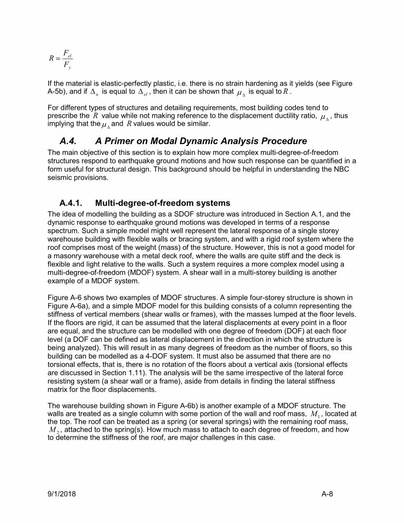
9/1/2018 A-8

y

el

F

FR

If the material is elastic-perfectly plastic, i.e. there is no strain hardening as it yields (see Figure A-5b), and if u is equal to el , then it can be shown that is equal toR . For different types of structures and detailing requirements, most building codes tend to prescribe the R value while not making reference to the displacement ductility ratio, , thus implying that the and R values would be similar.

A.4. A Primer on Modal Dynamic Analysis Procedure The main objective of this section is to explain how more complex multi-degree-of-freedom structures respond to earthquake ground motions and how such response can be quantified in a form useful for structural design. This background should be helpful in understanding the NBC seismic provisions.

A.4.1. Multi-degree-of-freedom systems The idea of modelling the building as a SDOF structure was introduced in Section A.1, and the dynamic response to earthquake ground motions was developed in terms of a response spectrum. Such a simple model might well represent the lateral response of a single storey warehouse building with flexible walls or bracing system, and with a rigid roof system where the roof comprises most of the weight (mass) of the structure. However, this is not a good model for a masonry warehouse with a metal deck roof, where the walls are quite stiff and the deck is flexible and light relative to the walls. Such a system requires a more complex model using a multi-degree-of-freedom (MDOF) system. A shear wall in a multi-storey building is another example of a MDOF system. Figure A-6 shows two examples of MDOF structures. A simple four-storey structure is shown in Figure A-6a), and a simple MDOF model for this building consists of a column representing the stiffness of vertical members (shear walls or frames), with the masses lumped at the floor levels. If the floors are rigid, it can be assumed that the lateral displacements at every point in a floor are equal, and the structure can be modelled with one degree of freedom (DOF) at each floor level (a DOF can be defined as lateral displacement in the direction in which the structure is being analyzed). This will result in as many degrees of freedom as the number of floors, so this building can be modelled as a 4-DOF system. It must also be assumed that there are no torsional effects, that is, there is no rotation of the floors about a vertical axis (torsional effects are discussed in Section 1.11). The analysis will be the same irrespective of the lateral force resisting system (a shear wall or a frame), aside from details in finding the lateral stiffness matrix for the floor displacements. The warehouse building shown in Figure A-6b) is another example of a MDOF structure. The walls are treated as a single column with some portion of the wall and roof mass, 1M , located at the top. The roof can be treated as a spring (or several springs) with the remaining roof mass,

2M , attached to the spring(s). How much mass to attach to each degree of freedom, and how to determine the stiffness of the roof, are major challenges in this case.

9/1/2018 A-9

Figure A-6. MDOF systems: a) multi-storey shear wall building; b) warehouse with flexible roof.

A.4.2. Seismic analysis methods The question of interest to structural engineers is how to determine a realistic seismic response for MDOF systems? The possible approaches are: static analysis, and dynamic analysis (modal analysis or time history method).

The simplest method is the equivalent static analysis procedure (also known as the quasi-static method) in which a set of static horizontal forces is applied to the structure (similar to a wind load). These forces are meant to emulate the maximum effects in a structure that a dynamic analysis would predict. This procedure works well when applied to small, simple structures, and also to larger structures if they are regular in their layout. NBC 2015 specifies a dynamic analysis as the default method. The simplest type of dynamic analysis is the modal analysis method. This method is restricted to linear systems, and consists of a dynamic analysis to determine the mode shapes and periods of the structure, and then

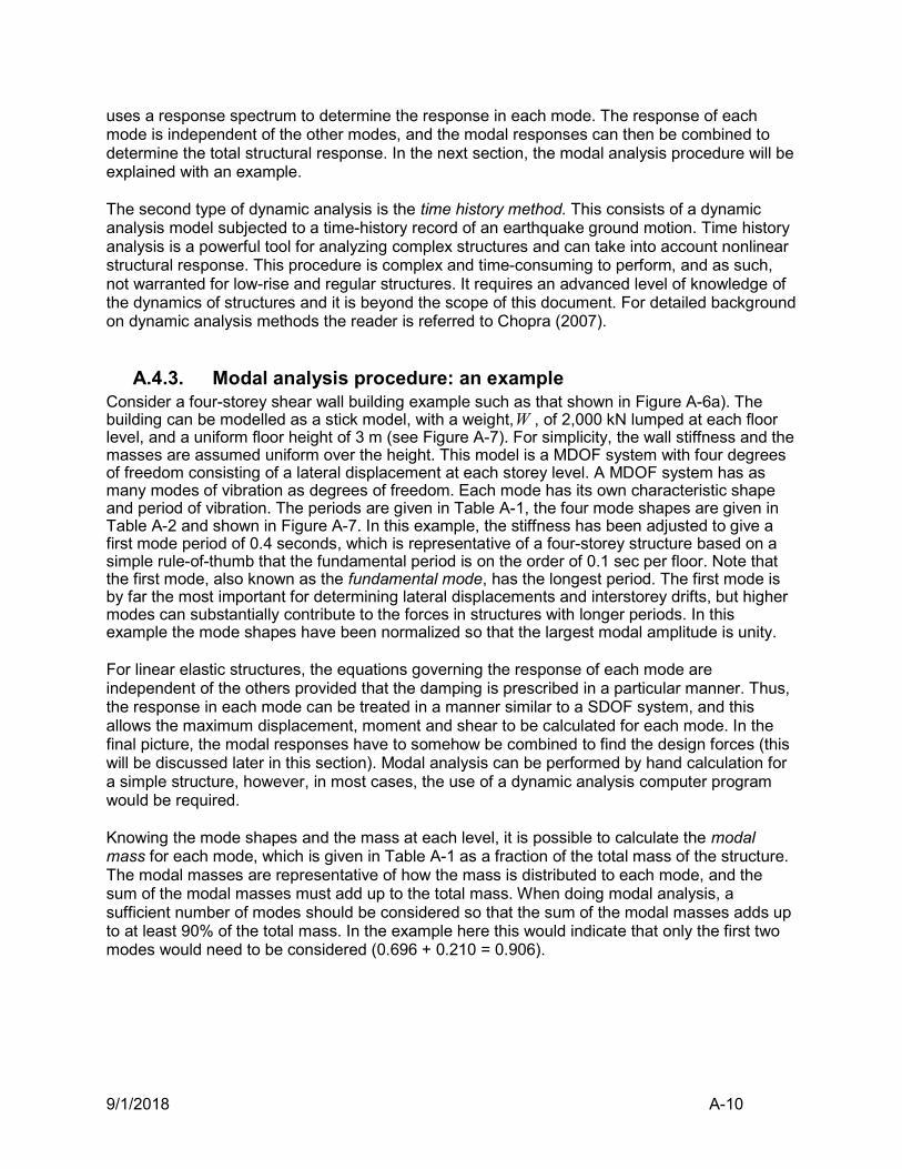
9/1/2018 A-10

uses a response spectrum to determine the response in each mode. The response of each mode is independent of the other modes, and the modal responses can then be combined to determine the total structural response. In the next section, the modal analysis procedure will be explained with an example. The second type of dynamic analysis is the time history method. This consists of a dynamic analysis model subjected to a time-history record of an earthquake ground motion. Time history analysis is a powerful tool for analyzing complex structures and can take into account nonlinear structural response. This procedure is complex and time-consuming to perform, and as such, not warranted for low-rise and regular structures. It requires an advanced level of knowledge of the dynamics of structures and it is beyond the scope of this document. For detailed background on dynamic analysis methods the reader is referred to Chopra (2007).

A.4.3. Modal analysis procedure: an example Consider a four-storey shear wall building example such as that shown in Figure A-6a). The building can be modelled as a stick model, with a weight,W , of 2,000 kN lumped at each floor level, and a uniform floor height of 3 m (see Figure A-7). For simplicity, the wall stiffness and the masses are assumed uniform over the height. This model is a MDOF system with four degrees of freedom consisting of a lateral displacement at each storey level. A MDOF system has as many modes of vibration as degrees of freedom. Each mode has its own characteristic shape and period of vibration. The periods are given in Table A-1, the four mode shapes are given in Table A-2 and shown in Figure A-7. In this example, the stiffness has been adjusted to give a first mode period of 0.4 seconds, which is representative of a four-storey structure based on a simple rule-of-thumb that the fundamental period is on the order of 0.1 sec per floor. Note that the first mode, also known as the fundamental mode, has the longest period. The first mode is by far the most important for determining lateral displacements and interstorey drifts, but higher modes can substantially contribute to the forces in structures with longer periods. In this example the mode shapes have been normalized so that the largest modal amplitude is unity. For linear elastic structures, the equations governing the response of each mode are independent of the others provided that the damping is prescribed in a particular manner. Thus, the response in each mode can be treated in a manner similar to a SDOF system, and this allows the maximum displacement, moment and shear to be calculated for each mode. In the final picture, the modal responses have to somehow be combined to find the design forces (this will be discussed later in this section). Modal analysis can be performed by hand calculation for a simple structure, however, in most cases, the use of a dynamic analysis computer program would be required. Knowing the mode shapes and the mass at each level, it is possible to calculate the modal mass for each mode, which is given in Table A-1 as a fraction of the total mass of the structure. The modal masses are representative of how the mass is distributed to each mode, and the sum of the modal masses must add up to the total mass. When doing modal analysis, a sufficient number of modes should be considered so that the sum of the modal masses adds up to at least 90% of the total mass. In the example here this would indicate that only the first two modes would need to be considered (0.696 + 0.210 = 0.906).

9/1/2018 A-11

Figure A-7. Four-storey shear wall building model and modal shapes.

As an example of how the different modes can be used to determine the structural response, Figure A-8 shows a typical design acceleration response spectrum which will be used to determine the modal displacements and accelerations. The four modal periods are indicated on the spectrum (note that only the first two periods are identified on the diagram; T1=0.40 and T2=0.062 sec) and the spectral acceleration Sa at each of the periods is given in Table A-3.

Figure A-8. Design acceleration response spectrum.

A very useful feature of the modal analysis procedure is that it gives the base shear in each mode as a product of the modal mass and the spectral acceleration Sa for that mode, as shown in Table A-3. For example, the base shear for the first mode is equal to (8000kN x 0.696) x 0.74 = 4127 kN). Note that the spectral acceleration is higher for the higher modes, but because the modal mass for these modes is smaller, the base shear is smaller. The inertia forces from each floor mass act in the same directions as the mode shape, that is, some forces are positive while others are negative for the higher modes (refer to mode shapes shown in Figure A-7). It can be seen from the figure that the forces from the first mode all act in the same direction at the same time, while the higher modes will have both positive and negative forces. Thus, the base shear from the first mode is usually larger than that from the other modes.

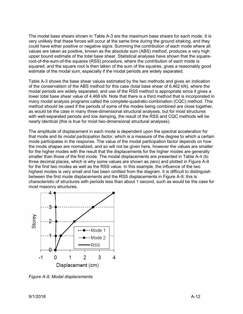
9/1/2018 A-12

The modal base shears shown in Table A-3 are the maximum base shears for each mode. It is very unlikely that these forces will occur at the same time during the ground shaking, and they could have either positive or negative signs. Summing the contribution of each mode where all values are taken as positive, known as the absolute sum (ABS) method, produces a very high upper bound estimate of the total base shear. Statistical analyses have shown that the square-root-of-the-sum-of-the squares (RSS) procedure, where the contribution of each mode is squared, and the square root is then taken of the sum of the squares, gives a reasonably good estimate of the modal sum, especially if the modal periods are widely separated. Table A-3 shows the base shear values estimated by the two methods and gives an indication of the conservatism of the ABS method for this case (total base shear of 6,462 kN), where the modal periods are widely separated, and use of the RSS method is appropriate since it gives a lower total base shear value of 4,468 kN. Note that there is a third method that is incorporated in many modal analysis programs called the complete-quadratic-combination (CQC) method. This method should be used if the periods of some of the modes being combined are close together, as would be the case in many three-dimensional structural analyses, but for most structures with well-separated periods and low damping, the result of the RSS and CQC methods will be nearly identical (this is true for most two-dimensional structural analyses). The amplitude of displacement in each mode is dependent upon the spectral acceleration for that mode and its modal participation factor, which is a measure of the degree to which a certain mode participates in the response. The value of the modal participation factor depends on how the mode shapes are normalized, and so will not be given here, however the values are smaller for the higher modes with the result that the displacements for the higher modes are generally smaller than those of the first mode. The modal displacements are presented in Table A-4 (to three decimal places, which is why some values are shown as zero) and plotted in Figure A-9 for the first two modes as well as the RSS value. In this example, the influence of the two highest modes is very small and has been omitted from the diagram. It is difficult to distinguish between the first mode displacements and the RSS displacements in Figure A-9; this is characteristic of structures with periods less than about 1 second, such as would be the case for most masonry structures.

Figure A-9. Modal displacements.

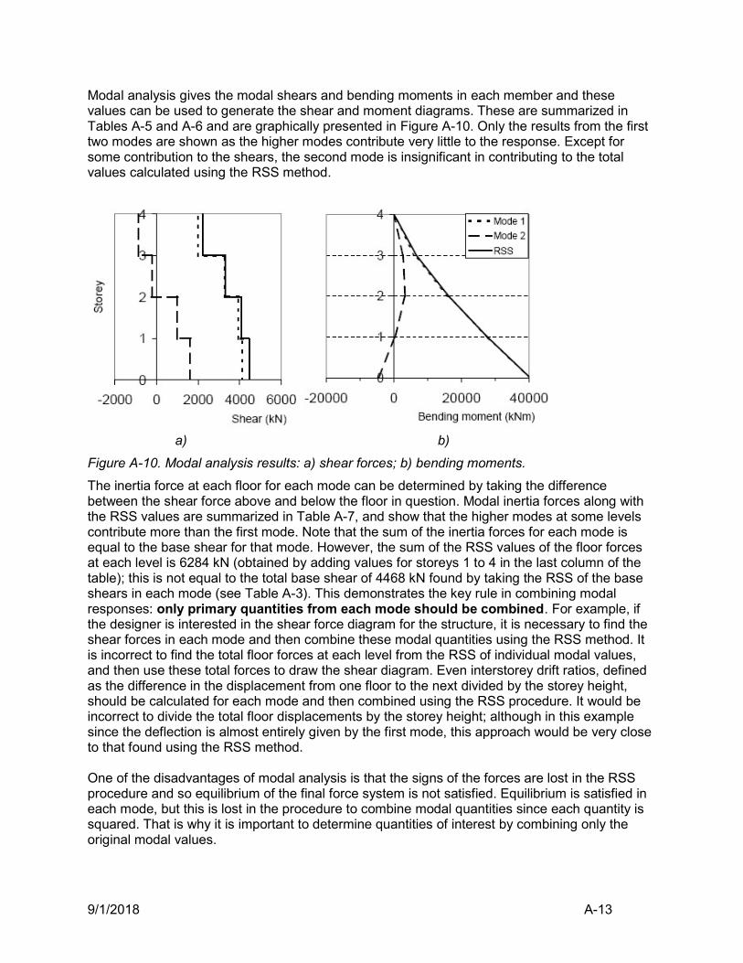
9/1/2018 A-13

Modal analysis gives the modal shears and bending moments in each member and these values can be used to generate the shear and moment diagrams. These are summarized in Tables A-5 and A-6 and are graphically presented in Figure A-10. Only the results from the first two modes are shown as the higher modes contribute very little to the response. Except for some contribution to the shears, the second mode is insignificant in contributing to the total values calculated using the RSS method.

a) b)

Figure A-10. Modal analysis results: a) shear forces; b) bending moments.

The inertia force at each floor for each mode can be determined by taking the difference between the shear force above and below the floor in question. Modal inertia forces along with the RSS values are summarized in Table A-7, and show that the higher modes at some levels contribute more than the first mode. Note that the sum of the inertia forces for each mode is equal to the base shear for that mode. However, the sum of the RSS values of the floor forces at each level is 6284 kN (obtained by adding values for storeys 1 to 4 in the last column of the table); this is not equal to the total base shear of 4468 kN found by taking the RSS of the base shears in each mode (see Table A-3). This demonstrates the key rule in combining modal responses: only primary quantities from each mode should be combined. For example, if the designer is interested in the shear force diagram for the structure, it is necessary to find the shear forces in each mode and then combine these modal quantities using the RSS method. It is incorrect to find the total floor forces at each level from the RSS of individual modal values, and then use these total forces to draw the shear diagram. Even interstorey drift ratios, defined as the difference in the displacement from one floor to the next divided by the storey height, should be calculated for each mode and then combined using the RSS procedure. It would be incorrect to divide the total floor displacements by the storey height; although in this example since the deflection is almost entirely given by the first mode, this approach would be very close to that found using the RSS method. One of the disadvantages of modal analysis is that the signs of the forces are lost in the RSS procedure and so equilibrium of the final force system is not satisfied. Equilibrium is satisfied in each mode, but this is lost in the procedure to combine modal quantities since each quantity is squared. That is why it is important to determine quantities of interest by combining only the original modal values.

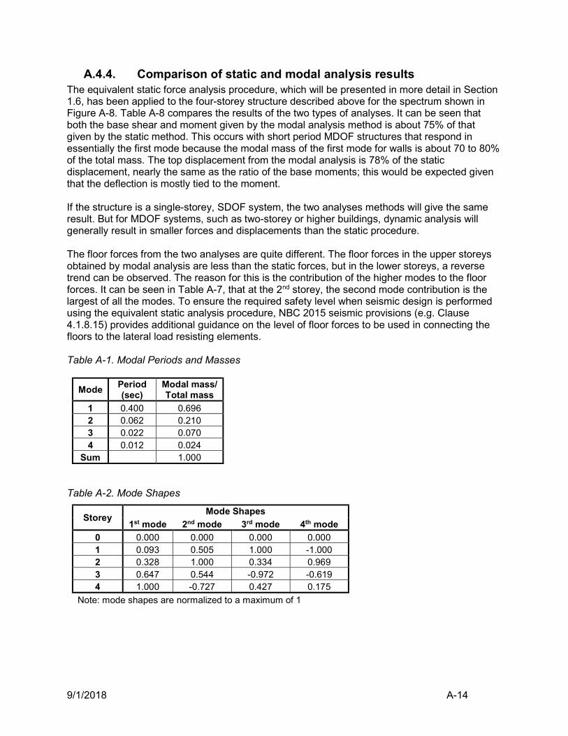
9/1/2018 A-14

A.4.4. Comparison of static and modal analysis results The equivalent static force analysis procedure, which will be presented in more detail in Section 1.6, has been applied to the four-storey structure described above for the spectrum shown in Figure A-8. Table A-8 compares the results of the two types of analyses. It can be seen that both the base shear and moment given by the modal analysis method is about 75% of that given by the static method. This occurs with short period MDOF structures that respond in essentially the first mode because the modal mass of the first mode for walls is about 70 to 80% of the total mass. The top displacement from the modal analysis is 78% of the static displacement, nearly the same as the ratio of the base moments; this would be expected given that the deflection is mostly tied to the moment. If the structure is a single-storey, SDOF system, the two analyses methods will give the same result. But for MDOF systems, such as two-storey or higher buildings, dynamic analysis will generally result in smaller forces and displacements than the static procedure. The floor forces from the two analyses are quite different. The floor forces in the upper storeys obtained by modal analysis are less than the static forces, but in the lower storeys, a reverse trend can be observed. The reason for this is the contribution of the higher modes to the floor forces. It can be seen in Table A-7, that at the 2nd storey, the second mode contribution is the largest of all the modes. To ensure the required safety level when seismic design is performed using the equivalent static analysis procedure, NBC 2015 seismic provisions (e.g. Clause 4.1.8.15) provides additional guidance on the level of floor forces to be used in connecting the floors to the lateral load resisting elements. Table A-1. Modal Periods and Masses

Mode Period (sec)

Modal mass/ Total mass

1 0.400 0.696 2 0.062 0.210 3 0.022 0.070 4 0.012 0.024

Sum 1.000

Table A-2. Mode Shapes

Storey Mode Shapes

1st mode 2nd mode 3rd mode 4th mode

0 0.000 0.000 0.000 0.000 1 0.093 0.505 1.000 -1.000 2 0.328 1.000 0.334 0.969 3 0.647 0.544 -0.972 -0.619 4 1.000 -0.727 0.427 0.175

Note: mode shapes are normalized to a maximum of 1

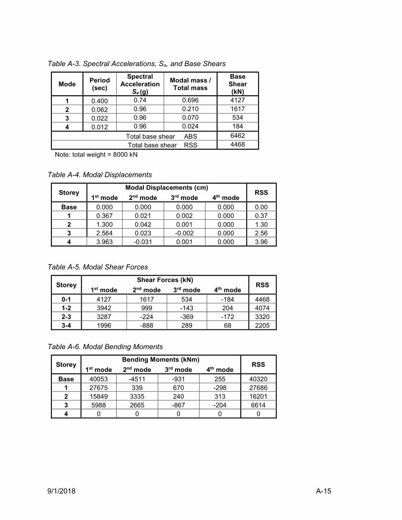
9/1/2018 A-15

Table A-3. Spectral Accelerations, Sa, and Base Shears

Mode Period (sec)

Spectral Acceleration

Sa (g)

Modal mass / Total mass

Base Shear (kN)

1 0.400 0.74 0.696 4127

2 0.062 0.96 0.210 1617

3 0.022 0.96 0.070 534

4 0.012 0.96 0.024 184

Total base shear ABS 6462

Total base shear RSS 4468

Note: total weight = 8000 kN

Table A-4. Modal Displacements

Storey Modal Displacements (cm)

RSS 1st mode 2nd mode 3rd mode 4th mode

Base 0.000 0.000 0.000 0.000 0.00 1 0.367 0.021 0.002 0.000 0.37 2 1.300 0.042 0.001 0.000 1.30 3 2.564 0.023 -0.002 0.000 2.56 4 3.963 -0.031 0.001 0.000 3.96

Table A-5. Modal Shear Forces

Storey Shear Forces (kN)

RSS 1st mode 2nd mode 3rd mode 4th mode

0-1 4127 1617 534 -184 4468 1-2 3942 999 -143 204 4074 2-3 3287 -224 -369 -172 3320 3-4 1996 -888 289 68 2205

Table A-6. Modal Bending Moments

Storey Bending Moments (kNm)

RSS 1st mode 2nd mode 3rd mode 4th mode

Base 40053 -4511 -931 255 40320 1 27675 339 670 -298 27686 2 15849 3335 240 313 16201 3 5988 2665 -867 -204 6614 4 0 0 0 0 0

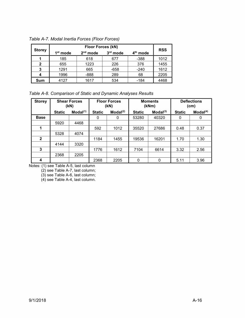
9/1/2018 A-16

Table A-7. Modal Inertia Forces (Floor Forces)

Storey Floor Forces (kN)

RSS 1st mode 2nd mode 3rd mode 4th mode

1 185 618 677 -388 1012 2 655 1223 226 376 1455 3 1291 665 -658 -240 1612 4 1996 -888 289 68 2205

Sum 4127 1617 534 -184 4468

Table A-8. Comparison of Static and Dynamic Analyses Results

Storey Shear Forces (kN)

Floor Forces (kN)

Moments (kNm)

Deflections (cm)

Static Modal(1) Static Modal(2) Static Modal(3) Static Modal(4) Base 0 0 53280 40320 0 0

5920 4468 1 592 1012 35520 27686 0.48 0.37 5328 4074

2 1184 1455 19536 16201 1.70 1.30 4144 3320

3 1776 1612 7104 6614 3.32 2.56 2368 2205

4 2368 2205 0 0 5.11 3.96 Notes: (1) see Table A-5, last column (2) see Table A-7, last column; (3) see Table A-6, last column; (4) see Table A-4, last column.

9/1/2018 B-1

TABLE OF CONTENTS – APPENDIX B

B RELEVANT RESEARCH STUDIES AND CODE BACKGROUND B-2

B.1 Shear/Diagonal Tension Resistance B-2

B.2 Sliding Shear Resistance B-8

B.3 Ductile Seismic Response of Reinforced Masonry Shear Walls B-12

B.4 Wall Height-to-Thickness Ratio Restrictions B-16

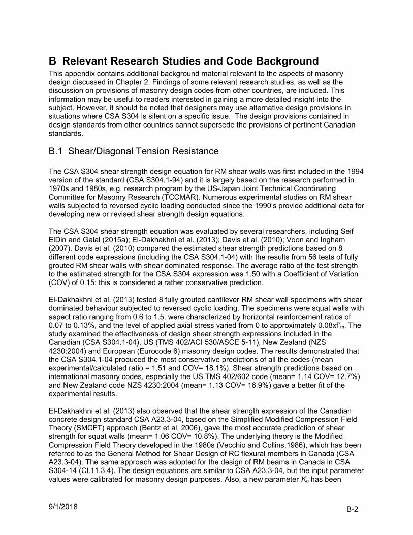
9/1/2018 B-2

B Relevant Research Studies and Code Background This appendix contains additional background material relevant to the aspects of masonry design discussed in Chapter 2. Findings of some relevant research studies, as well as the discussion on provisions of masonry design codes from other countries, are included. This information may be useful to readers interested in gaining a more detailed insight into the subject. However, it should be noted that designers may use alternative design provisions in situations where CSA S304 is silent on a specific issue. The design provisions contained in design standards from other countries cannot supersede the provisions of pertinent Canadian standards.

B.1 Shear/Diagonal Tension Resistance The CSA S304 shear strength design equation for RM shear walls was first included in the 1994 version of the standard (CSA S304.1-94) and it is largely based on the research performed in 1970s and 1980s, e.g. research program by the US-Japan Joint Technical Coordinating Committee for Masonry Research (TCCMAR). Numerous experimental studies on RM shear walls subjected to reversed cyclic loading conducted since the 1990’s provide additional data for developing new or revised shear strength design equations. The CSA S304 shear strength equation was evaluated by several researchers, including Seif ElDin and Galal (2015a); El-Dakhakhni et al. (2013); Davis et al. (2010); Voon and Ingham (2007). Davis et al. (2010) compared the estimated shear strength predictions based on 8 different code expressions (including the CSA S304.1-04) with the results from 56 tests of fully grouted RM shear walls with shear dominated response. The average ratio of the test strength to the estimated strength for the CSA S304 expression was 1.50 with a Coefficient of Variation (COV) of 0.15; this is considered a rather conservative prediction. El-Dakhakhni et al. (2013) tested 8 fully grouted cantilever RM shear wall specimens with shear dominated behaviour subjected to reversed cyclic loading. The specimens were squat walls with aspect ratio ranging from 0.6 to 1.5, were characterized by horizontal reinforcement ratios of 0.07 to 0.13%, and the level of applied axial stress varied from 0 to approximately 0.08xf’m. The study examined the effectiveness of design shear strength expressions included in the Canadian (CSA S304.1-04), US (TMS 402/ACI 530/ASCE 5-11), New Zealand (NZS 4230:2004) and European (Eurocode 6) masonry design codes. The results demonstrated that the CSA S304.1-04 produced the most conservative predictions of all the codes (mean experimental/calculated ratio = 1.51 and COV= 18.1%). Shear strength predictions based on international masonry codes, especially the US TMS 402/602 code (mean= 1.14 COV= 12.7%) and New Zealand code NZS 4230:2004 (mean= 1.13 COV= 16.9%) gave a better fit of the experimental results. El-Dakhakhni et al. (2013) also observed that the shear strength expression of the Canadian concrete design standard CSA A23.3-04, based on the Simplified Modified Compression Field Theory (SMCFT) approach (Bentz et al. 2006), gave the most accurate prediction of shear strength for squat walls (mean= 1.06 COV= 10.8%). The underlying theory is the Modified Compression Field Theory developed in the 1980s (Vecchio and Collins,1986), which has been referred to as the General Method for Shear Design of RC flexural members in Canada (CSA A23.3-04). The same approach was adopted for the design of RM beams in Canada in CSA S304-14 (Cl.11.3.4). The design equations are similar to CSA A23.3-04, but the input parameter values were calibrated for masonry design purposes. Also, a new parameter Kb has been

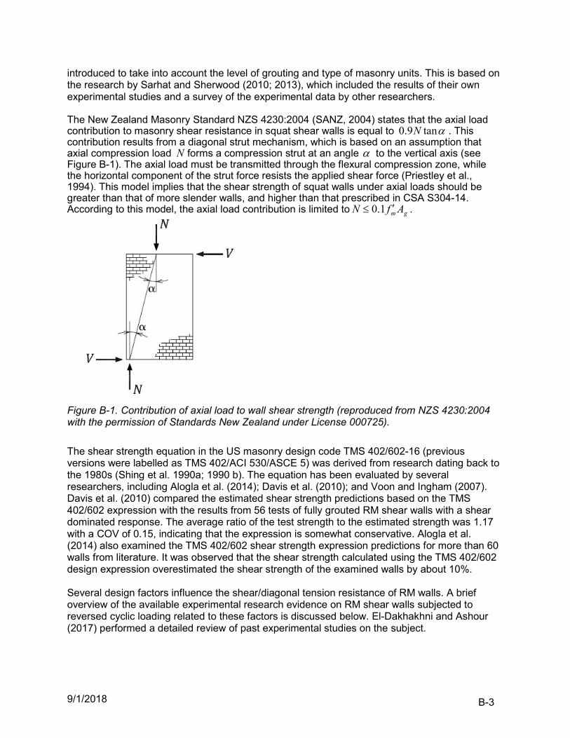
9/1/2018 B-3

introduced to take into account the level of grouting and type of masonry units. This is based on the research by Sarhat and Sherwood (2010; 2013), which included the results of their own experimental studies and a survey of the experimental data by other researchers. The New Zealand Masonry Standard NZS 4230:2004 (SANZ, 2004) states that the axial load contribution to masonry shear resistance in squat shear walls is equal to tan9.0 N . This contribution results from a diagonal strut mechanism, which is based on an assumption that axial compression load N forms a compression strut at an angle to the vertical axis (see Figure B-1). The axial load must be transmitted through the flexural compression zone, while the horizontal component of the strut force resists the applied shear force (Priestley et al., 1994). This model implies that the shear strength of squat walls under axial loads should be greater than that of more slender walls, and higher than that prescribed in CSA S304-14. According to this model, the axial load contribution is limited to gmAfN 1.0 .

Figure B-1. Contribution of axial load to wall shear strength (reproduced from NZS 4230:2004 with the permission of Standards New Zealand under License 000725).

The shear strength equation in the US masonry design code TMS 402/602-16 (previous versions were labelled as TMS 402/ACI 530/ASCE 5) was derived from research dating back to the 1980s (Shing et al. 1990a; 1990 b). The equation has been evaluated by several researchers, including Alogla et al. (2014); Davis et al. (2010); and Voon and Ingham (2007). Davis et al. (2010) compared the estimated shear strength predictions based on the TMS 402/602 expression with the results from 56 tests of fully grouted RM shear walls with a shear dominated response. The average ratio of the test strength to the estimated strength was 1.17 with a COV of 0.15, indicating that the expression is somewhat conservative. Alogla et al. (2014) also examined the TMS 402/602 shear strength expression predictions for more than 60 walls from literature. It was observed that the shear strength calculated using the TMS 402/602 design expression overestimated the shear strength of the examined walls by about 10%. Several design factors influence the shear/diagonal tension resistance of RM walls. A brief overview of the available experimental research evidence on RM shear walls subjected to reversed cyclic loading related to these factors is discussed below. El-Dakhakhni and Ashour (2017) performed a detailed review of past experimental studies on the subject.

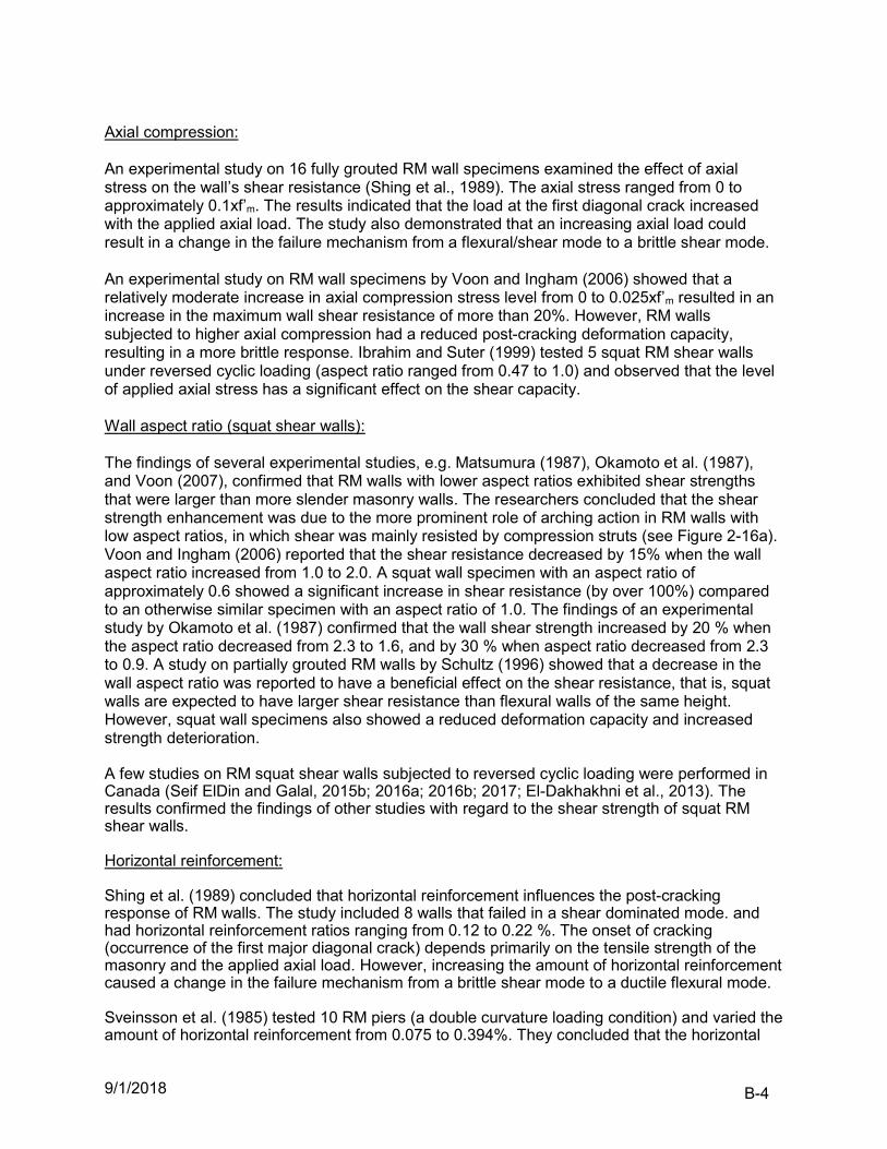
9/1/2018 B-4

Axial compression: An experimental study on 16 fully grouted RM wall specimens examined the effect of axial stress on the wall’s shear resistance (Shing et al., 1989). The axial stress ranged from 0 to approximately 0.1xf’m. The results indicated that the load at the first diagonal crack increased with the applied axial load. The study also demonstrated that an increasing axial load could result in a change in the failure mechanism from a flexural/shear mode to a brittle shear mode. An experimental study on RM wall specimens by Voon and Ingham (2006) showed that a relatively moderate increase in axial compression stress level from 0 to 0.025xf’m resulted in an increase in the maximum wall shear resistance of more than 20%. However, RM walls subjected to higher axial compression had a reduced post-cracking deformation capacity, resulting in a more brittle response. Ibrahim and Suter (1999) tested 5 squat RM shear walls under reversed cyclic loading (aspect ratio ranged from 0.47 to 1.0) and observed that the level of applied axial stress has a significant effect on the shear capacity. Wall aspect ratio (squat shear walls): The findings of several experimental studies, e.g. Matsumura (1987), Okamoto et al. (1987), and Voon (2007), confirmed that RM walls with lower aspect ratios exhibited shear strengths that were larger than more slender masonry walls. The researchers concluded that the shear strength enhancement was due to the more prominent role of arching action in RM walls with low aspect ratios, in which shear was mainly resisted by compression struts (see Figure 2-16a). Voon and Ingham (2006) reported that the shear resistance decreased by 15% when the wall aspect ratio increased from 1.0 to 2.0. A squat wall specimen with an aspect ratio of approximately 0.6 showed a significant increase in shear resistance (by over 100%) compared to an otherwise similar specimen with an aspect ratio of 1.0. The findings of an experimental study by Okamoto et al. (1987) confirmed that the wall shear strength increased by 20 % when the aspect ratio decreased from 2.3 to 1.6, and by 30 % when aspect ratio decreased from 2.3 to 0.9. A study on partially grouted RM walls by Schultz (1996) showed that a decrease in the wall aspect ratio was reported to have a beneficial effect on the shear resistance, that is, squat walls are expected to have larger shear resistance than flexural walls of the same height. However, squat wall specimens also showed a reduced deformation capacity and increased strength deterioration. A few studies on RM squat shear walls subjected to reversed cyclic loading were performed in Canada (Seif ElDin and Galal, 2015b; 2016a; 2016b; 2017; El-Dakhakhni et al., 2013). The results confirmed the findings of other studies with regard to the shear strength of squat RM shear walls. Horizontal reinforcement: Shing et al. (1989) concluded that horizontal reinforcement influences the post-cracking response of RM walls. The study included 8 walls that failed in a shear dominated mode. and had horizontal reinforcement ratios ranging from 0.12 to 0.22 %. The onset of cracking (occurrence of the first major diagonal crack) depends primarily on the tensile strength of the masonry and the applied axial load. However, increasing the amount of horizontal reinforcement caused a change in the failure mechanism from a brittle shear mode to a ductile flexural mode. Sveinsson et al. (1985) tested 10 RM piers (a double curvature loading condition) and varied the amount of horizontal reinforcement from 0.075 to 0.394%. They concluded that the horizontal

9/1/2018 B-5

reinforcement was effective in increasing shear strength, but higher amounts of reinforcement did not correspond to a proportional gain in strength. For example, a 16% increase in the shear strength was observed in a specimen which had twice the amount of horizontal reinforcing bars compared to an otherwise similar specimen. Shear reinforcement in RM shear walls does not seem to be as effective as in RC shear walls. A possible explanation is that the reinforcing bars located where the inclined crack crosses near the end of the bar are unable to develop their full yield strength in the masonry walls. To account for this phenomenon, the New Zealand Masonry Standard NZS 4230:2004 (SANZ, 2004) prescribes a coefficient of 0.8 in the sV equation, while CSA S304-14 uses a 0.6 factor. This phenomenon is particularly pronounced in short walls, where it is likely that the length of the shear reinforcement is insufficient to fully develop its yield strength. Seif ElDin and Galal (2015b) tested 9 squat RM walls under quasi-static cyclic loading. Contrary to the previous experimental studies, they observed that the horizontal reinforcement contributes to the wall shear resistance with its full yield capacity (there is no reduction coefficient as discussed above). This can be explained by the redistribution in the shear resistance between the reinforcement and the masonry, especially at high ductility demands. Most previous researchers quantified shear contribution of reinforcement based on the difference between the shear capacities of specimens with different transverse reinforcement ratios. It appears that horizontal reinforcement in RM shear walls does not have as good anchorage as the corresponding reinforcement in RC shear walls. Anderson and Priestley (1992) have noted that straight bars or 90 hooks were used in some experimental studies (see Figure B-2a), whereas the horizontal reinforcement in RC shear walls is usually anchored in a more effective way, such as by 180 hooks. The type and extent of anchorage are expected to influence the effectiveness of shear reinforcement. Sveinsson et al. (1985) tested 10 fully grouted RM piers and studied (among other factors) the effect of anchorage conditions in horizontal reinforcement (90 versus 180 hooks). They recommended the use of 180 hooked end anchorage for horizontal reinforcement because it produced better energy dissipation, and enabled the bars to develop their full tensile strength This is particularly true for shorter walls/piers. Seif ElDin and Galal (2016a) tested 3 squat RM wall specimens with shear dominant behaviour under reversed cyclic loading. The specimens were identical, except for the end anchorage of the horizontal reinforcing bars: the first specimen had 180 hooks, the second one 90 hooks, and the third one had straight bars (no hooks). The results showed that the specimen with 180 hooks provided the most effective anchorage and attained the largest shear capacity and displacement ductility, while the specimen with straight bars attained the smallest shear capacity and displacement ductility. However, the difference in the strength values was not significant (it was within 10%). The most significant difference was in the post-peak behaviour. The specimen with straight bars showed the most rapid post-peak degradation of the lateral load resistance. The 180 hooks proved to be effective in providing confinement for the vertical end bars in the wall, while the 90 hooks were less effective. For that reason, displacement ductility of the specimen with 180 hooks (4.2) was higher than the specimen with 90 hooks (3.9) and the one with straight bars (3.6). This difference again indicates the superior ductility potential of the 180 end hooks, but the other anchorage conditions may be acceptable in some cases. The researchers recommended the use of horizontal reinforcing bars with 90 hooks for masonry structures located in regions of low to moderate seismic hazard, and/or outside the plastic hinge regions in ductile shear walls.

9/1/2018 B-6

Vertical reinforcement: Anderson and Priestley (1992) found that shear strength didn’t show any correlation with the vertical reinforcement ratio, hence the CSA S304 shear design equation ignore the effect of vertical reinforcement. However, according to some researchers (Shing et al., 1990; Tomazevic, 1999; Voon, 2007), a fraction of the wall shear resistance can be attributed to the presence of vertical reinforcement. Dowel action in vertical reinforcing bars enables shear transfer across a diagonal crack by the localized kinking in reinforcing bars due to their relative displacement (see Figure B-2b) (note that compression kinks cancel out some of the tension kinks). However, once the vertical reinforcement yields, as it would in the plastic hinge zone of ductile walls, its contribution to the shear resistance drops significantly and could be ignored.

Figure B-2. Wall reinforcement contributing to shear resistance: a) horizontal reinforcement acting in tension; b) dowel action in vertical reinforcement (Tomazevic, 1999, reproduced by permission of the Imperial College Press).

Ductility: Experimental studies on RM shear walls with shear dominant behaviour (aspect ratio less than 2.0) have demonstrated that significant levels of ductility and energy dissipation capacity are possible in these walls (Sveinsson et al. 1985; Shing et al. 1989; Voon and Ingham 2006; El-Dakhakhni et al. 2013). Shing et al. (1989) observed that the displacement ductility ratio tends to increase with an increase of axial load for the shear dominated specimens. They attributed the increased ductility level to the aggregate interlock forces which are enhanced by the increase of axial load. It has been recognized that shear degradation at higher ductility demands occurs in shear-dominated RM walls. In their empirical equation which estimates the shear strength of RM shear walls, Anderson and Priestley (1992) proposed factor k to account for the degradation of the shear resistance provided by masonry for the inelastic response when the displacement ductility ratio increases from 2.0 to 4.0. The value decreases linearly from 1.0 to 0 as the displacement ductility ratio increases from 2.0 to 4.0.

9/1/2018 B-7

Grouting: Experimental studies have reported a significant reduction in the shear resistance of partially grouted walls compared to otherwise identical fully grouted walls. Brzev (2011) performed a review of available experimental data related to the subject. The review included 29 partially grouted RM wall specimens tested in the period from 1978 to 2010, including Nolph (2010); Nolph and ElGawady (2012); Elmapruk (2010); Minae et al. (2010); Maleki (2008); Maleki et al. (2009); Voon (2007a); Schultz (1996); and Chen et al. (1978). Most specimens (24 out of 29) were squat RM walls and had a horizontal reinforcement ratio of 0.07% or higher and 180 hooks. All specimens had a vertical reinforcement ratio of 0.07% or higher, while 15 out of 29 specimens had a vertical reinforcement ratio of 0.3% or higher. Lateral load resisting mechanisms for lightly reinforced partially grouted RM shear walls are significantly different than for fully grouted walls. Research evidence related to the seismic response of partially grouted walls consists primarily of experimental studies where individual wall specimens were subjected to quasi-static cyclic loading, although there are also a few shake-table studies. Most research studies on specimens subjected to quasi-static cyclic loading report shear dominated mechanism of seismic response characterized by stair-stepped and/or diagonal tension cracks in the masonry panels enclosed by grouted bond beams and vertical cells. These cracks are indicative of the formation of compression struts within the panel. The failure is often accompanied by spalling of face shells in the block units (Nolph, 2010). In general, the response of tested specimens to the cyclic loads was reasonably stable. None of the specimens displayed a sudden failure, and the resistance gradually deteriorated with progressively increasing cyclic loading. Most specimens achieved a displacement ductility ratio of 2.0 or higher, except for the specimens tested by Nolph (2010) and Elmapruk (2010), which were characterized by relatively high vertical reinforcement ratios (0.46% for the Nolph specimens and 0.33% for the Elmapruk specimens). It was observed that the displacement ductility ratio decreased with an increase in the vertical reinforcement ratio. The specimens tested by Voon (2007a) also showed a ductility ratio of less than 2.0, but these specimens had no horizontal reinforcement. Schultz (1996) tested a series of 6 partially grouted RM wall specimens under in-plane cyclic loads. Only the outermost vertical cores and a single course bond beam at midheight were grouted. The mechanism of shear resistance in the tested walls was characterized by the development of vertical cracks between the ungrouted and grouted masonry due to stress concentrations or planes of weakness (this mechanism is different from the one expected to develop in solidly grouted RM walls). It was also reported that an increase in horizontal reinforcement ratio did not have a significant effect on the overall shear resistance. An experimental study by Voon and Ingham (2006) showed that the shear strength of a solidly grouted wall specimen was approximately 110% higher than an otherwise identical specimen with 30% grouted cores. Also, the specimen with 55% grouted cores had a shear strength more than 50% higher than the specimen with 30% grouted cores. However, the difference decreases when the shear stress is compared using the net wall area.

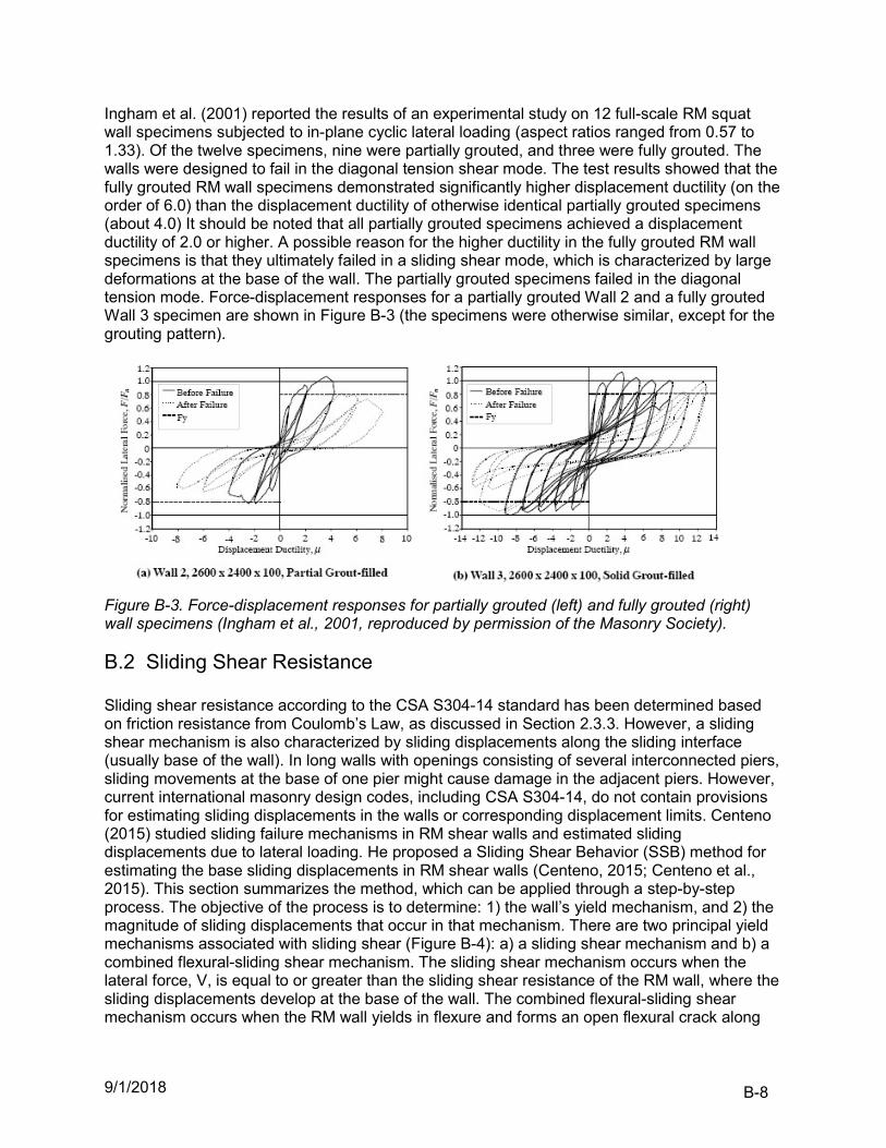
9/1/2018 B-8

Ingham et al. (2001) reported the results of an experimental study on 12 full-scale RM squat wall specimens subjected to in-plane cyclic lateral loading (aspect ratios ranged from 0.57 to 1.33). Of the twelve specimens, nine were partially grouted, and three were fully grouted. The walls were designed to fail in the diagonal tension shear mode. The test results showed that the fully grouted RM wall specimens demonstrated significantly higher displacement ductility (on the order of 6.0) than the displacement ductility of otherwise identical partially grouted specimens (about 4.0) It should be noted that all partially grouted specimens achieved a displacement ductility of 2.0 or higher. A possible reason for the higher ductility in the fully grouted RM wall specimens is that they ultimately failed in a sliding shear mode, which is characterized by large deformations at the base of the wall. The partially grouted specimens failed in the diagonal tension mode. Force-displacement responses for a partially grouted Wall 2 and a fully grouted Wall 3 specimen are shown in Figure B-3 (the specimens were otherwise similar, except for the grouting pattern).

Figure B-3. Force-displacement responses for partially grouted (left) and fully grouted (right) wall specimens (Ingham et al., 2001, reproduced by permission of the Masonry Society).

B.2 Sliding Shear Resistance Sliding shear resistance according to the CSA S304-14 standard has been determined based on friction resistance from Coulomb’s Law, as discussed in Section 2.3.3. However, a sliding shear mechanism is also characterized by sliding displacements along the sliding interface (usually base of the wall). In long walls with openings consisting of several interconnected piers, sliding movements at the base of one pier might cause damage in the adjacent piers. However, current international masonry design codes, including CSA S304-14, do not contain provisions for estimating sliding displacements in the walls or corresponding displacement limits. Centeno (2015) studied sliding failure mechanisms in RM shear walls and estimated sliding displacements due to lateral loading. He proposed a Sliding Shear Behavior (SSB) method for estimating the base sliding displacements in RM shear walls (Centeno, 2015; Centeno et al., 2015). This section summarizes the method, which can be applied through a step-by-step process. The objective of the process is to determine: 1) the wall’s yield mechanism, and 2) the magnitude of sliding displacements that occur in that mechanism. There are two principal yield mechanisms associated with sliding shear (Figure B-4): a) a sliding shear mechanism and b) a combined flexural-sliding shear mechanism. The sliding shear mechanism occurs when the lateral force, V, is equal to or greater than the sliding shear resistance of the RM wall, where the sliding displacements develop at the base of the wall. The combined flexural-sliding shear mechanism occurs when the RM wall yields in flexure and forms an open flexural crack along

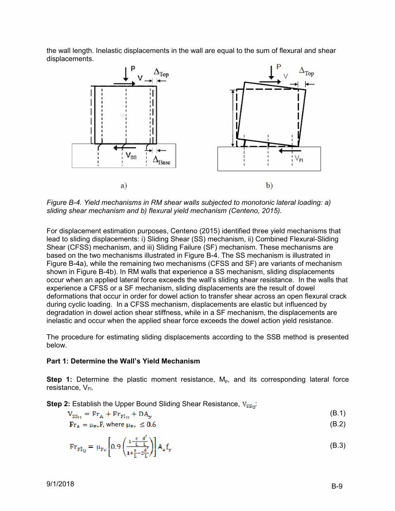
9/1/2018 B-9

the wall length. Inelastic displacements in the wall are equal to the sum of flexural and shear displacements.

Figure B-4. Yield mechanisms in RM shear walls subjected to monotonic lateral loading: a) sliding shear mechanism and b) flexural yield mechanism (Centeno, 2015).

For displacement estimation purposes, Centeno (2015) identified three yield mechanisms that lead to sliding displacements: i) Sliding Shear (SS) mechanism, ii) Combined Flexural-Sliding Shear (CFSS) mechanism, and iii) Sliding Failure (SF) mechanism. These mechanisms are based on the two mechanisms illustrated in Figure B-4. The SS mechanism is illustrated in Figure B-4a), while the remaining two mechanisms (CFSS and SF) are variants of mechanism shown in Figure B-4b). In RM walls that experience a SS mechanism, sliding displacements occur when an applied lateral force exceeds the wall’s sliding shear resistance. In the walls that experience a CFSS or a SF mechanism, sliding displacements are the result of dowel deformations that occur in order for dowel action to transfer shear across an open flexural crack during cyclic loading. In a CFSS mechanism, displacements are elastic but influenced by degradation in dowel action shear stiffness, while in a SF mechanism, the displacements are inelastic and occur when the applied shear force exceeds the dowel action yield resistance. The procedure for estimating sliding displacements according to the SSB method is presented below.

Part 1: Determine the Wall’s Yield Mechanism

Step 1: Determine the plastic moment resistance, Mp, and its corresponding lateral force resistance, VFl. Step 2: Establish the Upper Bound Sliding Shear Resistance, :

(B.1)

, where (B.2)

(B.3)

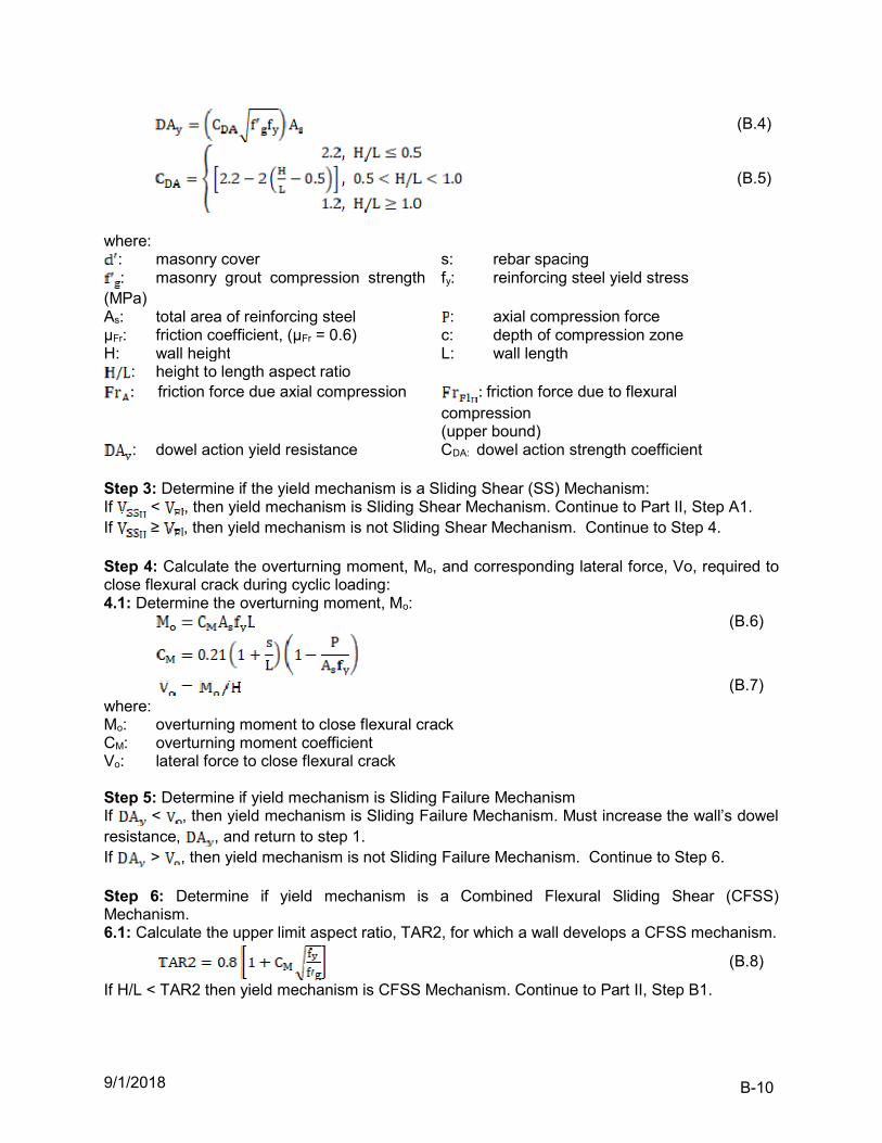
9/1/2018 B-10

(B.4)

(B.5)

where:

: masonry cover s: rebar spacing : masonry grout compression strength

(MPa) fy: reinforcing steel yield stress

As: total area of reinforcing steel : axial compression force µFr: friction coefficient, (µFr = 0.6) c: depth of compression zone H: wall height L: wall length

: height to length aspect ratio : friction force due axial compression : friction force due to flexural

compression (upper bound)

: dowel action yield resistance CDA: dowel action strength coefficient Step 3: Determine if the yield mechanism is a Sliding Shear (SS) Mechanism: If < , then yield mechanism is Sliding Shear Mechanism. Continue to Part II, Step A1. If ≥ , then yield mechanism is not Sliding Shear Mechanism. Continue to Step 4. Step 4: Calculate the overturning moment, Mo, and corresponding lateral force, Vo, required to close flexural crack during cyclic loading: 4.1: Determine the overturning moment, Mo:

(B.6)

(B.7) where: Mo: overturning moment to close flexural crack CM: overturning moment coefficient Vo: lateral force to close flexural crack Step 5: Determine if yield mechanism is Sliding Failure Mechanism If < , then yield mechanism is Sliding Failure Mechanism. Must increase the wall’s dowel resistance, , and return to step 1. If > , then yield mechanism is not Sliding Failure Mechanism. Continue to Step 6. Step 6: Determine if yield mechanism is a Combined Flexural Sliding Shear (CFSS) Mechanism. 6.1: Calculate the upper limit aspect ratio, TAR2, for which a wall develops a CFSS mechanism.

(B.8)

If H/L < TAR2 then yield mechanism is CFSS Mechanism. Continue to Part II, Step B1.

9/1/2018 B-11

If H/L ≥ TAR2 then yield mechanism is a Flexural Mechanism. Sliding displacements in the wall design will be small. If necessary, the sliding displacements can be measured by continuing to Part II, Step B1. Part II: Estimate the Sliding Displacements Step A: Estimate sliding displacements for a SS mechanism A1: Calculate the upper limit aspect ratio, TAR1, for which a wall develops a SS mechanism. TAR1 = H/L (when ) (B.9) (Note: Calculating TAR1 requires trying multiple values of H/L until finding the aspect ratio that meets the condition in equation B.9) A2: Calculate the friction from flexural compression, , This is a correction of the friction force component that corresponds to flexural yielding, because in a wall that develops a sliding shear mechanism not all of the tension reinforcement will reach its yielding stress due to flexure. Therefore, the friction force, FrFl, is only a fraction of the upper bound friction force, , determined in step 2.

(B.10)

A3: Determine sliding shear resistance, VSS, due to a SS mechanism:

(B.11) A4: Calculate wall lateral stiffness, , Following the recommended empirical equation by Shing et al. (1990) for the lateral stiffness of a wall with a shear-dominant response:

(B.12)

(B.13)

where: : elastic shear stiffness : Elastic Modulus of Masonry

: post-cracking shear stiffness : Poisson ratio, (for Masonry, = 0.2) t: wall thickness A5: Sliding Displacement Equation for SS Mechanism,

, when (B.14)

where: : wall base sliding displacement

µ: displacement ductility ratio Step B: Estimate sliding displacements for a CFSS mechanism B1: Determine Triggering aspect ratios: TAR1, TAR2 and TAR3. TAR1 = H/L when (B.9)

(B.8)

TAR3 = H/L when (B.15)

9/1/2018 B-12

Note that calculation of TAR1 and TAR3 requires trying multiple values of H/L until finding the aspect ratio that meets the condition in equations B.9 and B.15, respectively) B2: Calculate dowel action secant stiffness coefficient, Ck.

(B.16a)

(B.17b)

where: µ: displacement ductility ratio B3: Determine dowel action yield stiffness, kDA.

(B.18)

Note: f’g (MPa), db (mm) (B.19)

B4: Calculate base sliding displacement, ∆Base.

(B.20)

B.3 Ductile Seismic Response of Reinforced Masonry Shear Walls A prime consideration in seismic design is the need to have a structure that is capable of deforming in a ductile manner when subjected to several cycles of lateral loading well into the inelastic range. This section explains a few key terms related to ductile seismic response, including ductility ratio, curvature, plastic hinge, etc. It is important for a structural designer to have a good understanding of these concepts before proceeding with the seismic design and detailing of ductile masonry walls according to CSA S304-14. In particular, the content of this section is related to the ductility check for RM shear walls discussed in Section 2.6.3. Ductility is a measure of the capacity of a structure or a member to undergo deformation beyond yield level, while maintaining most of its load-carrying capacity. Ductile structural members are able to absorb and dissipate earthquake energy by inelastic (plastic) deformations that are usually associated with permanent structural damage. These inelastic deformations are concentrated mainly in regions called plastic hinges. In general, plastic hinges develop in shear walls responding in the flexural mode and are typically formed at their base. An example of a plastic hinge formed in a RM wall subjected to seismic loading is shown in Figure 2-8a. The concept of ductility and ductile seismic response was introduced in Section 1.4.3. A common way to quantify ductility in a structure is through the displacement ductility ratio . This is the ratio of the maximum lateral displacement experienced by the structure at the ultimate ( u ), to the displacement at the onset of inelastic response ( y ) (see Figure 1-5c).

y

u

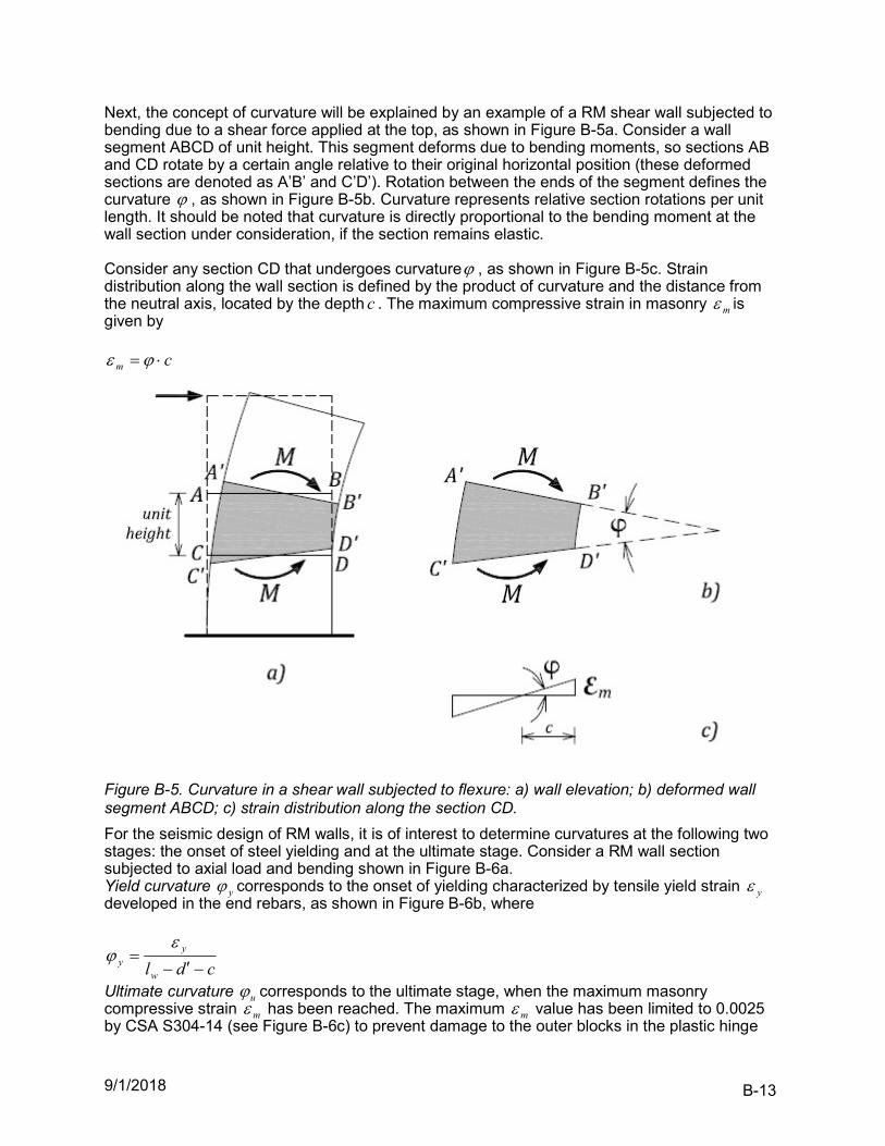
9/1/2018 B-13

Next, the concept of curvature will be explained by an example of a RM shear wall subjected to bending due to a shear force applied at the top, as shown in Figure B-5a. Consider a wall segment ABCD of unit height. This segment deforms due to bending moments, so sections AB and CD rotate by a certain angle relative to their original horizontal position (these deformed sections are denoted as A’B’ and C’D’). Rotation between the ends of the segment defines the curvature , as shown in Figure B-5b. Curvature represents relative section rotations per unit length. It should be noted that curvature is directly proportional to the bending moment at the wall section under consideration, if the section remains elastic. Consider any section CD that undergoes curvature , as shown in Figure B-5c. Strain distribution along the wall section is defined by the product of curvature and the distance from the neutral axis, located by the depth c . The maximum compressive strain in masonry m is given by

cm

Figure B-5. Curvature in a shear wall subjected to flexure: a) wall elevation; b) deformed wall segment ABCD; c) strain distribution along the section CD.

For the seismic design of RM walls, it is of interest to determine curvatures at the following two stages: the onset of steel yielding and at the ultimate stage. Consider a RM wall section subjected to axial load and bending shown in Figure B-6a. Yield curvature y corresponds to the onset of yielding characterized by tensile yield strain y developed in the end rebars, as shown in Figure B-6b, where

cdlw

yy

Ultimate curvature u corresponds to the ultimate stage, when the maximum masonry compressive strain m has been reached. The maximum m value has been limited to 0.0025 by CSA S304-14 (see Figure B-6c) to prevent damage to the outer blocks in the plastic hinge

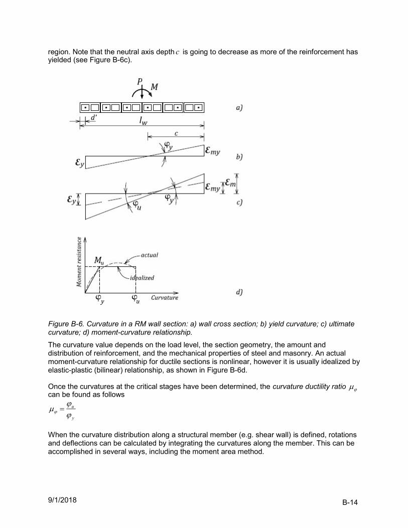
9/1/2018 B-14

region. Note that the neutral axis depth c is going to decrease as more of the reinforcement has yielded (see Figure B-6c).

Figure B-6. Curvature in a RM wall section: a) wall cross section; b) yield curvature; c) ultimate curvature; d) moment-curvature relationship.

The curvature value depends on the load level, the section geometry, the amount and distribution of reinforcement, and the mechanical properties of steel and masonry. An actual moment-curvature relationship for ductile sections is nonlinear, however it is usually idealized by elastic-plastic (bilinear) relationship, as shown in Figure B-6d. Once the curvatures at the critical stages have been determined, the curvature ductility ratio can be found as follows

y

u

When the curvature distribution along a structural member (e.g. shear wall) is defined, rotations and deflections can be calculated by integrating the curvatures along the member. This can be accomplished in several ways, including the moment area method.

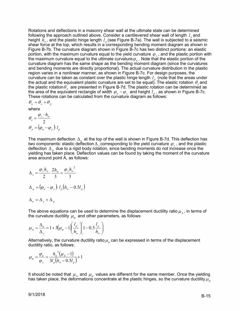
9/1/2018 B-15

Rotations and deflections in a masonry shear wall at the ultimate state can be determined following the approach outlined above. Consider a cantilevered shear wall of length wl and height wh , and the plastic hinge length pl (see Figure B-7a). The wall is subjected to a seismic shear force at the top, which results in a corresponding bending moment diagram as shown in Figure B-7b. The curvature diagram shown in Figure B-7c has two distinct portions: an elastic portion, with the maximum curvature equal to the yield curvature y , and the plastic portion with the maximum curvature equal to the ultimate curvature u . Note that the elastic portion of the curvature diagram has the same shape as the bending moment diagram (since the curvatures and bending moments are directly proportional). The actual curvature distribution in the plastic region varies in a nonlinear manner, as shown in Figure B-7c. For design purposes, the curvature can be taken as constant over the plastic hinge length pl (note that the areas under the actual and the equivalent plastic curvature are set to be equal). The elastic rotation e and the plastic rotation p are presented in Figure B-7d. The plastic rotation can be determined as the area of the equivalent rectangle of width yu and height pl , as shown in Figure B-7c. These rotations can be calculated from the curvature diagram as follows:

peu

where

2wy

e

h

pyup l

The maximum deflection u at the top of the wall is shown in Figure B-7d. This deflection has two components: elastic deflection y corresponding to the yield curvature y , and the plastic deflection p due to a rigid body rotation, since bending moments do not increase once the yielding has taken place. Deflection values can be found by taking the moment of the curvature area around point A, as follows:

33

2

2

2wywwy

y

hhh

pwpyup lhl 5.0

pyu

The above equations can be used to determine the displacement ductility ratio , in terms of the curvature ductility and other parameters, as follows:

w

p

w

p

y

u

h

l

h

l5.01131

Alternatively, the curvature ductility ratio can be expressed in terms of the displacement ductility ratio, as follows:

1

5.03

12

pwp

w

y

u

lhl

h

It should be noted that and values are different for the same member. Once the yielding has taken place, the deformations concentrate at the plastic hinges, so the curvature ductility

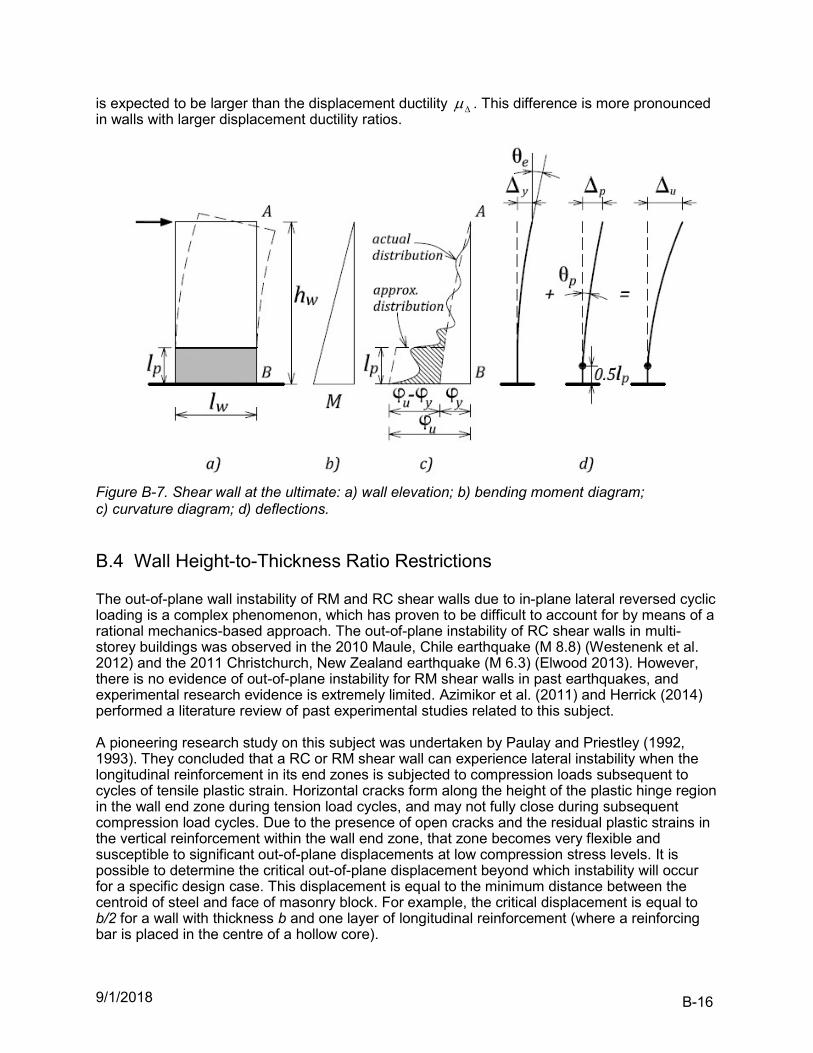
9/1/2018 B-16

is expected to be larger than the displacement ductility . This difference is more pronounced in walls with larger displacement ductility ratios.

Figure B-7. Shear wall at the ultimate: a) wall elevation; b) bending moment diagram; c) curvature diagram; d) deflections.

B.4 Wall Height-to-Thickness Ratio Restrictions The out-of-plane wall instability of RM and RC shear walls due to in-plane lateral reversed cyclic loading is a complex phenomenon, which has proven to be difficult to account for by means of a rational mechanics-based approach. The out-of-plane instability of RC shear walls in multi-storey buildings was observed in the 2010 Maule, Chile earthquake (M 8.8) (Westenenk et al. 2012) and the 2011 Christchurch, New Zealand earthquake (M 6.3) (Elwood 2013). However, there is no evidence of out-of-plane instability for RM shear walls in past earthquakes, and experimental research evidence is extremely limited. Azimikor et al. (2011) and Herrick (2014) performed a literature review of past experimental studies related to this subject. A pioneering research study on this subject was undertaken by Paulay and Priestley (1992, 1993). They concluded that a RC or RM shear wall can experience lateral instability when the longitudinal reinforcement in its end zones is subjected to compression loads subsequent to cycles of tensile plastic strain. Horizontal cracks form along the height of the plastic hinge region in the wall end zone during tension load cycles, and may not fully close during subsequent compression load cycles. Due to the presence of open cracks and the residual plastic strains in the vertical reinforcement within the wall end zone, that zone becomes very flexible and susceptible to significant out-of-plane displacements at low compression stress levels. It is possible to determine the critical out-of-plane displacement beyond which instability will occur for a specific design case. This displacement is equal to the minimum distance between the centroid of steel and face of masonry block. For example, the critical displacement is equal to b/2 for a wall with thickness b and one layer of longitudinal reinforcement (where a reinforcing bar is placed in the centre of a hollow core).

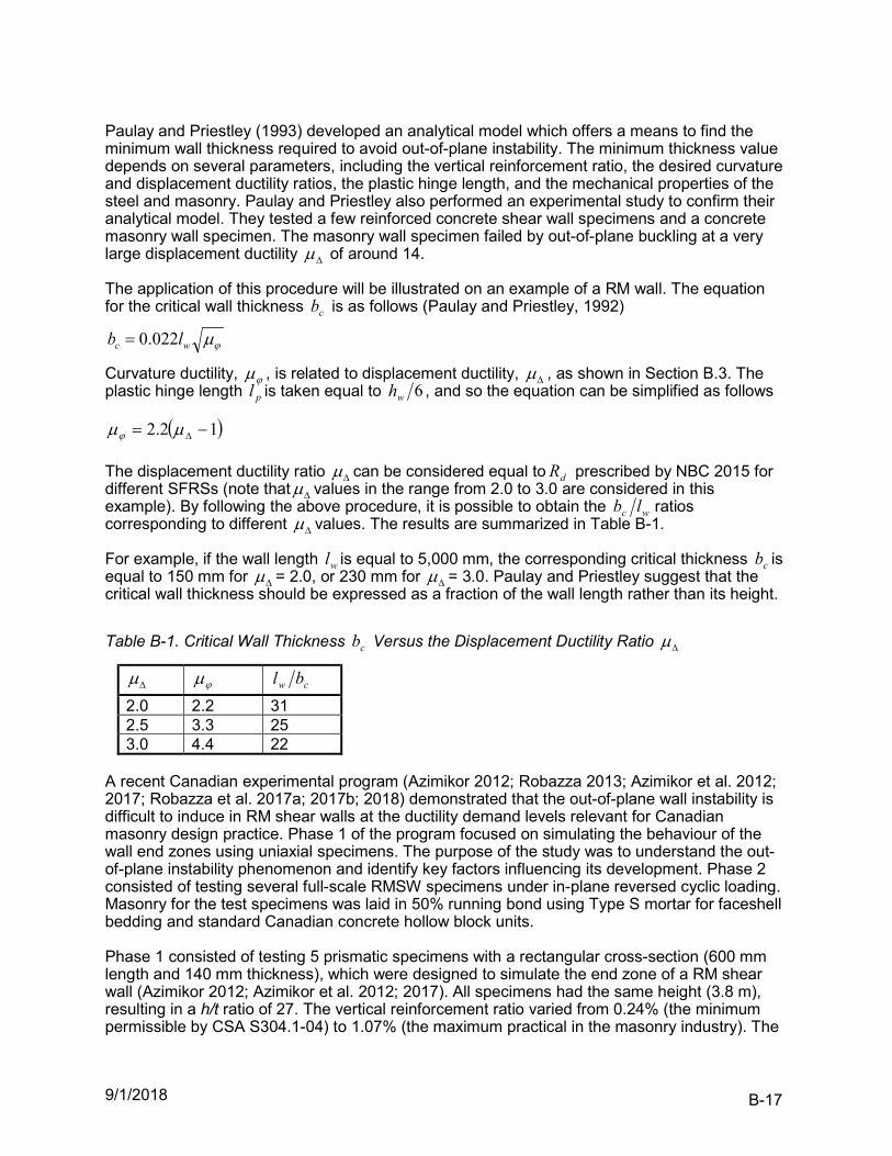
9/1/2018 B-17

Paulay and Priestley (1993) developed an analytical model which offers a means to find the minimum wall thickness required to avoid out-of-plane instability. The minimum thickness value depends on several parameters, including the vertical reinforcement ratio, the desired curvature and displacement ductility ratios, the plastic hinge length, and the mechanical properties of the steel and masonry. Paulay and Priestley also performed an experimental study to confirm their analytical model. They tested a few reinforced concrete shear wall specimens and a concrete masonry wall specimen. The masonry wall specimen failed by out-of-plane buckling at a very large displacement ductility of around 14. The application of this procedure will be illustrated on an example of a RM wall. The equation for the critical wall thickness cb is as follows (Paulay and Priestley, 1992)

wc lb 022.0

Curvature ductility, , is related to displacement ductility, , as shown in Section B.3. The plastic hinge length pl is taken equal to 6wh , and so the equation can be simplified as follows

12.2

The displacement ductility ratio can be considered equal to dR prescribed by NBC 2015 for different SFRSs (note that values in the range from 2.0 to 3.0 are considered in this example). By following the above procedure, it is possible to obtain the wc lb ratios corresponding to different values. The results are summarized in Table B-1. For example, if the wall length wl is equal to 5,000 mm, the corresponding critical thickness cb is equal to 150 mm for = 2.0, or 230 mm for = 3.0. Paulay and Priestley suggest that the critical wall thickness should be expressed as a fraction of the wall length rather than its height.

Table B-1. Critical Wall Thickness cb Versus the Displacement Ductility Ratio

cw bl

2.0 2.2 31 2.5 3.3 25 3.0 4.4 22

A recent Canadian experimental program (Azimikor 2012; Robazza 2013; Azimikor et al. 2012; 2017; Robazza et al. 2017a; 2017b; 2018) demonstrated that the out-of-plane wall instability is difficult to induce in RM shear walls at the ductility demand levels relevant for Canadian masonry design practice. Phase 1 of the program focused on simulating the behaviour of the wall end zones using uniaxial specimens. The purpose of the study was to understand the out-of-plane instability phenomenon and identify key factors influencing its development. Phase 2 consisted of testing several full-scale RMSW specimens under in-plane reversed cyclic loading. Masonry for the test specimens was laid in 50% running bond using Type S mortar for faceshell bedding and standard Canadian concrete hollow block units. Phase 1 consisted of testing 5 prismatic specimens with a rectangular cross-section (600 mm length and 140 mm thickness), which were designed to simulate the end zone of a RM shear wall (Azimikor 2012; Azimikor et al. 2012; 2017). All specimens had the same height (3.8 m), resulting in a h/t ratio of 27. The vertical reinforcement ratio varied from 0.24% (the minimum permissible by CSA S304.1-04) to 1.07% (the maximum practical in the masonry industry). The

9/1/2018 B-18

loading protocol consisted of reversed-cyclic uniaxial tension and compression displacement cycles of incrementally increasing magnitude until failure. Four specimens experienced out-of-plane instability, while the fifth specimen was a reference specimen which was subjected to monotonic compression and experienced a compression/crushing failure. These tests had some limitations: the specimens were isolated and were not able to simulate actual boundary conditions along the wall height and the effect of strain gradient along the wall length. It was concluded that the level of applied tensile strain in a wall end-zone was one of the critical factors governing its out-of-plane stability. The maximum tensile strain that may be imposed on a ductile RM shear wall’s end-zone could be determined, at least in part, by a kinematic relationship between the axial strain and the out-of-plane displacement. A preliminary mechanical model was proposed which provided a theoretical prediction of the maximum tensile strain before an instability would take place. Phase 2 comprised of an experimental study of 8 full-size RMSW specimens of varying h/t and aspect (h/L) ratios, vertical and horizontal reinforcement amounts and detailing, applied axial pre-compression, and cross-section shape (6 specimens had regular rectangular cross-sections, while the other 2 specimens had T-shaped cross-sections) (Robazza 2013; Robazza et al. 2017a; 2017b; 2018). The specimens were subjected to either cyclic or reversed-cyclic loading until failure. All specimens were designed to exhibit flexure-controlled behavior characterized by the development of high tensile strains over a distinct region of plastic hinging, which is a theoretical prerequisite for the occurrence of out-of-plane instability. The specimens had aspect ratios varying from 1.5 to 3.0, which were required to maintain a relatively large plastic hinge height while still avoiding a shear failure. The specimens were designed with relatively high h/t ratios, ranging from 21.1 to 28.6, which exceeded the maximum CSA S304.1-04 limits for ductile RM shear walls. However, only one specimen experienced out-of-plane displacements large enough to precipitate instability, which occurred only after the wall had reached its ultimate shear capacity and experienced substantial degradation. It was found that several factors may influence the out-of-plane response of RM shear wallsubjected to in-plane loading, including ductility and tensile strain demands, applied pre-compression levels and construction practices, as well as the effects of alternative failure mechanisms. This research also demonstrated that the strain gradient in a RM wall is a very important factor. This was not included in previous numerical models for out-of-plane stability in RM or RC shear walls, which were developed exclusively based on data from testing uniaxial specimens (e.g. Paulay and Priestley, 1993; Chai and Elayer, 1999). The estimates based on these models may lead to overly conservative h/t requirements. Findings of the research by Paulay and Priestley (1992; 1993) were incorporated in the seismic design provisions for RM shear walls in New Zealand. The New Zealand masonry design standard NZS 4230:2004 prescribes the following minimum thicknesses for limited ductility walls ( of 2.0) and ductile walls ( of 4.0): 1. For walls up to 3 storeys high (Cl.7.4.4.1 and 7.3.3), minimum thickness t should not be

less than 20nL (or nL05.0 ), where nL denotes clear vertical distance between lines of effective horizontal support or clear horizontal distance between lines of effective vertical support. Commentary to Cl.7.3.3 states that “for a given wall thickness, t , and the case when lines of horizontal support have a clear vertical spacing of tLn 20 , then vertical lines of support having a clear horizontal spacing of tLn 20 shall be provided.”

2. For walls more than 3 storeys high (Cl.7.4.4.1) minimum thickness t shall not be less than 3.13nL (or nL075.0 ). However, a smaller wall thickness can be used provided that one of

the following conditions is satisfied (maximum strain in masonry u is equal to 0.003 according to NZS 4230:2004) (see Figure 2-28):

a) tc 4 or

9/1/2018 B-19

b) wlc 3.0 or

c) tc 6 from the inside of a wall return of a flanged wall, which has a minimum length

nL2.0 .

The relaxed thickness requirement applies to the cases where the neutral axis depth is small, and so the compressed area may be so small that the adjacent vertical strips of the wall will be able to stabilize it. This is likely the case with rectangular walls subjected to low axial compression. Commentary to NZS 4230 Cl.7.4.4.1 states that it is considered unlikely that failure due to lateral instability of the wall will occur in structures less than 3 storeys high, because of the rapid reduction in flexural compression with height. This is also in line with the statement made by Paulay (1986), that out-of-plane stability is likely to take place in walls with large plastic hinge length (one storey or more). Paulay and Priestley (1992) stated that “where the wall height is less than three storeys, a greater slenderness should be acceptable. In such cases, or where inelastic flexural deformations cannot develop, the wall thickness t need not be less than nL05.0 ” (where

nL denotes clear wall length between the supports). FEMA 306 (1999) also discusses the issue of wall instability. This document also refers to the procedure by Paulay and Priestley (1993) and provides the following recommendation for minimum wall thickness in ductile walls ( of 4.0):

24wlt or 18ht

Note that the above requirement, which applies to the walls with displacement ductility ratio ( ) equal to 4.0. FEMA 306 (1999) also points out that “the lack of evidence for this type of failure in existing structures may be due to the large number of cycles at high ductility that must be achieved – most conventionally designed masonry walls are likely to experience other behaviour modes such as diagonal shear before instability becomes a problem.”

9/1/2018 C-1

TABLE OF CONTENTS – APPENDIX C

C RELEVANT DESIGN BACKGROUND ............................................................................ C-2

C.1 Design for Combined Axial Load and Flexure .......................................................... C-2 C.1.1 Reinforced Masonry Walls Under In-Plane Seismic Loading ............................................... C-2 C.1.2 Reinforced Masonry Walls Under Out-of-Plane Seismic Loading ........................................ C-9

C.2 Wall Intersections and Flanged Shear Walls .......................................................... C-15 C.2.1 Effective Flange Width ........................................................................................................ C-15 C.2.2 Types of Intersections ......................................................................................................... C-16 C.2.3 Shear Resistance at the Intersections ................................................................................ C-18

C.3 Wall Stiffness Calculations ...................................................................................... C-22 C.3.1 Lateral Load Distribution ..................................................................................................... C-22 C.3.2 Wall Stiffness: Cantilever and Fixed-End Model ................................................................. C-23 C.3.3 Approximate Method for Force Distribution in Masonry Shear Walls ................................. C-24 C.3.4 Advanced Design Approaches for Reinforced Masonry Shear Walls with Openings ......... C-27 C.3.5 The Effect of Cracking on Wall Stiffness ............................................................................. C-32

9/1/2018 C-2

C Relevant Design Background This appendix contains additional information relevant for masonry design as discussed in Chapter 2, but it is not directly related to the seismic design provisions of CSA S304-14. Applications of the design methods and procedures presented in this appendix can be found in Chapter 3, which contains several design examples. This appendix addresses in detail several topics of interest to masonry designers, e.g., the calculation of in-plane wall stiffness, including the effect of cracking, and force distribution in perforated shear walls. However, modeling and analysis of multi-storey perforated shear walls are not covered in this document.

C.1 Design for Combined Axial Load and Flexure

C.1.1 Reinforced Masonry Walls Under In-Plane Seismic Loading 10.2

Seismic shear forces acting at floor and roof levels cause overturning bending moments in shear walls, which reach a maximum at the base level. In general, shear walls are subjected to the combined effects of flexure and axial gravity loads. The theory behind the design of masonry wall sections subjected to effects of flexure and axial load is well established, and is essentially the same as that of reinforced concrete walls. A typical reinforced masonry wall section is shown in Figure C-1a), along with the distribution of internal forces and strains arising from the axial load and moment. According to CSA S304-14, the strain distribution along the wall length is based on the assumptions that the wall section remains plane and that the maximum compressive masonry strain m is equal to 0.003 (see Figure C-1b)). Figure C-1c) shows the distribution of internal forces on the base of the wall, as well as the axial load, fP and the bending moment, fM . In the compression zone, the equivalent rectangular stress block has a depth a , and a maximum stress intensity of mm f '85.0 . Note that the factor assumes a value of 1.0 for members subjected to compression perpendicular to the bed joints, such as structural walls (S304-14 Cl.10.2.6). Each reinforcing bar develops an internal force (either tension or compression) equal to the product of the factored stress and the corresponding bar area. The internal vertical forces must be in equilibrium with fP , and the factored moment capacity rM can be determined by taking the sum of the moments of the internal forces around the centroid of the section. The following three design scenarios and the related simplified design procedures will be discussed in this section:

1. Wall reinforcement (both concentrated and distributed) and axial load are given – find moment capacity

2. Wall is reinforced with distributed reinforcement only – find moment capacity 3. Wall reinforcement needs to be estimated (factored bending moment and axial force are

given) The first two are applicable for the common situations where a designer assumes the minimum seismic reinforcement amount and desires to find its moment capacity. Approximate design approaches that can be used to assist designers in each of these scenarios are presented below. For detailed analysis and design procedures, the reader is referred to Drysdale and Hamid (2005) and Hatzinikolas, Korany and Brzev (2015).

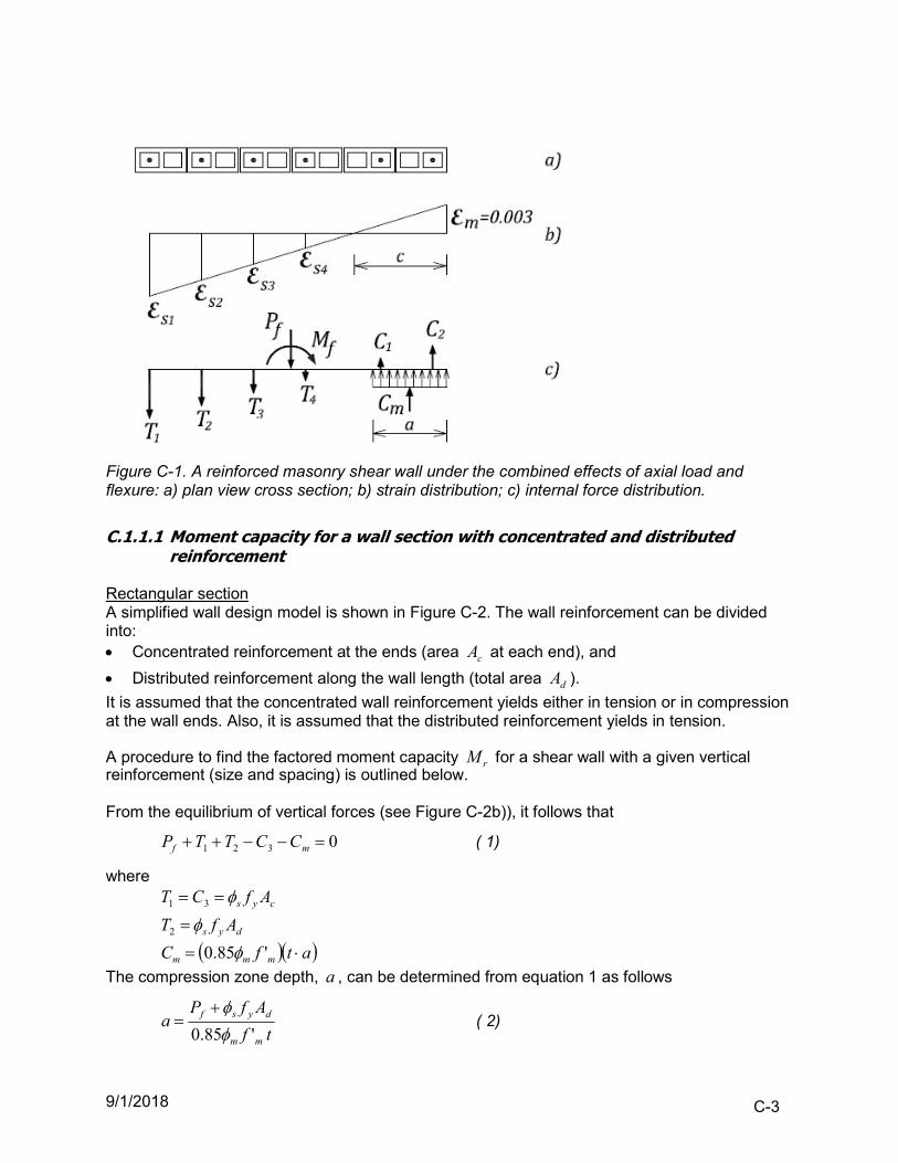
9/1/2018 C-3

Figure C-1. A reinforced masonry shear wall under the combined effects of axial load and flexure: a) plan view cross section; b) strain distribution; c) internal force distribution.

C.1.1.1 Moment capacity for a wall section with concentrated and distributed

reinforcement Rectangular section A simplified wall design model is shown in Figure C-2. The wall reinforcement can be divided into: Concentrated reinforcement at the ends (area cA at each end), and

Distributed reinforcement along the wall length (total area dA ).

It is assumed that the concentrated wall reinforcement yields either in tension or in compression at the wall ends. Also, it is assumed that the distributed reinforcement yields in tension. A procedure to find the factored moment capacity rM for a shear wall with a given vertical reinforcement (size and spacing) is outlined below. From the equilibrium of vertical forces (see Figure C-2b)), it follows that

0321 mf CCTTP ( 1)

where

cys AfCT 31

dys AfT 2

atfC mmm '85.0

The compression zone depth, a , can be determined from equation 1 as follows

tf

AfPa

mm

dysf

'85.0

( 2)

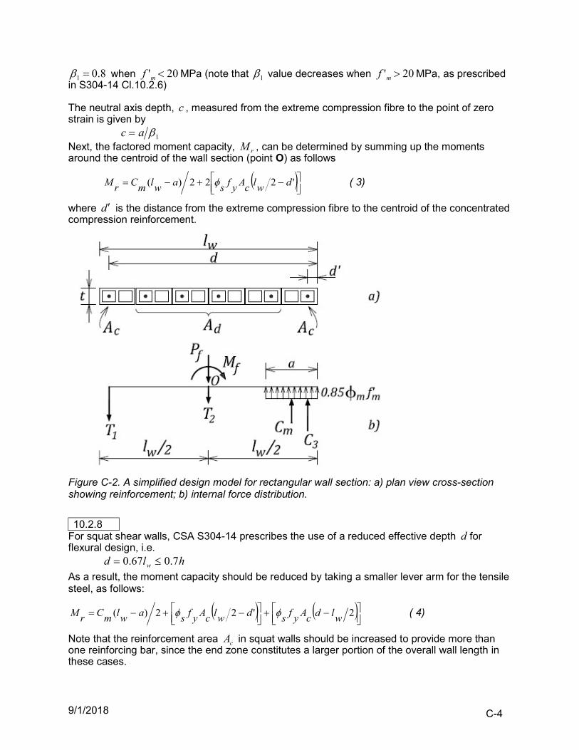
9/1/2018 C-4

8.01 when 20' mf MPa (note that 1 value decreases when 20' mf MPa, as prescribed in S304-14 Cl.10.2.6) The neutral axis depth, c , measured from the extreme compression fibre to the point of zero strain is given by 1ac Next, the factored moment capacity, rM , can be determined by summing up the moments around the centroid of the wall section (point O) as follows

'222)( dwlcAyfsawlmCrM ( 3)

where d is the distance from the extreme compression fibre to the centroid of the concentrated compression reinforcement.

Figure C-2. A simplified design model for rectangular wall section: a) plan view cross-section showing reinforcement; b) internal force distribution.

10.2.8

For squat shear walls, CSA S304-14 prescribes the use of a reduced effective depth d for flexural design, i.e.

hld w 7.067.0

As a result, the moment capacity should be reduced by taking a smaller lever arm for the tensile steel, as follows:

2'22)( wldcAyfsdwlcAyfsawlmCrM ( 4)

Note that the reinforcement area cA in squat walls should be increased to provide more than one reinforcing bar, since the end zone constitutes a larger portion of the overall wall length in these cases.

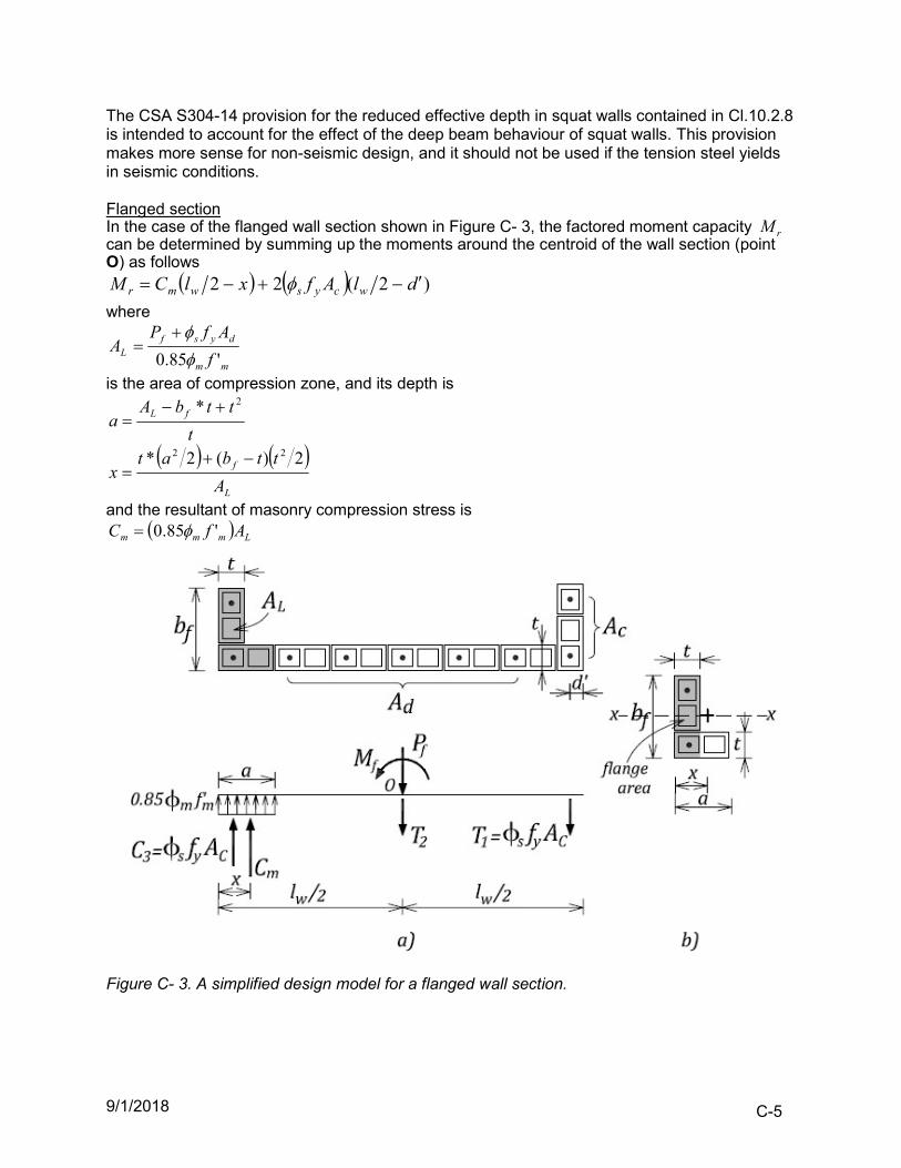
9/1/2018 C-5

The CSA S304-14 provision for the reduced effective depth in squat walls contained in Cl.10.2.8 is intended to account for the effect of the deep beam behaviour of squat walls. This provision makes more sense for non-seismic design, and it should not be used if the tension steel yields in seismic conditions. Flanged section In the case of the flanged wall section shown in Figure C- 3, the factored moment capacity rM can be determined by summing up the moments around the centroid of the wall section (point O) as follows

)2(22 dlAfxlCM wcyswmr

where

mm

dysfL f

AfPA

'85.0

is the area of compression zone, and its depth is

t

ttbAa fL

2*

L

f

A

ttbatx

2)(2* 22

and the resultant of masonry compression stress is Lmmm AfC '85.0

Figure C- 3. A simplified design model for a flanged wall section.

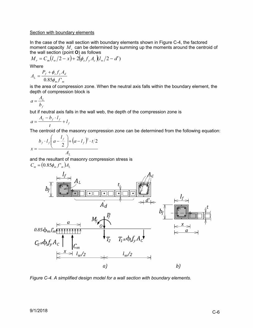
9/1/2018 C-6

Section with boundary elements In the case of the wall section with boundary elements shown in Figure C-4, the factored moment capacity rM can be determined by summing up the moments around the centroid of the wall section (point O) as follows

)2(22 dlAfxlCM wcyswmr

Where

mm

dysfL f

AfPA

'85.0

is the area of compression zone. When the neutral axis falls within the boundary element, the depth of compression block is

f

L

b

Aa

but if neutral axis falls in the wall web, the depth of the compression zone is

fffL l

t

lbAa

The centroid of the masonry compression zone can be determined from the following equation:

L

ff

ff

A

tlal

alb

x

22

2

and the resultant of masonry compression stress is Lmmm AfC '85.0

Figure C-4. A simplified design model for a wall section with boundary elements.

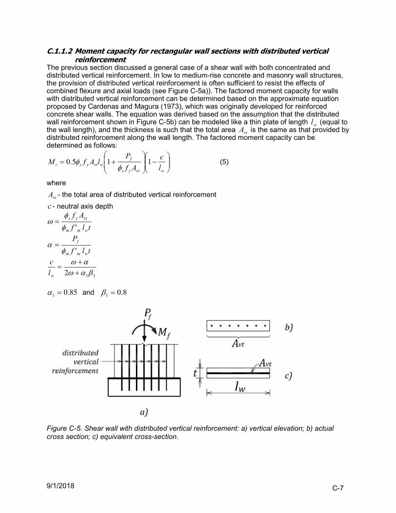
9/1/2018 C-7

C.1.1.2 Moment capacity for rectangular wall sections with distributed vertical reinforcement

The previous section discussed a general case of a shear wall with both concentrated and distributed vertical reinforcement. In low to medium-rise concrete and masonry wall structures, the provision of distributed vertical reinforcement is often sufficient to resist the effects of combined flexure and axial loads (see Figure C-5a)). The factored moment capacity for walls with distributed vertical reinforcement can be determined based on the approximate equation proposed by Cardenas and Magura (1973), which was originally developed for reinforced concrete shear walls. The equation was derived based on the assumption that the distributed wall reinforcement shown in Figure C-5b) can be modeled like a thin plate of length wl (equal to the wall length), and the thickness is such that the total area vtA is the same as that provided by distributed reinforcement along the wall length. The factored moment capacity can be determined as follows:

wvtys

fwvtysr l

c

Af

PlAfM 115.0

(5)

where

vtA - the total area of distributed vertical reinforcement

c - neutral axis depth

tlf

Af

wmm

vtys

'

tlf

P

wmm

f

'

112

wl

c

85.01 and 8.01

Figure C-5. Shear wall with distributed vertical reinforcement: a) vertical elevation; b) actual cross section; c) equivalent cross-section.

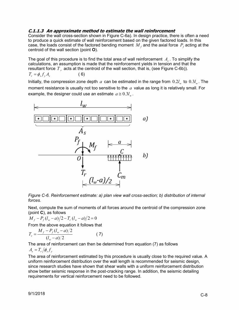
9/1/2018 C-8

C.1.1.3 An approximate method to estimate the wall reinforcement Consider the wall cross-section shown in Figure C-6a). In design practice, there is often a need to produce a quick estimate of wall reinforcement based on the given factored loads. In this case, the loads consist of the factored bending moment fM and the axial force fP acting at the centroid of the wall section (point O). The goal of this procedure is to find the total area of wall reinforcement sA . To simplify the calculations, an assumption is made that the reinforcement yields in tension and that the resultant force rT acts at the centroid of the wall section, that is, (see Figure C-6b)).

sysr AfT ( 6)

Initially, the compression zone depth a can be estimated in the range from 0.2 wl to 0.3 wl . The

moment resistance is usually not too sensitive to the a value as long it is relatively small. For example, the designer could use an estimate wla 3.0 .

Figure C-6. Reinforcement estimate: a) plan view wall cross-section; b) distribution of internal forces.

Next, compute the sum of moments of all forces around the centroid of the compression zone (point C), as follows

02)(2)( alTalPM wrwff

From the above equation it follows that

2)(

2)(

al

alPMT

w

wffr

( 7)

The area of reinforcement can then be determined from equation (7) as follows

ysrs fTA

The area of reinforcement estimated by this procedure is usually close to the required value. A uniform reinforcement distribution over the wall length is recommended for seismic design, since research studies have shown that shear walls with a uniform reinforcement distribution show better seismic response in the post-cracking range. In addition, the seismic detailing requirements for vertical reinforcement need to be followed.

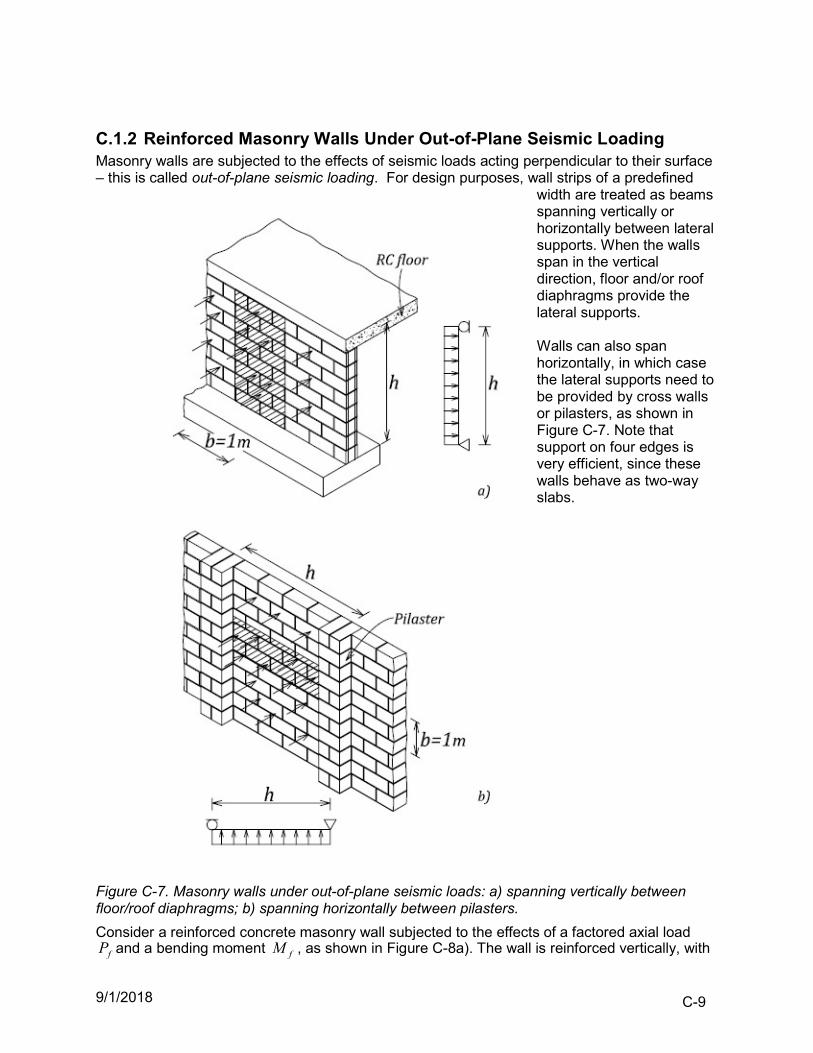
9/1/2018 C-9

C.1.2 Reinforced Masonry Walls Under Out-of-Plane Seismic Loading Masonry walls are subjected to the effects of seismic loads acting perpendicular to their surface – this is called out-of-plane seismic loading. For design purposes, wall strips of a predefined

width are treated as beams spanning vertically or horizontally between lateral supports. When the walls span in the vertical direction, floor and/or roof diaphragms provide the lateral supports. Walls can also span horizontally, in which case the lateral supports need to be provided by cross walls or pilasters, as shown in Figure C-7. Note that support on four edges is very efficient, since these walls behave as two-way slabs.

Figure C-7. Masonry walls under out-of-plane seismic loads: a) spanning vertically between floor/roof diaphragms; b) spanning horizontally between pilasters.

Consider a reinforced concrete masonry wall subjected to the effects of a factored axial load fP and a bending moment fM , as shown in Figure C-8a). The wall is reinforced vertically, with

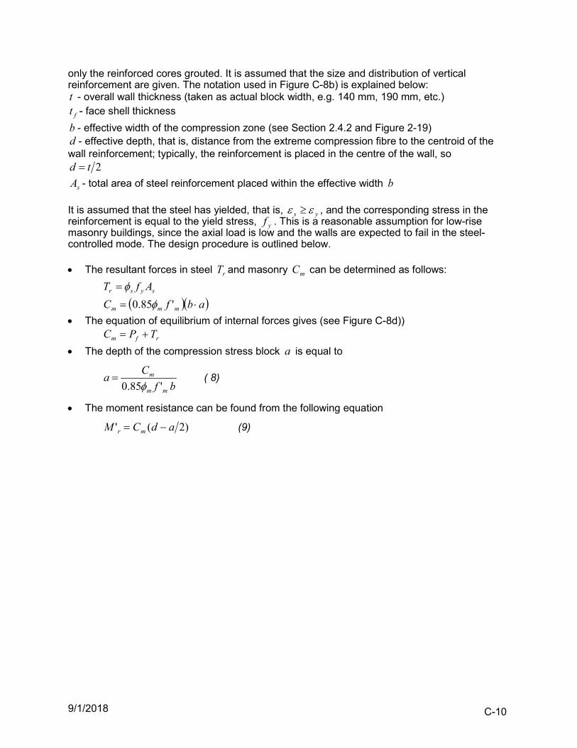
9/1/2018 C-10

only the reinforced cores grouted. It is assumed that the size and distribution of vertical reinforcement are given. The notation used in Figure C-8b) is explained below: t - overall wall thickness (taken as actual block width, e.g. 140 mm, 190 mm, etc.)

ft - face shell thickness

b - effective width of the compression zone (see Section 2.4.2 and Figure 2-19) d - effective depth, that is, distance from the extreme compression fibre to the centroid of the wall reinforcement; typically, the reinforcement is placed in the centre of the wall, so

2td

sA - total area of steel reinforcement placed within the effective width b

It is assumed that the steel has yielded, that is, ys , and the corresponding stress in the reinforcement is equal to the yield stress, yf . This is a reasonable assumption for low-rise masonry buildings, since the axial load is low and the walls are expected to fail in the steel-controlled mode. The design procedure is outlined below. The resultant forces in steel rT and masonry mC can be determined as follows:

sysr AfT

abfC mmm '85.0

The equation of equilibrium of internal forces gives (see Figure C-8d))

rfm TPC

The depth of the compression stress block a is equal to

bf

Ca

mm

m

'85.0 ( 8)

The moment resistance can be found from the following equation

)2(' adCM mr (9)

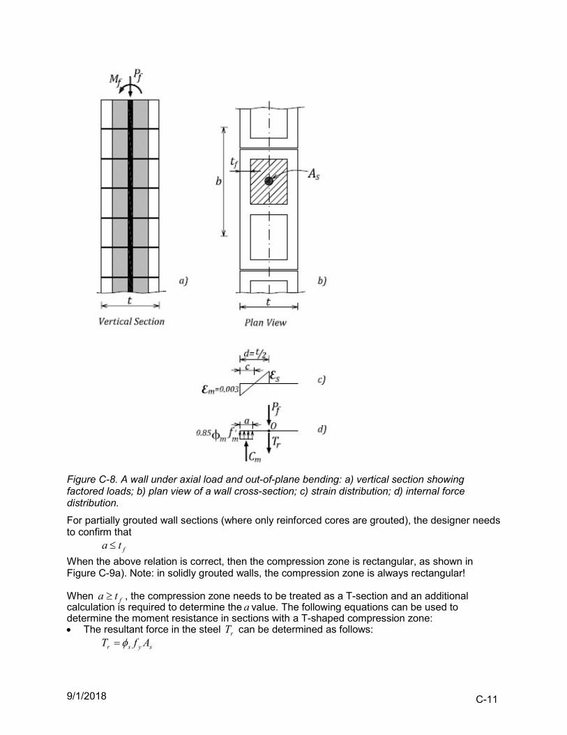
9/1/2018 C-11

Figure C-8. A wall under axial load and out-of-plane bending: a) vertical section showing factored loads; b) plan view of a wall cross-section; c) strain distribution; d) internal force distribution.

For partially grouted wall sections (where only reinforced cores are grouted), the designer needs to confirm that

fta

When the above relation is correct, then the compression zone is rectangular, as shown in Figure C-9a). Note: in solidly grouted walls, the compression zone is always rectangular! When fta , the compression zone needs to be treated as a T-section and an additional calculation is required to determine the a value. The following equations can be used to determine the moment resistance in sections with a T-shaped compression zone: The resultant force in the steel rT can be determined as follows:

sysr AfT

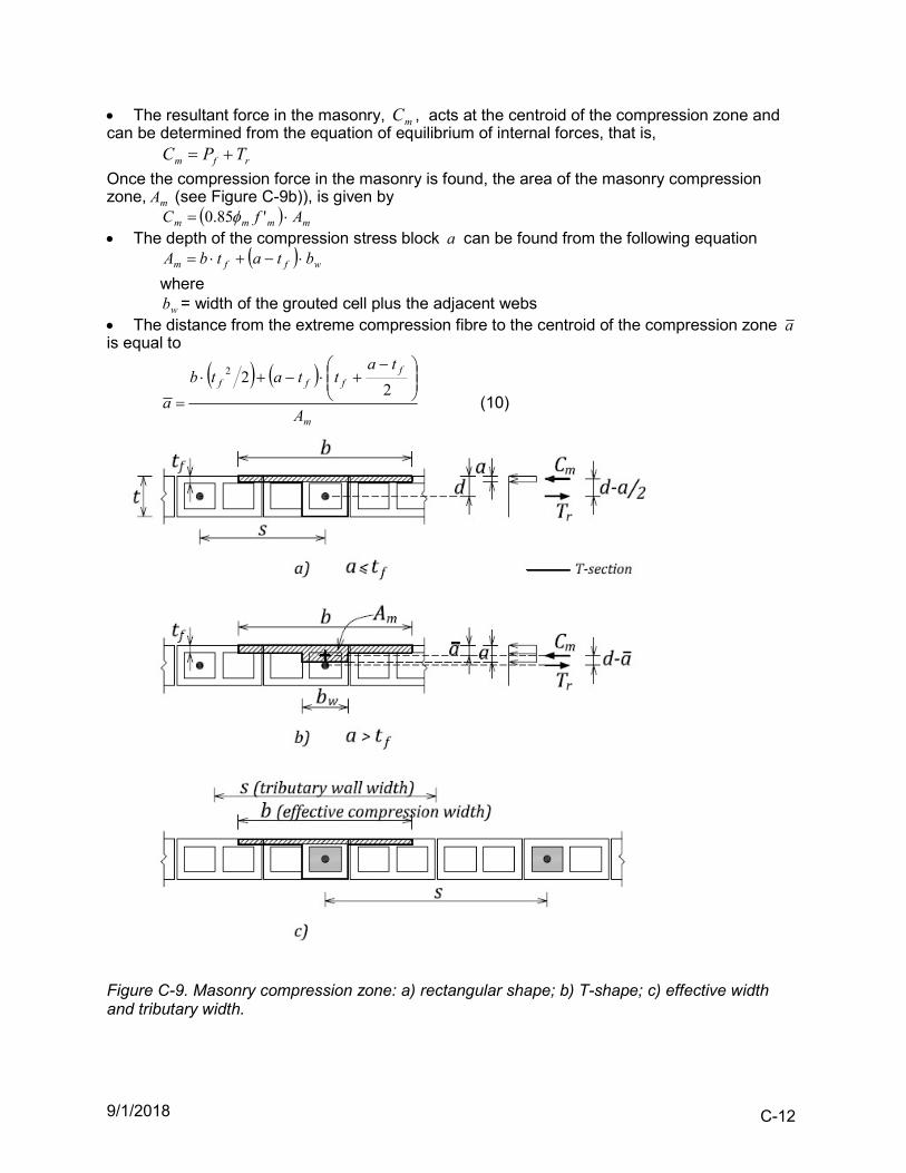
9/1/2018 C-12

The resultant force in the masonry, mC , acts at the centroid of the compression zone and can be determined from the equation of equilibrium of internal forces, that is,

rfm TPC

Once the compression force in the masonry is found, the area of the masonry compression zone, mA (see Figure C-9b)), is given by

mmmm AfC '85.0 The depth of the compression stress block a can be found from the following equation

wffm btatbA

where

wb = width of the grouted cell plus the adjacent webs The distance from the extreme compression fibre to the centroid of the compression zone a is equal to

m

ffff

A

tattatb

a

2

22

(10)

Figure C-9. Masonry compression zone: a) rectangular shape; b) T-shape; c) effective width and tributary width.

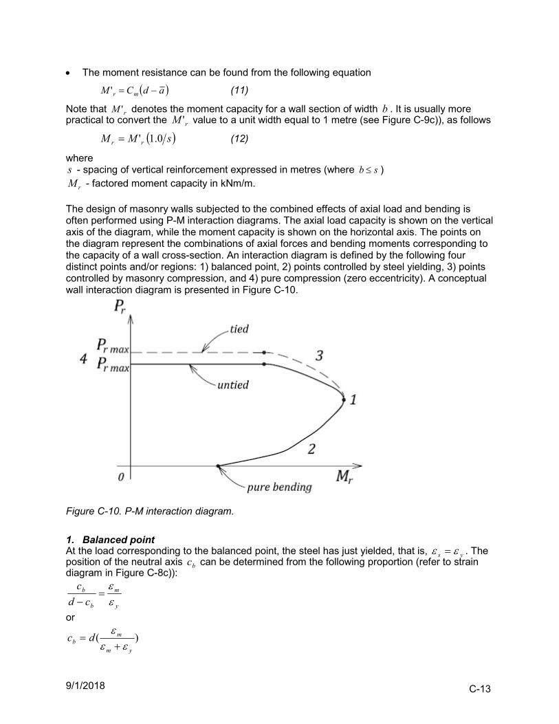
9/1/2018 C-13

The moment resistance can be found from the following equation

adCM mr ' (11)

Note that rM ' denotes the moment capacity for a wall section of width b . It is usually more practical to convert the rM ' value to a unit width equal to 1 metre (see Figure C-9c)), as follows

sMM rr 0.1' (12)

where s - spacing of vertical reinforcement expressed in metres (where sb )

rM - factored moment capacity in kNm/m. The design of masonry walls subjected to the combined effects of axial load and bending is often performed using P-M interaction diagrams. The axial load capacity is shown on the vertical axis of the diagram, while the moment capacity is shown on the horizontal axis. The points on the diagram represent the combinations of axial forces and bending moments corresponding to the capacity of a wall cross-section. An interaction diagram is defined by the following four distinct points and/or regions: 1) balanced point, 2) points controlled by steel yielding, 3) points controlled by masonry compression, and 4) pure compression (zero eccentricity). A conceptual wall interaction diagram is presented in Figure C-10.

Figure C-10. P-M interaction diagram.

1. Balanced point At the load corresponding to the balanced point, the steel has just yielded, that is, ys . The position of the neutral axis bc can be determined from the following proportion (refer to strain diagram in Figure C-8c)):

y

m

b

b

cd

c

or

)(ym

mb dc

9/1/2018 C-14

For 400yf MPa and 002.0y it follows that

dcb 6.0

2. Points controlled by steel yielding For bcc , the steel will yield before the masonry reaches its maximum useful strain (0.003). Since the steel is yielding, it follows that ys . The designer needs to assume the neutral axis depth ( c ) value so that bcc . The compression zone depth can then be calculated as

cca 8.01 (this is valid for MPafm 20 according to S304-14 Cl.10.2.6). Combinations of axial force and moment values corresponding to an assumed neutral axis depth can be found from the following equations of equilibrium (see Figure C-8d)).

rmr TCP

where

sysr AfT (note that the stress in the steel is equal to yf since the steel is yielding)

Moment resistance depends on the shape of the masonry compression zone, that is, on whether the section is partially or solidly grouted. For a solidly grouted section or a partially grouted section with the compression zone in the face shells only:

)2(' adCM mr where

abfC mmm '85.0

For a partially grouted section with the compression zone extending into the grouted cells: adCM mr '

where mmmm AfC '85.0

3. Points controlled by masonry compression For bcc , the steel will remain elastic, that is, ys and ys ff , while the masonry reaches its maximum strain of 0.003. The designer needs to assume the neutral axis depth ( c ) value so that bcc , and the strain in steel can then be determined from the following proportion (see Figure C-8c)):

cddsm

thus

c

cdms

The stress in the steel can be determined from Hooke’s Law as follows

sss Ef * (note that steel stress ys ff )

where sE is the modulus of elasticity for steel. The equations of equilibrium are the same as used in part 2 above, except that

sssr AfT

The point corresponding to 2tc is considered as a special case. At that point, the strain distribution is defined by the following values

003.0m and 0s

9/1/2018 C-15

thus 0rT

4. Pure compression (zero eccentricity) In the case of pure axial compression (S304-14 Cl.10.4.1) the axial load resistance for untied sections can be determined as follows:

emmr AfP 85.0 actual axial compression resistance

and

rr PP 8.0max design axial compression resistance

According to S304-14 Cl.10.4.2, when the steel bars are tied as specified in Cl.12.2, then the steel contribution can be considered for the compression resistance. The design equation for tied wall sections is as follows:

syssemmr AfAAfP )(85.0

and

rr PP 8.0max

C.2 Wall Intersections and Flanged Shear Walls Flanged shear wall configurations are encountered when a main shear wall intersects a cross-wall (or transverse wall). Examples of flanged walls in masonry buildings are very common, since the bearing wall systems often consist of walls laid in two orthogonal directions. Also, in medium-rise wood frame apartment buildings, elevator shafts are usually of masonry construction, and the intersecting masonry walls that form the core can be considered as flanged walls.

C.2.1 Effective Flange Width 10.6.2

In flanged shear walls, a portion of the cross wall is considered to act as the flange, while the main shear wall acts at the web. Depending on the cross-wall configuration, flanged shear walls may be of I, T- or L-section. An I-section is characterized by the two end flanges, similar to that in Figure C-11 (left), a T-section is characterized with one flanged end and one rectangular/ non-flanged end, while a L-section is characterized by one flanged end (similar to that shown in Figure C-11 (right), and one rectangular-shaped (non-flanged) end. Design codes prescribe the maximum effective flange width that may be considered in the shear wall design. The CSA S304-14 requirements for overhanging flange widths for these wall sections are summarized in Table C-1 and Figure C-11. For masonry buildings with substantial flanges the height ratio limits will usually govern.

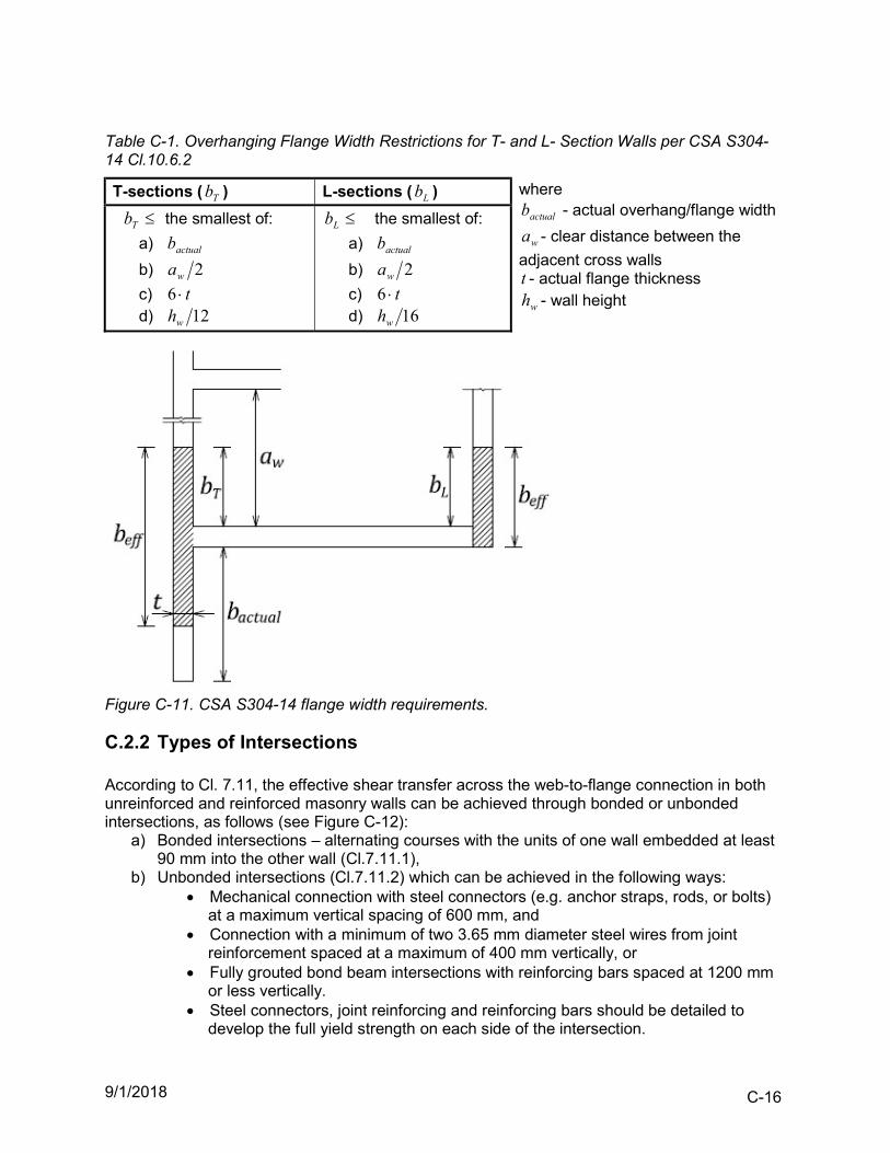
9/1/2018 C-16

Table C-1. Overhanging Flange Width Restrictions for T- and L- Section Walls per CSA S304-14 Cl.10.6.2

T-sections ( Tb ) L-sections ( Lb ) where

actualb - actual overhang/flange width

wa - clear distance between the

adjacent cross walls t - actual flange thickness

wh - wall height

Tb the smallest of:

a) actualb

b) 2wa

c) t6 d) 12wh

Lb the smallest of:

a) actualb

b) 2wa

c) t6 d) 16wh

Figure C-11. CSA S304-14 flange width requirements.

C.2.2 Types of Intersections According to Cl. 7.11, the effective shear transfer across the web-to-flange connection in both unreinforced and reinforced masonry walls can be achieved through bonded or unbonded intersections, as follows (see Figure C-12):

a) Bonded intersections – alternating courses with the units of one wall embedded at least 90 mm into the other wall (Cl.7.11.1),

b) Unbonded intersections (Cl.7.11.2) which can be achieved in the following ways: Mechanical connection with steel connectors (e.g. anchor straps, rods, or bolts)

at a maximum vertical spacing of 600 mm, and Connection with a minimum of two 3.65 mm diameter steel wires from joint

reinforcement spaced at a maximum of 400 mm vertically, or Fully grouted bond beam intersections with reinforcing bars spaced at 1200 mm

or less vertically. Steel connectors, joint reinforcing and reinforcing bars should be detailed to

develop the full yield strength on each side of the intersection.

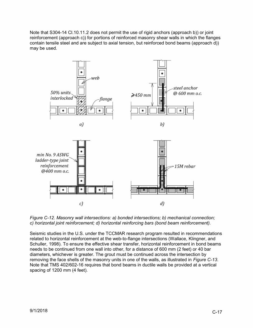
9/1/2018 C-17

Note that S304-14 Cl.10.11.2 does not permit the use of rigid anchors (approach b)) or joint reinforcement (approach c)) for portions of reinforced masonry shear walls in which the flanges contain tensile steel and are subject to axial tension, but reinforced bond beams (approach d)) may be used.

Figure C-12. Masonry wall intersections: a) bonded intersections; b) mechanical connection; c) horizontal joint reinforcement; d) horizontal reinforcing bars (bond beam reinforcement). Seismic studies in the U.S. under the TCCMAR research program resulted in recommendations related to horizontal reinforcement at the web-to-flange intersections (Wallace, Klingner, and Schuller, 1998). To ensure the effective shear transfer, horizontal reinforcement in bond beams needs to be continued from one wall into other, for a distance of 600 mm (2 feet) or 40 bar diameters, whichever is greater. The grout must be continued across the intersection by removing the face shells of the masonry units in one of the walls, as illustrated in Figure C-13. Note that TMS 402/602-16 requires that bond beams in ductile walls be provided at a vertical spacing of 1200 mm (4 feet).

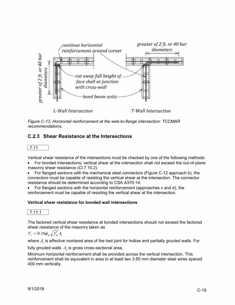
9/1/2018 C-18

Figure C-13. Horizontal reinforcement at the web-to-flange intersection: TCCMAR recommendations.

C.2.3 Shear Resistance at the Intersections 7.11

Vertical shear resistance of the intersections must be checked by one of the following methods: For bonded intersections, vertical shear at the intersection shall not exceed the out-of-plane masonry shear resistance (Cl.7.10.2). For flanged sections with the mechanical steel connectors (Figure C-12 approach b), the connectors must be capable of resisting the vertical shear at the intersection. The connector resistance should be determined according to CSA A370-14. For flanged sections with the horizontal reinforcement (approaches c and d), the reinforcement must be capable of resisting the vertical shear at the intersection. Vertical shear resistance for bonded wall intersections 7.11.1

The factored vertical shear resistance at bonded intersections should not exceed the factored shear resistance of the masonry taken as

emmr AfV 16.0

where eA is effective mortared area of the bed joint for hollow and partially grouted walls. For

fully grouted walls eA is gross cross-sectional area.

Minimum horizontal reinforcement shall be provided across the vertical intersection. This reinforcement shall be equivalent in area to at least two 3.65 mm diameter steel wires spaced 400 mm vertically.

9/1/2018 C-19

Vertical shear resistance for unbonded wall intersections 7.11.2

Where wall intersections are not bonded in accordance with Cl.7.11.1, or where additional capacity is required, the factored shear resistance of the web-to-flange joint shall be based on the shear friction resistance taken as

hmr CV

where = 1.0 coefficient of friction for the web-to-flange joint

hC = compressive force in the masonry acting normal to the head joint, normally taken as the factored tensile force at yield of the horizontal reinforcement that crosses the vertical section. The reinforcement must be detailed to enable it to develop its yield strength on both sides of the vertical masonry joint, which may be hard to achieve in practice. Commentary

For flanged walls with horizontal reinforcement, resistance to vertical shear sliding is provided by the frictional forces between the sliding surfaces, that is, the web and the flange of the wall. The shear friction resistance rV is proportional to the coefficient of friction , and the clamping

force hC acting perpendicular to the joint of height h (see Figure C-14a)).

hC is equal to the sum of the tensile yield forces developed in reinforcement of area sA spaced

at the distance s , that is,

h s y sC f A h s

In case of a flanged shear wall with openings, shear friction resistance rV is provided by wall segments between the openings, as shown in Figure C-14b). Reinforcement providing the shear friction resistance should be distributed uniformly across the joint. The bars should be long enough so that their yield strength can be developed on both sides of the vertical joint, as shown in Figure C-15b). Cl.7.11.2 lists three approaches (a, b, and c) that can be used to ensure shear transfer at the web-to-flange interface for unbonded masonry. The U.S. masonry design standard TMS 402/602-16 prescribes intersecting bond beams in intersecting walls at maximum spacing of 1200 mm (4 ft) on centre. The bond beam reinforcement area shall not be less than 200 mm2 per metre of wall height (0.1 in2/ft), and the reinforcement shall be detailed to develop the full yield stress at the intersection.

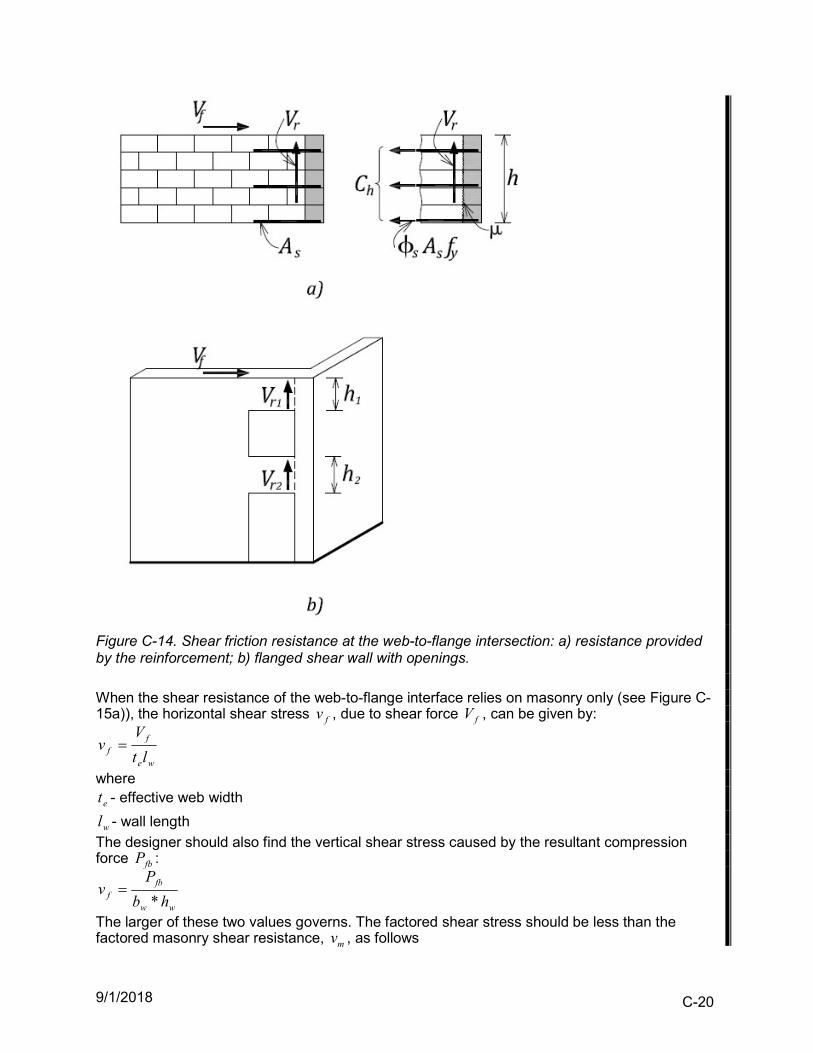
9/1/2018 C-20

Figure C-14. Shear friction resistance at the web-to-flange intersection: a) resistance provided by the reinforcement; b) flanged shear wall with openings.

When the shear resistance of the web-to-flange interface relies on masonry only (see Figure C-15a)), the horizontal shear stress fv , due to shear force fV , can be given by:

we

ff lt

Vv

where

et - effective web width

wl - wall length

The designer should also find the vertical shear stress caused by the resultant compression force fbP :

ww

fbf hb

Pv

*

The larger of these two values governs. The factored shear stress should be less than the factored masonry shear resistance, mv , as follows

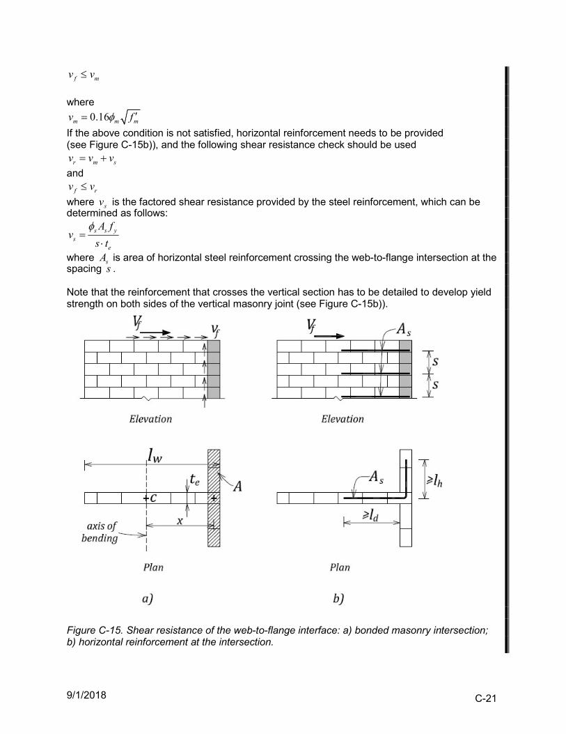
9/1/2018 C-21

f mv v

where

0.16m m mv f

If the above condition is not satisfied, horizontal reinforcement needs to be provided (see Figure C-15b)), and the following shear resistance check should be used

r m sv v v

and

f rv v

where sv is the factored shear resistance provided by the steel reinforcement, which can be determined as follows:

s s ys

e

A fv

s t

where sA is area of horizontal steel reinforcement crossing the web-to-flange intersection at the spacing s . Note that the reinforcement that crosses the vertical section has to be detailed to develop yield strength on both sides of the vertical masonry joint (see Figure C-15b)).

Figure C-15. Shear resistance of the web-to-flange interface: a) bonded masonry intersection; b) horizontal reinforcement at the intersection.

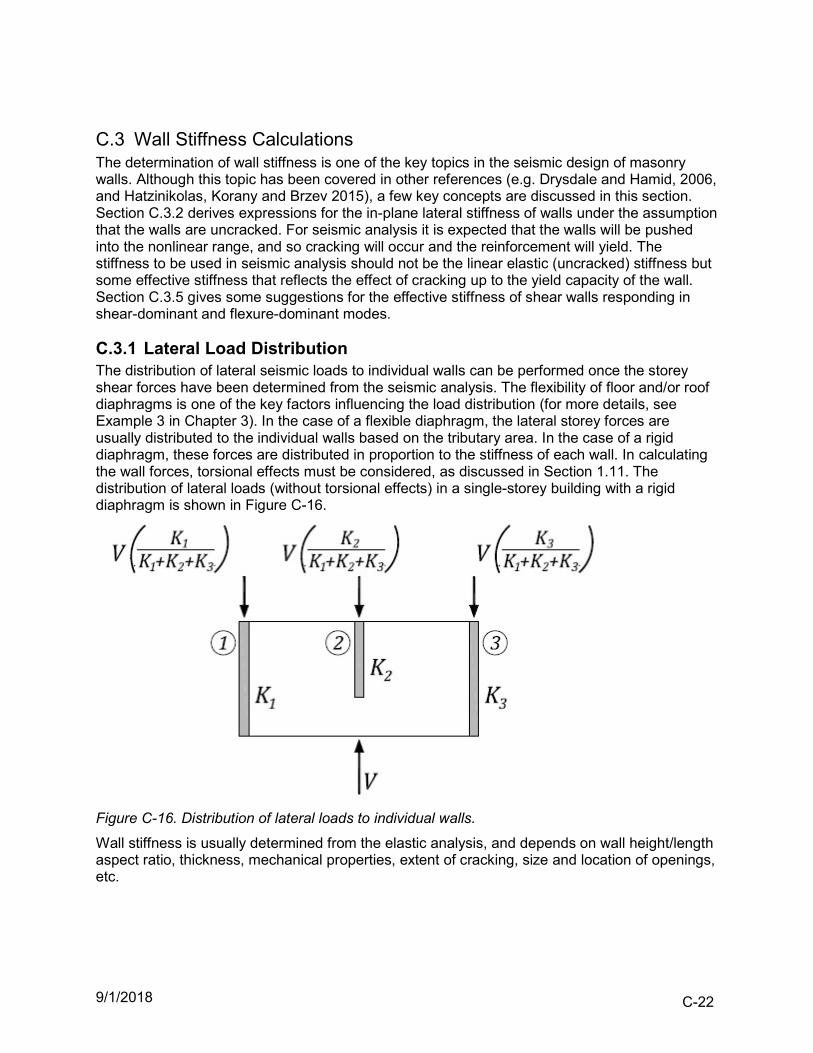
9/1/2018 C-22

C.3 Wall Stiffness Calculations The determination of wall stiffness is one of the key topics in the seismic design of masonry walls. Although this topic has been covered in other references (e.g. Drysdale and Hamid, 2006, and Hatzinikolas, Korany and Brzev 2015), a few key concepts are discussed in this section. Section C.3.2 derives expressions for the in-plane lateral stiffness of walls under the assumption that the walls are uncracked. For seismic analysis it is expected that the walls will be pushed into the nonlinear range, and so cracking will occur and the reinforcement will yield. The stiffness to be used in seismic analysis should not be the linear elastic (uncracked) stiffness but some effective stiffness that reflects the effect of cracking up to the yield capacity of the wall. Section C.3.5 gives some suggestions for the effective stiffness of shear walls responding in shear-dominant and flexure-dominant modes.

C.3.1 Lateral Load Distribution The distribution of lateral seismic loads to individual walls can be performed once the storey shear forces have been determined from the seismic analysis. The flexibility of floor and/or roof diaphragms is one of the key factors influencing the load distribution (for more details, see Example 3 in Chapter 3). In the case of a flexible diaphragm, the lateral storey forces are usually distributed to the individual walls based on the tributary area. In the case of a rigid diaphragm, these forces are distributed in proportion to the stiffness of each wall. In calculating the wall forces, torsional effects must be considered, as discussed in Section 1.11. The distribution of lateral loads (without torsional effects) in a single-storey building with a rigid diaphragm is shown in Figure C-16.

Figure C-16. Distribution of lateral loads to individual walls.

Wall stiffness is usually determined from the elastic analysis, and depends on wall height/length aspect ratio, thickness, mechanical properties, extent of cracking, size and location of openings, etc.

9/1/2018 C-23

C.3.2 Wall Stiffness: Cantilever and Fixed-End Model Wall stiffness depends on the end support conditions, that is, whether a wall or pier is fixed or free to move and/or rotate at its ends. Two models for wall stiffness include the cantilever model and the fixed-end model, as shown in Figure C-17. In the cantilever model, the wall is free to rotate and move at the top in the horizontal direction – this is usually an appropriate model for the walls in a single-storey masonry building. The stiffness can be defined as the lateral force required to produce a unit displacement, but it is determined by taking the inverse of the combined flexural and shear displacements produced by a unit load. It should be noted that flexural displacements will govern for walls with an aspect ratio of 2 or higher. For example, the contribution of shear deformation in a wall with a height/length aspect ratio of 2.0, is 16% for the cantilever model and 43% for the fixed-end model. The stiffness equations presented in this section take into account both shear and flexural deformations. The stiffness of a cantilever wall or a pier can be determined from the following equation (see Figure C-17 a)):

34

1

* 2

ww

m

l

h

l

htE

K ( 13)

The stiffness of a wall or a pier with the fixed ends can be determined from the following equation (see Figure C-17 b)):

3

1

* 2

ww

m

l

h

l

htE

K ( 14)

where h - wall height (cantilever model) or clear pier height (fixed-end model) wl - wall or pier length

mm fE 850 modulus of elasticity for masonry The following assumptions have been taken in deriving the above equations:

mm EG 4.0 modulus of rigidity for masonry (shear modulus)

12

* 3we lt

I uncracked wall moment of inertia

6

**5 wev

ltA shear area (applies to rectangular wall sections only)

where et = effective wall thickness.

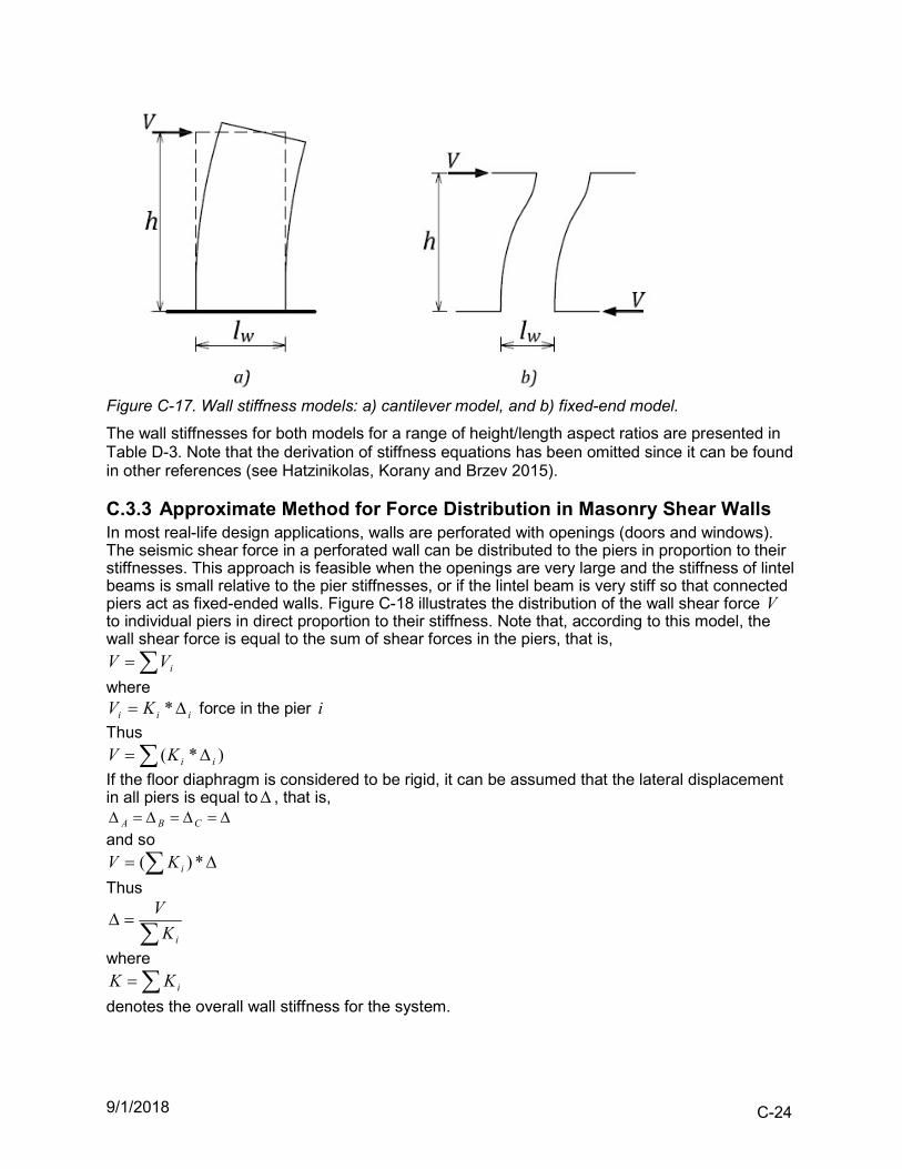
9/1/2018 C-24

Figure C-17. Wall stiffness models: a) cantilever model, and b) fixed-end model.

The wall stiffnesses for both models for a range of height/length aspect ratios are presented in Table D-3. Note that the derivation of stiffness equations has been omitted since it can be found in other references (see Hatzinikolas, Korany and Brzev 2015).

C.3.3 Approximate Method for Force Distribution in Masonry Shear Walls In most real-life design applications, walls are perforated with openings (doors and windows). The seismic shear force in a perforated wall can be distributed to the piers in proportion to their stiffnesses. This approach is feasible when the openings are very large and the stiffness of lintel beams is small relative to the pier stiffnesses, or if the lintel beam is very stiff so that connected piers act as fixed-ended walls. Figure C-18 illustrates the distribution of the wall shear force V to individual piers in direct proportion to their stiffness. Note that, according to this model, the wall shear force is equal to the sum of shear forces in the piers, that is,

iVV

where

iii KV * force in the pier i

Thus )*( iiKV

If the floor diaphragm is considered to be rigid, it can be assumed that the lateral displacement in all piers is equal to , that is,

CBA and so

*)( iKV

Thus

iK

V

where

iKK

denotes the overall wall stiffness for the system.

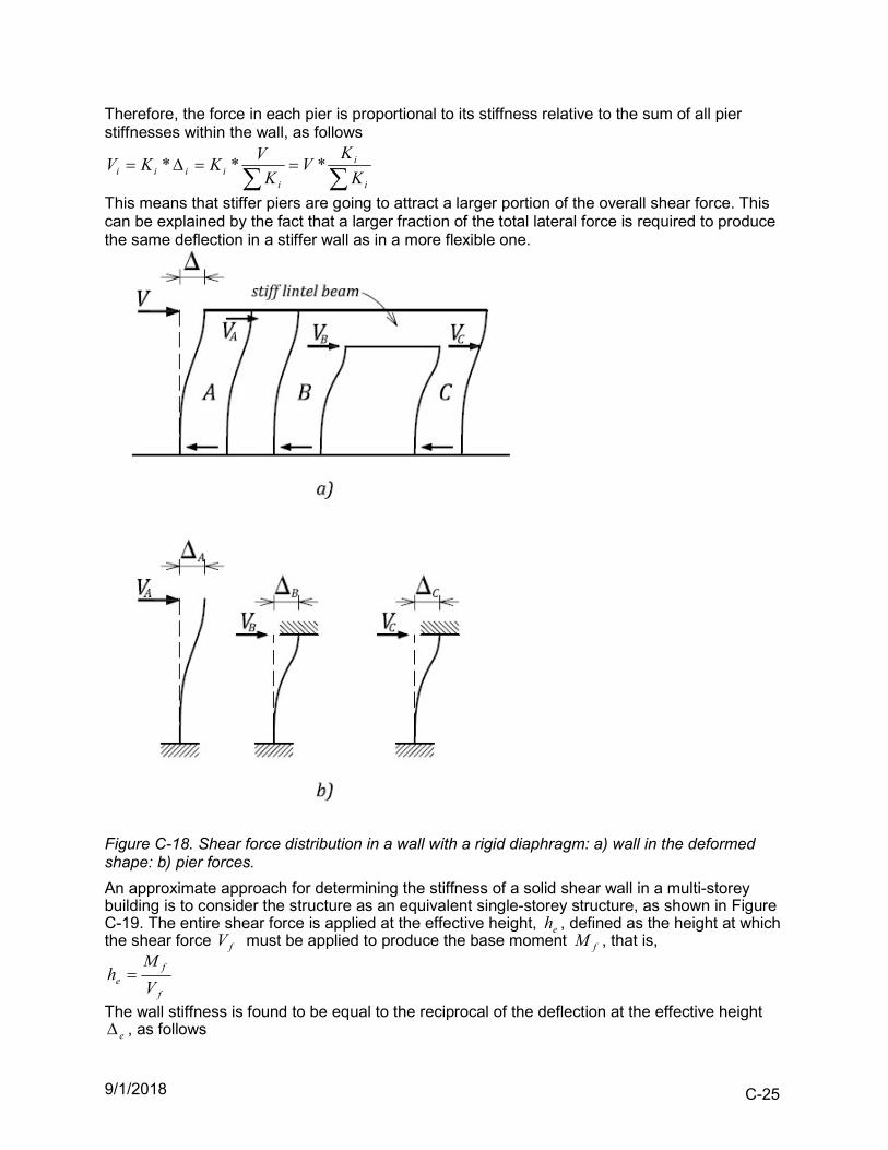
9/1/2018 C-25

Therefore, the force in each pier is proportional to its stiffness relative to the sum of all pier stiffnesses within the wall, as follows

i

i

iiiii K

KV

K

VKKV ***

This means that stiffer piers are going to attract a larger portion of the overall shear force. This can be explained by the fact that a larger fraction of the total lateral force is required to produce the same deflection in a stiffer wall as in a more flexible one.

Figure C-18. Shear force distribution in a wall with a rigid diaphragm: a) wall in the deformed shape: b) pier forces.

An approximate approach for determining the stiffness of a solid shear wall in a multi-storey building is to consider the structure as an equivalent single-storey structure, as shown in Figure C-19. The entire shear force is applied at the effective height, eh , defined as the height at which the shear force fV must be applied to produce the base moment fM , that is,

f

fe V

Mh

The wall stiffness is found to be equal to the reciprocal of the deflection at the effective height e , as follows

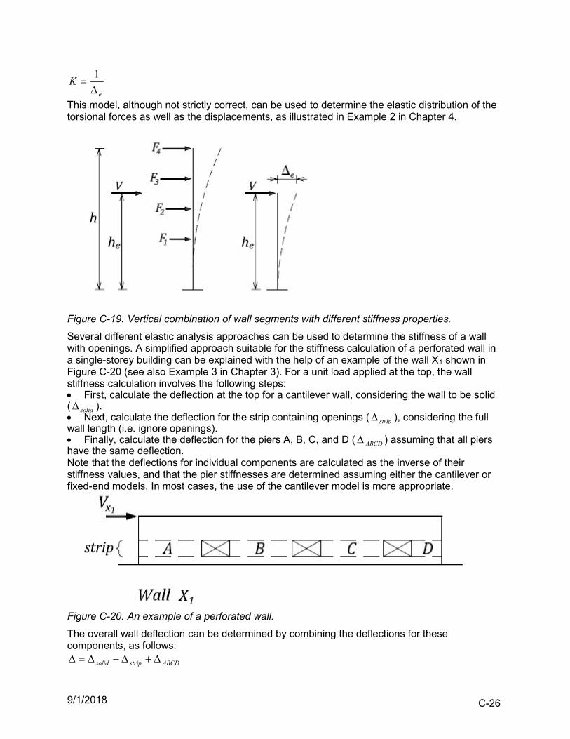
9/1/2018 C-26

e

K

1

This model, although not strictly correct, can be used to determine the elastic distribution of the torsional forces as well as the displacements, as illustrated in Example 2 in Chapter 4.

Figure C-19. Vertical combination of wall segments with different stiffness properties.

Several different elastic analysis approaches can be used to determine the stiffness of a wall with openings. A simplified approach suitable for the stiffness calculation of a perforated wall in a single-storey building can be explained with the help of an example of the wall X1 shown in Figure C-20 (see also Example 3 in Chapter 3). For a unit load applied at the top, the wall stiffness calculation involves the following steps: First, calculate the deflection at the top for a cantilever wall, considering the wall to be solid ( solid ). Next, calculate the deflection for the strip containing openings ( strip ), considering the full wall length (i.e. ignore openings). Finally, calculate the deflection for the piers A, B, C, and D ( ABCD ) assuming that all piers have the same deflection. Note that the deflections for individual components are calculated as the inverse of their stiffness values, and that the pier stiffnesses are determined assuming either the cantilever or fixed-end models. In most cases, the use of the cantilever model is more appropriate.

Figure C-20. An example of a perforated wall.

The overall wall deflection can be determined by combining the deflections for these components, as follows:

ABCDstripsolid

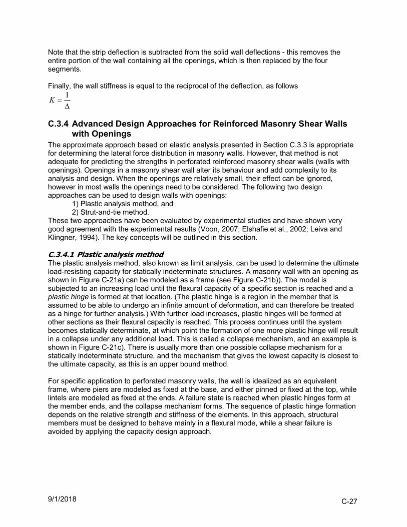
9/1/2018 C-27

Note that the strip deflection is subtracted from the solid wall deflections - this removes the entire portion of the wall containing all the openings, which is then replaced by the four segments. Finally, the wall stiffness is equal to the reciprocal of the deflection, as follows

1K

C.3.4 Advanced Design Approaches for Reinforced Masonry Shear Walls with Openings

The approximate approach based on elastic analysis presented in Section C.3.3 is appropriate for determining the lateral force distribution in masonry walls. However, that method is not adequate for predicting the strengths in perforated reinforced masonry shear walls (walls with openings). Openings in a masonry shear wall alter its behaviour and add complexity to its analysis and design. When the openings are relatively small, their effect can be ignored, however in most walls the openings need to be considered. The following two design approaches can be used to design walls with openings:

1) Plastic analysis method, and 2) Strut-and-tie method.

These two approaches have been evaluated by experimental studies and have shown very good agreement with the experimental results (Voon, 2007; Elshafie et al., 2002; Leiva and Klingner, 1994). The key concepts will be outlined in this section. C.3.4.1 Plastic analysis method The plastic analysis method, also known as limit analysis, can be used to determine the ultimate load-resisting capacity for statically indeterminate structures. A masonry wall with an opening as shown in Figure C-21a) can be modeled as a frame (see Figure C-21b)). The model is subjected to an increasing load until the flexural capacity of a specific section is reached and a plastic hinge is formed at that location. (The plastic hinge is a region in the member that is assumed to be able to undergo an infinite amount of deformation, and can therefore be treated as a hinge for further analysis.) With further load increases, plastic hinges will be formed at other sections as their flexural capacity is reached. This process continues until the system becomes statically determinate, at which point the formation of one more plastic hinge will result in a collapse under any additional load. This is called a collapse mechanism, and an example is shown in Figure C-21c). There is usually more than one possible collapse mechanism for a statically indeterminate structure, and the mechanism that gives the lowest capacity is closest to the ultimate capacity, as this is an upper bound method. For specific application to perforated masonry walls, the wall is idealized as an equivalent frame, where piers are modeled as fixed at the base, and either pinned or fixed at the top, while lintels are modeled as fixed at the ends. A failure state is reached when plastic hinges form at the member ends, and the collapse mechanism forms. The sequence of plastic hinge formation depends on the relative strength and stiffness of the elements. In this approach, structural members must be designed to behave mainly in a flexural mode, while a shear failure is avoided by applying the capacity design approach.

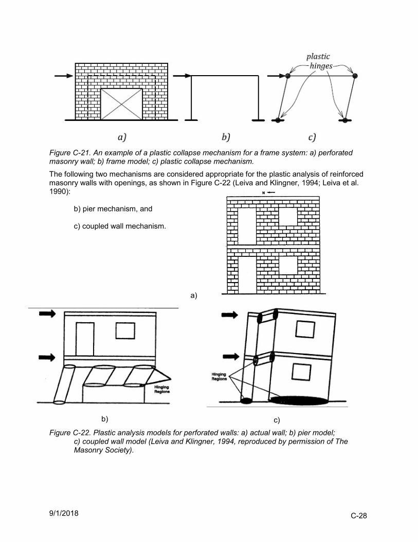
9/1/2018 C-28

Figure C-21. An example of a plastic collapse mechanism for a frame system: a) perforated masonry wall; b) frame model; c) plastic collapse mechanism.

The following two mechanisms are considered appropriate for the plastic analysis of reinforced masonry walls with openings, as shown in Figure C-22 (Leiva and Klingner, 1994; Leiva et al. 1990):

b) pier mechanism, and c) coupled wall mechanism.

a)

b)

c)

Figure C-22. Plastic analysis models for perforated walls: a) actual wall; b) pier model; c) coupled wall model (Leiva and Klingner, 1994, reproduced by permission of The Masonry Society).

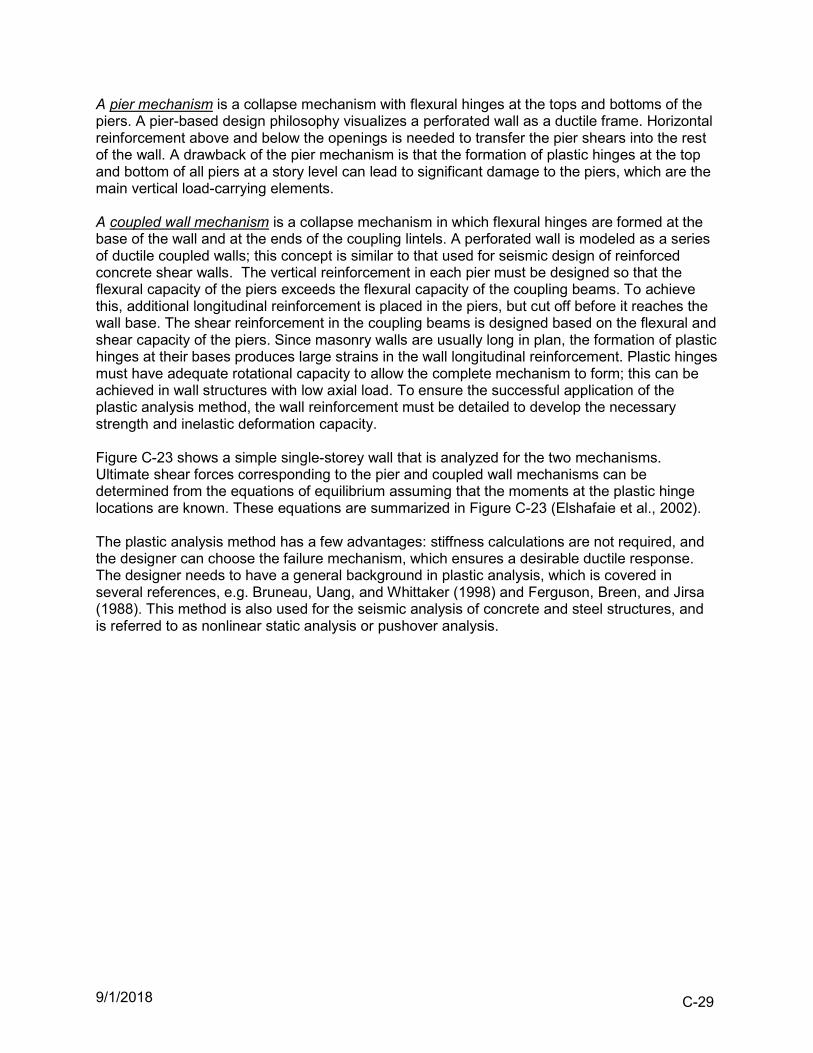
9/1/2018 C-29

A pier mechanism is a collapse mechanism with flexural hinges at the tops and bottoms of the piers. A pier-based design philosophy visualizes a perforated wall as a ductile frame. Horizontal reinforcement above and below the openings is needed to transfer the pier shears into the rest of the wall. A drawback of the pier mechanism is that the formation of plastic hinges at the top and bottom of all piers at a story level can lead to significant damage to the piers, which are the main vertical load-carrying elements. A coupled wall mechanism is a collapse mechanism in which flexural hinges are formed at the base of the wall and at the ends of the coupling lintels. A perforated wall is modeled as a series of ductile coupled walls; this concept is similar to that used for seismic design of reinforced concrete shear walls. The vertical reinforcement in each pier must be designed so that the flexural capacity of the piers exceeds the flexural capacity of the coupling beams. To achieve this, additional longitudinal reinforcement is placed in the piers, but cut off before it reaches the wall base. The shear reinforcement in the coupling beams is designed based on the flexural and shear capacity of the piers. Since masonry walls are usually long in plan, the formation of plastic hinges at their bases produces large strains in the wall longitudinal reinforcement. Plastic hinges must have adequate rotational capacity to allow the complete mechanism to form; this can be achieved in wall structures with low axial load. To ensure the successful application of the plastic analysis method, the wall reinforcement must be detailed to develop the necessary strength and inelastic deformation capacity. Figure C-23 shows a simple single-storey wall that is analyzed for the two mechanisms. Ultimate shear forces corresponding to the pier and coupled wall mechanisms can be determined from the equations of equilibrium assuming that the moments at the plastic hinge locations are known. These equations are summarized in Figure C-23 (Elshafaie et al., 2002). The plastic analysis method has a few advantages: stiffness calculations are not required, and the designer can choose the failure mechanism, which ensures a desirable ductile response. The designer needs to have a general background in plastic analysis, which is covered in several references, e.g. Bruneau, Uang, and Whittaker (1998) and Ferguson, Breen, and Jirsa (1988). This method is also used for the seismic analysis of concrete and steel structures, and is referred to as nonlinear static analysis or pushover analysis.

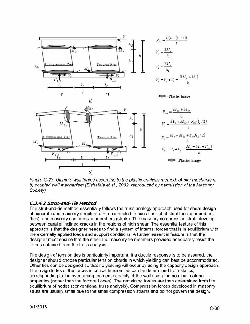
9/1/2018 C-30

a)

b)

Figure C-23. Ultimate wall forces according to the plastic analysis method: a) pier mechanism; b) coupled wall mechanism (Elshafaie et al., 2002, reproduced by permission of the Masonry Society).

C.3.4.2 Strut-and-Tie Method The strut-and-tie method essentially follows the truss analogy approach used for shear design of concrete and masonry structures. Pin-connected trusses consist of steel tension members (ties), and masonry compression members (struts). The masonry compression struts develop between parallel inclined cracks in the regions of high shear. The essential feature of this approach is that the designer needs to find a system of internal forces that is in equilibrium with the externally applied loads and support conditions. A further essential feature is that the designer must ensure that the steel and masonry tie members provided adequately resist the forces obtained from the truss analysis. The design of tension ties is particularly important. If a ductile response is to be assured, the designer should choose particular tension chords in which yielding can best be accommodated. Other ties can be designed so that no yielding will occur by using the capacity design approach. The magnitudes of the forces in critical tension ties can be determined from statics, corresponding to the overturning moment capacity of the wall using the nominal material properties (rather than the factored ones). The remaining forces are then determined from the equilibrium of nodes (conventional truss analysis). Compression forces developed in masonry struts are usually small due to the small compression strains and do not govern the design.

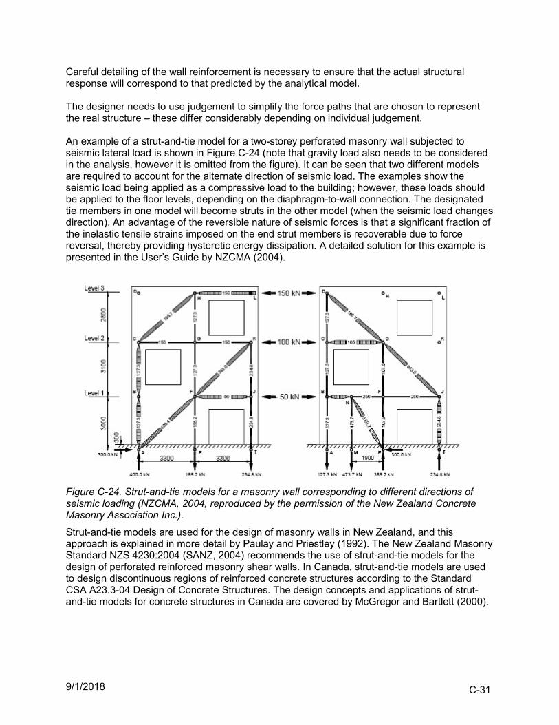
9/1/2018 C-31

Careful detailing of the wall reinforcement is necessary to ensure that the actual structural response will correspond to that predicted by the analytical model. The designer needs to use judgement to simplify the force paths that are chosen to represent the real structure – these differ considerably depending on individual judgement. An example of a strut-and-tie model for a two-storey perforated masonry wall subjected to seismic lateral load is shown in Figure C-24 (note that gravity load also needs to be considered in the analysis, however it is omitted from the figure). It can be seen that two different models are required to account for the alternate direction of seismic load. The examples show the seismic load being applied as a compressive load to the building; however, these loads should be applied to the floor levels, depending on the diaphragm-to-wall connection. The designated tie members in one model will become struts in the other model (when the seismic load changes direction). An advantage of the reversible nature of seismic forces is that a significant fraction of the inelastic tensile strains imposed on the end strut members is recoverable due to force reversal, thereby providing hysteretic energy dissipation. A detailed solution for this example is presented in the User’s Guide by NZCMA (2004).

Figure C-24. Strut-and-tie models for a masonry wall corresponding to different directions of seismic loading (NZCMA, 2004, reproduced by the permission of the New Zealand Concrete Masonry Association Inc.).

Strut-and-tie models are used for the design of masonry walls in New Zealand, and this approach is explained in more detail by Paulay and Priestley (1992). The New Zealand Masonry Standard NZS 4230:2004 (SANZ, 2004) recommends the use of strut-and-tie models for the design of perforated reinforced masonry shear walls. In Canada, strut-and-tie models are used to design discontinuous regions of reinforced concrete structures according to the Standard CSA A23.3-04 Design of Concrete Structures. The design concepts and applications of strut-and-tie models for concrete structures in Canada are covered by McGregor and Bartlett (2000).

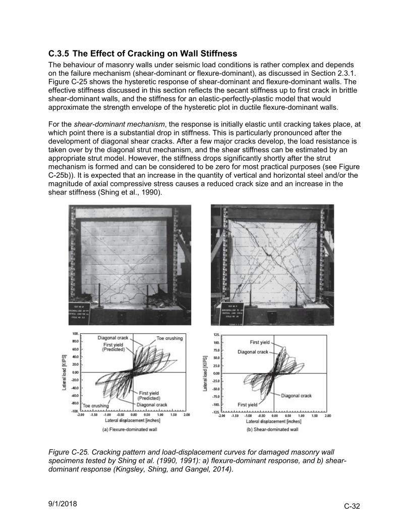
9/1/2018 C-32

C.3.5 The Effect of Cracking on Wall Stiffness The behaviour of masonry walls under seismic load conditions is rather complex and depends on the failure mechanism (shear-dominant or flexure-dominant), as discussed in Section 2.3.1. Figure C-25 shows the hysteretic response of shear-dominant and flexure-dominant walls. The effective stiffness discussed in this section reflects the secant stiffness up to first crack in brittle shear-dominant walls, and the stiffness for an elastic-perfectly-plastic model that would approximate the strength envelope of the hysteretic plot in ductile flexure-dominant walls. For the shear-dominant mechanism, the response is initially elastic until cracking takes place, at which point there is a substantial drop in stiffness. This is particularly pronounced after the development of diagonal shear cracks. After a few major cracks develop, the load resistance is taken over by the diagonal strut mechanism, and the shear stiffness can be estimated by an appropriate strut model. However, the stiffness drops significantly shortly after the strut mechanism is formed and can be considered to be zero for most practical purposes (see Figure C-25b)). It is expected that an increase in the quantity of vertical and horizontal steel and/or the magnitude of axial compressive stress causes a reduced crack size and an increase in the shear stiffness (Shing et al., 1990).

Figure C-25. Cracking pattern and load-displacement curves for damaged masonry wall specimens tested by Shing et al. (1990, 1991): a) flexure-dominant response, and b) shear-dominant response (Kingsley, Shing, and Gangel, 2014).

9/1/2018 C-33

For the flexure-dominant mechanism, a drop in the stiffness immediately after the onset of cracking is not very significant. As can be seen from Figure C-25a), the stiffness drops after the yielding of vertical reinforcement takes place, and continues to drop with increasing inelastic lateral deformations (this depends on the ductility capacity of the wall under consideration). The specimen for which the results are shown in Figure C-25a) showed yielding of vertical reinforcement and compressive crushing of masonry at the wall toes (Shing et al., 1989). Note that the height of wall test specimens shown in Figure C-23 was 1.8 m (6 feet), thus a 2.5% drift ratio permitted by the NBC 2015 for regular buildings corresponds to 45 mm (1.8 inch ) displacement. It can be seen that the displacements and drifts in these specimens are very low, particularly so for the shear-dominant specimen shown in Figure C-25b). Evidence from studies that focus on quantifying the changes in in-plane wall stiffness under increasing lateral loading are limited, so CSA S304-14 and other masonry codes do not provide guidance related to this issue. Shing et al. (1990) tested a series of 22 cantilever block masonry wall specimens that were laterally loaded at the top, with a height/length aspect ratio of 1.0. Based on the experimental test data, they have recommended the following empirical equation for the lateral stiffness of a wall with a shear-dominant response

elshearce KKfK )1073.02.0( ( 15)

where

w

emshear

l

h

tEK

*3

* is the shear stiffness of a wall/pier

h = wall height

wl = wall length

et = effective wall thickness

cf = axial compressive stress (MPa)

The above equation is based on the force/displacement measurements taken just after the first diagonal crack developed, in specimens with a height/length ratio of 1.0. For seismic applications where the walls are expected to yield in flexure before failing in shear, and the lateral stiffness is used to estimate the fundamental period of the structure and to determine the seismic displacements, it is more appropriate to determine the effective stiffness from a cracked section analysis at first yield of the tension reinforcement. A study by Priestley and Hart (1989), based on the cracked transformed section stiffness at first yield of the tension reinforcement, recommends that the effective moment of inertia, eI , of a wall can be approximated by:

gem

f

ye I

Af

P

fI )

100(

( 16)

where

yf = steel yield strength (MPa)

fP = factored axial load

eA = effective cross-sectional area for the wall

mf = masonry compressive strength, and

9/1/2018 C-34

12

*

3we

g

ltI is the gross moment of inertia of the wall.

Note that the first term in the bracket, yf100 , is equal to 0.25 for 400yf MPa (Grade 400 steel). The second term is a ratio of axial compressive stress in the wall, equal to ef AP , and the masonry compressive strength, mf . The above relation is based solely on consideration of flexural stiffness, and is a best fit relationship for several different values of height/length ratio ( wlh ), steel strength, vertical reinforcement ratio and axial load. Other considerations are whether the vertical reinforcement is uniformly distributed across the wall length or concentrated at the ends, and the effect of tension stiffening. The vertical reinforcement ratio is not included in the above expression, and as a result, the wall stiffness is overestimated for lightly reinforced walls and underestimated for heavily reinforced walls. If it is assumed that wall cracking causes the same proportional decrease in the effective shear area as it does for the moment of inertia, then the stiffnesses can be combined to give the following equation for the reduced wall stiffness, ceK ,

cem

f

yce K

Af

P

fK )

100(

(17)

where

34

*2

ww

emc

l

h

l

h

tEK

is the combined stiffness of an uncracked cantilever wall or pier, considering both the flexural and shear deformation components (refer to Section C.3.2 for the wall stiffness equations). The terms in the large right-hand bracket of the cK equation give the comparative value of flexural deformation to shear deformation. At a wlh ratio of 1.0, flexure contributes 4/7 of the total deformation and shear 3/7, while at a wlh ratio of 0.5, shear contributes ¾ of the total defection. The Priestley and Hart equation was obtained using experimental data related to cantilever wall specimens, however it may also be used for fixed-end walls. The stiffness equation for these walls, feK , is the same as for the cantilever walls, that is,

fem

f

yfe K

Af

P

fK )

100(

(18)

where

3

*2

ww

emf

l

h

l

h

tEK is the stiffness of an uncracked fixed-end wall or a pier

A comparison of the proposed equations for a masonry block wall under axial compressive stress is presented in Figure C-26. The following values were used in the calculations:

400yf MPa, ef AP = 1 MPa, and mf = 10 MPa.

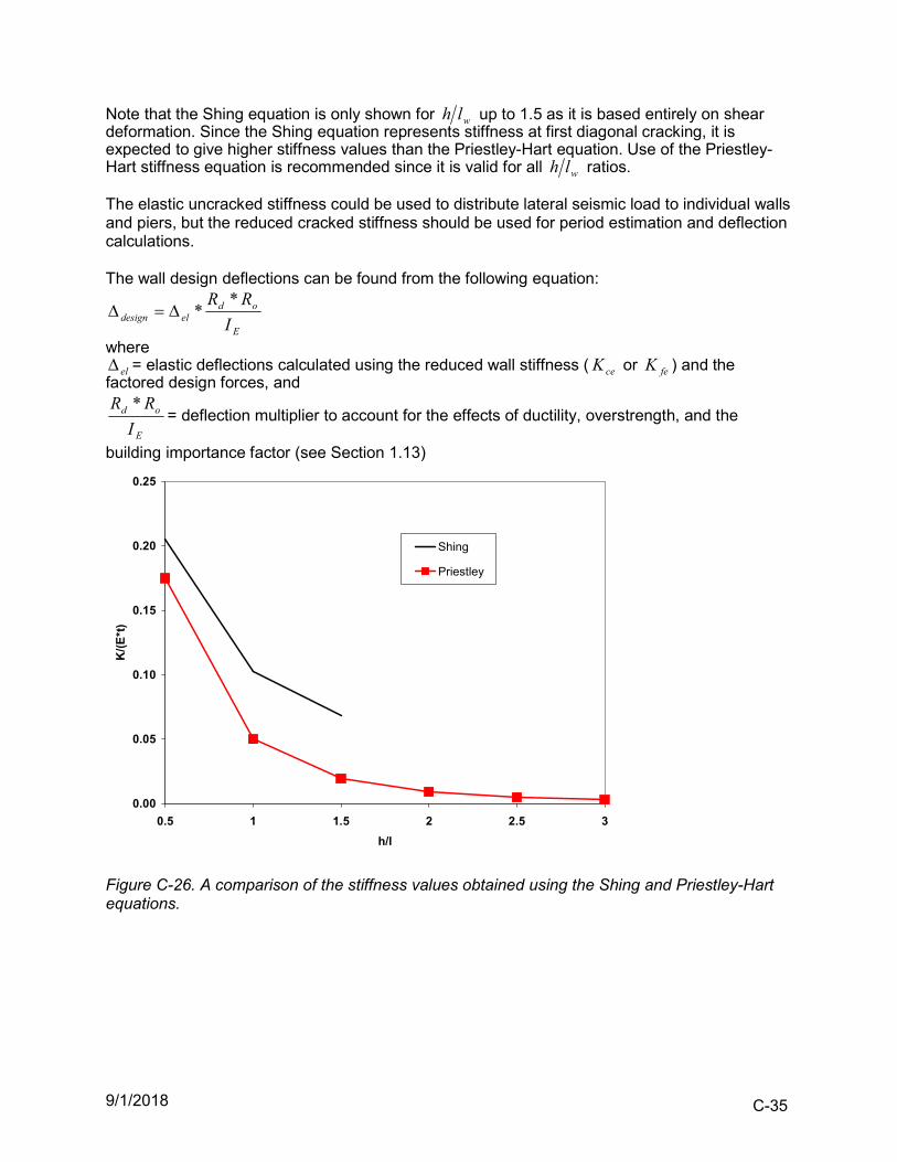
9/1/2018 C-35

Note that the Shing equation is only shown for wlh up to 1.5 as it is based entirely on shear deformation. Since the Shing equation represents stiffness at first diagonal cracking, it is expected to give higher stiffness values than the Priestley-Hart equation. Use of the Priestley-Hart stiffness equation is recommended since it is valid for all wlh ratios. The elastic uncracked stiffness could be used to distribute lateral seismic load to individual walls and piers, but the reduced cracked stiffness should be used for period estimation and deflection calculations. The wall design deflections can be found from the following equation:

E

odeldesign I

RR **

where el = elastic deflections calculated using the reduced wall stiffness ( ceK or feK ) and the

factored design forces, and

E

od

I

RR *= deflection multiplier to account for the effects of ductility, overstrength, and the

building importance factor (see Section 1.13)

0.00

0.05

0.10

0.15

0.20

0.25

0.5 1 1.5 2 2.5 3

h/l

K/(

E*t

)

Shing

Priestley

Figure C-26. A comparison of the stiffness values obtained using the Shing and Priestley-Hart equations.

9/1/2018 D-1

TABLE OF CONTENTS – APPENDIX D D DESIGN AIDS D-2 Table D-1. Properties of Concrete Masonry Walls (per metre or foot length) D-2 Table D-2. wlc ratio, yf = 400 MPa D-3

Figure D-1. wlc ratio, yf = 400 MPa D-4

Table D-3. Wall Stiffness Values tEK m * D-5

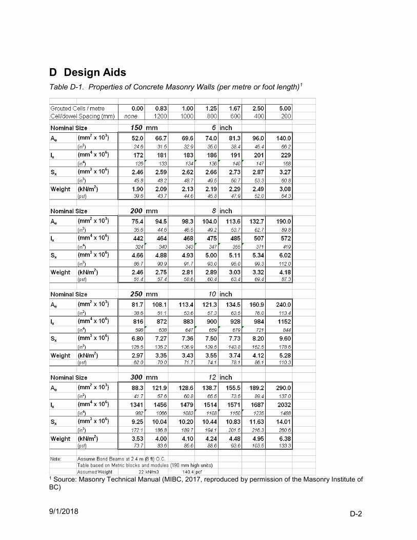
9/1/2018 D-2

D Design Aids Table D-1. Properties of Concrete Masonry Walls (per metre or foot length)1

1 Source: Masonry Technical Manual (MIBC, 2017, reproduced by permission of the Masonry Institute of BC)

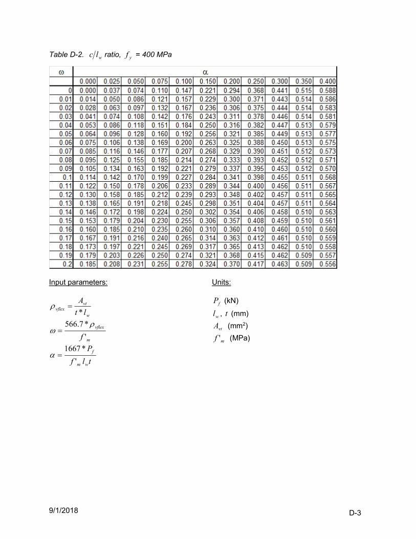
9/1/2018 D-3

Table D-2. wlc ratio, yf = 400 MPa

Input parameters:

w

vtvflex lt

A

*

m

vflex

f '

*7.566

tlf

P

wm

f

'

*1667

Units:

fP (kN)

wl , t (mm)

vtA (mm2)

mf ' (MPa)

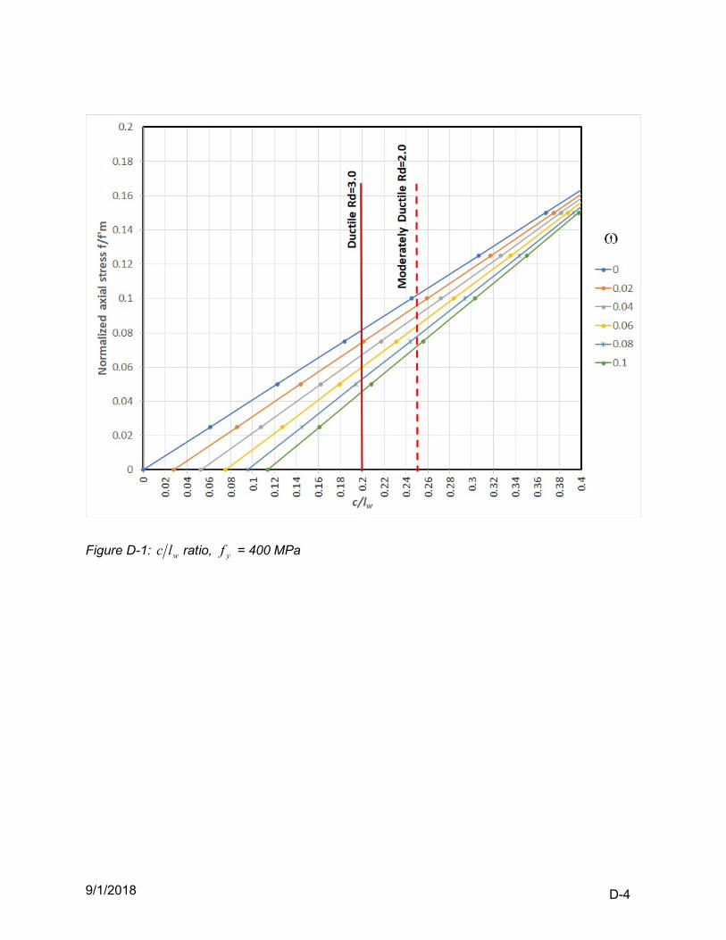
9/1/2018 D-4

Figure D-1: wlc ratio, yf = 400 MPa

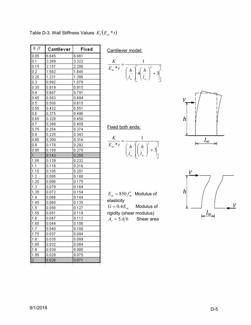
9/1/2018 D-5

Table D-3. Wall Stiffness Values tEK m *

Fixed both ends:

3

1

* 2

ww

m

l

h

l

htE

K

mm fE 850 Modulus of

elasticity

mEG 4.0 Modulus of

rigidity (shear modulus) 65AAv Shear area

Cantilever model:

34

1

* 2

ww

m

l

h

l

htE

K

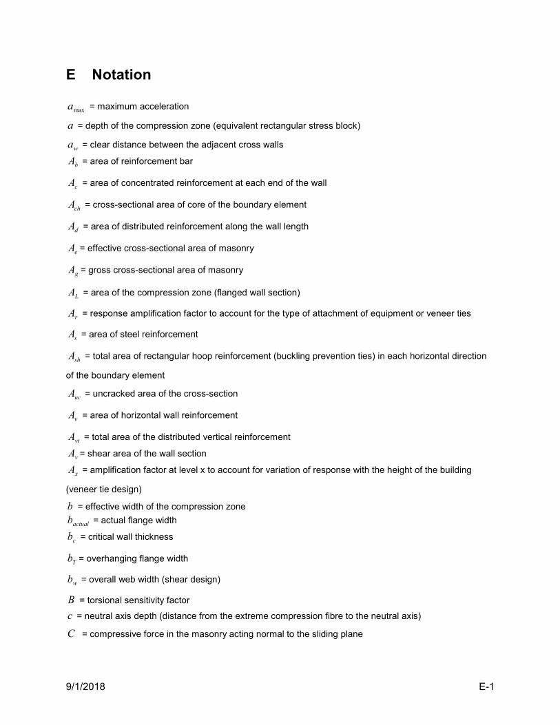
9/1/2018 E-1

E Notation

maxa = maximum acceleration

a = depth of the compression zone (equivalent rectangular stress block)

wa = clear distance between the adjacent cross walls

bA = area of reinforcement bar

cA = area of concentrated reinforcement at each end of the wall

chA = cross-sectional area of core of the boundary element

dA = area of distributed reinforcement along the wall length

eA = effective cross-sectional area of masonry

gA = gross cross-sectional area of masonry

LA = area of the compression zone (flanged wall section)

rA = response amplification factor to account for the type of attachment of equipment or veneer ties

sA = area of steel reinforcement

shA = total area of rectangular hoop reinforcement (buckling prevention ties) in each horizontal direction

of the boundary element

ucA = uncracked area of the cross-section

vA = area of horizontal wall reinforcement

vtA = total area of the distributed vertical reinforcement

vA = shear area of the wall section

xA = amplification factor at level x to account for variation of response with the height of the building

(veneer tie design)

b = effective width of the compression zone

actualb = actual flange width

cb = critical wall thickness

Tb = overhanging flange width

wb = overall web width (shear design)

B = torsional sensitivity factor

c = neutral axis depth (distance from the extreme compression fibre to the neutral axis)

C = compressive force in the masonry acting normal to the sliding plane

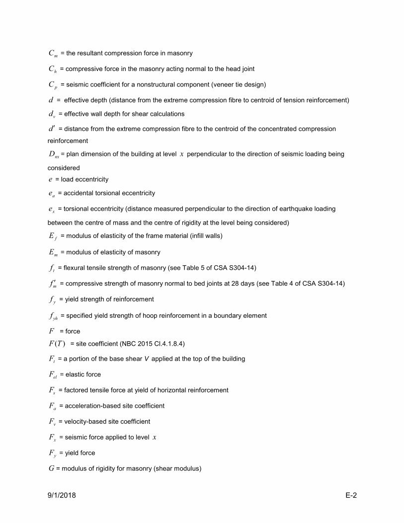
9/1/2018 E-2

mC = the resultant compression force in masonry

hC = compressive force in the masonry acting normal to the head joint

pC = seismic coefficient for a nonstructural component (veneer tie design)

d = effective depth (distance from the extreme compression fibre to centroid of tension reinforcement)

vd = effective wall depth for shear calculations

d = distance from the extreme compression fibre to the centroid of the concentrated compression

reinforcement

nxD = plan dimension of the building at level x perpendicular to the direction of seismic loading being

considered

e = load eccentricity

ae = accidental torsional eccentricity

xe = torsional eccentricity (distance measured perpendicular to the direction of earthquake loading

between the centre of mass and the centre of rigidity at the level being considered)

fE = modulus of elasticity of the frame material (infill walls)

mE = modulus of elasticity of masonry

tf = flexural tensile strength of masonry (see Table 5 of CSA S304-14)

mf = compressive strength of masonry normal to bed joints at 28 days (see Table 4 of CSA S304-14)

yf = yield strength of reinforcement

yhf = specified yield strength of hoop reinforcement in a boundary element

F = force

( )F T = site coefficient (NBC 2015 Cl.4.1.8.4)

tF = a portion of the base shear V applied at the top of the building

elF = elastic force

sF = factored tensile force at yield of horizontal reinforcement

aF = acceleration-based site coefficient

vF = velocity-based site coefficient

xF = seismic force applied to level x

yF = yield force

G = modulus of rigidity for masonry (shear modulus)

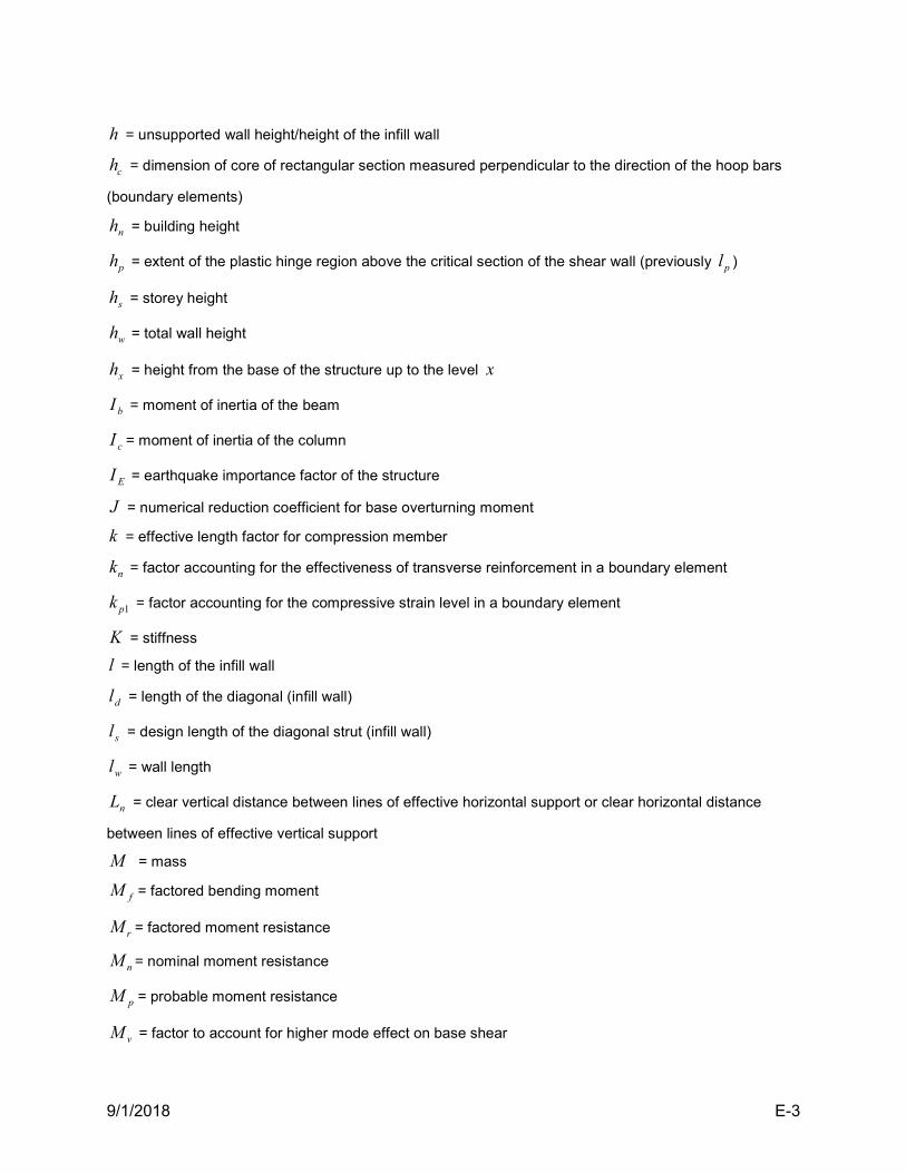
9/1/2018 E-3

h = unsupported wall height/height of the infill wall

ch = dimension of core of rectangular section measured perpendicular to the direction of the hoop bars

(boundary elements)

nh = building height

ph = extent of the plastic hinge region above the critical section of the shear wall (previously pl )

sh = storey height

wh = total wall height

xh = height from the base of the structure up to the level x

bI = moment of inertia of the beam

cI = moment of inertia of the column

EI = earthquake importance factor of the structure

J = numerical reduction coefficient for base overturning moment

k = effective length factor for compression member

nk = factor accounting for the effectiveness of transverse reinforcement in a boundary element

1pk = factor accounting for the compressive strain level in a boundary element

K = stiffness

l = length of the infill wall

dl = length of the diagonal (infill wall)

sl = design length of the diagonal strut (infill wall)

wl = wall length

nL = clear vertical distance between lines of effective horizontal support or clear horizontal distance

between lines of effective vertical support

M = mass

fM = factored bending moment

rM = factored moment resistance

nM = nominal moment resistance

pM = probable moment resistance

vM = factor to account for higher mode effect on base shear

9/1/2018 E-4

ln = total number of longitudinal bars in the boundary element cross-section that are laterally supported

by the corner of hoops or by hooks of seismic cross-ties

N = axial load arising from bending in coupling beams or piers

fp = distributed axial stress

refPGA = reference Peak Ground Acceleration (PGA) for determining ( )F T

dP = axial compressive load on the section under consideration

crP = critical axial compressive load

DLP = dead load

fbP = the resultant compression force (flanged walls)

rP = factored axial load resistance

1P = compressive force in the unreinforced masonry acting normal to the sliding plane

hP = horizontal component of the diagonal strut compression resistance (infill walls)

vP = the vertical component of the diagonal strut compression resistance (infill walls)

ultP = ultimate tie strength

dR = ductility-related force modification factor

oR = overstrength-related force modification factor

pR = element or component response modification factor (veneer tie design)

s = reinforcement spacing

TS = design spectral acceleration

)(TSa = 5% damped spectral response acceleration

eS = section modulus of effective wall cross-sectional area

pS = horizontal force factor for part or portion of a building and its anchorage (veneer tie design)

t = overall wall thickness

et = effective wall thickness

ft = face shell thickness

T = fundamental period of vibration of the building

xT = torsional moment at level x

rT = the resultant force in steel reinforcement

yT = factored tensile force at yield of the vertical reinforcement

9/1/2018 E-5

fv = distributed shear stress

mv = masonry shear strength

maxv = maximum velocity

V = lateral earthquake design force at the base of the structure

eV = lateral earthquake elastic force at the base of the structure

fV = factored shear force

frV = shear flow resistance

nbV = the resultant shear force corresponding to the development of nominal moment resistance nM at

the base of the wall

mV = masonry shear resistance

rV = factored shear resistance

sV = average shear wave velocity in the top 30 m of soil or rock

sV = factored shear resistance of steel reinforcement

w = diagonal strut width (infill walls)

ew = effective diagonal strut width (infill walls)

W = seismic weight, equal to the dead weight plus some portion of live load that would move laterally

with the structure

pW = weight of a part or a portion of a structure (veneer tie design)

xW = a portion of seismic weight W that is assigned to level x

h = vertical contact length between the frame and the diagonal strut (infill walls)

L = horizontal contact length between the frame and the diagonal strut (infill walls)

= damping ratio

d = ratio of the factored dead load moment to the total factored moment

1 = ratio of depth of rectangular compression block to depth of the neutral axis

g = factor to account for partially grouted or ungrouted walls that are constructed of hollow or semi-solid

units

max = the maximum storey displacement at level x at one of the extreme corners in the direction of

earthquake

9/1/2018 E-6

ave = the average storey displacement determined by averaging the maximum and minimum

displacements of the storey at level x

= lateral displacement

p = plastic displacement

y = displacement at the onset of yielding

el = elastic displacement

max = maximum displacement

u = inelastic (plastic) displacement

m = the maximum compressive strain in masonry

s = strain in steel reinforcement

y = yield strain in steel reinforcement

= factor used to account for direction of compressive stress in a masonry member relative to the

direction used for determination of mf

= curvature

u = ultimate curvature

y = yield curvature corresponds to the onset of yielding

er = resistance factor for member stiffness

m = resistance factor for masonry

s = resistance factor for steel reinforcement

= resistance factor

h = horizontal reinforcement ratio

s = volumetric ratio of circular hoop reinforcement for buckling prevention ties

v = vertical reinforcement ratio

= coefficient of friction

= displacement ductility ratio

= curvature ductility ratio

= displacement ductility ratio

= angle of diagonal strut measured from the horizontal

9/1/2018 E-7

e = elastic rotation

ic = inelastic rotational capacity

id = inelastic rotational demand

p = plastic rotation

= natural frequency