The Intertidal Biota of Puget Sound Gravel Beaches

Part 1. Spatial and Temporal Comparisonsbetween 1999 and 2000

Part 2. Recommendations for Future Sampling

G. Carl Schoch Oregon State University

Contact address: 1199 Bay Ave.

Homer, AK 99603

and

Megan Dethier Friday Harbor Laboratories University of Washington Friday Harbor, WA 98250

April, 2001

Report for the Washington State Department of Natural ResourcesNearshore Habitat Program

i

Executive Summary

This project continued our study of spatial and temporal variability of shoreline biota in the South and Central Puget Sound Basins. Sampling done in summer 2000 focused on quantifying interannual variation among biota, and testing the stability of the north-south negative trend in species diversity seen in the more extensive 1999 sampling. Preliminary data from our 1999 intertidal surveys of pebble beaches suggested that wave energy gradients along the axis of Puget Sound affect community structure by forcing the removal of fine sediments. In June 2000, we resampled 21 pebble beaches from the original 45 sampled in 1999, to compare data among years. We retained the nested sampling design in order to compare within and among different spatial scales. In each of 7 areas, the biota from three replicate beaches were sampled in the low zone along a 50 meter horizontal transect. The 7 areas consisted of three bays in the southern basin of Puget Sound, and four circulation cells in the central basin. Replicate beaches were selected based on similarity of the geomorphic form, sediment size, slope angle, aspect, wave energy, surface roughness, and pore water chemistry. Data on mean annual water temperature, salinity, air temperature, precipitation, and wind speed and direction were also used to compare basin scale differences. Biota were sampled using standard quadrat and core techniques. All macroscopic algae and invertebrates were identified and abundances were estimated.

In 2000, we found a total of 123 taxa in 210 quadrats and cores (21 sites), as opposed to 150 taxa in 1999 from those same sites (we found a total of 230 taxa from all 48 sites sampled in 1999). Of the 178 combined taxa found in both years, 110 taxa were observed in both years, while 15 were found only in 2000, and 44 were found only in 1999. Species richness generally decreased from north to south, with a greater decrease observed in quadrat samples compared to core samples. Annelids, molluscs, arthropods, and rhodophytes represented 85% of the observed taxa. Non-metric ordinations were used to compare community structure among all samples collected in 1999 and 2000. We found that an along axis trend in community structure was present in both years. There is correlative evidence suggesting that higher wave energy decreases the amount of small sediments in the northern beaches. Our data show a high degree of similarity among the communities from replicate beaches within a bay (south basin) or a circulation cell (central basin). This similarity could be due to larval retention within these areas, and/or a higher degree of physical similarity among beaches that are close together. There was a significant change in the communities between the 1999 and 2000 samples. There was a greater difference between years in the central basin than in the southern basin, but no clear explanation for this pattern. There is some evidence suggesting that an increased number of amphipods were sampled in 2000 in the Central Basin. Differences among communities are much greater spatially than temporally. The observed spatial differences were highly correlated to measured physical properties of the beaches whereas the observed temporal shifts have no clear explanation from the current dataset.

We recommend that future sampling incorporate a mix of high-resolution sampling, as has been done to date, and lower-resolution sampling that will save time and taxonomic expertise. All surface-quadrat sampling should continue to be done at the ‘high-

ii

resolution’ level for consistency among sites and years; this should be possible with minimal additional training for DNR personnel. Infaunal identifications in some future years should be able to consist of lower-resolution, family-level work, since in many cases family-level identifications allow researchers to see the same patterns as species-level work. At regular intervals (perhaps every 3-5 years), higher-resolution sampling should be conducted on these beaches to look for trends in species diversity. We recommend that all the beaches sampled in 2001 (by DNR and by UW/OSU personnel) be sampled at the same, high-resolution level to allow a full 3-year temporal comparison of the biota at these beaches

iii

TABLE OF CONTENTS

EXECUTIVE SUMMARY ………………………………………………… i

INTRODUCTION ………………………………………………………… 1

PART 1. Spatial and Temporal Comparisons between 1999 and 2000 … 1

Methods ………………………………………………………… 1 Results ………………………………………………………… 2 Discussion ………………………………………………………… 5

PART 2. Recommendations for Future Sampling ………………………… 8

Site Recommendations ………………………………………… 8 Taxonomic Resolution: Literature Review ………………………… 8 Taxonomic Resolution: Recommendations ………………………… 10

REFERENCES ………………………………………………………… 13

FIGURES ………………………………………………………… 15

TABLES Table 1 ………………………………………………………… 31 Table 2 ………………………………………………………… 37 Table 3 ………………………………………………………… 38

APPENDICES

Appendix A (digital only) Appendix B ………………………………………………………… 40

1

Introduction

Benthic organisms within estuarine and marine nearshore ecosystems are sensitive to environmental gradients and may serve as indicators of changes occurring in the coastal ocean (Warwick and Clarke, 1993). These organisms may have life spans ranging from days to seasons or years, and they frequently occur in large numbers, thus providing an attractive baseline for statistical analyses. For these reasons, and because of logistical accessibility, detecting change in nearshore biological communities is a key component of experimental ecological research and applied monitoring programs.

The ecological linkages between the nearshore ocean and the benthos are poorly understood. For example, production in some intertidal communities may be regulated by the delivery of nutrients from the ocean or by nutrients delivered from nearby rivers and estuaries, larval recruitment may be regulated by coastal current patterns, and wave energy may structure communities by direct forces on organisms or through sediment transport processes. However, it is clear that there is strong physical and biological coupling between the nearshore and intertidal habitats. Such “edge” communities at the transition between one regime and another may provide a rare opportunity to study linkages and how changes in the environment can affect those linkages.

Our ongoing study in the Southern and Central basins of Puget Sound (Schoch and Dethier 1997, 1999, Dethier and Schoch 2000) seeks to quantify these linkages while characterizing the shoreline biota, and assessing its spatial and interannual variability. Ultimately, we hope to be able to explain much of the variation seen in shoreline communities by the geophysical differences among them, allowing us to then assess the impacts of other (including anthropogenic) events. In 1999 we performed an extensive sampling of pebble beaches in numerous oceanographic cells from southern to north-central Puget Sound, and found clear north-south trends in diversity and various physical parameters. In 2000 we resampled a subset of these sites to test for interannual variation and to see if the north-south trends persisted from year to year. Part 1 of this report presents the results of the data analysis. Part 2 presents the results of a literature review on potential methods for lower-resolution sampling, and provides recommendations for a system to test in 2001.

Part 1: Temporal and Spatial Analyses of 1999 and 2000 data

Methods

Our approach for increasing the statistical power of comparisons among communities and populations from intertidal beaches is to decrease the physical variability among sample sites by selecting a series of replicate beaches based on the physics and physical structure of the shoreline. We segment complex biogeochemical shoreline gradients using a combination of qualitative and quantitative partitioning criteria. Previous studies have often failed to develop quantitative links between specific intertidal assemblages and physical attributes of habitats, thus making it impossible to “scale up” in either time or

2

space from limited in situ sampling (Menge et al., 1997). This method addresses the needs of coastal ecologists seeking to make comparisons among spatially independent beach sites. This method relies on the quantification of physical features known to cause direct and indirect biological responses, and uses these as criteria for partitioning complex shorelines into a spatially nested series of physically homogeneous segments. For example, at the spatial scales of bays and inlets in Puget Sound, geophysical parameters such as sediment grain size, wave energy, substrate dynamics, and pore water chemistry are quantified. At large spatial scales such as within the basins of Puget Sound, water chemistry attributes such as temperature and salinity are used to identify major oceanic climates. These nested segments can be used to study within-segment and among-segment variability, which in turn will support studies of the biotic and abiotic processes that control variability. Detailed descriptions of these methods have been presented in earlier reports.

Figure 1 shows the south and central basins of Puget Sound and the seven bays and nearshore cells that were chosen for this intertidal sampling project. In 1999, we sampled three sets of replicate beaches each in Budd Inlet, Case Inlet and Carr Inlet from the south basin (a 3 x 1 x 3 design). We also sampled three sets of three replicate beaches in each of four nearshore cells in the central basin (a 3 x 3 x 4 design). This nested design allowed us to compare the variability of community structure within and among the bays and cells and basins of Puget Sound. In 2000, we sampled each of the replicate beaches in Budd, Case and Carr Inlets of the south basin (3 x 1 x 3), but only one out of three sets of replicates in each of the cells of the central basin (3 x 1 x 4).

Samples were collected in the lower zone only (MLLW or 0 meters elevation). At this level the biota are diverse and therefore sensitive to changes in the marine environment. In addition, this low level is still subject to anthropogenic stressors from both land (when emersed) and sea (when immersed). We collected 10 random samples along a 50 m horizontal transect positioned near the center of the beach segment. Each sample consisted of quantifying surface macroflora and fauna abundance in a 0.25 m2 quadrat, and infauna in a 10-cm diameter core dug to 15 cm depth. Percent cover was estimated for all sessile taxa in the quadrats, and all mobile epifauna were counted. Core samples were sieved through a 2 mm mesh and taxa were counted. All organisms not identifiable to the species level in the field were placed in formalin and identified in the lab. Taxonomic identifications for invertebrates were according to Kozloff (1987), and Gabrielson et al. (1989) for macroalgae.

Results

Figure 2a shows data from the National Weather Service (NWS) observation sites at Port Angeles, Everett, SeaTac Airport, and Olympia. Note that the mean annual air temperature shows little spatial variation along the axis of Puget Sound, but there is a two fold increase in the mean annual precipitation between the north and south end of the Sound. Figure 2b shows the spatial variation in tide range along the axis of the Sound. The mean high tide elevation at Olympia is twice as high as the same datum at Port

3

Angeles. Therefore, for any given beach at Port Angeles, a beach with the same slope angle will have approximately twice the surface area near Olympia.

Figure 3 illustrates the mean monthly variation of air temperature along the Sound. There does not appear to be a difference among the four NWS sites, and as expected the air temperature is highest during the months of July and August and lowest in December and January.

The mean sea surface temperature and salinity data at 2 meters depth for sites monitored by the Washington Department of Ecology were compared along the axis of Puget Sound for the last five years of observations (or the available period of record). The sites are shown on the map in Figure 4, and the data in Figures 5a and 5b. As expected, there is an increase in water temperature and a decrease in salinity from north to south along the axis of the Central and South Basins. Figures 6a and b show the data collected by boat transects in April 1999. These higher spatial density data show a phenomenon not evident from the DOE data, which are collected from single points along the axis of Puget Sound. We were interested in quantifying any across axis gradient in the bays and inlets of the South Basin and across the Central Basin. Our April 1999 data show a marked gradient in salinity (Figure 6b) across the Central Basin, but very little temperature gradient. This same pattern was measured in Budd, Case, and Carr Inlets in the South Basin. The survey transects were repeated in July 2000, but no clear pattern was evident. This may be due to the difference in survey dates. The earlier surveys of April 1999 may have picked up a signal from higher stream flows entering the Central Basin during the period of peak snowmelt. The lack of pattern in the later July survey of 2000 may result from lower summer flows following the spring rains and snow melt period. If across axis comparisons of beaches and beach biota are to be made in the future, then the salinity gradients need to be refined at every spatial scale in the South and Central Basins of Puget Sound.

Figure 7a shows the calculated wave energy for the sampled beaches as per Komar (1997), and explained in earlier reports. The wave energy on beaches in South Sound is about half the energy on beaches in the northern part of the central basin. Interestingly, as shown on Figure 7b, there are about two to three times as many sand sized substrate particles on the pebble beaches in the South Sound as on the Central Sound pebble beaches, and about 1.5 times more pebble sized substrate particles in the Central Sound as in the South Basin. Wave energy was regressed against substrate size and not surprisingly, the two parameters are highly correlated (R2 = .84, n = 7 sites).

Pore water temperature and salinity measured in holes dug at the sampled beaches, are shown on Figure 8a and b. Pore water temperatures show a slightly positive trend from north to south with minimal variation within a site. The salinity data shows a slightly decreasing trend from north to south, but the within site variation is very high so that any conclusions about spatial trends are inappropriate.

In 2000, we found a total of 123 taxa in 210 quadrats and cores (21 sites), as opposed to 150 taxa in 1999 from those same sites (we found a total of 230 taxa from all 48 sites

4

sampled in 1999). Of the 178 combined taxa found in both years, 110 taxa were observed in both years, while 15 were found only in 2000, and 44 were found only in 1999. About 30% of these taxa were observed in fewer than 10 samples. The identified taxa, their ranked frequency of observation (number of samples where any individuals were found), and trophic levels are shown in Table 1. The full dataset is given in Appendix A. As we observed in 1999, species richness shows a negative trend from north to south in both quadrat and core samples. These data are shown in Figure 9. Figure 10a shows the trophic distribution of the observed taxa. Deposit feeders, carnivores, suspension feeders, and primary producers are most characteristic of the pebble beach communities. Interestingly, herbivores are not well represented in these communities. Scavengers outnumbered herbivores by 2 to 1. In terms of phyla, annelids, molluscs, arthropods, and rhodophytes represent 85% of the observed taxa (Figure 10b). Figure 11 shows the trophic level groupings for the organisms found at each sample site. 34 taxa occurred on only a single beach (and nowhere else), and only 11 taxa were found on more than half of the sampled beaches. Only 2 groups of taxa were represented by at least one individual on every beach: barnacles, and bladed green algae.

Non-metric ordinations were used to compare community structure among all samples collected in 1999 and 2000. We found that an along axis trend in community structure was present in both sample years. Figure 12 shows the ordination results. The symbols represent the sampled communities from each quadrat/core combination with open symbols for those sampled in 1999 and the solid symbols in 2000. These data show a high degree of biological similarity among the replicate beaches within a bay (South Basin) or a circulation cell (Central Basin). Figure 13 is the same plot as Figure 12, but highlights the geographic distribution with polygons drawn around the samples collected from the same beach in each sample year. There was a significant difference between the 1999 and 2000 samples (p-value << .01), even though the along axis pattern is basically the same. There was a greater difference between the 1999 and 2000 samples in the central basin than in the southern basin, but there is no clear evidence from our data to explain this difference.

A divisive clustering technique, two-way indicator species analysis (TWINSPAN), was used to analyze the data for major biological divisions. This analysis showed that the first major division, or first major difference in all the observed communities, separated the communities along the north to south axis of Puget Sound. However, the division was not clearly related to a basin effect, since many of the samples from the southern portion of the Central Basin overlapped with those from the northern portion of the South Basin. Polygons were drawn over those samples identified by TWINSPAN and are shown on Figure 14 (same ordination plot as Figure 13). The taxa most responsible for this division are listed inside each polygon. These lists should be interpreted to mean that there were more individuals found of any listed taxa in the corresponding polygon than in the other polygon, and not necessarily that no observations of these taxa were made in the other polygon.

The second major biological division (Figure 15) split the data from the Central Basin roughly between the two sample years (1999 in tan and 2000 in red). However, the

5

temporal change is not clearly evident in all cases. Some of the samples from Carkeek 2000, Possession 1999, and Brace 1999 overlap the two TWINSPAN polygons, indicating that no significant change occurred at these sites between the sample years. The second division of the TWINSPAN analysis provides some evidence suggesting that an increased number of highly mobile amphipods and hermit crabs were present in the 2000 samples from the Central Basin beaches.

The third major division, also shown on Figure 15, divided the Budd Inlet samples (yellow polygon) from the Case and Carr Inlet samples (purple polygon). Observe however that the Redondo 1999 (from the Central Basin) samples are also in the purple polygon and that the Carr 2000 samples span both polygons. These analyses suggest that the observed differences among communities are much greater spatially than temporally in the South Basin.

Figure 16 shows the same ordination plot as Figure 13 but with an overlay of vectors that represent the physical parameters most correlated to the observed patterns. The vectors are all aligned with the axis of Puget Sound with higher wave energy towards the north (and low energy towards the south), more cobbles in the substrate towards the north, more sand in the substrate towards the south, and higher precipitation and water temperatures towards the south. The measured physical attributes explain the variation along the axis of Puget Sound and the differences between the Central and South Basins, but do not explain the differences observed among the sample years. The taxonomic differences observed in the Central Basin among the sample years suggest that a biological shift occurred within the communities. This could be a real biological shift, a sampling artifact, or an artifact of taxonomic identification. The TWINSPAN analysis showed that there were more amphipods and hermit crabs observed in 2000 than in 1999. These organisms are highly mobile and not necessarily a stable member of the patch of ground sampled with a .25 m2 quadrat.

Discussion

Our study has identified the spatial patterns and physical causes of variation in the pebble beach marine communities of Puget Sound. The temporal variation is the subject of on-going work, but the TWINSPAN analysis has identified the taxa most variable between the 1999 and 2000 sample years. In some cases this variability can be explained, such as with amphipods and hermit crabs. In other cases this variability may be an indication of a more significant change or shift occurring in the biological community as a response to a greater natural and anthropogenic forcing. However, without knowing what that forcing is, we are left with an observed change but no clear mechanism(s) to explain that change. Our study has shown how important it is to quantify the natural spatial variability of beach communities in Puget Sound, and we are beginning to accumulate evidence for natural changes that can be expected in the biological communities over time from non-spatial forcing. We have also shown that pebble beach communities have a high degree of fidelity to specific combinations of small spatial scale physical forcings, so that predictions can be made about what communities can be expected in different places in

6

Puget Sound. This has important implications for baseline data and damage assessments, as well as for making predictions about what communities can be expected on beaches not actually sampled but where the important physical forcing mechanisms can be quantified.

In terms of monitoring for a change in the intertidal biota, it is clear from our study that both the physical and biological components of the system need to be monitored over time in order to provide us with sufficient variables to explain observed changes. Our data, consisting of a single sample per year, are apparently adequate to explain the spatial variability observed in the data, but we do not know much about what causes the temporal changes. We know that physical conditions of the habitat play an important role in structuring the communities. But what physical changes occur in the habitat that we do not observe over the course of the year? It is likely, for example that wave energy increases in the winter, and since this is highly correlated to substrate size, it is also likely that more fines are in suspension during the winter than during the summer, particularly following erosional events. More disconcerting is that we do not know much about the temporal variability of wind driven surface currents, and the patterns of water circulation at the scale of beaches or even at the scale of bays. We learned from the data that differences occur in the biota at scales of bays and inlets in the South Basin, and of circulation cells in the Central Basin. But we have not yet studied important aspects of the natural system. For example, where do the larvae come from? Where do they go? What are the rates of recruitment to adult populations? Perhaps most importantly, what are the factors that control recruitment to pebble beaches?

With that noted, the power of this dataset has not been fully developed. With an additional year on the time series, we can begin to do power analyses on individual taxa to evaluate which organisms, or group of organisms, are most appropriate to sample with the objective of change detection over time and space. This would narrow our focus down to perhaps just a few key players in pebble beach communities. At this point a key issue that remains unresolved is to determine the important spatial, temporal and taxonomic scales of change. We have seen that few organisms occur on all beaches in the Sound. When an organism does not occur (or is not sampled) on a beach, then it is no longer an indicator of the health of that habitat. So if we restrict ourselves to using the abundance of a particular taxon as an indicator of habitat health, our indicator taxon loses its usefulness when it reaches zero abundance. Natural spatial variability within the sound can cause this without any evidence of an unhealthy habitat. We have seen that a Puget Sound scale evaluation of habitat health would have to rely on a barnacle index, one of the few species that occurs everywhere, but this may not be very meaningful in light of recruitment failures, freezing events, etc. Therefore, monitoring for a change may rely on a different set of organisms for different areas of the Sound. Similarly, the taxonomic resolution required to detect a change may also vary in different areas of the Sound. Table 1 is useful for the discussion about which taxa are most meaningful at different scales and taxonomic resolutions. The organisms have been arranged according to the number of observations made per year (i.e. the number of quadrats the organism was observed for each year). Also listed are the rank order (from highest to lowest for year 2000) of each organism according to the number of times it was seen. It is interesting to

7

note how the organisms we observed change in rank from 1999 to 2000. The number of times, or frequency an organism was observed is an indication of how spatially uniform the distribution of an organism is at any time. Lower frequencies indicate more patchiness, and therefore these organisms are less likely to tell us much about Sound-wide changes. There are columns showing which organisms were observed in each year. These are interesting to compare to see which organisms are temporally stable and which are either temporally patchy or are not being sampled consistently. Following the “2000 Count” column down the list to # 10, this is Tellina modesta (organism number 67, rank number 66). All 97 organisms below this rank were observed in fewer than 10 quadrats or cores over the entire length of Puget Sound. Continuing down the “2000 Count” column to # 117, this is Alaria sp. All 47 organisms below this ranking were not observed in both years, and 91% were only seen in 1999. Since they occur below the rank of 117 and were not observed in both years, they do not tell us anything about the condition of the pebble beach habitats. Based on the two years of sampling, we have no better than a 50% chance of finding these organisms on any given year. These chance occurrences or observations do little to increase the power of the dataset for change detection. However, they are useful in terms of monitoring the diversity of the habitat. But this diversity cannot be used to monitor for change since it is unlikely that even the 28% change that this represents from 1999 to 2000 is ecologically meaningful.

While Part 2 of this report addresses the use of taxonomic resolution in terms of applying the hierarchical taxonomic classification to preserved invertebrate samples collected from core samples, this discussion and Table 1 introduce the use of “complexes” to group taxa observed in the field into categories representing morphological similarity. The use of complexes speeds the field identification considerably and in most cases little information is lost while statistical rigor is enhanced. This is useful for taxa such as hermit crabs, red crusts, worm tubes and others that are difficult to rapidly identify in the field, or taxa that occur in very low numbers so that individual species become too infrequent to be statistically useful for comparisons. Species of Pagurus are not difficult to tell apart except that one has to wait for the crab to come out of its shell to make the identification. With the hundreds of hermit crabs found in the field, this would take too much time. Unless there is a specific need to make the species level identification on a Pagurus, a complex of Pagurus or even “hermit crabs” will do just as well statistically (since the number of observations is high). Red crusts and filamentous diatoms are other example of complexes that are frequently seen but are too difficult to identify to species in the field. Nereids are generally infrequent, but by grouping them into a complex their numbers are high enough to use as a monitoring signal. We have been using complexes (inadvertently) for our field identifications since this project started in 1997 and recommend that the field protocol continue using generally the same taxonomic categories as listed in Table 1 for the quadrat samples (see Part 2).

As we have seen in the analyses, the large number of species in the database does not add much to our ability to detect a change in the pebble beach communities over space or over time. However, these data are interesting in terms of monitoring the diversity of these communities. With that result identified, we recommend that sampling be conducted at a lower level of resolution every year, and that higher taxonomic resolution

8

sampling be conducted periodically to track changes in diversity over time. At a minimum, the same sites sampled in 2000 should be sampled again in 2001. This will be suitable if the question of interest is among beach variation, and within Puget Sound variation. What cannot be addressed with this design is within bay, or within cell variation. To address within cell variation, all the sample sites from 1999 (the 3 x 3 x 4 design) in the Central Basin would need to be sampled. In addition we would have to find 6 more sites in Budd, Case, and Carr Inlets to match the statistical design. What may be more interesting is to sample physically similar sites on the west side of the Central Basin at the same latitude as the sample sites on the east side. Then we have along and across axis trends to analyze over time. The higher taxonomic resolution sampling should be done periodically, but as noted earlier, there was a 28% decrease in richness between 1999 and 2000 over the same sample sites, so diversity may not be a good indicator of change since many variables come into play when many different, but individually infrequent, species are collected and identified.

Part 2: Recommendations for Future Sampling

Site Recommendations

We recommend, for continuity, that the sites sampled in 2001 with the higher taxonomic resolution include all of the sites sampled in Summer 2000, as listed in Table 2. These include at least 9 beaches in South Sound and 12 beaches in Central Sound, one set of 3 beaches in each cell. We recommend that all surface quadrat sampling ("high" and "low" resolution) be done using the same taxonomic categories for year to year consistency. The "low resolution" sampling will thus consist of sites whose infauna (from core samples) are identified only to higher taxonomic categories (see below). If funding permits, identifying infauna from the 2001 samples to the species level for most or all sites will allow a good time series (1999 to 2001) for temporal analyses; thereafter, high-resolution sampling frequency could be reduced (see below).

Taxonomic Resolution: Literature Review

There is now adequate justification in the literature and in analyses of Puget Sound data for us to recommend a concrete methodology for lower-taxonomic-resolution sampling of shoreline biota, when time, funds, or taxonomic expertise do not permit the full high-resolution sampling used in the past. A variety of recent studies have considered the taxonomic levels at which spatial patterns can be detected. Most literature has examined pollution effects, and has shown that analyses at the level of family or even order are as good at detecting trends as are species-level analyses, allowing substantial savings of time and taxonomic expertise (reviewed by Somerfield and Clarke 1995, Olsgard et al. 1997, Olsgard and Somerfield 2000). Most studies have been done along minimal environmental gradients, so that the major extrinsic factor affecting the biota has been the anthropogenic disturbance under study. Organismal patterns are presumed to be closely linked to abiotic conditions, such that differences in the environment (e.g., in pollution level) result in differences in the biota that can be seen even when species are aggregated. If the same inferences about patterns in nature can be drawn from both species- and

9

higher-taxa information, then the latter has been termed “sufficient” (Ellis 1985), or the former even “redundant” (Ferraro and Cole 1992). Such data have been used to define pollution indicators that are whole families rather than species. In some circumstances this could be misleading since species within an aggregation have the capacity to function independently of each other, and might undergo compensatory changes in response to a physical or chemical stressor. For example, one species might increase while another in the same family decreased; in this case, the family-level aggregation would appear insensitive to that stress. But if most of the species within a higher taxonomic category respond similarly to a stress, then those higher categories will be good indicators (Frost et al. 1992).

Anthropogenic factors may overwhelm faunal differences that might otherwise be seen along geophysical gradients. Olsgard et al. (1997) found that environmental variables like depth, sediment grain size and sorting, and % silt did not correlate with the spatial biotic patterns seen, whereas various parameters relating to the pollution source (an oil drilling platform) did. In contrast, in the one similar study in an undisturbed (unpolluted) systems, James et al. (1995) assessed the ability of family-level analyses to detect the same spatial patterns seen at the species level. They found that differences among depth gradients in infaunal sand-habitat communities were detected just as well at the family level, using both multivariate and univariate analyses. Olsgard and Somerfield (2000) recently examined the ability of higher taxonomic units to detect patterns in polluted, slightly polluted, and unpolluted areas. In all areas, family-level analyses (both examining diversity, and using multivariate analyses) closely correlated with species-level analyses, i.e. there was high concordance among trends seen using the different taxonomic categories. In highly polluted areas, there was still high correlation between species-level patterns and those detected by order- and phylum-level analyses, but these correlations were weak or absent in unpolluted areas. Polychaetes, the most abundant organisms in these samples, followed these general patterns but did not completely drive them, i.e. when the role of polychaetes in the data was reduced by subsampling them, the same patterns held. In the unpolluted areas, physical gradients such as water currents and overall grain size appear to drive the patterns and generate diverse communities, and there is apparently enough “redundancy” in terms of species per family that spatial patterns still are visible at the family level.

In our basic study of linkages between organisms and geophysical features (Schoch and Dethier 1997, 1999, Dethier and Schoch 2000), we needed the high sensitivity of the species level to test with rigor whether differences in soft-sediment fauna exist along natural (and subtle) physical gradients. We have demonstrated such linkages at the species level, but it also appears that the family level is sufficient to see faunal differences with relatively subtle changes in physical factors. Analyses of our 1997 data from Carr Inlet (for mud, sand, and cobble) showed that aggregating species at the family level distinguishes among communities in different substrate types as well as does the species-level data; the different substrate types in Carr Inlet contain significantly different communities at the family level. This is not surprising, since families of organisms like the dominant polychaetes have different lifestyles and thus might be expected to separate out by habitat type. When similar analyses were done within one substrate type but

10

comparing different oceanographic cells, i.e. large regions of Carr Inlet differing primarily in wave energy and salinity, spatial patterns at both the species- and family-level again were quite similar. For example for the mud, there was almost no overlap in either species or families between the two cells; as salinity and wave energy shift, not only species but also families shift as well. Spatial patterns are somewhat less clear for the sand and the cobble, but in each case, patterns seen at the species level are echoed fairly closely at the family level. Clearly cell-level shifts in geophysical features affect the sand and cobble fauna less strongly than the mud fauna, but this contrast shows up regardless of taxonomic aggregation. Within a cell, for the mud there are visible differences among segments in both species and families; this means that the fauna is shifting predictably (even at the family level) among beaches within a cell. In the other two substrate types there is much higher overlap among beaches in the organisms present, or greater homogeneity at the within-cell level.

Thus overall, our preliminary analyses and the published literature indicate that family-level data are effective at distinguishing spatial patterns that correlate with shifts in geophysical features such as wave energy, salinity, and substrate type. Given that there are few species in most families in this database, it is likely that families shift among beaches at least in part because the species shift among beaches. Thus for the fauna in a relatively undisturbed portion of Puget Sound’s shorelines, both species and families are tied to environmental gradients, especially in terms of substrate types. In these systems, results suggest (along with the various pollution studies) that the family level can be sufficient to detect change caused by either natural or anthropogenic factors.

Taxonomic Resolution: Recommendations

Similar analyses of the detectability of spatial patterns at different taxonomic levels have not yet been attempted with the pebble-substrate data from our more recent sampling efforts. Examination of the taxonomic lists from this habitat, however, strongly suggest that family-level sampling will allow us to distinguish patterns, in large part because of the distribution of species among higher taxonomic categories. Figure 17 shows that the 222 species found in pebble beaches at MLLW in Puget Sound (not including unidentified organisms or taxa identified only at a high level, such as Phylum Nemertea) are distributed among only 15 phyla and 23 classes, but 116 families. This suggests that analyses at the Phylum or Class level would be unlikely to detect patterns (no resolution possible), but that the large number of families probably would. Figure 17 also illustrates the distribution of species among families. One polychaete family (Spionidae) contained 14 species (many rare), and one polychaete (Cirratulidae) and one clam (Tellinidae) family contained 7 each, but this within-family diversity is rare; the vast majority (85%) of families contained only 1 or 2 species. This implies that identifying organisms only to family level (in both the field and in preserved lab samples) will result in a relatively small loss of information.

Table 3 lists the taxa we recommend for “low resolution” sampling in low-shore pebble habitats, divided by epifauna and epiflora (quadrat sampling), and infauna (later lab identification). Most of the animal taxa constitute families, although in the many cases

11

where we have found only one species per family (e.g. in the anemones and some of the molluscs) we simply list the genus, as providing a more recognizable name. In a few cases we recommend the use of a higher taxon, usually when distinguishing families (e.g. of flatworms, nemerteans, brittle stars) is difficult in either the field or lab. Appendix B lists all of the species found, and the recommended higher taxon that they belong to. The epiflora separate less effectively by family (almost every species of algae found is in its own family) and the empirical justification of dividing by family that exists for marine invertebrates is lacking for the seaweeds. We thus recommend instead using algal functional groups, which have good theoretical and practical justification (e.g., Littler and Littler 1980, Steneck and Dethier 1994, Underwood and Petraitis 1993, Hixon and Brostoff 1996) as ecologically meaningful groupings. The groups we recommend (Table 3) are somewhat more finely divided than standard algal functional groups; they represent an attempt to maintain some potentially significant ecological distinctions among taxa (e.g. Fucus vs. kelps, which both could be lumped into “leathery macrophytes” but which have different growth modes and lifespans) while still lumping species that are likely to be similar and are difficult to distinguish in the field.

The major benefit of being able to detect patterns (natural or anthropogenic) at higher taxonomic levels is the clear savings in time and taxonomic expertise needed. We did not do a quantitative comparison of costs of different analyses, but the cost of family level identification in another study (Ferraro and Cole 1995) was 55% less than species-level.This figure will clearly vary greatly with number of species per family, types of organisms present (in taxonomically straightforward vs. difficult families), and type of taxonomic expertise available. In our Puget Sound samples, much of the time and expense of processing samples has been in identifying polychaetes to species; identifying them to family is quite simple and rapid, and the process is relatively straightforward for a non-expert to learn. Another possible advantage of using higher taxonomic categories was suggested by Ferraro and Cole (1990): such groupings may dampen natural variability in faunal patterns, i.e. fluctuations in the abundances of individual species, thus increasing statistical power to assess small pollution impacts.

Another, more pessimistic reason to do family-level analyses is that in most cases we have little information on the life history and ecology of the species (especially the less common ones), so that we do not necessarily gain an improved ability to interpret patterns when we analyze to the species level (James et al. 1995). A practical solution in many cases may be to store samples long-term, in the expectation that future analyses could be done at a finer level of taxonomic resolution if we learn more about sensitivities of particular species.

If further studies prove family-level analyses to be useful in detecting change, this has significant implications for monitoring programs. Beaches of a given geophysical type can be predicted to contain certain families, at least in Puget Sound. If one can quantify ‘normalcy’ or health of the biota of a given beach at the family level, then additional effort that might have gone into species identifications could be used instead for improved spatial replication.

12

At this time, no studies have clearly identified the processes that enable taxonomic aggregations to “work” in terms of detecting spatial patterns, although a variety of theories are discussed in Olsgard et al. (1997) and Olsgard and Somerfield (2000). Because our communities are taxonomically diverse at the family level, it is probabilistic that similar patterns in space will be found at the family and species levels. Warwick (1988) suggested that “gradients in natural environmental variables, such as water depth and sediment granulometry, are more likely to influence the fauna by species replacement than by changes in proportions of major taxa”, but this does not appear to be the case in our data.

The major cost of analyses done at higher taxonomic levels is the potential loss of important information visible only at the species level. The importance of this depends on how similar ecologically are the species within an aggregate. Clarke and Warwick (1998) found that several species within taxa and functional groups (e.g., deposit-feeding polychaetes) appear to react in similar ways to environmental variability (polluted and unpolluted areas). In contrast, Rakocinski et al. (1997) found that species-level analyses were very useful for understanding community shifts relative to a contamination gradient in their system, because even within a group (e.g., capitellids) there were fine-scale differences in species relationships to contaminants. Our data suggest a similar meaningful separation of capitellid polychaetes among areas, and this may be group for which we want to continue to gather high-resolution data. Rakocinski et al. (1997) did note that “relationships were often qualitatively similar within a group,” suggesting a link between the scale of the gradient to be analyzed and the level of taxonomic resolution needed. Frost et al. (1992) note that while natural variability is likely to be higher at the species level than for taxonomic aggregates, the tradeoff is that abundances of species may be more sensitive indicators of stress. They suggest that effective indicators of stress may comprise intermediate levels of aggregation (e.g., genus or family rather than either species or order), which can provide the best combination of sensitivity and variability.

13

REFERENCES

Clarke KR, Warwick RM (1998) Quantifying structural redundancy in ecological communities. Oecologia 113:278-289

Dethier MN, Schoch GC (2000) The shoreline biota of Puget Sound: extending spatial and temporal comparisons. Report for the Washington State Dept. of Natural Resources, Nov. 2000 (171 pages)

Ellis D (1985) Taxonomic sufficiency in pollution assessment. Mar Pollut Bull 16:459

Ferraro, SP, Cole FA (1990) Taxonomic level and sample size sufficient for assessing pollution impacts on the Southern California Bight macrobenthos. Mar Ecol Prog Ser 67:251-262

Ferraro SP, Cole FA (1992) Taxonomic level sufficient for assessing a moderate impact on macrobenthic communities in Puget Sound, Washington, USA. Can J Fish Aquat Sci 49:1184-1188

Ferraro SP, Cole FA (1995) Taxonomic level sufficient for assessing pollution impacts on the Southern California Bight macrobenthos - revisited. Enviro Tox Chem 6:1031-1040

Frost TM, Carpenter SR, Kratz TK (1992) Choosing ecological indicators: effects of taxonomic aggregation on sensitivity to stress and natural variability. pp. 215-227 in: McKenzie DH, Hyatt DE, McDonald VJ, eds. Ecological Indicators, Volume 1. Elsevier Applied Science, London

Hixon MA, Brostoff WN (1996) Succession and herbivory: effects of differential fish grazing on Hawaiian coral-reef algae. Ecol Monogr 66:67-90

James RJ, Lincoln Smith MP, Fairweather PG (1995) Sieve mesh-size and taxonomic resolution needed to describe natural spatial variation of marine macrofauna. Mar Ecol Prog Ser 118:187-198

Komar PD (1997) Beach processes and sedimentation 2nd ed.. Prentice-Hall, Englewood Cliffs, NJ, 544 pp

Littler MM, Littler DS (1980) The evolution of thallus form and survival strategies in benthic marine macroalgae: field and laboratory tests of a functional-form model. Am Nat 116:25-44

Menge BA, Daley BA, Wheeler PA, Dahloff E, Sanford E, Strub PT (1997). Benthic-pelagic links and rocky intertidal communities: Bottom-up effects or top-down control? Proceedings of the National Academy of Sciences 94: 14530-14535

14

Olsgard, F., Somerfield PJ (2000). Surrogates in marine benthic investigation – which taxonomic unit to target? J. Aquatic Ecosystem Stress and Recovery 7:25-42

Olsgard F, Somerfield PJ, Carr MR (1997) Relationships between taxonomic resolution and data transformations in analyses of a macrobenthic community along an established pollution gradient. Mar Ecol Prog Ser 149:173-181

Rakocinski CF, Brown SS, Gaston GR, Heard RW, Walker WW, Summers JK (1997) Macrobenthic responses to natural and contaminant-related gradients in northern Gulf of Mexico estuaries. Ecol Applic 7:1278-1298

Schoch GC, Dethier MN (1997) Analysis of shoreline classification and bio-physical data for Carr Inlet (FY97-078, Task 1 and Task 2). Report to the Washington State Dept. of Natural Resources, 67 pp

Schoch GC, Dethier MN (1999) Spatial and temporal comparisons of shoreline biota in South Puget Sound (FY98-112 Task 1e). Report to the Washington State Dept. of Natural Resources, 80 pp

Somerfield PJ, Clarke KR (1995) Taxonomic levels, in marine community studies, revisited. Mar Ecol Prog Ser 127:113-119

Steneck RS, Dethier MN (1994) A functional group approach to the structure of algal-dominated communities. Oikos 69:476-497

Underwood AJ, Petraitis PS (1993) Structure of intertidal assemblages in different locations: how can local processes be compared? Pp. 39-51 in: RW Ricklefs and D Schluter, eds. Species diversity in ecological communities. Univ. of Chicago Press, IL

Warwick RM (1988) The level of taxonomic discrimination required to detect pollution effects on marine benthic communities. Mar Pollut Bull 19:259-268

Warwick RM, Clarke KR (1993) Increased variability as a symptom of stress in marine communities. Journal of Experimental Marine Biology and Ecology 172: 215-226

CA

SE

INLE

T

CA

RR

INLE

T

BU

DD

INLE

T

TAC

OM

A

SE

ATT

LE

ED

MO

ND

S

CE

NTR

AL

BA

SIN

SO

UTH

BA

SIN

PR

OJE

CT

AR

EA

RE

DO

ND

O

BR

AC

E

CA

RK

EE

K

PO

SS

ES

SIO

NF

igu

re 1

Thi

s m

ap o

f the

S

outh

and

Cen

tral

B

asin

s of

Pug

et

Sou

nd s

how

s th

e si

tes

sam

pled

for

this

stu

dy. B

udd,

C

ase,

and

Car

r In

lets

in th

e S

outh

B

asin

, and

Red

ondo

, B

race

, Car

keek

, and

P

osse

ssio

n in

the

Cen

tral

Bas

in.

15

Me

an

Tid

e R

ang

e in

Pu

ge

t S

ou

nd

012345

Port

Angele

sF

riday

Harb

or

Kin

gsto

nS

hils

hole

Tacom

aO

lym

pia

Tid

e S

tati

on

Mean Elevation (m)

Mea

n An

nual

Air

Tem

p an

d P

reci

p

01020304050

Por

t Ang

eles

Eve

rett

Sea

Tac

Oly

mpi

a

Loca

tion

Mean Precip (in)02040608010

0

Mean Air Temperature (oC)

Pre

cipi

tatio

nA

ir te

mpe

ratu

re

MS

L

MLWMH

W

Fig

ure

2

A.

B.

Nor

thS

outh

Nor

thS

outh

Fig

ure

A s

how

s th

e an

nual

air

tem

pera

ture

an

d pr

ecip

itatio

n tr

ends

alo

ng th

e ax

is

of P

uget

Sou

nd. E

rror

ba

rs s

how

one

SD

. T

he a

ir te

mpe

ratu

re

show

s lit

tle v

aria

tion,

bu

t the

pre

cipi

tatio

n is

ap

prox

imat

ely

twic

e as

hi

gh in

Oly

mpi

a as

P

ort A

ngel

es. F

igur

e B

sh

ows

the

pred

icte

d va

riatio

n in

tide

ran

ge

alon

g th

e ax

is o

f Pug

et

Sou

nd. T

he r

ange

is

twic

e as

hig

h at

O

lym

pia

as P

ort

Ang

eles

.

16

Pu

ge

t S

ou

nd

Me

an M

on

thly

Air

Te

mp

era

ture

010203040506070

Jan

FebM

arAprM

ay

Jun

Jul

AugSepOctNovDec

Oly

_avg

Sea

_avg

Eve

r_av

g

PA

_avg

Fig

ure

3

Thi

s fig

ure

show

s th

e m

ean

mon

thly

air

tem

pera

ture

alo

ng

the

axis

of P

uget

S

ound

ave

rage

d fr

om 1

995

to 2

000.

N

ote

that

ther

e is

lit

tle d

iffer

ence

am

ong

the

mea

sure

men

tst

atio

ns, t

hey

all

exhi

bit t

he s

ame

gene

ral t

empe

ratu

re

rang

es.

17

%U %U%U %U

%U %U %U %U%U %U %U %U %U %U %U %U

%U%U %U %U

%U%U

%U%U %U %U

%U %U %U

%U%U

%U%U

%U

%U %U %U %U %U %U %U %U %U %U %U%U %U

%U%U

%U %U %U%U %U

%U%U

%U %U %U%U %U %U %U

%U %U%U %U %U %U

%U %U %U %U %U %U %U %U%U %U

%U%U

%U%U %U

%U%U

%U%U

%U%U

%U%U

%U%U

%U%U

%U%U

%U

%U%U

%U%U

%U%U

%U%U

%U%U

%U%U

%U

%U%U

%U%U

%U%U

%U%U

%U%U

%U%U

%U

%U%U

%U

%U%U

%U%U

%U%U

%U%U

%U %U %U %U %U %U %U %U %U %U %U %U %U %U

%U%U

%U

%U%U

%U %U

%U%U

%U %U %U %U %U%U %U %U %U %U %U %U %U %U %U %U

%U %U %U %U %U%U %U %U

%U %U %U %U %U %U %U%U %U %U

%U %U%U

%U %U %U %U

%U%U

%U%U

%U%U

%U

%U%U

%U

%U%U

%U%U

%U

%U%U

%U %U

%U%U

%U %U %U %U%U

%U

%U%U

%U%U

%U%U

%U%U

%U %U %U %U %U %U%U %U %U %U %U %U

%U%U

%U%U

%U%U

%U

%U%U

%U %U %U %U%U

%U%U

%U%U

%U %U%U %U

%U%U

%U

%U%U

%U%U

%U %U %U%U %U %U %U %U %U %U

%U %U%U %U %U %U

%U%U

%U %U%U

%U %U %U %U%U

%U %U %U %U %U %U%U

%U

%U%U

%U%U

%U%U

%U%U

%U%U

%U%U

%U

%U %U

%U%U %U

%U

%U%U

%U

%U%U

%U%U

%U

%U%U

%U

%U%U

%U

%U%U

%U

%U%U

%U

%U

%U

%U

%U%U

%U%U

%U

%U%U

%U %U%U

%U

%U%U

%U%U

%U%U

%U%U

%U%U

%U%U

%U%U

%U

%U%U

%U%U

%U%U

%U%U

%U%U

%U

DO

E W

ater

Qu

alit

y M

on

ito

rin

g S

tati

on

s

DN

R S

amp

leS

tati

on

s

Fig

ure

4T

his

map

of t

he

Sou

th a

nd C

entr

al

Bas

ins

of P

uget

S

ound

sho

ws

the

site

s sa

mpl

ed

mon

thly

by

the

Was

hing

ton

Dep

artm

ent o

f E

colo

gy a

s pa

rt o

f a

wat

er q

ualit

y pr

ogra

m (

in r

ed),

an

d th

e W

ashi

ngto

n D

epar

tmen

t of

Nat

ural

Res

ourc

es

tran

sect

s sa

mpl

ed

as p

art o

f thi

s st

udy

1

2

3 4

5

6 7

8

9

10

18

Mea

n A

nnua

l Sea

Sur

face

Tem

pera

ture

(fro

m D

OE

)

468101214161820

12

34

56

78

910

Stat

ion

#

Sea Surface Temperature (OC@ 2m)

Mea

n Se

a Su

rface

Sal

inity

(fro

m D

OE)

2022242628303234

12

34

56

78

910

Stat

ion

#

Sea Surface Salinity (psu)

Fig

ure

5

A.

B.

Nor

thS

outh

Nor

thS

outh

Fig

ure

A s

how

s th

e m

ean

annu

al s

ea

surf

ace

tem

pera

ture

at

the

DO

E s

ites

at 2

m

dep

th. E

rror

bar

s sh

ow o

ne S

D. N

ote

the

posi

tive

tren

d in

w

ater

tem

pera

ture

fr

om n

orth

to s

outh

al

ong

the

axis

of

Pug

et S

ound

. Fig

ure

B s

how

s th

e w

ater

sa

linity

whi

ch s

how

s a

nega

tive

tren

d al

ong

the

axis

.

19

Cen

tral

Bas

in S

alin

ity

20.0

22.0

24.0

26.0

28.0

30.0

32.0

34.0

110

1928

3746

5564

7382

9110

010

911

8

Alo

ng

-ax

is S

tati

on

#

Salinity (ppt)

Wes

t

Cen

tral

Eas

t

Cen

tral

Bas

in S

ea S

urf

ace

Tem

per

atu

re

4.0

6.0

8.0

10.0

12.0

14.0

16.0

18.0

20.0

110

1928

3746

5564

7382

9110

010

911

8

Alo

ng

-ax

is S

tati

on

#

Temperature (0C)

Wes

t

Cen

tral

Eas

t

Fig

ure

6

Nor

thS

outh

Nor

thS

outh

A.

B.

Fig

ure

A s

how

s th

e re

sults

of t

he W

DN

R

tem

pera

ture

sur

vey

alon

g an

d ac

ross

the

axis

of P

uget

Sou

nd.

The

re is

app

roxi

mat

ely

2 de

gree

s di

ffere

nce

betw

een

the

nort

h an

d so

uth

ends

of t

he

tran

sect

. Fig

ure

B

show

s th

e sa

linity

da

ta. W

hile

ther

e ar

e th

e ex

pect

ed

decr

ease

s in

sal

inity

in

Pos

sess

ion

Sou

nd,

Elli

ot B

ay a

nd

Com

men

cem

ent B

ay,

ther

e is

als

o a

slig

htly

ne

gativ

e tr

end

from

no

rth

to s

outh

. In

tere

stin

gly,

thes

e da

ta s

how

a m

arke

d ac

ross

axi

s gr

adie

nt

with

hig

her

salin

ity

wat

er a

long

the

wes

t si

de o

f the

Sou

nd.

20

Wav

e E

ne

rgy

01234567

Bud

dC

ase

Car

rR

edon

doB

race

Car

keek

Pos

sess

ion

Lo

cati

on

Energy Class

Subs

trate

Size

Dist

ribut

ion

0%20%

40%

60%

80%

100%

Budd

Case

Carr

Redo

ndo

Brac

eCa

rkeek

Poss

essio

n

Loca

tion

Percent Cover

Sand

Gran

ules

Pebb

les

Cobb

les

Fig

ure

7

A.

B.

Nor

thS

outh

Nor

thS

outh

Fig

ure

A s

how

s th

e ca

lcul

ated

mea

n an

nual

wav

e en

ergy

fo

r th

e sa

mpl

e si

tes

used

in th

is s

tudy

. E

rror

bar

s sh

ow o

ne

SD

. The

nor

ther

n si

tes

have

hig

her

wav

e en

ergy

than

th

e so

uthe

rn s

ites

mos

tly a

s a

func

tion

of w

ind

velo

city

si

nce

the

othe

r at

trib

utes

of t

he

beac

hes

wer

e th

e sa

me

e.g.

asp

ect,

slop

e an

gle,

etc

. F

igur

e B

sho

ws

the

subs

trat

e si

ze

dist

ribut

ion

for

the

sam

pled

bea

ches

. T

here

is a

mar

ked

incr

ease

in s

and

from

nor

th to

sou

th

and

a de

crea

se in

co

arse

r pa

rtic

les.

21

Po

re W

ate

r T

em

pe

ratu

re (

DN

R)

0.00

5.00

10.0

0

15.0

0

20.0

0

Bud

dC

ase

Car

rR

edon

doB

race

Car

keek

Poss

essi

on

Lo

cati

on

Temperature (oC)

Po

re W

ater

Sal

init

y (D

NR

)

15

.00

20

.00

25

.00

30

.00

35

.00

Bu

dd

Ca

seC

arr

Re

do

nd

oB

race

Ca

rke

ek

Po

sse

ssio

n

Lo

ca

tio

n

Salinity (psu)

Fig

ure

8

Nor

thS

outh

Nor

thS

outh

A.

B.

Fig

ure

A s

how

s th

e po

re w

ater

tem

pera

ture

fo

r th

e sa

mpl

ed

beac

hes.

Fig

ure

B

show

s th

e po

re w

ater

sa

linity

. Err

or b

ars

on

both

figu

res

are

at o

ne

SD

. The

re is

littl

e di

scer

nibl

e tr

end

in

thes

e da

ta. S

alin

ity

varie

s co

nsid

erab

ly

with

in a

nd a

mon

g si

tes

and

tem

pera

ture

sta

ys

rela

tivel

y co

nsta

nt.

22

Spat

ial D

istrib

utio

n by

Rich

ness

0102030405060

Budd

Case

Carr

Redo

ndo

Brac

eCa

rkeek

Poss

essi

on

Loca

tion

Number of OrganismsQu

ads

Core

s

Fig

ure

9

Nor

thS

outh

Thi

s fig

ure

show

s th

e al

ong

axis

ric

hnes

s of

th

e sa

mpl

es c

olle

cted

fr

om th

e th

ree

beac

hes

at e

ach

loca

tions

. The

ric

hnes

s da

ta h

as

been

par

titio

ned

to

show

the

rela

tive

cont

ribut

ions

from

qu

adra

ts a

nd c

ores

. T

here

is a

neg

ativ

e tr

end

in r

ichn

ess

from

no

rth

to s

outh

m

anife

sted

in b

oth

quad

rat a

nd c

ore

sam

ples

. In

tere

stin

gly,

the

cont

ribut

ion

from

co

res

incr

ease

s fr

om

nort

h to

sou

th, b

ut

this

may

be

a fu

nctio

n of

the

incr

easi

ng a

mou

nt o

f fin

e su

bstr

ate

part

icle

s.23

Tro

ph

ic D

istr

ibu

tion

of O

bse

rved

Tax

a

38

2624

2419

109

8

051015202530354045

Depos

itCar

nivor

esSus

pens

ion

Primar

y Sacve

nger

sHer

bivor

esOm

nivor

es Commen

sals

Tro

ph

ic L

ev

el

Number Observed

Nu

mb

ers

of O

bse

rved

Ph

yla

52

43

27

148

73

22

11

0102030405060 Anneli

dsM

ollus

ca Arthro

poda

Rhodo

phyte

s

Echino

derm

ata

Phaeo

phyta

Cnidar

ia Chloro

phyte

Nemer

tea Cho

rdat

e

Platyh

elmint

hes

Ob

serv

ed

Ph

yla

Numbers Observed

Fig

ure

10

A.

B.

Fig

ure

A s

how

s th

e tr

ophi

c di

strib

utio

n fo

r th

e or

gani

sms

foun

d in

20

00. T

he Y

axi

s re

pres

ents

the

num

ber

of o

ccur

renc

es in

all

the

quad

rats

and

cor

es

sam

pled

. Fig

ure

B

show

s th

e nu

mbe

r of

oc

curr

ence

s fo

r ea

ch

phyl

a.

24

Spat

ial D

istrib

ution

by T

roph

ic lev

el

0102030405060

Budd

Case

Carr

Redo

ndo

Brac

eCa

rkeek

Poss

essio

n

Loca

tion

Number of Organisms

Omni

Comm

Susp

Depo

sit

Scav

enge

rs

Carn

Herb

Prim

ary

Fig

ure

11

Nor

thS

outh

The

num

ber

of

orga

nism

s ob

serv

ed

at e

ach

sam

ple

site

is

sho

wn

here

pa

rtiti

oned

by

trop

hic

leve

l. T

here

is a

di

scer

nibl

e ne

gativ

e tr

end

from

nor

ht to

so

uth

in c

arni

vore

s,

alga

e, h

erbi

vore

s,

and

depo

sit f

eede

rs.

25

Axi

s 2

Axis 1

Fig

ure

12

Pos

sess

ion

Car

keek

Bra

ce

Red

ondo

Car

r

Cas

e

Bud

d

1999

200

0T

his

figur

e sh

ows

the

ordi

natio

n pl

ot

for

the

com

mun

ities

sa

mpl

ed in

bot

h 19

99 a

nd 2

000.

E

ach

data

poi

nt

repr

esen

ts a

qu

adra

t/cor

esa

mpl

e. N

ote

that

qu

adra

t/cor

es fo

r m

ost b

each

es a

re

grou

ped

clos

e to

geth

er s

ugge

stin

g a

com

mun

ity w

ith

high

fide

lity

to

spec

ific

beac

h ha

bita

ts. S

olid

sy

mbo

ls a

re fo

r sa

mpl

es c

olle

cted

in

2000

, and

the

open

sy

mbo

ls a

re fo

r 19

99

sam

ples

.

26

Axi

s 2

Axis 1

Bud

d_99

Cas

e_99

Car

r_99

Red

ondo

_99

Bra

ce_9

9

Car

keek

_99

Pos

sess

ion_

99

Bud

d_20

Cas

e_20

Car

r_20

Red

ondo

_20

Bra

ce_2

0

Pos

sess

ion_

20

Car

keek

_20

Fig

ure

13

Thi

s fig

ure

show

s th

e sa

me

ordi

natio

n pl

ot a

s F

igur

e 12

, bu

t pol

ygon

s ha

ve

been

dra

wn

arou

nd

the

sam

ple

poin

ts

from

eac

h si

te to

sh

ow th

e ge

ogra

phic

di

strib

utio

n of

the

com

mun

ities

. The

pl

ot s

how

s th

at

sam

ples

from

the

nort

hern

site

s ar

e to

war

ds th

e to

p of

th

e pl

ot, w

hile

sa

mpl

es fr

om th

e so

uth

are

tow

ards

th

e bo

ttom

of t

he

plot

. Sam

ples

from

19

99 a

re to

war

ds

the

right

and

sa

mpl

es fr

om 2

000

are

tow

ards

the

left.

27

Axi

s 2

Axis 1

Bud

d_99

Cas

e_99

Car

r_99

Red

ondo

_99

Bra

ce_9

9

Car

keek

_99

Pos

sess

ion_

99

Bud

d_20

Cas

e_20

Car

r_20

Red

ondo

_20

Bra

ce_2

0

Pos

sess

ion_

20

Car

keek

_20

Fig

ure

14

Alia

gau

sap

ata

Lit

tori

na

scu

tula

taP

un

ctar

ia e

xpan

saS

pio

chae

top

teru

s co

star

um

tub

esC

rep

idu

la d

ors

ata

Gra

cila

ria

pac

ific

aH

emig

rap

sus

ore

go

nen

sis

Ho

les

Lac

un

avi

nct

aP

orp

hyr

asp

.M

edio

mas

tus

calif

orn

ien

sis

Mac

om

a in

qu

inat

aP

laty

hel

min

thes

Tre

sus

cap

axH

esio

nid

sp. (

un

iden

t.)

Lu

mb

rin

eris

zo

nat

aO

nch

ido

ris

bila

mel

lata

Thi

s fig

ure

show

s th

e sa

me

ordi

natio

n pl

ot a

s F

igur

e 13

, bu

t her

e w

ith th

e re

sults

of t

he

TW

INS

PA

N a

naly

sis

for

the

first

maj

or

divi

sion

of

com

mun

ities

. Not

e th

at R

edon

do 1

999

is in

the

low

er g

roup

, an

d R

edon

do 2

000

is in

the

uppe

r gr

oup.

Thi

s su

gges

ts

that

the

spat

ial

divi

sion

is n

ot r

elat

ed

to a

ny g

eogr

aphi

c fe

atur

e of

Pug

et

Sou

nd, a

nd th

at

geog

raph

ic s

hifts

oc

cur

over

tim

e ba

sed

on o

ther

fe

atur

es o

f the

ha

bita

t and

/or

spec

ies

beha

vior

.

28

Axi

s 2

Axis 1

Bud

d_99

Cas

e_99

Car

r_99

Red

ondo

_99

Bra

ce_9

9

Car

keek

_99

Pos

sess

ion_

99

Bud

d_20

Cas

e_20

Car

r_20

Red

ondo

_20

Bra

ce_2

0

Pos

sess

ion_

20

Car

keek

_20

Fig

ure

15

An

iso

gam

mar

us

pu

get

ten

sis

Myt

ilus

tro

ssu

lus

Ter

ebel

lides

cal

ifo

rnic

aE

og

amm

aru

s o

clai

riP

agu

rus

spp

Acr

osi

ph

on

ia c

oal

ita

Mac

om

aju

ven

iles

Lac

un

avi

nct

aL

ott

ia s

trig

atel

laN

oto

mas

tus

ten

uis

Hem

ipo

du

sb

ore

alis

Mas

toca

rpu

s p

apill

atu

sH

ole

sM

ytilu

s tr

oss

ulu

sL

iru

lari

a su

ccin

cta

Lo

ttia

pel

ta

Alia

gau

sap

ata

Cre

pid

ula

fo

rnic

ata

Nas

sari

us

men

dic

us

No

tom

astu

s lin

eatu

sP

un

ctar

ia e

xpan

saL

epto

syn

apta

cla

rki

Mo

pal

ia li

gn

osa

Thi

s fig

ure

show

s th

e sa

me

ordi

natio

n bu

t with

the

resu

lts

of th

e se

cond

and

th

ird T

WIN

SP

AN

di

visi

ons.

The

upp

er

grou

p fr

om F

igur

e 14

ha

s be

en d

ivid

ed

roug

hly

into

the

sam

ples

col

lect

ed in

19

99 (

tan)

, and

the

sam

ples

col

lect

ed in

20

00 (

red)

. The

lo

wer

gro

up w

as

divi

ded

into

sam

ples

fr

om B

udd

Inle

t (y

ello

w)

for

both

19

99 a

nd 2

000,

and

fo

r C

ase,

Car

r an

d R

edon

do 1

999

(pur

ple)

.

29

Axi

s 2

Axis 1

Bud

d_99

Cas

e_99

Car

r_99

Red

ondo

_99

Bra

ce_9

9

Car

keek

_99

Pos

sess

ion_

99

Bud

d_20

Cas

e_20

Car

r_20

Red

ondo

_20

Bra

ce_2

0

Pos

sess

ion_

20

Car

keek

_20

Hig

her

wav

e en

erg

y

Mo

reC

ob

ble

s

Mo

reS

and

Hig

her

wat

er t

emp

erat

ure

s

Hig

her

pre

cip

itat

ion

Fig

ure

16

Thi

s fig

ure

show

s th

e sa

me

ordi

natio

n pl

ot

but w

ith th

e co

rrel

ated

ph

ysic

al a

ttrib

utes

sh

own

as v

ecto

rs o

n th

e ge

ogra

phic

po

lygo

ns. T

he le

ngth

an

d di

rect

ion

of th

e ve

ctor

indi

cate

s th

e st

reng

th o

f the

co

rrel

atio

n to

the

plot

ted

poin

ts

(pol

ygon

s). T

his

figur

e sh

ows

that

the

nort

hern

com

mun

ities

ar

e co

rrel

ated

to

high

er w

ave

ener

gy

and

larg

er s

ubst

rate

si

ze th

an th

e so

uthe

rn

com

mun

ities

. Als

o th

e so

uthe

rn c

omm

uniti

es

are

corr

elat

ed to

mor

e sa

nd, h

ighe

r pr

ecip

itatio

n, a

nd

wat

er te

mpe

ratu

re.

30

#20

00 O

rgan

ism

Ran

k20

00C

ou

nt

2000

Ran

k19

99C

ou

nt

1999

Ran

kB

oth

2000

1999

PH

YL

UM

FA

MIL

YT

RO

PH

IC1

Ulv

oid

Com

plex

209

120

22

XC

hlor

ophy

taP

rim2

Bal

anus

gla

ndul

a20

72

208

1X

Art

hrop

oda

Bal

anid

aeS

usp

3R

ed C

rust

Com

plex

189

318

73

XR

hodo

phyt

aP

rim4

Lotti

a pe

lta17

04

176

4X

Mol

lusc

aLo

ttiid

aeH

erb

5P

agur

us C

ompl

ex15

55

128

8X

Art

hrop

oda

Pag

urid

aeS

cav

6M

ytilu

s tr

ossu

lus

145

614

85

XM

ollu

sca

Myt

ilida

eS

usp

7M

asto

carp

us p

apill

atus

128

711

211

XR

hodo

phyt

aP

etro

celid

acea

eP

rim8

Not

omas

tus

tenu

is12

78

133

6X

Ann

elid

aC

apite

llida

eD

ep9

Nuc

ella

lam

ello

sa12

09

105

14X

Mol

lusc

aN

ucel

lidae

Car

n10

Por

phyr

a C

ompl

ex11

810

118

9X

Rho

doph

yta

Ban

giac

eae

Prim

11F

latw

orm

Com

plex

102

1158

23X

Pla

tyhe

lmin

thes

Car

n12

Acr

osip

honi

a co

alita

9412

133

7X

Chl

orop

hyta

Acr

osip

honi

acea

eP

rim13

Hem

igra

psus

ore

gone

nsis

9213

113

10X

Art

hrop

oda

Gra

psid

aeS

cav

14P

olyn

oid

Com

plex

8514

7020

XA

nnel

ida

Pol

ynoi

dae

Car

n15

Onc

hido

ris b

ilam

ella

ta81

1546

28X

Mol

lusc

aO

nchi

dorid

idae

Car

n16

Pun

ctar

ia e

xpan

sa78

1610

613

XP

haeo

phyt

aP

unct

aria

ceae

Prim

17H

emip

odus

bor

ealis

7617

105

15X

Ann

elid

aG

lyce

ridae

Car

n18

Scy

tosi

phon

lom

enta

ria73

1810

812

XP

haeo

phyt

aS

cyto

siph

onac

eae

Prim

19M

opal

ia li

gnos

a73

1977

19X

Mol

lusc

aM

opal

iidae

Her

b20

Pol

ysip

honi

a C

ompl

ex70

2039

32X

Rho

doph

yta

Rho

dom

elac

eae

Prim

21La

cuna

vin

cta

6821

8816

XM

ollu

sca

Lacu

nida

eH

erb

22A

mph

ipho

lis s

quam

ata

6622

2444

XE

chin

oder

mat

aA

mph

iurid

aeS

cav

23H

oles

Com

plex

6423

8317

XM

isc

24M

acom

a in

quin

ata

6224

3333

XM

ollu

sca

Tel

linid

aeD

ep25

Sab

ellid

Tub

e C

ompl

ex61

2579

18X

Ann

elid

aS

abel

lidae

Sus

p26

Nem

erte

an C

ompl

ex61

2640

30X

Nem

erte

aC

arn

27S

axid

omus

gig

ante

us ju

v.57

2745

29X

Mol

lusc

aV

ener

idae

Sus

p28

Gra

cila

ria p

acifi

ca56

2816

55X

Rho

doph

yta

Gra

cila

riace

aeP

rim

Tab

le 1

. The

org

anis

ms

foun

d in

a to

tal o

f 210

qua

drat

s an

d co

res

over

21

site

s in

yea

r 20

00. T

he o

rgan

ism

s ar

e lis

ted

by c

ount

(o

ut o

f a p

ossi

ble

210)

, and

by

rank

for

each

sam

ple

year

. If a

n or

gani

sm w

as p

rese

nt in

bot

h sa

mpl

e ye

ars,

or

in e

ither

yea

r, th

enan

"X

" is

sho

wn

in c

olum

ns la

belle

d B

oth,

200

0, o

r 19

99. T

he p

hylu

m, f

amily

, and

trop

hihc

leve

l for

eac

h or

gani

sm is

als

o lis

ted.

31

#20

00 O

rgan

ism

Ran

k20

00C

ou

nt

2000

Ran

k19

99C

ou

nt

1999

Ran

kB

oth

2000

1999

PH

YL

UM

FA

MIL

YT

RO

PH

IC29

Alia

gau

sapa

ta50

2948

27X

Mol

lusc

aC

olum

belli

dae

Car

n30

Mac

oma

inqu

inat

a ju

veni

les

4930

7021

XM

ollu

sca

Tel

linid

aeD

ep31

Fila

men

tous

Dia

tom

s48

310

X32

Med

iom

astu

s ca

lifor

nien

sis

4632

5224

XA

nnel

ida

Cap

itelli

dae

Dep

33T

ereb

ellid

Tub

e C

ompl

ex41

330

XA

nnel

ida

Ter

ebel

lidae

Dep

34Li

rula

ria s

ucci

ncta

4034

6722

XM

ollu

sca

Tro

chid

aeH

erb

35E

ogam

mar

us o

clai

ri38

358

73X

Art

hrop

oda

Ani

soga

mm

arid

aeS

cav

36C

repi

dula

dor

sata

3736

3136

XM

ollu

sca

Cal

yptr

aeid

aeS

usp

37P

roto

thac

a st

amin

ea36

3726

40X

Mol

lusc

aV

ener

idae

Sus

p38

Lotti

a st

rigat

ella

3438

5026

XM

ollu

sca

Lotti

idae

Her

b39

Tre

sus

capa

x33

3913

61X

Mol

lusc

aM

actr

idae

Sus

p40

Exo

spha

erom

a in

orna

ta32

4026

41X

Art

hrop

oda

Fla

belli

fera

Sca

v41

Her

mis

send

a cr

assi

corn

is30

4119

49X

Mol

lusc

aF

acel

inid

aeC

arn

42Lu

mbr

iner

is z

onat

a27

4222

46X

Ann

elid

aLu

mbr

iner

idae

Om

ni43

Maz

zael

la h

eter

ocar

pa27

433

97X

Rho

doph

yta

Gig

artin

acea

eP

rim44

Sip

hons

2644

111

7X

45N

otom

astu

s lin

eatu

s25

4525

43X

Ann

elid

aC

apite

llida

eD

ep46

Loph

opan

opeu

s be

llus

bellu

s25

4623

45X

Art

hrop

oda

Xan

thid

aeC

arn

47S

emib

alan

us c

ario

sus

2447

3235

XA

rthr

opod

aA

rcha

eoba

lani

dae

Sus

p48

Mon

ocor

ophi

um a

cher

usic

um24

480

XA

rthr

opod

aC

orop

hiid

aeS

cav

49S

pio

filic

orni

s21

4917

54X

Ann

elid

aS

pion

idae

Dep

/Sus

p50

Hes

ioni

d C

ompl

ex20

5033

34X

Ann

elid

aH

esio

nida

eO

mni

51C

apite

lla c

apita

ta18

514

85X

Ann

elid

aC

apite

llida

eD

ep52

Cirr

atul

us c

ingu

latu

s17

5219

50X

Ann

elid

aC

irrat

ulid

aeD

ep53

Gly

cind

e pi

cta

1653

1656

XA

nnel

ida

Gon

iadi

dae

Car

n54

Lam

inar

ia s

acch

arin

a16

544

86X

Pha

eoph

yta

Lam

inar

iace

aeP

rim55

Lept

osyn

apta

cla

rki

1555

3137

XE

chin

oder

mat

aS

ynap

tidae

Dep

56A

rman

dia

brev

is14

5631

38X

Ann

elid

aO

phel

iidae

Dep

57C

repi

dula

forn

icat

a14

5726

42X

Mol

lusc

aC

alyp

trae

idae

Sus

p58

Ant

hopl

eura

ele

gant

issi

ma

1458

1851

XC

nida

riaA

ctin

iidae

Car

n59

Pro

toth

aca

stam

inea

juv.

1459

1852

XM

ollu

sca

Ven

erid

aeS

usp

60S

axid

omus

gig

ante

us14

6013

62X

Mol

lusc

aV

ener

idae

Sus

p61

Ner

eis

zona

ta14

610

XA

nnel

ida

Ner

eida

eO

mni

Tab

le 1

. co

nti

nu

ed

32

#20

00 O

rgan

ism

Ran

k20

00C

ou

nt

2000

Ran

k19

99C

ou

nt

1999

Ran

kB

oth

2000

1999

PH

YL

UM

FA

MIL

YT

RO

PH

IC62

Tre

sus

capa

x ju

veni

les

1362

5225

XM

ollu

sca

Mac

trid

aeS

usp

63H

arm

otho

e im

bric

ata

1363

1068

XA

nnel

ida

Pol

ynoi

dae

Car

n64

Pod

odes

mus

cep

io12

6420

48X

Mol

lusc

aA

nom

iidae

Sus

p65

Gno

rimos

phae

rom

a or

egon

ense

1265

1459

XA

rthr

opod

aS

phae

rom

atid

aeS

cav

66T

ellin

a m

odes

ta10

668

74X

Mol

lusc

aT

ellin

idae

Dep

67P

horo

nops

is h

arm

eri

967

1853

XP

horo

nida

Pho

roni

dae

Sus

p68

Ner

eis

proc

era

968

1558

XA

nnel

ida

Ner

eida

eO

mni

69G

unne

l Com

plex

969

1264

XC

hord

ata

Car

n70

Can

cer

Cra

b C

ompl

ex9

703

98X

Art

hrop

oda

Can

crid

eaC

arn

71Le

itosc

olop

los

puge

ttens

is8

7113

63X

Ann

elid

aO

rbin

iidae

Dep

72N

assa

rius

men

dicu

s7

7228

39X

Mol

lusc

aN

assa

riida

eS

cav

73Id

otea

sp.

773

969

XA

rthr

opod

aId

otei

dae

Her

b74

Prio

nitis

Com

plex

774

970

XR

hodo

phyt

aH

alym

enia

ceae

Prim

75H

iate

lla a

rctic

a7

750

XM

ollu

sca

Hia

telli

dae

Sus

p76

Ner

eid

Com

plex

676

487

XA

nnel

ida

Ner

eida

eO

mni

77P

ectin

aria

gra

nula

ta6

774

88X

Ann

elid

aP

ectin

ariid

aeD

ep78

Pin

noth

erid

sp.

(un

iden

t.)6

782

107

XA

rthr

opod

aP

inno

ther

idae

Com

m79

Pan

omya

chr

ysis

679

0X

Mol

lusc

aH

iate

llida

e80

Fuc

us g

ardn

eri

680

0X

Pha

eoph

yta

Fuc

acea

eP

rim81

Nep

htys

Com

plex

581

489

XA

nnel

ida

Nep

htyi

dae

Car

n82

Ow

enia

fusi

form

is4

829

71X

Ann

elid

aO

wen

iidae

Dep

83E

ucly

men

e sp

.A4

837

77X

Ann

elid

aM

alda

nida

eD

ep84

Odo

ntha

lia fl

occo

sa4

847

78X

Rho

doph

yta

Rho

dom

elac

eae

Prim

85C

irrifo

rmia

sp.

A4

852

108

XA

nnel

ida

Cirr

atul

idae

Dep

86P

laty

nere

is b

ican

alic

ulat

a4

861

118

XA

nnel

ida

Ner

eida

eO

mni

87E

dwar

dsia

sip

uncu

loid

es4

871

119

XC

nida

riaE

dwar

dsiid

aeS

usp

88E

ucly

men

e sp

.B (

cf. z

onal

is)

388

490

XA

nnel

ida

Mal

dani

dae

Dep

89T

ectu

ra s

cutu

m3

893

99X

Mol

lusc

aLo

ttiid

aeH

erb

90O

dost

omia

sp.

(un

iden

t.)3

902

109

XM

ollu

sca

Pyr

amid

ellid

aeC

arn

91M

alm

gren

iella

nig

ralb

a3

911

120

XA

nnel

ida

Pol

ynoi

dae

Com

m92

Luci

na te

nuis

culp

ta3

921

121

XM

ollu

sca

Luci

nida

eS

usp

93T

anai

d.C

393

0X

94N

epht

ys c

aeco

ides

294

779

XA

nnel

ida

Nep

htyi

dae

Car

n

Tab

le 1

. co

nti

nu

ed

33

#20

00 O

rgan

ism

Ran

k20

00C

ou

nt

2000

Ran

k19

99C

ou

nt

1999

Ran

kB

oth

2000

1999

PH

YL

UM

FA

MIL

YT

RO

PH

IC95

Gly

cera

am

eric

ana

295

683

XA

nnel

ida

Gly

cerid

aeC

arn

96C

irrat

ulus

mul

tiocu

lata

(?)

296

584

XA

nnel

ida

Cirr

atul

idae

Dep

97A

xiot

hella

rub

roci

ncta

297

310

0X

Ann

elid

aM

alda

nida

eD

ep98

Aph

eloc

haet

a m

ultif

ilis

298

211

0X

Ann

elid

aC

irrat

ulid

aeD

ep99

Den

dras

ter

exce

ntric

us2

992

111

XE

chin

oder

mat

aD

endr

aste

ridae

Sus

p10

0M

acom

a na

suta

210

02

112

XM

ollu

sca

Tel

linid

aeD

ep10

1N

epht

ys fe

rrug

inea

210

11

122

XA

nnel

ida

Nep

htyi

dae

Car

n10

2H

amin

oea

vesi

cula

210

20

XM

ollu

sca

Aty

idae

Her

b10

3P

seud

opyt

hina

rug

ifera

210

30

XM

ollu

sca

Mon

tacu

tidae

Com

m10

4S

tron

glyo

cent

rotu

s dr

oeba

chie

n1

104

2147

XE

chin

oder

mat

aS

tron

gylo

cent

rotid

aeH

erb

105

Neo

tryp

aea

calif

orni

ensi

s1

105

1165

XA

rthr

opod

aC

allia

nass

idae

Dep

106

Met

ridiu

m s

enile

110

68

75X

Cni

daria

Met

ridiid

aeS

usp

107

Lept

aste

rias

hexa

ctis

110

77

80X

Ech

inod

erm

ata

Ast

eriid

aeC

arn

108

Clin

ocar

dium

nut

talli

i1

108

781

XM

ollu

sca

Car

diid

aeS

usp

109

Sar

codi

othe

ca s

p. (

unid

.)1

109

491

XR

hodo

phyt

aS

olie

riace

aeP

rim11

0P

heru

sa p

lum

osa

111

03

101

XA

nnel

ida

Fla

belli

gerid

aeD

ep11

1M

icro

poda

rke

dubi

a 1

111

112

3X

Ann

elid

aH

esio

nida

eO

mni

112

Nic

omac

he ?

pers

onat

a1

112

112

4X

Ann

elid

aM

alda

nida

eD

ep11

3E

teon

e pa

cific

a1

113

112

5X

Ann

elid

aP

hyllo

doci

dae

Car

n11

4P

uget

tia g

raci

lis1

114

112

6X

Art

hrop

oda

Maj

idae

Sca

v11

5M

ysel

la tu

mid

a1

115

112

7X

Mol

lusc

aM

onta

cutid

aeS

usp

116

Tra

nsen

nella

tant

illa

111

61

128

XM

ollu

sca

Ven

erid

aeS

usp

117

Ala

ria s

p. (

unid

ent)

111

71

129

XP

haeo

phyt

aA

laria

ceae

Prim

118

Am

phar

ete

labr

ops

111

80

XA

nnel

ida

Am

phar

etid

aeD

ep11

9M

alda

ne s

arsi

111

90

XA

nnel

ida

Mal

dani

dae

Dep

120

Sco

lopl

os a

rmig

er1

120

0X

Ann

elid

aO

rbin

iidae

Dep

121

Oph

iura

lutk

eni

112

10

XE

chin

oder

mat

aO

phiu

ridae

Sca

v12

2T

ellin

a nu

culo

ides

112

20

XM

ollu

sca

Tel

linid

aeD

ep12

3Lu

cina

ann

ulat

a1

123

0X

Mol

lusc

aLu

cini

dae

124

Ter

ebel

lides

cal

iforn

ica

040

31X

Ann

elid

aT

richo

bran

chid

aeD

ep12

5A

mer

icor

ophi

um s

alm

onis

016

57X

Art

hrop

oda

Cor

ophi

idae

Sca

v12

6C

ereb

ratu

lus

sp.

014

60X

Nem

erte

aLi

neid

aeC

arn

127

Clin

ocar

dium

nut

talli

i juv

enile

s0

1166

XM

ollu

sca

Car

diid

aeS

usp

Tab

le 1

. co

nti

nu

ed

34

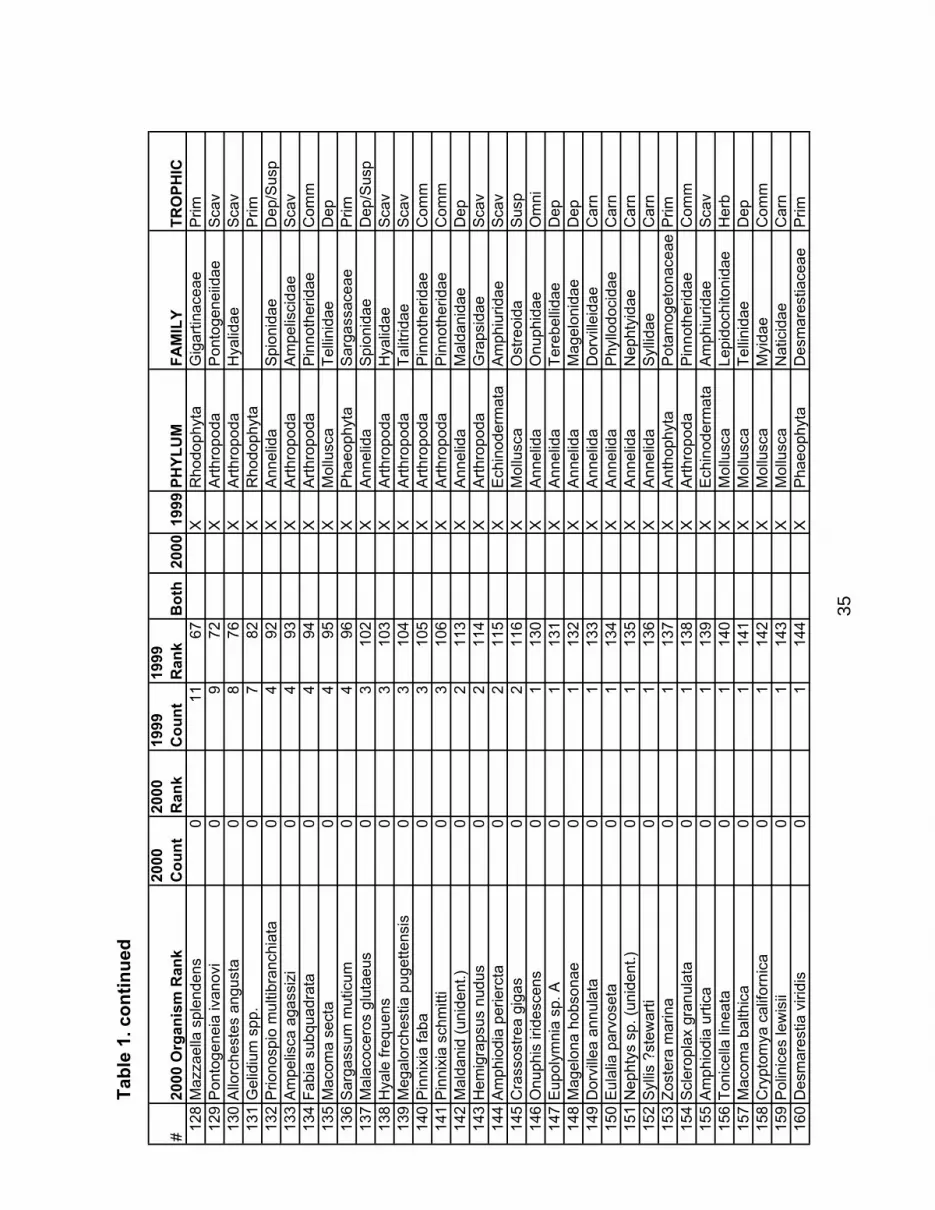
#20

00 O

rgan

ism

Ran

k20

00C

ou

nt

2000

Ran

k19

99C

ou

nt

1999

Ran

kB

oth

2000

1999

PH

YL

UM

FA

MIL

YT

RO

PH

IC12

8M

azza

ella

spl

ende

ns0

1167

XR

hodo

phyt

aG

igar

tinac

eae

Prim

129

Pon

toge

neia

ivan

ovi

09

72X

Art

hrop

oda

Pon

toge

neiid

aeS

cav

130

Allo

rche

stes

ang

usta

08

76X

Art

hrop

oda

Hya

lidae

Sca

v13

1G

elid

ium

spp

.0

782

XR

hodo

phyt

aP

rim13

2P

riono

spio

mul

tibra

nchi

ata

04

92X

Ann

elid

aS

pion

idae

Dep

/Sus

p13

3A

mpe

lisca

aga

ssiz

i0

493

XA

rthr

opod

aA

mpe

lisci

dae

Sca

v13

4F

abia

sub

quad

rata

04

94X

Art

hrop

oda

Pin

noth

erid

aeC

omm

135

Mac

oma

sect

a0

495

XM

ollu

sca

Tel

linid

aeD

ep13

6S

arga

ssum

mut

icum

04

96X

Pha

eoph

yta

Sar

gass

acea

eP

rim13

7M

alac

ocer

os g

luta

eus

03

102

XA

nnel

ida

Spi

onid

aeD

ep/S

usp

138

Hya

le fr

eque

ns0

310

3X

Art

hrop

oda

Hya

lidae

Sca

v13

9M

egal

orch

estia

pug

ette

nsis

03

104

XA

rthr

opod

aT

alitr

idae

Sca

v14

0P

inni

xia

faba

03

105

XA

rthr

opod

aP

inno

ther

idae

Com

m14

1P

inni

xia

schm

itti

03

106

XA

rthr

opod

aP

inno

ther

idae

Com

m14

2M

alda

nid

(uni

dent

.)0

211

3X

Ann

elid

aM

alda

nida

eD

ep14

3H

emig

raps

us n

udus

02

114

XA

rthr

opod

aG

raps

idae

Sca

v14

4A

mph

iodi

a pe

rierc

ta0

211

5X

Ech

inod

erm

ata

Am

phiu

ridae

Sca

v14

5C

rass

ostr

ea g

igas

02

116

XM

ollu

sca

Ost

reoi

daS

usp

146

Onu

phis

irid

esce

ns0

113

0X

Ann

elid

aO

nuph

idae

Om

ni14

7E

upol

ymni

a sp

. A0

113

1X

Ann

elid

aT

ereb

ellid

aeD

ep14

8M

agel

ona

hobs

onae

01

132

XA

nnel

ida

Mag

elon

idae

Dep

149

Dor

ville

a an

nula

ta0

113

3X

Ann

elid

aD

orvi

lleid

aeC

arn

150

Eul

alia

par

vose

ta0

113

4X

Ann

elid

aP

hyllo

doci

dae

Car

n15

1N

epht

ys s

p. (

unid

ent.)

01

135

XA

nnel

ida

Nep

htyi

dae

Car

n15

2S

yllis

?st

ewar

ti0

113

6X

Ann

elid

aS

yllid

aeC

arn

153

Zos

tera

mar

ina

01

137

XA

ntho

phyt

aP

otam

oget

onac

eae

Prim

154

Scl

erop

lax

gran

ulat

a0

113

8X

Art

hrop

oda

Pin

noth

erid

aeC

omm

155

Am

phio

dia

urtic

a0

113

9X

Ech

inod

erm

ata

Am

phiu

ridae

Sca

v15

6T

onic

ella

line

ata

01

140

XM

ollu

sca

Lepi

doch

itoni

dae

Her

b15

7M

acom

a ba

lthic

a0

114

1X

Mol

lusc

aT

ellin

idae

Dep

158

Cry

ptom

ya c

alifo

rnic

a0

114

2X

Mol

lusc

aM

yida

eC

omm

159

Pol

inic

es le

wis

ii0

114

3X

Mol

lusc

aN

atic

idae

Car

n16

0D

esm

ares

tia v

iridi

s0

114

4X

Pha

eoph

yta

Des

mar

estia

ceae

Prim

Tab

le 1

. co

nti

nu

ed

35

#20

00 O

rgan

ism

Ran

k20

00C

ou

nt

2000

Ran

k19

99C

ou

nt

1999

Ran

kB

oth

2000

1999

PH

YL

UM

FA

MIL

YT

RO

PH

IC16

1C

aula

cant

hus

sp.

01

145

XR

hodo

phyt

aC

aula

cant

hace

aeP

rim16

2C

eram

ium

sp.

01

146

XR

hodo

phyt

aC

eram

iace

aeP

rim16

3S

mith

ora

naia

dum

01

147

XR

hodo

phyt

aE

ryth

rope

ltida

ceae

Prim

Tab

le 1

. co

nti

nu

ed

36

High-Resolution Sampling Sites Low-Resolution Sampling SitesBasin Location Cell # Segment # Basin Location Cell # Segment #South Budd 7 4 South Case 9 15

5 166 17

Case 8 181920

Carr 1 5370 Central Brown 10 1

102 23

Central (east) Redondo 10 4 Normandy 10 75 86 9

Brace 11 13 Seahurst 11 1014 1115 12

Carkeek 12 22 Alki 11 1623 1724 18

Possession 13 31 West Pt 12 1932 2033 21

Central (west) to be identified X Wells 12 25X 26X 27X Edmonds 13 28X 29X 30X Double Bluff 13 34X 35X 36XXX

Table 2. We recommend that the sites sampled in 2000 be sampled again in 2001 using the same protocols to insure temporal consistency. To allow for comparisons of communities between the east and west shores of the Central Basin, we recommend that the same sampling protocols be used. If low taxonomic resolution sampling is attempted this year, then the remaining transects in the Central Sound nearshore cells should be revisited using those protocols. However, it may be determined by WADNR that the best use of low taxonomic resolution sampling will be during the intervening years between high taxonomic resolution sampling.

37

Epifauna (identify in field) Epiflora (identify in field)Polynoidae (scaleworms) Zostera marina

Sabellidae

Serpulidae green filaments (Acrosiphonia, Cladophora)

green blades and tubes (Ulva, Enteromorpha, Monostroma, Ulvaria)

Order Amphipoda

Sphaeromid isopods Alaria sp.Idoteid isopods Laminaria spp.

Hippolytid shrimp Desmarestia spp.

Class Cirripedia Fucus spp.

Cancrid crabs (list species if possible) Punctaria

Hemigrapsus (list species if possible) Sargassum

Majid (spider) crabs small brown blades and tubes (Scytosiphon, Petalonia)

Pagurid (hermit) crabs

Xanthid crabs (Lophopanopeus) Porphyra sp.

wirey branched reds (Endocladia, Gelidium, Caulacanthus)

Anthopleura spp. thin red filaments (Polysiphonia, Ceramium, Microcladia)

Metridium branched red blades (Mastocarpus, Mazzaella spp., Prionitis)

branched red tubes (Gracilaria, Sarcodiotheca)

Cl. Ophiuroidea (brittle stars) Rhodomelaceae (Neorhodomela, Odonthalia)

Leptasterias Encrusting algae

Evasterias

Dendraster VertebratesStrongylocentrotus Cottidae (sculpins)

Stichaeidae (gunnels and pricklebacks)

Mopalia spp.

Tonicella

Haminoea slugs

Hermissenda

Onchidoris spp.

Alia spp.

Bittium spp.

Crepidula (list species if possible)

Lacuna spp.

Littorina spp.

Lottiid limpets

Nassarius spp.

Nucella (list species if possible)

Odostomia spp.

Polinices

Calliostoma

Lirularia

Anomiidae (jingle shells)

Mytilus spp.

oysters

Pholadidae (boring clams)

Ph. Nemertea (ribbon worms)

Ph. Platyhelminthes (flatworms)

Table 3. Recommended "low resolution" taxa, with rare organisms omitted

38

Table 3, continued. Recommended low-resolution taxa

Infauna (identify later in preserved samples)Polychaeta Capitellidae (maybe separate by species)

Chaetopteridae

Cirratulidae

Dorvilleidae

Glyceridae

Goniadidae

Hesionidae

Lumbrineridae

Maldanidae

Nephtyidae

Nereidae

Onuphidae

Opheliidae

Orbiniidae

Oweniidae

Pectinariidae

Pholoidae

Phyllodocidae

Polynoidae

Spionidae

Syllidae

Terebellidae

Callianassidae

Crustacea Upogebiidae

Sphaeromid isopods

Pinnotherid crabs

Tanaidacea

Edwardsiidae

Cnidaria Cl. Ophiuroidea

Echinodermata Synaptidae

Cardiidae (Clinocardium)

Bivalvia Hiatellidae

Lucinidae

Mactridae (Tresus)

Myidae

Tellinidae

Veneridae

Misc. Ph. Nemertea

Ph. Phoronida

39

Appendix B. All species from Puget Sound database (unidentified taxa omitted) sorted by phylum and family.( ) = rare, omitted for Table 3.PHYLUM FAMILY SPECIES Recommended "low resolution" taxaAnnelida Ampharetidae Ampharete labrops Ampharetidae

Annelida Capitellidae Capitella capitata Capitellidae

Decamastus gracilis

Mediomastus californiensis

Notomastus lineatus

Notomastus tenuis

Annelida Chaetopteridae Spiochaetopterus costarum Chaeotopteridae

Annelida Cirratulidae Aphelochaeta multifilis Cirratulidae

Caulleriella ?pacifica

Cirratulus cingulatus

Cirratulus multioculata(?)

Cirratulus robustus

Cirriformia sp.A

Tharyx parvus

Annelida Dorvilleidae Dorvillea annulata Dorvilleidae

Annelida Flabelligeridae Pherusa plumosa (Flabelligeridae)

Annelida Glyceridae Glycera americana Glyceridae

Glycera siphonostoma

Glycera tenuis

Glycinde polygnatha

Hemipodus borealis

Annelida Goniadidae Glycinde picta Goniadidae

Goniada annulata

Annelida Hesionidae Kefersteinia sp. Hesionidae

Micropodarke dubia

Podarke pugettensis

Podarkeopsis glabrus

Annelida Lumbrineridae Lumbrineris pallida Lumbrineridae

Lumbrineris zonata

Annelida Magelonidae Magelona hobsonae Magelonidae

Annelida Maldanidae Axiothella rubrocincta Maldanidae

Euclymene sp.A

Euclymene sp.B (cf. zonalis)

Maldane sarsi

Nicomache ?personata

Annelida Nephtyidae Nephtys caeca Nephtyidae

Nephtys caecoides

Nephtys ferruginea

Nephtys longosetosa

Annelida Nereidae Nereis brandti Nereidae

Nereis limnicola

Nereis procera

Nereis vexillosa

Nereis zonata

Platynereis bicanaliculata

Annelida Onuphidae Diopatra ornata Onuphidae

Nothria conchylega

Onuphis 'holobranchiata'

Onuphis iridescens

40

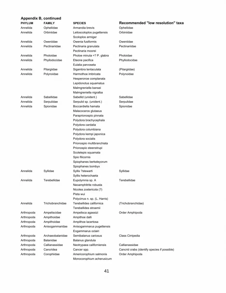
Appendix B, continuedPHYLUM FAMILY SPECIES Recommended "low resolution" taxaAnnelida Opheliidae Armandia brevis Opheliidae

Annelida Orbiniidae Leitoscoloplos pugettensis Orbiniidae

Scoloplos armiger

Annelida Oweniidae Owenia fusiformis Oweniidae

Annelida Pectinariidae Pectinaria granulata Pectinariidae

Pectinaria moorei

Annelida Pholoidae Pholoe minuta =? P. glabra Pholoidae

Annelida Phyllodocidae Eteone pacifica Phyllodocidae

Eulalia parvoseta

Annelida Pilargiidae Sigambra tentaculata (Pilargiidae)

Annelida Polynoidae Harmothoe imbricata Polynoidae

Hesperonoe complanata

Lepidonotus squamatus

Malmgreniella bansei

Malmgreniella nigralba

Annelida Sabellidae Sabellid (unident.) Sabellidae

Annelida Serpulidae Serpulid sp. (unident.) Serpulidae

Annelida Spionidae Boccardiella hamata Spionidae

Malacoceros glutaeus

Paraprionospio pinnata

Polydora brachycephala

Polydora cardalia

Polydora columbiana

Polydora kempi japonica

Polydora socialis

Prionospio multibranchiata

Prionospio steenstrupi

Scolelepis squamata

Spio filicornis

Spiophanes berkeleyorum

Spiophanes bombyx

Annelida Syllidae Syllis ?stewarti Syllidae

Syllis heterochaeta

Annelida Terebellidae Eupolymnia sp. A Terebellidae

Neoamphitrite robusta

Nicolea zostericola (?)

Pista wui

Polycirrus n. sp. (L. Harris)

Annelida Trichobranchidae Terebellides californica (Trichobranchidae)

Terebellides stroemii

Arthropoda Ampeliscidae Ampelisca agassizi Order Amphipoda

Arthropoda Ampithoidae Ampithoe dalli

Arthropoda Ampithoidae Ampithoe lacertosa

Arthropoda Anisogammaridae Anisogammarus pugettensis

Eogammarus oclairi

Arthropoda Archaeobalanidae Semibalanus cariosus Class Cirripedia

Arthropoda Balanidae Balanus glandula

Arthropoda Callianassidae Neotrypaea californiensis Callianassidae

Arthropoda Cancridea Cancer spp. Cancrid crabs (identify species if possible)

Arthropoda Corophiidae Americorophium salmonis Order Amphipoda

Monocorophium acherusicum

41

Appendix B, continuedPHYLUM FAMILY SPECIES Recommended "low resolution" taxaArthropoda Sphaeromatidae Exosphaeroma inornata Sphaeromatid isopods

Gnorimosphaeroma oregonense

Arthropoda Grapsidae Hemigrapsus nudus Grapsid crabs (identify species if possible)

Hemigrapsus oregonensis

Arthropoda Hippolytidae Heptacarpus sitchensis Hippolytid shrimp

Hippolyte clarki

Arthropoda Hyalidae Allorchestes angusta Order Amphipoda

Hyale frequens

Arthropoda Idoteidae Idotea sp. Idoteid isopods

Arthropoda Ligiidae Ligia occidentalis (Ligiidae)

Arthropoda Majidae Pugettia gracilis Majid crabs

Arthropoda Paguridae Pagurus spp. Paguridae

Arthropoda Pinnotheridae Fabia subquadrata Pinnotheridae

Pinnixia eburna

Pinnixia faba

Pinnixia schmitti

Pinnixia tubicola

Scleroplax granulata

Arthropoda Pontogeneiidae Pontogeneia ivanovi Order Amphipoda

Arthropoda Talitridae Megalorchestia pugettensis Order Amphipoda

Arthropoda Tanaidacea Leptochelia dubia Tanaidacea

Arthropoda Upogebiidae Upogebia pugettensis Upogebiidae

Arthropoda Xanthidae Lophopanopeus bellus bellus Xanthid crabs

Chordata Cottidae Oligocottus maculosus Cottidae

Chordata Stichaeidae Anoplarchus purpurescens Stichaeidae

Chordata Gunnel (unident.)

Cnidaria Actiniidae Anthopleura elegantissima Anthopleura

Cnidaria Edwardsiidae Edwardsia sipunculoides Edwardsiidae

Edwardsia sp.

Cnidaria Metridiidae Metridium senile Metridium

Echinodermata Amphiuridae Amphiodia periercta Cl. Ophiuroidea

Amphiodia urtica

Amphipholis squamata

Echinodermata Asteriidae Evasterias troschelii Evasterias

Leptasterias hexactis Leptasterias

Echinodermata Dendrasteridae Dendraster excentricus Dendraster

Echinodermata Ophiuridae Ophiura lutkeni Cl. Ophiuroidea

Echinodermata Strongylocentrotidae Stronglyocentrotus droebachiensis Strongylocentrotus

Echinodermata Synaptidae Leptosynapta clarki Synaptidae

Hemichordata Unid Saccoglossus sp. (Ph. Hemichordata)

Mollusca Anomiidae Pododesmus cepio Anomiidae

Mollusca Atyidae Haminoea vesicula Haminoea

Mollusca Calyptraeidae Crepidula dorsata Crepidula spp. (identify to species if possible)

Crepidula fornicata

Mollusca Cardiidae Clinocardium nuttallii Cardiidae

Mollusca Cerithiidae Bittium eschrichtii Cerithiidae

Mollusca Columbellidae Alia gausapata Columbellidae

Mollusca Facelinidae Hermissenda crassicornis Facelinidae

Mollusca Hiatellidae Hiatella arctica Hiatellidae

Panomya chrysis

Mollusca Lacunidae Lacuna vincta Lacunidae

42

Appendix B, continuedPHYLUM FAMILY SPECIES Recommended "low resolution" taxaMollusca Lepidochitonidae Tonicella lineata Tonicella

Mollusca Littorinidae Littorina scutulata Littorinidae

Mollusca Lottiidae Lottia pelta Lottiidae

Lottia strigatella

Tectura scutum

Mollusca Lucinidae Lucina annulata Lucinidae

Lucina tenuisculpta

Mollusca Mactridae Tresus capax Mactridae

Mollusca Montacutidae Mysella tumida Montacutidae

Pseudopythina rugifera

Mollusca Mopaliidae Mopalia lignosa Mopalia spp.

Mollusca Myidae Cryptomya californica Myidae

Mya arenaria

Mollusca Mytilidae Mytilus trossulus Mytilidae

Mollusca Nassariidae Nassarius mendicus Nassariidae

Nassarius perpinguis

Mollusca Naticidae Polinices lewisii Naticidae

Mollusca Nucellidae Nucella canaliculata Nucella (identify to species if possible)

Nucella lamellosa

Mollusca Onchidorididae Onchidoris bilamellata Onchidoris

Mollusca Ostreoida Crassostrea gigas oysters

Ostrea edulis

Ostrea lurida

Mollusca Pholadidae Piddock clam (unident.) Pholadidae

Mollusca Pyramidellidae Odostomia sp. (unident.) Odostomia

Turbonilla sp. (unident.)

Mollusca Tellinidae Macoma balthica Tellinidae

Macoma inquinata

Macoma nasuta

Macoma secta

Tellina bodegensis

Tellina modesta

Tellina nuculoides

Mollusca Trochidae Calliostoma sp. Calliostoma

Lirularia succincta Lirularia

Mollusca Veneridae Compsomyax subdiaphana Veneridae

Protothaca staminea

Saxidomus giganteus

Tapes philippinarum

Transennella tantilla

Nemertea Emplectonematidae Paranemertes peregrina Ph. Nemertea

Nemertea Lineidae Cerebratulus sp.

Nemertea Nemertean (unident.)

Phoronida Phoronidae Phoronopsis harmeri Ph. Phoronida

Platyhelminthes Childiidae Freemania litoricola Ph. Platyhelminthes

Platyhelminthes Flatworm (unident.)

Sipuncula Phascolosomatidae Phascolosoma agassizii (Ph. Sipuncula)

43

Appendix B, continuedPHYLUM FAMILY SPECIES Recommended "low resolution" taxaAnthophyta Potamogetonaceae Zostera marina Zostera marina

Chlorophyta Acrosiphoniaceae Acrosiphonia coalita green filaments

Chlorophyta Ulvoids (unident.) green blades and tubes

Phaeophyta Alariaceae Alaria sp. (unident) Alaria sp.

Phaeophyta Desmarestiaceae Desmarestia viridis Desmarestia spp.

Phaeophyta Fucaceae Fucus gardneri Fucus spp.

Phaeophyta Laminariaceae Laminaria saccharina Laminaria spp.

Phaeophyta Punctariaceae Punctaria expansa Punctaria

Phaeophyta Sargassaceae Sargassum muticum Sargassum

Phaeophyta Scytosiphonaceae Scytosiphon lomentaria small brown blades and tubes

Petalonia fascia

Rhodophyta Bangiaceae Porphyra sp. Porphyra sp.

Rhodophyta Caulacanthaceae Caulacanthus sp. wirey branched reds

Endocladiaceae Endocladia muricata

Gelidiaceae Gelidium spp.

Rhodophyta Ceramiaceae Ceramium sp. thin red filaments

Microcladia borealis

Rhodomelaceae Polysiphonia sp. (unident.)

Rhodophyta Erythropeltidaceae Smithora naiadum (Smithora)

Rhodophyta Gigartinaceae Mazzaella heterocarpa branched red blades

Mazzaella splendens

Rhodophyta Halymeniaceae Prionitis sp. (unident.)

Rhodophyta Petrocelidaceae Mastocarpus papillatus

Rhodophyta Gracilariaceae Gracilaria pacifica branched red tubes

Solieriaceae Sarcodiotheca sp. (unid.)

Rhodophyta Rhodomelaceae Neorhodomela larix Rhodomelaceae

Odonthalia floccosa

Encrusting algae (unid.) Encrusting algae

44