intertidal benthic diatoms of the tagus estuary - core
TRANSCRIPT

UNIVERSIDADE DE LISBOA
FACULDADE DE CIÊNCIAS
DEPARTAMENTO DE BIOLOGIA VEGETAL
Intertidal benthic diatoms of the Tagus estuary:
Taxonomic composition and spatial-temporal
variation
(Volume 1)
Lourenço Luís Cardoso Soares Ribeiro
DOUTORAMENTO EM BIOLOGIA
Especialidade Biodiversidade
2010


UNIVERSIDADE DE LISBOA
FACULDADE DE CIÊNCIAS
DEPARTAMENTO DE BIOLOGIA VEGETAL
Intertidal benthic diatoms of the Tagus estuary:
Taxonomic composition and spatial-temporal
variation
(Volume 1)
Lourenço Luís Cardoso Soares Ribeiro
Tese orientada por:
Prof. Doutora Vanda Brotas e Prof. Doutor Yves Rincé
DOUTORAMENTO EM BIOLOGIA
Especialidade Biodiversidade
2010


à Laura e ao Luís Alberto


O apanhador de nabos
aponta o caminho
com um nabo
Issa Kobayashi, séc. XVIII-XIX.
versão de Jorge Sousa Braga,
in “Primeira Neve”, Ed. Assírio & Alvim


i
INDEX
Acknowledgements ................................................................................................................................................ iii
Summary ................................................................................................................................................................. v
Resumo .................................................................................................................................................................. vii
1. Introduction ................................................................................................................................................... 3
2. Study area..................................................................................................................................................... 15
2.1. Tagus estuary ..................................................................................................................................... 15
2.2. Alcochete intertidal flats .................................................................................................................... 19
2.2.1. Sediment characterisation and environmental parameters ....................................................... 20
2.2.2. MPB biomass, MPB pigment and microalgal composition ........................................................ 23
3. Material and methods ................................................................................................................................. 29
3.1. Sampling and slide preparation ........................................................................................................ 29
3.1.1. Diatom sampling, extraction, and preservation .......................................................................... 29
3.1.2. Diatom cleaning procedures and slide preparation .................................................................... 31
3.1.3. Diatom identification and cell counting ....................................................................................... 32
3.2. Data screening: species datasets ....................................................................................................... 33
3.3. Diversity .............................................................................................................................................. 34
3.4. Multivariate data analysis ................................................................................................................. 36
3.4.1. Similarity measurement: Bray-Curtis Similarity ....................................................................... 36
3.4.2. Classification: CLUSTER ............................................................................................................. 37
3.4.3. Ordination: MDS ........................................................................................................................... 38
3.4.4. Hypothesis testing for differences between groups of samples: ANOSIM ................................ 38
3.4.5. Species similarities percentage analysis: SIMPER ..................................................................... 39
3.4.6. Linking multivariate community structure to environmental variables: BIOENV ................ 40
3.5. Terminology of functional-groups, life-forms and size-classes ...................................................... 42
4. Results ........................................................................................................................................................... 49
4.1. Diversity .............................................................................................................................................. 49
4.2. Diatom community structure: biotic and environmental multivariate patterns (ANOSIM, MDS, CLUSTER, BIOENV) .......................................................................................................................... 51
4.3. Diatom community structure: taxonomic composition of the assemblages (SIMPER) ............... 57
4.4. Diatom community physiognomy: spatial distribution of size-classes, functional-groups and life-forms .......................................................................................................................................................... 61
4.4.1. Size-classes ...................................................................................................................................... 61
4.4.2. Functional groups and Life-forms ................................................................................................ 63
4.5. Temporal variation of diatom assemblages and individual species ............................................... 65
5. Discussion ..................................................................................................................................................... 73
5.1. Spatial variation and the role of sediment texture .......................................................................... 73

ii
5.2. Two main types of communities ........................................................................................................ 76
5.2.1. Epipsammon-dominated community ........................................................................................... 77
5.2.2. Epipelon-dominated community .................................................................................................. 82
5.3. Temporal variation in both types of communities ........................................................................... 88
5.3.1. Epipsammon ................................................................................................................................... 89
5.3.2. Epipelon .......................................................................................................................................... 91
5.4. Diversity .............................................................................................................................................. 95
6. Assessing alternative approaches to species abundance-by-sample community structure description in intertidal benthic diatoms ......................................................................................................... 101
6.1. Introduction ...................................................................................................................................... 101
6.2. Methods ............................................................................................................................................. 104
6.2.1. Matrix selection and data transformation ................................................................................. 104
6.2.2. Matrix comparison and multivariate analyses .......................................................................... 105
6.3. Results ............................................................................................................................................... 107
6.3.1. Higher taxonomical resolution: species presence/absence matrix ........................................... 109
6.3.2. Higher taxonomical resolution: species relative biovolume matrix ......................................... 109
6.3.3. Lower taxonomical resolution: genera matrices ....................................................................... 110
6.3.4. Alternative classifications: size-classes and life-forms matrices .............................................. 113
6.4. Discussion .......................................................................................................................................... 114
6.4.1. Rare species exclusion ................................................................................................................. 114
6.4.2. Qualitative analysis: species presence-absence ......................................................................... 115
6.4.3. Species relative biovolume analysis ............................................................................................ 116
6.4.4. Taxonomic sufficiency: genus-level analyses ............................................................................. 118
6.4.5. Taxonomic surrogacy: size-classes and life-forms analysis ...................................................... 120
6.5. Conclusion......................................................................................................................................... 122
7. Diatom Identification Guide ..................................................................................................................... 127
7.1. Introduction ...................................................................................................................................... 127
7.2. Diatom taxa entries .......................................................................................................................... 129
7.3. Diatom taxa list ................................................................................................................................. 277
8. Concluding Remarks ................................................................................................................................. 283
9. References................................................................................................................................................... 289

iii
Acknowledgements
First and foremost, I wish to thank my two supervisors, Prof. Vanda Brotas and Prof.
Yves Rincé for their support and advice. I am deeply grateful to Prof. Vanda Brotas for
introducing me to microphytobenthos ecology and for always foster my interest in diatom
taxonomy. To Prof. Yves Rincé, many thanks for kindly receiving me in his laboratory
and home and for his promptness in responding to my solicitations, even when I was not
in France. To both of them, I acknowledge their trust, patience and graciousness in deal-
ing with a sometimes stubborn and single-minded student.
Some of the fondest memories of this period are from my stays at the Laboratoire de
Biologie Marine in Nantes. For welcoming me as part of the family, I would like to thank
the staff of the “ISOMER”. So, to Bruno, Christophe, Jean-Bernard, Laurent, Philippe,
Pierre, Priscilla, Richard, Sindy, Vona et tous les autres: un grand merci!
I am very grateful to my colleagues of the Instituto of Oceanografia and, in particular, to
the botany group. It will be hard to name everyone who works or worked there without,
regretfully, forgetting someone. So, to all of you: thank you for your steady and generous
support, companionship and example. In spite of all the difficulties and complaints you
kept showing up, every morning, with an undying passion for the science you do! Special
thanks to Bruno Jesus, Paulo Cartaxana and Rafael Mendes for all the hard work during
the HIMOM project. Their enormous contribution to this work was absolutely essential.
Most of the electron microscopy presented in this work was made by Prof. Dr. Dr. h.c.
Horst Lange-Bertalot, Manfred Ruppel (J.-W. Goethe University) and Prof. Dr. hab.
Andrzej Witkowski (University of Szczecin). For kindly accepting to explore the Tagus
estuary material, but also for the fruitful and lasting discussions on the taxonomy and
beauty of marine benthic diatoms, my sincere and deepest gratitude.
I would also like to express my gratefulness to the fellow diatomists who provided their
PhD. thesis or research papers and gave me great insights and knowledge on the difficult
subject of marine benthic diatom taxonomy. I have particularly appreciated the “argu-
ments” given by Frithjof Sterrenburg; the discussions on Amphora with Eugenia Sar and

iv
the suggestions given by Koen Sabbe, whose own work on the ecology and systematics of
the benthic diatoms of the Westerschelde estuary greatly influenced this thesis.
The diatom plates in Volume 2 were made possible by the expertise and know-how of my
cousins Bárbara and Tiago Soares Ribeiro (Zazádesign – Dá saúde e faz crescer). I will be
forever grateful for their wonderful work and, mostly, for their lifelong friendship.
I am very thankful to all my friends and family for all their love and support during all
these years. It would have been impossible without their belief in me and their help in
putting things into perspective. In particular, I would like to thank my father for putting
on the lab coat and helping me with the preparation of the diatom slides. It was great fun!
Muito obrigado a todos!
Finally, I specially thank Susanne, my partner in all of this and in much more. I cannot
imagine pulling trough this thesis without your constant support, love and understanding.
Merci viu mau für aues!
This work was funded by FCT - Fundação para a Ciência e Tecnologia with a PhD re-
search grant from SFRM/BD-10426-02.

v
Summary The taxonomic composition of intertidal benthic diatom communities of many estuarine
and coastal areas worldwide is still fairly unknown. In order to increase knowledge on the
biodiversity and community structure of the intertidal benthic diatoms of the Tagus estu-
ary, a two-year survey was carried out in 6 stations with distinct sediment structure. The
main output of the study is the Identification Guide which is supplemented by 1019 mi-
crographs (volume 2). This detailed systematic account of 185 diatom taxa observed in-
cludes: morphological descriptions and comparisons to similar species, as well as infor-
mation on biogeography and autoecology. Moreover, the structure of the diatom commu-
nities was characterized by its diversity and other features related to community physiog-
nomy, such as size-class or life-form distribution. Temporal patterns were clearly subor-
dinate to spatial ones; mud content was found to be the environmental variable most cor-
related to the multivariate patterns of the biotic data. The level of physical disturbance of
the sediment was found to be responsible for the structure of the diatom communities as it
controls the interplay between two different functional groups composing the diatom as-
semblages: the epipelon and the epipsammon. The epipelon, a less diverse community,
mainly composed of medium-sized species, shows a certain degree of seasonal variation.
This community dominates sheltered areas and its occurrence can be predicted by the
mud content of the sediment, a good indicator of the level of sediment exposure. The
epipsammon, a very diverse community composed by minute species, does not show
temporal patterns. Its occurrence is conditioned by the presence of the substrate (i.e. sand-
grains) that is colonized by several types of life-forms. Alternatives to species-level iden-
tification were examined in order to bridge the gap between functional and structural eco-
logical studies. The major multivariate patterns were mostly replicated but with unequal
success. Species presence/absence and genus-level abundance data generated the best
results. However, the temporal patterns were clouded by the decrease in taxonomical
resolution or the loss of abundance data. The great intrinsic value of biodiversity assess-
ment, even of microscopic organisms, is recognized and well established nowadays. Flo-
ristic studies made in conjunction with ecological-oriented research on microphytoben-
thos enhance our understanding of the structure and function of this important community
and provide much needed data on the biogeography and autoecology of these microorgan-
isms. Key words: diatoms, ecology, taxonomy, microphytobenthos, spatial-temporal distribution,
diversity, epipelon, epipsammon, life-form, community, intertidal flat, estuary.

vi

vii
Resumo
As diatomáceas bênticas são o componente principal das comunidades de algas micros-
cópicas que colonizam as zonas de sedimentos intertidais na maioria dos estuários e áreas
costeiras da costa atlântica europeia, formando extensos biofilmes à superfície desse
sedimentos. Essas comunidades são também conhecidas como microfitobentos (MPB) e
são responsáveis pela elevada produção primária nos espraiados de maré, que pode cor-
responder a 50% do total da produção primária estuarina (Underwood & Kromkamp
1999). As diatomáceas presentes nessas comunidades têm sido tradicionalmente classifi-
cadas como epipsâmicas, quando vivem agarradas a partículas de areia, e epipélicas,
quando vivem em sedimentos vasosos. No entanto estas definições foram consideradas
demasiado simplistas por alguns autores (Sabbe 1997), tendo sido mesmo rejeitada por
outros (de Jonge 1985).
Grande parte da investigação científica sobre o microfitobentos tem sido focada em diver-
sos aspectos da sua ecologia funcional como, por exemplo, os padrões espácio-temporais
de biomassa e/ou de produção primária, o seu papel na circulação de nutrientes ou em
detalhes ligados à sua ecofisiologia (e.g. ritmos migratórios endógenos dos biofilmes
microfitobênticos). Apesar ter sublinhado o papel fundamental que o microfitobentos tem
para o funcionamento dos ecossistemas estuarinos, este género de investigação tende a
considerar os biofilmes de microfitobentos como um todo (uma “caixa-negra”) ou então a
limitar o estudo da estrutura das comunidades microfitobênticas à análise pigmentar,
recorrendo cromatografia líquida de alta precisão (HPLC). A análise pigmentar, no entan-
to, apenas permite estabelecer a identidade e a contribuição de cada grupo de microalgas
que constituem esse biofilmes (e.g. diatomáceas, euglenófitas e cianobactérias), mas não
fornece mais informação sobre a estrutura taxonómica contida em cada uma dessas frac-
ções. Por outro lado, os estudos florísticos que se debruçam sobre a estrutura dessas
comunidades e/ou a taxonomia das espécies que as constituem são comparativamente

RESUMO
viii
mais raros que os estudos funcionais, havendo igualmente um divórcio cada vez mais
claro entre estas duas vertentes (Underwood 2005, Underwood & Barnett 2006). As difi-
culdades associadas aos estudos florísticos das comunidades de diatomáceas bênticas
estuarinas são inúmeras e encontram-se resumidas na introdução desta tese (capítulo 1).
Como resultado, pouco se sabe da auto-ecologia e da taxonomia de muitas das espécies
diatomáceas bênticas intertidais. Além disso, a biodiversidade e a estrutura das comuni-
dades praticamente desconhecida em muitas áreas costeiras e estuários, entre os quais o
estuário do Tejo.
Esta tese tem como principais objectivos: (1) identificar, descrever e ilustrar as espécies
que compõem as comunidades de diatomáceas bênticas dos substratos móveis intertidais
do estuário do Tejo; (2) determinar os diferentes tipos de comunidades de diatomáceas
bênticas, descrever a suas variações espácio-temporais e relacioná-las com as variáveis
ambientais; (3) avaliar e comparar o desempenho de alternativas à identificação ao nível
das espécies, na detecção de padrões espácio-temporais nas comunidades de diatomáceas
bênticas estuarinas. De forma a aumentar o conhecimento sobre a composição taxonómi-
ca e estrutura das comunidades de diatomáceas bênticas intertidais do estuário do Tejo,
um programa de amostragem foi conduzido durante 2 anos (2003-2004) em 6 estações de
amostragem com estrutura sedimentar distinta e organizadas em 2 transectos, tendo um
sedimento mais vasoso e outro sedimento mais arenoso. A área de estudo, bem como o
estuário do Tejo, são descritos no capítulo 2.
Na primeira parte desta tese é descrita a estrutura e a variação espácio-temporal das
comunidades de diatomáceas bênticas encontradas nas 6 estações de amostragem durante
o período de estudo. A estrutura das comunidades de diatomáceas foi caracterizada não só
em termos da sua composição taxonómica e diversidade, mas também através da sua
fisiognomia. Neste estudo, o termo “fisiognomia das comunidades” foi utilizado no senti-
do botânico clássico do termo, isto é, referindo-se a aspectos podem ser ligados à aparên-
cia e tipo de “formação vegetal” como, por exemplo, a distribuição dos indivíduos encon-
trados em classes de tamanho ou descriminando as diferentes “formas de vida” presentes.
Todos estes termos encontram-se definidos no capítulo dedicado ao material e métodos
(capítulo 3). A dinâmica dos padrões espácio-temporais na estrutura das comunidades de
diatomáceas foi determinada utilizando métodos estatísticos não-paramétricos de análise
multivariada, baseados em similaridades Bray-Curtis, e que derivam de uma matriz de
abundâncias de espécies (Clarke & Warwick 2001). Adicionalmente, essa matriz biótica

RESUM0
ix
foi correlacionada, também através de métodos estatístico não-paramétricos (BIO-ENV),
com a matriz das variáveis ambientais. Os resultados deste trabalho são apresentados no
capítulo 4 e discutidos em detalhe no capítulo 5.
Os padrões temporais foram claramente subordinados aos padrões espaciais, de acordo
com a análise de similaridades (ANOSIM). Em termos espaciais, parece haver uma sepa-
ração clara das amostras por estação de amostragem, ao passo que, em termos temporais,
apenas nas estações de sedimento vasoso houve uma separação significativa entre amos-
tras colhidas no Inverno/Primavera e as amostras colhidas no Verão/Outono. As amostras
das estações arenosas e as amostras provenientes das estações de sedimento vasoso mos-
traram ter o menor grau de similaridade. Embora menos evidente, houve também uma
distinção entre amostras provenientes de estações arenosas com texturas sedimentares
diferentes. A análise da composição e da fisiognomia comunidades demonstrou que as
diferenças entre povoamentos das estações de amostragem eram taxonómicas, sendo tam-
bém dependentes das abundâncias das espécies presentes. Por outro lado, essas diferenças
puderam ser replicadas pelas diferenças entre as proporções relativas dos dois grupos fun-
cionais (i.e. o epipsammon e o epipelon) ou na distribuição das formas de vida que estão
incluídas em cada desses grupos funcionais.
Os povoamentos encontrados em sedimentos muito vasosos tinham uma diversidade bai-
xa, sendo dominadas apenas por algumas espécies de diatomáceas birafídeas e móveis
como Navicula spartinetensis, Navicula gregaria, Gyrosigma fasciola e Cylindrotheca
signata. As amostras provenientes das estações mais vasosas tiveram as similaridades
intra-estação mais baixas. Estas comunidades mostraram, ainda, um certo grau de sazona-
lidade, causado pela alternância temporal das espécies que foram dominando sucessiva-
mente os povoamentos durante o período de estudo. Em relação à fisiognomia das comu-
nidades encontradas nas estações mais vasosas, houve uma quase total dominância de
formas epipélicas móveis, embora também seja de registar a presença um pequeno grupo
de formas diminutas e imóveis (e.g. Cymatosira belgica). Estas formas comportam-se,
aparentemente, como partículas de silte, usando a ressuspensão dos sedimentos como
forma de dispersão (viz. Sabbe 1997). Em termos da distribuição das classes de tamanho,
estes povoamentos foram dominados por diatomáceas de tamanho médio (i.e. 250-1000
μm3), um grupo composto maioritariamente por espécies de Navicula. Houve também
grupo menos abundantes de espécies grandes (i.e. >1000 μm3) e de espécies pequenas

RESUMO
x
(i.e. 100-250 µm3). As espécies muito pequenas (i.e. <100 μm3) estiveram praticamente
ausentes nas estações vasosas.
Os povoamentos de diatomáceas presentes nas estações arenosas apresentaram diversida-
des bastante mais elevadas que os presentes nas estações vasosas e não mostraram
nenhum padrão sazonal, mantendo-se a estrutura das comunidades constante ao longo de
todo o período de estudo. Estas comunidades eram tipicamente formadas por diatomáceas
pequenas ou muito pequenas (i.e. com um biovolume <250 µm3), sendo compostas por
variadas formas de vida epipsâmicas. Uma das formas de vida mais importantes nas esta-
ções arenosas foi o grupo formado por pequenas espécies móveis pertencentes aos géne-
ros Navicula (e.g. N. viminoides, N. aff. aleksandrae; N. germanopolonica), Fallacia,
Nitzschia ou Cocconeiopsis. Outra forma de vida bastante comum nessas estações foi a
das espécies prostradas, que vivem mais firmemente agarradas aos grãos de areia. Estas
espécies podem ser birafídeas (e.g. Biremis lucens, Catenula adhaerens, Catenula sp.1)
ou monorafídeas como Planothidium delicatulum e espécies do género Cocconeis (e.g. C.
hauniensis, C. peltoides e C. pelta). As espécies arafídeas, que se encontram ligadas à
superfície dos grãos de areia por um pedúnculo de mucilagem, correspondem a uma ter-
ceira forma de vida epipsâmica. Estas espécies pedunculadas pertenciam essencialmente
aos géneros Opephora e Fragilaria (e.g. O. guenter-grassii, Opephora sp.1) e ocorreram
quase exclusivamente na estação mais elevada do transecto arenoso. Esta estação distin-
guia-se também por ser composta por sedimento arenoso de calibre médio e fino. As res-
tantes estações arenosas eram compostas principalmente por areias de calibre médio e
grosseiro, tendo também uma maior fracção de sedimento vasoso. Este último facto pare-
ce ter contribuído para distinção entre os povoamentos encontrados na primeira estação
dos das outras estações arenosas, pois com o aumento do conteúdo em vasa aumentou
também a importância relativa das diatomáceas epipélicas, enquanto a abundância relati-
va das pequenas espécies epipsâmicas móveis (e.g. Navicula germanopolonica; N. boze-
nae) diminuiu drasticamente.
De facto, este estudo confirmou a importância fundamental que o tipo de sedimento tem
na estrutura das comunidades estuarinas de diatomáceas bênticas encontradas em substra-
tos móveis intertidais. De acordo com a rotina BIO-ENV, que relaciona as variáveis
ambientais à matriz de abundância das espécies, o conteúdo em vasa (i.e. siltes e argilas)
mostrou ter maior correlação significativa com a matriz biótica, apresentando uma corre-
lação elevada (ρ = 0.863, p <0.1 %). O teor em vasa é um excelente indicador do grau de

RESUM0
xi
exposição do sedimento. A perturbação física do sedimento, causada pelas correntes de
maré, ondas ou pela bioturbação, parece ser o factor determinante para estrutura das
comunidades de diatomáceas bênticas em substratos móveis intertidais. Assim, nas zonas
menos hidrodinâmicas, a vasa deposita-se e os espraiados entre-marés são dominados por
espécies epipélicas (móveis ou não), sendo que a ausência de grãos de areia não permite a
colonização dessas áreas por espécies epipsâmicas. A diversidade desses povoamentos é
baixa, provavelmente devido a fenómenos de competição inter-específica que causam a
dominância de apenas algumas espécies e, em parte, a alternância sazonal destas. Nas
zonas mais hidrodinâmicas, há acumulação de grão de areias mas o siltes e argilas não se
conseguem depositar. Nessas áreas instala-se uma comunidade epipsâmica que é muito
diversa não só devido ao tamanho reduzido das espécies, mas também devido à maior
variedade de formas de vida que exploram diferentemente os microhabitats existentes em
cada grão de areia. Além disso, a constante perturbação mecânica a que esses sedimentos
estão sujeitos promove a diversidade e impede a dominância, ao manter o número de
indivíduos de cada espécie relativamente baixo, bem como forçando a estabilidade sazo-
nal na estrutura dessas comunidades. Ambas as comunidades podem, no entanto, co-
existir desde que as condições locais possibilitem a deposição de partículas de vasa e a
sobrevivência das espécies epipélicas, sendo dinâmicas o suficiente para não permitir que
o substrato das espécies epipsâmicas (i.e. os grão de areia) fique completamente soterra-
do. Mesmo nestes casos, os padrões temporais das duas comunidades permanecem inde-
pendentes, como já tinha sido demonstrado anteriormente por Sabbe (1993).
Tendo descrito a estrutura das comunidades de diatomáceas bênticas com o máximo de
resolução taxonómica possível, bem como a dinâmica dos padrões espácio-temporais
dessas comunidades, foi realizado um exercício de comparação de alternativas à identifi-
cação ao nível da espécie que possam fornecer alguma dessa mesma informação (capítu-
lo 6). O objectivo desta análise comparativa foi avaliar o desempenho de alternativas
como a utilização de dados qualitativos (i.e. presença-ausência), da identificação taxonó-
mica apenas até ao nível do género, a conversão dos dados de abundância relativa em
biovolume relativo, a utilização substitutos taxonómicos (i.e. classes de tamanho ou for-
mas de vida) e, finalmente, o efeito de exclusão de espécies muito raras. Este sexto capí-
tulo é, de certa forma, independente dos três capítulos anteriores, embora utilize o mesmo
conjunto de dados e partilhe muitos métodos estatísticos multivariados. Como se insere
numa problemática diferente, possui uma introdução, métodos, resultados e discussão

RESUMO
xii
próprias. Apesar de este género de exercício ser comum em estudos sobre diatomáceas
bênticas de água doce (e.g. Lavoie et al. 2008) ou sobre a meiofauna estuarina (e.g. War-
wick 1988), nunca foi realizado em diatomáceas bênticas estuarinas. Neste contexto, é
pertinente avaliar se existem alternativas válidas à identificação até à espécie que sejam
mais acessíveis à maioria dos investigadores trabalhando em ecologia do microfitobentos,
mas que consigam descrever satisfatoriamente a estrutura das comunidades de diatomá-
ceas bênticas estuarinas.
Os resultados mostram que a exclusão das espécies muito raras teve um efeito muito
reduzido mas, de certa forma, positivo pois aumentou ligeiramente a nitidez dos padrões
multivariados observados e a correlação com os dados ambientais. A matriz de presença-
ausência de espécies (i.e. elevada resolução mas sem abundâncias) e a matriz de géneros
(i.e. resolução mais baixa mas com abundâncias) parecer ser as alternativas que melhor
replicam os padrões multivariados obtidos pela matriz de abundância de espécies. No
entanto, e apesar de terem ambas tido correlações elevadas com a matriz das espécies (ρ ≥
0.95), não conseguiram detectar quaisquer variações sazonais nas estações de sedimento
vasoso que são dominadas por espécies epipélicas. Por essa razão, o uso destas duas
alternativas deve ser aconselhado somente para trabalhos que apenas requeiram uma dis-
tinção espacial. De realçar que todas as outras alternativas falharam na detecção de dife-
renças espaciais mais subtis, como a ligeira distinção entre povoamentos nas estações
arenosas, para além de não detectarem diferenças sazonais nas comunidades epipélicas.
A principal contribuição deste trabalho é, sem dúvida, o Guia de Identificação de Diato-
máceas (capítulo 7) que é suplementado com 1019 fotografias em microscopia óptica e
electrónica de varrimento, organizadas em 59 estampas (volume 2). Este guia representa,
provavelmente, a mais detalhada descrição florística das comunidades de diatomáceas
bênticas das zonas estuarinas intertidais feita até ao momento em Portugal. O guia inclui a
seguinte informação: (1) dados morfométricos que resultaram de mais de 7000 medições
biométricas (e.g. intervalos de tamanhos das valvas, densidade de estrias ou biovolume);
(2) informação importante sobre a biogeografia e ecologia das espécies encontradas; (3)
discussão da literatura relevante para cada taxon; (4) comparação com outras espécies que
sejam morfologicamente semelhantes e facilmente confundíveis.
No total, 185 taxa de diatomáceas foram observados e descritos até ao nível do género,
espécies ou infra-específico (secção 7.3). Desses, 108 foram identificados até ao nível da

RESUM0
xiii
espécie (ou infra-específico), não tendo sido possível determinar a identidade de 77 taxa
(42% do total de taxa). Neste segundo grupo, 45 taxa (24% do total) foram atribuídos
provisoriamente a uma espécie conhecida, o que é indicado pelas abreviações “cf.” ou
“aff.” no binomial. Neste grupo encontram-se taxa que são semelhante a espécies cuja
identidade taxonómica ou auto-ecológica se encontra ainda aberta a debate. Os restantes
32 taxa (27 % do total) não puderam ser inequivocamente identificados para além do
género a que se julga pertencerem. Neste último grupo incluem-se espécies mas também
géneros que poderão ser novos para a ciência (e.g. Haslea sp.1, Catenula sp.1 e Catenula
sp.2). A descrição formal de um novo género e uma espécie nova, Pierrecomperia cate-
nuloides, encontra-se a aguardar publicação (Sabbe et al. submitted).
A flora descrita neste trabalho é bastante semelhante às encontradas noutras áreas interti-
dais das costas atlânticas do Norte da Europa (e.g. Hustedt 1939, Sabbe 1997) e, em par-
ticular, na costa ocidental francesa (e.g. Méléder et al. 2007). Tendo em conta que apenas
foi estudada uma zona bastante restrita do estuário, o número total de espécies de diato-
máceas bênticas existentes no estuário do Estuário do Tejo é provavelmente bastante mais
elevado. Uma estimativa conservadora apontaria para um número superior aos 300 taxa,
em consonância com os valores obtidos para os estuários do Tamisa (Juggins 1992) e do
Escalda Ocidental (Sabbe 1997).
Num contexto de uma crescente percepção do importante papel que a biodiversidade tem
nos ecossistemas marinhos mas também do contributo que a correcta identificação taxo-
nómica pode ter em trabalhos de ecologia, espera-se que este trabalho, ainda que de forma
incompleta, possa contribuir preencher uma lacuna existente nos estudos do microfitoben-
tos do estuário de Tejo e ajude, futuramente, na melhor compreensão dessa importante
comunidade de microrganismos.


1
Chapter 1
Introduction

2

3
1. Introduction
Diatoms (Bacillariophyta) are an extremely diverse group of microalgae with an esti-
mated number of species between 104–105, depending on the species concept (Stoermer
& Smol 1999). Mann & Droop (1996) suggested that the total species number could be as
high as two hundred thousand. They have a worldwide distribution and constitute a major
component of planktonic and benthic algal communities, from oceanic oligotrophic wa-
ters to polar ice caps; from moist soils to freshwater alkaline lakes or eutrophic estuaries
(e.g. Round et al. 1990). Diatoms have a global significance, as they may to be responsi-
ble for one-fifth of the total of the Earth’s photosynthesis (Mann 1999). Their contribu-
tion to total global primary production is bigger than all of the rainforests put together
(Nelson et al. 1995, Field et al. 1998, Mann 2010) with the important difference that their
organic carbon is rapidly consumed and made available to the foodwebs. The diatoms are
a fairly recent group of heterokontic eukaryotes (i.e. Stramenopiles; Patterson 1999, Adl
et al. 2005). They rose to prominence in the early Cretaceous oceans (e.g. Medlin et al.
1993, Sims et al. 2006) and effectively changed the global silicon and carbon cycle, low-
ering the Earth’s atmospheric carbon concentration to modern levels about 50 million
years ago (Armbrust 2009). Apart from their distinctive siliceous cell wall (i.e. frustule),
diatoms have a range of animal-like attributes that separates them from other primary
producers and help to explain their undeniable success. For example, diatoms have a
complete urea cycle (Armbrust et al. 2004) and are able to heterotrophically metabolize
organic substrates (e.g. Tuchman et al. 2006). They also combine the animal-like ability
to generate chemical energy from the breakdown of fat with a plant-like ability to gener-
ate metabolic intermediates from the same breakdown, a combination of features that
probably allows diatoms to survive long periods of darkness and then resume to photo-
synthesis when re-exposed to light (Armbrust 2009 and references herein).
In estuarine and shallow coastal benthic environments, diatoms are often the most impor-
tant and dominant component of the benthic microalgal assemblages (Round 1971,
McIntire & Moore 1977, Admiraal 1984, Sullivan 1999). The terminology chosen to de-
scribe these communities may differ, depending on the author or their habitat, but it al-
ways refers to biofilms composed of a mix of microscopic algae, bacteria and fungi that

CHAPTER 1 - INTRODUCTION
4
cover the different available subtracts. Periphyton and microphytobenthos (MPB) are two
of the most commonly used terms. Periphyton is usually applied to describe any biofilm
covering hard substrata (i.e. rocks, plants, debris) in freshwaters but also in intertidal and
subtidal areas (Trobajo 2007). Microphytobenthos mainly refers to the specific transient
microalgal biofilms that colonize the illuminated subtidal and intertidal sediments (e.g.
MacIntyre et al. 1996), although non-European authors still prefer to use other terms,
such as edaphic microalgae (e.g. Sullivan & Currin 2002) or, simply, benthic microalgae
(Cahoon 1999). In addition to diatoms, the microphytobenthic biofilms can be composed
by a diverse array of microalgal groups, such as cyanobacteria, euglenids, dinoflagellates
and chrysophytes (e.g. Cariou-Le Gall & Blanchard 1995, Brotas & Plante-Cuny 2003).
However, in most cases, pennate diatoms are ubiquitous and the dominant group in terms
of biomass (e.g. McIntire & Moore 1977, Admiraal 1984, Consalvey et al. 2004, Under-
wood & Barnett 2006).
Microphytobenthos are the main primary producer in the intertidal flats, which are char-
acterized by high biological productivity (e.g. Heip & Herman 1995, Heip et al. 2005). In
the turbid estuarine and coastal waters the primary production of the MPB can be very
high (Brotas & Catarino 1995, MacIntyre et al. 1996, Cahoon 1999, Cahoon 2006) and
may contribute with more than 50% of the total estuarine primary production (Under-
wood & Kromkamp 1999). The MPB primary production is of such importance that
Guarini et al. (2008) suggested its global production may well correspond to the “missing
carbon sink” from the global budget, estimated at ca. 1.8 ± 0.5 (Pg C) y-1 by Schindler
(1999). These diatom-dominated biofilms are also important mediators in several biogeo-
chemical processes (e.g. nitrogen, phosphorus and silicon cycles), namely in nutrient
transformation and exchange in the intertidal sediments surface (e.g. Cabrita & Brotas
2000, Dong et al. 2000, Sundbäck & Miles 2002, Rysgaard-Petersen 2003) and, therefore,
contribute to the attenuation of the elevated water-column nutrient concentration, brought
by high nutrient loads in coastal areas. Another important property of these biofilms is the
production of vast amounts of mucilage, also known as extracellular polymeric sub-
stances (EPS), that plays a central role in the stability of the sediments, increasing the
erosion-threshold of the tidal platforms (e.g. Paterson 1989, Black et al. 2002, Under-
wood & Paterson 2003). The EPS seems to be mainly produced by pennate motile dia-
toms, exuded when diatoms migrate through the sediment (e.g. Smith & Underwood
1998). Additionally, EPS production can act as an photo-protective overflow mechanism

CHAPTER 1 - INTRODUCTION
5
in photosynthesis (e.g. Staats et al. 2000a). Given its massive production, EPS is essen-
tial in the construction of the biofilm matrix that binds the particles together and aug-
ments the cohesiveness of the sediments (e.g. Decho 2000, Stal & de Brouwer 2003). The
organic matter produced by the MPB is transferred very rapidly and efficiently to the bac-
teria and into the benthic food chains (e.g. Sullivan & Moncreiff 1990, Miller et al. 1996,
Herman et al. 2000, Middleburg et al. 2000, Cook et al. 2004), which makes MPB a very
important resource for a wide array of benthic grazers and deposit feeders (e.g. McLusky
& Elliott 2004). Also, due to sediment resuspension and benthic-pelagic coupling (e.g.
Marcus & Boero 1998, Lucas et al. 2000, Lucas et al. 2001), coastal and estuarine benthic
diatoms are an important resource to pelagic food-webs and to suspension feeders (e.g.
Cognie et al. 2001, Decottignies et al. 2007).
Benthic diatom communities of intertidal flats have traditionally been divided in two
main groups, with regard of their structure: the epipelon and the epipsammon (e.g. Round
1965, Round 1971, Admiraal 1984). The epipelon consists of free-living diatoms and
dominates the mudflat assemblages, whereas the epipsammon is mainly composed by
diatoms attached to sand-grains and, therefore, more common in sandflats. The epipelic
diatoms are usually larger and motile species, while the epipsammic diatoms are fre-
quently small, sessile or slow-moving. As it equally refers to the type of sediment colo-
nized and the way the diatoms attach (or not) to the sediment particles, this practical dis-
tinction is not always clear-cut in natural assemblages (McIntire & Moore 1977). On tidal
flats with mixed sandy and muddy sediments the diatom assemblages consist of both
epipsammic and epipelic taxa (Hamels et al. 1998). Partly as a result of the continuous
effect of resuspension and re-deposition of sediment particles and diatom cells in estua-
rine areas, some authors defend the existence of a continuum from species easily sus-
pended from the sediment to those firmly attached to sand grains (van den Hoek et al.
1979, de Jonge 1985, Delgado et al. 1991b, de Jonge & van Beusekom 1995). Nonethe-
less, this division remains very useful and with slight modifications to the long-
established definitions it can still provide meaningful ecological insights (Sabbe 1997, but
see below section 3.5). Namely, this distinction clear reflects the fundamental influence
that the physical and chemical properties of the sediments themselves have over the taxo-
nomical structure of sediment-associated estuarine diatom assemblages (e.g. Hustedt
1939, Riznyk & Phinney 1972, Amspoker & McIntire 1978, Whiting & McIntire 1985,
Sabbe 1993, Hamels et al. 1998, Sahan et al. 2007). Given that the epipelic diatoms are

CHAPTER 1 - INTRODUCTION
6
larger, motile and easily resuspended, they require simpler sampling techniques, such as
the lens-tissue method (Eaton & Moss 1966), that selectively but easily collects these
diatoms from the sediments. As a consequence, the epipelon has been more thoroughly
studied than the difficult to sample epipsammon (e.g. Sabbe 1997, Paterson & Hagerthey
2001). Therefore, the importance of the epipsammic diatoms has been considerably over-
looked (e.g. Sabbe 1993, Méléder et al. 2007) even though they may dominate, both in
abundance and biomass, many costal and estuarine diatom communities (e.g. Riznyk
1973, Sundbäck 1983, Sabbe & Vyverman 1991, Witkowski 1991, Asmus & Bauerfeind
1994).
Numerous studies have dealt with the spatial and seasonal distribution of sediment-
associated benthic diatom assemblages in coastal and estuarine intertidal areas world-
wide, albeit they were mainly concentrated in Northern European and North American
estuaries (Round 1971, McIntire & Moore 1977) and, as mentioned above, usually re-
stricted to the epipelic fraction (e.g. Riaux 1983, Oppenheim 1991, Underwood 1994,
Haubois et al. 2005, Ohtsuka 2005). When considering the entire tidal profile, it is well
established that saltmarsh diatom assemblages are floristically distinct from the tidal flat
assemblages (e.g. Oppenheim 1988, Zong & Horton 1998, Sullivan & Currin 2002). In
the sheltered tidal platforms the distribution of diatom assemblages has been long recog-
nized as patchy (e.g. Hustedt 1939, Brockmann 1950, Hendey 1964) although in certain
environments, like wave-exposed beaches, the diatom spatial distribution is more ho-
mogenous (Amspoker 1977). This spatial patchiness has been perceived over different
scales (i.e. cm to km) and it has also been detected in terms of biomass (e.g. Jesus et al.
2005). Sediment properties, like texture and granulometry or cohesiveness, were signalled
by early researchers (Hustedt 1939, Brockmann 1950) as a major environmental variable
responsible for the taxonomic structure of the tidal flat diatom assemblages. This percep-
tion was later confirmed with the introduction of multivariate analyses in spatial distribu-
tion studies (e.g. Amspoker & McIntire 1978, Whiting & McIntire 1985, Saburova et al.
1995). Seasonal shifts in sediment texture may also explain the replacement of epip-
sammon-dominated assemblages by epipelon dominated ones, during calm, less hydrody-
namic periods (Wulff et al. 1997, Méléder et al. 2007). Other variables were also found to
be important in epipelon-oriented studies, where the spatial distribution patterns of the
epipelic species have been related to salinity and nutrient gradients (e.g. Peletier 1996,
Underwood et al. 1998, Underwood 2005) or to tidal elevation (Sullivan 1982, Oppen-

CHAPTER 1 - INTRODUCTION
7
heim 1988). Seasonality of the epipelic species has been attributed to variations in cli-
matic factors such as temperature and light regimes (e.g. Sabbe 1993, Underwood 1994)
or to grazing pressures (e.g. Hagerthey et al. 2002). On the other hand, still little is known
about the epipsammic communities, except that are mainly influenced by changes in
sediment granulometry and local hydrological conditions (Sundbäck 1983, Delgado et al.
1991a). In addition, epipsammic species do not show any apparent seasonality (e.g. Whit-
ing & McIntire 1985, Sabbe 1997).
Community structure and distributional studies rely heavily on sound taxonomic identifi-
cation of the encountered species. However, when compared to freshwater and oceanic
environments, the taxonomy of many estuarine diatoms, both benthic and planktonic, is
poorly known. The autoecology of individual species is also poorly understood, with the
ecological optima and life-forms of many species still undetermined or confusing. The
identification of resident benthic diatoms species in any intertidal area has traditionally
been a difficult and complex task (Sullivan & Currin 2002). Several of difficulties are
associated with the diatom analysis, taxonomy and systematics of intertidal benthic dia-
toms. These reasons are manifold but are mainly related to:
1. Separation of diatoms from sediment samples and slide preparation is technically
difficult when compared to plankton and periphyton. As referred above, the main
problem is to find a method that does not selectively favours the epipsammon or
the epipelon fraction, while discarding most of silt and clay particles. In addition,
the possible contamination from deposits of epilithic, epiphytic and planktonic
diatoms and the problem of separating living and dead cells should also be con-
sidered (McIntire & Moore 1977). The destruction of the frustule of fragile forms
during strong-acid cleaning, particularly in the epipelon, can also create important
biases, during cell counts, causing an over-representation of diatoms with sturdier
frustules (Sabbe 1997).
2. Shortage of specialized literature. Floras like the “Süsswasserflora von Mitteleu-
ropa” (Krammer & Lange-Bertalot 1986, 1988, 1991a, 1991b) or identification
guides of marine planktonic diatoms (e.g. Hasle & Syversten 1996) have been in-
strumental in the recent worldwide progress in freshwater and marine diatom stud-
ies. The lack of a similar counterpart for brackish waters has long hampered re-
search in coastal benthic environments. Diatomists have to make do with older

CHAPTER 1 - INTRODUCTION
8
works (e.g. Peragallo & Peragallo 1897-1908, Hendey 1964) and with numerous
and scattered literature. There are also very few monographic works on marine
taxa (Sullivan 1999, Sullivan & Currin 2002), which reflects the basic lack of ex-
perts in diatom taxonomy and a consequence of the continuous, decades-long, dis-
investment in taxonomy of science budgets worldwide (Kociolek & Stoermer
2001, Sterrenburg 2005). Further difficulties are brought by various nomenclatural
and taxonomic problems, such as a high level of synonymy in benthic diatom tax-
onomy (Underwood & Barnett 2006), which were further exacerbated by the re-
cent developments in diatom systematics (Sabbe 1997). Finally, in many pub-
lished ecological and even floristic studies, the available taxonomical information
is limited to a taxa list, often only to the genus level, thus not allowing any com-
parative analysis of the literature (Underwood 1994, Sterrenburg 2005).
3. Considerable morphological variability of widely distributed taxa (Cox 1986) is
particularly common in estuarine species, which exhibit high morphological plas-
ticity along the salinity gradient (Underwood & Provot 2000, Trobajo 2007). This
leads to problems related to the interpretation of morphological variation patterns
(Tropper 1975, Sabbe et al. 1995, Trobajo et al. 2004). Furthermore, this variabil-
ity can be related to cryptodiversity phenomena in benthic diatoms, where the oc-
currence of slightly different morphotypes can be related to ecological differences
but may also have a genetic basis (Sarno & Kooistra 2005, Créach et al. 2006,
Vanelslander et al. 2009a).
4. Force-fitting of taxa into existing freshwater and marine species (Sabbe 1997, Ko-
ciolek & Stoermer 2001, Flower 2005). The force-fitting or “shoe-horning” of
taxa aggravates even further the problems associated with the identification of
coastal and estuarine benthic diatoms, as it inevitably leads to the overestimation
of the range of morphological variability of the diatom species. In addition, it arti-
ficially increases the biogeographical range attributed to many species (Morales et
al. 2001, Vanormelingen et al. 2008). Therefore, the reliability of published eco-
logical and biogeographical information is jeopardized.
Regardless of these difficulties, several relevant works on marine benthic diatoms have
been produced over the last 20 years. Several PhD theses (e.g. Kuylenstierna 1989-1990,
Rincé 1993, Sabbe 1997), regional studies (e.g. Cardinal et al. 1984, Poulin et al. 1984a,
b, c, Bérard-Therriault et al. 1986, Cardinal et al. 1986, Witkowski 1994a, Pienitz et al.

CHAPTER 1 - INTRODUCTION
9
2003) and one major flora (Witkowski et al. 2000) became valid alternatives to the
widely use of freshwater floras. These works also provide other invaluable insights to
ecologists and taxonomist alike, such as morphometry data, biogeographical,
autoecological and bibliographical information on a great number of diatom species. One
example is the series of 5 identification guides that resulted of the species intercalibration
programme by the Baltic Marine Biologists (Snoeijs 1993, Snoeijs & Vilbaste 1994,
Snoeijs & Potopova 1995, Snoeijs & Kasperoviciene 1996, Snoeijs & Balashova 1998).
By bringing together illustrations, literature listings and other relevant information pub-
lished in a simple and succinct fashion (Kociolek 2005) this intercalibration programme
was in the basis of an important and ever growing number of publications on coastal ben-
thic diatom ecology and distribution in the Baltic Sea and elsewhere (e.g. Vilbaste et al.
2000, Busse & Snoeijs 2002, Snoeijs et al. 2002, Busse & Snoeijs 2003a, Ulanova &
Snoeijs 2006). It has, therefore, become less complicated to correctly identify marine ben-
thic diatoms. In spite of this, many of the worldwide intertidal flat areas lack basic floris-
tic data on the diatom communities (Sterrenburg 2005). Even in the relatively well stud-
ied European Atlantic coast a survey of the floristic, distributional and taxonomical litera-
ture on tidal flat diatoms reveals that most of published studies are from the North Sea,
British and French Atlantic coasts. The intertidal diatom flora of the Iberian Atlantic
coasts remains conspicuously unexplored.
Functional studies form the bulk of the benthic diatom ecological studies in most coastal
and estuarine areas since the 1970’s, when research became dominated by studies focused
on ecological processes and mechanisms (McIntire & Moore 1977, Admiraal 1984). Most
of these studies ignore species composition and focus on the MPB biofilm (i.e. a “black
box” approach; Kociolek & Stoermer 2001, Underwood 2005) used, for example, in en-
ergy flow studies. Ideally, as McIntyre and Moore (l977) wrote, ‘both the structural and
functional attributes of diatom assemblages should be investigated simultaneously, al-
though there are very few examples of such studies in the literature’. Furthermore, it has
become clear that species composition influences the MPB biofilm function (Underwood
et al. 2005, Underwood & Barnett 2006) and the role of biodiversity of benthic diatom
assemblages on ecosystem-function has began to be explored (e.g. Forster et al. 2006,
Vanelslander et al. 2009b). However, in the last decades, a widening gap has grown be-
tween MPB functional studies on biofilms and intertidal benthic diatom species distribu-
tion studies. These floristic or structural studies usually have a very descriptive approach

CHAPTER 1 - INTRODUCTION
10
and may disregard the intrinsic changeable nature of the intertidal environment (Under-
wood 2005). This partly results from the traditional separation between the disciplines of
Ecology and Taxonomy in diatom studies brought by different approaches to taxonomy
and the limited number of formally trained diatom taxonomists that could work in col-
laboration with ecologists (Kociolek & Stoermer 2001, Kociolek 2005). Many research
groups in MPB ecology lack a diatom flora of their main study area and/or have limited
training in diatom identification finding it hard to produce “consistent taxonomy” (viz.
Kociolek & Stoermer 2001, Kociolek 2005). They are, therefore, constrained to more
functional-oriented research and to a pigment analysis of the communities (Cariou-Le
Gall & Blanchard 1995, Brotas & Plante-Cuny 2003), with taxonomic resolution limited
to the major MPB algal groups.
Several alternatives have been suggested to address this problem. Ideally, taxonomists
and ecologists should increase their collaborations and a maximum of taxonomic infor-
mation (e.g. micrographs, nomenclatural synonymies or ecological data) should be made
easily available online, in an effort involving museums and collections but also ongoing
research projects (e.g. Sterrenburg 2002, Flower 2005, Kociolek 2006, Mann et al. 2006).
Another alternative to circumvent this “Taxonomic Impediment” (Taylor 1983) is the use
of higher taxonomical resolution or other surrogates to species-level identification in rou-
tine community ecology or environmental monitoring studies (e.g. Hill et al. 2001, Passy
2007, Lavoie et al. 2008). Albeit not consensual and much less ambitious than the latter
alternatives it has obvious practical advantages to many ecologists with reduced diatom
identification skills and could help bridge the gap between functional and structural eco-
logical studies in MPB research.
The MPB research in the Tagus estuary certainly reflects this divide between functional
and structural studies. Microphytobenthos ecology has been continuously studied over the
past 25 years, with an handful of PhD and MSc thesis and extensive and relevant pub-
lished research, covering a wide range of subjects, such as spatial-temporal patterns of
variability of MPB biomass (e.g. Brotas et al. 1995, Jesus et al. 2009), MPB primary pro-
duction (e.g. Brotas & Catarino 1995, Serôdio & Catarino 1999, Perkins et al. 2001), ni-
trogen cycling (Cabrita & Brotas 2000), endogenous epipelic migratory rhythms (e.g.
Serôdio et al. 1997, Tolhurst et al. 2003, Jesus et al. 2006a), remote sensing and photo-
physiolgy (e.g. Serôdio et al. 2001, Jesus et al. 2006a, Jesus et al. 2006c, Jesus et al.

CHAPTER 1 - INTRODUCTION
11
2008) or pigment analysis (Brotas & Plante-Cuny 1998, Cartaxana et al. 2006). In spite of
this large and significant scientific production, only one published research paper has
directly addressed the taxonomic composition of the Tagus epipelic diatom assemblages
(Ribeiro et al. 2003) and two others provided micrographs of the most important diatom
taxa (Brotas & Plante-Cuny 1998, Jesus et al. 2009). This general lack of illustrated pub-
lished reports of coastal diatoms is extendable to other estuarine and intertidal areas of the
Portuguese coast (Moita & Vilarinho 1998). One illustrative example of this situation is
the 128-taxa list corresponding to slide nº 50 of the second edition of the Tempére & Per-
agallo diatom collection (1907-1915) and made from material of a Sado estuary mudflat.
Given it was almost fully illustrated in the “Diatomées Marines de France” (Peragallo &
Peragallo 1897-1908) it still remains as one of the most complete floristic accounts of
intertidal benthic diatoms of the Portuguese coast.
The present study tries to address the paucity of data on taxonomical composition of the
benthic diatom flora of the Tagus estuary. The main objectives of this work were:
1. Determine and describe the spatial-temporal distribution of diatom com-
munities and its relationship with measured environmental variables
An ecological study of the structure and distribution of the benthic diatom communities
of six stations on the Tagus estuary over a two-year period was the one of the main out-
puts of this thesis (chapters 3, 4 and 5). The structure of the diatom communities was
characterized in terms of their taxonomic composition and diversity but also by other fea-
tures related to community physiognomy, such as size-class or life-form distribution in
each assemblage. Spatial-temporal distributional patterns of the assemblages were de-
scribed and considered in relation to the measured environmental patterns using non-
parametric multivariate analysis.
2. Evaluate and compare the performance of alternatives to species-level
identification in the detection of spatial-temporal distribution patterns of
intertidal benthic diatom communities
Although species-level identification cannot be entirely replaced in community structure
ecological studies, MPB ecologists would probably welcome a valid alternative that could
approximately but correctly describe the diatom community structure and replicate the

CHAPTER 1 - INTRODUCTION
12
spatial-temporal patterns given by species abundances datasets. Having described these
patterns, as well as the structure of the intertidal benthic diatom communities with the
highest resolution possible, the third and final objective of this work was to assess the
possibility of using surrogates to species-level identification in intertidal benthic diatom
community structure studies (chapter 6). The effect of excluding rare diatom taxa and
abundance data, reducing the taxonomic resolution to genus-level and using taxonomic
surrogates (i.e. size-classes, life-forms) on multivariate analysis was tested and compared.
3. Identify, describe and illustrate the taxa composing the benthic diatom
communities present in the Tagus estuary
A detailed systematic account of the observed diatom flora represents the largest part of
this study (chapter 7). Information on each taxon includes, light microscopy (LM) and,
often, scanning electron microscopy (SEM); morphometric data (e.g. size ranges, striae
density, biovolume); biogeography and also detailed autoecological information (e.g. sea-
sonal dynamics, preferred substrate and life-form). In many cases a detailed morphologi-
cal description is also given. This chapter is organized as an identification guide that can
be useful to ecologists and taxonomists alike. The procedure and rationale behind the
identification of each taxon is explained in detail and includes discussions on relevant
literature and on morphologically similar species.

13
Chapter 2
Study area

14

15
2. Study area
2.1. Tagus estuary
The river Tagus is the longest river in the Iberian Peninsula, extending over 1038 kilome-
tres. It has the second largest in drainage basin of the Peninsula, after the Douro basin,
with a total area of about 80629 km². The Tagus estuary (38º44’N, 9º08 W) is located
near Lisbon and is one of the largest wetlands in Western Europe, with a total area of
circa 320 km2. The morphology of the estuary fits better into the category of tidal la-
goons, as defined by Dronkers and Zimmerman (1982), and can be divided in four sec-
tions (Silva 1987):
1. The freshwater tidal reach, between Muge and the upstream limit of saline in-
trusion in Vila Franca de Xira, 80 km and 50 km from the river mouth, respec-
tively.
2. An upper section, delimited between Vila Franca de Xira and a line linking Al-
cochete (south margin) and Sacavém (north margin). It characteristically has a
deltoid formation in the northern area and comprises the majority of the inter-
tidal flats of the estuary. The average depth is of 2 m. This area includes the
Tagus Estuary Nature Reserve, with 14660 ha and a Ramsar site.
3. An intermediate section, with an average depth of 7 m, where most of the inter-
tidal flats are located in the convoluted southern shore. Most of the heavy in-
dustry and densely populated areas are located in this part of the estuary. To-
gether with the upper section, it forms a large inner basin (over 25 km long and
15 km wide).
4. A lower section, mainly composed by a straight channel, about 15 km long and
2 km wide, linking the vast inner basin to river mouth and the sea. The inlet is
very deep, attaining a maximal depth of 46 m.
The Tagus estuary is a mesotidal estuary with semidiurnal tides. Tidal range, i.e. surface
level difference between consecutive high and low water in a tidal cycle, varies from 0.8
m during neap tides to 4.0 m in spring tides (Fortunato et al. 1999). The average volume

CHAPTER 2 – STUDY AREA
16
of water entering and leaving the estuary, during each tidal cycle, is about 7.5 x 10⁸ m3
which is about 40 % of total subtidal volume of the estuary (i.e. 19 x 108 m3, Vale &
Sündby 1987). According to Vale (1986), the tidal currents attain a maximal velocity of
1.2 m s-1 and a minimum of 0.2 m s-1 near the bottom and during neap tides.
The Tagus River is the main source of freshwater into the estuary. The freshwater dis-
charge in the estuary shows large seasonal fluctuations, with an average monthly value
varying from 120 m3 s–1 in summer to 653 m3 s–1 during winter (Gameiro & Brotas 2010).
This means that, in each tidal cycle, the freshwater influx to the estuary is usually com-
paratively small to the water already in the estuary and that the influx is concentrated in
the winter months. In addition, the winter inflow can also show great inter-annual varia-
tion (Gameiro et al. 2007). The estimated water residence times ranges from 6 to <65
days, for winter and summer average river discharges, respectively (Martins et al. 1984).
One consequence of the typical seasonal variation in freshwater discharge is fluctuation
of salinity in the central basin, with the polyhaline and mesohaline zones moving down-
stream during the winter and upstream during the summer (e.g. Costa & Salgado 1999).
Most nutrient concentrations in the water column seem also to follow a seasonal pattern
and are negatively correlated to salinity. Dissolved inorganic nitrogen (DIN) and silicate
maximal concentrations occur in winter−spring, indicating a freshwater origin, while dis-
solved inorganic phosphorus (DIP) does not show any evident seasonal pattern (Gameiro
& Brotas 2010). The total annual nitrogen loading to the estuary was estimated, for 1997,
in 26 000 tones by Cabeçadas et al. (2000) and the average DIN concentrations in the
water column range from 5.4 to 42.3µmol l-1 (Ferreira 2000, Gameiro et al. 2004).
As a result of its relative shallowness, strong tidal currents and low river input, the Tagus
estuary as been classified as partially mixed during neap tides and well mixed during
spring tides (Vale & Sündby 1987). The water column is usually highly turbid even in
neap tides (Gameiro et al. 2007). According to Vale (1986), the turbidity of the water is
mainly controlled by the amplitude of the tide and maximal sediment resuspension is
achieved during spring tides. The action of the wind in water turbidity is only of secon-
dary importance, namely in the intermediate section of the estuary (Gameiro 2009). Water
circulation is, therefore, mainly driven by the tides, which redistribute the resuspended
sediments and make the southern margin the main deposition area (Freitas et al. 1999).

CHAPTER 2 – STUDY AREA
17
The Tagus estuary has extensive intertidal areas (circa 126 Km2) that correspond to 22%
and 38% of the estuary total area in neap and spring tides, respectively (Brotas & Ca-
tarino 1995). These areas are mainly composed of salt marshes, mud and sandflats and
ancient oyster beds, but also by sandy estuarine beaches and artificial margins and cliffs.
Brotas (1995) estimated that the intertidal flats have a total area of about 100 km2.
Most of the intertidal sediments are muddy, being composed in more than 96% by silt and
clays (Calvário 1982). Sandflats are comparatively rare and most of the sandy sediments
are associated with the estuarine beaches, mainly found along the southern margin, from
Alcochete to Alfeite (Taborda et al. 2009). These sandy beaches are protected from the
ocean waves but are still subject to a low energy wave climate, related to locally gener-
ated wind waves. The dominant wind directions are N and NW and have a maximum
fetch of 13 km (Freire & Andrade 1999, Freire et al. 2007). The locally generated waves,
with heights from 0.3 to 1.3 m (in extreme conditions), can cause bottom-sand resuspen-
sion in the shallow intertidal flats at 1 to 2 m water depth (Freire & Andrade 1999).
The intertidal flats of the Tagus estuary are known to support important and diverse ben-
thic invertebrate communities (Calvário 1982, Rodrigues et al. 2006, Silva et al. 2006)
which, in turn, are preyed upon large populations of waders and other resident and migra-
tory shorebirds (Granadeiro et al. 2007, Rosa et al. 2008), as well as nekton and fish as-
semblages (Salgado et al. 2004, França et al. 2008).
The microphytobenthic communities are the main primary producers in the soft-bottom
intertidal flats of the Tagus estuary. The mean annual MPB primary production (PP) for
the intertidal areas of the Tagus estuary has been estimated in 113 g C m-2 year-1 (Brotas
& Catarino 1995) and 156 g C m-2 year-1 (Serôdio & Catarino 2000), which are similar to
values estimated for the MPB in other temperate estuarine areas (MacIntyre et al. 1996,
Underwood & Kromkamp 1999), and well above the PP average value estimated for the
phytoplankton of the Tagus estuary (i.e. 85 g C m-2 year-1) by Gameiro (2009). Microphy-
tobenthos biomass proxies, like chlorophyll a concentration, have been estimated within
10 – 240 mg m-2 (Brotas et al. 1995), also within the range reported for other estuarine
areas (MacIntyre et al. 1996). The bulk of MPB biomass is concentrated in the top milli-
metre, just beneath the surface, although in sandy sediments it is distributed further down
(Brotas & Serôdio 1995, Cartaxana et al. 2006, Jesus et al. 2006a). Spatial patterns of
biomass distribution seem to be quite variable and mainly dependent on tidal height and

CHAPTER 2 – STUDY AREA
18
sediment type (Brotas et al. 1995, Mendes 2005, Jesus et al. 2009). Biomass was found to
be positively correlated to elevation, which is also in agreement with the higher rates of
primary productivity observed for areas with longer emersion times (Serôdio & Catarino
2000). There are also clear indications that MPB biomass does not show any clear tempo-
ral patterns in mudflats (Brotas et al. 1995, Cabrita & Brotas 2000, Jesus et al. 2009),
although seasonal variations in biomass may be present in sandflats (Jesus et al. 2009).
Microphytobenthos seem also to be important mediators of the nutrient fluxes between
sediment and the water column and may act as relevant sinks of nitrogen in the Tagus
estuary (Cabrita & Brotas 2000). Recurrent studies in sediment pigment analysis by
HPLC have given valuable information on the overall structure of the microphytobenthic
communities found in the Tagus intertidal flats, as well as their seasonal and spatial varia-
tion. Diatoms completely dominate most of these assemblages, particularly in mudflats.
Occasionally, euglenids and cyanobacteria may be also important components of these
communities, especially during summer (e.g. Brotas & Plante-Cuny 1998, Brotas &
Plante-Cuny 2003, Mendes 2005, Cartaxana et al. 2006, Jesus et al. 2009).
Figure 1 – Study area. Sampling stations identified by the letters in the box, grey areas represent intertidal
areas. Adapted from Jesus (2006).

CHAPTER 2 – STUDY AREA
19
2.2. Alcochete intertidal flats
This study is a continuation of research work developed under the European project HI-
MOM (contract EVK3-2001-00043) that took place from 2002 to 2004, in the Alcochete
intertidal flats site and that has been previously published (Cartaxana et al. 2006, Jesus
2006, Jesus et al. 2006a, Jesus et al. 2009). This resulted in a very complete description
of the microphytobenthos and of the environmental conditions of that area of the Tagus
estuary. Therefore, only a summarized account of the main environmental parameters and
of the spatial and temporal variation of MPB community, that was found to be relevant to
this study on benthic diatoms, is given. For further details, including sampling and analy-
sis methods, the above mentioned works must be consulted.
The sampling area (Figure 1) was located on the eastern shore of the Tagus Estuary in the
estuarine beach, south of the town of Alcochete. This beach typical of a mesotidal estu-
ary, given that the tidal range is higher than the normal wave height (Freire et al. 2006).
These estuarine beaches are divided in two geomorphological units: a beach face, charac-
terized by a steep slope, and a broad low-tide terrace, where dissipative conditions pre-
vail. At the Tagus estuary, this lower unit can also be considered as a tidal flat, since it is
not always connected to a beach face and is locally dominated by fine-grained sediments,
suggesting that wind-induced waves are not the prevailing sediment reworking processes
of this unit (Freire et al. 2007).
The sampling consisted of two transects, 1 km apart, running perpendicular to the shore
and crossing the tidal flat. Each transect was 270 m long and was composed of 3 sam-
pling sites. The two transects were chosen because of their very contrasting sediment
structure. Transect V (stations V1, V2 and V3) was muddier and crossed a mud flat that
bordered an ancient oyster reef. The site nearest to the shore (V1) was located at a zone
were the mudflat became sandier, due to the influence of the neighbouring sandy beach.
Transect A (stations A1, A2 and A3) crossed a sandflat. The tidal heights (relative to the
hydrographical zero) were: 2.17, 1.16 and 1.02 m at A1, A2 and A3, respectively, and
1.4, 0.98 and 1.06 m at V1, V2 and V3, respectively. Since the station were located in the
medium intertidal zone, their low tide exposure period was of about 1h30-2h30.

CHAPTER 2 – STUDY AREA
20
Sampling was carried out in two consecutive days and always at spring low tide. The
study area was sampled every two months, in a total of 12 field campaigns, from Septem-
ber 2002 to July 2004. Diatom sampling was carried out simultaneously but, since it only
started in January 2003, it was prolonged until November 2004 in order to complete also
12 field campaigns (see below section 3.1.1.).
2.2.1. Sediment characterisation and environmental parameters
Multidimensional scaling ordination (MDS) based on sediment grain size distribution
(Figure 2), clearly separated samples accordingly to the sediment type found in each sta-
tion (Figure 3). The sediment type changed little throughout the two years in most sites
and their samples always clustered together.
Figure 2 – Multidimensional scaling ordination (MDS) of sediment samples collected at the studied sites.
MDS was performed based standardized sediment grain size fractions and Euclidean distance similarity.
The two dimensional ordination has a stress value of 0.01
The sites V2 and V3 were very distinct from the other 4 sites. They were composed of
well to moderately well sorted muddy sediments. Although both sites had little temporal
variation, V2 had a small but increasing contribution of the sand fraction. Site A1 was the

CHAPTER 2 – STUDY AREA
21
sandiest, being composed essentially by fine and medium sand. The sediment was moder-
ately sorted and had some temporal variation, seen by the point dispersion in Figure 2.
Sites A2 and A3 were very similar and the most stable throughout the sampling period.
They had poorly sorted, slightly muddy sands, mainly composed by medium and coarse
sands, with a small but significant contribution of mud. Site V1 had the highest average
mud content found in the sandy sites and it was the site that showed the biggest temporal
variation (Jesus et al. 2006a). It had an important mud fraction in January and March
2003 (35 and 25% of sediment below 63 µm, respectively) but, after those initial months,
it became progressively sandier. In this station, the sediment was poorly sorted, with the
medium sands being the biggest individual contributor; coarse and fine sands had similar
average contributions. The analysis of the < 63 µm fraction in all stations showed that this
sediment fraction was composed by an average 66% of silt to 34 % of argyles. Thus the
sands and muddy sands can be described as slightly silty and the muddy sediments as
clayey silts accordingly to the sediment classification by Flemming (2000).
Figure 3 – Average grain size distribution in the studied sites. Grain size fractions expressed in percentage
and consist of mud (<63 µm), very fine sand (63-125µm), fine sand (125-250 µm), medium sand 250-500
µm), coarse sand (500-1000 µm) and gravel (>1000 µm).
The sediment water and organic contents were very different in muddy and sandy stations
(Figure 4A and 4B). Stations V2 and V3 had much higher water content and ash-free dry
0%
50%
100%
A1 A2 A3 V1 V2 V3
mud very fine sand fine sand medium sand coarse sand > 1000 μm

CHAPTER 2 – STUDY AREA
22
weight (AFDW). Conversely, the station V1 had a value range for those variables that
were still closer to the values found for the stations of the sandy transect.
Figure 4 – Physical and Chemical characteristics of the sampled sites. Water content and Ash-free dry
weight (AFDW) expressed in percentage; nutrients in µM.
The concentrations of the nutrients found in the sediment interstitial water varied consid-
erable over time in all sites, but usually within the same range (Figs. 4C-4F). The sea-
sonal variations are explained in detail in Jesus (2006). The NO3-+NO2
- concentration had
a wide variation. The upper shore sites (A1 and V1) had, on average, lower values than
the lower shore sites (A3 and V3) (Figure 4C). According to Jesus (2006) there was a
seasonal peak in winter. The SiO2 concentration also showed an average increase from
upper shore sites to lower shore sites (Figure 4F). However, the values were, on average,
much lower in the sandy sites (A1-A3). In the latter sites, it also exhibited a seasonal pat-
tern, similar to the one found in the NO3-+NO2
- concentrations. This pattern was not evi-
dent in sites V2 and V3. The NH4+ concentrations ranged from 0.3 to 22 µM and did not
A1 A2 A3 V1 V2 V3
% H
2O
10
20
30
40
50
60
70
80
A1 A2 A3 V1 V2 V3
NH
4-
0
5
10
15
20
25
A1 A2 A3 V1 V2 V3
PO
43
- ( M
)
1,5
2,0
2,5
3,0
3,5
4,0
4,5
5,0
5,5
A1 A2 A3 V1 V2 V3
SiO
2 (
0
20
40
60
80
100
120
A1 A2 A3 V1 V2 V3
AF
DW
(%
)
0
2
4
6
8
10
12
A1 A2 A3 V1 V2 V3
N0
3- +
NO
2-
(M
)
0
10
20
30
40
50
60
70
A B
C D
E F

CHAPTER 2 – STUDY AREA
23
show any kind of spatial or seasonal pattern (Figure 4D). The PO43- did not show a spatial
pattern, as well, but the values had a much smaller variation in range (Figure 4E).
Figure 5 – Temporal variation of Salinity and Temperature (average of all sites) during the sampling period.
Includes data from two previous sampling campaigns (September and November 2002).
Interstitial water salinity also showed a wide variation during the sampling period (Figure
5). The salinity did not show any significant differences between stations (ANOSIM test
for site differences not rejected: R = -0.08, p = 99.5%). There was, however, a clear sea-
sonal trend: salinity rose to around 30, in the warmer summer months, while in the colder
and rainier autumn and winter months it was much lower (viz. around 10 in 2003 and 20
in 2004). This means that this area shifts between two salinity classifications changing,
according to the Venice system (Anonymous, 1958), from mesohaline in the winter to
polyhaline during the summer. It should also be noted that in January and March 2003 the
salinity was lower than in the rest of the studied period.
2.2.2. MPB biomass, MPB pigment and microalgal composition
Microphytobenthic biomass on the sediment surface (Figure 6, cf. Jesus 2006) was esti-
mated by different proxies: Spectral reflectance (NDVI), Fluorescence measurements

CHAPTER 2 – STUDY AREA
24
(F015) and Chlorophyll a content (chla) (viz. Jesus 2006, Jesus et al. 2009). Chlorophyll a
concentrations of the sediment’s top 2 mm varied from a maximum of 155 ± 11 mg.m-2 in
A1, to a minimum of 21±2 mg.m-2 in A3. In the sandy transect, the concentrations de-
creased from the upper shore to the lower shore whereas, in the muddy transect, the oppo-
site happened: V1 had lower chla concentrations than V3. The same pattern occurred with
the other biomass proxies, NDVI and Fo15 (Figure 6). Tidal exposure and, to some extent,
SiO2 concentration were more important structuring biomass distribution than sediment
type (Jesus et al. 2009). Regarding the biomass temporal patterns (Figure 7, cf. Jesus et
al. 2009), only in A2 and A3 an obvious late winter/spring peak was recorded. In the
other stations a clear pattern was not perceived, with the exception of a common decrease
in biomass in November 2003.
Figure 6 – Microphytobenthos biomass proxy parameters. A, F015; B; NDVI; C, chlorophyll a content; D,
chlorophyll a concentration; E, chlorophyll a content corrected for depth distribution; F, chlorophyll a con-
centration corrected for depth distribution. Adapted from Jesus (2006).
Chlorophyll a depth profile concentrations differed with sediment type. In muddy sedi-
ments, chla typically had high concentrations on the first 500 µm whereas, in the sandy
sediments, chla was fairly constant throughout the sediment profile (Cartaxana et al.
2006).

CHAPTER 2 – STUDY AREA
25
Figure 7 – Biomass variation at the 6 sampling stations over the course of the sampling period. Only chlo-
rophyll a concentration corrected for depth distribution is presented. y-axis is different for each station.
Adapted from Jesus et al. (2009).
Microalgal group counts established that diatoms were the most dominant group in all
stations. Cyanobacteria were absent at site V2 but were present, in a small proportion, at
the other sites. Euglenids only appeared in A1. These results confirmed the pigment
analysis. Chlorophyll a correlated highly with pigments present in diatoms, like fucoxan-
thin and chlc, but to a lesser extent to zeaxantin (typical of cyanobacteria) and not with
chlb (present in euglenids) at the muddy transect (Cartaxana et al. 2006, Jesus et al.
2009). The source of chlb at these stations was probably detritus material either from
macroalgae or from vascular plants. Conversely, in the sandy transect zeaxantin and chlb
correlated with cyanobacteria and euglenid counts, respectively (Jesus et al. 2009). There-
fore, sandier sites were more diverse, in terms of MPB taxonomic groups, than the muddy
sites, which were composed almost exclusively by diatoms

CHAPTER 2 – STUDY AREA
26
.

27
Chapter 3
Material and methods

28

29
3. Material and methods
3.1. Sampling and slide preparation
3.1.1. Diatom sampling, extraction, and preservation
Samples for diatom community analysis were collected by scraping the surface of the
exposed sediment (upper 2 mm) with a scalpel. An approximate 3 mL of sediment was
collected and placed in disposable 5 mL polypropylene tubes, to which was added ap-
proximately 1 mL of a 2.5 % glutaraldehyde solution in filtered estuarine water, thus
reaching a final and constant volume of 4 mL. Three samples per station were collected
and stored at 6 ºC for later processing.
Figure 8 – Microphytobenthos extraction method.
The method chosen to extract the MPB communities from the sediment was an isopycnic
separation technique using the silica sol Ludox® (HS-40) which is schematically de-

CHAPTER 3 – MATERIAL AND METHODS
30
scribed in Figure 8. This technique was first applied to diatoms of intertidal sediments by
de Jonge (1979). The protocol followed was adapted from Blanchard et al. (1988), Bur-
gess (2001) and Méléder et al. (2007), in order to minimize the effect of sediment granu-
lometry on the extraction efficiency and selectiveness. Density gradient centrifugation
was unnecessary due to the very different densities of the two main fractions of the sedi-
ment: the mineral fraction and the organic fraction (i.e. biofilms and meiofauna).
The sediment samples were homogenized in a vortex mixer and transferred to 50 mL
polypropylene centrifuge tubes, to which was added full concentrated Ludox, with a den-
sity of 1.31 g cm-3. Sensitivity to divalent cations in seawater may cause gelling of the
Ludox but it seldom occurred (two samples lost), given the reduced quantity of sample
pore water, in most samples, and the fact that it usually had a lower salinity than sea-
water. The risk of losing cells by pre-washing the sediment in distilled water, prior to
adding Ludox, was considered higher. Approximate 25 mL of Ludox were added to the
centrifuge tube, resulting in a final sample volume of 30 mL. Circa 20 mL of air were left
in the tube to allow the sample to be thoroughly mixed. Samples composed of sandy
sediment were ultrasonicated for 10 minutes, permitting the separation of the epipsammic
diatoms attached to the sand grains. After this step, all samples were mixed during 30
seconds at maximum speed in the vortex mixer. The centripetal acceleration was then
slowly reduced to half, permitting the sediment/Ludox mélange to continue in a fluid
state. The samples were left in the vortex mixer for 3 minutes, in order to allow a greater
interaction of the sediment particles with the silica sol. During this step no excessive
damage to the cells was noticed and even large cyanobacterial colonies (e.g. Merismope-
dia) were preserved. The samples were then centrifuged at 5100 rpm, during 15 minutes
in a Rotinna 35 R Hettich centrifuge (i.e. 3720 g). This centrifugation accelerates the
sedimentation of the mineral fraction of the sediment (including the fine silts and clay)
and pellets it firmly to the bottom of the tube. Most organic material and the silica sol did
not deposit at this g force. The supernate was then poured evenly in 4 centrifuge tubes (50
mL tubes) which were filled with ultra pure distilled water. This step was necessary to
rinse the excess Ludox, thus separating the organics from the silica sol. A relatively mild
centrifugation (at 1300 rpm) was used to accelerate the deposition of the MPB and or-
ganic material. The supernate (i.e. silica sol) was discarded and the tubes filled again with
distilled water. This step was repeated 4-7 times to ensure a complete elimination of Lu-
dox vestiges. Finally, the rinsed pellets (extracts) were transferred to a single 1.5 mL ep-

CHAPTER 3 – MATERIAL AND METHODS
31
pendorf microcentrifuge tube filled with distilled water and a few drops of 2.5 % glu-
taraldehyde. The extracts were stored at 6 ºC for microalgae group counts and diatom
analysis.
3.1.2. Diatom cleaning procedures and slide preparation
Microscopic observations of the extracts, prior to diatom cleaning, revealed high abun-
dances of very fragile and barely silicified diatoms, in particular Cylindrotheca closterium
and C. signata, in several samples. These species are usually destroyed when the tradi-
tional oxidation cleaning methods are used (e.g. Sabbe 1997).In order to avoid the under-
estimating of at least these two very important elements of the assemblages, two comple-
mentary cleaning methods were used and, as a result, two permanent slides were made for
each sample. The two methods were the following:
Oxidation method: The method chosen was essentially adapted from Batterbee (1986). It
is a relative aggressive chemical procedure that cleaned thoroughly the frustules by oxida-
tion but destroyed the Cylindrotheca frustules. A subsample of 750 µl of extract was oxi-
dized with 5-7 mL of hydrogen peroxide (30 %) at 90 ºC for at least 4 hours. When the
reaction was over, 2 mL of hydrochloric acid (6M) were added for the elimination of car-
bonates. Subsequently the oxidized extract was washed 4 times with ultrapure distilled
water and a few drops of ammonia, for extra clay removal. The cleaned extract (diatom
valves) was deposited in previously cleaned coverglasses and, after drying in a dust-free
environment, mounted in Naphrax™ (refractive index, 1.73).
Incineration method: The method chosen was adapted from Méléder et al. (2007). It is a
gentler method that consumes the organic matter by incineration, leaving all frustules
intact. However, it also hinders the identification of very small diatoms as it may also
leave mineral material (e.g. carbonates) that may hide important fine structure details of
the frustules. A 15 µl subsample of extract and 400 µl of ultrapure distilled water were
placed on previously cleaned 20 mm coverglasses. The resulting water meniscus was ho-
mogenized with a Pasteur’s pipette to ensure an evenly distribution of the frustules and it
was left to settle and dry in a dust free environment for 24-48 hours. The coverglasses
were placed in a Muffle oven during 2h at 450 ºC, and mounted in NaphraxTM.

CHAPTER 3 – MATERIAL AND METHODS
32
3.1.3. Diatom identification and cell counting
Cell counting and the observation and identification of diatom valves was made in a Zeiss
Axioskop 50 optical microscope, equipped with Bright field, Phase and DIC optical mi-
croscopy (MO), was used to count and identify diatoms valves. Observations and counts
were made using the Plan-NEOFLUAR oil immersion objective 100 coupled with a 1.6x
optovar. Digital microphotographs were made using a Nikon DS-5M digital camera.
Scanning electron microscopy (SEM) was carried out, using a Hitachi S 4500, at the Bo-
tanical Institute of J.-W. Goethe University, Frankfurt am Main (Germany). The stubs
were deposited in Coll. LANGE-BERTALOT.
Diatom identification, mainly followed: Krammer and Lange-Bertalot (1986, 1988,
1991a, 1991b); Lange-Bertalot (2001); Sabbe (1997); Simonsen (1987); Snoeijs (1993);
Snoeijs and Vilbaste (1994); Snoeijs and Potapova (1995); Snoeijs and Kasperoviciene
(1996); Snoeijs and Balashova (1998); Witkowski et al. (2000). The complete literature
used in the identification of each taxon is given in chapter 7.
As explained above, the significant presence of fragile Cylindrotheca spp. required the
diatom cell counting on two types of slides per sample. For each sample, the relative per-
centage of C. signata and C. closterium determined first, from the counts of 300-500 frus-
tules in the slide of the incinerated material. Secondly, 300-500 valves of all the other
diatom taxa were scored in the slide of the oxidised material. The percentage abundance
of each taxon was calculated in relation to the previously established relative percentage
of Cylindrotheca. For example, in a sample where the Cylindrotheca specimens ac-
counted for 55 % of the total scores in the “incinerated” slide (V3, September 2003), the
relative abundances of the other species were recalculated for the remaining 45 %. It was
thus assumed that the distribution of all other species was equal in both types of slides of
a given sample.
A random field counting method is preferable to a transect method, since it allows to
counter the common margin effect, caused by non random valve/frustule deposition in
cover glasses, when counting transects in permanent slides (Alverson et al. 2003). In or-
der to produce random fields, the Cartesian coordinate range that delimits the coverglass
perimeter in the permanent slides was determined, using the Vernier scale of the micro-

CHAPTER 3 – MATERIAL AND METHODS
33
scope platinum stage. The coordinates of 100 random fields per slide were then gener-
ated, using the RAND function in Microsoft ExcellTM 2003. All complete valves/frustules
in each field were counted until the above mentioned 300-500 scores were reached and a
minimum of 50 random fields were covered. Only pennate diatoms with at least one pole
and the central area were considered complete. In the case of centric diatoms, more than
50 % of the valve surface, including the central area, was necessary.
The contamination effect of dead frustules in the diatom counts was considered negligi-
ble, since the Ludox method effectively separated them from the “live” diatoms when
extracting organic matter from the sediment. This was confirmed during the microalgal
group counts, when the almost complete absence of empty, “dead” frustules was noticed.
A similar result was obtained by Vilbaste et al. (2000), for Baltic Sea benthic diatoms
preserved in glutaraldehyde. Previous comparisons showed also that the ratio between
live and dead cells in epipsammic and epipelic communities is quite stable (Sundbäck &
Snoeijs 1991, Sabbe 1993) and, therefore, does not seriously affect the counts.
3.2. Data screening: species datasets
The species abundance-by-sample matrix that resulted from cell counts consisted of 181
taxa and 68 samples. The term “species” is used throughout this work to denote different
taxa. Not only species but other taxa, such as varieties, morphotypes and merged species
(see chapter 7). This initial matrix is henceforth named as SPECIES DATASET 1 (DS1)
and it was already standardized, due to the counting procedure (see above, section 3.1.3).
It was used for calculating diversity indexes (section 3.3) and in describing graphically
the diatom size-classes, functional groups and life-forms (section 3.5)
The abundance data matrix (DS1) was reduced, both in number of taxa and in number of
samples, prior to multivariate analysis (section 3.4). All species with less than two occur-
rences and/or that never surpassed, at least in one sample, 1% of abundance were dis-
carded. After this screening the abundance matrix was standardized again. The species
abundance matrix is referred as SPECIES DATASET 2 (DS2). This dataset consisted of
68 samples and 94 species (see Diatom taxa list, section 7.3).

CHAPTER 3 – MATERIAL AND METHODS
34
The deletion of species from the data matrix is not absolutely necessary for non-
parametric multivariate analysis and it can be often an arbitrary process (Clarke & War-
wick 2001). However, it was considered best to eliminate the species with very low and
erratic sparse counts. These species were extremely rare and many of were probably al-
lochtonous (see chapter 7). The effect of this data screening was studied in detail and it
was confirmed that it did not caused important loss of information in the several multi-
variate routines used (see below, chapter 6).
Finally, the linkage of the biotic, species abundance dataset and the environmental vari-
ables dataset mandates a complete correspondence in sample label and number (see sec-
tion 3.4.6). Consequently, the SPECIES DATASET 2 (DS2) had to be reduced to the
same number of samples present in the environmental dataset, thus creating a SPECIES
DATASET 3 (DS3) with 52 samples but with the same 94 species of DS2.
3.3. Diversity
Diatom assemblage diversity was measured using univariate statistics, such as diversity
indexes, but also by construction of graphical/distributional plots, such as the k-
dominance curves. Both type of routines were made using the software package
PRIMER© version 6.1.9. (Plymouth Marine Laboratory, U.K.) and accordingly to meth-
ods described in Clarke & Warwick (2001) and Clarke & Gorley (2006).
Besides the Species richness (S), expressed as number of species per sample, the calcu-
lated species indexes included the Shannon’s (H and H’), Margalef’s (d) and Hill’s num-
bers, (N1, N2 and N∞) Diversity indexes; the Pielou’s (J’) and Simpson’s (λ) Dominance
and indexes and, finally, the Inverted Simpson’s (1-λ) Evenness indexes. The formulae
are listed in table below (Table 1):

CHAPTER 3 – MATERIAL AND METHODS
35
Table 1 – Formulae of the Diversity, Dominance and Evenness indexes. S = number of species
per sample; pi = ni/N, with ni as the number of cells of species i and N total number of cells per
sample.
Index Formula
H (log2) i
S
ii ppH 2
1
log
H' (loge) ie
S
ii ppH log'
1
d (S-1)/log N
N1 e H’
N2 1 / pi2
N∞ 1 / max pi
J' H / logeS
1-λ 1 – (pi2)
λ pi2
The information obtained from the indices was supplemented with diversity profiles that
resulted from plotting k-dominance curves (Lambshead et al. 1983). They are similar to
ranked species abundance curves (or Dominance curves), where the species, ranked in a
log scale (x-axis), in decreasing order of their importance in terms of abundance, are plot-
ted against their actual values of abundance percentage (i.e. % of dominance). In the case
of k-dominance curves, the log species rank (x-axis) is plotted against the cumulative
ranked abundances (y-axis). This has an effect of smoothing the curves. In both cases
logging the x (rank) axis enables the distribution of the commoner species to be better
visualized (Clarke & Warwick 2001). However, in k-dominance plots, the most elevated

CHAPTER 3 – MATERIAL AND METHODS
36
curves have the lowest diversity. Given that the diversity cannot be assessed unambigu-
ously in a plot with 68 curves (i.e. the total number of samples in DS1), it was decided to
average the species abundance per site before plotting the curves.
3.4. Multivariate data analysis
Community structure studies such as this one typically generate species abundance per
sample datasets. These data matrixes have extremely high dimensionality, with scores or
even hundreds of species as variables (rows) and the samples in columns. The prevalence
of “zero values” also makes the distribution of the individual species counts depart from
normality. It is then advisable to use non-parametric multivariate methods that are robust
and need to make very few assumptions on the normality of the original data set (Clarke
1993). Therefore, diatom community structure was analyzed using non-parametric multi-
variate tools, found in PRIMER software package, accordingly to methods described in
detail in Clarke & Warwick (2001) and Clarke & Gorley (2006) and, in a summarized
fashion, in the following sections.
3.4.1. Similarity measurement: Bray-Curtis Similarity
Most of the multivariate methods (e.g. clustering, ordination and discriminating tests)
used in this study are based on the similarity of the assemblages found between any pair
of samples. The similarity coefficient chosen to build the similarity triangular (sample-by-
sample) resemblance matrix was the non-correlation based Bray-Curtis coefficient (Sjk),
which varies from 0 (total dissimilarity) to 100 (total similarity):
p
i ikij
p
i ikij
jkyy
yyS
1
11100
where yij represents the abundance of the ith species in the jth sample (p; j = 1, 2, …, n),
and yik stands for the count of the same species (ith) on the kth sample. Samples with more

CHAPTER 3 – MATERIAL AND METHODS
37
species in common, as well as similar species abundance will have higher similarity,
making this index ecologically relevant (Clarke & Warwick 2001). In order to avoid an
over-domination of few very abundant species, it is advisable to pre-transform the origi-
nal data matrix. Root-root transformation was used to down-weight the contribution of
the most abundant species, allowing the mid-range as well as the rarer species to exert
influence on the calculation of similarity (Clarke & Green 1988). This kind of transforma-
tion is recommended by several authors (e.g. Thorne et al. 1999), as it lets abundance
retain a certain role, albeit reduced. The final result is a triangular matrix that compares
similarity of all samples with each other.
3.4.2. Classification: CLUSTER
The PRIMER’s classification routine CLUSTER uses Hierarchical Agglomerative Clus-
tering of the samples and it was performed on the triangular similarity matrix (see section
3.4.1), using group-average linking. This kind of link clustering joins two groups of sam-
ples together at the average level of similarity, that is, at the average distance of any
member of the first group to any member of the second group of samples (Field et al.
1982). The statistical significance of the cluster groups created was tested by a “similarity
profile” routine (SIMPROF), during the construction of the dendrogram. Calculated for
every node, SIMPROF is a permutation test of the null hypothesis that a set of samples
below a node does not show any multivariate structure (Clarke & Gorley 2006).
A similarity profile is a plot of the ordered similarities of a given group of samples
against their rank of resemblances. Very similar samples have the highest rank and very
dissimilar samples, the lowest. The departure of this real similarity curve from the shape
of the “expected” shape under the null hypothesis is the basis of the test. The mean null
hypothesis profile is obtained from averaging 1000 random similarity profiles derived
from permuting the species entries in that subset of samples, separately for each species,
thus randomly creating rearranged samples with no group structure. The summed absolute
distances between the real similarity profile and this simulated mean profile is the test
statistic (π). This process is repeated another 999 times in order to produce a null hy-
pothesis distribution of a 1000 π statistics, a range of likely null π values. If the real π is

CHAPTER 3 – MATERIAL AND METHODS
38
larger than any of the simulated values, then there is evidence of group structure at a sig-
nificance level of p < 0.1 %. The level of significance can be chosen. In the SIMPROF
test performed, a p-level of 1 % was picked so that at each successive node of the dendro-
gram, this process was repeated until a non-significant group was detected.
3.4.3. Ordination: MDS
In order to better visualise the structure of Bray-Curtis similarity matrix in a two dimen-
sional plot, a non-metric Multi-Dimensional Scaling (MDS) ordination was performed.
This non-parametric unconstrained ordination, constructs a configuration “map” of sam-
ples, which attempts to satisfy all the conditions imposed by the underlying similarity
matrix (Clarke 1993, Clarke & Warwick 2001). The distances between pairs of samples
in the plot reflect their relative dissimilarity in species composition and abundance. This
is achieved by rank-ordering the similarities of all the samples (points in the map) in rela-
tion to each one of them, by an iterative analytical process. The most similar samples
have a lower rank order and are closely placed on the plot; whereas the most dissimilar
have a higher rank order and are more distant. The stress value indicates the degree to
which the two-dimensional plot successfully reflects the multidimensional sample rela-
tionships. Consequently, good two-dimensional representations have the lowest stress
values (e.g. Clarke 1993). The MDS was chosen above other ordination methods because
it is a good method to use when data are not normally distributed (Clarke & Warwick
2001, Quinn & Keough 2002) but also because it relieves the "zero-truncation problem"
(Beals 1984), which affects all other ordination methods (e.g. PCA, CCA, DCA) of het-
erogeneous data sets (McCune & Grace 2002).
3.4.4. Hypothesis testing for differences between groups of samples:
ANOSIM
The analysis of similarities routine, or ANOSIM, allows determining if there are any sta-
tistically significant differences between groups of samples defined a priori, such as rep-

CHAPTER 3 – MATERIAL AND METHODS
39
licates or samples from a number of different sites and/or collected in different dates
(Clarke & Warwick, 2001).
It is a Mantel-type permutation procedure that does not make any distributional assump-
tions, since it depends only on sample rank similarities. It is analogous to the univariate
ANOVA test (Clarke & Warwick 2001), but compares the difference between rank simi-
larities between and within groups of samples defined a priori (e.g. sites, times) using a
randomisation test of significance. The test statistic R, varies from 0 (null hypothesis ac-
cepted) to 1 (null hypothesis rejected) at a significance level that depends of the times the
true value of R is compared with the permuted values (usually 999 for a p < 0.1 %, Clarke
& Warwick 2001). The permuted values are obtained in a similar fashion as in the SIM-
PROF test.
Since there were no replicates (one sample per each date at each site) the ANOSIM two-
way crossed (with no replicates) layout was chosen to test the spatial and temporal differ-
ences, as it also allows a pairwise removal of missing data (i.e. missing samples). The
routine rationale and method is explained in detail in Clarke & Warwick (1994). The two
null hypotheses tested were: H01, “there are no site-to-site differences”; H02, “there are no
temporal differences”, in this case, no difference between sampling dates. The two-way
ANOSIM removes the effects of one factor (e.g. time) when considering the significance
of the other factor (e.g. site). If one of the two null hypotheses is not rejected (e.g. time),
then a one-way ANOSIM test can be performed the other factor (i.e. site). In that case, the
samples collected throughout the study period are considered as site replicates. Pairwise
ANOSIM tests comparing sites can, consequently, be computed.
3.4.5. Species similarities percentage analysis: SIMPER
Analysis of similarity percentages (SIMPER) was used to identify diatom species primar-
ily responsible for differences between sites. This routine, based on root-root transformed
data matrix, examines the actual contribution of individual species to the measures of
Bray-Curtis similarities/dissimilarities between groups of samples in what is called Simi-
larity Breakdown (Clarke & Warwick 2001). This approach is much more informative
than the simple ranking of each species’ average abundance.

CHAPTER 3 – MATERIAL AND METHODS
40
A given species (i) typifies a group if it is consistently abundant throughout the samples
of that group, i.e. it has to have a high average contribution (iS ) to the overall similarity (
S ) and its standard deviation SD (Si) is low.
Since the calculation of the Dissimilarity between two samples j and k (δjk) derives from
equation:
δjk = 100 – Sjk
a similar reasoning can be followed: a species (i) is considered as a good discriminating
species if it has a high average contribution ( i ) to the overall dissimilarity ( ) and a low
standard deviation SD (δi), when all pairs of inter-group samples are being compared.
The most influential species to the assemblage structure, i.e. the ones that better typify a
particular group of samples or help to discriminate two groups of samples are not neces-
sarily the most abundant ones.
3.4.6. Linking multivariate community structure to environmental
variables: BIOENV
The relationship between the multivariate diatom community structure and certain envi-
ronmental variables at the same set of samples were examined using the biological envi-
ronmental gradients procedure (BIO-ENV). The premise of this method is that pairs of
samples that are similar in terms of physico-chemical variables should be expected to
have similar species composition, provided that the environmental parameters relevant in
structuring the communities were included in the analysis (Clarke & Ainsworth 1993). If
that is the case, it is expected that an ordination based on the abiotic information would
group samples in the same way as for the biotic information (Clarke & Warwick 2001). If
not, the omission of key environmental variables may deteriorate the matching of the
plots, which can also be worsened by the inclusion of variables irrelevant to the commu-
nity structure.
The BIO-ENV routine tries to find the combination of environmental variables that pro-
duce the best match between the biotic and abiotic datasets. This best fitting environ-

CHAPTER 3 – MATERIAL AND METHODS
41
mental combination is, therefore, the one that is most responsible for the community mul-
tivariate patterns. To measure the agreement between the two datasets, the BIO-ENV rou-
tine computes a rank correlation coefficient of all the elements of the two triangular simi-
larity matrices underlying the ordinations of environmental variables and biota. Even
though the two matrices may have different similarity measures (Euclidean for abiotic
and Bray-Curtis for biotic matrices), the ordering of the samples (rank-order) within each
matrix can always be compared. The coefficient used was the Spearman’s coefficient (ρs),
defined has:
2
12)(
)1(
61 i
N
i is srNN
where ri (i = 1, …, N) are the ranks of all sample similarities calculated using the biotic
data, si (i = 1, …, N} are the ranks of sample similarities calculated using the abiotic data
and N = n(n-1)/2, with n as the number of samples. The coefficient ρs varies between -1
and 1. Values around zero correspond to the absence of any match and around 1 to a
complete agreement of the two sets of ranks.
The two datasets are matched in the following way: using always the same species abun-
dance matrix, combinations of the n environment variables are considered at steadily in-
creasing levels of complexity, i.e., k variables at a time (k = 1, 2, 3…v). The best matches
of the biotic and the created abiotic similarity matrices for each k, as measured by ρs, are
sequentially retained. The process ends when all combinations were tried, and the combi-
nation with the highest correlation with the biotic matrix is the one that best explains the
community patterns.
A global match permutation test was performed during the BIO-ENV procedure. The null
hypothesis of “no agreement in the multivariate pattern” between two resemblances ma-
trices can be measured by the rank correlation coefficient ρ, and corresponds to ρ = 0. By
randomly permuting one set of sample labels relative to the other, and then running
through the full BIO-ENV procedure a best match ρ is generated. This process can be
repeated again and again (in this case, 999 times), thus generating 999 ρ values that repre-
sent the null hypothesis case. The real ρ is compared with these and if it is larger than any
of them, the null hypothesis is rejected at p<0.1%.

CHAPTER 3 – MATERIAL AND METHODS
42
Regarding the studied datasets, several remarks must be made. The environmental vari-
ables chosen were: Tidal height, Temperature, Light, Salinity, >1000, 1000-500, 500-250,
250-125, 125-63 and <63 µm sediment size-fractions and the pore-water concentrations
of NH4+, NO2
-, total-N, PO3+4 and SiO2. As the mud fraction, the sediment water content
and organic matter content showed very high Pearson’s correlations (>0.95), only the
mud content was included in the consequent analysis. The nutrient concentrations were
log-transformed prior to the construction of a normalised Euclidean distance triangular
matrix. The matching of the matrices during the BIO-ENV routine implies the same num-
ber (and labels) of samples in the biotic and the abiotic matrices. There the biotic dataset
(i.e. DS2) had to be reduced to the same number of samples of the abiotic dataset (see
section 3.2).
3.5. Terminology of functional-groups, life-forms and size-
classes
The purpose of this section is to define unambiguously a series of ecological terms that
are recurrently employed throughout this study.
Diatom community – this term is used here in the most general sense. It is also consid-
ered as a synonym of diatom assemblage, following the definition, advanced by Round
(1971), of an assemblage as “a collection of populations of different species, within a
defined area or volume”. Round (1971) also mentioned that the term “assemblage” could
just refer to any collection diatom frustules, such as fossil deposits or samples with live
and dead cells. However, since the diatom slides seemed to consist mainly of live diatoms
(see section 3.1.3) the correspondence between community and assemblage was thought
to be valid.
Community physiognomy – this term is used in the classical botanical sense. It can be
defined as way of “describing vegetation by means of broad-scale morphological charac-
ters, abstracting from specific species identities” (Jax 2009). It is, therefore a “combina-
tion of the external appearance of vegetation, its architecture or biomass structure and the
growth forms of its dominant taxa (Barbour et al. 1987). In diatom studies this term has

CHAPTER 3 – MATERIAL AND METHODS
43
been applied mostly to community structure description using life-forms (e.g. Hudon &
Legendre 1987, Pringle 1990).
Functional group – The terms epipsammon and epipelon were not considered as life-
forms (viz. Round 1971) but as “functional groups” (viz. Forster et al. 2006), each one of
with several possible types of life-form. One common synonym of “functional group” in
community ecology is the term guild, which is defined as a “group species that exploit
the same class of environmental resources in a similar way” (Root 1967). This has been
mainly use in animal ecology (e.g. Simberloff & Dayan 1991) but it was recently em-
ployed to diatom studies to designate the epipelon, the epipsammon and the epiphyton
(Passy 2007). The definitions of epipelon and epipsammon proposed by Sabbe (1997)
were adopted:
Epipelon – groups “all taxa that live in loose association with the sediment, i.e.
including (mainly larger) motile pennate diatoms but also immotile taxa such as
araphids and centrics” (Sabbe 1997). Therefore, the term epipelon is to be used sensu
the original definition by Round (1956), which considers epipelic diatoms as “diatoms
that live freely on and in sediments” and not only to “pennate motile diatoms” (Admiraal,
1984) or to the widely used “diatoms growing in mud”. This means that, diatom epipelic
species can co-habit with the epipsammic community in sandy sediments, moving on and
between sand grains (viz. Moss & Round 1967, Round et al. 1990), thus including large
motile diatoms living in sandy sediments. According to the broader definition of Sabbe
(1997), the tychoplanktonic taxa, that accumulates in muddy sediments (e.g. Cyclotella or
Thalassiosira spp.), as well as the species living interstitial space between sand grains
should also be considered as part of the epipelon (see below, life-form categories).
Epipsammon – includes “those taxa that live in close association (either at-
tached or free-living) with individual sediment particles” (Sabbe 1997). Since it in-
cludes small motile diatoms, capable of exploring the micro-environment and topography
of a single sand-grain, the term epipsammon is to be used in a slightly different sense than
in Round et al. (1990) or Admiraal (1984), i.e., “attached or almost immobile diatoms
growing in sand grains”.
Life-form – this term was used here as an equivalent of growth-form, found in classical
Plant Ecology, thus referring both to the architecture of the organism and to its auto-
ecology. In the physiognomic classification proposed here, life-forms are to be considered

CHAPTER 3 – MATERIAL AND METHODS
44
as categories of the function-groups. The life-form of each taxon was determined by mi-
croscopical examination and by literature research (mainly Round et al. 1990, Sabbe
1997, Witkowski et al. 2000). Following the definitions proposed by Sabbe (1997) and
Sundbäck (1983), ten categories were established:
1. Adnate: these diatoms are tightly appressed to the sand grain surface by their
valve face (mainly monoraphid taxa such as many Achnanthes and all Cocconeis and An-
orthoneis species) or by their girdle (e.g. colony forming biraphid diatoms Catenula ad-
haerens or Biremis lucens).
2. Stalked: includes mainly araphid diatom taxa (e.g. Opephora and Fragilaria
spp.) which are attached to the sand grains by means of (usually) short stalks.
3. Epipsammic motile < 20 µm (Mo<20sm): small, mostly biraphid taxa (mainly
Navicula, Amphora and Fallacia) which live in close association with sand grains.
4. Epipelic motile < 20 µm (Mo<20pl): group small diatoms including represen-
tatives of the genera Navicula and Nitzschia. It roughly corresponds to size-class B in
mudflats.
5. Motile > 20 µm (Mo>20): this group mainly comprises the larger taxa belong-
ing to genera Amphora, Diploneis, Gyrosigma, Navicula and Nitzschia. This group
roughly corresponds to size-class C and D in mudflats but also includes a few large mo-
tile species that live in sandflats (e.g. Petroneis).
6. Tychoplankton: this life-form (as applied here) refers to non-motile species,
mainly found in muddy benthic environments, which are easily resuspended to the water
column. It includes centric diatoms belonging to the Cymatosiraceae but also genera like
Cyclotella or Thalassiosira). A few araphid taxa (e.g. Rhaphoneis and Neodelphineis) are
also included in this group.
7. Interstitial: this group is composed by free-living non-motile species that occur
in interstitial spaces between particles in sandy sediments. It only includes a small num-
ber of little-known taxa (e.g. Leyanella, Pierrecomperia).
8. Plankton: includes truly planktonic species (e.g. Coscinodiscus spp.), which
are allochtonous to the benthic environment.

CHAPTER 3 – MATERIAL AND METHODS
45
9. Epiphyton: comprises taxa which live attached to macro-algae and higher
plants. In our material it mainly concerns taxa that have been washed in from vegetated
areas (e.g. Cocconeis scutellum) and are allochtonous to the tidal flats.
10. Undefined: includes taxa which have an unknown or undetermined life-form
but also the ones which cannot be included in the 9 life-form categories defined above
(e.g. tube-dwelling diatoms) and that were represented by only a few species.
More detailed autoecological information can be found in the systematic part (chapter 7)
and the exact life-form of each taxon is given in the Appendix (section 7.1.3.). Life-form
categories 1 to 3 were assigned to the Epipsammon and life-forms 4 to 7 to the
Epipelon. The few tube-dwelling species found in this study were also assigned to the
epipelon, since they were always biraphid motile species.
Size-classes – in the present study, the size classes were defined in terms of cell bio-
volume, i.e. in µm3. For each species, an average biovolume was determined following
the geometrical calculations proposed by Hillebrand et al. (1999) and Olenina et al.
(2006). Diatom length, width or cell diameters were determined from micrographs of
valve views. Pervalvar axes were obtained from girdle views but, in several cases, they
had to be estimated from SEM micrographs and from literature. Snoeijs et al. (2002) pre-
sented a very extensive list of coastal diatom biovolumes (515 taxa) and that work was
used for confirmation of the calculations. The established four size classes (Table 2) were
adapted from Sundbäck (1983) and Snoeijs et al. (2002) but with some important differ-
ences: Snoeijs et al. (2002) established just two groups (smaller or bigger than 1000
µm3), whereas Sundbäck (1983) subdivided the diatoms smaller than 250 µm3 in 3
groups. The separation, proposed by Sundbäck (1983), of diatoms with volumes smaller
than 50 µm3 and smaller than 100 µm3 seemed unrealistic and far too dependent of a cor-
rect (and extremely difficult) measurement of the pervalvar axis.
The contribution of each function-group, life-form and size-class in each sample was cal-
culated by simple aggregation of the relative abundances of the taxa allocated to each
group and then averaged per station. Relative abundances of each species in each sample
were also weighted by each species median biovolume (see section 7.1.3.). Then, the en-
suing standardized matrix was reorganized accordingly, thus giving the relative contribu-
tion of each species to the total biovolume of each sample.

CHAPTER 3 – MATERIAL AND METHODS
46
Table 2 – Biovolume size-classes and the length range (and median value) of the pennate diatom allocated
to each class. Diameters of cylindrical centric diatoms were not considered in the length range.
Size-Class Biovolume (µm3) Length range (µm)
A – Very small < 100 4 - (9) - 16
B – Small 100 – 250 8- (13) - 30
C – Medium-sized 250 – 1000 11 - (20) - 126
D – Large and very large > 1000 20 - (57) -170

47
Chapter 4
Results

48

49
4. Results
4.1. Diversity
Most of the diversity indexes used in marine communities studies are presented in Table
3. Species richness (S) and diversity (H, H´, d, N1, N2 and N∞) was higher, in average, in
the sandier sites (A1, A2, A3 and V1). The assemblages in the muddier sites, V2 and V3,
had in average a much higher dominance (λ) and lower evenness (J´, 1-λ). Site A1 had a
slighter lower diversity, when compared with the other sandy sites. The muddy sediment
sites were typically colonized by a small number of species that dominated the assem-
blages.
Table 3 – Main diversity, evenness and dominance indexes averaged per site. Diversity: Species richness
(S), Mergalef’s index (d), Shannon’s indexes (H and H’) and Hill’s numbers, (N1, N2 and N∞). Evenness:
Pielou’s index (J') and inverted Simpson’s index (1-λ). Dominance: Simpson’s index (λ).
Index A1 A2 A3 V1 V2 V3
S 48 ± 5 58 ± 7 63 ± 6 52 ± 9 30 ± 6 19 ± 4
d 10.1 ± 1.2 12.4 ± 1.5 13.4 ± 1.3 11.0 ± 2.1 6.5 ± 1.3 3.8 ± 0.9
H 4.35 ± 0.33 4.96 ± 0.18 4.96 ± 0.40 4.44 ± 0.82 2.94 ± 0.44 2.51 ± 0.30
H' 3.01 ± 0.23 3.43 ± 0.13 3.44 ± 0.27 3.08 ± 0.57 2.03 ± 0.31 1.74 ± 0.21
N1 20.8 ± 5.4 31.3 ± 4.0 32.2 ± 7.9 24.3 ± 9.8 7.9 ± 2.1 5.8 ± 1.2
N2 12.9 ± 4.5 20.9 ± 4.1 19.7 ± 7.6 14.9 ± 7.5 4.9 ± 1.5 4.3 ± 1.1
N∞ 6.0 ± 2.2 8.6 ± 1.9 7.2 ± 2.7 6.1 ± 2.8 2.9 ± 0.8 2.8 ± 0.8
J' 0.78 ± 0.04 0.85 ± 0.02 0.83 ± 0.05 0.78 ± 0.12 0.59 ± 0.08 0.60 ± 0.07
1-λ 0.92 ± 0.02 0.95 ± 0.01 0.94 ± 0.03 0.89 ± 0.12 0.77 ± 0.09 0.75 ± 0.07
λ 0.08 ± 0.02 0.05 ± 0.01 0.06 ± 0.03 0.11 ± 0.12 0.23 ± 0.09 0.25 ± 0.07

CHAPTER 4 - RESULTS
50
This spatial pattern can be seen more clearly when plotting the averaged ranked species-
abundance dominance curves (Figure 9). The k-dominance curves of sites V2 and V3
have distinct logarithmic profile that contrasts with the almost semi-sinusoidal profile of
the curves of the other sites. The logarithmic profile is an indication of lower diversity,
given that a cumulative dominance of circa 80% is attained with only 5 species, in the
muddy sites. The site A1 has the less semi-sinusoidal curve of the sandier sites.
Figure 9 – k-Dominance curves. Diatom abundance samples averaged per site.
Figure 10 – Shannon’s diversity index values (H’) during the study period in each of the six sampling sta-
tions.

CHAPTER 4 - RESULTS
51
There was no evident seasonal pattern in the variation of Shannon (H’) diversity index
during the two-year sampling period (Figure 10). Sites A1, A2 and A3 ranged between
3.96 and 5.49, whereas sites V2 and V3 varied between 1.95 and 3.45 but there was no
consistent increase or decrease in H’ values in summer or winter samples in any of the
sites. The only noteworthy evidence of a temporal shift was seen in the station V1, where
after two months of lower values (January and March 2003), the diversity increased to
values similar to the ones observed in the sandy transect sites. This shift mirrored the
changes observed in mud content and salinity at site V1.
4.2. Diatom community structure: biotic and environmental
multivariate patterns (ANOSIM, MDS, CLUSTER, BIOENV)
The two-way crossed ANOSIM (with no replicates) test revealed that differences in the
structure of the diatom assemblages among sites were very important (R = 0.932, in an
Rmax=1) and significant (p < 0.01 %); whereas the magnitude of the differences between
sampling dates was much lower (R = 0.308) but still statistically significant (p < 0.01 %).
This meant that both null hypotheses, i.e. “no site-to-site differences” (H01) and “no sam-
pling dates differences” (H02), could be rejected and that a one-way ANOSIM test on site
differences could not be performed. However, such a low value of the global test on the
time effects implies that a global separation of the samples throughout the sampling pe-
riod existed but was relatively weak.
Given the extremely high value of the R statistic obtained for the “no site differences”
test, even if not precluding the “time differences”, the SIMPER routine was performed to
calculate the average similarity ( S ) of the samples of each site, but also the average dis-
similarity ( ) of all pairs of inter-site samples (Table 4). The average similarity percent-
ages were above 70% in the three stations of the sandy transect, while the lowest intra-site
similarity occurred in mudflat site V2 (58.6%). The stations A2 and A3 had the lowest
inter-site dissimilarity (28%), followed by the pairs A1vs.A2 and A3vs.V1. The two mud-
flat sites (V2vs.V3) had intermediate inter-site dissimilarities (43%), which was also the
case of the pairs V1vs.A1, V1vs.A2 and A1vs.A3. The highest dissimilarities were be-
tween the sandy stations (A1, A2, A3 and V1) and the muddy sites (V2 and V3).

CHAPTER 4 - RESULTS
52
Table 4 - SIMPER analysis. Values on the diagonal (light grey) are average similarity of diatom samples
within each site __
S (%) and values below the diagonal (dark grey) are the average dissimilarity of sample
between two sites __
(%).
A1 A2 A3 V1 V2 V3
A1 70.5 %
A2 36% 77.4 %
A3 43 % 28 % 73.0 %
V1 52 % 43 % 37 % 63.3 %
V2 80 % 77 % 66 % 58 % 58.6 %
V3 89 % 86 % 76 % 67 % 43 % 62.3 %
Non-metric Multi-Dimensional scaling (MDS) ordination (Figure 11) and the hierarchical
clustering dendrogram (Figure 12), based on root-root transformed densities and Bray-
Curtis similarities for 94 diatom species (DS2), produced the same general multivariate
pattern of the diatom samples from the six studied sites. Two very dissimilar groups can
de distinguished: one grouping the 4 sandier sites (A1, A2, A3 and V1) and another
grouping by the two muddy sites (V2 and V3). According to the SIMPER analysis, these
two groups had an average intra-sample similarity of 62.4 % (sandy sites) and 58.7 %
(muddy sites) and an average inter-group dissimilarity of 74.8 %, in an indication of the
clear differences between two groups.
The stress value of the MDS ordination two-dimension plot (Figure 11) was 0.09, which
corresponds to a good representation with no real prospect of misleading interpretation
(Clarke and Warwick, 2001). Presenting an homogenous cluster in the left, the samples of
site A1 are positioned closely to a more loose cluster composed by the samples of the
sites A2, A3 and, finally, by samples of V1. Opposite to this main group, the other cluster
aggregates the samples of the site V2 and, more to the right, site V3. The samples of these
two muddy sites are more scattered about than the samples from the sandier sires, an evi-
dence of lower intra-sample similarity. Positioned between these two main groups, there

CHAPTER 4 - RESULTS
53
are two isolated samples of V1, corresponding to the assemblages of January (right) and
March (left) 2003.
Figure 11 – Multidimensional scaling ordination (MDS) of the diatom assemblages from the six sampling
sites. It was performed on standardized and root-root transformed abundance data. The two dimensional
ordination has a stress value of 0.09. The two overlay lines aggregate clusters at the 28 % (inside lines) and
58 % (outside lines) Bray–Curtis similarity levels.
The SIMPROF test, associated to CLUSTER analysis (Figure 12), allows an objective
selection of the groups and sub-groups of dendrogram, where each subdivision marked by
dashed lines indicates a group of samples without further significant multivariate struc-
ture, thus establishing the boundary of permissible interpretation of the complex structure
of the dendrogram. According to this analysis, there was evidence of further multivariate
structure beyond the simple separation of the diatom samples per station, with the estab-
lishment of 9 groups of samples, 2 pairs and a singleton, at a SIMPROF test significance
level of p<1%.The samples of the muddy sites (V2 and V3) split form the others at a very
low similarity level. This separation had a very high test statistic (π = 13.8) at a very low
significance level (p<0.1 %). A pair of isolated samples of V1, already singled out in the

CHAPTER 4 - RESULTS
54
MDS ordination (i.e. January and March 2003; Figure 11), also detached early from the
samples of the sandy sites (π = 5.1, p<0.1%).
Figure 12 –Dendrogram for hierarchical clustering of diatom abundance samples of the studied sites using
group average linking of Bray–Curtis similarities. Data previously standardized and root-root transformed.
Grey dotted indicate non-significant clustering (SIMPROF test; significance level: p < 1%); the π-values of
several nodes are referred in the text. Sampling stations: A1 (○); A2 (□); A3 (); V1 (●); V2 (■); V3 (▲).

CHAPTER 4 - RESULTS
55
Around the 57% similarity level the Station A1 formed a separate group form the other
sandy stations (π = 4.1, p<0.1%) but still further showed evidence of structure (π = 1.1,
p<0.6%). Most of the samples from V1 split, later, from the samples from A2 and A3 (π =
3.0 p<0.1%) without further evidence of multivariate structure. On the contrary, the sam-
ples of the sites A2 and A3 (and one from V1) subdivided in more groups with still a sig-
nificant multivariate structure (always with p<1% significance level) which composed of
samples from different sites.
Regarding the assemblages of V2 and V3, the significant groupings were established at
similarity levels around 58 % (π = 1.04, p < 0.6 %) and 55% (π = 1.55, p < 0.6 %) and
were composed of samples from both sites. One group corresponded to the smaller
smoothed convex hull in the MDS ordination (Figure 11, lower right) and comprised
samples from January, March and May of both years, with the exception of two samples
of V3. The other two groups mostly aggregated samples from July, September and No-
vember (the smallest one, only including 4 samples from V2). This evidence of a separa-
tion of mudflat diatom assemblages in winter-early spring and summer-autumn assem-
blages is not perceived in multivariate structuring of the samples from the sandy sites.
The results of a BIOENV analysis showed that sediment grain size composition can be
considered as the main factor explaining the structure of the diatom assemblages found in
this study (Table 5). The best fit between the diatom community patterns and a single
environmental variable was achieved with the sediment’s fraction of silt and clay, which
had a very high correlation (ρ = 0.863, p < 0.1 %). Actually, the mud content alone was
also the best “set” of variables and the only one present in all the 10 selections of vari-
ables with the highest correlations. Its importance can clearly be perceived when the sam-
ples’ mud content is superimposed over the MDS ordination obtained from the diatom
abundance data (Figure 13). Other high correlation sets of variables included several
sediment fractions (e.g. medium sand and coarse sand), sometimes associated with tidal
height. Most of the sediment fractions and the tidal height had much higher individual
correlations than any of the other environmental variables, such as nutrients concentration
or salinity (Table 6).

CHAPTER 4 - RESULTS
56
Table 5 – Correlations (ρ) of the ten best environmental variable selections with the diatom abundance data
matrix, using the BIOENV routine. Global match permutation test significance level p < 0.01% (999 ran-
dom permutations).
Nº of variables ρ Selections of variables
1 0.863 Mud
4 0.847 Tidal height; Coarse sand; Medium sand; Mud
3 0.842 Tidal height; Medium sand; Mud
4 0.836 Coarse sand; Medium sand; Fine sand; Mud
3 0.830 Medium sand; Medium sand; Mud
5 0.809 Tidal height; Temperature; Coarse sand ; Medium sand; Mud
5 0.806 Temperature; Coarse sand; Medium sand; Fine sand; Mud
5 0.803 Tidal height ; Salinity; Coarse sand; Medium sand; Mud
5 0.803 Tidal height; Light; Coarse sand; Medium sand; Mud
5 0.801 Light ; Coarse sand; Medium sand; Fine sand; Mud
Table 6 – BIOENV routine correlations of individual environmental variables with the diatom abundance
matrix. Global match permutation test significance level p < 0.01% (999 random permutations).
Variable ρ Variable ρ Variable ρ
Mud 0.863 Very coarse sand 0.191 Very fine sand -0.001
Medium sand 0.723 SiO2 0.188 Salinity -0.003
Coarse sand 0.451 Total N 0.053 Temperature -0.011
Fine sands 0.435 NO2- 0.049 Light -0,024
Tidal height 0.293 NH4+ 0.025 PO3
+4 -0.042

CHAPTER 4 - RESULTS
57
Figure 13 – Bubble plot. Sediment mud content superimposing the MDS ordination of the diatom assem-
blages (see Figure 8). Larger circles represent a larger percentage of the mud fraction
4.3. Diatom community structure: taxonomic composition of the
assemblages (SIMPER)
The examination of the individual contributions of each species to average sample simi-
larity in each of the 6 sites (Table 7), but also to all 15 inter-site dissimilarities (Table 8),
allowed to highlight the diatom taxa most responsible for the multivariate patterns and
assemblage structure. The following remarks can be made:
1. The sites A1, A2, A3 (and to some extent, V1) had many epipsammic species
in common. A typically diverse group of small-sized Navicula (e.g. N. vimi-
noides; N. aleksandrae; N. germanopolonica; N. bozenae; Navicula sp.2) was
accompanied by other biraphid species like Nitzschia frustulum, Biremis lu-
cens, Amphora cf. tenuissima, Cocconeiopsis breviata, Fallacia spp. (e.g. F.
florinae, F.cf. teneroides) and finally, Catenula adhaerens and Catenula sp. 1.
Monoraphid taxa like Planothidium (e.g. different morphotypes of P. delicatu-
lum) and Cocconeis (e.g. C. hauniensis, C. peltoides and C. pelta) were also
important.

CHAPTER 4 - RESULTS
58
2. In the sandy transect, the assemblages of A1 diverged from the assemblages of
A2 and A3 for three main reasons. The first was the much more relevant pres-
ence of araphid species, especially from the genus Opephora (e.g. O. guenter-
grassii, Opephora sp.1) in the site A1. Secondly, to differences in the spatial
distribution of several common species, such as some small motile epipsammic
species (e.g. N. germanopolonica; N. bozenae) that had particular higher con-
tributions to the average intra-site similarity in A1 samples, or Navicula sp.2
and N. cf. aleksandrae in the samples from A2 and A3. Thirdly, the existence
of several epipelic species in A2 and A3 was also noteworthy. Although not as
important to the overall assemblage structure as the epipsammic taxa, the co-
occurrence of motile epipelic species like Navicula cf. phyllepta, N. gregaria
m.1, Cylindrotheca closterium, Dickieia sp.1 and Gyrosigma fasciola further
contributed to the distinction of the assemblages of A2 and A3 from the diatom
assemblages found in A1 samples (Table 8) . Minor differences in the abun-
dance of epipelic species were the main cause of the dissimilarities between the
two down shore sites (Table 8, A2vs.A3).
3. The assemblages in site V1 were similar to ones encountered in A2 and A3.
Composed mostly by the same taxa, the assemblages of these 3 sites differed in
the relative contributions of each species. But in fact, the muddy sandy sedi-
ments of station V1 were actually dominated numerically by epipelic species
(Figure 16). The constant presence of epipsammic species was responsible for
augmenting intra-site average similarity in V1 (Table 7) and separating those
assemblages from the ones found in V2 and V3 (Table 8).
4. The assemblages of the muddy sites V2 and V3 were completely dominated by
motile epipelic species of the genus Navicula (e.g. N. spartinetensis, N. gre-
garia, N. cf. phyllepta), Cylindrotheca (C. closterium and C. cf. gracilis) and
Gyrosigma (e.g. G. acuminatum and G. fasciola). Nitzschia cf. aequorea, N. cf.
parvula, Plagiotropis vanheurckii apiculata were also important but had much
lower percentages of contribution to intra-site average similarity (i.e. below
5%, Table 7). Apart from the motile taxa, tychoplanktonic species like

59
A1 A2 A3 N. viminoides 4.1 9.1 5.7 N. aleksandrae 3.1 10.4 4.0 B. lucens 2.9 11.9 3.9
N. frustulum 4.0 9.2 5.6 N. viminoides 2.9 12.4 3.8 N.. aleksandrae 2.4 11.6 3.3
N. bozenae 3.8 10.6 5.3 B. lucens 2.9 9.3 3.8 N. gregaria m.1 2.3 2.8 3.2
N. germanopolonica 3.4 6.5 4.8 A. cf. tenuissima 2.6 10.8 3.3 A. cf. tenuissima 2.1 8.2 2.9
P. delicatulum m. 2 3.1 6.5 4.5 P. delicatulum m.2 2.5 13.8 3.2 C. breviata 2.1 8.0 2.8
P. delicatulum m. 1 2.8 8.9 4.0 C. hauniensis 2.4 9.9 3.2 N. viminoides 2.1 14.0 2.8
B. lucens 2.5 9.0 3.6 N. frustulum 2.4 12.6 3.2 F. cf. teneroides 2.0 9.9 2.8
A. cf. tenuissima 2.5 5.0 3.5 P. delicatulum m.1 2.3 6.2 3.0 N. frustulum 2.0 8.0 2.7
F. florinae 2.5 8.2 3.5 F. cf. teneroides 2.3 8.5 3.0 N. cf. phyllepta 1.9 4.7 2.6
O. guenter-grassii 2.4 5.9 3.5 N. cf. aleksandrae 2.3 7.9 3.9 N. cf. aleksandrae 1.8 13.1 2.5
V1 V2 V3 N. cf. phyllepta 3.6 4.6 5.7 N. spartinetensis 7.2 6.2 12.3 N. spartinetensis 10.0 7.7 16.1
B. lucens 2.9 7.9 4.6 N. cf. phyllepta 6.6 5.9 11.2 G. fasciola 9.6 7.5 15.3
N. gregaria m. 1 2.9 3.4 4.5 G. fasciola 6.5 6.2 11.1 C. signata 9.2 3.7 14.8
N. spartinetensis 2.6 4.9 4.1 N. gregaria m. 1 5.7 4.1 9.6 N. cf. phyllepta 8.4 6.3 13.5
G. fasciola 2.5 2.9 4.0 C. signata 4.0 1.8 6.8 N. gregaria m. 1 7.4 4.0 11.9
A. cf. tenuissima 2.5 8.9 3.9 C. closterium 3.4 1.9 5.8 C. closterium 3.1 1.0 5.0
C. breviata 2.1 5.1 3.3 N. cf. aequorea 2.8 1.9 4.8 Navicula sp.3 2.7 1.0 4.3
P. delicatulum m.1 2.1 6.5 3.3 P. minima 2.5 2.0 4.3 G. acuminatum 2.4 1.1 3.9
P. delicatulum m.2 2.0 5.8 3.2 N. cf. parvula 2.4 1.3 4.1 P. vanheurckii 1.9 0.8 3.0
C. hauniensis 2.0 6.5 3.2 T. pseudonana 2.3 2.0 4.0 T. pseudonana 1.5 0.9 2.4
Species iS iS /SD % Species
iS iS /SD % Species iS iS /SD %
Table 7 - SIMPER analysis. The most contributing species of intra-site similarities are reported with their average similarity, Si, ratio values, Si / SD(Si), and per-
centage of contribution to the average intra-group similarity (%).

60
Table 8 - SIMPER analysis. The most contributing species for inter-site dissimilarities are reported with their average dissimilarity ( i ), i /SD ratio values and percentage of contribu-
tion to the average intra-group dissimilarity.
A1 & A2 A1 & A3 A2 & A3 A1 & V1 A2 & V1
O. guenter-grassii 1.1 2.7 3.1 O. guenter-grassii 1.2 3.6 2.8 C. closterium 0.8 1.4 2.8 N. cf. phyllepta 1.6 1.7 3.1 N. cf. phyllepta 1.2 1.5 2.9 Navicula sp.2 1.0 2.9 2.7 N. gregaria m.1 1.0 1.5 2.3 N. gregaria m.1 0.8 1.4 2.7 N. bozenae 1.6 3.5 3.1 G. fasciola 1.0 1.7 2.3
N. cf. aleksandrae 0.9 1.9 2.6 C. closterium 1.0 1.5 2.2 N. cf. phyllepta 0.6 1.3 2.2 N. germanopolonica 1.6 2.6 3.0 N. bozenae 1.0 2.4 2.3
N. diserta 0.9 1.9 2.5 Dickieia sp.1 1.0 1.7 2.2 G. fasciola 0.6 1.4 2.1 G. fasciola 1.4 2.4 2.7 N. viminoides 0.9 1.5 2.2
Dickieia sp.1 0.8 1.5 2.2 Cavinula sp.1 0.9 2.7 2.2 Dickieia sp.1 0.6 1.4 2.1 N. viminoides 1.3 1.8 2.5 N. diserta 0.9 1.7 2.2
Opephora sp.1 0.8 1.8 2.2 N. cf. phyllepta 0.9 1.8 2.1 N. spartinetensis 0.6 1.4 2.0 O. guenter-grassii 1.3 2.8 2.4 N. spartinetensis 0.9 1.8 2.1
N. germanopolonica 0.8 1.7 2.1 N. bozenae 0.8 3.1 2.0 N. gregaria m.2 0.6 1.3 2.0 N. spartinetensis 1.3 2.7 2.4 P. vanheurckii 0.9 1.6 2.1
H. caotica 0.8 3.0 2.1 H. caotica 0.8 2.3 2.0 N. arenaria 0.6 1.3 2.0 N. frustulum 1.0 1.8 2.0 C. cf. hauniensis 0.8 3.5 2.1
A. cf. fogedii 0.8 2.0 2.1 N. spartinetensis 0.8 2.1 1.9 P. vanheurckii 0.6 1.5 2.0 C. closterium 1.0 1.6 1.9 C. closterium 0.9 1.5 2.0
P. cf. perminuta 0.8 2.0 2.0 G. fasciola 0.8 1.7 1.9 S. salina 0.5 1.0 1.9 N. gregaria m.1 1.0 1.5 1.9 F. cf. scaldensis 0.8 2.7 1.9
A3 & V1 A1 & V2 A2 & V2 A3 & V2 V1 & V2
H. caotica 0.8 2.5 2.1 N. spartinetensis 2.7 3.5 3.4 N. spartinetensis 2.1 2.7 2.8 B. lucens 1.9 4.7 2.9 B. lucens 1.9 3.7 3.3 Dickieia sp.1 0.7 1.3 2.0 G. fasciola 2.5 3.8 3.2 B. lucens 1.9 4.3 2.5 N. aleksandrae 1.4 3.3 2.2 A. cf. tenuissima 1.5 3.5 2.6
N. flagellifera 0.7 1.3 2.0 N. viminoides 2.5 4.0 3.1 N. viminoides 1.9 3.6 2.5 A. cf. tenuissima 1.4 3.7 2.2 C. hauniensis 1.3 2.9 2.3
N. germanopolonica 0.7 1.9 1.9 N. germanopolonica 2.4 5.4 3.0 G. fasciola 1.9 2.5 2.5 N. viminoides 1.3 3.0 2.0 P. delicatulum m.1 1.2 2.3 2.1
N. diserta 0.7 1.5 1.8 N. bozenae 2.3 4.9 2.9 N. aleksandrae 1.8 4.1 2.4 N. spartinetensis 1.3 2.3 2.0 P. delicatulum m.2 1.2 2.4 2.1
P. vanheurckii 0.7 1.5 1.8 N. cf. phyllepta 2.2 2.0 2.7 C. signata 1.7 2.2 2.2 F. cf. teneroides 1.3 3.1 2.0 C. cf. placentula 1.2 1.9 2.1
N. cf. phyllepta 0.7 1.2 1.8 N. frustulum 1.9 2.9 2.4 A. cf. tenuissima 1.7 4.1 2.2 C. breviata 1.3 2.3 1.9 Catenula sp.1 1.2 2.4 2.1
S. salina 0.7 1.2 1.8 P. delicatulum m.2 1.9 3.4 2.3 N. cf. phyllepta 1.6 1.8 2.1 Cavinula sp.1 1.3 3.6 1.9 C. breviata 1.2 2.0 2.1
N. cf. parvula 0.6 1.1 1.8 C. signata 1.9 2.2 2.3 C. hauniensis 1.6 4.1 2.1 Catenula sp.1 1.2 3.9 1.9 C. signata 1.2 1.5 2.0
N. arenaria 0.6 1.3 1.8 O. guenter-grassii 1.8 4.9 2.2 C. adhaerens 1.6 5.4 2.0 G. fasciola 1.2 1.5 1.9 N. flagellifera 1.1 1.1 1.9
A1 & V3 A2 & V3 A3 & V3 V1 & V3 V2 & V3
C. signata 3.0 3.4 3.4 C. signata 2.7 3.4 3.1 B. lucens 2.2 6.4 2.9 B. lucens 2.2 4.7 3.3 C. signata 1.8 1.1 4.1 N. viminoides 2.9 5.9 3.3 N. viminoides 2.3 5.3 2.6 C. signata 2.1 2.0 2.3 C. signata 2.0 1.9 2.9 N. cf. parvula 1.6 1.3 3.6
G. fasciola 2.9 4.4 3.3 B. lucens 2.2 5.8 2.6 C. breviata 1.7 4.5 2.2 A. cf. tenuissima 1.7 3.8 2.5 Navicula sp.3 1.5 1.3 3.5
N. frustulum 2.8 6.2 3.2 N. spartinetensis 2.2 3.1 2.5 F. cf. teneroides 1.7 8.0 2.2 P. delicatulum m.1 1.7 5.5 2.5 C. closterium 1.5 1.4 3.5
N. spartinetensis 2.8 4.4 3.2 G. fasciola 2.2 2.8 2.5 N. viminoides 1.6 5.3 2.1 C. breviata 1.7 3.8 2.5 N. cf. aequorea 1.5 1.5 3.5
N. bozenae 2.8 9.6 3.1 N. aleksandrae 2.0 3.1 2.3 A. cf. tenuissima 1.6 4.0 2.1 P. delicatulum m.2 1.7 5.7 2.5 G. acuminatum 1.3 1.4 3.0
N. germanopolonica 2.7 5.4 3.0 C. hauniensis 1.9 9.1 2.2 N. aleksandrae 1.6 2.6 2.1 C. hauniensis 1.6 6.1 2.5 P. minima 1.3 1.5 2.9
P. delicatulum m.2 2.4 6.3 2.7 A. cf. tenuissima 1.9 4.5 2.2 N. frustulum 1.5 4.6 2.0 Catenula sp.1 1.4 2.8 2.1 S. lucens 1.2 1.2 2.9
N. cf. phyllepta 2.2 2.0 2.5 P. delicatulum m.2 1.9 10.8 2.2 N.cf. aleksandrae 1.5 8.4 2.0 N. frustulum 1.4 2.6 2.0 T. apiculata 1.2 1.4 2.7
P. delicatulum m.1 2.1 7.5 2.4 F. cf. teneroides 1.9 7.5 2.1 Cavinula sp.1 1.5 5.7 1.9 C. cf. placentula 1.3 1.8 2.0 N. gregaria m.1 1.1 1.4 2.6
Species i i /SD % Species i i /SD % Species i i /SD % Species i i /SD % Species i i /SD %

CHAPTER 4 - RESULTS
61
Thalassiocyclus lucens and several Thalassiosira spp. also had relevant contri-
butions to intra-site similarity in the mudflat stations. Only 10 taxa contributed
for the most part of the intra-site similarity (74 % in V2; 91 % in V3) and most
of the epipsammic taxa were absent in these assemblages or had extremely low
abundances. The slight differences between V2 and V3 assemblages were
caused by differences in the relative contributions of a restricted number of
species. For example, Cylindrotheca cf. gracilis was more abundant in V3 than
in V2, whereas the opposite happened to Nitzschia cf. parvula.
4.4. Diatom community physiognomy: spatial distribution of
size-classes, functional-groups and life-forms
4.4.1. Size-classes
With an average cell volume of only 22 µm3, Lunella cf. garyae was the smallest diatom
encountered. The largest one was Gyrosigma balticum, with an average biovolume
244295 µm3 (see section 7.1.3.). When the relative abundances of each species (averaged
per site) were allocated to one of the four size classes, clear differences could be seen
between assemblages of the sandier sites and of the muddy sites (Figure 14).
In the sandy transect, the assemblages were mainly composed of small-sized diatoms
(classes A and C), but with an increase of medium and large species in sites A2 an A3.
This caused by a greater contribution of medium sized and larger motile epipelic species
(e.g. N. gregaria, S. salina). This left-skewed size distribution reflected the importance, in
the sandy sediments, of the small-sized species of the genus Navicula, Fallacia, Plan-
othidium and Amphora. A completely different diatom size distribution was present in the
assemblages of the muddy sites (V2 and V3). The size-class A (i.e. < 100 µm3) was al-
most inexistent and the most important contribution was given by species of size-classes
B (i.e.100 – 250 µm3), C (i.e. 250 – 1000 µm3) and D (i.e. > 1000 µm3).

CHAPTER 4 - RESULTS
62
Figure 14 - Size-class distribution in the six studied sites. Average relative abundance of 4 size-classes: A
(< 100 µm3); B (100 – 250 µm3); C (250 – 1000 µm3) and D (> 1000 µm3).
In these sites, these classes were mainly represented by small and medium sized species
of the genus Navicula, Cylindrotheca and the large species of Gyrosigma, Plagiotropis
and Surirella. Site V1 had an intermediate size-class distribution and somewhat similar to
site A3. In both sites, the small epipsammic species co-occurred with the medium-sized
and large motile epipelic species. Finally, regarding size-classes B and C, there was a
taxonomic shift from the sandy sites to the muddy sites. Navicula cf. phyllepta and Cylin-
drotheca closterium dominated size class B in the mudflat sites but also in V1 and A3. In
sites A1 and A2, N. germanopolonica, P. delicatulum m.1 were the most important spe-
cies of size-class B. Considering the medium sized diatoms (i.e. size-class C), Biremis
lucens was very important in the sandy sites, but disappeared in sites V2 and V3, which
were dominated by Cylindrotheca signata, Navicula gregaria and Navicula spartineten-
sis.
The species diversity was not constant across the size-spectrum in most sites (Figure 15).
The fractions of the diatom assemblages corresponding to the very small and small dia-
toms (size-classes A and B) were more diverse than the fractions of the other size-classes.
This was particularly evident the sandy stations and less so in the mudflat stations (i.e. V2
and V3), where the smaller diatoms became less diverse and abundant. Even though the
differences were less obvious, the diversity of size-classes C (i.e.250 – 1000 µm3) and D
(i.e. > 1000 µm3) were slightly higher, in average, in the sandy sites.

CHAPTER 4 - RESULTS
63
Figure 15 – Shannon’s diversity index values (H’) of 4 size-class fractions in each sampling station during
the study period. Biovolume range of each class: A (< 100 µm3); B (100 – 250 µm3); C (250 – 1000 µm3)
and D (> 1000 µm3).
4.4.2. Functional groups and Life-forms
The differences between muddy and sandy sites were also very clear when the ecology of
each diatom species was considered. Figure 16 (top) displays the relative proportions of
the cumulative abundances of the epipsammic and epipelic species along the 6 studied
sites. These two function-groups represented, in average, 97.5 to 99.5 % of the total num-
ber of diatoms present in each station. The sandy stations A3 and V1 contrasted with the
other two sandy stations by having a much larger epipelic fraction, which even dominated
the diatom assemblages in V1. The stations A3 and V1 had higher average mud content
than the other sandy stations (7.7 and 13.5 %, respectively). The larger size of these spe-
cies greatly accentuated the relative contribution of epipelic fraction to total biovolume at
each site (Figure 16, bottom). The cumulative biovolume of the epipelon was almost
equal to the epipsammon in A2 and completely dominant in site A3, even if the epipelic
diatoms were much less abundant than the epipsammic taxa in those sites.
The differences between muddy and sandy stations were also very evident when the rela-
tive abundance of each life-form was considered (Figure 17). In the mudflat stations (V2
and V3), the assemblages were almost completely composed by medium and large motile

CHAPTER 4 - RESULTS
64
species. In both sites, the group Mo<20pl roughly corresponds taxonomically to size class
B and group Mo>20 to the sum of size-classes C and D (see above, Figure 14).
The diatom assemblages of the sandy sites showed a wider variety of life-forms and, in
addition, had different distributions of those life-forms in each station. Station A1, for
example, was dominated by small motile diatoms (e.g. Navicula germanopolonica) and it
had a small contribution of staked species (e.g. Opephora guenter-grassii), a lifeform that
was almost absent in the other stations. The minute epipelic fraction in stations A1 and
A2 was almost entirely composed of large motile biraphid diatoms (e.g. Dickieia sp.1). In
stations A3 and V1, the lower abundances of small motile epipsammic diatoms were re-
placed by a larger presence of large motile epipelic taxa. The adnate life-form was the
only one which had relatively constant abundance in all 4 sandy stations.
Figure 16 – Average relative abundances (top) and average contributions to total biovolume (bottom) of the
epipelic (dark grey) and epipsammic (light grey) fractions of the diatom assemblages in the six studied
sites.
0
20
40
60
80
100
A1 A2 A3 V1 V2 V3
0
20
40
60
80
100
A1 A2 A3 V1 V2 V3

CHAPTER 4 - RESULTS
65
All the other life forms had very low average abundances. For example, epiphytic or tube-
dwelling taxa (e.g. Parlibellus, Berkeleya) appeared mainly in sites A2 and A3 but never
surpassed the 0.8 % of total average abundance. Most of the counts scored refer to
tychoplanktonic diatoms (e.g. Thalassiocyclus lucens, Cymatosira belgica). The presence
of planktonic and tychoplanktonic was mainly recorded in the muddy transect, reflecting
the higher deposition conditions of those sites but the truly planktonic species were ex-
tremely rare.
Figure 17 – Average relative abundances of Diatom life-forms in the six studied sites. Motile pennate dia-
toms were divided in 3 length classes: Epipsammic with less than 20 µm (Mo<20sm); Epipelic with less
than 20 µm (Mo<20pl) and Epipelic with more than 20 µm (Mo>20). Stalked and adnate diatoms are also
represented, whereas the abundances of plankton, tychoplankton and other life-forms were merged in a
single column (Other). Standard deviation is not shown for visual clarity.
4.5. Temporal variation of diatom assemblages and individual species
The multivariate analysis detected some temporal variation of the diatom assemblages
underpinning the much more obvious spatial variation (see section 4.2).The examination
of the changes in relative abundance of some of the most important species found in each
V3
V2
V1
A3
A2
A10
20
40
60
80
Other Stalked Adnate Mo<20sm Mo<20pl Mo>20

66
Figure 18 – Temporal variation of dominant diatom species of at sites A1, A2 and A3. Values represent percentages values relative to the entire assemblage.

67
Figure 19 – Temporal variation of dominant diatom species of at sites V1, V2 and V3. Values represent percentages values relative to the entire assemblage

CHAPTER 4 - RESULTS
68
site, during the two years of sampling (Figures 18 and 19) demonstrated that the taxa be-
longing to the epipelon exhibit clear temporal (and seasonal) patterns, in sharp contrast to
the much more slight variation in abundances of the epipsammic diatoms.
The epipsammic species persisted throughout the seasons in more stable numbers. Spe-
cies like B. lucens, N. viminoides, N. frustulum or P. delicatulum (Figure 18) showed
minimal changes in their relative abundance, during the studied period. This also reflected
the multivariate analysis results. Higher intra-site similarity and lower point dispersion in
the MDS plot (Figure 11) are consequences of this lack of seasonal patterns in the sandy
sites assemblages. In fact, CLUSTER analysis of the samples of the sandy site, that in-
cluded only epipsammic taxa, failed to find any significant multivariate structure (SIM-
PROF test: π= 4.3, sig. level: p < 0.1 %), beside the separation between A1 samples and
the ones from other two sites (Figure 20, but compare also to Figure 12). The epipelic
species, regardless if they were found muddy or sandy sediments exhibited much more
perceptible temporal patterns. Navicula gregaria m.1 and C. closterium were two exam-
ples, showing obvious seasonal patterns, with regular synchronous blooms in spring/early
summer, either it the sandy sites A3 and V1 or in the muddy transect sites V2 and V3).
The other abundant epipelic taxa present in site V1 (muddy sand), even if they did not
dominated the assemblage, also had smaller but punctuated seasonal peaks (Figure 19).
Figure 20 – Dendrogram for hierarchical clustering of epipsammic diatoms abundance samples of the sandy
transect sites using group average linking of Bray–Curtis similarity. Data previously standardized and root-
root transformed. Dotted grey lines indicate non-significant clustering (SIMPROF test; sig. level: p < 0.1
%). Sampling stations: A1 (○); A2 (□); A3 ();

CHAPTER 4 - RESULTS
69
During the two year survey there was a perceptible and parallel succession of epipelic
species replacing themselves in the dominance of the assemblages, in the mudflats sites
V2 and V3 (Figure 19). In 2003, an initial dominance of N. cf. phyllepta was replaced,
gradually, by a mixed assemblage of N. gregaria m.1, C. closterium and N. spartineten-
sis. Towards the end of the year, C. cf. gracilis and G. fasciola became increasingly im-
portant. In 2004, N. cf. phyllepta was much less abundant than in the preceding year and
the winter assemblage was composed mainly by G. fasciola. This dominance was again
replaced by N. gregaria, N. spartinetensis and C. closterium during spring/summer and C.
cf. gracilis and G. fasciola reappeared in great numbers, later in the year. These abrupt
shifts in the relative abundances of the epipelic species may explain the higher point dis-
persion of the mudflat assemblage samples in the multivariate space, suggested by the
CLUSTER, MDS and SIMPER analysis (section 4.2.). The clustering in winter/spring vs.
summer/autumn assemblages reflected the succession described above. The domination
of N. cf. phyllepta in the first months of sampling was the main cause of the low diversity
values registered in V2, V3 and especially in V1. Its decline in 2004, together with the
relative increase of G. fasciola, seems to indicate that there was also inter-annual varia-
tion.

70

71
Chapter 5
Discussion

72

73
5. Discussion
In this study, multivariate analysis was used to investigate the spatial and temporal pat-
terns of the intertidal benthic diatom communities but also to relate those patterns to the
measured abiotic environment. In addition, the assemblages were compared in terms of
diversity but also by using useful descriptors of the physiognomy of the diatom communi-
ties, such as size-class and life-form distribution.
Three main results could be gathered from the multivariate analysis used on our data. The
first was the fact that the temporal patterns appeared to be clearly subordinate to spatial
ones (ANOSIM). The second was the selection of sediment texture as the main responsi-
ble for diatom distributional patterns, according to the BIO-ENV routine. Mud content, in
particular, had a very high correlation with the biotic matrix. Finally, the third major re-
sult was the clear distinction between the diatom assemblages of the mudflat and sandflat
stations and, to a lower but still significant degree, between sandy sites with different
sand textures (MDS, CLUSTER and SIMPER). The outcome is believed to be a thorough
and detailed description of the structure of benthic diatom communities of the surveyed
area. Spatial and temporal patterns, as well as community physiognomy and diversity are
discussed separately.
5.1. Spatial variation and the role of sediment texture
The multivariate results obtained in this work underline the paramount role of sediment
composition in structuring benthic diatom communities, particularly when considering the
mesoscale (i.e. up to 1 km2), in spatial-temporal studies of estuarine tidal areas. In our
study, sediment texture had such an overriding effect that was hard to discern the contri-
butions of other abiotic variables to the structure and spatial patterns of the diatom as-
semblages. As sampling was limited to a small area of the estuary, many environmental
variables had similar values in the sampled sites (e.g. salinity). Other variables were inti-
mately linked to sediment grain size distribution (e.g. ASFDW and sediment water con-
tent). Moreover, a possible effect of gradients in nutrient concentrations (e.g. SiO2 in the

CHAPTER 5 - DISCUSSION
74
sandy transect) or of tidal height was hidden or confused by the abrupt changes of sedi-
ment type along the vertical profile on both transects. The difficulty of separating the ef-
fects of concurring or opposing gradients in diatom communities on tidal shores and estu-
aries has already been pointed out by Round (1960) and Underwood (Underwood 2005).
The distribution of diatoms in the intertidal zone is more a mosaic than a series of more or
less clearly defined parallel zones (Hendey 1964). This perception agrees with our obser-
vations, as sediment composition varied considerably along the intertidal gradient (Figure
3), and this factor was clearly more important than elevation. In any case, mud content
alone had an extremely high and significant correlation with the diatom abundances ma-
trix (ρ=0.863) and was the abiotic variable most responsible for the structure of the dia-
tom communities in the surveyed area.
The grain size composition of the sediment determines its porosity and other important
factors, such as water and organic matter content. The sediment may also have a direct
influence on benthic diatom communities, as sand grains act as a substratum for epip-
sammic diatoms and influence community composition and microscale distribution pat-
terns through their microtopography (e.g. Sabbe 1997). However, the most relevant fea-
ture to the structure and spatial distribution benthic diatom communities is that sediment
texture directly reflects the degree of exposure to wave action and currents. Since the dis-
tribution of different sediment types along estuarine intertidal areas is mainly related to
local hydrodynamic conditions (Flemming 2000), so would be the case of the benthic
diatom communities.
Exposure to wave action is a major environmental factor affecting the structure diatom
epiphytic communities of the Baltic Sea (Busse & Snoeijs 2002, Snoeijs et al. 2002,
Busse & Snoeijs 2003a, Ulanova & Snoeijs 2006) but also of epipsammic assemblages in
subtidal sandy sediments (Sundbäck 1983). Several works in European (e.g. Brockmann
1950, Colijn & Nienhuis 1978, Sabbe & Vyverman 1991) and North American (Riznyk
1973, Amspoker & McIntire 1978) estuarine tidal flats documented floristic discontinui-
ties which were attributed to differences in sediment type. Saburova et al. (1995) studied
the structure of an intertidal diatom-dominated MPB community in different spatial scales
(cm2 to 10 km2), and concluded that spatial distribution of MPB on the mesoscale de-
pends mostly on the granulometry of sediments and on factors influenced by particle size
and density (i.e. water or organic content). Other works, however, found less obvious
differences and described more gradual transitions in intertidal flats (e.g. Admiraal &

CHAPTER 5 - DISCUSSION
75
Peletier 1980, Colijn & Dijkema 1981, Whiting & McIntire 1985, Asmus & Bauerfeind
1994, Méléder et al. 2007) or in subtidal sandy sediments (Sundbäck 1983, Vilbaste et al.
2000). Finally, more comprehensive studies, which included large sets of sediment sam-
ples covering whole estuaries, established that there is a general absence of sharp discon-
tinuities, both in space and time and a gradual turnover in species composition, along
various environmental gradients, is to be expected in large scale studies (e.g. Juggins
1992, Sabbe 1997). These two latter works also concluded that the structure of diatom
communities is strongly related to spatial gradients in sediment composition, followed by
salinity and, to a lesser degree, elevation.
In our study, the multivariate spatial patterns of the diatom abundance taxa (CLUSTER
and MDS) point to a patchy distribution. In a relatively small area (transect points only
distancing about 100m) several discrete assemblages were found for muddy samples (V2
& V3), sandy muddy (V1, January and March 2003), medium to fine sands (A1) and me-
dium to coarser muddy sands (V1, A2 and A3). However, it should be noted that only six
stations were sampled and a wide but not continuous range of sediment types was sam-
pled (Figs. 2 and 3). For example, none of sampling stations had sandy muddy sediment
(50-75% of mud content; Flemming 2000). In spite of the obvious taxonomical differ-
ences between mudflat and sandflat assemblages (Table 8), that were greatly responsible
for inter-site dissimilarities (Table 4), there was also some overlap in the distribution of
individual taxa along both transects. This was particularly noticeable in sites of compara-
ble sediment composition (e.g. A2/A3 and V2/V3), where the assemblage structure was
much more similar (Table 4) and the differences encountered had also to be partially at-
tributed to quantitative rather than qualitative variations (Tables 7 and 8). Nevertheless,
the diatom assemblages maintained their site-specificity, as the ANOSIM test demon-
strated (section 4.2.).
This dichotomy of a continuous vs. patchy spatial distribution of benthic diatom in estua-
rine areas seems, therefore, to be partly related to the scale of the surveyed area (i.e.
mesoscale or macroscale) and to the chosen sampling strategy. A more continuous and
gradual spatial distribution is attainable when a considerable number of sites, including
all sediment types, are sampled in large areas (cf. Juggins 1992, Sabbe 1997). Alterna-
tively, gradual distribution patterns could also be found when a restricted number of sites
are sampled along less extreme variations in sediment composition and exposure gradi-
ents (Vilbaste et al. 2000) or when the sampling method (e.g. lens-tissue; Eaton & Moss

CHAPTER 5 - DISCUSSION
76
1966) selectively collects only the motile epipelic diatoms (e.g. Colijn & Dijkema 1981,
Oppenheim 1988, 1991, Ribeiro et al. 2003).
To further understand the spatial patterns, it seemed useful to study the diatom abundance
data in function of the diatom community physiognomy. As it is shown in Figure 16, the
shift from sandflat diatom assemblages to mudflat diatom assemblages can be clearer
assessed as a shift between epipsammic dominated assemblages and epipelon dominated
ones. As a proxy for hydrodynamic physical disturbance, sediment texture affects the
interplay between these two diatom functional groups found in intertidal flats. In less dy-
namic areas silt accumulates and a cycle of resuspension-deposition is established (de
Jonge & van Beusekom 1995). These conditions are most favourable to the epipelic dia-
toms; either motile or easy resuspended (i.e. tychoplankton). In areas of higher hydro-
dynamism, only sand grains are deposited. Even though they are being constantly re-
worked, they provide a series of microhabitats that can be explored and occupied by epip-
sammic diatoms. Different levels of dynamism select different sizes of sand grains and
favour different epipsammic taxa. In certain hydrological conditions mixed sediment can
be deposited and both diatom communities can co-exist: the sand grains provide habitats
for the epipsammon and the silt accretion, a signal of frequent periods of low hydro-
dynamism, allows the establishment of the epipelon. The discussion of the distribution
and physiognomy of the two functional groups is pursued in detail in the next section.
5.2. Two main types of communities
The similarity distances of the diatom abundance samples in the MDS ordination (Figure
11) corresponded also to differences or resemblances in terms physiognomy of the diatom
community. Two main types of diatom communities could be described; one dominated
by the epipsammon and the other by the epipelon. These two were found to differ in size-
class distributions life-forms types and were addressed and discussed separately.

CHAPTER 5 - DISCUSSION
77
5.2.1. Epipsammon-dominated community
5.2.1.1. Size-class distribution
In site A1 and A2, the left-skewed biovolume distribution (Figure 14) was in agreement
with the size-class abundance distributions found in epipsammon-dominated sandflats
(Asmus & Bauerfeind 1994, Sabbe 1997, Hamels et al. 1998, Woelfel et al. 2007) or
shallow brackish water sand bottoms (e.g. Sundbäck 1983, Sundbäck & Snoeijs 1991,
Vilbaste et al. 2000) or tropical marine sands (Plante-Cuny 1973). The dominance of
small sized diatoms is a well known characteristic of the epipsammon in freshwater and
marine habitats (Round 1971). Small diatoms have obvious advantages when living
highly dynamic sandy sediments. Their smaller size protects them from abrasive forces
and also lets them to colonize the sheltered small valleys and crevices of sand grains
(Miller et al. 1987). A higher surface-to-volume (S/V) ratio is another advantage of
smaller cells for it allows higher light absorption and nutrient assimilation (Hudon &
Legendre 1987). The sandy site A1 had the lowest concentrations of SiO2 and NO3--NO2
-
but, conversely, also had the highest Chla content (Jesus et al. 2009).
5.2.1.2. Life-forms
Small motile epipsammic forms (Mo<20sm): Small motile diatoms were the dominant
epipsammic life-form in the sandy transect and were also very common in site V1. This
group was also the most diverse of the epipsammic life-forms (37 taxa), which was quite
elucidative of this life-form importance and of the quantity of niches it encloses. Such a
high diversity is partly explained by the uneven distribution of these species across the
sandy sites. Some species were more abundant in site A1, namely N. frustulum, N. boz-
enae or N. germanopolonica, while others (e.g. N. aleksandrae) were more abundant in
the coarser sands of A2 and A3 (Table 7 and 8).
The importance of this characteristic life-form was already remarked by Sundbäck (1983)
for subtidal sediments in the Baltic Sea and also by Sabbe (1993, 1997) and Hamels et al.
(1998), for intertidal flats of the Westerschelde estuary. In that North Sea estuary, these
forms were most abundant in medium sandy sediments and seemed to avoid muddier

CHAPTER 5 - DISCUSSION
78
sediments (Sabbe & Vyverman 1991, Sabbe 1997). This was confirmed by our own ob-
servations as all sandy sites had an important medium sand fraction (Figure 3). There was
also a sharp decrease in sites A3 and V1, when compared with site A2, of similar tidal
height, and site A1. This decrease in the relative abundance of this life-form seems likely
to be linked to the increase of mud content (Figure 17), as these diatoms were probably
more affected by the presence of silts and clays than by the larger fine sand fraction or
longer emersion time characteristic of site A1. Exactly the same pattern was, again, no-
ticed by Sabbe (1997), who further suggested that silt accretion on sand grain surfaces
may impair the motility of small forms, thus contributing for a less successful coloniza-
tion by this life-form of the silty sandflats in the Westerschelde estuary.
Small motile diatoms are more fragile and prone to resuspension than their adnate or
stalked counterparts (de Jonge & van den Bergs 1987), so their obvious aptitude to domi-
nate diatom assemblages in dynamic sandy environments could come as a surprise. How-
ever, the adequacy of small Navicula to flourish in constantly moving sands was already
tested in a study by Delgado et al. (1991a) where, after seven days of steady moving in-
oculated sands, a natural multispecific epipelic assemblage (namely species from Navi-
cula, Nitzschia, Pleurosigma) became dominated by small Navicula. As Sabbe (1997)
explained, there are actually several advantages in possessing motility when living in
coarse-grained sands. Firstly, as discussed above, small diatoms have a lower probability
of being smashed by colliding sand grains. Secondly, their motility allows them to fully
explore the micro-topography of a sand grain. In more dynamic conditions, they can ac-
tively seek for protection from abrasion in crevices and depressions, while in calmer peri-
ods they can avoid the over-crowded sheltered areas and occupy regions with better light
conditions or less nutrient-depleted (cf. Hudon & Legendre 1987). In these conditions, a
more dispersed distribution would stimulate cell division (Hudon & Bourget 1981) and
the fact that these forms are easily resuspended, allows them to quickly occupy bare sand
grains recently brought back to the surface (cf. Patrick 1967). Small Navicula are known
to have very fast doubling times (Williams 1964b). So, it is likely that these species can
compensate losses suffered during high energy-events more quickly than the more resis-
tant adnate and stalked forms. In conclusion, although more fragile than other epipsam-
mic life-forms, the flexibility and opportunistic traits of small motile diatoms make them
extremely well adapted and successful in a continuously disturbed environment.

CHAPTER 5 - DISCUSSION
79
Adnate forms: The adnate forms were the second most common life-form in the sandy
sites but were less diverse (26 species) and less abundant than small motile epipsammic
diatoms. It was the only epipsammic life-form that did not show any kind of preference
for a particular sandy sediment composition and was equally numerous in all sandy sites.
This feature was already noticed by Asmus and Bauerfeind (1994), Whiting & McIntire
(1985) and by Sabbe (1997). Differences in species-level distribution patterns were ob-
served, but it was evident that many adnate species colonized the sites of the sandy tran-
sect regardless variations in sediment silt content (e.g. B. lucens), or to differences in sand
fractions (e.g. C. adhaerens) or to both (e.g. P. delicatulum species group).
Tightly appressed to the substrate, adnate diatoms are probably the growth form most
resistant to scouring. Living below the boundary lawyer adjacent to wet sand grain sur-
faces, they are subjected to much smaller drag forces (Silvester & Sleigh 1985) and have
strong adherence as they attach along their raphe-bearing valve(s). Albeit their low motil-
ity, adnate diatoms tend to concentrate in crevices and hollowed areas of sand grains (e.g.
Miller et al. 1987, Mudryk & Podgórska 2006) which gives them extra protection from
abrasion. All these features make adnate forms extremely resilient to any kind of sedi-
ment reworking (Sundbäck 1983, Sundbäck & Snoeijs 1991) and, concomitantly, mean
that their distribution is most likely less affected by sediment grain size or sorting coeffi-
cient. The distribution of individual species and genera is to likely to be more dependent
on sand grain crevice size (Bergey 1999, Bergey & Weaver 2004) and roughness (Nickels
et al. 1981, Murdock & Dodds 2007); nutrient uptake (Burkholder et al. 1990) or grazing
(McCormick 1991, Hagerthey et al. 2002).
To conclude, it should be noted that adnate and small motile diatoms are probably part of
the same continuum of small prostrate diatoms that trade high adherence and lower dis-
persion rates (low-risk strategy) for higher motility but also higher resuspension/dispersal
rates (high-risk strategy). In one end of this spectrum there are adnate species like Caten-
ula adhaerens or Cymbellonitzschia diluviana, which have very strong adherence and low
motility (Sundbäck & Medlin 1986) and are probably slow growing (Jewson & Lowry
1993). Extremely resistant, they form flat ribbon-like colonies and may have to endure
local nutrient depletions, poor light conditions and accumulation of excretory products
(Hudon & Legendre 1987). On the other end of the spectrum, are the small motile Navi-
cula (i.e. Mo<20sm). They are more affected by resuspension and abrasion during high
energy events but can out-compete and out-grow adnate forms in calmer periods. This

CHAPTER 5 - DISCUSSION
80
said, it should be noted that is difficult to place in this spectrum species like the
monoraphid diatom Planothidium delicatulum, that seems to be easily resuspended (de
Jonge 1985) or many Fallacia species, considered by some authors (Sabbe et al. 1999) as
adnate forms. The exact motility capabilities of these species are still to be explored.
More studies on the auto-ecology of adnate and small motile diatoms in intertidal marine
sediments are needed.
Stalked species: The presence of stalked diatoms was almost exclusive to site A1. Spe-
cies like Opephora guenter-grassii and Opephora sp.1, although not dominant, were
among the taxa that most separated samples of A1 from other epipsammic dominated
assemblages.
Epipsammic assemblages where stalked, protruding diatoms co-dominate with prostrate
species are usually associated with non-cohesive sediments under calmer hydrodynamic
conditions (Paterson & Hagerthey 2001). Sundbäck (1983) studied the diatom assem-
blages of two Baltic Sea sub-tidal sites with similar fine sand sediments. In her study, the
most exposed site was only colonized by prostrate, i.e., adnate and small motile diatoms,
while an assemblage composed by prostrate and stalked species colonized the site less
exposed to water movements. Sabbe and Vyverman (1995) noticed that species like
Opephora guenter-grassii or O. mutabilis were actually indifferent to sediment silt con-
tent or salinity in the Westerschelde tidal flats and that they were absent in medium sandy
sediments. Sabbe (1997) also reported that the correlation between very fine and fine
sands and the epipsammon was solely due to stalked diatoms, in the same estuary.
It is extremely difficult to separate the effects of wave energy and particle size on bio-
logical communities (McLachlan 1996). Although the exclusive occurrences of chain-
forming stalked species such as O. mutabilis (Sundbäck 1987, Sabbe & Vyverman 1995)
or species like O. guenter-grassii (Witkowski 1994a, Witak & Jankowska 2005), indicate
lower sediment disturbance in site A1, the absence of stalked species in the coarser sandy
sediments of A2 and A3 cannot be attributed with absolute certainty to stronger wave
action. Conditions in those sites were sufficiently calm to allow mud particles to settle
and the presence of an epipelic community throughout the studied period. However, it is
plausible that calm periods of higher silt accretion in those lower shore stations are inter-
rupted by intervals of higher dynamism that are deleterious to both epipelic (Delgado et
al. 1989) and stalked diatoms (Weise & Rheinheimer 1978), but facilitates the accumula-

CHAPTER 5 - DISCUSSION
81
tion of coarse sand grains in sites A2 and A3. As these intervals are followed by calmer
conditions, the deposition of silt resumes and the fast re-colonisation by epipelic diatoms
is favoured (see below 5.2.2).
Apart from the hydrodynamic conditions the actual grain size composition could also be
playing major roles in the selective distribution of the stalked species recorded in the
sandy transect during this study. Stalked species like Martyana martyi, for example, pos-
sess a flexible but strong mucilage stalk that make these forms extremely well adapted to
endure life in exposed areas of sand grains (Witkowski et al. 1995b) being, concurrently,
less prone to be resuspended by water currents than even adnate species, such as P. deli-
catulum or C. adhaerens (de Jonge & van den Bergs 1987). They also have a characteris-
tic cell division, dispersion and ecology that are explained in detail, for M. martyi, by
Jewson et al. (2007). After division, the two daughter cells remain linked by their apical
pore fields, in a hinged position. When in contact to an adjacent sand grain, the second
cell is able to swing, bridge out and attach its free apex to its surface by developing a
stalk. Only then separation occurs. This peculiar process enables an easy dispersion for
these non-motile species that, actually, is favoured by the continuous rearrangement of
sand grains. As stalked diatoms are able to colonize bare substrata (Miller et al. 1987, and
references herein), they are excellent pioneers of exposed areas of sand grains. A random
distribution on the micro-topography of sand-grains (Jewson et al. 2007) or, even, a pre-
disposition to occupy the exposed surfaces of sand grains may enable, consequently, the
diatoms with this life-forms to avoid competition for space and co-exist with the prostrate
diatoms in the same sand grain.
The most common stalked species found in our study are likely to have a similar disper-
sion method. As fine grained sands are more densely packed and have much more contact
points between grains, the dispersion of these species is greatly facilitated. Higher divi-
sion rates and easier dispersion can, therefore, compensate for the continuous burial and
dislodging processes typical of these dynamic benthic environments. In coarser sands,
scouring is stronger and dispersion between larger grains is likely to be much harder. It is
probable that the compensation point will not be attained making impossible, for a species
like O. guenter-grassii to colonize successfully the sediments of sites A2 and A3. The
larger fraction of fine sands of site A1 may have given these stalked species a favourable
subtract and higher dispersion opportunities to maintain a small but continuous presence
in that diatom community.

CHAPTER 5 - DISCUSSION
82
5.2.2. Epipelon-dominated community
5.2.2.1. Size-class distribution
Only a few works (i.e. Riaux 1983, Baillie 1987, Snoeijs et al. 2002, Haubois et al. 2005)
explored the size distribution of the epipelic diatoms and, as different methods were used
to establish size-classes, a certain care was necessary when comparing those results to the
ones obtained in this study. Using length measurements, Baille (1987) found a bimodal
size distribution in the epipelic assemblages with a more abundant group of small-sized
diatoms and a second, less important, fraction of larger cells. This distinction was already
noticed by Riaux (1983) when she divided the epipelic diatoms into nanophytobenthos (<
30 μm in length) and microphytobenthos (> 30 μm in length). These two length classes
roughly correspond to the two biovolume classes (in μm3) proposed by Snoeijs et al.
(2002) for epiphytic diatom communities of the Baltic Sea (see section 3.5). Recently,
Haubois et al. (2005) used these biovolume classes to follow seasonal changes of inter-
tidal epipelic diatom assemblages of the Marennes-Oléron bay (West French coast),
where the domination of small species (i.e. < 1000 µm3, mostly Navicula spp.) was some-
times interrupted by the dominance of larger cells (i.e. > 1000 µm3, mostly Gyrosigma
spp.) when considering their relative contribution to total biovolume per sample, but not
in regard to relative abundances of each sample.
In our study, the size-class distribution in the epipelon dominated muddy sites was right-
skewed, with an abundance peak in the 250-1000 μm3 size-group (class C, Figure 14). If
the size classes A, B and C were to be fused in one < 1000 µm3 “small diatoms” groups,
then our results would be very similar to any of the works cited above. The division of the
“small diatoms” fraction in three size-classes provided further information that was not
available in the former works. The taxonomical analysis revealed that the diatom species
colonising the mudflat stations (i.e. V2 and V3) could be allocated into a small-size group
(Class B, i.e. 100-250 µm3), mainly composed by C. closterium and N. cf. phyllepta); a
medium-size group (Class C, i.e. 250-1000 µm3), essentially composed by N. sparti-
netensis, N. gregaria and C. cf. gracilis) and finally a large-size group, (Class D, i.e. >
1000 µm3), mainly corresponding to the Gyrosigma spp.. The trimodal distribution of cell
length-classes described for site V2 by Jesus et al. (2009) is a reflection of this pattern,
although the cells of Cylindrotheca were not counted in that study. This said, the com-

CHAPTER 5 - DISCUSSION
83
monly attributed dominance of smaller diatoms in European mudflats (e.g. Riaux 1983,
Admiraal et al. 1984, Haubois et al. 2005, Sahan et al. 2007) should, in fact, be attributed
to a medium-sized group (i.e. 250 – 1000 μm3) which is mainly composed of several
Navicula species.
The micro-scale bio-physical conditions such as sediment viscosity, grain-size and a
compact, dense, EPS matrix (e.g. Paterson 1989, Decho 2000, Herlory et al. 2004) proba-
bly does not allow for biraphid diatoms with less than 15 μm in length (and <100 μm3 in
biovolume) to move efficiently and be competitive in this environment (Sabbe 1997).
These species were limited to more sandy sites where they lived in association to sand
grains (see above, section 5.2.1). Size-class A (i.e. <100 µm3) was almost absent in the
muddy sites, being mainly composed by small non-motile tychoplanktonic species.
The stable, less hydrodynamic conditions, clearly favour larger diatoms which can cover
larger distances at higher speeds (Hay et al. 1993), migrate vertically and horizontally at
the surface and sub-surface of cohesive sediments (e.g. Saburova et al. 1995, Herlory et
al. 2004, Jesus et al. 2006b) and exhibit the typical endogenous rhythms observed in in-
tertidal mudflats (e.g. Serôdio et al. 1997, Consalvey et al. 2004). High superficial bio-
mass and small particle size produce severe vertical gradients (Paterson et al. 1998),
which result in a very restricted spatial biotope demarcation (Paterson & Hagerthey
2001). However, the distribution of the epipelic diatoms in three different size-classes
could be used to indicate putative temporal differentiations in the way this same habitat is
explored during one tidal cycle. Temporal changes in surface species composition in in-
tertidal mudflats, during an emersion period have been frequently reported (e.g. Round
1981, Paterson et al. 1998). Brotas et al. (2003) described the sequential replacement of
smaller diatoms (<25 μm in length), that dominated the first emersion hours, by medium
and larger diatoms towards the end of an emersion period in a Tagus estuary mudflat.
Similar patterns were also found in other Tagus (Tolhurst et al. 2003) and U.K. tidal mud-
flats (e.g. Paterson 1986, Consalvey 2002, Underwood et al. 2005). Species-specific
photo-physiological adaptations and behaviour responses to light conditions seem to be
responsible (Sauer et al. 2002, Underwood et al. 2005) for the complex micro-migrations
observed within biofilms (e.g. Kromkamp et al. 1998). Diatom size could be a crude re-
flection of those species-specific differences but could also be playing, per se, a major
role in biofilm cell micro-cycling and stratification potentiating niche differentiation in
MPB biofilms.

CHAPTER 5 - DISCUSSION
84
The three size-classes may also have differences in cell doubling times and nutrient up-
take rates. Small Navicula spp. and C. closterium may have more than 2 cell divisions per
day (Williams 1964b), while the doubling time of larger Gyrosigma and Pleurosigma spp.
vary between 2 to 5 days (Williams 1964b, Smith et al. 1996) depending on light, salinity
and temperature. Small cells, with their higher S/V ratios and lower silica needs, as well
as their higher division rates, do certainly have an advantage in the densely packed, po-
tentially nutrient-deficient, biofilms. In our study, an overall dominance of medium sized
diatoms was, at times, replaced by the smaller diatoms group (i.e. the N. cf. phyllepta
bloom in the beginning of 2003) or, in the winter 2003/04, by the large diatoms fraction
(i.e. the G. fasciola bloom). Evidence of a seasonal succession of different size-groups in
epipelic biofilms was also reported by Haubois et al. (2005) and could be linked to sea-
sonal variations in nutrient concentrations in the intertidal sediments. The seasonal varia-
tions of the N:P and Si:P ratios for the studied sites, given in Jesus (2006), show that
these ratios were below the Redfield ratios (Redfield et al. 1963) with the exception to the
2003/04 winter period. This period corresponds to a bloom of larger diatoms (mostly G.
fasciola) but, in the precedent winter, when the ratios were below the Redfield ratios this
bloom did not occur. This period had also the lowest observed salinities, which may have
given a competitive advantage to the small sized N. cf. phyllepta (see below, section 5.3.).
An occasional nutrient-deficiency in the biofilms could, therefore, be limiting the growth
of larger species in some periods of the year. However, nutrient concentrations alone are
not the only cause of epipelic species successions and many other factors are certainly
evolved (see below, section 5.3). In the particular case of G. fasciola, an inherent higher
capacity of Non-photochemical quenching (NPQ) seems to protect this species from high
irradiances at lower temperatures, giving this species a competitive advantage in the win-
ter months (Serôdio et al. 2005). It remains, however, difficult to discern the separate
effects of irradiance, temperature, salinity and nutrient concentrations that fluctuate sea-
sonally. Nevertheless, it still remains reasonable to assume that the observed suboptimal
nutrient concentrations could explain the recurrent numerical dominance of the small and
medium sized diatoms in the epipelic assemblages. Sporadically, the rarer, slow-dividing
larger species may, for several reasons, out-compete them but only if the nutrient re-
quirements are met.
Finally, grazing could also have played a part in the observed size-class distribution. Es-
pecially mudflat meiofauna is known for being particularly selective, as is the case of

CHAPTER 5 - DISCUSSION
85
benthic ciliates (Fenchel 1968, Epstein et al. 1992, Hamels et al. 2005), nematodes (Ad-
miraal et al. 1983), harpaticoids (Azovsky et al. 2005, De Troch et al. 2006a, De Troch et
al. 2006b). This grazer selectivity to particular diatom sizes could have an impact in the
community structure and size-class distribution (Admiraal 1984 and references herein).
However, this effect may be limited to the meiofauna as the macrofaunal consumers, such
as polychaethes, gastropods or amphipods (Smith et al. 1996, Hagerthey et al. 2002) and
the mugilid fish Liza ramada (Almeida et al. 1993, Laffaille et al. 2002) are much less
selective. Macrofaunal impact on the benthic diatom communities appears to be more
important, when considering MPB biomass variations (Peletier 1996, Trites et al. 2005).
Nevertheless, the above mentioned seasonal shift in size-class dominance could also be
related to changes in diatom-grazing community but this could not be assessed as the
meiobenhic community was not studied at the sampled sites.
5.2.2.2. Life-forms
Small and large motile forms: motile pennate diatoms completely dominated the as-
semblages inhabiting mudflat sites (V2 and V3). Extensive reviews explain the reasons
for the success of epipelic diatoms in intertidal cohesive sediments, where they can have
very high biomass and productivity (MacIntyre et al. 1996, Underwood & Kromkamp
1999). Motility is one of the main reasons, as it offers them great advantage in an envi-
ronment where superficial cells are constantly buried (Admiraal 1984, Consalvey et al.
2004) but also allows them to counter resuspension by withdrawing into deeper layers of
the sediment, prior to inundation (e.g. Pinckney et al. 1994, Kingston 1999). Finally, mi-
cro-migrations (or microcycling) could allow motile epipelic to adjust to local conditions
(in a µm level), thus avoiding overexposure to high irradiances, high temperatures, to
grazing or escape nutrient and CO2 limitation (e.g. Perkins et al. 2001, Consalvey et al.
2004, Underwood et al. 2005 and references herein).
Dominating the assemblages in the muddy sites, motile epipelic diatoms also were an
important component of the diatom assemblage in sites with relatively low mud content.
Stations A2, A3 and V1 had an average mud content of 5, 8 and 14 %, respectively, had
epipelic fractions that represented 12, 40 and 63 % of the total average cell counts (re-
spectively). The difficulty of these diatoms to withstand great physical disturbances in
sandy sediments is well-known (Delgado et al. 1991a), so it could be hypothesized that

CHAPTER 5 - DISCUSSION
86
the epipelic diatoms counted were deposited there and were not a viable, active part of the
sandflat diatom community. However, microscopic observations of the MPB extracts
during microalgal group counts showed that the majority of the epipelic diatoms were in
good condition, unbroken and with plastids. Therefore, the aptitude of viable epipelic
fractions to survive throughout the two-year study period, in exposed sandy sites was un-
questionable. Diatoms like Navicula gregaria and the fragile Cylindrotheca closterium
had similar average relative abundances in A3, V1, V2 and V3 (around 4 and 11%, re-
spectively), some were less common in the sandier sites (e.g. Navicula spartinetensis,
Gyrosigma fasciola and Cylindrotheca cf. gracilis) while others more abundant in these
sites than in the mudflat ones (e.g. Staurophora salina, Plagiotropis vanheurckii and
Pleurosigma angulatum).
Mixed epipelon/epipsammic assemblages have been frequently found in other estuarine
sandflats (Sabbe 1993, Hamels et al. 1998, Méléder et al. 2007). They occur when physi-
cal disturbances decrease sufficiently to allow the resettling of silts and clay particles and
of resuspended epipelic diatoms and their survival (Paterson & Hagerthey 2001). If fine
particle accretion proceeds, it can lead to the establishment of an assemblage dominated
by the epipelon (Wulff et al. 1997). The high mobility of the epipelic diatoms, in this
situation, is a selective advantage over the epipsammon.
Studies in the Ems and Shelde estuaries demonstrated that epipelic diatoms are easily
resuspended, along silt and clay, by wind-induced waves during high tide (Delgado et al.
1991b, de Jonge & van Beusekom 1995). They are subsequently redistributed in the tidal
channels in low tide and, during the next high tides. Re-sedimentation can take place in
the channels and in submerged tidal flats, under calmer weather conditions (de Jonge &
van Beusekom 1992). It is likely that, following a similar cycle, the muddy coarse sands
of sites V1 and A3 were able to maintain a recurrent but important fraction of epipelic
diatoms. Station V1 was very close to the muddy sites (circa 100 m) and A3 was the low-
est and the most offshore site of the sandy transect, making these sites privileged areas for
the resettling of suspended sediment particles and epipelic diatoms. Physicochemical
conditions were suitable enough to permit their maintenance there and it should also be
noted that nutrient concentration ranges in those sites were similar to the muddy sites
(Figure 4). These conditions were probably not met in site A2, although it had similar
sediment texture to A3, for the epipelic presence was much less important. As for site A1,

CHAPTER 5 - DISCUSSION
87
even though wave exposure was probably less important (see above, section 5.2.1) the
elevation impeded the resettling of mud and epipelic diatoms in that higher shore station.
In the present study, a small group of large motile diatoms was found exclusively in
sandy sediments. Large biraphid diatoms with heavy, sturdy frustules are frequently re-
ferred as part of the diatom assemblages living in unstable, wave-exposed, sandflats (e.g.
Brockmann 1950, Colijn & Dijkema 1981). They are, by definition, part of the epipelon
but their distributions is limited to the sandflats and are adapted to a very different envi-
ronment of other large species found exclusively in mudflats. They certainly seem to cope
better the collisions with sand grains but are also able to migrate down and avoid the
wave-disturbed sediment surface during high tide (Admiraal 1984 and references herein,
Kingston 1999) or to escape high irradiance conditions (Mitbavkar & Anil 2004). Only
Dickieia sp.1, Navicula flagellifera and Navicula cf. mollis appeared consistently in the
sandy sites, but always in low abundances. Some species, like Petroneis humerosa, were
so rare that had less than 1% abundance in one sample and never plus than 2 occurrences.
As a consequence, were not used in the multivariate analysis. In spite of this, optical mi-
croscopy screening of the sand samples at low magnification showed that the presence of
P. humerosa was not negligible. Moreover, the relative contribution of these large species
to total biovolume was important in the sandy stations (Figure 16). The fixed number of
around 400 valves scored per slide, during diatom counts, caused the underestimation of
this group. In future studies, separate counts of small and large diatoms, as suggested by
Snoeijs (2002), should perhaps be applied in sandflat areas in order to explore the eco-
logical role in Tagus estuary sandflat diatom communities of this apparently well defined
growth form.
Tychoplankton: this life-form was never common in the sampled sites, never surpassing
5 % in relative abundance and occurred mainly in high deposition areas, i.e. mudflat sites
and/or low shore sandy stations. In certain conditions tychoplankton can be the dominant
epipelic life-form, with species like Paralia sulcata, Brockmanniella brockmanni or Cy-
matosira belgica representing more than 50% of total cell counts in certain mudflats and
coastal areas (e.g. Vos & de Wolf 1988, Sabbe & Vyverman 1991, Trites et al. 2005) but
that was not the case in our study area.
It should be stressed that the chosen definition of tychoplankton is more restricted than
the more classical definition of “non-adapted (benthic) organisms present in the water

CHAPTER 5 - DISCUSSION
88
mainly by chance” (cf. Reynolds 2006). In estuarine areas subject to strong tidal flushing
and to wind-induced wave action (de Jonge & van Beusekom 1992), this broader defini-
tion should include also many motile species (e.g. Cylindrotheca, Navicula, Surirella)
that seem to be, nonetheless, primarily adapted to live on the benthic environment but are
found recurrently in plankton samples. By restricting to non-motile centric or araphid
diatoms that live more or less freely between sediment particles, Sabbe (1997) attempted
to circumscribe tychoplankton as a growth-form that “behaves” like silt particles, using
resuspension as a way of facilitating dispersion. Many species were very small (i.e. < 100
µm3) and were placed the size-class A, replacing the very small motile diatoms in the
muddy sites (Figure 17). They are probably very well-adapted to benthic silty environ-
ments, with physiological mechanisms to cope burial periods and low-light/low oxygen
episodes (cf. Jewson et al. 2007) but, unfortunately, sill little is known about the
autoecology of these species.
5.3. Temporal variation in both types of communities
During the two year period of this study temporal variations of the diatom assemblages
were much less evident the sediment-driven spatial patterns the spatial ones. Neverthe-
less, as the multivariate analysis detected, temporal variations did exist but were mostly
limited to mudflat assemblages. Part of the temporal variation must be attributed to
changes in sediment composition in each site, with the best example being the transfor-
mation observed in site V1 in the first months of the study (i.e. January to march 2003).
Seasonal variations in sediment texture, caused by cyclic changes in hydrological condi-
tions (and consequently sediment texture), are known to add a temporal effect in MPB
spatial community structure (e.g. Méléder et al. 2007). However, in the other sampling
stations of the muddy transect (i.e. V2 and V3) , the sediment composition (particularly
the mud content) remained more or less constant throughout the studied period (Figure 2),
thus reducing its overall temporal effect.
Climate-related environmental variables such as sediment temperature, light, interstitial
water salinity had seasonal variations that were similar in all studied sites (Figure 5). Re-
garding nutrient concentrations clear seasonal patterns were not always visible (Jesus

CHAPTER 5 - DISCUSSION
89
2006). Nevertheless there was a clear distinction in temporal patterns observed in mudflat
and sandflat diatom communities, a phenomenon already reported in short-term (Sabbe
1993) or long-term (Sabbe 1997, Hamels et al. 1998) spatial-temporal estuarine diatom
studies. This contrasting seasonality is, therefore another contributing factor, adding to
distinct size-class distributions or diverse life-forms, to elucidate the basic differences
between the epipsammic and epipelic communities. The temporal variation of both func-
tional groups will be discussed separately.
5.3.1. Epipsammon
Considering the variation of biomass and Fucoxanthin/Chla ratios during the study pe-
riod, the epipsammic diatoms in the sandy transect showed a certain seasonal periodicity,
with peaks on late spring/early summer (Jesus et al. 2009). However, the epipsammic
community structure, in the same sites, remained constant and no seasonal patterns were
observed. High intra-site average similarity (Table 4) and the non-significant clustering
(SIMPROF test, Fig 19) of the epipsammon-dominated assemblages of the sandy transect
stations indicate that there was no distinct temporal succession of taxa and that epipsam-
mic species relative abundances remained fairly stable throughout the two-year study pe-
riod.
In station A1, in particular, variations in MPB biomass and summer peaks of cyanobacte-
ria and euglenids (Jesus et al. 2009) were not reflected in discernible changes of the taxo-
nomical structure of the diatom communities, throughout the studied period. In Septem-
ber 2003, that station was dominated by euglenids, a bloom that was detected by cell
counts, pigment analysis (Jesus 2006, Jesus et al. 2009). However, in the station with the
highest intra-site average similarities, the diatom assemblages of that month had Bray-
Curtis similarities with the immediate preceding and following samples above 70 %.
Seemingly, the epipsammic diatom community structure was not greatly affected by fluc-
tuations in biomass or by increasing interactions with other microalgae. Hamels et al.
(1998) draw a similar conclusion when studying both the pigmented and non-pigmented
microbenthic communities on intertidal estuarine flats of the Westerschelde

CHAPTER 5 - DISCUSSION
90
The absence of clear seasonal trends in the estuarine an coastal epipsammic flora has been
frequently reported (e.g. Riznyk 1973, Sundbäck 1983, Sabbe 1993, Asmus & Bauerfeind
1994, Sabbe 1997, Hamels et al. 1998, Vilbaste et al. 2000, Woelfel et al. 2007), even
when biomass/cell numbers estimations detect spring peaks (Taasen & Høisæter 1981,
Asmus & Bauerfeind 1994) or steady increases during short-term study periods (Sabbe
1993).
With the exception of extreme storm events that destroy and remove biomass and the
MPB community (Miller 1989, de Jonge & van Beusekom 1992), the constant reworking
of the upper layers of sandy sediments, is actually capable of promoting a unvarying and
predictable environment for species well adapted to this kind of physical stress. Punctu-
ated storm events, with extreme high-energy wave conditions, probably affect the epip-
sammic community as a whole and do not selectively favour certain epipsammic species
over the others. Highly resilient to physical disturbance, epipsammic diatoms are also
capable of withstanding other adverse conditions. Several species are capable of surviving
extended periods of anoxia and darkness (Moss 1977, Sundbäck et al. 1996) and recover
astonishingly quickly when brought to the upper layers (Jewson et al. 2007). This means
that large standing stocks of living diatoms on the deeper layers are being continuously
brought to the surface by the constant sediment reworking and that this endlessly trade-
off of specimen burial and resurfacing stabilizes the assemblage structure (Amspoker
1977). Their small size and higher surface-to-volume (S/V) ratio also makes them less
susceptible to seasonal drops in nutrient availability (Hillebrand et al. 2000) and also al-
lows them to escape grazing (Admiraal 1984).
Grazing seems to have a lesser impact on epipsammic communities than on epipelic ones
including in their temporal patterns (Sahan et al. 2007). Ciliates, for example, prefer feed-
ing on free-living diatoms to epipsammic taxa (Hamels et al. 1998). When comparing the
dynamics of ciliate communities in sandy and muddy sediments for a 1-year period,
Hamels et al. (2005) concluded that the food webs in sandy sediments are more complex
and their structure remains stable over time. Harpaticoids also prefer to graze on medium-
sized epipelic diatoms, even when living in silty fine-grained sands (Azovsky et al. 2005).
Nonetheless, epipsammon can be potentially grazed by more generalist sediment surface
consumers; such has the amphipod Bathyporeia pilosa (Sundbäck & Persson 1981).

CHAPTER 5 - DISCUSSION
91
In conclusion, a continuous cycle of abrasion/removal and re-colonization of barren areas,
as well as, burial and resurfacing of sand grains creates a “fluctuating but predictable en-
vironment” for epipsammic diatoms (Kingston et al. 1983). Seasonal variations in light,
temperature, salinity and nutrients, affect the community as a whole and are responsible
for biomass peaks and crashes or the occurrence of other algal groups. However, these
seasonal environmental changes do not seem alter the basic taxonomic structure of the
intertidal diatom epipsammic community.
5.3.2. Epipelon
The epipelic diatom dominated mudflat MPB communities did not exhibited evident sea-
sonal patterns in terms of biomass (Jesus et al. 2009) but, contrary to the epipsammic
fraction, the epipelon showed a clear temporal succession of dominant species throughout
the studied period (Figure 19). A bi-modal annual biomass (or cell numbers) pattern, with
peaks in spring and late summer, is frequently recorded for European intertidal epipelic
diatoms estuarine communities (Riaux 1983, Hamels et al. 1998, Sahan et al. 2007) al-
though it does not always occur (Oppenheim 1991, Wolfstein et al. 2000). A lack of sea-
sonal MPB biomass patterns in other Tagus estuary mudflats had also been recorded by
Brotas et al. (1995), who further suggested that a lower position, in the tidal profile, par-
tially, be responsible for this lack of a clear seasonal pattern. This seems also to be the
case in stations V2 and V3 (Jesus et al. 2009). Lower shore mudflats have shorter light
exposure periods annually and are subjected to a minor degree of seasonal variation in
environmental conditions than higher shore mudflats (Underwood 1994). For example,
lower shore sites are subjected to less pronounced effects of desiccation (Riznyk & Phin-
ney 1972). Bi-monthly sampling also reduced the perception of an epipelon biomass tem-
poral pattern, although it did not completely hidden changes in epipelon community
structure.
Even though percentage abundance does not necessarily reproduce the abundance in ab-
solute cell numbers, as diatom population density varies over time (Peletier 1996), the
seasonal patterns of replacement and species alternation in the assemblage dominance can
still be clearly reflected (Figure 19). This typical temporal succession of epipelic diatom

CHAPTER 5 - DISCUSSION
92
species have been recorded in many works (Aleem 1950, Round 1960, Hendey 1964,
Underwood 1994, Sabbe 1997, Witkowski et al. 2004b, Haubois et al. 2005) and con-
trasts with the apparent seasonal stability of the structure of the epipsammic assemblage
(see above 5.3.1). This discrepancy was particularly clear in the mixed
epipelon/epipsammon assemblages of sites A3 and V1 (Figure 18 and 19) and has already
been observed in other studies (Sabbe 1993, 1997, Hamels et al. 1998). These works con-
cluded that both fractions fluctuated independently from one another. In a short-term
study (Sabbe 1993), where sediment samples were collected every two days during a
month, temporal variations of the epipsammon were reduced and remained unaccounted
for, while the rapid expansion of the epipelic diatom fraction was attributed (in part) to
the increase of irradiance and organic matter. Epipelic diatoms may be more affected by
temporal changes in environmental conditions (such as irradiance or resuspension) but
also are capable of responding more rapidly than the epipsammon. This translates in a
more pronounced fluctuation in biomass and/or assemblage structure and is in agreement
with the findings of our study.
There was a distinction between Winter/Spring and Summer/Autumn epipelic assem-
blages in mudflat stations V2 and V3. This temporal separation was stronger than the
spatial differences, as both clusters include samples from the two mudflat stations (Figure
11 and 12). A similar pattern was found in the mudflats in the German Bight (Witkowski
et al. 2004b) and in the Westerschelde estuary (Sahan et al. 2007). Haubois et al. (2005)
found a Spring/Summer and Autumn/Winter distinction but it had a different dominant
species set. In the above mentioned studies and our own work, the separation into two-
season groups was observed and it was always due to periodical sharp shifts in abundance
of a few dominant species, most of them occurring throughout the year.
The sequential replacement of the dominant diatom species in intertidal mudflats
throughout the seasons has long been attributed to species-specific differences in the re-
sponses to environmental conditions (Hendey 1964) and to the great impact that inter-
specific competition has on the taxa composition of densely populated biofilms. In a se-
ries of algal culture competition experiments, de Jong & Admiraal (1984) demonstrated
that different combinations of temperature, salinity and inorganic carbon favoured differ-
ent epipelic diatom species and determined the outcome of the competition experiments.
Temperature and light (Admiraal & Peletier 1980), salinity (e.g. Williams 1964a) and/or
nitrate and ammonium concentrations have a profound effect on epipelic diatom division

CHAPTER 5 - DISCUSSION
93
rates (Underwood & Provot 2000). Brackish water benthic diatoms possess somewhat
wide niches and are very euryhaline and eurythermal (Snoeijs 1999) but they do have
specific growth optima (but see Underwood 2005). Therefore, spatial concomitant
changes in salinity, nutrients or irradiance have been related to spatial distribution of es-
tuarine mudflat (i.e. epipelic) diatoms (Juggins 1992, Underwood et al. 1998, Cabrita &
Brotas 2000, Underwood 2002).
By the same reasoning, temporal changes of the structure of estuarine epipelic assem-
blages can be attributed to fluctuations in these environmental conditions. In epipelic
biofilms, the dense accumulation of cells promotes interspecific competition and the
dominance of just a few species (Paterson & Hagerthey 2001). Seasonal changes in tem-
perature and other variables will sequentially enhance or impair the growth and competi-
tive ability of the different dominant species causing the community structure to continu-
ously shift. Admiraal et al. (1984), were able to replicate seasonal pattern of two domi-
nant Ems-Dollar diatoms in culture competition experiments by controlling the tempera-
ture, light and desiccation periods. Oppenheim (1991) showed that variations of salinity,
organic matter, pH and moisture content were instrumental on the seasonal changes de-
tected in the structure of the epipelic diatom assemblages and Peletier (1996) attributed
the long-term shift in species composition detected for the Ems-Dollar estuary epipelic
assemblages to the reduction in organic waste input (notably ammonium concentration).
These fluctuations in assemblage structure are usually more pronounced in early spring in
brackish sites with the concomitant changes in salinity, temperature, day-length and light
(Sabbe 1993, Sahan et al. 2007). Finally, the seasonal succession of the ciliates and other
meiofaunal communities (e.g. Hamels et al. 1998) may also influence the taxonomical
temporal sequence of the estuarine epipelon.
It is extremely difficult to explain the temporal pattern of each dominant species because
of the rareness of autoecological data for estuarine benthic diatoms (Sullivan 1999).
However, comparisons can be made between the seasonal patterns of the most abundant
epipelic diatoms found in this study and the patterns described for them in the literature
(Table 9). Being one of the south-most European tidal flat areas, the similarity of the sea-
sonal patterns of Tagus estuary diatoms with the ones of their counterparts of the North
Sea was very striking. The environmental conditions seem to have been sufficiently simi-
lar to allow the occurrence of many of the same taxa and their temporal variations were
parallel enough to produce the same temporal patterns.

CHAPTER 5 - DISCUSSION
94
Table 9 - Reported seasonality of the dominant epipelic species in other European estuaries.
Taxon Season Location Reference
C. closterium
Late Spring/early Summer
Late Spring/early Summer
Spring
Spring
Spring
Tagus estuary
Severn estuary
Whitstable coast
Severn estuary
Westerschelde estuary
this study
Underwood 1994
Aleem 1949
Oppenheim 1991
Sabbe 1993
C. cf. gracilis Late Summer/Autumn
Summer (as C. signata?)
Tagus estuary
Severn estuary
this study
Underwood 1994
G. fasciola
Winter
Winter
Winter
Tagus estuary
Dee estuary
Ems-Dollar estuary
this study
Round 1960
Admiral et al. 1984; Peletier 1996
N. gregaria
Spring
Spring/Summer
Late Spring / Summer
Late Spring / Summer
Common throughout the year
Tagus estuary
Nord-Finistère coast
Westerschelde estuary
Elbe estuary
Severn estuary
this study
Riaux 1983
Sabbe 1997
Gätje 1992
Oppenheim 1991
N. spartinetensis
Summer (common throughout year)
Summer
Spring/ Summer
Tagus estuary
German Bight
Bourgneuf Bay
this study
Witkowski et al. 2004
Méléder 2007
N. cf. phyllepta
Winter/early Spring 2003
Winter (as N. phylleptosoma?)
Brackish (lower salinities)
Tagus Estuary
German Bight
Westerschelde Estuary
this study
Witkowski et al. 2004
Sabbe et al. 2004; Créach et al. 2006
Beside the seasonal differences, there were also slight distinctions between the two years
of the study, namely between the two winters surveyed. If the 2004 bloom of G. fasciola
could be attributed, in part, to higher nutrient concentrations (see above, 4.2.2.1), the al-
most complete dominance of N. cf. phyllepta in the first months of 2003 in the muddy
transect was most likely related to the lower salinity observed during this period (Figure
5). N. cf. phyllepta seems to be a semi-cryptic species included in the N. phyllepta species
group but with a different genome from N. phyllepta s.s. and very slight morphological
differences (Sabbe et al. 2004b, Vanelslander et al. 2009a). It has been described recently
for the oligohaline reaches of the Westerschelde estuary (viz. Créach et al. 2006). Since

CHAPTER 5 - DISCUSSION
95
our study area is situated in the fluctuating poly-oligohaline boundary, the exceptional
drop in salinity that occurred in the beginning 2003 seems to have triggered the over-
dominance of this otherwise uncommon species.
5.4. Diversity
Differences in assemblage diversity mirrored the spatial variation, revealed by the multi-
variate analysis and by the physiognomic description of those assemblages (i.e. size-class
and life-form distribution), whilst not showing any discernible seasonal pattern in any of
the six sampling stations (Figure 10). There was a clear distinction between assemblages
living in cohesive sediments (low diversities) and non-cohesive sediments (high diversi-
ties) with the assemblages occurring in sites with mixed sediment types (i.e. muddy
sands) being the most diverse. This pattern was also registered by several other authors in
coastal and estuarine intertidal flats (e.g. Juggins 1992, Sabbe 1997, Méléder et al. 2007).
Low diversity and high dominance have long been attributed to epipelic communities that
populate intertidal mudflats (e.g. Round 1971, Admiraal & Peletier 1980, Underwood
1994, Witkowski et al. 2004b), where the assemblages may even form almost monospeci-
fic mats (Peletier et al. 1996, Agatz et al. 1999). This low diversity is a direct conse-
quence of the habitat characteristics but also of the physiognomy of the epipelic assem-
blages. During low tide, MPB primary production and biomass is concentrated in a very
narrow superficial layer (about 200 µm) in cohesive intertidal sediments (e.g. Jesus et al.
2006a, Tolhurst et al. 2007). The biological activity of the biofilms and the nature of the
sediment (e.g. porosity and permeability) are the main factors behind the formation of
steep vertical gradients of nutrients, light or oxygen (e.g. Paterson et al. 1998, Stal & de
Brouwer 2003). This implies that there is a very restricted spatial zonation and that, in
these densely packed mats, local nutrient depletion and inhibitory effects are bound to be
established. Competitive interactions can also become an important factor (de Jong &
Admiraal 1984) in lowering diversity but also in triggering the seasonal succession of
dominant epipelic species (Admiraal et al. 1984). The biofilm, being a narrow band of
diatoms and bacteria embedded within a matrix of extracellular polymeric secretions
(EPS) which closely surround sediment particles, seems only to allow the establishment

CHAPTER 5 - DISCUSSION
96
of two specialized diatom life-forms (i.e. motile pennate diatoms and tychoplankton).
This lack of variety in life-form types, derived from low niche availability, is likely to be
partly responsible for the lower diversities observed in mudflat diatom assemblages,
which are more susceptible to inter-specific competition and grazing (Hamels et al.
2005). These two factors seem to be driving forces in the seasonal shift in the species
composition (de Jong & Admiraal 1984, Sahan et al. 2007), while keeping the epipelon
diversity low.
The sandy sites diversity values were characteristically high and very similar to the ones
reported in other works (e.g. Amspoker 1977, Sundbäck 1983, Vilbaste et al. 2000). The
physiognomy of the sandflats diatom assemblages seems to be instrumental for their high
diversity and low dominance: First, the different micro-habitats provided by the topogra-
phy of individual sand grains allows the establishment of various epipsammic life forms
in a fashion that does not occur in cohesive sediments. In addition to high niche differen-
tiation, the constant physical disturbance keeps the cell numbers of each species low and
maintains the epipsammic communities in non-equilibrium pioneer state (Miller et al.
1987). Consequently, direct interspecific competition for resources appears to be reduced
to the occasional competition for space (e.g. in sand grain crevices) and does not have the
same structuring effect to the community as in epipelon. Finally, the minuteness of the
majority of the epipsammic diatoms seemed also to influence the final diversity of the
sandflat assemblages. As figure 15 shows, the two size-classes where smaller species
were allocated (i.e. <250 µm3) were much more diverse than the others, contributing posi-
tively to the higher diversity observed in the sandy sites.
The highest diversities were found in sites with mixed muddy sandy sediments (i.e. A2,
A3 and V1), where epipelic and epipsammic species coexisted and, therefore, in the
sediments which provided the highest niche differentiation. The slightly lower diversity
found in the almost mud-less site A1, where the epipelic forms were almost absent, seems
to confirm this supposition. However, the higher variety of life-forms present in the sandy
stations cannot explain, alone, the small diversity differences found in the sandy transect.
Actually, the higher diversity values in A2 and A3 are maintained even if the epipelic
species are excluded from the calculation of the indexes. Furthermore, site A1 was less
diverse than A2 in spite of having a similar epipelon/epipsammon ratio plus the exclusive
contribution of stalked diatoms (Figure 17). By examining the k-dominance profiles (Fig-
ure 6) and the SIMPER analysis (Table 7), it becomes clear that site A1 differs from the

CHAPTER 5 - DISCUSSION
97
other sandier sites thanks to a slightly higher predominance of a small group of epipsam-
mic species (viz. N. viminoides, N. frustulum, N. bozenae and N. germanopolonica) that
decreased the overall diversity. Therefore, factors other than niche differentiation seem to
be involved in shaping diversity in the sandy sites.
Paterson and Hagerthey (2001) explained in great detail the main physical constraints that
regulate the composition of the MPB assemblages in cohesive and non-cohesive intertidal
sediments. In that review, the authors proposed a conceptual model where the stability of
intertidal sediments is a function of both hydrodynamics and biology. Along the contin-
uum from non-cohesive to cohesive sediment the maximum of diversity is attained in
mixed sediments where, thanks to the presence of mud and sand-grains, the epipelic and
epipsammic fractions may co-exist. If there is a reduction in disturbance episodes, the
EPS production by the epipelic diatoms will favour the deposition of silt, making the
sediment even more cohesive. The epipsammic diatoms may then disappear if their sub-
stratum (i.e. sand-grains) is covered permanently in fine mud. Furthermore, the diversity
in the epipelic fraction will decrease due to competition (e.g. Admiraal & Peletier 1980)
and/or herbivory (e.g. Hagerthey et al. 2002, Trites et al. 2005). In the non-cohesive end
of the continuum, high hydro-dynamism does not allow the settling accumulation of mud
particles and the epipelic diatoms are unable to survive in such harsh conditions (e.g.
Delgado et al. 1991a). In the most extreme cases, only coarse sand is selected and just a
few epipsammic species can thrive there, thus diminishing the diversity. This conceptual
model was inspired in the Intermediate Disturbance Hypothesis (IDH), which predicts
that diversity will be highest in communities with intermediate levels of disturbance
(Connell 1978, Collins & Glenn 1997).
From this perspective, the diversity patterns found in our study seem to basically confirm
the conceptual model proposed by Paterson and Hagerthey (2001). Even the diversity
found in station A1, with a particular sediment texture (fine sands with low mud content)
can still be explained within the empirical framework of their model, although it was not
explicitly investigated in their study. As discussed above (section 5.2.2.1) the presence of
stalked diatoms in A1, the higher MPB biomass (Figure 6), as well as a larger fraction of
fine sands (Figure 3), seem to support the notion than the diatom assemblages of that sta-
tion endured less dynamic conditions than that other assemblages of the same transect.
Conversely, the coarser sands found in the muddy sandy sites (i.e. A2, A3 and V1) may
indicate intermittence of strong hydrodynamic episodes with calmer periods when silt

CHAPTER 5 - DISCUSSION
98
accretion is favoured. Therefore, the lower diversity of diatom assemblages of the station
A1 could be a reflection of lower wave exposure, a likely result of tidal elevation
(McLachlan 1996). This hypothesis is also supported by the observations made by Sabbe
(1997) in Westerschelde Estuary, where he found out that diversity tended to be maximal
at median grain sizes and that epipsammic diversity decreased when sediments became
less dynamic and the predominance of fewer species become established.

99
Chapter 6
Assessing alternative approaches

100

101
6. Assessing alternative approaches to species abun-
dance-by-sample community structure description in
intertidal benthic diatom studies
6.1. Introduction
Environmental monitoring and community ecology studies are dependent on the correct
taxonomic identification and sound multivariate analysis. These two factors are decisive
for an accurate description of the community structure patterns and a meaningful linkage
between these patterns and the measured environmental variables (Olsgard et al. 1998).
However, structural studies have often been criticised for being time-consuming, expen-
sive and laborious, both in field sampling and laboratory analysis. In order to have sound
species-level identification the services of a trained taxonomist is also mandatory. De-
pending on the biological group studied, this expertise can be difficult to find. For exam-
ple, in the case of the present work, the diatom analysis required lengthy sample process-
ing and the scoring of 300 to 600 valves per slide (see chapter 3). In a total 68 samples,
52398 diatoms were counted and identified.
Less time-consuming and less effort demanding approaches have been consistently ex-
plored by community ecologists, particularly after the application of novel non-
parametric multivariate analysis in community studies (e.g. Warwick 1988, Somerfield &
Clarke 1995) and the great increase in water-quality bioassessment studies in freshwater
and marine environments (e.g. Olsgard et al. 1997, Schmidt-Kloiber & Nijboer 2004).
The discussion has been centred on benthic invertebrate communities, although there are
some examples of diatom studies (e.g. Hill et al. 2001, Kociolek 2005, Lavoie et al.
2008). It has been mainly focused on the subject of taxonomic sufficiency (TS), which
proposes the reduction of taxonomic resolution or the use of functional surrogates in wa-
ter-quality and bioassessment programs. Related methodological arguments have also
been thoroughly discussed. Two significant examples have been the effect of rare species
exclusion (e.g. Cao & Williams 1999, Marchant 1999) and the consequences of different

CHAPTER 6 – ASSESSING ALTERNATIVE APPROACHES
102
transformations of abundances-by-sample data in multivariate analysis (e.g. Thorne et al.
1999, Heino 2008).
Taxonomic sufficiency (TS) is the minimum taxonomic resolution needed to meet the
study objective (Ellis 1985) and can be seen as the best compromise between scientifi-
cally sound community description and logistical limitations caused by the lack of avail-
able expertise, time and money. The defenders of TS emphasize that there is great struc-
tural redundancy in the natural communities, in the way that only a small set of species
(e.g. Clarke & Warwick 1998) or higher taxonomical levels (e.g. Olsgard et al. 1997)
may be required to fully describe the community patterns and its response to natural or
anthropogenic disturbances. The accuracy of higher taxa identification by non-experts is
also more easily assured. Therefore, providing it maintains strong correlations with spe-
cies-level analysis (e.g. Chainho et al. 2007, Mendes et al. 2007), the advantages in time-
and cost-savings in large scale or long-term monitoring programs are obvious (Dauvin et
al. 2003).
Another way to circumvent what has been coined as taxonomic impediment (Taylor
1983) in community ecology is to use functional surrogates as the “fundamental building
blocks” of the community instead of the taxonomical units (Simberloff & Dayan 1991).
This functional surrogacy has usually been based in growth forms or ecological guilds in
diatom studies (e.g. Passy 2007). Size-class frequency distribution has also been re-
garded, if not as an alternative, at least as a complementary approach to taxonomic de-
scription of phytoplankton community structure (Quintana et al. 2006, Kamenir et al.
2010). In benthic diatom communities of the Baltic Sea, the small and large diatom spe-
cies seemed to respond differently to the environmental gradients (Busse & Snoeijs 2002,
Snoeijs et al. 2002, Busse & Snoeijs 2003a, Ulanova & Snoeijs 2006), so the size of the
diatom taxa may also have a structuring effect on the community. Other studies also
demonstrated that ecological information can still be preserved when excluding rare spe-
cies (e.g. Marchant 1999 and references herein) or, even, when restricting to qualitative,
presence/absence, species datasets (e.g. Carballo & Naranjo 2002).
However, as several authors argue, there is no biological justification for excluding rare
species (Cao et al. 2001). Taxonomic surrogacy and the use of higher rank taxa also lacks
justification and it is founded on misconceptions about the properties of Linnaean classi-
fication (Bertrand et al. 2006). Maurer (2000) criticized the use of TS and the exclusion

CHAPTER 6 – ASSESSING ALTERNATIVE APPROACHES
103
of rare species from benthos monitoring studies because it may lead to unacceptable
losses of ecological information and promotes even further disinvestment in taxonomy
and systematics training, thus exacerbating the taxonomic illiteracy in the context of in-
creasing biodiversity concerns.
Most of these relevant questions have not yet been addressed in the context of the micro-
phytobenthos studies and intertidal benthic diatom communities. The description of the
community structure of the MPB has often been limited to the account of the major mi-
croalgal groups revealed, for example, by HPLC pigment analysis (e.g. Cariou-Le Gall &
Blanchard 1995, Brotas & Plante-Cuny 2003). This method lacks sufficient taxonomic
resolution and gives no insight on the structure contained within each microalgal fraction,
particularly in the diatom-dominated biofilms found in the temperate estuaries (MacIntyre
et al. 1996, Underwood & Kromkamp 1999). Although a species-level survey provides
information on diatom community structure which cannot be obtained otherwise (e.g.
Juggins 1992, Sabbe 1997), MPB ecologists would probably welcome a valid alternative
that retains much of the communities structural information, without having to invest the
huge effort and time required for taxonomic identification. The existence of such an alter-
native could help narrowing the gap between functional studies, that view the MPB
“biofilm” as a black box and ignore species composition, and the more descriptive studies
mainly based on species distribution (Underwood 2005).
The preceding chapter described in great detail the taxonomical structure of the diatom
communities in contrasting intertidal flats, with additional information on life-form and
size-class distribution. Having as a starting point this very complete species abundance
dataset, the present study provides an excellent opportunity to test several of the alterna-
tive approaches to species-level studies referred above. Only by comparing the perform-
ance of the different approaches, deriving from the same dataset, it is possible to objec-
tively evaluate the usefulness of each alternative and to determine exactly what kind of
information is lost in each simplification.

CHAPTER 6 – ASSESSING ALTERNATIVE APPROACHES
104
6.2. Methods
6.2.1. Matrix selection and data transformation
Several different approaches were tested in this study. Some discarded or transformed the
abundance data, while maintaining a high taxonomic resolution. Others reduced the taxo-
nomic resolution or used a different classification but kept the abundance data. The tested
matrices either derived from the original 181-species abundances matrix, i.e. SPECIES
DATASET 1 (DS1), or from 94-taxa SPECIES DATASET 2 (DS2), which excluded all
extremely rare taxa and was used in the multivariate analysis presented above, in chapter
4. Both datasets were also compared to each other, in an exercise that allowed testing if
the criteria chosen to eliminate extremely rare species were sound (see section 3.2). For
this test the species abundance matrix DS1 was root-root transformed (cf. in DS2).
The matrices selected were:
1. Presence/absence (species-level): The original species abundances matrix (DS1)
was chosen because in a real situation, where this approach was to be applied, the
deletion of extremely rare species would not have been possible, as a result of the
lack of abundance data. The DS1 matrix was transformed in a presence/absence
matrix which gives the same weight to all species present in each sample. There-
fore, it shifts the emphasis of the multivariate description of the communities from
the dominant and intermediate species to the rarer taxa and to changes in the taxo-
nomic composition only (Clarke & Warwick 2001). This approach discarded the
abundance data, whilst maintaining the highest taxonomic resolution available.
2. Biovolume: A matrix based on the relative contribution of each taxon to the total
biovolume present in each sample was constructed (cf. Haubois et al. 2005). This
matrix was derived from the standardised SPECIES DATASET 2 (DS2). For each
sample, the weighted relative biovolume of each taxon derived from its relative
abundance and from its previously calculated median biovolume (see Diatom taxa
list; section 7.3.). This approach should be considered as a severe data transforma-
tion that counters the over-estimation of the abundant small diatoms, during cell
counts, whilst still retaining a high taxonomical resolution (Snoeijs et al. 2002).

CHAPTER 6 – ASSESSING ALTERNATIVE APPROACHES
105
3. Genus level: the genera abundances-per-sample matrix was obtained from DS2 by
simple aggregation of the species abundance to the genus level. The resulting spe-
cies abundances matrix was root transformed.
4. Presence/absence (genus level): as in the case of the species presence/absence
matrix, original DS1 was chosen and root transformed.
5. Size-classes: the size-class abundances-per-sample matrix was obtained from DS2
by simple aggregation of species abundance in one of the 4 size-classes defined in
section 3.2. The resulting abundances matrix was root transformed.
6. Life-forms: the life-form abundances-per-sample matrix was obtained from DS2
by simple aggregation of the species abundance to each of the 10 life-form catego-
ries. Life-form types were defined in section 3.2. The resulting abundances matrix
was root transformed.
In summary, matrices with abundance data (i.e. biovolume, genus, size-class, life-forms
and function-groups matrices) derived from DS2, whilst the presence/absence matrices
(species and genus) derived from the initial species abundances matrix (DS1). Finally, a
species abundance matrix that included only species from the genus Navicula present in
DS2 was also selected and tested. All the above mentioned matrices were composed by
68 samples collected in the six sampling stations during the study period (see sections 2.2
and 3.2).
6.2.2. Matrix comparison and multivariate analyses
Sample similarities of all matrices were calculated with the Bray-Curtis coefficient (see
section 3.4.1). The resulting similarity matrices, also known as resemblance matrices,
were compared with each other in two different ways:
1. RELATE test and Second-stage MDS
The RELATE routine allows to measure how closely related two sets of multivariate data
are. For a matching set of samples, it calculates the rank correlation coefficient (Spear-
man’s ρ) between all the elements of their respective similarity matrices (Clarke & Gorley

CHAPTER 6 – ASSESSING ALTERNATIVE APPROACHES
106
2006). Very similar to the BIO-ENV routine, it is also a Mantel type test (i.e. with ele-
ment-by-element correlations of two similarity matrices). As all resemblance matrices
tested derived from the initial DS1, the permutations tests are not independent. Therefore,
the concordance between two matrices was not evaluated by the significance of the test
but only by the strength of their rank correlation (ρ). Not only correlations with DS2 were
calculated, but all inter-matrix rank correlations were also determined. This allowed a
construction of a “second-stage” non-metric MDS (Somerfield & Clarke 1995), which
permits simultaneous comparisons of all different datasets. This second-stage ordination
uses rank correlations calculated between pairs of similarity matrices, derived from the
different datasets, which become elements of a second similarity matrix, which then is
used as the input resemblance matrix of the MDS. In this ordination each point represents
a similarity matrix derived from each dataset (defined in section 6.2.1.) and the distances
between them (and particularly to DS2) can be evaluated.
2. ANOSIM test, diatom assemblage multivariate patterns (MDS, SIMPER) and
linkage to abiotic matrix (BIOENV)
In chapter 4, the spatial and temporal patterns of the intertidal benthic diatom communi-
ties, as well as their relation to the measured abiotic environment, were investigated using
several multivariate analyses. Another way of comparing the performance of the different
approaches (as defined in 6.2.1.) and determine their validity and usefulness, is to apply
to them the same multivariate routines used with the species abundance dataset (i.e. DS2).
The multivariate routines used were:
a) The ANOSIM hypothesis test for differences between groups of samples
(see section 3.4.4). The two-way crossed (with no replicates) layout was
chosen to test the spatial and temporal differences (Clarke & Warwick
1994). The two null hypotheses tested were: H01, no spatial differences
and H02, no temporal differences. The significance level of sample statistic
was 0.1% (i.e. 999 permutations). When one of the null hypotheses was
not rejected a one-layout was carried out.
b) MDS ordinations were performed to better visualise the different similar-
ity matrices (see section 3.4.3). CLUSTER analyses with the associated
SIMPROF test (see section 3.4.2) were also carried out, in some of the

CHAPTER 6 – ASSESSING ALTERNATIVE APPROACHES
107
similarity matrices (e.g. DS1 species abundance and presence/absence
sets). The significance level of the tests was 5%.
c) The linkages of the different biotic matrices to the environmental matrix
were made with the BIOENV routine (see section 3.4.6). The associated
global match permutation tests had a significance level of 0.1%, above
which there was no agreement in the multivariate pattern of the biotic and
abiotic matrix. The biotic matrices had the same number of samples as the
abiotic matrix (i.e. 52 samples).
6.3. Results
The root-root transformed Bray-Curtis similarity matrices of the two species abun-
dances datasets (DS1 and DS2) scored the highest correlation (Table 10; ρ = 0.996)
and there was a superposition of both points in the second-stage MDS ordination
(Figure 21). The match between the two resemblance matrices was almost perfect and
this was a strong indication that the removal of more than 100 extremely rare species
caused only small differences between the two species datasets. The other multivari-
ate routines applied to DS1 bore similar results to DS2, as can be seen in the MDS or-
dination (Figure 22). In both cases, the two-way ANOSIM test rejected the null hy-
potheses (Table 11). However, with the DS1 species abundance data, the SIMPROF
test associated with the CLUSTER analysis failed to find significant separation be-
tween winter/spring and summer/autumn samples in the mudflat stations V2 and V3,
even at a 5% p-level (Figure 23; π= 0.58, p=14.1%). The linkage of DS1 to the envi-
ronmental data (BIOENV) was significant (match test p=0.1%) and there was a high
correlation between matrices (ρ= 0.860); also very similar to the one obtained with
DS2 abundance matrix (Table 11). On the whole, these results confirm that there was
no significant loss of information with the screening of data chosen in section 3.2, and
that the multivariate routines gained in clarity with the species matrix reduction and
simplification. For these reasons, the comparisons between the alternative approaches
to species-level analysis were made in relation to DS2 species abundance matrix,
which was used to study the multivariate patterns of the benthic diatom assemblages

CHAPTER 6 – ASSESSING ALTERNATIVE APPROACHES
108
of the studied area (see sections 3.4, 4.2 and 5.1). The multivariate results for the dif-
ferent approaches are presented separately.
Table 10 – Pairwise Spearman’s rank correlation between similarity matrices. All species abundance matri-
ces (DS1, DS2 and Navicula) were previously root-root transformed. Genera abundance matrix, life-form
and size-class matrices were previously root-transformed. The relative biovolume dataset was not trans-
formed. All correlations significantly different from zero by a permutation test (RELATE) at p < 0.1 %
(999 permutations).
Species DS2 Species DS1 Species 0-1 Biovolume Genera Gen. 0-1 Navicula Size-class
Species DS1 0.996
Species 0-1 0.971 0.979
Biovolume 0.617 0.605 0.506
Genera 0.950 0.946 0.901 0.629
Genera 0-1 0.890 0.898 0.935 0.455 0.844
Navicula 0.849 0.841 0.763 0.713 0.787 0.644
Size-class 0.796 0.793 0.726 0.612 0.780 0.648 0.760
Life-forms 0.831 0.827 0.738 0.672 0.829 0.656 0.833 0.912
Figure 21 – Second-stage ordination by MDS of ranked inter-matrix pairwise Spearman rank correlations.
Resemblance matrices included: DS1, DS2 and Navicula species abundances datasets; Species relative
biovolume dataset; Species and genera presence-absence datasets; Life-form and Size-class abundances
datasets.

CHAPTER 6 – ASSESSING ALTERNATIVE APPROACHES
109
6.3.1. Higher taxonomical resolution: species presence/absence matrix
The DS1 species presence/absence similarity matrix scored an extremely high Spear-
men’s rank correlation with DS2 species abundance similarity matrix (ρ=0.971, Table
10). The MDS ordination was very similar to the ones obtained with species abundance
data (Figure 22). Even so, it had a higher stress value (0.12) and the samples of sites V2
and V3 were more dispersed, comparatively.
Both spatial and temporal null-hypotheses were rejected (Table 11), but the global statis-
tic for temporal differences was considerable lower (R = 0.190). Conversely, most sites
were well discriminated, with a global test R statistic for spatial differences of R = 0.927
(p < 0.01%). However, the SIMPROF test associated with the CLUSTER analysis failed
find any significant multivariate groups within the mudflat samples, at a 5% p-level (Fig-
ure 24; π = 0.34, p = 89.3%). This indicated a higher sample superposition than with the
species abundances set and, although temporal null-hypothesis in the 2-way ANOSIM
test was not rejected, the R statistics was very low. Finally, in the BIO-ENV routine the
mud content scored a high correlation (ρ = 0.822, p < 0.1 %) with the biotic, pres-
ence/absence species matrix.
6.3.2. Higher taxonomical resolution: species relative biovolume matrix
While maintaining a high taxonomical resolution, the resemblance matrix of the species
relative biovolumes scored the lowest correlation with the species abundance similarity
matrix (ρ = 0.617). This matrix was also relatively separated from the other matrices (Ta-
ble 10 and Figure 21), including from the size-classes matrix (ρ = 0.612). The species
biovolume set had also did not reject the temporal null-hypothesis (at a p-level = 0.1%)
and scored the lowest global R values for the spatial null-hypothesis (R = 0.644), failing
to discriminate four pairs of sites. The correlation with the environmental variable set was
also low (ρ = 0.599), when compared with the other matrices. Mud content, together with
coarse sand and tidal height, was selected as the best environmental variable set.

CHAPTER 6 – ASSESSING ALTERNATIVE APPROACHES
110
Figure 22 – MDS ordinations, based on Bray-Curtis similarity. Resemblance matrices included: DS1, DS2
and Navicula species abundances datasets; species relative biovolume dataset; species and genera presence-
absence datasets; life-form and size-class abundances datasets. Sampling stations: A1 (○); A2 (□); A3 ();
V1 (●); V2 (■); V3 (▲).
6.3.3. Lower taxonomical resolution: genera matrices
The DS1 species abundance matrix was composed by 57 genera, 29 of which were repre-
sented by only one species. Navicula, with 29 species, was the most diverse and abundant
genus; followed by Cocconeis (12 species) and Fallacia (10 species). Several genera
were extremely rare and 25 of them were excluded from the DS2 species matrix because
they had less the 1% in abundance and less than two occurrences. The genera abundances
similarity matrix was highly correlated with the ranked similarities of the DS2 species
abundances matrix (ρ = 0.95). Conversely, the genera presence/absence matrix had a
much lower correlation (ρ = 0.89) and was relatively isolated from all other matrices in
the second-stage MDS ordination (Figure 21).

CHAPTER 6 – ASSESSING ALTERNATIVE APPROACHES
111
Figure 23– Dendrogram derived from DS1 species abundances matrix. Dendrogram for hierarchical cluster-
ing of diatom samples of the studied sites using group average linking of Bray–Curtis similarity. Data pre-
viously standardized and root-root transformed. Grey dotted indicate non-significant clustering (SIMPROF
test; significance level: p < 5%).
Figure 24 – Dendrogram derived from DS1 presence/absence matrix. Dendrogram for hierarchical cluster-
ing of diatom samples of the studied sites using group average linking of Bray–Curtis similarity. Grey dot-
ted indicate non-significant clustering (SIMPROF test; significance level: p < 5%).

112
Table 11 – Comparison of different approaches used to study the multivariate structure of the diatom communities. The ANOSIM global test statistic (R) and the results of the sites’ pair-wise tests (significance level p <
0.01%) allow evaluating if the ability to discriminate sites is maintained. The BIOENV best environmental variable set correlation Spearman’s value (ρ) measures the link between the environmental set and the different
transformations of the biotic data
Similarity matrix 2-way ANOSIM not rejected hypothesis
2-way ANOSIM Global R
1-way ANOSIM non-significant inter-site pairwise tests (p > 0.01%)
BIOENV (ρ) Best environmental variable set
Species - DS1 sites: 0.916 time: 0.293
0.860 Mud
Species - DS2 sites: 0.932 time: 0.308
0.863 Mud
Navicula spp. sites: 0.688 time: 0.271
0.749 Mud, coarse sand, tidal height
Species (pres./abs.) Sites: 0.927 Time:0.190
0.822 Mud
Species - DS2 (biovolume) H02 (0.1%) sites: 0.644 time: 0.168
A2/A3 (0.06%); A3/V1 (6.3%); V1/V2 (0.06%); V2/V3 (27.7%)
0.599 Mud, coarse sand, tidal height
Genus H02 (0.03%) sites: 0.889 time: 0.215
A3/V1 (0.2%); V2/V3 (0. 1 %) 0.859 Mud, coarse sand, medium sand, tidal height
Genus (pres./abs.) H02 (11.2%) sites: 0.840 time: 0.048
V2/V3 (1.1%) 0.767 Mud, coarse sand, medium sand
Size-classes H02 (0.4%) sites: 0.682 time: 0.131
A1/A2 (0.5%); A3/V1 (2.6%); V2/V3 (73.3 %)
0.707 Mud
Life-forms H02 (3.1%) sites: 0.806 time: 0.103
A1/A2 (0.02%); A2/A3 (0.03%); A3/V1 (0.5%); V2/V3 (25.6%)
0.773 Mud

CHAPTER 6 – ASSESSING ALTERNATIVE APPROACHES
113
It had a higher concordance with species presence/absence matrix than with the abun-
dance matrices of species and genera (Table 10 and Figure 21).This lower correlation
with the species matrices can be perceived in the MDS ordinations (Figure 22), where the
genera presence/absence matrix has higher point dispersion, particularly the samples from
station A1 and the muddy sites.
Both genera matrices did not reject the second hypothesis of the 2-way ANOSIM (i.e.
temporal differences). In the case of the genera abundance matrix, the second hypothesis
was not rejected at a slightly higher p-level (Table 11). In any way, the global R for “time
differences” was low and, considering the 1-way pairwise test, the genera matrices also
failed to discriminate between mudflat samples. The genera abundance matrix presented a
high correlation with the environmental matrix (ρ = 0.859; Table 11). The best set of
abiotic variables included mud content, coarse and medium sand fractions and tidal
height. The same sediment fractions were also selected by the genus presence/absence
matrix, but that set had a lower correlation (ρ = 0.795; Table 11) with the biotic data.
According to the SIMPER analysis of the genera abundances data, the genus Navicula,
albeit being the biggest contributor to each intra-site similarity, it seldom had an impact in
inter-site dissimilarities. As the most abundant and diverse genus, the 29-species Navicula
abundance matrix had a relatively high correlation with DS2 abundance matrix (ρ =
0.849; Table 10), while maintaining both spatial and temporal signals (i.e. both 2-way
ANOSIM hypothesis rejected, Table 11) and a relatively high correlation with abiotic
matrix (ρ = 0.749; Table 11).
6.3.4. Alternative classifications: size-classes and life-forms matrices
The resemblance matrix, derived from the 4 size-classes abundance matrix, scored the
second lowest Spearman’s rank correlations with the DS2 species abundance set (ρ =
0.796; Table 10) as well as with the environmental set (ρ = 0.707; Table 11). Addition-
ally, it was unable to reject the temporal null-hypothesis in the 2-way ANOSIM test. Fur-
thermore, it had low global R values, in comparison with the other matrices. In the 1-way
ANOSIM test, it failed to discriminate three pairs of sites (A1/A2, A3/V1 and V2/V3;
Table 11), a pattern easily perceived in the MDS ordination (Figure 22).

CHAPTER 6 – ASSESSING ALTERNATIVE APPROACHES
114
The similarity matrix of the different life-forms abundances had a correlation of ρ = 0.831
with the species abundances set. It scored the highest correlation with the size-class abun-
dances set (ρ = 0.912; Table 10). Both similarity matrices were separated for the others in
the second-stage MDS (Figure 21). The life-form abundance matrix also failed to reject
the temporal null-hypothesis, in the 2-way ANOSIM test. In the one-way ANOSIM test
for spatial differences it was unable to discriminate the A3/V1 and V2/V3 pairs of sites
(Table 11). The linkage to the environmental matrix was significant but it only attained a
Spearman’s rank correlation of ρ = 0.773, selecting only mud content as the best variable
set.
6.4. Discussion
6.4.1. Rare species exclusion
The simplification of the diatom abundances matrix from the 181 taxa DS1 to the 94 taxa
DS2 had a minor influence in the overall results. Contrary to PCA and DCA ordinations,
the construction of Bray-Curtis resemblance matrices or MDS ordinations does not re-
quire the exclusion of rare species (Clarke & Warwick 2001). Rare taxa exclusion can be
somewhat arbitrary and may have a great impact in the overall results of several multi-
variate approaches (Cao et al. 1997, 1999, Cao et al. 2001) but it also eliminates acciden-
tal occurrences that cloud the final multivariate outcome (Marchant 1999). In a careful
study that evaluated the effect of exclusion of diatom taxa and of taxonomical resolution
on multivariate analysis, Lavoie et al. (2008) concluded that the exclusion of taxa based
on relative abundances could be confidently made until the ≥ 2 % threshold, however
extra care must be taken when excluding taxa based on frequency of occurrence. The op-
timal combination for excluding rare species depends on the starting dataset and of the
number of samples (Cao et al. 2001).
In our study, a very conservative cut-off line was chosen: species were not excluded if
more less than two occurrences (in a total of 68 samples) and more than 1 % in relative
abundance in one sample at least. The Bray-Curtis similarity matrices derived from DS1

CHAPTER 6 – ASSESSING ALTERNATIVE APPROACHES
115
and from DS2 were an almost perfect match with a very high correlation (Figure 21). In
fact, the multivariate results gained in clarity with the exclusion of extremely rare taxa.
The temporal signal in the mudflat assemblages became more obvious, as the SIMPROF
tests of the CLUSTER analysis suggest. The elimination of allochtonous species (e.g. all
phytoplanktonic taxa) reduced the point dispersion of the samples from V2 and V3 in the
MDS ordination (Figure 22). These results showed that the chosen cut-off line proved to
be adequate for it excluded 48% of DS1 taxa without loss of information.
6.4.2. Qualitative analysis: species presence-absence
Species composition studies only score the presence or the absence of taxa in each sam-
ple. High taxonomical resolution is maintained but there is no species abundance data.
This approach is much less time-consuming since the scoring of 300-600 cells per sample
is not necessary. However, most authors advise against the use of binary data in monitor-
ing studies. Lavoie et al. (2008) demonstrates that ordinations based on presence/absence
data are only capable of gross separations between impacted and reference sites in large-
scale monitoring studies, while Thorne et al. (1999) showed that clustering of Bray-Curtis
similarities and ANOSIM analyses on binary matrices performed poorer than any other
transformation of the same data (i.e. original, root and root-root transformed data). Giving
the same weight to all taxa may have major consequences when the community patterns
are dependent on the abundance of a few dominant species.
Our results showed that the matrix based on binary data replicated well the several multi-
variate analyses outcomes and had high correlation with the environmental variables ma-
trix. Conversely, it barely rejected the temporal ANOSIM null-hypothesis, and the
CLUSER analysis failed to find any significant multivariate structure within the group of
samples from the mudflat sites (stations V2 and V3), thus indicating that the seasonal
signal of the epipelon is considerably diminished when the species abundances are dis-
carded. This was expected since the SIMPER analysis of the DS2 demonstrated that the
differences between sites were mainly taxonomic. The assemblages of the mudflat sites,
however, where mainly distinguished by differences in the abundances of a restricted
number of species (see above, chapter 4). The temporal variation of diatom mudflat as-

CHAPTER 6 – ASSESSING ALTERNATIVE APPROACHES
116
semblages was also mainly caused by shifts in abundance of the dominant species (Figure
19, chapter 4). In both cases, the binary data transformation resulted in important loss of
information in the epipelon-dominated sites.
Taxonomical information alone seemed, nonetheless sufficient to spatially discriminate
samples from different sediments. Therefore, it can be concluded that, given the particu-
larities of the studied sites, the information taken from multivariate analysis based on bi-
nary, qualitative data was sufficient to adequately display the spatial patterns shown by
the benthic diatom communities surveyed. However, this approach should not be used in
seasonal variation studies of epipelon-dominated assemblages. Ultimately, special caution
is advised in larger spatial surveys, as small differences present in similar sediment sites
may remain undetected.
6.4.3. Species relative biovolume analysis
Diatoms, as other microalgae, possess a wide variety of shapes and a wide range of cell
sizes, spanning over several orders of magnitude (Round et al. 1990). Relative abundance
may inadequately represent diatom community structure because it does not account for
volume differences among taxa (Hillebrand et al. 1999, Lavoie et al. 2006). As it can be
seen in Figure 16 (chapter 4), high relative abundances of small-sized epipsammic dia-
toms may actually contribute to a smaller fraction of the overall community, when it is
expressed in terms of biovolume. It also underestimates large diatoms, not only because
of their higher cell volume, but also because of their rareness in routine counts (Snoeijs et
al. 2002).
Even though these facts have long been recognised, relatively few studies have been car-
ried out regarding the question of whether diatom community analysis should be based on
biovolume or abundance data. They have been limited to the epiphyton of the Baltic Sea
(Busse & Snoeijs 2002, Snoeijs et al. 2002, 2003a, Ulanova & Snoeijs 2006) and of Ca-
nadian freshwater systems (Cattaneo et al. 1997, Wunsam et al. 2002, Lavoie et al. 2006).
Only a study by Haubois et al. (2005) dealt with this question in intertidal flats communi-
ties. The effect of biovolume in community multivariate analysis (viz. CCA and DCA
ordinations) was measured but with different approaches. The Baltic Sea studies sepa-

CHAPTER 6 – ASSESSING ALTERNATIVE APPROACHES
117
rated the diatom abundance matrix in two datasets (viz. small and large diatoms), whereas
Haubois et al. (2005) and Lavoie et al. (2006) transformed the species relative abun-
dances matrix in a relative biovolume one.
To our knowledge, the present study is the first to explore the merits of biovolume met-
rics in non-parametric, similarities-based, multivariate analysis in marine benthic diatom
communities. The results showed that the species relative biovolume matrix performed
rather poorly, when compared with the abundance-based and qualitative approaches. It
had the lowest correlations with the species abundance matrices and with the environ-
mental variables. In spite of the high taxonomic resolution, it failed to detect temporal
changes and to discriminate between several pairs of sites. The studies by Haubois et al.
(2005) and Lavoie et al. (2006) showed that both relative abundance and relative bio-
volume metrics obtained the same results but the explained percentage of species variance
was higher with relative abundance data than with the relative biovolume metric.
Besides a lower ability in highlighting the spatial and temporal differences present in this
group of samples, this approach has further problems. In addition to the lengthy taxo-
nomical identifications, biovolume calculations add substantially time to the analysis in
order to correctly apply the geometric formulas for each genus presented, for example, by
Hildebrand et al. (1999). Cell size variations, brought by each species life cycle, make
average biovolume measurements for each species throughout the year and from different
sites inaccurate to use (Hillebrand et al. 1999). Biremis lucens is an excellent example of
the large variations in cell-size that can be found in natural populations (Sabbe et al.
1995). Moreover, cytology and morphological plasticity of algal cells are affected by en-
vironmental conditions (Sicko-Goad & Ladewski 1977), which imply that a different
vacuole correction would have to be applied for each species in every sample. It is, there-
fore, impractical to account for vacuole size in routine biovolume estimates since a single
correction factor cannot be applied. Therefore, the employment of the relative biovolume
approach in routine monitoring programs or seasonal studies in intertidal flats should be
avoided.

CHAPTER 6 – ASSESSING ALTERNATIVE APPROACHES
118
6.4.4. Taxonomic sufficiency: genus-level analyses
Reduction of taxonomical resolution in analyses of multivariate patterns of benthic com-
munities has obvious advantages. As lower taxonomical expertise is needed, labour and
time spent on the surveys may be considerably reduced (Warwick 1988). The aggregation
of species abundances to genus, family or even phylum level is fairly common in marine
macroinvertebrate community analysis (Anderson et al. 2005 and references herein)
seems to be very effective, at least to the family level (Bailey et al. 2001). In diatom stud-
ies, genus-level identification has been used in stream water-quality assessment with
mixed results (e.g. Hill et al. 2001, Passy & Bode 2004). Round (1991) considered dia-
tom generic identifications use in bioassessment highly dubious and Kociolek (2005)
strongly advised against it, as it greatly affects diversity and richness values. Lavoie et al.
(2008) found that genus-level multivariate analysis was only capable of detecting gross
differences between impacted and reference sites, mirroring the effects of binary data
transformation or to excessive exclusion of rare taxa. Conversely, other authors found
rather high correlations between diatom species and genus richness (e.g. Hill et al. 2001,
Passy & Legendre 2006) and/or assemblage structure (Heino & Soininen 2007).
Since the community analysis, in this study, was made at the species level, a simple ag-
gregation of the species abundances data allowed testing the effect of genus-level identi-
fication. Further reduction of taxonomical resolution seemed to be premature, although
Heine & Soininen (2007) tested family level analysis. Many higher taxonomical groups
are paraphyletic (Round et al. 1990, Medlin & Kaczmarska 2004) and a more natural sys-
tem of classification with monophyletic groups, determined by morphological and mo-
lecular techniques still needs to be implemented (Williams & Kociolek 2007). Even at the
genus level, some problems still persist. Some genera, like Navicula s.s. (Cox 1995,
Lange-Bertalot 2001), have been more correctly circumscribed but in others cases (e.g.
Nitzschia) still much research is needed. Moreover, the high species-to-genus ratios in
diatoms may result in lower correlations between species and genus matrices, when com-
pared to the ones obtained with other groups of organisms used in monitoring programs,
such as the macroinvertebrates (Heino & Soininen 2007).
On the whole, no notable differences between the analyses of species and genus abun-
dances data were found. The genus-level dataset had an extremely high correlation with

CHAPTER 6 – ASSESSING ALTERNATIVE APPROACHES
119
the full species dataset and both similarity matrices can be considered interchangeable.
The overall pattern of community structure was retained (MDS, Figure 22), and even the
correlation with the environmental variables set was very high. These were all strong in-
dications that little information was lost by the reduction in taxonomical resolution and
that change in intertidal diatom communities can still be clearly reflected at the genus-
level. The massive effect of sediment composition on community structure, reflected by
the high structural redundancy (at species-level), was also replicated here. Genus-level
identification could, therefore, be considered as more than sufficient to detect changes in
diatom community structure living in contrasting sediment types.
There are, however, some cautionary points that should be discussed. First, the seasonal
changes in the mudflat assemblages were reduced to changes in the relative proportions
of, essentially, three genera (i.e. Navicula, Cylindrotheca and Gyrosigma). The species-
specific blooms (e.g. N. gregaria and N. spartinetensis) disappeared with the aggregation
to genus-level. Temporal changes may, therefore, become less visible with a reduction of
taxonomical resolution. Second, when sediment differences were less marked, or the as-
semblages were less diverse (e.g. mudflat assemblages) the detection of community
change, at the genus-level, became much more difficult (one-way ANOSIM test, table
11). Finally, some information is bound to be lost when dealing with ubiquitous, abundant
genus such as Navicula, which have high beta-diversity (with large variations in species
from site to site). The analysis of the 29-species Navicula set, clearly showed the impor-
tance of this genus and of species-level community studies. It still had a high correlation
with the full species set even though it failed to discriminate between muddy sites.
As in the case of the presence/absence data, some of the more subtle spatial and temporal
changes may pass undetected with the genus–level approach (viz. Somerfield & Clarke
1995, Hill et al. 2001, Lavoie et al. 2008). Some authors (e.g. Bowman & Bailey 1997,
Thorne et al. 1999) consider that preservation of abundance data is preferable to the
maintenance of high taxonomic resolution in qualitative data. In our study the genus
abundance matrix had lower discriminative power (ANOSIM) but a higher correlation
with the abiotic data (BIOENV). Both approaches produced very similar results and the
recommendations given above for the use of binary data are also applicable to genus-level
analyses. On the other hand, when binary data is coupled with lower taxonomical resolu-
tion the results were considerably worse (Table 11; Figures 21 and 22 ), which is in
agreement with several other studies (Bowman & Bailey 1997, Heino 2008).

CHAPTER 6 – ASSESSING ALTERNATIVE APPROACHES
120
6.4.5. Taxonomic surrogacy: size-classes and life-forms analysis
A different cost-effective approach is to avoid diatom identification altogether, using
more straightforward alternative classifications that still can provide relevant ecological
information on community structure. One simple way to do so is to separate the diatoms
into size-classes. As discussed above, cell size has important ecological consequences
but, instead of transforming the species abundances dataset into species relative bio-
volumes, one can re-organize the diatom abundance data in a few, well defined size-
classes. This approach was tested by Cattaneo et al. (1997) and Wunsam et al. (2002) in
freshwater periphytic communities. These authors concluded that there was no complete
correspondence between the set of environmental variables most responsible for the dis-
tributions of the diatom size-classes and of the diatom species. Nevertheless, the size
class approach was still able to detect the effect of nutrient and trophic gradients in
freshwater periphyton.
In this study, the size-class relative abundance matrix achieved average results, when
compared with the other essayed approaches. The issuing resemblance matrix had lower
correlations with the species matrices and with environmental dataset, but still above 0.7
and significant. It failed, however, to detect the temporal signal and to discriminate sig-
nificantly the samples of 3 pairs of sites (Table 11). This seemed to be one of the greater
limitations, given that it was unsuccessful in separating the assemblages from stations
with distinct sediment textures (i.e. A1/A2 and V1/V2). Moreover, the actual ecological
meaning in the intertidal context of the four predefined size-classes remains to be con-
firmed. For example, the fact that the small motile epipsammic and epipelic species are
included in the same size-class may pose a problem. Nevertheless, this approach pro-
duced interpretable multivariate results, separating the mudflat and sandflat assemblages
and linking this pattern to sediment texture. Nonetheless, the results of multivariate analy-
sis on size-classes datasets in intertidal benthic diatom studies seem limited.
Another alternative is to aggregate biota into functional groups with consistent morphol-
ogy, behaviour and/or life history strategies. The functional group approach stresses simi-
larities among unrelated species that share critical organismal features (Steneck & Dethier
1994). Functional groups have been recurrently used in estuarine and coastal macrofaunal
(e.g. Bonsdorff & Pearson 1999), fish (Elliott et al. 2007) and macroalgal (Steneck &

CHAPTER 6 – ASSESSING ALTERNATIVE APPROACHES
121
Dethier 1994) community ecology studies, and recently in oceanic phytoplankton (Nair et
al. 2008). The ecological value of epiphytic algal growth forms is well established in lotic
systems studies (Biggs 1996) and the advantages of integrating morphology, ecological
and physiological functions in an epibenthic diatom growth form approach were already
pointed out by Hudon and Legendre (1987). This approach has been successfully applied
by Kutka & Richards (1996) and Passy (2007), which obtained a high congruence be-
tween diatom species distribution and diatom ecological guild distribution along nutrient
and disturbance gradients in running freshwaters.
Overall, the life-form approach had a slightly better performance than the size-class ap-
proach. The basic separation between mudflat and sandflat assemblages was maintained
and a fairly high and significant correlation with mud content was achieved. Nevertheless,
it failed to detect any temporal signal and to discriminate sites with similar sediment. In
addition, it was only capable discriminating the samples from sites A1 and A2 at a
slightly higher significance level (p-level = 0.02%). These two sites had slightly different
sediment texture and the stalked diatoms were almost exclusively present in A1 (Figure
17, chapter 4). The great similarity between the life-form and size-class resemblance ma-
trices was probably due to the fact that the separation of motile biraphid diatoms in three
life-forms was partially size-based (i.e. Mo<20sm, Mo<20pl and Mo>20pl). This classifi-
cation replicated the division between diatoms with biovolumes above or below 1000
µm3 (viz. sections 3.5 and 4.4). Although the life-form groups have greater ecological
meaning than cruder size-class separations, there was still a relevant loss of information
in comparison to the other approaches. This was probably caused by the remaining spe-
cies variability, still contained within each functional group. As discussed in section 4.4.,
there were differences in the spatial distribution of individual species on small motile
epipsammic diatom taxa, in the sandy transect, and also in the distribution of motile
epipelic species in the mudflat stations. An additional caveat of this approach is the as-
signment of each species to the correct life-form. The autoecology of most coastal benthic
species is little known (Sullivan 1999) and, as stated in section 4.4., there may be an ap-
parent superposition between life-forms (e.g. the adnate-small motile epipsammic forms
continuum). The functional group approach does not perform as well as the species, but
may legitimately be used to detect shifts in the dominant algal form (Phillips et al. 1997).

CHAPTER 6 – ASSESSING ALTERNATIVE APPROACHES
122
6.5. Conclusion
We do not advocate replacement of species-level identification by any surrogate and we
are well aware of the limitations that can brought by a lack of sufficient taxonomic reso-
lution in community ecology studies (Kociolek & Stoermer 2001, Kociolek 2005). The
impressive performance of the set composed by the 29 species of Navicula is a shining
example of the variation that exists within each genus and the amount of useful informa-
tion that is contained in species-level studies. However, taking into account that many
MPB ecologists lack satisfactory diatom identification skills, we hope that this type of
study can allow them to confidently choose the surrogate to species-level analysis that is
more adequate to their particular kind of study.
All approaches performed quite well and replicated more or less satisfactorily the multi-
variate patterns given by the species-level study (described in detail in chapter 4). This
overall success in detecting shifts in community structure seems to be, at least in part, a
consequence of the particular set of samples chosen in this study. As discussed in chapter
4, the very contrasting sediment textures and disturbance conditions of the 6 sampling
stations were clearly reflected in the differences in community structure, not only taxo-
nomically but also in diatom size functional groups distribution. Therefore, all alternative
approaches tested here were sensitive enough to detect these sharp environmental
changes. There were, however, sufficient differences between the performances of the
tested approaches to establish a set of guidelines to be followed:
1. Species presence/absence and genera abundances approaches were the most
promising alternative approaches to species abundance studies. If a fast and
crude spatial distinction of tidal flats with contrasting sediments is suspected,
probably the most adequate choice is a genus-level abundances matrix. This ap-
proach retains some of the abundance information and does not need great identi-
fication skills.
2. Seasonal variations can only be confidently detected with species level abun-
dance studies. Species-specific blooms disappear even in the presence/absence
and genus-level alternatives and they are responsible for the temporal shifts in the

CHAPTER 6 – ASSESSING ALTERNATIVE APPROACHES
123
mudflat diatom assemblages. Hence, neither the qualitative nor the genera ap-
proaches are advised to temporal studies.
3. Size class or life-form surrogate datasets may not detect important environ-
mental shifts, such as slight differences in sediment texture. However, their
suitability in detecting nutrient gradients should be further explored. They also
bring pertinent functional information to the ecology of the community.
4. The relative biovolume approach should be avoided. This method is very time-
consuming and failed to detect important differences in the structure of assem-
blages collected in different sediments.
5. The employment of a surrogate should always keep in mind the study objec-
tives and the sediment characteristics of sampled areas. Each of the surrogates
can be very practical and useful depending on the objectives of the study. How-
ever, if the sampled area has only slight variations of sediment texture or the de-
tecting the seasonal variation of epipelic communities is a main objective of the
study, species abundance matrices with high taxonomic resolution are mandatory
for community studies.

CHAPTER 6 – ASSESSING ALTERNATIVE APPROACHES
124

125
Chapter 7
Diatom Identification
Guide

126

127
7. Diatom Identification Guide
7.1. Introduction
The classification system adopted in this guide was recently proposed by Medlin &
Kaczmarska (2004). It combines molecular and morphological data in its construction and
intends to replace the former three-class system established by Round et al. (1990). The
latter system proved to be wrong, given that the ancestor of the two pennate diatoms
groups (i.e. araphids and raphids) was not also the ancestor of the centric diatoms group;
instead, the possible ancestor was a centric diatom belonging to one of several benthic
centric diatom lineages (Medlin 2006, Williams & Kociolek 2007, Mann 2010). The
newer classification acknowledged this fact and created two subdivisions: Coscinodisco-
phytina and Bacillariophytina. The first subdivision is composed by the emended class
Coscinodiscophyceae and includes all radial centric diatoms. The second subdivision in-
cludes the class Mediophyceae (for the bipolar centrics and Thalassiosirales) and an
emended class of Bacillariophyceae (comprising all pennate diatoms). Mann (in Adl et al.
2005) mostly agreed with this new system and adopted Medlin & Kaczmarska's names
but noted that the subdivision Coscinodiscophytina and the class Mediophyceae might be
paraphyletic. In his proposed system, the formal taxa advanced by Medlin & Kaczmarska
(2004) were used only where there seemed to be good support for monophyly (i.e. the
Bacillariophytina and Bacillariophyceae). However, both systems were heavily criticized
for still producing paraphyletic groups (Williams & Kociolek 2007). This discussion on
the phylogeny and systematics of diatoms falls outside the scope of the present work and,
although not consensual, the new system was adopted. This new classification is thought
to have a more natural arrangement than the system proposed by Round et al. (1990), for
it better reflects the findings of the fossil record (e.g. Sims et al. 2006).
As a matter of convenience, the system proposed by Medlin & Kaczmarska (2004) was
preferred over the one advanced in Adl et al. (2005). Following suggestions by Medlin &
Kaczmarska (2004), the orders of the Bacillariophyta given in Round et al. (1990) were
rearranged in the three classes. The taxa described in this guide were ordered alphabeti-

CHAPTER 7 – DIATOM IDENTIFICATION GUIDE
128
cally within each family and genus. Following suggestions by Medlin & Kaczmarska
(2004), the orders of the Bacillariophyta given in Round et al. (1990) were rearranged in
the three classes. For each taxon entry the following information is given (fields in bold):
Name and author
Micrographs – plate and number of LM and/or SEM micrographs
Synonyms – list of the most commonly used synonyms
Similar species – list of morphologically similar taxa
Morphometrics
o Biovolume – median cell volume in µm3. Calculated according to Hillebrand et al.
(1999). For further information see section 3.5.
o Frustule geometry – genus cell volume geometry proposed by Hillebrand et al. (1999).
o Length – valve length (in µm), with minimum - (median) - maximum values and number
of measurements (n). For radial centrics the diameter is given.
o Width – valve largest breadth (in µm), with minimum - (median) - maximum values and
number of measurements (n).
o Pervalvar axis – estimated or measured width of cells girdle view (in µm).
o Striae – number of striae in 10 µm with minimum – (median) – maximum values and
number of measurements (n). Separate measurements were made in heterovalvar and dor-
siventral pennate frustules. For centric diatoms, the number of areolae and/or striae was
noted. When of interest the number of punctae (in 10 µm) composing the striae is also
given.
o Processes/other features – remarks (e.g. number and/or arrangement) on rimoportulae
and fultoportulae of centric and pennate diatoms.
Description – a detailed morphological description was added in the case of taxa that were not
identified to the species level. In the other cases the references given should be consulted.
Notes – remarks on morphology, nomenclature and systematics. It may include plots with striae
densities of closely related taxa.
Distribution & Ecology – information on spatial and seasonal distribution, biogeography and
ecology. In the case of common or important taxa, a table with average relative abundances and
occurrences per sampling station was added. Data on ecology was obtained from the results of this
study and from consulted references.
References – relevant bibliography with descriptions and/or illustrations of the identified taxon.
Terminology used in the description of the cell wall, raphe structure, valve outline and
other features follows the definitions gathered in Barber & Haworth (1981), Cox (1996),
Krammer & Lange-Bertalot (2000b), Ross et al. (1979) and Round et al. (1990).

CHAPTER 7 – DIATOM IDENTIFICATION GUIDE
129
7.2. Diatom taxa entries
DIVISION BACILLARIOPHYTA
SUBDIVISION COSCINODISCOPHYTINA
CLASS COSCINODISCOPHYCEAE
ORDER COSCINODISCALES
Fam. Hemisdicaceae Hendey emend. Si-monsen
Actinocyclus Ehrenberg 1837
Genus description: Round et al. (1990), Hasle & Syversten (1996)
Actinocyclus normanii (Gregory) Hustedt 1857
Micrographs: Pl. 1:1-2
Synonyms: Coscinodiscus normanii Gregory in Greville Coscinodiscus subsalsus Juhlin-Dannfelt
Similar species: Thalassiosira bramaputrae (Ehrenberg) Håkansson & Locker
Morphometrics: Biovolume (µm3): 2788 Frustule geometry: cylinder Diameter (µm): 11 – (17.2) – 22.6 (n=7) Pervalvar axis (µm): 12 (estimated) Valve areolae/striae in 10 µm: 9 – (10) – 11 (n=7, valve face)
Processes/other features: marginal rimopor-tulae; central annulus indistinct or missing and also a sole marginal “pseudonodulus”, typical of this family (Hasle & Syversten 1996).
Notes: Actinocyclus normanii has two for-mae (f.), mainly differing in size: f. normanii and f. subsalsus. Our specimens are close to f. subsalsus which is smaller and, more abundant in lower salinities than the nomina-tive form, occurring even in freshwaters (e.g. Round et al. 1990). However there seems to exist a large overlap both in dimensions and in salinity ranges (Sabbe 1997 and refer-ences herein).
Distribution & Ecology: only a few valves were found in our sediment samples. Actino-cyclus normanii is a cosmopolitan, mainly brackish water, planktonic species, common in European estuaries (e.g. Hasle & Syver-sten 1996, Witkowski et al. 2000). It is an invasive species in North America (Kipp 2008). It blooms in late summer and autumn.
References: Hasle & Syversten (1996) – pg. 119 Krammer & Lange-Bertalot (1991) – pg. 88, fig. 81/1-5; 82/1-7 Snoeijs & Vilbaste (1994) – # 105/106 Witkowski et al. (2000) – pg. 21 fig. 4/7
Fam. Heliopeltaceae H.L. Smith
Actinoptychus Ehrenberg 1843
Genus description: Round et al. (1990)

CHAPTER 7 – DIATOM IDENTIFICATION GUIDE
130
Actinoptychus senarius (Ehrenberg) Ehren-berg 1843
Micrographs: Pl. 1: 3-4; Pl. 37: 1
Synonyms: Actinoptychus undulatus (Bailey) Ralfs in Pritchard
Morphometrics: Biovolume (µm3): 6923 Frustule geometry: cylinder Diameter (µm): 14.9 – (24.2) – 35.0 (n=5) Pervalvar axis (µm): 15 (estimated) Valve areolae/striae in 10 µm: 5 (n=2)
Notes: valves are usually divided in six sec-tors with one marginal rimoportula for each raised sector. The central area is hyaline in LM.
Distribution & Ecology: cosmopolitan, solitary, thycoplanktonic species. It was extremely rare, with only two occurrences in the studied samples.
References: Bérard-Therriault et al. (1987) – fig. 77, 79 Hasle & Syversten (1996) – pg. 141 Hendey (1964) – pg. p. 95, fig. XXIII: 1-2 Hustedt (1930) – pg. 475, fig. 264 Snoeijs & Potapova (1995) – # 208
ORDER MELOSIRALES
Fam. Melosiraceae Kützing
Pseudopodosira Jousé in Proschkina-Lavrenko 1949
Genus description: Olshtynskaya (1990)
Pseudopodosira sp.1
Micrographs: Pl. 1: 5-6
Similar species: Pseudopodosira kosugii Tanimura & Sato
Morphometrics: Biovolume (µm3): 589 Frustule geometry: sphere Diameter (µm): 9.2 – (10.4) – 11.5 (n=3) Processes/other features: this genus has ri-moportulae in the valve mantle but they were not observed in our specimens.
Notes: this taxon was provisionally assigned to the genus Pseudopodosira because it shared many common characters with P. kosugii, an extant coastal marine/brackish water species (García-Rodríguez & Wit-kowski 2003). Namely, both are sub-spherical heavily silicified diatoms of the same size range, with tube-like spines and granules scattered on the valve surface. However, only a few valves were found, no observations in SEM pictures were made and this taxon has almost no recognizable features in LM. Therefore, a sound and cor-rect identification of this small diatom was impossible. It can be easily confused with the, usually larger, Melosira resting spores (Tanimura & Sato 1997). Ecology unknown but, most probably, it is a thycoplanktonic species.
ORDER AULACOSEIRALES
Fam. Aulacoseiraceae Crawford
Aulacoseira Thwaites 1848
Genus description: Round et al. (1990); Krammer & Lange-Bertalot (1991a)
Aulacoseira granulata (Ehrenberg) Simon-sen 1979
Micrographs: Pl. 1: 7-8; Pl. 37: 3

CHAPTER 7 – DIATOM IDENTIFICATION GUIDE
131
Synonyms: Melosira granulata (Ehrenberg) Ralfs in Pritchard (1861)
Morphometrics: Biovolume (µm3): 568 Frustule geometry: cylinder Diameter (µm): 4.4 – (5.1) – 6.6. (n=10) Pervalvar axis (µm): 24.2 – (27.8) – 33.2 (n=6) Valve mantle areolae (in 10 µm): 11 – (12) – 13 (n=7) areolae on each row Processes/other features: the processes were not seen in our observations but are situated in the valve mantle near the ringleiste (i.e. internal annular ledge, cf. Round et al. 1990).
Notes: Aulacoseira granulata is an easily identifiable species, within the genus of Au-lacoseira, because it has a large pervalvar axis, coarse mantle areolae and long linking spines. However, it is most probably that A. granulata is a species complex with a large amount of variation in characters within populations (Edgar & Theriot 2004).
Distribution & Ecology: Aulacoseira granulata is a typical planktonic species of eutrophic freshwaters (Cox 1996). The few valves found in our samples (3 occurrences) were most likely brought from the freshwa-ter inflows.
References: Germain (1981) – pg. 24, fig. 3: 1-6 Kobayasi, Idei et al.(2006) – fig. 11/12 Krammer & Lange-Bertalot (1991ab) – pg. 23, fig.16: 1, 5; 17: 1-14: 19: 1-9
Aulacoseira islandica (O. Müller) Simonsen 1979
Micrographs: Pl. 1: 9-12; Pl. 37: (?) 2
Synonyms: Melosira islandica O. Müller
Similar species: Aulacoseira crenulata (Ehrenberg) Thwaites
Morphometrics: Biovolume (µm3): 362 Frustule geometry: cylinder Diameter (µm): 4.8 – (5.7) – 7.4 (n=3) Pervalvar axis (µm): 14 (estimated) Valve mantle areolae (in 10 µm): 12 (n=1) areolae for each row; 11 (n=1) areolae rows Valve face areolae (in 10 µm): 31 (n=2) Processes/other features: ringleiste of me-dium depth. Rimoportulae located both close to the ringleiste and in the middle of the mantle (Usoltseva & Likhoshway 2007).
Notes: in Aulacoseira islandica the rows of mantle areolae are more or less parallel to the pervalvar axis, as it is the case in A. crenulata (Krammer & Lange-Bertalot 1991a). This latter species, however, has more robust valves and longer connection spines.
Distribution & Ecology: freshwater plank-tonic species, probably cosmopolitan (e.g. Krammer and Lange-Bertalot 1991a) found very rarely in our samples (only 3 occur-rences).
References: Babanarzarova et al. (1996) – figs. 37-40 Bérard-Therriault et al. (1999) – pg. 29, fig. 12d Crawford & Likhoshway (2002) – figs. 23-36 Snoeijs & Vilbaste (1994) – # 113 Krammer & Lange-Bertalot (1991a) – pg. 26, fig. 22: 1-12
Aulacoseira subartica (O. Müller) Haworth 1988
Micrographs: Pl. 1: 13-16; Pl. 37: 4-5
Synonyms: Melosira italica subsp. subartica O. Müller Aulacoseira italica subsp. subartica (O. Müller) Simonsen
Similar species: Aulacoseira ambigua (Grunow) Simonsen

CHAPTER 7 – DIATOM IDENTIFICATION GUIDE
132
Morphometrics: Biovolume (µm3): 302 Frustule geometry: cylinder Diameter (µm): 3.4 – (6.2) – 9.1 (n=5) Pervalvar axis (µm): 10 (estimated) Valve mantle areolae (in 10 µm): 18 – (22) – 25 (n=3) areolae in each row
Notes: Aulacoseira subartica has typically acute connection spines that are formed every two areolae rows. This feature, as well as a more inward developed ringleiste, helps to distinguish this species from A. ambigua, which also has helicoidally mantle areola rows.
Distribution & Ecology: cosmopolitan freshwater planktonic species (Krammer & Lange-Bertalot 1991a). Extremely rare, with only one occurrence during cell counts but it was also found in the SEM analyses.
References: Crawford & Likhoshway (2002) – figs. 17-22 Kobayasi et al. (2006) – figs. 19, 20 Krammer & Lange-Bertalot (1991ab) – pg. 28; figs. 2: 1; 3: 3; 23:1-11 Snoeijs & Kasperoviciene (1996) – # 321
SUBDIVISION BACILLARIOPHYTINA
CLASS MEDIOPHYCEAE
ORDER ANAULALES
Fam. Anaulaceae (Schütt) Lemmermann
Eunotogramma Weisse 1854
Genus description: Round et al. (1990)
Eunotogramma dubium Hustedt 1939
Micrographs: Pl. 2: 1-8
Similar species: Eunotogramma laevis Grunow Eunotogramma marinum (W. Smith) Pera-gallo
Morphometrics: Biovolume (µm3): 120 Frustule geometry: half-elliptic prism Length (µm): 8.7 – (11.4) – 21.6 (n=9) Width (µm): 2.7 – (3.7) – 4.2 (n=6) Pervalvar axis (µm): 5.6 – (7.3) – 10.5 (n=3) Processes/other features: one small rimopor-tula near the central ventral margin. Areola-tion on valve face is not resolvable in LM and each valve has 2-5 transverse pseu-dosepta.
Notes: according to Fourtanier & Kociolek (2007), the type of this genus is not correctly designated in Round et al. (1990) due to the use of E. laevis Grunow as the generitype that is “an untenable choice unless it can be demonstrated that this species is conspecific with the material considered in the original publication”. This problem was also ad-dressed by Hustedt (1939), in his original description of E. dubium, and it was caused by an incomplete original description and illustration by Grunow. These two species are quite similar and can be distinguished by the fact that E. laevis is larger and has areo-lation easily resolvable in the LM (Wit-kowski et al. 2000). Additionally, E. dubium has a less clear valve convexity in the con-nective view than the E. laevis.
Distribution & Ecology: this species was originally described by Hustedt (1939) for intertidal sandflats of the Wadden Sea. It was also reported as common in the sandy sediments of the Westerschelde estuary (Sabbe 1997) and Brazil (Garcia-Baptista 1993). This species is likely adnate or it may be living in the interstitial space between sand grains. In our samples it was rare, with only 6 occurrences and with very low abun-dances, mainly in stations A3 and V1 (sandy muddy sediments), and during autumn and winter months.

CHAPTER 7 – DIATOM IDENTIFICATION GUIDE
133
References: Hustedt (1939) – fig. 8-10 Klein (2006) – figs. 4/3(?), 5; 9/2 Sabbe (1997) – fig. 3-6 Simonsen (1987) – fig. 374/1-6
ORDER CYMATOSIRALES
Fam. Cymatosiraceae Hasle, Von Stosch & Syvertsen
Cymatosira Grunow 1862
Genus description: Hasle et al. (1983); Round et al. (1990)
Cymatosira belgica Grunow in Van Heurck 1881
Micrographs: Pl. 2: 9-15; Pl. 37: 6-7
Synonyms: Cymatosira elliptica Salah
Similar species: Cymatosira lorenziana Grunow
Morphometrics: Biovolume (µm3): 295 Frustule geometry: prism on parallelogram Length (µm): 7.0 – (10.4) – 18.6 (n=22) Width (µm): 3.4 – (4.1) – 4.5 (n=15) Pervalvar axis (µm): 4.4 (n=4) Punctae in 10 µm: 9 – (11) – 13 (n=21) Processes/other features: one rimoportula placed off-centre in one valve only (per frus-tule). Rimoportulae present on both valves in the case of end cells. Two small ocelli, one located in each apex. Non-areolated area present in the middle of the valve but not forming a real sternum.
Notes: this species, as well as the genus, is described in detail in Hasle et al. (1983). Cymatosira belgica, as it is common in
many Cymatosiraceae, exhibits a wide varia-tion in shape and size. The recorded size range was in concordance with the observa-tions by Sabbe (1997).
Distribution & Ecology: Cymatosira bel-gica is a common, cosmopolitan species found both in plankton and in the benthos. In the latter case, it is frequently found in sandy beaches (e.g. Hendey 1964; Hasle et al. 1983) but it can also be very abundant in silty sediments (e.g. Underwood 1994; Sabbe 1997). This colonial, thycoplanktonic species (e.g. Vos & de Wolf 1993), is proba-bly interstitial and was found recurrently in our samples of sandy muddy stations but also in one low shore mudflat station. Al-though it had a high number of occurrences (23) it was present always with extremely low relative abundances (lower than 1%).
References: Hasle et al. (1983) – figs. 26-71 Round et al. (1990) – pg. 296; figs. b-g Witkowski et al. (2000) – pg. 27; fig. 10/18-22
Cymatosira sp.1
Micrographs: Pl. 2: 16-17
Morphometrics: Biovolume (µm3): 325 Frustule geometry: prism on parallelogram Length (µm): 13 (n=1) Width (µm): 5.3 (n=1) Pervalvar axis (µm): 3 (estimated) Punctae in 10 µm: 20 (n=1)
Description: valves broadly lanceolate with a row of marginal linking spines (apparently, in LM) and a sub central rimoportula near the margin. Areolae are randomly scattered along the valve face and the higher bright-ness observed in the valve ends in phase-contrast LM may be attributed to the pres-ence of apical ocelli.
Notes: only one valve was found during this study, making identification and the mor-phological description very difficult and

CHAPTER 7 – DIATOM IDENTIFICATION GUIDE
134
incomplete. All the above described features place this unidentified species in the genus Cymatosira (see Hasle et al. 1983) but this needs to be confirmed by further observa-tions. Ecological preferences could not to be determined, although it is likely a thy-coplanktonic species.
Plagiogrammopsis Hasle, von Stosch & Syvertsen 1983 Genus description: Hasle et al. (1983), Round et al. (1990), Gardner & Crawford (1994)
Plagiogrammopsis minima (Salah 1955) Sabbe & Witkowski comb.nov. prov.
Micrographs: Pl. 2: 18-25; Pl. 37: 8-11
Synonyms: Plagiogramma minimum Salah
Similar species: Plagiogrammopsis crawfordii Witkowski, Lange-Bertalot & Metzeltin Plagiogrammopsis mediaequatus Gardner & Crawford Plagiogrammopsis vanheurckii (Grunow in Van Heurck) Hasle, von Stosch & Syversten
Morphometrics: Biovolume (µm3): 113 Frustule geometry: elliptic prism Length (µm): 3.5 – (7.9) – 16.5 (n=21) Width (µm): 1.5 – (2.0) – 2.7 (n=16) Pervalvar axis (µm): 4 – (9) – 13(n=3) Punctae in 10 µm: 11 – (17) – 29 (n=18) Processes/other features: one transversal pseudoseptum within a fascia in the slightly constricted centre of the valve. One rimopor-tula per frustule located on the side of the pseudoseptum and slightly offset. At the poles raised ocelli open laterally in the oppo-site directions. Areolae are not present at the central fascia and at the poles. They are rounded and occluded externally by cribrate vela, where the presence of spinules was not asserted. All copulae apparently lack por-
oids. Marginal spines long, thin, branching only in flattened ends.
Notes: this species must be transferred from the genus Plagiogramma to the genus Pla-giogrammopsis (Sabbe et al. submitted) given that Plagiogramma is not heteroval-vous and does not have processes (Hasle et al. 1983, Round et al. 1990). Conversely, the presence of pili, which is a typical feature of Plagiogrammopsis, was not yet confirmed. Nonetheless, the transfer seems to be justifi-able as all other features correspond to the genus description of Plagiogrammopsis (e.g. plastid morphology, presence of pseu-dosepta; long spines, rimoportulae, apical elevations bearing ocelli and absence of sternum), and do not occur in Pla-giogramma. The closely related genus Brockmanniella does not possess pseudosepta or external cribra with spinules (viz. Gardner & Craw-ford, 1994). Moreover it has flat valves, small marginal spines and non-elevated ocelli. Cymatosira, conversely, lacks fascia, pseudosepta and has a different type of spines. The pseudoseptum is not an obligatory fea-ture of Plagiogrammopsis, as two species (P. mediaequatus and P. crawfordii) lack this structure. Plagiogrammopsis crawfordii is extremely close to P. minima since the only differences seem to be the absence of pseudosepta, the existence of a fascia and a higher areolae density. In fact, Sabbe et al. (submitted) suggest that figs. 37-39 of plate 10 in Witkowski et al. (2000) rather refer to P. minima and not to P. crawfordii.
Distribution & Ecology: Plagiogrammopsis minima forms small zigzag colonies (2-3 cells) that are attached to themselves and to sand grains by the poles (Sabbe et al. sub-mitted). It has been reported for the North Sea (e.g. Salah 1955) but also for North America (Cooper 1995, Witkowski et al. 2000). Sabbe (1997) reported this species has being restricted to fine and medium sandy sediments in the poly- to euhaline reaches of the Westerschelde estuary, whit peak abundances during summer. In our study it appeared recurrently in the samples of all stations at relatively low abundances (always less than 5%), although it was more

CHAPTER 7 – DIATOM IDENTIFICATION GUIDE
135
common during summer and in sandy muddy to muddy stations.
References: Cooper (1995) – fig. 101 Sabbe (1997) – figs. 4/6-9, 36/7-8 Salah (1955) – figs. 1/15 Witkowski et al. (2000) – figs. 10/37-39(?)
Pierrecomperia Sabbe, Vyverman & Ribeiro gen. nov. prov.
Genus description: taken from Sabbe et al. (submitted)
Cells without processes, rectangular in girdle view, forming ribbon-like colonies. Valves semi-elliptical to slightly semi-arcuate; no sternum or fascia is present. One plastid per cell, lying beneath one valve. Valve face more or less flat to curved (in transapical direction); sometimes, the central part ap-pears to be raised. Mantle shallow. Areolae very small, more or less irregularly distrib-uted. Simple, sometimes bifurcate linking spines are present along the valve face mar-gin. Subapical ocelluli diagonally opposite. Cingulum deep, copulae numerous, finely porous, open, slightly ligulate. Probably belongs to the interstitial or attached flora of marine sandflats.
Pierrecomperia catenuloides Sabbe, Vy-verman & Ribeiro spec. nov. prov.
Micrographs: Pl. 2: 26-30; Pl. 38: 1-4
Similar species: Brockmanniella brockmannii (Hustedt) Hasle, von Stosch & Syvertsen Catenula adhaerens Mereschkowsky Hyalinella lateripunctata Witkowski, Lange-Bertalot & Metzeltin Pteroncola inane (Giffen) Round
Morphometrics: Biovolume (µm3): 51
Frustule geometry: elliptic prism Length (µm): 7.6 – (8.7) – 10.8 (n=7) Width (µm): 2.2 – (2.5) – 3.0 (n=7) Pervalvar axis (µm): 3 (estimated) Punctae in 10 µm: 26 – (28) – 30 (n=3)
Description: valves small, semi-elliptical to semi-arcuate, with a slight dorsiventral asymmetry and with cuneate to rostrate ends. Valve face is almost flat, sometimes curved (in transapical direction), with the central part slightly raised. Areolation is minute, barely visible in LM, and arranged more or less irregularly in the centre of the valve. No clear hyaline area, fascia or sternum present. At each pole, an ocellus is present, opening slightly laterally, in opposite directions. The subapical ocelli have about 8 porelli. The presence of a subcentral rimoportula was not confirmed and the valves are linked by a marginal ring of simple, sometimes bifur-cate, small spines.
Notes: even if the presence of a subcentral rimoportulae was not established, this taxon most probably belongs to Cymatosiraceae. Sabbe (1997) discusses the possible appurte-nance to the sub-family Exotubocelluloideae (see Hasle et al. 1983), given the lack of central area and the areolae ultrastructure. However, Exotubocellulus, the only genus of this sub-family has a considerable higher pervalvar/apical axis length ratio, i.e. the valves are almost circular and cingulum has many copulae. This species was initially assigned to Brockmanniella because the valves may have a slightly bulged centre and the offset position of the ocelli but it differs from B. brockmannii by the absence of fascia. In LM, this species may be confused with small specimens of the biraphid species Catenula adhaerens (see below), which also occurs in the same psammic habitats and also forms ribbon-like colonies. Other hyaline araphid species like Pteroncola inane or Hyalinella lateripunctata are larger and more robust a have completely different morphological features in SEM (see Witkowski et al. 2000). A more complete description and other re-marks are given in Sabbe et al. (submitted).
Distribution & Ecology: This species typi-cally forms ribbon-like colonies and is asso-

CHAPTER 7 – DIATOM IDENTIFICATION GUIDE
136
ciated to detrital particles (Sabbe et al. sub-mitted). Pierrecomperia catenuloides was found in the fine/medium sand stations, throughout the sampling period, with very low abundances (up to 1.1%). Sabbe (1997) also recorded this species has part of the interstitial flora living in fine sandy sedi-ments in the poly- euhaline reaches of the Westerschelde estuary. He remarked that distribution contrasted with the distribution of C. belgica and B. brockmannii which occurred in silty sediments. He also reported that P. catenuloides is present in Hustedt’s material from the German Wadden Sea.
References: Sabbe (1997) – pg. 71; figs. 4/16-17; 37/3-4
ORDER THALASSIOSIRALES
Fam. Thalassiosiraceae Lebour
Minidiscus Hasle 1973
Genus description: Quiroga & Chrétiennot-Dinet (2004); Round et al. (1990)
Minidiscus chilensis Rivera in Rivera & Koch 1984
Micrographs: Pl. 2:31-34; Pl. 38: 5-6
Similar species: Minidiscus decoratus Quiroga & Chrétien-not-Dinet
Morphometrics: Biovolume (µm3): 75 Frustule geometry: cylinder Diameter (µm): 3.5 – (4.6) – 7.3 (n=11) Pervalvar axis (µm): 4 (estimated) Valve areolae in 10 µm: 98 (n=3, marginal rows of areolae) Processes/other features: 3 central fultopor-tulae around the central areola, one near the
depressed area and the other two on the ele-vated area. The rimoportulae are located between these two elevated fultoportulae.
Notes: it is extremely difficult to correctly identify Minidiscus species in LM, since their very small cells can be easily over-looked. Our observations in the SEM consis-tently found the same taxon, M. chilensis, in different samples. This species differs from the other closely related taxa not only by its characteristic central process arrangement but also for having, typically, very small and dense areolae organized on radial rows that are present only near the margin of the valve.
Distribution & Ecology: coastal marine planktonic species originally described for the coast of Chile but also found the Mexi-can Pacific coast, in the NW Atlantic coasts (e.g. Gulf of St. Laurent) and in the Indian ocean (e.g. Kerguelen Islands coast). Com-mon in the Antarctic ocean (Kang et al. 2003). More recently it has been found in the English Channel and in the French Atlantic coast (Quiroga & Chrétiennot-Dinet; 2004). This constitutes, most likely, the first de-scription of the species for Portugal. Ex-tremely rare in our samples, with only two occurrences during cell counts, but it was also found during the SEM studies.
References: Bérard-Therriault et al. (1999) – pg. 29, fig. 2/b Bérard-Therriault et al. (1987) – fig. 21 Hasle and Syvertsen (1996) – pg. 39; fig 2 Quiroga & Chrétiennot-Dinet (2004) – figs. 7, 8 and 16 Kang et al. (2003) – figs 2/a-f, 3/a-f
Thalassiosira Cleve 1873
Genus description: Hasle & Syversten (1996), Round et al. 1990

CHAPTER 7 – DIATOM IDENTIFICATION GUIDE
137
Thalassiosira angulata (Gregory) Hasle 1978
Micrographs: Pl. 2: 35-39; Pl. 39: 4
Synonyms: Thalassiosira decipiens (Grunow) Jørgensen non Thalassiosira decipiens (Grunow) Jør-gensen in Hasle
Similar species: Thalassiosira decipiens (Grunow) Jørgensen Thalassiosira pacifica Gran & Angst
Morphometrics: Biovolume (µm3): 796 Frustule geometry: cylinder Diameter (µm): 8.7 – (13.0) – 20.5 (n=35) Pervalvar axis (µm): 6 (estimated) Valve areolae/striae in 10 µm: 10 – (14) – 17 (n=35, valve face); 14 – (19) – 23 (n=23, valve margin) Processes: marginal fultoportulae, 2 – (3) – 5 in 10 µm (n=28); one central fultoportula; one submarginal rimoportula, between two fultoportulae and closer to one of them.
Notes: Thalassiosira angulata is morpho-logically very similar to T. decipiens, with which it can be easily confused, as they can co-occur in the same estuaries and coastal zones. Hasle (e.g. 1978c) compared the holotype of both species and concluded that T. angulata has smaller areolae and a larger distance between the marginal fultoportulae (about 3 in 10 µm). The position of the mar-ginal rimoportula is also different (close to one fultoportula in T. angulata, between two fultoportulae in T. decipiens). Other differ-ences include the shape of the ends of the fultoportulae external tubes and the ar-rangement of the areolae near the mantle (but see Muylaert & Sabbe 1996b). In addi-tion, it should be noted that the position of the submarginal rimoportulae may vary slightly with salinity in T. decipiens (McMillan & Johansen 1988).
Distribution & Ecology: Thalassiosira angulata is considered to be mainly plank-tonic and a typical marine species (Hasle, 1978), whereas T. decipiens is more com-mon in great inland seas, estuaries, bays,
shallow coastal waters and rivers influenced by the tide (Hasle 1979). These two species can co-occur but have different autoecolo-gies. It is likely that T. decipiens is a thy-coplanktonic and even benthic species (Muylaert & Sabbe 1996b and references herein). Extremely rare in our samples, it had only 8 occurrences, mainly in silty sediments, and always with less than 0.3 % in relative abundance.
References: Harris et al. (1995) – figs. 3, 21 Hasle (1978a) – figs. 70-99 Hasle & Syversten (1996) – pg. 51 Hoppenrath et al. (2007) – figs. 4-5 Muylaert & Sabbe (1996) – figs. 2-6
Thalassiosira binata Fryxell 1977
Micrographs: Pl. 2: 40-41; Pl. 39: 5-6
Similar species: Thalassiosira nordenskioeldii Cleve
Morphometrics: Biovolume (µm3): 99 Frustule geometry: cylinder Diameter (µm): 6.0 – (6.5) – 7.5 (n=4) Pervalvar axis (µm): 3 (estimated) Valve areolae/striae in 10 µm: Irresolvable in the LM, 30-40. Areolae in radial rows. Processes: one central fultoportula; five marginal fultoportulae, (n=4); one marginal rimoportula, near a fultoportula.
Notes: this taxon was described in detail by Hasle & Fryxell (1977) and by Takano (1978). It resembles T. nordenskioeldii, as both species have similar process patterns and have a sharp shift of angle of the valve at the mantle. Thalassiosira binata is gener-ally smaller and has much finer areolation than T. nordenskioeldii. Additionally it has a shorter pervalvar axis.
Distribution & Ecology: Planktonic coastal and estuarine species occurring in temperate to warm waters (Hasle & Syversten 1996). This species only occurred twice in our study (max. abundance < 3%).

CHAPTER 7 – DIATOM IDENTIFICATION GUIDE
138
References: Hasle (1978c) – pg. 78 Hasle & Fryxell (1977) – figs. 24-38 Licea (1990) – fig. 2 Takano (1978) – figs 1-9
Thalassiosira minima Gaarder 1951
Micrographs: Pl. 2: 42-47; Pl. 38: 7-8
Synonyms: Thalassiosira floridana (Cooper) Hasle
Similar species: Thalassiosira decipiens (Grunow) Jørgensen (small valves)
Morphometrics: Biovolume (µm3): 201 Frustule geometry: cylinder Diameter (µm): 7.5 – (8.0) – 9 (n=4) Pervalvar axis (µm): 4 (estimated) Valve areolae/striae in 10 µm: 40 (n= 1, valve face), in LM areolation barely resolv-able at the centre of the valve. Processes: 4 marginal fultoportulae in 10 µm (n=2), 7-8 in total; two central fultoportulae; one marginal rimoportula, next to one strut-ted process.
Notes: this species has very small frustules and is one of the few Thalassiosira that has two central strutted processes and one ring of marginal fultoportulae.
Distribution & Ecology: planktonic, cos-mopolitan with the exception of polar re-gions (Hasle & Syversten 1996). Extremely rare in our samples, it was found only once during cell counts and twice in the SEM mounts.
References: Bérard-Therriault et al. (1999) – pg. 25, fig. 11/f-g(?) Harris et al. (1995) – figs. 14, 31 Hasle & Syversten (1996) – pg. 65 Hoppenrath et al. (2007) – figs. 38-40 Muylaert & Sabbe 1996 – figs. 2-6
Thalassiosira cf. profunda (Hendey) Hasle 1973
Micrographs: Pl. 2: 48-49
Similar species: Thalassiosira proschkinae Makarova in Makarova, Genkal & Kuzmln
Morphometrics: Biovolume (µm3): 35 Frustule geometry: cylinder Diameter (µm): 3 (n=2) Pervalvar axis (µm): 3 (estimated) Valve areolae in 10 µm: irresolvable in LM, 40-50 (in Aké-Castillo et al. 1999) Processes: four marginal fultoportulae; one central fultoportulae; two marginal rimopor-tulae (in Aké-Castillo et al. 1999).
Notes: Thalassiosira profunda has very small valves and almost imperceptible fea-tures in LM, making identification tentative without SEM. However, the size range and the marginal processes make this identifica-tion very plausible.
Distribution & Ecology: probably thy-coplanktonic. It was recurrently found in samples of the muddy transect but with low abundances (<2%). This species is described for temperate to subtropical waters (Hasle 1973 b, Hallegraeff 1984).
References: Aké-Castillo et al. (1999) – fig. 22
Thalassiosira proschkinae Makarova in Makarova, Genkal & Kuzmln 1979
Micrographs: Pl. 2: 50-51; Pl. 38: (?) 9-10
Synonyms: Thalassiosira spinulata Takano 1981 Thalassiosira proschkinae var. spinulata (Takano) Makarova 1988
Similar species: Thalassiosira perpusilla Kozlova

CHAPTER 7 – DIATOM IDENTIFICATION GUIDE
139
Thalassiosira levanderi Van Goor
Morphometrics: Biovolume (µm3): 88 Frustule geometry: cylinder Diameter (µm): 4.4 – (6.1) – 8.7 (n=15) Pervalvar axis (µm): 3 (estimated) Valve areolae in 10 µm: 20 – (27) – 31 (n=13, valve face) Processes: 4 – (5) – 6 marginal fultoportulae in 10 µm (n=15); one central fultoportula; one subcentral rimoportula.
Notes: this very small species is easily rec-ognisable and can be distinguished from other small Thalassiosira, not only by its areolation and marginal fultoportulae pattern but, especially, by its uncommon subcentral rimoportula (viz. Hasle & Syversten 1996). T. spinulata has silicified spines covering the external valve face (seen only with SEM) that were not observed in our specimens. Both taxa have been considered conspecific (Hasle & Syversten 1996).
Distribution & Ecology: cosmopolitan, frequently found in plankton (e.g. Hasle and Syversten 1996, Krammer and Lange-Bertalot 1991a) and in the benthic assem-blages in brackish waters worldwide (e.g. Bérard-Therriault et al. 1987; Snoeijs 1993). Muylaert and Sabbe (1996) frequently found this species in the polyhaline and mesohaline reaches of the Schelde estuary, particularly in intertidal sediments. According to these authors most of its cells are covered with sediment and detrital material, which can cause suspended cells to sink faster. They concluded that this could be an indication that it is a truly thycoplanktonic life-form and might play a role in confining T. proschkinae mainly to estuaries. This taxon was extremely rare in our samples, with only two occurrences (max. abundance < 0.63%).
References: Bérard-Therriault et al. (1987) – fig. 57 Bérard-Therriault et al. (1999) – pg. 27; fig. 11/a Hasle & Syversten (1996) – pg. 84; fig. 13/a-c Hoppenrath et al. (2007) – fig. 48 Muylaert & Sabbe (1996) – fig. 24, 26
Krammer & Lange-Bertalot (1991a) – pg. 79; fig. 78/1-3 Snoeijs (1993) – #99 Witkowski (1994a) – pg. 82; fig. II/3-5, III/6-7
Thalassiosira cf. pseudonana Hasle & Heimdal 1970
Micrographs: Pl. 2: 52-53; Pl. 39: 1
Synonyms: Cyclotella pseudonana (Hasle & Heimdal) Chang in Chang & Steinberg
Similar species: Thalassiosira guillardii Hasle Thalassiosira mala Takano Thalassiosira oceanica Hasle
Morphometrics: Biovolume (µm3): 50 Frustule geometry: cylinder Diameter (µm): 4.2 – (4.6) – 5.8 (n=3) Pervalvar axis (µm): 3 (estimated) Valve areolae/striae in 10 µm: irresolvable in LM Processes: One central fultoportula; 8 – (10) – 12 marginal fultoportulae (n=3); one mar-ginal rimoportula, close to one marginal fultoportula.
Notes: the very minute valves found during this study do not totally suit the descriptions and illustrations, given in the literature, for either T. pseudonana or T. oceanica. Appar-ently, they have one central fultoportula and a marginal rimoportulae close to a marginal fultoportula, which is in agreement with the descriptions of T oceanica. Additionally, the cells have the same size range and valve areolae of T. oceanica are also irresolvable in the LM. However, the marginal fultopor-tulae are not has widely spaced (they are around 8 in 10 µm, see references below). The density marginal processes is closer to the one found in T. pseudonana. This spe-cies, however, may have zero to three sub-central fultoportulae and marginal rimopor-tulae midway between two strutted proc-esses, accordingly to Hasle and Heimdal

CHAPTER 7 – DIATOM IDENTIFICATION GUIDE
140
(1970) in their original LM and SEM obser-vations of T. pseudonana (see also Hasle & Syversten 1996). The SEM micrograph of the external valve was not conclusive (although it is most probably T. oceanica). For these reasons, the diatom found in our study was provisionally identified as T. cf. pseudonana. It is possible that both species were co-occurring in our samples but no distinction was made during counts.
Distribution & Ecology: Thalassiosira pseudonana is a cosmopolitan planktonic species, occurring both in freshwater (e.g. Krammer and Lange-Bertalot 1991a) and in estuarine and coastal waters (see references below). As for T. oceanica, this species is reported mainly for warm water coastal ar-eas (Hasle and Syversten 1996). Frequently found in our samples, with 34 occurrences and being present in almost all muddy tran-sect samples. Relative abundances varied from 0.2 to 4.6%, being most common dur-ing autumn/winter.
References: only for T. pseudonana. Please check also T. oceanica Aké-Castillo et al. – figs. 23-25 Bérard-Therriault et al. (1999) – pg. 27; figs. 11/b, e Harris et al. (1995) – fig. 25 Hasle & Heimdal (1970) – figs. 27-38 Hasle & Syversten (1996) – pg. 79; figs. 11/a-c Muylaert & Sabbe (1996) – fig. 28 Krammer & Lange-Bertalot (1991) – pg. 80; fig. 60/6a-6b Simonsen (1987) – fig.657/20-21 Snoeijs (1993) – #100
Thalassiosira cf. visurgis Hustedt 1957
Micrographs: Pl. 2: 54-55; Pl. 39: 2
Similar species: Thalassiosira oestrupii (Ostenfeld) Hasle Thalassiosira elsayedii Fryxell
Morphometrics: Biovolume (µm3): 333 Frustule geometry: cylinder Diameter (µm): 8.7 – (10.3) – 12.3 (n=4) Pervalvar axis (µm): 4 (estimated) Valve areolae in 10 µm: 10 – (12) – 14 (n=4, valve face); 17 – (20) – 24 (n=4, valve mar-gin) Processes: four marginal fultoportulae in 10 µm (n=5); one central fultoportula and 2 marginal rimoportulae almost opposite to each other.
Notes: the few valves found in our study correspond well to the descriptions and pho-tographs given by Aké-Castillo et al. (1999) and by Bérard-Therriault et al. (1987) for smaller specimens of T. visurgis. Namely, there was a good agreement in marginal and valve face areolae densities and the marginal fultoportulae distances. These authors fol-lowed description advanced by Hasle (1978b) but the overall areolation pattern, in these smaller specimens, seems to be differ-ent from the one observed in larger speci-mens taken from Hustedt’s type material (viz. Simonsen 1987, Krammer & Lange-Bertalot 1991a). This discrepancy needs to be addressed in subsequent studies. Never-theless, in the specimens found in our study, the presence of one central fultoportula and two marginal rimoportulae (a rare feature in this genus) was confirmed in the SEM. It was decided, therefore, to provisionally identify this taxon as T. cf. visurgis.
Distribution & Ecology: planktonic species common in fresh and brackish-waters in Europe and in both coasts of North America. Extremely rare in our samples, it had one occurrence in LM cell counts but was also found in SEM mounts.
References: Aké-Castillo et al. (1999) – figs. 45, 46 Bérard-Therriault et al. (1987) – fig. 51, 53 Krammer & Lange-Bertalot (1991) – pg. 78; figs. 77/5a-b

CHAPTER 7 – DIATOM IDENTIFICATION GUIDE
141
Thalassiosira sp.1
Micrographs: Pl. 3: 1-3
Morphometrics: Biovolume (µm3): 468 Frustule geometry: cylinder Diameter (µm): 8.4 – (12.2) – 15.4 (n=9) Pervalvar axis (µm): 4 (estimated) Valve areolae/striae in 10 µm: irresolvable in the LM Processes: two to three sub-marginal ful-toportulae in 10 µm (n=8); one central ful-toportula and 1 marginal rimoportula, placed beside a sub-marginal fultoportula.
Description: valves weakly silicified, with the exception of the apparently operculate fultoportulae and the random deposition of silica over the indistinct areolae. One sub-central fultoportula is located the centre of the valve. The areolation pattern is unclear in LM.
Notes: only a few valves of this unknown species were found and in a single sample during our study. Since some of the useful details (e.g. areolae pattern and density) are invisible in LM, added to the overall the fragility of the valves, it was not possible to identify this Thalassiosira. It seems to bare some similarities to T. rosulata (Takano 1985) but in this species, the ring of strutted processes is near the margin and the labiate process is more isolated, in a sub marginal position and between two fultoportulae. The ecology is also unknown, although it is probably planktonic, given its rarity.
Fam. Stephanodiscaceae (Fricke) Round
Cyclotella (Kützing) ex Brébisson 1838
Genus description: Round et al. 1990; Håkansson (2002)
Cyclotella cf. ambigua Grunow in Cleve & Grunow 1880
Micrographs: Pl. 3: 7-9
Synonyms: Cyclotella striata var. ambigua (Grunow) Grunow in Van Heurck
Similar species: Cyclotella striata (Kützing) Grunow in Cleve & Grunow Cyclotella baltica (Grunow) Håkansson = Cyclotella littoralis Lange & Syvertsen
Morphometrics: Biovolume (µm3): 1191 Frustule geometry: cylinder Diameter (µm): 13.8 – (17.4) – 23 (n=3) Pervalvar axis (µm): 5 (estimated) Valve areolae/striae in 10 µm: irresolvable in the LM Processes/other features: two central ful-toportulae seen in one specimen; 8-9 mar-ginal costae in 10 µm (n=3); marginal ful-toportulae and rimoportula not determined.
Notes: the few specimens found in our study have valves that are divided in a clearly stri-ated marginal ring and a strongly tangen-tially undulate central area, which has a col-liculate structure (i.e. covered with small, rounded or hill-like elevations). This in-cludes them in the Cyclotella striata species complex, which has been revised by Håkansson (1996). From the several species studied by this author, our specimens corre-spond to either C. striata or to C. ambigua, although the size range, marginal costa den-sity and, apparently, valve fultoportulae are closer to the latter species. The position of the rimoportula and the density of the mar-ginal fultoportulae could not be determined and these characters are fundamental for a correct and definite identification.
Distribution & Ecology: Cyclotella striata is a cosmopolitan planktonic, brackish-marine species common in the Northern Hemisphere (Hasle & Syversten 1996), whereas C. ambigua is an estuarine species that can be found further inland (Hustedt

CHAPTER 7 – DIATOM IDENTIFICATION GUIDE
142
1927-1930). This species was only present in a single sample.
References: Hustedt (1927-1930) – pg. 347; fig. 176/d-e Håkansson (1996) – figs. 40-44 Håkansson (2002) – pg. 104; figs. 371-372
Cyclotella atomus Hustedt 1937
Micrographs: Pl. 3:4-6
Similar species: Cyclotella choctawhatcheeana Prasad Cyclotella cryptica Reimann, Lewin & Guil-lard Cyclotella meduane Germain Cyclotella meneghiniana Kützing (small valves)
Morphometrics: Biovolume (µm3): 57 Frustule geometry: cylinder Diameter (µm): 3.0 – (4.9) – 6.7 (n=17) Pervalvar axis (µm): 3 (estimated) Valve areolae/striae in 10 µm: irresolvable in LM and located in the marginal zone. The central area is structureless. Processes/other features: 10 – (17) – 22 marginal costae in 10 µm (n=17). Every third or fourth costa is thickened. One sub-central fultoportula is visible. The marginal fultoportulae and one marginal rimoportula are located in some of the costa but this is visible only in SEM.
Notes: a very complete description of the morphology of this species (including type material) is given in Håkansson & Clarke (1997), which also includes comparisons with similar taxa. Genkal and Kiss (1993) described a new variety, named C. atomus var. gracilis, which is mainly distinguished from the nominate variety by a clear division of the marginal “closed” chambers from the hyaline central area, instead of a me-neghiniana-like continuity between the cen-tre and the marginal “open” chambers. This distinction is not clearly seen in the LM and, as Sabbe (1997) and Håkansson & Clarke (1997) pointed out, this feature is very vari-
able. However, there is a clear difference in the position of the marginal fultoportulae in both varieties. Since it was not possible to do SEM studies on our material, the variety was not determined.
Distribution & Ecology: planktonic, cos-mopolitan species, it has been found world-wide in freshwaters but also coastal marine areas (Hasle 1962). It is considered to be primarily an oligohaline species (Hasle 1962). With only two occurrences, it was extremely rare in our samples.
References: Germain (1981) – figs. 8/1-7 Genkal & Kiss (1993) – figs. 1-16 Hasle (1962) – fig.III/19, IV/20-22, V/23-28, VI/32 Håkansson (2002) – pg. 106; figs. 381-388 Håkansson & Clarke (1997) – figs. 1-21 Kramer & Lange-Bertalot (1991a) – pg. 53; fig. 51/19-21 Simonsen (1987) – fig. 320/9-12 Snoeijs & Potapova (1995) – #226
Cyclotella meneghiniana Kützing 1844
Micrographs: Pl. 3: 10-12; Pl. 39:11-12
Synonyms: Cyclotella kuetzingiana var. meneghiniana (Kützing) Brun
Similar species: Cyclotella atomus Hustedt Cyclotella caspia Grunow Cyclotella choctawhatcheeana Prasad Cyclotella cryptica Reimann, Lewin & Guil-lard Cyclotella scaldensis Muylaert & Sabbe
Morphometrics: Biovolume (µm3): 957 Frustule geometry: cylinder Diameter (µm): 4.9 – (13.2) – 27.5 (n=19) Pervalvar axis (µm): 7 (estimated) Valve areolae/striae in 10 µm: irresolvable in LM; in SEM 52 areolae in 10 µm (n=1, intercostae striae)

CHAPTER 7 – DIATOM IDENTIFICATION GUIDE
143
Processes/other features: central area usually undulated with one subcentral fultoportula in the elevated part. Marginal area well defined by radial costae, 6 – (8) – 11 in 10 µm (n=18). Short marginal fultoportulae (4 in 10 µm, n=1) present in almost every costae (i.e. 60% of costae). One marginal rimoportula located in one costa, opposite to the central fultoportula and radially oriented.
Notes: Cyclotella meneghiniana is one of the most problematic species in diatom stud-ies, showing a wide range of habitat types and a large morphological variation (Håkansson & Cherpurnov 1999). Recently, the genetic variability of this species has been studied and it was found to consist of a large number of cryptic species (Beszteri et al. 2007). In estuarine waters and sediments it can be easily confused with several close species, in particular with C. scaldensis. The specimens observed in the SEM show sev-eral features that are common to both C. scaldensis and C. meneghiniana, such as a smooth central area (inside valve view) and marginal fultoportulae with 3 satellite pores (instead of the two pores existing in C. ato-mus, C. choctawatcheeana and C. caspia fultoportulae). It also has only marginal ful-toportulae in 60% of the costae, which is a character frequently encountered in C. scaldensis (Muylaert & Sabbe 1996a). How-ever, many other features of our specimens point to C. meneghiniana, namely, the open alveolar chambers and the radially oriented rimoportula. Moreover, in the external valve view, many characters typical of C. scalden-sis are lacking, viz. the defined external openings of the fultoportulae, distinctly shaped external marginal spines and also a conspicuously colliculate central area (Besz-teri et al. 2005). The presence of a fultopor-tula in every costate interstria may not be an obligatory character in C. meneghiniana (Håkansson 2002, fig. 278). This said, al-though the SEM micrographs unmistakably illustrate C. meneghiniana, it is possible that during counts both C. scaldensis and C. me-neghiniana were co-occurring, and no dis-tinction between them was made in the LM cell counts.
Distribution & Ecology: Cyclotella me-neghiniana is a planktonic/thycoplanktonic
cosmopolitan species that is known to prefer brackish waters or eutrophic waters with high conductivity (Sabbe 1997 and refer-ences herein). C. scaldensis was more re-cently described for the Schelde estuary (Muylaert and Sabbe 1996). These authors found that, in this estuary, C. meneghiniana was more common in the mesohaline reaches of the estuary, during colder months, whereas C. scaldensis was more abundant during spring and in the oligohaline and freshwater tidal reaches of the same estuary. In our study, only a few valves were found and only in our mudflat samples (3 occur-rences, max abundance <0.32%).
References: Bérard-Therriault et al. (1987) – figs. 7, 9-10 Beszteri et al. (2005) – figs. 1-26 (both C. scaldensis and C. meneghiniana) Germain (1981) – pg. 32, figs. 7/1-6 Håkansson (2002) – pg. 79; figs. 263-268 Håkansson & Cherpurnov (1999) – figs. 1-49 Krammer & Lange-Bertalot (1991) – pg. 44, fig. 43/1-10 Snoeijs (1993) – #32
Thalassiocyclus Håkansson & Mahood 1993
Genus description: Håkansson & Mahood 1993
Thalassiocyclus lucens (Hustedt) Håkans-son & Mahood 1993
Micrographs: Pl. 3: 13-15; Pl. 39: 7-10
Synonyms: Cyclotella lucens (Hustedt) Simonsen Stephanocostis lucens (Hustedt) Genkal & Makarova in Makarova & Genkal Stephanodiscus lucens Hustedt
Similar species: Thalassiocyclus pankensis Hiroyuki and Tamotsu

CHAPTER 7 – DIATOM IDENTIFICATION GUIDE
144
Morphometrics: Biovolume (µm3): 236 Frustule geometry: cylinder Diameter (µm): 5.2 – (10.0) – 26.1 (n=26) Pervalvar axis (µm): 3 (estimated) Valve areolae/striae in 10 µm: irresolvable in LM; 65 – (87) – 112 (n=6, valve face), 87 (n=1, mantle) in SEM Processes: one to three subcentral fultoportu-lae; 3 – (5) – 6 marginal fultoportulae in 10 µm (n=11); one marginal rimoportula, near one of the fultoportula. The fultoportulae appear to have 5 satellite pores.
Notes: a detailed morphological description of this species can be found in Håkansson & Mahood (1993). These authors established the genus Thalassiocyclus to accommodate Stephanodiscus lucens, a species that com-bines features of Stephanodiscus (e.g. mar-ginal fultoportulae at the distal end of inter-fascicules), Thalassiosira (e.g. fultoportulae with four satellite pores, areolae organized in fascicules) and Cyclotella (e.g. tangentially undulate central area, external opening with-out tubulus). The taxonomical validity of the genus Stephanocostis, proposed earlier by Makarova and Genkal (1989) to accommo-date the same taxon, was not attested. Recently, Hiroyuki and Tamotsu (2008) described a new species, Thalassiocyclus pankensis, found in a brackish water swamp in Northern Japan and the second species to be described in this genus. However, apart from a slightly higher density of marginal fascicules (and of marginal fultoportulae), the two species are virtually indistinct in the LM. Most of the diagnosis of T. pankensis is based on SEM observations, where small differences were detected. As an example, in T. pankensis a small siliceous thickening transversely separates the fascicules in the central area and, in the larger cells, this fea-ture also occurs in the marginal area. The authors also proposed that the number and position of valve face fultoportulae is differ-ent in the two species: 1 to 3 valve face ful-toportulae in the elevated part and always one on the depressed part, in T. pankensis and only one valve face fultoportulae in T. lucens. However, our own SEM observa-tions, as well as of Simonsen (1987), show that the number of valve face fultoportulae is highly variable. We frequently found 3 strut-ted processes in the elevated part of the cen-
tral area and, in one case, a fultoportula in the depressed part. Other minute differences noticed by the authors, such as the variable number of satellite pores of the valve face fultoportulae, external openings of the ri-moportulae and marginal fultoportulae may not be sufficient to cast away the possibility of conspecificity between these two close taxa. A more thorough analysis of both types, in order to establish the range of mor-phological variability, is therefore advisable.
Distribution & Ecology: Hustedt (1939) originally described this species from sedi-ments of the Ems estuary and considered it has oligohalobous. Subsequently it has been reported for estuaries in Europe and also in San Francisco Bay (e.g. Krammer & Lange-Bertalot 1991a, Sabbe 1997). This species is probably interstitial and/or thycoplanktonic but, due to the very few reports available, its ecology is still unknown. It was fairly com-mon in our samples (20 occurrences) being most abundant in sandy muddy and mudflat stations (up to 3.7 % of maximal abun-dance), in particularly during winter, when the salinity is lower.
References: Ludes & Coste (1996) – figs. III/12-14 pg 172 Krammer & Lange-Bertalot (1991) – pg. 75; figs. 78/4-7 Simonsen (1987) – pg. 250; 372/1-10
ORDER TRICERATIALES
Fam. Plagiogrammaceae De Toni
Dimeregramma Ralfs in Pritchard 1861
Genus description: Round et al. 1990

CHAPTER 7 – DIATOM IDENTIFICATION GUIDE
145
Dimeregramma minor (Gregory) Ralfs in Pritchard 1861
Micrographs: Pl. 3: 16-21
Synonyms: Denticula minor Gregory 1857
Morphometrics: Biovolume (µm3): 916 Frustule geometry: elliptic prism Length (µm): 11.0 – (19.7) – 25.0 (n=3) Width (µm): 7.4 (n=3) Pervalvar axis (µm): 8 (estimated) Striae in 10 µm: 10 – (13) – 14 (n=3) Processes/other features: no rimoportula. Apical pore plates present.
Notes: most valves found in our study seemed to be of the nominate variety but valves of a smaller form (length: 11 µm, width, 7.6 µm) were also encountered and might correspond to the variety Dimere-gramma minor var. nana (Gregory) Van Heurck 1885. However, the striae density of those smaller valves is lower (10 in 10 µm) than the one given in the description of that variety (e.g. 14 in 10 µm, Hustedt 1927-1930). Moreover, the larger specimens found in our study have, actually, a finer striation than what is given in the literature for the nominate variety Dimeregramma minor var. minor (e.g. 10 in 10 µm, Hustedt 1927-1930). This lack of correspondence to the original descriptions has been repeatedly noticed (e.g. Poulin et al. 1984c, Sabbe 1997) and Cooper (1995) combined both varieties, because she found intermediate forms in her study, as well as no direct rela-tionship between length and striae density.
Distribution & Ecology: apparently cos-mopolitan benthic species (e.g. Hendey 1964, Cooper 1995 and references herein) it is usually more abundant in sandy sediments of the polyhaline reaches in estuaries and bays (e.g. Sabbe 1997). It is a stalked species that attaches to the sand grains or other al-gae. It was very rarely found in our study, and only in samples from sandy sediments (4 occurrences, < 0.5 % of abundance).
References: Cooper (1995) pg. 56; figs. 16/a-b Round et al. (1990) – pg. 242; figs. a-k Snoeijs & Potopova (1995) – #230 Tolomio et al. (1999) – figs. 23-24Floras: Witkowski et al. (2000) – pg. 29; figs. 11/3-9
CLASS BACILLARIOPHYCEAE
ORDER FRAGILARIALES
Fam. Fragilariaceae Greville
The family Fragilariaceae is a traditionally difficult group given the problematic identi-fication of many species and the distinction between them. This results from a relatively character-poor morphology of most taxa in LM; but it also derives from a confusing and complicated taxonomy, associated to most species. The classification and systematics of fragi-larioid diatoms have been subject to a lively debate during the past two decades. Kram-mer & Lange-Bertalot (1991a, 2000a) and colleagues (e.g. Witkowski et al. 1995a, Witkowski et al. 1995b) defended the main-tenance (and even amplification) of Fragi-laria sensu lato, mainly on the grounds that preserving a “conservative nomenclature” (i.e. attributing a sub-generic status to spe-cies groups within Fragilaria s.l.) was pref-erable to a over-splitting of Fragilaria s.l. in several monotypic genera, and thus increas-ing enormously the number of synonyms of already chaotic nomenclatural situation (Lange-Bertalot 1997a). With an opposite position, Williams & Round (1987) and Round et al. (1990 advocated the splitting of the large genus Fragilaria s.l. and created or re-established several genera. This separa-tion and the breakup of Fragilaria s.l. relies heavily on new morphological information brought by electron microscopy, such as the presence/absence of rimoportulae; the struc-ture of the striae; the presence/absence of marginal spines, their shape and type; or the

CHAPTER 7 – DIATOM IDENTIFICATION GUIDE
146
presence and structure of the apical pore fields. In recent years, this second classification system seems to have prevailed and it has been improved by the refining or by the enlarging of the circumscription of the re-cently created genera but also of the re-established ones (e.g. Opephora, Sabbe & Vyverman 1995). The description of even more fragilarioid genera and the consequent transfer of numerous taxa from the old Fragilaria s.l. has also been taking place (e.g. Morales 2003). Witkowski et al. (2000) still maintained a rather enlarged Fragilaria s.l. but accepted the transfer of several spe-cies and the creation of some of the new genera (e.g. Pseudostaurosira) proposed by Williams & Round (1987). In this study the sensu stricto definition of Fragilaria was adopted (see below).
Fragilaria Lyngbye 1819
Genus description: sensu stricto, Williams & Round (1987) Round et al. (1990); sensu lato, Krammer & Lange-Bertalot (1991a).
The sensu stricto definition of Fragilaria restricts this genus to mostly freshwater taxa that form ribbon-like colonies, have striae composed by simple rows of areolae, sepa-rated in the middle by a central longitudinal sternum, and have a single rimoportula. Given the still recent discussions on the con-cept of this genus (see above) the correct taxonomic position of some taxa is not yet known. Therefore, it is explicitly stated when the species assigned here do not be-long to Fragilaria sensu stricto.
Fragilaria cf. cassubica Witkowski & Lange-Bertalot 1993
Micrographs: Pl. 4: 1-2
Synonyms: Fragilaria subsalina (Grunow) Lange-Bertalot
Similar species: Fragilaria atomus Hustedt Fragilaria gedanensis Witkowski Fragilaria schulzii Brockmann
Morphometrics: Biovolume (µm3): 81 Frustule geometry: elliptic prism Length (µm): 10.3 – (12.8) – 14 (n=3) Width (µm): 2.2 – (2.7) – 2.9 (n=3) Pervalvar axis (µm): 3 (estimated) Striae in 10 µm: 17 – (18) – 19 (n=3)
Description: valves heteropolar, with a broadly rounded head pole and a cuneately rounded to slightly produced rostrate foot pole. Axial area absent and striae parallel throughout and opposite. Their structure is indistinct in LM and they are not present near the apices.
Notes: the specimens found in our study belong to the group of species around F. schulzii and F. atomus, which have as com-mon feature striae running uninterrupted from margin to margin of the valve (Wit-kowski & Lange-Bertalot 1993). Snoeijs et al. (1991) considered that both species did not belong to Fragilaria s.s. but their pro-posed transfer to Martyana, a freshwater genus, needs further study (Witkowski & Lange-Bertalot 1993, Sabbe 1997). Fragi-laria cassubica also belongs to this group and has similar size range and striae density to our specimens (Witkowski et al. 2000). However, only a few valves were found in our study and we were unable to confirm (with SEM) if the transapical striae were composed by circular areolae and also the existence of marginal spines. Therefore, we restrain to make a more definitive identifica-tion. According to Sabbe (1997) it is possi-ble that F. cassubica and F. atomus are very closely related, but the type material of the latter was not yet studied in SEM, making it impossible to infer on their conspecificity. The differences to O. gedanensis are ex-plained elsewhere (Witkowski 1993c). With no rimoportula and central sternum, neither

CHAPTER 7 – DIATOM IDENTIFICATION GUIDE
147
F. atomus nor F. cassubica seem to belong to Fragilaria sensu stricto.
Distribution & Ecology: small stalked spe-cies. F. cassubica is reported as an epip-sammic species, widespread in the Baltic Sea littoral sandy sediments (Witkowski et al. 2000). In this study only a couple of valves of this taxon were found in a single sample of the upper shore station of the sandy transect.
References: Krammer & Lange-Bertalot (2000a) – pgs. 138, 582; figs. 127/9-14 (as F. subsalina) Witkowski & Lange-Bertalot (1993) – pg. 65; figs. 4/a-m Witkowski et al. (2000) – pg. 49; 24/28-31
Fragilaria cf. sopotensis Witkowski & Lange-Bertalot 1993
Micrographs: 4: 3-7;
Synonyms: (?) Nanofrustulum shiloi (Lee et al.) Round, Hallsteinsen & Paasche (syn. Fragilaria shiloi Lee, Reimer & McEnery; Pseu-dostaurosira shiloi (Lee et al.) Hallegraeff & Burford)
Similar species: Fragilaria sopotensis Witkowski Opephora krumbeinii Witkowski, Witak & Stachura
Morphometrics: Biovolume (µm3): 63 Frustule geometry: elliptic prism Length (µm): 4.4 – (5.2) – 6.7 (n=9) Width (µm): 4.1 – (4.4) – 4.9 (n=7) Pervalvar axis (µm): 4 (estimated) Striae in 10 µm: 16 – (19) – 22 (n=9)
Description: valves elliptical, almost circu-lar. Axial area is distinct, linear to lanceo-late. The striae are finely punctate in LM, parallel at the centre and slightly radiate towards the apices. A marginal ring of short spines seems to be present.
Notes: our specimens belong to the group of small and more or less circular species around F. sopotensis, F. shiloi and O. krum-beinii. These species have many similarities and overlapping size ranges and striae densi-ties that were all considered as synonyms of Nanofrustulum shiloi by Sabbe et al. (2003). The authors did not, however, substantiate this transfer, even though N. shiloi (syn. F. shiloi) does show a certain degree of mor-phological variability (Round et al. 1999). The removal of, at least, F. shiloi from Fragilaria s.s. seems to be consensual but its transfer to the freshwater genus Pseu-dostaurosira does not seem justified (e.g. Witkowski et al. 2000). Nanofrustulum, a marine a brackish water genus, was therefore created to reallocate F. shiloi (Round et al. 1999). Due to its rarity, we were unable to study this diatom in SEM and cannot be absolutely certain of its identity. The striae density in our specimens is slightly higher than the one given for F. sopotensis (13-17 in 10 µm, Witkowski et al. 2000). Conversely, F. shiloi has more distinctly punctate striae and O. krumbeinii has a zigzag shaped sternum and lacks the marginal ring of spines (cf. Witkowski et al. 2000). The ultrastructural similarities of N. shiloi (see Round et al. 1999) and F. sopotensis (Witkowski et al. 2000, Trobajo 2007) are striking and a transfer of F. sopotensis to the genus Pseudostaurosira should be consid-ered. Further studies are needed, however, to determine if both taxa are really conspecific.
Distribution & Ecology: Fragilaria sopo-tensis has been mainly reported for the Bal-tic Sea but also for the Mediterranean (Wit-kowski et al. 2000). Nanofrustulum shiloi is a cosmopolitan species that has been isolated from coastal and littoral environments across the world (e.g. Round et al. 1999, Sabbe et al. 2003), both in brackish and marine wa-ters. Both species, as well as the specimens found in this study, can form small chain-like colonies attaching to substrates. In our study this diatom was extremely rare, only found in two samples from sandy stations and at a very low abundances (max. abun-dance < 0.28%).

CHAPTER 7 – DIATOM IDENTIFICATION GUIDE
148
References: Bogaczewicz-Adamczak & Dziengo (2003) – figs. 11-13 Sabbe et al. (2003) – pg. 239; figs 16 & 17 (as N. shiloi) Trobajo (2007) – fig. 3/16 Witkowski & Lange-Bertalot (1993) – pg. 67; figs. 6/a-p Witkowski et al. (2000) – pg. 54; figs. 17/27-31, 28/36-39
Fragilaria sp.1
Micrographs: Pl. 4: 8-9
Similar species: Fragilaria subsalina (Grunow) Lange-Bertalot 1993
Morphometrics: Biovolume (µm3): 104 Frustule geometry: elliptic prism Length (µm): 9.6 (n=1) Width (µm): 4.6 (n=1) Pervalvar axis (µm): 3 (estimated) Striae in 10 µm: 18 (n=1)
Description: valves elliptical and almost isopolar, with slightly produced, cuneately rounded apices. The axial area is more or less narrow and lanceolate. The striae are finely punctate and their structure is not resolvable in LM. They are almost parallel at the centre and slight radiate towards the apices. In addition, the striae alternate very slightly. In LM, the valve margin seems to be covered by a ring of interlocking spines.
Notes: the specimens found in our study are very reminiscent of the cosmopolitan species Fragilaria subsalina. However, they differ from that species by the fact that they have a lanceolate axial area and the striae are not distinctly punctate in LM and have a slightly higher density. Further studies, including SEM are necessary to identify the species and to determine if it even belongs to Fragi-laria sensu stricto.
Distribution & Ecology: this diatom only occurred in a sample from the upper shore
sandy station of the mudflat transect. It is epipsammic, probably stalked and, given the presence of spines may form ribbon-like colonies.
Opephora Petit 1888
Genus description: Round et al. (1990), Sabbe & Vyverman (1995)
Traditionally a “waste bin genus” used to accommodate many heteropolar fragilarioid diatoms, Opephora was circumscribed by Round et al. (1990) to house marine species, with no linking spines, no rimoportula, two apical pore fields and striae composed by slit-like areolae which are occluded by com-plex vela. Their definition was thought to be too narrow by several authors (e.g. Wit-kowski et al. 1995a). For example, the oc-currence of a marginal ring of spines was found to be facultative. Although advocating that the genus Opephora should be main-tained and that the alveolar ultrastructure of the striae (only visible in SEM) should be considered a generic feature, Sabbe & Vy-verman (1995) proposed widening the inter-pretation given by Round et al. (1990), in order to include spine-bearing taxa. This suggestion was followed, for example, by Andrén (1997) in her study of O. marina (Gregory) Petit. More recently, Morales (2003) decided to follow the narrower cir-cumscription of Round et al. (1990) in order to create new genera (e.g. Pseudostaurosi-ropsis, Sarcophagodes) to accommodate the taxa transferred from Opephora that do not share all the above mentioned features. However, in our study we decided to follow Sabbe & Vyverman (1995) wider definition of the genus. Further studies are still needed to clearly establish the taxonomic signifi-cance of morphological features (e.g. mar-ginal ring of spines) within this group.

CHAPTER 7 – DIATOM IDENTIFICATION GUIDE
149
Opephora guenter-grassii (Witkowski & Lange-Bertalot) Sabbe & Vyverman 1995
Micrographs: Pl. 4: 10-28; Pl. 40: 1-2
Synonyms: Fragilaria guenter-grassii Witkowski & Lange-Bertalot
Similar species: Fragilaria gedanensis Witkowski Opephora horstiana Witkowski
Morphometrics: Biovolume (µm3): 62 Frustule geometry: elliptic prism Length (µm): 5.7 – (9.6) – 19.2 (n=50) Width (µm): 2.0 – (2.4) – 2.8 (n=34) Pervalvar axis (µm): 2.8 – (3.4) – 4.7 (n=15) Striae in 10 µm: 10 – (13) – 16 (n=52)
Notes: this species was described in detail, both in LM and SEM, by Witkowski (1994) and by Sabbe & Vyverman (1995). The original description by Witkowski & Lange-Bertalot (1993) was not consulted. Sabbe & Vyverman (1995), after numerous measure-ments, expanded the original morphometric data range (e.g. striae 9-12 in 10 µm in Wit-kowski 1994, striae density 12-17 in 10 µm in Sabbe & Vyverman 1995) and transferred this species from the genus Fragilaria to the genus Opephora. Our specimens fully corre-spond to the above mentioned descriptions. The valves have alternating striae, which are composed by areolae with indistinct cross lineolate in LM and which are not crossed by marginal longitudinal crossbars. The valves seem also to lack interlocking spines and rimoportulae. The similarities of O. guenter-grassii to F. gedanensis were already discussed by Sabbe & Vyverman (1995) and it is very difficult to distinguish both species in LM, given the overlapping size and striae density ranges. The only distinctive feature visible in LM is the opposite stria (i.e. the striae do not alter-nate) whether, in SEM, the structure of the areolae of both species seems to be different (e.g. Witkowski 1993c, Witkowski 1994a). It is, therefore, possible that F. gedanensis is present in our samples but it was scored together with O. guenter-grassii, as both
species are known to co-occur (Witkowski 1994, Sabbe 1997). Opephora horstiana is another very closely related species, also with overlapping size and striae density ranges and alternating striae pattern. The main differences to O. guenter-grassii are the existence of marginal longitudinal crossbars from which minute interlocking spines are developed externally (Witkowski 1994). These features are not easily seen in LM. Given the fact that, in the incinerated slides, some O. guenter-grassii-like frustules formed chain like colonies, instead of the usual short radiating colonies (see below), it is possible that O. horstiana was also co-occurring in the samples stud-ied. These possible co-occurrences may only be confirmed with further SEM observations of the collected Tagus estuary material. Recently Morales (2002) suggested the transfer of O. guenter-grassii to the freshwa-ter genus Staurosirella (Williams & Round 1987) on the grounds that it could not be maintained in Opephora sensu stricto. He did not elaborated on this decision but, given the lack of interlocking spines in O. guenter-grassii, it is probably related to the structure of the areolae. He also considered that the closely related O. horstiana and O mutabilis should be taken out of Opephora, although he did not clarify if they should be trans-ferred to Staurosirella. It should be noted that, according to Williams & Round (1987), the species of Staurosirella have marginal spines.
Distribution & Ecology: this species has been commonly reported for sandy sedi-ments in brackish water to marine sediments in the Baltic Sea and the North Sea coasts (Witkowski et al. 2000). This small epip-sammic species has a stalked life-form. In the incinerated slides, the frustules were found solitary, in couples linked by the poles in a hinged position or in short radiating colonies. This confirms the observations made by Sabbe & Vyverman (1995) al-though, small chain-like colonies were also found (but see discussion above on O. hor-stiana). This taxon was mainly found in the upper shore fine sandy station of the sandy transect (17 occurrences), being the most common Opephora species found in this study (max. abundance <9.13%).

CHAPTER 7 – DIATOM IDENTIFICATION GUIDE
150
References: Sabbe (1997) – pg. 86; figs. 5/27-35, 39/3-4 Sabbe & Vyverman (1995) – pg. 241; figs. 29-42, 66-71 Witkowski (1994) – pg. 127; figs. 5/27-31, 8/1-5 Witkowski et al. (2000) – pg. 70; figs. 24/40-44
Opephora mutabilis (Grunow) Sabbe & Vyverman 1995
Micrographs: Pl. 4: 29-35
Synonyms: Opephora olsenii M. Møller Opephora parva (Grunow in Van Heurck) Krasske Sceptroneis mutabilis Grunow (marina var?) in Cleve & Möller
Similar species: Opephora guenter-grassii (Witkowski & Lange-Bertalot) Sabbe & Vyverman Opephora horstiana Witkowski Opephora naveana Le Cohu (syn. Pseu-dostaurosira naveana (Le Cohu) Morales & Edlund)
Morphometrics: Biovolume (µm3): 167 Frustules geometry: elliptic prism Length (µm): 5.6 – (13.6) – 23.0 (n=18) Width (µm): 2.7 – (3.9) – 5.9 (n=11) Pervalvar axis (µm): 3.7 – (3.95) – 4.1 (n=5) Striae in 10 µm: 8 – (9) – 11 (n=17) Lineolatae in 10 µm: 25 (n=1)
Notes: a detailed LM and SEM description of this species (as O. olsenii) was given by Sundbäck (1987). Sabbe & Vyverman (1995) described and explained the intricate nomenclatural history of this taxon. Accord-ing to the latter authors, this species is closely related to O. horstiana and O. guenter-grassii. In LM, the main differences to those species are the usually very narrow sternum, the clearly cross-lineolae areolae composing the striae and, especially, the distinct longitudinal ring of spines along the valve margin. The striae alternate and are
interrupted by a longitudinal crossbar. The specimens found in the Tagus estuary have a lower striae density than the specimens ob-served by Sabbe & Vyverman (1995) but conform well to the observations made by Sundbäck (1987).
Distribution & Ecology: this species is cosmopolitan and widespread in brackish waters, being abundant in the Baltic Sea and the North Sea (e.g. Witkowski et al. 2000). It is a small, epipsammic stalked species. It typically forms short ribbon-like colonies, which are attached to sand grains by a muci-lage stalk (Sundbäck 1987). According to Sabbe & Vyverman (1995) it seems indiffer-ent to the silt content in the sandy sediments. In our study it was much rarer than O. guenter-grassii (max. abundance <1.65 %) and it was found exclusively in the upper shore station of the sandy transect, which has low mud content and finer sands.
References: Krammer & Lange-Bertalot (1991a) – pg. 166; fig. 134/9-20 (as O. olsenii) Sabbe (1997) – pg. 89; figs. 5/18-25, 39/7 Sabbe & Vyverman (1995) – pg. 241; figs. 13-28, 61-63 Snoeijs (1993) – # 79 Sundbäck (1987) – pg. 142; figs. 1-39 (as O. olsenii) Witkowski (1994) – pg. 174; figs. 11/4-6, 12/14-17 (as O. olsenii) Witkowski et al. (2000) – pg. 72, figs. 25/10-17
Opephora pacifica (Grunow) Petit 1888
Micrographs: Pl. 4: 36-39
Synonyms: Fragilaria pacifica Grunow Grunoviella pacifica (Grunow) F.W. Mills Sceptroneis pacifica (Grunow) Elmore
Similar species: Opephora mutabilis (Grunow) Sabbe & Vyverman

CHAPTER 7 – DIATOM IDENTIFICATION GUIDE
151
Morphometrics: Biovolume (µm3): 443 Frustule geometry: elliptic prism Length (µm): 14.6 – (21.5) – 26.0 (n=5) Width (µm): 7.0 – (7.5) – 8.4 (n=4) Pervalvar axis (µm): 3.5 (estimated) Striae in 10 µm: 6 – (7) – 7 (n=5)
Notes: detailed descriptions of this well-known species were given, for example, by Poulin et al. (1984c, 1991a) or by Sabbe & Vyverman (1995), who studied the isotype material. The specimens found in this study conform to those descriptions even though they were only observed in LM. This taxon shows similarities to O. mutabilis (= O. ol-senii) and O. naveana, having a certain over-lap in size and striae density ranges, but it can be distinguished by the type of areolar occlusions, the absence of marginal crossbar and spines (Sabbe & Vyverman 1995).
Distribution & Ecology: stalked, epipsam-mic and cosmopolitan species, reported for sandy intertidal sediments and as an epi-phytic species in European and in the Pacific coasts (e.g. Sabbe & Vyverman 1995; Wit-kowski et al. 2000). According to Sabbe & Vyverman (1995) it occurs in solitary cells. In our study, it was very rare with only two occurrences, although one of those samples had a relative abundance of 2.12 %. It was only found in the upper shore station of the sandy transect.
References: Krammer & Lange-Bertalot (1991a) – pg.160 figs. 134/32-33 Round et al. (1990) –pg. 392; figs. d-j Sabbe & Vyverman (1995) – pg. 244; figs. 45-53, 72 Witkowski (1994) – pg. 174; Witkowski et al. (2000) – pg. 72, figs. 25/18-26
Opephora sp.1
Micrographs: Pl. 4: 40-44; Pl. 40: 3-(?) 4
Morphometrics: Biovolume (µm3): 137
Frustule geometry: elliptic prism Length (µm): 5.9 – (12.4) – 17.8 (n=12) Width (µm): 3.9 – (4.7) – 6.2 (n=12) Pervalvar axis (µm): 3 (estimated) Striae in 10 µm: 13 – (14) – 15 (n=12) Punctae in 10 µm: 43-44 (n=2)
Description: valves are elliptical, heteropo-lar to almost isopolar, with broadly rounded to cuneate apices. The valve face is flat, merging gradually to a shallow mantle. The axial area is very narrow and linear. The striae are parallel at the centre and slightly radiate at the poles. In LM they are not dis-tinctly punctate and alternate slightly throughout the valve. In SEM, the striae are composed by apically elongate areolae, which are internally occluded by vela. Inter-locking spines are visible externally, along the narrow marginal crossbar. These were seldom seen in LM. Typical to this species were the minute siliceous granules on the vimines, between the areolae. On both api-ces there are apical pore fields. In the larger pole, these pores seem to be organized api-cally, whereas in the more cuneate pole they are randomly placed.
Notes: this taxon seems to correspond to the unidentified Opephora sp.1 described by Sabbe (1995) for the Westerschelde estuary. Both SEM and LM observations, as well as the morphometric data conform well to his observations. Sabbe (1997) also discusses the similarities and differences between his Opephora sp.1 and O. mutabilis, to which our taxon seems also to be close, namely the identical areolar occlusions and apical pore fields. Valve outline and the “small spines” found in the vimines allow the separation of both taxa. Sabbe (1995) further discusses the similarities to Fragilaria flavovirens Takano (1986) but this could not be assessed in the present study.
Distribution & Ecology: Sabbe (1997) re-ported this taxon as a common species in fine and medium sands in the lower reaches of the Westerschelde estuary and also found in Salah’s material from Blakeney Point (England, U.K.). It is a stalked, epipsammic species, forming small ribbon-like colonies. In our study this taxon was mainly found in the upper station of the sandy transect (10

CHAPTER 7 – DIATOM IDENTIFICATION GUIDE
152
out of 13 occurrences) where it also reached its higher abundances (max. abundance < 2.93%).
References: Sabbe (1997) – pg. 93; figs. 5/36-40, 39/9-10, 40/2
Pseudostaurosira Williams & Round 1987
Genus description: Williams & Round (1987); Round et al. (1990); Sabbe & Vy-verman (1995)
This genus was split from Fragilaria by Williams and Round (1987) to include a group of small species that usually form ribbon-like colonies and that are character-ised by a broad sternum and by marginal areolae with branched areolar occlusions. The marginal ring of spines is obligatorily present, with each spine located between each pair of striae. Rimoportulae are absent and apical pore fields are sometimes present. Sabbe & Vyverman (1995) slightly emended the original description of the genus, in order to include taxa with more than two marginal areolae and variable sternum shape.
Pseudostaurosira cf. perminuta (Grunow) Sabbe & Vyverman 1995
Micrographs: Pl. 4: 45-46; Pl. 40: 5
Synonyms: Fragilaria neoelliptica Witkowski Opephora marina var. perminuta (Grunow in Van Heurck) Proschkina-Lavrenko Opephora perminuta (Grunow in Van Heurck) Frenguelli Grunoviella perminuta (Grunow in Van Heurck) Peragallo & Peragallo Sceptroneis marina var. perminuta Grunow in Van Heurck
Similar species: Staurosira elliptica (Schuman) Round & Williams
Morphometrics: Biovolume (µm3): 85 Frustule geometry: elliptic prism Length (µm): 13.9 – (15.1) – 17.1 (n=6) Width (µm): 2.2 – (2.4) – 2.6 (n=5) Pervalvar axis (µm): 3 (estimated) Striae in 10 µm: 12 – (14) – 16 (n=6)
Description: valves usually heteropolar with cuneate to obtusely rounded apices. The valve face is flat, gradually tapering to the mantle. A lanceolate axial area is present, usually occupying half of the valve width. The striae are parallel to slightly radiate in the centre, becoming more radiate towards the apices. They more or less alternate and are composed by areolae that become in-creasingly apically elongate towards the margin. A ring of spines interrupts the striae in the margin but these continue, descending the mantle. In the cuneate foot-pole there is a large apical pore field, with the pori organ-ized in more or less parallel rows. Appar-ently, in the other pole there also exists a smaller pore field.
Notes: this taxon is very reminiscent of P. perminuta as it is described and illustrated in Sabbe & Vyverman (1995). The most typical features of that species, namely the marginal ring of spines, interrupting the striae which continue below the spines and the lanceolate axial area can clearly be attested in the SEM micrograph. However, this is not the case of the additional accompanying siliceous gran-ules or spines (cf. Sabbe & Vyverman 1995, Snoeijs & Balashova 1998). We therefore restrained ourselves to make a positive iden-tification of this species without further stud-ies. It was however easily distinguished form the co-occurring O. mutabilis and O. guenter-grassii by its larger axial area, the almost opposite striae (indistinct in LM) and the marginal ring of spines. For discussion of close and similar taxa, as well as the nomenclatural history of P. per-minuta, please see Sabbe & Vyverman (1995).
Distribution & Ecology: like O. mutabilis, P. perminuta is a stalked epipsammic spe-cies that forms short, ribbon-like colonies. Pseudostaurosira perminuta is referred for brackish and marine sediments in the North

CHAPTER 7 – DIATOM IDENTIFICATION GUIDE
153
Sea coasts and for the Baltic Sea (Witkowski et al. 2000). According to Sabbe (1997), O. perminuta prefers higher salinities, being more abundant in poly- and euhaline reaches of the Westerschelde estuary. In our study, P. cf. perminuta was found almost exclu-sively in the upper shore sandy station (10 occurrences) where it was present through-out the study period but never at high abun-dances (max. abundance < 1.4%).
References: Sabbe & Vyverman (1995) – pg. 237; figs. 1-12, 54-60 Snoeijs & Balashova (1998) – # 481 Witkowski (1994) – pg. 128; figs. 10/1-13 (F. neoelliptica) Witkowski et al. (2000) – pg. 76; figs. 25/35-37
Incertae sedis
Micrographs: Pl. 3: 25-27
Similar species: Fragilaria amicorum Witkowski & Lange-Bertalot
Morphometrics: Biovolume (µm3): 30 Frustules geometry: elliptic prism Length (µm): 4.1 (n=1) Width (µm): 2 (n=1) Pervalvar axis (µm): 5 (estimated) Striae in 10 µm: 72 (n=1)
Description: valves very small and almost elliptical. In LM, they look structureless but a close observation shows that the valves are covered by fine striae, above the density that could make them resolvable in LM.
Notes: this extremely small diatom was impossible to identify with only a few ob-servations in LM. It should be noted that it was not confused with close copulae of very small species (e.g. F. cf. sopotensis) because of their outline and thickness of the margin. Additionally, the changing of the focal plane in LM clearly showed that the specimens possessed a valve face. Without SEM studies
it is not possible to even determine the ge-nus. A relation to the araphid species Fragi-laria amicorum is, nonetheless, an avenue that may be explored in future studies, given the similar size range, outline (it is linear elliptical), probable ecology and the barely resolvable (in LM) transapical striae.
Distribution & Ecology: epipsammic, probably interstitial. In this study it was only found in the upper shore station of the sandy transect where it was found in just two sam-ples and at very low abundances (max. abundance <0.27%).
ORDER RHAPHONEIDALES
Fam. Rhaphoneidaceae Forti
Neodelphineis Takano 1982
Genus description: Round et al. (1990); Ta-kano (1982)
Neodelphineis pelagica Takano 1982
Micrographs: Pl. 3: 22-23; Pl. 40: 6
Similar species: Delphineis ovata Andrews (fossil) Delphineis penelliptica Andrews (fossil)
Morphometrics: Biovolume (µm3): 100 Frustule geometry: box Length (µm): 6.5 – (10.0) – 13.8 (n=10) Width (µm): 4.4 – (5.1) – 6.0 (n=10) Pervalvar axis (µm): 3 (estimated) Striae in 10 µm: 16 – 18 – 21 (n=10) Punctae in 10 µm: 17 – (20) – 25 (n=5)
Notes: Takano (1982) and Hernández-Becerril (1990) explain in detail the main differences between Neodelphineis and the closely related genera Delphineis and Ra-

CHAPTER 7 – DIATOM IDENTIFICATION GUIDE
154
phoneis. The most striking differences are: the clear discontinuity of the transverse striae across the axial area; the striae almost do not radiate and seem to alternate; spinulae occur on the edge of the margin between the striae. Neodelphineis pelagica has typically one rimoportula at each apex to one side of the sternum, as it is clearly visible in Pl. 40: 6 in one of the apices. The apical pore fields are reduced to a single small pore occurring adjacent to each rimoportula, between it and the valve apex.
Distribution & Ecology: this species forms zigzag colonies in the estuarine and coastal marine plankton. Originally described for Japan by Takano (1982), where it was also found living in mudflats (Ohtsuka 2005). It is probably interstitial and thycoplanktonic. Frequently found in southern North Ameri-can coasts (e.g. Hernández-Becerril 1990, Round et al. 1990) but also occurring in Chesapeake Bay (Cooper 1995). To our knowledge, this is the first report for Europe. In our study, this species was rare, with only 7 occurrences and always at very low abun-dances (<0.5%).
References: Cooper (1995) – figs. 32a-b, 48 Hernández-Becerril (1990) – figs. 1-13 Round et al. (1990) – pg. 412; figs. a-i Takano (1982) – figs. 1-34
ORDER THALASSIONEMATALES
Fam. Thalassionemataceae Round
Thalassionema Grunow ex Mereschkowsky 1902
Genus description: Round et al. (1990)
Thalassionema nitzschioides (Grunow) Mereschkowsky 1902
Micrographs: Pl. 3: 24
Synonyms: Synedra nitzschioides Grunow Thalassiothrix nitzschioides Grunow in Van Heurck Thalassionema nitzschioides (Grunow) Van Heurck
Morphometrics: Biovolume (µm3): 291 Frustule geometry: box Length (µm): 29.1 – (31.1) – 34.5 (n=3) Width (µm): 2.9 – (3.1) – 3.5 (n=3) Pervalvar axis (µm): 3 (estimated) Striae in 10 µm: 8 – (9) – 10 (n=3)
Notes: this taxon is described in detail else-where (e.g. Hasle & Syversten 1996, Bérard-Therriault et al. 1999).
Distribution & Ecology: Thalassionema nitzschioides is a common neritic planktonic species that forms zigzag or stellate colonies. It is a cosmopolitan species, widespread in coastal areas but with the apparent exception of the Polar Regions (Hasle & Syversten, 1996). Frequently found in estuarine phyto-plankton and in the Portuguese coast where it is part of the spring bloom (e.g. Resende et al. 2007) but with only one occurrence in our samples.
References: Bérard-Therriault et al. (1999) – pg. 58; figs. 48/d,e,g Hasle & Syvertsen 1996, pg. 257; figs. 56/2, 57/b Poulin et al. (1984c), p. 363, fig. 92, 9 Snoeijs & Vilbaste (1994) – #194
ORDER LYRELLALES
Fam. Lyrellaceae Mann
Petroneis Stickle & Mann 1990
Genus description: Round et al. (1990)

CHAPTER 7 – DIATOM IDENTIFICATION GUIDE
155
Petroneis humerosa (Brébisson ex W. Smith) Stickle & Mann 1990
Micrographs: Pl. 5: 1-2
Synonyms: Navicula humerosa Brébisson
Similar species: Petroneis latissima (Gregory) Stickle & Mann Petroneis marina (Ralfs) Mann
Morphometrics: Biovolume (µm3): 29779 Frustule geometry: box Length (µm): 55.9 – (70.5) – 96.1 (n=4) Width (µm): 34.5 – (35.2) – 35.7 (n=4) Pervalvar axis (µm): 12 (estimated) Striae in 10 µm: 10 – (11) – 12 (n=4) Lineolae in 10 µm: 10 – (13) – 15 (n=4)
Notes: recently, Jones et al. (2005) pub-lished a very detailed account of the valve and protoplast morphology, cell division and sexual reproduction of P. humerosa and other species of the genus Petroneis.
Distribution & Ecology: Petroneis hu-merosa is a marine and brackish water spe-cies, widespread along European coasts and the Baltic Sea (Witkowski et al. 2000) but also elsewhere (e.g. South Africa, Skinner et al. 2006). It preferably occurs in fine to me-dium sandy intertidal sediments, although usually in low numbers (e.g. Sabbe 1997). It is a typical example of a large epipelic spe-cies which colonizes sandflats. Occurring in our sandy transect samples, it was extremely rare during counts (only 3 occurrences). However, when examining the slides at low magnifications numerous cells were ob-served. Given its biovolume and apparent rareness, its importance in the sandflat dia-tom communities is probably underesti-mated.
References: Germain (1981) – pg 216; pl. 82/1 Hendey (1964) – pg. 206; fig. XXXI/14 Jones et al. (2005) – figs. 1-3, 15, 17, 23, 30-32 Round et al. (1990) – pg. 462, figs. a-i Snoeijs & Vilbaste (1994) – #180
Witkowski et al. (2000) – pg 327, figs, 101/2-3, 102/3
ORDER CYMBELLALES
Fam. Anomoeoneidaceae Mann
Dickieia Berkeley ex Kützing 1844
Genus description: Cox (1985), Mann (1994a)
Dickieia sp.1
Micrographs: Pl. 6: 1-4; Pl. 40: 7-10
Similar species: Dickieia ulvacea Berkeley ex Kützing Dickieia subinflata (Grunow in Cleve & Möller) Mann Navicula pseudoinflata Giffen
Morphometrics: Biovolume (µm3): 638 Frustule geometry: elliptic prism Length (µm): 20.3 – (23.9) – 32.5 (n=10) Width (µm): 4.8 – (5.7) – 6.7 (n=10) Pervalvar axis (µm): 6 (estimated) Striae in 10 µm: 11 – (13) – 14 (n=10) Lineolae in 10 µm: 33 – (48) – 58 (n=4)
Description: valves linear-elliptical, apices broadly rounded. Valve face is almost flat, curving into a rather deep mantle. The valve is slightly thicker near the apices. Axial area is straight and narrow, central area transapi-cally expanded and slightly asymmetrical, with two smaller striae, giving it a stauros-like facet. Striae radiate from the centre be-coming parallel and narrowly spaced, half-way to each apex. In the apices, the striation becomes very dense. Their structure is ir-resolvable in LM. In SEM, the striae are finely but distinctly punctuate. They are composed by dense uniseriate rows of

CHAPTER 7 – DIATOM IDENTIFICATION GUIDE
156
rounded poroids, which have a simple exter-nal opening but seem to be internally oc-cluded (FIGX). Raphe is straight, with cen-tral raphe endings pore-like and slightly deflected. Internally, terminal raphe endings are straight and finish near a narrow rib-like or helictoglossa-like structure. Externally, the terminal raphe fissures are curved over the valve apex, with the curve opening to-wards the secondary side, but with an initial angular deflection. The valvocopulae have two transverse rows of round poroids. The plastid shape was not determined.
Notes: this taxon most probably belongs to the genus Dickieia which was resurrected by Mann (1994) to harbour Navicula ulvacea (Berkeley) Cleve, Navicula subinflata Grunow in Cleve and its close relatives. It is certainly very reminiscent of Dickieia ulva-cea with which it shares many morphologi-cal characters, described in detail in Hanic & Lobban (1979) and in Cox (1985). However, Dickieia sp.1 is narrower than D. ulvacea, it has a slightly lower striae density and the striae are more finely punctate. Navicula subinflatoides Hustedt bares even more simi-larities to the taxon found in Tagus estuary but it was found to be a large form of D. ulvacea, through morphological and auxo-spore formation studies carried out by Cox (1985). The striation pattern and the stauros-like central area are similar to the ones found in Dickieia subinflata but this species has more coarsely punctate striae and the polar raphe curvature turns in opposite directions. An-other similar taxon is Navicula pseudoinflata Giffen (not yet formally transferred to Dickieia) but it has a higher striae density and very strongly marked central striae, which are also much more distinctly widely spaced. This taxon can only be confidently placed in the genus Dickieia after the struc-ture and morphology of the plastid is deter-mined.
Distribution & Ecology: very common and frequent in coarse/medium sandy muddy stations. It was especially abundant during summer (September) with over 10 % of rela-tive abundances. Probably epipelic but it may be tube-dwelling. The exact life-form is not yet determined. Considering the close
taxa, Dickieia subinflata is a free-living spe-cies living in sandy sediments (e.g. Hustedt 1961-1966, Cox 1985), but D. ulvacea is known to live in mucilage sacs (Cox, 1985) or even in foliose colonies (Hanic & Lobban 1979), although it can also be epipelic.
Dickieia sp.2
Micrographs: Pl. 6: 5
Similar species: Dickieia ulvacea Berkeley ex Kützing 1844
Morphometrics: Biovolume (µm3): 103 Frustule geometry: elliptic prism Length (µm): 8.3 (n=2) Width (µm): 3.2 (n=2) Pervalvar axis (µm): 6 (estimated) Striae in 10 µm: 22 (n=2)
Description: small elliptical valves, slightly asymmetrical, almost bean-shaped in valve view. Valve face curves in an apparently deep mantle. Axial area is straight and nar-row. Striae slightly radiate, being more widely spaced at the central area. Raphe straight, with central raphe end slightly ex-panded.
Notes: just a few valves were observed (in the LM) making identification only tenta-tive. The valve shape (with a deep mantle) and the striation pattern recalls D. ulvacea, especially sensu Witkowski et al. (2000). However, it has much smaller valves and a higher striae density than what is given in works that studied the type of D. ulvacea (i.e. Hanic & Lobban 1979) and others (e.g. Cox 1985, Witkowski et al. 2000). Even if the identification here is only tentative with-out further information, there are enough reasons to believe this taxon rightfully be-longs to the genus Dickieia.
Distribution & Ecology: present in me-dium/coarse sandy muddy stations. Very rarely found in our samples, with only 4 occurrences and at very low abundances (< 0.3%). It is most probably small motile epip-

CHAPTER 7 – DIATOM IDENTIFICATION GUIDE
157
sammic species but the exact life-form is unknown.
References: Witkowski et al. (2000) – pg. 181
Staurophora Mereschkowsky 1903
Genus description: Round et al. 1990
Staurophora salina (W. Smith) Mereschkowsky 1903
Micrographs: Pl. 6: 6-8; Pl. 41: 1-3
Synonyms: Navicula salina (W. Smith) Schütt Schizonema salinum (W. Smith) Kuntze Stauroneis salina W. Smith
Similar species: Staurophora amphioxys (Gregory) Mann in Round, Crawford & Mann Staurophora wislouchii (Poretzky & Anisi-mova) Mann in Round, Crawford & Mann
Morphometrics: Biovolume (µm3): 2278 Frustule geometry: elliptic prism Length (µm): 26.0 – (42.5) – 58.2 (n=17) Width (µm): 7.4 – (9.8) – 14.2 (n=17) Pervalvar axis (µm): 7 (estimated) Striae in 10 µm: 18 – (20) – 21 (near central area, n=18); 24 (near apices, n=2) Punctae in 10 µm: 40 – (47) – 52 (n=5)
Notes: the distinction between Staurophora amphioxys and the very similar S. salina is very problematic. When the literature is consulted (e.g. Hustedt 1931-1959, Hendey 1964, Krammer & Lange-Bertalot 1986), it becomes evident that S. amphioxys (syn. Stauroneis gregorii Ralfs in Pritchard), S. salina (syn. Stauroneis salina Smith) and S. wislouchii (see below) are all euryhaline species that have overlapping size ranges (i.e. 38 to 100 µm, although S. amphioxys is considered to be the largest). These species
also have similar striae densities (around 20 in 10 µm) and striation patterns (slightly radiate to parallel). The main differences these authors mention are slight changes in the shape of the valves and valve ends, like an apparently narrower stauros in S. salina, a species that also seems to have a “somewhat more delicate structure”. Hustedt (1931-1959) also pointed out for the existence in S. gregorii of “rudimentary pseudosepta” in the valve ends. Our specimens do not look very distant from S. salina, as it is illustrated in the above mentioned works and from type material specimen illustrated in Cox (1988). Addi-tionally, we failed to see, in LM and SEM, the apical thickenings that might correspond to Husted’s “pseudosepta” of S. amphioxys. This led us to identify the specimens found in our study as S. salina. This said, it should be noticed the SEM micrographs (Pl. 41: 1-3) correspond quite well to the illustrations given in Round et al. (1990) of specimens (apparently) of S. amphioxys, the lectotype of the genus Staurophora, although this is not explicitly said in the text (pg. 482). Therefore, a thorough investigation of type material of these taxa is necessary. See Sabbe (1997) for other taxonomical prob-lems concerning this genus.
Distribution & Ecology: Staurophora am-phioxys and S. salina taxa are found in brackish-marine sediments worldwide (Hustedt 1931-1959, Witkowski et al. 2000) and have the same solitary epipelic life-style. With 27 occurrences, it was a very common species in our samples. It was especially common in coarse/medium sandy muddy stations, during summer, when it had its maximal abundance (around 15% of relative abundances).
References: Cox (1988) – fig. 44 Hendey (1964) – pgs. 218-219; figs. XXXVII/13-14 Hustedt (1931-1959) – pgs. 787, 790; figs. 1133/a-d, 1135/a-d Krammer & Lange-Bertalot (1986) – pg. 250; figs. 91/14-15 Snoeijs & Balashova (1998) – #485 Round et al. (1990) – pg. 482; figs. a-i

CHAPTER 7 – DIATOM IDENTIFICATION GUIDE
158
Witkowski et al. (2000) – pg. 353; figs. 149/13
Staurophora wislouchii (Poretzky & Anisi-mova) Mann in Round, Crawford & Mann 1990
Micrographs: Pl. 6: 9-11; Pl. 41: 4-5
Synonyms: Stauroneis wislouchii Poretzky & Anisi-mova
Similar species: Staurophora salina (W. Smith) Mereschkowsky Staurophora amphioxys (Gregory) Mann in Round, Crawford & Mann Stauroneis tackei (Hustedt) Krammer & Lange-Bertalot
Morphometrics: Biovolume (µm3): 2116 Frustule geometry: elliptic prism Length (µm): 30.4 – (36.6) – 41.9 (n=6) Width (µm): 9.5 – (10.5) – 13.3 (n=6) Pervalvar axis (µm): 7 (estimated) Striae in 10 µm: 20 – (23) – 26 (n=6) Punctae in 10 µm: 43 (n=2)
Notes: this taxon is also very similar to the above mentioned S. salina and S. amphioxys. The main differences seem to be their rela-tively smaller size, the slightly more pro-tracted bluntly rounded ends and slightly denser striation. These very faint differences make it very plausible that all these three species are, in fact, part of the same size continuum and only reflect the morphologi-cal variability of the same taxon. This hy-pothesis was already put forward by Kram-mer & Lange-Bertalot (1986). The taxo-nomic significance of these species, as well as other close ones, should be investigated (viz. Sabbe 1997). Auxosporulation studies, as the ones realized by Cox (1985) and Mann (1984) on the closely related genus Dickieia, seem particularly useful in order to clarify these questions.
Distribution & Ecology: Staurophora wis-louchii has been mostly described for saline inland waters of Eurasia (Hustedt 1931-1959, Krammer & Lange-Bertalot 1986) but it was also found as a solitary epipelic spe-cies in the Baltic Sea (Snoeijs & Balashova 1998). Very rarely found in our samples (only 4 occurrences) but it attained almost 4% of relative abundance in one sandy sta-tion in September 2004.
References: Hustedt (1931-1959) – pg. 792; figs. 1137 Krammer & Lange-Bertalot, 1986 – pg. 250; figs. 91/16-17 Snoeijs & Balashova (1998) – #487
ORDER ACHNANTHALES
According to the classification proposed by Round et al. (1990), the order Achnanthales was placed within the raphid diatoms and grouped all monoraphid families and genera. Quite recently, in a cladistic analysis includ-ing protoplast and frustule characters, Cox and Williams (2006) reinstated the hypothe-sis that monoraphid genera have arisen inde-pendently from different naviculoid diatoms and that Achnanthes sensu stricto should be transferred to the Mastogloiales (see also Cox 2006). Molecular analyses (Medlin & Kaczmarska 2004) also have shown that marine and freshwater species within the Achnanthales have evolved separately, thus reinforcing the notion of paraphyly of this group. Although acknowledging monoraphid diatoms are in need of having their systemat-ics reassessed, it was decided, for the sake of convenience to maintain the Achnanthales sensu Round. The relatives of the monoraphid taxa, other than Achnanthes sensu stricto, still have to be found among naviculoid diatoms.
The nomenclature chosen describe the frus-tule of monoraphid diatoms (see above, sec-tion 7.1) designates the valve with raphe as

CHAPTER 7 – DIATOM IDENTIFICATION GUIDE
159
“Raphe-sternum valve” (= RSV or RS-valve) and the rapheless valve as “Sternum-valve” (= SV or S-valve).
Fam. Achnanthaceae Kützing
Achnanthes Bory de Saint-Vincent 1822
Genus description: Round et al. (1990); To-yoda et al. (2005) (sensu stricto)
Achnanthes sensu stricto, as defined in Round et al. (1990), should be a mono-phyleptic group of robust marine species close to A. brevipes Agardh and A. longipes Agardh. That is, monoraphid heterovalvar diatoms which are flexed in girdle view, usually with two H-lobed plastids with a central pyrenoid, that have valve and girdle band areolae occluded by cribra or volae (never by hymenes) and with internal raphe fissures coaxial, simple or slightly hooked to the same side. For this reason, in recent years the Achnanthes sensu lato (e.g. Hust-edt 1931-1959, Patrick & Reimer 1966, Lange-Bertalot & Krammer 1989) has been consistently split and many new genera have erected (e.g. Achnanthidium, Planothidium, Pauliella). However, there are still a number of species, within the genus, that are not “true” Achnanthes but have not yet been sufficiently studied to merit transfer to a new genus. Therefore, it is explicitly stated when the species assigned here do not belong to Achnanthes sensu stricto.
Achnanthes cf. amoena Hustedt 1952
Micrographs: Pl. 8: 17-23
Synonyms: Kolbesia amoena (Hustedt) Kingston Achnanthes biceps sensu Takano Achnanthes orientalis Hustedt non Petit Achnanthes triconfusa VanLandingham
Similar species: Achnanthes kolbei Hustedt Achnanthes lemmermannii var. obtusa Hust-edt Achnanthes biasolettiana var. linearis Grunow
Morphometrics: Biovolume (µm3): 111 Frustule geometry: elliptic prism Length (µm): 11.2 – (13.2) – 17.7 (SV, n=7); 10.7 – (12.4) – 15.0 (RSV, n=6) Width (µm): 4.0 – (4.5) – 5.8 (SV, n=7); 4.0 – (4.4) – 5.7 (RSV, n=6) Pervalvar axis (µm): 2 (estimated) Striae in 10 µm: 14 – (16) – 18 (SV, n=7); 16 – (18) – 19 (RSV, n=6)
Notes: our specimens, particularly the RS-valves, are very reminiscent of A. amoena. This species was described and illustrated in detail by Chang (1992) and Krammer & Lange-Bertalot (1991b). The main morpho-logical features of this taxon are the charac-teristic lateral sterna that interrupt the striae of the rapheless valve and the clear differ-ences in striation density between the RS-valves and the S-valves. This was not the case of the specimens found in our study. They do have lateral sterna in the S-valves but the RS-valves do not have a much higher striation density (i.e. 20-26 in 10 µm, Krammer & Lange-Bertalot 1991b) although the striae seem to be con-tinuous. The few RS-valves observed during our study were part of complete frustules and, since they have a very short pervalvar axis, a shade effect of the overlying coarser striae of rapheless valve could be causing an illusion of coarser striae in the RS-valve face. In any case and until further studies are made, this taxon was only tentatively identi-fied as A. cf. amoena. Regarding A. amoena, Chang (1992) and Krammer & Lange-Bertalot (1991b) con-sider it to be closely related to A. lemmer-mannii var. obtusa Hustedt and to A. biaso-lettiana var. linearis Grunow (see also re-marks below on A. lemmermannii var. ob-tusa). Apart for not having clear differences in stria density between the RS- and the S-valves, these species also lack characteristic lateral sterna in the rapheless valve. Con-versely, the slit-like areolae with no visible

CHAPTER 7 – DIATOM IDENTIFICATION GUIDE
160
internal occlusions (see fig. 6/3 in Krammer & Lange-Bertalot 1991b) are quite close to the continuous “alveolate” striae of A. lem-mermannii var. obtusa (Sabbe 1997). Achnanthes amoena is also quite reminiscent of the freshwater species A. kolbei, a syno-nym of Kolbesia kolbei (Hustedt) Round & Bukhtiyarova which was transferred to the genus Kolbesia by Kingston (2000). How-ever, this transfer, as well as the relation between K. kolbei and A. amoena, needs to be further investigated. As Sabbe (1997) pointed out, the North American freshwater specimens seem to have distinctly punctate striae making them, also in our opinion, even more similar to Kolbesia but different from A. amoena, as illustrated in Krammer & Lange-Bertalot (1991b). In any case, this taxon is not an Achnanthes sensu stricto.
Distribution & Ecology: the life-form and distribution of this uncommon species in not very clear. Chang (1992) and Krammer & Lange-Bertalot (1991b) reported it for brack-ish/marine waters and Snoeijs (1993) de-scribed it as a stalked species found mainly in the Bothnian Sea (salinities ~5‰). Sabbe (1997) found it rarely in fine sandy sedi-ments at higher salinities (18 ‰). Krammer & Lange-Bertalot (1991b) also refer it as common in “electrolyte-rich freshwater”, which is in accord with the North American observations (but see above). It was ex-tremely rare in our samples (only two occur-rences).
References: Chang (1992) – figs. 2-5 Krammer & Lange-Bertalot (1991b) – pg. 44; figs. 26/7-23, 6/3 Lange-Bertalot & Krammer (1989) – pg. 21; figs. 43/30-45, 44/1-2 Simonsen (1987) – pg. 385; fig. 583/21-24 Snoeijs (1993) – #1 Witkowski et al. (2000) – pg. 85; fig. 51/34-36
Achnanthes cf. fogedii Håkansson 1978
Micrographs: Pl. 8: 24-35; Pl. 41: 6
Similar species: Achnanthes fogedii Håkansson Achnanthes holsatica Hustedt Fistulifera saprophila (Lange-Bertalot & Bonik) Lange-Bertalot Navicula difficillimoides Hustedt Navicula indifferens Hustedt
Morphometrics: Biovolume (µm3): 97 Frustule geometry: elliptic prism Length (µm): 6.8 – (10.4) – 12.3 (SV, n=15); 6.5 – (9.5) – 13.0 (RSV, n=11) Width (µm): 3.9 – (5.0) – 5.9 (SV, n=15); 3.2 – (4.7) – 6.5 (RSV, n=11) Pervalvar axis (µm): 3 (estimated) Striae in 10 µm: 29 – (32) – 36 (SV, n=13)
Description: the frustules are saddle-shaped, being slightly folded along the transapical axis. Valves are elliptical to rhombic-lanceolate with cuneately-obtuse apices and seem to be extremely delicate and unorna-mented. Only the SV has striae visible in the LM and these are limited to the edge of the valve. They are composed by a single transapically oriented elliptical areola, oc-cluded internally by a velum. The rapheless valve (SV) has a slightly silicified sternum that is only easily seen in phase-contrast LM. In the RSV, the axial area is narrow and linear-lanceolate and central area small and roundish. The raphe is straight and appar-ently lies on a heavily silicified raphe-sternum. The central raphe endings are straight, expanded and fairly distant. The central nodule is particularly bright in LM. The distal raphe endings are located at the margin of the apices and seem to be de-flected to the same side, near the apical mar-gin. The striae are irresolvable in LM.
Notes: this taxon is extremely reminiscent of A. fogedii. Both valves, particularly the ra-pheless one, have very similar features to the valves of that species (see Håkansson 1978, Snoeijs & Kasperoviciene 1996; Witkowski et al. 2000). However, the striation density in the SV is slightly higher and, more impor-tantly, the RSV striae are not visible in LM. Achnanthes fogedii, as described by Håkans-son (1978), has striae in the RSV with a density of 22-25 in 10 µm and which are interrupted on the valve. Since there were no SEM images of the RS-valves from speci-

CHAPTER 7 – DIATOM IDENTIFICATION GUIDE
161
mens collected in this study, we could not attest if the putative transapical striae were also interrupted on the RS-valves. Con-versely, the raphe structure seems to be very similar to what is observed in the LM mi-crographs available in the literature (see references below). Even so, when a single RSV is observed in LM, it might be con-fused with valves from freshwater species N. indifferens (see Krammer & Lange-Bertalot 1996, pg. 213) or even F. saprophila. The study of the incinerated slides confirmed that the SV and RSV belonged together. As it is the case of A. fogedii and Achnanthes sp.1, this taxon is not part of Achnanthes sensu stricto.
Distribution & Ecology: small epipsammic species, probably a small motile or adnate diatom. In our study, it was only found in the sandy stations where it was fairly common (31 occurrences), particularly in the me-dium-coarse sands, albeit never very abun-dant (max. abundance <1.75 %). Achnanthes fogedii was initially described for sub-fossil sediments in the Baltic Proper, accompanied by other brackish water species (Håkansson 1978). Witkowski et al. (2000) considered A. fogedii as an extant species, having fre-quently found it in Mediterranean material and concluded that is probably a widespread (but overlooked) species.
References: Håkansson (1978) – figs. A-G Snoeijs & Kasperoviciene (1996) – #302 Witkowski et al. (2000) – pg. 89; figs. 51/11-15
Achnanthes lemmermannii var. obtusa Hustedt 1939
Micrographs: Pl. 8: 11-16
Synonyms: Achnanthes biasolettiana var. linearis Grunow
Similar species: Achnanthes lemmermannii var. lemmerman-nii Hustedt Achnanthes amoena Hustedt
Achnanthes minuscula Hustedt
Morphometrics: Biovolume (µm3): 53 Frustule geometry: elliptic prism Length (µm): 7.5 – (8.9) – 11.2 (SV, n=7); 7.5 – (8.9) – 10.3 (RSV, n=5) Width (µm): 2.9 – (3.9) – 4.4 (SV, n=7); 2.8 – (3.6) – 4.4 (RSV, n=5) Pervalvar axis (µm): 2 (estimated) Striae in 10 µm: 20 – (21) – 23 (SV, n=7); 21 – (22) – 23 (RSV, n=5)
Notes: Achnanthes lemmermannii var. ob-tusa was described by Hustedt (1939) but, according to Krammer & Lange-Bertalot (1991b), it has nothing to do with the nomi-nate variety A. lemmermannii var. lemmer-mannii. The same authors defend it is con-specific with A. biasolettiana var. sublin-earis which, again, is not related to the nominate variety of A. biasolettiana. Al-though very reminiscent of A. lemmermannii in LM, it has a finer striation and the striae structure is completely different. Achnanthes lemmermannii var. lemmermannii has mul-tiseriate triangular striae, reason for its re-cent transfer to the genus Planothidium (Morales 2006 and see below), whereas the striae of A. lemmermannii var. obtusa are quite similar to the ones in A. amoena (see above). According to Sabbe (1997), the striae are composed of “alveoli” (this term is not used as in Pinnularia) but are not inter-rupted by lateral sterna (i.e. like A. amoena). With the transfer of the nominate variety to the genus Planothidium (see below), the taxonomic position of A. lemmermannii var. obtusa remains unresolved. It cannot be transferred to this genus, for the reasons explained above, and even its position in the Achnanthes may be put in question if the hymenate occlusions in the striae are con-firmed.
Distribution & Ecology: solitary, adnate or small motile epipsammic species. It has been described for intertidal estuarine sandflats of the Schelde estuary and of the German Wadden Sea (Lange-Bertalot & Krammer 1989; Sabbe 1997). Found in the same sandy stations has P. lemmermannii, although not as abundant (20 occurrences in 40 samples

CHAPTER 7 – DIATOM IDENTIFICATION GUIDE
162
and 1.9 % of max. relative abundance). No clear seasonality was found.
References: Lange-Bertalot & Krammer (1989) – pg. 95; figs. 43/32-32’ Sabbe (1997) – pg. 115; fig. 8/8-11, 42/2,7 Simonsen (1987) – pg. 254; fig. 376/15-20
Achnanthes s.l. sp.1
Micrographs: Pl. 8: 36-47; Pl. 41: 7- (?) 9
Similar species: Achnanthes fogedii Håkansson 1978 Platessa bavarica Lange-Bertalot & Hofman Platessa holsatica (Hustedt) H. Lange-Bertalot
Morphometrics: Biovolume (µm3): 55 Frustule geometry: elliptic prism Length (µm): 7.4 – (8.8) – 10.8 (SV, n=11); 7.4– (8.8) – 11.2 (RSV, n=18) Width (µm): 2.9 – (3.8) – 4.4 (SV, n=11); 3.3 – (4.1) – 5.4 (RSV, n=18) Pervalvar axis (µm): 2 (estimated) Striae in 10 µm: 29 – (31) – 33 (SV, n=8); 30 – (32) – 36 (RSV, n=10)
Description: valves lanceolate with broadly rounded, slightly produced, rostrate apices. Both valves seem very delicate. The raphe-sternum valve (RSV) is flat and has a straight raphe, with simple, more or less distant, central endings, which are only slightly expanded. The raphe apical endings have external fissures bent towards the same side. The axial area is narrow and linear and the central area asymmetrical and slightly expanded transapically. Since the striae are very fine, only the raphe and the central nodule are easily discernible in LM. The striae radiate throughout the valve, particu-larly at the centre. In SEM, it can be seen that they are composed by slit-like areolae, which are transapically orientated near the margins and sometimes are biseriate. The striae then become monoseriate and change to apically orientated and almost rounded towards the axial area. Internally, the separa-
tion between the poroids forming the striae becomes less clear towards the margins, with a probable fusion of the vimines. The raphe-less valve (SV) only has striae near the mar-gin, radiating throughout the valve. These are composed by a single, large slit-like poroids, oriented towards the centre. They are slightly coarser than in the RSV but usu-ally are clearly visible in LM. The sternum is also easily discernible visible in LM. In SEM, it is externally marked by what ap-pears to be small longitudinally aligned im-pressions, along the length of the sternum.
Notes: this species is quite unique and unlike anything described in the literature consulted. It clearly does not belong to Ach-nanthes sensu stricto, as defined in Round et al. (1990), but it is also not obvious to which achnanthoid genus it may belong. The mar-ginal striation in the SV is reminiscent of P. holsatica (syn. A. holsatica Hustedt) or P. bavarica but the striae ultrastructure is quite different. The biseriate striae and the strong virgae of Platessa are closer to the striae found in Planothidium (cf. Krammer & Lange-Bertalot 2004; pl. 92) than to what is observed in our specimens. Additionally, the RS valves are quite different from those two genera and only superficially resemble the RSV of the Psammothidium species (cf. Bukhtiyarova & Round 1996). The closest related taxon seems to be Achnanthes foge-dii, which has similar striae ultrastructure in the rapheless valve (viz. Håkansson 1978, Snoeijs & Kasperoviciene 1996). However, the taxon found in our study differs in valve outline, in the pattern of the striae of the RSV and in the striae ultrastructure.
Distribution & Ecology: small epipsammic species, probably adnate. This species was present in all sandy stations (31 occur-rences), thus seemingly indifferent to silt content and sand grain size. Even though it was never very abundant (max. abundance < 1.3%) a slight increase in numbers during winter was detected.
Achnanthes s.l. sp.2
Micrographs: Pl. 12: 1-11; Pl. 41: 10
CHAPTER 7 – DIATOM IDENTIFICATION GUIDE
163
Similar species: Pauliella taeniata (Grunow) Round & Bas-son Astartiella bahusiensis (Grunow) Wit-kowski, Lange-Bertalot & Metzeltin Astartiella bremeyeri (Hustedt) Witkowski, Lange-Bertalot & Metzeltin
Morphometrics: Biovolume (µm3): 270 Frustule geometry: elliptic prism Length (µm): 12.6 – (15.9) – 19.0 (SV, n=5); 13.2 – (17.3) – 21.4 (RSV, n=10) Width (µm): 4.9 – (5.1) – 5.3 (SV, n=5); 3.9 – (5.1) – 5.9 (RSV, n=10) Pervalvar axis (µm): 4 (estimated) Striae in 10 µm: 25 – (28) – 30 (SV, n=5); 21– (29) – 34 (RSV, central area n=6)
Description: valves broadly elliptical with broadly rounded apices. Raphe-sternum valve has a straight raphe, with simple cen-tral raphe endings and apical raphe ending also straight and distant from the apical mar-gins. The axial area (sternum) is parallel-sided to the raphe and slightly expanded at the centre. Striae of the RSV are uniseriate, slightly radiating and almost invisible in LM, with the exception of the ones delimit-ing the roundish central area. Rapheless valve (SV) with a more or less broad ster-num, linear to lanceolate, but it is never very narrow. Striae parallel at the centre to slightly radiating and visible throughout the valve face in LM.
Notes: this taxon does not belong to Ach-nanthes s.s. (sensu Round et al. 1990) and seems to be closer to the genera Pauliella (see Round & Basson 1997) and Astartiella (see Moser et al. 1998), that were recently created with taxa formerly in Achnanthes s.l.. The taxon to which it seems to have the greater similarities is the benthic coastal species Astartiella bremeyeri [former Ach-nanthes bremeyeri, see Lange-Bertalot & Krammer (1989) for a thorough discussion of this species]. However, it lacks the very narrow sternum in the SV, typical of A. bre-meyeri and A. bahusiensis. Additionally, the striae seem to be composed by slit like areo-lae, instead of rounded poroids occluded by hymenate vela. The relation to the arctic planktonic species Pauliella taeniata (for-
mer Achnanthes taeniata) should also be explored in future studies.
Distribution & Ecology: solitary, epip-sammic species, with unknown life-form, but probably motile. Recurrently found in samples of the medium coarse sandy sta-tions, especially during late autumn and winter. Never very abundant (max. abun-dance < 2%)
Vikingea Witkowski, Lange-Bertalot & Metzeltin 2000
Genus description: Witkowski et al. (2000)
The systematic position of this recently de-scribed monoraphid genus is uncertain. However, as the authors (Witkowski et al. 2000) pointed out several similarities to the group of “taxa around Achnanthes brevipes” (i.e. to Achnanthes s.s.), we tentatively placed this genus in the family Achnantha-ceae.
Vikingea sp.1
Micrographs: Pl. 7: 38-40
Similar species: Vikingea gibbocalyx (Brun) Witkowski, Lange-Bertalot & Metzeltin
Morphometrics: Biovolume (µm3): 310 Frustule geometry: elliptic prism Length (µm): 11.8 (SV, n=1) Width (µm): 6.7 (SV, n=1) Pervalvar axis (µm): 5 (estimated) Striae in 10 µm: 17 (SV, n=1)
Description: only the raphe-sternum valve is described. RS-valve is convex and heavily silicified with a marginal rib surrounding the whole valve. The apices are slightly de-pressed, indicating that the convexity of the

CHAPTER 7 – DIATOM IDENTIFICATION GUIDE
164
apical axis is not very strong. The sternum is narrow and linear. The striae slightly radiate throughout and are composed by three or more large areolae, almost quadrangular. The exception is the central striae, where an extremely large, transapically expanded areola occupies most of the space.
Notes: this unknown species definitively belongs to Vikingea, since it shares many morphological features to both V. gibbocalyx and V. promunturii; the only two known species attributed to this recently described genus (see Witkowski et al. 2000).
Distribution & Ecology: this species only occurred once in this study. The ecology is unknown.
Fam. Achnanthidiaceae Mann
Achnanthidium Kützing 1844
Genus description: the concept of Achnan-thidium, as used here, follows that proposed by Round and Bukhtiyarova (1996), rather than that adopted by Round et al. (1990).
Achnanthidium exiguum (Grunow) Czarnecki 1994
Micrographs: Pl. 7: 35-36
Synonyms: Achnanthes exigua Grunow in Cleve & Grunow
Morphometrics: Biovolume (µm3): 120 Frustule geometry: elliptic prism Length (µm): 12.5 (n=1) Width (µm): 4.9 (n=1) Pervalvar axis (µm): 3 (estimated) Striae in 10 µm: 26 (n=1)
Notes: only one RS-valve of this periphytic freshwater taxon was found. Valve outline,
morphometrics and morphological charac-ters, such as the very narrow sternum and the central hyaline area in one side of the valve, correspond to the descriptions and illustra-tions given by Lange-Bertalot & Krammer (1989) and Krammer & Lange-Bertalot (1991b). It is most probably allochtonous.
References: Krammer & Lange-Bertalot (1991b) – pg. 38; fig. 23/1-27, 6/4 Lange-Bertalot & Krammer (1989) – pg. 51; figs. 45/4-36
Achnanthidium minutissimum (Kützing) Czarnecki 1994
Micrographs: Pl. 7: 37
Synonyms: Achnanthes minutissima Kützing
Morphometrics: Biovolume (µm3): 53 Frustule geometry: elliptic prism Length (µm): 9.0 (n=1) Width (µm): 3.0 (n=1) Pervalvar axis (µm): 3 (estimated) Striae in 10 µm: 30 (n=1)
Notes: Achnanthidium minutissimum is a large species-complex of common benthic freshwater taxa (e.g. Krammer & Lange-Bertalot 1991b). Due to its importance in water quality surveys it has been extensively studied in the pasts 15 years (e.g. Potapova & Hamilton 2007). With only one occur-rence, its presence in an intertidal estuarine environment can only be considered alloch-tonic.
References: Krammer & Lange-Bertalot (1991 b) – pg. 56; figs. 32, 34, 35/1-3 Potapova & Hamilton (2007) – figs. 4/a, 8/a-am

CHAPTER 7 – DIATOM IDENTIFICATION GUIDE
165
Planothidium Round & Bukhtiyarova 1996
Genus description: Round & Bukhtiyarova (1996)
The genus Planothidium was erected by Round & Bukhtiyarova (1996) to accommo-date achnanthoid taxa that presented typical “fasciculate” striae, composed of bundles of tiny areolae, which are separated by ribs visible in the valve interior. This group of species was formerly included in the genus Achnanthes s.l. and, later, in Achnanthidium sensu Round et al. (1990). Lange-Bertalot (1997b) created the genus Achnantheiopsis, to accommodate the same group of species, but it is a later synonym of Planothidium. This publication remains, nonetheless, an excellent morphological and ultrastructural description of these taxa. Lange-Bertalot separated them in two main groups: one group around the freshwater species Achnan-thes lanceolata Brébisson ex Kützing, with a characteristic hoof-mark or cavum in the central region of the RS-valve and another group, around the marine/brackish species Achnanthes delicatula (Kützing) Grunow in Cleve & Grunow, that does not possess this cavum but can have a central interruption of the striation in one side of the RS-valve. Recently, Morales (2006) made a revision of the North-American freshwater species of Planothidium and organized them in 4 main groups based mainly on features of the cen-tral region of the rapheless valve.
Planothidium delicatulum s.l. (Kützing) Round & Bukhtiyarova 1996 morphotype 1 (m.1)
Micrographs: Pl. 7: 1-7; Pl. 42: 1-5
Synonyms: Achnanthidium delicatulum Kützing Achnanthes delicatula (Kützing) Grunow in Cleve & Grunow Achnantheiopsis delicatula (Kützing) Lange-Bertalot
Similar species:
Planothidium minutissimum (Krasske) Morales
Morphometrics: Biovolume (µm3): 140 Frustule geometry: elliptic prism Length (µm): 5.3 – (11.3) – 19.0 (SV, n=18); 5.9 – (10.3) – 18.2 (RSV, n=16) Width (µm): 3.9 – (5.9) – 9.1 (SV, n=17); 3.5 – (5.4) – 8.5 (RSV n=16) Pervalvar axis (µm): 3 (estimated) Striae in 10 µm: 10 – (14) – 19 (SV, n=17); 9 – (14) – 19 (RSV n=16)
Description: valves elliptic to lanceolate with slightly produced, subrostrate apices. Valve face flat abruptly curving into a shal-low mantle. RS-valve has a straight raphe with pore-like, slightly expanded, central endings and external distal terminal fissures that are bent to the same side. The raphe sternum is rather narrow, with a roundish, slightly expanded central area. In the S-valve, the sternum is wider, varying from the lanceolate to rhombic and always with a central hyaline area, in one of the sides of the valve, caused by widely spaced striae central. In both valves the striae slightly radiate and are multiseriate, being distinctly wedge-shaped in the centre of the valve. The striae are composed by 4-5 rows of areolae (near the mantle) and are separated, inter-nally, by costate virgae.
Notes: most of the “Planothidium delicatu-lum” specimens found in our samples do not completely correspond to any formal species or varieties of the “Achnanthes delicatula-Sippenkomplex”, proposed by Kramer & Lange-Bertalot (1991), nor to the four spe-cies referred by Round & Bukhtiyarova, (1996), for the same group of species (i.e. P. delicatulum, P. hauckianum, P. engel-brechtii, P. septentrionalis). In fact, only P. septentrionalis could be easily identified in our samples (see below). The taxonomy and nomenclature of this group species is ex-tremely complex and is discussed thoroughly in Kramer & Lange-Bertalot (1991b). Most of the valves observed showed charac-ters that are more close to P. hauckianum than to P. delicatulum, such as radiating striae and a broader, lanceolate, sternum in the S-valve (Lange-Bertalot & Kramer

CHAPTER 7 – DIATOM IDENTIFICATION GUIDE
166
1989). Conversely, the striae density, an-other character that separates both species, is above the range given for P. hauckianum, which is of about 8-11 in 10 µm (e.g. Wit-kowski et al. 2000). Concerning valve out-line, Tropper (1975) demonstrated that it can be extremely variable in natural populations where elliptic valves (i.e. A. hauckiana var. elliptica) can coexist with lanceolate valve with subrostrate (i.e. A. hauckiana var. ros-trata) or cuneate (i.e. A. hauckiana var. hauckiana) ends, further hindering identifi-cation. Finally, it should be mentioned that there is no certainty that the specimens from brackish sites commonly identified as A. hauckiana have anything to do with the specimens from the type locality, according to Lange-Bertalot & Krammer (1989). Therefore, the specimens found in our study could not be assigned to a known species, other than P. delicatulum sensu latissimo (see Krammer & Lange-Bertalot 1991b). Nonetheless, there was a persistent morpho-logical consistency of some of the forms encountered in our study. Therefore, infor-mal, easily recognized morphotypes were created to designate the specimens found during the study. The criteria that were cho-sen may or may not reflect differences of taxonomical significance. They mainly refer to valve outline in combination with the presence/absence of an interruption in the striae in one of the sides of the central RS-valve (viz. Morales 2006). Morphotype 1 (m.1) is very similar to A. hauckiana var. rostrata Schulz (sensu Pat-rick & Reimer 1966) but with a very clear space on one side of the centre of the S-valve. This makes it very close to the fresh-water P. minutissimum, both in outline and striation pattern. The main differences seem to be the size range as well as the fact that the striae are composed of maximum of 3 rows of areolae.
Distribution & Ecology: Planothidium delicatulum sensu latissimo was one of the most common epipsammic taxa, appearing in all samples from sandy sediments with maximal relative abundances up to 15% of the total diatom assemblage. It seems to be indifferent to average grain size of sand and even to the presence of silt, especially in the case of morphotype 1. Planothidium delica-tulum seems to be an extremely common and
cosmopolitan diatom (e.g. Witkowski et al. 2000), being often identified as A. hauckiana, A delicatula and their varieties (Laws 1988, Kuylenstierna 1989-1990, Sabbe 1993, Snoeijs 1993, Méléder et al. 2007). Morphotype 1 seems particularly similar to the specimens found in intertidal flats of the Westerschelde estuary by Sabbe (1997). We have considered it as an adnate species but it may as well be a small motile epipsammic species.
References: Krammer & Lange-Bertalot (1991b) – pg. 72 Lange-Bertalot & Krammer (1989) – pg. 44; figs. 80/1-23, 87/14-23’, 90/1-2, 90/5-6 Patrick & Reimer (1966) – pg. 269, fig. 17/33-34 Sabbe (1997) – pg. 129; figs. 9/1-10, 43/3 Snoeijs (1993) – #3 Sundbäck & Snoeijs (1991) – fig. 8/a Witkowski et al. (2000) – pgs. 118, 120; figs. 46/28-29, 48/1-2, 48/39-41
Planothidium delicatulum s.l. (Kützing) Round & Bukhtiyarova 1996 morphotype 2 (m.2)
Micrographs: Pl. 7: 8-13; Pl. 42: 6 (?) -9
Similar species: Planothidium deperditum (Giffen) Wit-kowski, Lange-Bertalot & Metzeltin
Morphometrics: Biovolume (µm3): 62 Frustule geometry: elliptic prism Length (µm): 4.9 – (8.0) – 10.4 (SV, n=11); 5.7 – (6.6) – 9.0 (RSV, n=9) Width (µm): 3.7 – (4.4) – 5.4 (SV, n=11); 2.9 – (4.1) – 5.4 (RSV, n=9) Pervalvar axis (µm): 3 (estimated) Striae in 10 µm: 12 – (15) – 18 (SV, n=11); 16 – (19) – 23 (RSV, n=9)
Description: valves flat, elliptical with broadly rounded apices. RS-valve has a nar-row raphe-sternum with a very small asym-metrical central area. Raphe straight with pore-like, slightly expanded, central endings and external distal terminal fissures clearly

CHAPTER 7 – DIATOM IDENTIFICATION GUIDE
167
bent to the same side (cf. morphotypes 1). The S-valve has a large, lanceolate sternum and the lateral hyaline area is caused by the lack of two central striae, in one side of the valve, and not by a wider distance between the central striae, as it seems to be the case in morphotype 1. The striae are wedge-shaped in the centre and radiate throughout the valve. They are composed by rows of 3-4 tiny areolae, near the mantle, that are oc-cluded by hymens. The costate virgae that separate the striae seem similar to morpho-type 1, hence they are less deep and rein-forced than in morphotype 3 (see below).
Notes: for a general discussion on Plan-othidium delicatulum see morphotype 1. Apart from the elliptical valve outline, mor-photype 2 looks very similar to morphotype 1. It has the same size range, striae density and orientation, as well as the same lateral gap in the centre of the S-valve. The ultra-structural details observed in SEM, such as the similar raphe structure or striae composi-tion, shape and density confirm the closeness between these two morphotypes. Also the lateral hyaline area does not have a depression, which is a feature common to other forms around P. delicatulum group. Therefore, a simple difference in valve out-line is probably not sufficient to give this morphotype any taxonomical recognition, other than a probable synonymy to Achnan-thes hauckiana var. elliptica or to Achnan-thes var. hauckiana, both of dubious taxo-nomical validity (Krammer & Lange-Bertalot 1991b). Conversely, it is interesting to notice that morphotypes m.1 and m.2 have practically the same size range and similar median length and width values. This means that small lanceolate valves may coexist with larger elliptical valves. However, no in-depth morphological study was made in this natural population and Tropper (1975) con-cluded that quantified change in shape with size of Achnanthes hauckiana actually obeys to Geitler’s generalizations that state that the apical axis decreasing more rapidly than the transapical axis and the valve outlines be-coming smoother with the decrease in size (Geitler 1932, but see Round et al. 1990). The fact that both morphotypes coexist natu-rally in our studied sites makes this kind of research promising.
Distribution & Ecology: it has the same life-form and ecology as morphotype 1 (see above). However, when separating the counts and comparing the distribution of both morphotypes, it can be seen that mor-photype 2 is slightly more abundant and has a considerable preference for the fine-medium sandy site with low mud content. Conversely, the very slight temporal varia-tions in relative abundances were more or less parallel in both morphotypes, with a minor increase in spring, followed by a short collapse in late summer. This morphotype was also found in San Francisco Bay (Laws 1988) and in the Baltic Sea (Witkowski 1994).
References: Laws (1988) – Fig. 17/14 (as Achnanthes hauckiana)
Planothidium delicatulum s.l. (Kützing) Round & Bukhtiyarova 1996 morphotype 3 (m.3)
Micrographs: Pl. 7: 14-19; Pl. 42: 10 (?) -12
Similar species: Planothidium conspicuum (Mayer) Morales
Morphometrics: Biovolume (µm3): 91 Frustule geometry: elliptic prism Length (µm): 5.8 – (8.6) – 10.7 (SV, n=14); 7.3 – (10.2) – 13.3 (RSV, n=12) Width (µm): 3.9 – (4.9) – 7.7 (SV, n=14); 3.5 – (5.2) – 7.7 (RSV, n=12) Pervalvar axis (µm): 3 (estimated) Striae in 10 µm: 13 – (15) – 18 (SV, n=14); 12 – (15) – 19 (RSV, n=12)
Description: valves elliptical with broadly rounded apices. RS-valve with a narrow raphe-sternum, only slightly expanded in the central area due to the smaller central striae. Raphe straight, barely non-coaxial, with simple central nodules and distal raphe ends just slightly deflected to the same side. S-valve has a large, lanceolate and slightly asymmetrical sternum. There is no lateral

CHAPTER 7 – DIATOM IDENTIFICATION GUIDE
168
interruption of the striae in the centre of the valve. The striae are parallel at the centre, where they are wedge-shaped, and radiate towards the ends. They are composed by rows of 3-5 tiny areolae, near the mantle, that are occluded by hymenes. The costate virgae that separate the striae seem to be deeper and reinforced, when compared with the other morphotypes of P. delicatulum (see above).
Notes: in many ways, this morphotype is the most reminiscent of P. hauckianum, as it is presented in the literature (e.g. Witkowski et al. 2000, Krammer & Lange-Bertalot, 1991b), because it has an elliptical valve outline and no lateral interruption of the striae. In addition it has reinforced costate virgae and slight differences in raphe fea-tures (e.g.no pore-like central nodules and distal ends barely bent), making it distinct from the other two morphotypes described above. It should be noted, however, that it is extremely hard to distinguish the elliptical RS-valves of morphotypes 2 and 3 in LM and that it has similar size range and striae density to the above mentioned morphotypes of P. delicatulum (i.e. m.1 and m.2). There-fore, it was decided to maintain it as one of the forms within the P. delicatulum sensu latissimo. The RS-valve of A. delicatulum illustrated by Kuylenstierna (1989-1990) seems to be almost identical to our specimens in SEM, although the S-valve illustrated there and in Sundbäck & Snoeijs (1991) has a narrower, linear sternum. The specimens illustrated in Witkowski et al. (2000) as Planothidium cf. hauckianum (Pl. 48/39-41) seem to be the most similar ones (including striae density) to the specimens of this morphotype found in our study. Planothidium conspicuum is, apparently, the freshwater equivalent of this morphotype (see Morales, 2006), with the same striae density and size range. All morphotypes of P. delicatulum were found in the same environment. The relation between them and the different species (found in different freshwater environments) that deserved taxonomical recognition should be further explored. When following the rules established by Morales (1996) the three P. delicatulum morphotypes described here could have justified the rank of species. The group around P. delicatulum sorely
needs a complete revision and research in-cluding molecular data.
Distribution & Ecology: similar life-form and ecology to the above mentioned mor-photypes. When cell counts of the different morphotypes of P. delicatulum are sepa-rated, this morphotype was the least com-mon of the three (maximal relative abun-dance of 1.9%) and occurred mainly in the sandy transect, showing no preference be-tween fine and coarser sands. As mentioned above, this morphotype seems to be only illustrated in Kuylenstierna (1989-1990) and Witkowski et al. (2000) but most likely has a much wider distribution than the Baltic Sea.
References: Krammer & Lange-Bertalot – figs. 40/9-13 Kuylenstierna (1989-1990) – figs. 35/348-349 Sundbäck & Snoeijs (1991) – fig. 8/b-c Witkowski et al. (2000) – figs. 48/39-41
Planothidium deperditum (Giffen) Wit-kowski, Lange-Bertalot & Metzeltin 2000
Micrographs: Pl. 7: 20-25
Synonyms: Cocconeis deperdita Giffen
Similar species: Planothidium delicatulum s.l. (Kützing) Round & Bukhtiyarova morphotype 2
Morphometrics: Biovolume (µm3): 54 Frustule geometry: elliptic prism Length (µm): 7.7 – (8.2) – 8.8 (SV, n=5); 8.4 (RSV, n=2) Width (µm): 3.6 – (4.2) – 4.6 (SV n=5); 4.3 (RSV, n=2) Pervalvar axis (µm): 2 (estimated) Striae in 10 µm: 14 – (16) – 21 (SV, n=5); 17 (RSV, n=2)
Notes: only S-valves were found. According to Witkowski et al. (2000) this species is related to the group around P. delicatulum, as the multiseriate striae and the absence of a

CHAPTER 7 – DIATOM IDENTIFICATION GUIDE
169
depression in the hyaline lateral area seem to indicate. The higher striae density and nar-row central sternum on the S-valve distin-guishes this species from the very similar morphotype 2 of P. delicatulum (see above).
Distribution & Ecology: epipsammic and probably adnate species. In our study, it was very rare (just 3 occurrences and max. abun-dance of 0.6 %), only occurring in the me-dium/fine sandy site. Sabbe (1997) reported for the Westerschelde estuary, stating it had a different autoecology of P. delicatulum, as it mainly appeared in fine sandy sediments but never in sediments with higher silt con-tent, thus agreeing with our distribution. Cosmopolitan, it was originally described for the Saldanha Bay in South Africa (Giffen 1975), but it was also reported for the Thames estuary (Juggins 1992, as Achnan-thes sp.2) and by Witkowski (1994a) for the gulf of Gdansk and the Mississippi Delta.
References: Giffen (1975) – fig. I/26-28 Juggins (1992) – fig. A1/3 Sabbe (1997) – pg. 131; fig. 9/17-18, 43/8-9 (as Achnanthidium sp.1) Witkowski (1994a) – fig. 18/4 (as A. delica-tula) Witkowski et al. (2000) – pg. 119; fig. 36/31-33, 49/12-13
Planothidium lanceolatum (Brébisson ex Kützing) Lange-Bertalot 1999
Micrographs: Pl. 7: 30-34
Synonyms: Achnanthes lanceolata (Brébisson ex Kütz-ing) Grunow in Cleve & Grunow Achnanthidium lanceolatum Brébisson ex Kützing Planothidium lanceolatum (Brébisson) Round & Bukhtiyarova
Morphometrics: Biovolume (µm3): 96 Frustule geometry: elliptic prism Length (µm): 10.4 – (11.4) – 12.7 (SV, n=3); 11.2 (RSV, n=2)
Width (µm): 5.0 – (5.3) – 5.9 (SV, n=3); 4.5 (RSV, n=2) Pervalvar axis (µm): 2 (estimated) Striae in 10 µm: 13 – (14) – 16 (SV, n=3); 14 (RSV, n=2)
Notes: Planothidium lanceolatum is a freshwater species. As P. delicatulum it shows considerable morphological variation, although retaining its typical lateral “hoof-mark”. A thorough discussion of this taxon can be found in Krammer & Lange-Bertalot (1991b). Considering the several varieties of P. lanceolatum that may correspond to this specimen, the var. rostrata seems to be the most plausible one.
Distribution & Ecology: only a small num-ber of valves of this cosmopolitan freshwater epipsammic species were found. Juggins (1992) reported it as common in the fresh-water sandy tidal reaches of the Thames estuary and Sabbe (1997) also found few valves in the Westerschelde estuary, suppos-ing they were washed away from the fresh-water areas.
References: Lange-Bertalot (1989) – pg. 83; figs. 84, 85, 86, 87/1-13 Krammer & Lange-Bertalot – pg. 75; figs. 41, 42, 43, 44
Planothidium cf. lemmermannii Hustedt (Morales) 2006
Micrographs: Pl. 8: 1-10
Synonyms: Achnanthes lemmermannii Hustedt
Similar species: Achnanthes lemmermannii var. obtusa Hust-edt Achnanthes minuscula Hustedt Planothidium daui (Foged) Lange-Bertalot
Morphometrics: Biovolume (µm3): 75 Frustule geometry: elliptic prism

CHAPTER 7 – DIATOM IDENTIFICATION GUIDE
170
Length (µm): 8.0 – (10.3) – 17.6 (SV, n=6); 7 – (11.6) – 17.3 (RSV, n=6) Width (µm): 3.4 – (4.1) – 6.1 (SV, n=7); 3.7 – (4.8) – 6.3 (RSV, n=6) Pervalvar axis (µm): 2 (estimated) Striae in 10 µm: 13 – (18) – 19 (SV, n=5); 14 – (16) – 19 (RSV, n=6)
Notes: this taxon has a complex taxonomy and an ambiguous ecological status. Origi-nally described for a freshwater site (Hustedt 1931-1959) as Achnanthes lemmermannii var. lemmermannii, it has been commonly found in the type locality (Krammer & Lange-Bertalot, 1991b) but also in North American freshwater sites (e.g. Morales 2006). Conversely, a brackish water mor-phospecies with a very similar valve outline, striation density and size range has been found recurrently in European estuarine and coastal sediments (e.g. Sundbäck 1983, Kuylenstierna 1989-1990, Sabbe 1997, Wit-kowski et al. 2000) and even by Hustedt (1939), in North Sea sandflats. This mor-phospecies has been commonly designated by Achnanthes cf. lemmermannii and corre-sponds well to specimens observed in our samples. Hustedt (1939) suggested that A. lemmermannii was actually a coastal diatom that “migrated” to the freshwater areas but did not explain the abundance in the type locality. Both Krammer & Lange-Bertalot (1991b) and Sabbe (1997) doubt that it is the same species, given the differences in autoecology, but admit that the morphologi-cal differences are subtle and, apparently, only limited to the (sub)-rostrate (and not capitate) apices of the brackish water species (see figures 26/30-40 in Krammer & Lange-Bertalot 1991b). The relation with A. minus-cula Hustedt is also not clear (Krammer & Lange-Bertalot 1991b). Observations in the SEM of coastal forms of A. lemmermannii, made by Kuylenstierna (1989-1990) and Sabbe (1997), show that the striae are constituted by rows of poroids just as in Planothidium species (Round & Bukhtiyarova 1996b). Recently, Morales (2006) demonstrated that the freshwater A. lemmermannii var. lemmermannii also has multiseriate triangular striae and transferred it to the genus Planothidium. When compar-ing these SEM micrographs, i.e. the ones presented in by Morales (2006), and the ones from the former coastal studies, the morpho-
logical differences become even less clear, making the case for conspecificity between the freshwater and brackish water strains more tenable. Only SEM examination of the type material and access to molecular data of both ecotypes can help clarify this situation.
Distribution & Ecology: solitary, epip-sammic species frequently found in Euro-pean coastal fine and medium sandy sedi-ments (see references above) but also in brackish water “salinas” in Chile (Krammer & Lange-Bertalot 1991b). An alternate freshwater ecology cannot be excluded (see above). It is probably an adnate diatom. In our samples, it was common in the sandy stations (28 presences in 45 samples), occur-ring throughout the year, usually at low abundances (max. abundance 1.4%).
References: Krammer & Lange-Bertalot (1991) pg. 44; fig. 26/33-40 Kuylenstierna (1989-1990) – pg. 77; figs. 32/312, 34/336-337 Lange-Bertalot & Krammer (1989) – pg. 94-9; fig. 79/1-10 Morales (2006) – figs. 85-90 Sabbe (1997) – pg. 132; figs. 9/11-16, 43/1-2 (as Achnanthidium sp.2) Simonsen (1987) – figs. 220/10-12 Snoeijs & Kasperoviciene (1996)– #305 Witkowski et al. (2000) – pg. 97; figs. 48/35-41, 51/32-33
Planothidium septentrionalis (Østrup) Round & Bukhtiyarova 1996
Micrographs: Pl. 7: 26-29
Synonyms: Achnanthes septentrionalis Østrup Achnanthes delicatula subsp. septentrionalis (Østrup) Lange-Bertalot
Similar species: Planothidium delicatulum s.l. (Kützing) Round & Bukhtiyarova
Morphometrics: Biovolume (µm3): 300

CHAPTER 7 – DIATOM IDENTIFICATION GUIDE
171
Frustule geometry: elliptic prism Length (µm): 15.0 – (17.2) – 19.2 (SV, n=6); 11.0 – (14.0) – 18.4 (RSV, n=6) Width (µm): 6.9 – (8.8) – 9.8 (SV, n=6); 5.3 – (7.6) – 9.6 (RSV, n=6) Pervalvar axis (µm): 3 (estimated) Striae in 10 µm: 9 – (11) – 14 (SV, n=6); 9 – (11) – 13 (RSV, n=6)
Notes: complete descriptions of the mor-phology, taxonomy and ecology of this taxon can be found elsewhere (e.g. Krammer & Lange-Bertalot 1991b). This species is very close to P. delicatulum (see above) being mainly distinguished by its larger broadly elliptic valves, its narrow sternum and by the drawn out apices.
Distribution & Ecology: cosmopolitan, marine and brackish water species. Probably adnate in our study it was mainly found in the sandy transect, especially in the finer sandy station. Never very common it in-creased to a maximal abundance of 3.7 % at the end of the study period (i.e. winter 2004).
References: Krammer & Lange-Bertalot (1991b) – pg. 71; figs. 39/15-19 Lange-Bertalot & Krammer (1989) – pg. 46; figs. 80/24-31, 82/ 1-24, 90/3-4 Witkowski et al. (2000) – pg. 124; figs. 46/20-22
Planothidium sp.1
Micrographs: Pl. 8: 48-55
Morphometrics: Biovolume (µm3): 42 Frustule geometry: elliptic prism Length (µm): 7.2 – (7.8) – 8.8 (SV, n=7); 6.9 (RSV, n=2) Width (µm): 3.3 – (3.6) – 3.8 (SV, n=7); 3.0 (RSV, n=2) Pervalvar axis (µm): 2 (estimated)
Description: valves lanceolate-rhombic with slightly protracted blunted apices. Both valves are delicate and structureless. Only
the slight expansions of the median costa (i.e. raphe-sternum) in the central area and on the poles are perceivable in LM. In the SV, the central sternum is even more per-ceivable in LM. The striae are irresolvable in LM. The central raphe endings on the RSV are straight and simple.
Notes: the identity of this peculiar diatom is not at all clear. Superficially it looks like a taxon belonging to the genus Fistulifera, given the obvious similarities, in LM, to the freshwater species F. saprophila or F. pel-liculosa (see Lange-Bertalot 2001). How-ever, observations of the incinerated slides indicated that it is most probable that this unknown species is a monoraphid diatom. The hypothesis that these could be the raphid valves of Achnanthes sp.1 (see above), with a similar valve outline, was abandoned after the observation of intact frustules of that taxon, in which the raphid valve lacks the prominent raphe-sternum. In fact, this taxon is very reminiscent of an unknown species described by Sabbe (1997) and tentatively identified as Achnanthidium sp.4 (but Ach-nanthidium sensu Round et al. 1990). He was fortunate to observe is species on SEM and concluded the RSV were related to Ach-nanthes cf. delicatissima (sensu Sundbäck & Snoeijs 1991), and Achnanthes sp. C (sensu Kuylenstierna 1989-1990). All these taxa have striae composed of alveoli, which is typical of the striae structure in Plan-othidium. Therefore, even though it was not confirmed with direct observations this spe-cies is provisionally considered as Plan-othidium sp.1.
Distribution & Ecology: small motile, probably epipsammic, species. Even though it was never very abundant (max. abundance < 0.7%), this species was fairly frequent in the sandy station but it was also found in a few mudflat samples (21 occurrences). Sabbe (1997) reported this taxon for the Westerschelde estuary, found mainly in the medium sandy sediments in the lower reaches and the mouth of that estuary.

CHAPTER 7 – DIATOM IDENTIFICATION GUIDE
172
Fam. Cocconeidaceae Kützing
Anorthoneis Kützing 1844
Genus description: Sterrenburg (1988), Round et al. 1990, Hein (1991)
Anorthoneis excentrica (Donkin) Grunow 1867
Micrographs: Pl. 11: 1-4
Synonyms: Cocconeis excentrica Donkin Orthoneis excentrica (Donkin) Peragallo & Peragallo
Similar species: Anorthoneis minima Foged Anorthoneis hummii Hustedt Anorthoneis vortex Sterrenburg Anorthoneis pulex Sterrenburg
Morphometrics: Biovolume (µm3): 2522 Frustule geometry: elliptic prism Length (µm): 22.3 – (26.8) – 29.4 (SV, n=4); 21.2 – (27.2) – 33.9 (RSV, n=6) Width (µm): 19.8 – (22.9) – 27.2 (SV, n=4); 20.2 – (24.2) – 29.8 (RSV, n=6) Pervalvar axis (µm): 5 (estimated) Striae in 10 µm: 9 – (10) – 13 (SV, n=4); 11 – (12) – 12 (RSV, n=6)
Notes: according to Sterrenburg (1988), Anorthoneis excentrica distinguishes itself from other Anorthoneis species, namely A. vortex and A. pulex, by the lack of a hyaline area on either of the valves, coarser striation and larger size. The specimens illustrated by Witkowski (1994) correspond to A. vortex, as the author corrected latter (Witkowski et al. 2000). Likewise, the specimen illustrated by Snoeijs & Vilbaste (1994) seems also to be A. vortex.
Distribution & Ecology: cosmopolitan, marine and brackish water species occurring in coastal sandy sediments. Although some-
times referred as free living among sand grains and present in “foam from the beach”, Sterrenburg (1988) established that this spe-cies is mainly epipsammic, probably adnate. An epiphytic life-style was also discarded. In our samples, it was very rare (max. abun-dance 0.53%), occurring only in a few sandy sediment samples. The low abundances of Anorthoneis taxa seem to be recurrent in the literature (e.g. Foged 1975, Garcia & Tal-gatti 2008), as Sterrenburg (1988) points out.
References: Hendey (1964) – pg. 182, fig. XXXVIII/10 Poulin et al.(1984a) – fig. 4 Round et al. (1990) – pg. 510 Sterrenburg (1988) – figs. 1/3,5-6, 4/24-27 Witkowski et al. (2000) – pg. 97; figs. 42/20, 54/9-10
Anorthoneis cf. tenuis Hustedt 1955
Micrographs: Pl. 11: 5-14; Pl. 43: 1
Similar species: Anorthoneis dulcis Hein Anorthoneis pulex Sterrenburg Anorthoneis vortex Sterrenburg Cocconeis tenuis Hustedt
Morphometrics: Biovolume (µm3): 309 Frustule geometry: elliptic prism Length (µm): 11.1 – (13.1) – 15.8 (SV, n=11); 10.8 – (13.8) – 17.3 (RSV, n=12) Width (µm): 7.9 – (9.5) – 12.0 (SV, n=11); 6.2 – (9.8) – 12.6 (RSV, n=12) Pervalvar axis (µm): 3 (estimated) Striae in 10 µm: 13 – (16) – 18 (SV near sternum, n=11); 14 – (17) – 20 (RSV near sternum, n=10); 17.0 – (21) – 23 (RSV near margin, n=11) Punctae in 10 µm: 13.8 – 17.3 – 19.7 (SV, n=4); 19.7 – 23.3 – 26.2 (RSV, n=5)
Notes: of the three groups Sterrenburg (1988) created to sort out the valid species of Anorthoneis, this taxon belongs to group III (i.e. “with dilated central hyaline area on both valves”). This group includes A. pulex, A. vortex, A. dulcis and A. tenuis, as illus-

CHAPTER 7 – DIATOM IDENTIFICATION GUIDE
173
trated by Simonsen (1987), which are also part of the lower size range group (with the exception of A. vortex). The distinction be-tween them is quite difficult, as a result of several factors. Firstly, they have quite simi-lar S-valves and the low pervalvar height of the frustules makes it very difficult to dis-cern the fragile RS-valves. It is seemingly impossible to determine the complete struc-ture of the frustule without SEM examina-tion of the material. Secondly, there are only a few, often incomplete studies regarding this genus. For example, for some species (e.g. C. tenuis and A. tenuis) the holotype consists of only one RS-valve and an S-valve. Finally, the morphological variation in most of these taxa is little known and the taxonomical relevance of morphological features, such as size and shape of central area, striation density or the presence and shape of the punctae in the marginal zone are largely undetermined (see Hein 1991, Sterrenburg 1988 and Sabbe 1997). The specimens found in our study seem to be the same as the one described as A. cf. tenuis by Sabbe (1997). Even though it is very similar to A. pulex and A. dulcis in size range and, especially, when considering the S-valve, it can be distinguished from these taxa by several ultra-structural aspects. The most conspicuous difference to A. pulex is that the RS-valves do not correspond at all to the one illustrated and described by Ster-renburg (figs. 19-21, 1988). However, as Sabbe (1997) remarked, Sterrenburg’s illus-trations probably refer to whole frustules, with the depicted raphe system belonging to a finely areolated RS-valve that was hidden by the S-valve and, therefore, were not cor-rectly described. It was also it very difficult to photograph RS-valves in complete frus-tules, in the slides of incinerated material. Sabbe (1997) described and illustrated two types of RS-valves, of the same size range of A. pulex, that were previously unreported, and that he attributed to A. cf. pulex and A. cf. tenuis. The latter ones are very similar to the RS-valves found in our slides, with the central striae having a lower density than the ones attributed to A. cf. pulex but close to the ones attributed to A. cf. tenuis (sensu Sabbe 1997). Additionally, and as Sabbe (1997) remarked, the distinct striation pattern in the marginal zone is not only due to the inser-tion of short striae but it seems rather inde-
pendent and composed by more elongated, square areolae, in opposition with the more rounded ones in the central area. Consider-ing the rapheless valve, there is a small or absent central hyaline area, often filled with “faint” striae up to the sternum, where a vestigial raphe is frequently present. Both features are clearly visible in our SEM mi-crographs and seem to be rarer in A. pulex (Sterrenburg 1988), which has a much larger hyaline central area and also has a slighter finer striation in the RSV, near the sternum. As for A. dulcis, the fact that it has a higher similarity between both valves, allows a simple distinction between both species (Hein 1991, Garcia & Talgatti 2008). Sabbe (1997) considered this taxon to be very close to A. tenuis but the identity of the latter species is also problematic. The protologue is based only in a single S-valve (see Simonsen 1987), that has a striation density of 18-20 in 10 µm and no vestigial areolae. Following Sabbe’s (1997) rationale, this S-valve does not correspond to the RS-valve of C. tenuis (as suggested by Simon-sen 1988), which he further considered as a putative synonym of A. pulex. Our observa-tions confirm that the RS-valve A. cf. tenuis is different from C. tenuis and from A. pulex. Unfortunately Sterrenburg (1988) could not examine the type material of both these taxa when he described A. pulex. A complete LM and SEM study of the complete frustules (including type material) is necessary to discern the relationships between all these taxa.
Distribution & Ecology: as most species of Anorthoneis, this taxon seems to be part of the adnate, epipsammic fraction of estua-rine/marine sandy sediments. Similar speci-mens were found in the polyhaline reaches of the Westerschelde estuary (Sabbe 1997), Chesapeake Bay (Cooper 1995) and proba-bly also in Tanzania (Witkowski et al. 2000). In our samples it was very rare (only 5 occurrences; max. abundance of 0.3 %) and only present in sandy sediments.
References: Cooper (1995) – fig. 71 Sabbe (1997) – pg. 120; figs. 10/9-12, 10/13(?), 10/16 (?), 44/4-6 Simonsen (1987) – pg. 405; figs. 603/15-20

CHAPTER 7 – DIATOM IDENTIFICATION GUIDE
174
Witkowski et al. (2000) – fig. 51/2? (as A. pulex)
Cocconeis Ehrenberg 1837
Genus description: Lange-Bertalot & Krammer (1989); Krammer & Lange-Bertalot (1991b), Round et al. (1990)
Cocconeis cf. discrepans A. Schmidt in Schmidt et al. 1894
Micrographs: Pl. 9: 17-22; Pl. 43: 3
Synonyms: Raphoneis tenuis Hustedt
Similar species: Amphicocconeis disculoides (Hustedt) De Stefano & Marino (syn. Cocconeis discu-loides Hustedt) Amphicocconeis debesi (Hustedt) De Ste-fano Psammococconeis brasiliensis Garcia
Morphometrics: Biovolume (µm3): 110 Frustule geometry: elliptic prism Length (µm): 8.5 – (11.0) – 14.5 (SV n=8); 9.0 (RSV n=2) Width (µm): 5.0 – (5.5) – 6.0 (SV n=8); 4.8 (RSV n=2) Pervalvar axis (µm): 3 (estimated) Striae in 10 µm: 13 – (16) – 18 (n=8); 21 (RSV n=5) Punctae in 10 µm: 11 – (12) – 14 (n=5)
Description: valves elliptic to narrowly elliptic, with acute apices. The S-valve has a narrow, very slightly lanceolate sternum. The striae are coarse, composed by transapi-cally elongated poroids, arranged in longitu-dinal rows. The poroids are, apparently, located at the bottom of crater-shaped exter-nal openings. The striation is parallel at the centre and slightly radiating towards the apices. RS-valve has striae that radiate
throughout the valve and that seem to be interrupted by two lateral areas. The raphe-sternum is narrow with a circular central area. Raphe is straight with the central end-ings approximate.
Notes: the specimens found in our study show clear resemblances to C. discrepans as it is depicted and described in Witkowski et al. (2000) and Witon & Witkowski (2006), specially when considering the sternum valve, where there was total agreement re-garding the morphometric data. This valve is also very reminiscent of Raphoneis tenuis Hustedt (see Simonsen 1987, Cooper 1995) which was considered a synonym of C. dis-crepans by Witkowski et al. (2000). Sabbe (1997) also found a similar taxon in the Westerschelde estuary (Cocconeis sp.5) but most of his specimens had lower striation density (with the exception of Figs. 11/21-22). However, the raphe-sternum valves described and illustrated in the above men-tioned works have always very fine striation, barely resolvable in LM. In our study, we were only capable of finding two RS-valves still part of complete frustules. The striation visible in the RS-valves could be caused by the reflection of the coarser striation on the S-valve standing below, since the pervalvar axis is very short. Conversely, the RS-valves seem to have a slightly more radiating stria-tion pattern and lateral interruption of the striae. It was, therefore, decided not to make a definitive positive identification as C. dis-crepans without further studies. The only valve depicted in the SEM micro-graph (Pl. 43: 3) had slightly lower striation density (13 in 10µm) than the ones observed in LM, but within the striae density range of Cocconeis sp.5 sensu Sabbe. If further stud-ies confirm that all these taxa (including C. discrepans sensu Schmidt) have poroids located at the bottom of crater-like external openings, it will be advisable to transfer them to either Psammococconeis or Amphi-cocconeis (see Garcia 2001, De Stefano & Marino 2003, Sar et al. 2003a). However, at this moment there is not enough information. For example, it was impossible to determine if the poroids are occluded internally by fimbriate hymenes (viz. Psammococconeis) or simple hymenes (viz. Amphicocconeis).

CHAPTER 7 – DIATOM IDENTIFICATION GUIDE
175
Distribution & Ecology: Epipsammic, probably adnate species. It was extremely rare in our study, only present in me-dium/coarse sandy stations and with very few occurrences (4), always at very low abundances (max. abundance < 0.3 %). Coc-coneis discrepans is reported for coasts of the Atlantic and Indian oceans.
References: Cooper (1995) – figs. 31/a-c Simonsen (1987) – pg 369, figs. 554/1-4 Witon & Witkowski (2006) – figs. 133, 134 Witkowski et al. (2000) – pg. 106; figs. 41/35-40, 42/26-27
Cocconeis cf. distans Gregory 1857
Micrographs: Pl. 9: 1-7; Pl. 43: 2
Similar species: Cocconeis distans Gregorii Cocconeis guttata Hustedt & Aleem Cocconeis nitida Gregory
Morphometrics: Biovolume (µm3): 1845 Frustule geometry: elliptic prism Length (µm): 18 – (20.9) – 26 (SV, n=6); 16.8 – (22.6) – 26 (RSV, n=11) Width (µm): 14.3 – (16.7) – 21.8 (SV, n=6); 13.9 – (18.9) – 26.3 (RSV, n=11) Pervalvar axis (µm): 3 (estimated) Striae in 10 µm: 7 – (9) – 11 (SV near ster-num, n=6); 13 – (15) – 16 (RSV near ster-num, n=11)
Description: valves broadly elliptic, almost flat and with a narrow mantle. RS-valve has a slightly eccentric and narrow raphe-sternum and small rounded central area. The raphe is simple, almost straight but it is non-coaxial, with the central endings turning slightly to opposite sides, internally. The distal endings finish near the apices. The striae radiate throughout and are uniseriate up to the valve margin. They are composed by rounded areolae internally occluded by non-perforated hymenes. Near the mantle fold there is a marginal row of simple ellip-tical, transapically elongated, punctae that
are also occluded by non-perforated hyme-nes. The sternum valve has completely dif-ferent transapical striae, which are composed by rounded, robust areolae, more or less irregularly spaced and loosely delineating the radiating striae. The sternum is very slightly eccentric and it is linear to slightly lanceolate. There is also a marginal ring of finer poroids.
Notes: the complex and confusing taxo-nomical history of Cocconeis distans has been recently revised by De Stefano et al. (2006), where historical collections and live material were analysed. Our specimens do not correspond completely to the description given there and in Hustedt (1931-1959) be-cause the RS-valves lack the characteristic submarginal hyaline area, reinforced by a thickened rim. Additionally, it has slightly coarser striation. However, many other mor-phological features show that both taxa are very closely related. Several authors, includ-ing Hustedt (1955); Kuylenstierna (1989-1990) and Witkowski et al. (2000) seem to have found exactly the same type of speci-mens we encountered in our study and iden-tified them as C. distans or C. cf. distans. It is most probably a variety, but further stud-ies are needed to determine its taxonomical validity.
Distribution & Ecology: epipsammic, probably adnate species. This taxon was very rare in our study and it was only present in samples of the medium/coarse sandy sta-tions (7 occurrences), always at very low abundances (max. abundance <0.55%). It has been reported as rare in sandy sediments for the Southern and Western Baltic Sea (e.g. Kuylenstierna 1989-1990, Witkowski 1994) and for the Gulf of Saint Laurent (Poulin et al. 1084). Cocconeis distans has a more cosmopolitan distribution either in sandy sediments (e.g. Hustedt 1931-1959) or as epiphyte in seagrasses (e.g. De Stefano et al. 2006).
References: Hustedt (1955) – fig. 5/4-5 (as C. distans) Kuylenstierna (1989-1990) – fig. 37/361-362 as C. distans) Poulin et al. (1984a) – pg. 51; fig. 29-32 (as C. aff. distans?)

CHAPTER 7 – DIATOM IDENTIFICATION GUIDE
176
Witkowski (1994a) – fig. XIV/6 (as C. dis-tans) Witkowski et al. (2000) – fig. 38/31-34 (as C. cf. distans)
Cocconeis hauniensis Witkowski emend. Witkowski 2000
Micrographs: Pl. 10: 1-5; Pl. 43: 4-5
Similar species: Cocconeis sp.1 Cocconeis peltoides Hustedt
Morphometrics: Biovolume (µm3): 54 Frustule geometry: elliptic prism Length (µm): 5.4 – (7.8) – 11.5 (SV, n=24); 6.1 – (7.4) – 8.7 (RSV, n=6) Width (µm): 3.4 – (4.6) – (5.6) (SV, n=25); 2.1 – (4.1) – 4.9 (RSV, n=6) Pervalvar axis (µm): 2 (estimated) Striae in 10 µm: 21 – (26) – 32 (SV, n=26); 24 – (25) – 27 (RSV, n=7) Punctae in 10 µm: 32 – (46) – 58 (SV, n=5)
Notes: a detailed morphological description was made by Witkowski (1993a) and, with corrections relatively to the RS-valve, by Witkowski et al. (2000). The delicate raphe-sternum valve of Cocconeis hauniensis shows close resemblances to the RS-valve of C. peltoides, C. pelta and even Cocconeis sp.1. All these taxa lack a distinct placentu-loid submarginal ring of silica in their RS-valve. Conversely, the S-valves, which are more robust, can be distinguished from the other similar species by their size, striation density, the lack of lateral hyaline areas (viz. C. peltoides) or by the absence of poroids on the mantle (viz. Cocconeis sp.1). Other im-portant characters are the uniseriate striae and the existence interstria fimbriate projec-tions on the valvocopulae. Cocconeis sp.2 described by Sabbe (1997) is probably con-specific to C. hauniensis, since it has the same size range, similar striae density in the sternum valves and seems to be indistinct in the LM. Nevertheless, when comparing the SEM micrographs of the external RS-valves (i.e. Figs. 45/7, Sabbe 1997; 55/1; Wit-
kowski et al. 2000), the Westerschelde specimens seem to be slightly different. They have higher marginal striae density (approximately 70 in 10 µm) and non-coaxial raphe branches, with central raphe endings deflected in opposite directions. Unfortunately, in our study no external views of the RS-valves were found in the SEM.
Distribution & Ecology: solitary, epip-sammic and probably adnate species. Wit-kowski et al. (2000) describes this species as widespread in the Baltic Sea. Sabbe (1997) refers to Cocconeis sp.2 as very common in fine sandy to silty sediments, throughout the Westerschelde estuary. In our study C. hauniensis was very common, occurring in all samples from the sandy stations through-out the study period. Maximal relative abun-dances (max. abundance <5.5%) were regis-tered in medium coarse sands, especially in late spring/early summer.
References: Sabbe (1997) – pg. 126; figs. 10/17-22, 45/7-8 Witkowski (1993) – figs. 1/E-N, 2/A-C, 3/A-D Witkowski et al. (2000) – pg. 108, fig. 42/1-7, 55/1
Cocconeis cf. hauniensis Witkowski 1993
Micrographs: Pl. 10: 6-11
Similar species: Achnanthes levanderi Hustedt
Morphometrics: Biovolume (µm3): 60 Frustule geometry: elliptic prism Length (µm): 8 – (8.4) – 8.8 (SV, n=5); 9.8 (RSV, n=2) Width (µm): 3.8 – (4) – 4.2 (SV, n=5); 4.7 (RSV, n=2) Pervalvar axis (µm): 2 (estimated) Striae in 10 µm: 22 – (24) – 26 (SV, n=5); 25 (RSV, n=1)

CHAPTER 7 – DIATOM IDENTIFICATION GUIDE
177
Notes: only RS-valves were found. This taxon is probably conspecific to C. haunien-sis (see above) because it has the same size, striation density and orientation of the striae. However, the RS-valves are consistently more narrowly elliptic (i.e. with less broadly rounded ends) and with a considerably wider and longer lanceolate sternum. In addition, the striae seem to be more robust, with al-most distinct punctae in LM, and limited to the valve margin. The axial area and stria-tion make this taxon very reminiscent of the freshwater oligotrophic species Achnanthes levanderi (e.g. Krammer & Lange-Bertalot 1991b). Witkowski (1993a) admits the RS-valve of C. hauniensis can have either small axial areas, irregularly widened in the centre of the valve, or large lanceolate axial areas. Finally, figure 10/17 in Sabbe (1997) dis-plays a specimen of Cocconeis sp.2 (see above in C. hauniensis) very similar to the specimens found in our study. Therefore, further studies are needed to fully under-stand the relations and morphological vari-ability of these small taxa.
Distribution & Ecology: solitary, epip-sammic and, probably, adnate species. Less common than C. hauniensis, it mainly oc-curred in the sandy transect stations (29 of 45 sandy sediment samples) and at much lower abundances (max. abundance < 1.8%).
References: Sabbe (1997) – pg. 126; figs. 10/17-22, 45/7-8 Witkowski (1993) – figs. 1/E-N, 2/A-C, 3/A-D
Cocconeis pelta Schmidt 1874
Micrographs: Pl. 10: 12-17; Pl. 43: 10-11
Similar species: Cocconeis fluminensis (Grunow) Peragallo & Peragallo Cocconeis cf. pelta (see below) Cocconeis peltoides Hustedt
Morphometrics: Biovolume (µm3): 221
Frustule geometry: elliptic prism Length (µm): 11.3 – (12.8) – 14 (SV, n=6); 14.2 (RSV, n=2) Width (µm): 7.1 – (8.5) – 9.8 (SV, n=6); 9.0 (RSV, n=2) Pervalvar axis (µm): 3 (estimated) Striae in 10 µm: 19 – (22) – 26 (SV, n=8); 25 (RSV, n=2) Punctae in 10 µm: 50 (n=3)
Notes: the sternum valves of C. peltoides and C. fluminensis resemble C. pelta in its characteristically large lanceolate axial area, bordered by marginal costae. Frequently overlooked, due to their fine structure, our observations show that the fragile RS-valves of C. peltoides, C. pelta and C. cf. pelta are virtually indistinguishable in LM (see de-scription below, Cocconeis cf. pelta)
Distribution & Ecology: epipsammic ad-nate species. Cosmopolitan, marine, com-mon in European estuaries (e.g. Baltic Sea), but also present in Patagonian coast (Sar 2003). In our study, C. pelta was very com-mon in the sandy sediment samples (40 oc-currences out of 45 samples) but with low abundances (max. abundances < 3.3 %).
References: Hendey (1964) – pg. 181 Hustedt (1931-1959) – pg. 361; fig. 815 Peragallo & Peragallo (1897-1908) – pg. 10; fig. II/6 Sar et al. (2003a) – pg. 91; fig. 33 Witkowski et al. (2000) – pg. 111; fig. 41/7-10
Cocconeis cf. pelta Schmidt 1874
Micrographs: Pl. 10: 18-22; Pl. 43: 9
Similar species: Cocconeis fluminensis (Grunow) Peragallo & Peragallo Cocconeis pelta Schmidt
Morphometrics: Biovolume (µm3): 166 Frustule geometry: elliptic prism

CHAPTER 7 – DIATOM IDENTIFICATION GUIDE
178
Length (µm): 9.0 – (11.2) – 13.0 (SV, n=6); 11.3 (RSV, n=2) Width (µm): 6.4 – (7.5) – 8.3 (SV, n=6); 7.8 (RSV, n=2) Pervalvar axis (µm): 3 (estimated) Striae in 10 µm: 21 – (23) – 25 (SV, n=6); 28 (RSV, n=2) Punctae in 10 µm: 63 (SV, n=1)
Description: valves elliptical with a narrow mantle. S-valves have a large, broadly lanceolate, axial area bordered by delicate marginal costate virgae, radiating throughout the valve. The striae are located in the inter-costae; they are uniseriate and composed by rounded poroids, occluded internally by non-perforated hymenes. Sometimes an elevated, broadly lanceolate central sternum is present and a vestigial raphe is frequently visible in the middle of this sternum. Although very reminiscent of C. pelta, the random drop-like depositions of silica on the axial area of the S-valve do not occur. RS-valves are very fragile and undulate longitudinally. Axial area is narrow and raphe simple and straight. Distal raphe ends near the apices, central raphe ends quite approximate and central area small and circular. Striae are barely visible in the LM and only near the sternum, probably becoming biseriate (and irresolv-able in LM) closer to the valve margins.
Notes: very reminiscent of C. pelta, the main differences are the lack of any drop-like patterns caused by silica deposition in the central area of the RS-valve, a slightly higher marginal striae density and the appar-ently less reinforced costate virgae. It is also slightly smaller than C. pelta but still only a few specimens were measured. The S-valves look extremely similar to Cocconeis sp.3 depicted in Sabbe (1997), but this taxon has even denser striation. Probably a morpho-type of C. pelta, but without more complete studies, such as ultra-structural investiga-tions of the different valves in the SEM, it is not possible to determine the relations of these close taxa.
Distribution & Ecology: epipsammic, probably adnate. This taxon is extremely rare, with only 5 occurrences in our samples (in sandy stations) and always at very low abundances (max. abundance < 0.5%). Not
referred in the consulted literature, with the possible exception of Sabbe (1997) for the sandy sediments of the Westerschelde estu-ary. It has been probably overlooked and/or identified as C. pelta.
References: Sabbe (1997) – pg. 127; fig. 11/16-17
Cocconeis peltoides Hustedt 1939
Micrographs: Pl. 10: 23-30; Pl. 43: 6-7
Similar species: Cocconeis fluminensis (Grunow) Peragallo & Peragallo Cocconeis pelta Schmidt
Morphometrics: Biovolume (µm3): 175 Frustule geometry: elliptic prism Length (µm): 9.6 – (12.7) – 16.3 (SV, n=8); 6.2 – (11.2) – 20.7 (RSV, n=15) Width (µm): 6.3 – (8.3) – 9.7 (SV, n=8); 4.5 – (7.2) – 9.6 (RSV, n=15) Pervalvar axis (µm): 3 (estimated) Striae in 10 µm: 15 – (16) – 17 (SV, n=8); 20 – (27) – 30 (RSV, n=10) Areolae in 10 µm: 20 – (25) – 27 (SV, n=7)
Notes: common and very easily distinguish-able species with its coarsely punctate S-valves, which have lateral hyaline areas, caused by raised sections of the valve. How-ever, it has seldom been illustrated in the SEM (e.g. Sabbe 1997, Snoeijs & Vilbaste 1994). The internal views of our specimens closely match the ones depicted by Sund-bäck & Snoeijs (1991). In both cases, the specimens have small rounded poroids at the end of each stria, near the mantle, with well developed rim. This feature was also re-marked by Sar et al. (2003, fig. 39). The RS-valves of C. peltoides are very reminiscent of C. pelta (see discussion above). In LM, the striae are only visible in a more or less lanceolate area near the raphe-sternum be-cause they become biseriate as they are closer to the valve margin (Sabbe 1997).

CHAPTER 7 – DIATOM IDENTIFICATION GUIDE
179
Distribution & Ecology: Cocconeis pel-toides is a cosmopolitan epipsammic, adnate species found in sandy sediments of estuar-ies and coastal areas of Northern and West-ern Europe but also in North America (e.g. Hustedt 1955), South America (Sar et al. 2003) and South Africa (Giffen 1975). Fairly common in the sandy stations studied (22 occurrences in 45 samples) it was never very abundant (max. abundance < 1.9 %).
References: Brockmann (1950) – fig. 6/5,7 Cooper (1995) – fig. 49 Hendey (1964) – pg. 181 Hustedt (1939 (1939)) – pg. 606; fig. 23-27 Kuylenstierna (1989-1990) – pg. 81; fig. 37/364-366 Sabbe (1997) – pg. 122; figs. 11/1-4, 43/5, 44/1-3 Sar et al. (2003) – pg. 91; fig. 34-41 Simonsen (1987) – pg. 253; fig. 376/1-10 Snoeijs & Vilbaste (1994) – # 119 Sundbäck & Snoeijs (1991) – figs. 9/a-c Witkowski et al. (2000) – pg. 111; fig. 41/7-10
Cocconeis cf. peltoides Hustedt 1939
Micrographs: Pl. 10: 31-34; Pl. 43: 8
Similar species: Cocconeis fluminensis (Grunow) Peragallo & Peragallo Cocconeis pelta Schmidt
Morphometrics: Biovolume (µm3): 146 Frustule geometry: elliptic prism Length (µm): 7.4 – (10.9) – 14.5 (SV, n=10) Width (µm): 5.3 – (6.8) – 8.2 (SV, n=10) Pervalvar axis (µm): 3 (estimated) Striae in 10 µm: 13 – (16) – 17 (SV, n=10) Punctae in 10 µm: 23 (n=2)
Notes: only sternum valves were found. These specimens have the same general morphology as C. peltoides (see above) but with one main difference: the typical longi-tudinal hyaline lines, delimiting the lanceo-late depressed central area, are not clearly
visible in the LM. In C. peltoides, these are formed not only by the lateral undulation of the valve face, but also by external siliceous thickenings that form longitudinal costae and transverse interstriae in the valve surface (see Snoeijs & Vilbaste 1994). The SEM external view of the S-valve shows that the longitudinal elevation, halfway between the sternum and the valve margin is less devel-oped and longitudinal costae and interstriae are much less silicified, being almost com-pletely disorganized and imperceptible. Sar et al. (2003) found similar features in speci-mens of the Gulf of San Matías (Argentina) and decided to maintain them in C. pel-toides. It may be that the specimens found in our study are only morphotypes, included the range of variation existing within this species However, they do not correspond completely to the ones depicted in that study (figs. 37 and 38, Sar et al. 2003). Since they lack the longitudinal lines and were clearly distinct from typical C. peltoides in LM, it was decided to name them C. cf. peltoides.
Distribution & Ecology: epipsammic, probably adnate species, quite common in the sandy stations (37 occurrences in 45 samples) it was more frequently found than C. peltoides, although with the same abun-dances (max. abundance 1.7%). Besides the possible reports referred above, Cooper (1995) found very similar R-valve in Chesa-peake Bay sediments.
References: Cooper (1995) – figs. 35a-b Sar et al. (2003) – pg. 91; fig. 34-41
Cocconeis cf. placentula Ehrenberg 1838
Micrographs: Pl. 10: 35-44
Similar species: Cocconeis neodiminuta Krammer Cocconeis neothumensis Krammer Cocconeis neothumensis var. marina De Stefano Marino & Mazzella Cocconeis placentula var. euglypta (Ehren-berg) Grunow

CHAPTER 7 – DIATOM IDENTIFICATION GUIDE
180
Morphometrics: Biovolume (µm3): 96 Frustule geometry: elliptic prism Length (µm): 5.8– (9.2) – 12.2 (SV, n=20); 7.7 – (9.0) – 10.8 (RSV, n=9) Width (µm): 3.4 – (4.8) – 6.0 (SV, n=19); 4.4 – (5.3) – 6.2 (RSV, n=9) Pervalvar axis (µm): 3 (estimated) Striae in 10 µm: 22 – (25) – 30 (SV, n=20); 19 – (24) – 28 (RSV, n=9) Punctae in 10 µm: 19 – (22) – 25 (SV, n=11)
Description: valves elliptic, with broadly rounded apices. RS-valve has a very narrow, linear and slightly raised raphe-sternum. An obvious submarginal rim encircles the valve, interrupting striae near the margin of the valve. The striation has a slightly radiating pattern but the striae are almost parallel in the centre. The raphe is straight and it is not easy to distinguish the central and distal ends in LM, as the distal ends seem to finish close to the submarginal ring. Central area very small and central raphe endings approxi-mate. S-valve has a narrow, linear central sternum. Striae are slightly radiating (as in the RS-valve) and formed by transapically elongate poroids (more than 5 in each hemi-valve). Between the striae, there are sili-ceous ribs that create wavy longitudinal lines (seen in LM) across the striae.
Notes: the same taxon was reported and described by Sabbe (1997) for the poly- and euhaline reaches of Westerschelde estuary As he states in his remarks, even though it largely corresponds to the description of C. placentula (sensu Krammer & Lange-Bertalot 1991b) this species has a different striae density and a different autoecology, being typical of freshwater or slightly brack-ish water (e.g. Juggins 1992, Snoeijs 1993). The variety C. placentula var. euglypta is thought to be more estuarine (e.g. Cooper, 1995, Kuylenstierna 1989-1990, Snoeijs & Balashova 1998) but it is much larger and has coarser striation (Krammer & Lange-Bertalot 1991b, but see below). The marine taxon Cocconeis neothumensis var. marina is another species that closely resembles C. cf. plancentula in its general appearance, especially when considering the S-valves of C. placentula var. euglypta, (De Stefano et al. 2000). However, the RS-valve
of C. neothumensis var. marina is quite dif-ferent, as it lacks the typical submarginal hyaline line, common to all placentuloid varieties, including our described taxon. Other important differences are discussed in two studies by De Stefano et al. (2000) and Sar et al. (2003a).While considering it to be most probably a variety of C. placentula, we decided to follow Sabbe (1997) and hesitate to make a definitive identification of this taxon without further studies.
Distribution & Ecology: one of the most common adnate epipsammic species found in our study, occurring in 37 of 45 samples from the sandy stations. It was particularly common in the medium/coarse sandy sta-tions where it achieved its relative maximal abundance (<4.1%). Sabbe (1997) reports this taxon as common in fine sandy sedi-ments throughout the Westerschelde estuary. Besides this study, well documented and illustrated, it is difficult to access where the taxon described here might have been occur-ring with certainty, as there are many reports of C. plancentula and its varieties from freshwater to fully marine conditions (see Cooper 1995, for references list).
References: Sabbe (1997) – pg. 123; figs. 11/12-12, 46/5-6
Cocconeis scutellum Ehrenberg var. parva (Grunow) Cleve in Van Heurck 1880
Micrographs: Pl. 10: 45-46
Synonyms: Cocconeis aggregata Kützing Cocconeis consociata Kützing Cocconeis transversalis Gregory Cocconeis scutellum var. minor Schmidt
Similar species: Cocconeis scutellum var. scutellum Ehren-berg Cocconeis diminuta Pantosek Cocconeis stauroneiformis (W. Smith) Okuno Cocconeis neothumensis Krammer

CHAPTER 7 – DIATOM IDENTIFICATION GUIDE
181
Morphometrics: Biovolume (µm3): 532 Frustule geometry: elliptic prism Length (µm): 19.7 (SV, n=2) Width (µm): 11.5 (SV, n=2) Pervalvar axis (µm): 3 (estimated) Striae in 10 µm: 13 (SV, n=2) Punctae in 10 µm: 12 (SV, n=1)
Notes: a revision of this species and its va-rieties has been recently published by De Stefano et al. (2008). Although only a few sternum valves were found, the size range and striae density point to one of the smaller varieties of C. scutellum, the var. parva. According to De Stefano et al. (2008), this variety can also be distinguished “by the absence of biseriate striae on the mantle, submarginal hyaline areas in both valves and papillae on RS-valve”. Regarding the S-valve, the monoseriate striae seem to end near the mantle in large apically elongated poroid areolae (Figs. 91-92 in De Stefano et al. 2008), making the marginal ring more difficult to discern than in other varieties. Cocconeis scutellum var. parva can also be easily confused with C. diminuta Pantosek, which has the same size range, but this spe-cies has transapically elongated poroids and lacks the characteristic marginal ring of fine punctuate striae (Poulin et al. 1984a).
Distribution & Ecology: Cocconeis scutel-lum var. parva has a cosmopolitan distribu-tion (e.g. Witkowski 2000) often co-occurring with the nominate variety (Hendey 1964) being especially abundant in brackish and estuarine environments (De Stefano et al. 2008). This adnate species has been commonly reported as epiphytic in phan-erogam leaves or even other (larger) diatoms (De Stefano et al. 2008). It has also been reported for hard substrates (Poulin et al. 1984b) and, more rarely, as epipsammic in intertidal flats (Riaux-Gobin 1991). In our study, it was fairly frequent in the sandy station samples (12 occurrences in 45 sam-ples) but always at very low abundances (max. abundance < 0.9 %).
References: Archibald (1983) – pg. 76; fig. 168 De Stefano et al. (2008) – pg. 530; figs. 90-105
Hendey (1964) – pg. 180 Krammer & Lange-Bertalot (1991b) – pg 93; figs. 57/5-7 Poulin et al. (1984a) – pg. 56; figs. 49–53 Riaux-Gobin (1991) – pg. 129, figs. 2/9–11 Snoeijs (1993) – # 25 (nominate variety) Witkowski et al. (2000) – pg. 114; figs. 38/10, 42/17-19
Cocconeis sp.1
Micrographs: Pl. 9: 8-13; Pl. 44: 1-2
Similar species: Cocconeis hauniensis Witkowski emend. Witkowski Cocconeis peltoides Hustedt
Morphometrics: Biovolume (µm3): 109 Frustule geometry: elliptic prism Length (µm): 8.5 – (10.5) – 13.7 (SV, n=10); 8.4 – (8.8) – 9.4 (RSV, n=3) Width (µm): 2.7 – (5.9) – 8.3 (SV, n=10); 3.9 – (4.4) – 5.0 (RSV, n=3) Pervalvar axis (µm): 3 (estimated) Striae in 10 µm: 15 – (17) – 20 (SV, n=10); 24 – (25) – 26 (RSV, n=3) Punctae in 10 µm: 27 (SV, n=2)
Description: valves elliptical with broadly rounded apices. The RS-valve with a very narrow raphe-sternum; central raphe endings approximate and transapical striae quite faint in LM, parallel at the centre to strongly radi-ate at the ends. The S-valve has a more ro-bust striation, radiating throughout; central sternum more or less wide and lanceolate. The SEM micrograph of S-valve internal view shows that striae are uniseriate, com-posed by rounded poroids, which are oc-cluded by hymenate vela. At the end of each stria, near the valve face-mantle junction, there is a very small pore.
Notes: The raphe-sternum valve is similar to the one of small specimens of Cocconeis peltoides but the sternum valve is closer to Cocconeis hauniensis, which has the same size range but finer and denser striation. A unique character is the marginal ring of

CHAPTER 7 – DIATOM IDENTIFICATION GUIDE
182
small pores, at the end of the striae, which was only found in Cocconeis sp.1, described and illustrated by Sabbe (1997). The latter taxon S- and RS-valves correspond very well to the specimens found in our study, with the exception of the co-existence of uniseriate and biseriate striae in the RS-valve in Sabbe’s taxon.
Distribution & Ecology: Sabbe (1997) re-ports this taxon as common for fine sandy sediments of the Westerschelde estuary, also referring that Juggins (1992) found it in the outer sandy stations of the Thames estuary. Epipsammic diatom, it is probably an adnate species. In our study, it appears infrequently and only in the samples of the sandy stations (12 occurrences in 45 samples), always at low abundances (max. abundance < 0.9%) and throughout the year.
References: Juggins (1992) – pg. 206; fig. A.1/2 Sabbe (1997) – pg. 125; figs. 11/5-10, 45/4-5
Cocconeis sp.2
Micrographs: Pl. 9: 14-17
Similar species: Cocconeis neodiminuta Krammer = Coc-coneis diminuta Pantosek Cocconeis stauroneiformis (W. Smith) Okuno Cocconeis neothumensis Krammer Cocconeis sp. sensu Sar et al. (2003)
Morphometrics: Biovolume (µm3): 110 Frustule geometry: elliptic prism Length (µm): 7.8 – (10.2) – 14.9 (SV, n=11) Width (µm): 4.3 – (5.5) – 6.9 (SV, n=11) Pervalvar axis (µm): 3 (estimated) Striae in 10 µm: 15 – (16) – 17 (SV, n=5 m.1); 24 (SV, n=4 m.2) Punctae in 10 µm: 13 – (14) – 19 (SV, n=4)
Description: only sternum valves were found. Valves elliptical with rounded to
slightly cuneate-obtuse apices. The S-valves have a linear-lanceolate central sternum. The S-valve striae are fairly coarse, uniseriate and are almost parallel at the valve centre, becoming more radiate towards the valve ends. They are composed by circular to quadrangular areolae, more or less aligned in at least four longitudinal rows in each hemivalve. The central stria in one of the sides of the valve is reduced to one large areola, near the mantle, thus giving the im-pression of an half of a “stauros”.
Notes: our specimens were particularly simi-lar to C. diminuta, but this name was consid-ered nomen dubium by Krammer (1990), who pointed out several problems with the original description. Additionally, C. di-minuta was originally described by Pantosek as a freshwater species of Lake Balaton (Slovakia) and Hustedt (1931-1959) fol-lowed this autoecology. Finally, Krammer and Lange-Bertalot (1991b) considered it as a possible synonym of the freshwater taxon C. neodiminuta Krammer. Nevertheless, it has been frequently reported for coastal and estuarine waters (e.g. Taylor 1972, Poulin et al. 1984a, Laws 1988, Cooper 1995, MOL-TEN 2004), although these specimens de-picted in those works do not completely match the morphology of the valid species C. neodiminuta. This is also the case of Coc-coneis sp. in Sar et al. (2003; pg. 83, Figs 9-12) and means that the true identity of all these marine taxa remains problematic. The specimens found in our study have also a lanceolate sternum, the same size range and/or the same striation density as the taxa referred above. Conversely, the sternum valve has, typically, a short stria in the cen-tre of the valve, which is very reminiscent of some C. stauroneiformis (see Figs. 42/10-11 in Witkowski et al. 2000). The ultrastructure of the valves of C. stauroneiformis is, how-ever, completely different (e.g. Romero 1996) as well as the morphometry. A final note should be added. Two groups of S-valves with different striae densities were found. This fact and given that we were un-able to find the RS-valves meant that this taxon remained unidentified.
Distribution & Ecology: epipsammic, probably adnate species. It was quite infre-

CHAPTER 7 – DIATOM IDENTIFICATION GUIDE
183
quent in our samples (7 occurrences and only present in stations with coarse/medium sands, always at very low abundances (max. abundance <0.7 %).
ORDER NAVICULALES
Suborder Neidiineae
Fam. Amphipleuraceae Grunow
Frustulia Rabenhorst 1853
Genus description: Lange-Bertalot (2001), Round et al. (1990)
Frustulia interposita (Lewis) De Toni 1891
Micrographs: Pl. 13: 13-14; Pl. 44: 10-11
Synonyms: Brebissonia interposita (Lewis) Kuntze Navicula interposita Lewis
Morphometrics: Biovolume (µm3): 22066 Frustule geometry: elliptic prism Length (µm): 109.1 – (152.6) – 228.0 (n=4) Width (µm): 13.7 – (20.7) – 24.8 (n=4) Pervalvar axis (µm): 9 (estimated) Transversal striae in 10 µm: 19 – (20) – 21 (n=3) Longitudinal striae in 10 µm: 13 – (21) – 19 (n=3)
Notes: a detailed LM description of this species is given by Patrick & Reimer (1966).
Distribution & Ecology: epipelic. The ecology and geographical distribution is unclear. According to Patrick & Reimer (1966), the type locality is uncertain (South America) and the authors described it for low mineral content water in Eastern USA
and California. However, it has been re-ported as common for hypersaline waters (e.g. Servant-Vildary et al.1990) or as part of estuarine benthic diatom communities (e.g. DeFelice & Lynts 1978, Laws 1988). In the Tagus estuary it has been frequently found in mudflat epipelic assemblages (e.g. Ribeiro et al. 2003). In our study it was ex-tremely rare, with only 3 occurrences (max. abundance < 0.8%).
References: Laws (1988) – fig. 19/13 Patrick & Reimer (1966) – pg. 305; figs. 22/5 Servant-Vildary et al.(1990) – figs. 39-45
Fam. Berkeleyaceae Mann
Berkeleya Greville 1862
Genus description: Cox (1975a, 1975b, Round et al. (1990)
Berkeleya rutilans (Trentepohl ex Roth) Grunow 1880
Micrographs: Pl. 12: 12-15
Synonyms: Conferva rutilans Trentepohl ex Roth Amphipleura rutilans (Trentepohl ex Roth) Cleve
Morphometrics: Biovolume (µm3): 347 Frustule geometry: elliptic prism Length (µm): 22.8 – (27.3) – 34.7 (n=5) Width (µm): 4. – (5.4) – 6.4 (n=5) Pervalvar axis (µm): 3 (estimated) Striae in 10 µm: 24 – (26) – 25 (n=5)
Notes: a detailed description of this taxon, both in LM and SEM is given by Cox (1975a, 1975b)

CHAPTER 7 – DIATOM IDENTIFICATION GUIDE
184
Distribution & Ecology: cosmopolitan tube-dwelling species in estuarine to marine waters worldwide. In our study, this species was very infrequent (5 occurrences) and present only in muddy sands at very low abundances (max. abundance < 1.5%).
References: Cox (1975a) – figs. 8-12, 15, 31-32 Cox (1975b) –figs. 3-4, 8, 12-13, 20, 30-35 Houpt (1994) – figs. 3-4 Snoeijs (1993) – # 13 Witkowski et al. (2000) – pg. 157; fig. 62/14-17
Climaconeis Grunow 1862
Genus description: Cox (1982); Round et al. (1990)
Climaconeis fasciculata (Grunow ex Cleve) Cox 1982
Micrographs: Pl. 12: 32-33
Synonyms: Navicula fasciculata (Grunow in Cleve & Möller) M. Peragallo Navicula scopulorum var. fasciculata Grunow in Cleve & Möller Okedenia scopulorum var. fasciculata (Grunow in Cleve & Möller) Mereschkowsky
Similar species: Berkeleya scopulorum (Brébisson) Cox
Morphometrics: Biovolume (µm3): 18079 Frustule geometry: box Length (µm): 167.4 (n=1) Width (µm): 12.8 – (13.5) –14.6 (n=3) Pervalvar axis (µm): 8 (estimated) Striae in 10 µm: 15(n=3) Punctae in 10 µm: 16 (n=2)
Notes: when only considering the frustule morphology, this taxon can be easily con-
fused with smaller specimens of Berkeleya scopulorum, which have similar valve out-lines and striation density. There are, never-theless, important differences in striation pattern and shape of the valve ends as well as undulations of the valve margin in C. fasciculata, as Hustedt (1961-1966) pointed out. Furthermore, there are clear differences when the chloroplast structure is taken into account. Berkeleya spp. have one plastid, formed by two plates appressed to the girdle and united by a narrow isthmus (Cox 1979a), whereas this taxon possesses four to six pairs of H-shaped chloroplasts, each with a pyrenoid, arranged along the length of the valve (Jesus, pers. comm.). This means this taxon was correctly transferred to the genus Climaconeis by Cox (1982) in spite of lack-ing the characteristic transapical craticular bars, typical of some species of this genus (Cox, 1982, Round et al. 1990).
Distribution & Ecology: epipelic, eury-haline saltwater species. This taxon has been seldom reported since its original description from material collected at Elephant Point, Bengal (Cox 1982). According to this au-thor, Mereschkowsky found it in California in 1901. Recently, Park et al. (2007) re-ported and illustrated an extremely similar Climaconeis sp., which we consider to be conspecific to C. fasciculata. In their report, they state that this taxon occurs in estuarine tidal flats in Korea but it is also present in Japanese and Chinese coasts. Since Hustedt (1961-1966) states that C. fasciculata was not present in European coasts and given the paucity of reports on this species, we believe this constitutes the first report for Europe. In our study, it occurred only once, in a mudflat sample, and at an extremely low relative abundance (0.3%). It has been, however, recurrently found in other samples from mudflats of the Tagus estuary and identified as Berkeleya sp. (e.g. Ribeiro et al. 2003).
References: Cox (1982) – figs. 10; 16-17 Hustedt (1961-1966) – pg. 28, fig. 1187 Park et al. (2007) – figs. 3-5

CHAPTER 7 – DIATOM IDENTIFICATION GUIDE
185
Lunella Snoeijs 1996
Genus description: Snoeijs (1996)
Lunella cf. garyae Ulanova & Snoeijs 2006
Micrographs: Pl. 12: 16-17
Similar species: Lunella bisecta Snoeijs Lunella ghalebii Witkowski, Lange-Bertalot & Metzeltin Lunella sp.1 (sensu Sabbe 1997)
Morphometrics: Biovolume (µm3): 22 Frustule geometry: half-elliptic prism Length (µm): 6.9 (n=1) Width (µm): 2.7 (n=1) Pervalvar axis (µm): 3 (estimated) Striae in 10 µm: 29 (n=1)
Notes: only one valve was found during our study, in the upper shore fine-medium sandy station. Its morphology seems to correspond fairly well to the recently described Lunella garyae (Ulanova & Snoeijs, 2006), since it has the same catenuloid shape and it is of about the same size and striation density. Lunella is a very small genus of marine epipsammic diatoms with only 3 species described at the moment (Fourtanier & Ko-ciolek 2007). Sabbe (1997) found a similar unidentified Lunella species in the fine sandy sediments of the Westerschelde estu-ary but the striation of his specimens is coarser (i.e. 18-25 str./10 µm) and the cen-tral raphe endings are turned towards the dorsal side. It is possible that both taxa are conspecific (see figs. 46/1-2, Sabbe 1997), in spite of the difference in stria density and habitat, but further studies are necessary. Since L. garyae was described for hyper-saline supralittoral rock pools the only valve we studied was cautiously identified as L. cf. garyae. The life form and ecology are un-known.
References: Sabbe (1997) – pg. 135; figs. 12/1-3, 46/1-2
Ulanova & Snoeijs (2006) – figs. 4-55
Parlibellus Cox 1988
Genus description: Cox (1988); Round et al. (1990)
Parlibellus berkeleyi (Kützing) Cox 1988
Micrographs: Pl. 13: 1-3; Pl. 44: 3-4
Synonyms: Navicula comoides (Dillwyn) Peragallo & Peragallo Navicula grevillei var. comoides Aleem Navicula pseudocomoides Hendey Micromega berkeleyi Kützing Schizonema berkeleyi (Kützing) Rabenhorst
Similar species: Parlibellus hendeyi Witkowski, Lange-Bertalot & Metzeltin Parlibellus bennikei Witkowski, Lange-Bertalot & Metzeltin
Morphometrics: Biovolume (µm3): 625 Frustule geometry: elliptic prism Length (µm): 13.7 – (18.5) – 25.9 (n=10) Width (µm): 5.2 – (6.1) – 7.1 (n=9) Pervalvar axis (µm): 7 (estimated) Striae in 10 µm: 20 – (23) – 25 (n=10) Punctae in 10 µm: 29 (n=2)
Notes: For a complete morphological de-scription of this species, as well as of its complicated taxonomic history, two works by Cox (1978, 1988) should be consulted.
Distribution & Ecology: Parlibellus berke-leyi in one of the best known examples of endotubular (i.e. tube-dwelling) diatoms that colonize the intertidal areas of the European and North American coasts (e.g. Lobban 1984). In our study, it was never very abun-dant (max. abundance <1.6%) as hard sub-strates are a better habitat for the fronds than soft sediments (Houpt, 1994), but it was

CHAPTER 7 – DIATOM IDENTIFICATION GUIDE
186
fairly frequent (12 occurrences). It was pre-sent in all stations but it was more common in the coarser sandy stations.
References: Cox (1988) – pg. 21; figs. 6-10, 16 Hendey (1964) – pg.192; fig. XXX/2 (as N. pseudocomoides) Hustedt (1961-1966) – pg. 304; fig. 1423 (as N. comoides) Houpt (1994) – pg. 2, 8, 15, 17 Peragallo & Peragallo (1897-1908) – fig. VIII/13 Snoeijs & Vilbaste (1994) – #176 Witkowski et al. (2000) pg. 320; figs. 104/24-26, 105/26-29
Parlibellus cf. calvus Witkowski, Metzeltin & Lange-Bertalot 1996
Micrographs: Pl. 13: 4-5
Morphometrics: Biovolume (µm3): 252 Frustule geometry: elliptic prism Length (µm): 10.1 – (15.0) – 18.7 (n=3) Width (µm): 3.7 – (4.3) – 4.7 (n=3) Pervalvar axis (µm): 6 (estimated) Striae in 10 µm: 22 – (23) – 24 (n=3) Punctae in 10 µm: ~25 (n=1)
Description: valves lanceolate, with broadly rounded apices. Valve face is flat, gently curving to a deep mantle. Axial area narrow, central area expanded transapically, almost reaching the margin, giving it a “stauros”-like facet. The central area is asymmetrical and bordered by one short stria in one side and by two short striae on the other side of the valve. Raphe is straight with the central raphe endings distant and slightly expanded. Raphe distal ends are placed very near the apical marginal and seem to be deflected to the same side. Striae slightly radiate throughout the valve and become parallel near the apices. In the centre, the striae are more widely spaced, particularly on the side where the proximal raphe ends deflect. The punctae composing the striae are barely visi-ble in LM.
Notes: specimens found in our study corre-spond fairly well to the P. calvus, a taxon described by Witkowski et al. (Metzeltin & Witkowski 1996). Size range and striae den-sity are the same but there are also important differences such as the lack of short striae, bordering the fascia margin, in P. calvus and also the existence of slight constriction, seen in girdle view, which was not confirmed in our specimens. Finally, P. calvus seem to be a mainly Arctic species (see below). The identification remains, therefore, only tenta-tive.
Distribution & Ecology: Parlibellus cf. calvus only occurred in the medium/coarse sandy stations (14 occurrences) and always at extremely low relative abundances (max. abundance < 0.6%). Parlibellus calvus was originally described for the marine sedi-ments of the Bear Island (Barents Sea) but it was also found in the West Baltic Sea (Wit-kowski et al. 2000). Life-form and ecology are unknown but it could be epipelic or tube-dwelling.
References: Metzeltin & Witkowski (1996) – pg. 24; figs. 54/10-14 Witkowski et al. (2000) – pg. 320; figs. 104/18-19, 105/17-21
Parlibellus sp.1
Micrographs: Pl. 13: 11-12
Similar species: Navicula protracta f. elliptica Hustedt Navicula sp.R (sensu Kuylenstierna 1989-1990) Navicula utlandshoerniensis Van Landing-ham Parlibellus protracta (Grunow) Witkowski, Lange-Bertalot & Metzeltin Parlibellus sp.2 (sensu Sabbe 1997) Stauroneis legleri Hustedt
Morphometrics: Biovolume (µm3): 2672 Frustule geometry: elliptic prism Length (µm): 23.2 – (25.8) – 28.5 (n=12)

CHAPTER 7 – DIATOM IDENTIFICATION GUIDE
187
Width (µm): 5.3 – (6.6) – 8.9 (n=11) Pervalvar axis (µm): 19.9 (n=1) Striae in 10 µm: 14 – (17) – 20 (n=12)
Description: valves lanceolate to linear-lanceolate, with slightly cuneately-round apices. Valve face slightly curved. Axial area is narrow, central area slightly ex-panded and elliptical. Raphe is straight, cen-tral raphe endings fairly distant and ex-panded. Raphe apical ends usually not clearly visible in LM but seem to be de-flected to the same side. Striae slightly radi-ate throughout the valve and parallel near the apices. In the centre of the valve, the striae are more widely spaced; sometimes the striae pattern is not symmetrical at the cen-tre. The striae become more densely packed near the apices and their structure is indis-tinct in LM.
Notes: even though the plastid type and the valve ultrastructure of this unknown diatom was not observed, this taxon shows very strong similarities to species of the genus Dickieia and Parlibellus, namely the striae and raphe structure. It is very reminiscent to the unidentified diatoms Navicula sp.R sensu Kuylenstierna (1989-1990) and, in a lesser degree, to Parlibellus sp.2 sensu Sabbe (1997). The curved valve face and striae structure exclude all three taxa from Navicula sensu stricto. Referring to his taxon, Sabbe (1997) pointed out to the simi-larities it shared with group around N. pro-tracta and to S. legleri but also to the fact that it had a butterfly-shaped single chloro-plast, which is typical of the genus Parlibel-lus (Round et al. 1990). Navicula protracta, for example, was also later transferred to the genus Parlibellus by Witkowski et al. (2000). Navicula utlandshoerniensis is also quite similar to our specimens but more studies are needed to check if N. utlandsho-erniensis belongs or not to the Navicula sensu stricto. It should be noted that the structure of the plastid was not checked in the specimens found in our study which, additionally, do not correspond completely to Parlibellus sp.2 sensu Sabbe (1997) because they lack the shorter striae in the centre of the valves. We believe, however, that they belong to
this genus, rather than to Dickieia (the other possibility), but further studies are needed.
Life form & Ecology: this taxon was rarely found during our study (15 occurrences), almost exclusively in the sandy stations and mainly in the medium/coarse sandy sedi-ments, but always at very low abundances (max. abundance <0.9%). Life-form is un-known, probably epipelic.
References: Krammer & Lange-Bertalot (1991b) – pg. 163; figs. 55/5-10 Kuylenstierna (1989-1990) – pg. 120, figs. 723-724 Sabbe (1997) – pg. 138, figs. 12/6-13, 47/5 Witkowski et al. (2000) – pgs. 311, 324; figs. 108/8-9, 134/13-18
Parlibellus sp.2
Micrographs: Pl. 13: 6-10
Similar species: Parlibellus adnatus (Heiden) Witkowski, Lange-Bertalot & Metzeltin Parlibellus bennikei Witkowski, Lange-Bertalot & Metzeltin Parlibellus berkeleyi (Kützing) Cox
Morphometrics: Biovolume (µm3): 736 Frustules geometry: elliptic prism Length (µm): 16.9 – (20.1) – 22 (n=3) Width (µm): 4.1 – (4.7) – 5.0 (n=3) Pervalvar axis (µm): 10 (estimated) Striae in 10 µm: 17 – (18) – 19 (n=3)
Description: valves elliptic with cuneate apices. Valve face gently curves to a rather deep mantle. Axial area is narrow and the central area is elliptical, more or less ex-panded. Raphe is straight, central raphe end-ings fairly distant and expanded. Raphe dis-tal ends are deflected to the same side. Striae very slightly radiate throughout the valve and parallel near the apices. The punctae composing the striae are resolvable in LM.

CHAPTER 7 – DIATOM IDENTIFICATION GUIDE
188
Notes: during our study, a few specimens were found that did not quite correspond to P. berkeleyi, although there were many re-semblances. Some of these similar morpho-logical features were: the stria areolae struc-ture, the raphe shape and size range. The striation density and pattern were also simi-lar but the shape of the central area is notori-ously different. Some specimens had in fact, a small elliptical central area, as in P. adna-tus (Fig.104/16-17, Witkowski et al. 2000); others had a larger, almost circular central area, as in P. bennikei (Fig.104/16-17, Wit-kowski et al. 2000). However, both these two species have much larger frustules. Since only a few valves were observed, it was not possible to further advance the iden-tification of these specimens.
Distribution & Ecology: with only 8 occur-rences, Parlibellus sp.2 was mainly found in the sandy transect lower shore stations (me-dium/coarse sands) and with low abundances (max. abundance <1.5 % but in the rest of occurrences with < 0.4 %). Diatom with unknown ecology but it is probably tube-dwelling and/or epipelic.
References: Witkowski et al. (2000) – pg. 319; figs. 104/11-17 (P. adnatus & P. beninikei)
Fam. Cavinulaceae Mann
Cavinula Mann & Stickle in Round, Craw-ford & Mann 1990
Genus description: Round et al. (1990)
Cavinula sp.1
Micrographs: Pl. 12: 19-31; Pl. 44: 5
Similar species: Cavinula jaernefeltii (Hustedt) Mann & Stickle
Cavinula mollicula (Hustedt) Lange-Bertalot in Lange-Bertalot & Metzeltin
Morphometrics: Biovolume (µm3): 98 Frustule geometry: elliptic prism Length (µm): 6.9 – (9.0) – 11.5 (n=17) Width (µm): 4.0 – (4.6) – 5.5 (n=17) Pervalvar axis (µm): 3 (estimated) Striae in 10 µm: 24 – (29) – 33 (n=16)
Description: valves elliptical with broadly rounded apices. Axial area is thickened, narrow and linear-lanceolate, extending all the way to the valve ends. Central area is transversely expanded and slightly asymmet-rical. Raphe straight, central raphe ends ex-panded and somewhat distant; the distal raphe ends, not clearly seen apparently turn-ing in opposite (?) directions. Striae proba-bly finely punctate with confluent poroids aligned inside the striae (Pl. 44: 5, to be con-firmed). The striae radiate throughout the valve. In the centre of the valve the striae are shorter and slightly more distant but there is no alternation between shorter and longer striae.
Notes: Cavinula is described as a freshwater genus (Round et al. 1990) and it was erected to accommodate the species-group around Navicula cocconeiformis Gregory which, among other features, has finely punctate radiating striae, a thickened raphe-sternum, ending short of the apices, and expanded central raphe endings. Two species, C. jaernefeltii and C. mollicula, are very remi-niscent of the taxon found in our study and, although it is considered a freshwater taxa, Witkowski et al. (2000) reported C. mol-licula for the brackish reaches of the Baltic Sea (as N. mollicula, pg. 291, figs. 109/1-3). The specimens found in our samples do not correspond entirely to its description, par-ticularly in the central area, which is slightly enlarged transapically and with no alterna-tion of short and long striae. Literature research showed that the taxon that had more morphological similarities with our own was, apparently, Navicula subatomoides Hustedt which is, in fact, the raphe-sternum valve of a freshwater oligotrophic species of Achnanthidiaceae (see discussion in Krammer & Lange-

CHAPTER 7 – DIATOM IDENTIFICATION GUIDE
189
Bertalot 1991b, pg. 24-25). Nonetheless, the taxon found in our study is undoubtedly biraphid (see Pl. 12: 26 and 29). In conclusion, the taxon described here is of uncertain identity without further studies, namely SEM observations. Given it cannot be a Navicula sensu stricto and it shared several common features with Cavinula, it was decided to assign it provisionally to this genus.
Distribution & Ecology: unknown but it is probably a small motile epipsammic species. Not very abundant (max. abundance < 3.6%), but occurring consistently in almost all samples from the medium-coarse sandy stations, particularly in the first year of the study (only 3 in 34 occurrences were in other stations).
Fam. Scoliotropidaceae Mereschkowsky
Biremis Mann & Cox 1990
Genus description: Round et al. 1990
Biremis ambigua (Cleve) Mann in Round, Crawford & Mann 1990
Micrographs: Pl. 14: 1-5
Synonyms: Pinnularia ambigua Cleve
Morphometrics: Biovolume (µm3): 5286 Frustule geometry: elliptic prism Length (µm): 37.6 – (47.3) – 65.0 (n=11) Width (µm): 8.6 – (9.6) – 10.2 (n=3) Pervalvar axis (µm): 15 (n=1) Striae in 10 µm: 7 – (7) – 8 (n=11)
Notes: a very complete morphological de-scription and historical background of this taxon is given in Cox (1990). It is also well
illustrated in Round et al. (1990) and com-pared with B. lucens in Sabbe et al. (1995)
Life form & Ecology: it is a common, cos-mopolitan and epipelic diatom living in sandy sediments (Cox 1990, Witkowski et al. 2000). Sabbe (1997) reported that this species was mainly found in rather coarse sandy sediments, which had a higher median grain size than the optimum grain size at-tributed for the epipsammic adnate B. lucens (see below). In our study, it was rather infre-quent, with 6 occurrences in the medium-coarse sandy stations and low abundances (max. abundance < 1.6 %).
References: Cox (1990) – fig. 1-28 Hendey (1964) – pg. 223; fig, XXXIV/5-8 Round et al. (1990) – pg. 548 Sabbe et al. (1995) – fig. 34, 35, 38, 51, 52 Sabbe (1997) – pg. 142; figs. 14/1-3, 46/3,8 Snoeijs & Kasperoviciene (1996) – #323 Witkowski et al. (2000) – pg. 158; fig. 155/2-6
Biremis lucens (Hustedt) Sabbe, Witkowski & Vyverman 1995
Micrographs: Pl. 14: 6-10; Pl. 44: 6-9
Synonyms: Navicula lucens Hustedt Fallacia lucens (Hustedt) Mann
Morphometrics: Biovolume (µm3): 439 Frustule geometry: elliptic prism Length (µm): 8.4 – (16.6) – 30.0 (n=25) Width (µm): 2.9 – (4.0) – 5.4 (n=18) Pervalvar axis (µm): 5.8 – (8.4) – 12.6 (n=4) Striae in 10 µm: 14 – (15) – 17 (n=8, mor-photype 1), 10 – (12) – 13 (n=12, morpho-type 2)
Notes: a very complete morphological de-scription, as well as a detailed taxonomic and ecological discussion, is given by Sabbe et al. (1995b). As the authors of the men-tioned work, we were aware of the existence of two morphotypes of B. lucens co-

CHAPTER 7 – DIATOM IDENTIFICATION GUIDE
190
occurring in our samples. One morphotype had a striae density of 14-17 striae in 10 µm (m.1) and another with 10-13 striae /10 µm (m.2), as Figure 25 shows. The latter one seemed to dominate but no consistent counts of both morphotypes were made. This co-occurrence of both morphotypes is a known phenomenon in other European estuaries and coasts (see Sabbe et al. 1995b).
Figure 25 – Transapical striae density vs. valve width of B. lucens m.1 (♦) and B. lucens m.2 (□).
Life form & Ecology: cosmopolitan species present in marine and brackish sandy sedi-ments (Witkowski et al. 2000). Epipsammic with an adnate life-form, it adheres to the sand grains by the girdle. Solitary, it can also form small ribbon-like colonies (Sabbe et al.1995). In our study, it was one of the most frequent and common species in the sandy sediments. It occurred in all samples from the sandy stations (total 48 occurrences) being also present in 3 samples from mud-flats but in very low numbers. It was quite abundant, ranging from 1.1% to 13.8 %, representing one of the co-dominant taxa of the sandy stations. This conforms to the observations given by Sabbe (1997), who reported the largest abundances of B. lucens for the middle reaches stations of the West-erschelde estuary (salinity 10 - 25 ‰).
In our study, B. lucens seemed to show a slight preference for the lower shore me-dium/coarse sandy stations of the sandy transect and for sandy station in the muddier transect (Table 12, but see also section 4.3). The lower abundance in the fine sands sta-tion was, therefore, a bit surprising. How-ever, Sabbe et al. (1995b) investigated the
ecological preferences of both morphotypes of B. lucens and concluded that the morpho-type 2 (which apparently dominates in our samples) seems to thrive well in sands with a certain amount of silt content. Station A1 has the lowest mud content, whereas the other stations had always a significant mud fraction. Since morphotype 2 seemed to be the dominant form in our samples (albeit unconfirmed!) this may explain spatial dis-tribution found in our study. Additional work will be needed to confirm this pattern. Sabbe et al. (1995b) raises interesting points on the relationship between spatial and sea-sonal distribution of these morphotypes and should be consulted. Even though it is not very obvious, there was a small seasonal pattern in B. lucens numbers, with a slight peak in its relative abundance in late spring - early summer.
Table 12 – Occurrence (%), average relative abundance (%) of B. lucens and average mud content (%) per sampling station. Standard devia-tion given within brackets.
Station Occurrence Abundance Mud content
A1 100 2.5 (1.2) 2.3 (1.0) A2 100 7.9 (3.0) 5.4 (2.4) A3 100 8.5 (1.8) 7.7 (3.1) V1 100 5.9 (3.6) 13.5 (9.3) V2 18 0.1 (0.1) 90.0 (7.3) V3 8 0.0(0.1) 96.5 (2.2)
References: Hustedt (1961-1966) – pg. 171; fig. 1311 Sabbe et al. (1995) – figs. 1-33, 39-53 Simonsen (1987) – pg. 174; fig. 275/27-29 Snoeijs & Kasperoviciene (1996) – #324 Witkowski et al. (2000) – pg. 159; figs. 155/9-15
9
10
11
12
13
14
15
16
17
18
2 3 4 5 6
stri
a de
nsit
y (n
º str
. in
10 µ
m)
valve witdth (µm)

CHAPTER 7 – DIATOM IDENTIFICATION GUIDE
191
Suborder Sellaphorineae
Fam. Sellaphoraceae Mereschkowsky
Fallacia Stickle & Mann 1990
Genus description: Round et al. (1990)
Fallacia aequorea (Hustedt) Mann 1990
Micrographs: Pl. 15: 1-3
Synonyms: Navicula aequorea Hustedt Navicula misella Hustedt (but see Simonsen 1987)
Similar species: Fallacia cryptolyra Brockman Fallacia cassubiae Witkowski
Morphometrics: Biovolume (µm3): 120 Frustule geometry: elliptic prism Length (µm): 9.8 – (10) – 10.3 (n=3) Width (µm): 5.0 – (5.1) – 5.2 (n=3) Pervalvar axis (µm): 3 (estimated) Striae in 10 µm: 23 – (25) – 26 (n=3) Punctae in 10 µm: 50 (n=1)
Notes: the small lyratae taxa are extremely difficult to study due to the minuteness of the valve details in LM. As an example, Simonsen (1987) considered one holotype of N. misella Hustedt as conspecific of N. cryp-tolyra Brockman and another as conspecific of N. aequorea Hustedt. In our study, during the cells counts, both species (i.e. F. cryptolyra and F. aequorea) were also confused and counted together. There are, however, a few morphological features that allow an easier discrimination between both taxa: F. aequorea has straight raphe branches, with straight distal raphe ends; it does not have areolae within the area enclosed by the lateral areas and it has an orbicular central area. The lyra is, therefore, limited to rudimentary lateral sterna, almost
parallel to the raphe. For a complete descrip-tion, as well as for a discussion on the rela-tions with morphologically similar taxa, Sabbe et al. (1999) should be consulted.
Distribution & Ecology: cosmopolitan, brackish to marine species (Sabbe et al. 1999, Witkowski et al. 2000). Solitary, epip-sammic diatom, the exact life-form is un-known, either adnate or a small motile epip-sammic form. Sabbe (1997) reported as common in fine sandy sediments in poly-haline reaches of the Westerschelde estuary. In our study, it was scored with F. cryp-tolyra during counts (see below).
References: Hustedt (1961-1966) – pg. 184; figs. 1318 Simonsen (1987) – pg. 256; figs. 379/8-14 (pg.415, fig. 617/21-23 as N. misella) Sabbe et al. (1999) – pg. 9; figs. 7-10, 60, 61 Witkowski et al. (2000) – pg. 200; figs. 71/35-36
Fallacia amphipleuroides (Hustedt) Mann 1990
Micrographs: Pl. 15: 4-6; Pl. 45: 2-3
Synonyms: Navicula amphipleuroides Hustedt Navicula margin-ornata Salah Navicula fenestrella Hustedt Fallacia fenestrella (Hustedt) Mann
Similar species: Fallacia margino-punctata Sabbe & Muylaert Fallacia teneroides (Hustedt) Mann Fallacia wuestii (Simonsen) Sabbe & Muylaert
Morphometrics: Biovolume (µm3): 85 Frustule geometry: elliptic prism Length (µm): 7.8 – (8.0) – 8.2 (n=4) Width (µm): 4.2 – (4.5) – 4.6 (n=4) Pervalvar axis (µm): 3 (estimated) Striae in 10 µm: 19 – (21) – 22 (n=4)

CHAPTER 7 – DIATOM IDENTIFICATION GUIDE
192
Notes: For a complete description as well as for a discussion on the relations with mor-phological similar taxa Håkansson & Stabell (1977) and Sabbe et al. (1999) should be consulted.
Distribution & Ecology: cosmopolitan, brackish to marine species (Sabbe et al. 1999, Witkowski et al. 2000). Solitary, epip-sammic diatom, the exact life-form is un-known, either adnate or small. In our study, it was very frequent, present in almost all samples from the sandy stations (41 occur-rences). It was one of the common species of Fallacia in those assemblages (max. abun-dance < 3.2 %). There were very slight dif-ferences in abundance throughout the year; but it seems to be slightly more common in spring and autumn.
References: Håkansson & Stabell (1977) – figs.1/A, D-E Hustedt (1955) – pg. 30; figs. 5/33-34 Simonsen (1987) – pg. 415; figs. 619/20-26 Sabbe et al. (1999) – pg. 11; figs. 22-25 Witkowski et al. (2000) – pg. 200; figs. 71/43-44
Fallacia clepsidroides Witkowski 1994
Micrographs: Pl. 15: 10-12; Pl. 45: 4
Similar species: Fallacia cassubiae Witkowski Fallacia cryptolyra Brockman Navicula suspirii Cholnoky
Morphometrics: Biovolume (µm3): 128 Frustule geometry: elliptic prism Length (µm): 8.3 – (10.3) – 13.2 (n=5) Width (µm): 4.3 – (5.1) – 6.5 (n=5) Pervalvar axis (µm): 3 (estimated) Striae in 10 µm: 22 – (22) – 27 (n=5) Punctae in 10 µm: 31 (n=2)
Notes: described by Witkowski (1994a), this taxon is very similar to the forms in the F. cassubiae / F. cryptolyra group (see discus-sion above). Both Sabbe (1999) and Wit-kowski et al. (2000) agree that this taxon
does not belong in the above mentioned group. It can be distinguished by its lower striae density, the lack of conopeum, the shape of the central area (square in F. clep-sidroides) but, primarily, by its pronounced lyra, which is clearly distinct in LM. The specimen shown in SEM completely corre-sponds to the figures in Witkowski (1994) but not to fig. 69 in Sabbe et al. (1999). A possible synonymy with N. suspurii should be investigated.
Distribution & Ecology: cosmopolitan brackish to marine species, found from the Baltic Sea to the Mediterranean (e.g. Wit-kowski et al. 2000). It is probably a small motile epipsammic diatom. In our study it was extremely rare, with only 3 occurrences in the sandy stations and at very low abun-dances (max. abundance <0.8 %).
References: Garcia (2003) – pg. 311; figs. 1-13 Sabbe et al. (1999) – pg. 15; figs. 37-41, 73 Snoeijs & Potapova (1995) – # 239 Witkowski (1994) – pg. 120, fig. XXVI/1-12 Witkowski et al. (2000) – pg. 202; figs. 70/31-34
Fallacia cryptolyra (Brockmann) Stickle & Mann 1990
Micrographs: Pl. 15: 13-16; Pl. 45: 1
Synonyms: Navicula cryptolyra Brockman (?) Fallacia cassubiae Witkowski Lyrella phyllohordae Guslakov Navicula misella Hustedt (but see Simonsen 1987)
Similar species: Fallacia aequorea (Hustedt) Mann Fallacia clepsidroides Witkowski
Morphometrics: Biovolume (µm3): 87 Frustule geometry: elliptic prism Length (µm): 6.9 – (9.1) – 10.3 (n=7) Width (µm): 3.8 – (4.9) – 5.9 (n=7) Pervalvar axis (µm): 3 (estimated)

CHAPTER 7 – DIATOM IDENTIFICATION GUIDE
193
Striae in 10 µm: 26 – (29) – 33 (n=7) Punctae in 10 µm: 50 (n=1)
Notes: given that there was an early confu-sion with F. aequorea (see above), F. cryp-tolyra was interpreted in the broadest sense and no attempt was made to discriminate it from the extremely similar F. cassubiae. These two taxa may be distinguished by size, striae density, a more distinctive ap-pearance of the lyra in LM and several mor-phological features observed in SEM (Wit-kowski 1991, 1994). They remain, however, very difficult to discern in LM and some authors (e.g. Sabbe et al. 1999) believe them to be conspecific. This question can only be answered when Brockman’s original mate-rial is analysed in SEM. Unfortunately, dur-ing our study, these specimens were not found in the material selected for SEM analysis. We do have, however, a SEM mi-crograph from older Tagus estuary material (Ribeiro et al. 2003) that corresponds fairly well to the illustrations given by Witkowski (figs. XXVII/11-12, 1994) for F. cassubiae. Interestingly, this specimen does not corre-spond to others, given by Håkansson & Sta-bell (1977), Witkowski (1991), Snoeijs & Potapova (1995) and Sabbe et al. (1999) and that were identified either as F. cassubiae or as F. cryptolyra. A distinction based on fine ultrastructure may, therefore, be possible, but the identity of these taxa is still very confusing. The morphological differences concerning F. clepsidroides are much more obvious and explained above.
Distribution & Ecology: small motile epip-sammic species. In our study occurred rather infrequently (only in 11 samples) and mainly in the upper shore fine/medium sandy station but it was never very abundant (max. abun-dance <1.4%). Fallacia cryptolyra is re-ported as a cosmopolitan species, particu-larly in brackish sediments (Sabbe et al. 1999, Witkowski et al. 2000). Sabbe (1997) reported it as “common in the epipsammon of medium sandy sediments in the eu- and polyhaline reaches of the Westerschelde estuary”. Fallacia cassubiae is considered by Witkowski et al. (2000) as a brackish water species, very common in the Baltic Sea.
References: Brockman (1950) – pg. 19; fig. 22, 23 Håkansson & Stabell (1977) – figs.2/A-C Krammer & Lange-Bertalot (1986) – pg. 172; figs. 65/7-9 Sabbe et al. (1999) – pg. 13; 42-45, 70 Simonsen (1987) – pg. 415, fig. 617/18-20 (as N. misella Hustedt) Snoeijs & Potapova (1995) – # 240 Sundbäck & Snoeijs (1991) – fig. 9/d-e Witkowski (1991) – pg. 403; figs. 2-17 Witkowski (1994) – pgs. 119, 121; figs. 26/13-16, 26/11-12, 28/1 (F. cassubiae), 27/17-19 (F. cryptolyra) Witkowski et al. (2000) – pgs. 201, 203; figs. 70/39-41 (F. cassubiae), 70/42-45 (F. cryptolyra)
Fallacia dithmarsica (König ex Hustedt) Mann 1990
Micrographs: Pl. 15: 8-9
Synonyms: Navicula dithmarsica König ex Hustedt
Similar species: Fallacia clipeiformis (König) Mann
Morphometrics: Biovolume (µm3): 185 Frustule geometry: elliptic prism Length (µm): 12.5 – (14.4) – 15.8 (n=5) Width (µm): 3.8 – (5.4) – 6.5 (n=5) Pervalvar axis (µm): 3 (estimated) Striae in 10 µm: 19 – (19) – 20 (n=5) Punctae in 10 µm: 19 (n=1)
Notes: a detailed description of this species is given elsewhere (Hustedt 1961-1966; Witkowski et al. 2000).
Distribution & Ecology: originally found in a sandflat of the Dithmarschen region in the German Wadden Sea. (Hustedt 1961-1966) but also known from the Bear Island (Wit-kowski et al. 2000). It is most likely an epip-sammic form. In our study, it was also found the sandy stations (medium-coarse sands) but only twice and with an extremely low abundance (max. abundances < 0.31%).

CHAPTER 7 – DIATOM IDENTIFICATION GUIDE
194
References: Hustedt (1961-1966) – pg. 550; fig. 1588 Kuylenstierna (1989-1989) – pg. 108; fig. 53/629 Witkowski et al. (2000) – pg. 204; figs. 71/21-22
Fallacia florinae (Moeller) Witkowski 1993
Micrographs: Pl. 15: 7; Pl. 45: 7-8
Synonyms: Navicula florinae Moeller (?) Navicula sibayiensis Archibald
Similar species: Fallacia oculiformis (Hustedt) Mann Fallacia zonata Hustedt Mann
Morphometrics: Biovolume (µm3): 113 Frustule geometry: elliptic prism Length (µm): 7.2 – (10.2) – 13.9 (n=21) Width (µm): 4.0 – (5.7) – 8.2 (n=21) Pervalvar axis (µm): 3 (estimated) Striae in 10 µm: 22 – (29) – 34 (n=20)
Notes: this taxon is described in detail by Witkowski (1993b). It is very similar to F. oculiformis (see below) in the way that there is a clear demarcation between the striated marginal area and the axial area. In the case of F. florinae, the striae are limited to the marginal areas and the row of punctae along the internal edge of the lateral area does not occur (viz. F. oculiformis). The striae are more widely spaced at the centre of the valve (around 24 striae/10 µm) than in the apices (around 33/10). The SEM observa-tions confirm and complete the ones by Wit-kowski (1993b), and it can be seen that the conopeum almost completely covers the valve face. Apart from the slits directly above the striae and some pores in the api-ces, the conopeum seems only to be perfo-rated by small randomly placed pores, within the two longitudinal lateral areas, delimiting the axial area. Sabbe (1997) suggested that
Navicula sibayiensis Archibald could be a possible synonym.
Distribution & Ecology: cosmopolitan. This taxon seems to be a typical component of brackish and marine intertidal and sub-tidal sandy assemblages in Europe and else-where (see Witkowski 1993a and references herein). Probably a small motile epipsammic diatom but it may as well be adnate. In our study, it was one of the most common Falla-cia species (44 occurrences), being very frequent in all sandy stations. It showed a clear preference for the medium/fine sandy station, where it reached the highest abun-dances (average abundance 2.2%, max. abundance < 3.6%).
References: Garcia (2003) – pg. 311; figs. 14-15, 17-23 Hendey (1964) – pg. 213; fig. XXXIII/6 (as N. florinae; fig. 7, F. oculiformis?) Hustedt (1961-1966) – pg. 660, fig. 1660 (as N. florinae) Kuylenstierna (1989-1990) – pg. 109; fig. 52/609 (as N. florinae) Sabbe (1997) – pg. 150; fig. 13/8. Snoeijs & Kasperoviciene (1996) – # 341 Witkowski (1993b)) – figs. 1-48 Witkowski (1994a) – pg. 121; figs. XXV/1-6, XXVIII/2 Witkowski et al. (2000) – pg. 204; figs. 71/45-49
Fallacia oculiformis (Hustedt) Mann 1990
Micrographs: Pl. 15: 21-26; Pl. 45: 5-6
Synonyms: Navicula oculiformis Hustedt Navicula pseudony Hustedt Fallacia pseudony (Hustedt) Mann
Similar species: Fallacia florinae (Moeller) Witkowski Fallacia zonata Hustedt) Mann
Morphometrics: Biovolume (µm3): 136 Frustule geometry: elliptic prism Length (µm): 8.8 – (12.3) – 18.2 (n=18)

CHAPTER 7 – DIATOM IDENTIFICATION GUIDE
195
Width (µm): 6.0 – (7.8) – 10.0 (n=18) Pervalvar axis (µm): 3 (estimated) Striae in 10 µm: 23 – (24) – 29 (valve cen-tre, n=18); 27 – (28) – 29 (valve ends, n=6) Punctae in 10 µm: 28 – (33) – 40 (n=4)
Notes: one of the defining characters of this taxon is that the axial area is separated from the lateral areas by rows of short striae, al-lowing a simple distinction from similar taxa (i.e. F. florinae). This feature is not always easily seen, in particular in the constriction of the axial area in centre of the valve. The SEM internal views show that the areolae composing these striae may not reach the interior of the valve on the centre. Finally, F. zonata is also a similar taxon but it is con-siderably smaller. Hustedt (1955) described Navicula oculi-formis, along with N. pseudony, in his work on the marine littoral diatoms from the Beaufort Bay (USA). Simonsen (1987), when studying both types, believed them to be conspecific. He considered N. pseudony to be a synonym of the former but both taxa were transferred to Fallacia by Mann (Round et al. 2000). Fallacia oculiformis should be the preferable name, as Witkowski et al. (2000) suggested.
Distribution & Ecology: cosmopolitan species, found in European and North American coasts but also in the tropics (e.g. Coste & Ricard 1984, Garcia 2003). It is probably a small motile epipsammic species. In our study it was one of the most common Fallacia species, being present in almost all samples from the sandy stations (44 occur-rences) and quite abundant for an epipsam-mic species (max. abundance < 4.5%).
References: Garcia (2003) – pg. 314; fig. 51 (as F. pseu-dony) Hustedt (1955) – pg. 22, fig. 8/6-7 Simonsen 1987, p. 408, fig. 61/12-24 (as N. oculiformis and N. pseudony) Snoeijs & Kasperoviciene (1996) – # 343 (as F. pseudony) Witkowski (1994) – pg. 122; figs. XXV/12-13, XXVVII/3-4 (as F. pseudony) Witkowski et al. (2000) – pg. 210; figs. 71/30
Fallacia cf. scaldensis Sabbe & Muylaert 1999
Micrographs: Pl. 15: 27-33; Pl. 45: 9
Similar species: Fallacia pygmaea Kützing Stickle & Mann Fallacia forcipata (GreviIle) Stickle & Mann Fallacia clepsidroides Witkowski
Morphometrics: Biovolume (µm3): 230 Frustule geometry: elliptic prism Length (µm): 9.6– (13.8) – 19.5 (n=13) Width (µm): 5.7 – (7.1) – 8.5 (n=13) Pervalvar axis (µm): 3 (estimated) Striae in 10 µm: 19 – (21) – 22 (n=13) Punctae in 10 µm: 27 (n=2)
Description: valves lanceolate with broadly rounded apices. Axial area narrow and cen-tral area square to rectangular. The central area never extends laterally further than the branches of the lyra which is, therefore, con-stricted in the middle. The raphe is straight with central endings expanded and distant. Striae slightly radiate and are indistinct in LM. The external view of a frustule in SEM micrograph shows a flat valve, completely covered by the conopeum, the depressed lyra, the straight raphe with the central end-ing distant and the distal ones bending to the same side but the striae are still indistinct.
Notes: the specimens found during our sur-vey agree almost completely with the de-scription and illustrations given by Sabbe et al. (1999) which originally described this species, except in striae density. Our speci-mens have lower average striae density, as it was the case in Witkowski et al. (2000), and this was the reason we refrain from making a positive identification. The relations with similar taxa are carefully discussed in Sabbe et al. (1999), where the importance of the morphological features, such as lyra shape and striae structure, on the correct identifica-tion of these taxa is stressed.
Distribution & Ecology: this taxon was fairly recently described from the intertidal fine and medium sandy sediments of the

CHAPTER 7 – DIATOM IDENTIFICATION GUIDE
196
Westerschelde estuary (Sabbe et al. 1999) and there are still few reports. It was found in Hustedt’s Beaufort material and in the Baltic Sea (Sabbe et al. 1999, Witkowski et al. 2000). It is most probably an epipelic species. In our study, it was fairly frequent (29 occurrences), particularly in the sandy transect where it reached its highest abun-dance (max. abundance < 2.5%).
References: Sabbe et al. (1999) – pg. 18; fig. 52-58 Witkowski et al. (2000) – pg. 212; figs. 70/35-36
Fallacia subforcipata (Hustedt) Mann 1990
Micrographs: Pl. 15: 34-36
Synonyms: Navicula subforcipata Hustedt
Similar species: Fallacia brachium (Hustedt) Mann Fallacia forcipata (Greville) Stickle & Mann Fallacia pygmaea (Kützing) Stickle & Mann Fallacia scaldensis Sabbe & Muylaert
Morphometrics: Biovolume (µm3): 204 Frustule geometry: elliptic prism Length (µm): 10.2 – (12.4) – 13.7 (n=5) Width (µm): 6.5 – (7.0) – 7.4 (n=5) Pervalvar axis (µm): 3 (estimated) Striae in 10 µm: 17 – (18) – 19 (n=5) Punctae in 10 µm: 18 (n=2)
Notes: this taxon is described in detail by Hustedt (1961-1966) and by Witkowski et al. (2000). It can be distinguished from simi-lar taxa, like F. forcipata or F. pygmaea, by its size range and/or striae density and from F. scaldensis by the different shape of the lyra and the distinctly punctate striae. Falla-cia brachium is larger, with twice the width and wider lateral areas.
Distribution & Ecology: marine species with a widespread distribution (Witkowski et al. 2000). A small motile epipsammic form,
in our study appeared in the sandy stations, were it was fairly frequent (20 occurrences) but never abundant (max. abundance <1.61 %). This species mainly occurs in the me-dium/coarse sandy stations.
References: Garcia (2003) – pg. 315; figs. 48-50, 52-53 Hustedt (1961-1966) – pg. 533, fig. 156 Laws (1988) – fig. 25/5 Simonsen (1987) – pg. 490, fig. 751/2-7 Witkowski et al. (2000) – pg. 213; figs. 72/20-23
Fallacia tenera (Hustedt) Mann 1990
Micrographs: Pl. 15: 37-39; Pl. 45: 10
Synonyms: Navicula tenera Hustedt in Schmidt Navicula uniseriata Hustedt Navicula dissipata Hustedt Navicula auriculata Hustedt Navicula biseriate Brockmann Navicula insociabilis var. dissipatoides Hustedt
Similar species: Fallacia teneroides (Hustedt) Mann
Morphometrics: Biovolume (µm3): 103 Frustule geometry: elliptic prism Length (µm): 6.7 – (9.3) – 11.0 (n=15) Width (µm): 3.8 – (4.7) – 5.3 (n=14) Pervalvar axis (µm): 3 (estimated) Striae in 10 µm: 18 – (21) – 24 (n=15)
Notes: detailed descriptions are given by Schoeman & Archibald (1976-1980), Sabbe et al. (1999), Krammer & Lange-Bertalot (1986) and by Witkowski et al. (2000). It is a highly variable species and it can be seen that the specimens found in our study do possess rows of punctae in both sides of the raphe branches (see Sabbe et al. 1999). The main difference to the very similar F. cf. teneroides is the presence of longitudinal ribs crossing the striae (see below) and the distinction to F. arenaria is the coarser stria-tion.

CHAPTER 7 – DIATOM IDENTIFICATION GUIDE
197
Distribution & Ecology: cosmopolitan, present in marine and brackish waters in coastal areas (Witkowski et al. 2000). This species is epipelic and it can be found in both sandy and silty sediments (Sabbe et al. 1999). In our study it occurred mainly in the sandy stations being one of the most fre-quent (38 occurrences) Fallacia species but not one of the most abundant (max. abun-dance < 2.5%). In the station where it was more common, it had a slight peak during winter.
References: Coste & Ricard (1982) – fig. 6/9 Krammer & Lange-Bertalot (1986) – pg. 175; figs. 66/19-23, 83/5 Sabbe et al. (1999) – pg. 18; figs. 1-4, 75, 78, 82 Simonsen 1987, p. 162, fig. 255: 6-10 Snoeijs & Potapova (1995) – # 242 Witkowski et al. (2000) – pg. 214; figs. 71/52-56
Fallacia cf. teneroides (Hustedt) Mann 1999
Micrographs: Pl. 15: 17-20; Pl. 45: 11-12
Synonyms: Navicula teneroides Hustedt Navicula umpatica Cholnoky Fallacia umpatica (Cholnoky) Mann
Similar species: Fallacia pulchella Sabbe & Muylaert Fallacia tenera (Hustedt) Mann Fallacia wuestii (Simonsen) Sabbe & Muylaert
Morphometrics: Biovolume (µm3): 87 Frustule geometry: elliptic prism Length (µm): 5.7 – (8.5) – 10.6 (n=18) Width (µm): 3.9 – (4.4) – 4.9 (n=18) Pervalvar axis (µm): 3 (estimated) Striae in 10 µm: 20 – (21) – 26 (n=18)
Description: valves elliptical with broadly rounded apices. Axial area narrow, raphe with branches strongly curved. Central raphe endings expanded. Striae are parallel at the
centre and radiate near the apices. They are interrupted by a wide, longitudinal, fan–shaped hyaline area. On the concave side of the raphe branches, the striae are composed by two distinct punctae (Pl. 45: 11-12), while on the convex side, there is usually just one row of punctae (but not always).
Notes: this taxon is almost certainly the same as the F. cf. teneroides described and illustrated in Sabbe et al. (1999). Our speci-mens are on average slightly smaller but we performed considerably more morphological measurements. The taxonomy of this species is discussed in detail in the above mentioned work and we renounced making a positive identification for the same reason as the authors: the central raphe ends were not widely spaced and sometimes additional punctae were detected in the convex side of the raphe braches, which never occurs in F. teneroides (Simonsen 1987, Sabbe et al. 1999). In our observations in SEM we failed to see the lyre-shaped depression, dividing the two internal punctae of the striae in the concave side of the raphe branches (fig 81, Sabbe et al. 1999). The relations with similar taxa (e.g. F. tenera, F. wuestii) are also dis-cussed by the latter authors.
Distribution & Ecology: small motile epip-sammic species. Sabbe et al. (1999) report F. cf. teneroides as mainly present in rather marine sandy sediments in the mouth of the Westerschelde estuary. In our study, which concerns a typical brackish area in the mid-dle reaches of the estuary, this taxon was the most common and abundant Fallacia species in the sandy stations (45 occurrences, max. abundance < 6.9 %) and co-occurred with F. tenera (see above), a typical brackish spe-cies. However, it should be noted that it increased in abundance during the late spring and summer months, when the salin-ity peaked, and decreased in numbers when the salinity dropped during winter. Fallacia teneroides (Hustedt) Mann is considered as a truly brackish species and it is reported for South America (Hustedt 1961-1966) and in South Africa as N. umpatica (Schoeman & Archibald 1976-1980).
References: Hustedt (1961-1966) – pg. 178; fig. 1312

CHAPTER 7 – DIATOM IDENTIFICATION GUIDE
198
Sabbe et al. (1999) –pg. 19; figs. 5, 6, 81 Simonsen (1987) – pg. 437; figs. 654/1-9 Witkowski et al. (2000) – pg. 215; figs. 71/?58-59
Navicula ponticula Giffen 1970
Micrographs: Pl. 15: 40-45
Similar species: Fallacia clipeiformis (König) Mann 1990 Cocconeiopsis fraudulenta (Schmidt) Wit-kowski, Lange-Bertalot & Metzeltin
Morphometrics: Biovolume (µm3): 313 Frustule geometry: elliptic prism Length (µm): 10.4 – (14.4) – 18.5 (n=11) Width (µm): 6.9 – (9.2) – 11.0 (n=11) Pervalvar axis (µm): 3 (estimated) Striae in 10 µm: 20 – (22) – 25 (n=11) Punctae in 10 µm: 25 – (26) – 28 (n=3)
Notes: This taxon does not belong to Navi-cula sensu stricto. Witkowski et al. (2000) suggested it could be placed in the Fallacia, given its similarities to F. clipeiformis. In fact, the main difference between both taxa is the “distinctly finer valve structure” of N. ponticula. Our specimens are very similar to the illustration of Navicula clipeiformis König in Hustedt (fig. 1589, 1961-1966) and of Navicula (Fallacia?) ponticula Giffen in Witkowski et al. (2000) giving rise to ques-tions of conspecificity between the two taxa, but neither the original descriptions nor the types were yet critically compared and ana-lysed. Another question this taxon raises is a possi-ble transfer to the genus Cocconeiopsis. The striae structure appears to be very similar, with its distinctly punctate striae. The more distant areolae near the raphe sternum may appear to be a blurred lyra (cf. Fallacia) but it also occurs in C. fraudulenta (fig. 68/9 Witkowski et al. 2000). However, the main reasons for this possible transfer are the ap-parent lack of conopea and the raphe struc-ture. The raphe is straight; the distal ends are not bending to one side of the valves and the central ends are distant, expanded and, ap-
parently, placed in drop-like external depres-sions (cf. C. breviata). SEM studies are needed to enlighten these questions.
Distribution & Ecology: Marine brackish species reported for warm waters (Wit-kowski et al. 2000). Without considering its presumed conspecificity to F. clipeiformis, this is, to our knowledge, the first report for the European coasts. It is most likely an epipelic form. In our study, it only occurred in the sandy transect, mainly on the stations with coarser sands (12 occurrences) but al-ways at very low abundances (max. abun-dance <0.83%).
References: Witkowski et al. (2000) – pg. 211; figs. 67/21
Taxon of unknown affiliation
Cocconeiopsis Witkowski, Lange-Bertalot & Metzeltin 2000
This small genus was recently created (Wit-kowski et al. 2000) to accommodate the group of species around Navicula ortho-neoides Hustedt which could not formally remain in the genus Navicula sensu stricto. One of the main reasons for this is that these species have distinctly punctate striae and composed by more or less circular areolae, externally covered by vela and internally occluded with hymens. Another main differ-ence to the Naviculaceae is the raphe struc-ture, which is straight and filiform and, typi-cally, has completely straight central and terminal raphe endings. The latter ones usu-ally terminate at a distance from the apical marginal and are bordered by two small parallel depressions. Apparently, the position of this genus is not yet known and the plastid structure remains undetermined. Several details of striae and raphe structure show similarities to other members of the sub-order Sellaphorineae (e.g. Cavinula, Diadesmis or Fallacia) but

CHAPTER 7 – DIATOM IDENTIFICATION GUIDE
199
further (possible molecular) studies are sorely needed to clarify the systematics of this genus.
Cocconeiopsis breviata (Hustedt) Wit-kowski, Lange-Bertalot & Metzeltin 2000
Micrographs: Pl. 14: 21-24; Pl. 46: 1-5
Synonyms: Navicula breviata Hustedt
Similar species: Cocconeiopsis pullus (Hustedt) Witkowski, Lange-Bertalot & Metzeltin
Morphometrics: Biovolume (µm3): 120 Frustule geometry: elliptic prism Length (µm): 8.4 – (10.3) – 11.6 (n=22) Width (µm): 4.7 – (5.9) – 6.7 (n=21) Pervalvar axis (µm): 3 (estimated) Striae in 10 µm: 19 – (22) – 26 (22) Punctae in 10 µm: 18 – (24) – 33 (15)
Notes: detailed descriptions of this rarely recorded species can be found elsewhere (Hustedt 1961-1966; Witkowski et al. 2000) to which the quite complete SEM examina-tion of this species, our study permitted, is an addition.
Table 21 – Occurrence (%), average relative abundance (%) of C. breviata and average mud content (%) per sampling station. Standard devia-tion given within brackets.
Station Occurrence Abundance Mud content
A1 100 2.2 (2.0) 2.3 (1.0) A2 100 2.6 (1.4) 5.4 (2.4) A3 100 3.6 (2.5) 7.7 (3.1) V1 100 2.2 (1.5) 13.5 (9.3) V2 36 0.1 (0.2) 90.0 (7.3) V3 8 0.0 (0.0) 96.5 (2.2)
Distribution & Ecology: Small motile epip-sammic species. According to Witkowski et al. (2000) this taxon is only described for the Indo-Malayan area and the Aegean Sea. Very recently it was also found in subtidal
sandy sediments in Balaklava and Sevasto-pol bays in the Crimean coast (E. Nevrova, personal communication). This species was common in our study, being mainly in the sandy stations (Table 21) where it was one of the main components of the sandflat as-semblages (max. abundance < 9.2%). This species was particularly abundant during late-summer and autumn.
References: Hustedt (1961-1966) – pg. 637; figs. 1635 Simonsen 1987, p. 500, fig. 763: 4-6 Witkowski et al. (2000) – pg. 172; figs. 72
Suborder Diploneidineae
Fam. Diploneidaceae Mann
Diploneis (Ehrenberg) Cleve 1894
Genus description: Round et al. 1990
Diploneis didyma (Ehrenberg) Cleve 1894
Micrographs: Pl. 16: 6-7; Pl. 46: 7
Synonyms: Navicula (Pinnularia) didyma Ehrenberg
Similar species: Diploneis alpina Meister Diploneis bombus Ehrenberg
Morphometrics: Biovolume (µm3): 3895 Frustule geometry: elliptic prism Length (µm): 28.0 – (32.6) – 41.5 (n=6) Width (µm): 13.3 – (15.2) – 18.6 (n=6) Pervalvar axis (µm): 10 (estimated) Striae in 10 µm: 9 – (10) – 10 (n=7)
Notes: detailed descriptions are given else-where (see references below). It is some-times confused with the also very common D. bombus, of similar size range and outline.

CHAPTER 7 – DIATOM IDENTIFICATION GUIDE
200
In fact the two species are quite different: D. bombus has lateral longitudinal channels constricted in the middle, whereas in D. didyma they are slightly widened transapi-cally.
Distribution & Ecology: cosmopolitan epipelic species, common in marine to brackish waters (e.g. Witkowski et al. 2000). In our study it was extremely rare, with only 4 occurrences, in one sandy station and al-ways with very low abundances (max. abun-dance < 0.3%).
References: Hendey (1964) – pg. 226; XXXII/12 Hustedt (1931-1959) – pg. 685; fig. 1075 Krammer & Lange-Bertalot (1986) – pg. 292; figs. 112/7 Patrick & Reimer (1966) – pg. 417 Round et al. (1990) – pg. 562; figs. b, f, g Snoeijs (1993) – # 39 Tolomio et al. (1999) – fig. 25 Witkowski et al. (2000) – pg.185, figs. 87/17-19
Diploneis papula (A. Schmidt) Cleve 1894
Micrographs: Pl. 16: 1-5; Pl. 46: 6
Synonyms: Navicula papula A. Schmidt
Similar species: Diploneis notabilis (Greville) Cleve Diploneis vetula (A. Schmidt) Cleve
Morphometrics: Biovolume (µm3): 754 Frustule geometry: elliptic prism Length (µm): 12.8 – (16.8) – 22.9 (n=9) Width (µm): 7.6 – (9.5) – 11.6 (n=9) Pervalvar axis (µm): 6 (estimated) Striae in 10 µm: 15 – (16) – 19 (n=8)
Notes: detailed descriptions can be found elsewhere (e.g. Husted 1931-1959, Wit-kowski et al. 2000). In these descriptions, a striation density of 10-14 str./10 µm is given. Sabbe (1997) noticed that in his study and in referenced papers from colder waters
(Salah 1952, Giffen 1970, Droop 1994) D. papula specimens were characterized by higher stria density, well in the same range of the specimens found in our study. Dip-loneis notabilis is usually larger and, on average, has coarser striation. In D. papula the striae are composed by two transapically elongated areolae, separated by a short bar. The bars are more or less aligned, forming submarginal longitudinal ribs. In D. notabi-lis, the striae have several areolae, crossed bars, having several wavy longitudinal ribs.
Distribution & Ecology: epipelic species occurring mainly in sandy sediments. Dip-loneis papula has been mainly reported for warm waters (Hustedt 1931-1959, Sabbe 1997 and references herein) but it can be found in all oceanic coasts (Witkowski et al. 2000 and see above). In our study, this spe-cies was only found in the sandy transect, where it was quite rare (9 occurrences) and never abundant (max. abundance <0.32 %?).
References: Hustedt (1931-1959) – pg. 680; fig. 1071 Sabbe (1997) – pg. 165; figs. 15/4-8, 49/2 Witkowski et al. (2000) – pg.190; figs. 86/14-15, 89/22-25
Diploneis cf. parca (A. Schmidt) Boyer 1927
Micrographs: Pl. 16: 10-11
Synonyms: Navicula parca Schmidt Navicula advena var. parca (Schmidt) Van Heurck Schizonema parcum (A. Schmidt) Kuntze
Similar species: Diploneis litoralis (Donkin) Cleve
Morphometrics: Biovolume (µm3): 1901 Frustule geometry: elliptic prism Length (µm): 24.4 (n=1) Width (µm): 12.4 (n=1) Pervalvar axis (µm): 8 (estimated) Striae in 10 µm: 15 (n=1)

CHAPTER 7 – DIATOM IDENTIFICATION GUIDE
201
Notes: only one tilted valve was found and the identification is only tentative. Size range, striae density and pattern and overall shape of the longitudinal channels point to D. parca. Diploneis litoralis (Donkin) Cleve is a similar taxon but it is usually much lar-ger and has a coarser striation.
Distribution & Ecology: only one occur-rence during our study. Diploneis parca is an epipelic, widespread marine species (Witkowski et al. 2000). According to Hust-edt (1931-1959) it is common in English sandy coasts.
References: Hustedt (1931-1959) – pg. 664; fig. 1061 Witkowski et al. (2000) – pg.191, figs. 89/4-5
Diploneis stroemi Hustedt 1937
Micrographs: Pl. 16: 8-9
Synonyms:
Similar species: Diploneis interrupta (Kützing) Cleve
Morphometrics: Biovolume (µm3): 3763 Frustule geometry: elliptic prism Length (µm): 30.6 – (37.1) – 40.5 (n=3) Width (µm): 10.6 – (12.9) – 15.0 (n=3) Pervalvar axis (µm): 10 (estimated) Striae in 10 µm: 10 – (11) – 12 (n=3)
Notes: detailed descriptions given elsewhere (e.g. Husted 1931-1959, Witkowski et al. 2000). This species can be distinguished from the similar D. interrupta by the charac-teristic poroid outer layer of the striae, by the arrangement of the transapical ribs and, ad-ditionally, by the linear longitudinal chan-nels (Husted 1931-1959).
Distribution & Ecology: epipelic species, commonly found in the sandy coast of the North Sea and Baltic Sea (Husted 1931-1959, Witkowski et al. 2000). In our study it
was found only in one sample of a sandy transect station.
References: Hustedt (1931-1959) – pg. 608; fig. 1022 Simonsen (1988) – pg. 225; figs. 331/5-8 Witkowski et al. (2000) – pg.194; figs. 86/4, 87/1-3
Suborder Naviculineae
Fam. Naviculaceae Kützing
Chamaepinnularia Lange-Bertalot & Met-zeltin 1996
Genus description: Lange-Bertalot & Met-zeltin (1996)
Chamaepinnularia cf. alexandrowiczii Witkowski, Lange-Bertalot & Metzeltin 2000
Micrographs: Pl. 14: 16-20
Similar species: Chamaepinnularia clamans (Hustedt) Wit-kowski, Lange-Bertalot & Metzeltin Navicula clamans var. minor Cholnoky
Morphometrics: Biovolume (µm3): 76 Frustule geometry: elliptic prism Length (µm): 7.7 – (9.2) – 10.7 (n=6) Width (µm): 3.4 – (4.2) – 5.2 (n=6) Pervalvar axis (µm): (estimated) Striae in 10 µm: 20 – (23) – 26 (n=6)
Notes: some specimens found during this study were very reminiscent of C. alex-androwiczii, a recently described species (Witkowski et al. 2000), which mainly dif-fers from the very similar C. clamans by its smaller size and higher density striation.

CHAPTER 7 – DIATOM IDENTIFICATION GUIDE
202
However, without SEM observations to con-firm this finding, we refrain to make a posi-tive identification. Additionally, a possible conspecificity to N. clamans var. minor (Cholnoky 1959) should also be investi-gated.
Distribution & Ecology: small motile epip-sammic species. According to Witkowski et al. (2000), C. alexandrowiczii has only been reported for its type locality (i.e. in the Red Sea), the Tanzania coast and the Adriatic Sea. In our study, it occurred almost exclu-sively in the sandy stations (19 occurrences) but it was never very abundant (max. abun-dance < 1.81%). It had a slight abundance increase in late summer and autumn, which means it had the same spatial and temporal distribution as C. clamans (see below).
References: Witkowski et al. (2000) – pg. 168; figs. 69/1-6
Chamaepinnularia clamans (Hustedt) Wit-kowski, Lange-Bertalot & Metzeltin 2000
Micrographs: Pl. 14: 14-15
Synonyms: Navicula clamans Hustedt
Similar species: Chamaepinnularia alexandrowiczii Wit-kowski, Lange-Bertalot & Metzeltin
Morphometrics: Biovolume (µm3): 272 Frustule geometry: Length (µm): 13.6 – (15.5) – 16.8 (n=4) Width (µm): 6.3 – (6.4) – 6.5 (n=4) Pervalvar axis (µm): 4 (estimated) Striae in 10 µm: 20 (n=4)
Notes: a detailed description of this species can be found elsewhere (e.g. Hustedt 1961-1966, Hendey 1964, Witkowski et al. 2000).
Distribution & Ecology: small motile epip-sammic species. This species is frequent in the North Sea coasts (Hendey 1964), al-
though it is usually found with low abun-dances and mainly associated to sandflats (see Hustedt 1939, 1961-1966). It is most probably cosmopolitan, as the numerous reports for South Africa (Archibald 1983 and references herein) seem to indicate. In our study, it occurred almost exclusively in the sandy stations (21 occurrences) but it was never very abundant (max. abundance < 0.8%). It had a slight abundance increase in late summer and autumn.
References: Archibald (1983) – pg. 153; figs. 257-259 Hendey (1964) – pg. 205; Hustedt (1939) – pg. 624; figs. 75-77 Hustedt (1961-1966) – pg. 179; fig. 1313 Kuylenstierna (1989-1990) – pg. 106; fig. 772 Simonsen (1987) – pg. 257; fig. 379/20-22) Snoeijs & Potapova – #251 Witkowski et al. (2000) pg 169; fig. 69/12
Geissleria Lange-Bertalot & Metzeltin 1996
Genus description: Lange-Bertalot (2001)
Geissleria cf. cummerowi (Kalbe) Lange-Bertalot 2001
Micrographs: Pl. 14: 11
Synonyms: Geissleria schoenfeldii (Hustedt) Lange-Bertalot & Metzeltin Navicula cummerowii Kalbe
Morphometrics: Biovolume (µm3): 65 Frustule geometry: elliptic prism Length (µm): 8.1 (n=2) Width (µm): 4.1 (n=2) Pervalvar axis (µm): 3 (estimated) Striae in 10 µm: 22 (n=2)
Description: valves elliptic with bluntly rounded apices. Axial area is narrow and

CHAPTER 7 – DIATOM IDENTIFICATION GUIDE
203
linear, central area small but widened transapically. Raphe straight with central raphe endings straight and slightly ex-panded. Striae radiate becoming almost par-allel in the apices. In the centre, one of the two middle striae is typically much shorter than the other. The striae structure is indis-tinct in LM.
Notes: the few specimens found in our study seem to correspond quite well to the smaller, elliptical specimens of G. cummerowi, a freshwater species. However, we were un-able to confirm, with only LM, the charac-teristic interruption of the last two apical striae in each apex (Lange-Bertalot 2000). Without further information this identifica-tion is only tentative.
Distribution & Ecology: this taxon only occurred once in this study. If it is later con-firmed to be G. cummerowi, its origin is probably allochtonous.
References: Lange-Bertalot (2001) – pg. 122; figs. 94/18-23
Geissleria decussis (Østrup) Lange-Bertalot & Metzeltin 1996
Micrographs: Pl. 14: 12-13
Synonyms: Navicula decussis Østrup
Morphometrics: Biovolume (µm3): 469 Frustule geometry: elliptic prism Length (µm): 21.6 (n=2) Width (µm): 6.9 (n=2) Pervalvar axis (µm): 4 (estimated) Striae in 10 µm:18 (n=2)
Notes: a detailed description of this very distinct species can be found elsewhere (e.g. Germain 1981, Krammer & Lange-Bertalot 1986, Lange-Bertalot 2001).
Distribution & Ecology: this species only occurred once in this study. Since it is a
freshwater species of oligosaprobic waters with average to moderately higher electro-lyte content (Lange-Bertalot 2001) it is most probably allochtonous.
References: Germain (1981) – pg. 194; fig. 73/6 Krammer & Lange Bertalot (1986) – pg. 141; figs. 47/10-18 Lange-Bertalot (2001) – pg. 123; figs. 95/1-17, 96/11
Haslea Simonsen 1974
Genus description: Round et al. (1990); Cox (1999b)
Haslea sp.1
Micrographs: Pl. 17: 1-3
Similar species: Haslea britannica (Hustedt & Aleem) Wit-kowski, Lange-Bertalot & Metzeltin Haslea nautica (Cholnoky) Giffen Navicula duerrenbergiana Hustedt
Morphometrics: Biovolume (µm3): 1085 Frustule geometry: elliptic prism Striae in 10 µm: 40.5 – (45) – 49.1 (n=7) Width (µm): 7.5 – (7.7) – 7.8 (n=7) Pervalvar axis (µm): 4 (estimated) Striae in 10 µm: 13 – (13) – 14 (n=7) Lineolae in 10 µm: 22 – (24) – 25 (n=7)
Description: valves linear-lanceolate with cuneate apices, sometimes tapering rather brusquely. The central area is absent while the axial area is straight and very narrow. The raphe sternum is prominent and heavily silicified. The raphe is straight, with the central raphe endings approximate. The dis-tal raphe endings are not clearly seen in LM

CHAPTER 7 – DIATOM IDENTIFICATION GUIDE
204
but seem to be slightly bent to the same side. The transapical striae are parallel at the cen-tre and slightly radiate near the apices. The striae have a typical “haslean” organisation, being uniseriate and composed by rectangu-lar poroids separated by longitudinal lines, continuous from pole to pole (see Round et al. 1990).
Notes: this taxon is somewhat reminiscent of Haslea britannica, which has similar size range and density of the longitudinal lines. Conversely, that species, as described by Hustedt & Aleem (1951) has striae density of 20 in 10 µm, while our specimens have a coarser striation (around 13 in 10 µm). Wit-kowski et al. (2000) lowered the limit of the range of the stria density to 18 in 10 µm, most probably after measuring the type specimens depicted by Simonsen (1987). In any case the difference in striae density be-tween H. britannica and our specimens is important. Additionally, the valve outline of H. britannica is much more lanceolate, with the margin clearly convex (Hustedt & Aleem 1951). Haslea nautica is another similar species, with the same size and striae den-sity, but it has much coarser longitudinal ribs (around 15 in 10 µm, Witkowski et al. 2000). The specimens found in our study seem to be very similar to ones depicted by Cox (1999b), which she considers to be a yet undescribed marine species of Haslea. The apices, raphe shape and striae structure are very similar and the morphometric data are within similar ranges, although her speci-mens are larger (62 µm long x 9 µm). Addi-tionally, the areolae density, which we measured in SEM photos provided in her paper, are slightly denser (around 29 in µm). Cox (1999b) briefly discussed the similari-ties with N. duerrenbergiana which, accord-ing to her should also be transferred to Haslea and has slight differences in size and striae density. Both the taxon described by Cox (1999b) and N. duerrenbergiana seem to have striae composed by areolae more
densely packed (and irresolvable in LM, Witkowski et al. 2000) than the diatom de-scribed here.
Distribution & Ecology: this taxon is a motile epipelic species. It occurred only in two samples of the muddy transect (one of them sandy) and it was never very abundant (max. abundance < 0.3%).
Hippodonta Lange-Bertalot, Witkowski & Metzeltin 1996
Genus description: Lange-Bertalot (2001)
This genus is defined by a combination of morphologic features (polythetic definition) which permit its separation from the very similar genus Navicula, namely a rather simplified raphe system and the recurrent heavy silicification of comparatively small cells (see Lange-Bertalot 2001). Even though acknowledging that there are differ-ences to the type species of Navicula, i.e. N. tripunctata (Müller) Bory, Cox (1999) did not agree with the separation of Hippodonta from Navicula sensu stricto, stating that there is sufficient morphological variation within Navicula s.s., to include the species transferred to Hippodonta (see also discus-sion below, Navicula).
Hippodonta caotica Witkowski, Lange-Bertalot & Metzeltin 2000
Micrographs: Pl. 18: 1-8; Pl. 46: (?) 8
Similar species: Navicula cincta Ehrenberg
Morphometrics: Biovolume (µm3): 159 Frustule geometry: elliptic prism

CHAPTER 7 – DIATOM IDENTIFICATION GUIDE
205
Length (µm): 8.4 – (10.7) – 14.4 (n=15) Width (µm): 3.8 – (4.7) – 5.7 (n=15) Pervalvar axis (µm): 4 (estimated) Striae in 10 µm: 10 – (13) – 15 (n=14)
Notes: the specimens found in our study are very reminiscent of H. caotica, described by Witkowski et al. (2000), having similar morphometric data, elliptical valves and a typically disorganized array of the striae. Witkowski (1994) originally identified his specimens as N. ostreopii Schulz non Cleve, but later separate them in two species of Hippodonta: H. linearis and H. caotica (Witkowski 1994, figs. 32/4, 6). We were unable to find in the literature SEM micro-graphs of H. caotica and, therefore, cannot confirm that Pl. 46: 8 is an internal view of that taxon. There are striking similarities to N. sjoersii (see Busse & Snoeijs 2002, figs. 24-29), namely in the internal raphe structure, but this species has distinctly punctate striae, clearly seen in LM. Additionally the smaller specimens of Navicula cincta (see Lange-Bertalot 2001) are difficult to distinguish in LM from H. caotica, since they have similar striation density, densely packed lineolae and a conspicuous Voigt’s fault, disorganiz-ing the typical central-radiation/apical-convergence striation pattern in the larger specimens of N. cincta. Further studies are needed to clarify the identity of H. caotica which is morphologically somewhat border-line between Hippodonta and Navicula.
Distribution & Ecology: Small motile epipsammic species, only de-scribed for the type locality in the gulf of Gdansk (Witkowski et al. 2000). In our study it was fairly frequent (29 occurrences), being mainly present in the lower shore muddy sandy stations of the sandy transect (max. abundance < 2.6%). It appeared throughout the study period.
References: Witkowski (1994) – figs. 32/4, 6 Witkowski et al. (2000) – pg. 225; figs. 131/25-29
Navicula Bory de Saint-Vincent 1822
Genus description: Cox (1979b), Round et al. (1990), Cox (1999a) and Lange-Bertalot (2001)
In the past three decades, the formerly huge and heterogeneous genus Navicula sensu lato (e.g. Hustedt 1961-1966) has been split up into several new or resurrected genera (e.g. Fallacia, Parlibellus, Biremis, Dickieia, etc.). With the redefinition of Navicula sensu stricto by Cox (1979b), the genus was circumscribed to the group of species analogous to the generitype Navicula tripunctata (Müller) Bory which, after Round et al. (1990) continued this revision, should roughly correspond to the section Lineolatae. As Mann (1994) put it, “Navi-cula itself emerged (...) as a well-defined entity, with linear areolae, two girdle-appressed chloroplasts per cell (each con-taining an elongate, rod-like pyrenoid), and a characteristic type of raphe system”. Notwithstanding a clearer and narrower definition of a more homogenous Navicula s.s. there are still many species, within the genus, that do not correspond to the generi-type. This seems to be particularly true for numerous marine and brackish water species (Lange-Bertalot 2001). As an example, Sabbe (1997) refers the species group around Navicula crucifera Grunow, which do not have flat valves. Other examples are given by Witkowski et al. (1998). Aware of this problem and wanting to prevent that a too narrow definition of Navicula s.s. would cause unnecessary splitting within the group, Cox (1999) further elaborated on the ac-cepted morphological variability within the genus and made a more complete definition of Navicula s.s., which extended her initial circumscription. An alternative solution was proposed earlier by Lange-Bertalot & Moser (1994), who described a new catch-all genus Naviculadicta to harbour temporarily all the taxa that cannot remain in Navicula s.s. but are of unknown generic affiliation. Albeit practical, this solution was rejected by many authors (e.g. Kociolek 1996) on the grounds that established a non-monophyletic (i.e. unnatural) group and that could eventually create insurmountable nomenclatural prob-lems in the near future. A final decision

CHAPTER 7 – DIATOM IDENTIFICATION GUIDE
206
could pass through one of the alternatives proposed in Lange-Bertalot (2001):
- Expanding the generic diagnosis - Restructuring the expanded genus in
revaluated subgenera - Defining new genera from the sec-
tion Lineolatae The issue of this debate falls outside the scope of our study but it still directly affects it, as it was the case in other works in marine benthic diatoms (e.g. Sabbe 1997, Wit-kowski et al. 2000), since several of Navi-cula species we found did not fit into the current interpretation of Navicula sensu stricto. Following the example of the afore-mentioned authors, the broader interpretation (i.e. Navicula s.l.) was taken in those cases and it is explicitly stated if each taxon be-longs to Navicula s.s. or not.
Navicula abscondita Hustedt 1939
Micrographs: Pl. 17: 4-10
Synonyms:
Similar species: Navicula duerrenbergiana Hustedt Navicula flagellifera Hustedt Navicula subrostellata Hustedt Navicula sp. 1 (see below)
Morphometrics: Biovolume (µm3): 642 Frustule geometry: elliptic prism Length (µm): 24.4 – (32.3) – 38.1 (n=8) Width (µm): 5.4 – (6.3) – 6.8 (n=8) Pervalvar axis (µm): 4 (estimated) Striae in 10 µm: 13 – (14) – 15 (n=8)
Notes: our specimens are in agreement with the protologue of N. abscondita in Hustedt (1939) and with the observations made by Sabbe (1997). The latter author clarified that there was an error in Simonsen’s (1987) lectotypification and only the illustrations 16 and 17 (in Pl. 378, slide 267/3, “Linke nº 31”) correspond to the type description. The other illustrations are from another taxa, yet undescribed, that both Sabbe (1997, as Navi-cula sp.8) and ourselves (Navicula sp1, see
below), found in our respective material. Sabbe (1997) also found other misidentifica-tions in Simonsen (1987) regarding other probable N. abscondita specimens (see ref-erences below). Having very weakly silicified frustules, N. abscondita can be easily confused with very similar N. duerrenbergiana (Krammer &Lange-Bertalot 1986) but it has larger, more discrete central nodule, small roundish central area and indistinct striae (Sabbe 1997). Other species, such as N. flagellifera or N. subrostellata Hustedt also have striae with lineolae resolvable in LM.
Distribution & Ecology: according to Sabbe (1997) this species has only been reported from North Sea coasts (e.g. Hustedt 1939, Brockmann 1950) and the Mediterra-nean (Simonsen 1987, as N. pavillardii, see references below). Sabbe (1997) reported it as rare in silty sediments, while Hustedt (1939) and Brockman (1950) found it in sandy sediments from the Wadden Sea. In our study it was very infrequent but actually quite abundant (max. abundance <6.1%) in one of the seven samples from the sandy transect in which it occurred. It is most probably an epipelic form.
References: Hustedt (1939) – pg. 620; figs. 53-54 Sabbe (1997) – pg. 169; figs. 17/7-8, 49/4 Simonsen (1987) – figs. 378/16-17 (not figs. 378/11-15), 380/12-12 (as N. flagellifera), 381/3-4 (as N. pavillardii) Witkowski et al. (2000) – pg. 265; figs. 130/24, 33
Navicula aleksandrae Lange-Bertalot, Bogaczewicz-Adamczak & Witkowski 2003
Micrographs: Pl. 18: 19-23; Pl. 47: 1-3
Similar species: Navicula biskanterae Hustedt Navicula bozenae Lange-Bertalot, Wit-kowski & Zgrundo Navicula germanopolonica Witkowski & Lange-Bertalot

CHAPTER 7 – DIATOM IDENTIFICATION GUIDE
207
Navicula paul-schulzii Witkowski & Lange-Bertalot
Morphometrics: Biovolume (µm3): 76 Frustule geometry: elliptic prism Length (µm): 7.4 – (9.5) – 13.3 (n=32) Width (µm): 2.4 – (4.1) – 5.2 (n=32) Pervalvar axis (µm): 3 (estimated) Striae in 10 µm: 169 – (21) – 23 (n=32) Lineolae in 10 µm: 39 – (43) – 47 (n=6)
Notes: Navicula aleksandrae is one of the several small-sized coastal Navicula s.s. that have been described in the recent years. These species have been probably over-looked in older studies since they are quite difficult to identify without detailed LM and SEM studies. Lange-Bertalot et al. (2003), who described this taxon, made comprehen-sive morphological comparison between these easily confused diatoms and this work should be consulted. Navicula aleksandrae is particularly close to N. germanopolonica and to N. bozenae, which can co-occur in the same sandy sedi-ments (Lange-Bertalot et al. 2003). It can be distinguished from N. germanopolonica by the closer central raphe endings, which are distinctly rounded (and not drop-like) and by curved terminal raphe fissures, but the main difference is the lineolae density. With ap-proximately 30 lineolae in 10 µm, the striae of N. germanopolonica are still distinctly punctate in LM, whereas the striae of N. aleksandrae are irresolvable in LM (ap-proximately 40 lineolae in 10 µm). The cen-tral area of N. germanopolonica is also manifestly larger and transapically expanded and there are also other minor differences in valve outline, striae orientation and shape of external slits of the areolae that should be taken into account. Regarding N. bozenae, it has coarser striae than N. aleksandrae, a distinctly radiating striation pattern in the centre of the valve and a clearly lanceolate valve outline. The differences in SEM are, nonetheless, less obvious, as they have the same high lineolae density and very similar raphe structure. As for other similar species, such as N. paul-schulzii or N. biskanterae, these taxa have a higher striation density as well as a clear radiating striae pattern in the middle of the valve.
Before the formal description by Lange-Bertalot and colleagues, other authors have encountered this taxon. Sabbe (1997) re-ported it as Navicula sp.4 and the internal valve view, depicted in his work, clearly corresponds to ours and to the valve shown in Lange-Bertalot et al. (2003). All of them have a slightly thickened raphe-sternum in the central nodule, helictoglossae in the dis-tal raphe endings but no accessory longitu-dinal rib. Regarding the striae, they all have more or less rectangular areolae and the semicircle of small punctae around the ter-minal nodules.
Distribution & Ecology: this species has only been reported for the Baltic Sea (e.g. Lange-Bertalot et al., 2003), namely for the type locality (small freshwater creek in So-pot) and for sandy sediments of Puck Bay (brackish water). However it seems that Sabbe (1997) also found it in the Wester-schelde estuary, especially in medium sandy intertidal sediments in the lower reaches of the estuary. As a small motile epipsammic species, it has been probably overlooked or only identified to the genus level in other works in European coasts. In our study it was one of the most common species, with 50 occurrences, most of them in sandy sta-tions. The maximal abundances (almost 12% of relative abundance) were found in the medium/coarse sediments of the lower shore stations of the sandy transect. The temporal variations throughout the study were subtle but there was a slight but regular increase in numbers during spring, especially in the second year of the study.
References: Lange-Bertalot et al. (2003) – figs. 1-20 Sabbe (1997) – pg. 198; 18/33-35, 52/2
Navicula cf. aleksandrae Lange-Bertalot, Bogaczewicz-Adamczak & Witkowski 2003
Micrographs: Pl. 18: 24-28
Similar species: Navicula bozenae Lange-Bertalot, Wit-kowski & Zgrundo

CHAPTER 7 – DIATOM IDENTIFICATION GUIDE
208
Morphometrics: Biovolume (µm3): 47 Frustule geometry: elliptic prism Length (µm): 4.4 – (8.2) – 9.5 (n=12) Width (µm): 2.3 – (2.9) – 3.7 (n=12) Pervalvar axis (µm): 3 (estimated) Striae in 10 µm: 18 – (21) – 23 (n=12)
Description: only LM description is given. Valves are flat and small, elliptical to nar-rowly elliptical-lanceolate with cuneately rounded apices, which are never protracted. Raphe is straight with expanded central end-ings and only slightly distant. The distal raphe endings are, apparently, both turned to the same (secondary?) side. Axial are narrow and central area very small and rounded. Striae are parallel or very slightly radiate, being always parallel near the apices. Their structure is indistinct in LM.
Notes: this taxon is very similar to N. alek-sandrae (see above) in size range and in density and orientation of the striae. The only difference is the valve outline, which is elliptical to narrow-elliptical with bluntly rounded apices, instead of elliptical-lanceolate with shortly protracted ends. This outline is somewhat reminiscent of N. boz-enae (see below) but the striae density and orientation are different. It is possible that the specimens found in our study are a mor-photype of N. aleksandrae but SEM studies are needed for a detailed comparison. Fur-thermore, both taxa have very similar spatial distributions and in opposition to the distri-bution of N. bozenae (see below).
Distribution & Ecology: Navicula cf. alek-sandrae is most probably a small motile epipsammic diatom. This taxon had a spa-tial-temporal distribution that mirrored the distribution of N. aleksandrae. Even though it was less abundant (max. abundance <6.55%) and frequent (40 occurrences) than N. aleksandrae, it was mostly found in the sandy stations, particularly in the medium-coarse sandy stations, lower shore in the sandy transect. Regarding the seasonal varia-tion, it was more abundant during spring and in the second year of the study.
Navicula arenaria Donkin 1861
Micrographs: Pl. 19: 1-6; Pl. 46: 10-11
Synonyms: Navicula lanceolata var. arenaria (Donkin) Van Heurck (syn. N. arenaria var. arenaria) Navicula rostellata Kützing sensu Brock-mann (1950), Hendey (1964) (?) Navicula normalis Hustedt (possible synonyms of N. arenaria var. rostellata)
Similar species: Navicula mollis (Smith) Cleve
Morphometrics: Biovolume (µm3): 3290 Frustule geometry: elliptic prism Length (µm): 37.6 – (49.3) – 62.4 (n=22) Width (µm): 5.6 – (8.5) – 9.7 (n=22) Pervalvar axis (µm): 10 (estimated) Striae in 10 µm: 9 – (11) – 12 (n=21) Lineolae in 10 µm: 25 – (29) – 32 (n=16)
Description: only SEM ultrastructural de-tails are given. Valve face is flat, gently curving into the mantle. Raphe-sternum distinct, becoming externally expanded in the centre. Internally, the raphe-sternum is broader and in the centre the accessory lon-gitudinal rib is interrupted. Externally, the central raphe endings are hooked in the same direction (secondary side) although, in some eroded valves, this is not observed. The ter-minal raphe endings bend towards the pri-mary side but the terminal fissures have a strong, angular, hook over the valve apex, opening towards the secondary side. The striae are composed by lineolae, occluded internally by hymenes. Externally they are slit-like and appear to be longitudinally aligned, except near the apices, where there are no terminal pores.
Notes: no distinction was made between N. arenaria var. arenaria Van Heurck and N. arenaria var. rostellata Lange-Bertalot dur-ing counts. The varieties differ mainly in valve outline and the shapes of the apices but have distinct taxonomic histories (caused by a misinterpretation of N. rostellata Kütz-ing, see Krammer & Lange-Bertalot 1986). Our specimens showed a certain amount of

CHAPTER 7 – DIATOM IDENTIFICATION GUIDE
209
morphological variability, especially in valve outline and in the shape of the central areas (both square and circular central areas were found) but most of them seem to be of the variety rostellata. Nonetheless, the specimens all correspond to N. arenaria, as the SEM micrographs attest (compare with Cox 1999). Even though it is common, this taxon is seldom illustrated by SEM (to our knowledge, only in Cox 1999 and Sabbe 1997) and for this reason a detailed descrip-tion of the valves ultrastructure is given (see above).
Distribution & Ecology: Navicula arenaria is considered to be an epipelic, cosmopolitan species, common in both sandy and silty sediments, particularly in the North Sea coasts and the Baltic Sea (Krammer & Lange-Bertalot 1986). In our study it was present in all types of sediment (29 occur-rences), but mainly in the sandy sediments. Although not very abundant it seemed to reach a seasonal peak in the winter/spring period (max. abundance < 5.2%).
References: Brockmann (1950) – pg. 17; figs. 1/49,50,56 Cox (1999) – figs. 22, 37, 65 (SEM) Hendey (1964) – pgs. 196, 200; figs. XXX/11,15 Krammer & Lange-Bertalot 1986, p. 118, fig. 39/1, 2 Kuylenstierna (1989-1990) – pg. 105, figs. 591 Sabbe (1997) – pg. 171; figs. 16/13-15, 49/5-6 Snoeijs & Balashova (1998) – # 452 Witkowski et al. (2000) – pg. 267; figs. 116/16-21, 129/29, 134/8-9
Navicula bozenae Lange-Bertalot, Wit-kowski & Zgrundo 2003
Micrographs: Pl. 18: 29-31; Pl. 46: 9
Similar species: Navicula aleksandrae Lange-Bertalot, Bogaczewicz-Adamczak & Witkowski Navicula biskanterae Hustedt
Navicula germanopolonica Witkowski & Lange-Bertalot Navicula paul-schulzii Witkowski & Lange-Bertalot
Morphometrics: Biovolume (µm3): 91 Frustule geometry: elliptic prism Length (µm): 7.0 – (10.1) – 14.7 (n=11) Width (µm): 3.2 – (3.8) – 4.5 (n=11) Pervalvar axis (µm): 3 (estimated) Striae in 10 µm: 16 – (18) – 20 (n=11) Lineolae in 10 µm: 45 (n=1)
Notes: Navicula bozenae is one of small Navicula s.s. described by Lange-Bertalot et al. (2003). That work should be consulted for a detailed description and comparison with similar taxa. For further information the entries on N. germanopolonica and N. alek-sandrae in our work should also be inquired. Considering the valve ultrastructure, as it is seen in SEM, the differences between N. bozenae and N. aleksandrae are quite mini-mal and seem limited to valve outline and to striae density and orientation. The only con-spicuous difference found in the raphe struc-ture is the marked longitudinal lines border-ing the raphe-sternum externally (Lange-Bertalot et al. 2003). This is not seen in our specimens of N. aleksandrae, although they seem to be “suggested” in figs. 17-19 in Lange-Bertalot et al. (2003). Additionally, although not referred by the authors, both species have the same semi-circular row of punctae in the apices. This feature can be seen in SEM valve external views depicted by Lange-Bertalot et al. (2003) but also in SEM valve internal views depicted in Sabbe (1997) where both N. bozenae and N. alek-sandrae were found and named Navicula sp.1 and Navicula sp.4, respectively. Navi-cula paul-schulzii also has the semicircle of areolae along the apical margin (Lange-Bertalot et al. 2003) but not N. ger-manopolonica, which also has different dis-tal raphe endings, thus indicating that it is not as closely related to the other small Navicula species (see below). In conclusion, the main differences between the two species seem to be, therefore, limited to the striation pattern (more parallel in N. aleksandrae) and density (slightly lower in N. bozenae). We therefore, speculate on the

CHAPTER 7 – DIATOM IDENTIFICATION GUIDE
210
possibility of N. bozenae and N. aleksandrae being varieties of the same species, in spite of their easy discrimination in LM.
Distribution & Ecology: to our knowledge, this species has only been found in the Baltic Sea, in the type locality (Sopot), in the sandy sediments of Puck Bay (Lange-Bertalot et al. 2003) and in the Westerschelde (Sabbe 1997), where it was one of the most common epipsammic diatoms in fine sandy intertidal sediments throughout the estuary. It is a small motile epipsammic species. In our study it was one of the most frequent species in the sandy sediments (39 occurrences). Interestingly, it had a complementary distri-bution to N. aleksandrae in the sandy tran-sect (see above) as it was particularly abun-dant in the upper shore medium fine sandy station (max. abundance < 18.5%), thus con-firming the observations by Sabbe (1997).
References: Lange-Bertalot et al. (2003) – figs. 21-33 Sabbe (1997) – pg. 195; 18/28-32, 52/1
Navicula cf. celinei Witkowski, Metzeltin & Lange-Bertalot in Metzeltin & Witkowski 1996
Micrographs: Pl. 18: 51-52
Similar species: Navicula salinicola Hustedt
Morphometrics: Biovolume (µm3): 122 Frustule geometry: elliptic prism Length (µm): 10.7 – (12.4) – 16.5 (n=6) Width (µm): 3.3 – (4.1) – 5.6 (n=6) Pervalvar axis (µm): 3 (estimated) Striae in 10 µm: 15 – (17) – 18 (n=6)
Notes: this taxon is somewhat similar to N. germanopolonica or N. salinicola but it does not have striae composed by lineolae resolv-able in LM and it has a clearly delineated central area, composed by the shortening of the two central striae. Together, with size range and striae density, these morphologi-cal features point to Navicula celinei, a
taxon which has only been described for its type locality (Bear Island in the Barents Sea) and for the Norwegian Sea near Narvik (Witkowski et al. 2000). Without further studies we cautiously refrain ourselves to make a positive identification.
Distribution & Ecology: probably a small motile epipsammic species. In our study it was mainly found in sandy sediments (22 occurrences), particularly in medium-coarse sandy sediments on the lower shore stations of the sandy transect, but it was never very abundant (max. abundance < 2%). It was more commonly found in the second year of the survey and typically disappeared during summer.
References: Witkowski et al. (2000) – pg. fig. 272; figs. 141/16-18
Navicula dilucida Hustedt 1939
Micrographs: Pl. 18: 47-50
Similar species: Navicula dehissa Giffen
Morphometrics: Biovolume (µm3): 195 Frustule geometry: elliptic prism Length (µm): 19.6 – (20.5) – 22.0 (n=5) Width (µm): 3.2 – (3.5) – 3.8 (n=5) Pervalvar axis (µm): 4 (estimated) Striae in 10 µm: 19 – (20) – 21 (n=5)
Notes: there are not many species that have very narrowly lanceolate valves, with acutely rounded apices, central and axial areas narrow and striae that radiate through-out the valve. In fact only N. dilucida and N. dehissa seem to have this rather unique combination of morphological features. Our specimens fully correspond to the diagnosis given by Hustedt (1939) and to the lecto-types shown by Simonsen (1987). A direct comparison to Giffen’s (1973) N. dehissa protologue was not made, but the specimens shown in Witkowski et al. (2000) are more

CHAPTER 7 – DIATOM IDENTIFICATION GUIDE
211
broadly lanceolate and have a denser stria-tion.
Distribution & Ecology: Navicula dilucida is an epipelic species that was rarely re-corded since Hustedt (1939) described it for sandflats in Memmert Island (German Bight). Sullivan (1975a) reported it as part of the edaphic diatom community in a Dela-warean saltmarsh (West Coast, U.S.A.) and in our study it was exclusively found in mudflat samples. It was extremely rare (4 occurrences) and scarce (max. abundance < 1.1%).
References: Hustedt (1939) – pg. 627; figs. 53-54 Simonsen (1987) – pg. 258; figs. 379: 28-32 Witkowski et al. (2000) – pg. 274
Navicula diserta Hustedt 1939
Micrographs: Pl. 18: 9-14
Similar species: Navicula hansenii Møller Navicula perminuta Grunow in Van Heurck non Østrup Navicula salinicola Hustedt
Morphometrics: Biovolume (µm3): 54 Frustule geometry: elliptic prism Length (µm): 6.5 – (9.3) – 11.3 (n=13) Width (µm): 2.6 – (2.9) – 3.4 (n=12) Pervalvar axis (µm): 3 (estimated) Striae in 10 µm: 15 – (17) – 18 (n=13)
Notes: Navicula diserta is one of the many coastal and estuarine diatoms with small lanceolate naviculoid valves and shortened central striae that are similar and/or were synonymised to Navicula perminuta (e.g. Krammer & Lange-Bertalot 1986, Wit-kowski et al. 2000). This species group is extremely difficult to study given the fact that populations, found and indentified as N. perminuta (or its synonyms) in numerous studies, are rather character-poor (Wit-kowski et al. 2000). They have a highly variable morphology (e.g. striae density: 14-
20 in 10 µm) and an additional difficulty is the fact that Grunow’s type material of N. perminuta was never studied in SEM. None-theless, it was examined by Krammer & Lange-Bertalot (1985, 1986) who published LM micrographs of several lectotypes (Plate 35, figs. 14-16, Krammer & Lange-Bertalot 1986). Since then, these lectotypes have been critically compared with type slides of known synonyms (e.g. N. hansenii, N. dis-erta) or to newly described species, which have similar morphological features (e.g. N. sjoersii, N. bossvikensis). It should be noted that the lectotypes of N. perminuta have a high striae density (approximately 20 in 10 µm), a rectangular central area and the type material probably derives from an epiphyton sample (Sabbe 1997). Regarding N. diserta, there is a great deal of taxonomic confusion, which is described in detail by Sabbe (1997) and also by Busse & Snoeijs (2003b). Briefly:
- Hustedt indicated Leybucht (near Dollar Bay, German Bight) as the type locality but placed the name N. diserta on the slide N6/23, from an-other locality (sandflat near Ness-mersiel). This slide was interpreted by Archibald (1983) and Krammer & Lange-Bertalot (1985) as the type slide of this species. Later, Simon-sen (1987) designated the correct type slide (N12/36, from Leybucht) and indicated another slide (397/75, from a sandflat in Memmert Island, East Frisia) where this species was also present.
- Archibald (1983) considered that N. hansenii and N. pseudoincerta Giffen were similar to the specimens of N. diserta he observed in the Nessmersiel slide and made them synonyms. Krammer & Lange-Bertalot (1985) compared that same Nessmersiel slide with Grunow’s type slide of N. perminuta and con-cluded that N. diserta and N. per-minuta too, were also synonyms. They followed Archibald (1983) and transferred the synonymies to N. perminuta.
- Sabbe (1997) studied the type slides selected by Simonsen (i.e. N12/36 and 397/75), performing addition-ally a SEM examination of material

CHAPTER 7 – DIATOM IDENTIFICATION GUIDE
212
from the type locality and finally compared it to his own material from the Westerschelde estuary. He determined that there was a problem in the lectotypification made by Si-monsen (1987). The illustrated lec-totype from the type slide (Pl. 379, Figs. 39-40) has slightly curved dis-tal raphe endings and central raphe endings and actually concerns an-other species, N. starmarchioides Witkowski & Lange-Bertalot. The second illustrated lectotype (Pl. 379, Figs. 41-43) corresponds well with the original Hustedt description and was considered by Sabbe to be the “true” N. diserta. He found this taxon in both Hustedt’s slides (N12/36 and 397/75), as well as in his own Westerschelde material. He also questioned the significance of the distinctiveness of the lineolate striae in LM, a main feature pointed by Hustedt (1939), as specimens with and without lineolate striae could be found within the same slide.
- The synonymy of N. diserta with N. perminuta was, therefore, chal-lenged as N. diserta specimens have a lower striation density (14-18 in 10 µm) than the lectotypes of N. perminuta, a more lanceolate elliptic valve outline, a smaller average size, a central area that is not always rec-tangular and the terminal raphe fis-sures that are strongly hooked in sharp angles, instead of a the more “curved” hook in N. perminuta (viz. Busse & Snoeijs 2003). Sabbe fur-ther supports his claim that N. dis-erta is an independent species by the fact that it has a completely different ecology, being a small motile epip-sammic species, common in inter-tidal sandflats, instead of a tube-dwelling species, common in the pe-riphyton, as N. perminuta is sus-pected to be (Kuylenstierna 1989-1990, Snoeijs 1993, Witkowski 1994, Busse & Snoeijs 2003). Fi-nally, and to give further support, other authors (i.e. Kuylenstierna 1989-1990, Witkowski 1994) also had independently discriminated N.
diserta-like specimens from the N. perminuta specimens found in their studies.
- N. hansenii was also considered an independent species and cannot be referred as a synonym of N. diserta or N. perminuta. It has also a rather complex taxonomical history (see Kuylenstierna 1989-1990, Sabbe, 1997, Busse & Snoeijs 2002, Lange-Bertalot et al. 2003), with two dif-ferent forms in its diagnosis, as a study of the type material by Kuylenstierna (1989-1990) demon-strated. One of the forms may be conspecific to N. perminuta, whereas the other formally desig-nated as a lectotype of N. hansenii in Lange-Bertalot et al. (2003) is lar-ger, with coarser striation, parallel margins and a rectangular central area, being different from both N. perminuta and N. diserta. Finally, the taxonomic status of N. pseudoin-certa Giffen is uncertain.
We agree with the claim made by Sabbe (1997) and also consider N. diserta as an independent species. The specimens found in our study conform almost completely to his observations and it also occurred in sandy intertidal sediments. Most of speci-mens found did not have distinct lineolae in LM as well (but see below N. cf. diserta).
Distribution & Ecology: According to Sabbe (1997), N. diserta was one of the most common small motile epipsammic through-out the Westerschelde estuary. He also re-ferred that this species has been observed with certainty in samples from the Baltic Sea, the Wadden Sea, the North Sea coasts of England and Netherlands and also in samples from the Somme estuary (France) and South America. In our study, it was also one of the most frequently found epipsam-mic diatoms with 37 occurrences, almost all in sandy stations. It was particularly abun-dant (max. abundance <5%) in the coarser grained lower shore stations of the sandy transect, where it had fairly constant num-bers throughout the study period.
References: Hustedt (1939) – pg. 627; figs. 78-79

CHAPTER 7 – DIATOM IDENTIFICATION GUIDE
213
Kuylenstierna (1989-1990) – pg. 118, figs. 58/718-719 (as Navicula sp.U) Sabbe (1997) – pg. 175; figs. 18/10-18, 51/1-3,6 Simonsen (1987) – pg. 258; figs. 39-43 Witkowski (1994) – pg. 155; figs. XXXV/5-8 (as N. cf. perminuta)
Navicula cf. diserta Hustedt 1939
Micrographs: Pl. 18: 15-16; Pl. 47: 10-11
Similar species: Navicula sjoersii Busse & Snoeijs
Morphometrics: Biovolume (µm3): 58 Frustule geometry: elliptic prism Length (µm): 6.0 – (8.7) – 11.0 (n=12) Width (µm): 2.8 – (3.4) – 4.0 (n=11) Pervalvar axis (µm): 3 (estimated) Striae in 10 µm: 14 – (16) – 18 (n=12) Lineolae in 10 µm: 30 – (32) – 34 (n=3)
Notes: Hustedt (1939), in his rather summa-rized diagnosis of N. diserta, said that this taxon “Von den übrigen kleinen Formen durch die deutlich linierten Streifen zu unterscheiden.”, meaning that it could be differentiated from other small forms by its clearly lineolate striae. However, this feature is not very obvious in his drawings (figs. 78-79) or in the lectotypes of the species shown in Simonsen (1987). Sabbe (1997) mini-mized the importance of this criterion, as he found specimens with or without lineolate striae on the type slide (see above), mention-ing that this feature may be influenced by the erosion in such small valves. Even though Navicula cf. diserta is very similar to N. diserta (see above), as it can be inferred by the morphometric data, we used Hustedt’s criterion to distinguish the speci-mens during the cell counts in order to de-termine if there were differences in abun-dance and distribution. It was also noticed that these specimens had invariably larger central areas, which were limited by one sole areola in both margins. Furthermore, a cou-ple of specimens of this form were examined in SEM and there were slight differences to
specimens illustrated by Sabbe (1997), namely the central raphe endings seem to be strongly hooked and deflected to the secon-dary side (as N. cf. perminuta in Cox 1999), instead of being pore-like. Also the smaller striae in the central area in N. diserta sensu Sabbe are quite variable and may be com-posed by more than one mantle areola. Fi-nally, we could not discern any kind of ru-dimentary conopeum in the central area, nor its extension along the raphe branches. However, such minor differences in valve minutiae may not be sufficient to separate both morphotypes of N. diserta, but further studies will be needed. Nevertheless, the SEM observations exposed very vividly the differences to what is pre-sumed to be the true N. perminuta (see Busse & Snoeijs, 2002), namely the differ-ences in the external raphe fissures and end-ings. Nor does N. cf. diserta conforms to N. sjoersii, which is also a small N. perminuta-like species with distinctly lineolate striae in LM, because of the fact that N. sjoersii has more broadly rounded apices, straight and expanded external central raphe endings and distal raphe endings that show a gentle curve hook to the secondary side (Busse & Snoeijs 2002).
Distribution & Ecology: probably a small motile epipsammic diatom, as N. diserta. This taxon was much rarer (only 8 occur-rences) and less abundant (max. abundance <2.6%) than N. diserta. Nonetheless it mir-rored the spatial distribution of N. diserta (see above) being more common in the lower shore stations of the sandy transect. This lower occurrence and abundance is also in agreement with the observations by Sabbe (1997), when he stated that the distinctly lineolate forms of N. diserta were much less abundant in the Westerschelde estuary than the typical form of N. diserta (see above).
References: Cox (1999) – fig. 3 (?) (as N. cf. perminuta)
Navicula flagellifera Hustedt 1939
Micrographs: Pl. 20: 11-14

CHAPTER 7 – DIATOM IDENTIFICATION GUIDE
214
Similar species: Navicula sp.3 (see below) Navicula abscondita Hustedt
Morphometrics: Biovolume (µm3): 757 Frustule geometry: elliptic prism Length (µm): 30.8 – (35.0) – 44.8 (n=4) Width (µm): 5.7 – (6.9) – 8.0 (n=4) Pervalvar axis (µm): 4 (estimated) Striae in 10 µm: 11 – (12) – 13 (n=5) Lineolae in 10 µm: 32 – (33) – 34 (n=3)
Notes: with raised apices, a small but dis-tinct central area and lineolae density around 30 in 10 µm, these specimens correspond to N. flagellifera, as it is described and illus-trated in Hustedt (1939), Simonsen (1987) and Witkowski et al. (2000). This taxon could, therefore, be easily distinguished from Navicula sp.3 (see discussion below). They seem to have, however, a slightly more broadly lanceolate valve outline than in the above mentioned descriptions.
Distribution & Ecology: N. flagellifera is a cosmopolitan epipelic species, reported for sandy littoral sediments (Hustedt 1939, Wit-kowski et al. 2000). In our study, it appeared only in the sandy stations (20 occurrences) in a complementary distribution to Navicula sp.3. It showed a strong seasonal peak in summer (max. abundance < 15.9%).
References: Hustedt (1939) – pg. 628; figs. 94-95 Simonsen (1987) – pg. 258; figs. 380/9-10, 13-14 (not 11-12, see N. abscondita) Witkowski et al. (1998) – figs. 69-70 Witkowski et al. (2000) – pg. 277; figs. 129/3, 6-8, ?19, 20
Navicula germanopolonica Witkowski & Lange-Bertalot 1993
Micrographs: Pl. 18: 39-46; Pl. 47: 4-6
Similar species: Navicula aleksandrae Lange-Bertalot, Bogaczewicz-Adamczak & Witkowski Navicula biskanterae Hustedt
Navicula bozenae Lange-Bertalot, Wit-kowski & Zgrundo Navicula paul-schulzii Witkowski & Lange-Bertalot
Morphometrics: Biovolume (µm3): 132 Frustule geometry: elliptic prism Length (µm): 8.7 – (12.2) – 17.4 (n=22) Width (µm): 3.7– (4.7) – 5.7 (n=22) Pervalvar axis (µm): 3 (estimated) Striae in 10 µm: 16 – (19) – 21 (n=22) Lineolae in 10 µm: 25 – (29) – 32 (n=14)
Notes: Navicula germanopolonica is very reminiscent of N. aleksandrae and N. boz-enae (see above) but it differs from both in having lower areolation density (around 30 in 10 µm) which is still resolvable in LM, and by the shape of the raphe endings. Navi-cula biskanterae and N. paul-schulzii also have higher areolation densities and the cen-tral striae are clearly curved radiate in valve centre. In fact, considering the raphe and other features observable in SEM, N. ger-manopolonica seems to be not as close to N. viminoides, as the above mentioned four Navicula species, being probably closer to the group around N. gregaria or N. phyllepta (Cox 1995), although further studies are needed.
Distribution & Ecology: this species has been reported for the Baltic Sea and North Sea coasts (e.g. Witkowski et al. 2000), where it seems to be a common member of the epipsammic communities in sandy sedi-ments (e.g. Vilbaste et al. 2000, references listed below). It is a small motile epipsam-mic species that has been probably over-looked. Therefore it is possible that it has a much wider distribution. To our knowledge, the Tagus estuary is the first reported South-European location. In our study, N. ger-manopolonica was one of the most fre-quently encountered diatoms in the sandy transect (36 occurrences), being particularly abundant and common in the upper shore, medium fine sandy station (max. abundance < 20%).
References: Lange-Bertalot (2001) – pg. 35, fig. 15/14-19

CHAPTER 7 – DIATOM IDENTIFICATION GUIDE
215
Lange-Bertalot et al. (2003) – figs. 34-48 Snoeijs & Potapova (1995) – # 255 Sundbäck (1983) – pg. 117; figs. 2/d,g (as Navicula sp.1) Kuylenstierna (1989-1990) – pg. 118, figs. 60/761-763 (as Navicula sp. C) Witkowski (1994) – pg. 148; figs. XXX/4-7 Witkowski et al. (2000) – pg. fig. 279; figs. 119/13-18
Navicula gregaria Donkin 1861 morpho-type 1 (m.1)
Micrographs: Pl. 21: 13-14; Pl. 48: 1-5
Synonyms: Navicula gottlandica Grunow sensu Hustedt Navicula gregalis Cholnoky Navicula phyllepta Kützing sensu Brock-mann et sensu Hendey Schizonema gregarium (Donkin) Kuntze 1898
Similar species: Navicula cryptocephala Kützing Navicula phyllepta Kützing Navicula veneta Kützing
Morphometrics: Biovolume (µm3): 831 Frustule geometry: elliptic prism Length (µm): 20.7 – (29.1) – 38.6 (n=40) Width (µm): 4.9 – (7.3) – 8.4 (n=35) Pervalvar axis (µm): 5 (estimated) Striae in 10 µm: 15 – (17) – 19 (n=37) Lineolae in 10 µm: 24 – (29) – 36 (n=36)
Notes: several authors (e.g. Brockman 1955, Hendey 1964) confused N. gregaria with N. phyllepta (see below), which can co-occur in the same brackish areas and has similar size and valve outline. Nonetheless, there are several clearly distinct features. Navicula gregaria has more or less diagonally off-set plastids; the apices are usually rather rostrate in N. gregaria and subrostrate in N. phyllepta; the central striae in N. phyllepta radiate, whereas in N. gregaria they are al-most transverse and parallel and may be distinctly punctate and longitudinally
aligned. Additionally, the central area of N. gregaria is typically asymmetrical, being rounded on one side and more square and transapically expanded on the other side, i.e. the primary side, to where the external cen-tral raphe endings are clearly pointing. Inter-nally, in this area of the raphe, the axial sili-ceous rib, lying beside it, is also clearly asymmetrical and conspicuously thickened, expanding towards the primary side of the valve. Finally, there are two features of the central raphe endings, seen in SEM, which can also be used to separate both taxa. Ex-ternally, there is lightly broader siliceous thickening around the central raphe endings in N. phyllepta. Internally, there is a clear discontinuity between the fissures of the central raphe endings in N. gregaria (which are facing the secondary side), whereas in N. phyllepta a central groove creates the ap-pearance of a continuous internal fissure (see also Cox 1995, for further differences). In the Tagus estuary, this taxon has been fre-quently confused with the freshwater species N. cryptocephala (e.g. Brotas & Plante-Cuny 1998, fig. 7/J). A more complete description of N. gregaria and similar taxa can be found in Krammer & Lange-Bertalot (1986), Cox (1995) and Lange-Bertalot (2001). Cox (1987, 1995) and Lange-Bertalot (1993, 2001) studied in detail N. gregaria and discussed its rather confusing typification. Both authors agreed that there are several morphological forms within N. gregaria (Cox 1987). Lange-Bertalot considered it to be a complex of subspecies or even species (“Sippencom-plex”, viz. Lange Bertalot 1993, 2001; Wit-kowski et al. 2000). However, the groupings established by Cox and Lange-Bertalot do not totally agree. One of them (Sippe nº 2 sensu Lange-Bertalot, N. gregaria sp B sensu Cox) concerns a smaller form, with denser and more finely punctuated striae (lineolae density > 40/10 µm), that has a freshwater ecological optimum but may also live in slightly brackish waters, in eutrophic conditions. Conversely, the “true” N. gre-garia (form A, sensu Cox 1987), which cor-responds to the type of N. gregaria and lives in truly brackish conditions, was interpreted differently by both authors. Cox (1987, 1995) established a wider morphological range for this form including specimens with and without distinctly punctuated striae in

CHAPTER 7 – DIATOM IDENTIFICATION GUIDE
216
LM. Conversely, Lange-Bertalot (2001) established a “Sippe nº1”, corresponding to the form similar to Donkin’s type, and a “Sippe nº 3”, which combines specimens with broader valves with relatively coarser lineolae and that live in the same brackish water conditions. Both “Sippen” are found in the type slide of N. gregaria (Lange-Bertalot, 2001). He later elevated “Sippe nº 3” to the rank of species, as Navicula super-gregaria Lange & Rumrich (e.g. Lange-Bertalot, 2001) basing his decision on mor-phological differences (in LM), namely size-range and the more widely spaced lineolae, which is a constant morphological feature in many Navicula species. Most of the specimens found in our study closely conform to N. supergregaria mor-phological features but it was decided not to identify them as N. supergregaria. The rea-sons for this decision are threefold: Firstly, SEM observations of several valve exteriors and interiors failed to encounter any differ-ences to the ultrastructure description given in Cox (1995), as attested by the differential diagnosis to N. phyllepta, given above. This was also admitted by Lange-Bertalot (2001), when comparing the outer surface of the valves of both taxa. Secondly, a smaller and more finely punctuated morphotype (m.2, see below) was also found and co-occurred with the larger form in several samples. This morphotype conforms better to the type of N. gregaria (“Sippe nº1”, sensu Lange-Bertalot 2001) but, apparently, has the same ecology. Thirdly, some specimens had smaller valves but retained the distinctly punctuated striae, thus having an intermedi-ate form between both morphotypes. Our morphotype 1 (m.1) has therefore, a wider morphological range (see above) than the one given in the diagnosis of N. supergre-garia by Lange-Bertalot (e.g. striae, 13-15/10 µm; lineolae, 24-27/10 µm). It is most possible that both morphotypes have also differences at the molecular level and they are actually different (i.e. not con-specific) taxa but, in view of the apparently similar ecological preferences, further stud-ies are needed. However, since we could not effectively distinguish, in all confidence, between the N. supergregaria-like speci-mens and the ones more close to N. gregaria s.s. sensu Lange-Bertalot, it was decided to establish these two morphotypes of N. gre-
garia, where only the specimens with unmis-takably denser lineolae (i.e. > 30 in 10 µm) were placed in morphotype 2 (see below).
Distribution & Ecology: Navicula gregaria is a cosmopolitan, motile epipelic species. It is one of the most common diatoms in Europe (Krammer & Lange-Bertalot 1986). It is euryhaline and mesohalobic and it is frequently encountered in samples from brackish water with silty sediments (Sabbe 1997, Witkowski et al. 2000). The formal distinction between both forms is quite re-cent and it is still not reflected frequently in the bibliography. Anyway, they seem to co-occur regularly (e.g. Lange-Bertalot 2001, Snoeijs & Vilbaste 1994). Also in our study it was one of the most frequently found spe-cies, with 64 occurrences in 68 samples. The spatial distribution of N. gregaria seems to be dependent of the sediment mud content but to a lesser extent than other typical mud-flat free motile epipelic species (e.g. N. spartinetensis, C. signata) as it can be gath-ered from Table 13. As one of the most important species in the mudflat diatom assemblages, it was equally abundant in the two sandy stations with higher mud content. Conversely, it was the epipelic species with the most marked sea-sonality (see section 4.5), peaking invariably during spring, both in muddy and sandy stations.
Table 13 – Occurrence (%), average relative abundance (%) of N. gregaria m.1 and average mud content (%) per sampling station. Standard deviation given within brackets.
Station Occurrence Abundance Mud content
A1 73 0.7 (0.7) 2.3 (1.0) A2 82 3.0 (3.8) 5.4 (2.4) A3 100 11.4 (10.2) 7.7 (3.1) V1 100 8.8 (8.3) 13.5 (9.3) V2 100 11.7 (9.8) 90.0 (7.3) V3 100 13.1 (13.5) 96.5 (2.2)
References: Archibald (1983) – pg. 167, fig. 37 Cox (1995) – figs. 37-42, 67-62 Germain (1981) – pg. 170; fig. 63/7, 157/2 Krammer & Lange-Bertalot (1986) – pg. 116; figs. 38/10-15

CHAPTER 7 – DIATOM IDENTIFICATION GUIDE
217
Hendey (1964) – fig. 36/3 (as N. phyllepta Kützing) Kuylenstierna (1989-1990) – pg. 109; figs. 52/610-613, 62/779 Lange-Bertalot (2001) – pg. 85; figs. 35/7-13 (as N. gregaria); pg. 92; figs. 38/19-25 (as N. supergregaria) Sabbe (1997) – pg. 183; figs. 21/7-8, 19, 53/3-4 Snoeijs & Vilbaste (1994) – #160 Witkowski et al. (2000) – pg. 280; figs. 122/8-25, 129/9, 142/4-5
Navicula gregaria Donkin 1861 morpho-type 2 (m.2)
Micrographs: Pl. 21: 15; Pl. 48: 6-8
Similar species: as above (see N. gregaria m.1)
Morphometrics: Biovolume (µm3): 271 Frustule geometry: elliptic prism Length (µm): 15.9 – (18.3) – 23.6 (n=6) Width (µm): 4.2 – (4.7) – 5.1 (n=6) Pervalvar axis (µm): 4 (estimated) Striae in 10 µm: 20 – (22) – 25 (n=6) Lineolae in 10 µm: 33 – (35) – 37 (n=3)
Notes: this morphotype differs from N. gre-garia m.1 by its smaller average size, by having more bluntly rounded to subrostrate apices (cf. N. cryptocephala), instead of the clearly rostrate apices of morphotype 1 and by having slightly more densely spaced striae. The striae are also much more finely punctate and barely visible in the LM (i.e. higher than 30 in 10 µm). Conversely, no notable differences were found between morphotypes in the external valve views observed in SEM, apart from the above men-tioned striae and lineolae density. The striation pattern of this morphotype is, actually, closer to the one observed in the lectotypes and in Kützing’s material (figs. 37-42, Cox 95; figs. 8-9), as well as to the specimens from “Sippe 2” sensu Lange-Bertalot (= “N. gregaria B” sensu Cox). However, the valve outline is somewhat different, as the specimens found in our
study were less broadly lanceolate and did not have so clearly drawn out apices.
Distribution & Ecology: for the worldwide distribution of N. gregaria see above. This morphotype is also motile epipelic diatom. Present in 23 samples, Navicula gregaria m.2 occurred in all stations but it was almost absent in the samples from the first year of study (only 4 occurrences). In the second year of sampling, it was more commonly found in medium-coarse sandy muddy sta-tions and also in one of the mudflat sites. Never very abundant (max. abundance <5.7%), it was mainly found from January 2004 to July 2004, always co-occurring with morphotype 1.
References: as above (see N. gregaria m.1)
Navicula cf. gregaria Donkin 1861
Micrographs: Pl. 21: 16-18
Similar species: Navicula litoris Salah Navicula namibica Lange-Bertalot & Rum-rich in Lange-Bertalot
Morphometrics: Biovolume (µm3): 275 Frustule geometry: elliptic prism Length (µm): 13.3 – (19.7) – 29.0 (n=10) Width (µm): 4.7 – (5.9) – 9.0 (n=10) Pervalvar axis (µm): 3 (estimated) Striae in 10 µm: 14 – (18) – 19 (n=10) Lineolae in 10 µm: 23 – (28) – 33 (n=9)
Description: valves lanceolate with cuneately obtuse apices. Axial area is narrow and the central area transapically expanded and asymmetrical. Raphe straight with cen-tral endings distant, expanded and straight to very slightly deflected. In the central raphe endings area (central nodule?) there is a unilaterally thickening of the accessory rib towards the larger side of the central area (primary side). The distal raphe endings are expanded and deflected to the same (pri-mary) side, apparently followed by a deflec-tion of the raphe fissures to the secondary

CHAPTER 7 – DIATOM IDENTIFICATION GUIDE
218
side. The striae are distinctly punctate, slightly radiating at the centre and conver-gent towards the apices.
Notes: this taxon is closely related to N. gregaria, particularly to the larger punctate form (i.e. “N. supergregaria form”, see above N. gregaria m. 1). The main differ-ences are the lack of produced apices, less obvious central unilateral thickening of the accessory rib and of the deflection of the central raphe endings. The wide range of cell sizes found in our study seems to indicate that the apical shape was not affected by size reduction, which seems also to be the case with N. gregaria s.s. (see Sabbe 1997 for other references). Navicula cf. gregaria completely corre-sponds to “N. gregaria f.1” described by Sabbe (1997) for the Westerschelde estuary. This author remarked the reminiscence of this taxon to N. namibia (see Lange-Bertalot 2001), which has straight central raphe end-ings and slightly protracted ends. He also pointed out the similarities to N. litoris but we were unable to investigate this.
Distribution & Ecology: epipelic form. Sabbe (1997) reported this very taxon as very characteristic of fine sandy sediments throughout Westerschelde estuary, thus in contrast with N. gregaria, typically found in more silty sediments. In our study too, this taxon was almost exclusively found in the sandy stations (20 out of 21 total occur-rences) and mainly in the sandy transect. It occurred throughout the study period but it was never very abundant (max. abundance < 1.5%).
References: Sabbe (1997) – pg. 184; 21/1-6, 53/1-2
Navicula cf. microdigitoradiata Lange-Bertalot 1993
Micrographs: Pl. 21: 22-29
Synonyms: Navicula cincta f. minuta Van Heurck
Similar species: Navicula digitoradiata (Gregory) Ralfs in Pritchard Navicula “species 4” sensu Lange-Bertalot (2001) = Navicula “species 4” sensu Wit-kowski et al. (2004)
Morphometrics: Biovolume (µm3): 194 Frustule geometry: elliptic prism Length (µm): 12.8 – (18.1) – 30.6 (n=37) Width (µm): 4.1 – (4.6) – 5.4 (n=37) Pervalvar axis (µm): 3 (estimated) Striae in 10 µm: 15 – (17) – 19 (n=37)
Description: valves lanceolate to linear lanceolate with cuneately rounded apices. Valve face is slightly curved and strongly silicified. Axial area is narrow and some-times slightly lateral (as seen in LM), proba-bly because of the valve curvature. Central area small and somewhat asymmetrical thanks to the uneven shortening of the cen-tral striae. Raphe is straight or slightly curved. Central raphe endings quite proxi-mate, slightly expanded, straight or (more frequently) slightly deflected to the (secon-dary?) side. Both distal raphe endings are deflected to the same side as the central ra-phe endings. The striae strongly radiate throughout the valve but become parallel to slightly convergent near the apices. The striae are finely punctate and the lineolae are imperceptible in LM. Virgae much more strongly silicified than the vimines (as in N. digitoradiata).
Notes: this taxon is very reminiscent of N. microdigitoradiata, having the same striae pattern and density (Lange-Bertalot 2001). However, it has a narrower valve outline (seen even in larger cells) and the central raphe ends seem to be slightly more distant than in N. microdigitoradiata. Based on these very characters, Lange-Bertalot (2001) separated a “Navicula species 4” from N. microdigitoradiata which additionally has a higher lineolae density. Since we were un-able to observe these specimens in SEM, we could not confirm if they had more widely spaced lineolae than N. microdigitoradiata. Moreover, the striae density given in the short diagnosis of “Navicula species 4” is 12-15 in 10/µm and, therefore, is lower than

CHAPTER 7 – DIATOM IDENTIFICATION GUIDE
219
the range given in our own measurements. Although we strongly suspect this taxon is not N. microdigitoradiata s.s., we could not confirm with certainty that it is “Navicula. species 4” sensu Lange-Bertalot (2001). It was decided to name these specimens Navi-cula cf. microdigitoradiata until further studies confirm if they are conspecific to either N. microdigitoradiata or to the, yet not formally described, “Navicula species 4” sensu Lange-Bertalot (2001).
Distribution & Ecology: motile epipelic species. Found mostly in sandy muddy sta-tions but it was extremely infrequent (5 oc-currences) and rare (max. abundance < 0.32%). Both N. microdigitoradiata and “N. species 4” have been reported for coastal areas, estuaries and intertidal mudflats (e.g. Witkowski et al. 2004b, Forster et al. 2006).
References: Kuylenstierna (1989-1990) – pg. 106; figs. 52/599 (Navicula cincta f. minuta = N. mi-crodigitoradiata) Lange-Bertalot (2001) – pg. 49, 68; fig. 52/1-7 (N. microdigitoradiata), 52/8-29 (Navicula spec. 4) Sabbe (1997) – pg. 187; figs. 20/4-10, 53/5-6 (N. microdigitoradiata) Snoeijs & Potapova (1995) - # 257 (N. mi-crodigitoradiata) Witkowski et al. (2000) – pg. 290; fig. 126/1-7 (N. microdigitoradiata), 126/29 (Navicula spec.) Witkowski et al. (2004) – fig. 23-26 (Navi-cula spec. 4)
Navicula cf. mollis (W. Smith) Cleve 1895
Micrographs: Pl. 19: 7-9
Similar species: Navicula ramosissima (Agardh) Cleve 1895
Morphometrics: Biovolume (µm3): 254 Frustule geometry: elliptic prism Length (µm): 15.7 – (20.0) – 22.7 (n=5) Width (µm): 3.9 – (4.6) – 5.6 (n=5) Pervalvar axis (µm): 4 (estimated)
Striae in 10 µm: 13 – (15) – 16 (n=5)
Description: valves lanceolate with cuneate apices. Valve face apparently curved into a possible shallow mantle. Axial area is nar-row, central area of variable size and usually rectangular. Raphe more or less straight, central raphe endings are expanded, straight or just slightly deflected to the same side. Terminal raphe endings deflected to the same side. Striae parallel to slightly radiate at the centre and slightly convergent near the apices. The structure of the striae is indis-tinct in LM.
Notes: Sabbe (1997) provisionally identified specimens extremely reminiscent to ours as Navicula cf. mollis. This identification was based on a common combination of features such as size range, striae density, an almost parallel striation pattern and the hooked distal raphe fissures. However, N. mollis has a distinctly rounded central area and a lanceolate valve outline, whereas Navicula cf. mollis sensu Sabbe has a more linear-lanceolate valve outline. There are also dif-ferences in ecological preferences: N. mollis is a tube dwelling diatom (e.g. Hendey 1964), whereas N. cf. mollis was found in sandy sediments in the Westerschelde estu-ary and in our study (see below). Other taxa are also quite similar to N. cf. mollis but have one (or more) fundamental differences: N. tripunctata is larger and has coarser striation; N. recens has distinctly radiate striae at the valve centre; N. ramosis-sima, another tube-dwelling diatom, is larger and wider, and has a striation density of 12-13 striae in 10 µm (Witkowski et al. 2000).
Distribution & Ecology: epipelic motile diatom, living in sandy sediments. Sabbe (1997) reported as common in fine sandy sediments of the polyhaline reaches and in the mouth of the Westerschelde estuary. In our study it was extremely infrequent (2 occurrences) and rare (max. abundance < 0.65%). It was only found in lower shore stations of the sandy transect.
References: Sabbe (1997) – pg. 188; figs. 20/15-18; 50/4, 51/7

CHAPTER 7 – DIATOM IDENTIFICATION GUIDE
220
Navicula paeninsulae Cholnoky 1963
Micrographs: Pl. 20: 1-5; Pl. 48: 11
Similar species: Navicula stompsii Cholnoky Navicula schroeteri Meister Navicula pavillardii Hustedt
Morphometrics: Biovolume (µm3): 4159 Frustule geometry: elliptic prism Length (µm): 47.3 – (59.8) – 67 (n=3) Width (µm): 11.4 – (12.7) – 14.0 (n=3) Pervalvar axis (µm): 7 (estimated) Striae in 10 µm: 9 (n=3) Lineolae in 10 µm: 18 – (20) – 21 (n=3)
Description: valves lanceolate with cuneate apices. Valve face is gently curving into a shallow mantle and with a slightly depressed central area. Axial area is narrow and linear, widening gradually to a rounded, lanceolate and asymmetrically expanded central area. Raphe is straight and in LM seems to be associated to a (bright) longitudinal siliceous rib. Central raphe endings are straight or just slightly defecting in the same direction. They are rather proximate, expanded and drop-like. The distal raphe endings slightly deflect to the same side. The striae strongly radiate throughout the valve, becoming par-allel very near the apices. The striae are composed by large, apically elongated areo-lae and separated by strongly silicified vir-gae. The lineolae are more or less longitudi-nally aligned, except at the centre, where the striae radiate more strongly and the vimines form concentric lines. The areolae near the central area are smaller, giving a pointed shape to the shorter central striae.
Notes: this species was originally described by Cholnoky (1963) in his paper on littoral marine diatoms of South Africa. To our knowledge this is the first report of this spe-cies outside the type locality. For this reason, an adapted English version of the original diagnosis in German and Latin is given in this study. The identification was also con-firmed through the comparison with micro-graphs of the type material kindly sent by R.E.M. Archibald (Pl. 20: 1-2). As Cholnoky
(1963) refers, N. paeninsulae is rather simi-lar to N. stompsii, but the latter species has a very small central area. Both species seem to be related to N. pavillardii. The relations between N. paeninsulae and N. schroeteri should also be investigated as both taxa have similar size range, striae and lineolae density, raphe systems and an asymmetrical central area. The main differ-ences seem to be the fact that N. schroeteri has linear lanceolate valves and the central area is more transapically expanded.
Distribution & Ecology: motile epipelic diatom. Like other large epipelic species living in sandy sediments (e.g. P. humerosa, see above) it was hardly ever encountered during the cells counts (5 occurrences). It was only found in the medium-coarse sands of the lower shore stations of the sandy tran-sect, during autumn and winter (max. abun-dance < 2.3%).
References: Cholnoky (1963) – pg. 63; fig. 67
Navicula pargemina Underwood & Yallop 1994
Micrographs: Pl. 18: 17-18
Similar species: Proschkinia bulnheimii (Grunow) Karayeva
Morphometrics: Biovolume (µm3): 74 Frustule geometry: elliptic prism Length (µm): 5.3 – (8.9) – 11.9 (n=5) Width (µm): 3.7 – (4.0) – 4.2 (n=5) Pervalvar axis (µm): 3 (estimated) Striae in 10 µm: 20 – (23) – 25 (n=5)
Notes: a complete description of N. pargemina is given in Underwood & Yallop (1994). The valves of this small naviculoid diatom typically remain in pairs after the acid treatment; reason for it could be con-fused with a small Proschkinia species, such as P. bulnheimii. However, the latter species

CHAPTER 7 – DIATOM IDENTIFICATION GUIDE
221
has a higher striae count and multiple girdle bands (Underwood & Yallop 1994, Wit-kowski et al. 2000).
Distribution & Ecology: this species is typically a motile epipelic diatom, being reported for intertidal mudflats in several English estuaries (e.g. Paterson et al. 1998, Underwood et al. 1998, Underwood & Bar-nett 2006) and for the Narvik Coast (Wit-kowski et al. 2000). In our study, it was rarely found (6 occurrences) and only in the muddy transect, always at extremely low abundances (max. abundance < 0.64%).
References: Underwood & Yallop (1994) – figs. 1-14 Witkowski et al. (2004) – pg. 295; fig. 142/35
Navicula phyllepta Kützing 1844
Micrographs: Pl. 21: 1-5; Pl. 49: 1-3
Synonyms: Navicula lanceolata var. phyllepta (Kützing) Van Heurck
Similar species: Navicula gregaria Donkin Navicula cryptocephala Kützing Navicula veneta Kützing
Morphometrics: Biovolume (µm3): 228 Frustule geometry: elliptic prism Length (µm): 16.8 – (21.1) – 25.3 (n=17) Width (µm): 4.0 – (5.6) – 7.0 (n=17) Pervalvar axis (µm): 3 (estimated) Striae in 10 µm: 15 – (17) – 19 (n=17) Lineolae in 10 µm: 44 – (49) – 54 (n=17)
Notes: this species has been frequently mis-identified and confused with N. gregaria (see above for differential diagnosis) and with N. cryptocephala, a freshwater species with similar size and striation pattern. For a full description consult Germain (1981), Krammer & Lange-Bertalot (1986) or Cox (1995). The latter author also compares N. phyllepta with similar taxa. In the Tagus
estuary, N. phyllepta has probably been con-fused as well as N. gregaria with the similar freshwater taxon N. cryptocephala (see above). These specimens correspond to lectotype of N. phyllepta (see figs. 32/5 in Krammer & Lange-Bertalot 1986; fig. 28 in Cox 1995) as the valves are larger, wider and have coarser striae (17/10 µm in average) than other specimens found in our study, that were smaller and had higher striae density (22/10 µm in average) and were designated Navi-cula cf. phyllepta. For a detailed differential diagnosis between the two morphospecies, see below.
Distribution & Ecology: motile epipelic species, usually found in muddy sediments in brackish and coastal waters (e.g. Wit-kowski et al. 2000, Thornton et al. 2002, Haubois et al. 2005). Probably cosmopolitan (e.g. Sabbe et al. 2003) but due to frequent misidentification the exact distribution is not known with certainty (Lange-Bertalot 2001). Additionally, there are a series of conflicting reports on spatial and temporal distribution, with maximal abundances given for estua-rine areas of higher (e.g. Underwood et al. 1998, Zong & Horton 1998) or lower salini-ties (e.g. Cox 1995, Thornton et al. 2002). Seasonal peaks have been reported for late spring/summer (e.g. Sabbe 1993), winter (Gätje 1992) but N. phyllepta has also been considered as common throughout the year (Peletier 1996, Haubois et al. 2005). These discrepancies have been associated to differ-ences in organic waste and nutrient concen-trations (Peletier 1996, Thornton et al. 2002) and recently to different forms of the species (Créach et al. 2006). Navicula phyllepta s.s. is probably a higher salinity brackish form (Sabbe et al. 2004) but for further informa-tion see below (in N. cf. phyllepta). In our study it was not very abundant (max. abundance < 1.9%) nor was it very frequent (19 occurrences). It was found equally in mudflat samples and in samples from the lower shore stations of the sandy transect. These stations had a small but consistently present mud fraction. Abundances were low and fairly constant throughout the study period.

CHAPTER 7 – DIATOM IDENTIFICATION GUIDE
222
References: Cox (1995) – figs. 28-29, 58-61 Germain (1981) – pg. 190; fig. 72/14-18, 157/5-5a Krammer & Lange-Bertalot (1986) – pg. 104; figs. 32/5-(9?)-11 Kuylenstierna (1989-1990) – pg. 113; figs. 55/662-664, 62/775-776 Lange-Bertalot (2001) – pg. 56; figs. 46/1-9 Riaux & Germain (1980) – pl. 2 (except figs. 1’’ & 2’’) Sabbe (1997) – pg. 193; figs. 21/1-(2?)-3, 52/3 Snoeijs & Potapova (1995) – #258, Form 1 Witkowski et al. (2000) – pg. 280; figs. 122/1-9 Witkowski et al. (2004b) –figs. 1/16-18
Navicula cf. phyllepta Kützing 1844
Micrographs: Pl. 21: 6-12; Pl. 49: 4-9
Similar species: Navicula phylleptosoma Lange-Bertalot in Lange-Bertalot & Genkal Navicula salinarum Giffen (= N. pseudosa-linarioides in Witkowski et al. 2000)
Morphometrics: Biovolume (µm3): 137 Frustule geometry: elliptic prism Length (µm): 9.6 – (15.7) – 21.4 (n=60) Width (µm): 3.5 – (4.5) – 7.0 (n=60) Pervalvar axis (µm): 3 (estimated) Striae in 10 µm: 17 – (21) – 25 (n=60) Lineolae in 10 µm: 44 – (49) – 54 (n=13)
Description: valves lanceolate, apices are cuneate or they are slightly produced and subrostrate. Axial area is narrow, slightly widening at the centre and externally thick-ened (SEM). Central area is very small, rounded and almost imperceptible in LM. Raphe is straight, central raphe endings are straight, slightly expanded and proximate. Internally, the central raphe endings are al-most contiguous, placed at the centre of a boarder thickening of the raphe rib and fac-ing the valve interior (as in N. phyllepta). The longitudinal siliceous additional rib, lying, beside the raphe, reduces its thickness
near the central nodule and merges with the virgae at the apices. The distal raphe ends are turned towards the same (secondary) side and, internally, have helictoglossae. The striae slightly radiate in the centre and are parallel to slightly convergent in the apices. The striae are finely punctate and composed by slit-like lineolae, elongated apically.
Notes: this taxon has several features in common to N. phyllepta s.s., N. phyllepto-soma and N. pseudosalinarum. All of them have the same striation pattern, similar valve outlines and also have an externally raised sternum in the central nodule area, a feature also present in N. cryptocephala. Size range and striae and lineolae density are compara-ble to N. phylleptosoma (viz. Lange-Bertalot, 2001) but the overall ultrastructural appear-ance agrees more with the description and illustrations of N. phyllepta s.s. given in Cox (1995). Namely, the apically elongated lineolae and external raphe features look very similar to the ones depicted in this work. There is, however, one main character that separates the specimens found in our study from both N. phyllepta s.s. and N. phylleptosoma: the minuteness of the central area. This makes the combination of features in this taxon quite unique and easily distin-guishable, even in LM. A small parenthesis regarding the descrip-tions and illustrations of N. phyllepta and N. phylleptosoma, given in Cox (1995) and in Lange-Bertalot (2001), should be added: the SEM external views do not totally agree, as the central raphe fissures are slightly de-flected to one side in the latter work and are almost straight in the former. Moreover, this feature was used by Lange-Bertalot (2001) do discriminate between N. phyllepta and N. phylleptosoma. In our opinion, the distinc-tion between the two taxa needs to be better clarified, as well as the ecological status of N. phylleptosoma. It should be noted that N. phylleptosoma, although initially reported for Eurasian continental and desert salt-springs (Lange-Bertalot, 2001), has been increasingly referred for brackish coastal areas, such as salt marshes and intertidal flats (Witkowski et al. 2000, Lange-Bertalot, 2001), and seem to be especially abundant during winter (Witkowski et al. 2004). Our specimens fully correspond, both mor-phologically and ecologically, to a pseu-

CHAPTER 7 – DIATOM IDENTIFICATION GUIDE
223
docryptic species of N. phyllepta found in the Westerschelde estuary and studied by Sabbe et al. (2004b), Créach et al. (2006) and, particularly, by Vanelslander et al. (2009a). Theses authors describe two clus-ters of strains of N. phyllepta that are mo-lecular, morphological (i.e. size, valve width and striae density) and ecophysiologically distinct. One corresponds morphologically to N. phyllepta s.s. (see above) and has higher growth rates in higher salinities, being is particularly common in the polyhaline reaches of the estuary. The other one, pre-cisely similar to N. cf. phyllepta, as de-scribed here has higher growth rates at lower salinities and is more abundant in the oligo-haline reaches of the Westerschelde estuary. The morphological differences between N. phyllepta and N. cf. phyllepta found in our study can be clearly attested in the following plot (Figure 26) and confirm the results pre-sented by Sabbe et al. (2004b) and Vanel-slander et al. (2009a):
Figure 26 – Transapical striae density vs. valve width of N. phyllepta (♦) and N. cf. phyllepta (□).
Regarding the ill-known species N. salina-rum, the main difference to the other similar taxa seem to be the higher valve width (7-9 µm) and length (24-35 µm), since the striae density is around 20 in 10 µm (Giffen 1975; Witkowski et al. 2000, where it is wrongly referred as N. pseudosalinarioides Giffen in pg. 300). Whether they correspond to the upper size limit of N. cf. phyllepta or N. phylleptosoma or, indeed to an independent species needs further study. Therefore it was decided to name provision-ally the taxon described here as Navicula cf. phyllepta but its relations to N. phyllepto-
soma, N. cf. phyllepta sensu Witkowski et al. (2004) and the taxa found in the Wester-schelde estuary need to be further studied.
Distribution & Ecology: small motile epipelic diatom found mainly in mudflats. In our study, it was one of the most frequently found diatoms (57 occurrences in 68 sam-ples), especially abundant in the mudflat stations, but also occurring in the sandy muddy stations. We came to the conclusion that this taxon is the same as the semicryptic morphospecies of N. phyllepta, described for the oligohaline reaches in the Westerschelde estuary (see above) and that its ecological preference for lower salinities (Sabbe 1997, Sabbe et al. 2004b, Créach et al. 2006, Vanelslander et al. 2009a) may explain its rather peculiar temporal variation during period of our study. Navicula cf. phyllepta completely dominated the assemblages in the muddy transect in January and March 2003 (relative abundances up to 68%). The abundances were also high in the all sandy transect sta-tions during those sampling periods (relative abundances: 6-8%), particularly when com-pared to the rest of the study period (relative abundances 0-2%). This initial dominance, in all sediment types, can only be explained by the low salinities observed during the particularly rainy winter of 2002/2003 (see Fig. 5, section 2.2.1). The numbers dropped with the salinity rise in spring and summer but, when the salinity decreased again in November 2003 the numbers of this taxon increased. However, this peak in numbers was not as important in the preceding winter, probably because the salinities did not drop to 10 psu, as in the preceding winter. Proba-bly due to the fact that it lives mainly in the oligohaline reaches of the Westerschelde estuary, N. cf. phyllepta had different sea-sonal pattern from what was observed in the polyhaline sites of the Tagus estuary (this study): it peaks in late spring (Sabbe 1997, Créach et al. 2006), when the salinity rises in oligohaline areas of the Westerschelde.
References: Riaux & Germain (1980) – 2/1’’-2’’ Sabbe (1997) – pg. 193; figs. 21/(2?) Snoeijs & Potapova (1995) – #258, Form 2 Vanelslander et al. (2009a) – fig. 4A
12
14
16
18
20
22
24
26
2 3 4 5 6 7 8
stri
a de
nsit
y (n
º str
./10
µm
)
valve witdth (µm)

CHAPTER 7 – DIATOM IDENTIFICATION GUIDE
224
Witkowski et al. (2004b) –figs. 1/11-12, 13-15(?)
Navicula platyventris Meister 1935
Micrographs: Pl. 18: 53-55; Pl. 48: 9-10
Similar species: Navicula perrhombus Hustedt ex Simonsen Navicula rhaphoneis (Ehrenberg) Kützing
Morphometrics: Biovolume (µm3): 172 Frustule geometry: elliptic prism Length (µm): 10.0 – (12.4) – 15.0 (n=7) Width (µm): 5.4 – (5.9) – 6.4 (n=7) Pervalvar axis (µm): 3 (estimated) Striae in 10 µm: 10 – (11) – 12 (n=7) Lineolae in 10 µm: 24 – (26) – 29 (n=5)
Notes: a description of N. platyventris can be found in Witkowski et al. (2000). It has some similarities to N. perrhombus but this species has usually rhombic valves with acute apices and not elliptic ones with capi-tate, produced apices. Navicula rhaphoneis (see Archibald 1983, pg. 198) has a similar valve outline to the taxon found in the Tagus but it is most probably conspecific to N. perrhombus, according to the same author. The main differences to either N. perrhom-bus or to N. rhaphoneis is that the frustules are smaller and the striae have more densely packed lineolae than in N. platyventris. Ad-ditionally, the virgae seem much more de-veloped, clearly delimitating each stria, in N. perrhombus. Finally, the SEM micrographs of our specimens correspond perfectly with the ones illustrated in Witkowski et al. (1998), although the valvocopulae with short outgrowths could not be confirmed. The shape and structure of the raphe and of the lineolae, and the semi circle of areolae in the apical margin may indicate a close relation with the group around N. viminoides. Navicula aff. perrhombus (pl. 143/21-23, Witkowski et al. 2000) is also very reminis-cent of the specimens found in our study, given the size and the presence of the capi-tate apices. However, the lineolae density
(around 24/10 µm) and the heavily silicified virgae are similar to N. perrhombus s.s.
Distribution & Ecology: this taxon is mainly found in warm waters of tropical sea coasts, where it has been reported as a mem-ber of the periphyton in mangroves, saltmarshes and saltwater cenotes (e.g. Fer-nandes et al. 1999, Chen et al. 2005). It was never reported for the European coast, with the exception of the Mediterranean (Wit-kowski et al. 2000). In our samples it was almost exclusively found in the medium-coarse sandy stations, where it was probably a small motile epipsammic species. In the sandy stations, it was quite frequently found (24 occurrences) it was never abundant (max. abundance <1.6%).
References: Witkowski et al. (1998) – 77-78 Witkowski et al. (2000) – pg. 299; figs. 143/16-19
Navicula recens (Lange-Bertalot) Lange-Bertalot 1985
Micrographs: Pl. 19: 10-11; Pl. 48: 12-13
Synonyms: Navicula cari var. recens Lange-Bertalot
Similar species: Navicula arenaria Donkin Navicula cari Ehrenberg
Morphometrics: Biovolume (µm3): 1218 Frustule geometry: elliptic prism Length (µm):34.8 – (38.8) – 48.3 (n=6) Width (µm): 7.5 – (8.0) – 8.5 (n=6) Pervalvar axis (µm): 5 (estimated) Striae in 10 µm: 11 – (11) – 12 (n=6) Lineolae in 10 µm: 29 – (30) – 32 (n=6)
Notes: we believe that our specimens corre-spond to N. recens, one of the many (linear)-lanceolate Navicula species with cuneate ends and striae that radiate at the centre, becoming parallel to convergent towards apices. The morphometric data is completely

CHAPTER 7 – DIATOM IDENTIFICATION GUIDE
225
consistent with the author’s description (in Kramer & Lange-Bertalot 1986, Lange-Bertalot 2001) and to other published reports of this taxon (e.g. Fukushima et al. 1990). The relations with similar taxa are discussed in Krammer & Lange-Bertalot (1986) and Lange-Bertalot (2001). Our SEM micro-graphs confirm its appurtenance to the group around N. tripunctata, namely due to the fact that the raphe-sternum is not raised exter-nally (Cox 1979), as in N. cari for example. Navicula mollis seems also to be a close species but it has a higher striation density and is a tube-dwelling diatom.
Life form & Ecology: Navicula recens is an epipelic, cosmopolitan species, found mainly in brackish-waters and freshwaters with high electrolyte content (Kramer & Lange-Bertalot 1986, Witkowski et al. 2000). Ac-cording to Lange-Bertalot (2001) it is a pol-lution tolerant species, living even in critical levels (β-α-meso-saprobic). In our study, it was extremely rare, with only two occur-rences and at very low abundances (max. abundance < 0.63%).
References: Fukushima et al. (1990) – figs. 1-6 Krammer & Lange-Bertalot (1986) – pg. 95; figs. 27/7-11 Lange-Bertalot (2001) – pg. 62; figs. 1/16-22 Witkowski et al. (2000) – pg. 301; figs. 142/28-31
Navicula spartinetensis Sullivan & Reimer 1975
Micrographs: Pl. 22: 1-23; Pl. 49: 10-13
Similar species: Navicula flanatica Grunow Navicula ammophila Grunow sensu Archi-bald (1983) Navicula peregrinoides Muzafarov
Morphometrics: Biovolume (µm3): 299 Frustule geometry: elliptic prism Length (µm): 17.4 – (25.9) – 35.0 (n=120)
Width (µm): 2.6 – (4.9) – 5.2 (n=120) Pervalvar axis (µm): 3 (estimated) Striae in 10 µm: 13 – (15) – 17 (n=121) Lineolae in 10 µm: 20 – (25) – 30 (n=114)
Notes: Witkowski (unpublished data) com-pared N. spartinetensis with similar taxa and concluded that it is indubitably an independ-ent species. The true identity of N. flanatica is not yet clearly sorted out, but N. sparti-netensis is clearly different from Grunow’s original concept of N. flanatica as well as from the slightly different Hustedt’s (1939) concept of the same taxon. Navicula flanatica sensu Hustedt has been widely followed by later authors (e.g. Brockman 1950, Hendey 1964, Krammer & Lange-Bertalot 1986, Sabbe 1997 and Witkowski et al. 2000). The differences to N. flanatica sensu Hustedt are a smaller average size, with less broader valves that lack slightly protracted apices and a higher striae density (11-15 striae in 10 µm, instead of 9-11 striae/10 µm in N. flanatica). Additionally, the central striae, immediately opposite to the central nodule are usually much shorter in N. flanatica (Hendey 1964).
Distribution & Ecology: Navicula sparti-netensis is an epipelic species originally described as an edaphic diatom, living under the canopy of Spartina alterniflora Liosel, in a saltmarsh from the East Coast of the United States (Sullivan & Reimer 1975). Only recently, Witkowski et al. (2004) re-ported N. spartinetensis for an intertidal mudflat in Dangast (German North Sea Coast) followed by a subsequent finding by Méléder et al. (2007) in intertidal flats in Bourgneuf Bay (French Atlantic Coast). This 30 years hiatus between published re-ports and the surprisingly recent discovery of an abundant species in the European At-lantic intertidal coasts led Witkowski (un-published data) to review most of the floris-tic and ecological studies conducted in European and North American coasts, as well as to examine collection slides (e.g. Brockmann 1950, König 1959, Hendey 1977) and slides from material collected in recent studies in European coasts. He came to three surprising conclusions:
- N. spartinetensis is currently one of the most commonly found epipelic

CHAPTER 7 – DIATOM IDENTIFICATION GUIDE
226
species in European Atlantic coasts, appearing exclusively in intertidal muddy sediments. It is apparently rarer in Danish, German and Dutch North Sea coasts and in the French coast of the English Channel, be-coming increasingly more abundant in the French Atlantic coast and in the Tagus estuary (our study).
- This taxon is not present (i.e. illus-trated) in any “classical” floristic study from the Wadden Sea (e.g. Hustedt 1939; Brockmann 1955), the Dutch and English North Sea coasts (e.g. Aleem 1950, Salah 1952, 1955, Hendey 1964, Sabbe 1997) prior to Witkowski et al. (2004). The absence N. spartineten-sis in the well studied Baltic Sea is likely due to the lower salinities found there and also the lack of tidal flushing.
- N. spartinetensis was found in a slide from König’s collection with material from a tidal flat form the Gulf of Arcachon (France) sampled in 1957, that is, almost 20 years be-fore the formal description!
The historical presence of this taxon in the European coasts could not be completely assessed by Witkowski (unpublished data) as most ecological studies only include a spe-cies list and N. spartinetensis may have been wrongly identified as N. flanatica, N. cf. flanatica or placed in the Navicula spp. group, the fact remained undetected for so many years cannot be yet completely ex-plained. As for North America, it was only detected again in slides of San Francisco Bay, from Hanna’s collection (Witkowski, unpublished data), probably as a reflection on an even smaller number of floristic stud-ies of saltmarsh and intertidal flats floras. The biogeographical distribution of this spe-cies remains, therefore uncertain and is an excellent example of how the lack of floris-tic studies, illustrations in published ecologi-cal works and eventual force fitting in identi-fications hinders the study of the worldwide distribution and autoecology of marine ben-thic diatoms. Navicula spartinetensis was one of the most common species found in our study, with 55 occurrences in 68 samples, it is one of the finest examples of how some epipelic spe-
cies seem to be positively correlated to the sediment’s mud content, as it can be seen in Table 14:
Table 14 – Occurrence (%), average relative abundance (%) of N. spartinetensis and average mud content (%) per sampling station. Standard deviation given within brackets.
Station Occurrences Abundances Mud content
A1 27 0.1 (0.2) 2.3 (1.0) A2 55 0.3 (0.3) 5.4 (2.4) A3 100 1.6 (1.5) 7.7 (3.1) V1 100 4.3 (3.3) 13.5 (9.3) V2 100 25.0 (18.1) 90.0 (7.3) V3 100 17.5 (7.0) 96.5 (2.2)
It was one of the most important components of the mudflats diatom flora but it was also relatively common in the sandy stations with higher mud content. Like other motile epipelic species, N. spartinetensis showed a marked seasonality. Although it was fre-quently found throughout all the study pe-riod, it was particularly common during summers, when it reached the maximal abundance (65% in V2). Navicula flanatica, to which it can be easily confused (see above), is known to reach its abundance peak during late winter-early spring (e.g. Admiraal et al. 1984, Sabbe 1997). These observations differ from the original ecological parameters taken by Sullivan & Reimer (1975), when first described this species, which reported as particularly abun-dant during the cold winter months on a Delawarean saltmarsh (USA). It is more in accordance with other reports for European tidal flats (Méléder et al. 2007, Witkowski et al. 2004) where it occurred also throughout the year and peaked in abundance in spring and summer. It should be noticed that, as reported by Méléder et al. (2007), N. sparti-netensis is not completely limited to strictly muddy sediments, but it can also occur (in lower abundances) in sandy muddy intertidal flats.
References: Méléder et al. (2007) – S1/f Sullivan & Reimer (1975b) – pg. 118; figs. 1/3, 2/3 Witkowski et al. (2004b) – fig. 21-22

CHAPTER 7 – DIATOM IDENTIFICATION GUIDE
227
Navicula viminoides Giffen ssp. cos-momarina Lange-Bertalot, Witkowski, Bogaczewicz-Adamczak & Zgrundo 2003
Micrographs: Pl. 18: 36-38; Pl. 47: 7-9
Synonyms: Navicula viminoides Giffen sensu auct. non-null.
Similar species: Navicula viminoides Giffen ssp. viminoides
Morphometrics: Biovolume (µm3): 96 Frustule geometry: elliptic prism Length (µm): 6.7 – (10.3) – 15.3 (n=19) Width (µm): 3.9 – (4.8) – 5.4 (n=19) Pervalvar axis (µm): 3 (estimated) Striae in 10 µm: 13 – (15) – 17 (n=18) Lineolae in 10 µm: 15 – (22) – 26 (n=14)
Notes: the specimens found in our study fully correspond to N. viminoides ssp. cos-momarina, described by Lange-Bertalot and colleagues (2003). According to these au-thors, this subspecies differs from ssp. vimi-noides, described by Giffen (1975), on sev-eral features that warrant a ssp. status, at least until the type of nominate subspecies is found and studied. Basing their comparison on the detailed protocol given by Giffen, the authors considered that spp. cosmomarina has an elliptic-lanceolate valve shape (and not simply elliptical), raphe central endings that are more widely spaced, it possesses a distinct central area and striae with higher lineolae density and converging near the apices. The study of the type material of N. viminoides and its comparison to the ssp. cosmomarina, as well as to N. viminea Hust-edt, will determine to which taxon it is more closely related, if ssp. cosmomarina merits the rank of an independent species or, by the contrary, if these taxa are conspecific. It seems clear that N. viminoides ssp. cos-momarina is rather closely related to N. aleksandrae, N. bozenae and to N. paul-schulzii (see above), as in our own observa-tions (see above), as well as the illustrations of these taxa in Lange-Bertalot et al. (2003) demonstrate. All these species seem to have the same kind of raphe system with similar
central and distal endings and helictoglossa, the same type of slightly elongate hymenate lineolae and all of them have a semi-circle of marginal areolae in the apices. Navicula viminoides ssp. cosmomarina distinguishes from these taxa by the distinctly punctate striae and by the raphe-sternum that is better developed externally, particularly in the centre. Navicula germanopolonica does not have any of these features, with the excep-tion of the punctate striae. N. viminoides ssp. cosmomarina has been recurrently found and identified as N. vimi-noides, particularly in the Baltic Sea sandy sediments (e.g. Snoeijs & Potapova 1995, Witkowski et al. 2000, Lange-Bertalot 2003). Sabbe (1997) encountered this spe-cies in the Westerschelde estuary and also separated it from N. viminoides sensu Giffen (1975) and also from N. germanopolonica. He named it Navicula sp.7, given its higher striae density and slightly different central area than N. viminoides sensu Giffen, which is “distinctly circular”.
Distribution & Ecology: Navicula vimi-noides ssp. cosmomarina has been reported for the Baltic Sea and the Mississippi delta (e.g. Witkowski et al. 2000) and also for the fine sandy to very fine sandy sediments in the mesohaline reaches of the Westerschelde estuary (Sabbe 1997). It is a small motile epipsammic species that was very frequently found during our study (46 occurrences). It was almost exclusively found in the sandy stations, particularly in the upper shore me-dium-fine sandy station of the sandy tran-sect, where it reached the highest abun-dances (max. abundance <23.4%).
References: Lange-Bertalot et al. (2003) – pg. 265; figs. 65-77 Sabbe (1997) – pg. 200; figs. 18/20-21, 52/4 Snoeijs & Potapova (1995) – # 261 Witkowski et al. (2000) – pg. 315; figs. 136/27-33, 141/13-15
Navicula sp.1
Micrographs: Pl. 20: 6-7

CHAPTER 7 – DIATOM IDENTIFICATION GUIDE
228
Similar species: Navicula abscondita Hustedt
Morphometrics: Biovolume (µm3): 258 Frustule geometry: elliptic prism Length (µm): 17.8 – (19.5) – 21.1 (n=4) Width (µm): 4.4 – (4.8) – 5.0 (n=4) Pervalvar axis (µm): 4 (estimated) Striae in 10 µm: 17 – (19) – 20 (n=4)
Description: valves lanceolate, apparently slightly silicified, with a very flat valve face and cuneate apices. Axial and central areas narrow. Raphe straight, raphe-sternum very distinct, with distal and central nodules pro-nounced. Central raphe endings close to-gether and expanded. Striae parallel throughout the valve or very slightly radiate in the centre and slightly convergent near the apices. The striae are irresolvable in LM.
Notes: this taxon corresponds to Navicula sp.8, described and illustrated by Sabbe (1997). As this author explains, this taxon was also illustrated by Simonsen (1987, figs. 378/11-15) where it was wrongly considered as the lectotype of Navicula abscondita Hustedt. Although they are both very simi-lar, Navicula sp.8 has a higher striation den-sity and lack the small and rounded central area. It therefore does not correspond to Hustedt’s (1939) protologue and illustrations of N. abscondita, nor to the other specimens shown by Simonsen (1987, figs. 378/16-17) as types of that species.
Distribution & Ecology: to our knowledge this taxon was only found by Simonsen (1987) in a Hustedt’s slide from silty sedi-ments of the East Frisian Memmert Island littoral (German Bight coast) and by Sabbe (1997) in different sediment type on meso-haline reaches of the Westerschelde estuary. In our study it also appeared in muddy and sandy sediments, being extremely rare (4 occurrences and max. abundance < 0.58%). It is most probably an epipelic species.
References: Sabbe (1997) – pg. 201; figs. 21/9-10 (as Navicula sp. 8) Simonsen (1987) – figs. 378/11-15 (as N. abscondita)
Navicula sp.2
Micrographs: Pl. 18: 32-35
Similar species: Navicula biskanterae Hustedt Navicula paul-schulzii Witkowski & Lange-Bertalot
Morphometrics: Biovolume (µm3): 74 Frustule geometry: elliptic prism Length (µm): 5.3 – (9.3) – 11.9 (n=7) Width (µm): 3.7 – (4.2) – 4.4 (n=7) Pervalvar axis (µm): 3 (estimated) Striae in 10 µm: 20 – (23) – 25 (n=7)
Description: valves elliptic or elliptic-lanceolate with slightly produced, cuneately rounded apices. Axial area is narrow and central area small and variable in shape. Central raphe endings expanded and seem to be rather distant. Most specimens exhibited a peculiar striation pattern: the secondary side has parallel striation, whereas in the primary side the striae in the middle radiate and are almost parallel near the apices. In the pri-mary side, the central area is slightly wider and the striae radiate pattern seems to be caused by the shortening of one of the cen-tral striae. The striae are composed by densely packed lineolae, irresolvable in LM.
Notes: apart from the consistently asymmet-rical striation pattern, this taxon is very reminiscent of N. paul-schulzii and of N. biskanterae, given they all have similar size range, striae density and valve outline. The relations between N. biskanterae and N. paul-schulzii are quite problematic and war-rant further study. Besides the size range (where there is great overlap), minor differ-ences in other features such as valve outline, striation pattern near the apices and the shape of the central area and of the central raphe ends have been used to separate these two species (Witkowski 1994, Witkowski et al. 2000, Lange-Bertalot et al. 2003). In the protologue, Hustedt (1939) described N. biskanterae, as “elliptically to broadly elliptic-lanceolate with blunt rounded, not produced ends” and having striae that radiate slightly in the middle, becoming parallel

CHAPTER 7 – DIATOM IDENTIFICATION GUIDE
229
near the ends. His illustrations (Hustedt 1939, 1961-1966) only show elliptical valves with an almost imperceptible radiate striation pattern. Witkowski (1990) de-scribed N. paul-schulzii, in its protologue, as having lanceolate valves with acutely rounded ends and striae that distinctly radi-ate throughout the valve. Conversely, Si-monsen’s (1987) lectotype specimens of N. biskanterae have distinctly radiate striae, some of them also have slightly produced apices (Plate 379/18-19) and could be easily identified as N. paul-schulzii. There were no marked specimens in the slides with material from localities referred in Hustedt’s protologue and Simonsen (1987) had to se-lect one slide from Memmert as the lecto-type. Therefore, the true identity still re-mains unclear as SEM studies on the types of N. biskanterae were not yet conducted to unravel its identity (Gaul et al. 1993, Hen-derson & Reimer 2003). There are also some issues regarding N. paul-schulzii that need to be clarified. Wit-kowski (1994), in the description of SEM external valve views, refers the expanded central raphe endings as an important feature and later describes them as “distant”, in op-position to the “approximate central end-ings” of N. biskanterae (Witkowski et al. 2000). However, in the comparison of both taxa made by Lange-Bertalot et al. (2003), it is the central pores of N. paul-schulzii that are described as “close-standing”, being this feature used to separate the two taxa. The true identity of N. biskanterae needs, therefore, to be assessed. If Simonsen lecto-typification is confirmed, perhaps both taxa should be synonymised. If not, the differ-ences between N. paul-schulzii and N. bis-kanterae can hereafter be more easily clari-fied. We could not allocate, with absolute cer-tainty, the specimens found in our samples to either one of these two taxa. But they seem to have more features in common with N. paul-schulzii, as illustrated in Lange-Bertalot et al. (2003) or Witkowski (1994) than with the specimens of N. biskanterae illustrated and described by Hustedt (1939, 1961-1966). The bizarre asymmetrical stria-tion pattern does not seem sufficient to war-rant a new species status to our specimens. The possibility that the specimens are only morpho- or ecotypes of one of the above-
mentioned species is a more likely assump-tion. However, without SEM observations that would allow close comparison of mor-phological features, a positive identification cannot be confirmed.
Distribution & Ecology: Hustedt (1961-1966) considered N. biskanterae to be a marine species found frequently in (sandy) sediments of the North Sea German coast. As for N. paul-schulzii, is was reported as widespread in the Baltic sea (Witkowski et al. 2000), particularly in sandy sediments (Kuylenstierna 1989-1990, as Navicula sp.D; Lange-Bertalot et al. 2003). In our study, Navicula sp.2 appeared exclusively in the medium-coarse sandy sediments, particu-larly in the lower shore stations of the sandy transect (22 occurrences, max. abundance < 2.5%).
Navicula sp.3
Micrographs: Pl. 20: 8-10; Pl. 46: 14
Similar species: Navicula flagellifera Hustedt
Morphometrics: Biovolume (µm3): 675 Frustule geometry: elliptic prism Length (µm): 21.4 – (32.3) – 44.8 (n=23) Width (µm): 4.3– (6.7) – 8.1 (n=22) Pervalvar axis (µm): 4 (estimated) Striae in 10 µm: 16 – (17) – 19 (n=24) Lineolae in 10 µm: 47 – (53) – 58 (n=8)
Description: valves lanceolate with slightly produced rostrate apices. Valve face flat, curving abruptly into the mantle. Axial area is very narrow and the central area small. Raphe is almost straight, with pronounced distal and central nodules. Raphe-sternum slightly expanded in the centre, with central raphe fissures distinctly interrupted and fac-ing the secondary side of the valve. In addi-tion, a thick accessory rib runs alongside the raphe sternum. Central raphe endings ap-proximate and expanded, drop-like and ex-ternally turning to the secondary side; distal raphe endings clearly bent towards the sec-

CHAPTER 7 – DIATOM IDENTIFICATION GUIDE
230
ondary side and with helictoglossae. Striae parallel throughout the valve or very slightly radiate in the centre and slightly convergent near the apices. The striae show a faint un-dulating pattern, especially in the middle of the valve and are irresolvable in LM.
Notes: this taxon shows many similarities to N. flagellifera, as it is described and illus-trated in Hustedt (1939), Simonsen (1987) and Witkowski et al. (2000). However there are some fundamental differences: the apices are not raised (compare with figs. 69-70 in Witkowski et al. 1998) and the central area is much smaller and not distinctly rounded. Finally, even though the striae have a similar structure with the virgae more strongly sili-cified than the vimines, the density of the lineolae is much higher in Navicula sp.3 (approximately 50 in 10 µm and not circa 30 in 10 µm, as in N. flagellifera). Navicula sp.3 is also somewhat similar to Navicula abscondita (see above) but it has a slightly finer striation than that taxon and it has a less distinct central area.
Distribution & Ecology: epipelic species. In our study this species was quite frequent (26 occurrences) and it was mainly found in the muddy transect. Although more abun-dant in the mudflat stations, it occurred also in upper shore sandy station of the muddy transect, lower shore station of the sandy transect, that is, in sandy sediment with highest fractions of mud. This species showed a marked seasonality, mainly occur-ring during late summer and early autumn, when it reached the maximal abundance in the mudflat stations (12.4 %).
Navicula sp.4
Micrographs: Pl. 21: 19-21
Similar species: Navicula cryptocephala Kützing Navicula phyllepta Kützing Navicula veneta Kützing
Morphometrics: Biovolume (µm3): 169
Frustule geometry: elliptic prism Length (µm): 12.3 – (16.5) – 21 (n=6) Width (µm): 3.4 – (4.3) – 5.0 (n=6) Pervalvar axis (µm): 3 (estimated) Striae in 10 µm: 17 – (19) – 21 (n=6)
Description: valves lanceolate, with rounded, cuneate apices to very slightly pro-duced and subrostrate. Axial area is narrow but central area is quite expanded transapi-cally, butterfly-shaped and very slightly asymmetrical. In LM it gives the impression of being heavily silicified internally. Raphe is straight, central raphe endings are straight, slightly expanded and more or less proxi-mate. The distal raphe ends are turned to-wards the same (secondary) side. The striae radiate throughout the valve but become parallel to slightly convergent near the api-ces. The striae are finely punctate and the lineolae are imperceptible in LM. A Voigt’s discontinuity is usually present in the secon-dary side.
Notes: this taxon is similar to N. crypto-cephala and allied species (Cox 1995, Lange-Bertalot 2001). In this group of spe-cies the valves have a moderately large cen-tral area, striae (composed by densely packed lineolae) radiating at the centre of the valve and converging at the apices. Some specimens were actually quite reminiscent to the brackish water species N. veneta, but they have slightly higher striae density, while others have more cuneate ends (as in N. phyllepta). Therefore, they do not corre-spond completely to any above-mentioned species. Additionally, there is a most re-markable and unique feature, which is the very bright and heavily silicified central area, not seen in other similar species. Whether this warrants a separation of from similar taxa needs further study, namely SEM studies.
Distribution & Ecology: motile epipelic diatom. This taxon was quite rare (12 occur-rences) appearing mainly in mudflat samples and usually at very low abundances. It showed a strong temporal variability as its abundance numbers peaked (max. abun-dance < 2.6%) in the spring of both study years.

CHAPTER 7 – DIATOM IDENTIFICATION GUIDE
231
Eolimna Lange-Bertalot & Schiller 1997
Genus description: Schiller & Lange-Bertalot (1997)
Eolimna minima (Grunow in Van Heurck) Lange-Bertalot 1998
Micrographs: Pl. 12: 18
Synonyms: Navicula minima Grunow in Van Heurck Navicula atomoides Grunow in Van Heurck
Similar species: Psammothidium subatomoides (Hustedt) Bukhtiyarova & Round Sellaphora seminulum (Grunow) Mann
Morphometrics: Biovolume (µm3): 62 Frustule geometry: elliptic prism Length (µm): 5.9 – (7.6) – 9.3 (n=8) Width (µm): 2.9 – (3.4) – 4.6 (n=8) Pervalvar axis (µm): 3 (estimated) Striae in 10 µm: 25 – (29) – 34 (n=8)
Notes: only a few valves were found during our study and only in two samples, collected in the beginning of the survey (January and March 2003). These specimens were very reminiscent of Eolimna minima, with their small elliptical valves, fine striation and a large, rectangular, central area, bordered by very short striae. Given the size range the variety atomoides [syn. Navicula minima var. atomoides (Grunow in Van Heurck) Cleve] seem to be the form present in our sample. Additional SEM studies are neces-sary to positively confirm this identification. E. minima is a cosmopolitan, freshwater species, considered to be mainly epilithic and aerophilic being found abundantly in rocky seepage areas (Germain 1981; Kram-mer & Lange-Bertalot, 1996). It is a eutro-phic species usually associated to α-meso and polysaprobic conditions (i.e. high or-ganic content and low oxygen). Considering its ecology, the valves encountered in our study were almost certainly washed in from
nearby freshwater areas, during the excep-tionally wet winter season of 2003. There-fore, it is probably allochtonous.
References: Germain (1981) – pg. 232; figs. 85/41, 158/7 Krammer & Lange-Bertalot – 229; figs. 76/39-47
Fam. Plagiotropidaceae Mann
Plagiotropis Pfitzer 1871
Genus description: Paddock (1988), Round et al. (1990)
Plagiotropis vanheurckii Grunow in Van Heurck 1883
Micrographs: Pl. 26: 1-3; Pl. 50: 1-5
Synonyms: Amphiprora vanheurckii (Grunow in Van Heurck) Pelletan Tropidoneis vanheurckii (Grunow in Van Heurck) Cleve Amphoropsis vanheurckii (Grunow) Mereschkowsky
Similar species: Plagiotropis tayrecta Paddock Plagiotropis vitrea (Smith) Kuntze
Morphometrics: Biovolume (µm3): 9078 Frustule geometry: prism on parallelogram Length (µm): 28.2 – (56.6) – 69.8 (n=10) Width (µm): 9.1 – (10.2) – 10.8 (valve man-tle depth, n=3) Pervalvar axis (µm): 20 (estimated) Striae in 10 µm: 22 – (23) – 25 (n=7) Punctae in 10 µm: 38 (n=3)
Notes: a detailed description of the isotypes of this taxon is given by Paddock (1988). It has been rarely observed in SEM (e.g. Pad-

CHAPTER 7 – DIATOM IDENTIFICATION GUIDE
232
dock & Sims 1981, Paddock 1988, Méléder 2003). The raphe lays on top a eccentric keel and the valves are typically asymmetrical: on one side of the raphe the valve face is greater and deeper, with large hyaline mar-gin (i.e. with no striae); on the other side of the raphe, the valve face is smaller, with the striae extending to the valve margin and it possesses two conspicuously arcuate lateral folds at each pole. The central and distal external raphe endings are deflected to the side with the lateral folds. Plagiotropis vitrea has a similar frustule architecture but the cells are larger, have coarser transverse striation and the distal raphe endings are unusually forked (Paddock 1988).
Distribution & Ecology: this species is referred as common in marine and brackish waters of North Sea coast and Baltic Sea (Witkowski et al. 2000). It is large motile epipelic species. In our study it was one of the most recurrently found species (41 oc-currences) being present in all sampling stations (Table 15). It was particularly abun-dant in the sandy upshore muddy station (max. abundance < 12.5%) and during spring, late summer and autumn.
Table 15 – Occurrence (%), average relative abundance (%) of P. vanheurckii and average mud content (%) per sampling station. Standard deviation given within brackets.
Station Occurrence Abundance Mud content
A1 36 0.1 (0.2) 2.3 (1.0) A2 36 0.1 (0.2) 5.4 (2.4) A3 73 0.7 (0.7) 7.7 (3.1) V1 75 3.3 (3.6) 13.5 (9.3) V2 73 0.7 (0.8) 90.0 (7.3) V3 67 0.5 (0.6) 96.5 (2.2)
References: Brockman (1950) – pg. 22 Hendey (1964) – pg. 256 Méléder (2003) – pg. vii; fig. 50 (as P. vitrea) Paddock (1988) – pg. 24; figs. 1-7 Snoeijs & Kasperoviciene (1996) – #381 Witkowski et al. (2000) – pg. 340; figs. 174/4-5
Fam. Pleurosigmataceae Mereschkowsky
Gyrosigma Hassall 1845
Genus description: Cardinal et al. (1989); Round et al. (1990); Sterrenburg (1991a). A series of publications on systematics of Gy-rosigma and Pleurosigma by Sterrenburg (e.g. 1990b, 1991a, 1992, 1993) and Reid & Williams (2003) should be consulted.
Gyrosigma acuminatum (Kützing) Raben-horst 1853
Micrographs: Pl. 23: 1-5; Pl. 50: 6-7; Pl. 51: 1-2
Synonyms: Frustulia acuminata Kützing Gyrosigma spenceri (Quekett) Griffith & Henfrey ? Pleurosigma acuminatum var. gallica (Grunow in Van Heurck) Peragallo & Pera-gallo [= Gyrosigma acuminatum var. gallica (Grunow in Van Heurck) Cleve]
Similar species: Gyrosigma attenuatum f. hippocampus (W. Smith) Brockmann Gyrosigma distortum (Smith) Griffith & Henfrey Gyrosigma enhippus (W. Smith) Sterrenburg & Ross “Gyrosigma spenceri var. curvula (Grunow) Reimer 1966” Gyrosigma wromleyi (Sullivant in Sullivant & Wormley) Boyer
Morphometrics: Biovolume (µm3): 20790 Frustule geometry: prism on parallelogram Length (µm): 89.0 – (105.4) – 124.4 (n=10) Width (µm): 14.6 – (15.7) – 18.4 (n=12) Pervalvar axis (µm): 8 (estimated) Striae in 10 µm: 20 – (21) – 22 (trans. str., n=11); 19 – (20) – 22 (long. str., n=11) Longitudinal/transverse stria ratio: 0.90– (0.97) – 1.04 (n=11)

CHAPTER 7 – DIATOM IDENTIFICATION GUIDE
233
Notes: this species was described and illus-trated in detail by Sterrenburg (1995a). This author determined that the type material of the well-known G. spenceri (Quekett) Grif-fith & Henfrey corresponds to the more slender specimens of G. acuminatum and, being a later synonym, is consequently a superfluous and illegitimate name (Sterren-burg 1994, 1995a). Through the careful study of bibliography and the type material, Sterrenburg also established that G. acumi-natum is a freshwater to slightly brackish water species and that the numerous reports of G. spenceri from brackish to marine lo-calities are not, forcibly, G. acuminatum (see discussion in Sterrenburg 1995a). In fact, Sterrenburg & Underwood (1997) later pro-posed that many of these records refer to G. limosum (see below). In the case of the specimens found in our study, they were extremely abundant in the mudflat stations in a typically brackish area of the estuary (see below) but the morpho-logical features matched to the ones of G. acuminatum. Namely, these features agreed completely with the criteria proposed by Sterrenburg (1991a) for identifying Gy-rosigma species and the LM and SEM illus-trations given in the references (see below):
- The longitudinal/transverse stria ra-tio is approximately 1.0 to 0.9, an indication that the specimens belong to section Acuminati sensu Pera-gallo (e.g. Sterrenburg 1995a)
- The frustules are heterovalvar and dimorphic, with the central raphe fissures curved in opposite direc-tions but in one valve pointing to the concave side of the raphe-sternum and in the other valve pointing to the convex side (i.e. like mirror images).
- The terminal areas of the raphe have unilaterally dilated funnels, in a se-milateral position.
- A crescent of apical microforamina is present around the helictoglossae in the hyaline terminal area.
This combination of features is only present in G. acuminatum. The only noticeable dif-ference to the type material is the valve out-line. The valves are slightly more linear-lanceolate, tapering less gradually to subacute apices. However, the valve outline is not a completely reliable criterion and can only be used in the general sense (Sterren-
burg 1991a). Conversely, a similar outline can be seen in the reference material of G. acuminatum, presented by Sterrenburg (1995a, fig. 12). It also shows great similari-ties to G. spenceri var. curvula sensu Reimer (Patrick & Reimer 1966), particularly in valve outline, but this taxon is probably re-lated to G. limosum (see Sterrenburg & Un-derwood 1997, for full discussion). The morphological correspondence to G. acuminatum has been established but the ecological differences need to be further investigated. We propose that the following possibility could be explored:
- Peragallo & Peragallo (1897-1908) described and illustrated a Pleu-rosigma acuminatum var. gallica (syn. G. acuminatum var. gallica) which they referred as a variety “saumâtre” of G. acuminatum. The few morphometric data given corre-sponds to the specimens found in the Tagus estuary, namely the striae density: “diffère du type par ses ex-trémités un peu plus atténuées, subaiguëes et sa striation plus fine, 20 à 21 stries long., et trans.”.
- This variety could correspond to some of the reports of both G. acu-minatum and G. spenceri in estua-rine areas and to our own material. But first Grunow’s material of Pleu-rosigma scalprum var. gallica (gal-licum) Grunow in Van Heurck, probably available in Van Heurck’s collection needs to be checked.
Almost all the illustrated references con-sulted during this study show G. acumi-natum with the typical lanceolate, moder-ately sigmoid valves with gently tapering to fairly obtuse to subacute ends. They all refer to freshwater to slightly brackish areas. The relations of G. acuminatum, G. attenua-tum f. hippocampus sensu Brockman and its probable synonym G. enhippus (see Sterren-burg 1992) need to be further studied. The specimen depicted by Brockman (1955) does not have an offset central area (as in G. at-tenuatum) and it seems to be extremely simi-lar to the specimens found in our study but have coarser striation (around 12 longitudi-nal striae in 10 µm).
Distribution & Ecology: Large motile epipelic species living mainly in mudflats.

CHAPTER 7 – DIATOM IDENTIFICATION GUIDE
234
Given the earlier confusions with G. spen-ceri the exact distribution of G. acuminatum is not well defined (see above). If the valid-ity of the brackish variety G. acuminatum var. gallicum is confirmed, then this taxon has been reported at least, for the Normandy coast (see Peragallo & Peragallo 1897-1990) and for the Bourgneuf Bay (France West Coast, Méléder 2003). In our study, this taxon was almost exclusively found in the two mudflat stations (15 occurrences) being particularly abundant throughout the first year of the survey (max. abundance < 2.6%).
References: Germain (1981) – pg. 132; figs. 49/2-5 Germain (1989) – figs. 1/6-7 Krammer & Lange-Bertalot (1986) – pg. 296; figs. 114/4,8 Laws (1988) – figs. 20/3-4 Méléder (2003) – fig. 47 (as G. distortum) Peragallo & Peragallo (1897-1908) – pg. 168; fig. 34/13 (var. gallica) Ribeiro (2000) – pg. 25; figs. 3/7, 10/1-4 Snoeijs & Vilbaste (1994) – #142 Schoeman & Archibald (1986) – figs. 49, 52, 53 (type material) Sterrenburg (1995a) – figs. 1-6 (as G. spen-ceri); 7-16, 20-21, 23-30 (as G. acuminatum)
Gyrosigma balticum (Ehrenberg) Raben-horst 1853
Micrographs: Pl. 23: 6-8
Synonyms: Navicula baltica Ehrenberg
Morphometrics: Biovolume (µm3): 244295 Frustule geometry: prism on parallelogram Length (µm): 352.9 (n=1) Width (µm): 29.4 (n=2) Pervalvar axis (µm): 14 (estimated) Striae in 10 µm: 14 (trans. str., n=2); 13 (long. str., n=2) Longitudinal/transverse stria ratio: 0.93 (n=3)
Notes: there are several taxa included in the Gyrosigma balticum species complex (see Sterrenburg 1995b, Reid & Williams 2003). Nonetheless, the specimens found during this study do conform to G. balticum s.s. in all morphological features, namely the offset central area and the “small crescent of apical foramina” (viz. Sterrenburg 1995b).
Distribution & Ecology: G. balticum is large motile epipelic species found world-wide, usually associated with cohesive sediments (Sterrenburg 1995b, Reid & Wil-liams 2003). In certain conditions, this spe-cies can exhibit an erect life-form, standing upright and above the surface of the biofilm thanks to a mucilaginous stalk (Jönsson et al. 1994). In our study, it was extremely rare and it was only found in mudflat samples (2 occurrences) at very low abundances (max. abundance <0.27%).
References: Cardinal et al. (1986) – pg. 171; fig. 15 Krammer & Lange-Bertalot (1986) – pg. 299; 115/5 Reid & Williams (2003) – figs. 45-50 Snoeijs & Vilbaste (1994) – #144 Sterrenburg (1995b) – figs. 1-4, 13-15 (neo-type material)
Gyrosigma distortum (W. Smith) Griffith & Henfrey 1856
Micrographs: Pl. 25: 6-7; Pl. 51: 3-4
Synonyms: Gyrosigma distortum (W. Smith) Cleve Pleurosigma distortum W. Smith Scalprum (Scalptrum) distortum (W. Smith) Kuntze
Similar species: Gyrosigma acuminatum (Kützing) Raben-horst Gyrosigma wormleyi (Sullivant) Boyer [syn.: G. distortum var. parkeri (Harrison) Cleve]
Morphometrics: Biovolume (µm3): 7549

CHAPTER 7 – DIATOM IDENTIFICATION GUIDE
235
Frustule geometry: prism on parallelogram Length (µm): 62.6 – (66.6) – 71.0 (n=5) Width (µm): 13.0 – (14.4) – 15.2 (n=5) Pervalvar axis (µm): 5 (estimated) Striae in 10 µm: 26 – (27) – 28 (trans. str., n=5); 34 – (37) – 40 (long. str., n=5) Longitudinal/transverse stria ratio: 1.3 – (1.4) – 1.5 (n=5)
Notes: detailed description of this species can be found elsewhere (e.g. Sterrenburg 1994). It can be easily distinguished from G. acuminatum by its finer striation, the more or less straight and simple central raphe end-ings, the distal raphe endings, which are laterally expanded (i.e. “flag-shaped”, Ster-renburg 1994) and that are bordered by a row of areolae curving along the apical mar-gin. The specimens found in our study (both in LM and SEM) have slightly more dense striation than what is given in the literature (Patrick & Reimer 1966, Sterrenburg 1994) and the longitudinal/transverse stria ratio is also higher for a species, supposedly in the section Acuminati sensu Peragallo. The similar taxon G. wormleyi is a freshwater species and the references of its synonym “G. parkeri” for brackish waters are proba-bly erroneous (Sterrenburg 1994).
Distribution & Ecology: Gyrosigma distor-tum is large motile epipelic diatom. It is a cosmopolitan, marine species, frequently found in mudflats (Sterrenburg 1994). In our study, it was fairly frequent (17 occur-rences). It was found in the mudflat stations but mainly in the sandy muddy stations, where it reached its maximal abundance (4.2 %).
References: Hustedt & Aleem (1951) – fig. 2/c Patrick & Reimer (1966) – pg. 326; 24/6 Sterrenburg (1994) – pg. 232; figs. 29-32, 63-68 Ribeiro (2000) – pg. 27; figs. 3/1, 9/1-2
Gyrosigma fasciola (Ehrenberg) Griffith & Henfrey 1856
Micrographs: Pl. 25: 8-11; Pl. 51: 5-9
Synonyms: Ceratoneis fasciola Ehrenberg Pleurosigma fasciolum (Ehrenberg) W. Smith
Similar species: Gyrosigma fogedii Stidolph
Morphometrics: Biovolume (µm3): 6614 Frustule geometry: prism on parallelogram Length (µm): 66.5 – (82.0) – 99.4 (n=9) Width (µm): 9.5 – (11.4) – 13.9 (n=9) Pervalvar axis (µm): 5 (estimated) Striae in 10 µm: 22 – (23) – 24 (trans. str., n=11); 20 – (25) – 29 (long. str., n=9) Longitudinal/transverse stria ratio: 0.9 – (1.1) – 1.4 (n=9)
Notes: the taxonomic history of this taxon is given in detail by Stidolph (1994) and the differences between the main varieties of G. fasciola are given in Cardinal et al. (1986). Following the latter authors, the specimens found in our study may belong to the variety G. fasciola var. arcuata (Donkin) Cleve, which has a denser striation than the nomi-nate variety. This taxon is also discussed and typified by Jahn et al. (2005).
Distribution & Ecology: G. fasciola is a common motile epipelic species in European (e.g. Hendey 1964, Krammer & Lange-Bertalot 1986), North American (e.g. Cardi-nal et al. 1986, Patrick & Reimer 1966) coasts, being also reported for the Southern Hemisphere (e.g. Stidolph 1980). In this study, it was one of the most common epipelic species (55 occurrences) and it was mainly found, but not exclusively, in the mudflat stations (Table 16) where it reached a maximum in abundance of approximately 50%. Like other dominant epipelic species, it had a very marked seasonality (Fig. 19, chapter 4) being the dominant epipelic spe-cies during late autumn and winter in the mudflats stations. Its presence was particu-larly important in the second year of the survey.

CHAPTER 7 – DIATOM IDENTIFICATION GUIDE
236
Table 16 – Occurrence (%), average relative abundance (%) of G. fasciola and average mud content (%) per sampling station. Standard devia-tion given within brackets.
Station Occurrence Abundance Mud content
A1 18 0.0 (0.1) 2.3 (1.0) A2 55 0.3 (0.6) 5.4 (2.4) A3 82 1.6 (1.3) 7.7 (3.1) V1 100 5.8 (5.5) 13.5 (9.3) V2 100 17.4 (13.5) 90.0 (7.3) V3 100 18.3 (11.1) 96.5 (2.2)
References: Cardinal et al. (1986) – pg. Krammer & Lange-Bertalot (1986) – pg. 300; fig. 116/5 Hendey (1964) – pg. 248 Patrick & Reimer (1966) – pg. 328; fig. 26/4 Stidolph (1994) – figs. 5-9 (as G. aff. fas-ciola) Snoeijs & Kasperoviciene (1996) – #347
Gyrosigma cf. limosum Sterrenburg & Un-derwood 1997
Micrographs: Pl. 24: 6-10; Pl. 52: 1-2
Synonyms: “Gyrosigma spenceri” sensu Hustedt (1930), Van der Werff & Huls (1957-1974) et aucto-rum aliorum
Similar species: Gyrosigma exilis (Grunow) Reimer Gyrosigma peisonis (Grunow) Hustedt Gyrosigma wansbecki (Donkin) Cleve Gyrosigma wansbeckii var. minuta Cardinal, Poulin & Bérard-Therriault 1986
Morphometrics: Biovolume (µm3): 7436 Frustule geometry: prism on parallelogram Length (µm): 56.2 – (72.4) – 100.3 (n=23) Width (µm): 7.2 – (8.8) – 11.0 (n=23) Pervalvar axis (µm): 7 (estimated) Striae in 10 µm: 20 – (22) – 25 (trans. str., n=26); 25 – (29) – 32 (long. str., n=25) Longitudinal/transverse stria ratio: 0.67 – (0.78) – 0.89 (n=25)
Description: Gyrosigma cf. limosum has a slightly sigmoid valve with an almost linear outline, usually with little tapering and bluntly rounded ends. The longitudinal stria-tion is conspicuously finer and the longitu-dinal/transverse stria ratio is < 0.85 (i.e. falling in the Strigiles section sensu Pera-gallo). The central area is rather small and the central raphe endings of this dimorphic species are deflected in opposite directions (“left-handed” crooks, Sterrenburg 1993a) that were easily seen in LM, using DIC mi-croscopy.
Notes: This taxon is quite similar with G. wansbeckii (see below) but the latter species belongs to the section Acuminati sensu Per-agallo, having longitudinal and transverse stria of similar density. Using this criterion, the specimens of both taxa found during our study were quite easily separated. Gy-rosigma exilis, a freshwater species (Patrick & Reimer 1966, Sterrenburg 2005), is also very similar, especially to the smaller speci-mens of G. limosum. It is also in the section Strigiles, but it is more finely striated and the central area is larger and longitudinally ex-panded. Conversely, the distinction between G. limo-sum and G. peisonis, seemed to us, to be rather difficult, using the available literature. Both taxa are described in detail by Sterren-burg & Underwood (1997) and Sterrenburg (1997) and they both belong to the section Strigiles sensu Peragallo, having similar transverse and longitudinal striae densities (striae ratio around 0.8), as well as compara-ble size ranges. Their ecology is also very similar: G. peisonis is found in estuaries and inland salt lakes (i.e. brackish to estuarine, Sterrenburg (1997)) and G. limosum is an estuarine to marine species (Sterrenburg and Underwood 1997). Most of specimens found in the samples studied have an almost linear valve outline and the oppositely deflected central raphe ending were easily seen in LM (as in G. peisonis). However, the central area is rather small as in G. limosum. The axial area (and raphe-sternum) was not clearly eccentric over half its length and its central portion was not clearly flexed like a large "S" (as in G. peisonis) nor was it practically median throughout the valve and with a straight central portion near the ends (as in G. limosum). Most of the specimens found

CHAPTER 7 – DIATOM IDENTIFICATION GUIDE
237
seemed to share more morphological fea-tures with G. limosum, but it is plausible that during counts both species were encoun-tered. A similar case seems to have been detected by Hustedt (1955) in his Beaufort Bay samples but he decided to identify both forms as G. peisonis.
Distribution & Ecology: Sterrenburg and Underwood (1997) established that the many of the worldwide marine records of “G. spenceri”, a late synonym of G. acuminatum (see above) do not refer to this freshwater species, thanks to ecological and morpho-logical differences. They recommended that in the future the past reports of “G. specieri” should be attributed to G. wansbecki, G. peisonis, and particularly to G. limosum. The latter species seems to be typically found in cohesive sediments, as the ones present in mudflats. In our study, G. cf. limosum taxon also occurred in the sandy muddy stations but it was mainly found in the mudflat sam-ples (8 of 14 occurrences) where it was more common (max. abundance <1.6%).
References: Hustedt (1955) – pg. 34; fig. 10/4-5 Sterrenburg & Underwood (1997) – figs. 1-7 (G. limosum) Underwood (1994) – fig. 12 (G. limosum as G. spenceri)
Gyrosigma wansbeckii (Donkin) Cleve 1894
Micrographs: Pl. 24: 1-5; Pl. 52: 4
Synonyms: Pleurosigma balticum var. wansbeckii (Donkin) H. Peragallo Pleurosigma wansbeckii Donkin Gyrosigma balticum var. wansbeckii (Donkin) Heiden in Heiden & Kolbe
Similar species: Gyrosigma balticum (Ehrenberg) Rabenhorst Gyrosigma peisonis (Grunow) Hustedt
Morphometrics: Biovolume (µm3): 27104 Frustule geometry: prism on parallelogram
Length (µm): 68.8 – (130.8) – 176.5 (n=9) Width (µm): 10.3 – (15.3) – 18.6 (n=11) Pervalvar axis (µm): 7 (estimated) Striae in 10 µm: 17 – (18) – 19 (trans. str., n=10); 18 – (19) – 21 (long. str., n=10) Longitudinal/transverse stria ratio: 0.95 – (1.03) – 1.18 (n=10)
Notes: a detailed description of this species is given in Reid & Williams (2003). This taxon could be easily distinguished from G. peisonis (see above G. cf. limosum) because it has longitudinal and transverse striae with similar density (i.e. section Acuminati sensu Peragallo) and from G. balticum, thanks to its smaller size, finer striation and its ellipti-cal but symmetric central area. Conversely, the specimens found in our study had a slightly lower striae density than the one given in other reports (i.e. transverse and longitudinal around 21-24, Cardinal et al. 1986; Reid & Williams 2003), but they de-finitively belong to the section Acuminati.
Distribution & Ecology: G. wansbeckii is a large motile epipelic diatom, probably cos-mopolitan and especially common in brack-ish to marine waters (e.g. Hendey 1964, Hustedt 1931-1959, Sterrenburg 1997a). In our study it was rarely found and almost exclusively in mudflat samples (6 out of 7 occurrences) during winter and spring, but it was never very abundant (max. abundance < 0.54%).
References: Cardinal et al. (1986) – pg. 179; fig. 45, 46 (G. wansbeckii var. minuta) Brockmann (1950) – fig. 6/9 Hendey (1964) – pg. 248; fig. 35/5 Kuylenstierna (1989-1990) – pg. 103; fig. 579-580 Reid & Williams (2003) – figs. 23-29
Pleurosigma Smith 1852
Genus description: Cardinal et al. (1989); Round et al. (1990); Sterrenburg (1991b).

CHAPTER 7 – DIATOM IDENTIFICATION GUIDE
238
Pleurosigma angulatum sensu W. Smith emend Sterrenburg 1991
Micrographs: Pl. 25: 1-5; Pl. 52: 5-6
Synonyms: Navicula angulata Quekett pro parte quoad typum Navicula aestuarii Brébisson ex Kützing Pleurosigma aestuarii (Brébisson ex Kütz-ing) W. Smith Pleurosigma angulatum var. aestuarii (Bré-bisson ex Kützing) Van Heurck Pleurosigma quadratum W. Smith Pleurosigma angulatum var. quadratum (W. Smith) Van Heurck, Pleurosigma angulatum var. undulatum Grunow
Similar species: Pleurosigma rhombeum (Grunow in Cleve & Grunow) H. Peragallo Pleurosigma stidolphii Sterrenburg
Morphometrics: Biovolume (µm3): 38153 Frustule geometry: prism on parallelogram Length (µm): 86.8 – (110.4) – 188.2 (n=7) Width (µm): 17.1 – (24.4) – 46.1 (n=7) Pervalvar axis (µm): 9 (estimated) Striae in 10 µm: 20 – (20) – 21 (transverse striae, n=3); 17 – (18) – 19 (oblique striae, n=3)
Notes: the nomenclatural problems, morpho-logical variability and references on P. angu-latum and its presumed varieties were given in detail by Sterrenburg (1990a, 1991b). After studying several slides (including Smith’s slides), this author came to the con-clusion that there is no morphological dis-continuity between the well known taxa P. quadratum, P. angulatum and P. aestuarii. This continuum was observed in size range, outline, width-length ratio, degree of valve silicification, stria angle and stria density. Regarding the valve outline, the “pinched” apices often considered as a character of P. aestuarii are probably a result of valve morphogenesis in narrower frustules and occurred also in “agulatum” specimens. Additionally, the terminal bipolar perpen-dicular stria occurs in all specimens studied
by Sterrenburg and should be considered specific, as they do not exist in other known species of the genus (e.g. P. rhombeum or P. stidolphii). Finally, Sterrenburg gives an extended description of P. aestuarii sensu Smith, which includes all these individual entities. The specimens found in our study could be allocated to either “P. angulatum sensu Smith” or to “P. aestuarii”. However, the majority of the valves found were of an in-termediate form between these two “mor-photypes”. This conforms to the observa-tions made by Sterrenburg (1991b) in Dutch and British coast samples, where the larger quadratum, the medium angulatum and the smaller aestuarii forms should be considered as morphological stages of a vegetative cy-cle of a single organism.
Distribution & Ecology: large motile epipelic species thought to be cosmopolitan. However, Sterrenburg (1991b) casted some doubts on the correctness of the reports from the tropics. In the Northern Hemisphere, the Iberian Peninsula seems to be the southern-most limit. In our study, it was fairly com-mon, with 20 occurrences, most of them during the second year of the survey and in all stations. However, it was much more abundant in the upper shore sandy muddy station of the muddy transect (max. abun-dance < 6.7% in March 2004).
References: Hendey (1964) – pg 243, 245; figs. 35/1-3, 36/5, 41/5-6 Krammer & Lange-Bertalot (1986) – pg. 294; figs. 113/1-2, 114/1-2 Kuylenstierna (1989-1990) – pg. 122; fig. 581 Patrick & Reimer (1966) – pg. 331-332; figs. 27/1a-c,3a-c Ribeiro (2000) – pg. 31-32; fig. 3/2-3, 9/5-6 Snoeijs & Kasperoviciene (1996) – #383, # 384

CHAPTER 7 – DIATOM IDENTIFICATION GUIDE
239
ORDER THALASSIOPHYSALES
Fam. Catenulaceae Mereschkowsky
Amphora Ehrenberg ex Kützing 1844
Genus description: Round et al. (1990), Na-gumo (2003); Levkov (2009)
Amphora sensu lato is a large and heteroge-neous genus, comprising more than 1400 names (Fourtanier & Kociolek 2007). This heterogeneity was recognised by Cleve (1895), who divided the genus in several subgenera (e.g. Amphora, Halamphora, Cymbamphora). However, he did not taken into account protoplast morphology and other cytological features and some subgen-era were found to be heterogeneous (e.g. Mann 1994b, Sabbe et al. 2004a). Therefore, a major revision of the genus, in different lines from Cleve’s suggestion, has long been advocated (e.g. Krammer & Lange-Bertalot 1986, Round et al. 1990).
Recently, Levkov (2009) revised the genus and established several new genus using in frustule and/or valve morphology, plastid morphology (according to the classification by Mereschkowsky 1903), raphe structure and areolae structure. For example, the spe-cies group around Amphora coffeaeformis was transferred to the new genus Halam-phora (see below). A very complete descrip-tion of Amphora sensu stricto is given by Levkov (2009) and also by Nagumo (2003, as a subgenus). It includes species close to Amphora ovalis Kützing with one butterfly-shaped plastid appressed to the ventral girdle (type 1 sensu Mereschkowsky 1903), unise-riate striae, and the raphe is usually biarcuate and raised above the rest of the valve. Other important features in Amphora sensu stricto is the way central raphe endings terminate internal, internally, in simple and narrow
helictoglossae and the fact that are open and without any visible poroids in LM.
Amphora arenicola Grunow in Cleve 1895
Micrographs: Pl. 26: 4-8
Synonyms: Amphora marina var. arenicola Grunow in Cleve & Möller
Morphometrics: Biovolume (µm3): 1109 Frustule geometry: half-rotational ellipsoid Length (µm): 40.7– (43.1) – 45.3 (n=5) Width (µm): 7.3 – (8.2) – 9.5 (n=3) Pervalvar axis (µm): (estimated) Striae in 10 µm: 12 – (12) – 14 (dorsal striae n=5); 11 – (12) – 12 (ventral striae n=5)
Notes: a detailed description of this species is given by Hendey (1964). Given its rather deep ventral side, the outline of the valve can vary considerably in LM, depending on the position of the valve.
Distribution & Ecology: this species is considered to be cosmopolitan (Witkowski et al. 2000). In our study it was extremely rare with only one occurrence in the upper shore station of the sandy transect (relative abundance = 0.27%). It is a large motile epipelic species that prefers sandy sedi-ments.
References: Hendey (1964) – pg. 262; fig. 38/10 Peragallo & Peragallo (1897-1908) –pg. 201; fig. 44/11 Witkowski et al. (2000) – pg. 129; figs. 162/1-2, 163/1-3

CHAPTER 7 – DIATOM IDENTIFICATION GUIDE
240
Amphora cf. helenensis Giffen 1973
Micrographs: Pl. 27: 14-16
Similar species: Amphora pediculus (Kützing) Grunow
Morphometrics: Biovolume (µm3): 79 Frustule geometry: half-rotational ellipsoid Length (µm): 8.1 – (9.3) – 10.1 (n=5) Width (µm): 2.6 – (2.8) – 3.0 (n=5) Pervalvar axis (µm): 6 (estimated) Striae in 10 µm: 23 – (25) – 29 (dorsal striae, n=5); 20 – (23) – 27 (ventral striae, n=4)
Description: valves semi-elliptical with a convex dorsal margin and ventral margin straight to concave. Raphe is slightly bi-arcuate. Ventral striae interrupted in the centre and more or less parallel. The dorsal striae are parallel in the centre of the valve, becoming radiate near the apices. They are distinctly interrupted by longitudinal hyaline area in the middle of the dorsal side of the valve.
Notes: even though they are smaller and with a higher striae density, these specimens are very reminiscent of A. helenensis, espe-cially from the specimens of that species reported for the Baltic Sea (e.g. Kuylenstierna 1989-1990, Snoeijs & Balashova 1998, Witkowski et al. 2000). SEM studies are necessary to confirm that they all belong to the same taxon. It can be distinguished from A. pediculus, a similar species of comparable size, by the fact that the dorsal striae are interrupted longitudinally in the centre of the valve and not interrupted transversely as in that species (see below).
Distribution & Ecology: this taxon was extremely rare, with only 4 occurrences at very low abundances (max. abundance < 0.57%). Their ecological optimum is uncer-tain but it mainly occurred in sandy stations, being probably a small motile epipsammic species. This coincides with the observations by Sabbe (1997) for the Westerschelde estu-ary. As for A. helenensis, it is considered as
a cosmopolitan marine species (Witkowski et al. 2000).
References: Giffen (1975) – pg. 74, fig. 7-9 Sabbe (1997) – pg. 217; 23/10-14 Snoeijs & Balashova (1998) – # 409 Witkowski et al. (2000) – pg. 139, fig. 163/31-33
Amphora cf. pediculus (Kützing) Grunow in Schmidt et al. 1875
Micrographs: Pl. 27: 17-19; Pl. 52: 7 (Mor-photype 1); Pl. 52: 8-9 (Morphotype.2)
Synonyms: Amphora ovalis var. pediculus (Kützing) Van Heurck Cymbella pediculus Kützing Encyonema pediculus (Kützing) H. Pera-gallo
Similar species: Amphora copulata (Kützing) Schoeman & Archibald Amphora helenensis Giffen Amphora iraniensis Krammer
Morphometrics: Morphotype 1 Biovolume (µm3): 74 Frustule geometry: half-rotational ellipsoid Length (µm): 6.7 – (8.7) – 11.5 (n=7) Width (µm): 2.7 – (3.5) – 4.1 (n=6) Pervalvar axis (µm): 6 (estimated) Striae in 10 µm: 16 – (29) – 23 (dorsal striae, n=9); 17 – (20) – 23 (ventral striae, n=4) Morphotype 2 Biovolume (µm3): 79 Frustule geometry: half-rotational ellipsoid Length (µm): 6.1 – (7.9) – 10.1 (n=9) Width (µm): 1.8 – (2.2) – 2.7 (n=9) Pervalvar axis (µm): 6 (estimated) Striae in 10 µm: 22 – (24) – 23 (dorsal striae, n=9); 23 – (24) – 25 (ventral striae, n=4)

CHAPTER 7 – DIATOM IDENTIFICATION GUIDE
241
Description: two different forms seemed to be present but were only distinguished with SEM. They look very similar in LM and both forms were scored together during counts. The SEM descriptions of both mor-photypes are given separately. In LM both forms have broadly elliptical frustules. The valves are semi-elliptical, with cuneate apices. The dorsal margin is convex and the ventral margin is straight to slightly concave or very slightly bi-arcuate. The raphe is straight with a narrow axial area and straight central raphe endings. The dorsal striae slightly radiate and have indistinct structure in LM (morphotype 1) or are faintly punctate (morphotype 2). The ventral striae radiate in the centre and are parallel to convergent near the apices. The central area is transapically expanded to both ventral and dorsal side (although not attaining the dorsal margin). A longitudinal hyaline bar can sometimes be seen in the dorsal side of the valve, interrupting the dorsal striae. In SEM, both morphotypes have a flat valve face with the ventral and proximal dorsal side on the same plane. The distal dorsal side lies in an almost right angle and is delimited by a longitudinal hyaline bar. Morphotype 1 has striae which are composed by transapi-cally elongated, slit–like punctae. The ven-tral striae are composed by a single punc-tum, while the ventral striae have one punc-tum in the proximal dorsal side and one in the distal dorsal side. The raphe is slightly bi-arcuate and the dorsal conopeum is only expanded near the apices. The distal raphe endings are dorsally deflected. The central area is limited to the ventral side and proxi-mal dorsal side. A small punctum-like de-pression is present in the dorsal side of the central area, near the central nodule. It is probably a vestigial punctum of the central dorsal striae, since it is aligned with the punctum in the distal dorsal side. Morpho-type 2 has punctate striae. The ventral striae are composed by just one punctum. The dorsal striae are composed by 2-3 punctae in the proximal side and 2 transversely elon-gated punctae in the distal dorsal side. The raphe is straight and the apical raphe endings are strongly dorsally deflected.
Notes: Given that there were two different forms, it was decided to designate these specimens as Amphora cf. pediculus. Both
morphotypes belong to A. pediculus species complex and not to the group of species around A. copulata (see Nagumo 2003) or to the group around of A. helenensis (see above). The almost straight raphe and the transversely expanded central area, which is delimited in the ventral side at the central raphe endings level, are discriminating mor-phological features that separate both forms from the mentioned species groups. With its punctate striae in LM, morphotype 2 is very similar to the A. pediculus s.s. (Schoeman & Archibald 1976-1980, Round & Bukhtiyarova 1996a, Nagumo 2003), whereas morphotype 1 is reminiscent of A. inariensis, apart from the fact that it seems to almost lack a dorsally expanded conopeum (e.g. Krammer & Lange-Bertalot 1986, Nagumo 2003) and to A. pediculus form B, described by Lee & Round (1989). Both A. pediculus and A. inariensis are con-sidered to be common and typical freshwater species (Krammer & Lange-Bertalot 1986), but A. pediculus is often reported for brack-ish waters (Bérard-Therriault et al. 1986, Snoeijs 1993, Witkowski 1994b, Sabbe 1997). Interestingly, morphotype 1 corre-sponds almost completely to the specimens depicted in Snoeijs (1993) and Sabbe (1997) and collected in the Bothnian Sea and the Westerschelde estuary, respectively. To our knowledge, whether the freshwater and brackish water specimens of A. pedicu-lus do all belong to the same taxon has not yet been accessed. Since the morphological features do not seem sufficient, molecular studies are needed to clarify this question.
Distribution & Ecology: Amphora cf. pedi-culus is probably a small motile epipsammic species. In this study it was quite common (39 occurrences), being recurrently found in the sandy transect and it also occurred in the upper shore sandy station of the muddy tran-sect. It was particular abundant (max. abun-dance <4.1%) in the upper shore station of the sandy transect, with fine to medium sands. This distribution agrees with the ob-servations made by Sabbe (1997) for the Westerschelde estuary. Even though, it oc-curred throughout the year, as do most of the epipsammic species, it had a faint seasonal increase in numbers during summer and autumn of the two years surveyed.

CHAPTER 7 – DIATOM IDENTIFICATION GUIDE
242
References: Lee & Round (1989) – figs. 16-17 (? as A. pediculus form B) Sabbe (1997) – pg. 224; figs. 31/1-9, 56/4-7 (as A. cf. pediculus form 1) Snoeijs (1993) – #10
Catenula Mereschkowsky 1903
Genus description: Round et al. (1990). This small genus has only three described species: C. adhaerens, C. pelagica Mereschkowsky and C. robusta, recently described by Witkowski and colleagues (Witkowski et al. 2000). The type of the genus, C. pelagica, has not yet been studied in detail and its relationship to C. adhaerens is not well established (Snoeijs 1996).
Catenula adhaerens (Mereschkowsky) Mereschkowsky 1902
Micrographs: Pl. 31: 4-7; Pl. 53: 9-11
Synonyms: Navicula adhaerens Mereschkowsky Amphora sabyii Salah
Similar species: Lunella bisecta Snoeijs
Morphometrics: Biovolume (µm3): 34 Frustule geometry: half-elliptic prism Length (µm): 5.1 – (9.8) – 14.7 (n=10) Width (µm): 2.3 – (2.8) – 3.9 (n=10) Pervalvar axis (µm): 3 (estimated) Striae in 10 µm: 28 – (31) – 34 (n=5)
Notes: this species is described in detail by Sundbäck & Medlin (1986). Even though it looks similar (in LM) to the lunate species of the genus Lunella (see above), it can be dis-tinguished by the lack of poroids in the copulae and of striae in the valve face. The elongated transverse areolae in the mantle
are also typical of this species. The mor-phology of the smaller specimens was slightly different with the raphe in a less eccentric position (Pl. 31: 4). These speci-mens were extremely rare (4 occurrences and max. abundance < 0.36%).
Distribution & Ecology: Catenula ad-haerens is a cosmopolitan marine to brack-ish water species and commonly found at-tached to sand grains (e.g. Sundbäck & Medlin 1986, Witkowski et al. 2000). With a adnate lifeform, it typically forms ribbon-like colonies, attaching to the surface of the sand grains by the ventral margin, where the raphe is located in a fashion very similar to the freshwater species Cymbelonitzschia diluviana Hustedt (Jewson & Lowry 1993). It is one of the most frequently found epip-sammic species in the European coasts (Hustedt 1939, Brockmann 1950). Sabbe (1997) reported it as especially abundant in fine to very fine sandy sediments of the Westerschelde estuary and indifferent to the amount of silt in the sediment. In our study, it was also one of the most frequently found epipsammic species in the sandy stations (42 occurrences), particularly along the sandy transect. It did not occur in the mudflat sta-tions. With an average abundance of 1-2% throughout the study period, it had large peaks in abundance in the samples of late autumn in both years of the surveyed period (max. abundances of 6-9%).
References: Brockmann (1950) – pg. 22; fig. 1/9 Cooper (1995) – pg. 66; fig. 44a-b, 52 Kuylenstierna (1989-1990) – pg. 95, figs. 490, 799 Round et al. (1990) – pg. 598 Salah (1955) – pg. 99; fig. 2/10 Simonsen (1962) – pg. 87 Snoeijs (1993) – #19 Sundbäck & Medlin (1986) – figs. 1-23 Witkowski et al. (2000) – pg. 168; fig. 170/1-12
Catenula sp.1
Micrographs: Pl. 31: 8-15; Pl. 54: 1-3

CHAPTER 7 – DIATOM IDENTIFICATION GUIDE
243
Similar species: Amphora micrometra Giffen Catenula adhaerens Mereschkowsky Lunella bisecta Snoeijs
Morphometrics: Biovolume (µm3): 42 Frustule geometry: half-elliptic prism Length (µm): 6.7 – (10.0) – 17.4 (n=11) Width (µm): 1.7 – (2.7) – 3.0 (n=10) Pervalvar axis (µm): 3 (estimated) Mantle slits in 10 µm: 52 (n=2)
Description: valves are semi-lanceolate and have a clear dorsiventral symmetry. The ventral margin is almost straight and only slightly convex, while the dorsal margin is convex. In the smaller valves, the apices are weakly subrostrate whereas, in the larger valves the ends are subcapitate. In both cases, the apices always point to the ventral side of the valve. Valve face is flat with sharp transition, almost at a right angle to the comparatively deep mantle. The raphe is close to the ventral valve mar-gin. In LM, it seems to be straight, but only the branches near the central nodule are clearly visible. The central raphe ends are fairly distant and slightly expanded, sepa-rated by a bright, distinct central nodule. In SEM, the raphe looks rather simple and, in the external view, the central nodules are faintly turned to the dorsal side and the ra-phe branches are slightly sinusoidal, bending gently towards the ventral side and finishing near the mantle. The raphe distal endings are clearly within the apices but distant from the apical margin. The inside view confirms the simple structure of the raphe, with the only remarkable feature being the heavily silici-fied central nodule. There is no prominent helictoglossa in the apical raphe ends. The striae are not visible in LM and only a bright “halo” is perceptible near the valve margin. They are uniseriate, parallel or radi-ating slightly and do not penetrate through the valve. They are filled by siliceous depo-sitions in the valve face and are inexistent in the valve interior. The only true pores are seen near the dorsal and ventral mantles and seem to be associated to the transapically elongate mantle pores. In the internal view, it can be seen that every two inter-striae/pores are slightly reinforced internally,
being responsible for the bright marginal “halo” seen in LM.
Notes: this taxon shows striking similarities to two small marine epipsammic diatoms, which also have a dorsiventral symmetry, small size a fine structure: C. adhaerens and L. bisecta. These two taxa belong to two very small genera that, although looking alike, are not closely related (Sundbäck & Medlin 1986, Snoeijs 1996). This taxon is virtually indistinguishable from L. bisecta in LM due to the same size range. The only features that may allow a correct identifica-tion in LM are slight differences in valve outline, such as the capitate apices and the brighter marginal “halo” in Catenula sp.1. The differences to C. adhaerens in LM are more evident, given the fact that this species has a straight ventral margin, bright distal raphe ends and the striae are usually dis-cernible in LM. However, the observations in SEM reveal that the taxon found in our study is a species of Catenula. Instead of having striae, com-posed by copulae with poroids that continue across the valve face mantle junction, cf. L. bisecta (Snoeijs 1996), the taxon described here has filled-in striae, practically identical to the ones of C. adhaerens, as well as the transapical elongate mantle poroids that exist in that species (see Sundbäck & Medlin, 1986). Another clear difference is the much simpler raphe structure while the thickened axial rib surrounding the raphe slits found in Lunella (see Snoeijs 1996) does not seem to exist. A third taxon that has some similarities with this one is the small hyaline Amphora mi-crometra described by Giffen (1966) for the South African marine littoral. This species is well illustrated in Kuylenstierna (1989-1990), Snoeijs & Potopova (1995) and Archibald (1983) where the fine multiseriate striae, as shown in EM, clearly state that is an unrelated taxon. Since this genus counts currently only these three species, the taxon described here is indubitable a new and yet undescribed spe-cies of Catenula.
Life form & Ecology: Epipsammic, proba-bly adnate species. Very frequent, it oc-curred in almost all samples from the sandy

CHAPTER 7 – DIATOM IDENTIFICATION GUIDE
244
stations (41 occurrences in 45 samples), appearing only once in the mudflat samples. It was never very abundant (max. abundance < 3.4%) and no clear seasonal pattern could be observed.
Catenula sp.2
Micrographs: Pl. 31: 16-21; Pl. 54: 4-6
Morphometrics: Biovolume (µm3): 65 Frustule geometry: half-elliptic prism Length (µm): 13.7 – (15.6) – 19.0 (n=12) Width (µm): 3.1 – (3.5) – 4.4 (n=12) Pervalvar axis (µm): 3 (estimated) Striae in 10 µm: 13 – (14) – 15 (dorsal striae, n=12) Puncta in 10 µm: 36 (n=1)
Description: valve lunate, with a flat ventral margin, a convex dorsal margin and rostrate apices. Valve face is flat with sharp transi-tion, almost at a right angle to the compara-tively deep mantle. The raphe is straight and very close to the ventral valve margin. The terminal raphe endings are close to the api-ces and the central raphe endings are con-spicuously distant from each other (about a third of the valve length). In SEM, it can be seen that the central nodule is more heavily silicified that the rest of the valve, that both the central and terminal raphe endings are only very slightly deflected to the dorsal side and that they terminate in small helictoglos-sae. The striae are very conspicuous and limited to the dorsal side. They slightly radiate and are more distant in the middle of the valve. Even though they have a more or less indis-tinct structure in LM, they are composed by transversely elongated occluded punctae, which are aligned in uniseriate rows bur-rowed between the heavily silicified inter-striae. There are no apparent mantle poroids
Notes: this taxon is only tentatively allo-cated in the genus Catenula. It shares many morphological features with C. adhaerens, such as valve outline and symmetry and a rather simple raphe structure. Additionally,
C. adhaerens also has dorsal striae (e.g. Sundbäck & Medlin 1986; Round et al. 1990), although they are much less con-spicuous and invisible in LM. Conversely, there is one main difference that may deter-mine the creation of a new genus to allocate this taxon: the apparent lack of mantle por-oids. However, a more complete SEM study is needed (e.g. external valve views), as well as the observation of alive cells to determine plastid structure are necessary before this step can be pursued.
Distribution & Ecology: this species is epipsammic probably with an adnate life-form. It was extremely rare (9 occurrences) and it was only found in the sandy transect, always at abundances below 1%. Like C. adhaerens it increased in numbers in No-vember 2003 and 2004.
Halamphora (Cleve) Levkov 2009
The genus Halamphora was created by Levkov (2009), who recently revised the Amphora sensu lato and elevated the subge-nus Halamphora Cleve to the genus status. A complete description of this genus is given there. This taxon includes species around Amphora coffeaeformis, which are character-ised by having elliptical to lanceolate frus-tules, a girdle composed of numerous punc-tate bands, valves usually with rostrate or capitate ends and punctate striae, a straight or slightly curved raphe near the ventral margin, with a narrow raphe sternum (cf. Sala et al. 2006). The main differences to the genus Amphora sensu stricto (i.e. subgenus Amphora Cleve) are given by Levkov (2009) and report, for example, to the presence of a single H-shaped plastid (i.e. type 2 sensu Mereschkowsky) or to raphe ultrastructure: in most Halamphora species, the proximal raphe endings terminate internally with fused central helictoglossae, whereas in Am-phora s.s., each raphe branch terminates with separate central helictoglossae (e.g. Edlund et al. 2009).

CHAPTER 7 – DIATOM IDENTIFICATION GUIDE
245
Halamphora cf. abuensis (Foged) Levkov 2009
Micrographs: Pl. 27: 20-21
Synonyms: Amphora abuensis Foged Cymbellopsis abuensis (Foged) Krammer
Similar species: Amphora tenuissima Hustedt Amphora cf. tenuissima Hustedt (see below) Halamphora aponina (Kützing) Levkov Halamphora gasseae Levkov Halamphora luciae (Cholnoky) Levkov Halamphora tenerrima (Aleem & Hustedt) Levkov
Morphometrics: Biovolume (µm3): 112 Frustule geometry: half-rotational ellipsoid Length (µm): 9.4 – (11.7) – 16.6 (n=8) Width (µm): 2.6 – (3.0) – 3.6 (n=8) Pervalvar axis (µm): 6 (estimated) Striae in 10 µm: 18 – (19) – 20 (dorsal striae, n=8); 29 (ventral striae, n=2)
Description: valves semi-elliptical with rostrate to slightly capitate apices and slightly ventrally bent. Dorsal margin is convex and the ventral margin more or less straight. In LM, ventral striae are invisible; the dorsal striae radiate throughout the valve, although only very slightly at the centre. Their structure is indistinct in LM.
Notes: this taxon is very reminiscent of H. abuensis, although the valves are slightly smaller (and narrower) than what is given by Levkov (2009) for that species. The combinations of characters consisting of comparatively low dorsal striae density, non-punctuated dorsal striae (in LM) and apices ventrally bent, separates this taxon from H. gasseae (see Levkov 2009) and H. luciae (see Archibald 1983, Snoeijs & Balashova 1998, Witkowski et al. 2000, Levkov 2009). Halamphora aponina also has dorsal striae with irresolvable punctae in LM and similar striation density and but it has significantly larger valves and capitate ends (Archibald & Schoeman 1984; Levkov 2009).
The size range of this taxon overlaps the range of other small species with ventral striae that are irresolvable in LM, namely H. tenerrima and Amphora cf. tenuissima (see below) which was also found in our sample. The distinction between both species during cell counts was mainly based on a lower dorsal striae density (see Figure 27) and slight differences in valve outline (but see discussion below). Given the lack of SEM observations of our own material, it was not possible to confirm several ultrastructure features of H. abuen-sis, namely the uniseriate striae, the central area fascia and the abrupt transition from the dorsal valve side to the dorsal mantle, were present in our specimens. This taxon is therefore only tentatively identified as Ha-lamphora cf. abuensis.
Figure 27 – dorsal striae density vs. valve width of H. cf. abuensis (○, LM) and A. cf. tenuissima (◊, LM; ♦, SEM).
Distribution & Ecology: this diatom is either an adnate or a small motile epipsam-mic species. It had a similar distribution to A. cf. tenuissima, although it was less abun-dant (max. abundance < 4%) and less fre-quent (34 occurrences). It was mainly found in the sandy transect stations. Halamphora abuensis has only been described for Ghana and it is probably a freshwater species (Levkov 2009).
References: Levkov (2009) – pg. 166; 106/7-19, 238/5-6 Witkowski et al. (2000) – 161/14 (as A. luciae?)
16
18
20
22
24
26
28
30
32
2,0 2,5 3,0 3,5 4,0
stri
a de
nsit
y (n
º str
./10
µm
)
valve width (µm)

CHAPTER 7 – DIATOM IDENTIFICATION GUIDE
246
Halamphora cf. tumida (Hustedt) Levkov 2009
Micrographs: Pl. 53: 7
Similar species: Halamphora acutiuscula (Kützing) Levkov Halamphora ghanensis Levkov Halamphora sabiniana (Reimer) Levkov Halamphora sydowii (Cholnoky) Levkov
Morphometrics: Biovolume (µm3): 324 Frustule geometry: half-rotational ellipsoid Length (µm): 18.4 (n=2) Width (µm): 4.1 (n=2) Pervalvar axis (µm): 10 (estimated) Striae in 10 µm: 20 (dorsal striae, n=2); 42 (ventral striae, n=2) Puncta in 10 µm: 44 (dorsal striae n=2)
Description: only a SEM description is given. Valves are semi-elliptical with slightly capitate apices. Dorsal margin is convex and the ventral margin more or less straight. The valves are vaulted and the dor-sal striae are biseriate to about 1/2 or 2/3 of the length of the striae and become uniseri-ate towards the dorsal margin. The ventral striae are two times denser than the dorsal striae and are formed by transapically elon-gated single areolae. The ventral striae are not interrupted in the centre where they are reduced to extremely small puncta. The dor-sal conopeum runs parallel to raphe branches, thus forming an obtuse angle. It is slightly expanded near the apices, just before it tapers abruptly near the distal raphe ends. The raphe branches are arranged in a weak but clear angle, with the central raphe end-ings approximate and very slightly deflected dorsally. The distal raphe endings are clearly turned to the dorsal side.
Notes: this specimen coincides with the descriptions and illustrations of Halamphora (Amphora) tumida given by Sar et al. (2004, type material), Garcia & Souza (2008) and Levkov (2009) but it is also very similar to H. ghanensis (Levkov 2009). In both men-tioned taxa, the dorsal striae are biseriate near the raphe ledge and formed by two rows of alternating areolae, which are inter-
rupted by longitudinal and fragmented sili-ceous thickenings towards the dorsal valve margin, thus giving a uniseriate-like facet to the striae. The main difference of our speci-mens to the ones illustrated in the above mentioned works seems to be the less thick-ened external costae (or inter-striae) which make the biseriate portion of the dorsal striae in those specimens to appear clearly sunken. Conversely, the ventral striae are uniseriate and transversely elongated as in the litera-ture (where they appear with both round or elongated areolae) but are not completely interrupted on the central area and are slightly above the striae density range given by Sar et al. (2004). Finally, a last and min-ute difference is the fact that the specimens of A. tumida seems to have a rather straight raphe, with the central endings more distant from one another (Sar et al. 2004, Garcia & Souza 2008). The angle of the raphe branches and the less thickened transverse dorsal costae makes the Tagus specimens all more similar to the freshwater western African species H. ghanensis, recently described by Levkov (2009). This author did not critically com-pare H. ghanensis to H. tumida and we find particularly difficult to distinguish between the two taxa, even with SEM, as both spe-cies share exactly the same ultrastructure of the dorsal striae and have uninterrupted ven-tral striae. The single row of dorsal areolar close to the raphe, typical in H. ghanensis, seems also to be present in H. tumida, as the observations made by Sar et al. (2004) and Garcia & Souza (2008) attest. Halamphora ghanensis diagnosis states that the dorsal striae are coarser (i.e. 14-16 in 10 µm) than in the Tagus estuary specimen and that the valves are larger (Levkov 2009). The correspondence between specimens observed in SEM to the ones observed in LM can sometimes be very difficult, particu-larly in the case of the Catenulaceae. No match was found between this particular specimen and the ones encountered and mi-crographed in LM, in spite of coming from the same samples. Specimens of this taxon, when observed in LM, probably have invisi-ble ventral striae and indistinctly punctate dorsal striae, slightly radiating throughout the valve, as is the case of H. tumida or H. coffeaeformis. Halamphora sp.1 (see below) has a similar size and also has dorsal striae

CHAPTER 7 – DIATOM IDENTIFICATION GUIDE
247
with no distinct punctuations in LM, but it cannot be confused with this taxon, given the fact that it has slightly coarser dorsal striae density and visible ventral striae. Con-sidering valve outline and striae density, this may mean that some of the larger specimens scored as H. abuensis could in fact corre-spond to this species. Therefore, the exami-nation of a single specimen in SEM has proven to be insufficient to identify this taxon in light of the available literature. Therefore, this taxon is only tentatively iden-tified as Halamphora cf. tumida. Distribution & Ecology: unknown in our samples, but probably epipelic. Halamphora tumida is described as a brackish and ma-rine, cosmopolitan species (Levkov 2009). References: Garcia & Souza (2008) – figs. 1-17 Levkov (2009) – pg. 239; figs. 102/9-16; 236/1-2,4 Sar et al. (2004) – figs. 1-14 Simonsen (1987) – figs. 654/12-19 (LM only)
Halamphora sp.1
Micrographs: Pl. 27: 1-6; Pl. 53: 1-4
Similar species: Halamphora coffeaeformis (Agardh) Levkov Halamphora acutiuscula (Kützing) Levkov Halamphora exigua (Gregory) Levkov Halamphora tumida (Hustedt) Levkov
Morphometrics: Biovolume (µm3): 951 Frustule geometry: half-rotational ellipsoid Length (µm): 25.0 – (32.1) – 43.4 (n=13) Width (µm): 4.3 – (5.3) – 7.0 (n=12) Pervalvar axis (µm): 11 (estimated) Striae in 10 µm: 15 – (16) – 19 (dorsal striae, n=13); 19 – (23) – 26 (ventral striae, n=10) Puncta in 10 µm: 70 (dorsal striae, n=2)
Description: valves are semi-lanceolate, with the dorsal margin convex and the ven-tral margin usually slightly concave. Valve ends capitate. Axial area narrow and central
area laterally expanded only towards the ventral side. In LM, the dorsal striae radiate slightly and have an indistinct structure, while the ventral striae are fairly conspicu-ous, formed by single, transversely elon-gated areola and are interrupted at the centre of the valve. A translucid longitudinal band covers the raphe and dorsal axial area. In SEM this structure is revealed as a wide partial conopeum (cf. Levkov 2009), running alongside the raphe, expanding to the dorsal side and covering the apices. The raphe more or less straight, with central raphe end-ings slightly deflected to the dorsal side. Internally, the distal raphe endings each finish in a small helictoglossa; while a tongue-like dorsal flap hides the central ra-phe endings (i.e. fused helictoglossae). The dorsal striae are formed by transapically elongated depressions which are perforated by a double row of fine pores throughout the whole length of the stria. The dorsal striae seem to be interrupted externally by a nar-row longitudinal costa, running along the dorsal margin of the valve. Internally this siliceous expansion is not noticed. The ven-tral striae are probably uniseriate and are not completely interrupted in the centre of the valve, being reduced to very small round puncta in the central area.
Notes: the identification of this taxon proved to be extremely problematic and unsatisfac-tory. It is an excellent example of the diffi-culties that hinder the identification of many species belonging to the genus Halamphora. This has been brought about by the scarcity of EM studies of the type materials (see Archibald & Schoeman 1984; Clavero et al. 2000; Sala et al. 2006) but also by inconsis-tencies on the true identity of some well known taxa. Considering the LM observations, the lack of punctuated dorsal striae, the valve outline and length makes the Tagus specimens very reminiscent of Halamphora (Amphora) cof-feaeformis sensu stricto and Halamphora (Amphora) aponina. The former A. coffeae-formis var. aponina, considered a variety of A. coffeaeformis by Archibald & Schoeman (1984), was recently reassessed as a species on its own right, within the newly estab-lished genus of Halamphora (Levkov 2009). However there are patent differences be-tween the Tagus specimens and both above

CHAPTER 7 – DIATOM IDENTIFICATION GUIDE
248
mentioned species, as they have a higher dorsal striae density (around 20 in 10 µm) and, in the case of H. aponina, the valves are considerably narrower when compared to the Tagus specimens. In fact, the specimens found in our study correspond quite well to a type material specimen of Amphora acutiuscula (in Kütz-ing’s type slide BM 18173) depicted by Wachnicka & Gaiser (2007, fig. 15) and which they believe to be the correct charac-terization of the species. Their specimens seem to be very similar to the ones found in our study, in valve outline and length, striae density and the existence of a developed partial conopeum on the dorsal side of the raphe-sternum. In addition, the striae are not clearly punctate in LM and there is also an apparent dorsal marginal bar that may well correspond to the continuous longitudinal dorsal ridge seen in our material (see de-scription above). However, our specimens seem to have slightly wider valves and, since Wachnicka & Gaiser (2007) did not pro-vided SEM illustrations of A. acutiuscula, we could not infer with absolute certainty if the specimens found in the Tagus estuary correspond to the same taxonomic entity. As a matter of fact, Kützing’s material of A. acutiuscula has not been yet studied in SEM. Regarding A. acutiuscula, it should also be added that there is a considerable incongru-ence in the references concerning its true taxonomical identity. Archibald (1983), who also studied Kützing’s type material of A. acutiuscula (type slide BM 18173) in LM, concluded that this confusion derives from the fact that there are different forms present in the type slide, none of which “had very clearly punctate striae” and , additionally, because there are two conflicting interpreta-tions of A. acutiuscula. After studying Van Heurck’s slide Nº 261 of A. acutiuscula, Archibald (1983) decided to follow the lat-ter’s definition of this taxon ,which restricts A. acutiuscula to specimens with distinctly punctate dorsal striae (in LM). This interpre-tation of A. acutiuscula became widely dis-seminated and it has been followed by many authors (e.g. Hustedt 1930, Bérard-Therriault et al. 1986, Snoeijs & Potopova 1995, Witkowski et al. 2000). Very recently, Levkov (2009) also preferred this interpreta-tion when transferring this taxon to the new genus Halamphora. His SEM studies seem
to conform with the EM observations of the “punctate taxon” made by Archibald (1983), which show the dorsal striae changing from a biseriate structure to a uniseriate one near the mantle, but neither Kützing’s nor van Heurck’s material were analysed in SEM. This feature of the dorsal striae is also com-mon to A. subholsatica or to A. tumida (Sar et al. 2003b, Sar et al. 2004) and is clearly different from the biseriate dorsal striae found on the Tagus estuary taxon. As for the specimens Archibald (1983) found in Kützing’s putative type slide of A. acutiuscula, i.e. with no “clearly punctate striae” and with “distinct longitudinal band transversing the striae near the raphe” (pos-sibly a partial conopeum), he did not clarify what the Kützing’s specimens were, apart from being “closely allied to A. exigua”. In fact, A. exigua does not seem to be closely related to either the Tagus estuary specimens or to the type specimen given by Wachnicka & Gaiser (2007). A. exigua lacks a devel-oped conopeum and the raphe is very close to the ventral margin (Hendey, 1964). Considering the SEM observations of the Tagus estuary material, these specimens are quite reminiscent of A. coffeaeformis type material, as it is described an illustrated by Archibald & Schoeman (1984). The fact that the dorsal striae are biseriate and the overall ultrastructure of the valves (seen in SEM) reinforce this closeness to A. coffeaeformis, particularly to the specimens illustrated by Bérard-Therriault et al. (1986), Sabbe (1997) and Sala et al. (1998). However, apart from the coarser dorsal striation mentioned above, such a conspicuous and continuous dorsal marginal ridge is not usually seen in that species (Archibald & Schoeman 1984). The specimens depicted in the study by Bérard-Therriault et al. (1986) are probably conspecific to the Tagus estuary specimens and seem to share exactly the same difficul-ties in “fitting” in the accepted morphologi-cal variability of the type material of A. cof-feaeformis, as shown by Archibald & Schoeman (1984), that is: coarser striation and a reinforced dorsal marginal ridge. Con-versely, this last feature is commonly found in H. aponina (figs. 163-168, Archibald & Schoeman 1984; figs. 233/1-8, Levkov 2009). Additionally, numerous others simi-larities can be observed, especially when comparing striae ultrastructure, namely the

CHAPTER 7 – DIATOM IDENTIFICATION GUIDE
249
fact that the dorsal interstriae striae are slightly reinforced in comparison to A. cof-feaeformis. This is particularly true, when referring to the type material TEM observa-tions made by Archibald & Schoeman (1984), who noticed that the valves had a “coarser appearance”. A subsequent SEM study of the Kützing’s A. aponina type mate-rial seems to be both promising and neces-sary. The SEM observations made by Levkov (2009) are from slightly different material which was not collected in the type locality. In conclusion: a final identification of the Tagus estuary specimens was unattainable. The LM observations pointed in the direc-tion of the original Kützing’s type A. acuti-uscula (and not to A. acutiuscula sensu van Heurck), both in valve size and striae den-sity, while the SEM observations exposed the great ultrastructural similarities to H. coffeaeformis and, especially to H. aponina. Even though all the above mentioned species have been repeatedly studied (e.g. Archibald 1983, Archibald & Schoeman 1984, Wachnicka & Gaiser 2007, Levkov 2009) further work is still needed. Particularly SEM studies of Kützing’s type material of both A. acutiuscula and A. aponina are direly required in order to finally determine the true nature of these taxa, as well as their relationship to the specimens found in the Tagus estuary.
Distribution & Ecology: Halamphora sp. 1 is probably a motile epipelic species. It was one of the most commonly found common Amphora species during our study with 27 occurrences and a maximal abundance of about 6%. Nevertheless, its distribution was restricted do the sandy stations, appearing throughout the sandy transect but also in the upper shore sandy station of the muddy tran-sect, where it attained the maximal average abundance. It showed a seasonal peak in abundance in late winter and early spring.
References: Bérard-Therriault et al. (1986) – pg. 408; figs. 12-14 (as A. coffeaeformis?) Wachnicka & Gaiser (2007) – pg. 396; fig. 15-16 (as A. acutiuscula?)
Halamphora sp.2
Micrographs: Pl. 27: 7-8, Pl. 53: 6 (Mor-photype.1); Pl. 27: 9-13, Pl. 53:5 (Morpho-type 2)
Similar species: Amphora acutiuscula Kützing sensu Archi-bald Amphora holsaticoides Nagumo & Kobayasi Amphora pseudoholsatica Nagumo & Ko-bayasi Halamphora holsatica (Hustedt) Levkov Halamphora subholsatica Krammer Halamphora tumida (Hustedt)
Morphometrics: Morphotype 1 Biovolume (µm3): 345 Frustule geometry: half-rotational ellipsoid Length (µm): 15.1 – (18.7) – 26.3 (n=12) Width (µm): 3.8 – (4.2) – 4.6 (n=12) Pervalvar axis (µm): 6 (estimated) Striae in 10 µm: 17 – (19) – 22 (dorsal striae, n=9); 26 (ventral striae, n=1)
Morphotype 2 Biovolume (µm3): 799 Frustule geometry: half-rotational ellipsoid Length (µm): 16.9 – (25.4) – 34.5 (n=17) Width (µm): 3.8 – (5.5) – 6.7 (n=17) Pervalvar axis (µm): 6 (estimated) Striae in 10 µm: 14 – (17) – 20 (dorsal striae, n=17); 20 – (23) – 27 (ventral striae, n=17)
Description: valves semi-elliptical with rostrate to slightly capitate apices. Dorsal margin is convex and the ventral margin is more or less straight or slightly inflated. In some specimens the ventral striae are very conspicuous visible in LM and are inter-rupted at the centre, while in others the ven-tral striae were not visible in LM. In both cases, the dorsal striae radiate throughout the valve, although only very slightly at the centre. Their structure is clearly punctate in LM, particularly towards the dorsal margin. Only two specimens, which were examined in SEM, could be tied to similar LM speci-mens in size and other morphometric pa-

CHAPTER 7 – DIATOM IDENTIFICATION GUIDE
250
rameters. In the case of the specimen in ex-ternal valve view (Pl. 53: 6); the dorsal striae are composed mainly by a uniseriate row of rounded areolae, while the ventral striae consist of small single rounded puncta, probably invisible in LM. Below the dorsal partial conopeum, the proximal areolae of each dorsal stria is composed by several minute perforations (biseriate?), while the other areolae seem to be more simply struc-tured and occluded internally. A well devel-oped partial conopeum runs parallel to the raphe, with a constant breadth, until it tapers very abruptly in the apices. Externally, the central raphe endings are very slightly de-flected dorsally, the distal raphe endings bend towards the dorsal side, skirting the conopeum end. In the second specimen (Pl. 53: 5), we see only the valve interior and, in spite of similar size and striae densities, the ultrastructure details do not correspond completely to the former specimen’s external view. The ven-tral striae are more conspicuous and com-posed by what seems to be transversely elongated areola. Additionally, the dorsal striae are only distinctly uniseriate near the dorsal margin and seem to start from the raphe ledge as biseriate. Near the raphe, there is an internal longitudinal rib, parallel to it, which separates the first row of areolae from the rest of the biseriate row of alternat-ing puncta composing the biseriate portion of each dorsal stria. Notes: as can be gathered from the descrip-tion given above, at least two slightly differ-ent forms (species?) were scored together. The main criteria used during valve counts, i.e. valve size and density of the punctuated dorsal striae, were not sufficient to separate them. Further studies will be needed, both in LM and SEM, as it is still extremely difficult to tie the LM photos to a single interior valve view or an external view in SEM. In any case, given the coincidence of mor-phometric parameters, it can be argued that most specimens with invisible ventral striae in LM correspond to the specimen with small rounded ventral areolae and are here-upon designated as morphotype 1. This dia-tom is very reminiscent of H. holsatica, with its clearly punctate, almost completely uniseriate dorsal striae and the distinctively convex dorsal margin. However, these
specimens are smaller and have a higher dorsal striae areolae density than H. hol-satica. Additionally, the areolae of the ven-tral striae are rounded, the central raphe endings are not distinctly dorsally bent and, just below the conopeum, the dorsal striae are biseriate and composed of small areolae, sunken in transapical depressions. This last feature does not occur in H. holsatica but it is quite typical of H. sydowii, as it is de-scribed and illustrated by Levkov (2009, Fig. 242/1-4). In addition, this taxon does not have ventral striae visible in LM and has dorsal striae with discernible punctuation in LM. It should be noted, nonetheless, that the areolae of the ventral striae of H. sydowii are transversely elongated; there is no interrup-tion of the ventral striae on the central area and the dorsal striae seem to be more finely punctuated than in the Tagus estuary speci-mens. Amphora sp. 6, described by Sabbe (1997), is also very reminiscent of the morphotype 1. The ventral striae are interrupted in the central area and have a density of around 26 striae in 10 µm (as in Pl. 27:6) but are not usually obvious in LM. The biseriate part of the dorsal striae is also limited to the area adjacent to the raphe ledge. Finally, they also have a clearly convex dorsal margin and are probably conspecific to our morphotype 1 specimens. With regard to the specimens with visible, elongated areolae composing the ventral striae (clearly distinct in LM), they most probably match the second specimen de-scribed with SEM; hereupon designated as morphotype 2. A closer look on the dorsal striae of these specimens does seem to sug-gest that the dorsal striae near the raphe ledge are formed by compacted areolae and then turn to clearly individual punctae, near the margin (Pl. 27: 9-13; Pl. 53: 5). This last feature makes morphotype 2 close to the group of punctate species around A. acutius-cula sensu van Heurck (see discussion above Halamphora sp.1) but also to species that do not have punctate dorsal striae in LM, such as H. ghanensis or H. tumida (see above). Morphotype 2 is very reminiscent to the punctate A. acutiuscula specimens, depicted by Archibald (1983, figs. 490-492). It also shows remarkable resemblances to the specimens to A. subholsatica, depicted by Witkowski et al. (2000). These morphologi-

CHAPTER 7 – DIATOM IDENTIFICATION GUIDE
251
cal similarities include comparable size ranges, ventral and dorsal striae densities and the fact that the raphe shows a weak angle (cf. A. subholsatica, see Snoeijs & Balashova 1998). Amphora subholsatica was originally de-scribed by Krammer (1997), being critically compared to A. holsatica and close species by this author, Sar et al. (2003) and Levkov (2009, as Halamphora subholsatica). Sar et al. (2003) stressed that the biseriate structure of the dorsal striae near the raphe ledge and the shift to a uniseriate portion near the mar-gin (i.e. in a similar way to morphotype 2 specimens), could well indicate that A. sub-holsatica is conspecific, or at least closely related to the South African specimens of A. acutiuscula depicted by Archibald (1983, see Halamphora sp. 1 and discussion above). Conversely, the SEM observations of material from the Finish coast made by Levkov (2009) shows specimens in external view with uniseriate dorsal striae which are composed by large elongated areolae. None-theless, their internal structure is biseriate, which means the striae ultrastructure is dif-ferent from H. holsatica but also from the group around A. acutiuscula sensu van Heurck and, therefore from our own mate-rial. It should be noted that the original text illustrations given by Krammer (1997) are not entirely conclusive on the exact ultra-structure of the dorsal striae and further re-search on the type material is advisable. If the observations made by Levkov (2009) are confirmed, then morphotype 2 or A. acutius-cula depicted by Archibald (1983) cannot be considered as H. holsatica. In conclusion: even though it seems clear that two different entities were scored to-gether during counts, it was not possible to determine with certainty the identity of ei-ther of them. The scarcity of SEM micro-graphs of the Tagus specimens, together with complex or incomplete studies of simi-lar and closely-related taxa did not allow reaching a final and satisfactory decision on their respective identity. Distribution & Ecology: probably a motile epipelic diatom. It occurred almost exclu-sively in the sandy stations (35 occurrences). They were not very abundant during the study period but, in January 2003, there was a peak in abundance on the medium/coarse
sandy stations (3-5% in relative abun-dances). Amphora subholsatica is described has a brackish water species, found in inland saline waters and coastal areas (Witkowski et al. 2000, Levkov 2009), A. acutiuscula sensu van Heurck is considered a cosmopoli-tan species, present in marine to brackish-water coastal areas (Witkowski et al. 2000, but see discussion above). Sabbe (1997) reported his Amphora sp. 6 as common in the mesohaline reaches of the Westerschelde estuary and present in different sediment types. He also noticed it was present in Salah’s material from Blakeney Point (North Sea coast, U.K.).
References: Archibald (1983) – pg. 34; figs. 1/3-4, 3/89-92, 23/490-492 (morphotype 2(?), as A. acu-tiuscula) Sabbe (1997) – pg. 233; figs. 25/1-6, 58/1-2 (morphotype 1(?), as Amphora sp. 6) Snoeijs & Potopova (1995) – # 209 (mor-photype 2(?) as A. acutiuscula) Witkowski et al. (2000) – fig. 161/18-19 (morphotype 2(?) as A. subholsatica); figs. 161/10-13
Amphora cf. subacutiuscula Schoeman 1972
Micrographs: Pl. 27: 30-33; Pl. 53: 8
Similar species: Halamphora acutiuscula (Kützing) Levkov Halamphora coffeaeformis (Agardh) Levkov Halamphora exigua (Gregory) Levkov Halamphora salinicola Levkov & Diaz Halamphora tumida (Hustedt) Levkov
Morphometrics: Biovolume (µm3): 190 Frustule geometry: Half-rotational ellipsoid Length (µm): 11.5 – (17.2) – 25.2 (n=5) Width (µm): 2.6 – (3.2) – 4.3 (n=5) Pervalvar axis (µm): 9 (estimated) Striae in 10 µm: 26 – (29) – 32 (dorsal striae, n=5)
Description: valves are semi-elliptical, with a convex dorsal margin and a somewhat

CHAPTER 7 – DIATOM IDENTIFICATION GUIDE
252
linear ventral margin. The apices are only slightly produced and cuneate. The raphe is arcuate and, if the specimen observed in SEM was correctly allocated here, it appears that the central endings are proximate but separated by a distinct central nodule, a typi-cal Halamphora-like fused helictoglossae. The ventral striae are invisible or barely visible in LM, whereas the dorsal striae are clearly coarser at the centre of the valve. They are parallel at the centre and slightly radiate at the ends.
Notes: these specimens were mainly identi-fied by valve size and outline and the typi-cally coarser central dorsal striae and the indistinct structure (in LM) of the ventral side of the valve. They correspond fairly well to the description and illustrations of A. subacutiuscula by Archibald (1983) and of A. cf. subacutiuscula by Sabbe (1997). Only a few individuals were found and, since Archibald (1983) pointed out that “the cor-rect identity of A. subacutiuscula Schoeman (l.c.) is not certain”, it was decided to follow Sabbe (1997) and refer to this taxon as A. cf. subacutiuscula. Amphora cf. subacutiuscula shows close similarities to several members of the Ha-lamphora genus, such as H. coffeaeformis. Likewise, Amphora subacutiuscula also has numerous Halamphora features but has not yet been formally transferred to the new genus recently created by Levkov (2009). The specimens from the Tagus estuary, as well as the type material of Amphora subacutiuscula need to be studied thor-oughly in SEM.
Distribution & Ecology: Sabbe reported Amphora cf. subacutiuscula as common in fine sandy sediments of the Westerschelde estuary and considered it to be a motile epipelic diatom. In our study it was not very frequent (only 11 occurrences) and it was only found in the sandy stations but always at very low abundances (max. abundance < 0.62%). It occurred mainly in the lower shore stations of the sandy transect, com-posed mostly of medium and coarse sands.
References:
Archibald (1983) – pg. 56; figs. 134-136, 508-512. Sabbe (1997) – pg. 227; figs. 26/8-16; 57/2,6 Wachnicka & Gaiser (2007) – pg. 409; fig. 71 Witkowski et al. (2000) – pg. 151; figs. 161/7
Amphora cf. tenuissima Hustedt 1955
Micrographs: Pl. 27: 22-29; Pl. 52: 10-14
Synonyms: Amphora tenellula Giffen
Similar species: Amphora luciae Cholnoky Amphora tenerrima Aleem & Hustedt Amphora tenuissima Hustedt
Morphometrics: Biovolume (µm3): 102 Frustule geometry: half-rotational ellipsoid Length (µm): 7.5 – (10.8) – 18.6 (n=41) Width (µm): 2.1 – (3.0) – 3.9 (n=40) Pervalvar axis (µm): 5 (estimated) Striae in 10 µm: 21 – (26) – 31 (dorsal striae, n=40); 35 – (41) – 47 (ventral striae, n=8) Puncta in 10 µm: 35 – (42) – 46 (dorsal striae, n=3)
Description: valves semi-elliptical with rostrate to slightly capitate apices. Dorsal margin convex and ventral margin slightly inflated (i.e. convex) at the centre. In LM, ventral striae are invisible; the dorsal striae radiate throughout the valve, although only very slightly at the centre. Their structure is indistinct in LM. In SEM, the dorsal striae are composed by a uniseriate row of rounded to elliptical, irregularly positioned areolae, while each ventral stria consists of a single transversely elongated slit. In the dorsal striae, each areola seems to be composed by several perforations which, in the case of the first (i.e. proximal) areola, are usually fused in two kidney-shape holes per areola. The ventral striae are not interrupted in the cen-tral area but are reduced to very small slits, defining a half elliptical central area. A well

CHAPTER 7 – DIATOM IDENTIFICATION GUIDE
253
developed dorsal conopeum is present and it is sometimes seen in LM, as a longitudinal line running parallel to the raphe. In SEM the valve is vaulted and the dorsal conopeum is placed over a shallow groove, close to the raphe, covering the proximal areolae of the dorsal striae. The conopeum is of equal breadth along the axial area but it tapers abruptly near the apices. Externally, the central raphe endings are very slightly de-flected dorsally, the distal raphe endings bend towards the dorsal side, at the conopeum end. Internally, the central raphe ends are hidden beneath a tongue-like sili-ceous expansion (i.e. fused helictoglossae as in H. coffeaeformis) and the distal raphe endings terminate in small helictoglossae. The dorsal cingulum is composed by at least 6 copulae, each bearing two rows of small round poroids.
Notes: given its small average size, valve outline and the fact that the ventral striae are irresolvable in LM, Amphora cf. tenuissima belongs to the group of brackish marine taxa around A. tenerrima and A. tenuissima. This group has long been known for its extreme complexity (e.g. Aleem & Hustedt 1951, Sullivan 1979) and recently Clavero et al. (2000) characterized the type materials of the above mentioned taxa in SEM. As it was the case with other studies (Sullivan 1979, Bérard-Therriault et al. 1986), the specimens found in our study do not completely corre-spond to either A. tenerrima or A. tenuis-sima, or to others, such as the recently de-scribed species A. pseudotenuissima (Wachnicka & Gaiser 2007). Levkov (2009) did not transfer A. tenuissima or A. pseudotenuissima to the new genus Halamphora, he only transferred A. tener-rima, which he personally studied. It is clear, however, that A. tenuissima (see figs. 32-33 in Clavero et al. 2000), as well as our speci-mens, do possess the tongue-like expansion, forming the fused central helictoglossae. A formal transfer to the new genus is, therefore recommended.
This taxon found in our study has similar dorsal striae density and the size range of H. tenerrima. Given the possibility of both taxa being present in the samples, they could have been scored together, during the cell
counts, as they are particularly difficult to distinguish in LM. However, there are clear differences between the two taxa, but most of them refer to features only seen in SEM. In any case, Amphora cf. tenuissima has: 1) a finer poroid density in the connective bands; 2) dorsal margin is convex even in the larger specimens and never parallel to the ventral margin, which is usually slightly convex (not parallel as in A. tenerrima); 3) dorsal striae are monoseriate ( not biseriate as in A. tenerrima) and not interrupted by a longitudinal costa in the dorsal margin; 4) ventral striae are slightly denser and are not interrupted in the central area, even though they are reduced to small rounded puncta; 5) the conopeum is not dorsally expanded and is truncated near the apices. In fact, the taxon found in our study is very reminiscent of A. tenuissima, especially of A. pseudotenuissima. The main common fea-tures are the irregular, more or less elon-gated, puncta composing the monoseriate stria and the conopeum shape, with truncated distal ends. However, both species have striae densities clearly above 30 in 10 µm, which is the upper limit of the striae density of the specimens allocated to Amphora cf. tenuissima (Figure 27, see H. cf. abuensis). Finally, it is also possible that these speci-mens correspond to Form B of A. tenuis-sima, described by Clavero et al. (2000) and selected by Simonsen (1987, pl. 664/9-11) to illustrate the type of A. tenuissima (Sabbe 1997; Clavero et al. 2000). This form has a striation density of 30 in 10 µm and the dor-sal striae have irregularly spaced puncta, according to Clavero et al. (2000). However only two SEM micrographs of the valve interior of one specimen are depicted by Clavero et al. (2000) and although it corre-sponds quite well to the internal valve views of our specimens, it is not sufficient to make a positive match. The taxon Amphora sp. L06, described by Wachnicka & Gaiser (2007), probably also matches A. tenuissima form B, given its several similarities. The specimens studied by Sullivan (1979) are also very reminiscent of A. tenuissima and have irregular areolation of the dorsal striae; however, their connective bands do not have rounded areola (cf. A. tenuissima and our specimens). Finally the taxon mistakenly identified as A. tenerrima by Bérard-Therriault et al. (1986) has uniseriate dorsal

CHAPTER 7 – DIATOM IDENTIFICATION GUIDE
254
striae and similar range, in several mor-phometric features, to the specimens found in the Tagus estuary. Needless to say that further studies are needed to clarify the ac-tual relations between all these taxa.
Distribution & Ecology: this species is probably adnate or a small motile epipsam-mic diatom. It occurred almost exclusively in the sandy stations (45 out if 49 occur-rences) being found throughout the study period, with a slight increasing in numbers during spring. It was one of the most com-monly found Amphora species and it was particularly abundant in the medium/coarse sands of the lower shore stations of the sandy transect (max abundance < 8.5%).
ORDER BACILLARIALES
Fam. Bacillariaceae Ehrenberg
Bacillaria Gmelin (1788) emend. Schmid & Jahn 2007
Genus description: Round et al. (1990); Schmid (2007); Jahn & Schmid (2007)
As one of the oldest described diatom genus, Bacillaria has long been considered a mono-specific, ubiquitous and cosmopolitan taxon (e.g. Hendey 1964, Krammer & Lange-Bertalot 1988, Witkowski et al. 2000, Ussing et al. 2004) with a unique and typical colony formation. Recently, Schmid (2007) established that there are at least three mor-phologically different groups that can pro-duce Bacillaria-like colonies and that only the group comprising brackish-freshwater taxa belong to the revised Bacillaria s.s. (Jahn & Schmid 2007) given that it includes the type species B. paxillifera.
Bacillaria paxillifera (O. F. Müller) Hendey 1951
Micrographs: Pl. 29: 7, Pl. 54: 7
Synonyms: Bacillaria paradoxa Gmelin Vibrio paxillifer O.F. Müller
Morphometrics: Biovolume (µm3): 2721 Frustule geometry: box Length (µm): 74.7 – (77.9) – 83.4 (n=3) Width (µm): 6.6 – (7.0) – 7.4 (n=3) Pervalvar axis (µm): 5 (estimated) Striae in 10 µm: 23 – (24) – 25 (n=4) Punctae in 10 µm: 53 (n=3) Fibulae in 10 µm: 7 (n=1)
Notes: the specimens found in the Tagus estuary correspond to the description of B. paxillifera given in detail by Jahn & Schmid (2007) and Schmid (2007). Many morpho-logical features such as the deep mantle, branched transapical ribs, uniseriate striae and the raphe structure (e.g. T-shaped exter-nal raphe endings, irregular flange) corre-spond completely to our observations.
Distribution & Ecology: According to Jahn & Schmid (2007) this taxon is colonial and epipelic or epiphytic, living in brackish wa-ter or in freshwaters with high electrolyte content, subject to great fluctuations on sa-linity. In our study it occurred only once but it is a commonly found species in other Ta-gus estuary intertidal flats (e.g. Ribeiro 2003). Apparently it is frequent in European coasts (e.g. Baltic Sea) and inland saline lakes (e.g. Neusiedler See), but the alleged worldwide distribution needs yet to be con-firmed.
References: Krammer & Lange-Bertalot (1988) – pg. 8; fig. 87/4-7 Jahn & Schmid (2007) – figs.1-4, 12-17 Round et al. (1990) – pg. 608, figs. a-b Schmid (2007) – figs. 1/a,b,g, 4/a-f, 7/a,b, 8/a-c, 9/a, Witkowski et al. (2000) – pg. 357, 212/9-12

CHAPTER 7 – DIATOM IDENTIFICATION GUIDE
255
Cylindrotheca Rabenhorst 1859
Genus description: Reimann & Lewin (1964); Reimann et al. (1965); Round et al. (1990).
Jahn & Kusber (2005) recently proposed the reinstatement of the genus Ceratoneis, which has priority over the name Cylindro-theca, using Ceratoneis closterium as the lectotype. However and despite of being incorrect according to the ICBN, Medlin & Mann (2007) proposed the conservation of Cylindrotheca, using C. gerstenbergeri Ra-benh. Grunow (syn. C. gracilis Bréb. ex Kütz.) as the lectotype. The authors point several reasons for this measure, namely the 100-year consistency, although technically incorrect, of the use of Ceratoneis as an araphid freshwater diatom genus. The addi-tional nomenclatural confusion brought to the ever growing literature of two model organisms, C. fusiformis and C. closterium which, in the latter case, is already hampered by this enduring use of the synonym Nitzschia closterium (e.g. Espinosa et al. 2008, Levy et al. 2009) should also be avoided and countered. According to Round et al. (1990), “Nitzschia and Cylindrotheca are closely related but the reduced and slightly silicified valves, the spiral twist of the frustule (present in C. closterium but only near the poles), the fib-ula structure and the girdle together serve to separate Cylindrotheca from all other ‘nitzschioid’ genera”. The fibulate raphe system is similar to the one found in Bacil-laria (Schmid 2007), with the raphe fissure bordered by reinforced strips or ribs and by the arched (i.e. “arcuate”) fibulae serving as clamps, holding the structure together (viz. Reimann et al. 1965). This type of raphe architecture is much simpler than the “canal-raphe” system, seen in the Nitzschia sensu stricto, Epithemia or Surirella, in which a more or less separate marginal cytoplasmic channel is clearly defined (sometimes form-ing keel) and linked to rest of the cell by a series of perforations (see Round et al. 1990, pg. 46, figs. 37).
Cylindrotheca closterium (Ehrenberg) Re-imann & Lewin 1964
Micrographs: Pl. 28: 1-2
Synonyms: Ceratoneis closterium Ehrenberg Nitzschia closterium (Ehrenberg) W. Smith
Similar species: Nitzschia longissima (Brébisson in Kützing) Grunow Nitzschia reversa W. Smith
Morphometrics: Biovolume (µm3): 247 Frustule geometry: rotational ellipsoid Length (µm): 53.8 – (70.8) – 100.4 (n=5) Width (µm): 2.6 – (3.8) – 5.0 (n=5) Fibulae in 10 µm: 12 – (14) – 16 (n=2)
Notes: this taxon is known by the synonym N. closterium in most of the major floras (e.g. Hustedt 1930, Germain 1981, Krammer & Lange-Bertalot 1988, Witkowski et al. 2000). The reason for this is its unique posi-tion among the other Cylindrotheca species, namely the horned-fusiform shape and, es-pecially, the lack of twisting of the raphe in the mid-portion of the valve (e.g. Germain 1981). However, like Hasle & Syversten (1996) pointed out, Cylindrotheca does not belong to Nitzschia sensu stricto and several molecular studies have shown that they con-stitute an isolated cluster within the Bacil-lariaceae (e.g. Medlin 1990, Lundholm et al. 2002). It may well be a species complex (Haitao et al. 2007) which is an additional reason for not using this taxon as the lecto-type of the genus (c.f. Ceratoneis, Jahn & Kusber 2005). In estuarine and coastal waters it can be confused with weakly silicified N. longis-sima or with N. reversa. Nitzschia longis-sima usually has straight apical extremities and is very finely striated (e.g. Hendey 1964, Hasle & Syversten 1996), while N. reversa has the finely drawn ends typically bent in opposite directions (Germain 1981).
Distribution & Ecology: cosmopolitan species usually referred as marine planktonic (Hasle & Syversten 1996) even in estuarine
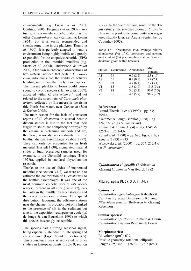
CHAPTER 7 – DIATOM IDENTIFICATION GUIDE
256
environments (e.g. Lucas et al. 2001, Coutinho 2005, Brogueira et al. 2007). Ac-tually, it is a mainly epipelic diatom, as the other Cylindrotheca taxa (Reimann & Lewin 1964), but it is easily resuspended and spends some time in the plankton (Round et al. 1990). It is perfectly adapted to benthic environment being highly mobile and greatly responsible for the exopolysaccharide (EPS) production in the intertidal mudflats (e.g. Staats et al. 2000b, Underwood & Provot 2000). Our own microscopic observations of live material noticed that certain C. closte-rium individuals had the ability of actively bending and flexing the finely drawn apices. The marine planktonic forms could corre-spond to cryptic species (Haitao et al. 2007), allocated within C. closterium s.l., and not related to the specimens of Ceratoneis clos-terium, collected by Ehrenberg in the rising tide North Sea water, near Cuxhaven (Jahn & Kusber 2005). The main reason for the lack of consistent reports of C. closterium in coastal benthic diatom studies is due to the fact that their fragile frustules are completely destroyed by the classic acid-cleaning methods and are, therefore, seriously underestimated in the benthic diatom assemblages (Sabbe 1997). They can only be accounted for in fresh material (Hustedt 1930), incinerated material slides or lugol preserved samples used, for example, in the Utermöhl technique (Hasle 1978a), applied in standard phytoplankton research. Thanks to the use of slides of incinerated material (see section 3.1.2) we were able to estimate the contribution of C. closterium to the benthic assemblages. It was one of the most common epipelic species (49 occur-rences), present in all sites (Table 17), par-ticularly in the mudflat transect stations and the lower shore sand station. This spatial distribution, favouring the offshore stations near the channel, is probably not only linked to the presence of silt in the sediment but also to the deposition-resuspension cycle (cf. de Jonge & van Beusekom 1995) to which this species is strongly susceptible.
The species had a strong seasonal signal, being especially abundant in late spring and early summer (Figs. 18 and 19, section 4.5). This abundance peak is replicated in other studies in European coasts (Table 9, section
5.3.2). In the Sado estuary, south of the Ta-gus estuary, the seasonal bloom of C. closte-rium in the planktonic community was regis-tered slightly later, i.e. August-September by Coutinho (2005).
Table 17 – Occurrence (%), average relative abundances (%) of C. closterium and average mud content (%) per sampling station. Standard deviation given within brackets.
Station Occurrence Abundance Mud content
A1 36 0.9 (2.2) 2.3 (1.0) A2 55 0.7 (0.9) 5.4 (2.4) A3 91 4.7 (6.1) 7.7 (3.1) V1 83 3.8 (3.0) 13.5 (9.3) V2 91 3.0 (3.1) 90.0 (7.3) V3 75 4.3 (5.9) 96.5 (2.2)
References: Bérard-Therriault et al.(1999) – pg. 63; 55/d-e Krammer & Lange-Bertalot (1988) – pg. 124; 87/1-2 (as N. closterium) Reimann & Lewin (1964) – figs. 124/1-6, 125/1-8, 126/1-4,6 Round et al. (1990) – pg. 626, fig. a, c, h, i Snoeijs (1993) – #33 Witkowski et al. (2000) – pg. 374; 212/4-6 (as N. closterium)
Cylindrotheca cf. gracilis (Brébisson in Kützing) Grunow in Van Heurck 1882
Micrographs: Pl. 28: 3-5, Pl. 54: 8
Synonyms: Cylindrotheca gerstenbergeri Rabenhorst Ceratoneis gracilis Brébisson in Kützing Nitzschiella gracilis (Brébisson in Kützing) Rabenhorst
Similar species: Cylindrotheca fusiformis Reimann & Lewin Cylindrotheca signata Reimann & Lewin
Morphometrics: Biovolume (µm3): 639 Frustule geometry: rotational ellipsoid Length (µm): 62.0 – (76.3) – 126.7 (n=7)

CHAPTER 7 – DIATOM IDENTIFICATION GUIDE
257
Width (µm): 2.8 – (3.6) – 4.0 (n=7) Fibulae in 10 µm: 18 – (19) – 22 (n=9)
Notes: the three species of needle-shaped Cylindrotheca (i.e. C. fusiformis, C. gracilis and C. signata), described by Reimann & Lewin (1964), are not very easily distin-guished and can all live in same habitat (i.e. marine littoral mud). Cylindrotheca fusi-formis differs from the other two by the fact that it is slightly smaller and has slightly higher fibulae density but the main differ-ences are the swelling of the frustule in the middle of the cell and two additional hyaline strips bordering the raphe, one at each side. As for C. gracilis and C. signata, the dis-criminating feature is the silicified strips, bordering the raphe fissure, which are perfo-rated in C. signata. Unfortunately, this can only be clearly seen in TEM (figs. 129/3b-4; Reimann & Lewin 1964). Cylindrotheca signata is slightly shorter and slender and has lower fibulae density than C. gracilis, in particular when considering C. gracilis var. major, but there is a large overlap in size range and fibulae density (Reimann & Lewin 1964, Krammer-Lange-Bertalot 1988). Our LM and SEM observations were insufficient to determine if the specimens found in our study are .C. signata or small C. gracilis specimens. As both taxa seem almost impossible to distinguish in LM, an interesting question on the distribution of both species in European coasts is raised. Cylindrotheca gracilis is commonly referred in most European floras (e.g. Germain 1981, Krammer & Lange-Bertalot 1988, Wit-kowski et al. 2000), including from the Brit-ish Isles (Hendey 1964), while C. signata is a much obscure taxa, mainly appearing in ecological MPB studies on the British coasts (e.g. Paterson 1988, Underwood 1994, Bel-linger et al. 2005) after the original descrip-tion by Reimann & Lewin (1964). Whether C. signata is limited to the British Isles needs to be confirmed with TEM studies on British and continental material. Our specimens do look extremely similar to C. signata as it is illustrated in MPB eco-logical studies from the British Isles (e.g. Underwood, 1994). However, it is impossi-ble to validate this identification with only SEM and LM, therefore, we prefer to desig-nate this taxon temporarily by C. cf. gracilis.
Distribution & Ecology: both C. gracilis and C. signata are referred as motile epipelic species living in marine littoral mud. Re-imann & Lewin (1964) stated that the nomi-nate variety of C. gracilis lives in fresh-waters with high saline content (e.g. Neus-iedler See), while the larger C. gracilis var. major lives in the marine littoral. However, Krammer-Lange-Bertalot (1988) raised some doubts on the validity of the separation of these two varieties and, consequently, on the spatial distribution of C. gracilis/C. ger-stenbergeri. For instance, Van Heurck’s authenticated “type” slide of C. gracilis (Type 417, Medlin & Mann 2007) was made from material collected in Wedel, down-stream from Hamburg and probably was sampled in the brackish water reaches of the Elbe estuary, since the accompanying spe-cies is Navicula pygmaea Kützing. In our study, C. cf. gracilis was one of the most common motile epipelic species (38 occurrences), even though it appeared al-most exclusively in the muddy transect (Ta-ble 18). It was also one of the most abundant diatoms in the mudflat stations (max. abun-dance < 55.5%), showing a strong seasonal signal (cf. C. closterium), particularly in late summer and early autumn. As it was the case with C. closterium, the contribution of this species would have been completely under-estimated if only the peroxide-cleaned slides were counted.
Table 18 – Occurrence (%), average relative abundance (%) of C. cf. gracilis and average mud content (%) per sampling station. Standard deviation given within brackets.
Station Occurrence Abundance Mud content
A1 0 0.1 (0.3) 2.3 (1.0) A2 9 0.1 (0.2) 5.4 (2.4) A3 55 0.5 (0.7) 7.7 (3.1) V1 67 1.4 (1.8) 13.5 (9.3) V2 82 7.7 (7.4) 90.0 (7.3) V3 100 22.5 (16.6) 96.5 (2.2)
References: Germain (1981) – pg. 324; fig. 120/ Hendey (1964) – pg. 284 Krammer & Lange-Bertalot (1988) – pg. 134; 87/3 Reimann & Lewin (1964) – pl. 126-129

CHAPTER 7 – DIATOM IDENTIFICATION GUIDE
258
Underwood (1994) – fig. 24 Witkowski et al. (2000) – pg. 212; fig. 212/7
Nitzschia Hassall 1845
Genus description: Round et al. (1990)
Comprising more than 900 valid taxa (Lundholm & Moestrup 2000), Nitzschia is one of the largest and most difficult diatom genus. The reasons for this are multiple, many of them are discussed, for example, by Mann (1986), Lundholm & Moestrup (2000) or Witkowski et al. (2004a). One of the reasons highlighted by these and other authors is the delicate structure and similar morphology of many species, which hinders a correct and easy identification. This seems to be especially true in the sec-tion “Lanceolatae” (see discussion below N. cf. aequorea). Another important reason pointed out, namely by Mann (1986) is the lack of a recent and comprehensive mono-graph of the genus, which particularly af-flicts the marine taxa (Witkowski et al. 2004a). Furthermore, there is a lack of consensus on the status of several sections within the Nitzschia s.l. (see discussion below Try-blionella). The genus Nitzschia has been traditionally divided in many sections, most of them established by Grunow (see Hendey 1964). Mann (1978) gives a detailed descrip-tion and historical background of all sections of Nitzschia sensu lato established by Grunow.
Nitzschia cf. aequorea Hustedt 1939
Micrographs: Pl. 33: 12-15
Synonyms: Nitzschia subfrustulum Hustedt Nitzschia stimulus Cholnoky
Similar species: Nitzschia agnita Hustedt
Nitzschia lanceolata W. Smith var. minima Peragallo & Peragallo Nitzschia rosenstockii Lange-Bertalot Nitzschia pusilla (Kützing) Grunow emend. Lange-Bertalot
Morphometrics: Biovolume (µm3): 145 Frustule geometry: prism on parallelogram Length (µm): 9.4 – (17.1) – 28 (n=37) Width (µm): 2.4 – (3.3) – 4.8 (n=32) Pervalvar axis (µm): 3 (estimated) Striae in 10 µm: 31 – (34) – 37 (n=6) Fibulae in 10 µm: 13 – (15) – 19 (n=35)
Description: valves typically lanceolate with convex margins and acute slightly pro-duced weakly capitate apices. Raphe strongly eccentric with short fibulae, more or less evenly spaced. The central fibulae are not more widely spaced. The striae are barely visible in LM.
Notes: this taxon is part of Nitzschia sect. Lanceolatae, a section that also includes N. aurariae, N. frustulum and N. valdestriata. Most members of this section are very diffi-cult to identify given the character poor frus-tule morphology in LM, the enormous num-ber of species (more than 300, according to Mann, 1978) and the fact that many of them seem to grow in similar habitats. To this it should be added that many superfluous taxa were described and that some species de-scriptions have been based on the observa-tion of very few specimens resulting in sev-eral species with similar valve outlines and overlapping striation and fibula densities (see comments by Sabbe 1997). An enor-mous effort was carried out in the past dec-ades, particularly by Lange-Bertalot and colleagues (Lange-Bertalot 1976, Lange-Bertalot & Simonsen 1978, Lange-Bertalot 1980, Lange-Bertalot & Krammer 1987, Krammer & Lange-Bertalot 1988), in trying to sort out this “most problematic group of diatoms” (see discussion by Krammer & Lange-Bertalot 1988, pg. 76). This task was daunting, since it had to be mainly based in SEM studies of type materials, in a group where many species are known for their extreme plasticity in size range and/or striae and fibulae density (e.g. N. intermedia, Krammer & Lange-Bertalot 1988) and, for

CHAPTER 7 – DIATOM IDENTIFICATION GUIDE
259
most cases, there is incomplete autoecologi-cal data. In spite of these great efforts many taxonomic problems concerning species of this group still remain unresolved, particu-larly in regard to marine or brackish-water species. Such is the case of this particular taxon; it clearly belongs to the species-complex around N. aequorea and N. agnita, which includes many brackish water taxa (see dis-cussion by Krammer & Lange-Bertalot 1998, pg. 116). The main difference between these two particular species seems to be striae density (i.e. higher than 35 striae in 10 µm in N. agnita; between 32-35/10 µm in N. aequorea). Nitzschia rosentockii and N. lanceolata var. minima are also likely candi-dates, particularly given the size-range. However, latter taxon is poorly defined and the type material is probably lost (Krammer & Lange-Bertalot 1988); whereas the former species is from electrolyte- rich freshwaters (Lange-Bertalot 1980). It is possible that the specimens found in our study belong to a set of different species (with some specimens belonging to N. pu-silla cf. Snoeijs & Potapova 1995, # 267) but we failed to seem any discontinuity in length vs. width, fibulae vs. length or fibulae vs. width plots, obtained from our morphomet-ric data. Moreover, this fragile species was not studied in SEM. Therefore, this taxon can only be tentatively identified as N. cf. aequorea. The main reasons supporting this tentative claim are the fact that the striae are around 35 in 10 µm (see above) and the specimens are in average smaller than the that what has been reported for N. agnita, which has a size range of 18-40 µm (viz. Hustedt 1939, Hustedt 1957, Archibald 1983, Witkowski et al. 2000).
Table 19 – Occurrence (%), average relative abundance (%) of N. cf. aequorea and average mud content (%) per sampling station. Standard deviation given within brackets.
Station Occurrence Abundance Mud content
A1 36 0.2 (0.3) 2.3 (1.0) A2 55 0.2 (0.3) 5.4 (2.4) A3 64 0.4 (0.4) 7.7 (3.1) V1 83 1.4 (1.7) 13.5 (9.3) V2 91 1.3 (1.1) 90.0 (7.3) V3 42 0.3 (0.7) 96.5 (2.2)
Distribution & Ecology: motile epipelic species. According to Lange-Bertalot & Simonsen (1978), N. aequorea has been only occasionally recorded and even Hustedt (1939) found it rarely in the original material from sandy muddy flats of the North Sea coast (“im Schlicksandwatt”, Simonsen 1987). Witkowski et al. (2000) considered this species to be “widespread” (cosmopoli-tan). Regarding N. agnita, it has been mainly reported for South Africa (see discussion by Archibald 1983, pg. 232). It is possible that this very taxon has also been identified as N. lanceolata var. minima (viz. Peragallo & Peragallo 1897-1990) or N. rosenstockii (cf. Sabbe 1997). In our study this taxon was one of the most frequently found species of Nitzschia (42 occurrences), being present in all stations (i.e. in muddy and sandy sedi-ments) but it was more commonly found in the muddy transect (Table 19). It was never very abundant (max. abundance < 5%) being slightly more common during winter and spring.
References: Hustedt (1939) – pg. 663; fig. 120 Krammer & Lange-Bertalot (1988) – pg. 117; 82/1-5 Kuylenstierna (1989-1990) – fig. 811 Lange-Bertalot & Simonsen (1978) – pg. 15; figs. 179-180 Simonsen (1987) – figs. 382/15-20 Witkowski et al. (2000) – pg. 367; fig. 210/14-15
Nitzschia angularis W. Smith 1853
Micrographs: Pl. 29: 5-6, Pl. 55: 3-5
Synonyms: Homoeocladia angularis (W. Smith) Kuntze 1898
Morphometrics: Biovolume (µm3): 12016 Frustule geometry: prism on parallelogram

CHAPTER 7 – DIATOM IDENTIFICATION GUIDE
260
Length (µm): 112.5 – (118.2) – 122.5 (n=3) Width (µm): 13.3 – (16.1) – 19.0 (n=3) Pervalvar axis (µm): 8 (estimated) Striae in 10 µm: 33 – (35) – 37 (n=3) Fibulae in 10 µm: 5 – (6) – 9 (n=3)
Notes: this species was described in detail by Hendey (1964) or by Poulin et al. (1990), where SEM micrographs of this taxon can also be found.
Distribution & Ecology: Cox (1977) re-ported it as a tube-dwelling species in the Severn estuary (U.K) and Mann (1978) ex-plained that N. angularis may live associated with two symbionts in these tubes: N. lanceolata W. Smith and N. frustulum (Kützing) Grunow. Kuylenstierna (1989-1990) found it as epiphyte of macroalgae and hydroids. In our study it occurred only once.
References: Hendey (1964) – pg. 281; fig. 39/6 Mann (1978) – figs. 234-243 Poulin et al. (1990) – pg. 78; figs, 16-22 Peragallo & Peragallo (1897-1908) – pg. 284; fig. 73/6-7 Ricard (1987) – figs. 1073-1074 Witkowski et al. (2000) – pg. 368; figs. 199/5-6
Nitzschia cf. aurariae Cholnoky 1965
Micrographs: Pl. 28: 11, Pl. 56: 12-13
Synonyms: Nitzschia elliptica var. alexandrina Chol-noky Nitzschia alexandrina (Cholnoky) Lange-Bertalot & Simonsen
Morphometrics: Biovolume (µm3): 36 Frustule geometry: prism on parallelogram Length (µm): 7.1 – (8.3) – 9.3 (n=6) Width (µm): 2.5 – (2.8) – 3.0 (n=6) Pervalvar axis (µm): 2 (estimated) Striae in 10 µm: 52 – (55) – 57 (n=3) Punctae in 10 µm: 56 (n=2) Fibulae in 10 µm: 17 – (18) – 19 (n=5)
Notes: detailed descriptions of this taxon are given by Krammer & Lange-Bertalot (1988) and by Witkowski et al. (2000). The speci-mens found in the Tagus estuary are very similar to the ones described for the Baltic Sea (Sundbäck & Snoeijs 1991; Snoeijs & Potapova 1995) and have more elliptic-lanceolate outline, instead of the more lin-ear-elliptic one found in Cholnoky’s type material (Fig. 80/18-19, Krammer & Lange-Bertalot 1988). Besides the similar striae and fibulae density and the lack of central nod-ule, both forms also share the typical quin-cunx pattern of the areolae. It is easily dis-tinguishable of the smaller specimens of N. frustulum by the fact that the striae are ir-resolvable in LM and the lack of central nodule. Trobajo (2007) also found very simi-lar specimens (fig. 13/103) in the Empordà wetlands (NE Spain) but identified them as N. pusila Grunow. Even tough, the speci-mens found in SEM seem to be unques-tionably N. aurariae, a more detailed study is necessary to confidently determine the identity of the specimens observed in LM.
Distribution & Ecology: cosmopolitan, widespread species, found in electrolyte rich freshwater and common in the Baltic Sea (Krammer & Lange-Bertalot 1988; Wit-kowski et al. 2000). Sundbäck & Snoeijs (1991) reported it as living in subtidal sand in the more brackish/marine areas of the Baltic (viz. in NE Skagerrak, Tjärnö, Swe-den). The existence of two ecological mor-photypes should be explored. It is a small motile epipelic species (cf. Snoeijs & Pota-pova 1995). In our study it was extremely rare, with only 4 occurrences and always at very low abundances (max. abundance < 0.45%).
References: Krammer & Lange-Bertalot (1988) – pg. 113; 80/16-21 Ludes & Coste (1996) – fig. 29/20 Snoeijs & Potapova (1995) – #262 Sundbäck & Snoeijs (1991) – pg. 353; fig. 9i Witkowski et al. (2000) – pg. 369; fig. 210/21

CHAPTER 7 – DIATOM IDENTIFICATION GUIDE
261
Nitzschia cf. dissipata (Kützing) Grunow 1862
Micrographs: Pl. 28: 6-10, Pl. 56: 2
Similar species: Nitzschia distans Gregory 1857
Morphometrics: Biovolume (µm3): 193 Frustule geometry: prism on parallelogram Length (µm): 12.7 – (19.3) – 29.5 (n=12) Width (µm): 2.7 – (3.2) – 3.8 (n=12) Pervalvar axis (µm): 4 (estimated) Striae in 10 µm: 53 (n=2) Punctae in 10 µm: 52 (n=1) Fibulae in 10 µm: 6 – (8) – 10 (n=12)
Description: valves lanceolate or narrowly-lanceolate with slightly capitate apices. The canal-raphe is only slightly eccentric and the distance between two adjacent fibulae is not constant. The central fibulae are not widely spaced. The striae are finely punctate and are irresolvable in LM. In SEM, the striae are interrupted in the two longitudinal thicken-ings, on both sides of the canal-raphe, from which the fibulae stem.
Notes: this species is very similar to the freshwater species N. dissipata in outline, size-range and fibulae. It is possible that several dissipata-like species were lumped together in our study. The smaller specimens are extremely reminiscent of the small N. dissipata depicted by Krammer & Lange-Bertalot (1988, figs. 11/4-5) and Sabbe (1997, as N. cf. dissipata). However, in a larger valve, observed in SEM, the striae are interrupted near the canal-raphe, a feature that does not occur in N. dissipata (Mann 1978, figs. 808-811; Poulin et al. 1999, figs. 29; Snoeijs & Kasperoviciene 1996, #369). In spite of several reports (e.g. Poulin et al. 1990) the presence of N. dissipata in brack-ish and marine areas has been always prob-lematic (Krammer & Lange-Bertalot 1988), although a certain tolerance to salinity has been acknowledged (e.g. Germain 1981). The specimens found in Tagus estuary seem to correspond to the N. cf. dissipata de-scribed by Sabbe (1997) for the Wester-schelde estuary (see also his discussion on
“dissipata-like” taxa) and, particularly, to Nitzschia sp.D described by Kuylenstierna (1989-1990) which has “two unmarked fields along the canal-raphe”.
Distribution & Ecology: apart from the reports of Kuylenstierna (1989-1990) and Sabbe (1997) the geographical distribution of this taxon is unknown. As it was the case in the above mentioned works, this diatom was fairly rare in our study (20 occurrences), appearing in the muddy transect but also in the lower shore muddy sandy stations of the sandy transect. It was never very abundant (max. abundance < 1.61).
References: Krammer & Lange-Bertalot (1988) – pg. 19; figs. 11/1-7 Kuylenstierna (1989-1990) – pg. 140; fig. 886 Sabbe (1997) – pg. 244; fig. 30/1-4
Nitzschia cf. distans Gregory 1857
Micrographs: Pl. 29: 3-4, Pl. 56: 1
Similar species: Nitzschia affinis Grunow [syn. N. angularis var. affinis (Grunow) Grunow in Van Heurck)]
Morphometrics: Biovolume (µm3): 1343 Frustule geometry: prism on parallelogram Length (µm): 31.4 – (42.3) – 73.1 (n=9) Width (µm): 3.4 – (4.3) – 5.2 (n=4) Pervalvar axis (µm): 10 (estimated) Striae in 10 µm: 49 (n=1) Punctae in 10 µm: 72 (n=1) Fibulae in 10 µm: 4 – (6) – 7 (n=9)
Description: valves narrowly-lanceolate, with acutely rounded, slightly capitate api-ces. In girdle view, short wing-like expan-sions are clearly seen in the apices but are not as drawn-out as in N. spathulata (see below). The canal-raphe central to slightly eccentric, the central fibulae are not more widely spaced and the distance between adjacent fibulae is not regular. The striae are

CHAPTER 7 – DIATOM IDENTIFICATION GUIDE
262
not resolvable in LM and are finely punctate. These areolae are continuous throughout the stria, which seems to end at the margin of the canal-raphe.
Notes: even though the specimens found in this study are very similar to N. distans, they are much smaller and with denser fibulae than the customary morphometric data given for that species (e.g. 130-220 µm in length and 1.5-3 fibulae in 10 µm, Witkowski et al. 2000). They correspond, however, to the taxa reported and illustrated by Giffen (1963), Kuylenstierna (1989-1990), Snoeijs & Kasperoviciene (1996), all of them identi-fied as N. distans or N. cf. distans. Accord-ing to Mann (1978), the only taxon on the “Spathulatae” section with similar mor-phometrics is N. affinis but this taxon was rarely recorded and has a more lanceolate valve outline (Peragallo & Peragallo 1897-1990). Both Mann (1978) and Kuylenstierna (1989-1990) acknowledge that a revision of this group is needed, as there are many in-termediate forms between species.
Distribution & Ecology: motile epipelic species. It has been reported for subtidal sandy and muddy sediments from the ma-rine/brackish water Skagerrak and Kattegat Swedish coast (Kuylenstierna 1989-1990, Snoeijs & Kasperoviciene 1996). The specimens reported by Giffen (1963, Tro-bajo 2007) also came from “strongly brack-ish water” of a Eastern Cape province estu-ary (South Africa). In our study, this taxon was infrequent (9 occurrences) and never very abundant (max. abundances < 0.94%) it was mainly found in the muddy transect.
References: Giffen (1963) – pg. 245; fig. 85 Hendey (1964) – pg. 378 Kuylenstierna (1989-1990) – pg. 132; fig. 829-830 Poulin et al. (1990) – pg. 81; fig. 38-41 Snoeijs & Kasperoviciene (1996) – # 370 Witkowski et al. (2000) – pg. 378; 203/7-9
Nitzschia cf. dubia W. Smith 1853
Micrographs: Pl. 29: 1-2
Synonyms: Homoeocladia dubia (W. Smith) Kuntze
Similar species: Nitzschia bilobata W. Smith Nitzschia commutata Grunow in Cleve & Grunow Nitzschia hybrida Grunow in Cleve & Grunow
Morphometrics: Biovolume (µm3): 5529 Frustule geometry: prism on parallelogram Length (µm): 62.2 – (83.3) – 110 (n=3) Width (µm): 9.0 – (10.6) – 12 (n=3) Pervalvar axis (µm): 8 (estimated) Striae in 10 µm: 22 – (27) – 32 (n=4) Fibulae in 10 µm: 11 – (12) – 12 (n=4)
Description: individual valves usually in girdle view and more or less linear-lanceolate, being slightly constricted in the middle. The apices are broadly rounded, slightly rostrate and asymmetric (i.e. turned towards the cingulum). Each fibula ends in one interstria and the central fibulae are only slightly more distant.
Notes: in spite of a slightly denser striation this taxon is very similar to N. dubia (for comparison see Witkowski et al. 2000). The middle constriction is not as pronounced as in related species, such as N. bilobata or N. hybrida and, additionally, the striae are not clearly punctate in LM as in N. commutata. The existence of smaller specimens of N. dubia with higher striae density in brackish waters was already noticed by Kuylenstierna (1989-1990, as Nitzschia sp.I)
Distribution & Ecology: large motile epipelic diatom. Nitzschia dubia s.s., it is a cosmopolitan species living in brackish and marine waters. Nitzschia cf. dubia was found rarely in our study (8 occurrences), only during winter and, mainly, in the muddy transect.

CHAPTER 7 – DIATOM IDENTIFICATION GUIDE
263
References: Germain (l981) – pg. 338; figs. 128/1,2 Krammer & Lange-Bertalot (l988) – pg. 55; figs. 41/1-2 Kuylenstierna (1989-1990) – pg. 132, 141; fig. 83 Sabbe (1997) – pg. 245; fig. 31/9 Snoeijs & Potapova (1995) – #264 Witkowski et al. (2000) – pg. 378; 190/7-8
Nitzschia frustulum (Kützing) Grunow in Cleve & Grunow 1880
Micrographs: Pl. 33: 4-8, Pl. 56: 6-11
Synonyms: Homoeocladia frustulum (Kützing) Kuntze 1898 Nitzschia inconspicua Grunow (sensu stricto non N. abbreviata Hustedt) Synedra frustulum Kützing 1844 See Trobajo et al. (2004) for full list of synonyms
Similar species: Nitzschia aurariae Cholnoky
Morphometrics: Biovolume (µm3): 38 Frustule geometry: prism on parallelogram Length (µm): 4.2 – (9.2) – 25 (n=41) Width (µm): 2.0 – (2.7) – 4.0 (n=39) Pervalvar axis (µm): 2 (estimated) Striae in 10 µm: 22 – (28) – 32 (n=41) Punctae in 10 µm: 32 – (39) – 46 (n=9) Fibulae in 10 µm: 10 – (13) – 16 (n=38)
Notes: Wendker (1990) discussed in detail the morphology of this taxon and Trobajo & Cox (2006) described the type material of N. frustulum. The conspecificity of N. frustulum and N. inconspicua has long been discussed (e.g. Lange-Bertalot & Simonsen 1978; Krammer & Lange-Bertalot 1988). The two species are traditionally only distinguished by size, the shape of the apices and autoecology (Sabbe 1997; Trobajo & Cox 2006): N. frustulum is reported for brackish water and has “longer, thinner” valves with cuneate/subrostrate apices; N. inconspicua occurs in freshwaters
and has “shorter, fatter” valves, with broadly rounded apices. Studying natural populations along the salin-ity gradient of the Schlei estuary (Germany), Wendker (1990) demonstrated that there is a morphological continuum between both species, with the “inconspicua“-form being more abundant in the freshwater reaches of the estuary and the “frustulum”-form more common in the brackish water reaches and the mouth of the estuary. Recently, Trobajo et al. (2006) established in a series of culture experiments that it was possible to obtain “inconspicua“-like cells from a “frustulum”-like clonal culture in different salinities, N:P ratios and water movements, all factors af-fected the length, width and/or fibula density of the frustules . Salinity was the main factor responsible for valve outline but increasing water movement may also augment cell width. These results corroborate the con-specificity of both species but also that the pattern found by Wendker (1990) is not nec-essarily always replicated in nature (Trobajo et al. 2006). Conversely, Kuylenstierna (1989-1990) noticed that in his material for the Swedish west coast N. inconspicua had two rows of areolae on the mantle near the raphe, while N. frustulum had only one row. The latter feature can also be seen in the type material of N. frustulum, studied by Trobajo & Cox (2006). However, as our own SEM observa-tions show, the number of rows areolae on the mantle near the raphe does not seem to be a stable morphological feature and small, “inconspicua”-like specimens, with only one row of pores were found (Pl. 56: 7). The taxonomical validity of this criterion is, therefore, questioned. Finally, and still regarding the specimens found in our study, most of them had an “inconspicua” shape, in spite of being col-lected in a brackish water site. The fact that this species was most abundant in the sandy stations (see below), may imply that factors, other than salinity (e.g. water movement, cf. Trobajo et al. 2006) were likely responsible for an increase in average valve frustule width and a decrease in cell length and, therefore, for the “inconspicua” likeness of most specimens scored during counts.

CHAPTER 7 – DIATOM IDENTIFICATION GUIDE
264
Table 20 – Occurrence (%), average relative abundance (%) of N. frustulum and average mud content (%) per sampling station. Standard devia-tion given within brackets.
Station Occurrence Abundance Mud content
A1 100 12.4 (2.9) 2.3 (1.0) A2 100 3.9 (1.7) 5.4 (2.4) A3 100 2.2 (0.9) 7.7 (3.1) V1 92 1.3 (0.9) 13.5 (9.3) V2 64 0.4 (0.5) 90.0 (7.3) V3 8 0.0 (0.1) 96.5 (2.2)
Distribution & Ecology: N. frustulum is a common, cosmopolitan and markedly eury-haline species (e.g. Witkowski et al. 2000; Trobajo et al. 2006). This species was one of the most common and frequent (52 occur-rences) Nitzschia found in our study. It was particularly abundant in the sandy transect, especially in upper shore fine sandy station (Table 20). References: Germain (1981) – pg. 352; fig. 134/1 Krammer & Lange-Bertalot (1988) – pg. 94-95; figs. 68/1-8 (N. frustulum), 69/1-13 (N. inconspicua) Lange-Bertalot & Simonsen (1978) Poulin et al. (1990) – pg. 84; figs. 44-48 Snoeijs (1994) – #76 (N. inconspicua), #78 (N. frustulum) Trobajo & Cox (2006) – figs. 1-19 (type material) Trobajo (2004) – figs. 7-14 Wendker (1990) – figs. 1-33 Witkowski et al. (2000) – pg. 382; figs. 209/13-17
Nitzschia littorea Grunow in Van Heurck 1881
Micrographs: Pl. 30: 1-3
Synonyms: Hantzschia fogedii (Møller) Simonsen Nitzschia thermalis var. littoralis Grunow in Cleve & Grunow Nitzschia fogedii Møller
Similar species: Nitzschia commutata Nitzschia lacunarum Hustedt
Morphometrics: Biovolume (µm3): 6436 Frustule geometry: prism on parallelogram Length (µm): 129.5 (n=2) Width (µm): 9.0 (n=2) Pervalvar axis (µm): 7 (estimated) Striae in 10 µm: 30 (n=2) Punctae in 10 µm: 23 (n=1) Fibulae in 10 µm: 9 (n=2)
Notes: a detailed description of this species is given by Krammer & Lange-Bertalot (1998) or by Witkowski et al. (2000). It can be distinguished from the similar species by a clear quincunx striation pattern (Snoeijs & Kasperoviciene 1996).
Distribution & Ecology: large epipelic species. Common in marine European coasts (Krammer & Lange-Bertalot 1988, Wit-kowski et al. 2000), it has been reported several times for the Öresund and the Kat-tegat (e.g. Simonsen 1962, Kuylenstierna 1989-1990, Snoeijs & Kasperoviciene 1996), in the Swedish West coast. In our study, it was found once, in the upper shore station of the sandy transect.
References: Krammer & Lange-Bertalot (1988) – pg. 67; 54/1-3a Lange-Bertalot & Krammer (1987) – pg. 18, 34; fig. 23/4-5 Snoeijs & Kasperoviciene (1996) – #373 Simonsen (1962) – pg. 99 (as H. fogedii) Witkowski et al. (2000) – pg. 391; fig. 197/11-16
Nitzschia lorenziana Grunow in Cleve & Möller 1879
Micrographs: Pl. 30: 4
Synonyms: Homoeocladia lorenziana (Grunow in Cleve & Møller; Grunow in Cleve & Grunow) Kuntze

CHAPTER 7 – DIATOM IDENTIFICATION GUIDE
265
Nitzschiella lorensiana (Grunow in Cleve & Møller; Grunow in Cleve & Grunow) Pera-gallo & Peragallo
Morphometrics: Biovolume (µm3): 1914 Frustule geometry: prism on parallelogram Length (µm): 75.0 (n=1) Width (µm): 6.5 (n=1) Pervalvar axis (µm): 5 (estimated) Striae in 10 µm: 16 (n=1) Fibulae in 10 µm: 7 (n=1)
Notes: this species is described in detail by Krammer & Lange-Bertalot (1988) and Poulin et al. (1990). As we found very few specimens we abstain of determining the variety of N. lorenziana found in our sam-ples.
Distribution & Ecology: cosmopolitan brackish water species, found also in marine coasts (Krammer & Lange-Bertalot 1988; Witkowski et al. 2000). Large motile epipelic species, also reported as pelagic in coastal areas (Snoeijs & Balashova 1998). In this study, this species was only found in one sample.
References: Krammer & Lange-Bertalot (1988) – pg. 125; figs. 86/6-10 Poulin et al. (1990) – pg. 87; figs. 63-72 Snoeijs & Balashova (1998) – #464 Witkowski et al. (2000) – pg. 392; figs. 210/24-25, 211/3, 212/1-3
Nitzschia sigma (Kützing) W. Smith 1853
Micrographs: Pl. 30: 5-7, Pl. 56: 3-5
Synonyms: Homoeocladia sigma (Kützing) Sigmatella sigma (Kützing) Frenguelli Synedra sigma Kützing
Morphometrics: Biovolume (µm3): 15304 Frustule geometry: prism on parallelogram Length (µm): 57.6 – (107.8) – 225.3 (n=8) Width (µm): 5.7 – (7.5) – 13.2 (n=8)
Pervalvar axis (µm): 3 (estimated) Striae in 10 µm: 25 – (28) – 34 (n=10) Punctae in 10 µm: 18 – (24) – 34 (n=5) Fibulae in 10 µm: 7 – (9) – 11 (n=7)
Notes: detailed descriptions of this species are given by Germain (1981) or by Krammer & Lange Bertalot (1988). It is most probably a species complex (Witkowski et al. 2000)
Distribution & Ecology: large motile epipelic taxon. Cosmopolitan species, it is widespread in most marine coasts and estu-aries (Witkowski et al. 2000). In our study, it was fairly rare (18 occurrences) being mainly found in the lower shore stations of both transects. It had very low abundances (max. abundance < 0.8%), but its relative numbers increased during summer.
References: Germain (1981) – pg. 368; pl. 139/1-6 Krammer & Lange-Bertalot (1988) – pg. 32; figs. 23/19 Ohtsuka (2005) – pg. 146; figs. 44-45 Poulin et al. (1990) – pg. 92; figs. 90-92 Snoeijs & Vilbaste (1994) – # 173 Witkowski et al. (2000) – pg. 404; figs. 206/1-10
Nitzschia spathulata Brébisson ex W. Smith 1853
Micrographs: Pl. 31: 1-3, Pl. 55: 1-2
Synonyms: Homoeocladia spathulata (Brébisson ex W. Smith) Kuntze 1898
Similar species: Nitzschia distans var. tumescens Grunow Nitzschia angularis W. Smith
Morphometrics: Biovolume (µm3): 8327 Frustule geometry: prism on parallelogram Length (µm): 82.0 – (87.8) – 92.0 (n=5) Width (µm): 5 (estimated) Pervalvar axis (µm): 15 (n=4) Striae in 10 µm: 40 (n=1) Fibulae in 10 µm: 5 – (6) – 10 (n=9)

CHAPTER 7 – DIATOM IDENTIFICATION GUIDE
266
Notes: this taxon is described and illustrated in detail by Mann (1978) but also by Hendey (1964) and Witkowski et al. (2000). It can be distinguished from the other species on the “Spathulatae” group not only by its di-mensions but also by the very large wing-like expansions in the apices.
Distribution & Ecology: this species is widespread in the European marine coasts (Witkowski et al. 2000) but it also occurs in South Africa (Giffen 1963), in the North-American Pacific coast (Riznyk 1973) or in New Zealand (Chapman et al. 1957). It is a large motile epipelic species. The specimens studied by Brockmann (1950), Giffen (1963), Riznyk (1973) and Mann (1978) were found in intertidal sand. Round (1979) referred N. spathulata as an associated spe-cies of the epipelic assemblages living below the surface of intertidal sandflats. In the present study, it was found only once but I found it frequently in other samples from sandy sediments of the Tagus estuary.
References: Brockmann (1950) – pg. ; fig. 4/23 Giffen (1963) – pg. 248; fig. 94 Hendey (1964) – pg. 281 Mann (1978) – pg. 222; figs. 247-252, 815-831 (except 817) Peragallo & Peragallo (1897-1908) – pg. 284; fig. 73/4 Witkowski et al. (2000) – pg. 405; fig. 206/19-20
Nitzschia valdestriata Aleem & Hustedt 1951
Micrographs: Pl. 33: 9, Pl. 56: 14
Similar species: Nitzschia frustulum Kützing Nitzschia valdecostata Lange-Bertalot & Simonsen
Morphometrics: Biovolume (µm3): 39 Frustule geometry: prism on parallelogram Length (µm): 6.3 – (9.5) – 18.2 (n=7) Width (µm): 2.0 – (2.6) – 3.7 (n=7)
Pervalvar axis (µm): 2 (estimated) Striae in 10 µm: 14 – (18) – 22 (n=6) Punctae in 10 µm: 53 (n=1) Fibulae in 10 µm: 6 – (10) – 15 (n=6)
Notes: this taxon is described in detailed by Lange-Bertalot & Simonsen (1979) or by Krammer & Lange-Bertalot (1988). Nitzschia valdestriata differs from the small forms of N. frustulum (see above) by the more linear outline, the blunt ends and the rougher structure (Aleem & Hustedt 1951). This structure, where each fibula spans two interstriae, is also replicated in N. valde-costata, with the exception of the central fibulae (see Lange-Bertalot & Simonsen 1979; Krammer & Lange-Bertalot 1988).
Distribution & Ecology: small motile spe-cies, cosmopolitan and widespread in brack-ish waters (Krammer & Lange-Bertalot 1986, Witkowski et al. 2000). In our study it was fairly frequent (22 occurrences) al-though it was never very abundant (max. abundance <1.8%). It occurs in both mudflat and sandflat stations but it was more fre-quent and abundant in sandy sediments.
References: Aleem & Hustedt (1951) – pg. 19; figs. 5a-b Kuylenstierna (1989-1990) – pg. 139; fig. 864-865 Krammer & Lange-Bertalot (1988) – pg. 121; figs. 89/9-11 Lange-Bertalot & Simonsen (1978) – pg. 58; figs. 254-259, 271, 272 Simonsen (1987) – figs. 551/9-13 Snoeijs & Vilbaste (1994) – #174 Witkowski (1994) – pg. 172; fig. 61/21 Witkowski et al. (2000) – pg. 407; figs. 203/19-21, 207/14-16
Nitzschia sp.1
Micrographs: Pl. 32: 1-4, Pl. 55: 6-7
Morphometrics: Biovolume (µm3): 3493 Frustule geometry: prism on parallelogram Length (µm): 69.9 – (82.6) – 92.0 (n=4) Width (µm): 10.0 – (10.8) – 11.2 (n=4)

CHAPTER 7 – DIATOM IDENTIFICATION GUIDE
267
Pervalvar axis (µm): 5 (estimated) Striae in 10 µm: 29 – (30) – 31 (n=4) Punctae in 10 µm: 51 (n=1) Fibulae in 10 µm: 13 – (13) – 14 (n=3)
Description: valves broadly linear-lanceolate, with a slight central constriction of the margin bearing the raphe. The apices are acutely-rounded, slightly rostrate and asymmetric (i.e. turned towards the cin-gulum). The fibulae are relatively small and separated by two to three striae, except in the middle, where they are more distant. The SEM shows that the striae are monoseriate and composed by round occluded punctae. They are parallel throughout the valve and separated, externally, by transversal costae, with the exception of the marginal canal-raphe.
Notes: we were unable to identify this quite unique taxon. It may belong to the Nitzschia sect. Dubiae, given its overall valve outline and shape. However, the external structure of the striae was not observed in other mem-bers of this section (cf. Mann 1978; Lange-Bertalot & Krammer 1987). Further studies are needed.
Distribution & Ecology: large motile epipelic species. In our study it occurred only once.
Nitzschia sp.2
Micrographs: Pl. 33: 1-3, Pl. 54: 9-11
Similar species: Nitzschia hummii Hustedt
Morphometrics: Biovolume (µm3): 3393 Frustule geometry: prism on parallelogram Length (µm): 179.4 – (183.5) – 185.6 (n=3) Width (µm): 2.5 – (6.5) – 9.0 (n=4) Pervalvar axis (µm): 5 (estimated) Striae in 10 µm: 31 (n=2) Punctae in 10 µm: 46 (n=1) Fibulae in 10 µm:16 (n=2)
Description: frustules are arcuate, extremely long, and narrow and distinctively curved, which gives them a bow-like appearance. The apices taper progressively and, depend-ing on the valve position, seem to be slightly turned towards the concave side. The trans-verse striae are clearly seen in LM but their punctate structure is only perceived in SEM as monoseriate rows of rounded punctae. The most conspicuous structure of each valve is the huge canal-raphe. It is simple and shallow but the heavily silicified and expanded fibulae clearly separate the canal-raphe from the rest of the cell lumen (cf. Round et al. 2000). The canal-raphe ultra-structure is rather complex: the fibulae are large in relation to the transapical costae and have two longitudinal ridges. These two ridges are separated by a few poroids, since the striae continue through both the proximal and distal (outer) sides of the raphe (near the raphe slit). The inside portulae are elliptical and better defined than the secondary, outer portulae of the second ridge. This corre-sponds to raphe-type vii (cf. Mann 1978).
Notes: this species is rather unique and we were not able to find anything like it in the references consulted. Perhaps the most simi-lar species is Nitzschia hummii, described by Hustedt (1955) for the Beaufort Bay (USA). This species, however, has wider valves and striae more coarsely punctate (see figs. 634/1-4, Simonsen 1987). The raphe ultra-structure (see above) appears to be very similar to what is found in sect. Nitzschia (e.g. N. sigma, N. sigmaformis), at least ac-cording to the criteria established by Mann (1978)
Life form & Ecology: large epipelic species probably motile. In our study it only oc-curred in 3 samples from the muddy transect (max abundance < 0.63%). However, this large and conspicuous diatom has been de-tected in other samples from the Tagus estu-ary, mainly from sandy sediments. Apart from the Tagus estuary, this diatom has also been found in estuarine intertidal mudflats in Southern Brittany (France) by M. Loir (pers. communication).

CHAPTER 7 – DIATOM IDENTIFICATION GUIDE
268
Nitzschia sp.3
Micrographs: Pl. 28: 12-13
Morphometrics: Biovolume (µm3): 46 Frustule geometry: prism on parallelogram Length (µm): 7.9 – (8.7) – 9.3 (n=3) Width (µm): 3.2 – (3.4) – 4.0 (n=3) Pervalvar axis (µm): 2 (estimated) Striae in 10 µm: 29 (n=3) Fibulae in 10 µm: 16 (n=3)
Description: valves broadly lanceolate with cuneately round apices. The canal-raphe is eccentric with relatively large fibulae, which are more or less equidistant. The striae are barely visible in LM and are parallel in the middle and slightly radiant near the apices.
Notes: this taxon clearly belongs to the Nitzschia sect. Lanceolatae, as do N. aequo-rea, N. aurariae and N. valdestriata (see above). Contrary to the mentioned species, it has cuneate apices, which are not even slightly rostrate or subcapitate. It is some-what reminiscent of N. frustulum (see above) but the valves are much wider and the stria-tion is finer. As only a few specimens were found, we were unable to identify them.
Distribution & Ecology: motile epipelic species. In our study, it was extremely rare (4 occurrences) and found only in the muddy transect, with very low abundances (max. abundance < 0.4%).
Nitzschia sp.4
Micrographs: Pl. 33: 19-21
Morphometrics: Biovolume (µm3): 1166 Frustule geometry: prism on parallelogram Length (µm): 42.5 (n=2) Width (µm): 7.8 (n=2) Pervalvar axis (µm): 5 (estimated) Fibulae in 10 µm: 11 (n=2)
Description: valves broadly linear-lanceolate, with a very slight central con-striction of the margin bearing the raphe. The apices are acutely-rounded, slightly rostrate and asymmetric. The canal-raphe is very eccentric, with relatively small fibulae unevenly distributed. The median fibulae are more distant than the others and the striae are irresolvable in LM.
Notes: this taxon seems to belong to the Nitzschia sect. Dubiae, as do N. dubia and Nitzschia sp.1 (see above). However, since only a few specimens were found, we were unable to identify this taxon.
Distribution & Ecology: motile epipelic species. In our study it occurred only in 3 samples and at extremely low relative abun-dances (max. abundance 0.2%).
Tryblionella Smith 1853
Genus description: Round et al. (1990) but see Mann (1978) for an detailed historical review of the Nitzschia sect. Tryblionella.
This genus is defined by a combination of morphologic features, such as the very ec-centric raphe and the longitudinal fold of the valve. The reestablishment of this genus made by Round et al. (1990) is still not fol-lowed by all main authors (e.g. Krammer & Lange-Bertalot 1988, Witkowski et al. 2000) and many taxonomical transfers from Nitzschia to Tryblionella still remain to be correctly done (see below). Interestingly, we could not find any reference to molecular phylogenetics works, within the Bacillario-phyceae, that included Tryblionella. There-fore, the relationships between Nitzschia, Tryblionella and Psammodictyon still remain to be elucidated. We decided to accept the reestablishment of the genus Tryblionella and its validity. We also include in this section the entries of two Nitzschia species (N. parvula; N. pararos-trata) that still await a proper nomenclatural transfer to the genus Tryblionella.

CHAPTER 7 – DIATOM IDENTIFICATION GUIDE
269
Tryblionella apiculata Gregory 1857
Micrographs: Pl. 34: 2-6; Pl. 57: 1-7
Synonyms: Nitzschia constricta (Kützing) Ralfs non (Gregory 1855) Grunow Nitzschia apiculata (Gregory) Grunow Tryblionella constricta (Kützing) Poulin non Gregory
Similar species: Tryblionella acuminata Smith Tryblionella hungarica (Grunow) Mann Tryblionella marginulata (Grunow in Cleve & Grunow) Mann
Morphometrics: Biovolume (µm3): 863 Frustule geometry: elliptic prism Length (µm): 20.9 – (31.2) – 45.5 (n=25) Width (µm): 5.9 – (7.0) – 8.5 (n=23) Pervalvar axis (µm): 5 Striae in 10 µm: 16 – (17) – 20 (n=25) Punctae in 10 µm: 61 – (64) – 69 (n=4) Fibulae in 10 µm: 16 – (17) – 19 (n=21)
Notes: Tryblionella apiculata has a complex nomenclatural history that is explained in detail by Krammer & Lange-Bertalot (1988) and Sabbe (1997). It is still frequently named by its most common synonym Nitzschia constricta (Kützing) Ralfs (e.g. Witkowski et al. 2000) but it should not be confused with a different species, Psam-modictyon constrictum Gregory (Mann), which has a common synonym with the same specific epithet: Nitzschia constrica (Gregory 1855) Grunow 1880. Tryblionella apiculata has a very obvious transverse striation formed by ribs separating the striae. It can be distinguished from T. acuminata and T. hungarica, which are also common species in brackish-marine waters, because it is smaller than the former and does not have an unequal number of striae and fibulae, as the latter. Finally, the striae have 3-4 rows of punctae (Schoeman & Archibald 1976-1980, Archibald 1983) as could be seen in the SEM. A detailed description of T. apiculata and close taxa is given by Mann (1978).
Distribution & Ecology: Tryblionella api-culata is a common, cosmopolitan and wide-spread species in freshwater (electrolyte-rich), estuarine and marine sediments worldwide (Hendey 1964, Admiraal 1984, Krammer & Lange-Bertalot 1988, Cox 1996, Witkowski et al. 2000). It is a large motile epipelic species that, in our study, occurred in samples of all stations (34 occurrences), especially in the muddy sandy sediments and in one of the mudflat stations. It had rela-tively low relative abundances (max. abun-dance <2.2 %) and appeared throughout the 2 sampling years. It has been recurrently found in the Tagus estuary (e.g. Brotas 1995, as N. tryblionella Hantzsch; Ribeiro 2000, 2003; Jesus 2006).
References: Germain (1981) – pg. 336 fig. 127/8 Krammer & Lange-Bertalot (1988) – pg. 43; figs. 35/1-6 Mann (1978) – pg. 162; figs. 174-175, 742-743 Ribeiro (2000) – pg. 37; figs. 5/10, 14/5-7 Sabbe (1997) – pg. 253; fig. 60/2 Snoeijs & Vilbaste (1994) – #196 Witkowski et al. (2000) – pg. 377; figs. 187/8-12
Tryblionella levidensis W. Smith 1856
Micrographs: Pl. 34: 1
Synonyms: Nitzschia levidensis 'salinarum'-Sippen sensu Krammer & Lange-Bertalot Nitzschia tryblionella var. salinarum Grunow in Cleve & Grunow Tryblionella salinarum (Grunow in Cleve & Grunow) Pelletan
Similar species: Tryblionella calida (Grunow in Cleve & Grunow) Mann in Round, Crawford & Mann Tryblionella gracilis W. Smith Tryblionella victoriae Grunow
Morphometrics: Biovolume (µm3): 386 Frustule geometry: elliptic prism

CHAPTER 7 – DIATOM IDENTIFICATION GUIDE
270
Length (µm): 16.0 (n=2) Width (µm): 7.7 (n=2) Pervalvar axis (µm): 4 (estimated) Striae in 10 µm: 15 (n=2) Fibulae in 10 µm: 9 (n=2)
Notes: a detailed description of this taxon is given by Krammer & Lange-Bertalot (1988) and Sabbe (1997). The specimens found in our study have no discernible striae in LM and the valve is crossed by numerous transapical ribs, as it is the case of the simi-lar species Tryblionella victoriae and the nominate variety of T. levidensis. However, we believe that these specimens belong to the variety salinarum, which can be distin-guished from the nominate variety by the narrower and denser transapical ribs and for the indistinct zigzag-shaped contact line between neighbouring ribs (Krammer & Lange-Bertalot, 1988). Sabbe (1997) did not raise this taxon to species level (Tryblionella salinarum) on the grounds that the morpho-logical variability within T. levidensis is still not sufficiently clear but he proposed a new combination: Tryblionella levidensis var. salinarum (Grunow in Cleve & Grunow) Sabbe comb. nov. prov. To our knowledge, this new combination has not yet been for-mally published.
Distribution & Ecology: Tryblionella levidensis var. salinarum (syn. Nitzschia tryblionella var. salinarum) is a common, cosmopolitan and widespread species in estuarine and marine sediments worldwide (Snoeijs & Potapova 1995, Witkowski et al. 2001). Only a couple of specimens were observed in our material and only in a sam-ple from a mudflat station. It is a motile epipelic species.
References: Sabbe (1997) – pg. 257; fig. 31/2 Snoeijs & Potapova (1995) – # 299 Krammer & Lange-Bertalot (1988) – pg. 37; figs. 28/5-10, fig. 29/1-5 Witkowski et al. (2000) – pg. 389; figs. 181/6-9
Tryblionella littoralis (Grunow in Cleve & Grunow) Mann in Round, Crawford & Mann 1990
Micrographs: Pl. 34: 7-8; Pl. 57: 11-12
Synonyms: Nitzschia littoralis Grunow in Cleve & Grunow Nitzschia tryblionella var. littoralis (Grunow) Grunow in Van Heurck
Similar species: Tryblionella circumsuta (J.W. Bailey) Ralfs in Pritchard Tryblionella gracilis W. Smith Tryblionella debilis Arnott ex O'Meara Tryblionella levidensis W. Smith Tryblionella plana (W. Smith) Pelletan
Morphometrics: Biovolume (µm3): 4940 Frustule geometry: elliptic prism Length (µm): 48.6 – (60.5) – 67.5 (n=4) Width (µm): 14.6 – (14.8) – 15.0 (n=3) Pervalvar axis (µm): 7 (estimated) Striae in 10 µm: 34 (n=3) Fibulae in 10 µm: 8 (n=3)
Notes: a detailed description of this species is given by Krammer & Lange-Bertalot (1988). Tryblionella littoralis has transapical rib-like thickenings irregularly spaced across the valve (as in T. debilis, T. gracilis, T. levidensis) but these ribs are denser and much less developed than in those species. Another difference is the fact that the striae are barely resolvable but usually detectable in the LM. Tryblionella circumsuta and T. plana are also quite similar to T. littoralis, but the valves totally lack transapical ribs and the striae are coarser.
Distribution & Ecology: Tryblionella lit-toralis is a common, cosmopolitan and widespread species in intertidal zones of estuaries and marine coasts worldwide (e.g. Krammer & Lange-Bertalot 1988, Wit-kowski et al. 2000). It is a large motile epipelic species. Only a couple of specimens were observed in our material. It has been previously reported by the author (Ribeiro 2000, 2003) as frequent in another mudflat

CHAPTER 7 – DIATOM IDENTIFICATION GUIDE
271
in the Tagus estuary (i.e. Pancas) but it was mistakenly identified as T. gracilis.
References: Germain (1981) – pg. 334; figs. 125/3-5 Hustedt (1930) – fig. 762 Krammer & Lange-Bertalot (1988) – pg. 41; figs. 30/6-10 Ribeiro (2000) – pg. 38; figs. 5/11-13, 14/1-2 Snoeijs & Vilbaste (1994) – #199 Witkowski et al. (2000) – pg. 390; figs. 182/7-11
Nitzschia cf. pararostrata (Lange-Bertalot) Lange-Bertalot 2000
Micrographs: Pl. 33: 10-11
Synonyms: Nitzschia compressa var. pararostrata Lange-Bertalot
Similar species: Nitzschia compressa (J.W. Bailey) Boyer Nitzschia hustedtiana Salah Tryblionella punctata W. Smith Tryblionella granulata (Grunow) Mann in Round, Crawford & Mann
Morphometrics: Biovolume (µm3): 224 Frustule geometry: prism on parallelogram Length (µm): 13.6 (n=1) Width (µm): 7.0 (n=1) Pervalvar axis (µm): 4(estimated) Striae in 10 µm: 16 (n=1) Punctae in 10 µm: 17 (n=1) Fibulae in 10 µm: 16 (n=1)
Description: valves broadly lanceolate-elliptic with short rostrate apices. The raphe is eccentric and not easily seen in LM, ap-parently with evenly spaced fibulae and no central break or nodule. The striae are punc-tate and in the same number as the fibulae. An apical fold in the centre of the valve is quite indistinct.
Notes: this taxon belongs to the species group around Nitzschia compressa and Try-
blionella granulata. These species have an equal number of fibulae and transapical cos-tae and also lack conspicuous central raphe endings (Mann 1978). Considering its small size, striae/fibulae density and the fact that the apical fold and canal-raphe are less visi-ble than in the larger members of this spe-cies group, Nitzschia hustedtiana (see Archibald 1983) and N. pararostrata (see Witkowski et al. 2000) are the most likely candidates. The relations between these two taxa have not yet been established and de-serve further study. It is possible that they are conspecific. Since only very few speci-mens were found during our study this taxon is only tentatively identified as N. cf. pararostrata, the taxon with the earliest synonym (Lange-Bertalot et al. 1996). A detailed study of this species group is needed to determine if they belong to the genus Psammodictyon, Tryblionella or, in the case of these smaller taxa above mentioned, Nitzschia sect. Lanceolatae (viz. Mann 1978).
Distribution & Ecology: motile epipelic species. Found only once during this study. Nitzschia pararostrata is reported for the Icelandic coast and for tidal flats in the Netherlands and elsewhere in the North Sea (Witkowski et al. 2000). Nitzschia husted-tiana was reported for the type locality (i.e. Blakeney Point, Norfolk, U.K) by Salah (1952) and for the South Africa coast (see Archibald 1983 and references herein).
References: Archibald (1983) – pg. 262; figs. 392-394, 554 (N. hustedtiana) Lange-Bertalot et al. (1996) – pg.164; figs. 48/6-6’ (N. compressa var. pararostrata) Salah (1952) – pg. 166; fig. 2/9 Trobajo (2007) – fig. 109 Witkowski et al. (2000) – pg. 398; figs. 185/14-16
Nitzschia cf. parvula W. Smith 1853 non Lewis 1862
Micrographs: Pl. 33: 16-18; Pl. 57: 8-10

CHAPTER 7 – DIATOM IDENTIFICATION GUIDE
272
Synonyms: Homoeocladia parvula (W. Smith) Kuntze Tryblionella parvula (W. Smith) Sabbe comb. nov. prov.
Similar species: Nitzschia schweikertii Witkowski, Lange-Bertalot, Ruppel & Kociolek Nitzschia ligowskii Witkowski, Lange-Bertalot, Kociolek & Brseznińska Tryblionella marginulata var. subconstricta f. minuta (Poulin) Tryblionella apiculata Gregory
Morphometrics: Biovolume (µm3): 219 Frustule geometry: prism on parallelogram Length (µm): 14.3 – (21.7) – 30.0 (n=37) Width (µm): 3.4 – (4.3) – 4.8 (n=37) Pervalvar axis (µm): 3 (estimated) Striae in 10 µm: 28 – (31) – 34 (n=36) Punctae in 10 µm: 40 (n=3) Fibulae in 10 µm:12 – (14) – 17 (n=35)
Description: valves linear slightly con-stricted in the middle and with weakly ros-trate apices. The raphe is strongly eccentric and the fibulae evenly spaced (separated by one interstria and two striae), with the ex-ception of the more widely spaced central ones (two interstriae and three striae). The transapical striae are finely punctate and composed by round to elliptical occluded poroids which are irresolvable in LM. A very distinct apical fold in the centre of the valve interrupts the striae.
Notes: given the slight constriction in the middle of the valve this taxon is very remi-niscent of N. parvula. However, it is smaller and has a higher striae and fibulae density than reported by Krammer & Lange-Bertalot (1998) and Witkowski et al. (2004a), who studied the type material of N. parvula. It corresponds completely to the specimens of T. parvula found by Sabbe (1997) in the Westerschelde estuary. Recently, Witkowski et al. (2004a) de-scribed four new species, similar to N. par-vula, as well as summarized the morphomet-ric data of several other taxa belonging to the group of taxa around that species. Of the species referred in that article only N. schweikertii has a similar fibulae and striae
density range to the specimens found in the Tagus estuary but it is considerably larger. Nitzschia ligowskii is also quite similar and it has a comparable size range; Conversely, the striation is slightly coarser and the valves are more distinctly constricted. Given the similitude to N. parvula, particu-larly sensu Sabbe (1997), we decided to name this taxon provisionally Nitzschia cf. parvula until additional studies are made. It should be noted that it is not possible to study the type material of on N. parvula in EM (Lange-Bertalot & Simonsen 1978; Witkowski et al. 2004). All the above mentioned species are very close to T. apiculata or to T. hungarica, i.e. belonging to the sect. “Apiculatae” sensu Grunow (viz. Mann 1978) and could be for-mally transferred to the genus Tryblionella. To our knowledge, the new combination Tryblionella parvula (W. Smith) Sabbe comb. nov. prov. proposed by Sabbe (1997) has not yet been formally established.
Distribution & Ecology: motile epipelic species. In this study, it was one of the most frequent nitzschioid diatoms (34 occur-rences), being present in all stations. It was mainly common in the two upper shore sta-tions of the muddy transect (max. relative abundance <9.4 %) and but also in the lower shore muddy sandy stations of sandy tran-sect. This species had a particularly strong seasonal signal: it was almost completely absent during summer and autumn and reach its abundance peak in winter.
References: Krammer & Lange-Bertalot (1988) – pg. 44; figs. 51/10-11 Lange-Bertalot & Simonsen (1978) – pg. 42; figs. 54-57 Sabbe (1997) – pg. 259; figs. 31/5-6 Witkowski et al. (2000) – pg. 398; figs. 195/8-9 Witkowski et al. (2004a) – pg. 582; figs. 7-9

CHAPTER 7 – DIATOM IDENTIFICATION GUIDE
273
Fam. Entomoneidaceae Reimer 1975
Entomoneis (Ehrenberg) Ehrenberg 1845
Genus description: Round et al. (1990); Pat-rick & Reimer (1975)
Entomoneis paludosa var. paludosa (W. Smith) Reimer in Patrick & Reimer 1975
Micrographs: Pl. 34: 9-10
Synonyms: Amphicampa paludosa (W. Smith) Raben-horst Amphiprora paludosa W. Smith Amphitropis paludosa (W. Smith) Raben-horst
Similar species: Entomoneis gigantea (Grunow) Kennett Entomoneis paludosa var. duplex (Donkin) Makarova & Akhmetova Entomoneis pseudoduplex Osada & Koba-yasi
Morphometrics: Biovolume (µm3): 2869 Frustule geometry: half-elliptic prism Length (µm): 34.0 – (39.1) – 45.5 (n=7) Width (µm): 8.9 – (10.4) – 11.5 (n=3) Pervalvar axis (µm): 12 (estimated) Striae in 10 µm: 20 – (22) – 24 (n=7) Punctae in 10 µm: 40 (n=3)
Notes: this well-known species is described in detail by Osada & Kobayasi (1990) or by Krammer & Lange-Bertalot (1986). It is very fragile and only a few specimens were found in sufficient good condition to be identified. Some of them (not included in the morphometrics) had a markedly denser stria-tion (around 29 in 10 µm) and probably be-longed to either Entomoneis paludosa var. duplex or to Entomoneis pseudoduplex but the valves were too damaged for a sound identification. In any case it is probably that
they were scored together with the more common E. paludosa.
Distribution & Ecology: motile epipelic species, cosmopolitan and common world-wide in brackish waters on marine coasts (Witkowski et al. 2000). In our study this species was extremely rare, with only two occurrences and very low abundances (max. abundance < 0.32%). Due to the fragility of the frustules it was probably underestimated during cell counts.
References: Osada & Kobayasi (1990) – pg. 162; figs. 1-2, 32-4 Krammer & Lange-Bertalot (1986) – pg. 439; figs. 204/2-4 Snoeijs & Potapova (1995) – #235 Witkowski et al. (2000) – pg. 199; figs. 109/26-27, 173/8
Fam. Surirellaceae Kützing 1844
Petrodictyon Mann in Round, Crawford & Mann 1990
Genus description: Round et al. (1990)
Petrodictyon gemma (Ehrenberg) Mann in Round, Crawford & Mann 1990
Micrographs: Pl. 35: 4-6, Pl. 58: 1-2
Synonyms: Novilla gemma (Ehrenberg) Heiberg Surirella gemma Ehrenberg
Morphometrics: Biovolume (µm3): 22764 Frustule geometry: elliptic prism Length (µm): 44.5 – (59.8) – 93.7 (n=49) Width (µm): 20.0 – (25.5) – 37.1 (n=4) Pervalvar axis (µm): 19 (estimated) Striae in 10 µm: 24 (n=3) Punctae in 10 µm: 28 (n=3)

CHAPTER 7 – DIATOM IDENTIFICATION GUIDE
274
Transapical costae (primary ribs) in 10 µm: 2 – (3) – 4 (n=4) Secondary ribs in 10 µm: 8 (n=1)
Notes: this well-known species is described in detail elsewhere (e.g. Krammer & Lange-Bertalot 1988; Witkowski et al. 2000). The specimens found in this study are shorter, thinner and have denser striation than the usual morphometrics given for this species in the literature (e.g. 72- 140 µm for length in Hendey 1964). However, other authors have also recorded smaller specimens of this taxon in their studies (see Archibald 1983).
Distribution & Ecology: large motile epipelic species, with a cosmopolitan distri-bution in marine and brackish waters (Wit-kowski et al. 2000). In our study, this spe-cies was very rare (4 occurrences, 3 in the mudflat stations) and never very abundant (max. abundance < 1.4 %)
References: Archibald (1983) – pg. 312 Hendey (1964) – pg. 288; figs. 50/5, 52/4 Krammer & Lange-Bertalot (1988) – pg. 191; 140/1-3 Round et al. (1990) – pg. 638 Sabbe (1997) – pg. 261; fig. 59/3 Snoeijs & Vilbaste (1996) – # 179 Witkowski et al. (2000) – pg. 413; figs. 216/8-9
Surirella Turpin 1828
Genus description: Lange-Bertalot & Krammer (1987); Round et al. (1990)
The different sections of this genus used in this study were defined by Peragallo & Per-agallo (1897-1990). It should be noted that Sect. Fastuosae sensu Peragallo has less restricted interpretation that it is perceived from the taxonomic keys constructed by Krammer & Lange-Bertalot (2000), but see discussion below (in Surirella sp.1)
Surirella atomus Hustedt 1955
Micrographs: Pl. 34: 11- (?) 13; Pl. 58: 8-9
Similar species: Surirella brebissonii Krammer & Lange-Bertalot Surirella minuta Brébisson ex Kützing Surirella ostentata Cholnoky Surirella ovalis Brébisson
Morphometrics: Biovolume (µm3): 294 Frustule geometry: elliptic prism Length (µm): 6.1 – (11.6) – 17.0 (n=6) Width (µm): 4.2 – (6.4) – 8.8 (n=6) Pervalvar axis (µm): 5 (estimated) Striae in 10 µm: 59 (n=2) Punctae in 10 µm: 185 (n=1)
Notes: the specimens found in the Tagus estuary clearly correspond to the original description by Hustedt (1955) and to the LM micrographs of type specimens, provided by Simonsen (1987). This minute species can be distinguished from the small specimens of S. brebissonii, S. minuta or S. ovalis by the lack of rib-like fibulae, tapering and extending from the margin, in the internal side of the valves, and the fact that the striae are irresolvable in LM. The valve face is only very slightly undulate and the structural details of the valves (e.g. fibulae) can only be seen in SEM. It is also very similar to the freshwater species S. ostentata (see Archi-bald 1983)
Distribution & Ecology: small motile epipelic species. Since the original descrip-tion by Hustedt (1955), who found it in a muddy sediment sample of Beaufort Beach (USA), this species has been rarely recorded. Apart from this reference and Archibald (1983) we were unable to have access to other references or reports of this taxon. According to Henderson et al. (2003) there are only two other works that provide SEM micrographs of this species, but we could not confirm if they corresponded to our own observations. In this study, only a couple of valves of this species were found in the muddy transect. The author (Ribeiro, 2000; Ribeiro et al. 2003) had already recorded

CHAPTER 7 – DIATOM IDENTIFICATION GUIDE
275
this species for another Tagus estuary mud-flat but wrongly identified it as S. brebis-sonii. In that study it was a much more common species and occurred mostly in winter and spring.
References: Admiral (1983) – pg. 311; figs. 459-460 Hustedt (1955) – pg. 48; fig. 16/23 Simonsen (1987) – pg. 425; figs. 628/15-16 Ribeiro (2000) – pg. 41; figs. 7/7, 15/7-8
Surirella curvifacies Brun 1895
Micrographs: Pl. 36: 1-4; Pl. 59: 1-9
Synonyms: Surirella traunsteineri Hustedt
Similar species: Surirella brebissonii Krammer & Lange-Bertalot Surirella fluminensis Grunow Surirella striatula Turpin
Morphometrics: Biovolume (µm3): 14697 Frustule geometry: elliptic prism Length (µm): 53.6 – (76.0) – 101.5 (n=13) Width (µm): 28.2 – (35.2) – 45.0 (n=13) Pervalvar axis (µm): 7 (estimated) Striae in 10 µm: 22 – (23) – 24 (n=4) Punctae in 10 µm: 19 (n=3)
Notes: this species has been barely recorded since it was described by Brun (1895) and it was identified with the help of A. Witkowski and E. Ruck (pers. communications). Ac-cording to Hustedt (see Simonsen 1987), S. traunsteineri is described for the Indian Ocean (Schmidt 1874-1959) and is probably conspecific to S. curvifacies. This taxon has a quite unique structure given, for example, the slight helicoid torsion of the frustule about the apical axis (the torsion is not com-plete as in S. spiralis), irregularly shaped longitudinal sternum in the centre of the valves and clearly alveolate striae.
Distribution & Ecology: large motile epipelic species. The worldwide distribution
is unknown and we were unable to find more references on both S. curvifacies and S. traunsteineri. The type locality of S. curvifa-cies is in the Japanese coast, according to its Index Nominum Algarum card (http://ucjeps.berkeley.edu/cgi-bin/porp_cgi.pl?652510). Therefore, this may well be the first confirmed report for the European coast and probably the first time it was observed in SEM. In this study it was the most commonly found Surirella (16 occurrences), being almost completely lim-ited to the mudflat station and to winter samples, when it reached its maximal rela-tive abundance (4.7%, in January 2004). It has been recurrently found in Tagus estuary samples (e.g. Ribeiro 2000, fig. 7/6 as Suri-rella sp.)
References: Brun (1895) – figs. 15/36-37 Schmidt et al. (1874-1959) – heft 70, year 1912; fig. 283/12 (as S. traunsteineri) Simonsen (1987) – pg. 28; fig. 19/1-4 (as S. traunsteineri)
Surirella sp.1
Micrographs: Pl. 35: 1-3; Pl. 58: 3-7
Synonyms: Surirella punctata (Grunow in Schmidt et al.) M. Peragallo
Similar species: Surirella brebissonii Krammer & Lange-Bertalot Surirella brightwelli var. baltica (Schu-mann) Krammer Surirella fastuosa var. cuneata (A. Schmidt) Peragallo & Peragallo Surirella fastuosa var. punctata Grunow in Schmidt et al. 1877
Morphometrics: Biovolume (µm3): 3529 Frustule geometry: elliptic prism Length (µm): 34.2 – (37.1) – 40.7 (n=4) Width (µm): 20.7 – (21.1) – 21.4 (n=4) Pervalvar axis (µm): 6 (estimated) Punctae in 10 µm: 87 (n=1)

CHAPTER 7 – DIATOM IDENTIFICATION GUIDE
276
Description: frustules in girdle view are more or less clavate. Valves are heteropolar, obovate, with one broadly rounded apex and the other apex more or less cuneate. Raphe system is marginal and small. Wing absent. Fibulae are marginal and only clearly visible in SEM. The surface is extremely undulated and composed by marginal domes, arranged concentrically. The elevated central area (sternum) is narrowly lanceolate. Striae con-centric, multiseriate and finely punctate; they are barely visible in LM and seem to be only present in the valve interior, inside the domes but also extending towards the ster-num. The external surface of the valve is sparsely covered by siliceous warts or spines.
Notes: this taxon is particularly interesting since it combines morphological features that define two different sections of the ge-nus Surirella. Since it does not possess wings and is somewhat similar to S. ovalis Brébisson, it could well belong to the sect. Pinnatae sensu Peragallo (cf. S. brebissonii, S. brightwelli). Conversely, it has to be ex-cluded from this section because of the con-spicuous presence of an elevated central sternum (see Krammer & Lange-Bertalot 1988, 2000). This “central crown shaped field” (viz. Krammer & Lange-Bertalot 2000) and the overall shape and size makes it very reminiscent of some species of the sect. Fastuosae sensu Peragallo, namely S. fastuosa var. cuneata and especially S. fas-tuosa var. punctata. However, it lacks the infundibula, characteristic of most members of this section (see Krammer & Lange-
Bertalot 1988, 2000b), particularly the spe-cies cluster around S. fastuosa.
The sect. Fastuosae needs further study or, maybe even, a major revision in order to determine the taxonomic status of most of these marine species and varieties. For ex-ample, Peragallo & Peragallo (1897-1990) refer a subsection of the Fastuosae that in-cluded species that are similar to S. fastuosa but that do not have a central band of striae (i.e. the infundibulae are “absentes ou rudi-mentares”). This group includes S. fluminen-sis (and probably S. curvifacies, see above) but also S. intercedens. Interestingly, when Schmidt (1874-1959) defined S. fastuosa var. punctata, he clearly stated that “ist nach des Autors Ansicht seiner S. intercedens nähernd”. This closeness to S. intercedens needs to be confirmed and, in that case, this variety should be taken off the S. fastuosa group. For the moment, and without addi-tional information, we refrain ourselves of identifying this taxon.
Distribution & Ecology: large motile epipelic species. Found rarely in this study (4 occurrences) and never very abundant (max. abundance < 0.32%). It has been re-currently found in other mudflats of the Ta-gus estuary (e.g. Ribeiro 2000, Ribeiro et al. 2003) where it was tentatively but wrongly indentified as S. cf. brightwelli.
References: Schmidt et al. (1874-1959) – heft 14, year 1877; figs. 56/7

CHAPTER 7 – DIATOM IDENTIFICATION GUIDE
277
7.3. Diatom taxa list
The diatom taxa list enumerates all 184 diatom taxa observed during this study. It provides details of their aver-
age biovolume (µm3), valve length/width ratio (L/W) and size-class (A: < 100 µm3; B: 100 – 250 µm3; C: 250 –
1000 µm3; D: > 1000 µm3). Ecological affiliations are divided in 2 columns: Functional groups [Epipelic (Eplc);
Epipsammic (Epsmc); Undefined (Other)] and Life-forms [Adnate (Adnt); Stalked (Stal); Small motile epip-
sammic (Mo<20es), Small motile epipelic (Mo<20pl), Large motile (Mo>20); Tychoplanktonic (Tych); Plank-
tonic (Plank); Epiphytic (Epiph); Undefined (Other). For more information on the different life-form and func-
tional group definitions, see above section 3.5. In the last column, species that were selected for SPECIES-
DATASET 2 and 3 (D.S. 2/3), used in the multivariate analyses, are marked with an x.
Species Biovolume
(µm3) L/W Size-class F. group Life-form D.S. 2/3
Achnanthes cf. amoena 111 2.9 B Epsmc Stal (?)
Achnanthes cf. fogedii 97 2.0 A Epsmc Adnt x
Achnanthes lemmermannii var. obtusa 53 2.3 A Epsmc Mo<20es x
Achnanthes s.l. sp.1 55 2.2 A Epsmc Adnt x
Achnanthes s.l. sp.2 270 3.3 C Epsmc Mo<20es x
Achnanthidium exiguum 120 2.6 B Other Other
Achnanthidium minutissimum 53 3.0 A Other Other
Actinocyclus normanii 2788 1.0 D Other Plank
Actinoptychus senarius 6923 1.0 D Other Tych
Amphora arenicola 1109 5.3 D Eplc Mo>20
Amphora cf. helenensis 79 3.3 A Epsmc Mo<20es
Amphora cf. pediculus 82 2.5 A Epsmc Mo<20es x
Amphora cf. subacutiuscula 190 5.3 B Eplc Mo<20pl
Amphora cf. tenuissima 102 3.6 B Epsmc Mo<20es x
Anorthoneis excentrica 2522 1.1 D Epsmc Adnt
Anorthoneis cf. tenuis 309 1.4 C Epsmc Adnt
Aulacoseira granulata 568 1.0 C Other Plank
Aulacoseira islandica 362 1.0 C Other Plank
Aulacoseira subartica 302 1.0 C Other Plank
Bacillaria paxillifera 2721 11.1 D Eplc Mo>20
Berkeleya rutilans 347 5.1 C Other Other x
Biremis ambigua 5286 4.9 D Eplc Mo>20 x
Biremis lucens 439 4.1 C Epsmc Adnt x
Catenula adhaerens 34 3.5 A Epsmc Adnt x
Catenula sp.1 42 3.8 A Epsmc Adnt x
Catenula sp.2 65 4.5 A Epsmc Adnt
Cavinula sp.1 98 1.8 A Epsmc Mo<20es x
Chamaepinnularia cf. alexandrowiczii 76 2.2 A Epsmc Mo<20es x
Chamaepinnularia clamans 272 2.4 C Epsmc Mo<20es
Climaconeis fasciculata 18079 12.4 D Eplc Mo>20
Cocconeiopsis breviata 120 1.7 B Epsmc Mo<20es x
Cocconeis cf. discrepans 110 2.0 B Epsmc Adnt
Cocconeis cf. distans 1845 1.2 D Epsmc Adnt
Cocconeis hauniensis 54 1.7 A Epsmc Adnt x
Cocconeis cf. hauniensis 60 2.1 A Other Adnt x
Cocconeis pelta 221 1.5 B Epsmc Adnt x
Cocconeis cf. pelta 166 1.5 B Epsmc Adnt
Cocconeis peltoides 175 1.6 B Epsmc Adnt x
Cocconeis cf. peltoides 146 1.6 B Epsmc Adnt x
Cocconeis cf. placentula 96 1.7 A Epsmc Adnt x

CHAPTER 7 – DIATOM IDENTIFICATION GUIDE
278
Species Biovolume
(µm3) L/W Size-class F. group Life-form D.S. 2/3
Cocconeis scutellum var. parva 532 1.7 C Other Ephy
Cocconeis sp.1 109 1.8 B Epsmc Adnt
Cocconeis sp.2 110 1.9 B Epsmc Adnt
Cyclotella cf. ambigua 1191 1.0 D Other Plank
Cyclotella atomus 57 1.0 A Other Plank
Cyclotella meneghiniana 957 1.0 C Other Tych
Cylindrotheca closterium 247 8.3 B Eplc Mo>20 x
Cylindrotheca cf. gracilis 639 19.1 C Eplc Mo>20 x
Cymatosira belgica 295 2.5 C Other Tych
Cymatosira sp.1 325 2.5 C Other Tych (?)
Dickieia sp.1 638 4.2 C Eplc Mo>20 x
Dickieia sp.2 103 2.6 B Epsmc Mo<20es
Dimeregramma minor 916 2.7 C Epsmc Stal
Diploneis didyma 3895 2.1 D Eplc Mo>20
Diploneis papula 754 1.8 C Eplc Mo<20pl
Diploneis cf. parca 1901 2.0 D Eplc Mo>20
Diploneis stroemi 3763 2.9 D Eplc Mo>20
Entomoneis paludosa var. paludosa 2869 3.8 D Eplc Mo>20
Eolimna minima 62 2.2 A Eplc Mo<20pl
Eunotogramma dubium 120 3.1 B Epsmc Adnt
Fallacia aequorea 120 2.0 B Epsmc Mo<20es n.a.
Fallacia amphipleuroides 85 1.8 A Epsmc Mo<20es x
Fallacia clepsidroides 128 2.1 B Epsmc Mo<20es
Fallacia cryptolyra 87 1.9 A Epsmc Mo<20es x
Fallacia dithmarsica 185 2.7 B Epsmc Mo<20es
Fallacia florinae 113 1.8 B Epsmc Mo<20es x
Fallacia oculiformis 136 1.8 B Epsmc Mo<20es x
Fallacia cf. scaldensis 230 2.0 B Epsmc Mo<20es x
Fallacia subforcipata 204 1.8 B Epsmc Mo<20es x
Fallacia tenera 103 2.0 B Eplc Mo<20pl x
Fallacia cf. teneroides 87 1.9 A Epsmc Mo<20es x
Fragilaria cf. cassubica 81 4.8 A Epsmc Stal
Fragilaria cf. sopotensis 63 1.2 A Epsmc Stal
Fragilaria sp.1 104 2.1 B Epsmc Stal
Frustulia interposita 22066 7.3 D Eplc Mo>20
Geissleria cummerowi 65 1.9 A Eplc Mo<20pl
Geissleria decussis 469 3.1 C Eplc Mo>20
Gyrosigma acuminatum 20790 6.7 D Eplc Mo>20 x
Gyrosigma balticum 244295 12.0 D Eplc Mo>20
Gyrosigma distortum 7549 4.6 D Eplc Mo>20 x
Gyrosigma fasciola 6614 7.2 D Eplc Mo>20 x
Gyrosigma cf. limosum 7436 8.3 D Eplc Mo>20 x
Gyrosigma wansbeckii 27104 9.1 D Eplc Mo>20 x
Halamphora cf. abuensis 112 3.9 B Epsmc Mo<20es x
Halamphora cf. tumida 324 4.5 C Eplc Mo>20 n.a.
Halamphora sp.1 951 6.0 C Eplc Mo>20 x
Halamphora sp.2 799 4.6 C Eplc Mo>20 x
Haslea sp.1 1085 5.9 D Eplc Mo>20
Hippodonta caotica 159 2.3 B Epsmc Mo<20es x
Incertae sedis 30 2.0 A Epsmc Other
Lunella cf. garyae 22 2.6 A Other Other
Minidiscus chilensis 75 1.0 A Other Plank

CHAPTER 7 – DIATOM IDENTIFICATION GUIDE
279
Species Biovolume
(µm3) L/W Size-class F. group Life-form D.S. 2/3
Navicula abscondita 642 5.1 C Eplc Mo>20 x
Navicula aleksandrae 76 2.3 A Epsmc Mo<20es x
Navicula cf. aleksandrae 47 2.8 A Epsmc Mo<20es x
Navicula arenaria 3290 5.8 D Eplc Mo>20 x
Navicula bozenae 91 2.6 A Epsmc Mo<20es x
Navicula cf. celinei 122 3.0 B Epsmc Mo<20es x
Navicula dilucida 195 6.2 B Eplc Mo<20pl x
Navicula diserta 54 3.2 A Epsmc Mo<20es x
Navicula cf. diserta 58 2.6 A Epsmc Mo<20es x
Navicula flagellifera 757 5.1 C Eplc Mo>20 x
Navicula germanopolonica 132 2.7 B Epsmc Mo<20es x
Navicula gregaria m.1 831 4.0 C Eplc Mo>20 x
Navicula gregaria m.2 271 3.9 C Eplc Mo<20pl x
Navicula cf. gregaria 275 3.3 C Epsmc Mo<20es x
Navicula cf. microdigitoradiata 194 4.0 B Eplc Mo<20pl
Navicula cf. mollis 254 4.3 C Eplc Mo>20
Navicula paeninsulae 4159 4.7 D Eplc Mo>20 x
Navicula pargemina 74 5.4 A Eplc Mo<20pl
Navicula phyllepta 228 3.7 B Eplc Mo>20 x
Navicula cf. phyllepta 137 3.5 B Eplc Mo<20pl x
Navicula platyventris 172 2.1 B Epsmc Mo<20es x
Navicula ponticula 313 1.6 C Eplc Mo<20pl
Navicula recens 1218 4.9 D Eplc Mo>20
Navicula spartinetensis 299 5.3 C Eplc Mo>20 x
Navicula viminoides ssp. cosmomarina 96 2.2 A Epsmc Mo<20es x
Navicula sp.1 258 4.1 C Epsmc Mo<20es
Navicula sp.2 74 2.3 A Epsmc Mo<20es x
Navicula sp.3 675 4.8 C Eplc Mo>20 x
Navicula sp.4 169 3.8 B Eplc Mo<20pl x
Neodelphineis pelagica 100 2.0 B Other Tych
Nitzschia cf. aequorea 145 5.5 B Eplc Mo<20pl x
Nitzschia angularis 12016 7.4 D Eplc Mo>20
Nitzschia cf. aurariae 36 3.0 A Eplc Mo<20pl
Nitzschia cf. dissipata 193 6.1 B Eplc Mo<20pl x
Nitzschia cf. distans 1343 10.5 D Eplc Mo>20
Nitzschia cf. dubia 5529 7.9 D Eplc Mo>20 x
Nitzschia frustulum 38 3.5 A Epsmc Mo<20es x
Nitzschia littorea 6436 14.3 D Eplc Mo>20
Nitzschia lorenziana 1914 11.5 D Eplc Mo>20
Nitzschia sigma 15304 14.3 D Eplc Mo>20
Nitzschia spathulata 8327 10.9 D Eplc Mo>20
Nitzschia valdestriata 39 3.7 A Epsmc Mo<20es x
Nitzschia cf. pararostrata 224 1.9 B Eplc Mo<20pl
Nitzschia cf. parvula 219 5.0 B Eplc Mo<20pl x
Nitzschia sp.1 3493 7.7 D Eplc Mo>20
Nitzschia sp.2 3393 31.2 D Eplc Mo>20
Nitzschia sp.3 46 2.6 A Eplc Mo<20pl
Nitzschia sp.4 1166 5.5 D Eplc Mo>20
Opephora guenter-grassii 62 4.0 A Epsmc Stal x

CHAPTER 7 – DIATOM IDENTIFICATION GUIDE
280
Species Biovolume
(µm3) L/W Size-class F. group Life-form D.S. 2/3
Opephora mutabilis 167 3.5 B Epsmc Stal x
Opephora pacifica 443 2.9 C Epsmc Stal x
Opephora sp.1 137 2.6 B Epsmc Stal x
Parlibellus berkeleyi 625 3.0 C Other Other x
Parlibellus cf. calvus 252 3.5 C Other Other
Parlibellus sp.1 2672 3.9 D Eplc Mo>20
Parlibellus sp.2 736 4.3 C Other Other x
Petrodictyon gemma 22764 2.3 D Eplc Mo>20 x
Petroneis humerosa 29779 2.0 D Eplc Mo>20
Pierrecomperia catenuloides 51 3.5 A Epsmc Tych x
Plagiogrammopsis minima 113 3.9 B Epsmc Stal x
Plagiotropis vanheurckii 9078 5.5 D Eplc Mo>20 x
Planothidium delicatulum s.l. m.1 140 2.0 B Epsmc Adnt x
Planothidium delicatulum s.l. m.2 62 1.7 A Epsmc Adnt x
Planothidium delicatulum s.l. m.3 91 1.9 A Epsmc Adnt x
Planothidium deperditum 54 2.0 A Epsmc Adnt
Planothidium lanceolatum 96 2.1 A Epsmc Adnt
Planothidium cf. lemmermannii 75 2.5 A Epsmc Mo<20es x
Planothidium septentrionalis 300 1.9 C Epsmc Adnt x
Planothidium sp.1 42 2.2 A Epsmc Adnt
Pleurosigma angulatum 38153 4.5 D Eplc Mo>20 x
Pseudopodosira sp.1 589 1.0 C Other Tych x
Pseudostaurosira cf. perminuta 85 6.3 A Epsmc Stal x
Staurophora salina 2278 4.4 D Eplc Mo>20 x
Staurophora wislouchii 2116 3.5 D Eplc Mo>20 x
Surirella atomus 294 1.8 C Eplc Mo<20pl
Surirella curvifacies 14697 2.2 D Eplc Mo>20 x
Surirella sp.1 3529 1.7 D Eplc Mo>20
Thalassiocyclus lucens 236 1.0 B Other Tych x
Thalassionema nitzschioides 291 10.0 C Other Plank
Thalassiosira angulata 796 1.0 C Other Plank
Thalassiosira binata 99 1.0 A Other Plank
Thalassiosira minima 201 1.0 B Other Plank
Thalassiosira cf. profunda 35 1.0 A Other Tych x
Thalassiosira proschkinae 88 1.0 A Other Tych
Thalassiosira cf. pseudonana 50 1.0 A Other Tych x
Thalassiosira cf. visurgis 333 1.0 C Other Plank
Thalassiosira sp.1 468 1.0 C Other Plank
Tryblionella apiculata 863 4.4 C Eplc Mo>20 x
Tryblionella levidensis 386 2.1 C Eplc Mo<20pl
Tryblionella littoralis 4940 4.1 D Eplc Mo>20
Vikingea sp.1 310 1.8 C Other Other

281
Chapter 8
Concluding Remarks

282

283
8. Concluding Remarks
The synergy between diatom taxonomy and ecology is the guiding principle behind the
present thesis. Ecological studies have great to gain if they apply consistent and correct
taxonomy for it provides accurate diversity and abundance estimates (Kociolek 2005).
This helps the data analysis in the immediate study but it also allows a sound comparison
with other ecological studies (Kociolek & Stoermer 2001). Conversely, illustrated floris-
tic studies, associated to ecology-oriented research projects, could function as regional
floras, thus giving important information to taxonomists on species biogeography and
ecological preferences (e.g. Kociolek 2006). This greater interplay between taxonomy
and ecology in diatom studies is clearly perceived by the three main objectives this thesis
intended to accomplish. The illustrated floristic account of the diatom taxa (chapter 7 and
volume 2) should serve as a complement to studies on MPB ecology already published
(Cartaxana et al. 2006, Jesus et al. 2006b, Jesus et al. 2009). The use of fine-grained tax-
onomy, according to the consistent criteria documented in the floristic study, allowed a
detailed taxonomic description of the structure of the benthic diatom communities, their
spatial-temporal distribution and the relationships with environmental variables (chapters
3, 4 and 5). In addition, other metrics were used to describe the communities, such as
size-classes and life-forms, thus allowing a more sophisticated community description.
The high-resolution species abundances dataset was the departure point of the third and
final aim of this thesis: to investigate if there are any valid alternatives to species-level
identification that could be available to MPB ecologists, with low expertise in diatom
taxonomy, but interested in community structure description. Chapter 6 consists of an
exercise that aims to objectively compare and test the effects that these alternatives could
have on the results and interpretation of multivariate analysis, used in the description of
community spatial-temporal patterns and in the linkage to environmental variables.
Arguably, the most important chapter of this thesis is the Diatom Identification Guide
(chapter 7 and volume 2). The main ambition was to create an accessible tool that could
be useful for future researchers, such as ecologists and geologists, working in the Tagus
estuary or elsewhere. For this reason, we tried to collect a maximum of information on
each taxon (e.g. on morphometrics and autoecology) and to provide as many LM and
SEM micrographs as possible. In addition, the procedure leading to the identification of

CHAPTER 8 – CONCLUDING REMARKS
284
each taxon is, generally, explained in a way that is reproducible by other researchers. Pos-
sible errors or misinterpretations made during identifications can, therefore, be easily de-
tected (and corrected) by future users of this guide.
During this study 185 diatom taxa were observed. While 108 taxa were identified to spe-
cies (or infraspecific) level, it was not possible to determine the identity of 77 taxa (42%
of all taxa). In this second group, 45 taxa (24% of all taxa) were assigned to a known spe-
cies and are indicated by the abbreviations “cf.” or “aff.”. This group comprises taxa that
closely resembles a known species but may differ from the type description (for example,
in size or striae density). Within the scope of this study, we could not always establish
whether theses specimens belonged or not to the morphological continuum of the nomi-
nate species. The remaining 32 taxa (27 % of all taxa) could not be unambiguously identi-
fied. They were given a serial number in the genus we believe they belong to. A few taxa
included in this group (species and genera) are most likely new to science (e.g. Catenula
sp.1 e Catenula sp.2), although still further research is needed.
This guide is the most extensive and detailed report on the Tagus estuary benthic diatoms
to date, but is by no means an exhaustive account of all intertidal diatoms of the Tagus
estuary. It should be noted that a limited number of samples was studied and were all col-
lected in a small area of the estuary. The intertidal areas downstream and upstream from
the Alcochete flats, are most probably colonized by diatom taxa that were not reported in
the present study due to role of salinity in determining the taxonomic composition of ben-
thic estuarine diatoms. In addition, it is now well established that saltmarsh benthic dia-
tom communities, in the upper intertidal zone, are floristically distinct from the unvege-
tated intertidal flats (e.g. Oppenheim 1991, Zong & Horton 1998, Sullivan 1999). The
periphytic flora, growing on stems of halophytes and on rocks, also remains to be studied.
In order to determine the biodiversity of these important communities, an ambitious,
whole estuary survey could be envisaged in the future, particularly if it covered the yet
unexplored fresh-water tidal area, upstream from Vila Franca de Xira.
Many species encountered in this work, particularly the ones most frequently found in the
mudflat and sandflat assemblages, are also often reported for other intertidal and subtidal
areas of North-West Europe, from the Baltic Sea to the English and the French West coast
(e.g. Hustedt 1939, Brockmann 1950, Sundbäck & Persson 1981, Sundbäck 1983, Jug-
gins 1992, Rincé 1993, Underwood 1994, Witkowski 1994a, Sabbe 1997, Méléder et al.

CHAPTER 8 – CONCLUDING REMARKS
285
2007). There are also great similarities to the diatom floras found in North American (e.g.
Hustedt 1955, Laws 1988) and South African coasts (e.g. Giffen 1971, Giffen 1975), thus
supporting the long accepted perception of the cosmopolitan nature of estuarine and ma-
rine diatoms (e.g. McIntire & Moore 1977). However, the “ubiquity hypothesis” (cf.
Finlay 2002, Fenchel & Finlay 2004), which advocates the global distribution of diatoms
species and other protists, has recently been challenged for freshwater diatoms (e.g.
Vanormelingen et al. 2008). Given the morphological variability associated to brackish
water diatoms, the widespread practice of force-fitting diatom taxa into known entities
and the general lack of specialized floras, it seems hard to access at present the biogeog-
raphy of brackish water and coastal diatoms. The cosmopolitan nature of the majority of
estuarine and coastal diatoms should, therefore, be considered with great care. A caution-
ary example is brought by a study on Skeletonema costatum, a “ubiquitous” species that is
frequently reported all over the world. Based on morphological and molecular data on the
species, that study concluded that there were several S. costatum-like entities, which had
distinct ecological characteristics (e.g. different blooming seasons) and geographical dis-
tribution, thus putting into question the recurrent worldwide reports for this species
(Sarno & Kooistra 2005). Conversely, the recent discovery of Navicula spartinetensis as
common and even dominant component of the mudflat assemblages of several European
mudflats (see section 7.2), although it was only reported before for its type locality (in
Delaware, USA), is another reminder of the fractional information we still have for most
coastal benthic diatom species.
A single tidal area (circa 1 km2), composed by a mosaic of sediment types from sandflats
with different sand textures to extremely silty mudflats, was studied in this thesis. Multi-
variate analysis established that temporal variation patterns of the diatom communities
were clearly subordinate to spatial ones and mud content was the environmental variable
that was more closely related to the biotic spatial-temporal patterns. The structure of the
intertidal diatom communities could be roughly divided in two functional groups: the
epipelon and the epipsammon. The epipelon is composed of large or medium-sized motile
species, capable of endogenous migrations to the sediment surface; and small immotile
species (e.g. Cymatosira belgica), which are easily resuspended. The epipsammon is
composed by species that live in close association to individual sand grains and can be
divided in three groups: stalked species, attached to the surface by a short stalk; adnate
species, which are strongly attached to the sand grains; and small motile biraphid dia-

CHAPTER 8 – CONCLUDING REMARKS
286
toms. These two latter lifeforms probably form a continuum of small prostrate diatoms
that trade high adherence and lower dispersion rates (low-risk strategy) for higher motility
but also higher resuspension/dispersal rates (high-risk strategy). The epipelon completely
dominated the sampling stations of the sheltered areas (i.e. mudflats) whereas the epip-
sammon was the dominant functional group in the sandy transect (i.e. sandflats). How-
ever, both functional groups co-existed in two sandy stations with low mud contents (8
and 14 %, in average). The epipelic communities found in this study were mainly com-
posed by medium sized motile diatoms (e.g. Navicula gregaria. N. spartinetensis) while
the epipsammic were composed by a mix of the three life-forms referred above. The spa-
tial distribution of these three life-forms was not uniform, whereas the temporal variation
of epipsammic assemblages was very limited. The co-existence of different life-forms
within the epipsammon and the epipelon is a phenomenon rarely studied (e.g. Miller et al.
1987, Jewson et al. 2007) but the way these different life-strategies cope with a changing
benthic environment has important implications on their ecology, function and distribu-
tion (Sabbe 1997).
Since diatoms of all species are constantly redistributed over intertidal areas by tidal
action, their absence from any area indicates an inability to survive there (cf. Riznyk &
Phinney 1972, Sullivan 1999). This apparently self-evident or trivial observation is abso-
lutely essential to fully understand why benthic diatom communities are not uniformly
distributed within a tidal flat. Most motile epipelic diatoms are larger than epipsammic
ones and are more prone to be destroyed by the collision with sand grains. They are,
therefore, less likely to survive in exposed sediments and are directly controlled by the
intensity, duration and frequency of sediment physical disturbance. Conversely, the epip-
sammon is well adapted to cope with the frequent abrasion and burial that occurs in non-
cohesive sediments. Physical stress may still play an important role, particularly with re-
gard to the occurrence of stalked species. Nevertheless, the presence of epipsammon
seems to be mainly determined by the availability of a suitable substrate to grow (i.e. sand
grains). Few epipsammic species occur in mudflats because any available sand grains are
quickly covered by settling silt. Physical disturbance of the sediment seems, therefore, to
be the primary structuring factor of the intertidal benthic diatom communities. The mo-
saic of sediment textures found in this study was mainly created by the complex interac-
tion of tidal currents, wind-induced waves and bioturbation, which had site-specific inten-
sities and frequencies. Epipelic diatoms also contribute to the cohesiveness of the mudflat

CHAPTER 8 – CONCLUDING REMARKS
287
sediment by the continuous production of EPS. Consequently, mud content should be
seen as a good indicator of the degree of sediment exposure and a predictor of the pres-
ence of epipelic species.
When considering the whole estuary, salinity and nutrient concentrations should play a
more important role as they influence the taxonomic composition of the communities.
The bloom of Navicula cf. phyllepta in early 2003, when salinities were very low, is an
example of these effects. Even if the assemblages change their taxonomic composition
throughout the estuary, the physiognomy of benthic diatom communities continues to be
mainly determined by physical stress as life-forms have a different resistance and resil-
ience to physical disturbance.
By directly comparing diversity, taxonomic structure and physiognomy, this study
stressed the ecological differences of both epipelic and epipsammic communities in inter-
tidal benthic environments. Ecological models must take into account their fundamental
differences, namely in diversity and temporal patterns. However, still much research is
needed on life strategies and autoecology of individual diatom species. Experimental
studies exploring the effect of species richness and identity on epipelic biomass (e.g.
Vanelslander et al. 2009b) or describing in detail cell attachment or the formation and
recovery of resting cells of epipsammic species (Jewson et al. 2007) should be pursued in
the future. Further development of these lines of research will help to determine with
more certainty which combination of factors (e.g. nutrients, grazers and light conditions)
is behind the actual taxonomical composition of any given assemblage of estuarine ben-
thic diatoms.
Chapter 6 demonstrated that less time-consuming alternatives are able to replicate the
major multivariate patterns given by species-level analysis. The most consistent alterna-
tive approaches to species-abundance data were: (1) maintaining a high taxonomic resolu-
tion but not performing cell counts; (2) lowering the taxonomic resolution to genus-level,
while counting the diatom cells. These two user-friendly approaches could, therefore, be
confidently used by ecologists only interested in describing the major shifts in intertidal
benthic diatom community structure. However, temporal patterns were clouded by the
decrease in taxonomical resolution or the loss of abundance data. Given that most of the
temporal signal in the intertidal benthic diatom communities is given by the succession of
species-specific seasonal blooms of epipelic diatoms, identification to the species level is

CHAPTER 8 – CONCLUDING REMARKS
288
mandatory to detect temporal variations. Sharp spatial discontinuities, caused by distinct
sediment types, were always detected. Nonetheless, some approaches failed to correctly
access more subtle structural changes caused by slight differences in sediment textures.
Consequently careful consideration of the appropriate approach to be chosen must take
into account the sediment characteristics of sampling area and the study objectives. The
good performance obtained by the 29 Navicula species-abundance dataset is an important
reminder of the amount of information on community structure and distribution contained
within a single species.

289
9. References
Adl SM, Simpson AGB, Farmer MA, Anderson RA, Anderson OR, Barta J, Bowser S, Brugerolle G, Fen-
some R, Fredericq S, James TY, Karpov S, Kugrens P, Krug J, Lane C, Lewis LA, Lodge J, Lynn DH, Mann DG, McCourt RM, Mendoza L, Moestrup Ø, Mozeley-Standridge SE, Nerad TA, Sher-aer C, Spiegel F, Taylor MFJR (2005) The new higher level classification of eukaryotes and tax-onomy of protists. Journal of Eukaryotic Microbiology 52:399-451
Admiraal W (1984) The ecology of estuarine sediment-inhabiting diatoms. In: Chapman DJ, Round FE (eds) Progress in Phycological Research. Biopress, p 269-322
Admiraal W, Bouwman L, Hoekstra L, Romeyn K (1983) Qualitative and quantitative interactions between microphytobenthos and herbivorous meiofauna on a brackish intertidal mudflat. Internationale Re-vue der gesamten Hydrobiologie und Hydrographie 68:175-191
Admiraal W, Peletier H (1980) Influence of seasonal variations of temperature and light on the growth rate of cultures and natural populations of intertidal diatoms. Marine Ecology Progress Series 2:35-43
Admiraal W, Peletier H, Brouwer T (1984) The seasonal succession patterns of diatom species on an inter-tidal mudflat: An experimental analysis. Oikos 42:30-40
Agatz M, Asmus RM, Deventer B (1999) Structural changes in the benthic diatom community along a eu-trophication gradient on a tidal flat. Helgoland Marine Research 53:92-101
Aké-Castillo JA, Hernández-Becerril DU, Meave del Castillo ME (1999) Species of the Genus Thalas-siosira (Bacillariophyceae) from the Gulf of Tehuantepec, Mexico. Botanica Marina 42:487-503
Aleem AA (1950) The diatom community inhabiting the mud-flats at Whitstable. New Phytologist 49:174-188
Aleem AA, Hustedt F (1951) Einige neue Diatomeen von der Südküste Englands. Botaniska Notiser 1951:13-20
Almeida P, Moreira F, Costa JL, Assis C (1993) The feeding strategies of Liza ramada (Risso, 1826) in fresh and brackish water in the River Tagus, Portugal. Journal of Fish Biology 42:95-106
Alverson AJ, Manoylov KM, Stevenson RJ (2003) Laboratory sources of error for algal community attrib-utes during sample preparation and counting. Journal of Applied Phycology 15:357-369
Amspoker MC (1977) The distribution of intertidal epipsammic diatoms on Scripps Beach, La Jolla, Cali-fornia, USA. Botanica Marina 20:227-232
Amspoker MC, McIntire CD (1978) Distribution of intertidal diatoms associated with sediments in Yaquina estuary, Oregon. Journal of Phycology 14:387-395
Anderson MJ, Connell SD, Gillanders BM, Diebel CE, Blom WM, Saunders JE, Landers TJ (2005) Rela-tionships between taxonomic resolution and spatial scales of multivariate variation. Journal of Animal Ecology 74:636-646
Andrén E (1997) A study of the diatom Opephora marina (Gregory) Petit. Diatom Research 12:199-205 Archibald REM (1983) The diatoms from the Sundays and Great Fish rivers in the Eastern Cape Province
of South Africa Bibliotheca Diatomologica. J.Cramer, Vaduz Archibald REM, Schoeman FR (1984) Amphora coffeaeformis (Agardh) Kützing: a revision of the species
under light and electron microscopy. South African Journal of Botany 3:83-102 Armbrust EV (2009) The life of diatoms in the world's oceans. Nature 459:185-192 Armbrust EV, Berges JA, Bowler C, Green BR, Martinez D, Putnam NH, Zhou S, Allen AE, Apt KE, Be-
chner M, Brzezinski MA, Chaal BK, Chiovitti A, Davis AK, Demarest MS, Detter JC, Glavina T, Goodstein D, Hadi MZ, Hellsten U, Hildebrand M, Jenkins BD, Jurka J, Kapitonov VV, Kroger N, Lau WWY, Lane TW, Larimer FW, Lippmeier JC, Lucas S, Medina M, Montsant A, Obornik M, Parker MS, Palenik B, Pazour GJ, Richardson PM, Rynearson TA, Saito MA, Schwartz DC, Tha-matrakoln K, Valentin K, Vardi A, Wilkerson FP, Rokhsar DS (2004) The Genome of the Diatom Thalassiosira pseudonana: Ecology, Evolution, and Metabolism. Science 306:79-86

290
Asmus RM, Bauerfeind E (1994) The microphytobenthos of Königshafen - spatial and seasonal distribution on a sandy tidal flat. Helgoland Marine Research 48:257-276
Azovsky AI, Saburova MA, Chertoprood ES, Polikarpov IG (2005) Selective feeding of littoral harpacti-coids on diatom algae: hungry gourmands? Marine Biology 148:327-337
Babanarzarova OV, Likhoshway YV, Sherbakov DY (1996) On the morphological variability of Aulaco-seira baicalensis and Aulacoseira islandica (Bacillariophyta) of Lake BaikaI, Russia Phycologia 35:113-123
Bailey RC, Norris RH, Reynoldson TB (2001) Taxonomic resolution of benthic macroinvertebrate commu-nities in bioassessments. Journal of the North American Benthological Society 20:280-286
Baillie PW (1987) Diatom size distributions and community stratification in estuarine intertidal sediments. Estuarine, Coastal and Shelf Science 25:193-209
Barber HG, Haworth EY (1981) A Guide to the Morphology of the Diatom Frustule, with a Key to the British Freshwater Genera. Freshwater Biological Association, Ambleside
Barbour MG, Burk JH, Pitts WD (1987) Terrestrial Plant Ecology, second edition. Benjamin/Cummings, Menlo Park, California, p 634
Batterbee RW (1986) Diatom analysis. In: Berglund BE (ed) Handbook of Holocene Palaeoecology. John Wiley, Chichester, p 527-570
Beals EW (1984) Bray-Curtis ordination: an effective strategy for analysis of multivariate ecological data. Advances in Ecological Research 14:1–55
Bellinger BJ, Abdullahi AS, Gretz MR, Underwood GJC (2005) Biofilm polymers: relationship between carbohydrate biopolymers from estuarine mudflats and unialgal cultures of benthic diatoms. Aquatic Microbial Ecology 38:169-180
Bérard-Therriault L, Cardinal A, Poulin M (1986) Les diatomeés benthiques de substrats durs des eaux marines et saumâtres du Québec. 6. Naviculales: Cymbellaceae et Gomphonemaceae. Naturaliste canadien 113:405-429
Bérard-Therriault L, Cardinal A, Poulin M (1987) Les diatomeés benthiques de substrats durs des eaux marines et saumâtres du Québec. 8. Centrales. Naturaliste canadien 114:81-103
Bérard-Therriault L, Poulin M, Bossé L (1999) Guide d'identification du phytoplancton marin de l'estuaire et du golfe du Saint-Laurent incluant également certains protozoaires. Publ. spéc. can. sci. halieut. aquat., Ottawa
Bergey EA (1999) Crevices as refugia for stream diatoms: Effect of crevice size on abraded substrates. Limnology and Oceanography 44:1522-1529
Bergey EA, Weaver JE (2004) The influence of crevice size on the protection of epilithic algae from graz-ers. Freshwater Biology 49:1014–1025
Bertrand Y, Pleijel F, Rouse GW (2006) Taxonomic surrogacy in biodiversity assessments, and the mean-ing of Linnaean ranks. Systematics and Biodiversity 4:149-159
Beszteri B, Ács E, Medlin L (2005) Conventional and geometric morphometric studies of valve ultrastruc-tural variation in two closely related Cyclotella species (Bacillariophyta). European Journal of Phycology 40:89-103
Beszteri B, John U, Medlin LK (2007) An assessment of cryptic genetic diversity within the Cyclotella meneghiniana species complex (Bacillariophyta) based on nuclear and plastid genes, and ampli-fied fragment length polymorphisms. European Journal of Phycology 42:47-60
Biggs BJF (1996) Hydraulic habitat of plants in streams. Regulated rivers: Research & Management 12:131-144
Black KS, ToIhurst TJ, Paterson DM, Hagerthey SE (2002) Working with natural cohesive sediments. Journal of Hydraulic Engineering 128:2-8
Blanchard G, Chrétiennot-Dinet MJ, Dinet A, Robert JM (1988) Méthode simplifiée pour l'extraction du microphytobenthos des sédiments marins par le gel de silice Ludox. Comptes Rendus de l'Acadé-mie des Sciences 307:569-376
Bogaczewicz-Adamczak B, Dziengo M (2003) Using benthic diatom communities and diatom indices to assess water pollution in the Puck Bay (southern Baltic Sea) littoral zone. Oceanological and Hy-drobiological Studies 32:131-157
Bonsdorff E, Pearson TH (1999) Variation in the sublittoral macrozoobenthos of the Baltic Sea along envi-ronmental gradients: A functional-group approach. Austral Ecology 24:312-326
Bowman MF, Bailey RC (1997) Does taxonomic resolution affect the multivariate description of the struc-ture of freshwater benthic macroinvertebrate communities? Canadian Journal of Fisheries and Aquatic Sciences 54:1802-1807
Brockmann C (1950) Die Watt-Diatomeen de schleswig-holsteinischen Westküste. Abhandlungen der Senckenbergischen Naturforschenden Gesellschaft 487:1-26

291
Brogueira MJ, Oliveira MR, Cabeçadas G (2007) Phytoplankton community structure defined by key envi-ronmental variables in Tagus estuary, Portugal. Marine Environmental Research 64:616–628
Brotas V (1995) Distribuição espacial e temporal do microfitobentos do Estuário de Tejo (Portugal): Pig-mentos fotossitéticos, povoamentos e produção primária. PhD thesis. Universidade de Lisboa, Université de la Mediterranée
Brotas V, Cabrita MT, Portugal A, Serôdio J, Catarino F (1995) Spatio-temporal distribution of the micro-phytobenthic biomass in intertidal flats of Tagus Estuary (Portugal). Hydrobiologia 300/301:93-104
Brotas V, Catarino F (1995) Mycrophytobenthos primary production of Tagus estuary intertidal flats (Por-tugal). Netherlands Journal of Aquatic Ecology 29:333-339
Brotas V, Plante-Cuny M-R (2003) The use of HPLC pigment analysis to study microphytobenthos com-munities Acta Oecologica 24:109-115
Brotas V, Plante-Cuny MR (1998) Spatial and temporal patterns of microphytobenthic taxa of estuarine tidal flats in the Tagus Estuary (Portugal) using pigment analysis by HPLC. Marine Ecology Pro-gress Series 171:43-57
Brotas V, Risgaard-Petersen N, Serôdio J, Ottosen L, Dalsgaard T, Ribeiro L (2003) In situ measurements of photosynthetic activity and respiration of intertidal benthic microalgal communities undergoing vertical migration. Ophelia 57:13-26
Brotas V, Serôdio J (1995) A mathematical model for the vertical distribution of chlorophyll a in estuarine intertidal sediments. Netherlands Journal of Aquatic Ecology 29:315–321
Brun J (1895) Diatomées lacustres, marines ou fossiles, espèces nouvelles ou insuffisamment connues. Le Diatomiste 2: pls. 14-17, 19-20
Bukhtiyarova L, Round FE (1996) Revision of the genus Achnanthes sensu lato. Psammothidium, a new genus based on A.marginulatum. Diatom Research 11:1-30
Burgess R (2001) An improved protocol for separating meiofauna from sediments using colloidal silica sols. Marine Ecology Progress Series 214:161-165
Burkholder JM, Wetzel RL, Klomparens KL (1990) Direct comparison of phosphate uptake by adnate and loosely attached microalgae within an intact biofilm matrix. Applied and Environmental Microbi-ology 56:2882-2890
Busse S, Snoeijs P (2002) Gradient responses of diatom communities in the Bothnian Bay, northern Baltic Sea. Nova Hedwigia 74:501-525
Busse S, Snoeijs P (2003a) Gradient responses of diatom communities in the Bothnian Sea (northen Baltic Sea), with emphasis onresponses to water movement. Phycologia 42:451-464
Busse S, Snoeijs P (2003b) Navicula sjoersii sp. nov., N. bossvikensis sp. nov. and N. perminuta Grunow from the Baltic Sea. Diatom Research 17:271-282
Cabeçadas G, Brogueira MJ, Cabeçadas L (2000) Southern Portugal: the Tagus and Sado estuaries. In: Sheppard CRC (ed) Seas at the Millennium: an Environmental Evaluation, p 151-165
Cabrita MT, Brotas V (2000) Seasonal variation in denitrification and dissolved nitrogen fluxes in intertidal sediments of the Tagus estuary, Portugal. Marine Ecology Progress Series 202:51-65
Cahoon LB (1999) The role of benthic microalgae in neritic ecosystems. Oceanography and Marine Biol-ogy: An Annual Review 37:47-86
Cahoon LB (2006) Upscaling primary production estimates: Regional and global scale estimates of micro-phytobenthos production. In: Kromkamp J, de Brouwer JFC, Blanchard GF, Forster RM, Créach V (eds) Functioning of microphytobenthos in estuaries. Royal Netherlands Academy of Arts and Sci-ences, p 99-106
Calvário J (1982) Étude préliminaire des peuplements benthics intertidaux (substrats meubles) de l'estuaire du Tage (Portugal) et sa cartographie. Arquivos do Museu Bocage 2:187-206
Cao Y, Bark AW, Williams P (1997) A comparison of clustering methods for river benthic community analysis. Hydrobiologia 347:25-40
Cao Y, Larsen DP, Thorne RSJ (2001) Rare species in multivariate analysis for bioassessment: some con-siderations. Journal of North American Bethological Society 20:144-153
Cao Y, Williams DD (1999) Rare species are important in bioassessment (Reply to the comment by Mar-chant). Limnology and Oceanography 44:1841-1842
Cao Y, Williams DD, Williams NE (1999) Data transformation and standartdization in the multivariate analysis of river water quality. Ecological Applications, 9:669-677
Carballo JL, Naranjo S (2002) Environmental assessment of a large industrial marine complex based on a community of benthic filter-feeders. Marine Pollution Bulletin 44:605-610
Cardinal A, Poulin M, Bérard-Therriault L (1984) Les diatomeés benthiques de substrats durs des eaux marines et saumâtres du Québec. 4. Naviculales, Naviculaceae (à l'excIusion des genres Navicula, Donkinia, Gyrosigma et Pleurosigma). Naturaliste canadien 111:396-394

292
Cardinal A, Poulin M, Bérard-Therriault L (1986) Les diatomeés benthiques de substrats durs des eaux marines et saumâtres du Québec. 5. Naviculales, Naviculaceae; les genres Donkinia, Gyrosigma et Pleurosigma. Naturaliste canadien 113:167-190
Cardinal A, Poulin M, Bérard-Therriault L (1989) New criteria for species characterization in the genera Donkinia, Gyrosigma and Pleurosigma (Naviculaceae, Bacillariophyceae). Phycologia 28:15-27
Cariou-Le Gall V, Blanchard GF (1995) Monthly HPLC measurements of pigment concentration from an intertidal muddy sediment of Marennes-Oléron Bay, France. Marine Ecology Progress Series 121:171-179
Cartaxana P, Mendes CR, van Leeuwen MA, Brotas V (2006) Comparative study on microphytobenthic pigments of muddy and sandy intertidal sediments of the Tagus estuary. Estuarine, Coastal and Shelf Science 66:225-230
Cattaneo A, Kerimian T, Roberge M, Marty J (1997) Periphyton distribution and abundance on substrata of different size along a gradient of stream trophy. Hydrobiologia 354:101-110
Chainho P, Lane MF, Chaves ML, Costa JL, Costa MJ, Dauer DM (2007) Taxonomic sufficiency as a use-ful tool for typology in a poikilohaline estuary. Hydrobiologia 587:63-78
Chang T-P (1992) On Achnanthes amoena Hustedt Diatom Research 7:397-402 Chapman VJ, Thompson RH, Segar ECM (1957) Check list of the fresh-water algae of New Zealand.
Transactions and Proceedings of the Royal Society of New Zealand 84:695-747 Chen C-P, Gao Y-H, Peng L (2005) Four newly recorded species of Bacillariophyta from the mangroves in
China Acta Phytotaxonomica Sinica 44:95-99 Cholnoky BJ (1959) Neue und seltene Diatomeen aus Afrika IV. Diatomeen aus der Kaap-Provinz. Plant
Systematics and Evolution 106:1-69 Cholnoky BJ (1963) Beiträge zur Kenntnis des marinen Litorals von Südafrika. Botanica Marina 5:38-83 Clarke KR (1993) Non-parametric multivariate analyses of changes in community structure. Australian
Journal of Ecology 18:117-143 Clarke KR, Ainsworth M (1993) A method of linking multivariate community structure to environmental
variables. Marine Ecology Progress Series 92:205-219 Clarke KR, Gorley RN (2006) PRIMER v6: User manual/tutorial. PRIMER-E, Plymouth, UK Clarke KR, Green RH (1988) Statistical design and analysis for a 'biological effects' study. Marine Ecology
Progress Series 46:213-226 Clarke KR, Warwick RM (1994) Similarity-based testing for community pattern: the 2-way layout with no
replication. Marine Biology 118 Clarke KR, Warwick RM (1998) Quantifying structural redundancy in ecological communities. Oecologia
113:278-289 Clarke KR, Warwick RM (2001) Change in Marine Communities: An Approach to Statistical Analysis and
Interpretation. PRIMER-E, Plymouth, UK. Clavero E, Grimalt JO, M. H-M (2000) The fine structure of two small Amphora species, A. tenerrima
Aleem & Hustedt and A. tenuissima Hustedt. Diatom Research 15:195-208 Cleve PT (1895) Synopsis of the Naviculoid Diatoms, Part II. Kongliga Svenska-Vetenskaps Akademiens
Handlingar 27:1-219 Cognie B, Barillé L, Rincé Y (2001) Selective feeding of the oyster Crassostrea gigas fed on a matural
microphytobenthos assemblage. Estuaries 24:126-131 Colijn F, Dijkema KS (1981) Species composition of benthic diatoms and distribution of chlorophyll a on
intertidal flat in the Dutch Wadden Sea. Marine Ecology Progress Series 4:9-21 Colijn F, Nienhuis H (1978) The intertidal microphytobenthos of the 'Hohe Weg' shallows in the German
Wadden Sea. Forschungsstelle Norderney, Jahresbericht 1977 XXIV:149-174 Collins SL, Glenn SM (1997) Intermediate disturbance and its relationship to within- and between-patch
dynamics. New Zealand Journal of Ecology 21:103-110 Connell JH (1978) Diversity in tropical rain forest and coral reefs. Science 199:1302-1310 Consalvey M (2002) The structure and function of microphytobenthic biofilms. Ph.D. thesis, St. Andrews
University Consalvey M, Paterson DM, Underwood GJC (2004) The ups and downs of life in a benthic biofilm: migra-
tion of benthic diatoms. Diatom Research 19:181-202 Cook PLM, Revill AT, Clementson LA, Volkman JK (2004) Carbon and nitrogen cycling on intertidal
mudflats of a temperate Australian estuary. III. Sources of organic matter. Marine Ecology Pro-gress Series 280:55-72
Cooper SR (1995) Diatoms in sediment cores from the mesohaline Cheasapeake Bay, U.S.A. Diatom Re-search 10:38-89
Costa MJ, Salgado P (1999) O estuário do Tejo. Cotovia, Lisbon

293
Coste M, Ricard M (1982) Contribution a l'etude des diatomres d'eau douce des Seychelles et de l'Ile Mau-rice. Cryptogamie Algologie 3:279-313
Coutinho MTP (2005) Comunidade Fitoplanctónica do Estuário do Sado. Estrutura, Dinâmica e Aspectos Ecológicos. Provas de acesso à categoria de Investigador Auxiliar, IPIMAR-INIAP
Cox EJ (1975a) A reappraisal of the diatom genus Amphipleura Kütz. Using light and electron microscopy. European Journal of Phycology 10:1-12
Cox EJ (1975b) Further studies on the genus Berkeleya Grev. European Journal of Phycology 10:205-221 Cox EJ (1977) The tube-dwelling diatom flora at two sites in the Severn Estuary. Botanica Marina 20:111-
119 Cox EJ (1979a) Studies on the diatom genus Navicula Bory. Navicula scopulorum Bréb. and a further
comment on the genus Berkeleya Grev. British Phycological Journal 14:161-173 Cox EJ (1979b) Taxonomic studies on the diatom genus Navicula Bory: the typification of the Genus Bacil-
laria 2:137-153 Cox EJ (1982) Taxonomic studies on the diatom genus Navicula Bory. IV. Climaconeis Grun., a genus
including Okedenia inflexa (Bréb.) Eulenst. ex De Toni and members of Navicula sect. John-sonieae sensu Hustedt. European Journal of Phycology 17:147-168
Cox EJ (1985) Auxosporulation by a naviculoid diatom and the taxonomic implications European Journal of Phycology 20:169-179
Cox EJ (1986) Some taxonomic and ecological considerations of morphological variation within natural populations of benthic diatoms. In: Proceedings of the 8th Diatom Symposium, Paris p163-172
Cox EJ (1987) Studies on the diatom genus Navicula Bory. VI. The identity, structure and ecology of some freshwater species. Diatom Research 2:159-174
Cox EJ (1988) Taxonomic studies on the diatom genus Navicula V. The establishment of Parlibellus gen. nov. for some members of Navicula sect. Microstigmaticae. Diatom Research 3:9-38
Cox EJ (1990) Biremis ambigua (Cleve) D.G. Mann, an unusual marine epipelic diatom in need of further investigation. . In: Ricard M (ed) Ouvrage dédié à H Germain Koeltz, Koenignstein, p 63-72
Cox EJ (1995) Studies on the diatom genus Navicula Bory. VII. The identify and typification of Navicula gregaria Donkin, N. cryptocephala Kütz. and related taxa. Diatom Research 10:91-111
Cox EJ (1996) Identification of freshwater diatoms from live material. Chapman & Hall, London Cox EJ (1999a) Studies on the diatom genus Navicula Bory. VIII. Variation in valve morphology in relation
to the generic diagnosis based on Navicula tripunctata (O.F. Müller) Bory. Diatom Research 14:207-237
Cox EJ (1999b) Variations in patterns of valve morphogenesis between representatives of six biraphid dia-tom genera (Bacillariophyceae). Journal of Phycology 35:1297-1312
Cox EJ (2006) Achnanthes sensu stricto belongs with genera of the Mastogloiales rather than with other monoraphid diatoms (Bacillariophyta). European Journal of Phycology 41:67 - 81
Cox EJ, Williams DM (2006) Systematics of naviculoid diatoms (Bacillariophyta): a preliminary analysis of protoplast and frustule characters for family and order level classification. Systematics and Bio-diversity 4:385–399
Crawford RM, Likhoshway Y (2002) The velum of species of the diatom genus Aulacoseira Thwaites. In: John J (ed) Proceedings of the 15th International Diatom Symposium. Koeltz, Königstein, p 275-287
Créach V, Ernst A, Sabbe K, Vanelslander B, Wyverman W, Stal LJ (2006) Using quantitative PCR to dertermine the distribution of semicryptic benthic diatom, Navicula phyllepta (Bacillariophyceae). Journal of Phycology 42:1142-1154
Dauvin JC, Gomez Gesteira JL, Salvande Fraga M (2003) Taxonomic sufficiency: an overview of its use in the monitoringof sublittoral benthic communities after oil spills. Marine Pollution Bulletin 46:552–555
de Jong L, Admiraal W (1984) Competition between three estuarine benthic diatom species in mixed cul-tures. Marine Ecology Progress Series 18:269-275
de Jonge VN (1979) Quantitative separation of benthic diatoms from sediments using density gradient cen-trifugation in the coloidal silica Ludox-TM. Marine Biology 51:267-278
de Jonge VN (1985) The occurrence of 'epipsammic' diatom populations: a result of interaction between physical sorting of sediment and certain properties of diatom species. Estuarine, Coastal and Shelf Science 21:607-622
de Jonge VN, van Beusekom JFF (1992) Contribution of resuspended microphytobenthos to total phyto-plankton in the Ems estuary and its possible role for grazers. Netherlands Journal of Sea Reseach 30:91-105
de Jonge VN, van Beusekom JFF (1995) Wind- and tide-induced resuspension of sediment and microphy-tobenthos from tidal flats in the Ems estuary. Limnology and Oceanography 40:766-778

294
de Jonge VN, van den Bergs J (1987) Experiments on the resuspension of estuarine sediments containing benthic diatoms. Estuarine, Coastal and Shelf Science 24:725-740
De Stefano M, Marino D (2003) Morphology and taxonomy of Amphicocconeis gen. nov. (Achnanthales, Bacillariophyceae, Bacillariophyta) with considerations on its relationship to other monoraphid diatom genera. European Journal of Phycology 38:361-370
De Stefano M, Marino D, Mazzella L (2000) Marine taxa of Cocconeis on leaves of Posidonia oceanica, including a new species and two new varieties. European Journal of Phycology 35:225-242
De Stefano M, Romero OE, Totti C (2008) A comparative study of Cocconeis scutellum Ehrenberg and its varieties (Bacillariophyta). Botanica Marina 51:438-449
De Stefano M, Sacchi U, Totti C, Romero OE (2006) Cocconeis distans Gregory and Amphicocconeis de-besi (Hustedt) De Stefano comb. nov. (Bacillariophyta), an intricate taxonomical history. Botanica Marina 49:438-449
De Troch M, Chepurnov VA, Gheerardyn H, Vanreusel A, Ólafsson E (2006a) Is diatom size selection by harpacticoid copepods related to grazer body size? Journal of Experimental Marine Biology and Ecology 322:1-11
De Troch M, Houthoofd L, Chepurnov VA, Vanreusel A (2006b) Does sediment grain size affect diatom grazing by harpacticoid copepods? Marine Environmental Research 61:265-277
Decho AW (2000) Microbial biofilms in intertidal systems: an overview. Continental Shelf Research 20:1257-1273
Decottignies P, Beninger PG, Rincé Y, Richard JR, Pascal R (2007) Exploitation of natural food sources by two sympatric, invasive suspension-feeders: Crassostrea gigas and Crepidula fornicata. Marine Ecology Progress Series 334:179-192
DeFelice DR, Lynts GW (1978) Benthic marine diatom associations: upper Florida Bay (Florida) and asso-ciated sounds. Journal of Phycology 14:25-33
Delgado M, de Jonge VN, Peletier H (1991a) Effect of sand movement on the growth of benthic diatoms Journal of Experimental Marine Biology and Ecology 145:221-231
Delgado M, de Jonge VN, Peletier H (1991b) Sediment grain size effect on benthic microalgal biomass in shallow aquatic ecosystems. Marine Biology 108:321-328
Dong LF, Thornton DCO, Nedwell DB, Underwood GJC (2000) Denitrification in sediments of the River Colne estuary, England. Marine Ecology Progress Series 203:109-122
Dronkers J, Zimmerman JTF (1982) Somer principles of mixing in tidal lagoons. Oceanologica Acta 5:107-117
Droop SJM (1994) Morphological variation in Diploneis smithii and D. fusca (Bacillariophyceae). Archiv fuer Protistenkunde 144:249270
Eaton JW, Moss B (1966) The estimation of numbers ad pigment content in epipelic algal populations. Limnology and Oceanography 11:584-595
Edgar SM, Theriot EC (2004) Phylogeny of Aulacoseira (Bacillariophyta) based on molecules and mor-phology. Journal of Phycology 40:772-788
Edlund MB, Shinneman ALC, Levkov Z (2009) Diatom biodiversity in Mongolia: A new amphoroid dia-tom from saline lakes in western Mongolia, Amphora soninkhishigae sp. nov. Acta Botanica Croatica 68 251-262
Elliott M, Whitfield AK, Potter IC, Blaber SJM, Cyrus DP, Nordlie FG, Harrison TD (2007) The guild approach to categorizing estuarine fish assemblages: a global review. Fish and Fisheries 8:241-268
Ellis D (1985) Taxonomic sufficiency in pollution assessment. Marine Pollution Bulletin 16:459 Epstein SS, Burkovsjy IV, Shiaris MP (1992) Ciliate grazing on bacteria, flagellates, and microalgae in a
temperate zone sandy tidal flat: Ingestion rates and food niche partitioning. Journal of Experimen-tal Marine Biology and Ecology 165:103-123
Espinosa EP, Allam B, Ford SE (2008) Particle selection in the ribbed mussel Geukensia demissa and the Eastern oyster Crassostrea virginica: Effect of microalgae growth stage. Estuarine, Coastal and Shelf Science 79:1-6
Fenchel T (1968) The ecology of marine microbenthos. II. The food of marine benthic ciliates. Ophelia 5:73–121
Fenchel T, Finlay BJ (2004) The ubiquity of small species: patterns of local and global diversity. BioSci-ence 54:777-784
Fernandes LF, Brandini FP, Gutseit KS, Fonseca AL, Pelizzari FM (1999) Benthic diatoms growing on glass slides in the Paranaguá Bay, Southern Brazil: taxonomic structure and seasonal variation. In-sula 28:53-100
Ferreira JG (2000) Development of an estuarine quality index based on key physical and biogeochemical features. Ocean & Coastal Manegement 43:99-122

295
Field CB, Behrenfeld MJ, Randerson JT, Falkowski PG (1998) Primary production of the Biosphere: inte-grating terrestrial and oceanic components. Science 281:237-240
Field JG, Clarke KR, Warwick RM (1982) A practical strategy for analysing multispecies distribution pat-terns. Marine Ecology Progress Series 8:37-52
Finlay BJ (2002) Global dispersal of free-living microbial eukaryote species. Science 296:1061-1063 Flemming BW (2000) A revised textural classification of gravel-free muddy sediments on the basis of ter-
nary diagrams. Continental Shelf Research 20:1125-1137 Flower RJ (2005) A review of diversification trends in diatom research with special reference to taxonomy
and environmental applications using examples from Lake Baikal and elsewhere. Proceedings of the California Academy of Sciences 56 107-128
Foged N (1975) Some littoral diatoms from the coast of Tanzania Bibliotheca Phycologica. J.Cramer, Ber-lin-Stuttgart
Forster RM, Créach V, Sabbe K, Vyverman W, Stal LJ (2006) Biodiversity-ecosystem function relationship in microphytobenthic diatoms of the Westerschelde estuary. Marine Ecology Progress Series 311:191-201
Fortunato AB, Oliveira A, Baptista AM (1999) On the efect of tidal flats on the hydrodynamics of the Ta-gus estuary. Oceanologica Acta 22:31-44
Fourtanier I, Kociolek JP (2007) Catalogue of Diatom Names, California Academy of Sciences, On-line Version. Compiled by Elisabeth Fourtanier & J. Patrick Kociolek. Available online at http://www.calacademy.org/research/diatoms/names/index.asp
França S, Pardal MA, Cabral HN (2008) Mudflat nekton assemblages in the Tagus estuary (Portugal): dis-tribution and feeding patterns. Scientia Marina 72:591-602
Freire P, Andrade C (1999) Wind-induced sand transport in Tagus estuarine beaches. First results. Aquatic Ecology 33:225–233
Freire P, Taborda R, Andrade C (2006) Caracterização das Praias Estuarinas do Tejo 8º Congresso da Água. APRH Figueira da Foz
Freire P, Taborda R, Silva AM (2007) Sedimentary characterization of Tagus estuarine beaches (Portugal). A contribution to the sediment budget assessment Journal of Soils and Sediments 7:296-302
Freitas MC, Andrade C, Moreno JC, Munhá JM, Cachão M (1999) The sedimentary record of recent (last 500 years) environmental changes in the Seixal Bay marsh, Tagus estuary, Portugal. Geologie en Mijnbouw 77:283-293
Fukushima H, Kobayashi T, Ohtsuka H, Yoshitake S (1990) Morphological variability of Navicula recens (Lange-Bertalot) Lange-Bertalot 11th Diatom symposium, p 143-154
Gameiro C (2009) Fitoplâncton do Estuário do Tejo (Portugal): Dinâmica sazonal, interanual e produção primária. Ph.D. thesis, Universidade de Lisboa
Gameiro C, Brotas V (2010) Patterns of Phytoplankton Variability in the Tagus Estuary (Portugal). Estuar-ies and Coasts 33:311-323
Gameiro C, Cartaxana P, Brotas V (2007) Environmental drivers of phytoplankton distribution and compo-sition in Tagus Estuary, Portugal. Estuarine, Coastal and Shelf Science 75:21-34
Gameiro C, Cartaxana P, Cabrita MT, Brotas V (2004) Variability in chlorophyll and phytoplankton com-position in an estuarine system. Hydrobiologia 525:113-124
Garcia-Baptista M (1993) Psammic algae from Praia Azul, Brazil, Vol 94. J. Cramer, Vaduz García-Rodríguez F, Witkowski A (2003) Inferring sea level variation from relative percentages of Pseudo-
podosira kosugji in Rocha Lagoon, SE Uruguay. Diatom Research 18:49-59 Garcia M (2001) Psammococconeis, a new genus of Bacillariophyta from Brazilian sandy beaches. Diatom
Research 16:307-316 Garcia M (2003) Observations on the diatom genus Fallacia (Bacillariophyta) from southern Brazilian
sandy beaches. Nova Hedwigia 77:309-330 Garcia M, Souza VF (2008) Amphora tumida Hustedt (Bacillariophyceae) from southern Brazil. Iheringia
Série Botânica 63:139-143 Garcia M, Talgatti DM (2008) The Diatom Anorthoneis dulcis Hein from Southern Brazil: Morphology and
Ecology. Research Letters in Ecology 2008:1-5 Gardner C (1994) A description of Plagiogrammopsis mediaequatus Gardner & Crawford, sp. nov. (Cyma-
tosiraceae, Bacillariophyta) using light and electron microscopy. Diatom Research 9:53-63 Gätje C (1992) Artenzusammensetzung, Biomasse und Primärproduktion des Mikrophytobenthos des Elbe-
Ästuars. Ph.D. thesis, University of Hamburg Gaul U, Geissler U, Henderson M, Mahoney R, Reimer CW (1993) Bibliography on the Fine-Structure of
Diatom Frustules (Bacillariophyceae). Proceedings of the Academy of Natural Sciences of Phila-delphia 144:69-238

296
Geitler L (1932) Der Formweschel der pennaten Diatomeen (Kiesenalgen). Archiv für Protistenkunde 78:1-226
Genkal SI, Kiss KT (1993) Morphological variability of the diatom Cyclotella atomus Hustedt var. ato-mus and C. atomus var. gracilis var. nov. Hydrobiologia 269/270:39-47
Germain H (1981) Flore des diatomées : eaux douces et saumâtres. Editions Boubée Paris Germain H (1989) Dissemblance entre les côtes externes et internes de la valve observée en microscopie
électronique a balayage chez quelques diatomées pennées. Cryptogamie, Algologie 10:173-179 Giffen MH (1963) Contributions to the diatom flora of South Africa . I. Diatoms of the estuaries of the
Eastern Cape Province. Hydrobiologia 21:201-265 Giffen MH (1966) Contributions to the diatom flora of South Africa. III. Diatoms of the marine littoral
regiom Kidd's beach near East London, Cape Province, South Africa. Nova Hedwigia 13:245-292 Giffen MH (1970) Contributions to the diatom flora of South Africa. IV. The marine littoral diatoms of the
estuary of the Kowie River, Port Alfred, Cape Province. Nova Hedwigia 31:259-312 Giffen MH (1971) Marine littoral diatoms from the Gordon's Bay, region of False Bay Cape province,
South Africa. Botanica Marina 14:1-16 Giffen MH (1973) Diatoms of the marine littoral of Steenberg's Cove in St. Helena Bay Cape Provence,
South Africa. Botanica Marina 16:32-48 Giffen MH (1975) An account of the littoral diatoms from Langebaan, Saldanha Bay, Cape Province, South
Africa. Botanica Marina 18:71-95 Granadeiro JP, Santos CD, Dias MP, Palmeirim JM (2007) Environmental factors drive habitat partitioning
in birds feeding in Intertidal flats: implications for conservation. Hydrobiologia 587:291–302 Guarini J-M, Chavaud L, Coston-Guarini J (2008) Can the intertidal benthic microalgal primary production
account for the “Missing Carbon Sink”? Journal of Oceanography, Research and Data 1:13-19 Hagerthey SE, Defew EC, Paterson DM (2002) Influence of Corophium volutator and Hydrobia ulvae on
intertidal benthic diatom assemblages under different nutrient and temperature regimes. Marine Ecology Progress Series 245:47-59
Haitao L, Guanpin Y, Ying S, Suihan W, Xiufang Z (2007) Cylindrotheca closterium is a species complex as was evidenced by the variations of rbc L gene and SSU rDNA. Journal of Ocean University of China 6:167-174
Håkansson H (1978) Achnanthes fogedii, a new subfossil diatom from South Sweden. Botaniska notiser 131:407-408
Håkansson H (1996) Cyclotella striata complex: typification and new combinations Diatom Research 11:241-260
Håkansson H (2002) A compilation and evaluation of species in the general Stephanodiscus, Cyc-lostephanos and Cyclotella with a new genus in the family Stephanodiscaceae Diatom Research 17:1-139
Håkansson H, Cherpurnov V (1999) A study of variation in valve morphology of the diatom Cyclotella meneghiniana in monoclonal cultures: effect of auxospore formation and different salinity condi-tions. Diatom Research 14:251-272
Håkansson H, Clarke KB (1997) Morphology and taxonomy of the centric diatom Cylotella atomus. Nova Hedwigia 65:207-219
Håkansson H, Mahood A (1993) Thalassiocyclos gen. nov.: a new genera in the Bacillariophyceae with comparison with closely related genera. Nova Hedwigia, Beiheft 106:197-202
Håkansson H, Stabell B (1977) Identification of some smalI species of Navicula. Botaniska notiser 130:477-481
Hamels I, Muylaert K, Sabbe K, Vyverman W (2005) Contrasting dynamics of ciliate communities in sandy and silty sediments of an estuarine intertidal flat. European Journal of Protistology 41:214-250
Hamels I, Sabbe K, Muylaert K, Barranguet C, Lucas C, Herman P, Vyverman W (1998) Organisation of microbenthic communities in intertidal estuarine flats, a case study from the Molenplaat (Wester-schelde estuary, The Netherlands). European Journal of Protistology 34:308-320
Hanic LA, Lobban CS (1979) Observations on Navicula ulvacea, a rare foliose marine diatom. Journal of Phycology 15:174-181
Harris ASD, Medlin L, Jones KJ (1995) Thalassiosira species (Bacillariophyceae) from a Scottish sea-loch. European Journal of Phycology 30:117-131
Hasle GR (1962) Three Cyclotella species from marine localities studied in the light and electron micro-scopes. Nova Hedwigia 4:299-307
Hasle GR (1978a) Phytoplankton manual: the inverted microscope method. In: Sournia A (ed) Monographs on Oceanic Methodology. UNESCO, Paris, p 88-96
Hasle GR (1978b) Some freshwater and brackish water species of the diatom genus Thalassiosira Cleve. Phycologia 17:263-292

297
Hasle GR (1978c) Some Thalassiosira species with one central process (Bacillariophyceae). Nordic Journal of Botany 25:77-110
Hasle GR (1979) Thalassiosira decipiens (Grun.) Jørg. (Bacillariophyceae). Bacillaria 2:85-108 Hasle GR, Fryxell GA (1977) Thalassiosira conferta and T. binata, two new diatom species. Norwegian
Journal of Botany 24:239-248 Hasle GR, Heimdal BR (1970) Some species of the centric diatom genus Thalassiosira studied in the light
and electron microscopes. Nova Hedwigia, Beiheft 31:543-581 Hasle GR, Syversten EE (1996) Marine diatoms. In: Tomas CR (ed) Identifying marine phytoplankton.
Academic Press, London p5-385 Hasle GR, von Stosch HA, Syvertsen EE (1983) Cymatosiraceae, a New Diatom Family. Bacillaria 6:9-156 Haubois A-G, Sylvestre F, Guarini J-M, Richard P, Blanchard GF (2005) Spatio-temporal structure of the
epipelic diatom assemblage from an intertidal mudflat in Marennes-Oléron Bay, France. Estuarine, Coastal and Shelf Science 64:385-394
Hay SI, Maitland TC, Paterson DM (1993) The speed of diatom migration through natural and artificial substrata. Diatom Research 8:371–384
Hein MK (1991) Anorthoneis dulcis sp. nov., a new freshwater diatom from Northern Florida, U.S.A. Dia-tom Research 6:267-280
Heino J (2008) Influence of taxonomic resolution and data transformation on biotic matrix concordance and assemblage-environment relationships in stream macroinvertebrates. Boreal Environment Re-search 13:359-369
Heino J, Soininen J (2007) Are higher taxa adequate surrogates for species-level assemblage patterns and species richness in stream organisms? Biological Conservation 137:78-89
Heip CHR, Herman P (1995) Major biological processes in European tidal estuaries: a synthesis of the JEEP-92 Project. Hydrobiologia 311:1-7
Heip CHR, Herman P, Middelburg JJM, Moodley L, Soetaert K, Ysebaer T (2005) The ecology of estua-rine intertidal flats – the example of Westerschelde. In: Wilson JG (ed) The Intertidal Ecosystem: The Value of Ireland’s Shores. Royal Irish Academy, Dublin, p 179-195
Henderson MV, Reimer CW (2003) Bibliography on the Fine Structure of Diatom Frustules (Bacillariophy-ceae), II & Deletions, Addenda and Corrigenda for Bibliography I. In: Witkowski A (ed) Diatom Monographs. Koeltz Scientific Books, Koenigstein
Hendey NI (1964) An Introductory Account of the Smaller Algae of British Coastal Waters. V. Bacillario-phyceae (Diatoms). H.M. Stationery Office London
Hendey NI (1977) The species diversity index of some in-shore diatom communities and its use in assess-ing the degree of pollution insult on parts of the North coast of Cornwall. Nova Hedwigia Beihefte 54:355-378
Herlory O, Guarini J-M, Richard P, Blanchard GF (2004) Microstructure of microphytobenthic biofilm and its spatio-temporal dynamics in an intertidal mudflat (Aiguillon Bay, France). Marine Ecology Progress Series 282:33-44
Herman PMJ, Middelburg JJM, Widdows J, Lucas CH, Heip CHR (2000) Stable isotopes as trophic tracers: combining field sampling and manipulative labelling of food resources for macrobenthos. Marine Ecology Progress Series 204:79-92
Hernández-Becerril DU (1990) Observations on the morphology and distribution of the planktonic diatom Neodelphineis pelagica. European Journal of Phycology 25:315-319
Hill BH, Stevenson RJ, Pan Y, Herlihy AT, Kaufmann PR, Johnson CB (2001) Comparison of correlations between environmental characteristics and stream diatom assemblages characterized at genus and species Levels. Journal of the North American Benthological Society 20:299-310
Hillebrand C, Dürselen CD, Kirschtel D, Pollingher U, Zohary T (1999) Biovolume calculation for pelagic and benthic microalgae. Journal of Phycology 35:403-324
Hillebrand H, Worm B, Lotze HK (2000) Marine microbenthic community structure regulated by nitrogen loading and grazing pressure. Marine Ecology Progress Series 204:27-38
Hiroyuki T, Tamotsu N (2008) Thalassiocyclus pankensis sp. nov., a new diatom from the Panke Swamp, northern Japan (Bacillariophyta). Phycological Research 56:83-88
Hoppenrath M, Beszteri B, Drebes G, Halliger H, Van Beusekom JEE, Janisch S, Wiltshire KH (2007) Thalassiosira species (Bacillariophyceae, Thalassiosirales) in the North Sea at Helgoland (German Bight) and Sylt (North Frisian Wadden Sea) - a first approach to assessing diversity. European Journal of Phycology 42:271-288
Houpt PM (1994) Marine tube-dwelling diatoms and their occurrence in the Netherlands. Netherlands Jour-nal of Aquatic Ecology 28:77-84
298
Hudon C, Bourget E (1981) Initial colonization of artificial substrate: community development and struc-ture studied by scanning electron microscopy. Canadian Journal of Fisheries and Aquatic Sciences 38:1371-1384
Hudon C, Legendre P (1987) The ecological implications of growth forms in epibenthic diatoms. Journal of Phycology 23:434-441
Hustedt F (1927-1930) Die Kieselalgen Deutschlands,Oesterreichs und der Schweiz unter Beruecksichti-gung der uebrigen Laender Europas sowie der angrenzenden Meeresgebiete, Vol Band VII, Teil 3. Akademische Verlagsgesellschaft, Leipzig
Hustedt F (1930) Bacillariophyta. Süsswasserflora von Mitteleuropa Heft 10. Pascher, Jena Hustedt F (1931-1959) Die Kieselalgen Deutschlands,Oesterreichs und der Schweiz unter Beruecksichti-
gung der uebrigen Laender Europas sowie der angrenzenden Meeresgebiete Dr L Rabenhorst's Kryptogamen-Flora von Deutschland, Osterreich und der Schweiz Band VII, Teil 2. Akademische Verlagsgesellschaft, Leipzig
Hustedt F (1939) Die Diatomeenflora des Kustengebietes der Nordsee vom Dollart bis zur Elbmündung. I. Die Diatomeenflora in den Sedimenten der unteren Ems sowie auf den Watten der Leybucht, des Memmert und bei der Insel Juist. Abhandlungen herausgegeben vom naturwissenschaftlichen Ver-eine zu Bremen 31:572-677
Hustedt F (1955) Marine Littoral Diatoms of Beaufort, North Carolina. Bulletin of the Marine Laboratory of Duke University 6:67
Hustedt F (1957) Die Diatomeenflora des Flußsystems der Weser im Gebiet der Hansestadt Bremen. Ab-handlungen des Naturwissenschaftlichen Verein zu Bremen 34:181-440
Hustedt F (1961-1966) Die Kieselalgen Deutschlands,Oesterreichs und der Schweiz unter Beruecksichti-gung der uebrigen Laender Europas sowie der angrenzenden Meeresgebiete Dr L Rabenhorst's Kryptogamen-Flora von Deutschland, Osterreich und der Schweiz Band VII, Teil 3. Akademische Verlagsgesellschaft, Leipzig, p 816
Hustedt F, Aleem AA (1951) Littoral diatoms from the Salstone, near Plymouth. Journal of the Marine Biological Association of the United Kingdom 30:177-196
Jahn R, Kusber W-H (2005) Reinstatement of the genus Ceratoneis Ehrenberg and lectotypification of its type specimen: C. closterium Ehrenberg. Diatom Research 20:295-304
Jahn R, Schmid AMM (2007) Revision of the brackish-freshwater diatom genus Bacillaria Gmelin (Bacil-lariophyta) with the description of a new variety and two new species. European Journal of Phy-cology 42:295-312
Jahn R, Sterrenburg FAS, Kusber W-H (2005) Typification and taxonomy of Gyrosigma fasciola (Ehrenb.) J.W. Griffith et Henfrey. Diatom Research 20:305-311
Jax K (2009) The persistence of physiognomic approaches in ecosystem ecology: Problem or chance? 93rd
ESA Annual Meeting, Milwaukee, USA Jesus B (2006) Ecophysiology and spatial distribution of microphytobenthic biofilms. Ph.D. thesis, Univer-
sidade de Lisboa Jesus B, Brotas V, Marani M, Paterson DM (2005) Spatial dynamics of microphytobenthos determined by
PAM fluorescence. Estuarine, Coastal and Shelf Science 65:30-42 Jesus B, Brotas V, Ribeiro L, Mendes CR, Cartaxana P, Paterson DM (2009) Adaptations of microphyto-
benthos assemblages to sediment type and tidal position. Continental Shelf Research 29:1624-1634 Jesus B, Mendes CR, Brotas V, Paterson DM (2006a) Effect of sediment type on microphytobenthos verti-
cal distribution: modeling the productive biomass and improving ground truth measurements. Journal of Experimental Marine Biology and Ecology 332:60-74
Jesus B, Mouget J-L, Perkins RG (2008) Detection of diatom xanthophyll cycle using spectral reflectance. Journal of Phycology 44:1349-1359
Jesus B, Perkins RG, Consalvey M, Brotas V, Patterson DM (2006b) Effects of vertical migrations by ben-thic microalgae on fluorescence measurements of photophysiology. Marine Ecology Progress Se-ries 315:55-66
Jesus B, Perkins RG, Mendes CR, Brotas V, Paterson DM (2006c) Chlorophyll fluorescence as a proxy for microphytobenthic biomass: alternatives to the current methodology. Marine Biology 150:17-28
Jewson DH, Lowry ST (1993) Cymbellonitzschia diluviana Hustedt (Bacillariophyceae): Habitat and auxo-sporulation. Hydrobiologia 269/270:87-96
Jewson DH, Lowry ST, Bowen R (2007) Co-existence and survival of diatoms on sand grains. European Journal of Phycology 41:131-146
Jones HM, Simpson GJ, Stickle AJ, Mann DG (2005) Life history and systematics of Petroneis (Bacillario-phyta), with special reference to British waters. European Journal of Phycology 40:61-87
Jönsson B, Sundbäck K, Nilsson C (1994) An upright life-form of an epipelic motile diatom: on the behav-iour of Gyrosigma balticum European Journal of Phycology 19:11-15

299
Juggins S (1992) Diatoms in the Thames Estuary,England: Ecology, Palaeoecology, and Salinity Transfer Function. Bibliotheca Diatomologica. J. Cramer, Berlin-Stuttgart
Kamenir Y, Dubinsky Z, Harris R (2010) Taxonomic size structure consistency of the English Channel phytoplankton. Journal of Experimental Marine Biology and Ecology 383:305-330
Kang J-S, Kang S-H, Kim D, Kim D-Y (2003) Planktonic centric diatom Minidiscus chilensis dominated sediment trap material in eastern Bransfield Strait, Antarctica. Marine Ecology Progress Series 255:93-99
Kingston JC (2000) New combinations in the freshwater Fragilariaceae and Achnanthidiaceae. Diatom Research 2:407-409
Kingston JC, Lowe RL, Stoermer EF, Ladewski TB (1983) Spatial and temporal distribution of benthic diatoms in northern Lake Michigan. Ecology 64:1566-1580
Kingston MB (1999) Wave Effects on the Vertical Migration of Two Benthic Microalgae: Hantzschia vir-gata var. intermedia and Euglena proxima. Estuaries 22:81-91
Kipp RM (2008) Actinocyclus normanii fo. subsalsa USGS Nonindigenous Aquatic Species Database, Gainesville, FL<http://naserusgsgov/queries/FactSheetasp?speciesID=1695>Revision Date: 6/15/2007
Kobayasi H, Idei M, Mayama S, Nagumo T, Osada K (2006) H. Kobayasi’s Atlas of Japanese Diatoms based on electron microscopy. Uchida Rokakuho Publishing Co. Ltd., Tokyo
Kociolek JP (1996) Comment: Taxonomic instability and the creation of Naviculadicta Lange-Bertalot in Lange-Bertalot & Moser, a new catch-all genus of diatoms. Diatom Research 11:219-222
Kociolek JP (2005) Taxonomy and ecology: Further considerations. Proceedings of the California Academy of Sciences 56:97-187.
Kociolek JP (2006) Some thoughts on the development of a diatom flora for freshwater ecosystems in the continental United States and a listing of recent taxa described from U.S. freshwaters. Proceedings of the California Academy of Sciences 57:561-586
Kociolek JP, Stoermer EF (2001) Opinion: Taxonomy and Ecology: a marriage of necessity. Diatom Re-search 16:433-442
König D (1959) Diatomeen der Bucht von Arcachon (Dep. Gironde, Frankreich). Zeitschrift der Deutschen Geologischen Gesellschaft 111:33-61
Krammer K (1990) Zur Identität von Cocconeis diminuta Pantocsek und Cocconeis thumensis A. Mayer. In: Ricard M (ed) Ouvrage dédié à H Germain. Koeltz, Koenigstein, p 145-156
Krammer K (1997) Die cymbelloiden Diatomeen: Eine Monographie der weltweit bekannten Taxa, Vol 2. J. Cramer, Berlin
Krammer K, Lange-Bertalot H (1986) Süßwasserflora von Mitteleuropa. Band 2. Bacillariophyceae. Navi-culaceae, Vol 1. Gustav Fischer Verlag Stuttgart
Krammer K, Lange-Bertalot H (1988) Süßwasserflora von Mitteleuropa. Band 2. Bacillariophyceae. Bacil-lariaceae, Epithemiaceae, Surirellaceae, Vol 2. Gustav Fischer Verlag Stuttgart
Krammer K, Lange-Bertalot H (1991a) Süßwasserflora von Mitteleuropa. Band 2. Bacillariophyceae. Cen-trales, Fragilariaceae, Eunotiaceae, Vol 3. Gustav Fischer Verlag, Stuttgart
Krammer K, Lange-Bertalot H (1991b) Süßwasserflora von Mitteleuropa. Band 2. Bacillariophyceae. Ach-nanthaceae. Kritische Ergänzungen zu Achnanthes s.l., Navicula s.str., Gomphonema, Vol 4. Gus-tav Fischer Verlag Stuttgart
Krammer K, Lange-Bertalot H (2000a) Süßwasserflora von Mitteleuropa. Band 2. Bacillariophyceae. Cen-trales, Fragilariaceae, Eunotiaceae, Vol 3. Spektrum Verlag, Heidelberg
Krammer K, Lange-Bertalot H (2000b) Süßwasserflora von Mitteleuropa. Band 2. Bacillariophyceae. Eng-lish and French translation of the keys, Vol 5. Spektrum Akademischer Verlag, Heidelberg-Berlin
Kromkamp J, Barranguet C, Peene J (1998) Determination of microphytobenthos PSII quantum efficiency and photosynthetic activity by means of variable chlorophyll fluorescence. Marine Ecology Pro-gress Series 162:45-55
Kutka FJ, Richards C (1996) Relating diatom assemblage structure to stream habitat quality. Journal of North American Bethological Society 15
Kuylenstierna M (1989-1990) Benthic algal vegetation in the Nordre Älv Estuary (Swedish west coast). Ph.D. thesis University of Göteborg
Laffaille P, Feunteun E, Lefebvre C, Radureau A, Sagan G, Lefeuvre J-C (2002) Can thin-lipped mullet directly exploit the primary and detritic production of european macrotidal salt marshes? Estuarine, Coastal and Shelf Science 54:729-736
Lambshead PJD, Platt HM, Shaw KM (1983) The detection of differences among assemblages of marine benthic species based on an assessment of dominance and diversity. Journal of Natural History 17:859-874

300
Lange-Bertalot H (1976) Eine Revision zur Taxonomie der Nitzschiae lanceolatae Grunow. Die "klas-sischen" bis 1930 beschriebenen Süsswasserarten Europas. Nova Hedwigia 27:253-307
Lange-Bertalot H (1980) New species, combinations and synonyms in the genus Nitzschia Bacillaria 3:41-77
Lange-Bertalot H (1993) 85 neue Taxa und uber 100 weitere neu definierte Taxa ergänzend zur Süsswasser-flora von Mitteleuropa Vol. 2/1-4. Bibliotheca Diatomologica. J.Cramer, Berlin, p 454
Lange-Bertalot H (1997a) As a practical diatomist, how does one deal with the flood of new names? Dia-tom 13:9-12
Lange-Bertalot H (1997b) Zur Revision der Gattung Achnanthes sensu lato (Bacillariophyceae): Achnan-theiopsis, eine neue Gattunq mit dem Typus generis A. lanceolata Archiv für Protistenkunde 148:199-208
Lange-Bertalot H (2001) Diatoms of Europe. Diatoms of the European Inland Waters and Comparable Habitats. Navicula sensu stricto. 10 Genera separated from Navicula sensu lato. Frustulia, Vol 2. A.R.G. Gantner Verlag K.G., Ruggell
Lange-Bertalot H, Krammer K (1987) Bacillariaceae, Epithemiaceae, Surirellaceae. Neue und wenig bekannte Taxa, neue Kombinationen und Synonyme sowie Bemerkungen und Ergänzungen zu den Naviculaceae. J.Cramer, Berlin-Stuttgart
Lange-Bertalot H, Krammer K (1989) Achnanthes, eine Monographie der Gattung mit Definition der Gat-tung Cocconeis und Nachträgen zu den Naviculaceae. In: Lange-Bertalot H (ed) Bibliotheca Dia-tomologica. Cramer, Berlin
Lange-Bertalot H, Külbs K, Lauser T, Nörpel-Schempp M, Willmann M (1996) Dokumentation und Revi-sion der von Georg Krasske beschriebenen Diatomeen-Taxa. Koeltz, Königstein
Lange-Bertalot H, Metzeltin D (1996) Indicators of oligotrophy - 800 taxa representative of three ecologi-cally distinct lake types. Carbonate buffered - Oligodystrophic - Weakly buffered soft water. Iconographia Diatomologica. Koeltz Scientific Books, Königstein
Lange-Bertalot H, Moser G (1994) Brachysira. Monographie der Gattung. Wichtige Indikator-Species für das Gewässer-Monitoring und Naviculadicta nov.gen. Ein Lösungsvorschlag zu dem Problem Navicula sensu lato ohne Navicula sensu stricto. Bibliotheca Diatomologica. J. Cramer Berlin
Lange-Bertalot H, Simonsen R (1978) A taxonomic revision of the Nitzschiae lanceolatae Grunow 2. Euro-pean and related extra-European fresh water and brackish water taxa. Bacillaria 1:11-111
Lange-Bertalot H, Witkowski A, Bogaczewicz-Adamczack B, Zgrundo A (2003) Rare and new small-celled taxa of Navicula s. str. in the Gulf of Gdansk and in its freshwater affluents. Limnologica 33:258-270
Lavoie I, Campeau S, Fallu M-A, Dillon PJ (2006) Diatoms and biomonitoring: should cell size be ac-counted for? Hydrobiologia 573:1-16
Lavoie I, Dillon PJ, Campeau S (2008) The effect of excluding diatom taxa and reducing taxonomic resolu-tion on multivariate analyses and stream bioassessment. Ecological Indicators 9:213-225
Laws RA (1988) Diatoms (Bacillariophyceae) from surface sediments in the San Francisco Bay Estuary. Proceedings of the California Academy of Sciences 45:133-254
Lee K, Round FE (1989) Studies on freshwater Amphora species. III. Amphora pediculus (Kütz.) Grun. and some possibly related forms. Diatom Research 4:79-87
Levkov Z (2009) Diatoms of Europe. Amphora sensu lato, Vol 5. Gantner Verlag, Ruggel Levy JL, Stauber JL, Wakelin SA, Jolley DF (2009) The effect of bacteria on the sensitivity of microalgae
to copper in laboratory bioassays. Chemosphere 74:1266-1274 Licea S (1990) Thalassiosira species from the Southern Gulf of Mexico. In: Kociolek JP (ed) Proceedings
of 11th International Diatom Symposium. California Academy of Sciences San Francisco, p 311-335
Lobban CS (1984) Marine tube-dwelling diatoms of eastern Canada: descriptions, checklist, and illustrated key. Canadian Journal of Botany 62:281-289
Lucas CH, Banham C, Holligan PM (2001) Benthic-pelagic exchange of microalgae at a tidal flat. 2. Taxo-nomic analysis. Marine Ecology Progress Series 212:39-52
Lucas CH, Widdows J, Brinsley MD, Salked PN, Herman PMJ (2000) Benthic-pelagic exchange of micro-algae at a tidal flat. 1. Pigment analysis. Marine Ecology Progress Series 196:59-73
Ludes B, Coste M (1996) Diatomées et Médecine Légale. Lavoisier Technique et Documentation, Paris Lundholm N, Daugbjerg N, Moestrup O (2002) Phylogeny of the Bacillariaceae with emphasis on the ge-
nus Pseudo-nitzschia (Bacillariophyceae) based on partial LSU rDNA. European Journal of Phy-cology 37:115-134
Lundholm N, Moestrup Ø (2000) Morphology of the marine diatom Nitzschia navis-varingica, sp. nov. (Bacillariophyceae), another producer of the neurotoxin domic acid. Journal of Phycology 36:1162-1174

301
MacIntyre HL, Geider RJ, Miller DC (1996) Microphytobenthos: The Ecological Role of the "Secret Gar-den" of Unvegetated, Shallow-Water Marine Habitats. I. Distribution, Abundance and Primary Production. Estuaries 19:186-201
Makarova IV, Genkal SI (1989) [On the systematic status of Stephanodiscus lucens (Bacillariophyta) (in Russian)]. Botanicheskii Zhurna 74:891-892
Mann DG (1978) Studies in the Nitzschiaceae (Bacillariophyta). Ph.D. thesis, University of Bristol Mann DG (1986) Nitzschia Subgenus Nitzschia (Notes for a Monograph of the Bacillariaceae, 2). In: Ricard
M (ed) Proceedings of the 8th International Diatom Symposium. Koeltz Scientific Books, Koenig-stein, p 215-226
Mann DG (1994a) Auxospore formation, reproductive plasticity and cell structure in Navicula ulvacea and the resurrection of the genus Dickieia (Bacillariophyta) European Journal of Phycology 29:141-157
Mann DG (1994b) The systematics of amphoroid diatoms: the life history of Amphora arcus. Nova Hed-wigia 58:335-352
Mann DG (1999) The Species concept in diatoms. Phycologia 38:437-495 Mann DG (2010) Diatoms. Version 07 February 2010 (under construction).
http://tolweb.org/Diatoms/21810/2010.02.07 in The Tree of Life Web Project, http://tolweb.org/ Mann DG, Droop S (1996) 3. Biodiversity, biogeography and conservation of diatoms. Hydrobiologia
336:19-32 Mann DG, Droop SJM, Hicks A, Marshall AD, Martin RR, Rosin PL, Witkowski A (2006) Alleviating the
taxonomic impediment in diatoms: prospects for automatic and web-based identification systems. In: Proceedings of the 18th International Diatom Symposium. Biopress Limited, Bristol, p 265-285
Marchant R (1999) How important are rare species in aquatic community ecology and bioassessment? A comment on the conclusions of Cao et al. Limnology and Oceanography 44:1840-1841
Marcus NH, Boero F (1998) Minireview: The Importance of Benthic-Pelagic Coupling and the Forgotten Role of Life Cycles in Coastal Aquatic Systems. Limnology and Oceanography 43:763-768
Martins MM, Ferreira J, Calvão T, Figueiredo H (1984) Nutrientes no estuário do Tejo-Comparação da situação em caudais médios e em cheia, com destaque para alterações na qualidade da água. I Sim-posium Luso-Brasileiro de Engenharia Sanitária e Ambiental
Maurer D (2000) The dark side of Taxonomic Suffciency (TS). Marine Pollution Bulletin 40:98-101 McCormick PV (1991) Lotic protistan herbivore selectivity and its potential impact on benthic algal assem-
blages Journal of the North American Benthological Society 10:238-250 McCune B, Grace JB (2002) Analysis of Ecological Communities. MjM Software, Gleneden Beach, Ore-
gon, USA McIntire CD, Moore WW (1977) Marine litoral diatoms: ecological considerations. In: Werner D (ed) The
Biology of Diatoms. Blackwell Scientific Publications, Oxford, p 333-371 McLachlan A (1996) Physical factors in benthic ecology: effects of changing sand particle size on beach
fauna. Marine Ecology Progress Series 131:205-217 McLusky DS, Elliott M (2004) Estuarine Ecosystem: Ecology, Threats and Management. Oxford Univer-
sity Press Oxford McMillan M, Johansen JR (1988) Changes in valve morphology of Thalassiosira decipiens (Bacillariophy-
ceae) cultured in media of four different salinities. European Journal of Phycology 24:307-316 Medlin L, Williams DM, Sims PA (1993) The evolution of the diatoms (Bacillariophyta). I. Origin of the
group and assessment of the monophyly of its major divisions European Journal of Phycology 28:261-275
Medlin LK (1990) Comparison of restriction endonuclease sites in the small subunit 16S-like rRNA gene from the major genera of the family Bacillariaceae. Diatom Research 5:63-71
Medlin LK (2006) Mini review: The evolution of the diatoms and a report on the current status of their classification. In: Kromkamp J, de Brouwer JFC, Blanchard GF, Forster RM, Créach V (eds) Functioning of microphytobenthos in estuaries. Royal Netherlands Academy of Arts and Sciences, p 3-6
Medlin LK, Kaczmarska I (2004) Evolution of the diatoms: V. Morphological and cytological support for the major clades and a taxonomic revision. Phycologia 43:245-270
Medlin LK, Mann DG (2007) Proposal to conserve the name Cylindrotheca against Ceratoneis (Bacillario-phyceae). Taxon 56:953–955
Méléder V (2003) Étude de la structure des peuplements intertidaux du microphytobenthos. Apport de la Télédétection Visible-infrarouge. Ph.D. thesis, Université de Nantes
Méléder V, Rincé Y, Barillé L, Gaudin P, Rosa P (2007) Spatiotemporal changes in microphytobenthos assemblages in a macrotidal flat (Bourgneuf bay, france). Journal of Phycology 43:1177 1190

302
Mendes CLT, Tavares M, Soares-Gomes A (2007) Taxonomic sufficiency for soft-bottom sublittoral mol-lusks assemblages in a tropical estuary, Guanabara Bay, Southeast Brazil. Marine Pollution Bulle-tin 54:377-387
Mendes CR (2005) Composição e diversidade pigmentar na comunidade de microfitobentos do Estuário do Tejo. M.Sc. Thesis, University of Lisbon
Mereschkowsky C (1903) Les types de l’endochrome chez les diatomées. Scripta Botanica Horti Universi-tatis Imperialis Petropolitanae 21:107–193
Metzeltin D, Witkowski A (1996) Diatomeen der Bären Insel. Süsswasser und marine Arten: 3-232 Vol 4. Koeltz Science, Königstein
Middleburg JJ, Barranguet C, Boschker HTS, Herman PMJ, Moens T, Heip CHR (2000) The fate of inter-tidal microphytobenthos carbon: an in situ 13C-labeling study Limnology and Oceanography 45:1224-1234
Miller AR, Lowe RL, Rotenberry JT (1987) Succession of diatom communities on sand grains. Journal of Ecology 75:693-709
Miller DC (1989) Abrasion effects on microbes in sandy sediments. Marine Ecology Progress Series 33:73-82
Miller DC, Geider RJ, MacIntyre HL (1996) Microphytobenthos: the ecological role of the "Secret Garden" of unvegetated, shallow-water marine habitats. II. Role in sediment stability and shallow-water food webs. Estuaries 19:202-212
Mitbavkar S, Anil AC (2004) Vertical migratory rhythms of benthic diatoms in a tropical intertidal sand flat: influence of irradiance and tides. Marine Biology 145:9-20
Moita MT, Vilarinho MG (1998) Checklist of phytoplankton species off Portugal: 70 Years (1929-1998) of studies. Portugaliae Acta Biologica 18:5-50
MOLTEN (2004) Monitoring long-term trends in eutrophication and nutrients in the coastal zone. (http://Craticula.ncl.ac.uk/Molten/jsp/)
Morales EA (2002) Studies in selected fragilarioid diatoms of potential indicator value from Florida (USA) with notes on the genus Opephora Petit (BaciIIariophyceae). Limnologica 32:102-113
Morales EA (2006) Small Planothidium Round et Bukhtiyarova (Bacillariophyceae) taxa related to P. daui (Foged) Lange-Bertalot from the United States. Diatom Research 21:325-342
Morales EA, Siver PA, Trainor FR (2001) Identification of diatoms (Bacillariophyceae) during ecological assessments: Comparison between Light Microscopy and Scanning Electron Microscopy tech-niques. Proceedings of the Academy of Natural Sciences of Philadelphia 151:95-103
Moser G, Lange-Bertalot H, Metzeltin D (1998) Insel der Endemiten. Geobotanisches Phänomen Neukale-donien = Island of Endemics. New Caledonia - a botanical phenomenon, Vol 38. Cramer, Berlin
Moss B (1977) Adaptations of epipelic and epipsammic freshwater algae. Oecologia 28:103-108 Moss B, Round FE (1967) Observations on standing crops of epipelic and epipsamic algal communities in
Shear Water, Wilts. British Pycological Bulletin 3:241-248 Mudryk Z, Podgórska B (2006) Scanning electron microscopy investigation of bacterial colonization of
marine sand grains. Baltic Coastal Zone 10:61-72 Murdock JN, Dodds WK (2007) Linking benthic algal biomass to stream substratum. Journal of Phycology
43:449-460 Muylaert K, Sabbe K (1996a) Cyclotella scaldensis spec. nov. (Bacillariophyceae), a new estuarine diatom.
Nova Hedwigia 63:335-345 Muylaert K, Sabbe K (1996b) The diatom genus Thalassiosira (Bacillariophyta) in the estuaries of the
Schelde (Belgium/The Netherlands) and the Elbe (Germany). Botanica Marina 39:103-115 Nagumo T (2003) Taxonomic studies of the subgenus Amphora Cleve of the genus Amphora (Bacillario-
phyceae) in Japan. J. Cramer, Berlin-Stuttgart Nair A, Sathyendranath S, Platt T, Morales J, Stuart V, Forget M-H, Devred E, Bouman H (2008) Remote
sensing of phytoplankton functional types. Remote Sensing of Environment 112:3366-3375 Nelson DM, Treguer P, Brzezinski MA, Leynaert A, Queguiner B (1995) Production and dissolution of
biogenic silica in the ocean: revised global estimates, comparison with regional data and relation-ship to biogenic sedimentation. Globlal Biogeochemical Cycles 9:359-372
Nickels JS, Bobbie RJ, Martz RF, Smith GA, White DC, Richards NL (1981) Effect of silicate grain shape, structure, and location on the biomass and community structure of colonizing marine microbiota. Applied and Environmental Microbiology 41:1262-1268
Ohtsuka T (2005) Epipelic diatoms blooming in Isahaya Tidal Flat in the Ariake Sea, Japan, before the drainage following the Isahaya-Bay Reclamation Project. Phycological Research 53:138-148
Olenina I, Hajdu S, Edler L, Andersson A, Wasmund N, Busch S, Göbel J, Gromisz S, Huseby S, Huttunen M, Jaanus A, Kokkonen P, Ledaine I, Niemkiewicz E (2006) Biovolumes and size-classes of phytoplankton in the Baltic Sea. HELCOM Baltic Sea Environmental Proceedings No 106

303
Olsgard F, Somerfield PJ, Carr MR (1997) Relationships between taxonomic resolution and data transfor-mations in analyses of a macrobenthic community along an established pollution gradient. Marine Ecology Progress Series 149:173-181
Olsgard F, Somerfield PJ, Carr MR (1998) Relationships between taxonomic resolution, macrobenthic community patterns and disturbance. Marine Ecology Progress Series 172:25-36
Olshtynskaya A (1990) Morphology of the diatom genus Pseudopodosira. In: Simola H (ed) Proceedings of the 10th International Diatom Symposium. Koeltz Scientific Books, Koenigstein, p 93-101
Oppenheim DR (1988) The distribution of epipelic diatoms along an intertidal shore in relation to principal physical gradients. Botanica Marina 31:65-72
Oppenheim DR (1991) Seasonal changes in epipelic diatoms along an intertidal shore, Berrow flats, Som-merset. Journal of the Marine Biological Association of the United Kingdom 71:579-596
Osada K, Kobayasi H (1990) Observations on the Forms of the Diatom Entomoneis paludosa and Related Taxa 10th International Diatom Symposium
Paddock TBB (1988) Plagiotropis Pfitzer and Tropidoneis Cleve, a summary account. J. Cramer Berlin-Stuttgart
Paddock TBB, Sims PA (1981) A morphological study of keels of various raphe-bearing diatoms. Bacillaria 4:177-222
Park J, Ohtsuka T, Koh K-H (2007) Taxonomic notes on two marine benthic diatoms in Korean tidal flats: Climaconeis sp. and Petrodictyon voigtii (Skvortsov) J. Park & C.H. Koh, comb. nov. In: Kusber W-H, Jahn R (eds) 1st Central European Diatom Meeting. BGBM, Berlin Botanic Garden and Bo-tanical Museum Berlin-Dahlem, Freie Universität Berlin
Passy SJ (2007) Diatom ecological guilds display distinct and predictable behavior along nutrient and dis-turbance gradients in running waters. Aquatic Botany 86:171-178
Passy SJ, Bode RW (2004) Diatom model affinity (DMA), a new index for water quality assessment. Hy-drobiologia 524:241-251
Passy SJ, Legendre P (2006) Power law relationships among hierarchical taxonomic categories in algae reveal a new paradox of the plankton. Globlal Ecology and Biogeography 15:528-535
Paterson DM (1986) The migratory behaviour of diatom assemblages in a laboratory tidal micro-ecosystem examined by low temperature scanning electron microscopy. Diatom Research 1:227–239
Paterson DM (1988) The influence of epipelic diatoms on the erodibility of an artificial sediment 10th Dia-tom Symposium, p 345-355
Paterson DM (1989) Short-term changes in the erodibility of intertidal cohesive sediments related to the migratory behavior of epipelic diatoms. Limnology and Oceanography 34:223-234
Paterson DM, Hagerthey SE (2001) Microphytobenthos in contrasting coastal ecosystems: Biology and dynamics. In: Ecological Comparisons of Sedimentary shores, Ecological studies, Vol 151, p 105-125
Paterson DM, Wiltshire KH, Milles A, Blackburn J, Davidson I, Yates MG, McGrorty S, Eastwood JA (1998) Microbiological mediation of spectral reflectance from intertidal cohesive sediments. Lim-nology and Oceanography 43:1207-1221
Patrick R (1967) The effect of invasion rate, species pool, and size of area on the structure of the diatom community. Proceedings of the National Academy of Sciences 58:1335-1342.
Patrick R, Reimer CW (1966) The diatoms of the United States, exclusive of Alaska and Hawaii. Vol. 1. Academy of Natural Sciences of Philadelphia Monograph No 13
Patrick R, Reimer CW (1975) The diatoms of the United States, exclusive of Alaska and Hawaii - Ento-moneidaceae, Cymbellaceae, Gomphonemaceae, Epithemaceae. Vol. 2. Academy of Natural Sci-ences of Philadelphia Monograph No 13
Patterson DJ (1999) The Diversity of Eukaryotes. The American Naturalist 154:96-124 Peletier H (1996) Long-term changes in intertidal estuarine diatom assemblages related to reduced input of
organic waste. Marine Ecology Progress Series 137:265-271 Peletier H, Gieskes WWC, Buma AGJ (1996) Ultraviolet-B radiation resistance of benthic diatoms isolated
from tidal flats in the Dutch Wadden Sea. Marine Ecology Progress Series 135:163-168 Peragallo H, Peragallo M (1897-1908) Les Diatomees marines de France et des districts maritimes voisins.
Tempère, M.J., Grez-sur-Loing (S.-et-M.) Perkins RG, Underwood GJC, Brotas V, Snow GC, Ribeiro L (2001) Responses of microphytobenthos to
ligth: primary production and carbohydrate allocation over an emersion period. Marine Ecology Progress Series 223:101-112
Phillips JC, Kendrick GA, Lavery PS (1997) A test of a functional group approach to detecting shifts in macroalgal communities along a disturbance gradient. Marine Ecology Progress Series 153:125-138

304
Pienitz R, Fedje D, Poulin M (2003) Marine and non-marine diatoms from the Haida Gwaii archipelago and surrounding Coasts, Northeastern Pacific, Canada. J. Cramer, Berlin-Stuttgart
Pinckney J, Piceno Y, Lovell CR (1994) Short-term changes in the vertical distribution of benthic microal-gal biomass in intertidal muddy sediments. Diatom Research 9:143-153
Plante-Cuny MR (1973) The size of diatoms living in submerged tropical marine sands. Nova Hedwigia, Beiheft 45 279-289
Potapova M, Hamilton PB (2007) Morphological and ecological variation within the Achnanthidium minutissimum (Bacillariophyceae) species complex. Journal of Phycology 43:561–575
Poulin M, Bérard-Therriault L, Cardinal A (1984a) Les diatomeés benthiques de substrats durs des eaux marines et saumâtres du Québec. 1. Cocconeioideae (Achnanthales, Achnanthaceae). Naturaliste canadien 111:45-61
Poulin M, Bérard-Therriault L, Cardinal A (1984b) Les diatomeés benthiques de substrats durs des eaux marines et saumâtres du Québec. 2. Tabellarioideae et Diatomoideae (Fragilariales, Fragilari-aceae). Naturaliste canadien 111:275-295
Poulin M, Bérard-Therriault L, Cardinal A (1984c) Les diatomeés benthiques de substrats durs des eaux marines et saumâtres du Québec. 3. Fragilarioideae (Fragilariales. Fragilariaceae). Naturaliste ca-nadien 111:349-367
Pringle CM (1990) Nutrient spatial heterogeneity: effects on community structure, physiognomy and diver-sity of stream algae. Ecology 71:905-920
Quinn GP, Keough MJ (2002) Experimental design and data analysis for biologists. Cambridge University Press, Cambridge
Quintana XD, Boix D, Badosa A, Brucet S, Compte J, Gascón S, López-Flores R, Sala J, Moreno-Amich R (2006) Community structure in mediterranean shallow lentic ecosystems: size-based vs. taxon-based approaches. Limnetica 25:303-320
Quiroga I, Chrétiennot-Dinet M-J (2004) A new species of Minidiscus (Diatomophyceae, Thalas-siosiraceae) from the eastern English Channel, France. Botanica Marina 47:341-348
Redfield AC, Ketchum BH, Richar FA (1963) The influence of organisms on the composition of sea water. In: Hill MN (ed) The Sea Vol 2 - The Composition of Seawater. Wiley-Liss, New York, p 26-77
Reid G, Williams DM (2003) Systematics of the Gyrosigma balticum complex (Bacillariophyta), including three new species. Phycological Research 51:126-142
Reimann BEF, Lewin JMC (1964) The diatom genus Cylindrotheca Rabenhorst (with a reconsideration of Nitzschia closterium ). Journal of the Royal Microscopical Society 83:283-296
Reimann BEF, Lewin JMC, Volcani BE (1965) Studies on the biochemistry and fine structure of silica shell formation in. diatoms, I. The structure of the cell wall of Cylindrotheca fusiformis Reimann and Lewin. Jornal of Cell Biology 24:39-55
Resende P, Azeiteiro UM, Gonçalves F, Pereira MJ (2007) Distribution and ecological preferences of dia-toms and dinoflagellates in the west Iberian Coastal zone (North Portugal). Acta Oecologica 32:224-235
Reynolds CS (2006) The Ecology of Phytoplankton. Cambridge University Press, Cambridge Riaux-Gobin C (1991) Diatomées d'une vasière intertidale do Nord Finistère (Dourduff): Genres Cocconeis,
Campyloneis, Delphineis, Mastogloia et Rhaphoneis. Diatom Research 6:125-135 Riaux C (1983) Structure d'un peuplement estuarien de diatomées epipeliques du Nord-Finistère.
Oceanologica Acta 6:173-183 Riaux C, Germain H (1980) Peuplement de diatomées épipéliques d'une slikke de Bretagne Nord. Impor-
tance relative do genre Cocconeis Ehr. Cryptogamie, Algologie 1:265-280 Ribeiro L, Brotas V, Mascarell G, Couté A (2003) Taxonomic survey of the microphytobenthic communi-
ties of two Tagus estuary mudflats. Acta Oecologica 24:117–123 Ricard M (1987) Atlas du Phytoplankton Marin: Diatomophycées, Vol II. Editions du Centre National de la
Recherche Scientifique, Paris Rincé Y (1993) Les diatomées marines de la region de Basse-Loire: inventaire, distribution spatio-
temporelle et devinir experiméntal des peuplements naturels d'écosystèmes ostréicoles. Ph.D., Université des Nantes
Riznyk RZ (1973) Interstitial diatoms from two tidal flats in Yaquina estuary, Oregon, USA. Botanica Ma-rina 16:113-138
Riznyk RZ, Phinney HK (1972) The distribution of intertidal phytopsammon in an Oregon estuary. Marine Biology 13:318-324
Rodrigues AM, Meireles S, Pereira T, Gama A, Quintino V (2006) Spatial patterns of benthic macroinver-tebrates in intertidal areas of a Southern European estuary: the Tagus, Portugal. Hydrobiologia 555:99-113

305
Romero O (1996) Ultrastructure of four species of the diatom genus Cocconeis with the description of C. pseudocostata spec. nov. Nova Hedwigia 63:361-396
Root RB (1967) The niche exploitation pattern of the blue-gray gnatcatcher. Ecological Monographs 37:317-350
Rosa S, Granadeiro JP, Vinagre C, França S, Cabral HN, Palmeirim JM (2008) Impact of predation on the polychaete Hediste diversicolor in estuarine intertidal flats. Estuarine, Coastal and Shelf Science 78:655-664
Ross R, Cox EJ, Karayeva NI, Mann DG, Paddock TBB, Simonsen R, Sims PA (1979) An amended termi-nology for the siliceous components of the diatom cell. Nova Hedwigia 64:513-533
Round FE (1956) A note on some communities of the littoral zone of lakes. Archiv für Hydrobiologie 52:398-405
Round FE (1960) The diatom flora of a salt marsh on the River Dee. New Phytologist 59:332-348 Round FE (1965) The epipsammon; a relatively unknown freshwater algal association. British Phycological
Bulletin 2:456-462 Round FE (1971) Marine Benthic Diatoms. In: Barnes H (ed) Oceanography and Marine Biology Annual
Review, Vol 9. George Allen & Unwin Ltd, London, p 83-139 Round FE (1979) A Diatom Assemblage Living Below the Surface of Intertidal Sand Flats. Marine Biology
54:219-223 Round FE (1981) The Ecology of Algae. Cambrigde University press, Cambrigde, p 653 Round FE (1991) Diatoms in river-monitoring studies. Journal of Applied Phycology 3:129-145 Round FE, Basson PW (1997) A new monoraphid diatom genus (Pogoneis) from Bahrain and the transfer
of previously described species A. hungarica & A. taeniata to new genera. Diatom Research 12: (pp. 71-81
Round FE, Bukhtiyarova L (1996a) Epipsammic diatoms—communities of British rivers. Diatom Research 11:363-372
Round FE, Bukhtiyarova L (1996b) Four new genera based on Achnanthes (Achnanthidium) together with a re-definition of Achnanthidium. Diatom Research 11:345-361
Round FE, Crawford RM, Mann DG (1990) The Diatoms. Biology & morphology of the genera. Cam-bridge University Press, Cambridge
Round FE, Hallsteinsen H, Paasche E (1999) On a previously controversial “fragilarioid” diatom now placed in a new genus Nanofrustulum. Diatom Research 14:343-356
Rysgaard-Petersen N (2003) Coupled nitrification–denitrification in autotrophic and heterotrophic estuarine sediments: on the influence of benthic microalgae. Limnology and Oceanography 48:93-105
Sabbe K (1993) Short-term fluctuations in benthic diatom numbers on an intertidal sandflat in the Wester-schelde estuary (Zeeland, The Netherlands). Hydrobiologia 269/270:275-284
Sabbe K (1997) Systematics and Ecology of Intertidal Benthic Diatoms of the Westerschelde Estuary (The Netherlands). Ph.D. thesis, Universiteit Gent
Sabbe K, Chepurnov VA, Mann DG, Vyverman W (2004a) Sexual behaviour, auxosporulation and chloro-plast dynamics in a marine Amphora (Bacillariophyceae) studied in culture. Botanica Marina 47:53-63
Sabbe K, Vanelslander B, Creach V, Chepurnov VA, Ernst A, Stal LJ, Vyverman W (2004b) Molecular, ecophysiological and morphological data suggest that Navicula phyllepta Kützing s.l. is a species complex. In: Witkowski A, Radziejewska T, Wawrzyniak-Wydrowska B, Daniszewska-Kowalczyck G, Bak M (eds) 18th International Diatom Symposium, Abstract Book, p 32
Sabbe K, Vanelslander B, Ribeiro L, Witkowski A, Muylaert K, Vyverman W (submitted) A new genus, Pierrecomperia gen. nov., a new species and two new combinations in the marine diatom family Cymatosiraceae. Vie & Milieu
Sabbe K, Verleyen E, Hodgson DA, VanHoutte, Vyverman W (2003) Benthic diatom flora of freshwater and saline lakes in the Larsemann Hills and Rauer Islands, East Antarctica. Antarctic Science 15:227-248
Sabbe K, Vyverman W (1991) Distribution of benthic diatom assemblages in the Westerschelde (Zeeland, The Netherlands). Belgium Journal of Botany 124:91-101
Sabbe K, Vyverman W (1995) Taxonomy, morphology and ecology of some widespread representatives of the diatom genus Opephora. European Journal of Phycology 30:235-249
Sabbe K, Vyverman W, Muylaert K (1999) New and little-known Fallacia species (Bacillariophyta) from brackish and marine intertidal sandy sediments in Northwest Europe and North America. Phycolo-gia 38:8-22
Sabbe K, Witkowski A, Vyverman W (1995) Taxonomy, morphology and ecology of Biremis lucens comb. nov. (Bacillariophyta): A brackish-marine, benthic diatom species comprising different morpho-logical types. Botanica Marina 38:379-391

306
Saburova MA, Polikarpov IG, Burkovsky IV (1995) Spatial structure of an intertidal sandflat microphyto-benthic community as related to different spatial scales. Marine Ecology Progress Series 129:229-239
Sahan E, Sabbe K, Créach V, Hernandez-Raquet G, Vyverman W, Stal LJ, Muyzer G (2007) Community structure and seasonal dynamics of diatom biofilms and associated grazers in intertidal mudflats. Aquatic Microbial Ecology 47
Sala SE, Sar EA, Ferrario ME (1998) Review of materials reported as containing Amphora cofeaeformis (Agardh) Kuetzing in Argentina. Diatom Research 13:323-336
Sala SE, Sar EA, Hinz F, Sunensen I (2006) Studies on Amphora subgenus Halamphora (Bacillariophyta): the revision of some species described by Hustedt using type material. European Journal of Phy-cology 41:155-167
Salah MM (1952) Diatoms from Blakeney Point, Norfolk. New species and new records for Great Britain. Journal of the Royal Microscopical Society 72:155-169
Salah MM (1955) Some new diatoms from Blakeney Point (Norfolk). Hydrobiologia 7:88-102 Salgado JP, Costa MJ, Cabral HN, Deegan L (2004) Comparison of the fish assemblages in tidal salt marsh
creeks and in adjoining mudflat areas in the Tejo estuary (Portugal). Cahiers de Biologie Marine 45:213-224
Sar EA, Romero O, Sunesen I (2003a) Cocconeis Ehrenberg and Psammococconeis Garcia (Bacillario-phyta) from the Gulf of San Matías, Patagonia, Argentina. Diatom Research 18:79-106
Sar EA, Sala SE, Hinz F, Sunensen I (2004) An emended description of Amphora tumida Hustedt (Bacil-lariophyceae). Diatom Research 19:71-80
Sar EA, Sala SE, Hinz F, Sunesen I (2003b) Revision of Amphora holsatica (Bacillariophyceae). European Journal of Phycology 38:73-81
Sarno D, Kooistra WHCF (2005) Diversity in the genus Skeletonema (Bacillariophyceae): II. An assess-ment of the taxonomy of S. costatum-like species, with the description of four new species. Journal of Phycology 41:176
Sauer J, Wenderoth K, Maier UG, Rhiel E (2002) Effects of salinity, light and time on the vertical migra-tion of diatom assemblages. Diatom Research 17:189-203
Schiller W, Lange-Bertalot H (1997) Eolimna martinii n.gen., n.sp. (Bacillariophyceae) aus dem Unter-Oligozan von Sieblos/Rhon im Vergleich mit ahnlichen rezenten Taxa. Paläontologische Zeitschrift 71:163-172
Schimd AMM (2007) The 'paradox' diatom Bacillaria paxillifer (Bacillariophyta) revisited. Journal of Phy-cology 43:139-155
Schindler DW (1999) Carbon cycling: The mysterious missing sink. Nature 398:105-107 Schmidt-Kloiber A, Nijboer RC (2004) The effect of taxonomic resolution on the assessment of ecological
water quality classes. Hydrobiologia 516:269-283 Schmidt A (1874-1959) Atlas der Diatomaceenkunde, Vol 1-120. R. Reisland, Ascherleben, Leipzig Schoeman FR, Archibald REM (1976-1980) The Diatom Flora of Southern Africa, Vol 1-6. CSIR Special
Report WAT 50 Schoeman FR, Archibald REM (1986) Gyrosigma rautenbachiae Cholnoky (Bacillariophyceae): its Mor-
phology and Taxonomy. Nova Hedwigia 43:129-157 Serôdio J, Catarino F (1999) Fortnightly light and temperature variability in estuarine intertidal sediments
and implications for microphytobenthos primary productivity. Aquatic Ecology 33:235-241 Serôdio J, Catarino F (2000) Modelling the primary productivity of intertidal microphytobenthos: time
scales of variability and effects of migratory rhythms. Marine Ecology Progress Series 192:13-30 Serôdio J, Cruz S, Vieira S, Brotas V (2005) Non-photochemical quenching of chlorophyll fluorescence
and operation of the xanthophyll cycle in estuarine microphytobenthos. Journal of Experimental Marine Biology and Ecology 326:157-169
Serôdio J, Marques da Silva J, Catarino F (1997) Nondestructive tracing of migratory rhythms of intertidal benthic microalgae using in vivo chlorophyll a fluorescence. Journal of Phycology 33:542-553
Serôdio J, Marques da Silva J, Catarino F (2001) Use of in vivo chlorophyll a fluorescence to quantify short-term variations in the productive biomass of intertidal microphytobenthos. Marine Ecology Progress Series 218:45-61
Servant-Vildary S, Rodchy JM, Pierre C, Foucault A (1990) Marine and continental water contributions to a hypersaline basin using diatom ecology, sedimentoldgy and stable isotopes: an example in the Late Miocene of the Mediterranean (Hellin Basin, southern Spain). Palaeogeography, Palaeoclimatol-ogy, Palaeoecology 79:189-204
Sicko-Goad L, Ladewski BG (1977) A morphometric method for correcting phytoplankton cell volume estimates. Protoplasma 93:147-163

307
Silva G, Costa JL, Almeida PR, Costa MJ (2006) Structure and dynamics of a benthic invertebrate commu-nity in an intertidal area of the Tagus estuary, western Portugal: a six year data series. Hydrobiol-ogy 555:115–128
Silva MC (1987) A bacia hidrográfica do Tejo, projectos. Metodologia de gestão da água. Comissão Na-cional do Ambiente. Estudo ambiental do Estuário do Tejo. Publicações 2ª série CNA/TEJO nº 5. Relatório 4
Silvester NR, Sleigh MA (1985) The forces on microorganisms at surfaces in flowing water. Freshwater Biology 15:433–448
Simberloff D, Dayan D (1991) The Guild concept and the structure of ecological communities. Annual Review of Ecology and Systematics 22 115-143
Simonsen R (1962) Untersuchungen zur Systematik und Okologie der Bodendiatomeen der westlichen Ostsee. Internationale Revue der Gesamten Hydrobiologie, Systematische Beihefte 1:1-144
Simonsen R (1987) Atlas of the Diatom Types of Friedrich Hustedt, Vol 1: Catalogue, Vol 2 Atlas, Taf. 1-395. Vol 3 Atlas, Taf. 396-772. J. Cramer, Berlin-Stuttgart
Sims PA, Mann DG, Medlin L (2006) Evolution of the diatoms: insights from fossil, biological and mo-lecular data. Phycologia 45:361-402
Skinner T, Adams JB, Gama PT (2006) The effect of mouth opening on the biomass and community struc-ture of microphytobenthos in a small oligotrophic estuary. Estuarine, Coastal and Shelf Science 70
Smith DJ, Hughes RG, Cox EJ (1996) Predation of epipelic diatoms by the amphipod Corophium volutator and the polychaete Nereis diversicolor. Marine Ecology Progress Series 145:53-61
Smith DJ, Underwood GJC (1998) Exopolymer production by intertidal epipelic diatoms. Limnology and Oceanography 43:1578-1591
Snoeijs P (1993) Intercalibration and distribution of diatom species in the Baltic Sea, Vol 1. Opulus Press, Uppsala
Snoeijs P (1996) The establishment of Lunella gen. nov. (Bacillariophyta). Diatom Research 11:143-154 Snoeijs P (1999) Diatoms and environmental change in brackish waters. In: Stoermer EF, J.P. S (eds) The
Diatoms: Applications to the Environmental and Earth Sciences. Cambridge University Press, Cambridge, p 298-333
Snoeijs P, Balashova J (1998) Intercalibration and distribution of diatom species in the Baltic Sea, Vol 5. Opulus Press, Uppsala
Snoeijs P, Busse S, Potapova M (2002) The importance of diatom cell size in community analysis. Journal of Phycology 38:265-272
Snoeijs P, Hällfors G, Leskinen E (1991) The transfer of two epipsammic diatom species to the genus Martyana. Diatom Research 6:165-173
Snoeijs P, Kasperoviciene J (1996) Intercalibration and distribution of diatom species in the Baltic Sea, Vol 4. Opulus Press, Uppsala
Snoeijs P, Potopova M (1995) Intercalibration and distribution of diatom species in the Baltic Sea, Vol 3. Opulus Press, Uppsala
Snoeijs P, Vilbaste S (1994) Intercalibration and distribution of diatom species in the Baltic Sea, Vol 2. Opulus Press, Uppsala
Somerfield PJ, Clarke KR (1995) Taxonomic levels, in marine community studies, revisited. Marine Ecol-ogy Progress Series 127:113-119
Staats N, Stal LJ, de Winder B, Mur LR (2000a) Oxygenic photosynthesis as driving process in exopoly-saccharide production of benthic diatoms Marine Ecology Progress Series 193:261-269
Staats N, Stal LJ, Mur LR (2000b) Exopolysaccharide production by the epipelic diatom Cylindrotheca closterium: effects of nutrient conditions. Journal of Experimental Marine Biology and Ecology 249:13-27
Stal LJ, de Brouwer JFC (2003) Biofilm formation by benthic diatoms and their influence on the stabiliza-tion of intertidal mudflats. Berichte - Forschungszentrum Terramare 12:109-111
Steneck RS, Dethier MN (1994) A functional group approach to the structure of algal-dominated communi-ties. Oikos 69:476-498
Sterrenburg FAS (1988) Observations on the genus Anorthoneis Grunow. Nova Hedwigia 47:363-376 Sterrenburg FAS (1990a) The quest for Quekett - In search of Navicula angulata Quekett. Microscopy
36:468-474 Sterrenburg FAS (1990b) Studies on the genera Gyrosigma and Pleurosigma (Bacillariophyceae). A new
phenomenon: co-existence of dissimilar raphe structures in populations of several species. In: Ri-card M, Coste M (eds) Ouvrage dédié à H Germain. Koeltz, Königstein, p 235-242
Sterrenburg FAS (1991a) Studies on the genera Gyrosigma and Pleurosigma (Bacillariophyceae). Light microscopical criteria for taxonomy. Diatom Research 6:367-389

308
Sterrenburg FAS (1991b) Studies on the genera Gyrosigma and Pleurosigma (Bacillariophyceae). The typus generis of Pleurosigma , some presumed varieties and imitative species. Botanica Marina 34:561-573
Sterrenburg FAS (1992) Studies on the genera Gyrosigma and Pleurosigma (Bacillariophyceae). The type of the genus Gyrosigma and other attenuati sensu Peragallo. Diatom Research 7:137-155
Sterrenburg FAS (1993) Studies on the genera Gyrosigma and Pleurosigma (Bacillariophyceae). Rules controlling raphe fissure morphogenesis in Gyrosigma. Diatom Research 8:475-463
Sterrenburg FAS (1994) Studies on the genera Gyrosigma and Pleurosigma (Bacillariophyceae). [The spe-cies of Sullivant & Wormley 1859, synonymy and differentiation from other Gyrosigma taxa.]. Proceedings of the Academy of Natural Sciences of Philadelphia 146:217-236
Sterrenburg FAS (1995a) Studies on the genera Gyrosigma and Pleurosigma (Bacillariophyceae). Gy-rosigma acuminatum (Kützing) Rabenhorst, G. spenceri (Quekett) Griffith, and G. rautenbachiae Cholnoky. Proceedings of the Academy of Natural Sciences of Philadelphia 146:467-480
Sterrenburg FAS (1995b) Studies on the genera Gyrosigma and Pleurosigma (Bacillariophyceae). Gy-rosigma balticum (Ehrenberg) Rabenhorst, G. pellsacolae sp. n. and Simulacrum Species. Botanica Marina 38:401-408
Sterrenburg FAS (1997) Studies on the genera Gyrosigma and Pleurosigma (BaciIIariophyceae). Gy-rosigma kützingii (Grunow) Cleve and G. peisonis (Grunow) Hustedt. Proceedings of the Acad-emy of Natural Sciences of Philadelphia 148:157-163
Sterrenburg FAS (2002) Opinion: Taxonomy and the web? Diatom Research 17:461-463 Sterrenburg FAS (2005) Taxonomy and Ecology: An inseparable pair. Proceedings of the California Acad-
emy of Sciences 56:156-161 Sterrenburg FAS, Underwood GJC (1997) Studies on the genera Gyrosigma and Pleurosigma (BaciIlario-
phyceae). The marine "Gyrosigma spenceri" records: Gyrosigma limosum Sterrenburg et Under-wood nov. sp. Proceedings of the Academy of Natural Sciences of Philadelphia 148:165-169
Stidolph SR (1980) A record of some coastal marine diatoms from Porirua Harbour, North Island, New Zealand. New Zealand Journal of Botany 18:379-403
Stidolph SR (1994) Observations and remarks on morphology and taxonomy of the diatom genera Gy-rosigma Hassall and Pleurosigma W. Smith. IV. Gyrosigma fogedii sp. nov. and some diatoms similar to G. fasciola (Ehrenb.) Griffith & Henfrey Diatom Research 9:213-224
Stoermer EF, Smol JP (1999) The Diatoms: Applications for the Environmental and Earth Sciences. Cam-bridge University Press, Cambridge
Sullivan JM (1975a) Diatom communities from a Delaware salt marsh. Journal of Phycology 11:384-390 Sullivan M, Currin C (2002) Community structure and functional dynamics of benthic microalgae in salt
marshes. In: Concepts and Controversies in Tidal Marsh Ecology, p 81-106 Sullivan MJ (1975b) Some diatoms (Bacillariophyceae) from a Delaware salt marsh - four of which are
described as new. Botanica Marina 18:112-115 Sullivan MJ (1979) Taxonomic notes on epiphytic diatoms of Mississippi Sound, USA. Nova Hedwigia
Beihefte 64:241-253 Sullivan MJ (1982) Distribution of edaphic diatoms in a Mississippi salt marsh: a canonical correlation
analysis. Journal of Phycology 18:130-133 Sullivan MJ (1999) Applied diatom studies in estuaries and shallow coastal environments. In: Stoermer EF,
Smol JP (eds) The Diatom: Applications for the Environmental and Earth Sciences. Cambridge Univ. Press, Cambridge p334–351
Sullivan MJ, Moncreiff CA (1990) Edaphic algae are an important component of salt-marsh food-webs - Evidence from multiple stable isotope analyses. Marine Ecology Progress Series 62:149-159
Sundbäck K (1983) Microphytobenthos on sand in shallow brackish water, Öresund, Sweden. Primary production, Chlorophyll a content and species composition (diatoms) in relation to some ecological factors. Ph.D. thesis, Lund University
Sundbäck K (1987) The epipsammic marine diatom Opephora olsenii Møller. Diatom Research 2:241-249 Sundbäck K, Medlin LK (1986) A light and electron microscopic study of the epipsammic diatom Catenula
adhaerens Mereschkowsky. Diatom Research 1:283-290 Sundbäck K, Miles A (2002) Role of microphytobenthos and denitrification for nutrient turnover in em-
bayments with floating macroalgal mats: a spring situation. Aquatic Micro 30:91-101 Sundbäck K, Nilsson C, Odmark S, Wulff A (1996) Does ambient UV-B radiation influence marine dia-
tom-dominated microbial mats? A case study. Aquatic Microbial Ecology 11:151-159 Sundbäck K, Persson LE (1981) The effect of microbenthic grazing by an amphipod, Bathyporeia pilosa,
Lindström. Kiel Meeresforsch (Sonderh) 5: 573-575 Sundbäck K, Snoeijs P (1991) Effects of nutrient enrichment on microalgal comunity composition in a
coastal shallow-water sediment system: An experimental study. Botanica Marina 34:341-358

309
Taasen JP, Høisæter T (1981) The shallow-water softbottom benthos in Lindåspollene, western Norway. 4. Benthic marine diatoms, seasonal density fluctuations. Sarsia 66:293-316
Taborda R, Freire P, Silva A, Andrade C, Freitas MC (2009) Origin and evolution of Tagus estuarine beaches. Journal of Coastal Research 56:213-217
Takano H (1978) Scanning electron microscopy of diatoms - IV. Thalassiosira binata Fryxell Bulletin of Tokai Regional Fisheries Research Laboratory 94:45-49
Takano H (1982) New and rare diatoms from Japanese marine waters - VIII. Neodelphineis pelagica gen. et sp. nov. Bulletin of Tokai Regional Fisheries Research Laboratory 106:45-53
Takano H (1985) Two new diatoms in the genus Thalassiosira from Japanese marine waters. Bulletin of Tokai Regional Fisheries Research Laboratory 116:1-11
Takano H (1986) A new diatom in the genus Fragilaria from shallow waters in Mikawa Bay, Japan. Bulle-tin of Tokai Regional Fisheries Research Laboratory 120:27-37
Tanimura Y, Sato H (1997) Pseudopodosira kosugii: A new Holocene diatom found to be a useful indicator to identify former sea levels. Diatom Research 12:357-368
Taylor DL (1972) Ultrastructure of Cocconeis diminuta pantocsek. Archives of Microbiology 81:136-145 Taylor RW (1983) Descriptive taxonomy: Past, present, and future. In: Highley E, Taylor RW (eds) Austra-
lian systematic entomology: A bicentenary perspective. CSIRO, Canberra, p 93–134 Tempére J, Peragallo H (1907-1915) Diatomées du Monde Entier. 2ème Édition . Fasc. 1, p. 1–16. 1907;
Fasc. 2–7, p. 17–112, 1908; Fasc. 8–12, p. 113–208, 1909; Fasc. 13–16, p. 209–256, 1910; Fasc. 17–19, p. 257–304, 1911; Fasc. 20–23, p. 305–352, 1912; Fasc. 24–28, p. 353–448, 1913; Fasc. 29–30, p. 449–480, 1914; Tables, p. 1–68, 1915, Arcachon, Grez-sur-Loing (S.-et-M.)
Thorne RSJ, Williams WP, Cao Y (1999) The influence of data transformations on biological monitoring studies using macroinvertebrates. Water Research 33:343-350
Thornton DCO, Dong LE, Underwood GJC, Nedwell DB (2002) Factors affecting microphytobenthic bio-mass, species composition and production in the Colne Estuary (UK). Marine Ecology Progress Series 27:285-300
Tolhurst TJ, Consalvey M, Paterson DM (2007) Changes in cohesive sediment properties associated with the growth of a diatom biofilm. Hydrobiologia 596:225-239
Tolhurst TJ, Jesus B, Brotas V, Paterson DM (2003) Diatom migration and sediment armouring - an exam-ple from the Tagus Estuary, Portugal. Hydrobiologia 503:183-193
Tolomio C, Moro I, Moschin E, Valandro A (1999) Résultats préliminaires sur les diatomées benthiques de substrats meubles dans la lagune de Venise, Italie (Mars 1994-Janvier 1995). Diatom Research 14:367-379
Toyoda K, Cox EJ, Sims PA, Williams DM (2005) The typification of Achnanthes Bory based on Echinella stipitata Lyngbye, with an account of the morphology and fine structure of Lyngbye’s species. Diatom Research 20:375–386
Trites M, Kaczmarska I, Ehrman JM, Hicklin PW, Ollerhead J (2005) Diatoms from two macro-tidal mud-flats in Chignecto Bay, Upper Bay of Fundy, New Brunswick, Canada. Hydrobiologia 544:299-319
Trobajo R (2007) Ecological analysis of periphytic diatoms in Mediterranean coastal wetlands ( Empordá wetlands, NE Spain). Diatom Monographs. A.R.G.Gantner Verlag, Ruggell
Trobajo R, Cox EJ (2006) Examination of the type material of Nitzschia frustulum, N. palea and N. palea var. debilis. In: Witkowski A (ed) Proceedings of the 18th International Diatom Symposium. Bio-press Limited, Bristol, p 431-445
Trobajo R, Cox EJ, Quintana XD (2004) The effects of some environmental variables on the morphology of Nitzschia frustulum (Bacillariophyta), in relation its use as a bioindicator. Nova Hedwigia 79:433-445
Tropper CB (1975) Morphological variation of Achnanthes hauckiana (Bacillariophyceae) in the field. Journal of Phycology 11:297-302
Tuchman NC, Schollett MA, Rier ST, Geddes P (2006) Differential nheterotrophic utilization of organic compounds by diatoms and bacteria under light and dark conditions. Hydrobiologia 561:167–177
Ulanova A, Snoeijs P (2006) Gradient responses of epiIithic diatom communities in the Baltic Sea proper. Estuarine, Coastal and Shelf Science 68:661-674
Underwood GJC (1994) Seasonal and spatial variation in epipelic diatom assemblages in the Severn estu-ary. Diatom Research 9:451-472
Underwood GJC (2002) Adaptations of tropical marine microphytobenthic assemblages along a gradient of light and nutrient availability in Suva Lagoon, Fiji. European Journal of Phycology 37:449-462
Underwood GJC (2005) Microalgal (microphytobenthic) biofilms in shallow coastal waters: how important are species? Proceedings of the California Academy of Sciences 56:162-169

310
Underwood GJC, Barnett M (2006) What determines species composition in microphytobenthic biofilms? In: Kromkamp J, de Brouwer JFC, Blanchard GF, Forster RM, Créach V (eds) Functioning of mi-crophytobenthos in estuaries. Royal Netherlands Academy of Arts and Sciences, p 121-138
Underwood GJC, Kromkamp J (1999) Primary production by phytoplankton and microphytobenthos in estuaries. Advances in Ecological Research 29:93-153
Underwood GJC, Paterson DM (2003) The importance of extracellular carbohydrate production by marine epipelic diatoms. Advances in Botanical Research 40:184-240
Underwood GJC, Perkins RG, Consalvey M, Hanlon ARM, Oxborough K, N.R. B, Paterson DM (2005) Patterns in microphytobenthic primary productivity: species-specific variation in migratory rhythms and photosynthesis in mixed-species biofilms. Limnology and Oceanography 50:755–767
Underwood GJC, Philiphs J, Saunders K (1998) Distribution of estuarine benthic diatom species along salinity and nutrient gradients. European Journal of Phycology 33:173-183
Underwood GJC, Provot L (2000) Determining the environmental preferences of four estuarine epipelic diatom taxa: growth across a range of salinity, nitrate and ammonium conditions. European Journal of Phycology 35:173-182
Underwood GJC, Yallop ML (1994) Navicula pargemina sp. nov. - a small epipelic species from the Sev-ern Estuary, U.K. Diatom Research 9:473-478
Usoltseva MV, Likhoshway YV (2007) An analysis of type material of Aulacoseira islandica (O. Müller) Simonsen. Diatom Research 22:209-216
Ussing PA, Gordon R, Ector L, Buczko K, Desnitskiy AG, Vanlandingham SL (2004) The Colonial Diatom "Bacillaria paradoxa": Chaotic Gliding Motility, Lindenmeyer Model of Colonial Morphogenesis, and Bibliography, with translation of O. F. Müller (1783)."About a peculiar being in the beach wa-ter'. Vol 5. Koeltz Scientific Books, Koenigstein
Vale C (1986) Distribuição de metais e matéria particulada em suspensão no sistema estuarino do Tejo. Ph.D. thesis, Instituto Nacional de Investigação das Pescas
Vale C, Sündby B (1987) Suspended sediment fluctuations in the Tagus estuary on semi-diurnal and fort-nightly time scales Estuarine, Coastal and Shelf Science 25:495-508
van den Hoek C, Admiraal W, Colijn F, De Jonge VN (1979) The role of algae and seagrasses in the eco-system of the Wadden Sea: a review. In: Wolff WJ (ed) Flora and vegetation of the Wadden Sea Report 3 of the Wadden Sea Working Group, Texel, The Netherlands, p 9-118
van der Werff A, Huls H (1957-1974) Diatomeeenflora van Nederland, Vol 1-10. De Hoef, Abcoude Vanelslander B, Créach V, Vanormelingen P, Ernst A, Chepurnov VA, Sahan E, Muyzer G, Stal LJ, Vy-
verman W, Sabbe K (2009a) Ecological differentiation between sympatric pseudocryptic species in the estuarine benthic diatom Navicula phyllepta (Bacillariophyceae). Journal of Phycology 45:1278-1289
Vanelslander B, De Wever A, van Oostende N, Kaewnuratchadasorn P, Vanormelingen P, Hendrickx F, Sabbe K, Vyverman W (2009b) Complementarity effects drive positive diversity effects on bio-mass production in experimental benthic diatom biofilms. Journal of Ecology 97:1075-1082
Vanormelingen P, Verleyen E, Vyverman W (2008) The diversity and distribution of diatoms: from cos-mopolitanism to narrow endemism. Bioderversity and Conservation 17:393-405
Vilbaste S, Sundbäck K, Nilsson C, Truu J (2000) Distribution of benthic diatoms in the littoral zone of the Gulf of Riga, the Baltic Sea. European Journal of Phycology 35:373-385
Vos PC, de Wolf H (1988) Methodological aspects of paleo-ecological diatom research in coastal areas of the Netherlands. Geologic en Mijnbouw 67:31-40
Vos PC, de Wolf H (1993) Reconstruction of sedimentary environments in Holocene coastal deposits of the southwest Netherlands; the Poortvliet boring, a case study of palaeoenvironmental diatom re-search. Hydrobiologia 269/270:285-296
Wachnicka A, Gaiser E (2007) Characterization of Amphora and Seminavis from South Florida, U.S.A. Diatom Research 22:387-455
Warwick RM (1988) Analysis of community attributes of the macrobenthos of FrierfjordILangesundfjord at taxonomic levels higher than species. Marine Ecology Progress Series 46:167-170
Weise W, Rheinheimer G (1978) Scanning electron microscopy and epifluorescence investigation of bacte-rial colonization of marine sand sediments. Microbial Ecology 4:175-188
Wendker S (1990) Morphologische Untersuchungen an Populationen aus dem Formenkreis um Nitzschia frustulum (Kützing) Grunow. Diatom Research 5:179-187
Whiting MC, McIntire CD (1985) An investigation of distributional patterns in the diatom flora of Netarts Bay, Oregon, by correspondence analysis. Journal of Phycology 21:655-661
Williams DM, Round FE (1987) Revision of the genus Fragilaria. Diatom Research 2:267-288 Williams LG (1964a) Possible relationships between Plankton-diatom species numbers and water-quality
estimates. Ecology 45:809-823

311
Williams RB (1964b) Division rates of salt Marsh diatoms in relation to salinity and cell size. Ecology 45:877-888
Williams RB, Kociolek JP (2007) Pursuit of a natural classification of diatoms: History, monophyly and the rejection of paraphyletic taxa. European Journal of Phycology 42:313-319
Witak M, Jankowska D (2005) The Vistula Lagoon evolution based on diatom records. Baltica 18:68-76 Witkowski A (1991) Diatoms of the Puck Bay coastal shallows (Poland, Southern Baltic). Nordic Journal
of Botany 11:689-701 Witkowski A (1993a) Cocconeis hauniensis sp. nov., a new epipsammic diatom from Puck Bay (Southern
Baltic Sea), Poland. Nordic Journal of Botany 13:467-471 Witkowski A (1993b) Fallacia florinae (Møller) comb. nov., a marine epipsammic diatom. Diatom Re-
search 8:215-219 Witkowski A (1993c) Fragilaria gedanensis sp. nov. (Bacillariophyceae), a new epipsammic diatom spe-
cies from the Baltic Sea. Nova Hedwigia 56:497-503 Witkowski A (1994a) Recent and fossil diatom flora of the Gulf of Gdansk, Southern Baltic Sea. Origin,
composition and changes of diatom assemblages during the Holocene. Bibliotheca Diatomologica. J. Cramer, Berlin-Stuttgart
Witkowski A (1994b) Species composition and ecology of the Puck Bay (southern Baltic Sea) coastal shal-low microbial mat. Zeszyty Naukowe - Oceanografia 13:85-99
Witkowski A, Lange-Bertalot H (1993) Established and new diatom taxa related to Fragilaria schulzii Brockmann. Limnologica 23:59-70
Witkowski A, Lange-Bertalot H, Kociolek JP, Ruppel M, Wawrzyniak-Wydrowska B, Bak M, Brzezinska A (2004a) Four new species of Nitzschia sect. Tryblionella (Bacillariophyceae) resembling N. par-vula. Phycologia 43:579-595
Witkowski A, Lange-Bertalot H, Metzeltin D (1995a) The diatom species Fragilaria martyi (Heribaud) Lange-Bertalot, identity and ecology. Archiv für Protistenkunde 146:281-292
Witkowski A, Lange-Bertalot H, Metzeltin D (2000) Diatom flora of marine coasts. I. Iconographia Diato-mologica. Koeltz Scientific Books, Königstein
Witkowski A, Lange-Bertalot H, Stachura K (1998) New and confused species in the genus Navicula (Ba-cillariophyceae) and the consequences of restrictive generic circumscription. Cryptogamie, Algo-logie 19:83-108
Witkowski A, Lange-Bertalot H, Witak M (1995b) Diatom taxa of unusual frustule structure belonging to the genus Fragilaria. Fragmenta Floristica et Geobotanica 40:729-741
Witkowski A, Pilzen M, Kort R, Rhiel E, Wawrzyniak-Wydrowska B, Lange-Bertalot H, Bak M, Daniszewska G (2004b) Investigations on the seasonal succession of Wadden Sea inhabiting dia-toms at Dangast (North Sea, German Bight) over a one year period Vie et Milieu 54:181-189
Witon E, Witkowski A (2006) Holocene diatoms (Bacillariophyceae) from Faeroe Islands Fjords, Northern Atlantic Ocean. II. Distribution and taxonomy of marine taxa with special reference to benthic forms. Diatom Research 21:175-215
Woelfel J, Schumann R, Adler S, Hübener T, Karsten U (2007) Diatoms inhabiting a wind flat of the Baltic Sea: Species diversity and seasonal succession. Estuarine, Coastal and Shelf Science 75:296-307
Wolfstein K, Colijn F, Doerffer R (2000) Seasonal dynamics of microphytobenthos biomass and photosyn-thetic characteristics in the Northern German Wadden Sea, obtained by the photosynthetic light dispensation dystem. Estuarine, Coastal and Shelf Science 51:651-662
Wulff A, Sundbäck K, Nilsson C, Carlson L, Jönsson B (1997) Effect of sediment load on the shallow-water sandy sediment microbenthic community of a shallow-water sandy sediment. Estuaries 20:547-558
Wunsam S, Cattaneo A, Bourassa N (2002) Comparing diatom species, genera and in biomonitoring: a case study from streams in the Laurentians (Québec, Canada). Freshwater Biology 47:325-340
Zong Y, Horton BP (1998) Diatom zones across intertidal flats and coastal saltmarshes in Britain. Diatom Research 13:375-394


