sampling-free linear bayesian update of polynomial chaos representations

http://www.digibib.tu-bs.de/?docid=00039000 01/04/2011

Bojana V. Rosic, Alexander Litvinenko,Oliver Pajonk and Hermann G. Matthies

Direct Bayesian updateof polynomial chaos

representations

Institute of Scientific ComputingCarl-Friedrich-Gauß-FakultatTechnische Universitat Braunschweig

Brunswick, Germany


This document was created February 2011 using LATEX 2ε.

Informatikbericht 2011-02Institute of Scientific ComputingTechnische Universitat BraunschweigHans-Sommer-Straße 65D-38106 Braunschweig, Germany

url: www.wire.tu-bs.de

mail: [email protected]

CCScien

tifi omputing

Copyright c© by Bojana V. Rosic, Alexander Litvinenko, Oliver Pajonkand Hermann G. Matthies

This work is subject to copyright. All rights are reserved, whether thewhole or part of the material is concerned, specifically the rights of transla-tion, reprinting, reuse of illustrations, recitation, broadcasting, reproductionon microfilm or in any other way, and storage in data banks. Duplicationof this publication or parts thereof is permitted in connection with reviewsor scholarly analysis. Permission for use must always be obtained from thecopyright holder.

Alle Rechte vorbehalten, auch das des auszugsweisen Nachdrucks, derauszugsweisen oder vollstandigen Wiedergabe (Photographie, Mikroskopie),der Speicherung in Datenverarbeitungsanlagen und das der Ubersetzung.


http://www.wire.tu-bs.de

mailto:[email protected]?subject=Direct Bayesian update of polynomial chaos representations

Direct Bayesian update of polynomial chaos

representations

Bojana V. Rosic, Alexander Litvinenko, Oliver Pajonk andHermann G. Matthies

Institute of Scientific Computing, TU [email protected]

Abstract

We present a fully deterministic approach to a probabilistic inter-pretation of inverse problems in which unknown quantities are rep-resented by random fields or processes, described by a non-Gaussianprior distribution. The description of the introduced random fieldsis given in a “white noise” framework, which enables us to solve thestochastic forward problem through Galerkin projection onto polyno-mial chaos. With the help of such representation, the probabilisticidentification problem is cast in a polynomial chaos expansion settingand the linear Bayesian form of updating. By introducing the Hermitealgebra this becomes a direct, purely algebraic way of computing theposterior, which is inexpensive to evaluate. In addition, we show thatthe well-known Kalman filter method is the low order part of this up-date. The proposed method has been tested on a stationary diffusionequation with prescribed source terms, characterised by an uncertainconductivity parameter which is then identified from limited and noisydata obtained by a measurement of the diffusing quantity.

Keywords: minimum squared error estimate, minimum variance es-timate, polynomial chaos expansion, linear Bayesian update, Kalmanfilter

1 Introduction

The mathematical model of a physical system is often characterised by quan-tities which may be described as uncertain due to incomplete knowledge.

iii


mailto:[email protected]?subject=Direct Bayesian update of polynomial chaos representations

The reduction of the uncertainty with the help of noisy and incomplete data,obtained by measuring a function of the system response due to differentexcitations, is the subject of this paper. This is a so-called inverse prob-lem of identification. The goal is to circumvent the “ill-posedness”of the in-verse problem in the sense of Hadamard by a Bayesian regularisation method[49, 48], which uses a priori knowledge as additional information to the givenset of data. In this paper we especially focus on the use of a linear Bayesianapproach [18] in the framework of “white noise” analysis.

In order to fix ideas, a Darcy-like flow through the porous medium isconsidered as an example. In this particular case, the mathematical model ofthe system represents a finite-element discretisation of the governing station-ary diffusion equation. The corresponding identification problem is cast in alinear Bayesian framework [2, 19, 21, 29, 35, 36, 50, 51], taking a probabilis-tic model for the uncertain conductivity field with the prior assumption in aform of a lognormal random field with some covariance function. The goal isto update the description of the conductivity field from the data, obtained bymeasuring the hydraulic head in certain locations due to applied hydraulicloading.

Since the parameters of the model to be estimated are uncertain, all rele-vant information may be obtained via their probability density functions. Inorder to extract information from the posterior density most estimates takethe form of integrals over the posterior. These integrals may be numericallycomputed via asymptotic, deterministic or sampling methods. The most of-ten used technique represents a Markov chain Monte Carlo (MCMC) method[13], which takes the posterior distribution for the asymptotic one. This thenallows the approximation of the desired posterior expectations by ergodicaverages. With the intention of accelerating the MCMC method many au-thors [29, 36, 45] have tried to introduce the stochastic spectral methods intothe computation. Expanding the prior random process into the polynomialchaos [52] or a Karhunen-Loeve (K–L) expansion [17, 37, 38], the inverseproblem transforms to inference on a truncated sequence of weights of theKL modes. This approach employs the dimensionality reduction of the prob-lem by estimating the likelihood function from the approximated solutionand further sampling it in the MCMC way. Pence [45] proposed a new ap-proach which combines polynomial chaos theory with maximum likelihoodestimation, where the parameter estimates are calculated in a recursive oriterative manner. In order to improve the acceptance probability of proposedmoves, Christen and Fox [10] have applied a local linearisation of the forwardmodel, while some authors [7, 33, 31] have tried to employ the collocationmethods as a more efficient sampling technique.

iv


The previously mentioned methods require a large number of samplesin order to obtain satisfying results. Due to this, they are not suitable forhigh dimensional problems and another procedure has to be introduced. Themain idea of this work is to perform the Bayesian update of the polynomialchaos expansion of the a priori information to an a posteriori one without anysampling, but in a direct, purely algebraic way in a sequel to [44], where thiskind of update was used in a case when the complete state of a dynamicalsystem is measured. This idea has appeared independently in [8] in a simplercontext.

The paper is organised in a following manner: Section 2 gives the math-ematical description of an abstract physical system, whose identification isfurther considered in Section 3 in the framework of the introduced method.In Section 4 we describe the example scenario of the forward problem —the stationary diffusion equation with uncertainties. Section 5 outlines dis-cretisation of the obtained equations in both the deterministic and stochasticcontext. Following this we are able to pose the inverse problem with respectto the polynomial chaos representation of quantities of consideration and pro-pose the linear Bayesian estimator in Section 6. This allows us to use theHermite algebra in the algorithm described in Section 7. The validation andtesting of the proposed algorithm is shown in Section 8 for different cases ofthe analytical form of the “true”value of the model parameter. The paper isthen concluded in Section 9.

2 Abstract Problem Setting

Let us represent the — so-called — forward model of some physical systemby an operator A, which describes the relation between the model parametersq, external influence f , and the system state u:

A(u; q) = f. (1)

For simplicity we assume the response u to be an element of a vector spaceU , and the external influence in the dual space U∗. More importantly here,we also assume the model parameters q to be elements of some vector spaceQ; and that Eq. (1) defines a well-posed problem such that there exists aunique “solution” u satisfying:

u = S(q; f), (2)

where S is the solution operator describing the explicit relationship betweenu and the model parameters q. We further define an observation operator Y

v


relating the complete model response u to an observation y in some vectorspace Y

y = Y (q;u) = Y (q;S(q; f)). (3)

However, the measurements are in practice always disturbed by some kindof error ε, which determines the difference between the actual value y of ameasured quantity and the observed value z

z = y + ε. (4)

The random elements in ε are assumed to be independent of the uncertaintyin the model parameters q.

3 General Bayes Filter

3.1 The Identification or Assimilation Problem

Let us suppose that one may subject the system Eq. (1) to varying exter-nal influences f , and observe the output z, as the observation of the modelparameters q is not possible. The goal is to update the knowledge of the pos-sible parameter values q from observations z in a typical Bayesian setting,here choosen as an approach based on a minimisation of the squared error(MSE).

Let us assume that the true q is unknown, but as we are uncertain our bestguess at the moment is a random variable qf (the index f is for “forecast”)with values in Q, i.e. qf : Ω → Q is a measurable mapping, where Ω is thebasic probability set of elementary events. The set Ω defines a probabilityspace (Ω,A,P), with A being a σ-algebra of subsets of Ω and P a probabilitymeasure.

For simplicity we assume that Q is a Hilbert space with inner product〈·|·〉Q, and S := L2(Ω) the space of random variables of finite variance suchthat the Q-valued random variables form a Hilbert space Q := Q ⊗ S ∼=L2(Ω,Q) with inner product

〈〈q1|q2〉〉Q := E(〈q1(ω)|q2(ω)〉Q

). (5)

A frequent procedure is then to take a closed subspace Qf of Q as rep-resenting our current knowledge, and to assume that qf is the orthogonalprojection — i.e. the point closest to q in Qf in the norm generated by 〈·|·〉Q— of q onto the subspace Qf .

In case one has no knowledge whatsoever prior to any observation, it ispossible to take simply qf ≡ 0 corresponding to Q = 0. Assume that from

vi


the observations — which we assume to be in a Hilbert space Y := Y ⊗S ofY-valued random variables — analogous to Q — we obtain more information,and these observation random variables generate a subspace Y0 ⊆ Y . On theother hand, from our prior knowledge qf we predict the observation y = Hqf ,where H is a linear map from Q onto Y. Then these observations in Y0

generate the subspace

Q0 = H∗ (Y0) (6)

in Q. The subspace Qf + Q0 ⊂ Q now represents the combined informationboth from our prior knowledge and from the observation. What we want nowis the projection of q onto Qf + Q0 to assimilate the new observation, giventhat we know qf ∈ Qf .In this situation we may paraphrase a projection theorem from [32], a gen-eralisation of the Gauss-Markov theorem, which in turn is the basis of mostregression procedures:

Theorem 3.1. In the setting just described, the random variable qa ∈ Q— “a” stands for “assimilated” or “analysis” — is the orthogonal (MSE)projection of q onto the subspace Qf + Q0:

qa(ω) = qf (ω) +K(z(ω)− y(ω)), (7)

with qf being the orthogonal projection onto Qf and K the “Kalman gain”operator given by

K = Cqfy (Cy + Cε)−1, (8)

where Cqfy = Cov(qf , y) = E ((qf − E (qf ))⊗ (y − E (y))), and similarlyCy = Cov(y, y), Cε = Cov(ε, ε).

In other words, qa(ω) is the orthogonal projection of q(ω) onto Qa =Qf + Q0, which may be written as

Qa = Qf + Q0 = Qf ⊕Qi, (9)

where the information gain (or innovation) space Qi is orthogonal to Qf .This orthogonal decomposition in Eq. (9) is reflected in Eq. (7), whereK(z(ω)−y(ω)) generates Qi, and hence the variances of the terms in Eq. (7)are related through Pythagoras’s theorem.

Even if the spaces Q and Y were finite-dimensional, the spaces Q and Yare infinite-dimensional, and hence it is not possible to work with Theorem3.1 directly in a computational setting. Hence, one approximates Q by afinite dimensional subspace Q := QN ⊗ SJ with the orthogonal projector

vii


P : Q → Q, satisfying P ∗ = P . In other words, one “projects” the projectionEq. (7) onto the subspace Q :

qa(ω) = P qa(ω) = P (qf (ω) +K(z(ω)− y(ω))) = P qf (ω) + PK(z(ω)− y(ω))

= qf (ω) + PK(z(ω)− y(ω)), (10)

where y(ω) = HPqf (ω) = Hqf (ω). The orthogonal decomposition Eq. (9) ishence replaced by

PQa = Qa = PQf ⊕ PQi = Qf ⊕ Qi. (11)

With all spaces now finite-dimensional, the update in the finite-dimensionalprojection Eq. (10) reduces effectively to a matrix equation and is hencereadily computed, see also Eq. (34), Eq. (38) and Eq. (39) in Section 6.1.

4 Stochastic Forward Problem — An Example

4.1 Stochastic Forward Problem

The particular model problem considered here is formally a stationary diffu-sion equation described by a conductivity parameter. It may, for example,describe the groundwater flow through a porous subsurface rock / sand for-mation [9, 15, 24, 41, 53]. Since the conductivity parameter in such cases ispoorly known and may be considered as uncertain, one may model it as arandom field and try to reconstruct it with data obtained by measurements.

Let us introduce a bounded spatial domain of interest G ⊂ Rd togetherwith the hydraulic head u, the conductivity parameter κ appearing in Darcy’slaw for the seepage flow q = −κ∇u, and f as flow sinks and sources. Forthe sake of simplicity we only consider a scalar conductivity, although aconductivity tensor would be more appropriate. By applying the principle ofconservation of mass one arrives at an equilibrium equation:

− div(κ(x, ω)∇u(x, ω)) = f(x, ω) a.e. x ∈ G, G ⊂ R2,u(x, ω) = 0 a.e. x ∈ ∂G. (12)

The conductivity κ and the source f are defined as random fields over theprobability space Ω. Thus Eq. (12) is required to hold almost surely in ω,i.e. P-almost everywhere.

As the conductivity κ has to be positive, and is thus restricted to a positivecone in a vector space, we consider its logarithm as the primary quantity,which may have any value. Assuming that it has finite variance one may

viii


choose for maximum entropy a Gaussian distribution. Hence the conductivityis initially log-normally distributed. Such kind of assumption is known as apriori information/distribution:

κ(x) := exp(q(x)), q(x) ∼ N(µq, σ2q ). (13)

Also initially an exponential covariance function Covq(x, y) = σ2q exp(−|x −

y|/lc) with prescribed covariance length lc is chosen for q(x).In order to make sure that the numerical methods will work well, we

strive to have similar overall properties of the stochastic system Eq. (12) asin the deterministic case (for fixed ω). For this to hold, it is necessary thatthe operator in Eq. (1) implicitly described by Eq. (12) is continuous andcontinuously invertible, i.e. both κ(x, ω) and 1/κ(x, ω) have to be essentiallybounded (have finite L∞ norm) [5, 41, 38]:

κ(x, ω) > 0 a.e., ‖κ‖L∞(G×Ω) <∞, ‖1/κ‖L∞(G×Ω) <∞. (14)

Two remarks are in order here: one is that for a heterogeneous mediumeach realisation κ(x, ω) should be modelled as a tensor field. This would entaila bit more cumbersome notation and not help to explain the procedure anybetter. Hence for the sake of simplicity we stay with the unrealistically simplemodel of a scalar conductivity field. As a second remark we note that theconductivity has to be positive, and hence the set of possible conductivityfields is a cone — also a smooth manifold which can be equipped with a Liegroup structure — in the vector space of random fields, but not a subspace.Therefore it is not possible to update it directly via a linear projection —see the discussion in [3, 4, 43] for symmetric positive matrices. Hence, wetake the logarithm q(x, ω) = log κf , which maps the random field onto thetangent space at the neutral element of the mentioned Lie group. In thisvector space one may use the projection setting of Theorem 4.1. After theupdate, the assimilated log of the random field qa is transformed back tothe posterior field κa by an exponential mapping. Due to this, the updateformulas of Section 6 may be used on q.

The strong form given in Eq. (12) is not a good starting point for theGalerkin approach. Thus, as in the purely deterministic case, a variationalformulation is needed, leading — via the Lax-Milgram lemma — to a well-posed problem. Hence, we search for u ∈ U := U ⊗S such that for all v ∈ Uholds:

a(v, u) := E (a(ω)(v(·, ω), u(·, ω))) = E (〈`(ω), v(·, ω)〉) =: 〈〈`, v〉〉. (15)

Here E (b) := E (b(ω)) :=∫Ωb(ω) P(dω) is the expected value of the random

variable (RV) b. The double bracket 〈〈·, ·〉〉U is interpreted as duality pairingbetween U and its dual space U ∗.

ix


The bi-linear form a in Eq. (15) is defined using the usual deterministicbi-linear (though parameter-dependent) form :

a(ω)(v, u) :=

∫G∇v(x) · (κ(x, ω)∇u(x)) dx, (16)

for all u, v ∈ U := H1(G) = u ∈ H1(G) | u = 0 on ∂G. The linear form` in Eq. (15) is similarly defined through its deterministic but parameter-dependent counterpart:

〈`(ω), v〉 :=

∫Gv(x)f(x, ω) dx, ∀v ∈ U , (17)

where f has to be chosen such that `(ω) is continuous on U and the linearform ` is continuous on U , the Hilbert space tensor product of U and S.

Let us remark that — loosely speaking — the stochastic weak formulationis just the expected value of its deterministic counterpart, formulated on theHilbert tensor product space U⊗S, i.e. the space of U-valued RVs with finitevariance, which is isomorphic to L2(Ω,P;U). In this way the stochastic prob-lem can have the same theoretical properties as the underlying deterministicone, which is highly desirable for any further numerical approximation.

4.2 Measurement of Data

The coercive bilinear form in Eq. (15) defines a selfadjoint positive and con-tinuous linear map

A : U 7→ U ∗, (18)

which depends continuously on κ and hence on q. This operator is contin-uously invertible, and thus it defines the solution operator as it is given inEq. (2), which also depends continuously on the model parameter q.

The goal of this paper is to identify the parameter κ from observationsand a priori information. However, one cannot measure the conductivityκ = exp(q) directly — only some functional of the solution u; here denotedby y. Let us assume that we perform the experiments providing us withmeasurements of y, made in finitely many patches L:

G := x1, ..., xL ⊂ G, L := |G|. (19)

An example of such a functional is the average hydraulic head:

y(u, ω) := [..., y(xj), ...] ∈ RL, y(xj) =

∫Gju(x, ω)dx, (20)

x


where Gj ⊂ G is a little patch centred at xj ∈ G.Now one can interpretate the “true” measurements y ∈ RL as one reali-

sation in ω of y:y = [y(x1, ω), ..., y(xL, ω)]

T. (21)

Since uncertainties in measurements are inevitable, some measurement noiseis added such that z := y + ε, where ε = (ε1, .., εL)T is a centred Gaussianrandom vector with covariance Cε.

5 Discretisation

In order to numerically solve Eq. (12), one has to perform its full discretisa-tion, in both the deterministic and stochastic spaces.

5.1 Spatial Discretisation

The spatial part of Eq. (15) is discretised by a standard finite element method.However, any other type of discretisation technique could be used. Since wedeal with Galerkin methods in the stochastic space, assuming this also in thespatial domain gives a more compact representation of the problem. Takinga finite element ansatz UN := φn(x)Nn=1 ⊂ U [47, 11, 56] as a correspondingsubspace, the solution may be approximated by:

u(x, ω) =N∑n=1

un(ω)φn(x), (22)

where the coefficients un(ω) are now RVs in S. Inserting the ansatz Eq. (22)back into Eq. (15) and applying the spatial Galerkin conditions [41, 38], onearrives at:

A(ω)[u(ω)] = f(ω), (23)

where the parameter dependent symmetric and uniformly positive definitematrix A(ω) is defined similarly to a usual finite element stiffness ma-trix as (A(ω))m,n := a(ω)(φm, φn) with the bi-linear form a(ω) given byEq. (16). Furthermore, the right hand side (r.h.s.) is determined by(f(ω))m := 〈`(ω), φm〉 where the linear form `(ω) is given in Eq. (17), whileu(ω) = [u1(ω), . . . , uN (ω)]T is introduced as a vector of random coefficientsas in Eq. (22).

Eq. (23) represents a linear equation with random r.h.s. and random ma-trix. It is a semi-discretisation of some sort since it involves the variableω and is still computationally intractable, as in general one needs infinitelymany coordinates to parametrise Ω.

xi


5.2 Stochastic Discretisation

The semi-discretised Eq. (23) is approximated such that the stochastic inputdata A(ω) and f(ω) are described with the help of RVs of some knowntype, here through a stochastic Galerkin (SG) method for the stochasticdiscretisation of Eq. (23) [15, 40, 24, 5, 53, 30, 41, 6, 53, 1, 54, 46]. Basicconvergence of such an approximation may be established via Cea’s lemma[41, 38].

In order to express the unknown coefficients (RVs) un(ω) in Eq. (22), wechoose as ansatz functions multivariate Hermite polynomials Hα(θ(ω))α∈Jin Gaussian RVs, also known under the name Wiener’s polynomial chaosexpansion (PCE) [28, 15, 40, 41, 38]

un(θ) =∑α∈J

uαnHα(θ(ω)), or u(θ) =∑α∈J

uαHα(θ(ω)), (24)

where uα := [uα1 , . . . , uαn]T . The Cameron-Martin theorem assures us that

the algebra of Gaussian variables is dense in L2(Ω) [23, 34, 22, 20]. Here

the index set J is taken as a finite subset of N(N)0 , the set of all finite non-

negative integer sequences, i.e. multi-indices. Although the set J is finite

with cardinality |J | = R and N(N)0 is countable, there is no natural order on

it; and hence we do not impose one at this point.Inserting the ansatz Eq. (24) into Eq. (23) and applying the Bubnov-

Galerkin projection onto the finite dimensional subspace UN ⊗ SJ , one re-quires that the weighted residuals vanish:

∀β ∈ J : E ([f(θ)−A(θ)u(θ)]Hβ(θ)) = 0. (25)

With fβ := E (f(θ)Hβ(θ)) and Aβ,α := E (Hβ(θ)A(θ)Hα(θ)), Eq. (25)reads:

∀β ∈ J :∑α∈J

Aβ,αuα = fβ , (26)

which is a linear, symmetric and positive definite system of equations of sizeN × R. The system is well-posed in the sense of Hadamard since the Lax-Milgram lemma applies on the subspace UN ⊗ SJ .

To expose the structure of and compute the terms in Eq. (26), the para-metric matrix in Eq. (23) is expanded in the Karhunen-Loeve expansion(KLE) [41, 39, 16, 14] as

A(θ) =∞∑j=0

Ajξj(θ) (27)

xii


with scalar RVs ξj . Together with Eq. (15), it is not too hard to see that Aj

can be defined by the bilinear form

aj(v, u) :=

∫G∇v(x) · (κjgj(x)∇u(x)) dx, (28)

with gj(x) being the coefficient of the KL expansion of κ(x, ω) =∑j κjgj(x)ξj(θ) and (Aj)m,n := aj(φm, φn). These Aj can be com-

puted as “usual”finite element stiffness matrices with the “materialproperties”κjgj(x). It is worth noting that A0 is just the usual deterministicor mean stiffness matrix, obtained with the mean diffusion coefficient κ0(x)as parameter.

The parametric r.h.s. in Eq. (23) has an analogous expansion to Eq. (27),which may be either derived directly from the RN -valued RV f(ω) — effec-tively a finite dimensional KLE — or from the continuous KLE of the randomlinear form in Eq. (17). In either case

f(ω) =∑i

ϕiψi(ω)f i, (29)

and, as in Eq. (27), only a finite number of terms are needed. For sparserepresentation of KLE see [25, 26]. The components in Eq. (26) may nowbe expressed as fβ =

∑i ϕif

iβf i with f iβ := E (Hβψi). Observe that the

random variables describing the input to the problem are ξj and ψi.Introducing the expansion Eq. (27) into Eq. (26) one obtains:

∀β :∞∑j=0

∑α∈J

∆jβ,αAju

α = fβ , (30)

where ∆jβ,α = E (HβξjHα). Denoting the elements of the tensor product

space RN ⊗RR in an upright bold font as for example u, and similarly linearoperators on that space, as for example A, one may further rewrite Eq. (30)in terms of tensor products [41, 38]:

Au :=

∞∑j=0

Aj ⊗∆j

(∑α∈J

uα ⊗ eα)

=

(∑α∈J

fα ⊗ eα)

=: f , (31)

where eα denotes the canonical basis in RR. The tensor product is understoodsuch that for B ∈ RN×N , b ∈ RN , G ∈ RR×R, and g ∈ RR, one has(B⊗G)(b⊗g) = (Bb)⊗(Gg). A concrete representation in terms of matricesand column vectors may be obtained by interpreting the symbol⊗ everywhere

xiii


as a Kronecker product. On the other hand, if u is simply represented as theN × R matrix u = [. . . ,uα, . . .] , then by exploiting the isomorphy betweenRN ⊗RR and RN×R the term (Aj ⊗∆j) acts as Aju(∆j)T . With the helpof Eq. (29) and the relations directly following it, the r.h.s. in Eq. (31) maybe rewritten as

f =∑α∈J

∑i

ϕifiαf i ⊗ eα =

∑i

ϕif i ⊗ gi, (32)

where gi :=∑α∈J f

iαe

α. Now the tensor product structure is exhibited alsofor the fully discrete counterpart to Eq. (15), and not only for the solution uand r.h.s. f , but also for the operator or matrix A.

The operator A in Eq. (31) inherits the properties of the operator inEq. (15) in terms of symmetry and positive definiteness [41, 38]. The sym-metry may be verified directly from Eq. (26), while the positive definitenessfollows from the Galerkin projection and the uniform convergence in Eq. (31)on the finite dimensional space R(N×N) ⊗ R(R×R).

In order to make the procedure computationally feasible, of course theinfinite sum in Eq. (27) has to be truncated at a finite value, say at M . Thechoice ofM is now part of the stochastic discretisation and not an assumption.One simple guide for the choice of a minimal M is naturally the wish tointroduce as much of the variance of the random field into the computationas possible. As the total variance σ2

κ is known, one may choose M such thatthe variance σ2

κ,M of the truncated field covers a desired fraction σ2κ,M/σ

2κ

of the total variance. Sometimes the truncated series may be scaled up bythe inverse of the square root of that fraction to have again the full variance;in this way the first two moments of the random components describing theproblem are correct, but of course higher moments are not.

Due to the uniform convergence alluded to above the sum can be extendedfar enough such that the operators A in Eq. (31) are uniformly positivedefinite with respect to the discretisation parameters [41, 38]. This is insome way analogous to the use of numerical integration in the usual FEM[47, 11, 56].

The fully discrete forward problem may finally be announced as

Au =

M∑j=0

Aj ⊗∆j

u = f . (33)

Hence given κ(x, ω) := exp(q(x, ω)) and f(x, ω), the matrix A(q) is thediscrete form of the operator A in Eq. (1), and its inverse is the discrete formof the solution operator in Eq. (2).

xiv


6 Inverse Problem

On the system described by Eq. (1) we perform measurements formalisedin Eq. (3). Typically these measurements z are only a shadow of the realquantity of interest q — like in Plato’s cave alegory — which we would liketo identify, but are unable to observe. The measurements typically carry lessinformation, and are disturbed by errors ε.

If we now view the parameters q due to the uncertainty as a randomvariable (with values in the space of admissible log-conductivity fields) andwant to approximate this random variable with our previous knowledge —the prior random variable qf (see Sec. 3) and the measurements z, then theminimum mean square estimator is one frequently used approximation. Theestimator is also the minimum variance estimator, i.e. a linear Bayesianupdate with the variance of the difference as loss function. In the case of alinear problem and Gaussian random variables it is well known in the guiseof the Kalman filter.

6.1 Linear Bayesian Estimator

We want to use Theorem 3.1, to update the information through projection,and we repeat the projected formula Eq. (10) in a matrix setting

qa(ω) = qf (ω) +K(z(ω)− y(ω)), (34)

withK = Cqfy (Cy +Cε)

−1. (35)

By now — through the discretisation of the partial differential equation, thespaces Q and Y have become finite dimensional, so the Kalman gain K inEq. (35) is represented by a matrix. In the ensemble Kalman filter (EnKF)[12] this method is used in a way where qf , qa, ε, and y are represented byMonte Carlo ensembles. Here, as already indicated at the end of Section 3,we want “to project the projection formula” Eq. (34) onto the polynomialchaos. The projection is simply computed — as the polynomial chaos isorthogonal — by multiplying Eq. (34) with each Hβ , taking the expectation,and dividing by ‖Hβ‖2L2(Ω) = β!, i.e. ∀β :

qβa = E (qaHβ) /β!

and so on for qβf , zβ , εβ and yβ . With this one has

∀β : qβa = qβf +K(zβ − yβ), (36)

xv


where zβ = y · δβ,0+εβ , and δβ,γ is the Kronecker symbol. This is again atensorial equation, by setting for example as in Eq. (31):

qa =∑β∈J

qβa ⊗ eβ , (37)

and so on for z and y, where eβ is the canonical basis in RR as before. Theupdate Eq. (36) then may be written as

qa = qf + (K ⊗ I) (z− y). (38)

Again the simplest representation of the tensor product is to collect all thecolumn vectors into a matrix, e.g. Qa = [..., qβa , ...], Z = [...,zβ , ...] andY = [...,yβ , ...] as indicated following Eq. (31). With this interpretationEq. (38) reads

Qa = Qf +K(Z − Y ). (39)

6.2 The Kalman filter as a special case

Let us remark that the term with β = 0 in Eq. (36), Eq. (38), or Eq. (39) isthe update of the mean, thus recovering the well-known linear Bayes/ Kalmanupdate for the mean. These equations also contain the Kalman update forthe variance. For any expansion like

qa(θ) =∑β∈J

qβaHβ(θ), (40)

the variance is given by (see Appendix E)

Cqa = E (qa(·)⊗ qa(·)) =∑γ,β>0

qγa ⊗ qβa E (HγHβ) =∑γ>0

qγa ⊗ qγaγ!, (41)

as E (HγHβ) = δγβγ!. Here qa denotes qa with the first term equal to zero.Defining the Gram matrix (in this case diagonal)

(∆0)γβ

= E (HγHβ) =

diag(γ!), and using the matrix representation like in Eq. (39), Eq. (41) be-comes

Cqa = Qa∆0Qa

T, (42)

where Qa is Qa with the γ = 0 term (the mean) missing. Using the assump-tion that Cqf ε = 0, one may obtain from Eq. (39) the matrix equation:

Cqa = Qa∆0Qa

T=(

(Qf +K(Z − Y ))∆0(Qf +K(Z − Y ))T)

(43)

= Cqf +KCεKT +KCyK

T −CqfyKT −KCT

qfy

= Cqf +K(Cy +Cε)KT −CqfyK

T −KCTqfy

xvi


With K from Eq. (35), one obtains

Cqa = Cqf +Cqfy (Cy +Cε)−1CTqfy− 2Cqfy (Cy +Cε)

−1CTqfy

(44)

= Cqf −Cqfy (Cy +Cε)−1CTqfy

This is exactly the usual Kalman filter update for the variance estimate.Notice that in Eq. (36), Eq. (38), or Eq. (39) the complete random variable

is updated — up to the order kept in the PCE — and not just the first twomoments, as in the usual case of the Gauss-Markov theorem (for example inthe guise of the Kalman filter).

7 Algorithm

The linear Bayesian update procedure described in this paper can be imple-mented as is shown in Algorithm 1.

Linear Bayesian Update

Input: a priori qf (ω) and measurement z(ω)- approximate a priori information qf (ω) and input z(ω) by PCE:

Qf = [..., qβf , ...], Z = [...,zβ , ...];

- centralise Z to Z (take out the mean);- solve stochastic forward problem

u(ω) = S(qf (ω);f(ω));- forecast of measurement

y(ω) = Y (qf (ω);u(ω)) = Y (qf (ω);S(qf (ω);f(ω)));- PCE representation of y(ω):

Y = [...,yβ , ...];- centralise Y to Y ;- compute covariance (see Eq. (41))

Cd = Cy +Cε = Y ∆0YT

+Cε;- solve with an appropriate method for G (e.g., QR or SVD)

G = C−1d (Z − Y );- compute covariance

Cqfy = Qf∆0Y

T;

- compute formula in Eq. (39)Qa = Qf +CqfyG;

Output: assimilated data Qa = [..., qβa , ...]

Algorithm 1: Implementation of a general linear Bayesian update basedon PCE

xvii


The inputs are defined as a priori information qf (ω) and the given mea-surements z, which are assumed to be obtained by experiments. In this paperthe measurements are simulated, and modelled as uncertain due to existingmeasurement noise ε. In order to identify the posterior with the help of pre-viously described direct update procedure, the input data are transformedto a corresponding polynomial chaos expansions. These data are then storedin a matrix format Qf and Z respectively, where each column contains thevector of a certain PCE coefficients. For the sake of simplicity the measure-ment error is assumed centred Gaussian with covariance Cε := σ2

εI. Withthe PCE of the a priori parameter one may solve the forward problem andobtain the PCE of the solution u, which allows the calculation of some func-tional of the solution — the forecast of the measurement — y. Subtractingthe mean value, one may compute the covariance Cy (see Eq. (41)), then findthe pseudo-inverse of Cd and multiply it by the difference (Z−Y ). Further,it is easy to find the covariance Cqfy between the a priori and simulateddata and to compute the formula Eq. (39) in order to get the matrix of PCEcoefficients of the posterior Qa (see Appendix E).

Due to the absence of real experiments the measurement data in this paperare simulated as shown in Algorithm 2. Namely, taking some deterministicvalues for the parameters and deterministic loading conditions, we obtain thesolution u (i.e. y). As such obtained values are ’exact’, we disturbe them bya previously described noise ε, to simulate a “real”measurement.

Virtual Reality — Simulation of a Measurement

Input: q(x), f(x), x ∈ G- Conductivity κ(x) = exp(q(x));- solve for u(x) from:

−div(κ(x)∇u(x)) = f(x),∀x ∈ G;u(x) = 0, ∀x ∈ ∂G;

- Compute “true” measurementsyi =

∫Gi u(x)dx, ∀Gi ∈ G, i = 1, 2, ..., L ;

- Generate measurement noisehere ε ∼ N(0,Cε) ∈ RL;

- Compute noisy measurementsz = y + ε;

- Approximate z by truncated PCEz =

∑β∈J z

βHβ ;

Output: Z = [...,zβ , ...]

Algorithm 2: Simulation of measurement

xviii


The step of solving the forward problem may be performed in severalways. Here the so-called low-rank sparse stochastic Galerkin method [42, 55]and tensorial algebra as it is provided in [27] were used.

8 Numerical Results

The direct Bayesian update method is tested on the example introduced inSection 4, defined on a bounded L-shaped domain. The numerical resultsare analysed with respect to the known analytic solution, the “truth”used inAlgorithm 2.

8.1 The Measurement and the “True”Value of κ

Reality — the “truth”— (see Algorithm 2) is taken in three different scenar-ios, where the “true”conductivity parameter is assumed as either:

1. a constant value over the spatial domain G, here κ = 2;

2. a linear function of the position x ∈ G, here κ = 2 + 0.3 · (x+ y);

3. a quadratic function in terms of x ∈ G, here κ = 2.2− 0.1 · (x2 + y2).

Note that these models are not intended to describe a specific real systembut are rather set up to demonstrate the method. Furthermore, we choose theright hand side in all experiments as a deterministic sinusoidal function f =f0 sin( 2π

λ xTd+ ϕ) where f0 represents the amplitude, λ the wave-length, ϕ

the phase, and d = [cos α sin α] the direction of the sinusoidal wave specifiedby an angle α ∈ [−π/2, π/2]. The values of these parameters are specific toeach experiment and are given later in the text.

The forward problem is solved within the finite element framework bydiscretising the spatial domain into 1032 triangular elements. In this way,the hydraulic head data y are obtained on the measurement points, chosen tobe uniformly distributed over the whole domain except the boundary nodes,which have been excluded from the measurement as a trivial case.

8.2 Stochastic Forward Problem Example

The stationary diffusion equation may be cast as a forward model that pre-dicts the value of the hydraulic head field at specific locations from the con-ductivity field. The initial assumption — the a priori distribution — onthis parameter is given by a lognormal random field described by a spatiallyconstant mean value κ = 2.4 and standard deviation σκ = 0.4. The field

xix


−1

0

1

−1

0

1−4

−2

0

2

4

u

−1

0

1

−1

0

10

0.05

0.1

0.15

0.2

var u

Figure 1: Mean value u and variance of simulated data u

is a nonlinear transformation of a Gaussian random field described by anexponential covariance function and correlation length lc = 1 as it is given inEq. (13). It is approximated through a KL-expansion in 50 terms, followedby a polynomial chaos expansion of order 3 [41]. The spatial discretisationis the same as in the simulation of the measurement.

As an example of the stochastic forward response for the a priori distri-bution the mean value and standard deviation of the solution for the righthand side f = sin (2πx+ π/8) are displayed in Fig. 1.

8.2.1 Update Procedure

The experiment is set up by averaging the hydraulic head u over a numberof patches, the centres of which are shown in Tab. 1. This constitutes the“true”measurement y.

The measurements are often performed several times by applying eachtime different loading conditions which come from a change of the wave-lengthλ, the phase ϕ = [0, 2π], and the direction d (by changing α ∈ [−π/2, π/2])of the sinusoidal wave. Due to this the parameter estimation is repeated herein a sequential process (see Tab. 2). Each series of updates is an experiment,which is performed independently for a different number of measurementpoints, to show the influence of the amount of the measured information.Thus in each experiment the posterior from the first update represents theprior for the second update and so on.

xx


−1 0 1−1

−0.5

0

0.5

1

−1 0 1−1

−0.5

0

0.5

1

a) 447 measurement patches b) 239 measurement patches

−1 0 1−1

−0.5

0

0.5

1

−1 0 1−1

−0.5

0

0.5

1

c) 120 measurement patches d) 10 measurement patches

Table 1: Position of measurement points (FEM nodes) used in the experi-ments

Exp. L εp εa: 1st up. 2nd up. 3rd up. 4th up.1. 477 0.45 0.08 0.04 0.03 0.032. 239 0.45 0.08 0.05 0.05 0.043. 120 0.45 0.07 0.05 0.05 0.044. 60 0.45 0.07 0.06 0.05 0.055. 10 0.45 0.13 0.08 0.07 0.07

Table 2: “Constant truth”: Decay of the relative error εa in each experi-ment

xxi


In order to describe the properties of the update procedure, let us definethe relative errors εa and εa corresponding to the posterior distribution aftereach update:

εa :=‖κa − κt‖L2(Ω⊗G)

‖κt‖L2(Ω⊗G); εa :=

|E(κa)− E(κt)||E(κt)|

(45)

where κt represents the truth. The corresponding errors for the initial priorare denoted by εp and εp respectively. With this we define errors ratiosρ := εa/εp and ρ := εa/εp: which define the quantity:

I = 1− ρ, (46)

here called the total improvement of the update. This quantity describesthe relation between the prior and posterior, i.e., how much the posterior hasimproved after the update procedure from the prior compared to the “truth”.

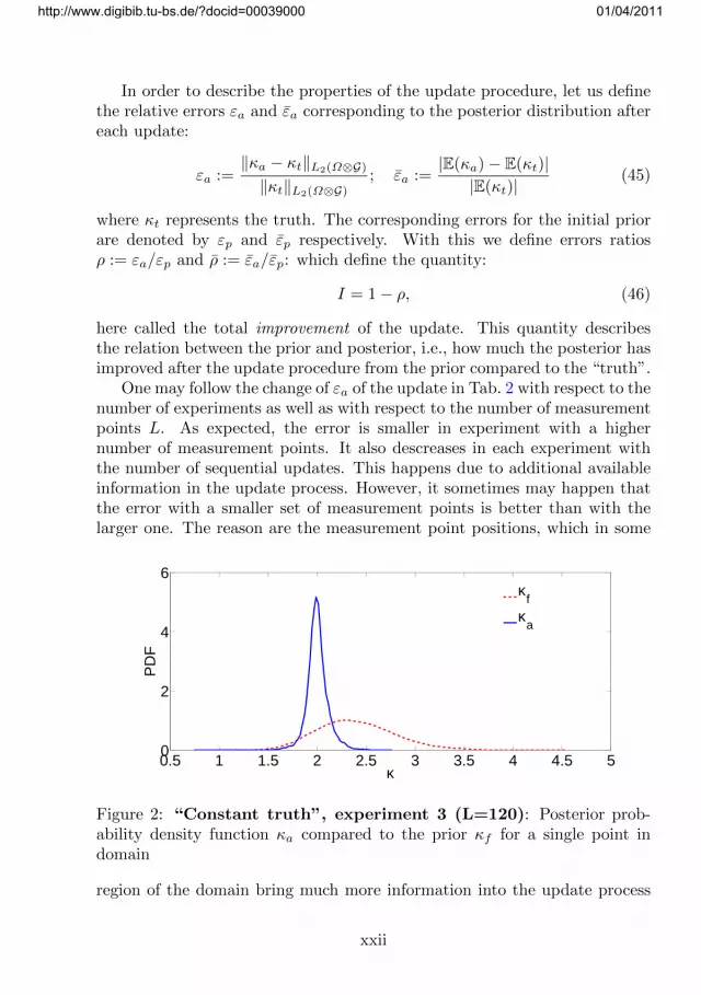
One may follow the change of εa of the update in Tab. 2 with respect to thenumber of experiments as well as with respect to the number of measurementpoints L. As expected, the error is smaller in experiment with a highernumber of measurement points. It also descreases in each experiment withthe number of sequential updates. This happens due to additional availableinformation in the update process. However, it sometimes may happen thatthe error with a smaller set of measurement points is better than with thelarger one. The reason are the measurement point positions, which in some

0.5 1 1.5 2 2.5 3 3.5 4 4.5 50

2

4

6

κ

PD

F

κf

κa

Figure 2: “Constant truth”, experiment 3 (L=120): Posterior prob-ability density function κa compared to the prior κf for a single point indomain

region of the domain bring much more information into the update process

xxii


than in others. For example the boundary nodes bring trivial informationinto the update process and hence we exclude them. In the case of the“constant truth ”already ca. 10 measurement points suffice after four updatesto reduce the error to 7%. We have not tried to optimise the position ofthe measurement points/patches or the loading in the experiments, which isbeyond the scope of this paper.

−10

1

−10

10

1

2

a) εa [%]

−10

1

−10

15.5

6

6.5

b) εa [%]

−10

1

−10

176

78

80

c) I [%]

Figure 3: “Constant truth”, experiment 1 (L=447) after 4th up-date: a) Relative error εa (the mean of the posterior compared to the meanof the truth) b) relative error εa (the posterior compared to the truth) c)improvement I (the posterior compared to the prior)

1 2 3 4 50.01

0.015

0.02

0.025

0.03

0.035

0.04

0.045

Number of sequential updates

Rel

ativ

e er

ror

in th

e m

ean

KL=3KL=5KL=10

Figure 4: “Constant truth”, experiment 1 (L=447): Convergence of therelative error in the mean of the posterior, εa, with the number of sequentialupdates and a different number of KL terms in the expansion of the prior

xxiii


1 2 3 4 50.1

0.15

0.2

0.25

0.3

0.35


Rel

ativ

e va

rianc

e ρ va

r

KL=3KL=50

Figure 5: “Constant truth”, experiment 1 (L=447): Convergence ofρvar with the number of updates and the measurement points

0 1 2 3 410

−2

10−1

100


Rel

ativ

e er

ror

ε a

447 pt239 pt120 pt60 pt10 pt

Figure 6: “Linear truth”, experiment 1 (L=447): Convergence be-haviour of the relative error εa with respect to the number of sequentialupdates and measurement points

xxiv


Furthermore, comparing the probability density function of the a prioriand a posteriori distribution in one point of the domain (experiment 3.) inFig. 2, one may notice that the latter one is more narrowed and centredaround the “true”value 2. This is also shown in Fig. 3a, where the relativeerror εa in the mean already after the first update reduces to 2%, whichmeans that the first order moment is almost instantaneously identified.

−10

1

−10

10

5

10

a) εa [%]

−10

1

−10

16

8

10

b) εa [%]

−10

1

−10

1

60

80

100

c) I [%]

Figure 7: “Linear truth”, experiment 1 (L=447) after 4th update:a) Relative error εa (the mean of the posterior compared to the truth) b)relative RMS error εa (the posterior compared to the truth) c) improvementI (the posterior compared to the prior)

−10

1

−10

11

2

3

a) κf

−10

1

−10

12

2.1

2.2

b) true κ

−10

1

−10

12

2.1

2.2

c) κa

Figure 8: “Quadratic truth”, experiment 1 (L=447) after 4th up-date: a) mean of the prior, κf b) truth, κ c) mean of the posterior, κa

However, the error in higher order terms (see Fig. 3b) is more important

xxv


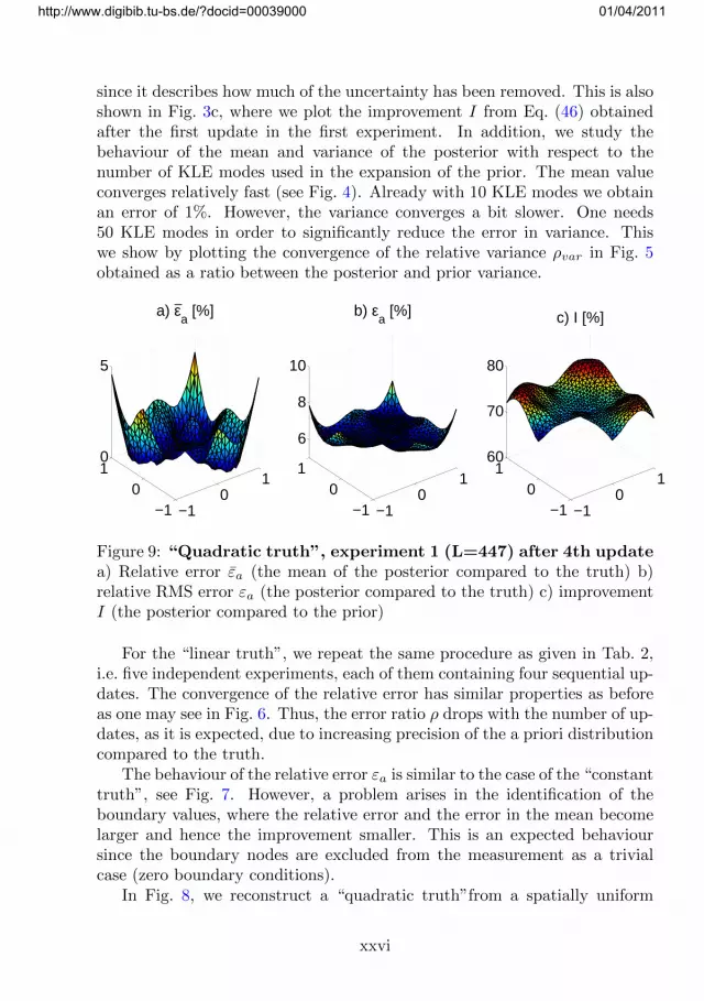
since it describes how much of the uncertainty has been removed. This is alsoshown in Fig. 3c, where we plot the improvement I from Eq. (46) obtainedafter the first update in the first experiment. In addition, we study thebehaviour of the mean and variance of the posterior with respect to thenumber of KLE modes used in the expansion of the prior. The mean valueconverges relatively fast (see Fig. 4). Already with 10 KLE modes we obtainan error of 1%. However, the variance converges a bit slower. One needs50 KLE modes in order to significantly reduce the error in variance. Thiswe show by plotting the convergence of the relative variance ρvar in Fig. 5obtained as a ratio between the posterior and prior variance.

−10

1

−10

10

5

a) εa [%]

−10

1

−10

1

6

8

10

b) εa [%]

−10

1

−10

160

70

80

c) I [%]

Figure 9: “Quadratic truth”, experiment 1 (L=447) after 4th updatea) Relative error εa (the mean of the posterior compared to the truth) b)relative RMS error εa (the posterior compared to the truth) c) improvementI (the posterior compared to the prior)

For the “linear truth”, we repeat the same procedure as given in Tab. 2,i.e. five independent experiments, each of them containing four sequential up-dates. The convergence of the relative error has similar properties as beforeas one may see in Fig. 6. Thus, the error ratio ρ drops with the number of up-dates, as it is expected, due to increasing precision of the a priori distributioncompared to the truth.

The behaviour of the relative error εa is similar to the case of the “constanttruth”, see Fig. 7. However, a problem arises in the identification of theboundary values, where the relative error and the error in the mean becomelarger and hence the improvement smaller. This is an expected behavioursince the boundary nodes are excluded from the measurement as a trivialcase (zero boundary conditions).

In Fig. 8, we reconstruct a “quadratic truth”from a spatially uniform

xxvi


0 1 2 3 4 5 610

−2

10−1

100

101

102


Rel

ativ

e er

ror

ε a

σε=0.2

σε=0.1

σε=1e−6

Figure 10: “Quadratic truth”, experiment 1 (L=447): Convergence ofthe relative error with the number of updates and the measurement error σεobtained for 447 measurement points

lognormal prior. The error behaviour in Fig. 9 is similar to the previous caseof the “linear truth”.

Having in mind that the measurements are disturbed with centred Gaus-sian noise with standard deviation σε, we have investigated the influence ofthis parameter on the update process in Fig. 10. Here one may learn thatthis parameter has only a minor influence on the update. Obviously themain contribution to the error for the range of tested σε still comes from theincomplete information in the measurement.

9 Conclusion

A linear Bayesian estimation of unknown parameters is formulated in a pur-erly deterministic and algebraic way, without the need for any kind of sam-pling techniques like MCMC. The regularisation of the ill-posed problem isachieved by introduction of a priori information approximated by a combi-nation of Karhunen-Loeve and polynomial chaos expansions truncated to afinite number of terms. This representation enters a stochastic forward model,solved by a Galerkin procedure in a low-rank and sparse format. Taking theforward solution to forecast the measurement, the update of the prior is aprojection of the minimum variance estimator from linear Bayesian updating

xxvii


onto the polynomial chaos basis. The new estimate is obtained for all termsof the PCE, i.e. one is able to estimate all higher order moments, not justthe mean and the variance. We have shown that for the mean and variancethe estimation is of the Kalman type.

The suggested method is tested on the stationary diffusion equation withprescribed source terms and unknown conductivity parameter. The identifi-cation experiment, characterised by a sequential update process, is performedfor a “deterministic truth”with increasing spatial compability. In this waywe have shown the influence of additional information and loading conditionson the update process.

The presented linear Bayesian update does not need any linearity in theforward model, and it can readily update non-Gaussian uncertainties. Inaddition, it accommodates noisy measurements and skewed RVs.

Acknowledgement: The support of the Deutsche Forschungsgemein-schaft (DFG), German Luftfahrtforschungsprogramm, the Federal Ministryof Economics (BMWA), and SPT Group GmbH in Hamburg is gratefullyacknowledged.

xxviii


Appendix

These appendices list some fundamental properties of the polynomial chaosexpansion (PCE), the connected Hermite algebra, and the use of the Hermitetransform.

A Multi-Indices

In the above formulation, the need for multi-indices of arbitrary length arises.Formally they may be defined by

α = (α1, . . . , αj , . . .) ∈ N(N)0 := N , (47)

which are sequences of non-negative integers, only finitely many of whichare non-zero. As by definition 0! := 1, the following expressions are welldefined:

|α| :=∞∑j=1

αj , α! :=∞∏j=1

αj !, `(α) := maxj ∈ N |αj > 0. (48)

B Hermite Polynomials

As there are different ways to define — and to normalise — the Hermitepolynomials, a specific way has to be chosen. In applications with probabilitytheory it seems most advantageous to use the following definition [20, 22, 23,34]:

hk(t) := (−1)ket2/2

(d

dt

)ke−t

2/2; ∀t ∈ R, k ∈ N0, (49)

where the coefficient of the highest power of t — which is tk for hk — is equalto unity.

The first five polynomials are:

h0(t) = 1, h1(t) = t, h2(t) = t2 − 1,

h3(t) = t3 − 3t, h4(t) = t4 − 6t2 + 3.

The recursion relation for these polynomials is

hk+1(t) = t hk(t)− k hk−1(t); k ∈ N. (50)

These are orthogonal polynomials w.r.t standard Gaussian probabilitymeasure Γ, where Γ(dt) = (2π)−1/2e−t

2/2 dt — the set hk(t)/√k! | k ∈ N0

xxix


forms a complete orthonormal system (CONS) in L2(R,Γ) — as the Hermitepolynomials satisfy ∫ ∞

−∞hm(t)hn(t) Γ(dt) = n! δnm. (51)

Multi-variate Hermite polynomials will be defined right away for an in-finite number of variables, i.e. for t = (t1, t2, . . . , tj , . . .) ∈ RN, the spaceof all sequences. This uses the multi-indices defined in Appendix A: Forα = (α1, . . . , αj , . . .) ∈ N remember that except for a finite number all otherαj are zero; hence in the definition of the multi-variate Hermite polynomial

Hα(t) :=

∞∏j=1

hαj (tj); ∀t ∈ RN, α ∈ N , (52)

except for finitely many factors all others are h0, which equals unity, and theinfinite product is really a finite one and well defined.

The space RN can be equipped with a Gaussian (product) measure [20,22, 23, 34], again denoted by Γ. Then the set Hα(t)/

√α! | α ∈ N is a

CONS in L2(RN,Γ) as the multivariate Hermite polynomials satisfy∫RNHα(t)Hβ(t) Γ(dt) = α! δαβ , (53)

where the Kronecker symbol is extended to δαβ = 1 in case α = β and zerootherwise.

C The Hermite Algebra

Consider first the usual univariate Hermite polynomials hk as defined inAppendix B, Eq. (49). As the univariate Hermite polynomials are a linearbasis for the polynomial algebra, i.e. every polynomial can be written as linearcombination of Hermite polynomials, this is also the case for the product oftwo Hermite polynomials hkh`, which is clearly also a polynomial:

hk(t)h`(t) =k+∑

n=|k−`|

c(n)k` hn(t) (54)

The coefficients are only non-zero [34] for integer g = (k + `+ n)/2 ∈ N andif g ≥ k ∧ g ≥ ` ∧ g ≥ n. They can be explicitly given

c(n)k` =

k! `!

(g − k)! (g − `)! (g − n)!, (55)

xxx


and are called the structure constants of the univariate Hermite algebra.For the multivariate Hermite algebra, analogous statements hold [34]:

Hα(t)Hβ(t) =∑γ

cγαβHγ(t). (56)

with the multivariate structure constants

cγαβ =∞∏j=1

cγjαjβj

, (57)

defined in terms of the univariate structure constants Eq. (55).From this it is easy to see that

E (HαHβHγ) = E

(Hγ

∑ε

cεαβHε

)= cγαβγ!. (58)

Products of more than two Hermite polynomials may be computed recur-sively, we here look at triple products as an example, using Eq. (56):

HαHβHδ =

(∑γ

cγαβHγ

)Hδ =

∑ε

(∑γ

cεγδcγαβ

)Hε. (59)

D The Hermite Transform

A variant of the Hermite transform maps a random variable onto the set ofexpansion coefficients of the PCE [22]. Any random variable r ∈ L2(Ω,V)which may be represented with a PCE

r(ω) =∑

α∈N(N)0

%αHα(θ(ω)), (60)

is mapped ontoH (r) := (%α)α∈N = (%) ∈ RN . (61)

This way r := E(r) = %0 and H (r) = (%0, 0, 0, ...), as well a r(ω) = r(ω)− rand H (r) = (0, (%α)α∈J ,α>0) are explicitly given. These sequences maybe seen also as the coefficients of power series in infinitely many complexvariables z ∈ CN, namely by ∑

α∈N(N)0

%αzα,

xxxi


where zα :=∏j z

αj

j . This is the original definition of the Hermite transform[22].

It can be used to easily compute the Hermite transform of the ordinaryproduct like in Eq. (56), as

H (HαHβ) = (cγαβ)γ∈N(N)

0. (62)

With the structure constants Eq. (57) one defines the matrices Qγ2 := (cγαβ)

with indices α and β. With this notation the Hermite transform of theproduct of two random variables r1(ω) =

∑α∈N(N)

0%α1Hα(θ) and r2(ω) =∑

β∈N(N)0%β2Hβ(θ) is

H (r1r2) =((%1)Qγ

2(%2)T ))γ∈N(N)

0(63)

Each coefficient is a bilinear form in the coefficient sequences of the factors,and the collection of all those bilinear forms Q2 = (Qγ

2)γ∈N(N)

0is a bilinear

mapping that maps the coefficient sequences of r1 and r2 into the coefficientsequence of the product

H (r1r2) =: Q2((%1), (%2)) = Q2 (H (r1),H (r2)) . (64)

Products of more than two random variables may now be defined recur-sively through the use of associativity. e.g. r1r2r3r4 = (((r1r2)r3)r4):

∀k > 2 : H

k∏j=1

rj

:= Qk((%1), (%2), . . . , (%k)) :=

Qk−1(Q2((%1), (%2)), (%3) . . . , (%k)). (65)

Each Qk is again composed of a sequence of k-linear forms Qγkγ∈N(N)

0, which

define each coefficient of the Hermite transform of the k-fold product.

E Higher order moments

Consider RVs rj(ω) =∑α∈N ρ

αjHα(θ) with values in a vector space V (see

Appendix D), then r, r(ω), as well as ραj are in V. More generally, anymoment may be easily computed knowing the PCE. The k-th centred momentof the RVs r1(ω), r2(ω), ..., rk(ω) is defined as

Mkr1...rk

= E(⊗kj=1rj

), (66)

xxxii


a tensor of order k. Hence the k-point correlation (the k-th moment) may beexpressed as

Mkr1...rk

=∑

γ1,...,γk>0

E

k∏j=1

Hγj (θ)

k⊗m=1

ργj

m , (67)

and in particular:

Cr1r2= M2

r1r2= E (r1 ⊗ r2) =

∑γ,β>0

ργ1 ⊗ ρβ2 E (HγHβ) =

∑γ>0

ργ1 ⊗ ργ2γ!,

(68)as E (HγHβ) = δγβγ!. The expected values of the products of Hermite poly-nomials in Eq. (67) may be computed analytically, using the formulas fromAppendix C and D.

References

[1] S. Acharjee and N. Zabaras. A non-intrusive stochastic Galerkin ap-proach for modeling uncertainty propagation in deformation processes.Computers & Structures, 85:244–254, 2007.

[2] M. Arnst, R. Ghanem, and C. Soize. Identification of Bayesian posteriorsfor coefficients of chaos expansions. Journal of Computational Physics,229(9):3134 – 3154, 2010.

[3] V. Arsigny, P. Fillard, X. Pennec, and N. Ayache. Geometric meansin a novel vector space structure on symmetric positive-definite matri-ces. SIAM Journal on Matrix Analysis and Applications, 29(1):328–347,2006.

[4] V. Arsigny, P. Fillard, X. Pennec, and N. Ayache. Log-euclidean metricsfor fast and simple calculus on diffusion tensors. Magnetic Resonance inMedicine, 56(2):411–421, 2006.

[5] I. Babuska, R. Tempone, and G. E. Zouraris. Galerkin finite elementapproximations of stochastic elliptic partial differential equations. SIAMJournal on Numerical Analysis, 42(2):800–825, 2004.

[6] I. Babuska, R. Tempone, and G. E. Zouraris. Solving elliptic boundaryvalue problems with uncertain coefficients by the finite element method:the stochastic formulation. Computer Methods in Applied Mechanicsand Engineering, 194(12-16):1251–1294, 2005.

xxxiii


[7] S. Balakrishnan, A. Roy, M. G. Ierapetritou, G. P. Flach, and P. G.Georgopoulos. Uncertainty reduction and characterization for complexenvironmental fate and transport models: An empirical Bayesian frame-work incorporating the stochastic response surface method. Water Re-sources Research, 39(12):1350–1362, December 2003.

[8] E. D. Blanchard. Polynomial Chaos Approaches to Parameter Estima-tion and Control Design for Mechanical Systems with Uncertain Param-eters. PhD thesis, Department of Mechanical Engineering, VirginiaTechUniversity, 2010.

[9] G. Christakos. Random Field Models in Earth Sciences. Academic Press,San Diego, CA, 1992.

[10] J. A. Christen and C. Fox. MCMC using an approximation. Journal ofComputational and Graphical Statistics, 14(4):795 – 810, 2005.

[11] P. G. Ciarlet. The Finite Element Method for Elliptic Problems. North-Holland, Amsterdam, 1978.

[12] Geir Evensen. The ensemble Kalman filter for combined state and pa-rameter estimation. IEEE Control Systems Magazine, 29:82–104, 2009.

[13] D. Gamerman and H. F. Lopes. Markov Chain Monte Carlo: StochasticSimulation for Bayesian Inference. Chapman and Hall/CRC, 2006.

[14] R. Ghanem. Ingredients for a general purpose stochastic finite elementimplementation. Computer Methods in Applied Mechanics and Engi-neering, 168(1–4):19–34, 1999.

[15] R. Ghanem. Stochastic finite elements for heterogeneous media withmultiple random non-Gaussian properties. Journal of Engineering Me-chanics, 125:24–40, 1999.

[16] R. Ghanem and R. Kruger. Numerical solutions of spectral stochasticfinite element systems. Computer Methods in Applied Mechanics andEngineering, 129(3):289–303, 1996.

[17] R. Ghanem and P. D. Spanos. Stochastic finite elements—A spectralapproach. Springer-Verlag, New York, 1991.

[18] M. Goldstein and D. Wooff. Bayes linear statistics. Wiley Series inProbability and Statistics. John Wiley & Sons Ltd., Chichester, 2007.

xxxiv


[19] S. B. Hazra, H. Class, R. Helmig, and V. Schulz. Forward and inverseproblems in modeling of multiphase flow and transport through porousmedia. Computational Geosciences, 8(1):21–47, 2004.

[20] T. Hida, H.-H. Kuo, J. Potthoff, and L. Streit. White Noise Analysis-Aninfinite dimensional calculus. Kluwer, Dordrecht, 1993.

[21] D. Higdon, H. Lee, and C. Holloman. Markov chain Monte Carlo-basedapproaches for inference in computationally intensive inverse problems.Bayesian Statistics, (7):181–197, 2003.

[22] H. Holden, B. Øksendal, J. Ubøe, and T.-S. Zhang. Stochastic PartialDifferential Equations. Birkhauser Verlag, Basel, 1996.

[23] S. Janson. Gaussian Hilbert spaces. Cambridge University Press, 1997.

[24] M. Jardak, C.-H. Su, and G. E. Karniadakis. Spectral polynomialchaos solutions of the stochastic advection equation. In Proceedings ofthe Fifth International Conference on Spectral and High Order Methods(ICOSAHOM-01) (Uppsala), volume 17, pages 319–338, 2002.

[25] B. N. Khoromskij and A. Litvinenko. Data sparse computation of theKarhunen-Loeve expansion. Numerical Analysis and Applied Mathe-matics: International Conference on Numerical Analysis and AppliedMathematics, AIP Conf. Proc., 1048(1):311–314, 2008.

[26] B. N. Khoromskij, A. Litvinenko, and H. G. Matthies. Application ofhierarchical matrices for computing Karhunen-Loeve expansion. JournalComputing, 84(1-2):49–67, 2009.

[27] T. G. Kolda and B. W. Bader. Matlab tensor classes for fast algorithmprototyping. Technical report, ACM Trans. Math. Software, 2004.

[28] P. Kree and Ch. Soize. Mathematics of random phenomena. D. ReidelPublishing Co., Dordrecht, 1986.

[29] A. Kucerova and H. G. Matthies. Uncertainty updating in the descrip-tion of heterogeneous materials. Technische Mechanik, 30((1-3)):211–226, 2010.

[30] O. P. Le Maıtre, H. N. Najm, R. G. Ghanem, and O. M. Knio. Multi-resolution analysis of Wiener-type uncertainty propagation schemes.Journal of Computational Physics, 197(2):502–531, 2004.

xxxv


[31] Jia Li and D. Xiu. A generalized polynomial chaos based ensembleKalman filter with high accuracy. Journal of Computational Physics,228(15):5454–5469, August 2009.

[32] D. G. Luenberger. Optimization by Vector Space Methods. John Wileyand Sons, Inc., New York, 1969.

[33] X. Ma and N. Zabaras. An efficient Bayesian inference approach toinverse problems based on an adaptive sparse grid collocation method.Inverse Problems, 25(3):035013, 2009.

[34] P. Malliavin. Stochastic Analysis. Springer Verlag, Berlin, 1997.

[35] Y. M. Marzouk, H. N. Najm, and L. A. Rahn. Stochastic spectral meth-ods for efficient Bayesian solution of inverse problems. Journal of Com-putational Physics, 224(2):560–586, June 2007.

[36] Y. M. Marzouk and D. Xiu. A stochastic collocation approach toBayesian inference in inverse problems. Communications in Compu-tational Physics, 6(4):826–847, 2009.

[37] H. G. Matthies. Computational aspects of probability in non-linear me-chanics. In A. Ibrahimbegovic and B. Brank, editors, Engineering Struc-tures under Extreme Conditions. Multi-physics and multi-scale computermodels in non-linear analysis and optimal design of engineering struc-tures under extreme conditions, volume 194 of NATO Science Series III:Computer and System Sciences. IOS Press, Amsterdam, 2005.

[38] H. G. Matthies. Stochastic finite elements: Computational approachesto stochastic partial differential equations. Zeitschrift fur AngewandteMathematik und Mechanik (ZAMM), 88(11):849–873, 2008.

[39] H. G. Matthies, Christoph E. Brenner, Christoph G. Bucher, and Car-los Guedes Soares. Uncertainties in probabilistic numerical analysisof structures and solids—stochastic finite elements. Structural Safety,19(3):283–336, 1997.

[40] H. G. Matthies and Ch. Bucher. Finite elements for stochastic mediaproblems. Computer Methods in Applied Mechanics and Engineering,168(1–4):3–17, 1999.

[41] H. G. Matthies and A. Keese. Galerkin methods for linear and nonlinearelliptic stochastic partial differential equations. Computer Methods inApplied Mechanics and Engineering, 194(12-16):1295–1331, 2005.

xxxvi


[42] H. G. Matthies and E. Zander. Solving stochastic systems with low-ranktensor compression. Linear Algebra and Application, submitted, 2010.

[43] M. Moakher. A differential geometric approach to the geometric mean ofsymmetric positive-definite matrices. SIAM Journal on Matrix Analysisand Applications, 26(3):735–747, 2005.

[44] O. Pajonk, B. V. Rosic, A. Litvinenko, and H. G. Matthies. A determin-istic filter for non-Gaussian Bayesian estimation. Physica D: NonlinearPhenomena, 2011.

[45] B.L. Pence, H.K. Fathy, and J.L. Stein. A maximum likelihood approachto recursive polynomial chaos parameter estimation. In Proceedings ofAmerican Control Conference (ACC), pages 2144–2151, 2010.

[46] L. J. Roman and M. Sarkis. Stochastic Galerkin method for ellipticSPDEs: a white noise approach. Discrete and Continuous Dynami-cal Systems. Series B. A Journal Bridging Mathematics and Sciences,6(4):941–955, 2006.

[47] G. Strang and G. J. Fix. An Analysis of the Finite Element Method.Wellesley-Cambridge Press, Wellesley, MA, 1988.

[48] A. M. Stuart. Inverse problems: A Bayesian perspective. Acta Numerica,19:451–559, 2010.

[49] A. Tarantola. Inverse Problem Theory and Methods for Model ParameterEstimation. Society for Industrial and Applied Mathematics, 2005.

[50] A. Tarantola. Popper, Bayes and the inverse problem. Nature Physics,2(8):492–494, August 2006.

[51] J. Wang and N. Zabaras. Using Bayesian statistics in the estimationof heat source in radiation. International Journal of Heat and MassTransfer, 48(1):15–29, January 2005.

[52] Norbert Wiener. The homogeneous chaos. American Journal of Mathe-matics, 60:897–936, 1938.

[53] D. Xiu and G. E. Karniadakis. Modeling uncertainty in steady statediffusion problems via generalized polynomial chaos. Computer Methodsin Applied Mechanics and Engineering, 191:4927–4948, 2002.

[54] X. F. Xu. A multiscale stochastic finite element method on elliptic prob-lems involving uncertainties. Computer Methods in Applied Mechanicsand Engineering, 196(25-28):2723–2736, 2007.

xxxvii


[55] E. Zander. Stochastic Galerkin library. http://github.com/ezander/sglib,2008.

[56] O. C. Zienkiewicz and R. L. Taylor. The Finite Element Method.Butterwort-Heinemann, Oxford, 5th ed., 2000.

xxxviii


Technische Universitat BraunschweigInformatik-Berichte ab Nr. 2008-03

2008-03 R. van Glabbeek, U. Goltz,J.-W. Schicke

Symmetric and Asymmetric Asynchronous Interaction

2008-04 R. van Glabbeek, U. Goltz,J.-W. Schicke

On Synchronous and Asynchronous Interaction inDistributed Systems

2008-05 M. V. Cengarle, H. GronnigerB. Rumpe

System Model Semantics of Class Diagrams

2008-06 M. Broy, M. V. Cengarle,H. Gronniger B. Rumpe

Modular Description of a Comprehensive SemanticsModel for the UML (Version 2.0)

2008-07 C. Basarke, C. Berger, K. Berger,K. Cornelsen, M. DoeringJ. Effertz, T. Form, T. Gulke,F. Graefe, P. Hecker, K. HomeierF. Klose, C. Lipski, M. Magnor,J. Morgenroth, T. Nothdurft,S. Ohl, F. Rauskolb, B. Rumpe,W. Schumacher, J. Wille, L. Wolf

2007 DARPA Urban Challenge Team CarOLO -Technical Paper

2008-08 B. Rosic A Review of the Computational StochasticElastoplasticity

2008-09 B. N. Khoromskij, A. Litvinenko,H. G. Matthies

Application of Hierarchical Matrices for Computing theKarhunen-Loeve Expansion

2008-10 M. V. Cengarle, H. GronnigerB. Rumpe

System Model Semantics of Statecharts

2009-01 H. Giese, M. Huhn, U. Nickel,B. Schatz (Herausgeber)

Tagungsband des Dagstuhl-Workshops MBEES:Modellbasierte Entwicklung eingebetteter Systeme V

2009-02 D. Jurgens Survey on Software Engineering for ScientificApplications: Reuseable Software, Grid Computing andApplication

2009-03 O. Pajonk Overview of System Identification with Focus on InverseModeling

2009-04 B. Sun, M. Lochau, P. Huhn,U. Goltz

Parameter Optimization of an Engine Control Unitusing Genetic Algorithms

2009-05 A. Rausch, U. Goltz, G. Engels,M. Goedicke, R. Reussner

LaZuSo 2009: 1. Workshop f—r langlebige undzukunftsfahige Softwaresysteme 2009

2009-06 T. Muller, M. Lochau, S. Detering,F. Saust, H. Garbers, L. Martin,T. Form, U. Goltz

Umsetzung eines modellbasierten durchgangigenEnwicklungsprozesses fur AUTOSAR-Systeme mitintegrierter Qualitatssicherung

2009-07 M. Huhn, C. Knieke Semantic Foundation and Validation of Live ActivityDiagrams

2010-01 A. Litvinenko and H. G. Matthies Sparse data formats and efficient numerical methods foruncertainties quantification in numerical aerodynamics

2010-02 D. Grunwald, M. Lochau,E. Borger, U. Goltz

An Abstract State Machine Model for the Generic JavaType System

2010-03 M. Krosche, R. Niekamp Low-Rank Approximation in Spectral Stochastic FiniteElement Method with Solution Space Adaption

2011-01 L. Martin, M. Schatalov, C. Knieke Entwicklung und Erweiterung einer Werkzeugkette imKontext von IT-kosystemen

2011-02 B. V. Rosic, A. Litvinenko,O. Pajonk, H. G. Matthies

Direct Bayesian update of polynomial chaosrepresentations


sampling-free linear bayesian update of polynomial chaos representations

Documents