polynomial chaos-based macromodeling of multiport systems using an input-output approach
TRANSCRIPT

INTERNATIONAL JOURNAL OF NUMERICAL MODELLING: ELECTRONIC NETWORKS, DEVICES AND FIELDS
Int. J. Numer. Model. 2014; 00:2–31
Published online in Wiley InterScience (www.interscience.wiley.com). DOI: 10.1002/jnm
Polynomial Chaos-Based Macromodeling of Multiport Systems
using an Input-Output Approach
Domenico Spina1∗, Francesco Ferranti1, Tom Dhaene1, Luc Knockaert1 and Giulio
Antonini2
1Department of Information Technology, Internet Based Communication Networks and Services (IBCN), Ghent
University – iMinds, Gaston Crommenlaan 8 Bus 201, B-9050 Gent, Belgium.
2UAq EMC Laboratory, Dipartimento di Ingegneria Industriale e dell’Informazione e di Economia, Universita degli
Studi dell’Aquila, Via G. Gronchi 18, 67100, L’Aquila, Italy.
SUMMARY
An innovative technique to build stochastic frequency-domain macromodels of generic linear multiport
systems is presented. The proposed method calculates a macromodel of the system transfer function
including its statistical properties, making it tailored for variability analysis. The combination of the
modeling power of the Vector Fitting algorithm with the Polynomial Chaos expansion applied at an input-
output level allows to accurately and efficiently describe the system variability features. Thanks to its
versatility and automated order selection, the proposed technique is suitable to be applied to a large range
of complex modern electrical systems (e.g. filters, interconnections) and can tackle the case of correlated
random variables. The performance in terms of accuracy and computational efficiency of the proposed
method are compared with respect to the standard Monte Carlo analysis for two pertinent numerical
examples. Copyright c© 2014 John Wiley & Sons, Ltd.
Received . . .
KEY WORDS: Multiport systems; frequency-domain; macromodeling; variability analysis; polynomial
chaos.
Copyright c© 2014 John Wiley & Sons, Ltd.
Prepared using jnmauth.cls [Version: 2010/03/27 v2.00]

2 D. SPINA ET AL.
1. INTRODUCTION
Nowadays, the analysis of the effects of geometrical or electrical parameters variability on the
performance of integrated circuits is fundamental. Indeed, many techniques [1]-[6], based on
the Polynomial Chaos (PC) expansion [7]-[11], were developed over the last years to study
the stochastic variations of electrical circuits as alternative to the computationally cumbersome
Monte Carlo (MC) based techniques. The MC analysis is considered the standard approach for
variability analysis, thanks to its robustness and ease of implementation. The drawback of MC is
its slow convergence rate, that forces the designers to perform a large number of simulations to
obtain reliable results. Considering that both the operative bandwidth and complexity of modern
electrical systems are constantly increasing, the high computational time required by the MC
analysis is a clear limitation. The PC-based techniques proposed so far allow to overcome the
computational cumbersomeness of the MC-based approaches, but they were designed for specific
systems: multiconductor transmission lines [1]-[4] or lumped elements circuits [5], [6].
Recently, a PC-based technique was presented in [12] to perform variability analysis on a generic
linear multiport system. This technique first builds a set of deterministic univariate frequency-
domain models of the system transfer function, that can be expressed in different forms (e.g.
scattering, impedance or admittance parameters), and then uses the PC expansion to perform the
variability analysis. In particular, the PC expansion of the system transfer function is obtained
by combining a deterministic set of system equations expressed in state-space form with the PC
model of the system’s state-space matrices, through the use of Galerkin projections [1]-[6]. This
approach, while applicable to a large range of microwave systems, has a main drawback: the PC
model of the system transfer function must be calculated for each frequency of interest solving
∗Correspondence to: Domenico Spina, Department of Information Technology, Internet Based Communication Networks
and Services (IBCN), Ghent University – iMinds, Gaston Crommenlaan 8 Bus 201, B-9050 Gent, Belgium. E-mail:
Contract/grant sponsor: This research has been funded by the Interuniversity Attraction Poles Programme BESTCOM
initiated by the Belgian Science Policy Office.
Copyright c© 2014 John Wiley & Sons, Ltd. Int. J. Numer. Model. (2014)
Prepared using jnmauth.cls DOI: 10.1002/jnm

3
a linear system. Note that, the set of frequency values of interest can be freely chosen over the
frequency range of the initial set of deterministic univariate frequency-domain models of the system
transfer function. Finally, despite its accuracy and efficiency, the technique [12] does not offer the
possibility to enforce the stability of the calculated PC-based model.
The novel approach presented in this paper calculates a PC-based frequency-domain macromodel
of a generic linear multiport system, described by its scattering parameters, which is suitable for
variability analysis. Furthermore, the macromodel is obtained through the application of the PC
expansion at an input-output level without intermediate state-space models as in [12], adopting an
efficient model-building procedure that
• proposes an algorithm that adaptively chooses the number of basis functions of the PC model;
• it is straightforward to implement.
Finally, we propose a method to enforce the stability and check the passivity of the calculated PC-
based macromodel.
The starting point of the proposed technique is the evaluation of the system scattering parameters
on a discrete set of values of the frequency and the parameters involved in the variability analysis.
Next, the PC model of the system transfer function for the chosen frequencies is calculated through
an iterative procedure. Finally, a frequency-domain stochastic macromodel is built as weighted
summation of frequency-dependent rational functions of the PC matrix coefficients by means of
the Vector Fitting (VF) algorithm [13], [14].
This paper is structured as follows. First, an overview of PC properties is given in Section 2. The
new frequency–domain macromodeling technique is described in Section 3, while its validation is
described in Section 4 by means of two numerical examples. The conclusions are summed up in
Section 5.
Copyright c© 2014 John Wiley & Sons, Ltd. Int. J. Numer. Model. (2014)
Prepared using jnmauth.cls DOI: 10.1002/jnm

4 D. SPINA ET AL.
2. POLYNOMIAL CHAOS PROPERTIES
The PC expansion allows to express a stochastic process X with finite variance [7] as
X =∞∑
i=0
αiϕi(~ξ) (1)
where the terms αi are scalar coefficients, ~ξ is a vector of normalized random variables and the
basis functions ϕi(~ξ) are orthogonal polynomials with respect to the probability measure W (~ξ)
with support Ω as [9]
< ϕi(~ξ), ϕj(~ξ) >=∫Ω
ϕi(~ξ)ϕj(~ξ)W (~ξ)d~ξ = aiδij (2)
where δij is the Kronecker delta and ai are positive numbers. Therefore, (1) expresses a stochastic
process X as a series of orthogonal polynomials with suitable coefficients.
Of particular interest is the case of a stochastic process X composed of independent random
variables. Indeed, the basis functions ϕi(~ξ) can be computed as products combinations of the
orthogonal polynomials corresponding to each individual random variable ξi [11]. Furthermore,
in this case it is possible to truncate (1) up to basis functions of a maximum degree P , called order
of the expansion, and a maximum number of basis function M + 1 as
ϕi(~ξ) =N∏
k=1
φjk(ξk) with
N∑k=1
jk ≤ P and 0 ≤ i ≤ M (3)
where φjk(ξk) represent the polynomial function of degree j corresponding to the random variable
ξk. It can be easily proven that, if the definition (3) is used, the total number of basis functions
M + 1 used in the PC expansion is [8]
M + 1 =(N + P )!
N !P !(4)
If the independent random variables ~ξ have arbitrary probability density functions (PDFs), the
corresponding basis functions can be calculated numerically following the approach described
in [9]. That approach allows to calculate the basis function ϕi(~ξ) under the condition that their
weighting function W (~ξ) corresponds to the PDF of the associated random variable in standard
form. Hence, an exponential convergence rate of the PC expansion can be achieved [9], and the basis
Copyright c© 2014 John Wiley & Sons, Ltd. Int. J. Numer. Model. (2014)
Prepared using jnmauth.cls DOI: 10.1002/jnm

5
functions used are optimal. Furthermore, for random variables with specific PDFs (i.e. Gaussian,
Uniform, Beta distribution) the optimal basis functions are the polynomials of the Wiener-Askey
scheme [10]. In the sequel, these particular PDFs are referred as standard distributions.
The basis function in (1) can be calculated also in the more general case of correlated random
variables with arbitrary PDFs, following the approaches described in [7]-[9], [11]. In this case, a
variable transformation, such as the Nataf transformation [15] or the Karhunen-Loeve expansion
[16], can be used to achieve decorrelation, even if the PC expansion convergence rate may not be
exponential.
Finally, upon determination of the M + 1 basis functions ϕi(~ξ), (1) is truncated as
X ≈M∑i=0
αiϕi(~ξ) (5)
where the only unknowns are the PC coefficients αi that can be calculated following different
approaches [8].
The most attractive feature of the PC expansion is the analytical representation of the system
variability. Indeed, the mean µ and the variance σ2 of the stochastic process X can be expressed as
[8]
µ = α0 (6)
σ2 =M∑i=1
α2i < ϕi(~ξ), ϕi(~ξ) > (7)
Furthermore, apart from the others moments, more complex stochastic functions of X , such as the
PDF, can be efficiently calculated following standard analytical formulas or numerical schemes [17].
Finally, the extension of the PC expansion to a stochastic process written in a matrix form X is
straightforward. In this case, (5) becomes
X ≈M∑i=0
αiϕi(~ξ) (8)
where αi is the matrix of PC coefficients, corresponding to the i-th polynomial basis, calculated for
each entry of X. For an extensive reference to polynomial chaos theory, the reader may consult [7]
– [11].
Copyright c© 2014 John Wiley & Sons, Ltd. Int. J. Numer. Model. (2014)
Prepared using jnmauth.cls DOI: 10.1002/jnm
6 D. SPINA ET AL.
3. MACROMODELING STRATEGY
3.1. PC modeling of system transfer function
The scattering parameters are widely used to describe the broadband frequency behavior of
microwave systems. Indeed, the use of the appropriate reference impedances to all system ports
overcomes the difficulties in the measurement of impedance, admittance and hybrid parameters
caused by short-circuit, open-circuit, and test-circuit parasitics at microwave frequencies [18].
Also, the scattering parameters have in general a smoother and more bounded behavior with
respect to the impedance, admittance and hybrid parameters. This makes the scattering parameters
particularly suitable to be efficiently modeled with a PC-based approach.
Therefore, the proposed technique aims at building a PC model for the scattering parameters of a
generic multiport system of the form
S(s, ~ξ) ≈M∑i=0
αi(s)ϕi(~ξ) (9)
where the matrix S represents the system scattering parameters and αi(s) is a univariate frequency-
domain rational model of the i-th PC coefficient matrix and s is the Laplace variable. As will be
demonstrated in the sequel, this goal can be achieved by
• determining the basis function ϕi(~ξ);
• deciding on the number of basis functions M (4);
• calculating and solving an equivalent linear system for the coefficients of the PC expansion of
S;
• calculating a rational model for each PC coefficient matrix obtained.
Without loss of generality, in the sequel we will limit our attention to stochastic processes
composed by independent random variables with the corresponding PDFs included in the standard
distributions. Hence, the optimal basis functions are the polynomials of the Wiener-Askey scheme.
Note, however, that in the most general case of correlated random variables with arbitrary
Copyright c© 2014 John Wiley & Sons, Ltd. Int. J. Numer. Model. (2014)
Prepared using jnmauth.cls DOI: 10.1002/jnm
7
distributions, the corresponding basis functions can also be calculated using the techniques
described in [7]-[9], [11].
The starting point of this work is the calculation of the scattering parameters S for a discrete
set of values of the frequency [fl]Ll=1 corresponding to the Laplace variable [sl = j2πfl]Ll=1 and the
normalized random variables[~ξj
]K
j=1. Equation (9) can therefore be written as
S(sl, ~ξ) ≈M∑i=0
αi(sl)ϕi(~ξ) (10)
where only the coefficients αi(sl) and the number of basis functions M must be estimated. Next, the
linear regression technique [8] is used to obtain the desired PC coefficients. This approach allows
to calculate the PC coefficients in (10) solving, for each value of the Laplace variable [sl]Ll=1, a
least-square system [8] in the form
Φα = R (11)
with
Φ =
ϕ0
(~ξ1
). . . ϕM
(~ξ1
)...
......
ϕ0
(~ξK
). . . ϕM
(~ξK
)
α =
α0(sl)
...
αM (sl)
R =
S(sl, ~ξ1)
...
S(sl, ~ξK)
(12)
and where α contains the matrices of the unknown PC coefficients [αi(sl)]Mi=0, the j−th row of
the matrix Φ is formed by the elements of the multivariate polynomial basis [ϕi]Mi=0 evaluated in[
~ξj
]K
j=1multiplied by the identity matrix of the same dimension of the scattering parameters, and
the matrix R collects the corresponding set of scattering parameters values S(sl, ~ξj) for[~ξj
]K
j=1.
Copyright c© 2014 John Wiley & Sons, Ltd. Int. J. Numer. Model. (2014)
Prepared using jnmauth.cls DOI: 10.1002/jnm
8 D. SPINA ET AL.
Note that the system (11) must be over-determined to be solved in a least-square sense. Therefore,
the number of basis functions M must be chosen to evaluate the number of initial samples K needed
to solve (11). Since the order of expansion P is limited for practical applications [10], several
techniques [1]-[6], [12] choose upfront the number of basis function M , according to (4).
We propose a fully automatic procedure, explained in Algorithm 1, to determine the minimum
order of expansion P that guarantees accurate results and, therefore, the estimated number of basis
functions M (4).
Let us assume that the basis functions up to polynomials of order P ′ are calculated before starting
Algorithm 1. P ′ is chosen, see (4), aimed at keeping the corresponding number of basis functions
M ′ + 1 limited. At this point the number of initial samples K > M ′ + 1 can be chosen. In [19] it
is recommended to use a number of samples equal to the double of the basis function used, i.e.,
K ≈ 2 (M ′ + 1).
We will now describe in detail the iterative procedure summarized in Algorithm 1. Initially, the
basis functions for polynomials of order one and two, indicated in Algorithm 1 with the symbols
Φ1 and Φ2, respectively, are selected. Next, the corresponding linear system (11) is solved for both
PC expansion models. Following equations (6) and (7), it is now obvious to estimate the mean
and the variance for the two PC models. Now, if the difference between the mean and variance of
the two PC models exceeds a suitable threshold, then the PC model with polynomials up to order
one is discarded and the basis functions corresponding to polynomials of order three are chosen.
The procedure is repeated iteratively until the error between the mean and variance predicted by
two consecutive PC models is lower than the chosen threshold. If the previous condition cannot
be achieved upon calculation of the basis functions up to polynomials of order P ′, the PC model
of order P ′ is chosen. It is important to notice that, in Algorithm 1 the computation of the PC
coefficients corresponding to basis functions of polynomials of increasing order is not nested: a
linear system in the form (11) must be solved for each PC model computed up to a specific order of
expansion.
Copyright c© 2014 John Wiley & Sons, Ltd. Int. J. Numer. Model. (2014)
Prepared using jnmauth.cls DOI: 10.1002/jnm

9
Input: Basis function up to order P ′:[Φ1, . . . , ΦP ′
], S(sl, ~ξj)
Output: PC model of order P : Basischosen, αchosen
Basis1 = Φ1;
Basis2 = Φ2;
α1=Solve (11) for Basis1;
µ1 =Solve (6) for Basis1 and α1;
σ1 =Solve (7) for Basis1 and α1;
α2=Solve (11) for Basis2;
µ2 =Solve (6) for Basis2 and α2;
σ2 =Solve (7) for Basis2 and α2;
Error(µ) = µ2−µ1µ2
Error(σ) = σ2−σ1σ2
i = 2;
Error = errorchosen;
while Error(µ) > Error || Error(σ) > Error do
if i < P ′ thenBasis1 = Basis2;
α1 = α2;
µ1 = µ2;
σ1 = σ2;
Basis2 = Φi+1;
α2=Solve (11) for Basis2;
µ2 =Solve (6) for Basis2 and α2;
σ2 =Solve (7) for Basis2 and α2;
Error(µ) = µ2−µ1µ2
Error(σ) = σ2−σ1σ2
;
i = i + 1;
elseend while
end
end
if Error(µ) ≤ Error && Error(σ) ≤ Error thenBasischosen = Basis1;
αchosen = α1;
elseBasischosen = Basis2;
αchosen = α2;
endAlgorithm 1: Iterative procedure to build the PC model.
Copyright c© 2014 John Wiley & Sons, Ltd. Int. J. Numer. Model. (2014)
Prepared using jnmauth.cls DOI: 10.1002/jnm
10 D. SPINA ET AL.
System transfer
function evaluated at
[ ξl ]Kk=1 [ sl ]l=1
L
PC model in the form (10)
with αi( sl ) for [ sl ]l=1L
Solving Φα = X
Vector Fitting
PC model in the form (9)
with αi( sl )
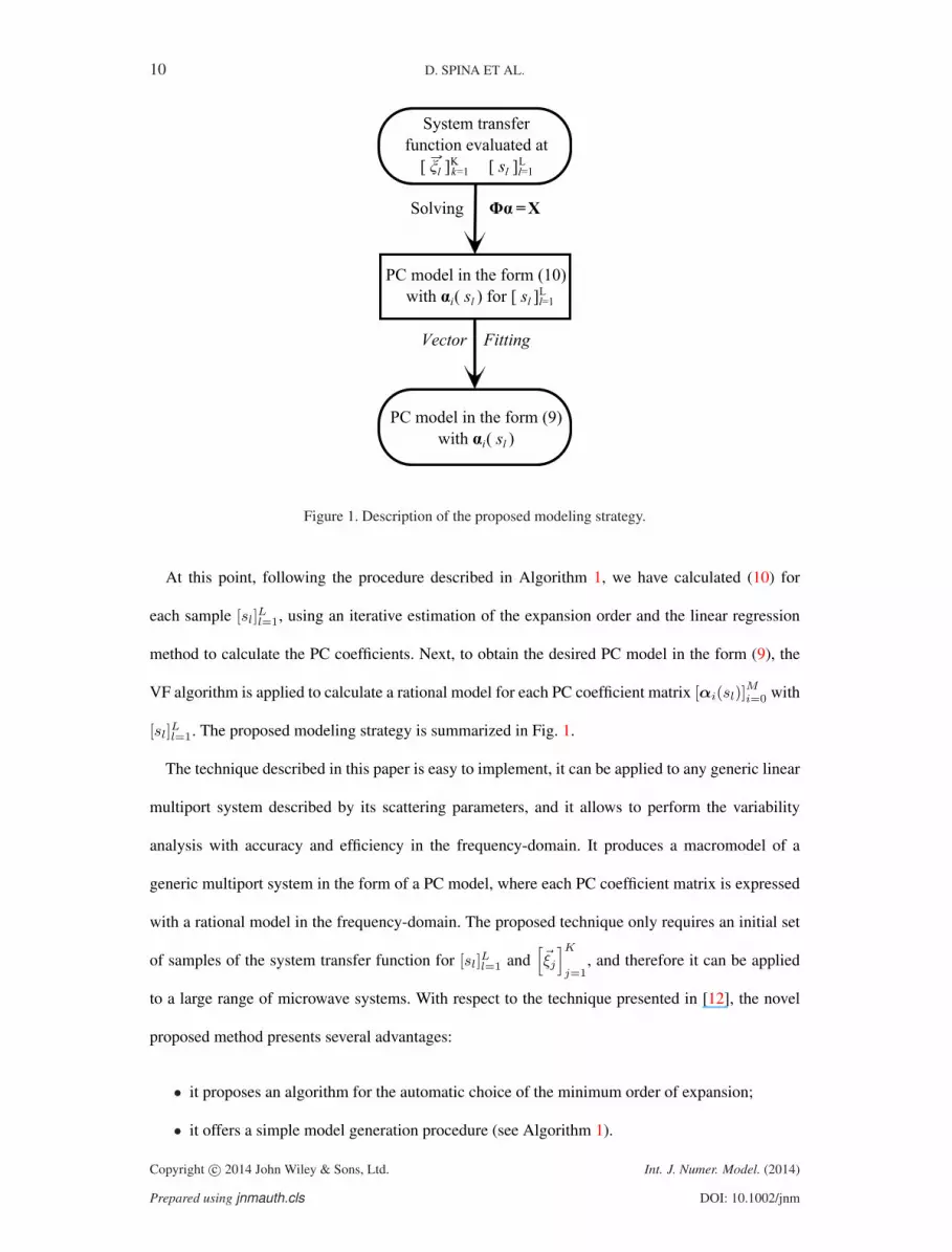
Figure 1. Description of the proposed modeling strategy.
At this point, following the procedure described in Algorithm 1, we have calculated (10) for
each sample [sl]Ll=1, using an iterative estimation of the expansion order and the linear regression
method to calculate the PC coefficients. Next, to obtain the desired PC model in the form (9), the
VF algorithm is applied to calculate a rational model for each PC coefficient matrix [αi(sl)]Mi=0 with
[sl]Ll=1. The proposed modeling strategy is summarized in Fig. 1.
The technique described in this paper is easy to implement, it can be applied to any generic linear
multiport system described by its scattering parameters, and it allows to perform the variability
analysis with accuracy and efficiency in the frequency-domain. It produces a macromodel of a
generic multiport system in the form of a PC model, where each PC coefficient matrix is expressed
with a rational model in the frequency-domain. The proposed technique only requires an initial set
of samples of the system transfer function for [sl]Ll=1 and[~ξj
]K
j=1, and therefore it can be applied
to a large range of microwave systems. With respect to the technique presented in [12], the novel
proposed method presents several advantages:
• it proposes an algorithm for the automatic choice of the minimum order of expansion;
• it offers a simple model generation procedure (see Algorithm 1).
Copyright c© 2014 John Wiley & Sons, Ltd. Int. J. Numer. Model. (2014)
Prepared using jnmauth.cls DOI: 10.1002/jnm
11
• it does not require to calculate a deterministic model, e.g. state-space models as in [12], prior
to the application of the PC expansion;
• it calculates a PC-based macromodel in the form of weighted summation of rational functions,
therefore it is not required to solve a linear system to evaluate the obtained PC-based
macromodel over a discrete set of frequencies as in [12];
It is worthwhile to notice that the proposed technique can calculate a stable frequency-domain
macromodel. Indeed, the macromodel in the form (9) is expressed as a weighted sum of frequency-
dependent rational functions. Since a weighted sum of stable frequency-dependent rational functions
is also stable [20], the stability of the proposed macromodel can be ensured by calculating a stable
rational model for each PC coefficient matrix [αi(sl)]Mi=0, using the VF algorithm. Furthermore,
the passivity of the proposed macromodel can be checked by means of standard techniques (see
Appendix 6.2 for further details).
Note that, the loads can be included in the variability analysis by means of the Galerkin
projections [1]-[6], as shown in [12].
4. NUMERICAL EXAMPLES
In this Section, the proposed technique is applied to different structures. In each example, a
comparison with the MC analysis is shown in order to validate the efficiency and accuracy of our
novel technique. In particular, the results of the variability analysis obtained with the novel proposed
method are compared with the corresponding results obtained with a MC analysis that requires a
comparable computational cost as the proposed technique and with a MC analysis performed using
a large set of samples.
To calculate the PC model by means of the method described in Algorithm 1, the maximum
relative error between the mean and the variance of two consecutive PC models with increasing
order is set to 0.01. Furthermore, the rational model of each PC coefficient matrix [αi(sl)]Mi=0 for
Copyright c© 2014 John Wiley & Sons, Ltd. Int. J. Numer. Model. (2014)
Prepared using jnmauth.cls DOI: 10.1002/jnm

12 D. SPINA ET AL.
[sl]Ll=1, is calculated with the VF algorithm with the following relative error measure
Err =maxr,c,l
(|αrc
i (sl) − αrci (sl)|
1A2L
∑Ar=1
∑Ac=1
∑Ll=1 |αrc
i (sl)|
)
for r, c = 1, . . . , A; l = 1, . . . , L;
(13)
where the symbol αrci (sl) is the element (r, c) of the matrix αi(sl) of size A × A, where A is the
number of ports, and αrci (sl) is the corresponding value of the rational model. The simulations are
performed with MATLAB† 2010a on a computer with an Intel(R) Core(TM) i3 processor and 4 GB
RAM.
4.1. Hairpin Filter, 3 Independent Random Variables
In the first example, a bandpass hairpin filter of length L = 12 mm has been modeled within the
frequency range [1.5 − 3.5] GHz. Its layout is shown in Fig. 2. The filter conductors have width
W1 = 0.33 mm, while W2 = 0.66 mm is the width of the conductors at the input and output port. The
spacing between the port and the filter conductors is D1 = D2 = 0.3 mm and the spacing between
the filter conductors is D3 = 1 mm. The distance C is equal to 2.5 mm. The substrate of thickness
0.635 mm has a relative dielectric constant εr = 9.9.
Figure 2. Example A. Geometry of the bandpass hairpin filter.
Three parameters are considered as independent random variables with uniform PDFs: the
spacing D1, D2, and D3, varying by ±10% with respect to their previously indicated nominal value.
†The Mathworks Inc., Natick, MA, USA.
Copyright c© 2014 John Wiley & Sons, Ltd. Int. J. Numer. Model. (2014)
Prepared using jnmauth.cls DOI: 10.1002/jnm
13
The selected random variables are normalized as
D1 = µD1(1 + σD1ξ1) (14)
D2 = µD2(1 + σD2ξ2) (15)
D3 = µD3(1 + σD3ξ3) (16)
where ξ1, ξ2, ξ3 are random variables with uniform PDFs over the interval [−1, 1]. The
corresponding probability measure (2) is
W (ξ) =
2−N , |ξi| ≤ 1, i = 1, ...., N
0, elsewhere
(17)
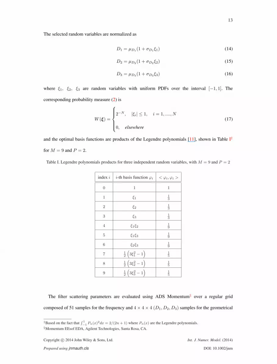
and the optimal basis functions are products of the Legendre polynomials [11], shown in Table I‡
for M = 9 and P = 2.
Table I. Legendre polynomials products for three independent random variables, with M = 9 and P = 2
index i i-th basis function ϕi < ϕi, ϕi >
0 1 1
1 ξ113
2 ξ213
3 ξ313
4 ξ1ξ219
5 ξ1ξ319
6 ξ2ξ319
7 12
(3ξ2
1 − 1)
15
8 12
(3ξ2
2 − 1)
15
9 12
(3ξ2
3 − 1)
15
The filter scattering parameters are evaluated using ADS Momentum§ over a regular grid
composed of 51 samples for the frequency and 4 × 4 × 4 (D1, D2, D3) samples for the geometrical
‡Based on the fact that∫ 1−1 Pn(x)2dx = 2/(2n + 1) where Pn(x) are the Legendre polynomials.
§Momentum EEsof EDA, Agilent Technologies, Santa Rosa, CA.
Copyright c© 2014 John Wiley & Sons, Ltd. Int. J. Numer. Model. (2014)
Prepared using jnmauth.cls DOI: 10.1002/jnm

14 D. SPINA ET AL.
1.5 2 2.5 3 3.5
−80
−70
−60
−50
−40
−30
−20
−10
0
Frequency [GHz]
|S11
| [dB
]
Figure 3. Example A. Variability of the magnitude of S11. The green thick line corresponds to the central
value for (D1, D2, D3), while the blue lines are the results of the MC simulations performed using 10000
(D1, D2, D3) samples.
parameters. The number K of initial samples for the geometrical parameters is chosen according
to the relation K ≈ 2 (M ′ + 1), considering a maximum number of basis function M ′ = 34 and a
corresponding order P ′ = 4, according to (4). The frequency samples are divided in two groups:
modeling points (26 samples) and validation points (25 samples). Figure 3 shows an example of the
variability of the scattering parameters with respect to the chosen random variables.
To build the rational model of the PC coefficients, the VF algorithm is used targeting 0.01 as
maximum error (13). The PC-based model calculated with the proposed technique has P = 3,
according to Algorithm 1, and M = 19, according to (4), and it shows an excellent accuracy
and superior efficiency compared with the standard MC analysis in computing system variability
features. Indeed, an example of the comparison results for the proposed technique and the MC
analysis can be seen in Figs. 4 - 6, while in Table II the computational time required by the two
approaches is reported. In particular, Figs. 4 - 5 show the mean and the standard deviation of
the real part of S11 for the validation frequencies obtained with the proposed technique, a MC
analysis with a comparable computational cost (performed using 64 (D1, D2, D3) samples) and a
Copyright c© 2014 John Wiley & Sons, Ltd. Int. J. Numer. Model. (2014)
Prepared using jnmauth.cls DOI: 10.1002/jnm
15
MC analysis performed using 10000 (D1, D2, D3) samples. It is important to notice that around
the filter resonance frequency the accuracy of the MC method performed using 64 samples for
the geometrical parameters is drastically reduced. Furthermore, the computation of higher order
moments like the PDF and the CDF can not be performed accurately using such a reduced set
of samples. Indeed, Fig. 6 describes the PDF and the CDF of S11 for the central frequency of
the filter obtained with the proposed method and the MC analysis performed using a large set of
samples. Finally, it is worth specifying that in Table II the total computational time of the proposed
PC-based technique is split into two contributions: the time needed to calculate the initial samples
over the modeling frequencies and to build the PC-based macromodel of the scattering parameters
and evaluate it on the validation frequencies. Note that, the computational cost to build the PC-
based macromodel shown in Table II includes the cost to compute the PC-model of the scattering
parameters in the form (10) for all the orders P ≤ 4 as described by Algorithm 1. Similar results
can be obtained for the other entries of the scattering matrix.
Table II. Example A. Efficiency of the Proposed PC-based Technique
Technique Computational time
Monte Carlo Analysis (10000 samples, validation frequencies) 165 h, 3 min, 28.94 s
Monte Carlo Analysis (64 samples, validation frequencies) 63 min, 22.94 s
PC-based technique 67 min, 21.01 s
Details PC-based technique Computational time
Initial simulations EM (64 samples, modeling frequencies) 67 min, 14.16 s
PC model scattering parameters 6.85 s
Finally, the proposed technique is compared with respect to the PC-based method presented
in [12]. The variability analysis performed with the technique [12] uses the same sampling for
the geometrical parameters and frequency and adopts the same order of the expansion as for the
proposed technique, leading to a PC model of order P = 3 and M = 19 basis functions.
Copyright c© 2014 John Wiley & Sons, Ltd. Int. J. Numer. Model. (2014)
Prepared using jnmauth.cls DOI: 10.1002/jnm

16 D. SPINA ET AL.
1.5 2 2.5 3 3.5−1
−0.4
0.2
Frequency [GHz]µ(
Rea
l(S11
))
1.5 2 2.5 3 3.50
0.01
0.02
Frequency [GHz]
Abs
olut
e E
rror
Figure 4. Example A. The top plot shows a comparison between the mean of the real part of S11
obtained with the MC analysis performed using first 10000 (D1, D2, D3) samples (full black line), then
64 (D1, D2, D3) samples (dashed green line), and the proposed PC-based method (red circles: ()) for the
validation frequencies. The lower plot shows the corresponding absolute error.
1.5 2 2.5 3 3.50
0.06
0.12
Frequency [GHz]
σ(R
eal(S
11))
1.5 2 2.5 3 3.50
0.005
0.01
0.015
Frequency [GHz]
Abs
olut
e E
rror
Figure 5. Example A. The top plot shows a comparison between the standard deviation of the real part of
S11 obtained with the MC analysis performed using first 10000 (D1, D2, D3) samples (full black line), then
64 (D1, D2, D3) samples (dashed green line), and the proposed PC-based method (red circles: ()) for the
validation frequencies. The lower plot shows the corresponding absolute error.
Copyright c© 2014 John Wiley & Sons, Ltd. Int. J. Numer. Model. (2014)
Prepared using jnmauth.cls DOI: 10.1002/jnm

17
−80 −60 −40 −20 00
0.03
0.06
Magnitude S11
(freq=2.5 GHz, D1, D
2, D
3) [dB]
PD
F
−80 −60 −40 −20 00.0
0.2
0.4
0.6
0.8
1.0
−80 −60 −40 −20 00
0.2
0.4
0.6
0.8
1
CD
F
Figure 6. Example A. PDF and CDF of the magnitude of S11 at 2.5 GHz. Full black line: PDF computed
using the novel technique; Dashed black line: CDF computed using the novel technique; Circles (): PDF
computed using the MC technique; Squares (2): CDF computed using the MC technique.
First, state-space matrices (root macromodels) with common order are computed for all the
4 × 4 × 4 (D1, D2, D3) samples for the geometrical parameters over the modeling frequencies using
the VF algorithm. In order to estimate the required number of poles, −50 dB is chosen as maximum
absolute model error between the scattering parameters and the corresponding root macromodels.
As a result, 8 poles are used to compute the root macromodels for all the 4 × 4 × 4 (D1, D2, D3)
samples. Next, the PC coefficients of the root macromodels are estimated using the linear regression
technique. Hence, the PC model of the state-vector is computed by solving a suitable linear system
(see [12], equation (17)). Finally, the PC model of the filter scattering parameters over the validation
frequencies can be directly computed starting from the PC model of the state-vector.
The proposed approach and the technique [12] have a similar accuracy and computational cost in
computing the filter variability features, as shown in Fig. 7 and Table III, respectively.
The calculation of the initial samples via EM simulations is the principal component of the
computational time for the proposed approach and the technique [12], as shown in Tables II and
III. However, the proposed approach requires the half of the time to compute the PC model of the
Copyright c© 2014 John Wiley & Sons, Ltd. Int. J. Numer. Model. (2014)
Prepared using jnmauth.cls DOI: 10.1002/jnm

18 D. SPINA ET AL.
1.5 2 2.5 3 3.50
0.01
0.02
0.03
Frequency [GHz]σ(
Imag
(S12
))
1.5 2 2.5 3 3.50
2
4x 10
−4
Frequency [GHz]
Abs
olut
e E
rror
Figure 7. Example A. The top plot shows a comparison between the standard deviation of the imaginary part
of S12 obtained with the MC analysis performed using 10000 (D1, D2, D3) samples (full black line), the
technique [12] (dashed magenta line), and the proposed PC-based method (red circles: ()) for the validation
frequencies. The lower plot shows the corresponding absolute error.
Table III. Example A. Efficiency of the PC-based Technique [12]
PC-based technique [12] Computational time
Initial simulations EM (64 samples, modeling frequencies) 67 min, 14.16 s
PC model scattering parameters 13.27 s
Total computational time 67 min, 27.43 s
filter scattering parameters for the evaluation frequencies, see the element “PC model scattering
parameters” in Tables II and III, despite the proposed approach uses an adaptive model order
selection and it computes the PC-models of the scattering parameters in the form (10) for all the
orders P ≤ 4 as described by Algorithm 1. This superior efficiency is obtained thanks to the simpler
model building procedure of the proposed approach.
The technique [12] requires the computation of a set of root macromodels in a state-space form
with common order for each (D1, D2, D3) sample prior to the application of the PC expansion.
Copyright c© 2014 John Wiley & Sons, Ltd. Int. J. Numer. Model. (2014)
Prepared using jnmauth.cls DOI: 10.1002/jnm
19
Then, the desired PC model of the scattering parameters over the evaluation frequencies is obtained
by solving an augmented system of dimension 320 × 320 (see [12], equation (17)) for each
validation frequency sample. Building such a system required the computation of 8000 triple
integrals depending on the normalized variables (ξ1, ξ2, ξ3) obtained via Galerkin projections [1]-
[6]. Note that these projections are frequency-independent, can be calculated upfront and can be
used for each problem involving three uniform random variables since they depend on normalized
random variables (ξ1, ξ2, ξ3). Hence, the corresponding computational time is not included in Table
III.
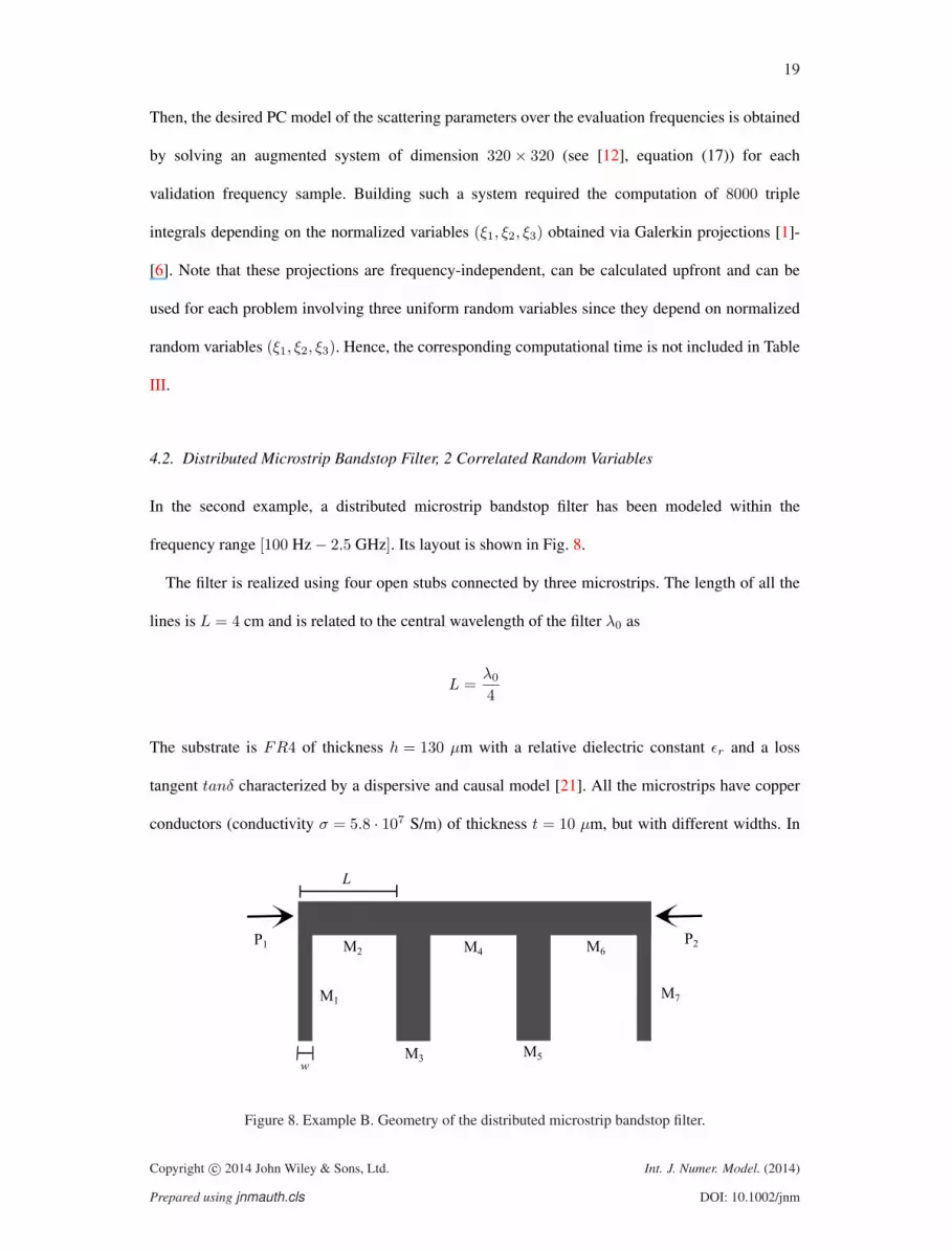
4.2. Distributed Microstrip Bandstop Filter, 2 Correlated Random Variables
In the second example, a distributed microstrip bandstop filter has been modeled within the
frequency range [100 Hz − 2.5 GHz]. Its layout is shown in Fig. 8.
The filter is realized using four open stubs connected by three microstrips. The length of all the
lines is L = 4 cm and is related to the central wavelength of the filter λ0 as
L =λ0
4
The substrate is FR4 of thickness h = 130 µm with a relative dielectric constant εr and a loss
tangent tanδ characterized by a dispersive and causal model [21]. All the microstrips have copper
conductors (conductivity σ = 5.8 · 107 S/m) of thickness t = 10 µm, but with different widths. In
M5 M3
M7 M1
M2 M4 M6
w
L
P1P2
Figure 8. Example B. Geometry of the distributed microstrip bandstop filter.
Copyright c© 2014 John Wiley & Sons, Ltd. Int. J. Numer. Model. (2014)
Prepared using jnmauth.cls DOI: 10.1002/jnm

20 D. SPINA ET AL.
particular the lines M2, M4 and M6 have a conductor of width w = 120 µm; for the lines M1 and
M7 the conductor width is w = 20 µm, while w = 160 µm for the lines M3 and M5.
The scattering parameters are considered as a stochastic process that depends on two correlated
random variables with Gaussian PDFs: the length L of the microstrip M2 and the width w of the
shunt M1. Assuming a worst case analysis, the correlation coefficient is chosen equal to ρ = 0.9
and, for both the random variables (L, w), the normalized standard deviation is ±5% with respect
to their nominal value, indicated in the following with the symbols L0 for the length and w0 for the
width. The corresponding correlation matrix is
C =
(L0σL)2 ρL0σLw0σw
ρL0σLw0σw (w0σw)2
where σL and σw represent the normalized standard deviations of the length and the width,
respectively. In this case C is positive-definite, hence the couple of random variables (L,w) follow
the non-degenerate multivariate normal distribution [22]
W~η =1
2πdet(C)12exp
(−1
2(~η − ~µ)T C−1 (~η − ~µ)
)(18)
where the symbol det(·) is used to represent the matrix determinant, while ~η = [L,w]T and
~µ = [L0, w0]T .
Applying the Karhunen-Loeve expansion [16], the scattering parameters can be considered as
a stochastic process with respect to the pair of uncorrelated Gaussian random variables with zero
mean and unit variance (ξ1, ξ2). In particular, the vector of correlated random variables ~η can be
expressed with respect to the vector of uncorrelated random variables ~ξ as
~η = ~µ + UΛ12 ~ξ (19)
where Λ is a diagonal matrix containing the eigenvalues of the correlation matrix C and U is the
matrix of the corresponding eigenvectors. See Appendix 6.1 for further details. Therefore, due to
the use of the Karhunen-Loeve expansion, it is possible to express the scattering parameters as
a stochastic process that depends on the pair of uncorrelated random variables ~ξ = [ξ1, ξ2]T and,
Copyright c© 2014 John Wiley & Sons, Ltd. Int. J. Numer. Model. (2014)
Prepared using jnmauth.cls DOI: 10.1002/jnm

21
since the variables ξ1 and ξ2 are Gaussian, they are also independent. Hence, the corresponding
basis functions are products of the Hermite polynomials [11], as shown in Table IV for M = 5 and
P = 2, while the probability measure (2) is
W (~ξ) =12π
exp(−1
2~ξT ~ξ
)(20)
The evaluation of the scattering parameters is performed using a quasi-analytical model [23] over
a regular grid composed of 81 samples for the frequency and 8 × 8 samples for the geometrical
parameters (L,w). Again, the number K of initial samples for the couple of geometrical parameters
is chosen according to the relation K ≈ 2 (M ′ + 1), considering a maximum order of expansion
P ′ = 6 and a corresponding number of basis functions M ′ = 27, according to (4). Next, the
frequency samples are divided in two groups: modeling points (41 samples) and validation points
(40 samples).
This second example represents a particular difficult structure to model since, as shown in Fig.
9, the random variables chosen have a high impact on the scattering parameters of the structure:
the range of the stop-band frequencies is influenced by the random variables chosen and in the
band-pass frequencies the magnitude of the element S11 has a high variability, often over −20 dB,
compromising the correct behavior of the filter.
Table IV. Hermite polynomials products for two independent random variables, with M = 5 and P = 2 [2]
index i i-th basis function ϕi < ϕi, ϕi >
0 1 1
1 ξ1 1
2 ξ2 1
3 ξ21 − 1 2
4 ξ1ξ2 1
5 ξ22 − 1 2
Copyright c© 2014 John Wiley & Sons, Ltd. Int. J. Numer. Model. (2014)
Prepared using jnmauth.cls DOI: 10.1002/jnm

22 D. SPINA ET AL.
0 0.5 1 1.5 2 2.5−70
−60
−50
−40
−30
−20
−10
0
Frequency [GHz]
|S11
| [dB
]
Figure 9. Example B. Variability of the magnitude of S11. The green thick line corresponds to the nominal
value for (L, w), while the blue lines are the results of the MC simulations performed using 10000 (L, w)
samples.
We note that, the variability analysis shown in this example cannot be performed with previous
developed techniques [1]-[4], even if the filter is realized using only microstrips. Indeed, the
techniques [1]-[4] employ a stochastic model of the per-unit-length parameters and the length of
a line cannot be assumed as parameter for the variability analysis.
The PC model of the scattering parameters for the modeling frequencies has order P = 5,
according to Algorithm 1, and M = 20, according to (4), while 0.01 is targeted as maximum error
(13) between the PC coefficients and the corresponding rational models. The obtained PC-based
model shows an excellent accuracy compared with the classical MC analysis in computing system
variability features, as shown in Figs. 10 - 12. In particular, Figs. 10 - 11 show the mean and the
standard deviation of the imaginary part of the element S12 for the validation frequencies computed
with the proposed method, a MC analysis with the similar computational cost (performed using 64
(L,w) samples) and a MC analysis performed using 10000 (L,w) samples. It is important to notice
that for this highly dynamic system the PC method offers a much higher accuracy in estimating
these statistical moments than the MC analysis with the similar computational cost. Finally, Fig. 12
Copyright c© 2014 John Wiley & Sons, Ltd. Int. J. Numer. Model. (2014)
Prepared using jnmauth.cls DOI: 10.1002/jnm

23
0 0.5 1 1.5 2 2.5−1
0
1
Frequency [GHz]µ(
Imag
(S12
))
0 0.5 1 1.5 2 2.50
0.05
0.1
Frequency [GHz]
Abs
olut
e E
rror
Figure 10. Example B. The top plot shows a comparison between the mean of the imaginary part of S12
obtained with the MC analysis performed using first 10000 (D1, D2, D3) samples (full black line), then
64 (D1, D2, D3) samples (dashed green line), and the proposed PC-based method (red circles: ()) for the
validation frequencies. The lower plot shows the corresponding absolute error.
describes the PDF and the CDF of S11 at the frequency of 281.25 MHz. Note that similar results
can be obtained for the other entries of the scattering matrix.
The proposed technique offers a great computational efficiency in addition to its accuracy; in
Table V the computational time needed for the MC analysis (performed on the validation frequencies
using 64 and 10000 (L,w) samples) and the proposed PC-based technique is reported. As in the
previous example, in Table V the computational time of the new PC-based technique is explicitly
divided into the time needed to calculate the initial samples and to build the polynomial model of
the scattering parameters (including the computational cost to build the PC-model of the scattering
parameters in the form (10) for all the orders P ≤ 6, as described by Algorithm 1) and evaluate it
on the validation frequencies.
As for the previous numerical example, the proposed technique is compared with respect to the
PC-based method presented in [12]. The comparison of the accuracy and efficiency of the two
PC-based techniques is performed using the same sampling for the geometrical parameters and
Copyright c© 2014 John Wiley & Sons, Ltd. Int. J. Numer. Model. (2014)
Prepared using jnmauth.cls DOI: 10.1002/jnm

24 D. SPINA ET AL.
0 0.5 1 1.5 2 2.50
0.2
0.4
Frequency [GHz]σ(
Imag
(S12
))
0 0.5 1 1.5 2 2.50
0.02
0.04
0.06
Frequency [GHz]
Abs
olut
e E
rror
Figure 11. Example B. The top plot shows a comparison between the standard deviation of the imaginary
part of S12 obtained with the MC analysis performed using first 10000 (D1, D2, D3) samples (full black
line), then 64 (D1, D2, D3) samples (dashed green line), and the proposed PC-based method (red circles:
()) for the validation frequencies. The lower plot shows the corresponding absolute error.
−50 −45 −40 −35 −30 −25 −20 −150
0.08
0.16
Magnitude S11
(freq= 281.25 MHz, L, w) [dB]
PD
F
−50 −45 −40 −35 −30 −25 −20 −150.0
0.2
0.4
0.6
0.8
1.0
−50 −45 −40 −35 −30 −25 −20 −150
0.2
0.4
0.6
0.8
1
CD
F
Figure 12. Example B. PDF and CDF of the magnitude of S11 at 281.25 MHz. Full black line: PDF computed
using the novel technique; Dashed black line: CDF computed using the novel technique; Circles (): PDF
computed using the MC technique; Squares (2): CDF computed using the MC technique.
Copyright c© 2014 John Wiley & Sons, Ltd. Int. J. Numer. Model. (2014)
Prepared using jnmauth.cls DOI: 10.1002/jnm

25
Table V. Example B. Efficiency of the Proposed PC-based Technique
Technique Computational time
Monte Carlo Analysis (10000 samples, validation frequencies) 7 h 36 min, 43.7 s
Monte Carlo Analysis (64 samples, validation frequencies) 2 min, 55.38 s
PC-based technique 3 min 32.82 s
Details PC-based technique Computational time
Initial simulations (64 samples, modeling frequencies) 3 min 1.36 s
PC model scattering parameters 31.46 s
frequency and adopting the same order of the expansion as for the proposed technique, leading to a
PC model of order P = 5 and M = 20 basis functions.
The state-space matrices are calculated using the VF algorithm, targeting −40 dB as maximum
absolute model error between the scattering parameters and the corresponding root macromodels
in order to estimate the required number of poles. As a result, 35 poles are used to compute the
root macromodels for all the 8 × 8 samples of the geometrical parameters (L,w). Note that trying
to impose a better accuracy ( < −40 dB) does not provide good results, since the VF state-space
matrices become nonsmooth as functions of the stochastic parameters.
Again, the proposed approach and the technique [12] have a similar accuracy in estimating the
filter variability features, as shown in Fig. 13, and both show a great efficiency with respect to the
MC analysis, as described in Tables V and VI.
Table VI. Example B. Efficiency of the PC-based Technique [12]
PC-based technique [12] Computational time
Initial simulations (64 samples, modeling frequencies) 3 min 1.36 s
PC model scattering parameters 1 min 30.76 s
Total computational time 4 min, 32.12 s
Copyright c© 2014 John Wiley & Sons, Ltd. Int. J. Numer. Model. (2014)
Prepared using jnmauth.cls DOI: 10.1002/jnm
26 D. SPINA ET AL.
0 0.5 1 1.5 2 2.5−1
0
1
Frequency [GHz]µ(
Rea
l(S11
))
0 0.5 1 1.5 2 2.50
2
4
6x 10
−3
Frequency [GHz]
Abs
olut
e E
rror
Figure 13. Example B. The top plot shows a comparison between the mean of the real part of S11 obtained
with the MC analysis performed using 10000 (L, w) samples (full black line), the technique [12] (dashed
magenta line), and the proposed PC-based method (red circles: ()) for the validation frequencies. The lower
plot shows the corresponding absolute error.
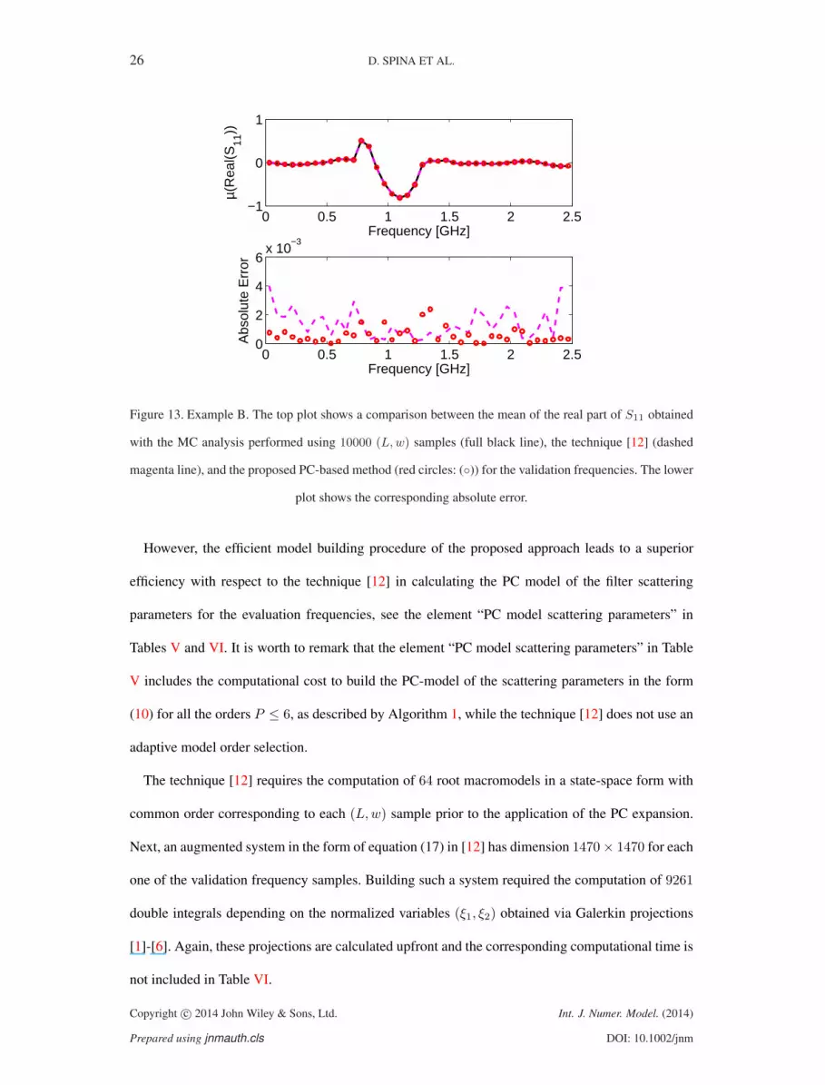
However, the efficient model building procedure of the proposed approach leads to a superior
efficiency with respect to the technique [12] in calculating the PC model of the filter scattering
parameters for the evaluation frequencies, see the element “PC model scattering parameters” in
Tables V and VI. It is worth to remark that the element “PC model scattering parameters” in Table
V includes the computational cost to build the PC-model of the scattering parameters in the form
(10) for all the orders P ≤ 6, as described by Algorithm 1, while the technique [12] does not use an
adaptive model order selection.
The technique [12] requires the computation of 64 root macromodels in a state-space form with
common order corresponding to each (L,w) sample prior to the application of the PC expansion.
Next, an augmented system in the form of equation (17) in [12] has dimension 1470 × 1470 for each
one of the validation frequency samples. Building such a system required the computation of 9261
double integrals depending on the normalized variables (ξ1, ξ2) obtained via Galerkin projections
[1]-[6]. Again, these projections are calculated upfront and the corresponding computational time is
not included in Table VI.
Copyright c© 2014 John Wiley & Sons, Ltd. Int. J. Numer. Model. (2014)
Prepared using jnmauth.cls DOI: 10.1002/jnm
27
5. CONCLUSIONS
In this paper, we present an innovative technique to calculate frequency-domain macromodels
for efficient variability analysis of general multiport systems. It is based on the use of the PC
expansion, applied at an input-output level, to describe the system variability features in combination
with rational identification in the frequency-domain. The presented technique is straightforward to
implement, it selects the PC expansion order automatically, and it can be applied to a large range of
microwave systems. Comparisons with the standard MC approach and with the PC-based technique
[12] are performed for two pertinent numerical examples, validating the accuracy and efficiency of
the proposed method.
6. APPENDIX
6.1. Karhunen-Loeve expansion and Correlated Gaussian Random Variables
If the correlation matrix CN×N is symmetric and positive-definite, then it has N orthogonal
eigenvectors [~ui]Ni=1, and can be diagonalized as
C = UΛUT (21)
where Λ is the diagonal matrix of the eigenvalues of C, the symbol T indicates the matrix transpose
and U is the orthogonal matrix defined as U = [~u1, . . . , ~uN ]. Using (21) in (18) leads to
W~η =1
2πdet(Λ)12exp
(−1
2(~η − ~µ)T UΛ−1UT (~η − ~µ)
)(22)
Therefore, for correlated Gaussian random variables that follow the non-degenerate multivariate
normal distribution (18), the Karhunen-Loeve expansion is a simple change of variables. The joint
probability density (22) can be written with respect to a vector of independent Gaussian random
variable ~x, with zero mean and variance equal to [Λii]Ni=1, as
W~x =1
2πdet(Λ)12exp
(−1
2~xT Λ−1~x
)(23)
where
~x = UT (~η − ~µ) (24)
Copyright c© 2014 John Wiley & Sons, Ltd. Int. J. Numer. Model. (2014)
Prepared using jnmauth.cls DOI: 10.1002/jnm

28 D. SPINA ET AL.
Next, the vector ~x can be expressed with respect to the vector of normalized Gaussian random
variables ~ξ with zero mean and unitary variance as
~x = Λ12 ~ξ (25)
Combining (24) and (25) leads to (19).
6.2. Passivity Verification of the PC-based Macromodel
The proposed technique does not guarantee the passivity of the frequency-domain macromodel in
the form (9). However, the passivity of the proposed macromodel can be verified, since the matrix
coefficients [αi(s)]Mi=0 in (9) are rational functions of the Laplace variable s. Hence, the coefficients
αi(s) can be written as transfer functions:
αi(s) = Ci (sIi − Ai)−1 Bi + Di
where Ii is the identity matrix with the same dimensions as the matrix Ai. The state space matrices
[Ai,Bi,Ci,Di]Mi=0 are obtained for each αi(s) by means of system identification techniques such
as VF. It should be noted that VF can enforce stability by pole flipping techniques.
Equation (9) can therefore be rewritten as
S(s, ~ξ) ≈M∑i=0
(Ci (sIi − Ai)
−1 Bi + Di
)ϕi(~ξ) (26)
Since (26) is a weighted sum of rational transfer functions, it is itself a rational transfer function,
i.e.,
S(s, ~ξ) ≈ C(sI − A
)−1
B(~ξ) + D(~ξ) (27)
Copyright c© 2014 John Wiley & Sons, Ltd. Int. J. Numer. Model. (2014)
Prepared using jnmauth.cls DOI: 10.1002/jnm

29
where
A = blockdiagonal (A0,A1, . . . ,AM )
B(~ξ) =
B0ϕ0(~ξ)
B1ϕ1(~ξ)
...
BMϕM (~ξ)
C =
[C0 C1 . . . CM
]D(~ξ) =
M∑i=0
Diϕi(~ξ)
Here blockdiagonal (·) represents the blockdiagonal matrix with blocks [Ai]Mi=0 on the main
diagonal and I is the identity matrix with the same dimensions as the matrix A.
The passivity of the macromodel (27), and of the corresponding form (9), can be assessed by
computing the following Hamiltonian matrix [24, 25] :A − B(~ξ)R(~ξ)D(~ξ)T C −B(~ξ)R(~ξ)B(~ξ)T
CT S(~ξ)C −AT + CT D(~ξ)R(~ξ)B(~ξ)T
(28)
where T stands for the matrix transpose and
R(~ξ) =(D(~ξ)T D(~ξ) − I
)−1
, S(~ξ) =(D(~ξ)D(~ξ)T − I
)−1
The transfer function S(s, ~ξ) is passive if and only if the Hamiltonian matrix (28) does not admit
purely imaginary eigenvalues. It is important to note that the Hamiltonian matrix (28) only depends
on the normalized random variables ~ξ. Therefore, it is always possible to identify a compact smooth
region Ξ ⊂ Ω where the macromodel (9) is passive, if the corresponding macromodel (27) is passive
for the values of ~ξ corresponding with the nominal values of the parameters under consideration, in
other words for the operating point.
Note that, the passivity region Ξ ⊂ Ω corresponds with all points ~ξ ∈ Ω where the Hamiltonian
matrix (28) does not admit purely imaginary eigenvalues. Equivalently, the passivity region Ξ ⊂ Ω
Copyright c© 2014 John Wiley & Sons, Ltd. Int. J. Numer. Model. (2014)
Prepared using jnmauth.cls DOI: 10.1002/jnm

30 D. SPINA ET AL.
can be found [26] by selecting the points ~ξ ∈ Ω where the H∞ norm ‖S(s, ~ξ)‖∞ ≤ 1.¶ Finally, if
one wants a parameter span or closed hyper-rectangle inside the passivity region Ξ, this can always
be obtained, since if a point (here the operating point) is in the interior of a smooth compact region
Ξ, then one can always find a closed hyper-rectangle inside Ξ containing that interior point.
REFERENCES
1. Manfredi P, Stievano IS, Canavero FG. Stochastic evaluation of parameters variability on a terminated signal bus.
EMC Europe 2011, York, UK, 2011; 362 –367.
2. Stievano IS, Manfredi P, Canavero FG. Parameters variability effects on multiconductor interconnects via Hermite
polynomial chaos. IEEE Trans. Compon., Packag., Manuf. Technol. Aug 2011; 1(8):1234–1239.
3. Stievano IS, Manfredi P, Canavero FG. Stochastic analysis of multiconductor cables and interconnects. IEEE Trans.
Electromagn. Compat. May 2011; 53(2):501–507.
4. Vande Ginste D, De Zutter D, Deschrijver D, Dhaene T, Manfredi P, Canavero F. Stochastic modeling-based
variability analysis of on-chip interconnects. IEEE Trans. Compon., Packag., Manuf. Technol. Jul 2012; 2(7):1182
–1192.
5. Su Q, Strunz K. Stochastic polynomial-chaos-based average modeling of power electronic systems. IEEE Trans.
Power Electron. Apr 2011; 26(4):1167 –1171.
6. Strunz K, Su Q. Stochastic formulation of SPICE-type electronic circuit simulation with polynomial chaos. ACM
Trans. Model. Comput. Simulation Sep 2008; 18(4):501–507.
7. Blatman G, Sudret B. An adaptive algorithm to build up sparse polynomial chaos expansions for stochastic finite
element analysis. Probabilistic Engineering Mechanics Apr 2010; 25(2):183 – 197.
8. Eldred MS. Recent advance in non-intrusive polynomial-chaos and stochastic collocation methods for uncertainty
analysis and design. Proc. 50th AIAA/ASME/ASCE/AHS/ASC Struct., Structural Dynam., Mat. Conf., AIAA-2009-
2274, Palm Springs, California, 2009.
9. Witteveen JAS and Bijl H. Modeling Arbitrary Uncertainties Using Gram-Schmidt Polynomial Chaos. Proc. 44th
AIAA Aerosp. Sci. Meeting and Exhibit, AIAA-2006-0896, Palm Springs, California, 2006.
10. Xiu D and Karniadakis GM. The Wiener-Askey polynomial chaos for stochastic differential equations. SIAM J.
Sci. Comput. Apr 2002; 24(2):619–644.
11. Soize C and Ghanem R. Physical systems with random uncertainties: Chaos representations with arbitrary
probability measure. SIAM J. SCI. COMPUT. Jul 2004; 26(2):395–410.
¶Note that this proves in fact that the passivity region Ξ is smooth and compact, since norms are continuous functions
of their argument and S(s, ~ξ) is by construction a continuous function of its arguments.
Copyright c© 2014 John Wiley & Sons, Ltd. Int. J. Numer. Model. (2014)
Prepared using jnmauth.cls DOI: 10.1002/jnm

31
12. Spina D, Ferranti F, Dhaene T, Knockaert L, Antonini G, Vande Ginste D. Variability analysis of multiport systems
via polynomial-chaos expansion. IEEE Trans. Microw. Theory Tech. Aug 2012; 60(8):2329 –2338.
13. Gustavsen B and Semlyen A. Rational approximation of frequency domain responses by vector fitting. IEEE Trans.
Power Del. Jul 1999; 14(3):1052–1061.
14. Deschrijver D, Mrozowski M, Dhaene T, and De Zutter D. Macromodeling of multiport systems using a fast
implementation of the vector fitting method. IEEE Microw. Wireless Compon. Lett. Jun 2008; 18(6):383–385.
15. Der Kiureghian A and Liu PL. Structural reliability under incomplete probability information,. J. Eng. Mech., ASCE
Jan 1986; 112(1):85–104.
16. Loeve M. Probability Theory. 4-th edn., Springer-Verlag: Berlin, Germany, 1977.
17. Papoulis A. Probability, Random Variables and Stochastic Processes. McGraw-Hill College: New York, 1991.
18. The RF and Microwave Handbook (Electrical Engineering Handbook). CRC Press, 2000.
19. Hosder S, Walters RW, Balch M. Efficient Sampling for Non-Intrusive Polynomial Chaos Applications with
Multiple Uncertain Input Variables. Proc. 48th AIAA/ASME/ASCE/AHS/ASC Struct., Structural Dynam., Mat.
Conf., AIAA-2007-1939, Honolulu, HI, 2007.
20. Ferranti F, Knockaert L, Dhaene T. Guaranteed passive parameterized admittance-based macromodeling. IEEE
Trans. Adv. Packag. Aug 2010; 33(3):623 –629.
21. Djordjevic AR, Biljic RM, Likar-Smiljanic VD, Sarkar TK. Wideband frequency-domain characterization of FR-4
and time-domain causality. IEEE Trans. Electromagn. Compat. Nov 2001; 43(4):662–667.
22. Bischoff W. Characterizing multivariate normal distributions by some of its conditionals. Statistics & Probability
Letters Feb 1996; 26(2):105 – 111.
23. Gupta KC, Garg R, Bahl I, and Bhartia P. Microstrip Lines and Slotlines. 2nd edn., Artech House, Inc., Norwood,
MA: Norwood, MA, 1996.
24. Knockaert L, Ferranti F, Dhaene T. Generalized eigenvalue passivity assessment of descriptor systems with
applications to symmetric and singular systems. International Journal of Numerical Modelling: Electronic
Networks, Devices and Fields January/February, 2013; 26(1):1–14.
25. Grivet-Talocia S, Ubolli A. Passivity enforcement with relative error control. IEEE Trans. Microw. Theory Tech.
Nov 2007; 55(11):2374 –2383.
26. Ferranti F, Knockaert L, Dhaene T. Passivity-preserving interpolation-based parameterized macromodeling of
scattered S-data. IEEE Microw. Wireless Compon. Lett. Mar 2010; 20(3):133 –135.
Copyright c© 2014 John Wiley & Sons, Ltd. Int. J. Numer. Model. (2014)
Prepared using jnmauth.cls DOI: 10.1002/jnm