Profits, Cycles and Chaos

by

Marc Jarsulic*

Working Paper No. 20

April 1989

Submitted to The Jerome Levy Economics Institute

Bard College

*Department of Economics, University of Notre Dame, Notre Dame, IN and The Jerome Levy Economics Institute, Bard College, Annandale-On-Hudson, NY.

1. INTRODUCTION

Some time ago Goodwin (1967) offered an elegant and

influential model to represent part of Marx's thinking on business

cycles. In that model he was able to show how the interaction of

the reserve army of labor and the process of capital accumulation

could produce self-sustaining oscillatory behavior. Increases in

the real wage cause decreases in the rate of growth of the capital

stock, since all wages are consumed and all profits invested. The

declining rate of accumulation in turn causes a decline in the

employment rate, which eventually causes the wage rate to decline.

The eventual expansion in the growth rate of the capital stock

begins the process over again. This behavior was described by

fitting a model of a one good economy into the Lotka-Volterra

equations, the solution to which is well known. While it has

proved extremely fruitful, this model also has some well known

limitations. It is first of all a center, so that no limit cycle

produced by the model is stable. Second, it takes a rather asocial

approach to the creation of the labor force, assuming that it is

governed exclusively by an exogenously given rate of population

growth. Also, the model assumes that all technical change occurs

at a constant, autonomously given rate, and allows for no induced

components.

In what follows some minor alterations to the Goodwin model

are shown to introduce interesting new behavior. By making

technical change depend on economic and social phenomena, and by

assuming that the labor force grows at least in part in response

to social phenomena, it is easy to show that the model will now

generate stable limit cycles. When the model is changed still

further, to allow for systematic periodic influences -- such as

those an economy might experience as a result of seasonal changes

in labor force participation or productivity -- somewhat more

dramatic dynamic behavior follows. Under certain conditions, the \

model ceases to be periodic and instead becomes chaotic. The

resulting behavior is more business-cycle-like because of it is

irregular. But at the same time the existence chaos implies

difficulties for empirical 88deseasonalization1t of data.

The possibility of chaos introduces some questions for the

study of business cycles. One is whether it is possible to

discriminate between economic phenomena which are induced by chaos-

generating non-linearities, and those which are introduced by

stochastic shocks to some underlying non-linear system. The model

is used to illustrate this problem and show how an existing

technique for testing for chaos -- the calculation of Lyapunov

exponents -- is able to handle it.

2. A MODIFIED GOODWIN CYCLE MODEL

the definitions

X =

Y =

a =

b =

C =

e =

The Goodwin growth cycle model is easy to represent. Given

the employment rate

labor's share in net output

the output/capital ratio, assumed fixed

the rate of growth of the labor force

the rate of growth of output per unit of labor

a threshold value of the employment rate

the model is given

Z/X = a-ay-b-c

G/y = x - e

Let us begin

representation of

(1)

to develop

labor force

characteristics of a capitalist

the model by first altering the

growth. One of the outstanding

economy, as Marx recognized, is its

ability to change social reality if the need for labor becomes

strong enough. It can do this by defining groups of workers in or

out of the labor force as convenient (e.g. the recognition of the

productive abilities of women during wartime, and the denial when

war ends); increasing immigration or emigration by changing laws

governing the treatment of aliens; and by destroying non-capitalist

economic formations over time. This point of view is part of

contemporary neo-marxian analysis as well. Marglin

(1984, PP. 108-9) notes that:

The labor force available to the capitalist sector expands (or contracts) according to demand. In the neo-Marxian view, a buoyant capitalism will meet its labor requirements much as the countries of northern and southern Europe did in the quarter century of expansion that followed World War II, first by drawing on the labor resources of family agriculture and other noncapitalist modes of production, then by drawing on the labor resources of an ever-widening geographical periphery that ultimately included the entire Mediterranean basin and beyond.

By the same token, a stagnant capitalism will simply fail to attract labor. In the extreme case of declining demand for labor, the labor force available to the capitalist sector will decline absolutely. In the place of the overt unemployment that characterizes stagnation in the neo-Keynesian view, neo-Marxian unemployment is characteristically "disguised unemploymentUV...

Now the implication of this point of view is that the dynamics

of labor supply are complex and historically specific. Hence any

attempt to model them must be a bit inadequate. However, we can

go -a little way toward including them in the Goodwin model by

replacing the constant b with the term

b, + b,x2 (2)

This slight alteration allows increasing employment rates to have

a negative impact on their own growth. It can be taken to stand

for the self-correcting behavior of capitalist economies in labor

SUPPlY-

Next we want to say something about technical change. Since

this is a subject about which knowledge is slim, it is hard to do

so with much confidence. However, the empirical work of Gordon

et al. (1985) suggests that wage rates and employment rates have,

respectively, positive and negative effects on productivity growth.

This is a consequence of their effect on the cost of job loss. The

higher the real wage, the more is lost when one is out of work.

And the greater the employment rate, the higher the probability

that a new job can be found. Hence we will replace the constant

c with the term

.

co + c,y - c2x (3)

The alterations suggested in (2) and (3) can be combined to

alter the expression for G/x. These changes, together with a

specification for the wage determination equation which is slightly

faster moving than the one in (l), allows us to rewrite the system

(1) as

G/x = a - by + cx - dx2 (4)

G/y = (1. - e/x)m m>O

The values of the coefficients of this system can be interpreted

in obvious ways.

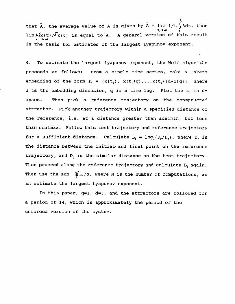
The dynamics of system (4) can be determined by well known

methods. The isoclines of the system are displayed in figure 1.

There are three fixed points in the figure, and the one of interest

to us is labeled A. The behavior of the system around point A can

be determined in part by looking at the Jacobian

(5)

The stability of A will depend on the value of Tr(J) evaluated at

A. Some calculation will show that given the parameters in (4),

the value of Tr(J) will pass from positive to negative as the .

vertical isocline is moved from the origin past the maximum value

of the G = 0 isocline. That is, the system changes from unstable

to stable as the $ = 0 isocline is moved from left to right. Now

by appealing to the Hopf bifurcation theorem (Guckenheimer and

Holmes, 1983, pp. 151-2), we know that this change in stability

implies the existence of a limit cycle about point A. The

amplitude of this cycle will increase as the value of Tr(J)

increases. What we do not know from the evaluation of (5) is the

nature of the limit cycle. It could be everywhere attractive

. (supercritical) or attractive from only one side (subcritical).

However, by evaluating an index (Liu et al., 1986) of the form

I = (v'C)-'[(B(F,,,+G,,,)+2D(F,,,+G,,)+C(F,,+G,))v'

+(DF,,+CF,,) (BF,,+X)F,,+CF,)

-(DG,+BG,,) (BG,,+2DG,,+CG,)

-B2F,,G,,- DB(FXyGXX+FXXGXY)

+C'F,G,+DC(F,,G,+F,G,,) I, (6)

where F(x,y) = G, G(x,y) = t, C = GX, D = F,, B = -F,, and v2 =

(BC-D)', it is possible to tell what is going on. When I > 0 the

limit cycle is subcritical, and when I c 0 it is supercritical.

Some calculation will show that I c 0 when Tr(J) > 0, so the limit

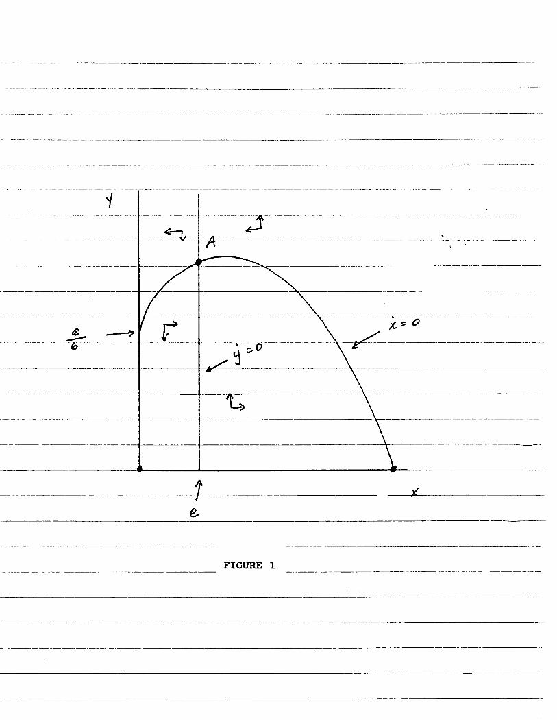
cycle is supercritical. The behavior of this system can of course

be simulated. A time series produced by such a simulation is

displayed in figure 2.

3.. PERIODIC TERMS AND DYNAMIC BEHAVIOR .

While it is instructive to know that the alterations in the

Goodwin model generate limit cycle behavior, we can get somewhat

more from it by acknowledging the existence of periodic forces

which act on the state variables of the system. For example, there

are undoubtedly many seasonalities in labor force participation

rates -- students move in and out of the labor force with

vacations: people seek temporary work over certain holidays -- and

in productivity growth -- weather changes and regular vacation

periods no doubt affect it. The interactions of these periodic

forces can generate complex effects.' We

impact by including a term in cos(wt) among

in the first equation in (4). For purposes

by redefining the constant a as

aO - a,cos(w t)

will summarize their

the existing constants

of exposition we do so

(7)

noting that this is not intended to represent a fluctuating capital

output ratio. The effects of this change in (4) can be seen

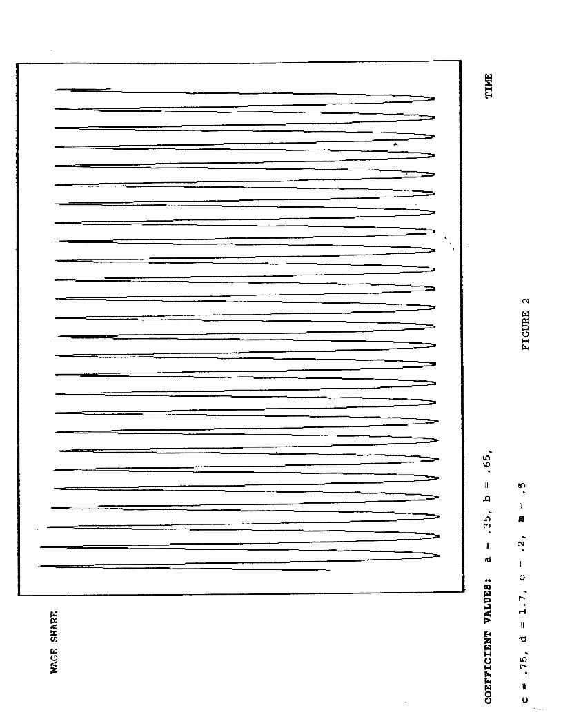
through simulation. The outcomes are dependent on the values of

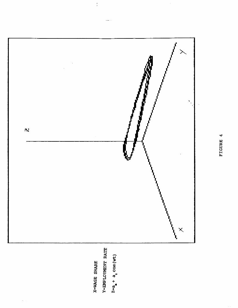
the three constants in (7). For the values a,=.35, a,=.07, w=.4,

with all other coefficients the same as those which obtain for the

simulation displayed in figure 2, the time series produced are

still periodic, as can be seen from figure 3. The behavior is now

more complex than it was, since the system is now three

dimensional. The three dimensional plot of the system in.figure

4 shows that it exhibits motion on a torus. This is not the end

of the possible behavior for this system, however. It is well

known (Thompson and Stewart, 1985, pp. 84-107) that the addition

of forcing terms to dynamical systems can sometimes induce chaotic

behavior. Indeed, Inoue and Kamifukumoto (1984) have shown that

a differently modified version of the Lotka-Volterra equations can

produce chaos with forcing if the frequency of the forcing term has

particular values. In their model, the unforced system has an

angular frequency of 2.3. By adding the forcing term and

simulating while varying the angular frequency of forcing over the

interval [2,5, 4.01, they were able to locate subintervals where

chaos appears. Although system (4) is different from that used by

Inoue and Kamifukumoto, some of the dynamic properties appear

similar. Notably, for

generate chaos in their

some of the values of rc[2.5,4.0] which

system, values of w satisfying w/14 = r/2.3

will generate apparently aperiodic behavior in (4). However, the

intervals containing the parameter values in which chaos exists are

narrower than in their system.2

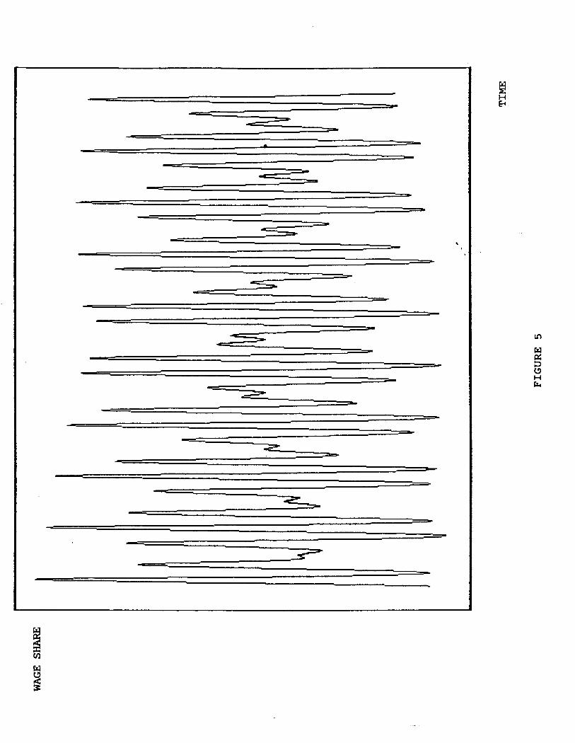
When, for example, the value of w is increased to .594,

behavior of the system appears to become aperiodic. A time series

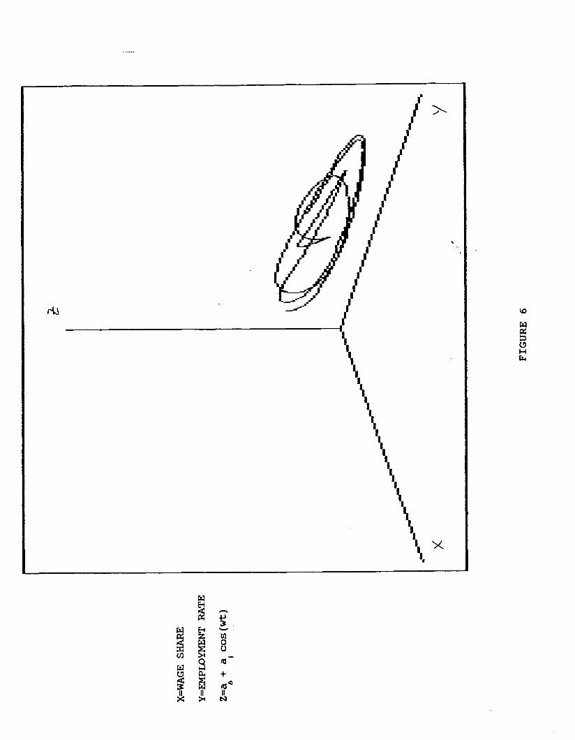
for this altered system is displayed in figure 5. The three

dimensional portrait of the system is given in figure 6. It is

significantly distorted from the nicely behaved torus, and appears

folded and stretched as the Lorenz and Rgssler attractors do. It

certainly looks

Appearance

"chaotic I1 .

can be deceiving, of course, and we need to do more

to establish the chaotic nature of this attractor. Short of a

proof, which does not offer itself at the moment, there are some

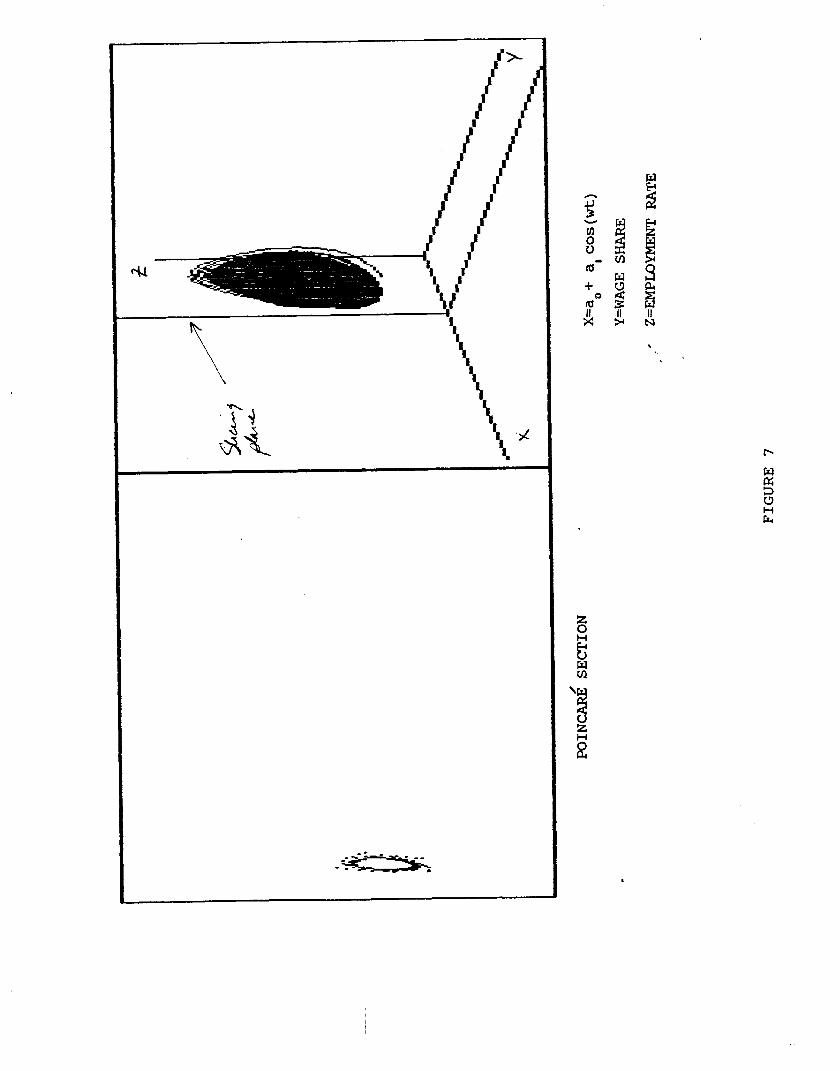
techniques which can be used. One is to construct a Poincare/

section for the attractor, and to look for the folding behavior in

the section. A Poincaresection for system, constructed by holding

the value of expression (7) constant at .4, and then recording the

first intersection with that plane on each orbit of the attractor,

is shown in figure 7. It has a folded structure, and as such is

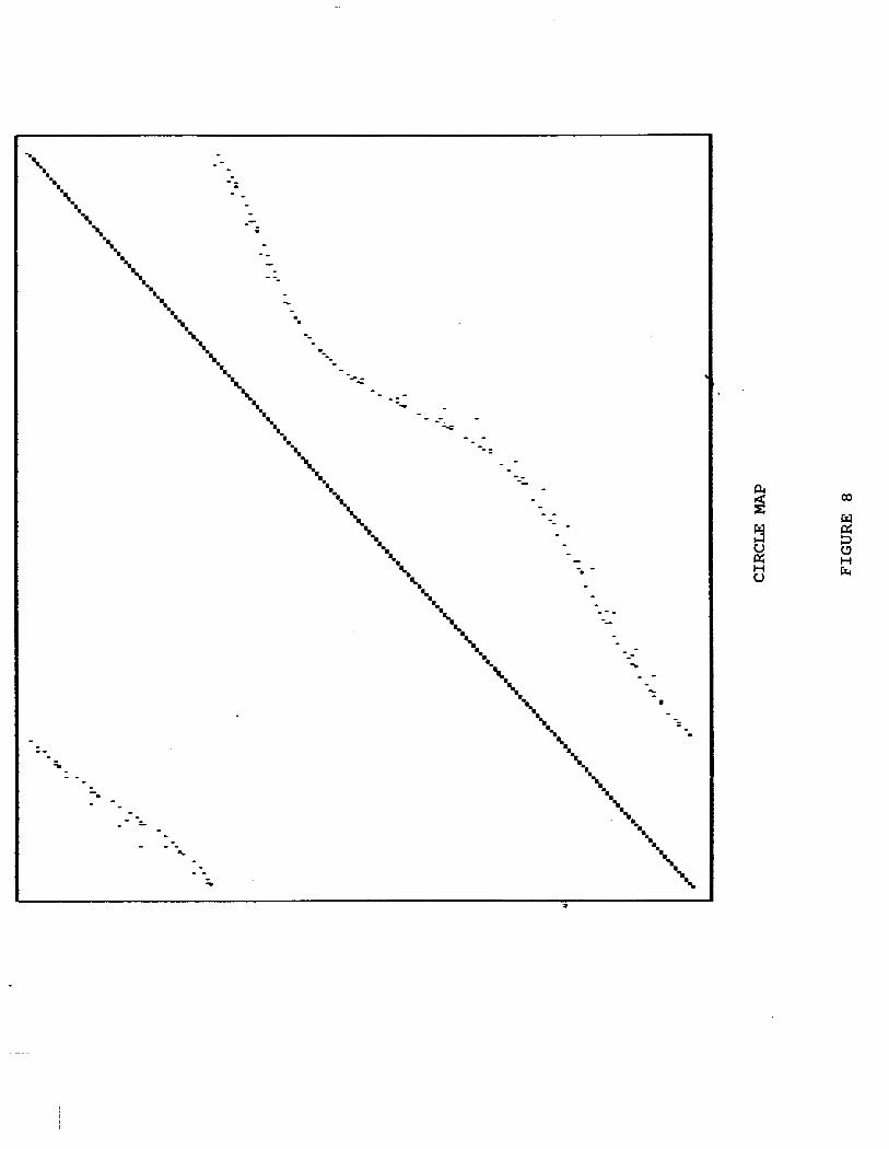
consistent with chaos. The Poincare map can also be used to

construct a circle map. The the angles each point on he map,

relative to an appropriately selected center, are calculated. Each

angle z(t) is plotted against the previously calculated angle z(t-

1) l This plot is the circle map. For a non-chaotic system, the

plots suggest monotonicity and continuity. For chaotic systems,

continuity and monotonicity break down. The circle map for the

system with w = .594 is given in figure 8. The map has the broken

appearance exhibited by maps of chaotic systems. This may be taken

as another indication that we have chaos.

As another test of the nature of this attractor, we will

estimate the largest Lyapunov exponent using one of the time series

generated by the simulation. Lyapunov exponents can be considered

.generalized eigenvalues. When looking at a difficult-to-solve

system of ordinary differential equations at a fixed point, the

local dynamics can be derived by linearizing the system and then

calculating the eigenvalues of the Jacobian. (This is what was

behind the consideration of (5).) This procedure is generalized

over an entire attractor to produce . time-varying quantities which

describe the dynamic behavior of state variables. To illustrate, \

consider at three dimensional system of ordinary differential

equations

X(t) = (G&8) (8)

and denote its flow, i.e. the solution of X(t) from an initial

vector (xi,yi,zi) , as fi(t) . Now the difference in flows for any

two points can be written as

<f(t) = f,(t) - fz(t) (9)

where 6, 1s the first difference operator. To actually know the

value of (9) requires solving (8), but by linearization we have

gf;t) =[dX(t)/df(t)](6f(O)) (10)

where dX(t)/df(t) is evaluated with changing local coordinates.

The Lyapunov exponents are calculated by manipulating dX(t)/df(t)

in ways analogous to those used to extract eigenvalues from a

constant matrix. However, since the elements of X(t) vary with

time, it is necessary to look for an average value over the

attractor.3 For a chaotic attractor, the largest exponent will

be positive. This makes sense if nearby points are to diverge --

if there is to be sensitive dependence on initial conditions.

Now to obtain an estimate of the largest exponent for an

attractor, one can use a technique developed by Wolf (1985). It

requires taking a time series for one of the variab;les and \.

performing a Takens reconstruction of the the attractor. The

largest Lyapunov exponent is then calculated by following nearby

trajectories around the attractor. For system (4) with forcing, the

exponent, estimated from a time series of 20,000 observations on

the wage share is .03. This is consistent with chaos. m This value,

it should be noted, is dependent on the way one chooses to follow

the trajectories around the attractor.4

4. DISTINGUISHING CHAOTIC FROM STOCRASTIC SYSTEMS

Since any actual economic data may contain stochastic

elements, it is useful to ask whether the techniques used to test

for chaos can distinguish between a deterministic system subject

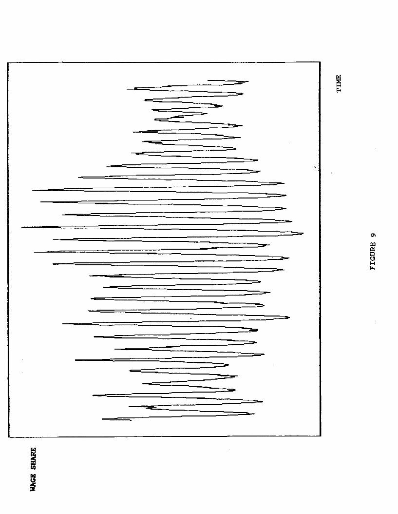
to shocks and a chaotic one. To look at this issue in the the

context of the present model, the system was simulated with no

forcing term, but with all state variables subject to a random

shock every ten iterations. The shocks were uniformly distributed,

with a maximum absolute value of .07. A time series for this

system is displayed in figure 9. It looks appropriately disturbed.

These data were also transformed and the Lyapunov exponent

calculated. These data were analyzed in the same way as those for

the chaotic attractor. The estimated Lyapunov exponent was .1672.

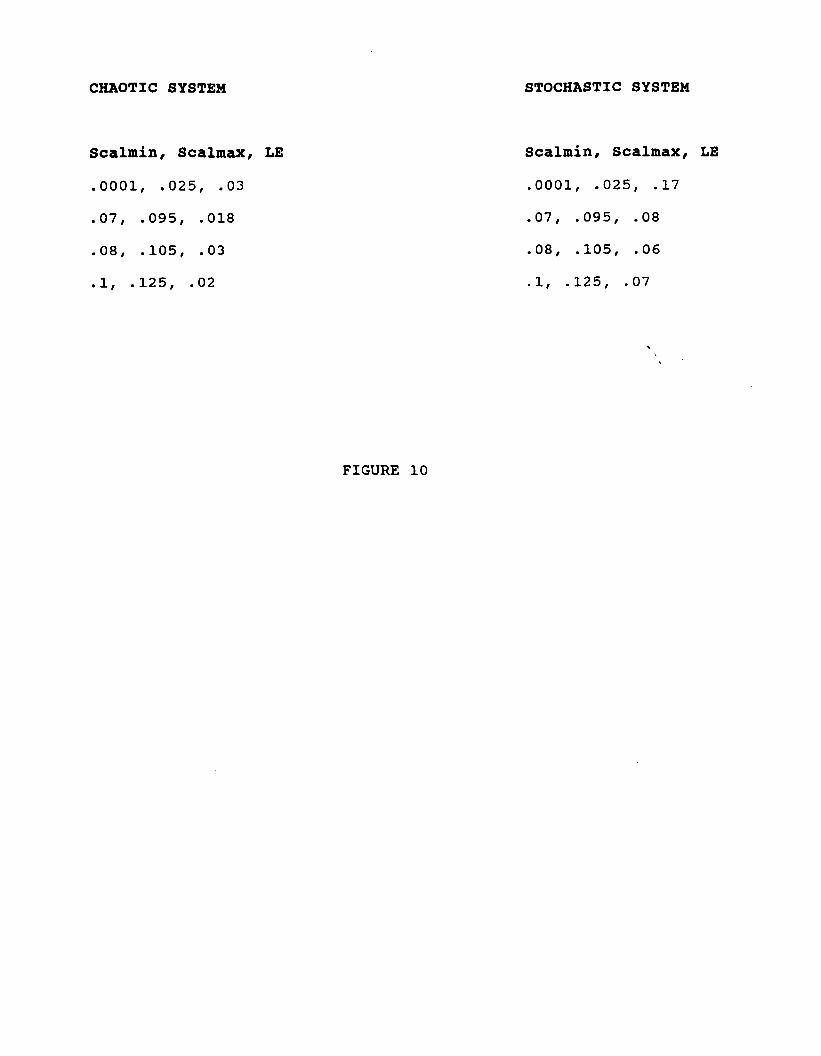
This is not enormously encouraging. However, it has been suggested

that the effects of noise can be reduced by changing the way in

which trajectories are followed around the reconstructed attractor.

By increasing the minimum distance between trajectories being

followed from some initial point, overestimates of the exponent are \

less likely. The results of varying this distance are shown in

figure 10. As the minimum distance (scalmin) is increased, the

estimated exponent for the stochastic system falls, but not

consistently. For the chaotic attractor, the exponent is sometimes

reduced, but not always. Discerning something from these patterns

as an empirical economist would clearly be a trying experience.

5. CONCLUSIONS

By making some relatively minor alterations to the Goodwin

growth cycle model, it has been possible to extend its economic

reach. The phenomenon of self-sustaining growth cycles was shown

to be compatible with endogenously determined technical change and

a self-correcting labor supply process. Both these modifications

are part of the current neo-marxian economic analysis. After

integrating these ideas into the model, its dynamic possibilities

can be expanded still more by adding consideration of

seasonalities. Along with stable limit cycles, such a system can

produce the irregularites of chaotic dynamics.

The time series from the chaotic version of the model look a

bit more like the time series which we actually observe in a real

economy. Since they are constructed by introducing interaction

among periodicities, they have an interesting implication for the

classic problem of "deseasonalizingtt time series data.

Deseasonalization is an attempt to clean up observations by

identifying and removing the periodic blips that clutter them.

However, even if the intuition of an underlying seasona4ity is

correct, cleaning up the data may be an,impossible task. This will

be so if the interaction of the underlying regularities produces

chaotic outcomes.

The simulations

another problem for

in distinguishing

of the model are also useful in illustrating

empirical economics. They show a difficulty

between data produced by chaotic and

stochastically perturbed non-linear systems. Lyapunov exponents

from chaotic and stochastic versions of this model are close, even

when appropriate adjustments are made in the estimating procedure.

Sorting out one from the other will clearly require the use of

other measurement techniques, such as the correlation integral.

Berg;, P., Pomeau, Y. and Vidal, C. 1984. Order within Chaos.

New York: J. Wiley and Sons.

Goodwin, R. 1967. A Growth Cycle. In C. Feinstien (ed),

Socialism, Capitalism and Economic Growth. Cambridge:

Cambridge University Press. \ I

Gordon, D., Weisskopf, T., and Bowles, S. 1985. Hearts and

Minds. Brookinss Paners, No. 1.

Grassberger, P. and Procaccia, I. 1984. Dimensions and Entropies

of Strange Attractors from a Fluctuating Dynamics Approach.

Phvsica D, 13, pp. 34-54.

Guckenheimer, J. and Holmes, P. 1983. Nonlinear Oscillations,

Dvnamical Systems. and Bifurcations of Vector Fields. New

York: Springer Verlag.

Inoue, M. and Kamifukumoto, H. 1984. Scenarios Leading To Chaos

In A Forced Lotka-Volterra Model. Proaress Of Theoretical

Physics. 71: 930-37.

Liu, W., Levin, S. and Yoh, I. 1986. Influence of Nonlinear

Incidence Rates Upon The Behavior of SIRS Epidemiological

Models. Journal Of Mathematical Biolosv. 23: 187-204.

Marglin, S. 1984. Growth, Distribution and Prices. Cambridge,

MA: Harvard University Press.

Thompson, J. and Stewart, H. 1986. Nonlinear Dvnamics and Chaos.

New York: J. Wiley and Sons.

Wolf, A. 1986

A.V. Holden

Press, pp.

Quantifying Chaos with Lyapunov Exponents: In:

(ed) I Chaos. Manchester: Manchester University

273-90.

FOOTNOTES

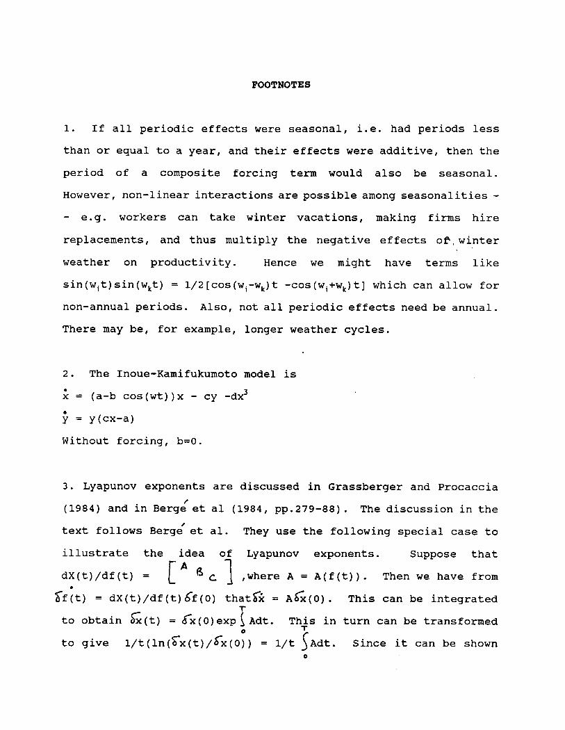
1. If all periodic effects were seasonal, i.e. had periods less

than or equal to a year, and their effects were additive, then the

period of a composite forcing term would also be seasonal.

However, non-linear interactions are possible among seasonalities -

- e.g. workers can take winter vacations,

replacements, and thus multiply the negative

weather on productivity. Hence we might

making firms hire

effects of,winter b

have terms like

sin(wit)sin(w,t) = 1/2[cos(wi-w,)t -cos(wi+w,)t] which can allow for

non-annual periods. Also, not all periodic effects need be annual.

There may be, for example, longer weather cycles.

2. The Inoue-Kamifukumoto model is

& (a-b cos(wt))x - cy -dx3

; = y(cx-a)

Without forcing, b=O.

3. Lyapunov exponents

(1984) and in Bergeet

text follows Berg& et

illustrate the idea

dX(t)/df(t) = c A(3

.

are discussed in Grassberger and Procaccia

al (1984, pp.279-88). The discussion in the

al. They use the following special case to

of

1

Lyapunov exponents. Suppose that

C ,where A = A(f(t)). Then we have from

6f(t) = dX(t)/df(t)bf(O) that6 = A&(O). This can be integrated l-

to obtain G(t) = dx(O)exp{Adt. Th+s in turn can be transformed

to give l/t(ln(bx(t)/bx(O;) = l/t 5 Adt. Since it can be shown 0

T

that xi, the average value of A is given by i = lim l/t (Adt, then *+a

limMc(t)/~x(o) is equal to Z. A general version of this result f*fi

is the basis for estimates of the largest Lyapunov exponent.

4. To estimate the largest Lyapunov exponent, the Wolf algorithm

proceeds as follows: From a single time series, make a Takens

embedding of the form zi = (x(ti), X(ti+q),...X(ti+(d-l)q)), where

d is the embedding dimension, q is a time lag. Plot the zi in d-

space. Then pick a reference trajectory on the constructed \

attractor. Pick another trajectory within a specified distance of

the reference, i.e. at a distance greater than scalmin, but less

than scalmax. Follow this test trajectory and reference trajectory

for a sufficient distance. Calculate Li = log,(D,/D,), where D, is

the distance between the initiaL and final point on the reference

trajectory, and D, is the similar distance on the test trajectory.

Then proceed along the reference trajectory and calculate Li again.

Then use the sum sLi/N, i

where N is the number of computations, as

an estimate the largest Lyapunov exponent.

In this paper, q=l, d=3, and the attractors are followed for

a period of 14, which is approximately the period of the

unforced version of the system.

-. ___-__ _____________.____.--

_____ ~_______________ ----____ _____~_

~- __- ___- ___---

___.~_~__._____.___~~.~_._ ---__._

4 -c3 _--- ----._- *_--

?_.

___.____

f r ______

r- -~--- _A- _-.________

\

$

-- .----

--.

__ ._ .-__.. _. _

- \

f ---L----

e .-- --~ --._

FIGURE 1 - ___- ___~.____ __~__.~_.____

--

--

Y

Y E

sa

CHAOTIC SYSTEM

Scalmin, Scalmax, LE

. 0001, .025, .03

. 07, .095, .018

. 08, .105, .03

. 1, ,125, .02

STOCHASTIC SYSTEM

Scalmin, Scalmax, LE

. 0001, .025, .17

. 07, .095, .08

.08, .105, .06

. 1, .125, .07

FIGURE 10