Run-time System for an Extensible Embedded Processor with Dynamic Instruction Set Lars Bauer, Muhammad Shafique, Stephanie Kreutz, Jörg Henkel

University of Karlsruhe, CES − Chair for Embedded Systems, Karlsruhe, Germany {lars.bauer, shafique, henkel} @ informatik.uni-karlsruhe.de

Abstract

One of the upcoming challenges in embedded processing is to in-corporate an increasing amount of adaptivity in order to respond to the multifarious constraints induced by today’s embedded sys-tems that feature complex and diverse application behaviors.

We present a novel concept (evaluated with a hardware proto-type) that moves traditional design-time jobs to run time in order to increase efficiency (in this paper we focus on performance). Adaptivity is achieved dynamically through what we call Special Instructions (SIs) which may change during run time according to non-predictable application behavior. The new contribution of this paper is the principal component that actually makes the en-tire embedded processor work efficiently, namely the “Special In-struction Scheduler”. It determines during run time ‘when’ and ‘how’ Special Instructions are composed and executed.

We achieve a 2.38x performance increase over a reconfigura-ble processor system with dynamic instruction set (Molen [19]). Our whole platform consists of a toolchain including estimation and simulation tools plus a running hardware prototype. Throughout this paper, we discuss the functionality by means of an H.264 video encoder in detail even though the concept is not limited to this application.

1. Introduction and motivation Embedded processors are key components for rapidly growing application fields ranging from automotive to personal mobile communication/entertainment etc. ASIPs (Application Specific Instruction Set Processors) have proven to be very efficient in terms of performance per chip area, performance per power con-sumption etc. However, today’s landscape of embedded applica-tions is rapidly changing as we see more complex functionalities, which makes it increasingly difficult to estimate a system’s beha-vior sufficiently accurate at design time.

In fact, after extensive exploration of complex real world em-bedded applications, we have found that it is hard or even im-possible to predict the performance and other design criteria ac-curately during design time. Consequently, the more critical de-sign decisions are fixed during design time, the less flexible an embedded processor can react to non-predictable application be-haviors. Hence, the embedded processor performs the lesser effi-cient, the more complex the application is.

We have analyzed state-of-the-art embedded processors and encountered a problem of inefficient utilization of hardware re-sources. We will illustrate this problem by means of an ITU-T H.264 video encoder [8]. During the execution, the processing flow migrates from one computational hot spot to another, i.e. from “Motion Estimation” (ME) to “Encoding Engine” (EE) to “Loop Filter” (LF) and back to ME. This movement demands a switch from one set of custom instructions to another, since the requirements within these hot spots are different.

State-of-the-art ASIPs typically provide dedicated hardware (e.g. in form of Special Instructions (SIs)) to efficiently address hot spots. However, when many diverse hot spots are addressed it means that many SIs need to be provided. Hence, a significant hardware overhead is the result. According our studies with truly large and inherently diverse applications, the necessary overhead can easily grow twice the size of the original processor core. Since often only one hot spot is executed at a certain time, the major hardware resources reserved for other hot spots are idling. This indicates an inefficiency that is an implication of the extens-

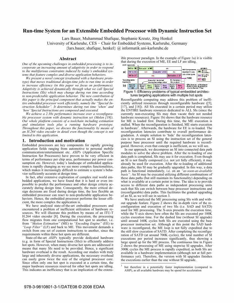
ible processor paradigm. In the example of Figure 1a) it is visible that during the execution of ME, EE and LF are idling.

Figure 1: Efficiency problems of typical embedded architec-

tures targeting applications with multiple hot spots Reconfigurable computing may address this problem of ineffi-ciently utilized resources through reconfigurable hardware ([5], [17], and [18]). All SIs executed in a certain period may utilize the ENTIRE hardware resources dedicated to ALL SIs (since the currently non-executing SIs may then vacate their not needed hardware resources). Figure 1b) shows that the hardware resource for ME is loaded first. During this time, the ME execution is stalled. When the reconfiguration is finished, ME starts execution in hardware1. Afterwards, the hardware for EE is re-loaded. The reconfiguration latencies contribute to overall performance de-gradation. A simple solution to ‘hide’ the reconfiguration laten-cies is to process an SI using the instruction set of the general purpose base processor until the required hardware is reconfi-gured. However, even that concept is inefficient, as we will see.

In our approach, we decompose an SI into connected data path modules to solve the above problem. After the re-loading of one data path is completed, SIs may use it for execution. Even though an SI is not finally composed (i.e. not yet fully efficient), it may already be used for execution. After the re-loading of additional data paths, this SI may be gradually upgraded. In this way, a data path is functional immediately, i.e. on an “as-soon-as-available basis”. An SI may be executed utilizing different combinations of these data paths (but still maintain its functionality) depending on what is available at a certain point in time. The idea is to provide access to different data paths as independent processing units such that SIs can switch between base processor instructions and (reconfigurable) data paths. This facilitates the gradual upgrading of an SI, as we will see in section 3.

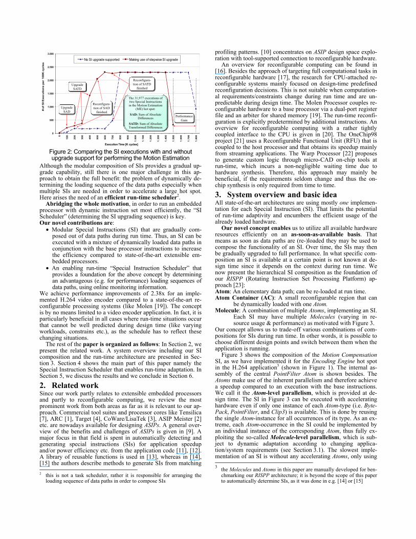
We have analyzed the ME processing using SIs with and with-out upgrade feature. Figure 2 shows the in-depth view of the re-configuration and execution of two SIs (i.e. SAD and SATD) used for ME processing. The X-axis presents the execution time, while the Y-axis shows how often the SIs are executed per 100K cycles execution time. For the dashed line (without SI upgrade) until around 160K cycles both SIs are executed using the base processor instruction set. Although at this point the SAD hard-ware is reconfigured, the ME loop is not fully expedited due to the still slow execution of SATD. After completing the reconfigu-ration of SATD (at around 700K cycles), the total number of SI executions per period increases significantly, thus showing a large speed up for the ME process. The continuous line in Figure 2 shows the processing of ME using stepwise SI upgrades. After 300K cycles the ME process is rapidly expedited, as both SIs are available in a hardware implementation (although not at full per-formance yet). Therefore, the version with SI upgrades finishes the executions earlier than the one without SI upgrade. 1 but therefore in a potentially faster implementation (compared to

ASIP), as all available hardware may be spend for acceleration

978-3-9810801-3-1/DATE08 © 2008 EDAA

0

500

1.000

1.500

2.000

2.500

3.000

0

100

200

300

400

500

600

700

800

900

1.00

0

1.10

0

1.20

0

1.30

0

1.40

0

1.50

0

1.60

0

1.70

0

1.80

0

# o

f SI E

xecu

tion

s pe

r 10

0K c

ycle

s

Execution Time [K cycles]

No SI upgrade supported Making use of stepwise SI upgrade

Reconfigura-tion of SATD

finished

Performance Gain

Reconfigura-tion of SAD

finished

Upgrade SATD

Upgrade SAD

The 31,977 executions oftwo Special Instructionsin the Motion Estimation

(ME) hot spot:

SAD: Sum of Absolute Differences

SATD: Sum of Absolute Transformed Differences

Figure 2: Comparing the SI executions with and without upgrade support for performing the Motion Estimation

Although the modular composition of SIs provides a gradual up-grade capability, still there is one major challenge in this ap-proach to obtain the full benefit: the problem of dynamically de-termining the loading sequence of the data paths especially when multiple SIs are needed in order to accelerate a large hot spot. Here arises the need of an efficient run-time scheduler2.

Abridging the whole motivation, in order to run an embedded processor with dynamic instruction set most efficiently, the “SI Scheduler” (determining the SI upgrading sequence) is key. Our novel contributions are:

• Modular Special Instructions (SI) that are gradually com-posed out of data paths during run time. Thus, an SI can be executed with a mixture of dynamically loaded data paths in conjunction with the base processor instructions to increase the efficiency compared to state-of-the-art extensible em-bedded processors.

• An enabling run-time “Special Instruction Scheduler” that provides a foundation for the above concept by determining an advantageous (e.g. for performance) loading sequences of data paths, using online monitoring information.

We achieve performance improvements of 2.38x for an imple-mented H.264 video encoder compared to a state-of-the-art re-configurable processing systems (like Molen [19]). The concept is by no means limited to a video encoder application. In fact, it is particularly beneficial in all cases where run-time situations occur that cannot be well predicted during design time (like varying workloads, constrains etc.), as the schedule has to reflect these changing situations.

The rest of the paper is organized as follows: In Section 2, we present the related work. A system overview including our SI composition and the run-time architecture are presented in Sec-tion 3. Section 4 shows the main part of this paper namely the Special Instruction Scheduler that enables run-time adaptation. In Section 5, we discuss the results and we conclude in Section 6.

2. Related work Since our work partly relates to extensible embedded processors and partly to reconfigurable computing, we review the most prominent work from both areas as far as it is relevant to our ap-proach. Commercial tool suites and processor cores like Tensilica [7], ARC [1], Target [4], CoWare/LisaTek [3], ASIP Meister [2] etc. are nowadays available for designing ASIPs. A general over-view of the benefits and challenges of ASIPs is given in [9]. A major focus in that field is spent in automatically detecting and generating special instructions (SIs) for application speedup and/or power efficiency etc. from the application code [11], [12]. A library of reusable functions is used in [13], whereas in [14], [15] the authors describe methods to generate SIs from matching 2 this is not a task scheduler, rather it is responsible for arranging the

loading sequence of data paths in order to compose SIs

profiling patterns. [10] concentrates on ASIP design space explo-ration with tool-supported connection to reconfigurable hardware.

An overview for reconfigurable computing can be found in [16]. Besides the approach of targeting full computational tasks in reconfigurable hardware [17], the research for CPU-attached re-configurable systems mainly focused on design-time predefined reconfiguration decisions. This is not suitable when computation-al requirements/constraints change during run time and are un-predictable during design time. The Molen Processor couples re-configurable hardware to a base processor via a dual-port register file and an arbiter for shared memory [19]. The run-time reconfi-guration is explicitly predetermined by additional instructions. An overview for reconfigurable computing with a rather tightly coupled interface to the CPU is given in [20]. The OneChip98 project [21] uses a Reconfigurable Functional Unit (RFU) that is coupled to the host processor and that obtains its speedup mainly from streaming applications. The Warp Processor [22] proposes to generate custom logic through micro-CAD on-chip tools at run-time, which incurs a non-negligible waiting time due to hardware synthesis. Therefore, this approach may mainly be beneficial, if the requirements seldom change and thus the on-chip synthesis is only required from time to time.

3. System overview and basic idea All state-of-the-art architectures are using mostly one implemen-tation for each Special Instruction (SI). That limits the potential of run-time adaptivity and encumbers the efficient usage of the already loaded hardware.

Our novel concept enables us to utilize all available hardware resources efficiently on an as-soon-as-available basis. That means as soon as data paths are (re-)loaded they may be used to compose the functionality of an SI. Over time, the SIs may then be gradually upgraded to full performance. In what specific com-position an SI is available at a certain point is not known at de-sign time since it depends on the context during run time. We now present the hierarchical SI composition as the foundation of our RISPP (Rotating Instruction Set Processing Platform) ap-proach [23]: Atom: An elementary data path; can be re-loaded at run time. Atom Container (AC): A small reconfigurable region that can

be dynamically loaded with one Atom. Molecule: A combination of multiple Atoms, implementing an SI.

Each SI may have multiple Molecules (varying in re-source usage & performance) as motivated with Figure 3.

Our concept allows us to trade-off various combinations of com-positions for SIs during run time. In other words, it is possible to choose different design points and switch between them when the application is running.

Figure 3 shows the composition of the Motion Compensation SI, as we have implemented it for the Encoding Engine hot spot in the H.264 application3 (shown in Figure 1). The internal as-sembly of the central PointFilter Atom is shown besides. The Atoms make use of the inherent parallelism and therefore achieve a speedup compared to an execution with the base instructions. We call it the Atom-level parallelism, which is provided at de-sign time. The SI in Figure 3 can be executed with accelerating hardware even if only one instance of each Atom-type (i.e. Byte-Pack, PointFilter, and Clip3) is available. This is done by reusing the single Atom-instance for all occurrences of its type. As an ex-treme, each Atom-occurrence in the SI could be implemented by an individual instance of the corresponding Atom, thus fully ex-ploiting the so-called Molecule-level parallelism, which is sub-ject to dynamic adaptation according to changing applica-tion/system requirements (see Section 3.1). The slowest imple-mentation of an SI is without any accelerating Atoms, only using 3 the Molecules and Atoms in this paper are manually developed for ben-

chmarking our RISPP architecture; it is beyond the scope of this paper to automatically determine SIs, as it was done in e.g. [14] or [15]

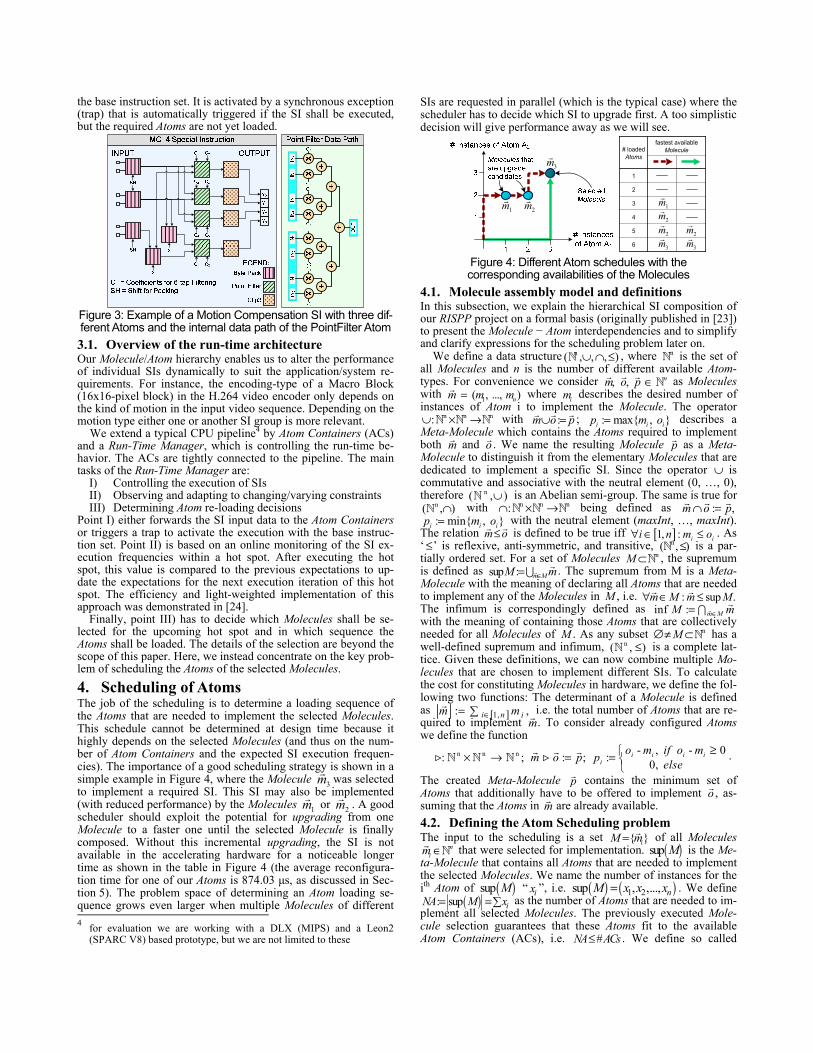
the base instruction set. It is activated by a synchronous exception (trap) that is automatically triggered if the SI shall be executed, but the required Atoms are not yet loaded.

Figure 3: Example of a Motion Compensation SI with three dif-ferent Atoms and the internal data path of the PointFilter Atom 3.1. Overview of the run-time architecture Our Molecule/Atom hierarchy enables us to alter the performance of individual SIs dynamically to suit the application/system re-quirements. For instance, the encoding-type of a Macro Block (16x16-pixel block) in the H.264 video encoder only depends on the kind of motion in the input video sequence. Depending on the motion type either one or another SI group is more relevant.

We extend a typical CPU pipeline4 by Atom Containers (ACs) and a Run-Time Manager, which is controlling the run-time be-havior. The ACs are tightly connected to the pipeline. The main tasks of the Run-Time Manager are:

I) Controlling the execution of SIs II) Observing and adapting to changing/varying constraints III) Determining Atom re-loading decisions

Point I) either forwards the SI input data to the Atom Containers or triggers a trap to activate the execution with the base instruc-tion set. Point II) is based on an online monitoring of the SI ex-ecution frequencies within a hot spot. After executing the hot spot, this value is compared to the previous expectations to up-date the expectations for the next execution iteration of this hot spot. The efficiency and light-weighted implementation of this approach was demonstrated in [24].

Finally, point III) has to decide which Molecules shall be se-lected for the upcoming hot spot and in which sequence the Atoms shall be loaded. The details of the selection are beyond the scope of this paper. Here, we instead concentrate on the key prob-lem of scheduling the Atoms of the selected Molecules.

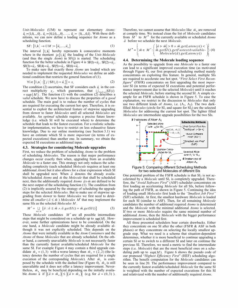
4. Scheduling of Atoms The job of the scheduling is to determine a loading sequence of the Atoms that are needed to implement the selected Molecules. This schedule cannot be determined at design time because it highly depends on the selected Molecules (and thus on the num-ber of Atom Containers and the expected SI execution frequen-cies). The importance of a good scheduling strategy is shown in a simple example in Figure 4, where the Molecule 3m was selected to implement a required SI. This SI may also be implemented (with reduced performance) by the Molecules 1m or 2m . A good scheduler should exploit the potential for upgrading from one Molecule to a faster one until the selected Molecule is finally composed. Without this incremental upgrading, the SI is not available in the accelerating hardware for a noticeable longer time as shown in the table in Figure 4 (the average reconfigura-tion time for one of our Atoms is 874.03 μs, as discussed in Sec-tion 5). The problem space of determining an Atom loading se-quence grows even larger when multiple Molecules of different 4 for evaluation we are working with a DLX (MIPS) and a Leon2

(SPARC V8) based prototype, but we are not limited to these

SIs are requested in parallel (which is the typical case) where the scheduler has to decide which SI to upgrade first. A too simplistic decision will give performance away as we will see.

3m

2m1m

6

5

4

3

2

1

fastest availableMolecule# loaded

Atoms

1m2m

3m2m 2m

3m

Figure 4: Different Atom schedules with the corresponding availabilities of the Molecules

4.1. Molecule assembly model and definitions In this subsection, we explain the hierarchical SI composition of our RISPP project on a formal basis (originally published in [23]) to present the Molecule − Atom interdependencies and to simplify and clarify expressions for the scheduling problem later on.

We define a data structure n( , , , )∪ ∩ ≤ , where n is the set of all Molecules and n is the number of different available Atom-types. For convenience we consider , , ∈ nm o p as Molecules with 1 ( , ..., )= nm m m where im describes the desired number of instances of Atom i to implement the Molecule. The operator

n n n:∪ × → with :m o p∪ = ; : max{ , }i i ip m o= describes a Meta-Molecule which contains the Atoms required to implement both m and o . We name the resulting Molecule p as a Meta-Molecule to distinguish it from the elementary Molecules that are dedicated to implement a specific SI. Since the operator ∪ is commutative and associative with the neutral element (0, …, 0), therefore n( , )∪ is an Abelian semi-group. The same is true for

n( , )∩ with n n n:∩ × → being defined as : ,∩ =m o p : min{ , }=i i ip m o with the neutral element (maxInt, …, maxInt).

The relation m o≤ is defined to be true iff [ ]1, : i ii n m o∀ ∈ ≤ . As ‘ ≤’ is reflexive, anti-symmetric, and transitive, n( , )≤ is a par-tially ordered set. For a set of Molecules nM ⊂ , the supremum is defined as sup : m MM m∈=∪ . The supremum from M is a Meta-Molecule with the meaning of declaring all Atoms that are needed to implement any of the Molecules in M , i.e. : sup .∀ ∈ ≤m M m M The infimum is correspondingly defined as inf : ∈= ∩m MM m with the meaning of containing those Atoms that are collectively needed for all Molecules of M . As any subset nM∅≠ ⊂ has a well-defined supremum and infimum, n( , )≤ is a complete lat-tice. Given these definitions, we can now combine multiple Mo-lecules that are chosen to implement different SIs. To calculate the cost for constituting Molecules in hardware, we define the fol-lowing two functions: The determinant of a Molecule is defined as [ ]1,: ,∈= ∑ i n im m i.e. the total number of Atoms that are re-quired to implement m. To consider already configured Atoms we define the function

n n n - , - 0: ; : ; : 0, ≥⎧× → = = ⎨

⎩i i i i

io m if o mm o p p else

.

The created Meta-Molecule p contains the minimum set of Atoms that additionally have to be offered to implement o , as-suming that the Atoms in m are already available. 4.2. Defining the Atom Scheduling problem The input to the scheduling is a set { }= iM m of all Molecules

∈ nim that were selected for implementation. ( )sup M is the Me-

ta-Molecule that contains all Atoms that are needed to implement the selected Molecules. We name the number of instances for the ith Atom of ( )sup M “ ix ”, i.e. ( ) ( )1 2sup , ,...,= nM x x x . We define

( ): sup= =∑ iNA M x as the number of Atoms that are needed to im-plement all selected Molecules. The previously executed Mole-cule selection guarantees that these Atoms fit to the available Atom Containers (ACs), i.e. #≤NA ACs . We define so called

Unit-Molecules (UM) to represent our elementary Atoms: ( )1 : 1,0,...,0=u , ( )2 : 0,1,0,...,0=u , …, :nu = ( )0,...,0,1 . With these defi-

nitions, we can now define a loading sequence for Atoms as a scheduling function.

[ ] { }1SF: 1,k : , ...,→ = nUM u u (1) The interval [ ]1, k hereby represents k consecutive moments where in the moment [ ]j 1, k∈ the loading of the Unit-Molecule (and thus the single Atom) in SF(j) is started. The scheduling function for the better schedule in Figure 4 is 2SF(1) =u , 2SF(2) =u ,

1SF(3) =u , 1SF(4) =u , 2SF(5) =u , 1SF(6) =u . To make sure that exactly those Atoms are loaded which are

needed to implement the requested Molecules we define an addi-tional condition that restricts the general function of (1).

[ ] { }i 1,n : | SF( )∀ ∈ = =i ij j u x (2) The condition (2) ascertains, that SF considers each iu in the cor-rect multiplicity ix , which guarantees, that [ ]i 1,n SF( )i∀ ∈∪

( )sup M= . The function (1) with the condition (2) describes a valid schedule. We now have to discuss the properties of a good schedule. The main goal is to reduce the number of cycles that are required for executing the current hot spot. Therefore, it is es-sential to exploit the architectural feature of stepwise upgrading from slower to faster Molecules until all selected Molecules are available. An optimal schedule requires a precise future know-ledge (i.e. which SI will be executed when) to determine the schedule that leads to the fastest execution. For a realistic schedu-ler implementation, we have to restrict on less exhaustive future knowledge. Due to our online monitoring (see Section 3.1) we have an estimate which SI is more important (in terms of ex-pected executions) than another one. In summary, we obtain the expected SI executions as additional input. 4.3. Strategies for considering Molecule upgrades First, we reduce the problem of scheduling Atoms to the problem of scheduling Molecules. The reason is that major performance changes occur exactly then when, upgrading from an available Molecule to a faster one. This strategy not only reduces the sche-duling complexity (each scheduled Molecule requires at least one additional Atom) but it also allows for a clear expression which SI shall be upgraded next. When a denotes the already availa-ble/scheduled Atoms and m the Molecule that shall be scheduled next, then the additionally required Atoms a m are defined to be the next output of the scheduling function (1). The condition from (2) is implicitly assured by the strategy of scheduling the upgrade steps for the selected Molecules. But to make use of stepwise up-grading from slower to faster Molecules we first need to deter-mine all smaller ( ≤o m ) Molecules ′M that may implement the same SIs as the selected Molecules .M

{ }: . () . ()∈

′ = ≤ ∧ =∪m M

M o o m o getSI m getSI (3)

These Molecule candidates ′M are all possible intermediate steps that might be considered on a schedule up to ( )sup M . How-ever, some further optimizations have to be considered. On the one hand, a Molecule candidate might be already available al-though it was not explicitly scheduled. This depends on the Atoms that were initially available in the Atom Containers and the Atoms of those Molecules that are already scheduled. On the oth-er hand, a currently unavailable Molecule is not necessarily faster than the currently fastest available/scheduled Molecule for the same SI. For example Figure 4 may contain a third upgrade can-didate 4 (1, 3)=m with a worse latency than 2 (2, 2)=m (the la-tency denotes the number of cycles that are required for a single execution of the corresponding Molecule). After 2m is com-posed by the schedule with the dashed line (Figure 4), 4m is still unavailable and it does not offer a latency improvement. Never-theless, 4m may be beneficial depending on the initially availa-ble Atoms a if ( ) ( )4 2≤a m a m (e.g. for (0, 3)=a ).

Therefore, we cannot assume that Molecules like 4m are removed at compile time. We instead clean the list of Molecule candidates from ′M to ′′M for the currently available or scheduled Atoms a before we schedule the next Molecule.

0 . (): . (). -

( ). ()

⎧ ⎫⎛ ⎞> ∧ <⎪ ⎪⎜ ⎟′′ ′= ∈⎨ ⎬⎜ ⎟⎪ ⎪⎝ ⎠⎩ ⎭

a m m getLatencyM m M m getSI getFastestAvailable

M olecule a getLatency (4)

4.4. Determining the Molecule loading sequence As the possibility to upgrade from one Molecule to a faster one can lead to a significant improved execution time (as motivated through Figure 4), our first proposed scheduling method mainly concentrates on exploiting this feature. In general, multiple SIs are required to accelerate one hot spot. “First Select First Recon-figure” (FSFR) concentrates on first upgrading the most impor-tant SI (in terms of expected SI executions and potential perfor-mance improvement due to the selected Molecule) until it reaches the selected Molecule, before starting the second SI. A simple ex-ample for an FSFR schedule is shown in Figure 5. To ease the explanation, we restrict in the discussion to Molecules that only use two different kinds of Atoms, i.e. (A1, A2). The two dark-filled Molecules (circle for SI1 and square for SI2) are the selected Molecules for addressing the current hot spot. The lighter filled Molecules are intermediate upgrade possibilities for the two SIs.

( )1 2

1 2

sup { , }= ∪m mm m

1m

2m

Figure 5: Comparing different Scheduling Methods

for two selected Molecules of different SIs One potential problem of the FSFR schedule is that SI2 is not ac-celerated by a Molecule until SI1 is completely upgraded. There-fore, the “Avoid Software First” (ASF) scheduler concentrates on first loading an accelerating Molecule for all SIs, before follow-ing the path of FSFR, as shown in Figure 5. Continuing the idea of loading small Molecules first leads to the “Smallest Job First” (SJF) schedule. At first, the smallest hardware Molecule is loaded for each SI (similar to ASF). Then, for all remaining Molecule candidates the number of additional required Atoms is determined and the Molecule with the minimal additional Atoms is selected. If two or more Molecules require the same minimal number of additional Atoms, then the Molecule with the bigger performance improvement is scheduled first.

All three presented schedulers bear certain drawbacks. Either they concentrate on one SI after the other (FSFR & ASF in both phases) or they concentrate on selecting the locally smallest up-grade step. What we need is a scheme that situation-dependent determines, whether it is more beneficial to continue upgrading a certain SI or to switch to a different SI and later on continue the previous SI. Therefore, we need a metric to find the intermediate steps (i.e. Molecule) that are the most beneficial ones on a sche-duling path up to sup( ).M Figure 6 shows the pseudo code of our proposed “Highest Efficiency First” (HEF) scheduling algo-rithm. The benefit computation for the Molecule candidates can be seen in line 20. The performance improvement compared to the currently fastest available/scheduled Molecule for the same SI is weighted with the number of expected executions for this SI and relativized with the number of additionally required Atoms.

1. // consider all smaller Molecules, see equation (3) 2. ;′ ← ∅M 3. ∈m M∀ 4. : . () . ()≤ ∧ =o o m o getSI m getSI∀ 5. { };′ ′← ∪M M o 6. // initialize the bestLatency array 7. ←a currentlyAvailableAtom s; 8. ∈m M∀

9. . (). . (). ( ). ();

←m getSI bestLatency m getSIgetFastestAvailableM olecule a getLatency

10. // schedule the Molecule candidates 11. ;← ∅scheduledL ist 12. ( ) {′ ≠ ∅Mw hile 13. // clean Molecule candidates, see equation (4) 14. ′∈m M∀ 15. ( ) . () . ().≤ ∨ ≥m a m getLatency m getSI bestLatencyif 16. \ { };′ ′←M M m 17. ( ) break ;′ = ∅Mif 18. 0;←bestBenefit 19. {′∈o M ∀ 20. ( )

. (). () ;. (). . ()∗← −

o getSI getExpectedExecutionsbenefit o getSI bestLatency o getLatency a o

21. ( ) {>benefit bestBenefitif 22. ;←bestBenefit benefit ;←m o 23. } 24. } 25. // schedule the chosen Molecule 26. ( ) . ( );∈i iA tom s a a m scheduledList push a∀ 27. ;← ∪a a m 28. . (). . ();←m getSI bestLatency m getLatency 29. } 30. return ;scheduledL ist

Figure 6: Our implemented scheduling method “Highest Efficiency First” (HEF)

5. Evaluation and results We will now present a detailed analysis of the presented schedu-lers from Section 4 by benchmarking them with an implementa-tion of the H.264 video encoder and a CIF-video (352x288) with 140 frames (more details about the application are given in [25]). Then, we compare a state-of-the-art reconfigurable computing system [19] with our architectural extension of stepwise upgrad-ing the Molecules to their final implementation and highlight the speedup that we additionally achieve by our proposed Special In-struction Scheduler. Table 1 summarizes our implemented SIs for the H.264 encoder with the different required types of Atoms and the number of available Molecules.

Special In-struction

# Atom-types

# Mole-cules

Motion Estimation (ME)

SAD 1 3SATD 4 20

Encoding Engine (EE)

(I)DCT 3 12(I)HT 2x2 1 2(I)HT 4x4 2 7

MC 4 3 11IPred HDC 2 4IPred VDC 1 3

Loop Filter (LF) LF_BS4 2 5Table 1: Implemented SIs of H.264 with number of required

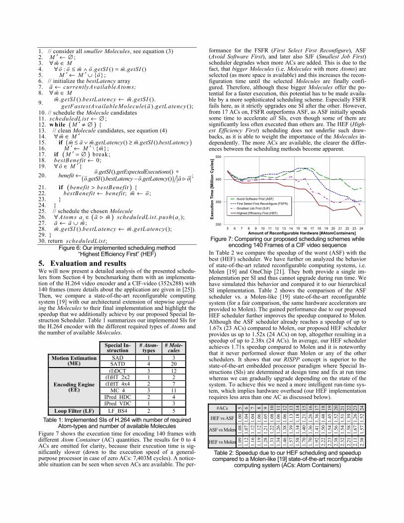
Atom-types and number of available Molecules Figure 7 shows the execution time for encoding 140 frames with different Atom Container (AC) quantities. The results for 0 to 4 ACs are omitted for clarity, because their execution time is sig-nificantly slower (down to the execution speed of a general-purpose processor in case of zero ACs: 7,403M cycles). A notice-able situation can be seen when seven ACs are available. The per-

formance for the FSFR (First Select First Reconfigure), ASF (Avoid Software First), and later also SJF (Smallest Job First) scheduler degrades when more ACs are added. This is due to the fact, that bigger Molecules (i.e. Molecules with more Atoms) are selected (as more space is available) and this increases the recon-figuration time until the selected Molecules are finally confi-gured. Therefore, although these bigger Molecules offer the po-tential for a faster execution, this potential has to be made availa-ble by a more sophisticated scheduling scheme. Especially FSFR fails here, as it strictly upgrades one SI after the other. However, from 17 ACs on, FSFR outperforms ASF, as ASF initially spends some time to accelerate all SIs, even though some of them are significantly less often executed than others are. The HEF (High-est Efficiency First) scheduling does not underlie such draw-backs, as it is able to weight the importance of the Molecules in-dependently. The more ACs are available, the clearer the differ-ences between the scheduling methods become apparent.

200

300

400

500

5 6 7 8 9 10 11 12 13 14 15 16 17 18 19 20 21 22 23 24

Exec

utio

n Ti

me

[Mill

ion

Cyc

les]

Amount of Reconfigurable Hardware [#AtomContainers]

Avoid Software First (ASF)First Select First Reconfigure (FSFR)Smallest Job First (SJF)Highest Efficiency First (HEF)

Figure 7: Comparing our proposed scheduling schemes while

encoding 140 Frames of a CIF video sequence In Table 2 we compare the speedup of the worst (ASF) with the best (HEF) scheduler. We have further on analyzed the behavior of state-of-the-art related reconfigurable computing systems, i.e. Molen [19] and OneChip [21]. They both provide a single im-plementation per SI and thus cannot upgrade during run time. We have simulated this behavior and compared it to our hierarchical SI implementation. Table 2 shows the comparison of the ASF scheduler vs. a Molen-like [19] state-of-the-art reconfigurable system (for a fair comparison, the same hardware accelerators are provided to Molen). The gained performance due to our proposed HEF scheduler further improves the speedup compared to Molen. Although the ASF scheduler already reaches a speedup of up to 1.67x (23 ACs) compared to Molen, our proposed HEF scheduler provides us up to 1.52x (24 ACs) on top, altogether resulting in a speedup of up to 2.38x (24 ACs). In average, our HEF scheduler achieves 1.71x speedup compared to Molen and it is noteworthy that it never performed slower than Molen or any of the other schedulers. It shows that our RISPP concept is superior to the state-of-the-art embedded processor paradigm where Special In-structions (SIs) are determined at design time and fix at run time whereas we can gradually upgrade depending on the state of the system. To achieve this we need a more intelligent run-time sys-tem, which implies hardware overhead (our HEF implementation requires less area than one AC as discussed below).

#ACs 5 6 7 8 9 10

11

12

13

14

15

16

17

18

19

20

21

22

23

24

HEF vs ASF 1.00

1.

04

1.04

1.

06

1.05

1.

08

1.06

1.

06

1.13

1.

18

1.21

1.

26

1.36

1.

48

1.45

1.

52

1.51

1.

39

1.26

1.

52

ASF vs Molen 1.08

1.

07

1.12

1.

12

1.21

1.

22

1.26

1.

38

1.39

1.

34

1.40

1.

36

1.41

1.

50

1.54

1.

56

1.54

1.

58

1.67

1.

57

HEF vs Molen 1.09

1.

12

1.16

1.

19

1.28

1.

31

1.34

1.

46

1.57

1.

58

1.70

1.

70

1.92

2.

22

2.23

2.

38

2.32

2.

21

2.11

2.

38

Table 2: Speedup due to our HEF scheduling and speedup compared to a Molen-like [19] state-of-the-art reconfigurable

computing system (ACs: Atom Containers)

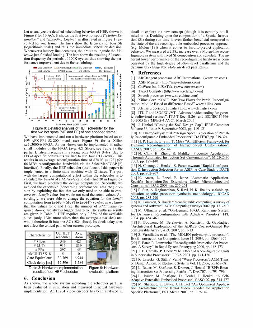
Let us analyze the detailed scheduling behavior of HEF, shown in Figure 8 for 10 ACs. It shows the first two hot spots (“Motion Es-timation” and “Encoding Engine” as illustrated in Figure 1) ex-ecuted for one frame. The lines show the latencies for four SIs (logarithmic scale) and thus the immediate scheduler decision. Whenever a latency line decreases, the Atoms to upgrade the Mo-lecule just finished loading. The bars show the resulting SI execu-tion frequency for periods of 100K cycles, thus showing the per-formance improvement due to the scheduling.

110

100

1,00

010

,000

0 2 4 6 8 10 12 14 16 18 20 22 240

1,00

02,

000

3,00

04,

000

SAD Execution SATD Execution MC Execution DCT ExecutionSAD Latency SATD Latency MC Latency DCT Latency

Lin

es: S

I Lat

ency

[Cyc

les]

(Log

Sca

le)

Bar

s: #

of S

I Exe

cutio

ns p

er 1

00K

Cyc

les

Execution Time [100K Cycles]

Latency of SAD is decreasing

Continuation of Latency lines for SAD and SATD are omitted for clarity

Latency of SATD is decreasing

Figure 8: Detailed analysis of HEF scheduler for the

first two hot spots (ME and EE) of one encoded frame We have implemented and run a hardware platform based on an HW-AFX-FF1152-200 board (see Figure 9) for a Xilinx xc2v3000-6 FPGA. As our Atoms can be implemented in rather small modules of the FPGA (avg. 421 Slices, see Table 3), the partial Bitstream requires in average only 60,488 Bytes (due to FPGA-specific constraints we had to use four CLB rows). This results in an average reconfiguration time of 874.03 μs [23] (for 66 MB/s reconfiguration bandwidth via the SelectMap/ICAP [6] interface). Finally, the HEF scheduler (the focus of this paper) is implemented in a finite state machine with 12 states. The part with the largest computational effort within the scheduler is to calculate the benefit of a Molecule candidate (line 20 in Figure 6). First, we have pipelined the benefit computation. Secondly, we avoided the expensive (concerning performance, area etc.) divi-sion by exploiting the fact that we only need to be able to com-pare two benefit values but we do not need the actual values. Ac-cordingly, we were able to change the equation for the benefit computation from (a·b)/c > (d·e)/f to (a·b)·f > (d·e)·c, as we know that the values for c and f (i.e. the number of additionally re-quired Atoms) are always bigger than zero. The synthesis results are given in Table 3. HEF requires only 3.83% of the available slices (only 1.30x more slices than the average Atom size) and would therefore fit into one AC (1024 slices). Its clock delay does not affect the critical path of our current prototype.

Characteristics Our HEF scheduler

Avg. Atom

# Slices 549 421 # LUTs 915 839 # FFs 297 45

#MULT18X18 5 0 Gate Equivalents 30,769 6,944 Clock delay [ns] 12.596 1.284 Table 3: Hardware implementation

results of our HEF scheduler Figure 9: Hardware evaluation platform

6. Conclusion As shown, the whole system including the scheduler part has been evaluated in simulation and measured in actual hardware implementation. An H.264 video encoder has been analyzed in

detail to explore the new concept (though it is certainly not li-mited to it). Deciding upon the composition of a Special Instruc-tion (SI) during run time is even farther beneficial compared to the state-of-the-art reconfigurable embedded processor approach (e.g. Molen [19]) when it comes to hard-to-predict application behavior. We measured a 2,38x increase over a Molen-like recon-figurable system with fixed SI composition and schedule. The in-herent lower performance of the reconfigurable hardware is com-pensated by the high degree of Atom-level parallelism and the dynamically changeable Molecule-level parallelism.

7. References [1] ARCtangent processor. ARC International. (www.arc.com) [2] ASIP Meister. (http://asip-solutions.com) [3] CoWare Inc, LISATek. (www.coware.com) [4] Target Compiler (http://www.retarget.com) [5] Stretch processor (www.stretchinc.com) [6] Xilinx Corp. “XAPP 290: Two Flows for Partial Reconfigu-ration: Module Based or difference Based” www.xilinx.com [7] Xtensa processor, Tensilica Inc.: www.tensilica.com [8] ITU-T and ISO/IEC JVT “Advanced video coding for gener-ic audiovisual services”, ITU-T Rec. H.264 and ISO/IEC 14496-10:2005 (E) (MPEG-4 AVC), March 2005 [9] J. Henkel “Closing the SoC Design Gap”, IEEE Computer Volume 36, Issue 9, September 2003, pp. 119-121 [10] A. Chattopadhyay et al. “Design Space Exploration of Partial-ly Re-configurable Embedded Processors”, DATE’07, pp. 319-324 [11] H. P. Huynh, E. Sim, T. Mitra “An Efficient Framework for Dynamic Reconfiguration of Instruction-Set Customization”, CASES 2007, pp. 135-144 [12] N. Clark H. Zhong S. Mahlke “Processor Acceleration Through Automated Instruction Set Customization”, MICRO-36 2003, pp. 129-140 [13] N. Cheung, J. Henkel, S. Parameswaran “Rapid Configura-tion & Instruction Selection for an ASIP: A Case Study”, DATE 2003, pp. 802-807 [14] K. Atasu, L. Pozzi, P. Ienne “Automatic Application-Specific Instruction-Set Extensions Under Microarchitectural Constraints”, DAC 2003, pp. 256-261 [15] F. Sun, A. Raghunathan, S. Ravi, N. K. Jha “A scalable ap-plication specific processor synthesis methodology”, ICCAD 2003, pp. 283-290 [16] K. Compton, S. Hauck “Reconfigurable computing: a survey of systems and software”, ACM Computing Surveys 2002, pp. 171-210 [17] M. Ullmann et al. “On-Demand FPGA Run-Time System for Dynamical Reconfiguration with Adaptive Priorities” FPL 2004, pp. 454–463 [18] F. Bouwens, M. Berekovic, A. Kanstein, G. Gaydadjiev “Architectural Exploration of the ADRES Coarse-Grained Re-configurable Array”, ARC 2007, pp. 1-13 [19] S. Vassiliadis et al. “The MOLEN polymorphic processor”, IEEE Transaction on Computers, Issue 11, 2004, pp. 1363-1375 [20] F. Barat, R. Lauwereins “Reconfigurable Instruction Set Proces-sors: A Survey”, in Rapid System Prototyping 2000, pp. 168-173 [21] J. E. Carrillo, P. Chow “The Effect of Reconfigurable Units in Superscalar Processors”, FPGA 2001, pp. 141-150 [22] R. Lysecky, G. Stitt, F. Vahid “Warp Processors”, ACM Trans. on Design Autom. of Electronic Systems Vol. 11, 2006, pp. 659-681 [23] L. Bauer, M. Shafique, S. Kramer, J. Henkel “RISPP: Rotat-ing Instruction Set Processing Platform”, DAC’07, pp.791-796 [24] L. Bauer, M. Shafique, D. Teufel, J. Henkel “A Self-Adaptive Extensible Embedded Processor”, SASO’07, pp. 344-377 [25] M. Shafique, L. Bauer, J. Henkel “An Optimized Applica-tion Architecture of the H.264 Video Encoder for Application Specific Platforms”, ESTIMedia 2007, pp. 119-142