neolithic transitions - run
TRANSCRIPT

Neolithic Transitions
Can genetic data help us understand a
major demographic event in human
prehistory?
Ana Rita Rodrigues Rasteiro de Campos
Dissertation presented to obtain the Ph.D degree in Biology
Instituto de Tecnologia Química e Biológica | Universidade Nova de Lisboa
Oeiras,
February, 2012


Neolithic Transitions:
Can genetic data help us understand
a major demographic event in human
prehistory?
Ana Rita Rodrigues Rasteiro de Campos
Dissertation presented to obtain the Ph.D degree in Biology
Instituto de Tecnologia Química e Biológica | Universidade Nova de Lisboa
Research work coordinated by:
Oeiras,
February, 2012


Esta tese obteve o apoio financeiro da FCT e do FSE no âmbito doQuadro Comunitário de Apoio, BD nº SFRH/BD/30821/2006.


À minha família


Abstract
The Neolithic transition is probably the most important cultural, eco-nomic and demographic revolution in human prehistory. It profoundlymodified the distribution of human genes, languages and cultures world-wide. However, the study of the transition from hunting and gatheringto farming societies has generated major controversies among archae-ologists and geneticists alike, with one side favouring demic diffusionmodels and the other the cultural diffusion models. As a first approxima-tion two alternative demographic scenarios can be considered. Underthe cultural diffusion models the transition to agriculture is regarded es-sentially as a cultural phenomenon, involving the movement of ideasand practices, rather than people. In the demic diffusion models, amovement of people is involved. It can be shown that both modelscan be seen as special cases of an admixture model between Palae-olithic/Mesolithic and Neolithic populations. In this thesis, I used non-equilibrium and spatial admixture model approaches to help answer thislong-standing controversy. I showed that demic diffusion models betterexplain the patterns of genetic diversity found in today’s European andJapanese populations, but I do not rule out the role of cultural processeslocally.In the first part of my thesis, we tried to address the transition to farm-ing in the Japanese islands. The first inhabitants of Japan, the hunter-gatherers Jomon, had their culture completely replaced by that of theYayoi farmers, who arrived later in the archipelago. Exactly how this cul-tural replacement occurred is still controversial today. Surprisingly, this

issue was never been addressed from an admixture point of view before,even though this is probably the only point on which most studies agree,i.e. that there was admixture between the two groups of humans. Weused Y-chromosome data and an admixture approach to quantify thelevel of admixture across the Japanese archipelago. The method used,which accounts for genetic drift since the admixture event, clearly pointsto a demic diffusion process, similar to the process that was suggestedfor Europe also using Y-chromosome data.In the second part of my thesis, we integrated Y-chromosome and mito-chondrial DNA (mtDNA) data into the same admixture approach to studythe European Neolithic transition. We found that contrary to severalstatements claiming the opposite, both contemporary Y-chromosomeand mtDNA data clearly favour a demic diffusion process, i.e. bothmales and females underwent the same admixture history. However,key differences in the female and male demographic histories werealso identified, most likely related with sex-related differences in effec-tive size and migration patterns. Additionally, using an ApproximateBayesian Computation approach and one of the largest ancient DNAdataset available, we compared several demographic models with andwithout population structure and admixture. Our results show that demicdiffusion is again favoured, but population structure and differential growthbetween farmers and hunter-gatherers are necessary to explain the pro-cess.Finally, a new multi-population spatial simulation framework was devel-oped and applied to study the consequence of sex-biased migration inthe genetic make-up of populations, during the European Neolithic tran-sition. Archaeological and anthropological data suggest that changes inpost-marital residence rules between males and females took place asa consequence of sedentism and new rules of land control by men. Ourresults show that the Neolithic transition must have left its mark in thegenome of Europeans and confirm that farming was accompanied by

reduced male migration and a movement of females to their husband’sbirthplace.All together, the studies presented in this thesis allow us to draw a co-herent picture of the Neolithic transition in Europe (and to some extentin Japan), which not only provides an explanation for the patterns ofgenetic diversity found today and in our past, but also for the apparentcontradiction between phylogeographic and model-based studies.


Resumo
A transição Neolítica é provavelmente a revolução cultural, económicae demográfica mais importante da Pré-História Humana. Esta mudouprofundamente a distribuição de genes, de linguagens e culturas nomundo. No entanto, o estudo da transição de sociedades caçadoras-recolectoras para sociedades agricultoras tem gerado muita polémicatanto entre geneticistas, como entre arqueólogos, com um lado favore-cendo modelos de difusão démica e o outro modelos de difusão cul-tural. Nos modelos de difusão cultural, a transição para a agricul-tura é vista essencialmente como um fenómeno cultural, que envolveo movimento de ideias e práticas, ao invés de pessoas. Pelo contrário,nos modelos de difusão démica, um movimento de pessoas está en-volvido. Ambos os modelos podem ser vistos como casos especiaisde miscigenação/mistura entre populações do Paleolítico/Mesolítico eNeolítico. Nesta tese foram usados métodos aplicados a modelos demiscigenação, quer em situações de não-equilíbrio, quer distribuídosno espaço, para ajudar a responder a esta controvérsia. Os nossosresultados mostram que modelos de difusão démica explicam melhoros padrões de diversidade genética encontrados actualmente, em pop-ulações europeias e japonesas, mas ao mesmo tempo não descartamo papel de processos culturais locais.Na primeira parte da tese, procurou-se abordar a transição para a pro-dução agrícola nas ilhas japonesas. Os primeiros habitantes do Japão,os caçadores-recoletores Jomon, tiveram a sua cultura completamentesubstituída pela dos agricultores Yayoi, que chegaram mais tarde no

arquipélago. O modo exacto como ocorreu esta substituição cultural éainda controverso nos dias de hoje. Surpreendentemente, esta questãonunca foi abordada do ponto de vista de miscigenação, ainda que esteseja o único ponto em que a maioria dos estudos concorda, ou seja,que houve um processo de miscigenação entre os dois grupos de sereshumanos. Usámos dados do cromossoma Y e uma abordagem de mis-cigenação para quantificar o nível de mistura em todo o arquipélagojaponês. O método utilizado, que tem em conta a deriva genética desdeo evento de mistura, aponta claramente para um processo de difusãodémica, similar ao processo que foi sugerido para a Europa, tambémusando dados do cromossoma Y.Na segunda parte desta tese, integrámos dados de ADN mitocondrial(ADNmt) e de cromossoma Y na mesma abordagem de miscigenação,para estudar a transição Neolítica europeia. Mostrámos que, ao con-trário de várias várias declarações afirmando o contrário, tanto os da-dos de cromossoma Y e como os de ADNmt contemporâneos favore-cem claramente um processo de difusão démica, ou seja, tanto homenscomo mulheres foram submetidos à mesma história de miscigenação.No entanto, diferenças importantes nas histórias demográficas femi-ninas e masculinas também foram identificadas, provavelmente rela-cionadas com diferenças sexuais no tamanho efectivo das populaçõese padrões de migração. Além disso, utilizando a abordagem “Approxi-mate Bayesian Computation” e um dos maiores conjunto de dados deADN antigo disponível, foram comparados vários modelos demográ-ficos com e sem estrutura populacional e mistura. Estes resultadosfavorecem novamente a difusão démica, mas também apontam a ne-cessidade de introduzir estrutura populacional e crescimento diferen-cial, entre os agricultores e caçadores-recolectores, para explicar o pro-cesso.Finalmente, desenvolvemos um novo programa computacional capazde simular diferentes populações no espaço. Este foi aplicado para es-

tudar a consequência da migração enviesada a favor de um sexo naconstituição genética das populações, durante a transição Neolítica eu-ropeia. Dados arqueológicos e antropológicos sugerem que mudançasnas regras de residência pós-marital, entre homens e mulheres, ocor-reram como consequência do sedentarismo e de novas regras de con-trolo da terra pelos homens. Os nossos resultados mostram que atransição Neolítica deve ter deixado sua marca no genoma europeu econfirmam que a agricultura foi acompanhada por uma redução da mi-gração masculina e pelo movimento de mulheres para o local de nasci-mento do seu marido.Ao todo, os estudos apresentados nesta tese permitiu-nos desenharum quadro coerente da transição Neolítica na Europa (e até certo pontotambém no Japão), que não só fornece uma explicação para os padrõesde diversidade genética quer encontrados hoje, como no passado, mastambém para a aparente contradição entre estudos filogeográficos eaqueles baseados em modelos.


Acknowledgements
The completion of this thesis would not have been possible withoutthe help and encouragement of many people. Their support has takenmany forms, and I want to show here my deepest gratitude to them.
Lounès Chikhi was both the instigator and the supervisor of theresearch presented in this thesis. The quality of my work owes muchto his dynamic and motivating leadership at its high competence andscientific rigor. I also thanks for the friendship he has shown in meduring these years.
Instituto Gulbenkian de Ciência (IGC) and Instituto de TecnologiaQuímica e Biológica (ITQB) for providing me a platform for my PhDwork.
Isabel Gordo and Élio Sucena, who kindly have agreed to be membersof my thesis committee.
Giorgio Bertorelle, António Amorim, Nuno Ferrand and GabrielaGomes for agreeing to be part of my PhD defense jury.
The IT services of IGC for showing a great willingness to help mesolve the computer problems I encountered during my work.
Pedro Fernandes, responsible for the High Performance Comput-

ing Centre (HERMES) at IGC, for all the support.
Vítor Sousa for introducing me to the wonderful world of R andHigh Performance Computing. Thank you for all the help and for ourmany discussions.
Bárbara Parreira for all the discussions, especially when the Pop-ulation and Conservation Genetics Group (PCG) was composed withjust both of us, Vítor and Lounès.
To Pierre-Antoine Bouttier and Damien Mounier, INSA (Toulouse)students, who worked alongside us in the development of SINS.
To all members of PCG, past and current, for making possible towork on a pleasant, motivating and dynamic group. João, Isabel, Jordi,Cristina, Isa, Célia, Sam, Cécile, Fabrice, among others.
Special thanks to Reeta Sharma, for all the discussions, kindnessand friendship.
The continued support of all my family and friends for encouragehigher education, especially that of my parents and sister.

Contents
List of Figures ix
List of Tables xiii
List of Algorithms xv
1 General Introduction 1
1.1 The use of genetic data to characterize human populations . . . . . 1
1.2 Neolithic transition . . . . . . . . . . . . . . . . . . . . . . . . . . . . 3
1.3 Inference of Human Past Demography . . . . . . . . . . . . . . . . . 6
1.3.1 Admixture models . . . . . . . . . . . . . . . . . . . . . . . . 8
1.3.1.1 Thus, how can one go about detecting admixture? . 9
1.3.2 Spatial models . . . . . . . . . . . . . . . . . . . . . . . . . . 11
1.4 Aims . . . . . . . . . . . . . . . . . . . . . . . . . . . . . . . . . . . . 14
1.5 References . . . . . . . . . . . . . . . . . . . . . . . . . . . . . . . . 15
2 Admixture in Japan 23
2.1 Abstract . . . . . . . . . . . . . . . . . . . . . . . . . . . . . . . . . . 23
i

CONTENTS
2.2 Introduction . . . . . . . . . . . . . . . . . . . . . . . . . . . . . . . . 24
2.3 Material and Methods . . . . . . . . . . . . . . . . . . . . . . . . . . 27
2.3.1 Populations used . . . . . . . . . . . . . . . . . . . . . . . . . 27
2.3.2 The Admixture Model . . . . . . . . . . . . . . . . . . . . . . 28
2.3.3 Choice of parental populations . . . . . . . . . . . . . . . . . 28
2.3.4 Calculating Drift . . . . . . . . . . . . . . . . . . . . . . . . . 30
2.3.5 Spatial variation of admixture: regression analysis . . . . . . 30
2.3.6 FST analysis . . . . . . . . . . . . . . . . . . . . . . . . . . . 31
2.4 Results . . . . . . . . . . . . . . . . . . . . . . . . . . . . . . . . . . 31
2.4.1 Admixture proportions . . . . . . . . . . . . . . . . . . . . . . 31
2.4.2 Drift . . . . . . . . . . . . . . . . . . . . . . . . . . . . . . . . 35
2.4.3 FST . . . . . . . . . . . . . . . . . . . . . . . . . . . . . . . . 37
2.5 Discussion . . . . . . . . . . . . . . . . . . . . . . . . . . . . . . . . 39
2.5.1 Dual origins of Japanese . . . . . . . . . . . . . . . . . . . . 39
2.5.2 The continental origin of the Yayoi farmers . . . . . . . . . . . 40
2.6 References . . . . . . . . . . . . . . . . . . . . . . . . . . . . . . . . 42
3 Admixture in Europe 47
3.1 Abstract . . . . . . . . . . . . . . . . . . . . . . . . . . . . . . . . . . 47
3.2 Introduction . . . . . . . . . . . . . . . . . . . . . . . . . . . . . . . . 48
3.3 Material and Methods . . . . . . . . . . . . . . . . . . . . . . . . . . 51
3.3.1 Estimating admixture between Palaeolithic HG and Neolithicfarmers using extant genetic data . . . . . . . . . . . . . . . . 51
3.3.1.1 The admixture model . . . . . . . . . . . . . . . . . 51
ii

CONTENTS
3.3.1.2 Populations used . . . . . . . . . . . . . . . . . . . 52
3.3.1.3 Choice of Parental Populations . . . . . . . . . . . . 53
3.3.1.4 Validation of the admixture analysis with negativecontrols . . . . . . . . . . . . . . . . . . . . . . . . . 53
3.3.1.5 Regression Analysis . . . . . . . . . . . . . . . . . . 54
3.3.1.6 FST analysis . . . . . . . . . . . . . . . . . . . . . . 55
3.3.2 aDNA and Coalescent Analysis . . . . . . . . . . . . . . . . . 55
3.3.2.1 Populations’ datasets . . . . . . . . . . . . . . . . . 55
3.3.2.2 Demographic Models: testing for the continuity anddiscontinuity hypotheses . . . . . . . . . . . . . . . 55
3.3.2.3 Distribution of pairwise FST values across modelsand validation of our simulation approach . . . . . . 57
3.3.2.4 Approximate Bayesian Computations (ABC) for modelchoice and parameter estimation . . . . . . . . . . . 58
3.4 Results . . . . . . . . . . . . . . . . . . . . . . . . . . . . . . . . . . 62
3.4.1 Admixture analyses: The Neolithic contribution decreases withdistance from the Near-East, for both NRY and mtDNA data . 62
3.4.2 The Neolithic transition in the Caucasus and European is-lands: NRY admixture analyses . . . . . . . . . . . . . . . . . 62
3.4.3 Drift in paternal and maternal lineages: NRY and mtDNA datasupport the DDM but not the same demographic histories . . 63
3.4.4 Ancient DNA, coalescent simulations and model identificationusing ABC . . . . . . . . . . . . . . . . . . . . . . . . . . . . 66
3.5 Discussion . . . . . . . . . . . . . . . . . . . . . . . . . . . . . . . . 69
iii

CONTENTS
3.5.1 Both contemporary NRY and mtDNA data support DDM, buttell different demographic histories . . . . . . . . . . . . . . . 69
3.5.2 aDNA supports Demic Diffusion . . . . . . . . . . . . . . . . 72
3.5.3 Towards an integrated model of Neolithic transition . . . . . . 73
3.6 Conclusion . . . . . . . . . . . . . . . . . . . . . . . . . . . . . . . . 76
3.7 References . . . . . . . . . . . . . . . . . . . . . . . . . . . . . . . . 77
4 Sex-biased migration in the Neolithic 85
4.1 Summary . . . . . . . . . . . . . . . . . . . . . . . . . . . . . . . . . 86
4.2 Introduction . . . . . . . . . . . . . . . . . . . . . . . . . . . . . . . . 87
4.3 Material and Methods . . . . . . . . . . . . . . . . . . . . . . . . . . 89
4.3.1 General Framework . . . . . . . . . . . . . . . . . . . . . . . 89
4.3.2 Neolithic transition model . . . . . . . . . . . . . . . . . . . . 91
4.3.3 Variable parameters: sex-biased migration and admixture . . 92
4.3.4 Fixed Parameters . . . . . . . . . . . . . . . . . . . . . . . . 93
4.3.5 Summary statistics . . . . . . . . . . . . . . . . . . . . . . . . 93
4.4 Results . . . . . . . . . . . . . . . . . . . . . . . . . . . . . . . . . . 94
4.4.1 General results across all scenarios . . . . . . . . . . . . . . 94
4.4.2 No admixture scenarios . . . . . . . . . . . . . . . . . . . . . 95
4.4.3 Influence of HG postmarital behaviour on the Farmers geneticdiversity . . . . . . . . . . . . . . . . . . . . . . . . . . . . . . 97
4.4.4 Influence of HG postmarital behaviour on the Farmers geneticdifferentiation . . . . . . . . . . . . . . . . . . . . . . . . . . . 100
4.5 Discussion . . . . . . . . . . . . . . . . . . . . . . . . . . . . . . . . 100
iv

CONTENTS
4.5.1 Main results: (i) first farmers were patrilocal and (ii) differentpostmarital residence systems have a different impact on hu-man genetic patterns . . . . . . . . . . . . . . . . . . . . . . 100
4.5.2 Behaviour of summary statistics . . . . . . . . . . . . . . . . 101
4.5.3 Mutation rates can generate asymmetries between mtDNAand NRY data . . . . . . . . . . . . . . . . . . . . . . . . . . 102
4.5.4 Admixture decreases Farmers NRY genetic diversity . . . . . 102
4.5.5 Comparison with other sex-biased migration studies . . . . . 103
4.6 Conclusion . . . . . . . . . . . . . . . . . . . . . . . . . . . . . . . . 104
4.7 References . . . . . . . . . . . . . . . . . . . . . . . . . . . . . . . . 104
5 SINS: Simulating INdividuals in Space 111
5.1 Summary . . . . . . . . . . . . . . . . . . . . . . . . . . . . . . . . . 111
5.2 Introduction . . . . . . . . . . . . . . . . . . . . . . . . . . . . . . . . 112
5.3 Methods . . . . . . . . . . . . . . . . . . . . . . . . . . . . . . . . . . 112
5.3.1 Demography . . . . . . . . . . . . . . . . . . . . . . . . . . . 112
5.3.2 Genetics . . . . . . . . . . . . . . . . . . . . . . . . . . . . . 114
5.3.3 Outputs and Summary Statistics . . . . . . . . . . . . . . . . 114
5.4 Implementation . . . . . . . . . . . . . . . . . . . . . . . . . . . . . . 115
5.5 Discussion . . . . . . . . . . . . . . . . . . . . . . . . . . . . . . . . 115
5.6 References . . . . . . . . . . . . . . . . . . . . . . . . . . . . . . . . 116
6 General Discussion 117
6.1 Neolithic transition in Japan and Europe . . . . . . . . . . . . . . . . 117
6.2 Spatial expansion and the European Neolithic . . . . . . . . . . . . . 119
v

CONTENTS
6.3 Perspectives . . . . . . . . . . . . . . . . . . . . . . . . . . . . . . . 121
6.3.0.1 SINS’ new features . . . . . . . . . . . . . . . . . . 121
6.3.0.2 SINS’ in an ABC framework . . . . . . . . . . . . . 122
6.4 Conclusion . . . . . . . . . . . . . . . . . . . . . . . . . . . . . . . . 123
6.5 References . . . . . . . . . . . . . . . . . . . . . . . . . . . . . . . . 124
A Appendix: Admixture in Europe 127
A.1 Supplementary Tables . . . . . . . . . . . . . . . . . . . . . . . . . . 127
A.2 Supplementary Figures . . . . . . . . . . . . . . . . . . . . . . . . . 129
B Appendix: Neolithic transition in the Iberian Peninsula 135
C Appendix: Sex-biased migration in the Neolithic 149
C.1 Details on the simulation framework . . . . . . . . . . . . . . . . . . 149
C.1.1 Carrying Capacity and Friction . . . . . . . . . . . . . . . . . 149
C.1.2 Admixture . . . . . . . . . . . . . . . . . . . . . . . . . . . . . 149
C.1.3 Logistic growth . . . . . . . . . . . . . . . . . . . . . . . . . . 150
C.1.4 Short range migrations . . . . . . . . . . . . . . . . . . . . . 151
C.2 Simulation framework algorithm . . . . . . . . . . . . . . . . . . . . . 152
C.3 Mutation rates . . . . . . . . . . . . . . . . . . . . . . . . . . . . . . 154
C.4 Validation of the method . . . . . . . . . . . . . . . . . . . . . . . . . 154
C.5 Supplementary Tables . . . . . . . . . . . . . . . . . . . . . . . . . . 155
C.6 Supplementary Figures . . . . . . . . . . . . . . . . . . . . . . . . . 158
D Appendix: SINS user guide 171
vi

CONTENTS
D.1 General Introduction . . . . . . . . . . . . . . . . . . . . . . . . . . . 171
D.2 Demographic model . . . . . . . . . . . . . . . . . . . . . . . . . . . 172
D.2.1 Logistic Growth . . . . . . . . . . . . . . . . . . . . . . . . . . 172
D.2.2 Migration . . . . . . . . . . . . . . . . . . . . . . . . . . . . . 173
D.2.2.1 Number of migrants . . . . . . . . . . . . . . . . . . 173
D.2.2.2 Sex-biased migration . . . . . . . . . . . . . . . . . 174
D.2.3 Interaction between layers . . . . . . . . . . . . . . . . . . . . 174
D.2.3.1 Competition . . . . . . . . . . . . . . . . . . . . . . 174
D.2.3.2 Admixture . . . . . . . . . . . . . . . . . . . . . . . 175
D.3 Genetic Model . . . . . . . . . . . . . . . . . . . . . . . . . . . . . . 175
D.3.1 Reproduction . . . . . . . . . . . . . . . . . . . . . . . . . . . 176
D.3.2 Mutation model . . . . . . . . . . . . . . . . . . . . . . . . . . 176
D.4 SINS organization and Settings . . . . . . . . . . . . . . . . . . . . . 177
D.4.1 SINS Inputs . . . . . . . . . . . . . . . . . . . . . . . . . . . . 178
D.4.1.1 World and output files . . . . . . . . . . . . . . . . . 179
D.4.1.2 Environment folder . . . . . . . . . . . . . . . . . . . 183
D.4.1.3 Genetic Folder . . . . . . . . . . . . . . . . . . . . . 183
D.4.1.4 Layer parameters folder . . . . . . . . . . . . . . . . 186
D.4.2 SINS Outputs . . . . . . . . . . . . . . . . . . . . . . . . . . . 187
D.4.2.1 Demographic output . . . . . . . . . . . . . . . . . . 187
D.4.2.2 Genetic output . . . . . . . . . . . . . . . . . . . . . 188
D.5 SINS-stat: sampling and genetic analysis . . . . . . . . . . . . . . . 190
D.5.1 SINS-stat inputs . . . . . . . . . . . . . . . . . . . . . . . . . 191
vii

CONTENTS
D.5.2 SINS-stats summary statistics and outputs . . . . . . . . . . 192
D.6 SINS and SINS-stat Implementation and Installation . . . . . . . . . 193
D.7 Running SINS and SINS-stat . . . . . . . . . . . . . . . . . . . . . . 194
E References to Appendices 195
E.1 References . . . . . . . . . . . . . . . . . . . . . . . . . . . . . . . . 195
viii

List of Figures
1.1 SE-NW gradients in Europe . . . . . . . . . . . . . . . . . . . . . . . 2
1.2 Neolithic transition . . . . . . . . . . . . . . . . . . . . . . . . . . . . 4
1.3 Cultural and Demic diffusion models . . . . . . . . . . . . . . . . . . 5
1.4 Demographic models used in Population Genetics . . . . . . . . . . 8
1.5 Neolithic contribution across Europe . . . . . . . . . . . . . . . . . . 10
1.6 Admixture model . . . . . . . . . . . . . . . . . . . . . . . . . . . . . 11
2.1 Map of the Japanese Islands . . . . . . . . . . . . . . . . . . . . . . 25
2.2 Jomon contribution, across Japan . . . . . . . . . . . . . . . . . . . 33
2.3 Jomon and Yayoi contributions, across Japan . . . . . . . . . . . . . 34
2.4 Spatial variation of admixture and drift . . . . . . . . . . . . . . . . . 35
2.5 Distributions of the ti’s for all Japanese populations . . . . . . . . . . 36
2.6 Population differentiation with Ainu and Okinawa populations . . . . 38
3.1 Spatial variation of admixture and drift, across Europe . . . . . . . . 60
3.2 Genetic diversity across Europe . . . . . . . . . . . . . . . . . . . . . 64
3.3 Genetic differentiation across Europe . . . . . . . . . . . . . . . . . . 65
ix

LIST OF FIGURES
3.4 Demographic models used in the aDNA analysis and their posteriorprobabilities . . . . . . . . . . . . . . . . . . . . . . . . . . . . . . . . 66
3.5 Probability of obtaining genetic differentiation values close to the ob-served in the real data . . . . . . . . . . . . . . . . . . . . . . . . . . 69
4.1 Model of spatial expansion . . . . . . . . . . . . . . . . . . . . . . . 90
4.2 Genetic diversity and differentiation in modern populations, under noadmixture . . . . . . . . . . . . . . . . . . . . . . . . . . . . . . . . . 95
4.3 Genetic diversity in present-day Farmers, under admixture . . . . . . 98
A.1 Split with differential growth model (SDG) . . . . . . . . . . . . . . . 129
A.2 Palaeolithic contribution to modern European (p1) posterior distribu-tions . . . . . . . . . . . . . . . . . . . . . . . . . . . . . . . . . . . . 130
A.3 Linear regression of Neolithic contribution (1 − p1), against geo-graphical distance from the Near East, using NRY data . . . . . . . 131
A.4 Caucasus and European Islands: linear regression of Neolithic con-tribution (1 − p1), against geographical distance from the Near East,using NRY data . . . . . . . . . . . . . . . . . . . . . . . . . . . . . . 132
A.5 Distributions of the t i’s for all populations, using NRY . . . . . . . . . 133
A.6 Distributions of the t i’s for all populations, using mtDNA . . . . . . . 134
C.1 Genetic diversity under admixture scenarios . . . . . . . . . . . . . . 158
C.2 Genetic diversity in a 30×30 lattice, for patrilocal Farmers under ad-mixture scenarios . . . . . . . . . . . . . . . . . . . . . . . . . . . . . 160
C.3 Genetic differentiation in present-day populations under admixturescenarios . . . . . . . . . . . . . . . . . . . . . . . . . . . . . . . . . 162
C.4 Genetic differentiation under admixture scenarios . . . . . . . . . . . 164
x

LIST OF FIGURES
C.5 Genetic differentiation in a 30×30 lattice, for patrilocal Farmers underadmixture scenarios . . . . . . . . . . . . . . . . . . . . . . . . . . . 166
C.6 Framework validation . . . . . . . . . . . . . . . . . . . . . . . . . . . 168
C.7 Genetic diversity and differentiation in the no admixture scenarios,with a sampling scheme . . . . . . . . . . . . . . . . . . . . . . . . . 169
D.1 SINS organization . . . . . . . . . . . . . . . . . . . . . . . . . . . . 177
D.2 Inputs and outputs of SINS . . . . . . . . . . . . . . . . . . . . . . . 178
D.3 Input files and folders . . . . . . . . . . . . . . . . . . . . . . . . . . 179
D.4 Example of a world.txt file, for a one-layer scenario . . . . . . . . . . 181
D.5 Example of a world.txt file, for a two-layer scenario . . . . . . . . . . 182
D.6 Example of an output.txt . . . . . . . . . . . . . . . . . . . . . . . . . 183
D.7 Example of a genotype.txt file . . . . . . . . . . . . . . . . . . . . . . 185
D.8 Allele files . . . . . . . . . . . . . . . . . . . . . . . . . . . . . . . . . 185
D.9 Example of a <name of layer>.txt . . . . . . . . . . . . . . . . . . . . 186
D.10 Output folders and files generated by SINS . . . . . . . . . . . . . . 188
D.11 Demography output . . . . . . . . . . . . . . . . . . . . . . . . . . . 189
D.12 Genetic output . . . . . . . . . . . . . . . . . . . . . . . . . . . . . . 189
D.13 SINS-stat . . . . . . . . . . . . . . . . . . . . . . . . . . . . . . . . . 190
D.14 SINS-stat input folders and files . . . . . . . . . . . . . . . . . . . . . 191
D.15 Layout of sampling<g>.txt . . . . . . . . . . . . . . . . . . . . . . . . 192
D.16 SINS-stat output . . . . . . . . . . . . . . . . . . . . . . . . . . . . . 193
xi


List of Tables
2.1 Spatial variation of admixture and drift . . . . . . . . . . . . . . . . . 32
2.2 Population differentiation in Japan . . . . . . . . . . . . . . . . . . . 39
3.1 Demographic parameters estimated under the Split with DifferentialGrowth (SDG) model . . . . . . . . . . . . . . . . . . . . . . . . . . . 68
3.2 Probability of simulated FST values being higher than observed ones 68
A.1 Validation of the ABC model selection procedure . . . . . . . . . . . 127
A.2 Neolithic archaeological sites dates . . . . . . . . . . . . . . . . . . . 128
C.1 Sex ratio migration parameters . . . . . . . . . . . . . . . . . . . . . 155
C.2 Expected Heterozygosity among European populations. . . . . . . . 156
C.3 Genetic differentiation, among European populations . . . . . . . . . 157
xiii


List of Algorithms
C.1 Simulation framework algorithm . . . . . . . . . . . . . . . . . . . . . 153
D.1 Generating individuals . . . . . . . . . . . . . . . . . . . . . . . . . . 176D.2 How to create a world.txt file . . . . . . . . . . . . . . . . . . . . . . 180D.3 How to create a genotype.txt file . . . . . . . . . . . . . . . . . . . . 184
xv


1. General Introduction
1.1 The use of genetic data to characterize human popu-lations
The study of human variation has a long and controversial history. During centuries,human variation was classified only by phenotypic traits and was the root of socialinequalities among different populations [Marks, 2007].At the turn of the 20th century, the immunological characterization of the ABO bloodgroup system and its mode of inheritance provided the first genetic marker to mea-sure human variation. However, it was at the end of World War I that the firststudy in human population genetics came about. Hirschfeld and Hirschfeld [1919]analysed blood samples from soldiers and locals assembled in the Macedonianfront and demonstrated that there was variability in the frequency of the ABO bloodgroups, in the so-called ‘racial groups’. Other blood groups systems were discov-ered and the same type of results were found [Boyd, 1950; Mourant, 1949]. Later,in the 1950s, it was already possible to ascertain the degree of population geneticvariation in the serum proteins [Connell & Smithies, 1959; Smithies, 1959].However, it was from the 1960s onwards, with the molecularization on Biology,that the question of how to infer and interpret the genetic patterns of human di-versity started to be more emphasised. Luigi Luca Cavalli-Sforza was one of themain drivers of this movement. He used classical genetic markers to infer humanPrehistory, culminating in the publication of ‘The History and Geography of Hu-man Genes’ in 1994. In this work, Cavalli-Sforza and colleagues [1994] performedPrincipal Component analyses and presented it as synthetic maps (Fig. 1.1). Theyfound genetic clines across populations and argued that if variations in many genes
1

1. GENERAL INTRODUCTION
Figure 1.1: SE-NW gradients in Europe - Synthetic map of the first principal com-ponent of variation found by Cavalli-Sforza and colleagues [1994]). For the authors,this genetic cline represents the spread of agriculture from the Near East, during theNeolithic transition.
between populations are investigated simultaneously, they often correspond to pop-ulation migrations due to, for example, new sources of food, improved transporta-tion, or shifts in political power. In fact, the genetic clines found in Europe can beconnected to the demographic past of the European populations, based on archae-ological and linguistic data [Cavalli-Sforza et al., 1994]. Thus, human variation canbe seen as continuous, as opposite to discrete, and is not compatible with racialclassifications [Marks, 2007]. It was in this context that archaeogenetics emerged.Having been coined independently by Colin Renfrew [2001] and António Amorim[1999], it refers to the application of techniques of molecular population genetics tothe study of the human past.
The description of human populations genetic structure has evolved since the daysof ABO blood groups typing. More and more genetic data are available for manypresent-day human populations and different types of genetic markers [Belle & Bar-bujani, 2007; Liu et al., 2006; Pritchard et al., 1999; Quintana-Murci et al., 2008;Richards et al., 2000] or whole genomes [Gronau et al., 2011; Laval et al., 2010]
2

1.2 Neolithic transition
are gradually being used to reconstruct the demographic history and prehistoryof human populations. Studies using mitochondrial DNA (mtDNA) and the non-recombining portion of the Y-chromosome (NRY) are particularly useful for geneticanthropology and archaeogenetics. Both mtDNA and NRY are inherited almost un-altered by the female and male lineages, respectively and are thus good markers tostudy sex-biased processes in human evolution [Wilkins, 2006; Wilkins & Marlowe,2006].
However, how much information can genetic data really give us? It is in this contextthat this thesis is integrated with special emphasis for a specific human demo-graphic event: the Neolithic transition.
1.2 Neolithic transitionThe development and spread of farming, referred to as the ‘Neolithic transition’ isone of the major demographic events of human prehistory. Gordon Childe [1936]named it Neolithic ‘Revolution’ and is considered by Mithen [2007] as the ‘definingevent of human history’. The several transformations that occurred during this pe-riod: either social, demographic, economic, cultural or nutritional, were linked to anew way of life mostly based on food production and sedendism. This transitiontook place independently in different regions of the planet (Fig. 1.2), over a few mil-lenia, and led to the domestication of many plants and animals [Abbo et al., 2006;Tresset & Vigne, 2011]. The shift from hunter-gathering to farming economies co-incide with an increase of archaeological data in the Near East [Bocquet-Appel,2009, 2011; Gkiasta et al., 2003] and in other parts of the world [Bellwod & Oxen-ham, 2008]. This suggest a major demographic growth after this period [Bellwood,2004; Price, 2000], that was named by Bocquet-Appel [2002] as ‘Neolithic Demo-graphic Transition’.The earliest Neolithic period in the world started in the Near-East, around 11,0000 BPin the region that is known as the Fertile Crescent (see Figure 1.2), and later ex-panded into Europe and other directions [Ammerman & Cavalli-Sforza, 1984; Bell-wood, 2004; Cavalli-Sforza et al., 1994; Diamond & Bellwood, 2003]. Still, if we
3

1. GENERAL INTRODUCTION
Figure 1.2: Neolithic transition - Different independent points of origin, in specificclimatic and geographical contexts (adapted from Diamond and Bellwood [2003]).
want to understand how agriculture was adopted by human groups, clearly, a globalapproach should be taken and genetic data should be analysed using similar ap-proaches in different regions.As a first approximation, it is possible to consider two alternative demographic sce-narios to explain the spread of farming technologies: the cultural (CDM) or thedemic (DDM) diffusion models (see Fig. 1.3). Under the CDM the transition to agri-culture is regarded essentially as a cultural phenomenon, involving the movementof ideas and practices rather than people [Zvelebil & Zvelebil, 1998]. It is expectedthat the genetic impact of the neighbouring farmers on the local hunter-gatherers(HG) will be thus limited. In the DDM, a movement of people is involved, and thetransmission of agriculture technologies is mostly due to a significant arrival of newpeople [Ammerman & Cavalli-Sforza, 1984].
During two decades, most genetic studies were based on data from Europe andthey all seemed to be in better agreement with the DDM than the CDM. In particu-
4

1.2 Neolithic transition
Figure 1.3: Cultural and Demic diffusion models - Two different models to explainthe spread of agriculture. The CDM (on the left) assumes that the transmission of thefarming technologies occurred by an acculturation process, whereas the DDM (on theright) assumes that a movement of individuals was involved and thus a movement ofgenes. In the CDM, the genetic makeup of present-today populations is expected tobe similar to that of the Palaeolithic/Mesolithic HGs, whereas in the DDM, if admixturebetween populations occurred, it is a "mix" between HGs and farmers. Furthermore, inthe DDM it is expected that through successive admixture events, the "Neolithic genepool" would have suffered a dilution effect since the point of origin and along the axisof expansion (adapted from Jobling and colleagues [2003]).
lar, many studies found very strong correlations between genetic and archaeologi-cal maps representing the earliest dates of arrival of agriculture in Europe [Menozziet al., 1978] or between genetic and linguistic data across different regions [Bar-bujani & Pilastro, 1993]. However, some authors argued, based on mtDNA data,that the contribution of the early Palaeolithic or Mesolithic HGs was more importantthan previously thought [Richards, 2003; Richards et al., 1996, 2000, 2002]. Therationale was based on the fact that most haplogroups found in Europe were ingeneral old (>10,000 years) and this was interpreted as an indication that Neolithichaplotypes were a minor contribution. This has generated a major controversy. Inparticular, it was argued that the age of haplogroups had little to do with the age
5

1. GENERAL INTRODUCTION
of populations and that model-based approaches should be used to infer demo-graphic parameters [Barbujani & Chikhi, 2006; Barbujani et al., 1995; Chikhi, 2009;Chikhi et al., 2002].Despite the increasing amount of available data, and the numerous studies thathave been published in the last decade, a very heated debate between the defend-ers of the CDM and DDM models was still taking place at the time of start of thisthesis [Barbujani et al., 1998; Chikhi et al., 1998, 2002; Dupanloup et al., 2004;Richards, 2003; Richards et al., 2000; Semino et al., 2000]. This clearly suggestedthat more work was needed to improve our understanding on the processes thattook place during the Neolithic transition in different regions of the world. One ofthe reasons that have led to some controversy is the disagreement revolving aroundthe manner in which genetic data should be analysed. It seemed that any methodused to analyse the genetic data should be demonstrated to work on data for whichthe history is known with certainty. In other words, it should first be applied with suc-cess to simulated data. Unfortunately, the methods that have been most used in theliterature are based on the interpretation of networks of DNA sequences [Bandeltet al., 1999]. However, despite a very widespread use, these methods have neverbeen tested on simulated data sets. There is no demonstration, so far, that thesenetwork-based methods actually provide reliable inference when they are appliedto real data, for which we do not know the history. This is why, in this thesis, Ifavoured model-based approaches, which have the advantages of explicitly statingthe assumptions used to make inference, and of being testable using simulateddata [Beaumont et al., 2010].
1.3 Inference of Human Past Demography using model-based approaches
Natural populations are very different from the ones idealized by the Wright-Fishermodel (WFM) [Fisher, 1922; Wright, 1931] in population genetics. Real popula-tions are not constant in size, they could have very complex histories like bottle-necks, expansions or admixture and also could receive immigrants from neighbour-
6

1.3 Inference of Human Past Demography
ing populations. Moreover, real populations are not panmitic. In humans, panmixiacould only be achieved if marriages were completely random, independently of ge-ographic boundaries, beliefs, languages, ethnies and social classes. And even thenpeople would choose with whom to mate.Genetic studies have consistently found differences between human populations[Cavalli-Sforza et al., 1994; Rosenberg et al., 2002] and their actual structure andhistory is very complex. Therefore, genetic data can help us to infer parametersvalues for simple [Beaumont et al., 2002] or more complex demographic models[Fagundes et al., 2007]. This is called a parameter-based inference, where pa-rameters are estimated and hypotheses tested to study the distribution of geneticdiversity and variation.The first step for demographic inference is to choose the demographic model(s),which could explain the patterns of genetic diversity that we see in today’s popula-tions. As it is clearly impossible to model the full biological complexity of popula-tion demography, one should look for the simplest model that captures the relevantfeatures of the known demography of the population. Population Genetics usesseveral types of demographic models that try to capture the demography of pop-ulations and that represent deviations to the Wright-Fisher model (see Fig. 1.4).However, the effects such complications have on population genetic inference, howsuch deviations can be detected and how it may be possible to estimate some ofthe important parameters relating to the demographic models are some of the mainquestions when using demographic inference.Of course, any real population may well have experienced several of these demo-graphic complexities and to model them we need a priori knowledge of the demog-raphy of the populations. In the case of human populations, to build our models weuse several fonts of information like archaeology, linguistics, anthropology or genet-ics.In the next sections, I will discuss some of the different types of demographic mod-els that will be applied to The Neolithic transition in this thesis.
7

1. GENERAL INTRODUCTION
tim
e
tim
e
tim
e
(A) (B) (C)
(D) (E)
Figure 1.4: Demographic models used in Population Genetics - (A) Bottleneck,(B) expansion and (C) admixture represent some of the non-equilibrium models usedin Population Genetics. Population structure can also be modelled, with or without thedimension space integrated, like the (D) 2D stepping-stone (E) or the island models,respectively. In the 2D stepping-stone model [Kimura & Weiss, 1964], individuals fromone deme can only migrate to their neighbours, in the four cardinal directions, while inthe island model [Wright, 1931] they are able to migrate in any direction.
1.3.1 Admixture models
Admixture in human populations is both widespread and important. In admixture, anew population (hybrid) is formed from two or more source populations that cometogether for a limited period of time. Such models can be applied to many humanspopulations, like for example in the colonization of America by Europeans [Carvajal-Carmona et al., 2000; Salzano, 2004] or in the Anglo-Saxon transition in the BritishIsles [Capelli et al., 2003; Weale et al., 2002]. They can also be applied to olderevents like the the Neolithic transition. We could consider that during the Neolithictransition the Mesolithic populations and the first Neolithic populations come to-
8

1.3 Inference of Human Past Demography
gether and create an hybrid population and that modern populations are the resultof this event.It has been shown that the CDM and DDM can been seen as as extreme cases ofan admixture model, whereby two or more parental populations mixed in the past toproduce the hybrid ancestors of present-day populations [Chikhi et al., 2002; Currat& Excoffier, 2005]. Thus, in extreme cases of admixture, with no genetic contribu-tion of one of the parental populations (see Fig. 1.6), we would expect that thegene pool of present-day populations is similar to the Mesolithic HGs, in the caseof CDM, or to the Neolithic farmers, in the case of DDM. However, it was also shownthat the genetic consequences of CDM and DDM models are more complex than isusually believed particularly when spatial processes are considered [Chikhi et al.,2002; Currat & Excoffier, 2005] (see Fig. 1.3 and 1.5). For instance, if we considera process where the first farmers arrive to a new land, admix with the indigenouspopulations (HGs) and, as a result, raise the carrying capacity of that same area,due to new ways of exploring the land and food resources. Consequently, the sizeof the newly admixed population increases until the carrying capacity is reached,forcing part of the individuals to move and repeat the admixture process. This pro-cess would lead to a dilution of the "Neolithic genes", through the axis of expansionand was described for the European Neolithic transition by Chikhi et al. [2002] (seeFig. 1.5).
1.3.1.1 Thus, how can one go about detecting admixture?
In 1931, Bernstein (see [Bertorelle & Excoffier, 1998]) was the first to describe howgenetic data could be used to estimate the contribution of two parental populationsto a hybrid one. Traditionally, over the last 60 years, the estimation of the degreeof admixture relied on the comparison of allele frequencies of each parental andhybrid populations [Chakraborty & Weiss, 1986, 1988; Long, 1991].Recently, several methods were developed that differ either on the type of informa-tion available for the putative parental populations or on the assumptions related tothe time of admixture. On on hand,For example, if there is no a priori choice forspecific source populations and as long as the admixture event is recent, clustering
9

1. GENERAL INTRODUCTION
Figure 1.5: Neolithic contribution across Europe - In 2002, Chikhi and colleaguesanalysed a large published Y-chromosome dataset [Semino et al., 2000], using an ad-mixture approach (see Fig. 1.6) described in chapters 2 and 3. Their results revealeda significantly larger genetic contribution from Neolithic farmers than did previous in-direct approaches based on the distribution of haplotypes. In this figure (taken fromChikhi and colleagues [2002]) is represented the linear regression of Neolithic contri-bution (1-p1) against the geographic distance from the Near East, where they detecteda significant decrease in admixture across the entire range between the Near East andWestern Europe, supporting the DDM.
algorithms can be used to group similar classes of individuals within a populationand identify individuals that are admixed [Pritchard et al., 2000]. In contrast, if thereis information from putative source populations, even old admixture events can bedetected and the relative contribution of source populations estimated [Chikhi et al.,2001; Sousa et al., 2009; Wang, 2003]. Hence, admixture can be estimated by in-corporating information on the molecular diversity present in the admixed and inparental populations [Bertorelle & Excoffier, 1998; Dupanloup & Bertorelle, 2001]and also by explicitly taking into account the genetic drift of allele frequencies sincethe admixture event [Chikhi et al., 2001; Sousa et al., 2009; Wang, 2003].
Several different approaches have been developed to calculate the relative genetic
10

1.3 Inference of Human Past Demography
P1 Ph P2
Present
T t1 = T/N1
th = T/Nh t2 = T/N2
p1 1 - p1
Figure 1.6: Admixture model - In this model, two populations join together sometimein the past to create an hybrid population. After the admixture event, the three popula-tions evolve independently under pure genetic drift, with no mutation, no selection andno migration involved. This is the model used by the Chikhi et al. [2001] method.
contribution of each parental population in single admixture event scenarios, includ-ing Bayesian [Chikhi et al., 2001] (see Fig. 1.6) and maximum-likelihood [Wang,2003] methods. While these approaches are computationally intensive, they havebeen shown to produce good estimates with smaller variances across independentsimulations [Chikhi et al., 2001; Choisy et al., 2004; Wang, 2003]. More recently,a new Approximate Bayesian Computation (ABC) approach was developed to esti-mate admixture parameters [Bray et al., 2010; Sousa et al., 2009]. This method isconsiderable faster than the others and is able to model more complex scenarios,like with one or two admixture events and with two or three parental populations.
1.3.2 Spatial models
The admixture models described before just account for time and not space. How-ever, if we want to study the effect of geographical space in the patterns of geneticdiversity, we have to use models that specifically add the dimension space. Be-low, I will focus on one type of spatial model used to study spatial expansions: the
11

1. GENERAL INTRODUCTION
stepping-stone model [Kimura & Weiss, 1964], where demes can only change indi-viduals with their neighbours.Recently, several studies have used this kind of models coupled with geographicinformation to study the consequences of spatial range expansions on genetic di-versity. Some studies used one-dimensional (1D) stepping-stone modelling, i.e.individuals can only migrate in two directions, to simulate the colonization of theworld through a serial founder effect [Deshpande et al., 2009; Estoup et al., 2004;Liu et al., 2006; Prugnolle et al., 2005; Ramachandran et al., 2005].
Other methods were developed, not only to study the consequence range ex-pansions, but also the consequence of the interaction between different culturalgroups (like admixture) on genetic diversity. These methods use a more realisticgeographic modelling approach, the two-dimensional (2D) stepping-stone model,where individuals can migrate in the four cardinal directions. Itan et al. [2009]applied this model to study of lactase persistence in Europe and found an asso-ciation between the lactase persistence expansion and the dissemination of theNeolithic culture in Central Europe. In this work, they modelled space using onelayer (i.e. one 2D stepping-stone lattice), where each deme had associated differ-ent cultural groups (HG and dairying farmers) that could interact and have differentdemographic parameters associated to them.
A similar, yet different approach, was developed the by Laurent Excoffier lab andis partially incorporated in SPLATCHE [Currat et al., 2004], recently upgraded toSPLATCHE2 [Ray et al., 2010]. Contrary to the Itan et al. [2009] study, each cul-tural group is associated with a layer (i.e. a different 2D stepping-stone lattice).In turn, each layer can have different demographic parameters and different layerscan interact either by admixture or competition. In addition, environmental infor-mation obtained from Geographical Information Systems (GIS) can be added toconstrain migration and deme densities. They applied this framework to severalquestions on human evolution, like the colonization of the world by early modernhumans [Ray et al., 2005] and to the Neanderthal and the modern humans cohabi-tation/hybridization problematic [Currat & Excoffier, 2004, 2011]. It was also applied
12

1.3 Inference of Human Past Demography
to study: i) gender-related asymmetries on gene flow [Hamilton et al., 2005b]; ii) re-cent migration rates estimates after a spatial expansion [Hamilton et al., 2005a]; iii)intra-deme molecular diversity in expanding populations [Ray et al., 2003]; iv) thefate of mutations that are on the edge of a range expansion, commonly know as"surfing" phenomenon [Klopfstein et al., 2006] and recently, v) the importance ofthe Gibraltar Strait on the Iberian peninsula [Currat et al., 2010]. Finally, as one ofthe most important issues on human evolution, the Neolithic transition was also ad-dressed by using this approach in Currat et al. [2005]. In this study, they estimatethe contribution of HG and farmer populations to the genetic diversity of modernEuropeans. Their results show that even a very limited HG contribution can leadto situations where the current human European gene pool could be traced to thePalaeolithic. The Neolithic contribution was also found to decrease very quicklyalong the axis of colonization, from the Neolithic point of origin. In fact, the allelefrequency clines often found after a range expansion [Barbujani et al., 1995; Chikhiet al., 2002; Currat & Excoffier, 2005; Hallatschek & Nelson, 2008; Klopfstein et al.,2006; Liu et al., 2006; Long, 1991] can be explained by demographic events like"surfing" phenomena [Edmonds et al., 2004; Hallatschek & Nelson, 2008; Klopf-stein et al., 2006; Long, 1991]. Surfing describes the geographic spread of anallele that rides on the front of the wave of advance of a spatial expansion and isfavoured when populations at the wave front grow rapidly and exchange genes withtheir neighbours [Hallatschek & Nelson, 2008]. Regarding the Neolithic transition,surfing alleles can explain the "dilution" of the Neolithic lineages along the axis ofexpansion (see also section 1.3.1).All the frameworks presented above use coalescent theory to generate the geneticdiversity of the populations. Thus, the whole population does not need to be simu-lated. While this has several advantages in efficiency and computing time, as onlythe sampled genealogies are simulated, there are some disadvantages as well. Forexample, with this kind of approach more complex scenarios that take into accountcertain aspects of cultural practices, like sex-biased migration, cannot be model.In addition, at the time of start of this thesis, SPLATCHE2 [Ray et al., 2010] wasnot available to the public and thus it was not possible to simulate different cultural
13

1. GENERAL INTRODUCTION
groups, in our case HG and farmers. This is why we developed and tested a newsimulation framework, based on forward simulations, that enable us to model differ-ent cultural groups and to address more realistic scenarios in human populations(see chapters 4 and 5).
1.4 AimsDespite the progress made in the last decade, both in terms of the increasing num-ber of datasets, and the new model-based approaches that have been developed,(i) the debate between the two opposite models (CDM and DDM), is still going onand (ii) more work is needed to model the Neolithic transition in different regions ofthe world. Thus the work presented here aims to:
• Study the spread of farming using genetic data, taking into account anthropo-logical, linguistic and archaeological data
• Model the consequence of admixture between the Palaeolithic populationsand the Neolithic ones, using contemporary and ancient DNA.
• Use model-based approaches to infer if the processes that can be inferred inEurope are also found in other regions of the world.
• Ascertain if different patterns of genetic differentiation and diversity are en-countered between present-day mtDNA and Y-chromosome data. Infer ifthese differences are due to different demographic histories for both femalesand males.
Chapters 2 and 3 of this thesis look at two case studies of admixture in humanpopulations, with particular emphasis on migration, population size, and cultural be-haviours. In particular, I applied a model-based admixture analysis to the Neolithictransition in Japan (Chapter 2) and Europe (Chapter 3). I also applied ApproximateBayesian Computation (ABC) to analyse a Central European Mesolithic and Ne-olithic aDNA dataset (Chapter 3).
14

1.5 References
The results of the analysis of Chapter 3 led us to believe that there were differ-ences between the demographics histories of females and males. Chapters 4 and5 explore the development and application to the European Neolithic of a spatialexpansion simulation framework that allows the study of sex-biased processes.
1.5 ReferencesABBO, S., GOPHER, A., PELEG, Z., SARANGA, Y., FAHIMA, T., SALAMINI, F. & LEV-
YADUN, S. (2006). The ripples of "the Big (agricultural) Bang": the spread of early wheatcultivation. Genome, 49, 861–3.
AMMERMAN, A.J. & CAVALLI-SFORZA, L.L. (1984). The Neolithic transition and the genet-ics of populations in Europe. Princeton University Press, Princeton.
AMORIM, A. (1999). Archaeogenetics. Journal of Iberian Archaeology , 1, 15–25.BANDELT, H.J., FORSTER, P. & ROHL, A. (1999). Median-joining networks for inferring
intraspecific phylogenies. Mol Biol Evol , 16, 37–48.BARBUJANI, G. & CHIKHI, L. (2006). Population genetics: DNAs from the European Ne-
olithic. Heredity , 97, 84–85.BARBUJANI, G. & PILASTRO, A. (1993). Genetic evidence on origin and dispersal of human
populations speaking languages of the Nostratic macrofamily. Proc Natl Acad Sci U S A,90, 4670–3.
BARBUJANI, G., SOKAL, R.R. & ODEN, N.L. (1995). Indo-European origins: a computer-simulation test of five hypotheses. Am J Phys Anthropol , 96, 109–32.
BARBUJANI, G., BERTORELLE, G. & CHIKHI, L. (1998). Evidence for Paleolithic and Ne-olithic gene flow in Europe. Am J Hum Genet , 62, 488–492.
BEAUMONT, M.A., ZHANG, W. & BALDING, D.J. (2002). Approximate Bayesian Computa-tion in population genetics. Genetics, 162, 2025–35.
BEAUMONT, M.A., NIELSEN, R., ROBERT, C., HEY, J., GAGGIOTTI, O., KNOWLES, L.,ESTOUP, A., PANCHAL, M., CORANDER, J., HICKERSON, M., SISSON, S.A., FAGUNDES,N., CHIKHI, L., BEERLI, P., VITALIS, R., CORNUET, J.M., HUELSENBECK, J., FOLL, M.,YANG, Z., ROUSSET, F., BALDING, D. & EXCOFFIER, L. (2010). In defence of model-based inference in phylogeography. Mol Ecol , 19, 436–446.
BELLE, E.M.S. & BARBUJANI, G. (2007). Worldwide analysis of multiple microsatellites:language diversity has a detectable influence on DNA diversity. Am J Phys Anthropol ,133, 1137–46.
BELLWOD, P. & OXENHAM, M. (2008). The expansions of farming societies and the role of
15

1. GENERAL INTRODUCTION
the Neolithic Demographic Transition, 13–34. Springer.BELLWOOD, P. (2004). First Farmers: the origins of agricultural societies. Blackwell Pub-
lishing, Oxford.BERTORELLE, G. & EXCOFFIER, L. (1998). Inferring admixture proportions from molecular
data. Mol Biol Evol , 15, 1298–1311.BOCQUET-APPEL, J.P. (2002). Paleoanthropological traces of a Neolithic demographic tran-
sition. Curr Anthropol , 43, 637–650.BOCQUET-APPEL, J.P. (2009). The demographic impact of the agricultural system in human
history. Curr Anthropol , 50, 657–660.BOCQUET-APPEL, J.P. (2011). When the world’s population took off: the springboard of the
Neolithic Demographic Transition. Science, 333, 560–561.BOYD, W.C. (1950). Use of blood groups in human classification. Science, 112, 187–96.BRAY, T., SOUSA, V., PARREIRA, B., BRUFORD, M. & CHIKHI, L. (2010). 2BAD an applica-
tion to estimate the parental contributions during two independent admixture events. MolEcol Resour , 10, 538–541.
CAPELLI, C., REDHEAD, N., ABERNETHY, J.K., GRATRIX, F., WILSON, J.F., MOEN,T., HERVIG, T., RICHARDS, M., STUMPF, M.P.H., UNDERHILL, P.A., BRADSHAW, P.,SHAHA, A., THOMAS, M.G., BRADMAN, N. & GOLDSTEIN, D.B. (2003). A Y chromo-some census of the British Isles. Curr Biol , 13, 979–84.
CARVAJAL-CARMONA, L.G., SOTO, I.D., PINEDA, N., ORTÍZ-BARRIENTOS, D., DUQUE,C., OSPINA-DUQUE, J., MONTOYA, M.M.P., ALVAREZ, V.M., BEDOYA, G. & RUIZ-LINARES, A. (2000). Strong Amerind/White sex bias and a possible sephardic contri-bution among the founders of a population in Northwest Colombia. Am J Hum Genet ,67, 1287–1295.
CAVALLI-SFORZA, L.L., MENOZZI, P. & PIAZZA, A. (1994). The History and Geography ofHuman Genes. Princeton University Press, Princeton.
CHAKRABORTY, R. & WEISS, K.M. (1986). Frequencies of complex diseases in hybridpopulations. Am J Phys Anthropol , 70, 489–503.
CHAKRABORTY, R. & WEISS, K.M. (1988). Admixture as a tool for finding linked genes anddetecting that difference from allelic association between loci. Proc Natl Acad Sci U S A,85, 9119–9123.
CHIKHI, L. (2009). Update to Chikhi et al.’s "Clinal variation in the nuclear DNA of euro-peans" (1998): genetic data and storytelling–from archaeogenetics to astrologenetics?Hum Biol , 81, 639–643.
CHIKHI, L., DESTRO-BISOL, G., PASCALI, V., BARAVELLI, V., DOBOSZ, M. & BARBUJANI,
16

1.5 References
G. (1998). Clinal variation in the nuclear DNA of Europeans. Hum Biol , 70, 643–657.CHIKHI, L., BRUFORD, M.W. & BEAUMONT, M.A. (2001). Estimation of admixture pro-
portions: a likelihood-based approach using Markov chain Monte Carlo. Genetics, 158,1347–1362.
CHIKHI, L., NICHOLS, R.A., BARBUJANI, G. & BEAUMONT, M.A. (2002). Y genetic datasupport the Neolithic demic diffusion model. Proc Natl Acad Sci U S A, 99, 11008–11013.
CHILDE, V.G. (1936). Man Makes Himself . Oxford University Press, Oxford.CHOISY, M., FRANCK, P. & CORNUET, J.M. (2004). Estimating admixture proportions with
microsatellites: comparison of methods based on simulated data. Mol Ecol , 13, 955–968.
CONNELL, G.E. & SMITHIES, O. (1959). Human haptoglobins: estimation and purification.Biochem J, 72, 115–121.
CURRAT, M. & EXCOFFIER, L. (2004). Modern humans did not admix with Neanderthalsduring their range expansion into Europe. PLoS Biol , 2, e421.
CURRAT, M. & EXCOFFIER, L. (2005). The effect of the Neolithic expansion on Europeanmolecular diversity. Proc R Soc B, 272, 679–688.
CURRAT, M. & EXCOFFIER, L. (2011). Strong reproductive isolation between humans andNeanderthals inferred from observed patterns of introgression. Proc Natl Acad Sci U SA, 108, 15129–15134.
CURRAT, M., RAY, N. & EXCOFIER, L. (2004). SPLATCHE: a program to simulate geneticdiversity taking into account environmental heterogeneity. Mol Ecol Notes, 4, 139–142.
CURRAT, M., POLONI, E.S. & SANCHEZ-MAZAS, A. (2010). Human genetic differentiationacross the Strait of Gibraltar. BMC Evol Biol , 10, 237.
DESHPANDE, O., BATZOGLOU, S., FELDMAN, M.W. & CAVALLI-SFORZA, L.L. (2009). Aserial founder effect model for human settlement out of Africa. Proc Biol Sci , 276, 291–300.
DIAMOND, J. & BELLWOOD, P. (2003). Farmers and their languages: the first expansions.Science, 300, 597–603.
DUPANLOUP, I. & BERTORELLE, G. (2001). Inferring admixture proportions from moleculardata: extension to any number of parental populations. Mol Biol Evol , 18, 672–675.
DUPANLOUP, I., BERTORELLE, G., CHIKHI, L. & BARBUJANI, G. (2004). Estimating theimpact of prehistoric admixture on the genome of Europeans. Mol Biol Evol , 21, 1361–1372.
EDMONDS, C.A., LILLIE, A.S. & CAVALLI-SFORZA, L.L. (2004). Mutations arising in thewave front of an expanding population. Proc Natl Acad Sci , 101, 975–9.
17

1. GENERAL INTRODUCTION
ESTOUP, A., BEAUMONT, M., SENNEDOT, F., MORITZ, C. & CORNUET, J.M. (2004). Ge-netic analysis of complex demographic scenarios: spatially expanding populations of thecane toad, Bufo marinus. Evolution, 58, 2021–2036.
FAGUNDES, N.J.R., RAY, N., BEAUMONT, M., NEUENSCHWANDER, S., SALZANO, F.M.,BONATTO, S.L. & EXCOFFIER, L. (2007). Statistical evaluation of alternative models ofhuman evolution. Proc Natl Acad Sci U S A, 104, 17614–9.
FISHER, R.A. (1922). On the dominance ratio. Proc R Soc Edin, 42, 321–341.GKIASTA, M., RUSSELL, T., SHENNAN, S. & STEELE, J. (2003). Neolithic transition in
Europe: the radiocarbon revisited. Antiquity , 77, 45–62.GRONAU, I., HUBISZ, M.J., GULKO, B., DANKO, C.G. & SIEPEL, A. (2011). Bayesian
inference of ancient human demography from individual genome sequences. Nature Ge-netics, 43, 1031–1034.
HALLATSCHEK, O. & NELSON, D.R. (2008). Gene surfing in expanding populations. TheorPopul Biol , 73, 158–170.
HAMILTON, G., CURRAT, M., RAY, N., HECKEL, G., BEAUMONT, M. & EXCOFFIER, L.(2005a). Bayesian estimation of recent migration rates after a spatial expansion. Genet-ics, 170, 409–417.
HAMILTON, G., STONEKING, M. & EXCOFFIER, L. (2005b). Molecular analysis revealstighter social regulation of immigration in patrilocal populations than in matrilocal pop-ulations. Proc Natl Acad Sci U S A, 102, 7476–80.
HIRSZFELD, L. & HIRSZFELD, H. (1919). Serological differences between the blood of dif-ferent races. Lancet , 194, 675–679.
ITAN, Y., POWELL, A., BEAUMONT, M.A., BURGER, J. & THOMAS, M.G. (2009). The originsof lactase persistence in Europe. PLoS Comput Biol , 5, e1000491.
JOBLING, M.A., HURLES, M. & TYLER-SMITH, C. (2003). Human Evolutionary Genetics:Origins, Peoples and Disease. Garland Science, New York.
KIMURA, M. & WEISS, G.H. (1964). The stepping stone model of population structure andthe decrease of genetic correlation with distance. Genetics, 49, 561–76.
KLOPFSTEIN, S., CURRAT, M. & EXCOFFIER, L. (2006). The fate of mutations surfing onthe wave of a range expansion. Mol Biol Evol , 23, 482–490.
LAVAL, G., PATIN, E., BARREIRO, L.B. & QUINTANA-MURCI, L. (2010). Formulating a His-torical and Demographic Model of Recent Human Evolution Based on ResequencingData from Noncoding Regions. PLoS One, 5, e10284.
LIU, H., PRUGNOLLE, F., MANICA, A. & BALLOUX, F. (2006). A geographically explicitgenetic model of worldwide human-settlement history. Am J Hum Genet , 79, 230–237.
18

1.5 References
LONG, J.C. (1991). The genetic structure of admixed populations. Genetics, 127, 417–428.MARKS, J. (2007). Long shadow of Linnaeus’s human taxonomy. Nature, 447, 28.MENOZZI, P., PIAZZA, A. & CAVALLI-SFORZA, L. (1978). Synthetic maps of human gene
frequencies in Europeans. Science, 201, 786–792.MITHEN, S. (2007). Did farming arise from a misapplication of social intelligence? Philos
Trans R Soc Lond B Biol Sci , 362, 705–718.MOURANT, A.E. (1949). The ethnological distribution of the Rh and MN blood-groups. Adv
Sci , 5, 313.PRICE, T.D. (2000). Europe’s First Farmers: an introduction, chap. 1, 1–18. Cambridge
University Press, Cambridge.PRITCHARD, J.K., SEIELSTAD, M.T., PEREZ-LEZAUN, A. & FELDMAN, M.W. (1999). Popu-
lation growth of human Y chromosomes: a study of Y chromosome microsatellites. MolBiol Evol , 16, 1791–1798.
PRITCHARD, J.K., STEPHENS, M. & DONNELLY, P. (2000). Inference of population structureusing multilocus genotype data. Genetics, 155, 945–959.
PRUGNOLLE, F., MANICA, A. & BALLOUX, F. (2005). Geography predicts neutral geneticdiversity of human populations. Curr Biol , 15, R159–R160.
QUINTANA-MURCI, L., QUACH, H., HARMANT, C., LUCA, F., MASSONNET, B., PATIN, E.,SICA, L., MOUGUIAMA-DAOUDA, P., COMAS, D., TZUR, S., BALANOVSKY, O., KIDD,K.K., KIDD, J.R., VAN DER VEEN, L., HOMBERT, J.M., GESSAIN, A., VERDU, P., FRO-MENT, A., BAHUCHET, S., HEYER, E., DAUSSET, J., SALAS, A. & BEHAR, D.M. (2008).Maternal traces of deep common ancestry and asymmetric gene flow between Pygmyhunter-gatherers and Bantu-speaking farmers. Proc Natl Acad Sci U S A, 105, 1596–601.
RAMACHANDRAN, S., DESHPANDE, O., ROSEMAN, C.C., ROSENBERG, N.A., FELDMAN,M.W. & CAVALLI-SFORZA, L.L. (2005). Support from the relationship of genetic andgeographic distance in human populations for a serial founder effect originating in Africa.Proc Natl Acad Sci U S A, 102, 15942–15947.
RAY, N., CURRAT, M. & EXCOFFIER, L. (2003). Intra-deme molecular diversity in spatiallyexpanding populations. Mol Biol Evol , 20, 76–86.
RAY, N., CURRAT, M., BERTHIER, P. & EXCOFFIER, L. (2005). Recovering the geographicorigin of early modern humans by realistic and spatially explicit simulations. GenomeRes, 15, 1161–1167.
RAY, N., CURRAT, M., FOLL, M. & EXCOFFIER, L. (2010). SPLATCHE2: a spatially explicitsimulation framework for complex demography, genetic admixture and recombination.
19

1. GENERAL INTRODUCTION
Bioinformatics, 26, 2993–2994.RENFREW, C. (2001). From molecular genetics to archaeogenetics. Proc Natl Acad Sci U
S A, 98, 4830–4832.RICHARDS, M. (2003). The neolithic invasion of Europe. Annu Rev Anthropol , 32, 135–162.RICHARDS, M., CÔRTE-REAL, H., FORSTER, P., MACAULAY, V., WILKINSON-HERBOTS,
H., DEMAINE, A., PAPIHA, S., HEDGES, R., BANDELT, H.J. & SYKES, B. (1996). Pale-olithic and neolithic lineages in the European mitochondrial gene pool. Am J Hum Genet ,59, 185–203.
RICHARDS, M., MACAULAY, V., HICKEY, E., VEGA, E., SYKES, B., GUIDA, V., RENGO,C., SELLITTO, D., CRUCIANI, F., KIVISILD, T., VILLEMS, R., THOMAS, M., RYCHKOV,S., RYCHKOV, O., RYCHKOV, Y., GÖLGE, M., DIMITROV, D., HILL, E., BRADLEY, D.,ROMANO, V., CALÌ, F., VONA, G., DEMAINE, A., PAPIHA, S., TRIANTAPHYLLIDIS, C.,STEFANESCU, G., HATINA, J., BELLEDI, M., RIENZO, A.D., NOVELLETTO, A., OPPEN-HEIM, A., NØRBY, S., AL-ZAHERI, N., SANTACHIARA-BENERECETTI, S., SCOZARI, R.,TORRONI, A. & BANDELT, H.J. (2000). Tracing european founder lineages in the NearEastern mtDNA pool. Am J Hum Genet , 67, 1251–1276.
RICHARDS, M., MACAULAY, V., TORRONI, A. & BANDELT, H.J. (2002). In search of geo-graphical patterns in European mitochondrial DNA. Am J Hum Genet , 71, 1168–1174.
ROSENBERG, N.A., PRITCHARD, J.K. & FELDMAN, M.W. (2002). Genetic Structure of Hu-man Populations. Science, 298, 2381–2385.
SALZANO, F.M. (2004). Interethnic variability and admixture in latin America–social impli-cations. Rev Biol Trop, 52, 405–15.
SEMINO, O., PASSARINO, G., OEFNER, P.J., LIN, A.A., ARBUZOVA, S., BECKMAN, L.E.,BENEDICTIS, G.D., FRANCALACCI, P., KOUVATSI, A., LIMBORSKA, S., MARCIKIAE,M., MIKA, A., MIKA, B., PRIMORAC, D., SANTACHIARA-BENERECETTI, A.S., CAVALLI-SFORZA, L.L. & UNDERHILL, P.A. (2000). The genetic legacy of Paleolithic Homo sapi-ens sapiens in extant Europeans: a Y chromosome perspective. Science, 290, 1155–1159.
SMITHIES, O. (1959). An improved procedure for starch-gel electrophoresis: further varia-tions in the serum proteins of normal individuals. Biochem J, 71, 585–587.
SOUSA, V.C., FRITZ, M., BEAUMONT, M.A. & CHIKHI, L. (2009). Approximate bayesiancomputation without summary statistics: the case of admixture. Genetics, 181, 1507–1519.
TRESSET, A. & VIGNE, J.D. (2011). Last hunter-gatherers and first farmers of Europe. C RBiol , 334, 182–189.
20

1.5 References
WANG, J. (2003). Maximum-likelihood estimation of admixture proportions from geneticdata. Genetics, 164, 747–765.
WEALE, M.E., WEISS, D.A., JAGER, R.F., BRADMAN, N. & THOMAS, M.G. (2002). Ychromosome evidence for Anglo-Saxon mass migration. Mol Biol Evol , 19, 1008–21.
WILKINS, J.F. (2006). Unraveling male and female histories from human genetic data. CurrOpin Genet Dev , 16, 611–7.
WILKINS, J.F. & MARLOWE, F.W. (2006). Sex-biased migration in humans: what should weexpect from genetic data? Bioessays, 28, 290–300.
WRIGHT, S. (1931). Evolution in Mendelian Populations. Genetics, 16, 97–159.ZVELEBIL, M. & ZVELEBIL, K. (1998). Agricultural transition and Indo-European dispersals.
Antiquity , 62, 574–583.
21


2. Revisiting the peopling ofJapan: an admixture perspectiveRita Rasteiro1 and Lounès Chikhi1,2,3
1Instituto Gulbenkian de Ciência, Rua da Quinta Grande, 6, 2780-156 Oeiras,Portugal; 2CNRS, Laboratoire Évo-
lution et Diversité Biologique (EDB), Bât. 4R3 b2, 118 Route de Narbonne, 31062 Toulouse cédex 9, France;
3Université de Toulouse, UPS, EDB, Bât. 4R3 b2, 118 Route de Narbonne, 31062 Toulouse cédex 9, France
Data collection: R Rasteiro
Analysis: R Rasteiro
Manuscript: R Rasteiro and L Chikhi
Citation: Rasteiro R, Chikhi L (2009) Revisiting the peopling of Japan: an admixture per-
spective. J Hum Genet 54: 349-54
2.1 AbstractThe first inhabitants of Japan, the Jomon hunter-gatherers, had their culture sig-nificantly modified by that of the Yayoi farmers, who arrived at a later stage frommainland Asia. How this change took place is still debated, but it has been sug-gested that modern Japanese are the product of admixture between these twopopulations. Here, we applied for the first time an admixture approach to study theJomon-Yayoi transition, using previously published Y-chromosomal data.
Our results suggest that the Neolithic transition, in this part of the world, probablytook place by a process of demic diffusion. We also show that for two populations
23

2. ADMIXTURE IN JAPAN
that could not have contributed to this process, our approach is able to detect in-consistencies when they are used as parental populations. However, despite thesepromising results, we could not locate precisely the geographical origin of the Yayoiin mainland Asia, as different potential sources gave similarly good results. Thissuggests that more loci would be required for a better understanding of the peo-pling of Japan.
Keywords: Japan/Neolithic/Jomon/Yayoi/admixture/Y-chromosome
2.2 IntroductionThe development and spread of farming, referred to as the Neolithic transition wasone of the major demographic events of human prehistory [Bellwood, 2004]. Thisprocess took place independently in different geographic areas, each one mostlikely associated with different demographic changes and with different domesti-cated animals and plants. In principle, each of these changes can be describedas a process by which at least two human groups (Palaeolithic hunter-gatherers[HG] and Neolithic farmers) admixed to different extents. These processes can beseen as admixture models and although they have been used to study the Neolithictransition in Europe [Chikhi et al., 2002; Currat & Excoffier, 2005; Dupanloup et al.,2004], this has not been the case for Asia. Here, we focus on Eastern Asia, wherethe transition to agriculture has long been controversial, specifically regarding theprehistory of Japan [Cavalli-Sforza et al., 1994; Hanihara, 1991; Matsumura, 2001;Mizoguchi, 1986].Archaeological data suggest that there were probably two migratory waves of in-coming people, both from the Asian continent to Japan. The first migration tookplace c. 38,000 - 37,000 BP, before the Pleistocene land bridges were submerged[Pope & Terrell, 2008], and later gave rise to the Jomon culture (≥ 12,000 BP) [Onoet al., 2002]. Although they were a HG society, the Jomon were the holders of oneof the oldest pottery cultures known in the world and probably also led a sedentaryor semi-sedentary life, well before showing any clear evidence of having devel-
24

2.2 Introduction
Figure 2.1: Map of the Japanese Islands - Approximate geographical locations ofthe Japanese populations analysed in the present study. The other samples used asparental are not represented on the map.
oped agriculture [Bellwood, 2004; Highman, 2005]. A long time after this period,c. 2,300 BP, a second wave of people, together with a ‘wet rice culture’, weav-ing and metalwork, entered the southern Kyushu island (Figure 2.1), through theKorean Peninsula [Jin et al., 2003], and then spread northeastward, starting theYayoi period. The transformation and the replacement models represent the twoopposite extremes of the demographic models that have been proposed to explain
25

2. ADMIXTURE IN JAPAN
the peopling of Japan and the contribution of both Jomon and Yayoi populationsto modern Japanese. While the latter model claims that modern Japanese shouldbe descendants of the incoming Yayoi who replaced completely the Jomon people[Cavalli-Sforza et al., 1994], the former entails a movement of the Yayoi culture andideas rather than people, with consequently no genetic contribution of the Yayoito modern Japanese [Mizoguchi, 1986]. However, reality must have been less ex-treme and currently, it is widely accepted that modern Japanese are the result ofadmixture between the two populations that produced both the Jomon and Yayoicultures. This was suggested by Hanihara [1991] and Matsumura [2001] basedon dental and cranial characteristics, and more recently by a number of authorswho used genetic data [Hammer & Horai, 1995; Hammer et al., 2006; Horai et al.,1996; Omoto & Saitou, 1997; Sokal & Thomson, 1998], including ancient DNA [Ho-rai et al., 1991; Oota et al., 1995].Since, one of the few points on which all studies agree is that at least two humangroups admixed at some point in the past, a simplified way to explain the data is theuse of an admixture approach. However, one of the limitations, of most of admix-ture models, is that they usually ignore genetic drift since the admixture event. Thisis why we used an approach [Chikhi et al., 2001] that has already been applied toaddress the Neolithic transition in Europe [Belle et al., 2006; Chikhi, 2003; Chikhiet al., 2002] and where drift is explicitly accounted for. We expect that the admix-ture process varied geographically, as the incomers (early farmers) were meetingand admixing with the local populations and their descendants were themselvesmixing with other populations. While the admixture process must have been com-plex, we can predict that a correlation should exist between the admixture level ata particular location, measured by the contribution of one parental population, andthe geographic distance from that parental population, as has been shown in Eu-rope [Chikhi et al., 2002]. We also expect that this relationship should not hold, ifthe same analysis was performed using parental populations that could not havecontributed. We note here that in order to carry out the admixture analysis, twomodern populations are chosen to approximate the haplotype frequencies of theoriginal parental populations (Jomon and Yayoi). The choice of these parental pop-
26

2.3 Material and Methods
ulations is based on archaeological evidence and is described in the Material andMethods section.Thus, the aim of this work was to determine whether an admixture approach couldbe fruitful to study the Neolithic transition in Japan. To do this we analysed Y-chromosomal data from the literature, using different ‘parental’ populations, in or-der to test different hypotheses. In a first set of analyses, the parental populationswere chosen among a set of Asian populations (see below for details). The datawere also analysed by using, as a negative test, populations that were unlikely tohave contributed to the gene pool of modern Japanese, namely a European (Sar-dinia) and a geographically closer (Oceania) population, and for which comparableY-chromosomal data was available. Altogether, we show that admixture models canprovide indeed interesting insights in the peopling of Japan. In particular, our re-sults strongly suggest that the Yayoi immigrants spread by a process similar to thedemic diffusion, first proposed for Europe by Ammerman and Cavalli-Sforza [1984].
2.3 Material and Methods
2.3.1 Populations used
The analyses presented in this work were based on published non recombiningY-chromosome (NRY) data of Japanese and other Asian populations. A total of275 individuals, representing each of the Japanese islands (Figure 2.1), were anal-ysed: Ainu (20), Aomori (26), Shizuoka (61), Tokushima (70), Kyushu (53) andOkinawa (45). All the Japanese data were published by Hammer and colleagues[2006], except the Ainu data that were pooled with data from Tajima et al. [2004].Mainland Asian data [Hammer et al., 2006] were obtained for populations fromNortheast (441), Southeast (683) and Central (419) Asia and also a sample fromKorea (43) [Xue et al., 2006]. We also used two additional populations, Sardinia (77)[Semino et al., 2000] and Oceania (209) [Hammer et al., 2006], as parental popula-tions in the admixture model used (see below). Y-chromosome binary haplogroups,were defined by the analysis of the binary polymorphisms described in Hammer etal. [Hammer et al., 2006]. The Y-chromosome lineages from Japan, mainland
27

2. ADMIXTURE IN JAPAN
Asia, Korea, Oceania and Sardinia followed the haplogroups nomenclature of theY Chromosome Consortium [2002].
2.3.2 The Admixture Model
The admixture method used assumes that an ‘admixed’ or ‘hybrid’ population (H),of size Nh, is the result of the admixture of two independent parental populations,P1 and P2, of size N1 and N2, T generations ago, with respective contributions p1
and p2 (p2 = 1 − p1). After the admixture event, the three populations are isolatedand assumed to evolve independently under pure genetic drift (Fig. 1.6). The ad-vantage of this model, and of the associated inference methods, is that (i) the threepopulations have different N i (where i can be 1, 2 or h) and (ii) drift and admixtureare separated. It is important to note that, by explicitly accounting for drift after theadmixture event, the method allows for present-day samples from parental popula-tions to have drifted significantly from the original unknown parental populations.Also, the method does not fix the original parental allele frequencies. Instead,they were allowed to vary and this uncertainty is explicitly taken into account. ABayesian full-likelihood method based on this model was developed by Chikhi andcolleagues [2001], implemented in the LEA (Likelihood-based Estimation of Admix-ture) software [Langella et al., 2001]. LEA implements a Monte Carlo Markov Chainalgorithm to jointly infer all the parameters of the admixture model, including the an-cestral allelic configurations that are compatible with the present, observed allelicfrequencies. For each analysis, LEA was run for 300 000 steps, as it has beenshown that it is enough to reach equilibrium for Y-chromosomal data [Chikhi et al.,2001, 2002].
2.3.3 Choice of parental populations
For simplicity and consistency, the P1 population was always used to representthe HG or Jomon, whereas the population P2 was used to represent the farmersof the Yayoi period. Hence, the parameter p1 represents the ‘Jomon’ contribution,at the moment of admixture, whereas p2 would represent the ‘Yayoi’ contribution.
28

2.3 Material and Methods
However, like all admixture methods, it requires that these parental populations bedefined. While it is unlikely that today’s populations are direct descendants fromany of the original groups, we can use current archaeological and anthropologicaldata to identify populations that are likely to be less admixed, and use them as de-scendants from the original parental populations. It is noteworthy that if there hasbeen a lot of admixture in these parental populations, the general effect should beto blur the original signal, and make it less clear. Therefore, any signal observedtoday should be an indication that some information is still present in the data. Al-though the Jomon culture has almost been replaced across Japan, there are someindigenous minority ethnic groups who live in the peripheral areas of Japan, whichare considered descendants of this ancient culture [Hanihara, 1991; Horai et al.,1996; Omoto & Saitou, 1997; Tajima et al., 2004]. Those are the Ainu people, in thenorthern part of the Hokkaido Island, and the Ryukyuans, in the southern RyukyuIslands. Moreover, the Ainu lived in relative isolation until the end of the 19th cen-tury [Hudson, 1994], and show unique physical characteristics such as hairiness,wavy hair and deep-set eyes, which are different from those of most Japanese.On the other hand, the Ryukyuan kingdom had past-relations with mainland Japansince medieval, with possibly frequent gene flow [Haneji et al., 2007; Toma et al.,2007], but it is thought to have nevertheless maintained genetic differentiation frommainland Japan [Yamaguchi-Kabata et al., 2008]. For these reasons the admixtureanalyses were performed using either the Ainu or the Ryukyuans, the latter repre-sented by the Okinawa sample, as descendants of the P1population, in the differentanalyses. For the descendants of the Yayoi (considered the P2 population), differ-ent parental populations from mainland Asia were also used, namely NEA (NorthEast Asia), SEA (South East Asia), CAS (Central Asia), and Korea.To determine whether our approach was robust to incorrect specification of theparental populations, we also used as P2 two populations that are unlikely to havecontributed to the gene pool of the Japanese: one from Europe (Sardinia) and theother from a closer geographical area, Oceania. We expected that there shouldbe no correlation (or at least much less) between admixture and geographical dis-tances in these cases. Altogether, each of the four Japanese ‘admixed’ populations
29

2. ADMIXTURE IN JAPAN
(Aomori, Shizuoka, Tokushima, Kyushu) were analysed using two populations forP1 (Ainu and Okinawa), six populations for P2 (including Sardinia and Oceania),making a total of 12 different sets of admixture analyses. In addition, for each ad-mixture analysis, the parental populations were also considered as ‘admixed’ pop-ulations. For example, we used the Ainu as P1, as H, against the six different P2
populations. This kind of analysis allowed us to quantify the uncertainty around theestimation ofp1, since the hybrid and one parental (here P1) are exactly identical.Thus, the p1 posteriors should always have a mode equal or very close to one, witha variance related to both the sample size and drift since the admixture event. Ofcourse, when the Ainu and Okinawa are used as ‘pseudo-hybrids’ the correspond-ing posteriors were not used in the regression analysis described below.
2.3.4 Calculating Drift
The LEA software also allowed us to estimate genetic drift since the admixtureevent in the three populations, through the parameters ti = T/N i, where i corre-sponds to 1 (Jomon parental population), 2 (Yayoi parental population) or h (Japanesehybrid population). Populations that have developed agriculture earlier would haveincreased in size earlier and would thus exhibit lower amounts of drift since theadmixture event. Consequently, if the admixture model is consistent, the ttextsub-script1 values should in general be higher than the t2 values, whereas th valuesshould be more variable across populations.
2.3.5 Spatial variation of admixture: regression analysis
To detect, quantify, and assess the significance of any geographical trend in admix-ture proportions across Japan, we used a linear regression approach similar to thatused by Chikhi et al. [2002]. The idea is to determine whether there is a correla-tion between the ‘Yayoi contribution’, measured by p2, and the geographic distancefrom the population used for P2. For each location sampled in Japan, we computeda geographic distance from the sample used as P2 and then estimated a linear re-gression between this distance and p2. To account for the uncertainty around p2,
30

2.4 Results
we followed the resampling approach used by Chikhi et al. [2002]. For each of theJapanese samples, one p2 value was randomly sampled from the correspondingposterior distribution. This process was repeated 1,000 times to obtain the empir-ical distribution of regression lines. This was done independently, for each set ofadmixture analyses performed, using a particular pair of parental populations. Asimilar approach was used for th, to determine whether drift in the admixed pop-ulations was also correlated with geographic distance. The geographic distancewas calculated as a straight line from the central point of the area correspondingto the population used as P2(e.g. close to Seoul for Korea), taking in account anentering in Japan from Korea, through Kyushu. It is worth noting that the spatialpoints used are necessarily non-independent, because of local gene flow, as wasfor instance noted by Sokal and colleagues [1989]. As a consequence, allele orhaplotype frequencies are spatially autocorrelated, and hence violate the assump-tion of independence necessary to calculate the significance of a linear regression,using classical approaches. This is why we did not perform such tests, and usedthe values to represent the relationship between the parameter of interest and ge-ographical distance.
2.3.6 FST analysis
The genetic structure of the populations was also described using FST values.These values were computed with the equation FST = (HT - HS) / HT [Nei, 1977],using the Okinawans and Ainu against all other Asian populations.
2.4 Results
2.4.1 Admixture proportions
Figure 2.2 shows, for the different pairs of parentals tested, the mode of the p1
posterior distributions (represented in Figure 2.3a), where p1 represents the HGcontribution to the Japanese populations. The modes represent the most probablevalues, but since the p1 distributions are wide they should be interpreted with cau-
31

2. ADMIXTURE IN JAPAN
tion. In fact, previous simulation results suggest that any point estimate (median,mean or mode) should be interpreted with care [Chikhi et al., 2001] and we shouldrather focus on spatial trends, if any, across the populations [Chikhi et al., 2002].Although it was difficult to infer precise contributions, this figure shows a clear dif-ference in the results, whether Asian or non-Asian populations are used as P2: i)with Sardinia or Oceania, the p1 modes are equal to one, indicating no contributionof these populations to the Japanese populations and ii) with Asian populations, themodal p1 values are widespread and are most of the time higher than 0.2, suggest-ing a variable but significant contribution of the HG. There is one exception, whenwe use the CAS population as P2 the p1 modes for the Ainu are very low, which iscounterintuitive. A closer look at these posteriors shows that they are very flat andhence that there is little information to infer p1.
Table 2.1: Spatial variation of admixture and drift
P2
P1
Ainu Okinawar p2 r th r p2 r th
NEA -0.08730 0.03413 -0.24240 0.64510CAS -0.04634 0.06180 -0.18400 0.48580SEA -0.17550 0.06690 -0.11460 0.65360Korea -0.13770 0.06445 -0.19810 0.66640Oceania 0.16190 0.03664 0.24639 0.62980Sardinia 0.15670 -0.02782 -0.00095 0.56270
Abbreviations: NEA, Northeast Asia; CAS, Central Asia; SEA, Southeast Asia.Correlation values (r ), for the p2 and th regression analyses described in section 2.3.5, for the parentalpopulation pairs used (represented by P1 and P2).
Even though there is an uncertainty on p1 values for specific populations (see Fig-ure 2.3a), a geographical trend in the ‘Yayoi’ contribution (p2) is found (Figure 2.3b).The randomization approach applied to test this trend is summarized in Table 2.1(and Figure 2.4a), where the correlation coefficients obtained, from the linear re-gressions, are represented. Although the values are small, this figure shows againa clear signal. First, when the Sardinian or Oceanian samples are used as P2,
32

2.4 Results
p1((m
ode))
●
●
●
●
●
●
●
●
●
●
●
●
●
●
●
● ● ● ● ●
●
●
●
●
●
●
● ●
●
●
●
●
●
●
● ● ● ● ● ●
AIN
U_K
OR
OK
IN_K
OR
AIN
U_N
EA
OK
IN_N
EA
AIN
U_S
EA
OK
IN_S
EA
AIN
U_C
AS
OK
IN_C
AS
AIN
U_O
CE
A
OK
IN_O
CE
A
AIN
U_S
AR
D
OK
IN_S
AR
D
0.0
0.2
0.4
0.6
0.8
1.0
●
●
AinuAomoriShizuokaTokushimaKyushuOkinawa
Figure 2.2: Jomon contribution, across Japan - Mode of the p1 posterior distri-butions, for all the Japanese populations analysed, with p1 representing the hunter-gatherers Jomon contribution to modern Japanese. In the x axis are represented theparental populations used (P1 followed by P2). The letter codes are as follows: AINU− Ainu, OKIN − Okinawa, KOR − Korea, NEA − Northeast Asia, SEA − SoutheastAsia, CAS − Central Asia, OCEA − Oceania and SARD − Sardinia.
which are unlikely to have contributed to the Japanese gene pool, there is a pos-itive or no correlation, suggesting that the contribution of these two populationsincreases (or stays constant) with geographical distance from their current location.Second, in all the other analyses (namely when the P2 populations are Korea, NEA,SEA and CAS), the correlation coefficients values are negative, that is, p2 logically
33

2. ADMIXTURE IN JAPAN
0.0 0.2 0.4 0.6 0.8 1.0
0.0
0.5
1.0
1.5
2.0
dens
ity
p1
a
1000 1500 2000
0.0
0.2
0.4
0.6
0.8
1.0
Distance from Korea (km)
p2
●
●●
●
●
b
Figure 2.3: Jomon and Yayoi contributions, across Japan - (a) Posterior distribu-tions of p1 for all Japanese populations (Kyushu − grey, Tokushima − dashed grey,Shizuoka − black, Aomori − dashed black and Okinawa − dotted black) and parentalpopulations (thinner lines: Ainu − dark grey and Korea − dashed dark grey) used .Each curve corresponds to the analysis of a specific hybrid population. (b) Linear re-gression of p2 against geographical distance from P2 (Korea). The circles representthe mean value for each population. These analyses were done using the Ainu andKorean populations as P1 and P2, respectively.
34

2.4 Results
decreases with geographic distance from the population used as P2. Also, with theexception of SEA as P2, when comparing the analyses of Ainu vs. Okinawa asP1, the most negative correlation values seem to be associated with the Ainu. Thistrend is, however, only close to significance (p = 0.058).
Figure 2.4: Spatial variation of admixture and drift - Correlation values (r ), for the(a) p2 and (b) th regression analyses described in the Material and Methods. In thex axis are represented the parental populations used (P1 followed by P2). The lettercodes are as follows: AINU − Ainu, OKIN − Okinawa, KOR − Korea, NEA − NortheastAsia, SEA − Southeast Asia, CAS − Central Asia, OCEA − Oceania and SARD −Sardinia.
2.4.2 Drift
In Figures 2.5a and 2.5b, the amount of drift between the present-day samplesof the populations used as P1 orP2 ,and the ancestral populations, is representedthrough t1 and t2,respectively. Comparing the t1 and t2 distributions clearly indicatesthat the two estimates are extremely different. In fact, in all the analyses performed,the t1 modal values, of all the Japanese populations studied, were always greater
35

2. ADMIXTURE IN JAPAN
than t2 and, at the same time, were higher if we used the Ainu sample as P1, in-stead of Okinawa (data not shown). Moreover, the t1 posteriors were wider andhad more variable modal values than t2, especially when using the Ainu as P1, butnevertheless were similar to each other.
0.0 0.5 1.0 1.5 2.0
0.0
0.2
0.4
0.6
dens
ity
t1
a
0.00 0.05 0.10 0.15 0.20 0.25
05
1015
2025
30
dens
ity
t2
b
Figure 2.5: Distributions of the ti’s for all Japanese populations - (a) Posteriordistributions of t1. The different curves represent the amount of genetic drift, since theadmixture event, between the present sample of Ainu and the ancestral populations ofHG (Jomon) that interbred with the incoming farmers (Yayoi). (b)Posterior distributionsof t2. As in a, but for the drift between the Korean and Yayoi populations instead. Thecolour codes are as in Figure 2.3
When we analysed the th estimates, they appeared to be highly variable (data not
36

2.4 Results
shown) and to display a geographical trend. As for p2, we applied a regression ofthese estimates against the geographical distance, from the population used as P2,to all the possible combinations of parentals. The correlation coefficients obtainedfrom these linear regressions, are represented in Table 2.1 (and Figure 2.4b). Allthe correlation coefficients are positive (except with Ainu vs. Sardinia), showing thatthe th values increase as geographical distance increases, but at the same time aremuch smaller when we use the Ainu as P1, on the order of 0.034 to 0.065 vs. the0.486 to 0.666 for the Okinawans.
2.4.3 FST
Table 2.2 (see also Figure 2.6) shows higher FST values in the pairwise compar-isons involving the Ainu, compared to those involving the Okinawans. It also showsthat for both sets of pairwise comparisons, the FST values increase when the ge-ographic distance increases in a southwestern direction from the northern tip ofHonshu (Aomori) towards Kyushu. This is particularly interesting since the Ainu andOkinawan are located on opposite sides of the Japanese archipelago and henceof this axis. We also note that this trend of FST values shows a clear and suddenincrease when the samples are taken from the Asian continent, starting with Korea.This is particularly clear despite the fact that, when we consider only the Japanesepopulations, the FST values involving Okinawans and Ainu are on different scales,the first set of values being all below 0.1 and the others all above 0.1. In fact, theFST between the Ainu and Okinawans (0.096) is the smallest FST value among thepairs involving the Ainu (which vary from 0.096 to 0.219 in Kyushu), but it is thelargest among the pairs involving the Okinawans (which vary from 0.018 in Aomorito 0.096 against the Ainu). Another consequence of this cline is that the Okinawanpopulation seems genetically close to the northernmost populations of Honshu, butstrangely not to the Ainu, the only sampled population north of Honshu. Indeed,the FST with the latter is higher than the FST values between Okinawans and allother Japanese populations. Thus, the Okinawans appear to be the Japanese thatare genetically closest to the Ainu from the Ainu viewpoint, whereas it is exactly the
37

2. ADMIXTURE IN JAPAN
opposite from the Okinawans viewpoint. It is as if the Okinawans were ‘virtually’located in northern Honshu, and the Ainu were genetically close to them but hadbeen submitted to significant drift.
●
●
●●
●
●
●
●●
●
●●
●●
●
●
●
●
FS
T
AIN
UA
OM
OR
I
SH
IZU
OK
A
TO
KU
SH
IMA
KY
US
HU
OK
INA
WA
KO
RE
A
CA
S
NE
A
SE
A
0.0
0.1
0.2
0.3
0.4
Figure 2.6: Population differentiation with Ainu and Okinawa populations - FSTvalues, for Ainu (open circles) or Okinawans (filled circles), against the other Asianpopulations. As a simplified geographical representation, we plotted these FST values,by taking distances from a ‘ central point’ which we took to be Kyushu, the islandthrough which the Yayoi farmers are thought to have entered Japan. Thus, positivedistances correspond to distances between Kyushu and populations located northeast(the Japanese samples) of Kyushu and negative distance values correspond to thoselocated west (Continental samples) or southwest (Okinawa) of Kyushu.
38

2.5 Discussion
Table 2.2: Population differentiation with Ainu and Okinawans populations.
FST
Ainu Okinawa
Ainu 0.000 0.096Aomori 0.159 0.018Shizuoka 0.195 0.029Tokushima 0.210 0.042Kyushu 0.219 0.047Okinawa 0.096 0.000Korea 0.329 0.131NEA 0.213 0.107CAS 0.308 0.174SEA 0.311 0.125
Abbreviations: NEA, Northeast Asia; CAS, Central Asia; SEA,Southeast Asia.
2.5 Discussion
2.5.1 Dual origins of Japanese
While our results may only reflect the paternal history of the Japanese, they con-firm the idea that a significant admixture took place and thus do not support ei-ther the replacement or the transformation models between the incoming Yayoi andthe local Jomon. Indeed, in the replacement model the estimate of p1 should beequal to zero (or at least very close, due to statistical uncertainty), whereas in thetransformation model p1 would be close or equal to 1. This is clearly not what weobserve. Moreover, our results show a decreasing geographical trend in the Yayoicontribution across Japan, when populations are sampled in a southwest-northeastdirection (Figures 2.3a and 2.3b). These results agree with a model in which thefirst farmers entered in Japan from Korea, through the closest island (Kyushu), andthen spread across most of Japan moving to the northeast (until the geographicallimits of the Honshu Island). During the expansion of farmers, it is expected thatthe rise in population density, due to food production, should lead to a more limiteddrift (since populations were larger). This can be seen in the gradient observed withthe th estimates, which suggests that drift is higher in the northernmost populations
39

2. ADMIXTURE IN JAPAN
(with a maximum observed in the Ainu), where the archaeological record suggestsa later arrival of agriculture [Highman, 2005]. Also, the differences encounteredbetween t1 and t2 estimates (t1 >> t2) are consistent with a model of an expandingpopulation who dispersed to a less populated area, i.e., the P2 populations (Yayoi)increased in size earlier in time, having suffered a lower amount of drift. Interest-ingly, the t1 values are higher than the ones found in Europe [Chikhi et al., 2002],which could be due to an earlier introduction of agriculture in Europe.
During the admixture process, it is important to note that the indigenous popula-tions, the Jomon, who admixed with the Yayoi, were probably genetically differen-tiated from each other across the Japanese islands. How differentiated they were,some 2,000 years ago, is difficult to say, but this pre-admixture differentiation shouldhave some implication in the analyses, and their interpretation. The fact that all t1posteriors were very similar to each other suggests that even if there was differ-entiation between HG populations, prior to the arrival of the Yayoi, they were notdramatically different, compared with the amount of drift that occurred since the ad-mixture event. This indirectly shows that our model, despite its simplicity, capturesimportant aspects of the ‘Neolithic transition’ in the Japanese archipelago. We notehowever that, depending on whether we use the Ainu or Okinawans as P1, the t1estimates are rather different, suggesting much higher drift when the Ainu are used.This, together with the fact that the Ainu have much higher FST than the Okinawansagainst all other populations, suggests that the Ainu have probably had a muchlower effective size than the Okinawans. It could be due to a greater isolation, alater and more limited influence of agriculture or a combination of both.
2.5.2 The continental origin of the Yayoi farmers
Several hypotheses have been suggested regarding the geographic origin of theAsian populations, which gave rise to the Yayoi, even though it is usually acceptedthat they probably entered Japan through South Korea. Nevertheless, skull andteeth morphology inference [Hanihara, 1991] and classical markers [Omoto & Saitou,1997; Sokal & Thomson, 1998] support a NEA origin.
40

2.5 Discussion
More recently, Hammer and colleagues [2006] placed the Yayoi farmers as havingoriginated in SEA. However, with the same data as Hammer at al. [2006] (with theexception of the Korean data), the admixture model we used could not establishwith so much accuracy the continental origins of these populations, but our resultssuggest that they entered in Japan through the Korean Peninsula. It may be impor-tant to note that our approach is model-based and has been tested on simulateddata [Chikhi et al., 2001], whereas the conclusion reached by Hammer et al. [2006]were based on visual patterns of allele or haplogroup frequencies and were nei-ther justified by any statistical test, nor by analyses of simulated data. Thus, ourapproach is not ‘just’ confirming established results, but rather adding more solidresults to conclusions whose statistical validity was not determined. Also, whenwe found that the exact location of the Yayoi cannot be ascertained with certaintywhereas Hammer et al. [2006] assert that they arrived from SEA, one should ques-tion the strength of the latter statement. This should not be taken as a criticism ofHammer et al. [2006] study, which provided both new results and hypotheses totest. Rather, what our results show is that it might be possible, using an admix-ture approach, to test different hypotheses, something that has not been done sofar. Indeed, our method was able to identify populations that clearly could not havecontributed to the modern Japanese gene pool at that time (namely Sayearparrdiniaand Oceania). If some of the Asian parental populations analysed had generatedresults similar to those of Sardinia and Oceania, they could have been identifiedas unlikely parentals. This type of results was not observed, which suggests thatthese data do not contain enough information to clearly identify the most likely de-scendent of one of the parental populations of modern Japanese, namely the Yayoi.This is not necessarily surprising since the Y-chromosome represents only one setof linked markers. We believe thus that until more loci are obtained this questionmay not be easily answered, and should remain open. If we have contributed tomake this statement, we feel that a significant step will have been done.
In summary, our results support at least one admixture event in the peopling ofJapan, namely the spread of Yayoi farmers by a process of demic diffusion, simi-lar to the one in Europe during the Neolithic [Ammerman & Cavalli-Sforza, 1984;
41

2. ADMIXTURE IN JAPAN
Barbujani et al., 1995; Chikhi et al., 2002]. We suggest that when the Yayoi malesentered Japan, and brought with them agriculture and new technologies, they alsoraised the carrying capacity of the area first colonized, leading to an increase in sizeof the newly admixed populations. When this area could no longer support the in-creased population, their descendants expanded into new territories, repeating theadmixture process. By the time the geographic limits of Japan were reached (north-eastward until the Hokkaido Island and southwestward in the Ryukyu Islands), therewas a gradual dilution of the Yayoi’s gene pool. However, in spite of having de-tected the presence of Jomon and Yayoi contributions in Japanese populations,the method we used was not capable of locate precisely the area of origin of theancestral populations, and different populations seemed to produce similarly con-sistent results. Nevertheless, the general approach appears to provide interestingand promising results, which should open new avenues for research.
AcknowledgementsR.R. was supported by a Fundação para a Ciência e Tecnologia (FCT) grant (ref.SFRH/BD/30821/2006). L.C. was partly funded by the CNRS, the FCT grant PTDC/BIA-BDE/71299/2006, and the Institut Français de la Biodiversité, Programme Biodiversité del’Océan Indien (CD-AOOI-07-003). L.C. travels, between Toulouse and Lisbon, were partlyfunded by the Programme d’Actions Universitaires Intégrées Luso-françaises 2007/2008,and were made possible thanks to Prof. A. Coutinho and B. Crouau-Roy. LEA calculationswere performed, with the help of P. Fernandes, using the High Performance ComputingCentre (HERMES, FCT grant H200741/re-equip/2005). We are grateful to V. Sousa and toanonymous reviewers for helpful comments.
2.6 ReferencesAMMERMAN, A.J. & CAVALLI-SFORZA, L.L. (1984). The Neolithic transition and the genet-
ics of populations in Europe. Princeton University Press, Princeton.BARBUJANI, G., SOKAL, R.R. & ODEN, N.L. (1995). Indo-European origins: a computer-
simulation test of five hypotheses. Am J Phys Anthropol , 96, 109–32.BELLE, E.M.S., LANDRY, P.A. & BARBUJANI, G. (2006). Origins and evolution of the Eu-
ropeans’ genome: evidence from multiple microsatellite loci. Proc R Soc B, 273, 1595–
42

2.6 References
1602.BELLWOOD, P. (2004). First Farmers: the origins of agricultural societies. Blackwell Pub-
lishing, Oxford.CAVALLI-SFORZA, L.L., MENOZZI, P. & PIAZZA, A. (1994). The History and Geography of
Human Genes. Princeton University Press, Princeton.CHIKHI, L. (2003). Admixture in Europe: Y chromosome datat support the demic diffusion
model , 435–447. McDonald Institute fo Archaeological Science, Cambridge.CHIKHI, L., BRUFORD, M.W. & BEAUMONT, M.A. (2001). Estimation of admixture pro-
portions: a likelihood-based approach using Markov chain Monte Carlo. Genetics, 158,1347–1362.
CHIKHI, L., NICHOLS, R.A., BARBUJANI, G. & BEAUMONT, M.A. (2002). Y genetic datasupport the Neolithic demic diffusion model. Proc Natl Acad Sci U S A, 99, 11008–11013.
CURRAT, M. & EXCOFFIER, L. (2005). The effect of the Neolithic expansion on Europeanmolecular diversity. Proc R Soc B, 272, 679–688.
DUPANLOUP, I., BERTORELLE, G., CHIKHI, L. & BARBUJANI, G. (2004). Estimating theimpact of prehistoric admixture on the genome of Europeans. Mol Biol Evol , 21, 1361–1372.
HAMMER, M.F. & HORAI, S. (1995). Y chromosomal DNA variation and the peopling ofJapan. Am J Hum Genet , 56, 951–962.
HAMMER, M.F., KARAFET, T.M., PARK, H., OMOTO, K., HARIHARA, S., STONEKING, M.& HORAI, S. (2006). Dual origins of the Japanese: common ground for hunter-gathererand farmer Y chromosomes. J Hum Genet , 51, 47–58.
HANEJI, K., HANIHARA, T., SUNAKAWA, H., TOMA, T. & ISHIDA, H. (2007). Non-metricdental variation of Sakishima Islanders, Okinawa, Japan: a comparative study amongSakishima and neighboring populations. Anthropol Sci , 115, 35–45.
HANIHARA, K. (1991). Dual structure model for the population history of the Japanese. JpnRev , 2, 1–33.
HIGHMAN, C. (2005). East Asian agriculture and its impact , 234–263. Thames and Hudson,London.
HORAI, S., KONDO, R., MURAYAMA, K., HAYASHI, S., KOIKE, H. & NAKAI, N. (1991).Phylogenetic affiliation of ancient and contemporary humans inferred from mitochondrialDNA. Philos Trans R Soc Lond B Biol Sci , 333, 409–16; discussion 416–7.
HORAI, S., MURAYAMA, K., HAYASAKA, K., MATSUBAYASHI, S., HATTORI, Y., FUCHAROEN,G., HARIHARA, S., PARK, K.S., OMOTO, K. & PAN, I.H. (1996). mtDNA polymorphismin East Asian populations, with special reference to the peopling of Japan. Am J Hum
43

2. ADMIXTURE IN JAPAN
Genet , 59, 579–590.HUDSON, M. (1994). The Linguistic Prehistory of Japan: some archaeological speculations.
Anthropol Sci , 102, 231–255.JIN, H.J., KWAK, K.D., HAMMER, M.F., NAKAHORI, Y., SHINKA, T., LEE, J.W., JIN, F.,
JIA, X., TYLER-SMITH, C. & KIM, W. (2003). Y-chromosomal DNA haplogroups andtheir implications for the dual origins of the Koreans. Hum Genet , 114, 27–35.
LANGELLA, O., CHIKHI, L. & BEAUMONT, M. (2001). LEA (likelihood-based estimation ofadmixture) : a program to simultaneously estimate admixture and the time since admix-ture. Mol Ecol Notes, 1, 357–358.
MATSUMURA, H. (2001). Differentials of Yayoi immigration to Japan as derived from dentalmetrics. Homo, 52, 135–156.
MIZOGUCHI, Y. (1986). Contributions of prehistoric far east populations to the populationof modern Japan: a Q-mode path analysis based on cranial measurements, 107–136.University of Tokyo Press, Tokyo.
NEI, M. (1977). F-statistics and analysis of gene diversity in subdivided populations. AnnHum Genet , 41, 225–233.
OMOTO, K. & SAITOU, N. (1997). Genetic origins of the Japanese: a partial support for thedual structure hypothesis. Am J Phys Anthropol , 102, 437–446.
ONO, A., SATO, H., TSUTSUMI, T. & KUDO, Y. (2002). Radiocarbon dates and archaeologyof the late Pleistocene in the Japanese islands. Radiocarbon, 44, 447–494.
OOTA, H., SAITOU, N., MATSUSHITA, T. & UEDA, S. (1995). A genetic study of 2,000-year-old human remains from Japan using mitochondrial DNA sequences. Am J PhysAnthropol , 98, 133–145.
POPE, K.O. & TERRELL, J.E. (2008). Environmental setting of human migrations in thecircum-Pacific region. J Biogeogr , 35, 1–21.
SEMINO, O., PASSARINO, G., OEFNER, P.J., LIN, A.A., ARBUZOVA, S., BECKMAN, L.E.,BENEDICTIS, G.D., FRANCALACCI, P., KOUVATSI, A., LIMBORSKA, S., MARCIKIAE,M., MIKA, A., MIKA, B., PRIMORAC, D., SANTACHIARA-BENERECETTI, A.S., CAVALLI-SFORZA, L.L. & UNDERHILL, P.A. (2000). The genetic legacy of Paleolithic Homo sapi-ens sapiens in extant Europeans: a Y chromosome perspective. Science, 290, 1155–1159.
SOKAL, R.R. & THOMSON, B.A. (1998). Spatial genetic structure of human populations inJapan. Hum Biol , 70, 1–22.
SOKAL, R.R., HARDING, R.M. & ODEN, N.L. (1989). Spatial patterns of human genefrequencies in Europe. Am J Phys Anthropol , 80, 267–294.
44

2.6 References
TAJIMA, A., HAYAMI, M., TOKUNAGA, K., JUJI, T., MATSUO, M., MARZUKI, S., OMOTO, K.& HORAI, S. (2004). Genetic origins of the Ainu inferred from combined DNA analysesof maternal and paternal lineages. J Hum Genet , 49, 187–193.
TOMA, T., TSUNEHIKO, H., HAJIME, S., KUNIAKI, H. & HAJIME, I. (2007). Metric den-tal diversity of Ryukyu Islanders: a comparative study among Ryukyu and other Asianpopulations. Anthropol Sci , 115, 119–131.
XUE, Y., ZERJAL, T., BAO, W., ZHU, S., SHU, Q., XU, J., DU, R., FU, S., LI, P., HURLES,M.E., YANG, H. & TYLER-SMITH, C. (2006). Male demography in East Asia: a north-south contrast in human population expansion times. Genetics, 172, 2431–2439.
YAMAGUCHI-KABATA, Y., NAKAZONO, K., TAKAHASHI, A., SAITO, S., HOSONO, N., KUBO,M., NAKAMURA, Y. & KAMATANI, N. (2008). Japanese population structure, based onSNP genotypes from 7003 individuals compared to other ethnic groups: effects onpopulation-based association studies. Am J Hum Genet , 83, 445–456.
YCC (2002). A nomenclature system for the tree of human Y-chromosomal binary hap-logroups. Genome Res, 12, 339–348.
45


3. Female and Male Shared Viewson the Neolithic Transition inEurope: clues from ancient andmodern genetic dataRita Rasteiro1 and Lounès Chikhi1,2,3
1Instituto Gulbenkian de Ciência, Rua da Quinta Grande, 6, 2780-156 Oeiras,Portugal; 2CNRS, Laboratoire Évo-
lution et Diversité Biologique (EDB), Bât. 4R3 b2, 118 Route de Narbonne, 31062 Toulouse cédex 9, France;
3Université de Toulouse, UPS, EDB, Bât. 4R3 b2, 118 Route de Narbonne, 31062 Toulouse cédex 9, France
Data collection: R Rasteiro
Admixture Analysis: R Rasteiro and L Chichi
aDNA Analysis: R Rasteiro
Manuscript: R Rasteiro and L Chikhi
3.1 AbstractThe arrival of agriculture into Europe during the Neolithic transition brought a sig-nificant shift in human lifestyle and subsistence. However, the conditions underwhich the spread of the new culture and technologies occurred are still debated.Similarly, the roles played by women and men during the Neolithic transition arenot well understood, probably due to the fact that mitochondrial DNA (mtDNA) and
47

3. ADMIXTURE IN EUROPE
Y-chromosome (NRY) data are usually studied independently rather than within thesame statistical framework. Here, we applied an integrative approach, using dif-ferent model-based inferential techniques, to analyse published datasets from con-temporary and ancient European populations. By integrating mtDNA and NRY datainto the same admixture approach we show that males and females underwent thesame admixture history, hence supporting the Demic Diffusion model of Ammer-man and Cavalli-Sforza [1984]. Similarly, the patterns of genetic diversity found inextant and ancient populations demonstrate that both modern and ancient mtDNAsupport the Demic Diffusion model. They also show that population structure anddifferential growth between farmers and hunter-gatherers are necessary. However,we also found some differences between male and female markers, suggesting thatthe female effective population size was larger than that of the males, probably dueto different demographic histories. We argue that these differences are probablyrelated to the various shifts in cultural practices and lifestyles that followed the Ne-olithic Transition, such as sedentism, the shift from polygyny to monogamy and theincrease of patrilocal residence systems.
3.2 IntroductionMajor progress has been made in the use of genetic data to reconstruct the de-mographic history of human populations and compare alternative models of humanorigins [Currat & Excoffier, 2005; Fagundes et al., 2007; Goldstein & Chikhi, 2002].Despite these advances, one of the most important cultural, economic and de-mographic revolutions in human prehistory, the Neolithic transition [Mithen, 2007],remains the subject of continuing and hotly debated controversies [Barbujani &Chikhi, 2006; Bellwood, 2004; Chikhi, 2009; Chikhi et al., 2002; Goldstein & Chikhi,2002; Richards, 2003; Richards et al., 2000, 2002]. Even for Europe, where mostgenetic studies have been carried out, there is a major disagreement among ar-chaeologists and anthropologists [Bellwood, 2004; Bocquet-Appel et al., 2009; Gki-asta et al., 2003; Pinhasi & von Cramon-Taubadel, 2009; Pinhasi et al., 2005] andamong geneticists [Chikhi et al., 2002; Dupanloup et al., 2004; Richards et al.,
48

3.2 Introduction
2000; Semino et al., 2000]. Some favour the hypothesis that this process resultedfrom an active migratory process starting in the Near-East, where the odomesti-cation of Old World animals and plants began [Bellwood, 2004], whereas othersbelieve that it was merely due to cultural contact between hunter-gathering andfarming societies. These two extreme alternatives are usually encapsulated intwo widely used models assuming either Demic Diffusion (DDM) [Ammerman &Cavalli-Sforza, 1984] or Cultural Diffusion (CDM) [Zvelebil & Zvelebil, 1998]. TheCDM predicts that there should be no or very little contribution in Europe from theNear-Eastern populations. The genetic consequences of the DDM are much lessstraightforward and depend on the details of the spatial processes that took placeduring the expansion, including the importance of intermarriage (admixture) eventsbetween farmers and hunter-gatherers (HG) [Chikhi et al., 1998, 2002; Currat &Excoffier, 2005]. For instance, Chikhi et al. [2002] showed that even assumingthat farmers represented 90% of all the newly formed farming societies (and withonly 10% of HG) as they expanded into Europe, the average contribution of Near-Eastern genes in Europe could be as low as a few per cent, due to a dilution effectalong the expansion axis, and close to zero on the western borders of Europe.They stressed a fundamental asymmetry between the two models in terms of ge-netic patterns and the need to use model-based approaches explicitly accountingfor drift and admixture. These points were also stressed by Currat and Excoffier[2005], who used more complex and sophisticated models.Until now, one of the major limitations in the studies published is the fact that theyeither use mtDNA or NRY (non-recombinant region of the Y-chromosome) data,which are sometimes claimed to favour opposite models [Balter, 2009], even thoughthey have never been used jointly. For instance, mtDNA data are often claimed tosupport CDM [Richards, 2003; Richards et al., 2000, 2002] whereas NRY datawould support the DDM [Balaresque et al., 2010; Chikhi et al., 2002; Rosser et al.,2000]. It is indeed very tempting to imagine that, during the Neolithic expansion inEurope, male farmers eliminated HG males whereas they integrated HG femalesin the newly founded farming societies, hence generating an asymmetry betweenmale and female lineages similar to that described between Bantu speakers and
49

3. ADMIXTURE IN EUROPE
African HG societies [Quintana-Murci et al., 2008] or during the colonization of theAmericas by Europeans [Salzano, 2004].In addition, recent technological advances have allowed the use of ancient DNA(aDNA) from early HG and farmer societies, hence raising new hopes that thelong-lasting controversy between the CDM and DDM can be resolved. However,the recent attempts to model the colonization of Europe using ancient and modernDNA jointly [Bramanti et al., 2009; Haak et al., 2005, 2010; Malmström et al., 2009],have assumed very simple models that fail to incorporate crucial aspects of the de-mographic history of early Europeans including Neolithic farmers. They have also,in most cases, failed to use some recent advances in population genetics modellingand statistical inference. This has led to contradictory and inconsistent conclusionsas we shall discuss here.In a recent work (see chapter 4), we have carried out one of the first studies wheremtDNA and NRY data were analysed jointly to model ancient demographic events.Here, we continue along that road and use a simple admixture model (Fig. 1.6) tostudy the spread of agriculture in Europe, by expanding the modern NRY dataset[Rosser et al., 2000] and by adding modern mtDNA data [Richards et al., 2000].We also take an Approximate Bayesian Computation (ABC) approach [Beaumontet al., 2002; Blum & François, 2009] using one of the largest aDNA dataset avail-able [Bramanti et al., 2009], to identify the demographic scenarios that could explainboth modern and ancient DNA data.We show for the first time that (i) there are no major contradictions between NRYand mtDNA data, (ii) both exhibit a clear decrease of the Neolithic contribution withgeographic distance from the Near-East, (iii) both favour a DDM. But there are alsodifferences between the two markers. We show that (iv) the female effective pop-ulation size was larger than that of the males, suggesting that the demographichistory of males and females was significantly different before and during the Ne-olithic transition, probably due to differences in the migration patterns and matingsystems prior to and after the arrival of agriculture. By combining evidence fromboth modern and ancient mtDNA we also demonstrate that (v) genetic drift andpopulation structure were extremely important in both HG and farming societies,
50

3.3 Material and Methods
explaining why aDNA data can produce many alleles with frequencies that are sig-nificantly different from present-day frequencies and (vi) that aDNA also supportthe DDM. Altogether, we propose a synthetic model of colonization that accountsfor both modern and ancient mtDNA and NRY data.
3.3 Material and Methods
3.3.1 Estimating admixture between Palaeolithic HG and Neolithic farm-ers using extant genetic data
3.3.1.1 The admixture model
We applied a Bayesian full-likelihood method, described in Chikhi et al. [2001],to make statistical inference on the Neolithic Transition. The original method isimplemented in the LEA software [Langella et al., 2001], including a recent paral-lelized version of it [Giovannini et al., 2009] and has been applied to the Neolithictransition in several regions of the world [Belle et al., 2006; Chikhi et al., 2002;Rasteiro & Chikhi, 2009]. However, it may be worth emphasizing that the idea ofusing admixture models to study the Neolithic transition is implicit in several previ-ous population genetic studies (e.g. [Barbujani et al., 1995b]). The method usedhere makes this model very explicit (Fig. 1.6) and assumes that T generations inthe past, an ‘admixed’ population H (representing the European populations), isformed by members of two independent parental populations, P1 (representing thelocal hunter-gatherers, per instance) and P2 (representing the incoming farmers),whose contributions to H are p1 and p2 (p2 = 1 − p1), respectively. After the ad-mixture event, the three populations are assumed to evolve independently underpure genetic drift (i.e. mutations after admixture are assumed to be negligible).Therefore, all populations are allowed to have changed in allele frequency sincethe time of admixture by genetic drift. Changes in allele frequency will depend onboth T and on the effective population sizes (N1, N2 and Nh). Genetic drift is thusmodelled by the three parameters, namely t1 = T/N1, (drift in the hunter-gatherers(HG) since admixture) t2 = T/N2 (drift in the Near-Eastern population) and th =
51

3. ADMIXTURE IN EUROPE
T/Nh (drift in the admixed population, namely the different European populationsanalysed). Although very simple, by separating the effects of admixture from drift,the model should be able to capture the essential features of European prehistoryas has been shown by simulation [Chikhi et al., 2002; Sousa et al., 2009]. Notealso that each analysis of an European population is performed independently withthe same parental populations. This means that the method can in principle explainthe genetic data in different European populations by varying any of the model pa-rameters. We expect that if the model captures important aspects of the Neolithictransition, the parameters that will vary most are p1 (the admixture parameter) asa function of geographic distance from the Near East and th, (drift in the admixedpopulation) as a function of both geographical distance and local effective sizes.On the contrary, for data for which an admixture model is unlikely to be meaningful,the same data set could in principle be explained by increasing or decreasing driftin any of the parental populations (t1, t2). This is not what we observe (see belowfor the validation and in the main text for the use of negative controls).As noted above, the admixture method is implemented in the LEA software [Lan-gella et al., 2001], which uses a MCMC algorithm to sample the posterior distribu-tions of the model parameters (p1, t1, t2 and th), using the full information from hap-lotypes frequencies observed today. For each analysis, LEA was run for 300,000steps, as it has been shown that it is enough to reach equilibrium for single-locusdata [Chikhi et al., 2001, 2002; Giovannini et al., 2009; Sousa et al., 2009].
3.3.1.2 Populations used
In order to compare the demographic history of both female and male lineages,we selected a large number of modern European and circum-European popula-tions, for which haplogroup frequencies were published for both paternally- andmaternally- inherited markers. The Rosser et al. [2000] dataset comprises 3616NRY, for a total of 47 populations. The Richards et al. [2000] dataset consists of4095 individuals typed for their mitochondrial DNA (mtDNA). These data were alsocompared to the previously analysed NRY data of Semino et al. [2000] to deter-mine whether similar trends were observed across the two NRY data. Semino et
52

3.3 Material and Methods
al. [2000] typed more genetic markers (and identified more haplotypes) but for asmaller sample size (n = 1007).
3.3.1.3 Choice of Parental Populations
Archaeological, linguistic and genetic studies suggest that the Neolithic transitionstarted in the Near East and expanded in several directions, including a North-west movement towards Europe. To represent the descendants of the Near East-ern Neolithic farmers, most genetic studies (e.g., [Barbujani et al., 1995b; Chikhiet al., 2002; Goldstein & Chikhi, 2002]) have used samples from Turkey, Iraq, Iran,Lebanon, or Syria (i.e. the regions where farming most probably originated). Wetherefore used the Turkish sample for the Rosser et al. [2000] dataset, whereasfor the Richards et al. [2000] dataset we pooled the Iraq, Syria, Palestine, Druze,Turkey and Kurds samples. To represent the descendants of the Palaeolithic hunter-gathering populations we used the Basque population. We note that under theCDM, all European populations are supposed to be mostly derived from local Palae-olithic ancestors, and could thus be used to that aim. However, based on linguisticand genetic evidence the Basques appear to represent one of the European popu-lations less influenced by the Neolithic transition [Brion et al., 2003; Cavalli-Sforza,1998; Menozzi et al., 1978; Semino et al., 2000; Wilson et al., 2001]). As an inde-pendent test similar to the test performed by Chikhi et al. [2002] we also decidedalso to repeat the admixture analyses by using Sardinia instead of the Basquesfor the Rosser et al. dataset, because this island is considered a genetic isolate[Francalacci et al., 2003; Fraumene et al., 2006], with an independent evolution-ary history from the Italian peninsula [Barbujani et al., 1995a]. We also note thatsince all European population must have had some level of admixture, our approachshould provide underestimates of the Near Eastern farmers in Europe.
3.3.1.4 Validation of the admixture analysis with negative controls
Several European or circum-European populations, for which mtDNA and NRY dataare available, are unlikely, due to their geographical location, to have been involved
53

3. ADMIXTURE IN EUROPE
in the simple expansion and admixture model implicit in the DDM. This was the caseof Iceland, Scandinavian countries like Sweden (including the Island of Gotland)and Norway, Baltic countries (Latvia and Lithuania), some Slavic samples (Rus-sia and Belarus) and of the Uralic (Sami, Mari, Estonian and Finnish) and Altaic(Chuvash) language families. These populations were used as negative controls.Indeed, our prediction is that for these populations, the decrease of admixture pro-portion with increasing geographical distance from the Near East should not hold,or should be much less obvious. We also note that for some populations fromthe Afroasiatic language family (Algeria and the North Africa sample) the predic-tions are more difficult to make. We analyse these populations here, to determinewhether their admixture level may provide some hint regarding the expansion of theAfro-Asiatic language, but the limited number of samples makes this a conjecturethat will need more samples to be tested.
3.3.1.5 Regression Analysis
A linear regression approach was used to detect, quantify, and assess the signif-icance of any geographical trend in admixture proportions across Europe [Chikhiet al., 2002]. Based on the samples available for the genetic analyses, the geo-graphic distance was calculated from the middle point: i) of Turkey [Rosser et al.,2000] and ii) between Syria and Turkey [Richards et al., 2000]. Given that we donot have access to the exact value of p1 for the samples analysed, but rather to aposterior distribution which presents some level of uncertainty, the regression wasperformed by repeatedly sampling from the p1 distributions in the following man-ner. For each of the European samples, one p1 value was randomly sampled fromthe corresponding posterior distribution. A linear regression was then calculatedbetween this set of values and geographic distance. This process was repeated1,000 times to obtain the empirical distribution of regression curves. A similar ap-proach was used for = T/Nh.
54

3.3 Material and Methods
3.3.1.6 FST analysis
To further analyse the genetic structure of the populations, and to ascertain thedifferences between male and female variation patterns we used F ST statistics,computed according to Nei [1977], as it only requires allele frequencies. The pair-wise F ST values were calculated for both NRY and mtDNA datasets, using the NearEastern samples against all the other populations. These values were then plottedagainst the geographical distance from the same locations used for the regressionanalyses.
3.3.2 aDNA and Coalescent Analysis
3.3.2.1 Populations’ datasets
At the time of writing and analysis, the two largest European aDNA data sets avail-able were those of Haak et al. [2005] and of Bramanti et al. [2009]. Both presentmtDNA data from Central European HG [Bramanti et al., 2009] and from earlyLBK/AVK (Linear Pottery/Alföld Linear Pottery) farmers [Haak et al., 2005] skele-tons, respectively. They were analysed with modern mtDNA data from the samegeographical regions following the original authors [Bramanti et al., 2009].
3.3.2.2 Demographic Models: testing for the continuity and discontinuity hypothe-ses
The aDNA used in the present study were taken from two studies (see above) whichreached opposite conclusions regarding the continuity versus discontinuity hypoth-esis in Europe. The study of Haak et al. [2005] claimed that the change in haplo-type frequency between Neolithic and modern samples could not be explain by driftalone, particularly due to the high frequency of the N1a haplotype, which was foundat a frequency of 25% in the aDNA samples and is nearly absent in present-day Eu-ropean populations. They thus suggested that the Neolithic farmers were not theancestors of modern-day Europeans and favoured a continuity hypothesis. Bra-manti and colleagues [2009] used a simple panmictic model to ask whether there
55

3. ADMIXTURE IN EUROPE
was continuity between local Central European HG aDNA samples and modern-daysamples from the same geographical region. They also used aDNA samples fromNeolithic farmers, and concluded that the continuity hypothesis should be rejected,i.e. that present-day Europeans are not descendants from the local Palaeolithicpopulations. One serious problem with this study is that assumes totla panmixiaand hence cannot actually test for genetic continuity or descontinuity. We show thatthis model makes unrealistic and self-contradictory assumptions. Their model as-sumes total panmixia across all Central Europe, across all human populations (i.e.farmers and HG are assumed to be part of the same panmictic population) over thewhole period of Europe colonization (45,000 years). Such extreme assumption, aswe show, explains why they rarely observed the high F ST values that are computedfrom real data. We show that by using very simple structured models, the high F ST
values observed in real data are actually easily generated.To do this we performed coalescent simulations under three different sets of mod-els. First, we simulated data under the model of Bramanti and colleagues [2009] tovalidate our approach and reproduce their results. We named this model Total Pan-mixia (TP) for the reasons explained above. The TP model assumes that HG andfarmers are part of the same panmictic population over Central Europe and werenever separated into different populations or communities. The Bramanti modelalso assumes a single modern female effective population size NM (12,000,000)and two periods of exponential growth: i) the first starting with an Upper Palae-olithic (UP) population of effective size NUP, sampled from an ancestral Africanfemale population of constant size 5,000, corresponding to the initial colonizationof Central Europe 45,000 years ago and ii) the second following the Neolithic Tran-sition 7,500 years ago, from a population of effective size NN. Both NUP and NN
population sizes were allowed to vary between 10 to 5,000 and 1,000 to 100,000,respectively [Bramanti et al., 2009]. To avoid making the rather strong assumptionof panmixia between HG and farmers communities, while keeping the models sim-ple and allowing comparisons with their results, we built two models that are similarbut allow for some population structure. In the Split Model (S) we assumed that theUpper Palaeolithic population was structured in two sub-populations of equal size,
56

3.3 Material and Methods
45,000 years ago. These sub-populations were assumed to grow independently (nogene flow) until they joined at the beginning of the Neolithic, in Central Europe. Forsimplicity and to avoid having some Palaeolithic samples in one of the two subpop-ulations and others in the other subpopulation we assumed that all the Palaeolithicsequences were sampled from the same subpopulation. The main reason for usingthis model is that it is probably the simplest structured model imaginable under theframework proposed by Bramanti et al.. It corresponds, for instance, to a scenariowhere HG where subdivided into two main populations (one in Central Europe, andthe other following a southern route) that joined during the Neolithic, with no ge-netic contribution from other populations. We also used a more complex splittingmodel that we named the Split with Differential Growth (SDG) model. The SDGmodel is similar to the S model but one of the two sub-populations was allowed tohave a higher growth rate between 10,000 and 7,500 years ago. It is compatiblewith a scenario where the ‘left’ population corresponds to HG, whereas the otherone corresponds to Near Eastern farmers arriving and mixing with HG during theNeolithic expansion. This kind of model is an admixture model [Chikhi et al., 2002;Goldstein & Chikhi, 2002]. It is important to note, that for technical reasons, in theSDG model, we constrained one of the subpopulations (deme 1, corresponding tothe HG) at the Neolithic to have a size 1/20th of NN. (see Fig. A.1)Note that all models allowed the same parameters to vary, including the growthrates which were computed on the basis of population size values which in turnwere sampled from the priors.
3.3.2.3 Distribution of pairwise FST values across models and validation of oursimulation approach
We used Bayesian Serial SimCoal software (BayeSSC) [Anderson et al., 2005; Ex-coffier et al., 2000] to simulate aDNA and modern DNA data, by tracing the ancestryof the female modern samples and incorporating ancient DNA samples of both HGand farmers. We used the same parameter values (and/or priors) for sequencesizes, mutations rates, transition bias, distribution of mutations rate among sites,populations effective sizes and periods of time as in Bramanti et al. [2009].
57
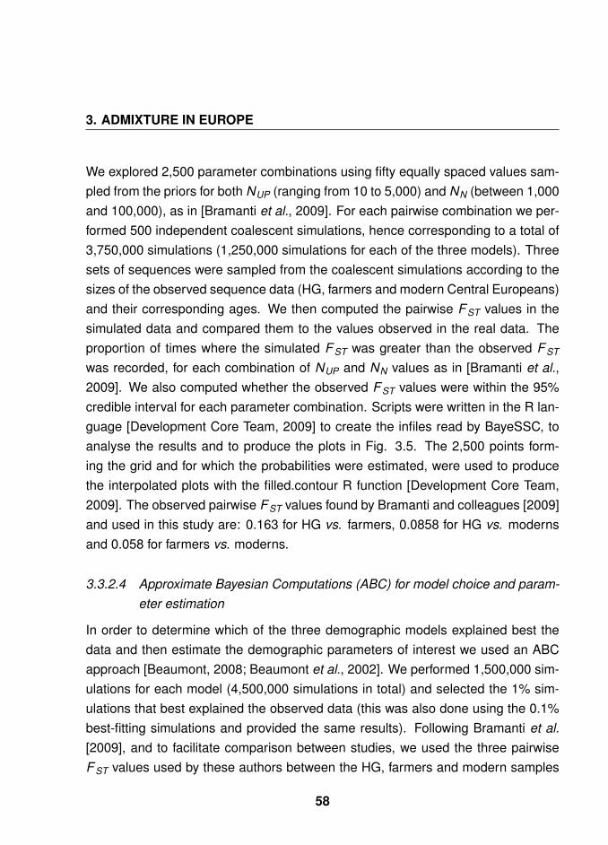
3. ADMIXTURE IN EUROPE
We explored 2,500 parameter combinations using fifty equally spaced values sam-pled from the priors for both NUP (ranging from 10 to 5,000) and NN (between 1,000and 100,000), as in [Bramanti et al., 2009]. For each pairwise combination we per-formed 500 independent coalescent simulations, hence corresponding to a total of3,750,000 simulations (1,250,000 simulations for each of the three models). Threesets of sequences were sampled from the coalescent simulations according to thesizes of the observed sequence data (HG, farmers and modern Central Europeans)and their corresponding ages. We then computed the pairwise F ST values in thesimulated data and compared them to the values observed in the real data. Theproportion of times where the simulated F ST was greater than the observed F ST
was recorded, for each combination of NUP and NN values as in [Bramanti et al.,2009]. We also computed whether the observed F ST values were within the 95%credible interval for each parameter combination. Scripts were written in the R lan-guage [Development Core Team, 2009] to create the infiles read by BayeSSC, toanalyse the results and to produce the plots in Fig. 3.5. The 2,500 points form-ing the grid and for which the probabilities were estimated, were used to producethe interpolated plots with the filled.contour R function [Development Core Team,2009]. The observed pairwise F ST values found by Bramanti and colleagues [2009]and used in this study are: 0.163 for HG vs. farmers, 0.0858 for HG vs. modernsand 0.058 for farmers vs. moderns.
3.3.2.4 Approximate Bayesian Computations (ABC) for model choice and param-eter estimation
In order to determine which of the three demographic models explained best thedata and then estimate the demographic parameters of interest we used an ABCapproach [Beaumont, 2008; Beaumont et al., 2002]. We performed 1,500,000 sim-ulations for each model (4,500,000 simulations in total) and selected the 1% sim-ulations that best explained the observed data (this was also done using the 0.1%best-fitting simulations and provided the same results). Following Bramanti et al.[2009], and to facilitate comparison between studies, we used the three pairwiseF ST values used by these authors between the HG, farmers and modern samples
58

3.3 Material and Methods
as summary statistics. The simulations were performed with the BayeSCC pro-gram, but contrary to the previous section we did not use a grid of values but ratherproper a priori distributions. The ABC inference procedure was performed usingthe abc R package [Csillery et al., 2010]. The postpr function was used to selectthe best model (estimate the posterior probability of each of the three models). Thiswas done using two approaches (i) the Beaumont et al. [2008](2008) multinomiallogistic regression (MLR) model, and (ii) the nonlinear conditional heteroscedas-tic (NCH) model that uses a neural network approach [Blum & François, 2009].The latter approach uses a non-linear regression correction to minimize departurefrom non-linearity, that enhances accuracy when compared to the regression algo-rithm proposed by Beaumont et al. [2002; 2010]. For the model that was selectedwe then we estimated the selected model’s parameters of interest (NUP and NN),using the 1% simulations (15,000 values) associated with the shortest Euclidiandistances from the observed data. The NCH regression-ABC method, proposed by(Blum and François, 2010), jointly with a logit transformation, was used to estimatethe parameters based on the observed and simulated pairwise F ST values.The model selection approach was validated by calculating the power to recover thetrue model. For that, we took randomly 1,000 datasets, from the original BayeSSCruns for ABC analysis, for each of the three demographic models. We thus assignedeach of these datasets to a model, by using again the function postpr. However,this time we used the pairwise F ST values of the simulated datasets as pseudo-observed summary statistics. Finally, we counted the number of times that the truemodel was correctly identified (see appendix Table A.1).
59

3. ADMIXTURE IN EUROPE
Figure 3.1 (facing page): Spatial variation of admixture and drift, across Europe- In (A) are represented the posterior distributions of the Palaeolithic contribution (HGcontribution to modern European), for each of the European populations analysed,using mtDNA data. Each curve corresponds to the analysis of a specific hybrid pop-ulation (Armenia – red, Caucasus – dashed red, Azeri – dotted red, Egypt – dotdashred, Iran – twodash red, Central Mediterranean – black, East Mediterranean – dashedblack, West Mediterranean – dotted black, Southeast Europe – green, North and Cen-tral Europe – blue, Northeast Europe – dashed blue, Northwest Europe – dotted blue,Alps, dotdash blue and Scandinavia – aquamarine). (B) Linear regression of Neolithiccontribution, against geographical distance from Near East, using mtDNA data. Meanvalues for each population are represented by solid circles (mtDNA data) and opentriangles and circles (for two different NRY datasets, Rosser et al. [2000] and Seminoet al. [2000], respectively). In (C) is represented the linear regression of th (drift in theadmixed populations) against geographic distance from the Near East for mtDNA data.The close-up shows the mtDNA regression on a different scale for the Y-axis. Meanvalues for each population are represented both for mtDNA and NRY datasets, withthe symbol codes as in (B). Calibrated radiocarbon dates of Neolithic archaeologicalsites [Pinhasi et al., 2005] (see also table A.2) are also plotted against the distancefrom the Near East (blue open circles), with the linear regression represented by theblue line.
60

3.3 Material and Methods
0.0
0.2
0.4
0.6
0.8
1.0
0.00.51.01.52.02.53.0
Pal
aeol
ithic
con
trib
utio
n
density(A)
1000
2000
3000
4000
0.00.20.40.60.81.0
Dis
tanc
e fr
om N
ear
Eas
t (km
)
Neolithic contribution
●
●
●
●
●
●
●
●
●
●
●●
●
●
●
●
●●
●
●●
●●
●
●
●
●●●
(B)
1000
2000
3000
4000
0.00.20.40.60.81.0
Dis
tanc
e fr
om N
ear
Eas
t (km
)
th
●●
●●
●●
●●
●
●
●
●
●
●
●
●
●●
●
●
●
●
●●
●
●
●●●
(C)
●●
●
●
●
●
●
●
●
●
●
●
●
●
●
●●
●
●
●
●
8642
KYr (cal BP)
500
1500
2500
3500
0.000.040.08
●
●●
●●
●
●
●
●
61

3. ADMIXTURE IN EUROPE
3.4 Results
3.4.1 Admixture analyses: The Neolithic contribution decreases withdistance from the Near-East, for both NRY and mtDNA data
Figures 3.1A (mtDNA) and A.2 (NRY) show the posterior distributions for p1, thePalaeolithic contribution to the European populations analysed. As expected fromsimulations [Chikhi et al., 2001; Sousa et al., 2009], the distributions are ratherwide and each single population estimate has a large standard error, confirmingthat population genetic parameters estimated using single locus data are rarelyvery accurate. Nevertheless, when all populations are considered jointly, a cleargeographic pattern is seen in both the new NRY and mtDNA (Fig. 3.1B) datasets.This pattern shows that the proportion of Neolithic genes (1 - p1) decreases frommodal values of around 100% in Greece and Cyprus, to 75% in Romania, 30% inFrance and 20% in Spain (Fig. 3.1B). This confirms previous results theat usedanother independent NRY data set [Chikhi et al., 2002]. This trend is detectedfor the first time in mtDNA data, which have repeatedly been claimed to exhibitno SE-NW spatial pattern [Richards et al., 2000, 2002]. Fig. 3.1B shows that thethree (two NRY and one mtDNA) datasets produce the same general trend, hencesupporting a parallel decrease of female and male lineages from Neolithic farmersin the genome of modern Europeans, as we move away from the Near-East.
3.4.2 The Neolithic transition in the Caucasus and European islands:NRY admixture analyses
Another set of new results is found with the NRY samples from the Caucasus (Ar-menia, Georgia and Ossetia). First, the admixture level of these populations is ex-actly at the level expected if they had been on a SE-NW expansion axis (i.e. alongthe general direction of farmers expansion towards Europe during the Neolithic),even though they are geographically located NE of the Fertile Crescent and not NW(Fig. A.3A). Second, when the Caucasus data are analysed independently from therest of the data, we find a significant geographical trend, as expected if agriculture
62

3.4 Results
has expanded demically from the Near East outwards in several directions, i.e. notjust towards Europe (Fig. A.4A), as predicted by Renfrew [1991]. Third, the sameanalysis performed using populations that are unlikely to have played a major roleduring the Neolithic transition, due to their geographic location (i.e. negative con-trols, see SI Material and Methods) exhibit no such trend despite their much largersample sizes (Fig. A.3B). Fourth, contrary to the negative controls used, severalEuropean islands population samples (Cyprus, Sardinia, Ireland and British Islespopulations ) appear to also fit within the general decrease in admixture across Eu-rope (Fig. A.4B). Thus, we find clines in in the Caucasus and European Islands,but not in populations from the Eastern/ Northern Europe.
3.4.3 Drift in paternal and maternal lineages: NRY and mtDNA datasupport the DDM but not the same demographic histories
Genetic drift is represented by parameter t i that represents t i the ratio of T, the timesince the admixture event, and N i the effective size of population i (see Fig.1.6).Thus, genetic drift in the different parental populations is represented by the pa-rameters t1 and t2 for the Palaeolithic and Neolithic populations, respectively. Eachof the t1 and t2 posterior distributions is obtained independently by the analysis ofone European population (Fig. A.5A-B, A.6A-B). First, we find that the t1 posteriorvalues are always higher than the t2 values suggesting that genetic drift has beenmore important in the ‘Palaeolithic’ than in the ‘Neolithic’ parental population, inagreement with a later population size increase related with the arrival of agricul-ture. Second, for all the European populations analysed the t1 (and t2) posteriordistributions are tightly clustered, rather than spread out, even though each anal-ysis is performed independently. Third, the different t1 posterior values are morediverse (i.e. less clustered) than the t2 distributions, which is expected if the earlyHG populations were differentiated, due to their smaller effective sizes. Fourth, thet1 and t2 posteriors obtained for the mtDNA datasets support much lower valuesthan the corresponding NRY t1 and t2 posteriors, suggesting a much larger female(N f) than male (Nm) population effective size and/or higher female gene flow.
63

3. ADMIXTURE IN EUROPE
Fifth, Fig. 3.1C shows the results for the parameter th which represents drift
●
●●
● ●
●
●
●●
●●
●
●
0 1000 2000 3000 4000 5000
0.0
0.2
0.4
0.6
0.8
1.0
Distance from Near East (km)
He
●●
●●●
●●
●
●
●
●●
●
●●
●●
●
●
●
●
●
●
●
●
●
●
●
Figure 3.2: Genetic diversity across Europe - Expected heterozygozyty He valuesfor each European population analysed are regressed against the geographic distancefrom the Near East, both for NRY (solid circles) and mtDNA (open circles). The lin-ear regressions calculated from these points are represented by the solid (NRY) anddashed (mtDNA) lines.
in the different European populations since the admixture event. We find that forNRY data, th is positively correlated with distance from the Near-East and with theearliest date of arrival of agriculture in the different locations based on archaeolog-ical artefacts (i.e. drift increases for European populations that had a HG lifestylefor a longer period and admixed later). Sixth, for the mtDNA data, the geograph-ical trend is very different. Similarly low th values are observed in the Near-East,but instead of increasing with distance they exhibit (almost) no trend (see close-
64

3.4 Results
● ●●
●●
●
●
●
●
●
●
●
●
0 1000 2000 3000 4000 5000
0.00
0.05
0.10
0.15
0.20
Distance from Near East (km)
FS
T
●●
●
● ●
●
●
●
●
●
●
●
●
●
●
●
●
●●
●
●
●
●
●
●
●
●
●
Figure 3.3: Genetic differentiation across Europe - Each point represents pairwiseF ST values, between European populations and the Near East, regressed against dis-tance from the latter. The symbol and line codes are as in Fig. 3.2.
up in Fig. 3.1C showing a decrease). It thus appears that the mtDNA and NRYth results require different explanations for the demographic history of males andfemales, while favouring both the DDM. Seventh, differences between males andfemales are also observed when measures of genetic diversity (He) and differen-tiation (F ST) are regressed against geographic distance from the Near-East. FormtDNA, genetic differentiation between Europeans and Near Easterners increasesmuch less with increasing geographical distance than for NRY data (Fig. 3.2). Inagreement with this trend, differences in diversity levels are also less important inmtDNA than in NRY data (Fig.3.3). Both support a higher effective population sizeof females and/or higher female migration rates.
65

3. ADMIXTURE IN EUROPE
3.4.4 Ancient DNA, coalescent simulations and model identificationusing ABC
Figure 3.4 represents the three demographic scenarios tested together with theirposterior probabilities, using two ABC model choice algorithms on aDNA data [Bra-manti et al., 2009]. Whether we use the multinomial logistic regression (MLR)method of Beaumont [2008] or the non-linear heteroscedastic neural network (NCH)approach of Blum and François [2009], the support for the Total Panmixia (TP)model is nil, whereas the best supported model, with a posterior probability> 0.957,is the Split with Differential Growth (SDG) model which assumes a differentialgrowth between Neolithic and Palaeolithic farmers. These results suggest thatstructure is required between HG and farmers to explain the observed data (SDGand S (Split) versus TP) and that differential growth is also required (SDG versusS). Furthermore, the parameters estimated for the SDG suggest that the growthrate in the HG populations, during the Palaeolithic, was very low or null (see table
Figure 3.4 (facing page): Demographic models used in the aDNA analysis andtheir posterior probabilities - Three different demographic models were tested usingancient and modern mtDNA data. In the Total Panmixia (TP) model (A), HG and farm-ers were part of the same panmictic population over Central Europe and were neverseparated in different populations or communities. This is the model used by Bramantiet al. [2009] and assumes a single modern female effective population size NM andtwo periods of exponential growth: i) the first starting with an Upper Palaeolithic (UP)population of effective size NUP, sampled from an ancestral African female popula-tion of constant size, corresponding to the initial colonization of Central Europe 45,000years ago and ii) the second following the Neolithic Transition 7,500 years ago, froma population of effective size NN. Both NUP and NN population sizes were allowed tovary using the same priors as in [Bramanti et al., 2009]. In the Split Model (S) (B),the UP population was structured in two sub-populations of equal size, 45,000 yearsago. These sub-populations were assumed to grow independently (no gene flow), untilthey joined together at the beginning of the Neolithic, in Central Europe. The Split withDifferential Growth (SDG) model (C) is similar to the S model but has a more complexsplitting, in which one of the two sub-populations was allowed to have a higher growthrate between 10,000 and 7,500 years ago. In (D) are represented the posterior proba-bilities under each model, calculated using the ABC framework, for two different typesof post-rejection adjustments: multinomial logistic regression (MLR: white bars) andnon-linear heteroscedastic neural network (NCH: grey bars).
66

3.4 Results
(A)
Tota
l P
anm
ixia
(T
P)
(B)
Split
(S
) (C
) S
plit
with D
iffe
rential G
row
th
(S
DG
)
NN
NM
NU
P
NN
NM
NU
P
NN
NM
NU
P
Pre
se
nt T
(D)
67

3. ADMIXTURE IN EUROPE
3.1).
Table 3.1: Demographic parameters estimated under the Split with DifferentialGrowth (SDG) model. Weighted (ω) median, 5% and 95% percentiles values arerepresented for NN and NUP. Deme 1 and 2 correspond to the demes without and withdifferential growth, respectively (see Fig. A.1).
ω Median ω 5% Perc. ω 95% Perc. Prior
NNTotal 18 374.80 3 529.00 77 274.60 U: 1 000 – 100 000Deme 1 967.10 185.74 4 067.09Deme 2 17 407.70 3 343.26 73 207.51NUPTotal 2 248.12 297.64 4 717.56 U: 10 – 5 000Deme 1 1 124.06 148.82 2 358.78Deme 2 1 124.06 148.82 2 358.78
Table 3.2: Probability of simulated F ST values being higher than observed ones(PS > O), in the aDNA analysis. Maximum values of PS > O, for each of the models andpairwise comparisons analysed in this study.
Models PS > OHG v.s. Farmers HG v.s. Modern Farmers v.s. Modern
TP (this study) 0.018 0.032 0.152TP [Bramanti et al., 2009] 0.022 0.028 –S 0.132 0.278 0.192SDG 0.990 1.000 0.612
The same kind of results, but using another approach, is showed in Fig. 3.5. Thisfigure represents the estimated probability of obtaining F ST values that are equalor higher than those observed in the real data (PS > O), for the three scenarios.The data simulated under the TP model (Fig. 3.5A-C) show results identical tothose obtained by Bramanti and colleagues [2009], hence validating our simulationapproach and the exagerated simplicity of the model used by these authors. Forthis model, the parameter space explaining the observed data is extremely limited.However, as soon as structure is incorporated in the models (S and SDG), the
68
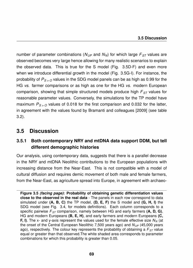
3.5 Discussion
number of parameter combinations (NUP and NN) for which large F ST values areobserved becomes very large hence allowing for many realistic scenarios to explainthe observed data. This is true for the S model (Fig. 3.5D-F) and even morewhen we introduce differential growth in the model (Fig. 3.5G-I). For instance, theprobability of PS > O values in the SDG model panels can be as high as 0.99 for theHG vs. farmer comparisons or as high as one for the HG vs. modern Europeancomparison, showing that simple structured models produce high F ST values forreasonable parameter values. Conversely, the simulations for the TP model havemaximum PS > O values of 0.018 for the first comparison and 0.032 for the latter,in agreement with the values found by Bramanti and colleagues [2009] (see table3.2).
3.5 Discussion
3.5.1 Both contemporary NRY and mtDNA data support DDM, but telldifferent demographic histories
Our analysis, using contemporary data, suggests that there is a parallel decreasein the NRY and mtDNA Neolithic contributions to the European populations withincreasing distance from the Near-East. This is not compatible with a model ofcultural diffusion and requires demic movement of both male and female farmers,from the Near-East, as agriculture spread into Europe, in agreement with archaeo-
Figure 3.5 (facing page): Probability of obtaining genetic differentiation valuesclose to the observed in the real data - The panels in each row correspond to datasimulated under (A, B, C) the TP model, (D, E, F) the S model and (G, H, I) theSDG model (see Fig. 3.4, for models definitions). Each column corresponds to aspecific pairwise F ST comparison, namely between HG and early farmers (A, D, G),HG and modern Europeans (B, E, H), and early farmers and modern Europeans (C,F, I). The x- and y-axis represent the values used for the female effective size NN (atthe onset of the Central European Neolithic 7,500 years ago) and NUP (45,000 yearsago), respectively. The colour key represents the probability of obtaining a F ST valueequal or greater than that observed.The white shaded area corresponds to parametercombinations for which this probability is greater than 0.05.
69

3. ADMIXTURE IN EUROPE
70

3.5 Discussion
logical data [Bocquet-Appel et al., 2009; Gkiasta et al., 2003; Pinhasi et al., 2005].This parallel decrease also suggests that both males and females admixed withthe local Palaeolithic populations that inhabited Europe at the time, resulting in aprogressive dilution of the Near-East genes. We also found that the demic diffu-sion process was centrifugal, with samples from the Caucasus fitting in the generaltrend, as was already suggested by Renfrew [1991] and others [Balanovsky et al.,2011] and in agreement with linguistic data too [Gray & Atkinson, 2003]. Moreover,the European islands appear also to fit within this trend. This suggests that the seadid not represent major barrier to the Neolithic expansion and that the peopling ofthese islands was not subjected to major drift effects or radically different admixturehistories compared to neighbouring continental populations [Bocquet-Appel et al.,2009].It therefore appears that, when we use one coherent statistical framework, bothdatasets from male and female markers (mtDNA [Richards et al., 2000] and NRY[Rosser et al., 2000]), support the DDM. These results are at odds with the originalconclusions drawn by Richards et al. [2000] (i.e. using only mtDNA), who advo-cated that mtDNA data favoured the CDM. However, they are in agreement withthe clines described by Rosser et al. [2000] (i.e. only with NRY data). It is worthnoting that the methods used by the two studies are not comparable. Richards etal. [Richards et al., 2000] used the age of mtDNA mutations and haplogroups todate major demographic events. This kind of approach has been criticised as itcan lead to misinterpretation of the data [Barbujani & Chikhi, 2006; Barbujani et al.,1998; Goldstein & Chikhi, 2002]. Rosser et al. [2000] used spatial autocorrelationmethods instead, to identify statistically significant clines. This method has beensimilarly criticised, as a cline in itself does not indicate the time at which it wasestablished. Model-based approaches, like those applied here, explicitly state theassumptions used to make inference and are probably the most suitable to inferdemographic parameters [Chikhi & Beaumont, 2005; Chikhi et al., 2002; Currat &Excoffier, 2005], such as the Neolithic contribution to European populations.The fact that extant NRY and mtDNA both support the DDM does not imply thatother details of the male and female demography were identical, particularly in re-
71

3. ADMIXTURE IN EUROPE
lation with the amount of drift experienced by each sex [Wilkins, 2006]. Indeed, ourresults point to a higher N f over Nm, in agreement with the larger coalescence timesfor mtDNA [Tang et al., 2002; Wilder et al., 2004]. But before addressing this issueand proposing a model accounting for these results we turn to the aDNA results.
3.5.2 aDNA supports Demic Diffusion
The first aDNA study using model-based approaches, on samples identified as Lin-ear Pottery Culture (LBK), argued in favour of CDM [Haak et al., 2005]. Later, thesame LBK data was compared to samples from Palaeolithic/Mesolithic archaeo-logical sites and modern data from the same region, by Bramanti et al. [2009].They interpreted the genetic differentiation observed in the real data as being toohigh to ‘be explained by population continuity alone’ [2009], hence arguing for aNeolithic immigration in Central Europe. Their study thus disagreed with that un-dertaken previously by Haak et al. [2005]. These studies [Bramanti et al., 2009;Haak et al., 2005] had in common that all DNA samples, ancient and modern alike,were assumed to belong to the same panmictic population (see Fig. 3.4A). Whilethis may seem surprising, the model assumed in these two studies is the one thatwe call Total Panmixia. This model surprisingly assumes that there was no popu-lation structure and that HG and farmers were allowed to mate freely, making thedistinction between HG and farmers unclear.What our new aDNA simulation framework suggests is that it is actually possibleto explain the large genetic differentiation between samples if we explicitly modelboth population structure and different population growth rates between Neolithicand Palaeolithic populations before they admixed. In a recent work, Haak and col-leagues [2010] also allowed for some population structure, namely between pop-ulations of Central Europe and the Near-East. Their results suggested an affinitybetween the first LBK farmers and modern Near-Easterners, but they still could notexplain the high population differentiation encountered between the LBK farmersand present-day Central European populations. On the contrary, our SDG model,could explain the high F ST values encountered between HG and farmers and be-
72

3.5 Discussion
tween farmers (or HG) and modern-day Central Europeans. We believe that themain difference with the Haak et al. study [2010] is that they did not allow variablepopulation growth rates in their simulations. However, by varying the growth ratesbetween HG and farmers, as between the onset of farming and the following period,we could explain these high F ST values.Differential growth between farmers and HG is supported by anthropological andarchaeological data [Galeta & Bruzek, 2009; Shennan, 2009]. Indeed, at the onsetof the Neolithic expansion in the Near-East and in the front of the wave of expan-sion, it has been shown that a very high growth rate is expected from the colonizingpopulations until their size reaches the new carrying capacity ceilings [Shennan,2009]. Interestingly, our estimates suggest that the female growth rate remainedquasi-constant during the Palaeolithic, and that there was an expansion with theadvent of farming, which is also in agreement with archaeological data [Bocquet-Appel et al., 2005; Gignoux et al., 2011]. Such an increase in N f could also beexplained by an increase in gene flow following the arrival of farming, for instance ifit was accompanied by a change in post-marital residence patterns in females.
3.5.3 Towards an integrated model of Neolithic transition
Altogether, the work presented here allows us to draw a coherent integrated modelfor the Neolithic transition in Europe which accounts for both the congruent admix-ture results between mtDNA and NRY data, their difference in terms of diversity anddifferentiation (drift), and the constraints imposed by the aDNA data. On that ba-sis, we propose (i) an establishment of farming communities in Europe by a demicdiffusion process, with an origin in the Near-East, in agreement with archaeological[Bocquet-Appel et al., 2009; Galeta & Bruzek, 2009; Gkiasta et al., 2003; Pinhasiet al., 2005; Price et al., 2001] and anthropological studies [Bentley et al., 2003;Bocquet-Appel, 2002; Pinhasi & von Cramon-Taubadel, 2009], along with a pro-cess of admixture with the local HG [Bentley et al., 2003]; (ii) a spread in differentdirections from the Near-East, with the Caucasus and European Islands being partof this gradual expansion. Furthermore, we propose that (iii) both male and fe-
73

3. ADMIXTURE IN EUROPE
male farmers were involved in this demic movement, and that (iv) the demographichistories of the two sexes were probably different during and perhaps before the Ne-olithic transition. In particular, we propose that the difference in the amount of driftexperienced by males and females can be explained by a change in the patternsof gene flow and by a shift in human mating systems, from polygyny to monogamyduring to the Neolithic transition. Below we go through the rationale and data thatcorroborate this scenario.As noted above, one of our main results is that N f > Nm and/or that migration rateswere higher in females compared with males (Fig. 3.1C). Anthropological, linguis-tic and archaeological evidence suggest that the transition from hunting-gatheringto farming or herding communities usually leads to an increase in patrilocality (i.e.when the marital residence is the groom’s birthplace) due to the fact that malestend to control and inherit wealth (i.e the land or the herds), hence leading to higherfemale migration rates [Baker & Jacobsen, 2006; Bentley et al., 2002, 2008; Cavalli-Sforza & Minch, 1997; Fortunato & Jordan, 2010; Haak et al., 2008; Langergraberet al., 2007]. Given that forager communities do not accumulate wealth, migrationpatterns are more likely to be symmetrical, and this is indeed what has been ob-served. In other words, sedentism that accompanied the Neolithic transition [Bell-wod & Oxenham, 2008] is expected to have led to a decrease in male gene flow,whereas female gene flow would either have remained constant or would have in-creased to compensate the decrease in male gene flow. This would explain twoof our results, namely the higher mtDNA diversity, the higher NRY differentiation,and the higher difficulty found by several authors to identify clines in mtDNA data,compared to NRY. Interestingly, this would also be in agreement with the larger co-alescent times described for mtDNA compared to NRY [Tang et al., 2002; Wilderet al., 2004] and would partly explain the results and interpretation of Richard et al.[2000].Another cultural change that is thought to have taken place in Europe during theNeolithic transition is a shift from polygyny to monogamy [Fortunato, 2011; Lager-löf, 2010]. In fact, several Neolithic burials [Bentley et al., 2008; Haak et al., 2008]show evidences of nuclear families, which may reflect a monogamous marriage
74

3.5 Discussion
system. A shift from polygyny to monogamy would have the effect of decreas-ing male variance in reproductive success, since more males would now be ableto mate, and consequently would increase the effective population size of males.This could result in a signal of population growth in NRY data that would be morerecent compared to that observed in mtDNA and is exactly what Dupanloup andcolleagues [2003] have argued and found. Our results are in good agreement withtheirs. Indeed, we found that th increased in males but not in females as we movedaway from the Near East (Fig. 3.1C), with th being the ratio of T, the time sincethe admixture event, and Nh, the effective size of the admixed population. Giventhat T necessarily decreases as we move away from the Near East, an increaseof this ratio suggests that the decrease of T was compensated by a rapid increasein Nh. In other words, the admixture process between HG and farmers led to avery rapid increase in the effective population size of male whereas this increasewas more limited in females. Indeed, a shift from polygyny to monogamy wouldhave less influence on N f, which would anyway be higher than that of males, due totheir lower variance in reproductive success. Altogether, a model in which humansocieties began to adopt farming as a means of subsistence, with the correlatedpatrilocality and monogamy as a mating system, would be in agreement with all theresults presented here, including the aDNA (for instance, it was rather impressive tofind that the most probable scenarios, independently inferred no significant growthin Palaeolithic females), and allow us to put in a single picture, results from severalgenetic and anthropological studies.While we claim that a more coherent picture emerges from our results, we can-not claim that other scenarios could not also explain the results. Many layers ofcomplexities could be added. For instance, female hypergamy (i.e. the fact thatlower social status women are more likely to mate with males from a higher statusthan the opposite) has been described in several human migration and colonizationevents [Quintana-Murci et al., 2008; Salzano, 2004; Thomas et al., 2006], and it isbelieved that it probably happened during the Neolithic transition in Europe [Bent-ley et al., 2003], with HG females marrying into farmer communities [Bentley et al.,2009]. Qualitatively, female hypergamy would increase female mobility and lead to
75

3. ADMIXTURE IN EUROPE
low levels of mtDNA genetic differentiation between populations. Thus, one shouldexpect lower mtDNA gradients and (almost) no geographic trend in drift, which isexactly what we see. The exclusion of HG males would lead to an increase ofNRY genetic differentiation, explaining the clear geographic trend found in geneticdrift. However, we must add that this scenario, which may indeed have taken place,would not as easily fit with the admixture patterns that we find and which are similarin males and females. Thus, at this stage, we would be cautious before arguing foror against female hypergamy. We should also insist on the fact that the patternsidentified here correspond to global patterns, and are not in contradiction with re-gional studies arguing against the demic diffusion. Several processes are likely tohave taken place during the millennia corresponding to the arrival of farming com-munities in Europe. Similarly, it is increasingly clear that different routes (coastalor continental) were followed by different groups of humans. Still, the genetic datapoint to a major input from Near-eastern populations. This cannot be explained bycultural diffusion at a European scale, and as we have argued repeatedly, usingthe age of haplogroups or haplotypes to reconstruct human prehistory still awaitsformal validation, despite the large literature that uses it [Barbujani & Chikhi, 2006;Barbujani et al., 1998; Chikhi, 2009].
3.6 ConclusionOur study represents the first attempt to integrate contemporary mtDNA and NRYdata, together with aDNA. This has allowed us to draw a coherent picture of the Ne-olithic Transition in Europe, which not only provides an explanation for the patternsof genetic diversity found today and in our past, but also for the apparent contra-diction between phylogeographic and model-based studies. The aDNA modellingapproach described here could be applied to other aDNA datasets and we are ap-plying it to unpublished data from an Iberian Neolithic population (see apendix B).The results from these independent data appear to validate the suggestion thatstructured models with varying growth rates explain better the genetic distancesobserved between ancient and modern DNA than simpler models. The Neolithic
76

3.7 References
transition in Europe is one of the most studied periods of human prehistory andthe source of much debate. It is our hope that the work presented here may helpprovide a consistent framework to address certain aspects of this ‘long-standing’controversy.
AcknowledgementsThe authors are grateful to C. van Schaik, A. Coutinho, G. Gomes, V. Sousa, J. Salmona, J.Alves, C. Gamba and S. Davis for useful comments on earlier versions of this manuscript.The simulations were partly carried out on the HULK simulation server (European Com-mission grant MEXT-CT-2004-14338 to G. Gomes) and on the HERMES High PerformanceComputing Centre (FCT grant H200741/re-equip/2005 to P. Fernandes). R.R. was sup-ported by FCT grant (ref. SFRH/BD/30821/2006). L.C. was partly funded by the CNRS andthe FCT grant PTDC/BIA-BDE/71299/2008. Travels between Toulouse and Lisbon weremade possible thanks to A Coutinho, E. Danchin, C. Thébaud and B Crouau-Roy. A. Barelliis also thanked for her support.
3.7 ReferencesAMMERMAN, A.J. & CAVALLI-SFORZA, L.L. (1984). The Neolithic transition and the genet-
ics of populations in Europe. Princeton University Press, Princeton.ANDERSON, C.N.K., RAMAKRISHNAN, U., CHAN, Y.L. & HADLY, E.A. (2005). Serial sim-
COAL: a population genetics model for data from multiple populations and points in time.Bioinformatics, 21, 1733–4.
BAKER, M. & JACOBSEN, J. (2006). A human capital-based theory of postmarital residencerules. J Law Econ Organ, 23, 208–241.
BALANOVSKY, O., DIBIROVA, K., DYBO, A., MUDRAK, O., FROLOVA, S., POCHESHKHOVA,E., HABER, M., PLATT, D., SCHURR, T., HAAK, W., KUZNETSOVA, M., RADZHABOV, M.,BALAGANSKAYA, O., ROMANOV, A., ZAKHAROVA, T., SORIA HERNANZ, D.F., ZALLOUA,P., KOSHEL, S., RUHLEN, M., RENFREW, C., WELLS, R.S., TYLER-SMITH, C. & AND,E.B. (2011). Parallel evolution of genes and languages in the Caucasus region. Mol BiolEvol .
BALARESQUE, P., BOWDEN, G., ADAMS, S., LEUNG, H., KING, T., ROSSER, Z., GOOD-WIN, J., MOISAN, J., RICHARD, C., MILLWARD, A. et al. (2010). A predominantly Ne-olithic origin for European paternal lineages. PLoS biology , 8, e1000285.
77

3. ADMIXTURE IN EUROPE
BALTER, M. (2009). Archaeology: ancient DNA says Europe’s first farmers came from afar.Science, 325, 1189.
BARBUJANI, G. & CHIKHI, L. (2006). Population genetics: DNAs from the European Ne-olithic. Heredity , 97, 84–85.
BARBUJANI, G., BERTORELLE, G., CAPITANI, G. & SCOZZARI, R. (1995a). Geographicalstructuring in the mtDNA of Italians. Proc Natl Acad Sci U S A, 92, 9171–9175.
BARBUJANI, G., SOKAL, R.R. & ODEN, N.L. (1995b). Indo-European origins: a computer-simulation test of five hypotheses. Am J Phys Anthropol , 96, 109–32.
BARBUJANI, G., BERTORELLE, G. & CHIKHI, L. (1998). Evidence for Paleolithic and Ne-olithic gene flow in Europe. Am J Hum Genet , 62, 488–492.
BEAUMONT, M. (2008). Joint determination of topology, divergence time, and immigration inpopulation trees, 135–154. McDonald Institute for Archaeological Research, Cambridge.
BEAUMONT, M.A., ZHANG, W. & BALDING, D.J. (2002). Approximate Bayesian Computa-tion in population genetics. Genetics, 162, 2025–35.
BEAUMONT, M.A., NIELSEN, R., ROBERT, C., HEY, J., GAGGIOTTI, O., KNOWLES, L.,ESTOUP, A., PANCHAL, M., CORANDER, J., HICKERSON, M., SISSON, S.A., FAGUNDES,N., CHIKHI, L., BEERLI, P., VITALIS, R., CORNUET, J.M., HUELSENBECK, J., FOLL, M.,YANG, Z., ROUSSET, F., BALDING, D. & EXCOFFIER, L. (2010). In defence of model-based inference in phylogeography. Mol Ecol , 19, 436–446.
BELLE, E.M.S., LANDRY, P.A. & BARBUJANI, G. (2006). Origins and evolution of the Eu-ropeans’ genome: evidence from multiple microsatellite loci. Proc R Soc B, 273, 1595–1602.
BELLWOD, P. & OXENHAM, M. (2008). The expansions of farming societies and the role ofthe Neolithic Demographic Transition, 13–34. Springer.
BELLWOOD, P. (2004). First Farmers: the origins of agricultural societies. Blackwell Pub-lishing, Oxford.
BENTLEY, R.A., PRICE, T.D., LÜNING, J., GRONENBORN, D., WAHL, J. & FULLAGAR, P.D.(2002). Human migration in early Neolithic Europe. Curr Anthropol , 43, 799–804.
BENTLEY, R.A., CHIKHI, L. & PRICE, T.D. (2003). The Neolithic transition in Europe: com-paring broad scale genetic and local scale isotopic evidence. Antiquity , 77, 63–66.
BENTLEY, R.A., WAHP, J., PRICE, T.D. & ATKINSON, T.C. (2008). Isotopic signatures andhereditary traits: snapshot of a Neolithic community in Germany. Antiquity , 82, 290–304.
BENTLEY, R.A., LAYTON, R.H. & TEHRANI, J. (2009). Kinship, marriage, and the geneticsof past human dispersals. Hum Biol , 81, 159–79.
BLUM, M.G.B. & FRANÇOIS, O. (2009). Non-linear regression models for Approximate
78

3.7 References
Bayesian Computation. Stat Comput , 20, 63–73.BOCQUET-APPEL, J.P. (2002). Paleoanthropological traces of a Neolithic demographic tran-
sition. Curr Anthropol , 43, 637–650.BOCQUET-APPEL, J.P., DEMARS, P.Y., NOIRET, L. & DOBROWSKY, D. (2005). Estimates of
Upper Palaeolithic meta-population size in Europe from archaeological data. J ArchaeolSci , 32, 1656–1668.
BOCQUET-APPEL, J.P., NAJI, S., LINDEN, M.V. & KOZLOWSKI, J.K. (2009). Detection ofdiffusion and contact zones of early farming in Europe from the space-time distributionof 14C dates. J Archaeol Sci , 36, 807–820.
BRAMANTI, B., THOMAS, M.G., HAAK, W., UNTERLAENDER, M., JORES, P., TAMBETS,K., ANTANAITIS-JACOBS, I., HAIDLE, M.N., JANKAUSKAS, R., KIND, C.J., LUETH, F.,TERBERGER, T., HILLER, J., MATSUMURA, S., FORSTER, P. & BURGER, J. (2009).Genetic discontinuity between local hunter-gatherers and central Europe’s first farmers.Science, 326, 137–140.
BRION, M., SALAS, A., GONZÁLEZ-NEIRA, A., LAREU, M.V. & CARRACEDO, A. (2003).Insights into Iberian population origins through the construction of highly informative Y-chromosome haplotypes using biallelic markers, STRs, and the MSY1 minisatellite. AmJ Phys Anthropol , 122, 147–161.
CAVALLI-SFORZA, L.L. (1998). The Basque population and ancient migrations in Europe.Munibe (Antropología-Arqueología), 6 (Suppl), 129–137.
CAVALLI-SFORZA, L.L. & MINCH, E. (1997). Paleolithic and Neolithic lineages in the Euro-pean mitochondrial gene pool. Am J Hum Genet , 61, 247–254.
CHIKHI, L. (2009). Update to Chikhi et al.’s "Clinal variation in the nuclear DNA of euro-peans" (1998): genetic data and storytelling–from archaeogenetics to astrologenetics?Hum Biol , 81, 639–643.
CHIKHI, L. & BEAUMONT, M.A. (2005). Modelling human genetic history . John Wiley, NewYork.
CHIKHI, L., DESTRO-BISOL, G., BERTORELLE, G., PASCALI, V. & BARBUJANI, G. (1998).Clines of nuclear DNA markers suggest a largely Neolithic ancestry of the Europeangene pool. Proc Natl Acad Sci U S A, 95, 9053–9058.
CHIKHI, L., BRUFORD, M.W. & BEAUMONT, M.A. (2001). Estimation of admixture pro-portions: a likelihood-based approach using Markov chain Monte Carlo. Genetics, 158,1347–1362.
CHIKHI, L., NICHOLS, R.A., BARBUJANI, G. & BEAUMONT, M.A. (2002). Y genetic datasupport the Neolithic demic diffusion model. Proc Natl Acad Sci U S A, 99, 11008–11013.
79

3. ADMIXTURE IN EUROPE
CSILLERY, K., FRANCOIS, O. & BLUM, M.G.B. (2010). abc: estimation and model selectionwith Approximate Bayesian Computation (ABC).
CURRAT, M. & EXCOFFIER, L. (2005). The effect of the Neolithic expansion on Europeanmolecular diversity. Proc R Soc B, 272, 679–688.
DEVELOPMENT CORE TEAM, R. (2009). R: A language and environment for statistical com-puting.
DUPANLOUP, I., PEREIRA, L., BERTORELLE, G., CALAFELL, F., PRATA, M.J., AMORIM,A. & BARBUJANI, G. (2003). A recent shift from polygyny to monogamy in humans issuggested by the analysis of worldwide Y-chromosome diversity. J Mol Evol , 57, 85–97.
DUPANLOUP, I., BERTORELLE, G., CHIKHI, L. & BARBUJANI, G. (2004). Estimating theimpact of prehistoric admixture on the genome of Europeans. Mol Biol Evol , 21, 1361–1372.
EXCOFFIER, L., NOVEMBRE, J. & SCHNEIDER, S. (2000). SimCoal: a general coalescentprogram for the simulation of molecular data in interconnected populations with arbitrarydemography. J Hered , 91, 506–9.
FAGUNDES, N.J.R., RAY, N., BEAUMONT, M., NEUENSCHWANDER, S., SALZANO, F.M.,BONATTO, S.L. & EXCOFFIER, L. (2007). Statistical evaluation of alternative models ofhuman evolution. Proc Natl Acad Sci U S A, 104, 17614–9.
FORTUNATO, L. (2011). Reconstructing the history of marriage strategies in Indo-European-speaking societies: monogamy and polygyny. Hum Biol , 83, 87–105.
FORTUNATO, L. & JORDAN, F. (2010). Your place or mine? a phylogenetic comparativeanalysis of marital residence in Indo-European and Austronesian societies. Philos TransR Soc B, 365, 3913–22.
FRANCALACCI, P., MORELLI, L., UNDERHILL, P.A., LILLIE, A.S., PASSARINO, G., USELI,A., MADEDDU, R., PAOLI, G., TOFANELLI, S., CALÒ, C.M., GHIANI, M.E., VARESI,L., MEMMI, M., VONA, G., LIN, A.A., OEFNER, P. & CAVALLI-SFORZA, L.L. (2003).Peopling of three mediterranean islands (corsica, sardinia, and sicily) inferred by y-chromosome biallelic variability. Am J Phys Anthropol , 121, 270–279.
FRAUMENE, C., BELLE, E.M.S., CASTRÌ, L., SANNA, S., MANCOSU, G., COSSO, M.,MARRAS, F., BARBUJANI, G., PIRASTU, M. & ANGIUS, A. (2006). High resolution anal-ysis and phylogenetic network construction using complete mtDNA sequences in sar-dinian genetic isolates. Mol Biol Evol , 23, 2101–2111.
GALETA, P. & BRUZEK, J. (2009). Demographic model of the neolithic transition in centralEurope. Documenta Praehistorica, 36 ( Neolithic Studies 16), 139–150.
GIGNOUX, C.R., HENN, B.M. & MOUNTAIN, J.L. (2011). Rapid, global demographic ex-
80

3.7 References
pansions after the origins of agriculture. Proc Natl Acad Sci U S A, 108, 6044–9.GIOVANNINI, A., ZANGHIRATI, G., BEAUMONT, M.A., CHIKHI, L. & BARBUJANI, G. (2009).
A novel parallel approach to the likelihood-based estimation of admixture in populationgenetics. Bioinformatics, 25, 1440–1441.
GKIASTA, M., RUSSELL, T., SHENNAN, S. & STEELE, J. (2003). Neolithic transition inEurope: the radiocarbon revisited. Antiquity , 77, 45–62.
GOLDSTEIN, D.B. & CHIKHI, L. (2002). Human migrations and population structure: whatwe know and why it matters. Annu Rev Genomics Hum Genet , 3, 129–152.
GRAY, R.D. & ATKINSON, Q.D. (2003). Language-tree divergence times support the Ana-tolian theory of Indo-European origin. Nature, 426, 435–9.
HAAK, W., FORSTER, P., BRAMANTI, B., MATSUMURA, S., BRANDT, G., TÄNZER, M.,VILLEMS, R., RENFREW, C., GRONENBORN, D., ALT, K.W. & BURGER, J. (2005). An-cient DNA from the first european farmers in 7500-year-old neolithic sites. Science, 310,1016–1018.
HAAK, W., BRANDT, G., DE JONG, H.N., MEYER, C., GANSLMEIER, R., HEYD, V.,HAWKESWORTH, C., PIKE, A.W.G., MELLER, H. & ALT, K.W. (2008). Ancient DNA,strontium isotopes, and osteological analyses shed light on social and kinship organiza-tion of the later stone age. Proc Natl Acad Sci U S A, 105, 18226–31.
HAAK, W., BALANOVSKY, O., SANCHEZ, J.J., KOSHEL, S., ZAPOROZHCHENKO, V., ADLER,C.J., DER SARKISSIAN, C.S.I., BRANDT, G., SCHWARZ, C., NICKLISCH, N., DRESELY,V., FRITSCH, B., BALANOVSKA, E., VILLEMS, R., MELLER, H., ALT, K.W. & AND, A.C.(2010). Ancient DNA from european early neolithic farmers reveals their Near Easternaffinities. PLoS Biol , 8, e1000536.
LAGERLÖF, N.P. (2010). Pacifying monogamy. J Econ Growth, 15, 235–262.LANGELLA, O., CHIKHI, L. & BEAUMONT, M. (2001). LEA (likelihood-based estimation of
admixture) : a program to simultaneously estimate admixture and the time since admix-ture. Mol Ecol Notes, 1, 357–358.
LANGERGRABER, K.E., SIEDEL, H., MITANI, J.C., WRANGHAM, R.W., REYNOLDS, V.,HUNT, K. & VIGILANT, L. (2007). The genetic signature of sex-biased migration in pa-trilocal chimpanzees and humans. PLoS One, 2, e973.
MALMSTRÖM, H., GILBERT, M.T.P., THOMAS, M.G., BRANDSTRÖM, M., STORA, J., MOL-NAR, P., ANDERSEN, P.K., BENDIXEN, C., HOLMLUND, G., GÖTHERSTRÖM, A. &WILLERSLEV, E. (2009). Ancient DNA reveals lack of continuity between neolithic hunter-gatherers and contemporary scandinavians. Curr Biol , 19, 1758–62.
MENOZZI, P., PIAZZA, A. & CAVALLI-SFORZA, L. (1978). Synthetic maps of human gene
81

3. ADMIXTURE IN EUROPE
frequencies in Europeans. Science, 201, 786–792.MITHEN, S. (2007). Did farming arise from a misapplication of social intelligence? Philos
Trans R Soc Lond B Biol Sci , 362, 705–718.NEI, M. (1977). F-statistics and analysis of gene diversity in subdivided populations. Ann
Hum Genet , 41, 225–233.PINHASI, R. & VON CRAMON-TAUBADEL, N. (2009). Craniometric data supports demic
diffusion model for the spread of agriculture into Europe. PLoS One, 4, e6747.PINHASI, R., FORT, J. & AMMERMAN, A.J. (2005). Tracing the origin and spread of agricul-
ture in Europe. PLoS Biol , 3, e410.PRICE, T.D., BENTLEY, R.A., LÜNING, J., GRONENBORN, D. & WAHL, J. (2001). Prehis-
toric human migration in the Linearbandkeramik of Central Europe. Antiquity , 75, 593–603.
QUINTANA-MURCI, L., QUACH, H., HARMANT, C., LUCA, F., MASSONNET, B., PATIN, E.,SICA, L., MOUGUIAMA-DAOUDA, P., COMAS, D., TZUR, S., BALANOVSKY, O., KIDD,K.K., KIDD, J.R., VAN DER VEEN, L., HOMBERT, J.M., GESSAIN, A., VERDU, P., FRO-MENT, A., BAHUCHET, S., HEYER, E., DAUSSET, J., SALAS, A. & BEHAR, D.M. (2008).Maternal traces of deep common ancestry and asymmetric gene flow between Pygmyhunter-gatherers and Bantu-speaking farmers. Proc Natl Acad Sci U S A, 105, 1596–601.
RASTEIRO, R. & CHIKHI, L. (2009). Revisiting the peopling of Japan: an admixture per-spective. J Hum Genet , 54, 349–354.
RENFREW, C. (1991). Before Babel: Speculations on the Origins of Linguistic Diversity.Camb Archaeol J, 1, 3–23.
RICHARDS, M. (2003). The neolithic invasion of Europe. Annu Rev Anthropol , 32, 135–162.RICHARDS, M., MACAULAY, V., HICKEY, E., VEGA, E., SYKES, B., GUIDA, V., RENGO,
C., SELLITTO, D., CRUCIANI, F., KIVISILD, T., VILLEMS, R., THOMAS, M., RYCHKOV,S., RYCHKOV, O., RYCHKOV, Y., GÖLGE, M., DIMITROV, D., HILL, E., BRADLEY, D.,ROMANO, V., CALÌ, F., VONA, G., DEMAINE, A., PAPIHA, S., TRIANTAPHYLLIDIS, C.,STEFANESCU, G., HATINA, J., BELLEDI, M., RIENZO, A.D., NOVELLETTO, A., OPPEN-HEIM, A., NØRBY, S., AL-ZAHERI, N., SANTACHIARA-BENERECETTI, S., SCOZARI, R.,TORRONI, A. & BANDELT, H.J. (2000). Tracing european founder lineages in the NearEastern mtDNA pool. Am J Hum Genet , 67, 1251–1276.
RICHARDS, M., MACAULAY, V., TORRONI, A. & BANDELT, H.J. (2002). In search of geo-graphical patterns in European mitochondrial DNA. Am J Hum Genet , 71, 1168–1174.
ROSSER, Z.H., ZERJAL, T., HURLES, M.E., ADOJAAN, M., ALAVANTIC, D., AMORIM, A.,
82

3.7 References
AMOS, W., ARMENTEROS, M., ARROYO, E., BARBUJANI, G., BECKMAN, G., BECKMAN,L., BERTRANPETIT, J., BOSCH, E., BRADLEY, D.G., BREDE, G., COOPER, G., CÔRTE-REAL, H.B., DE KNIJFF, P., DECORTE, R., DUBROVA, Y.E., EVGRAFOV, O., GILIS-SEN, A., GLISIC, S., GÖLGE, M., HILL, E.W., JEZIOROWSKA, A., KALAYDJIEVA, L.,KAYSER, M., KIVISILD, T., KRAVCHENKO, S.A., KRUMINA, A., KUCINSKAS, V., LAVINHA,J., LIVSHITS, L.A., MALASPINA, P., MARIA, S., MCELREAVEY, K., MEITINGER, T.A.,MIKELSAAR, A.V., MITCHELL, R.J., NAFA, K., NICHOLSON, J., NØRBY, S., PANDYA, A.,PARIK, J., PATSALIS, P.C., PEREIRA, L., PETERLIN, B., PIELBERG, G., PRATA, M.J.,PREVIDERÉ, C., ROEWER, L., ROOTSI, S., RUBINSZTEIN, D.C., SAILLARD, J., SAN-TOS, F.R., STEFANESCU, G., SYKES, B.C., TOLUN, A., VILLEMS, R., TYLER-SMITH,C. & JOBLING, M.A. (2000). Y-chromosomal diversity in Europe is clinal and influencedprimarily by geography, rather than by language. Am J Hum Genet , 67, 1526–1543.
SALZANO, F.M. (2004). Interethnic variability and admixture in latin America–social impli-cations. Rev Biol Trop, 52, 405–15.
SEMINO, O., PASSARINO, G., OEFNER, P.J., LIN, A.A., ARBUZOVA, S., BECKMAN, L.E.,BENEDICTIS, G.D., FRANCALACCI, P., KOUVATSI, A., LIMBORSKA, S., MARCIKIAE,M., MIKA, A., MIKA, B., PRIMORAC, D., SANTACHIARA-BENERECETTI, A.S., CAVALLI-SFORZA, L.L. & UNDERHILL, P.A. (2000). The genetic legacy of Paleolithic Homo sapi-ens sapiens in extant Europeans: a Y chromosome perspective. Science, 290, 1155–1159.
SHENNAN, S. (2009). Evolutionary demography and the population history of the Europeanearly Neolithic. Hum Biol , 81, 339–55.
SOUSA, V.C., FRITZ, M., BEAUMONT, M.A. & CHIKHI, L. (2009). Approximate bayesiancomputation without summary statistics: the case of admixture. Genetics, 181, 1507–1519.
TANG, H., SIEGMUND, D.O., SHEN, P., OEFNER, P.J. & FELDMAN, M.W. (2002). Frequen-tist estimation of coalescence times from nucleotide sequence data using a tree-basedpartition. Genetics, 161, 447–59.
THOMAS, M.G., STUMPF, M.P.H. & HÄRKE, H. (2006). Evidence for an apartheid-likesocial structure in early anglo-saxon England. Proc R Soc B, 273, 2651–7.
WILDER, J., MOBASTER, Z. & HAMMER, M. (2004). Genetic evidence for unequal effectivepopulation sizes of human females and males. Mol Biol Evol , 21, 2047–2057.
WILKINS, J.F. (2006). Unraveling male and female histories from human genetic data. CurrOpin Genet Dev , 16, 611–7.
WILSON, J.F., WEISS, D.A., RICHARDS, M., THOMAS, M.G., BRADMAN, N. & GOLD-
83

3. ADMIXTURE IN EUROPE
STEIN, D.B. (2001). Genetic evidence for different male and female roles during culturaltransitions in the British Isles. Proc Natl Acad Sci U S A, 98, 5078–83.
ZVELEBIL, M. & ZVELEBIL, K. (1998). Agricultural transition and Indo-European dispersals.Antiquity , 62, 574–583.
84

4. Investigating sex-biasedmigration during the Neolithictransition in Europe, using anexplicit spatial simulationframeworkRita Rasteiro1, Pierre-Antoine Bouttier1,†, Vítor C. Sousa1,‡ and Lounés Chikhi1,2,3
1Instituto Gulbenkian de Ciência, Rua da Quinta Grande, 6, 2780-156 Oeiras, Portugal; 2CNRS, Laboratoire Évo-
lution et Diversité Biologique (EDB), Bât. 4R3 b2, 118 Route de Narbonne, 31062 Toulouse cédex 9, France;
3Université de Toulouse, UPS, EDB, Bât. 4R3 b2, 118 Route de Narbonne, 31062 Toulouse cédex 9, France;
†New address: Université de Grenoble and CNRS, Laboratoire Jean Kutzmann, France; ‡New address: Depart-
ment of Genetics, Rutgers University, NJ, USA
Development of the simulation framework: R Rasteiro, P-A Bouttier, VC Sousa and
L Chikhi
Analysis: R Rasteiro
Manuscript: R Rasteiro and L Chikhi
textbfCitation: Rasteiro R, Bouttier P-A, Sousa VC and Chikhi L (2012) Investigating sex-
biased migration during the Neolithic transition in Europe, using an explicit spatial simulation
framework. Proc R Soc B (advanced online)
85
4. SEX-BIASED MIGRATION IN THE NEOLITHIC
4.1 SummaryCultural practices can deeply influence genetic diversity patterns. The Neolithictransitions that took place at different times and locations around the world led tomajor cultural and demographic changes that influenced and therefore left theirmarks on human genetic diversity patterns. Several studies on the European Ne-olithic transition suggest that mtDNA and Y-chromosome data can exhibit differentpatterns, which could be due to different demographic histories for females andmales. Archaeological and anthropological data suggest that the transition fromhunter-gatherers to farmers’ societies is probably associated with changes in socialorganization, particularly in postmarital residence rules (i.e. patrilocality, matrilocal-ity or bilocality). The movements of humans and genes associated with these rulescan be seen as sex-biased short-range migrations. We developed a new individual-based simulation approach to explore the genetic consequences of 45 differentscenarios, where we varied the patterns of postmarital residence and admixture be-tween hunter-gatherers and farmers. We recorded mtDNA and Y-chromosome dataand analysed their diversity patterns within and between populations, through timeand space. We also collected published mtDNA and Y-chromosome data from Eu-ropean and Near-Eastern populations in order to identify the scenarios that wouldbest explain them. We show that (i) different postmarital residence systems canlead to different patterns of genetic diversity and differentiation, (ii) asymmetriesbetween mtDNA and Y-chromosome can be due to different behaviours betweenmales and females, but also to different mutations rates (iii) patrilocality in farmersexplains the present patterns of genetic diversity better than matrilocality or bilocal-ity. Moreover, we found that (iv) the genetic diversity of farmers change dependingon the hunter-gatherers postmarital residence rules even though they are assumedto disappear more than 5000 years ago in our simulations.
Keywords: postmarital residence, migration, spatial expansion, Neolithic, Palae-olithic, admixture
86
4.2 Introduction
4.2 IntroductionThe Neolithic transition was one of the greatest cultural transitions in human pre-history [Bellwood, 2004; Davis, 2005; Mithen, 2007]. The demographic and culturalchanges that it triggered unquestionably changed how human genes, cultures andlanguages are distributed around the world today [Ammerman & Cavalli-Sforza,1984; Bellwood, 2004; Davis, 2005; Mithen, 2007]. Although Europe is probablythe most studied area, there are still major disagreements among archaeologists[Bellwood, 2004; Diamond & Bellwood, 2003; Gkiasta et al., 2003; Pinhasi et al.,2005] and among geneticists [Barbujani et al., 1995, 1998; Belle et al., 2006; Chikhiet al., 2002; Richards et al., 2000, 2002] on how the transition into farming-basedsocieties happened in this region, and on how archaeological and genetic datashould be interpreted [Chikhi, 2009]. As a first approximation, the Neolithic transi-tion has mainly been modelled by considering one or the other of the following al-ternative scenarios: the Cultural Diffusion model (CDM) [Zvelebil & Zvelebil, 1998]and the Demic Diffusion model (DDM) [Ammerman & Cavalli-Sforza, 1984; Feld-man & Cavalli-Sforza, 1976; Itan et al., 2009]. The CDM proposes that agricultureand related technologies arrived in Europe without a significant movement of farm-ers. It predicts that there should be no or very little genetic contribution in Europefrom the Near-Eastern populations. In the DDM the spread of Neolithic innovationswas a consequence of the movement of people that either eliminated or integratedthe less densely populated hunter-gatherer (HG) societies [Ammerman & Cavalli-Sforza, 1984]. A movement of genes is thus predicted, even though its geneticconsequences are much more complex than is usually acknowledged (e.g. [Chikhiet al., 2002; Currat & Excoffier, 2005]). In the last fifteen years, the CDM hasgained momentum, mainly from the support of mitochondrial DNA (mtDNA) analy-ses [Richards et al., 2000, 2002], despite some criticisms that suggest that the mi-tochondrial data actually support the DDM (e.g. [Barbujani et al., 1998; Goldstein& Chikhi, 2002]). NRY (non-recombining region of the Y-chromosome) data werealso interpreted in favour of the CDM by some authors [Semino et al., 2000], butother studies have generated opposite conclusions [Balaresque et al., 2010; Belle
87

4. SEX-BIASED MIGRATION IN THE NEOLITHIC
et al., 2006] results of both the mtDNA and NRY are thus controversial. However,if we assume that mtDNA and NRY data could indeed be interpreted in differentways, one favouring CDM and the other the DDM respectively, this would open thepossibility that the demographic histories of females and males were different (e.g.[Bentley et al., 2003; Cavalli-Sforza & Minch, 1997]). For instance, differences inmigration patterns after marriage could lead to major differences in terms of geneticdiversity within and between populations when comparing mtDNA and NRY data.This is why it is very important to analyse jointly these two markers, rather thanindependently as is too often done to identify possible causes for the differencesobtained beyond stochasticity (see chapter 3).Archaeological and anthropological data suggest that the transition from a hunter-gatherer to a farmer society is correlated with drastic changes in lifestyle [Wilkins &Marlowe, 2006] and probably also with changes in postmarital residence systems.Moreover, the majority of today’s human populations (ca. 74%) are patrilocal (i.e.the woman moves to her husband’s birthplace after marriage) [Baker & Jacobsen,2006; Langergraber et al., 2007], but HG societies appear to be more variable, withbilocality (both males and females can move after marriage, with no clear bias to-wards one of the sexes) and matrilocality (higher male migration rates) practicesbeing more frequent than in other societies (i.e. farmers and pastoralists) [Mar-lowe, 2004]. This observation has led to the suggestion that patrilocality startedto increase after the emergence of agriculture [Fortunato, 2011; Marlowe, 2004;Wilkins, 2006; Wilkins & Marlowe, 2006].However, there has been no formal test assessing whether there was such a shiftduring the Neolithic transition in Europe, using genetic data. Our aim is to studythe impact of different postmarital systems on genetic diversity and to investigate ifgenetic data can give us any indication on whether such an increase in patrilocalityindeed occurred after the Neolithic transition. Here, we use realistic spatial forwardsimulations of individuals and record their NRY and mtDNA data to explore a widespectrum of scenarios where HG and Farmer populations are allowed to be eitherpatrilocal, bilocal or matrilocal. These postmarital rules are modelled by varying themale and female migration rates.
88

4.3 Material and Methods
4.3 Material and Methods
4.3.1 General Framework
To address questions related with the changes in postmarital rules during the Euro-pean Neolithic Transition, we developed a new forward spatial simulation approachthat incorporates both geographical and demographic data, as well as several typesof genetic markers. The general principle is very similar to that followed by theSPLATCHE and SPLATCHE2 software [Currat et al., 2004; Ray et al., 2010]. Likein those software, space is divided into “layers”, which are themselves subdividedinto demes, as in a two-dimensional stepping-stone model. Our framework allowsto simulate different “layers” (such as HG and Farmers), inhabiting the same ge-ographical space as in Currat and Excoffier [2004]. Each deme can exchangemigrants, at a certain rate (m), with up to four neighbours depending on its geo-graphical location relative to the edges. Each deme is characterized by a carryingcapacity (K ) and a friction (F ) values (Fig. 4.1) which can be different betweenlayers. Density is logistically regulated within each deme (either in the HG or Farm-ers layers), with intrinsic K and growth rate (r ). Mating between layers (HG andFarmers) is modelled with an admixture parameter (γ). See appendices C.1.1 andC.1.2, for details on these parameters.However, contrary to SPLATCHE and SPLATCHE2, our approach is not based onthe coalescent. It uses a forward individual- rather than backward/coalescent gene-based simulation framework, where the demographic and genetic simulations arecarried simultaneously. While computationally slower, it also has several advan-tages. We can: (i) model complex situations that occur in human societies (e.gvariation in male and female migration rates) more easily, (ii) follow multilocus geno-types within individuals and (iii) simulate all the individuals of a deme. This last pointis particularly important to study the Neolithic Transition, as one of the assumptionsof the coalescent is that the effective population size is large compared to the sam-ple size. This is unlikely to have been the case in founder HG and Farmers demes,particularly if there was high variance in reproductive success (i.e. multiple coales-cent events, not allowed by standard coalescent theory, but that are incorporated in
89

4. SEX-BIASED MIGRATION IN THE NEOLITHIC
Farmers Layer
T=1200 (10 Kyr)
HG Layer
HG deme
T=0 (40 Kyr)
γ
Farmers deme
Figure 4.1: Model of spatial expansion - Two different layers (Farmers and HG) oc-cupying the same geographical space. Demes are numbered using rows and columns,with deme 0_0 being the upper-left corner deme. The cross, in the bottom-right cornerdeme (deme 9_9 in the 10×10 lattice or deme 29_29 in the 30×30 lattice), indicateswhere the expansion starts at time T. Admixture (γ) represents gene flow betweenlayers. In our simulations, admixture was unidirectional from the HG to the Farmerslayer.
SPLATCHE2, which uses a generation by generation algorithm).The fact that our approach aims at simulating in a realistic manner the movement ofindividuals, rather than that of genes leads to several other differences: (i) founda-tion events must involve at least one male and one female; (ii) the Maynard-Smithand Slatkin Maynard-Smith & Slatkin [1973] logistic growth formula is used and cor-rected (formula 4.1) to account for the fact that growth is limited by the number ofreproductive females,
90

4.3 Material and Methods
Nt+1 = 2Nf,t1 + r
1 + r2Nf,t
K
(4.1)
where Nf,t is the number of females at generation t; (iii) growth is not deterministic,as the number of individuals in generation t+1 is drawn from a Poisson distribution,with mean Nt+1, as given by equation (4.1); and (iv) the number of migrants in thedifferent directions is also stochastically drawn from binomial distributions; (v) sex-biased migration can be simulated using a sex ratio migration parameter given bymSR = mf/(mf +mm), where mf and mm are the female and male migration rates,respectively. This parameter is applied after the number of migrants in each direc-tion is calculated. Details related with the growth formula, migration (including mSRparameter) and algorithm are in appendices C.1.3, C.1.4 and C.2, respectively.
4.3.2 Neolithic transition model
To study the properties of spatial expansions during the Neolithic transition we sim-ulated NRY and mtDNA data assuming a regular lattice. We assumed that (i) therewere two different layers, each corresponding to the HG and Farmer layers, (ii) thefirst wave of expansion by HG started 40 kyr ago (1600 generations ago, assuminga generation time of 25 years [Currat & Excoffier, 2005]), corresponding to T = 0),(ii) the second wave started 10 kyr ago (T = 1200 generations) to represent thespread of the Farmers [Currat & Excoffier, 2005].Due to the computational cost of the simulations, our scenarios (see below) weretested with regular lattices of 100 demes (i.e. 10 by 10) per layer. The most likelyscenarios were then also tested in 30 by 30 lattices (900 demes per layer). For allsimulations, both the HG and Farmer expansions started at the bottom-right cornerdeme (Fig. 4.1). While, a Lotka-Volterra [Lotka, 1932; Volterra, 1931] competitionmodel could be incorporated in our logistic growth formula to eliminate the HG pop-ulations, we decided to model the HG extinction by increasing the friction to 1 andreducing K in the HG layer at a time related to the size of the lattice used in thesimulations. Once again, this was due to the computational cost of the simulations.
91

4. SEX-BIASED MIGRATION IN THE NEOLITHIC
Thus, the HG populations were led to extinction at T = 1300 (7.5 kyr ago) in the10×10 lattice and T = 1400 (5 kyr ago) in the 30×30 lattice simulations. Thesevalues were chosen to reflect the fact that it takes more time for the Farmers tooccupy the available space in the 30×30 lattice simulations. As a consequence,cohabitation between HG and Farmers could be variable in space for a particularsimulation and between the 10×10 and 30×30 sets of simulations.
4.3.3 Variable parameters: sex-biased migration and admixture
We were interested in determining the genetic consequences of sex-related migra-tion patterns, in both HG and Farmer societies. All combinations of bilocal, patrilo-cal or matrilocal societies were simulated corresponding to a total of nine scenarios(table C.1), using the mSR parameter. When mSR = 0.5, males and femaleshave the same probability to migrate (bilocality). For mSR > 0.5, males migrateat a lower rate (patrilocality), whereas the opposite is true when mSR < 0.5 (ma-trilocality). The following values of mSR (0.25, 0.5, and 0.75) were used to testmatrilocality, bilocality and patrilocality, respectively. Thus, all individuals of a demewill conform to the postmarital residence system of the layer.In all simulations, we assumed unidirectional admixture, from the HG to the Farmerslayer. We used the same framework as in [Currat & Excoffier, 2005], in agreementwith anthropological data suggesting that asymmetrical gene flow occurs when adominant group invades a new region, like it is supposed to have happened duringthe Bantu expansion [Quintana-Murci et al., 2008] or in the colonization of Brazilby Europeans [Salzano, 2004]. Five values of γ (0, 0.25, 0.5, 0.75 and 1) wereused for each of the nine scenarios above, for a total of 45 different simulation setscarried out in the 10×10 lattices. For each set, 500 independent replicates wererun. The results of the above simulations strongly suggested that the most proba-ble scenarios were those with Farmers patrilocality. We repeated these scenariosusing a 30×30 lattice (i.e. on a wider geographical region), using four values for γ(0, 0.25, 0.5 and 0.75), to determine whether significantly different results would beobserved with a larger lattice corresponding to a larger area. No major differences
92

4.3 Material and Methods
were observed in the genetic diversity within demes, in agreement with Hamilton etal. [Hamilton et al., 2005], who also compared lattices with different sizes in theirspatial simulations (30×30 and 50×50).
4.3.4 Fixed Parameters
To reduce the number of simulations required we fixed the values of K, r and m tothose from Currat and Excoffier [2005], who calibrated and tested them to simulatethe effect of the Neolithic expansion in Europe. We performed some additional testsusing different values and found that the values in [Currat & Excoffier, 2005] usuallyproduced He and F ST values that were close to the observed data (not shown). Thecarrying capacity of hunter-gatherers (He) was set to 40, corresponding to a densityof 0.064 individuals per Km2 (see [Currat & Excoffier, 2005]). K F was set to be 20times larger than K HG (K F = 800). Both values correspond to 625 Km2 demes. Thegrowth rates used were rHG = 0.4 and rF = 0.8 and the migration rate was m = 0.25,as in [Currat & Excoffier, 2005]. All the simulations were done under a randommating framework, using a male to female ratio of 1:1. The NRY and mtDNA allelefrequencies in the starting deme, both for HG and Farmers, were sampled fromthe same allelic distributions, using present-day Near-Eastern populations for themtDNA [Richards et al., 2000] and NRY [Rosser et al., 2000] data. This was doneto limit the number of simulations required to reproduce similar levels of geneticdiversity in simulated and real data.
4.3.5 Summary statistics
Since we were interested in migration patterns of males and females, the compar-ison of the different scenarios to real data was evaluated by measures of geneticdiversity and differentiation. Thus, we computed the mean expected heterozygosity(He) and mean F ST [Nei, 1977] for NRY and mtDNA simulated data, across genera-tions and only for demes along the diagonal. In the 10×10 lattices, we sampled theten diagonal demes, with deme 9_9 (bottom-right corner) being the starting demeand deme 0_0 (upper-left corner) the last colonized (Fig. 4.1). In the pairwise F ST
93

4. SEX-BIASED MIGRATION IN THE NEOLITHIC
analyses, we compared all the demes in the diagonal against the starting deme(9_9). This allowed us to study the trajectory of these statistics through time andspace (in the expansion axis), for the two types of markers jointly.To compare our simulations results with real data, we computed a regression for He
and F ST values, using published NRY [Rosser et al., 2000] and mtDNA [Richardset al., 2000] data from present-day European and Near-Eastern populations. Weused these datasets because they are two large-scale studies that address the Ne-olithic transition in Europe, despite being around ten years old, represent some ofthe best data available. Indeed, more recent studies tend to focus on specific hap-logroups which can be different across studies, and thus cannot be used here. Forthe real data, the pairwise F ST values were obtained comparing European againstNear-Eastern populations.
4.4 ResultsAs expected, our simulations show that both He and F ST values differ for Y-linkedand mtDNA markers when migration patterns differ in males and females. However,our results also demonstrate complex patterns that would have been difficult topredict without simulations. We will concentrate on the patterns observed for theFarmers, since they correspond to the modern populations.
4.4.1 General results across all scenarios
Looking at all samples obtained at a particular generation, we found that as timegoes from generation 1300 to 1600 the set of He values becomes more concen-trated in one region (Fig. 4.2a-c; see also Fig. C.1). In other words, we found fewerdifferences on levels of genetic diversity across modern populations (generation1600) compared to ancient populations (generation 1300).At the genetic differentiation level, the F ST values against the starting deme (9_9)increase with distance from it, as expected. This increase can be significantlygreater for the NRY compared to mtDNA data (as in Fig. 4.2f), or the opposite (asin Fig. 4.2e) depending on the scenarios (see below), but the F ST values increase
94

4.4 Results
with distance from the starting deme. As generations go, F ST values between thestarting and last deme decrease with time (Fig. 4.2d-f), in agreement with the factthat He values are increasingly similar among samples. Thus, in these simulationsmodern populations are genetically less differentiated than ancient ones.
4.4.2 No admixture scenarios
In the scenarios without admixture (Fig. 4.2), the He values decrease along theaxis of the expansion, with the highest values being observed in the starting deme(9_9) and the lowest in the last colonized deme (0_0). This is observed for all gen-erations sampled. Moreover, these points typically move, as a group and acrossgenerations, from higher to lower NRY diversity and from lower to higher mtDNAdiversity. In other words, present-day populations have more mtDNA diversity andslightly less NRY diversity than ancient populations, whichever the postmarital res-idence pattern. Note that this is true when the set of samples from the diagonalare analysed as a group but not necessarily for each sample individually, due to thefact that the points are also more compact, as we noted above. For instance, thestarting deme (9_9) loses NRY diversity (Fig. 4.2) whereas the last colonized demeactually sees its NRY diversity increase. Another very striking result was that thethree scenarios (bi-, matri- and patrilocality) exhibit clearly differentiated patterns
Figure 4.2 (facing page): Genetic diversity and differentiation in modern popula-tions, under no admixture - Panels (a) to (c) represent average He values whereaspanels (d-f) represent average F ST values. Only the Farmer’s populations were sam-pled since they represent modern populations. The different columns correspond toscenarios where Farmers were bilocal (a and d), matrilocal (b and e), and patrilocal (cand f), respectively. He and F ST values were computed for the demes located in thediagonal of the 10×10 lattice. A line was drawn going through all demes between theplotted numbers (9 and 0) that represent the coordinates of deme 9_9 (the first demeto be colonized: bottom-right corner) and 0_0 (the last: upper-left corner). Each colourrepresents a time step (black and grey are generations 1300 and 1600, respectively),for which the summary statistics were calculated (T = 1600 is the present-day gener-ation). The solid line represents cases where NRY and mtDNA values are equal. Thedashed line is the regression obtained with the real observed data.
95

4. SEX-BIASED MIGRATION IN THE NEOLITHIC
0.2
0.4
0.6
0.8
1.0
0.20.40.60.81.0
0
909
Y−
chro
mos
ome H
e
mtDNA He
(a)
0.2
0.4
0.6
0.8
1.0
0.20.40.60.81.0
09 09
Y−
chro
mos
ome H
emtDNA He
(b)
0.2
0.4
0.6
0.8
1.0
0.20.40.60.81.0
09
09
Y−
chro
mos
ome H
e
mtDNA He
(c)
0.00
0.05
0.10
0.15
0.000.050.100.15
0
80
8
Y−
chro
mos
ome F
ST
mtDNA FST
(d)
0.00
0.05
0.10
0.15
0.000.050.100.15
0
8
0
8
Y−
chro
mos
ome F
ST
mtDNA FST
(e)
0.00
0.05
0.10
0.15
0.000.050.100.15
08
08
Y−
chro
mos
ome F
ST
mtDNA FST
(f)
96

4.4 Results
(Fig. 4.2). This can be seen in the way the points are arranged in “parallel lines”through time.In bilocality scenarios, with no admixture, the points are arranged in a direction par-allel to the dashed line corresponding to equal values for the x and y axes (i.e. formtDNA and NRY data). Interestingly, we observed that, despite the bilocality He
values were higher for mtDNA than for NRY data (Fig. 4.2a), whereas F ST valueswere quite similar (Fig. 4.2d). The difference in He values is probably due to differ-ences in the mutation rates, higher in mtDNA (see appendix C.3). Indeed, when werepeated these simulations by assuming the same mutation rate for the two mark-ers, we found symmetrical results (not shown).In the matrilocal scenarios, all demes had similar NRY He, hence generating val-ues forming “lines” parallel to the y-axis (Fig. 4.2b). As expected, the mtDNA F ST
values were higher than the NRY F ST values (Fig. 4.2e), that were themselves verysimilar between demes (i.e. the gene flow between demes was high), generating“lines” near-parallel to the y-axis. On the contrary, in scenarios with Farmer patrilo-cality (and still no admixture), a similar behaviour is seen but inverted for the twomarkers (i.e. higher NRY F ST), and with almost no variation along the y-axis (Fig.4.2f). Similarly, the He values also show this behaviour (Fig. 4.2c). A particularlyinteresting result was that this trend was parallel to the regression obtained fromthe real data from modern populations (solid line in Fig. 4.2). This was true for bothF ST and He values and was not observed in the other scenarios (matrilocality andbilocality).
4.4.3 Influence of HG postmarital behaviour on the Farmers geneticdiversity
In the scenarios with admixture between HG and Farmers, some significant changesare found on the level of genetic diversity (Fig. 4.3; see also Fig. C.1 and C.2): First,compared to the no admixture scenarios, the sets of points are shifted towardslower NRY diversity when γ increases, whereas mtDNA diversity does not changevery much or shows a slight increase. Thus, in our simulations, admixture leads to
97

4. SEX-BIASED MIGRATION IN THE NEOLITHIC
a decrease in NRY diversity in all cases compared to the no admixture scenarios.Second, scenarios with patrilocality in HG populations generated fewer changesrelative to the no admixture scenarios in NRY diversity compared to bilocality andmatrilocality. This is true whether the Farmers were patrilocal, matrilocal or bilocaland can be seen in Fig. 4.3 where the points with a P (HG patrilocality) are closer tothe points of the no admixture scenarios (Fig. 4.3a, 4.3d and 4.3g) compared to thepoints with a B (HG bilocality) and even more with an M (HG matrilocality). In otherwords, in situations where HG could mate with Farmers, the postmarital behaviourof HG populations clearly leads to differences in the distribution of Farmers geneticdiversity, in modern populations that have the same postmarital residence system.Third, when Farmers are patrilocal, a higher admixture rate (Fig. 4.3i) would tend toblur this effect and make He pattern almost indistinguishable, whichever postmaritalbehaviour the HG may have had. However, the simulations that seem to better fitthe trend of the observed data are the ones from patrilocality in Farmers, whateverthe HG’s postmarital behaviour is and whatever the admixture rate is.
Figure 4.3 (facing page): Genetic diversity in present-day Farmers, under ad-mixture - He values that were computed for the demes located in the diagonal of the10×10 lattice, between the starting deme (9_9) and the last to be colonized (0_0) rep-resented by 9 and 0, respectively. To make the panels easier to read a line was drawngoing through all demes between these two points, but the other demes identificationsare not represented. Each column corresponds to one value of the admixture param-eter γ (0, 0.5 and 1) and each row corresponds to one postmarital residence systemfor the Farmers layer (bilocality, matrilocality and patrilocality). Within each panel thethree possible scenarios for the postmarital residence system of the HG are repre-sented. Each colour and letter represent a different residence pattern in the HG layer(colours blue, green and black and letters B, M and P correspond to scenarios whereHG are bilocal, matrilocal and patrilocal, respectively). Cases where NRY and mtDNAhave the same He values would fall on the solid line. The dashed line is the regressionobtained for the real (i.e. observed) data.
98
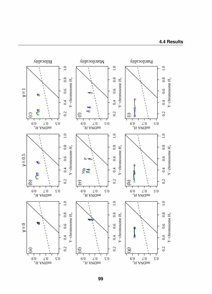
4.4 Results
0.2
0.4
0.6
0.8
1.0
0.50.70.9
γ=
0
Y−
chro
mos
ome H
e
mtDNA He
09 09 09
(a)
0.2
0.4
0.6
0.8
1.0
0.50.70.9
γ=
0.5
Y−
chro
mos
ome H
e
mtDNA He
090
9 09
(b)
0.2
0.4
0.6
0.8
1.0
0.50.70.9
γ=
1
Y−
chro
mos
ome H
e
mtDNA He
090
9 09
Bilocality
(c)
0.2
0.4
0.6
0.8
1.0
0.50.70.9
Y−
chro
mos
ome H
e
mtDNA He
09 09 09
(d)
0.2
0.4
0.6
0.8
1.0
0.50.70.9
Y−
chro
mos
ome H
e
mtDNA He
09B
09P09M
(e)
0.2
0.4
0.6
0.8
1.0
0.50.70.9
Y−
chro
mos
ome H
e
mtDNA He
0909
09
Matrilocality
(f)
0.2
0.4
0.6
0.8
1.0
0.50.70.9
Y−
chro
mos
ome H
e
mtDNA He
09
09
09
(g)
0.2
0.4
0.6
0.8
1.0
0.50.70.9
Y−
chro
mos
ome H
e
mtDNA He
09
09 0
9
(h)
0.2
0.4
0.6
0.8
1.0
0.50.70.9Y
−ch
rom
osom
e He
mtDNA He
09
09
09
Patrilocality
(i)
99

4. SEX-BIASED MIGRATION IN THE NEOLITHIC
4.4.4 Influence of HG postmarital behaviour on the Farmers geneticdifferentiation
Interestingly, in a 10×10 lattice, the modern samples F ST values seem less affectedby the postmarital residence system of the HG, than the corresponding He values(Fig. C.3). In particular, the analyses of only the last generation data show thatthe F ST values were nearly identical across all HG scenarios with and without ad-mixture. Conversely, in the generations that follow the admixture events there wereclear differences between the no admixture and admixture scenarios (Fig. C.4).However, in the scenarios analysed using a larger lattice (30×30) was possible toseparate postmarital residence system of the HG, on the basis of F ST values (Fig.C.5).
4.5 DiscussionAltogether, our simulations allowed us to study the effect of i) variable migrationrates in males and females within the HG and Farmers layers and ii) variable ad-mixture between layers, on the patterns of genetic diversity and differentiation inpresent-day populations.
4.5.1 Main results: (i) first farmers were patrilocal and (ii) differentpostmarital residence systems have a different impact on hu-man genetic patterns
Patrilocality was the most probable scenario among Farmers. It was particularly ob-vious in the no admixture scenarios, but was also found in the scenarios with admix-ture. This result agrees with ancient DNA (aDNA) and Strontium isotope analysesthat suggested patrilocality in Linear [Bentley et al., 2002] and Corded [Haak et al.,2008] Ware Culture burials from Germany. Cultural phylogenetics studies also sug-gest that patrilocality started to increase after the advent of agriculture [Fortunato,2011; Fortunato & Jordan, 2010].Changes in postmarital residence systems were also found to lead to different ge-
100

4.5 Discussion
netic patterns in present-day populations. In particular, the Farmers’ He valueschanged significantly depending on whether the HG were patrilocal, bilocal or ma-trilocal. Thus, it appears that even though HG populations disappear as far backas 5000 years before the present in our simulations, they influence present-daypatterns in modern-day populations.
4.5.2 Behaviour of summary statistics
Pairwise F ST statistics were much less influenced than He values by the postmaritalresidence pattern of the HG populations. While F ST values were different acrossscenarios after the start of admixture, this signal disappeared in the modern sam-ples. However, when a larger lattice (30×30) is analysed (corresponding to a largergeographic area) it was possible to distinguish between the postmarital residencesystems of the HG populations. This is compatible with the notion that the degree ofgenetic differentiation between two demes depends of their geographical distance,on the migration rate between local demes and on the time since the populationsstarted expanding. If migration rates are large and/or necessary time has passed,then it may be necessary to use large lattices to avoid this homogenizing effect inF ST values. This F ST statistics’ dependence on geographical distances implies thatinferences based on local/regional sampling is valid only for the most recent history,while sampling from more distant places may be able to recover older patterns, apoint that has been stressed by Wilkins and Marlowe [2006].Furthermore, the access to the genetic composition of ancient HG populations maybe not only useful but necessary to provide us with significant information on thisissue. In other words, aDNA may be required to allow us to determine the postmar-ital behaviour of HG populations in Europe before and after the Neolithic transition.Currently, the number of aDNA studies about the Neolithic transition are slowly in-creasing [Bramanti et al., 2009; Haak et al., 2005, 2010; Malmström et al., 2009]but are unfortunately limited to the mtDNA. Our results suggest that obtaining NRYDNA from the same samples would be particularly important, as was done in a re-cent study [Lacan et al., 2011].
101

4. SEX-BIASED MIGRATION IN THE NEOLITHIC
To identify the most probable scenario we focused on the trend observed in thestatistics of both simulated and real data. Our approach was thus to some extentqualitative. To obtain a better fit, one would also need to consider the spread ofpopulations in both the simulated and real data (not just the regression slope). Intheory, simulating different scenarios should allow us to better tune migration rates,and identify the original level of diversity in both HG and Farmers populations, thatare compatible with the observed modern-day data.
4.5.3 Mutation rates can generate asymmetries between mtDNA andNRY data
Although mtDNA and NRY data are often presented as symmetrical counter partsof the female and male demography, respectively, this is not necessarily that simple.The difference in mutation rates can generate an asymmetry between mtDNA andNRY He values in bilocal scenarios with no sex-related variance in reproductivesuccess (Fig. 4.2a and 4.3a). This is something to keep in mind when analysingdifferences observed in real mtDNA and NRY data because such differences areoften interpreted in terms of differences in male and female behaviours [Seielstadet al., 1998; Wilder et al., 2004; Wilkins, 2006].
4.5.4 Admixture decreases Farmers NRY genetic diversity
We found this surprising at first, as it is usually assumed that regions where popu-lations admix will exhibit higher levels of genetic diversity. However, the underlyingassumption is that admixing populations have similar Ne. Several studies haveshown that during spatial expansions the expanding population is diluted [Chikhiet al., 2002; Edmonds et al., 2004; Klopfstein et al., 2006]. We thus believe thatas admixture took place between populations with different sizes (i.e. HG havingmuch smaller populations than the Farmers), the incoming population will dilute theFarmers genetic diversity and led to the decrease in NRY genetic diversity. Thiscan be seen in the simulations where the decrease is observed even when bothHG and Farmers had the same pattern of postmarital rules. However, this is not
102

4.5 Discussion
necessarily a general result as mtDNA genetic diversity did not always decrease.Again, the difference in mutation rates between mtDNA and NRY markers may in-teract in a complex way with demographic parameters leading to asymmetries inpresent-day data.
4.5.5 Comparison with other sex-biased migration studies
Until now, the inference of patterns of sex-biased migration have relied mainly onthe comparison and estimation of dispersal from pairwise NRY and mtDNA F ST
values [47][48] and by cultural phylogenetics [Fortunato, 2011; Fortunato & Jordan,2010; Jordan et al., 2009] in modern populations.Hamilton et al. [2005] also used spatial framework, using NRY and mtDNA data,to study matrilocal and patrilocal groups from northern Thailand. In their study theauthors applied a modified version of SPLATCHE and were not interested in de-tecting shifts in postmarital residence patterns, which were assumed to be invariantin their simulations. Instead, their aim was to compare male and female migrationrates in known patrilocal and matrilocal societies that would explain present-daylevels of genetic differentiation and diversity. Here our aim was to understand howpostmarital residence interacts with admixture between different societies, to gen-erate differences in maternally or paternally-inherited markers analysed jointly.Model-based approaches have many advantages as they allow us to identify pa-rameters that have a significant impact on the data. However they also rely onstrong assumptions. In our study, it was necessary to make assumptions on thelevel and patterns of gene flow, carrying capacities and genetic make-up of thefounder populations, which suggests that some of the conclusions presented hereshould not be taken at face value. Hitherto, we believe that the general trends iden-tified are to some extent robust. For instance, our simulations were performed ona 10×10 lattice. But when we repeated the patrilocal scenarios on a 30×30 latticewe found essentially the same results, the main difference being that the power toidentify scenarios was increased in the 30×30 lattice.The simulated framework introduced here owes much to the work of Currat et al.
103

4. SEX-BIASED MIGRATION IN THE NEOLITHIC
[2005], but is sufficiently different to represent an interesting alternative to identifythe critical assumptions that are robust and those that are not, and the type of datarequired to separate scenarios. Altogether, our simulations helped identify impor-tant parameters and scenarios, together with data that would be needed to studythe Neolithic transition in Europe (NRY aDNA), but much work is still necessary.
4.6 ConclusionThere are still very few studies that have dealt with the kind of complex scenariosthat involve the characterization of the expansion of two demographically differ-ent populations across the same geographical area when migration patterns andadmixture levels vary, and those that exist do not deal with sex-biased migration[Currat & Excoffier, 2005][Currat & Excoffier, 2004]. Our work provides some of thefirst insights into the consequences of complex demographic changes that probablytook place during the European Neolithic, on present-day human genetic patterns.
AcknowledgementsPart of this work was performed using HPC resources from CALMIP, Toulouse (Grant 2010-P1038). We are grateful to B. Parreira for the stimulating comments and discussions.We would also like to thank C. Gamba and I. Alves and anonymous reviewers for read-ing and constructively commenting a previous version of the manuscript. RR and VCSwere supported by FCT grants (ref. SFRH/BD/30821/2006 and SFRH/BD/22224/2005,respectively). PAB was supported by funding from the IGC. LC was funded by the FCTprojects PTDC/BIA-BDE/71299/2006 and PTDC/BIA-BEC/100176/2008 and grant no. CD-AOOI-07-003 from the Institut Français de la Biodiversité, Programme Biodiversité des îlesde l’Océan Indien. This work was also partly funded by the "Laboratoire d’Excellence(LABEX)entitled TULIP (ANR-10-LABX-41)".
4.7 ReferencesAMMERMAN, A.J. & CAVALLI-SFORZA, L.L. (1984). The Neolithic transition and the genet-
ics of populations in Europe. Princeton University Press, Princeton.BAKER, M. & JACOBSEN, J. (2006). A human capital-based theory of postmarital residence
rules. J Law Econ Organ, 23, 208–241.
104

4.7 References
BALARESQUE, P., BOWDEN, G., ADAMS, S., LEUNG, H., KING, T., ROSSER, Z., GOOD-WIN, J., MOISAN, J., RICHARD, C., MILLWARD, A. et al. (2010). A predominantly Ne-olithic origin for European paternal lineages. PLoS biology , 8, e1000285.
BARBUJANI, G., BERTORELLE, G., CAPITANI, G. & SCOZZARI, R. (1995). Geographicalstructuring in the mtDNA of Italians. Proc Natl Acad Sci U S A, 92, 9171–9175.
BARBUJANI, G., BERTORELLE, G. & CHIKHI, L. (1998). Evidence for Paleolithic and Ne-olithic gene flow in Europe. Am J Hum Genet , 62, 488–492.
BELLE, E.M.S., LANDRY, P.A. & BARBUJANI, G. (2006). Origins and evolution of the Eu-ropeans’ genome: evidence from multiple microsatellite loci. Proc R Soc B, 273, 1595–1602.
BELLWOOD, P. (2004). First Farmers: the origins of agricultural societies. Blackwell Pub-lishing, Oxford.
BENTLEY, R.A., PRICE, T.D., LÜNING, J., GRONENBORN, D., WAHL, J. & FULLAGAR, P.D.(2002). Human migration in early Neolithic Europe. Curr Anthropol , 43, 799–804.
BENTLEY, R.A., CHIKHI, L. & PRICE, T.D. (2003). The Neolithic transition in Europe: com-paring broad scale genetic and local scale isotopic evidence. Antiquity , 77, 63–66.
BRAMANTI, B., THOMAS, M.G., HAAK, W., UNTERLAENDER, M., JORES, P., TAMBETS,K., ANTANAITIS-JACOBS, I., HAIDLE, M.N., JANKAUSKAS, R., KIND, C.J., LUETH, F.,TERBERGER, T., HILLER, J., MATSUMURA, S., FORSTER, P. & BURGER, J. (2009).Genetic discontinuity between local hunter-gatherers and central Europe’s first farmers.Science, 326, 137–140.
CAVALLI-SFORZA, L.L. & MINCH, E. (1997). Paleolithic and Neolithic lineages in the Euro-pean mitochondrial gene pool. Am J Hum Genet , 61, 247–254.
CHIKHI, L. (2009). Update to Chikhi et al.’s "Clinal variation in the nuclear DNA of euro-peans" (1998): genetic data and storytelling–from archaeogenetics to astrologenetics?Hum Biol , 81, 639–643.
CHIKHI, L., NICHOLS, R.A., BARBUJANI, G. & BEAUMONT, M.A. (2002). Y genetic datasupport the Neolithic demic diffusion model. Proc Natl Acad Sci U S A, 99, 11008–11013.
CURRAT, M. & EXCOFFIER, L. (2004). Modern humans did not admix with Neanderthalsduring their range expansion into Europe. PLoS Biol , 2, e421.
CURRAT, M. & EXCOFFIER, L. (2005). The effect of the Neolithic expansion on Europeanmolecular diversity. Proc R Soc B, 272, 679–688.
CURRAT, M., RAY, N. & EXCOFIER, L. (2004). SPLATCHE: a program to simulate geneticdiversity taking into account environmental heterogeneity. Mol Ecol Notes, 4, 139–142.
DAVIS, S.J.M. (2005). Why domesticate food animals? Some zoo-archaeological evidence
105

4. SEX-BIASED MIGRATION IN THE NEOLITHIC
from the Levant. J Archaeol Sci , 32, 1408–1416.DIAMOND, J. & BELLWOOD, P. (2003). Farmers and their languages: the first expansions.
Science, 300, 597–603.EDMONDS, C.A., LILLIE, A.S. & CAVALLI-SFORZA, L.L. (2004). Mutations arising in the
wave front of an expanding population. Proc Natl Acad Sci , 101, 975–9.FELDMAN, M.W. & CAVALLI-SFORZA, L.L. (1976). Cultural and biological evolutionary pro-
cesses, selection for a trait under complex transmission. Theor Popul Biol , 9, 238–259.FORTUNATO, L. (2011). Reconstructing the history of residence strategies in Indo-
European-speaking societies: neo-, uxori-, and virilocality. Hum Biol , 83, 107–28.FORTUNATO, L. & JORDAN, F. (2010). Your place or mine? a phylogenetic comparative
analysis of marital residence in Indo-European and Austronesian societies. Philos TransR Soc B, 365, 3913–22.
GKIASTA, M., RUSSELL, T., SHENNAN, S. & STEELE, J. (2003). Neolithic transition inEurope: the radiocarbon revisited. Antiquity , 77, 45–62.
GOLDSTEIN, D.B. & CHIKHI, L. (2002). Human migrations and population structure: whatwe know and why it matters. Annu Rev Genomics Hum Genet , 3, 129–152.
HAAK, W., FORSTER, P., BRAMANTI, B., MATSUMURA, S., BRANDT, G., TÄNZER, M.,VILLEMS, R., RENFREW, C., GRONENBORN, D., ALT, K.W. & BURGER, J. (2005). An-cient DNA from the first european farmers in 7500-year-old neolithic sites. Science, 310,1016–1018.
HAAK, W., BRANDT, G., DE JONG, H.N., MEYER, C., GANSLMEIER, R., HEYD, V.,HAWKESWORTH, C., PIKE, A.W.G., MELLER, H. & ALT, K.W. (2008). Ancient DNA,strontium isotopes, and osteological analyses shed light on social and kinship organiza-tion of the later stone age. Proc Natl Acad Sci U S A, 105, 18226–31.
HAAK, W., BALANOVSKY, O., SANCHEZ, J.J., KOSHEL, S., ZAPOROZHCHENKO, V., ADLER,C.J., DER SARKISSIAN, C.S.I., BRANDT, G., SCHWARZ, C., NICKLISCH, N., DRESELY,V., FRITSCH, B., BALANOVSKA, E., VILLEMS, R., MELLER, H., ALT, K.W. & AND, A.C.(2010). Ancient DNA from european early neolithic farmers reveals their Near Easternaffinities. PLoS Biol , 8, e1000536.
HAMILTON, G., STONEKING, M. & EXCOFFIER, L. (2005). Molecular analysis reveals tightersocial regulation of immigration in patrilocal populations than in matrilocal populations.Proc Natl Acad Sci U S A, 102, 7476–80.
ITAN, Y., POWELL, A., BEAUMONT, M.A., BURGER, J. & THOMAS, M.G. (2009). The originsof lactase persistence in Europe. PLoS Comput Biol , 5, e1000491.
JORDAN, F.M., GRAY, R.D., GREENHILL, S.J. & MACE, R. (2009). Matrilocal residence is
106

4.7 References
ancestral in Austronesian societies. Proc R Soc B, 276, 1957–64.KLOPFSTEIN, S., CURRAT, M. & EXCOFFIER, L. (2006). The fate of mutations surfing on
the wave of a range expansion. Mol Biol Evol , 23, 482–490.LACAN, M., KEYSER, C., RICAUT, F.X., BRUCATO, N., DURANTHON, F., GUILAINE, J.,
CRUBÉZY, E. & LUDES, B. (2011). Ancient DNA reveals male diffusion through the Ne-olithic Mediterranean route. PNAS, early edition.
LANGERGRABER, K.E., SIEDEL, H., MITANI, J.C., WRANGHAM, R.W., REYNOLDS, V.,HUNT, K. & VIGILANT, L. (2007). The genetic signature of sex-biased migration in pa-trilocal chimpanzees and humans. PLoS One, 2, e973.
LOTKA, A.J. (1932). The growth of mixed populations : two species competing for a com-mon food supply. Journal of Washington Academy of Sciences, 22, 461–469.
MALMSTRÖM, H., GILBERT, M.T.P., THOMAS, M.G., BRANDSTRÖM, M., STORA, J., MOL-NAR, P., ANDERSEN, P.K., BENDIXEN, C., HOLMLUND, G., GÖTHERSTRÖM, A. &WILLERSLEV, E. (2009). Ancient DNA reveals lack of continuity between neolithic hunter-gatherers and contemporary scandinavians. Curr Biol , 19, 1758–62.
MARLOWE, F. (2004). Marital residence among foragers. Curr Anthropol , 45, 277–283.MAYNARD-SMITH, J. & SLATKIN, M. (1973). The stability of predator-prey systems. Ecol-
ogy , 54, 384–391.MITHEN, S. (2007). Did farming arise from a misapplication of social intelligence? Philos
Trans R Soc Lond B Biol Sci , 362, 705–718.NEI, M. (1977). F-statistics and analysis of gene diversity in subdivided populations. Ann
Hum Genet , 41, 225–233.PINHASI, R., FORT, J. & AMMERMAN, A.J. (2005). Tracing the origin and spread of agricul-
ture in Europe. PLoS Biol , 3, e410.QUINTANA-MURCI, L., QUACH, H., HARMANT, C., LUCA, F., MASSONNET, B., PATIN, E.,
SICA, L., MOUGUIAMA-DAOUDA, P., COMAS, D., TZUR, S., BALANOVSKY, O., KIDD,K.K., KIDD, J.R., VAN DER VEEN, L., HOMBERT, J.M., GESSAIN, A., VERDU, P., FRO-MENT, A., BAHUCHET, S., HEYER, E., DAUSSET, J., SALAS, A. & BEHAR, D.M. (2008).Maternal traces of deep common ancestry and asymmetric gene flow between Pygmyhunter-gatherers and Bantu-speaking farmers. Proc Natl Acad Sci U S A, 105, 1596–601.
RAY, N., CURRAT, M., FOLL, M. & EXCOFFIER, L. (2010). SPLATCHE2: a spatially explicitsimulation framework for complex demography, genetic admixture and recombination.Bioinformatics, 26, 2993–2994.
RICHARDS, M., MACAULAY, V., HICKEY, E., VEGA, E., SYKES, B., GUIDA, V., RENGO,
107

4. SEX-BIASED MIGRATION IN THE NEOLITHIC
C., SELLITTO, D., CRUCIANI, F., KIVISILD, T., VILLEMS, R., THOMAS, M., RYCHKOV,S., RYCHKOV, O., RYCHKOV, Y., GÖLGE, M., DIMITROV, D., HILL, E., BRADLEY, D.,ROMANO, V., CALÌ, F., VONA, G., DEMAINE, A., PAPIHA, S., TRIANTAPHYLLIDIS, C.,STEFANESCU, G., HATINA, J., BELLEDI, M., RIENZO, A.D., NOVELLETTO, A., OPPEN-HEIM, A., NØRBY, S., AL-ZAHERI, N., SANTACHIARA-BENERECETTI, S., SCOZARI, R.,TORRONI, A. & BANDELT, H.J. (2000). Tracing european founder lineages in the NearEastern mtDNA pool. Am J Hum Genet , 67, 1251–1276.
RICHARDS, M., MACAULAY, V., TORRONI, A. & BANDELT, H.J. (2002). In search of geo-graphical patterns in European mitochondrial DNA. Am J Hum Genet , 71, 1168–1174.
ROSSER, Z.H., ZERJAL, T., HURLES, M.E., ADOJAAN, M., ALAVANTIC, D., AMORIM, A.,AMOS, W., ARMENTEROS, M., ARROYO, E., BARBUJANI, G., BECKMAN, G., BECKMAN,L., BERTRANPETIT, J., BOSCH, E., BRADLEY, D.G., BREDE, G., COOPER, G., CÔRTE-REAL, H.B., DE KNIJFF, P., DECORTE, R., DUBROVA, Y.E., EVGRAFOV, O., GILIS-SEN, A., GLISIC, S., GÖLGE, M., HILL, E.W., JEZIOROWSKA, A., KALAYDJIEVA, L.,KAYSER, M., KIVISILD, T., KRAVCHENKO, S.A., KRUMINA, A., KUCINSKAS, V., LAVINHA,J., LIVSHITS, L.A., MALASPINA, P., MARIA, S., MCELREAVEY, K., MEITINGER, T.A.,MIKELSAAR, A.V., MITCHELL, R.J., NAFA, K., NICHOLSON, J., NØRBY, S., PANDYA, A.,PARIK, J., PATSALIS, P.C., PEREIRA, L., PETERLIN, B., PIELBERG, G., PRATA, M.J.,PREVIDERÉ, C., ROEWER, L., ROOTSI, S., RUBINSZTEIN, D.C., SAILLARD, J., SAN-TOS, F.R., STEFANESCU, G., SYKES, B.C., TOLUN, A., VILLEMS, R., TYLER-SMITH,C. & JOBLING, M.A. (2000). Y-chromosomal diversity in Europe is clinal and influencedprimarily by geography, rather than by language. Am J Hum Genet , 67, 1526–1543.
SALZANO, F.M. (2004). Interethnic variability and admixture in latin America–social impli-cations. Rev Biol Trop, 52, 405–15.
SEIELSTAD, M.T., MINCH, E. & CAVALLI-SFORZA, L.L. (1998). Genetic evidence for ahigher female migration rate in humans. Nat Genet , 20, 278–80.
SEMINO, O., PASSARINO, G., OEFNER, P.J., LIN, A.A., ARBUZOVA, S., BECKMAN, L.E.,BENEDICTIS, G.D., FRANCALACCI, P., KOUVATSI, A., LIMBORSKA, S., MARCIKIAE,M., MIKA, A., MIKA, B., PRIMORAC, D., SANTACHIARA-BENERECETTI, A.S., CAVALLI-SFORZA, L.L. & UNDERHILL, P.A. (2000). The genetic legacy of Paleolithic Homo sapi-ens sapiens in extant Europeans: a Y chromosome perspective. Science, 290, 1155–1159.
VOLTERRA, V. (1931). Variations and fluctuations of the numbers of individuals in animalspecies living together , 409–448. McGraw-Hill, New York.
WILDER, J.A., KINGAN, S.B., MOBASHER, Z., PILKINGTON, M.M. & HAMMER, M.F.
108

4.7 References
(2004). Global patterns of human mitochondrial DNA and Y-chromosome structure arenot influenced by higher migration rates of females versus males. Nat Genet , 36, 1122–5.
WILKINS, J.F. (2006). Unraveling male and female histories from human genetic data. CurrOpin Genet Dev , 16, 611–7.
WILKINS, J.F. & MARLOWE, F.W. (2006). Sex-biased migration in humans: what should weexpect from genetic data? Bioessays, 28, 290–300.
ZVELEBIL, M. & ZVELEBIL, K. (1998). Agricultural transition and Indo-European dispersals.Antiquity , 62, 574–583.
109


5. SINS: forward simulation ofindividuals through time andspaceRita Rasteiro1, Pierre-Antoine Bouttier1,†, Damien Monier1, Vítor C. Sousa1,‡ andLounès Chikhi1,2,3
1Instituto Gulbenkian de Ciência, Rua da Quinta Grande, 6, 2780-156 Oeiras, Portugal; 2CNRS, Laboratoire Évo-
lution et Diversité Biologique (EDB), Bât. 4R3 b2, 118 Route de Narbonne, 31062 Toulouse cédex 9, France;
3Université de Toulouse, UPS, EDB, Bât. 4R3 b2, 118 Route de Narbonne, 31062 Toulouse cédex 9, France;
†New address: Université de Grenoble and CNRS, Laboratoire Jean Kutzmann, France; ‡New address: Depart-
ment of Genetics, Rutgers University, NJ, USA.
Development of the simulation framework: R Rasteiro, P-A Bouttier, D Monier, VC Sousa and
L Chikhi
Manuscript: R. Rasteiro and L. Chikhi
5.1 SummarySINS is a computer program that simulates genetic data under complex demo-graphic scenarios using a spatial framework. Space is divided into layers, whichare themselves subdivided into demes that harbour male and female individuals.Each deme is characterized by carrying capacity (K ) and friction (F ) values whichdefine the maximum population size and the difficulty to move into that deme, re-
111

5. SINS: SIMULATING INDIVIDUALS IN SPACE
spectively. SINS allows the user to simulate (i) variable K and F maps across timeand space, (ii) expansions from multiple sources, (iii) contractions and habitat frag-mentation, (iv) admixture and competition between populations from two or morelayers corresponding to the same geographical space, (v) variance in reproductivesuccess in males and females and (vi) sex-biased migration. The program uses anindividual-based approach to simulate forward in time several types of molecularmarkers (sequences, SNPs and microsatellites) and genetic objects (X and Y chro-mosomes, autosomes and mitochondrial DNA). The flexibility of SINS should allowits application to many species and evolutionary questions. A companion program,SINS-Stat, samples SINS genetic outputs and performs several population geneticstatistics.Availability: SINS and SINS-Stat are freely available at [TBA], together with a userguide (appendix D) and examples.
5.2 IntroductionSINS (for Simulating INdividuals in Space) is a program that simulates the demog-raphy of populations and their resulting genetic diversity in a spatial setting. It is anindividual-based tool that incorporates both geographical and demographic data,allowing to generate several types of genetic markers. SINS owes much of its con-ception to SPLATCHE [Currat et al., 2004], recently been upgraded to SPLATCHE2[Ray et al., 2010]. SINS and SPLATCHE share significant features, but are comple-mentary due to some differences that we detail below.
5.3 Methods
5.3.1 Demography
SINS uses a 2D bouncing edges stepping-stone model framework, where demes(populations) are connected by gene flow (with migration rate m) and arranged ina grid (layer). Several layers can occupy the same geographical space, and indi-viduals from different layers can interact either by competition, admixture or both.
112

5.3 Methods
Each deme is characterized by carrying capacity (K ) and friction (F ) values, whichcan be different among demes and layers and can change with time. Migration isconstrained by the F value of neighbouring demes. Expansion, contraction andfragmentation of populations are simulated by defining appropriate K and F maps.Expansions can start from multiple sources and at different times. Mating betweenindividuals from different layers can be asymmetrical and is modelled by an ad-mixture parameter (γ). These features are, apart from minor differences, sharedwith SPLATCHE (one layer) and SPLATCHE2 (a maximum of two layers). We nowoutline several features that are specific to SINS:
1. Population size is logistically regulated within each deme, with intrinsic growthrate (r i for layer i), but the specificity of SINS is that (i) foundation events mustinvolve at least one male and one female, (ii) the Maynard-Smith and Slatkin[1973] logistic growth formula is used and corrected (equation 5.1) to accountfor the fact that growth is limited by the number of reproductive females. Thisavoids unrealistic situations where a female may have a biologically unreal-istic number of offspring. The Lotka-Volterra model is used to incorporatecompetition into the logistic growth equation (5.1), through a parameter αij
that varies between 0 and 1 and represents the pressure exerted by popula-tions from layer j over populations from layer i. Thus, the population size in ademe from layer i at time t+1 is calculated as:
Ni,t+1 = 2Nf,i,t1 + ri
1 +∑nlayer
j=1 riαij2Nf,i,t
Ki
(5.1)
where Nf,i,t is the number of reproductive females in the same deme fromlayer i, at time t and nlayer is the number of layers. Another difference is that(iii) growth is not deterministic, with the actual values of population size drawnfrom a Poisson distribution with mean Ni,t+1, as given by equation (5.1).
2. Random mating is assumed by default, but it is possible to simulate the vari-ance in the reproductive success of individuals, by giving as input the per-centage of males and females that reproduce.
113

5. SINS: SIMULATING INDIVIDUALS IN SPACE
3. Sex-biased migration is simulated through parameter mSR (equation 5.2) thatallows the user to vary the ratio of female (mf ) to male (mm) migration rates.
mSR =mf
mf +mm(5.2)
4. Most processes are stochastic such that the total number of migrants, thedirection of migration events and the deme population sizes are drawn fromstatistical distributions.
5.3.2 Genetics
SINS simulates individuals whose sex is defined by their sexual chromosomes (XXfor the female and XY for the males). Multilocus genotypes can be simulated forseveral types of markers (SNPs, microsatellites and sequences). The program as-sumes that the loci are either independent or totally linked. It is thus possible tosimulate autosomes, sexual chromosomes and mitochondrial DNA (mtDNA), mak-ing it possible to follow the parallel history of any set of chromosomes and compare,for instance, Y-chromosome and mtDNA data from the same populations.The genetic make-up of founding populations can be taken from pre-specified allelefrequencies (from observed or simulated data). When several layers are simulated,it is also possible to found a new population by sampling the corresponding demefrom another layer.
5.3.3 Outputs and Summary Statistics
SINS produces demographic and genetic outputs. The demographic output is asingle text file, where the number of individuals is recorded for each deme, layerand generation time. The genetic outputs are divided by chromosome/locus. Foreach locus, one file is created with the genotypes of all individuals, on all demesand layers, for the time steps chosen by the user. Each individual is identified by itslayer, deme, sex and time step. Moreover, the parents of each individual are alsorecorded, together with their original birth deme.
114

5.4 Implementation
A companion program (SINS-Stat) is also available to sample individuals from spec-ified demes and layers and to compute single locus population genetic statistics.
5.4 ImplementationBoth SINS and SINS-Stat are written in Java and require JRE 1.6 to be installed.Depending on the size of the simulated world and the number of generations, largeamounts of RAM may be required for SINS to run. Since it is a non-graphicalconsole program, it can be easily used in computer clusters, hence decreasing theexecution time (see user guide to details).
5.5 DiscussionRecent years have seen the development of coalescent-based programs to simu-late complex demographic histories. The advantage of such programs is that theyare extremely efficient because only the sampled genealogies are simulated. Incontrast, with forward simulations the whole population has to be simulated. Whilethis makes forward methods computationally less efficient, they are beginning start-ing to be used again once more [Balloux, 2001; Guillaume & Rougemont, 2006;Neuenschwander et al., 2008; Peng & Kimmel, 2005]. Forward simulations are in-tuitively easier to grasp and code, particularly in the case of complex scenarios thatinvolve spatial expansions or selection. The two types of approaches should thusbe complementary rather than opposed, depending on the questions one asks. Forinstance, in a recent study simulating the spatial expansion of North African popu-lation across Gibraltar, Currat et al., [2010] used modified versions of SPLATCHEincorporating both coalescent and forward simulations for markers under selection.Similarly, SINS should be seen as a program that is complementary to SPLATCHE.It incorporates features that are more realistic, but will probably be difficult to usefor species with very large population sizes. However, the development and growthof computing power should make it possible for SINS to be useful for statistical in-ference under increasingly complex scenarios. These would include features suchas sex-biased migration and variance in the reproductive success together with ex-
115

5. SINS: SIMULATING INDIVIDUALS IN SPACE
pansions from Pleistocene refugia or contractions due to environmental fluctuationsor habitat loss and fragmentation. To our knowledge, no other forward simulationprogram is capable of simulating individuals from populations with different demo-graphic histories, inhabiting the same geographic space (i.e. layers).
AcknowledgementsWe are grateful to I. Alves and C. Chaouiya for useful comments on an earlier ver-sion of the manuscript. This work was funded by Fundação para a Ciência eTecnologia [SFRH/BD/30821/2006 to R.R., SFRH/BD/22224/2005 to V.S., PTDC/BIA-BDE/71299/2006 and PTDC/BIA-BEC/100176/2008 to L.C.), Instituto Gulbenkian de Ciên-cia [P.A.B.,D.M.] and Institut Français de la Biodiversité, Programme Biodiversité des Îlesde l’Océan Indien [CD-AOOI-07-003 to L.C.].
5.6 ReferencesBALLOUX, F. (2001). Easypop (version 1.7): a computer program for population genetics
simulations. J Hered , 92, 301–302.CURRAT, M., RAY, N. & EXCOFIER, L. (2004). SPLATCHE: a program to simulate genetic
diversity taking into account environmental heterogeneity. Mol Ecol Notes, 4, 139–142.CURRAT, M., POLONI, E.S. & SANCHEZ-MAZAS, A. (2010). Human genetic differentiation
across the Strait of Gibraltar. BMC Evol Biol , 10, 237.GUILLAUME, F. & ROUGEMONT, J. (2006). Nemo: an evolutionary and population genetics
programming framework. Bioinformatics, 22, 2556–2557.MAYNARD-SMITH, J. & SLATKIN, M. (1973). The stability of predator-prey systems. Ecol-
ogy , 54, 384–391.NEUENSCHWANDER, S., HOSPITAL, F., GUILLAUME, F. & GOUDET, J. (2008). quantiNemo:
an individual-based program to simulate quantitative traits with explicit genetic architec-ture in a dynamic metapopulation. Bioinformatics, 24, 1552–1553.
PENG, B. & KIMMEL, M. (2005). simuPOP: a forward-time population genetics simulationenvironment. Bioinformatics, 21, 3686–3687.
RAY, N., CURRAT, M., FOLL, M. & EXCOFFIER, L. (2010). SPLATCHE2: a spatially explicitsimulation framework for complex demography, genetic admixture and recombination.Bioinformatics, 26, 2993–2994.
116

6. General DiscussionThe increasing availability of genetic data from current human populations hasallowed geneticists and archaeologists to reconstruct their demographic history.Several past demographic events led to major cultural, social and demographicchanges that most likely influenced and therefore left their marks on human ge-netic diversity patterns, being the Neolithic transition considered to be one of themost important ones [Mithen, 2007]. Such changes have been suggested eitherby archaeological and anthropological data, but there have been very few studiesto address these issues from a genetic point of view. In this thesis, we decided touse model-based approaches to study the consequences of the cultural, social anddemographic shifts that followed the Neolithic transition, on the patterns of geneticdiversity.
6.1 Neolithic transition in Japan and EuropeFirst, in chapter 2, we decided to test this approach on the colonization of Japan,by hunter-gatherers (HG) Jomon and rice cultivators Yayoi. While geographicallyJapan is a relatively small region, the genetic contribution of these two popula-tions on modern Japanese was yet the focus of much dispute, between archaeolo-gists, anthropologists and geneticists. When we published this work, there were nodata available from mtDNA and the Pan-Asian HUGO SNP consortium database[Ngamphiw et al., 2011] was not yet released. Nevertheless, using published Y-chromosome data, our results clearly point to a demic diffusion process, similar tothe process that was suggested for Europe. However, we could not pinpoint the ori-gin of the Yayoi farmers in mainland Asia. More studies using more loci are neededto answer this question.
117

6. GENERAL DISCUSSION
In chapter 3, the same admixture approach is applied to the European Neolithic.Chikhi et al. [2002] had already applied it to Europe, using Y-chromosome data,but we decided to integrate in the same study mtDNA and Y chromosome data.Indeed, one of the major limitations in published studies is the fact that they eitheruse mtDNA or Y-chromosome data. Moreover, different statistical methodologieswere used on the different markers. This has led to the claim that the differentmarkers favour opposite models for the Neolithic transition. For the first time, weused the same methodological approaches for both contemporary mtDNA and Y-chromosome data. We found that both Y-chromosome and mtDNA data clearlyfavour a demic diffusion process, but that they also identify key differences in thefemale and male demographic histories, most likely related with sex-related dif-ferences in effective size and migration rates. These differences are probably re-lated to the various shifts in cultural practices and lifestyles that followed the Ne-olithic Transition, such as sedentism [Bellwood, 2004], the shift from polygyny tomonogamy [Dupanloup et al., 2003; Fortunato, 2011a] or the increase of patrilocalresidence systems [Fortunato, 2011b; Wilkins & Marlowe, 2006].
In the same study, we also analyzed ancient and modern data from Central Europe,using an ABC approach. We found that the patterns of genetic diversity, encoun-tered in current and ancient populations, demonstrate that both modern and ancientmtDNA support the demic diffusion model. Our results also show that we need toincorporate ancient population structure and differential growth between Neolithicand Palaeolithic populations to explain the patterns of genetic diversity found todayand in our past. We also applied this model approach to the Iberian Neolithic (seeappendix B) and found the same kind of results.Altogether, the study of chapter 3 represents the first attempt to integrate under thesame framework contemporary mtDNA and NRY data, together with aDNA, andprovides an explanation for the patterns of genetic diversity that we see today.
118

6.2 Spatial expansion and the European Neolithic
6.2 Spatial expansion and the European NeolithicThe results of chapter 3 made us believe that other kind of models should be usedto study the consequence of space, structure and also of culture on the patternsof genetic diversity. Indeed, in human population genetic studies, is being increas-ingly recognised the influence of social structure and cultural practices in the to-day’s patterns of human genetic diversity and demography [Hamilton et al., 2005;Wilkins, 2006; Wilkins & Marlowe, 2006]. For our study, we were particularly in-terested in models that that incorporate space, heterogeneous environments andsex-biased processes and that allow to simulate different population groups inhab-iting the same geographic space.
At the beginning of this thesis, SPLATCHE [Currat et al., 2004] was the only avail-able computer program that simulated genetic data under complex demographicscenarios, using a spatial framework. However, the available version just allowedsimulating one population group. Moreover, SPLATCHE is a coalescence-basedprogram and although it is extremely efficient, because only the sampled genealo-gies are simulated, there are certain constraints on the complexity of scenariospossible to simulate. Thus, we started to develop SINS (chapter 5), which alsosimulates the demography of populations and their resulting genetic diversity in aspatial expansion setting. We wanted to apply it to questions related not only withHuman Evolution, but also with Conservation Genetics (other of the scopes of ourresearch group). SINS owes much of its conception to SPLATCHE, but it is a for-ward individual-based tool and the whole population has to be simulated. While thismakes SINS computationally less efficient, it also allows simulating certain popu-lation demographic scenarios, which were not otherwise possible with SPLATCHE,such as sex-biased migration. We believe that both SPLATCHE and SINS ap-proaches should be seen as complementary, rather than opposed, depending onthe questions one asks.
In chapter 4, we applied SINS to study several aspects of the Neolithic transition
119

6. GENERAL DISCUSSION
from hunter-gathering to farming societies in Europe. We were particularly inter-ested in the consequences of various post-marital residence systems (i.e. patrilo-cality, matrilocality and bilocality) and admixture between hunter-gatherers (HG)and farmers on patterns of genetic diversity, during the spatial expansions that ledto the colonization of Europe by humans. We compared the genetic diversity of Y-chromosome and mtDNA data, in order to infer the male and female demographichistories, respectively. Our results suggest that (i) different post-marital residencesystems can lead to different patterns of genetic diversity and differentiation, (ii) pa-trilocality (when the women move to their husband’s birthplace) explains the presentpatterns of genetic diversity better than matrilocality (the men follow their wives) orbilocality (both sexes can move with equal probability).
The study of chapter 4 is not a full inference study, as it would require simulatingthe HG and farmers initial genetic diversity from some statistical distribution. In-stead, due to the limited speed of the simulations, we decided to use the allelicfrequencies observed today as a starting distribution. However, the actual allelicfrequencies in specific simulations were not fixed and could vary between simula-tions. Nevertheless, we believe that much work is still needed to understand howspatial expansions influence present-day allele frequencies and how this could berobust to ancient allele frequencies.
In this thesis, we did not use full potentialities of SINS, such as heterogeneous en-vironments fluctuations along time and space. In chaper 4, we only have testedscenarios in a homogeneous environment, with rectangular lattices. Indeed, wedid not consider the effect of present and past geography and land topology on thedistribution of individuals in space. We also did not consider past climatic changes,such as glaciations, and the resulting population contractions and expansions. Infact, the increase of human populations in Europe after the Last Maximum Glacia-tion is believed to have had a great impact on human genetic diversity [Barbujani &Chikhi, 2000; Semino et al., 2000]. In principle, we could increase the complexityof the scenarios and add more realism to the models, by using geographic infor-
120

6.3 Perspectives
mation systems to create the carrying capacity and friction maps used in the SINSsimulations.
Another interesting study, would be to construct samples similar to those foundin European Neolithic transition aDNA studies [Bramanti et al., 2009; Haak et al.,2005, 2010; Lacan et al., 2011; Malmström et al., 2009] (appendix B), look at thedistribution of F ST values and compare them to the observed data. This kind ofstudy could be coupled with the above scenarios as real data are typically obtainedfrom individuals living sometimes hundreds of km from each other and spread overcenturies or millennia.
6.3 Perspectives
6.3.0.1 SINS’ new features
Other features are implemented or are soon to be implemented in a modified ver-sion of the SINS framework and would allow simulating even more complex scenar-ios. These new features include different mating systems, long-distance migrationand sex-biased admixture but, they are not yet validated. In fact, the general frame-work of SINS was validated for publication (see appendix C.4), under the simplestsituation: we simulated the genetic evolution of a population by creating a scenariowith conditions similar to a Wright-Fisher model, and for which we know what toexpect due to Population Genetics theory.
Currently in SINS, we assume that individuals mate randomly. However, popula-tions are rarely panmictic. In humans, several mating systems have been described(monogamy or polygamy), that may significantly influence the genetic patterns of apopulation, namely the female and male effective population sizes [Wilkins, 2006].Anthropological evidence says that humans are moderate polygynous [Lagerlöf,2010], but in Europe monogamy is suggested to be old and associated with theintroduction of agriculture [Fortunato, 2011a]. In fact, it has been reported as a
121

6. GENERAL DISCUSSION
response to class cleavages, in order to appease non-elite men against rebellion[Lagerlöf, 2010]. This is consistent with Y-chromosome data pointing to a declinein variance in male reproductive success after the advent of farming [Dupanloupet al., 2003] and also with archaeological evidence of monogamy in Neolithic buri-als [Bentley et al., 2008; Haak et al., 2008]. The implementation of different matingsystems and, at the same time, the introduction of variance in the reproductive suc-cess is one of the new features of SINS. It would be interesting to apply it to theEuropean Neolithic and to simulate the shift from polygyny to monogamy in severalscenarios of European colonization by HG and farmers.
The implementation of long-distance migration events is another feature that is cru-cial to understand several phenomena of postglacial recolonization, which havebeen described in many species [Hewitt, 2000]. Exploring these alternative demo-graphic scenarios using simulations could be informative too.
The new sex-biased admixture parameter allows to study the influence of limitedadmixture by one sex, on patterns of genetic diversity. This could apply to fe-male hypergamy, phenomenon that is described in several human migration andcolonization events [Carvajal-Carmona et al., 2000; Quintana-Murci et al., 2008;Salzano, 2004; Thomas et al., 2006], and it is also believed to have happenedduring the Neolithic transition in Europe [Bentley et al., 2003], with HG femalesmarrying into farmer communities [Bentley et al., 2009].
6.3.0.2 SINS’ in an ABC framework
In order to increase the complexity of models it is necessary to have a good knowl-edge of the parameters used to avoid incertitude. Recent years have seen the de-velopment of new inferential methods in population genetics, named ApproximateBayesian Computation (ABC) [Beaumont, 2008; Beaumont et al., 2002]. They re-quire genetic data to be simulated within a particular model or sets of models. Afterthe data have been simulated, they are compared to real or observed data. If the
122

6.4 Conclusion
simulated data are very different from the real data, they are simply rejected. How-ever, when they are arbitrarily close, the parameters that were used to obtain thesimulated data are saved and used for inference. The rationale is that parametersthat generate data close to the real ones are more likely than those producing datathat are very different. It is possible to incorporate an ABC framework in SINS, ei-ther for model parameter estimation or selection of the best demographic scenario.This was recently done, but still much is needed to test it using simulated data sets,for which the parameter values are known and applying it to real datasets.
The incorporation of and ABC framework and the development and growth of com-puting power, should make it possible for SINS to be useful for statistical inferenceunder increasingly complex scenarios. In fact, a parallel approach is being de-veloped to use it in computing cluster and decrease the computing time of thesimulations.
6.4 ConclusionOverall, the work presented in this thesis points to a scenario where the demicdiffusion model had an important role in the dissemination of agriculture, and thusgenes, in certain parts of the world (Japan and Europe). Furthermore, althoughthere are some discrepancies between males and females, both sexes supportdemic diffusion during the European Neolithic. These differences are probably dueto sex-biased processes, such as sex-biased migration, that leave their mark incontemporary patterns of genetic diversity.
Here we studied the influence of sex-biased migrations systems, but almost noth-ing is known about the influence of mating systems in human populations’ geneticdiversity. Still much is needed to be done to understand the influence of space,structure and culture in the genetic make-up of human populations. Indeed, webelieve that our spatial forward framework could be used to explore (i) the conse-quences of various spatial processes and (ii) the influence of social structure anddifferent cultural practices, on today’s patterns of human genetic diversity and de-
123

6. GENERAL DISCUSSION
mography.
We thus believe that this thesis represents a significant advance in our understand-ing of one of the most important economic, demographic and cultural transitions inhuman Prehistory: the Neolithic transition.
6.5 ReferencesBARBUJANI, G. & CHIKHI, L. (2000). Genetic population structure of Europeans inferred
from nuclear and mitochondrial DNA polimorphisms, 119–130. McDonald Institute forArchaeological Research, Cambridge.
BEAUMONT, M. (2008). Joint determination of topology, divergence time, and immigration inpopulation trees, 135–154. McDonald Institute for Archaeological Research, Cambridge.
BEAUMONT, M.A., ZHANG, W. & BALDING, D.J. (2002). Approximate Bayesian Computa-tion in population genetics. Genetics, 162, 2025–35.
BELLWOOD, P. (2004). First Farmers: the origins of agricultural societies. Blackwell Pub-lishing, Oxford.
BENTLEY, R.A., CHIKHI, L. & PRICE, T.D. (2003). The Neolithic transition in Europe: com-paring broad scale genetic and local scale isotopic evidence. Antiquity , 77, 63–66.
BENTLEY, R.A., WAHP, J., PRICE, T.D. & ATKINSON, T.C. (2008). Isotopic signatures andhereditary traits: snapshot of a Neolithic community in Germany. Antiquity , 82, 290–304.
BENTLEY, R.A., LAYTON, R.H. & TEHRANI, J. (2009). Kinship, marriage, and the geneticsof past human dispersals. Hum Biol , 81, 159–79.
BRAMANTI, B., THOMAS, M.G., HAAK, W., UNTERLAENDER, M., JORES, P., TAMBETS,K., ANTANAITIS-JACOBS, I., HAIDLE, M.N., JANKAUSKAS, R., KIND, C.J., LUETH, F.,TERBERGER, T., HILLER, J., MATSUMURA, S., FORSTER, P. & BURGER, J. (2009).Genetic discontinuity between local hunter-gatherers and central Europe’s first farmers.Science, 326, 137–140.
CARVAJAL-CARMONA, L.G., SOTO, I.D., PINEDA, N., ORTÍZ-BARRIENTOS, D., DUQUE,C., OSPINA-DUQUE, J., MONTOYA, M.M.P., ALVAREZ, V.M., BEDOYA, G. & RUIZ-LINARES, A. (2000). Strong Amerind/White sex bias and a possible sephardic contri-bution among the founders of a population in Northwest Colombia. Am J Hum Genet ,67, 1287–1295.
CHIKHI, L., NICHOLS, R.A., BARBUJANI, G. & BEAUMONT, M.A. (2002). Y genetic datasupport the Neolithic demic diffusion model. Proc Natl Acad Sci U S A, 99, 11008–11013.
124

6.5 References
CURRAT, M., RAY, N. & EXCOFIER, L. (2004). SPLATCHE: a program to simulate geneticdiversity taking into account environmental heterogeneity. Mol Ecol Notes, 4, 139–142.
DUPANLOUP, I., PEREIRA, L., BERTORELLE, G., CALAFELL, F., PRATA, M.J., AMORIM,A. & BARBUJANI, G. (2003). A recent shift from polygyny to monogamy in humans issuggested by the analysis of worldwide Y-chromosome diversity. J Mol Evol , 57, 85–97.
FORTUNATO, L. (2011a). Reconstructing the history of marriage strategies in Indo-European-speaking societies: monogamy and polygyny. Hum Biol , 83, 87–105.
FORTUNATO, L. (2011b). Reconstructing the history of residence strategies in Indo-European-speaking societies: neo-, uxori-, and virilocality. Hum Biol , 83, 107–28.
HAAK, W., FORSTER, P., BRAMANTI, B., MATSUMURA, S., BRANDT, G., TÄNZER, M.,VILLEMS, R., RENFREW, C., GRONENBORN, D., ALT, K.W. & BURGER, J. (2005). An-cient DNA from the first european farmers in 7500-year-old neolithic sites. Science, 310,1016–1018.
HAAK, W., BRANDT, G., DE JONG, H.N., MEYER, C., GANSLMEIER, R., HEYD, V.,HAWKESWORTH, C., PIKE, A.W.G., MELLER, H. & ALT, K.W. (2008). Ancient DNA,strontium isotopes, and osteological analyses shed light on social and kinship organiza-tion of the later stone age. Proc Natl Acad Sci U S A, 105, 18226–31.
HAAK, W., BALANOVSKY, O., SANCHEZ, J.J., KOSHEL, S., ZAPOROZHCHENKO, V., ADLER,C.J., DER SARKISSIAN, C.S.I., BRANDT, G., SCHWARZ, C., NICKLISCH, N., DRESELY,V., FRITSCH, B., BALANOVSKA, E., VILLEMS, R., MELLER, H., ALT, K.W. & AND, A.C.(2010). Ancient DNA from european early neolithic farmers reveals their Near Easternaffinities. PLoS Biol , 8, e1000536.
HAMILTON, G., STONEKING, M. & EXCOFFIER, L. (2005). Molecular analysis reveals tightersocial regulation of immigration in patrilocal populations than in matrilocal populations.Proc Natl Acad Sci U S A, 102, 7476–80.
HEWITT, K. (2000). The genetic legacy of the Quartenary ice ages. Nature, 405, 907–913.LACAN, M., KEYSER, C., RICAUT, F.X., BRUCATO, N., DURANTHON, F., GUILAINE, J.,
CRUBÉZY, E. & LUDES, B. (2011). Ancient DNA reveals male diffusion through the Ne-olithic Mediterranean route. PNAS, early edition.
LAGERLÖF, N.P. (2010). Pacifying monogamy. J Econ Growth, 15, 235–262.MALMSTRÖM, H., GILBERT, M.T.P., THOMAS, M.G., BRANDSTRÖM, M., STORA, J., MOL-
NAR, P., ANDERSEN, P.K., BENDIXEN, C., HOLMLUND, G., GÖTHERSTRÖM, A. &WILLERSLEV, E. (2009). Ancient DNA reveals lack of continuity between neolithic hunter-gatherers and contemporary scandinavians. Curr Biol , 19, 1758–62.
MITHEN, S. (2007). Did farming arise from a misapplication of social intelligence? Philos
125

6. GENERAL DISCUSSION
Trans R Soc Lond B Biol Sci , 362, 705–718.NGAMPHIW, C., ASSAWAMAKIN, A., XU, S., SHAW, P.J., YANG, J.O., GHANG, H., BHAK,
J., LIU, E., TONGSIMA, S., & THE HUGO PAN-ASIAN SNP CONSORTIUM (2011).PanSNPdb: The Pan-Asian SNP Genotyping Database. PLoS ONE , 6, e21451.
QUINTANA-MURCI, L., QUACH, H., HARMANT, C., LUCA, F., MASSONNET, B., PATIN, E.,SICA, L., MOUGUIAMA-DAOUDA, P., COMAS, D., TZUR, S., BALANOVSKY, O., KIDD,K.K., KIDD, J.R., VAN DER VEEN, L., HOMBERT, J.M., GESSAIN, A., VERDU, P., FRO-MENT, A., BAHUCHET, S., HEYER, E., DAUSSET, J., SALAS, A. & BEHAR, D.M. (2008).Maternal traces of deep common ancestry and asymmetric gene flow between Pygmyhunter-gatherers and Bantu-speaking farmers. Proc Natl Acad Sci U S A, 105, 1596–601.
SALZANO, F.M. (2004). Interethnic variability and admixture in latin America–social impli-cations. Rev Biol Trop, 52, 405–15.
SEMINO, O., PASSARINO, G., OEFNER, P.J., LIN, A.A., ARBUZOVA, S., BECKMAN, L.E.,BENEDICTIS, G.D., FRANCALACCI, P., KOUVATSI, A., LIMBORSKA, S., MARCIKIAE,M., MIKA, A., MIKA, B., PRIMORAC, D., SANTACHIARA-BENERECETTI, A.S., CAVALLI-SFORZA, L.L. & UNDERHILL, P.A. (2000). The genetic legacy of Paleolithic Homo sapi-ens sapiens in extant Europeans: a Y chromosome perspective. Science, 290, 1155–1159.
THOMAS, M.G., STUMPF, M.P.H. & HÄRKE, H. (2006). Evidence for an apartheid-likesocial structure in early anglo-saxon England. Proc R Soc B, 273, 2651–7.
WILKINS, J.F. (2006). Unraveling male and female histories from human genetic data. CurrOpin Genet Dev , 16, 611–7.
WILKINS, J.F. & MARLOWE, F.W. (2006). Sex-biased migration in humans: what should weexpect from genetic data? Bioessays, 28, 290–300.
126

A. Appendix: Admixture inEurope
A.1 Supplementary Tables
Table A.1: Validation of the ABC model selection procedure. Each line corre-sponds to the percentage of times that a model was assigned to each of the models,by a higher posterior probability.
% Attribution
TP S SDGTP 74.7 21.3 4.0S 44.7 38.1 17.2SDG 2.6 9.6 87.8
Note: When data are simulated under the S model our results show that a significant proportion ofthe data sets are identified as being generated under another model (and as many as 44.7% areassigned to the TP model). This is less the case for the data generated under the TP model (but stillthey represent as much as 25% altogether) and even less under the SDG model. Thus despite nonnegligible error rates, these simulations suggest that there is a bias favouring the TP model, and muchless the S and SDG models. One reason for this is that the ABC algorithm used here followed theprocedure of Bramanti and colleagues [Bramanti et al., 2009], and was only based on three statistics,which were available. However, the results also show that the SDG model is the model which is mosteasily identified with nearly 88% of positive results. Given that the results obtained from the real dataprovide no support for the TPM, and less than 5% for the S model, we are confident that the inferenceof the model is unlikely to be incorrect hence demonstrating the importance of differential growth. Thisexplains why Haak et al. [2010] were unable to explain the observed F ST values with their split model.
127

A. APPENDIX: ADMIXTURE IN EUROPE
Table A.2: Calibrated radiocarbon dates of Neolithic archaeological sites. Loca-tion and type of Neolithic culture (EN – Early Neolithic, LBK – Linear Pottery Culture)are also represented in this table [Pinhasi et al., 2005].
Location Archaeological site Culture Dates(Yrs cal BP)
Georgia Arkb1 Pottery Neolithic 7 937Cyprus Cypro-EPPNB Kissonega-Mylouthkia 10 494Greece Knossos EN 8 946Bulgaria Polyanista-Platoto1 EN 8 145Czech Republic Bylany LBK 7 604Slovakia Sturovo LBK 7 146Romania Trestiana Starcevo,Cri 7 539Yugoslavia Apatin Starcevo 7 932Hungary Endrod Köros 7 765Poland Strezelce LBK 7 150Italy Praia di Mare EN 8 324Germany Klein Denkte LBK 8 803Netherlands Geleen LBK 7 317Denmark Christiansholm Mose Neolithic 6 139France Pontcharaud Epicardial 7 930Belgium Omal LBK 7 412Scotland Boghead Mound Neolithic 6 839Cornwall Carn Bea Neolithic 5 761East Anglia Strawberry Hill Neolithic 7 677Ireland Carrowmore Neolithic 6 038Spain Cueva del Nasciemento EN 7 637Portugal Pena D’Água Cardial 7 629Northern Sweden Skoteholm Neolithic 6 297Lithuania Daktariske Neolithic 6 317
128

A.2 Supplementary Figures
A.2 Supplementary Figures
NN
NM
NUP
Present
T
Figure A.1: Split with differential growth model (SDG) - Name of the demes arewritten in the figure
129

A. APPENDIX: ADMIXTURE IN EUROPE
A
B
Figure A.2: Palaeolithic contribution to modern European (p1) posterior distribu-tions - Each curve corresponds to the analysis of a specific hybrid (European) popu-lation using NRY data [Rosser et al., 2000]. In (A) are represented all the populationsused in this study and in (B) are the populations used as negative control (see section3.3.1.4).
130

A.2 Supplementary Figures
B
A
Figure A.3: Linear regression of Neolithic contribution (1 − p1), against geo-graphical distance from the Near East, using NRY data - In (A) are represented allthe populations used in this study and in (B) are the populations used as negative con-trol (see chapter 3, section 3.3.1.4). Mean values for each population are representedby red circles.
131

A. APPENDIX: ADMIXTURE IN EUROPE
A
B
Figure A.4: Caucasus and European Islands: linear regression of Neolithic con-tribution (1 − p1), against geographical distance from the Near East, using NRYdata - In (A) are represented the Caucasus populations (note the different scale on thex-axis) and in (B) are the European Islands population samples (Cyprus, Sardinian, UKand Ireland) used in this study. Mean values for each population are represented byred circles. 132

A.2 Supplementary Figures
A
B
Figure A.5: Distributions of the t i’s for all populations, using NRY - (A) Posteriordistributions of t1. The different curves represent the amount of genetic drift, since theadmixture event, between the present sample of Basques and the ancestral popula-tions of HG that interbred with the incoming farmers. (B) Posterior distributions of t2.As in (A), but for the drift between the Near East and the first farmer populations. Thecolour codes are as in Fig. A.2A.
133

A. APPENDIX: ADMIXTURE IN EUROPE
A
B
Figure A.6: Distributions of the t i’s for all populations, using mtDNA - (A) Poste-rior distributions of t1. (B) Posterior distributions of t2 (see Fig. A.5 for more detailedexplanation. Note that the panel B has a different scale on the x-axis compared topanel A and Fig. A.5
134

B. Appendix: Neolithic transitionin the Iberian PeninsulaCitation: C Gamba, E Fernandez, M Tirado, M F Deguillon, M H Pemonge, P Utrilla, M
Edo, M Molist, Rita Rasteiro, Lounès Chikhi and E Arroyo-Pardo (2012) Ancient DNA from
an Early Neolithic Iberian population supports a pioneer colonization by first farmers. Mol
Ecol 21: 25-56
In this paper, we collaborated on the statistical analyses of the aDNA data. Partic-ularly, it were used the same demographic models and R scripts developed for theanalyses presented in chapter 3,
135

Ancient DNA from an Early Neolithic Iberianpopulation supports a pioneer colonization by firstfarmers
C. GAMBA,* E. FERNANDEZ,*† M. TIRADO,* M. F . DEGUILLOUX,‡ M. H. PEMONGE,‡
P. UTRILLA,§ M. EDO,– M. MOLIST,* * R . RASTEIRO,†† L. CHIKHI††‡‡§§ and E. ARROYO-PARDO*
*Laboratorio de Genetica Forense y Genetica de Poblaciones, Facultad de Medicina, Pabellon 7, 4ª Planta, Universidad
Complutense de Madrid, Avenida Complutense s ⁄ n, 28040 Madrid, Spain, †Instituto de Arqueologia e Paleociencias,
Universidade do Algarve, 8005-139 Faro, Portugal, ‡UMR 5199 PACEA, Laboratoire d’Anthropologie Des Populations Passees
et Presentes, Universite Bordeaux 1, 33405 Talence cedex, France, §Departamento de Ciencias de la Antiguedad, Universidad de
Zaragoza, 50009 Zaragoza, Spain, –Departament de Prehistoria, Historia Antiga i Arqueologia, Universitat de Barcelona, 08032
Barcelona, Spain, **Departamento de Prehistoria, Universitat Autonoma de Barcelona, 08193 Bellaterra, Spain, ††Instituto
Gulbenkian de Ciencia, P-2780-156 Oeiras, Portugal, ‡‡CNRS, Universite Paul Sabatier, ENFA; UMR 5174 EDB (Laboratoire
Evolution & Diversite Biologique); 118 route de Narbonne, F-31062 Toulouse, France, §§Universite de Toulouse; UMR 5174
EDB, F-31062 Toulouse, France
Abstract
The Neolithic transition has been widely debated particularly regarding the extent to
which this revolution implied a demographic expansion from the Near East. We
attempted to shed some light on this process in northeastern Iberia by combining ancient
DNA (aDNA) data from Early Neolithic settlers and published DNA data from Middle
Neolithic and modern samples from the same region. We successfully extracted and
amplified mitochondrial DNA from 13 human specimens, found at three archaeological
sites dated back to the Cardial culture in the Early Neolithic (Can Sadurnı and Chaves)
and to the Late Early Neolithic (Sant Pau del Camp). We found that haplogroups with a
low frequency in modern populations—N* and X1—are found at higher frequencies in
our Early Neolithic population (�31%). Genetic differentiation between Early and
Middle Neolithic populations was significant (FST �0.13, P < 10)5), suggesting that
genetic drift played an important role at this time. To improve our understanding of the
Neolithic demographic processes, we used a Bayesian coalescence-based simulation
approach to identify the most likely of three demographic scenarios that might explain
the genetic data. The three scenarios were chosen to reflect archaeological knowledge and
previous genetic studies using similar inferential approaches. We found that models that
ignore population structure, as previously used in aDNA studies, are unlikely to explain
the data. Our results are compatible with a pioneer colonization of northeastern Iberia at
the Early Neolithic characterized by the arrival of small genetically distinctive groups,
showing cultural and genetic connections with the Near East.
Keywords: ancient DNA, Iberian Peninsula, mitochondrial DNA, Neolithic
Received 8 July 2011; revision received 5 October 2011; accepted 11 October 2011
Introduction
The Neolithic transition that transformed Europe arose
in the Near East more than 10 000 BP and spread
towards Western and Central Europe during an expan-
sion that lasted several millennia (Price 2000). It represents
a major if not the most important economic revolution to
take place in Western and Central Europe. Foraging was
replaced by agriculture and animal farming, eliciting a
simultaneous demographic response characterized by a
sharp increase in birth rate (Bocquet-Appel & Bar-YosefCorrespondence: Cristina Gamba, Fax: +34 913941576;
E-mail: [email protected]
� 2011 Blackwell Publishing Ltd
Molecular Ecology (2012) 21, 45–56 doi: 10.1111/j.1365-294X.2011.05361.x
136

2008). The last 50 years have witnessed a major scien-
tific controversy over how this spread took place,
basically focused on its demographic or cultural nature,
usually defined by two extreme models of cultural
diffusion (CDM) and demic diffusion (DDM) (Childe 1964;
Zvelebil 2001). Intermediate models, such as Infiltration,
Leapfrog colonization, Folk migration, Frontier mobility,
Elite dominance or Contact, have been also suggested
(Zvelebil 2001). In the Iberian Peninsula, archaeological
data suggest a dual model (coastal DDM and inland
CDM) (Bernabeu 1997; Fernandez & Gomez 2009)
and radiocarbon dates support a rapid spread of
Neolithic culture in a framework of a maritime pioneer
colonization (Zilhao 2001), which suppose the arrival of
small Neolithic groups to coastal areas.
To quantify the relative genetic contribution of Near
Eastern Neolithic populations to the European gene
pool, modern genetic variability has been explored with
contradictory results depending on the type of markers
studied and ⁄ or the approaches involved in data analy-
ses (Richards 2003; Dupanloup et al. 2004; Barbujani &
Chikhi 2006; Soares et al. 2010). Whereas phylogeo-
graphic studies using Y chromosome and mitochondrial
DNA suggested limited contributions (around 20–30%)
and concluded in favour of the CDM (Richards et al.
2000; Semino et al. 2000), simulation analyses per-
formed with some of these data provided a much wider
range of possible contributions, perhaps as much as
80%, depending on the populations analysed (Chikhi
et al. 2002), and favoured a DDM.
Ancient DNA (aDNA) analyses have made a step for-
ward in the last few years. Although this approach has
some limitations, such as a restricted number of sam-
ples, it provides valuable first-hand information about
human ancestry. The Neolithic transition in Central
Europe has been explored using aDNA and up to 42
Neolithic skeletons associated with the Linear Pottery
Culture [LBK, Linearbandkeramik, 5500–4900 cal. before
the common era (BCE)] were successfully typed (Haak
et al. 2005, 2010). Moreover, the Mesolithic background
in the same region was also studied (Bramanti et al.
2009). The LBK Neolithic population showed high fre-
quency of haplogroup N1a (�25%), a haplogroup that
is very rare in the modern-day European population
(0.2%). This result was interpreted as suggesting a Pal-
aeolithic ancestry for modern Europeans (Haak et al.
2005). This haplogroup was then proposed to be a
genetic signature of the Neolithic spread in Central
Europe, which was supported by its absence in the
Mesolithic population of the surrounding areas (Bra-
manti et al. 2009). Haplogroup N1a was later detected
in one Neolithic individual from a French Megalithic
burial, suggesting that these interpretations might be
incorrect (Deguilloux et al. 2011). The dispersion of this
lineage through pioneer Neolithic groups to western
France was proposed by these authors. Recently, Haak
et al. (2010) analysed all LBK mitochondrial lineages
available at the time and showed that they had affinities
with modern populations from the Near East. They con-
cluded that it favoured the DDM with an important
genetic contribution during the Neolithic spread
towards Europe, hence contradicting the previous study
of Haak et al. (2005).
While many ‘phylogeographical’ studies have tended
to use network-based ‘methods’ to ‘reconstruct’ the
demographic history of human populations, there is
now an increasing recognition that evolutionary factors
(e.g. mutation rate and genetic drift) are intrinsically
noisy, that haplogroups cannot be identified to popula-
tions (Barbujani et al. 1998) or cultures and that model-
based approaches are necessary to make progress in the
statistical analyses of complex population scenarios
(Beaumont et al. 2010), such as the Neolithic contribu-
tion to the European gene pool.
The colonization of Europe is thought to have taken
place following two main routes, namely the Central
European and the Mediterranean route of Neolithic
spread. In contrast to the former, the Mediterranean
route is linked to the Cardial pottery complex instead
of the LBK and has been poorly studied. In this frame-
work, Iberia represents an interesting case study, as it is
located at the westernmost edge of the Neolithic expan-
sion. The only Iberian Neolithic aDNA study in that
region was carried out on Middle Neolithic (MN) sam-
ples (3500–3000 cal. BCE) from northeastern Iberia
(Sampietro et al. 2007). Haplogroup frequencies were
very similar to those of present-day populations and
were interpreted as favouring a genetic continuity
between Neolithic and modern-day Iberian populations.
In the light of these divergent results between the
Iberian Peninsula and Central Europe (because only the
Haak et al. 2005 study had then been published), the
authors assumed that two different mechanisms of
Neolithic diffusion were involved: cultural diffusion in
Central Europe and demic diffusion in the Mediterranean
(Sampietro et al. 2007). However, some bias could have
been introduced considering the MN data (3500–
3000 cal. BCE) as representative of the first Neolithic
settlers of the region (around 5500 BCE) owing to the
age gap between them.
Here, we address this issue by presenting the first
Early Neolithic (EN) (Cardial and post-Cardial pottery
cultures) aDNA data from northeastern Iberian speci-
mens. Data from these first Neolithic settlers were com-
pared with later inhabitants of the same region in a
diachronic context using different simulation scenarios.
Our results show that the simple panmictic models
assumed by previous aDNA studies (with the exception
46 C. GAMB A ET AL.
� 2011 Blackwell Publishing Ltd
137

of Haak et al. 2010; R. Rasteiro and L. Chikhi, submit-
ted) are rejected. We show that the genetic data support
structured models that are compatible with a pioneer
colonization by the first Neolithic groups in northeast-
ern Iberia.
Materials and methods
Sample information
Forty-nine samples from a minimum of 22 individuals
found in three Neolithic sites of northeastern Iberia
were studied: Can Sadurnı (N = 7, Barcelona province,
5475–5305 cal. BCE, Blasco et al. 2005), Chaves (N = 3,
Huesca province, 5329–4999 cal. BCE, Utrilla et al. 2008)
and Sant Pau del Camp (N = 12, Barcelona province,
4250–3700 cal. BCE, Molist et al. 2008) (see sites location
in Fig. 1 and sample description in Table S1, Support-
ing information). Can Sadurnı and Chaves samples are
dated back to the EN and are associated with the Car-
dial culture. Sant Pau del Camp samples are slightly
more recent and are dated back to Epicardial or Late
EN. Can Sadurnı archaeological site is a cave located at
the Garraf mountains, 450 m above sea level and about
25 km west of Barcelona (northeastern Spain). Excava-
tions started in 1978 and are still in progress. Twenty-
eight different levels have been identified, ranging from
Epipalaeolithic (10 840–10 410 cal. BCE) to the Roman
period. In layer 18, 80% of impressed pottery was deco-
rated with Cardium shells. Inside one of these Cardial
potteries, a conglomerate of seeds was found and radio-
carbon-dated (5475–5305 cal. BCE, Blasco et al. 2005).
Human skeletons were found in graves but not in ana-
tomical connection owing to the fall of the entrance of
the cave. Twenty-four loose teeth were selected follow-
ing external preservation criteria. Dental study identi-
fied a minimum of 5 individuals (Blasco et al. 2005),
but by comparing this information with archaeological
and genetic results presented here, we were able to
establish a minimum of seven individuals. The Chaves
archaeological site is also a cave, located in Bastaras,
Huesca province (northeastern Spain). Excavations took
place from 1984 to 1992, identifying a long-time occupa-
tion of the site, spanning from the Palaeolithic (Solu-
trean, 19 390–20 010 cal. BCE, Montes & Utrilla 2008) to
the Bronze Age. The five teeth studied belonged to
three individuals, which were found in anatomical con-
nection and come from the Cardial Neolithic level,
where radiocarbon datings were directly performed on
human bones (5329–4999 cal. BCE, Utrilla et al. 2008).
Sant Pau del Camp is an open-air site found in the city
of Barcelona. Excavations performed at the church of
the same name revealed different occupation phases,
ranging from the Early Neolithic, associated with Car-
dial pottery, to the Roman period. The 21 studied sam-
ples came from 12 individuals and were found in the
Post-Cardial level, where human bones in anatomical
connection were radiocarbon-dated (4250–3700 cal. BCE,
Molist et al. 2008).
Entire teeth samples, without external fissures or car-
ies, were selected by the Population Genetics and
Forensic Genetic Laboratory staff, with the exception of
two bones from the 1CH0102 specimen (Chaves site),
for which dental samples were not available. Whenever
possible, at least two teeth or bones per individual were
selected. Further information about samples is provided
in Table S1 (Supporting information).
Ancient DNA analyses
Criteria of authenticity. Genetic analyses were carried
out in specialized aDNA laboratories located in
the same building but with physical separation of Pre-
polymerase chain reaction (PCR), PCR and Post-PCR
procedures. Sample cleaning, grinding and extraction
were performed in the Pre-PCR laboratory. PCRs were
set up in the PCR laboratory and then amplified in a
distant-separated room in which no DNA analyses were
performed. Agarose gel analysis, PCR purification, clon-
ing and sequencing were performed in a post-PCR labo-
ratory. Pre-PCR and PCR laboratories were UV-
irradiated before and after each experiment. Work-
benches and laboratory equipment were regularly
cleaned with 70% bleach to reduce carry-over contami-
nation. Staff access to aDNA laboratories was restricted
Fig. 1 Archaeological sites location and population groups.
The three population groups analysed here: (i) Early Neolithic
samples (present study, Can Sadurnı, Chaves and Sant Pau del
Camp sites, white spots), (ii) Middle Neolithic samples (Sam-
pietro et al. 2007; Camı de Can Grau site, black spot) and (iii)
Modern samples from the same region (Garcıa et al. 2011,
Catalonia and Aragon, shady).
ANCIENT DNA FROM FIRST NEOLITH IC IBERIANS 47
� 2011 Blackwell Publishing Ltd
138

to three people. Moreover, in this case, all experimental
analyses were carried out by a single researcher (CG) to
reduce exogenous DNA contamination. Sample cleaning
and grinding, DNA extraction and PCR amplifications
were carried out wearing disposable laboratory cover-
alls, masks, caps, glasses, shoe covers and gloves. All
reagents and consumables employed were DNase and
RNase free. All procedures were carried out in a lami-
nar flow cabinet previously cleaned with bleach and
UV-irradiated. Laboratory contamination was moni-
tored with extraction blanks (one each seven samples),
and at least three PCR-negative controls were included
every seven samples. Only samples without any con-
tamination in all stages were considered for further
analyses (see Results).
The silica-based extraction method (Rohland & Hofre-
iter 2007) together with the Multiplex PCR kit (Qiagen)
used to amplify aDNA in monoplex reactions proved to
be a powerful tool for increasing aDNA yield and typ-
ing. Because this amplification kit has been shown to be
very sensitive to contamination (data not shown), we
designed a set of experiments in which noncontaminat-
ed extraction blanks (EBs), previously amplified at least
twice, were re-amplified repeatedly to detect possible
contamination. The overall results showed a 7% ran-
dom contamination of EBs, neither related to staff nor
to reagents but possibly attributed to random carry-over
from floating molecules. Despite this evidence about
difficulties in complete elimination of exogenous con-
tamination at these phases, our data showed a low inci-
dence of this problem and almost no contamination
reproducibility in the same PCR set, so there was no
chance of confusion with endogenous DNA data. To
identify the potential sources of contamination, genetic
profiles were recovered from all people involved in
sample manipulation, including laboratory staff, anthro-
pologist and archaeologists (Table S5, Supporting infor-
mation). Sampling was performed by collecting blood
spots on Whatman filter paper; samples were extracted
with the QIAamp DNA Mini kit (Qiagen) and amplified
with primers 1A and 1B under standard conditions
(Table S6, Supporting information).
Results’ reproducibility was assessed by setting up
independent extractions and amplifications from the
same skeleton. When different bones or teeth from
the same individual were not available, two portions of
the same tooth ⁄ bone were analysed in parallel. At least
two amplifications of each mitochondrial DNA(mtDNA)
region were performed on all aDNA extracts. Only con-
sistent results among extractions and amplifications
were considered. Moreover, five of 14 individuals typed
were replicated by CG in an independent aDNA labora-
tory (LAPP, PACEA, Bordeaux 1 University—CNRS,
France), using similar methodology and facilities as
those described above. Consistent independent amplifi-
cations were cloned (Table S7, Supporting information),
and endogenous DNA was identified taking care to fol-
low reproducibility criteria. Staff contamination was
identified by comparing the results with staff genetic
profiles, and carry-over contamination by comparing
the results from the same round of cleaning, DNA
extraction or amplification. Moreover, frequencies of
transitions (type I and II) and transversions derived
from molecular damage were calculated. Authenticity
of results is supported by the excess of type II transi-
tions (CG fi TA, 68%) over type I transitions
(TA fi CG, 28%) and transversions (4%), as already
suggested in the literature (Brotherton et al. 2007; Gil-
bert et al. 2007). Haplogroup single nucleotide polymor-
phism (SNP) typing results were in concordance with
HVR-I information, supporting the authenticity of the
recovered haplotypes.
Sample cleaning and grinding. Samples were cleaned
using a Sand Blaster (Dentalfarm Base 1 Plus), which
allows the removal of about a millimetre of the bone ⁄ -tooth surface using aluminium oxide powder under
pressure. The aim of this procedure is to clean the
sample and remove contaminant DNA molecules from
its outer surface. Samples were then irradiated with
UV light for about 30 min per side in a laminar flow
cabinet and transferred to sterile grinding vials. Grind-
ing was performed in a Freezer Mill (SPEX Model
6700) filled with liquid nitrogen. The resulting powder
was stored at )20 �C until DNA extraction was per-
formed.
DNA extraction. DNA was extracted from approxi-
mately 500 mg of powdered sample following the pro-
tocol published by Rohland & Hofreiter (2007). In this
protocol, DNA is absorbed to silica in the presence of
high concentrations of a chaotropic salt, guanidinium
thiocyanate (GuSCN).
Mitochondrial DNA amplification. Two overlapping frag-
ments of the hypervariable region I (HVR-I) of the
mtDNA were amplified by PCR. The primer pairs used
(see Table S6 for primer sequences, Supporting infor-
mation) allowed typing 294 bp (bases pairs) of the
HVR-I (positions 16106–16399). PCRs were set up using
the Qiagen Multiplex PCR kit in a final volume of
25 lL (12.5 lL Qiagen Multiplex PCR Master Mix, 9 lL
RNAse-Free Water, primers at 2.5 mM and 3 lL DNA
extract). Hot-start amplifications were carried out in a
Multigene II Personal Thermal Cycler (Labnet Interna-
tional, Inc.), consisting of an initial denaturation at
95 �C for 15 min, 40 cycles of 30 s at 94 �C, 90 s at 55–
59 �C, 90 s at 72 �C, and a 10-min final extension at
48 C. GAMB A ET AL.
� 2011 Blackwell Publishing Ltd
139

72 �C. Amplifications were checked in 2% agarose gels,
and positive amplifications were purified using the
QIAquick PCR Purification kit (Qiagen), obtaining a
final volume of 30 lL.
Sequencing and cloning. Purified PCR products were
directly sequenced in ABI Prism 310 Genetic Analyzer
(Applied Biosystems, Life Technologies) or sent to the
C.A.I. laboratory (Centro de Apoyo a la Investigacion,
Research Support Centre, Universidad Autonoma de
Madrid, Cantoblanco, Madrid, Spain) and run in ABI
Prism 3700 Genetic Analyzer (Applied Biosystems, Life
Technologies). Consistent amplifications were cloned
using the pGEM-T Easy Vector System (Promega) or
TOPO TA Cloning kit (Invitrogen) following the manu-
facturer’s instructions. Twenty colonies with insert were
grown in a different plate. Presence of DNA insert was
then double-checked by colony PCR using vector prim-
ers SP6 and T7. PCRs were performed in a final volume
of 10 lL under standard conditions and reagents (Bio-
tools B&M LAbs, S.A.). Amplifications were carried out
in an Eppendorf Mastercycler PCR Thermalcycler (10-
minute initial denaturation at 94 �C, 30 cycles at 94 �C
for 60 s, 55 �C for 60 s and 72 �C for 60 s, and final
extension at 72 �C for 10 min). Amplified DNA was
then run in 2% agarose gels, and only products of right
size were selected for purification. DNA was directly
purified from bacterial colonies using the QIAprep
Miniprep kit (Qiagen) and sent to the C.A.I. laboratory
to be run in a ABI Prism 3700 Genetic Analyzer
(Applied Biosystems, Life Technologies). See Table S7
(Supporting information) for cloning alignments.
Consensus haplotype identification. Sequencing electro-
pherograms were read using the program Mutation
Surveyor (Demo) version 3.24 (SoftGenetics, LLC).
Sequences were then aligned and consensus haplotypes
were established using the following criteria:
Only those haplotypes that were repeated between dif-
ferent samples from the same individual using indepen-
dent DNA extractions and amplifications were
considered as endogenous.
Consensus haplotypes had to be congruent within the
two fragments and with SNP typing.
Haplotypes matching those from laboratory staff,
archaeologists or anthropologists were not considered.
Miscoding lesions were identified and removed from
consensus haplotypes.
Jumping PCRs and cross-contaminations were individu-
ally estimated for each sample.
For further details about consensus haplotypes, see
clones alignments (Table S7, Supporting information).
Haplogroup prediction and detection. Haplogroup predic-
tion was based on mutations of the HVR-I according to
Richards et al. (2000) and van Oven & Kayser (2009).
Ambiguities were resolved by comparison of consensus
haplotypes with available modern mtDNA sequences
collected in public databases (mtDNA manager, Lee
et al. 2008) and publications (Richards et al. 2000).
Haplogroups were then confirmed by the amplification
of SNPs in the mtDNA coding region using specific
primers (Table S6, Supporting information), following
the constantly upgraded phylogeny available developed
by van Oven & Kayser (2009). PCR amplification, gel
electrophoresis, purification and sequencing were per-
formed as described earlier.
Ancient DNA data analysis
Summary statistics (FST). Following the recent studies of
Haak et al. (2005) and Bramanti et al. (2009), we esti-
mated pairwise genetic differentiation between three
‘populations’ using the FST parameter (Reynolds et al.
1983; Slatkin 1995) considering two overlapping frag-
ments spanning 255 bp on mitochondrial HVR-I (16126–
16379) and excluding primer annealing region, using
Arlequin software, version 3.5.1.2. The three population
groups were as follows: (i) EN (present study, N = 13,
Can Sadurnı, Chaves and Sant Pau del Camp sites), (ii)
MN (Sampietro et al. 2007; N = 11, Camı de Can Grau
site) and (iii) a modern samples from the same region
(Garcıa et al. 2011; N = 363). The modern data set is a
pool of ‘Aragon’ (N = 119), ‘Catalonia–Aragon’
(N = 164) and ‘Catalonia’ (N = 80) populations, fully
described in the Supplementary Information from Gar-
cıa et al. (2011).
Simulations and demographic models. Simulations with
aDNA data were performed using the BayeSSC pro-
gram (Excoffier et al. 2000) available at http://
www.stanford.edu/group/hadlylab/ssc/index.html.
This program uses the Bayesian version of the serial
coalescent algorithm to run simulations on genealogies
backward in time according to the demographic model
tested. We simulated three different data sets (Early
Neolithic, Middle Neolithic, Modern Catalonia and
Aragon) to match the observed data set in terms of
sample sizes and time, as described earlier. In this
framework, calibrated years BCE have been trans-
formed to BP by adding 1950.
The previous studies of Haak et al. (2005) and Bra-
manti et al. (2009) assumed one model of panmixia
across wide geographical areas and for tens of thou-
sands of years. Here, we explored three demographic
models to test genetic continuity in the studied area:
TPM (total panmixia model), SM (split model) and
ANCIENT DNA FROM FIRST NEOLITH IC IBERIANS 49
� 2011 Blackwell Publishing Ltd
140

SDGM (split with differential growth model) (Fig. 2).
For all three models, we followed the general frame-
work developed in the previous studies, where an
Upper Palaeolithic population was randomly sampled
from a hypothetical African source population with a
constant female effective size of 5000, representing the
first modern humans that settled in Europe ‘out of
Africa’ around 45 000 BP. The first model, named total
panmixia model (TPM), was the simplest scenario and
represented a random mating population settled in
northeastern Spain, showing genetic continuity from the
Upper Palaeolithic until the present. Even though this
model is not realistic, it was tested to compare this
unstructured model with the other two structured sce-
narios implemented here. TPM has been already used
by Haak et al. (2005) and Bramanti et al. (2009) to test
genetic continuity in Central Europe. R. Rasteiro and
L. Chikhi (submitted) have shown that it was not con-
sistent with Central European data and that structured
models explained the data better. Here, we follow R.
Rasteiro and L. Chikhi (submitted) and use the same
demographic models. The second model tested (split
model, SM) was designed to represent a simple depar-
ture from the TPM and allow for some structure. This
scenario assumed that the original populations that col-
onized Europe 45 000 years ago split in two populations
of the same size (demes 1 and 2) that met 7500 years
ago, when the Neolithic spread into this region. The
two branches can be seen as representing the Palaeolith-
ic background of northeastern Spain and the Palaeolith-
ic population in which the Neolithic arose in Near East.
The third model (split with differential growth model,
SDGM) was designed to reflect a different scenario with
a larger Neolithic contribution. The SDGM was based
on the same assumptions as the previous one, but one
of the two demes represents the Near Eastern Neolithic
population that starts growing around 10 000 BP at a
higher rate than the other ‘Palaeolithic’ deme. As in the
SM, the two demes join around 7500 BP, but the Neo-
lithic branch (deme 2) is assumed to reach a population
size 20 times larger than that of the other branch (deme
1). To summarize, the SDGM and SM differ in the effec-
tive sizes of the two demes between 10 000 and 7500 BP:
in the SM, demes 1 and 2 have the same effective size,
while in the SDGM, the size of deme 1 is constrained to
be 1 ⁄ 20th of deme 2 at time t = 7500 BP (Fig. 2).
For all these models, we assumed a sequence length
of 255 bp, a fixed mutation rate of 7.5 · 10)6 per base
pair and per generation (corresponding to 3 · 10)7 sub-
stitution per base pair and per year, Endicott & Ho
2008), a transition over transversion bias of 0.9841, a
uniform gamma distribution of mutations with a shape
parameter of 0.205 (Bandelt et al. 2006) and 25 years
per generation. The modern population effective size
(Ne) was set to two million. This number corresponds
to around one-sixth of the census size of the region
sampled and represents the effective population size of
mitochondrial DNA. To estimate this value, we consid-
ered that (i) the population census size of the studied
area is around 12 million (Statistics National Institute,
Spain, http://www.ine.es), (ii) mtDNA represents only
the female population, being around one-half of the
total, and (iii) just around one-third of the female popu-
lation reproduces (Cela-Conde & Ayala 2007). Effective
population sizes at Upper Palaeolithic (UP; 45 000 BP)
and Neolithic (N; 7500 BP) periods were estimated to
have been around 700 for the former and 15 000 for the
latter. These values were calculated from estimated
population densities, around 0.064 individuals per km2
for hunter-gatherers and 20 times this value for farmers
(Steele et al. 1998; Alroy 2001). Given the uncertainty on
these values, we followed Bramanti et al. (2009) and
used wide uniform prior distributions, spanning from
10 to 5000 for UP and from 200 to 100 000 for N, by
simulating 1 million genealogies per model. Growth
rates were computed on the basis of UP and N effective
population sizes sampled from the priors.
We then compared the simulated and observed FST
(simFST and obsFST, respectively) under an approximate
Bayesian computation (ABC) approach (Beaumont et al.
2002; Blum & Francois 2009), using the abc package
(Csillery et al. 2010) implemented in the R 2.10.1 version
(R Development Core Team, 2009). Parameters were
estimated by retaining 10 000 simulated values, associ-
Fig. 2 Demographic models explored. From left to right: TPM, total panmixia model; split model, SM; split with differential growth
model, SDGM; Ne, effective population sizes ranges.
50 C. GAMB A ET AL.
� 2011 Blackwell Publishing Ltd
141

ated with the shortest Euclidean distances (toler-
ance = 0.01, corresponding to the 1% closest data sets).
Post rejection adjustments were made using the neural-
net method and logit transformation (Blum & Francois
2009) available in the abc package (Table S4, Supporting
information). On the basis of Ne posterior distributions
obtained with the ABC framework, we set 10 values
equally distributed within the UP size range (10–5000)
and 30 values for the N size (20 ranging between 200
and 20 000 and 10 between 20 000 and 100 000). Then,
we again used BayeSSC to run 1000 simulations for each
of these size combinations (10 · 30 = 300 combinations)
and for each model (i.e. 900 000 simulations). After-
wards, we calculated for each parameter combination
the probabilities of obtaining larger simFST values than
observed (obsFST), under the three scenarios and plotted
them using the filled.countour function in R version 2.10.1
(R Development Core Team, 2009), following previous
studies using this approach (Bramanti et al. 2009; Malm-
strom et al. 2009). Comparisons between simFST and
obsFST values within all N–Ne values explored are
shown in Fig. S1 (Supporting information). The ABC
framework was also used to identify the model that best
explains the observed FST, by computing posterior prob-
abilities for each model (Beaumont 2008). To do this, we
used the postpr function included in the abc package
(Csillery et al. 2010) in R version 2.10.1 (R Development
Core Team, 2009), using a nonlinear conditional heteros-
cedastic method that applies a neural network approach
(Blum & Francois 2009). This procedure was further val-
idated by applying this approach to data sets for which
the original model was known. We used 500 replicates
within the 1 million simulated data set under each
model (i.e. using the FST of the replicates as pseudo-
observed FST values) and calculated how often the ABC
procedure identified the correct model by a higher pos-
terior probability (Table S4, Supporting information).
We tested this approach when the three models were
used together (i.e. choose one of three models) and in
pairwise comparisons (TPM vs. SM and TPM vs.
SDGM). Finally, we performed simulations by slightly
changing the SM and SDGM models so as to have half
of the aDNA samples in deme 1 or 2 by reducing the
date at which the two demes join from 7500 to 7395 BP.
Our aim was to determine whether the posterior proba-
bilities of the structured models would change if we had
had access to older aDNA samples.
Results
Haplotypes and haplogroups
We obtained consistent mitochondrial DNA results for
21 of 49 samples (42% success), corresponding to 13 of
22 individuals. The remaining 26 samples were dis-
carded because of absence of results, lack of reproduc-
ibility or staff contamination. Samples recovered from
caves (Can Sadurnı and Chaves, 42% and 100% suc-
cess, respectively) yielded a higher success rate than
those from an open-air settlement (San Pau del Camp,
29% success), which agrees with earlier suggestions
that caves offer stable temperature conditions all year
round (de Torres et al. 2002) and protect samples from
adverse climate conditions, such as rainfall (Hedges &
Millard 1995).
Five different haplotypes were identified in the Can
Sadurnı archaeological site (Table 1). This information,
combined with odontological age estimation (Table S1,
Supporting information), allowed us to establish a min-
imum number of seven individuals, considering that
samples with the same estimated age and haplotype
were from the same individual. Altogether nine differ-
ent haplotypes were found for the whole aDNA data
set (Table 1). Most of them are currently widely dis-
tributed throughout Europe and belonged to the major
European haplogroups H, K and U5. The first two ha-
plogroups are currently distributed with high (H,
�46%) and moderate (K, �6%) frequencies in Europe
(Richards et al. 2000). U5 is currently present in
around 9% of modern Europeans (Richards et al.
2000), and a recent aDNA analysis from Central Euro-
pean hunter-gatherers has shown that this haplogroup
was present at a high frequency (64%) (Bramanti et al.
2009).
Three of the haplotypes were represented in more
than one individual: 16224C, 16311C (one individual at
each site), 16223T, 16362C (two individuals from the
same site) and 16147T, 16223T, 16362C (two individuals
from two different sites). These last two were assigned
through SNP typing to haplogroup N*. This haplogroup
was absent in MN and in the modern sample from
northeastern Iberia (Table S2, Supporting information),
but it has been previously detected in modern popula-
tions from the Near East and Eastern Europe (Table S3,
Supporting information) and in a 25 000-year-old Cro-
Magnon specimen from the Paglicci cave, southern Italy
(Caramelli et al. 2003). However, haplogroup N*
appears to be rare in modern populations as it could
not be found in a combined search in most common
databases (Richards et al. 2000; Lee et al. 2008; van
Oven & Kayser 2009). We also identified the rare X1
branch in one Eastern Iberian Neolithic sample. Haplo-
group X is found at low frequencies (2–3%) in Europe-
ans, Near Easterners, North Africans and native
Americans (Reidla et al. 2003). Subclade X1 has an early
coalescence time (42 900 ± 11 900 BP) and is currently
restricted to Northern and Eastern Africa and the Near
East (Table S3, Supporting information) (Reidla et al.
ANCIENT DNA FROM FIRST NEOLITH IC IBERIANS 51
� 2011 Blackwell Publishing Ltd
142

2003). Only the branch X2 has been previously detected
in ancient samples from French MN and Central Euro-
pean Corded Ware Culture (Haak et al. 2008; Deguil-
loux et al. 2011).
Genetic distances and simulation results
Our EN samples were compared with published data
from MN (Sampietro et al. 2007) and with modern pop-
ulations (Garcıa et al. 2011) from the same geographical
area. Differences in haplotype composition between EN
and modern samples were reflected in the high and
highly significant pairwise FST value (FST = 0.131,
P < 10)5). A similarly high and significant value was
observed between EN and MN populations
(FST = 0.101, P < 10)5). However, the MN and modern
Iberian samples presented a lower and nonsignificant
pairwise FST value (FST = 0.032, P = 0.072), suggesting
significant drift between the Early and Middle Neolithic
but less between the latter and the present. Compari-
sons between simFST and obsFST values are shown in
Fig. 3. The left-hand panels (a.1–3) represent the com-
parison between MN and modern populations, whereas
the central (b.1–3) and right-hand (c.1–3) panels corre-
spond to the EN vs. modern-day and EN vs. MN sam-
ples. The top panels (a–c.1) correspond to the results
under the TPM, whereas the central (a–c.2) and bottom
(a–c.3) panels correspond to the SM and SDGM, respec-
tively. The three models can explain the obsFST between
MN and modern-day samples for all population sizes
tested (panels a.1–3 and Fig. S1, Supporting informa-
tion). However, the obsFST value between EN and mod-
ern populations can be only explained under small
Neolithic population sizes (<1000 under the TPM and
up to 2000 for SM and SDGM, panels b.1–3). When
comparing EN and MN populations (panels c.1–3), it
can be seen that structured models explain the observed
statistics for a wider range of combinations of Neolithic
effective population sizes than the unstructured model
(TPM). Thus, to explain the three obsFST values, the
TPM only allows a very limited ranges of parameter
values.
Table 2 shows the posterior probabilities for each of
the three demographic models, estimated under an
ABC model choice framework. The lowest posterior
probability (16%) value was obtained for TPM, whereas
posterior probability values were higher (>40%) for the
structured models (SM and SDGM) when we compared
the three models at once. When we compare the models
by pairs, the posterior probabilities of the structured
models are always much higher (>72%) than that of the
TPM (<28%), whereas the difference between the two
structured models is limited. These results clearly
favour the structured models over the TPM. It isTab
le1
Mit
och
on
dri
alD
NA
hap
loty
pes
and
hap
log
rou
ps
of
the
stu
die
dsa
mp
les
Sit
eP
erio
dD
ate
Sp
ecim
enH
aplo
typ
eS
ing
len
ucl
eoti
de
po
lym
orp
his
ms
typ
ing
Hap
log
rou
p
Can
Sad
urn
ıE
arly
Neo
lith
ic(C
ard
ial)
5475
–530
5ca
l.B
CE
CS
A05
1116
223T
,16
362C
5178
C,
4833
A,
1087
3T,
1039
8A,
1040
0C,
1023
8T
N*
Can
Sad
urn
ıE
arly
Neo
lith
ic(C
ard
ial)
5475
–530
5ca
l.B
CE
CS
A09
1622
3T,
1636
2C51
78C
,48
33A
,10
873T
,10
398A
,
1040
0C,
1023
8T
N*
Can
Sad
urn
ıE
arly
Neo
lith
ic(C
ard
ial)
5475
–530
5ca
l.B
CE
CS
A15
2223
1622
4C,
1631
1C10
550G
K
Can
Sad
urn
ıE
arly
Neo
lith
ic(C
ard
ial)
5475
–530
5ca
l.B
CE
CS
A16
1636
2C70
28C
H
Can
Sad
urn
ıE
arly
Neo
lith
ic(C
ard
ial)
5475
–530
5ca
l.B
CE
CS
A24
1613
6C,
1619
2T,
1627
0T14
766T
,31
97C
U5
Can
Sad
urn
ıE
arly
Neo
lith
ic(C
ard
ial)
5475
–530
5ca
l.B
CE
CS
A26
1618
3C,
1618
9C(h
et),
1622
3T,
1627
8T
7028
T,
1719
G,
6371
TX
1
Can
Sad
urn
ıE
arly
Neo
lith
ic(C
ard
ial)
5475
–530
5ca
l.B
CE
CS
A29
1614
7T,
1622
3T,
1636
2C10
398A
,10
400C
,10
873T
,10
238T
N*
Ch
aves
Ear
lyN
eoli
thic
(Car
dia
l)53
29–4
999
cal.
BC
E1C
H01
0216
224C
,16
311C
1055
0GK
Ch
aves
Ear
lyN
eoli
thic
(Car
dia
l)53
29–4
999
cal.
BC
E2C
H01
02C
RS
7028
CH
Ch
aves
Ear
lyN
eoli
thic
(Car
dia
l)53
29–4
999
cal.
BC
E3C
H01
1612
9A70
28C
H
San
tP
aud
elC
amp
Lat
eE
arly
Neo
lith
ic42
50–3
700
cal.
BC
E6S
P01
0216
224C
,16
311C
1055
0GK
San
tP
aud
elC
amp
Lat
eE
arly
Neo
lith
ic42
50–3
700
cal.
BC
E26
SP
0102
1621
8T,
1632
8A,
(163
62C
)70
28C
H20
San
tP
aud
elC
amp
Lat
eE
arly
Neo
lith
ic42
50–3
700
cal.
BC
E27
SP
0102
1614
7T,
1622
3T,
1636
2C10
873T
,70
28T
,10
238T
N*
Inth
ista
ble
,m
tDN
Are
sult
sar
ere
po
rted
(hap
loty
pe,
hap
log
rou
pan
dco
din
gre
gio
ns
amp
lifi
ed),
inco
rres
po
nd
ence
of
each
spec
imen
nam
e,ar
chae
olo
gic
alsi
tean
dag
e.
52 C. GAMB A ET AL.
� 2011 Blackwell Publishing Ltd
143

interesting to note that the support for the TPM is much
lower than obtained in the validation under any of the
models (Table S4, Supporting information), which again
suggests that the TPM is a very unlikely model. Finally,
when we modified the SM and SDGM to have aDNA
samples in deme 1 or 2, we found that the posterior
distributions for the structured models increased signifi-
cantly (>93%).
Discussion
For several decades, the Neolithic transition has been at
the centre of ongoing controversies among archaeolo-
gists and geneticists, particularly since the advent of
mtDNA and Y chromosome data in the 1990s (Richards
et al. 1996; Barbujani et al. 1998; Semino et al. 2000; Chi-
khi et al. 2002; Richards 2003). Beyond the methodologi-
cal disagreements among authors, it is important to
note that several genetic studies, while defending one
model of Neolithic spread, have acknowledged the pos-
sibility that different regions may have witnessed differ-
ent processes (Barbujani & Chikhi 2006). They have
thus called for regional studies to determine whether it
is possible to separate demic from cultural processes
using both modern and aDNA. Our study addresses
exactly these issues by presenting the first aDNA evi-
dence from the earliest Neolithic communities reaching
the Iberian Peninsula.
This study demonstrates that it is possible to recover
ancient endogenous DNA from temperate environments
such as northeastern Iberia. Moreover, the results
obtained suggest that aDNA preservation depends
Upp
er P
aleo
lithi
c N
e
Neolithic Ne
200 2200 4200 6200 8200 200 2200 4200 6200 8200
10
1010
10
1010
2010
3010
4010(a1) (c1)
(a2) (c2)
(a3) (c3)
2010
3010
4010
10
1010
2010
3010
4010
10
1010
2010
3010
4010
10
1010
2010
3010
4010
10
1010
2010
3010
4010
10
1010
2010
3010
4010
10
1010
2010
3010
4010
10
1010
2010
3010
4010
0.00
0.01
0.02
0.03
0.04
0.05
(b1)
(b2)
(b3)
200 2200 4200 6200 8200
200 2200 4200 6200 8200200 2200 4200 6200 8200200 2200 4200 6200 8200
200 2200 4200 6200 8200 200 2200 4200 6200 8200 200 2200 4200 6200 8200
Fig. 3 Probabilities of obtaining simulated FST greater than observed. (a–c.1) TPM model, (a–c.2) SM model, (a–c.3) SDGM model,
(a.1–3) MN and modern-day populations FST; (b.1–3) EN and modern-day populations FST; (c.1–3) MN and EN populations FST. Val-
ues higher than 0.05 are in white. N–Ne range represented is up to 10 000. Plots with all N–Ne values explored are available in Fig. S1
(Supporting information). UP-Ne, Upper Palaeolithic effective population size; N–Ne, Neolithic effective population size; TPM, total
panmixia model; split model, SM; split with differential growth model, SDGM; MN, Middle Neolithic; EN, Early Neolithic.
Table 2 Posterior probabilities of the three models (TPM, SM
and SDGM)
Models Posterior model
probabilities (%)
Total panmixia (TPM) 16.1
Split (SM) 40.4
Split with differential growth (SDGM) 43.4
Posterior probabilities of the three models estimated using the
approximate Bayesian computation (ABC) scheme described in
the text. Posterior probabilities were obtained using the
neuralnet method with a tolerance = 0.1, as implemented in the
R abc package.
ANCIENT DNA FROM FIRST NEOLITH IC IBERIANS 53
� 2011 Blackwell Publishing Ltd
144

more on depositional conditions than on sample age, in
agreement with previous observations (Nielsen-Marsh
& Hedges 2000).
Haplotype and haplogroup composition of EN and
MN populations allow us to infer possible genetic rela-
tionships between populations and ⁄ or archaeological
sites. For example, shared haplotypes among Can Sad-
urnı and Sant Pau del Camp could point at a certain
degree of genetic continuity during the Neolithic in
northeastern Iberia. Regarding the haplogroup composi-
tion, modern and MN populations differ from EN sam-
ples, mostly due to the presence of rare haplogroups N*
and X1 in the latter. These differences are reflected in
high obsFST. Similarly, high simFST values could also be
observed for a wide range of parameter values in the
two structured models (SM and SDGM) but very rarely
in TPM (Fig. 3). Within this range, the effect of genetic
drift could have produced the loss of rare haplogroups
N* and X1, as has been suggested for haplogroup N1a
in Central Europe (Barbujani & Bertorelle 2001; Barbu-
jani & Chikhi 2006; Haak et al. 2010; R. Rasteiro and L.
Chikhi, submitted). This explains why our simulations
favour the models considering previous population
structure over an unstructured model (TPM) (Table 2).
While the latter model is clearly too simplistic, it has
been the one used in recent aDNA studies (Haak et al.
2005; Bramanti et al. 2009). Geographical and chrono-
logical origins of N* and X1 rare lineages found in Ibe-
rian EN are difficult to trace with current information.
These are, however, currently present in the Near East
(Table S3, Supporting information). The possibility that
these haplogroups were carried by Neolithic immi-
grants from the Near East seems to be supported from
an archaeological point of view. For example, affinities
in certain burial rituals (Hodder 2007; Utrilla et al.
2008) have been detected along the Neolithic spread in
Europe, including the Cardial culture. In this particular
case, individual 1CH0102 (Chaves site) showed a Near
Eastern burial ritual. Other haplogroups found at high
frequency in our sample, such as H and K, could have
also been introduced together with the Neolithic expan-
sion (Barbujani et al. 1998; Barbujani & Chikhi 2006).
Further aDNA data from Near Eastern Neolithic and
Iberian Mesolithic specimens are needed, as well as a
wider analysis of specimens belonging to the Cardial
culture (western Italy, southern France, Mediterranean
and Atlantic coast of the Iberian Peninsula) to better
identify haplotypes and haplogroups that were present
in different locations spanning the Near East and all of
Europe. Our results allowed us to reject the TPM but
did not allow us to easily separate the two structured
models. We expect that the incorporation of new aDNA
data from older northeastern Iberian Mesolithic and
Near Eastern Neolithic sites could help distinguish
them. Most of the samples used here were relatively
recent in relation to the date at which demes 1 and 2
joined. However, when we modified this date to simu-
late the availability of more ancient aDNA, we found
that it improved our ability to separate the models.
To conclude, we can tentatively propose a scenario
that could explain our results, namely (i) the presence
of currently rare haplogroups (N* and X1) in EN sam-
ples, (ii) high genetic drift during the period between
the Early and Middle Neolithic, (iii) genetic affinities
between EN and the Near East area and (iv) cultural
connections with the Near East. This scenario would
require that genetic drift played an important role at
the beginning of the Neolithic with Near Eastern con-
nections, hence pointing at a succession of pioneer colo-
nization events from the Near East, which might point
at other migration events along the Mediterranean,
which might be identified in future studies.
Acknowledgements
This work was supported by CGL2006-07828 ⁄ BOS and
CGL2009-07959 research projects (Ministry of Science and Inno-
vation (MICINN), Spanish Government). Human resources
were funded by an FPU grant (ref. AP2006-01586, Spanish
Government) for C.G., a grant (ref. SFRH ⁄ BD ⁄ 30821 ⁄ 2006, Fun-
dacao para a Ciencia e Tecnologia, Portugal) for R.R. and a
MICINN researcher contract ‘Juan de la Cierva’ for E.F. (par-
tially supported by the European Social Fund). Replications
analyses in Bordeaux have been partly supported by the CNRS
(Centre National de Recherches Scientifiques). Funding was
provided to LC by the ‘‘Laboratoire d’Excellence (LABEX)’’
entitled TULIP (ANR -10-LABX-41). We would like to thank all
archaeologists and anthropologists who collaborated in this
work: Anna Blasco, Marıa Josefa Villalba, Marıa Sana, Teresa
Cabellos, Jordi Ruiz (Can Sadurnı); Vicente Baldellou (Chaves);
Josep Anfruns, Alejandro Perez-Perez, Mohammad Alrousan,
Ferran Estebaranz, Laura Martınez (Sant Pau del Camp).
Thanks to Juan Alvarez for developping the sequence analysis
program used here. The simulations were carried out in the
HPC resources from CALMIP, Toulouse, France (Grant 2010-
P1038).
References
Alroy J (2001) A multispecies overkill simulation of the end-
Pleistocene megafaunal mass extinction. Science, 292, 1893–
1896.
Bandelt H-J, Macaulay V and Richards M (eds) (2006)
Estimation of mutation rates and coalescence times: some
caveats. In: Human Mitochondrial DNA and the Evolution of
Homo sapiens, vol. 18(part 1), pp. 47–90. Springer, Berlin,
Heidelberg.
Barbujani G, Bertorelle G (2001) Genetics and the population
history of Europe. Proceedings of the National Academy of
Sciences of the United States of America, 98, 22–25.
Barbujani G, Chikhi L (2006) DNAs from the European
Neolithic. Heredity, 97, 84–85.
54 C. GAMB A ET AL.
� 2011 Blackwell Publishing Ltd
145

Barbujani G, Bertorelle G, Chikhi L (1998) Evidence for
Paleolithic and Neolithic gene flow in Europe. American
Journal of Human Genetics, 62, 488–492.
Beaumont MA (2008) Joint determination of topology,
divergence time, and immigration in population trees. In:
Simulation, Genetics, and Human Prehistory (eds Matsumura S,
Forster P and Renfrew C), pp. 135–154. McDonald Institute
for Archaeological Research, Cambridge.
Beaumont MA, Zhang W, Balding DJ (2002) Approximate
Bayesian computation in population genetics. Genetics, 162,
2025–2035.
Beaumont MA, Nielsen R, Robert C et al. (2010) In defence of
model-based inference in phylogeography. Molecular Ecology,
19, 436–446.
Bernabeu J (1997) Indigenism and migrationism. The
neolithisation of the Iberian peninsula. Documenta
Praehistorica, XXIV, 1–17.
Blasco A, Edo M, Villalba MJ, Sana M (2005) Primeros datos
sobre la utilizacion sepulcral de la Cueva de Can Sadurnı
(Begues, Baix Llobregat) en el Neolıtico Cardial. In: Actas del
III Congreso del Neolıtico en la Penınsula Iberica (eds Arias P,
Otanon R and Garcıa-Monco C), pp. 625–634. Servicio de
Publicaciones, Universidad de Cantabria, Santander.
Blum MGB, Francois O (2009) Non-linear regression models
for approximate Bayesian computation. Statistics and
Computing, 20, 63–73.
Bocquet-Appel J-P, Bar-Yosef O (2008) The Neolithic
Demographic Transition and its Consequences. Springer,
Dordrecht, The Netherlands.
Bramanti B, Thomas MG, Haak W et al. (2009) Genetic
discontinuity between local hunter-gatherers and Central
Europe’s first farmers. Science, 326, 137–140.
Brotherton P, Endicott P, Sanchez JJ et al. (2007) Novel high-
resolution characterization of ancient DNA reveals C > U-
type base modification events as the sole cause of post
mortem miscoding lesions. Nucleic Acids Research, 35, 5717–
5728.
Caramelli D, Lalueza-Fox C, Vernesi C et al. (2003) Evidence
for a genetic discontinuity between Neandertals and 24,000-
year-old anatomically modern Europeans. Proceedings of the
National Academy of Sciences of the United States of America,
100, 6593–6597.
Cela-Conde CJ, Ayala FJ (2007) Human Evolution: Trails from the
Past, 1st edn. Oxford University Press, New York.
Chikhi L, Nichols RA, Barbujani G, Beaumont MA (2002) Y
genetic data support the Neolithic demic diffusion model.
Proceedings of the National Academy of Sciences of the United
States of America, 99, 11008–11013.
Childe VG (1964) The Dawn of European Civilization, 6th edn.
Vintage Books, New York.
Csillery K, Blum MGB, Gaggiotti OE, Francois O (2010)
Approximate Bayesian computation (ABC) in practice.
Trends in Ecology & Evolution, 25, 410–418.
Deguilloux M-F, Soler L, Pemonge M-H, Scarre C, Joussaume
R, Laporte L (2011) News from the west: ancient DNA from
a French megalithic burial chamber. American Journal of
Physical Anthropology, 144, 108–118.
Dupanloup I, Bertorelle G, Chikhi L, Barbujani G (2004)
Estimating the impact of prehistoric admixture on the genome
of Europeans. Molecular Biology and Evolution, 21, 1361–1372.
Endicott P, Ho SYW (2008) A Bayesian evaluation of human
mitochondrial substitution rates. American Journal of Human
Genetics, 82, 895–902.
Excoffier L, Novembre J, Schneider S (2000) Computer note.
SIMCOAL: a general coalescent program for the simulation
of molecular data in interconnected populations with
arbitrary demography. Journal of Heredity, 91, 506–509.
Fernandez J, Gomez M (2009) Climate change and population
dynamics during the Late Mesolithic and the Neolithic
transition in Iberia. Documenta Praehistorica, XXVIII, 67–96.
Garcıa O, Fregel R, Larruga JM et al. (2011) Using
mitochondrial DNA to test the hypothesis of a European
post-glacial human recolonization from the Franco-
Cantabrian refuge. Heredity, 106, 37–45.
Gilbert MTP, Binladen J, Miller W et al. (2007)
Recharacterization of ancient DNA miscoding lesions:
insights in the era of sequencing-by-synthesis. Nucleic Acids
Research, 35, 1–10.
Haak W, Forster P, Bramanti B et al. (2005) Ancient DNA from
the first European farmers in 7500-year-old Neolithic sites.
Science, 310, 1016–1018.
Haak W, Brandt G, de Jong HN et al. (2008) Ancient DNA,
Strontium isotopes, and osteological analyses shed light on
social and kinship organization of the Later Stone Age.
Proceedings of the National Academy of Sciences of the United
States of America, 105, 18226–18231.
Haak W, Balanovsky O, Sanchez JJ et al. (2010) Ancient DNA
from European early Neolithic farmers reveals their near
eastern affinities. PLoS Biology, 8, e1000536.
Hedges REM, Millard AR (1995) Bones and groundwater:
towards the modelling of diagenetic processes. Journal of
Archaeological Science, 22, 155–164.
Hodder I (2007) Excavating Catalhoyuk: South, North and KOPAL
Area Reports from the 1995–99 Seasons. McDonald Institute for
Archaeological Research, Cambridge.
Lee HY, Song I, Ha E, Cho S-B, Yang WI, Shin K-J (2008)
mtDNAmanager: a web-based tool for the management and
quality analysis of mitochondrial DNA control-region
sequences. BMC Bioinformatics, 9, 483.
Malmstrom H, Gilbert MTP, Thomas MG et al. (2009) Ancient
DNA reveals lack of continuity between Neolithic hunter-
gatherers and contemporary scandinavians. Current Biology,
19, 1758–1762.
Molist M, Vicente O, Farre R (2008) El jaciment de la caserna
de Sant Pau del Camp: aproximacio a la caracteritzacio d’un
assentament del neolıtic antic. Quarhis, 4, 14–24.
Montes L, Utrilla P (2008) Le Paleolithique Superieur dans la
moyenne vallee de l’Ebre. L’Anthropologie, 112, 168–181.
Nielsen-Marsh CM, Hedges REM (2000) Patterns of diagenesis
in bone I: the effects of site environments. Journal of
Archaeological Science, 27, 1139–1150.
van Oven M, Kayser M (2009) Updated comprehensive
phylogenetic tree of global human mitochondrial DNA
variation. Human Mutation, 30, E386–E394.
Price TD (2000) Europe’s First Farmers. Cambridge University
Press, New York.
R Development Core Team (2009) R: A Language and
Environment for Statistical Computing. R Foundation for
Statistical Computing, Vienna, Austria. Available at: http://
www.R-project.org.
ANCIENT DNA FROM FIRST NEOLITH IC IBERIANS 55
� 2011 Blackwell Publishing Ltd
146

Reidla M, Kivisild T, Metspalu E et al. (2003) Origin and
diffusion of mtDNA haplogroup X. The American Journal of
Human Genetics, 73, 1178–1190.
Reynolds J, Weir BS, Cockerham CC (1983) Estimation of the
coancestry coefficient: basis for a short-term genetic distance.
Genetics, 105, 767–779.
Richards M (2003) The Neolithic invasion of Europe. Annual
Review of Anthropology, 32, 135–162.
Richards M, Corte-Real H, Forster P et al. (1996) Paleolithic
and neolithic lineages in the European mitochondrial gene
pool. American Journal of Human Genetics, 59, 185–203.
Richards M, Macaulay V, Hickey E et al. (2000) Tracing
European founder lineages in the near Eastern mtDNA pool.
American Journal of Human Genetics, 67, 1251–1276.
Rohland N, Hofreiter M (2007) Ancient DNA extraction from
bones and teeth. Nature Protocols, 2, 1756–1762.
Sampietro ML, Lao O, Caramelli D et al. (2007) Palaeogenetic
evidence supports a dual model of Neolithic spreading into
Europe. Proceedings of the Royal Society B: Biological Sciences,
274, 2161–2167.
Semino O, Passarino G, Oefner PJ et al. (2000) The genetic
legacy of paleolithic Homo sapiens sapiens in Extant Europeans:
a Y chromosome perspective. Science, 290, 1155–1159.
Slatkin M (1995) A measure of population subdivision based
on microsatellite allele frequencies. Genetics, 139, 457–462.
Soares P, Achilli A, Semino O et al. (2010) The archaeogenetics
of Europe. Current Biology, 20, R174–R183.
Steele J, Adams J, Sluckin T (1998) Modelling Paleoindian
dispersals. World Archaeology, 30, 286–305.
de Torres T, Ortiz JE, Llamas FJ, Canoira L, Julia R, Garcıa-
Martınez MJ (2002) Bear dentine aspartic acid racemization
analysis: a proxy for the dating of Pleistocene cave infills.
Archaeometry, 44, 417–426.
Utrilla P, Lorenzo JI, Baldellou V, Sopena MC, Ayuso P (2008)
Enterramiento masculino en fosa, cubierto de cantos
rodados, en el neolıtico antiguo de la cueva de Chaves. In:
IV Congreso del Neolıtico Peninsular (eds Hernandez MS, Soler
JA and Lopez JA), vol. 2, pp. 131–140. Museo Arqueologico
de Alicante (MARQ), Alicante.
Zilhao J (2001) Radiocarbon evidence for maritime pioneer
colonization at the origins of farming in west Mediterranean
Europe. Proceedings of the National Academy of Sciences, 98,
14180–14185.
Zvelebil M (2001) The agricultural transition and the origins of
Neolithic society in Europe. Documenta Praehistorica, XXVIII,
1–29.
CG, EF, MT, MFD, MHP and EAP are interested in using
ancient DNA genetic analyses to gain insights into archaeologi-
cal and demographic aspects of ancient human populations,
particularly in the genetic impact of the Neolithic. CG, RR and
LC are interested in applying model-based approaches to
study the demographic past of populations, using either
ancient and/or modern genetic data. PU, ME and MM are
interested in the archaeological and demographic Prehistory of
European, Near Eastern and Iberian populations.
Data accessibility
Sequence alignments are available in the Supporting informa-
tion.
Supporting information
Additional supporting information may be found in the online
version of this article.
Fig. S1 Plots with N–Ne values explored.
Table S1 Samples description.
Table S2 Haplogroup frequencies in studied populations.
Table S3 Haplogroup N* and X1 frequencies in the Near East.
Table S4 Posterior distribution of population sizes and power
to recover the true model.
Table S5 Staff’s mtDNA.
Table S6 Primer sequences.
Table S7 Cloned sequences alignments.
Please note: Wiley-Blackwell are not responsible for the content
or functionality of any supporting information supplied by the
authors. Any queries (other than missing material) should be
directed to the corresponding author for the article.
56 C. GAMB A ET AL.
� 2011 Blackwell Publishing Ltd
147


C. Appendix: Sex-biasedmigration in the Neolithic
C.1 Details on the simulation frameworkOur simulation framework, which is implemented in Java, owes much of its con-ception to SPLATCHE [Currat et al., 2004]. They share significant features, butare complementary due to some differences that we detail below. Recently, an im-proved version of SPLATCHE (SPLATCHE2 [Ray et al., 2010]) was published andwe refer to it when necessary.
C.1.1 Carrying Capacity and Friction
• Carrying capacity (K ): number of individuals (which can be either males andfemales) that each deme can support under a logistic model of populationgrowth (see main text in chapter 4, for details of the equation used in thisstudy). In SPLATCHE only genes are considered and there are no differencebetween males and females.
• Friction (F ): value associated to each deme that translates how difficult it isto migrate there. Friction values are used to compute the relative number ofmigrants that emigrate from a particular deme to its neighbours (see below).Friction values vary between 0 (very easy to go) to 1 (impossible to colonise).
C.1.2 Admixture
• Admixture: corresponds to migration between layers. These events can beuni-or bi-directional but only take place between demes that have the same
149

C. APPENDIX: SEX-BIASED MIGRATION IN THE NEOLITHIC
coordinates in the different layers. The number of individuals that can migrate,between layers, is calculated using the formula developed in Currat and Ex-coffier [2005].
Nij = Niγij ×2NiNj
(Ni +Nj)2(C.1)
Equation C.1 gives the number of individuals that migrate from layer i to layerj. These migrants integrate the new deme and take part to the reproductionphase in their new layer. In our framework we need to provide the admixtureparameters (γij and γji) from layers i to j, and from layer j to layer i, respec-tively. In our simulations, we considered layers 1 and 2 to host the HG andFarmers populations, respectively. We only allowed migration from 1 to 2, butnot the other way around (γ21 = 0). It is also important to add that SPLATCHE2allows simulating competition and admixture in two layers scenarios.
C.1.3 Logistic growth
The fact that our framework aims at simulating in a realistic manner the movementof individuals, rather than that of genes leads to several differences with SPLATCHEand SPLATCHE2, that are briefly presented here. In SPLATCHE and SPLATCHE2,the logistic growth is computed using the following equation,
Nt+1 = Nt(1 + rk −Nt
K) (C.2)
where Nt is the size of a population in a the deme at time t and r is the growth rate[Currat & Excoffier, 2004]. Instead of using this formula we used the equation ofMaynard-Smith and Slatkin [1973]:
Nt+1 = Nt1 + r
1 + rNtK
(C.3)
Indeed, when Nt > > K, Nt+1 can become negative with equation C.2, but neverwith equation C.3. While this situation is rare when there is only one layer, it can
150

C.1 Details on the simulation framework
happen when there is admixture between layers that have different K values.Both equations ignore sex and allow the foundation of a population by one individual(either male or female) or gene, which, outside mythological oddities, is unlikely tohappen in humans. This can also lead to unrealistic growth rates when a populationis founded by fewer females than males. In that case, applying equations (C.2) or(C.3) would lead to unrealistically high numbers of children per female, when K ishigh.To avoid such situations, we only allow foundation events involving at least onemale and one female and we corrected the logistic growth formula in (C.3), usingthe females as a limiting factor for population growth.
Nt+1 = 2Nf,t1 + r
1 + r2Nf,t
K
(C.4)
where Nft is the number of females at generation t. Equation (C.4) behaves asequation (C.3) when the number of females is equal to the number of males. An-other difference in our model is that growth is not deterministic, as the number ofindividuals in generation t+1 is drawn from a Poisson distribution, with mean = Nt+1,as given by equation (C.4).
C.1.4 Short range migrations
In all our simulations, we assumed that space was divided in demes according to atypical 2D stepping-stone model [Kimura & Weiss, 1964]. Migration could only takeplace in four different directions at most. For simplicity these directions were namedaccording to the four cardinal points, North (N), East (E), South (S) and West (W).For each deme, the number of individuals that will emigrate is drawn from a Poissondistribution, with mean M, where M is given by the following equation,
M = Ntmnd4
(C.5)
where Nt is the number of individuals that occupy the deme at time t and m is themigration rate that we define (m = 0.25), and nd is the number of neighbouring
151

C. APPENDIX: SEX-BIASED MIGRATION IN THE NEOLITHIC
demes to where it is possible to send migrants. Note that nd varies from a minimumof zero for an isolated deme to a maximum of four.The migrants are distributed stochastically among the neighbouring demes usingbinomial distributions (B(P, n)) based on the following probability:
Pdir =1 − Fdir
nd − Ft(C.6)
where dir represents the direction (i.e. N, E, S, or W), Fdir is the friction of thedeme located in the direction dir considered and Ft is the sum of the frictions of thend receiving demes. For instance, in the case where the four cardinal points areaccessible to migrants, their numbers are distributed as follows:
MN = B (PdirN ,M) (C.7a)
ME = B
(PdirE
PdirE + PdirS + PdirW,M −MN
)(C.7b)
MS = B
(PdirS
PdirS + PdirW,M −MN −ME
)(C.7c)
MW = M −MN −ME −MS (C.7d)
To avoid any statistical bias, the order of the migration directions (N, E, S and W)is chosen randomly, for each deme and each generation. Once these calculationsare made, the sex-ratio parameter is applied to determine how many males andfemales migrate in the different directions, as explained in the main text. Contrary toour framework, in SPLATCHE2 stochasticity in the migration model is not availablewhen two layers are simulated.
C.2 Simulation framework algorithmNext is described our framework algorithm for each simulation.
152

C.2 Simulation framework algorithm
Algorithm C.1 Simulation framework algorithm
foreach generation [1 to 1600 (total nb of generations)] dowhile Farmers layer expansion time (1200) is not reached do
In the HG layer:1. Calculate number of individuals per deme (logistic growth);while the number of individuals is not reached do
• Take randomly one reproductive male and one reproductive female;• Their child receives randomly:
– one sex chromosome from each parent– mtDNA from the mother
end2. Eliminate parental individuals;3. Calculate total number of mutations per generation and per deme;while the number of mutations is not reached do
• Take randomly one individual• add one mutation
end4. Migrations
(a) Calculate the total number of migrants(b) Calculate number of female and male migrants(c) Calculate the migration direction probability(d) Send female and males individuals to each direction
endelse
foreach layer [1 (HG) to 2 (Farmers)] do1. Logistic growth;2. Eliminate parental individuals;3. Calculate total number of mutations per generation and per deme;4. Migrations;
end5. Unidirectional admixture (from HG layer to Farmers layer)
endend
153

C. APPENDIX: SEX-BIASED MIGRATION IN THE NEOLITHIC
C.3 Mutation ratesThe mutation rates for mtDNA and the Y-chromosome data were set to 4.5×10⁻⁶
[Richards et al., 2000] and 3×10⁻⁸ [Xue et al., 2009] per nucleotide per generation,respectively.
C.4 Validation of the methodIn order to test whether our simulation algorithm was producing reasonable resultsin agreement with analytical or simulation results by other programs/authors, weperformed a series of simple simulations by assuming a single deme and compar-ing our results with those expected in a Wright-Fisher model (WFM). We simulatedthe genetic evolution of a population by considering one layer and one deme, withconstant size, no migration and random mating. Under these conditions our modelis very similar to a WFM, except that in our model we simulated actual diploid indi-viduals rather than haploid genes, as is usually assumed. Also, since our model isstochastic, we expect some variation in the actual population size, which will neverbe perfectly constant, but will vary around K, the carrying capacity. We thus ex-pected slight differences with the WFM. We simulated thus one deme with K = 200,during 2000 generations (to ensure equilibrium), and a starting population size of100 individuals. For each individual we simulated DNA fragments with 100 bpseach, for the two sex chromosomes, mtDNA and one autosome. The initial popula-tion genetic diversity was assumed to be zero. We did 1000 independent replicatesof these simulations. After 2000 generations, we computed several genetic sum-mary statistics and averages across the 1000 replicates to compare them with theexpected value and those obtained using the ms [Hudson, 2002] software. The re-sults of this simple validation showed that the average computed from our replicateswas nearly-identical to the values expected for the different chromosomes (see fig-ure S6) with different effective sizes. We should note however, that we also foundthat genetic diversity was slightly lower in our simulations than expected under theWFM. As noted above, this is expected for several reasons. First, the effective pop-ulation size in our simulations was stochastically variable due to random variation
154

C.5 Supplementary Tables
around K and to the existence of sexes. As a consequence it is expected that theeffective size should be lower than K, whereas it was exactly equal to K in the WFM.Second, the mutation model assumed in the WFM is an infinite site model whereasin our simulations SNPs could mutate more than once. Third, since we computedour statistics using the whole population we were by definition sampling kin, whichis assumed to be very unlikely in a random sample. Moreover, the coalescent as-sumes that the sample size is small compared to the population size, which meansthat it will be unlikely to sample related individuals/genes and hence is expectedto produce larger diversity values. More work is needed to validate this and othercomplex programs.
C.5 Supplementary Tables
Table C.1: Sex ratio migration parameters values. Different values were used forhunter-gatherers (mSRHG) and farmers (mSRF), generating a total of nine possiblecombinations for each of the five admixture values (see section 4.3.3 in chapter 4).Since the HG populations peopled Europe before the Farmers these scenarios can beseen as shifts in the patterns of residence when HG were replaced (with or withoutadmixture) by the Farmer populations.
Scenarios mSRHG mSRF
Matrilocal to matrilocal 0.25 0.25Matrilocal to bilocal 0.25 0.50Matrilocal to patrilocal 0.25 0.75Bilocal to matrilocal 0.50 0.25Bilocal to bilocal 0.50 0.50Bilocal to patrilocal 0.50 0.75Patrilocal to matrilocal 0.75 0.25Patrilocal to bilocal 0.75 0.50Patrilocal to patrilocal 0.75 0.75
155

C. APPENDIX: SEX-BIASED MIGRATION IN THE NEOLITHIC
Table C.2: Expected Heterozygosity among European populations While the twostudies used (Rosser et al. [2000] and Richards et al. [2000], for NRY and mtDNA,respectively) as real data have the same regions, sometimes wider populations wereused. For example, we have Italy for NRY and the wider region Central Mediterraneanarea for mtDNA. These data was used for the regression lines in Fig. 4.2 and 4.3.
Populations NRY mtDNA
Ossetia (NRY) Caucasus (mtDNA) 0.685 0.828Armenia (NRY) Armenia (mtDNA) 0.749 0.799Greece (NRY) East Mediterranean (mtDNA) 0.776 0.747Bulgaria (NRY) South East Europe (mtDNA) 0.740 0.769Romania (NRY) South East Europe (mtDNA) 0.792 0.769Czech Republic (NRY) North and Central Europe (mtDNA) 0.765 0.717Poland (NRY) North and Central Europe (mtDNA) 0.639 0.717Germany (NRY) North and Central Europe (mtDNA) 0.707 0.717Denmark (NRY) North and Central Europe (mtDNA) 0.636 0.717Italy (NRY) Central Mediterranean (mtDNA) 0.720 0.753Sardinia (NRY) Central Mediterranean (mtDNA) 0.700 0.753Bavaria (NRY) Alps (mtDNA) 0.693 0.715France (NRY) North West Europe (mtDNA) 0.674 0.712Spain (NRY) West Mediterranean (mtDNA) 0.505 0.704South Portugal (NRY) West Mediterranean (mtDNA) 0.626 0.704North Portugal (NRY) West Mediterranean (mtDNA) 0.573 0.704
156

C.5 Supplementary Tables
Table C.3: Genetic differentiation (measured by F ST values), among Europeanpopulations. While the two studies used (Rosser et al. [2000] and Richards et al.[2000], for NRY and mtDNA, respectively) as real data have the same regions, some-times wider populations were used. For example, we have Italy for NRY and the widerregion Central Mediterranean area for mtDNA. These data was used for the regressionlines in Fig. 4.2 and 4.3.
Populations NRY mtDNA
Ossetia (NRY) Caucasus (mtDNA) 0.024 0.005Armenia (NRY) Armenia (mtDNA) 0.005 0.004Greece (NRY) East Mediterranean (mtDNA) 0.014 0.014Bulgaria (NRY) South East Europe (mtDNA) 0.027 0.009Romania (NRY) South East Europe (mtDNA) 0.011 0.009Czech Republic (NRY) North and Central Europe (mtDNA) 0.051 0.022Poland (NRY) North and Central Europe (mtDNA) 0.110 0.022Germany (NRY) North and Central Europe (mtDNA) 0.064 0.022Denmark (NRY) North and Central Europe (mtDNA) 0.057 0.022Italy (NRY) Central Mediterranean (mtDNA) 0.028 0.012Sardinia (NRY) Central Mediterranean (mtDNA) 0.053 0.012Bavaria (NRY) Alps (mtDNA) 0.054 0.019France (NRY) North West Europe (mtDNA) 0.056 0.024Spain (NRY) West Mediterranean (mtDNA) 0.115 0.022South Portugal (NRY) West Mediterranean (mtDNA) 0.068 0.022North Portugal (NRY) West Mediterranean (mtDNA) 0.086 0.022
157

C. APPENDIX: SEX-BIASED MIGRATION IN THE NEOLITHIC
C.6 Supplementary Figures
Figure C.1 (facing page): Genetic diversity under admixture scenarios - This fig-ure represents He values that were computed for the demes located in the diagonalof the 10×10 lattice, between the starting deme (9_9) and the last to be colonized(0_0). The numbers represent the coordinates of the 9_9 and 0_0 demes. Sinceonly diagonal demes were analysed they are simply represented by 9 and 0, respec-tively. To make the panels easier to read a line was drawn going through all demesbetween these two points, but their identifications are not represented. The panelsare arranged in a way such that each of the columns corresponds to one value of theadmixture parameter γ (0, 0.25, 0.5, 0.75 and 1) and each of the rows correspondsto one post-marital residence system for the Farmers layer (the first, second and thirdrows correspond to scenarios where the Farmers are bilocal, patrilocal and matrilocal,respectively). In each panel the three possible scenarios for the HG layer are repre-sented by a different colour (blue, black and green correspond to scenarios where HGare bilocal, patrilocal and matrilocal, respectively). In each panel the different linescorrespond to different time points (T = 1300, 1400, 1500 and 1600). The arrowsshow the overhall direction of the changes in the He values from the older generation(1300) to the most recent one (1600). Cases where Y-chromosome and mtDNA havethe same He values would fall on the dashed line. The dotted line is the regressionobtained for the real (i.e. observed) data.
158

C.6 Supplementary Figures
159

C. APPENDIX: SEX-BIASED MIGRATION IN THE NEOLITHIC
Figure C.2 (facing page): Genetic diversity in a 30×30 lattice, for patrilocal Farm-ers under admixture scenarios - All He values were computed for the diagonal of the30×30 lattice, between the starting deme (29_29) and the last to be colonized (0_0).To make the figures easier to read a line was drawn going through all demes betweenthese two points, but just the last deme is represented by 0. In each plot the threepossible scenarios of the HG layer are represented. Each colour represents a differentscenario in the HG layer (blue, black and green correspond to scenarios where HGare bilocal, patrilocal and matrilocal, respectively). Each line corresponds to a differenttime point (T = 1400, 1500 and 1600), being the last/present-day generation (1600) asolid one. The dashed line corresponds to cases where Y-chromosome and mtDNA Hevalues are equal (x = y), whereas the dotted line is the regression obtained for the realobserved data. The different panels correspond to different values of the admixtureparameter γ (0, 0.25, 0.5 and 0.75).
160

C.6 Supplementary Figures
0.0 0.2 0.4 0.6 0.8 1.0
0.0
0.2
0.4
0.6
0.8
1.0
γ = 0
Y−chromosome He
mtD
NA
He
0
*0
*0
*
0
*0
*0*
0
*0
*0
*
●
●
●
Bilocal to PatrilocalPatrilocal to PatrilocalMatrilocal to Patrilocal
0.0 0.2 0.4 0.6 0.8 1.0
0.0
0.2
0.4
0.6
0.8
1.0
γ = 0.25
Y−chromosome He
mtD
NA
He
0*0 *0 *
0*0
*0 *
0
*0
*0*
●
●
●
Bilocal to PatrilocalPatrilocal to PatrilocalMatrilocal to Patrilocal
0.0 0.2 0.4 0.6 0.8 1.0
0.0
0.2
0.4
0.6
0.8
1.0
γ = 0.5
Y−chromosome He
mtD
NA
He
0*0 *0 *
0*0 *0 *
0
*0*0
*
●
●
●
Bilocal to PatrilocalPatrilocal to PatrilocalMatrilocal to Patrilocal
0.0 0.2 0.4 0.6 0.8 1.0
0.0
0.2
0.4
0.6
0.8
1.0
γ = 0.75
Y−chromosome He
mtD
NA
He
0*0 *0 *
0*0 *0 *
0*0 *0
*
●
●
●
Bilocal to PatrilocalPatrilocal to PatrilocalMatrilocal to Patrilocal
161

C. APPENDIX: SEX-BIASED MIGRATION IN THE NEOLITHIC
Figure C.3 (facing page): Genetic differentiation in present-day populations un-der admixture scenarios - This figure represents the F ST values in the last generationof the simulations corresponding to T = 1600. All F ST values were computed betweenthe starting deme (deme 9_9) and demes from the diagonal (8_8, 7_7, ..., 1_1, 0_0.).The numbers represent the coordinates of the diagonal of the 10×10 lattice, deme 8_8being the closest to the starting deme and 0_0 the last to be colonized. Since only di-agonal demes were analysed they are simply represented by 8 and 0, respectively. Tomake the panels easier to read a line was drawn going through all F ST values betweenthese two points but the identifications of the other demes are not represented. Eachcolour represents a scenario (shades of grey, blue and pink correspond to scenarioswhere Farmers are bilocal, patrilocal and matrilocal, respectively). The dashed linecorresponds to x = y thus to cases where Y-chromosome F ST values would be equalto the mtDNA F ST values and the dotted line is the regression obtained for the realobserved data. The different panels correspond to different values of the admixtureparameter γ (0, 0.25, 0.5, 0.75 and 1).
162

C.6 Supplementary Figures
0.00
0.02
0.04
0.06
0.08
0.10
0.000.020.040.060.080.10
γ=0
Y−
chro
mos
ome
FS
T
mtDNA FST
0
8
0
8
0
8
0
8
0
8
0
80
8
0
8
0
8
(a)
0.00
0.02
0.04
0.06
0.08
0.10
0.000.020.040.060.080.10
γ=0.
25
Y−
chro
mos
ome
FS
T
mtDNA FST
0
8
0
8
0
8
0
8
0
8
0
80
8
0
8
0
8
(b)
0.00
0.02
0.04
0.06
0.08
0.10
0.000.020.040.060.080.10
γ=0.
5
Y−
chro
mos
ome
FS
T
mtDNA FST
0
8
0
8
0
8
0
8
0
8
0
80
8
0
8
0
8
(c)
● ● ● ● ● ● ● ● ●
Bilo
cal t
o B
iloca
l
Pat
riloc
al to
Bilo
cal
Mat
riloc
al to
Bilo
cal
Bilo
cal t
o P
atril
ocal
Pat
riloc
al to
Pat
riloc
al
Mat
riloc
al to
Pat
riloc
al
Bilo
cal t
o M
atril
ocal
Pat
riloc
al to
Mat
riloc
al
Mat
riloc
al to
Mat
riloc
al
0.00
0.02
0.04
0.06
0.08
0.10
0.000.020.040.060.080.10
γ=0.
75
Y−
chro
mos
ome
FS
T
mtDNA FST
0
8
0
8
0
8
0
8
0
8
0
80
8
0
8
0
8
(d)
0.00
0.02
0.04
0.06
0.08
0.10
0.000.020.040.060.080.10
γ=1
Y−
chro
mos
ome
FS
T
mtDNA FST
0
8
0
8
0
8
0
8
0
8
0
80
8
0
8
0
8
(e)
163

C. APPENDIX: SEX-BIASED MIGRATION IN THE NEOLITHIC
Figure C.4 (facing page): Genetic differentiation under admixture scenarios -All F ST values were computed between the starting deme (9_9) and demes from thediagonal (8_8, 7_7, ..., 1_1, 0_0). The numbers represent the coordinates of thediagonal of the 10×10 lattice, deme 8_8 being the closest to the starting deme and0_0 the last to be colonized. Since only diagonal demes were analysed they are simplyrepresented by their row number (8 and 0, respectively). To make the panels easier toread a line was drawn going through all demes between these two points, but the otherdemes identifications are not represented. The panels are arranged in a way suchthat each of the five columns corresponds to one value of the admixture parameter γ(0, 0.25, 0.5, 0.75 and 1) and each of the three rows corresponds to one post-maritalresidence system in the Farmers layer (the first, second and third rows correspond toscenarios where the Farmers are bilocal, patrilocal and matrilocal, respectively). Ineach plot the three possible scenarios of the HG layer are represented. Each colourrepresents a different scenario in the HG layer (blue, black and green correspond toscenarios where HG are bilocal, patrilocal and matrilocal, respectively).In each panelthe different lines correspond to a different time point (T = 1300, 1400, 1500 and1600). The arrows show the changes in the F ST values from the older generation(1300) to the most recent one (1600). The dashed line corresponds to cases whereY-chromosome F ST values equal to the mtDNA F ST values and the dotted line is theregression obtained for the real (i.e. observed) data.
164

C.6 Supplementary Figures
165

C. APPENDIX: SEX-BIASED MIGRATION IN THE NEOLITHIC
Figure C.5 (facing page): Genetic differentiation in a 30×30 lattice, for patrilocalFarmers under admixture scenarios - All F ST values were computed values for thediagonal of the 30×30 lattice, between the starting deme (deme 29_29) and demesfrom the diagonal (28_28, 27_27, ..., 1_1, 0_0). To make the figures easier to reada line was drawn going through all demes between these two points, but just the lastdeme to be colonized is represented by 0. In each plot the three possible scenariosof the HG layer are represented. Each colour represents a different scenario in theHG layer (blue, black and green correspond to scenarios where HG are bilocal, pa-trilocal and matrilocal, respectively). Each line corresponds to a different time point(T = 1400, 1500 and 1600), being the last/present-day generation (1600) a solid one.The dashed line corresponds to cases where Y-chromosome and mtDNA values areequal, whereas the dotted line is the regression obtained for the real observed data.The different panels correspond to different values of the admixture parameter γ (0,0.25, 0.5 and 0.75).
166

C.6 Supplementary Figures
0.00 0.05 0.10 0.15 0.20 0.25
0.00
0.02
0.04
0.06
0.08
0.10
γ = 0
Y−chromosome FST
mtD
NA
FS
T
0
*
0
*
0
*
0
*
0
*
0
*
0
*
0
*
0
*
●
●
●
Bilocal to PatrilocalPatrilocal to PatrilocalMatrilocal to Patrilocal
0.00 0.05 0.10 0.15 0.20 0.25
0.00
0.02
0.04
0.06
0.08
0.10
γ = 0.25
Y−chromosome FST
mtD
NA
FS
T
0
*
0
*
0
*
0
*
0
*
0
*
0
*
0
*
0
*
●
●
●
Bilocal to PatrilocalPatrilocal to PatrilocalMatrilocal to Patrilocal
0.00 0.05 0.10 0.15 0.20 0.25
0.00
0.02
0.04
0.06
0.08
0.10
γ = 0.5
Y−chromosome FST
mtD
NA
FS
T
0
*
0
*
0
*
0
*
0
*
0
*
0
*
0
*
0
*
●
●
●
Bilocal to PatrilocalPatrilocal to PatrilocalMatrilocal to Patrilocal
0.00 0.05 0.10 0.15 0.20 0.25
0.00
0.02
0.04
0.06
0.08
0.10
γ = 0.75
Y−chromosome FST
mtD
NA
FS
T
0
*
0
*
0
*
0
*
0
*
0
*
0
*
0
*
0
*
●
●
●
Bilocal to PatrilocalPatrilocal to PatrilocalMatrilocal to Patrilocal
167

C. APPENDIX: SEX-BIASED MIGRATION IN THE NEOLITHIC
Y−chromosome
D
Fre
quen
cy
−0.5 0.0 0.5 1.0 1.5 2.0
020
060
010
00
our frameworkms
mtDNA
D
Fre
quen
cy
−0.5 0.0 0.5 1.0 1.5 2.00
200
600
1000
our frameworkms
pi
Fre
quen
cy
0.0 0.2 0.4 0.6 0.8 1.0 1.2
020
060
010
00
our frameworkms
pi
Fre
quen
cy
0.0 0.2 0.4 0.6 0.8 1.0 1.2
020
060
010
00
our frameworkms
Figure C.6: Framework validation - This figure represents the Tajima D and π dis-tributions in the sampled DNA sequences across the 1000 independent simulationsfor the Y-chromosome and the mtDNA sequences. The green and blue vertical linescorrespond to the average value for the simulations under a Wright-Fisher model us-ing the framework presented in this study and ms, respectively (when the values arealmost the same just one colour is visible in the plot). Similar and good results werealso found for autosomes and X-chromosome and for segregation sites statistics.
168

C.6 Supplementary Figures
Figure C.7 (facing page): Genetic diversity and differentiation in the no admix-ture scenarios, with a sampling scheme - All the panels are similar to the ones offigure 4.2 and the same axes limits were used. However, a sampling scheme was usedwhere 170 individuals were sampled for the mtDNA and 100 for the NRY. The solid linecorresponds to cases where Y-chromosome and mtDNA values are equal, whereasthe dashed line is the regression obtained for the real observed data.
169

C. APPENDIX: SEX-BIASED MIGRATION IN THE NEOLITHIC
0.2
0.4
0.6
0.8
1.0
0.20.40.60.81.0
0
909
Y−
chro
mos
ome H
e
mtDNA He
(a)
0.2
0.4
0.6
0.8
1.0
0.20.40.60.81.0
09 09
Y−
chro
mos
ome H
emtDNA He
(b)
0.2
0.4
0.6
0.8
1.0
0.20.40.60.81.0
09
09
Y−
chro
mos
ome H
e
mtDNA He
(c)
0.00
0.05
0.10
0.15
0.000.050.100.15
0
80
8
Y−
chro
mos
ome F
ST
mtDNA FST
(d)
0.00
0.05
0.10
0.15
0.000.050.100.15
0
8
0 8
Y−
chro
mos
ome F
ST
mtDNA FST
(e)
0.00
0.05
0.10
0.15
0.000.050.100.15
80
8
Y−
chro
mos
ome F
ST
mtDNA FST
(f)
170

D. Appendix: SINS user guideThe main purpose of this document is to quickly present the main functionalities of
SINS. First, we present the demographic and genetic models implemented andthen detail the input/output of the program. Finally we describe SINS-stat, a
companion program developed to analyse the SINS outputs and explain how torun both programs.
D.1 General IntroductionSINS (for Simulating INdividuals in Space) is a new forward and individual-basedspatial simulation approach that incorporates both geographical and demographicdata, as well as several types of genetic markers. The general principle is verysimilar to that followed by the SPLATCHE and SPLATCHE2 software [Currat et al.,2004; Ray et al., 2010]. However, SINS is not based on the coalescent, but usesan individual-, rather than gene-, based forward simulation framework where thedemographic and genetic simulations are carried simultaneously. While this makesour program computationally slower, it has several advantages:
• possible to track ancestral information;• follow evolutionary processes through time and space, and not just the out-
come;• follow multilocus genotypes within individuals;• model complex realistic biological demographic events easier (like variation
in male and female migration rates) than in a coalescent framework.
171

D. APPENDIX: SINS USER GUIDE
D.2 Demographic modelSpace is assumed to be divided in demes according to a typical 2D stepping-stonemodel [Kimura & Weiss, 1964]. SINS allows to simulate different “layers”, in thesame geographical space as in Currat and Excoffier [Currat & Excoffier, 2004,2005]. Each deme can exchange migrants, at a certain rate m, with up to four neigh-bours depending on its geographical location relative to the edges. Each deme ischaracterized by carrying capacity (K ) and friction (F ) parameters, which definethe maximum population size and the difficulty to move into that deme (0 ≤ F ≤ 1),respectively. Carrying capacity and friction values can be different among demesand layers and can change with time. Density is logistically regulated within eachdeme, with intrinsic K and growth rate (r ). Interaction between layers can be doneeither by competition and/or admixture.For each generation the demographic events occur by the following order:
1. Logistic growth with/without competition2. Migration (i.e. within layers)3. Admixture (i.e. between layers)
Both competition and admixture are only modelled if more than one layer is simu-lated.
D.2.1 Logistic Growth
SINS computes a corrected version of the Maynard-Smith and Slatkin [1973] equa-tion for logistic growth (equation D.1), using the females as a limiting factor forpopulation growth:
Nt+1 = 2Nf,t1 + r
1 + r2Nf,t
K
, (D.1)
where Nt+1 is the total population size at generation t+1, Nf,t is the number ofreproductive females in the deme, at generation t, r is the growth rate and K is
172

D.2 Demographic model
the carrying capacity. In addition, foundation events are only allowed if they involveat least one male and one female. Growth is not deterministic, as the number ofindividuals in generation t+1 is drawn from a Poisson distribution, with mean =Nt+1,as given by equation D.1.
D.2.2 Migration
D.2.2.1 Number of migrants
Migration can only take place in four different directions at most. For each deme,the number of individuals that will emigrate is drawn from a Poisson distribution,with mean M, where M is given by the following equation,
M = Ntmnd4
(D.2)
where Nt is the number of individuals that occupy the deme at time t, m is themigration rate and nd is the number of neighbouring demes to where it is possibleto send migrants. Note that nd varies from a minimum of zero for an isolated demeto a maximum of four.The migrants are distributed stochastically among the neighbouring demes using
binomial distributions (B(P, n)) based on the following probability:
Pdir =1 − Fdir
nd − Ft(D.3)
where dir represents the direction, Fdir is the friction of the deme located in thedirection dir considered and Ft is the sum of the frictions of the nd receiving demes.To avoid any statistical bias, the order of the migration directions is chosen ran-domly, for each deme and each generation.
173

D. APPENDIX: SINS USER GUIDE
D.2.2.2 Sex-biased migration
Once the number of migrants is calculated, for each direction, a sex-ratio parameteris applied to determine how many males and females will migrate in the differentdirections. The mSR parameter (equationD.4) allows the user to vary male (mm)and female (mf ) migration rates and simulate sex-biased migration.
mSR =mf
mm +mf(D.4)
Thus, if mSR values are:
• = 0.5, the probability of males and females migrate is similar;• > 0.5, females migrate more;• < 0.5, males migrate more.
D.2.3 Interaction between layers
Both admixture and competition can be uni-or bi-directional, but only take placebetween demes that have the same coordinates in the different layers.
D.2.3.1 Competition
The Lotka-Volterra model [Lotka, 1932; Volterra, 1931] is used to incorporate com-petition on logistic growth (equation D.5), such that for each layer i, the user candefine several terms αij that give the pressure exerted by each layer j over layer i.Thus, the size of deme i at time t+ 1 is calculated as:
Ni,t+1 = 2Nf,i,t1 + ri
1 +∑nlayer
j=1 riαij2Nf,i,t
Ki
, (D.5)
where Nf,i,t and Nf,j,t are the number of females in the deme, at time t, in popula-tion i and j, respectively.
174

D.3 Genetic Model
D.2.3.2 Admixture
The number of individuals that can migrate between layers, is calculated using theformula developed in Currat and Excoffier [Currat & Excoffier, 2005]:
Nij,t = Ni,tγij ×2Ni,tNj,t
(Ni,t +Nj,t)2. (D.6)
where Nij,t is the number of individuals that migrate from layer i to layer j, Ni,t
and Nj,t are the number of individuals in layers i and j, respectively and γij is an"admixture" or "interbreeding" parameter. These migrants integrate the new demeand take part in the reproduction phase in their new layer. The user needs toprovide the admixture parameters (γij and γji) from layers i to j, and from layer jto layer i, respectively. A value of zero indicates that the two layers do not admix,whereas a value of one means that the two layers exchange migrants as if theywere in random mating [Currat & Excoffier, 2005].
D.3 Genetic ModelSINS’s genetic model is built in a forward framework and can simulate several typesof molecular markers (sequences, SNPs and microsatellites). This is done defininggenetic objects and assigning them to each individual. An individual is character-ized by different genetic objects:
• Sex chromosomes define that the sex of the individual (XX or XY, for femaleor male respectively);
• mtDNA;• n independent non recombining loci (two sequences with the same length),
that for simplicity we will refer as "autosomes".
At the moment, the main assumptions of the genetic model of SINS are based onthe Wright-Fisher model [Fisher, 1922; Wright, 1931]:
• non-overlapping generations (once the new generation is created, the parental
175

D. APPENDIX: SINS USER GUIDE
one is “eliminated”);• no selection;• random mating.
D.3.1 Reproduction
Random mating is assumed by default and individuals are generated as describedin algorithm D.1. However, it is possible to simulate the variance in the reproductivesuccess of individuals, by giving as input the percentage of reproductive femalesand males (see section D.4.1).
Algorithm D.1 Generating individualsCalculate new number of individuals per deme (logistic growth)while the number of individuals is not reached do
• Take randomly one reproductive male and one reproductive female of previous gen-eration;
• Their child receives randomly:– one sex chromosome from each parent– mtDNA from the mother– for each "autosome", one sequence from each parent
end
D.3.2 Mutation model
Once the new generation is created, equation D.7 is applied to calculate the totalnumber of mutations, per deme and generations (Nmutation).
Nmutation ∼ Poisson(Nind × µ×Nmarker) (D.7)
where Nind is the number of individuals in the deme, µ the mutation rate andNmarker the length of the marker (number of SNPs or length of the sequence).Then, for each mutation an individual is randomly chosen to have that mutation(mutate from 0 to 1 or vice-versa). Microsatellites are simulated under a stepwise
176

D.4 SINS organization and Settings
mutation model (SMM).
D.4 SINS organization and SettingsDue to the individual-based and forward nature of the simulation framework, bothdemographic and genetic parameters are simulated at the same time (Fig. D.1).
LAYER n
Demographic parameters
LAYER 1
Demographic parameters
WORLD DEME
Females INDIVIDUALS
GENOTYPE
X Y mt a1 … an
Genetic objects
SEQUENCE SNP1 SNP2 … SNPn
DEMOGRAPHY (growth, migration, admixture, competition)
GENETICS (reproduction, mutation)
ENVIRONMENT K and F maps
male1 male2 … malenm
STR1 STR2 … STRn
female1 female2 … femalenf
Males .
..
Figure D.1: SINS organization - Representation of the several demographic and ge-netic classes and objects that that constitute SINS and the correspondent demographicand genetic events.
Figure D.2 represents the inputs and outputs of SINS. To launch a simulation SINSneeds several user-defined settings. They are basically contained in four majorclasses: world, environment, genetics and layer parameters. Once a simulation
177

D. APPENDIX: SINS USER GUIDE
is finished the output is divided in two main set of files corresponding to the de-mographic and genetic data. In the following sections, we describe in detail thestructure of the input and output files.
INPUT
OUPUT
Genetic types of markers; mutation
rates; genotypes
Environment Friction and Carrying Capacity
maps
Layer parameters growth and migration rates;
mSR; percentage of reproductive males and females
World nb sims; nb of generations; time
start of expansion; nb layers; admixture; competition
SIN
S si
mu
lati
on
Demography
Genetics
Figure D.2: Inputs and outputs of SINS - Representation of the several demographicand genetic parameters that are needed to launch SINS and its outputs.
IMPORTANT: the input and output files are all in text format.
D.4.1 SINS Inputs
Figure D.3 shows the structure of the input files and folders. Sequentially, each boxcorresponds to a folder (with their name in bold), that in turn have sub-folders and/ortext files. The input folder can contain several different <name of project> folders,
178

D.4 SINS organization and Settings
for each of the scenarios you want to simulate. In turn, the <name of project>folder has several sub-folders corresponding to different types of parameters calledenvironment, genetic and layer, and two text files (world and output) that containspecific settings for the simulations.
input <name of project>
world.txt output.txt
environment <name of layer>CCInit.txt <name of layer>FInit.txt <name of layer>CC<i>.txt <name of layer>F<i>.txt
genetic
<name of of layer> genotype.txt allelesA<j>.txt allelesMT.txt allelesX.txt allelesY.txt
layer_parameters <name of layer>.txt <name of layer>_init.txt
Figure D.3: Input files and folders - Organization of the input files and folders neededto launch SINS. Note that the names that appear between < > are labels set by theuser (i = [1: total number of environmental changes] and j = [1: total number of "auto-somes"]).
D.4.1.1 World and output files
SINS requires two text files (world.txt and output.txt). The world.txt file has someof the main parameters defining the world to be simulated (number of simulations,
179

D. APPENDIX: SINS USER GUIDE
number of generations and number of layers) (Fig. D.4 and D.5). This file has aspecific layout and both the order and number of parameters are important (algo-rithm D.2). The number of parameters depends on (i) the number of layers and on(ii) the number of environmental fluctuations, i.e. how many times the user wantsto change the K and F maps.
Algorithm D.2 How to create a world.txt filenumberOfSimulations # Total number of simulations
numberOfGenerations # Total number of generations to be simulated
numberOfLayers # Total number of layers to be simulated
for l=0 to l=(numberOfLayers-1) do• layerName<l> # Name layer l
• expansionTime<l> # Start of expansion time of layer l (in generations)
endfor i=0 to i=(numberOfLayers-1) do
for j=0 to j=(numberOfLayers-1) do• admixture<ij> # admixture parameter (γij), from layer i to layer j
endendfor i=0 to i=(numberOfLayers-1) do
for j=0 to j=(numberOfLayers-1) do• competition<ij> # competition parameter (αij), pressure exerted by layer
j on layer i
endendnumberOfEnvVarEvents # Number of environmental variation events (number of
times the K and F maps) are changed
for e=1 to e=numberOfEnvVarEvents do• EnvVarTime<e> # Environmental variation events time (in generations)
endNote: Comments for each parameter appear after the # sign.
Figures D.4 and D.5 show simple examples of world.txt files for one and two layers,respectively.
180

D.4 SINS organization and Settings
numberOfSimulations 1
numberOfGenerations 2000
numberOfLayers 1
layerName0 layer0
expansionTime0 0
admixture00 1.
competition00 1.
numberOfEnvVarEvents 0
Name given by the user to the layer
Start of expansion
(T=0, means 2000 generations ago)
No environmental changes
(K and F maps are always the same)
Figure D.4: Example of a world.txt file, for a one-layer scenario - In this example,SINS will simulate one layer (named layer0), that started to expand at time 0 andwill run for 2000 generations. In addition, no environmental events are going to besimulated, i.e., the simulations will use always the same initial K and F maps, givenin the appropriate folder. Because it is just one layer, there is no interaction betweenlayers and the admixture and competition parameters are set to one, i.e. SINS uses asimple logistic growth.
181

D. APPENDIX: SINS USER GUIDE
numberOfSimulations 1
numberOfGenerations 100
numberOfLayers 2
layerName0 diamonds
expansionTime0 0
layerName1 hearts
expansionTime1 30
admixture00 1.
admixture01 0.5
admixture10 0.
admixture11 1.
competition00 1.
competition01 0.
competition10 0.
competition11 1.
numberOfEnvVarEvents 2
envVarTime1 50
envVarTime2 60
Two environmental variation events:
one at T=50 and another at T=60.
Admixture parameters
Competition parameters
Figure D.5: Example of a world.txt file, for a two-layer scenario - In this example,SINS will simulate two layers, named diamonds and hearts, that started to expand attime 0 and 30, respectively, for 100 generations (the second layer hearts was emptyuntil generation 30) In addition, two environmental events are going to be simulated,i.e. the simulations will change K and F maps at generations 50 and 60.This meansthat the user has defined three different set of K and F maps, that are located in theappropriated folders. In this example, admixture is unidirectional and the admixtureparameter from layer diamonds to hearts is set to 0.5, whereas admixture in the otherdirection is set to zero. There is no competition between layers. Within layers, theadmixture and competition layers are set to one (i.e. no competition and full admixture).
The output.txt file (Fig. D.6)is used by SINS to determine the type of output the userwishes. This is where the user defines the time intervals to record the genetic anddemographic data and if the demographic data is recorded or not.
In both output.txt and world.txt files, each line corresponds to one parameter. Eachline has a label, separated from the parameter value by a space. This layout mustbe maintained.
182

D.4 SINS organization and Settings
Popsize 1
generationsIntervalDem 500
generationsIntervalGen 500
Record demographic output? Yes(1) or no (0)
(0)Record demographic output (1) or not (0 Time intervals to record demographic (Dem) and
genetic (Gen) outputs (e. g. each 500 generations)
Figure D.6: Example of an output.txt - In this example, the demographic output,together with the genetic output, are recorded every 500 generations.
IMPORTANT: the layer name specified in the world.txt file must be used to definethe environmental, genetic and layer parameters. It is important to always use the
same layer names.
D.4.1.2 Environment folder
The environment folder contains the K and F maps, for each layer and each envi-ronmental variation event. The maps are in a rectangular matrix format.At the start of expansion or colonization of a layer, the files named <name oflayer>CCInit.txt and <name of layer>FInit.txt were used by SINS to define K andF maps, respectively. If environmental variation events are defined in the world.txtfile, additional set of K and F maps are required for each event. These maps arein files named <name of layer>CC<i>.txt and <name of layer>F<i>.txt, where i = [1to total number of environmental variation events].Thus, for the example in Fig. D.5, the following files are required in the environmen-tal folder:
• layer0 K maps: diamondsCCInit.txt; diamondsCC1.txt; diamondsCC2.txt• layer0 F maps: diamondsFInit.txt; diamondsF1.txt; diamondsF2.txt• layer1 K maps: heartsCCInit.txt; heartsCC1.txt; heartsCC2.txt• layer1 F maps: heartsFInit.txt; heartsF1.txt; heartsF2.txt
D.4.1.3 Genetic Folder
This folder contains subfolders named according to the <name of layer> defined inthe world.txt file, each with a genotype.txt file (see algorithm D.3). The genotype.txt
183

D. APPENDIX: SINS USER GUIDE
file contains information about the genetic markers to be simulated. Optionally, filescan be provideed by the user specifying the initial allele frequencies of the markerssimulated (see Fig. D.3). When no allele frequency file is given (algorithm D.3 andFig. D.7) the simulations will start with diversity zero.
Algorithm D.3 How to create a genotype.txt fileXlength #length of X chromosome marker
typeX #type of X chromosome marker
Ylength #length of Y-chromosome marker
typeY #type of Y-chromosome marker
mtDNAlength #length of mtDNA
typeMT #type of mtDNA marker
nbAutosomes #total number of autosomes
for a=1 to a=numberAutosomes do• A<a>length #length of autosome <a> marker
• typeA<a> #type of autosome <a> marker
endXmutationRate #X chromosome mutation rate
YmutationRate #Y-chromosome mutation rate
mtDNAmutationRate # mtDNA mutation rate
for a=1 to a=numberAutosome do• A<a>mutationRate #autosome<a> mutation rate
endNote: Comments for each parameter appear after the # sign.
The allele frequencies files are written in the format presented in Fig. D.8. The firstline corresponds to the total number of alleles/haplotypes and the following lines tothe frequencies of each one. Thus, the first number corresponds to the frequencyitself and the followings to the allele/haplotype with a length equal to the one definedin the genotype.txt file.
184

D.4 SINS organization and Settings
Xlength 1
typeX microsat
Ylength 1
typeY microsat
mtDNAlength 10
typeMT seqSNP
nbAutosomes 2
A1length 1
typeA1 microsat
A2length 1
typeA2 microsat
XmutationRate 0.01
YmutationRate 0.03
mtDNAmutationRate 0.00005
A1mutationRate 0.05
A2mutationRate 0.05
Corresponds to the number of
microsatellites or SNPs
Mutation rates for each marker
Figure D.7: Example of a genotype.txt file - This where the user defines the typeof markers (microsat or seqSNP for microsatellites and sequences or SNPs, respec-tively), for each locus, their length and mutation rates. In this example, SINS willsimulate one microsattelite for two "autosomes", for the X and Y-chromosomes and asequence of length ten for mtDNA
(a) nbAllelesMT 3
0.3 0 0 0 0 0 1 0 0 1 0
0.6 0 0 0 0 1 1 0 0 0 0
0.1 1 1 1 0 0 1 0 0 1 0
(b) nbAllelesA2 1
1. 30
Figure D.8: Allele files - Example of allele frequencies files for (a) SNPs and (b)microsatellites. In (a), is represented an allelesMT.txt file with three different alleles,with frequencies 0.3, 0.6 and 0.1, respectively. Note that the length of the sequence is10, as it must to be equal to the value defined in the genotype.txt file (see Fig. D.7).The allelesA2.txt file represented in (b), has just one allele with frequency and lengthone.
185

D. APPENDIX: SINS USER GUIDE
The genetic make-up of founding populations can be taken from pre-specified allelefrequencies, which can thus be obtained from observed or simulated data. Whenseveral layers are simulated, it is also possible to found a new population by sam-pling the corresponding deme from another layer (see section D.4.1.4).
In SINS, SNPs and sequences are represented (Fig. D.8a) using a binary nota-tion (0 and 1 for ancestral and derived mutation, respectively). Microsatellites aremodelled adding or subtracting one repeat, under SMM. Thus, the size of the re-peat does not matter to the program and the user must take in account this issue.While it is not important for the analysis, in order not to have negative values in themicrosatellites the user can start with a higher value of repeats (see Fig. D.8b).
D.4.1.4 Layer parameters folder
This where the layers’ parameters(growth and migration rates, mSR and percent-age of reproductive males and females) are defined (<name of layer>.txt file, seeFig. D.9) and how a layer is founded when more than one layer is simulated (settlingof the layer).
growthRate 0.8
migrationRate 0.5
mSR 0.5
reprodMales 1.0
reprodFemales 1.0
ratioSettlers 0.3
settlers diamonds Percentage of individuals that layer “diamonds”
is going to donate to found this layer
Define sex ratio migration
Define percentage of reproductive males and females
Figure D.9: Example of a <name of layer>.txt - In this file, the parameters of thelayer are defined by the user. Note that the label of the file should correspond to thelabel defined in the world.txt file
SINS can found a layer by a sampling individuals from another one. In that case,
186
D.4 SINS organization and Settings
the user should set the percentage of individuals that are going to move and thename of the layer of origin (Figure 9), using the ratioSettlers parameter. If onthe other hand, the user does not want a founding event from another layer theratioSettlers must be zero and the program will use the genetic input defined inthe genetic folder.In the <name of layer>_init.txt file, the starting demes of expansion are going to bedefined. This file has a rectangular matrix similar to the ones in the K maps files inthe environment folder. However, all demes must have values equal to zero, exceptthe ones where the founding events start. Thus, if the ratioSettlers > 0 the sourcedemes just need a number different than zero. If the ratioSettlers = 0, then theuser should choose a start deme size (6 K), remembering that the initial geneticdiversity is going to be taken from the input in the genetic folder.
Once the input files are correctly written and placed, you are ready to run SINS(see section D.7).
D.4.2 SINS Outputs
SINS produces demographic and genetic outputs which can be tailored to the user’swishes. All outputs are recorded inside the results folder. If the this folder doesnot exist, SINS automatically creates it. SINS creates automatically a <name ofproject> subfolder, with the label used in the input folder (Fig. D.10).Each simulationhas its own folder.
D.4.2.1 Demographic output
The demographic output is a single text file, named dem.txt (Fig. D.11). This filecontains the number of individuals recorded for each deme, layer and generationtime. Depending on the user’s input files options, these numbers can be saved atpre-specified generations (for instance, every 10, 50 or 500 generations) or for all
187

D. APPENDIX: SINS USER GUIDE
results
<name of project>
simulation_<i>
dem.txt
<name of layer>_A<j>.txt <name of layer>_MT.txt <name of layer>_X.txt <name of layer>_Y.txt
Figure D.10: Output folders and files generated by SINS - SINS generates a resultsfolder, which contains a subfolder per scenario (project) simulated. SINS uses thelabels that were defined by the user (i = [1: total number of simulations] and j = [1:total number of autosomes])
generations. Beware that this file can be huge.
D.4.2.2 Genetic output
For each layer, the genetic outputs are divided by chromosome/locus (D.10). Foreach locus one file is created with the genotypes of all individuals for all demes andtime steps pre-specified by the user (Fig.D.12). Each individual is identified by itslayer, deme, sex and time step. Moreover, the parents of each individual are alsorecorded, together with their original birth deme. Both the individuals’ and parents’labels are built with a S_I_L_R_C structure:
• S: sex of the individual (M or F for male or females, respectively);• I: individual index given by the program to each individual in a deme;
188

D.4 SINS organization and Settings
simulation1
diamonds
sizeat_1
0 0
300 0
simulation1
hearts
sizeat_1
0 0
0 0
Simulation number
<layer name>
Generation time
Deme sizes
Figure D.11: Demography output - Example of a dem.txt file. In this file, the demo-graphic output is recorded, for each simulation, layer and generation interval that wasset by the user. In this example, a 2×2 matrix is simulated for two layers. Thus atgeneration 1 (sizeat_1), diamonds layer have 300 individuals at the bottom-left cornerdeme of the matrix (this is the founding deme), whereas the hearts layer is empty.
• L: layer of birth. From 0 to the [total number of layers -1];• R and C: coordinates of the deme of birth (row and column of matrices, re-
spectively).
10 0 0 F_1_0_0_0 F_369_0_0_0 M_40_0_0_0 300
10 0 0 F_2_0_0_0 F_306_0_0_0 M_40_0_0_0 301
10 0 0 M_3_0_0_0 F_33_0_0_0 M_61_0_0_0 299
10 0 0 M_4_0_0_0 F_0_0_0_0 M_303_0_0_0 300
10 0 0 M_5_0_0_0 F_433_0_1_0 M_61_0_0_0 301
10 0 0 M_6_0_0_0 F_65_0_0_0 M_150_0_0_0 300
10 1 1 F_415_0_1_1 F_46_0_1_1 M_60_0_1_1 300
10 1 1 F_416_0_1_1 F_268_0_1_1 M_236_0_1_1 302
gen
era
tio
n n
Individuals Parents
dem
e
gen
oty
pe
Figure D.12: Genetic output -
189

D. APPENDIX: SINS USER GUIDE
The genetic output files are organized as exemplified in Fig. D.12. In the first col-umn is the generation time, the second and third columns correspond to the demecoordinates (row and column of the K and F matrices, respectively). The fourth,fifth and sixth columns correspond to the individuals and their mother and fatherlabels, respectively, followed by the individual genotype.
IMPORTANT: The numbering of both layers and deme coordinates starts at zero.
D.5 SINS-stat: sampling and genetic analysisA companion package (SINS-stat) is also available to sample individuals from spec-ified demes and layers and to compute single locus population genetic statistics(Fig. D.13).
INPUT OUPUT
SIN
S-st
at s
amp
ling
and
co
mp
uta
tio
n
SumStats SINS output (Genetics)
Figure D.13: SINS-stat - Representation of a SINS-stat sampling and computation.
190

D.5 SINS-stat: sampling and genetic analysis
D.5.1 SINS-stat inputs
Similarly to SINS, SINS-stat requires a specific organization of the input files andfolders that should be created by the user. Fig. D.14 shows this structure, with eachbox corresponding to a folder (with their name in bold), that in turn have other foldersand/or text files. The general SINS-stat folder (stats) can contain several different<name of project> folders, for each of the scenarios simulated by SINS. In turn, the<name of project> folder has an input subfolder, which holds a generations.txt andsampling files (Fig. D.14).
stats
<name of project>
input generations.txt sampling<g>.txt
Figure D.14: SINS-stat input folders and files - Note that the names that appear be-tween < > are labels set by the user (g = generation time(s) defined in generations.txt)
In the generations.txt file, the user defines the generation time(s) from where thesamples should be taken. Then, for each generation from which samples are re-quired, a corresponding sampling<g>.txt file must be created., which will define thesamples. In this file, the samples are defined by their layer name, deme coordi-
191

D. APPENDIX: SINS USER GUIDE
nates, and by the number of individuals the user wants to sample from: i) femaleand ii) male X-chromosomes, iii) Y-chromosome, iv) mtDNA and v) autosomes. Theautosomes are the last to be defined and they appear in the same order as in thegenetic input files in SINS (from A1 until An, with n as the total number of auto-somes). The sampling<g>.txt file must always have this organization. The numberof individuals to be sampled can go from 1 to the total number of individuals (max)that occupy the specified deme, at a certain time.
Layer demeR demeC XFem XMale Y MtDNA A1 ... An
hearts 0 0 1 1 1 1 max max
hearts 0 1 1 1 1 1 max max
diamonds 0 0 1 1 1 1 max max
diamonds 0 1 1 1 1 1 max max
Figure D.15: Layout of sampling<g>.txt - In this example, for generation g, thehearts and diamonds layers are sampled in demes 0_0 and 1_1 (g = generation time(s)defined in generations.txt file).
D.5.2 SINS-stats summary statistics and outputs
For each SINS simulation, SINS-stat creates a new folder named after the SINSsimulation folder (see Fig. D.16) and estimate the summary statistics described be-low. In each SINS-stat simulation folder several files are created for each summarystatistic and locus.Thus, from a data set of diploid or haploid genetic markers, SINS-stat calculatesthe following summary statistics:
• Allele frequency estimated per locus and sample and overall;• Allelic richness [Foulley & Ollivier, 2006] estimated per locus and sample and
overall;• Tajima’s D [Tajima, 1989] estimated per locus and sample;• Observed heterozygosity (Ho) estimated per locus and sample and overall;
192

D.6 SINS and SINS-stat Implementation and Installation
stats
<name of project>
input generations.txt sampling<g>.txt
simulation<i>
Figure D.16: SINS-stat output - SINS-stat creates a simulation folder, with summarystatistics files, for each of the SINS simulations (i = [1: total number of simulations])
• Nei’s [1978] estimators of genetic diversity (He) and differentiation (GST ), es-timated per locus and sample and overall;
• Weir and Cockerham’s [1984] Capf (FIT ), θ (FST ) and smallf (FIS) estimatedper locus and sample.
D.6 SINS and SINS-stat Implementation and InstallationSINS and SINS-stat are written in Java and require JRE 1.6 (Java Runtime Environ-ment) to be installed. Because they are written in Java both programs are portableand run on any Operating System (Linux, Windows and Mac). One archive is avail-able to download (SINS1.zip). The SINS1 archive has two jar files (a kind of JAVAexecutable) named SINS.jar and SINS-stat.jar, together with several input exam-ples.
193

D. APPENDIX: SINS USER GUIDE
D.7 Running SINS and SINS-statBoth SINS and SINS-stat are command-line programs. To launch a set of SINSsimulations or SINS-stat, open a terminal in the SINS folder where the input and jarfiles are located. Then enter:
• java -jar SINS.jar <name of project>• java -jar SINS-stat.jar <name of project> <number of simulations>
For e.g., to run simulations for a scenario named one_layer in SINS:
• java -jar SINS.jar one_layer
For e.g., to analyse the SINS’s one_layer output in SINS-stat (1000 simulations) :
• java -jar SINS-stat.jar one_layer 1000
IMPORTANT: jar files, input, results and stat folders, must always be placed in thesame folder.
194

E. References to Appendices
E.1 ReferencesBRAMANTI, B., THOMAS, M.G., HAAK, W., UNTERLAENDER, M., JORES, P., TAMBETS,
K., ANTANAITIS-JACOBS, I., HAIDLE, M.N., JANKAUSKAS, R., KIND, C.J., LUETH, F.,TERBERGER, T., HILLER, J., MATSUMURA, S., FORSTER, P. & BURGER, J. (2009).Genetic discontinuity between local hunter-gatherers and central Europe’s first farmers.Science, 326, 137–140.
CURRAT, M. & EXCOFFIER, L. (2004). Modern humans did not admix with Neanderthalsduring their range expansion into Europe. PLoS Biol , 2, e421.
CURRAT, M. & EXCOFFIER, L. (2005). The effect of the Neolithic expansion on Europeanmolecular diversity. Proc R Soc B, 272, 679–688.
CURRAT, M., RAY, N. & EXCOFIER, L. (2004). SPLATCHE: a program to simulate geneticdiversity taking into account environmental heterogeneity. Mol Ecol Notes, 4, 139–142.
FISHER, R.A. (1922). On the dominance ratio. Proc R Soc Edin, 42, 321–341.FOULLEY, J.L. & OLLIVIER, L. (2006). Estimating allelic richness and its diversity. Livest
Sci , 101, 150–158.GILLESPIE, J.H. (2004). Population Genetics : A Concise Guide. Princeton University
Press, The Johns Hopkins University Press.HAAK, W., BALANOVSKY, O., SANCHEZ, J.J., KOSHEL, S., ZAPOROZHCHENKO, V., ADLER,
C.J., DER SARKISSIAN, C.S.I., BRANDT, G., SCHWARZ, C., NICKLISCH, N., DRESELY,V., FRITSCH, B., BALANOVSKA, E., VILLEMS, R., MELLER, H., ALT, K.W. & AND, A.C.(2010). Ancient DNA from european early neolithic farmers reveals their Near Easternaffinities. PLoS Biol , 8, e1000536.
HUDSON, R.R. (2002). Generating samples under a Wright-Fisher neutral model of geneticvariation. Bioinformatics, 18, 337–8.
KIMURA, M. & WEISS, G.H. (1964). The stepping stone model of population structure andthe decrease of genetic correlation with distance. Genetics, 49, 561–76.
LOTKA, A.J. (1932). The growth of mixed populations : two species competing for a com-
195

E. REFERENCES TO APPENDICES
mon food supply. Journal of Washington Academy of Sciences, 22, 461–469.MAYNARD-SMITH, J. & SLATKIN, M. (1973). The stability of predator-prey systems. Ecol-
ogy , 54, 384–391.NEI, M. (1978). Estimation of average heterozygosity and genetic distance from a small
number of individuals. Genetics, 89, 583–590.PINHASI, R., FORT, J. & AMMERMAN, A.J. (2005). Tracing the origin and spread of agricul-
ture in Europe. PLoS Biol , 3, e410.RAY, N., CURRAT, M., FOLL, M. & EXCOFFIER, L. (2010). SPLATCHE2: a spatially explicit
simulation framework for complex demography, genetic admixture and recombination.Bioinformatics, 26, 2993–2994.
RICHARDS, M., MACAULAY, V., HICKEY, E., VEGA, E., SYKES, B., GUIDA, V., RENGO,C., SELLITTO, D., CRUCIANI, F., KIVISILD, T., VILLEMS, R., THOMAS, M., RYCHKOV,S., RYCHKOV, O., RYCHKOV, Y., GÖLGE, M., DIMITROV, D., HILL, E., BRADLEY, D.,ROMANO, V., CALÌ, F., VONA, G., DEMAINE, A., PAPIHA, S., TRIANTAPHYLLIDIS, C.,STEFANESCU, G., HATINA, J., BELLEDI, M., RIENZO, A.D., NOVELLETTO, A., OPPEN-HEIM, A., NØRBY, S., AL-ZAHERI, N., SANTACHIARA-BENERECETTI, S., SCOZARI, R.,TORRONI, A. & BANDELT, H.J. (2000). Tracing european founder lineages in the NearEastern mtDNA pool. Am J Hum Genet , 67, 1251–1276.
ROSSER, Z.H., ZERJAL, T., HURLES, M.E., ADOJAAN, M., ALAVANTIC, D., AMORIM, A.,AMOS, W., ARMENTEROS, M., ARROYO, E., BARBUJANI, G., BECKMAN, G., BECKMAN,L., BERTRANPETIT, J., BOSCH, E., BRADLEY, D.G., BREDE, G., COOPER, G., CÔRTE-REAL, H.B., DE KNIJFF, P., DECORTE, R., DUBROVA, Y.E., EVGRAFOV, O., GILIS-SEN, A., GLISIC, S., GÖLGE, M., HILL, E.W., JEZIOROWSKA, A., KALAYDJIEVA, L.,KAYSER, M., KIVISILD, T., KRAVCHENKO, S.A., KRUMINA, A., KUCINSKAS, V., LAVINHA,J., LIVSHITS, L.A., MALASPINA, P., MARIA, S., MCELREAVEY, K., MEITINGER, T.A.,MIKELSAAR, A.V., MITCHELL, R.J., NAFA, K., NICHOLSON, J., NØRBY, S., PANDYA, A.,PARIK, J., PATSALIS, P.C., PEREIRA, L., PETERLIN, B., PIELBERG, G., PRATA, M.J.,PREVIDERÉ, C., ROEWER, L., ROOTSI, S., RUBINSZTEIN, D.C., SAILLARD, J., SAN-TOS, F.R., STEFANESCU, G., SYKES, B.C., TOLUN, A., VILLEMS, R., TYLER-SMITH,C. & JOBLING, M.A. (2000). Y-chromosomal diversity in Europe is clinal and influencedprimarily by geography, rather than by language. Am J Hum Genet , 67, 1526–1543.
TAJIMA, F. (1989). Statistical method for testing the neutral mutation hypothesis by DNApolymorphism. Genetics, 123, 585–595.
VOLTERRA, V. (1931). Variations and fluctuations of the numbers of individuals in animalspecies living together , 409–448. McGraw-Hill, New York.
196

E.1 References
WATTERSON, G.A. (1975). On the number of segregating sites in genetical models withoutrecombination. Theor Popul Biol , 7, 256–276.
WEIR, B.S. & COCKERHAM, C.C. (1984). Estimation of average heterozygosity and geneticdistance from a small number of individuals. Evolution, 38, 1358–1370.
WRIGHT, S. (1931). Evolution in Mendelian Populations. Genetics, 16, 97–159.XUE, Y., WANG, Q., LONG, Q., NG, B.L., SWERDLOW, H., BURTON, J., SKUCE, C.,
TAYLOR, R., ABDELLAH, Z., ZHAO, Y., , MACARTHUR, D.G., QUAIL, M.A., CARTER,N.P., YANG, H. & TYLER-SMITH, C. (2009). Human Y chromosome base-substitutionmutation rate measured by direct sequencing in a deep-rooting pedigree. Curr Biol , 19,1453–7.
197

