reviewer 1 - biogeosciences

We are grateful for the constructive comments from the Reviewers. We have addressed all the

comments and questions. In our response the comments have been marked in black and our

responses have been marked in blue. Furthermore, the manuscript has been checked by a native

speaker.

Reviewer 1

1. I agree with the other referees that the biggest problem with the paper is the overinterpretation of

rather few measurements. I will not repeat their points, but this aspect needs to be toned down.

We agree with the Reviewers that the conclusions provided in the text are too strong. We have

included several changes in the text. Please see reply to comment 1 and 2 from the Reviewer 3.

2. Abstract (and related discussions)

My only real objection here concerns line 25, which claims that dynamical approaches are a ’viable

objective’ for all CTMs. I am not convinced that this is really true. What are data requirements and

shortages? Do the authors expect data on fertilizer practices, irrigation, soil characteristics, and

legislation and farming traditions to be available in the near (or forseeable) future?

We do not expect detailed data on fertilizer practices, irrigation and so on in the near feature but it

was shown by Skjøth et al. (2011) that even with scarce and rather uncertain information about

agricultural practice and production methods, improvements in CTM modelling may be obtained

from applying a dynamic NH3 emission model. Our study suggests that results could be further

improved by incorporation of national practices into the model. However, an application of a

dynamic approach requires more computer power and lengthens a simulation time which is a

disadvantage of this method. Recently it has also been shown that the concept of a sector based

emission inventory (e.g. separating emission from fertilizer and buildings) and simulating the

fertilizer application using a Gaussian Model with Growing Degree Hours was a viable approach for

the global model Geos-Chem that was run on 2.5 x 2.5 degree resolution (Paulot et al., 2014). With

this approach and reasonable assumptions it was possible to create global data with sufficient high

quality that could be used in Geos-Chem and it was shown that this approach was better than fixed

profiles for Europe, China and USA, respectively.

We have modified the sentence:

Page 2022, line 25

Implementing a dynamical approach for simulation of ammonia emission is a reliable but challenging

objective for CTM models that continue to use fixed emission profiles. Such models could handle

ammonia emissions in a similar way to other climate-dependant emissions (e.g. biogenic volatile

organic compounds).

3. Other points on the abstract:

- could be shorter

The abstract has been shortened.

- omit or define NWP

Omitted.

4. P2024,L8. The cited Riddick paper is for tropical seabird colonies, which is a bit exotic for a paper

dealing with Poland. The paper by Simpson et al. (1999) suggested that in Europe the NH3 emissions

from ’natural’ sources were almost negligible compared to agricultural.

We have change the citation from (Riddick et al., 2014) to (Andersen et al., 1999), (Hansen et al.,

2013) and (Sutton et al., 1997), which concern: ammonia emission from a spruce forest in Denmark,

ammonia emission from a deciduous forest in Denmark and emission from hill surface (grass

moorland and blanket bog) in the UK, respectively. We have included also the study of (Simpson et

al., 1999).

Modified test:

023, line 7-8

Ammonia is mainly emitted to the atmosphere from agricultural operations (Bouwman et al., 1997),

but also from natural sources (e.g. Andersen et al., 1999; Hansen et al., 2013; Sutton et al., 1997).

Agriculture’s share in total ammonia emission in European Union was 94% in 2010 (European

Environment Agency 2014, www.eea.europa.eu) and is largely from animal excreta and fertilizers.

The contribution of natural emission is negligible compared to agricultural for the most European

area (Simpson et al., 1999; Friedrich 2007).

5. P2024. First paragraph - explain which regions are being discussed by the cited studies.

The focus is on European areas. We have clarified this in the text:

Page 2024, line 3

Ammonia affects the acidification of European soils that arises from the deposition of N from the

atmosphere (Sutton et al., 2009; Theobald et al., 2009).

6. P2025 and elswhere. There is no such thing as the ’WRF-Chem model for Poland’.WRF-Chem was not

built for Poland, and there is no unique model version; there may even be several groups running

WRF-Chem for Poland. Please state whose implementation of WRF-Chem you are referring to, and

give this a name.

We agree with the comment. We have removed the reference to WRF-Chem throughout the text,

where it was used in the context of the constant emission. Please see also reply to point 10 (below).

7. P2026,L14 - ’default values were implemented...’. Who, where? (In this study, or in Skjoth?)

We have clarified this in the text:

Page 2026, line 14

Default values were therefore implemented by Skjøth et al. (2011) for many European countries.

8. P2028,L3 refers to Sect. 2.1.1, but no such section exists.

Correct reference is 2.2 – this has been corrected.

9. P2077,L5 how and when is W as ventilation used and estimated?

We have clarified this in the text:

Page 2027, line 5

Ventilation is parameterised by using a large European data set from Seedorf et al. (1998a, 1998b).

The derivation is fully described in Gyldenkærne et al. (2005) and uses outside temperatures and

management practice in open and closed barns.

10. P2028,L11. I found these scenarios and their explanation confusing. Usually one begins to explain

the 1st scenario and then develop explanations for the following ones. Here the authors begin with

the last. And as noted by referee #3, the names change at different points in the paper. I miss also an

explanation of the motives and thinking behind NOFERT. Please itemize better and explain each

scenario, and then stick to the chosen naming convention throughout. As a minor point, it seemed

odd to put scenario 3 (FLAT) in the middle of the non-WRF scenarios.

We agree with the Reviewer. We have changed the order of scenarios and keep it clear throughout

the text (changed all figures and tables related to the scenarios). We have clarified the definition of

the scenarios. Please see the modifications given below.

Page 2025, line 10-18

With this we will compare a constant emission approach (FLAT, scenario 1) against: 2) a dynamic

approach based on the European-wide default settings (Skjøth et al., 2011, scenario DEFAULT), 3) a

dynamic approach that takes into account Polish practice and less regulation compared to Denmark

(POLREGUL), 4) a scenario that focuses on emissions from agricultural buildings (NOFERT). We will

test all four scenarios for a full year with a simplified chemical transport model (CTM) in order to

minimize the computational penalty and discuss the results from our four scenarios against related

results that have been obtained for Denmark (Skjøth et al., 2011), Germany (Skjøth et al., 2011) and

France (Hamaoui-Laguel et al., 2014).

Page 2028, line 10

The annual gridded NH3 emissions were then used to construct 4 scenarios termed FLAT (1),

DEFAULT (2), POLREGUL (3) and NOFERT (4) (Table 2). Applying the scenarios DEFAULT and FLAT

shows the advantage of implementation of the dynamic emission model (DEFAULT) instead of using

a constant emission profile (FLAT). This step is especially important for the area of Poland, as the

dynamic approach at high spatial and temporal resolution has not been used before and because

Poland is a large country where the spatial variations in the climate cause changes in crop growth

throughout the country, thereby affecting agricultural activity. Then, by replacing the default setup

in the dynamic model with Polish regulations (POLREGUL) we wanted to provide some outlines for

the users of this or similar models concerning the expected range of changes in ammonia emission.

This is considered particularly important due to the expanding use of this open-source model. These

differences in emissions are caused by variations in agricultural practice in different countries, which

are caused by both climate (thus affecting agricultural activity) and national regulations. A detailed

description of the POLREGUL approach is provided below. In the fourth scenario (NOFERT) we

wanted to show the sensitivity of the dynamic model to application of manure and fertilizers, mainly

in respect of spring ammonia emission peak, thereby demonstrating that the implementation of the

method should carefully assess national regulations on manure application for optimal performance

of the model.

11. P2031,L18. What are ’specific’ geographical areas.

Specific geographical area concerns location of stations listed in the bracket. We have modified the

text to make it more clear:

Page 2031, line 18-19

Three of these EMEP stations are located in specific geographical areas, e.g. sea coast in the north

(Łeba), the highest peak in the Sudety Mountains (Śnieżka), and a large forestland in NE Poland

(Diabla Góra).

12. P2032,L12. Why 250m and 750m?

We have explained this in the text.

Page 2032, line 11-13

6 trajectories were run for each day with an episode from group 1, once every 6 hours. The

trajectories were run for the receiving heights of 250 m and 750 m, as it was suggested by

Hernández-Ceballos et al. (2014) that trajectories between 300 and 700 m do not show large

differences in transport path within the first 12-24 hours.

13. P2038,L18. I assume you mean dissociation, not evaporation? You should give a reference for that

process also (eg Fowler et al, 2009 for a recent review).

We meant evaporation, here. It is explained below:

Page 2038, line 17-19

Another factor that can cause an increase of ammonia concentrations within a plant canopy coupled

with altered microclimate could be evaporation of ammonium containing aerosol (Fowler et al.,

2009; Nemitz et al., 2004).

14. P2056, Fig. 3. The legend gives function names, but the axis says emissions. These are different

things. Also, the yellow Fct10 line is very hard to see in my copy. Different line styles, bolder, and

maybe some markers would help.

We have clarified in the figure caption that description in the legend concerns emission from given

functions. We have improved the figure.

Page 2056, figure 3 caption

Fig 3. Time series of the seasonal variation in emission (POLREGUL run) for various agricultural

emission categories in Jarczew. Description in the legend concerns emission from functions (Fct)

described in Table1.

15. P2057, Fig. 4. Why compare one day’s 3 hour period of emission with a monthly mean from FRAME?

Compare like with like.

We agree with the comment. The emission has been aggregated into monthly values.

16. P2060, Fig 7. Which scenario is this - be explicit in the captions.

Clarified in the caption:

Fig 7. Modelled emission (POLREGUL) and measured concentration for the Jarczew station

17. P2061, Fig 8. It would be easier to see the trajectories with bolder lines. Also, are these 250m or

750m trajectories.

We have have changed the line style to bold. These are 250 m (upper row) and 750 m (lower row) –

we have marked this in upper-right corner.

References:

Andersen, H. V, Hovmand, M. F., Hummelshøj, P. and Jensen, N. O.: Measurements of ammonia

concentrations, fluxes and dry deposition velocities to a spruce forest 1991-1995, Atmos.

Environ., 33(9), 1367–1383, 1999.

Bouwman, A. F., Lee, D. S., Asman, W. A. H., Dentener, F. J., Van Der Hoek, K. W. and Olivier, J. G. J.:

A global high-resolution emission inventory for ammonia, Global Biogeochem. Cycles, 11(4),

561–587, doi:10.1029/97GB02266, 1997.

Fowler, D., Pilegaard, K., Sutton, M. A., Ambus, P., Raivonen, M., Duyzer, J., Simpson, D., Fagerli, H.,

Fuzzi, S., Schjoerring, J. K., Granier, C., Neftel, A., Isaksen, I. S. A., Laj, P., Maione, M., Monks,

P. S., Burkhardt, J., Daemmgen, U., Neirynck, J., Personne, E., Wichink-Kruit, R., Butterbach-

Bahl, K., Flechard, C., Tuovinen, J. P., Coyle, M., Gerosa, G., Loubet, B., Altimir, N.,

Gruenhage, L., Ammann, C., Cieslik, S., Paoletti, E., Mikkelsen, T. N., Ro-Poulsen, H., Cellier,

P., Cape, J. N., Horváth, L., Loreto, F., Niinemets, Ü., Palmer, P. I., Rinne, J., Misztal, P.,

Nemitz, E., Nilsson, D., Pryor, S., Gallagher, M. W., Vesala, T., Skiba, U., Brüggemann, N.,

Zechmeister-Boltenstern, S., Williams, J., O’Dowd, C., Facchini, M. C., de Leeuw, G.,

Flossman, A., Chaumerliac, N. and Erisman, J. W.: Atmospheric composition change:

Ecosystems–Atmosphere interactions, Atmos. Environ., 43(33), 5193–5267,

doi:10.1016/j.atmosenv.2009.07.068, 2009.

Friedrich, R.: Improving and applying methods for the calculation of natural and biogenic emissions

and assessment of impacts to the air quality, Final project activity report 2007, 2007.

Gyldenkærne, S., Skjøth, C. A., Hertel, O. and Ellermann, T.: A dynamical ammonia emission

parameterization for use in air pollution models, J. Geophys. Res., 110(D7), D07108,

doi:10.1029/2004JD005459, 2005.

Hamaoui-Laguel, L., Meleux, F., Beekmann, M., Bessagnet, B., Génermont, S., Cellier, P. and Létinois,

L.: Improving ammonia emissions in air quality modelling for France, Atmos. Environ., 92,

584–595, doi:10.1016/j.atmosenv.2012.08.002, 2014.

Hansen, K., Sørensen, L. L., Hertel, O., Geels, C., Skjøth, C. A., Jensen, B. and Boegh, E.: Ammonia

emissions from deciduous forest after leaf fall, Biogeosciences, 10(7), 4577–4589,

doi:10.5194/bg-10-4577-2013, 2013.

Hernández-Ceballos, M. A., Skjøth, C. A., García-Mozo, H., Bolívar, J. P. and Galán, C.: Improvement

in the accuracy of back trajectories using WRF to identify pollen sources in southern Iberian

Peninsula, Int. J. Biometeorol., 58, 2031–2043, doi:10.1007/s00484-014-0804-x, 2014.

Nemitz, E., Sutton, M. A., Wyers, G. P., Otjes, R. P., Mennen, M. G., van Putten, E. M. and Gallagher,

M. W.: Gas-particle interactions above a Dutch heathland: II. Concentrations and surface

exchange fluxes of atmospheric particles, Atmos. Chem. Phys. Discuss., 4, 1519–1565,

doi:10.5194/acpd-4-1519-2004, 2004.

Paulot, F., Jacob, D. J., Pinder, R. W., Bash, J. O., Travis, K. and Henze, D. K.: Ammonia emissions in

the United States, European Union, and China derived by high-resolution inversion of

ammonium wet deposition data: Interpretation with a new agricultural emissions inventory

(MASAGE_NH3), J. Geophys. Res. Atmos., 119(7), 4343–4364, doi:10.1002/2013JD021130,

2014.

Riddick, S. N., Blackall, T. D., Dragosits, U., Daunt, F., Braban, C. F., Tang, Y. S., MacFarlane, W.,

Taylor, S., Wanless, S. and Sutton, M. A.: Measurement of ammonia emissions from tropical

seabird colonies, Atmos. Environ., 89, 35–42, doi:10.1016/j.atmosenv.2014.02.012, 2014.

Seedorf, J., Hartung, J., Schröder, M., Linkert, K. H., Pedersen, S., Takai, H., Johnsen, J. O., Metz, J. H.

M., Groot Koerkamp, P. W. G., Uenk, G. H., Phillips, V. R., Holden, M. R., Sneath, R. W., Short,

J. L. L., White, R. P. and Wathes, C. M.: A Survey of Ventilation Rates in Livestock Buildings in

Northern Europe, J. Agric. Eng. Res., 70(1), 39–47, doi:10.1006/jaer.1997.0274, 1998a.



J. L., White, R. P. and Wathes, C. M.: Temperature and Moisture Conditions in Livestock

Buildings in Northern Europe, J. Agric. Eng. Res., 70(1), 49–57, doi:10.1006/jaer.1997.0284,

1998b.

Simpson, D., Winiwarter, W., Borjesson, G., Cinderby, S., Ferreiro, A., Guenther, A., Hewitt, C. N.,

Janson, R., Khalil, M. A. K., Owen, S., Pierce, T. E. and Puxbaum, H.: Inventorying emissions

from nature in Europe, J. Geophys. Res., 104(98), 8113–8152, 1999.

Skjøth, C. A., Geels, C., Berge, H., Gyldenkærne, S., Fagerli, H., Ellermann, T., Frohn, L. M.,

Christensen, J., Hansen, K. M., Hansen, K. and Hertel, O.: Spatial and temporal variations in

ammonia emissions – a freely accessible model code for Europe, Atmos. Chem. Phys.,

11(11), 5221–5236, doi:10.5194/acp-11-5221-2011, 2011.

Sutton, M. A., Nemitz, E., Theobald, M. R., Milford, C., Dorsey, J. R., Gallagher, M. W., Hensen, A.,

Jongejan, P. A. C., Erisman, J. W., Mattsson, M., Schjoerring, J. K., Cellier, P., Loubet, B.,

Roche, R., Neftel, A., Hermann, B., Jones, S. K., Lehman, B. E., Horvath, L., Weidinger, T.,

Rajkai, K., Burkhardt, J., Löpmeier, F. J. and Daemmgen, U.: Dynamics of ammonia exchange

with cut grassland: strategy and implementation of the GRAMINAE Integrated Experiment,

Biogeosciences, 6(3), 309–331, doi:10.5194/bg-6-309-2009, 2009.

Sutton, M. A., Perthue, E., Fowler, D., Storeton-West, R. L., Cape, J. N., Arends, G. G. and Mols, J. J.:

Vertical distribution and fluxes of ammonia at Great Dun Fell, , 31(16), doi:10.1016/S1352-

2310(96)00180-X, 1997.

Theobald, M. R., Bealey, W. J., Tang, Y. S., Vallejo, A. and Sutton, M. A.: A simple model for screening

the local impacts of atmospheric ammonia., Sci. Total Environ., 407(23), 6024–33,

doi:10.1016/j.scitotenv.2009.08.025, 2009.

Reviewer 2

Some attention to the English is required throughout – I have not identified all errors in the specific

comments below so suggest a final revision by a native English speaker.

The language has been carefully checked by a native speaker.

Specific comments:

P1 L15 Define CTM

Defined.

P1 L22 Define NWP

Defined.

P1 L30 change ‘was compared’ to ‘were compared’

Changed.

P4 L1 What is the WRF model (and subsequently WRF-Chem and WRF-ARW)?

WRF (Weather Research and Forecasting model) and WRF-ARW (The Advanced Research WRF) was

used interchangeably in the text. We have clarified this and now only WRF is used. WRF-Chem is a

chemical transport model (WRF coupled with chemistry). Reference to WRF-Chem was removed

from this sentence.

Modified text:

Page 2025, lines 8-11

We will connect the model directly with the meteorological calculations from the Weather Research

and Forecasting model (WRF, Skamarock and Klemp, 2008) according to the vision of Sutton et al.

(2013).

P5 L5 ‘stables’ is often used as a term for livestock housing by non-native English speakers in Europe;

however, in English, stables is normally understood to refer specifically to housing for horses. Please

change the term here and elsewhere in the manuscript to ‘livestock housing’ or similar.

The term was changed to “livestock housing”.

P5 L7 What are the units for the various parameters in Eq. 1 (and 2 on following page). I have to

admit to not fully understanding the subsequent description of the derivation of the functions – is

the function an emission value itself, or a multiplier to be applied to the emission input data.

Perhaps this description could be expanded slightly to aid understanding.

The units have been explained:

Ei(x,y) [kg ha-1 year-1]

Epoti(x,y) [unitless]

Ti(x,y) [ºC]

Wi(x,y) [m s-1]

The description has been expanded for clarity:

Page 2026, line 11; new text:

The individual functions are distributed into two groups: Gaussian functions for short term emission

sources and annual functions. Both groups respond to the environmental variables wind speed and

temperature. The Gaussian functions are linked to a crop growth model developed by Olesen &

Plauborg (1995). The crop growth model uses accumulated temperature sums to determine the

timing of the maximum value of the individual gauss functions.

2027, lines 15-17 (modified and expanded text)

Here, μi is the mean value for the parameterized distribution. This means that μi (given in days or

hours) corresponds to the time of the year when the Gaussian function obtains its maximum value.

This is the optimal time for the farmer to apply manure according to crop growth. Therefore, the

value of μi depends on the results from the crop growth model which vary from cell to cell over the

entire model grid. σi is the spread of the Gauss function, which here parameterizes the amount of

time that all farmers carry out this specific activity in each grid cell. A large σi means that the

emission from the corresponding activity takes place during most of the year, while a small σi means

that emission takes place during a few weeks. Here t is the actual time of the year. The temperature

correction Tcorr and the emission potential Epoti(x,y) (calculated in the preprocessing) is given in eq.

(3).

�� =�(.��∗�(�,�� fori=8,9,10,11,12,13

�� = 1 otherwise

"#$%&(', (� ≠ 1 fori=8,9,10,11,12,13

"#$%&(', (� = 1 otherwise

P6-7 It would be good to include some introduction as to why these 4 specific scenarios are being

modelled.

We agree with the Reviewer. We have included some introduction (please see below). We have also

changed the order of scenarios as it was suggested by Reviewer 1 (It concerns all figures and tables

related to the scenarios).

Page 2028, line 10

The annual gridded NH3 emissions were then used to construct 4 scenarios termed FLAT (1),

DEFAULT (2), POLREGUL (3) and NOFERT (4) (Table 2). Applying the scenarios DEFAULT and FLAT

shows the advantage of implementation of the dynamic emission model (DEFAULT) instead of using

a constant emission profile (FLAT). This step is especially important for the area of Poland, as the

dynamic approach at high spatial and temporal resolution has not been used before and because

Poland is a large country where the spatial variations in the climate cause changes in crop growth

throughout the country, thereby affecting agricultural activity. Then, by replacing the default setup

in the dynamic model with Polish regulations (POLREGUL) we wanted to provide some outlines for

the users of this or similar models concerning the expected range of changes in ammonia emission.

This is considered particularly important due to the expanding use of this open-source model. These

differences in emissions are caused by variations in agricultural practice in different countries, which

are caused by both climate (thus affecting agricultural activity) and national regulations. A detailed

description of the POLREGUL approach is provided below. In the fourth scenario (NOFERT) we

wanted to show the sensitivity of the dynamic model in respect to application of manure and

fertilizers, mainly in respect of spring ammonia emission peak, thereby demonstrating that the

implementation of the method should carefully assess national regulations on manure application

for optimal performance of the model.

P7 L8 It is not clear here whether you mean 20% of all manure, which equates with all slurry, or 20%

of slurry bein applied to grassland. Please clarify.

We have clarified the sentence:


In Poland the solid and slurry fractions of the manure is applied differently due to national

regulations. Solid manure goes into annual crops as only slurry is allowed on grasslands. Between

10% and 20% of the slurry fraction is applied to grassland, which covers about 25% of the entire

agricultural area.

P11 L9-10 Values are presented for the grid square (5x5km) containing the Jarczew station?

Yes, values are presented for the grid square. It has been clarified in the text:

Page 2033, line 12-13

The seasonal variation of emission (POLREGUL run) for different agricultural categories for the grid

representing Jarczew station is shown in Fig. 3.

P11 L15-17 Does this sentence apply generally for Poland or specifically for this grid square

containing the Jarczew station? If it is a general statement for Poland, can anything be said about the

spatial variation in large pig farms and cattle farming?

It is a general statement for Poland. It was clarified in the text. Pig and cattle farming in Poland is

highly fragmented. There are many small farms in southern part of the country with a low number

of cattle, between 2 and 10 (Litwińczuk and Grodzki, 2014). Dairy farms are, located in the north-

eastern and central Poland, where the specialisation in milk production results in high animal

numbers at each farm. Cattle kept for meat production are usually kept in herds of 25 and are

farmed in north-eastern Poland. The highest concentration of pig farming as well as the largest

farms are in central part of Poland (GUS, 2011).

P13 L11 I don’t see any Fig. 8 – is it missing? And what is the RIP tool?

Figure 8 is attached in the Biogeosciences Discussion paper. Please see page 2061. RIP (which stands

for Read/Interpolate/Plot) is a Fortran program used for visualizing output from gridded

meteorological data sets.

We have expanded a description of the RIP tool:


RIP version 4.5 (Stoelinga, 2009), which is a is a Fortran program used for visualizing output from

gridded meteorological data sets, was implemented to get 36 h backward trajectories for the

Jarczew station.

P14 L6-8 But data presented here show the opposite to what is being said in this sentence i.e. the

data here show moving from the DEFAULT to POLREGUL gives a decrease in spring emissions.

We agree with the comment. We wanted to emphasize here the range of changes, which could be

expected due to an application of national practice into the dynamic model. A scale and character of

changes will vary between countries and depend on local infrastructure and practice.

We clarified it in the text:

Page 2036, line 27

The scale and character of changes between the POLREGUL and DEFAULT simulations with the

dynamic ammonia model will vary between countries and depend on local agricultural infrastructure

and practice.

References:

Litwińczuk, Z. and Grodzki, H.: Stan hodowli i chowu bydła w Polsce oraz czynniki warunkujące

rozwój tego sektora, Przegląd Hod., 6/2014, 1–5, 2014.

Olesen, J. E. and Plauborg, F.: MVTOOL Version 1.10 for Developing MARKVAND, Danish Institute of

Plant and Soil Science, Research Centre Foulum, 1-64, 1995.

Skamarock, W. C. and Klemp, J. B.: A time-split nonhydrostatic atmospheric model for weather

research and forecasting applications, J. Comput. Phys., 227, 3465–3485,

doi:10.1016/j.jcp.2007.01.037, 2008.

Stoelinga, M.: A Users ’ Guide to RIP Version 4 : A Program for Visualizing Mesoscale Model Output,

Univ. Washingt., 1–82, 2009.

Sutton, M. A., Reis, S., Riddick, S. N., Dragosits, U., Nemitz, E., Theobald, M. R., Tang, Y. S., Braban, C.

F., Vieno, M., Dore, A. J., Mitchell, R. F., Wanless, S., Daunt, F., Fowler, D., Blackall, T. D.,

Milford, C., Flechard, C. R., Loubet, B., Massad, R., Cellier, P., Personne, E., Coheur, P. F.,

Clarisse, L., Van Damme, M., Ngadi, Y., Clerbaux, C., Skjøth, C. A., Geels, C., Hertel, O.,

Wichink Kruit, R. J., Pinder, R. W., Bash, J. O., Walker, J. T., Simpson, D., Horváth, L.,

Misselbrook, T. H., Bleeker, A., Dentener, F. and de Vries, W.: Towards a climate-dependent

paradigm of ammonia emission and deposition., Philos. Trans. R. Soc. Lond. B. Biol. Sci.,

368(1621), 20130166, doi:10.1098/rstb.2013.0166, 2013.

Reviewer 3

1. My main concern is the strong conclusions made in the paper which appear to be based on two

measurement stations. The paper concludes that the performance is much better based on two

locations, where the other 3 locations do no show improvement. Based on the time series I see only

improvement in Rzecin. Hence, it seems that the evidence for an improved modelling of the

ammonia budget over Poland are indicative.

We agree that the best improvement is for Rzecin, which is seen both in the time series (Fig. 6) and

in the statistics (Table 5) but there is also a general improvement for the POLREGUL run in

comparison to DEFAULT. FLAT simulation provides low MAE for all sites but simultaneously the

results have poor correlation with the observations. If we consider both statistics MAE and R, the

results from POLREGUL are better than from DEFAULT for 4 stations (instead of Diabla Góra) and the

correlation coefficient for POLREGUL is better for 4 stations in comparison to FLAT. The modelling

setup we used here was 1) one year of simulation with the meteorological model WRF; 2) several

emission scenarios with the atmospheric transport model FRAME. This setup enables us to get an

overview of three aspects: a) what is the advantage of using dynamic emission instead of constant

emission, b) what is the advantage of implementation of national practice into the dynamic emission

model and c) what is the sensitivity of the model on application of manure and mineral fertilizer.

We agree with the Reviewer that the conclusions provided in the text are too strong. Based on this

we have modified following paragraph in the Discussion section:

Page 2037 line 19 – page 2038 line 4

Text after changes:

The monthly correlation coefficients obtained with the FRAME model for the agricultural sites are

comparable to the model results that are obtained with both DEHM (Skjøth et al., 2011) and the

DAMOS system (Geels et al., 2012). Application of Polish practice into the ammonia dynamic model

improves the FRAME results in comparison to the European default settings of the dynamic model.

This suggests that similar improvements can be obtained for other European areas. For Polish

conditions, with lack of detailed information about location of the agricultural fields and the

location, amount and type of livestock, a higher mean absolute error for the dynamic simulations is

observed in comparison to the constant emission approach. This also suggests that spatial allocation

of emission might have a greater influence on concentration results obtained from a dynamic than

from a constant emission approach.

2. In addition, I think the motivation and discussion on the use of the simplified chemistry transport

model needs some more attention as the validation shows that the stations are not really located in

source areas. Are the assumptions of the simplified chemistry warranted? Frame was ran on a

monthly time resolution. What does this mean for the ammonia emissions? Is part of the connection

between meteorological dependent ammonia emissions and meteorological dependent fate in the

atmosphere lost due to this set-up?

We agree with the Reviewer that it is appropriate with a more in-depth discussion of the impact of

FRAME. In our opinion the simplified chemistry model warranted in this case. We have used the

model in connection with monthly mean inputs and not episodes. The emission input is therefore

the mean emission during the actual month, based on hourly meteorological dependent emissions.

This will mean that the part of meteorological dependent emission is not lost. Similarly, the

observations of ammonia concentrations are on a monthly basis. The used chemistry-transport

model will mean that the part of the meteorological dependent fate of ammonia emissions can be

too simple. However, similar principles to FRAME are present in local scale models like OML (Geels

et al., 2012) and OPS (Van Jaarsveld, 2004; Velders et al., 2011). It is shown with these models that in

relation to ammonia and on spatial scales of 0.5-16 km it is sufficient to neglect chemical

transformation and wet deposition even on a daily and weekly basis (Geels et al., 2012). OML and

FRAME use similar principles for the near source domain. In relation to ammonia and the fate due to

chemical conversion and wet deposition, then the FRAME methodology is more advanced than the

OML method. The FRAME model does represent the important chemical reactions for ammonia

(reaction with HNO3 and H2SO4) as well loss through both wet and dry deposition (please see

expanded description given below). As an example, OML does not include chemical conversion or

wet deposition. Still the annual correlation coefficients are high (0.7-0.75) and the bias is low when

OML is compared with observations. This shows, that the governing processes on ammonia on this

scale is due to emissions and initial dispersion and only to a small degree chemical conversion and

deposition (dry and wet) and fully corresponds with the two latest reviews on this subject (Hertel et

al., 2006, 2012).

To make this more clear we have included a new text:

Page 2037 line 16 (after “… a large computational overhead.”)

Similar principles to FRAME are present in local scale models like OML (Geels et al., 2012) and OPS

(Van Jaarsveld, 2004; Velders et al., 2011). It is shown with these models that in relation to ammonia

and on spatial scales of 0.5-16 km it is sufficient to neglect chemical transformation and wet

deposition even on a daily and weekly basis (Geels et al., 2012). OML and FRAME use similar

principles for the near source domain. In relation to ammonia and the fate due to chemical

conversion and wet deposition, the FRAME methodology is more advanced than the OML method.

Although the OML model does not include chemical conversion or wet deposition, the annual

correlation coefficients are high (0.7-0.75) and the bias is low, when compared with observations.

This shows that the governing processes on ammonia concentrations on this scale are due to

emissions and dispersion within the agricultural areas and only to a small degree chemical

conversion and deposition (dry and wet). These results correspond well with the two latest reviews

on this subject (Hertel et al., 2006, 2012).

We have provided additional information on processes implemented in the FRAME model:

Page 2030, line 28 (after “…and frequency roses.”)

Vertical diffusion of gaseous and particulate species is described with K-theory eddy diffusivity, and

solved with the Finite Volume Method. The FRAME model chemistry scheme is similar to the one

used in the EMEP Lagrangian model (Barrett and Seland, 1995). The prognostic chemical variables

calculated in FRAME are: NH3, NO, NO2, HNO3, PAN, SO2, H2SO4, as well as NH4+, NO3

- and SO4-

aerosol. NH4NO3 aerosol is formed by the equilibrium reaction between HNO3 and NH3. A second

category of large nitrate aerosol is presented and simulates the deposition of nitric acid on to soil

dust or marine aerosol. The formation of H2SO4 by gas phase oxidation of SO2 is represented by a

predefined oxidation rate. H2SO4 then reacts with NH3 to form ammonium sulphate aerosol. The

aqueous reactions considered in the model include the oxidation of S(IV) by O3, H2O2 and the metal

catalysed reaction with O2.

Dry deposition of SO2, NO2 and NH3 is calculated individually for five different land cover categories

(arable, forest, moor-land, grassland and urban) using a canopy resistance model (Singles et al.,

1998). Wet deposition is calculated with scavenging coefficients and a constant drizzle approach,

using precipitation rates calculated from a map of average annual precipitation. An increased

washout rate is assumed over hill areas due to the seeder-feeder effect. It is assumed that the

washout rate for the orographic component of rainfall due to the seeder-feeder effect is twice that

used for the non-orographic components (Dore et al., 1992).

3. The definition of the scenarios runs is not consistent throughout the paper. And sometimes 3 or 4

scenarios are mentioned. - Default (Skjoth et al. 2011) - No application emissions - Is the existing

emission method in WRF-CHEM a constant emission over time as it is termed FLAT in section 2.2? If

so, this is not common practice in European chemistry transport models. I would call it “constant

emissions” - Polish regulation and practice: Often regulation is mentioned but practice could be a

better word for this simulation.

We agree with the Reviewer. We clarified the definition of the scenarios throughout the text. We

removed the reference to WRF-Chem where it was used in the general context of the constant

emissions. The “the existing method used in WRF-Chem” is the same as “flat emission” and it was

unified in the text. The “flat emission” term was change to “constant emission”. “Polish regulation

and practice” term was changed to “Polish practice”.

We have modified the text:

Page 2025, line 10-18

With this we will compare a constant emission approach (FLAT, scenario 1) against: 2) a dynamic

approach based on the European-wide default settings (Skjøth et al., 2011, scenario DEFAULT), 3) a

dynamic approach that takes into account Polish practice and less regulation compared to Denmark

(POLREGUL), 4) a scenario that focuses on emissions from agricultural buildings (NOFERT). We will

test all four scenarios for a full year with a simplified chemical transport model (CTM) in order to

minimize the computational penalty and discuss the results from our four scenarios against related

results that have been obtained for Denmark (Skjøth et al., 2011), Germany (Skjøth et al., 2011) and

France (Hamaoui-Laguel et al., 2014).

4. In our modelling system we found that the change in diurnal cycle of the emissions can induce large

changes in modelled annual mean ammonia levels (using the same emission total). You have

changed both the day to day variability as the diurnal cycle. Do you have an idea how much this

effects your results?

FRAME is not sensitive to this kind of variation as it by definition calculates monthly mean values.

This kind of experiment requires a more advanced atmospheric transport model like the DEHM

(Brandt et al., 2012), LOTUS-EUROS (Mues et al., 2014) or WRF-Chem modelling systems (Grell et al.,

2005). Having said this, the emission model alone can also have an impact on the total emission and

thus also on the annual mean ammonia levels.

Specific comments:

5. P2020,L8-9 It is stated the model is robust with respect to stable and storage emissions. What do

you mean?

Our scenario run without fertilizer shows that the model output is very sensitive to the timing of manure application. Additionally, the calibration of the temperature functions that are used inside buildings are used on a data-rich and European-wide data set by Seedorf et al. (1998a, 1998b).

6. P2026, L13: Default values for the contribution of the total ammonia emission to each

activity i.

Changed.

7. P2026, L23: In equation 1 and 2 I miss the consequent use of the index for the hour/time of the year.

The explanation of the equations in the lines below is not really understandable without the original

publication. Please provide the calculation of Epot as well.

The explanation of the equations has been expanded:


Here, μi is the mean value for the parameterized distribution. This means that μi (given in days or

hours) corresponds to the time of the year when the Gaussian function obtains its maximum value.

This is the optimal time for the farmer to apply manure according to crop growth. Therefore, the

value of μi depends on the results from the crop growth model which vary from cell to cell over the

entire model grid. σi is the spread of the Gauss function, which here parameterizes the amount of

time that all farmers carry out this specific activity in each grid cell. A large σi means that the

emission from the corresponding activity takes place during most of the year, while a small σi means

that emission takes place during a few weeks. Here t is the actual time of the year. The temperature

correction Tcorr and the emission potential Epoti(x,y) (calculated in the preprocessing) is given in eq.

(3).

�� =�(.��∗�(�,�� fori=8,9,10,11,12,13

�� = 1 otherwise

"#$%&(', (� ≠ 1 fori=8,9,10,11,12,13

"#$%&(', (� = 1 otherwise

8. P2027, L3: refer to section 2.2

Changed.

9. P2028, L6: I assume from the text that all fields in a province get the same amounts of fertilizer and

manure. Or is the manure application performed per commune? The provinces are rather large. Do

you think this affects the results?

Yes, all the fields in a province get the same amount of fertilizer and manure. This simplified

information is used because of data availability.

10. P2029, L10 Are the Poland default settings in Table 2 consistent with the Polish emission inventory?

Yes, the sum of dynamic ammonia emission from DEFAULT is consistent with the Polish emission

inventory.

11. P2033 L17: Figure 3 shows large emissions for FKt(15) although this emission source accounts only

1% of the annual emission total. Please explain. Is Jarczew the best location to show this plot for?

We are sorry; we have uploaded a wrong figure. Large emission on Jarczew station in summer is

related to application of manure (Fct 10), not to ammonia treated straw as it was showed in the

previous (incorrect) figure. The location was selected because an air quality station working within

the EMEP network is operating there.

12. P2034, L6: In the description of Figure 5 it is mentioned that there is a large variability between day

and night. This variability is only 25 %. I would remove the word large and insert the quantification.

25% is rather small compared to traditional estimates in variability as commonly used in other

modelling studies.

We agree. The sentence has been changed:

Due to diurnal variability in air temperature and wind speed there is a day-night variation in

emission. The mean for the entire year diurnal variation is equal to 20% (Wrocław) - 25% (Leszno),

with the lowest values during winter (about 10%) and highest in spring and summer (about 30%).

13. P2034, L20 is much higher than

Corrected.

14. P2035. The discussion in 3.3 and the figure highlights the need for hour-by-hour calculations.

We agree that hour-by-hour calculations are relevant and are state of the art. Please see a reply to

the comment 1, where we explained the reason we used the setup presented in this study.

15. P2037. L17-29. The conclusions here are based on two sites that compare favorably, whereas the

other sites seem to say something different. The evaluation at more remote locations seem to show

that in Poland the atmospheric transport and transformation are important processes. The

conclusion that it is only emission driven seems not warranted. In my opinion it is not possible to

conclude for Poland that this study obtained as good results as for Denmark with DEHM and

DAMOS. The evaluation basis is completely different to support this statement. The study is a step

forward in ammonia modelling over Poland, but maybe these statements are a bit too enthousiastic.

We agree with the Reviewer that the statements were too enthusiastic. We have provided several

modifications to the text (as given in reply to comment 1 and 2). Modifications in the text are

recalled below.

Page 2037 line 19 – page 2038 line 4

Text after changes:

The monthly correlation coefficients obtained with the FRAME model for the agricultural sites are

comparable to the model results that are obtained with both DEHM (Skjøth et al., 2011) and the

DAMOS system (Geels et al., 2012). Application of Polish practice into the ammonia dynamic model

improves the FRAME results in comparison to the European default settings of the dynamic model.

This suggests that similar improvements can be obtained for other European areas. For Polish

conditions, with lack of detailed information about location of the agricultural fields and the

location, amount and type of livestock, a higher mean absolute error for the dynamic simulations is

observed in comparison to the constant emission approach. This also suggests that spatial allocation

of emission might have a greater influence on concentration results obtained from a dynamic than

from a constant emission approach.

Page 2037 line 16 (after “… a large computational overhead.”)

Similar principles to FRAME are present in local scale models like OML (Geels et al., 2012) and OPS

(Van Jaarsveld, 2004, Velders et al. 2011). It is shown with these models that in relation to ammonia

and on spatial scales of 0.5-16 km it is sufficient to neglect chemical transformation and wet

deposition even on daily and weekly basis (Geels et al., 2012). OML and FRAME use similar principles

for the near source domain. In relation to ammonia and the fate due to chemical conversion and wet

deposition, the FRAME methodology is more advanced than the OML method. Although the OML

model does not include chemical conversion or wet deposition, the annual correlation coefficients

are high (0.7-0.75) and the bias is low, when compared with observations. This shows that the

governing processes on ammonia concentrations on this scale are due to emissions and dispersion

within the agricultural areas and only to a small degree chemical conversion and deposition (dry and

wet). These results correspond well with the two latest reviews on this subject (Hertel et al., 2013,

Hertel et al., 2006).

16. P.2038. The results for Diabla Gora show clearly that the our understanding or modelling approach is

not sufficient to explain the measured concentrations. Assuming that in Poland temperatures are

well below zero and snow cover and frozen open water are often present I wonder if the presented

explanation is more than speculation. Are these conditions represented well in the model system?

Why are so many references being made to WRF-CHEM? There are more models available to study

this issues on higher temporal resolutions that are further concerning ammonia modelling and easier

to handle.

We agree with the comment. The meteorological conditions were based on the WRF model and also observations data from 210 rainfall sites in Poland. The meteorological data suggest that the natural emission could take place over the Diabla Góra station up to the late autumn, because after that period (December and January) mean daily temperatures are below zero. The long-term evaluation of the WRF model (Kryza et al., 2015) shows, that the model resolves these conditions well. The text has been modified: Page 2038, line 16 Natural emission could explain the high ammonia concentrations at the Diabla Góra station in autumn and late autumn (until beginning of December), when mean daily temperature is above zero and no snow cover present. Based on the emission and measurements data as well as model results it is difficult to explain the high ammonia concentrations in the mid-winter period. These could be more efficiently studied with chemistry transport models which are connected online with both meteorology like e.g. GATOR-MMTD (Jacobson et al., 1996), WRF-Chem (Grell et al., 2005), GEM-AQ (Kaminski et al., 2007), and a dynamic ammonia emission model. We have changed the reference from WRF-CHEM to general on-line coupled meteorology and chemistry models in the entire text.

17. A multi-year simulation which is easily performed with FRAME could have made a

stronger case.

A multi-year simulation would also require simulations with the dynamic ammonia emission model

and the WRF meteorological model. With the approach used in this study, we have minimised the

calculation costs by running FRAME for the same metrological conditions (one year) but showed the

importance of application of different emission approaches and implementation of national practice

to ammonia model. The results show that the dynamic approach to ammonia emission is important

for this area, therefore we propose further studies to apply the dynamic emission in a more complex

atmospheric transport model and for a longer study period.

References:

Barrett, K. and Seland, O.: European Transboundary Acidifying Air Pollution: Ten Years Calculated

Fields and Budgets to the End of the First Sulphur Protocol, European transboundary air

pollution report, 1- 150,1995.

Brandt, J., Silver, J. D., Frohn, L. M., Geels, C., Gross, A., Hansen, A. B., Hansen, K. M., Hedegaard, G.

B., Skjøth, C. A., Villadsen, H., Zare, A. and Christensen, J. H.: An integrated model study for

Europe and North America using the Danish Eulerian Hemispheric Model with focus on

intercontinental transport of air pollution, Atmos. Environ., 53, 156–176,

doi:10.1016/j.atmosenv.2012.01.011, 2012.

Dore, A. J., Choularton, T. W. and Fowler, D.: An improved wet deposition map of the United

Kingdom incorporating the seeder-feeder effect over mountainous terrain., Atmos. Environ.,

doi:10.1016/0960-1686(92)90122-2, 1992.

Geels, C., Andersen, H. V., Ambelas Skjøth, C., Christensen, J. H., Ellermann, T., Løfstrøm, P.,

Gyldenkærne, S., Brandt, J., Hansen, K. M., Frohn, L. M. and Hertel, O.: Improved modelling

of atmospheric ammonia over Denmark using the coupled modelling system DAMOS,

Biogeosciences, 9(7), 2625–2647, doi:10.5194/bg-9-2625-2012, 2012.

Grell, G., Peckham, S. E., Schmitz, R., McKeen, S., Frost, G., Skamarock, W. C. and Eder, B.: Fully

coupled “online” chemistry within the WRF model, Atmos. Environ., 39(37), 6957–6975,

doi:10.1016/j.atmosenv.2005.04.027, 2005.

Hamaoui-Laguel, L., Meleux, F., Beekmann, M., Bessagnet, B., Génermont, S., Cellier, P. and Létinois,

L.: Improving ammonia emissions in air quality modelling for France, Atmos. Environ., 92,

584–595, doi:10.1016/j.atmosenv.2012.08.002, 2014.

Hertel, O., Skjøth, C. A., Løfstrøm, P., Geels, C., Frohn, L. M., Ellermann, T. and Madsen, P. V.:

Modelling Nitrogen Deposition on a Local Scale—A Review of the Current State of the Art,

Environ. Chem., 3(5), 317, doi:10.1071/EN06038, 2006.

Hertel, O., Skjøth, C. A., Reis, S., Bleeker, A., Harrison, R. M., Cape, J. N., Fowler, D., Skiba, U.,

Simpson, D., Jickells, T., Kulmala, M., Gyldenkærne, S., Sørensen, L. L., Erisman, J. W. and

Sutton, M. A.: Governing processes for reactive nitrogen compounds in the European

atmosphere, Biogeosciences, 9(12), 4921–4954, doi:10.5194/bg-9-4921-2012, 2012.

Van Jaarsveld, H.: The Operational Priority Substances model: Description and validation of OPS-Pro

4.1., National Institute for Public Health & Environment, 1-156, 2004.

Jacobson, M. Z., Lu, R., Turco, R. P. and Toon, O.: Development and application of a new air pollution

model system e Part I: Gas-phase simulations, Atmos. Env, 30, 1939–1963, 1996.

Kaminski, J., Neary, L., Lupu, A., McConnell, J., Struzewska, J., Zdunek, M. and Lobocki, L.: High

Resolution Air Quality Simulations with MC2-AQ and GEM-AQ, in Air Pollution Modeling and

Its Application XVII SE - 86, edited by C. Borrego and A.-L. Norman, pp. 714–720, Springer

US., 2007.

Kryza, M., Wałszek, K., Ojrzyńska, H., Szymanowski, M., Werner, M. and Dore, A. J.: High resolution

dynamical downscaling of ERA-Interim using the WRF regional climate model (Part 1) –

model configuration and statistical evaluation for the 1981-2010 period, Pure Appl.

Geophys., In revision, 2015.

Mues, A., Kuenen, J., Hendriks, C., Manders, A., Segers, A., Scholz, Y., Hueglin, C., Builtjes, P. and

Schaap, M.: Sensitivity of air pollution simulations with LOTOS-EUROS to the temporal

distribution of anthropogenic emissions, Atmos. Chem. Phys., 14(2), 939–955,

doi:10.5194/acp-14-939-2014, 2014.



J. L. L., White, R. P. and Wathes, C. M.: A Survey of Ventilation Rates in Livestock Buildings in

Northern Europe, J. Agric. Eng. Res., 70(1), 39–47, doi:10.1006/jaer.1997.0274, 1998a.



J. L., White, R. P. and Wathes, C. M.: Temperature and Moisture Conditions in Livestock

Buildings in Northern Europe, J. Agric. Eng. Res., 70(1), 49–57, doi:10.1006/jaer.1997.0284,

1998b.

Singles, R., Sutton, M. A. and Weston, K. J.: A multi-layer model to describe the atmospheric

transport and deposition of ammonia in Great Britain, Atmos. Environ., 32(3), 393–399,

doi:10.1016/S1352-2310(97)83467-X, 1998.

Skjøth, C. A., Geels, C., Berge, H., Gyldenkærne, S., Fagerli, H., Ellermann, T., Frohn, L. M.,

Christensen, J., Hansen, K. M., Hansen, K. and Hertel, O.: Spatial and temporal variations in

ammonia emissions – a freely accessible model code for Europe, Atmos. Chem. Phys.,

11(11), 5221–5236, doi:10.5194/acp-11-5221-2011, 2011.

Velders, G. J. M., Snijder, A. and Hoogerbrugge, R.: Recent decreases in observed atmospheric

concentrations of SO2 in the Netherlands in line with emission reductions, Atmos. Environ.,

45(31), 5647–5651, doi:10.1016/j.atmosenv.2011.07.009, 2011.

Understanding emissions of ammonia from buildings and application of 1

fertilizers: an example from Poland 2

3

M. Werner1,2, C. Ambelas Skjøth1, M. Kryza2, A. J. Dore3 4

[1] National Pollen and Aerobiology Research Unit, University of Worcester, United 5

Kingdom 6

[2] Department of Climatology and Atmosphere Protection, University of Wroclaw, Poland 7

[3] Centre for Ecology and Hydrology, Edinburgh, United Kingdom 8

Correspondence to: M. Werner ([email protected]) 9

10

Abstract 11

A Europe-wide dynamic ammonia (NH3) emissions model has been applied for one of the 12

large agricultural countries in Europe, and its sensitivity on the distribution of emissions 13

among different agricultural functions was analyzed by comparing with observed ammonia 14

concentrations and by implementing all scenarios in a Chemical Transport Model (CTM). 15

The results suggest that the dynamic emission model is most sensitive to emission from 16

animal manure, in particular how animal manure and its application on fields is connected to 17

national regulations. To incorporate the national regulations, we obtained activity information 18

on agricultural operations at the sub-national level for Poland, information about 19

infrastructure on storages and current regulations on manure practice from Polish authorities. 20

The information was implemented in the existing emission model and was connected directly 21

with the NWP calculations from the Weather Research and Forecasting model (WRF-ARW). 22

The model was used to calculate four emission scenarios with high spatial (5 km x 5 km) and 23

temporal resolution (3h) for the entire year 2010. In the four scenarios, we have compared the 24

European-wide default model settings against: 1) a scenario that focuses on emission from 25

agricultural buildings, 2) the existing emission method used in WRF-Chem in Poland, and 3) 26

a scenario that takes into account Polish infrastructure and agricultural regulations. a constant 27

emission approach (FLAT, scenario 1) against: 2) a dynamic approach based on the Europe-28

wide default settings (Skjøth et al., 2011, scenario DEFAULT), 3) a dynamic approach that 29

takes into account Polish practice and less regulation compared to Denmark (POLREGUL), 30

4) a scenario that focuses on emissions from agricultural buildings (NOFERT). The ammonia 31

emission was implemented into the chemical transport model FRAME and modelled 1

ammonia concentrations was were compared with measurements. The results for an 2

agricultural area suggest that the default setting in the dynamic model is an improvement 3

compared to a non-dynamical emission profile. The results also show that further 4

improvements can be obtained at aon the national scale by replacing the default information 5

on manure practice with information that is connected with local practice and national 6

regulations. Implementing a dynamical approach for simulation of ammonia emission is a 7

viable objective for all CTM models that continue to use fixed emission profiles. 8

Implementing a dynamical approach for simulation of ammonia emission is a reliable but 9

challenging objective for CTM models that continue to use fixed emission profiles. Such 10

models should handle ammonia emissions in a similar way to other climate dependent 11

emissions (e.g. Biogenic Volatile Organic Compounds). Our results, compared with previous 12

results from the DEHM and the GEOS-CHEM models, suggest that implementing dynamical 13

approaches improves simulations in general even in areas with limited information about 14

location of the agricultural fields, livestock and agricultural production methods such as 15

Poland. 16

17

Keywords: NH3, dynamic emission modelling, application of fertilizers, Poland 18

19

1 Introduction 20

Ammonia is emitted to the atmosphere, mainly from agricultural operations (Bouwman et al., 21

1997), but also from natural sources (Riddick et al., 2014). Ammonia is mainly emitted to the 22

atmosphere from agricultural operations (Bouwman et al., 1997), but also from natural 23

sources (e.g. Andersen et al., 1999; Hansen et al., 2013; Sutton et al., 1997). Agriculture’s 24

share in total ammonia emission in European Union was 94% in 2010 (European 25

Environment Agency 2014, www.eea.europa.eu) and is largely from animal excreta and 26

fertilizers. The contribution of natural emission is negligible compared to agricultural for the 27

most European area (Simpson et al., 1999; Friedrich 2007). Ammonia is the main alkaline gas 28

in the atmosphere (Hertel et al., 2012) and is responsible for neutralizing acids (sulphuric and 29

nitric acid) formed through the oxidation of sulphur dioxide (SO2) and nitrogen oxides (NOx) 30

(Seinfeld and Pandis, 2006). This leads to creation of ammonium (NH4+) salts, which are 31

incorporated in atmospheric aerosols (Banzhaf et al., 2013; Reis et al., 2009). The emission of 32

3

NH3 makes a major contribution to the formations of particulate matter, PM10 and PM2.5 (de 1

Meij et al., 2009; Werner et al., 2014), accounting for up to 50% of the total mass of PM2.5 2

(Anderson et al., 2003). As such, ammonia-containing aerosols are a very important 3

component in regional and global aerosols processes (Xu and Penner, 2012). There is a direct 4

climate penalty on ammonia emission (Skjøth and Geels, 2013), mainly because the 5

volatilization potential of ammonia nearly doubles for every 5ºC temperature increase (Sutton 6

et al., 2013). In the fifth report of IPCC, ammonia emission is highlighted as an important 7

component with a considerable feedback effect on climate and air quality that remains to be 8

understood (IPCC, September 2013). There is therefore a need to improve the descriptions of 9

ammonia emission models and advance the level of input data to these models (Flechard et 10

al., 2013; Guevara et al., 2013; Wichink Kruit et al., 2012) and correspondingly use them with 11

chemistry transport models. Ideally, this improved approach should directly use results from 12

climate or numeric weather prediction models (Sutton et al., 2013) because the fluxes of 13

ammonia with the surface are directly and non-linear related to meteorology (Baklanov et al., 14

2014). 15

Ammonia affects the acidification of European soils that arises from the deposition of N from 16

the atmosphere (Sutton et al., 2009; Theobald et al., 2009). The two governing processes for 17

nitrogen deposition are wet deposition of ammonium-containing aerosols and dry deposition 18

of ammonia (Bash et al., 2013; Hertel et al., 2012). Ammonia also contributes to the 19

eutrophication of terrestrial ecosystems and surface waters and the development of a lower 20

tolerance to stress in woodland and forests (Sutton et al., 1998, 2009). This eutrophication 21

leads to loss of plant diversity in a wide range of habitats (Emmett, 2007; Jones et al., 2011; 22

Stevens et al., 2004). Nitrogen deposition exceeds the critical loads in most European 23

countries, such as France (van Grinsven et al., 2012), the Netherlands (Jones et al., 2011), 24

Belgium (Jones et al., 2011), Germany (Nagel and Gregor, 2001) and Poland (Hettelingh et 25

al., 2009; Kryza et al., 2013a). The regions with the highest nitrogen deposition are the areas 26

with intense agricultural production, high ammonia emission and corresponding high 27

deposition of ammonia containing compounds (Hertel et al., 2012; Wichink Kruit et al., 28

2012). The calculation of maps of critical load exceedance require Chemical Transport 29

Models (CTMs) to generate estimates of nitrogen deposition (Flechard et al., 2013). These 30

exceedance maps generally require high spatial and temporal resolution in the atmospheric 31

models (Geels et al., 2012; Mues et al., 2014) and it has been shown that this requires detailed 32

information on emission from different agricultural operations (e.g. Skjøth et al., 2011). These 33

operations also rely on national legislations on manure management (e.g. Gyldenkærne et al., 34

2005), regional husbandry methods (e.g. Skjøth et al., 2011), as well as prevailing crops and 1

use of mineral fertilizer (Gyldenkærne et al., 2005; Misselbrook et al., 2006). This 2

information can be obtained from agricultural databases in countries like Denmark (e.g. 3

Gyldenkærne et al., 2005), the Netherlands (van Pul et al., 2008) and the UK (Hellsten et al., 4

2008), but has so far not been available in countries with substantial ammonia emissions such 5

as France, Italy and Poland. Simplified approaches to agricultural production methods 6

(activity data) have therefore been applied in existing models that aim at making Europe-scale 7

calculations (Skjøth et al., 2011), which will decrease the quality of the results. It has 8

therefore been highlighted that there is a need to obtain national and detailed activity data and 9

integrate this information into models (Flechard et al., 2013). 10

The aim of this paper is to obtain activity information on agricultural operations at the 11

subnational level for Poland, one of the largest agricultural countries in Europe, Poland, and 12

implement these data in an existing ammonia emission model (Skjøth et al., 2004, 2011). We 13

will connect the model directly with the meteorological calculations from the Weather 14

Research and Forecasting model (WRF, Skamarock and Klemp, 2008) according to the 15

suggestion of Sutton et al. (2013). We will connect the model directly with the NWP 16

calculations from the WRF model (Skamarock and Klemp, 2008) according to the vision of 17

Sutton et al. (2013). on a model grid that is identical to the WRF-Chem model for Poland 18

(Werner et al., 2014). With this we will compare the Europe-wide default settings (Skjøth et 19

al., 2011) against: 1) a scenario that focuses on emissions from agricultural buildings 2) the 20

existing method used in WRF-Chem over Poland and 3) and a scenario that takes into account 21

Polish infrastructure and less regulation compared to Denmark. We will test all four scenarios 22

for a full year with a simplified chemical transport model (CTM) in order to minimize the 23

computational penalty with WRF-Chem and discuss the results from our four scenarios 24

against related results that have been obtained for Denmark (Skjøth et al., 2011), Germany 25

(Skjøth et al., 2011) and France (Hamaoui-Laguel et al., 2014). 26

With this we will compare a constant emission approach (FLAT, scenario 1) against: 2) a 27

dynamic approach based on the Europe-wide default settings (Skjøth et al., 2011, scenario 28

DEFAULT), 3) a dynamic approach that takes into account Polish practice and less regulation 29

compared to Denmark (POLREGUL), 4) a scenario that focuses on emissions from 30

agricultural buildings (NOFERT). We will test all four scenarios for a full year with a 31

simplified CTM in order to minimize the computational penalty and discuss the results from 32

our four scenarios against related results that have been obtained for Denmark (Skjøth et al., 33

2011), Germany (Skjøth et al., 2011) and France (Hamaoui-Laguel et al., 2014). 34

5

2 Methodology 1

2.1 Emission model 2

NH3 emissions have been calculated with a dynamic model originally developed for 3

Denmark. The fundamentals of the model are provided by Gyldenkærne (2005), Skjøth et al. 4

(2004) and Skjøth et al. (2011). The general idea behind the emission model is to use the 5

gridded annual total NH3 emissions (data described in the next section) and to use available 6

activity data to make a disaggregation of the gridded annual totals into specific agricultural 7

sectors with a similar emission pattern. The emission from each sector then uses a 8

parameterization that depends on both the volatilization as a function of meteorology and the 9

temporal pattern of the activity. This creates a set of additive continuous emission functions, 10

denoted as Fcti, typically with a time resolution of 1 or 3 h. The methodology allows for either 11

normalization to full agreement with national annual official emissions (Skjøth et al., 2011) or 12

freely fluctuating emissions due to meteorology, where the freely fluctuating emissions can be 13

either larger or smaller compared to official estimates (Skjøth and Geels, 2013). The emission 14

parameterization consists of 16 additive continuous functions (Table 1), describing emission 15

from animal houses and storage (3 functions), application of manure and mineral fertilizer (7 16

functions), emission from crops (4 functions), grazing animals, ammonia treatment of straw 17

and road traffic. The individual functions are distributed into two groups: Gaussian functions 18

for short term emission sources and annual functions. Both groups respond to the 19

environmental variables wind speed and temperature. The Gaussian functions are linked to a 20

crop growth model developed by Olesen & Plauborg (1995). The crop growth model uses 21

accumulated temperature sums to determine the timing of the maximum value of the 22

individual Gauss functions. The applied functions were originally derived for Danish 23

conditions and presented in Skjøth et al. (2004) but Skjøth et al. (2011) suggest that a majority 24

of the functions may be directly applicable for a large part of Europe. Default values were 25

therefore implemented by Skjøth et al. (2011) for many European countries. Several of the 26

underlying studies for producing parameterizations, such as the applied growth model (Olesen 27

and Plauborg, 1995) and the farm surveys by Seedorf et al. (1998a, 1998b), are based on 28

Europe-wide studies and are considered appropriate for large geographical regions (Skjøth et 29

al., 2011), while the parameterizations for manure application may need adaptation to national 30

regulation, which is known to change over time (Skjøth et al., 2008). 31

The functions for emission from stables livestock housing and manure storage are defined in 1

Eq. (1), and the temporal profile of emission depends on air temperature and wind speed in a 2

given grid cell: 3 �� = �� ,� �� , ∗ �� , 0. ∗ �� , 0. 6 i=[1; 3]. (1) 4

Ei(x,y) [kg ha-1 year-1] 5

Epoti(x,y) [unitless] 6

Ti(x,y) [ºC] 7

Wi(x,y) [m s-1] 8

Index i refers to functions 1-3 and x and y refer to the coordinate in the east-west direction 9

and south-north direction. Fct1 refers to animal houses with forced ventilation, Fct2 refers to 10

open animal houses, and Fct3 to manure store. Ei(x, y) is the emission input into the model 11

and Epoti(x, y) is the emission potential scaling factor for a given grid cell. The emission 12

potential is used to scale the annual emission up/down in accordance with the officially 13

reported value. Input emission data for the Poland domain was obtained according to the 14

procedure described in section 2.1.12.2. Ti(x, y) is the temperature in either animal houses or 15

at the surface of the manure storage, and W is either the ventilation inside the building or the 16

10 m wind speed above the storages. Ventilation is parameterised by using a large European 17

data set from Seedorf et al. (1998a, 1998b). The derivation is fully described in Gyldenkærne 18

et al. (2005) and uses outside temperatures and management practice in open and closed 19

barns. The emission potential is approximated by the 2 m air temperature, provided by the 20

WRF-ARW model and a simple parameterization for temperatures and ventilation in 21

livestock housingstable systems (Gyldenkærne et al., 2005). The WRF-ARW model 22

configuration and evaluation is provided in the following sections. 23

24

Table 1 25

26

Functions Fct4 – Fct15 are related to plant growth and include emissions from plants and 27

emissions due to applications of fertilizer and manure (Table 1). Functions 4 to 15 depend on 28

both air temperature and wind speed. The temporal variations for these activities have 29

therefore been parameterized by the Gauss functions (Eq. 2). 30

7

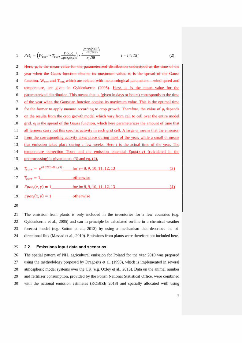
�� = �� ∗ �� ,� �� , ∗ � �−�� , 2−2��2 ,��√ � i = [4; 15] (2) 1

Here, μi is the mean value for the parameterized distribution understood as the time of the 2

year when the Gauss function obtains its maximum value. σi is the spread of the Gauss 3

function. Wcorr and Tcorr, which are related with meteorological parameters – wind speed and 4

temperature, are given in Gyldenkærne (2005). Here, μi is the mean value for the 5

parameterized distribution. This means that μi (given in days or hours) corresponds to the time 6

of the year when the Gaussian function obtains its maximum value. This is the optimal time 7

for the farmer to apply manure according to crop growth. Therefore, the value of μi depends 8

on the results from the crop growth model which vary from cell to cell over the entire model 9

grid. σi is the spread of the Gauss function, which here parameterizes the amount of time that 10

all farmers carry out this specific activity in each grid cell. A large σi means that the emission 11

from the corresponding activity takes place during most of the year, while a small σi means 12

that emission takes place during a few weeks. Here t is the actual time of the year. The 13

temperature correction Tcorr and the emission potential Epoti(x,y) (calculated in the 14

preprocessing) is given in eq. (3) and eq. (4). 15 �� = � 0.0 ∗� , for i= 8, 9, 10, 11, 12, 13 (3) 16 �� = 1 otherwise 17 �� , ≠ 1 for i= 8, 9, 10, 11, 12, 13 (4) 18 �� , = 1 otherwise 19

20

The emission from plants is only included in the inventories for a few countries (e.g. 21

Gyldenkærne et al., 2005) and can in principle be calculated on-line in a chemical weather 22

forecast model (e.g. Sutton et al., 2013) by using a mechanism that describes the bi-23

directional flux (Massad et al., 2010). Emissions from plants were therefore not included here. 24

2.2 Emissions input data and scenarios 25

The spatial pattern of NH3 agricultural emission for Poland for the year 2010 was prepared 26

using the methodology proposed by Dragosits et al. (1998), which is implemented in several 27

atmospheric model systems over the UK (e.g. Oxley et al., 2013). Data on the animal number 28

and fertilizer consumption, provided by the Polish National Statistical Office, were combined 29

with the national emission estimates (KOBIZE 2013) and spatially allocated with using 30

gridded data from the Corine Land Cover map (European Commission, 2005). Data on animal 1

numbers were available at commune level and fertilizer consumption at province level. 2

Detailed information about the calculation methodology used for Poland is described in Kryza 3

et al. (2011). The annual NH3 emissions were gridded to a spatial resolution of 5 km x 5 km 4

to be in accordance with the mesh in the meteorological model (Fig. 1). 5

Table 2 6

The annual gridded NH3 emissions were then used to construct 4 scenarios termed DEFAULT 7

(1), NOFERT(2), FLAT(3), and POLREGUL(4), respectively (Table). 8

The annual gridded NH3 emissions were then used to construct four scenarios, termed FLAT 9

(1), DEFAULT (2), POLREGUL (3) and NOFERT (4) (Table 2). Applying the scenarios 10

DEFAULT and FLAT shows the advantage of implementation of the dynamic emission 11

model (DEFAULT) instead of using a constant emission profile (FLAT). This step is 12

especially important for the area of Poland, as the dynamic approach at high spatial and 13

temporal resolution has not been used before and because Poland is a large country where the 14

spatial variations in the climate cause changes in crop growth throughout the country, thereby 15

affecting agricultural activity. Then, by replacing the default setup in the dynamic model with 16

Polish practice and regulations (POLREGUL) we wanted to provide some outlines for the 17

users of this or similar models concerning the expected range of changes in ammonia 18

emission. This is considered particularly important due to the expanding use of this open-19

source model. These differences in emissions are caused by variations in agricultural practice 20

in different countries, which are caused by both climate (thus affecting agricultural activity) 21

and national regulations. A detailed description of the POLREGUL approach is provided 22

below. In the fourth scenario (NOFERT) we wanted to show the sensitivity of the dynamic 23

model in respect to application of manure and fertilizers, mainly in respect of spring ammonia 24

emission peak, thereby demonstrating that the implementation of the method should carefully 25

assess national regulations on manure application for optimal performance of the model. 26

For the POLREGUL scenario the information on Polish infrastructure and management 27

methods was obtained from the IIASA review for the Danish and Polish area (Klimont and 28

Brink, 2004). Firstly, both countries have a ban on application of manure and mineral 29

fertilizer before 1 March. Secondly, the manure storage capacity in Poland is about 3 months, 30

compared to 7-9 months in Denmark. This means that farmers in Poland need to apply 31

manure during spring, summer and autumn. In Poland between 10-20% of husbandry manure 32

(only slurry) are applied to grassland, while they cover about 25% of the agricultural area. In 33

9

Poland the solid and slurry fractions of the manure is applied differently due to national 1

regulations. Solid manure goes into annual crops as only slurry is allowed on grasslands. 2

Between 10% and 20% of the slurry fraction is applied to grassland, which covers about 25% 3

of the entire agricultural area. Poland does not have a detailed nitrogen quota system at the 4

field level like Denmark does, and the Polish regulations do not contain definitions of 5

manure-N efficiency. The Danish regulations force farmers to apply most of the mineral 6

fertilizer and husbandry manure into growing crops, and there is a strict limit on how much 7

manure and mineral fertilizer is allowed to be added to each field in Denmark (Skjøth et al., 8

2008). A consequence is that a limited amount of mineral fertilizer is used in Denmark and 9

that the majority (90%) is applied to growing crops (April-May) and the remaining part to 10

grassland (summer). This is not the case in Poland, where there is a larger consumption of 11

mineral fertilizer. Assuming that all fields in Poland receive sufficient fertilizer (manure and 12

mineral) without an upper limit forced by regulation, a consequence is that as much manure as 13

possible will be used early in the season and that the majority of the mineral fertilizer will be 14

used on grasslands during summer (especially June, July and August) as there is a ban on 15

applying mineral fertilizer to meadows and pasture after 15 August. Therefore the simple 16

assumption therefore is that all fields will have equal amounts of manure and mineral 17

fertilizers during spring and summer (Table 3, Poland scenario). Finally, the regulations in 18

Poland allow farmers to apply manure to fields throughout October, which is not allowed in 19

Denmark. A consequence is that the timing of this autumn application, when the farms empty 20

their storages, has its peak 2-4 weeks later than in Denmark. We have therefore chosen 21

ordinal day number 290 (counted from the beginning of January each year, in our study 2010) 22

as the default peak time for this activity in Poland. 23

Table 3 24

2.3 Meteorological input data – WRF-ARW model configuration and model 25

performance 26

The Advanced Research WRF model was used with three one-way nested domains 27

(Skamarock and Klemp, 2008). The outer domain (131 x 131 gridpoints) covers Europe with 28

a horizontal resolution of 45 km x 45 km. The intermediate domain covers the area of central 29

Europe with a resolution of 15 km x 15 km (94 x 94 grid points). The innermost domain (194 30

x 194 gridpoints) covers the area of Poland at 5 km x 5 km resolution. Meteorological data 31

from the innermost domain are used in this study. Vertically, the domains are composed of 35 32

terrain-following hydrostatic-pressure coordinates, with the top fixed at 10 hPa. The 33

simulation was driven by the NCEP final analysis available every 6 h with 1.0o x 1.0o spatial 1

resolution. Analysis nudging was applied for the first two domains. 2

The model uses the same configuration of physics as presented by Kryza et al. (2013b), 3

including the Goddard microphysics scheme (Tao et al., 1989), Yonsei University planetary 4

boundary layer scheme (Hong et al., 2006), MM5 similarity surface layer and RRTMG and 5

RRTM schemes for short- and longwave radiation (Iacono et al., 2008; Mlawer et al., 1997). 6

The Kain-Fritsch cumulus scheme is applied for the first two domains (Kain, 2004). For the 7

innermost domain, cumulus convection is explicitly resolved. 8

Because the WRF-ARW derived spatial information on air temperature and wind speed is a 9

key input for the emission model, the modelled meteorological data were extensively 10

evaluated by comparison with the measurements. The measurements were available every 6 h 11

from 69 meteorological stations located in Poland. The model error was calculated for each 12

station and summarized using domain wide error The domain wide error statistics were 13

calculated and summarized with three error statistics: mean error (ME), mean absolute error 14

(MAE) and index of agreement (IOA, unitless). The definitions of the aforementioned error 15

measures are listed in the Supplement (Table 1). Air temperature at 2 m (T2) and wind speed 16

at 10 m a.g.l. (W10), which are used by the dynamic model of ammonia emission, show good 17

agreement with the measurements (Table 4). The air temperature is slightly underestimated, 18

but the IOA is very close to 1.0. The wind speed is slightly overestimated, with the ME >0. 19

Table 4 20

2.4 The FRAME model 21

The standard version of the Fine Resolution Atmospheric Multi-pollutant Exchange model 22

(FRAME) provides information on the annual mean oxidized sulphur and oxidized and 23

reduced nitrogen atmospheric air concentrations and deposition. A detailed description of the 24

FRAME model is given in Singles et al. (1998), Fournier et al. (2004), Dore et al. (2006) and 25

Vieno et al. (2010). Details on the model configuration for Poland can be found in Kryza et al. 26

(2010), Kryza et al. (2012) and Werner et al. (2014). FRAME is a Lagrangian model which 27

describes the main atmospheric processes in a column of air moving along straight-line 28

trajectories following specified wind directions. The model consists of 33 vertical layers of 29

varying thickness, ranging from 1 m at the surface to 100 m at the top of the domain. As such 30

the FRAME model is designed for studies where processes on local scale and landscape scale 31

will be governing (e.g. ammonia emissions) and have a simplified treatment of long-distance 32

11

transport and associated chemistry. Trajectories are advected with different starting angles at a 1

1° resolution using directionally dependent wind speed and frequency roses. 2

Vertical diffusion of gaseous and particulate species is described with K-theory eddy 3

diffusivity, and solved with the Finite Volume Method. The FRAME model chemistry 4

scheme is similar to the one used in the EMEP Lagrangian model (Barrett and Seland, 1995). 5

The prognostic chemical variables calculated in FRAME are: NH3, NO, NO2, HNO3, PAN, 6

SO2, H2SO4, as well as NH4+, NO3

- and SO4- aerosol. NH4NO3 aerosol is formed by the 7

equilibrium reaction between HNO3 and NH3. A second category of large nitrate aerosol is 8

presented and simulates the deposition of nitric acid on to soil dust or marine aerosol. The 9

formation of H2SO4 by gas phase oxidation of SO2 is represented by a predefined oxidation 10

rate. H2SO4 then reacts with NH3 to form ammonium sulphate aerosol. The aqueous reactions 11

considered in the model include the oxidation of S(IV) by O3, H2O2 and the metal catalysed 12

reaction with O2. 13

Dry deposition of SO2, NO2 and NH3 is calculated individually for five different land cover 14

categories (arable, forest, moor-land, grassland and urban) using a canopy resistance model 15

(Singles et al., 1998). Wet deposition is calculated with scavenging coefficients and a constant 16

drizzle approach, using precipitation rates calculated from a map of average annual 17

precipitation. An increased washout rate is assumed over hill areas due to the seeder-feeder 18

effect. It is assumed that the washout rate for the orographic component of rainfall due to the 19

seeder-feeder effect is twice that used for the non-orographic components (Dore et al., 1992) 20

Concentrations at the boundary of the model domain are calculated with the FRAME-Europe 21

model, which is a model similar to FRAME but which runs for the whole of Europe on the 22

EMEP grid at 50 km x 50 km resolution. For this study the model was adapted to run and 23

provide results at monthly resolution. Monthly wind roses were developed from the WRF data 24

using a method similar to that described by Dore et al. (2006). Information on rainfall for 25

FRAME was calculated by using observed data from 210 rainfall sites in Poland. 26

Geographically weighted regression kriging, with elevation used as an independent 27

explanatory variable (Szymanowski et al., 2013), was used here to produce a 5 km x 5 km 28

gridded data set that matches the meteorological grid from the WRF model. 29

FRAME was run four times for each month. Simulations for 1 month differ in the emission 30

scenario, which are described in Table 2 (section 2.2). 31

2.5 Measurements of ammonia (NH3) and ammonium (NH4+) air 32

concentrations & backward trajectories from the WRF-ARW model 33

Verifying observations are obtained from stations within the EMEP network (Aas et al., 1

2012). Four EMEP stations that measure daily air concentrations of gaseous ammonia and 2

aerosol ammonium (NH3+NH4+) and NH4

+ are available for Poland: PL02 Jarczew, PL03 3

nie ka, PL04 Łeba, PL05 Diabla żóra (Fig. 1). Three of these EMEP stations are located in 4

specific geographical areas (Łeba – sea coast in the north, nie ka – the highest peak in the 5

Sudety Mountains, SW Poland, Diabla Góra – in a large forestland, NE Poland). Three of 6

these EMEP stations are located in specific geographical areas, e.g. sea coast in the north 7

(Łeba), the highest peak in the Sudety Mountains (nie ka), and a large forestland in NE 8

Poland (Diabla Góra). These areas contain limited or even no agricultural activity. Only 9

Jarczew station, located in central-eastern Poland, is located in an agriculture area, and 10

therefore best suited for validation of the model results. One additional site from the 11

NitroEurope network provided measured monthly ammonia concentration. This site, Rzecin, 12

is located in a wetland area, which is surrounded by forests with full coverage of woodland 13

within the nearest 1 km. Land cover outside this woodland is mainly agricultural, and with the 14

highest ammonia emissions in Poland. 15

Error statistics ME, MAE and R for modelled and measured NH3 concentrations were 16

presented for each site individually, and mean statistics based on five stations were calculated 17

for the entire year and for the periods with (March-October) and without application of 18

manure (January, February, November, December). The definitions of the error measures are 19

listed in the supplementary material (Table 1). 20

Additionally, for Jarczew, the 3-hourly emissions from the dynamic model were aggregated 21

into daily values and plotted with average daily concentrations from the station. The daily 22

observations and aggregated model calculations were then sorted in two groups: (1) a group 23

with high concentrations of NH3 that were not simulated by the emissions model, and (2) the 24

remaining days. Group 1 was then investigated in detail with air mass trajectories calculated 25

with WRF-ARW data. RIP version 4.5 (Stoelinga., 2008) was used to get 36 hours backward 26

trajectories for the Jarczew station RIP version 4.5 (Stoelinga, 2009), which is a is a Fortran 27

program used for visualizing output from gridded meteorological data sets, was implemented 28

to get 36 h backward trajectories for the Jarczew station. 29

. 6 trajectories were run for each day with an episode from group 1, once every 6 hours and 30

for the receiving heights 250 m and 750 m. 6 trajectories were run for each day with an 31

episode from group 1, once every 6 hours. The trajectories were run for the receiving heights 32

of 250 m and 750 m, as it was suggested by Hernández-Ceballos et al. (2014) that trajectories 33

Formatted: Tab stops: 5.03 cm, Left

13

between 300 and 700 m do not show large differences in transport path within the first 12-24 1

hours. Each episode was then analyzed with respect to potential atmospheric transport from 2

neighborhood regions with high ammonia emissions. 3

3 Results 4

The results are organized as follows: first the annual ammonia emission and results from the 5

POLREGUL option of the dynamic model for Poland are described. In the second subsection 6

FRAME model concentrations from four runs (FLAT, DEFAULT, POLREGUL, NOFERT) 7

(DEFAULT, NOFERT, FLAT and POLREGUL) are presented and compared with 8

measurements. Finally, the relationship between the dynamically modelled emissions and 9

measured concentrations for one selected station was presented. 10

3.1 NH3 emission in Poland in 2010 11

Total ammonia emission (sum for the total country area) in Poland in 2010 was 270 Gg. The 12

highest annual emissions are in the central part of the country, and locally exceed 35 kg ha-1 13

year-1 (maximum 45 kg ha-1 year-1, Fig. 2). These are areas with agricultural activity 14

contributing to the majority of NH3 emissions in Poland. The NH3 emissions are in the range 15

of 1 to 10 kg ha-1 year-1 over 70% area of the country. The lowest emissions are in the west, 16

north-west and south-east, where agricultural activity is less intense and large areas are 17

covered with forests. 18

Figure 1 19

From analysis of the monthly total (Fig. 2), it can be seen April is the month of the highest 20

emission for both the DEFAULT and POLREGUL model run. In the case of the DEFAULT 21

run about 40% of the annual emission is related to this month and minor emission peaks 22

appear in March, July and September. For the POLREGUL scenario the April peak is lower 23

by about 40% in comparison to DEFAULT, and the increased emission also appears in July 24

and October (Fig. 2). Generally, there was higher emission in the period with average 25

monthly temperature above 5.0ºC. 26

The seasonal variation of emission (POLREGUL run) for different agricultural categories for 27

the grid representing Jarczew station is shown in Fig. 3. In April, which is also the month with 28

the highest ammonia emission for the total area of Poland, three functions have their highest 29

values. At this time, the peaks are observed for applications of manure on bare soils, 30

application of fertilizers and manure on crops. Ammonia treated straw (Fct15) is responsible 31

for high ammonia emission in summer, whereas the autumn peak of emission (end of 32

September, October) is related mainly to application of manure. Application of manure 1

(Fct10) is responsible for peak of emission in summer and autumn. Emission related to 2

livestock is dominated in Poland by Fct1 because of large-scale farming of pigs in Poland (37 3

cattle and 99 pigs per 100 ha of agricultural land, GUS Central Statistical Office of Poland 4

2010, stat.gov.pl). Due to meteorological conditions (temperature), their contribution is 5

doubled in the summer season in comparison to winter. 6

Figure 2 7

Figure 3 8

The spatial distribution of ammonia emission for selected days (sum of emission between 9

hours 12-15 UTC for the 15th day of a month) is presented in Fig. 4. The three hourly 10

averages for the total area of Poland are equal to 0.5, 8.0, 3.0, 2.7 g ha-1, respectively, in 11

February, April, June and September. The spatial distribution of ammonia emission for 12

selected months of each season (February, April, June and September) is presented in Fig. 4. 13

The monthly averages for the total area of Poland are equal to 0.11, 2.56, 0.42, 0.70 kg ha-1 in 14

February, April, June and September, respectively. The maximum values are observed in 15

April in the central part of the country, where they reach 50 10-12 kg ha-1. 16

Figure 4 17

18

For the three selected locations (names of the locations are taken after the nearest towns, 19

marked in Fig. 1) in Poland – Wrocław (south-west), Suwałki (north-east) and close to Leszno 20

(middle-west) - hourly emissions for the selected period (from March to May) are shown in 21

Fig. 5. Two of these locations represent the areas of the longest (Wrocław) and the shortest 22

(Suwałki) growing season in Poland. The spring increase in emission appears first in Wroclaw 23

(middle of March) and then almost four weeks later in Suwałki. Leszno is located in the area 24

with the highest ammonia emissions in Poland. There is a large day to night emission 25

variability due to diurnal variability in air temperature and wind speed. Due to diurnal 26

variability in air temperature and wind speed there is a day-night variation in emission. The 27

mean for the entire year diurnal variation is equal to 20% (Wrocław) - 25% (Leszno), with the 28

lowest values during winter (about 10%) and highest in spring and summer (about 30%). 29

Figure 5 30

3.2 NH3 concentration calculated with the FRAME model 31

Formatted: Superscript

15

The spatial distribution of modelled NH3 concentration from the POLREGUL scenario for 1

February, April, June and September is illustrated in Fig. 4. The highest concentrations are in 2

the agricultural areas in the central part of Poland, with maximum values equal to 1.32, 26.0, 3

16.5 and 9.2 µg m-3 for February, April, June and September, respectively. High spatial 4

correlation (≥0.9) between the modelled ammonia emission and FRAME ammonia 5

concentration (Fig 4.) was calculated for each month. 6

Time series and error statistics of modelled (FLAT, DEFAULT, POLREGUL, 7

NOFERT)(DEFAULT, NOFERT, FLAT, POLREGUL) and measured NH3 concentrations 8

are presented in Fig. 6 and Table 5. For most sites (Rzecin, Jarczew, Łeba and nie ka) R and 9

MAE are best for the NOFERT and POLREGUL runs. The best performance was obtained 10

for Jarczew and Rzecin. For each station the DEFAULT run calculates that the concentrations 11

peak in April which is not present in the measurements or is much lower higher than observed 12

(Jarczew, Rzecin). Application of Polish regulations practice in the dynamic model has 13

improved the results most significantly in comparison to the DEFAULT for Rzecin and 14

Jarczew. Jarczew is the only station located directly in an agricultural area, whereas Rzecin is 15

under the influence of an agricultural region with the highest ammonia emission in Poland. 16

The poorest performance for each model run is for Diabla Góra, for which the measured time 17

series has a totally different pattern in comparison to the other sites. High measured 18

concentrations for this station are obtained in late autumn and the winter months. 19

For three model runs (FLAT, DEFAULT, NOFERT) (DEFAULT, NOFERT, FLAT) 20

correlation coefficients are lowest for the summer period in comparison to the entire year 21

(Table 6), whereas the summer period has the highest correlation coefficients for the 22

POLREGUL scenario. The POLREGUL scenario therefore improved the results significantly 23

in comparison to DEFAULT for summer period – the correlation coefficient increased from 24

0.21 to 0.73 and MAE decreased from 0.83 to 0.68. 25

Figure 6 26

Table 5 27

Table 6 28

3.3 Comparison of daily emissions with measured concentrations and 29

backward trajectories case study 30

Due to the high spatial correlation between ammonia emission and concentration (Fig 4) we 31

looked for the relationship between the dynamically modelled emissions and measured 32

concentrations for Jarczew station (Fig. 7). The main peaks in emissions (April, September) 1

are reflected in the concentration data. There are also some peaks in concentrations (e.g. end 2

of February, beginning of June and end of October) which are not resolved by the emission 3

model. These could suggest the limitations of the emission model, or could be related to 4

meteorology which has resulted in the transport of ammonia from neighboring areas. 5

Backward trajectories, for the mentioned high concentration episodes (end of February, 6

beginning of June and end of October), were calculated with the RIP tool (Fig. 8) in order to 7

check whether it is possible to connect these observed peaks in concentrations with 8

atmospheric transport of ammonia. We have found that for these episodes the trajectories 9

have a similar pattern - transport from the south or south-west sector. The air masses that 10

reached Jarczew have during these episodes passed areas with high ammonia emissions in 11

comparison to the local area surrounding the station. 12

Figure 7 13

Figure 8 14

4 Discussion and conclusion 15

The temporal and spatial variability of ammonia emission has been analysed over Poland with 16

four scenarios: FLAT (no temporal variation), DEFAULT (matches the Europe-wide default 17

settings in the ammonia emission model, Skjøth et al. 2011), POLREGUL (takes into account 18

Polish infrastructure and less regulation compared to DEFAULT) and NOFERT (excludes 19

application of manure and mineral fertilizer). 20

DEFAULT (matches the Europe-wide default settings in the ammonia emission model, Skjøth 21

et al. 2011), NOFERT (excludes application of manure and mineral fertilizer), FLAT (the 22

existing emission method (no temporal variations) used in WRF-Chem over Poland) and 23

POLREGUL (takes into account Polish infrastructure and current and less regulation 24

compared to DEFAULT). The emissions were then been implemented in the FRAME model 25

for a fast response on simulating the effect of the scenarios in relation to atmospheric 26

chemistry. The results show that, in general, the model simulations results for the agricultural 27

areas were improved by applying a dynamical model by using Europe-wide (default) settings 28

instead of using a fixed emission profile. However, If Polish infrastructure practice and 29

national regulation is incorporated into the emission model, the FRAME model performance 30

is further improved much better results are achieved for agricultural areas. 31

17

The model results show large difference in emissions between months, as well as between day 1

and night. This is due to increased volatilization of ammonia caused by increased 2

temperatures (Eq. 1 and 2) and emission from animal and mineral fertilizer that are applied 3

over short time periods during spring, summer and autumn (Eq. 2). Taking into account the 4

entire area of the country, the highest emission is obtained during spring (especially in April). 5

The spring emission peak (and corresponding concentrations) is mainly related to the 6

application of fertilizers and manure, which is clearly illustrated by comparing the POLREG 7

and NOFERT simulations (Fig. 6). The sensitivity of the model to the application of manure 8

is highlighted by the large difference between the DEFAULT and POLREGUL scenarios. In 9

April the emission is 40% lower in the POLREGUL scenario than in the default scenario. 10

This is not surprising, as previous results have shown that national regulation can change 11

emissions from manure to increase by more than 100% in spring and decrease during summer 12

to less than 10% (Skjøth et al., 2008). The scale and character of changes between the 13

POLREGUL and DEFAULT simulations with the dynamic ammonia model will vary 14

between countries and depend on local agricultural infrastructure and practice. The dynamic 15

model predicts the spring peak in emission to start in south-west Poland and then progressing 16

to the rest of the country (Fig. 5). South-west Poland has the longest growing season 17

( mudzka, 2012) and is the area where farmers initiate their field activities in Poland. In this 18

region, field work, including application of fertilizers or manure, can start earlier than in other 19

regions of the country. This aspect of a ”northward progressing ammonia plume” due to 20

spring application is therefore very well captured by the model and has also been 21

implemented in the GEOS-CHEM model (Paulot et al., 2014) and DEHM models (Skjøth et 22

al., 2011). 23

Major NH3 emission peaks modelled for the Jarczew agricultural station are also observed in 24

NH3 concentration measurements. However, some peaks in concentrations are not reflected in 25

the emission data. As suggested by Asman et al. (1998) and Fowler et al. (1998) atmospheric 26

ammonia can be transported up to 100 km. According to Geels et al. (2012) the fraction of 27

locally emitted NH3 depositing locally is on of the order of 15-30% for a grid of 16 km x 16 28

km. In our study, the analysis of backward trajectories showed that increased concentrations 29

can be related to transport of ammonia from neighboring areas with high emission. A more 30

thorough investigation on this scale requires more sophisticated modelling tools than FRAME 31

such as WRF-Chem. 32

FRAME is a relatively simple Lagrangian model and the results were found to be in good 1

agreement with measurements for Poland (Kryza et al., 2011, 2012; Werner et al., 2014) and 2

for the UK (Dore et al., 2015). This enables us to run several scenarios for the entire year 3

without a large computational overhead. Similar principles to FRAME are present in local 4

scale models like OML (Geels et al., 2012) and OPS (Van Jaarsveld, 2004; Velders et al., 5

2011). It is shown with these models that in relation to ammonia and on spatial scales of 0.5-6

16 km it is sufficient to neglect chemical transformation and wet deposition even on a daily 7

and weekly basis (Geels et al., 2012). OML and FRAME use similar principles for the near 8

source domain. In relation to ammonia and the fate due to chemical conversion and wet 9

deposition, the FRAME methodology is more advanced than the OML method. Although the 10

OML model does not include chemical conversion or wet deposition, the annual correlation 11

coefficients are high (0.7-0.75) and the bias is low, when compared with observations. This 12

shows that the governing processes on ammonia concentrations on this scale are due to 13

emissions and dispersion within the agricultural areas and only to a small degree chemical 14

conversion and deposition (dry and wet). These results correspond well with the two latest 15

reviews on this subject (Hertel et al., 2006, 2012). 16

Furthermore, the results with FRAME are considered good enough for this study on the 17

emission patterns, as the obtained monthly correlation coefficients on the POLREGUL 18

scenario are similar to the model results that are obtained both with DEHM (Skjøth et al., 19

2011) and the DAMOS system (Geels et al., 2012). In fact, the very high spatial correlation 20

between ammonia emission and ammonia concentration (Fig. 4) suggests, that on a monthly 21

basis, the governing process for ammonia concentrations is emission and only to a smaller 22

degree atmospheric transport and transformation. The four scenarios show that focus on the 23

agricultural practice, national regulations and the infrastructure (e.g. storage facilities) is a key 24

challenge but very important for obtaining the best results. For Poland it was possible to 25

obtain almost as good results as DEHM for Danish and German sites, despite the lack of 26

detail about location of the agricultural fields and the location, amount and type of livestock 27

in Poland. This suggests that similar improvements can be obtained for other European areas. 28

The monthly correlation coefficients obtained with the FRAME model for the agricultural 29

sites are comparable to the model results that are obtained with both DEHM (Skjøth et al., 30

2011) and the DAMOS system (Geels et al., 2012). Application of Polish practice into the 31

ammonia dynamic model improves the FRAME results in comparison to the European default 32

settings of the dynamic model. This suggests that similar improvements can be obtained for 33

19

other European areas. For Polish conditions, with lack of detailed information about location 1

of the agricultural fields and the location, amount and type of livestock, a higher mean 2

absolute error for the dynamic simulations is observed in comparison to the constant emission 3

approach. This also suggests that spatial allocation of emission might have a greater influence 4

on concentration results obtained from a dynamic than from a constant emission approach. 5

One of the sites (Diabla Góra) has an inverted time series in comparison to all other stations - 6

the highest ammonia concentration appears in late autumn and in the winter months. Our 7

calculations, which took into account only agricultural sources, were not able to catch peaks 8

in this period. The Diabla Góra station is located in a large forested area called “Borecka 9

Żorest”, surrounded by lakeland, with a small contribution of arable land in the region. Due to 10

this location, high ammonia concentrations in this period may be related with natural sources. 11

Open water areas (Barrett, 1998; Sørensen et al., 2003) and natural land areas (Duyzer, 1994) 12

have been shown to emit NH3. Emission of NH3 from ecosystems are found to take place 13

when the atmospheric NH3 concentration is lower than the stomatal NH3 compensation point 14

(Mattsson et al., 2009), as a result of decomposing leaf litter and due to cuticular desorption 15

(David et al., 2009; Hansen et al., 2013). As suggested by Hansen et al. (2013), natural 16

ammonia emission from deciduous forests should be considered as an emissions source which 17

could be dynamically simulated with atmospheric transport models. Another factor that can 18

cause an increase of ammonia concentrations within a plant canopy coupled with altered 19

microclimate could be evaporation of ammonium containing aerosol (Fowler et al., 2009; 20

Nemitz et al., 2004).. Another factor that can cause an increase of ammonia concentrations 21

could be evaporation from ammonium containing aerosols. Ammonium-chloride, 22

ammonium-nitrate and ammonium-bi-sulphate are all formed from reversible processes in the 23

atmosphere. Such processes can more efficiently be studied with models like WRF-Chem, 24

once they have been connected with a dynamical ammonia emission model. Natural emission 25

could explain the high ammonia concentrations at the Diabla Góra station in autumn and late 26

autumn (until beginning of December), when mean daily temperature is above zero and no 27

snow cover present. Based on the emission and measurements data as well as model results it 28

is difficult to explain the high ammonia concentrations in the mid-winter period. These could 29

be more efficiently studied with chemistry transport models which are connected online with 30

both meteorology like e.g. GATOR-MMTD (Jacobson et al., 1996), WRF-Chem (Grell et al., 31

2005), GEM-AQ (Kaminski et al., 2007), and a dynamic ammonia emission model. 32

The dynamical approach has consistently provided good results for agricultural regions during 1

the winter months, which is due to the large response on ammonia emission from agricultural 2

buildings caused by outside temperatures. An implementation of this type of emission model 3

into WRF-Chem CTM online coupled with meteorology will be a direct response to the 4

suggestion by Sutton et al. (2013) and a direct coupling between ammonia emission, 5

meteorology and chemistry and can address some of the challenges in the modelling of air 6

pollution that have been highlighted (Baklanov et al., 2014). 7

For regional modelling of ammonia in Europe, the overall results suggest that it will be an 8

advantage to move from a static to a dynamic approach. The Europe-wide default setting in 9

the model given by Skjøth et al. (2011) can be expected to improve the results over large 10

areas, but a better picture over Poland will be obtained if the values from Table 2 in Skjøth et 11

al. (2011) are replaced with the values from our POLREGUL scenario. Further improvement 12

on ammonia emissions is likely to be related to natural sources (Hansen et al., 2013; Riddick 13

et al., 2014) as well as the dependence on emission from fertilizer on soil type as shown by 14

the CHIMERE model (Hamaoui-Laguel et al., 2014). These initiatives are currently beeing 15

adressed by the ECLAIRE project (http://www.eclaire-fp7.eu/), which focuses on climate 16

driven emissions (BVOCs and ammonia) as suggested by the latest IPCC report (2013), that 17

calls for more studies on the feedback mechanisms between climate and air quality. 18

19

Acknowledgments 20

The study received support from the Polish National Science through projects no. UMO-21

2013/09/B/ST10/00594 and UMO-2011/03/B/ST10/06226. Preparation of the meteorological 22

data was carried out at the Wrocław Centre for Networking and Supercomputing 23

(http://www.wcss.wroc.pl) (grant no. 170). 24

References 25

Aas, W., Tsyro, S., Bieber, E., Bergström, R., Ceburnis, D., Ellermann, T., Fagerli, H., Frölich, 26

M., Gehrig, R., Makkonen, U., Nemitz, E., Otjes, R., Perez, N., Perrino, C., Prévôt, A. S. H., 27

Putaud, J.-P., Simpson, D., Spindler, G., Vana, M. and Yttri, K. E.: Lessons learnt from the 28

first EMEP intensive measurement periods, Atmos. Chem. Phys., 12(17), 8073–8094, 29

doi:10.5194/acp-12-8073-2012, 2012. 30

Field Code Changed

Formatted: English (U.K.)

http://www.eclaire-fp7.eu/

21

Andersen, H. V, Hovmand, M. F., Hummelshøj, P. and Jensen, N. O.: Measurements of 1

ammonia concentrations, fluxes and dry deposition velocities to a spruce forest 1991-1995, 2

Atmos. Environ., 33(9), 1367–1383, 1999. 3

Anderson, N., Strader, R. and Davidson, C.: Airborne reduced nitrogen: ammonia emissions 4

from agriculture and other sources., Environ. Int., 29(2-3), 277–86, doi:10.1016/S0160-5

4120(02)00186-1, 2003. 6

Asman, W. A. H., Sutton, M. A. and Schjorring, J. K.: Ammonia: emission, atmospheric 7

transport and deposition, New Phytol., 139(1), 27–48, doi:10.1046/j.1469-8137.1998.00180.x, 8

1998. 9

Baklanov, A., Schlünzen, K., Suppan, P., Baldasano, J., Brunner, D., Aksoyoglu, S., Carmichael, 10

G., Douros, J., Flemming, J., Forkel, R., Galmarini, S., Gauss, M., Grell, G., Hirtl, M., Joffre, 11

S., Jorba, O., Kaas, E., Kaasik, M., Kallos, G., Kong, X., Korsholm, U., Kurganskiy, A., 12

Kushta, J., Lohmann, U., Mahura, A., Manders-Groot, A., Maurizi, A., Moussiopoulos, N., 13

Rao, S. T., Savage, N., Seigneur, C., Sokhi, R. S., Solazzo, E., Solomos, S., Sørensen, B., 14

Tsegas, G., Vignati, E., Vogel, B. and Zhang, Y.: Online coupled regional meteorology 15

chemistry models in Europe: current status and prospects, Atmos. Chem. Phys., 14(1), 317–16

398, doi:10.5194/acp-14-317-2014, 2014. 17

Banzhaf, S., Schaap, M., Wichink Kruit, R. J., Denier van der Gon, H. A. C., Stern, R. and 18

Builtjes, P. J. H.: Impact of emission changes on secondary inorganic aerosol episodes across 19

Germany, Atmos. Chem. Phys., 13(23), 11675–11693, doi:10.5194/acp-13-11675-2013, 20

2013. 21

Barrett, K.: Oceanic ammonia emissions in Europe and their transboundary fluxes, Atmos. 22

Environ., 32(3), 381–391, doi:10.1016/S1352-2310(97)00279-3, 1998. 23

Barrett, K. and Seland, O.: European Transboundary Acidifying Air Pollution: Ten Years 24

Calculated Fields and Budgets to the End of the First Sulphur Protocol, European 25

transboundary air pollution report, 1-150, 1995. 26

Bash, J. O., Cooter, E. J., Dennis, R. L., Walker, J. T. and Pleim, J. E.: Evaluation of a regional 27

air-quality model with bidirectional NH3 exchange coupled to an agroecosystem model, 28

Biogeosciences, 10(3), 1635–1645, doi:10.5194/bg-10-1635-2013, 2013. 29

Bouwman, A. F., Lee, D. S., Asman, W. A. H., Dentener, F. J., Van Der Hoek, K. W. and 30

Olivier, J. G. J.: A global high-resolution emission inventory for ammonia, Global 31

Biogeochem. Cycles, 11(4), 561–587, doi:10.1029/97GB02266, 1997. 32

David, M., Loubet, B., Cellier, P., Mattsson, M., Schjoerring, J. K., Nemitz, E., Roche, R., 1

Riedo, M. and Sutton, M. A.: Ammonia sources and sinks in an intensively managed 2

grassland canopy, Biogeosciences, 6(9), 1903–1915, doi:10.5194/bg-6-1903-2009, 2009. 3

Dore, A. J., Carslaw, D. C., Braban, C., Chemel, C., Conolly, C., Derwent, R. G., Griffiths, S. J., 4

Hall, J., Hayman, G., Lawrence, S., Metcalfe, S. E., Redington, A., Simpson, D., Sutton, M. 5

A., Sutton, P., Tang, Y. S., Vieno, M., Werner, M. and Whyatt, J. D.: Evaluation of the 6

performance of different atmospheric chemical transport models and inter-comparison of 7

nitrogen and sulphur deposition estimates for the UK, Atmos. Environ., In review, 1–24, 8

2015. 9

Dore, A. J., Choularton, T. W. and Fowler, D.: An improved wet deposition map of the United 10

Kingdom incorporating the seeder-feeder effect over mountainous terrain., Atmos. Environ., 11

26A(8), 1375-1381, 1992. 12

Dore, A. J., Vieno, M., Fournier, N., Weston, K. J. and Sutton, M. A.: Development of a new 13

wind-rose for the British Isles using radiosonde data, and application to an atmospheric 14

transport model, Q. J. R. Meteorol. Soc., 132(621), 2769–2784, doi:10.1256/qj.05.198, 2006. 15

Dragosits, U., Sutton, M. A., Place, C. J. and Bayley, A. A.: Modelling the spatial distribution of 16

agricultural ammonia emissions in the UK, Environ. Pollut., 102(1), 195–203, 17

doi:10.1016/S0269-7491(98)80033-X, 1998. 18

Duyzer, J.: Dry deposition of ammonia and ammonium aerosols over heathland, J. Geophys. 19

Res., 99(D9), 18757, doi:10.1029/94JD01210, 1994. 20

Emmett, B. A.: Nitrogen saturation of terrestrial ecosystems: some recent findings and their 21

implications for our conceptual framework, Water Air Soil Pollut., 7, 99–109, 2007. 22

Flechard, C. R., Massad, R.-S., Loubet, B., Personne, E., Simpson, D., Bash, J. O., Cooter, E. J., 23

Nemitz, E. and Sutton, M. A.: Advances in understanding, models and parameterizations of 24

biosphere-atmosphere ammonia exchange, Biogeosciences, 10(7), 5183–5225, 25

doi:10.5194/bg-10-5183-2013, 2013. 26

Fournier, N., Dore, A. J., Vieno, M., Weston, K. J., Dragosits, U. and Sutton, M. A.: Modelling 27

the deposition of atmospheric oxidised nitrogen and sulphur to the United Kingdom using a 28

multi-layer long-range transport model, Atmos. Environ., 38(5), 683–694, 29

doi:10.1016/j.atmosenv.2003.10.028, 2004. 30

Fowler, D.: Regional mass budgets of oxidized and reduced nitrogen and their relative 31

contribution to the N inputs of sensitive ecosystems, Environ. Pollutution (Nitrogen Conf. 32

Spec. Issue), 102, 337 – 342, 1998. 33

23

Fowler, D., Pilegaard, K., Sutton, M. A., Ambus, P., Raivonen, M., Duyzer, J., Simpson, D., 1

Fagerli, H., Fuzzi, S., Schjoerring, J. K., Granier, C., Neftel, A., Isaksen, I. S. A., Laj, P., 2

Maione, M., Monks, P. S., Burkhardt, J., Daemmgen, U., Neirynck, J., Personne, E., Wichink-3

Kruit, R., Butterbach-Bahl, K., Flechard, C., Tuovinen, J. P., Coyle, M., Gerosa, G., Loubet, 4

B., Altimir, N., Gruenhage, L., Ammann, C., Cieslik, S., Paoletti, E., Mikkelsen, T. N., Ro-5

Poulsen, H., Cellier, P., Cape, J. N., Horváth, L., Loreto, F., Niinemets, Ü., Palmer, P. I., 6

Rinne, J., Misztal, P., Nemitz, E., Nilsson, D., Pryor, S., Gallagher, M. W., Vesala, T., Skiba, 7

U., Brüggemann, N., Zechmeister-Boltenstern, S., Williams, J., O’Dowd, C., Żacchini, M. C., 8

de Leeuw, G., Flossman, A., Chaumerliac, N. and Erisman, J. W.: Atmospheric composition 9

change: Ecosystems–Atmosphere interactions, Atmos. Environ., 43(33), 5193–5267, 10

doi:10.1016/j.atmosenv.2009.07.068, 2009. 11

Friedrich, R.: Improving and applying methods for the calculation of natural and biogenic 12

emissions and assessment of impacts to the air quality, Final project activity report 2007, 13

2007. 14

Geels, C., Andersen, H. V., Ambelas Skjøth, C., Christensen, J. H., Ellermann, T., Løfstrøm, P., 15

Gyldenkærne, S., Brandt, J., Hansen, K. M., Frohn, L. M. and Hertel, O.: Improved modelling 16

of atmospheric ammonia over Denmark using the coupled modelling system DAMOS, 17

Biogeosciences, 9(7), 2625–2647, doi:10.5194/bg-9-2625-2012, 2012. 18

Grell, G., Peckham, S. E., Schmitz, R., McKeen, Stuart Frost, G., Skamarock, W. C. and Eder, 19

B.Ś Żully coupled “online” chemistry within the WRŻ model, Atmos. Environ., 39(37), 6957–20

6975, doi:10.1016/j.atmosenv.2005.04.027, 2005. 21

Van Grinsven, H. J. M., ten Berge, H. F. M., Dalgaard, T., Fraters, B., Durand, P., Hart, A., 22

Hofman, G., Jacobsen, B. H., Lalor, S. T. J., Lesschen, J. P., Osterburg, B., Richards, K. G., 23

Techen, A.-K., Vertès, F., Webb, J. and Willems, W. J.: Management, regulation and 24

environmental impacts of nitrogen fertilization in northwestern Europe under the Nitrates 25

Directive; a benchmark study, Biogeosciences, 9(12), 5143–5160, doi:10.5194/bg-9-5143-26

2012, 2012. 27

Guevara, M., Martínez, F., Arévalo, G., Gassó, S. and Baldasano, J. M.: An improved system for 28

modelling Spanish emissions: HERMESv2.0, Atmos. Environ., 81, 209–221, 29

doi:10.1016/j.atmosenv.2013.08.053, 2013. 30

Gyldenkærne, S., Skjøth, C. A., Hertel, O. and Ellermann, T.: A dynamical ammonia emission 31

parameterization for use in air pollution models, J. Geophys. Res., 110(D7), D07108, 32

doi:10.1029/2004JD005459, 2005. 33

Hamaoui-Laguel, L., Meleux, F., Beekmann, M., Bessagnet, B., Génermont, S., Cellier, P. and 1

Létinois, L.: Improving ammonia emissions in air quality modelling for France, Atmos. 2

Environ., 92, 584–595, doi:10.1016/j.atmosenv.2012.08.002, 2014. 3

Hansen, K., Sørensen, L. L., Hertel, O., Geels, C., Skjøth, C. A., Jensen, B. and Boegh, E.: 4

Ammonia emissions from deciduous forest after leaf fall, Biogeosciences, 10(7), 4577–4589, 5

doi:10.5194/bg-10-4577-2013, 2013. 6

Hellsten, S., Dragosits, U., Place, C. J., Vieno, M., Dore, A. J., Misselbrook, T. H., Tang, Y. S. 7

and Sutton, M. A.: Modelling the spatial distribution of ammonia emissions in the UK., 8

Environ. Pollut., 154(3), 370–9, doi:10.1016/j.envpol.2008.02.017, 2008. 9

Hernández-Ceballos, M. a., Skjøth, C. a., García-Mozo, H., Bolívar, J. P. and Galán, C.: 10

Improvement in the accuracy of back trajectories using WRF to identify pollen sources in 11

southern Iberian Peninsula, Int. J. Biometeorol., 58, 2031–2043, doi:10.1007/s00484-014-12

0804-x, 2014. 13

Hertel, O., Skjøth, C. A., Løfstrøm, P., Geels, C., Frohn, L. M., Ellermann, T. and Madsen, P. 14

V.: Modelling Nitrogen Deposition on a Local Scale—A Review of the Current State of the 15

Art, Environ. Chem., 3(5), 317, doi:10.1071/EN06038, 2006. 16

Hertel, O., Skjøth, C. A., Reis, S., Bleeker, a., Harrison, R. M., Cape, J. N., Fowler, D., Skiba, 17

U., Simpson, D., Jickells, T., Kulmala, M., Gyldenkærne, S., Sørensen, L. L., Erisman, J. W. 18

and Sutton, M. a.: Governing processes for reactive nitrogen compounds in the European 19

atmosphere, Biogeosciences, 9(12), 4921–4954, doi:10.5194/bg-9-4921-2012, 2012. 20

Hettelingh, J. P., Posch, M. and Slootweg, J.: Progress in the Modelling of Critical Thresholds 21

and Dynamic Modelling, Including Impacts on Vegetation in Europe, CCE Status Rep., 1-22

182, 2009. 23

Hong, S.-Y., Noh, Y. and Dudhia, J.: A New Vertical Diffusion Package with an Explicit 24

Treatment of Entrainment Processes, Mon. Weather Rev., 134(9), 2318–2341, 25

doi:10.1175/MWR3199.1, 2006. 26

Iacono, M. J., Delamere, J. S., Mlawer, E. J., Shephard, M. W., Clough, S. A. and Collins, W. 27

D.: Radiative forcing by long-lived greenhouse gases: Calculations with the AER radiative 28

transfer models, J. Geophys. Res., 113(D13), D13103, doi:10.1029/2008JD009944, 2008. 29

Van Jaarsveld, H.: The Operational Priority Substances model: Description and validation of 30

OPS-Pro 4.1., 1-156, 2004. 31

Jacobson, M. Z., Lu, R., Turco, R. P. and Toon, O. .: Development and application of a new air 32

pollution model system e Part I: Gas-phase simulations, Atmos. Env, 30, 1939–1963, 1996. 33

25

Jones, M. L. M., Norris, D., Hall, J. and Petit, S.: Developing an indicator-modelling approach to 1

forecast changes in nitrogen critical load exceedance across Europe arising from agricultural 2

reform, Ecol. Indic., 11(1), 16–26, doi:10.1016/j.ecolind.2009.06.005, 2011. 3

Kain, J. S.: The Kain–Fritsch Convective Parameterization: An Update, J. Appl. Meteorol., 4

43(1), 170–181, 2004. 5

Kaminski, J., Neary, L., Lupu, A., McConnell, J., Struzewska, J., Zdunek, M. and Lobocki, L.: 6

High Resolution Air Quality Simulations with MC2-AQ and GEM-AQ, in Air Pollution 7

Modeling and Its Application XVII SE - 86, edited by C. Borrego and A. L. Norman, pp. 8

714–720, Springer US., 2007. 9

Klimont, Z. and Brink, C.: Modelling of Emissions of Air Pollutants and Greenhouse Gases from 10

Agricultural Sources in Europe, Ina. Rep. R. Minist. Environ. Oslo, Norw, 2004. 11

Kryza, M., Dore, A. J., Bła , M. and Sobik, M.Ś Modelling deposition and air concentration of 12

reduced nitrogen in Poland and sensitivity to variability in annual meteorology., J. Environ. 13

Manage., 92(4), 1225–36, doi:10.1016/j.jenvman.2010.12.008, 2011. 14

Kryza, M., Mill, W., Dore, A. J., Werner, M. and Bła , M.Ś Calculation of Sulphur and Nitrogen 15

Deposition with the Frame Model and Assessment of the Exceedance of Critical Loads in 16

Poland, Ecol. Chem. Eng. S, 20(2), 279–290, doi:10.2478/eces-2013-0020, 2013a. 17

Kryza, M., Werner, M., Bła , M., Dore, A. J. and Sobik, M.Ś The effect of emission from coal 18

combustion in nonindustrial sources on deposition of sulfur and oxidized nitrogen in Poland., 19

J. Air Waste Manag. Assoc., 60(7), 856–66, 2010. 20

Kryza, M., Werner, M., Dore, A. J., Bła , M. and Sobik, M.Ś The role of annual circulation and 21

precipitation on national scale deposition of atmospheric sulphur and nitrogen compounds., J. 22

Environ. Manage., 109, 70–9, doi:10.1016/j.jenvman.2012.04.048, 2012. 23

Kryza, M., Werner, M., Wałszek, K. and Dore, A. J.Ś Application and evaluation of the WRŻ 24

model for high-resolution forecasting of rainfall – a case study of SW Poland, Meteorol. 25

Zeitschrift, 22(5), 595–601, doi:10.1127/0941-2948/2013/0444, 2013b. 26

Massad, R.-S., Nemitz, E. and Sutton, M. A.: Review and parameterisation of bi-directional 27

ammonia exchange between vegetation and the atmosphere, Atmos. Chem. Phys., 10(21), 28

10359–10386, doi:10.5194/acp-10-10359-2010, 2010. 29

Mattsson, M., Herrmann, B., David, M., Loubet, B., Riedo, M., Theobald, M. R., Sutton, M. A., 30

Bruhn, D., Neftel, A. and Schjoerring, J. K.: Temporal variability in bioassays of the stomatal 31

ammonia compensation point in relation to plant and soil nitrogen parameters in intensively 32

managed grassland, Biogeosciences, 6(2), 171–179, doi:10.5194/bg-6-171-2009, 2009. 33

De Meij, A., Thunis, P., Bessagnet, B. and Cuvelier, C.: The sensitivity of the CHIMERE model 1

to emissions reduction scenarios on air quality in Northern Italy, Atmos. Environ., 43(11), 2

1897–1907, doi:10.1016/j.atmosenv.2008.12.036, 2009. 3

Misselbrook, T. H., Sutton, M. A. and Scholefield, D.: A simple process-based model for 4

estimating ammonia emissions from agricultural land after fertilizer applications, Soil Use 5

Manag., 20(4), 365–372, doi:10.1111/j.1475-2743.2004.tb00385.x, 2006. 6

Mlawer, E. J., Taubman, S. J., Brown, P. D., Iacono, M. J. and Clough, S. A.: Radiative transfer 7

for inhomogeneous atmospheres: RRTM, a validated correlated-k model for the longwave, J. 8

Geophys. Res., 102(D14), 16663, doi:10.1029/97JD00237, 1997. 9

Mues, A., Kuenen, J., Hendriks, C., Manders, A., Segers, A., Scholz, Y., Hueglin, C., Builtjes, P. 10

and Schaap, M.: Sensitivity of air pollution simulations with LOTOS-EUROS to the temporal 11

distribution of anthropogenic emissions, Atmos. Chem. Phys., 14(2), 939–955, 12

doi:10.5194/acp-14-939-2014, 2014. 13

Nagel, H. D. and Gregor, H. D.: Derivation and mapping of critical loads for nitrogen and trends 14

in their exceedance in Germany., ScientificWorldJournal., 1 Suppl 2(x), 936–44, 15

doi:10.1100/tsw.2001.330, 2001. 16

Nemitz, E., Sutton, M. a., Wyers, G. P., Otjes, R. P., Mennen, M. G., van Putten, E. M. and 17

Gallagher, M. W.: Gas-particle interactions above a Dutch heathland: II. Concentrations and 18

surface exchange fluxes of atmospheric particles, Atmos. Chem. Phys. Discuss., 4, 1519–19

1565, doi:10.5194/acpd-4-1519-2004, 2004. 20

Olesen, J. E. and Plauborg, F.: MVTOOL Version 1.10 for Developing MARKVAND, Danish 21

Institute of Plant and Soil Science, Research Centre Foulum, 1995. 22

Oxley, T., Dore, A. J., ApSimon, H., Hall, J. and Kryza, M.: Modelling future impacts of air 23

pollution using the multi-scale UK Integrated Assessment Model (UKIAM)., Environ. Int., 24

61, 17–35, doi:10.1016/j.envint.2013.09.009, 2013. 25

Paulot, F., Jacob, D. J., Pinder, R. W., Bash, J. O., Travis, K. and Henze, D. K.: Ammonia 26

emissions in the United States, European Union, and China derived by high-resolution 27

inversion of ammonium wet deposition data: Interpretation with a new agricultural emissions 28

inventory (MASAGE_NH3), J. Geophys. Res. Atmos., 119(7), 4343–4364, 29

doi:10.1002/2013JD021130, 2014. 30

Van Pul, W. A. J., van Jaarsveld, J. A., Vellinga, O. S., van den Broek, M. and Smits, M. C. J.: 31

The VELD experiment: An evaluation of the ammonia emissions and concentrations in an 32

agricultural area, Atmos. Environ., 42(34), 8086–8095, doi:10.1016/j.atmosenv.2008.05.069, 33

2008. 34

27

Reis, S., Pinder, R. W., Zhang, M., Lijie, G. and Sutton, M. a.: Reactive nitrogen in atmospheric 1

emission inventories, Atmos. Chem. Phys., 9(19), 7657–7677, doi:10.5194/acp-9-7657-2009, 2

2009. 3

Riddick, S. N., Blackall, T. D., Dragosits, U., Daunt, F., Braban, C. F., Tang, Y. S., MacFarlane, 4

W., Taylor, S., Wanless, S. and Sutton, M. A.: Measurement of ammonia emissions from 5

tropical seabird colonies, Atmos. Environ., 89, 35–42, doi:10.1016/j.atmosenv.2014.02.012, 6

2014. 7

Seedorf, J., Hartung, J., Schröder, M., Linkert, K. H., Pedersen, S., Takai, H., Johnsen, J. O., 8

Metz, J. H. M., Groot Koerkamp, P. W. G., Uenk, G. H., Phillips, V. R., Holden, M. R., 9

Sneath, R. W., Short, J. L. L., White, R. P. and Wathes, C. M.: A Survey of Ventilation Rates 10

in Livestock Buildings in Northern Europe, J. Agric. Eng. Res., 70(1), 39–47, 11

doi:10.1006/jaer.1997.0274, 1998a. 12

Seedorf, J., Hartung, J., Schröder, M., Linkert, K. H., Pedersen, S., Takai, H., Johnsen, J. O., 13

Metz, J. H. M., Groot Koerkamp, P. W. G., Uenk, G. H., Phillips, V. R., Holden, M. R., 14

Sneath, R. W., Short, J. L., White, R. P. and Wathes, C. M.: Temperature and Moisture 15

Conditions in Livestock Buildings in Northern Europe, J. Agric. Eng. Res., 70(1), 49–57, 16

doi:10.1006/jaer.1997.0284, 1998b. 17

Seinfeld, J. H. and Pandis, S. N.: Atmospheric Chemistry and Physics: From Air Pollution to 18

Climate Change, John Wiley Sons Inc., New York, 2006. 19

Simpson, D., Winiwarter, W., Borjesson, G., Cinderby, S., Ferreiro, A., Guenther, A., Hewitt, C. 20

N., Janson, R., Khalil, M. A. K., Owen, S., Pierce, T. E. and Puxbaum, H.: Inventorying 21

emissions from nature in Europe, J. Geophys. Res., 104(98), 8113–8152, 1999. 22

Singles, R., Sutton, M. A. and Weston, K. J.: A multi-layer model to describe the atmospheric 23

transport and deposition of ammonia in Great Britain, Atmos. Environ., 32(3), 393–399, 24

doi:10.1016/S1352-2310(97)83467-X, 1998. 25

Skamarock, W. C. and Klemp, J. B.: A time-split nonhydrostatic atmospheric model for weather 26

research and forecasting applications, J. Comput. Phys., 227, 3465–3485, 27

doi:10.1016/j.jcp.2007.01.037, 2008. 28

Skjøth, C. A. and Geels, C.: The effect of climate and climate change on ammonia emissions in 29

Europe, Atmos. Chem. Phys., 13(1), 117–128, doi:10.5194/acp-13-117-2013, 2013. 30

Skjøth, C. A., Geels, C., Berge, H., Gyldenkærne, S., Fagerli, H., Ellermann, T., Frohn, L. M., 31

Christensen, J., Hansen, K. M., Hansen, K. and Hertel, O.: Spatial and temporal variations in 32

ammonia emissions – a freely accessible model code for Europe, Atmos. Chem. Phys., 33

11(11), 5221–5236, doi:10.5194/acp-11-5221-2011, 2011. 34

Skjøth, C. A., Geels, C., Hvidberg, M., Hertel, O., Brandt, J., Frohn, L. M., Hansen, K. M., 1

Hedegaard, G. B., Christensen, J. H. and Moseholm, L.: An inventory of tree species in 2

Europe—An essential data input for air pollution modelling, Ecol. Modell., 217(3-4), 292–3

304, doi:10.1016/j.ecolmodel.2008.06.023, 2008. 4

Skjøth, C. A., Hertel, O., Gyldenkærne, S. and T., E.: Implementing a dynamical ammonia 5

emission parameterization in the large-scale air pollution model ACDEP, J. Geophys. Res., 6

109(D6), D06306, doi:10.1029/2003JD003895, 2004. 7

Sørensen, L. L., Hertel, O., Skjøth, C. A., Lund, M. and Pedersen, B.: Fluxes of ammonia in the 8

coastal marine boundary layer, Atmos. Environ., 37, 167–177, doi:10.1016/S1352-9

2310(03)00247-4, 2003. 10

Stevens, C. J., Dise, N. B., Mountford, J. O. and Gowing, D. J.: Impact of nitrogen deposition on 11

the species richness of grasslands., Science, 303(5665), 1876–9, 12

doi:10.1126/science.1094678, 2004. 13

Stoelinga, M.Ś A Users ’ żuide to RIP Version 4 Ś A Program for Visualizing Mesoscale Model 14

Output, Univ. Washingt., 1–82, 2009. 15

Sutton, M. A., Burkhardt, J. K., Guerin, D., Nemitz, E. and Fowler, D.: Development of 16

resistance models to describe measurements of bi-directional ammonia surface–atmosphere 17

exchange, Atmos. Environ., 32(3), 473–480, doi:10.1016/S1352-2310(97)00164-7, 1998. 18

Sutton, M. A., Nemitz, E., Theobald, M. R., Milford, C., Dorsey, J. R., Gallagher, M. W., 19

Hensen, A., Jongejan, P. A. C., Erisman, J. W., Mattsson, M., Schjoerring, J. K., Cellier, P., 20

Loubet, B., Roche, R., Neftel, A., Hermann, B., Jones, S. K., Lehman, B. E., Horvath, L., 21

Weidinger, T., Rajkai, K., Burkhardt, J., Löpmeier, F. J., and Daemmgen, U.: Dynamics of 22

ammonia exchange with cut grassland Ś strategy and implementation of the żRAMINAE 23

Integrated Experiment, Biogeosciences, 6, 309–331, doi:10.5194/bg-6-309-2009, 2009. 24

Sutton, M. A., Perthue, E., Fowler, D., Storeton-West, R. L., Cape, J. N., Arends, G. G. and 25

Mols, J. J.: Vertical distribution and fluxes of ammonia at Great Dun Fell, , 31(16), 26

doi:10.1016/S1352-2310(96)00180-X, 1997. 27

Sutton, M. A., Reis, S., Riddick, S. N., Dragosits, U., Nemitz, E., Theobald, M. R., Tang, Y. S., 28

Braban, C. F., Vieno, M., Dore, A. J., Mitchell, R. F., Wanless, S., Daunt, F., Fowler, D., 29

Blackall, T. D., Milford, C., Flechard, C. R., Loubet, B., Massad, R., Cellier, P., Personne, E., 30

Coheur, P. F., Clarisse, L., Van Damme, M., Ngadi, Y., Clerbaux, C., Skjøth, C. A., Geels, 31

C., Hertel, O., Wichink Kruit, R. J., Pinder, R. W., Bash, J. O., Walker, J. T., Simpson, D., 32

Horváth, L., Misselbrook, T. H., Bleeker, A., Dentener, F. and de Vries, W.: Towards a 33

29

climate-dependent paradigm of ammonia emission and deposition., Philos. Trans. R. Soc. 1

Lond. B. Biol. Sci., 368(1621), 20130166, doi:10.1098/rstb.2013.0166, 2013. 2

Szymanowski, M., Kryza, M. and Spallek, W.: Regression-based air temperature spatial 3

prediction models: an example from Poland, Meteorol. Zeitschrift, 22(5), 577–585, 4

doi:10.1127/0941-2948/2013/0440, 2013. 5

Tao, W.-K., Simpson, J. and McCumber, M.: An Ice-Water Saturation Adjustment, Mon. 6

Weather Rev., 117(1), 231–235, 1989. 7

Theobald, M. R., Bealey, W. J., Tang, Y. S., Vallejo, A. and Sutton, M. A.: A simple model for 8

screening the local impacts of atmospheric ammonia., Sci. Total Environ., 407(23), 6024–33, 9

doi:10.1016/j.scitotenv.2009.08.025, 2009. 10

Velders, G. J. M., Snijder, A. and Hoogerbrugge, R.: Recent decreases in observed atmospheric 11

concentrations of SO2 in the Netherlands in line with emission reductions, Atmos. Environ., 12

45(31), 5647–5651, doi:10.1016/j.atmosenv.2011.07.009, 2011. 13

Vieno, M., Dore, A. J., Stevenson, D. S., Doherty, R., Heal, M. R., Reis, S., Hallsworth, S., 14

Tarrason, L., Wind, P., Fowler, D., Simpson, D. and Sutton, M. A.: Modelling surface ozone 15

during the 2003 heat-wave in the UK, Atmos. Chem. Phys., 10(16), 7963–7978, 16

doi:10.5194/acp-10-7963-2010, 2010. 17

Werner, M., Kryza, M. and Dore, A. J.: Differences in the Spatial Distribution and Chemical 18

Composition of PM10 Between the UK and Poland, Environ. Model. Assess., 19(3), 179–19

192, doi:10.1007/s10666-013-9384-0, 2014. 20

Wichink Kruit, R. J., Schaap, M., Sauter, F. J., van Zanten, M. C. and van Pul, W. A. J.: 21

Modeling the distribution of ammonia across Europe including bi-directional surface–22

atmosphere exchange, Biogeosciences, 9(12), 5261–5277, doi:10.5194/bg-9-5261-2012, 23

2012. 24

Xu, L. and Penner, J. E.: Global simulations of nitrate and ammonium aerosols and their 25

radiative effects, Atmos. Chem. Phys., 12(20), 9479–9504, doi:10.5194/acp-12-9479-2012, 26

2012. 27

mudzka, E.Ś Wieloletnie zmiany zasobów termicznych w okresie wegetacyjnym i aktywnego 28

wzrostu ro lin w Polsce, Woda- rodowisko-Obszary Wiej., T. 12, z. , 377–389, 2012. 29

30

31

32

33

Formatted: English (U.K.)

Formatted: Polish

Table 1. The functions describing the temporal variation in NH3 emissions from various 1 activities*. 2

Function Description Required meteorological parameters*

Fct1 Animal houses with forced ventilation Wi, Ti Fct2 Open animal houses Wi, Ti Fct3 Manure storage Wi, Ti

Fct8 Spring application of manure on bare soil Wcorr, Tcorr

Fct9 Application of manure on crops Wcorr, Tcorr

Fct10 Summer application of manure Wcorr, Tcorr

Fct11 Autumn application of manure Wcorr, Tcorr

Fct12 Spring application of fertilizers Wcorr, Tcorr

Fct13 Summer application of fertilizers Wcorr, Tcorr

Fct14 Emission related to grassing cattle Wcorr, Tcorr

Fct15 Emission related to ammonia treated straw Wcorr, Tcorr *Functions Fct4-Fct7 have not been simulated in this study (Fct4- Winter crops, Fct5-Spring crops, Fct6-Later spring crops, 3 Fct7- Grass) 4

31

Table 2. The emission scenarios used in this study. 1

Scenario* Description DEFAULT (1) A default emission distribution that matches the European-wide

default settings in the ammonia emission model, based on the original Danish model (Skjøth et al., 2011).

NOFERT (2) An emission scenario that excludes application of manure and mineral fertilizer.

FLAT (3) The existing emission method (no temporal variations) used in WRF-Chem over Poland (Werner et al., 2014; Werner, Kryza, & Dore, 2013).

POLREGUL (4) A scenario that takes into account Polish infrastructure and current and less regulation compared to Denmark (Klimont & Brink, 2004).

* Scenarios DEFAULT, NOFERT and POLREGUL were prepared with the ammonia emission model (Skjøth et al., 2011) 2 described in section 2.1. 3 4 5 Scenario* Description FLAT (1) No temporal variations.

DEFAULT (2) A default emission distribution that matches the Europe-wide default

settings in the ammonia emission model, based on the original Danish model (Skjøth et al., 2011).

POLREGUL (3) A scenario that takes into account Polish practice and current and less regulation compared to Denmark (Klimont and Brink, 2004).

NOFERT (4) An emission scenario that excludes application of manure and mineral fertilizer.

* Scenarios DEFAULT, POLREGUL and NOFERT were prepared with the ammonia emission model (Skjøth et al., 2011) 6 described in section 2.1. 7

Table 3. Relative distribution of the total NH3 emission from the agricultural activities in 1 Poland as defined by Fct1-Fct15. Poland default – distribution based on Europe-wide default 2 settings, Poland scenario – distribution based on Polish infrastructure practice and regulations. 3

Name Fct1 Fct2 Fct3 Fct8 Fct9 Fct10 Fct11 Fct11a Fct12 Fct13 Fct14 Fct15

Poland default 0.20 0.09 0.07 0.09 0.09 0.00 0.05 0.05 0.28 0.03 0.05 0.01 Poland scenario 0.20 0.09 0.07 0.07 0.05 0.02 0.07 0.07 0.10 0.20 0.05 0.01

4

33

Table 4. Domain wide error statistics for 2 m temperature (T2) and 10 m wind speed (W10) 1 over Poland for 2010. 2

ME MAE IOA

T2 -0.68 K 1.79 K 0.99

W10 0.16 m s-1 1.29 m s-1 0.84

3

Table 5. FRAME model results - error statistics for the individual sites (mean from 12 1 months). 2

Statistic Run Rzecin Jarczew Łeba nie ka Diabla Góra

DEFAULT -0.32 1.44 0.26 0.56 -0.02 ME NOFERT -0.76 -0.50 -0.14 0.21 -0.47

FLAT -0.34 0.31 0.00 0.13 -0.13

POLREGUL -0.36 1.30 0.24 0.51 -0.07

DEFAULT 0.68 1.75 0.48 0.56 0.74 MAE NOFERT 0.76 0.55 0.18 0.21 0.49

FLAT 0.63 0.62 0.24 0.16 0.25

POLREGUL 0.39 1.66 0.33 0.51 0.68

DEFAULT 0.48 0.55 0.06 0.38 -0.28 R NOFERT 0.92 0.81 0.64 0.43 -0.80

FLAT 0.02 0.72 -0.18 0.14 0.06

POLREGUL 0.85 0.84 0.65 0.65 -0.55 3

Statistic Run Rzecin Jarczew Łeba nie ka Diabla Góra

FLAT -0.34 0.31 0 0.13 -0.13 ME DEFAULT -0.32 1.44 0.26 0.56 -0.02

(µg m-3) POLREGUL -0.36 1.3 0.24 0.51 -0.07

NOFERT -0.76 -0.5 -0.14 0.21 -0.47

FLAT 0.63 0.62 0.24 0.16 0.25

MAE DEFAULT 0.68 1.75 0.48 0.56 0.74

(µg m-3) POLREGUL 0.39 1.66 0.33 0.51 0.68

NOFERT 0.76 0.55 0.18 0.21 0.49 FLAT 0.02 0.72 -0.18 0.14 0.06 R DEFAULT 0.48 0.55 0.06 0.38 -0.28 (unitless) POLREGUL 0.85 0.84 0.65 0.65 -0.55 NOFERT 0.92 0.81 0.64 0.43 -0.8

4

35

Table 6. FRAME error results - error statistics from all sites for summer (III-X) and winter 1 (XI-II) period. Unit for ME and MAE is µg m-3, R is unitless. 2

DEFAULT NOFERT FLAT POLREGUL year III -X XI-II year III -X XI-II year III -X XI-II year III -X XI-II ME 0.23 0.70 -0.25 -0.31 -0.36 -0.25 0.07 -0.12 0.25 0.16 0.65 -0.32 MAE 0.54 0.83 0.25 0.31 0.36 0.25 0.23 0.21 0.25 0.50 0.68 0.32 R 0.48 0.21 0.75 0.72 0.70 0.75 0.26 0.04 0.48 0.01 0.73 -0.71 3

FLAT DEFAULT POLREGUL NOFERT

year III -X XI-II year III -X XI-II year III -X XI-II year III -X XI-II ME 0.07 -0.12 0.25 0.23 0.7 -0.25 0.16 0.65 -0.32 -0.31 -0.36 -0.25

MAE 0.23 0.21 0.25 0.54 0.83 0.25 0.5 0.68 0.32 0.31 0.36 0.25

R 0.26 0.04 0.48 0.48 0.21 0.75 0.01 0.73 -0.71 0.72 0.7 0.75

4

Formatted Table

Fig 1.Total annual emission of NH3 in 2010 [kg ha-1 year-1]. NH3 measurement sites indicated by triangles. Additional locations discussed in the paper indicated by dots (Wrocław, Leszno, Suwałki).

37

Fig 2. Monthly emission of NH3 for DEFAULT and POLREGUL run and average temperature in 2010.

Fig 3. Time series of the seasonal variation in emission (POLREGUL run) for various agricultural emission categories in Jarczew. Description in the legend concerns emission from functions (Fct) described in Table1.

Time series of the seasonal variation in emission (POLREGUL run) for various agricultural emission categories in Jarczew (Functions (Fct) described in Table1).

39

Fig 4. Top: Spatial distribution of NH3 emissions over Poland for 15th February, 15th April, 15th June and 15th September 2010 at 12-15 UTC [kg ha-1 3 hoursmonth-1]. Bottom: Monthly mean ammonia concentrations calculated with the FRAME model (POLREGUL) for February, April, June and September 2010 [µg m-3]. Formatted: Superscript

Fig 5. The hourly variation in simulated NH3 emissions for POLREGUL scenario. Data from March to May for three locations in Poland (Wrocław, Suwałki and Leszno).

41

Fig 6. Time series of modelled and measured NH3 concentrations for 2010.

1

Fig 7. Modelled emission (POLREGUL) and measured concentration for the Jarczew 2

station 3

1

Fig 8. 36-hours backward trajectories ending in Jarczew during episodes (25-27.02.2010; 09-11.06.2010; 10-29.10.2010) with high NH3 2 measured concentrations. The first trajectory (gray) starts at 12.00 of the first day of each episode, and then starts every 6 hours, and are 3 presented in the following colours: blue, green, orange, red. Spatial distribution of modelled ammonia emission during the episodes (unit: g ha-1 4 48hours-1). 5

reviewer 1 - biogeosciences

Documents