reply to review comments reviewer #1 - amt - recent
TRANSCRIPT
Reply to review comments
We thank the reviewers for the time and effort spent on the manuscript and for providinghelpful comments. We considered all comments and hope that the revised draft properlyaddresses the open issues. Please find our point-by-point replies below (colored in blue).Note that references to figures and tables in this reply refer to the AMTD version of ourpaper. A revised manuscript with tracked changes has been attached to this document.
Reviewer #1
An innovative study is presented, applying machine learning techniques for PSC classifica-tion in limb emission infrared spectra. A SVM-based classifier is applied, using input fromPCA and KPCA feature extraction from a large set of BTDs, and a RF-based classifierusing BTD features without prior feature selection. The methods are compared with anestablished PSC classification method reported in the literature (Bayesian classifier). Per-formance of the new classifiers is assessed using MIPAS data from the Northern hemispherewinter 2006/2007 and the Southern hemisphere winter 2009. Potential advantages in com-parison to conventional methods are discussed. The presented study using ML approachesis timely and clearly of interest for PSC classification.
The manuscript is well organized and mostly written clearly. However, the assessmentand comparison of the new ML approaches with the conventional BC method is sometimesdifficult to follow. Overlap regions and potential ambiguities of the different classificationmethods used are not clearly defined. Benefits of the new methods should be elaboratedmore clearly: why should the user decide to choose one of the new methods instead ofestablished methods that are based on physical understanding and expert knowledge? Dothe new methods provide scientifically more robust results? I recommend publication afteraddressing the following points:
We gratefully thank the Reviewer for the helpful comments and suggestions. We triedto improve the comparison of the machine learning techniques with the established method(Bayesian classifier) by carefully addressing the individual comments listed below.
Major points
1) To assess the performance of the new ML methods, different classification schemesare used for the ‘conventional’ reference method (BC) and the new ML methods. A clearcomparison of the different classifications schemes, their overlap regions, and potentialambiguities is missing and should be provided prior to chapters 4.3.1 and 4.3.2. It shouldbe clearly defined what is counted as ‘ice’, ‘sts’ and ‘nat’ in the discussion in these chapters(e.g., is ‘nat sts’ counted to both, ‘nat’ and ‘sts’? What about ‘ice sts’? Can ‘stsmix’include ice or nat, too?). Furthermore, are the categories ‘ice’, ‘sts’ and ‘nat’ used inthe sense of composition classes such as used by Pitts et al. (2018) in the discussion and
1
Figs. 9-11? Or does it mean that the optical properties of these constituents can beidentified/are dominating? Clear definitions of used categories should be provided, and itshould be differentiated between PSC types, composition classes and constituents.
We agree that the term ”type” should only be used for the classical/historical PSCtype 1a, 1b and 2 classification, where 2 = ice, Type 1a = solid Nitric Acid hydrates,most likely NAT, and 1b liquid supercooled ternary (H2SO4-HNO3-H2O) solution droplets(STS). This terms are not really applied in the paper. We are using composition classes forour classifiers. As an example, we can consider the BC classes ice, NAT, STS mix wherethe IR spectra are dominated by a single composition (ice, small NAT, STS). The BChas also some STS NAT may be composed of STS plus small NAT respectively. The BChas also mixed composition classes, the NAT STS, ICE STS and ICE NAT. These classesare not present in the proposed ML approaches. While ICE STS and ICE NAT classes ofthe BC have a negligible population, samples belonging to the NAT STS class of the BC,characterized by a non-negligible population, are labeled as belonging to one of the newML classes (mostly STS 1 as it can be observed in Fig. 16 (added in the manuscript). Forthe proposed ML methods, we have also defined STS subclasses for the CSDB (dependingon temperature the amount oh HNO3 is changing in STS) and splitted NAT into small andlarge NAT classes. We have added an explanation on how the classes have been defined inSect. 3.1 an 3.3. We have also corrected the use of the terminology in the manuscript.
2) The benefits of the new methods should be elaborated more clearly. Are the newmethods really more ‘objective’? For interpretation, still comparisons with conventionaldata are needed, and in the end an expert needs to decide which method to trust. Arethe results scientifically more robust than conventional methods that are based on physicalunderstanding? From what has been learnt here, would it be possible to set up a robustML PSC classification without support by a conventional method and expert knowledge?
A general advantage of using ML methods is that they do not require a-priori expert’sknowledge. ML methods can automatically learn the prominent features from data, re-versing the task of finding complex patterns from an expert to an automatic algorithm.They are objective in the premises, i. e., the training and prediction can be performedwithout expert’s knowledge. However, it is true that evaluation in this particular studystill requires the presence of an expert, due to the fact that suitable ground truth data aremissing. For this reason, the only meaningful assessment we could do was to compare theclassification schemes against each other. Another advantage is that the ML models canbe enhanced when a new synthetic data set becomes available, making it straightforwardto expand the scope of the model to new classification tasks (f.e., considering differentparticle types or size distributions). Moreover, ML methods can be trained quickly andinference for large data sets can be performed in a short time. A specific advantage of theproposed ML methods is that they can predict not only small NAT but also large NAT.We have tested this capability against the BC on a subset of the CSDB dataset, selectingonly spectra of large NAT. While the BC cannot correctly classify them, the proposed MLschemes show promising results. We added Tab. 7 and commented on that in Sect. 4.2.
2
We revised also Sect. 5 to highlight the advantages of using ML methods.
Specific comments
1.8 is feature extraction really done from both (‘these’) datasets? If I understoodcorrectly, feature extraction is done using only the CSDB but not the observations.
The feature extraction models (PCA and KPCA) are fitted on the CSDB only, but fea-tures are extracted from both datasets for training and prediction. We provided additionalinformation in Sect. 3.3 to clarify.
1.12 This sentence suggests that PCA and KPCA in combination with both, RF andSVM. If I understood correctly, PCA and KPCA are done only in combination with SVM(i.e. PCA+SVM and KPCA+SVM). Cp 8.14: ‘RF ... without prior feature selection’
Correct, we rephrased this.
2.2 PSCs play another important role in ozone depletion by denitrification of the strato-sphere; this should be mentioned
We rephrased the sentence and added corresponding references.
2.3 ‘main types’ – the choice of the terms types, constituents and composition classesshould be taken with care. In reality, PSCs are often mixtures. Is ‘type’ used here in thesense of constituents or composition classes such as used by Pitts et al. (2018)? ‘mainconstituents’ seems more appropriate here.
We tried to improve the terminology (i. e., ‘types’, ‘constituents’, or ‘compositionclasses’) used throughout the paper and corrected this as suggested.
2.4 What defines a ‘main method’? What about airborne/balloon-borne non-opticalin situ observations (mass spectrometry, chemiluminescence) and remote sensing (lidar,limb)? There are many references on other methods in the literature (e.g. Voigt et al.,2000, Molleker et al., 2014, Woiwode et al., 2016, Voigt et al., 2018). Also, microwaveobservations where shown to be valuable to study PSCs (e.g. Lambert et al. 2012).
We agree that the phrase ‘main method’ was misleading and added more informationon the different observational methods and references in the introduction.
2.15 ‘from the simulated MIPAS spectra’ Is ‘simulated’ missing? If I understood cor-rectly, feature selection is done only from the simulated CSDB data but not from the realMIPAS spectra
The feature extraction methods have been fitted on the CSDB and then used to extractthe features from both, CSDB (input to the classifier for training) and from the MIPASmeasurements (input to the classifier for prediction). We provided additional informationin Sect. 3.3, explaining the ”two steps” of feature extraction, first fitting it on the CSDBand then extracting features from the CSDB and MIPAS data sets.
2.15 What is meant by ‘type’? Composition class? Or does it mean that the optical
3
properties of these constituents can be identified/are dominating?
Fundamentally, the classification is based on the micro- and macrophysical opticalproperties of the PSC particles as seen in the infrared spectra. Please see reply to 2.3.
2.16 ‘first time that ML methods ... MIPAS PSC observations’ This statement shouldbe revisited. In the literature, Bayesian classifiers such as used Spang et al., 2016 are fre-quently termed as ML methods (e.g. https://en.wikipedia.org/wiki/Naive_Bayes_
classifier, 26.2.2020). Could the work by Spang et al. be considered as first ML appli-cation to MIPAS?
We agree that the statement could be misleading and that it needs more explanation.However, we think the statement still holds as the Bayesian Classifier used by Spang et al.was tuned empirically, i. e., the process of “learning” was trivial in a sense that it was notdone by a machine. We rephrased the sentence to explain that we significantly extendedthe use of ML methods in this work based on more advanced learning strategies.
2.24f ’(PCA) and (KPCA) for feature selection, followed by ... (RF) and (SVM)’ Isthis consistent with 8.14 ‘RF ... without prior feature selection’? If I understood correctly,PCA and KPCA is not done in RF.
The reviewer is correct, thus we rephrased the sentence. Moreover, we added a newfigure in Section 3.3 to better visualize the full pipeline of the classification procedures.
3.17ff The use of windows should be revisited. Does spectral windows of 1 cm−1 meanthat the data is down-sampled or smoothed to a resolution of 1 cm−1 (cp Tab. 1, thewindows are broader than 1 cm−1)? Does five larger windows mean larger than 1 cm−1 orlarger than R1-R8? The latter does not seem to be the case. It should be differentiatedbetween spectral windows (such as R1-8 and W1-5) and spectral resolution.
In this study, the high-resolution MIPAS data have generally been down-sampled orsmoothed to a resolution of 1 cm−1. The reason why we did this is that such a resolution islargely sufficient to detect the broader scale spectral features used to discriminate betweendifferent PSC types. The only exception are five larger windows being broader than 1cm−1, which have been selected for consistency with previous work (e.g., by following thedefinitions of the cloud index or the NAT index). We revised the text accordingly to clarify.
3.24 What kind of background signals are removed?
Background signals arise from interfering species or instrument effects such as radio-metric calibration errors. We revised the text in the manuscript.
4.8 Hopfner et el. 2006 give an upper limit of r = 3µm instead of 2µm for small NATparticles
In our paper we considered to be small NAT those NAT particles with radius up tor = 2µm, so actually particles with r = 3µm are considered as large NAT. In Hoepfneret al. 2006 (Fig.9) it can be seen that NAT with r = 3µm are not clearly distinguishable
4
from particles of other composition considering the 820 cm−1 feature. In fact, the BC wasalready starting to misclassify spectra of NAT with r = 2µm. Restricting the analysis onCSDB to NAT spectra with r = 2µms, the BC classifies them as NAT: 0.868590 and STS:0.131410.
4.11ff This section should be revisited. Is there a difference between very thin, thinand thinnest, or is it the same? PSCs are often (very) thin clouds when compared to otherclouds. What is meant by atmospheric variability?
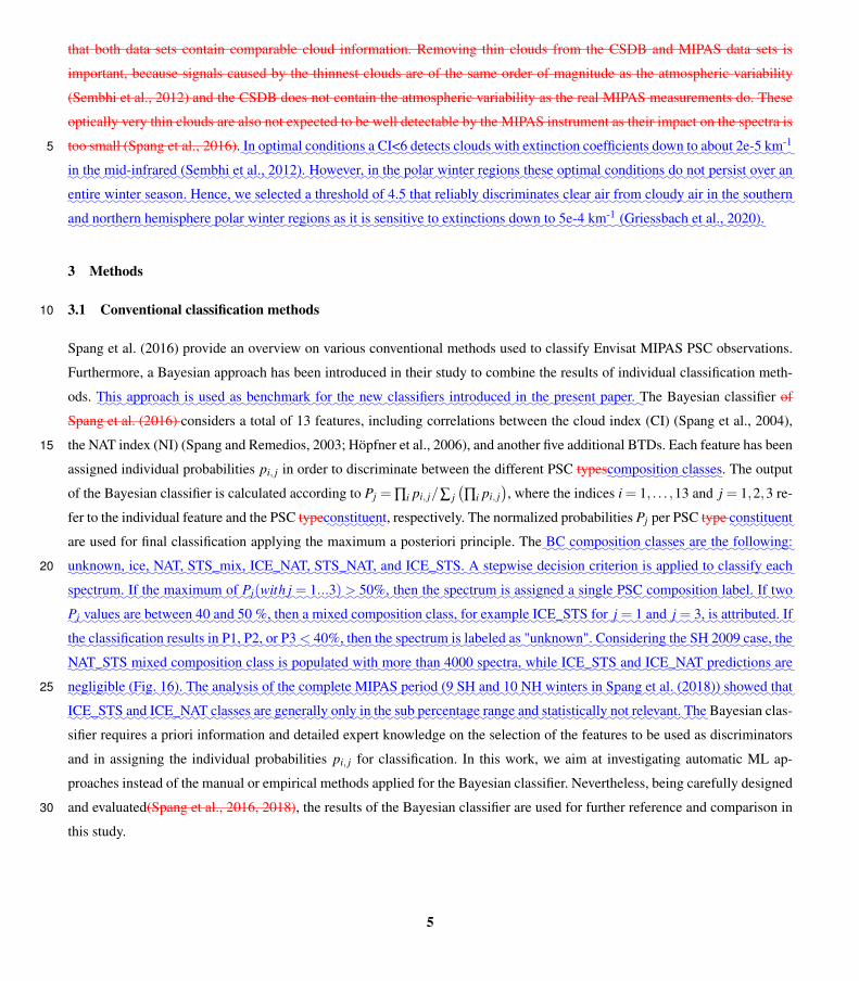
We rephrased the paragraph to be more precise on how we selected the threshold. Therevised paragraph now reads: ”To prepare both, the real MIPAS and the CSDB data forPSC classification, we applied the cloud index (CI) method of Spang et al. (2004) with athreshold of 4.5 to filter out clear air spectra. In optimal conditions a CI¡6 detects cloudswith extinction coefficients down to about 2e-5km-1 in the mid-IR (semhbi2012). However,in the polar winter regions these optimal conditions do not persist over an entire winterseason. Hence, we selected a threshold of 4.5 that reliably discriminates clear air fromcloudy air in the southern and northern hemisphere polar winter regions as it is sensitiveto extinctions down to 5e-4km-1 (Griessbach2020, Fig. 2c).”
4.23 Here it would be really helpful for the reader to introduce the types or compositionclasses identified by the BC and discuss here or later the overlap with the ML classificationand potential ambiguities. Which classes are summarized as nat, sts and ice in the latercomparison with the ML results? Just a suggestion: a tabular comparison might be helpfulto compare the different classifications and indicate what is counted as ‘nat’, ‘sts’ and ‘ice’.
As suggested by the reviewer, we explained how the Bayesian Classifier assigns theoutput labels to the composition classes. We also added more information on the outputclasses of the new ML methods.
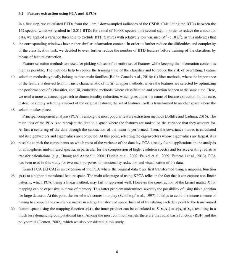
6.1ff Section 3.3 gives interesting general information about the ML methods, but thelink to the presented work is somehow missing to me. How are the methods used here?What kind of input data is used and what kind of output is generated? What are thecritical parameters here? The used classification scheme should be mentioned or at least areference to the compositions in section 2.2 should be added.
We revised Sect. 3.3 and added a new paragraph linking the general description of theML methods to the specific application in our paper. A new figure showing the flowchartof classification has been added to demonstrate the whole pipeline from the input data tothe output labels.
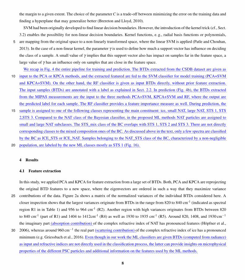
7.14ff a closer inspection shows ... In Fig. 2a, most of the area look yellowish to me itmight be helpful to adjust the color-coding. Furthermore, it might be helpful to highlightR1, R2 ... directly in Fig. 2a and 2b, since it is difficult to follow the discussion, connectregions and wave numbers with indices by using Tab. 1, and then try to identify indexranges on the panel axes. R1, R2 ... might be indicated also in Fig. 4 for easier reading.
In this revision, we restricted the color scale to remove the yellowish hue in Fig. 2a.
5

We also added labels to identify the regions R1, R2, ... in Figs. 2a and 2b.
7.17 What do the ‘pronounced features’ in the real an imaginary refractive index meanphysically? How are they related to the spectra? Why does it make sense to feed thecomplex refractive indices to the ML methods, while the goal is to classify measured limbspectra and not refractive indices? At least a short explanation should be provided.
Physically, the real part of the refractive index characterizes the scattering whereasthe imaginary part characterizes the absorption of radiance. The real and imaginary partdescribe the “microphysical properties” of the different PSC particles, so we would expectthat the classification methods are sensitive to it (as discussed in the paper). The classifica-tion methods are using measured or simulated radiances, only, but the spectra themselvesare affected by the refractive indices. We edited the manuscript to clarify on this point.
7.31 ‘similar clusters as Fig 2a’ I have difficulties in finding the similarities, since thediscussion uses wave numbers and regions while the figures use ‘index’. See above: it mightbe helpful to indicate R1 ... somehow in the panels.
Please see reply to 7.14ff.
8.4 ‘peak in imaginary part’ Which peak is meant here? ‘minimum in the real part’Which minimum is meant here? See comment to 7.17: how are these refractive indexfeatures related to the spectra?
We added a reference to the region and discussed it in more detail. Please see reply to7.17.
8.25 Possibly I missed it: how is the prediction accuracy determined? See Figs 12ff:How can the prediction accuracy be 99% for all methods while the classification results arerelatively heterogeneous?
The prediction accuracies reported in Tab. 6 and Fig. 5 are computed on the CSDBsynthetic dataset. Even though the classifiers score similarly on the synthetic data set,they may learn different mapping functions, so when deployed on real measurements theresults can vary. We discussed this later in the manuscript (P12 L17).
9.13ff Here and in in the following I got somewhat confused: For BC, the PSC classes‘unspec’, ‘ice’, ‘nat’, ‘stsmix’, ‘ice nat’, ‘nat sts’, ‘ice sts’ are used. For the other methods,the classes ‘ice’, ‘nat large’, ‘sts 1’, ‘sts 2’, ‘sts 3’ and ‘nat small’ are used. In Fig. 12-14,suddenly ‘sts mix1’, ‘sts mix2’ and ‘sts mix3’ are used (I guess ‘sts 1’, ‘sts 2’ and ‘sts 3’ ismeant here). In the text, the types or categories ‘nat’, ‘sts’ and ‘ice’ are used. The usedcategories and classifications should be clearly defined. Overlap regions of and potentialambiguities between the different classification schemes should be discussed (see commentsto 4.23 and 2.3).
We checked and corrected the class names of the ML methods used here to be consistentthroughout the manuscript. We also provided more information and explanation in Sect.3.1 and Sect. 3.3 as requested.
6
11.33 are the new approaches really ‘more objective’, reminding that they need to beassessed using a ‘conventional’ method based on a-priori knowledge and expert knowledge,and finally one needs make a choice?
As discussed earlier, it is true that in this study we still need expert knowledge forthe evaluation. This is largely caused by the fact that no suitable ground truth data areavailable for the use case. However, the ML methods themselves learn complex patternsautomatically from the data, without the need of hand tuning of the parameters. The MLmethods are more “objective” in that they are not making assumptions on the distributionof data but rather learn from them. Thus, we reformulated our statement in Sect. 5,explaining in what sense we think ML methods are more “objective”.
12.28 Just out of curiosity: would it be possible to make a meaningful search for furtherPSC constituents not covered by conventional classifications, such as nitric acid dihydrate?
In principle, if simulated radiance data for NAD can be generated, it would be possibleto train a ML classifier for this additional task. However, it would be tricky to assess theperformance of the classifier, unless ground truth data are available.
Technical
2.19 approaches
Corrected.
3.21 have been extracted
Corrected.
References
Voigt et al., Science, 290, 1756–1758, 2000
Molleker et al., Atmos. Chem. Phys., 14, 10785–10801, 2014
Woiwode et al., Atmos. Chem. Phys., 16, 9505–9532, 2016
Voigt et al., Atmos. Chem. Phys., 18, 15623–15641, 2018
Lambert et al., Atmos. Chem. Phys., 12, 2899–2931, 2012
We added these references in the introduction in the paragraph describing alternativemethods to acquire PSC measurements.
Reviewer #2
In their paper, Sedona et al. explore the potential of applying machine learning methodsto classify PSC observations of infrared limb sounders. To test their approach they use
7
the Envisat MIPAS data for one Antarctic winter and one Arctic winter. Different MLtechniques are tested and they find that all of them are suitable to retrieve informationon the composition of PSCs, but that the random forest method seems to be the mostpromising one. This is a very interesting study and deserves to be published in AMT.However, I have several major and minor comments that should be considered beforepublication.
We gratefully thank the Reviewer for the supportive comments.
General comments and questions:
1. A discussion on the previous classical schemes based on the optical properties ofPSCs (see Achtert and Tesche, 2014) in comparison to the ML methods is missing.
As requested by both reviewers, we added a new paragraph describing additional ob-servational methods and classification schemes for PSCs in the introduction (Sect. 1).
2. Are ML methods really better? What is the advantage? This needs to be discussedas well.
Following comments of both reviewers, we revised parts of the manuscript to highlightthe advantages of using ML methods. Please see the reply to major comment 2) of reviewer1.
3. The number of self citations is to high. I know that this study builds on what hasbeen done before, however, there are several occasions (see my specific comments) whereother references could be used. It simply does not correct when the entire introduction isbased on Spang et al. and Hoepfner et al. citations who are not only co-authors of thisstudy but also not the only scientists working on this topic.
In this revision, we tried to better balance the references by adding more references toother works and by removing the references to Spang et al. (2001, 2008).
4. What result would you get or could you expect when other winters are considered?Do the ML methods work in the same way for all different kinds of winters (cold or warm,dynamically more or less active)?
To address this question, we studied a NH and a SH winter, with rather differentmeteorological conditions. For example, the NH winter was much warmer than the SHone and showed a smaller portion of ice PSCs, as expected. In principle, we expect themethods to be applicable for all winters, as the training was done with simulated datarather than real measurements. In the future, we plan to apply the ML methods to allMIPAS measurements, but this is beyond the scope of the present study. We added asentence in Sect. 5 to better explain this: ” Models have been trained on the CSDB, asimulation dataset that has been created systematically sampling the parameter space, notreflecting the natural occurrence frequencies of parameters.”
8

5. Why have the two winters presented in this study been chosen?
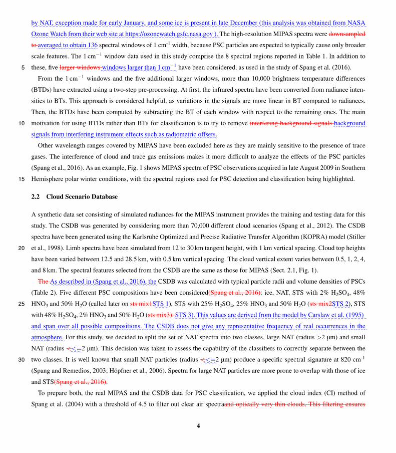
NH winter 2006/2007 has been selected because there was a notable PSC activity, witha large area covered by NAT, exception made for early January. Some ice is present inlate December. Additionally, it was used in previous works as Cordoba-Jabonero et al.(2009). Polar Stratospheric Cloud Observations in the 2006/07 Arctic Winter by Using anImproved Micropulse Lidar). 2009 SH winter presents a slightly higher than average PSCactivity, especially for ice in June and August. 2009 SH was also studied in Lambert etal. (2016). We have added this information in the manuscript. This analysis was obtainedfrom NASA Ozone Watch from their web site at https://ozonewatch.gsfc.nasa.gov, weinclude in the present reply document the plots (in Fig. 1). We added information aboutthe selected winters in Sect. 2.1.
Specific comments:
P2, L5-8: “... MIPAS measurements are considered to be of great importance for thestudy of PSCs ...” First of all, I would suggest to rephrase the sentence and to write either“are quite suitable for studying PSCs“ or “MIPAS measurements have been used to studyPSC processes.” Second here the self citations could be avoided or at least decreased. Itwould be enough to cite the two recent papers by Spang et al. and Hopfner et al. (thusthe 2018 papers). Even better would be if you would cite here some papers where MIPASobservations have actually been used to investigate PSCs and related processes as e.gArnone et al. (2012), Khosrawi et al. (2018), Tritscher et al. (2019).
We rephrased the sentence and changed the citations to avoid self references as sug-gested. The sentence now read: ”MIPAS measurements have beenused to study PSCprocesses (Arnone et al., 2012; Khosrawi et al., 2018; Tritscher et al., 2019).”
P2, L9: “... ice PSCs are generally thicker than NAT and STS (Spang et al., 2016)”.This is also something which is documented in the literature and where easily anothercitation could be picked than Spang et al. (2016).
We changed the reference to Fromm (2003)
P2, L13: Also here, there are many more adequate citations in this context availablethan Spang et al. (2018).
We changed the citations to Campbell (2008) and Pawson (1995)
P2, L20: Also here, avoid self citations.
Ask Reinhold We think that this specific references are correct since they are relatedto IR limb spectra, which have been analysed in detail with respect to PSC effects only inpublications where Spang or Hopfner are lead or co-author.
P2, L21ff: Add general references on the ML methods.
We added more general references to the SVM, RF, and PCA methods.
9
P2, L32: What is the motivation for picking these winters? Where these rather warmor cold winters? Where there special dynamical conditions observed during these winters?
Please see reply to general comments 4 and 5 of reviewer 2.
P3, L6: Why 14.3 orbits? Usually the number of orbits are given without position afterdecimal point.
The Envisat orbit period is 101 min. Therefore the satellite completes about 14.3 orbitsper day.
P3, L30-P4, 30: If you follow the approach given in Spang et al. (2016) it would beeasier if you would simply state that at the begin of the section instead of reference Spanget al. (2016) after every few sentences.
We rephrased this as suggested.
P4, L4-6: Where do you get these different composition numbers from? Are they basedon the MIPAS data or on literature values? This text part is really confusing and shouldbe rephrased.
The numbers used to create the CSDB dataset are based on the model by Carslaw etal. (doi 10.1029/95GL01668). Maximum volume density of STS and NAT are based on themaximum amount of HNO3 available for typical winter in the lower and mid stratosphere.The approach of the CSDB is also described in Spang et al. 2012. We added a sentence inSect. 2.2 to clarify on this point, which reads: ”This values are derived from the model byCarslaw et al. (1995) and span over all possible compositions. The CSDB does not giveany representative frequency of real occurrences in the atmosphere.”
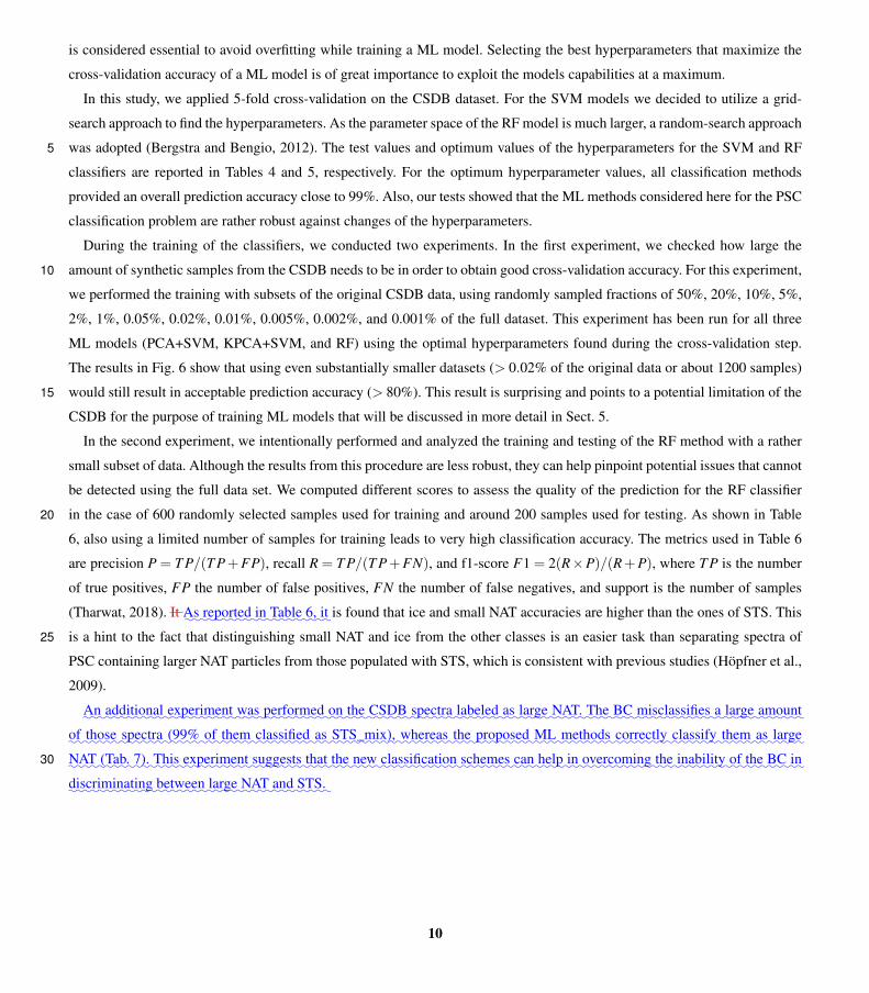
P9, L8: “It is found that ice and small NAT accuracies are higher than the ones ofSTS”. Where has this been found? In this study? If yes, be more clear. Otherwise, givethe according references.
It was found in this study, we added a reference to Table 6.
P9, L21: Also here other references than Spang et al. (2018) could be given here.
We changed the reference to Pitts et al. (2018).
P11, Summary and Conclusions: Looking at the figures I would conclude that theresults derived are quite different and that is hard to say which one performs best. Thus,I have bit trouble following your reasoning, that all ML methods are suitable for theclassification and that the RF performs best.
Unfortunately, there is no suitable ground truth data available for validation, meaningthat we can only compare the output of the classifiers against each other and provide aqualitative assessment and ranking of their performance. Overall, we think that the RFresults might be most realistic, because the Bayesian classifier is known to find less NAT forMIPAS compared to CALIOP satellite observations, especially for Northern Hemisphere
10
winter conditions. Moreover, the RF provides a direct view on which features it uses to dis-criminate between the classes. In this way it becomes possible to evaluate the consistencyof the classifier with respect to physical knowledge. In Sect. 5, we provided additionalinformation on the reason why we think the RF method is the most promising one.
Technical corrections:
P1, L2: enhance → improve
P1, L9: From the both → From both
P1, L21: repitition of “used”. Please rephrase the sentence.
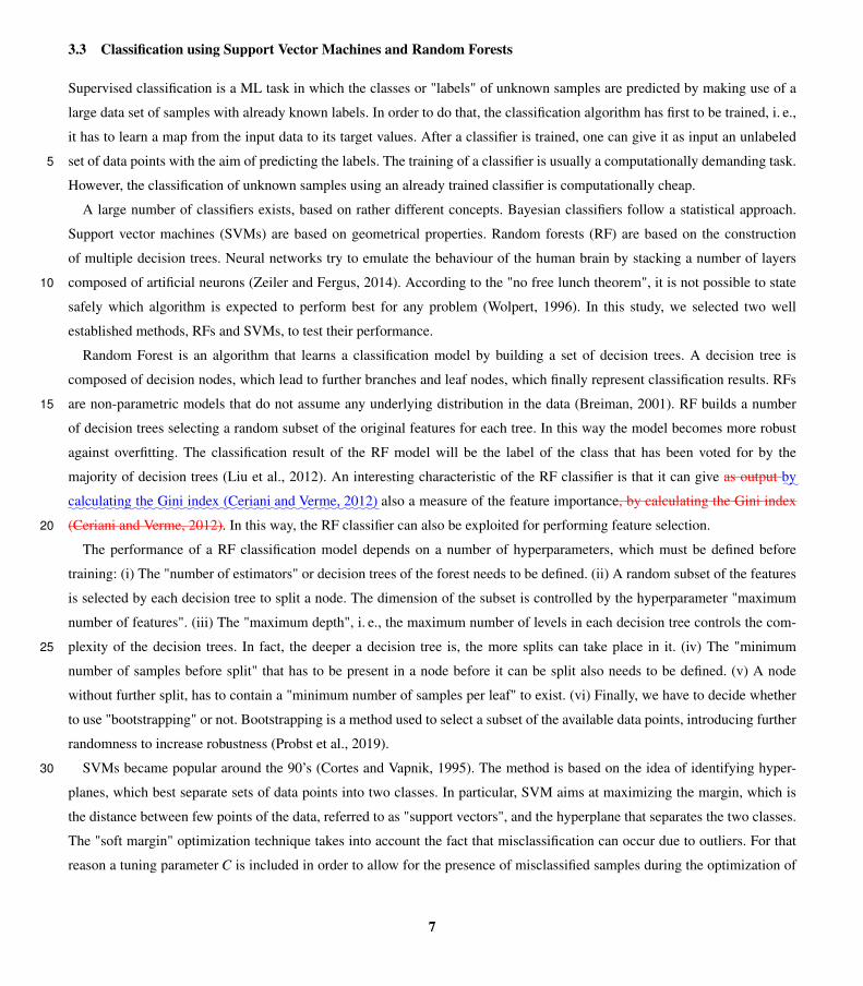
P6, L19: Rearrange sentence as follows: “An interesting characteristic of the RF clasifieris that it can give by calculating the Gini index (Ceriani and Verme, 2012) also a measureof the feature importance”
We fixed all technical corrections.
References:
Achtert, P., and M. Tesche, Assessing lidar-based classification schemes for polar strato-spheric clouds based on 16 years of measurements at Esrange, Sweden, J. Geophys. Res.Atmos.,119, 1386–1405,doi:10.1002/2013JD020355, 2014.
Arnone, E., Castelli, E., Papandrea, E., Carlotti, M., and Dinelli, B. M.: Extreme ozonedepletion in the 2010–2011 Arctic winter stratosphere as observed by MIPAS/ENVISAT us-ing a 2-D tomographic approach, Atmos. Chem. Phys., 12, 9149–9165, https://doi.org/10.5194/acp-12-9149-2012, 2012.
Khosrawi, F., Kirner, O., Stiller, G., Hopfner, M., Santee, M. L., Kellmann, S., andBraesicke, P.: Comparison of ECHAM5/MESSy Atmospheric Chemistry (EMAC) simula-tions of the Arctic winter 2009/2010 and 2010/2011 with Envisat/MIPAS and Aura/MLSobservations, Atmos. Chem. Phys., 18, 8873–8892, https://doi.org/10.5194/acp-18-8873-2018, 2018.
Tritscher, I., Grooß, J.-U., Spang, R., Pitts, M. C., Poole, L. R., Muller, R., and Riese,M.: Lagrangian simulation of ice particles and resulting dehydration in the polar winterstratosphere, Atmos. Chem. Phys., 19, 543–563, https://doi.org/10.5194/acp19-543-2019,2019.
We carefully considered the suggested references and added them in the manuscript.
11

(a)NH PSC Ice Area460 K MERRA2
0
2
4
6
mill
ion
km
2
Jul Aug Sep Oct Nov Dec Jan Feb Mar Apr May Jun
Min
10%
30%
Mean
70%
90%
Max
1978/1979−2018/2019P. Newman (NASA), E. Nash (SSAI), S. Pawson (NASA) 2019-07-09T18:00:14Z
2006/2007
(b)NH PSC NAT Area460 K MERRA2
0
5
10
15
20
mill
ion
km
2
Jul Aug Sep Oct Nov Dec Jan Feb Mar Apr May Jun
Min
10%
30%
Mean
70%
90%
Max
1978/1979−2018/2019P. Newman (NASA), E. Nash (SSAI), S. Pawson (NASA) 2019-07-09T18:00:13Z
2006/2007
(c)SH PSC Ice Area460 K MERRA2
0
5
10
15
20
mill
ion
km
2
Jan Feb Mar Apr May Jun Jul Aug Sep Oct Nov Dec
Min
10%
30%
Mean
70%
90%
Max
1979−2018P. Newman (NASA), E. Nash (SSAI), S. Pawson (NASA) 2019-08-22T19:11:23Z
2009
(d)SH PSC NAT Area460 K MERRA2
0
10
20
30
40
mill
ion
km
2
Jan Feb Mar Apr May Jun Jul Aug Sep Oct Nov Dec
Min
10%
30%
Mean
70%
90%
Max
1979−2018P. Newman (NASA), E. Nash (SSAI), S. Pawson (NASA) 2019-08-22T19:11:21Z
2009
Figure 1: Area covered by ice PSC (a) and NAT (b) in NH 2006/2007, by ice PSC (c) andNAT (d) in SH 2009.
12
Exploration of machine learning methods for the classification ofinfrared limb spectra of polar stratospheric cloudsRocco Sedona1,4, Lars Hoffmann1, Reinhold Spang2, Gabriele Cavallaro1, Sabine Griessbach1,Michael Höpfner3, Matthias Book4, and Morris Riedel41Jülich Supercomputing Centre (JSC), Forschungszentrum Jülich, Jülich, Germany2Institut für Energie- und Klimaforschung (IEK-7), Forschungszentrum Jülich, Jülich, Germany3Institut für Meteorlogie und Klimaforschung, Karlsruher Institut für Technologie, Karlsruhe, Germany4University of Iceland, Reykjavik, Iceland
Correspondence: Rocco Sedona ([email protected])
Abstract. Polar stratospheric clouds (PSC) play a key role in polar ozone depletion in the stratosphere. Improved observations
and continuous monitoring of PSCs can help to validate and enhance::::::improve
:chemistry-climate models that are used to predict
the evolution of the polar ozone hole. In this paper, we explore the potential of applying machine learning (ML) methods to
classify PSC observations of infrared limb sounders. Two datasets have been considered in this study. The first dataset is a
collection of infrared spectra captured in Northern Hemisphere winter 2006/2007 and Southern Hemisphere winter 2009 by the5
Michelson Interferometer for Passive Atmospheric Sounding (MIPAS) instrument onboard ESA’s Envisat satellite. The second
dataset is the cloud scenario database (CSDB) of simulated MIPAS spectra. We first performed an initial analysis to assess the
basic characteristics of these datasets:::the
::::::CSDB and to decide which features to extract from them
::it. Here, we focused on an
approach using brightness temperature differences (BTDs). From the both, the measured and the simulated infrared spectra,
more than 10,000 BTD features have been generated. Next, we assessed the use of ML methods for the reduction of the10
dimensionality of this large feature space using principal component analysis (PCA) and kernel principal component analysis
(KPCA) as well as the:::::::followed
:::by
:a:classification with the random forest (RF) and support vector machine (SVM)techniques.
:.:::The
:::::::random
:::::forest
:::::(RF)
:::::::::technique,
:::::which
:::::::embeds
:::the
::::::feature
::::::::selection
:::::step,
:::has
::::also
::::been
:::::used
::as
::::::::classifier.
:All methods
were found to be suitable to retrieve information on the composition of PSCs. Of these, RF seems to be the most promising
method, being less prone to overfitting and producing results that agree well with established results based on conventional15
classification methods.
1 Introduction
Polar stratospheric clouds (PSC) typically form in the polar winter stratosphere between 15 and 30 km of altitude. PSCs
can be observed only at high latitudes, as they exist only at very low temperatures (T < 195K) found in the polar vortices.
PSC are known to play an important role in ozone depletion (Solomon, 1999):::::caused
:::by
::::::::::::denitrification
::of
:::the
:::::::::::stratosphere20
::::::::::::::::::::::::::::(Solomon, 1999; Toon et al., 1986), as their surface acts as a catalyst for heterogeneous reactions. Ozone depletion is caused
by the presence of man-made chlorofluorocarbons (CFCs) in the stratosphere, which have been used for example in industrial
1
compounds used as::::::present
::in
:refrigerants, solvents, blowing agents for plastic foam. CFCs are inert compounds in the tropo-
sphere, but get transformed under stratospheric conditions to the chlorine reservoir gases HCl and ClONO2. PSC particles are
involved in the release of chlorine from the reservoirs.
PSCs exist in threemain types:::The
:::::main
::::::::::constituents
:::of
:::::PSCs
:::are
:::::three, i. e., nitric acid trihydrate (NAT), super-cooled
ternary solutions (STS), and ice (Lowe and MacKenzie, 2008). The main methods that are used to measure PSCs are in situ5
optical measurements from balloon or aircraft, infrared spectra acquired by satellite, as well as ground and satellite based lidar
(Buontempo et al., 2009). Michelson Interferometer for Passive Atmospheric Sounding (MIPAS) measurements are considered
to be of great importance for the study of PSCs (Höpfner et al. (2002, 2006); Höpfner et al. (2006), Spang et al. (2005); Eckermann et al. (2009))
::::have
::::been
::::used
::to:::::
study::::PSC
:::::::::processes
:::::::::::::::::::::::::::::::::::::::::::::::::::::(Arnone et al., 2012; Khosrawi et al., 2018; Tritscher et al., 2019). The infrared spec-
tra acquired by MIPAS are rather sensitive to optically thin clouds due to the limb observations geometry. This is particu-10
larly interesting for NAT and STS PSCs, as ice PSCs are in general optically thicker than NAT and STS (Spang et al., 2016)
::::::::::::(Fromm, 2003). As ice clouds form at a lower temperature than NAT and STS, they are mainly present in the Antarctic,
while their presence in the Arctic (where the stratospheric temperature minimum in polar winter is higher) is only notable for
extremely cold winter conditions (e. g., Spang et al., 2018)::::::::::::::::::::::::::::::::::::::::::::(e. g., Campbell and Sassen, 2008; Pawson et al., 1995).
::::::Besides
:::::using
::::::MIPAS
:::::::::::::measurements,
::::::::::classification
:::has
:::::been
::::::carried
::out
::::with
::::::::different
:::::::schemes
:::::based
::on
:::the
::::::optical
::::::::properties15
::of
:::::PSCs
::::with
:::::::LIDAR
:::::::::::::measurements.
::A
::::::review
:::of
:::::those
:::::::methods
::is::::::::
available:::in
::::::::::::::::::::::Achtert and Tesche (2014).
::::::::::::Classification
:::::::schemes
:::are
:::::based
::on
::::two
:::::::features,
::::::namely
:::the
::::::::::backscatter
::::ratio
:::and
:::the
::::::::::::depolarization
:::::ratio.
::As
:::::::exposed
::in
::::::::::::::::(Biele et al., 2001)
:,:::::::particles
:::::(type
:::II)
::::with
:::::large
::::::::::backscatter
::::ratio
::::and
::::::::::::depolarization
:::are
::::::likely
::to
:::be
:::::::::composed
::of
::::ice.
::::Type
::I:::::::particles
::::are
:::::::::::characterized
::by
::a::::low
::::::::::backscatter
::::ratio.
::::The
:::::::subtype
:::Ia
:::::::particles
:::::show
::a::::large
:::::::::::::depolarization
:::and
::::are
::::::::composed
:::of
:::::NAT,
:::::::whereas
::::::subtype
::Ib
:::::::particles
:::::have
:::low
::::::::::::depolarization
:::and
::::::consist
::in
:::::STS.
:::The
::::::::threshold
::to
::::::classify
:::the
:::::PSCs
:::::types
:::::varies
::::::among20
:::::::different
:::::works
:::::such
::as
::::::::::::::::::::::::::::::::::::::::::::::::::::::::::::::::::Browell et al. (1990); Toon et al. (1990); Adriani (2004); Pitts et al. (2009, 2011).
::::The
::::::::::::nomenclature
::::::::presented
:::::above
::is
:a::::::::::::simplification
::of
::::real
::::case
::::::::scenarios,
:::::since
:::::PSCs
:::can
:::::occur
::::also
::::with
::::::::mixtures
::of
:::::::particles
::::with
::::::::different
::::::::::composition
:::::::::::::::(Pitts et al., 2009).
:::::Other
:::::::methods
::::that
:::are
::::used
::to
:::::::measure
:::::PSCs
:::are
::in
:::situ
::::::optical
:::and
::::::::::non-optical
::::::::::::measurements
::::from
:::::::balloon
::or
:::::::aircraft
::as:::::
well::as
::::::::::microwave
:::::::::::observations
:::::::::::::::::::::::::::::::::::::::::::::::::::(Buontempo et al. (2009); Molleker et al. (2014); Voigt (2000)
:::::::::::::::::::::::::::::::::Voigt et al. (2018); Lambert et al. (2012))
:.25
The use of machine learning (ML) algorithms increased dramatically during the last decade. ML can offer valuable tools to
deal with a variety of problems. In this paper, we used ML methods for two different tasks. First, for the selection of informative
features from the::::::::simulated
:MIPAS spectra. Second, to classify the MIPAS spectra depending on the type
::::::::::composition of the
PSC. To our knowledge, this is the first time that ML methods have been applied::In
:::this
:::::work
:::we
:::::::::::significantly
::::::::extended
::the
::::::::::application
::of::::
ML::::::::methods for the analysis of MIPAS PSC observations. Standard methods that exploit infrared limb30
observation to classify PSCs are based on "empirical" approaches. Given physical knowledge of the properties of the PSC,
some features are::::have
::::been
:extracted from the spectra, as for example the ratio of the radiances between specific spectral
windows. These approach:::::::::approaches
:have been proven to be capable to detect and discriminate between different PSC types
::::::classes (Spang et al., 2004; Höpfner et al., 2006).
2

The purpose of this study is to explore the use of ML methods to improve the PSC classification for infrared limb satellite
measurements and to potentially gain more knowledge on the impact of the different PSC types:::::classes
:on the spectra. We com-
pare results from the most advanced "emprical" method, the Bayesian classifier of Spang et al. (2016), with::::three "automatic"
methods that rely::::::::::approaches.
:::The
::::first
:::one
:::::relies on principal component analysis (PCA) and kernel principal component anal-
ysis (KPCA) for feature selection::::::::extraction, followed by classification with the
::::::support
::::::vector
:::::::machine
:::::::(SVM).
::::The
::::::second5
:::one
::is
::::::similar
::to
:::the
:::::first,
:::but
::::uses
::::::kernel
:::::::principal
::::::::::component
:::::::analysis
:::::::(KPCA)
:::for
:::::::feature
::::::::extraction
:::::::instead
::of
:::::PCA.
::::The
::::third
:::one
::is::::::
based::on
::::the random forest (RF)and support vector machine (SVM)methods
:,:a::::::::
classifier::::
that:::::::directly
:::::::embeds
:a::::::feature
::::::::selection
:::::::::::::::::::::::::::::::::::::::::::::::::::::::::((Cortes and Vapnik, 1995; Breiman, 2001; Jolliffe and Cadima, 2016)
:). A common problem of ML is the
lack of annotated data. To overcome this limitation, we used a synthetic dataset for training and testing, the cloud scenario
database (CSDB), especially developed for MIPAS cloud and PSC analyses (Spang et al., 2012). As a "ground truth" for PSC10
classification is largely missing, we evaluate the ML results by comparing them with results from existing methods and show
that they are consistent with established scientific knowledge.
In Sect. 2, we introduce the MIPAS and synthetic CSDB data sets. A brief description of the ML methods used for feature
reduction and classification is provided in Sect. 3. In Sect. 4, we compare results of PCA+SVM, KPCA+SVM, and RF for
feature selection and classification. We present three case studies and statistical analyses for the 2006/2007 Arctic and 200915
Antarctic winter seasons. The final discussion and conclusions are given in Sect. 5.
2 Data
2.1 MIPAS
The MIPAS instrument (Fischer et al., 2008) was an infrared limb emission spectrometer onboard ESA’s Envisat satellite to
study the thermal emission of the Earth’s atmosphere constituents. Envisat operated from July 2002 to April 2012 in a polar20
low Earth orbit with a repeat cycle of 35 days. MIPAS measured up to 87°S and 89°N latitude and therefore provided nearly
global coverage at day- and nighttime. The number of orbits of the satellite per day was equal to 14.3, resulting in a total of
about 1000 limb scans per day.
The wavelength range covered by the MIPAS interferometer was about 4 to 15 µm. From the beginning of the mission to
spring 2004, the instrument operated in the full resolution (FR) mode (0.025 cm-1 spectral sampling). Lateron, this has to be25
changed to the optimized resolution (OR) mode (0.0625 cm-1) due to a technical problem of the interferometer (Raspollini
et al., 2006, 2013). The FR measurements were taken with a constant 3 km vertical and 550 km horizontal spacing, while for
the OR measurements the vertical sampling depended on altitude, varying from 1.5 to 4.5 km, and a horizontal spacing of 420
km was achieved. The altitude range of the FR and OR measurements varied from 5-70 km at the poles and to 12-77 km at the
equator.30
For our analyses, we used MIPAS Level-1B data (version 7.11) acquired at 15 – 30 km of altitude between May and Septem-
ber 2009 at 60 – 90 °S and between November 2006 and February 2007 at 60 – 90 °N.::::2009
:::SH
:::::winter
:::::::presents
::a::::::slightly
::::::higher
:::than
:::::::average
::::PSC
:::::::activity,
::::::::especially
:::for
:::ice
::in
::::June
:::and
:::::::August.
:::::::::2006/2007
:::NH
::::::winter
::is
:::::::::::characterized
::by
::a::::large
::::area
:::::::covered
3
::by
:::::NAT,
::::::::exception
:::::made
:::for
::::early
:::::::January,
::::and
:::::some
:::ice
:is:::::::
present::in
:::late
:::::::::December
::::(this
:::::::analysis
::::was
:::::::obtained
:::::from
::::::NASA
:::::Ozone
::::::Watch
::::from
::::their
::::web
:::site
::at
:::::::::::::::::::::::::::https://ozonewatch.gsfc.nasa.gov
:).:The high-resolution MIPAS spectra were downsampled
to:::::::averaged
::to
::::::obtain
:::136 spectral windows of 1 cm-1 width, because PSC particles are expected to typically cause only broader
scale features. The 1 cm−1 window data used in this study comprise the 8 spectral regions reported in Table 1. In addition to
these, five larger windows::::::::windows
:::::larger
::::than
::::::1 cm−1 have been considered, as used in the study of Spang et al. (2016).5
From the 1 cm−1 windows and the five additional larger windows, more than 10,000 brightness temperature differences
(BTDs) have extracted using a two-step pre-processing. At first, the infrared spectra have been converted from radiance inten-
sities to BTs. This approach is considered helpful, as variations in the signals are more linear in BT compared to radiances.
Then, the BTDs have been computed by subtracting the BT of each window with respect to the remaining ones. The main
motivation for using BTDs rather than BTs for classification is to try to remove interfering background signals::::::::::background10
::::::signals
::::from
:::::::::interfering
:::::::::instrument
::::::effects
::::such
::as
::::::::::radiometric
::::::offsets.
Other wavelength ranges covered by MIPAS have been excluded here as they are mainly sensitive to the presence of trace
gases. The interference of cloud and trace gas emissions makes it more difficult to analyze the effects of the PSC particles
(Spang et al., 2016). As an example, Fig. 1 shows MIPAS spectra of PSC observations acquired in late August 2009 in Southern
Hemisphere polar winter conditions, with the spectral regions used for PSC detection and classification being highlighted.15
2.2 Cloud Scenario Database
A synthetic data set consisting of simulated radiances for the MIPAS instrument provides the training and testing data for this
study. The CSDB was generated by considering more than 70,000 different cloud scenarios (Spang et al., 2012). The CSDB
spectra have been generated using the Karlsruhe Optimized and Precise Radiative Transfer Algorithm (KOPRA) model (Stiller
et al., 1998). Limb spectra have been simulated from 12 to 30 km tangent height, with 1 km vertical spacing. Cloud top heights20
have been varied between 12.5 and 28.5 km, with 0.5 km vertical spacing. The cloud vertical extent varies between 0.5, 1, 2, 4,
and 8 km. The spectral features selected from the CSDB are the same as those for MIPAS (Sect. 2.1, Fig. 1).
The::As
::::::::described
::in
::::::::::::::::(Spang et al., 2016)
:,:::the CSDB was calculated with typical particle radii and volume densities of PSCs
(Table 2). Five different PSC compositions have been considered(Spang et al., 2016): ice, NAT, STS with 2% H2SO4, 48%
HNO3 and 50% H2O (called later on sts mix1:::STS
:1), STS with 25% H2SO4, 25% HNO3 and 50% H2O (sts mix2
:::STS
::2), STS25
with 48% H2SO4, 2% HNO3 and 50% H2O (sts mix3).::::STS
::3).
::::This
::::::values
:::are
::::::derived
::::from
:::the
::::::model
::by
::::::::::::::::::Carslaw et al. (1995)
:::and
::::span
::::over
:::all
:::::::possible
::::::::::::compositions.
::::The
::::::CSDB
::::does
::::not
::::give
:::any
::::::::::::representative
:::::::::frequency
::of
::::real
::::::::::occurrences
:::in
:::the
::::::::::atmosphere. For this study, we decided to split the set of NAT spectra into two classes, large NAT (radius >2 µm) and small
NAT (radius <:::<=2 µm). This decision was taken to assess the capability of the classifiers to correctly separate between the
two classes. It is well known that small NAT particles (radius <::::<=2 µm) produce a specific spectral signature at 820 cm-130
(Spang and Remedios, 2003; Höpfner et al., 2006). Spectra for large NAT particles are more prone to overlap with those of ice
and STS(Spang et al., 2016).
To prepare both, the real MIPAS and the CSDB data for PSC classification, we applied the cloud index (CI) method of
Spang et al. (2004) with a threshold of 4.5 to filter out clear air spectraand optically very thin clouds. This filtering ensures
4
that both data sets contain comparable cloud information. Removing thin clouds from the CSDB and MIPAS data sets is
important, because signals caused by the thinnest clouds are of the same order of magnitude as the atmospheric variability
(Sembhi et al., 2012) and the CSDB does not contain the atmospheric variability as the real MIPAS measurements do. These
optically very thin clouds are also not expected to be well detectable by the MIPAS instrument as their impact on the spectra is
too small (Spang et al., 2016).::In
:::::::optimal
::::::::conditions
::a
::::CI<6
::::::detects
::::::clouds
::::with
::::::::extinction
::::::::::coefficients
:::::down
::to
::::about
::::2e-5
:::km
::
-15
::in
:::the
::::::::::mid-infrared
::::::::::::::::::(Sembhi et al., 2012).
::::::::However,
::in
:::the
:::::polar
:::::winter
:::::::regions
::::these
:::::::optimal
:::::::::conditions
::do
::::not
:::::persist
::::over
:::an
:::::entire
:::::winter
:::::::season.
::::::Hence,
::we
:::::::selected
::a::::::::threshold
::of
:::4.5
:::that
:::::::reliably
:::::::::::discriminates
:::::clear
::air
:::::from
::::::cloudy
::air
::in:::the
::::::::southern
:::and
:::::::northern
::::::::::hemisphere
::::polar
::::::winter
::::::regions
:::as
:it::is
:::::::sensitive
:::to
:::::::::extinctions
:::::down
::to
::::5e-4
:::km
:
-1::::::::::::::::::::(Griessbach et al., 2020)
:.
3 Methods
3.1 Conventional classification methods10
Spang et al. (2016) provide an overview on various conventional methods used to classify Envisat MIPAS PSC observations.
Furthermore, a Bayesian approach has been introduced in their study to combine the results of individual classification meth-
ods.::::This
:::::::approach
:::is
::::used
::as
::::::::::benchmark
:::for
:::the
::::new
::::::::classifiers
::::::::::introduced
::in
:::the
::::::present
::::::paper.
:The Bayesian classifier of
Spang et al. (2016) considers a total of 13 features, including correlations between the cloud index (CI) (Spang et al., 2004),
the NAT index (NI) (Spang and Remedios, 2003; Höpfner et al., 2006), and another five additional BTDs. Each feature has been15
assigned individual probabilities pi, j in order to discriminate between the different PSC types::::::::::composition
::::::classes. The output
of the Bayesian classifier is calculated according to Pj = ∏i pi, j/∑ j(∏i pi, j
), where the indices i = 1, . . . ,13 and j = 1,2,3 re-
fer to the individual feature and the PSC type::::::::constituent, respectively. The normalized probabilities Pj per PSC type
:::::::::constituent
are used for final classification applying the maximum a posteriori principle. The:::BC
:::::::::::composition
::::::classes
:::are
:::the
:::::::::following:
::::::::unknown,
:::ice,
:::::NAT,
:::::::::STS_mix,
:::::::::ICE_NAT,
:::::::::STS_NAT,
:::and
:::::::::ICE_STS.
::A
::::::::stepwise
:::::::decision
:::::::criterion
::is:::::::applied
::to
::::::classify
:::::each20
::::::::spectrum.
::If
:::the
::::::::maximum
:::of
:::::::::::::::::::::Pj(with j = 1...3)> 50%,
::::then
:::the
::::::::spectrum
:is::::::::
assigned:a::::::single
::::PSC
::::::::::composition
:::::label.
::If::::two
::Pj :::::
values:::are
:::::::between
:::40
:::and
:::50
::%,
::::then
:a::::::mixed
::::::::::composition
:::::class,
:::for
:::::::example
::::::::ICE_STS
:::for
:::::j = 1
:::and
::::::j = 3,
:is:::::::::attributed.
::If
::the
:::::::::::classification
::::::results
::in
:::P1,
:::P2,
::or
:::P3
::::::< 40%,
::::then
:::the
::::::::spectrum
::is
::::::labeled
::as
::::::::::"unknown".
::::::::::Considering
:::the
:::SH
::::2009
:::::case,
:::the
::::::::NAT_STS
::::::mixed
::::::::::composition
:::::class
::is
::::::::populated
::::with
:::::more
::::than
::::4000
:::::::spectra,
:::::while
::::::::ICE_STS
::::and
::::::::ICE_NAT
::::::::::predictions
:::are
::::::::negligible
::::(Fig.
::::16).
::::The
::::::analysis
:::of
:::the
:::::::complete
:::::::MIPAS
:::::period
:::(9
:::SH
:::and
::10
::::NH
::::::winters
::in
::::::::::::::::Spang et al. (2018)
:)::::::showed
::::that25
::::::::ICE_STS
:::and
::::::::ICE_NAT
::::::classes
:::are
::::::::generally
::::only
::in
:::the
:::sub
:::::::::percentage
:::::range
:::and
::::::::::statistically
:::not
:::::::relevant.
::::The Bayesian clas-
sifier requires a priori information and detailed expert knowledge on the selection of the features to be used as discriminators
and in assigning the individual probabilities pi, j for classification. In this work, we aim at investigating automatic ML ap-
proaches instead of the manual or empirical methods applied for the Bayesian classifier. Nevertheless, being carefully designed
and evaluated(Spang et al., 2016, 2018), the results of the Bayesian classifier are used for further reference and comparison in30
this study.
5
3.2 Feature extraction using PCA and KPCA
In a first step, we calculated BTDs from the 1 cm-1 downsampled radiances of the CSDB. Calculating the BTDs between the
142 spectral windows resulted in 10,011 BTDs for a total of 70,000 spectra. In a second step, in order to reduce the amount of
data, we applied a variance threshold to exclude BTD features with relatively low variance (σ2 < 10K2), as this indicates that
the corresponding windows have rather similar information content. In order to further reduce the difficulties and complexity5
of the classification task, we decided to even further reduce the number of BTD features before training of the classifiers by
means of feature extraction.
Feature selection methods are used for picking subsets of an entire set of features while keeping the information content as
high as possible. The methods help to reduce the training time of the classifier and to reduce the risk of overfitting. Feature
selection methods typically belong to three main families (Bolón-Canedo et al., 2016): (i) filter methods, where the importance10
of the feature is derived from intrinsic characteristic of it, (ii) wrapper methods, where the features are selected by optimizing
the performances of a classifier, and (iii) embedded methods, where classification and selection happen at the same time. Here,
we used a more advanced approach to dimensionality reduction, which goes under the name of feature extraction. In this case,
instead of simply selecting a subset of the original features, the set of features itself is transformed to another space where the
selection takes place.15
Principal component analysis (PCA) is among the most popular feature extraction methods (Jolliffe and Cadima, 2016). The
main idea of the PCA is to reproject the data to a space where the features are ranked on the variance that they account for.
At first a centering of the data through the subtraction of the mean is performed. Then, the covariance matrix is calculated
and its eigenvectors and eigenvalues are computed. At this point, selecting the eigenvectors whose eigenvalues are largest, it is
possible to pick the components on which most of the variance of the data lay. PCA already found applications in the analysis20
of atmospheric mid-infrared spectra, in particular for the compression of high-resolution spectra and for accelerating radiative
transfer calculations (e. g., Huang and Antonelli, 2001; Dudhia et al., 2002; Fauvel et al., 2009; Estornell et al., 2013). PCA
has been used in this study for two main purposes, dimensionality reduction and visualization of the data.
Kernel PCA (KPCA) is an extension of the PCA where the original data xxx are first transformed using a mapping function
φ(xxx) to a higher dimensional feature space. The main advantage of using KPCA relies in the fact that it can capture non-linear25
patterns, which PCA, being a linear method, may fail to represent well. However the construction of the kernel matrix K for
mapping can be expensive in terms of memory. This latter problem undermines severely the possibility of using this algorithm
for large datasets. At this point the kernel trick comes into play (Schölkopf et al., 1997). It helps to avoid the inconvenience of
having to compute the covariance matrix in a large transformed space. Instead of translating each data point to the transformed
feature space using the mapping function φ(xxx), the inner product can be calculated as K(xi,x j) = φ(xi)φ(x j), resulting in a30
much less demanding computational task. Among the most common kernels there are the radial basis function (RBF) and the
polynomial (Genton, 2002), which we also considered in this study.
6
3.3 Classification using Support Vector Machines and Random Forests
Supervised classification is a ML task in which the classes or "labels" of unknown samples are predicted by making use of a
large data set of samples with already known labels. In order to do that, the classification algorithm has first to be trained, i. e.,
it has to learn a map from the input data to its target values. After a classifier is trained, one can give it as input an unlabeled
set of data points with the aim of predicting the labels. The training of a classifier is usually a computationally demanding task.5
However, the classification of unknown samples using an already trained classifier is computationally cheap.
A large number of classifiers exists, based on rather different concepts. Bayesian classifiers follow a statistical approach.
Support vector machines (SVMs) are based on geometrical properties. Random forests (RF) are based on the construction
of multiple decision trees. Neural networks try to emulate the behaviour of the human brain by stacking a number of layers
composed of artificial neurons (Zeiler and Fergus, 2014). According to the "no free lunch theorem", it is not possible to state10
safely which algorithm is expected to perform best for any problem (Wolpert, 1996). In this study, we selected two well
established methods, RFs and SVMs, to test their performance.
Random Forest is an algorithm that learns a classification model by building a set of decision trees. A decision tree is
composed of decision nodes, which lead to further branches and leaf nodes, which finally represent classification results. RFs
are non-parametric models that do not assume any underlying distribution in the data (Breiman, 2001). RF builds a number15
of decision trees selecting a random subset of the original features for each tree. In this way the model becomes more robust
against overfitting. The classification result of the RF model will be the label of the class that has been voted for by the
majority of decision trees (Liu et al., 2012). An interesting characteristic of the RF classifier is that it can give as output::by
:::::::::calculating
:::the
::::Gini
:::::index
::::::::::::::::::::::(Ceriani and Verme, 2012) also a measure of the feature importance, by calculating the Gini index
(Ceriani and Verme, 2012). In this way, the RF classifier can also be exploited for performing feature selection.20
The performance of a RF classification model depends on a number of hyperparameters, which must be defined before
training: (i) The "number of estimators" or decision trees of the forest needs to be defined. (ii) A random subset of the features
is selected by each decision tree to split a node. The dimension of the subset is controlled by the hyperparameter "maximum
number of features". (iii) The "maximum depth", i. e., the maximum number of levels in each decision tree controls the com-
plexity of the decision trees. In fact, the deeper a decision tree is, the more splits can take place in it. (iv) The "minimum25
number of samples before split" that has to be present in a node before it can be split also needs to be defined. (v) A node
without further split, has to contain a "minimum number of samples per leaf" to exist. (vi) Finally, we have to decide whether
to use "bootstrapping" or not. Bootstrapping is a method used to select a subset of the available data points, introducing further
randomness to increase robustness (Probst et al., 2019).
SVMs became popular around the 90’s (Cortes and Vapnik, 1995). The method is based on the idea of identifying hyper-30
planes, which best separate sets of data points into two classes. In particular, SVM aims at maximizing the margin, which is
the distance between few points of the data, referred to as "support vectors", and the hyperplane that separates the two classes.
The "soft margin" optimization technique takes into account the fact that misclassification can occur due to outliers. For that
reason a tuning parameter C is included in order to allow for the presence of misclassified samples during the optimization of
7
the margin to a given extent. The choice of the parameter C is a trade-off between minimizing the error on the training data and
finding a hyperplane that may generalize better (Brereton and Lloyd, 2010).
SVM had been originally developed to find linear decision boundaries. However, the introduction of the kernel trick (cf., Sect.
3.2) enables the possibility for non-linear decision boundaries. Kernel functions, e. g., radial basis functions or polynomials,
are mapping from the original space to a non-linearly transformed space, where the linear SVM is applied (Patle and Chouhan,5
2013). In the case of a non-linear kernel, the parameter γ is used to define how much a support vector has influence on deciding
the class of a sample. A small value of γ implies that this support vector also has impact on samples far in the feature space, a
large value of γ has an influence only on samples that are close in the feature space.
:::We
:::::recap
::in
:::Fig.
::4:::the
:::::entire
:::::::pipeline
:::for
:::::::training
:::and
:::::::::prediction.
::::The
:::::BTDs
::::::::extracted
:::::from
:::the
:::::CSDB
:::::::dataset
:::are
::::given
:::as
::::input
::to
:::the
:::::PCA
::or
::::::KPCA
::::::::methods,
:::and
:::the
::::::::extracted
:::::::featured
:::are
:::fed
::to
:::the
:::::SVM
::::::::classifier
:::for
:::::model
:::::::training
:::::::::::(PCA+SVM10
:::and
:::::::::::::KPCA+SVM).
:::On
:::the
:::::other
:::::hand,
:::the
:::RF
::::::::classifier
::is::::::
given::as
:::::input
:::::BTDs
::::::::directly,
:::::::without
::::prior
::::::feature
::::::::::extraction.
:::The
:::::input
:::::::samples
:::::::(BTDs)
:::are
::::::::annotated
:::::with
:a:::::label
::as
::::::::explained
:::in
::::Sect.
::::2.2.
::In
:::::::::prediction
::::(Fig.
::::4b),
:::the
::::::BTDs
::::::::extracted
::::from
:::the
:::::::MIPAS
::::::::::::measurements
:::are
:::the
:::::input
::to
:::the
:::::three
:::::::methods
:::::::::::PCA+SVM,
:::::::::::KPCA+SVM
::::and
:::RF,
::::::where
:::the
::::::output
:::are
::the
::::::::predicted
:::::label
:::for
::::each
:::::::sample.
::::The
:::RF
:::::::classifier
::::::::provides
:a:::::::feature
:::::::::importance
:::::::measure
:::as
::::well.
::::::During
::::::::::prediction,
:::the
::::::sample
::is
:::::::assigned
::to
::::one
::of
:::the
::::::::following
::::::classes
:::::::::::representing
:::the
::::main
::::::::::constituent:
::::ice,
:::::small
::::NAT,
:::::large
:::::NAT,
::::STS
::1,
::::STS15
:::::2,STS
::3.
:::::::::Compared
::to
:::the
:::::NAT
::::class
:::of
:::the
::::::::Bayesian
::::::::classifier,
::in
:::the
::::::::proposed
::::ML
:::::::methods
:::::NAT
:::::::particles
:::are
::::::::assigned
::to
::::small
::::and
::::large
:::::NAT
:::::::::subclasses.
::::The
::::::::STS_mix
::::class
::of
:::the
::::BC
:::::::overlaps
::::with
::::STS
::1,
::::STS
:2::::and
::::STS
::3.
:::::There
:::are
:::not
:::::::directly
:::::::::::corresponding
::::::classes
::to:::the
::::::mixed
::::::::::composition
::::ones
::of
:::the
::::BC.
::As
::::::::discussed
:::::above
::in:::the
::::text,
::::only
::a
:::few
::::::spectra
:::are
::::::::classified
::by
:::the
:::BC
::as:::::::::
ICE_STS::or
:::::::::ICE_NAT.
:::::::Samples
:::::::::belonging
::to
:::the
:::::::::NAT_STS
::::class
:::of
:::the
:::BC,
:::::::::::characterized
:::by
::a
::::::::::::non-negligible
:::::::::population,
:::are
::::::labeled
:::by
:::the
:::new
::::ML
::::::classes
::::::mostly
::as
::::STS
::1
::::(Fig.
::::16).20
4 Results
4.1 Feature extraction
In this study, we applied PCA and KPCA for feature extraction from a large set of BTDs. Both, PCA and KPCA are reprojecting
the original BTD features to a new space, where the eigenvectors are ordered in such a way that they maximize variance
contributions of the data. Figure 2a shows a matrix of the normalized variances of the individual BTDs considered here. A25
closer inspection shows that the largest variances originate from BTDs in the range from 820 to 840 cm-1 (indicated as spectral
region R1 in in Table 1) and 956 to 964 cm-1 (R2). Another region with high variances originates from BTDs between 820
to 840 cm-1 (part of R1) and 1404 to 1412cm-1 (R4) as well as 1930 to 1935 cm-1 (R5). Around 820, 1408, and 1930 cm−1
the imaginary part:::::::::(absorption
:::::::::::contribution)
:of the complex refractive index of NAT has pronounced features (Höpfner et al.,
2006), whereas around 960 cm−1 the real part::::::::(scattering
:::::::::::contribution)
:of the complex refractive index of ice has a pronounced30
minimum (e.g. Griessbach et al., 2016).::::Even
::::::though
::in
:::our
:::::work
:::the
:::ML
:::::::::classifiers
::are
:::::given
:::::BTDs
:::::::::(computed
:::::from
::::::::radiance)
::as
::::input
::::and
::::::::refractive
::::::indices
::are
:::not
:::::::directly
::::used
::in
:::the
:::::::::::classification
:::::::process,
:::the
::::latter
:::can
:::::::provide
:::::::insights
::on
::::::::::::microphysical
::::::::properties
::of
:::the
:::::::different
:::::PSC
:::::::particles
:::and
:::::::::additional
::::::::::information
::on
:::the
:::::::features
::::used
:::by
::the
::::ML
::::::::methods.
8

The first and second principal components, which capture most of the variance in the data, are shown in Fig. 3. Comparing
PCA and KPCA, we note that they mostly differ in terms of order and amplitude. This means that the eigenvalues change,
but the eigenvectors are rather similar in the linear and non-linear case. For this dataset, the non-linear KPCA method (using a
polynomial kernel) does not seem to be very sensitive to non-linear patterns that are hidden to the linear PCA method. However,
it should be noted that the SVM classifier is sensitive to differences in scaling of the input features as they result from the use5
of PCA and KPCA for feature selection. Therefore, classification results of PCA+SVM and KPCA+SVM can still be expected
to differ and are tested separately.
As discussed in Sect. 3.3, RF itself is considered to be an effective tool not only for classification but also for feature
selection. It is capable of finding non-linear decision boundaries to separate between the classes. However, the method does
not group the features together in components like PCA or KPCA. It is rather delivering a measure of importance of all of the10
individual features. Figure 2b shows the feature importance matrix provided by the RF. Note that the values are normalized,
i. e., the feature importance values of the upper triangular matrix sum up to 1. We can observe that this approach highlights
similar clusters as Fig. 2a.
Similarly to PCA and KPCA, BTDs between windows in the range from 820 to 840 cm-1 (R1) and from 956 to 964 cm-1
(R2) are considered to be most important by the RF algorithm. BTDs between 1224 to 1250 cm-1 (R3) and 1404 to 1412 cm-115
(R4) are also regarded as important. Furthermore, we can see that the BTDs between 782 to 800 cm-1 and 810 to 820 cm-1
(both belonging to R1), and BTDs between 960 cm-1 (R2) and 1404 to 1412 cm-1 (R4) are quite important. Table 3 specifically
provides the most important BTDs between the different regions. Actually, Fig. 5 shows that all the windows or BTDs found
here by the RF are associated with physical features of the PSC spectra, namely a peak in the:::real
:::and
:imaginary part of the
complex refractive index of NAT:::::around
::::820
:::cm
:
-1:or a minimum in the real part of the complex refractive index of ice
::::::around20
:::960
:::cm
:
-1. STS can be identified based on the absence of these features.
A closer inspection reveals an interesting difference between PCA and KPCA on the one hand and RF on the other hand. Two
additionally identified windows around ∼790 and ∼1235 cm−1 are located at features in the imaginary part of the refractive
index of ice and NAT, respectively (Höpfner et al., 2006). This latter set of BTDs are considered to have a large feature
importance by the RF method but do not show a particularly large variance. This suggests that a supervised method like RF25
can capture important features where unsupervised methods like PCA and KPCA may fail.
4.2 Hyperparameter tuning and cross-validation accuracy
Concerning classification, we compared two SVM-based classifiers that take as input the features from PCA and KPCA and
the RF that uses the BTD features without prior feature selection. The first step in applying the classifiers is training and tuning
of the hyperparameters. Cross-validation is a standard method to find optimal hyperparameters and to validate a ML model30
(Kohavi, 1995). For cross-validation the dataset is split in a number of subsets, called folds. The model is trained on all the
folds, except for one, which is used for testing. This procedure is repeated until the model has been tested on all the folds.
The cross-validation accuracy refers to the mean error of the classification results for the testing data sets. Cross-validation
9
is considered essential to avoid overfitting while training a ML model. Selecting the best hyperparameters that maximize the
cross-validation accuracy of a ML model is of great importance to exploit the models capabilities at a maximum.
In this study, we applied 5-fold cross-validation on the CSDB dataset. For the SVM models we decided to utilize a grid-
search approach to find the hyperparameters. As the parameter space of the RF model is much larger, a random-search approach
was adopted (Bergstra and Bengio, 2012). The test values and optimum values of the hyperparameters for the SVM and RF5
classifiers are reported in Tables 4 and 5, respectively. For the optimum hyperparameter values, all classification methods
provided an overall prediction accuracy close to 99%. Also, our tests showed that the ML methods considered here for the PSC
classification problem are rather robust against changes of the hyperparameters.
During the training of the classifiers, we conducted two experiments. In the first experiment, we checked how large the
amount of synthetic samples from the CSDB needs to be in order to obtain good cross-validation accuracy. For this experiment,10
we performed the training with subsets of the original CSDB data, using randomly sampled fractions of 50%, 20%, 10%, 5%,
2%, 1%, 0.05%, 0.02%, 0.01%, 0.005%, 0.002%, and 0.001% of the full dataset. This experiment has been run for all three
ML models (PCA+SVM, KPCA+SVM, and RF) using the optimal hyperparameters found during the cross-validation step.
The results in Fig. 6 show that using even substantially smaller datasets (> 0.02% of the original data or about 1200 samples)
would still result in acceptable prediction accuracy (> 80%). This result is surprising and points to a potential limitation of the15
CSDB for the purpose of training ML models that will be discussed in more detail in Sect. 5.
In the second experiment, we intentionally performed and analyzed the training and testing of the RF method with a rather
small subset of data. Although the results from this procedure are less robust, they can help pinpoint potential issues that cannot
be detected using the full data set. We computed different scores to assess the quality of the prediction for the RF classifier
in the case of 600 randomly selected samples used for training and around 200 samples used for testing. As shown in Table20
6, also using a limited number of samples for training leads to very high classification accuracy. The metrics used in Table 6
are precision P = T P/(T P+FP), recall R = T P/(T P+FN), and f1-score F1 = 2(R×P)/(R+P), where T P is the number
of true positives, FP the number of false positives, FN the number of false negatives, and support is the number of samples
(Tharwat, 2018). It::As
:::::::reported
::in
:::::Table
::6,
::it is found that ice and small NAT accuracies are higher than the ones of STS. This
is a hint to the fact that distinguishing small NAT and ice from the other classes is an easier task than separating spectra of25
PSC containing larger NAT particles from those populated with STS, which is consistent with previous studies (Höpfner et al.,
2009).
::An
:::::::::additional
::::::::::experiment
:::was
:::::::::performed
:::on
:::the
:::::CSDB
:::::::spectra
::::::labeled
::as
:::::large
:::::NAT.
:::The
:::BC
:::::::::::misclassifies
::a
::::large
:::::::amount
::of
:::::those
::::::spectra
:::::(99%
::of
:::::them
::::::::classified
::as::::::::::
STS_mix),:::::::whereas
:::the
::::::::proposed
::::ML
:::::::methods
::::::::correctly
:::::::classify
:::::them
::as
:::::large
::::NAT
::::(Tab.
:::7).
::::This
::::::::::experiment
:::::::suggests
::::that
:::the
:::new
:::::::::::classification
::::::::schemes
:::can
::::help
::in
::::::::::overcoming
:::the
:::::::inability
::of
:::the
::::BC
::in30
::::::::::::discriminating
:::::::between
::::large
::::NAT
::::and
::::STS.
:
10
4.3 Classification using real MIPAS data
4.3.1 Case studies
For three case studies looking at individual days of MIPAS observations, two in the Southern Hemisphere and one in the
Northern Hemisphere winter season, we compared the results of the different classification methods (Figs. 7 to 9). Early in the
Southern Hemisphere PSC season, on 14 June 2009 (Fig. 7), we found that the classification results are mostly coherent among5
all the classifiers, not only from a quantitative point of view but also geographically, especially concerning the separation
of ice and STS PSCs. Further, we found that most of the PSCs, which were labeled as NAT by the Bayesian classifierof
Spang et al. (2016), were classified as STS by the ML classification methods. While both SVM classification schemes did not
indicate the presence of NAT, the RF found some NAT, but mostly at different places than the Bayesian classifier. Note that
from a climatological point of view, NAT PSCs are not expected to be the dominant PSC type until mid to end of June for the10
SH (Spang et al., 2018)::::::::::::::(Pitts et al., 2018).
Later in the Southern Hemisphere PSC season, on 26 August 2009 (Fig. 8), it is again found that the separation between ice
and non-ice PSCs is largely consistent for all the classifiers. The NAT predictions by the RF classifier tend to agree better with
the Bayesian classifier than the NAT classifications by the SVM method. Overall, the Southern Hemisphere case studies seem
to suggest that the SVM classifiers (using PCA or KPCA) underestimate the presence of NAT PSCs compared to the BC and15
the RF classifiers. We note that separating the NAT and STS classes from limb infrared spectra presents some difficulties.
As a third case study, we analyzed classification results for 25 January 2007 for the Northern Hemisphere (Fig. 9). This
case was already analyzed to some extent by Hoffmann et al. (2017). It is considered to be particularly interesting, as ice PSCs
have been detected over Scandinavia at synoptic-scale temperatures well above the frost point. Hoffmann et al. (2017) provided
evidence that the PSC formation in this case was triggered by orographic gravity waves over the Scandinavian Mountains. Also20
in this case study the classification of ice PSCs over Scandinvia shows a good agreement for the new ML methods with the
Bayesian classifier. Further, we see that the two SVM and the RF methods identified small NAT where the Bayesian classifier
also found NAT. However, at the locations, where the Bayesian classifier indicates a mixture of NAT and STS the ML methods
indicate STS, and the ML methods indicate large NAT at locations where the Bayesian classifier found STS.
4.3.2 Seasonal analyses25
For a seasonal analysis, we first considered MIPAS observations during the months from May to September 2009. Figures 10 to
12 show the area coverage for each type::::class of PSC along time and altitude. Comparing the times series of the classification
results, we can assess the agreement quantitatively. Taking a look at STS (Fig. 10), all the classifiers predict an early season
appearance. While the RF predicts a time series that resembles quite closely the one predicted by the Bayesian classifier, the
other two ML methods (PCA+SVM and KPCA+SVM) predict a significantly larger coverage of STS clouds over the winter.30
Regarding the ice PSCs (Fig. 11), the patterns in the time series are similar between all classifiers. However, we can observe that
even if the spatiotemporal characteristics are similar, both SVM methods predict a notably larger area covered by ice clouds.
Moreover, the KPCA+SVM classifier predicts an earlier emergence of ice with respect to the other classifiers. Considering
11
the NAT time series (Fig. 12), all the classifiers predict a late appearance during the season. The classification schemes based
on SVM predict a much lower presence of NAT with respect to the RF and the Bayesian classifier. Furthermore, most of the
bins with a high value of NAT coverage in the Bayesian classification scheme are predicted as small NAT particles. This result
confirms that the spectral features of small NAT are strong enough to find a good decision boundary, as explained in Sect. 2.2.
Figure 13 shows the overall percentages of the PSC classes for May to September 2009 for the Southern Hemisphere. The5
occurrence frequencies of ice PSCs are quite consistent ranging from 32 % for the Bayesian classifier to 39 % for KPCA+SVM.
It is found that the approaches based on SVM slightly overestimate the presence of ice with respect to the RF (35 %) and the
Bayesian classifier. However, the main differences that were encountered are in the separation between STS and NAT. The two
classification schemes using SVM predict a much smaller amount of NAT PSCs (17 and 26 % taking small and large NAT
together) compared to the RF (37 %) and the Bayesian classifier (38 % taking NAT and NAT_STS together). The RF and the10
Bayesian classifier are more coherent between themselves. Other interesting findings are related to the classification between
small and large NAT. Indeed, the vast majority of the NAT predictions in the KPCA+SVM and RF methods belong to the small
NAT class. This suggests once more that the discrimination between small NAT and STS PSCs is more easily possible using
mid-infrared spectra for classification, while larger NAT PSCs are harder to separate.
In addition to the results presented above, we conducted the seasonal analyses also for MIPAS observations acquired in the15
months from November 2006 to February 2007 in the Northern Hemisphere (Fig. 14). As expected, a much smaller fraction
of ice PSCs (4 – 6 %) has been found compared to the Southern Hemisphere. As in the Southern Hemisphere winter, the SVM
classifiers taking as input the PCA and KPCA features found significantly less NAT (both 6 %) than the Bayesian classifier
(15 %), whereas the RF classifier identified a significantly larger fraction of large NAT spectra (30 %) that resulted in a sig-
nificantly higher NAT detection rate (37 %). This finding may point to a potential improvement of the RF classifier compared20
to the Bayesian classifier. In fact, it had been already reported by Spang et al. (2016) that the Bayesian classifier for MIPAS
underestimated the fraction of NAT clouds compared to Cloud-Aerosol LIDAR with Orthogonal Polarization (CALIOP) obser-
vations. Further, the STS partitioning between the three STS mixes:::::::::subclasses is different between the Southern and Northern
Hemisphere winters. While in the Southern Hemisphere STS mix 1 is dominating, in the Northern Hemisphere STS mix 2 is
dominating and the fraction of STS mix 3 is significantly increased. This result is plausible, because the Northern Hemisphere25
winters are warmer than the Southern Hemisphere winters, and STS mix 1 (:::::forms
::at
:::::colder
:::::::::::temperatures
::::(e.g.
:∼189 K) forms
at colder temperatures than STS mix::::than
::::STS 2 (∼192 K) and STS mix 3 (∼195 K
::at
::50
::::hPa,
:::::::::::::::::Carslaw et al. (1995)).
Figure 15 shows::::::Figures
:::15
:::and
:::16
::::show
:cross tabulations between the classification results of the Bayesian classifier and the
three ML methods. It allows::::They
:::::allow
:us to directly assess how much the different classification schemes agree in terms of
their predictions for the different classes. For instance, considering the ice class of the ML classifiers, it can be seen that almost30
all of the samples were classified consistently with the Bayesian method. Concerning NAT, the RF classifier predicts as small
NAT more than 80% of what had been classified as NAT::::class by the Bayesian classifier. The PCA+SVM and KPCA+SVM
methods predict a smaller fraction of small NAT for the NAT class of the Bayesian classifier, around 50% and 60%, respectively.
The STS mixed classes:::::Since
:::the
:::BC
::is
::::::::designed
::to
::::take
::::into
::::::account
:::the
::::::::::::characteristic
:::::::features
::of
::::NAT
::::::::particles
::::with
:::::small
:::::radius
:::::::(present
::in
:::the
::::::::spectrum
::at
:::820
:::cm
:::
-1),:::this
:::::result
::::may
:::::::suggest
:::that
::::::::::PCA+SVM
:::and
::::::::::::KPCA+SVM
:::are
:::not
::as
::::::::sensitive
::as35
12
:::BC
:::for
:::::small
::::NAT
:::::::::detection,
:::::while
:::RF
::is.
:::::::::::Considering
:::the
::::STS
:::::::::subclasses of the ML classifiers also seems
:::::::::altogether,
::::they
::::seem
:to agree with the
::::::::STS_mix
:predictions of the Bayesian classifier. However, there is a non-negligible
::::There
:::is
:a:::::large
percentage of spectra predicted as::::large
:NAT by the Bayesian classifier
:::::::proposed
::::ML
:::::::methods
:that are instead classified as
STS mixes by the ML methods::by
:::the
:::BC, especially in the results of
::the
:RF scheme.
::::This
:is::::::::
probably::::::caused
:::by
:::the
:::fact
::::that
::the
::::BC
::::::::::misclassifies
::::::spectra
:::of
::::large
:::::NAT,
::as
::::::::discussed
::in
:::::Sect.
:::4.1
::for
:::the
:::::::CSDB.5
5 Summary and conclusions
In this study, we investigated whether ML methods can be applied for the PSC classification of infrared limb spectra. We
compared the classification results obtained by three different ML methods – PCA+SVM, KPCA+SVM, and RF – with those
of the Bayesian classifier introduced by Spang et al. (2016). First, we discussed PCA, KPCA, and RF as methods for feature
extraction from mid-infrared spectral regions and showed that the selected features correspond with distinct features in the10
complex refractive indices of NAT and ice PSCs. Then we compared classification results obtained by the ML methods with
respect to previous work using conventional classification methods combined with a Bayesian approach.
We presented three case studies as well as seasonal analyses for the validation and comparison of the classification results.
Based on the case studies, we showed that there is spatial agreement of the ML method predictions between ice and non-ice
PSCs. However, there is some disagreement between NAT and STS. We evaluated time series and pie charts of cloud coverage15
for the Southern Hemisphere polar winter 2009 and the Northern Hemisphere polar winter 2006/2007, showing that all methods
are highly consistent with respect to the classification of ice. For the NAT and STS predictions, RF and the Bayesian classifier
tend to agree best, whereas the SVM methods yielded larger differences. The agreement between the different classification
schemes was further quantified by means of cross tabulation. While the SVM methods found significantly less NAT than the
Bayesian classifier, the RF classifier found slightly more NAT than the Bayesian classifier. The RF results might be more20
realistic, because the Bayesian classifier is known to find less NAT for MIPAS compared to CALIOP satellite observations,
especially for Northern Hemisphere winter conditions (Spang et al., 2016).::A
:::::::practical
:::::::::advantage
::of
:::RF
::::::::presented
::in
:::::Sect.
:::3.3
:::and
::::::further
::::::::discussed
::in::::
4.1,::is
::::that
:it:::::::enables
:a::::::
better::::::control
::on
::::the
:::::::::importance
::of
:::the
:::::::features
::it::::::selects
::to
:::::train
:::the
::::::model.
::::::::Moreover,
:::RF
::is::a::::fully
:::::::::supervised
::::::::method,
::::from
::::::feature
::::::::selection
::to
::::::::training,
:::::::whereas
:::the
::::::feature
:::::::::extraction
:::::::methods
:::::PCA
:::and
::::::KPCA
:::are
:::::::::::unsupervised
:::::::methods
::::and
::::may
:::fail
::to
::::::capture
:::::::::important
:::::::features
::if
:::they
:::do
:::not
:::::show
::::high
::::::::variance.
:::::From
:::the25
:::user
:::::point
::of
:::::view,
:::RF
::is
::::also
:::::::simpler
::to
::::::deploy
::::since
::it:::::::embeds
::::::feature
::::::::selection
:::and
::::does
::::not
::::::require
:a::::::::two-step
::::::process
:::of
::::::feature
::::::::extraction
:::and
:::::::training
::::::(unlike
::::::::::PCA+SVM
::::and
::::::::::::KPCA+SVM).
:::::::Parallel
::::::::::::::implementations
::of
:::the
:::ML
::::::::methods
::::::::presented
::in
:::this
:::::paper
:::are
::::also
::::::::available,
::::::::enabling
:::::::::significant
::::::::::acceleration
::of
::::::model
:::::::training
:::and
:::::::::prediction
::::with
:::::large
::::::amount
:::of
::::data
:::::::::::::::::::::::::::::::::::(Cavallaro et al., 2015; Genuer et al., 2017).
:
The Bayesian method developed by Spang et al. (2016) requires a priori knowledge of a domain expert to select the deci-30
sion boundaries and to tune the probabilities used for classification for different areas in the feature space. The ML schemes
proposed in this work are more objective:in
::::the
:::::::premises
:and rely only on the available training data .
::::::without
:::::::::additional
::::::::::assumptions.
:::::::Models
::::have
:::::been
::::::trained
::on
:::the
:::::::CSDB,
:a:::::::::simulation
::::::dataset
::::that
:::has
::::been
:::::::created
::::::::::::systematically
::::::::sampling
:::the
13
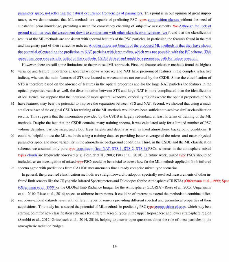
::::::::parameter
::::::space,
:::not
::::::::reflecting
:::the
::::::natural
:::::::::occurrence
::::::::::frequencies
::of
::::::::::parameters.
:This point is in our opinion of great impor-
tance, as we demonstrated that ML methods are capable of predicting PSC types::::::::::composition
::::::classes
:without the need of
substantial prior knowledge, providing a mean for consistency checking of subjective assessments. We:::::::Although
::::the
:::lack
:::of
::::::ground
::::truth
:::::::narrows
:::the
::::::::::assessment
:::::down
::to
::::::::::comparison
::::with
:::::other
:::::::::::classification
::::::::schemes,
:::we found that the classification
results of the ML methods are consistent with spectral features of the PSC particles, in particular, the features found in the real5
and imaginary part of their refractive indices.::::::Another
:::::::::important
::::::benefit
::of
:::the
::::::::proposed
:::ML
:::::::methods
::is::::that
::::they
::::have
::::::shown
::the
::::::::potential
::of
:::::::::extending
::the
:::::::::prediction
::to
:::::NAT
:::::::particles
::::with
::::large
::::::radius,
::::::which
:::was
:::not
:::::::possible
::::with
:::the
::::BC
:::::::scheme.
::::This
:::::aspect
:::has
::::been
:::::::::::successfully
:::::tested
::on
:::the
::::::::synthetic
::::::CSDB
::::::dataset
:::and
:::::might
:::be
:a:::::::::promising
::::path
:::for
:::::future
:::::::research.
:
However, there are still some limitations to the proposed ML approach. First, the feature selection methods found the highest
variance and feature importance at spectral windows where ice and NAT have pronounced features in the complex refractive10
indices, whereas the main features of STS are located at wavenumbers not covered by the CSDB. Since the classification of
STS is therefore based on the absence of features in the optical properties and for the large NAT particles the features in the
optical properties vanish as well, the discrimination between STS and large NAT is more complicated than the identification
of ice. Hence, we suppose that the inclusion of more spectral windows, especially regions where the optical properties of STS
have features, may bear the potential to improve the separation between STS and NAT. Second, we showed that using a much15
smaller subset of the original CSDB for training of the ML methods would have been sufficient to achieve similar classification
results. This suggests that the information provided by the CSDB is largely redundant, at least in terms of training of the ML
methods. Despite the fact that the CSDB contains many training spectra, it was calculated only for a limited number of PSC
volume densities, particle sizes, and cloud layer heights and depths as well as fixed atmospheric background conditions. It
could be helpful to test the ML methods using a training data set providing better coverage of the micro- and macrophysical20
parameter space and more variability in the atmospheric background conditions. Third, in the CSDB and the ML classification
schemes we assumed only pure type:::::::::constituent
::::(ice,
:::::NAT,
::::STS
:::1,
::::STS
::2,
::::STS
::3)
:PSCs, whereas in the atmosphere mixed
types:::::clouds
:are frequently observed (e.g. Deshler et al., 2003; Pitts et al., 2018). In future work, mixed type PSCs should be
included, as an investigation of mixed type PSCs could be beneficial to assess how far the ML methods applied to limb infrared
spectra agree with predictions from CALIOP measurements that already comprise mixed type scenarios.25
In general, the presented classification methods are straightforward to adopt on spectrally resolved measurements of other in-
frared limb sensors like the CRyogenic Infrared Spectrometers and Telescopes for the Atmosphere (CRISTA) (Offermann et al., 1999; Spang et al., 2001, 2008)
::::::::::::::::::::(Offermann et al., 1999) or the GLObal limb Radiance Imager for the Atmosphere (GLORIA) (Riese et al., 2005; Ungermann
et al., 2010; Riese et al., 2014) space- or airborne instruments. It could be of interest to extend the methods to combine differ-
ent observational datasets, even with different types of sensors providing different spectral and geometrical properties of their30
acquisitions. This study has assessed the potential of ML methods in predicting PSC types::::::::::composition
::::::classes, which may be a
starting point for new classification schemes for different aerosol types in the upper troposphere and lower stratosphere region
(Sembhi et al., 2012; Griessbach et al., 2014, 2016), helping to answer open questions about the role of these particles in the
atmospheric radiation budget.
14

Code and data availability. The MIPAS Level-1B IPF version 7.11 data can be accessed via ESA’s Earth Online portal at https://earth.esa.int/
(last access: 10 December 2019). The CSDB database can be obtained by contacting Michael Höpfner, Karlsruhe. The software repository
containing the ML codes developed for this study is available at https://gitlab.com/rocco.sedona/psc_mipas_classification.
Author contributions. GC, LH, and RSp developed the concept for this study. RoS developed the software and conducted the formal analysis
of the results. SG, MH, and RSp provided expertise on the MIPAS measurements. MH prepared and provided the CSDB. GC and MR5
provided expertise on the ML methods. RoS wrote the manuscript with contributions from all co-authors.
Competing interests. The authors declare that they have no conflict of interest.
Acknowledgements. We thank the European Space Agency (ESA) for making the Envisat MIPAS data available. We found the scikit-learn
software package (https://scikit-learn.org/, last access: 10 December 2019) of great importance for the development of the code for this study.
15
References
Achtert, P. and Tesche, M.: Assessing lidar-based classification schemes for polar stratospheric clouds based on 16 years of measurements at
Esrange, Sweden, Journal of Geophysical Research: Atmospheres, 119, 1386–1405, https://doi.org/10.1002/2013jd020355, 2014.
Adriani, A.: Climatology of polar stratospheric clouds based on lidar observations from 1993 to 2001 over McMurdo Station, Antarctica,
Journal of Geophysical Research, 109, https://doi.org/10.1029/2004jd004800, http://dx.doi.org/10.1029/2004JD004800, 2004.5
Arnone, E., Castelli, E., Papandrea, E., Carlotti, M., and Dinelli, B. M.: Extreme ozone depletion in the 2010âC“2011 Arctic winter strato-
sphere as observed by MIPAS/ENVISAT using a 2-D tomographic approach, Atmospheric Chemistry and Physics, 12, 9149–9165,
https://doi.org/10.5194/acp-12-9149-2012, 2012.
Bergstra, J. and Bengio, Y.: Random search for hyper-parameter optimization, J. Mach. Learn. Res., 13, 281–305, 2012.
Biele, J., Tsias, A., Luo, B. P., Carslaw, K. S., Neuber, R., Beyerle, G., and Peter, T.: Nonequilibrium coexistence of10
solid and liquid particles in Arctic stratospheric clouds, Journal of Geophysical Research: Atmospheres, 106, 22 991–23 007,
https://doi.org/10.1029/2001jd900188, http://dx.doi.org/10.1029/2001JD900188, 2001.
Bolón-Canedo, V., Sánchez-Maroño, N., and Alonso-Betanzos, A.: Feature selection for high-dimensional data, Progress in Artificial Intel-
ligence, https://doi.org/10.1007/s13748-015-0080-y, 2016.
Breiman, L.: Machine Learning, 45, 5–32, https://doi.org/10.1023/a:1010933404324, 2001.15
Brereton, R. G. and Lloyd, G. R.: Support Vector Machines for classification and regression, The Analyst, 135, 230–267,
https://doi.org/10.1039/b918972f, 2010.
Browell, E. V., Butler, C. F., Ismail, S., Robinette, P. A., Carter, A. F., Higdon, N. S., Toon, O. B., Schoeberl, M. R., and Tuck, A. F.:
Airborne lidar observations in the wintertime Arctic stratosphere: Polar stratospheric clouds, Geophysical Research Letters, 17, 385–388,
https://doi.org/10.1029/gl017i004p00385, http://dx.doi.org/10.1029/GL017i004p00385, 1990.20
Buontempo, C., Cairo, F., Di Donfrancesco, G., Morbidini, R., Viterbini, M., and Adriani, A.: Optical measurements of atmospheric
particles from airborne platforms: In situ and remote sensing instruments for balloons and aircrafts, Annals of Geophysics, 49,
https://doi.org/10.4401/ag-3149, 2009.
Campbell, J. R. and Sassen, K.: Polar stratospheric clouds at the South Pole from 5 years of continuous lidar data: Macrophysical, optical,
and thermodynamic properties, Journal of Geophysical Research, 113, https://doi.org/10.1029/2007jd009680, 2008.25
Carslaw, K. S., Luo, B., and Peter, T.: An analytic expression for the composition of aqueous HNO3-H2SO4stratospheric aerosols including
gas phase removal of HNO3, Geophysical Research Letters, 22, 1877–1880, https://doi.org/10.1029/95gl01668, 1995.
Cavallaro, G., Riedel, M., Richerzhagen, M., Benediktsson, J. A., and Plaza, A.: On Understanding Big Data Impacts in Remotely Sensed
Image Classification Using Support Vector Machine Methods, IEEE Journal of Selected Topics in Applied Earth Observations and Remote
Sensing, 8, 4634–4646, 2015.30
Ceriani, L. and Verme, P.: The origins of the Gini index: extracts from Variabilità e Mutabilità (1912) by Corrado Gini, J. Econ. Inequal., 10,
421–443, https://doi.org/10.1007/s10888-011-9188-x, 2012.
Cortes, C. and Vapnik, V.: Support-Vector Networks, Mach. Learn., https://doi.org/10.1023/A:1022627411411, 1995.
Deshler, T., Larsen, N., Weissner, C., Schreiner, J., Mauersberger, K., Cairo, F., Adriani, A., Di Donfrancesco, G., Ovarlez, J., Ovarlez, H.,
Blum, U., Fricke, K. H., and Dornbrack, A.: Large nitric acid particles at the top of an Arctic stratospheric cloud, J. Geophys. Res., 108,35
https://doi.org/10.1029/2003JD003479, 2003.
16
Dudhia, A., Morris, P. E., and Wells, R. J.: Fast monochromatic radiative transfer calculations for limb sounding, J. Quant. Spectrosc. Radiat.
Transfer, 74, 745–756, 2002.
Eckermann, S. D., Hoffmann, L., Höpfner, M., Wu, D. L., and Alexander, M. J.: Antarctic NAT PSC belt of June 2003: Observational
validation of the mountain wave seeding hypothesis, Geophys. Res. Lett., 36, https://doi.org/10.1029/2008GL036629, 2009.
Estornell, J., Martí-Gavliá, J. M., Sebastiá, M. T., and Mengual, J.: Principal component analysis applied to remote sensing, Model. Sci.5
Educ. Learn., https://doi.org/10.4995/msel.2013.1905, 2013.
Fauvel, M., Chanussot, J., and Benediktsson, J. A.: Kernel principal component analysis for the classification of hyperspectral remote sensing
data over urban areas, Eurasip J. Adv. Sign. Process., https://doi.org/10.1155/2009/783194, 2009.
Fischer, H., Birk, M., Blom, C., Carli, B., Carlotti, M., von Clarmann, T., Delbouille, L., Dudhia, A., Ehhalt, D., Endemann, M., Flaud, J. M.,
Gessner, R., Kleinert, A., Koopman, R., Langen, J., López-Puertas, M., Mosner, P., Nett, H., Oelhaf, H., Perron, G., Remedios, J., Ridolfi,10
M., Stiller, G., and Zander, R.: MIPAS: an instrument for atmospheric and climate research, Atmos. Chem. Phys., 8, 2151–2188, 2008.
Fromm, M.: A unified, long-term, high-latitude stratospheric aerosol and cloud database using SAM II, SAGE II, and POAM II/III data:
Algorithm description, database definition, and climatology, Journal of Geophysical Research, 108, https://doi.org/10.1029/2002jd002772,
2003.
Genton, M.: Classes of kernels for machine learning: a statistics perspective, J. Mach. Learn. Res., 2, 299–312, 2002.15
Genuer, R., Poggi, J.-M., Tuleau-Malot, C., and Villa-Vialaneix, N.: Random Forests for Big Data, Big Data Research, 9, 28–46,
https://doi.org/10.1016/j.bdr.2017.07.003, 2017.
Griessbach, S., Hoffmann, L., Spang, R., and Riese, M.: Volcanic ash detection with infrared limb sounding: MIPAS observations and
radiative transfer simulations, Atmos. Meas. Tech., 7, 1487–1507, https://doi.org/10.5194/amt-7-1487-214, 2014.
Griessbach, S., Hoffmann, L., Spang, R., von Hobe, M., Müller, R., and Riese, M.: Infrared limb emission measurements of aerosol in the20
troposphere and stratosphere, Atmos. Meas. Tech., 9, 4399–4423, https://doi.org/10.5194/amt-9-4399-2016, 2016.
Griessbach, S., Hoffmann, L., Spang, R., Achtert, P., von Hobe, M., Mateshvili, N., Müller, R., Riese, M., Rolf, C., Seifert, P., and Vernier,
J.-P.: Aerosol and cloud top height information of Envisat MIPAS measurements, Atmospheric Measurement Techniques, 13, 1243–1271,
https://doi.org/10.5194/amt-13-1243-2020, 2020.
Hoffmann, L., Spang, R., Orr, A., Alexander, M. J., Holt, L. A., and Stein, O.: A decadal satellite record of gravity wave activity in the lower25
stratosphere to study polar stratospheric cloud formation, Atmos. Chem. Phys., 17, 2901–2920, https://doi.org/10.5194/acp-17-2901-2017,
2017.
Höpfner, M., Oelhaf, H., Wetzel, G., Friedl-Vallon, F., Kleinert, A., Lengel, A., Maucher, G., Nordmeyer, H., Glatthor, N., Stiller, N., von
Clarmann, T., Fischer, H., Kröger, C., and Deshler, T.: Evidence of scattering of tropospheric radiation by PSCs in mid-IR limb emission
spectra: MIPAS-B observations and KOPRA simulations, J. Geophys. Res., 29, 1278–1291, https://doi.org/10.1029/2001GL014443, 2002.30
Höpfner, M., Larsen, N., Spang, R., Luo, B. P., Ma, J., Svendsen, S. H., Eckermann, S. D., Knudsen, B., Massoli, P., Cairo, F., Stiller, G.,
Von Clarmann, T., and Fischer, H.: MIPAS detects Antarctic stratospheric belt of NAT PSCs caused by mountain waves, Atmos. Chem.
Phys., 6, 1221–1230, 2006.
Höpfner, M., Luo, B. P., Massoli, P., Cairo, F., Spang, R., Snels, M., Di Donfrancesco, G., Stiller, G., Von Clarmann, T., Fischer, H., and
Biermann, U.: Spectroscopic evidence for NAT, STS, and ice in MIPAS infrared limb emission measurements of polar stratospheric35
clouds, Atmos. Chem. Phys., https://doi.org/10.5194/acp-6-1201-2006, 2006.
Höpfner, M., Pitts, M. C., and Poole, L. R.: Comparison between CALIPSO and MIPAS observations of polar stratospheric clouds, J.
Geophys. Res., https://doi.org/10.1029/2009JDO12114, 2009.
17
Huang, H.-L. and Antonelli, P.: Application of Principal Component Analysis to High-Resolution Infrared Measurement Compression and
Retrieval, J. Appl. Meteo., 40, 365–388, https://doi.org/10.1175/1520-0450(2001)040<0365:AOPCAT>2.0.CO;2, 2001.
Jolliffe, I. T. and Cadima, J.: Principal component analysis: a review and recent developments, Philosophical Transactions of the Royal
Society A: Mathematical, Physical and Engineering Sciences, 374, 20150 202, https://doi.org/10.1098/rsta.2015.0202, 2016.
Khosrawi, F., Kirner, O., Stiller, G., Höpfner, M., Santee, M. L., Kellmann, S., and Braesicke, P.: Comparison of ECHAM5/MESSy Atmo-5
spheric Chemistry (EMAC) simulations of the Arctic winter 2009/2010 and 2010/2011 with Envisat/MIPAS and Aura/MLS observations,
Atmospheric Chemistry and Physics, 18, 8873–8892, https://doi.org/10.5194/acp-18-8873-2018, 2018.
Kohavi, R.: A Study of Cross-Validation and Bootstrap for Accuracy Estimation and Model Selection, International Joint Conference of
Artificial Intelligence, 14, 1137–1145, 1995.
Lambert, A., Santee, M., Wu, D., and Chae, J. H.: A-train CALIOP and MLS observations of early winter Antarctic polar stratospheric10
clouds and nitric acid in 2008, Atmospheric Chemistry and Physics, 12, https://doi.org/10.5194/acp-12-2899-2012, 2012.
Liu, Y., Wang, Y., and Zhang, J.: New Machine Learning Algorithm: Random Forest, in: Information Computing and Applications, pp.
246–252, Springer Berlin Heidelberg, https://doi.org/10.1007/978-3-642-34062-8_32, 2012.
Lowe, D. and MacKenzie, A. R.: Polar stratospheric cloud microphysics and chemistry, J. Atm. Sol.-Terr. Phys., 70, 13–40,
https://doi.org/10.1016/j.jastp.2007.09.011, 2008.15
Molleker, S., Borrmann, S., Schlager, H., Luo, B., Frey, W., Klingebiel, M., Weigel, R., Ebert, M., Mitev, V., Matthey, R., Woiwode,
W., Oelhaf, H., Dörnbrack, A., Stratmann, G., Grooß, J.-U., Günther, G., Vogel, B., Müller, R., Krämer, M., Meyer, J., and Cairo, F.:
Microphysical properties of synoptic-scale polar stratospheric clouds: in situ measurements of unexpectedly large HNO3-containing
particles in the Arctic vortex, Atmospheric Chemistry and Physics, 14, 10 785–10 801, https://doi.org/10.5194/acp-14-10785-2014,
https://www.atmos-chem-phys.net/14/10785/2014/, 2014.20
Offermann, D., Grossmann, K.-U., Barthol, P., Knieling, P., Riese, M., and Trant, R.: Cryogenic Infrared Spectrometers and Telescopes for
the Atmosphere (CRISTA) experiment and middle atmosphere variability, J. Geophys. Res., 104, 16 311–16 325, 1999.
Patle, A. and Chouhan, D. S.: SVM kernel functions for classification, in: 2013 International Conference on Advances in Technology and
Engineering (ICATE), IEEE, https://doi.org/10.1109/icadte.2013.6524743, 2013.
Pawson, S., Naujokat, B., and Labitzke, K.: On the polar stratospheric cloud formation potential of the northern stratosphere, Journal of25
Geophysical Research, 100, 23 215, https://doi.org/10.1029/95jd01918, 1995.
Pitts, M. C., Poole, L. R., and Thomason, L. W.: CALIPSO polar stratospheric cloud observations: second-generation detection algorithm
and composition discrimination, Atmos. Chem. Phys., 9, 7577–7589, 2009.
Pitts, M. C., Poole, L. R., Dörnbrack, A., and Thomason, L. W.: The 2009-2010 Arctic polar stratospheric cloud season: A CALIPSO
perspective, Atmos. Chem. Phys., 11, 2161–2177, https://doi.org/10.5194/acp-11-2161-2011, 2011.30
Pitts, M. C., Poole, L. R., and Gonzalez, R.: Polar stratospheric cloud climatology based on CALIPSO spaceborne lidar measurements from
2006 to 2017, Atmos. Chem. Phys., 18, 10 881–10 913, https://doi.org/10.5194/acp-18-10881-2018, 2018.
Probst, P., Wright, M. N., and Boulesteix, A.-L.: Hyperparameters and tuning strategies for random forest, Wiley Interdisciplinary Reviews:
Data Mining and Knowledge Discovery, 9, https://doi.org/10.1002/widm.1301, 2019.
Raspollini, P., Belotti, C., Burgess, A., Carli, B., Carlotti, M., Ceccherini, S., Dinelli, B. M., Dudhia, A., Flaud, J. M., Funke, B., Höpfner,35
M., López-Puertas, M., Payne, V., Piccolo, C., Remedios, J. J., Ridolfi, M., and Spang, R.: MIPAS level 2 operational analysis, Atmos.
Chem. Phys., https://doi.org/10.5194/acp-6-5605-2006, 2006.
18
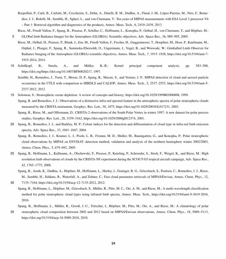
Raspollini, P., Carli, B., Carlotti, M., Ceccherini, S., Dehn, A., Dinelli, B. M., Dudhia, A., Flaud, J.-M., López-Puertas, M., Niro, F., Reme-
dios, J. J., Ridolfi, M., Sembhi, H., Sgheri, L., and von Clarmann, T.: Ten years of MIPAS measurements with ESA Level 2 processor V6
– Part 1: Retrieval algorithm and diagnostics of the products, Atmos. Meas. Tech., 6, 2419–2439, 2013.
Riese, M., Friedl-Vallon, F., Spang, R., Preusse, P., Schiller, C., Hoffmann, L., Konopka, P., Oelhaf, H., von Clarmann, T., and Höpfner, M.:
GLObal limb Radiance Imager for the Atmosphere (GLORIA): Scientific objectives, Adv. Space Res., 36, 989–995, 2005.5
Riese, M., Oelhaf, H., Preusse, P., Blank, J., Ern, M., Friedl-Vallon, F., Fischer, H., Guggenmoser, T., Hoepfner, M., Hoor, P., Kaufmann, M.,
Orphal, J., Ploeger, F., Spang, R., Suminska-Ebersoldt, O., Ungermann, J., Vogel, B., and Woiwode, W.: Gimballed Limb Observer for
Radiance Imaging of the Atmosphere (GLORIA) scientific objectives, Atmos. Meas. Tech., 7, 1915–1928, https://doi.org/10.5194/amt-7-
1915-2014, 2014.
Schölkopf, B., Smola, A., and Müller, K.-R.: Kernel principal component analysis, pp. 583–588,10
https://doi.org/https://doi.org/10.1007/BFb0020217, 1997.
Sembhi, H., Remedios, J., Trent, T., Moore, D. P., Spang, R., Massie, S., and Vernier, J. P.: MIPAS detection of cloud and aerosol particle
occurrence in the UTLS with comparison to HIRDLS and CALIOP, Atmos. Meas. Tech., 5, 2537–2553, https://doi.org/10.5194/amt-5-
2537-2012, 2012.
Solomon, S.: Stratospheric ozone depletion: A review of concepts and history, https://doi.org/10.1029/1999RG900008, 1999.15
Spang, R. and Remedios, J. J.: Observations of a distinctive infra-red spectral feature in the atmospheric spectra of polar stratospheric clouds
measured by the CRISTA instrument, Geophys. Res. Lett., 30, 1875, https://doi.org/10.1029/2003GL017231, 2003.
Spang, R., Riese, M., and Offermann, D.: CRISTA-2 observations of the South Polar Vortex in winter 1997: A new dataset for polar process
studies, Geophys. Res. Lett., 28, 3159–3162, https://doi.org/10.1029/2000gl012374, 2001.
Spang, R., Remedios, J. J., and Barkley, M. P.: Colour indices for the detection and differentiation of cloud type in infra-red limb emission20
spectra, Adv. Space Res., 33, 1041–1047, 2004.
Spang, R., Remedios, J. J., Kramer, L. J., Poole, L. R., Fromm, M. D., Muller, M., Baumgarten, G., and Konopka, P.: Polar stratospheric
cloud observations by MIPAS on ENVISAT: detection method, validation and analysis of the northern hemisphere winter 2002/2003,
Atmos. Chem. Phys., 5, 679–692, 2005.
Spang, R., Hoffmann, L., Kullmann, A., Olschewski, F., Preusse, P., Knieling, P., Schroeder, S., Stroh, F., Weigel, K., and Riese, M.: High25
resolution limb observations of clouds by the CRISTA-NF experiment during the SCOUT-O3 tropical aircraft campaign, Adv. Space Res.,
42, 1765–1775, 2008.
Spang, R., Arndt, K., Dudhia, A., Höpfner, M., Hoffmann, L., Hurley, J., Grainger, R. G., Griessbach, S., Poulsen, C., Remedios, J. J., Riese,
M., Sembhi, H., Siddans, R., Waterfall, A., and Zehner, C.: Fast cloud parameter retrievals of MIPAS/Envisat, Atmos. Chem. Phys., 12,
7135–7164, https://doi.org/10.5194/acp-12-7135-2012, 2012.30
Spang, R., Hoffmann, L., Höpfner, M., Griessbach, S., Müller, R., Pitts, M. C., Orr, A. M., and Riese, M.: A multi-wavelength classification
method for polar stratospheric cloud types using infrared limb spectra, Atmos. Meas. Tech., https://doi.org/10.5194/amt-9-3619-2016,
2016.
Spang, R., Hoffmann, L., Müller, R., Grooß, J.-U., Tritscher, I., Höpfner, M., Pitts, M., Orr, A., and Riese, M.: A climatology of polar
stratospheric cloud composition between 2002 and 2012 based on MIPAS/Envisat observations, Atmos. Chem. Phys., 18, 5089–5113,35
https://doi.org/10.5194/acp-18-5089-2018, 2018.
19
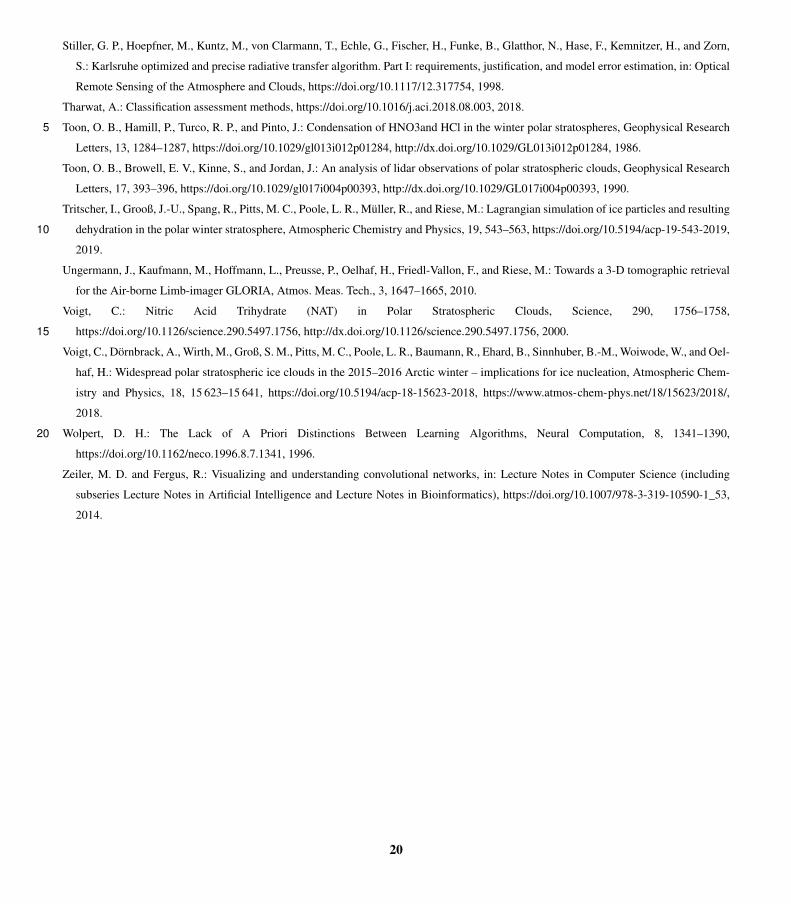
Stiller, G. P., Hoepfner, M., Kuntz, M., von Clarmann, T., Echle, G., Fischer, H., Funke, B., Glatthor, N., Hase, F., Kemnitzer, H., and Zorn,
S.: Karlsruhe optimized and precise radiative transfer algorithm. Part I: requirements, justification, and model error estimation, in: Optical
Remote Sensing of the Atmosphere and Clouds, https://doi.org/10.1117/12.317754, 1998.
Tharwat, A.: Classification assessment methods, https://doi.org/10.1016/j.aci.2018.08.003, 2018.
Toon, O. B., Hamill, P., Turco, R. P., and Pinto, J.: Condensation of HNO3and HCl in the winter polar stratospheres, Geophysical Research5
Letters, 13, 1284–1287, https://doi.org/10.1029/gl013i012p01284, http://dx.doi.org/10.1029/GL013i012p01284, 1986.
Toon, O. B., Browell, E. V., Kinne, S., and Jordan, J.: An analysis of lidar observations of polar stratospheric clouds, Geophysical Research
Letters, 17, 393–396, https://doi.org/10.1029/gl017i004p00393, http://dx.doi.org/10.1029/GL017i004p00393, 1990.
Tritscher, I., Grooß, J.-U., Spang, R., Pitts, M. C., Poole, L. R., Müller, R., and Riese, M.: Lagrangian simulation of ice particles and resulting
dehydration in the polar winter stratosphere, Atmospheric Chemistry and Physics, 19, 543–563, https://doi.org/10.5194/acp-19-543-2019,10
2019.
Ungermann, J., Kaufmann, M., Hoffmann, L., Preusse, P., Oelhaf, H., Friedl-Vallon, F., and Riese, M.: Towards a 3-D tomographic retrieval
for the Air-borne Limb-imager GLORIA, Atmos. Meas. Tech., 3, 1647–1665, 2010.
Voigt, C.: Nitric Acid Trihydrate (NAT) in Polar Stratospheric Clouds, Science, 290, 1756–1758,
https://doi.org/10.1126/science.290.5497.1756, http://dx.doi.org/10.1126/science.290.5497.1756, 2000.15
Voigt, C., Dörnbrack, A., Wirth, M., Groß, S. M., Pitts, M. C., Poole, L. R., Baumann, R., Ehard, B., Sinnhuber, B.-M., Woiwode, W., and Oel-
haf, H.: Widespread polar stratospheric ice clouds in the 2015–2016 Arctic winter – implications for ice nucleation, Atmospheric Chem-
istry and Physics, 18, 15 623–15 641, https://doi.org/10.5194/acp-18-15623-2018, https://www.atmos-chem-phys.net/18/15623/2018/,
2018.
Wolpert, D. H.: The Lack of A Priori Distinctions Between Learning Algorithms, Neural Computation, 8, 1341–1390,20
https://doi.org/10.1162/neco.1996.8.7.1341, 1996.
Zeiler, M. D. and Fergus, R.: Visualizing and understanding convolutional networks, in: Lecture Notes in Computer Science (including
subseries Lecture Notes in Artificial Intelligence and Lecture Notes in Bioinformatics), https://doi.org/10.1007/978-3-319-10590-1_53,
2014.
20
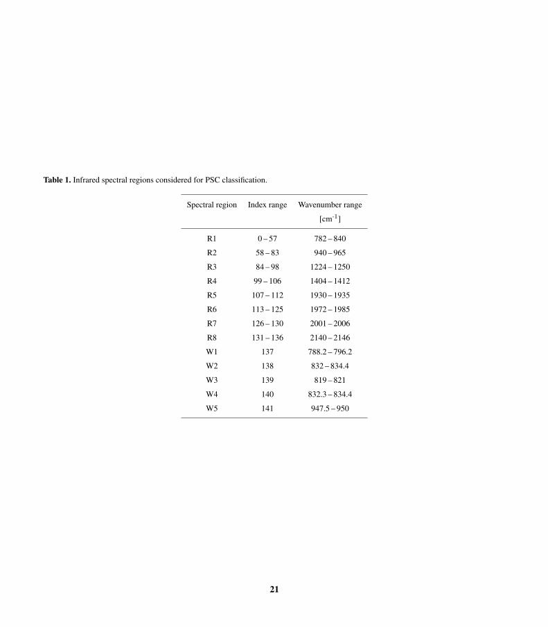
Table 1. Infrared spectral regions considered for PSC classification.
Spectral region Index range Wavenumber range
[cm-1]
R1 0 – 57 782 – 840
R2 58 – 83 940 – 965
R3 84 – 98 1224 – 1250
R4 99 – 106 1404 – 1412
R5 107 – 112 1930 – 1935
R6 113 – 125 1972 – 1985
R7 126 – 130 2001 – 2006
R8 131 – 136 2140 – 2146
W1 137 788.2 – 796.2
W2 138 832 – 834.4
W3 139 819 – 821
W4 140 832.3 – 834.4
W5 141 947.5 – 950
21
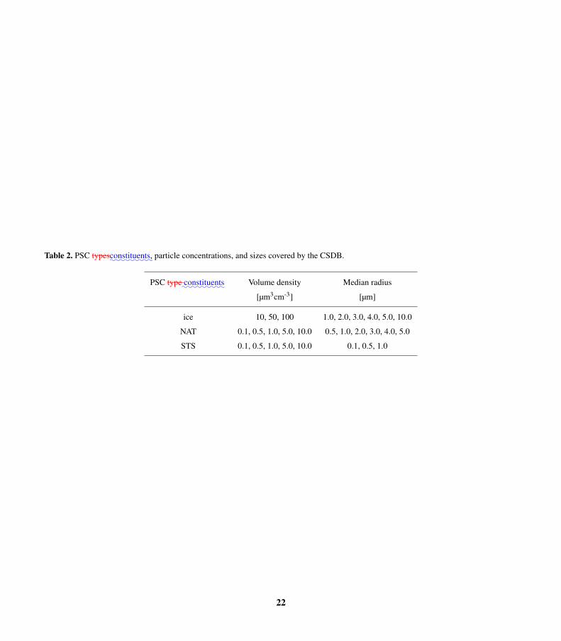
Table 2. PSC types:::::::::constituents, particle concentrations, and sizes covered by the CSDB.
PSC type:::::::::constituents Volume density Median radius
[µm3cm-3] [µm]
ice 10, 50, 100 1.0, 2.0, 3.0, 4.0, 5.0, 10.0
NAT 0.1, 0.5, 1.0, 5.0, 10.0 0.5, 1.0, 2.0, 3.0, 4.0, 5.0
STS 0.1, 0.5, 1.0, 5.0, 10.0 0.1, 0.5, 1.0
22
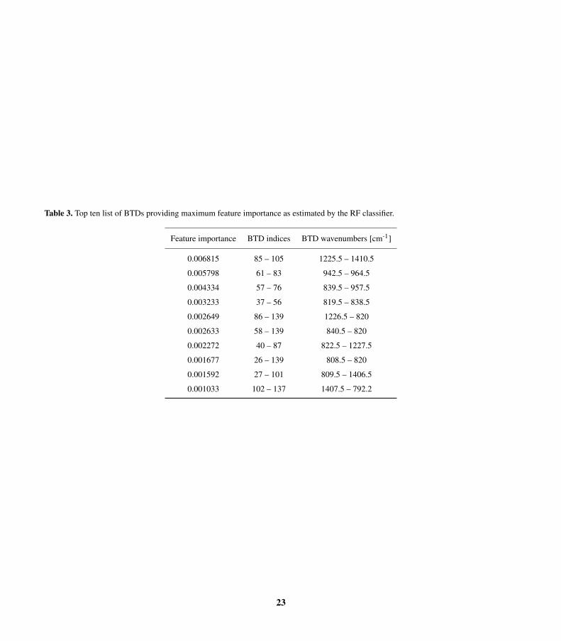
Table 3. Top ten list of BTDs providing maximum feature importance as estimated by the RF classifier.
Feature importance BTD indices BTD wavenumbers [cm-1]
0.006815 85 – 105 1225.5 – 1410.5
0.005798 61 – 83 942.5 – 964.5
0.004334 57 – 76 839.5 – 957.5
0.003233 37 – 56 819.5 – 838.5
0.002649 86 – 139 1226.5 – 820
0.002633 58 – 139 840.5 – 820
0.002272 40 – 87 822.5 – 1227.5
0.001677 26 – 139 808.5 – 820
0.001592 27 – 101 809.5 – 1406.5
0.001033 102 – 137 1407.5 – 792.2
23
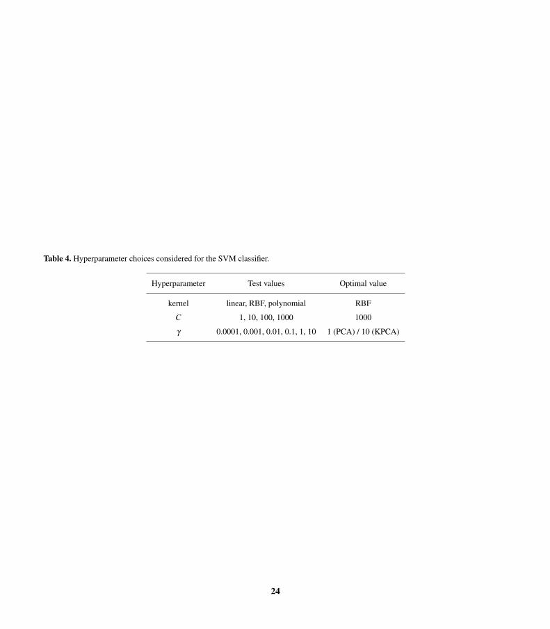
Table 4. Hyperparameter choices considered for the SVM classifier.
Hyperparameter Test values Optimal value
kernel linear, RBF, polynomial RBF
C 1, 10, 100, 1000 1000
γ 0.0001, 0.001, 0.01, 0.1, 1, 10 1 (PCA) / 10 (KPCA)
24
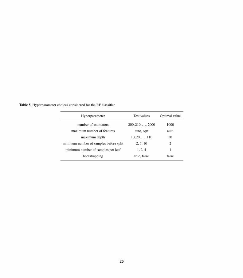
Table 5. Hyperparameter choices considered for the RF classifier.
Hyperparameter Test values Optimal value
number of estimators 200,210, . . . ,2000 1000
maximum number of features auto, sqrt auto
maximum depth 10,20, . . . ,110 50
minimum number of samples before split 2, 5, 10 2
minimum number of samples per leaf 1, 2, 4 1
bootstrapping true, false false
25
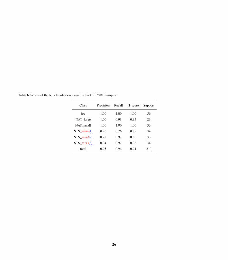
Table 6. Scores of the RF classifier on a small subset of CSDB samples.
Class Precision Recall f1-score Support
ice 1.00 1.00 1.00 56
NAT_large 1.00 0.91 0.95 23
NAT_small 1.00 1.00 1.00 33
STS_mix1:1:
0.96 0.76 0.85 34
STS_mix2:2:
0.78 0.97 0.86 33
STS_mix3:3:
0.94 0.97 0.96 34
total 0.95 0.94 0.94 210
26
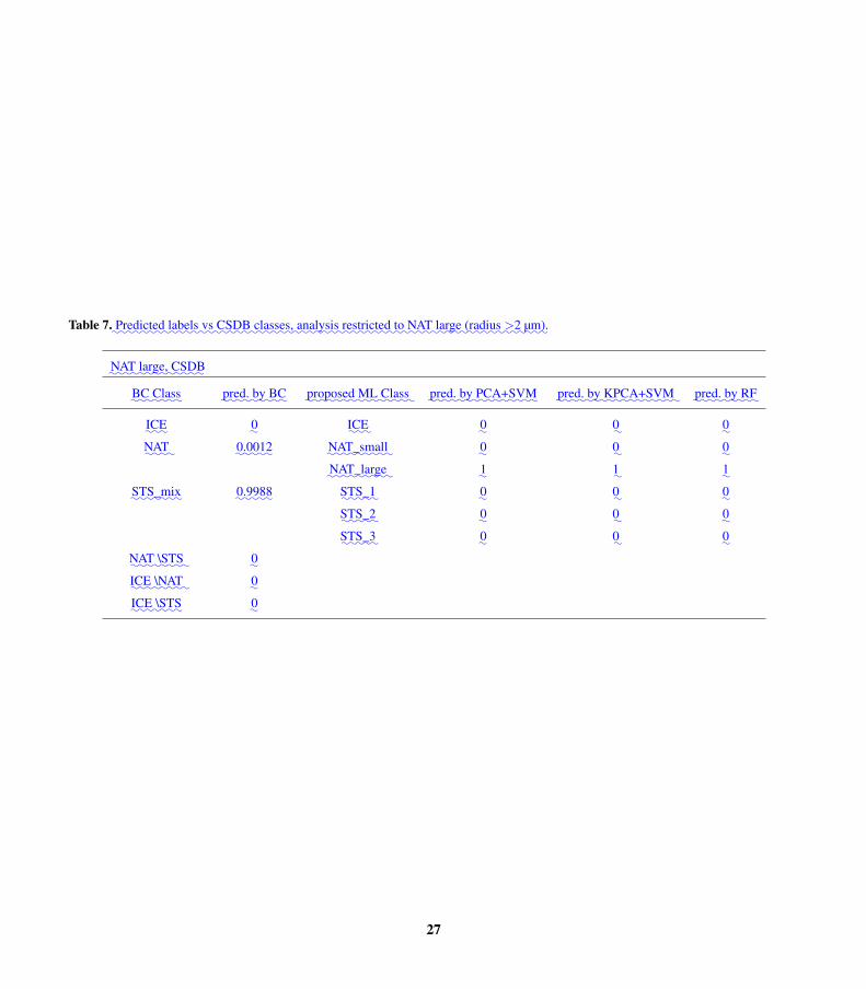
Table 7.:::::::Predicted
:::::labels
::vs
:::::CSDB
::::::classes,
::::::analysis
:::::::restricted
::to::::NAT
::::large
::::::(radius
::>2
:::µm
:).
::::NAT
::::large,
:::::CSDB
:::BC
::::Class
::::pred.
::by
:::BC
:::::::proposed
:::ML
::::Class
: ::::pred.
::by
:::::::::PCA+SVM
::::pred.
::by
::::::::::KPCA+SVM
: ::::pred.
::by
:::RF
:::ICE
:0
:::ICE
:0
:0
:0
:::NAT
: :::::0.0012
::::::::NAT_small
: :0
:0
:0
::::::::NAT_large
: :1
:1
:1
:::::::STS_mix
:::::0.9988
:::::STS_1
:0
:0
:0
:::::STS_2
:0
:0
:0
:::::STS_3
:0
:0
:0
:::NAT
::::\STS
: :0
:::ICE
::::\NAT
: :0
:::ICE
::::\STS
:0
27
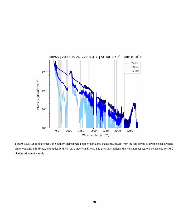
Figure 1. MIPAS measurements in Southern Hemisphere polar winter at three tangent altitudes from the same profile showing clear air (light
blue), optically thin (blue), and optically thick (dark blue) conditions. The grey bars indicate the wavenumber regions considered for PSC
classification in this study.
28
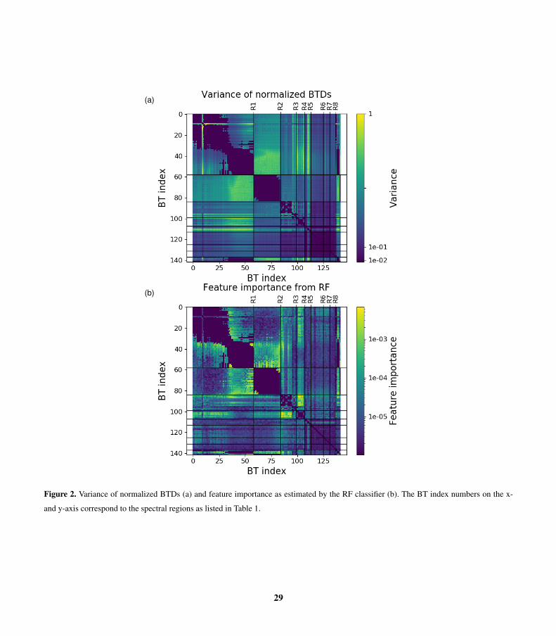
(a)
(b)
Figure 2. Variance of normalized BTDs (a) and feature importance as estimated by the RF classifier (b). The BT index numbers on the x-
and y-axis correspond to the spectral regions as listed in Table 1.
29
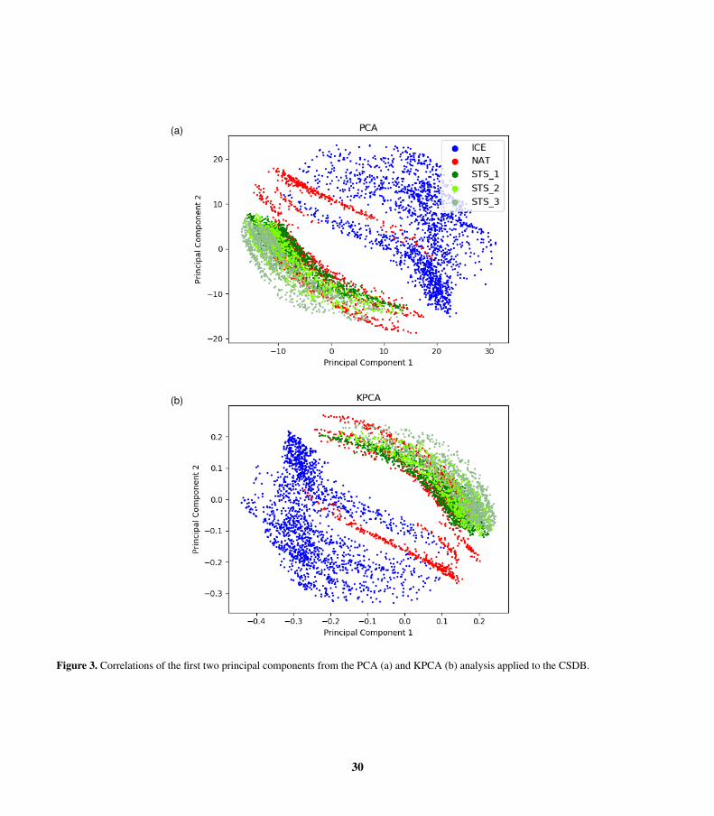
(a)
(b)
Figure 3. Correlations of the first two principal components from the PCA (a) and KPCA (b) analysis applied to the CSDB.
30
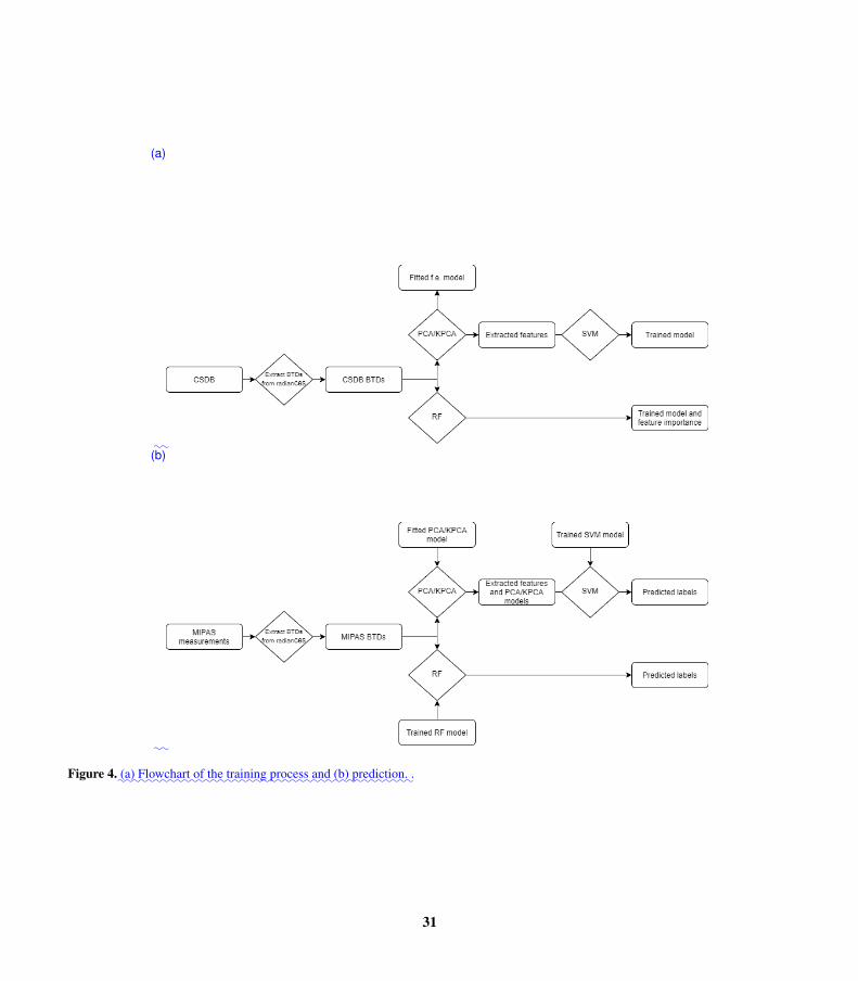
::
(a)
::
(b)
Figure 4.::(a)
::::::::Flowchart
::of
:::the
::::::training
::::::process
:::and
::(b)
::::::::prediction.
:.
31
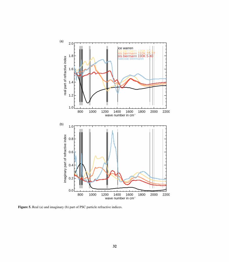
(a)
800 1000 1200 1400 1600 1800 2000 2200wave number in cm-1
1.0
1.2
1.4
1.6
1.8
2.0
real
par
t of r
efra
ctiv
e in
dex
ice warrensts biermann 195K 50-1sts biermann 192K 25-17sts biermann 190K 5-40natcoat biermann
(b)
800 1000 1200 1400 1600 1800 2000 2200wave number in cm-1
0.0
0.2
0.4
0.6
0.8
1.0
imag
inar
y pa
rt o
f ref
ract
ive
inde
x
Figure 5. Real (a) and imaginary (b) part of PSC particle refractive indices.
32
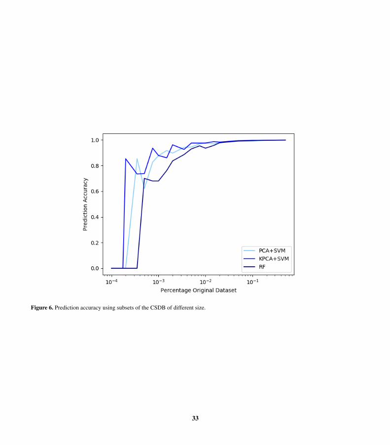
Figure 6. Prediction accuracy using subsets of the CSDB of different size.
33
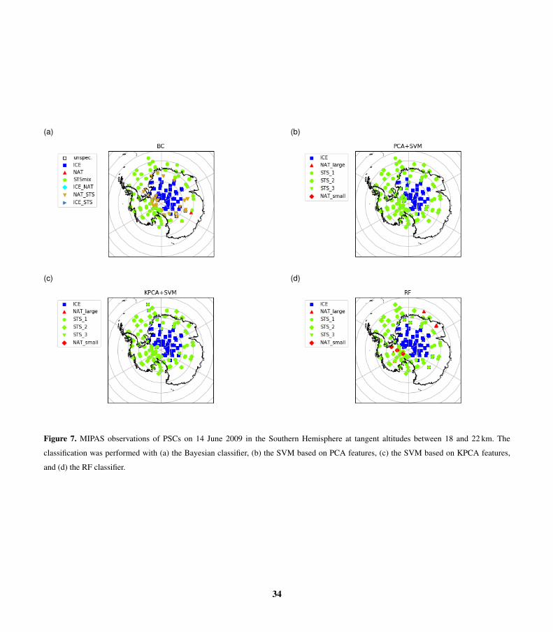
(a) (b)
(c) (d)
Figure 7. MIPAS observations of PSCs on 14 June 2009 in the Southern Hemisphere at tangent altitudes between 18 and 22 km. The
classification was performed with (a) the Bayesian classifier, (b) the SVM based on PCA features, (c) the SVM based on KPCA features,
and (d) the RF classifier.
34
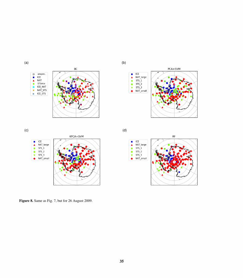
(a) (b)
(c) (d)
Figure 8. Same as Fig. 7, but for 26 August 2009.
35
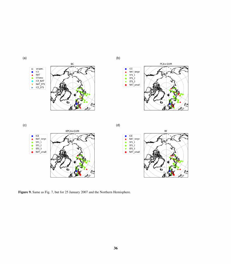
(a) (b)
(c) (d)
Figure 9. Same as Fig. 7, but for 25 January 2007 and the Northern Hemisphere.
36
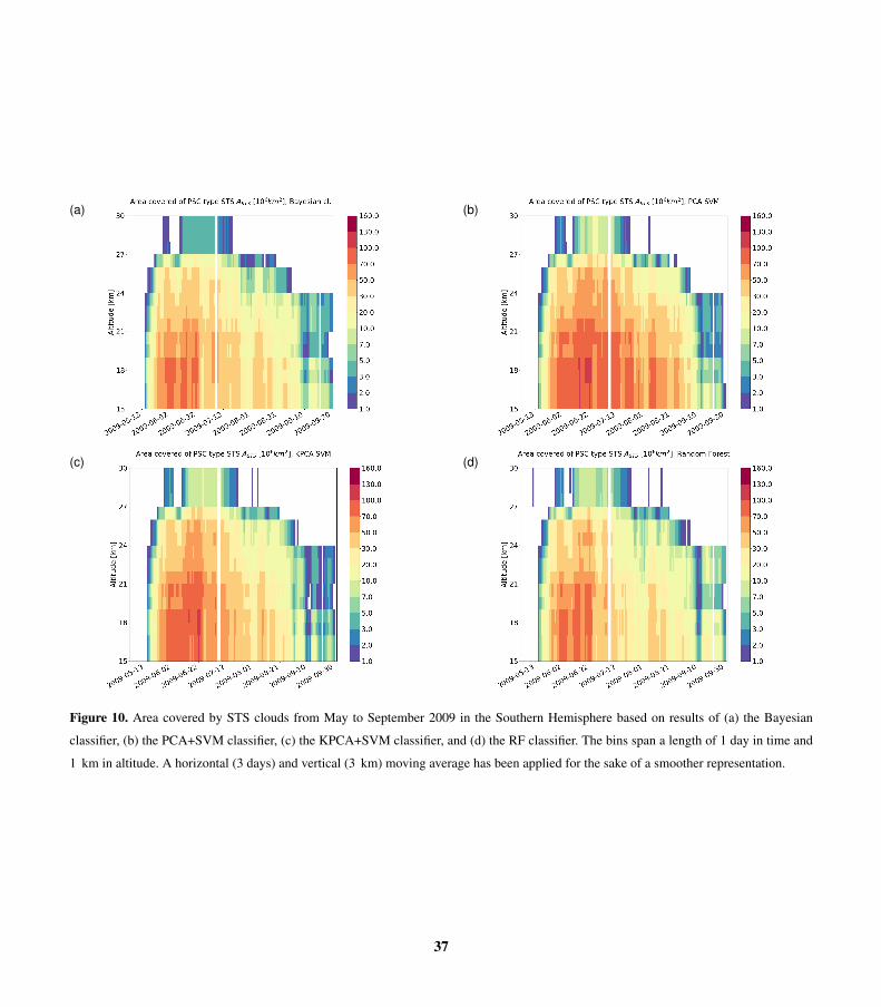
(a) (b)
(c) (d)
Figure 10. Area covered by STS clouds from May to September 2009 in the Southern Hemisphere based on results of (a) the Bayesian
classifier, (b) the PCA+SVM classifier, (c) the KPCA+SVM classifier, and (d) the RF classifier. The bins span a length of 1 day in time and
1 km in altitude. A horizontal (3 days) and vertical (3 km) moving average has been applied for the sake of a smoother representation.
37
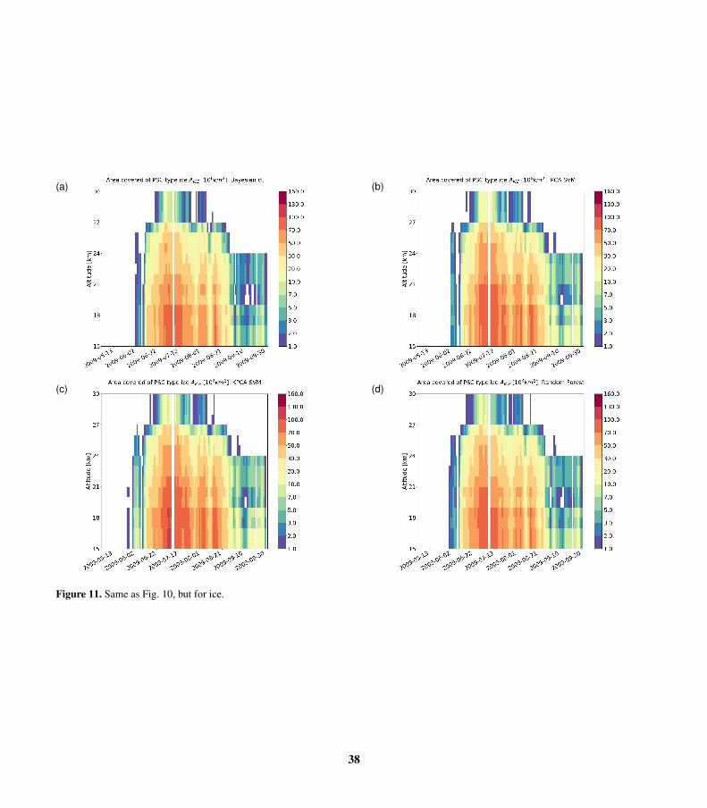
(a) (b)
(c) (d)
Figure 11. Same as Fig. 10, but for ice.
38

(a) (b)
(c) (d)
Figure 12. Same as Fig. 10, but for NAT.
39
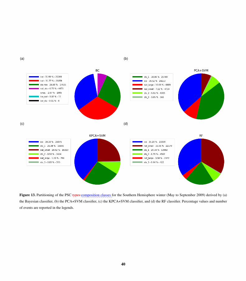
(a) (b)
(c) (d)
Figure 13. Partitioning of the PSC types:::::::::composition
:::::classes
:for the Southern Hemisphere winter (May to September 2009) derived by (a)
the Bayesian classifier, (b) the PCA+SVM classifier, (c) the KPCA+SVM classifier, and (d) the RF classifier. Percentage values and number
of events are reported in the legends.
40

(a) (b)
(c) (d)
Figure 14. Same as Fig. 13, but for November 2006 to February 2007 for the Northern Hemisphere.
41
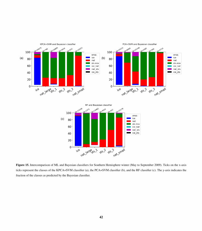
(a) (b)
(c)
Figure 15. Intercomparison of ML and Bayesian classifiers for Southern Hemisphere winter (May to September 2009). Ticks on the x-axis
ticks represent the classes of the KPCA+SVM classifier (a), the PCA+SVM classifier (b), and the RF classifier (c). The y-axis indicates the
fraction of the classes as predicted by the Bayesian classifier.
42
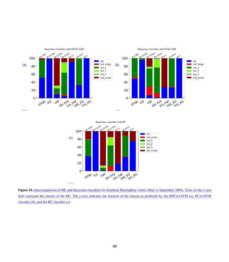
::
(a)
: ::
(b)
::
(c)
:
Figure 16.::::::::::::Intercomparison
::of
:::ML
:::and
:::::::Bayesian
::::::::classifiers
:::for
:::::::Southern
:::::::::Hemisphere
:::::winter
::::(May
::to
::::::::September
:::::2009).
:::::Ticks
::on
:::the
:::::x-axis
:::ticks
::::::::represent
:::the
:::::classes
::of:::
the::::
BC.:::The
:::::y-axis
:::::::indicates
:::the
:::::::fraction
::of
:::the
:::::classes
::as::::::::
predicted::by
:::the
:::::::::::KPCA+SVM
:::(a),
:::::::::PCA+SVM
::::::classifier
:::(b),
:::and
:::the
:::RF
:::::::classifier
::(c).
43