1

Response to referees’ comments

General: We are very much grateful to both the referees for appreciating our work and giving very helpful

suggestions and comments, which have significantly improved the manuscript. We have revised the

manuscript by carefully taking into account all the comments point by point. Text in red and blue colour

show the questions and answers, respectively.

Anonymous Referee #1

Received and published: 27 January 2016

This paper presents a year of data on CO and CO2 concentrations from a site in Ahmedabad. High quality

concentration data from urban areas in general are sparse, and such data from the large urban areas in

rapidly developing regions are especially limited. These observations can contribute to understanding

emission patterns in a poorly studied region that is critically important to the global carbon budget. The

experimental methods are excellent and include decent calibration scheme. The text provides a good

summary of the methods and defines precision and accuracy. However, the discussion needs to be more

focused and strive to present a consistent set of key findings. As noted in detailed comments, some of

the observed variations in concentrations may not contribute to interpreting emissions patterns. The

results will be more convincing by focusing on the key aspects of the data. It is important to distinguish

between patterns with information about atmospheric dynamics (vertical mixing and transport) and

patterns that have information about emission sources.

Comments and suggestions for revised analysis.

Page: 32200

With respect to the evolution of CO2 during night time. Even in cold regions there soils approach 0C

respiration continues throughout the night. At this site I don’t think you can attribute lack of increasing

CO2 during night in some seasons to respiration being dormant. There is certainly no evidence included

in the text for this. In this site I would only expect respiration to be suppressed by very dry soils, so it could

be a reason in the spring, but temperatures are probably not cold enough to suppress respiration. You

don’t show any data for night time winds. Differences in depth and strength of the nocturnal inversion and

2

whether winds persist at night are factors that would impact whether trace gases accumulate at the

surface during night. In subsequent section you show that night time concentrations of CO decline

continuously in the winter and spring season, which indicates that there is enough vertical mixing of low

CO air from above that once the CO source is turned off its concentration drops. Thus, the constant CO2

at night is evidence of a continued source in order to offset dilution by mixing of low CO2 air from aloft.

The dynamics of CO2 is not just the depth of mixing. You can note that because there is active CO2

uptake during seasons when vegetation is active the entire mixed layer is depleted during daytime and

when residual layer mixes to the surface in morning, low-CO2 air is mixed down.

Response: We are very much grateful for these wonderful explanation and suggestions. We have included

above suggestions in the explanation of the main text as well as we have also revised respective sections,

as per suggestions of the second referee. The revised text is given below.

Diurnal variation: CO2

“Figure 5a shows the mean diurnal cycles of atmospheric CO2 and associated 1-σ standard deviation

(shaded region) during all the four seasons. All times are in Indian Standard Time (IST), which is 5.5 hrs

ahead of the Universal Time (UT). Noticeable differences are observed in the diurnal cycle of CO2 from

season to season. In general, maximum concentration has been observed during morning (0700-0800

hrs) and evening (1800-2000 hrs) hours, when the ABL is shallow, traffic is dense and vegetation

respiration dominant due to absence of photosynthesis activity. The minimum of the cycles occurred in

the afternoon hours (1400-1600 hrs), when the PBL is deepest and well mixed as well as when the

vegetation photosynthesis is active. There are many interesting features in the period of 0000-0800 hrs.

CO2 concentrations start decreasing from 0000 to 0300 hrs and increases slightly afterwards till 0600-

0700 hrs during summer and autumn. Respiration of CO2 from the vegetation is mostly responsible for

this night time increase. During winter and spring seasons CO2 levels are observed constant during night

hours and small increase is observed only from 0600 to 0800 hrs during the winter season. While in

contrary to this, subsequent section shows a continuous decline in the night time concentrations of main

anthropogenic tracer CO, which indicates that there is enough vertical mixing of low CO air from above

once CO source is turned off, its concentration drops. Hence, constant levels of CO2 at night hours during

these seasons give the evidence of a continued but weak source (such as respiration) in order to offset

dilution of mixing of low CO2 air from aloft. Dry soil conditions could be one of the possible cause for weak

respirations. Further, distinct timings have been observed in the morning peak of CO2 during different

seasons. It is mostly related to the sunrise time, which decides the evolution time of PBL height and

beginning of vegetation photosynthesis. The sunrise occur at 0555-0620 hrs, 0620-0700 hrs, 0700-0723

3

hrs and 0720-0554 hrs during summer, autumn, winter and spring respectively. During spring and

summer, rush hour starts after sunrise, so the vehicular emissions occur when the PBL is already high

and photosynthetic activity has begun. The CO2 concentration is observed lowest in the morning during

the summer season as compared to other seasons. This is because CO2 uptake by active vegetation

deplete the entire mixed layer during day time and when residual layer mixes to the surface in the morning,

low-CO2 air is mixed down. In winter and autumn, rush hour starts parallel with the sunrise, so the

emissions occur when the PBL is low and concentration build up is much stronger in these seasons than

in spring and summer seasons”.

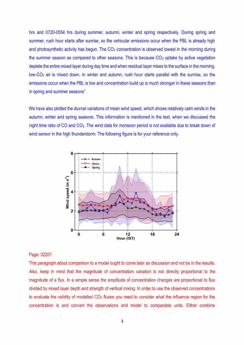
We have also plotted the diurnal variations of mean wind speed, which shows relatively calm winds in the

autumn, winter and spring seasons. This information is mentioned in the text, when we discussed the

night time ratio of CO and CO2. The wind data for monsoon period is not available due to break down of

wind sensor in the high thunderstorm. The following figure is for your reference only.

Page: 32201

This paragraph about comparison to a model ought to come later as discussion and not be in the results.

Also, keep in mind that the magnitude of concentration variation is not directly proportional to the

magnitude of a flux. In a simple sense the amplitude of concentration changes are proportional to flux

divided by mixed layer depth and strength of vertical mixing. In order to use the observed concentrations

to evaluate the validity of modelled CO2 fluxes you need to consider what the influence region for the

concentration is and convert the observations and model to comparable units. Either combine

4

concentration data and typical mixing depth evolution to estimate a change in column density, or merge

the CASA fluxes with a transport model to predict concentrations. The claim that model and observations

are inconsistent is not convincing. The greatest magnitude of net daytime uptake and difference between

CASA fluxes in day and night is in September through November, consistent with the peaks in amplitude

of mixing ratio diel cycle (day/night difference of CO2 concentration increases from 20 ppm in August to

50 ppm in October). So I don’t see where the observations suggest product ivity is higher in August than

Sept-October.

Response: Thank you very much for your kind suggestion. Now, we have moved this figure in Section

4.7.1

It is clear from Figure 6 that the CO2 flux diurnal cycle as modelled by CASA shows minimum day-night

variation amplitude during the summer monsoon time (Jun-July-Aug). Given that the biosphere over

Ahmedabad is water stressed for all other three seasons (except the summer monsoon time, Fig. 1A3),

the behaviour of CASA model simulated diurnal variation is not in line with biological capacity of the plants

to assimilate atmospheric CO2.

Due this underestimation of CO2 uptake in the summer monsoon season, we also find very large

underestimation of the seasonal trough by ACTM in comparison with observations (Fig. 11). The variations

in transport, PBL ventilation and horizontal winds are included in the ACTM simulation, therefore we do

include “proportional to flux divided by mixed layer depth and strength of vertical mixing” in our model

results.

For these reasons, we propose that summer time underestimation of CO2 flux diurnal simulation by CASA

is a clearly convincing case.

Page: 32202

The statement here on pg32302, line 26 about respiration contributing to CO2 is inconsistent with the

previous section suggesting that respiration was dormant.

Response: According the first suggestion, we have modified both explanations for CO2 and CO. In CO2

section, we have added following explanations.

“CO2 concentrations start decreasing from 0000 to 0300 hrs and increases slightly afterwards till 0600-

0700 hrs during summer and autumn. Respiration of CO2 from the vegetation is mostly responsible for

5

this night time increase. During winter and spring seasons CO2 levels are observed constant during night

hours and small increase is observed only from 0600 to 0800 hrs during the winter season. While in

contrary to this, subsequent section shows a continuous decline in the night time concentrations of main

anthropogenic tracer CO, which indicates that there is enough vertical mixing of low CO air from above

that once CO source is turned off, its concentration drops. Hence, constant levels of CO2 at night hours

during these seasons give the evidence of a continued but weak source (such as respiration) in order to

offset dilution of mixing of low CO2 air from aloft. Dry soil conditions could be one of the possible causes

for weak respirations”.

For CO section, we have modified the statement on pg32302, line 26.

“The third noticeable difference is that the CO levels decrease very fast after evening rush hours in all the

seasons while this feature is not observed in case of CO2, since respiration during night hours contributes

to the levels of CO2. The continuous drop of night time concentrations of CO indicates that there is enough

vertical mixing of low CO air from above once the CO source is turned off”.

Page: 32204

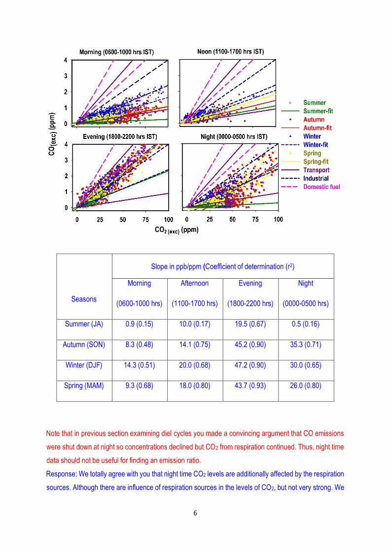
The regression slopes for CO: CO2 are not credible estimates of the emission ratio. The difference

between actual background CO2 and the assumed constant value that is used to compute excess is

correlated with time of day and thus with CO, so the slope of CO: CO2 will be corrupted I do notice that

the upper edge in all the figures appears to have a similar slope. That edge represents the air that is most

strongly influenced by CO emission sources. Although I think it would be better to split up the data into

groups that actually show a decent correlation, if you want to stick with the overall regression those lines

should be shown on the figure and for comparison include some lines that show the slopes for a few

representative emission sources.

Response: Thank you very much for raising this important point. As per the suggestion, we have removed

the old diagram and added a following new one diagram, which shows the correlation at different time

windows during different seasons and including the range of emission ratios of different sources from the

available literature. We have included the following table, which gives the summary of the new diagram.

According to diagram, we have significantly modified the text of the whole section.

6

Seasons

Slope in ppb/ppm (Coefficient of determination (r2)

Morning

(0600-1000 hrs)

Afternoon

(1100-1700 hrs)

Evening

(1800-2200 hrs)

Night

(0000-0500 hrs)

Summer (JA) 0.9 (0.15) 10.0 (0.17) 19.5 (0.67) 0.5 (0.16)

Autumn (SON) 8.3 (0.48) 14.1 (0.75) 45.2 (0.90) 35.3 (0.71)

Winter (DJF) 14.3 (0.51) 20.0 (0.68) 47.2 (0.90) 30.0 (0.65)

Spring (MAM) 9.3 (0.68) 18.0 (0.80) 43.7 (0.93) 26.0 (0.80)

Note that in previous section examining diel cycles you made a convincing argument that CO emissions

were shut down at night so concentrations declined but CO2 from respiration continued. Thus, night time

data should not be useful for finding an emission ratio.

Response: We totally agree with you that night time CO2 levels are additionally affected by the respiration

sources. Although there are influence of respiration sources in the levels of CO2, but not very strong. We

7

have discussed it previously in the revised manuscript also. Since the wind condition is calm during this

period due to no turbulence and most of dominant sources are shut off, the ratios during this period can

be useful for broadly understanding about the emission characteristic of dominating sources over

Ahmedabad.

I would suggest trying something similar to the analysis of Potosnak et al 1999 that seeks to extract the

influence from biosphere and mean diel cycle. (J. Geophys. Res., 104(D8), 9561–9569,

doi:10.1029/1999JD900102.)...

Response: It seems to be a good suggestion. However, it requires complete reanalysis of the data in

different time bins and beyond the scope of present work. We are extremely sorry.

Page: 32205

In the end the CO: CO2 ratios have such a wide range as to not be very useful at all. Unless you can

reanalyse them to bring a narrower estimate it is not worthwhile to show this section. It is curious that the

night time data have such a good correlation when the diel cycle analysis suggested that combustion

emissions of both CO and CO2 together were shut down. It would help to illustrate the relationship between

CO and CO2 in night by colouring the symbols for night-time data differently for time of day in Figure 8a I

suspect the daytime values, with low correlation coefficients are not reliable, as you suggest by indicating

the importance of CO2 uptake. When biospheric influence influences the CO2 mixing ratio you shouldn’t

bother to try to analyze the CO: CO2 ratio.

Response: Thank you very much for the suggestion. As per suggestion, we have removed old figure and

added a new one, in which the data are segregated in different time windows and coloured according to

different seasons. The modified diagram is already shown previously (Page:32204).

As we discussed previously also the CO2 levels are additionally affected by respiration sources during

night time, but not very strongly. We also discussed that CO levels drop very fast during night time, which

indicate that there is enough vertical mixing of low CO air from above that once the CO sources are turned

off. Hence this mixing will enhance the correlation during night time, since there are no significant sources,

which disturb their levels greatly. Correlation during day time is low only during monsoon season, since

biospheric productivity play a large role in influencing the levels of CO2. But for making the comparisons,

we have included the day time values. While during other seasons, correlation is pretty good during day

time due to significant atmospheric mixing of all emissions and comparatively lower biospheric

8

productivity. It concludes that during other seasons CO and CO2 levels are mostly dominated by common

emission sources. This whole section is now modified according to previous comments.

Page: 32206

The previous section about CO: CO2 slopes is rather muddled. It would be more convincing focussing on

demonstrating the validity of just the night-time and rush-hour periods that you are using here. Showing

the data for entire day just confuses things.

Response: As per the suggestion, now Section 4.5 includes the validity of EDGAR CO emissions from the

night-time and rush hour periods measurements only. We have discussed previously also the

measurements during these period will show combine influence from all anthropogenic sources mostly.

Hence, the estimated slopes for these period will be helpful to validate the anthropogenic CO emissions

of EDGAR inventory. According to that, we have modified our conclusion. We have replaced the fossil

fuel emission term by the anthropogenic emissions. It includes all emissions such as vehicular emission,

industrial emission as well as cooking sector emissions.

Assuming the discussion of ratios just for the relevant periods is more convincing you can also include

some calculation of the uncertainty, which then feeds into providing estimates of uncertainty in the

emissions you compute from those ratios and the CO2 inventory. Uncertainty estimates are critical to

include here.

Response: We are highly thankful for the suggestion. The possible causes for uncertainty are the

uncertainty in estimated slopes, uncertainty in CO and CO2 emissions used for EDGAR inventory and

uncertainty in the interpolation of the emission of both the gases. We have included the following text in

the section due to the uncertainty in slopes. However, due to unavailability of uncertainty information in

the emissions of EDGAR inventory, it is not possible to include these uncertainty in the calculation. We

are very sorry for that.

“Further the uncertainty in total estimated emission of CO due to uncertainty associated with used slope

is also calculated. Using this slope and based on CO2 emissions from EDGAR inventory, the estimated

fossil fuel emission for CO is observed to be 69.2±0.7 Gg (emission ± uncertainty) for the year of 2014.”

Page: 32235

Consider plotting actual CO and CO2 mixing ratios to see if the intercepts match the values chosen for

background. In the active growing season the biospheric influence will impart a wide range of CO2 for

9

given values of CO, which is what shows for most seasons. A meaningful slope is difficult to extract in this

case. A better estimate of CO2: CO could be derived by using information from the mean diel cycle

analysis to subtract a variable background, or restrict the analysis to just a fixed time of day, or analyze

night and daytime separately...

Response: We are very much thankful for your suggestion. According to previous and this suggestion, we

have modified the figure significantly, in which we have removed the diurnal variation of slopes and restrict

our analysis at different time windows separately.

Minor editing

32197 line 25

There must be a missing word in the sentence; ’resulting in concentrations at the surface in the summer

compared to the winter.

Response: Thank you very much for pointing out this slip. Yes, it was missing and we have corrected it

now.

10

Anonymous referee #2

General comments:

This paper addresses temporal variations of atmospheric CO2 and CO in an urban site in western India.

There are not so many studies on greenhouse gases in urban environments. Furthermore, such study is

rare in countries in development. This work is interesting to be published and is fully within the scope of

ACP.

The authors address the seasonal and the diurnal scales, as well as CO/CO2 ratios from which they infer

information on the anthropogenic vs natural sources of CO and CO2. They also propose a calculation of

CO emissions for the studied city using such ratio and CO2 emissions from inventory, as well as a short

model/observations comparison. I acknowledge the large amount of work provided by the authors and

interesting information issued from this study.

Response: We are very much grateful to the referee for the positive comments and appreciation of our

work. We have tried our best to give all the answers point by point.

However, there are also some major issues to be addressed and reviewed before publication in ACP.

These issues concern:

1. The form: The text is quite difficult to read and needs to be synthetized, especially the introduction, the

seasonal study and the diurnal study. Some sentences are even repeated twice.

Response: According to the suggestion, we have synthetized all mentioned sections very carefully after

removing, adding and rearranging sentences. Please note that, rather than adding, removing and

rearranging sentences in between the written text, we have added modified text of whole section in new

paragraph. The modified sections are given below.

Introduction:

Carbon dioxide (CO2) is the most important anthropogenically emitted greenhouse gas (GHG) and has

increased substantially from 278 to 390 parts per million (ppm) in the atmosphere since the beginning of

the industrial era (circa 1750). It has contributed to more than 65% of the radiative forcing increase since

1750 and hence has significant impact on the climate system (Ciais et al., 2013). Major causes of CO2

increase are anthropogenic emissions, especially fossil fuel combustion, cement production and land use

change. Land and oceans are the two important sinks of atmospheric CO2, which remove about half of

the anthropogenic emissions (Le Quéré et al., 2014). The prediction of future climate change and its

feedback rely mostly on our ability to quantify fluxes of greenhouse gases, especially CO2, at regional

(100-1000 km2) and global scales. Though the global fluxes of CO2 can be estimated fairly well, the

11

regional scale (fluxes are associated with quite high uncertainty, especially over the South Asian region

and the estimation uncertainty being larger than the value itself (Patra et al., 2013; Peylin et al., 2013).

Detailed scientific understanding of the flux distributions is also needed for formulating effective mitigation

policies.

Along with the need for atmospheric measurements for predicting the future levels of CO2, quantifying

the components of anthropogenic emissions of CO2 is similarly important for providing independent

verification of mitigation strategies as well as understanding the biospheric component of CO2. Only CO2

measurements cannot be helpful in making such study due to the larger role of biospheric fluxes in its

atmospheric distributions. The proposed strategy for quantification of the anthropogenic component of

CO2 emissions is to measure simultaneously anthropogenic tracers,. CO can be used as a surrogate

tracer for detecting and quantifying anthropogenic emissions from burning processes, since it is a major

product of incomplete combustion (Turnbull et al., 2006; Wang et al., 2010). The vehicular as well as

industrial emissions contribute large fluxes of CO2 and CO to the atmosphere in urban regions. Several

ground and aircraft based simultaneous studies of CO andCO2 have been made in the past from different

parts of the world (Turnbull et al., 2006; Wunch et al., 2009; Wang et al., 2010; Newman et al., 2013) but

such a study is lacking in India except recently reported results from weekly samples for three Indian sites

by Lin et al. (2015).

Measurements at different regions (eg. rural, remote, urban) and at different frequency (eg., weekly, daily,

hourly etc) have their own advantage and limitations. For example, the measurements at remote locations

at weekly interval can be useful for studying seasonal cycle, growth rate, and estimating the regional

carbon sources and sinks after combining their concentrations with inverse modelling and atmospheric

tracer transport models. However, some important studies, like diurnal variations, temporal

covariance...etc are not possible from these measurements. Analysis of temporal covariance of

atmospheric mixing processes and variation of flux on shorter time scales, e.g., sub-daily, is essential for

understanding local to urban scale CO2 flux variations (Ahmadov et al., 2007; Pérez-Landa et al., 2007;

Briber et al., 2013; Lopez et al., 2013; Ammoura et al., 2014; Ballav et al., 2015). Urban regions contribute

about 70% of global CO2 emission from anthropogenic sources and further projected to increase over the

coming decades. Therefore, measurements from these regions are very helpful for understanding

emissions, growth as well as verifying the mitigation policies. The first observations of CO2, CO and other

greenhouse gases started in February 1993 from Cape Rama (CRI: a coastal site) on the south-west

coast of India using flask samples (Bhattacharya et al., 2009). After that, several other groups have

initiated the measurements of surface level greenhouse gases (Mahesh et al., 2014; Sharma et al., 2014;

Tiwari et al., 2014; Lin et al., 2015). Most of these measurements are made at weekly or fortnightly time

intervals. Two aircraft based measurement programs, namely, Civil Aircraft for the regular Investigation

of the atmosphere Based on an Instrument Container (CARIBIC) (Brenninkmeijer et al., 2007) and

Comprehensive Observation Network for TRace gases by AIrLiner (CONTRAIL) (Machida et al., 2008)

have provided important first look on the South Asian CO2 budget, but these data have their own limitations

(Patra et al., 2011; Schuck et al., 2010, 2012). It is pertinent to mention here that till now, there are no

reports of CO2 measurements over the urban locations of the Indian subcontinent, which could be an

important player in the global carbon budget as well as mitigation purpose due to strong growing

anthropogenic activities specifically fast growing traffic sector and sinks (large areas of forests and

12

croplands). Hence, the present study is an attempt to reduce this gap by understanding the CO2 mixing

ratios in light of its sources and sinks at an urban region in India.

In the view from above, simultaneous continuous measurements of CO2 and CO have been made since

November 2013 from an urban site Ahmedabad located in the western India using very highly sensitive

laser based technique. The preliminary results of these measurements for one month period have been

reported in (Lal et al., 2015). These detailed measurements are utilized for studying the temporal

variations (diurnal and seasonal) of both gases, their emission characteristics on diurnal and seasonal

scale using their mutual correlations, estimating the contribution of vehicular and biospheric emission

components in the diurnal cycle of CO2 using the ratios of CO to CO2 and rough estimate of the annual

CO emissions from study region. Finally, the measurements of CO2 have been compared with simulations

using an atmospheric chemistry-transport model to discuss roles of various processes contributing to CO2

concentration variations.

Seasonal cycle of CO2 and CO:

The seasonal cycles of CO2 and CO are mostly governed by the strength of emission sources, sinks and

transport patterns. Although they follow almost identical seasonal patterns, but the factors responsible for

their seasonal behaviours are distinct as for the diurnal variations. We calculate the seasonal cycle of CO2

and CO using two different approaches. In the first approach, we use the monthly mean of all

measurements and in the second approach we use monthly mean of the afternoon period (1200-1600

hrs) measurements only. The seasonal cycle from first approach will present the overall variability in both

gases. On the other hand, second approach removes the auto covariance by excluding CO2 and CO data

mainly affected by local emission sources and represent seasonal cycles at the well mixed volume of the

atmosphere. The CO2 time series is detrended by subtracting a mean growth rate of CO2 observed at

Mauna Loa (MLO), Hawaii, i.e., 2.13 ppm yr−1 or 0.177 ppm/month (www.esrl.noaa.gov/gmd/ccgg/trends/)

for clearly depicting the seasonal cycle amplitude.

In general, total mean values of CO2 and CO are observed lower in July having concentration 398.78±2.8

ppm and 0.15±0.05 ppm respectively. During summer monsoon months predominance of south-westerly

winds which bring cleaner air from the Arabian Sea and the Indian Ocean over to Ahmedabad and high

VC (Figure 1) are mostly responsible for the lower concentration of total mean of both the gases. CO2 and

CO concentrations are also at their seasonal low in the northern hemisphere due to net biospheric uptake

and seasonally high chemical loss by reaction with OH, respectively. In addition, deep convections in the

summer monsoon season efficiently transport the Indian emission (for CO, hydrocarbons) or uptake (for

CO2) signals at the surface to the upper troposphere, resulting lower concentrations at the surface in the

as compared to the winter months (Kar et al., 2004; Randel and Park, 2006; Park et al., 2009; Patra et

al., 2011; Baker et al., 2012). During autumn and early winter (December), lower VC values cause trapping

of anthropogenically emitted CO2 and CO and is the major cause for high concentrations of both gases

during this period. In addition to this, wind changes from cleaner marine region to polluted continental

region, especially from IGP region and hence could be additional factor for higher levels of CO2 and CO

during these seasons (autumn and winter). Elevated levels during these seasons are also examined in

several other pollutants over Ahmedabad as discussed in previous studies (Sahu et al., 2006, Mallik et

13

al., 2016). Maximum concentrations of CO2 and CO are observed to be 424.85±17 ppm and 0.83±0.53

ppm, respectively, during November. From January to May the total mean concentration of CO2

decreases from 415.34±13.6 to 406.14±5.0 ppm and total mean concentration of CO decreases from

0.71±0.22 to 0.22±0.10 ppm. Higher VC and predominance of comparatively less polluted mixed air

masses from oceanic and continental region results in lower total mean concentrations of both gases

during this period.

There are some clear differences which are observed in the afternoon mean concentrations of CO2 as

compared to daily mean. The first distinct feature is that significant difference of about 5 ppm is observed

in the afternoon mean of CO2 concentration from July to August as compared to the difference in total

mean concentration about ∼0.38 ppm for the same period. Significant differences in the afternoon

concentrations of CO2 from July to August is mainly due to the increasing sink by net biospheric

productivity after the Indian summer monsoonal rainfall. Another distinct feature is that the daily mean

concentration of CO2 is found higher in November while the afternoon mean concentration of CO2 attain

maximum value (406±0.4 ppm) in April. Prolonged dry season combined with high daytime temperature

(about 41oC ) during April-May make the tendency of ecosystem to become a moderate source of carbon

exchange (Patra et al., 2011) and this could be responsible for the elevated mean noon time

concentrations of CO2. Unlike CO2, seasonal patterns of CO from total and afternoon mean concentrations

are identical, although levels are different. It shows that the concentrations of CO is mostly governed by

identical sources during day and night time throughout the year.

The average amplitude (max - min) of the annual cycle of CO2 is observed around 13.6 and 26.07 ppm

from the afternoon mean and total mean respectively. Different annual cycles and amplitudes have been

observed from other studies conducted over different Indian stations. Similar to our observations of the

afternoon mean concentrations of CO2, maximum values are also observed in April at Pondicherry (PON)

and Port Blair (PBL) with amplitude of mean seasonal cycles about 7.6±1.4 and 11.1±1.3 ppm

respectively (Lin et al., 2015). Cape Rama (CRI), a costal site on the south-west coast of India show the

seasonal maxima one month before than our observations in March annual amplitude about 9 ppm

(Bhattacharya et al., 2009). The Sinhagad (SNG) site located over the Western Ghats Mountains, show

very larger seasonal cycle with annual amplitude about 20 ppm (Tiwari et al., 2014). The amplitude of

mean annual cycle at the free tropospheric site Hanle at altitude of 4500 m is observed to be 8.2±0.4

ppm, with maxima in early May and the minima in mid-September (Lin et al., 2015). Distinct seasonal

amplitudes and patterns are due to differences in regional controlling factors for the seasonal cycle of CO2

over these locations, e.g., the Hanle is remotely located from all continental sources, Port Blair site

sampled predominantly marine air, Cape Rama observes marine air in the summer monsoon season and

Indian flux signals in the winter, and Sinhagad represents a forested ecosystem. These comparisons show

the need for CO2 measurements over different ecosystems for constraining its budget.

The annual amplitude in afternoon and daily mean CO concentration is observed to be about 0.27 and

0.68 ppm, respectively. The mean annual cycles of CO over PON and PBL show the maxima in the winter

months and minima in summer months same as our observations with annual amplitudes of 0.078±0.01

and 0.144±0.016 ppm, respectively. So the seasonal levels of CO are affected by large scale dynamics

which changes air masses from marine to continental and vice versa and by photochemistry. The

14

amplitudes of annual cycle at these locations differ due to their climatic conditions and sources/sinks

strengths.

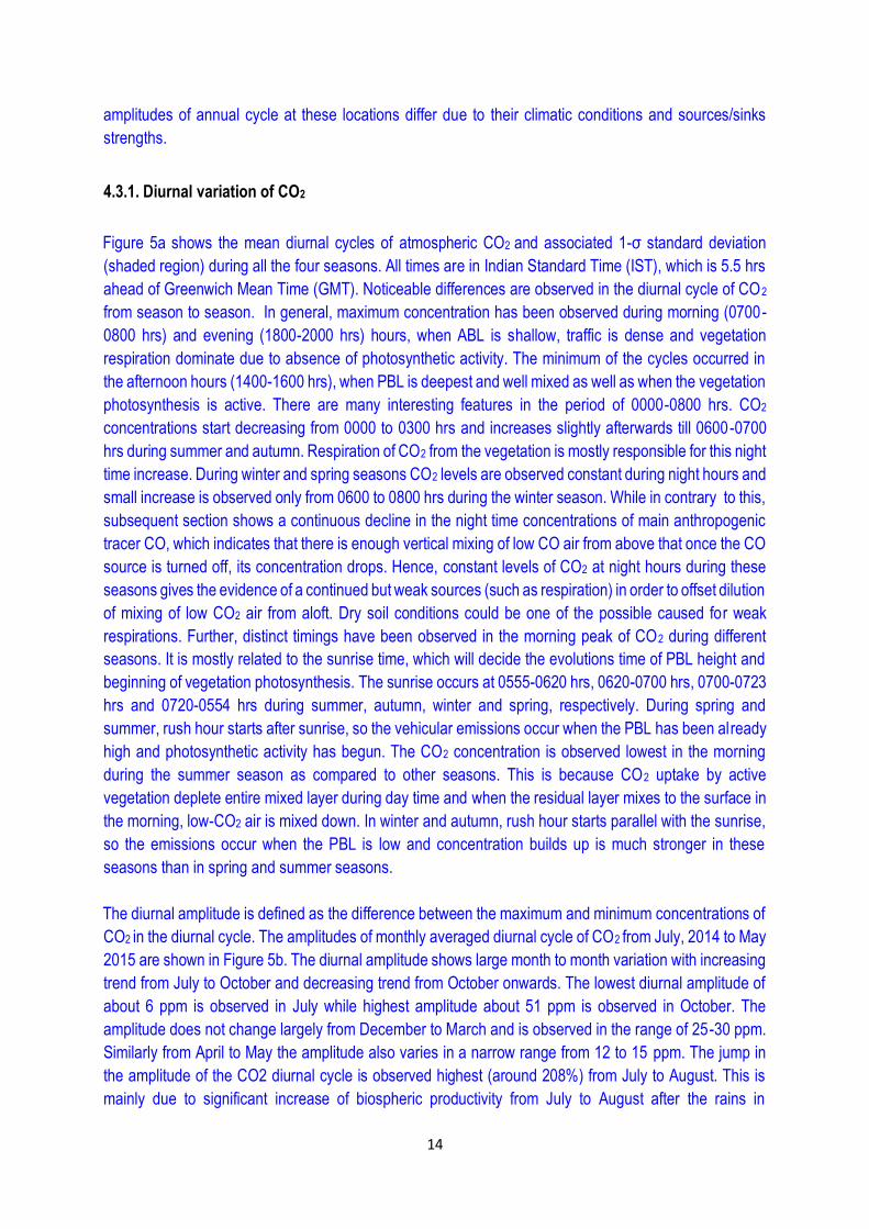
4.3.1. Diurnal variation of CO2

Figure 5a shows the mean diurnal cycles of atmospheric CO2 and associated 1-σ standard deviation

(shaded region) during all the four seasons. All times are in Indian Standard Time (IST), which is 5.5 hrs

ahead of Greenwich Mean Time (GMT). Noticeable differences are observed in the diurnal cycle of CO2

from season to season. In general, maximum concentration has been observed during morning (0700-

0800 hrs) and evening (1800-2000 hrs) hours, when ABL is shallow, traffic is dense and vegetation

respiration dominate due to absence of photosynthetic activity. The minimum of the cycles occurred in

the afternoon hours (1400-1600 hrs), when PBL is deepest and well mixed as well as when the vegetation

photosynthesis is active. There are many interesting features in the period of 0000-0800 hrs. CO2

concentrations start decreasing from 0000 to 0300 hrs and increases slightly afterwards till 0600-0700

hrs during summer and autumn. Respiration of CO2 from the vegetation is mostly responsible for this night

time increase. During winter and spring seasons CO2 levels are observed constant during night hours and

small increase is observed only from 0600 to 0800 hrs during the winter season. While in contrary to this,

subsequent section shows a continuous decline in the night time concentrations of main anthropogenic

tracer CO, which indicates that there is enough vertical mixing of low CO air from above that once the CO

source is turned off, its concentration drops. Hence, constant levels of CO2 at night hours during these

seasons gives the evidence of a continued but weak sources (such as respiration) in order to offset dilution

of mixing of low CO2 air from aloft. Dry soil conditions could be one of the possible caused for weak

respirations. Further, distinct timings have been observed in the morning peak of CO2 during different

seasons. It is mostly related to the sunrise time, which will decide the evolutions time of PBL height and

beginning of vegetation photosynthesis. The sunrise occurs at 0555-0620 hrs, 0620-0700 hrs, 0700-0723

hrs and 0720-0554 hrs during summer, autumn, winter and spring, respectively. During spring and

summer, rush hour starts after sunrise, so the vehicular emissions occur when the PBL has been already

high and photosynthetic activity has begun. The CO2 concentration is observed lowest in the morning

during the summer season as compared to other seasons. This is because CO2 uptake by active

vegetation deplete entire mixed layer during day time and when the residual layer mixes to the surface in

the morning, low-CO2 air is mixed down. In winter and autumn, rush hour starts parallel with the sunrise,

so the emissions occur when the PBL is low and concentration builds up is much stronger in these

seasons than in spring and summer seasons.

The diurnal amplitude is defined as the difference between the maximum and minimum concentrations of

CO2 in the diurnal cycle. The amplitudes of monthly averaged diurnal cycle of CO2 from July, 2014 to May

2015 are shown in Figure 5b. The diurnal amplitude shows large month to month variation with increasing

trend from July to October and decreasing trend from October onwards. The lowest diurnal amplitude of

about 6 ppm is observed in July while highest amplitude about 51 ppm is observed in October. The

amplitude does not change largely from December to March and is observed in the range of 25-30 ppm.

Similarly from April to May the amplitude also varies in a narrow range from 12 to 15 ppm. The jump in

the amplitude of the CO2 diurnal cycle is observed highest (around 208%) from July to August. This is

mainly due to significant increase of biospheric productivity from July to August after the rains in

15

Ahmedabad. It is observed that during July the noon time CO2 levels are found in the range of 394-397

ppm while in August the noon time levels are observed in the range of 382-393 ppm. The lower levels

could be due to the higher PBL height during afternoon and cleaner air, but in case of CO (will be

discussed in next section), average day time levels in August are observed higher than in July. It rules

out that the lower levels during August are due to the higher PBL height and presence of cleaner marine

air, and confirms the higher biospheric productivity during August.

Near surface diurnal amplitude of CO2 has been also documented in humid subtropical Indian station

Dehradun and a dry tropical Indian station Gadanki (Sharma et al., 2014). In comparison to Ahmedabad,

both these stations show distinct seasonal change in the diurnal amplitude of CO2. The maximum CO2

diurnal amplitude of about 69 ppm is observed during the summer season at Dehradun (30.3oN, 78.0oE,

435m), whereas maximum of about 50 ppm during autumn at Gadanki 400 (13.5oN, 79.2oE, 360 m).

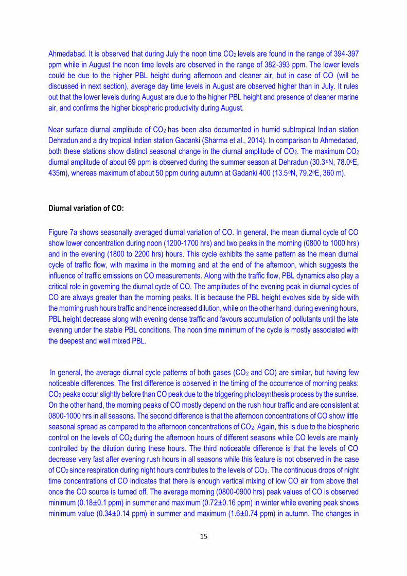
Diurnal variation of CO:

Figure 7a shows seasonally averaged diurnal variation of CO. In general, the mean diurnal cycle of CO

show lower concentration during noon (1200-1700 hrs) and two peaks in the morning (0800 to 1000 hrs)

and in the evening (1800 to 2200 hrs) hours. This cycle exhibits the same pattern as the mean diurnal

cycle of traffic flow, with maxima in the morning and at the end of the afternoon, which suggests the

influence of traffic emissions on CO measurements. Along with the traffic flow, PBL dynamics also play a

critical role in governing the diurnal cycle of CO. The amplitudes of the evening peak in diurnal cycles of

CO are always greater than the morning peaks. It is because the PBL height evolves side by side with

the morning rush hours traffic and hence increased dilution, while on the other hand, during evening hours,

PBL height decrease along with evening dense traffic and favours accumulation of pollutants until the late

evening under the stable PBL conditions. The noon time minimum of the cycle is mostly associated with

the deepest and well mixed PBL.

In general, the average diurnal cycle patterns of both gases (CO2 and CO) are similar, but having few

noticeable differences. The first difference is observed in the timing of the occurrence of morning peaks:

CO2 peaks occur slightly before than CO peak due to the triggering photosynthesis process by the sunrise.

On the other hand, the morning peaks of CO mostly depend on the rush hour traffic and are consistent at

0800-1000 hrs in all seasons. The second difference is that the afternoon concentrations of CO show little

seasonal spread as compared to the afternoon concentrations of CO2. Again, this is due to the biospheric

control on the levels of CO2 during the afternoon hours of different seasons while CO levels are mainly

controlled by the dilution during these hours. The third noticeable difference is that the levels of CO

decrease very fast after evening rush hours in all seasons while this feature is not observed in the case

of CO2 since respiration during night hours contributes to the levels of CO2. The continuous drops of night

time concentrations of CO indicates that there is enough vertical mixing of low CO air from above that

once the CO source is turned off. The average morning (0800-0900 hrs) peak values of CO is observed

minimum (0.18±0.1 ppm) in summer and maximum (0.72±0.16 ppm) in winter while evening peak shows

minimum value (0.34±0.14 ppm) in summer and maximum (1.6±0.74 ppm) in autumn. The changes in

16

CO concentrations show large fluctuations from morning peak to afternoon minima and from afternoon

minima to evening peak. From early morning maxima to noon minima, the changes in CO concentrations

are found in the range of 20 -200%, while from noon minima to late evening maxima the changes in CO

concentrations are found in the range of 85% to 680%. Similar diurnal variations with two peaks have also

been observed in earlier measurements of CO as well as NOx at this site (Lal et al., 2000).

The evening peak contributes significantly to the diurnal amplitude of CO. The largest amplitude in CO

cycle is observed in autumn (1.36 ppm) while the smallest amplitude is observed in summer (0.24 ppm).

The diurnal amplitudes of CO are observed to be about 1.01 and 0.62 ppm, respectively during winter

and spring. Like CO2, the diurnal cycle of CO (Figure 7b) shows the minimum (0.156 ppm) amplitude in

July and maximum (1.85 ppm) in October. After October the diurnal amplitude keeps on decreasing till

summer. The evening peak contributes significantly to the diurnal amplitude of CO. The largest amplitude

in CO cycle is observed in autumn (1.36 ppm) while the smallest amplitude is observed in summer (0.24

ppm). The diurnal amplitudes of CO are observed to be about 1.01 and 0.62 ppm, respectively during

winter and spring. The monthly diurnal cycle of CO (Figure 7b) shows the minimum (0.156 ppm) amplitude

in July and maximum (1.85 ppm) in October. After October the diurnal amplitude keeps on decreasing till

summer.

2. The content given on the emissions and the conclusions on the traffic sector vs the cooking and

industrial one: there is a lack of information on the studied region and on the relative role of the different

emission sectors that should be given quantitatively, with proper references. Especially, the part of

emissions due to residential and slum cooking is almost not discussed, while the available literature

explains that this emission sector is responsible for a large amount of atmospheric CO (less in CO2).

Response: As per suggestion, we have included following more information about the relative

contributions of different emission sectors in Section 2.

“An emission inventory for this city, which is developed for all known sources, shows the annual emissions

(for year 2010) of CO2 and CO about 22.4 million tons and 707,000 tons respectively

(http://www.indiaenvironmentportal.org.in/files/file/Air-Pollution-in-Six-Indian-Cities.pdf). Out of these

emissions, transport sector contribute about 36% in CO2 emission and 25% in CO emissions, power

plants contribute about 32% in CO2 emissions and 30% in CO emission, industries contribute about 18%

in CO2 emissions and 12% in CO emissions and domestic sources contribute about 6% in CO2 emissions

and 22% in CO emissions.”

The conclusion on the strong influence of traffic given in sector 4.4 is not convincing according to Table1.

Response: Thank you very much for raising these points. This is also pointed by the Referee #1. Now we

have modified our conclusions as per further suggestions. As per suggestions, we have removed old

figure and added a following new figure, in which the data are segregated seasonally in different time

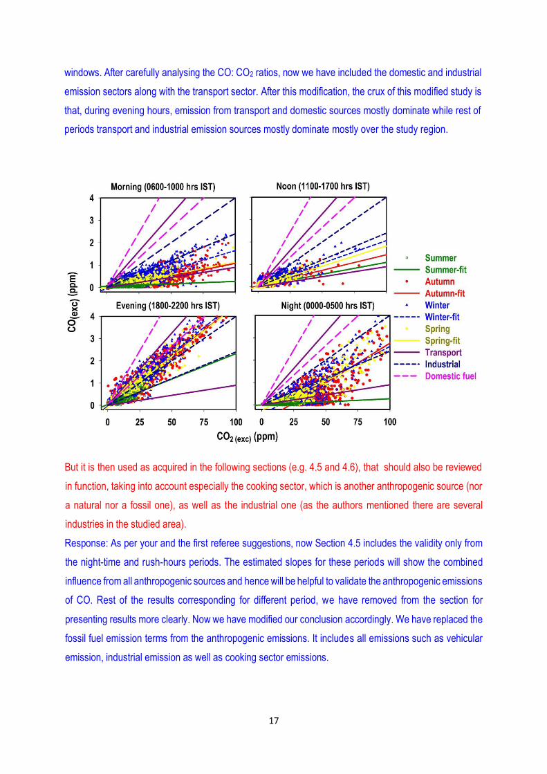
17

windows. After carefully analysing the CO: CO2 ratios, now we have included the domestic and industrial

emission sectors along with the transport sector. After this modification, the crux of this modified study is

that, during evening hours, emission from transport and domestic sources mostly dominate while rest of

periods transport and industrial emission sources mostly dominate mostly over the study region.

But it is then used as acquired in the following sections (e.g. 4.5 and 4.6), that should also be reviewed

in function, taking into account especially the cooking sector, which is another anthropogenic source (nor

a natural nor a fossil one), as well as the industrial one (as the authors mentioned there are several

industries in the studied area).

Response: As per your and the first referee suggestions, now Section 4.5 includes the validity only from

the night-time and rush-hours periods. The estimated slopes for these periods will show the combined

influence from all anthropogenic sources and hence will be helpful to validate the anthropogenic emissions

of CO. Rest of the results corresponding for different period, we have removed from the section for

presenting results more clearly. Now we have modified our conclusion accordingly. We have replaced the

fossil fuel emission terms from the anthropogenic emissions. It includes all emissions such as vehicular

emission, industrial emission as well as cooking sector emissions.

18

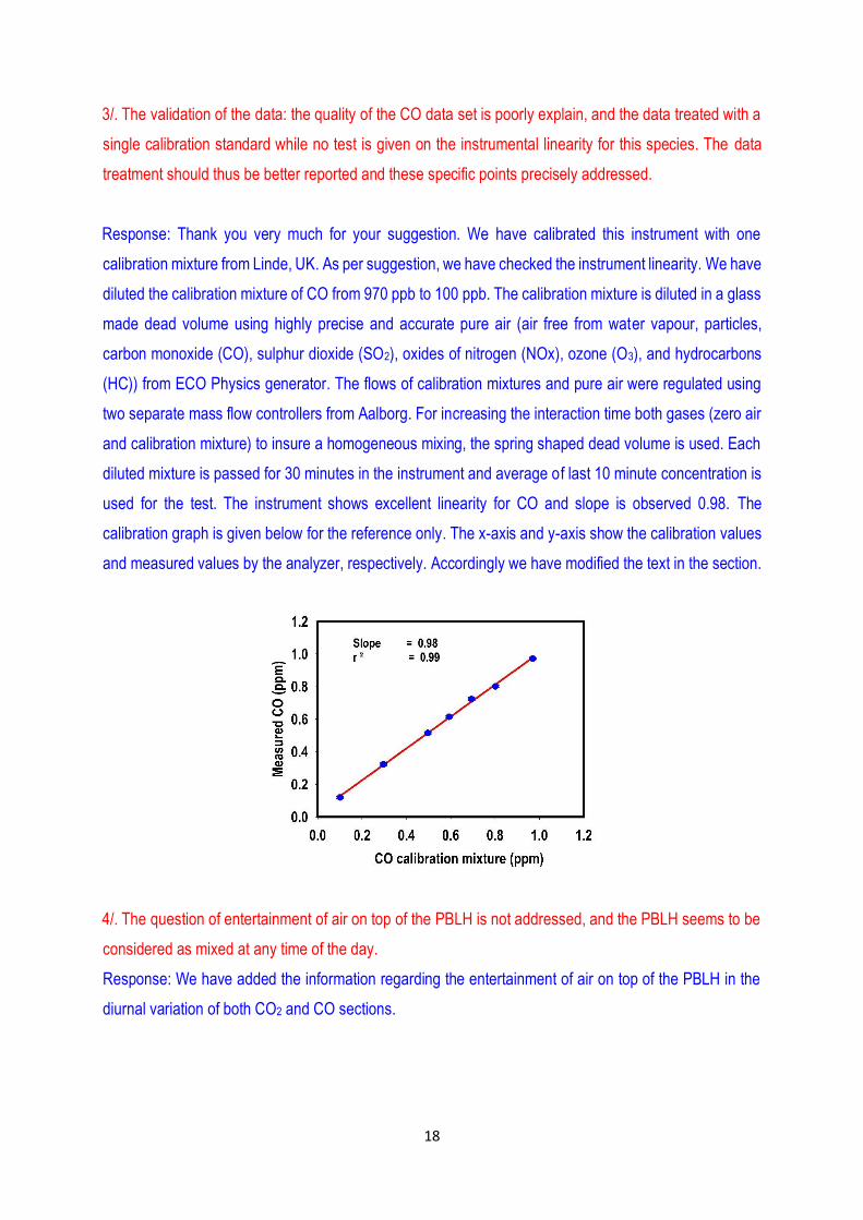
3/. The validation of the data: the quality of the CO data set is poorly explain, and the data treated with a

single calibration standard while no test is given on the instrumental linearity for this species. The data

treatment should thus be better reported and these specific points precisely addressed.

Response: Thank you very much for your suggestion. We have calibrated this instrument with one

calibration mixture from Linde, UK. As per suggestion, we have checked the instrument linearity. We have

diluted the calibration mixture of CO from 970 ppb to 100 ppb. The calibration mixture is diluted in a glass

made dead volume using highly precise and accurate pure air (air free from water vapour, particles,

carbon monoxide (CO), sulphur dioxide (SO2), oxides of nitrogen (NOx), ozone (O3), and hydrocarbons

(HC)) from ECO Physics generator. The flows of calibration mixtures and pure air were regulated using

two separate mass flow controllers from Aalborg. For increasing the interaction time both gases (zero air

and calibration mixture) to insure a homogeneous mixing, the spring shaped dead volume is used. Each

diluted mixture is passed for 30 minutes in the instrument and average of last 10 minute concentration is

used for the test. The instrument shows excellent linearity for CO and slope is observed 0.98. The

calibration graph is given below for the reference only. The x-axis and y-axis show the calibration values

and measured values by the analyzer, respectively. Accordingly we have modified the text in the section.

4/. The question of entertainment of air on top of the PBLH is not addressed, and the PBLH seems to be

considered as mixed at any time of the day.

Response: We have added the information regarding the entertainment of air on top of the PBLH in the

diurnal variation of both CO2 and CO sections.

19

“During winter and spring seasons CO2 levels are observed constant during night hours and small

increase is observed only from 0600 to 0800 hrs during the winter season. While in contrary to this,

subsequent section shows a continuous decline in the night time concentrations of main anthropogenic

tracer CO, which indicates that there is enough vertical mixing of low CO air from above that once the CO

source is turned off, its concentration drops. Hence, constant levels of CO2 at night hours during these

seasons gives the evidence of a continued but weak sources (such as respiration) in order to offset dilution

of mixing of low CO2 air from aloft. Dry soil conditions could be one of the possible caused for weak

respirations. Further, distinct timings have been observed in the morning peak of CO2 during different

seasons. It is mostly related to the sunrise time, which will decide the evolutions time of PBL height and

beginning of vegetation photosynthesis. The sunrise occurs at 0555-0620 hrs, 0620-0700 hrs, 0700-0723

hrs and 0720-0554 hrs during summer, autumn, winter and spring, respectively. During spring and

summer, rush hour starts after sunrise, so the vehicular emissions occur when the PBL has been already

high and photosynthetic activity has begun. The CO2 concentration is observed lowest in the morning

during the summer season as compared to other seasons. This is because CO2 uptake by active

vegetation deplete entire mixed layer during day time and when the residual layer mixes to the surface in

the morning, low-CO2 air is mixed down. In winter and autumn, rush hour starts parallel with the sunrise,

so the emissions occur when the PBL is low and concentration builds up is much stronger in these

seasons than in spring and summer seasons”.

The CO/CO2 ratio diurnal variability should take this into account, a point that carefully needs to be studied

at different time windows.

Response: As per the suggestions in further comments, we have modified this section, which discuss

about the diurnal variability of CO/CO2 ratios. Instead of using whole measurements of both gases for

studying the emission characteristics, now the modified section discuss the emission characteristics of

dominant emission sources at different time windows during all the four seasons. Most of details about

this section are given in the following comments.

After these major revisions, I am convinced that this work will be of very good quality for publication in

ACP.

Specific comments:

Abstract:

20

A sentence on your objectives should be given after the first sentence. What is the reliability of the CO2

emissions inventory?

Response: We thank you very much for the suggestions. We have added and rearranged following lines

in the abstract section.

“In order to draw effective emission mitigation policies for combating future climate change as well as

independently validate the emission inventories for constraining their large range of uncertainties,

especially over major metropolitan areas of developing countries, there is an urgent need for greenhouse

gases measurements over representative urban regions. India is a fast developing country, where fossil

fuel emissions have increased dramatically in the last three decades

and predicted further to continue to grow by at least 6% per year through 2025. In the absence of

systematic CO2 measurements over the Indian urban locations, CO2 along with an anthropogenic

emission tracer carbon monoxide (CO) are being measured at Ahmedabad, a major urban site in western

India, using a state-of-the-art laser based cavity ring down spectroscopy technique from November 2013

to May 2015 with a break during March to June 2014. These measurements enable us to understand the

diurnal and seasonal variation in atmospheric CO2 with respect to its sources (both anthropogenic and

biospheric) and biospheric sinks.”

Introduction

Much too long. Remove detailed information.

Response: Referee #1 also pointed out this issue. So now we have very carefully modified, rearranged

and synthesized the introductory section.

p. 32187

Remove lines 8-11 (too long) -------Removed

Line 14: a country can be very small or very large so give rather km (100-1000 km2 for the regional scale

generally) ---------Modified the text accordingly

Line 21: different… = this sentence is very unprecise ------ Removed

Line 28: not only traffic but also industry etc. ----- Changed accordingly

p. 32188

Lines 2-8: too long -------

Response: According to comment #1 we have synthesized the introductory section. So as a part of this

change, we have removed some information from this para and modified text by adding the following lines.

21

“Along with the need for atmospheric measurements for predicting the future levels of CO2, quantifying

the components of anthropogenic emissions of CO2 is similarly important for providing independent

verification of mitigation strategies as well as understanding the biospheric component of CO2. Only CO2

measurements can not be helpful for making such study due to the large role of biospheric fluxes in its

atmospheric distributions. The proposed strategy for quantification of the anthropogenic component of

CO2 emissions is to measure simultaneously the anthropogenic tracers. CO can be used as a surrogate

tracer for detecting and quantifying anthropogenic emissions from burning processes, since it is a major

product of incomplete combustion (Turnbull et al., 2006; Wang et al., 2010). The vehicular as well as

industrial emissions contribute large fluxes of CO2 and CO to the atmosphere in urban regions. Several

ground based and aircraft based simultaneous studies of CO andCO2 have been done in the past from

different parts of the world (Turnbull et al., 2006; Wunch et al., 2009; Wang et al., 2010; Newman et al.,

2013) but such study is lacking in India except recently reported results from weekly samples for three

Indian sites by Lin et al. (2015)”.

Line 9-29: too detailed info. Remove most of these lines, and focus more on urban studies. ------------

Response: As per general comments, we have synthesized the introductory section. We have removed

some detailed information and modified text by adding following lines.

“Measurements at different regions (e.g., rural, remote, urban) and at different frequency (e.g., weekly,

daily, hourly etc) have their own advantage and limitations. For example, measurements at remote

locations at weekly interval can be useful for studying seasonal cycle, growth rate, and estimating the

regional carbon sources and sinks after combining their concentrations with inverse modelling and

atmospheric tracer transport models. However, some important studies like their diurnal variations,

temporal covariance. etc are not possible from these measurements due to their limitations. Analysis of

temporal covariance of atmospheric mixing processes and variation of flux on shorter timescales, e.g.,

sub-daily, is essential for understanding local to urban scale CO2 flux variations (Ahmadov et al., 2007;

Pérez-Landa et al., 2007; Briber et al., 2013; Lopez et al., 2013; Ammoura et al., 2014; Ballav et al., 2015).

Urban regions contribute about 70% of global CO2 emission from anthropogenic sources and further

projected to increase further over the coming decades. Therefore, measurements over these regions are

very helpful for understanding emissions growth as well as verifying the mitigation policies. “

p.32190

22

Objectives not clear, reformulate please.

Response: We have added following lines before the paragraph for highlighting the importance of the

study.

“It is pertinent to mention here that till now there are no reports of CO2 measurements over the urban

locations of the Indian subcontinent, which could be an important player in the global carbon budget as

well as mitigation purpose due to strong growing anthropogenic activities specifically fast growing traffic

sector and sinks (large areas of forests and croplands). Hence, the present study is an attempt to reduce

this gap by understanding the CO2 mixing ratios in light of its sources and sinks at an urban region in

India”.

Section 2

Lines 15-27

What is the height of the sampling height above ground level?

Response: The sampling height is about 25 meter above the ground level. This information is already

given in the line #6 of p. 31293.

The information given on the emission sectors should be improved. It is a key point of your argumentation

next. Please quantify here and give numbers on the relative role of the different CO2 and CO emission

sectors in Ahmedabad (there are several sources to compare, here is one:

http://www.indiaenvironmentportal.org.in/files/file/Air-Pollution-in-Six-IndianCities.pdf).

Response: We thank you very much for bringing out these points. We have added following information

in Section 2.

“An emission inventory for this city, which is developed for all known sources, shows the annual emissions

(for year 2010) of CO2 and CO about 22.4 million tons and 707,000 tons respectively

(http://www.indiaenvironmentportal.org.in/files/file/Air-Pollution-in-Six-Indian-Cities.pdf). Out of these

emissions, transport sector contributes about 36% in CO2 emission and 25% in CO emissions, power

plants contribute about 32% in CO2 emissions and 30% in CO emission, industries contribute about 18%

in CO2 emissions and 12% in CO emissions and domestic sources contribute about 6% in CO2 emissions

and 22% in CO emissions”.

p.32191

Line 17 and line 21: check months consistency. …..Checked

23

Section 3

This section generally lacks of precision on the procedures.

p.32193

Lines 1-2: do you mean the CRDS instruments in general, or yours? Your instruments should be

discussed here, each CRDS instrumental is specific and needs to be validated (although this is right that

they are usually within WMO recommendations).

Response: In this section we have discussed mostly about our instrument. We have modified respective

sentences accordingly.

p.32194

Lines 1-12: this part is critical. The CO Dataset is calibrated with one single tank from Linde UK. Is it linked

to the WMO scale? Despite this single cal tank, no linearity tests are reported for CO. How can you make

sure your CO data set is not biased by an instrumental drift? Also, you need to report the accuracy of your

measurements (both CO2 and CO).

Response: The calibration tank of CO does not follow the WMO scale. Its traceability is based on NIST

by weight. The accuracy of both gases is included in the respective section. As per suggestion and

discussed previously, we have checked instrument linearity for CO and found that the instrument is highly

linear for CO. The graph is already given in the previous discussion for the reference only. The modified

text is given below.

“The measurement system is equipped with three high pressure aluminium cylinders containing gas

mixtures of CO2 (350.67±0.02, 399.68±0.002 and 426.20±0.006 ppm) in dry air from NOAA, Bolder USA,

and one cylinder of CO (970 ppb) from Linde UK. These tanks were used to calibrate the instrument for

CO2 and CO. An additional gas standard tank (CO2: 338 ppm, CO: 700 ppb), known as the “target”, is

used to monitor the instrumental drift and to assess the dataset accuracy and repeatability. The target

tank values are calibrated against the CO2 and CO calibration mixtures. The target tank and calibration

gases were measured mostly in the mid of every month (Each calibration gas is passed for 30 minute and

target tank for 60 minutes). The target gas is introduced into the instrument for a period of 24 hours also

once in a six month, for checking the diurnal variability of instrument drift. Maximum drift for 24 hours has

been calculated by subtracting the maximum and minimum value of 5 minute average, which were found

24

to be 0.2 ppm and 0.015 ppm respectively for CO2 and CO. For all calibration mixtures, the measured

concentration is calculated as the average of the last 10 minutes. The linearity of the instrument for CO2

measurements has been checked by applying the linear fit equation of the CO2 concentration of the

calibration standards (350.67 ppm, 399.68 ppm and 426.20 ppm) measured by the analyzer. The slope

is found in the range of 0.99 - 1.007 ppm with a correlation coefficient (r) of about 0.999. Further, linearity

of the instrument for CO is also checked by diluting the calibration mixture from 970 ppb to 100 ppb. The

calibration mixture is diluted in a glass made dead volume using highly precise and accurate pure air (air

free from water vapour, particles, carbon monoxide (CO), sulphur dioxide (SO2), oxides of nitrogen (NOx),

ozone (O3), and hydrocarbons (HC)) from ECO Physics generator and two mass flow controller. For

increasing the interaction time of both the gases (zero air and calibration mixture) and to insure a

homogeneous mixing, the spring shaped dead volume is used. Each diluted mixture is passed for 30

minutes in the instrument and average of last 10 minute data are used for the test. The instrument shows

excellent linearity for CO and slope is observed to be 0.98. The accuracy of the measurements is

calculated by subtracting the mean difference of measured CO2 and CO concentration from the actual

concentration of both gases in target gas. The accuracies of CO2 and CO are found in the range of 0.05-

0.2 ppm and 0.01-0.025 ppm respectively. The repeatability of both gases are calculated by the standard

deviation of the mean concentration of target gas measured by the analyser over the period of

observations and found 0.3 ppm and 0.04 ppm for CO2 and CO respectively.”

Section 4

p.32195

This part are interesting but too long.

Response: We have shorten this part after removing some sentences and rearranging them. The modified

text is given following.

“Figures 3a and 3c show the time series of 30 minute average CO2 and CO concentrations for the period

of November, 2013 - February, 2014 and July, 2014 to May, 2015. Large and periodic variations indicate

the stronger diurnal dependence of both gases. Overall, the concentrations and variability of both gases

are observed lowest in the month of July and August, while maximum scatter in the concentrations and

several plumes of very high levels both gases have been observed from October, 2014 until mid-March

2015. Almost all plumes of CO2 and CO are one to one correlated and are found mostly during evening

rush hours and late nights. Figures 3e and 3f show the variations of CO2 and CO concentrations with wind

speed and direction for the study period except July, August and September due to non-availability of

25

wind data. Most of the high and low concentrations of both gases are found to be associated with low and

high wind speeds. There is no specific direction for high levels of these gases. This probably indicates the

transport sector is an important contributor to the local emissions since the measurement site is

surrounded by city roads”.

Lines 23-26: please reformulate

Response: We have reformulate the sentences, which are given below.

“Figures 3b and 3d show the probability distributions or frequency distributions of CO2 and CO

concentration during the study period. Both gases show different distributions from each other. This

difference could be attributed due to the additional role of biospheric cycle (photosynthesis and

respiration) on the levels of CO2, apart from the common controlling factors (local sources, regional

transport, PBL dynamics etc) responsible for distributions of both gases. The control of the boundary layer

is common for the diurnal variations of these species because of their chemical lifetimes are longer (>

months) than the timescale of PBL height variations (∼ hrs)”.

p.32196

Lines 22-23: what is the demonstration for this argument?

Response: We have modified the sentence. The modified part is given below.

“The seasonal cycle from first approach will present the overall variability in both gases. On the other

hand, second approach removes the auto-covariance by excluding CO2 and CO data mainly affected by

local emission sources and represent seasonal cycles at the well mixed volume of the atmosphere”.

p.32197

Remove lines 1-2 ------------ Removed.

Lines 9-11: not clear ---- As mentioned in general comments, this section is synthesise and hence these

lines are removed.

Lines 11-18: synthesise ---- As mentioned in previous comments also, after synthesising the respective

section, some of mentioned lines are rearranged, while some are removed.

Lines 17-20: how much of the data coverage does this step represent? ------- Mean of every month ~24

hrs*30 = 720 hrs data.

26

p.32200

Lines 1-4: reformulate ------------- As per previous suggestion for synthesizing this section, these sentences

are already modified. The modified text is given below.

“CO2 concentrations start decreasing from 0000 to 0300 hrs and increases slightly afterwards till 0600-

0700 hrs during summer and autumn. Respiration of CO2 from the vegetation is mostly responsible for

this night time increase. During winter and spring seasons CO2 levels are observed constant during night

hours and small increase is observed only from 0600 to 0800 hrs during the winter season. In contrary to

this, subsequent section shows a continuous decline in the night time concentrations of the main

anthropogenic tracer CO, which indicates that there is enough vertical mixing of low CO air from above

that once the CO source is turned off, its concentration drops. Hence, constant level of CO2 at night hours

during these seasons give the evidence of a continued but weak sources (such as respiration) in order to

offset dilution of mixing of low CO2 air from aloft. Dry soil conditions could be one of the possible cause

for weak respirations.”

p.32202

Lines: 15-20: reformulate

Response: We have reformulate the text by the following lines.

“The first difference is observed in the timing of the occurrence of morning peaks: CO2 peaks occur slightly

before the CO peak due to the triggering photosynthesis process by the sunrise. On the other hand, the

morning peaks of CO mostly depend on the rush hour traffic and are consistent at 0800-1000 hrs in all

seasons. The second difference is that the afternoon concentrations of CO show little seasonal spread as

compared to the afternoon concentrations of CO2. Again, this is due to the biospheric control on the levels

of CO2 during the afternoon hours of different seasons while CO levels are mainly controlled by the dilution

during these hours”.

p.32203

Define the baseline and background terms.

Response: Both words are used for same purpose: “the least affected levels of CO2 from local sources”.

But since there may be some misunderstanding from different terminology, we have removed baseline

word from the text. We have included the following lines for defining the background.

27

“The measurements are generally affected by the dilution due to the boundary layer dynamics, but

considering their ratios will cancel this effect. Further, the interpretation of correlation ratios in terms of

their dominant emission sources needs to isolate first the local urban signal. For this, the measurements

have to be corrected from their background influence. The background concentrations are generally those

levels which have almost negligible influence from the local emission sources”.

How sensitive is your 5th percentile method? This was for example assessed against MACC fields in

Ammoura et al ACPD 2015 (a new method…). Give clues.

Response: We have added following lines for clarity about using 5th percentile method for calculating the

background.

“It is observed that the mixing ratios of both gases at low wind speed, which show the influence of local

urban signal, are significantly higher than background levels and hence confirm that the definition of

background will not significantly affect the derived ratios (Ammoura et al., 2015). This technique of

measuring the background is extensively studied by Ammoura et al (2015) and found suitable for both the

gases CO and CO2, even having the role of summer uptake on the levels of CO2”.

p.32204

The role of cooking (poor combustion => large co/co2), other FF sources etc should be considered here.

Response: We have modified whole section according to previous comments and Referee #1 comments.

p.32205

Be careful here at hours when the PBLH evolves (see general)

Lines 17-20: this is critical. I do not agree with your argumentation. Table 1 does not show that the

observed ratios (30-50 ppb/ppm) are much lower than the domestic sources (52.99 ppb/ppm). You cannot

conclude that this is driven by gasoline emissions. And several solutions exist. You could have a mix of

emissions from traffic and domestic sources for example. At what time do people have diner in

Ahmedabad? Same time than rush hours or not? Etc. This section needs to be thought more and the

different options argued to drive to a solid conclusion.

Response: The average dinner time is 1900-2100 hrs. So these ratios could be influenced by the mix

emission sources such as vehicular emissions, domestic sources. Hence rather than fossil fuel emission

28

now we have included anthropogenic emission. We have added following explanations in the modified

text.

“Except monsoon, the ∆CO (exc) /∆CO2 (exc) ratios and their correlations are fairly comparable in other

seasons in the evening rush hours, which indicate stronger influence of common emission sources. Ratios

during this time can be considered as fresh emissions since dilution and chemical loss of CO can be

considered negligible for this time. Most of these data fall in the domestic and transport sector emission

ratio lines, which indicate that during this time intervals these sources mostly dominate (Table 1). On the

other hand, during other time intervals most of the data are scattered between industrial and transport

sectors emission ratio lines. Hence, from this we can conclude that during evening hours, transport and

domestic sources mostly dominate while during other periods transport and industrial emission sources

mostly dominate”.

p.32206

Remind the question of the entrainment pb in the morning for example (check my general comments).

Response: We have already discussed the modified sentence previously according the general

comments.

p.32207

It would be interesting to try to give an explanation about this. What emissions is EDGAR missing then?

Is it a sector or is it underestimated on all sectors? What about emissions from slum /residential cooking

for example? You might found this paper interesting on the CO emissions from New Delhi:

http://aaqr.org/VOL15_No3_June2015/36_AAQR-14-07-TN0132_1137-1144.pdf

Response: Thank you very much for the reference and wonderful suggestion. Accordingly we have added

following explanation in the text.

“The EDGAR inventory estimate the relative contributions of CO from industrial, transport and

slum/residential sectors to be about 42%, 42% and 10%, respectively. The possible cause for

underestimation of CO by the EDGAR inventory could be the underestimation of residential emission,

since other inventory particularly for major urban Indian cities

(http://www.indiaenvironmentportal.org.in/files/file/Air-Pollution-in-Six-Indian-Cities.pdf) show large

relative contributions from residential sector. The uncertainty associated with the emission factors for

different sectors could be another cause for the underestimation of CO emissions, since these are

important parameters for developing the inventory (Sahu et al., 2015)”.

29

Lines 14-15: following my remarks above, I do not agree with your argument on the large role you attribute

to CO emissions from fossil fuels incomplete combustion only. Other sectors are still on the race as long

as you did not demonstrate the contrary.

Response: We have modified the sentence. We replace the fossil fuel term from the anthropogenic

emission. Accordingly text is modified.

“CO has virtually no natural source in an urban environments except oxidation of hydrocarbons and hence

can help to disentangle the relative contributions of anthropogenic (from transport, power plant, industrial

etc) and the biospheric sources (mainly from respiration) of CO2 , by serving as a tracer of combustion

activity on shorter timescale (Duren and Miller, 2012).”

Lines 27-28: this was not clearly demonstrated as well.

Response: We have modified/removed the text by following lines.

“Figure 9a shows the excess diurnal variations of CO2 above the background levels during different

seasons. The observed concentrations of both gases can also be directly used for calculating the emission

ratio, provided the measured levels are not highly affected from natural sources as well as share the same

origin. We have used the evening time (1900-2100 hrs) data of CO2exc and COexc for whole study period

to calculate the emission ratio of CO/CO2 from predominant anthropogenic emission sources, since the

correlation (r = 0.95) for this period is very high and can hence, be considered that the levels of both gases

for this period are mostly affected by same types of anthropogenic sources. Also there can be considered

negligible contribution of biospheric sources in CO2”.

p.32208

Lines 4-6: very surprising, aren’t people cooking at this time? 47 ppb/ppm is more than gasoline and in

between gasoline and biofuels/coal.

Response: We have modified the sentence. As discussed previously also, this ratio is mostly dominating

by vehicular and domestic fuel emissions. So we have included anthropogenic emission source in place

of gasoline and biofuels.

Line 13: same, no solid argumentation given for this

Response: We have removed the sentence from the text.

30

Lines 26-27: I do not agree here as well. I do not think this is true to say that the other sources do not emit

CO. What about wood burning, cooking etc. again. These are not natural but anthropogenic.

Response: This sentence is already modified as per previous suggestions.

p. 32209

Lines 1-13: this part should be fully rewritten according to the comments above.

Response: We have modified this section by adding following lines in the text.

“The average diurnal cycles of CO2 above its background for each season are shown in (Figure 9a). In

Section 4.3.1, we have discussed qualitatively the role of different sources in the diurnal cycle of CO2.

With the help of the above method, now the contributions of anthropogenic (CO2 (ant)) and biospheric

sources (CO2 (bio)) are discussed quantitatively. Due to unviability of PBL measurements, we cannot

disentangle the contributions of boundary layer dynamics. The diurnal pattern of CO2 (ant) (Figure 9c)

reflects the pattern like CO, because we are using constant RCO/CO2 (ant) for all seasons. Overall, this

analysis suggests that the anthropogenic emissions of CO2, mostly from transport and industrial sectors

during early morning during 0600-1000 hrs varied from 15 to 60% (4-15 ppm). During afternoon hours

(1100-1700 hrs), the anthropogenic originated (transport and industrial sources, mainly) CO2 varied

between 20 and 70% (1-11 ppm). During evening rush hours (1800-2200 hrs), highest contributions of

combined emissions of anthropogenic sources (mainly transport and domestic) are observed. During this

period the contributions vary from 50 to 95% (2-44 ppm. During night/early morning hours (0000-0700

hrs) non-anthropogenic sources (mostly biospheric respiration) contribute from 8 to 41 ppm of CO2 (Figure

9d). The highest contributions from 18 to 41 ppm are observed in the autumn from the respiration sources

during night hours, since there is more biomass during this season after the South Asian summer

monsoon. During the afternoon hours, lower biospheric component of CO2 could be due to a combination

of the effects of afternoon anthropogenic emissions, biospheric uptake of CO2 and higher PBL height”.

Line 19: rewrite with 1 time « component », not 3 times; remove « diurnal amplitude»; add « s » to

observation.

Response: Done as per suggestion.

Lines 24-26: give reference

31

Response: We have included the following reference.

Law, R. M., Peters, W., Rödenbeck, C., Aulagnier, C., Baker, I., Bergmann, D. J., Bousquet, P., Brandt, J.,

Bruhwiler, L., Cameron-Smith, P. J., Christensen, J. H., Delage, F., Denning, A. S., Fan, S., Geels, C.,

Houweling, S., Imasu, R., Karstens, U., Kawa, S. R., Kleist, J., Krol, M. C., Lin, S.-J., Lokupitiya, R., Maki,

T., Maksyutov, S., Niwa, Y., Onishi, R., Parazoo, N., Patra, P. K., Pieterse, G., Rivier, L., Satoh, M., Serrar,

S., Taguchi, S., Takigawa, M., Vautard, R., Vermeulen, A. T., and Zhu, Z.: TransCom model simulations

of hourly atmospheric CO2: Experimental overview and diurnal cycle results for 2002, Global

Biogeochemical Cycles, 22, doi:10.1029/2007GB003050, gB3009, 2008.

p.32211

Line 23: this part is vague about the tracers you used. Please give more clues to the reader.

Response: We have modified the explanations by adding informations in detail and following reference.

“Separate correlations of each CO2 tracer with the observations are helpful to determine relative

importance of each flux component in the CO2 variation (Patra et al., 2008). Hence we separately studied

the correlation between biospheric component of CO2 and anthropogenic component of CO2, estimated

by model using CASA-3hr fluxes and EDGAR v4.2 inventory, and the measurements. The correlation

coefficients give the hint about major controlling factors on the levels of CO2. Figure 11b shows the

resulting correlations for separate flux component with respect to measurements”.

Patra, P. K., Law, R. M., Peters, W., Rödenbeck, C., Takigawa, M., Aulagnier, C., Baker, I., Bergmann, D.

J., Bousquet, P., Brandt, J., Bruhwiler, L., Cameron-Smith, P. J., Christensen, J. H., Delage, F., Denning,

A. S., Fan, S., Geels, C., Houweling, S., Imasu, R., Karstens, U., Kawa, S. R., Kleist, J., Krol, M. C., Lin,

S.-J., Lokupitiya, R., Maki, T., Maksyutov, S., Niwa, Y., Onishi, R., Parazoo, N., Pieterse, G., Rivier, L.,

Satoh, M., Serrar, S., Taguchi, S., Vautard, R., Vermeulen, A. T., and Zhu, Z.: TransCom model

simulations of hourly atmospheric CO2: Analysis of synoptic-scale variations for the period 2002–2003,

Global Biogeochemical Cycles, 22, doi:10.1029/2007GB003081, gB4013, 2008.

p.32212

5 Conclusions

Lines 2-4 Transition with CO should be improved. .......Improved

Lines 7-10: yes, this is an excellent remark! ........Modified

Lines 20: here again you mix seasons and climate features. Please modify. ----------Done

32

p.32214

Line 2: remove (fossil fuel) unless you manage to demonstrate it correctly.......

Response: We have modified the text after including the following lines according to the change made in

the respective sections previously.

“The availability of simultaneous and continuous measurements of CO2 and CO have made it possible to

study their correlations at different time windows (during morning (0600-1000 hrs), noon (1100-1700 hrs),

evening (1800-2200) and night (0000-0500 hrs) hours) of distinct seasons. Using the correlation slopes

and comparing them with the emission ratios of different sources, contributions of distinct sources is

discussed qualitatively. It is observed that during the evening hours, measurements over the study region

are mostly affected by transport and domestic sources, while during other periods the levels of both gases

are mostly dominated by the emissions from transport and industrial sources”.

Lines 7-9: These lines should be changed (see remarks p.32208) .........Changed

Technical corrections:

Define ppm as part per million .........Defined in the beginning of text

Do not mix season and climate regime (ex. winter and monsoon => winter and summer) ------------

Replaced monsoon by the summer monsoon season.

CO should be expressed in ppb (to be defined) and not in ppm, for consistency with the tables.

Do not mix noon (12h) and afternoon. ...... Changes

Add « the » before model or before CASA model. You can also replace model by modeling framework to

avoid repetitions. ......Done

Title:

« In CO2 and CO » should be replaced by « of atmospheric ». .........Replaced

The short title « CO2 over urban region » requires as well the keywords CO and India.

Abstract

Line 25: replace variations by ones.........Replaced

Introduction

P.32157 Line 18: remove (such as the Kyoto Protocol) .........Removed

33

Section 2

P.32191 line 9/10: already said p.32190 line 17. ..........This sentence is removed.

Section 3

Lines 12-26: check English style please (First… the second…).....We have checked the style and suitably

modified the text wherever needed. The modified text is the following.

“The ambient measurements of CO2 and CO concentrations have been made using the wavelength

scanned cavity ring down spectroscopic (CRDS) technique based analyser (Picarro-G2401) at 0.5 Hz.

CRDS offers highly sensitive and précised measurements of trace gases in the ambient air, due to its

three main characteristics (Bitter et al., 2005; Chen et al., 2010; Karion et al., 2013). (1) Longer interaction

path length (around 20 km). (2) Low operating pressure (~140 Torr) of cell to avoid pressure broadening

which ensures that the peak height or area is linearly proportional to the concentration. (3) Decay time of

light intensity is measured instead of the absorption of light intensity, making it independent of the

fluctuation in the incident light intensity. “

P.32194 Line 23/24: remove for the model simulations ........Done

Section 4

P.32196 Line 19: In the first approach .........Done

(Fig.4a)… 5 Conclusions .........Done

p.32212

Line 12: remove « The unique flow of ». .........Removed

Line 20: is « transported » the right term?

Response: Thank you very much for pointing this. The appropriate term is emitted. We have removed the

sentence “representing CO2 and CO transported from anthropogenic sources” for more clear explanation.

Lines 23-24: remove « seasonal… season) » and replace by activity (do not explain such process in your

conclusions) .........We have modified the sentence accordingly

p.32213

Line 12: replace effects of by undergo .........Replaced

p.32215

Line 3: validity is a bit strong... You could say we assessed independently, which is more neutral.

.........Done

34

Tables

Table 4: the legend does not seem appropriate to the table. The legend has been changed by the following

text.

“Seasonal mean concentrations and diurnal amplitudes (max-min) of CO2 and CO over Ahmedabad.” Figures

Figure 1: « from the EDGAR… » ….. Corrected

Figure 2: does the pump belongs to the CRDS analyzer? Then make a box of both items together. Replace

analysis system by « experimental set-up ».Replace « in » by « upstream of ». Remove the from « from

the ambient air ». Replace « the calibration mixtures (three) » by « Three calibration mixtures ». .........

We have made all the mentioned corrections. Further, a box around the analyser and pump and two boxes

around the two stage water removing systems (designed at PRL) have been made.

Manuscript prepared for Atmos. Chem. Phys.with version 2014/09/16 7.15 Copernicus papers of the LATEX class copernicus.cls.Date: 26 April 2016

Temporal variations in of atmospheric CO2 and COat Ahmedabad in western IndiaNaveen Chandra1,2, Shyam Lal1, S. Venkataramani1, Prabir K. Patra3, andVarun Sheel1

1Physical Research Laboratory Ahmedabad 380009, India2Indian Institute of Technology, Gandhinagar 382355, India3Department of Environmental Geochemical Cycle Research, JAMSTEC, Yokohama, 2360001,Japan

Correspondence to: Shyam Lal (shyam@prl.res.in)

Abstract. About 70% of the anthropogenic carbon dioxide (CO2) is emitted from the mega-cities and

urban areas of the world. In order to draw effective emission mitigation policies for combating future

climate change as well as independently validate the emission inventories for constraining their large

range of uncertainties, especially over major metropolitan areas of developing countries, there is an

urgent need for greenhouse gases measurements over representative urban regions. India is a fast5

developing country, where fossil fuel emissions have increased dramatically in the last three decades

and predicted further to continue to grow by at least 6% per year through 2025. In the absence of sys-

tematic CO2 measurements over the Indian urban locations, CO2 along with an anthropogenic emis-

sion tracer carbon monoxide (CO) are being measured at Ahmedabad, a major urban site in western

India, using a state-of-the-art laser based cavity ring down spectroscopy technique from November10

2013 to May 2015 with a break during March to June 2014. These measurements enable us to under-

stand the diurnal and seasonal variation in atmospheric CO2with respect to its sources (both anthro-

pogenic and biospheric) and biospheric sinks. In-situ simultaneous measurements of carbon dioxide

(CO2) and carbon monoxide (CO) have been made using a state-of-the-art laser based cavity ring

down spectroscopy technique at Ahmedabad, an urban site in western India, from November 2013 to15

May 2015 with a break during March to June 2014. These measurements enable us to understand the

diurnal and seasonal variation in atmospheric CO2 with respect to its anthropogenic and biospheric

sources and sinks. The observed annual average concentrations of CO2 and CO have been found to

be are 413.0±13.7 ppm and 0.50±0.37 ppm respectively. Both the species CO2 and CO show strong

seasonality, with lower concentrations (400.3±6.8 ppm and 0.19±0.13 ppm) , respectively during20

the south-west monsoon and higher values of concentrations (419.6±22.8 ppm and 0.72±0.68 ppm),

respectively in during the autumn (SON) season. Strong diurnal variations are also observed for both

1

the species. The common factors for diurnal cycles of CO2 and CO are the vertical mixing and rush

hour traffic, while the influence of biospheric fluxes is also seen in CO2 diurnal cycle. Using CO and

CO2 covariation, we differentiate the anthropogenic and biospheric components of CO2 and found25

that significant contributions of biospheric respiration and anthropogenic emission in the late night

(0000 - 0500 hrs) and evening rush hours (1800-2200 hrs) respectively. We compute total yearly

emission of CO to be 69.2±0.07 Gg for the study region using the observed CO:CO2 correlation

slope and bottom-up CO2 emission inventory. This calculated emission of CO is 52% larger than the

estimated emission of CO by the EDGAR inventory. The observations of CO2 have been compared30

with an atmospheric chemistry transport model (i.e., ACTM), which incorporates various compo-

nents of CO2 fluxes. ACTM is able to capture the basic variabilities, but both diurnal and seasonal

amplitudes are largely underestimated compared to the observations. We attribute this underestima-

tion by model to uncertainties in terrestrial biosphere fluxes and coarse model resolution. The fossil

fuel signal from the model shows fairly good correlation with observed CO2 variations, which sup-35

ports the overall dominance of fossil fuel emissions over the biospheric fluxes in this urban region.

1 Introduction

Carbon dioxide (CO2) is the most important anthropogenically emitted greenhouse gas (GHG) and

has increased substantially from 278 ppm to 390 parts per million (ppm) in the atmosphere since

the beginning of the industrial era (circa 1750). It has contributed to more than 65% of the radia-40

tive forcing increase since 1750 and hence leads to thehas significant impact on the climate system

(Ciais et al., 2013). Major causes of CO2 increase are anthropogenic emissions, especially fos-

sil fuel combustion, cement production and land use change. The cumulative anthropogenic CO2

emissions from the preindustrial era to 2011, are estimated to be 545±85 PgC, out of which fossil

fuel combustion and cement production contributed 365±30 PgC and land use change (including45

deforestation, afforestation and reforestation) contributed 180±80 PgC. Land and oceans are the

two important sinks of atmospheric CO2, which remove about half of the anthropogenic emissions

(Le Quéré et al., 2014). The prediction of future climate change and its feedback rely mostly on our

ability to quantifying fluxes of greenhouse gases, especially CO2 at regional (100-1000 km2) and

global scale. Though the global fluxes of CO2 can be estimated fairly well, the regional scale (e.g.50

sub-continent and country level) fluxes are associated with quite high uncertainty especially over

the South Asian region;and the estimation uncertainty being larger than the value itself (Patra et al.,

2013; Peylin et al., 2013). Detailed scientific understanding of the flux distributions is also needed for

formulating effective mitigation policies. (such as Kyoto Protocol). In inverse modelling, CO2 flux is

estimated from atmospheric CO2 observations and using an atmospheric transport model. Therefore,55

it is necessary to measure CO2 concentrations covering different ecosystems and geographical areas

2

of the world, which unfortunately is not the case

Along with the need of atmospheric measurements for predicting the future levels of CO2, quan-

tifying the components of anthropogenic emissions of CO2 is similarly important for providing60

independent verification of mitigation strategies as well as understanding the biospheric component

of CO2. Alone CO2 measurements could not be helpful in making such study due to the large role

of biospheric fluxes in its atmospheric distributions. The proposed strategy for quantification of the

anthropogenic component of CO2 emissions is to measure simultaneously the anthropogenic trac-

ers (Duren and Miller, 2012). Although, carbon monoxide (CO) is not a direct GHG but it affects65

climate and air quality through the formation of CO2 and ozone (O3). It affects the oxidizing capacity

of atmosphere through reaction with the free OH radicals. Additionally, CO can be used as a sur-

rogate tracer for detecting and quantifying anthropogenic emissions from burning processes, since

it is a major product of incomplete combustion (Turnbull et al., 2006; Wang et al., 2010; Duren

and Miller, 2012). The vehicular as well as industrial emissions contribute large fluxes of CO270

and CO to the atmosphere in urban regions. The verification of future mitigation activities demand

for quantifying the spatiotemporal distribution of these emissions. The CO emissions have large

uncertainty as compared to CO2, because its emission strongly depends on the combustion efficiency,

the vehicle engine and their adopted technology as well as driving conditions. The correlation

slope between the atmospheric variations of CO and CO2 can be used to quantify the fossil fuel75

contribution, distinguish between different burning processes or to determine the burning efficiency

and overall trend of anthropogenic emissions of CO in that city.The CO:CO2 ratios are higher for low

combustion sources (e.g. forest fires) and lower for good or efficient combustion sources. Further,

the CO:CO2 ratio can be used for estimating the total emission of CO over an urban area provided

the total CO2 emission is known for that area. Hence, the information about CO:CO2 ratio will be80

helpful to understand the effects on the CO emissions after adopting the newer vehicular technologies

and new cleaner emission norms and finally will be beneficial for reducing the uncertainties in CO

emission inventories. Several grounds based and aircraft based correlation simultaneous studies of

CO: and CO2 have been done in the past from different parts of the world (Turnbull et al., 2006;

Wunch et al., 2009; Wang et al., 2010; Newman et al., 2013) but such study has not been done in85

India except recently reported results from weekly samples for three Indian sites by Lin et al. (2015).

Measurements at different regions (eg., rural, remote, urban) and at different frequency (eg.,

weekly, daily, hourly etc) have their own advantage and limitations. For example, the measurements

at remote locations at weekly interval can be useful for studying seasonal cycle, growth rate, and90

estimating the regional carbon sources and sinks after combining their concentrations with inverse

modelling and atmospheric tracer transport models. However, some important studies, like diurnal

variations, temporal covariance, etc are not possible from these measurements. Analysis of temporal

3

covariance of atmospheric mixing processes and variation of flux on shorter time scales, e.g., sub-

daily, is essential for understanding local to urban scale CO2flux variations (Ahmadov et al., 2007;95

Pérez-Landa et al., 2007; Briber et al., 2013; Lopez et al., 2013; Ammoura et al., 2014; Ballav et al.,

2015). Urban regions contribute about 70% of global CO2 emission from anthropogenic sources and

further projected to increase over the coming decades (Duren and Miller, 2012). Therefore, measure-

ments from these regions are very helpful for understanding emissions, growth as well as verifying

the mitigation policies. The first observations of CO2, CO and other greenhouse gases started in100

February 1993 from Cape Rama (CRI: a coastal site) on the south-west coast of India using flask

samples (Bhattacharya et al., 2009). After that, several other groups have initiated the measurements

of surface level greenhouse gases (Mahesh et al., 2014; Sharma et al., 2014; Tiwari et al., 2014;

Lin et al., 2015). Most of these measurements are made at weekly or fortnightly time intervals.

Two aircraft based measurement programs, namely, Civil Aircraft for the regular Investigation of105

the atmosphere Based on an Instrument Container (CARIBIC) (Brenninkmeijer et al., 2007) and

Comprehensive Observation Network for TRace gases by AIrLiner (CONTRAIL) (Machida et al.,

2008) have provided important first look on the South Asian CO2budget, but these data have their

own limitations (Patra et al., 2011; Schuck et al., 2010, 2012). It is pertinent to mention here that till

now there are no reports of CO2measurements over the urban locations of the Indian subcontinent,110

which could be an important player in the global carbon budget as well as mitigation purpose due to

strong growing anthropogenic activities specifically fast growing traffic sector and sinks (large areas

of forests and croplands). Hence, the present study is an attempt to reduce this gap by understanding

the CO2mixing ratios in light of its sources and sinks at an urban region in India.

115

India is the second largest populous country in the world having about 1.3 billion inhabitants.

Rapid socioeconomic developments and urbanization have made it the third largest CO2 emitter

next to China and USA since 2011 but it ranks at 137th level based on the per capita emission

rate of CO2 (EDGAR v4.2; CDIAC - . For example, in 2010 India’s emission rate was 2.2 ton

CO2 eq/capita while the developed countries like USA, Russia and UK had emission rates of about120

21.6, 17.6 and 10.9 ton CO2 eq/capita respectively (EDGAR v4.2). The budgets of these gases on

regional as well as global scales can be estimated by bottom-up and top down approaches. Large

uncertainties are associated in the GHGs budgets over South Asia, especially over India than for

other continents. Based on the atmospheric CO2 inversion using model calculations, found that the

biosphere in South Asia acted as the net CO2 sink during 2007-2008 and estimated CO2 flux of about125

-104±150 TgC yr−1. Further, based on the bottom-up approach, gave an estimate of biospheric flux

of CO2 of about -191±193 TgC yr−1 for the period of 2000-2009. Both these approaches show the

range of uncertainty 100-150%. One of the major sources of these large uncertainties is the lack

of spatial and temporal observations of these gases . The first observations of CO2, CO and other

greenhouse gases started in February 1993 from Cape Rama (CRI) on the south-west coast of India130

4

using flask samples . After that, several other groups have initiated the measurements of surface level

greenhouse gases . Most of these measurements are made at weakly or fortnightly time intervals

or at lower accuracy. These data are very useful for several studies like analyzing seasonal cycle,

growth rate, and estimating the regional (subcontinental) carbon sources and sinks after combining

their concentrations with inverse modelling and atmospheric tracer transport models. However, some135

important studies like their diurnal variations, temporal covariance...etc are not possible from these

measurements due to their limitations. Analysis of temporal covariance of atmospheric mixing

processes and variation of flux on shorter timescales, e.g., sub-daily, is essential for understanding

local to urban scale CO2 flux variations. Two aircraft based measurements programs namely, Civil

Aircraft for the regular Investigation of the atmosphere Based on an Instrument Container (CARIBIC)140

and Comprehensive Observation Network for TRace gases by AIrLiner (CONTRAIL) have provided

important first look on the South Asian CO2 budget, but these data have their own limitations . The

focus of the Indigenous research is lacking in terms of making the continuous and simultaneous

measurements of CO2 and CO over the urban regions, where variety of emission sources influence

the level of these gases.145

In the view of above, Ssimultaneous continuous measurements of CO2 and CO have been made

since November 2013 from an urban site Ahmedabad located in the western India using very highly

sensitive laser based technique. The preliminary results of these measurements for one month period

have been reported in (Lal et al., 2015). These detailed measurements are utilized for studying the

temporal variations (diurnal and seasonal) of both gases, their emissions characteristics on diurnal150

and seasonal scale using their mutual correlations, estimating the contribution of vehicular anthro-

pogenic and biospheric emission components in the diurnal cycle of CO2 using the ratios of CO to

CO2 and rough estimate of the annual CO emissions from study region. Finally, the measurements

of CO2 have been compared with simulations using an atmospheric chemistry-transport model to

discuss roles of various processes contributing to CO2 concentrations variations.155

2 Site description, local emission sources and meteorology

The measurement facility is housed inside the campus of the Physical Research Laboratory (PRL),

situated in the western part of Ahmedabad (23.03oN, 72.55oE, 55 m AMSL) in the Gujarat state of

India (Fig.1). It is a semi-arid, urban region in western India, having a variety of large and small scale160

industries (Textile mills and pharmaceutical production facilities) in east and north outskirts. The in-

stitute is situated about 15-20 km away from these industrial areas and surrounded by tree on all

sides. The western part is dominated by the residential areas. The city has a population of about 5.6

million (Census India, 2011) and has large number of automobiles (about 3.2 million), which are in-

creasing at the rate of about 10% per year. Most of the city buses and auto-rickshaws (three-wheelers)165

5

use compressed natural gas (CNG) as a fuel. The transport-related activities are the major contribu-

tors of various pollutants (Mallik et al., 2015). An emission inventory for this city, which is devel-

oped for all known sources, shows the annual emissions (for year 2010) of CO2 and CO about 22.4

million tons and 707,000 tons respectively (http://www.indiaenvironmentportal.org.in/files/file/Air-

Pollution-in-Six-Indian-Cities.pdf). Out of these emissions, transport sector contributes about 36%170

in CO2 emission and 25% in CO emissions, power plants contribute about 32% in CO2 emissions

and 30% in CO emission, industries contribute about 18% in CO2 emissions and 12% in CO emis-

sions and domestic sources contribute about 6% in CO2 emissions and 22% in CO emissions. The

Indo-Gangetic Plain (IGP) is situated in the northeast of Ahmedabad, which is very densely popu-

lated region and has high levels of pollutants emitted from various industries and power plants along175

with anthropogenic emissions from burning of fossil fuels and traditional biofuels (wood, cow-dung

cake etc). The Thar Desert and the Arabian Sea are situated in the northwest and southwest of

Ahmedabad respectively.

6

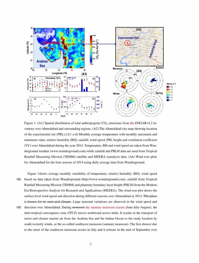
Longitude (oN)

Lat

itu

de

(oE

) Ahmedabad

Arabian

SeaMonsoon Autumn

Winter Spring

N

40%

20%

Experimental Site

CO

2(T

on

Km

-2yr

-1)

(A1) (A2)

(A3)(A4)

EW

S

Figure 1: (A1) Spatial distribution of total anthropogenic CO2 emissions from the EDGARv4.2 in-

ventory over Ahmedabad and surrounding regions. (A2) The Ahmedabad city map showing location

of the experimental site (PRL).(A3: a-d) Monthly average temperature with monthly maximum and

minimum value, relative humidity (RH), rainfall, wind speed, PBL height and ventilation coefficient

(VC) over Ahmedabad during the year 2014. Temperature, RH and wind speed are taken from Wun-

derground weather (www.wunderground.com) while rainfall and PBLH data are used from Tropical

Rainfall Measuring Mission (TRMM) satellite and MEERA reanalysis data. (A4) Wind rose plots

for Ahmedabad for the four seasons of 2014 using daily average data from Wunderground.

Figure 1shows average monthly variability of temperature, relative humidity (RH), wind speed

based on data taken from Wunderground (http://www.wunderground.com), rainfall from Tropical180

Rainfall Measuring Mission (TRMM) and planetary boundary layer height (PBLH) from the Modern-

Era Retrospective Analysis for Research and Applications (MEERA). The wind rose plot shows the

surface level wind speed and direction during different seasons over Ahmedabad in 2014. This place

is known for its semi-arid climate. Large seasonal variations are observed in the wind speed and

direction over Ahmedabad. During monsoon the summer monsoon season (June-July-August), the185

inter-tropical convergence zone (ITCZ) moves northward across India. It results in the transport of

moist and cleaner marine air from the Arabian Sea and the Indian Ocean to the study location by

south westerly winds, or the so-called southwest monsoon (summer monsoon). The first shower due

to the onset of the southwest monsoon occurs in July and it retreats in the mid of September over

7

Ahmedabad. Due to heavy rain and winds mostly from oceanic region, RH shows higher values in190

July, August and September. Highest RH of about 83% is observed in September. The long-range

transport of air masses from the northeast part of the Asian continent starts to prevail over Indian

region when ITCZ moves back southward in September and October. These months are regarded as

transition period for the monsoon. During autumn (September-October-November), the winds are

calm and undergo a change in their direction from south west to north east. When the transition of195

winds takes placed from oceanic to continental region in October, the air gets dryer and RH decreases

until December. The winds are north easterly during winter (December- January - February) and

transport pollutants mostly from continental region (IGP region). During pre-monsoon the spring

season (March - April - May), winds are north westerly and little south westerly which transport

mixed air masses from continent and oceanic regions. The average wind speed is observed higher in200

June and July while lower in October and March when transition of wind starts from oceanic to con-

tinental and continental to oceanic respectively. The monthly averaged temperature starts increasing

from January and attains maximum (34.6±1.4oC) in June, followed by a decrease until September

and temperature is slightly warmer in October compared to the adjacent months. The monthly vari-

ation in planetary boundary layer height (PBLH) closely resembles with the temperature pattern.205

Maximum PBLH of about 1130 m is found in June and it remains in the lower range at about 500 m

during July to January. The ventilation coefficient (VC) is obtained by multiplying wind speed and

PBL height which gradually increases from January to attain the maximum value in June and the

lowest values of VC are observed in October and November.

3 Experiment and model details210

3.1 Experimental method

The measurements of ambient measurements of CO2 and CO are performed concentrations have

been made using a Picarro-G2401 instrument, which is based on the wavelength scanned cavity

ring down spectroscopic (CRDS) technique based analyser (Picarro-G2401) at 0.5 Hz. CRDS of-

fersis a now a well-established technique for making highly sensitivety and high precision precised215

measurements of trace gases in the ambient air, due to its three main characteristics (Bitter et al.,

2005; Chen et al., 2010; Karion et al., 2013). (1). It provides very long Longer interaction path

length (around 20 km) between the sample and the incident wavelength, by utilizing a 3-mirror

configuration, which enhances its sensitivity over other conventional techniques like Non-dispersive

Infrared Spectroscopy (NDIR) and Fourier Transform Infrared Spectroscopy (FTIR). The second220

is its ability to (2). Low operating pressure ( 140 Torr) of cell to avoid pressure broadening The

operating low pressure ( 140 Torr) of cell allows to isolate a single spectral feature with a reso-

lution of 0.0003 cm−1, which ensures that the peak height or area is linearly proportional to the

concentration. The third advantage is that (3) Decay time of light intensity is measured instead of

8

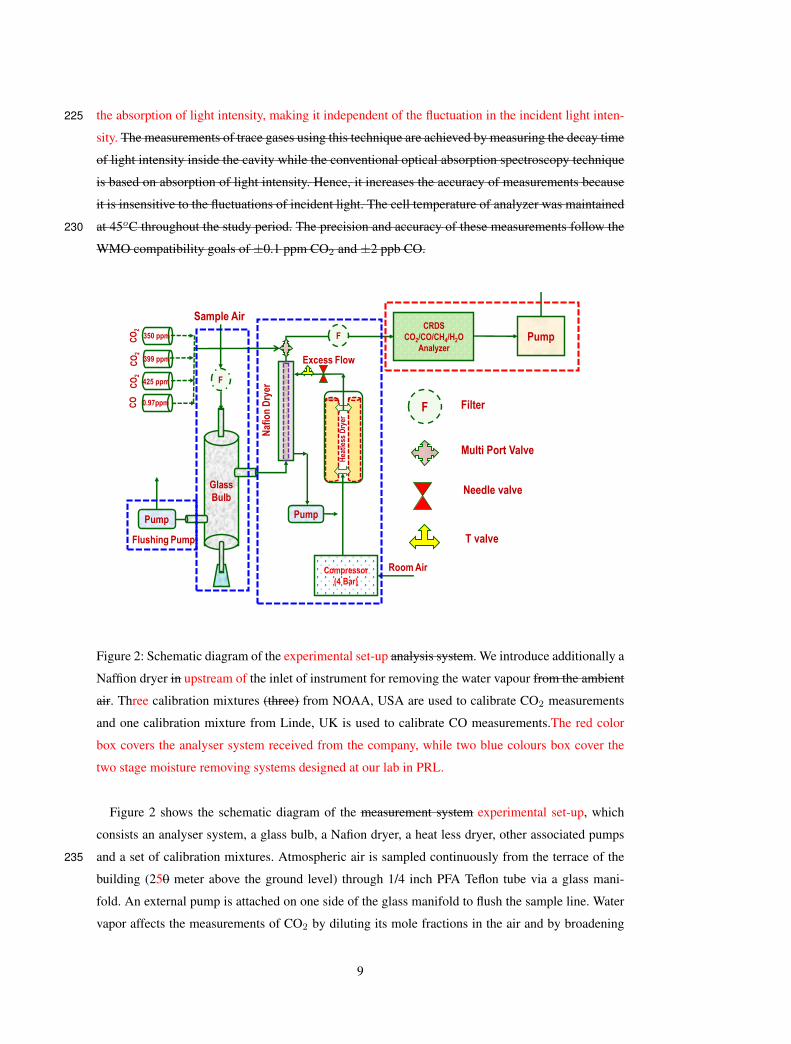
the absorption of light intensity, making it independent of the fluctuation in the incident light inten-225

sity. The measurements of trace gases using this technique are achieved by measuring the decay time

of light intensity inside the cavity while the conventional optical absorption spectroscopy technique

is based on absorption of light intensity. Hence, it increases the accuracy of measurements because

it is insensitive to the fluctuations of incident light. The cell temperature of analyzer was maintained

at 45oC throughout the study period. The precision and accuracy of these measurements follow the230

WMO compatibility goals of ±0.1 ppm CO2 and ±2 ppb CO.

CRDS

CO2/CO/CH4/H2O

AnalyzerPump

Glass

Bulb

Pump

F

F

Compressor

(4 Bar)

Pump

Sample Air

Hea

tles

s D

ryer

Excess Flow

Flushing Pump

350 ppm

399 ppm

425 ppm

Multi Port Valve

0.97ppm

CO

2C

O2

CO

2C

O

F Filter

Needle valve

Naf

ion

Dry

er

Room Air

T valve

Figure 2: Schematic diagram of the experimental set-up analysis system. We introduce additionally a

Naffion dryer in upstream of the inlet of instrument for removing the water vapour from the ambient

air. Three calibration mixtures (three) from NOAA, USA are used to calibrate CO2 measurements

and one calibration mixture from Linde, UK is used to calibrate CO measurements.The red color

box covers the analyser system received from the company, while two blue colours box cover the

two stage moisture removing systems designed at our lab in PRL.

Figure 2 shows the schematic diagram of the measurement system experimental set-up, which

consists an analyser system, a glass bulb, a Nafion dryer, a heat less dryer, other associated pumps

and a set of calibration mixtures. Atmospheric air is sampled continuously from the terrace of the235

building (250 meter above the ground level) through 1/4 inch PFA Teflon tube via a glass mani-

fold. An external pump is attached on one side of the glass manifold to flush the sample line. Water

vapor affects the measurements of CO2 by diluting its mole fractions in the air and by broadening

9

the spectroscopic absorption lines of other gases. Although, the instrument has ability to correct for

the water vapour interferes by using an experimentally derived water vapor correction algorithms240

(Crosson, 2008), but it has an absolute H2O uncertainty of ∼ 1% (Chen et al., 2010) and can in-

troduces a source of error using a single water vapor correction algorithm (Welp et al., 2013). This

error can be minimized by either generating the correction coefficients periodically in the labora-

tory or by removing the water vapour from the sample air. Conducting the water vapor correction

experiment is bit tricky and need extra care as discussed by Welp et al. (2013). Hence, we prefer to245

remove water vapour from the sample air by introducing a 50-strand Nafion dryer (Perma Pure, p/n

PD-50T-24MSS) in the upstream of the analyser. Nafion dryer contains a bunch of semi-permeable

membrane tubing separating an internal sample gas stream from a counter sheath flow of dry gas

in stainless steel outer shell. The partial pressure of water vapour in the sheath air should be lower

than the sample air for effectively removing the water vapour from the sample air. A heatless dryer250

generates dry air using a 4 bar compressor (KNF, MODEL: NO35ATE) which is used as a seath flow

in Naffion dryer. After drying, sample air passes through the PTFE filter (polytetrafluoroethylene;

5µm Sartorius AG, Germany) before entering the instrument cavity. This setup dries the ambient air

near to 0.03% (300 ppm) concentration of H2O.

255

The measurement system is equipped with three high pressure aluminum cylinders containing

gas mixtures of CO2 (350.67±0.02, 399.68±0.01 and 426.20±0.01 ppm) in dry air from NOAA,

Bolder USA, and one cylinder of CO (970 parts per billion (ppb)) from Linde UK. These tanks

were used to calibrate the instrument for CO2 and CO. An additional gas standard tank (CO2: 338

ppm, CO: 700 ppb), known as the “target”, is used to monitor the instrumental drift and to assess260

the dataset accuracy and repeatability. The target tank values are calibrated against the CO2 and

CO calibration mixtures. The target tank and calibration gases were measured mostly in the mid

of every month (Each calibration gas is passed for 30 minute and target tank for 60 minutes). The

target gas is introduced into the instrument for a period of 24 hours also once in a six month, for

checking the diurnal variability of instrument drift. Maximum drift for 24 hours has been calculated265

by subtracting the maximum and minimum value of 5 minute average, which were found to be

0.2 ppm and 0.015 ppm respectively for CO2 and CO. For all calibration mixtures, the measured

concentration is calculated as the average of the last 10 minutes. The linearity of the instrument for

CO2 measurements has been checked by applying the linear fit equation of the CO2 concentration

of the calibration standards (350.67 ppm, 399.68 ppm and 426.20 ppm) measured by the analyzer.270

The slope is found in the range of 0.99 - 1.007 ppm with a correlation coefficient (r) of about

0.999. Further, linearity of the instrument for CO is also checked by diluting the calibration mixture

from 970 ppb to 100 ppb. The calibration mixture is diluted in a glass made dead volume using

highly precise and accurate pure air (air free from water vapor, particles, carbon monoxide (CO),

sulphur dioxide (SO2), oxides of nitrogen (NOx), ozone (O3), and hydrocarbons (HC)) from ECO275

10

Physics generator. and two mass flow controllers. The flows of calibration mixture and pure air were

regulated using two separate mass flow controllers from Aalborg. For increasing the interaction time

of both the gases (zero air and calibration mixture) and to insure a homogeneous mixing, the spring

shaped dead volume is used. Each diluted mixture is passed for 30 minutes in the instrument and

average of last 10 minute data are used for the test. The instrument shows excellent linearity for280

CO and slope is observed to be 0.98. The accuracy of the measurements is calculated by subtracting

the mean difference of measured CO2 and CO concentration from the actual concentration of both

gases in target gas. The accuracies of CO2 and CO are found in the range of 0.05-0.2 ppm and 0.01-

0.025 ppm respectively. The repeatability of both gases are calculated by the standard deviation of

the mean concentration of target gas measured by the analyser over the period of observations and285

found 0.3 ppm and 0.04 ppm for CO2 and CO respectively.

The CO2 concentrations are reported on the WMO scale, using the three calibration mixtures of

CO2 (350.67±0.02, 399.68±0.002 and 426.20±0.006 ppm) from NOAA, Bolder USA, while the

concentration of CO is reported against a calibration mixture of CO (970 ppb) from Linde UK.

An additional gas standard tank (CO2: 338 ppm, CO: 700 ppm), known as the “target”, is used to290

determine the precision of the instrument. The target tank values are calibrated against the CO2 and

CO calibration mixtures. The target gas is introduced in the instrument for a period of 24 hours. For

CO2 and CO, the 5 minute precisions were found to be 0.015 ppm and 0.005 ppm respectively within

1σ. Maximum drift for 24 hours has been calculated by subtracting the maximum and minimum

value of 5 minute average which were found to be 0.2 ppm and 0.015 ppm respectively for CO2295

and CO. The linearity of the instrument for CO2 measurements has been checked by using three

calibration standards (350.67 ppm, 399.68 ppm and 426.20 ppm) of CO2. The linearity tests are

conducted very frequently and the slope is found in the range of 0.99 - 1.007 ppm with correlation

coefficient (r) of about 0.999.

3.2 Description of AGCM-based Chemistry Transport Model (ACTM)300

This study uses the Center for Climate System Research/National Institute for Environmental Stud-

ies/Frontier Research Center for Global Change (CCSR/NIES/FRCGC) atmospheric general circu-

lation model (AGCM)-based chemistry-transport model (ACTM). The model is nudged with reanal-

ysis meteorology using Newtonian relaxation method. The U and V components of horizontal winds

are used from the Japan Meteorological Agency Reanalysis (JRA-25) (Onogi et al., 2007). The305

model has 1.125o × 1.125o horizontal resolution (T106 spectral truncation) and 32 vertical sigma-

pressure layers up to about 50 km. Three components namely anthropogenic emissions, monthly

varying ocean exchange with net uptake and terrestrial biospheric exchange of surface CO2 fluxes are

used in the model. The fossil fuel emissions for the model simulations are taken from EDGAR inven-

tory for the year of 2010. Air-sea fluxes from Takahashi et al. (2009) have been used for the oceanic310

CO2 tracer. The oceanic fluxes are monthly and are linearly interpolated between mid-months. The

11

terrestrial biospheric CO2 tracers are provided from the Carnegie-Ames-Stanford-Approach (CASA)

process model (Randerson et al., 1997), after introducing a diurnal variability using 2 m air temper-

ature and surface short wave radiation from the JRA-25 as per Olsen and Randerson (2004). The

ACTM simulations has been extensively used in TransCom CO2 model inter-comparison studies315

(Law et al., 2008; Patra et al., 2008).

4 Results and Discussion

4.1 Time series and general statistics

Figures 3a and 3c show the time series of 30 minute average CO2 and CO concentrations for the

period of November, 2013 - February, 2014 and July, 2014 to May, 2015. The concentrations of320

both gases exhibit lLarge and periodic variations indicate stronger diurnal dependence of both the

gases.synoptic variability because the site is close to anthropogenic sources. Overall, the concen-

trations and variability of both the gases are observed lowest in the month of July and August,

maximum scatter in the concentrations and several plumes of very high levels both gases have been

observed from October, 2014 until mid-March 2015. Almost all plumes of CO2 and CO are one325

to one correlated and are mostly found during evening rush hours and late nights. Figures 3e and

3f show the variations of CO2 and CO concentrations with wind speed and direction for the study

period except July, August and September due to non-availability of wind data. Most of the high and

low concentrations of both these gases are found to be associated with low and high wind speeds.

There is no specific direction for high levels of these gases. This probably indicates the transport330

sector is an important contributor to the local emissions since the measurement site is surrounded by

the city roads.

Figures 3b and 3d show the probability distributions or frequency distributions of CO2 and CO

concentrations during the study period. Both gases show different distributions from each other. This335

difference could be attributed to the additional role of biospheric cycle (photosynthesis and respira-

tion) on the levels of CO2 apart from the common controlling factors (local sources, regional trans-

port, PBL dynamics etc) responsible for distributions of both gases. The frequency distribution of

CO2 shows almost normal distribution while CO shows skewed towards right (lower concentrations).

This is because, natural cycle of the biosphere (photosynthesis and respiration) along with some340

common controlling factors (local meteorology and anthropogenic sources), affects significantly the

levels of CO2. The control of the boundary layer is common for the diurnal variations of these

species because of their chemical lifetimes are longer (> months) than the timescale of PBL height

variations (∼ hrs). However, biospheric fluxes of CO2 can have strong hourly variations. During the

study period the CO2 concentrations varied between 382 - 609 ppm, with 16% of data lying below345

400 ppm, 50% lying in the range 400-420 ppm, 25% between 420-440 ppm and 9% in the range of

12

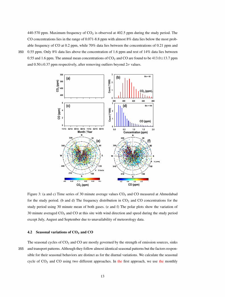
440-570 ppm. Maximum frequency of CO2 is observed at 402.5 ppm during the study period. The

CO concentrations lies in the range of 0.071-8.8 ppm with almost 8% data lies below the most prob-

able frequency of CO at 0.2 ppm, while 70% data lies between the concentrations of 0.21 ppm and

0.55 ppm. Only 8% data lies above the concentration of 1.6 ppm and rest of 14% data lies between350

0.55 and 1.6 ppm. The annual mean concentrations of CO2 and CO are found to be 413.0±13.7 ppm

and 0.50±0.37 ppm respectively, after removing outliers beyond 2σ values.

CO (ppm)CO2 (ppm)

CO

2 (p

pm

v)

400

450

500

550

11/13 02/14 05/14 08/14 11/14 02/15 05/15

CO

(p

pm

v)

0

2

4

6

CO2 (ppmv)

380 400 420 440 460

Co

un

t (*

1000

)

0

1

2

3

Bin = 100

CO (ppmv)

0.0 0.5 1.0 1.5 2.0

Co

un

t (*

1000

)

0

1

2

3

Bin = 50

Mixing ratios (ppmv)Month / year

(a) (b)

(c) (d)

(e) (f)

CO

2(p

pm

)C

O (

pp

m)

Concentration (ppm)Month / Year

CO (ppm)

CO2 (ppm)

Figure 3: (a and c) Time series of 30 minute average values CO2 and CO measured at Ahmedabad

for the study period. (b and d) The frequency distribution in CO2 and CO concentrations for the

study period using 30 minute mean of both gases. (e and f) The polar plots show the variation of

30 minute averaged CO2 and CO at this site with wind direction and speed during the study period

except July, August and September due to unavailability of meteorology data.

4.2 Seasonal variations of CO2 and CO

The seasonal cycles of CO2 and CO are mostly governed by the strength of emission sources, sinks

and transport patterns. Although they follow almost identical seasonal patterns but the factors respon-355

sible for their seasonal behaviors are distinct as for the diurnal variations. We calculate the seasonal

cycle of CO2 and CO using two different approaches. In the first approach, we use the monthly

13

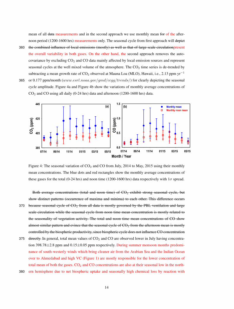
mean of all data measurements and in the second approach we use monthly mean for of the after-

noon period (1200-1600 hrs) measurements only. The seasonal cycle from first approach will depict

the combined influence of local emissions (mostly) as well as that of large scale circulationpresent360

the overall variability in both gases. On the other hand, the second approach removes the auto-

covariance by excluding CO2 and CO data mainly affected by local emission sources and represent

seasonal cycles at the well mixed volume of the atmosphere. The CO2 time series is de-trended by

subtracting a mean growth rate of CO2 observed at Mauna Loa (MLO), Hawaii, i.e., 2.13 ppm yr−1

or 0.177 ppm/month (www.esrl.noaa.gov/gmd/ccgg/trends/) for clearly depicting the seasonal365

cycle amplitude. Figure 4a and Figure 4b show the variations of monthly average concentrations of

CO2 and CO using all daily (0-24 hrs) data and afternoon (1200-1600 hrs) data.

Figure 4: The seasonal variation of CO2 and CO from July, 2014 to May, 2015 using their monthly

mean concentrations. The blue dots and red rectangles show the monthly average concentrations of

these gases for the total (0-24 hrs) and noon time (1200-1600 hrs) data respectively with 1σ spread.

Both average concentrations (total and noon time) of CO2 exhibit strong seasonal cycle, but

show distinct patterns (occurrence of maxima and minima) to each other. This difference occurs

because seasonal cycle of CO2 from all data is mostly governed by the PBL ventilation and large370

scale circulation while the seasonal cycle from noon time mean concentration is mostly related to

the seasonality of vegetation activity. The total and noon time mean concentrations of CO show

almost similar pattern and evince that the seasonal cycle of CO2 from the afternoon mean is mostly

controlled by the biospheric productivity, since biospheric cycle does not influence CO concentration

directly. In general, total mean values of CO2 and CO are observed lower in July having concentra-375

tion 398.78±2.8 ppm and 0.15±0.05 ppm respectively. During summer monsoon months predomi-

nance of south-westerly winds which bring cleaner air from the Arabian Sea and the Indian Ocean

over to Ahmedabad and high VC (Figure 1) are mostly responsible for the lower concentration of

total mean of both the gases. CO2 and CO concentrations are also at their seasonal low in the north-

ern hemisphere due to net biospheric uptake and seasonally high chemical loss by reaction with380

14

OH, respectively. In addition, deep convections in the summer monsoon season efficiently trans-

port the Indian emission (for CO, hydrocarbons) or uptake (for CO2) signals at the surface to the

upper troposphere, resulting lower concentrations at the surface in the summer compared to the win-

ter months (Kar et al., 2004; Randel and Park, 2006; Park et al., 2009; Patra et al., 2011; Baker

et al., 2012). During autumn and early winter (December), lower VC values cause trapping of an-385

thropogenically emitted CO2 and CO and is the major cause for high concentrations of both gases

during this period. In addition to this, wind changes from cleaner marine region to polluted conti-

nental region, especially from IGP region and hence could be additional factor for higher levels of

CO2 and CO during these seasons (autumn and winter). Elevated levels during these seasons are

also examined in several other pollutants over Ahmedabad as discussed in previous studies (Sahu390

and Lal, 2006; Mallik et al., 2016). Maximum concentrations of CO2 and CO are observed to be

424.8±17 ppm and 0.83±0.53 ppm, respectively, during November. From January to May the total

mean concentration of CO2 decreases from 415.3±13.6 to 406.1±5.0 ppm and total mean con-

centration of CO decreases from 0.71±0.22 to 0.22±0.10 ppm. Higher VC and predominance of

comparatively less polluted mixed air masses from oceanic and continental region results in lower395

total mean concentrations of both gases during this period. A sudden increase in the total mean

of both gases is observed from September to October and maximum concentrations of CO2 and

CO are observed to be 424.8±17 ppm and 0.83±0.53 ppm, respectively, during November. From

January to May the total mean concentration of CO2 decreases from 415.3±13.6 to 406.1±5.0 ppm

and total mean concentration of CO decreases from 0.71±0.22 to 0.22±0.10 ppm. During monsoon400

months predominance of south-westerly winds which bring cleaner air from the Arabian Sea and the

Indian Ocean over to Ahmedabad and high VC (Figure 1) are responsible for the lower concentration

of total mean of both the gases. CO2 and CO concentrations are also at their seasonal low in the

northern hemisphere due to net biospheric uptake and seasonally high chemical loss by reaction

with OH, respectively. In addition, deep convections in the southwest monsoon season efficiently405

transport the Indian emission (for CO, hydrocarbons) or uptake (for CO2) signals at the surface

to the upper troposphere, resulting lower concentrations at the surface in the summer compared to

the winter months . During autumn and early winter (December), lower VC values cause trapping of

anthropogenically emitted CO2 and CO. This is the major cause for high CO2 and CO concentrations

during this period. The north-easterly winds bring very high levels of pollutants from IGP region410

and could additionally enhance the levels of CO2 and CO during these seasons (autumn and winter).

Higher VC and predominance of comparatively less polluted mixed air masses from oceanic and

continental region results in the lower total mean concentrations of both gases.

There are some clear differences which are observed in the afternoon mean concentrations of CO2415

as compared to daily mean. The first distinct feature is that significant difference of about 5 ppm is

observed in the afternoon mean of CO2 concentration from July to August as compared to the dif-

15

ference in total mean concentration about ∼0.38 ppm for the same period. Significant differences in

the afternoon concentrations of CO2 from July to August is mainly due to the increasing sink by net

biospheric productivity after the Indian summer monsoonal rainfall. Another distinct feature is that420

the daily mean concentration of CO2 is found highest in November while the afternoon mean con-

centration of CO2 attains maximum value (406±0.4 ppm) in April. Prolonged dry season combined

with high daytime temperature (about 41oC ) during April-May make the tendency of ecosystem

to become moderate source of carbon exchange (Patra et al., 2011) and this could be responsible

for the elevated mean noon time concentrations of CO2. Unlike CO2, seasonal patterns of CO from425

total and afternoon mean concentrations are identical, although levels are different. It shows that the

concentrations of CO is mostly governed by identical sources during day and night time through out

the year.

The average amplitude (max - min) of the annual cycle of CO2 is observed around 13.6 and 26.07430

ppm from the afternoon mean and total mean respectively. Different annual cycles and amplitudes

have been observed from other studies conducted over different Indian stations. Similar to our obser-

vations of the afternoon mean concentrations of CO2, maximum values are also observed in April at

Pondicherry (PON) and Port Blair (PBL) with amplitude of mean seasonal cycles about 7.6±1.4 and

11.1±1.3 ppm respectively (Lin et al., 2015). Cape Rama (CRI), a costal site on the south-west coast435

of India show the seasonal maxima one month before than our observations in March annual am-

plitude about 9 ppm (Bhattacharya et al., 2009). The Sinhagad (SNG) site located over the Western

Ghats Mountains, show very larger seasonal cycle with annual amplitude about 20 ppm (Tiwari et al.,

2014). The amplitude of mean annual cycle at the free tropospheric site Hanle at altitude of 4500 m

is observed to be 8.2±0.4 ppm, with maxima in early May and the minima in mid-September (Lin440

et al., 2015). Distinct seasonal amplitudes and patterns are due to differences in regional controlling

factors for the seasonal cycle of CO2 over these locations, e.g., the Hanle is remotely located from

all continental sources, Port Blair site is sampling predominantly marine air, Cape Rama observes

marine air in the summer and Indian flux signals in the winter, and Sinhagad represents a forested

ecosystem. These comparisons show the need for CO2 measurements over different ecosystems for445

constraining its budget.

The annual amplitude in afternoon and daily mean CO concentration is observed to be about 0.27

and 0.68 ppm, respectively. The mean annual cycles of CO over PON and PBL show the maxima in

the winter months and minima in monsoon summer months same as our observations with annual450

amplitudes of 0.078±0.01 and 0.144±0.016 ppm, respectively. So the seasonal levels of CO are

affected by large scale dynamics which changes air masses from marine to continental and vice

versa and by photochemistry. The amplitudes of annual cycle at these locations differ due to their

climatic conditions and sources/sinks strengths.

16

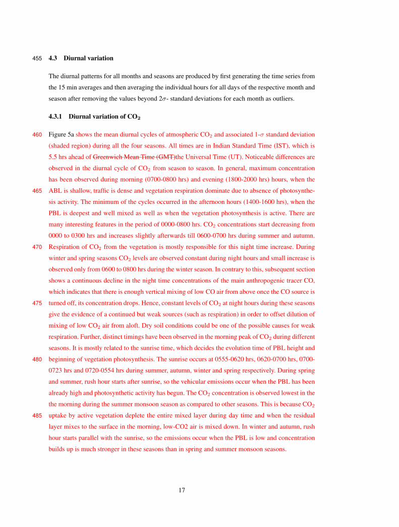
4.3 Diurnal variation455

The diurnal patterns for all months and seasons are produced by first generating the time series from

the 15 min averages and then averaging the individual hours for all days of the respective month and

season after removing the values beyond 2σ- standard deviations for each month as outliers.

4.3.1 Diurnal variation of CO2

Figure 5a shows the mean diurnal cycles of atmospheric CO2 and associated 1-σ standard deviation460

(shaded region) during all the four seasons. All times are in Indian Standard Time (IST), which is

5.5 hrs ahead of Greenwich Mean Time (GMT)the Universal Time (UT). Noticeable differences are

observed in the diurnal cycle of CO2 from season to season. In general, maximum concentration

has been observed during morning (0700-0800 hrs) and evening (1800-2000 hrs) hours, when the

ABL is shallow, traffic is dense and vegetation respiration dominate due to absence of photosynthe-465

sis activity. The minimum of the cycles occurred in the afternoon hours (1400-1600 hrs), when the

PBL is deepest and well mixed as well as when the vegetation photosynthesis is active. There are

many interesting features in the period of 0000-0800 hrs. CO2 concentrations start decreasing from

0000 to 0300 hrs and increases slightly afterwards till 0600-0700 hrs during summer and autumn.

Respiration of CO2 from the vegetation is mostly responsible for this night time increase. During470

winter and spring seasons CO2 levels are observed constant during night hours and small increase is

observed only from 0600 to 0800 hrs during the winter season. In contrary to this, subsequent section

shows a continuous decline in the night time concentrations of the main anthropogenic tracer CO,

which indicates that there is enough vertical mixing of low CO air from above once the CO source is

turned off, its concentration drops. Hence, constant levels of CO2 at night hours during these seasons475

give the evidence of a continued but weak sources (such as respiration) in order to offset dilution of

mixing of low CO2 air from aloft. Dry soil conditions could be one of the possible causes for weak

respiration. Further, distinct timings have been observed in the morning peak of CO2 during different

seasons. It is mostly related to the sunrise time, which decides the evolution time of PBL height and

beginning of vegetation photosynthesis. The sunrise occurs at 0555-0620 hrs, 0620-0700 hrs, 0700-480

0723 hrs and 0720-0554 hrs during summer, autumn, winter and spring respectively. During spring

and summer, rush hour starts after sunrise, so the vehicular emissions occur when the PBL has been

already high and photosynthetic activity has begun. The CO2 concentration is observed lowest in the

the morning during the summer monsoon season as compared to other seasons. This is because CO2

uptake by active vegetation deplete the entire mixed layer during day time and when the residual485

layer mixes to the surface in the morning, low-CO2 air is mixed down. In winter and autumn, rush

hour starts parallel with the sunrise, so the emissions occur when the PBL is low and concentration

builds up is much stronger in these seasons than in spring and summer monsoon seasons.

17

The diurnal amplitude is defined as the difference between the maximum and minimum concen-490

trations of CO2 in the diurnal cycle. The amplitudes of monthly averaged diurnal cycle of CO2 from

July, 2014 to May 2015 are shown in Figure 5b. The diurnal amplitude shows large month to month

variation with increasing trend from July to October and decreasing trend from October onwards.

The lowest diurnal amplitude of about 6 ppm is observed in July while highest amplitude about 51

ppm is observed in October. The amplitude does not change largely from December to March and495

is observed in the range of 25-30 ppm. Similarly from April to May the amplitude also varies in a

narrow range from 12 to 15 ppm. The jump in the amplitude of the CO2 diurnal cycle is observed

highest (around 208%) from July to August. This is mainly due to significant increase of biospheric

productivity from July to August after the rains in Ahmedabad. It is observed that during July the

noon time CO2 levels are found in the range of 394-397 ppm while in August the noon time levels500

are observed in the range of 382-393 ppm. The lower levels could be due to the higher PBL height

during afternoon and cleaner air, but in case of CO (will be discussed in next section), average day

time levels in August are observed higher than in July. It rules out that the lower levels during Au-

gust are due to the higher PBL height and presence of cleaner marine air, and confirms the higher

biospheric productivity during August.505

shows bi-modal feature in the diurnal cycle of CO2 during the four seasons with morning and

evening peaks. Both peaks are associated mostly with the vehicular emissions and PBL height during

rush hours. There are many interesting features in the 0000-0800 hrs period. All times are in Indian

Standard Time (IST), which is 5.5 hrs ahead of GMT. Concentrations of CO2 start decreasing from

0000 hrs to 0300 hrs and afterwards increases until 0600 and 0700 hrs during monsoon and autumn.510

It could be mostly due to the accumulation of CO2 emitted from respiration by the biosphere in

the nocturnal boundary layer. During winter and spring the concentrations during night hours are

almost constant and increase is observed only from 0600 hrs to 0800 hrs during winter. Dormant of

respiration during these two seasons due to lower temperature could be one of the possible factors

for no increase in CO2 concentrations during night. No peak during morning hours is observed in515

spring. Distinct timings for the occurrence of the morning peak during different seasons is generally

related to the sunrise time and consequently the evolutions of PBL height. The sunrise occur at

0555-0620 hrs, 0620-0700 hrs, 0700-0723 hrs and 0720-0554 hrs during monsoon, autumn, winter

and spring, respectively. During spring and monsoon, rush hour starts after sunrise, so the vehicular

emissions occur when the PBL is already high and photosynthetic activity has begun. But in winter520

and autumn rush hour starts parallely with the sunrise, so the emissions occur when the PBL is low

and concentration build up is much strong in these seasons than in spring and monsoon seasons. CO2

starts decreasing fast after these hours and attains minimum value around 1600 hrs. This quick drop

of CO2 after sunrise is linked to the dominance of photosynthesis over the respiration processes in

addition to the higher atmospheric mixing height. CO2 levels start increasing after 1600 hrs peak525

around 2100 hrs. Higher concentrations of CO2 during these hours are mainly due to the rush hour

18

vehicular emissions and less dilution due to the lower PBL height. Comparative levels of CO2 during

evening rush hours except monsoon confirm separately the major influence from the same type of

sources (vehicular emission) in its levels which do not show large variability as in post-midnight

hours.530

The diurnal amplitude is defined as the difference between the maximum and minimum concentrations

of CO2 in the diurnal cycle. The amplitudes of monthly averaged diurnal cycle of CO2 from July,

2014 to May 2015 are shown in Figure 5b. The diurnal amplitude shows large month to month

variation with increasing trend from July to October and decreasing trend from October onwards.535

Lowest diurnal amplitude of about 6 ppm is observed in July while highest amplitude about 51

ppm is observed in October. The amplitude does not change much from December to March and

is observed in the range of 25-30 ppm. Similarly from April to May the amplitude also varies in

a narrow range from 12 to 15 ppm. The jump in the amplitude of CO2 diurnal cycle is observed

highest (around 208%) from July to August. This is mainly due to significant increase of biospheric540

productivity from July to August after the rains in Ahmedabad. It is observed that during July the

noon time CO2 levels are found in the range of 394-397 ppm while in August the noon time levels

are observed in the range of 382-393 ppm. The lower levels could be due to the higher PBL height

during afternoon and cleaner air, but in case of CO, average day time levels in August are observed

higher than July. It rules out that the lower levels during August are due to the higher PBL height545

and presence of cleaner marine air, and confirms the higher biospheric productivity during August.

Diu

rnal

Am

plit

ud

e (p

pm

)

CO2

Month / YearHour (IST)

2418120600

380

400

420

440

460

CO

2(p

pm

)

MonsoonAutumn

Winter

Spring

(a)

Figure 5: (a) Average diurnal variation of CO2 over Ahmedabad during all the four seasons. (b)

Monthly variation of average diurnal amplitude of CO2 during from July, 2014 to May, 2015. All

times are in Indian Standard Time (IST), which is 5.5 hrs ahead of Universal Time (UT).

The monthly average diurnal cycles of the biospheric net primary productivity from the CASA

model for Ahmedabad and for the year of 2014 are shown Figure 10. The details of CASA flux

are given in the Section 3.2. It is observed that the model shows higher biospheric productivity in

September and October while the observations are suggesting higher productivity in August. This550

19

indicates that the CASA model is not able to capture the signal of higher biospheric productivity

for Ahmedabad and need to be improved. Similar discrepancy in the timing of maximum biospheric

uptake is also discussed earlier by Patra et al. (2011) using inverse model CO2 fluxes and CASA

biospheric fluxes.

555

Near surface diurnal amplitude of CO2 has been also documented in humid subtropical Indian

station Dehradun and a dry tropical Indian station Gadanki (Sharma et al., 2014). In comparison

to Ahmedabad, both these stations show distinct seasonal change in the diurnal amplitude of CO2.

The maximum CO2 diurnal amplitude of about 69 ppm is observed during the monsoon summer

season at Dehradun (30.3oN, 78.0oE, 435m), whereas maximum of about 50 ppm during autumn at560

Gadanki (13.5oN, 79.2oE, 360 m).

4.3.2 Diurnal variation of CO

Figure 6a shows seasonally averaged diurnal variation of CO. In general, the mean diurnal cycle

of CO show lower concentration during noon (1200-1700 hrs) and two peaks in the morning (0800

to 1000 hrs) and in the evening (1800 to 2200 hrs) hours. This cycle exhibits the same pattern as565

the mean diurnal cycle of traffic flow, with maxima in the morning and at the end of the afternoon,

which suggests the influence of traffic emissions on CO measurements. Along with the traffic flow,

PBL dynamics also play a critical role in governing the diurnal cycle of CO. The amplitudes of the

evening peak in diurnal cycles of CO are always greater than the morning peaks. It is because the

PBL height evolves side by side with the morning rush hours traffic and hence increased dilution,570

while on the other hand, during evening hours, PBL height decrease along with evening dense traf-

fic and favors accumulation of pollutants until the late evening under the stable PBL conditions.

The noon time minimum of the cycle is mostly associated with the deepest and well mixed PBL.In

general, the average diurnal cycle patterns of both gases (CO2 and CO) are similar, but having few

noticeable differences. The first difference is observed in the timing of the occurrence of morning575

peaks: CO2 peaks occur slightly before the CO peak due to the triggering photosynthesis process by

the sunrise. On the other hand, the morning peaks of CO mostly depend on the rush hour traffic and

are consistent at 0800-1000 hrs in all seasons. The second difference is that the afternoon concentra-

tions of CO show little seasonal spread as compared to the afternoon concentrations of CO2. Again,

this is due to the biospheric control on the levels of CO2 during the afternoon hours of different sea-580

sons while CO levels are mainly controlled by the dilution during these hours. The third noticeable

difference is that the levels of CO decrease very fast after evening rush hours in all the seasons while

this feature is not observed in the case of CO2 since respiration during night hours contributes to the

levels of CO2. The continuous drop of nighttime concentrations of CO indicates that there is enough

vertical mixing of low CO air from above once the CO source is turned off. The average morning585

(0800-0900 hrs) peak values of CO is observed minimum (0.18±0.1 ppm) in summer and maximum

20

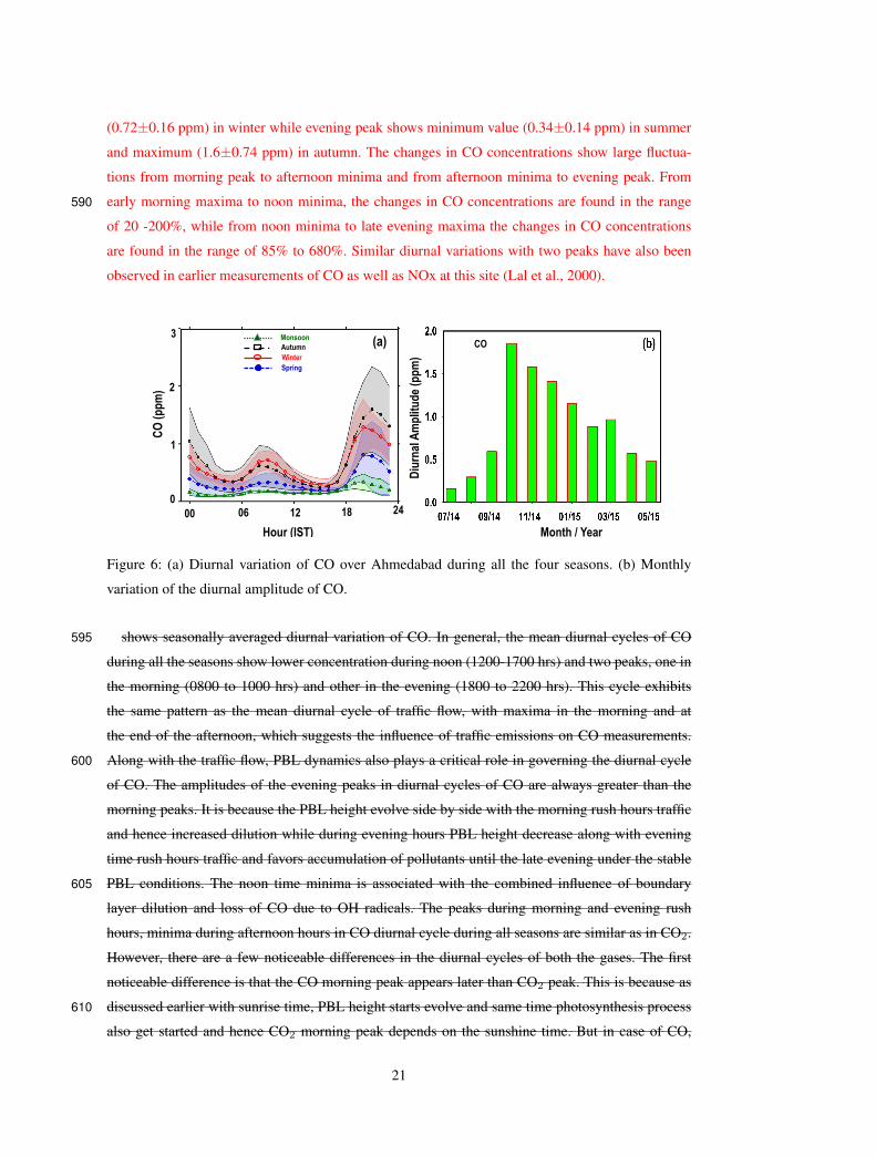
(0.72±0.16 ppm) in winter while evening peak shows minimum value (0.34±0.14 ppm) in summer

and maximum (1.6±0.74 ppm) in autumn. The changes in CO concentrations show large fluctua-

tions from morning peak to afternoon minima and from afternoon minima to evening peak. From

early morning maxima to noon minima, the changes in CO concentrations are found in the range590

of 20 -200%, while from noon minima to late evening maxima the changes in CO concentrations

are found in the range of 85% to 680%. Similar diurnal variations with two peaks have also been

observed in earlier measurements of CO as well as NOx at this site (Lal et al., 2000).

Hour (IST)

Diu

rnal

Am

plit

ud

e (p

pm

)

CO

Month / Year

2418120600

0

1

2

3

CO

(p

pm

)

(a)Monsoon

Autumn

Winter

Spring

Figure 6: (a) Diurnal variation of CO over Ahmedabad during all the four seasons. (b) Monthly

variation of the diurnal amplitude of CO.

shows seasonally averaged diurnal variation of CO. In general, the mean diurnal cycles of CO595

during all the seasons show lower concentration during noon (1200-1700 hrs) and two peaks, one in

the morning (0800 to 1000 hrs) and other in the evening (1800 to 2200 hrs). This cycle exhibits

the same pattern as the mean diurnal cycle of traffic flow, with maxima in the morning and at

the end of the afternoon, which suggests the influence of traffic emissions on CO measurements.

Along with the traffic flow, PBL dynamics also plays a critical role in governing the diurnal cycle600

of CO. The amplitudes of the evening peaks in diurnal cycles of CO are always greater than the

morning peaks. It is because the PBL height evolve side by side with the morning rush hours traffic

and hence increased dilution while during evening hours PBL height decrease along with evening

time rush hours traffic and favors accumulation of pollutants until the late evening under the stable

PBL conditions. The noon time minima is associated with the combined influence of boundary605

layer dilution and loss of CO due to OH radicals. The peaks during morning and evening rush

hours, minima during afternoon hours in CO diurnal cycle during all seasons are similar as in CO2.

However, there are a few noticeable differences in the diurnal cycles of both the gases. The first

noticeable difference is that the CO morning peak appears later than CO2 peak. This is because as

discussed earlier with sunrise time, PBL height starts evolve and same time photosynthesis process610

also get started and hence CO2 morning peak depends on the sunshine time. But in case of CO,

21

timing of the morning peak mostly depends on the rush hour traffic and is consistent at 0800-1000

hrs in all seasons. The second noticeable difference is the afternoon concentrations of CO show

little seasonal spread as compared to the afternoon concentrations of CO2. Again, this is due to the

biospheric control on the concentration of CO2 during the afternoon hours of different seasons while615

CO levels are mainly controlled by the dilution during these afternoon hours. The third noticeable

difference is that the levels of CO decrease very fast after evening rush hour in all seasons while

this feature is not observed in case of CO2 since respiration during night hours contributes to the

levels of CO2. The average morning (0800-0900 hrs) peak values of CO are observed minimum

(0.18±0.1 ppm) in monsoon and maximum (0.72±0.16 ppm) in winter while its evening peak620

shows minimum value (0.34±0.14 ppm) in monsoon and maximum (1.6±0.74 ppm) in autumn. The

changes in CO concentrations show large fluctuations from morning peak to afternoon minima and

from afternoon minima to evening peak. From early morning maxima to noon minima, the changes

in CO concentrations are found in the range of 20 -200% while from noon minima to late evening

maxima the changes in CO concentrations are found in the range of 85% to 680%. Similar diurnal625

variations with two peaks have also been observed in earlier measurements of CO as well as NOx at

this site.

The evening peak contributes significantly to the diurnal amplitude of CO. The largest amplitude

in CO cycle is observed in autumn (1.36 ppm) while the smallest amplitude is observed in summer

(0.24 ppm). The diurnal amplitudes of CO are observed to be about 1.01 and 0.62 ppm, respectively630

during winter and spring. Like CO2, the diurnal cycle of CO (Figure 6b) shows the minimum (0.156

ppm) amplitude in July and maximum (1.85 ppm) in October. After October the diurnal amplitude

keeps on decreasing till summer. The evening peak contributes significantly to the diurnal ampli-

tude of CO. The largest amplitude in CO cycle is observed in autumn (1.36 ppm) while the smallest

amplitude is observed in summer (0.24 ppm). The diurnal amplitudes of CO are observed to be635

about 1.01 and 0.62 ppm, respectively during winter and spring. The monthly diurnal cycle of CO

(Figure 6b) shows the minimum (0.156 ppm) amplitude in July and maximum (1.85 ppm) in Oc-

tober. After October the diurnal amplitude keeps on decreasing till summer monsoon. The monthly

diurnal cycle of CO (Figure 6b) shows minimum (0.156 ppm) amplitude in July and maximum (1.85

ppm) in October. After October the diurnal amplitude keep on decreasing till monsoon. The evening640

peak contributes significantly to the diurnal amplitude of CO. The largest amplitude in CO cycle is

observed in autumn (1.36 ppm) while smallest amplitude is observed in monsoon (0.24 ppm).

4.4 Correlation between CO and CO2

The relationships of CO to CO2 can be useful for investigating the CO source types and their com-645

bustion characteristics in the city region of Ahmedabad. The measurements are generally affected

by the dilution due to the boundary layer dynamics, but considering their ratios will cancel this

22

effect. Further, the interpretation of correlation ratios in terms of their dominant emission sources

needs to isolate first the local urban signal. For this, the measurements have to be corrected from

their background influence. The background concentrations are generally those levels which have650

almost negligible influence from the local emission sources. For correlations study, in principle the

baseline levels to be removed from the measured concentrations. Although, the most ideal case of

determining the background levels are the continuous measurement of respective gases at a cleaner

site. But due to unavailability of such measurements for our study period at cleaner sites, we use

the 5th percentile value of CO2 and CO for each day as a background for corresponding day. It is655

observed that the mixing ratios of both gases at low wind speed, which show the influence of local

urban signal, are significantly higher than background levels and hence confirm that the definition of

background will not significantly affect the derived ratios (Ammoura et al., 2014). This technique of

measuring the background is extensively studied by Ammoura et al. (2014) and found suitable for

both the gases CO and CO2, even having the role of summer uptake on the levels of CO2. The ex-660

cess CO2 (CO2(exc)) and CO (CO(exc)) above the background for Ahmedabad city, are determined

for each day after subtracting the background concentrations from the hours of each day (CO2(exc)

= CO2(obs) - CO2(bg), CO(exc) = CO(obs) - CO(bg)).

We use robust regression method for the correlation study. It is an alternative to least squares665

regression method and more applicable for analysing time series data with outliers arising from

extreme events (http://www.ats.ucla.edu/stat/stata/dae/rreg.htm). Figure 7 illustrates the correlations

between CO(exc) and CO2(exc) for the four seasons at different time windows of the day. Based

on the dominance of different atmospheric processes and different emission sources as discussed

in Section 4.3, the measurements are divided into the group of four different time windows: (1)670

Morning period (0600-1000 hrs), when PBL height is slowly evolving and rush hour traffic is there,

(2) Afternoon period (1100-1700 hrs), when atmospheric is well mixed and traffic is relatively less,

(3) Evening period (1800-2200 hrs), when influence of rush hour traffic is significantly high, (4)

Night period (0000-0500 hrs), when atmospheric is calm and the anthropogenic sources of both

gases are switched off. The measured slopes values for these time intervals are given in Table 1.675

The ranges of the emission ratios of CO/CO2 for transport, industrial and domestic sources, as given

in Table 2, are also plotted in the figures for broadly showing the dominance of different sources.

The ∆CO(exc)/∆CO2(exc) ratios are observed lowest during summer, with a range varying from

0.9 ppb/ppm in morning to 19.5 ppb/ppm in evening period. Lowest coefficient of determination is

also observed during this season, which suggest that the levels of CO and CO2 are controlled by680

different factors. As discussed previously, higher biospheric productivity during this season mostly

controls the CO2 concentrations while CO concentrations are mostly controlled by the long range

transport. During the winter season ∆CO(exc)/∆CO2(exc) ratios are observed highest and varies

from 14.3 ppb/ppm in morning to 47.2 ppb/ppm in evening period. Relatively higher ratios dur-

23

ing winter than other three seasons indicates contribution of CO emission from additional biofuel685

burning sources. From day to night, highest coefficient of determination is observed during spring

season. As illustrated by the diurnal cycle, the CO2 is not significantly removed by the biosphere

during spring with lower draw down in daily CO2. Along with this, higher VC during this season

will result in very fast mixing. Therefore, very fast mixing will mostly regulate their relative varia-

tion and will result in higher correlation in this season. Other factors like soil and plant respiration690

during this period may also control CO2 concentrations due to which the correlation coefficient is

not equal to 1. Except monsoon, the ∆CO(exc)/∆CO2(exc) ratios and their correlations are fairly

comparable in other seasons in the evening rush hours, which indicate stronger influence of com-

mon emission sources. Ratios during this time can be considered as fresh emissions since dilution

and chemical loss of CO can be considered negligible for this time. Most of these data fall in the695

domestic and transport sector emission ratio lines, which indicate that during this time intervals

these sources mostly dominate (Table 2). On the other hand, during other time intervals most of

the data are scattered between industrial and transport sectors emission ratio lines. Hence, from this

we can conclude that during evening hours, transport and domestic sources mostly dominate while

during other periods transport and industrial emission sources mostly dominate. The impact of the700

possible sources of CO and CO2 varies from month to month and hence season to season. The lowest

correlation (r = 0.62, p =0.0001) is observed during monsoon, with a ∆CO(exc)/∆CO2(exc) ratio of

0.6±0.1 ppb/ppm. Lowest correlation suggest that different mechanisms control the levels of CO and

CO2 during the monsoon season. As discussed previously, higher biospheric productivity during this

season mostly controls the CO2 concentrations while CO concentrations are mostly controlled by705

the long range transport and higher loss due to OH. Highest correlation (r = 0.87, p<0.0001) with

∆CO(exc)/∆CO2(exc) ratio of 8.4±0.17 ppb/ppm is observed during spring season. As illustrated

by the diurnal cycle, the CO2 is not significantly removed by the biosphere during spring with lower

draw down in daily CO2. Along withthis, higher VC during this season will result in very fast

mixing. Therefore, very fast mixing will mostly regulate their relative variation and will result in710

higher correlation in this season. Other factors like soil and plant respiration during this period may

also control CO2 concentrations due to which the correlation coefficient is not equal to 1. The ratio

of ∆CO(exc)/∆CO2(exc) is estimated to be 8.5±0.15 ppb/ppm (r = 0.72) and 12.7±0.17 ppb/ppm

(r = 0.74) in autumn and winter respectively. Relatively higher ratios during winter than other three

seasons indicates contribution of CO emission from additional biofuel burning sources. The winter715

time observed ratios are similar to the airmass influenced by both fossil fuel and biofuel emissions

as discussed by Lin et al. (2015) over Pondicherry. Using CARIBIC observations, Lai et al. (2010)

also reported the ∆CO/∆CO2 ratio in the range of 15.6-29.3 ppb/ppm from the airmass influenced

by both biofuel and fossil fuel burning in the Indo-Chinese Peninsula. Further, ∆CO/∆CO2 ratio is

also observed of about 13 ppb/ppm in South-east Asian outflow in February-April, 2001 during the720

TRACE-P campaign and suggest the combined influence of fossil fuel and biofuel burning (Russo

24

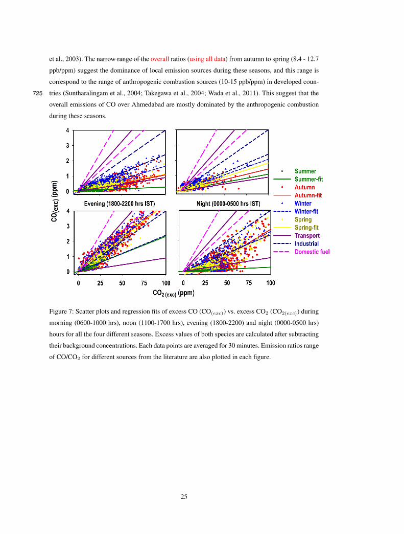
et al., 2003). The narrow range of the overall ratios (using all data) from autumn to spring (8.4 - 12.7

ppb/ppm) suggest the dominance of local emission sources during these seasons, and this range is

correspond to the range of anthropogenic combustion sources (10-15 ppb/ppm) in developed coun-

tries (Suntharalingam et al., 2004; Takegawa et al., 2004; Wada et al., 2011). This suggest that the725

overall emissions of CO over Ahmedabad are mostly dominated by the anthropogenic combustion

during these seasons.

Figure 7: Scatter plots and regression fits of excess CO (CO(exc)) vs. excess CO2 (CO2(exc)) during

morning (0600-1000 hrs), noon (1100-1700 hrs), evening (1800-2200) and night (0000-0500 hrs)

hours for all the four different seasons. Excess values of both species are calculated after subtracting

their background concentrations. Each data points are averaged for 30 minutes. Emission ratios range

of CO/CO2 for different sources from the literature are also plotted in each figure.

25

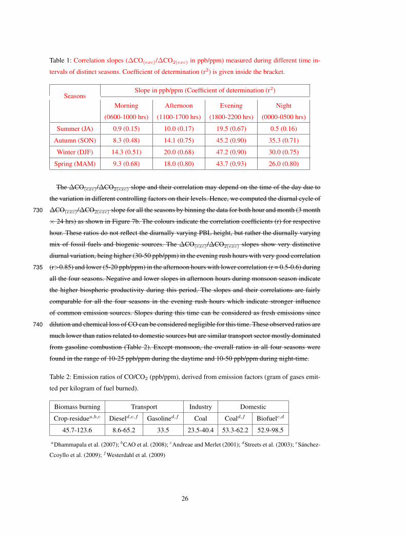
Table 1: Correlation slopes (∆CO(exc)/∆CO2(exc) in ppb/ppm) measured during different time in-

tervals of distinct seasons. Coefficient of determination (r2) is given inside the bracket.

SeasonsSlope in ppb/ppm (Coefficient of determination (r2)

Morning

(0600-1000 hrs)

Afternoon

(1100-1700 hrs)

Evening

(1800-2200 hrs)

Night

(0000-0500 hrs)

Summer (JA) 0.9 (0.15) 10.0 (0.17) 19.5 (0.67) 0.5 (0.16)

Autumn (SON) 8.3 (0.48) 14.1 (0.75) 45.2 (0.90) 35.3 (0.71)

Winter (DJF) 14.3 (0.51) 20.0 (0.68) 47.2 (0.90) 30.0 (0.75)

Spring (MAM) 9.3 (0.68) 18.0 (0.80) 43.7 (0.93) 26.0 (0.80)

The ∆CO(exc)/∆CO2(exc) slope and their correlation may depend on the time of the day due to

the variation in different controlling factors on their levels. Hence, we computed the diurnal cycle of

∆CO(exc)/∆CO2(exc) slope for all the seasons by binning the data for both hour and month (3 month730

× 24 hrs) as shown in Figure 7b. The colours indicate the correlation coefficients (r) for respective

hour. These ratios do not reflect the diurnally varying PBL height, but rather the diurnally varying

mix of fossil fuels and biogenic sources. The ∆CO(exc)/∆CO2(exc) slopes show very distinctive

diurnal variation, being higher (30-50 ppb/ppm) in the evening rush hours with very good correlation

(r>0.85) and lower (5-20 ppb/ppm) in the afternoon hours with lower correlation (r = 0.5-0.6) during735

all the four seasons. Negative and lower slopes in afternoon hours during monsoon season indicate

the higher biospheric productivity during this period. The slopes and their correlations are fairly

comparable for all the four seasons in the evening rush hours which indicate stronger influence

of common emission sources. Slopes during this time can be considered as fresh emissions since

dilution and chemical loss of CO can be considered negligible for this time. These observed ratios are740

much lower than ratios related to domestic sources but are similar transport sector mostly dominated

from gasoline combustion (Table 2). Except monsoon, the overall ratios in all four seasons were

found in the range of 10-25 ppb/ppm during the daytime and 10-50 ppb/ppm during night-time.

Table 2: Emission ratios of CO/CO2 (ppb/ppm), derived from emission factors (gram of gases emit-

ted per kilogram of fuel burned).

Biomass burning Transport Industry Domestic

Crop-residuea,b,c Dieseld,e,f Gasolined,f Coal Coald,f Biofuelc,d

45.7-123.6 8.6-65.2 33.5 23.5-40.4 53.3-62.2 52.9-98.5

aDhammapala et al. (2007); bCAO et al. (2008); cAndreae and Merlet (2001); dStreets et al. (2003); eSánchez-

Ccoyllo et al. (2009); fWesterdahl et al. (2009)

26

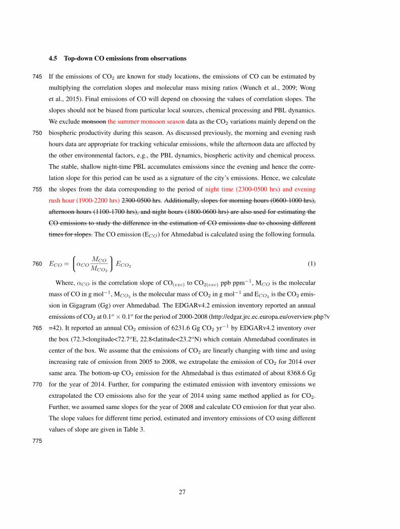
4.5 Top-down CO emissions from observations

If the emissions of CO2 are known for study locations, the emissions of CO can be estimated by745

multiplying the correlation slopes and molecular mass mixing ratios (Wunch et al., 2009; Wong

et al., 2015). Final emissions of CO will depend on choosing the values of correlation slopes. The

slopes should not be biased from particular local sources, chemical processing and PBL dynamics.

We exclude monsoon the summer monsoon season data as the CO2 variations mainly depend on the

biospheric productivity during this season. As discussed previously, the morning and evening rush750

hours data are appropriate for tracking vehicular emissions, while the afternoon data are affected by

the other environmental factors, e.g., the PBL dynamics, biospheric activity and chemical process.

The stable, shallow night-time PBL accumulates emissions since the evening and hence the corre-

lation slope for this period can be used as a signature of the city’s emissions. Hence, we calculate

the slopes from the data corresponding to the period of night time (2300-0500 hrs) and evening755

rush hour (1900-2200 hrs) 2300-0500 hrs. Additionally, slopes for morning hours (0600-1000 hrs),

afternoon hours (1100-1700 hrs), and night hours (1800-0600 hrs) are also used for estimating the

CO emissions to study the difference in the estimation of CO emissions due to choosing different

times for slopes. The CO emission (ECO) for Ahmedabad is calculated using the following formula.

ECO =

αCOMCO

MCO2

ECO2(1)760

Where, αCO is the correlation slope of CO(exc) to CO2(exc) ppb ppm−1, MCO is the molecular

mass of CO in g mol−1, MCO2 is the molecular mass of CO2 in g mol−1 and ECO2 is the CO2 emis-

sion in Gigagram (Gg) over Ahmedabad. The EDGARv4.2 emission inventory reported an annual

emissions of CO2 at 0.1o × 0.1o for the period of 2000-2008 (http://edgar.jrc.ec.europa.eu/overview.php?v

=42). It reported an annual CO2 emission of 6231.6 Gg CO2 yr−1 by EDGARv4.2 inventory over765

the box (72.3<longitude<72.7oE, 22.8<latitude<23.2oN) which contain Ahmedabad coordinates in

center of the box. We assume that the emissions of CO2 are linearly changing with time and using

increasing rate of emission from 2005 to 2008, we extrapolate the emission of CO2 for 2014 over

same area. The bottom-up CO2 emission for the Ahmedabad is thus estimated of about 8368.6 Gg

for the year of 2014. Further, for comparing the estimated emission with inventory emissions we770

extrapolated the CO emissions also for the year of 2014 using same method applied as for CO2.

Further, we assumed same slopes for the year of 2008 and calculate CO emission for that year also.

The slope values for different time period, estimated and inventory emissions of CO using different

values of slope are given in Table 3.

775

27

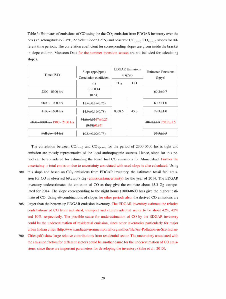
Table 3: Estimates of emissions of CO using the the CO2 emission from EDGAR inventory over the

box (72.3<longitude<72.7oE, 22.8<latitude<23.2oN) and observed CO(exc):CO2(exc) slopes for dif-

ferent time periods. The correlation coefficient for corresponding slopes are given inside the bracket

in slope column. Monsoon Data for the summer monsoon season are not included for calculating

slopes.

Time (IST)Slope (ppb/ppm)

Correlation coefficient

(r)

EDGAR Emissions

(Gg/yr)Estimated Emssions

Gg(yr)

CO2 CO

2300 - 0500 hrs13±0.14

(0.84)69.2±0.7

0600 - 1000 hrs 11.4±0.19(0.75) 60.7±1.0

1100 - 1600 hrs 14.9±0.19(0.78) 8368.6 45.3 79.3±1.0

1800 - 0500 hrs 1900 - 2100 hrs34.6±0.3747±0.27

(0.58)(0.95)184.2±1.9 250.2±1.5

Full day (24 hr) 10.8±0.09(0.73) 57.5±0.5

The correlation between CO(exc) and CO2(exc) for the period of 2300-0500 hrs is tight and

emission are mostly representative of the local anthropogenic sources. Hence, slope for this pe-

riod can be considered for estimating the fossil fuel CO emissions for Ahmedabad. Further the

uncertainty is total emission due to uncertainty associated with used slope is also calculated. Using

this slope and based on CO2 emissions from EDGAR inventory, the estimated fossil fuel emis-780

sion for CO is observed 69.2±0.7 Gg (emission±uncertainty) for the year of 2014. The EDGAR

inventory underestimates the emission of CO as they give the estimate about 45.3 Gg extrapo-

lated for 2014. The slope corresponding to the night hours (1800-0600 hrs) give the highest esti-

mate of CO. Using all combinations of slopes for other periods also, the derived CO emissions are

larger than the bottom-up EDGAR emission inventory. The EDGAR inventory estimate the relative785

contributions of CO from industrial, transport and slum/residential sector to be about 42%, 42%

and 10%, respectively. The possible cause for underestimation of CO by the EDGAR inventory

could be the underestimation of residential emission, since other inventories particularly for major

urban Indian cities (http://www.indiaenvironmentportal.org.in/files/file/Air-Pollution-in-Six-Indian-

Cities.pdf) show large relative contributions from residential sector. The uncertainty associated with790

the emission factors for different sectors could be another cause for the underestimation of CO emis-

sions, since these are important parameters for developing the inventory (Sahu et al., 2015).

28

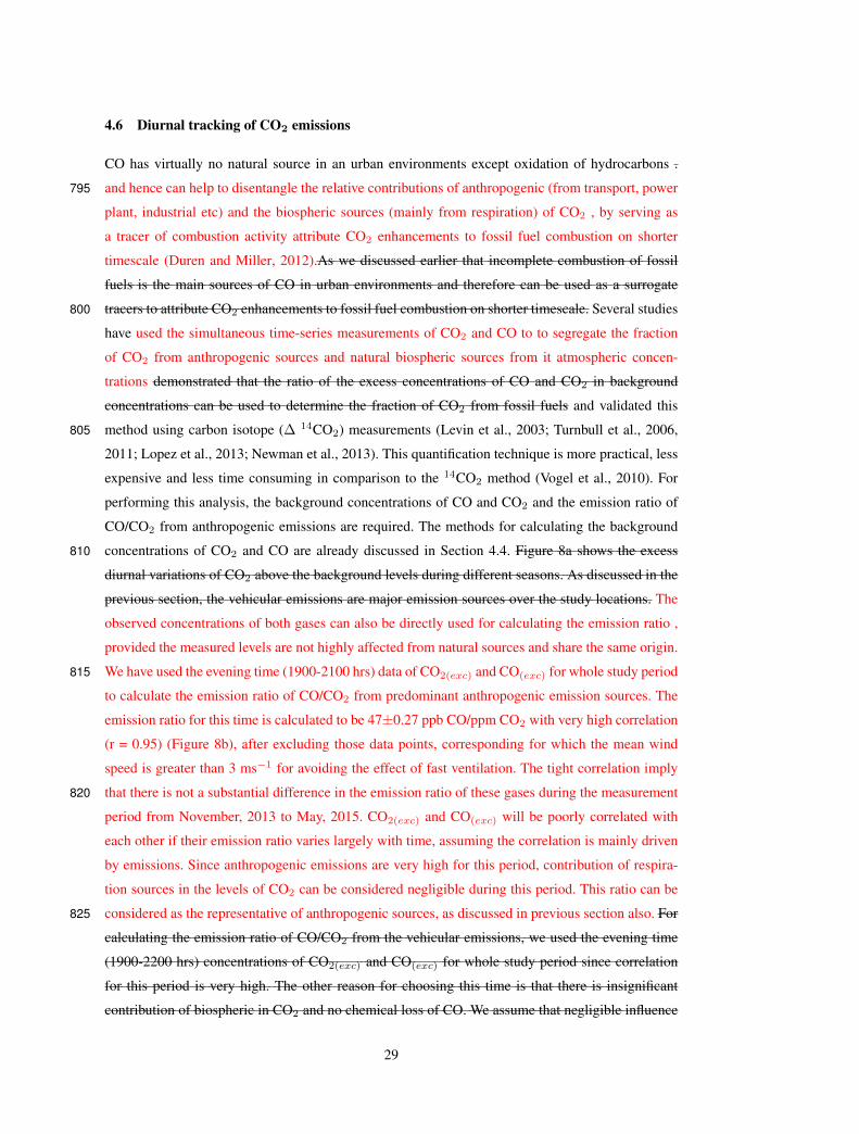
4.6 Diurnal tracking of CO2 emissions

CO has virtually no natural source in an urban environments except oxidation of hydrocarbons .

and hence can help to disentangle the relative contributions of anthropogenic (from transport, power795

plant, industrial etc) and the biospheric sources (mainly from respiration) of CO2 , by serving as

a tracer of combustion activity attribute CO2 enhancements to fossil fuel combustion on shorter

timescale (Duren and Miller, 2012).As we discussed earlier that incomplete combustion of fossil

fuels is the main sources of CO in urban environments and therefore can be used as a surrogate

tracers to attribute CO2 enhancements to fossil fuel combustion on shorter timescale. Several studies800

have used the simultaneous time-series measurements of CO2 and CO to to segregate the fraction

of CO2 from anthropogenic sources and natural biospheric sources from it atmospheric concen-

trations demonstrated that the ratio of the excess concentrations of CO and CO2 in background

concentrations can be used to determine the fraction of CO2 from fossil fuels and validated this

method using carbon isotope (∆ 14CO2) measurements (Levin et al., 2003; Turnbull et al., 2006,805

2011; Lopez et al., 2013; Newman et al., 2013). This quantification technique is more practical, less

expensive and less time consuming in comparison to the 14CO2 method (Vogel et al., 2010). For

performing this analysis, the background concentrations of CO and CO2 and the emission ratio of

CO/CO2 from anthropogenic emissions are required. The methods for calculating the background

concentrations of CO2 and CO are already discussed in Section 4.4. Figure 8a shows the excess810

diurnal variations of CO2 above the background levels during different seasons. As discussed in the

previous section, the vehicular emissions are major emission sources over the study locations. The

observed concentrations of both gases can also be directly used for calculating the emission ratio ,

provided the measured levels are not highly affected from natural sources and share the same origin.

We have used the evening time (1900-2100 hrs) data of CO2(exc) and CO(exc) for whole study period815

to calculate the emission ratio of CO/CO2 from predominant anthropogenic emission sources. The

emission ratio for this time is calculated to be 47±0.27 ppb CO/ppm CO2 with very high correlation

(r = 0.95) (Figure 8b), after excluding those data points, corresponding for which the mean wind

speed is greater than 3 ms−1 for avoiding the effect of fast ventilation. The tight correlation imply

that there is not a substantial difference in the emission ratio of these gases during the measurement820

period from November, 2013 to May, 2015. CO2(exc) and CO(exc) will be poorly correlated with

each other if their emission ratio varies largely with time, assuming the correlation is mainly driven

by emissions. Since anthropogenic emissions are very high for this period, contribution of respira-

tion sources in the levels of CO2 can be considered negligible during this period. This ratio can be

considered as the representative of anthropogenic sources, as discussed in previous section also. For825

calculating the emission ratio of CO/CO2 from the vehicular emissions, we used the evening time

(1900-2200 hrs) concentrations of CO2(exc) and CO(exc) for whole study period since correlation

for this period is very high. The other reason for choosing this time is that there is insignificant

contribution of biospheric in CO2 and no chemical loss of CO. We assume that negligible influence

29

of other sources (open biomass burning, oxidation of hydrocarbons) during this period. The emission830

ratio for this time is calculated to about 47±0.27 ppb CO/ppm CO2 with very high correlation (r =

0.95) (Figure 8b) after excluding those data points, corresponding for which the mean wind speed

is greater than 3 ms−1 for avoiding the effect of fast ventilation and transport from other sources.

The tight correlation imply that there is not a substantial difference in the emission ratio of these

gases during the measurement period from November, 2013 to May, 2015. CO2(exc) and CO(exc)835

will be poorly correlated with each other if their emission ratio varies largely with time, assuming

the correlation is mainly driven by emissions. Since this ratio is mostly dominated by the transport

sector, this analysis will give mainly the fraction of CO2 from the emissions of transport sector.We

define it as RCO/CO2(ant). The standard deviation shows the uncertainty associated with slope which

is very small. The contribution of transport sector (CO2(ant)) in the diurnal cycle of CO2 is calcu-840

lated using following formula.

CO2V eh =COobs −CObg

RCO/CO2(ant)

(2)

where CO(obs) is the observed CO concentration and CO(bg) is a background CO value. Uncer-

tainty in the CO2(ant) is dominated by the uncertainty in the RCO/CO2(ant)and by the choice of

CO(bg). The uncertainty in CO2(ant) due to the uncertainty in the RCO/CO2(ant)is about 0.5% or845

0.27 ppm and can be considered negligible. As discussed in Section 3, the uncertainty in the mea-

surements of CO(bg) is very small and also can be considered negligible. Further, the contributions

of CO2 from other major sources are calculated by subtracting the CO2(ant) from the excess concen-

trations of CO2. These sources are those sources which do not emit significant amount of CO and

can be considered mostly as natural sources (respiration), denoted by CO2(bio).850

30

Hour (IST)

-10

10

30

50

70(a)

CO

2exc

(pp

m)

0 6 12 18 24-10

10

30

50

70(c)

CO

2veh

(pp

m)

0 6 12 18 24

(d)

CO

2bio

(pp

m)

0 25 50 75 1000

1

2

3

4

Mo

nth

(b)

CO

exc

(pp

m)

CO2exc (ppm)

Monsoon

Autumn

Winter

Spring

Slope = 47.8 ppb/ppm

r = 0.95

Figure 8: (a) Diurnal cycle of excess CO2 over background levels during all the four seasons. (b)

Correlation between excess CO and CO2 for evening hours (1800-2100 hrs) during the study period.

Contributions of fossil fuel (c) and biosphere (d) in the diurnal variation of excess CO2 in all the

four seasons.

The average diurnal cycles of CO2 above its background for each season are shown in (Figure 8a).

In Section 4.3.1, we have discussed qualitatively the role of different sources in the diurnal cycle of

CO2. With the help of the above method, now the contributions of anthropogenic (CO2(ant)) and

biospheric sources (CO2(bio)) are discussed quantitatively. Due to unavailability of PBL measure-

ments, we cannot disentangle the contributions of boundary layer dynamics. The diurnal pattern of855

CO2(ant) (Figure 8c) reflects the pattern like CO, because we are using constant RCO/CO2(ant) for

all seasons. Overall, this analysis suggests that the anthropogenic emissions of CO2, mostly from

transport and industrial sectors during early morning during 0600-1000 hrs varied from 15 to 60%

(4-15 ppm). During afternoon hours (1100-1700 hrs), the anthropogenic originated (transport and

industrial sources, mainly) CO2 varied between 20 and 70% (1-11 ppm). During evening rush hours860

(1800-2200 hrs), highest contributions of combined emissions of anthropogenic sources (mainly

transport and domestic) are observed. During this period the contributions vary from 50 to 95%

31

(2-44 ppm. During night/early morning hours (0000-0700 hrs) non-anthropogenic sources (mostly

biospheric respiration) contribute from 8 to 41 ppm of CO2 (Figure 8d). The highest contributions

from 18 to 41 ppm are observed in the autumn from the respiration sources during night hours, since865

there is more biomass during this season after the South Asian summer monsoon. During the af-

ternoon hours, lower biospheric component of CO2 could be due to a combination of the effects of

afternoon anthropogenic emissions, biospheric uptake of CO2 and higher PBL height.

The average diurnal cycles of CO2 above its background for each seasons are shown in (Figure

8a). The diurnal pattern of CO2(ant) (Figure 8c) reflects the pattern like CO, because we are using870

constant RCO/CO2(ant)for all seasons. Overall, this analysis suggests that the anthropogenic emissions

of CO2 from transport sectors during early morning from 0600-1000 hrs varied from 15 to 60%

(4-15 ppm). During afternoon hrs (1100-1700 hrs), the vehicular emitted CO2 varied between 20

and 70% (1-11 ppm) and during evening rush hours (1800-2200 hrs), it varies from 50 to 95% (2-44

ppm). During night/early morning hours (0000-0700 hrs) respiration contributes from 8 to 41 ppm875

of CO2 (Figure 8d). The highest contributions from 18 to 41 ppm are observed in the autumn from

the respiration sources during night hours, since there is more biomass during this season after the

South Asian summer monsoon. During afternoon hours, lower biospheric component of CO2 could

be due to a combination of the effects of afternoon anthropogenic emissions, biospheric uptake of

CO2 and higher PBL height.880

4.7 Model – Observations comparison

4.7.1 Comparison of diurnal cycle of CO2

We first evaluate the ACTM in simulating the mean diurnal cycle of CO2 over Ahmedabad by com-

paring the model simulated surface layer mean diurnal cycle of CO2. The atmospheric concentrations

of CO2 are calculated by adding the anthropogenic component, oceanic component and biospheric885

component from CASA process model. Figure 9a and Figure 9b show the residuals (Hourly mean -

daily mean) of diurnal cycles of CO2 based on the observations and the model simulations respec-

tively. Model shows very little diurnal amplitude as compared to observationsal diurnal amplitude.

Larger differences and discrepancies in night time and morning CO2 concentrations between the

model and observations might be contributed by diurnal cycle of the anthropogenic fluxes from local890

emissions and biospheric fluxes, and uncertainties in the estimation of PBLH by the model (Law

et al., 2008). Hence, there is a need for efforts in improving the regional anthropogenic emissions

as well as module for estimating the PBL height. It may be pointed out that the model’s horizontal

resolution (1.125o × 1.125o) is coarse for analysing local scale observations. However, the model

is able to capture the trend of the diurnal amplitude, highest in autumn and lowest in monsoon the895

summer monsoon season. Figure 9c shows better agreement (r = 0.75) between the monthly change

in modelled and observational diurnal amplitude of CO2 from monthly mean diurnal cycle however

32

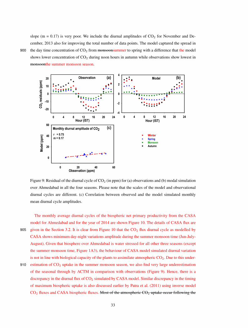
slope (m = 0.17) is very poor. We include the diurnal amplitudes of CO2 for November and De-

cember, 2013 also for improving the total number of data points. The model captured the spread in

the day time concentration of CO2 from monsoonsummer to spring with a difference that the model900

shows lower concentration of CO2 during noon hours in autumn while observations show lowest in

monsoonthe summer monsoon season.

Figure 9: Residual of the diurnal cycle of CO2 (in ppm) for (a) observations and (b) modal simulation

over Ahmedabad in all the four seasons. Please note that the scales of the model and observational

diurnal cycles are different. (c) Correlation between observed and the model simulated monthly

mean diurnal cycle amplitudes.

The monthly average diurnal cycles of the biospheric net primary productivity from the CASA

model for Ahmedabad and for the year of 2014 are shown Figure 10. The details of CASA flux are

given in the Section 3.2. It is clear from Figure 10 that the CO2 flux diurnal cycle as modelled by905

CASA shows minimum day-night variations amplitude during the summer monsoon time (Jun-July-

August). Given that biosphere over Ahmedabad is water stressed for all other three seasons (except

the summer monsoon time, Figure 1A3), the behaviour of CASA model simulated diurnal variation

is not in line with biological capacity of the plants to assimilate atmospheric CO2. Due to this under-

estimation of CO2 uptake in the summer monsoon season, we also find very large underestimation910

of the seasonal through by ACTM in comparison with observations (Figure 9). Hence, there is a

discrepancy in the diurnal flux of CO2 simulated by CASA model. Similar discrepancy in the timing

of maximum biospheric uptake is also discussed earlier by Patra et al. (2011) using inverse model

CO2 fluxes and CASA biospheric fluxes. Most of the atmospheric CO2 uptake occur following the

33

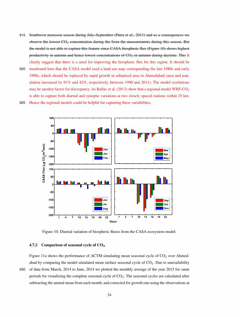
Southwest monsoon season during July–September (Patra et al., 2011) and as a consequences we915

observe the lowest CO2 concentration during the from the measurements during this season. But

the model is not able to capture this feature since CASA biospheric flux (Figure 10) shows highest

productivity in autumn and hence lowest concentrations of CO2 in autumn during daytime. This It

clearly suggest that there is a need for improving the biospheric flux for this region. It should be

mentioned here that the CASA model used a land use map corresponding the late 1980s and early920

1990s, which should be replaced by rapid growth in urbanised area in Ahmedabad (area and pop-

ulation increased by 91% and 42%, respectively, between 1990 and 2011). The model resolutions

may be another factor for discrepancy. As Ballav et al. (2012) show that a regional model WRF-CO2

is able to capture both diurnal and synoptic variations at two closely spaced stations within 25 km.

Hence the regional models could be helpful for capturing these variabilities.925

Figure 10: Diurnal variation of biospheric fluxes from the CASA ecosystem model.

4.7.2 Comparison of seasonal cycle of CO2

Figure 11a shows the performance of ACTM simulating mean seasonal cycle of CO2 over Ahmed-

abad by comparing the model simulated mean surface seasonal cycle of CO2. Due to unavailability

of data from March, 2014 to June, 2014 we plotted the monthly average of the year 2015 for same930

periods for visualizing the complete seasonal cycle of CO2. The seasonal cycles are calculated after

subtracting the annual mean from each month, and corrected for growth rate using the observations at

34

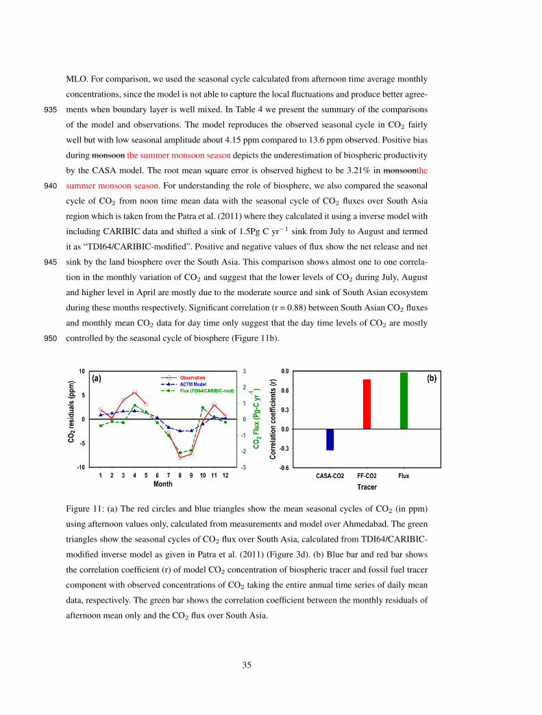
MLO. For comparison, we used the seasonal cycle calculated from afternoon time average monthly

concentrations, since the model is not able to capture the local fluctuations and produce better agree-

ments when boundary layer is well mixed. In Table 4 we present the summary of the comparisons935

of the model and observations. The model reproduces the observed seasonal cycle in CO2 fairly

well but with low seasonal amplitude about 4.15 ppm compared to 13.6 ppm observed. Positive bias

during monsoon the summer monsoon season depicts the underestimation of biospheric productivity

by the CASA model. The root mean square error is observed highest to be 3.21% in monsoonthe

summer monsoon season. For understanding the role of biosphere, we also compared the seasonal940

cycle of CO2 from noon time mean data with the seasonal cycle of CO2 fluxes over South Asia

region which is taken from the Patra et al. (2011) where they calculated it using a inverse model with

including CARIBIC data and shifted a sink of 1.5Pg C yr−1 sink from July to August and termed

it as “TDI64/CARIBIC-modified”. Positive and negative values of flux show the net release and net

sink by the land biosphere over the South Asia. This comparison shows almost one to one correla-945

tion in the monthly variation of CO2 and suggest that the lower levels of CO2 during July, August

and higher level in April are mostly due to the moderate source and sink of South Asian ecosystem

during these months respectively. Significant correlation (r = 0.88) between South Asian CO2 fluxes

and monthly mean CO2 data for day time only suggest that the day time levels of CO2 are mostly

controlled by the seasonal cycle of biosphere (Figure 11b).950

Figure 11: (a) The red circles and blue triangles show the mean seasonal cycles of CO2 (in ppm)

using afternoon values only, calculated from measurements and model over Ahmedabad. The green

triangles show the seasonal cycles of CO2 flux over South Asia, calculated from TDI64/CARIBIC-

modified inverse model as given in Patra et al. (2011) (Figure 3d). (b) Blue bar and red bar shows

the correlation coefficient (r) of model CO2 concentration of biospheric tracer and fossil fuel tracer

component with observed concentrations of CO2 taking the entire annual time series of daily mean

data, respectively. The green bar shows the correlation coefficient between the monthly residuals of

afternoon mean only and the CO2 flux over South Asia.

35

Separate correlations of each CO2 tracer with the observations are helpful to determine relative

importance of each flux component in the CO2 variation (Patra et al., 2008). Hence, we perform

separate correlation study between the measurements and biospheric, anthropogenic and oceanic

component of CO2, estimated by model using CASA-3hr fluxes (Randerson et al., 1997; Olsen and955

Randerson, 2004), EDGAR v4.2 inventory and air-sea fluxes from Takahashi et al. (2009) respec-

tively. The correlation coefficient give the hint about dominating controlling factors of deriving the

levels of CO2. Separate correlation between individual tracers of model and observed data has been

studied to investigate the relative contribution of individual tracer component in the CO2 variation

(Figure 11b shows the resulting correlations for separate flux component with respect to measure-960

ments. We did not include the oceanic tracer and observed CO2 correlation result, since no correla-

tion has been observed between them. The comparison is based on daily mean of entire time series.

Correlation between biospheric tracers and observed CO2 have been found negative. This is because

during growing season biospheric sources act as a net sink for CO2. Correlation of observed CO2

with fossil fuel tracer has been observed fairly well (r = 0.75). Hence, individual tracers correlation965

study also give the evidence of the overall dominance of fossil flux in overall concentrations of CO2

over Ahmedabad for entire study period, and by assuming fossil fuel CO2 emission we can derive

meaningful information on biospheric uptake cycle.

Table 4: Performance matrices used to quantify the level of agreement between the model simula-

tions and observations. These statistics are based on hourly values in each day.

Parameter Winter Autumn MonsoonSummer All months

MB (ppm) -2.72 12.64 -2.45 2.27

FGE (%) 0.96 3.12 2.0 1.76

RMSE (ppm) 5.21 12.82 9.14 8.60

RMSE (%) 1.27 3.21 2.20 2.09

This study suggest that the model is able to capture seasonal cycle with lower amplitude for970

Ahmedabad. However, the model fails to capture the diurnal variability since local transport and

hourly daily flux play important roles for governing the diurnal cycle and hence there is a need for

improving these features of the model.

5 Conclusions

We report simultaneous in-situ measurements of CO2 and CO concentrations in the ambient air at975

Ahmedabad, a semiarid urban region in western India using laser based CRDS technique during

2013-2015. Atmospheric concentrations of CO2 were measured along with an anthropogenic tracer

36

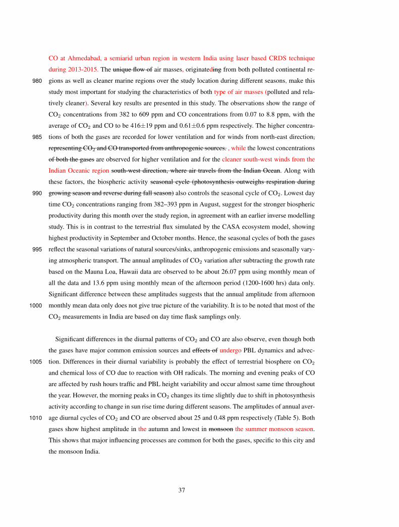
CO at Ahmedabad, a semiarid urban region in western India using laser based CRDS technique

during 2013-2015. The unique flow of air masses, originateding from both polluted continental re-

gions as well as cleaner marine regions over the study location during different seasons, make this980

study most important for studying the characteristics of both type of air masses (polluted and rela-

tively cleaner). Several key results are presented in this study. The observations show the range of

CO2 concentrations from 382 to 609 ppm and CO concentrations from 0.07 to 8.8 ppm, with the

average of CO2 and CO to be 416±19 ppm and 0.61±0.6 ppm respectively. The higher concentra-

tions of both the gases are recorded for lower ventilation and for winds from north-east direction,985

representing CO2 and CO transported from anthropogenic sources. , while the lowest concentrations

of both the gases are observed for higher ventilation and for the cleaner south-west winds from the

Indian Oceanic region south-west direction, where air travels from the Indian Ocean. Along with

these factors, the biospheric activity seasonal cycle (photosynthesis outweighs respiration during

growing season and reverse during fall season) also controls the seasonal cycle of CO2. Lowest day990

time CO2 concentrations ranging from 382–393 ppm in August, suggest for the stronger biospheric

productivity during this month over the study region, in agreement with an earlier inverse modelling

study. This is in contrast to the terrestrial flux simulated by the CASA ecosystem model, showing

highest productivity in September and October months. Hence, the seasonal cycles of both the gases

reflect the seasonal variations of natural sources/sinks, anthropogenic emissions and seasonally vary-995

ing atmospheric transport. The annual amplitudes of CO2 variation after subtracting the growth rate

based on the Mauna Loa, Hawaii data are observed to be about 26.07 ppm using monthly mean of

all the data and 13.6 ppm using monthly mean of the afternoon period (1200-1600 hrs) data only.

Significant difference between these amplitudes suggests that the annual amplitude from afternoon

monthly mean data only does not give true picture of the variability. It is to be noted that most of the1000

CO2 measurements in India are based on day time flask samplings only.

Significant differences in the diurnal patterns of CO2 and CO are also observe, even though both

the gases have major common emission sources and effects of undergo PBL dynamics and advec-

tion. Differences in their diurnal variability is probably the effect of terrestrial biosphere on CO21005

and chemical loss of CO due to reaction with OH radicals. The morning and evening peaks of CO

are affected by rush hours traffic and PBL height variability and occur almost same time throughout

the year. However, the morning peaks in CO2 changes its time slightly due to shift in photosynthesis

activity according to change in sun rise time during different seasons. The amplitudes of annual aver-

age diurnal cycles of CO2 and CO are observed about 25 and 0.48 ppm respectively (Table 5). Both1010

gases show highest amplitude in the autumn and lowest in monsoon the summer monsoon season.

This shows that major influencing processes are common for both the gases, specific to this city and

the monsoon India.

37

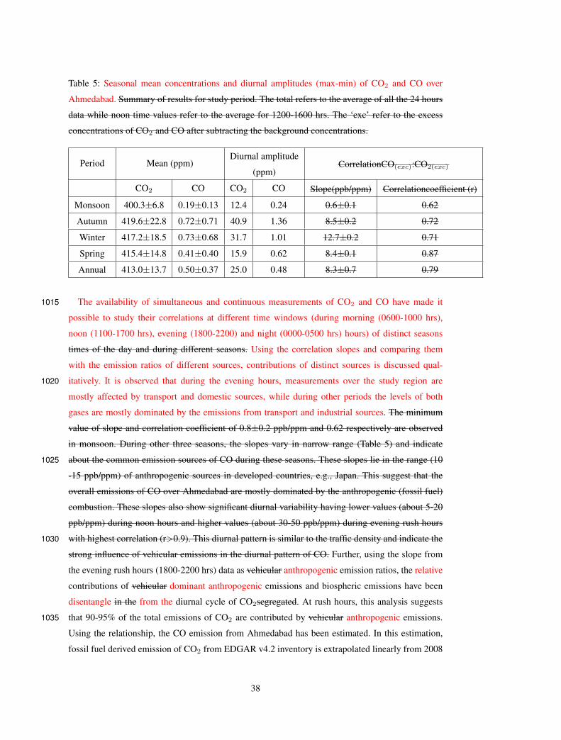
Table 5: Seasonal mean concentrations and diurnal amplitudes (max-min) of CO2 and CO over

Ahmedabad. Summary of results for study period. The total refers to the average of all the 24 hours

data while noon time values refer to the average for 1200-1600 hrs. The ‘exc’ refer to the excess

concentrations of CO2 and CO after subtracting the background concentrations.

Period Mean (ppm)Diurnal amplitude

(ppm)CorrelationCO(exc):CO2(exc)

CO2 CO CO2 CO Slope(ppb/ppm) Correlationcoefficient (r)

Monsoon 400.3±6.8 0.19±0.13 12.4 0.24 0.6±0.1 0.62

Autumn 419.6±22.8 0.72±0.71 40.9 1.36 8.5±0.2 0.72

Winter 417.2±18.5 0.73±0.68 31.7 1.01 12.7±0.2 0.71

Spring 415.4±14.8 0.41±0.40 15.9 0.62 8.4±0.1 0.87

Annual 413.0±13.7 0.50±0.37 25.0 0.48 8.3±0.7 0.79

The availability of simultaneous and continuous measurements of CO2 and CO have made it1015

possible to study their correlations at different time windows (during morning (0600-1000 hrs),

noon (1100-1700 hrs), evening (1800-2200) and night (0000-0500 hrs) hours) of distinct seasons

times of the day and during different seasons. Using the correlation slopes and comparing them

with the emission ratios of different sources, contributions of distinct sources is discussed qual-

itatively. It is observed that during the evening hours, measurements over the study region are1020

mostly affected by transport and domestic sources, while during other periods the levels of both

gases are mostly dominated by the emissions from transport and industrial sources. The minimum

value of slope and correlation coefficient of 0.8±0.2 ppb/ppm and 0.62 respectively are observed

in monsoon. During other three seasons, the slopes vary in narrow range (Table 5) and indicate

about the common emission sources of CO during these seasons. These slopes lie in the range (101025

-15 ppb/ppm) of anthropogenic sources in developed countries, e.g., Japan. This suggest that the

overall emissions of CO over Ahmedabad are mostly dominated by the anthropogenic (fossil fuel)

combustion. These slopes also show significant diurnal variability having lower values (about 5-20

ppb/ppm) during noon hours and higher values (about 30-50 ppb/ppm) during evening rush hours

with highest correlation (r>0.9). This diurnal pattern is similar to the traffic density and indicate the1030

strong influence of vehicular emissions in the diurnal pattern of CO. Further, using the slope from

the evening rush hours (1800-2200 hrs) data as vehicular anthropogenic emission ratios, the relative

contributions of vehicular dominant anthropogenic emissions and biospheric emissions have been

disentangle in the from the diurnal cycle of CO2segregated. At rush hours, this analysis suggests

that 90-95% of the total emissions of CO2 are contributed by vehicular anthropogenic emissions.1035

Using the relationship, the CO emission from Ahmedabad has been estimated. In this estimation,

fossil fuel derived emission of CO2 from EDGAR v4.2 inventory is extrapolated linearly from 2008

38

to 2014 and it is assumed that there are no year-to-year variations in the land biotic and oceanic CO2

emissions. The estimated annual emission CO for Ahmedabad is estimated to be 69.2±0.7 Gg for

the year of 2014. The extrapolated CO emission from EDGAR inventory for 2014 shows a value1040

smaller than this estimate by about 52%.

The observed results of CO2 are also compared with an atmospheric general circulation model

based chemistry transport model simulated CO2 concentrations. The model captures some basic fea-

tures like the trend of diurnal amplitude, seasonal amplitude etc, qualitatively but not quantitatively.1045

The model captures the seasonal cycle fairly good but the amplitude is very less as compared to the

observations. Similarly, performance of the model capturing the change in monthly averaged diurnal

amplitude is quiet good (r = 0.72), however the slope is very poor. We also examined the correla-

tion between the hourly averaged observed CO2 and tracer of fossil fuel from model simulation and

found fairly good correlation between them. However, no significant correlation has been observed1050

between observed CO2 and biospheric tracer. It suggests that the levels of CO2 over Ahmedabad are

mostly controlled by the fossil fuel combustion throughout the year.

This work demonstrate the usefulness of simultaneous measurements of CO2 and CO in an urban

region. The anthropogenic and biospheric component of CO2 have been studied from its temporally1055

varying atmospheric concentrations, and validity of “bottom-up” inventory have been assessed inde-

pendently. Use of CO(exc):CO2(exc) ratios avoid some of the problems with assumptions that have

to be made with modelling. These results represent a major urban region of India and will be helpful

in validating emission inventories, chemistry-transport and terrestrial ecosystem models. However,

a bigger network of sites is needed to elucidate more accurate distribution of emissions and their1060

source regions, and run continuously over multiple years for tracking the changes associated with

anthropogenic activities and emission mitigation policies.

Acknowledgements. We thank PRL and ISROGBP-ATCTM for funding and support. We acknowledge the

support of Mr. T.K. Sunil Kumar in making the measurements. We thank the reviewers for their exhaustive

comments and detailed suggestions in getting the MS to its present form. We thank the editor for his support1065

throughout the review process.

39

References

Ahmadov, R., Gerbig, C., Kretschmer, R., Koerner, S., Neininger, B., Dolman, A. J., and Sarrat, C.:

Mesoscale covariance of transport and CO2 fluxes: Evidence from observations and simulations using the

WRF-VPRM coupled atmosphere-biosphere model, Journal of Geophysical Research: Atmospheres, 112,1070

doi:10.1029/2007JD008552, d22107, 2007.

Ammoura, L., Xueref-Remy, I., Gros, V., Baudic, A., Bonsang, B., Petit, J.-E., Perrussel, O., Bonnaire, N.,

Sciare, J., and Chevallier, F.: Atmospheric measurements of ratios between CO2 and co-emitted species

from traffic: a tunnel study in the Paris megacity, Atmospheric Chemistry and Physics, 14, 12 871–12 882,

doi:10.5194/acp-14-12871-2014, 2014.1075

Andreae, M. O. and Merlet, P.: Emission of trace gases and aerosols from biomass burning, Global Biogeo-

chemical Cycles, 15, 955–966, doi:10.1029/2000GB001382, 2001.

Baker, A. K., Schuck, T. J., Brenninkmeijer, C. A. M., Rauthe-Schöch, A., Slemr, F., van Velthoven, P. F. J., and

Lelieveld, J.: Estimating the contribution of monsoon-related biogenic production to methane emissions from

South Asia using CARIBIC observations, Geophysical Research Letters, 39, doi:10.1029/2012GL051756,1080

l10813, 2012.

Ballav, S., PATRA, P. K., TAKIGAWA, M., GHOSH, S., DE, U. K., MAKSYUTOV, S., MURAYAMA,

S., MUKAI, H., and HASHIMOTO, S.: Simulation of CO2 Concentration over East Asia Using the Re-

gional Transport Model WRF-CO2, Journal of the Meteorological Society of Japan. Ser. I, 90, 959–976,

doi:10.2151/jmsj.2012-607, 2012.1085

Ballav, S., Patra, P. K., Sawa, Y., Matsueda, H., Adachi, A., Onogi, S., Takigawa, M., and De, U.: Simulation

of CO2 concentrations at Tsukuba tall tower using WRF−CO2 tracer transport model, J. Earth System Sci.,

in press, 2015.

Bhattacharya, S. K., Borole, D. V., Francey, R. J., Allison, C. E., Steele, L. P., Krummel, P., Langenfelds, R.,

Masarie, K. A., Tiwari, Y. K., and Patra, P.: Trace gases and CO2 isotope records from Cabo de Rama, India,1090

Current Science, 97, 2009.

Bitter, M., Ball, S. M., Povey, I. M., and Jones, R. L.: A broadband cavity ringdown spectrometer for in-situ mea-

surements of atmospheric trace gases, Atmospheric Chemistry and Physics, 5, 2547–2560, doi:10.5194/acp-

5-2547-2005, 2005.

Briber, B. M., Hutyra, L. R., Dunn, A. L., Raciti, S. M., and Munger, J. W.: Variations in Atmospheric CO21095

Mixing Ratios across a Boston, MA Urban to Rural Gradient, Land, 2, 304, doi:10.3390/land2030304, 2013.

CAO, G., ZHANG, X., GONG, S., and ZHENG, F.: Investigation on emission factors of particulate mat-

ter and gaseous pollutants from crop residue burning, Journal of Environmental Sciences, 20, 50 – 55,

doi:http://dx.doi.org/10.1016/S1001-0742(08)60007-8, 2008.

Chen, H., Winderlich, J., Gerbig, C., Hoefer, A., Rella, C. W., Crosson, E. R., Van Pelt, A. D., Steinbach,1100

J., Kolle, O., Beck, V., Daube, B. C., Gottlieb, E. W., Chow, V. Y., Santoni, G. W., and Wofsy, S. C.: High-

accuracy continuous airborne measurements of greenhouse gases (CO2 and CH4) using the cavity ring-down

spectroscopy (CRDS) technique, Atmospheric Measurement Techniques, 3, 375–386, doi:10.5194/amt-3-

375-2010, 2010.

Ciais, P., Sabine, C., Bala, G., Bopp, L., Brovkin, V., Canadell, J., Chhabra, A., DeFries, R., Galloway, J.,1105

Heimann, M., Jones, C., Quere, C., Myneni, R., Piao, S., and Thornton, P.: Carbon and Other Biogeochemical

40

Cycles, book section 6, p. 465–570, Cambridge University Press, Cambridge, United Kingdom and New

York, NY, USA, doi:10.1017/CBO9781107415324.015, 2013.

Crosson, E.: A cavity ring-down analyzer for measuring atmospheric levels of methane, carbon dioxide, and

water vapor, Applied Physics B, 92, 403–408, doi:10.1007/s00340-008-3135-y, 2008.1110

Dhammapala, R., Claiborn, C., Simpson, C., and Jimenez, J.: Emission factors from wheat and Kentucky blue-

grass stubble burning: Comparison of field and simulated burn experiments, Atmospheric Environment, 41,

1512 – 1520, doi:http://dx.doi.org/10.1016/j.atmosenv.2006.10.008, 2007.

Duren, R. M. and Miller, C. E.: Measuring the carbon emissions of megacities, Nature Clim. Change, 2, 560–

562, doi:http://dx.doi.org/10.1038/nclimate1629, 2012.1115

Kar, J., Bremer, H., Drummond, J. R., Rochon, Y. J., Jones, D. B. A., Nichitiu, F., Zou, J., Liu, J., Gille, J. C.,

Edwards, D. P., Deeter, M. N., Francis, G., Ziskin, D., and Warner, J.: Evidence of vertical transport of carbon

monoxide from Measurements of Pollution in the Troposphere (MOPITT), Geophysical Research Letters,

31, doi:10.1029/2004GL021128, 2004.

Karion, A., Sweeney, C., Wolter, S., Newberger, T., Chen, H., Andrews, A., Kofler, J., Neff, D., and Tans, P.:1120

Long-term greenhouse gas measurements from aircraft, Atmospheric Measurement Techniques, 6, 511–526,

doi:10.5194/amt-6-511-2013, 2013.

Lai, S. C., Baker, A. K., Schuck, T. J., van Velthoven, P., Oram, D. E., Zahn, A., Hermann, M., Weigelt, A.,

Slemr, F., Brenninkmeijer, C. A. M., and Ziereis, H.: Pollution events observed during CARIBIC flights in

the upper troposphere between South China and the Philippines, Atmospheric Chemistry and Physics, 10,1125

1649–1660, doi:10.5194/acp-10-1649-2010, 2010.

Lal, S., Naja, M., and Subbaraya, B.: Seasonal variations in surface ozone and its precursors over an urban site in

India, Atmospheric Environment, 34, 2713 – 2724, doi:http://dx.doi.org/10.1016/S1352-2310(99)00510-5,

2000.

Lal, S., Chandra, N., and Venkataramani, S.: A study of CO2 and related trace gases using a laser based tech-1130

nique at an urban site in western India., Current Science, 109, 2015.

Law, R. M., Peters, W., Rödenbeck, C., Aulagnier, C., Baker, I., Bergmann, D. J., Bousquet, P., Brandt, J., Bruh-

wiler, L., Cameron-Smith, P. J., Christensen, J. H., Delage, F., Denning, A. S., Fan, S., Geels, C., Houweling,

S., Imasu, R., Karstens, U., Kawa, S. R., Kleist, J., Krol, M. C., Lin, S.-J., Lokupitiya, R., Maki, T., Maksyu-

tov, S., Niwa, Y., Onishi, R., Parazoo, N., Patra, P. K., Pieterse, G., Rivier, L., Satoh, M., Serrar, S., Taguchi,1135

S., Takigawa, M., Vautard, R., Vermeulen, A. T., and Zhu, Z.: TransCom model simulations of hourly atmo-

spheric CO2: Experimental overview and diurnal cycle results for 2002, Global Biogeochemical Cycles, 22,

doi:10.1029/2007GB003050, gB3009, 2008.

Le Quéré, C., Moriarty, R., Andrew, R. M., Peters, G. P., Ciais, P., Friedlingstein, P., Jones, S. D., Sitch, S.,

Tans, P., Arneth, A., Boden, T. A., Bopp, L., Bozec, Y., Canadell, J. G., Chevallier, F., Cosca, C. E., Harris,1140

I., Hoppema, M., Houghton, R. A., House, J. I., Jain, A., Johannessen, T., Kato, E., Keeling, R. F., Kitidis,

V., Klein Goldewijk, K., Koven, C., Landa, C. S., Landschützer, P., Lenton, A., Lima, I. D., Marland, G.,

Mathis, J. T., Metzl, N., Nojiri, Y., Olsen, A., Ono, T., Peters, W., Pfeil, B., Poulter, B., Raupach, M. R.,

Regnier, P., Rödenbeck, C., Saito, S., Salisbury, J. E., Schuster, U., Schwinger, J., Séférian, R., Segschneider,

J., Steinhoff, T., Stocker, B. D., Sutton, A. J., Takahashi, T., Tilbrook, B., van der Werf, G. R., Viovy, N.,1145

41

Wang, Y.-P., Wanninkhof, R., Wiltshire, A., and Zeng, N.: Global carbon budget 2014, Earth System Science

Data Discussions, 7, 521–610, doi:10.5194/essdd-7-521-2014, 2014.

Levin, I., Kromer, B., Schmidt, M., and Sartorius, H.: A novel approach for independent budgeting of fossil fuel

CO2 over Europe by 14CO2 observations, Geophysical Research Letters, 30, doi:10.1029/2003GL018477,

2194, 2003.1150

Lin, X., Indira, N. K., Ramonet, M., Delmotte, M., Ciais, P., Bhatt, B. C., Reddy, M. V., Angchuk, D., Balakr-

ishnan, S., Jorphail, S., Dorjai, T., Mahey, T. T., Patnaik, S., Begum, M., Brenninkmeijer, C., Durairaj, S.,

Kirubagaran, R., Schmidt, M., Swathi, P. S., Vinithkumar, N. V., Yver Kwok, C., and Gaur, V. K.: Long-lived

atmospheric trace gases measurements in flask samples from three stations in India, Atmospheric Chemistry

and Physics, 15, 9819–9849, doi:10.5194/acp-15-9819-2015, 2015.1155

Lopez, M., Schmidt, M., Delmotte, M., Colomb, A., Gros, V., Janssen, C., Lehman, S. J., Mondelain, D.,

Perrussel, O., Ramonet, M., Xueref-Remy, I., and Bousquet, P.: CO, NOx and 13CO2 as tracers for fossil

fuel CO2: results from a pilot study in Paris during winter 2010, Atmospheric Chemistry and Physics, 13,

7343–7358, doi:10.5194/acp-13-7343-2013, 2013.

Machida, T., Matsueda, H., Sawa, Y., Nakagawa, Y., Hirotani, K., Kondo, N., Goto, K., Nakazawa, T., Ishikawa,1160

K., and Ogawa, T.: Worldwide Measurements of Atmospheric CO2 and Other Trace Gas Species Using

Commercial Airlines, J. Atmos. Oceanic Technol., 25, 1744–1754, doi:10.1175/2008JTECHA1082.1, 2008.

Mahesh, P., Sharma, N., Dadhwal, V., Rao, P., Apparao, B., Ghosh, A., Mallikarjun, K., and Ali, M.: Impact of

Land-Sea Breeze and Rainfall on CO2 Variations at a Coastal Station, Journal of Earth Science and Climatic

Change, 5, –, doi:10.4172/2157-7617.1000201, 2014.1165

Mallik, C., Lal, S., and Venkataramani, S.: Trace gases at a semi-arid urban site in western India: variability and

inter-correlations, Journal of Atmospheric Chemistry, pp. 1–22, doi:10.1007/s10874-015-9311-7, 2015.

Mallik, C., Chandra, N., Venkataramani, S., and Lal, S.: Variability of atmospheric carbonyl sulfide at

a semi-arid urban site in western India, Science of The Total Environment, 551–552, 725 – 737,

doi:http://dx.doi.org/10.1016/j.scitotenv.2016.02.014, 2016.1170

Newman, S., Jeong, S., Fischer, M. L., Xu, X., Haman, C. L., Lefer, B., Alvarez, S., Rappenglueck, B., Kort,

E. A., Andrews, A. E., Peischl, J., Gurney, K. R., Miller, C. E., and Yung, Y. L.: Diurnal tracking of anthro-

pogenic CO2 emissions in the Los Angeles basin megacity during spring 2010, Atmospheric Chemistry and

Physics, 13, 4359–4372, doi:10.5194/acp-13-4359-2013, http://www.atmos-chem-phys.net/13/4359/2013/,

2013.1175

Olsen, S. C. and Randerson, J. T.: Differences between surface and column atmospheric CO2 and implications

for carbon cycle research, Journal of Geophysical Research: Atmospheres, 109, doi:10.1029/2003JD003968,

http://dx.doi.org/10.1029/2003JD003968, d02301, 2004.

Onogi, K., Tsutsui, J., Koide, H., Sakamoto, M., Kobayashi, S., Hatsushika, H., Matsumoto, T., Yamazaki,

N., Kamahori, H., Takahashi, K., Kadokura, S., Wada, K., Kato, K., Oyama, R., Ose, T., Mannoji, N., and1180

Taira, R.: The JRA-25 Reanalysis, Journal of the Meteorological Society of Japan. Ser. II, 85, 369–432,

doi:10.2151/jmsj.85.369, 2007.

Park, M., Randel, W. J., Emmons, L. K., and Livesey, N. J.: Transport pathways of carbon monoxide in the Asian

summer monsoon diagnosed from Model of Ozone and Related Tracers (MOZART), Journal of Geophysical

Research: Atmospheres, 114, doi:10.1029/2008JD010621, 2009.1185

42

Patra, P. K., Law, R. M., Peters, W., Rödenbeck, C., Takigawa, M., Aulagnier, C., Baker, I., Bergmann, D. J.,

Bousquet, P., Brandt, J., Bruhwiler, L., Cameron-Smith, P. J., Christensen, J. H., Delage, F., Denning, A. S.,

Fan, S., Geels, C., Houweling, S., Imasu, R., Karstens, U., Kawa, S. R., Kleist, J., Krol, M. C., Lin, S.-J.,

Lokupitiya, R., Maki, T., Maksyutov, S., Niwa, Y., Onishi, R., Parazoo, N., Pieterse, G., Rivier, L., Satoh, M.,

Serrar, S., Taguchi, S., Vautard, R., Vermeulen, A. T., and Zhu, Z.: TransCom model simulations of hourly1190

atmospheric CO2: Analysis of synoptic-scale variations for the period 2002–2003, Global Biogeochemical

Cycles, 22, doi:10.1029/2007GB003081, gB4013, 2008.

Patra, P. K., Niwa, Y., Schuck, T. J., Brenninkmeijer, C. A. M., Machida, T., Matsueda, H., and Sawa, Y.: Carbon

balance of South Asia constrained by passenger aircraft CO2 measurements, Atmospheric Chemistry and

Physics, 11, 4163–4175, doi:10.5194/acp-11-4163-2011, 2011.1195

Patra, P. K., Canadell, J. G., Houghton, R. A., Piao, S. L., Oh, N.-H., Ciais, P., Manjunath, K. R., Chhabra, A.,

Wang, T., Bhattacharya, T., Bousquet, P., Hartman, J., Ito, A., Mayorga, E., Niwa, Y., Raymond, P. A., Sarma,

V. V. S. S., and Lasco, R.: The carbon budget of South Asia, Biogeosciences, 10, 513–527, doi:10.5194/bg-

10-513-2013, 2013.

Pérez-Landa, G., Ciais, P., Gangoiti, G., Palau, J. L., Carrara, A., Gioli, B., Miglietta, F., Schumacher, M.,1200

Millán, M. M., and Sanz, M. J.: Mesoscale circulations over complex terrain in the Valencia coastal region,

Spain - Part 2 : Modeling CO2 transport using idealized surface fluxes, Atmospheric Chemistry and Physics,

7, 1851–1868, doi:10.5194/acp-7-1851-2007, 2007.

Peylin, P., Law, R. M., Gurney, K. R., Chevallier, F., Jacobson, A. R., Maki, T., Niwa, Y., Patra, P. K., Peters, W.,

Rayner, P. J., Rödenbeck, C., van der Laan-Luijkx, I. T., and Zhang, X.: Global atmospheric carbon budget:1205

results from an ensemble of atmospheric CO2 inversions, Biogeosciences, 10, 6699–6720, doi:10.5194/bg-

10-6699-2013, 2013.

Randel, W. J. and Park, M.: Deep convective influence on the Asian summer monsoon anticyclone and asso-

ciated tracer variability observed with Atmospheric Infrared Sounder (AIRS), Journal of Geophysical Re-

search: Atmospheres, 111, doi:10.1029/2005JD006490, 2006.1210

Randerson, J. T., Thompson, M. V., Conway, T. J., Fung, I. Y., and Field, C. B.: The contribution of terrestrial

sources and sinks to trends in the seasonal cycle of atmospheric carbon dioxide, Global Biogeochemical

Cycles, 11, 535–560, doi:10.1029/97GB02268, 1997.

Russo, R. S., Talbot, R. W., Dibb, J. E., Scheuer, E., Seid, G., Jordan, C. E., Fuelberg, H. E., Sachse, G. W.,

Avery, M. A., Vay, S. A., Blake, D. R., Blake, N. J., Atlas, E., Fried, A., Sandholm, S. T., Tan, D., Singh,1215

H. B., Snow, J., and Heikes, B. G.: Chemical composition of Asian continental outflow over the western

Pacific: Results from Transport and Chemical Evolution over the Pacific (TRACE-P), Journal of Geophysical

Research: Atmospheres, 108, doi:10.1029/2002JD003184, 2003.

Sahu, L. and Lal, S.: Distributions of C2–C5 {NMHCs} and related trace gases at a tropical urban site in India,

Atmospheric Environment, 40, 880 – 891, doi:http://dx.doi.org/10.1016/j.atmosenv.2005.10.021, 2006.1220

Sahu, S., Beig, G., and Parkhi, N.: High Resolution Emission Inventory of NOx and CO for Mega City Delhi,

India, Aerosol and Air Quality Research, 15, 1137–1144, doi:10.4209/aaqr.2014.07.0132, 2015.

Schuck, T. J., Brenninkmeijer, C. A. M., Baker, A. K., Slemr, F., von Velthoven, P. F. J., and Zahn, A.: Green-

house gas relationships in the Indian summer monsoon plume measured by the CARIBIC passenger aircraft,

Atmospheric Chemistry and Physics, 10, 3965–3984, doi:10.5194/acp-10-3965-2010, 2010.1225

43

Schuck, T. J., Ishijima, K., Patra, P. K., Baker, A. K., Machida, T., Matsueda, H., Sawa, Y., Umezawa, T.,

Brenninkmeijer, C. A. M., and Lelieveld, J.: Distribution of methane in the tropical upper troposphere

measured by CARIBIC and CONTRAIL aircraft, Journal of Geophysical Research: Atmospheres, 117,

doi:10.1029/2012JD018199, d19304, 2012.

Sharma, N., Dadhwal, V., Kant, Y., Mahesh, P., Mallikarjun, K., Gadavi, H., Sharma, A., and Ali, M.: Atmo-1230

spheric CO2 Variations in Two Contrasting Environmental Sites Over India, Air, Soil and Water Research,

7, 61–68, doi:10.4137/ASWR.S13987, 2014.

Streets, D. G., Bond, T. C., Carmichael, G. R., Fernandes, S. D., Fu, Q., He, D., Klimont, Z., Nelson, S. M., Tsai,

N. Y., Wang, M. Q., Woo, J.-H., and Yarber, K. F.: An inventory of gaseous and primary aerosol emissions

in Asia in the year 2000, Journal of Geophysical Research: Atmospheres, 108, doi:10.1029/2002JD003093,1235

2003.

Suntharalingam, P., Jacob, D. J., Palmer, P. I., Logan, J. A., Yantosca, R. M., Xiao, Y., Evans, M. J., Streets,

D. G., Vay, S. L., and Sachse, G. W.: Improved quantification of Chinese carbon fluxes using CO2/CO corre-

lations in Asian outflow, Journal of Geophysical Research: Atmospheres, 109, doi:10.1029/2003JD004362,

2004.1240

Sánchez-Ccoyllo, O., Ynoue, R., Martins, L., Astolfo, R., Miranda, R., Freitas, E., Borges, A., Fornaro, A.,

Freitas, H., Moreira, A., and Andrade, M.: Vehicular particulate matter emissions in road tunnels in Sao

Paulo, Brazil, Environmental Monitoring and Assessment, 149, 241–249, doi:10.1007/s10661-008-0198-5,

2009.

Takahashi, T., Sutherland, S. C., Wanninkhof, R., Sweeney, C., Feely, R. A., Chipman, D. W., Hales, B.,1245

Friederich, G., Chavez, F., Sabine, C., Watson, A., Bakker, D. C., Schuster, U., Metzl, N., Yoshikawa-

Inoue, H., Ishii, M., Midorikawa, T., Nojiri, Y., Körtzinger, A., Steinhoff, T., Hoppema, M., Olafsson, J.,

Arnarson, T. S., Tilbrook, B., Johannessen, T., Olsen, A., Bellerby, R., Wong, C., Delille, B., Bates, N., and

de Baar, H. J.: Climatological mean and decadal change in surface ocean pCO2, and net sea–air {CO2}

flux over the global oceans, Deep Sea Research Part II: Topical Studies in Oceanography, 56, 554 – 577,1250

doi:http://dx.doi.org/10.1016/j.dsr2.2008.12.009, 2009.

Takegawa, N., Kondo, Y., Koike, M., Chen, G., Machida, T., Watai, T., Blake, D. R., Streets, D. G., Woo, J.-

H., Carmichael, G. R., Kita, K., Miyazaki, Y., Shirai, T., Liley, J. B., and Ogawa, T.: Removal of NOx and

NOy in Asian outflow plumes: Aircraft measurements over the western Pacific in January 2002, Journal of

Geophysical Research: Atmospheres, 109, doi:10.1029/2004JD004866, 2004.1255

Tiwari, Y. K., Vellore, R. K., Kumar, K. R., van der Schoot, M., and Cho, C.-H.: Influence of monsoons on atmo-

spheric CO2 spatial variability and ground-based monitoring over India, Science of The Total Environment,

490, 570 – 578, doi:http://dx.doi.org/10.1016/j.scitotenv.2014.05.045, 2014.

Turnbull, J. C., Miller, J. B., Lehman, S. J., Tans, P. P., Sparks, R. J., and Southon, J.: Comparison of 14CO2,

CO, and SF6 as tracers for recently added fossil fuel CO2 in the atmosphere and implications for biological1260

CO2 exchange, Geophysical Research Letters, 33, doi:10.1029/2005GL024213, 2006.

Turnbull, J. C., Karion, A., Fischer, M. L., Faloona, I., Guilderson, T., Lehman, S. J., Miller, B. R., Miller, J. B.,

Montzka, S., Sherwood, T., Saripalli, S., Sweeney, C., and Tans, P. P.: Assessment of fossil fuel carbon diox-

ide and other anthropogenic trace gas emissions from airborne measurements over Sacramento, California in

spring 2009, Atmospheric Chemistry and Physics, 11, 705–721, doi:10.5194/acp-11-705-2011, 2011.1265

44

Vogel, F. R., HAMMER, S., STEINHOF, A., KROMER, B., and LEVIN, I.: Implication of weekly and diurnal

14C calibration on hourly estimates of CO-based fossil fuel CO2 at a moderately polluted site in southwestern

Germany, Tellus B, 62, 512–520, doi:10.1111/j.1600-0889.2010.00477.x, 2010.

Wada, A., Matsueda, H., Sawa, Y., Tsuboi, K., and Okubo, S.: Seasonal variation of enhancement ratios of

trace gases observed over 10 years in the western North Pacific, Atmospheric Environment, 45, 2129 – 2137,1270

doi:http://dx.doi.org/10.1016/j.atmosenv.2011.01.043, 2011.

Wang, Y., Munger, J. W., Xu, S., McElroy, M. B., Hao, J., Nielsen, C. P., and Ma, H.: CO2 and its correlation

with CO at a rural site near Beijing: implications for combustion efficiency in China, Atmospheric Chemistry

and Physics, 10, 8881–8897, doi:10.5194/acp-10-8881-2010, 2010.

Welp, L. R., Keeling, R. F., Weiss, R. F., Paplawsky, W., and Heckman, S.: Design and performance of a Nafion1275

dryer for continuous operation at CO2 and CH4 air monitoring sites, Atmospheric Measurement Techniques,

6, 1217–1226, doi:10.5194/amt-6-1217-2013, 2013.

Westerdahl, D., Wang, X., Pan, X., and Zhang, K. M.: Characterization of on-road vehicle emission fac-

tors and microenvironmental air quality in Beijing, China, Atmospheric Environment, 43, 697 – 705,

doi:http://dx.doi.org/10.1016/j.atmosenv.2008.09.042, 2009.1280

Wong, K. W., Fu, D., Pongetti, T. J., Newman, S., Kort, E. A., Duren, R., Hsu, Y.-K., Miller, C. E., Yung,

Y. L., and Sander, S. P.: Mapping CH4: CO2 ratios in Los Angeles with CLARS-FTS from Mount Wilson,

California, Atmospheric Chemistry and Physics, 15, 241–252, doi:10.5194/acp-15-241-2015, 2015.

Wunch, D., Wennberg, P. O., Toon, G. C., Keppel-Aleks, G., and Yavin, Y. G.: Emissions of greenhouse gases

from a North American megacity, Geophysical Research Letters, 36, doi:10.1029/2009GL039825, 2009.1285

45