reliability engineering and system safety
TRANSCRIPT

Reliability Engineering and System Safety 174 (2018) 71–81
Contents lists available at ScienceDirect
Reliability Engineering and System Safety
journal homepage: www.elsevier.com/locate/ress
Reliability analysis of complex multi-state system with common cause
failure based on evidential networks
Jinhua Mi a , b , Yan-Feng Li b , ∗ , Weiwen Peng
b , Hong-Zhong Huang
b
a School of Automation Engineering, University of Electronic Science and Technology of China, No. 2006, Xiyuan Avenue, West Hi-Tech Zone, Chengdu, Sichuan
611731, China b Center for System Reliability and Safety, University of Electronic Science and Technology of China, No. 2006, Xiyuan Avenue, West Hi-Tech Zone, Chengdu, Sichuan
611731, China
a r t i c l e i n f o
Keywords:
Complex multi-state system
Evidence theory Bayesian network Common cause failure group
a b s t r a c t
With the increasing complexity and size of modern advanced engineering systems, the traditional reliability theory cannot characterize and quantify the complex characteristics of complex systems, such as multi-state properties, epistemic uncertainties, common cause failures (CCFs). This paper focuses on the reliability analysis of complex multi-state system (MSS) with epistemic uncertainty and CCFs. Based on the Bayesian network (BN) method for reliability analysis of MSS, the Dempster-Shafer (DS) evidence theory is used to express the epistemic uncertainty in system through the state space reconstruction of MSS, and an uncertain state used to express the epistemic uncertainty is introduced in the new state space. The integration of evidence theory with BN which called evidential network (EN) is achieved by adapting and updating the conditional probability tables (CPTs) into conditional mass tables (CMTs). When multiple CCF groups (CCFGs) are considered in complex redundant system, a modified 𝛽 factor parametric model is introduced to model the CCF in system. An EN method is proposed for the reliability analysis and evaluation of complex MSSs in this paper. The reliability analysis of servo feeding control system for CNC heavy-duty horizontal lathes (HDHLs) by this proposed method has shown that CCFs have considerable impact on system reliability. The presented method has high computational efficiency, and the computational accuracy is also verified.
© 2018 Elsevier Ltd. All rights reserved.
1
W
s
a
d
l
c
o
f
u
m
a
g
t
W
e
a
t
o
D
p
B
i
f
f
r
a
d
a
t
a
e
s
o
hRA0
. Introduction
The multi-state system (MSS) was firstly proposed by Barlow andu, it has been proved that lots of industrial systems belong to MSS,
uch as electrical power system, pipe transmission system, productionnd manufacturing system, aerospace system [1–3] . Those systems canefine the multi-state characteristics of components accurately by ana-yzing the system failure process and tracking the effect of the change ofomponent performance on the system reliability. There are four typesf methods used for reliability analysis of MSS, including multi-stateault tree method [4] , Markov process method [5,6] , Monte-Carlo sim-lation (MCS) method [7,8] and universal generating function (UGF)ethod [9,10] . The MSS plays a critical role in the reliability analysis
nd assessment of complex system and also has broad application fore-round.
The uncertainty caused by lack of data and scarcity of informa-ion is one of the most challenging issues in MSS reliability analysis.
hen the system state performances and state probabilities cannot bexactly defined and obtained, sometimes the bounds of system states
∗ Corresponding author. E-mail addresses: [email protected] (Y.-F. Li), [email protected] (H.-Z.
ttps://doi.org/10.1016/j.ress.2018.02.021 eceived 7 December 2016; Received in revised form 14 February 2018; Accepted 14 Februaryvailable online 16 February 2018 951-8320/© 2018 Elsevier Ltd. All rights reserved.
nd state probabilities can be expressed by some linguistic forms. Thenhe probability based methods are no longer applicable to this kindf system. Some non-probabilistic methods are developed, includingempster-Shafer evidence theory (DSET) [11] , fuzzy theory [12–15] ,robability-box [16–18] , interval theory [19] , possibility theory [20] ,ayesian method [21] , etc. The DS evidence theory has a flexible ax-
omatic system to describe uncertainty, and also has an independentrame to process uncertainty in system [22,23] . It has been widely usedor uncertainty modeling, quantification, reasoning and mitigation ineliability engineering [24–26] .
Bayesian network (BN) has been widely used in reliability and safetynalysis because of its obvious advantages in multi-state and non-eterministic fault logic description [27–29] . Evidence theory allowsn analyst to distribute the probability mass in overlapping regions ofhe sample space, which is useful when there are significant uncertaintynd conflicting evidence. There are many researches on BN based onvidence theory. Simon et al. [30,31] analyzed reliability of complexystem with epistemic uncertainty by using of BN, where evidence the-ry is used to quantify system uncertainty. Then the evidential networks
Huang).
2018
J. Mi et al. Reliability Engineering and System Safety 174 (2018) 71–81
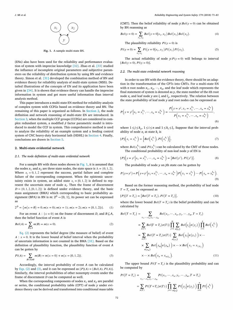
Fig. 1. A sample multi-state BN.
(
t
t
e
t
e
t
g
i
a
o
r
d
S
p
d
t
s
c
2
2
t
W
f
t
r
𝐷
m
s
a
2
t
𝐵
𝐴
o
d
c
𝑃
b
S
f
o
d
(
b
𝐵
𝑃
[
2
t
w
fi
n
t
𝑃
w
a
[
w
[
𝑃
𝑇
[
w
c
𝐵
b
𝑃
ENs) also have been used for the reliability and performance evalua-ion of system with imprecise knowledge [32] . Zhao et al. [33] studiedhe influence of incomplete original parameters and subjective param-ters on the reliability of distribution system by using BN and evidenceheory. Simon et al. [31] developed the combination method of BN andvidence theory for reliability analysis of multi-state system (MSS). De-ailed illustrations of the concepts of EN and its application have beeniven in [34] . It is shown that evidence theory can handle the imprecisenformation in system and get more useful information than intervalnalysis method.
This paper introduces a multi-state EN method for reliability analysisf complex system with CCFGs based on evidence theory and BN. Theemaining of this paper is organized as follows. In Section 2 , the nodeefinition and network reasoning of multi-state EN are introduced. Inection 3 , when the multiple CCF groups (CCFGs) are considered in com-lex redundant system, a modified 𝛽 factor parametric model is intro-uced to model the CCF in system. This comprehensive method is usedo analyze the reliability of an example system and a feeding controlystem of CNC heavy-duty horizontal lath (HDHL) in Section 4 . Finally,onclusions are drawn in Section 5 .
. Multi-state evidential network
.1. The node definition of multi-state evidential network
For a sample BN with three nodes shown in Fig. 1 , it is assumed thathe nodes x 1 and x 2 are three state nodes, the state space is Λ = {0 , 1 , 2} .
here 𝑥 𝑖 = 0 , 1 , 2 represent the success, partial failure and completeailure of the corresponding component. When the epistemic uncer-ainty exists in system, an added state 𝑥 𝑖 = [0 , 1 , 2] is defined to rep-esent the uncertain state of node x i . Then the frame of discernment = {0 , 1 , 2 , [0 , 1 , 2]} is defined under evidence theory, and the basicass assignment (BMA) which corresponding to basic probability as-
ignment (BPA) in BN is m : 2 D → [0, 1], its power set can be expresseds
𝐷 =
{𝑚
(𝑥 = ∅
)= 0; 𝑚 ( 𝑥 = 0 ) ; 𝑚 ( 𝑥 = 1 ) ; 𝑚 ( 𝑥 = 2 ) ; 𝑚 ( 𝑥 = [ 0 , 1 , 2 ] ) } . (1)
For an event 𝐴 ∶ { 𝑥 = 0} on the frame of discernment D , and B ⊆A ,hen the belief function of event A is
𝑒𝑙 ( 𝐴 ) =
∑𝐵⊆𝐴
𝑚 ( 𝐵 ) = 𝑚 ( 𝑥 = 0 ) . (2)
Eq. (2) represents the belief degree (the measure of belief) of event ∶ 𝑥 = 0 . It is the lower bound of belief interval when the probabilityf uncertain information is not counted in the BMA [31] . Based on theefinition of plausibility function, the plausibility function of event Aan be gotten by
𝑙 ( 𝐴 ) =
∑𝐵∩𝐴 ≠∅
𝑚 ( 𝐵 ) = 𝑚 { 𝑥 = 0 } + 𝑚 { 𝑥 = [ 0 , 1 , 2 ] } . (3)
Accordingly, the interval probability of event A can be calculatedy Eqs. (2) and (3) , and it can be expressed as [ 𝑃 ]( 𝐴 ) = [ 𝐵𝑒𝑙 ( 𝐴 ) , 𝑃 𝑙 ( 𝐴 )] .imilarly, the interval probabilities of other nonempty events under therame of discernment D can be computed as well.
When the corresponding components of nodes x 1 and x 2 are parallelr series, the conditional probability table (CPT) of node y under evi-ence theory can be derived and transformed into conditional mass table
72
CMT). Then the belief reliability of node y : 𝐵𝑒𝑙( 𝑦 = 0) can be obtainedy BN reasoning as
𝑒𝑙 ( 𝑦 = 0 ) =
∑𝑥 1 , 𝑥 2
𝐵 𝑒𝑙 (𝑦 = 0 ||𝑥 1 , 𝑥 2 )𝐵 𝑒𝑙
(𝑥 1 )𝐵 𝑒𝑙
(𝑥 2 ). (4)
The plausibility reliability 𝑃 𝑙( 𝑦 = 0) is
𝑙 ( 𝑦 = 0 ) =
∑𝑥 1 , 𝑥 2
𝑃 𝑙 (𝑦 = 0 ||𝑥 1 , 𝑥 2 )𝑃 𝑙 (𝑥 1 )𝑃 𝑙 (𝑥 2 ). (5)
The actual reliability of node y : 𝑃 ( 𝑦 = 0) will belongs to interval 𝐵𝑒𝑙( 𝑦 = 0) , 𝑃 𝑙( 𝑦 = 0)] .
.2. The multi-state evidential network reasoning
In order to use BN with the evidence theory, there should be an adap-ion in the transformation of the CPTs into CMTs. For a multi-state ENith n root nodes x 1 , x 2 , ⋅⋅⋅, x n , and the leaf node which represents thenal statement of system is denoted as y , the state number of the i th rootode x i and leaf node y are l i and l y , respectively. The relation betweenhe state probability of leaf node y and root nodes can be expressed as
(𝑦 = 𝑦 𝑗
|||𝑥 1 = 𝑥 𝑘 1 1 , ⋯ , 𝑥 𝑛 = 𝑥
𝑘 𝑛 𝑛
)=
𝑃 (𝑦 = 𝑦 𝑗 , 𝑥 1 = 𝑥
𝑘 1 1 , ⋯ , 𝑥 𝑛 = 𝑥
𝑘 𝑛 𝑛
)𝑃 (𝑥 1 = 𝑥
𝑘 1 1 , ⋯ , 𝑥 𝑛 = 𝑥
𝑘 𝑛 𝑛
) ,
(6)
here 1 ≤ j ≤ k y , 1 ≤ i ≤ n and 1 ≤ k i ≤ l i . Suppose that the interval prob-bility of node x i at state k i is
𝑃 ] (𝑥 𝑖 = 𝑥
𝑘 𝑖 𝑖
)=
[𝐵𝑒𝑙
(𝑥 𝑘 𝑖 𝑖
), 𝑃 𝑙
(𝑥 𝑘 𝑖 𝑖
)], (7)
here 𝐵𝑒𝑙( 𝑥 𝑘 𝑖 𝑖 ) and 𝑃 𝑙( 𝑥 𝑘 𝑖
𝑖 ) can be calculated by the CMT of those nodes.
The conditional probability of non-leaf node y of EN is
𝑃 ] (𝑦 = 𝑦 𝑗
|||𝑥 1 = 𝑥 𝑘 1 1 , ⋯ , 𝑥 𝑛 = 𝑥
𝑘 𝑛 𝑛
)=
[𝐵𝑒𝑙
(𝑦 𝑗 ), 𝑃 𝑙
(𝑦 𝑗 )]. (8)
The probability of node y on j th state can be gotten by
(𝑦 = 𝑦 𝑗
)= 𝑃
(𝑦 = 𝑦 𝑗
|||𝑥 1 = 𝑥 𝑘 1 1 , ⋯ , 𝑥 𝑛 = 𝑥
𝑘 𝑛 𝑛
)𝑃 (𝑥 1 = 𝑥
𝑘 1 1
)⋯ 𝑃
(𝑥 𝑛 = 𝑥
𝑘 𝑛 𝑛
).
(9)
Based on the former reasoning method, the probability of leaf node = 𝑇 𝑣 can be expressed as
𝑃 ] (𝑇 = 𝑇 𝑣
)=
[𝐵𝑒𝑙
(𝑇 = 𝑇 𝑣
), 𝑃 𝑙
(𝑇 = 𝑇 𝑣
)], (10)
here the lower bound 𝐵𝑒𝑙( 𝑇 = 𝑇 𝑣 ) is the belief probability and can bealculated by
𝑒𝑙 (𝑇 = 𝑇 𝑣
)=
∑𝑥 1 , ⋯ , 𝑥 𝑛 , 𝑦 1 , ⋯ , 𝑦 𝑚
𝐵𝑒𝑙 (𝑥 1 , ⋯ , 𝑥 𝑛 , 𝑦 1 , ⋯ , 𝑦 𝑚 , 𝑇 = 𝑇 𝑣
)=
∑𝜋( 𝑇 )
𝐵𝑒𝑙 (𝑇 = 𝑇 𝑣 |𝜋( 𝑇 ) ) 𝑚 ∏
𝑗=1
∑𝜋( 𝑦 1 )
𝐵𝑒𝑙 (𝑦 𝑗 |||𝜋(𝑦 𝑗 )) 𝑛 ∏
𝑖 =1 𝐵𝑒𝑙
(𝑥 𝑘 𝑖 𝑖
)=
∑𝜋( 𝑇 )
𝐵 𝑒𝑙 (𝑇 = 𝑇 𝑣 |𝜋( 𝑇 ) ) ∑
𝜋( 𝑦 1 ) 𝐵 𝑒𝑙
(𝑦 1 |||𝜋(𝑦 1 )) ×⋯
×∑𝜋( 𝑦 𝑚 )
𝐵𝑒𝑙 (𝑦 𝑚
|||𝜋(𝑦 𝑚 )) ×⋯ × 𝐵𝑒𝑙 (𝑥 1 = 𝑥 1 , 𝑘 1
)×⋯ × 𝐵𝑒𝑙
(𝑥 𝑛 = 𝑥 𝑛, 𝑘 𝑛
). (11)
The upper bound 𝑃 𝑙( 𝑇 = 𝑇 𝑣 ) is the plausibility probability and cane computed by
𝑙 (𝑇 = 𝑇 𝑣
)=
∑𝑥 1 , ⋯ , 𝑥 𝑛 , 𝑦 1 , ⋯ , 𝑦 𝑚
𝑃 𝑙 (𝑥 1 , ⋯ , 𝑥 𝑛 , 𝑦 1 , ⋯ , 𝑦 𝑚 , 𝑇 = 𝑇 𝑣
)=
∑𝜋( 𝑇 )
𝑃 𝑙 (𝑇 = 𝑇 𝑣 |𝜋( 𝑇 ) ) 𝑚 ∏
𝑗=1
∑𝜋( 𝑦 1 )
𝑃 𝑙 (𝑦 𝑗 |||𝜋(𝑦 𝑗 )) 𝑛 ∏
𝑖 =1 𝑃 𝑙
(𝑥 𝑘 𝑖 𝑖
)
J. Mi et al. Reliability Engineering and System Safety 174 (2018) 71–81
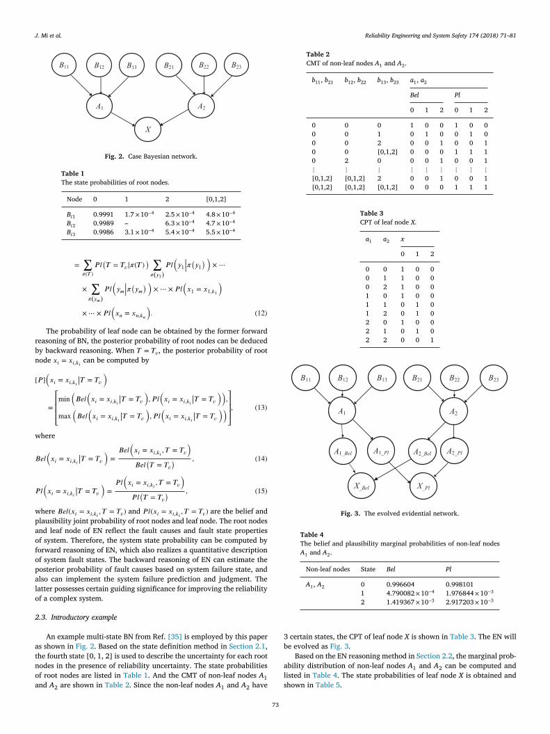
Fig. 2. Case Bayesian network.
Table 1
The state probabilities of root nodes.
Node 0 1 2 [0,1,2]
B i 1 0.9991 1.7 ×10 − 4 2.5 ×10 − 4 4.8 ×10 − 4
B i 2 0.9989 – 6.3 ×10 − 4 4.7 ×10 − 4
B i 3 0.9986 3.1 ×10 − 4 5.4 ×10 − 4 5.5 ×10 − 4
r
b
n
[
w
𝐵
𝑃
w
p
a
o
f
o
p
a
l
o
2
a
t
n
oa
Table 2
CMT of non-leaf nodes A 1 and A 2 .
b 11 , b 21 b 12 , b 22 b 13 , b 23 a 1 , a 2
Bel Pl
0 1 2 0 1 2
0 0 0 1 0 0 1 0 0 0 0 1 0 1 0 0 1 0 0 0 2 0 0 1 0 0 1 0 0 [0,1,2] 0 0 0 1 1 1 0 2 0 0 0 1 0 0 1 ⋮ ⋮ ⋮ ⋮ ⋮ ⋮ ⋮ ⋮ ⋮ [0,1,2] [0,1,2] 2 0 0 1 0 0 1 [0,1,2] [0,1,2] [0,1,2] 0 0 0 1 1 1
Table 3
CPT of leaf node X.
a 1 a 2 x
0 1 2
0 0 1 0 0 0 1 1 0 0 0 2 1 0 0 1 0 1 0 0 1 1 0 1 0 1 2 0 1 0 2 0 1 0 0 2 1 0 1 0 2 2 0 0 1
Fig. 3. The evolved evidential network.
Table 4
The belief and plausibility marginal probabilities of non-leaf nodes A 1 and A 2 .
Non-leaf nodes State Bel Pl
A 1 , A 2 0 0.996604 0.998101 1 4.790082 ×10 − 4 1.976844 ×10 − 3
2 1.419367 ×10 − 3 2.917203 ×10 − 3
3
b
a
l
s
=
∑𝜋( 𝑇 )
𝑃 𝑙 (𝑇 = 𝑇 𝑣 |𝜋( 𝑇 ) ) ∑
𝜋( 𝑦 1 ) 𝑃 𝑙
(𝑦 1 |||𝜋(𝑦 1 )) ×⋯
×∑𝜋( 𝑦 𝑚 )
𝑃 𝑙 (𝑦 𝑚
|||𝜋(𝑦 𝑚 )) ×⋯ × 𝑃 𝑙 (𝑥 1 = 𝑥 1 , 𝑘 1
)×⋯ × 𝑃 𝑙
(𝑥 𝑛 = 𝑥 𝑛, 𝑘 𝑛
). (12)
The probability of leaf node can be obtained by the former forwardeasoning of BN, the posterior probability of root nodes can be deducedy backward reasoning. When 𝑇 = 𝑇 𝑣 , the posterior probability of rootode 𝑥 𝑖 = 𝑥 𝑖, 𝑘 𝑖 can be computed by
𝑃 ] (𝑥 𝑖 = 𝑥 𝑖, 𝑘 𝑖
||𝑇 = 𝑇 𝑣
)=
⎡ ⎢ ⎢ ⎢ ⎣ min
(𝐵𝑒𝑙
(𝑥 𝑖 = 𝑥 𝑖, 𝑘 𝑖
||𝑇 = 𝑇 𝑣
), 𝑃 𝑙
(𝑥 𝑖 = 𝑥 𝑖, 𝑘 𝑖
||𝑇 = 𝑇 𝑣
)),
max (𝐵𝑒𝑙
(𝑥 𝑖 = 𝑥 𝑖, 𝑘 𝑖
||𝑇 = 𝑇 𝑣
), 𝑃 𝑙
(𝑥 𝑖 = 𝑥 𝑖, 𝑘 𝑖
||𝑇 = 𝑇 𝑣
))⎤ ⎥ ⎥ ⎥ ⎦ , (13)
here
𝑒𝑙 (𝑥 𝑖 = 𝑥 𝑖, 𝑘 𝑖
||𝑇 = 𝑇 𝑣
)=
𝐵 𝑒𝑙 (𝑥 𝑖 = 𝑥 𝑖, 𝑘 𝑖 , 𝑇 = 𝑇 𝑣
)𝐵 𝑒𝑙
(𝑇 = 𝑇 𝑣
) , (14)
𝑙 (𝑥 𝑖 = 𝑥 𝑖, 𝑘 𝑖
||𝑇 = 𝑇 𝑣
)=
𝑃 𝑙 (𝑥 𝑖 = 𝑥 𝑖, 𝑘 𝑖 , 𝑇 = 𝑇 𝑣
)𝑃 𝑙
(𝑇 = 𝑇 𝑣
) , (15)
here 𝐵𝑒𝑙( 𝑥 𝑖 = 𝑥 𝑖, 𝑘 𝑖 , 𝑇 = 𝑇 𝑣 ) and 𝑃 𝑙( 𝑥 𝑖 = 𝑥 𝑖, 𝑘 𝑖 , 𝑇 = 𝑇 𝑣 ) are the belief andlausibility joint probability of root nodes and leaf node. The root nodesnd leaf node of EN reflect the fault causes and fault state propertiesf system. Therefore, the system state probability can be computed byorward reasoning of EN, which also realizes a quantitative descriptionf system fault states. The backward reasoning of EN can estimate theosterior probability of fault causes based on system failure state, andlso can implement the system failure prediction and judgment. Theatter possesses certain guiding significance for improving the reliabilityf a complex system.
.3. Introductory example
An example multi-state BN from Ref. [35] is employed by this papers shown in Fig. 2 . Based on the state definition method in Section 2.1 ,he fourth state [0, 1, 2] is used to describe the uncertainty for each rootodes in the presence of reliability uncertainty. The state probabilitiesf root nodes are listed in Table 1 . And the CMT of non-leaf nodes A 1 nd A are shown in Table 2 . Since the non-leaf nodes A and A have
2 1 273
certain states, the CPT of leaf node X is shown in Table 3 . The EN wille evolved as Fig. 3 .
Based on the EN reasoning method in Section 2.2 , the marginal prob-bility distribution of non-leaf nodes A 1 and A 2 can be computed andisted in Table 4 . The state probabilities of leaf node X is obtained andhown in Table 5 .
J. Mi et al. Reliability Engineering and System Safety 174 (2018) 71–81
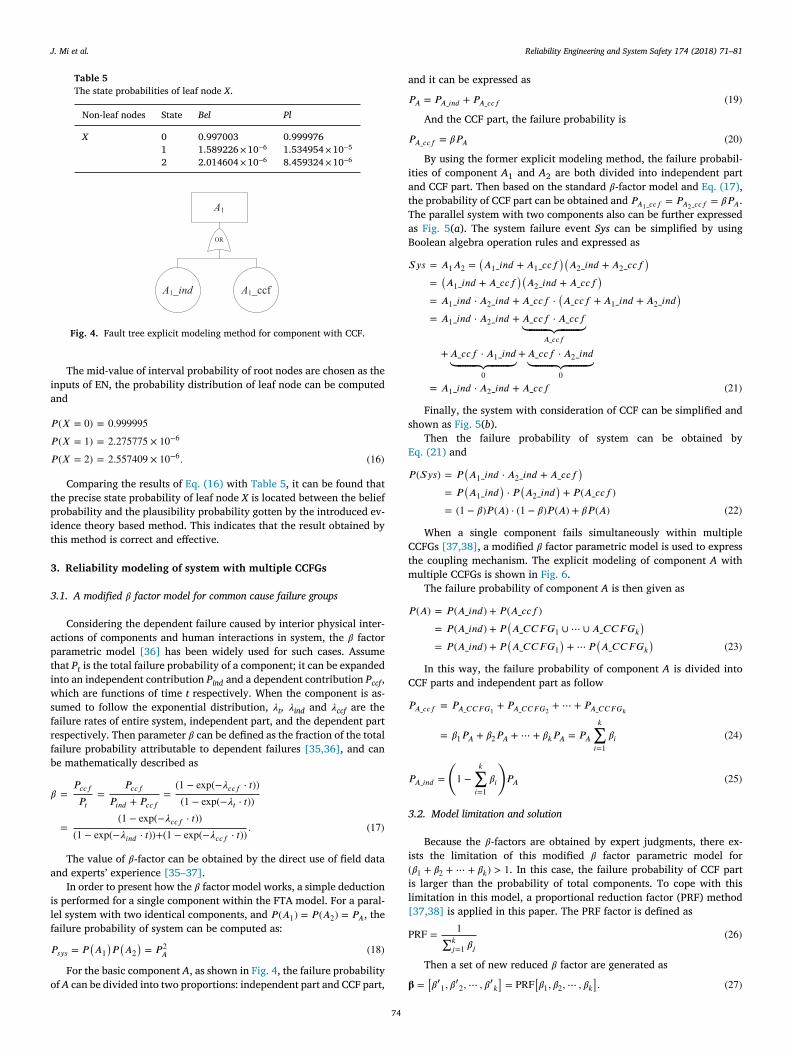
Table 5
The state probabilities of leaf node X .
Non-leaf nodes State Bel Pl
X 0 0.997003 0.999976 1 1.589226 ×10 − 6 1.534954 ×10 − 5
2 2.014604 ×10 − 6 8.459324 ×10 − 6
Fig. 4. Fault tree explicit modeling method for component with CCF.
i
a
𝑃
𝑃
𝑃
t
p
i
t
3
3
a
p
t
i
w
s
f
r
f
b
𝛽
a
i
l
f
𝑃
o
a
𝑃
𝑃
i
a
t
T
a
B
𝑆
s
E
𝑃
C
t
m
𝑃
C
𝑃
𝑃
3
i
(
i
l
[
P
𝛃
The mid-value of interval probability of root nodes are chosen as thenputs of EN, the probability distribution of leaf node can be computednd
( 𝑋 = 0) = 0 . 999995
( 𝑋 = 1) = 2 . 275775 × 10 − 6
( 𝑋 = 2) = 2 . 557409 × 10 − 6 . (16)
Comparing the results of Eq. (16) with Table 5 , it can be found thathe precise state probability of leaf node X is located between the beliefrobability and the plausibility probability gotten by the introduced ev-dence theory based method. This indicates that the result obtained byhis method is correct and effective.
. Reliability modeling of system with multiple CCFGs
.1. A modified 𝛽 factor model for common cause failure groups
Considering the dependent failure caused by interior physical inter-ctions of components and human interactions in system, the 𝛽 factorarametric model [36] has been widely used for such cases. Assumehat P t is the total failure probability of a component; it can be expandednto an independent contribution P ind and a dependent contribution P ccf ,hich are functions of time t respectively. When the component is as-
umed to follow the exponential distribution, 𝜆t , 𝜆ind and 𝜆ccf are theailure rates of entire system, independent part, and the dependent partespectively. Then parameter 𝛽 can be defined as the fraction of the totalailure probability attributable to dependent failures [35,36] , and cane mathematically described as
=
𝑃 𝑐 𝑐 𝑓
𝑃 𝑡 =
𝑃 𝑐 𝑐 𝑓
𝑃 𝑖𝑛𝑑 + 𝑃 𝑐 𝑐 𝑓 =
(1 − exp (− 𝜆𝑐 𝑐 𝑓 ⋅ 𝑡 )) (1 − exp (− 𝜆𝑡 ⋅ 𝑡 ))
=
(1 − exp (− 𝜆𝑐 𝑐 𝑓 ⋅ 𝑡 )) (1 − exp (− 𝜆𝑖𝑛𝑑 ⋅ 𝑡 )) + (1 − exp (− 𝜆𝑐 𝑐 𝑓 ⋅ 𝑡 ))
. (17)
The value of 𝛽-factor can be obtained by the direct use of field datand experts ’ experience [35–37] .
In order to present how the 𝛽 factor model works, a simple deductions performed for a single component within the FTA model. For a paral-el system with two identical components, and 𝑃 ( 𝐴 1 ) = 𝑃 ( 𝐴 2 ) = 𝑃 𝐴 , theailure probability of system can be computed as:
𝑠𝑦𝑠 = 𝑃 (𝐴 1
)𝑃 (𝐴 2
)= 𝑃 2
𝐴 (18)
For the basic component A , as shown in Fig. 4 , the failure probabilityf A can be divided into two proportions: independent part and CCF part,
74
nd it can be expressed as
𝐴 = 𝑃 𝐴 _ 𝑖𝑛𝑑 + 𝑃 𝐴 _ 𝑐 𝑐 𝑓 (19)
And the CCF part, the failure probability is
𝐴 _ 𝑐 𝑐 𝑓 = 𝛽𝑃 𝐴 (20)
By using the former explicit modeling method, the failure probabil-ties of component A 1 and A 2 are both divided into independent partnd CCF part. Then based on the standard 𝛽-factor model and Eq. (17) ,he probability of CCF part can be obtained and 𝑃 𝐴 1 _ 𝑐 𝑐 𝑓 = 𝑃 𝐴 2 _ 𝑐 𝑐 𝑓 = 𝛽𝑃 𝐴 .he parallel system with two components also can be further expresseds Fig. 5 ( a ). The system failure event Sys can be simplified by usingoolean algebra operation rules and expressed as
𝑦𝑠 = 𝐴 1 𝐴 2 =
(𝐴 1 _ 𝑖𝑛𝑑 + 𝐴 1 _ 𝑐 𝑐 𝑓
)(𝐴 2 _ 𝑖𝑛𝑑 + 𝐴 2 _ 𝑐 𝑐 𝑓
)=
(𝐴 1 _ 𝑖𝑛𝑑 + 𝐴 _ 𝑐 𝑐 𝑓
)(𝐴 2 _ 𝑖𝑛𝑑 + 𝐴 _ 𝑐 𝑐 𝑓
)= 𝐴 1 _ 𝑖𝑛𝑑 ⋅ 𝐴 2 _ 𝑖𝑛𝑑 + 𝐴 _ 𝑐 𝑐 𝑓 ⋅
(𝐴 _ 𝑐 𝑐 𝑓 + 𝐴 1 _ 𝑖𝑛𝑑 + 𝐴 2 _ 𝑖𝑛𝑑
)= 𝐴 1 _ 𝑖𝑛𝑑 ⋅ 𝐴 2 _ 𝑖𝑛𝑑 + 𝐴 _ 𝑐 𝑐 𝑓 ⋅ 𝐴 _ 𝑐 𝑐 𝑓
⏟⏞⏞⏞⏞⏞⏞⏞⏟⏞⏞⏞⏞⏞⏞⏞⏟𝐴 _ 𝑐 𝑐 𝑓
+ 𝐴 _ 𝑐 𝑐 𝑓 ⋅ 𝐴 1 _ 𝑖𝑛𝑑 ⏟⏞⏞⏞⏞⏞⏞⏞⏟⏞⏞⏞⏞⏞⏞⏞⏟
0
+ 𝐴 _ 𝑐 𝑐 𝑓 ⋅ 𝐴 2 _ 𝑖𝑛𝑑 ⏟⏞⏞⏞⏞⏞⏞⏞⏟⏞⏞⏞⏞⏞⏞⏞⏟
0
= 𝐴 1 _ 𝑖𝑛𝑑 ⋅ 𝐴 2 _ 𝑖𝑛𝑑 + 𝐴 _ 𝑐 𝑐 𝑓 (21)
Finally, the system with consideration of CCF can be simplified andhown as Fig. 5 ( b ).
Then the failure probability of system can be obtained byq. (21) and
( 𝑆𝑦𝑠 ) = 𝑃 (𝐴 1 _ 𝑖𝑛𝑑 ⋅ 𝐴 2 _ 𝑖𝑛𝑑 + 𝐴 _ 𝑐 𝑐 𝑓
)= 𝑃
(𝐴 1 _ 𝑖𝑛𝑑
)⋅ 𝑃
(𝐴 2 _ 𝑖𝑛𝑑
)+ 𝑃 ( 𝐴 _ 𝑐 𝑐 𝑓 )
= ( 1 − 𝛽) 𝑃 ( 𝐴 ) ⋅ ( 1 − 𝛽) 𝑃 ( 𝐴 ) + 𝛽𝑃 ( 𝐴 ) (22)
When a single component fails simultaneously within multipleCFGs [37,38] , a modified 𝛽 factor parametric model is used to expresshe coupling mechanism. The explicit modeling of component A withultiple CCFGs is shown in Fig. 6 .
The failure probability of component A is then given as
( 𝐴 ) = 𝑃 ( 𝐴 _ 𝑖𝑛𝑑 ) + 𝑃 ( 𝐴 _ 𝑐 𝑐 𝑓 ) = 𝑃 ( 𝐴 _ 𝑖𝑛𝑑 ) + 𝑃
(𝐴 _ 𝐶 𝐶 𝐹 𝐺 1 ∪⋯ ∪ 𝐴 _ 𝐶 𝐶 𝐹 𝐺 𝑘
)= 𝑃 ( 𝐴 _ 𝑖𝑛𝑑 ) + 𝑃
(𝐴 _ 𝐶 𝐶 𝐹 𝐺 1
)+ ⋯ 𝑃
(𝐴 _ 𝐶 𝐶 𝐹 𝐺 𝑘
)(23)
In this way, the failure probability of component A is divided intoCF parts and independent part as follow
𝐴 _ 𝑐 𝑐 𝑓 = 𝑃 𝐴 _ 𝐶 𝐶 𝐹 𝐺 1 + 𝑃 𝐴 _ 𝐶 𝐶 𝐹 𝐺 2 + ⋯ + 𝑃 𝐴 _ 𝐶 𝐶 𝐹 𝐺 𝑘
= 𝛽1 𝑃 𝐴 + 𝛽2 𝑃 𝐴 + ⋯ + 𝛽𝑘 𝑃 𝐴 = 𝑃 𝐴
𝑘 ∑𝑖 =1
𝛽𝑖 (24)
𝐴 _ 𝑖𝑛𝑑 =
(
1 −
𝑘 ∑𝑖 =1
𝛽𝑖
)
𝑃 𝐴 (25)
.2. Model limitation and solution
Because the 𝛽- factors are obtained by expert judgments, there ex-sts the limitation of this modified 𝛽 factor parametric model for 𝛽1 + 𝛽2 + ⋯ + 𝛽𝑘 ) > 1 . In this case, the failure probability of CCF parts larger than the probability of total components. To cope with thisimitation in this model, a proportional reduction factor (PRF) method37,38] is applied in this paper. The PRF factor is defined as
RF =
1 ∑𝑘 𝑗=1 𝛽𝑗
(26)
Then a set of new reduced 𝛽 factor are generated as
=
[𝛽′1 , 𝛽
′2 , ⋯ , 𝛽′𝑘
]= PRF
[𝛽1 , 𝛽2 , ⋯ , 𝛽𝑘
]. (27)

J. Mi et al. Reliability Engineering and System Safety 174 (2018) 71–81
Fig. 5. (a) Fault tree of two components parallel system with CCF; (b) Simplify fault tree of system.
Fig. 6. Explicit modeling of multiple CCFGs within fault tree.
a
𝑃
𝑃
c
t
t
c
c
3
o
p
p
c
s
d
m
i
c
(
Fig. 7. BN node with CCFGs.
l
𝑃
1
A
𝑃
4
w
4
p
h
t
C
m
p
e
a
m
g
In this way, the failure probability of CCF parts and independent partre rewritten as
𝐴 _ 𝑐 𝑐 𝑓 = 𝑃 𝐴
𝑘 ∑𝑖 =1
𝛽′𝑖 (28)
𝐴 _ 𝑖𝑛𝑑 =
(
1 −
𝑘 ∑𝑖 =1
𝛽′𝑖
)
𝑃 𝐴 = 0 (29)
The essence of the PRF method is an equilibrium process of the ac-umulated common cause parts on 𝛽 factor, which has weaken the con-radiction of the common cause part beyond the total failure probabilityo some extent. And the PRF method is just one of the methods whichan be used to solve this kind of logical contradiction; any other methodapable of dealing with such contradictions may be applicable.
.3. The Bayesian network node with CCFGs
When CCFs is considered in system reliability modeling, the failuref system can be divided into independent part and CCF part. The inde-endent part means the failure of system caused a single cause. The CCFart represents the simultaneous failure of multiple components whichaused by a common coupling mechanism, then those components con-titute a CCFG. For component A which exists in multiple CCFGs thatenoted as CCFG 1 , CCFG 2 , ⋅⋅⋅, CCFG k , by using the fault tree explicitodeling of multiple CCFGs in Section 3.2 and translate the fault tree
nto BN, as shown in Fig. 7 . When the independent failure probability of node A is P ( A ind ), the
orresponding 𝛽 factors of common cause nodes are 𝛽1 , 𝛽2 , ⋅⋅⋅, 𝛽k . When 𝛽 + 𝛽 + ⋯ + 𝛽 ) < 1 , the failure probability of node A can be calcu-
1 2 𝑘75
ated by Eqs. (22) –(26) and
′( 𝐴 ) = 𝑃 (𝐴 𝑖𝑛𝑑
)+ 𝑃
(𝐴 𝑐 𝑐 𝑓
)= 𝑃
(𝐴 𝑖𝑛𝑑
)+
𝑘 ∑𝑖 =1 𝛽𝑖
1 −
𝑘 ∑𝑖 =1 𝛽𝑖
𝑃 (𝐴 𝑖𝑛𝑑
)
=
1
1 −
𝑘 ∑𝑖 =1 𝛽𝑖
𝑃 (𝐴 𝑖𝑛𝑑
)(30)
When the sum of 𝛽 factors is larger than 1, that is ( 𝛽1 + 𝛽2 + ⋯ + 𝛽𝑘 ) > , by using the PRF method in Section 3.2 , the failure probability of node can be computed by Eqs. (26) –(29) and
′( 𝐴 ) = 𝑃 ′𝐴 _ 𝑐 𝑐 𝑓 + 𝑃 ′
𝐴 _ 𝑖𝑛𝑑 = 𝑃 𝐴
𝑘 ∑𝑖 =1
𝛽′𝑖 + 0 = 𝑃 𝐴 ⋅ 𝑃 𝑅𝐹 ⋅𝑘 ∑𝑖 =1
𝛽𝑖 . (31)
. Reliability analysis of feeding control system for CNC HDHLs
ith multiple CCFGs
.1. Fault tree modeling of feeding control system
The lathes are basic machine tools for manufacturing cylindricalarts. In recent years, the DL series computer numerical control (CNC)eavy-duty horizontal lathes (HDHLs) have been widely used in theransportation, energy, and aviation industries. High availability of theNC HDHL is required to maximize the efficiency and benefit of theseanufacturing industries [37] . The DL series horizontal lathes are com-uter numerical control (CNC) types which are used for the turning op-ration of rotational parts with outside and inside surface, such as axlesnd disc, and have the following work axes: X axis of tool head lateralovement, Z axis of tool head longitudinal movement, U 1 axis of left
ang tool movement and U axis of right gang tool movement. Fig. 8
2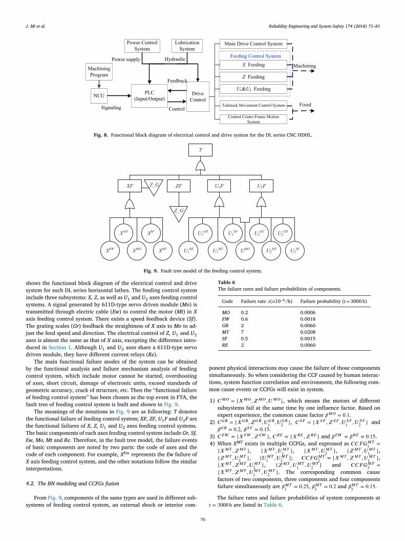
J. Mi et al. Reliability Engineering and System Safety 174 (2018) 71–81
Fig. 8. Functional block diagram of electrical control and drive system for the DL series CNC HDHL.
Fig. 9. Fault tree model of the feeding control system.
s
s
i
s
t
a
T
ja
d
d
b
c
o
g
o
f
t
t
T
E
o
c
X
i
4
s
Table 6
The failure rates and failure probabilities of components.
Code Failure rate 𝜆( ×10 − 6 /h) Failure probability ( t = 3000 h)
MO 0.2 0.0006 EW 0.6 0.0018 GR 2 0.0060 MT 7 0.0208 SF 0.5 0.0015 RE 2 0.0060
p
s
t
m
𝑡
hows the functional block diagram of the electrical control and driveystem for such DL series horizontal lathes. The feeding control systemnclude three subsystems: X, Z , as well as U 1 and U 2 axes feeding controlystems. A signal generated by 611D-type servo driven module ( Mo ) isransmitted through electric cable ( Ew ) to control the motor ( Mt ) in Xxis feeding control system. There exists a speed feedback device ( Sf ).he grating scales ( Gr ) feedback the straightness of X axis to Mo to ad-
ust the feed speed and direction. The electrical control of Z, U 1 and U 2 xes is almost the same as that of X axis, excepting the difference intro-uced in Section 1 . Although U 1 and U 2 axes share a 611D-type servoriven module, they have different current relays ( Re ).
The main functional failure modes of the system can be obtainedy the functional analysis and failure mechanism analysis of feedingontrol system, which include motor cannot be started, overshootingf axes, short circuit, damage of electronic units, exceed standards ofeometric accuracy, crack of structure, etc. Then the “functional failuref feeding control system ” has been chosen as the top event in FTA, theault tree of feeding control system is built and shown in Fig. 9 .
The meanings of the notations in Fig. 9 are as following: T denoteshe functional failure of feeding control system; XF, ZF, U 1 F and U 2 F arehe functional failures of X, Z, U 1 and U 2 axes feeding control systems.he basic components of each axes feeding control system include Gr, Sf,
w, Mo, Mt and Re . Therefore, in the fault tree model, the failure eventsf basic components are noted by two parts: the code of axes and theode of each component. For example, X
Ew represents the Ew failure of axis feeding control system, and the other notations follow the similar
nterpretations.
.2. The BN modeling and CCFGs fusion
From Fig. 9 , components of the same types are used in different sub-ystems of feeding control system, an external shock or interior com-
76
onent physical interactions may cause the failure of those componentsimultaneously. So when considering the CCF caused by human interac-ions, system function correlation and environment, the following com-on cause events or CCFGs will exist in system.
1) 𝐶 𝑀𝑂 = { 𝑋
𝑀𝑂 , 𝑍
𝑀𝑂 , 𝑈
𝑀𝑂 } , which means the motors of differentsubsystems fail at the same time by one influence factor. Based onexpert experience, the common cause factor 𝛽𝑀𝑂 = 0 . 1 .
2) 𝐶 𝐺𝑅 = { 𝑋
𝐺𝑅 , 𝑍
𝐺𝑅 , 𝑈
𝐺𝑅 1 , 𝑈
𝐺𝑅 2 } , 𝐶 𝑆𝐹 = { 𝑋
𝑆𝐹 , 𝑍
𝑆𝐹 , 𝑈
𝑆𝐹 1 , 𝑈
𝑆𝐹 2 } and
𝛽𝐺𝑅 = 0 . 2 , 𝛽𝑆𝐹 = 0 . 15 . 3) 𝐶 𝐸𝑊 = { 𝑋
𝐸𝑊 , 𝑍
𝐸𝑊 } , 𝐶 𝑅𝐸 = { 𝑋
𝑅𝐸 , 𝑍
𝑅𝐸 } and 𝛽𝐸𝑊 = 𝛽𝑅𝐸 = 0 . 15 . 4) When X
MT exists in multiple CCFGs, and expressed as 𝐶 𝐶 𝐹 𝐺
𝑀𝑇 1 =
{ 𝑋
𝑀𝑇 , 𝑍
𝑀𝑇 } , { 𝑋
𝑀𝑇 , 𝑈
𝑀𝑇 1 } , { 𝑋
𝑀𝑇 , 𝑈
𝑀𝑇 2 } , { 𝑍
𝑀𝑇 , 𝑈
𝑀𝑇 1 } ,
{ 𝑍
𝑀𝑇 , 𝑈
𝑀𝑇 2 } , { 𝑈
𝑀𝑇 1 , 𝑈
𝑀𝑇 2 } ; 𝐶 𝐶 𝐹 𝐺
𝑀𝑇 2 = { 𝑋
𝑀𝑇 , 𝑍
𝑀𝑇 , 𝑈
𝑀𝑇 1 } ,
{ 𝑋
𝑀𝑇 , 𝑍
𝑀𝑇 , 𝑈
𝑀𝑇 2 } , { 𝑍
𝑀𝑇 , 𝑈
𝑀𝑇 1 , 𝑈
𝑀𝑇 2 } and 𝐶 𝐶 𝐹 𝐺
𝑀𝑇 3 =
{ 𝑋
𝑀𝑇 , 𝑍
𝑀𝑇 , 𝑈
𝑀𝑇 1 , 𝑈
𝑀𝑇 2 } . The corresponding common cause
factors of two components, three components and four componentsfailure simultaneously are 𝛽𝑀𝑇
1 = 0 . 25 , 𝛽𝑀𝑇 2 = 0 . 2 and 𝛽𝑀𝑇
3 = 0 . 15 .
The failure rates and failure probabilities of system components at = 3000 h are listed in Table 6 .
J. Mi et al. Reliability Engineering and System Safety 174 (2018) 71–81
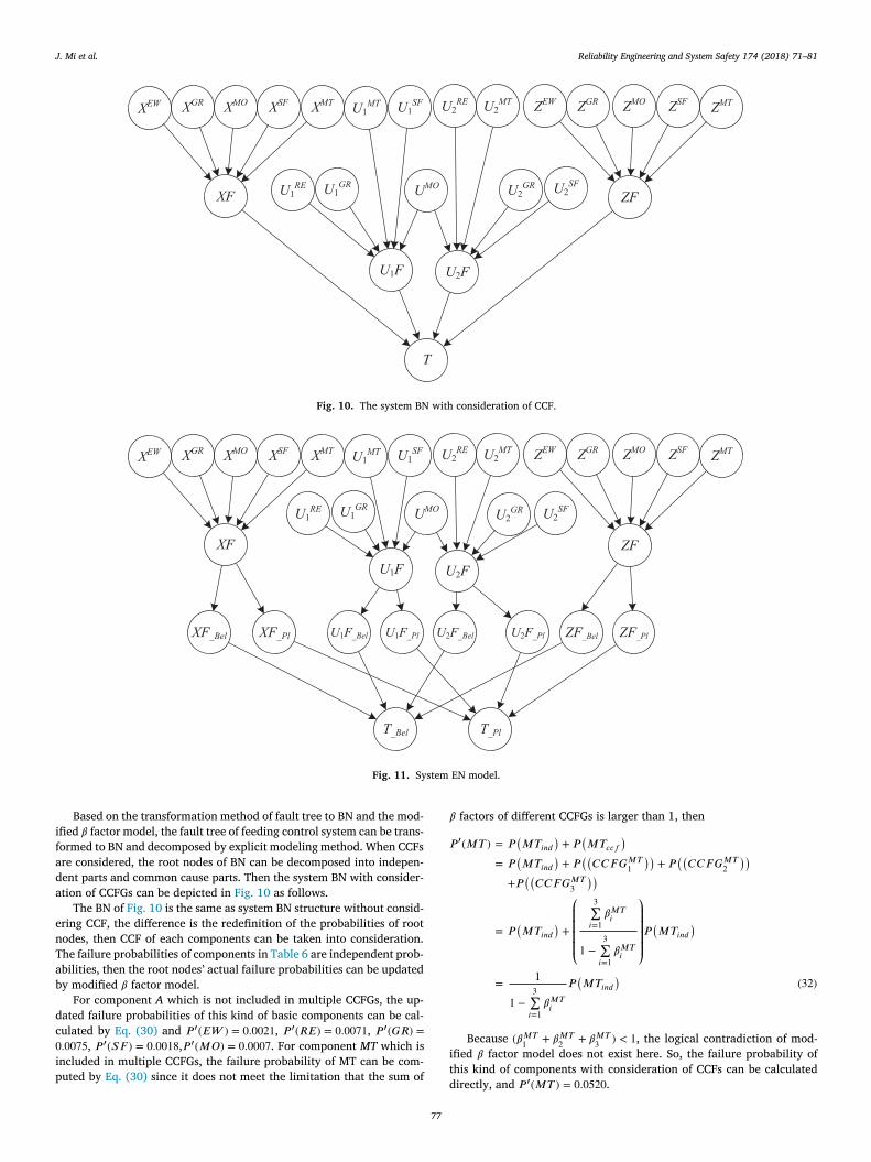
Fig. 10. The system BN with consideration of CCF.
Fig. 11. System EN model.
i
f
a
d
a
e
n
T
a
b
d
c
0
i
p
𝛽
𝑃
i
t
Based on the transformation method of fault tree to BN and the mod-fied 𝛽 factor model, the fault tree of feeding control system can be trans-ormed to BN and decomposed by explicit modeling method. When CCFsre considered, the root nodes of BN can be decomposed into indepen-ent parts and common cause parts. Then the system BN with consider-tion of CCFGs can be depicted in Fig. 10 as follows.
The BN of Fig. 10 is the same as system BN structure without consid-ring CCF, the difference is the redefinition of the probabilities of rootodes, then CCF of each components can be taken into consideration.he failure probabilities of components in Table 6 are independent prob-bilities, then the root nodes ’ actual failure probabilities can be updatedy modified 𝛽 factor model.
For component A which is not included in multiple CCFGs, the up-ated failure probabilities of this kind of basic components can be cal-ulated by Eq. (30) and 𝑃 ′( 𝐸𝑊 ) = 0 . 0021 , 𝑃 ′( 𝑅𝐸) = 0 . 0071 , 𝑃 ′( 𝐺𝑅 ) = . 0075 , 𝑃 ′( 𝑆𝐹 ) = 0 . 0018 , 𝑃 ′( 𝑀𝑂) = 0 . 0007 . For component MT which isncluded in multiple CCFGs, the failure probability of MT can be com-uted by Eq. (30) since it does not meet the limitation that the sum of
d
77
factors of different CCFGs is larger than 1, then
′( 𝑀𝑇 ) = 𝑃 (𝑀 𝑇 𝑖𝑛𝑑
)+ 𝑃
(𝑀 𝑇 𝑐 𝑐 𝑓
)= 𝑃
(𝑀 𝑇 𝑖𝑛𝑑
)+ 𝑃
((𝐶 𝐶 𝐹 𝐺
𝑀𝑇 1
))+ 𝑃
((𝐶 𝐶 𝐹 𝐺
𝑀𝑇 2
))+ 𝑃
((𝐶 𝐶 𝐹 𝐺
𝑀𝑇 3
))= 𝑃
(𝑀 𝑇 𝑖𝑛𝑑
)+
⎛ ⎜ ⎜ ⎜ ⎜ ⎝ 3 ∑𝑖 =1 𝛽𝑀𝑇 𝑖
1 −
3 ∑𝑖 =1 𝛽𝑀𝑇 𝑖
⎞ ⎟ ⎟ ⎟ ⎟ ⎠ 𝑃 (𝑀 𝑇 𝑖𝑛𝑑
)
=
1
1 −
3 ∑𝑖 =1 𝛽𝑀𝑇 𝑖
𝑃 (𝑀 𝑇 𝑖𝑛𝑑
)(32)
Because ( 𝛽𝑀𝑇 1 + 𝛽𝑀𝑇
2 + 𝛽𝑀𝑇 3 ) < 1 , the logical contradiction of mod-
fied 𝛽 factor model does not exist here. So, the failure probability ofhis kind of components with consideration of CCFs can be calculatedirectly, and 𝑃 ′( 𝑀𝑇 ) = 0 . 0520 .

J. Mi et al. Reliability Engineering and System Safety 174 (2018) 71–81
Table 7
The state probabilities of components at t = 3000 h with CCF.
Component State
0 1 2 [0,1,2]
MO 0.9993 – 0.0007 –EW 0.9979 – 0.0021 –GR 0.9925 – 0.0075 –MT 0.9304 0.0089 0.0520 0.0087 SF 0.9982 – 0.0018 –RE 0.9929 – 0.0071 –
4
s
i
s
d
1
s
a
t
s
b
t
p
b
i
n
n
l
m
i
i
l
𝐵
Table 9
The CMT of leaf node T .
XF ZF U 1 F U 2 F (OR) T
T _Bel T _ Pl
0 1 2 0 1 2
0 0 0 0 1 0 0 1 0 0 0 0 0 1 0 1 0 0 1 0 0 0 0 2 0 0 1 0 0 1 0 0 1 0 0 1 0 0 1 0 0 0 1 1 0 1 0 0 1 0 0 0 1 2 0 0 1 0 0 1 ⋮ ⋮ ⋮ ⋮ ⋮ ⋮ ⋮ ⋮ ⋮ ⋮ 2 2 2 1 0 0 1 0 0 1 2 2 2 2 0 0 1 0 0 1
𝑃
t
T
e
i
p
i
o
.3. Reliability analysis of feeding control system by using EN
As the main power take-off components of Horizontal lathe, the worktate of motors will affect the processing efficiency directly. Therefore,n this paper, there exists an intermediate state between the perfect worktate and failure state of the motors of DL series horizontal lathes, callederating work state. So the state space of motors can be expressed as {0,, 2}, where, 0 is the perfect working state, 1 is the derating workingtate and 2 represents failure state. The other components of system arell considered as two-state component. Due to the complexity of the sys-em, the coupling between components and the lack of data, there is aignificant amount of epistemic uncertainty which can be representedy an uncertain state [0,1,2] in the state space of system. Assume thathe life of all components obey exponential distribution, the basic com-onents state probabilities of feeding control system can be obtainedase on existing studies or experts experience and listed in Table 7 .
By using the EN node definition and probability reasoning methodntroduced in Sections 2.1 and 2.2 , the conditional mass table (CMT) ofon-leaf nodes of EN in Fig. 10 can be gotten. Table 8 is the CMT ofon-leaf nodes XF, ZF, U 1 F and U 2 F .
Then the system EN model can be shown as Fig. 11 , and the CMT ofeaf node T is shown in Table 9 . By using the multi-state EN reasoningethod in Section 2.2 , the belief probabilities and plausibility probabil-
ties of non-leaf nodes XF, ZF, U 1 F and U 2 F can be obtained and listedn Table 10 .
The belief and plausibility probabilities of leaf node T can be calcu-ated by Eqs. (11) and (12) , and
𝑒𝑙 ( 𝑇 = 0 ) = 𝑃 ( 𝑇 _ 𝐵𝑒𝑙 = 0 ) =
∑𝑋𝐹 ,𝑍𝐹 , 𝑈 1 𝐹 , 𝑈 2 𝐹
𝐵𝑒𝑙 (𝑋𝐹 , 𝑍𝐹 , 𝑈 1 𝐹 , 𝑈 2 𝐹 , 𝑇 = 0
)
gTable 8
The CMT of non-leaf nodes XF, ZF, U 1 F and U 2 F
X EW Z EW X GR Z GR X MO Z MO X SF Z SF
U
RE U
GR U
MO U
SF
0 0 0 0 0 0 0 0 0 0 0 0 0 0 0 0 0 0 0 2 0 0 0 2 ⋮ ⋮ ⋮ ⋮ 2 2 2 2 2 2 2 2 2 2 2 2 2 2 2 2
78
=
∑𝑋𝐹 ,𝑍𝐹 , 𝑈 1 𝐹 , 𝑈 2 𝐹
𝐵𝑒𝑙 (𝑇 = 0 ||𝑋𝐹 , 𝑍𝐹 , 𝑈 1 𝐹 , 𝑈 2 𝐹
) 𝑛 ∏𝑖 =1
𝐵𝑒𝑙 (𝑥 𝑘 𝑖 𝑖
)=
∑𝑋𝐹 ,𝑍𝐹 , 𝑈 1 𝐹 , 𝑈 2 𝐹
𝐵𝑒𝑙 (𝑇 = 0 ||𝑋𝐹 , 𝑍𝐹 , 𝑈 1 𝐹 , 𝑈 2 𝐹
)×𝐵 𝑒𝑙 ( 𝑋𝐹 ) 𝐵 𝑒𝑙 ( 𝑍𝐹 ) 𝐵 𝑒𝑙
(𝑈 1 𝐹
)𝐵 𝑒𝑙
(𝑈 2 𝐹
)(33)
𝑙 ( 𝑇 = 0 ) = 𝑃 ( 𝑇 _ 𝑃 𝑙 = 0 ) =
∑𝑋𝐹 ,𝑍𝐹 , 𝑈 1 𝐹 , 𝑈 2 𝐹
𝑃 𝑙 (𝑋𝐹 , 𝑍𝐹 , 𝑈 1 𝐹 , 𝑈 2 𝐹 , 𝑇 = 0
)=
∑𝑋𝐹 ,𝑍𝐹 , 𝑈 1 𝐹 , 𝑈 2 𝐹
𝑃 𝑙 (𝑇 = 0 ||𝑋𝐹 , 𝑍𝐹 , 𝑈 1 𝐹 , 𝑈 2 𝐹
) 𝑛 ∏𝑖 =1
𝑃 𝑙 (𝑥 𝑘 𝑖 𝑖
)=
∑𝑋𝐹 ,𝑍𝐹 , 𝑈 1 𝐹 , 𝑈 2 𝐹
𝑃 𝑙 (𝑇 =0 ||𝑋𝐹 , 𝑍𝐹 , 𝑈 1 𝐹 , 𝑈 2 𝐹
)𝑃 𝑙 ( 𝑋𝐹 ) 𝑃 𝑙 ( 𝑍𝐹 )
×𝑃 𝑙 (𝑈 1 𝐹
)𝑃 𝑙
(𝑈 2 𝐹
)(34)
Then the state belief probabilities and plausibility probabili-ies of leaf node T under epistemic uncertainty can be calculated.able 11 shows the results of system state probabilities when consid-ring the influence of CCFs and without CCFs. In order to illustrate thenfluence of epistemic uncertainty on system, the uncertain state of com-onent MT is classified as perfect work state 0. Then the state probabil-ties of system at t = 3000 h are calculated and also listed in Table 11 .
Based on the previous assumption that the lifetime of componentsbey exponential distribution, and the derating working state is re-arded as perfect state. From the belief and plausibility probability of
.
X MT Z MT (OR) XF, ZF, U 1 F, U 2 F
U
MT
Bel Pl
0 1 2 0 1 2
0 1 0 0 1 0 0 1 0 1 0 0 1 0 2 0 0 1 0 0 1 [0,1,2] 0 0 0 1 1 1 0 0 0 1 0 0 1 1 0 0 1 0 0 1 ⋮ ⋮ ⋮ ⋮ ⋮ ⋮ ⋮ 0 0 0 1 0 0 1 1 0 0 1 0 0 1 2 0 0 1 0 0 1 [0,1,2] 0 0 1 0 0 1

J. Mi et al. Reliability Engineering and System Safety 174 (2018) 71–81
Table 10
The state belief and plausibility probabilities of non-leaf nodes of BN.
Node State
Bel Pl
0 1 2 0 1 2
XF 0.919180 0.008793 0.063432 0.927775 0.017388 0.072027 ZF 0.919180 0.008793 0.063432 0.927775 0.017388 0.072027 U 1 F 0.914575 0.008749 0.068125 0.923127 0.017301 0.076677 U 2 F 0.914575 0.008749 0.068125 0.923127 0.017301 0.076677
Table 11
The state probabilities of leaf node T .
Leaf node T Considering CCFGs
State 0 1 2
Epistemic uncertainty Belief Prob. 0.706706 0.027431 0.232005 Plausibility Prob. 0.733514 0.056553 0.280306
Ignore uncertainty State Prob. 0.733514 0.028204 0.238282
Leaf node T Without considering CCFGs
State 0 1 2
Epistemic uncertainty Belief Prob. 0.808964 0.030368 0.119782 Plausibility Prob. 0.838640 0.062523 0.161703
Ignore uncertainty State Prob. 0.838640 0.031195 0.122977
Fig. 12. The contrast curves of the influence of epistemic uncertainty and CCFGs to system reliability.
f
u
i
t
W
b
5
e
k
a
A
i
0
r
t
q
m
eeding control system at state 2 in Table 11 , it has shown that the fail-re probability interval and failure rate interval of system at t = 3000 hs [0.232005, 0.280306] and [8.7991 ×10 − 5 , 1.0964 ×10 − 4 ]/h respec-ively when consider the influence of epistemic uncertainty and CCFGs.
hen the CCFGs are ignored, the system failure probability interval wille [0.119782, 0.161703], and failure rate interval is [4.2529 ×10 − 5 ,.8794 ×10 − 5 ]/h. The contrast curves of system reliability with consid-ration of CCF are also obtained and shown in Fig. 12 . From Fig. 12 wenow that when the influence of uncertainty is ignored, the failure prob-
79
bility and failure rate of system are 0.238282 and 9.072629 ×10 − 5 /h.nd when the CCF and uncertainty are both ignored, the correspond-
ng failure probability and failure rate of feeding control system are.122977 and 4.374068 ×10 − 5 /h. Finally, the contrast curves of systemeliability with epistemic uncertainty are shown in Fig. 13 .
This section has built an fault tree model of the feeding control sys-em of a DL series horizontal lath. The evidence theory is induced touantify the epistemic uncertainty caused by lack of data and infor-ation in this system, and combined with BN model formed an EN to

J. Mi et al. Reliability Engineering and System Safety 174 (2018) 71–81
Fig. 13. The contrast curves of the influence of CCFGs to system reliability without considering epistemic uncertainty.
r
m
F
c
w
e
C
p
b
b
s
s
w
I
a
i
5
w
s
m
b
o
a
f
a
p
a
b
a
t
d
a
C
r
m
n
d
t
p
s
t
p
c
A
n
A
t
J
R
ealize the system reliability indexes calculation. A modified 𝛽 factorodel is used to model the CCFGs in the system. From Table 11 and
ig. 12 , when the influence of epistemic uncertainty to system is in-luded, system reliability interval at t = 3000 h is [0.808964, 0.838640]ithout considering CCFs, and when the influence of CCFs is also consid-
red, the reliability interval is [0.706706, 0.733514]. This shows thatCFs has considerable impact on system reliability. The system staterobabilities in Table 11 when the epistemic uncertainty is ignored areetween the corresponding belief probabilities and plausibility proba-ilities, which verify the accuracy of results. From the results, we canee that the lower bound and upper bound of system reliability are withix digits of accuracy, which means the reliability uncertainty interval isith high accuracy, and sometimes it can be seen as a certain interval.
t is essential to distinguish this with the system reliability is accuratend not uncertain. That is to say the system reliability is uncertain butn a relatively certain interval.
. Conclusions
This paper introduces a reliability analysis method for complex MSSith epistemic uncertainty based on EN. The epistemic uncertainty of
ystem is quantified by adding an uncertain state of root nodes in theulti-state EN, and the state space is then constructed. After that, the
elief function and plausibility function are defined using evidence the-ry. Based on the BN forward reasoning, the measure system reliabilitynd failure probability can be computed. The case study confirms theeasibility of this comprehensive method, and realized a quantitativenalysis of system failure state. The backward reasoning can get theosterior probability of failure causes based on the system failure state,nd provide guidance for predicting the system failure types.
CCF is an important failure mode in complex system, so the relia-ility analysis of MSS with consideration of both epistemic uncertaintynd CCF are also investigated in this paper. When CCFGs exist in sys-em, a modified 𝛽 factor model is introduced and integrated with evi-ence theory based on BN, and realize the state expression and prob-bility reasoning for complex system with epistemic uncertainty andCFGs. The reliability analysis of the feeding control system of DL se-
80
ies HDHLs by this method has shown that, the proposed comprehensiveethod has high computing efficiency and theoretical value. In engi-eering practice, sometimes it is difficult to get enough data and theata are with large uncertainties, therefore this method also has rela-ive practical value with enough good data and sufficient evidence. Thisaper the nodes of EN are described as discrete variables, so when theystem inputs contain both discrete and continuous variables, how to usehe hybrid BN method to realize system reliability modeling and systemrobability reasoning, and how to express and synthesize the multipleomplex characteristics are worthwhile further studying and discussing.
cknowledgments
This research was partially supported by NSFC under the contractumber 51775090 and 51405065 , the Pre-research Project of Generalrmament Department under the contract number 41403040103 , and
he Open Project of Traction Power State Key Laboratory of Southwestiaotong University under the contract number TPL 1410 .
eferences
[1] Gu YK , Li J . Multi-state system reliability: a new and systematic review. ProcediaEng 2012;29:531–6 .
[2] Massim Y , Zeblah A , Benguediab M , Ghouraf A , Meziane R . Reliability evalua-tion of electrical power systems including multi-state considerations. Electr Eng2006;88(2):109–16 .
[3] Li YF , Zio E . A multi-state model for the reliability assessment of a distributed gener-ation system via universal generating function. Reliab Eng Syst Saf 2012;106:28–36 .
[4] Xue J . On multistate system analysis. IEEE Trans Reliab 1985;34(4):329–37 . [5] Lisnianski A , Elmakias D , Laredo D , Haim HB . A multi-state Markov model for
a short-term reliability analysis of a power generating unit. Reliab Eng Syst Saf2012;98(1):1–6 .
[6] Liu YW , Kapur KC . Reliability measures for dynamic multi-state nonrepairablesystems and their applications to system performance evaluation. IIE Trans2006;38:511–20 .
[7] Zio E , Podofillini L , Levitin G . Estimation of the importance measures of multi-stateelements by Monte Carlo simulation. Reliab Eng Syst Saf 2004;86(3):191–204 .
[8] Ramirez-Marquez JE , Coit DV . Composite importance measures for multi-state sys-tems with multi-state components. IEEE Trans Reliab 2005;54:517–29 .
J. Mi et al. Reliability Engineering and System Safety 174 (2018) 71–81
[
[
[
[
[
[
[
[
[
[
[
[
[
[
[
[
[
[
[
[
[
[
[
[
[
[
[
[
[
[9] Levitin G . The universal generating function in reliability analysis and optimization.Berlin, Germany: Springer-Verlag; 2005 .
10] Mi J , Li YF , Liu Y , Yang YJ , Huang HZ . Belief universal generating function analysisof multi-state systems under epistemic uncertainty and common cause failures. IEEETrans Reliab 2015;64(4):1300–9 .
11] Zhang Z , Jiang C , Wang GG , Han X . First and second order approximate reliabilityanalysis methods using evidence theory. Reliab Eng Syst Saf 2015;137:40–9 .
12] Mula J , Poler R , Garcia-Sabater JP . Material requirement planning with fuzzy con-straints and fuzzy coefficients. Fuzzy Set Syst 2007;158(7):783–93 .
13] Li YF , Mi J , Liu Y , Yang YJ , Huang HZ . Dynamic fault tree analysis based on con-tinuous-time Bayesian networks under fuzzy numbers. Proc Inst Mech Eng O-J RiskReliab 2015;229(6):530–41 .
14] Li YF, Huang HZ, Zhang H, Xiao NC, Liu Y. Fuzzy sets method of reliability predictionand its application to a turbocharger of diesel engines. Adv Mech Eng 2013 ArticleID 216192, 7 pages. doi: 10.1155/2013/216192 .
15] Li YF , Huang HZ , Liu Y , Xiao N , Li H . A new fault tree analysis method: fuzzy dynamicfault tree analysis. Eksploat Niezawodn 2012;14(3):208–14 .
16] Mehl CH . P-boxes for cost uncertainty analysis. Mech Syst Signal Process2013;37(1):253–63 .
17] Yang X , Liu Y , Zhang Y , Yue Z . Hybrid reliability analysis with both random andprobability-box variables. Acta Mech 2015;226(5):1341–57 .
18] Mi J , Li YF , Yang YJ , Peng W , Huang HZ . Reliability assessment of com-plex electromechanical systems under epistemic uncertainty. Reliab Eng Syst Saf2016;152:1–15 .
19] Sankararaman S , Mahadevan S . Likelihood-based representation of epistemic un-certainty due to sparse point data and/or interval data. Reliab Eng Syst Saf2011;96(7):814–24 .
20] Lorini E , Prade H . Strong possibility and weak necessity as a basis for a logic ofdesires. In: Working papers of the ECAI workshop on weighted logics for artificialintelligence; 2012. p. 99–103 .
21] Soundappan P , Nikolaidis E , Haftka RT , Grandhi R , Canfield R . Comparison of ev-idence theory and Bayesian theory for uncertainty modeling. Reliab Eng Syst Saf2004;85(1):295–311 .
22] Shah H , Hosder S , Winter T . Quantification of margins and mixed uncertainties usingevidence theory and stochastic expansions. Reliab Eng Syst Saf 2015;138:59–72 .
23] Yang JP , Huang HZ , Liu Y , Li YF . Quantification classification algorithm of multiplesources of evidence. Int J Inf Technol Decis Mak 2015;14(5):1017–34 .
81
24] Zhou Q , Zhou H , Zhou Q , Yang F , Luo L , Li T . Structural damage detection based onposteriori probability support vector machine and Dempster–Shafer evidence theory.Appl Soft Comput 2015;36:368–74 .
25] Zhou J , Liu L , Guo J , Sun L . Multisensory data fusion for water quality evaluationusing Dempster–Shafer evidence theory. Int J Distrib Sens Netw 2013;9(11):1–6 .
26] Kohlas J , Monney PA . A mathematical theory of hints: an approach to the Demp-ster–Shafer theory of evidence. Springer Science & Business Media; 2013 .
27] Pearl J . Fusion, propagation, and structuring in belief networks. Artif Intell1986;29(3):241–88 .
28] Li YF , Mi J , Huang HZ , Xiao NC , Zhu SP . System reliability modeling and assessmentfor solar array drive assembly based on Bayesian networks. Eksploat Niezawodn2013;16(2):117–22 .
29] Weber P , Simon C . Systems dependability assessment: benefits of Bayesian networkmodels. ISTE Ltd and John Wiley & Sons Inc; 2016 .
30] Simon C , Weber P , Levrat E . Bayesian networks and evidence theory to model com-plex systems reliability. J Comput 2007;2(1):33–43 .
31] Simon C , Weber P , Evsukoff A . Bayesian networks inference algorithm to im-plement Dempster Shafer theory in reliability analysis. Reliab Eng Syst Saf2008;93(7):950–63 .
32] Simon C , Weber P . Evidential networks for reliability analysis and performance eval-uation of systems with imprecise knowledge. IEEE Trans Rel 2009;58(1):69–87 .
33] Zhao S , Wang H , Cheng D . Power distribution system reliability evaluation by DSevidence inference and Bayesian network method. In: IEEE 11th international con-ference on probabilistic methods applied to power systems; 2010. p. 654–8 .
34] Simon C , Weber P , Sallak M . Uncertainty of data and important measures. In: Volume3 - security evaluation of SET systems coordinated by Jean-François Aubry. Londonand New Jersey: ISTE Ltd and John Wiley & Sons, Inc.; 2018. p. 119–69 .
35] Mi J , Li YF , Huang HZ , Liu Y , Zhang X . Reliability analysis of multi-state sys-tems with common cause failure based on Bayesian networks. Eksploat Niezawodn2013;15(2):169–75 .
36] Rausand M . Common-cause failures, in risk assessment. Hoboken, New Jersey: JohnWiley & Sons, Inc; 2011. p. 469–95 .
37] Mi J , Li YF , Peng W , Yang Y , Huang HZ . Fault tree analysis of feeding control systemfor computer numerical control heavy-duty horizontal lathes with multiple commoncause failure groups. J Shanghai Jiaotong Univ 2016;21(4):504–8 .
38] Kan čev D , Čepin M . A new method for explicit modelling of single failure eventwithin different common cause failure groups. Reliab Eng Syst Saf 2012;103:84–93 .