G eophy sical Prospecting, 1996, 44, 1 41 -7 60

Ray tracing based on Fermat's principle inirregular gridsl

Aldo L. Vesnaver '

Abstract

A new method to trace rays in irregular grids based on Fermat's principle of

minimum time is introduced. Besides the usual transmitted and reflected waves,

refracted, diffracted and converted waves can also be simulated. The proposed

algorithm is fast and stable, and respects the reciprocity principle between source and

receiver better than procedures adopting the shooting method. It is particularly

suited to form part of a traveltime inversion procedure. The use of irregular grids

allows adaptation of the earth discretization to the available acquisition geometry and

ray distribution, to obtain more stable and reliable tomographic images.

l n t roduc t i on

There are two principal approaches to ray tracing: the numerical solution of

differential equations derived from the wave equation, usually associated with the

shooting method as the tracing strategy, and minimum time methods, which

compute the raypath by iterated perturbations of an initial guess.

The two aPProaches

During the last few vears, various authors have proposed algorithms for the

calculation of raypath and traveltime, based on Fermat's principle instead of the

wave equation. Moser (1989, 1991), Saito (1939) and Fischer and Lees (1993)

introduced techniques where rays are defined as shortest traveltime traiectories and

the velocity field is represented by a regular network. The ray is then computed by

minimizing the traveltime from the source to the receiver, i.e. joining adjacent

network nodes properly. Although these methods are simple and fast, the choice of

node spacing is critical: if it is large, the computed path may be not sufficiently

accurate; if it is small, the computational costs increase. Asakawa and Kanawaka

(1993) eliminated most drawbacks of the network quantization by interpolating the

traveltimes of ray segments between the network nodes so that the trajectories

I paper presented at thc 55th EABG meeting, June 1993, Stavanger, Norway. Received May 1994, revision

accepted December 1995.2 Osservatorio Gcofisico Sperimentale, PO Box 2011, 34016 Trieste' Italy.

1) 1996 European Association of Geoscicntists & Engineers 741

742 A.L. Vesnaaer

obtained are not influenced too heavily by the network grain. Their implementation,however, still requires a regular distribution of the reference nodes and, in addition,it requires the computation of traveltimes between all the pairs of the network nodesthat could be part of the optimal raypath.

.Conventional methods are based on finite-difference extrapolation of the eikonalequation. Their main advantage over the above approach is their ability to reproducemost dynamics of wave propagation, such as amplitude and phase variations withoffset, geometrical spreading, angle-dependant reflectivity, etc. (see e.g. Julian andGubbins 1977; Nolet 1987; Cerveny 1987; Vidale 1988, 1990; Virieux and Farra1991; Pereyra 1992). Some difficulty occurs in this approach if the space is discretizedby pixels, as is the case in many procedures for linearized inversion: the velocity isassumed constant inside the pixels and changes step-wise in the earth model.Therefore, the velocity field cannot be derived at pixel boundaries and Snell's law oranother principle has to be used at all interfaces. Thus, the simulation of somephenomena (such as diffracted waves) is either infeasible or requires a localreformulation of the algorithm. This needs a much larger computational effort.

Consequently, a new technique for raypath and traveltime calculation was sought.The minimum-time approach was preferred because of its higher stability and theless restrictive requirements for the velocity field or representation of the geologicalstructures. Chander (1911) and Stc;ckli (1984) introduced algorithms of the bendingtype, able to estimate the raypaths in a medium consisting of homogeneous isotropicand non-isotropic layers with plane interfaces. The method presented here allows thesimulation of more complex media, with arbitrary interfaces and a blocky spatialdistribution of the velocity field. It is designed to be part of a tomographic inversionprocedure.

The use of irregular grids

In seismic tomography, pixels and rectangles are practically synonymous in 2D, asare voxels and parallelepipeds in 3D. Most authors adopt regular grids in theirinversion algorithms for two main reasons:

1. The software development is much simpler (for ray tracing, input/output,display, etc.).2. various postinversion procedures can be easily applied (filtering, smoothing,

image processing).on the other hand, there are also good reasons for using irregular grids:

1. Seismic resolution typically decreases with depth; the model discretizationshould consider this, by introducing small pixels near the surface and increasinglylarger ones in the deeper parts of the model, possibly according to some relationshipwith the size of the Fresnel zone.

2. The signal/noise ratio is poorer for late arrival times than for early ones, and sothe different statistical reliability of the two classes of data should also be reflected inthe model.

aO 1996 European Association of Geoscientists & Engineers, ()eophysical Prospecting, 44,741-760

Rag tracing 743

3. If we suppose, on the other hand, that traveltime picking errors are independent

of the arrival time, late arrivals are prone to larger errors in depth determination,

since velocities typically increase with depth.

In this paper irregular grids are considered because the second group of reasons

appears to be more consistent from a physical and statistical point of view.

Furthermore, some recent work in traveltime inversion (Vesnaver 1994a,b) showed

that irregular grids may help to reduce or control the non-uniqueness of the velocity

field estimated by seismic tomography.

Fe rma t ' s p r i nc ip le

Fermat's principle states that seismic energy travels between two given points along apath 'for which the first-order variation with all neighbouring paths is zero' (Sheriff

1973). Since mainly first arrivals or primary reflections are of interest here, this

formulation may be simplified by saying that raypaths are trajectories letting seismic

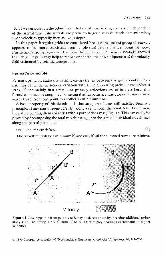
waves travel from one point to another in minimum time.A basic property of this definition is that any part of a ray still satisfies Fermat's

principle. If any pair of points (A', B') along a ray r from the point A to B is chosen'

the path r' joining them coincides with a part of the ray r (Fig. 1). This can easily beproved by decomposing the total traveltirn€ /6s into the sum of individual traveltimes

along the partial paths, i.e.

t6s : t66 ' * /n 's ' * /s 's . (1)

The traveltime will be a minimum if, and onlv if, all the summed terms are minima.

r) B'

A'

l _

Velocity

Figure 1 . Any raypath r from point A to B may be decomposed by inserting additional points

along r and obtaining a ray r' from A' to B'. Darker grey shadings correspond to highervelocit ies.

iI

D If ) i

Ii

IIIIiIiI

r

A

A 1996 European Association of Geoscicntists & Bngineers, Geophysical Prosp':cting, 44,741-760

744 A.L. Vesnaaer

Naturally, the raypath from A to B can be decomposed into as many parts asrequired, by choosing the intermediate points arbitrarily. consequently, the wholeraypath can be studied and computed bit by bit, exploiting the minimum-timeproperty at any scale.

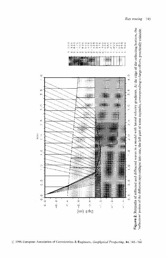
The velocity field is represented by pixels, i.e. zones with a homogeneous localvelocity, which is a typical choice in several methods for traveltime inversion. Therays are a sequence of straight segments whose extreme points are at the pixelboundaries. The angle between adjacent segments can generally be determined bySnell's law, which may be obtained directly from Fermat's principle. So the sameresult is expected, exploit ing either Snell 's law or Fermat's principle, except whenSnell's law does not hold, as in the presence of edges producing diffracted arrivals(Fie. 2) .

The m in im iza t i on p rocedu re

The raypath estimation is started by using some initial guess for the path joining thesource and the receiver (as discussed below in detail). If the earth is discretized bypixels, a raypath is represented completely and accurately by its intersections withthe pixel boundaries. In fact, two adjacent points are joined by a straight line if aconstant velocity in each pixel is assumed. This feature is simply an application ofFermat's principle on the smallest scale: a straight l ine is the shortest distancebetween two points.

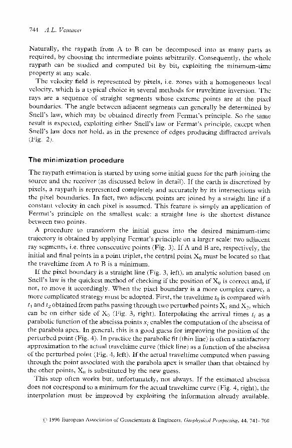
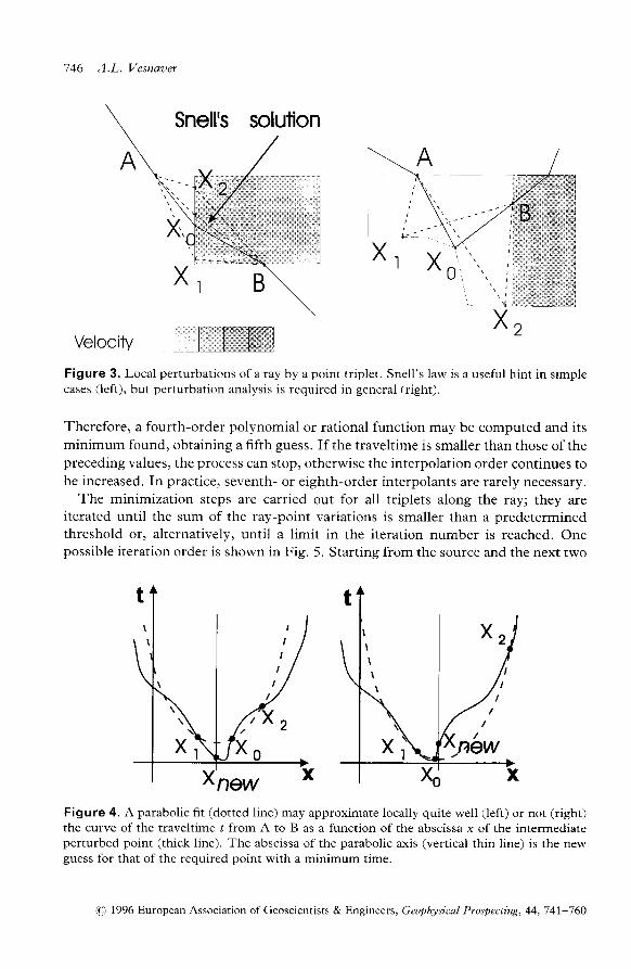
A procedure to transform the initial guess into the desired minimum-timetrajectory is obtained by applying Fermat's principle on a larger scale: two adjacentray segments, i.e. three consecutive points (Fig. 3). If A and B are, respectively, theinitial and final points in a point triplet, the central point Xe must be located so thatthe traveltime from A to B is a minimum.

If the pixel boundary is a straight line (Fig. 3, left), an analytic solution based onSnell's law is the quickest method of checking if the position of X6 is correct and, ifnot, to move it accordingly. $7hen the pixel boundary is a more complex curve) amore complicated strategy must be adopted. First, the traveltime le is compared withtl and t2 obtained from paths passing through two perturbed points X1 and X2, whichcan be on either side of Xe (Fig. 3, right). Interpolating the arrival t imes t; as &parabolic function of the abscissa points x; enables the computation of the abscissa ofthe parabola apex. In general, this is a good guess for improving the position of theperturbed point (Fig. 4). In practice the parabolic fit (thin line) is often a satisfactoryapproximation to the actual traveltime curve (thick line) as a function of the abscissaof the perturbed point (Fig. 4, left). If the actual traveltime computed when passingthrough the point associated with the parabola apex is smaller than that obtained bythe other points, X6 is substituted by the new guess.

This step often works but, unfortunately, not always. If the estimated abscissadoes not correspond to a minimum for the actual traveltime curve (Fig. 4, right), theinterpolation must be improved by exploiting the information already available.

t l , 1996 EuropeanAssociat ionof Geoscient is ts&Engineers, GeophysicalProspecLing,44,T4l-760

Ray tacing 745

o " :

i p- . =( o

l v

0 !

o ^

o U

E o- oi'^ v!

. - o d

< a Ju ] p ? o' F A .

rr U : ' ,

6 6

n i a @

f o ! ( !: oo > )- i :

c i on t t rN . ! -

> Lr ' 6

. . x _ Pt \ o o

H O

9 6o b g

. E ) i

U O O

9. .u

! ? !o , - 0

.r'. o.

n i 8o ' EL i )

l r J .

rl t\l cl fl ol N c! c\ O N.! (\l ol ol - -

O \r O |4 O L4 O La O !,1 O 4 O'ft O'rr O q'l O qr OO ol n tr O N rO f. O N r] r. O c\ ul l- O N 0 f. OO 0 m F F a t0 \t \t a N - - O o 03 m F- o ul r)

O N + O M C J N +

; d o o d - :l i l r r l

lu l l l urdan\ " ! r / - r T - - u

(,1 1996 European Association of Geoscientists & Engineers, Geophysical Prospecting, 44,741-7;0

Snell's

146 A.L. Vesnaaer

Velocity

Figure 3. Local perturbations of a ray by a point triplet. Snell's law is a useful hint in simplecases (left), but perturbation analysis is required in general (right).

Therefore, a fourth-order polynomial or rational function may be computed and itsminimum found, obtaining a fifth guess. If the traveltime is smaller than those of thepreceding values, the process can stop, otherwise the interpolation order continues tobe increased. In practice, seventh- or eighth-order interpolants are rarely necessary.

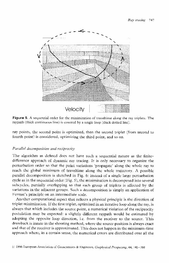
The minimization steps are carried out for all triplets along the rayl they areiterated until the sum of the ray-point variations is smaller than a predeterminedthreshold or, alternatively, until a limit in the iteration number is reached. Onepossible iteration order is shown in Fig. 5. Starting from the source and the next two

Figure 4. A parabolic fit (dotted line) may approximate locally quite well (left) or not (right)the curve of the traveltime I from A to Il as a function of the abscissa x of the intermediateperturbed point (thick line). The abscissa of the parabolic axis (vertical thin line) is the newguess for that of the required point with a minimum time.

(a) 1996 European Association of Geoscientists & Engineers, Geophysical Prospecting, 44,741-760

Ray tracing 747

IV\

VelocityFigure 5. A sequential order for the minimization of traveltime along the ray triplets. Theraypath (thick continuous line) is covered by a single loop (thick dotted line).

ray points, the second point is optimized, then the second triplet (from second tofourth point) is considered, optimizing the third poinr, and so on.

Parallel decomposition and reciprocity

The algorithm as defined does not have such a sequential nature as the finite-difference approach of dynamic ray tracing. It is only necessary to organize theperturbation order so that the point variations 'propagate' along the whole ray toreach the global minimum of traveltime along the whole trajectory. A possibleparallel decomposition is sketched in Fig. 6: instead of a single large perturbationcycle as in the sequential order (Fig. 5), the minimization is decomposed into severalsubcycles, partially overlapping so that each group of triplets is affected by thevariations in the adjacent groups. Such a decomposition is simply an application ofFermat's principle on an intermediate scale.

Another computational aspect that reflects a physical principle is the direction oftriplet minimization. If the first triplet, optimized in an iterative loop along the ray, isalways that which includes the source point, a numerical violation of the reciprocitypostulation may be expected: a slightly different raypath would be estimated byadopting the opposite loop direction, i.e. from the receiver to the source. Thisdrawback is innate in the shooting method, where the source position is always exactand that of the receiver is approximated. This does not happen in the minimum-timeapproach where, in a certain sense, the numerical errors are distributed over all the

ia f l996EuropeanAssociat ionof Geoscient is ts&Engineers, GeophysicalProspect ing,44,T4l-760

748 A.L. Vesnaxer

Velocity i- . . , t

Figure 6. A possible parallel decomposition of the minimization procedure. The raypath(thick continuous line) is covered by many overlapping loops (thick dotted lines).

intermediate points. Therefore, by alternating the loop direction (once from sourceto receiver, then vice versa), a much better reciprocity is obtained along the raypoints. At the ray extrema) the source and receiver positions are assigned exactly, andthe physical symmetry is better assured there.

solution

,. i

t:.,'l

Velocity

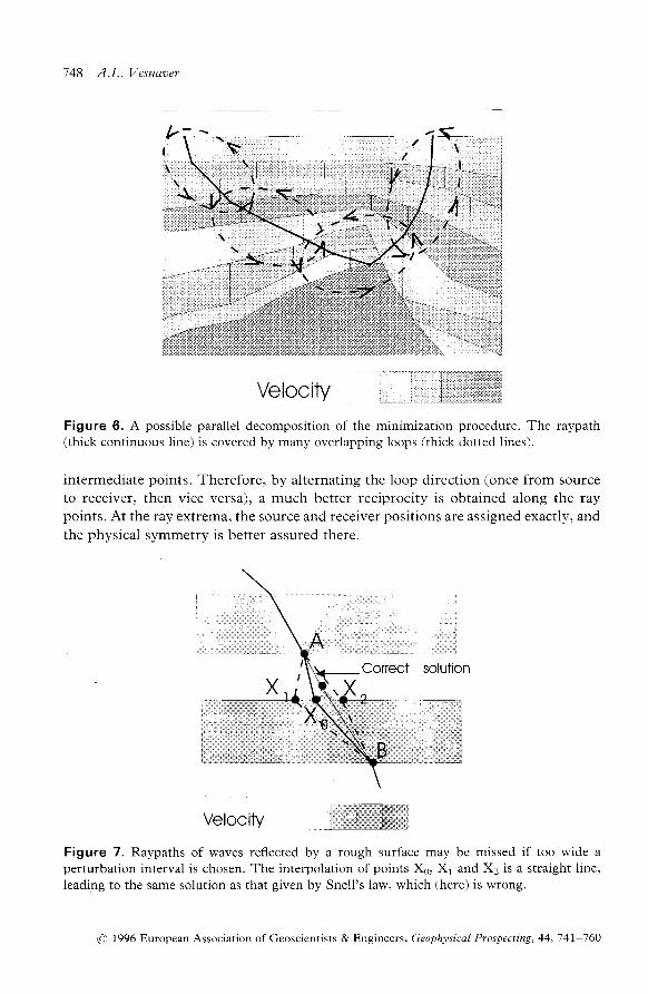
Figure 7. Raypaths of waves reflected by a rough surface may be missed if too wide aperturbation interval is chosen. The interpolation of points Xe, X1 and X2 is a straight line,leading to the same solution as that given by Snell's law, which (here) is wrong.

O 1996 European Association of Geoscientists & Engineers, Geophysical Prospecting, 44,741-760

\ , : : :\::

S- :l\ ,

II--''�- - "l

1 '

{', .ll'it'r.'*' I

, , 1 , 4 , v , lH'$uil"l$st1ll-_a{ Tlv

->ai: i . ,: r1'N z--T'flf )tg

i r i : i . r : : i1 i : i i t : : i r : t f \i::::':.:;:::J;r *tr.,.lj

t i t : : : i I

. ' : : I : i : : i : : i : a i : : a : : i : i l i ,

t : i : 1 l

( anra^i

Ray tracing 749

The perturbation interval

An important parameter in the minimization procedure is the size of the perturbation

interval, i.e. the distances of points X1 and X2 from Xs (Fig. 3). If this interval issmall, the convergence of the minimization procedure is slow, and one could reachthe upper limit of the iteration number unfruitfully and at higher computational costthan necessary; on the other hand, the precision in the raypath and traveltimecomputation is generally enhanced. If the perturbation interval is too large, the actual

traveltime behaviour, as a function of the offset of the perturbed points, cannot berepresented by a low-order polynomial or rational function, with sufficient precision.

If the reflecting marker is a rough surface (Fig. 7), the true minimum-time trajectorymay be not 'seen' by the minimization algorithm. Therefore, the perturbation

interval should be chosen, firstly, according to the smoothness of the reflecting

interfaces, and secondly, according to the required precision and the availablecomputational power. Naturally, many strategies could be adopted to avoid such

situations as that shown in Fig. 7. Many methods are given in the literature, if theproblem is considered from the purely numerical point of view (such as exhaustive

search, simulated annealing, etc.). Nevertheless, physical criteria should be

sufficient. Although ray theory assumes an infinite frequency band for the seismic

signals, field instruments provide a limited spatial resolution, and so these limits

should be present as much as possible in the model discretization.

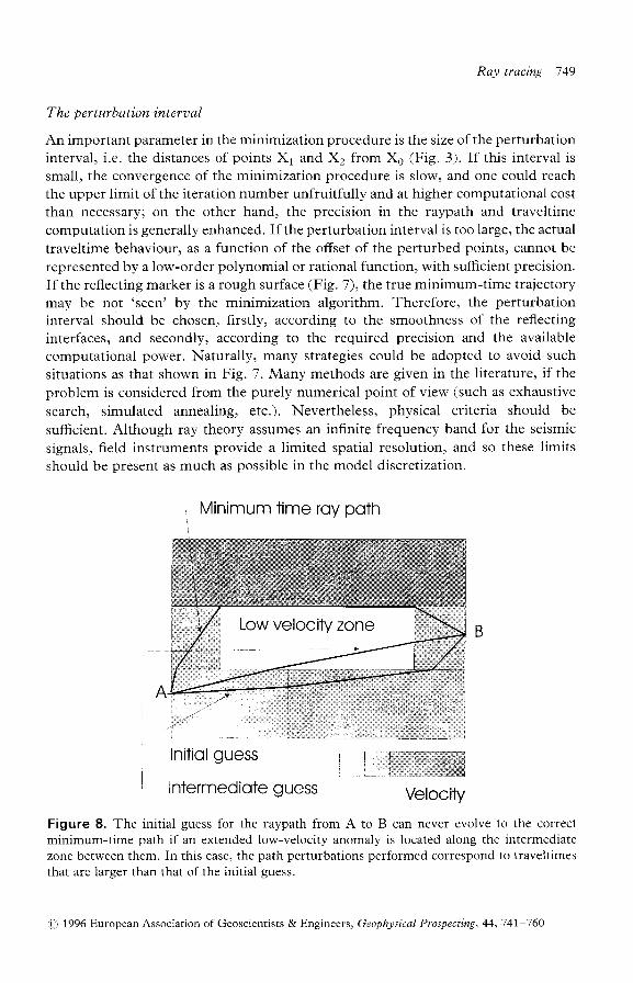
Minimum time roy poth

Intermediote guess VelocitV

Figure 8. The initial guess for the raypath from A to B can never evolve to the correctminimum-time path if an extended low-velocity anomaly is located along the intermediatezone between them. In this case, the path perturbations performed correspond to traveltimesthat are lareer than that of the initial euess.

(a) 1996 European Association of Geoscientists & Engineers, Geophysical Prospecting, 44,741-760

750 A.L. Vesnaaer

b0

0 0 0 0 0 0 0 0 0 0 0 0 0 0 0 0 0 0 0 0 00 0 0 0 0 0 0 0 0 0 0 0 0 0 0 0 0 0 0 0 0

i " l l 11 1 '11 : ' l i 1 \1 I 1 ' l 1 :1n q c l N f . l 0 l N c l c i N r ' 1 -

o{

o

n

d

C;I

(u1)+en

z ;> ' u- 2v h 0o 6

a q

q t

^ -u ' A. : :E Y

v 0

c - .

6 -

o i D

F o> p

o !

O O

r y E =^ -

P , E

o e

E U

0 b 0

^ -

N O .. F X

' F , a

. ! . ot r ^

T b oF 6

9 ' =

g ) oo o .L 6

r.r- ts

9r0

9LN

IN

i qo oI I

o o

C r N r . )

o o o ot t l

nII\0l0'

-q+a

O 1996 European Association of Geoscientists & Engineers, Geophysical l>rospecting, 44,741-760

Ray tracing 751

o 0 0 0 0 0 0 0 0 0 0 0 0 0 0 0 0 0 0 0 0o 0 0 0 0 0 0 0 0 0 0 0 0 0 0 0 0 0 0 0 0

: 1 1 \ 1 i i 1 1 i i * \ 1 1 1 : 1 : 1r ' l d c l N c I N N N N N N -

N E, 9d E

.F

tr(,o;q)

. l L; o au-

I ol n

trla0l0r

-a+

i

9 : 1 1 1 ! 9 t 1o o o o o o o o o

t t t t t t t l

(uq)+so

C) 1996 European Association of Geoscientists & Engineers, Geophysical Prospecting, 44,741-760

752 A.L. Vesnaver

The initial guess

A similar problem occurs in the presence of a low-velocity anomaly, which mayobstruct the evolution of the initial raypath towards the proper solution. For example(Fig. 8), if the traveltime of the perturbed path is higher than the initial guess, theminimization procedure could not suggest new points beyond the low-velocity zone,so not reaching the correct solution. A local minimum is therefore obtained here,instead of the global one.

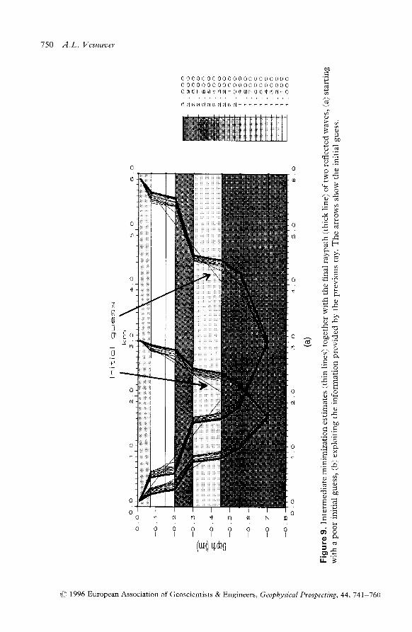
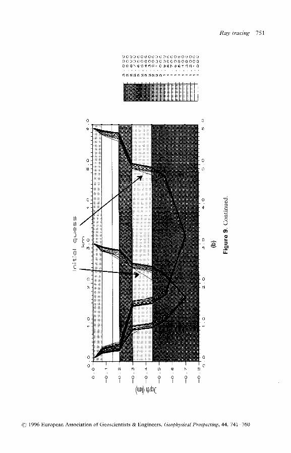
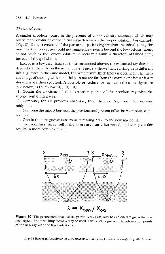
Except in a few cases (such as those mentioned above), the estimated ray does notdepend significantly on the initial guess. Figure 9 shows that, starting with differentinitial guesses in the same model, the same result (thick lines) is obtained. The mainadvantage of starting with an initial path not too far from the correct one is that feweriterations are then required. A possible procedure for rays with the same signature(see below) is the following (Fig. l0):

1. Obtain the abscissae of all intersection points of the previous ray with thesubhorizontal interfaces.2. Compute, for all previous abscissae, their distance Ar; from the previous

midpoint.3. Compute the ratio .\ between the previous and present offset between source and

receiver.4. Obtain the new guessed abscissae summing )Ax; to the new midpoint.This procedure works well if the layers are neariy horizontal, and also gives fair

results in more complex media.

1 : : X p e w l x o wFigure 10. The geometrical shape of the previous ray (left) may be exploited to guess the newone (right). The stretching factor ,\ may be used make a better guess at the intersection poinrsof the new ray with the layer interfaces.

O 1996 European Association of Geoscientists & Engineers, Geophysical Prospecting, 44,741-760

K A V I | ' A C t n S / > 3

The ray s i gna tu re

The wave type of raypath (P, S, converted) to be simulated and its propagationgeometry (transmitted, reflected, refracted, diffracted) is sometimes called the 'ray

signature' in the geophysical l i terature. In the algorithm proposed, it is decided bythe initial guess about the raypath, and by the velocity field. Except in a fewpathological cases (i.e. very rough reflecting surfaces or some velocity distributions),the initial guess decides only the ray signature, while the final computed raypath isquite independent of it. Thus a crude choice of initial guess can be made, althoughthen a larger number of iterations is required to obtain the desired precision.

The raypath of a transmitted wave can be guessed by simply joining the source andthe receiver by a straight line. The proper ray bending, according to Snell's law ordue to diffraction effects, will be introduced by the minimization process.

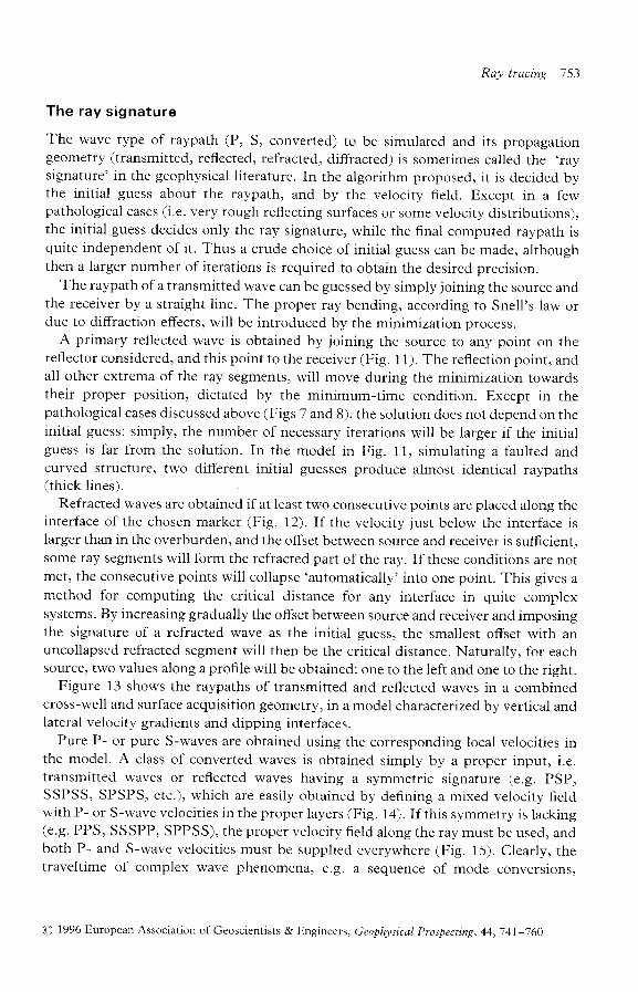
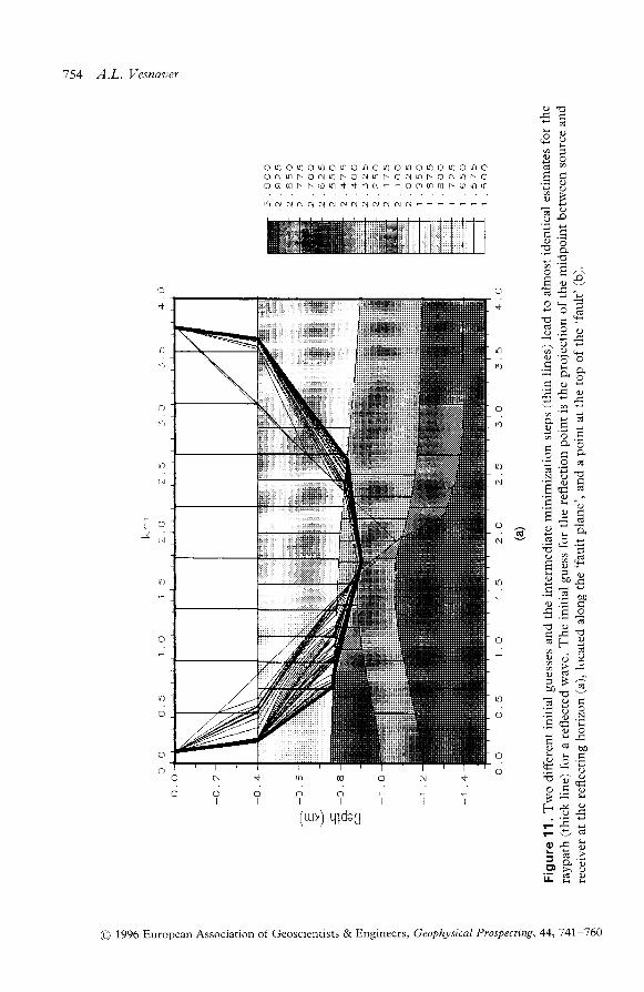
A primary reflected wave is obtained by joining the source to any point on thereflector considered, and this point to the receiver (Fig. 11). The reflection point, andall other extrema of the ray segments, will move during the minimization towardstheir proper position, dictated by the minimum-time condition. Except in thepathological cases discussed above (trigs 7 and 8), the solution does not depend on theinitial guess: simply, the number of necessary iterations will be larger if the initialguess is far from the solution. In the model in Fig. 11, simulating a faulted andcurved structure, two different initial guesses produce almost identical raypaths(thick l ines).

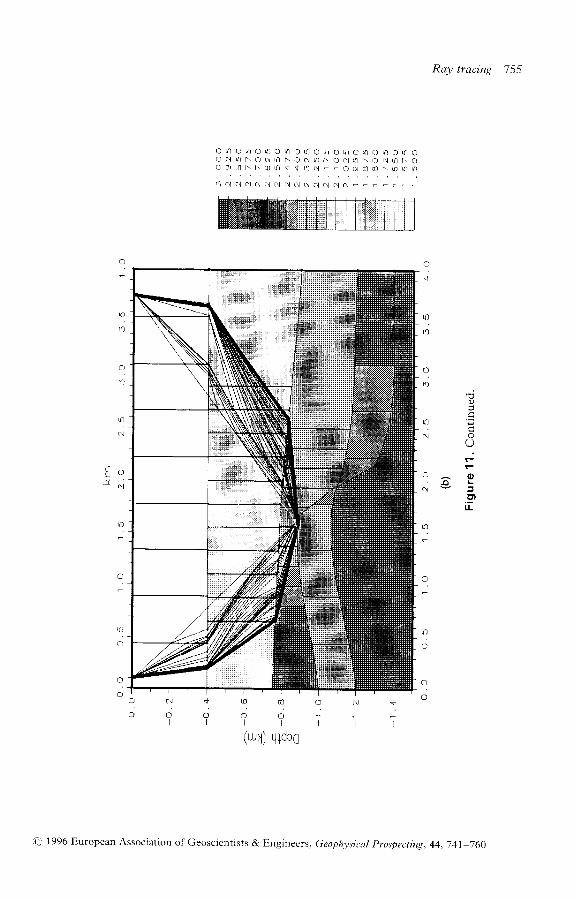
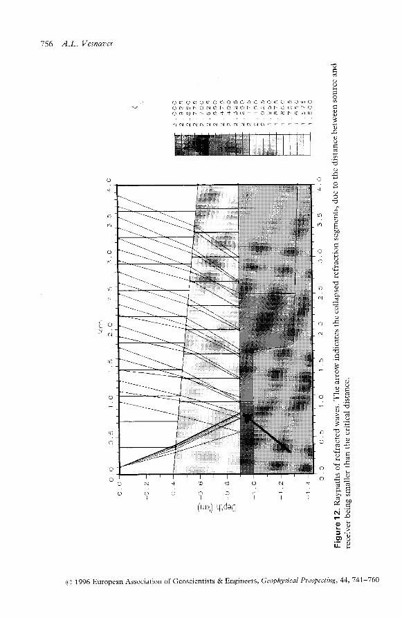
Refracted waves are obtained if at least two consecutive points are placed along theinterface of the chosen marker (Fig. 12). If the velocity just belou'the interface islarger than in the overburden, and the offset between source and receiver is sufficient,some ray segments will form the refracted part of the ray. If these conditions are notmet, the consecutive points will collapse 'automatically' into one point. This gives amethod for computing the critical distance for any interface in quite complexsystems. By increasing gradually the offset between source and receiver and imposingthe signature of a refracted wave as the initial guess, the smallest offset with anuncollapsed refracted segment will then be the critical distance. Naturally, for eachsource) two values along a profile will be obtained: one to the left and one to the right.

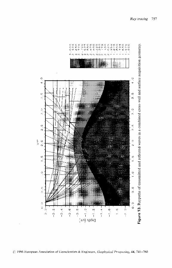
Figure 13 shows the raypaths of transmitted and reflected waves in a combinedcross-well and surface acquisition geometry, in a model characterized by vertical andIateral velocity gradients and dipping interfaces.

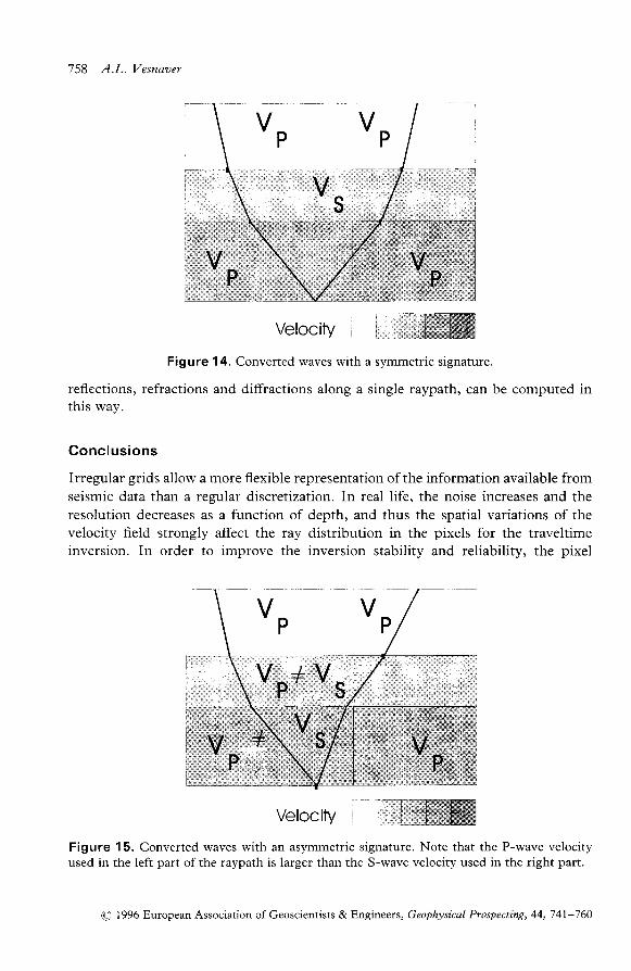
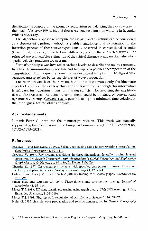
Pure P- or pure S-waves are obtained using the corresponding local velocities inthe model. A class of converted waves is obtained simply by a proper input, i.e.transmitted waves or reflected waves having a symmetric signature (e.g. pSp,ssPSS, SPSPS, etc.), which are easily obtained by defining a mixed velocity f ieldwith P- or S-wave velocities in the proper layers (Fig. 1a). If this symmetry is lacking(e.g. PPS, SSSPP, SPPSS), the proper velocity f ield along the ray must be used, andboth P- and S-'"vave velocities must be supplied everywhere (Fig. 15). clearly, thetraveltime of compiex wave phenomena, e.g. a sequence of mode conversions,

(t': ', 1996 European Association of Geoscientists & Engineers, Geophgsical Prospecting, 44,741-760

754 A.L. Vesnaaer

9 :

3 7H -

; 9'aJ I

p . :

: r ^E U -

d . 9 I^ 9 P

d o j:

^ P G

o . : P

o Y . =

6 ! rN O :

F d a

E i ho * 7c ! - !

i l * &E O ;g.l bo ;

Y X zt s t i x

9 4 j Pa > :C) .cg

6 . : !

. = x NL E !' -

o o

o .v bt)l ! C

E - e! ? , .9o t r EB = !

l - ! a

F - !

:., r,-.1 o= E >J 6 _ l

r J - u i

n N N N N N N N N o I N N . i N - -

O u1 L) rO O L1 O |n O O O ul O n O ur) O |o O |1) Oo c,i n F o ( !1 N o c'l n N o N ro f. o N n F oO 0 s: f.. N $ rO \t \t n N - - O D m I0 F rO $ L0

?

UI

N

o ^. ( u

i,,,1 q*.0

e ]j96 European Association of Geoscientists & Engineers, Geophysical Prospecting, 44, 741-760

Ray tracing 755

o (r] a Lo O'o o (] O n O !0 O u.t O !,1 o ra o !1 OO (1 ul l. O N t0 F O N n F O ol r4 tr O .'t rO f\ Oo o m F. N 0 ra t t n N - - o o qt 0l f.. (! s-l ro

ri'-'l ol o.l cl.'l N -l c! o/ ot N fl fl - -

6 d l

o ot t/ , , , , \ , , . , . t ^ -\w, l / L1+udu

.o

d

N Or t

-o ^ q )

II

i!:; 1996 European Association of Geoscicntists & Enginecrs, Geophysical I'rospecting, 44,741-760

756 A.L. Vesnaxer

c6

I

,a

d

d

.oo

O !

'o

u J d

o0o

, !

U

-m q

( ! d

O

c ! o

6a

g

! 'J ' i

cd 9{

, L . O

o -> d

> ' i

r n c l

c * f ,o o -

' a ? ,

x d> . 4J o o

a r h: >r ' ^o Ui i 9

n N c l N C l n N . 1 . ! N f l N c { N - -

o ( l .J n o' / t o L0 o tr l Lf n Lr f l o ul Q o o o ao N () t r o N | l1 f- o c! t r) I ' o. \ q F a. ' l 6 l . oQ D rJ F t' 0 |fl -t rt fl..,l - - o 0 (] m F 0 0 (]

+ ( a m o N +

. i d o -t t l l t l

(u1) u+d:C

(a) 1996 European Association of Geoscientists & Engineers, Geophysical Prospecting, 44' 741-760

Ray tracing 757

!q

b0

d

O O. 9. 6

Ed

' , o

I

^ tu n

n r oo

trq J o

N 6 6

o

N -"oO

I

" , O

- !

g

" , o

d A

G

ci ";o

o N + o D c o N + ( o m oc i c i o o c i - - - : : " ;

t t t t t t t l t l/ r r r> i ) u tdan\ * r / r r u

o !'l o !1 o ul 0 !r o q1 C) !,) o !') () !a o r'r o ro oO c'i rf) F. O N O l. O N lf, I' O c!'O F O N lf) 1.. O

: i ' l : ' l 1 o : 1 - : : ' 1 1 : : i in c l c , l . l . ' l O N N Q N N o l N N - -

A 1996 European Association of Geoscientists & Engineers, Geophysical Prospecting, 44,741-l60

758 A.L. Vesnaoer

Velocity

Figure 14. Converted waves with a symmetric signature.

reflections, refractions and diffractions along a single raypath, can be computed inthis way.

Conc lus ions

Irregular grids allow a more flexible representation of the information available fromseismic data than a regular discretization. In real life, the noise increases and theresolution decreases as a function of depth, and thus the spatial variations of thevelocity field strongly affect the ray distribution in the pixels for the traveltimeinversion. In order to improve the inversion stability and reliability, the pixel

V , V ,

\ vp+ v s /

f'F

Figure 15. Converted waves with an asymmetric signature. Note that the P-wave velocityused in the left part ofthe raypath is larger than the S-wave velocity used in the right part.

O 1996 European Association of Geoscientists & Engineers, Geophysical Prospecting, 44,741-760

Ray tracing 759

distribution is adapted to the geometry acquisition by balancing the ray coverage ofthe pixels (Vesnaver 1994a, b), and thus a ray-tracing algorithm working in irregulargrids is necessary.

The algorithm proposed to compute the raypath and traveltime can be consideredas a discretized bending method. It enables simulation and exploitation in theinversion process of those wave types usually observed in conventional seismics(transmitted, reflected, refracted and diffracted) and of the converted waves. For

refracted waves, it enables estimation of the critical distance at any marker, also whenspatial velocity gradients are present.

Fermat's principle was invoked at various levels: to describe the ray by segments,to define the minimization procedure and to propose a parallel decomposition of thecomputation. The reciprocity principle was exploited to optimize the algorithmic

sequence and to reflect better the physics of wave propagation.

The main drawback of the new method is that it estimates only the kinematic

aspects of a ray, i.e. the ray trajectory and the traveltime. Although this informationis sufficient for traveltime inversion, it is not sufficient for inverting the amplitudedecay. For that case, the dynamic components could be obtained by conventionaldynamic ray tracing (Cerveny 1987), possibly using the minimum-time solution as

the initial guess for the other approach.

Acknowledgements

I thank Peter Guidotti for the manuscript revision. This work was partially

supported by the Commission of the European Communities (DG XIII, contract no.

JOU2-CT93 -032r).

References

Asakawa E. and Kanawaka T. 1993. Seismic ray tracing using linear traveltime interpolation.

G eophysical Prospecting 41, 99-171.

Cerveny V. 1987. Ray tracing algorithms in three-dimensional laterally varying Iayered

structures. In'. Seismic Tomographg with Applications in Global Seismology and Exploration

Geophysics (ed. G. Nolet), pp. 99-133, D. Reidel Pub. Co.Chander R. 1977. On tracing seismic rays with specified end points in layers of constant

velocity and plane interfaces. Geophysical Prospecting 25, l2O-124.Fisher R. and Lees J.M. 1993. Shortest path ray tracing with sparse graphs. Geophysics 58,

987-996.

Julian B.R. and Gubbins D. 1977. Three-dimensional seismic ray tracing. Journal of

Geophysics 43,95-114.Moser T.J. 1989. Efficient seismic ray tracing using graph theory. 59th SEG meeting, Dallas,

Expanded Abstracts, 1 106-1 108.

Moser T.J. 1991. Shortest path calculation of seismic rays. Geophysics 56, 59-67.

Nolet G. 1987. Seismic wave propagation and seismic tomography. In:. Seismic Tomography

e) 1996 European Association of Geoscientists & Engineers, Geophysical Prospecting, 44,741-760

760 A.L. Vesnaaer

with Applications in Global Seismology and Exploration Geophgsics (ed. G. Nolet), pp. 7-23'

D. Reidel Pub. Co.Pereyra V. 1992. Two point ray tracing in general 3D media. Geophysical Prospecting 40,

267-287.Saito H. 1989. Traveltimes and raypaths of first arrival seismic waves. 59th SEG meeting,

Dallas, Expanded Abstracts, 244-247.Sherifl R.E. 1973. Encyclopaedic Dictionary of Exploration Geophysics. SEG, Tulsa, USA.

Stockli R.F. 1984. Two-point ray tracing in a three-dimensional medium consisting of

homogeneous nonisotropic layers separated by plane interfaces. Geophysics 49,767-770.

Vesnaver A. 1994a. The contribution of refracted waves to seismic tomography. 56th EAEG

meeting, Vienna, Austria, Extended Abstracts, P62.Vesnaver A. 1994b. Towards the uniqueness of tomographic inversion solutions. Journal of

S eismic Explor ation 3, 323-334.Vidale J. 1988. Finite difference calculation of traveltimes . Bulletin of the Seismological Society

of America 7 8, 2062-207 6.Vidale J. 1990. Finite-difference calculation of traveltimes in three dimensions. Geophysics 55,

52 t -526.Virieux J. and Farra V. 1991. Ray tracing in 3-D complex isotropic media: an analysis of the

problem. Geophy sics 56, 2057 -2069.

O 1996 European Association of Geoscientists & Engineers, Geophysical Prospecting,44,74l-760