quantifying the robustness of flight control systems using nichols exclusion regions and the...

http://pii.sagepub.com/Control Engineering

Engineers, Part I: Journal of Systems and Proceedings of the Institution of Mechanical

http://pii.sagepub.com/content/215/6/625The online version of this article can be found at:

DOI: 10.1243/0959651011541355

215: 625 2001Proceedings of the Institution of Mechanical Engineers, Part I: Journal of Systems and Control Engineering

D G Bates, R Kureemun and I Postlethwaitestructured singular value

Quantifying the robustness of flight control systems using Nichols exclusion regions and the

Published by:

http://www.sagepublications.com

On behalf of:

Institution of Mechanical Engineers

can be found at:Control EngineeringProceedings of the Institution of Mechanical Engineers, Part I: Journal of Systems andAdditional services and information for

http://pii.sagepub.com/cgi/alertsEmail Alerts:

http://pii.sagepub.com/subscriptionsSubscriptions:

http://www.sagepub.com/journalsReprints.navReprints:

http://www.sagepub.com/journalsPermissions.navPermissions:

http://pii.sagepub.com/content/215/6/625.refs.htmlCitations:

What is This?

- Sep 1, 2001Version of Record >>

by guest on September 6, 2012pii.sagepub.comDownloaded from

http://pii.sagepub.com/

http://pii.sagepub.com/content/215/6/625

http://www.sagepublications.com

http://www.imeche.org/home

http://pii.sagepub.com/cgi/alerts

http://pii.sagepub.com/subscriptions

http://www.sagepub.com/journalsReprints.nav

http://www.sagepub.com/journalsPermissions.nav

http://pii.sagepub.com/content/215/6/625.refs.html

http://pii.sagepub.com/content/215/6/625.full.pdf

http://online.sagepub.com/site/sphelp/vorhelp.xhtml


625

Quantifying the robustness of �ight control systemsusing Nichols exclusion regions and the structuredsingular value

D G Bates*, R Kureemun and I PostlethwaiteDepartment of Engineering, University of Leicester, UK

Abstract: This paper establishes some connections between classical stability metrics currently usedin the aerospace industry for the certi�cation of �ight control laws and modern tools for the robustnessanalysis of uncertain multivariable systems. Multiloop simultaneous gain and phase margin robustnessspeci�cations are written as Nichols plane exclusion regions for the open-loop frequency response ofeach loop of the system. Satisfaction of these robustness speci�cations for uncertain multivariablesystems is then shown to be exactly equivalent to satisfying a certain bound on the structured singularvalue í of the closed-loop system. The proposed tools are applied to the problem of analysing therobustness of an integrated �ight and propulsion control system for a future V/STOL aircraft conceptsubject to variations in aircraft mass and centre of gravity. In particular, the implications for theproposed method of diYculties in computing tight bounds on í are considered.

Keywords: robustness, analysis, multivariable, �ight, control

NOTATION ler design and analysis techniques [3 ], however, concen-trate on the open-loop frequency response, and measurerobustness in terms of allowable gain and phase marginIFPC integrated �ight and propulsion controloVsets in each loop of the system [4 ].LFT linear fractional transformation

In the robust control literature, gain and phase mar-LTI linear time invariantgins by themselves have been shown to be unreliableNP non-polynomialmeasures of robustness for both single-loop systemsRTAVS real time all vehicle simulator(considering simultaneous variations in gain and phase)VAAC vectored thrust aircraft advanced �ight[2 ] and multivariable systems (considering simultaneouscontroluncertainty in multiple loops) [5 ]. Robust control theor-V/STOL vertical/short takeoV and landingists have sought to overcome these shortcomings byWEM wide envelope modeldeveloping new measures of robustness such as the struc-tured singular value í [6, 7 ]. The resulting robustnesstests provide de�nite ‘worst case’ guarantees of stability1 INTRODUCTIONand performance robustness for uncertain multivariableplants. They do not, however, generally provide this

Modern robust controller design methods, such as H2 information in a form that is very meaningful to design-

mixed-sensitivity optimization [1 ] and í synthesis [1, 2 ], ers working in the framework of classical control.allow the designer to shape various closed-loop transfer Indeed, control system designers working in the aero-functions in order to maximize robustness—where space industry have long been aware of the shortcomingsrobustness is measured in terms of (structured or of gain and phase margins as robustness measures, andunstructured ) singular value margins. Classical control- have therefore relied on exclusion regions in the Nichols

plane to guarantee robustness with the classical margins.Consider, for example, the ‘classical’ robustness speci�-

The MS was received on 9 January 2001 and was accepted after revision cation described below, which is adapted from referencefor publication on 19 September 2001. [8 ] and is representative of the type of robustness tests* Corresponding author: Control and Instrumentation Research Group,

currently used in the industrial certi�cation process forDepartment of Engineering, University of Leicester, University Road,Leicester LE1 7RH, UK. �ight control laws [9 ].

I00301 © IMechE 2001 Proc Instn Mech Engrs Vol 215 Part I by guest on September 6, 2012pii.sagepub.comDownloaded from


626 D G BATES, R KUREEMUN AND I POSTLETHWAITE

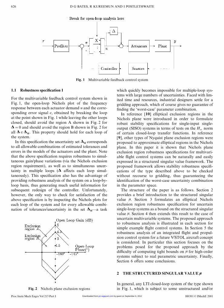
Fig. 1 Multivariable feedback control system

1.1 Robustness speci�cation 1 which quickly becomes impossible for multiple-loop sys-tems with large numbers of uncertainties. Faced with lim-

For the multivariable feedback control system shown in ited time and resources, industrial designers settle for aFig. 1, the open-loop Nichols plot of the frequency gridding approach, which of course gives no guarantee ofresponse between each actuator demand u and the corre- �nding the ‘worst-case’ parameter combination.sponding error signal e, obtained by breaking the loop In reference [10] elliptical exclusion regions in theat the point shown in Fig. 1 while leaving the other loops Nichols plane were introduced in order to formulateclosed, should avoid the region A shown in Fig. 2 for robust stability speci�cations for single-input single-¢=0 and should avoid the region B shown in Fig. 2 for output (SISO) systems in terms of tests on the H

2norm

all ¢µ¢M . This property should hold for each loop of of certain closed-loop transfer functions. In reference

the system. [9 ], other types of Nyquist plane exclusion regions wereIn this speci�cation the uncertainty set ¢

M corresponds proposed to approximate elliptical regions in the Nicholsto all allowable combinations of estimated tolerances and plane. In this paper it is shown that Nichols planeerrors in the models of the actuators and the plant. Note exclusion region robustness speci�cations for multivari-that the above speci�cation requires robustness to simul- able �ight control systems can be naturally and easilytaneous gain/phase variations (via the Nichols exclusion expressed in a structured singular value framework. Theregion requirement), as well as to simultaneous uncer- proposed framework allows stability robustness speci�-tainty in multiple loops (¢ aVects each loop simul- cations of the type described above to be checkedtaneously). This speci�cation also has the advantage of without recourse to gridding, thus guaranteeing theproviding robustness analysis of the system on a loop-by- identi�cation of the worst-case uncertainty combination

in the parameter space.loop basis, thus generating much useful information forThe structure of the paper is as follows. Section 2subsequent redesign of the controller. Unfortunately,

provides a brief introduction to the structured singularhowever, the only way to check for satisfaction of thevalue í. Section 3 formulates an elliptical Nicholsabove speci�cation is by inspecting the Nichols plots forexclusion region robustness speci�cation for uncertaineach loop of the system and for every allowable combi-single-loop systems as a bound on the structured singularnation of tolerances/uncertainty in the set ¢

M—a taskvalue í. Section 4 then extends this result to the case ofuncertain multivariable systems. The proposed approachto robustness analysis is illustrated in each section forsimple example �ight control systems. In Section 5 therobustness analysis of an integrated �ight and propul-sion control system for a future V/STOL aircraft conceptis considered. In particular this section focuses on theproblems posed for the proposed approach by thediYculty of computing tight bounds on í for high-ordersystems subject to real parametric uncertainty. Finally,Section 6 oVers some conclusions.

2 THE STRUCTURED SINGULAR VALUE í

In general, any LTI closed-loop system of the type shownFig. 2 Nichols plane exclusion regions in Fig. 1, which is subject to some unstructured and/or

I00301 © IMechE 2001Proc Instn Mech Engrs Vol 215 Part I by guest on September 6, 2012pii.sagepub.comDownloaded from


627QUANTIFYING THE ROBUSTNESS OF FLIGHT CONTROL SYSTEMS

suYciently tight, then little information is lost. Note thatto exploit fully the power of the structured singular valuetheory, tight upper and lower bounds on í are required.The upper bound provides only a suYcient condition forstability in the presence of a speci�ed level of structureduncertainty. The lower bound provides a suYcient con-dition for instability, and also returns a worst-case ¢,i.e. a worst-case combination of uncertain parametersfor the problem [12].

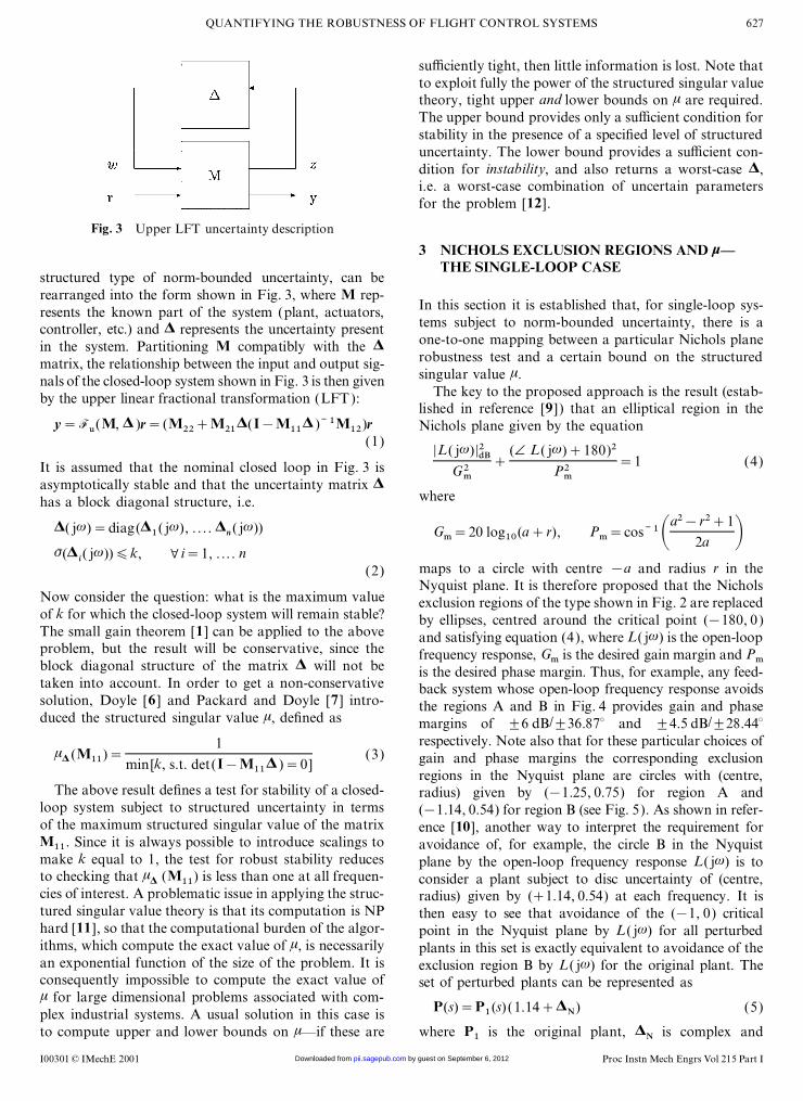
Fig. 3 Upper LFT uncertainty description

3 NICHOLS EXCLUSION REGIONS AND í—THE SINGLE-LOOP CASE

structured type of norm-bounded uncertainty, can berearranged into the form shown in Fig. 3, where M rep-

In this section it is established that, for single-loop sys-resents the known part of the system (plant, actuators,tems subject to norm-bounded uncertainty, there is acontroller, etc.) and ¢ represents the uncertainty presentone-to-one mapping between a particular Nichols planein the system. Partitioning M compatibly with the ¢robustness test and a certain bound on the structuredmatrix, the relationship between the input and output sig-singular value í.nals of the closed-loop system shown in Fig. 3 is then given

The key to the proposed approach is the result (estab-by the upper linear fractional transformation (LFT):lished in reference [9 ] ) that an elliptical region in the

y=Fu(M, ¢ )r=(M22

+M21

¢(I�M11

¢ )Õ1M12)r Nichols plane given by the equation

(1)|L( jö) |2dB

G2m+

(Ð L( jö)+180)2P2m

=1 (4)It is assumed that the nominal closed loop in Fig. 3 isasymptotically stable and that the uncertainty matrix ¢

wherehas a block diagonal structure, i.e.

¢( jö)=diag(¢1( jö), . . . . ¢n( jö)) Gm=20 log10(a+r), Pm=cosÕ1 Aa2�r2+1

2a Bó̄(¢

i( jö))åk, Y i=1, . .. . n

maps to a circle with centre �a and radius r in the(2)Nyquist plane. It is therefore proposed that the Nichols

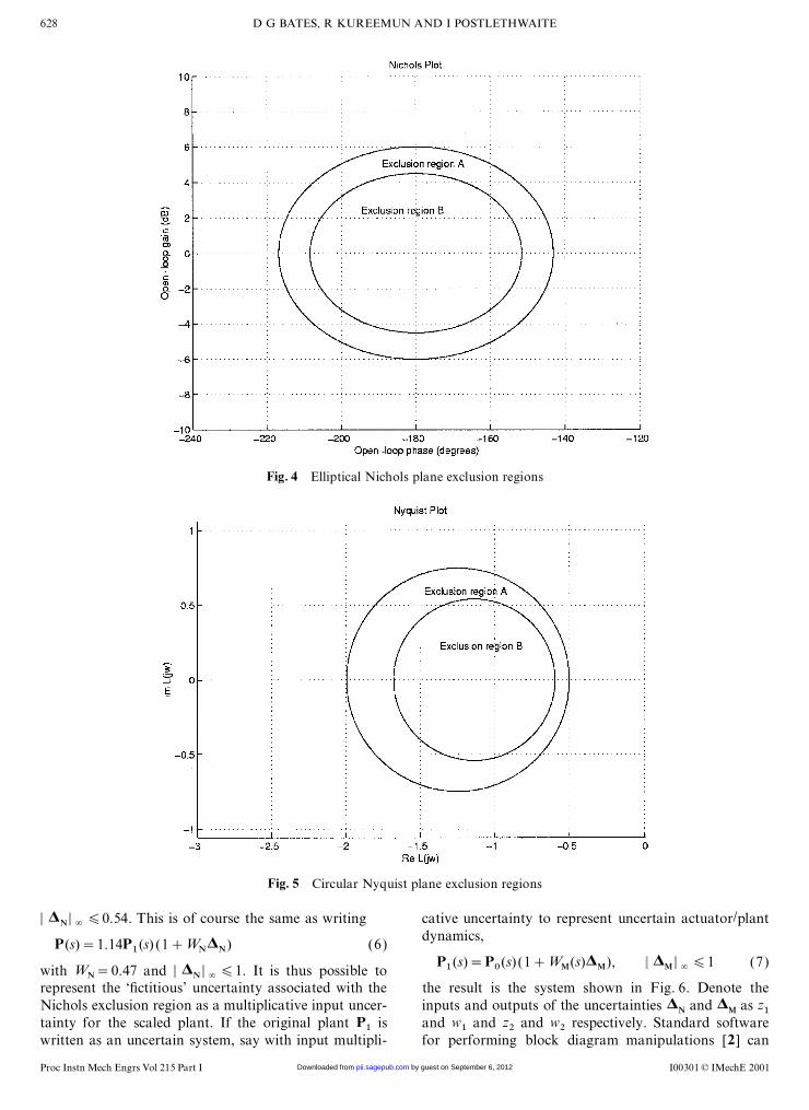
Now consider the question: what is the maximum value exclusion regions of the type shown in Fig. 2 are replacedof k for which the closed-loop system will remain stable? by ellipses, centred around the critical point (�180, 0)The small gain theorem [1 ] can be applied to the above and satisfying equation (4), where L( jö) is the open-loopproblem, but the result will be conservative, since the frequency response, Gm is the desired gain margin and Pmblock diagonal structure of the matrix ¢ will not be is the desired phase margin. Thus, for example, any feed-taken into account. In order to get a non-conservative back system whose open-loop frequency response avoidssolution, Doyle [6 ] and Packard and Doyle [7 ] intro- the regions A and B in Fig. 4 provides gain and phaseduced the structured singular value í, de�ned as margins of ±6 dB/±36.87° and ±4.5 dB/±28.44°

respectively. Note also that for these particular choices ofí¢ (M11)=

1

min[k, s.t. det(I�M11¢ )=0]

(3) gain and phase margins the corresponding exclusionregions in the Nyquist plane are circles with (centre,

The above result de�nes a test for stability of a closed- radius) given by (�1.25, 0.75) for region A andloop system subject to structured uncertainty in terms (�1.14, 0.54) for region B (see Fig. 5). As shown in refer-of the maximum structured singular value of the matrix ence [10], another way to interpret the requirement forM11. Since it is always possible to introduce scalings to avoidance of, for example, the circle B in the Nyquistmake k equal to 1, the test for robust stability reduces plane by the open-loop frequency response L( jö) is toto checking that í¢ (M11) is less than one at all frequen- consider a plant subject to disc uncertainty of (centre,cies of interest. A problematic issue in applying the struc- radius) given by (+1.14, 0.54) at each frequency. It istured singular value theory is that its computation is NP then easy to see that avoidance of the (�1, 0) criticalhard [11], so that the computational burden of the algor- point in the Nyquist plane by L( jö) for all perturbedithms, which compute the exact value of í, is necessarily plants in this set is exactly equivalent to avoidance of thean exponential function of the size of the problem. It is exclusion region B by L( jö) for the original plant. Theconsequently impossible to compute the exact value of set of perturbed plants can be represented así for large dimensional problems associated with com-

P(s)=P1(s) (1.14+¢N) (5)plex industrial systems. A usual solution in this case is

to compute upper and lower bounds on í—if these are where P1 is the original plant, ¢N is complex and




Fig. 4 Elliptical Nichols plane exclusion regions

Fig. 5 Circular Nyquist plane exclusion regions

d ¢N d

2å0.54. This is of course the same as writing cative uncertainty to represent uncertain actuator/plant

dynamics,P(s)=1.14P1(s) (1+WN¢

N) (6)P1(s)=P0(s) (1+WM(s)¢M), d ¢

M d2

å1 (7)with WN=0.47 and d ¢

N d2

å1. It is thus possible torepresent the ‘�ctitious’ uncertainty associated with the the result is the system shown in Fig. 6. Denote the

inputs and outputs of the uncertainties ¢N and ¢

M as z1Nichols exclusion region as a multiplicative input uncer-

tainty for the scaled plant. If the original plant P1 is and w1 and z2 and w2 respectively. Standard softwarefor performing block diagram manipulations [2 ] canwritten as an uncertain system, say with input multipli-




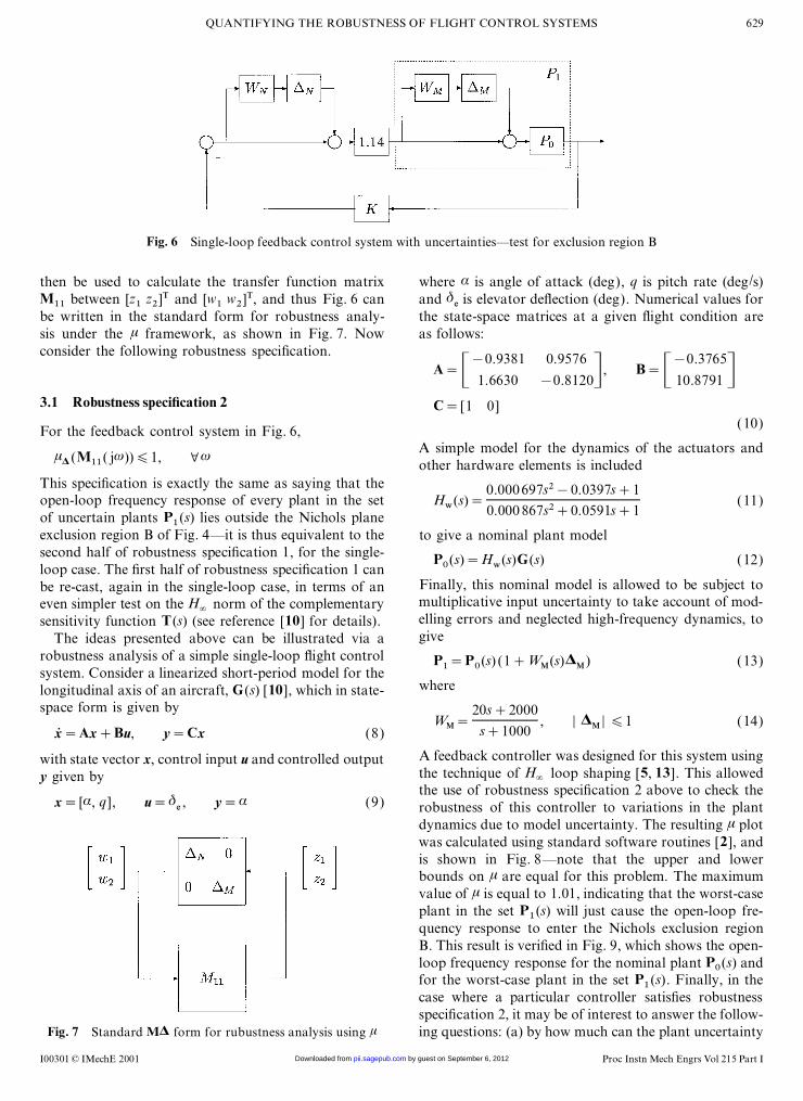
Fig. 6 Single-loop feedback control system with uncertainties—test for exclusion region B

then be used to calculate the transfer function matrix where á is angle of attack (deg), q is pitch rate (deg/s)and ä

e is elevator de�ection (deg). Numerical values forM11 between [z1 z2 ]T and [w1 w2 ]T, and thus Fig. 6 canbe written in the standard form for robustness analy- the state-space matrices at a given �ight condition are

as follows:sis under the í framework, as shown in Fig. 7. Nowconsider the following robustness speci�cation.

A=C�0.9381 0.9576

1.6630 �0.8120D , B=C�0.3765

10.8791 D3.1 Robustness speci�cation 2 C= [1 0]

(10)For the feedback control system in Fig. 6,A simple model for the dynamics of the actuators andí¢ (M11( jö))å1, Yöother hardware elements is included

This speci�cation is exactly the same as saying that theopen-loop frequency response of every plant in the set Hw(s)=

0.000697s2�0.0397s+1

0.000 867s2+0.0591s+1(11)

of uncertain plants P1(s) lies outside the Nichols plane

exclusion region B of Fig. 4—it is thus equivalent to the to give a nominal plant modelsecond half of robustness speci�cation 1, for the single- P

0(s)=Hw(s)G(s) (12)

loop case. The �rst half of robustness speci�cation 1 canFinally, this nominal model is allowed to be subject tobe re-cast, again in the single-loop case, in terms of anmultiplicative input uncertainty to take account of mod-even simpler test on the H

2norm of the complementary

elling errors and neglected high-frequency dynamics, tosensitivity function T(s) (see reference [10] for details).giveThe ideas presented above can be illustrated via a

robustness analysis of a simple single-loop �ight control P1=P

0(s) (1+WM(s)¢M ) (13)

system. Consider a linearized short-period model for thewherelongitudinal axis of an aircraft, G(s) [10], which in state-

space form is given byWM=

20s+2000

s+1000, d ¢

M d å1 (14)xÇ =Ax+Bu, y=Cx (8)

A feedback controller was designed for this system usingwith state vector x, control input u and controlled outputthe technique of H

2loop shaping [5, 13]. This allowedy given by

the use of robustness speci�cation 2 above to check thex= [á, q ], u=ä

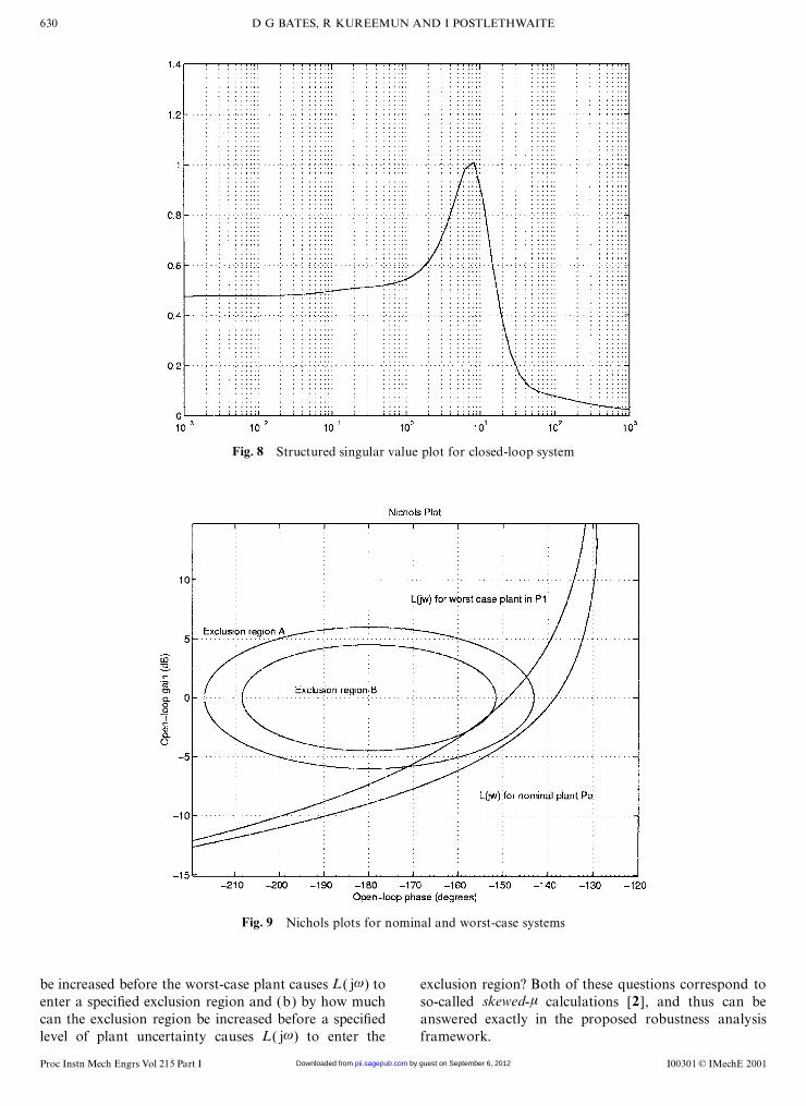
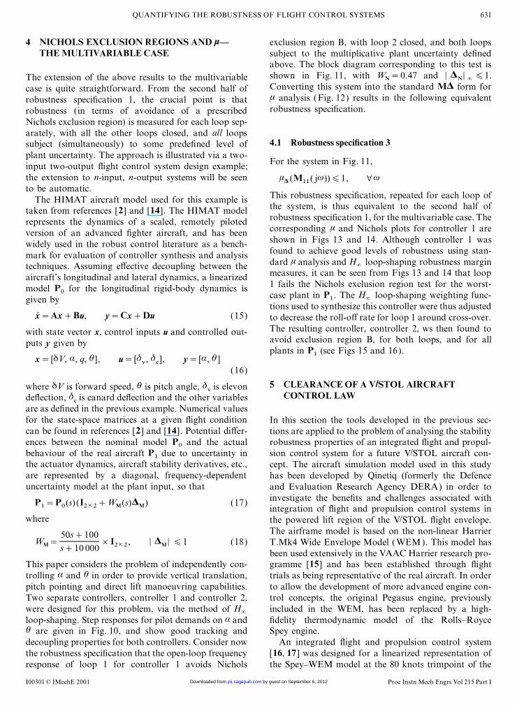
e , y=á (9) robustness of this controller to variations in the plantdynamics due to model uncertainty. The resulting í plotwas calculated using standard software routines [2 ], andis shown in Fig. 8—note that the upper and lowerbounds on í are equal for this problem. The maximumvalue of í is equal to 1.01, indicating that the worst-caseplant in the set P1(s) will just cause the open-loop fre-quency response to enter the Nichols exclusion regionB. This result is veri�ed in Fig. 9, which shows the open-loop frequency response for the nominal plant P0(s) andfor the worst-case plant in the set P

1(s). Finally, in thecase where a particular controller satis�es robustnessspeci�cation 2, it may be of interest to answer the follow-

Fig. 7 Standard M¢ form for rubustness analysis using í ing questions: (a) by how much can the plant uncertainty




Fig. 8 Structured singular value plot for closed-loop system

Fig. 9 Nichols plots for nominal and worst-case systems

be increased before the worst-case plant causes L( jö) to exclusion region? Both of these questions correspond toso-called skewed-í calculations [2 ], and thus can beenter a speci�ed exclusion region and (b) by how much

can the exclusion region be increased before a speci�ed answered exactly in the proposed robustness analysisframework.level of plant uncertainty causes L( jö) to enter the




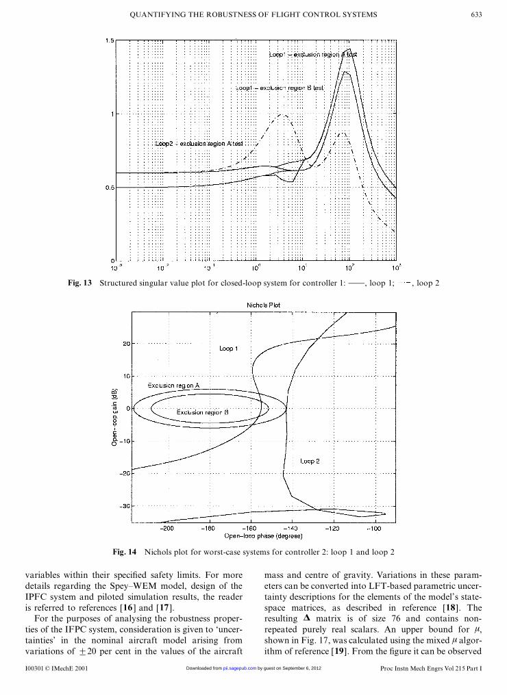
4 NICHOLS EXCLUSION REGIONS AND í— exclusion region B, with loop 2 closed, and both loopssubject to the multiplicative plant uncertainty de�nedTHE MULTIVARIABLE CASEabove. The block diagram corresponding to this test isshown in Fig. 11, with WN=0.47 and d ¢

N d2

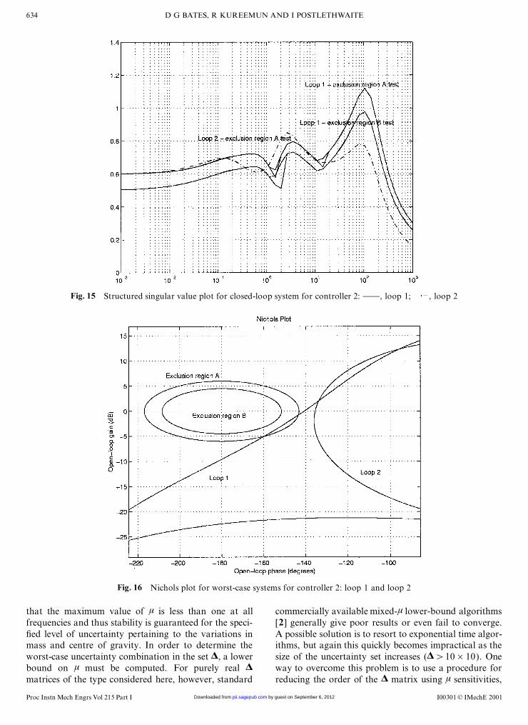
å1.The extension of the above results to the multivariableConverting this system into the standard M¢ form forcase is quite straightforward. From the second half ofí analysis (Fig. 12) results in the following equivalentrobustness speci�cation 1, the crucial point is thatrobustness speci�cation.robustness (in terms of avoidance of a prescribed

Nichols exclusion region) is measured for each loop sep-arately, with all the other loops closed, and all loops

4.1 Robustness speci�cation 3subject (simultaneously) to some prede�ned level ofplant uncertainty. The approach is illustrated via a two-

For the system in Fig. 11,input two-output �ight control system design example;the extension to n-input, n-output systems will be seen í¢ (M11( jö))å1, Y öto be automatic.

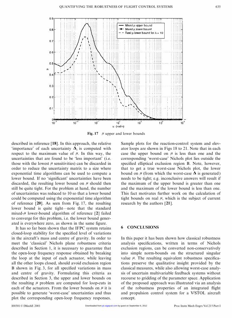
This robustness speci�cation, repeated for each loop ofThe HIMAT aircraft model used for this example isthe system, is thus equivalent to the second half oftaken from references [2 ] and [14]. The HIMAT modelrobustness speci�cation 1, for the multivariable case. Therepresents the dynamics of a scaled, remotely pilotedcorresponding í and Nichols plots for controller 1 areversion of an advanced �ghter aircraft, and has beenshown in Figs 13 and 14. Although controller 1 waswidely used in the robust control literature as a bench-found to achieve good levels of robustness using stan-mark for evaluation of controller synthesis and analysisdard í analysis and H

2loop-shaping robustness margintechniques. Assuming eVective decoupling between the

measures, it can be seen from Figs 13 and 14 that loopaircraft’s longitudinal and lateral dynamics, a linearized1 fails the Nichols exclusion region test for the worst-model P0 for the longitudinal rigid-body dynamics iscase plant in P1 . The H

2loop-shaping weighting func-given by

tions used to synthesize this controller were thus adjustedxÇ =Ax+Bu, y=Cx+Du (15) to decrease the roll-oV rate for loop 1 around cross-over.

The resulting controller, controller 2, ws then found towith state vector x, control inputs u and controlled out-avoid exclusion region B, for both loops, and for allputs y given byplants in P1 (see Figs 15 and 16).

x= [äV, á, q, õ], u= [äv , äc], y= [á, õ ]

(16)

5 CLEARANCE OF A V/STOL AIRCRAFTwhere äV is forward speed, õ is pitch angle, äv is elevon

CONTROL LAWde�ection, äc is canard de�ection and the other variables

are as de�ned in the previous example. Numerical valuesfor the state-space matrices at a given �ight condition In this section the tools developed in the previous sec-can be found in references [2 ] and [14]. Potential diVer- tions are applied to the problem of analysing the stabilityences between the nominal model P0 and the actual robustness properties of an integrated �ight and propul-behaviour of the real aircraft P1 due to uncertainty in sion control system for a future V/STOL aircraft con-the actuator dynamics, aircraft stability derivatives, etc., cept. The aircraft simulation model used in this studyare represented by a diagonal, frequency-dependent has been developed by Qinetiq (formerly the Defenceuncertainty model at the plant input, so that and Evaluation Research Agency DERA) in order to

investigate the bene�ts and challenges associated withP1=P0(s) (I2Ö2+WM(s)¢M) (17)integration of �ight and propulsion control systems in

where the powered lift region of the V/STOL �ight envelope.The airframe model is based on the non-linear Harrier

WM=50s+100s+10 000

×I2Ö2 , d ¢M d å1 (18) T.Mk4 Wide Envelope Model (WEM). This model has

been used extensively in the VAAC Harrier research pro-gramme [15] and has been established through �ightThis paper considers the problem of independently con-

trolling á and õ in order to provide vertical translation, trials as being representative of the real aircraft. In orderto allow the development of more advanced engine con-pitch pointing and direct lift manoeuvring capabilities.

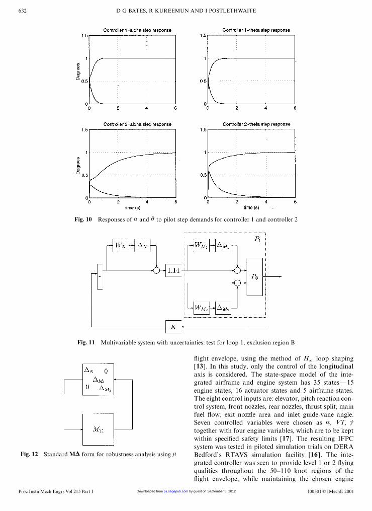
Two separate controllers, controller 1 and controller 2, trol concepts, the original Pegasus engine, previouslyincluded in the WEM, has been replaced by a high-were designed for this problem, via the method of H

2loop-shaping. Step responses for pilot demands on á and �delity thermodynamic model of the Rolls–Royce

Spey engine.õ are given in Fig. 10, and show good tracking anddecoupling properties for both controllers. Consider now An integrated �ight and propulsion control system

[16, 17 ] was designed for a linearized representation ofthe robustness speci�cation that the open-loop frequencyresponse of loop 1 for controller 1 avoids Nichols the Spey–WEM model at the 80 knots trimpoint of the



https://www.researchgate.net/publication/3029354_Correction_to_Feedback_properties_of_multivariable_systems_The_role_and_use_of_the_return_difference_matrix?el=1_x_8&enrichId=rgreq-f4cda9f28ac74d7c0fb648636eb8027a-XXX&enrichSource=Y292ZXJQYWdlOzIzODEwMzYwOTtBUzoxNjU5NzA5NzA2ODU0NDBAMTQxNjU4MTk3MTE2OA==



Fig. 10 Responses of á and õ to pilot step demands for controller 1 and controller 2

Fig. 11 Multivariable system with uncertainties: test for loop 1, exclusion region B

�ight envelope, using the method of H2

loop shaping[13 ]. In this study, only the control of the longitudinalaxis is considered. The state-space model of the inte-grated airframe and engine system has 35 states—15engine states, 16 actuator states and 5 airframe states.The eight control inputs are: elevator, pitch reaction con-trol system, front nozzles, rear nozzles, thrust split, mainfuel �ow, exit nozzle area and inlet guide-vane angle.Seven controlled variables were chosen as á, VT, çÁtogether with four engine variables, which are to be keptwithin speci�ed safety limits [17]. The resulting IFPCsystem was tested in piloted simulation trials on DERA

Fig. 12 Standard M¢ form for robustness analysis using í Bedford’s RTAVS simulation facility [16 ]. The inte-grated controller was seen to provide level 1 or 2 �yingqualities throughout the 50–110 knot regions of the�ight envelope, while maintaining the chosen engine




Fig. 13 Structured singular value plot for closed-loop system for controller 1: ——, loop 1; , loop 2

Fig. 14 Nichols plot for worst-case systems for controller 2: loop 1 and loop 2

variables within their speci�ed safety limits. For more mass and centre of gravity. Variations in these param-eters can be converted into LFT-based parametric uncer-details regarding the Spey–WEM model, design of the

IPFC system and piloted simulation results, the reader tainty descriptions for the elements of the model’s state-space matrices, as described in reference [18]. Theis referred to references [16 ] and [17 ].

For the purposes of analysing the robustness proper- resulting ¢ matrix is of size 76 and contains non-repeated purely real scalars. An upper bound for í,ties of the IFPC system, consideration is given to ‘uncer-

tainties’ in the nominal aircraft model arising from shown in Fig. 17, was calculated using the mixed í algor-ithm of reference [19]. From the �gure it can be observedvariations of ±20 per cent in the values of the aircraft




Fig. 15 Structured singular value plot for closed-loop system for controller 2: ——, loop 1; , loop 2

Fig. 16 Nichols plot for worst-case systems for controller 2: loop 1 and loop 2

that the maximum value of í is less than one at all commercially available mixed-í lower-bound algorithms[2 ] generally give poor results or even fail to converge.frequencies and thus stability is guaranteed for the speci-

�ed level of uncertainty pertaining to the variations in A possible solution is to resort to exponential time algor-ithms, but again this quickly becomes impractical as themass and centre of gravity. In order to determine the

worst-case uncertainty combination in the set ¢, a lower size of the uncertainty set increases (¢>10×10). Oneway to overcome this problem is to use a procedure forbound on í must be computed. For purely real ¢

matrices of the type considered here, however, standard reducing the order of the ¢ matrix using í sensitivities,




Fig. 17 í upper and lower bounds

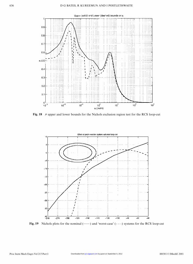
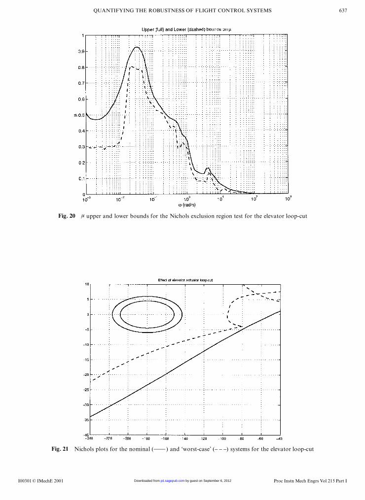
described in reference [18]. In this approach, the relative Sample plots for the reaction-control system and elev-ator loops are shown in Figs 18 to 21. Note that in each‘importance’ of each uncertainty ¢

iis computed with

respect to the maximum value of í. In this way, the case the upper bound on í is less than one and thecorresponding ‘worst-case’ Nichols plot lies outside theuncertainties that are found to be ‘less important’ (i.e.

those with the lowest í sensitivities) can be discarded in speci�ed elliptical exclusion region B. Note, however,that to get a true worst-case Nichols plot, the lowerorder to reduce the uncertainty matrix to a size where

exponential time algorithms can be used to compute a bound on í (from which the worst-case ¢ is generated)needs to be tight; e.g. inconclusive answers will result iflower bound. If no ‘signi�cant’ uncertainties have been

discarded, the resulting lower bound on í should then the maximum of the upper bound is greater than oneand the maximum of the lower bound is less than one.still be quite tight. For the problem at hand, the number

of uncertainties was reduced to 10 so that a lower bound This fact motivates further work on the calculation oftight bounds on real í, which is the subject of currentcould be computed using the exponential time algorithm

of reference [20]. As seen from Fig. 17, the resulting research by the authors [21 ].lower bound is quite tight—note that the standardmixed-í lower-bound algorithm of reference [2 ] failedto converge for this problem, i.e. the lower bound gener-ated is everywhere zero, as shown in the same �gure.

6 CONCLUSIONSIt has so far been shown that the IFPC system retainsclosed-loop stability for the speci�ed level of variationsin the aircraft’s mass and centre of gravity. In order to In this paper it has been shown how classical robustness

analysis speci�cations, written in terms of Nicholsmeet the ‘classical’ Nichols plane robustness criteriadescribed in Section 1, it is necessary to guarantee that exclusion regions, can be converted non-conservatively

into simple norm-bounds on the structured singularthe open-loop frequency response obtained by breakingthe loop at the input of each actuator, while leaving value í. The resulting equivalent robustness speci�ca-

tions preserve the qualitative insight provided by theall the other loops closed, should avoid exclusion regionB shown in Fig. 3, for all speci�ed variations in mass classical measures, while also allowing worst-case analy-

sis of uncertain multivariable feedback systems withoutand centre of gravity. Formulating this criteria asdescribed in Section 3, the upper and lower bounds on recourse to gridding of the parameter space. Application

of the proposed approach was illustrated via an analysisthe resulting í problem are computed for loop-cuts ineach of the actuators. From the lower bounds on í it is of the robustness properties of an integrated �ight

and propulsion control system for a V/STOL aircraftpossible to generate ‘worst-case’ uncertainties and thusplot the corresponding open-loop frequency responses. concept.




Fig. 18 í upper and lower bounds for the Nichols exclusion region test for the RCS loop-cut

Fig. 19 Nichols plots for the nominal (—— ) and ‘worst-case’ (– – –) systems for the RCS loop-cut




Fig. 20 í upper and lower bounds for the Nichols exclusion region test for the elevator loop-cut

Fig. 21 Nichols plots for the nominal (—— ) and ‘worst-case’ (– – –) systems for the elevator loop-cut




AIAA Conference on GNC, Boston, Massachusetts, 1998,ACKNOWLEDGEMENTSpp. 325–335.

11 Braatz, R., Young, P., Doyle, J. and Morari, M.The authors are grateful to QinetiQ (formerly DERAComputatinal complexity of í calculation. IEEE Trans.

Bedford ) for supplying the V/STOL aircraft model used Autom. Control, 1994, AC-39(5), 1000–1002.in this study and to the Engineering and Physical 12 Ferreres, G. A Practical Approach to Robustness AnalysisSciences Research Council for �nancial support. The with Aeronautical Applications, 1999 (Kluwer Academic,�rst author is pleased to acknowledge useful discussions New York).with Chris Fielding of BAE Systems. 13 McFarlane, D. and Glover, K. A loop shaping design pro-

cedure using H2

synthesis. IEEE Trans. Autom. Control,1992, AC-36, 759–769.

REFERENCES 14 Safonov, M. G., Laub, A. J. and Hartman, G. L. Feedbackproperties of multivariable systems: the role and use of thereturn diVerence matrix. IEEE Trans. Autom. Control,1 Skogestad, S. and Postlethwaite, I. Multivariable Feedback1981, AC-26(1), 47–65.Control, 1996 (John Wiley, New York).

15 Tischler, M. B. (Ed.) Advances in Flight Control, 19962 Balas, G. J., Doyle, J. C., Glover, K., Packard, A. and(Taylor and Francis, London).Smith, R. í-Analysis and Synthesis Toolbox User’s Guide,

16 Bates, D. G., Gatley, S. G., Postlethwaite, I. and Berry,1995 (The MathWorks, Natick, Massachusetts).A. J. Design and piloted simulation of a robust integrated3 Dorf, R. C. and Bishop, R. H. Modern Control Systems,�ight and propulsion controller. Am. Inst. Aeronaut.1998 (Addison-Wesley, Reading, Massachusetts).Astronaut. J. Guidance, Control Dynamics, 2000, 23(2),4 MIL-F-9490D, Military Speci�cations for Flight Control269–277.Systems—Design, Installation and Test of Piloted Aircraft,

17 Gatley, S. L., Bates, D. G. and Postlethwaite, I. A par-1992.titioned integrated �ight and propulsion control system5 Zhou, K., Doyle, J. C. and Glover, K. Robust and Optimalwith engine safety limiting. IFAC J. Control Engng Practice,Control, 1996 (Prentice-Hall, Englewood CliVs, New2000, 8(8), 845–859.Jersey).

18 Bates, D. G., Kureemun, R., Hayes, M. J. and Iordanov, P.6 Doyle, J. Analysis of feedback systems with structuredComputationand applicationof the real structured singularuncertainty. IEE Proc. Control Theory Applic., Part D,value. In Proceedings of the 14th International Conference1982, 129(6), 242–250.on Systems Engineering, Coventry, 2000, Vol. 1, pp. 60–66.7 Packard, A. and Doyle, J. The complex structured singular

19 Young, P. M., Newlin, M. P. and Doyle, J. C. Computingvalue. Automatica, 1993, 29(1), 71–109.bounds for the mixed í problem. Int. J. Robust Nonlinear8 Muir, E., Lambrechts, P., et al. Robust �ight control designControl, 1995, 5, 573–590.challenge problem formulation and manual: the high inci-

20 Dailey, R. A new algorithm for the real structured singulardence research model (HIRM). GARTEUR Technical-value. Proc. ACC, 1990, 2, 3036–3040.Publication TP-088-4, 1995.

21 Hayes, M. J., Bates, D. G. and Postlethwaite, I. New tools9 Aslin, P. P. and Glover, K. Technical Report P164/TR/401,for computing tight bounds on the real structured singularBAE Systems, 1990 (unpublished).value. Am. Inst. Aeronaut. Astronaut. J. Guidance, Control10 Deodhare, G. and Patel, V. V. A ‘modern’ look at gain and

phase margins: an H2

/í approach. In Proceedings of the Dynamics, 2001 (to appear).








quantifying the robustness of flight control systems using nichols exclusion regions and the...

Documents