quantification and assessment methods for large wood (lw) in
TRANSCRIPT

Libraries and Learning Services
University of Auckland Research Repository, ResearchSpace
Copyright Statement
The digital copy of this thesis is protected by the Copyright Act 1994 (New Zealand).
This thesis may be consulted by you, provided you comply with the provisions of the Act and the following conditions of use:
• Any use you make of these documents or images must be for research or private study purposes only, and you may not make them available to any other person.
• Authors control the copyright of their thesis. You will recognize the author's right to be identified as the author of this thesis, and due acknowledgement will be made to the author where appropriate.
• You will obtain the author's permission before publishing any material from their thesis.
General copyright and disclaimer
In addition to the above conditions, authors give their consent for the digital copy of their work to be used subject to the conditions specified on the Library Thesis Consent Form and Deposit Licence.
Quantification and assessment
methods for large wood (LW)
in fluvial systems
Gabriel Christoph SPREITZER
A thesis submitted
by
b
Department of Civil and Environmental Engineering
Faculty of Engineering The University of Auckland
September, 2019
in fulfilment of the requirements for the degree of
Doctor of Philosophy
in Civil and Environmental Engineering

i
ABSTRACT
Wood in rivers acts as a natural and ecological important element as it moderates stream power,
regulates sediment transport and provides habitat for fish and other living organisms. Besides
the beneficial effects of wood in rivers, an abundance of organic material, which is often
introduced to waterways by changing climatic conditions and modern land-use practices, may
impact stream ecology and flood mitigation adversely. The often sudden occurrence of large
wood (LW) during floods regularly affects stream systems, infrastructure and communities all
over the world.
Due to a lack of applicable remote sensing methodologies in LW research, to date little is
known about transport dynamics of wood in rivers. In order to expand the current
understanding of flow-sediment-wood interaction processes, especially at higher flow rates,
LW interactions with the environment need to be studied. This research project aims to apply
state-of-the-art technologies for quantifying and assessing LW interactions.
Nine-degree of freedom (9-DoF) smart sensors are implanted into scaled wooden dowels,
resulting in ‘SmartWood’, being able to capture complex movement processes of wood in a
hydraulic laboratory environment. Each of the smart sensors comprises an internal processor
for time-synchronisation of accelerometer, gyroscope and magnetometer data, and stores the
data on an on-board memory card. A measuring frequency of 100 Hz was found to accurately
measure transport, impact and accumulation processes. Structure form Motion (SfM)
photogrammetry is used for the generation of three-dimensional (3D) LW accumulation
models, as well as for the detection of changes in channel morphology due to LW obstructed
flow conditions. The technique uses two-dimensional (2D) images, with large image overlap,
for the generation of 3D point cloud models, which are edited and meshed, following a new
workflow-pipeline for LW specific applications. The use of those innovative methodologies
allow for novel insights into LW transport and deposition dynamics alongside effective and
accurate volumetric quantification opportunities.
An improved knowledge of wood movement processes is essential to better predict impacts on
channel morphology, river-crossing infrastructure and environment. Gained results will
contribute in a more reliable risk assessment for LW-prone stream systems, inform river and
forestry managers, and may help in the development of improved management strategies under
consideration of LW conveyance and filtering of critical key-logs.

iii
ACKNOWLEDGEMENTS
Firstly, I would like to thank my supervisors Dr Heide Friedrich and Dr Jon Tunnicliffe for
providing exceptional support and guidance continuously throughout my PhD program. Your
dedication and enthusiasm made this project possible. Under your supervision, I enjoyed a
variety of opportunities e.g. conferences, field trips, teaching assistance as well as access to
funds and software which allowed me to develop my academic skills. I appreciate your patience
and encouragement throughout my journey very much.
The University of Auckland doctoral scholarship as well as funding received from the George
Mason Centre for the Natural Environment and the Engineering New Zealand Rivers Group,
is gratefully acknowledged. A field trip to Kaikōura was funded by the Ministry of Business,
Innovation and Employment (MBIE) as part of the Endeavour Earthquake Induced Landscape
Dynamics (EILD) program. I also want to thank Manu Caddie for the invitation to the Te Mana
O Te Wai Tairāwhiti – Freshwater Conference in Tolaga Bay in 2017, which was a great
opportunity and a milestone for my PhD project.
Secondly, I also want to thank the technician-team of the Water Engineering Laboratory at the
Newmarket Campus for supporting my experiments in the laboratory and sharing their
profound technical knowledge with me; above all Geoff Kirby and Sujith Padiyara.
A big thanks goes to the entire Water-worked Environments Research-Group and my
colleagues, for their assistance during field and laboratory experiments as well as sharing their
expertise, especially Dr Stephane Bertin and Dr Wei Li for the provision of software codes.
Furthermore I appreciated the opportunity in providing assistance for Summer, Intern, Part-4
and Master students. I am grateful for your interest in this PhD project and thank you for your
contributions. I hope you enjoyed a great time at the University of Auckland.
Finally, I would like to thank my friends and especially my family, who have been my anchor
throughout this challenging but also exciting time all across the world. I thank you many times
for your endless support and encouragement. My journey would have not been possible without
you. Skyla, you have been my balance throughout this time and I appreciate your patience with
me and the sacrifices you had to make lately. I am very grateful to have you.


v
TABLE OF CONTENTS
Abstract ....................................................................................................................................... i
Acknowledgements .................................................................................................................. iii
Table of contents ........................................................................................................................ v
List of figures ............................................................................................................................ xi
List of tables ............................................................................................................................ xix
List of symbols and abbreviations .......................................................................................... xxi
Co-authorship forms ............................................................................................................. xxiv
.................................................................................................................................... 1
1.1. Motivation and scope of the research .............................................................................. 1
1.1.1. Definition of LW ...................................................................................................... 2
1.1.2. Challenges involving LW in fluvial systems ............................................................ 4
1.1.3. Assessment of LW in motion ................................................................................... 5
1.1.4. Assessment of LW accumulations ............................................................................ 7
1.1.5. State-of-the-art sensing technologies and methodologies ........................................ 8
1.2. Research objectives ....................................................................................................... 10
1.3. Thesis outline ................................................................................................................ 11
.................................................................................................................................. 13
2.1. Introduction ................................................................................................................... 13
2.1.1. LW definition and processes .................................................................................. 15
2.1.2. Remote sensing of LW ........................................................................................... 16
2.1.3. Objectives ............................................................................................................... 18
2.2. Experimental setup ........................................................................................................ 19
2.3. Methodology ................................................................................................................. 22
2.3.1. Verification tests ..................................................................................................... 22
2.3.2. Experimental tests................................................................................................... 25
vi
2.3.3. Data analysis ........................................................................................................... 25
2.4. Results and discussion ................................................................................................... 26
2.4.1. Sensor verification .................................................................................................. 26
2.4.2. Experimental results ............................................................................................... 32
2.4.3. Key findings ........................................................................................................... 39
2.5. Conclusions and outlook ............................................................................................... 40
.................................................................................................................................. 43
3.1. Introduction ................................................................................................................... 43
3.1.1. Large wood (LW) ................................................................................................... 43
3.1.2. Smart sensors .......................................................................................................... 44
3.1.3. Outlook and objectives ........................................................................................... 45
3.2. Experimental setup ........................................................................................................ 46
3.2.1. Hydraulic flume ...................................................................................................... 46
3.2.2. Smart sensors .......................................................................................................... 47
3.3. Methodology ................................................................................................................. 49
3.3.1. Channel hydraulics ................................................................................................. 49
3.3.2. Measuring impact forces ........................................................................................ 49
3.3.3. Video footage ......................................................................................................... 49
3.3.4. Experimental procedure .......................................................................................... 50
3.4. Results and discussion ................................................................................................... 50
3.4.1. Sensor data for acceleration .................................................................................... 50
3.4.2. Change of impact direction..................................................................................... 53
3.4.3. Travel velocity ........................................................................................................ 53
3.4.4. Nine-degree of freedom sensor data ....................................................................... 55
3.5. Conclusions ................................................................................................................... 56
.................................................................................................................................. 59
4.1. Introduction ................................................................................................................... 59
vii
4.1.1. Recent advances in LW research ............................................................................ 59
4.1.2. High-resolution techniques for LW estimation ...................................................... 61
4.1.3. Unstructured point cloud mesh ............................................................................... 64
4.1.4. Objectives ............................................................................................................... 66
4.2. Study sites ..................................................................................................................... 66
4.2.1. Whakatiwai River – Hunua Ranges, North Island, New Zealand .......................... 66
4.2.2. Hapuku River – Kaikōura, South Island, New Zealand ......................................... 68
4.3. Methodology ................................................................................................................. 69
4.3.1. Camera models ....................................................................................................... 69
4.3.2. Image acquisition .................................................................................................... 71
4.3.3. Point cloud processing ............................................................................................ 72
4.3.4. Point cloud meshing ............................................................................................... 73
4.3.5. Volumetric techniques ............................................................................................ 74
4.4. Results ........................................................................................................................... 77
4.4.1. Point cloud results .................................................................................................. 77
4.4.2. Meshing results ....................................................................................................... 79
4.4.3. Volumetric results................................................................................................... 81
4.5. Discussion ..................................................................................................................... 84
4.5.1. Complex LW accumulations .................................................................................. 84
4.5.2. Volumetric computations ....................................................................................... 86
4.5.3. LW accumulation assessment ................................................................................. 88
4.6. Conclusions ................................................................................................................... 91
.................................................................................................................................. 95
5.1. Introduction ................................................................................................................... 95
5.1.1. Large Wood (LW) accumulations and assessment ................................................. 95
5.1.2. Structure from Motion (SfM) for LW research ...................................................... 98
5.1.3. Objectives ............................................................................................................. 100
viii
5.2. Laboratory experiments ............................................................................................... 100
5.3. Methodology ............................................................................................................... 103
5.3.1. Procedure for volumetric estimates ...................................................................... 103
5.3.2. Image acquisition .................................................................................................. 103
5.3.3. Point cloud and mesh processing in Pix4D .......................................................... 104
5.3.4. Geometric volume (2.5D) ..................................................................................... 105
5.3.5. Pix4D volume tool (2.5D) and PSR Meshing (3D) .............................................. 107
5.3.6. Porosity of LW accumulations ............................................................................. 109
5.4. Results ......................................................................................................................... 110
5.4.1. Point cloud and mesh results ................................................................................ 110
5.4.2. Volumetric results................................................................................................. 113
5.5. Discussion ................................................................................................................... 116
5.5.1. Processing of elementary and complex LW accumulations ................................. 116
5.5.2. Point normals ........................................................................................................ 118
5.5.3. Volumetric computations ..................................................................................... 120
5.5.4. LW accumulation porosity ................................................................................... 122
5.6. Conclusions and outlook ............................................................................................. 123
................................................................................................................................ 127
6.1. Introduction ................................................................................................................. 127
6.1.1. Large Wood (LW) accumulations in rivers .......................................................... 127
6.1.2. Mapping of LW accumulations ............................................................................ 129
6.1.3. Objectives ............................................................................................................. 131
6.2. Experimental setup ...................................................................................................... 132
6.2.1. Hydraulic flume .................................................................................................... 132
6.2.2. Wooden dowels .................................................................................................... 133
6.2.3. Imaging and recording equipment ........................................................................ 134
6.3. Methodology ............................................................................................................... 135
ix
6.3.1. Experimental procedure ........................................................................................ 135
6.3.2. Image acquisition .................................................................................................. 136
6.3.3. Point cloud and mesh generation .......................................................................... 137
6.3.4. Accumulation assessment ..................................................................................... 138
6.4. Results ......................................................................................................................... 140
6.4.1. LW interception and passing rate ......................................................................... 140
6.4.2. LW accumulation volume and porosity ............................................................... 141
6.5. Discussion ................................................................................................................... 144
6.5.1. Assessment of water-worked LW accumulations ................................................ 144
6.5.2. Practical outcomes ................................................................................................ 150
6.6. Conclusions ................................................................................................................. 154
................................................................................................................................ 157
7.1. Introduction ................................................................................................................. 157
7.1.1. LW accumulations ................................................................................................ 157
7.1.2. Topographic surveys............................................................................................. 160
7.1.3. Current challenges and objectives ........................................................................ 161
7.2. Experimental setup ...................................................................................................... 162
7.2.1. Hydraulic flume .................................................................................................... 162
7.2.2. LW accumulation ................................................................................................. 165
7.2.3. Multi-camera array ............................................................................................... 165
7.2.4. Sediment ............................................................................................................... 166
7.3. Methodology ............................................................................................................... 167
7.3.1. Experimental procedure ........................................................................................ 167
7.3.2. Hydraulic conditions............................................................................................. 168
7.3.3. Optical data collection .......................................................................................... 169
7.3.4. Point cloud generation and processing ................................................................. 170
7.3.5. Estimation of sediment flux .................................................................................. 171
x
7.4. Results ......................................................................................................................... 171
7.4.1. Hydraulic conditions............................................................................................. 171
7.4.2. Sediment flux ........................................................................................................ 174
7.4.3. Point cloud results ................................................................................................ 178
7.4.4. LW accumulation results ...................................................................................... 180
7.5. Discussion ................................................................................................................... 181
7.5.1. Effects of a LW accumulation on channel-morphology and flow behaviour ....... 181
7.5.2. Point cloud processing .......................................................................................... 184
7.5.3. Volumetric channel calculations .......................................................................... 186
7.5.4. LW accumulation ................................................................................................. 187
7.6. Conclusion and perspectives ....................................................................................... 187
................................................................................................................................ 189
8.1. Bringing the field into the laboratory .......................................................................... 189
8.2. Transport dynamics of wood in rivers ......................................................................... 190
8.2.1. Contributions ........................................................................................................ 190
8.2.2. Implications and future research ........................................................................... 191
8.3. Quantification of wood volumes in rivers ................................................................... 193
8.3.1. Contributions ........................................................................................................ 193
8.3.2. Implications and future research ........................................................................... 195
8.4. Effects of LW on channel morphology ....................................................................... 196
8.5. Final remarks ............................................................................................................... 197
List of publications ................................................................................................................ 199
Journal articles .................................................................................................................... 199
Conference articles ............................................................................................................. 199
References .............................................................................................................................. 201
xi
LIST OF FIGURES
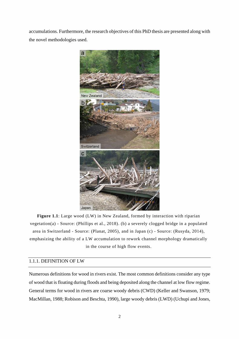
Figure 1.1: Large wood (LW) in New Zealand, formed by interaction with riparian
vegetation(a) - Source: (Phillips et al., 2018). (b) a severely clogged bridge in a
populated area in Switzerland - Source: (Planat, 2005), and in Japan (c) - Source:
(Rusyda, 2014), emphasizing the ability of a LW accumulation to rework channel
morphology dramatically in the course of high flow events. ......................................... 2
Figure 2.1: An exceptional example of LW accumulation on Tapuae Stream after a storm
event, New Zealand’s East Cape, 2017. ....................................................................... 14
Figure 2.2: Roll, pitch and yaw as a frame for orientation. .................................................... 18
Figure 2.3: Custom-designed hydraulic flume for LW research at the University of Auckland,
New Zealand (a). Three-dimensional Structure from Motion (SfM) model of the flume
channel (b). ................................................................................................................... 20
Figure 2.4: Sensor-tagged and scaled SmartWood dowel (267 mm long, 22 mm diameter),
individually coloured for the hydraulic flume experiments (a). Sketch of the
SmartWood dowel (b), showing the hollow, 10 mm central shaft for installation of the
smart sensor and the filled (density-compensated) cavities on both ends. The 9-DoF
smart sensor consisting of IMU (accelerometer, gyroscope, magnetometer, on-board
memory and battery) implanted in a cylindrical housing, 105 x 10 mm, with a NZD $2
coin for scale (c). The ends of the SmartWood dowel are sealed using PU-foam and
silicone. ........................................................................................................................ 21
Figure 2.5: Setup for smart sensor verification in the laboratory, consisting of a vertical drop
test (a, b), from a height of 75 mm onto a rubber layer (red), in order to measure
acceleration along the longitudinal axis of the sensor. (c) Rotational test for assessing
gyroscope and magnetometer performance, aligned to the longitudinal x-axis. (d, e) For
verification of the acceleration along the vertical z- and lateral y-axes of the IMU, a
platform is used to simulate drop tests from a height of 150 mm. A rotational test, shown
in (f) allows for verification of angular velocity and magnetic field strength around y-
and z-axes. .................................................................................................................... 24
Figure 2.6:Sensor data for drop test along the longitudinal x-axis, with raw data (a) and Euler
angles transformation output (b), the lateral y-axis (c, d) and the vertical z-axis (e, f).
...................................................................................................................................... 28
xii
Figure 2.7: Sensor data for gyroscope and magnetometer verification around the x-axis, with
raw data (a) and Euler angles (b), the lateral y-axis (c, d) and the vertical z-axis (e, f).
...................................................................................................................................... 30
Figure 2.8: Drop test impact along the longitudinal direction (x-axis) - high resolution (100Hz)
over a period of 1 s – unfiltered raw data for acceleration as read from the smart sensor.
The interval from 1.65 to 1.85 s shows the last milliseconds of (i) free fall
measurements, (ii) the impact, (iii) the first rebound after impact, (iv) the second
rebound after impact and an early stage of the attenuation phase. .............................. 31
Figure 2.9: Verification of angular velocity - a high resolution portion of the record for tests
along the sensor's x-axis. .............................................................................................. 32
Figure 2.10 SmartWood trajectory according video footage, showing starting orientation with
recruitment processes (A), rollover and transport processes (B), and interaction of
sensor-tagged wood dowel with channel boundaries (C). ........................................... 34
Figure 2.11: SmartWood raw data and Euler angle estimates for orientation, starting with an
inclination of 90˚, 45˚ and 0˚ to flow direction. ........................................................... 37
Figure 2.12: Experimental SmartWood tracking with an initial start orientation of 90˚ (a), 45˚
(b) and 0˚ (c) to flow direction, showing log trajectory in the scaled stream channel.
Flow direction is from the left to the right. Red indicates rolling processes (x-axis) and
blue shows rotation around the vertical axis (yaw), indicated by arrows. Straight LW
movement is displayed in black, and moments of rest are indicated with a cross. The
trajectory from initial layout to the bridge pier is 3 m. Significant movement behavior
is indicated with capital letters, from A to I, referring to stages in the raw data and
transformed Euler angle records, plotted in Figure 2.11, above. ................................. 38
Figure 3.1: Experimental Setup showing the project designed flume with conveyor-belt feeder,
channel and outlet structure from the top (a), side (b) and a perspective view (c). ..... 47
Figure 3.2: Smart sensors installed into miniature LW for application in the laboratory. ...... 48
Figure 3.3: Acceleration data obtained using the smart-sensor-tagged wooden dowel in the
hydraulic flume. (a) The data series represents the full trajectory of the dowel, from
delivery via conveyor-belt to deposition at the bridge pier. (b) Detail A, a higher
resolution record, detailing the impact of the dowel upon the bridge pier. ................. 52
Figure 3.4: A collection of screenshots showing the sequence of movements and travel times
for the sensor-tagged dowel. On the left-hand side, snapshots from the top camera are
xiii
displayed (a to f), whereas the middle column shows the snapshots from the side
perspective on the bridge pier (g to m). ....................................................................... 54
Figure 3.5: Schematic illustration of the smart-sensor-tagged miniature log and the feeding
process into the channel via conveyor-belt. ................................................................. 55
Figure 3.6: Plot of the measured data of our applied smart sensors – implanted into a wooden
dowel – for acceleration, angular velocity and magnetic field strength. ..................... 56
Figure 4.1: LW composition and required points/m3 to resolve a SfM photogrammetry point
cloud model. ................................................................................................................. 63
Figure 4.2: Whakatiwai River with scour hole and LW accumulation (a), single emerging
wood logs as part of the buried accumulation structure (b), fine gravel bar development
in downstream direction and coarse gravel bar upstream (c) in October 2017 when SfM
data have been obtained, in comparison to an accumulation stage in March 2018 (d).
...................................................................................................................................... 67
Figure 4.3: Organic material accumulation at the Hapuku River. Downstream view (a),
upstream view (b) and a perspective showing the boulder and wood log with intact
rootwad, initiating the accumulation (c). ..................................................................... 69
Figure 4.4: Compositional estimates of the accumulation at the Whakatiwai River and the
Hapuku River sites. ...................................................................................................... 69
Figure 4.5: Image overlap and the corresponding organic material accumulation for the
Whakatiwai River (a) and the Hapuku River (b). Green indicates areas with five and
more overlapping images, facilitating the generation of high-quality point cloud
models. Orange indicates the minimum number of two overlapping images required for
SfM photogrammetry. The black dotted lines represent the organic material
accumulation, showing an area of low overlapping images for the Whakatiwai
accumulation, which was partly inaccessible due to water (a), and full overlap for the
Hapuku accumulation (b). Both organic material accumulation models (on the right)
show oblique camera positions, obtained spirally around the object at an elevation of
1.5 to 2.0 m. ................................................................................................................. 71
Figure 4.6: SfM photogrammetry workflow. .......................................................................... 76
Figure 4.7: Point cloud models of the organic material accumulation at the Whakatiwai River
(a) and at the Hapuku River (b). .................................................................................. 77
xiv
Figure 4.8: Organic material accumulation from the Hapuku field site. The selection shows a
0.80 x 0.50 m section, displaying the original point cloud (a), the simplified Pix4D mesh
(b), the Delaunay 2.5D mesh (c) and the screened Poisson Surface Reconstruction
(PSR) mesh (d). ............................................................................................................ 80
Figure 4.9: Volume computation of the organic material accumulations using the Pix4D
volume tool. On the left (a): Whakatiwai and right (b): Hapuku River; Green: shows
the basal surface for volume computation, red: the vectors for volume estimation, and
orange: the mathematical cone model left and trapezoidal prism model right. Top view,
front view and side view perspective from the top to the bottom. ............................... 82
Figure 4.10: Simulation of the effects on channel morphology using the Whakatiwai
accumulation model embedded into a Delft3D (2011) environment. .......................... 91
Figure 5.1: Geometric Volume (2.5D): Geometric primitives for mathematical approximation
of the 2.5D Volume for One Dowel (a), Two Dowels (b and c) and Six Dowels formed
into a bundle (d). The fill volumes indicate the area according the applied mathematical
equations. ................................................................................................................... 107
Figure 5.2: Graphical illustration of the workflow for obtaining the 2.5D Pix4D and 3D PSR
Volume. ...................................................................................................................... 109
Figure 5.3: 3D models of our miniature LW accumulations. Elementary accumulations are
shown from a to f, more complex accumulation structures (g to j) and a mixture of wood
dowels and organic fine material (OFM) (k to n). Mesh generated via PSR (left), and
the fully closed 3D body of the corresponding LW accumulation (right). ................ 112
Figure 5.4: Volume estimates from Pix4D volume tool (2.5D). The base surface is shown in
green, and the modelled volume is displayed in red. The chequer-boards (raster of
25mm) are used for point cloud and model scaling. .................................................. 114
Figure 5.5: Volumetric results for elementary and complex LW accumulations, considering
the geometric volumes obtained in 2.5D and 3D, as well as volumes assessed using
Pix4D volume tool (2.5D) and PSR. .......................................................................... 116
Figure 5.6: Number of 3D points and faces used for constructing the LW accumulation models.
.................................................................................................................................... 117
Figure 5.7: Closing the bottom hole failed due to incorrect point normal computations, as an
example for the Eight Dowels (high photo count) LW accumulation. The position of a
missing dowel (not reconstructed in the PSR model) is delineated in red. ................ 119
xv
Figure 5.8: Reconstructed water tight 3D PSR mesh models of our miniature LW
accumulations. For Two Dowels (a), Six Dowels formed into a pile (b), Eight Dowels
(low photo count) (c) and Ten Dowels + OFM (d). ................................................... 122
Figure 6.1: Experimental setup in the Water Engineering Laboratory at the University of
Auckland. ................................................................................................................... 135
Figure 6.2: Analysis of intercepted materials at the critical cross-section (bridge pier), with
passing ratio set relative to the total introduced wood (number of wood dowels). LW
material was classified into three groups: fine LW (smaller than 1.5 m), standard LW
(2 to 4 m in length), and coarse LW (with a length of 6 m and longer)..................... 141
Figure 6.3: Point cloud models of a single design dowel (a), from a side perspective (b) and
for Pix4D mesh (c) and PSR model (d). A top view of paired design dowels from top
view (e), point cloud with from side view (f) and the mesh model in Pix4D (g) as well
as PSR (h).Volume estimates in Pix4D for individual and paired dowels are displayed
on the right (i). ........................................................................................................... 142
Figure 6.4: Volumetric results of the experimental LW accumulations are ranked in order of
increasing geometric volume (3D). Accumulation volumes A1 and A2 are magnified
by a factor of 10. Other LW accumulations were generated by a 20, 50 or 75 l·s-1 (L)
discharge and had a feed of either 521 or 1769 dowels (A3 to A18). ....................... 144
Figure 6.5: The relationship between 3D Geometric Volume (volume of individual dowels)
versus two techniques for estimating the envelope volume of the deposit. The 2.5D
technique consistently provides about three times the geometric volume, whereas the
3D PSR technique conforms more closely to the deposit and has a lower volume. This
relationship provides a means of determining the porosity of the deposit: about 66%
void space, according to the 2.5D technique. ............................................................ 148
Figure 6.6: Development of a LW accumulation (A17) consisting of individual dowels starting
from the rising limb at 20 l·s-1 (20L) in (a), reaching peak discharge 75 l·s-1 (75L) in
(c), and the falling limb back to base discharge 4 l·s-1 (4L) in (f), at the critical cross
section (bridge with central pier) from top view perspective. The blue line indicates a
reference line at the bridge, whereas the two red lines indicate the relaxation area of the
LW accumulation during recession from peak discharge (c) to base discharge 4 l·s-1 (f).
.................................................................................................................................... 150
Figure 6.7: Accumulation A17, displayed as mesh model in top (a) and front view (b). ..... 152
xvi
Figure 6.8: LW accumulation porosity respecting packing arrangement and component
mixtures. The lowest achievable porosity for uniformly shaped cylinders is 9%. For a
given volume of woody elements, porosity of the accumulation decreases as smaller
elements (e.g. organic fine material – OFM, sediments) increasingly occupy interstitial
spaces. Random mixtures of woody elements are typically around 70% or lower, while
individual structural members can show lower porosities too (10-30%); we have placed
indicative values from the published literature on the chart based on a subjective
assessment of the packing arrangements and mixtures as indicated in the accompanying
text or photos. ............................................................................................................. 154
Figure 7.1: Changes imparted to channel hydraulics by the introduction of a dam jam. By
changing the flow depth and velocity immediately upstream of the blockage, fluvial
transport capacity is reduced, leading to deposition upstream. Further downstream, flow
gradient and velocity increase markedly, leading to enhanced erosion. .................... 160
Figure 7.2: Experimental setup with natural channel course, live-bed conditions and critical
cross-section. .............................................................................................................. 163
Figure 7.3: Experimental setup of the miniature LW accumulation at the bridge section in
downstream direction (a) and the multi-camera array installed on a cart moving above
the channel (b). ........................................................................................................... 166
Figure 7.4: Grain size distribution for bed material and fed colour gravel. .......................... 167
Figure 7.5: Flow velocity profiles measured using ADV in the flume channel, both with and
without LW accumulation. Flow velocity measurements are obtained 1.5 m upstream
of the bridge cross-section A (a and b) and shortly upstream the LW accumulation at
cross-section B (c and d). The charts e and f show the flow condition immediately
downstream the LW accumulation at cross-section C. (g) shows the channel with the
LW accumulation at the critical cross-section and aggradation of the colour gravel feed
in the upstream section. .............................................................................................. 173
Figure 7.6: Water level development without and with LW accumulation at the critical cross-
section at a flume slope of 0.02. ................................................................................. 174
Figure 7.7: Evaluation of changes in channel morphology (spatial variability) by means of (a)
bulk measurements of bed material along the channel, and (b) SfM model indicating
changes in bed elevation for the experiment without a LW accumulation at the critical
cross-section (section 5). Results show erosion and aggradation rates of the bed material
xvii
(blue colour bars). The supply rates of colour gravel, fed via conveyor-belt system, are
displayed on a secondary axis. ................................................................................... 177
Figure 7.8: Evaluation of changes in channel morphology (spatial variability) by means of (a)
bulk measurements of bed material along the channel, and (b) SfM model indicating
changes in bed elevation for experiments with a LW accumulation at the critical cross-
section (section 5). Results show erosion and aggradation rates of the bed material (blue
colour bars). The supply rates of colour gravel, fed via conveyor-belt system, are
displayed on a secondary axis. Due to the LW accumulation at the bridge section, a
sediment transport interruption is revealed for the upstream area. None of the supplied
sediments (colour gravel) was transported through the critical cross-section. .......... 178
Figure 7.9: Statistics for point-cloud alignment and M3C2 computation. Distance uncertainty
between ‘reference’ and ‘data’ point cloud models (a & c), as well as standard deviation
from M3C2 model computation (b & d) for the experiments with and without LW
obstruction present. Distance error and standard deviation are important indicators for
the accuracy of computed volumes. ........................................................................... 180
Figure 7.10: LW accumulation model showing the integrating domain of the 2.5D volume in
Pix4Dmapper (a), and Poisson surface reconstruction (PSR) mesh (3D) in top (b) and
front view (c) from Meshlab, which provides several tools for 3D volume estimation.
The concrete brick in the background (a) serves for model orientation, whereas several
chequer-boards are placed around the miniature LW accumulation for scaling measures.
.................................................................................................................................... 181
Figure 7.11: Comparison of the point-cloud models without (a) and with (b) a LW
accumulation in the channel. Flow direction is from the left to the right, whereas the
yellow shaded area represents the critical cross-section (bridge with single pier row). A
number of chequer-boards were placed at the end of the experiments for scaling
purposes. .................................................................................................................... 184

xviii
xix
LIST OF TABLES
Table 1.1: LW definitions used in previous research. ............................................................... 3
Table 2.1: Smart sensor specifications. ................................................................................... 22
Table 2.2: Drift estimates for roll, pitch and yaw according plotted Euler angle computations.
...................................................................................................................................... 31
Table 4.1. Camera specifications used for data collection in the field. ................................... 70
Table 4.2: Data acquisition and Pix4D software processing settings and times. .................... 73
Table 4.3: Pix4D point cloud statistics. .................................................................................. 78
Table 4.4: Whakatiwai River organic material accumulation point cloud and mesh
characteristics with densities for projected footprint area and accumulation volume. 79
Table 4.5: Hapuku River organic material accumulation point cloud and mesh characteristics
(without boulder) with densities for projected footprint area and accumulation volume.
...................................................................................................................................... 81
Table 4.6: Overview of the results from measured and computed accumulation volumes. The
volume measured with the Pix4D Volume Tool represents our reference value for
volume comparison. Furthermore, measured dimensions from the field are presented
together with computed volumes, using a Mathematical Approximation, the Original
Point Cloud and three meshes of the organic material accumulation at the Whakatiwai
and Hapuku River. ....................................................................................................... 83
Table 5.1. The number and dimensions of dowels as well as OFM used to assemble the
miniature LW accumulations (Composition), the volume of each individual item
(Partial Volume), and the total accumulation volume (Geometric Volume (3D)).
Furthermore, an index of accumulation complexity is provided (Evolution Phase and
Classification). ........................................................................................................... 102
Table 5.2. Camera specifications used for data collection in the laboratory. ....................... 104
Table 5.3. Pix4D settings for processing of LW accumulations in the laboratory. .............. 105
Table 5.4. Point cloud and mesh specifications for the LW and OFM accumulation models.
.................................................................................................................................... 111
Table 5.5. Estimated volume and porosity values for LW accumulation models in the
laboratory. .................................................................................................................. 115
Table 6.1. Overview of dimension and quantity of the wooden dowels used in the experimental
setup. .......................................................................................................................... 134
xx
Table 6.2. Results of the volumetric estimates for the formed dowel accumulations in the
laboratory. Deviations for 3D PSR and 2.5D Pix4D volumes are computed with respect
to the 3D Geometric volume. ..................................................................................... 143
Table 7.1. Flume characteristics for channel, critical cross-section and conveyor-belt system.
.................................................................................................................................... 164
Table 7.2. Technical camera details. ..................................................................................... 165
Table 7.3. Colour gravel specifications for sediment supply via conveyor-belt system. ...... 166
Table 7.4. Overview for experimental procedure. ................................................................ 169
Table 7.5. Hydraulic flow characteristics for the simulation of flood events without and with
LW accumulation. ...................................................................................................... 172
Table 7.6. Estimated flow hydraulics from experimental data. ............................................ 174
Table 7.7. Channel morphological activities for the simulation of a flood event without and
with present LW accumulation. ................................................................................. 176
Table 7.8. Results for initial and densified point cloud processing steps. ............................ 179

xxi
LIST OF SYMBOLS AND ABBREVIATIONS
cm Centimetre
D Diameter
deg (˚) Degree
g Gram
G Acceleration
h hour
H Height
Hz Hertz
kg Kilogram
km Kilometre
kst Strickler-roughness value
l Litre
L Length
m Metres above sea level
mAh Milliampere hour
m.a.s.l. Metre above
mG Milli-G (acceleration)
MHz Megahertz
mm Millimetre
MP Megapixel
R Radius
rms root mean square
s Second
xxii
W Width
V Volt
VDel Delaunay 2.5D volume
VM.A Mathematical approximation volume
VP.C Point cloud volume
VPSR PSR volume
VP4D Pix4D volume
Vtot Total volume (bulk volume)
VSpl Simplified volume
Vv Void volume
~ Exempli Gratia
˚C Degree Celsius
µT Microtesla
ADV Acoustic Doppler velocimeter
ALS Aerial laser scanning
AHRS Attitude and heading reference system
BA Bundle adjustment
CCS Critical cross-section
CFD Computational fluid dynamics
CWD Coarse woody debris
DEM Digital elevation model
DoD DEM of Difference
DSM Digital surface model
DoF Degree of freedom
EVA Ethylene-vinyl acetate

xxiii
FoV Field of view
HFoV Horizontal field of view
GPS Global positioning system
GSD Ground sampling distance
IDW Inverse distance weighted
LiDAR Light detection and ranging
LW Large wood
LWD Large woody debris
MB Megabyte
M3C2 Multiscale model to model cloud comparison
NZ New Zealand
NZD New Zealand Dollar
IMU Inertial measurement unit
OFM Organic fine material
PSR Poisson surface reconstruction
pts Points
PU Polyurethane
PVC Polyvinyl chloride
RFID Radio-frequency identification
SfM Structure from motion
TLS Terrestrial laser scanning
WEL Water Engineering Laboratory

CO-AUTHORSHIP FORMS

xxv

xxvi

xxvii

xxviii

xxix

xxx
1
INTRODUCTION
1.1. MOTIVATION AND SCOPE OF THE RESEARCH
Large wood (LW) plays an important role in fluvial systems as it moderates stream power
(Megahan and Nowlin, 1976; Swanson et al., 1976; Platts et al., 1983; Bilby and Ward, 1989),
regulates sediment transport (Swanson and Lienkaemper, 1978; Bilby and Likens, 1980;
Harmon et al., 1986) and provides habitat for fish and other living organisms (Bisson et al.,
1987; Fausch and Northcote, 1992). Besides the beneficial roles of a balanced wood budget in
rivers, challenges arise for abundant quantities of accessible LW. Unnaturally large quantities
of wood have shown negative effects on stream ecology (Meehan et al., 1969; Elliot, 1978),
river-crossing infrastructure and flood mitigation (Lassettre and Kondolf, 2012; Schmocker
and Weitbrecht, 2013; Ruiz-Villanueva et al., 2017). The sudden and disastrous occurrence of
LW deposition during floods regularly affects communities and stream systems in New
Zealand (Phillips et al., 2018), but also on a global scale (Figure 1.1) (Gschnitzer et al., 2017).
A better understanding of LW in rivers is required to set up a compact assessment framework
(Wohl et al., 2016), which can be used by river and forestry managers to maintain safety for
river-crossing infrastructure, human populations and stream ecology.
In this chapter, the general scope of LW research is presented by providing background
information about: (i) the definition of LW in fluvial systems, (ii) arising challenges involving
LW during floods, (iii) measurement of LW transport dynamics, and (v) the assessment of LW
2
accumulations. Furthermore, the research objectives of this PhD thesis are presented along with
the novel methodologies used.
Figure 1.1: Large wood (LW) in New Zealand, formed by interaction with riparian
vegetation(a) - Source: (Phillips et al., 2018). (b) a severely clogged bridge in a populated
area in Switzerland - Source: (Planat, 2005), and in Japan (c) - Source: (Rusyda, 2014),
emphasizing the ability of a LW accumulation to rework channel morphology dramatically
in the course of high flow events.
1.1.1. DEFINITION OF LW
Numerous definitions for wood in rivers exist. The most common definitions consider any type
of wood that is floating during floods and being deposited along the channel at low flow regime.
General terms for wood in rivers are coarse woody debris (CWD) (Keller and Swanson, 1979;
MacMillan, 1988; Robison and Beschta, 1990), large woody debris (LWD) (Uchupi and Jones,
3
1967; Bilby, 1984), or large wood (LW) (Gregory et al., 2003). During the First International
Conference on Wood in World Rivers, held in the USA in October 2000, participants voted for
the replacement of the term ‘LWD’ with ‘LW’ (Gregory et al., 2003). A reason for the new
designation was that the term of ‘debris’ has a negative connotation, which is not necessarily
true for wood in rivers, acting as ecological drivers, and LW being an essential part of fluvial
systems (Murphy and Koski, 1989).
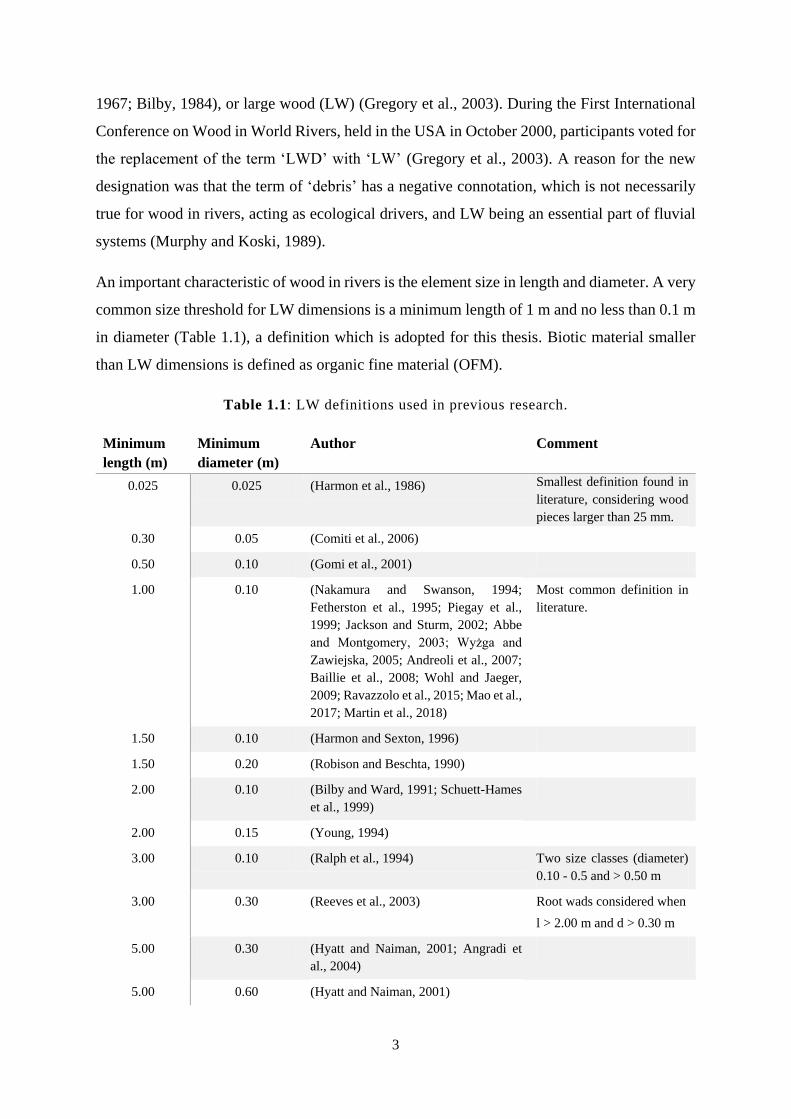
An important characteristic of wood in rivers is the element size in length and diameter. A very
common size threshold for LW dimensions is a minimum length of 1 m and no less than 0.1 m
in diameter (Table 1.1), a definition which is adopted for this thesis. Biotic material smaller
than LW dimensions is defined as organic fine material (OFM).
Table 1.1: LW definitions used in previous research.
Minimum
length (m)
Minimum
diameter (m)
Author Comment
0.025 0.025 (Harmon et al., 1986) Smallest definition found in
literature, considering wood
pieces larger than 25 mm.
0.30 0.05 (Comiti et al., 2006)
0.50 0.10 (Gomi et al., 2001)
1.00 0.10 (Nakamura and Swanson, 1994;
Fetherston et al., 1995; Piegay et al.,
1999; Jackson and Sturm, 2002; Abbe
and Montgomery, 2003; Wyżga and
Zawiejska, 2005; Andreoli et al., 2007;
Baillie et al., 2008; Wohl and Jaeger,
2009; Ravazzolo et al., 2015; Mao et al.,
2017; Martin et al., 2018)
Most common definition in
literature.
1.50 0.10 (Harmon and Sexton, 1996)
1.50 0.20 (Robison and Beschta, 1990)
2.00 0.10 (Bilby and Ward, 1991; Schuett-Hames
et al., 1999)
2.00 0.15 (Young, 1994)
3.00 0.10 (Ralph et al., 1994) Two size classes (diameter)
0.10 - 0.5 and > 0.50 m
3.00 0.30 (Reeves et al., 2003) Root wads considered when
l > 2.00 m and d > 0.30 m
5.00 0.30 (Hyatt and Naiman, 2001; Angradi et
al., 2004)
5.00 0.60 (Hyatt and Naiman, 2001)
4
LW accumulations were defined as a deposit of several wood pieces, consisting of at least one
wooden piece with LW dimensions that is partly or fully blocking a stream section (Gurnell,
2013).
1.1.2. CHALLENGES INVOLVING LW IN FLUVIAL SYSTEMS
Changing climatic (storm) conditions, along with modern land-use strategies, have resulted in
greater deliveries of woody material to streams (Cave et al., 2017; Phillips et al., 2018) in
certain physiographic environments. Once recruited by the river, LW may be mobilised at the
rising limb of floods (MacVicar et al., 2009), and then undergoes complex transport dynamics
on its journey downstream (Braudrick et al., 1997; Schenk et al., 2014). During transport, LW
may interact with other wood pieces, channel boundaries and infrastructure. Impacts that occur
during transport may damage bridge piers, decks and floodplain structures (Elliot et al., 2012).
Transport processes often end in LW accumulations that develop at constricted channel cross-
sections, such as bridges (Diehl, 1997) and hydraulic structures (Boes et al., 2017), but also at
natural bottle necks, such as gorges and encroaching vegetation (Phillips et al., 2018), as seen
in Figure 1.1a to c.
In recent years, a number of studies have concluded that most LW is transported during the
rising limb of the hydrograph (MacVicar and Piégay, 2012; Kramer and Wohl, 2014;
Ravazzolo et al., 2015), which means that LW accumulations have been fully developed at a
time of the highest flow magnitude. The scenario of a highly developed log formation, before
peak discharge is reached, affects the flow conveyance capacity of blocked cross-sections
significantly. OFM can fill interstitial space within the rapidly formed log skeleton (Schalko et
al., 2018), decreasing the porosity of the accumulation and further reducing the effective cross-
sectional area Figure 1.1b. Consequently, LW accumulations can result in the generation of
backwater effects (Schmocker et al., 2015; Hartlieb, 2017; Schalko et al., 2019a). Generally,
backwater effects lead to overtopping of river banks and flooding of populated areas (Braudrick
and Grant, 2001; Ruiz-Villanueva et al., 2017), as well as damages to river-crossing
infrastructure (Comiti et al., 2016; Lucia et al., 2018). LW accumulations additionally affect
the channel morphology (Schmocker and Weitbrecht, 2013; Marden et al., 2014; Phillips et al.,
2018), see Figure 1.1c.
5
In the areas upstream from a LW accumulation, a reduction in shear stress reduces the stream’s
ability to transport sediments; this effect is similar to sedimentation processes observed in
artificial reservoirs (Schleiss et al., 2016). The presence of LW accumulations has the potential
to increase the shear velocity, at the obstructed cross-section, promoting scour processes
around bridge piers and abutments (Melville and Dongol, 1992; Pagliara and Carnacina, 2010).
Elliot et al. (2012) found that LW accumulations are responsible for over 30% of the bridge
failures in the USA. Complexities of flow-sediment-wood interaction processes are still not
clearly understood to date (Wohl and Scott, 2017).
1.1.3. ASSESSMENT OF LW IN MOTION
LW movement behaviour in fluvial systems generally follows three main steps: (i)
recruitment/mobilisation, (ii) transport, and (iii) deposition. Depending on the ratio of log
length to bankfull channel width and the LW orientation in the channel (Bragg et al., 2000),
LW elements may be mobilised at higher discharge magnitudes (MacVicar et al., 2009; Mao
et al., 2013). Once recruited by the flow, transport of LW is ruled by a complex set of
parameters, involving hydraulic flow conditions (e.g flow depth, flow velocity) (Haga et al.,
2002), relative LW size (Young, 1991) and the bed and boundaries of the stream (Nakamura
and Swanson, 1993). The application of hydromechanics provides a basis for understanding
the mobilisation and transport of wood logs as a function of log geometries, flow depth and
drag forces (Braudrick and Grant, 2000), yet roughness and flow dynamics are compromised.
Flow dynamics and LW characteristics (e.g. surface texture, density) are assumed to affect log
movement significantly (Ruiz-Villanueva et al., 2016a; Rickli et al., 2018). Trees with intact
rootwad and branches were found to show more stability in stream channels (Braudrick and
Grant, 2000; Shields and Alonso, 2012; Davidson and Eaton, 2013), than LW in an advanced
decay stage, showing lower density and no branches and roots (Gurnell, 2003; Sear et al.,
2010). LW without branches or roots commonly enters waterways after forest fire or as a by-
product of commercial timber production (Cave et al., 2017). LW characteristics represent
important parameters for the prediction of log movement processes in 1D (Merten et al., 2010),
2D (Mazzorana et al., 2011; Ruiz-Villanueva et al., 2014a) and 3D (Allen and Smith, 2012)
numerical modelling, yet more reference studies from field and laboratory environments are
required to verify computed simulations.
6
There are differences in movement behaviour between individually transported logs and
congested transport (Braudrick et al., 1997). Individually transported logs tend to travel aligned
parallel with the flow, in the channel’s centre (Braudrick and Grant, 2001; MacVicar and
Piégay, 2012). In order to investigate transport behavior of individual logs, radio frequency
identification (RFID) tags were implanted into LW pieces in the field (MacVicar et al., 2009;
Schenk et al., 2014). Another study tracked log movement using RFID with additional GPS
data for LW tracking in rivers (Ravazzolo et al., 2015). Results, based on pre- and post-flood
surveys, revealed that about 80% of the RFID tagged wood logs traveled at the highest 20% of
the hydrograph, for distances of up to 100 km (Schenk et al., 2014).
Recent studies used video footage of wood-laden flows, which are of great value for visualising
congested transport dynamics and evaluating wood budgets. Results revealed insights into
hypercongested LW transport regimes, showing a broad variety of transport processes, ranging
from dry wood-laden flow over highly congested - yet floating - transport regime, to fully
floating wood transport (Ravazzolo et al., 2017; Ruiz-Villanueva et al., 2019). Major advances
have been made in identifying movement trajectories (Braudrick and Grant, 2001; MacVicar
and Piégay, 2012), yet little is known about the actual transport dynamics in the flow. A better
understanding of flow-wood interaction processes could allow for accurate prediction of LW
movement, in order to reduce the risk of catastrophic events resulting from LW blocked
channel cross-sections (Comiti et al., 2016). Pioneer studies have investigated and developed
LW retention structures for wood prone stream systems (Schmocker and Weitbrecht, 2013),
using prevailing flow conditions to filter LW.
When LW is transported, impacts may arise from collisions with river-crossing infrastructure,
floodplain structures, channel boundaries or among themselves. Impact forces from collisions
involving LW can be estimated (Haehnel and Daly, 2004) on the basis of LW velocity and
mass. The impact magnitude is a function of LW orientation with respect to the flow and
collision surface (Como and Mahmoud, 2013), thus there is good potential for such interactions
to be evaluated by means of video footage. However, challenges may arise for estimating the
total mass of partly or fully submerged LW pieces using camera technologies. Impacts on
hydraulic structures and channel boundaries arise frequently and are difficult to capture, for
which reason there is a great need for more detailed analysis (Goseberg et al., 2016; Gschnitzer
et al., 2017).
7
1.1.4. ASSESSMENT OF LW ACCUMULATIONS
While some LW accumulations are a permanent feature of stream channels (Triska and
Cromack, 1980), others have a short existence, being formed rapidly during a single flood event
(Comiti et al., 2016). Rapidly formed LW accumulations at critical cross-sections are
considered to be a greater hazard (Mazzorana et al., 2011) than permanent and mostly stable
LW accumulations situated on flood plains (Abbe and Montgomery, 1996). Once a LW
skeleton is formed, void spaces are filled with finer materials such as sediment and OFM,
reducing accumulation porosity (Livers et al., 2015). Within lower order stream systems
especially, up to 75% of OFM may be associated with LW accumulations (Bilby and Likens,
1980). OFM has not been widely considered previously. Thevenet et al. (1998) outlined the
need to better understand the effect of density for organic materials, decay stages and
accumulation porosity.
LW accumulation porosity and wood roughness parameters affect backwater effects and drag
forces on LW accumulations (Knauss, 1995; Manners et al., 2007; Pagliara and Carnacina,
2010). However, little is known about the volume of void space inside an accumulation
structure and roughness from surface texture, which can affect hydraulic flow conditions
(Smith et al., 2011). In recent years, studies have focused on the effects of LW accumulations
on flow behaviour. Backwater effects have been studied extensively, considering OFM and a
large a variety of hydraulic structures (Elliot et al., 2012; Schmocker et al., 2015; Gschnitzer
et al., 2017; Hartlieb, 2017; Schalko et al., 2019a). Investigations of LW accumulations at
bridge piers have revealed that LW tends to accumulate at low flow stages, with shallow flow
depth and low velocities (Lyn et al., 2003). Yet, other studies observed accumulation of LW at
bridge piers during higher flow magnitudes, showing that complex and stable LW
accumulations develop even at greater flow depths and velocities (Park et al., 2015; De Cicco
et al., 2016; Panici and de Almeida, 2018), bringing a greater risk of bridge scour (Melville
and Dongol, 1992; Pagliara and Carnacina, 2010). Congested transport behaviour may promote
clogging processes (Braudrick et al., 1997; Wohl et al., 2016). However, more accurate data
are required to better predict resulting impacts of log formations on the flow. At present it is
challenging to obtain precise LW accumulation volumes (Harmon et al., 1986; Ruiz-
Villanueva et al., 2016b; Benacchio et al., 2017; Steeb et al., 2017), which is one of the most
important parameters for LW budgeting and porosity estimates, and for developing further
assessment and management strategies in LW-prone fluvial systems.
8
Pioneering LW studies have shown connections between temporal wood storage and transport
rates (Lienkaemper and Swanson, 1987), and the frequency of log movement in relation to
stream order (Bilby and Ward, 1991). This required fundamental knowledge of the location
and quantity of available LW. Since then, wood budgeting became a key challenge in LW
research. Conventionally used methods to obtain LW volume include elementary approaches
such as counting and measuring of individual logs (Young, 1994; Dixon and Sear, 2014), or a
parallelepiped approach for estimating the air-wood volume (Boivin et al., 2015). These
methods do not consider the shape of individual wood elements, but rather the coarse bounding
dimensions of LW accumulations.
Geometrical approaches, in form of cylinders, spheres, and rectangles allow for rough volume
estimation of individual LW pieces and log formations, however these techniques are slowly
being outdated by modern techniques in terms of accuracy and safety. Conventionally applied
methods in LW research often pose concerns in regards to health and safety for field
technicians, researchers and applicants, who are required to walk on LW accumulations with
unstable logs and gaps, often partly submerged or surrounded by water, to obtain manual
measurements. More complex assessment methodologies, involving photographs (Smikrud
and Prakash, 2006) or laser scans (Boivin and Buffin-Bélanger, 2010), have been applied. The
achieved resolution was often not sufficiently high to fully resolve individual LW pieces (e.g.
pixel size is larger than log diameter) (Marcus et al., 2003). Laser scanning technologies are
advancing rapidly, and have been proven to work well for LW budgeting (Fleece, 2002;
Kasprak et al., 2012; Steeb et al., 2017), yet high end laser scanners are expensive.
1.1.5. STATE-OF-THE-ART SENSING TECHNOLOGIES AND METHODOLOGIES
The investigation of LW movement dynamics (Braudrick et al., 1997; Smikrud and Prakash,
2006; Ruiz-Villanueva et al., 2016b; Wohl and Scott, 2017; Zischg et al., 2018), together with
volumetric assessment (Harmon et al., 1986; Piegay et al., 1999; Boivin et al., 2015; Wohl and
Scott, 2017) of in-stream wood loading is challenging. From an ecological perspective, wood
budgets provide an integrated model of the flux of woody material from catchments, but we
still do not understand the dynamics of entrainment, interaction with channel flow and
boundaries, and final deposition, as the assessment is complex and challenging (Tonon et al.,
2018). In this thesis, state-of-the-art smart sensors and advanced image processing are used to
study LW transport and accumulation processes.
9
1.1.5.1 SMART SENSORS
While previously conducted studies on impact forces of LW considered one-degree of freedom
(1-DoF) load cells (Haehnel and Daly, 2004), major advances have been made in recent years
with the implementation of measuring tags into wood logs. The first generation of LW sensing
tags were comprised of active and passive RFID units, implanted into wood logs in the field
(MacVicar et al., 2009; Schenk et al., 2014). GPS data were registered at 1 Hz during transport,
and allowed for evaluation of log displacement over time (Ravazzolo et al., 2015). Log
recovery rates were between 40 and 75%. Pre and post surveying of location before and after
floor events allowed for determination of linear transport trajectories and estimation of
transport distance. However, accurate information about transport dynamics and impact forces
still remains unknown.
Although the use of smart sensors is still limited in LW studies, Goseberg et al. (2016) used a
6-DoF sensor unit, consisting of accelerometer and gyroscope for tracking floating debris
transported in tsunamis. Drift from sensor data computation is a major challenge, especially
during static or quasistatic conditions, as it affects orientation estimates (Madgwick et al.,
2011). Other studies applied 9-DoF sensor units for detection of movements in rockfill-dams
(Hiller et al., 2014), or sediment transport (Gronz et al., 2016). The application of 9-DoF smart
sensors for LW research could allow for capturing movement dynamics of transported wood
pieces in fluvial systems.
1.1.5.2 STRUCTURE FROM MOTION PHOTOGRAMMETRY
A more efficient way to assess LW accumulations, in contrast to rough geometric approaches,
can be achieved using Structure from Motion (SfM) photogrammetry (Westoby et al., 2012).
SfM photogrammetry is an image-based (low-cost) method for the generation of high spatial
resolution 3D point cloud surface models from randomly acquired image sets (Förstner, 1986;
Javernick et al., 2014). The methodology is increasingly becoming popular for mapping of
terrain and topography in geosciences (Westoby et al., 2012; Micheletti et al., 2015a;
Prosdocimi et al., 2015; Dietrich, 2016) and can be implemented with either freely available
software algorithms (e.g. Visual SfM (Wu, 2013; VisualSFM, 2018), SfM-Toolkit (Astre,
2015)), or with commercial software packages such as Pix4Dmapper (2018), Agisoft
PhotoScan (Agisoft LLC Russia, 2018), or Autodesk ReCap (2019). Due to the straightforward
workflow and the inherent versatility of the technique, SfM photogrammetry shows great
potential for the application in LW research (Peterson et al., 2015; Skagit Watershed Council,
10
2017; TRRP, 2018). Results from SfM surveys are highly accurate and detailed, rivalling the
performance of laser scanning systems (Mancini et al., 2013; Morgan et al., 2016). Challenges
may arise, however, from interferences such as moving water or vegetation in the background:
SfM photogrammetry algorithms require static scenery (Peterson et al., 2015). SfM
photogrammetry shows robust performance even with image acquisition from standard camera
devices (e.g. smartphone, action cameras) (Kim et al., 2013; Micheletti et al., 2015b;
Wróżyński et al., 2017), while drones are providing the opportunity for aerial image acquisition
for river reaches that are otherwise inaccessible to field surveyors (Woodget et al., 2017; Lucia
et al., 2018).
1.2. RESEARCH OBJECTIVES
Due to limitations of available sensing methodologies in LW research, little is known about
actual transport dynamics and LW volumes in fluvial systems to date. A lack of data restricts
advances in LW research and creates demand for effective and applicable quantification
methods. We still do not clearly understand the impacts of LW accumulations on channel
morphology and sediment transport, especially during floods (Braudrick et al., 1997; Seo et
al., 2010; Gschnitzer et al., 2017). Furthermore, a gap exists in regards to quantifying LW
movement behaviour on its journey downstream (MacVicar et al., 2009; Schenk et al., 2014;
Goseberg et al., 2016), and the determination of accurate LW accumulation volumes.
Quantification of movement dynamics and volumes of LW is difficult (Harmon et al., 1986),
yet of paramount importance for providing insights and understanding wood dynamics during
floods (Comiti et al., 2016). With the ability to block entire stream channels (Likens and Bilby,
1982), divert flow (Lassettre and Kondolf, 2012) and affect sediment transport rates (Lisle,
1986), there is a need to better understand LW related processes (Comiti et al., 2016; Wohl and
Scott, 2017; Schalko et al., 2019a).
This PhD thesis aims to provide novel insights into physical processes involving LW transport
in rivers using smart sensors and quantification of LW accumulations using SfM
photogrammetry. The overarching aim of this study is to encourage researchers to use more
state-of-the-art methodologies and interdisciplinary approaches to gain new knowledge, that
can inform freshwater and forestry managers, and may help to design more resilient river-
crossing infrastructure. The main objectives are listed below.
11
(i) Bring the field into the laboratory, by creating a fully-scaled New Zealand upland
stream environment in a hydraulic laboratory.
(ii) Use state-of-the-art technologies for quantification of complex LW processes in
fluvial systems.
(iii) Provide an efficient workflow-pipeline for the application of new technologies and
associated methodologies.
(iv) Capture LW transport dynamics using custom designed 9-DoF smart sensors.
(v) Provide a method to determine impact forces that arise from collisions of LW with
river-crossing infrastructure, hydraulic structures and channel boundaries.
(vi) Generate 3D models of LW accumulations by means of SfM photogrammetry and
compute accurate volumes.
(vii) Estimate porosity parameters of coarse LW accumulation structures using the
introduced photogrammetry-based technique.
(viii) Assess the effects of LW accumulations on channel morphology during high flows.
1.3. THESIS OUTLINE
This thesis is structured into eight chapters, and is representing a compilation of stand-alone
manuscripts, either published, accepted for publication or submitted for journal publication.
The thesis also includes one conference paper. As a consequence of the thesis structure, as well
as the need for stand-alone manuscripts, there is intersection and repetition of the presented
material. Each chapter is organised with an individual introduction and literature review,
experimental setup, methodology, results and discussion section, followed by a conclusion. All
chapters of the thesis are replicas of the manuscripts and have been modified for formatting or
information updating only. Relevant literature is listed in the bibliography at the end of the
thesis.
A brief description of the contents of each chapter is outlined below.
Chapter Two: A novel methodology, using 9-DoF smart sensors inserted into wooden dowels
‘SmartWood’, is presented. Sensor data verification tests and experiments provide unique
insights into LW movement behaviour. Transport dynamics are captured at high frequency for
the first time in LW research.
12
Chapter Three: Building on the second chapter this study focused on measuring impact
forces, arising from collisions of LW with river-crossing infrastructure and channel boundaries.
Impacts are captured at acquisition rates of 100 Hz, allowing for precise recording of dowel
acceleration and deceleration forces.
Chapter Four: This chapter presents an evaluation of SfM photogrammetry and point cloud
based techniques for capturing the geometry and volume of LW accumulations in the field.
The study demonstrates the importance of heavy image overlap to achieve sufficiently high
resolution of the LW accumulation models, robust against external influences. Advanced
technologies for mapping LW accumulations, involving accumulation volume and porosity,
are required for more reliable risk assessment and management of wood prone rivers.
Chapter Five: Spatial variability of the computed 2.5D and 3D volumes using SfM
photogrammetry from the geometric volume of manually organised dowel accumulations in
the laboratory is assessed. This laboratory study provides insights into the performance of the
image-based mapping methodology which shows great potential for log jam assessment.
Chapter Six: This chapter applies SfM photogrammetry for mapping randomly generated
dowel accumulations at a bridge section in the flume. The setup exclusively considers images
obtained from an aerial perspective. LW accumulation volume and porosity are estimated.
Chapter Seven: The effects of a LW accumulation on channel morphology during high flow
magnitudes are studied in the laboratory. Results confirm theoretical knowledge of the
presence of a LW accumulation, which cuts off the transport energy and results in
sedimentation in the upstream area of the blockage, whilst scouring processes are observed
beneath the jam formation and at the bridge pier.
Chapter Eight: This chapter concludes the thesis, outlining the main contributions of the
studies and providing an overview, as well as recommendations, for future research.
13
SMARTWOOD – QUANTIFICATION OF LARGE WOOD
MOVEMENT BEHAVIOUR
Related journal article:
Spreitzer, G., Gibson, J., Tang, M., Tunnicliffe, J. & Friedrich, F. 2019. SmartWood:
Laboratory experiments for assessing the effectiveness of smart sensors for monitoring large
wood movement behaviour. Catena, 182. doi: 10.1016/j.catena.2019.104145
2.1. INTRODUCTION
I Wood is recruited to river channels via a range of natural processes, such as wind throw, bank
failure (Rusyda et al., 2014), landslides and debris flows (Stubblefield et al., 2009), leading to
the entrainment of LW into a fluvial system. Large-scale forest harvesting in steep terrain may
also introduce wood to the channel (Phillips et al., 2018). Once LW enters a river channel, it
can be mobilized, transported and randomly deposited along channel margins. In some cases,
LW may form complex accumulation structures (Figure 2.1), interacting with riparian
vegetation, but also river-crossing infrastructure such as bridges and weirs. Such infrastructure
is a critical lifeline for rural communities, and these can be particularly vulnerable. LW impacts
can lead to bridge failure, causing disruption to transport and leading to the isolation of
communities (Gschnitzer et al., 2017). Thus, it is important to understand how LW movement
affects channel hydraulics and morphology, and follow-on effects for infrastructure and the
river ecology.
From an ecological perspective, wood budgets provide an integrated model of the flux of
woody material from catchments, but we still do not understand the dynamics of entrainment,
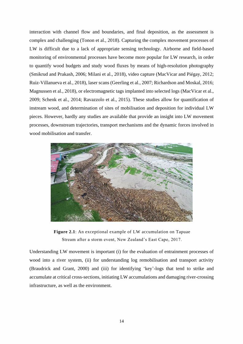
14
interaction with channel flow and boundaries, and final deposition, as the assessment is
complex and challenging (Tonon et al., 2018). Capturing the complex movement processes of
LW is difficult due to a lack of appropriate sensing technology. Airborne and field-based
monitoring of environmental processes have become more popular for LW research, in order
to quantify wood budgets and study wood fluxes by means of high-resolution photography
(Smikrud and Prakash, 2006; Milani et al., 2018), video capture (MacVicar and Piégay, 2012;
Ruiz-Villanueva et al., 2018), laser scans (Geerling et al., 2007; Richardson and Moskal, 2016;
Magnussen et al., 2018), or electromagnetic tags implanted into selected logs (MacVicar et al.,
2009; Schenk et al., 2014; Ravazzolo et al., 2015). These studies allow for quantification of
instream wood, and determination of sites of mobilisation and deposition for individual LW
pieces. However, hardly any studies are available that provide an insight into LW movement
processes, downstream trajectories, transport mechanisms and the dynamic forces involved in
wood mobilisation and transfer.
Figure 2.1: An exceptional example of LW accumulation on Tapuae
Stream after a storm event, New Zealand’s East Cape, 2017.
Understanding LW movement is important (i) for the evaluation of entrainment processes of
wood into a river system, (ii) for understanding log remobilisation and transport activity
(Braudrick and Grant, 2000) and (iii) for identifying ‘key’-logs that tend to strike and
accumulate at critical cross-sections, initiating LW accumulations and damaging river-crossing
infrastructure, as well as the environment.
15
2.1.1. LW DEFINITION AND PROCESSES
Wood from both natural and anthropogenic sources influences the ecology and geomorphology
of a river (MacVicar et al., 2009; Ravazzolo et al., 2015). It can influence the riparian processes
of erosion and sedimentation (Assani and Petit, 1995; Ravazzolo et al., 2015), as well as the
ecological diversity of rivers, forming aquatic habitat and acting as a food source for organisms
in the riparian environment (Gurnell et al., 2002). Previous studies have defined LW as pieces
of wood with length and diameter greater than 1 m and 0.1 m, respectively (Nakamura and
Swanson, 1994; Abbe and Montgomery, 2003; Wohl and Jaeger, 2009; Martin et al., 2018). In
general, LW undergoes three main processes in its downstream movement: (i) recruitment and
entrainment, followed by (ii) transportation in the stream channel before (iii) final deposition,
the latter often involving complex accumulation processes. Typical residence times of LW in
stream channels have been found to be in the order of a few years (Piegay et al., 1999) up to
several centuries (Keller and Tally, 1979; Harmon et al., 1986), depending on factors such as
the channel slope, floodplain width and the confinement of the valley.
Studies of wood in stream systems have found that when water depth reaches a point relative
to the log diameter, buoyant LW elements will float and become primed for entrainment. This
instability leads to mobilisation (Braudrick and Grant, 2001; Bocchiola et al., 2006; Davidson
et al., 2015). Braudrick and Grant (2000) further postulated that entrainment is a function of
four parameters, namely log length, diameter, density and orientation. Logs with an orientation
perpendicular to flow direction have shown a higher probability for transport initiation
(Davidson et al., 2015). A case study showed that in most native New Zealand streams, wood
deposited on floodplains or bars tends to be aligned perpendicular (90 degrees) to flow
direction (Baillie and Davies, 2002). Determining the actual sequence of mobilisation
processes is difficult due to a lack of applicable techniques and methodologies. For instance,
there are likely to be sliding and rotational movements (Ruiz-Villanueva et al., 2016a) that
contribute significantly to log entrainment, though these mechanics are poorly understood.
Improving our knowledge of mobilisation processes can help in developing probabilistic - or
even mechanistic - models of log recruitment.
LW is transported downstream during high flow events, normally in the rising limb of the
hydrograph (Ravazzolo et al., 2015), with increasing flow depth. Braudrick and Grant (2001)
found that LW is generally transported along the centreline of a stream and is aligned parallel
with the flow, however, interactions with other floating LW, embankments and in-stream bars
16
may disturb parallel and centred movement, adding more complexity to transport processes
and downstream trajectories. It has been found that as wood volume in transit increases,
transportation generally decreases, owing to congestion of woody elements (Ruiz-Villanueva
et al., 2016c). Movement of LW en masse becomes a probabilistic problem, and therefore more
estimates of transit times are needed to develop adequate models for the bulk transport of
riverborne wood.
We know that deposition generally occurs on the river bed or on bars in low flow conditions,
often in areas with high roughness (Wyżga et al., 2017). Individual logs, once deposited, tend
to collect even more LW and consequently one well-lodged wood element can become the
nucleus for a large jam. There is clearly a complex relationship between river stage, buoyancy
of a given wood mass, and the snagging of branches or rootwads with immobile boundary
elements (including other deposited wood).
2.1.2. REMOTE SENSING OF LW
LW in the riparian environment is a widely researched topic, with studies having been
undertaken both in situ (MacVicar et al., 2009; Ravazzolo et al., 2015; Ruiz-Villanueva et al.,
2016c; Wyżga et al., 2017) and in the laboratory environment (Rusyda et al., 2014; Davidson
et al., 2015; Gschnitzer et al., 2017). Some of these studies have looked at the use of sensors,
in the form of radio-frequency identification (RFID) tags to help understand LW movement,
but these are limited in their application as they only provide information about where LW
started and finished its journey (MacVicar et al., 2009; Ravazzolo et al., 2015; Wyżga et al.,
2017). Research in areas other than LW, such as debris transported through tsunamis (Goseberg
et al., 2016) or in geotechnics and fluvial geomorphology (Hiller et al., 2014; Olinde and
Johnson, 2015; Gronz et al., 2016; Valyrakis and Farhadi, 2017) has also applied RFID and
sensors. There have been tremendous advances and insights offered from these sensor-tagged
tracer studies that help to better understand the transfer of wood, debris and sediment through
various environments. Fluvial tracer studies have demonstrated that smart sensors can be
effectively used to characterise the probability functions for entrainment, movement modes,
deposition and rest times between transfer episodes.
Olinde and Johnson (2015) used active smart pebbles equipped with an accelerometer unit for
particle tracking, and reported difficulties in differentiating between real movement process
and clast rocking in place. Sensors that track orientation and position in three dimensional
17
space with great accuracy are not suitable for many applications due to the extreme cost or
inappropriate size (Ahmad et al., 2013). Motion can be tracked with Inertial Measurement
Units (IMUs), which are low cost, low processing power and compact orientation sensors.
These have been applied in a variety of research areas, including medical rehabilitation, sports
analysis and animal behaviour analysis (Ahmad et al., 2013; Aldoumani et al., 2015). Due to
forces from motion (accelerometer), changes in angular velocity (gyroscope) and magnetic
field (e-compass, magnetometer) position and orientation in all three-dimensions can be
estimated over time (Ahmad et al., 2013; Fischer et al., 2013; Goseberg et al., 2016). The ability
to measure body-frame rotations, as well as force energies, makes these types of sensors useful
for hydraulic research and LW tracking.
Despite the successful implantation of the sensors mentioned above, there are challenges in
using the obtained information for accurate translational and rotational motion tracking.
Orientation can be represented through the use of Euler angles or quaternions (Fischer et al.,
2013; Aldoumani et al., 2015). Euler angles of roll, pitch and yaw (Figure 2.2) are commonly
used, as they provide an intuitive representation of orientation, however they are prone to
errors, such as the issue of ‘gimbal lock’ (Madgwick et al., 2011). Gimbal lock refers to a
problem of axis parallelism, when at least two of the three gimbal axes align to a single plane,
resulting in the loss of one degree of freedom (Hoag, 1963). These same issues do not apply to
quaternions (Madgwick et al., 2011). Smart sensors allow the visualisation of orientation and
movement of LW as they are transported, without the need for constant visual contact. Position
estimates can be found through the integration of acceleration values through time, similar to
the process of dead reckoning commonly used in pedestrian tracking, following the rotation of
the sensor body frame to the global frame (Fischer et al., 2013). Each integration calculation
introduces a new component of drift error, typically resulting in large discrepancies between
observed and calculated results (Ahmad et al., 2013). There are a number of algorithms
available to suppress the drift in orientation using mathematical formulas (Madgwick et al.,
2011; Liu et al., 2018a), however, these algorithms work as a filter using a specific threshold
value with the aim of gait pattern tracking. This means that after each step, the sensor registers
a period of signals showing very few deviations, which suggests that the object is at rest.
Thereupon, the algorithm detects the touchdown on the ground and keeps orientation
computations static, which limits the drift, until threshold-exceeding signals are registered.
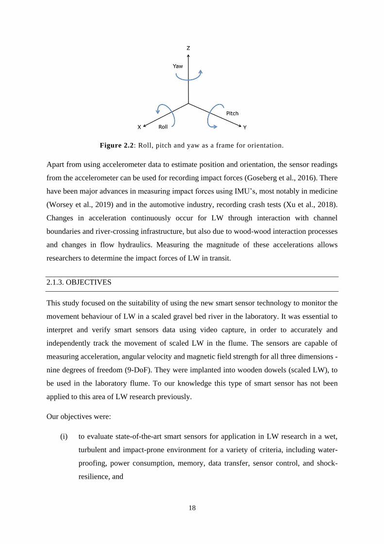
18
Figure 2.2: Roll, pitch and yaw as a frame for orientation.
Apart from using accelerometer data to estimate position and orientation, the sensor readings
from the accelerometer can be used for recording impact forces (Goseberg et al., 2016). There
have been major advances in measuring impact forces using IMU’s, most notably in medicine
(Worsey et al., 2019) and in the automotive industry, recording crash tests (Xu et al., 2018).
Changes in acceleration continuously occur for LW through interaction with channel
boundaries and river-crossing infrastructure, but also due to wood-wood interaction processes
and changes in flow hydraulics. Measuring the magnitude of these accelerations allows
researchers to determine the impact forces of LW in transit.
2.1.3. OBJECTIVES
This study focused on the suitability of using the new smart sensor technology to monitor the
movement behaviour of LW in a scaled gravel bed river in the laboratory. It was essential to
interpret and verify smart sensors data using video capture, in order to accurately and
independently track the movement of scaled LW in the flume. The sensors are capable of
measuring acceleration, angular velocity and magnetic field strength for all three dimensions -
nine degrees of freedom (9-DoF). They were implanted into wooden dowels (scaled LW), to
be used in the laboratory flume. To our knowledge this type of smart sensor has not been
applied to this area of LW research previously.
Our objectives were:
(i) to evaluate state-of-the-art smart sensors for application in LW research in a wet,
turbulent and impact-prone environment for a variety of criteria, including water-
proofing, power consumption, memory, data transfer, sensor control, and shock-
resilience, and
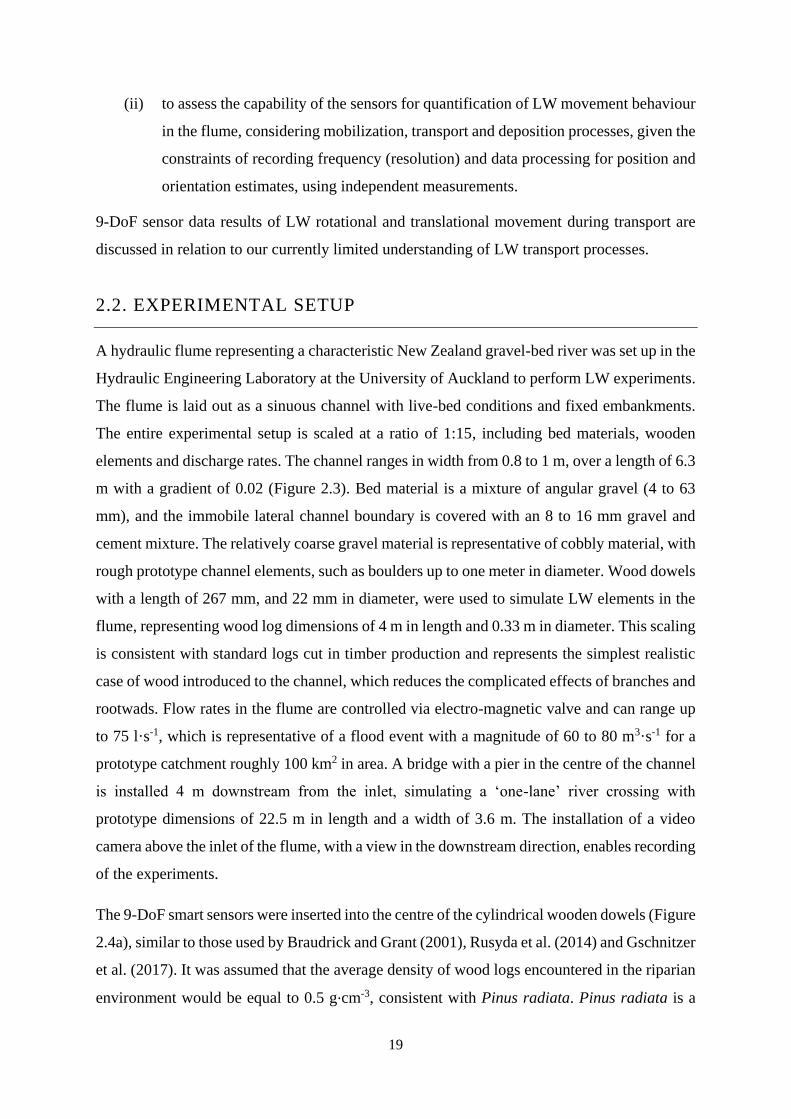
19
(ii) to assess the capability of the sensors for quantification of LW movement behaviour
in the flume, considering mobilization, transport and deposition processes, given the
constraints of recording frequency (resolution) and data processing for position and
orientation estimates, using independent measurements.
9-DoF sensor data results of LW rotational and translational movement during transport are
discussed in relation to our currently limited understanding of LW transport processes.
2.2. EXPERIMENTAL SETUP
A hydraulic flume representing a characteristic New Zealand gravel-bed river was set up in the
Hydraulic Engineering Laboratory at the University of Auckland to perform LW experiments.
The flume is laid out as a sinuous channel with live-bed conditions and fixed embankments.
The entire experimental setup is scaled at a ratio of 1:15, including bed materials, wooden
elements and discharge rates. The channel ranges in width from 0.8 to 1 m, over a length of 6.3
m with a gradient of 0.02 (Figure 2.3). Bed material is a mixture of angular gravel (4 to 63
mm), and the immobile lateral channel boundary is covered with an 8 to 16 mm gravel and
cement mixture. The relatively coarse gravel material is representative of cobbly material, with
rough prototype channel elements, such as boulders up to one meter in diameter. Wood dowels
with a length of 267 mm, and 22 mm in diameter, were used to simulate LW elements in the
flume, representing wood log dimensions of 4 m in length and 0.33 m in diameter. This scaling
is consistent with standard logs cut in timber production and represents the simplest realistic
case of wood introduced to the channel, which reduces the complicated effects of branches and
rootwads. Flow rates in the flume are controlled via electro-magnetic valve and can range up
to 75 l·s-1, which is representative of a flood event with a magnitude of 60 to 80 m3·s-1 for a
prototype catchment roughly 100 km2 in area. A bridge with a pier in the centre of the channel
is installed 4 m downstream from the inlet, simulating a ‘one-lane’ river crossing with
prototype dimensions of 22.5 m in length and a width of 3.6 m. The installation of a video
camera above the inlet of the flume, with a view in the downstream direction, enables recording
of the experiments.
The 9-DoF smart sensors were inserted into the centre of the cylindrical wooden dowels (Figure
2.4a), similar to those used by Braudrick and Grant (2001), Rusyda et al. (2014) and Gschnitzer
et al. (2017). It was assumed that the average density of wood logs encountered in the riparian
environment would be equal to 0.5 g·cm-3, consistent with Pinus radiata. Pinus radiata is a
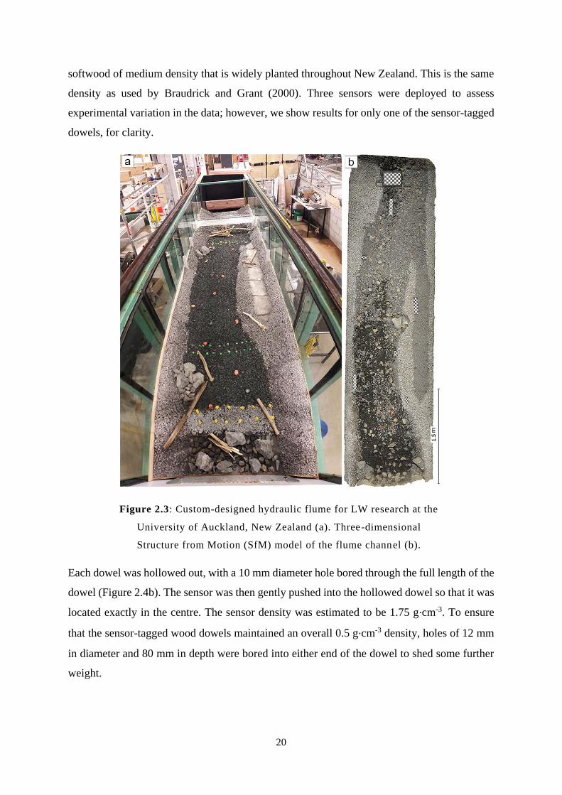
20
softwood of medium density that is widely planted throughout New Zealand. This is the same
density as used by Braudrick and Grant (2000). Three sensors were deployed to assess
experimental variation in the data; however, we show results for only one of the sensor-tagged
dowels, for clarity.
Figure 2.3: Custom-designed hydraulic flume for LW research at the
University of Auckland, New Zealand (a). Three-dimensional
Structure from Motion (SfM) model of the flume channel (b).
Each dowel was hollowed out, with a 10 mm diameter hole bored through the full length of the
dowel (Figure 2.4b). The sensor was then gently pushed into the hollowed dowel so that it was
located exactly in the centre. The sensor density was estimated to be 1.75 g·cm-3. To ensure
that the sensor-tagged wood dowels maintained an overall 0.5 g·cm-3 density, holes of 12 mm
in diameter and 80 mm in depth were bored into either end of the dowel to shed some further
weight.
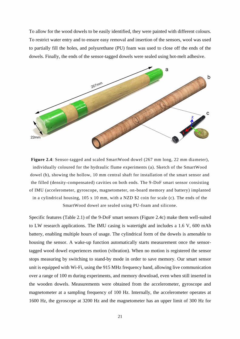
21
To allow for the wood dowels to be easily identified, they were painted with different colours.
To restrict water entry and to ensure easy removal and insertion of the sensors, wool was used
to partially fill the holes, and polyurethane (PU) foam was used to close off the ends of the
dowels. Finally, the ends of the sensor-tagged dowels were sealed using hot-melt adhesive.
Figure 2.4: Sensor-tagged and scaled SmartWood dowel (267 mm long, 22 mm diameter),
individually coloured for the hydraulic flume experiments (a). Sketch of the SmartWood
dowel (b), showing the hollow, 10 mm central shaft for installation of the smart sensor and
the filled (density-compensated) cavities on both ends. The 9-DoF smart sensor consisting
of IMU (accelerometer, gyroscope, magnetometer, on-board memory and battery) implanted
in a cylindrical housing, 105 x 10 mm, with a NZD $2 coin for scale (c). The ends of the
SmartWood dowel are sealed using PU-foam and silicone.
Specific features (Table 2.1) of the 9-DoF smart sensors (Figure 2.4c) make them well-suited
to LW research applications. The IMU casing is watertight and includes a 1.6 V, 600 mAh
battery, enabling multiple hours of usage. The cylindrical form of the dowels is amenable to
housing the sensor. A wake-up function automatically starts measurement once the sensor-
tagged wood dowel experiences motion (vibration). When no motion is registered the sensor
stops measuring by switching to stand-by mode in order to save memory. Our smart sensor
unit is equipped with Wi-Fi, using the 915 MHz frequency band, allowing live communication
over a range of 100 m during experiments, and memory download, even when still inserted in
the wooden dowels. Measurements were obtained from the accelerometer, gyroscope and
magnetometer at a sampling frequency of 100 Hz. Internally, the accelerometer operates at
1600 Hz, the gyroscope at 3200 Hz and the magnetometer has an upper limit of 300 Hz for
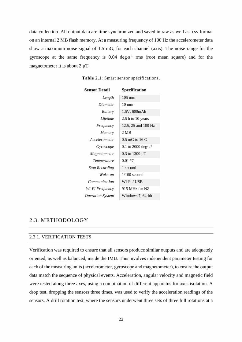
22
data collection. All output data are time synchronized and saved in raw as well as .csv format
on an internal 2 MB flash memory. At a measuring frequency of 100 Hz the accelerometer data
show a maximum noise signal of 1.5 mG, for each channel (axis). The noise range for the
gyroscope at the same frequency is 0.04 deg·s-1 rms (root mean square) and for the
magnetometer it is about 2 µT.
Table 2.1: Smart sensor specifications.
Sensor Detail Specification
Length 105 mm
Diameter 10 mm
Battery 1.5V, 600mAh
Lifetime 2.5 h to 10 years
Frequency 12.5, 25 and 100 Hz
Memory 2 MB
Accelerometer 0.5 mG to 16 G
Gyroscope 0.1 to 2000 deg·s-1
Magnetometer 0.3 to 1300 µT
Temperature 0.01 °C
Stop Recording 1 second
Wake-up 1/100 second
Communication Wi-Fi / USB
Wi-Fi Frequency 915 MHz for NZ
Operation System Windows 7, 64-bit
2.3. METHODOLOGY
2.3.1. VERIFICATION TESTS
Verification was required to ensure that all sensors produce similar outputs and are adequately
oriented, as well as balanced, inside the IMU. This involves independent parameter testing for
each of the measuring units (accelerometer, gyroscope and magnetometer), to ensure the output
data match the sequence of physical events. Acceleration, angular velocity and magnetic field
were tested along three axes, using a combination of different apparatus for axes isolation. A
drop test, dropping the sensors three times, was used to verify the acceleration readings of the
sensors. A drill rotation test, where the sensors underwent three sets of three full rotations at a
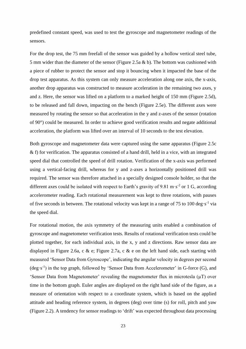
23
predefined constant speed, was used to test the gyroscope and magnetometer readings of the
sensors.
For the drop test, the 75 mm freefall of the sensor was guided by a hollow vertical steel tube,
5 mm wider than the diameter of the sensor (Figure 2.5a & b). The bottom was cushioned with
a piece of rubber to protect the sensor and stop it bouncing when it impacted the base of the
drop test apparatus. As this system can only measure acceleration along one axis, the x-axis,
another drop apparatus was constructed to measure acceleration in the remaining two axes, y
and z. Here, the sensor was lifted on a platform to a marked height of 150 mm (Figure 2.5d),
to be released and fall down, impacting on the bench (Figure 2.5e). The different axes were
measured by rotating the sensor so that acceleration in the y and z-axes of the sensor (rotation
of 90°) could be measured. In order to achieve good verification results and negate additional
acceleration, the platform was lifted over an interval of 10 seconds to the test elevation.
Both gyroscope and magnetometer data were captured using the same apparatus (Figure 2.5c
& f) for verification. The apparatus consisted of a hand drill, held in a vice, with an integrated
speed dial that controlled the speed of drill rotation. Verification of the x-axis was performed
using a vertical-facing drill, whereas for y and z-axes a horizontally positioned drill was
required. The sensor was therefore attached in a specially designed console holder, so that the
different axes could be isolated with respect to Earth’s gravity of 9.81 m·s-2 or 1 G, according
accelerometer reading. Each rotational measurement was kept to three rotations, with pauses
of five seconds in between. The rotational velocity was kept in a range of 75 to 100 deg·s-1 via
the speed dial.
For rotational motion, the axis symmetry of the measuring units enabled a combination of
gyroscope and magnetometer verification tests. Results of rotational verification tests could be
plotted together, for each individual axis, in the x, y and z directions. Raw sensor data are
displayed in Figure 2.6a, c & e; Figure 2.7a, c & e on the left hand side, each starting with
measured ‘Sensor Data from Gyroscope’, indicating the angular velocity in degrees per second
(deg·s-1) in the top graph, followed by ‘Sensor Data from Accelerometer’ in G-force (G), and
‘Sensor Data from Magnetometer’ revealing the magnetometer flux in microtesla (µT) over
time in the bottom graph. Euler angles are displayed on the right hand side of the figure, as a
measure of orientation with respect to a coordinate system, which is based on the applied
attitude and heading reference system, in degrees (deg) over time (s) for roll, pitch and yaw
(Figure 2.2). A tendency for sensor readings to ‘drift’ was expected throughout data processing
24
(Madgwick et al., 2011). Drift, for our purposes, is defined as the time-dependent deviation
between measured signal and real movement, which occurs during integration of raw sensor
data. These deviations become obvious during periods of idle sensor position, and are difficult
to determine for periods when the sensor is in motion.
Figure 2.5: Setup for smart sensor verification in the laboratory, consisting of a vertical
drop test (a, b), from a height of 75 mm onto a rubber layer (red), in order to measure
acceleration along the longitudinal axis of the sensor. (c) Rotational test for assessing
gyroscope and magnetometer performance, aligned to the longitudinal x -axis. (d, e) For
verification of the acceleration along the vertical z - and lateral y-axes of the IMU, a
platform is used to simulate drop tests from a height of 150 mm. A rotational test, shown
in (f) allows for verification of angular velocity and magnetic field stren gth around y-
and z-axes.
25
2.3.2. EXPERIMENTAL TESTS
Experimental data were generated using the SmartWood dowel that was mobilised and
transported downstream by flow. Flow rates were gradually ramped up from 4 to 10 l·s-1,
sufficient for the mobilisation and transport of the sensor-tagged dowel. At a predefined cross-
section, 3 m upstream from the bridge section, the SmartWood dowel (Figure 2.4) was placed
in the channel centre, set at a predefined angle relative to the flow direction, specifically 0°,
45° or 90°. Dowels were placed carefully with positive z-axis facing up, and the x-axis facing
downstream. Only a single SmartWood dowel was placed and tracked at a time. Discharge at
the outset was a base discharge of 4 l·s-1. The sensor was set to measure all nine sensor channels
at a frequency of 100 Hz. Simultaneously, a camera recorded the dowel’s movement. The
discharge was increased to 10 l·s-1 (a flood event of roughly 9 m3·s-1 in our prototype channel)
over a period of 10 seconds, entraining the SmartWood dowel and transporting it downstream.
After passing the bridge, the SmartWood dowel was collected at a wood retention screen
installed within the outlet structure of the flume. At this point, the measurement ended, the
discharge was decreased to base discharge, the memory was read out and the camera was
switched off.
2.3.3. DATA ANALYSIS
After each test, memory was read for further processing in Matlab. As the sensors contain an
inbuilt digital filter, the only pre-possessing that was necessary was to smooth the
magnetometer readings that exhibited noise, most likely due to the presence of metal in the
flume and laboratory environment. Quaternions were used to estimate the orientation of the
sensors. An Attitude and Heading Reference System (AHRS) was used to output these
quaternions, and convert them to Euler angles so they could be intuitively displayed
(Madgwick et al., 2011). The AHRS algorithm designed by Madgwick et al. (2011) was further
used to counteract the potential effects of gimbal lock. This process combines integrated
gyroscope readings with acceleration and magnetometer readings to estimate orientation,
which is then plotted, to allow novel insights into LW movement behaviour. Without the
gyroscope and magnetometer information it was very difficult to distinguish between
movement in the downstream direction and rocking in place, either from particle impacts or
water turbulence (Olinde and Johnson, 2015).
26
2.4. RESULTS AND DISCUSSION
All measurements were obtained using the same SmartWood dowel for verification and
experimental tests. Each test used about 0.2% of the available internal memory. Battery lifetime
was clearly adequate, as no change of battery was required for the entire experimental series,
with a remaining capacity of more than 30%. Reading of memory and program upload for the
next tests took one to three minutes; most of this time was dedicated to establishing the Wi-Fi
connection to the SmartWood dowel, which was located within a range of five meters. A check
of the deployed sensor unit at the conclusion of the experiments revealed the integrity of the
unit was not compromised by water or impacts.
2.4.1. SENSOR VERIFICATION
Verification tests for isolated axes were conducted to determine acceleration, angular velocity,
as well as magnetic flux for x, y and z-axes. No concurrent rotations around y and z-axis were
recorded in the raw data for the longitudinal x-axis (Figure 2.6a), due to locking the DoF along
this axis. However, for each drop (seconds 2, 13 and 26), a spin around the x-axis, indicating
rotation, was recorded with the gyroscope. This rotational signal was caused by the impact
upon the bottom of the drop apparatus, when the sensor rebounded upward, slightly,
introducing a spin around the x-axis. The rotation stopped once the sensor converted the kinetic
energy gained during free fall and remained still. The observed fluctuating signal, which was
measured in-between the drops, was generated while manually resetting the sensor to its
original starting position. The rubber layer at the bottom of the drop-test apparatus reduced
bouncing of the sensor, allowing for clearer verification results.
The impact forces measured by the accelerometer in a positive longitudinal direction were
captured at 100 Hz frequency. Impacts reached a value of 9 to 10 times the Earth’s gravitational
force G. A slight signal was registered on the y and z-axis channels, generated due to contact
with the guiding tube after impact at the bottom.
Changes in magnetic flux, in Figure 2.6a - bottom chart, were discernible during the drop, as
the sensor unit fell through the steel pipe (Figure 2.5a & b). When resetting the sensor to its
starting position, moving it back up the steel tube, the magnetic field strength also changed
back to its original readings. This indicates reliable and accurate raw data measurements. Euler
angles were computed (Figure 2.6b) and roll readings show the spin imparted by the impact,
in terms of absolute orientation. The two locked y and z axes did not experience significant
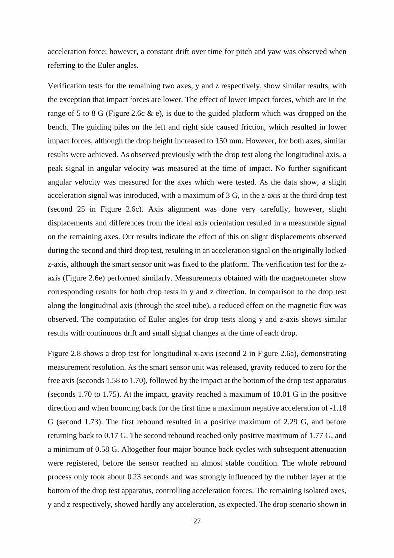
27
acceleration force; however, a constant drift over time for pitch and yaw was observed when
referring to the Euler angles.
Verification tests for the remaining two axes, y and z respectively, show similar results, with
the exception that impact forces are lower. The effect of lower impact forces, which are in the
range of 5 to 8 G (Figure 2.6c & e), is due to the guided platform which was dropped on the
bench. The guiding piles on the left and right side caused friction, which resulted in lower
impact forces, although the drop height increased to 150 mm. However, for both axes, similar
results were achieved. As observed previously with the drop test along the longitudinal axis, a
peak signal in angular velocity was measured at the time of impact. No further significant
angular velocity was measured for the axes which were tested. As the data show, a slight
acceleration signal was introduced, with a maximum of 3 G, in the z-axis at the third drop test
(second 25 in Figure 2.6c). Axis alignment was done very carefully, however, slight
displacements and differences from the ideal axis orientation resulted in a measurable signal
on the remaining axes. Our results indicate the effect of this on slight displacements observed
during the second and third drop test, resulting in an acceleration signal on the originally locked
z-axis, although the smart sensor unit was fixed to the platform. The verification test for the z-
axis (Figure 2.6e) performed similarly. Measurements obtained with the magnetometer show
corresponding results for both drop tests in y and z direction. In comparison to the drop test
along the longitudinal axis (through the steel tube), a reduced effect on the magnetic flux was
observed. The computation of Euler angles for drop tests along y and z-axis shows similar
results with continuous drift and small signal changes at the time of each drop.
Figure 2.8 shows a drop test for longitudinal x-axis (second 2 in Figure 2.6a), demonstrating
measurement resolution. As the smart sensor unit was released, gravity reduced to zero for the
free axis (seconds 1.58 to 1.70), followed by the impact at the bottom of the drop test apparatus
(seconds 1.70 to 1.75). At the impact, gravity reached a maximum of 10.01 G in the positive
direction and when bouncing back for the first time a maximum negative acceleration of -1.18
G (second 1.73). The first rebound resulted in a positive maximum of 2.29 G, and before
returning back to 0.17 G. The second rebound reached only positive maximum of 1.77 G, and
a minimum of 0.58 G. Altogether four major bounce back cycles with subsequent attenuation
were registered, before the sensor reached an almost stable condition. The whole rebound
process only took about 0.23 seconds and was strongly influenced by the rubber layer at the
bottom of the drop test apparatus, controlling acceleration forces. The remaining isolated axes,
y and z respectively, showed hardly any acceleration, as expected. The drop scenario shown in
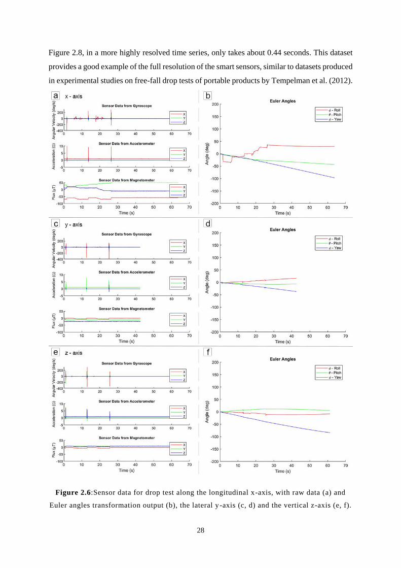
28
Figure 2.8, in a more highly resolved time series, only takes about 0.44 seconds. This dataset
provides a good example of the full resolution of the smart sensors, similar to datasets produced
in experimental studies on free-fall drop tests of portable products by Tempelman et al. (2012).
Figure 2.6:Sensor data for drop test along the longitudinal x-axis, with raw data (a) and
Euler angles transformation output (b), the lateral y -axis (c, d) and the vertical z-axis (e, f).
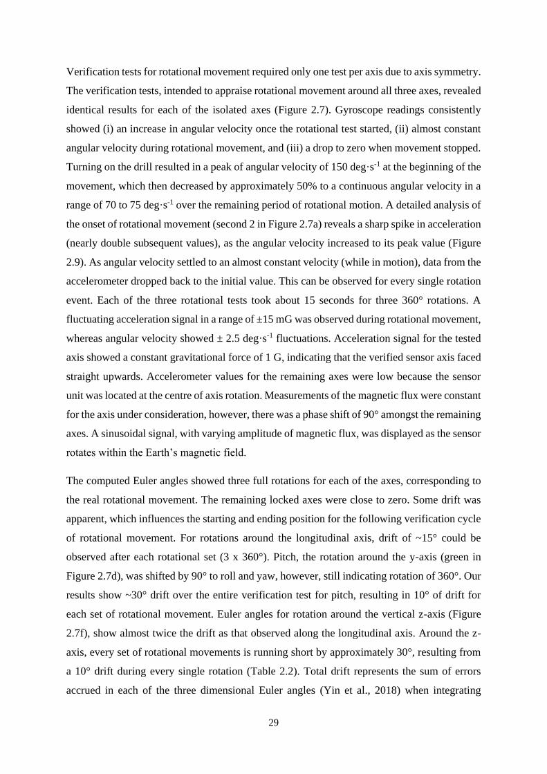
29
Verification tests for rotational movement required only one test per axis due to axis symmetry.
The verification tests, intended to appraise rotational movement around all three axes, revealed
identical results for each of the isolated axes (Figure 2.7). Gyroscope readings consistently
showed (i) an increase in angular velocity once the rotational test started, (ii) almost constant
angular velocity during rotational movement, and (iii) a drop to zero when movement stopped.
Turning on the drill resulted in a peak of angular velocity of 150 deg·s-1 at the beginning of the
movement, which then decreased by approximately 50% to a continuous angular velocity in a
range of 70 to 75 deg·s-1 over the remaining period of rotational motion. A detailed analysis of
the onset of rotational movement (second 2 in Figure 2.7a) reveals a sharp spike in acceleration
(nearly double subsequent values), as the angular velocity increased to its peak value (Figure
2.9). As angular velocity settled to an almost constant velocity (while in motion), data from the
accelerometer dropped back to the initial value. This can be observed for every single rotation
event. Each of the three rotational tests took about 15 seconds for three 360° rotations. A
fluctuating acceleration signal in a range of ±15 mG was observed during rotational movement,
whereas angular velocity showed ± 2.5 deg·s-1 fluctuations. Acceleration signal for the tested
axis showed a constant gravitational force of 1 G, indicating that the verified sensor axis faced
straight upwards. Accelerometer values for the remaining axes were low because the sensor
unit was located at the centre of axis rotation. Measurements of the magnetic flux were constant
for the axis under consideration, however, there was a phase shift of 90° amongst the remaining
axes. A sinusoidal signal, with varying amplitude of magnetic flux, was displayed as the sensor
rotates within the Earth’s magnetic field.
The computed Euler angles showed three full rotations for each of the axes, corresponding to
the real rotational movement. The remaining locked axes were close to zero. Some drift was
apparent, which influences the starting and ending position for the following verification cycle
of rotational movement. For rotations around the longitudinal axis, drift of ~15° could be
observed after each rotational set (3 x 360°). Pitch, the rotation around the y-axis (green in
Figure 2.7d), was shifted by 90° to roll and yaw, however, still indicating rotation of 360°. Our
results show ~30° drift over the entire verification test for pitch, resulting in 10° of drift for
each set of rotational movement. Euler angles for rotation around the vertical z-axis (Figure
2.7f), show almost twice the drift as that observed along the longitudinal axis. Around the z-
axis, every set of rotational movements is running short by approximately 30°, resulting from
a 10° drift during every single rotation (Table 2.2). Total drift represents the sum of errors
accrued in each of the three dimensional Euler angles (Yin et al., 2018) when integrating
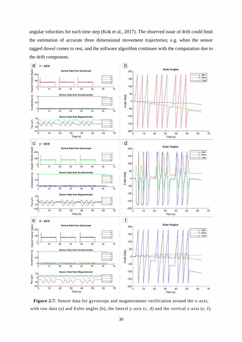
30
angular velocities for each time step (Kok et al., 2017). The observed issue of drift could limit
the estimation of accurate three dimensional movement trajectories; e.g. when the sensor
tagged dowel comes to rest, and the software algorithm continues with the computation due to
the drift component.
Figure 2.7: Sensor data for gyroscope and magnetometer verification around the x -axis,
with raw data (a) and Euler angles (b), the lateral y -axis (c, d) and the vertical z-axis (e, f).
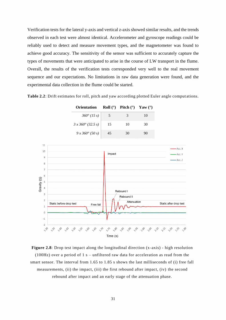
31
Verification tests for the lateral y-axis and vertical z-axis showed similar results, and the trends
observed in each test were almost identical. Accelerometer and gyroscope readings could be
reliably used to detect and measure movement types, and the magnetometer was found to
achieve good accuracy. The sensitivity of the sensor was sufficient to accurately capture the
types of movements that were anticipated to arise in the course of LW transport in the flume.
Overall, the results of the verification tests corresponded very well to the real movement
sequence and our expectations. No limitations in raw data generation were found, and the
experimental data collection in the flume could be started.
Table 2.2: Drift estimates for roll, pitch and yaw according plotted Euler angle comput ations.
Orientation Roll (°) Pitch (°) Yaw (°)
360° (15 s) 5 3 10
3 x 360° (32.5 s) 15 10 30
9 x 360° (50 s) 45 30 90
Figure 2.8: Drop test impact along the longitudinal direction (x-axis) - high resolution
(100Hz) over a period of 1 s – unfiltered raw data for acceleration as read from the
smart sensor. The interval from 1.65 to 1.85 s shows the last milliseconds of (i) free fall
measurements, (ii) the impact, (iii) the first rebound after impact, (iv) the second
rebound after impact and an early stage of the attenuation phase.
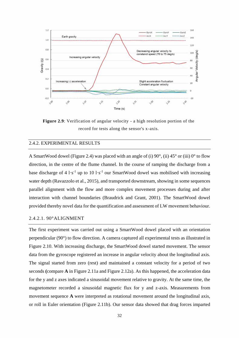
32
Figure 2.9: Verification of angular velocity - a high resolution portion of the
record for tests along the sensor's x-axis.
2.4.2. EXPERIMENTAL RESULTS
A SmartWood dowel (Figure 2.4) was placed with an angle of (i) 90°, (ii) 45° or (iii) 0° to flow
direction, in the centre of the flume channel. In the course of ramping the discharge from a
base discharge of 4 l·s-1 up to 10 l·s-1 our SmartWood dowel was mobilised with increasing
water depth (Ravazzolo et al., 2015), and transported downstream, showing in some sequences
parallel alignment with the flow and more complex movement processes during and after
interaction with channel boundaries (Braudrick and Grant, 2001). The SmartWood dowel
provided thereby novel data for the quantification and assessment of LW movement behaviour.
2.4.2.1. 90°ALIGNMENT
The first experiment was carried out using a SmartWood dowel placed with an orientation
perpendicular (90°) to flow direction. A camera captured all experimental tests as illustrated in
Figure 2.10. With increasing discharge, the SmartWood dowel started movement. The sensor
data from the gyroscope registered an increase in angular velocity about the longitudinal axis.
The signal started from zero (rest) and maintained a constant velocity for a period of two
seconds (compare A in Figure 2.11a and Figure 2.12a). As this happened, the acceleration data
for the y and z axes indicated a sinusoidal movement relative to gravity. At the same time, the
magnetometer recorded a sinusoidal magnetic flux for y and z-axis. Measurements from
movement sequence A were interpreted as rotational movement around the longitudinal axis,
or roll in Euler orientation (Figure 2.11b). Our sensor data showed that drag forces imparted
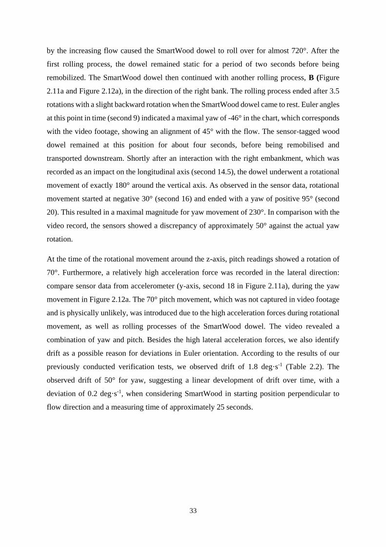
33
by the increasing flow caused the SmartWood dowel to roll over for almost 720°. After the
first rolling process, the dowel remained static for a period of two seconds before being
remobilized. The SmartWood dowel then continued with another rolling process, B (Figure
2.11a and Figure 2.12a), in the direction of the right bank. The rolling process ended after 3.5
rotations with a slight backward rotation when the SmartWood dowel came to rest. Euler angles
at this point in time (second 9) indicated a maximal yaw of -46° in the chart, which corresponds
with the video footage, showing an alignment of 45° with the flow. The sensor-tagged wood
dowel remained at this position for about four seconds, before being remobilised and
transported downstream. Shortly after an interaction with the right embankment, which was
recorded as an impact on the longitudinal axis (second 14.5), the dowel underwent a rotational
movement of exactly 180° around the vertical axis. As observed in the sensor data, rotational
movement started at negative 30° (second 16) and ended with a yaw of positive 95° (second
20). This resulted in a maximal magnitude for yaw movement of 230°. In comparison with the
video record, the sensors showed a discrepancy of approximately 50° against the actual yaw
rotation.
At the time of the rotational movement around the z-axis, pitch readings showed a rotation of
70°. Furthermore, a relatively high acceleration force was recorded in the lateral direction:
compare sensor data from accelerometer (y-axis, second 18 in Figure 2.11a), during the yaw
movement in Figure 2.12a. The 70° pitch movement, which was not captured in video footage
and is physically unlikely, was introduced due to the high acceleration forces during rotational
movement, as well as rolling processes of the SmartWood dowel. The video revealed a
combination of yaw and pitch. Besides the high lateral acceleration forces, we also identify
drift as a possible reason for deviations in Euler orientation. According to the results of our
previously conducted verification tests, we observed drift of 1.8 deg·s-1 (Table 2.2). The
observed drift of 50° for yaw, suggesting a linear development of drift over time, with a
deviation of 0.2 deg·s-1, when considering SmartWood in starting position perpendicular to
flow direction and a measuring time of approximately 25 seconds.
34
Figure 2.10 SmartWood trajectory according video footage, showing starting orientation
with recruitment processes (A), rollover and transport processes (B), and interaction of
sensor-tagged wood dowel with channel boundaries (C).
2.4.2.2. 45°ALIGNMENT
Data obtained from the 45° alignment to flow direction showed similar movement behaviour
as the previous experiment with 90° alignment. The main differences are in shorter resting
times for the SmartWood dowel in the channel, and almost continuous movement, involving a
360° rotation after interaction with the right embankment. With increasing discharge, the
SmartWood dowel experienced motion around the longitudinal axis. As captured on camera,
an approximately 160° rolling process was observed. This movement aligns with the measured
and computed sensor data - compare movement sequence D in Figure 2.11c & d and Figure
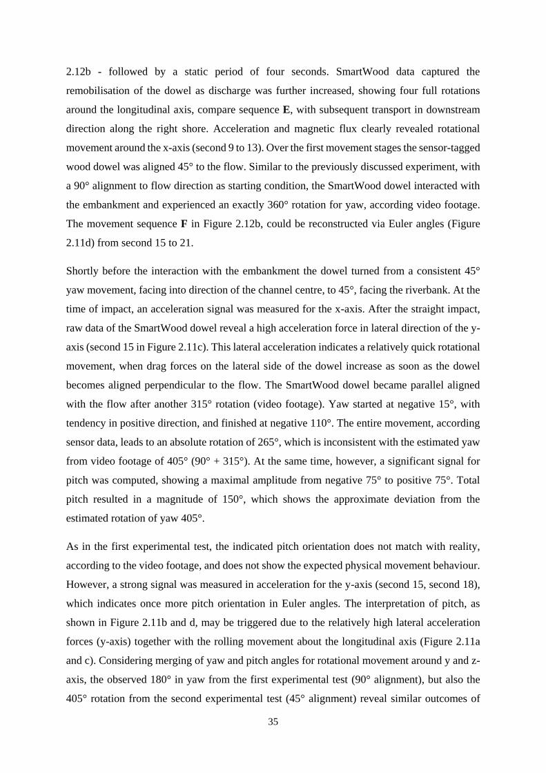
35
2.12b - followed by a static period of four seconds. SmartWood data captured the
remobilisation of the dowel as discharge was further increased, showing four full rotations
around the longitudinal axis, compare sequence E, with subsequent transport in downstream
direction along the right shore. Acceleration and magnetic flux clearly revealed rotational
movement around the x-axis (second 9 to 13). Over the first movement stages the sensor-tagged
wood dowel was aligned 45° to the flow. Similar to the previously discussed experiment, with
a 90° alignment to flow direction as starting condition, the SmartWood dowel interacted with
the embankment and experienced an exactly 360° rotation for yaw, according video footage.
The movement sequence F in Figure 2.12b, could be reconstructed via Euler angles (Figure
2.11d) from second 15 to 21.
Shortly before the interaction with the embankment the dowel turned from a consistent 45°
yaw movement, facing into direction of the channel centre, to 45°, facing the riverbank. At the
time of impact, an acceleration signal was measured for the x-axis. After the straight impact,
raw data of the SmartWood dowel reveal a high acceleration force in lateral direction of the y-
axis (second 15 in Figure 2.11c). This lateral acceleration indicates a relatively quick rotational
movement, when drag forces on the lateral side of the dowel increase as soon as the dowel
becomes aligned perpendicular to the flow. The SmartWood dowel became parallel aligned
with the flow after another 315° rotation (video footage). Yaw started at negative 15°, with
tendency in positive direction, and finished at negative 110°. The entire movement, according
sensor data, leads to an absolute rotation of 265°, which is inconsistent with the estimated yaw
from video footage of 405° (90° + 315°). At the same time, however, a significant signal for
pitch was computed, showing a maximal amplitude from negative 75° to positive 75°. Total
pitch resulted in a magnitude of 150°, which shows the approximate deviation from the
estimated rotation of yaw 405°.
As in the first experimental test, the indicated pitch orientation does not match with reality,
according to the video footage, and does not show the expected physical movement behaviour.
However, a strong signal was measured in acceleration for the y-axis (second 15, second 18),
which indicates once more pitch orientation in Euler angles. The interpretation of pitch, as
shown in Figure 2.11b and d, may be triggered due to the relatively high lateral acceleration
forces (y-axis) together with the rolling movement about the longitudinal axis (Figure 2.11a
and c). Considering merging of yaw and pitch angles for rotational movement around y and z-
axis, the observed 180° in yaw from the first experimental test (90° alignment), but also the
405° rotation from the second experimental test (45° alignment) reveal similar outcomes of
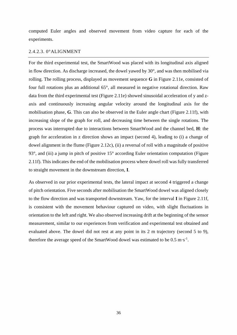
36
computed Euler angles and observed movement from video capture for each of the
experiments.
2.4.2.3. 0°ALIGNMENT
For the third experimental test, the SmartWood was placed with its longitudinal axis aligned
in flow direction. As discharge increased, the dowel yawed by 30°, and was then mobilised via
rolling. The rolling process, displayed as movement sequence G in Figure 2.11e, consisted of
four full rotations plus an additional 65°, all measured in negative rotational direction. Raw
data from the third experimental test (Figure 2.11e) showed sinusoidal acceleration of y and z-
axis and continuously increasing angular velocity around the longitudinal axis for the
mobilisation phase, G. This can also be observed in the Euler angle chart (Figure 2.11f), with
increasing slope of the graph for roll, and decreasing time between the single rotations. The
process was interrupted due to interactions between SmartWood and the channel bed, H: the
graph for acceleration in z direction shows an impact (second 4), leading to (i) a change of
dowel alignment in the flume (Figure 2.12c), (ii) a reversal of roll with a magnitude of positive
93°, and (iii) a jump in pitch of positive 15° according Euler orientation computation (Figure
2.11f). This indicates the end of the mobilisation process where dowel roll was fully transferred
to straight movement in the downstream direction, I.
As observed in our prior experimental tests, the lateral impact at second 4 triggered a change
of pitch orientation. Five seconds after mobilisation the SmartWood dowel was aligned closely
to the flow direction and was transported downstream. Yaw, for the interval I in Figure 2.11f,
is consistent with the movement behaviour captured on video, with slight fluctuations in
orientation to the left and right. We also observed increasing drift at the beginning of the sensor
measurement, similar to our experiences from verification and experimental test obtained and
evaluated above. The dowel did not rest at any point in its 2 m trajectory (second 5 to 9),
therefore the average speed of the SmartWood dowel was estimated to be 0.5 m·s-1.
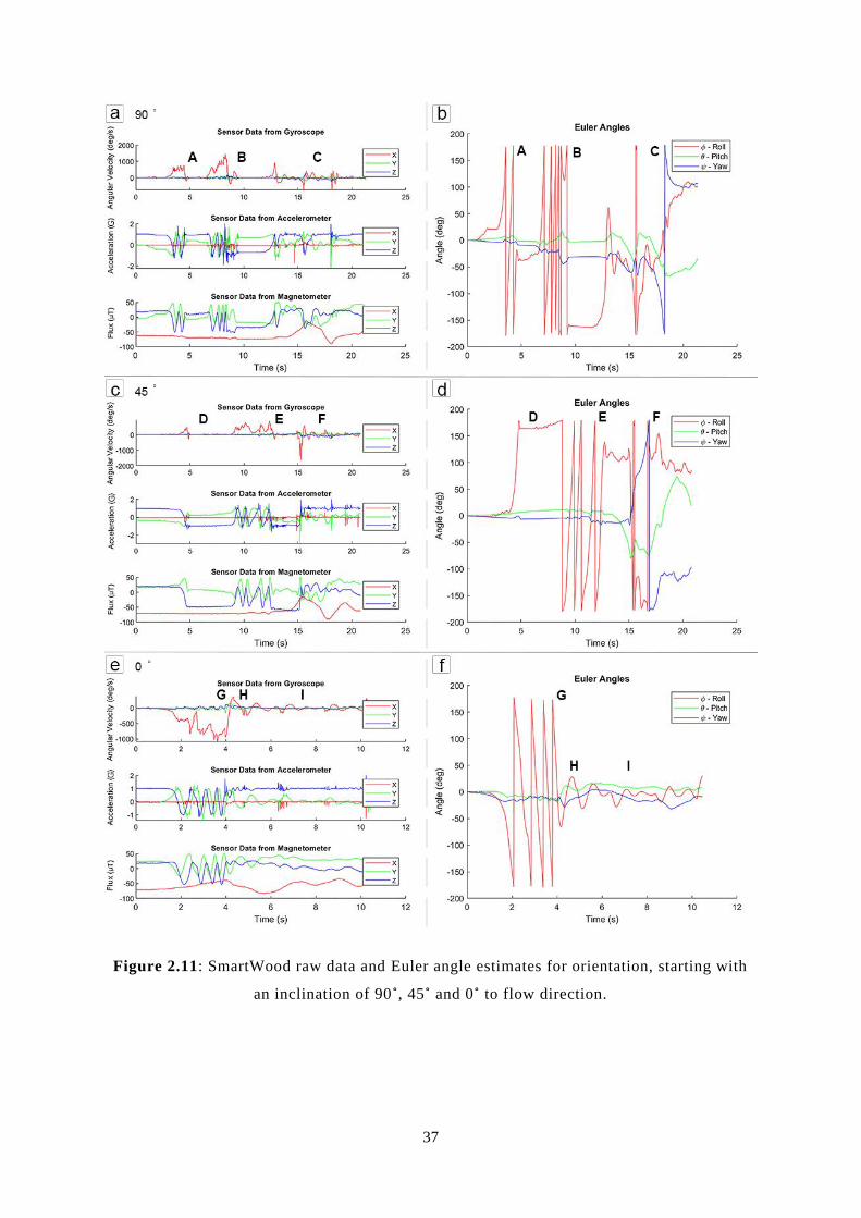
37
Figure 2.11: SmartWood raw data and Euler angle estimates for orientation, starting with
an inclination of 90˚, 45˚ and 0˚ to flow direction.
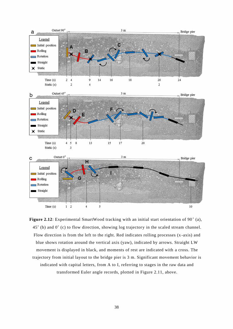
38
Figure 2.12: Experimental SmartWood tracking with an initial start orientation of 90 ˚ (a),
45˚ (b) and 0˚ (c) to flow direction, showing log trajectory in the scaled stream channel.
Flow direction is from the left to the right. Red indicates rolling processes (x -axis) and
blue shows rotation around the vertical axis (yaw), indicated by arrows. Straight LW
movement is displayed in black, and moments of rest are indicated with a cross. The
trajectory from initial layout to the bridge pier is 3 m. Significant movement behavior is
indicated with capital letters, from A to I, referring to stages in the raw data and
transformed Euler angle records, plotted in Figure 2.11, above.
39
2.4.3. KEY FINDINGS
SmartWood allows for the determination of active moving periods (transportation), and
depending on pre/post survey opportunities (MacVicar et al., 2009; Ravazzolo et al., 2015),
and records from other SmartWood equipped elements, residence times and the nature of
stochastic entrainment and terminal ‘hang ups’ can be assessed within the system. However, it
is possible that the wood may be ‘at rest’ relative to the local coordinate frame even while
drifting down the river, a scenario for which further research into signal conditioning is
required. The design of the SmartWood itself can allow for different dimensions and roughness
elements, and configurations such as branches and rootwads may be considered, which
significantly affect entrainment, transport and accumulation behaviour, similar to the work of
Davidson et al. (2015), and Gschnitzer et al. (2017). The following key findings result from
our study:
1.) This study provides a proof of concept for the application of 9-DoF smart sensors in a
wet, dynamic and impact-prone environment. The smart sensors satisfied our criteria
for size, battery life, data storage capacity and processing times for memory download
as well as instruction upload. A Wi-Fi connection enabled quick communication with
the embedded smart sensor unit at any time throughout our experiments.
2.) Verification tests demonstrated that the data generated from smart sensors meet the
measurement requirements, with respect to data accuracy and reliability, for LW
experiments in a flume environment. Specifically, the applied smart sensors have
shown good sensitivity to movements and impacts, and we were able to accurately
reconstruct real-world movements from the sensor data, as verified from experimental
observations.
3.) A smart sensor unit was implanted into a wooden dowel, a scale model of LW, for the
purpose of movement tracking in a flume environment. Experimental results show that
more complex sequences of movement, including simultaneous combinations of yaw,
pitch and roll, can be reconstructed from sensor data, as verified using a video record
of transport events in the flume.
4.) LW movement pathways, as reconstructed from time integration of sensor data, reveal
some deviations from the video record. Rates of drift in the rotation sensor are on the
order of 1.8 (± 0.2) deg·s-1. This results in errors of 3 to 10° for a single roll, pitch and
yaw movement (depending on the rate of rotation) throughout our experiments.
40
However, these deviations in rotation measurements, as a function of time, will have to
be controlled for, in order to achieve reconstruction of the full LW trajectory.
5.) At a data sampling rate of 100 Hz, it is shown that SmartWood can record impact forces
with sufficient resolution to reconstruct LW movements and interactions with channel
boundaries and river-crossing infrastructure.
2.5. CONCLUSIONS AND OUTLOOK
We presented verification and initial experimental tests using smart sensors in wooden dowels,
a method that promises to provide novel insights into LW movement behaviour. Verification
tests concentrated on quantifying sensor movement under controlled conditions and provided
comprehensive data of translational and rotational movement sequences. Experimental tests
carried out in a laboratory flume environment are presented, introducing a novel application of
SmartWood in LW research. Further verification tests are needed to better understand the
limitations of smart sensor measurements, and issues that arise from time-based integration for
reconstructing a sequence of movements of LW.
Whilst SmartWood data aligned well with the movements captured through a camera,
differences from measured sensor data and captured image data were observed. The sequence
of pitch data recorded in the first and second experimental tests does not align with the video
images. We believe that orientation estimates are impaired by significant lateral acceleration
of the dowels and the drift component. This requires future improvements in computation of
orientation estimates, which requires more advanced filtering, as well as zero-velocity-
correction for example, in order to subtract gravity and reduce drift. We recommend that further
work is needed to (i) evaluate the influence of a steel flume on magnetometer measurements,
(ii) compensate drift when integrating raw data for rotation estimates, and (iii) estimate
trajectories and obtain information about absolute position at any point of time. To obtain
information about absolute position at any point of time, an improved methodology is needed,
which can be achieved using a more refined verification procedure, testing SmartWood
movement sequences along a predetermined trail. Instead of axes-isolation, as introduced in
the present study, a well organised mixture of all axes should be considered for data generation,
to be computed with a software algorithm considering Earth coordinates with vertical up, and
verified according the actual trajectory. This verification method should be conducted in a non-
ferrous environment for more reliable magnetometer data.

41
Despite the limitations introduced by sensor drift, SmartWood has the potential to be used in
further studies, modelling interactions between LW and infrastructure. The SmartWood
methodology introduced here allows for future research on entrainment mechanisms, LW
transport trajectories, as well as measuring impact forces on channel boundaries, bridge piers
and multiple log interactions at existing LW accumulations, respectively. Ultimately, after
further development in the laboratory, SmartWood could be applied to in-situ studies. The
application of SmartWood will help to better understand LW transport and accumulation
processes, both in the field and in the laboratory.

43
Using smart sensors for measuring impact forces of large wood
(LW)
Related article:
Spreitzer, G., Tunnicliffe, J., & Friedrich, H. 2019. Using smart sensors for measuring impact
forces of large wood (LW). Proceedings of the 38th IAHR World Congress, Panama City,
Panama.
3.1. INTRODUCTION
3.1.1. LARGE WOOD (LW)
Changes in land use and climate have led to an increase in large wood (LW) in river systems
(Phillips et al., 2018), resulting in a pressing need to gain a better understanding of flow-wood
interaction processes. Although organic material plays an important role in a number of
ecological and geomorphic processes in a river system (Megahan and Nowlin, 1976; Bilby and
Likens, 1980; Harmon et al., 1986), overloading of wood can reduce these benefits, causing
progressive harm to the ecosystem (Meehan et al., 1969; Elliot, 1978) and river crossing
infrastructure (Schmocker and Weitbrecht, 2013; Rusyda, 2014). The majority of studies that
deal with wood in streams defined LW as pieces with a minimum diameter of 0.1 m and a
length of at least 1 m (Nakamura and Swanson, 1993; Martin et al., 2018). The variety of
transported organic material ranges from fine material with a size of a few millimetres to entire
trees with rootwad and branches, measuring more than 20 m in length. Remnants from
commercial forestry sites, on the other hand, will have a different distribution of woody
44
material, from clean cut logs with no branches and no rootwads, to slash consisting of
understory debris and branches stripped from mature trees. The composition of the LW load
may result in different transportation processes, depending on contributions from different
source areas. Slash from timber production is sometimes left behind on hill slopes where it
may be mobilized during major precipitation events, with devastating consequences (Cave et
al., 2017).
Once recruited to the fluvial system, LW tends to accumulate at river crossing infrastructure,
such as weirs and bridges, blocking or diverting flows and causing changes in hydraulic flow
behaviour upstream. Several studies investigated blocked stream cross-sections (Schmocker
and Hager, 2013; De Cicco et al., 2015; Gschnitzer et al., 2017; Schalko et al., 2018). In
addition to damage from entrainment and undermining of structures, there are also impacts that
can occur from logs strikes. This results in a need to better understand the trajectory of woody
elements, from recruitment to accumulation stages, in order to improve riparian management,
to design better river-crossing infrastructure, and to characterize the residence times of woody
material along river corridors. Due to various limitations in current methodologies and tracking
techniques, it has been difficult to effectively capture the dynamics of LW as it interacts with
the many complex boundaries in the river system, as well as with other mobile wood elements.
In this paper, we introduce a new technique, using a smart sensor that can record the rotations
and impacts of woody elements as they progress downstream.
3.1.2. SMART SENSORS
Smart sensors have revealed a very strong potential for revolutionising object tracking in
hydraulic engineering and geosciences in recent experimental work. In the same way that
colour tracers, radio frequency identification (RFID), and video tracking have spurred
scientific progress in understanding particle movement, multi-degree of freedom smart sensors
(Hiller et al., 2014; Goseberg et al., 2016), can provide enormous potential for LW-related
studies. In contrast to bedload particle tracking applications, LW research entails only minimal
size restrictions on the inertial measurement unit (IMU) and other components such as data
storage and battery (Schneider et al., 2010; Chapuis et al., 2014; Tsakiris et al., 2015). In LW
research, tracer elements can easily integrate GPS and RFID tracking (MacVicar et al., 2009;
Ravazzolo et al., 2015; Wyżga et al., 2017), directly into the wooden object. LW smart sensors
can therefore be equipped with high capacity batteries, internal memory and Wi-Fi, to enable
even live-streaming between the tracked object and a stationary communication device. A
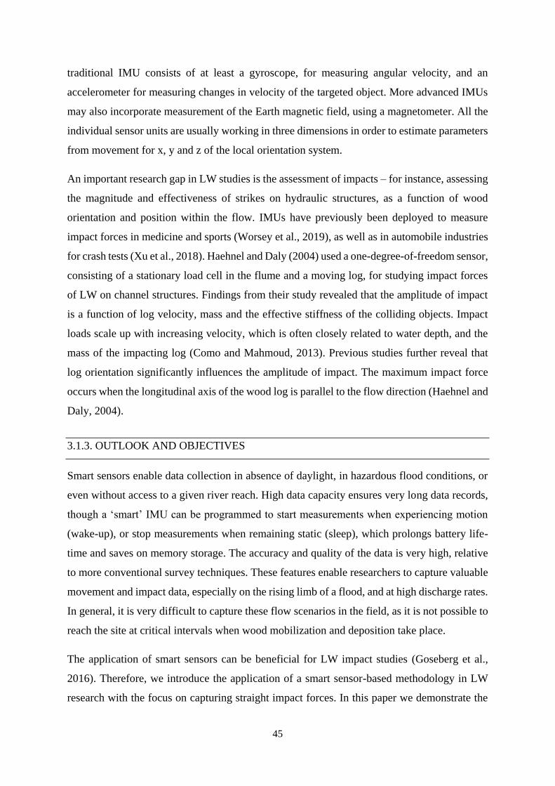
45
traditional IMU consists of at least a gyroscope, for measuring angular velocity, and an
accelerometer for measuring changes in velocity of the targeted object. More advanced IMUs
may also incorporate measurement of the Earth magnetic field, using a magnetometer. All the
individual sensor units are usually working in three dimensions in order to estimate parameters
from movement for x, y and z of the local orientation system.
An important research gap in LW studies is the assessment of impacts – for instance, assessing
the magnitude and effectiveness of strikes on hydraulic structures, as a function of wood
orientation and position within the flow. IMUs have previously been deployed to measure
impact forces in medicine and sports (Worsey et al., 2019), as well as in automobile industries
for crash tests (Xu et al., 2018). Haehnel and Daly (2004) used a one-degree-of-freedom sensor,
consisting of a stationary load cell in the flume and a moving log, for studying impact forces
of LW on channel structures. Findings from their study revealed that the amplitude of impact
is a function of log velocity, mass and the effective stiffness of the colliding objects. Impact
loads scale up with increasing velocity, which is often closely related to water depth, and the
mass of the impacting log (Como and Mahmoud, 2013). Previous studies further reveal that
log orientation significantly influences the amplitude of impact. The maximum impact force
occurs when the longitudinal axis of the wood log is parallel to the flow direction (Haehnel and
Daly, 2004).
3.1.3. OUTLOOK AND OBJECTIVES
Smart sensors enable data collection in absence of daylight, in hazardous flood conditions, or
even without access to a given river reach. High data capacity ensures very long data records,
though a ‘smart’ IMU can be programmed to start measurements when experiencing motion
(wake-up), or stop measurements when remaining static (sleep), which prolongs battery life-
time and saves on memory storage. The accuracy and quality of the data is very high, relative
to more conventional survey techniques. These features enable researchers to capture valuable
movement and impact data, especially on the rising limb of a flood, and at high discharge rates.
In general, it is very difficult to capture these flow scenarios in the field, as it is not possible to
reach the site at critical intervals when wood mobilization and deposition take place.
The application of smart sensors can be beneficial for LW impact studies (Goseberg et al.,
2016). Therefore, we introduce the application of a smart sensor-based methodology in LW
research with the focus on capturing straight impact forces. In this paper we demonstrate the
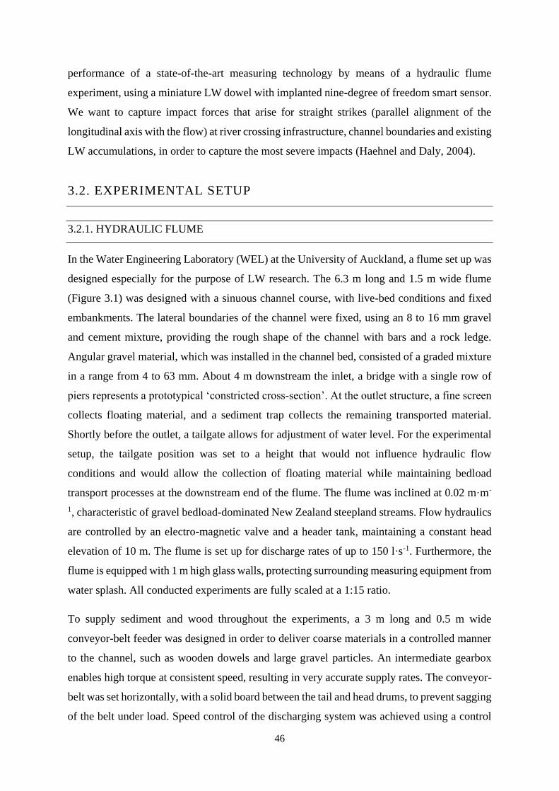
46
performance of a state-of-the-art measuring technology by means of a hydraulic flume
experiment, using a miniature LW dowel with implanted nine-degree of freedom smart sensor.
We want to capture impact forces that arise for straight strikes (parallel alignment of the
longitudinal axis with the flow) at river crossing infrastructure, channel boundaries and existing
LW accumulations, in order to capture the most severe impacts (Haehnel and Daly, 2004).
3.2. EXPERIMENTAL SETUP
3.2.1. HYDRAULIC FLUME
In the Water Engineering Laboratory (WEL) at the University of Auckland, a flume set up was
designed especially for the purpose of LW research. The 6.3 m long and 1.5 m wide flume
(Figure 3.1) was designed with a sinuous channel course, with live-bed conditions and fixed
embankments. The lateral boundaries of the channel were fixed, using an 8 to 16 mm gravel
and cement mixture, providing the rough shape of the channel with bars and a rock ledge.
Angular gravel material, which was installed in the channel bed, consisted of a graded mixture
in a range from 4 to 63 mm. About 4 m downstream the inlet, a bridge with a single row of
piers represents a prototypical ‘constricted cross-section’. At the outlet structure, a fine screen
collects floating material, and a sediment trap collects the remaining transported material.
Shortly before the outlet, a tailgate allows for adjustment of water level. For the experimental
setup, the tailgate position was set to a height that would not influence hydraulic flow
conditions and would allow the collection of floating material while maintaining bedload
transport processes at the downstream end of the flume. The flume was inclined at 0.02 m·m-
1, characteristic of gravel bedload-dominated New Zealand steepland streams. Flow hydraulics
are controlled by an electro-magnetic valve and a header tank, maintaining a constant head
elevation of 10 m. The flume is set up for discharge rates of up to 150 l·s-1. Furthermore, the
flume is equipped with 1 m high glass walls, protecting surrounding measuring equipment from
water splash. All conducted experiments are fully scaled at a 1:15 ratio.
To supply sediment and wood throughout the experiments, a 3 m long and 0.5 m wide
conveyor-belt feeder was designed in order to deliver coarse materials in a controlled manner
to the channel, such as wooden dowels and large gravel particles. An intermediate gearbox
enables high torque at consistent speed, resulting in very accurate supply rates. The conveyor-
belt was set horizontally, with a solid board between the tail and head drums, to prevent sagging
of the belt under load. Speed control of the discharging system was achieved using a control
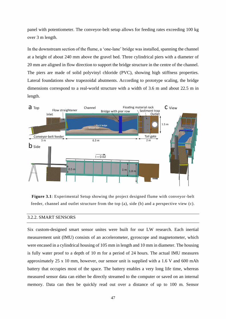
47
panel with potentiometer. The conveyor-belt setup allows for feeding rates exceeding 100 kg
over 3 m length.
In the downstream section of the flume, a ‘one-lane’ bridge was installed, spanning the channel
at a height of about 240 mm above the gravel bed. Three cylindrical piers with a diameter of
20 mm are aligned in flow direction to support the bridge structure in the centre of the channel.
The piers are made of solid polyvinyl chloride (PVC), showing high stiffness properties.
Lateral foundations show trapezoidal abutments. According to prototype scaling, the bridge
dimensions correspond to a real-world structure with a width of 3.6 m and about 22.5 m in
length.
Figure 3.1: Experimental Setup showing the project designed flume with conveyor -belt
feeder, channel and outlet structure from the top (a), side (b) and a perspective view (c).
3.2.2. SMART SENSORS
Six custom-designed smart sensor unites were built for our LW research. Each inertial
measurement unit (IMU) consists of an accelerometer, gyroscope and magnetometer, which
were encased in a cylindrical housing of 105 mm in length and 10 mm in diameter. The housing
is fully water proof to a depth of 10 m for a period of 24 hours. The actual IMU measures
approximately 25 x 10 mm, however, our sensor unit is supplied with a 1.6 V and 600 mAh
battery that occupies most of the space. The battery enables a very long life time, whereas
measured sensor data can either be directly streamed to the computer or saved on an internal
memory. Data can then be quickly read out over a distance of up to 100 m. Sensor
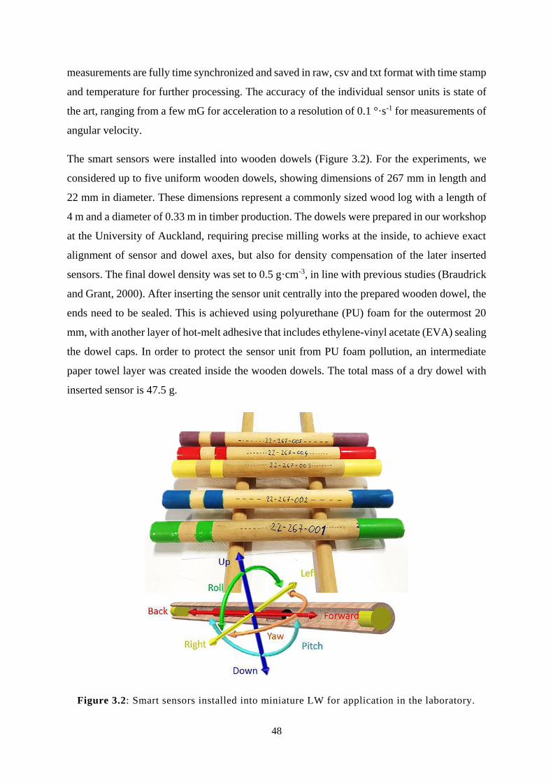
48
measurements are fully time synchronized and saved in raw, csv and txt format with time stamp
and temperature for further processing. The accuracy of the individual sensor units is state of
the art, ranging from a few mG for acceleration to a resolution of 0.1 °·s-1 for measurements of
angular velocity.
The smart sensors were installed into wooden dowels (Figure 3.2). For the experiments, we
considered up to five uniform wooden dowels, showing dimensions of 267 mm in length and
22 mm in diameter. These dimensions represent a commonly sized wood log with a length of
4 m and a diameter of 0.33 m in timber production. The dowels were prepared in our workshop
at the University of Auckland, requiring precise milling works at the inside, to achieve exact
alignment of sensor and dowel axes, but also for density compensation of the later inserted
sensors. The final dowel density was set to 0.5 g·cm-3, in line with previous studies (Braudrick
and Grant, 2000). After inserting the sensor unit centrally into the prepared wooden dowel, the
ends need to be sealed. This is achieved using polyurethane (PU) foam for the outermost 20
mm, with another layer of hot-melt adhesive that includes ethylene-vinyl acetate (EVA) sealing
the dowel caps. In order to protect the sensor unit from PU foam pollution, an intermediate
paper towel layer was created inside the wooden dowels. The total mass of a dry dowel with
inserted sensor is 47.5 g.
Figure 3.2: Smart sensors installed into miniature LW for application in the laboratory.
49
3.3. METHODOLOGY
3.3.1. CHANNEL HYDRAULICS
For our initial LW impact force experiments, we considered a flow depth of two times the
sensor-tagged dowel diameter. This resulted in a flow depth of 40 to 45 mm along the entire
channel. Based on this boundary condition, a discharge of 10 l·s-1 was chosen. In relation to
our experimental setup and the installed gravel bed, a discharge in this range appears relatively
low. However, initial tests on our experimental setup for LW impacts have shown that a water
depth of two times the dowel’s diameter performs very well in terms of dowel mobilization
and transport. For prototype conditions, this scenario may be considered analogous to the rising
limb of a flood event, or a slightly increased base discharge, capable of mobilizing LW. These
low flow conditions had the further benefit of fewer changes imparted to the channel
morphology during the experiments, which could affect LW transport due to realignment of
rough channel elements. The applied experimental setup and hydraulic flow conditions enabled
realistic and consistent conditions for testing impact forces of sensor-tagged miniature LW in
the channel.
3.3.2. MEASURING IMPACT FORCES
The sensor data generated from the experiment allows to reconstruct the dowel’s movement
behaviour on its journey downstream. Herewith we only focus on impacts forces, measured
using the inertial acceleration unit. At a resolution of 0.5 milli-G (mG) our applied sensor unit
measured acceleration forces in a range of -16 to +16 G. In order to capture the impacts at an
appropriate resolution, we set the measuring frequency to 100 Hz. We did not subtract the
Earth’s gravitational effect, as data of the Earth’s gravity field can help to better understand the
sensor data at the evaluation stage.
3.3.3. VIDEO FOOTAGE
In order to track the dowel movement during the experiments, two cameras – Microsoft
Logitech webcam series – were installed, aimed at the bridge. One camera captured the reach
one meter upstream from the bridge section from the top of the flume, whereas the other camera
was positioned on the right-hand side, outside the flume, with a view of the bridge pier. The
camera resolution selected was 854 x 480 pixels, which guaranteed simultaneous capture of
50
the experiments in real time. Higher resolution cameras we tested have been shown to be unable
to maintain a constant high frame rate when used simultaneously. The purpose of the cameras
was for verification of sensor data and estimation of flow velocity of the sensor-tagged dowel.
Analysis of individual frames using VirtualDub (2013) enabled velocity determinations, based
on video footage. Information captured with the side camera provided valuable close-range
views, and generally helped to support our interpretation of the sensor data and impact
processes.
3.3.4. EXPERIMENTAL PROCEDURE
In order to test sensor-tagged dowels for the application of measuring impact forces, an
elementary experimental procedure is performed. Prior the experiment, the sensor-tagged
dowel was soaked in water for a period of two hours, to enable realistic wetted condition of the
tested miniature log. The weight of the wet, experimental sensor-tagged dowel was 50 g,
resulting in a target density of 0.5 g·cm-3. Hydraulic discharge in the flume was set to a constant
rate of 10 l·s-1. The sensor-tagged dowel was always placed at the same orientation relative to
flume coordinates on the conveyor-belt, before data acquisition started, and the sensor-tagged
dowel fed into the channel at a speed of 3 mm·s-1. While the sensor was initiated, the two
cameras began recording. After being released from the conveyor-belt, the dowel dropped
roughly 0.5 m into the channel before being mobilised by the flow. Our impact tests were
considered successful when the sensor-tagged dowel hit the bridge pier head-on, i.e., the x-axis
of the dowel was oriented normal to the bridge. Measurements were automatically stopped
after approximately one minute of data recording. The sensor-tagged dowel was then removed
from the channel and memory was read out.
3.4. RESULTS AND DISCUSSION
3.4.1. SENSOR DATA FOR ACCELERATION
The results and analyses presented in this section provide some insight into one experimental
test for the LW impact force measurements. The following data were obtained using the green
coloured smart sensor-tagged dowel (Figure 3.2).
The sensor-tagged dowel started data acquisition about 13 seconds before being released into
the channel via conveyor-belt feeder. Continuous signals of almost 0 G were measured for the
51
axes x and z, along the horizontal plane. The vertical axis, represented as y-axis, showed almost
negative 1 G relative to Earth’s gravitational force. A slight deviation from the ideal
acceleration force could observed for the y and z-axis, which was caused by imperfect
alignment with the axes in our experiment, introducing a slight signal into each of the two axes.
While the dowel was transported towards the edge of the conveyor-belt, it started to incline as
it tipped over, which started to develop an acceleration force for the longitudinal axis (x). As
before, the acceleration force was measured relative to the inclination to the Earth’s
gravitational axis. As soon as the dowel leaves the conveyor-belt, a free-fall scenario is
observed in the sensor data, where acceleration for all three axes decrease to zero. The
subsequent impact in the channel is shown in Figure 3.3a (13.5 seconds), when a maximal
negative acceleration for the longitudinal axis of 7.05 G was captured, meaning the sensor
impacts straight on the channel bed. Shortly afterwards another strong signal was measured for
the z-axis (-4.44 G), which represents a lateral impact when the sensor falls over from the
vertically aligned position.
Over the following five seconds, the sensor-tagged dowel was mobilised and transported
downstream by the flow. As sensor data reveal, several rotations around the longitudinal axis
(roll - Figure 3.2) occurred. At a time of 19.36 seconds, the dowel broadsides the channel
boundary (rock ledge in Figure 3.1a), causing an acceleration signal of 3.86 G. With an
alignment parallel to the flow direction, the dowel continued its journey downstream until it
experienced a head-on impact with the bridge pier (Figure 3.4a-d). This impact is shown as the
first of three significant acceleration signals on the x-axis.
Figure 3.3b provides a detailed record of the impact series, consisting of the first impact (I) on
the bridge pier, a rebound phase with subsequent impact (II) and the final deposition of the
dowel. Sensor data for acceleration reveal that the second impact after rebound is of ~30%
higher amplitude than the first impact (I) with measured 1.394 G. After the second impact (II),
the dowel tended to move past the right side of the pier (Figure 3.4e and l). However,
measurements of acceleration forces show lateral impacts for y and z-axis at a time of 24.09
seconds (Figure 3.3b), when the dowel accumulated in front of the bridge pier (Figure 3.4f and
m). Sensor data for the remaining accumulation stage at low flow conditions show a slight
fluctuation of the signals.
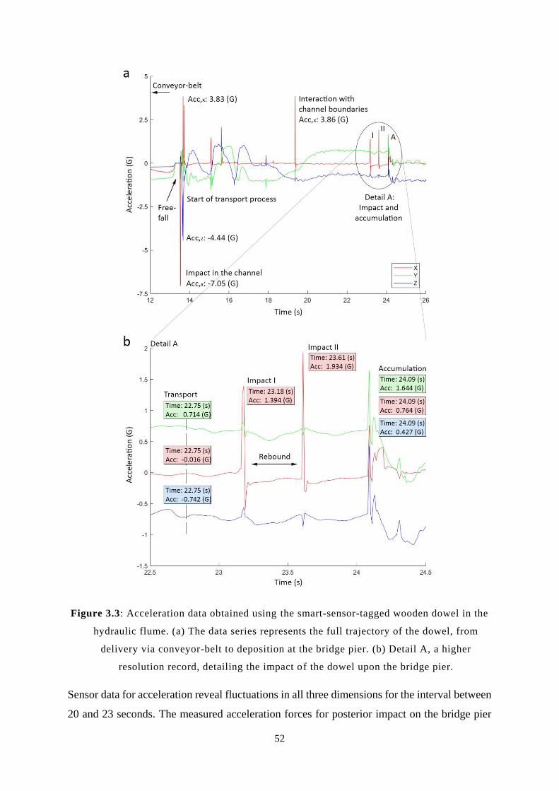
52
Figure 3.3: Acceleration data obtained using the smart-sensor-tagged wooden dowel in the
hydraulic flume. (a) The data series represents the full trajectory of the dowel, from
delivery via conveyor-belt to deposition at the bridge pier. (b) Detail A, a higher
resolution record, detailing the impact of the dowel upon the bridge pier.
Sensor data for acceleration reveal fluctuations in all three dimensions for the interval between
20 and 23 seconds. The measured acceleration forces for posterior impact on the bridge pier
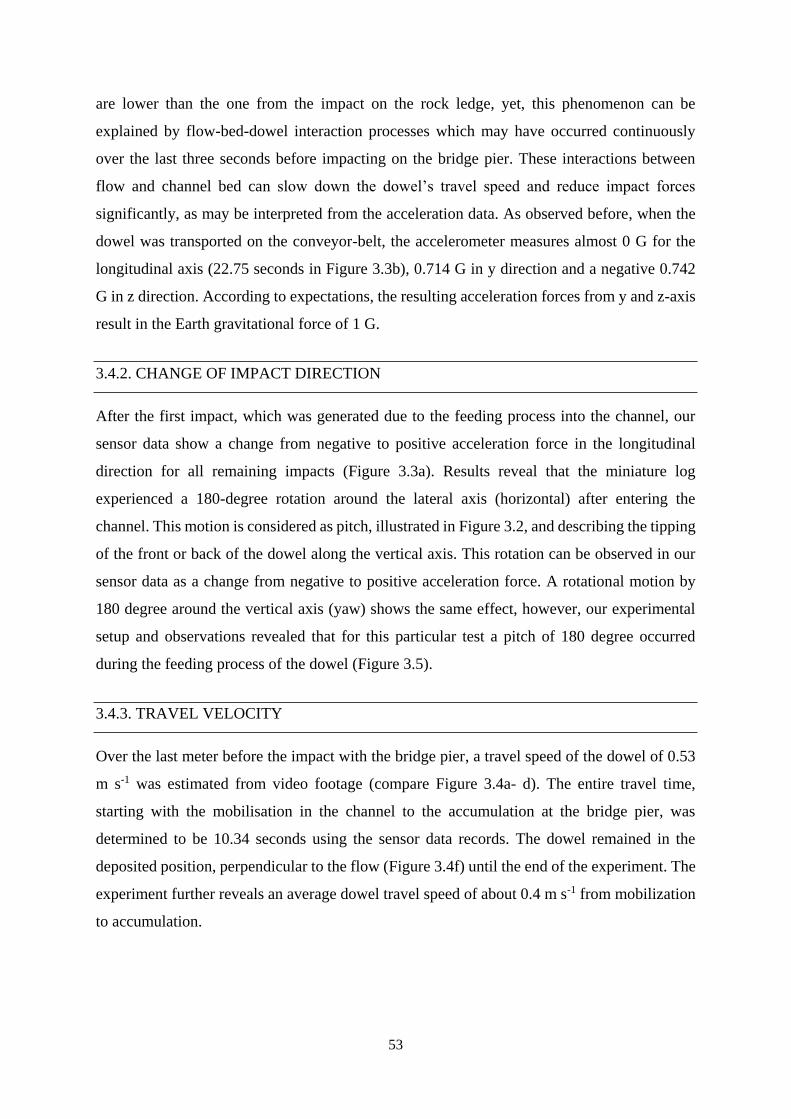
53
are lower than the one from the impact on the rock ledge, yet, this phenomenon can be
explained by flow-bed-dowel interaction processes which may have occurred continuously
over the last three seconds before impacting on the bridge pier. These interactions between
flow and channel bed can slow down the dowel’s travel speed and reduce impact forces
significantly, as may be interpreted from the acceleration data. As observed before, when the
dowel was transported on the conveyor-belt, the accelerometer measures almost 0 G for the
longitudinal axis (22.75 seconds in Figure 3.3b), 0.714 G in y direction and a negative 0.742
G in z direction. According to expectations, the resulting acceleration forces from y and z-axis
result in the Earth gravitational force of 1 G.
3.4.2. CHANGE OF IMPACT DIRECTION
After the first impact, which was generated due to the feeding process into the channel, our
sensor data show a change from negative to positive acceleration force in the longitudinal
direction for all remaining impacts (Figure 3.3a). Results reveal that the miniature log
experienced a 180-degree rotation around the lateral axis (horizontal) after entering the
channel. This motion is considered as pitch, illustrated in Figure 3.2, and describing the tipping
of the front or back of the dowel along the vertical axis. This rotation can be observed in our
sensor data as a change from negative to positive acceleration force. A rotational motion by
180 degree around the vertical axis (yaw) shows the same effect, however, our experimental
setup and observations revealed that for this particular test a pitch of 180 degree occurred
during the feeding process of the dowel (Figure 3.5).
3.4.3. TRAVEL VELOCITY
Over the last meter before the impact with the bridge pier, a travel speed of the dowel of 0.53
m s-1 was estimated from video footage (compare Figure 3.4a- d). The entire travel time,
starting with the mobilisation in the channel to the accumulation at the bridge pier, was
determined to be 10.34 seconds using the sensor data records. The dowel remained in the
deposited position, perpendicular to the flow (Figure 3.4f) until the end of the experiment. The
experiment further reveals an average dowel travel speed of about 0.4 m s-1 from mobilization
to accumulation.
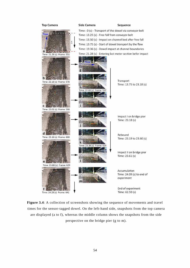
54
Figure 3.4: A collection of screenshots showing the sequence of movements and travel
times for the sensor-tagged dowel. On the left-hand side, snapshots from the top camera
are displayed (a to f), whereas the middle column shows the snapshots from the side
perspective on the bridge pier (g to m).

55
Figure 3.5: Schematic illustration of the smart-sensor-tagged miniature log and the feeding
process into the channel via conveyor-belt.
3.4.4. NINE-DEGREE OF FREEDOM SENSOR DATA
Results of the full nine-degree of freedom (9-DoF) dataset are presented. Figure 3.6 shows
measured raw data from accelerometer, gyroscope and magnetometer. Our sensor data show
consistency at a very high level, demonstrating the excellent performance of the experimental
setup, as well as the applied IMU for LW research. Gyroscope sensor data show some strong
signals along the x-axis from 13 to 17 seconds, which can be interpreted as roll movement.
Looking at the acceleration signal for this period of time, the signal for the longitudinal axis
remains almost constant, while y and z-axis alternates in a range of positive to negative Earth
gravitational force, also supporting the theory of rolling movement. Signals from
magnetometer are ranging in between 50 and negative 100 µT (microtesla), representing the
magnetic field strength in our tested environment. In the presented experiment, no significant
signals were measured in angular velocity or magnetic field strength at the moment of impact,
yet, it will be important to consider these signals for understanding log movement in channels
in future work. Once the sensor-tagged dowel accumulated at the bridge pier (24 seconds),
signals for magnetic field strength remained within very small fluctuations, as expected when
the dowel remains in a location, and angular velocity indicating the 90-degree yaw rotation (y-
axis), as well as some rolling processes (x-axis), which are driven by lateral interaction with
the flow.
56
Figure 3.6: Plot of the measured data of our applied smart sensors – implanted into a
wooden dowel – for acceleration, angular velocity and magnetic field strength.
3.5. CONCLUSIONS
In this paper we introduced an experimental laboratory setup and a smart-sensor-based
methodology for measuring LW impact forces. We successfully demonstrated that smart sensor
can be used for measuring impact forces of LW on channel boundaries and river-crossing
infrastructure. We presented initial results for one test out of our experimental series and
discussed the data collected from the smart-sensor-tagged dowel, as compared with video
footage from two cameras. While the impacts on the simulated infrastructure were relatively
low, prior interactions with channel boundaries indicated significant potential for destruction.
The experimental setup met key criteria for scaled simulation and provided good proof-of-
concept for deployment of ‘smart wood’ and data acquisition during transport and impact
events.
Our experimental observations are consistent with previous research, particularly in terms of
log alignment with the flow and following a trajectory in the centre-line of the channel
(Braudrick and Grant, 2001; Mazzorana et al., 2011; Davidson et al., 2015) for similar flow
conditions and wood densities (Braudrick and Grant, 2000). Achieving this kind of similitude
with field observations is important validation for laboratory work, and this provides some

57
good scope for eventually bringing our smart wood technique to the field. Further cross-
comparisons will help to refine any potentially applicable scaling laws for future laboratory
simulations.
We have presented the potentials for application of nine-degree of freedom smart sensors in
LW research. Our work aims to better understand LW processes in a watershed, beginning with
mobilization and transport, to accumulation mechanisms in a stream channel. Sensor-tagged
wood logs can play an important role for reconstructing the trajectory through the fluvial
system, as well as capturing the magnitude and distribution of impact forces during transit.
Often destruction is not the result of an individual impact, rather, it results from a series of
significant impacts that lead to material fatigue and immediate damage. Protracted exposure to
impacts can also lead to surface damage, resulting in corrosion and spreading damage over
time. More advanced knowledge of impact forces will help to develop and design more resilient
river crossing infrastructure, as well as managing and maintaining existing structures to reduce
risk from LW effects.

59
Using Structure from Motion photogrammetry to assess large
wood (LW) accumulations in the field
Related journal article:
Spreitzer, G., Tunnicliffe, J. & Friedrich, F. 2019. Using Structure from Motion
photogrammetry to assess large wood (LW) accumulations in the field. Geomorphology, 346.
doi: 10.1016/j.geomorph.2019.106851
4.1. INTRODUCTION
4.1.1. RECENT ADVANCES IN LW RESEARCH
Natural forest disturbance and modern forest harvesting techniques produce significant
quantities of large wood (LW) in steep mountain terrain. Once recruited to the fluvial system,
this organic material tends to accumulate and develop into jams. LW is defined according to
the characteristic dimensions (i.e. diameter) of the pieces. A widely used criteria is wood pieces
with a minimum diameter of 0.1 m and at least 1 m length (Nakamura and Swanson, 1994;
Jackson and Sturm, 2002; Baillie et al., 2008; Wohl and Jaeger, 2009; Ravazzolo et al., 2015;
Mao et al., 2017). Gurnell (2013) defined a LW accumulation as a deposit consisting of several
wood pieces, while at least one wood piece shows LW dimensions and blocks a stream section
partly or fully.
LW is, in general, a valuable part of a fluvial ecosystem, providing habitat and environmental
complexity for numerous living organisms (Fausch and Northcote, 1992). Wood can protect
stream sections from erosion and it regulates a river’s sediment budget, due to sediment storage
60
and energy dissipation processes (Megahan and Nowlin, 1976; Swanson et al., 1976; Platts et
al., 1983; Bilby and Ward, 1989; Montgomery et al., 2003). Besides the beneficial ecological
and hydraulic roles of LW in fluvial systems, there are also challenges. The presence of LW
accumulations in river channels may dramatically increase the risk potential for human
population and infrastructure during high-flow events (Braudrick and Grant, 2001; Le Lay et
al., 2013; Schmocker and Weitbrecht, 2013). Clogging processes at constricted cross-sections
can result in a reduction of the conveyance capacity (Rusyda et al., 2014; Gschnitzer et al.,
2017), leading to overtopping of stop banks and flooding of the riparian zone, as well as
changes in channel morphology (local erosion and aggradation processes), and backwater
effects (Knauss, 1995; Le Lay et al., 2013). Backwater effects potentially increase static and
hydrostatic pressure conditions at the blocked location, accompanied by stress on adjacent
hydraulic structures and the environment. Organic fine material (OFM) can fill interstitial
space within the LW jam, decreasing the porosity of the deposit and further reducing the
effective cross-sectional area. OFM is defined as discrete wood pieces, leaves or grass with
smaller dimensions than LW, and a minimum size of 1 mm. This added complexity within the
jam leads to further accumulation and exacerbation of backwater effects (Schmocker and
Weitbrecht, 2013; Schalko et al., 2016b). The role of OFM in jams and flood dynamics has
largely been neglected in past research, however it is assumed to significantly affect hydraulic
flow behaviour and LW accumulation structure.
There are a number of important quantities to be assessed in inventorying, monitoring and
modelling LW accumulations: deposit geometry (Piegay, 1993), accumulation porosity
(addressed by Boivin and Buffin-Bélanger (2010)), orientation of wood components (Ruiz-
Villanueva et al., 2016b), but also obtaining accurate measurements of the bulk volume of the
deposit with regards to the influenced stream reach, which all affect flow hydraulics and
channel morphology significantly (Gippel, 1995; Gschnitzer et al., 2017; Schalko et al., 2018).
In previous studies, several methods have been applied to estimate LW volume in riparian
zones and stream channels as a review of Ruiz-Villanueva et al. (2016b) reveals. For LW
accumulation assessment and wood-budgeting, Boivin et al. (2015) considered measurements
of the ‘air-wood’ volume by applying a rectangular model with accumulation length, width and
average height. Other volume assessing methods include developing scaling relationships
relating wood accumulation to catchment size, the proportion of forest cover in the catchment
upstream, forested river length (Uchiogi et al., 1996), and the density of landslide occurrence
upstream (Rigon et al., 2008). Wood load has further been related to wood flux estimations,
61
the nature of terrestrial supply sources, decay rates, and riparian storage (Benda and Sias,
2003). Other researchers, such as Cordova et al. (2006), Brown et al. (2014) and Dixon and
Sear (2014), counted and measured single wood logs along river sections in order to get a more
accurate estimation of LW volume. None of the previous studies have considered irregularities
of wood logs, which impacts the accuracy of estimates of volume and porosity. LW volume
can be determined accurately using water displacement methodology (Brown et al., 2014),
however this method is not efficient for estimates of larger wood quantities, e.g. an entire LW
accumulation and whole stream sections. Although volumetric assessment of LW has been
addressed throughout various LW investigations (Harmon et al., 1986; Lienkaemper and
Swanson, 1987; Gurnell et al., 2002; Webb and Erskine, 2003; Manners and Doyle, 2008;
Dixon and Sear, 2014; Wohl et al., 2017; Martin et al., 2018), the stated volumes are mostly
rough estimates rather than exact measurements. The importance of obtaining precise
assessments varies with the working scale of the study; rough measures are fine for broader
inventories of LW deposition and wood-flux budgeting, but site-specific process studies may
require more refined estimates. The complexity of these deposits introduces some important
challenges for accurately resolving volumes quickly, with minimum field effort.
Managers and researchers are often interested in capturing the volume of the LW
accumulations, as well as the composition, including sediments, OFM and LW pieces. High-
resolution photogrammetry can therefore be used for (i) LW budgeting, in order to estimate
how much organic material has been mobilized and deposited following higher magnitude
floods, (ii) identification of key logs, for a better understanding of initial LW accumulation
mechanisms and deposition processes, (iii) monitoring existing LW accumulation at
constricted cross-sections, to observe how wood structures develop over time, and (iv)
estimation of backwater effects that arise during flood events, due to the reduced cross-
sectional flow area.
4.1.2. HIGH-RESOLUTION TECHNIQUES FOR LW ESTIMATION
Quantitative assessment of fluxes of wood and sediment through river systems is undergoing
something of a revolution, with the introduction of light detection and ranging (LiDAR) scans
(Geerling et al., 2007; McKean et al., 2014; Magnussen et al., 2018), and Structure from
Motion (SfM) acquisition for capturing the geometric configuration of depositional forms
(Hildreth et al., 1995; Westoby et al., 2012; Javernick et al., 2014; Prosdocimi et al., 2015;
Smith et al., 2016; Wróżyński et al., 2017; Tunnicliffe et al., 2018). This has important
62
implications for wood budgeting applications (Janisch, 2006; Steeb et al., 2017), where
quantitative differences between river channel configuration can be used to assess system
trajectories and rates of transport. Floodplains, bars, and woody accumulations can be captured
at a density of over a million points/m2 (Smith et al., 2016).
Advanced measurement technology and methodologies have shed further light upon the
dynamics of LW accumulations. Airborne remote sensing methodologies have been used to
quantify volumes of large wood accumulations for mass balance models (Steeb et al., 2017),
detection of instream LW (Atha and Dietrich, 2016), and identification of LW sources
(Kasprak et al., 2012), however such studies tend to capture only coarse geometry of LW with
a resolution of 1-8 points/m2 interpolated from LiDAR scans. This resolution is sparse, relative
to wood size (Figure 4.1), and there is little potential for extracting detailed information about
surface texture and volume, leading to the need for further manual quantification methods
(Richardson and Moskal, 2016). Some studies have used terrestrial laser scanning (TLS) for
LW surveying (Boivin and Buffin-Bélanger, 2010; Tonon et al., 2014; Grigillo et al., 2015)
and have achieved spatial resolutions in the range of 150 points/m2 to 1 point/mm2 and higher.
Other LW researchers, using conventional photogrammetry techniques, have reported
inaccuracies when wood pieces were smaller than individual pixels (Marcus et al., 2003). With
lower resolution imagery, it can also be challenging to distinguish LW from gravel and other
objects with similar spectral characteristics (Colvard, 1998; Wright et al., 2000).
SfM photogrammetry is becoming a powerful tool to map surfaces and model topographic
terrains (Morgan et al., 2016; Smith et al., 2016). In-situ digital photogrammetry has already
been proven effective in fluvial geomorphology studies, from aerial mapping of larger stream
sections (Immerzeel et al., 2014; Dietrich, 2016; Tunnicliffe et al., 2018) to close-range studies
of grain sizes characteristics, in a range of a few millimeters (Snapir et al., 2014; Ferreira et
al., 2017; Wróżyński et al., 2017). The use of smartphones for SfM photogrammetry in the
field has been demonstrated by Nocerino et al. (2017), working on a 3D acquisition tool for
mobile-based object reconstruction, and Micheletti et al. (2015b), who developed a digital
terrain model (DTM) from a 5MP smartphone camera. Even with relatively low-resolution
images, suitable 3D models can be generated. The level of detail captured by lower resolution
cameras can be increased with a larger number of images (Dikovski et al., 2014) and close-
range image acquisition. In SfM photogrammetry applications, prototype equivalent pixel size
varies in a range of ~102 to 103 points/m2 (Smith and Vericat, 2015).
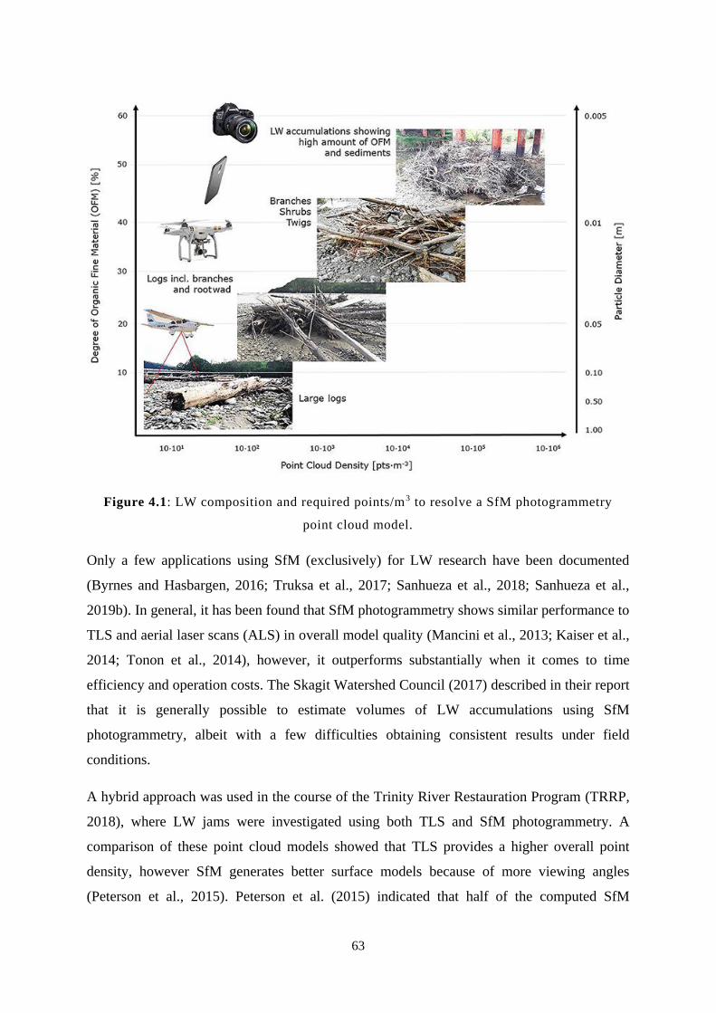
63
Figure 4.1: LW composition and required points/m3 to resolve a SfM photogrammetry
point cloud model.
Only a few applications using SfM (exclusively) for LW research have been documented
(Byrnes and Hasbargen, 2016; Truksa et al., 2017; Sanhueza et al., 2018; Sanhueza et al.,
2019b). In general, it has been found that SfM photogrammetry shows similar performance to
TLS and aerial laser scans (ALS) in overall model quality (Mancini et al., 2013; Kaiser et al.,
2014; Tonon et al., 2014), however, it outperforms substantially when it comes to time
efficiency and operation costs. The Skagit Watershed Council (2017) described in their report
that it is generally possible to estimate volumes of LW accumulations using SfM
photogrammetry, albeit with a few difficulties obtaining consistent results under field
conditions.
A hybrid approach was used in the course of the Trinity River Restauration Program (TRRP,
2018), where LW jams were investigated using both TLS and SfM photogrammetry. A
comparison of these point cloud models showed that TLS provides a higher overall point
density, however SfM generates better surface models because of more viewing angles
(Peterson et al., 2015). Peterson et al. (2015) indicated that half of the computed SfM
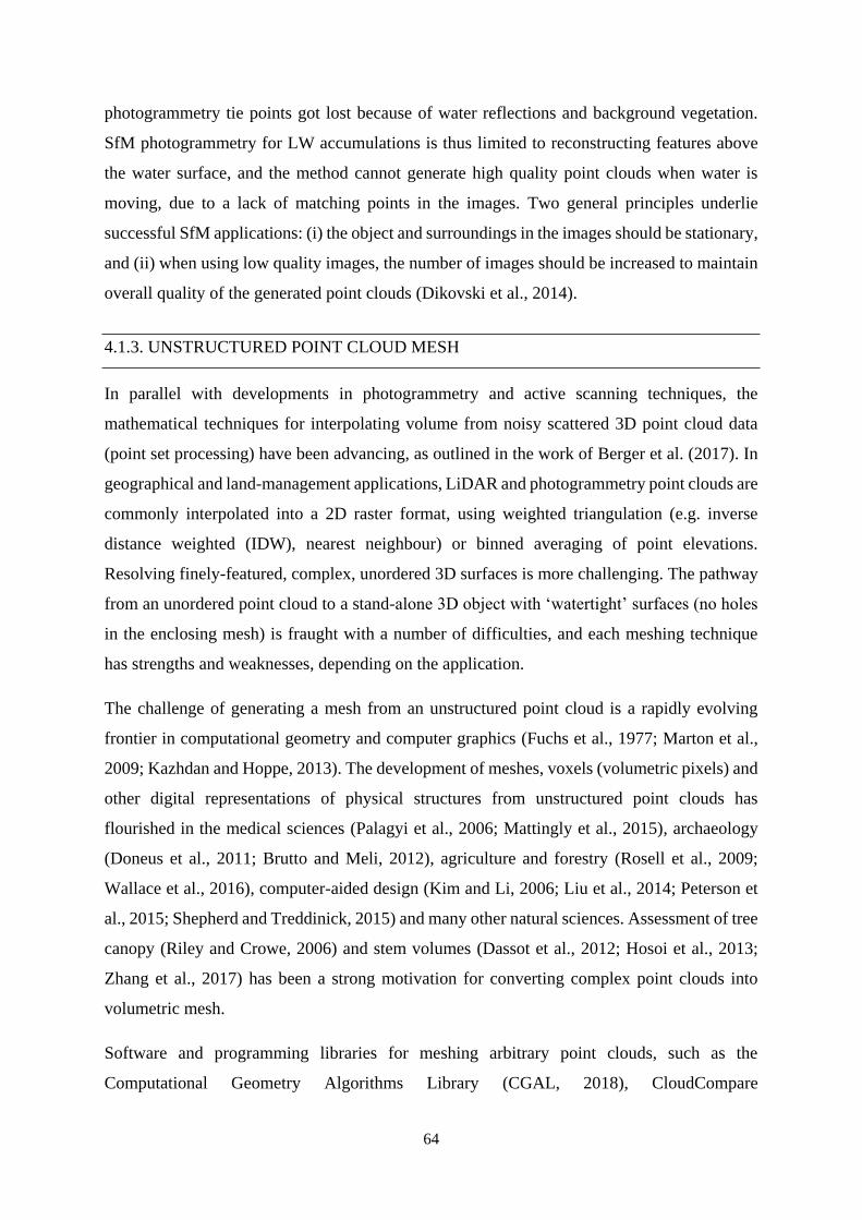
64
photogrammetry tie points got lost because of water reflections and background vegetation.
SfM photogrammetry for LW accumulations is thus limited to reconstructing features above
the water surface, and the method cannot generate high quality point clouds when water is
moving, due to a lack of matching points in the images. Two general principles underlie
successful SfM applications: (i) the object and surroundings in the images should be stationary,
and (ii) when using low quality images, the number of images should be increased to maintain
overall quality of the generated point clouds (Dikovski et al., 2014).
4.1.3. UNSTRUCTURED POINT CLOUD MESH
In parallel with developments in photogrammetry and active scanning techniques, the
mathematical techniques for interpolating volume from noisy scattered 3D point cloud data
(point set processing) have been advancing, as outlined in the work of Berger et al. (2017). In
geographical and land-management applications, LiDAR and photogrammetry point clouds are
commonly interpolated into a 2D raster format, using weighted triangulation (e.g. inverse
distance weighted (IDW), nearest neighbour) or binned averaging of point elevations.
Resolving finely-featured, complex, unordered 3D surfaces is more challenging. The pathway
from an unordered point cloud to a stand-alone 3D object with ‘watertight’ surfaces (no holes
in the enclosing mesh) is fraught with a number of difficulties, and each meshing technique
has strengths and weaknesses, depending on the application.
The challenge of generating a mesh from an unstructured point cloud is a rapidly evolving
frontier in computational geometry and computer graphics (Fuchs et al., 1977; Marton et al.,
2009; Kazhdan and Hoppe, 2013). The development of meshes, voxels (volumetric pixels) and
other digital representations of physical structures from unstructured point clouds has
flourished in the medical sciences (Palagyi et al., 2006; Mattingly et al., 2015), archaeology
(Doneus et al., 2011; Brutto and Meli, 2012), agriculture and forestry (Rosell et al., 2009;
Wallace et al., 2016), computer-aided design (Kim and Li, 2006; Liu et al., 2014; Peterson et
al., 2015; Shepherd and Treddinick, 2015) and many other natural sciences. Assessment of tree
canopy (Riley and Crowe, 2006) and stem volumes (Dassot et al., 2012; Hosoi et al., 2013;
Zhang et al., 2017) has been a strong motivation for converting complex point clouds into
volumetric mesh.
Software and programming libraries for meshing arbitrary point clouds, such as the
Computational Geometry Algorithms Library (CGAL, 2018), CloudCompare
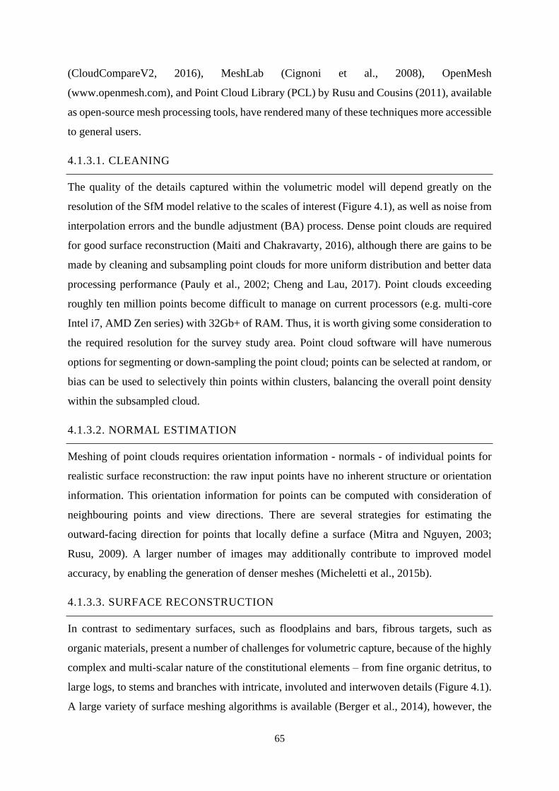
65
(CloudCompareV2, 2016), MeshLab (Cignoni et al., 2008), OpenMesh
(www.openmesh.com), and Point Cloud Library (PCL) by Rusu and Cousins (2011), available
as open-source mesh processing tools, have rendered many of these techniques more accessible
to general users.
4.1.3.1. CLEANING
The quality of the details captured within the volumetric model will depend greatly on the
resolution of the SfM model relative to the scales of interest (Figure 4.1), as well as noise from
interpolation errors and the bundle adjustment (BA) process. Dense point clouds are required
for good surface reconstruction (Maiti and Chakravarty, 2016), although there are gains to be
made by cleaning and subsampling point clouds for more uniform distribution and better data
processing performance (Pauly et al., 2002; Cheng and Lau, 2017). Point clouds exceeding
roughly ten million points become difficult to manage on current processors (e.g. multi-core
Intel i7, AMD Zen series) with 32Gb+ of RAM. Thus, it is worth giving some consideration to
the required resolution for the survey study area. Point cloud software will have numerous
options for segmenting or down-sampling the point cloud; points can be selected at random, or
bias can be used to selectively thin points within clusters, balancing the overall point density
within the subsampled cloud.
4.1.3.2. NORMAL ESTIMATION
Meshing of point clouds requires orientation information - normals - of individual points for
realistic surface reconstruction: the raw input points have no inherent structure or orientation
information. This orientation information for points can be computed with consideration of
neighbouring points and view directions. There are several strategies for estimating the
outward-facing direction for points that locally define a surface (Mitra and Nguyen, 2003;
Rusu, 2009). A larger number of images may additionally contribute to improved model
accuracy, by enabling the generation of denser meshes (Micheletti et al., 2015b).
4.1.3.3. SURFACE RECONSTRUCTION
In contrast to sedimentary surfaces, such as floodplains and bars, fibrous targets, such as
organic materials, present a number of challenges for volumetric capture, because of the highly
complex and multi-scalar nature of the constitutional elements – from fine organic detritus, to
large logs, to stems and branches with intricate, involuted and interwoven details (Figure 4.1).
A large variety of surface meshing algorithms is available (Berger et al., 2014), however, the
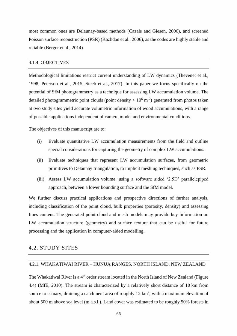
66
most common ones are Delaunay-based methods (Cazals and Giesen, 2006), and screened
Poisson surface reconstruction (PSR) (Kazhdan et al., 2006), as the codes are highly stable and
reliable (Berger et al., 2014).
4.1.4. OBJECTIVES
Methodological limitations restrict current understanding of LW dynamics (Thevenet et al.,
1998; Peterson et al., 2015; Steeb et al., 2017). In this paper we focus specifically on the
potential of SfM photogrammetry as a technique for assessing LW accumulation volume. The
detailed photogrammetric point clouds (point density > 106 m-2) generated from photos taken
at two study sites yield accurate volumetric information of wood accumulations, with a range
of possible applications independent of camera model and environmental conditions.
The objectives of this manuscript are to:
(i) Evaluate quantitative LW accumulation measurements from the field and outline
special considerations for capturing the geometry of complex LW accumulations.
(ii) Evaluate techniques that represent LW accumulation surfaces, from geometric
primitives to Delaunay triangulation, to implicit meshing techniques, such as PSR.
(iii) Assess LW accumulation volume, using a software aided ‘2.5D’ parallelepiped
approach, between a lower bounding surface and the SfM model.
We further discuss practical applications and prospective directions of further analysis,
including classification of the point cloud, bulk properties (porosity, density) and assessing
fines content. The generated point cloud and mesh models may provide key information on
LW accumulation structure (geometry) and surface texture that can be useful for future
processing and the application in computer-aided modelling.
4.2. STUDY SITES
4.2.1. WHAKATIWAI RIVER – HUNUA RANGES, NORTH ISLAND, NEW ZEALAND
The Whakatiwai River is a 4th order stream located in the North Island of New Zealand (Figure
4.4) (MfE, 2010). The stream is characterized by a relatively short distance of 10 km from
source to estuary, draining a catchment area of roughly 12 km2, with a maximum elevation of
about 500 m above sea level (m.a.s.l.). Land cover was estimated to be roughly 50% forests in
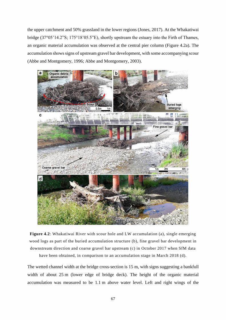
67
the upper catchment and 50% grassland in the lower regions (Jones, 2017). At the Whakatiwai
bridge (37°05’14.2”S; 175°18’05.5”E), shortly upstream the estuary into the Firth of Thames,
an organic material accumulation was observed at the central pier column (Figure 4.2a). The
accumulation shows signs of upstream gravel bar development, with some accompanying scour
(Abbe and Montgomery, 1996; Abbe and Montgomery, 2003).
Figure 4.2: Whakatiwai River with scour hole and LW accumulation (a), single emerging
wood logs as part of the buried accumulation structure (b), fine gravel bar development in
downstream direction and coarse gravel bar upstream (c) in October 2017 when SfM data
have been obtained, in comparison to an accumulation stage in March 2018 (d).
The wetted channel width at the bridge cross-section is 15 m, with signs suggesting a bankfull
width of about 25 m (lower edge of bridge deck). The height of the organic material
accumulation was measured to be 1.1 m above water level. Left and right wings of the
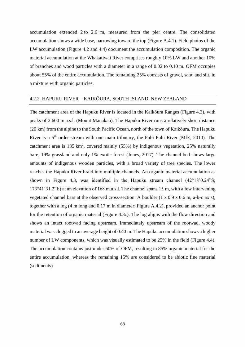
68
accumulation extended 2 to 2.6 m, measured from the pier centre. The consolidated
accumulation shows a wide base, narrowing toward the top (Figure A.4.1). Field photos of the
LW accumulation (Figure 4.2 and 4.4) document the accumulation composition. The organic
material accumulation at the Whakatiwai River comprises roughly 10% LW and another 10%
of branches and wood particles with a diameter in a range of 0.02 to 0.10 m. OFM occupies
about 55% of the entire accumulation. The remaining 25% consists of gravel, sand and silt, in
a mixture with organic particles.
4.2.2. HAPUKU RIVER – KAIKŌURA, SOUTH ISLAND, NEW ZEALAND
The catchment area of the Hapuku River is located in the Kaikōura Ranges (Figure 4.3), with
peaks of 2.600 m.a.s.l. (Mount Manakau). The Hapuku River runs a relatively short distance
(20 km) from the alpine to the South Pacific Ocean, north of the town of Kaikōura. The Hapuku
River is a 5th order stream with one main tributary, the Puhi Puhi River (MfE, 2010). The
catchment area is 135 km2, covered mainly (55%) by indigenous vegetation, 25% naturally
bare, 19% grassland and only 1% exotic forest (Jones, 2017). The channel bed shows large
amounts of indigenous wooden particles, with a broad variety of tree species. The lower
reaches the Hapuku River braid into multiple channels. An organic material accumulation as
shown in Figure 4.3, was identified in the Hapuku stream channel (42°18’0.24”S;
173°41’31.2”E) at an elevation of 168 m.a.s.l. The channel spans 15 m, with a few intervening
vegetated channel bars at the observed cross-section. A boulder (1 x 0.9 x 0.6 m, a-b-c axis),
together with a log (4 m long and 0.17 m in diameter; Figure A.4.2), provided an anchor point
for the retention of organic material (Figure 4.3c). The log aligns with the flow direction and
shows an intact rootwad facing upstream. Immediately upstream of the rootwad, woody
material was clogged to an average height of 0.40 m. The Hapuku accumulation shows a higher
number of LW components, which was visually estimated to be 25% in the field (Figure 4.4).
The accumulation contains just under 60% of OFM, resulting in 85% organic material for the
entire accumulation, whereas the remaining 15% are considered to be abiotic fine material
(sediments).
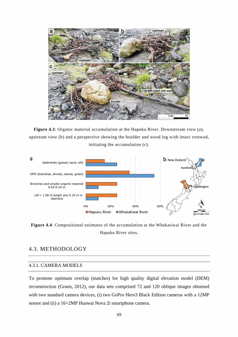
69
Figure 4.3: Organic material accumulation at the Hapuku River. Downstream view (a),
upstream view (b) and a perspective showing the boulder and wood log w ith intact rootwad,
initiating the accumulation (c).
Figure 4.4: Compositional estimates of the accumulation at the Whakatiwai River and the
Hapuku River sites.
4.3. METHODOLOGY
4.3.1. CAMERA MODELS
To promote optimum overlap (matches) for high quality digital elevation model (DEM)
reconstruction (Gruen, 2012), our data sets comprised 72 and 120 oblique images obtained
with two standard camera devices, (i) two GoPro Hero3 Black Edition cameras with a 12MP
sensor and (ii) a 16+2MP Huawai Nova 2i smartphone camera.
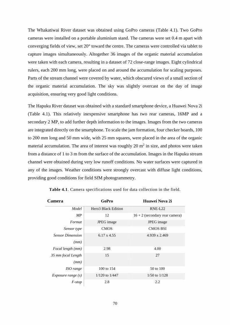
70
The Whakatiwai River dataset was obtained using GoPro cameras (Table 4.1). Two GoPro
cameras were installed on a portable aluminium stand. The cameras were set 0.4 m apart with
converging fields of view, set 20° toward the centre. The cameras were controlled via tablet to
capture images simultaneously. Altogether 36 images of the organic material accumulation
were taken with each camera, resulting in a dataset of 72 close-range images. Eight cylindrical
rulers, each 200 mm long, were placed on and around the accumulation for scaling purposes.
Parts of the stream channel were covered by water, which obscured views of a small section of
the organic material accumulation. The sky was slightly overcast on the day of image
acquisition, ensuring very good light conditions.
The Hapuku River dataset was obtained with a standard smartphone device, a Huawei Nova 2i
(Table 4.1). This relatively inexpensive smartphone has two rear cameras, 16MP and a
secondary 2 MP, to add further depth information to the images. Images from the two cameras
are integrated directly on the smartphone. To scale the jam formation, four checker boards, 100
to 200 mm long and 50 mm wide, with 25 mm squares, were placed in the area of the organic
material accumulation. The area of interest was roughly 20 m2 in size, and photos were taken
from a distance of 1 to 3 m from the surface of the accumulation. Images in the Hapuku stream
channel were obtained during very low runoff conditions. No water surfaces were captured in
any of the images. Weather conditions were strongly overcast with diffuse light conditions,
providing good conditions for field SfM photogrammetry.
Table 4.1. Camera specifications used for data collection in the field.
Camera GoPro Huawei Nova 2i
Model Hero3 Black Edition RNE-L22
MP 12 16 + 2 (secondary rear camera)
Format JPEG image JPEG image
Sensor type CMOS CMOS BSI
Sensor Dimension
(mm)
6.17 x 4.55 4.939 x 2.469
Focal length (mm) 2.98 4.00
35 mm focal Length
(mm)
15 27
ISO range 100 to 154 50 to 100
Exposure range (s) 1/120 to 1/447 1/50 to 1/128
F-stop 2.8 2.2
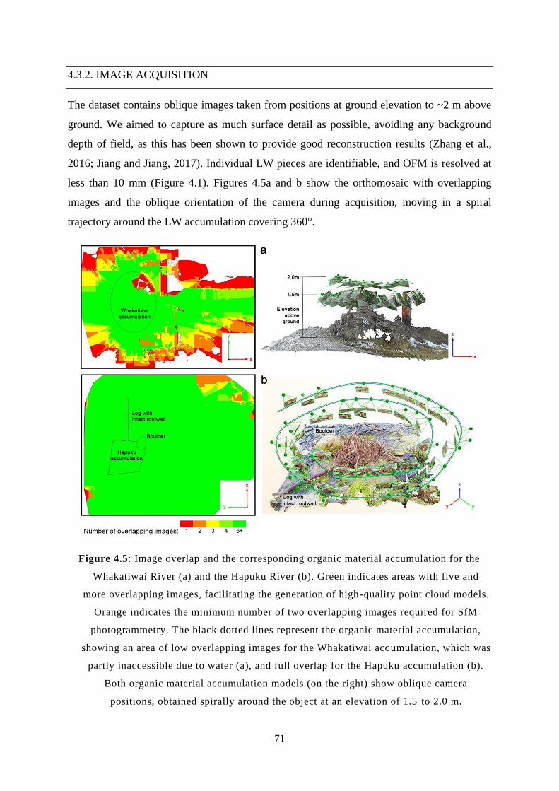
71
4.3.2. IMAGE ACQUISITION
The dataset contains oblique images taken from positions at ground elevation to ~2 m above
ground. We aimed to capture as much surface detail as possible, avoiding any background
depth of field, as this has been shown to provide good reconstruction results (Zhang et al.,
2016; Jiang and Jiang, 2017). Individual LW pieces are identifiable, and OFM is resolved at
less than 10 mm (Figure 4.1). Figures 4.5a and b show the orthomosaic with overlapping
images and the oblique orientation of the camera during acquisition, moving in a spiral
trajectory around the LW accumulation covering 360°.
Figure 4.5: Image overlap and the corresponding organic material accumulation for the
Whakatiwai River (a) and the Hapuku River (b). Green indicates areas with five and
more overlapping images, facilitating the generation of high -quality point cloud models.
Orange indicates the minimum number of two overlapping images required for SfM
photogrammetry. The black dotted lines represent the organic material accumulation,
showing an area of low overlapping images for the Whakatiwai accumulation, which was
partly inaccessible due to water (a), and full overlap for the Hapuku accumulation (b).
Both organic material accumulation models (on the right) show oblique camera
positions, obtained spirally around the object at an elevation of 1.5 to 2.0 m.
72
4.3.3. POINT CLOUD PROCESSING
Photogrammetric processing was carried out using a commercially available SfM software
package, Pix4DMapper (Pix4D Switzerland, 2018). Pix4D was selected for its user-friendly
interface and workflow. Pix4D provides a coherent metadata and data set, including all images,
camera models, point clouds, meshes, measurements (e.g. volume estimation) and a
comprehensive technical quality report.
After initial processing (Step 1, Figure 4.6 and Table 4.2), including point matching and point
cloud generation, internal and external camera parameters were iteratively adjusted. This is
done by loading automatically evaluated and optimised camera details into the Image
Properties Editor and setting the principal points for x and y of the centre of the image. Using
the BA technique, the software can determine the intrinsic camera parameters, such as lens
characteristics, and the extrinsic camera parameters, such as positional information (Eltner et
al., 2016). Our procedure continues with reprocessing of the first step, before the generated tie
points are scaled in Pix4D according to the previously placed scaling bars. An arbitrary
coordinate system was used, with the x-axis aligned to the flow direction.
The reoptimisation process incorporates prototype dimensions from scaling and orientation
input into the point cloud model. The point cloud densification (Step 2) was then carried out,
and a Digital Surface Model (DSM) was generated (Step 3), which is required to develop a
volumetric model. The densified point cloud model provides the basis for meshing and surface
reconstruction techniques described below. All software settings for our Pix4D workflow are
listed in Table 4.2. We used a desktop PC with Windows 7 64-bit, 16GB RAM, i7-6700
3.40GHz CPU and a NVIDIA Quadro K600 graphic card, resulting in processing times of ~20
hours for a dataset with 72 12-MP photos.
Following the densified point cloud generation, the LW accumulation was isolated from the
rest of the point cloud model using manual segmentation tools in CloudCompare, and cleaned
from outlier points for further processing steps, including surface reconstruction. The final
bounding dimensions for the LW accumulations in the point cloud model were 4.5 x 5.8 x 2.4
m (Whakatiwai River) and 3.3 x 3.8 x 1.8 m (Hapuku River).
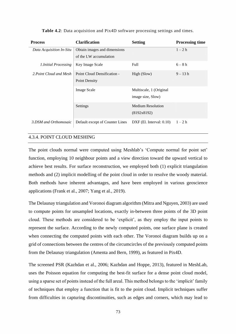
73
Table 4.2: Data acquisition and Pix4D software processing settings and times.
Process Clarification Setting Processing time
Data Acquisition In-Situ Obtain images and dimensions
of the LW accumulation
1 – 2 h
1.Initial Processing Key Image Scale Full 6 – 8 h
2.Point Cloud and Mesh Point Cloud Densification -
Point Density
High (Slow) 9 – 13 h
Image Scale Multiscale, 1 (Original
image size, Slow)
Settings Medium Resolution
(8192x8192)
3.DSM and Orthomosaic Default except of Counter Lines DXF (El. Interval: 0.10) 1 – 2 h
4.3.4. POINT CLOUD MESHING
The point clouds normal were computed using Meshlab’s ‘Compute normal for point set’
function, employing 10 neighbour points and a view direction toward the upward vertical to
achieve best results. For surface reconstruction, we employed both (1) explicit triangulation
methods and (2) implicit modelling of the point cloud in order to resolve the woody material.
Both methods have inherent advantages, and have been employed in various geoscience
applications (Frank et al., 2007; Yang et al., 2019).
The Delaunay triangulation and Voronoi diagram algorithm (Mitra and Nguyen, 2003) are used
to compute points for unsampled locations, exactly in-between three points of the 3D point
cloud. These methods are considered to be ‘explicit’, as they employ the input points to
represent the surface. According to the newly computed points, one surface plane is created
when connecting the computed points with each other. The Voronoi diagram builds up on a
grid of connections between the centres of the circumcircles of the previously computed points
from the Delaunay triangulation (Amenta and Bern, 1999), as featured in Pix4D.
The screened PSR (Kazhdan et al., 2006; Kazhdan and Hoppe, 2013), featured in MeshLab,
uses the Poisson equation for computing the best-fit surface for a dense point cloud model,
using a sparse set of points instead of the full areal. This method belongs to the ‘implicit’ family
of techniques that employ a function that is fit to the point cloud. Implicit techniques suffer
from difficulties in capturing discontinuities, such as edges and corners, which may lead to
74
artefacts in the resultant model. Despite this, the PSR method offers the best chances of
minimum holes and mesh distortions over a complex point cloud. Altogether we used three
meshing approaches:
(i) A simplified mesh model based on Delaunay triangulation was generated using Pix4D.
This mesh was generated on a restricted number of 106 faces in total (considering the entire
point cloud model). Resolution was kept as default with an octree depth of 12 over a texture
size of 8192 x 8192 pixels. The isolated LW accumulations consequently show about half a
million faces (7·105 faces for the Whakatiwai River and 4·105 faces for the Hapuku River).
(ii) The Delaunay triangulation (nearest-neighbour triangulation) with Voronoi filtering in
CloudCompare (CloudCompareV2, 2016) is used for a xy-plane with triangulation on the point
clouds’ convex hull. The maximum length for triangle edges is set to 0.1 and it produces a 3D
mesh structure based on the projected 2D point cloud (xy-plane) in this Delaunay 2.5D
approach.
(iii) For PSR (Kazhdan and Hoppe, 2013) in MeshLab (Cignoni et al., 2008), a
reconstruction depth of 12, with an adaptive octree depth of 5, has been selected to achieve the
best meshing results. The scaling factor is set to 1.0, with a minimum number of 5 samples.
All our meshes were filtered for isolated pieces, duplicated or unreferenced vertices, and zero
area faces in MeshLab, allowing a proper volumetric computation of the generated 3D LW
accumulation models.
4.3.5. VOLUMETRIC TECHNIQUES
Volumes of our 3D point cloud and mesh models were computed via two software workflows:
a predefined Pix4D tool ‘Volumes’, and CloudCompare’s ‘Compute 2.5D Volume’ tool. The
volume domain consists of the octree subdivided to its finest level (10) in CloudCompare and
with the standard resolution setting (12) in Pix4D. The volume is discretised into voxels, and
estimated according Equation (4.1). Model resolution is equivalent to the ground sampling
distance (GSD), the product of the length (Li) and width (Wi) of a basal surface cell. The
vertical dimension (𝐻𝑖) is the distance from the lower bounding basal surface to the top of the
mesh model.
𝑉𝑝4𝑑 = ∑ 𝐿𝑖 ∙ 𝑊𝑖 ∙ 𝐻𝑖 = ∑ 𝐺𝑆𝐷𝑖2 ∙ 𝐻𝑖𝑖𝑖 (4.1)
75
An essential modelling question involves specification of this lower basal surface, as well as
any lateral boundaries (e.g. pier column, boulders). There are potentially significant
uncertainties of this lower boundary between the wood accumulation and bed substrate.
Depending on the inferred characteristics of the subjacent surface (e.g. floodplain, bank,
bedform), one can either specify a plane or an undulating bed that best matches the observed
topography. This lower surface may be further obscured by deep/muddy water, overhanging
wooden pieces and reflections, making interpolation difficult. Lateral boundaries may be
further refined by trimming the model using geometric primitives, such as wedges, ellipsoids,
cylinders and cones.
Volume estimates in CloudCompare are generated using the 2.5D volume computation tool.
This tool allows the user to compute volumetric information of the generated meshes in Pix4D,
CloudCompare and Meshlab by subtracting a reference surface (based on a custom defined
footprint area). Similar to the algorithm applied in Pix4D, the volumetric tool in CloudCompare
also uses an elementary parallelepiped with corresponding footprint area that is multiplied by
the difference in height (CloudCompare, 2018). The grid step is set to a minimum of 0.001 m,
and empty cells between the top of the mesh and the basal reference surface are interpolated.
Empty cells are kept at minimum height for the 3D LW accumulation model. This tool samples
the same number of points on the mesh as on the original point cloud. The basal surface for the
Whakatiwai accumulation includes a planar bottom and a cylinder for the adjacent bridge pier.
The Hapuku model has a wavy surface that is consistent with the local surveyed topography;
points representing the large boulder were cropped out.
As a check on the level of precision gained in our volume models, we developed a geometrical
model of the LW accumulation for each field site using primitives in CAD to approximate the
woody elements within the organic material formation. Volume estimates from the geometrical
models are compared to the three mesh models. At the Whakatiwai River, the deposit most
closely resembles a cone, built up at the bridge pier, effectively a cylinder. The dimensions of
the organic material accumulation were obtained from measurements in the field (Figure.
A.4.1). The cylindrical volume of the bridge pier, R = 0.20 m and H = 1.10 m, is subtracted
from the cone model, R = 1.90 m and H = 1.10 m. All measurements from the Whakatiwai
field site are based on the predominant water level elevation. The resulting prototype volume
(VW,pro) was estimated using Equation (4.2), showing an approximation to prototype
geometries.
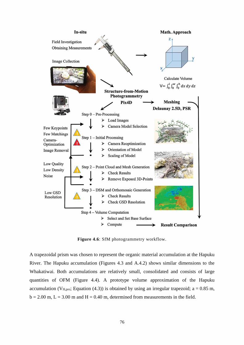
76
Figure 4.6: SfM photogrammetry workflow.
A trapezoidal prism was chosen to represent the organic material accumulation at the Hapuku
River. The Hapuku accumulation (Figures 4.3 and A.4.2) shows similar dimensions to the
Whakatiwai. Both accumulations are relatively small, consolidated and consists of large
quantities of OFM (Figure 4.4). A prototype volume approximation of the Hapuku
accumulation (VH,pro; Equation (4.3)) is obtained by using an irregular trapezoid; a = 0.85 m,
b = 2.00 m, L = 3.00 m and H = 0.40 m, determined from measurements in the field.
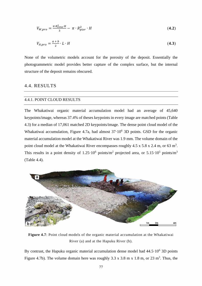
77
𝑉𝑊,𝑝𝑟𝑜 =𝜋∙𝑅𝑐𝑜𝑛𝑒
2 ∙𝐻
3− 𝜋 ∙ 𝑅𝑝𝑖𝑒𝑟
2 ∙ 𝐻 (4.2)
𝑉𝐻,𝑝𝑟𝑜 =𝑎 + 𝑏
2∙ 𝐿 ∙ 𝐻 (4.3)
None of the volumetric models account for the porosity of the deposit. Essentially the
photogrammetric model provides better capture of the complex surface, but the internal
structure of the deposit remains obscured.
4.4. RESULTS
4.4.1. POINT CLOUD RESULTS
The Whakatiwai organic material accumulation model had an average of 45,640
keypoints/image, whereas 37.4% of theses keypoints in every image are matched points (Table
4.3) for a median of 17,061 matched 2D keypoints/image. The dense point cloud model of the
Whakatiwai accumulation, Figure 4.7a, had almost 37·106 3D points. GSD for the organic
material accumulation model at the Whakatiwai River was 1.9 mm. The volume domain of the
point cloud model at the Whakatiwai River encompasses roughly 4.5 x 5.8 x 2.4 m, or 63 m3.
This results in a point density of 1.25·106 points/m2 projected area, or 5.15·105 points/m3
(Table 4.4).
Figure 4.7: Point cloud models of the organic material accumulation at the Whakatiwai
River (a) and at the Hapuku River (b).
By contrast, the Hapuku organic material accumulation dense model had 44.5·106 3D points
Figure 4.7b). The volume domain here was roughly 3.3 x 3.8 m x 1.8 m, or 23 m3. Thus, the
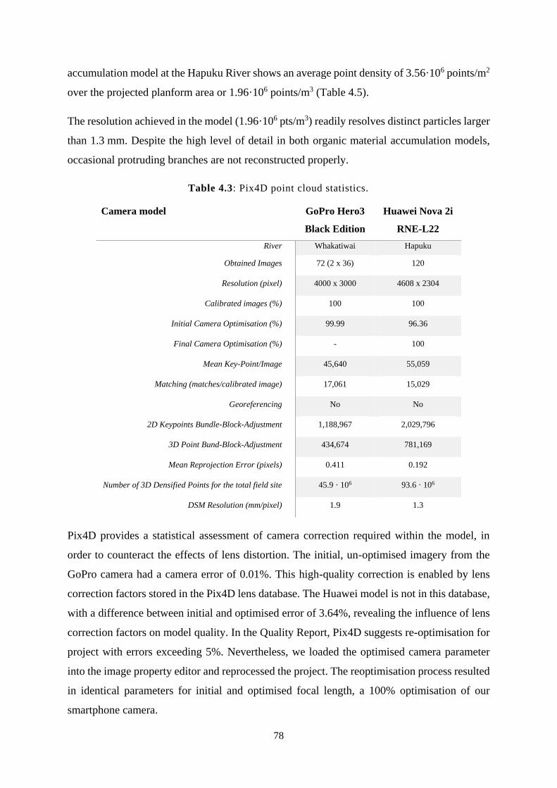
78
accumulation model at the Hapuku River shows an average point density of 3.56·106 points/m2
over the projected planform area or 1.96·106 points/m3 (Table 4.5).
The resolution achieved in the model (1.96·106 pts/m3) readily resolves distinct particles larger
than 1.3 mm. Despite the high level of detail in both organic material accumulation models,
occasional protruding branches are not reconstructed properly.
Table 4.3: Pix4D point cloud statistics.
Camera model GoPro Hero3
Black Edition
Huawei Nova 2i
RNE-L22
River Whakatiwai Hapuku
Obtained Images 72 (2 x 36) 120
Resolution (pixel) 4000 x 3000 4608 x 2304
Calibrated images (%) 100 100
Initial Camera Optimisation (%) 99.99 96.36
Final Camera Optimisation (%) - 100
Mean Key-Point/Image 45,640 55,059
Matching (matches/calibrated image) 17,061 15,029
Georeferencing No No
2D Keypoints Bundle-Block-Adjustment 1,188,967 2,029,796
3D Point Bund-Block-Adjustment 434,674 781,169
Mean Reprojection Error (pixels) 0.411 0.192
Number of 3D Densified Points for the total field site 45.9 · 106 93.6 · 106
DSM Resolution (mm/pixel) 1.9 1.3
Pix4D provides a statistical assessment of camera correction required within the model, in
order to counteract the effects of lens distortion. The initial, un-optimised imagery from the
GoPro camera had a camera error of 0.01%. This high-quality correction is enabled by lens
correction factors stored in the Pix4D lens database. The Huawei model is not in this database,
with a difference between initial and optimised error of 3.64%, revealing the influence of lens
correction factors on model quality. In the Quality Report, Pix4D suggests re-optimisation for
project with errors exceeding 5%. Nevertheless, we loaded the optimised camera parameter
into the image property editor and reprocessed the project. The reoptimisation process resulted
in identical parameters for initial and optimised focal length, a 100% optimisation of our
smartphone camera.
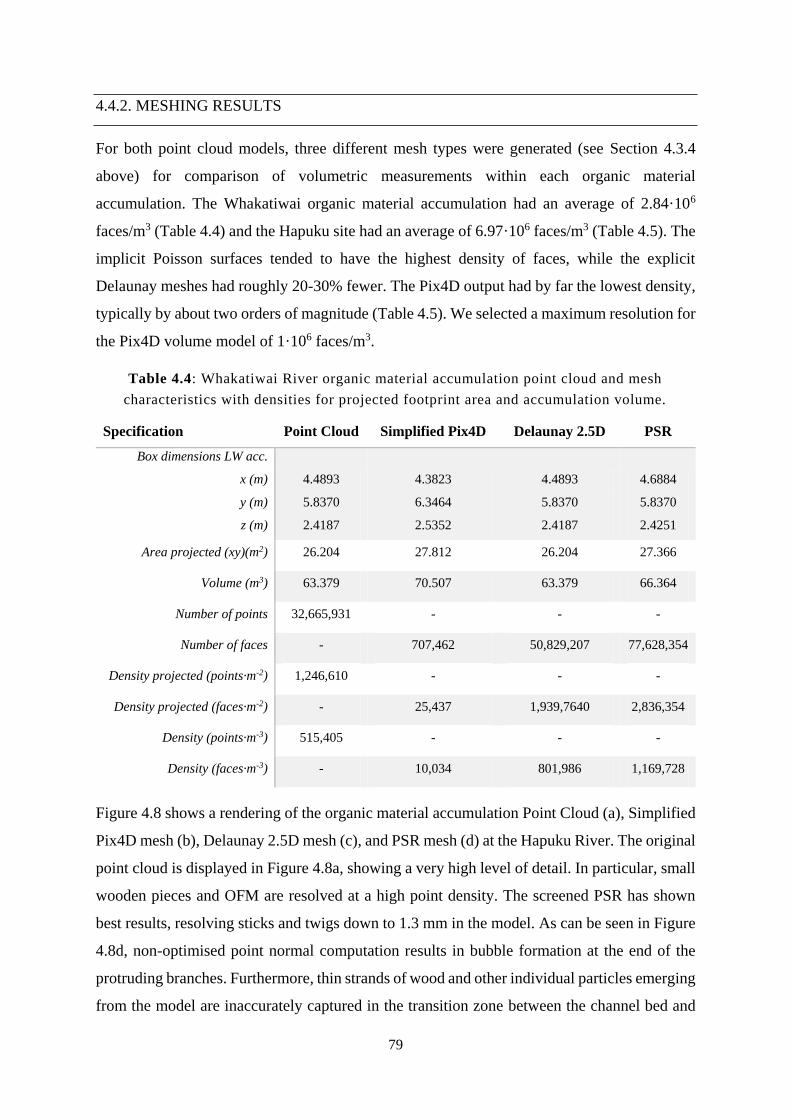
79
4.4.2. MESHING RESULTS
For both point cloud models, three different mesh types were generated (see Section 4.3.4
above) for comparison of volumetric measurements within each organic material
accumulation. The Whakatiwai organic material accumulation had an average of 2.84·106
faces/m3 (Table 4.4) and the Hapuku site had an average of 6.97·106 faces/m3 (Table 4.5). The
implicit Poisson surfaces tended to have the highest density of faces, while the explicit
Delaunay meshes had roughly 20-30% fewer. The Pix4D output had by far the lowest density,
typically by about two orders of magnitude (Table 4.5). We selected a maximum resolution for
the Pix4D volume model of 1·106 faces/m3.
Table 4.4: Whakatiwai River organic material accumulation point cloud and mesh
characteristics with densities for projected footprint area and accumulation volume.
Specification Point Cloud Simplified Pix4D Delaunay 2.5D PSR
Box dimensions LW acc.
x (m)
y (m)
z (m)
4.4893
5.8370
2.4187
4.3823
6.3464
2.5352
4.4893
5.8370
2.4187
4.6884
5.8370
2.4251
Area projected (xy)(m2) 26.204 27.812 26.204 27.366
Volume (m3) 63.379 70.507 63.379 66.364
Number of points 32,665,931 - - -
Number of faces - 707,462 50,829,207 77,628,354
Density projected (points·m-2) 1,246,610 - - -
Density projected (faces·m-2) - 25,437 1,939,7640 2,836,354
Density (points·m-3) 515,405 - - -
Density (faces·m-3) - 10,034 801,986 1,169,728
Figure 4.8 shows a rendering of the organic material accumulation Point Cloud (a), Simplified
Pix4D mesh (b), Delaunay 2.5D mesh (c), and PSR mesh (d) at the Hapuku River. The original
point cloud is displayed in Figure 4.8a, showing a very high level of detail. In particular, small
wooden pieces and OFM are resolved at a high point density. The screened PSR has shown
best results, resolving sticks and twigs down to 1.3 mm in the model. As can be seen in Figure
4.8d, non-optimised point normal computation results in bubble formation at the end of the
protruding branches. Furthermore, thin strands of wood and other individual particles emerging
from the model are inaccurately captured in the transition zone between the channel bed and
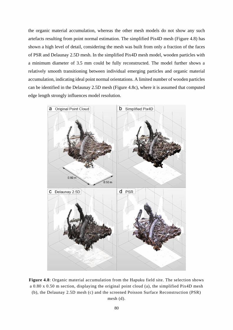
80
the organic material accumulation, whereas the other mesh models do not show any such
artefacts resulting from point normal estimation. The simplified Pix4D mesh (Figure 4.8) has
shown a high level of detail, considering the mesh was built from only a fraction of the faces
of PSR and Delaunay 2.5D mesh. In the simplified Pix4D mesh model, wooden particles with
a minimum diameter of 3.5 mm could be fully reconstructed. The model further shows a
relatively smooth transitioning between individual emerging particles and organic material
accumulation, indicating ideal point normal orientations. A limited number of wooden particles
can be identified in the Delaunay 2.5D mesh (Figure 4.8c), where it is assumed that computed
edge length strongly influences model resolution.
Figure 4.8: Organic material accumulation from the Hapuku field site. The selection shows
a 0.80 x 0.50 m section, displaying the original point cloud (a), the simplified Pix4D mesh
(b), the Delaunay 2.5D mesh (c) and the screened Poisson Surface Reconstruction (PSR)
mesh (d).
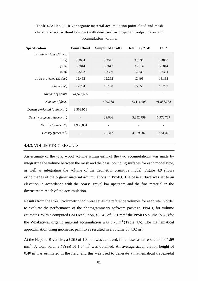
81
Table 4.5: Hapuku River organic material accumulation point cloud and mesh
characteristics (without boulder) with densities for projected footprint area and
accumulation volume.
Specification Point Cloud Simplified Pix4D Delaunay 2.5D PSR
Box dimensions LW acc.
x (m)
y (m)
z (m)
3.3034
3.7814
1.8222
3.2571
3.7647
1.2386
3.3037
3.7814
1.2533
3.4860
3.7814
1.2334
Area projected (xy)(m2) 12.492 12.262 12.493 13.182
Volume (m3) 22.764 15.188 15.657 16.259
Number of points 44,522,655 - - -
Number of faces - 400,068 73,116,103 91,886,732
Density projected (points·m-2) 3,563,951 - - -
Density projected (faces·m-2) - 32,626 5,852,799 6,970,707
Density (points·m-3) 1,955,804 - - -
Density (faces·m-3) - 26,342 4,669,907 5,651,425
4.4.3. VOLUMETRIC RESULTS
An estimate of the total wood volume within each of the two accumulations was made by
integrating the volume between the mesh and the basal bounding surfaces for each model type,
as well as integrating the volume of the geometric primitive model. Figure 4.9 shows
orthoimages of the organic material accumulations in Pix4D. The base surface was set to an
elevation in accordance with the coarse gravel bar upstream and the fine material in the
downstream reach of the accumulation.
Results from the Pix4D volumetric tool were set as the reference volumes for each site in order
to evaluate the performance of the photogrammetry software package, Pix4D, for volume
estimates. With a computed GSD resolution, Li · Wi, of 3.61 mm2 the Pix4D Volume (VP4D) for
the Whakatiwai organic material accumulation was 3.75 m3 (Table 4.6). The mathematical
approximation using geometric primitives resulted in a volume of 4.02 m3.
At the Hapuku River site, a GSD of 1.3 mm was achieved, for a base raster resolution of 1.69
mm2. A total volume (VP4D) of 1.54 m3 was obtained. An average accumulation height of
0.40 m was estimated in the field, and this was used to generate a mathematical trapezoidal
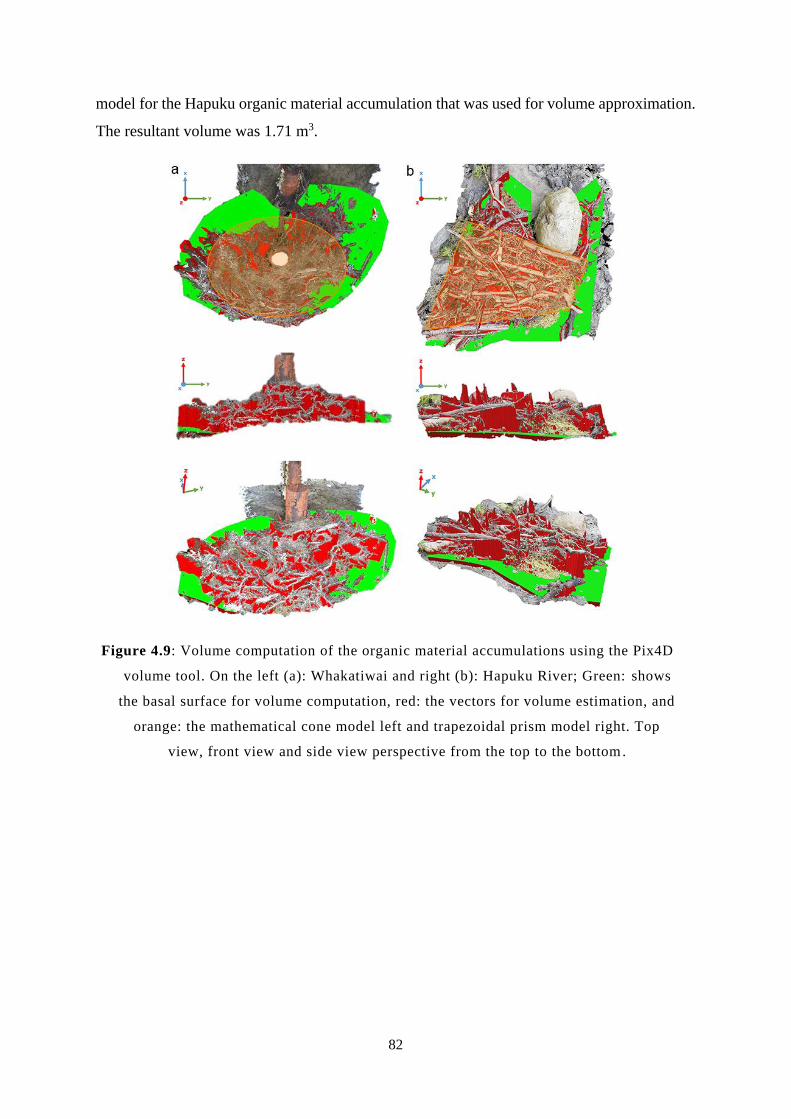
82
model for the Hapuku organic material accumulation that was used for volume approximation.
The resultant volume was 1.71 m3.
Figure 4.9: Volume computation of the organic material accumulations using the Pix4D
volume tool. On the left (a): Whakatiwai and right (b): Hapuku River; Green: shows
the basal surface for volume computation, red: the vectors for volume estimation, and
orange: the mathematical cone model left and trapezoidal prism model right. Top
view, front view and side view perspective from the top to the bottom.
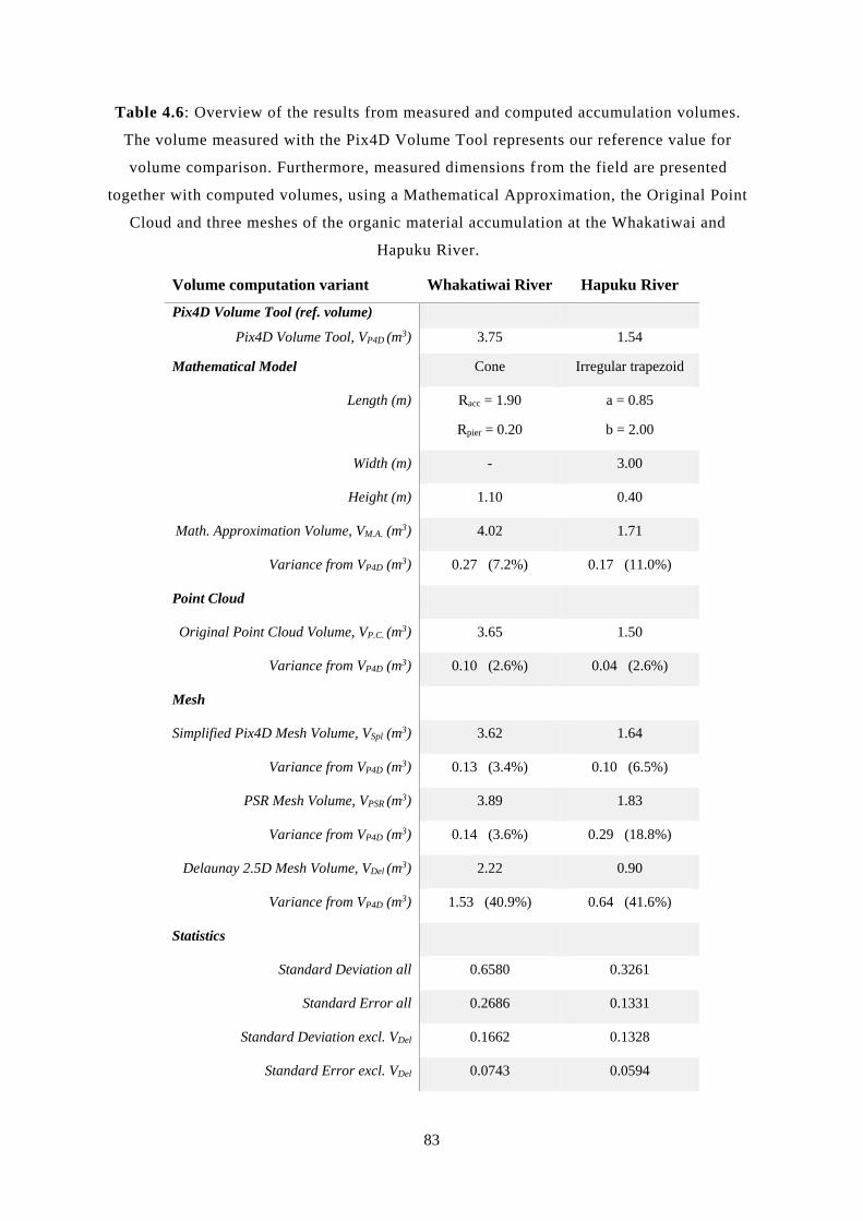
83
Table 4.6: Overview of the results from measured and computed accumulation volumes.
The volume measured with the Pix4D Volume Tool represents our reference value for
volume comparison. Furthermore, measured dimensions f rom the field are presented
together with computed volumes, using a Mathematical Approximation, the Original Point
Cloud and three meshes of the organic material accumulation at the Whakatiwai and
Hapuku River.
Volume computation variant Whakatiwai River Hapuku River
Pix4D Volume Tool (ref. volume)
Pix4D Volume Tool, VP4D (m3) 3.75 1.54
Mathematical Model Cone Irregular trapezoid
Length (m) Racc = 1.90
Rpier = 0.20
a = 0.85
b = 2.00
Width (m) - 3.00
Height (m) 1.10 0.40
Math. Approximation Volume, VM.A. (m3) 4.02 1.71
Variance from VP4D (m3) 0.27 (7.2%) 0.17 (11.0%)
Point Cloud
Original Point Cloud Volume, VP.C. (m3) 3.65 1.50
Variance from VP4D (m3) 0.10 (2.6%) 0.04 (2.6%)
Mesh
Simplified Pix4D Mesh Volume, VSpl (m3) 3.62 1.64
Variance from VP4D (m3) 0.13 (3.4%) 0.10 (6.5%)
PSR Mesh Volume, VPSR (m3) 3.89 1.83
Variance from VP4D (m3) 0.14 (3.6%) 0.29 (18.8%)
Delaunay 2.5D Mesh Volume, VDel (m3) 2.22 0.90
Variance from VP4D (m3) 1.53 (40.9%) 0.64 (41.6%)
Statistics
Standard Deviation all 0.6580 0.3261
Standard Error all 0.2686 0.1331
Standard Deviation excl. VDel 0.1662 0.1328
Standard Error excl. VDel 0.0743 0.0594
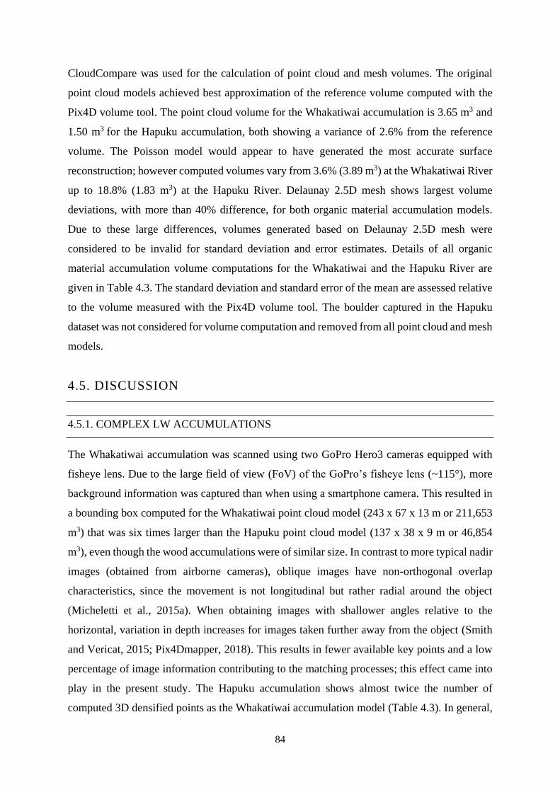
84
CloudCompare was used for the calculation of point cloud and mesh volumes. The original
point cloud models achieved best approximation of the reference volume computed with the
Pix4D volume tool. The point cloud volume for the Whakatiwai accumulation is 3.65 m3 and
1.50 m3 for the Hapuku accumulation, both showing a variance of 2.6% from the reference
volume. The Poisson model would appear to have generated the most accurate surface
reconstruction; however computed volumes vary from 3.6% (3.89 m3) at the Whakatiwai River
up to 18.8% (1.83 m3) at the Hapuku River. Delaunay 2.5D mesh shows largest volume
deviations, with more than 40% difference, for both organic material accumulation models.
Due to these large differences, volumes generated based on Delaunay 2.5D mesh were
considered to be invalid for standard deviation and error estimates. Details of all organic
material accumulation volume computations for the Whakatiwai and the Hapuku River are
given in Table 4.3. The standard deviation and standard error of the mean are assessed relative
to the volume measured with the Pix4D volume tool. The boulder captured in the Hapuku
dataset was not considered for volume computation and removed from all point cloud and mesh
models.
4.5. DISCUSSION
4.5.1. COMPLEX LW ACCUMULATIONS
The Whakatiwai accumulation was scanned using two GoPro Hero3 cameras equipped with
fisheye lens. Due to the large field of view (FoV) of the GoPro’s fisheye lens (~115°), more
background information was captured than when using a smartphone camera. This resulted in
a bounding box computed for the Whakatiwai point cloud model (243 x 67 x 13 m or 211,653
m3) that was six times larger than the Hapuku point cloud model (137 x 38 x 9 m or 46,854
m3), even though the wood accumulations were of similar size. In contrast to more typical nadir
images (obtained from airborne cameras), oblique images have non-orthogonal overlap
characteristics, since the movement is not longitudinal but rather radial around the object
(Micheletti et al., 2015a). When obtaining images with shallower angles relative to the
horizontal, variation in depth increases for images taken further away from the object (Smith
and Vericat, 2015; Pix4Dmapper, 2018). This results in fewer available key points and a low
percentage of image information contributing to the matching processes; this effect came into
play in the present study. The Hapuku accumulation shows almost twice the number of
computed 3D densified points as the Whakatiwai accumulation model (Table 4.3). In general,
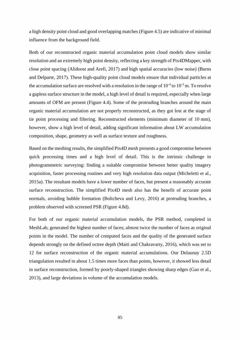
85
a high density point cloud and good overlapping matches (Figure 4.5) are indicative of minimal
influence from the background field.
Both of our reconstructed organic material accumulation point cloud models show similar
resolution and an extremely high point density, reflecting a key strength of Pix4DMapper, with
close point spacing (Alidoost and Arefi, 2017) and high spatial accuracies (low noise) (Burns
and Delparte, 2017). These high-quality point cloud models ensure that individual particles at
the accumulation surface are resolved with a resolution in the range of 10-4 to 10-3 m. To resolve
a gapless surface structure in the model, a high level of detail is required, especially when large
amounts of OFM are present (Figure 4.4). Some of the protruding branches around the main
organic material accumulation are not properly reconstructed, as they got lost at the stage of
tie point processing and filtering. Reconstructed elements (minimum diameter of 10 mm),
however, show a high level of detail, adding significant information about LW accumulation
composition, shape, geometry as well as surface texture and roughness.
Based on the meshing results, the simplified Pix4D mesh presents a good compromise between
quick processing times and a high level of detail. This is the intrinsic challenge in
photogrammetric surveying: finding a suitable compromise between better quality imagery
acquisition, faster processing routines and very high resolution data output (Micheletti et al.,
2015a). The resultant models have a lower number of faces, but present a reasonably accurate
surface reconstruction. The simplified Pix4D mesh also has the benefit of accurate point
normals, avoiding bubble formation (Boltcheva and Levy, 2016) at protruding branches, a
problem observed with screened PSR (Figure 4.8d).
For both of our organic material accumulation models, the PSR method, completed in
MeshLab, generated the highest number of faces; almost twice the number of faces as original
points in the model. The number of computed faces and the quality of the generated surface
depends strongly on the defined octree depth (Maiti and Chakravarty, 2016), which was set to
12 for surface reconstruction of the organic material accumulations. Our Delaunay 2.5D
triangulation resulted in about 1.5 times more faces than points, however, it showed less detail
in surface reconstruction, formed by poorly-shaped triangles showing sharp edges (Gao et al.,
2013), and large deviations in volume of the accumulation models.
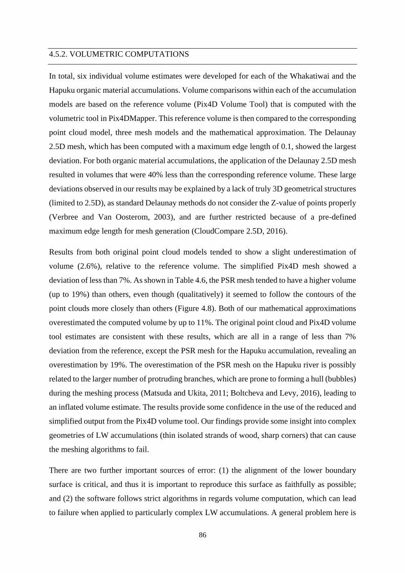
86
4.5.2. VOLUMETRIC COMPUTATIONS
In total, six individual volume estimates were developed for each of the Whakatiwai and the
Hapuku organic material accumulations. Volume comparisons within each of the accumulation
models are based on the reference volume (Pix4D Volume Tool) that is computed with the
volumetric tool in Pix4DMapper. This reference volume is then compared to the corresponding
point cloud model, three mesh models and the mathematical approximation. The Delaunay
2.5D mesh, which has been computed with a maximum edge length of 0.1, showed the largest
deviation. For both organic material accumulations, the application of the Delaunay 2.5D mesh
resulted in volumes that were 40% less than the corresponding reference volume. These large
deviations observed in our results may be explained by a lack of truly 3D geometrical structures
(limited to 2.5D), as standard Delaunay methods do not consider the Z-value of points properly
(Verbree and Van Oosterom, 2003), and are further restricted because of a pre-defined
maximum edge length for mesh generation (CloudCompare 2.5D, 2016).
Results from both original point cloud models tended to show a slight underestimation of
volume (2.6%), relative to the reference volume. The simplified Pix4D mesh showed a
deviation of less than 7%. As shown in Table 4.6, the PSR mesh tended to have a higher volume
(up to 19%) than others, even though (qualitatively) it seemed to follow the contours of the
point clouds more closely than others (Figure 4.8). Both of our mathematical approximations
overestimated the computed volume by up to 11%. The original point cloud and Pix4D volume
tool estimates are consistent with these results, which are all in a range of less than 7%
deviation from the reference, except the PSR mesh for the Hapuku accumulation, revealing an
overestimation by 19%. The overestimation of the PSR mesh on the Hapuku river is possibly
related to the larger number of protruding branches, which are prone to forming a hull (bubbles)
during the meshing process (Matsuda and Ukita, 2011; Boltcheva and Levy, 2016), leading to
an inflated volume estimate. The results provide some confidence in the use of the reduced and
simplified output from the Pix4D volume tool. Our findings provide some insight into complex
geometries of LW accumulations (thin isolated strands of wood, sharp corners) that can cause
the meshing algorithms to fail.
There are two further important sources of error: (1) the alignment of the lower boundary
surface is critical, and thus it is important to reproduce this surface as faithfully as possible;
and (2) the software follows strict algorithms in regards volume computation, which can lead
to failure when applied to particularly complex LW accumulations. A general problem here is
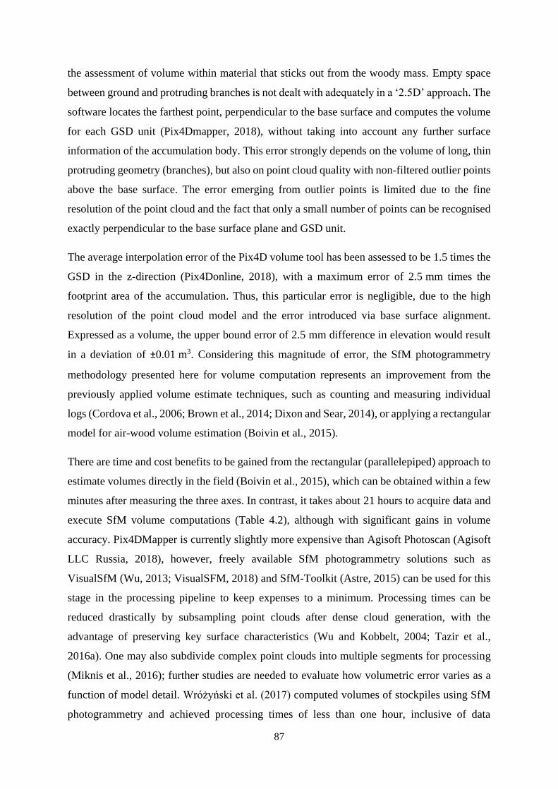
87
the assessment of volume within material that sticks out from the woody mass. Empty space
between ground and protruding branches is not dealt with adequately in a ‘2.5D’ approach. The
software locates the farthest point, perpendicular to the base surface and computes the volume
for each GSD unit (Pix4Dmapper, 2018), without taking into account any further surface
information of the accumulation body. This error strongly depends on the volume of long, thin
protruding geometry (branches), but also on point cloud quality with non-filtered outlier points
above the base surface. The error emerging from outlier points is limited due to the fine
resolution of the point cloud and the fact that only a small number of points can be recognised
exactly perpendicular to the base surface plane and GSD unit.
The average interpolation error of the Pix4D volume tool has been assessed to be 1.5 times the
GSD in the z-direction (Pix4Donline, 2018), with a maximum error of 2.5 mm times the
footprint area of the accumulation. Thus, this particular error is negligible, due to the high
resolution of the point cloud model and the error introduced via base surface alignment.
Expressed as a volume, the upper bound error of 2.5 mm difference in elevation would result
in a deviation of ±0.01 m3. Considering this magnitude of error, the SfM photogrammetry
methodology presented here for volume computation represents an improvement from the
previously applied volume estimate techniques, such as counting and measuring individual
logs (Cordova et al., 2006; Brown et al., 2014; Dixon and Sear, 2014), or applying a rectangular
model for air-wood volume estimation (Boivin et al., 2015).
There are time and cost benefits to be gained from the rectangular (parallelepiped) approach to
estimate volumes directly in the field (Boivin et al., 2015), which can be obtained within a few
minutes after measuring the three axes. In contrast, it takes about 21 hours to acquire data and
execute SfM volume computations (Table 4.2), although with significant gains in volume
accuracy. Pix4DMapper is currently slightly more expensive than Agisoft Photoscan (Agisoft
LLC Russia, 2018), however, freely available SfM photogrammetry solutions such as
VisualSfM (Wu, 2013; VisualSFM, 2018) and SfM-Toolkit (Astre, 2015) can be used for this
stage in the processing pipeline to keep expenses to a minimum. Processing times can be
reduced drastically by subsampling point clouds after dense cloud generation, with the
advantage of preserving key surface characteristics (Wu and Kobbelt, 2004; Tazir et al.,
2016a). One may also subdivide complex point clouds into multiple segments for processing
(Miknis et al., 2016); further studies are needed to evaluate how volumetric error varies as a
function of model detail. Wróżyński et al. (2017) computed volumes of stockpiles using SfM
photogrammetry and achieved processing times of less than one hour, inclusive of data
88
acquisition. These processing times may also apply for SfM photogrammetry-based LW
volume estimations, although wood accumulations show more complex surface texture.
4.5.3. LW ACCUMULATION ASSESSMENT
There is a need for accurate, detailed, and objective techniques for estimating wood volumes
in a variety of management contexts. Conventional large-scale surveying methods have gained
popularity for wood budgeting applications (Ulloa et al., 2016; Tonon et al., 2017), yet with
increasing distance between sensor and wood the spatial model accuracy decreases (Figure
4.1). Challenges arise when LW pieces are smaller than the achieved model resolution (Marcus
et al., 2003; Tonon et al., 2018). Therefore, a combination of field- and aerial surveying could
improve volume estimates significantly (Boivin et al., 2017).
Phillips et al (2017) outlined the need for a better quantitative capture of the effects from post-
harvest debris flows, in order to better inform predictive models. The same is required for
assessing wood inputs from natural forest disturbance such as fire, landslides and avalanches,
or heavy storm events. This is the current focus of numerous LW studies (Thevenet et al., 1998;
MacVicar et al., 2009; Ruiz-Villanueva et al., 2014b; Steeb et al., 2017; Sanhueza et al., 2018),
however, the mass and volume of wood still remains rarely described (Ruiz-Villanueva et al.,
2019). Although a broad variety of volumetric surveying methods for LW sources exists;
including LiDAR (Kasprak et al., 2012; Atha and Dietrich, 2016), aerial photogrammetry
(Boivin et al., 2017; Sanhueza et al., 2018) and manually conducted measurements (Piegay,
1993; Boivin et al., 2015), precise quantification of LW sources remains challenging.
Mazzorana and Fuchs (2010) found that transported wood act as a potential risk amplifier
during flood events, for which reason a fundamental knowledge of the available wooden
quantities in vulnerable fluvial systems is essential.
Risk analyses are a widely discussed topic in the LW community, with various analysis
proposed to better understand the probabilities and process linkages that bring wood from the
hillslope to the river (Comiti et al., 2016). Risk factors can be better characterised by carrying
out volumetric surveys of wood accumulations along this gradient (Zischg et al., 2018), before
the occurrence of ‘LW incidents’ (Cave et al., 2017). Our methodology provides an example
application for the assessment of LW volume at a high resolution, as suggested by Hübl et al.
(2002), but also for governmental authorities that require forestry and earthworks plans, where
SfM photogrammetry can be used to assess LW quantities, which are available at a field site
89
and at risk for entering a stream system during forest harvesting operations in a watershed
(Reddy, 2017). The technique can be widely and rapidly deployed, with data collection and
processing done within 24 hours and can be applied to emerging assessment frameworks, such
as the Risk Assessment for the National Environmental Standards for Plantation Forestry
(Ministry for Primary Industries, 2017).
Due to the fact that individual LW pieces and entire accumulation structures in a stream can
alter channel morphology (Mosley, 1981; Wohl and Scott, 2017) and discharge behaviour
(Gschnitzer et al., 2017; Schalko et al., 2018), all affecting safety aspects in regards discharge
conveyance and resilience of river-crossing infrastructure, investigations on LW accumulation
volume (Lienkaemper and Swanson, 1987), geometry (Cordova et al., 2006; Dixon and Sear,
2014), and orientation in the channel (Abbe and Montgomery, 2003; Ruiz-Villanueva et al.,
2016b) are essential. Detailed surveys providing high-resolution data of LW accumulations,
however, are infrequently reported. Thus a lack of meaningful assessment opportunities arise
in the field of LW research. The introduced method provides a powerful and compact tool for
accurate assessment of existing LW structures and wood sources in the riparian zone to gain
information about (i) wood budgeting and the quantity of available wood (Benda et al., 2003;
Schenk et al., 2014; Sanhueza et al., 2018; Tonon et al., 2018) on a basis of pre- and post-flood
assessment, (ii) residence times LW accumulation volume and development during flood
events, when organic material is removed or deposited (Sanhueza et al., 2018), and (iii)
accumulation structure and orientation with respect to the flow (Daniels, 2006; Ruiz-
Villanueva et al., 2016b). This is needed to estimate effects on hydraulic flow behaviour and
impacts on channel morphology.
Improving the compositional information, such as relative proportions of wood, branches,
sediment, organics and pore space (Piegay, 1993; Boivin and Buffin-Bélanger, 2010; Schalko
et al., 2018), is a major challenge in the quantification of LW accumulation assessment. The
techniques presented herewith perform well in capturing the ‘envelope’ of the deposit, and
providing a detailed record of the texture, yet estimates of deposit porosity remain biased
toward the outer shell. Backwater effects, changes in channel morphology and drag forces on
the accumulation body strongly depend on the ratio of void volume over total volume (Pagliara
and Carnacina, 2010; Schalko et al., 2018; Schalko et al., 2019a). Void volume may be
determined from surface texture, which can be filtered for colours (Orru et al., 2016) (e.g.
wood, grass, sediments) to broadly estimate compositional proportions. The mesh can be
further manipulated, using techniques such as mesh skeletonization (AlRatrout et al. (2018) in
90
order to resolve major compositional members (tree stems, major branches) and collect
statistical information on the geometrical arrangement of these structural items. Seitz et al.
(2018) successfully demonstrated the application of a SfM photogrammetry workflow to
estimate porosity of soil samples using a laboratory setup and water replacement methodology.
These previous studies on porosity estimates using SfM methodology can significantly
contribute to incorporating LW accumulations in computational fluid dynamics (CFD)
modelling. Accurate 3D mesh models, and information about roughness parameters (Gippel,
1995; Manners et al., 2007), angularity (Lisle, 1986; Lai and Bandrowski, 2014), hydraulic
losses (Knauss, 1995; Shields, 2001; Schalko et al., 2018) are furthermore of considerable
importance for CFD modelling (Xu and Liu, 2017). Major advances have been achieved in
recent years with the application of 2D (Ruiz-Villanueva et al., 2014a; Ventres-Pake et al.,
2019), but also 3D LW computational models (Smith et al., 2011; Allen and Smith, 2012; Lai,
2016) to evaluate hydraulic flow behaviour. For example, a prototype accumulation model can
be used for investigating the effects on flow and channel morphology in presence of a LW
accumulation (Figure 4.10). Low grid resolution can cause high distortions, numerical
diffusion and instabilities (Allen and Smith, 2012) in CFD models, and so it is important to
provide a smooth, yet sufficiently detailed model surface in order to capture the relevant
process(es) without introducing resistance from mesh imperfections. The work pipeline we
have presented here provides a number of options for developing a suitably detailed mesh for
hydraulic simulations involving LW accumulations.
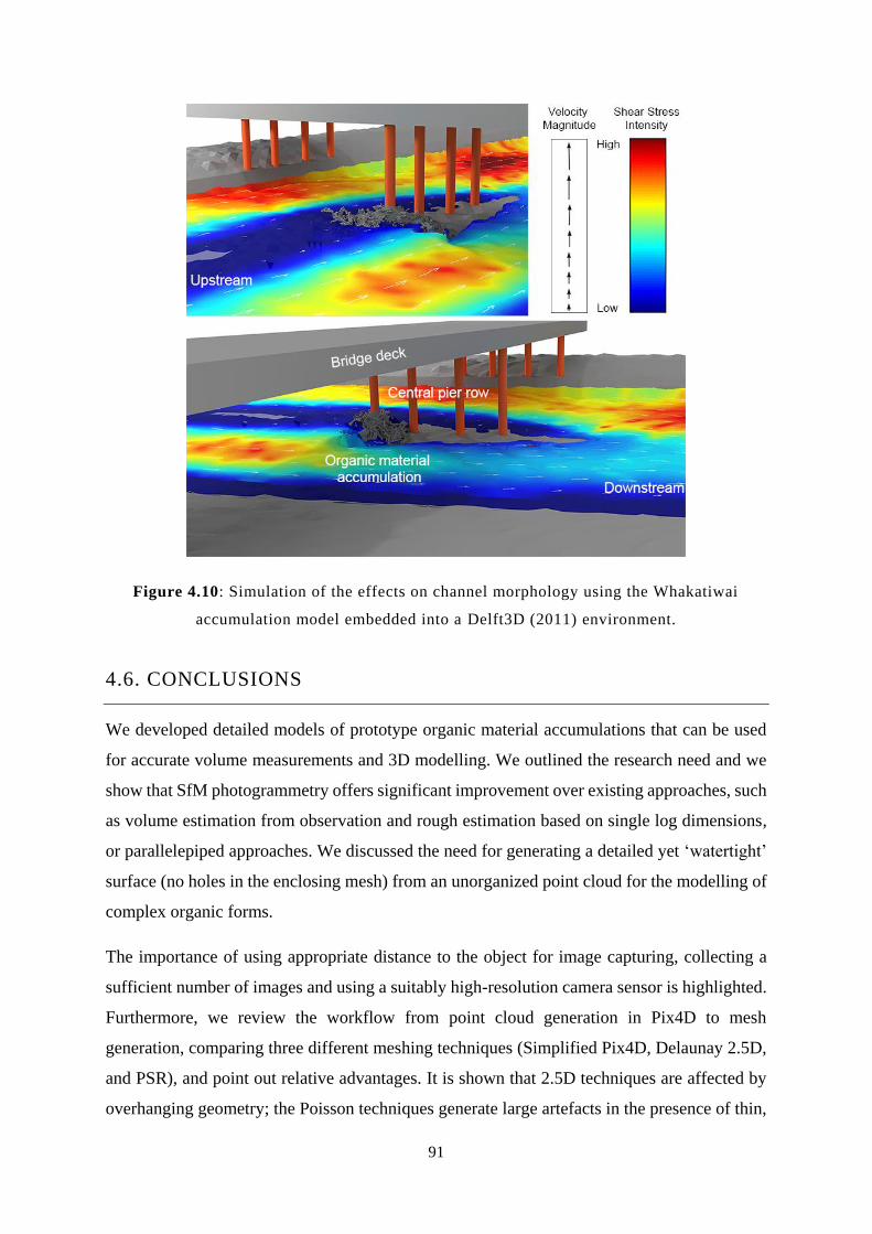
91
Figure 4.10: Simulation of the effects on channel morphology using the Whakatiwai
accumulation model embedded into a Delft3D (2011) environment.
4.6. CONCLUSIONS
We developed detailed models of prototype organic material accumulations that can be used
for accurate volume measurements and 3D modelling. We outlined the research need and we
show that SfM photogrammetry offers significant improvement over existing approaches, such
as volume estimation from observation and rough estimation based on single log dimensions,
or parallelepiped approaches. We discussed the need for generating a detailed yet ‘watertight’
surface (no holes in the enclosing mesh) from an unorganized point cloud for the modelling of
complex organic forms.
The importance of using appropriate distance to the object for image capturing, collecting a
sufficient number of images and using a suitably high-resolution camera sensor is highlighted.
Furthermore, we review the workflow from point cloud generation in Pix4D to mesh
generation, comparing three different meshing techniques (Simplified Pix4D, Delaunay 2.5D,
and PSR), and point out relative advantages. It is shown that 2.5D techniques are affected by
overhanging geometry; the Poisson techniques generate large artefacts in the presence of thin,
92
poorly defined branches that protrude from the main accumulation; the simplified Pix4D model
manages to avoid these pitfalls to generate a low-poly mesh that preserves important surface
details. It was further found that the Pix4D volume tool slightly overestimates the volume of
the initial point cloud model, by 2.6%, for both field sites. Using the PSR mesh provided the
best overall result relative to the reference volumes. While we conclude that the original point
cloud can be used for rapid volume estimates, a watertight hull is required for modelling
applications that take into consideration surface texture and roughness.
The final results reveal that the meshing algorithm from Pix4D is superior to the other
techniques in that it has a low poly count and a robust topology that is highly suited to volume
estimation and rapid processing. The other techniques generated more highly resolved models,
however, they also tended to have a very high number of faces, and more spurious features,
relative to the initial point cloud. The user needs to assess the requirements for their analysis,
with respect to model resolutions, processing times, and accuracy beforehand in order to
achieve the best project outcome.
We suggest that the technique should be used to improve the workflow (and subsequent
analyses) in the field, as well as in the laboratory, for a suite of LW assessment tasks in the
course of wood budgeting, habitat characterisation, assessing sediment retention while looking
at LW influence on river morphology, and potentially, modelling hydraulic interactions by
implementing most realistic prototype accumulation models.
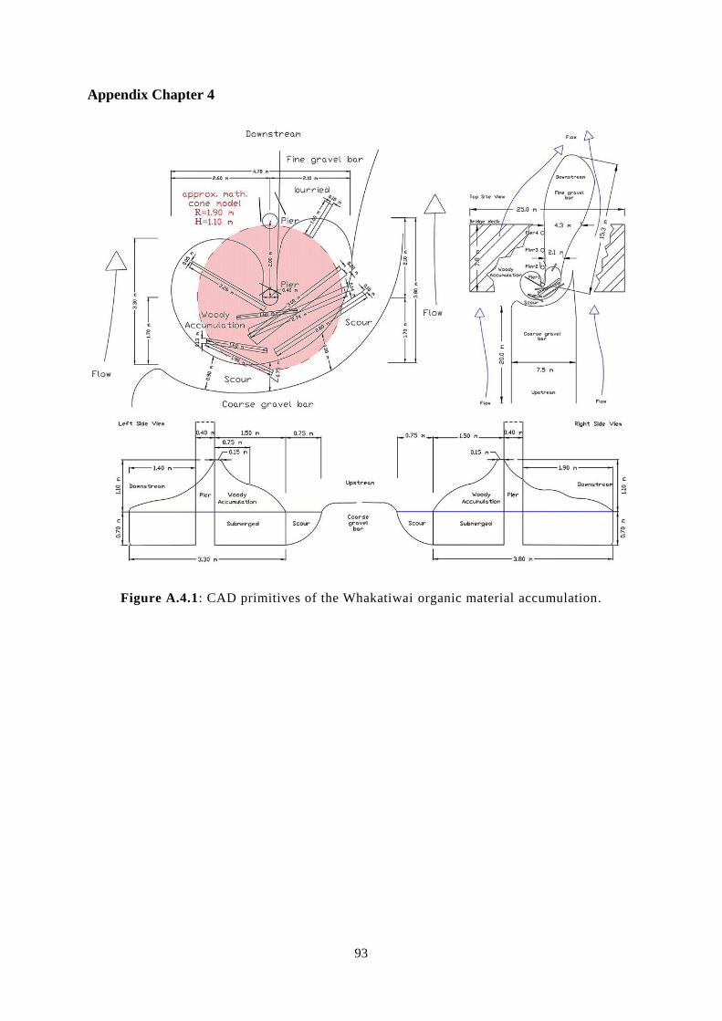
93
Appendix Chapter 4
Figure A.4.1: CAD primitives of the Whakatiwai organic material accumulation.
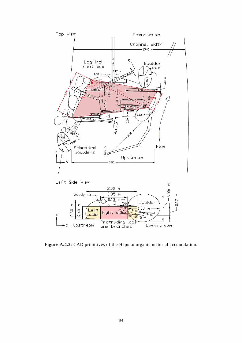
94
Figure A.4.2: CAD primitives of the Hapuku organic material accumulation.
95
LARGE WOOD (LW) 3D ACCUMULATION MAPPING AND
ASSESSMENT USING STRUCTURE FROM MOTION
PHOTOGRAMMETRY IN THE LABORATORY
Related journal article:
Spreitzer, G., Tunnicliffe, J. & Friedrich, F. 2019. Large wood (LW) 3D accumulation mapping
and assessment using Structure from Motion photogrammetry in the laboratory. Journal of
Hydrology 581. doi:10.1016/j.jhydrol.2019.124430
5.1. INTRODUCTION
5.1.1. LARGE WOOD (LW) ACCUMULATIONS AND ASSESSMENT
The majority of river-focused research defines large wood (LW) as wooden pieces with a
minimum length of 1 m and a diameter larger than 0.1 m (Nakamura and Swanson, 1994;
Fetherston et al., 1995; Wyżga and Zawiejska, 2005; Ravazzolo et al., 2015; Martin et al.,
2018), while smaller elements are considered as organic fine material (OFM). LW plays an
important role in moderating sediment transport and storage (Megahan and Nowlin, 1976;
Hornbeck et al., 1993), and stream channel morphology (Zimmerman et al., 1967; Keller and
Swanson, 1979; Bilby, 1984; Smith et al., 1993; Abbe and Montgomery, 1996), but it also
provides habitat for fish and other riverine organisms (Fausch and Northcote, 1992). Several
research projects have focused on the influence of log structures on channel forms, including
stream banks and bars (Keller and Swanson, 1979; Gippel et al., 1996), as well as on flow
hydraulics (energy losses, changes in roughness and flow dissipation) (Heede et al., 1972;
Gregory et al., 1985; Knauss, 1995; Anderson et al., 2006). Besides the positive effects of wood
in stream channels, LW accumulations at constricted cross-sections may represent a hazard to
river-spanning infrastructure, agriculture lands, as well as human populations in adjacent areas
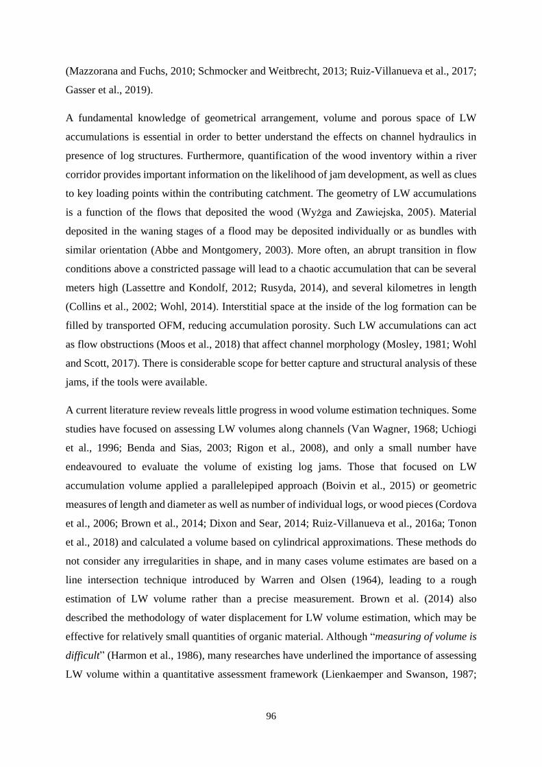
96
(Mazzorana and Fuchs, 2010; Schmocker and Weitbrecht, 2013; Ruiz-Villanueva et al., 2017;
Gasser et al., 2019).
A fundamental knowledge of geometrical arrangement, volume and porous space of LW
accumulations is essential in order to better understand the effects on channel hydraulics in
presence of log structures. Furthermore, quantification of the wood inventory within a river
corridor provides important information on the likelihood of jam development, as well as clues
to key loading points within the contributing catchment. The geometry of LW accumulations
is a function of the flows that deposited the wood (Wyżga and Zawiejska, 2005). Material
deposited in the waning stages of a flood may be deposited individually or as bundles with
similar orientation (Abbe and Montgomery, 2003). More often, an abrupt transition in flow
conditions above a constricted passage will lead to a chaotic accumulation that can be several
meters high (Lassettre and Kondolf, 2012; Rusyda, 2014), and several kilometres in length
(Collins et al., 2002; Wohl, 2014). Interstitial space at the inside of the log formation can be
filled by transported OFM, reducing accumulation porosity. Such LW accumulations can act
as flow obstructions (Moos et al., 2018) that affect channel morphology (Mosley, 1981; Wohl
and Scott, 2017). There is considerable scope for better capture and structural analysis of these
jams, if the tools were available.
A current literature review reveals little progress in wood volume estimation techniques. Some
studies have focused on assessing LW volumes along channels (Van Wagner, 1968; Uchiogi
et al., 1996; Benda and Sias, 2003; Rigon et al., 2008), and only a small number have
endeavoured to evaluate the volume of existing log jams. Those that focused on LW
accumulation volume applied a parallelepiped approach (Boivin et al., 2015) or geometric
measures of length and diameter as well as number of individual logs, or wood pieces (Cordova
et al., 2006; Brown et al., 2014; Dixon and Sear, 2014; Ruiz-Villanueva et al., 2016a; Tonon
et al., 2018) and calculated a volume based on cylindrical approximations. These methods do
not consider any irregularities in shape, and in many cases volume estimates are based on a
line intersection technique introduced by Warren and Olsen (1964), leading to a rough
estimation of LW volume rather than a precise measurement. Brown et al. (2014) also
described the methodology of water displacement for LW volume estimation, which may be
effective for relatively small quantities of organic material. Although “measuring of volume is
difficult” (Harmon et al., 1986), many researches have underlined the importance of assessing
LW volume within a quantitative assessment framework (Lienkaemper and Swanson, 1987;
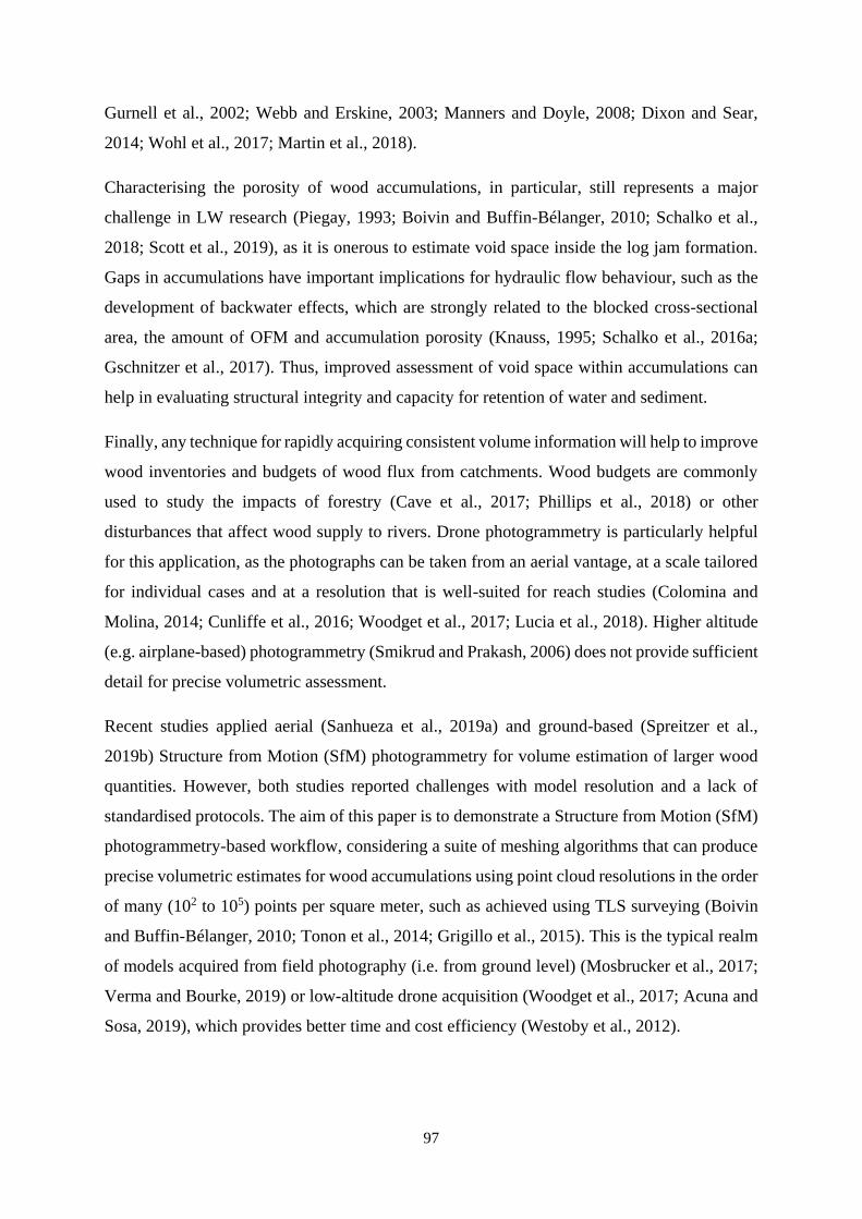
97
Gurnell et al., 2002; Webb and Erskine, 2003; Manners and Doyle, 2008; Dixon and Sear,
2014; Wohl et al., 2017; Martin et al., 2018).
Characterising the porosity of wood accumulations, in particular, still represents a major
challenge in LW research (Piegay, 1993; Boivin and Buffin-Bélanger, 2010; Schalko et al.,
2018; Scott et al., 2019), as it is onerous to estimate void space inside the log jam formation.
Gaps in accumulations have important implications for hydraulic flow behaviour, such as the
development of backwater effects, which are strongly related to the blocked cross-sectional
area, the amount of OFM and accumulation porosity (Knauss, 1995; Schalko et al., 2016a;
Gschnitzer et al., 2017). Thus, improved assessment of void space within accumulations can
help in evaluating structural integrity and capacity for retention of water and sediment.
Finally, any technique for rapidly acquiring consistent volume information will help to improve
wood inventories and budgets of wood flux from catchments. Wood budgets are commonly
used to study the impacts of forestry (Cave et al., 2017; Phillips et al., 2018) or other
disturbances that affect wood supply to rivers. Drone photogrammetry is particularly helpful
for this application, as the photographs can be taken from an aerial vantage, at a scale tailored
for individual cases and at a resolution that is well-suited for reach studies (Colomina and
Molina, 2014; Cunliffe et al., 2016; Woodget et al., 2017; Lucia et al., 2018). Higher altitude
(e.g. airplane-based) photogrammetry (Smikrud and Prakash, 2006) does not provide sufficient
detail for precise volumetric assessment.
Recent studies applied aerial (Sanhueza et al., 2019a) and ground-based (Spreitzer et al.,
2019b) Structure from Motion (SfM) photogrammetry for volume estimation of larger wood
quantities. However, both studies reported challenges with model resolution and a lack of
standardised protocols. The aim of this paper is to demonstrate a Structure from Motion (SfM)
photogrammetry-based workflow, considering a suite of meshing algorithms that can produce
precise volumetric estimates for wood accumulations using point cloud resolutions in the order
of many (102 to 105) points per square meter, such as achieved using TLS surveying (Boivin
and Buffin-Bélanger, 2010; Tonon et al., 2014; Grigillo et al., 2015). This is the typical realm
of models acquired from field photography (i.e. from ground level) (Mosbrucker et al., 2017;
Verma and Bourke, 2019) or low-altitude drone acquisition (Woodget et al., 2017; Acuna and
Sosa, 2019), which provides better time and cost efficiency (Westoby et al., 2012).
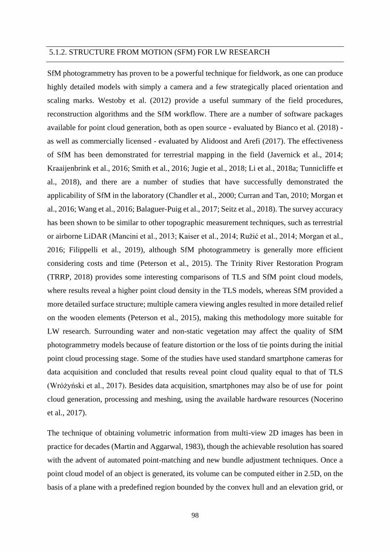
98
5.1.2. STRUCTURE FROM MOTION (SFM) FOR LW RESEARCH
SfM photogrammetry has proven to be a powerful technique for fieldwork, as one can produce
highly detailed models with simply a camera and a few strategically placed orientation and
scaling marks. Westoby et al. (2012) provide a useful summary of the field procedures,
reconstruction algorithms and the SfM workflow. There are a number of software packages
available for point cloud generation, both as open source - evaluated by Bianco et al. (2018) -
as well as commercially licensed - evaluated by Alidoost and Arefi (2017). The effectiveness
of SfM has been demonstrated for terrestrial mapping in the field (Javernick et al., 2014;
Kraaijenbrink et al., 2016; Smith et al., 2016; Jugie et al., 2018; Li et al., 2018a; Tunnicliffe et
al., 2018), and there are a number of studies that have successfully demonstrated the
applicability of SfM in the laboratory (Chandler et al., 2000; Curran and Tan, 2010; Morgan et
al., 2016; Wang et al., 2016; Balaguer-Puig et al., 2017; Seitz et al., 2018). The survey accuracy
has been shown to be similar to other topographic measurement techniques, such as terrestrial
or airborne LiDAR (Mancini et al., 2013; Kaiser et al., 2014; Ružić et al., 2014; Morgan et al.,
2016; Filippelli et al., 2019), although SfM photogrammetry is generally more efficient
considering costs and time (Peterson et al., 2015). The Trinity River Restoration Program
(TRRP, 2018) provides some interesting comparisons of TLS and SfM point cloud models,
where results reveal a higher point cloud density in the TLS models, whereas SfM provided a
more detailed surface structure; multiple camera viewing angles resulted in more detailed relief
on the wooden elements (Peterson et al., 2015), making this methodology more suitable for
LW research. Surrounding water and non-static vegetation may affect the quality of SfM
photogrammetry models because of feature distortion or the loss of tie points during the initial
point cloud processing stage. Some of the studies have used standard smartphone cameras for
data acquisition and concluded that results reveal point cloud quality equal to that of TLS
(Wróżyński et al., 2017). Besides data acquisition, smartphones may also be of use for point
cloud generation, processing and meshing, using the available hardware resources (Nocerino
et al., 2017).
The technique of obtaining volumetric information from multi-view 2D images has been in
practice for decades (Martin and Aggarwal, 1983), though the achievable resolution has soared
with the advent of automated point-matching and new bundle adjustment techniques. Once a
point cloud model of an object is generated, its volume can be computed either in 2.5D, on the
basis of a plane with a predefined region bounded by the convex hull and an elevation grid, or
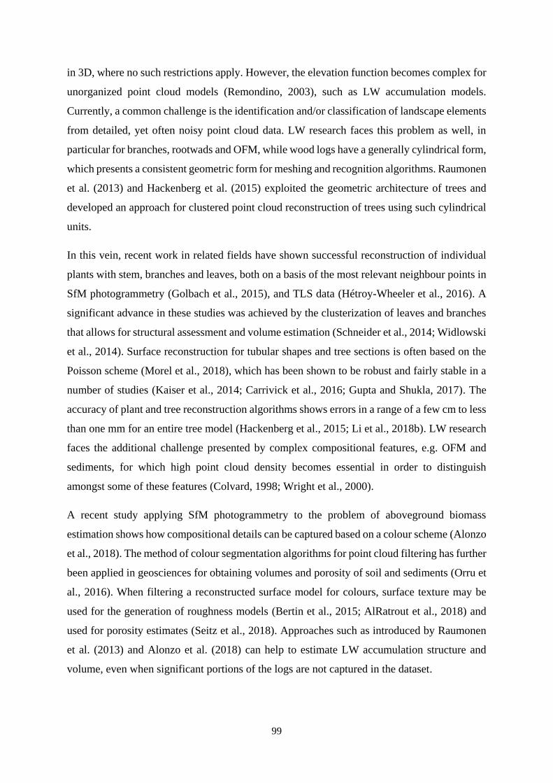
99
in 3D, where no such restrictions apply. However, the elevation function becomes complex for
unorganized point cloud models (Remondino, 2003), such as LW accumulation models.
Currently, a common challenge is the identification and/or classification of landscape elements
from detailed, yet often noisy point cloud data. LW research faces this problem as well, in
particular for branches, rootwads and OFM, while wood logs have a generally cylindrical form,
which presents a consistent geometric form for meshing and recognition algorithms. Raumonen
et al. (2013) and Hackenberg et al. (2015) exploited the geometric architecture of trees and
developed an approach for clustered point cloud reconstruction of trees using such cylindrical
units.
In this vein, recent work in related fields have shown successful reconstruction of individual
plants with stem, branches and leaves, both on a basis of the most relevant neighbour points in
SfM photogrammetry (Golbach et al., 2015), and TLS data (Hétroy-Wheeler et al., 2016). A
significant advance in these studies was achieved by the clusterization of leaves and branches
that allows for structural assessment and volume estimation (Schneider et al., 2014; Widlowski
et al., 2014). Surface reconstruction for tubular shapes and tree sections is often based on the
Poisson scheme (Morel et al., 2018), which has been shown to be robust and fairly stable in a
number of studies (Kaiser et al., 2014; Carrivick et al., 2016; Gupta and Shukla, 2017). The
accuracy of plant and tree reconstruction algorithms shows errors in a range of a few cm to less
than one mm for an entire tree model (Hackenberg et al., 2015; Li et al., 2018b). LW research
faces the additional challenge presented by complex compositional features, e.g. OFM and
sediments, for which high point cloud density becomes essential in order to distinguish
amongst some of these features (Colvard, 1998; Wright et al., 2000).
A recent study applying SfM photogrammetry to the problem of aboveground biomass
estimation shows how compositional details can be captured based on a colour scheme (Alonzo
et al., 2018). The method of colour segmentation algorithms for point cloud filtering has further
been applied in geosciences for obtaining volumes and porosity of soil and sediments (Orru et
al., 2016). When filtering a reconstructed surface model for colours, surface texture may be
used for the generation of roughness models (Bertin et al., 2015; AlRatrout et al., 2018) and
used for porosity estimates (Seitz et al., 2018). Approaches such as introduced by Raumonen
et al. (2013) and Alonzo et al. (2018) can help to estimate LW accumulation structure and
volume, even when significant portions of the logs are not captured in the dataset.
100
5.1.3. OBJECTIVES
Given the requirement for precise, in-situ volume estimation in LW research, there is high
demand for portable and easily deployed surveying tools, such as SfM photogrammetry, that
can efficiently capture the geometry of wooden deposits. To move from the unorganized point
cloud produced by photogrammetric techniques to a volumetric model requires testing of the
available meshing and volume integration algorithms, under controlled conditions. With our
work we aim to develop a SfM photogrammetry-based workflow (pipeline) to estimate the
volume of model LW accumulations that can be objectively verified.
The objectives are:
(i) To generate high quality point cloud models of LW accumulations under controlled
conditions in the laboratory,
(ii) To compute the geometric measures, including volume and porosity, of the
generated 2.5D and 3D LW accumulation models,
(iii) To evaluate and assess the computed LW volumes generated via SfM
photogrammetry in comparison with easily verifiable accumulation volumes,
(iv) To assess the challenges and opportunities arising from 2.5D volume estimation,
from elevation points that have been projected vertically onto a reference surface,
versus 3D volumes that may be obtained by detailed meshing of the point cloud.
SfM photogrammetry is a promising tool for LW research under controlled conditions in the
laboratory, considering its performance relative to other available mapping techniques.
Developing a quantitative framework for analysing LW accumulations will enable more
meaningful and compatible measures of accumulation composition and volumes, as well as
detailed assessment of surface structure, log age, detrital organic characteristics and other
features.
5.2. LABORATORY EXPERIMENTS
For estimates of LW accumulation volumes, based on SfM photogrammetry, we used a set of
wooden dowel structures, which were assembled on a smooth surface in the laboratory. The
wooden dowels were of a uniform cylindrical shape, varying in length and diameter. Altogether
seven distinctive accumulation structures (Table 5.1) were considered; starting with the most
101
elementary - a single wood dowel - working up to complex LW accumulations. We also
considered OFM as part of our experimental setup for a small number of experiments. For the
laboratory OFM substrate we used wood chips with a length of up to 65 mm, and bark pieces
in a range of 4 to 32 mm (b-axis). The OFM fills porous space in between the log skeleton
structure, reducing accumulation porosity. The species of the wooden material was Pinus
radiata (New Zealand Pine).
For the first experiment a single wooden dowel - One Dowel - with a length of 300 mm and 46
mm in diameter was used (Table 5.1). This setup appears trivial, however, it represents an
essential verification test for further volume assessment of LW accumulations.
The second structure comprised two wooden dowels - Two Dowels - both showing equal
dimensions (L=300 mm, D=46 mm). One of the dowels was placed on top of the other one, in
a perpendicular alignment. The distance between the grounded point of the top dowel and the
underlying, centrally-placed dowel was about three quarters of the top dowel’s length.
Six cylindrical wooden dowels - Six Dowels (dowel pile) - were used for a further elementary
LW accumulation. A triangular bundle was formed, with three logs at the base, two in the
middle and one on top. Tape was used to maintain the shape and position of the dowel pile.
The dowels had a length of 400 mm each, with a diameter of 32 mm.
A more complex LW accumulation was set up using eight wooden dowels - Eight Dowels
(high photo count) - that were randomly assembled, forming an accumulation skeleton. The
LW accumulation consisted of a mixture of the previously used dowels, comprising two dowels
with a length of 300 mm and 46 mm in diameter and another six dowels with lengths of
400 mm and 32 mm in diameter. For this experiment a relatively high number of images (529)
was obtained for the photogrammetric model.
Similar to the previous setup (Eight Dowels – high photo count), the same eight dowels were
used and assembled into another LW accumulation - Eight Dowels (low photo count) - on the
laboratory floor. A relatively low number of images (23) was acquired for the model. The
purpose is to demonstrate the effects of having a low number of images in comparison to a
high number of images for volume estimates.
An accumulation consisting of only OFM - OFM Accumulation - was formed to resemble a
heap, approximately 70 mm in height with a roughly circular planform diameter of 190 mm.
For material preparation, a measuring cylinder was filled with 1.00 10-3 m3 of wood chips (<
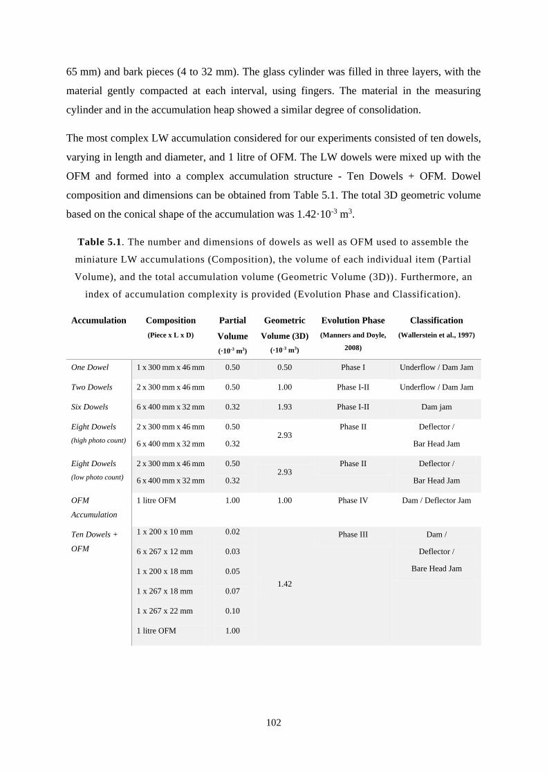
102
65 mm) and bark pieces (4 to 32 mm). The glass cylinder was filled in three layers, with the
material gently compacted at each interval, using fingers. The material in the measuring
cylinder and in the accumulation heap showed a similar degree of consolidation.
The most complex LW accumulation considered for our experiments consisted of ten dowels,
varying in length and diameter, and 1 litre of OFM. The LW dowels were mixed up with the
OFM and formed into a complex accumulation structure - Ten Dowels + OFM. Dowel
composition and dimensions can be obtained from Table 5.1. The total 3D geometric volume
based on the conical shape of the accumulation was 1.42·10-3 m3.
Table 5.1. The number and dimensions of dowels as well as OFM used to assemble the
miniature LW accumulations (Composition), the volume of each individual item (Partial
Volume), and the total accumulation volume (Geometric Volume (3D)) . Furthermore, an
index of accumulation complexity is provided (Evolution Phase and Classification).
Accumulation Composition
(Piece x L x D)
Partial
Volume
(·10-3 m3)
Geometric
Volume (3D)
(·10-3 m3)
Evolution Phase
(Manners and Doyle,
2008)
Classification
(Wallerstein et al., 1997)
One Dowel 1 x 300 mm x 46 mm 0.50 0.50 Phase I Underflow / Dam Jam
Two Dowels 2 x 300 mm x 46 mm 0.50 1.00 Phase I-II Underflow / Dam Jam
Six Dowels 6 x 400 mm x 32 mm 0.32 1.93 Phase I-II Dam jam
Eight Dowels
(high photo count)
2 x 300 mm x 46 mm
6 x 400 mm x 32 mm
0.50
0.32 2.93
Phase II Deflector /
Bar Head Jam
Eight Dowels
(low photo count)
2 x 300 mm x 46 mm
6 x 400 mm x 32 mm
0.50
0.32 2.93
Phase II Deflector /
Bar Head Jam
OFM
Accumulation
1 litre OFM 1.00 1.00 Phase IV Dam / Deflector Jam
Ten Dowels +
OFM
1 x 200 x 10 mm
6 x 267 x 12 mm
1 x 200 x 18 mm
1 x 267 x 18 mm
1 x 267 x 22 mm
1 litre OFM
0.02
0.03
0.05
0.07
0.10
1.00
1.42
Phase III Dam /
Deflector /
Bare Head Jam
103
5.3. METHODOLOGY
5.3.1. PROCEDURE FOR VOLUMETRIC ESTIMATES
We classified our accumulations into three categories; (i) elementary accumulations (One
Dowel, Two Dowels and Six Dowels), (ii) complex accumulations (Eight Dowels), and (iii)
OFM accumulations as a further advanced stage of complex accumulations (OFM
Accumulation and Ten Dowels + OFM). The aim of the experiments is to compare 3D and
2.5D volumes, estimated via SfM photogrammetry methodology, to the actual 3D (see 3D
geometric volume in Table 5.1) and 2.5D volumes (see 2.5D geometric volume in Figure 5.1),
computed via standard mathematical approximations to resolve the geometric aspects of the
constitutional elements (e.g., cylinders, cones, wedges).
The point cloud model was generated using a commercial SfM photogrammetry software
package, Pix4Dmapper (Pix4D Switzerland, 2018) version 4.1.25, which provides an efficient
workflow and offers a palette of useful tools for point cloud as well as mesh processing. The
volumes of the 2.5D and 3D photogrammetrically-derived meshes were assessed using freely
available, open-source software tools, namely, MeshLab (Cignoni et al., 2008) version 2016.12
and CloudCompareV2 (2016) version 2.6.3. In CloudCompare the initial unorganised point
cloud model was segmented for further object-oriented processing stages, including filtering
and cleaning of outlier points as well as meshing. The MeshLab implementation of the screened
Poisson Surface Reconstruction (PSR) (Kazhdan and Hoppe, 2013) was used for meshing the
unorganized point cloud, providing an initial mesh. The final refinement of the mesh involved
closing the grid surface, such that it was continuous (‘watertight’). For this operation we used
the commercial package Autodesk Fusion 360 (2018) version 2.0.5119. Having established
2.5D and 3D volumes, the porous space inside the LW accumulations could be estimated as
the volumetric difference between the two models.
5.3.2. IMAGE ACQUISITION
Experiments were mostly conducted in a custom-designed black room in the laboratory,
consisting of black walls with good light conditions (4 x 500 W halogen flood lights) from the
top and a table in the centre. A platform (400 x 500 mm) was mounted on the table, supporting
a rotating platter with a flat surface. This platform enabled easy setup for obtaining oblique and
nadir images without capturing any detail beyond the LW assembly (e.g. floor). The only
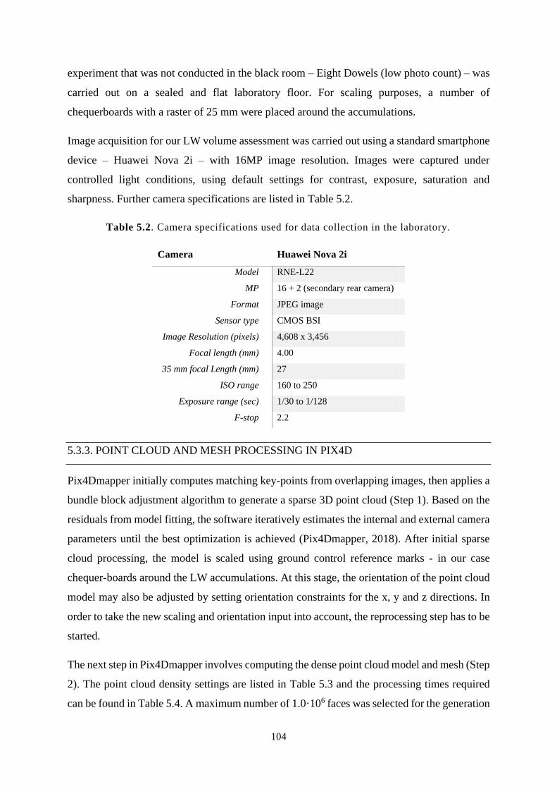
104
experiment that was not conducted in the black room – Eight Dowels (low photo count) – was
carried out on a sealed and flat laboratory floor. For scaling purposes, a number of
chequerboards with a raster of 25 mm were placed around the accumulations.
Image acquisition for our LW volume assessment was carried out using a standard smartphone
device – Huawei Nova 2i – with 16MP image resolution. Images were captured under
controlled light conditions, using default settings for contrast, exposure, saturation and
sharpness. Further camera specifications are listed in Table 5.2.
Table 5.2. Camera specifications used for data collection in the laboratory.
Camera Huawei Nova 2i
Model RNE-L22
MP 16 + 2 (secondary rear camera)
Format JPEG image
Sensor type CMOS BSI
Image Resolution (pixels) 4,608 x 3,456
Focal length (mm) 4.00
35 mm focal Length (mm) 27
ISO range 160 to 250
Exposure range (sec) 1/30 to 1/128
F-stop 2.2
5.3.3. POINT CLOUD AND MESH PROCESSING IN PIX4D
Pix4Dmapper initially computes matching key-points from overlapping images, then applies a
bundle block adjustment algorithm to generate a sparse 3D point cloud (Step 1). Based on the
residuals from model fitting, the software iteratively estimates the internal and external camera
parameters until the best optimization is achieved (Pix4Dmapper, 2018). After initial sparse
cloud processing, the model is scaled using ground control reference marks - in our case
chequer-boards around the LW accumulations. At this stage, the orientation of the point cloud
model may also be adjusted by setting orientation constraints for the x, y and z directions. In
order to take the new scaling and orientation input into account, the reprocessing step has to be
started.
The next step in Pix4Dmapper involves computing the dense point cloud model and mesh (Step
2). The point cloud density settings are listed in Table 5.3 and the processing times required
can be found in Table 5.4. A maximum number of 1.0·106 faces was selected for the generation
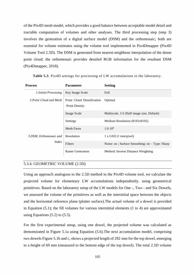
105
of the Pix4D mesh model, which provides a good balance between acceptable model detail and
tractable computation of volumes and other analyses. The third processing step (step 3)
involves the generation of a digital surface model (DSM) and the orthomosaic; both are
essential for volume estimates using the volume tool implemented in Pix4Dmapper (Pix4D
Volume Tool 2.5D). The DSM is generated from nearest-neighbour interpolation of the dense
point cloud; the orthomosaic provides detailed RGB information for the resultant DSM
(Pix4Dmapper, 2018).
Table 5.3. Pix4D settings for processing of LW accumulations in the laboratory.
Process Parameter Setting
1.Initial Processing Key Image Scale Full
2.Point Cloud and Mesh Point Cloud Densification
-Point Density
Optimal
Image Scale Multiscale, 1/2 (Half image size, Default)
Settings Medium Resolution (8192x8192)
Mesh Faces 1.0·106
3.DSM, Orthomosaic and
Index
Resolution 1 x GSD (1 mm/pixel)
Filters Noise: on ; Surface Smoothing: on – Type: Sharp
Raster Generation Method: Inverse Distance Weighting
5.3.4. GEOMETRIC VOLUME (2.5D)
Using an approach analogous to the 2.5D method in the Pix4D volume tool, we calculate the
projected volume for elementary LW accumulations independently, using geometrical
primitives. Based on the laboratory setup of the LW models for One -, Two - and Six Dowels,
we assessed the volume of the primitives as well as the interstitial space between the objects
and the horizontal reference plane (platter surface).The actual volume of a dowel is provided
in Equation (5.1); the fill volumes for various interstitial elements (1 to 4) are approximated
using Equations (5.2) to (5.5).
For the first experimental setup, using one dowel, the projected volume was calculated as
demonstrated in Figure 5.1a using Equation (5.6).The next accumulation model, comprising
two dowels Figure 5.1b and c, shows a projected length of 292 mm for the top dowel, emerging
to a height of 69 mm (measured to the bottom edge of the top dowel). The total 2.5D volume
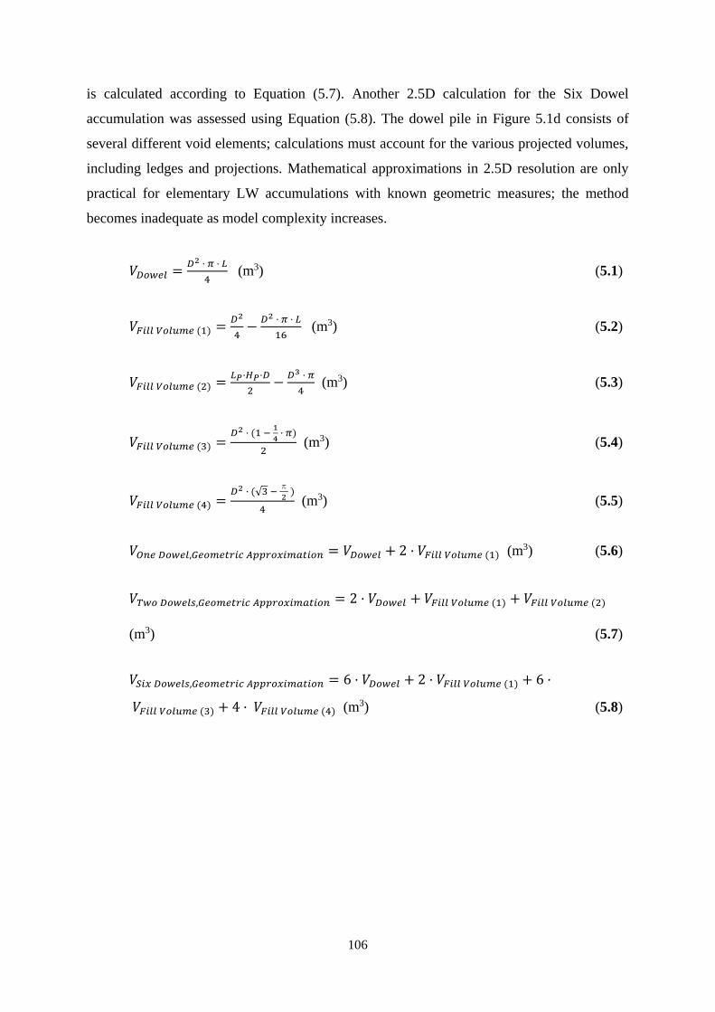
106
is calculated according to Equation (5.7). Another 2.5D calculation for the Six Dowel
accumulation was assessed using Equation (5.8). The dowel pile in Figure 5.1d consists of
several different void elements; calculations must account for the various projected volumes,
including ledges and projections. Mathematical approximations in 2.5D resolution are only
practical for elementary LW accumulations with known geometric measures; the method
becomes inadequate as model complexity increases.
𝑉𝐷𝑜𝑤𝑒𝑙 =𝐷2 · 𝜋 · 𝐿
4 (m3) (5.1)
𝑉𝐹𝑖𝑙𝑙 𝑉𝑜𝑙𝑢𝑚𝑒 (1) =𝐷2
4−
𝐷2 · 𝜋 · 𝐿
16 (m3) (5.2)
𝑉𝐹𝑖𝑙𝑙 𝑉𝑜𝑙𝑢𝑚𝑒 (2) =𝐿𝑃·𝐻𝑃·𝐷
2−
𝐷3 · 𝜋
4 (m3) (5.3)
𝑉𝐹𝑖𝑙𝑙 𝑉𝑜𝑙𝑢𝑚𝑒 (3) =𝐷2 · (1 −
1
4 · 𝜋)
2 (m3) (5.4)
𝑉𝐹𝑖𝑙𝑙 𝑉𝑜𝑙𝑢𝑚𝑒 (4) =𝐷2 · (√3 −
π
2 )
4 (m3) (5.5)
𝑉𝑂𝑛𝑒 𝐷𝑜𝑤𝑒𝑙,𝐺𝑒𝑜𝑚𝑒𝑡𝑟𝑖𝑐 𝐴𝑝𝑝𝑟𝑜𝑥𝑖𝑚𝑎𝑡𝑖𝑜𝑛 = 𝑉𝐷𝑜𝑤𝑒𝑙 + 2 · 𝑉𝐹𝑖𝑙𝑙 𝑉𝑜𝑙𝑢𝑚𝑒 (1) (m3) (5.6)
𝑉𝑇𝑤𝑜 𝐷𝑜𝑤𝑒𝑙𝑠,𝐺𝑒𝑜𝑚𝑒𝑡𝑟𝑖𝑐 𝐴𝑝𝑝𝑟𝑜𝑥𝑖𝑚𝑎𝑡𝑖𝑜𝑛 = 2 · 𝑉𝐷𝑜𝑤𝑒𝑙 + 𝑉𝐹𝑖𝑙𝑙 𝑉𝑜𝑙𝑢𝑚𝑒 (1) + 𝑉𝐹𝑖𝑙𝑙 𝑉𝑜𝑙𝑢𝑚𝑒 (2)
(m3) (5.7)
𝑉𝑆𝑖𝑥 𝐷𝑜𝑤𝑒𝑙𝑠,𝐺𝑒𝑜𝑚𝑒𝑡𝑟𝑖𝑐 𝐴𝑝𝑝𝑟𝑜𝑥𝑖𝑚𝑎𝑡𝑖𝑜𝑛 = 6 · 𝑉𝐷𝑜𝑤𝑒𝑙 + 2 · 𝑉𝐹𝑖𝑙𝑙 𝑉𝑜𝑙𝑢𝑚𝑒 (1) + 6 ·
𝑉𝐹𝑖𝑙𝑙 𝑉𝑜𝑙𝑢𝑚𝑒 (3) + 4 · 𝑉𝐹𝑖𝑙𝑙 𝑉𝑜𝑙𝑢𝑚𝑒 (4) (m3) (5.8)
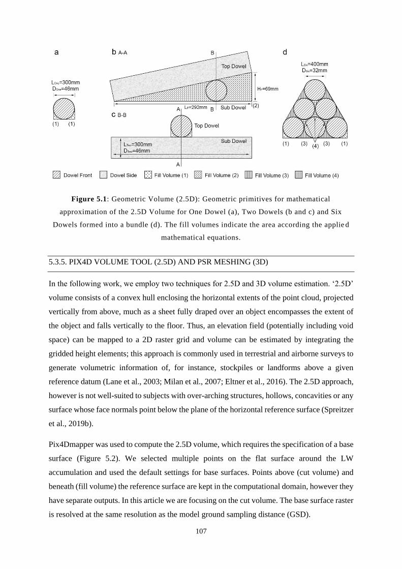
107
Figure 5.1: Geometric Volume (2.5D): Geometric primitives for mathematical
approximation of the 2.5D Volume for One Dowel (a), Two Dowels (b and c) and Six
Dowels formed into a bundle (d). The fill volumes indicate the area according the applie d
mathematical equations.
5.3.5. PIX4D VOLUME TOOL (2.5D) AND PSR MESHING (3D)
In the following work, we employ two techniques for 2.5D and 3D volume estimation. ‘2.5D’
volume consists of a convex hull enclosing the horizontal extents of the point cloud, projected
vertically from above, much as a sheet fully draped over an object encompasses the extent of
the object and falls vertically to the floor. Thus, an elevation field (potentially including void
space) can be mapped to a 2D raster grid and volume can be estimated by integrating the
gridded height elements; this approach is commonly used in terrestrial and airborne surveys to
generate volumetric information of, for instance, stockpiles or landforms above a given
reference datum (Lane et al., 2003; Milan et al., 2007; Eltner et al., 2016). The 2.5D approach,
however is not well-suited to subjects with over-arching structures, hollows, concavities or any
surface whose face normals point below the plane of the horizontal reference surface (Spreitzer
et al., 2019b).
Pix4Dmapper was used to compute the 2.5D volume, which requires the specification of a base
surface (Figure 5.2). We selected multiple points on the flat surface around the LW
accumulation and used the default settings for base surfaces. Points above (cut volume) and
beneath (fill volume) the reference surface are kept in the computational domain, however they
have separate outputs. In this article we are focusing on the cut volume. The base surface raster
is resolved at the same resolution as the model ground sampling distance (GSD).
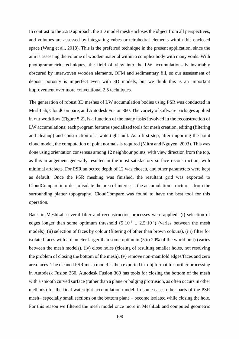
108
In contrast to the 2.5D approach, the 3D model mesh encloses the object from all perspectives,
and volumes are assessed by integrating cubes or tetrahedral elements within this enclosed
space (Wang et al., 2018). This is the preferred technique in the present application, since the
aim is assessing the volume of wooden material within a complex body with many voids. With
photogrammetric techniques, the field of view into the LW accumulations is invariably
obscured by interwoven wooden elements, OFM and sedimentary fill, so our assessment of
deposit porosity is imperfect even with 3D models, but we think this is an important
improvement over more conventional 2.5 techniques.
The generation of robust 3D meshes of LW accumulation bodies using PSR was conducted in
MeshLab, CloudCompare, and Autodesk Fusion 360. The variety of software packages applied
in our workflow (Figure 5.2), is a function of the many tasks involved in the reconstruction of
LW accumulations; each program features specialized tools for mesh creation, editing (filtering
and cleanup) and construction of a watertight hull. As a first step, after importing the point
cloud model, the computation of point normals is required (Mitra and Nguyen, 2003). This was
done using orientation consensus among 12 neighbour points, with view direction from the top,
as this arrangement generally resulted in the most satisfactory surface reconstruction, with
minimal artefacts. For PSR an octree depth of 12 was chosen, and other parameters were kept
as default. Once the PSR meshing was finished, the resultant grid was exported to
CloudCompare in order to isolate the area of interest – the accumulation structure – from the
surrounding platter topography. CloudCompare was found to have the best tool for this
operation.
Back in MeshLab several filter and reconstruction processes were applied; (i) selection of
edges longer than some optimum threshold (5·10-3 ± 2.5·10-4) (varies between the mesh
models), (ii) selection of faces by colour (filtering of other than brown colours), (iii) filter for
isolated faces with a diameter larger than some optimum (5 to 20% of the world unit) (varies
between the mesh models), (iv) close holes (closing of resulting smaller holes, not resolving
the problem of closing the bottom of the mesh), (v) remove non-manifold edges/faces and zero
area faces. The cleaned PSR mesh model is then exported in .obj format for further processing
in Autodesk Fusion 360. Autodesk Fusion 360 has tools for closing the bottom of the mesh
with a smooth curved surface (rather than a plane or bulging protrusion, as often occurs in other
methods) for the final watertight accumulation model. In some cases other parts of the PSR
mesh– especially small sections on the bottom plane – become isolated while closing the hole.
For this reason we filtered the mesh model once more in MeshLab and computed geometric
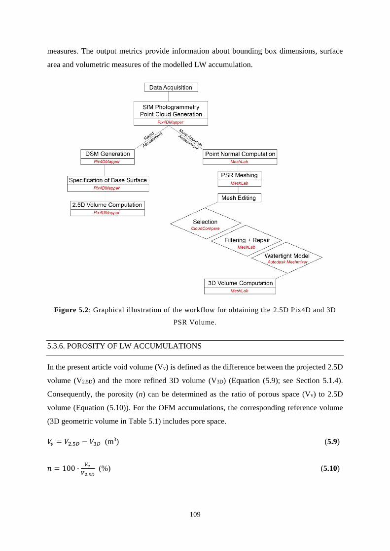
109
measures. The output metrics provide information about bounding box dimensions, surface
area and volumetric measures of the modelled LW accumulation.
Figure 5.2: Graphical illustration of the workflow for obtaining the 2.5D Pix4D and 3D
PSR Volume.
5.3.6. POROSITY OF LW ACCUMULATIONS
In the present article void volume (Vv) is defined as the difference between the projected 2.5D
volume (V2.5D) and the more refined 3D volume (V3D) (Equation (5.9); see Section 5.1.4).
Consequently, the porosity (n) can be determined as the ratio of porous space (Vv) to 2.5D
volume (Equation (5.10)). For the OFM accumulations, the corresponding reference volume
(3D geometric volume in Table 5.1) includes pore space.
𝑉𝑣 = 𝑉2.5𝐷 − 𝑉3𝐷 (m3) (5.9)
𝑛 = 100 ·𝑉𝑣
𝑉2.5𝐷 (%) (5.10)
110
5.4. RESULTS
5.4.1. POINT CLOUD AND MESH RESULTS
All of our laboratory LW accumulations resulted in high-resolution point cloud models, with
2.2·106 to 12.7 106 generated 3D points. The processing time in Pix4Dmapper for initial tie
point processing was between 10 minutes, for low image datasets, and 2.6 hours for datasets
with a higher number of images. Further point cloud processing times, including DSM and
orthomosaic generation, ranged from 30 minutes to 43 hours. Our 2.5D volume models,
computed and meshed in Pix4Dmapper, emerged with 1.0·106 faces, as per description in the
methodology (Section 5.3.3).
The 3D PSR algorithm generated between 2.6·106 to 15.2·106 faces, depending on the dowel
prototype complexity. Meshing the Eight Dowels (low image) point cloud required two
applications of the meshing process, in order to construct a watertight surface.
Table 5.4 provides an overview of point cloud and meshing results. Using PSR, the volumes
of elementary LW accumulations were computed (Figure 5.3a to f). The PSR operation, for the
elementary LW accumulations, only takes a few minutes in MeshLab. Processing times
increase slightly with more complex laboratory models (e.g. with OFM), however, the
maximum time required for PSR was one hour for the Eight Dowels (high photo count)
accumulation model. The final meshes are shown in Figure 5.3a to n, with the PSR model on
the left side and the corresponding water tight model on the right side.
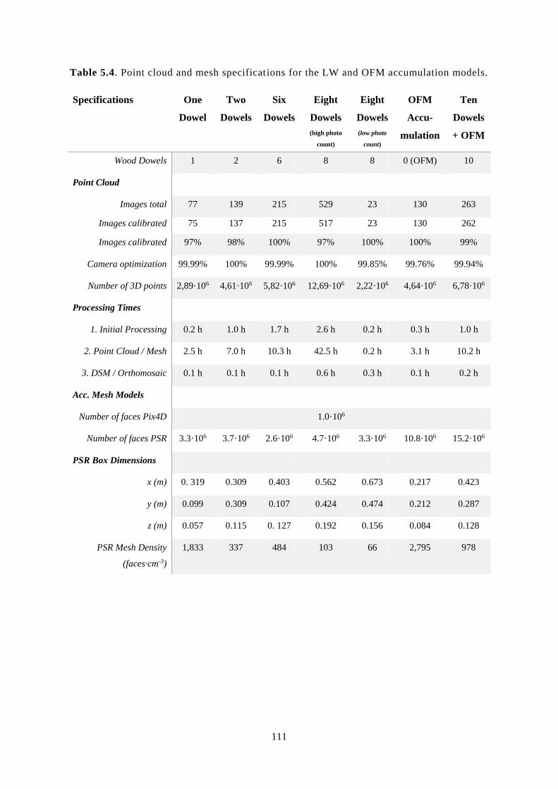
111
Table 5.4. Point cloud and mesh specifications for the LW and OFM accumulation models.
Specifications One
Dowel
Two
Dowels
Six
Dowels
Eight
Dowels
(high photo
count)
Eight
Dowels
(low photo
count)
OFM
Accu-
mulation
Ten
Dowels
+ OFM
Wood Dowels 1 2 6 8 8 0 (OFM) 10
Point Cloud
Images total 77 139 215 529 23 130 263
Images calibrated 75 137 215 517 23 130 262
Images calibrated 97% 98% 100% 97% 100% 100% 99%
Camera optimization 99.99% 100% 99.99% 100% 99.85% 99.76% 99.94%
Number of 3D points 2,89·106 4,61·106 5,82·106 12,69·106 2,22·106 4,64·106 6,78·106
Processing Times
1. Initial Processing 0.2 h 1.0 h 1.7 h 2.6 h 0.2 h 0.3 h 1.0 h
2. Point Cloud / Mesh 2.5 h 7.0 h 10.3 h 42.5 h 0.2 h 3.1 h 10.2 h
3. DSM / Orthomosaic 0.1 h 0.1 h 0.1 h 0.6 h 0.3 h 0.1 h 0.2 h
Acc. Mesh Models
Number of faces Pix4D 1.0·106
Number of faces PSR 3.3·106 3.7·106 2.6·106 4.7·106 3.3·106 10.8·106 15.2·106
PSR Box Dimensions
x (m) 0. 319 0.309 0.403 0.562 0.673 0.217 0.423
y (m) 0.099 0.309 0.107 0.424 0.474 0.212 0.287
z (m) 0.057 0.115 0. 127 0.192 0.156 0.084 0.128
PSR Mesh Density
(faces·cm-3)
1,833 337 484 103 66 2,795 978
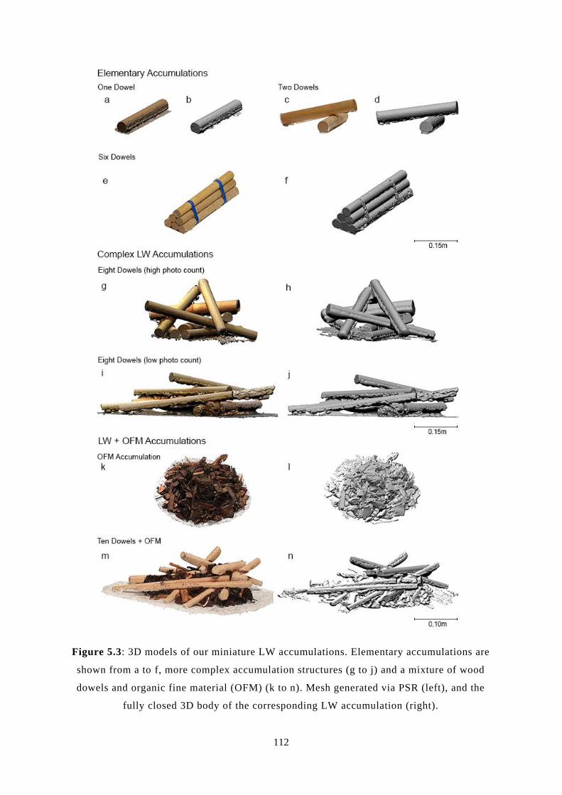
112
Figure 5.3: 3D models of our miniature LW accumulations. Elementary accumulations are
shown from a to f, more complex accumulation structures (g to j) and a mixture of wood
dowels and organic fine material (OFM) (k to n). Mesh generated via PSR (left), and the
fully closed 3D body of the corresponding LW accumulation (right).
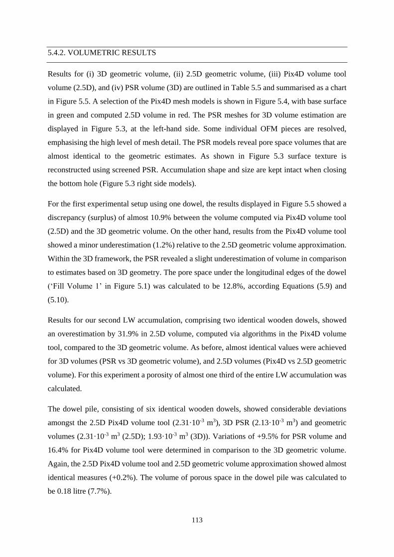
113
5.4.2. VOLUMETRIC RESULTS
Results for (i) 3D geometric volume, (ii) 2.5D geometric volume, (iii) Pix4D volume tool
volume (2.5D), and (iv) PSR volume (3D) are outlined in Table 5.5 and summarised as a chart
in Figure 5.5. A selection of the Pix4D mesh models is shown in Figure 5.4, with base surface
in green and computed 2.5D volume in red. The PSR meshes for 3D volume estimation are
displayed in Figure 5.3, at the left-hand side. Some individual OFM pieces are resolved,
emphasising the high level of mesh detail. The PSR models reveal pore space volumes that are
almost identical to the geometric estimates. As shown in Figure 5.3 surface texture is
reconstructed using screened PSR. Accumulation shape and size are kept intact when closing
the bottom hole (Figure 5.3 right side models).
For the first experimental setup using one dowel, the results displayed in Figure 5.5 showed a
discrepancy (surplus) of almost 10.9% between the volume computed via Pix4D volume tool
(2.5D) and the 3D geometric volume. On the other hand, results from the Pix4D volume tool
showed a minor underestimation (1.2%) relative to the 2.5D geometric volume approximation.
Within the 3D framework, the PSR revealed a slight underestimation of volume in comparison
to estimates based on 3D geometry. The pore space under the longitudinal edges of the dowel
(‘Fill Volume 1’ in Figure 5.1) was calculated to be 12.8%, according Equations (5.9) and
(5.10).
Results for our second LW accumulation, comprising two identical wooden dowels, showed
an overestimation by 31.9% in 2.5D volume, computed via algorithms in the Pix4D volume
tool, compared to the 3D geometric volume. As before, almost identical values were achieved
for 3D volumes (PSR vs 3D geometric volume), and 2.5D volumes (Pix4D vs 2.5D geometric
volume). For this experiment a porosity of almost one third of the entire LW accumulation was
calculated.
The dowel pile, consisting of six identical wooden dowels, showed considerable deviations
amongst the 2.5D Pix4D volume tool (2.31·10-3 m3), 3D PSR (2.13·10-3 m3) and geometric
volumes (2.31·10-3 m3 (2.5D); 1.93·10-3 m3 (3D)). Variations of +9.5% for PSR volume and
16.4% for Pix4D volume tool were determined in comparison to the 3D geometric volume.
Again, the 2.5D Pix4D volume tool and 2.5D geometric volume approximation showed almost
identical measures (+0.2%). The volume of porous space in the dowel pile was calculated to
be 0.18 litre (7.7%).
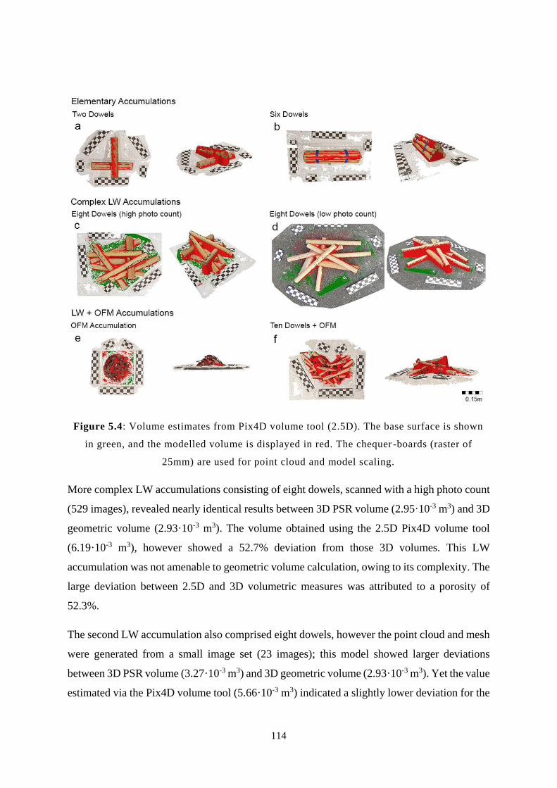
114
Figure 5.4: Volume estimates from Pix4D volume tool (2.5D). The base surface is shown
in green, and the modelled volume is displayed in red. The chequer -boards (raster of
25mm) are used for point cloud and model scaling.
More complex LW accumulations consisting of eight dowels, scanned with a high photo count
(529 images), revealed nearly identical results between 3D PSR volume (2.95·10-3 m3) and 3D
geometric volume (2.93·10-3 m3). The volume obtained using the 2.5D Pix4D volume tool
(6.19·10-3 m3), however showed a 52.7% deviation from those 3D volumes. This LW
accumulation was not amenable to geometric volume calculation, owing to its complexity. The
large deviation between 2.5D and 3D volumetric measures was attributed to a porosity of
52.3%.
The second LW accumulation also comprised eight dowels, however the point cloud and mesh
were generated from a small image set (23 images); this model showed larger deviations
between 3D PSR volume (3.27·10-3 m3) and 3D geometric volume (2.93·10-3 m3). Yet the value
estimated via the Pix4D volume tool (5.66·10-3 m3) indicated a slightly lower deviation for the
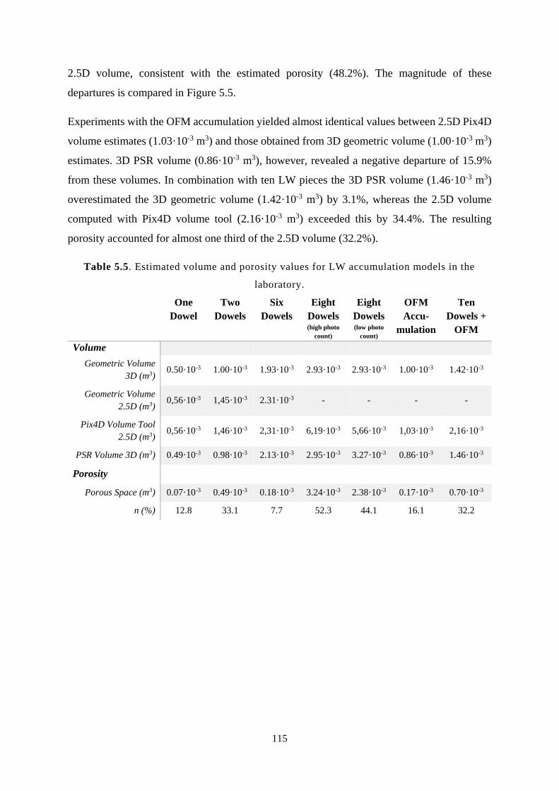
115
2.5D volume, consistent with the estimated porosity (48.2%). The magnitude of these
departures is compared in Figure 5.5.
Experiments with the OFM accumulation yielded almost identical values between 2.5D Pix4D
volume estimates (1.03·10-3 m3) and those obtained from 3D geometric volume (1.00·10-3 m3)
estimates. 3D PSR volume (0.86·10-3 m3), however, revealed a negative departure of 15.9%
from these volumes. In combination with ten LW pieces the 3D PSR volume (1.46·10-3 m3)
overestimated the 3D geometric volume (1.42·10-3 m3) by 3.1%, whereas the 2.5D volume
computed with Pix4D volume tool (2.16·10-3 m3) exceeded this by 34.4%. The resulting
porosity accounted for almost one third of the 2.5D volume (32.2%).
Table 5.5. Estimated volume and porosity values for LW accumulation models in the
laboratory.
One
Dowel
Two
Dowels
Six
Dowels
Eight
Dowels (high photo
count)
Eight
Dowels (low photo
count)
OFM
Accu-
mulation
Ten
Dowels +
OFM
Volume
Geometric Volume
3D (m3) 0.50·10-3 1.00·10-3 1.93·10-3 2.93·10-3 2.93·10-3 1.00·10-3 1.42·10-3
Geometric Volume
2.5D (m3) 0,56·10-3 1,45·10-3 2.31·10-3 - - - -
Pix4D Volume Tool
2.5D (m3) 0,56·10-3 1,46·10-3 2,31·10-3 6,19·10-3 5,66·10-3 1,03·10-3 2,16·10-3
PSR Volume 3D (m3) 0.49·10-3 0.98·10-3 2.13·10-3 2.95·10-3 3.27·10-3 0.86·10-3 1.46·10-3
Porosity
Porous Space (m3) 0.07·10-3 0.49·10-3 0.18·10-3 3.24·10-3 2.38·10-3 0.17·10-3 0.70·10-3
n (%) 12.8 33.1 7.7 52.3 44.1 16.1 32.2
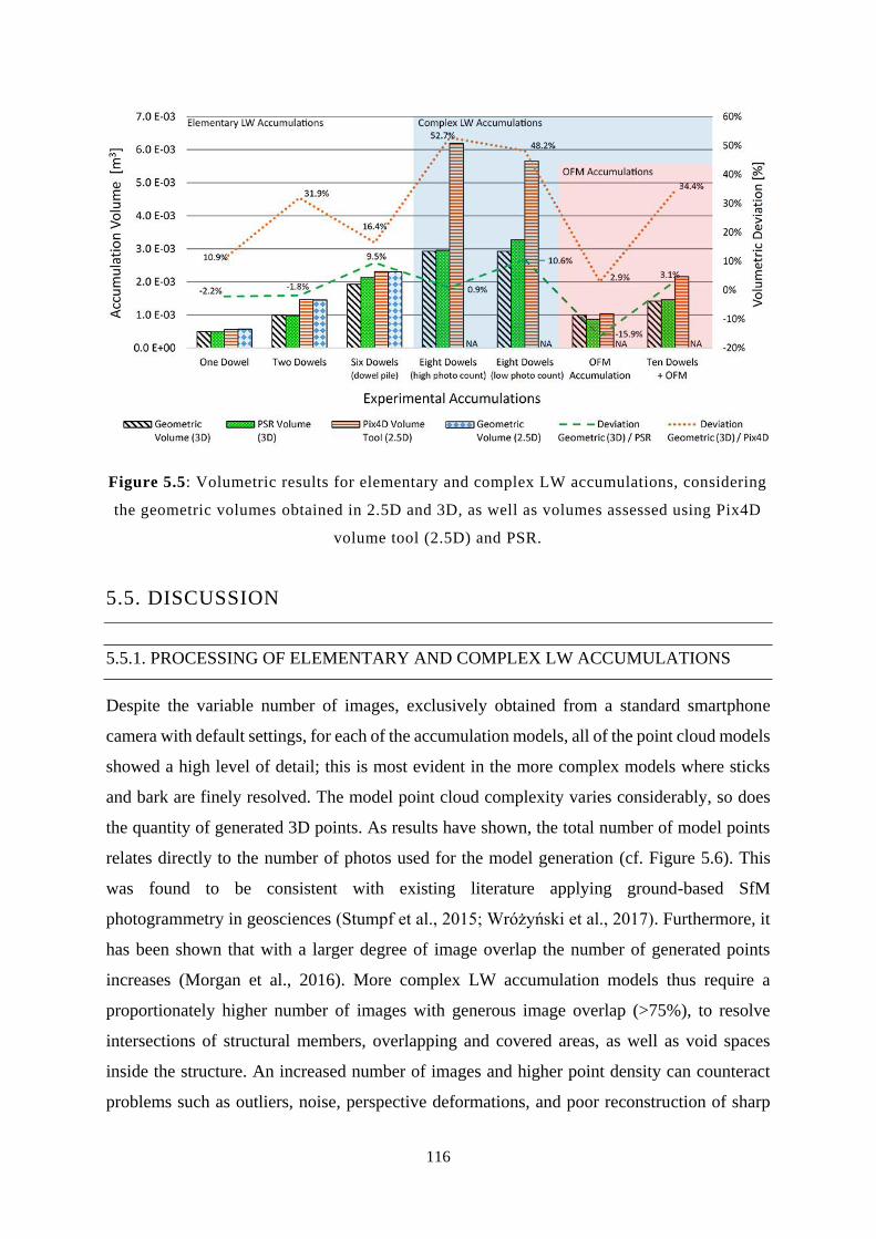
116
Figure 5.5: Volumetric results for elementary and complex LW accumulations, considering
the geometric volumes obtained in 2.5D and 3D, as well as volumes assessed using Pix4D
volume tool (2.5D) and PSR.
5.5. DISCUSSION
5.5.1. PROCESSING OF ELEMENTARY AND COMPLEX LW ACCUMULATIONS
Despite the variable number of images, exclusively obtained from a standard smartphone
camera with default settings, for each of the accumulation models, all of the point cloud models
showed a high level of detail; this is most evident in the more complex models where sticks
and bark are finely resolved. The model point cloud complexity varies considerably, so does
the quantity of generated 3D points. As results have shown, the total number of model points
relates directly to the number of photos used for the model generation (cf. Figure 5.6). This
was found to be consistent with existing literature applying ground-based SfM
photogrammetry in geosciences (Stumpf et al., 2015; Wróżyński et al., 2017). Furthermore, it
has been shown that with a larger degree of image overlap the number of generated points
increases (Morgan et al., 2016). More complex LW accumulation models thus require a
proportionately higher number of images with generous image overlap (>75%), to resolve
intersections of structural members, overlapping and covered areas, as well as void spaces
inside the structure. An increased number of images and higher point density can counteract
problems such as outliers, noise, perspective deformations, and poor reconstruction of sharp
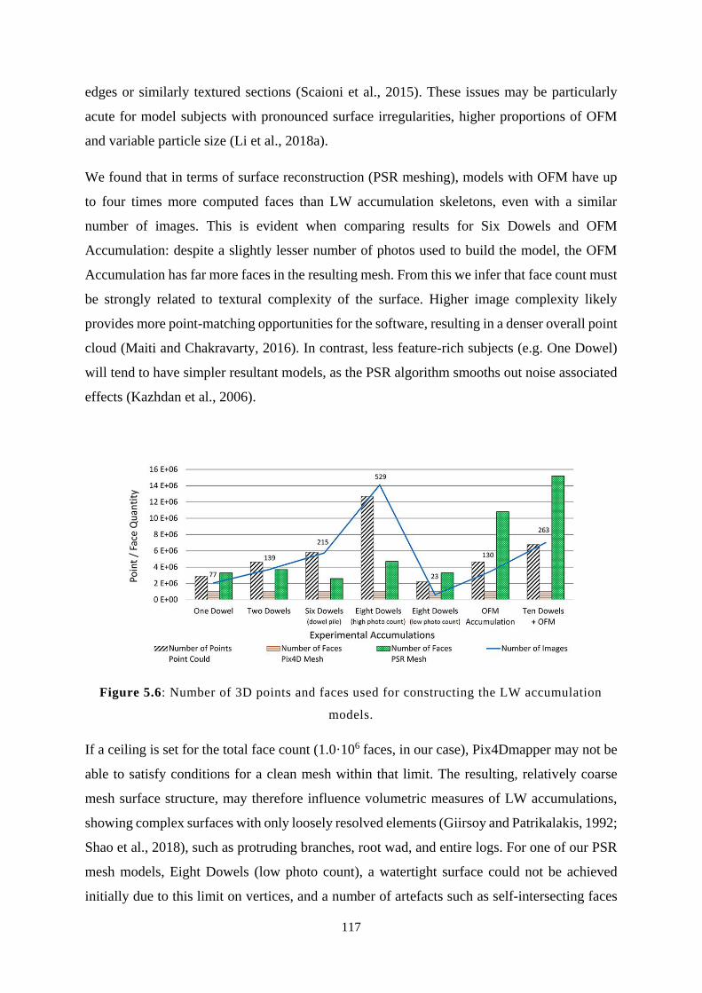
117
edges or similarly textured sections (Scaioni et al., 2015). These issues may be particularly
acute for model subjects with pronounced surface irregularities, higher proportions of OFM
and variable particle size (Li et al., 2018a).
We found that in terms of surface reconstruction (PSR meshing), models with OFM have up
to four times more computed faces than LW accumulation skeletons, even with a similar
number of images. This is evident when comparing results for Six Dowels and OFM
Accumulation: despite a slightly lesser number of photos used to build the model, the OFM
Accumulation has far more faces in the resulting mesh. From this we infer that face count must
be strongly related to textural complexity of the surface. Higher image complexity likely
provides more point-matching opportunities for the software, resulting in a denser overall point
cloud (Maiti and Chakravarty, 2016). In contrast, less feature-rich subjects (e.g. One Dowel)
will tend to have simpler resultant models, as the PSR algorithm smooths out noise associated
effects (Kazhdan et al., 2006).
Figure 5.6: Number of 3D points and faces used for constructing the LW accumulation
models.
If a ceiling is set for the total face count (1.0·106 faces, in our case), Pix4Dmapper may not be
able to satisfy conditions for a clean mesh within that limit. The resulting, relatively coarse
mesh surface structure, may therefore influence volumetric measures of LW accumulations,
showing complex surfaces with only loosely resolved elements (Giirsoy and Patrikalakis, 1992;
Shao et al., 2018), such as protruding branches, root wad, and entire logs. For one of our PSR
mesh models, Eight Dowels (low photo count), a watertight surface could not be achieved
initially due to this limit on vertices, and a number of artefacts such as self-intersecting faces
118
were evident. We resolved this issue by re-meshing the existing PSR mesh with the same initial
parameters and settings as were applied in the first instance for PSR in MeshLab, in order to
achieve a watertight surface covering the entire LW accumulation. The resulting accumulation
model (Figure 5.3h) shows less detail than the model that was generated on the basis of a very
high photo count (Figure 5.3j).
Results also reveal that processing times are proportional to the number of 3D points used for
densified point cloud generation (Table 5.4). However, we also found that the relatively long
processing times, which are required for densified point cloud generation using a high photo
count, resulted in better model reconstruction than those generated on a basis of a low photo
count. This means that there are compromises to be made between processing times, model
accuracy and field labour in the course of image acquisition. The software algorithm requires
relatively little operator intervention and can be scripted, to generate a great number of high
resolution, densified point cloud models. With available options of subsampling and
subdividing the point cloud, in order to better manage large data sets (Zhou and Chen, 2011;
Fan and Atkinson, 2019), the remaining editing and mesh processing times can be reduced
significantly, while maintaining surface details and mesh model quality (Tazir et al., 2016b;
Chen et al., 2017). The exact effects of subsampling and meshing of reduced LW
accumulations point cloud models, however require further research to be better understood.
5.5.2. POINT NORMALS
The orientation of point normals is particularly important for elementary accumulations, given
that there are fewer and larger faces available to represent the model topology. Reconstructing
the contours of occluded and obscured elements is a troublesome problem in computational
geometry (Hoppe et al., 1992; Mitra and Nguyen, 2003; Demarsin et al., 2007), as other results
from the PSR process highlight (Fuhrmann and Goesele, 2011; Lobos and Rojas-Moraleda,
2013; Wolff et al., 2016; Sheng et al., 2018). As can be seen in Figure 5.3h, i and j, a convex
hull is generated at the bottom (occluded) side of individual LW pieces, which is a common
effect when working with PSR, due to the inconsistent off-surface constraints (Mostegel and
Rumpler, 2012; Berger et al., 2017; Guerrero et al., 2018). Ideally, all of the surface normals
of each dowel would be neatly directed outward from the central axis. Fixing this problem is
very time- and memory-consuming, and prone to producing unreliable data and failed
convergence of mesh generation routines. The parameters contributing to the challenge are
various (Vosselman et al., 2004), such as orientation of the cylinder axis or the detection of a
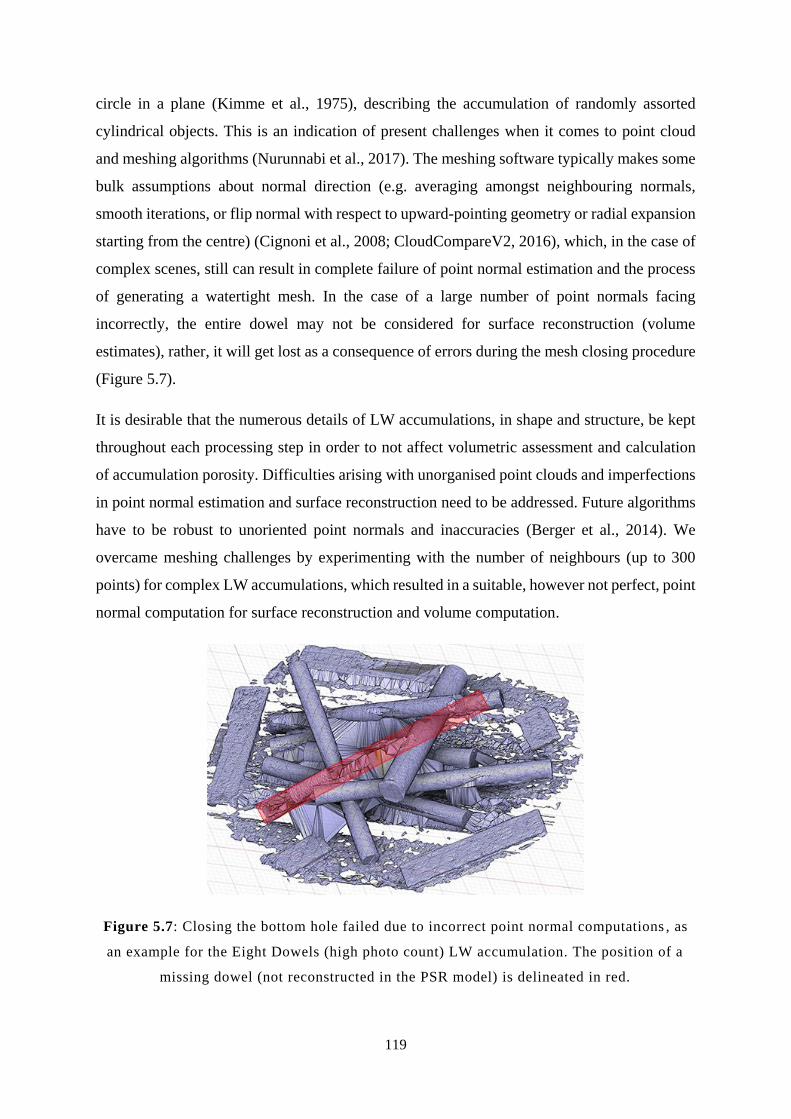
119
circle in a plane (Kimme et al., 1975), describing the accumulation of randomly assorted
cylindrical objects. This is an indication of present challenges when it comes to point cloud
and meshing algorithms (Nurunnabi et al., 2017). The meshing software typically makes some
bulk assumptions about normal direction (e.g. averaging amongst neighbouring normals,
smooth iterations, or flip normal with respect to upward-pointing geometry or radial expansion
starting from the centre) (Cignoni et al., 2008; CloudCompareV2, 2016), which, in the case of
complex scenes, still can result in complete failure of point normal estimation and the process
of generating a watertight mesh. In the case of a large number of point normals facing
incorrectly, the entire dowel may not be considered for surface reconstruction (volume
estimates), rather, it will get lost as a consequence of errors during the mesh closing procedure
(Figure 5.7).
It is desirable that the numerous details of LW accumulations, in shape and structure, be kept
throughout each processing step in order to not affect volumetric assessment and calculation
of accumulation porosity. Difficulties arising with unorganised point clouds and imperfections
in point normal estimation and surface reconstruction need to be addressed. Future algorithms
have to be robust to unoriented point normals and inaccuracies (Berger et al., 2014). We
overcame meshing challenges by experimenting with the number of neighbours (up to 300
points) for complex LW accumulations, which resulted in a suitable, however not perfect, point
normal computation for surface reconstruction and volume computation.
Figure 5.7: Closing the bottom hole failed due to incorrect point normal computations , as
an example for the Eight Dowels (high photo count) LW accumulation. The position of a
missing dowel (not reconstructed in the PSR model) is delineated in red.

120
5.5.3. VOLUMETRIC COMPUTATIONS
We have demonstrated that 2.5D computations using the Pix4D volume tool perform as
expected – the models are consistent with our geometric estimations of the 2.5D models, all
within a range of ±1.2% volume deviation (Table 5.5). Overall, the 2.5D model from
photogrammetry, such as also applied in the field (Spreitzer et al., 2019b), is more convenient
to develop than a watertight 3D mesh, which requires several software packages, as well as
advanced skills in point cloud and mesh editing. Thus, from the perspective of rapid assessment
of LW volume, it may be reasonable to accept errors inherent in this approximation, and
quantify 2.5D volume by using a standalone SfM photogrammetry software kit, such as
Pix4Dmapper. Yet, there is a variety of SfM photogrammetry toolboxes available, freely
(Astre, 2015; VisualSFM, 2018) or commercially, such as Agisoft LLC Russia (2018) and
Autodesk ReCap (2019).
If more precision is needed, particularly when dealing with significant deposit complexity
showing overarching structures, void spaces and protruding elements, it may be worth the
additional effort to develop a fully 3D-resolved model, such as suggested in this study. In our
experience, the PSR meshing algorithm followed by a mesh closing procedure provided the
best surface reconstruction and volume estimates, as has also been demonstrated in the course
of previously conducted studies (Kaiser et al., 2014; Carrivick et al., 2016; Gupta and Shukla,
2017). Considering the employment of the presented 3D SfM photogrammetry approach for
field applications, special attention must be paid at a stage of closing the bottom of the mesh,
which requires a basal surface that matches field conditions with a similar shape such as applied
for the 2.5D Pix4D approach.
Relative to the 3D geometric models, the 3D PSR volumes are overestimated by a maximum
of 10.6% for elementary and complex LW accumulations, all showing accumulation skeletons.
In the case of large amounts of OFM filling some of the void spaces inside the accumulation
skeletons, as demonstrated with experiments using OFM accumulations in Figure 5.3(k to n),
negative discrepancies of up to 15.9% were found (3D PSR mesh resulted in lower values).
This underestimation is likely related to the complex surface structure of the organic material.
The digital mesh surface conforms more closely to the fibrous mass than could be captured
during measurement using a glass measurement cylinder, when 1 litre of OFM was prepared
(c.f. OFM Accumulation and Ten Dowels + OFM in Section 2). While void spaces between
glass cylinder wall and the OFM have been accounted for in the 3D geometric model, the 3D
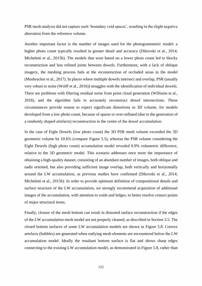
121
PSR mesh analysis did not capture such ‘boundary void spaces’, resulting in the slight negative
aberration from the reference volume.
Another important factor is the number of images used for the photogrammetric model: a
higher photo count typically resulted in greater detail and accuracy (Dikovski et al., 2014;
Micheletti et al., 2015b). The models that were based on a lower photo count led to blocky
reconstruction and less refined joints between dowels. Furthermore, with a lack of oblique
imagery, the meshing process fails at the reconstruction of occluded areas in the model
(Mosbrucker et al., 2017). In places where multiple dowels intersect and overlap, PSR (usually
very robust to noise (Wolff et al., 2016)) struggles with the identification of individual dowels.
There are problems with filtering residual noise from point cloud generation (Williams et al.,
2018), and the algorithm fails to accurately reconstruct dowel intersections. These
circumstances provide reason to expect significant distortions in 3D volume, for models
developed from a low photo count, because of sparse or over-inflated (due to the generation of
a randomly shaped artefacts) reconstruction in the centre of the dowel accumulation.
In the case of Eight Dowels (low photo count) the 3D PSR mesh volume exceeded the 3D
geometric volume by 10.6% (compare Figure 5.5), whereas the PSR volume considering the
Eight Dowels (high photo count) accumulation model revealed 0.9% volumetric difference,
relative to the 3D geometric model. This scenario addresses once more the importance of
obtaining a high-quality dataset, consisting of an abundant number of images, both oblique and
nadir oriented, but also providing sufficient image overlap, both vertically and horizontally
around the LW accumulation, as previous studies have confirmed (Dikovski et al., 2014;
Micheletti et al., 2015b). In order to provide optimum definition of compositional details and
surface structure of the LW accumulation, we strongly recommend acquisition of additional
images of the accumulation, with attention to voids and ledges, to better resolve contact points
of major structural items.
Finally, closure of the mesh bottom can result in distorted surface reconstruction if the edges
of the LW accumulation mesh model are not properly cleaned, as described in Section 3.5. The
closed bottom surfaces of some LW accumulation models are shown in Figure 5.8. Convex
artefacts (bubbles) are generated when outlying mesh elements are encountered below the LW
accumulation model. Ideally the resultant bottom surface is flat and shows sharp edges
connecting to the existing LW accumulation model, as demonstrated in Figure 5.8, rather than
122
bulged corners that distort the actual accumulation volume. Cleaning the mesh model is
therefore essential and enables the computation of realistic LW volumes from the 3D models.
Achieving a closed mesh is essential for 3D volume estimations, and we have yet to find a
satisfactory open-source software solution for this operation. Alternatively, we were able to
accomplish this rapidly, with few artefacts, in Autodesk Fusion 360.
Figure 5.8: Reconstructed water tight 3D PSR mesh models of our miniature LW
accumulations. For Two Dowels (a), Six Dowels formed into a pile (b), Eight Dowels (low
photo count) (c) and Ten Dowels + OFM (d).
5.5.4. LW ACCUMULATION POROSITY
LW accumulation porosity (n) is defined as the ratio of void volume to bulk volume (Pagliara
and Carnacina, 2010). For porosity estimates of our LW accumulation models in the laboratory,
we applied the 2.5D volume results from the Pix4D volume tool as the bulk volume, and the
3D PSR volume as solid volume, according to Equations (5.9) and (5.10) (see Section 5.1.4).
Results for accumulation porosity vary in a range of 7.7 to 52.3% (Table 5.5). The accuracy of
this technique is limited by the scale of investigation; with larger accumulations, it becomes
increasingly difficult to capture interior interstices and evaluate an aspect ratio (e.g. length,
diameter) as well as the packing matrix of structural elements and OFM. However, it provides
a good approximation and would be useful for first-order assessment of porosity characteristics
across a population of LW deposits, both in the field as well as in the laboratory. Our porosity
estimation approach has great potential for field applications and the improvement of recent
SfM photogrammetry studies (Sanhueza et al., 2019a; Spreitzer et al., 2019b), as there are no
visual estimates or manual calculations involved (such as a parallelepiped approach (Boivin et
al., 2015; Livers et al., 2015; Scott et al., 2019), and the introduced 3D approach is a major
123
advance for the development of semi-automated and automated methods, which allow for
accurate LW accumulation volume and porosity assessment. The porosity results correspond
to expected values, ranging from 30 – 50% (Dixon, 2016).
Additional information provided by SfM photogrammetry; e.g. colour information (Orru et al.,
2016), can significantly contribute to resolving accumulation structure and jam porosity. The
CANUPO plugin in CloudCompareV2 (2016) can be leveraged for automated identification
and classification of point values, which works similar to classifiers for land cover mapping
(Waske and Braun, 2009; Rodriguez-Galiano et al., 2012), and objects within a scene
(Yousefhussien et al., 2018). Furthermore, previously developed reconstruction algorithms of
tree and plant parts (Raumonen et al., 2013; Hackenberg et al., 2015), may be particularly
helpful for skeletonisation of LW accumulations, based on progressive simplification of the
geometry of structural members (Yrttimaa et al., 2019). Jacobson et al. (2013) developed a
robust method, which uses surface texture to reconstruct a tree skeleton. This will be of major
importance for future applications dealing with aspect ratios (packing matrix) (Zhang et al.,
2006), roughness parameters (e.g. sediment and flow retention) (Bocchiola et al., 2002;
Pagliara and Carnacina, 2010), obtained via SfM photogrammetry (Bretar et al., 2013; Verma
and Bourke, 2019). This paths the way for using LW accumulations, showing most realistic
features, in computer aided 2D (Ruiz-Villanueva et al., 2014a; Costabile and Macchione, 2015;
Ventres-Pake et al., 2019) and 3D (Smith et al., 2011; Allen and Smith, 2012; Lai, 2016)
modelling.
5.6. CONCLUSIONS AND OUTLOOK
Here we have demonstrated that both detailed ‘2.5D’ volume surfaces and ‘3D’ volumetric
meshes can be generated in order to assess the volume of a scaled LW accumulation in a
laboratory setting. As drone- or ground-based photogrammetric techniques are becoming
increasingly popular to quantify and model LW formations in river systems, it is important to
understand the potential and limitations of the technology. While SfM photogrammetry on
small and accessible wooden accumulations can be easily applied by means of exclusively
ground-based datasets, a combination of low altitude aerial flights (e.g. drone) and ground-
based mapping (where accessible) is suggested to better resolve 3D models of larger and more
complex LW accumulations in the field. Therefore, a better understanding of merged datasets
is required. Solutions to the essential problem of rendering volumetric models of constitutional
124
elements within LW accumulations from unorganized point clouds remain elusive, yet we have
shown how critical advances can be exploited.
The comparison of simple models from the Pix4D volume tool (2.5D) and the PSR (3D)
algorithm in MeshLab – relative to geometrically determined benchmarks - revealed that the
3D approach using PSR provided the most accurate results for LW accumulation assessment.
The 2.5D models consistently overestimated the volume, by an average of 28.2%; the 3D
models deviated by 6.3% (absolute) on average, with a mix of over- and under-estimation.
Overestimation of accumulation volumes was expected from 2.5D models, as they include
interstitial space within the accumulation. We found that for an accurate generation of a 3D
mesh model, a higher number of oblique and nadir images is required, than for conventional
2.5D mesh models. Occluded geometry in the models introduced the problem of mesh closure;
software algorithms must estimate this closure in sparse regions of the point cloud, often
resulting in strong distortions of the resultant volume model.
Using the difference between the 2.5D and 3D volumes as a measure of deposit void space, the
introduced methodology provides a consistent and objective measure for assessing void space
in the field. Our results showed void proportions of 7.7 to 52.3%; these measurements showed
good consistency with the results based on consideration of geometric primitive models of void
space.
We successfully computed high quality 3D models of miniature LW structures along with
OFM, in a controlled laboratory environment, and extracted precise accumulation volumes for
the first time. Our results demonstrated the capability of this SfM methodology, which provides
major advances for LW accumulation assessment in the field as well as in the laboratory. This
may be of further fundamental importance for prototype accumulation models (2D, 2.5D and
3D) in hydraulic engineering using numerical modelling. For instance, mesh generation
techniques will be useful for the estimation of obstructed cross-sectional area of LW
accumulations and surface roughness, which affect hydraulic flow behaviour and backwater
effects, respectively.
Some challenges arise for future work, including (i) properly resolving intersecting elements,
especially in the accumulation centre, (ii) mesh closure processes, without losing important
surface details, and (iii) assessing the effects of point sub-sampling on model quality, in order
to deploy SfM photogrammetry as an effective surveying tool. Thus, progress in point cloud
processing, editing and meshing algorithms is imperative, in order to generate more reliable
125
and robust models. The workflow should be able to counter problems with rendering mesh
(e.g. noise reduction, correct point normal estimation), resolving surface texture (e.g. mesh
closing, recognition of void spaces) and mitigating environmental noise (e.g. shades,
reflections, water surfaces), using standard camera devices such as smartphones or action
cameras.
This workflow will contribute to a better understanding of LW accumulations in fluvial
environments by providing parameters for accumulation volume and porosity, which are
known to affect channel hydraulics and bedload processes. Such indicators can facilitate
hydraulic studies and help to better assess LW accumulations in rivers. Apart from volume and
porosity estimates, our method can provide significant information about constitutional
materials of the accumulation, surface structure (roughness elements), log alignment and
geometries, which are all crucial parameters for studying formation processes of LW
accumulations. This understanding will allow for the identification of critical ‘key-logs’, which
are responsible for jam initiation, computation of the resulting hydraulic discharge behaviour,
and estimation of the effects on channel morphology in the presence of LW accumulations.

126
127
POROSITY AND VOLUME ASSESSMENTS OF LARGE
WOOD (LW) ACCUMULATIOS
Related journal article:
Spreitzer, G., Tunnicliffe, J. & Friedrich, F. 2019. Porosity and volume assessments of large
wood (LW) accumulations. Geomorphology 358. doi: 10.1016/j.geomorph.2020.107122
6.1. INTRODUCTION
6.1.1. LARGE WOOD (LW) ACCUMULATIONS IN RIVERS
Management concerns regarding large wood (LW) in rivers are raised more frequently in New
Zealand (Cave et al., 2017; Phillips et al., 2018) and other parts in the world (Ruiz-Villanueva
et al., 2019), especially in steep forested catchments, where in-stream wood may exhibit
dynamic transport and accumulation processes during floods (Naiman et al., 2002; Comiti et
al., 2016; Spreitzer et al., 2019a). While abundance of LW in stream systems is a natural
component of fluvial habitats and ecosystems (Wohl et al., 2016), exceptionally high rates of
in-stream wood, which is often produced by natural disasters (e.g. wind through, fires, snow
avalanches, landslides) or forestry activities, poses a hazard for river crossing infrastructure
(Piegay et al., 1999; Lassettre and Kondolf, 2012; Schmocker and Weitbrecht, 2013), and
human populations as a consequence of obstructed infrastructure (Mazzorana et al., 2011;
Comiti et al., 2016; Gschnitzer et al., 2017). Once LW enters the channel, it may be mobilised
and transported downstream, strongly depending on log geometries in relation to flow depth
(Bilby and Ward, 1989; Abbe et al., 1993). Often the transported LW ends up in an
accumulation together with smaller organic fine material (OFM) and sediments, showing a
broad range of packing ratios inside the accumulation matrix (porosity). Previous research has
128
shown that LW accumulation formation and frequency is strongly influenced by channel width,
log diameter, log length, forest type and age (Likens and Bilby, 1982; Gregory et al., 1993;
Gurnell et al., 2002; Abbe and Montgomery, 2003; Warren et al., 2009).
Flow magnitude (Ruiz-Villanueva et al., 2016c) and channel obstructions at constricted cross-
sections, such as at bridge piers (Rusyda, 2015; Panici and de Almeida, 2018), standing
vegetation (Gurnell et al., 2002; Bertoldi et al., 2013; Bertoldi et al., 2015), and already existing
LW formations in the channel (Abbe and Montgomery, 1996; Welber et al., 2013; Bertoldi et
al., 2014), are assumed to be dominant factors for the formation of LW jams, besides the
available quantity of LW (Keller and Swanson, 1979) and its transport regime (e.g.
uncongested, congested and hypercongested (Braudrick et al., 1997; Ruiz-Villanueva et al.,
2019)). Depending on the packing matrix, LW accumulations are posing high risk to redirect
flow as ‘deflector jams’ (Abbe and Montgomery, 2003; Lassettre and Kondolf, 2012),
reshaping of channel-bed topography, including scouring processes beneath an accumulation
(Melville and Dongol, 1992; Schalko et al., 2019b) and sedimentation in the upstream reach of
the obstruction (Marston, 1982; Mao et al., 2008; Spreitzer et al., 2018; Spreitzer et al., 2020
in Review). Beyond a certain threshold of channel obstruction and inter-weaving of woody
elements, detectable backwater effects begin to occur. The effects of LW accumulations on
backwater buildup have been studied (Hartlieb, 2017; Schalko et al., 2019a), yet variations in
composition and proportion of retained materials, as well as accumulation porosity, are difficult
to quantify for existing LW obstructions. Previous studies found that backwater effects develop
as a consequence of stream power reduction (Knauss, 1995; Ruiz-Villanueva et al., 2016b),
conveyance loss (Gippel et al., 1996; Gschnitzer et al., 2017) and roughness of LW (Maser et
al., 1988; Buffington and Montgomery, 1999). However, interstitial space inside an
accumulation body has to be accounted for, as well, and this can change due to dynamic forces
(e.g. compression and relaxation) and clogging processes with additional retained materials
(Livers et al., 2015). In general, four types of LW accumulations have been identified
(Wallerstein et al., 1997), each showing variation in composition and packing matrix that affect
flow hydraulics and channel morphology. Accumulation porosity is an important parameter for
the assessment of jam formations, from monitoring to modelling (Manners et al., 2007; Boivin
and Buffin-Bélanger, 2010), and varies significantly across studies. While a few studies have
estimated log jam porosity to be in a range of 13 to 90% (Thevenet et al., 1998; Sanhueza et
al., 2019a), most studies revealed porosity parameters between 25 and 70% (Livers et al., 2015;
Dixon, 2016). Log geometry governs porosity of accumulation skeletons, while the packing
129
matrix varies with the aspect ratio (e.g. diameter / length) of the structural members (Zhang et
al., 2006; Li et al., 2010).
Depending on moisture content density, and age of wooden pieces (Ruiz-Villanueva et al.,
2016a), an entire LW accumulation can float during flood events, while settling and changing
its structure with decreasing water level. Both scenarios, floating as well as settled LW
accumulations, may affect flow and channel morphology for each of the flow regimes, as LW
accumulation porosity changes. Investigations into log retention and jam formation at bridge
piers and decks have revealed important insights into accumulation processes (Diehl, 1997;
Gschnitzer et al., 2017; De Cicco et al., 2018; Panici and de Almeida, 2018). A laboratory
study conducted by Schalko et al. (2019b) in particular demonstrates the effects of a floating
dowel accumulation on scour development at a LW retention rack. However, there is still
limited understanding of the characteristic packing arrangements for a given LW structure (e.g.
compactness (ratio of solid matter to the bulk volume), porosity (ratio of void volume to the
bulk volume)), especially in the presence of high drag resistance (peak discharge) and during
the relaxation phase at the recession limb of a hydrograph. Estimating LW accumulation
porosity is challenging, as precise information about accumulation volumes is required.
6.1.2. MAPPING OF LW ACCUMULATIONS
Although the importance and need for volumetric measures of LW accumulations have been
frequently addressed in literature (Harmon et al., 1986; Lienkaemper and Swanson, 1987;
Gurnell et al., 2002; Webb and Erskine, 2003; Manners and Doyle, 2008; Dixon and Sear,
2014; Wohl and Scott, 2017; Martin et al., 2018), accurate assessment methods available for
the estimation of LW volume and accumulation porosity, are limited to date (Spreitzer et al.,
2019b). Conventional volumetric methods often consider manually obtained measurements of
individual logs (Cordova et al., 2006; Andreoli et al., 2007; Manners et al., 2007; Brown et al.,
2014; Dixon and Sear, 2014; Tonon et al., 2018), or entire accumulations by means of a
‘rectangular’ approach, measuring the bounding-box of the accumulation body in form of a
parallelepiped (Thevenet et al., 1998; Andreoli et al., 2007; Boivin et al., 2015). These methods
provide an initial, rough estimation of bulk volume, yet they are not effective for complex log
formations, nor applicable and safe for accumulations in rugged environments or non-wadable
streams. Airborne surveys, via light aircraft or unmanned aerial vehicle (UAV) (Casado et al.,
2015; Rusnák et al., 2018), present a highly advantageous platform for surveying with high
130
resolution image sensors or LiDAR systems (Rusnák et al., 2018; Sanhueza et al., 2019a); this
approach has become more popular and affordable in recent years.
UAV-based photogrammetry provides great potential for mapping of LW accumulations, yet
the resolution has to be sufficiently detailed to resolve individual LW pieces in the point cloud
model (Spreitzer et al., 2019b), and distinguish between gravel and wood particles of similar
optical characteristics (Colvard, 1998; Wright et al., 2000). A variety of volumetric techniques
are available to progress from a high-density point cloud to a volumetric mesh model. By
generating the convex hull of the points, it is possible to estimate the volume by voxel
techniques (Moskal and Zheng, 2011; Hosoi et al., 2013) or other geometric estimation
methods, such as cutting the object into thin slices along the z-axis (Chang et al., 2017), and
‘2.5D’ volumetric techniques, which are based on the vertical projection of the convex hull of
the point clouds onto a 2D raster grid (Remondino, 2003; Sanhueza et al., 2019a). The
relationship between 2.5D models, 3D meshes, and the true geometric volume of the wood
deposit is difficult to assess, particularly for overarching geometries and complex 3D forms.
As the size of the accumulation grows, relative to stem diameter and length, there is a
proportional increase in the volume of ‘occluded’ material that cannot be determined from
topographic surveys.
Mapping of LW accumulations, including volumetric assessment and porosity estimates, is
challenging due to the complex nature of jam formations, typically comprising a LW skeleton
(Manners and Doyle, 2008), and void spaces which can be empty or filled with OFM and
sediments (Thevenet et al., 1998; Linstead, 2001). Therefore a robust image-based
methodology, leading to a high quality point cloud model, will provide a high level of detail in
surface texture and geometries (Westoby et al., 2012; Dikovski et al., 2014; Micheletti et al.,
2015b), and can significantly increase the success rate of Structure from Motion (SfM)
photogrammetry for LW applications. A high-quality model will provide accurate
accumulation volume and porosity estimates.
High variability in surface texture and geometry is beneficial for SfM photogrammetry point-
matching algorithms (Maiti and Chakravarty, 2016). However, complex geometries (e.g.
multiple intersections of individual elements, or protruding logs and branches) can also cause
the reconstruction algorithm to fail (Spreitzer et al., 2019b). A rich variety of surface textures
(e.g. grass, sediment, wood) is advantageous for LW accumulation mapping, as colour filtering
can be used to classify components of the accumulation. Orru et al. (2016) used colour
131
segmentation from surface texture to gain information about spatial and temporal changes in
relative proportions of sand and gravel particles in a flume study. Furthermore, contrasting
surface textures can help to reveal void volume within the accumulation, where observable
from the surface (Glasbey et al., 1991; Anovitz and Cole, 2015). Methods to determine area
and volume of voids have previously been established in the field of crystalline materials
(Turner et al., 2011). Attempts to estimate porosity of soil samples have employed SfM
photogrammetry, geometrical models, and water displacement methods, however, further
innovations are required to achieve a more reliable outcome (Seitz et al., 2018).
Recent advances in survey technologies have allowed researchers to capture topographic
details quickly, safely and with remarkable accuracy and resolution. New survey techniques,
such as LiDAR and SfM, make it possible to resolve LW accumulations with spatial resolutions
in the range of 150 points/m2 to 1 point/mm2 (Boivin and Buffin-Bélanger, 2010; Tonon et al.,
2014; Grigillo et al., 2015). SfM has been demonstrated to deliver point-cloud accuracy that is
roughly similar to that of LiDAR (Mancini et al., 2013; Kaiser et al., 2014; Ružić et al., 2014),
at a much lower cost, although it is not able to penetrate leafy vegetation and tree canopy in
the way that LiDAR does.
6.1.3. OBJECTIVES
Our aim is to assess the volumetric characteristics of relatively coarse LW accumulations that
consist mainly of large structural members. By forming woody deposits in a flume
environment, we can reproduce the packing arrangement of natural, water-worked structures,
albeit with only the major ‘skeletal’ elements and none of the finer organic detritus. By
comparing three volume estimation approaches, we can assess the magnitude of ‘occluded
geometry’ within the core of complex accumulation models, which is beyond the reach of
lasers and optical sensors. Assessing the porosity of LW accumulations is important for in-
stream wood inventories, as well as assessing the hydraulic characteristics of channel-spanning
structures. Less porous structures reduce river flow capacity, leading to backwater effects
(overbank flooding) and flow diversion towards banks.
We present a solid SfM photogrammetry workflow, such as recently introduced in the course
of a laboratory study, using manually assembled miniature log piles for volume and porosity
estimates (Spreitzer et al., 2020), that can significantly contribute to an improved assessment
strategy of LW accumulation volume, porosity as well as wood characteristics, which have
132
been identified as important research goals for future LW projects by Pagliara and Carnacina
(2010) and Gschnitzer et al. (2017). In the present study, we increased model complexity by
using water worked LW accumulations in a flume setup and assessed log jam volume and
porosity from aerial-like imagery exclusively. Furthermore, we identify and reconstruct
arrangement and packing structures of major structural elements, which differs from the matrix
of slash, willows and finer material that eventually fill in interstitial space in the log-formation.
Finding the characteristic porosity of the structural members presents a challenging problem,
given the dynamic nature of river stage: volume estimates taken during low stage may be
different from conditions at high flow. The deposit may become more tightly enmeshed when
material is floating and/or compressed by river flows, while porosity may increase with the
relaxation processes during falling water levels. This study provides an essential contribution
to the data acquisition and processing stage of a systematic assessment framework, which is
urgently needed by river managers, engineers and researchers (Wohl et al., 2016), to better
understand and manage LW accumulations in rivers.
6.2. EXPERIMENTAL SETUP
6.2.1. HYDRAULIC FLUME
In the Water Engineering Laboratory at the University of Auckland, a 6 m long and 1.5 m wide
hydraulic flume with conveyor-belt feeder, live-bed conditions, floating material screen and
sediment trap was used to perform LW accumulation experiments (Figure 6.1a and b). The
flume is fully integrated into an automated pump system, with a pressure head of 10 m and
electro-magnetic flow meters, allowing for graded flow conditions without intermission. The
experimental setup is fully geometrically scaled at a ratio of 1:15 for in-stream elements (4 –
63 mm gravel), as well as simulated LW (wooden dowels), and inclined to a slope of 0.02,
typical of an upland gravel-bed river reach. The 75 mm thick active layer of the channel ranges
between 0.8 and 1.0 m in width over a slightly meandering course, and is limited by fixed
embankments (8 – 16 mm gravel-cement-mixture). Channel banks show an average height of
200 mm. The flume is equipped with floats, which function as point gauges to measure water
levels (sheltered from floating wood) at multiple cross-sections along the channel.
Situated 4 m downstream from the inlet, a bridge (1.5 m long, 240 mm wide) crosses the
channel; this represents a constricted cross-section in our laboratory environment, and its
central row of piers is prone to the formation of LW accumulations. The constricted cross-
133
section was set up with a free board of 240 mm between bridge deck and channel bed. The row
of piers consists of three cylindrical piles, each 20 mm in diameter.
A 0.55 m wide and 3 m long conveyor-belt was used for feeding sediment and LW into the
channel at the inlet section of the flume. The feeding system is operated via 12V DC motor and
an intermediate gear box, reducing conveyor-belt speed while increasing torque and input
accuracy. A control panel with potentiometer allows for speed control. The discharging speed
varies between 3 and 17 mm·s-1. Transported bedload along the flume channel is collected at a
downstream screen (25 mm grid raster for filtering floating materials e.g. wooden dowels) and
a bedload trap; both are situated at the flume outlet.
6.2.2. WOODEN DOWELS
In the course of our LW accumulation experiments, we used wooden dowels made from Pinus
radiata (Monterey pine). The dowels have a mean density of 0.5 g·cm-3, similar to wood
densities for LW in full-scale river systems (Ruiz-Villanueva et al., 2016a), and are commonly
used for experiments in a flume environment (Braudrick and Grant, 2000). The cylindrical
dowels represent wood logs in their simplest form (e.g. no rootwad, branches), comparable to
de-limbed and topped tree stems that are introduced as a result of forestry operations. The
dowels were categorized into three size classes and spray-painted according to length and
diameter (see Table 6.1). The dowels had diameters ranging from 6 to 28 mm, and lengths that
ranged between 67 and 533 mm (Figure 6.1d). The smallest class is considered as ‘fine LW’,
representing woody pieces with a prototype length between 1.0 and 1.5 m and a diameter
ranging from 0.09 to 0.15 m. Very large woody pieces are considered as ‘coarse LW’,
representing prototype tree boles 6.0 and 8.0 m in length and 0.18 to 0.42 m in diameter. All
organic material in-between fine and coarse LW is considered as ‘standard LW’. Five ‘design’
dowels, with individual colour code (green, yellow, blue, purple and red), were mixed into the
sample for additional analysis and verification purposes of the applied methodology. The five
design dowels represent a prototype wood log with a length of 4 m and diameter of 0.33 m.
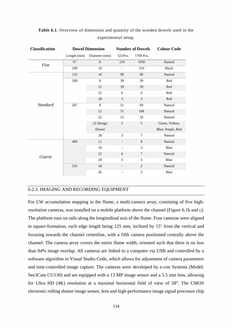
134
Table 6.1. Overview of dimension and quantity of the wooden dowels used in the
experimental setup.
Classification Dowel Dimension
Length (mm) Diameter (mm)
Number of Dowels
521Pcs. 1769 Pcs.
Colour Code
Fine 67 6 210 1050 Natural
100 10 - 310 Black
Standard
133 10 90 90 Natural
200 8 39 39 Red
12 39 39 Red
22 6 6 Red
28 3 3 Red
267 8 51 69 Natural
12 51 108 Natural
22 15 18 Natural
22 Design
Dowel
5 5 Green, Yellow,
Blue, Purple, Red
28 3 7 Natural
Coarse
400 12 - 8 Natural
18 - 3 Blue
22 6 7 Natural
28 3 3 Blue
533 18 - 2 Natural
26 - 2 Blue
6.2.3. IMAGING AND RECORDING EQUIPMENT
For LW accumulation mapping in the flume, a multi-camera array, consisting of five high-
resolution cameras, was installed on a mobile platform above the channel (Figure 6.1b and c).
The platform runs on rails along the longitudinal axis of the flume. Four cameras were aligned
in square-formation, each edge length being 125 mm, inclined by 15˚ from the vertical and
focusing towards the channel centreline, with a fifth camera positioned centrally above the
channel. The camera array covers the entire flume width, oriented such that there is no less
than 84% image overlap. All cameras are linked to a computer via USB and controlled by a
software algorithm in Visual Studio Code, which allows for adjustment of camera parameters
and time-controlled image capture. The cameras were developed by e-con Systems (Model:
See3Cam CU130) and are equipped with a 13 MP image sensor and a 5.5 mm lens, allowing
for Ultra HD (4K) resolution at a maximal horizontal field of view of 58°. The CMOS
electronic rolling shutter image sensor, lens and high-performance image signal processor chip
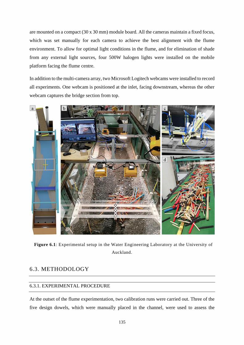
135
are mounted on a compact (30 x 30 mm) module board. All the cameras maintain a fixed focus,
which was set manually for each camera to achieve the best alignment with the flume
environment. To allow for optimal light conditions in the flume, and for elimination of shade
from any external light sources, four 500W halogen lights were installed on the mobile
platform facing the flume centre.
In addition to the multi-camera array, two Microsoft Logitech webcams were installed to record
all experiments. One webcam is positioned at the inlet, facing downstream, whereas the other
webcam captures the bridge section from top.
Figure 6.1: Experimental setup in the Water Engineering Laboratory at the University of
Auckland.
6.3. METHODOLOGY
6.3.1. EXPERIMENTAL PROCEDURE
At the outset of the flume experimentation, two calibration runs were carried out. Three of the
five design dowels, which were manually placed in the channel, were used to assess the
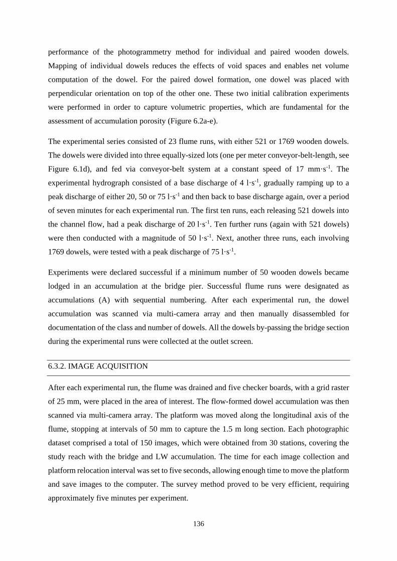
136
performance of the photogrammetry method for individual and paired wooden dowels.
Mapping of individual dowels reduces the effects of void spaces and enables net volume
computation of the dowel. For the paired dowel formation, one dowel was placed with
perpendicular orientation on top of the other one. These two initial calibration experiments
were performed in order to capture volumetric properties, which are fundamental for the
assessment of accumulation porosity (Figure 6.2a-e).
The experimental series consisted of 23 flume runs, with either 521 or 1769 wooden dowels.
The dowels were divided into three equally-sized lots (one per meter conveyor-belt-length, see
Figure 6.1d), and fed via conveyor-belt system at a constant speed of 17 mm·s-1. The
experimental hydrograph consisted of a base discharge of 4 l·s-1, gradually ramping up to a
peak discharge of either 20, 50 or 75 l·s-1 and then back to base discharge again, over a period
of seven minutes for each experimental run. The first ten runs, each releasing 521 dowels into
the channel flow, had a peak discharge of 20 l·s-1. Ten further runs (again with 521 dowels)
were then conducted with a magnitude of 50 l·s-1. Next, another three runs, each involving
1769 dowels, were tested with a peak discharge of 75 l·s-1.
Experiments were declared successful if a minimum number of 50 wooden dowels became
lodged in an accumulation at the bridge pier. Successful flume runs were designated as
accumulations (A) with sequential numbering. After each experimental run, the dowel
accumulation was scanned via multi-camera array and then manually disassembled for
documentation of the class and number of dowels. All the dowels by-passing the bridge section
during the experimental runs were collected at the outlet screen.
6.3.2. IMAGE ACQUISITION
After each experimental run, the flume was drained and five checker boards, with a grid raster
of 25 mm, were placed in the area of interest. The flow-formed dowel accumulation was then
scanned via multi-camera array. The platform was moved along the longitudinal axis of the
flume, stopping at intervals of 50 mm to capture the 1.5 m long section. Each photographic
dataset comprised a total of 150 images, which were obtained from 30 stations, covering the
study reach with the bridge and LW accumulation. The time for each image collection and
platform relocation interval was set to five seconds, allowing enough time to move the platform
and save images to the computer. The survey method proved to be very efficient, requiring
approximately five minutes per experiment.
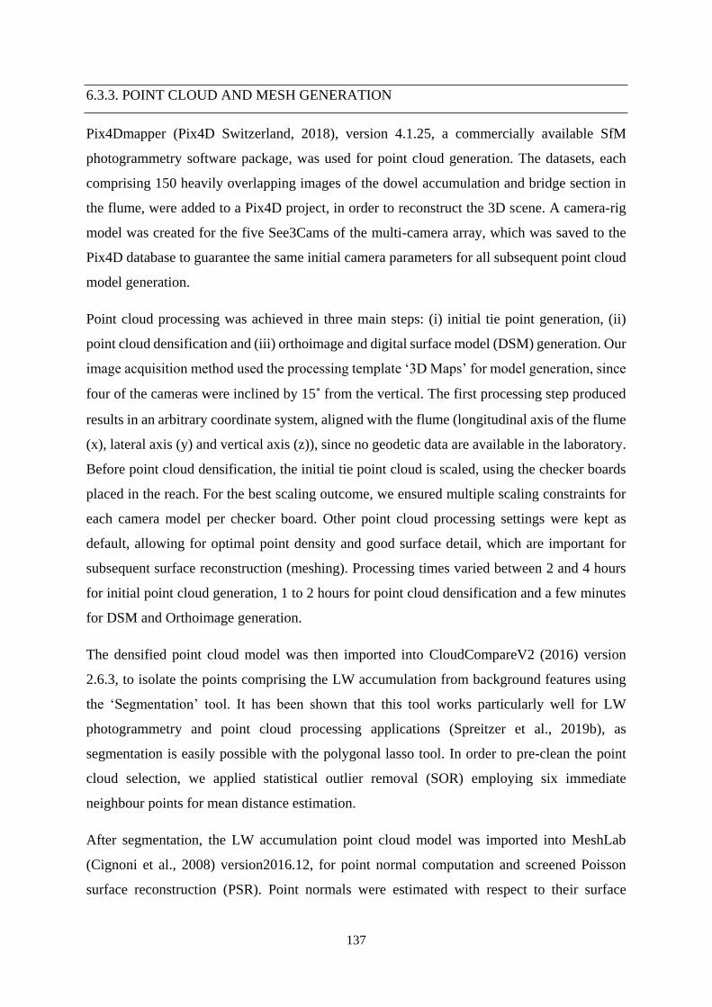
137
6.3.3. POINT CLOUD AND MESH GENERATION
Pix4Dmapper (Pix4D Switzerland, 2018), version 4.1.25, a commercially available SfM
photogrammetry software package, was used for point cloud generation. The datasets, each
comprising 150 heavily overlapping images of the dowel accumulation and bridge section in
the flume, were added to a Pix4D project, in order to reconstruct the 3D scene. A camera-rig
model was created for the five See3Cams of the multi-camera array, which was saved to the
Pix4D database to guarantee the same initial camera parameters for all subsequent point cloud
model generation.
Point cloud processing was achieved in three main steps: (i) initial tie point generation, (ii)
point cloud densification and (iii) orthoimage and digital surface model (DSM) generation. Our
image acquisition method used the processing template ‘3D Maps’ for model generation, since
four of the cameras were inclined by 15˚ from the vertical. The first processing step produced
results in an arbitrary coordinate system, aligned with the flume (longitudinal axis of the flume
(x), lateral axis (y) and vertical axis (z)), since no geodetic data are available in the laboratory.
Before point cloud densification, the initial tie point cloud is scaled, using the checker boards
placed in the reach. For the best scaling outcome, we ensured multiple scaling constraints for
each camera model per checker board. Other point cloud processing settings were kept as
default, allowing for optimal point density and good surface detail, which are important for
subsequent surface reconstruction (meshing). Processing times varied between 2 and 4 hours
for initial point cloud generation, 1 to 2 hours for point cloud densification and a few minutes
for DSM and Orthoimage generation.
The densified point cloud model was then imported into CloudCompareV2 (2016) version
2.6.3, to isolate the points comprising the LW accumulation from background features using
the ‘Segmentation’ tool. It has been shown that this tool works particularly well for LW
photogrammetry and point cloud processing applications (Spreitzer et al., 2019b), as
segmentation is easily possible with the polygonal lasso tool. In order to pre-clean the point
cloud selection, we applied statistical outlier removal (SOR) employing six immediate
neighbour points for mean distance estimation.
After segmentation, the LW accumulation point cloud model was imported into MeshLab
(Cignoni et al., 2008) version2016.12, for point normal computation and screened Poisson
surface reconstruction (PSR). Point normals were estimated with respect to their surface
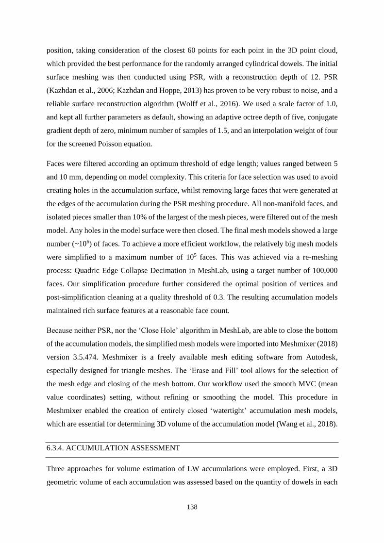
138
position, taking consideration of the closest 60 points for each point in the 3D point cloud,
which provided the best performance for the randomly arranged cylindrical dowels. The initial
surface meshing was then conducted using PSR, with a reconstruction depth of 12. PSR
(Kazhdan et al., 2006; Kazhdan and Hoppe, 2013) has proven to be very robust to noise, and a
reliable surface reconstruction algorithm (Wolff et al., 2016). We used a scale factor of 1.0,
and kept all further parameters as default, showing an adaptive octree depth of five, conjugate
gradient depth of zero, minimum number of samples of 1.5, and an interpolation weight of four
for the screened Poisson equation.
Faces were filtered according an optimum threshold of edge length; values ranged between 5
and 10 mm, depending on model complexity. This criteria for face selection was used to avoid
creating holes in the accumulation surface, whilst removing large faces that were generated at
the edges of the accumulation during the PSR meshing procedure. All non-manifold faces, and
isolated pieces smaller than 10% of the largest of the mesh pieces, were filtered out of the mesh
model. Any holes in the model surface were then closed. The final mesh models showed a large
number (~106) of faces. To achieve a more efficient workflow, the relatively big mesh models
were simplified to a maximum number of 105 faces. This was achieved via a re-meshing
process: Quadric Edge Collapse Decimation in MeshLab, using a target number of 100,000
faces. Our simplification procedure further considered the optimal position of vertices and
post-simplification cleaning at a quality threshold of 0.3. The resulting accumulation models
maintained rich surface features at a reasonable face count.
Because neither PSR, nor the ‘Close Hole’ algorithm in MeshLab, are able to close the bottom
of the accumulation models, the simplified mesh models were imported into Meshmixer (2018)
version 3.5.474. Meshmixer is a freely available mesh editing software from Autodesk,
especially designed for triangle meshes. The ‘Erase and Fill’ tool allows for the selection of
the mesh edge and closing of the mesh bottom. Our workflow used the smooth MVC (mean
value coordinates) setting, without refining or smoothing the model. This procedure in
Meshmixer enabled the creation of entirely closed ‘watertight’ accumulation mesh models,
which are essential for determining 3D volume of the accumulation model (Wang et al., 2018).
6.3.4. ACCUMULATION ASSESSMENT
Three approaches for volume estimation of LW accumulations were employed. First, a 3D
geometric volume of each accumulation was assessed based on the quantity of dowels in each
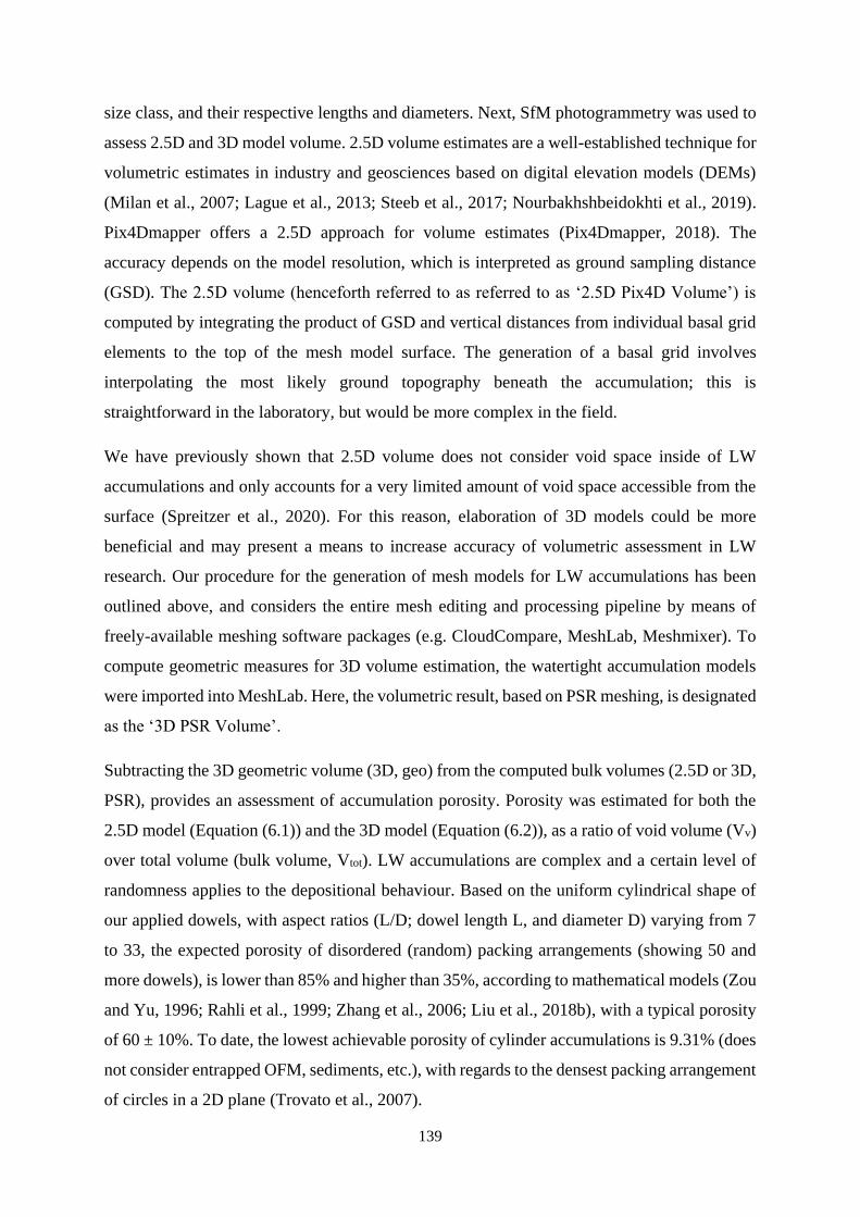
139
size class, and their respective lengths and diameters. Next, SfM photogrammetry was used to
assess 2.5D and 3D model volume. 2.5D volume estimates are a well-established technique for
volumetric estimates in industry and geosciences based on digital elevation models (DEMs)
(Milan et al., 2007; Lague et al., 2013; Steeb et al., 2017; Nourbakhshbeidokhti et al., 2019).
Pix4Dmapper offers a 2.5D approach for volume estimates (Pix4Dmapper, 2018). The
accuracy depends on the model resolution, which is interpreted as ground sampling distance
(GSD). The 2.5D volume (henceforth referred to as referred to as ‘2.5D Pix4D Volume’) is
computed by integrating the product of GSD and vertical distances from individual basal grid
elements to the top of the mesh model surface. The generation of a basal grid involves
interpolating the most likely ground topography beneath the accumulation; this is
straightforward in the laboratory, but would be more complex in the field.
We have previously shown that 2.5D volume does not consider void space inside of LW
accumulations and only accounts for a very limited amount of void space accessible from the
surface (Spreitzer et al., 2020). For this reason, elaboration of 3D models could be more
beneficial and may present a means to increase accuracy of volumetric assessment in LW
research. Our procedure for the generation of mesh models for LW accumulations has been
outlined above, and considers the entire mesh editing and processing pipeline by means of
freely-available meshing software packages (e.g. CloudCompare, MeshLab, Meshmixer). To
compute geometric measures for 3D volume estimation, the watertight accumulation models
were imported into MeshLab. Here, the volumetric result, based on PSR meshing, is designated
as the ‘3D PSR Volume’.
Subtracting the 3D geometric volume (3D, geo) from the computed bulk volumes (2.5D or 3D,
PSR), provides an assessment of accumulation porosity. Porosity was estimated for both the
2.5D model (Equation (6.1)) and the 3D model (Equation (6.2)), as a ratio of void volume (Vv)
over total volume (bulk volume, Vtot). LW accumulations are complex and a certain level of
randomness applies to the depositional behaviour. Based on the uniform cylindrical shape of
our applied dowels, with aspect ratios (L/D; dowel length L, and diameter D) varying from 7
to 33, the expected porosity of disordered (random) packing arrangements (showing 50 and
more dowels), is lower than 85% and higher than 35%, according to mathematical models (Zou
and Yu, 1996; Rahli et al., 1999; Zhang et al., 2006; Liu et al., 2018b), with a typical porosity
of 60 ± 10%. To date, the lowest achievable porosity of cylinder accumulations is 9.31% (does
not consider entrapped OFM, sediments, etc.), with regards to the densest packing arrangement
of circles in a 2D plane (Trovato et al., 2007).
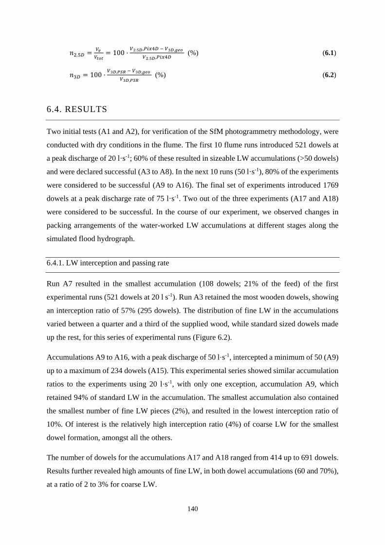
140
𝑛2.5𝐷 =𝑉𝑣
𝑉𝑡𝑜𝑡= 100 ·
𝑉2.5𝐷,𝑃𝑖𝑥4𝐷 − 𝑉3𝐷,𝑔𝑒𝑜
𝑉2.5𝐷,𝑃𝑖𝑥4𝐷 (%) (6.1)
𝑛3𝐷 = 100 ·𝑉3𝐷,𝑃𝑆𝑅 − 𝑉3𝐷,𝑔𝑒𝑜
𝑉3𝐷,𝑃𝑆𝑅 (%) (6.2)
6.4. RESULTS
Two initial tests (A1 and A2), for verification of the SfM photogrammetry methodology, were
conducted with dry conditions in the flume. The first 10 flume runs introduced 521 dowels at
a peak discharge of 20 l·s-1; 60% of these resulted in sizeable LW accumulations (>50 dowels)
and were declared successful (A3 to A8). In the next 10 runs (50 l·s-1), 80% of the experiments
were considered to be successful (A9 to A16). The final set of experiments introduced 1769
dowels at a peak discharge rate of 75 l·s-1. Two out of the three experiments (A17 and A18)
were considered to be successful. In the course of our experiment, we observed changes in
packing arrangements of the water-worked LW accumulations at different stages along the
simulated flood hydrograph.
6.4.1. LW interception and passing rate
Run A7 resulted in the smallest accumulation (108 dowels; 21% of the feed) of the first
experimental runs (521 dowels at 20 l s-1). Run A3 retained the most wooden dowels, showing
an interception ratio of 57% (295 dowels). The distribution of fine LW in the accumulations
varied between a quarter and a third of the supplied wood, while standard sized dowels made
up the rest, for this series of experimental runs (Figure 6.2).
Accumulations A9 to A16, with a peak discharge of 50 l·s-1, intercepted a minimum of 50 (A9)
up to a maximum of 234 dowels (A15). This experimental series showed similar accumulation
ratios to the experiments using 20 l·s-1, with only one exception, accumulation A9, which
retained 94% of standard LW in the accumulation. The smallest accumulation also contained
the smallest number of fine LW pieces (2%), and resulted in the lowest interception ratio of
10%. Of interest is the relatively high interception ratio (4%) of coarse LW for the smallest
dowel formation, amongst all the others.
The number of dowels for the accumulations A17 and A18 ranged from 414 up to 691 dowels.
Results further revealed high amounts of fine LW, in both dowel accumulations (60 and 70%),
at a ratio of 2 to 3% for coarse LW.
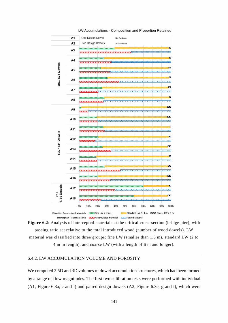
141
Figure 6.2: Analysis of intercepted materials at the critical cross-section (bridge pier), with
passing ratio set relative to the total introduced wood (number of wood dowels). LW
material was classified into three groups: fine LW (smaller than 1.5 m), standard LW (2 to
4 m in length), and coarse LW (with a length of 6 m and longer).
6.4.2. LW ACCUMULATION VOLUME AND POROSITY
We computed 2.5D and 3D volumes of dowel accumulation structures, which had been formed
by a range of flow magnitudes. The first two calibration tests were performed with individual
(A1; Figure 6.3a, c and i) and paired design dowels (A2; Figure 6.3e, g and i), which were
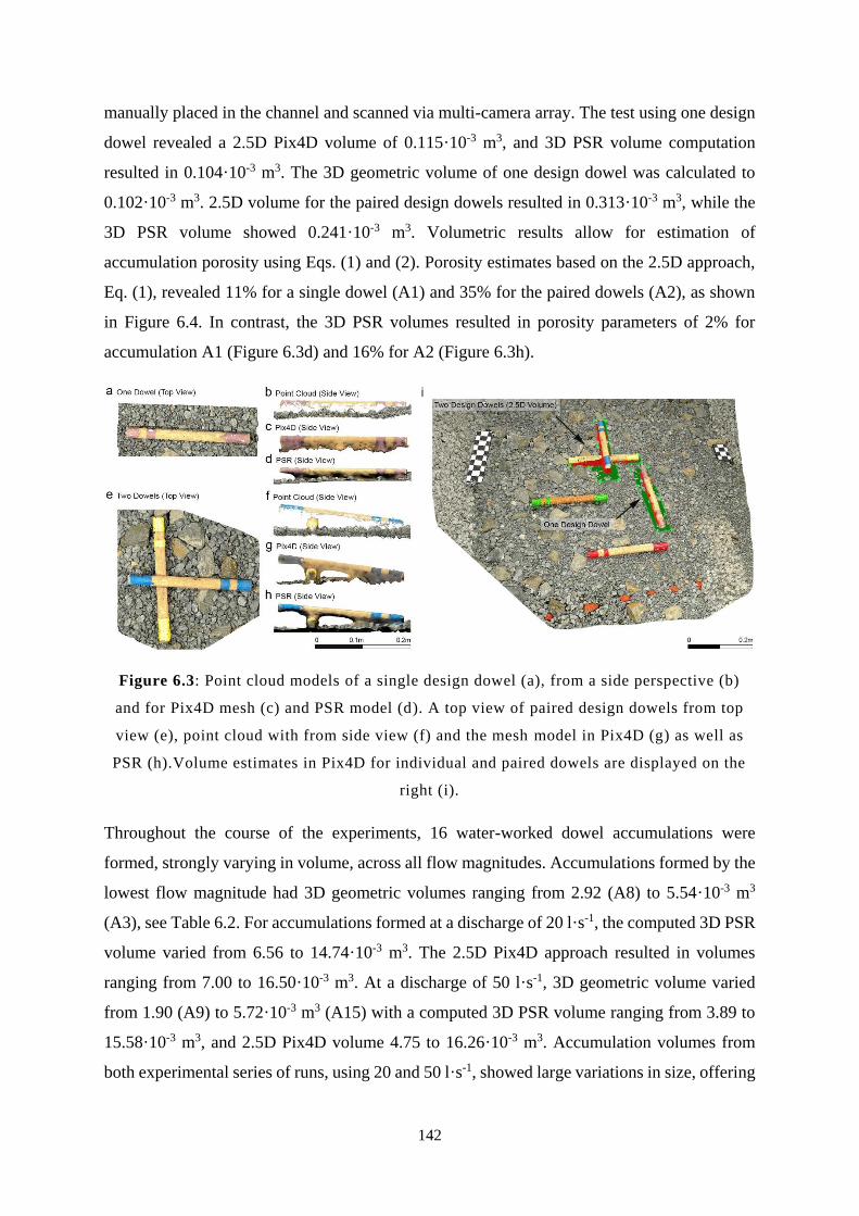
142
manually placed in the channel and scanned via multi-camera array. The test using one design
dowel revealed a 2.5D Pix4D volume of 0.115·10-3 m3, and 3D PSR volume computation
resulted in 0.104·10-3 m3. The 3D geometric volume of one design dowel was calculated to
0.102·10-3 m3. 2.5D volume for the paired design dowels resulted in 0.313·10-3 m3, while the
3D PSR volume showed 0.241·10-3 m3. Volumetric results allow for estimation of
accumulation porosity using Eqs. (1) and (2). Porosity estimates based on the 2.5D approach,
Eq. (1), revealed 11% for a single dowel (A1) and 35% for the paired dowels (A2), as shown
in Figure 6.4. In contrast, the 3D PSR volumes resulted in porosity parameters of 2% for
accumulation A1 (Figure 6.3d) and 16% for A2 (Figure 6.3h).
Figure 6.3: Point cloud models of a single design dowel (a), from a side perspective (b)
and for Pix4D mesh (c) and PSR model (d). A top view of paired design dowels from top
view (e), point cloud with from side view (f) and the mesh model in Pix4D (g) as well as
PSR (h).Volume estimates in Pix4D for individual and paired dowels are displayed on the
right (i).
Throughout the course of the experiments, 16 water-worked dowel accumulations were
formed, strongly varying in volume, across all flow magnitudes. Accumulations formed by the
lowest flow magnitude had 3D geometric volumes ranging from 2.92 (A8) to 5.54·10-3 m3
(A3), see Table 6.2. For accumulations formed at a discharge of 20 l·s-1, the computed 3D PSR
volume varied from 6.56 to 14.74·10-3 m3. The 2.5D Pix4D approach resulted in volumes
ranging from 7.00 to 16.50·10-3 m3. At a discharge of 50 l·s-1, 3D geometric volume varied
from 1.90 (A9) to 5.72·10-3 m3 (A15) with a computed 3D PSR volume ranging from 3.89 to
15.58·10-3 m3, and 2.5D Pix4D volume 4.75 to 16.26·10-3 m3. Accumulation volumes from
both experimental series of runs, using 20 and 50 l·s-1, showed large variations in size, offering
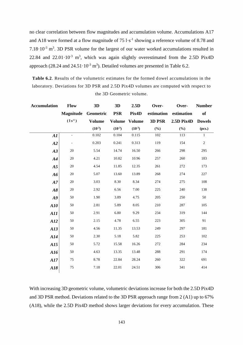
143
no clear correlation between flow magnitudes and accumulation volume. Accumulations A17
and A18 were formed at a flow magnitude of 75 l·s-1 showing a reference volume of 8.78 and
7.18·10-3 m3. 3D PSR volume for the largest of our water worked accumulations resulted in
22.84 and 22.01·10-3 m3, which was again slightly overestimated from the 2.5D Pix4D
approach (28.24 and 24.51·10-3 m3). Detailed volumes are presented in Table 6.2.
Table 6.2. Results of the volumetric estimates for the formed dowel accumulations in the
laboratory. Deviations for 3D PSR and 2.5D Pix4D volumes are computed with respect to
the 3D Geometric volume.
Accumulation Flow
Magnitude
( l s-1 )
3D
Geometric
Volume
(10-3)
3D
PSR
Volume
(10-3)
2.5D
Pix4D
Volume
(10-3)
Over-
estimation
3D PSR
(%)
Over-
estimation
2.5D Pix4D
(%)
Number
of
Dowels
(pcs.)
A1 - 0.102 0.104 0.115 102 113 1
A2 - 0.203 0.241 0.313 119 154 2
A3 20 5.54 14.74 16.50 266 298 295
A4 20 4.21 10.82 10.96 257 260 183
A5 20 4.54 11.85 12.35 261 272 173
A6 20 5.07 13.60 13.89 268 274 227
A7 20 3.03 8.30 8.34 274 275 108
A8 20 2.92 6.56 7.00 225 240 138
A9 50 1.90 3.89 4.75 205 250 50
A10 50 2.81 5.89 8.05 210 287 105
A11 50 2.91 6.80 9.29 234 319 144
A12 50 2.15 4.78 6.55 223 305 91
A13 50 4.56 11.35 13.53 249 297 181
A14 50 2.30 5.18 5.82 225 253 102
A15 50 5.72 15.58 16.26 272 284 234
A16 50 4.63 13.35 13.48 288 291 174
A17 75 8.78 22.84 28.24 260 322 691
A18 75 7.18 22.01 24.51 306 341 414
With increasing 3D geometric volume, volumetric deviations increase for both the 2.5D Pix4D
and 3D PSR method. Deviations related to the 3D PSR approach range from 2 (A1) up to 67%
(A18), while the 2.5D Pix4D method shows larger deviations for every accumulation. These
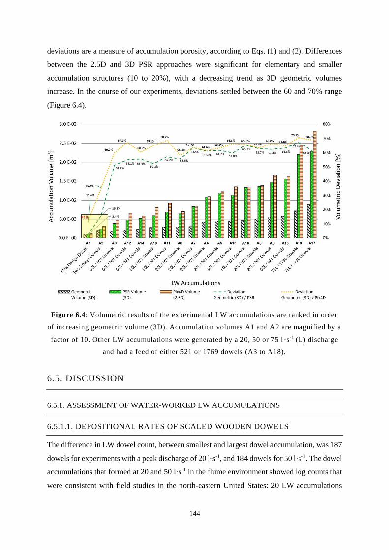
144
deviations are a measure of accumulation porosity, according to Eqs. (1) and (2). Differences
between the 2.5D and 3D PSR approaches were significant for elementary and smaller
accumulation structures (10 to 20%), with a decreasing trend as 3D geometric volumes
increase. In the course of our experiments, deviations settled between the 60 and 70% range
(Figure 6.4).
Figure 6.4: Volumetric results of the experimental LW accumulations are ranked in order
of increasing geometric volume (3D). Accumulation volumes A1 and A2 are magnified by a
factor of 10. Other LW accumulations were generated by a 20, 50 or 75 l ·s-1 (L) discharge
and had a feed of either 521 or 1769 dowels (A3 to A18).
6.5. DISCUSSION
6.5.1. ASSESSMENT OF WATER-WORKED LW ACCUMULATIONS
6.5.1.1. DEPOSITIONAL RATES OF SCALED WOODEN DOWELS
The difference in LW dowel count, between smallest and largest dowel accumulation, was 187
dowels for experiments with a peak discharge of 20 l·s-1, and 184 dowels for 50 l·s-1. The dowel
accumulations that formed at 20 and 50 l·s-1 in the flume environment showed log counts that
were consistent with field studies in the north-eastern United States: 20 LW accumulations
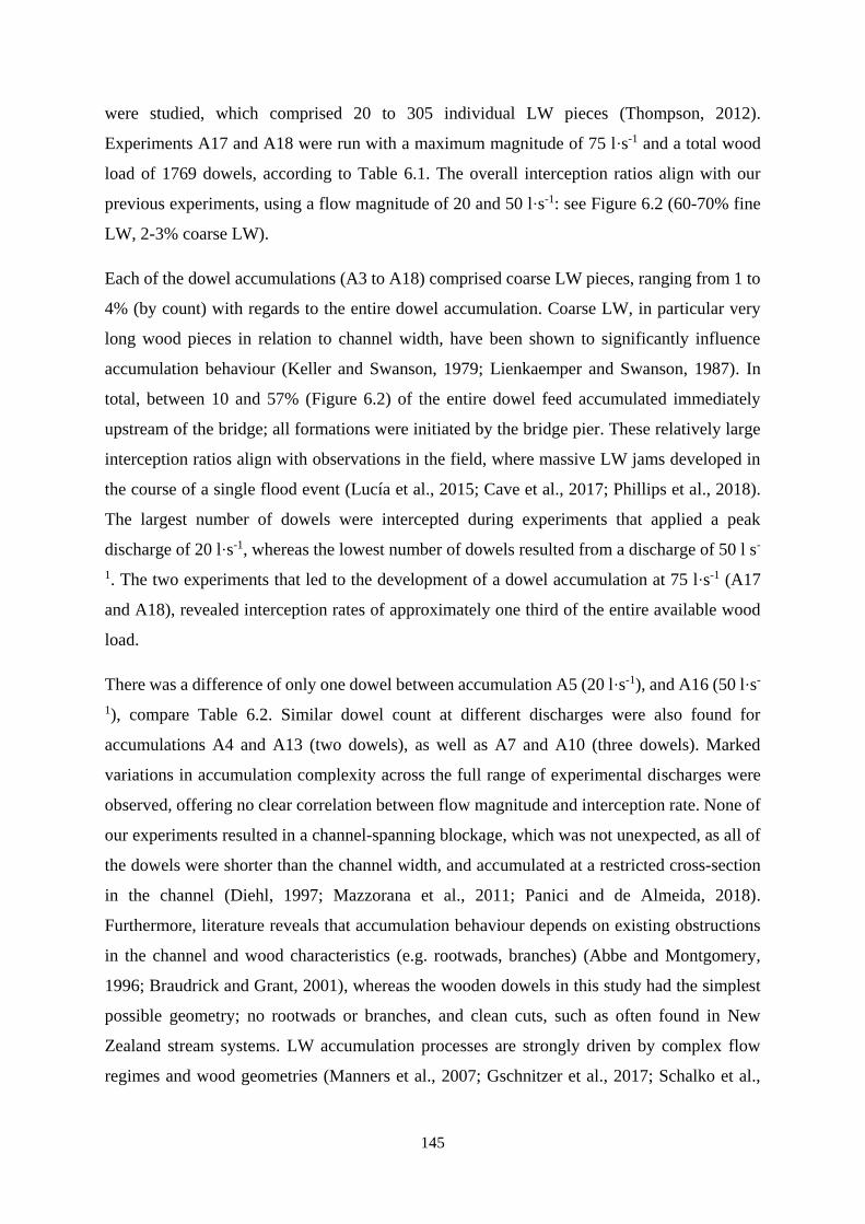
145
were studied, which comprised 20 to 305 individual LW pieces (Thompson, 2012).
Experiments A17 and A18 were run with a maximum magnitude of 75 l·s-1 and a total wood
load of 1769 dowels, according to Table 6.1. The overall interception ratios align with our
previous experiments, using a flow magnitude of 20 and 50 l·s-1: see Figure 6.2 (60-70% fine
LW, 2-3% coarse LW).
Each of the dowel accumulations (A3 to A18) comprised coarse LW pieces, ranging from 1 to
4% (by count) with regards to the entire dowel accumulation. Coarse LW, in particular very
long wood pieces in relation to channel width, have been shown to significantly influence
accumulation behaviour (Keller and Swanson, 1979; Lienkaemper and Swanson, 1987). In
total, between 10 and 57% (Figure 6.2) of the entire dowel feed accumulated immediately
upstream of the bridge; all formations were initiated by the bridge pier. These relatively large
interception ratios align with observations in the field, where massive LW jams developed in
the course of a single flood event (Lucía et al., 2015; Cave et al., 2017; Phillips et al., 2018).
The largest number of dowels were intercepted during experiments that applied a peak
discharge of 20 l·s-1, whereas the lowest number of dowels resulted from a discharge of 50 l s-
1. The two experiments that led to the development of a dowel accumulation at 75 l·s-1 (A17
and A18), revealed interception rates of approximately one third of the entire available wood
load.
There was a difference of only one dowel between accumulation A5 (20 l·s-1), and A16 (50 l·s-
1), compare Table 6.2. Similar dowel count at different discharges were also found for
accumulations A4 and A13 (two dowels), as well as A7 and A10 (three dowels). Marked
variations in accumulation complexity across the full range of experimental discharges were
observed, offering no clear correlation between flow magnitude and interception rate. None of
our experiments resulted in a channel-spanning blockage, which was not unexpected, as all of
the dowels were shorter than the channel width, and accumulated at a restricted cross-section
in the channel (Diehl, 1997; Mazzorana et al., 2011; Panici and de Almeida, 2018).
Furthermore, literature reveals that accumulation behaviour depends on existing obstructions
in the channel and wood characteristics (e.g. rootwads, branches) (Abbe and Montgomery,
1996; Braudrick and Grant, 2001), whereas the wooden dowels in this study had the simplest
possible geometry; no rootwads or branches, and clean cuts, such as often found in New
Zealand stream systems. LW accumulation processes are strongly driven by complex flow
regimes and wood geometries (Manners et al., 2007; Gschnitzer et al., 2017; Schalko et al.,
146
2019b), which still require extensive research to better predict log deposition and accumulation
formation processes.
6.5.1.2. ACCUMULATIONS VOLUME VS DOWEL COUNT
Previous studies have revealed that high flow events may redistribute LW in channels, while
removing old wood and depositing new material in existing LW accumulations (Lienkaemper
and Swanson, 1987). Although redistribution occurs in our experiments, similar structures are
formed in the course of each flood event (Evans et al., 1993). Despite the similar mode of
formation, there was no clear correlation between flow magnitude and the size of dowel
accumulation. Accumulations A17 and A18 retained up to almost three times the number of
dowels as previous experiments, and the 3D geometric volumes (7.18 to 8.78·10-3 m3), as well
as the 2.5D and 3D PSR volumes, were consistent with the trend of previous experiments.
Because of the different size classes of dowels used, the 3D geometric volume does not exactly
coincide with the number of dowels that make up the accumulations. A7 shows a larger volume
than A8, despite being comprised of fewer dowels, at a flow magnitude of 20 l·s-1. The same
applies to accumulations A4 and A5. Due to log orientation and geometric alignment
complexities ‘packing matrix’ during the accumulation processes (Braudrick and Grant, 2001;
Abbe and Montgomery, 2003), differences in 3D geometric volume may be relatively small (<
4% or 0.1·10-3 m3), while the computed volumes can show variations of 16 to 20% (~1.5·10-3
m3) (compare A7 and A8 (20 l·s-1) in Table 6.2). This effect was also observed for
accumulations formed at higher discharge rates of 50 l·s-1: compare accumulation A13 and
A16, as well as across the flow magnitudes. Accumulation A11 (50 l·s-1) retained 144 dowels,
which is 36 more than A7 (20 l·s-1), and yet A7 shows a larger 3D geometric volume. The
opposite is observed for accumulations A3 (5.54·10-3 m3) and A15 (5.72·10-3 m3) at flow
magnitudes of 20 and 50 l·s-1, (Table 6.2). A3 shows the smallest volume of the two, whilst
having 61 dowels less than A15. However, we found individual cases that show similar 3D
geometric, as well as 3D PSR volumes (A8 and A11) and 2.5D Pix4D volumes (A7 and A10;
A13 and A16; see Table 6.2).
Results revealed that the computed 3D PSR volume correlates very well to the number of
accumulated dowels, with only one major exception, accumulation A17. The number of
elements comprising a LW accumulation can significantly contribute to the complexity of the
accumulation skeleton (Shields, 2001; Pagliara and Carnacina, 2010; Thompson, 2012),
containing more void spaces at the inside of the jam formation, which are difficult to capture.
147
Our experiments, ranging from 20 to 75 l·s-1, revealed an evenly related proportional deviation
scale with the size of the accumulation, for both the 2.5D and 3D assessment techniques (Figure
6.4 and Figure 6.5).
6.5.1.3. 2.5D VS 3D ASSESSMENT
In each of our experiments, the 3D geometric volume was overestimated by the 3D PSR
method, and even further overestimated by the 2.5D Pix4D method, which was expected
(Spreitzer et al., 2020). This is also consistent with the assumptions inherent in the 2.5D
approach (Verbree and Van Oosterom, 2003; Pix4Dmapper, 2018). Absolute differentials
between 3D PSR and 2.5D Pix4D volumes generally reached values of up to 2.5·10-3 m3 (A11
and A18), with a maximum of 5.4·10-3 m3 (A17), indicating clearly that in all of our
experiments the 3D PSR approach performed better in capturing volumes. The reason for the
improved performance of the 3D method is, again, related to the higher fidelity capture of void
spaces from all angles of the accumulation surface (Glasbey et al., 1991; Lian et al., 2012).
Overhanging features and void spaces at the periphery of the deposit are not resolved when
applying the 2.5D approach (Jones et al., 2008; Spreitzer et al., 2020).
The 3D PSR approach performed reasonably accurately for a single dowel A1 (102% of 3D
geometric volume), however, the 2.5D Pix4D approach more severely overestimated the
reference 3D geometric volume (113%; compare A1 and A2 in Table 6.2). For the paired
wooden dowels (A2), deviations from the reference arose for both methods, although the
deviations in the case of the 3D PSR approach were less (119%) than those from the 2.5D
Pix4D approach (154%). Porosity for these elementary structures are slightly larger than
observed in previous laboratory studies on LW accumulation volumes (Spreitzer et al., 2020).
More complex LW accumulations revealed higher deviation (detailed parameters on the
overestimation are presented in Table 6.2), while accumulation A18 showed a maximum for
the 3D PSR (306%) as well as 2.5D Pix4D approach (341%). This overestimation is most likely
related to nadir image acquisition - as obtained in aerial surveys, such as taken from drones
(Rusnák et al., 2018), helicopters (Dietrich, 2016) and planes (Smikrud and Prakash, 2006) -
compared to ‘oblique’ images captured from various sub-vertical angles, as used in previous
studies (Rossi et al., 2017; Spreitzer et al., 2019b; Spreitzer et al., 2020).
In the present study we found that the 2.5D technique consistently provides about three times
‘3x’ the 3D Geometric Volume (a regression yields R2 = 0.98; see Figure 6.5), providing a
practical guideline for photogrammetric work on water-worked accumulations that consist
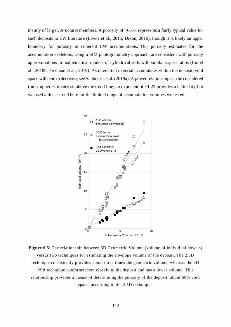
148
mainly of larger, structural members. A porosity of ~66%, represents a fairly typical value for
such deposits in LW literature (Livers et al., 2015; Dixon, 2016), though it is likely an upper
boundary for porosity in coherent LW accumulations. Our porosity estimates for the
accumulation skeletons, using a SfM photogrammetry approach, are consistent with porosity
approximations in mathematical models of cylindrical rods with similar aspect ratios (Liu et
al., 2018b; Freeman et al., 2019). As interstitial material accumulates within the deposit, void
space will tend to decrease; see Sanhueza et al. (2019a). A power relationship can be considered
(most upper estimates sit above the trend line; an exponent of ~1.22 provides a better fit), but
we used a linear trend here for the limited range of accumulation volumes we tested.
Figure 6.5: The relationship between 3D Geometric Volume (volume of individual dowels)
versus two techniques for estimating the envelope volume of the deposit. The 2.5D
technique consistently provides about three times the geometric volume, whereas the 3D
PSR technique conforms more closely to the deposit and has a lower volume. This
relationship provides a means of determining the porosity of the deposit: about 66% void
space, according to the 2.5D technique.
149
6.5.1.4. LW ACCUMULATION COMPRESSION AND RELAXATION
In assessing the formation of the dowel accumulations, it was observed that the packing
structure changed, during the waning stage of each run. In the present work we defined the
‘relaxation’ process as the settling of recently jammed wooden elements (the LW
accumulation) with dropping water levels. The opposite effect was called ‘compression’.
During peak discharge, dynamic forces acting on LW elements (Manners et al., 2007; Shields
and Alonso, 2012) may transform the nature of the structure. Medium density and wood
moisture content (often related to wood age) affect the buoyancy of the wooden material (Ruiz-
Villanueva et al., 2016a), resulting in floating LW accumulations, similar to the experimental
setup of a recent study on LW retention structures (Schalko et al., 2019b).
In our study, compression and relaxation effects correspond with flood magnitude (Figure 6.6).
Individual dowels (marked-up ellipses), which are embedded into the accumulation, were
identified and tracked to reveal compression and relaxation processes at varying discharge
rates. Compression and alignment processes were observed with increasing flow magnitude
(compare Figure 6.6a to c). At peak discharge, the accumulation reached a stagnation point,
resulting in a stable dowel accumulation. With decreasing water level, the LW accumulation
experienced a longitudinal expansion in the upstream direction, reaching a relaxation point at
base discharge (4 l·s-1). The relaxation point at the rising limb was reached at 50 l·s-1, see
stagnation and relaxation line in Figure 6.6b, c and f.
Identifying compression and relaxation processes of LW accumulations at varying flow
magnitudes is important to better understand and assess log formations, as the structure of the
accumulation body may change in terms of porosity that could affect discharge behavior at the
restricted cross-section (Heede et al., 1972; Gregory et al., 1985; Pagliara and Carnacina, 2010;
Gschnitzer et al., 2017; Schalko et al., 2018) and channel morphology (Keller and Swanson,
1979; Gippel et al., 1996). Accordingly, at high flow conditions, LW accumulations may show
a higher compactness than at a stage of low discharge (Manners et al., 2007), and at a time
when LW accumulations are usually assessed.
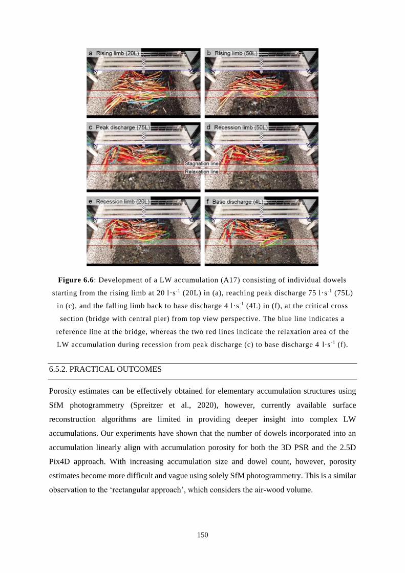
150
Figure 6.6: Development of a LW accumulation (A17) consisting of individual dowels
starting from the rising limb at 20 l·s-1 (20L) in (a), reaching peak discharge 75 l·s-1 (75L)
in (c), and the falling limb back to base discharge 4 l ·s-1 (4L) in (f), at the critical cross
section (bridge with central pier) from top view perspective. The blue line indicates a
reference line at the bridge, whereas the two red lines indicate the relaxation area of the
LW accumulation during recession from peak discharge (c) to base discharge 4 l·s-1 (f).
6.5.2. PRACTICAL OUTCOMES
Porosity estimates can be effectively obtained for elementary accumulation structures using
SfM photogrammetry (Spreitzer et al., 2020), however, currently available surface
reconstruction algorithms are limited in providing deeper insight into complex LW
accumulations. Our experiments have shown that the number of dowels incorporated into an
accumulation linearly align with accumulation porosity for both the 3D PSR and the 2.5D
Pix4D approach. With increasing accumulation size and dowel count, however, porosity
estimates become more difficult and vague using solely SfM photogrammetry. This is a similar
observation to the ‘rectangular approach’, which considers the air-wood volume.
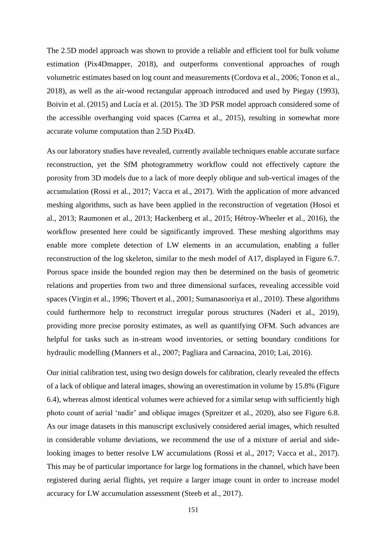
151
The 2.5D model approach was shown to provide a reliable and efficient tool for bulk volume
estimation (Pix4Dmapper, 2018), and outperforms conventional approaches of rough
volumetric estimates based on log count and measurements (Cordova et al., 2006; Tonon et al.,
2018), as well as the air-wood rectangular approach introduced and used by Piegay (1993),
Boivin et al. (2015) and Lucía et al. (2015). The 3D PSR model approach considered some of
the accessible overhanging void spaces (Carrea et al., 2015), resulting in somewhat more
accurate volume computation than 2.5D Pix4D.
As our laboratory studies have revealed, currently available techniques enable accurate surface
reconstruction, yet the SfM photogrammetry workflow could not effectively capture the
porosity from 3D models due to a lack of more deeply oblique and sub-vertical images of the
accumulation (Rossi et al., 2017; Vacca et al., 2017). With the application of more advanced
meshing algorithms, such as have been applied in the reconstruction of vegetation (Hosoi et
al., 2013; Raumonen et al., 2013; Hackenberg et al., 2015; Hétroy-Wheeler et al., 2016), the
workflow presented here could be significantly improved. These meshing algorithms may
enable more complete detection of LW elements in an accumulation, enabling a fuller
reconstruction of the log skeleton, similar to the mesh model of A17, displayed in Figure 6.7.
Porous space inside the bounded region may then be determined on the basis of geometric
relations and properties from two and three dimensional surfaces, revealing accessible void
spaces (Virgin et al., 1996; Thovert et al., 2001; Sumanasooriya et al., 2010). These algorithms
could furthermore help to reconstruct irregular porous structures (Naderi et al., 2019),
providing more precise porosity estimates, as well as quantifying OFM. Such advances are
helpful for tasks such as in-stream wood inventories, or setting boundary conditions for
hydraulic modelling (Manners et al., 2007; Pagliara and Carnacina, 2010; Lai, 2016).
Our initial calibration test, using two design dowels for calibration, clearly revealed the effects
of a lack of oblique and lateral images, showing an overestimation in volume by 15.8% (Figure
6.4), whereas almost identical volumes were achieved for a similar setup with sufficiently high
photo count of aerial ‘nadir’ and oblique images (Spreitzer et al., 2020), also see Figure 6.8.
As our image datasets in this manuscript exclusively considered aerial images, which resulted
in considerable volume deviations, we recommend the use of a mixture of aerial and side-
looking images to better resolve LW accumulations (Rossi et al., 2017; Vacca et al., 2017).
This may be of particular importance for large log formations in the channel, which have been
registered during aerial flights, yet require a larger image count in order to increase model
accuracy for LW accumulation assessment (Steeb et al., 2017).
152
Figure 6.7: Accumulation A17, displayed as mesh model in top (a) and front view (b).
Experimental results show that even for these elementary LW accumulations, the applied PSR
method cannot fully resolve the occluded geometry from aerial photogrammetry models. With
this experimental study we show that the 3D approach performs slightly better than the 2.5D
approach, yet the achieved outcome, considering exclusively aerial image datasets, is not
sufficiently accurate for reliable volumetric assessment. However, based on the 3D geometric
volume and the computed volumes, estimates of LW accumulation porosity can be made
(Figure 6.5). Given the accessibility of aerial/UAV photogrammetric techniques, we anticipate
that further improving the relationship between envelope volume and the porosity of water-
worked LW accumulation structures will be an important frontier in further LW inventory
work.
In providing more information about void spaces inside of LW accumulations, which represent
a substantial part of the deposit that potentially affects flow hydraulics (Manners et al., 2007;
Pagliara and Carnacina, 2010), LW-related challenges such as backwater effects and flow
diversion can be better tackled. The consistency in porosity of LW accumulation skeletons,
such as revealed in this study with roughly 66%, may be used as a correction factor for pore
153
space and finer debris for reconnaissance-scale work on LW inventories. Previous studies have
discussed porosity parameters, ranging from 13% (Sanhueza et al., 2019a) to 90% (Thevenet
et al., 1998), yet LW accumulations are complex, as (i) interstitial space can be empty (air),
partly or completely filled with finer biotic and abiotic detritus (Thevenet et al., 1998; Linstead,
2001), (ii) redistribution of LW materials may occur during floods (Lienkaemper and Swanson,
1987; Evans et al., 1993), and (iii) LW accumulations may undergo a matrix transformation
(e.g. compression, relaxation) affecting the packing process during rising and falling
hydrographs. Figure 6.8 provides an illustration of how LW accumulation porosity may be
related to packing matrices and material diversity. In Figure 6.8, we considered porosity
parameters for LW accumulations from existing literature and our laboratory studies. The
stated porosity parameters are furthermore consistent with mathematical models of random
cylinder arrangements, revealing porosities of 60 ± 10% for uniform cylindrical accumulations
(Zou and Yu, 1996; Rahli et al., 1999; Zhang et al., 2006; Liu et al., 2018b). Accordingly,
porous space inside the jam formation decreases with higher compactness of the formation
matrix and with a larger range of materials. While Sanhueza et al. (2019a) stated that LW
accumulation porosity must be very low (13%), Thevenet et al. (1998) suggested that
accumulation porosity must be lower than 90%, for similar LW accumulations – showing that
LW accumulations are complex and difficult to generalise.
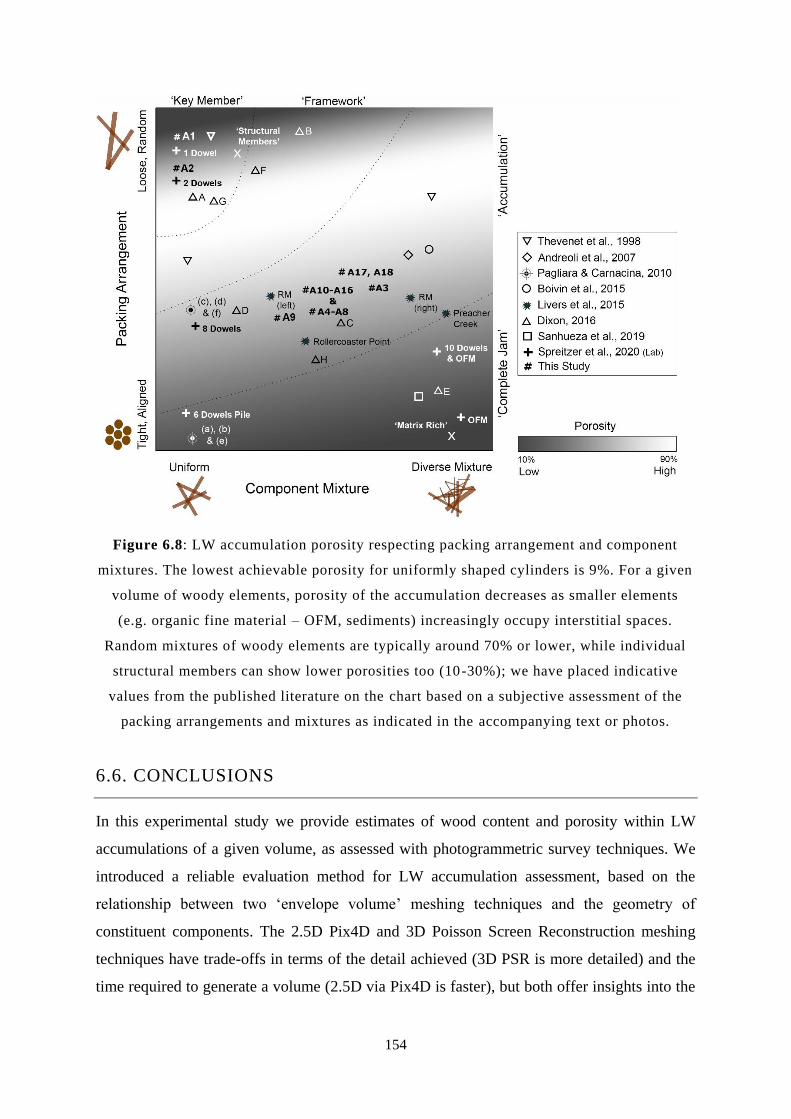
154
Figure 6.8: LW accumulation porosity respecting packing arrangement and component
mixtures. The lowest achievable porosity for uniformly shaped cylinders is 9%. For a given
volume of woody elements, porosity of the accumulation decreases as smaller elements
(e.g. organic fine material – OFM, sediments) increasingly occupy interstitial spaces.
Random mixtures of woody elements are typically around 70% or lower, while individual
structural members can show lower porosities too (10-30%); we have placed indicative
values from the published literature on the chart based on a subjective assessment of the
packing arrangements and mixtures as indicated in the accompanying text or photos.
6.6. CONCLUSIONS
In this experimental study we provide estimates of wood content and porosity within LW
accumulations of a given volume, as assessed with photogrammetric survey techniques. We
introduced a reliable evaluation method for LW accumulation assessment, based on the
relationship between two ‘envelope volume’ meshing techniques and the geometry of
constituent components. The 2.5D Pix4D and 3D Poisson Screen Reconstruction meshing
techniques have trade-offs in terms of the detail achieved (3D PSR is more detailed) and the
time required to generate a volume (2.5D via Pix4D is faster), but both offer insights into the
155
overall geometry of the deposit, and provide an accurate bulk volume that can then be used to
generate an estimate of wood content.
The main findings and conclusions are:
(i) We provide novel results of semi-automated LW accumulation volume and
porosity estimates that outperform conventionally applied methods, such as log
or parallelepiped approach. By considering exclusively aerial datasets for
photogrammetric model generation, the 3D watertight mesh technique performed
slightly better (up to 20% for elementary accumulations and up to 10% for more
complex accumulations) than the commonly applied 2.5D technique.
(ii) Complex LW accumulations skeletons were found to have porosity parameters in
a range of 60 to 70% (roughly 2/3rds), indicating that void space has three times
the volume of wooden elements. This aligns well with the upper boundary of
porosity estimates as per literature, considering log jam formations in the field.
(iii) A linear scaling relation was determined between envelope volume of the water-
worked deposits (determined via SfM) and the volume of the structural
components (dowel geometry). Refining this relationship for various mixtures
(structural and matrix materials) will provide a means for rapid assessment of
wood content in log jams.
(iv) Oblique and lateral images are important for generating accurate true 3D
photogrammetric models. Due to the limited range of views within our laboratory
setup (similar to drone- or airplane-based perspective), point cloud reconstruction
of underhanging surfaces was quite poor, and mesh reconstruction failed to
recreate dowel geometry in proper detail. This may be of particular importance
for large log formations in the channel, which have been registered during aerial
flights, yet require further images in order to resolve intersecting wooden
elements, as well as void spaces accessible from the surface, and to increase the
overall model accuracy for LW accumulation assessment.
(v) Variations and rearrangement of structural elements in the accumulation matrix
does change porosity, but not accumulation volume; meaning that the envelope
volume of the jam can change, but not the volume of constituent elements. LW
accumulation porosity is likely to be underestimated when mapped during low
156
flow magnitudes, due to observed compression (rising limb of the hydrograph +
LW supply) and relaxation processes of the accumulation matrix at the recession
limb of the hydrograph.
Our experimental findings provide evidence that both 2.5D and 3D photogrammetric
techniques are beneficial for estimating LW accumulation volume, and we provided a first
correlation between 3D geometric volume, computed volumes (2.5D, 3D) and jam porosity for
complex log skeletons. Both tested techniques represent efficient tools that allow for surface
mapping and the generation of LW accumulation models, which are of importance for future
approximations of the hidden mass under the surface of LW accumulations. We found that the
3D PSR approach performed better in capturing volumetric information than the 2.5D Pix4D
method; in particular for elementary accumulation structures, as void spaces, which are
accessible from the surface, are not considered by the 2.5D approach. However, perhaps of
greater importance, is developing a robust relationship between envelope volume (however
determined) and the volume of woody elements (compactness) or void spaces (porosity). This
will vary with the composition of the deposit, and thus a range of compositional types should
be explored, in a range of river environments.
Our work contributes to a better understanding of LW accumulations in stream systems. The
2.5D assessment technique provides an efficient workflow for rapid LW accumulation
assessment, while the 3D PSR technique is more labour intensive, but provides higher
resolution and more accurate volume estimates. The work presented in this article further
addresses the need for interdisciplinary approaches, such as advances in mesh computation
algorithms, that allow for the generation of LW accumulation skeletons and a significant
improvement of the proposed SfM photogrammetry assessment technique.
157
INITIATION OF UPSTREAM SEDIMENT DEPOSITION IN
THE PRESENCE OF LARGE WOOD (LW) BLOCKAGE:
LABORATORY EXPERIMENTS
Related journal article:
Spreitzer, G., Tunnicliffe, J. & Friedrich, F. 2019. Initiation of upstream sediment deposition
in the presence of large wood (LW) blockage: laboratory experiments. Submitted to
Environmental Engineering in October 2019.
7.1. INTRODUCTION
7.1.1. LW ACCUMULATIONS
The presence of large wood (LW) influences channel characteristics and hydraulic flow
behaviour. Wood has long been understood to be a formative influence on the development of
pools (Dolan et al., 1979; Beschta and Platts, 1986), thus influencing patterns of sediment
storage along the length of the river corridor. Major log formations influence a channel’s
natural discharge behaviour and flow may be dammed up, creating backwater effects due to
energy dissipation from debris and hydraulic roughness (Braudrick and Grant, 2001), or
diversion of the flow (Braudrick et al., 1997; Schmocker and Weitbrecht, 2013). Mosley (1981)
found that LW accumulations may function as zones of sediment deposition, storing mainly
coarse sediments. Other studies have reported the significant storage potential of LW
accumulations in steep mountain streams (Bilby and Likens, 1980; Harmon et al., 1986), which
can hold material of up to 15 times of the yearly sediment load (Megahan and Nowlin, 1976;
158
Swanson and Lienkaemper, 1978). An hypothesis introduced by Wohl and Scott (2017)
connects the form of sediment storage in wood-impacted streams with the size of catchment
area, and they conclude that the form of stored sediments changes from wedges in headwaters
to more dispersed accumulation fields further downstream. Mosley’s study considered a very
small stream with a width of 3.5 m; indeed most studies that have focused on channel
morphological processes in the presence of LW accumulations (Keller and Swanson, 1979;
Assani and Petit, 1995; Faustini and Jones, 2003; Jochner et al., 2015) have tended to focus on
steep headwater streams with catchments smaller than 100 km2, where channel-spanning
obstructions are more common (Wallerstein and Thorne, 2004). The potential effects of in-
stream LW formations on flow hydraulics and channel morphology are a function of log jam
size and stream width, while the blocking ratio plays a significant role (Gippel et al., 1996).
Blockages that impact less than 10% of cross-sectional area have been shown not to affect flow
hydraulics, yet with increasing ratio of blocked area over cross-sectional area, backwater
effects will rapidly manifest (Gippel, 1995; Kail et al., 2007).
The nature of LW accumulations is complex, showing large varieties in shape and orientation
to the flow (Keller et al., 1979; Abbe and Montgomery, 1996). To assess the effects of LW
accumulations on channel morphology, different types of generalized jam formations were
classified by Wallerstein et al. (1997), whereby the average riparian tree height as well as the
average channel top width are crucial influence parameters. The most common accumulation
types are: (i) underflow jam, (ii) dam jam, (iii) deflector jam, and (iv) parallel or bar head jam,
see Wallerstein et al. (2001, Figure 1). Each type of blockage tend to have distinctive effects
on channel morphology.
Experimental studies of LW formations often focus on floating LW accumulations (Pagliara
and Carnacina, 2010; Schalko et al., 2019b), which are disconnected from the channel bed and
dominated by underflow conditions. Underflow conditions will induce scour development
beneath the jam. By contrast, dam jams are fully developed ‘channel-spanning’ blockages,
resting on both channel bed and banks, and typically instigate backwater sedimentation
processes immediately upstream. Other effects include lateral bank scour due to flow diversion,
as well as pool formation shortly downstream of the LW accumulation, as a consequence of
flow passing over the dam (Wallerstein, 2003). The other two types of jams (iii and iv) show
limited impact upon channel morphology, yet, depending on their location in the channel,
deflector and parallel jams can initiate fluvial bank erosion, as flow forces its way around the
LW accumulation (Murgatroyd and Ternan, 1983; Wallerstein et al., 1997)
159
The impacts on channel morphology heavily rely on flow hydraulics (e.g. energy gradient, drag
forces) and LW accumulation porosity. Manners and Doyle (2008) proposed a four-phase
model of jam evolution, from a single key member lying across the channel to a complete jam,
where porosity of the deposit may approach zero, and the drag force reaches some maximum.
In the current work, we explore a jam with characteristics intermediate between a ‘framework’
(Phase II) and ‘accumulation’ (Phase III) (Manners and Doyle, 2008), where jam porosity is
low (roughly 60%), and the drag influence on flow is significant. This accumulation stage
represents a rapidly formed log skeleton in the course of a single flood event. Similar LW
accumulation structures may interrupt bedload transport due to a decrease in energy slope (via
increase in flow depth and decrease in velocity head) (Froehlich, 1973; Jackson and Sturm,
2002; Stewart and Martin, 2005; Schalko et al., 2019a), which can lead to a cut of sediment
transport power (reduced boundary shear stress, see Figure 7.1). This effect is generally
observed in the presence of artificial water storage (e.g. hydro dams), where sedimentation
processes reduce important storage capacity (Schleiss et al., 2016). Similar effects are expected
for log jam and backwater-influenced stream sections, which only have a fraction of retention
volume available.
Past research has focused mainly on log jam formations and their influence on hydraulic flow
behaviour (Schenk et al., 2014; Comiti et al., 2016; Gschnitzer et al., 2017; Schalko et al.,
2018), however, the effects of a LW accumulation on a channel’s morphology at a reach-scale,
which we are concentrating on, are still widely unexplored. Sedimentation processes in
association with LW accumulations have been observed in headwater streams (Keller et al.,
1995; Carroll and Robinsion, 2007; Ryan et al., 2014), yet challenges arise for the prediction
of sediment transport rates in larger stream systems that are struggling with rapidly formed log
jam formations (Wohl and Scott, 2017). The resulting sediment supply deficit in the
downstream section renders it susceptible to bed-scour processes and subsequent impacts to
infrastructure downstream (Melville and Dongol, 1992; Pagliara and Carnacina, 2010; Park et
al., 2015; Sreedhara, 2015). In our case we are dealing with a ‘phase II to III’ LW accumulation
structure (Manners and Doyle, 2008), as a combination of underflow dam and dam jam,
according the jam classification by Wallerstein et al. (1997).
Figure 7.1 illustrates the sediment transport capacity in a sloped channel for both equilibrium
conditions and for a scenario with a LW accumulation (dam jam) in place. With the decrease
in velocity head, and increase in flow depth (backwater rise), the shear stress at the boundary
drops below the critical threshold required for sediment mobilisation. This induces deposition
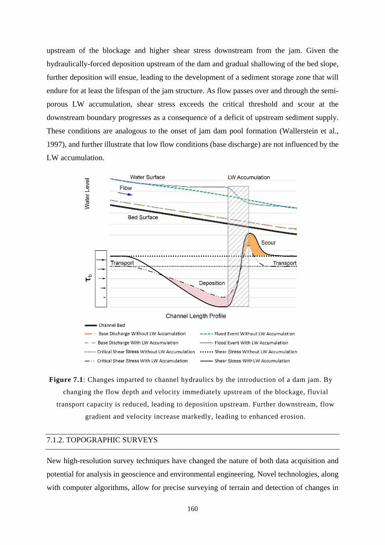
160
upstream of the blockage and higher shear stress downstream from the jam. Given the
hydraulically-forced deposition upstream of the dam and gradual shallowing of the bed slope,
further deposition will ensue, leading to the development of a sediment storage zone that will
endure for at least the lifespan of the jam structure. As flow passes over and through the semi-
porous LW accumulation, shear stress exceeds the critical threshold and scour at the
downstream boundary progresses as a consequence of a deficit of upstream sediment supply.
These conditions are analogous to the onset of jam dam pool formation (Wallerstein et al.,
1997), and further illustrate that low flow conditions (base discharge) are not influenced by the
LW accumulation.
Figure 7.1: Changes imparted to channel hydraulics by the introduction of a dam jam. By
changing the flow depth and velocity immediately upstream of the blockage, fluvial
transport capacity is reduced, leading to deposition upstream. Further downstream, flow
gradient and velocity increase markedly, leading to enhanced erosion.
7.1.2. TOPOGRAPHIC SURVEYS
New high-resolution survey techniques have changed the nature of both data acquisition and
potential for analysis in geoscience and environmental engineering. Novel technologies, along
with computer algorithms, allow for precise surveying of terrain and detection of changes in
161
topography. Many studies worked with terrestrial laser scanning (TLS) and aerial laser
scanning (ALS) techniques, revealing new river processes (Nelson et al., 1988; Riley and
Crowe, 2006; Schürch et al., 2011; Dassot et al., 2012; Calders et al., 2015; Wallace et al.,
2016; Tonina et al., 2018). Laser scanning techniques have been successfully applied, both, in
the field as well as in the laboratory (Leduc et al., 2019).
In recent years, Structure from Motion (SfM) photogrammetry, which was first developed in
the late 1970s (Ullman, 1979), has gained in popularity for surveying of Earth surface processes
(Westoby et al., 2012; Micheletti et al., 2015b; Dietrich, 2017). Several studies have
demonstrated the use of SfM photogrammetry for topographic surveying (Balaguer-Puig et al.,
2017; Li et al., 2018a; Tunnicliffe et al., 2018), showing similar performance to TLS and ALS
(Mancini et al., 2013; Kaiser et al., 2014; Ružić et al., 2014). The methodology of SfM has not
been applied extensively in LW research at present, although it provides an efficient workflow
performance with cost and time savings (Sanhueza et al., 2019a; Spreitzer et al., 2019b). LW
and SfM photogrammetry are furthermore discussed in context by Peterson et al. (2015),
Byrnes and Hasbargen (2016) and Truksa et al. (2017).
SfM algorithms show restricted abilities to process and reconstruct non-static subjects, such as
water in motion, as a large number of key-points become lost at the initial processing step
(Peterson et al., 2015). SfM photogrammetry is not yet suited for hydraulic research when it
comes to reflection or refraction from water surfaces. However, SfM has been successfully
used in LW research for log jam assessment (Spreitzer et al., 2019b), which allows for precise
quantification of LW geometries and volumes.
7.1.3. CURRENT CHALLENGES AND OBJECTIVES
Channels impacted by LW accumulations experience backwater effects (Schmocker et al.,
2015; Hartlieb, 2017; Schalko et al., 2018), changes in channel morphology (Marden et al.,
2014; Phillips et al., 2018) and the reduction of water storage capacity due to bedload
accumulation in the area upstream from a blocked cross-section (Schleiss et al., 2016; Wohl
and Scott, 2017). In the experimental work presented here, we have four aims:
(i) Assess the interruption of fractional sediment transport by a channel-spanning
structure.
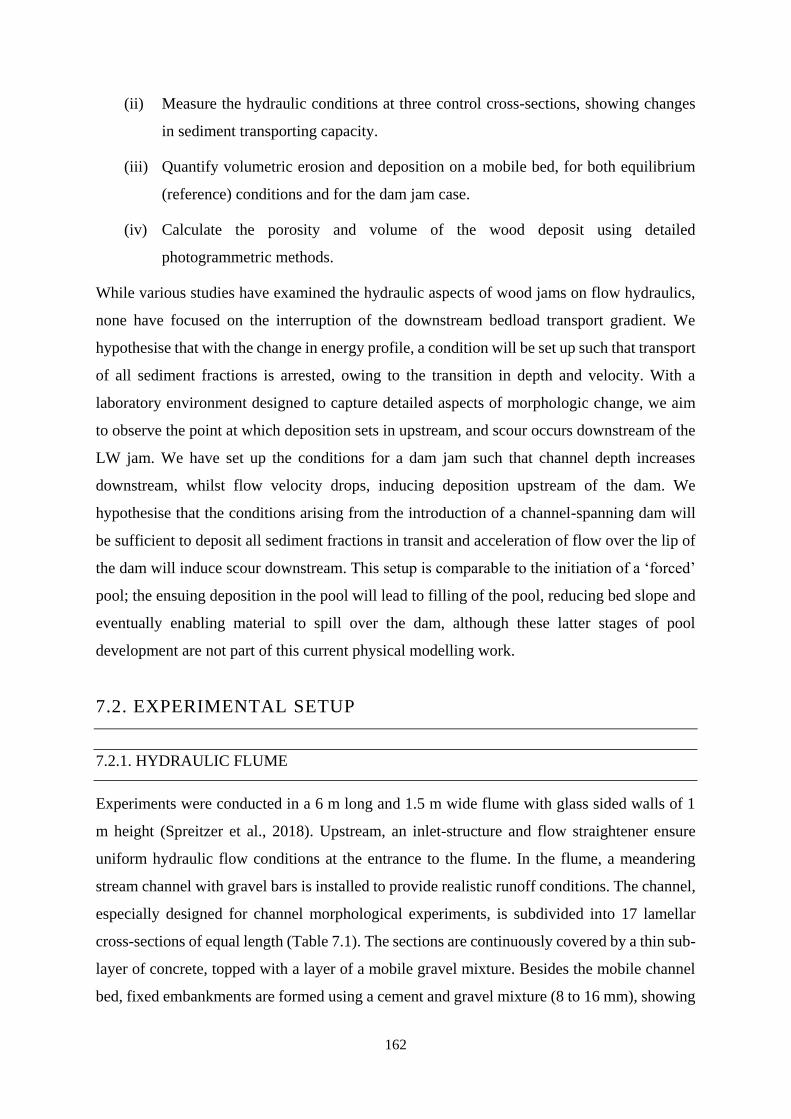
162
(ii) Measure the hydraulic conditions at three control cross-sections, showing changes
in sediment transporting capacity.
(iii) Quantify volumetric erosion and deposition on a mobile bed, for both equilibrium
(reference) conditions and for the dam jam case.
(iv) Calculate the porosity and volume of the wood deposit using detailed
photogrammetric methods.
While various studies have examined the hydraulic aspects of wood jams on flow hydraulics,
none have focused on the interruption of the downstream bedload transport gradient. We
hypothesise that with the change in energy profile, a condition will be set up such that transport
of all sediment fractions is arrested, owing to the transition in depth and velocity. With a
laboratory environment designed to capture detailed aspects of morphologic change, we aim
to observe the point at which deposition sets in upstream, and scour occurs downstream of the
LW jam. We have set up the conditions for a dam jam such that channel depth increases
downstream, whilst flow velocity drops, inducing deposition upstream of the dam. We
hypothesise that the conditions arising from the introduction of a channel-spanning dam will
be sufficient to deposit all sediment fractions in transit and acceleration of flow over the lip of
the dam will induce scour downstream. This setup is comparable to the initiation of a ‘forced’
pool; the ensuing deposition in the pool will lead to filling of the pool, reducing bed slope and
eventually enabling material to spill over the dam, although these latter stages of pool
development are not part of this current physical modelling work.
7.2. EXPERIMENTAL SETUP
7.2.1. HYDRAULIC FLUME
Experiments were conducted in a 6 m long and 1.5 m wide flume with glass sided walls of 1
m height (Spreitzer et al., 2018). Upstream, an inlet-structure and flow straightener ensure
uniform hydraulic flow conditions at the entrance to the flume. In the flume, a meandering
stream channel with gravel bars is installed to provide realistic runoff conditions. The channel,
especially designed for channel morphological experiments, is subdivided into 17 lamellar
cross-sections of equal length (Table 7.1). The sections are continuously covered by a thin sub-
layer of concrete, topped with a layer of a mobile gravel mixture. Besides the mobile channel
bed, fixed embankments are formed using a cement and gravel mixture (8 to 16 mm), showing
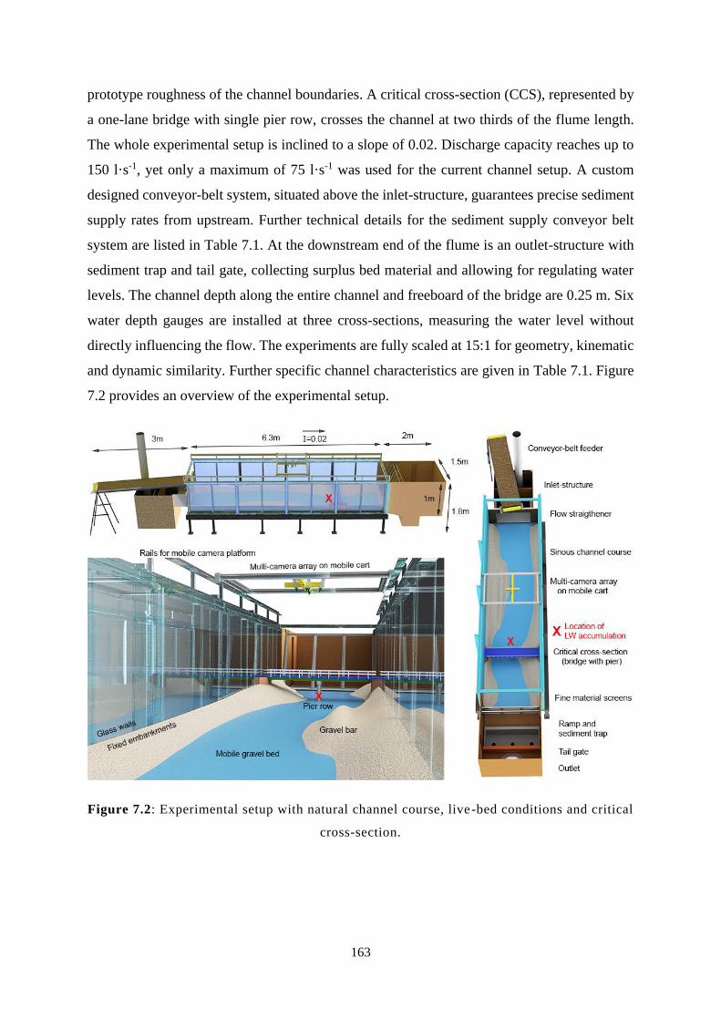
163
prototype roughness of the channel boundaries. A critical cross-section (CCS), represented by
a one-lane bridge with single pier row, crosses the channel at two thirds of the flume length.
The whole experimental setup is inclined to a slope of 0.02. Discharge capacity reaches up to
150 l·s-1, yet only a maximum of 75 l·s-1 was used for the current channel setup. A custom
designed conveyor-belt system, situated above the inlet-structure, guarantees precise sediment
supply rates from upstream. Further technical details for the sediment supply conveyor belt
system are listed in Table 7.1. At the downstream end of the flume is an outlet-structure with
sediment trap and tail gate, collecting surplus bed material and allowing for regulating water
levels. The channel depth along the entire channel and freeboard of the bridge are 0.25 m. Six
water depth gauges are installed at three cross-sections, measuring the water level without
directly influencing the flow. The experiments are fully scaled at 15:1 for geometry, kinematic
and dynamic similarity. Further specific channel characteristics are given in Table 7.1. Figure
7.2 provides an overview of the experimental setup.
Figure 7.2: Experimental setup with natural channel course, live-bed conditions and critical
cross-section.
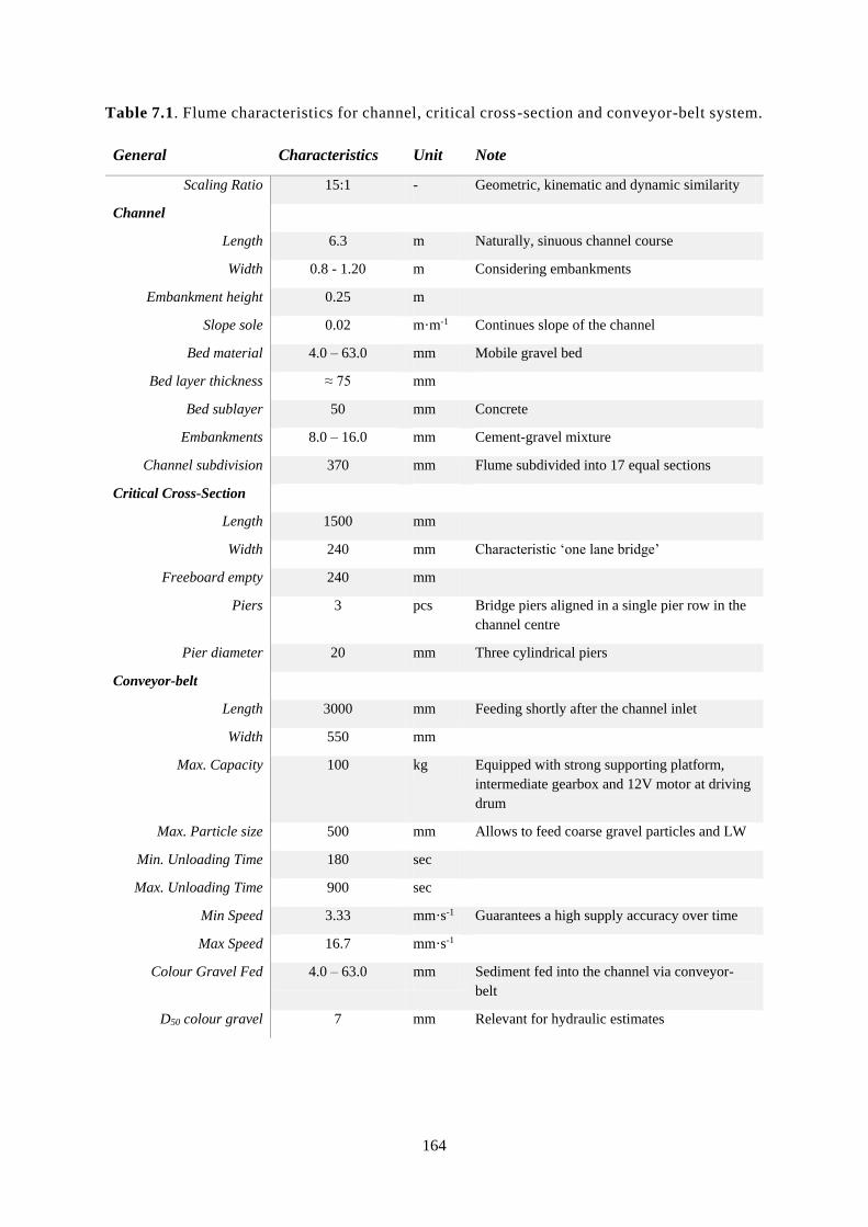
164
Table 7.1. Flume characteristics for channel, critical cross-section and conveyor-belt system.
General Characteristics Unit Note
Scaling Ratio 15:1 - Geometric, kinematic and dynamic similarity
Channel
Length 6.3 m Naturally, sinuous channel course
Width 0.8 - 1.20 m Considering embankments
Embankment height 0.25 m
Slope sole 0.02 m·m-1 Continues slope of the channel
Bed material 4.0 – 63.0 mm Mobile gravel bed
Bed layer thickness ≈ 75 mm
Bed sublayer 50 mm Concrete
Embankments 8.0 – 16.0 mm Cement-gravel mixture
Channel subdivision 370 mm Flume subdivided into 17 equal sections
Critical Cross-Section
Length 1500 mm
Width 240 mm Characteristic ‘one lane bridge’
Freeboard empty 240 mm
Piers 3 pcs Bridge piers aligned in a single pier row in the
channel centre
Pier diameter 20 mm Three cylindrical piers
Conveyor-belt
Length 3000 mm Feeding shortly after the channel inlet
Width 550 mm
Max. Capacity 100 kg Equipped with strong supporting platform,
intermediate gearbox and 12V motor at driving
drum
Max. Particle size 500 mm Allows to feed coarse gravel particles and LW
Min. Unloading Time 180 sec
Max. Unloading Time 900 sec
Min Speed 3.33 mm·s-1 Guarantees a high supply accuracy over time
Max Speed 16.7 mm·s-1
Colour Gravel Fed 4.0 – 63.0 mm Sediment fed into the channel via conveyor-
belt
D50 colour gravel 7 mm Relevant for hydraulic estimates
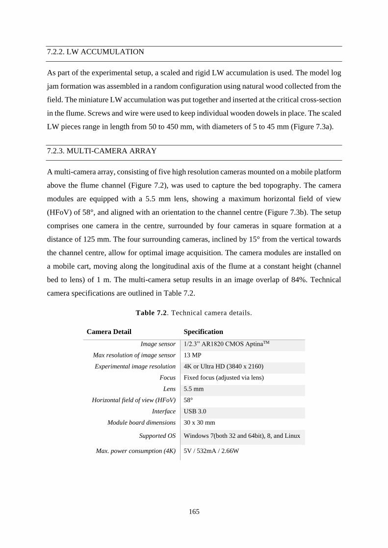
165
7.2.2. LW ACCUMULATION
As part of the experimental setup, a scaled and rigid LW accumulation is used. The model log
jam formation was assembled in a random configuration using natural wood collected from the
field. The miniature LW accumulation was put together and inserted at the critical cross-section
in the flume. Screws and wire were used to keep individual wooden dowels in place. The scaled
LW pieces range in length from 50 to 450 mm, with diameters of 5 to 45 mm (Figure 7.3a).
7.2.3. MULTI-CAMERA ARRAY
A multi-camera array, consisting of five high resolution cameras mounted on a mobile platform
above the flume channel (Figure 7.2), was used to capture the bed topography. The camera
modules are equipped with a 5.5 mm lens, showing a maximum horizontal field of view
(HFoV) of 58°, and aligned with an orientation to the channel centre (Figure 7.3b). The setup
comprises one camera in the centre, surrounded by four cameras in square formation at a
distance of 125 mm. The four surrounding cameras, inclined by 15° from the vertical towards
the channel centre, allow for optimal image acquisition. The camera modules are installed on
a mobile cart, moving along the longitudinal axis of the flume at a constant height (channel
bed to lens) of 1 m. The multi-camera setup results in an image overlap of 84%. Technical
camera specifications are outlined in Table 7.2.
Table 7.2. Technical camera details.
Camera Detail Specification
Image sensor 1/2.3” AR1820 CMOS AptinaTM
Max resolution of image sensor 13 MP
Experimental image resolution 4K or Ultra HD (3840 x 2160)
Focus Fixed focus (adjusted via lens)
Lens 5.5 mm
Horizontal field of view (HFoV) 58°
Interface USB 3.0
Module board dimensions 30 x 30 mm
Supported OS Windows 7(both 32 and 64bit), 8, and Linux
Max. power consumption (4K) 5V / 532mA / 2.66W
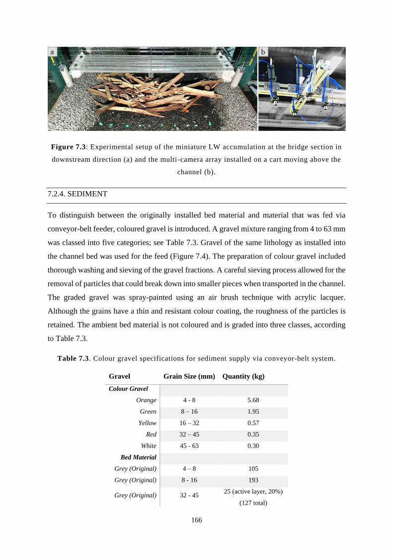
166
Figure 7.3: Experimental setup of the miniature LW accumulation at the bridge section in
downstream direction (a) and the multi-camera array installed on a cart moving above the
channel (b).
7.2.4. SEDIMENT
To distinguish between the originally installed bed material and material that was fed via
conveyor-belt feeder, coloured gravel is introduced. A gravel mixture ranging from 4 to 63 mm
was classed into five categories; see Table 7.3. Gravel of the same lithology as installed into
the channel bed was used for the feed (Figure 7.4). The preparation of colour gravel included
thorough washing and sieving of the gravel fractions. A careful sieving process allowed for the
removal of particles that could break down into smaller pieces when transported in the channel.
The graded gravel was spray-painted using an air brush technique with acrylic lacquer.
Although the grains have a thin and resistant colour coating, the roughness of the particles is
retained. The ambient bed material is not coloured and is graded into three classes, according
to Table 7.3.
Table 7.3. Colour gravel specifications for sediment supply via conveyor-belt system.
Gravel Grain Size (mm) Quantity (kg)
Colour Gravel
Orange 4 - 8 5.68
Green 8 – 16 1.95
Yellow 16 – 32 0.57
Red 32 – 45 0.35
White 45 - 63 0.30
Bed Material
Grey (Original) 4 – 8 105
Grey (Original) 8 - 16 193
Grey (Original) 32 - 45 25 (active layer, 20%)
(127 total)
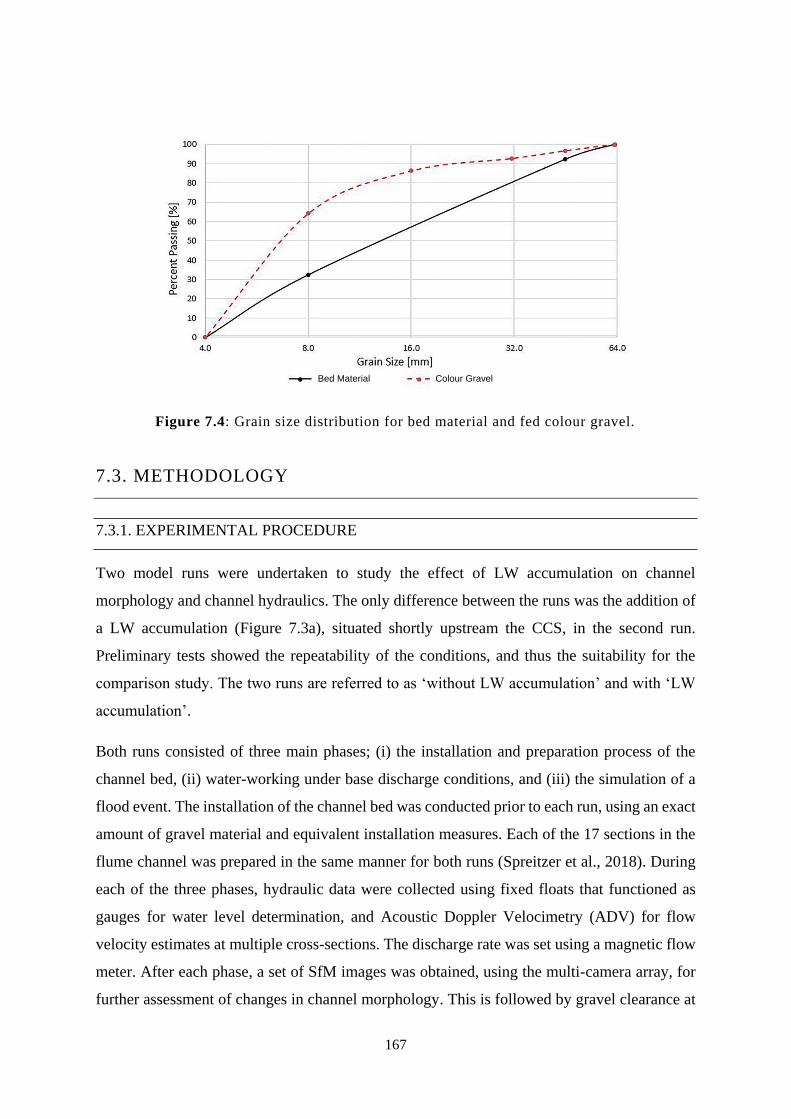
167
Figure 7.4: Grain size distribution for bed material and fed colour gravel.
7.3. METHODOLOGY
7.3.1. EXPERIMENTAL PROCEDURE
Two model runs were undertaken to study the effect of LW accumulation on channel
morphology and channel hydraulics. The only difference between the runs was the addition of
a LW accumulation (Figure 7.3a), situated shortly upstream the CCS, in the second run.
Preliminary tests showed the repeatability of the conditions, and thus the suitability for the
comparison study. The two runs are referred to as ‘without LW accumulation’ and with ‘LW
accumulation’.
Both runs consisted of three main phases; (i) the installation and preparation process of the
channel bed, (ii) water-working under base discharge conditions, and (iii) the simulation of a
flood event. The installation of the channel bed was conducted prior to each run, using an exact
amount of gravel material and equivalent installation measures. Each of the 17 sections in the
flume channel was prepared in the same manner for both runs (Spreitzer et al., 2018). During
each of the three phases, hydraulic data were collected using fixed floats that functioned as
gauges for water level determination, and Acoustic Doppler Velocimetry (ADV) for flow
velocity estimates at multiple cross-sections. The discharge rate was set using a magnetic flow
meter. After each phase, a set of SfM images was obtained, using the multi-camera array, for
further assessment of changes in channel morphology. This is followed by gravel clearance at
Bed Material Colour Gravel
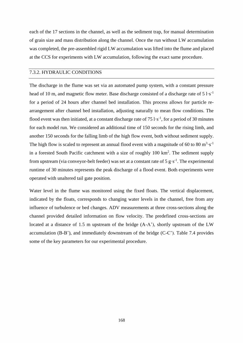
168
each of the 17 sections in the channel, as well as the sediment trap, for manual determination
of grain size and mass distribution along the channel. Once the run without LW accumulation
was completed, the pre-assembled rigid LW accumulation was lifted into the flume and placed
at the CCS for experiments with LW accumulation, following the exact same procedure.
7.3.2. HYDRAULIC CONDITIONS
The discharge in the flume was set via an automated pump system, with a constant pressure
head of 10 m, and magnetic flow meter. Base discharge consisted of a discharge rate of 5 l·s-1
for a period of 24 hours after channel bed installation. This process allows for particle re-
arrangement after channel bed installation, adjusting naturally to mean flow conditions. The
flood event was then initiated, at a constant discharge rate of 75 l·s-1, for a period of 30 minutes
for each model run. We considered an additional time of 150 seconds for the rising limb, and
another 150 seconds for the falling limb of the high flow event, both without sediment supply.
The high flow is scaled to represent an annual flood event with a magnitude of 60 to 80 m3·s-1
in a forested South Pacific catchment with a size of roughly 100 km2. The sediment supply
from upstream (via conveyor-belt feeder) was set at a constant rate of 5 g·s-1. The experimental
runtime of 30 minutes represents the peak discharge of a flood event. Both experiments were
operated with unaltered tail gate position.
Water level in the flume was monitored using the fixed floats. The vertical displacement,
indicated by the floats, corresponds to changing water levels in the channel, free from any
influence of turbulence or bed changes. ADV measurements at three cross-sections along the
channel provided detailed information on flow velocity. The predefined cross-sections are
located at a distance of 1.5 m upstream of the bridge (A-A’), shortly upstream of the LW
accumulation (B-B’), and immediately downstream of the bridge (C-C’). Table 7.4 provides
some of the key parameters for our experimental procedure.
169
Table 7.4. Overview for experimental procedure.
Experiment I II III
Dataset Initial
Channel
Base
Discharge
Flood
Event
Discharge (l·s-1) - 5 75
Time (min) - 1440 30
Water level measurement No Yes Yes
Flow velocity measurement No No Yes
Conveyor-belt speed (mm·s-1) - - 3.33
Sediment supply (kg)
(kg/s)
- - 8.85
0.00049
7.3.3. OPTICAL DATA COLLECTION
A multi-camera array, moving in steps of 100 mm along the channel, was used to capture the
bed configuration. After each flow simulation, chequer-boards with a 25 mm raster were placed
along the channel for posterior scaling. This process resulted in a continuous scan of the
channel bed, showing good image-overlap with shallow depth of field. Altogether, 50 stations
along the 6 m long active channel were scanned with all five cameras, resulting in a dataset of
250 single images. For image acquisition, we developed a software algorithm in Visual Studio
Code (2017) to control recording time and camera parameters. The majority of initial camera
parameters were kept as default, however, the white-balance parameter required adjustment,
resulting in a reduction from 5,000 to 3,300, in order to compensate for the yellowness
introduced by the halogen flood lights. All of the images were saved in .jpeg format for further
processing.
Image acquisition of the LW accumulation was conducted separately using a standard
smartphone device – Huawei Nova 2i – with a 16 + 2 MP image sensor (camera model RNE-
L22). Image resolution was set to 4608 x 3456 pixels. In total, 178 oblique and nadir images
of the LW accumulation were obtained for the LW accumulation reconstruction.
170
7.3.4. POINT CLOUD GENERATION AND PROCESSING
The flume images were further processed to point-cloud models, applying SfM
photogrammetry. Pix4Dmapper (2018), a commercially available SfM photogrammetry
software package, is used for point-cloud generation. With the option to calibrate and optimize
entire camera arrays, it represents a powerful tool for channel morphological research in the
laboratory. The semi-automated optimization of the camera array was applied to both
experiments in order to maintain uniform initial parameters of the cameras. For initial tie-point
generation, a full image scale was used, capturing channel morphological features at full
resolution. After initial processing, several scaling constraints were set using the tie-point
(‘sparse’) cloud. We considered images from every camera (1 to 5), in order to improve the
accuracy of the point-cloud model based on the input scaling information. An updated model
was computed during the optimization process. To minimise computational effort, the point-
cloud densification process used a multiscale level of 0.5 for the original image size (default
settings), with the setting “optimal” for point density. Point clouds were processed using a
constraint of a minimum number of three matches for each 3D point.
The point-cloud models of the channel morphological scans are based on 250 images and 178
images for the LW accumulation. After initial manual cleaning, the cut-tool in CloudCompare
was applied to remove outlier points. Point-cloud matching was achieved using fine
registration via iterative closest point (ICP), with RMS e-20, and 5·105 points as random
sampling limit. After ICP registration, a final point picking alignment of 30 point-pairs was
conducted. For point-cloud comparison in CloudCompare, we used the flood event point-cloud
model as ‘data’ model and the base discharge point model as ‘reference’ model. These point-
cloud models were required for the detection of channel morphological changes and estimation
of the sediment flux.
Point-cloud and mesh processing for the LW accumulation were conducted in Pix4Dmapper
(2018), cleaning and cutting in CloudCompareV2 (2016), further filtering and Poisson surface
reconstruction (PSR) in Meshlab by Cignoni et al. (2008), and closing the mesh to a watertight
accumulation body for 3D volume estimates was achieved in Autodesk Fusion 360 (2018). The
final volumetric output was computed in Pix4Dm using the integrated 2.5D volume tool, and
Meshlab, using the algorithm for computing geometric measures. By means of the computed
2.5D and 3D volume, accumulation porosity (n) was estimated using Equation (7.1).
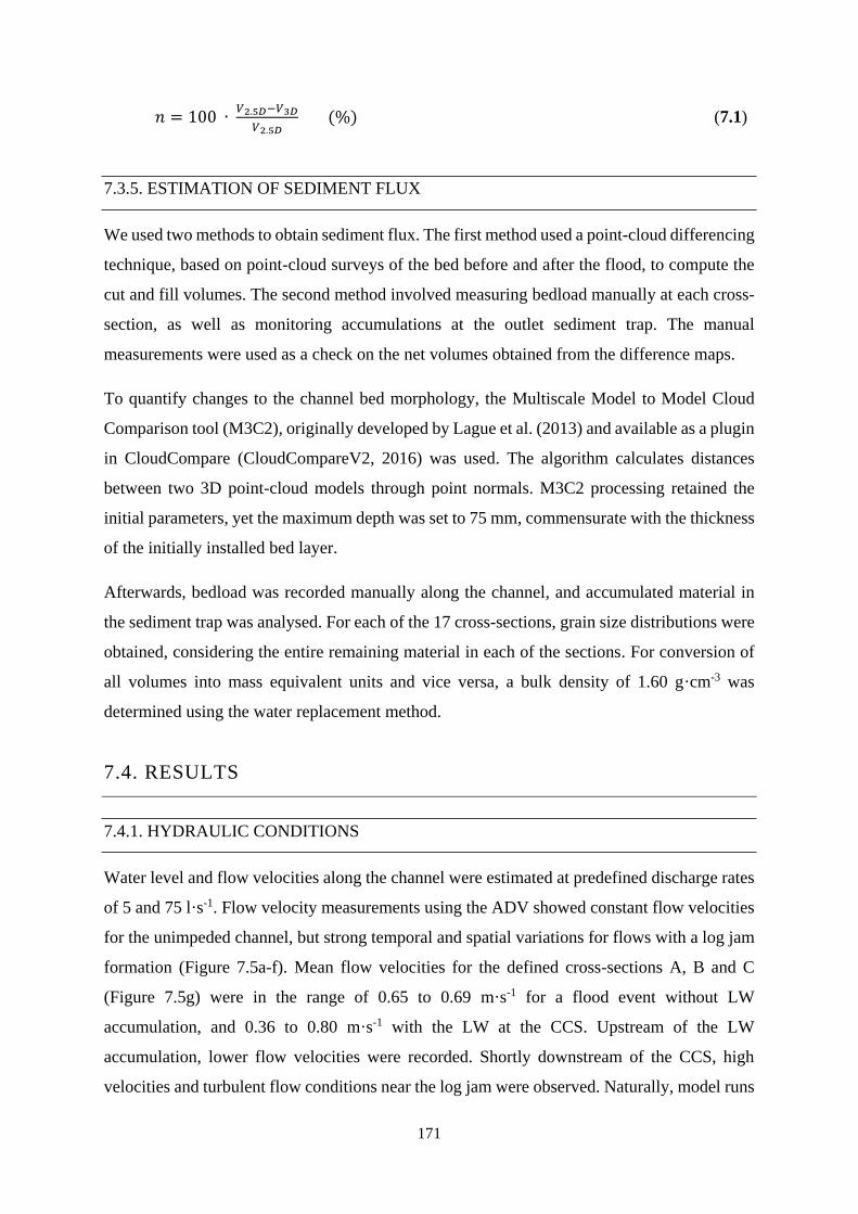
171
𝑛 = 100 ∙ 𝑉2.5𝐷−𝑉3𝐷
𝑉2.5𝐷 (%) (7.1)
7.3.5. ESTIMATION OF SEDIMENT FLUX
We used two methods to obtain sediment flux. The first method used a point-cloud differencing
technique, based on point-cloud surveys of the bed before and after the flood, to compute the
cut and fill volumes. The second method involved measuring bedload manually at each cross-
section, as well as monitoring accumulations at the outlet sediment trap. The manual
measurements were used as a check on the net volumes obtained from the difference maps.
To quantify changes to the channel bed morphology, the Multiscale Model to Model Cloud
Comparison tool (M3C2), originally developed by Lague et al. (2013) and available as a plugin
in CloudCompare (CloudCompareV2, 2016) was used. The algorithm calculates distances
between two 3D point-cloud models through point normals. M3C2 processing retained the
initial parameters, yet the maximum depth was set to 75 mm, commensurate with the thickness
of the initially installed bed layer.
Afterwards, bedload was recorded manually along the channel, and accumulated material in
the sediment trap was analysed. For each of the 17 cross-sections, grain size distributions were
obtained, considering the entire remaining material in each of the sections. For conversion of
all volumes into mass equivalent units and vice versa, a bulk density of 1.60 g·cm-3 was
determined using the water replacement method.
7.4. RESULTS
7.4.1. HYDRAULIC CONDITIONS
Water level and flow velocities along the channel were estimated at predefined discharge rates
of 5 and 75 l·s-1. Flow velocity measurements using the ADV showed constant flow velocities
for the unimpeded channel, but strong temporal and spatial variations for flows with a log jam
formation (Figure 7.5a-f). Mean flow velocities for the defined cross-sections A, B and C
(Figure 7.5g) were in the range of 0.65 to 0.69 m·s-1 for a flood event without LW
accumulation, and 0.36 to 0.80 m·s-1 with the LW at the CCS. Upstream of the LW
accumulation, lower flow velocities were recorded. Shortly downstream of the CCS, high
velocities and turbulent flow conditions near the log jam were observed. Naturally, model runs
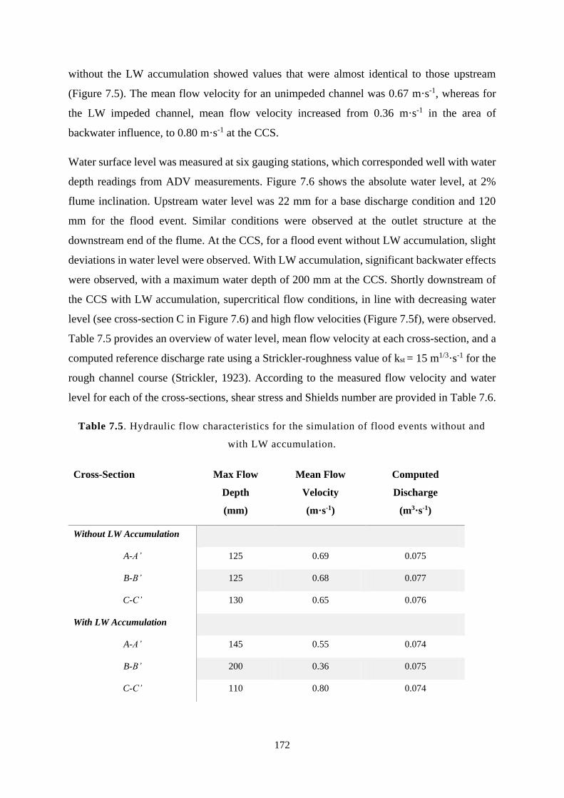
172
without the LW accumulation showed values that were almost identical to those upstream
(Figure 7.5). The mean flow velocity for an unimpeded channel was 0.67 m·s-1, whereas for
the LW impeded channel, mean flow velocity increased from 0.36 m·s-1 in the area of
backwater influence, to 0.80 m·s-1 at the CCS.
Water surface level was measured at six gauging stations, which corresponded well with water
depth readings from ADV measurements. Figure 7.6 shows the absolute water level, at 2%
flume inclination. Upstream water level was 22 mm for a base discharge condition and 120
mm for the flood event. Similar conditions were observed at the outlet structure at the
downstream end of the flume. At the CCS, for a flood event without LW accumulation, slight
deviations in water level were observed. With LW accumulation, significant backwater effects
were observed, with a maximum water depth of 200 mm at the CCS. Shortly downstream of
the CCS with LW accumulation, supercritical flow conditions, in line with decreasing water
level (see cross-section C in Figure 7.6) and high flow velocities (Figure 7.5f), were observed.
Table 7.5 provides an overview of water level, mean flow velocity at each cross-section, and a
computed reference discharge rate using a Strickler-roughness value of kst = 15 m1/3·s-1 for the
rough channel course (Strickler, 1923). According to the measured flow velocity and water
level for each of the cross-sections, shear stress and Shields number are provided in Table 7.6.
Table 7.5. Hydraulic flow characteristics for the simulation of flood events without and
with LW accumulation.
Cross-Section Max Flow
Depth
(mm)
Mean Flow
Velocity
(m·s-1)
Computed
Discharge
(m3·s-1)
Without LW Accumulation
A-A’ 125 0.69 0.075
B-B’ 125 0.68 0.077
C-C’ 130 0.65 0.076
With LW Accumulation
A-A’ 145 0.55 0.074
B-B’ 200 0.36 0.075
C-C’ 110 0.80 0.074
173
Figure 7.5: Flow velocity profiles measured using ADV in the flume channel, both with
and without LW accumulation. Flow velocity measurements are obtained 1.5 m
upstream of the bridge cross-section A (a and b) and shortly upstream the LW
accumulation at cross-section B (c and d). The charts e and f show the flow
condition immediately downstream the LW accumulation at cross-section C. (g)
shows the channel with the LW accumulation at the critical cross-section and
aggradation of the colour gravel feed in the upstream section.
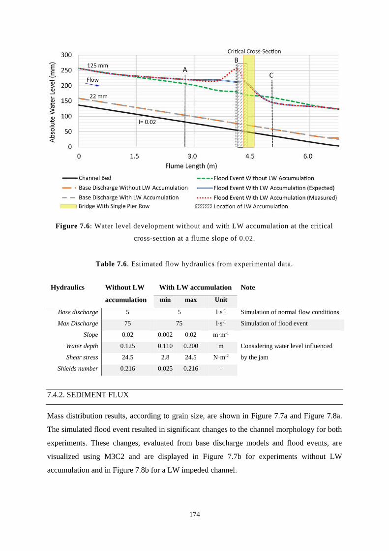
174
Figure 7.6: Water level development without and with LW accumulation at the critical
cross-section at a flume slope of 0.02.
Table 7.6. Estimated flow hydraulics from experimental data.
7.4.2. SEDIMENT FLUX
Mass distribution results, according to grain size, are shown in Figure 7.7a and Figure 7.8a.
The simulated flood event resulted in significant changes to the channel morphology for both
experiments. These changes, evaluated from base discharge models and flood events, are
visualized using M3C2 and are displayed in Figure 7.7b for experiments without LW
accumulation and in Figure 7.8b for a LW impeded channel.
Hydraulics Without LW
accumulation
With LW accumulation Note
min max Unit
Base discharge 5 5 l·s-1 Simulation of normal flow conditions
Max Discharge 75 75 l·s-1 Simulation of flood event
Slope 0.02 0.002 0.02 m·m-1
Considering water level influenced
by the jam
Water depth 0.125 0.110 0.200 m
Shear stress 24.5 2.8 24.5 N·m-2
Shields number 0.216 0.025 0.216 -
175
The experiment without LW accumulation manifested continuous bedload transport
throughout the entire flume channel. Point-cloud comparison revealed a total bedload of
23.8·10-3 m3 for the wood unimpeded experiments (Table 7.7). The M3C2 model (Figure 7.7b)
highlights the formation of channels (blue) and bars (red) in the stream section. Sections
displayed in light grey indicate that no significant topographic changes occurred in these areas.
At the inlet section, the M3C2 analysis indicates erosion at the location of sediment input via
conveyor-belt feeder. A total of 8.85 kg colour gravel was fed into the channel using the
conveyor-belt system. Over a period of 30 minutes, 1.68 kg of the fed material was transported
all the way to the sediment trap. Colour gravel exceeding a diameter of 45 mm deposited
immediately upon delivery into the channel. Smaller gravel fractions were distributed almost
uniformly along the channel length (compare Figure 7.7a - colour gravel axis). Upstream of
the CCS, a 2 m long bar (approx.) developed, which emerges more than 70 mm from the
original channel bed. In the centreline of the flume a straight channel was formed during high
flow conditions.
The model run without any LW influence revealed fluctuating sediment transport with
alternating channel and bar formation. In total, 48.60 kg gravel material accumulated in the
sediment trap, consisting of both colour gravel and the ambient bed material. The difference
between sediment output and input in the channel was 39.75 kg, which is equivalent to a
volume of 24.80·10-3 m3, using a bulk density of 1.60 g·cm-3 for the angular gravel material.
Comparison of the manually measured bedload volumes and the point-cloud difference model
shows a deviation of 1.05·10-3 m3 (i.e. a difference of +4%; more measured flux than resolved
in the difference model)
Results of the experimental run with LW accumulation showed less bedload transport activity
in the upstream area of the CCS, yet, a considerable amount of bedload was transported out of
the downstream section. A short distance downstream of the inlet, at the location of the
sediment input, deep erosion fields were revealed in M3C2 difference maps. The manually
obtained bedload measurements also show net erosion in the top sections. Both fed sediment
and eroded channel material accumulated over a length of 2.5 m along the upper section. The
accumulated material resulted in a rise of the channel bed of up to 60 mm for some areas. About
1 m upstream the LW accumulation bedload transport reached a minimum.
Changes to channel morphology were evident at the CCS, below the LW accumulation and
downstream from the bridge section (Figure 7.8a). A gravel bar formed in line with the row of
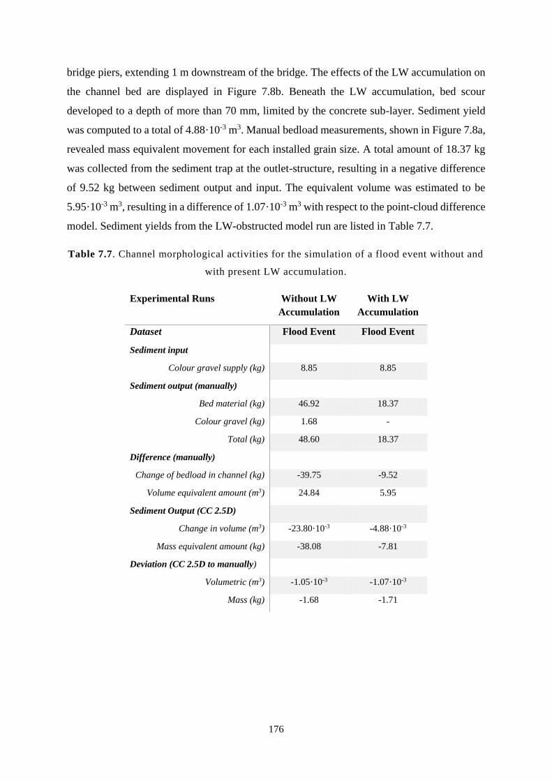
176
bridge piers, extending 1 m downstream of the bridge. The effects of the LW accumulation on
the channel bed are displayed in Figure 7.8b. Beneath the LW accumulation, bed scour
developed to a depth of more than 70 mm, limited by the concrete sub-layer. Sediment yield
was computed to a total of 4.88·10-3 m3. Manual bedload measurements, shown in Figure 7.8a,
revealed mass equivalent movement for each installed grain size. A total amount of 18.37 kg
was collected from the sediment trap at the outlet-structure, resulting in a negative difference
of 9.52 kg between sediment output and input. The equivalent volume was estimated to be
5.95·10-3 m3, resulting in a difference of 1.07·10-3 m3 with respect to the point-cloud difference
model. Sediment yields from the LW-obstructed model run are listed in Table 7.7.
Table 7.7. Channel morphological activities for the simulation of a flood event without and
with present LW accumulation.
Experimental Runs Without LW
Accumulation
With LW
Accumulation
Dataset Flood Event Flood Event
Sediment input
Colour gravel supply (kg) 8.85 8.85
Sediment output (manually)
Bed material (kg) 46.92 18.37
Colour gravel (kg) 1.68 -
Total (kg) 48.60 18.37
Difference (manually)
Change of bedload in channel (kg) -39.75 -9.52
Volume equivalent amount (m3) 24.84 5.95
Sediment Output (CC 2.5D)
Change in volume (m3) -23.80·10-3 -4.88·10-3
Mass equivalent amount (kg) -38.08 -7.81
Deviation (CC 2.5D to manually)
Volumetric (m3) -1.05·10-3 -1.07·10-3
Mass (kg) -1.68 -1.71
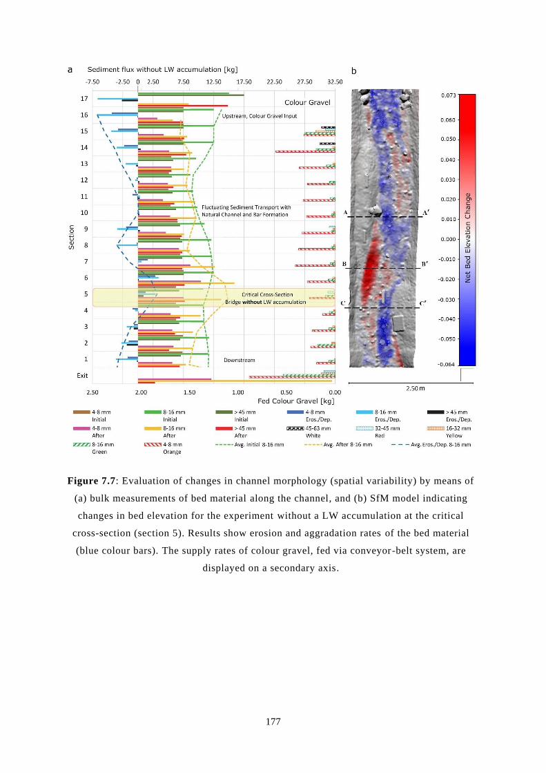
177
Figure 7.7: Evaluation of changes in channel morphology (spatial variability) by means of
(a) bulk measurements of bed material along the channel, and (b) SfM model indicating
changes in bed elevation for the experiment without a LW accumulation at the critical
cross-section (section 5). Results show erosion and aggradation rates of the bed material
(blue colour bars). The supply rates of colour gravel, fed via conveyor-belt system, are
displayed on a secondary axis.
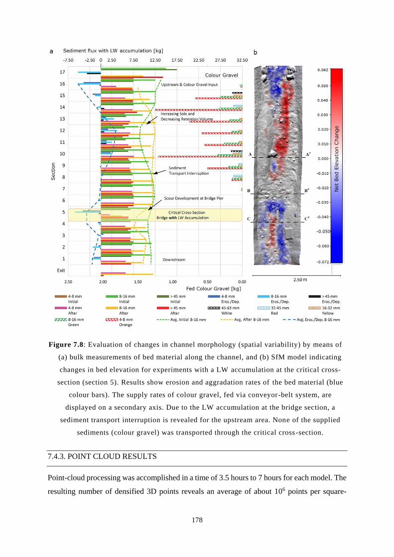
178
Figure 7.8: Evaluation of changes in channel morphology (spatial variability) by means of
(a) bulk measurements of bed material along the channel, and (b) SfM model indicating
changes in bed elevation for experiments with a LW accumulation at the critical cross-
section (section 5). Results show erosion and aggradation rates of the bed material (blue
colour bars). The supply rates of colour gravel, fed via conveyor-belt system, are
displayed on a secondary axis. Due to the LW accumulation at the bridge section, a
sediment transport interruption is revealed for the upstream area. None of the supplied
sediments (colour gravel) was transported through the critical cross -section.
7.4.3. POINT CLOUD RESULTS
Point-cloud processing was accomplished in a time of 3.5 hours to 7 hours for each model. The
resulting number of densified 3D points reveals an average of about 106 points per square-
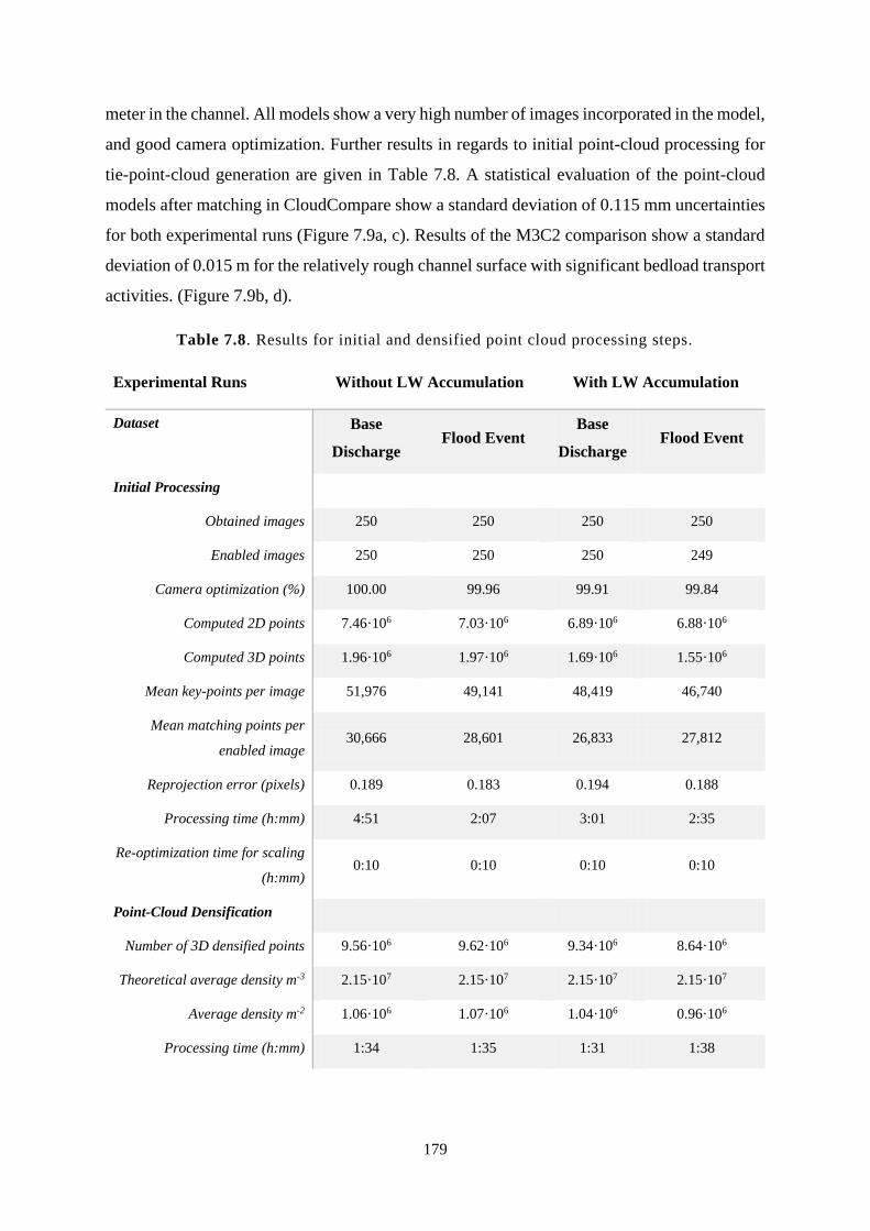
179
meter in the channel. All models show a very high number of images incorporated in the model,
and good camera optimization. Further results in regards to initial point-cloud processing for
tie-point-cloud generation are given in Table 7.8. A statistical evaluation of the point-cloud
models after matching in CloudCompare show a standard deviation of 0.115 mm uncertainties
for both experimental runs (Figure 7.9a, c). Results of the M3C2 comparison show a standard
deviation of 0.015 m for the relatively rough channel surface with significant bedload transport
activities. (Figure 7.9b, d).
Table 7.8. Results for initial and densified point cloud processing steps.
Experimental Runs Without LW Accumulation With LW Accumulation
Dataset Base
Discharge Flood Event
Base
Discharge Flood Event
Initial Processing
Obtained images 250 250 250 250
Enabled images 250 250 250 249
Camera optimization (%) 100.00 99.96 99.91 99.84
Computed 2D points 7.46·106 7.03·106 6.89·106 6.88·106
Computed 3D points 1.96·106 1.97·106 1.69·106 1.55·106
Mean key-points per image 51,976 49,141 48,419 46,740
Mean matching points per
enabled image 30,666 28,601 26,833 27,812
Reprojection error (pixels) 0.189 0.183 0.194 0.188
Processing time (h:mm) 4:51 2:07 3:01 2:35
Re-optimization time for scaling
(h:mm) 0:10 0:10 0:10 0:10
Point-Cloud Densification
Number of 3D densified points 9.56·106 9.62·106 9.34·106 8.64·106
Theoretical average density m-3 2.15·107 2.15·107 2.15·107 2.15·107
Average density m-2 1.06·106 1.07·106 1.04·106 0.96·106
Processing time (h:mm) 1:34 1:35 1:31 1:38
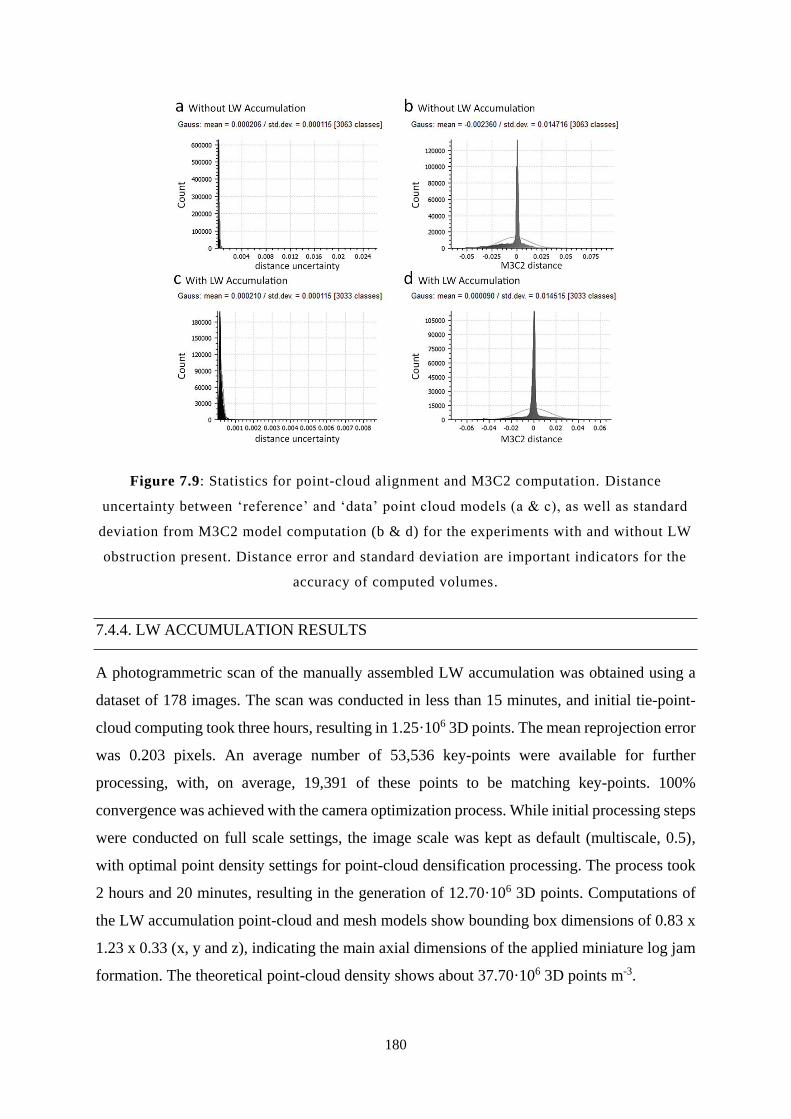
180
Figure 7.9: Statistics for point-cloud alignment and M3C2 computation. Distance
uncertainty between ‘reference’ and ‘data’ point cloud models (a & c), as well as standard
deviation from M3C2 model computation (b & d) for the experiments with and without LW
obstruction present. Distance error and standard deviation are important indicators for the
accuracy of computed volumes.
7.4.4. LW ACCUMULATION RESULTS
A photogrammetric scan of the manually assembled LW accumulation was obtained using a
dataset of 178 images. The scan was conducted in less than 15 minutes, and initial tie-point-
cloud computing took three hours, resulting in 1.25·106 3D points. The mean reprojection error
was 0.203 pixels. An average number of 53,536 key-points were available for further
processing, with, on average, 19,391 of these points to be matching key-points. 100%
convergence was achieved with the camera optimization process. While initial processing steps
were conducted on full scale settings, the image scale was kept as default (multiscale, 0.5),
with optimal point density settings for point-cloud densification processing. The process took
2 hours and 20 minutes, resulting in the generation of 12.70·106 3D points. Computations of
the LW accumulation point-cloud and mesh models show bounding box dimensions of 0.83 x
1.23 x 0.33 (x, y and z), indicating the main axial dimensions of the applied miniature log jam
formation. The theoretical point-cloud density shows about 37.70·106 3D points m-3.
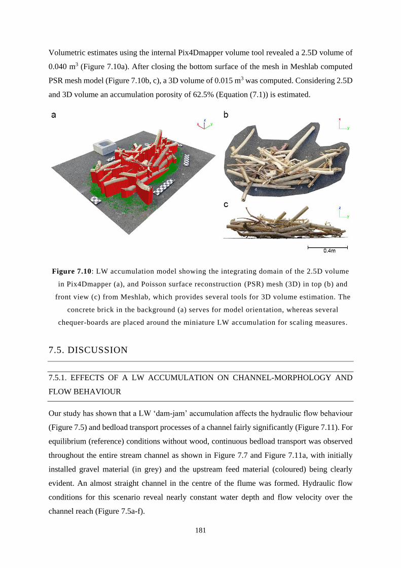
181
Volumetric estimates using the internal Pix4Dmapper volume tool revealed a 2.5D volume of
0.040 m3 (Figure 7.10a). After closing the bottom surface of the mesh in Meshlab computed
PSR mesh model (Figure 7.10b, c), a 3D volume of 0.015 m3 was computed. Considering 2.5D
and 3D volume an accumulation porosity of 62.5% (Equation (7.1)) is estimated.
Figure 7.10: LW accumulation model showing the integrating domain of the 2.5D volume
in Pix4Dmapper (a), and Poisson surface reconstruction (PSR) mesh (3D) in top (b) and
front view (c) from Meshlab, which provides several tools for 3D volume estimation. The
concrete brick in the background (a) serves for model orien tation, whereas several
chequer-boards are placed around the miniature LW accumulation for scaling measures.
7.5. DISCUSSION
7.5.1. EFFECTS OF A LW ACCUMULATION ON CHANNEL-MORPHOLOGY AND
FLOW BEHAVIOUR
Our study has shown that a LW ‘dam-jam’ accumulation affects the hydraulic flow behaviour
(Figure 7.5) and bedload transport processes of a channel fairly significantly (Figure 7.11). For
equilibrium (reference) conditions without wood, continuous bedload transport was observed
throughout the entire stream channel as shown in Figure 7.7 and Figure 7.11a, with initially
installed gravel material (in grey) and the upstream feed material (coloured) being clearly
evident. An almost straight channel in the centre of the flume was formed. Hydraulic flow
conditions for this scenario reveal nearly constant water depth and flow velocity over the
channel reach (Figure 7.5a-f).
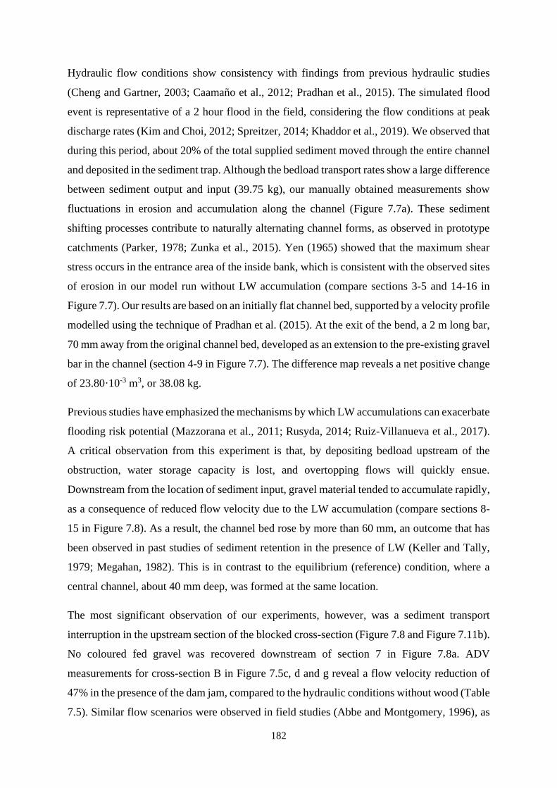
182
Hydraulic flow conditions show consistency with findings from previous hydraulic studies
(Cheng and Gartner, 2003; Caamaño et al., 2012; Pradhan et al., 2015). The simulated flood
event is representative of a 2 hour flood in the field, considering the flow conditions at peak
discharge rates (Kim and Choi, 2012; Spreitzer, 2014; Khaddor et al., 2019). We observed that
during this period, about 20% of the total supplied sediment moved through the entire channel
and deposited in the sediment trap. Although the bedload transport rates show a large difference
between sediment output and input (39.75 kg), our manually obtained measurements show
fluctuations in erosion and accumulation along the channel (Figure 7.7a). These sediment
shifting processes contribute to naturally alternating channel forms, as observed in prototype
catchments (Parker, 1978; Zunka et al., 2015). Yen (1965) showed that the maximum shear
stress occurs in the entrance area of the inside bank, which is consistent with the observed sites
of erosion in our model run without LW accumulation (compare sections 3-5 and 14-16 in
Figure 7.7). Our results are based on an initially flat channel bed, supported by a velocity profile
modelled using the technique of Pradhan et al. (2015). At the exit of the bend, a 2 m long bar,
70 mm away from the original channel bed, developed as an extension to the pre-existing gravel
bar in the channel (section 4-9 in Figure 7.7). The difference map reveals a net positive change
of 23.80·10-3 m3, or 38.08 kg.
Previous studies have emphasized the mechanisms by which LW accumulations can exacerbate
flooding risk potential (Mazzorana et al., 2011; Rusyda, 2014; Ruiz-Villanueva et al., 2017).
A critical observation from this experiment is that, by depositing bedload upstream of the
obstruction, water storage capacity is lost, and overtopping flows will quickly ensue.
Downstream from the location of sediment input, gravel material tended to accumulate rapidly,
as a consequence of reduced flow velocity due to the LW accumulation (compare sections 8-
15 in Figure 7.8). As a result, the channel bed rose by more than 60 mm, an outcome that has
been observed in past studies of sediment retention in the presence of LW (Keller and Tally,
1979; Megahan, 1982). This is in contrast to the equilibrium (reference) condition, where a
central channel, about 40 mm deep, was formed at the same location.
The most significant observation of our experiments, however, was a sediment transport
interruption in the upstream section of the blocked cross-section (Figure 7.8 and Figure 7.11b).
No coloured fed gravel was recovered downstream of section 7 in Figure 7.8a. ADV
measurements for cross-section B in Figure 7.5c, d and g reveal a flow velocity reduction of
47% in the presence of the dam jam, compared to the hydraulic conditions without wood (Table
7.5). Similar flow scenarios were observed in field studies (Abbe and Montgomery, 1996), as
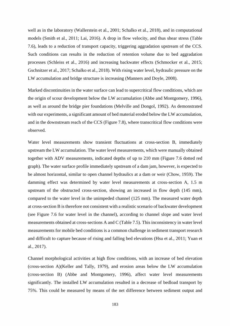
183
well as in the laboratory (Wallerstein et al., 2001; Schalko et al., 2018), and in computational
models (Smith et al., 2011; Lai, 2016). A drop in flow velocity, and thus shear stress (Table
7.6), leads to a reduction of transport capacity, triggering aggradation upstream of the CCS.
Such conditions can results in the reduction of retention volume due to bed aggradation
processes (Schleiss et al., 2016) and increasing backwater effects (Schmocker et al., 2015;
Gschnitzer et al., 2017; Schalko et al., 2018). With rising water level, hydraulic pressure on the
LW accumulation and bridge structure is increasing (Manners and Doyle, 2008).
Marked discontinuities in the water surface can lead to supercritical flow conditions, which are
the origin of scour development below the LW accumulation (Abbe and Montgomery, 1996),
as well as around the bridge pier foundations (Melville and Dongol, 1992). As demonstrated
with our experiments, a significant amount of bed material eroded below the LW accumulation,
and in the downstream reach of the CCS (Figure 7.8), where transcritical flow conditions were
observed.
Water level measurements show transient fluctuations at cross-section B, immediately
upstream the LW accumulation. The water level measurements, which were manually obtained
together with ADV measurements, indicated depths of up to 210 mm (Figure 7.6 dotted red
graph). The water surface profile immediately upstream of a dam jam, however, is expected to
be almost horizontal, similar to open channel hydraulics at a dam or weir (Chow, 1959). The
damming effect was determined by water level measurements at cross-section A, 1.5 m
upstream of the obstructed cross-section, showing an increased in flow depth (145 mm),
compared to the water level in the unimpeded channel (125 mm). The measured water depth
at cross-section B is therefore not consistent with a realistic scenario of backwater development
(see Figure 7.6 for water level in the channel), according to channel slope and water level
measurements obtained at cross-sections A and C (Table 7.5). This inconsistency in water level
measurements for mobile bed conditions is a common challenge in sediment transport research
and difficult to capture because of rising and falling bed elevations (Hsu et al., 2011; Yuan et
al., 2017).
Channel morphological activities at high flow conditions, with an increase of bed elevation
(cross-section A)(Keller and Tally, 1979), and erosion areas below the LW accumulation
(cross-section B) (Abbe and Montgomery, 1996), affect water level measurements
significantly. The installed LW accumulation resulted in a decrease of bedload transport by
75%. This could be measured by means of the net difference between sediment output and
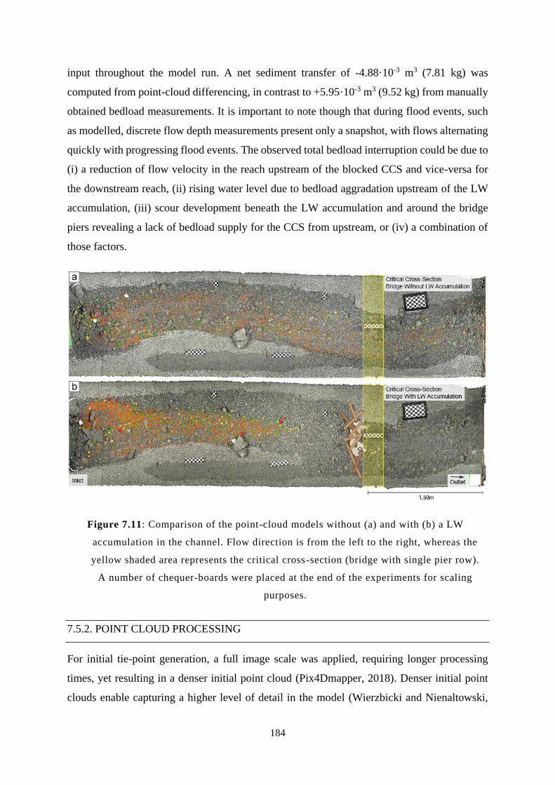
184
input throughout the model run. A net sediment transfer of -4.88·10-3 m3 (7.81 kg) was
computed from point-cloud differencing, in contrast to +5.95·10-3 m3 (9.52 kg) from manually
obtained bedload measurements. It is important to note though that during flood events, such
as modelled, discrete flow depth measurements present only a snapshot, with flows alternating
quickly with progressing flood events. The observed total bedload interruption could be due to
(i) a reduction of flow velocity in the reach upstream of the blocked CCS and vice-versa for
the downstream reach, (ii) rising water level due to bedload aggradation upstream of the LW
accumulation, (iii) scour development beneath the LW accumulation and around the bridge
piers revealing a lack of bedload supply for the CCS from upstream, or (iv) a combination of
those factors.
Figure 7.11: Comparison of the point-cloud models without (a) and with (b) a LW
accumulation in the channel. Flow direction is from the left to the right, whereas the
yellow shaded area represents the critical cross-section (bridge with single pier row).
A number of chequer-boards were placed at the end of the experiments for scaling
purposes.
7.5.2. POINT CLOUD PROCESSING
For initial tie-point generation, a full image scale was applied, requiring longer processing
times, yet resulting in a denser initial point cloud (Pix4Dmapper, 2018). Denser initial point
clouds enable capturing a higher level of detail in the model (Wierzbicki and Nienaltowski,
185
2019). The next step of point-cloud densification can therefore be processed using half image
scale, whilst still maintaining a high resolution. According to Pix4Dmapper (2018), excellent
model characteristics are achieved (i) when the percentage of enabled images per dataset
exceeds 95%, (ii) with an extraction of more than 10·103 key-points per enabled image, and
(iii) when the number of matching key-points per enabled image is higher than 1·103. In all of
our initial point-cloud modes, these suggested boundaries for high-quality models have been
exceeded, providing a valuable basis for accurate sediment flux computations. Point-cloud
quality is further assessed by the mean of the reprojection error, which should be smaller than,
or equal to the size of one pixel (Pix4Dmapper, 2018). Our results show reprojection errors in
a range of 0.183 to 0.194 pixels (Table 7.8), satisfying the conditions for high quality point-
cloud models. According to the generated number of 3D points, a model resolution of less than
1 mm is achieved, which represents one of the highest model resolutions in contrast to previous
studies, which range from 1 m for LiDAR scans (Kasprak et al., 2012; Atha and Dietrich, 2016;
Steeb et al., 2017) to a maximum resolution of 1 mm for TLS surveys (Boivin and Buffin-
Bélanger, 2010; Grigillo et al., 2015), and similar performances for other SfM-photogrammetry
applications (Smith et al., 2016).
The M3C2 method considers uncertainties in surface roughness and is more efficient compared
to cloud-to-mesh comparison (C2M) (Barnhart and Crosby, 2013; Lague et al., 2013). Another
advantage of the M3C2 comparison algorithm is based on a low number of pre-processing and
filtering steps required, which are essential for correction of systematic errors (Khoshelham
and Elberink, 2012), in order to generate high quality point-cloud models. This low number of
pre-processing steps maintains the originally processed model accuracy in terms of
preservation of shape and geometries. By computing differences in distance between the
reference and data model, the M3C2 method precisely visualizes changes of channel
morphological activities (Lague et al., 2013). Volumes are estimated using a 2.5D volume tool
in CloudCompare that allows for the comparison of two registered point-cloud models with an
effective output of a volumetric measure. The computational accuracy increases with
decreasing noise in the point-cloud model (Santise et al., 2018). Therefore, accuracy and
precision for initial point-cloud processing and point-cloud densification are important to
generate high-quality 3D models. Reducing noise by post-process filtering may affect surface
properties of especially rough and unorganized surfaces (Fua and Sander, 1992; Hoppe et al.,
1992; Remondino, 2003; Deschaud and Goulette, 2014) as observed also previously (Carrivick
et al., 2016).
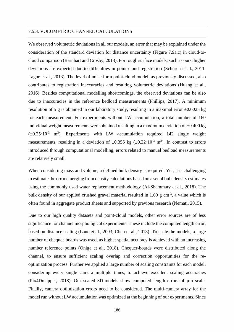
186
7.5.3. VOLUMETRIC CHANNEL CALCULATIONS
We observed volumetric deviations in all our models, an error that may be explained under the
consideration of the standard deviation for distance uncertainty (Figure 7.9a,c) in cloud-to-
cloud comparison (Barnhart and Crosby, 2013). For rough surface models, such as ours, higher
deviations are expected due to difficulties in point-cloud registration (Schürch et al., 2011;
Lague et al., 2013). The level of noise for a point-cloud model, as previously discussed, also
contributes to registration inaccuracies and resulting volumetric deviations (Huang et al.,
2016). Besides computational modelling shortcomings, the observed deviations can be also
due to inaccuracies in the reference bedload measurements (Phillips, 2017). A minimum
resolution of 5 g is obtained in our laboratory study, resulting in a maximal error ±0.0025 kg
for each measurement. For experiments without LW accumulation, a total number of 160
individual weight measurements were obtained resulting in a maximum deviation of ±0.400 kg
(±0.25·10-3 m3). Experiments with LW accumulation required 142 single weight
measurements, resulting in a deviation of ±0.355 kg (±0.22·10-3 m3). In contrast to errors
introduced through computational modelling, errors related to manual bedload measurements
are relatively small.
When considering mass and volume, a defined bulk density is required. Yet, it is challenging
to estimate the error emerging from density calculations based on a set of bulk density estimates
using the commonly used water replacement methodology (Al-Shammary et al., 2018). The
bulk density of our applied crushed gravel material resulted in 1.60 g·cm-3, a value which is
often found in aggregate product sheets and supported by previous research (Nemati, 2015).
Due to our high quality datasets and point-cloud models, other error sources are of less
significance for channel morphological experiments. These include the computed length error,
based on distance scaling (Lane et al., 2003; Chen et al., 2018). To scale the models, a large
number of chequer-boards was used, as higher spatial accuracy is achieved with an increasing
number reference points (Oniga et al., 2018). Chequer-boards were distributed along the
channel, to ensure sufficient scaling overlap and correction opportunities for the re-
optimization process. Further we applied a large number of scaling constraints for each model,
considering every single camera multiple times, to achieve excellent scaling accuracies
(Pix4Dmapper, 2018). Our scaled 3D-models show computed length errors of µm scale.
Finally, camera optimization errors need to be considered. The multi-camera array for the
model run without LW accumulation was optimized at the beginning of our experiments. Since
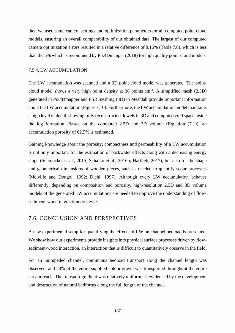
187
then we used same camera settings and optimization parameters for all computed point cloud
models, ensuring an overall comparability of our obtained data. The largest of our computed
camera optimization errors resulted in a relative difference of 0.16% (Table 7.8), which is less
than the 5% which is recommend by Pix4Dmapper (2018) for high quality point-cloud models.
7.5.4. LW ACCUMULATION
The LW accumulation was scanned and a 3D point-cloud model was generated. The point-
cloud model shows a very high point density at 38 points·cm-3. A simplified mesh (2.5D)
generated in Pix4Dmapper and PSR meshing (3D) in Meshlab provide important information
about the LW accumulation (Figure 7.10). Furthermore, the LW accumulation model maintains
a high level of detail, showing fully reconstructed dowels in 3D and computed void space inside
the log formation. Based on the computed 2.5D and 3D volume (Equation (7.1)), an
accumulation porosity of 62.5% is estimated.
Gaining knowledge about the porosity, compactness and permeability of a LW accumulation
is not only important for the estimation of backwater effects along with a decreasing energy
slope (Schmocker et al., 2015; Schalko et al., 2016b; Hartlieb, 2017), but also for the shape
and geometrical dimensions of wooden pieces, such as needed to quantify scour processes
(Melville and Dongol, 1992; Diehl, 1997). Although every LW accumulation behaves
differently, depending on composition and porosity, high-resolution 2.5D and 3D volume
models of the generated LW accumulations are needed to improve the understanding of flow-
sediment-wood interaction processes.
7.6. CONCLUSION AND PERSPECTIVES
A new experimental setup for quantifying the effects of LW on channel bedload is presented.
We show how our experiments provide insights into physical surface processes driven by flow-
sediment-wood interaction, an interaction that is difficult to quantitatively observe in the field.
For an unimpeded channel, continuous bedload transport along the channel length was
observed, and 20% of the entire supplied colour gravel was transported throughout the entire
stream reach. The transport gradient was relatively uniform, as evidenced by the development
and destruction of natural bedforms along the full length of the channel.
188
In contrast, our experiment with a fixed ‘dam jam’ in the channel shows that channel
morphological activities shifted along the channel and bedload rates decreased by 75% in total.
Aggradation processes dominated the reach upstream of the LW accumulation, and most
erosion was found to occur a short distance downstream of the log jam formation, caused by
supercritical flow conditions resulting from the blockage.
A key finding here is that the interruption of the hydraulic gradient results in a drop in transport
competence, and initiation of deposition immediately upstream of the dam jam. From a flood
hazard perspective, this provides a good example of the conditions that may abruptly give rise
to overbank flows, via forced changes to channel morphology. The subsequent acceleration of
flows across the obstruction, and the drop back to the bed downstream, gives rise to highly
erosive flows that act on the bank and the dam itself.
From the perspective of forced channel morphologies, the experiment provides some insight
into the incipient stages of forced pool formation. Again, through changes in the hydraulic
gradient, deposition ensues, and bedload storage is initiated upstream of the woody
accumulation. Some further perspective could be gained in future by altering the porosity of
the jam, the proportion of flow obstructed, or the hydraulic boundary conditions.
A direct comparison of the two point-cloud models without and with LW accumulation
demonstrates the potential of using high-quality surveying in the laboratory and allows for the
detection of channel morphological changes. By using a semi-automated multi-camera array,
topographic data obtained via photogrammetry can help to quantitatively assess changes to the
channel bed surface during high flow events. Studying roughness changes at grain scale, e.g.
gravel particles, the estimation of precise computational volume models still remains
challenging in geoscience. We discussed various sources of errors, such as identified during
point-cloud registration, caused by noise in the original models, and resulting in inaccurate
scaling of mass to volume units. Future work is needed not only to improve on the quality of
the topographic 3D surveys, yet also by changing more experimental parameters to improve
our knowledge on the underlying processes that lead to bedload transport interruptions in the
presence of LW accumulations.
189
SUMMARY AND CONCLUDING REMARKS
Remote sensing enables the quantification of fluvial processes and is gaining in importance for
a range of applications across many disciplines, such as hydraulics, geomorphology and
ecology. The presented study introduces novel methodologies and provides insights into
environmental processes, in particular large wood (LW) movement and accumulation
dynamics in fluvial systems, at high resolutions.
Due to the nature of this paper-based thesis, the previous chapters contain individual
conclusions. This chapter summarises the main research outcome and highlights important
implications of the research. Furthermore, useful information about limitations and challenges
but also recommendations for future research, are presented.
8.1. BRINGING THE FIELD INTO THE LABORATORY
This study aimed to introduce, further develop and apply state-of-the-art technologies for LW
research. A New Zealand characteristic fluvial environment was put in place in the Water
Engineering Laboratory at the University of Auckland to test both, IMU as well as
photogrammetry-based approaches under controlled conditions in the laboratory. Rough
channel elements, along with an artificially influenced stream cross-section (bridge with single
pier row), were considered to investigate mobilisation, transport and deposition behaviour of
smart sensor tagged wooden dowels. Smart sensors installed into wooden dowels, high
resolution cameras assembled in a multi-camera array, and an innovative sediment/wood feeder
in form of a conveyor-belt feeder were used for this research project. The custom designed
190
conveyor-belt system was shown to work particularly well for bulky materials (e.g. coarse
gravel particles, wooden dowels in all sizes), in delivering pre-defined loads of materials
accurately over time. The gained sensor data and generated 3D models are beneficial for the
creation of new knowledge about LW transport dynamics and quantification of in-stream wood
volumes. A rapid photogrammetric-surveying technique was then applied for determination of
LW volumes and accumulation porosity as well as for 3D mapping of in-stream terrains.
Merging both of the introduced methodologies will contribute to a better understanding of
flow-sediment-wood interaction processes in fluvial environments, especially for higher flow
magnitudes where sediments as well as LW dynamics are still unexplored.
The gained knowledge will inform freshwater and forestry management and could help
engineers with the design of more reliable and resilient river-crossing infrastructure, LW
retention and further hydraulic structures to withstand impacts and guarantee the safe
conveyance of wood in rivers. Future studies may consider the introduced SmartWood and
SfM photogrammetry technology to better understand flow-sediment-wood interaction
processes, for the creation of improved risk assessment models and strategies in order to reduce
the danger potential for human populations, river-crossing infrastructure and fluvial
ecosystems.
8.2. TRANSPORT DYNAMICS OF WOOD IN RIVERS
8.2.1. CONTRIBUTIONS
Transport dynamics of wood in river corridors are complex and thus difficult to measure.
Processes involve complex cycles of recruitment, mobilisation, transportation and deposition,
including wood pieces ‘key-logs’ that are likely to initiate a blockage at a constricted cross-
section (e.g. river-crossing infrastructure, gorge, riparian vegetation). Due to the destructive
impacts on property, infrastructure and environment, a better understanding of the interactions
between LW and flow hydraulics is required.
Towards this aim, LW movement behaviour and impacts on channel boundaries and hydraulic
structures are studied in the course of pre-experimental verification tests alongside with initial
experimental tests. Detailed movement sequences of wooden elements are recorded,
employing six custom-designed smart sensors which were implanted into scaled miniature
wood logs ‘SmartWood’. SmartWood dowels are released into the channel, while the
191
innovative smart sensors record detailed information on acceleration, rotation, and orientation
in all three dimensions (nine-degrees of freedom). The SmartWood methodology was
developed in the course of this research project and allows to capture high resolution data from
an on-board perspective, with a live-stream option of sensor data, during periods of motion.
Real-time measurements of acceleration, angular velocity and magnetic field strength provide
some novel insights into LW transport and deposition processes. Accurate measurements of
changes in acceleration, angular velocity and magnetic field strength are used to reconstruct
transport and accumulation behaviour of LW on its journey downstream. It is shown that LW
movement during transport, particularly starting, rolling, yawing and stopping processes, but
also LW impacts, can be quantified within a flume environment. Findings are consistent with
observations in the field and existing literature in terms of applied wood density (Braudrick
and Grant, 2000), mobilisation of wood at the rising limb of the hydrograph (MacVicar and
Piégay, 2012), and transport in the centre line of the channel (Braudrick and Grant, 2001).
SmartWood can furthermore be used to gain information about arising impact forces form
collisions between LW and in-stream infrastructure, channel boundaries and amongst wood
itself. Data acquisition in this study is performed at a frequency of 100 Hz, promising a
sufficiently high resolution to accurately record impacts which are occurring within a fraction
of a second. The robust on-board sensor unit, allowing for unrestricted and natural movement
behaviour of LW in a fluvial environment, provides a major improvement in remote sensing of
environment in contrast to previously conducted studies, investigating impact forces of LW by
means of a stationary installed one-degree of freedom load cells (Haehnel and Daly, 2004).
8.2.2. IMPLICATIONS AND FUTURE RESEARCH
SmartWood represents a promising tool for tackling transport and deposition dynamics of LW,
as it is capable to capture movement processes autonomously and independently from any
external influences (e.g cable/wireless connectivity, light conditions, temporal restrictions).
This means that the IMU-based tracking method can be used where conventional techniques,
such as optical technologies are unsuitable (Filippeschi et al., 2017), with another big
advantage of capturing inertia forces instantly besides any changes in orientation. The
suggested sensor technology can be used to accurately record transport processes and identify
flow regimes, such as occur during wood-laden flows (Ruiz-Villanueva et al., 2019), providing
high resolution sensor data in addition to video footage.
192
Chapters two and three of this thesis exclusively focus on uncongested transport behaviour of
SmartWood. Sensor data need to be further developed to obtain the translational movement
behaviour of LW, which is needed to refine probabilistic models of downstream trajectories
and LW accumulations. Key-logs are not identified to date, which however, is very important
for a better understanding of log jam formation processes and LW dynamics in fluvial systems.
MacVicar and Piégay (2012) addressed that most woody material is transported at the rising
limb of the hydrograph, often in form of hyper-congested transport regime (so called wood-
laden) which promotes jam formation (Braudrick et al., 1997; Wohl et al., 2016).
Consequently, to the hypercongested flow regime at the rising limb of the hydrograph, a highly
developed LW accumulation may already block the constricted cross-section at peak discharge,
increasing the risk of flooding. Further studies are needed to better understand congested
transport regimes.
Although the novel sensing technique shows great potential and advances in contrast to
conventionally applied methods, there is a big need for further testing and research in order to
achieve a higher level of confidence with the generated data. The introduced SmartWood
methodology requires further tests to better understand the phenomenon of ‘rocking in place’,
as already addressed by Olinde and Johnson (2015), which is currently limiting data analysis
and path reconstruction in terms of fail-interpretation of measured data as motion and
vibrations in one and the same location are difficult to distinguish. Another major challenge to
tackle will be the arising drift from sensor data integration (Ahmad et al., 2013), which must
be controlled to achieve the ultimate gaol of 3D trajectory reconstruction of wooden particles
on its journey downstream.
SmartWood is ideal for obtaining high quality data of LW movement processes without the
inherent limitations of field conditions e.g. high turbidity, night time conditions and inclement
weather. The SmartWood related work presented in this thesis was exclusively conducted in
the laboratory, yet the sensor tracking method should be considered for field applications in
the course of future research. Sensor data from a prototype environment, measuring natural
transport dynamics, are of great importance as complementary studies to laboratory
investigations. Smart sensors can furthermore be used to better understand overland transport
processes during wood recruitment, which are meaningful for protecting stream channels
against entering wood load (Raymond, 2015; Cave et al., 2017).
193
8.3. QUANTIFICATION OF WOOD VOLUMES IN RIVERS
8.3.1. CONTRIBUTIONS
In order to effectively manage impacts on property, infrastructure and the broader ecosystem,
as well as to better assess the interactions between LW, channel morphology and flow
hydraulics, more efficient and accurate surveying techniques are required. Although well-
established surveying techniques exist, they have not been applied yet for LW accumulation
assessment. Chapter four presents an evaluation of SfM photogrammetry and point cloud-based
techniques for capturing the geometry and volume of LW in the field. Wood accumulations
can be notoriously complex 3D objects with multi-scalar features and thus difficult to quantify
with photogrammetric methods. A novel workflow is introduced to generate volumetric
information of organic material accumulations, using SfM and a suite of meshing algorithms.
The volumes of two in-situ accumulations are assessed individually and compared to more
conventional volume estimates e.g. parallelepiped approach (Boivin et al., 2015). Results
reveal volumetric variations of less than 19% between the interpolated volumes from point
clouds and those of meshes, and a slight overestimation of volumes using simple geometric
primitives, measuring the wood-air volume. The nature of noise and errors that arise within
processed results from SfM software (Pix4D) are discussed, and some criteria for generating
high quality point cloud models of highly irregular and complex organic material piles are
offered.
The SfM technique is useful for routine inventory and rapid volume estimation of complex LW
structures that tend to divert or obstruct flow in rivers. In chapter five the photogrammetric
methodology, applying nadir and oblique obtained images, is validated by means of laboratory
experiments, ranging from elementary to complex arrangements of LW components and
organic fine material (OFM). Seven experimental setups are used as the basis for (i) manual
approximations of 2.5D and 3D geometric reference volumes, (ii) 2.5D volume models based
on mesh geometry, (iii) a closed (‘water tight’) 3D mesh from an unorganized point cloud and
(iv) estimates of porosity. A SfM photogrammetry software package, Pix4Dmapper, is used
for point cloud and simplified mesh generation. Pix4Dmapper features an integrated 2.5D
volume tool, which is commonly used for terrestrial and airborne surveys in industry and earth
sciences to generate volumetric information of stockpiles or landforms above a given reference
datum. In order to obtain more precise volumes, 3D surface models are required. Accordingly,
194
3D watertight mesh models of the unorganized point cloud are generated using PSR technique.
The Pix4D volume tool (2.5D) resulted in an overestimation of the geometric volume (3D),
due to the convex hull approximation of the geometry normal to the surface plane. PSR (3D)
resulted in more precise volumes, as the algorithm could capture concavities and involuted
surfaces on the accumulation. Assuming that the difference between 3D and 2.5D volume
models represents most of the voids that are visible within or on the surface of the deposit, this
volume can be used to estimate LW accumulation porosity.
Challenges arise for deposits of increasing size relative to the dimensions of structural elements
comprising a LW accumulations. While details of the outer deposit are captured in high
resolution, the core of the deposit remains occluded, and estimation is necessary. To evaluate
the performance of SfM photogrammetry for volume and porosity estimates of complex LW
accumulations another flume experiment was conducted, which is presented in chapter six.
Three flow magnitudes (20, 50 and 75 l·s-1) and two sets of simulated congested wood loads
(521 and 1769 dowels) are used in 23 experiments, of which 16 were successful in generating
LW accumulations of more than 50 individual wooden dowels. A semi-automated assessment
method was developed, using a multi-camera array - consisting of five high-resolution cameras,
positioned above the channel - enabling efficient image acquisition, processing and
computation of LW accumulation volume. The formed dowel accumulations are mapped from
an aerial perspective and point cloud models are computed using SfM photogrammetry. The
gained 2.5D and 3D volumes allowed for determination of accumulation porosity along with
the manually obtained 3D geometric volume of the dowel accumulations. Although exclusively
aerial images were applied, the 3D PSR approach produced more accurate volumetric data.
Results revealed a clear trend of LW accumulation porosity with increasing accumulation
volume, yet no correlations were found between porosity and flow magnitude. The presented
porosity parameters in a range of 66% are indicators of the upper boundary for coarse
accumulation structures, on a basis of packing matrices and aspect ratio of 3D geometrical
objects. The findings of this study may contribute to an improved porosity assessment of LW
formations and suggest that the image-based SfM methodology is well-suited for further
investigations in LW research, due to its time and cost efficiency in comparison with other
conventional surveying techniques (Westoby et al., 2012; Ruiz-Villanueva et al., 2019).
195
8.3.2. IMPLICATIONS AND FUTURE RESEARCH
The introduced photogrammetric method in this thesis, allows for rapid data acquisition and
3D model generation of LW accumulation, and demonstrates the practical application and
feasibility for future field studies. Of significant importance for future studies is the generation
of high-resolution 3D mesh representatives of LW accumulations, showing more surfaces
details (e.g. OFM, intersecting elements, void spaces) while keeping hard- and software
requirements at a minimum. The generated models will be effective for improved assessment
strategies of jam-induced floods, backwater effects and impacts on channel morphology. River
managers and researchers may use most realistic 3D LW accumulation models to quantify
accumulation volume and flow hydraulics (e.g. CFD modelling).
This thesis reveals that photogrammetry-based accumulation models can provide accurate
information about size, geometry and orientation of LW obstructions with respect to the flow,
besides accumulation volume and porosity. The application of advanced meshing algorithms
could enable the generation of LW accumulation skeletons, based on LW elements, accessible
form the surface, and the reconstruction of cylindrically shaped elements (Raumonen et al.,
2013; Hackenberg et al., 2015; Hétroy-Wheeler et al., 2016). This may furthermore provide an
opportunity for the estimation of organic fine material in a deposit from surface texture, or the
prediction of irregular porous structures at the inside of a jam (Naderi et al., 2019). The skeleton
models may furthermore be helpful for the prediction of permeability and roughness
parameters of LW accumulations.
The presented SfM method allows for rapid and accurate mapping of LW accumulations,
ranging from small accumulations at bridges, to log jams that increased in size over many years
(Sanhueza et al., 2019a). The effectivity and robust performance of the method, significantly
facilitates more frequent monitoring of LW accumulations, and can contribute to a more
reliable risk-assessment as well as better managing strategies to maintain safety for river-
crossing infrastructure and environment. Accumulation development and resulting effects
could be monitored over time, while appropriate countermeasures can be taken for negatively
progressing LW accumulations. SfM photogrammetry can be used safely from the shore,
utilising drones, which are becoming more efficient and affordable. For complex LW
accumulations a mixture of aerial and ground-based data-sets is suggested to improve model
resolution. The data-sets can be obtained separately, yet being computed together, providing a
major improvement in model detail and quality.
196
The generated 3D accumulation models may also be used to bring the field into the laboratory,
as prototype LW accumulations and jam-skeletons can be rebuilt (e.g. printed) for laboratory
experiments, in order to achieve better compatibility between prototype, physical and
computational modelling.
8.4. EFFECTS OF LW ON CHANNEL MORPHOLOGY
As outlined in the sections above, LW commonly forms log jams, influencing bed composition
and biota via complex flow-sediment-wood interactions. The placement of one or more LW
elements can strongly alter channel hydraulics and patterns of sediment transport, thus inducing
a ‘forced’ channel morphology. Using a mobile bed stream table, chapter seven examines the
potential of a channel-spanning blockage to induce the arrest of sediment transport upstream,
and enhance scour downstream. By interrupting the hydraulic energy gradient and creating a
pool, the movement of coarse sediment transport is damped, forcing deposition and initiating
the development of a sediment wedge upstream of the LW obstruction. A novel experimental
setup is presented to study the deposition of bedload gravel fractions in the presence of a rigid
LW accumulation, installed at the critical cross-section (bridge). During the experiments,
hydraulic conditions (flow depth and velocity) are surveilled at three control cross-sections up
and downstream from the bridge. The measurements were consistent with an elementary model
of channel flow and sediment transport. For the detection of morphological changes in the
channel, the bed is scanned via multi-camera array. SfM photogrammetry is then used for 3D
reconstruction of the channel topography. Based on point cloud comparison, changes in
channel morphology are evaluated and volumes of erosion and deposition are compared to
manually-obtained bedload measurements. The porosity characteristics of the LW
accumulation were detailed using previously applied volumetric meshing techniques. Results
are discussed in relation to the observed bedload transport interruption in the presence of a LW
accumulation during flood events. The quantitative results provide advanced insights into how
LW can force channel morphology (particularly sediment storage) through the alteration of
channel hydraulics, as well as some elaboration of new laboratory based SfM techniques. The
aim of this chapter is to further advance the current understanding of complex flow-sediment-
wood interaction processes of rapidly formed LW accumulations, during a single flood, in
stream systems.

197
8.5. FINAL REMARKS
The aim of this thesis is to contribute to a more coherent understanding of LW related processes
in fluvial systems, by the development and application of state-of-the-art methodologies. Both
of the introduced methods, SmartWood and SfM photogrammetry, may significantly facilitate
data collection in the field of LW research but also in interdisciplinary sectors in terms of (i)
health and safety for applicants due to advances in remote sensing, especially in fluvial
environments, (ii) achieved data quality and resolution, and (iii) time and cost efficiency. With
a trend going towards autonomous data generation and processing, smart sensors and
photogrammetry models are promising tools for further applications throughout nature science
studies.

199
LIST OF PUBLICATIONS
JOURNAL ARTICLES
Spreitzer, G., Gibson, J., Tang, M., Tunnicliffe, J., & Friedrich, H. 2019. SmartWood:
Laboratory experiments for assessing the effectiveness of smart sensors for monitoring large
wood movement behaviour. Catena, 182. doi: 10.1016/j.catena.2019.104145
Spreitzer, G., Tunnicliffe, J., & Friedrich, H. 2019. Using Structure from Motion
photogrammetry to assess large wood (LW) accumulations in the field. Geomorphology, 346.
doi: 10.1016/j.geomorph.2019.106851
Spreitzer, G., Tunnicliffe, J., & Friedrich, H. 2020. Large wood (LW) 3D accumulation
mapping and assessment using Structure from Motion photogrammetry in the laboratory.
Journal of Hydrology, 581. doi: 10.1016/j.jhydrol.2019.124430
Spreitzer, G., Tunnicliffe, J., & Friedrich, H. 2020. Porosity and volume assessments of large
wood (LW) accumulations. Geomorphology, 358. doi: 10.1016/j.geomorph.2020.107122
CONFERENCE ARTICLES
Spreitzer, G., Friedrich, H., & Tunnicliffe, J 2018. Application of Structure from Motion for
large woody debris. Proceedings of International Symposium on Ecohydraulics 2018. Tokyo,
Japan.
Spreitzer, G., Friedrich, H., & Tunnicliffe, J 2018. Effects of a large woody debris
accumulation on channel-bed morphology during flood events. E3S Web Conferences:
Volume 40. Proceedings of River Flow 2018 – Ninth International Conference on Fluvial
Hydraulics. Lyon, France.
Spreitzer, G., Tunnicliffe, J., & Friedrich, H. 2019 in Review. Using smart sensors for
measuring impact forces of large wood (LW). Proceedings of the 38th IAHR World Congress
2019. Panama City, Panama.

200
.
REFERENCES
ABBE, T. B. & MONTGOMERY, D. R. 1996. Large woody debris jams, channel hydraulics
and habitat formation in large rivers. Regulated Rivers: Research & Management, 12,
201-221.
ABBE, T. B. & MONTGOMERY, D. R. 2003. Patterns and processes of wood debris
accumulation in the Queets river basin, Washington. Geomorphology, 51, 81-107.
ABBE, T. B., MONTGOMERY, D. R., FETHERSTON, K. L. & MCCLURE, E. 1993. A
process-based classification of woody debris in a fluvial network: preliminary
analysis of the Queets River, Washington. EOS Transactions AGU, 74, 296.
ACUNA, M. & SOSA, A. 2019. Automated Volumetric Measurements of Truckloads
through Multi-View Photogrammetry and 3D Reconstruction Software. Croatian
Journal of Forest Engineering : Journal for Theory and Application of Forestry
Engineering, 40, 151-162.
AGISOFT LLC RUSSIA 2018. PhotoScan - photogrammetric processing of digital images
and 3D spatial data generation.
AHMAD, N., GHAZILLA, R. A. R., KHAIRI, N. M. & KASI, V. 2013. Reviews on Various
Inertial Measurement Unit (IMU) Sensor Applications. International Journal of
Signal Processing Systems, 256-262.
AL-SHAMMARY, A. A. G., KOUZANI, A. Z., KAYNAK, A., KHOO, S. Y., NORTON,
M. & GATES, W. 2018. Soil Bulk Density Estimation Methods: A Review.
Pedosphere, 28, 581-596.
ALDOUMANI, N., MEYDAN, T., DILLINGHAM, C. M. & ERICHSEN, J. T. 2015.
Enhanced tracking system based on micro initial measurements unit to track
sensorimotor responses in Pigeons. IEEE, 4.
ALIDOOST, F. & AREFI, H. 2017. Comparison of Uas-Based Photogrammetry Software for
3d Point Cloud Generation: A Survey over a Historical Site. ISPRS Annals of
Photogrammetry, Remote Sensing and Spatial Information Sciences, IV-4/W4, 55-61.
ALLEN, J. B. & SMITH, D. L. 2012. Characterizing the Impact of Geometric Simplification
on Large Woody Debris Using CFD. International Journal of Hydraulic Engineering,
1, 1-14.
202
ALONZO, M., ANDERSEN, H.-E., MORTON, D. & COOK, B. 2018. Quantifying Boreal
Forest Structure and Composition Using UAV Structure from Motion. Forests, 9,
119.
ALRATROUT, A., BLUNT, M. J. & BIJELJIC, B. 2018. Wettability in complex porous
materials, the mixed-wet state, and its relationship to surface roughness. Proc Natl
Acad Sci U S A, 115, 8901-8906.
AMENTA, N. & BERN, M. 1999. Surface Reconstruction by Voronoi Filtering. Discrete &
Computational Geometry, 22, 481-504.
ANDERSON, B. G., RUTHERFURD, I. D. & WESTERN, A. W. 2006. An analysis of the
influence of riparian vegetation on the propagation of flood waves. Environmental
Modelling & Software, 21, 1290-1296.
ANDREOLI, A., COMITI, F. & LENZI, M. A. 2007. Characteristics, distribution and
geomorphic role of large woody debris in a mountain stream of the Chilean Andes.
Earth Surface Processes and Landforms, 32, 1675-1692.
ANGRADI, T. R., SCHWEIGER, E. W., BOLGRIEN, D. W., ISMERT, P. & SELLE, T.
2004. Bank stabilization, riparian land use and the distribution of large woody debris
in a regulated reach of the upper Missouri River, North Dakota, USA. River Research
and Applications, 20, 829-846.
ANOVITZ, L. M. & COLE, D. R. 2015. Characterization and Analysis of Porosity and Pore
Structures. Reviews in Mineralogy and Geochemistry, 80, 61-164.
ASSANI, A. A. & PETIT, F. 1995. Log-jam effects on bed-load mobility from experiments
conducted in a small gravel-bed forest ditch. Catena, 25, 117-126.
ASTRE, H. 2015. SfMtoolkit, available at: http://www.visual-
experiments.com/demos/sfmtoolkit/.
ATHA, J. B. & DIETRICH, J. T. 2016. Detecting Fluvial Wood in Forested Watersheds
using LiDAR Data: A Methodological Assessment. River Research and Applications,
32, 1587-1596.
AUTODESK FUSION 360 2018. Integrated CAD, CAM and CAE software - Autodesk
Fusion 360. https://www.autodesk.com/products/fusion-360/overview.
AUTODESK RECAP 2019. ReCap 3D - Create accurate 3D models with reality capture by
Autodesk. https://www.autodesk.com/products/recap/overview.
BAILLIE, B. R. & DAVIES, T. R. 2002. Influence of large woody debris on channel
morphology in native forest and pine plantation streams in the Nelson region, New
Zealand. New Zealand Journal of Marine and Freshwater Research, 36, 763-774.
203
BAILLIE, B. R., GARRETT, L. G. & EVANSON, A. W. 2008. Spatial distribution and
influence of large woody debris in an old-growth forest river system, New Zealand.
Forest Ecology and Management, 256, 20-27.
BALAGUER-PUIG, M., MARQUES-MATEU, A., LERMA, J. L. & IBANEZ-ASENSIO, S.
2017. Estimation of small-scale soil erosion in laboratory experiments with Structure
from Motion photogrammetry. Geomorphology, 295, 285-296.
BARNHART, T. & CROSBY, B. 2013. Comparing Two Methods of Surface Change
Detection on an Evolving Thermokarst Using High-Temporal-Frequency Terrestrial
Laser Scanning, Selawik River, Alaska. Remote Sensing, 5, 2813-2837.
BENACCHIO, V., PIÉGAY, H., BUFFIN-BÉLANGER, T. & VAUDOR, L. 2017. A new
methodology for monitoring wood fluxes in rivers using a ground camera: Potential
and limits. Geomorphology, 279, 44-58.
BENDA, L., MILLER, D., SIAS, J., MARTIN, D., BILBY, R., VELDHUISEN, C. &
DUNNE, T. 2003. Wood recruitment processes and wood budgeting. American
Fisheries Society Symposium, 37, 49-73.
BENDA, L. E. & SIAS, J. C. 2003. A quantitative framework for evaluating the mass
balance of in-stream organic debris. Forest Ecology and Management, 172, 1-16.
BERGER, M., TAGLIASACCHI, A., SEVERSKY, L., ALLIEZ, P., GUENNEBAUND, G.,
LEVINE, J., SCHARF, A. & SILVA, C. 2017. A survay of surface reconstruction
from point clouds. Computer Graphics Forum, 36, 301-329.
BERGER, M., TAGLIASACCHI, A., SEVERSKY, L., ALLIEZ, P., LEVINE, J., SCHARF,
A. & SILVA, C. 2014. State of the art in surface reconstruction from point clouds.
Eurographics star reports, 1, 161-185.
BERTIN, S., FRIEDRICH, H., DELMAS, P., CHAN, E. & GIMEL’FARB, G. 2015. Digital
stereo photogrammetry for grain-scale monitoring of fluvial surfaces: Error evaluation
and workflow optimisation. ISPRS Journal of Photogrammetry and Remote Sensing,
101, 193-208.
BERTOLDI, W., GURNELL, A. M. & WELBER, M. 2013. Wood recruitment and retention:
The fate of eroded trees on a braided river explored using a combination of field and
remotely-sensed data sources. Geomorphology, 180-181, 146-155.
BERTOLDI, W., WELBER, M., GURNELL, A. M., MAO, L., COMITI, F. & TAL, M.
2015. Physical modelling of the combined effect of vegetation and wood on river
morphology. Geomorphology, 246, 178-187.
204
BERTOLDI, W., WELBER, M., MAO, L., ZANELLA, S. & COMITI, F. 2014. A flume
experiment on wood storage and remobilization in braided river systems. Earth
Surface Processes and Landforms, 39, 804-813.
BESCHTA, R. L. & PLATTS, W. S. 1986. MORPHOLOGICAL FEATURES OF SMALL
STREAMS: SIGNIFICANCE AND FUNCTION. Water Resources Bulletin, 22, 369-
379.
BIANCO, S., CIOCCA, G. & MARELLI, D. 2018. Evaluating the Performance of Structure
from Motion Pipelines. Journal of Imaging, 4, 98.
BILBY, R. 1984. Removal of woody debris may affect stream channel stability. Journal of
Forestry, 609-613.
BILBY, R. & LIKENS, G. 1980. Importance of organic debris dams in the structure and
function of stream ecosystems. Ecology, 61, No.5, 1107-1113.
BILBY, R. E. & WARD, J. W. 1989. Changes in Characteristics and Function of Woody
Debris with Increasing Size of Streams in Western Washington. Transactions of the
American Fisheries Society, 118, 368-378.
BILBY, R. E. & WARD, J. W. 1991. Characteristics and Function of Large Woody Debris in
Streams Draining Old-Growth, Clear-Cut, and Second-Growth Forests in
Southwestern Washington. Can. J. Fish. Aquat. Sci., 48, 2499-2508.
BISSON, P., BILBY, R., BRYANT, M., DOLLOFF, C., GRETTE, G., HOUSE, R.,
MURPHY, M., KOSKI, K. & SEDELL, J. 1987. Large woody debris in forested
streams in the Pacific Northwest: past, present, and future. . Streamside management:
forestry and fishery interactions, 57, 143-190.
BOCCHIOLA, D., CATALANO, F., MENDUNI, G. & PASSONI, G. 2002. An analytical–
numerical approach to the hydraulics of floating debris in river channels. Journal of
Hydrology, 269, 65-78.
BOCCHIOLA, D., RULLI, M. C. & ROSSO, R. 2006. Flume experiments on wood
entrainment in rivers. Advances in Water Resources, 29, 1182-1195.
BOES, R., BÜHLMANN, M., HOCHSTRASSER, H., KOLLY, J. C., LAUBER, G.,
MONNEY-UEBERL, J., PISTER, M., RADOGNA, R., SCHMOCKER, L.,
STUCKI, A. & URSO, F. 2017. Floating debris at reservoir dam spillways - Report of
the Swiss Committee on Dams on the state of floating debris issues at dam spillways.
Schweizerisches Talsperrenkomitee - Swiss Committee on Dams, 78.
205
BOIVIN, M. & BUFFIN-BÉLANGER, T. 2010. Using a terrestrial lidar for monitoring of
large woody debris jams in gravel-bed rivers. 7th Gravelbed Rivers Conference, 5-10
September 2010, Tadoussac, Quebec, Canada (poster).
BOIVIN, M., BUFFIN-BÉLANGER, T. & PIÉGAY, H. 2015. The raft of the Saint-Jean
River, Gaspé (Québec, Canada): A dynamic feature trapping most of the wood
transported from the catchment. Geomorphology, 231, 270-280.
BOIVIN, M., BUFFIN-BÉLANGER, T. & PIÉGAY, H. 2017. Estimation of large wood
budgets in a watershed and river corridor at interdecadal to interannual scales in a
cold-temperate fluvial system. Earth Surface Processes and Landforms, 42, 2199-
2213.
BOLTCHEVA, D. & LEVY, B. 2016. Simple and scalable surface reconstruction. [Research
Report] LORIA - Université de Lorraine; ; INRIA Nancy, hal-01349023v2f, 14.
BRAGG, D. C., KERSHNER, J. L. & ROBERTS, D. W. 2000. Modeling large woody debris
recruitment for small streams of the Central Rocky Mountains. Forestry Service -
General technical Report RMRS-GTR-55, 42.
BRAUDRICK, C. A. & GRANT, G. E. 2000. When do logs move in rivers? Water
Resources Research, 36, 571-583.
BRAUDRICK, C. A. & GRANT, G. E. 2001. Transport and deposition of large woody debris
in streams: a flume experiment. Geomorphology, 41, 263-283.
BRAUDRICK, C. A., GRANT, G. E., ISHIKAWA, Y. & IKEDA, H. 1997. Dynamics of
wood transport in streams - A Flume Experiment. Earth Surface Processes and
Landforms, 22, 669-683.
BRETAR, F., ARAB-SEDZE, M., CHAMPION, J., PIERROT-DESEILLIGNY, M.,
HEGGY, E. & JACQUEMOUD, S. 2013. An advanced photogrammetric method to
measure surface roughness: Application to volcanic terrains in the Piton de la
Fournaise, Reunion Island. Remote Sensing of Environment, 135, 1-11.
BROWN, A., MCBROOM, M. & ZHANG, Y. 2014. Developing a Large Woody Debris
Budget for the Lower San Antonio River. Texas Water Development Board, 258.
BRUTTO, M. & MELI, P. 2012. Computer vision tools for 3D modelling in archaeology.
International Journal of Heritage in the Digital Era, 1(1), 6.
BUFFINGTON, J. M. & MONTGOMERY, D. R. 1999. Effects of hydraulic roughness on
surface textures of gravel-bed rivers. Water Resources Research, 35, 3507-3521.
BURNS, J. H. R. & DELPARTE, D. 2017. Comparison of Commercial Structure-from-
Motion
206
Photogrammety Software Used for Underwater Three-Dimensional
Modeling of Coral Reef Environments. ISPRS - International Archives of the
Photogrammetry, Remote Sensing and Spatial Information Sciences, XLII-2/W3, 127-
131.
BYRNES, N. & HASBARGEN, L. 2016. Monitoring channel and woody debris dam
configurations in Silver Creek, NY. Geological Society of America, 48 (2).
CAAMAÑO, D., GOODWIN, P. & BUFFINGTON, J. M. 2012. Flow structure through
pool-riffle sequences and a conceptual model for their sustainability in gravel-bed
rivers. River Research and Applications, 28, 377-389.
CALDERS, K., NEWNHAM, G., BURT, A., MURPHY, S., RAUMONEN, P., HEROLD,
M., CULVENOR, D., AVITABILE, V., DISNEY, M., ARMSTON, J. &
KASSALAINEN, M. 2015. Nondestructive estimates of above-ground biomass using
terrestrial laser scanning. Methods in Ecology and Evolution, 6, 198-208.
CARREA, D., ABELLAN, A., DERRON, M.-H. & JABOYEDOFF, M. 2015. Automatic
Rockfalls Volume Estimation Based on Terrestrial Laser Scanning Data. 425-428.
CARRIVICK, J. L., SMITH, M. W. & QUINCEY, D. J. 2016. Structure from motion in the
geosciences. John Wiley & Sons, Ltd, 206.
CARROLL, S. & ROBINSION, E. G. 2007. The effects of large wood on stream channel
morphology on three low-gradient stream reaches in the Coastal Redwood Region.
USDA Forest Service General Technical Report, PSW-GTR-194, 35-44.
CASADO, M. R., GONZALEZ, R. B., KRIECHBAUMER, T. & VEAL, A. 2015.
Automated Identification of River Hydromorphological Features Using UAV High
Resolution Aerial Imagery. Sensors (Basel), 15, 27969-89.
CAVE, M., DAVIES, N. & LANGFORD, J. 2017. Cyclone Cook Slash Investigation 2017
Report. Gisborne District Council - Land and Soil Environmental Services and
Protection, 121.
CAZALS, F. & GIESEN, J. 2006. Delaunay triangulation based surface reconstruction. In
Effective Computational Geometry for Curves and Surfaces. Springer.
CGAL 2018. Computational Geometry Algorithms Library. Online
Webpage:"www.cgal.org".
CHANDLER, J., LANE, S. N. & ASHMORE, P. 2000. Measuring river-bed and flume
morphology and parameterising bed roughness with a Kodak DCS460 digital camera.
International Archives of Photogrammetry and Remote Sensing, XXXIII, 250-257.
207
CHANG, W. C., WU, C. H., TSAI, Y. H. & CHIU, W. Y. 2017. Object Volume Estimation
Based on 3D Point Cloud. 2017 International Automatic Control Conference (Cacs),
5.
CHAPUIS, M., BRIGHT, C. J., HUFNAGEL, J. & MACVICAR, B. 2014. Detection ranges
and uncertainty of passive Radio Frequency Identification (RFID) transponders for
sediment tracking in gravel rivers and coastal environments. Earth Surface Processes
and Landforms, 39, 2109-2120.
CHEN, J., MORA, O. E. & CLARKE, K. C. 2018. Assessing the Accuracy and Precision of
Imperfect Point Clouds for 3d Indoor Mapping and Modeling. ISPRS Annals of
Photogrammetry, Remote Sensing and Spatial Information Sciences, IV-4/W6, 3-10.
CHEN, S., TIAN, D., FENG, C., FELLOW, V. & KOVACEVI ˇ C, J. 2017. Fast Resampling
of 3D Point Clouds via Graphs.
CHENG, R. T. & GARTNER, J. W. 2003. Complete velocity distribution in river cross-
sections measured by acoustic instruments. Proceedings of the IEEE Working
Conference on Current Measurement, San Diego, CA, 21-26.
CHENG, S. & LAU, M. K. 2017. Denoising a point cloud for surface reconstruction. arXiv
preprint arXiv:1704.04038.
CHOW, V. T. 1959. Open-Channel Hydraulics. McGraw-Hill Book Co., New York, NY.
CIGNONI, P., CALLIERI, M., CORSINI, M., DELLEPIANE, M., GANOVELLI, F. &
RANZUGLIA, G. 2008. MeshLab: an open-source mesh processing tool.
Proceedings of the 2008 Eurographics Italian Chapter Conference.
CLOUDCOMPARE 2.5D 2016. Computation of Mesh \ Delaunay 2.5D (XY plane). Online
Webpage:
https://www.cloudcompare.org/doc/wiki/index.php?title=Mesh%5CDelaunay_2.5D_(
XY_plane).
CLOUDCOMPARE 2018. Compute 2.5D Volume; Description of the computation
algorithm. CloudCompare Wiki Homepage:
http://www.cloudcompare.org/doc/wiki/index.php?title=2.5D_Volume.
CLOUDCOMPAREV2 2016. CloudCompare V2, Version 2.6.3, Windows 64-bits
COLLINS, B. D., MONTGOMERY, D. R. & HAAS, A. D. 2002. Historical changes in the
distribution and functions of large wood in Puget Lowland rivers. Canadian Journal
of Fisheries and Aquatic Sciences, 59, 66-76.

208
COLOMINA, I. & MOLINA, P. 2014. Unmanned aerial systems for photogrammetry and
remote sensing: A review. ISPRS Journal of Photogrammetry and Remote Sensing,
92, 79-97.
COLVARD, J. R. 1998. Jamming in Yellowstone: Mapping Lagre Woody Debris in
America's first National Park. Master's Thesis on the Graduate School-NEw
Brunswick Rutgers, The State University of New Jersey, 60.
COMITI, F., ANDREOLI, A., LENZI, M. A. & MAO, L. 2006. Spatial density and
characteristics of woody debris in five mountain rivers of the Dolomites (Italian
Alps). Geomorphology, 78, 44-63.
COMITI, F., LUCÍA, A. & RICKENMANN, D. 2016. Large wood recruitment and transport
during large floods: A review. Geomorphology, 269, 23-39.
COMO, A. & MAHMOUD, H. 2013. Numerical evaluation of tsunami debris impact loading
on wooden structural walls. Engineering Structures, 56, 1249-1261.
CORDOVA, J. M., ROSI-MARSHALL, E. J., YAMAMURO, A. M. & LAMBERTI, G. A.
2006. Quantity, controls and functions of large woody debris in Midwestern USA
streams. River Research and Applications, 13.
COSTABILE, P. & MACCHIONE, F. 2015. Enhancing river model set-up for 2-D dynamic
flood modelling. Environmental Modelling & Software, 67, 89-107.
CUNLIFFE, A. M., BRAZIER, R. E. & ANDERSON, K. 2016. Ultra-fine grain landscape-
scale quantification of dryland vegetation structure with drone-acquired structure-
from-motion photogrammetry. Remote Sensing of Environment, 183, 129-143.
CURRAN, J. C. & TAN, L. 2010. An investigation of bed armoring processes and the
formation of microclusters. Joint Federal Interagency Conference, Las Vegas, 2, 12.
DANIELS, M. D. 2006. Distribution and dynamics of large woody debris and organic matter
in a low-energy meandering stream. Geomorphology, 77, 286-298.
DASSOT, M., COLIN, A., SANTENOISE, P., FOURNIER, M. & CONSTANT, T. 2012.
Terrestrial laser scanning for measuring the solid wood volume, including branches,
of adult standing trees in the forest environment. Computers and Electronics in
Agriculture, 89, 86-93.
DAVIDSON, S. L. & EATON, B. C. 2013. Modeling channel morphodynamic response to
variations in large wood: Implications for stream rehabilitation in degraded
watersheds. Geomorphology, 202, 59-73.
209
DAVIDSON, S. L., MACKENZIE, L. G. & EATON, B. C. 2015. Large wood transport and
jam formation in a series of flume experiments. Water Resources Research, 51,
10065-10077.
DE CICCO, P. N., PARIS, E., RUIZ-VILLANUEVA, V., SOLARI, L. & STOFFEL, M.
2018. In-channel wood-related hazards at bridges: A review. River Research and
Applications, 34, 617-628.
DE CICCO, P. N., PARIS, E. & SOLARI, L. 2015. Flume Experiments on Bridge Clogging
by Woody Debris: The Effect of Shape of Piers. IAHR World Congress, 36, 5.
DE CICCO, P. N., PARIS, E. & SOLARI, L. 2016. Wood accumulation at bridges:
Laboratory experiments on the effect of pier shape. 2341-2345.
DELFT3D 2011. Delft3D - Modelling software for simulation of hydrodynamics, sediment
transport, morphology and water quality; https://oss.deltares.nl/web/delft3d/.
DEMARSIN, K., VANDERSTRAETEN, D., VOLODINE, T. & ROOSE, D. 2007.
Detection of closed sharp edges in point clouds using normal estimation and graph
theory. Computer-Aided Design, 39, 276-283.
DESCHAUD, J. E. & GOULETTE, F. 2014. A fast and accurate plane detection algorithm
for large noisy point clouds using filtered normals and voxel growing. 3DPVT, May
2010, Paris, France. hal-01097361f, 9.
DIEHL, T. 1997. Potential Drift Accumulation at Bridges. U.S. Department of
Transportation - Federal Highway Administration, FHWA-RD-97-028, 52.
DIETRICH, J. T. 2016. Riverscape mapping with helicopter-based Structure-from-Motion
photogrammetry. Geomorphology, 252, 144-157.
DIETRICH, J. T. 2017. Bathymetric Structure-from-Motion: extracting shallow stream
bathymetry from multi-view stereo photogrammetry. Earth Surface Processes and
Landforms, 42, 355-364.
DIKOVSKI, B., LAMESKI, P., ZDRAVESKI, E. & KULAKOV, A. 2014. Structure from
motion obtained from low quality images in indoor environment. Conference Paper -
Vitola, Macedonia, 4.
DIXON, S. J. 2016. A dimensionless statistical analysis of logjam form and process.
Ecohydrology, 9, 1117-1129.
DIXON, S. J. & SEAR, D. A. 2014. The influence of geomorphology on large wood
dynamics in a low gradient headwater stream. Water Resources Research, 50, 9194-
9210.
210
DOLAN, R., HOWARD, A. & TRIMBLE, D. 1979. Structural control of the rapids and
pools on the Colorado River in the Grand Canyon. Science, 202, 629-631.
DONEUS, M., VERHOEVEN, G., FERA, M., BRIESE, C., KUCERA, M. & NEUBAUER,
W. 2011. From deposit to point cloud - A study of low-cost computer vision
approaches for the straightforward documentation of archaeological excavations.
Geoinformatics CTU FCE, 6, 81-88.
ELLIOT, R. C., FROEHLICH, D. C. & MACARTHUR, R. C. 2012. Calculating the
Potential Effects of Large Woody Debris Accumulations on Backwater, Scour, and
Hydrodynamic Loads. 1213-1222.
ELLIOT, S. 1978. Ecology of Rearing Fish, Annual Performance Report - Sport Fish
Investigations of Alaska. Alaska Department of Fish and Game - Sport Fish Division
- F-9-10, 19 16.
ELTNER, A., KAISER, A., CASTILLO, C., ROCK, G., NEUGIRG, F. & ABELLAN, A.
2016. Image-based surface reconstruction in geomorphometry – merits, limits and
developments. Earth Surface Dynamics, 4, 359-389.
EVANS, B. F., TOWNSEND, C. R. & CROWL, T. A. 1993. The retention of woody debris
structures in a small stream following a large flood. New Zealand Natural Sciences,
20, 35-39.
FAN, L. & ATKINSON, P. M. 2019. An Iterative Coarse-to-Fine Sub-Sampling Method for
Density Reduction of Terrain Point Clouds. Remote Sensing, 11, 947.
FAUSCH, K. D. & NORTHCOTE, T. G. 1992. Large Woody Debris and Salmonid Habitat
in a Small Coastal British Columbia Stream. Can. J. Fish. Aquat. Sci., 49, 682-693.
FAUSTINI, J. M. & JONES, J. A. 2003. Influence of large woody debris on channel
morphology and dynamics in steep, boulder-rich mountain streams, western
Cascades, Oregon. Geomorphology, 51, 187-205.
FERREIRA, E., CHANDLER, J., WACKROW, R. & SHIONO, K. 2017. Automated
extraction of free surface topography using SfM-MVS photogrammetry. Flow
Measurement and Instrumentation, 54, 243-249.
FETHERSTON, K. L., NAIMAN, R. J. & BILBY, R. E. 1995. Large woody debris, physical
process, and riparian forest development in montane river networks of the Pacific
Northwest. Geomorphology, 13, 133-144.
FILIPPELLI, S. K., LEFSKY, M. A. & ROCCA, M. E. 2019. Comparison and integration of
lidar and photogrammetric point clouds for mapping pre-fire forest structure. Remote
Sensing of Environment, 224, 154-166.
211
FILIPPESCHI, A., SCHMITZ, N., MIEZAL, M., BLESER, G., RUFFALDI, E. &
STRICKER, D. 2017. Survey of Motion Tracking Methods Based on Inertial Sensors:
A Focus on Upper Limb Human Motion. Sensors (Basel), 17.
FISCHER, C., SUKUMAR, P. T. & HAZAS, M. 2013. Tutorial: Implementing a pedestrian
tracker using inertial sensors. IEEE Pervasive Computing, 12 (2), 17-27.
FLEECE, W. C. 2002. Modeling the Delivery of Large Wood to Streams with Light
Detection and Ranging (LIDAR) Data. USDA Forest Service General Technical
Report, PSW-GTR-181, 71-83.
FÖRSTNER, W. 1986. A feature based correspondence algorithm for image matching. Int.
Arch. Photogramm, Remote Sens., 26 -3/3, 13.
FRANK, T., TERTOIS, A.-L. & MALLET, J.-L. 2007. 3D-reconstruction of complex
geological interfaces from irregularly distributed and noisy point cloud data.
Computers and Geosciences, 33, 932-943.
FREEMAN, J. O., PETERSON, S., CAO, C., WANG, Y., FRANKLIN, S. V. & WEEKS, E.
R. 2019. Random packing of rods in small containers. Granular Matter, 21.
FROEHLICH, H. A. 1973. Natural and man-caused slash in headwater streams. Logger's
Handbook, 33, 15-86.
FUA, P. & SANDER, P. T. 1992. Reconstructing surface from unstructured 3D points.
Proceedings Image Understanding Workshop, San Diego, CA, USA, 615-625.
FUCHS, H., KEDEM, Z. M. & USELTON, S. P. 1977. Optimal surface reconstruction from
planar contours. Communications of the ACM, 20(10), 693-702.
FUHRMANN, S. & GOESELE, M. 2011. Fusion of Depth Maps with Multiple Scales. The
definitive version was published in ACM Transactions on Graphics, 30, 8.
GAO, Z., YU, Z. & HOLST, M. 2013. Feature-preserving surface mesh smoothing via
suboptimal Delaunay triangulation. Graph Models, 75, 23-38.
GASSER, E., SCHWARZ, M., SIMON, A., PERONA, P., PHILLIPS, C., HÜBL, J. &
DORREN, L. 2019. A review of modeling the effects of vegetation on large wood
recruitment processes in mountain catchments. Earth-Science Reviews, 194, 350-373.
GEERLING, G. W., LABRADOR‐ GARCIA, M., CLEVERS, J. G. P. W., RAGAS, A. M.
J. & SMITS, A. J. M. 2007. Classification of floodplain vegetation by data fusion of
spectral (CASI) and LiDAR data. International Journal of Remote Sensing, 28, 4263-
4284.
212
GIIRSOY, H. N. & PATRIKALAKIS, N. M. 1992. An Automatic Coarse and Fine Surface
Mesh Generation Scheme Based on Medial Axis Transform: Part I Algorithms
Engineering with Computers 8, 121-137.
GIPPEL, C. 1995. Environmental Hydraulics of Large Woody Debris in Streams and Rivers.
Journal of Environmental Engineering, 121 (5), 388-395.
GIPPEL, C., O'NEILL, I., FINLAYSON, B. & SCHANTZ, I. 1996. Hydraulic guidelines for
the re-introduction and management of large woody debris in lowland rivers.
Regulated Rivers: Research & Management, 12, 223-236.
GLASBEY, C. A., HORGAN, G. W. & DARBYSHIRE, J. F. 1991. Image analysis and
three-dimensional modelling of pores in soil aggregates. Journal of Soil Science, 42,
479-486.
GOLBACH, F., KOOTSTRA, G., DAMJANOVIC, S., OTTEN, G. & VAN DE ZEDDE, R.
2015. Validation of plant part measurements using a 3D reconstruction method
suitable for high-throughput seedling phenotyping. Machine Vision and Applications,
27, 663-680.
GOMI, T., SIDLE, R. C., BRYANT, M. D. & WOODSMITH, R. D. 2001. The
characteristics of woody debris and sediment distribution in headwater streams,
southeastern Alaska. Canadian Journal of Forest Research, 31, 1386-1399.
GOSEBERG, N., NISTOR, I., MIKAMI, T., SHIBAYAMA, T., ASCE, M. & STOLLE, J.
2016. Nonintrusive spatiotemporal smart debris tracking in turbulent flows with
application to debris-laden tsunami inundation. Journal of Hydraulic Engineering,
142 (12), 17.
GREGORY, K. J., DAVIS, R. J. & TOOTH, S. 1993. Spatial distribution of coarse woody
debris dams in the Lymington Basin, Hampshire, UK. Geomorphology, 6, 207-224.
GREGORY, K. J., GURNELL, A. M. & HILL, C. T. 1985. The permanence of debris dams
related to river channel processes. Hydrological Sciences Journal, 30, 371-381.
GREGORY, S. V., BOYER, K. L. & GURNELL, A. M. 2003. The ecology and management
of wood in rivers. American Fisheries Society Symposium Bethesda, Maryland, 37.
GRIGILLO, D., VREČKO, A., MIKOŠ, M., GVOZDANOVIĆ, T., ANŽUR, A.,
VEZOČNIK, R. & PETROVIČ, D. 2015. Determination of large wood accumulaton
in steep forested torrent using laser scanning. Engineering Geology for Society and
Territory, 3, 127-130.
GRONZ, O., HILLER, P. H., WIRTZ, S., BECKER, K., ISERLOH, T., SEEGER, M.,
BRINGS, C., ABERLE, J., CASPER, M. C. & RIES, J. B. 2016. Smartstones: A
213
small 9-axis sensor implanted in stones to track their movements. Catena, 142, 245-
251.
GRUEN, A. 2012. Development and status of image matching in photogrammetry. The
Photogrammetric Record, 27(137), 36-57.
GSCHNITZER, T., GEMS, B., MAZZORANA, B. & AUFLEGER, M. 2017. Towards a
robust assessment of bridge clogging processes in flood risk management.
Geomorphology, 279, 128-140.
GUERRERO, P., KLEIMAN, Y., OVSJANIKOV, M. & MITRA, N. J. 2018. PCPNET
Learning Local Shape Properties from Raw Point Clouds. Eurographics 2018
proceedings, 11.
GUPTA, S. K. & SHUKLA, D. P. 2017. 3D reconstruction of a landslide by application of
UAV and Structure from Motion. AGILE 2017 – Wageningen, 7.
GURNELL, A. M. 2003. Wood storage and mobility. The Ecology and Management of Wood
in World Rivers, 37.
GURNELL, A. M. 2013. Wood in fluvial systems. Shroder, J. (Editorin Chief), Wohl, E.
(Ed.), Treatise on Geomorphology. Academic Press, San Diego, CA, 9, 163-188.
GURNELL, A. M., PIEGAY, H., SWANSON, F. J. & GREGORY, S. V. 2002. Large wood
and fluvial processes. Freshwater Biology, 47, 601-619.
HACKENBERG, J., SPIECKER, H., CALDERS, K., DISNEY, M. & RAUMONEN, P.
2015. SimpleTree —An Efficient Open Source Tool to Build Tree Models from TLS
Clouds. Forests, 6, 4245-4294.
HAEHNEL, R. B. & DALY, S. F. 2004. Maximum Impact Force of Woody Debris on
Floodplain Structures. Journal of Hydraulic Engineering, 130, 112-120.
HAGA, H., KUMAGAI, T. O., OTSUKI, K. & OGAWA, S. 2002. Transport and retention of
coarse woody debris in mountain streams: An in situ field experiment of log transport
and a field survey of coarse woody debris distribution. Water Resources Research, 38,
1-1-1-16.
HARMON, M. E., FRANKLIN, J. F., SWANSON, F. J., SOLLINS, P., GREGORY, S. V.,
LATTIN, J. D., ANDERSON, N. H., CLINE, S. P., AUMEN, N. G., SEDELL, J. R.,
LIENKAEMPER, G. W., CROMACK, K. & CUMMINS, K. W. 1986. Ecology of
Coarse Woody Debris in Temperate Ecosystems. Advances in Ecological Research,
15, 133-302.
214
HARMON, M. E. & SEXTON, J. 1996. Measurements of woody detritus in forest
ecosystems. U.S. LTER Network Office - College of Forest Resources - University of
Washington, 74.
HARTLIEB, A. 2017. Decisive Parameters for Backwater Effects Caused by Floating Debris
Jams. Open Journal of Fluid Dynamics, 07, 475-484.
HEEDE, B. H., FOREST, R. M. & STATION, R. E. 1972. Flow and channel characteristics
of two high mountain streams, Rocky Mountain Forest and Range Experiment
Station, Forest Service, U.S. Dept. of Agriculture.
HÉTROY-WHEELER, F., CASELLA, E. & BOLTCHEVA, D. 2016. Segmentation of tree
seedling point clouds into elementary units. International Journal of Remote Sensing,
37, 2881-2907.
HILDRETH, E. C., ANDO, H., ANDERSON, R. A. & TREUE, S. 1995. Recovering three-
dimensional Structure from Motion with Surface Reconstruction. Vision Res., 35/1,
117-137.
HILLER, P. H., LIA, L., ABERLE, J., WIRTZ, S. & CASPER, M. C. 2014. Riprap design on
the downstream slope of rockfill dams - Laboratory test rig and Smartstone sensors.
6.
HOAG, D. 1963. Apollo Guidance and Navigation Considerations of Apollo IMU Gimbal
Lock. MIT Instrumentation Laboratory Document E-1344
HOPPE, H., DEROSE, T., DUCHAMP, T., MCDONALD, J. & STUETZLE, W. 1992.
Surface Reconstruction from Unorganized Points. ACM SIGGRAPH, NEW York, 71-
78.
HORNBECK, J. W., ADAMS, M. B., CORBETT, E. S., VERRY, E. S. & LYNCH, J. A.
1993. Long-term impacts of forest treatments on water yield: A summary for
northeastern USA. Journal of Hydrology, 150, 323-344.
HOSOI, F., NAKAI, Y. & OMASA, K. 2013. 3-D voxel-based solid modeling of a broad-
leaved tree for accurate volume estimation using portable scanning lidar. ISPRS
Journal of Photogrammetry and Remote Sensing, 82, 41-48.
HSU, L., FINNEGAN, N. J. & BRODSKY, E. E. 2011. A seismic signature of river bedload
transport during storm events. Geophysical Research Letters, 38, n/a-n/a.
HUANG, J., WANG, Z., GAO, J., HUANG, Y. & TOWERS, D. P. 2016. High-Precision
Registration of Point Clouds Based on Sphere Feature Constraints. Sensors (Basel),
17.
215
HÜBL, J., KIENHOLZ, H. & LOIPERSBERGER, A. 2002. DOMODIS - Documentation of
Mountain Disasters - State of Discussion in the European Mountain Areas.
Interprevent, 1, 40.
HYATT, T. L. & NAIMAN, R. J. 2001. The residence time of large woody debris in the
Queets River, Washington, USA. Ecologicla Applcations, 11 (1), 191 - 202.
IMMERZEEL, W. W., KRAAIJENBRINK, P. D. A., SHEA, J. M., SHRESTHA, A. B.,
PELLICCIOTTI, F., BIERKENS, M. F. P. & DE-JONG, S. M. 2014. High-resolution
monitoring of Himalayan glacier dynamics using unmanned aerial vehicles. Remote
Sensing of Environment, 150, 93-103.
JACKSON, C. R. & STURM, C. A. 2002. Woody debris and channel morphology in first-
and second-order forested channels in Washington's coast ranges. Water Resources
Research, 38, 16-1-16-14.
JACOBSON, A., KAVAN, L. & SORKINE-HORNUNG, O. 2013. Robust inside-outside
segmentation using generalized winding numbers. ACM Transactions on Graphics,
32, 1.
JANISCH, J. 2006. Standard Operating Procedures for Estimating Large Woody Debris
Loads intersecting Headwater Channels.pdf>. Washington State Department of
Ecology - Environmental Assessment Program, 1, 10.
JAVERNICK, L., BRASINGTON, J. & CARUSO, B. 2014. Modeling the topography of
shallow braided rivers using Structure-from-Motion photogrammetry.
Geomorphology, 213, 166-182.
JIANG, S. & JIANG, W. 2017. Efficient structure from motion for oblique UAV images
based on maximal spanning tree expansion. ISPRS Journal of Photogrammetry and
Remote Sensing, 132, 140-161.
JOCHNER, M., TUROWSKI, J. M., BADOUX, A., STOFFEL, M. & RICKLI, C. 2015. The
role of log jams and exceptional flood events in mobilizing coarse particulate organic
matter in a steep headwater stream. Earth Surface Dynamics, 3, 311-320.
JONES, H. 2017. Factsheet: Land cover and why it is important. LAWA -
LandAirWaterAoteroa.
JONES, R. R., WAWRZYNIEC, T. F., HOLLIMAN, N. S., MCCAFFREY, K. J. W.,
IMBER, J. & HOLDSWORTH, R. E. 2008. Describing the dimensionality of
geospatial data in the earth sciences—Recommendations for nomenclature.
Geosphere, 4, 354.
216
JUGIE, M., GOB, F., VIRMOUX, C., BRUNSTEIN, D., TAMISIER, V., LE COEUR, C. &
GRANCHER, D. 2018. Characterizing and quantifying the discontinuous bank
erosion of a small low energy river using Structure-from-Motion Photogrammetry and
erosion pins. Journal of Hydrology, 563, 418-434.
KAIL, J., HERING, D., MUHAR, S., GERHARD, M. & PREIS, S. 2007. The use of large
wood in stream restoration: experiences from 50 projects in Germany and Austria.
Journal of Applied Ecology, 44, 1145-1155.
KAISER, A., NEUGIRG, F., ROCK, G., MÜLLER, C., HAAS, F., RIES, J. & SCHMIDT, J.
2014. Small-Scale Surface Reconstruction and Volume Calculation of Soil Erosion in
Complex Moroccan Gully Morphology Using Structure from Motion. Remote
Sensing, 6, 7050-7080.
KASPRAK, A., MAGILLIGAN, F. J., NISLOW, K. H. & SNYDER, N. P. 2012. A Lidar-
Derived Evaluation of Watershed-Scale Large Woody Debris Sources and
Recruitment Mechanisms: Coastal Maine, USA. River Research and Applications, 28,
1462-1476.
KAZHDAN, M., BOLITHO, M. & HOPPE, H. 2006. Poisson Surface Reconstruction.
Eurographics Symposium on Geometry Processing, 10.
KAZHDAN, M. & HOPPE, H. 2013. Screened poisson surface reconstruction. ACM
Transactions on Graphics, 32, 1-13.
KELLER, E., MACDONALD, A., TALLY, T. & MERRIT, N. J. 1979. Effects of Large
Organic Debris on Channel Morphology and Sediment Storage in Selcted Tributaries
of Redwood Creek, Northwestern California - Geomorphic Processes and Aquatic
Habitat in the Redwood Creek Basin, Northwestern California. U.S. Geolocial Survey
Professional Paper, 1454-P, 32.
KELLER, E., MACDONALD, A., TALLY, T. & MERRIT, N. J. 1995. Effects of Large
Organic Debris on Channel Morphology and Sediment Storage in Selected Tributaries
of Redwood Creek, Northwestern California. U.S. Geolocial Survey Professional
Paper, 29.
KELLER, E. & SWANSON, F. J. 1979. Effects of large organic material on channel form
and fluvial processes. Earth Surface Processes and Landforms, 4, 361-380.
KELLER, E. A. & TALLY, T. 1979. Effects of large organic debris on channel form and
fluvial processes in the coastal redwood environment. Ajustments of the Fluvial
System. 1979 Proceedings of Tenth Annual Geomorphology Symposium ( Ed. by D.D.
Rhodes and G.P. Williams), State Univ. of New York, Binghamton, 169-197.
217
KHADDOR, I., ACHAB, M., BEN JBARA, A. & HAFIDI ALAOUI, A. 2019. Estimation of
Peak Discharge in a Poorly Gauged Catchment Based on a Specified Hyetograph
Model and Geomorphological Parameters: Case Study for the 23–24 October 2008
Flood, KALAYA Basin, Tangier, Morocco. Hydrology, 6, 10.
KHOSHELHAM, K. & ELBERINK, S. O. 2012. Accuracy and resolution of Kinect depth
data for indoor mapping applications. Sensors (Basel), 12, 1437-54.
KIM, E. S. & CHOI, H. I. 2012. Estimation of the relative severity of floods in small
ungauged catchments for preliminary observations on flash flood preparedness: a case
study in Korea. Int J Environ Res Public Health, 9, 1507-22.
KIM, J., LEE, S., AHN, H., SEO, D., PARK, S. & CHOI, C. 2013. Feasibility of employing
a smartphone as the payload in a photogrammetric UAV system. ISPRS Journal of
Photogrammetry and Remote Sensing, 79, 1-18.
KIM, S. & LI, R. 2006. Complete 3D surface reconstruction from unstructured point cloud.
Journal of Mechanical Science and Technology, 20.
KIMME, C., BALLARD, D. & SKLANSKY, J. 1975. Finding circles by an array of
accumulators. Communications of the ACM, 18, 120-122.
KNAUSS, J. 1995. Von der oberen zur unteren Isar, Versuchsanst. für Wasserbau und
Wasserwirtschaft, Oskar-v.-Miller-Inst.
KOK, M., HOL, J. D. & SCHÖN, T. B. 2017. Using Inertial Sensors for Position and
Orientation Estimation. Foundations and Trends® in Signal Processing, 11, 1-153.
KRAAIJENBRINK, P. D. A., SHEA, J. M., PELLICCIOTTI, F., JONG, S. M. D. &
IMMERZEEL, W. W. 2016. Object-based analysis of unmanned aerial vehicle
imagery to map and characterise surface features on a debris-covered glacier. Remote
Sensing of Environment, 186, 581-595.
KRAMER, N. & WOHL, E. 2014. Estimating fluvial wood discharge using time-lapse
photography with varying sampling intervals. Earth Surface Processes and
Landforms, 39, 844-852.
LAGUE, D., BRODU, N. & LEROUX, J. 2013. Accurate 3D comparison of complex
topography with terrestrial laser scanner: application to the Rangitikei canyon (N-Z).
ISPRS - Journal of Photogrammetry and Remote Sensing, 82, 10-26.
LAI, Y. G. 2016. Quantitative Modeling Tools for Large Woody Debris and Other In-Stream
Structures. Reclamation - Managing Water in the West, 159.
LAI, Y. G. & BANDROWSKI, D. J. 2014. Large Wood Flow Hydraulics: A 3D Modelling
Approach. International Congress on Environmental Modelling and Software Society
218
22, 2163-2171.
LANE, S. N., WESTAWAY, R. M. & HICKS, D. M. 2003. Estimation of erosion and
deposition volumes in a large, gravel-bed, braided river using synoptic remote
sensing. Earth Surface Processes and Landforms, 28, 249-271.
LASSETTRE, N. S. & KONDOLF, G. M. 2012. Large Woody Debris in Urban Stream
Channels: Redefining the Problem. River Research and Applications, 28, 1477-1487.
LE LAY, Y. F., PIÉGAY, H. & MOULIN, B. 2013. 12.3 Wood Entrance, Deposition,
Transfer and Effects on Fluvial Forms and Processes: Problem Statements and
Challenging Issues. 20-36.
LEDUC, P., PEIRCE, S. & ASHMORE, P. 2019. Short communication: Challenges and
applications of structure-from-motion photogrammetry in a physical model of a
braided river. Earth Surface Dynamics, 7, 97-106.
LI, S., ZHAO, J., LU, P. & XIE, Y. 2010. Maximum packing densities of basic 3D objects.
Chinese Science Bulletin, 55, 114-119.
LI, W., BERTIN, S. & FRIEDRICH, H. 2018a. Combining Structure from Motion and close-
range stereo photogrammetry to obtain scaled gravel bar DEMs. International Journal
of Remote Sensing, 39, 9269-9293.
LI, W., GUO, Q., TAO, S. & SU, Y. 2018b. VBRT: A novel voxel-based radiative transfer
model for heterogeneous three-dimensional forest scenes. Remote Sensing of
Environment, 206, 318-335.
LIAN, Z. H., GODIL, A., ROSIN, P. L. & SUN, X. F. 2012. A New Convexity Measurement
for 3D Meshes. 2012 Ieee Conference on Computer Vision and Pattern Recognition
(Cvpr), 119-126.
LIENKAEMPER, G. W. & SWANSON, F. J. 1987. Dynamics of large woody debris in
streams in old-growth Douglas-fir forests. Can. j. For. Res., 17, 150-156.
LIKENS, G. & BILBY, R. 1982. Development and maintenance of organic debris dams in
New England streams. In Sediment Budgets and Routing in Forested Drainage Basins
, Swanson FJ, Janda RJ, Dunne T, Swanston DN (eds). Pacific Forest and Range
Experimental Station: Portland, OR, 122-128.
LINSTEAD, C. 2001. The effects of large woody debris accumulations on river hydraulics
and implications for physical habitat. Hydro-ecology: linking Hydrology and Aquatic
Ecology, 266, 91-99.
219
LISLE, T. 1986. Stabilization of a gravel channel by large streamside obstructions and
bedrock bends, Jacoby Creek, northwestern California. Geological Society of America
Bulletin, 97, 999-1011.
LIU, G.-X., SHI, L.-F., XUN, J.-H., CHEN, S., ZHAO, L. & SHI, Y.-F. 2018a. An
orientation estimation algorithm based on multi-source information fusion.
Measurement Science and Technology, 29, 115101.
LIU, L., YUAN, Y., DENG, W. & LI, S. 2018b. Evolutions of packing properties of perfect
cylinders under densification and crystallization. J Chem Phys, 149, 104503.
LIU, W., ZHOU, X., ZHANG, X. & NIU, Q. 2014. Three dimensional 3D CAD model
lightweight scheme for large scale assembly and simulation. International Journal of
Computer Integrated Manufacturing, 28, 520-533.
LIVERS, A., LININGER, K., KRAMER, N. & WOHL, E. 2015. Porosity Problems.
Proceedings of Wood in World Rivers Conference, Padova, Italy, June 2015.
LOBOS, C. & ROJAS-MORALEDA, R. 2013. FROM SEGMENTED MEDICAL IMAGES
TO SURFACE AND VOLUME MESHES, USING EXISTING TOOLS AND
ALGORITHMS. VI International Conference on Adaptive Modeling and Simulation
ADMOS 2013, 12.
LUCÍA, A., COMITI, F., BORGA, M., CAVALLI, M. & MARCHI, L. 2015. Dynamics of
large wood during a flash flood in two mountain catchments. Natural Hazards and
Earth System Sciences, 15, 1741-1755.
LUCIA, A., SCHWIENTEK, M., EBERLE, J. & ZARFL, C. 2018. Planform changes and
large wood dynamics in two torrents during a severe flash flood in Braunsbach,
Germany 2016. Sci Total Environ, 640-641, 315-326.
LYN, D. A., COOPER, T., YI, Y., SINHA, R. & RAO, R. 2003. Debris accumulation at
bridge crossings, laboratory and field studies. TRB Subject Code: 25-1 Publication
No.: FHWA/IN/JTRP-2003/10, SPR-2478.
MACMILLAN, P. 1988. Decomposition of coarse woody debris in an old-growth Indiana
forest. Can. j. For. Res., 18, 1353-1362.
MACVICAR, B. & PIÉGAY, H. 2012. Implementation and validation of video monitoring
for wood budgeting in a wandering piedmont river, the Ain River (France). ESPL, 37,
1272-1289.
MACVICAR, B. J., PIEGAY, H., HENDERSON, A., COMITI, F., OBERLIN, C. &
PECORARI, E. 2009. Quantifying the temporal dynamics of wood in large rivers:
220
field trials of wood surveying, dating, tracking, and monitoring techniques. Earth
Surface Processes and Landforms, 34, 2031-2046.
MADGWICK, S. O. H., HARRISON, A. J. L. & VAIDYANATHAN, R. 2011. Estimation of
IMU and MARG orientation using a gradient descent algorithm. IEEE International
Conference on Rehabilitation Robotics, 1-7.
MAGNUSSEN, S., NORD-LARSEN, T. & RIIS-NIELSEN, T. 2018. Lidar supported
estimators of wood volume and aboveground biomass from the Danish national forest
inventory (2012–2016). Remote Sensing of Environment, 211, 146-153.
MAITI, A. & CHAKRAVARTY, D. 2016. Performance analysis of different surface
reconstruction algorithms for 3D reconstruction of outdoor objects from their digital
images. Springerplus, 5, 932.
MANCINI, F., DUBBINI, M., GATTELLI, M., STECCHI, F., FABBRI, S. &
GABBIANELLI, G. 2013. Using Unmanned Aerial Vehicles (UAV) for High-
Resolution Reconstruction of Topography: The Structure from Motion Approach on
Coastal Environments. Remote Sensing, 5, 6880-6898.
MANNERS, R. B. & DOYLE, M. W. 2008. A mechanistic model of woody debris jam
evolution and its application to wood-based restoration and management. River
Research and Applications, 24, 1104-1123.
MANNERS, R. B., DOYLE, M. W. & SMALL, M. J. 2007. Structure and hydraulics of
natural woody debris jams. Water Resources Research, 43.
MAO, L., ANDREOLI, A., COMITI, F. & LENZI, M. A. 2008. Geomorphic effects of large
wood jams on a sub-antarctic mountain stream. River Research and Applications, 24,
249-266.
MAO, L., ANDREOLI, A., IROUMÉ, A., COMITI, F. & LENZI, M. A. 2013. Dynamics and
management alternatives of in-channel large wood in mountain basins of the southern
Andes. Bosque (Valdivia), 34, 15-16.
MAO, L., UGALDE, F., IROUME, A. & LACY, S. N. 2017. The Effects of Replacing
Native Forest on the Quantity and Impacts of In-Channel Pieces of Large Wood in
Chilean Streams. River Research and Applications, 33, 73-88.
MARCUS, W. A., LEGLEITER, C. J., ASPINALL, R. J., BOARDMAN, J. W. &
CRABTREE, R. L. 2003. High spatial resolution hyperspectral mapping of in-stream
habitats, depths, and woody debris in mountain streams. Geomorphology, 55, 363-
380.
221
MARDEN, M., HERZIG, A. & BASHER, L. 2014. Erosion process contribution to sediment
yield before and after the establishment of exotic forest: Waipaoa catchment, New
Zealand. Geomorphology, 226, 162-174.
MARSTON, R. A. 1982. The Geomorphic Significance of Log Steps in Forest Streams.
Annals of the Association of American Geographers, 72, 99-108.
MARTIN, D. J., HARDEN, C. P., TRAN, L. & OPAVLOWSKY, R. T. 2018. Investigating
patterns of in-channel wood deposition locations in a low gradient, variably-confined
alluvial river system. Progress in Physical Geography, 42 (2), 139 - 161.
MARTIN, W. N. & AGGARWAL, J. K. 1983. Volumetric descriptions of objects from
multiple views. IEEE TRANSACTIONS ON PATTERN ANALYSIS AND MACHINE
INTELLIGENCE,, PAMI-5,, 150-158.
MARTON, Z. C., RUSU, R. B. & BEETZ, M. 2009. On fast surface reconstruction methods
for large and noisy point clouds. IEEE International Conference of Robotics and
Automation (ICRA), 3218-3223.
MASER, C., TARRANT, R. F., TRAPPE, J. M. & FRANKLIN, J. F. 1988. From the Forest
to the Sea - A Story of Fallen Trees. 153.
MATSUDA, K. & UKITA, N. 2011. Direct shape carving - Smooth 3D points and normals
for surface reconstruction. IAPR Conference on Machine Vision Applications in Nara,
Japan, 104-107.
MATTINGLY, W. A., CHARIKER, J. H., PARIS, R., CHANG, D. J. & PANI, J. R. 2015.
3D Modeling of Branching Structures for Anatomical Instruction. J Vis Lang Comput,
29, 54-62.
MAZZORANA, B. & FUCHS, S. 2010. Fuzzy Formative Scenario Analysis for woody
material transport related risks in mountain torrents. Environmental Modelling &
Software, 25, 1208-1224.
MAZZORANA, B., HÜBL, J., ZISCHG, A. & LARGIADER, A. 2011. Modelling woody
material transport and deposition in alpine rivers. Natural Hazards, 56, 425-449.
MCKEAN, J., TONINA, D., BOHN, C. & WRIGHT, C. W. 2014. Effects of bathymetric
lidar errors on flow properties predicted with a multi-dimensional hydraulic model.
Journal of Geophysical Research: Earth Surface, 119, 644-664.
MEEHAN, W. R., FARR, W. A., BISHOP, D. M. & PATRIC, J. H. 1969. Some effects of
clearcutting on salmon habitat on two southeastern Alaska streams. USDA Forest
Service General Technical Report, PNW-82.
222
MEGAHAN, W. F. 1982. Channel sediment storage behind obstructions in forested drainage
basins draining the granitic bedrock of the Idaho Bathilith. Sediment Budgets and
Routing in Forested Drainage Basins - General Technical Report, PNW-141. USDA
Forest Service, Pacific Northwest Forest and Range Experiment Station, Portland,
OR., 114-121.
MEGAHAN, W. F. & NOWLIN, R. A. 1976. Sediment storage in channels draining small
forested watersheds in the mountains of central Idaho. v. 1976, 245100.
MELVILLE, B. W. & DONGOL, M. S. 1992. Bridge Pier Scour with Debris Accumulation.
Journal of Hydraulic Engineering, 118(9), 1306-1310.
MERTEN, E., FINLAY, J., JOHNSON, L., NEWMAN, R., STEFAN, H. & VONDRACEK,
B. 2010. Factors influencing wood mobilization in streams. Water Resources
Research, 46.
MESHMIXER 2018. Autodesk Meshmixer - State-of-the-art software for working with
triangle meshes. http://www.meshmixer.com/, Version 3.5.474.
MFE 2010. River Environment Classification NEw Zealand - Ministry for the Environment.
MICHELETTI, N., CHANDELER, J. H. & LANE, S. N. 2015a. Structure from Motion
(SfM) Photogrammetry. British Society of Geomorphology. In Clarke, L.E. and Nield,
J.M. (Eds.) Geomorphological Techniques (Online Edition), Chap. 2, Sec. 2.2, 12.
MICHELETTI, N., CHANDLER, J. H. & LANE, S. N. 2015b. Investigating the
geomorphological potential of freely available and accessible structure-from-motion
photogrammetry using a smartphone. Earth Surface Processes and Landforms, 40,
473-486.
MIKNIS, M., DAVIES, R., PLASSMANN, P. & WARE, A. 2016. Efficient Point Cloud Pre
processing using The Point Cloud Library. International Journal of Image Processing
(IJIP), 10, 63-72.
MILAN, D. J., HERITAGE, G. L. & HETHERINGTON, D. 2007. Application of a 3D laser
scanner in the assessment of erosion and deposition volumes and channel change in a
proglacial river. Earth Surface Processes and Landforms, 32, 1657-1674.
MILANI, G., VOLPI, M., TONOLLA, D., DOERING, M., ROBINSON, C.,
KNEUBÜHLER, M. & SCHAEPMAN, M. 2018. Robust quantification of riverine
land cover dynamics by high-resolution remote sensing. Remote Sensing of
Environment, 217, 491-505.
223
MINISTRY FOR PRIMARY INDUSTRIES 2017. Plantation Forestry Erosion Susceptibility
Classification - Risk assessment for the National Environmental Standards for
Plantation Forestry. MPI Technical 2017/47, 163.
MITRA, N. J. & NGUYEN, A. 2003. Estimating surface normals in noisy point cloud data.
Symposium on Computational Geometry, 1-7.
MONTGOMERY, D. R., COLLINS, B. D., BUFFINGTON, J. M. & ABBE, T. B. 2003.
Geomorphic effects of wood in rivers. American Fisheries Society Symposium 28.
MOOS, C., BEBI, P., SCHWARZ, M., STOFFEL, M., SUDMEIER-RIEUX, K. &
DORREN, L. 2018. Ecosystem-based disaster risk reduction in mountains. Earth-
Science Reviews, 177, 497-513.
MOREL, J., BAC, A. & VÉGA, C. 2018. Surface reconstruction of incomplete datasets: A
novel Poisson surface approach based on CSRBF. Computers & Graphics, 74, 44-55.
MORGAN, J. A., BROGAN, D. J. & NELSON, P. A. 2016. Application of Structure-from-
Motion photogrammetry in laboratory flumes. Geomorphology, 276, 125-143.
MOSBRUCKER, A. R., MAJOR, J. J., SPICER, K. R. & PITLICK, J. 2017. Camera system
considerations for geomorphic applications of SfM photogrammetry. Earth Surface
Processes and Landforms, 42, 969-986.
MOSKAL, L. M. & ZHENG, G. 2011. Retrieving Forest Inventory Variables with Terrestrial
Laser Scanning (TLS) in Urban Heterogeneous Forest. Remote Sensing, 4, 1-20.
MOSLEY, M. P. 1981. The influence of organic debris on channel morphology and bedload
transport in a New Zealand forest stream. Earth Surface Processes and Landforms, 6,
571-579.
MOSTEGEL, C. & RUMPLER, M. 2012. Robust Surface Reconstruction from Noisy Point
Clouds using Graph Cuts. Inst. for Computer Graphics and Vision Graz University of
Technology, Austria, 56.
MURGATROYD, A. L. & TERNAN, J. L. 1983. The impact of afforestation on stream bank
erosion and channel form. Earth Surface Processes and Landforms, 8, 357-369.
MURPHY, M. & KOSKI, K. 1989. Input and Depletion of Woody Debris in Alaska Streams
and Implications for Streamside Management. North American Journal of Fisheries
Management, 9, 427-436.
NADERI, S., DEAN, J. S. & ZHANG, M. 2019. Three-dimensional virtual microstructure
generation of porous polycrystalline ceramics. Ceramics International.
224
NAIMAN, R. J., BALIAN, E. V., BRATZ, K. K., BILBY, R. E. & LATTERELL, J. J. 2002.
Dead Wood Dynamics in Stream Ecosystems. USDA Forest Service Gen. Tech. Rep
PSW-GTR-181, 23-48.
NAKAMURA, F. & SWANSON, F. J. 1993. Effects of coarse woody debris on morphology
and sediment storage of a mountain stream system in Western Oregon. Earth Surface
Processes and Landforms, 18, 43-61.
NAKAMURA, F. & SWANSON, F. J. 1994. Distribution of coarse woody debris in a
mountain stream, western Cascade Range, Oregon. Can. J. Fish. Aquat. Sci., 24, 9.
NELSON, R., KRABILL, W. & TONELLI, J. 1988. Estimating Forest Biomass and Volume
Using Airborne Laser Data. Remote Sensing of Environment, 24, 247-267.
NEMATI, K. M. 2015. Aggregates for Concrete. Concrete Technology - The University of
Washington, 16.
NOCERINO, E., LAGO, F., MORABITO, D. R., F., PORZI, L., POIESI, F., ROTA BULO,
S., CHIPPENDALE, P., LOCHER, A., HAVLENA, M., VAN GOOL, L., EDER, M.,
FOETSCHL, A., HILSMANN, A., KAUSCH, L. & VAN GOOL, L. 2017. A
smartphone-based 3D pipeline for the creative industry - The replicate eu project -.
3D VIRTUAL RECONSTRUCTION AND VISUALIZATION OF COMPLEX
ARCHITECTURES, 42 (W3), 535-541.
NOURBAKHSHBEIDOKHTI, S., KINOSHITA, A., CHIN, A. & FLORSHEIM, J. 2019. A
Workflow to Estimate Topographic and Volumetric Changes and Errors in Channel
Sedimentation after Disturbance. Remote Sensing, 11, 586.
NURUNNABI, A., SADAHIRO, Y. & LINDENBERGH, R. 2017. Robust Cylinder Fitting
in Three-Dimensional Point Cloud Data. ISPRS - International Archives of the
Photogrammetry, Remote Sensing and Spatial Information Sciences, XLII-1/W1, 63-
70.
OLINDE, L. & JOHNSON, J. P. L. 2015. Using RFID and accelerometer-embedded tracers
to measure probabilities of bed load transport, step length, and rest times in mountain
stream. Water Resources Research, 51 (9), 7572-7589.
ONIGA, V.-E., BREABAN, A.-I. & STATESCU, F. 2018. Determining the Optimum
Number of Ground Control Points for Obtaining High Precision Results Based on
UAS Images. Proceedings, 2, 352.
ORRU, C., BLOM, A., CHAVARRIAS, V., FERRARA, V. & STECCA, G. 2016. A new
technique for measuring the bed surface texture during flow and application to a
225
degradational sand-gravel laboratory experiment. Water Resources Research, 52,
7005-7022.
PAGLIARA, S. & CARNACINA, I. 2010. Temporal scour evolution at bridge piers: effect
of wood debris roughness and porosity. Journal of Hydraulic Research, 48, 3-13.
PALAGYI, K., TSCHIRREN, J., HOFFMAN, E. A. & SONKA, M. 2006. Quantitative
analysis of pulmonary airway tree structures. Comput Biol Med, 36, 974-96.
PANICI, D. & DE ALMEIDA, G. A. M. 2018. Formation, Growth, and Failure of Debris
Jams at Bridge Piers. Water Resources Research, 54, 6226-6241.
PARK, J. H., SOK, C., PARK, C. K. & KIM, Y. D. 2015. A study on the effects of debris
accumulation at sacrificial piles on bridge pier scour: I. Experimental results. KSCE
Journal of Civil Engineering, 20, 1546-1551.
PARKER, G. 1978. Self-formed straight rivers with equilibrium banks and mobile bed. Part
2. The gravel river. Journal of Fluid Mechanics, 89, 127 - 146.
PAULY, M., GROSS, M. & KOBBELT, L. P. 2002. Efficient simplification of point-
sampled surfaces. Proceedings of the conference on Visualization'02 - IEEE
Computer Society, 163-170.
PETERSON, E. B., KLEIN, M. & STEWART, R. L. 2015. Whitepaper on Structure from
Motion (SfM) Photogrammetry: Constructing Three Dimensional Models from
Photography. Reclamation - Managing Water in the West, 47.
PHILLIPS, C., MARDEN, M. & BASHER, L. R. 2018. Geomorphology and forest
management in New Zealand's erodible steeplands: An overview. Geomorphology,
307, 107-121.
PHILLIPS, J. W. 2017. Accuracy, precision, and resolution in weight measurements.
Department of Mechanical Science and Engineering, University of Illinois.
PIEGAY, H. 1993. Nature mass and preferential sites of coase woody debirs deposition in the
lower ain valley (Mollon Reach), france. Regulated Rivers: Research and
Management, 8, 359-372.
PIEGAY, H., THEVENET, A. & CITTERIO, A. 1999. Input storage and distribution of large
woody debris along a mountain river continuum the Drome River, France. Catena,
35, 19-39.
PIX4D SWITZERLAND 2018. Pix4Dmapper Pro - Educational, Version 4.1.25.
PIX4DMAPPER 2018. Pix4Dmapper 4.1 - User Manual. 305.
PIX4DONLINE 2018. Pix4Dmapper volume calculation - Pix4D Support - Online Website.
226
PLANAT 2005. Die Nationale Plattform Naturgefahren - Luther Kanton NW - Hochwasser
Buochs (2005) - www.planat.ch/de/bilder-
detailansicht/datum/2010/10/28/hochwasser-buochs-2005/.
PLATTS, W. S., MEGAHAN, W. F. & MINSHALL, G. W. 1983. Methods For Evaluating
Stream, Riparian, and Biotic Conditions. United States Department of Agriculture -
General Technical Report INT-138, Forest Service, 76.
PRADHAN, A., KHATUA, K. K. & DASH, S. S. 2015. Distribution of Depth-Averaged
Velocity along a Highly Sinuous Channel. Aquatic Procedia, 4, 805-811.
PROSDOCIMI, M., CALLIGARO, S., SOFIA, G., FONTANA, G. D. & TAROLLI, P.
2015. Bank erosion in agricultural drainage networks: new challenges from structure-
from-motion photogrammetry for post-event analysis. ESPL, 40, 1891-1906.
RAHLI, O., TADRIST, L. & BLANC, R. 1999. Experimental analysis of the porosity of
randomly packed rigid fibers. Comptes Rendus de l'Académie des Sciences - Series
IIB - Mechanics-Physics-Astronomy, 327, 725-729.
RALPH, S. C., POOLE, G. C., CONQUEST, L. L. & NAIMAN, R. J. 1994. Stream Channel
Morphology and Woody Debris in Logged and Unlogged Basins of Western
Washington. Can. J. Fish. Aquat. Sci., 51, 37-51.
RAUMONEN, P., KAASALAINEN, M., ÅKERBLOM, M., KAASALAINEN, S.,
KAARTINEN, H., VASTARANTA, M., HOLOPAINEN, M., DISNEY, M. &
LEWIS, P. 2013. Fast Automatic Precision Tree Models from Terrestrial Laser
Scanner Data. Remote Sensing, 5, 491-520.
RAVAZZOLO, D., MAO, L., MAZZORANA, B. & RUIZ-VILLANUEVA, V. 2017. Brief
communication: The curious case of the large wood-laden flow event in the Pocuro
stream (Chile). Natural Hazards and Earth System Sciences, 17, 2053-2058.
RAVAZZOLO, D., MAO, L., PICCO, L. & LENZI, M. A. 2015. Tracking log displacement
during floods in the Tagliamento River using RFID and GPS tracker devices.
Geomorphology, 228, 226-233.
RAYMOND, K. 2015. Crisis. What Crisis? Maintaining our Social License to Harvest
Steepland Forests. New Zealand Journal of Forestry, 60, 43-45.
REDDY, P. 2017. Resource Management National Environmental Standards for Plantation
Forestry Regulations 2017. New Zealand Legislation - Parliamentary Counsel Office,
Ministry for Primary Industries, 174, 74.
227
REEVES, G. H., BURNETT, K. M. & MCGARRY, E. V. 2003. Sources of large wood in the
main stem of a fourth-order watershed in coastal Oregon. Canadian Journal of Forest
Research, 33, 1363-1370.
REMONDINO, F. 2003. From point cloud to surface the modeling and visulization problem.
International Archives of the Photogrammetry, Remote Sensing and Spatial
Information Sciences, XXXIV-5/W10, 11.
RICHARDSON, J. J. & MOSKAL, L. M. 2016. An Integrated Approach for Monitoring
Contemporary and Recruitable Large Woody Debris. Remote Sensing, 8, 13.
RICKLI, C., BADOUX, A., RICKENMANN, D., STEEB, N. & WALDNER, P. 2018. Large
wood potential, piece characteristics, and flood effects in Swiss mountain streams.
Physical Geography, 1-23.
RIGON, E., COMITI, F., MAO, L. & LENZI, M. A. 2008. Relationships among basin area,
sediment transport mechanisms and wood storage in mountain basins of the
Dolomites (Italian Alps). Monitoring, Simulation, Prevention and Remediation of
Dense Debris Flows Ii, 60, 163-172.
RILEY, P. & CROWE, P. 2006. Airborne and Terrestrial Laser Scanning - Applications for
Illawarra Coal. Coal Operators' Conference, 266-275.
ROBISON, E. G. & BESCHTA, R. L. 1990. Characteristics of Coarse Woody Debris for
Several Coastal Streams of South Alsaka, USA. Can. J. Fish. Aquat. Sci., 47, 10.
RODRIGUEZ-GALIANO, V. F., GHIMIRE, B., ROGAN, J., CHICA-OLMO, M. &
RIGOL-SANCHEZ, J. P. 2012. An assessment of the effectiveness of a random forest
classifier for land-cover classification. ISPRS Journal of Photogrammetry and Remote
Sensing, 67, 93-104.
ROSELL, J., LLORENS, J., SANZ, R., ARNO, J., RIBES-DASI, M., MASIP, J., ESCOLA,
A., CAMP, F., SOLANELLES, F., GRACIA, F., GIL, E., VAL, L., PLANAS, S. &
PALACIN, J. 2009. Obtaining the three-dimensional structure of tree orchards from
remote 2D terrestrial LIDAR scanning. Agricultural and Forest Meterology, 149,
1505-1515.
ROSSI, P., MANCINI, F., DUBBINI, M., MAZZONE, F. & CAPRA, A. 2017. Combining
nadir and oblique UAV imagery to reconstruct quarry topography: methodology and
feasibility analysis. European Journal of Remote Sensing, 50, 211-221.
RUIZ-VILLANUEVA, V., BLADÉ, E., SÁNCHEZ-JUNY, M., MARTI-CARDONA, B.,
DÍEZ-HERRERO, A. & BODOQUE, J. M. 2014a. Two-dimensional numerical
modeling of wood transport. Journal of Hydroinformatics, 16, 1077-1096.
228
RUIZ-VILLANUEVA, V., BÜRKLI, L., MAZZORANA, B., MAO, L., RAVAZZOLO, D.,
IRIBARREN, P., WOHL, E., NAKAMURA, F., STOFFEL, M., RIVIÈRE, N. &
PAQUIER, A. 2018. Defining and characterizing wood-laden flows in rivers using
home videos. E3S Web of Conferences, 40, 02014.
RUIZ-VILLANUEVA, V., DÍEZ-HERRERO, A., BALLESTEROS, J. A. & BODOQUE, J.
M. 2014b. Potential Large Woody Debris Recruitment Due to Landslides, Bank
Erosion and Floods in Mountain Basins: A Quantitative Estimation Approach. River
Research and Applications, 30, 81-97.
RUIZ-VILLANUEVA, V., MAZZORANA, B., BLADÉ, E., BÜRKLI, L., IRIBARREN-
ANACONA, P., MAO, L., NAKAMURA, F., RAVAZZOLO, D., RICKENMANN,
D., SANZ-RAMOS, M., STOFFEL, M. & WOHL, E. 2019. Characterization of
wood-laden flows in rivers. Earth Surface Processes and Landforms, 44, 1694-1709.
RUIZ-VILLANUEVA, V., PIEGAY, H., GAERTNER, V., PERRET, F. & STOFFEL, M.
2016a. Wood density and moisture sorption and its influence on large wood mobility
in rivers. Catena, 140, 182-194.
RUIZ-VILLANUEVA, V., PIEGAY, H., GURNELL, A. A., MARSTON, R. A. &
STOFFEL, M. 2016b. Recent advances quantifying the large wood dynamics in river
basins: New methods and remaining challenges. Reviews of Geophysics, 54, 611-652.
RUIZ-VILLANUEVA, V., WYŻGA, B., MIKUŚ, P., HAJDUKIEWICZ, M. & STOFFEL,
M. 2017. Large wood clogging during floods in a gravel-bed river: the Długopole
bridge in the Czarny Dunajec River, Poland. Earth Surface Processes and Landforms,
42, 516-530.
RUIZ-VILLANUEVA, V., WYŻGA, B., ZAWIEJSKA, J., HAJDUKIEWICZ, M. &
STOFFEL, M. 2016c. Factors controlling large-wood transport in a mountain river.
Geomorphology, 272, 21-31.
RUSNÁK, M., SLÁDEK, J., KIDOVÁ, A. & LEHOTSKÝ, M. 2018. Template for high-
resolution river landscape mapping using UAV technology. Measurement, 115, 139-
151.
RUSU, R. B. 2009. Semantic 3D object maps for everyday manipulation in human living
environments - Dissertation. 284.
RUSU, R. B. & COUSINS, S. 2011. 3D is here: Point Cloud Library (PCL). Robotics and
automation (ICRA), 2011 IEEE International Conference, 1-4.
229
RUSYDA, M. I. 2014. Woody debris jam formation by obstructions in river-floodplain
systems during floods. Department of Urban and Environmental Engineering -
Kyushu University, Fukuoka, Japan, Doctoral Thesis, 136.
RUSYDA, M. I. 2015. Log Jams at a Bridge with a Pier and a Bridge without Pier. Procedia
Engineering, 125, 277-283.
RUSYDA, M. I., HASHIMOTO, H. & IKEMATSU, S. 2014. Log jam formation by an
obstruction in a river. River Flow 2014, 717-724.
RUŽIĆ, I., MAROVIĆ, I., BENAC, Č. & ILIĆ, S. 2014. Coastal cliff geometry derived from
structure-from-motion photogrammetry at Stara Baška, Krk Island, Croatia. Geo-
Marine Letters, 34, 555-565.
RYAN, S. E., BISHOP, E. L. & DANIELS, J. M. 2014. Influence of large wood on channel
morphology and sediment storage in headwater mountain streams, Fraser
Experimental Forest, Colorado. Geomorphology, 217, 73-88.
SANHUEZA, D., IROUMÉ, A., ULLOA, H., PICCO, L. & RUIZ-VILLANUEVA, V. 2018.
Measurement and quantification of fluvial wood deposits using UAVs and structure
from motion in the Blanco River (Chile). 5th IAHR Europe Congress — New
Challenges in Hydraulic Research and Engineering, Proc. of the 5th IAHR Europe
Congress.
SANHUEZA, D., PICCO, L., RUIZ-VILLANUEVA, V., IROUMÉ, A., ULLOA, H. &
BARRIENTOS, G. 2019a. Quantification of fluvial wood using UAVs and structure
from motion. Geomorphology, 345, 106837.
SANHUEZA, D., ZINGARETTI, V., IROUMÉ, A. & PICCO, L. 2019b. Using UAV and
structure from motion to study large wood dynamics in a highly disturbed reach of the
Blanco-Este river (Calbuco, Chile). Proceedings of the 4th International Conference
Wood in World Rivers.
SANTISE, M., THOENI, K., RONCELLA, R., DIOTRI, F. & GIACOMINI, A. 2018.
Analysis of Low-Light and Night-Time Stereo-Pair Images for Photogrammetric
Reconstruction. ISPRS - International Archives of the Photogrammetry, Remote
Sensing and Spatial Information Sciences, XLII-2, 1015-1022.
SCAIONI, M., FENG, T., LU, P., QIAO, G., TONG, X., LI, R., BARAZZETTI, L.,
PREVITALI, M. & RONCELLA, R. 2015. Closerange photogrammetric techniques
for deformation measurement: Applications to landslides. Modern technologies for
landslide monitoring and prediction, 13-41.
230
SCHALKO, I., LAGEDER, C., SCHMOCKER, L., WEITBRECHT, V. & BOES, R. M.
2019a. Laboratory flume experiments on the formation of spanwise large wood
accumulations Part I: Effect on backwater rise. Water Resources Research, 55, 4854-
4870.
SCHALKO, I., LAGEDER, C., SCHMOCKER, L., WEITBRECHT, V. & BOES, R. M.
2019b. Laboratory Flume Experiments on the Formation of Spanwise Large Wood
Accumulations: Part II-Effect on local scour. Water Resources Research.
SCHALKO, I., SCHMOCKER, L., WEITBRECHT, V. & BOES, R. 2016a. Backwater rise
due to driftwood accumulation. Interpraevent 2016, 628-637.
SCHALKO, I., SCHMOCKER, L., WEITBRECHT, V. & BOES, R. 2016b. Modelling the
effect of organic fine material in a driftwood accumulation on backwater rise. River
Flow 2016, 2326-2332.
SCHALKO, I., SCHMOCKER, L., WEITBRECHT, V. & BOES, R. M. 2018. Backwater
Rise due to Large Wood Accumulations. Journal of Hydraulic Engineering, 144,
04018056.
SCHENK, E. R., MOULIN, B., HUPP, C. R. & RICHTER, J. M. 2014. Large wood budget
and transport dynamics on a large river using radio telemetry. Earth Surface
Processes and Landforms, 39, 487-498.
SCHLEISS, A. J., FRANCA, M. J., JUEZ, C. & DE CESARE, G. 2016. Reservoir
sedimentation. Journal of Hydraulic Research, 54, 595-614.
SCHMOCKER, L., BRÄNDLI, D., WEITBRECHT, V. & BOES, R. M. 2015. Backwater
rise due to driftwood accumulations. IAHR World Congress, 36th 28 June - 3 July,
The Hague, The Netherlands, 1-8.
SCHMOCKER, L. & HAGER, W. H. 2013. Scale Modeling of Wooden Debris
Accumulation at a Debris Rack. Journal of Hydraulic Engineering, 139, 827-836.
SCHMOCKER, L. & WEITBRECHT, V. 2013. Driftwood: Risk Analysis and Engineering
Measures. Journal of Hydraulic Engineering, 139, 683-695.
SCHNEIDER, F. D., LEITERER, R., MORSDORF, F., GASTELLU-ETCHEGORRY, J.-P.,
LAURET, N., PFEIFER, N. & SCHAEPMAN, M. E. 2014. Simulating imaging
spectrometer data: 3D forest modeling based on LiDAR and in situ data. Remote
Sensing of Environment, 152, 235-250.
SCHNEIDER, J., HEGGLIN, R., MEIER, S., TUROWSKI, J. M., NITSCHE, M. &
RICKENMANN, D. 2010. Studying sediment transport in mountain rivers by mobile
and stationary RFID antennas. River Flow Conference 2010, 8.
231
SCHUETT-HAMES, D., PLEUS, A. E., WARD, J., FOX, M. & LIGHT, J. 1999. Method
manual for the large woody debris survey. NW Indian Fisheries Commission -
Timber, Fish and Wildlife - TWF Monitoring Program, TFW-AM9-99-004, 83.
SCHÜRCH, P., DENSMORE, A. L., ROSSER, N. J., LIM, M. & MCARDELL, B. W. 2011.
Detection of surface change in complex topography using terrestrial laser scanning:
application to the Illgraben debris-flow channel. Earth Surface Processes and
Landforms, 36, 1847-1859.
SCOTT, D. N., WOHL, E. & YOCHUM, S. E. 2019. Wood Jam Dynamics Database and
Assessment Model (WooDDAM): A framework to measure and understand wood jam
characteristics and dynamics. River Research and Applications.
SEAR, D. A., MILLINGTON, C. E., KITTS, D. R. & JEFFRIES, R. 2010. Logjam controls
on channel:floodplain interactions in wooded catchments and their role in the
formation of multi-channel patterns. Geomorphology, 116, 305-319.
SEITZ, L., HAAS, C., NOACK, M. & WIEPRECHT, S. 2018. From picture to porosity of
river bed material using Structure-from-Motion with Multi-View-Stereo.
Geomorphology, 306, 80-89.
SEO, J. I., NAKAMURA, F. & CHUN, K. W. 2010. Dynamics of large wood at the
watershed scale: a perspective on current research limits and future directions.
Landscape and Ecological Engineering, 6, 271-287.
SHAO, H.-C., HWANG, W.-L. & CHEN, Y.-C. 2018. A Coarse-to-Fine Multiscale Mesh
Representation And Its Applications. Electrical Engineering and Systems Science -
Image and Video Processing, 15.
SHENG, B., ZHAO, F., YIN, X., ZHANG, C., WANG, H. & HUANG, P. 2018. A
Lightweight Surface Reconstruction Method for Online 3D Scanning Point Cloud
Data Oriented toward 3D Printing. Mathematical Problems in Engineering, 2018, 1-
16.
SHEPHERD, P. & TREDDINICK, J. 2015. Rapid processing of 3D colour point clouds for
3D printing. Proceedings of International Association for Shell and Spatial Structures
(IASS), 10.
SHIELDS, F. D. 2001. Effect of Large Woody Debris Structures on Stream Hydraulics.
From Proceedings of the conference on Wetland Engineering and River Restoration,
Reno, Nevada, 27-31.
SHIELDS, F. D. & ALONSO, C. V. 2012. Assessment of flow forces on large wood in
rivers. Water Resources Research, 48.
232
SKAGIT WATERSHED COUNCIL 2017. Skagit River Large Woody Debris Assessment -
Skagit Watershed Council. Natural Systems Design, 36.
SMIKRUD, K. M. & PRAKASH, A. 2006. Monitoring Large Woody Debris Dynamics in
the Unuk River, Alaska Using Digital Aerial Photography. GIScience & Remote
Sensing, 43, 142-154.
SMITH, D. L., ALLEN, J. B., ESLINGER, O., VALENCIANO, M., NESTLER, J. &
GOODWIN, R. A. 2011. Hydraulic modeling of large roughness elements with
computational fluid dynamics for improved realism in stream reconstruction planning.
Stream Restoration in Dynamic Fluvial Systems: Scientific Approaches, Analyses, and
Tools; Geophysical Monograph Series, 194, 115-123.
SMITH, M. W., CARRIVICK, J. L. & QUINCEY, D. J. 2016. Structure from motion
photogrammetry in physical geography. Progress in Physical Geography, 40 (2), 247-
275.
SMITH, M. W. & VERICAT, D. 2015. From experimental plots to experimental landscapes:
topography, erosion and deposition in sub-humid badlands from Structure-from-
Motion photogrammetry. Earth Surface Processes and Landforms, 40, 1656-1671.
SMITH, R. D., SIDLE, R. C., PORTER, P. E. & NOEL, J. R. 1993. Effects of experimental
removal of woody debris on the channel morphology of a forest, gravel-bed stream.
Journal of Hydrology, 152, 153-178.
SNAPIR, B., HOBBS, S. & WAINE, T. W. 2014. Roughness measurment over an
agricultural soil surface with Structure from Motion. ISPRS - International Archives
of the Photogrammetry and Remote Sensing, 96, 210-223.
SPREITZER, G. 2014. Untersuchung des Sedimenttransports in einem alpinen Einzugsgebiet
anhand von Freifeldversuchen sowie die Erforschung des Abflussverhaltens von
Wildbächen unter Einbezug des stetigen Klimawandels. Masterarbeit. Graz
University of Technology. 310.
SPREITZER, G., FRIEDRICH, H. & TUNNICLIFFE, J. 2018. Effects of a large woody
debris accumulation on channel-bed morphology during flood events. E3S Web of
Conferences, 40, 02024.
SPREITZER, G., GIBSON, J., TANG, M., TUNNICLIFFE, J. & FRIEDRICH, H. 2019a.
SmartWood: Laboratory experiments for assessing the effectiveness of smart sensors
for monitoring large wood movement behaviour. Catena, 182.
233
SPREITZER, G., TUNNICLIFFE, J. & FRIEDRICH, H. 2019b. Using Structure from
Motion photogrammetry to assess large wood (LW) accumulations in the field.
Geomorphology, 346, 20.
SPREITZER, G., TUNNICLIFFE, J. & FRIEDRICH, H. 2020. Large wood (LW) 3D
accumulation mapping and assessment using structure from Motion photogrammetry
in the laboratory. Journal of Hydrology, 581, 124430.
SPREITZER, G., TUNNICLIFFE, J. & FRIEDRICH, H. 2020 in Review. Initiation of
upstream sediment deposition in the presence of large wood (LW) blockage:
laboratory experiments. Earth Surface Processes and Landforms.
SREEDHARA, B. M. 2015. Comparative Study on different Bridge Scour Monitoring
Techniques: A Review. HYDRO 2015 INTERNATIONAL, 20th International
Conference on Hydraulics, Water Resources and River Engineering, 8.
STEEB, N., RICKENMANN, D., BADOUX, A., RICKLI, C. & WALDNER, P. 2017. Large
wood recruitment processes and transported volumes in Swiss mountain streams
during the extreme flood of August 2005. Geomorphology, 279, 112-127.
STEWART, T. L. & MARTIN, J. F. 2005. Energy Model to Predict Suspended Load
Deposition Induced by Woody Debris: Case Study. Journal of Hydraulic
Engineering, 131 (11), 1011-1016.
STRICKLER, A. 1923. Beiträge zur Frage der Geschwindigkeitsformel und der
Rauhigkeitszahlen fur Ströme, Kanäle und Geschlossene Leitungen. Berna.
STUBBLEFIELD, A. P., REUTER, J. E. & GOLDMAN, C. R. 2009. Sediment budget for
subalpine watersheds, Lake Tahoe, California, USA. Catena, 76, 163.172.
STUMPF, A., MALET, J. P., ALLEMAND, P., PIERROT-DESEILLIGNY, M. &
SKUPINSKI, G. 2015. Ground-based multi-view photogrammetry for the monitoring
of landslide deformation and erosion. Geomorphology, 231, 130-145.
SUMANASOORIYA, M., BENTZ, D. & NEITHALATH, N. 2010. Planar image-based
reconstruction of pervious concrete pore structure and permeability prediction. ACI
Materials Journal 107-M48, 413-421.
SWANSON, F. J. & LIENKAEMPER, G. W. 1978. Physical consequences of large organic
debris in pacific northwest streams. USDA Forest Service - General Technical Report
PNW-69, 17.
SWANSON, F. J., LIENKAEMPER, G. W. & SEDELL, J. R. 1976. History, Physical
Effects, and Management Implications of Large Organic Debris in Western Oregon
Streams USDA Forest Service General Technical Report PNW-56, 21.
234
TAZIR, M., CHECCHIN, P. & TRASSOUDAINE, L. 2016a. Color-based 3D point cloud
reduction. 14th International Conference on Control, Automation, Robotics and
Vision (ICARCV)- IEEE, 7.
TAZIR, M. L., CHECCHIN, P. & TRASSOUDAINE, L. 2016b. Color-based 3D Point
Cloud Reduction. 14th International Conference on Control, Automation, Robotics
and Vision (ICARCV), 1-7.
TEMPELMAN, E., DWAIKAT, M. M. S. & SPITÁS, C. 2012. Experimental and Analytical
Study of Free-Fall Drop Impact Testing of Portable Products. Experimental
Mechanics, 52, 1385-1395.
THEVENET, A., CITTERIO, A. & PIEGAY, H. 1998. A new methodology for the
assessment of large woody debris accumulations on highly modified rivers. Regulated
Rivers: Research & Management, 14, 467-483.
THOMPSON, D. M. 2012. The challenge of modeling pool-riffle morphologies in channels
with different densities of large woody debris and boulders. Earth Surface Processes
and Landforms, 37, 223-239.
THOVERT, J. F., YOUSEFIAN, F., SPANNE, P., JACQUIN, C. G. & ADLER, P. M. 2001.
Grain reconstruction of porous media: application to a low-porosity Fontainebleau
sandstone. Phys Rev E Stat Nonlin Soft Matter Phys, 63, 061307.
TONINA, D., MCKEAN, J. A., BENJANKAR, R. M., WRIGHT, C. W., GOODE, J. R.,
CHEN, Q., REEDER, W. J., CARMICHAEL, R. A. & EDMONDSON, M. R. 2018.
Mapping river bathymetries: Evaluating topobathymetric LiDAR survey. Earth
Surface Processes and Landforms, 44, 507-520.
TONON, A., IROUMÉ, A., PICCO, L., OSS-CAZZADOR, D. & LENZI, M. A. 2017.
Temporal variations of large wood abundance and mobility in the Blanco River
affected by the Chaitén volcanic eruption, southern Chile. Catena, 156, 149-160.
TONON, A., PICCO, L. & RAINATO, R. 2018. Test of methodology for developing a large
wood budget: A 1-year example from a regulated gravel bed river following ordinary
floods. Catena, 165, 115-124.
TONON, A., PICCO, L., RAVAZZOLO, D. & LENZI, M. A. 2014. Using a terrestrial laser
scanner to detect wood characteristics in gravel-bed rivers. Journal of Agricultural
Engineering, 45, 161.
TRISKA, F. J. & CROMACK, K. 1980. The role of Wood Dabris in Forestes and Streams.
Forests: Fesh Perspectives From Ecosystem Analysis, 171-191.
235
TROVATO, A., HOANG, T. X., BANAVAR, J. R. & MARITAN, A. 2007. Symmetry,
shape, and order. Proc Natl Acad Sci U S A, 104, 19187-92.
TRRP 2018. Trinity River Restoration Program. Online Webpage: "http://www.trrp.net/".
TRUKSA, T., BOWMAN, J. & GOODE, J. 2017. Can Drones Measure LWD?: High
resolution aerial imagery and structure from motion as a method for quantifying
instream wood. Geological Society of America, 49 (6).
TSAKIRIS, A., PAPANICOLAOU, A. N., MOUSTAKIDIS, I. V. & ABBAN, B. K. 2015.
Methodological considerations for particle tracking in riverine applications using
radio frequency identification (RFID). World Environmental and Water Resources
Congress 2015, 1752 - 1759.
TUNNICLIFFE, J., BRIERLEY, G., FULLER, I. C., LEENMAN, A., MARDEN, M. &
PEACOCK, D. 2018. Reaction and relaxation in a coarse-grained fluvial system
following catchment-wide disturbance. Geomorphology, 307, 50-64.
TURNER, M. J., MCKINNON, J. J., JAYATILAKA, D. & SPACKMAN, M. A. 2011.
Visualisation and characterisation of voids in crystalline materials. CrystEngComm,
13, 1804-1813.
UCHIOGI, T., SHIMA, J., TAJIMA, H. & ISHIKAWA, Y. 1996. Design methods for wood-
debris-entrapment. Proceedings of the Interprevent Conference, 5, 279-288.
UCHUPI, E. & JONES, G. 1967. Woody debris on the mainland shelf off Ventura Southern
California. Sedimentology, 8, 147-151.
ULLMAN, S. 1979. The interpretation of structure from motion. Proceedings of the Royal
Society of London B, 203, 405-426.
ULLOA, H., IROUMÉ, A., MAO, L., ANDREOLI, A., DIEZ, S. & LARA, L. E. 2016. Use
of remote imagery to analyse changes in morphology and longitudinal large wood
distribution in the blanco river after the 2008 chaitén volcanic eruption, southern
chile. Geografiska Annaler: Series A, Physical Geography, 97, 523-541.
VACCA, G., DESSÌ, A. & SACCO, A. 2017. The Use of Nadir and Oblique UAV Images
for Building Knowledge. ISPRS International Journal of Geo-Information, 6, 393.
VALYRAKIS, M. & FARHADI, H. 2017. Investigating coarse sediment particles transport
using PTV and" smart-pebbles" instrumented with inertial sensors. EGU General
Assembly Conference, 19, 9980.
VAN WAGNER, C. E. 1968. The line intersect method in forest fuel sampling. Forest
Science, 14, 20-27.
236
VENTRES-PAKE, R., NAHORNIAK, M., KRAMER, N., O'NEILL, J. & ABBE, T. 2019.
Integrating Large Wood Jams into hydraulic Models: Evaluating a Porous Plate
Modeling Method. 4th International Conference on Wood in World Rivers 2019,
Valdivia, Chile.
VERBREE, E. & VAN OOSTEROM, P. 2003. THE STIN METHOD: 3D-SURFACE
RECONSTRUCTION BY OBSERVATION LINES AND DELAUNAY TENS
Commission III, WG 3, 6.
VERMA, A. K. & BOURKE, M. C. 2019. A method based on structure-from-motion
photogrammetry to generate sub-millimetre-resolution digital elevation models for
investigating rock breakdown features. Earth Surface Dynamics, 7, 45-66.
VIRGIN, B., HASLUND, E. & HILFER, R. 1996. Rescaling relations between two- and
three-dimensional local porosity distributions for natural and artificial porous media
Physica A, 232, 1-20.
VIRTUALDUB 2013. VirtualDub Version: 1.10.4.
http://www.virtualdub.org/blog/pivot/entry.php?id=385.
VISUAL STUDIO CODE 2017. Visual Studio Code Version 1.18.1.
https://code.visualstudio.com/License/.
VISUALSFM 2018. VisualSFM Online platform, available at: http://ccwu.me/vsfm/.
VOSSELMAN, G., GORTE, B. G. H., SITHOLE, G. & RABBANI, T. 2004.
RECOGNISING STRUCTURE IN LASER SCANNER POINT CLOUDS. ISPRS
2004 : proceedings of the ISPRS working group VIII/2 : laser scanning for forest and
landscape assessment, University of Freiburg, 33-38.
WALLACE, L., LUCIEER, A., MALENOVSKY, Z., TURNER, D. & VOPENKA, P. 2016.
Assessment of forest structure using two UAV techniques - A comparison of airborne
laser scanning and structure from motion (SFM) point clouds. Forests, 7 (62), 16.
WALLERSTEIN, N. P. 2003. Dynamic model for constriction scour caused by large woody
debris. Earth Surface Processes and Landforms, 28, 49-68.
WALLERSTEIN, N. P., ALONSO, C. V., BENNETT, S. J. & THORNE, C. R. 2001.
Distorted Froude-scaled flume analysis of large woody debris. Earth Surface
Processes and Landforms, 26, 1265-1283.
WALLERSTEIN, N. P. & THORNE, C. R. 2004. Influence of large woody debris on
morphological evolution of incised, sand-bed channels. Geomorphology, 57, 53-73.
WALLERSTEIN, N. P., THORNE, C. R. & DOYLE, M. W. 1997. Spatial distribution and
impact of large woody debris in northern Mississippi. Management of Landscapes
237
Disturbed by Channel Incision, Wang SSY, Langendoen EJ, Shields FD (eds).
University of Mississippi: Mississippi, USA;, 145-150.
WANG, C., WANG, Q., MEIRE, D., MA, W., WU, C., MENG, Z., VAN DE KOPPEL, J.,
TROCH, P., VERHOEVEN, R., DE MULDER, T. & TEMMERMAN, S. 2016.
Biogeomorphic feedback between plant growth and flooding causes alternative stable
states in an experimental floodplain. Advances in Water Resources, 93, 223-235.
WANG, R., PEETHAMBARAN, J. & CHEN, D. 2018. LiDAR Point Clouds to 3-D Urban
Models$:$ A Review. IEEE Journal of Selected Topics in Applied Earth
Observations and Remote Sensing, 11, 606-627.
WARREN, D. R., KRAFT, C. E., KEETON, W. S., NUNERY, J. S. & LIKENS, G. E. 2009.
Dynamics of wood recruitment in streams of the northeastern US. Forest Ecology and
Management, 258, 804-813.
WARREN, W. G. & OLSEN, P. F. 1964. A Line Intersect Technique for Assessing Logging
Waste. Forest Science, 10, 267-276.
WASKE, B. & BRAUN, M. 2009. Classifier ensembles for land cover mapping using
multitemporal SAR imagery. ISPRS Journal of Photogrammetry and Remote Sensing,
64, 450-457.
WEBB, A. A. & ERSKINE, W. D. 2003. Distribution, recruitment, and geomorphic
significance of large woody debris in an alluvial forest stream: Tonghi Creek,
southeastern Australia. Geomorphology, 51, 109-126.
WELBER, M., BERTOLDI, W. & TUBINO, M. 2013. Wood dispersal in braided streams:
Results from physical modeling. Water Resources Research, 49, 7388-7400.
WESTOBY, M. J., BRASINGTON, J., GLASSER, N. F., HAMBREY, M. J. &
REYNOLDS, J. M. 2012. ‘Structure-from-Motion’ photogrammetry: A low-cost,
effective tool for geoscience applications. Geomorphology, 179, 300-314.
WIDLOWSKI, J.-L., CÔTÉ, J.-F. & BÉLAND, M. 2014. Abstract tree crowns in 3D
radiative transfer models: Impact on simulated open-canopy reflectances. Remote
Sensing of Environment, 142, 155-175.
WIERZBICKI, D. & NIENALTOWSKI, M. 2019. Accuracy Analysis of a 3D Model of
Excavation, Created from Images Acquired with an Action Camera from Low
Altitudes. ISPRS International Journal of Geo-Information, 8, 83.
WILLIAMS, F., SCHNEIDER, T., SILVA, C., ZORIN, D., BRUNA, J. & PANOZZO, D.
2018. Deep Geometric Prior for Surface Reconstruction. New York University: In
ArXiv 2018, 13.
238
WOHL, E. 2014. A legacy of absence: Wood removal in US rivers. Progress in Physical
Geography: Earth and Environment, 38, 637-663.
WOHL, E., BLEDSOE, B. P., FAUSCH, K. D., KRAMER, N., BESTGEN, K. R. &
GOOSEFF, M. N. 2016. Management of Large Wood in Streams: An Overview and
Proposed Framework for Hazard Evaluation. JAWRA Journal of the American Water
Resources Association, 52, 315-335.
WOHL, E. & JAEGER, K. 2009. A conceptual model for the longitudinal distribution of
wood in mountain streams. Earth Surface Processes and Landforms, 34, 329-344.
WOHL, E., LININGER, K. B., FOX, M., BAILLIE, B. R. & ERSKINE, W. D. 2017.
Instream large wood loads across bioclimatic regions. Forest Ecology and
Management, 404, 370-380.
WOHL, E. & SCOTT, D. N. 2017. Wood and sediment storage and dynamics in river
corridors. Earth Surface Processes and Landforms, 42, 5-23.
WOLFF, K., KIM, C., ZIMMER, H., SCHROERS, C., BOTSCH, M., SORKINE-
HORNUNG, O. & SORKINE-HORNUNG, A. 2016. Point Cloud Noise and Outlier
Removal for Image-Based 3D Reconstruction. 118-127.
WOODGET, A. S., AUSTRUMS, R., MADDOCK, I. P. & HABIT, E. 2017. Drones and
digital photogrammetry: from classifications to continuums for monitoring river
habitat and hydromorphology. Wiley Interdisciplinary Reviews: Water, 4, e1222.
WORSEY, M. T., ESPINOSA, H. G., SHEPHERD, J. B. & THIEL, D. V. 2019. Inertial
Sensors for Performance Analysis in Combat Sports: A Systematic Review. Sports
(Basel), 7.
WRIGHT, A., MARCUS, W. A. & ASPINALL, R. 2000. Evaluation of multispectral, fine
scale digital imagery as a tool for mapping stream morphology. Geomorphology, 33,
107-120.
WRÓŻYŃSKI, R., PYSZNY, K., SOJKA, M., PRZYBYŁA, C. & MURAT-
BŁAŻEJEWSKA, S. 2017. Ground volume assessment using ’Structure from
Motion’ photogrammetry with a smartphone and a compact camera. Open
Geosciences, 9.
WU, C. 2013. Towards linear-time incremental structure from motion. International
Conference on 3-D Vision - 3-DV, Seattle, WA, USA, 127-134.
WU, J. & KOBBELT, L. 2004. Obtimized sub-sampling of point sets for surface splatting.
Eurographics 2004, 23, 10.
239
WYŻGA, B., MIKUŚ, P., ZAWIEJSKA, J., RUIZ-VILLANUEVA, V., KACZKA, R. J. &
CZECH, W. 2017. Log transport and deposition in incised, channelized, and
multithread reaches of a wide mountain river: Tracking experiment during a 20-year
flood. Geomorphology, 279, 98-111.
WYŻGA, B. & ZAWIEJSKA, J. 2005. Wood storage in a wide mountain river: case study of
the Czarny Dunajec, Polish Carpathians. Earth Surface Processes and Landforms, 30,
1475-1494.
XU, T., SHENG, X., ZHANG, T., LIU, H., LIANG, X. & DING, A. 2018. Development and
Validation of Dummies and Human Models Used in Crash Test. Appl Bionics
Biomech, 2018, 3832850.
XU, Y. & LIU, X. 2017. Effects of Different In-Stream Structure Representations in
Computational Fluid Dynamics Models—Taking Engineered Log Jams (ELJ) as an
Example. Water, 9, 21.
YANG, L., HYDE, D., GRUJIC, O., SCHEIDT, C. & CAERS, J. 2019. Assessing and
visualizing uncertainty of 3D geological surfaces using level sets with stochastic
motion. Computers and Geosciences, 122, 54-67.
YEN, B. C. 1965. Characteristics of Subcritical Flow in a Meandering Channel. Ph.D
Dissertation, University of Iowa, Department of Mechanics and Hydraulics, Iowa
City, IA, June. 154.
YIN, L., WANG, X., NI, Y., ZHOU, K. & ZHANG, J. 2018. Extrinsic Parameters
Calibration Method of Cameras with Non-Overlapping Fields of View in Airborne
Remote Sensing. Remote Sensing, 10, 1298.
YOUNG, M. K. 1994. Movement and characteristics of stream-borne coarse woody debris in
adjacent burned and undisturbed watersheds in Wyoming. Can. j. For. Res., 24, 1933-
1938.
YOUNG, W. J. 1991. Flume study of the hydraulic effects of large woody debris in lowland
rivers. Regulated Rivers: Research & Management, 6, 203-211.
YOUSEFHUSSIEN, M., KELBE, D. J., IENTILUCCI, E. J. & SALVAGGIO, C. 2018. A
multi-scale fully convolutional network for semantic labeling of 3D point clouds.
ISPRS Journal of Photogrammetry and Remote Sensing, 143, 191-204.
YRTTIMAA, T., SAARINEN, N., LUOMA, V., TANHUANPÄÄ, T., KANKARE, V.,
LIANG, X., HYYPPÄ, J., HOLOPAINEN, M. & VASTARANTA, M. 2019.
Detecting and characterizing downed dead wood using terrestrial laser scanning.
ISPRS Journal of Photogrammetry and Remote Sensing, 151, 76-90.
240
YUAN, S., TANG, H., XIAO, Y., QIU, X. & XIA, Y. 2017. Water flow and sediment
transport at open-channel confluences: an experimental study. Journal of Hydraulic
Research, 56, 333-350.
ZHANG, R., SCHNEIDER, D. & STRAUß, B. 2016. Generation and Comparison of Tls and
Sfm Based 3d Models of Solid Shapes in Hydromechanic Research. ISPRS -
International Archives of the Photogrammetry, Remote Sensing and Spatial
Information Sciences, XLI-B5, 925-929.
ZHANG, W., THOMPSON, K. E., REED, A. H. & BEENKEN, L. 2006. Relationship
between packing structure and porosity in fixed beds of equilateral cylindrical
particles. Chemical Engineering Science, 61, 8060-8074.
ZHANG, Z., CAO, L. & SHE, G. 2017. Estimating forest structureal parameters using
canopy metrics from airborne LiDAR data in subtropical forests. Remote Sensing, 9,
26.
ZHOU, Q. & CHEN, Y. 2011. Generalization of DEM for terrain analysis using a compound
method. ISPRS Journal of Photogrammetry and Remote Sensing, 66, 38-45.
ZIMMERMAN, R. C., GOODLETT, J. C. & COMER, G. H. 1967. The influence of
vegetation on channel form of small streams. IAHS Publ. , 75, 255-275.
ZISCHG, A., GALATIOTO, N., DEPLAZES, S., WEINGARTNER, R. & MAZZORANA,
B. 2018. Modelling Spatiotemporal Dynamics of Large Wood Recruitment,
Transport, and Deposition at the River Reach Scale during Extreme Floods. Water,
10, 1134.
ZOU, R. P. & YU, A. B. 1996. Evaluation of the packing characteristics of mono-sized non-
spherical particles. Powder Technology, 88, 71-79.
ZUNKA, J. P. P., TULLOS, D. D. & LANCASTER, S. T. 2015. Effects of sediment pulses
on bed relief in bar-pool channels. Earth Surface Processes and Landforms, 40, 1017-
1028.