psacoin level ib intercomparison
TRANSCRIPT
:> - \' v - h&C*
An International Code Intercomparison Exercise on a Hypothetical Safety Assessment Case Study
for Radioactive Waste Disposal Systems
PSACOIN LEVEL IB INTERCOMPARISON
Probabilistic System Assessment Group (PSAG)
Gestlon JNIS Doc. enreg. le :3.fU$&£fjL N« TRN : M.J$x&.*XU Dest inat ion . I,I + D,D
This report was prepared on behalf of the PSAG by
R.A. KLOS (Switzerland) J.E. SINCLAIR (United Kingdom)
C. TORRES (Spain) U. BERGSTROM (Sweden)
D.A. GALSON (United Kingdom)
June 1993
NUCLEAR ENERGY AGENCY ORGANISATION FOR ECONOMIC CO-OPERATION AND DEVELOPMENT
ORGANISATION FOR ECONOMIC CO-OPERATION AND DEVELOPMENT
Pursuant to Article 1 of the Convention signed in Paris on 14th December 1960, and which came into force on 30th September 1961, the Organisation for Economic Co-operation and Development (OECD) shall promote policies designed:
— to achieve the highest sustainable economic growth and employment and a rising standard of living in Member countries, while maintaining financial stability, and thus to contribute to the development of the world economy;
— to contribute to sound economic expansion in Member as well as non-member countries in the process of economic development; and
— to contribute to the expansion of world trade on a multilateral, non-discriminatory basis in accordance with international obligations.
The original Member countries of the OECD are Austria, Belgium.Canada, Denmark, France, Germany, Greece, Iceland, Ireland, Italy, Luxembourg, the Netherlands, Norway, Portugal, Spain, Sweden, Switzerland, Turkey, the United Kingdom and the United States. The following countries became Members subsequently through accession at the dates indicated hereafter: Japan (28th April 1964), Finland (28th January 1969), Australia (7th June 1971) and New Zealand (29th May 1973). The Commission of the European Communities takes part in the work of the OECD (Article 13 of the OECD Convention).
NUCLEAR ENERGY AGENCY
The OECD Nuclear Energy Agency (NEA) was established on 1st February 1958 under the name of the OEEC European Nuclear Energy Agency. It received its present designation on 20th April 1972, when Japan became its first non-European full Member. NEA membership today consists of all Europear Member countries of OECD as well as Australia, Canada, Japan and the United States. The Commissiot. of the European Communities takes part in the work of the Agency.
The primary objective of NEA is to promote co-operation among the governments of its participating countries in fifrfheflnffTKe"develo'pm~ent~oj hut'leaf power as a safe, environmentally acceptable and economic energy source. \
This is achieved by: \ — encouraging tuirmonkation of national regulatory policies and practices, with particular
reference to the safety of nuclear installations, protection of man against ionising radiation and preservation of the environment, radioactive waste management, and nuclear third party liability and insurance;
— assessing the contribution of nuclear power to the overall energy supply by keeping under review the technical ana economic aspects of nuclear power growth and forecasting demand and supply for the different phases of the nuclear fuel cycle;
— developing exchanges of scientific and technical information particularly through participation in common services;
— setting up international research and development programmes and joint undertakings. In these and related tasks, NEA works in close collaboration with the International Atomic Energy
Agency in Vienna, with which it has concluded a Co-operation Agreement, as well as with other international organisations in the nuclear field.
©OECD 1993 Applications for permission to reproduce or translate all or part of this
publication should be made to: Head of Publications Service, OECD
2, rue Andre-Pascal, 75775 PARIS CEDEX 16, France
PREFACE.
The NEA Radioactive Waste Management Committee (RWMC), established in 1975, is an international committee of senior governmental experts familiar with the scientific, policy and regulatory issues involved in radioactive waste management. A primary objective of the RWMC is to improve the general level of understanding of waste management issues and strategies, particularly with regard to waste disposal, and to disseminate relevant information. Current NEA programmes under the RWMC focus on methodologies for the long-term safety assessment of waste disposal, and on site evaluation and design of experiments for radioactive waste disposal.
The NEA Probabilistic Systems Assessment Group (PSAG) was established by the RWMC in January 1985 (as PSAC - the Probabilistic Systems Assessment Code User Group) to help coordinate the development of probabilistic safety assessment codes in Member countries. It meets twice a year to discuss topical issues ami code inter-comparisons and to exchange information. This is the fourth in a planned series of code intercomparisons undertaken by the Group and published by the OECD/NEA.
The NEA Data Bank undertakes the collection, validation, and dissemination of computer programmes and scientific data within the NEA's field of interest. Among its tasks is the provision of computing support for radioactive waste management activities, including code exchange and the analysis of code intercomparisons.
3
Contents
List of Contributors to PSACOIN Level lb 5
Executive Summary 6
1. General Introduction 10 1.1 Background 10 1.2 Purpose of the Level lb Exercise 12 1.3 Problem Specification 12 1.4 Parameterisation of the Level lb Models 14 1.5 Choice of Radionuclides 15 1.6 Participants • 16
2. Questionnaire Results 18 2.1 Overview of the Questionnaire 18
2.1.1 Introduction 18 2.1.2 The Deterministic Results Questionnaire 18 2.1.3 The Stochastic Results Questionnaire 19
2.2 Deterministic Results 19 2.2.1 The Source Term 19 2.2.2 Biosphere Transport 19 2.2.3 Annual Individual Dose 25 2.2.4 Comments on the Deterministic Central Case Results 26
2.3 Stochastic Results 30 2.3.1 Individual Dose as a Function of Time 30 2.3.2 Ranking of Exposure Pathways as a Function of Time 32
2.4 Comparison of Deterministic and Stochastic Questionnaire Results 36 2.5 Summary of the Analysis of the Questionnaire Response 37
3. Additional Analyses 39 3.1 Introduction 39 3.2 Uncertainty and Global Sensitivity Analysis of the PSACOIN Level lb Results 39
3.2.1 Distribution of Annual Individual Dose 39 3.2.2 Sensitivity of Annual Individual Dose to the Input Parameters 40
3.2.2.1 Parameter Sensitivity as a Function of Time 40 3.2.2.2 Sensitive Parameters at the Times of the Peak Doses 45
3.3 Variations in the Level lb Specification 47 3.4 The Advantages of the PSACOIN Level lb Modelling Approach 49
3.4.1 Local Sensitivity Analysis of the Transport Mechanism in Soils 49 3.4.2 The Range of the Transfer Coefficients in the Level lb Model 54
3.5 Summary of the Additional Analyses 54
4. Summary and Conclusions 55 4.1 Principal Aims of the PSACOIN Level lb Exercise 55 4.2 The Wider Implications of the Results from the Additional Analyses 55 4.3 Overall Conclusions 57
References 59
Annex A - Specification of the PSACOIN Level lb Exercise 61 Annex B - The Level lb Questionnaire 77 Annex C-Descriptions of the Participating Codes 84 Annex D - Responses to the PSACOIN Level lb Questionnaire 90
4
LIST OF CONTRIBUTORS.
Case Specification:
RAKlos
Case Studies:
M Stevens T Andres B Goodwin C Saunders
THomma
C Torres I Simon B Roblec AAgiiero
U Bergstrom S Nordlandsr
RAKlos
J E Sinclair C S Mawbey
SFMobbs JTidey
Paul Scherrer Institute Switzerland
AECL
JAERI
CIEMAT
Studsvik
Paul Scherrer Institute
AEA Technology
NRPB
Case Analysis Task Group (Report Editors):
R A Klos (Chairman) Paul Scherrer Institute
C Torres
U Bergstrom
J E Sinclair
SFMobbs
D A Galson
CIEMAT
Studsvik
AEA Technology
NRPB
Galson Sciences
Canada
Japan
Spain
Sweden
Switzerland
United Kingdom
United Kingdom
Switzerland
Spain
Sweden
United Kingdom
United Kingdom
United Kingdom
This report includes case studies from each of the individuals and teams listed above. The conslusions arid recommendations presented here are those of PSAG only, and do not necessarily express the view of any Member country or international organisation.
5
EXECUTIVE SUMMARY.
The Probabilistic Systems Assessment Group (PSAG) was established by the Nuclear Energy Agency in 1985 to assist in the development of probabilistic safety assessment (PSA) codes by Member countries of the OECD. PSA codes are used in the preparation of environmental assessments to help quantify the variability and uncertainty associated with the calculations upon which assessments are largely based. In particular, PSA codes are of special interest in assessing concepts for the underground disposal of radioactive waste.
A major goal of PSAG is to enhance confidence in the capabilities of PSA and associated computer codes. Code intercomparisons can provide evidence that different codes developed and operated by different groups produce comprehensible results when applied to the same problem. Such evidence contributes to the verification of the codes involved.
This report documents the Group's fourth PSA code intercomparison (PSACOIN) exercise knevn as Level lb. This exercise is part of a succession of exercises that began with the Level 0 study and has been continued with Level E and Level la. Level 0 involved a highly idealised disposal system model, and code verification focused on the executive and postprocessing functions. In Level E the existence of an exact analytical solution was particularly important because it allowed not only an intercomparison of the results between codes, but also a benchmark against which the results from all codes could be compared. The Level la intercomparison was based on a less idealised system model involving deep geological disposal concepts with a relatively complex structure for the repository vault.
In contrast to the previous PSACOIN exercises, Level lb focuses on the biosphere modelling aspects of the assessment of the radiological impact of the disposal of radioactive waste in greater detail (and in doing so geosphere modelling is not included). In the earlier studies, the estimate of risk relied on the derivation of doses to individuals via their consumption of contaminated drinking water. In Level lb seven exposure pathways are modelled (drinking water, freshwater fish, meat, milk and grain consumption as well as external Y-irradiation and contaminated dust inhalation). These doses are assumed to be received by an individual residing in an agricultural biosphere featuring surface soils (i.e. the rooting zone for crops and pasture) in which crops are grown, and on which cattle are grazed. The hypothetical exposed individual is assumed to obtain all dietary requirements from locally grown produce and to obtain drinking water from the river that flows in the region. This river is also used as an irrigation source and to provide drinking water for cattle. Airborne dust can also be inhaled by the individual and y-irradiation from concentration of radionuclides in the soil also can lead to external doses. Annual exposures via these pathways assume that the hypothetical individual remains in the region on a yearly basis and doses via the inhalation pathway also take into account the possibility of enhanced airborne dust concentrations as a result of occupational activities such as ploughing for a limited fraction of the year. Variable parameters selected for the exposure pathway sub-model were chosen to focus on the exposure rates for these pathways.
6
Radionuclides released in groundwaters in the region will accumulate in the upper soil (where they will be taken up by plants) and in the river water (used for drinking and irrigation purposes). In order to model the accumulation of radionuclides in these parts of the biosphere, transport mechanisms between other parts of the biosphere must be modelled. The Level lb biosphere transport model takes into account a deeper soil layer which is not directly involved in root uptake processes, and a river sediment layer which may in the course of time become transferred to the associated farmland as a result of river ageing or dredging of the river. The variable parameters in the biosphere transport model included factors influenced by climate, the size of the river, the area of the biosphere affected by the release from the regional groundwaters and the mechanisms for the transport of radionuclides on solid material.
The biosphere system defined for the exercise is based on the type used in several Member countries to estimate the consequences of the release of radionuclides to inland terrestrial-aquatic biospheres. The transport and exposure pathway sub-models were precisely defined and, although the list of features, events and processes (FEPs) included in the Level lb representation of the biosphere is not exhaustive, the model as used in the exercise is able to illustrate many generic features of the biosphere response to the release of radionuclides via groundwaters. The exercise itself should not be seen as a model of a particular site or of a certain type of disposal concept, rather, the Level lb biosphere model should be seen as a test-bed for this type of biosphere representation in the context of PSA for radioactive waste disposal assessments.
The choice of the source term for Level lb reflects this usage. The timescales for the release to the biosphere are representative of those which may be expected in assessments of the geologic disposal of radioactive waste. The start time of the release to the biosphere is chosen, for convenience, to be time zero. The radionuclides selected were chosen because they have been shown to be of interest in other studies and because of their physical, chemical and radiological properties. Thus a single, relatively short-lived, mobile radionuclide and a relatively long-lived, sorbing, decay-chain parent were selected, because of the different ways in which they would interact with the biosphere system. The release of the parent of the chain causes the daughters to grow in in the biosphere. Each of the decay-chain members has specific properties, so adding to the variety of the biosphere response. Doses for the chain were calculated by summing over the radionuclides, so that the end point gives the dose associated with the release of the parent to the biosphere.
The objectives of the Level lb exercise can be summarised as follows:
1 to gain experience in the application of probabilistic systems assessment methodology to transport and radiological exposure sub-models for the biosphere and hence to methods of estimating the total risk to individuals, or groups of individuals;
2 to contribute to the verification of biosphere transport and exposure sub-models used by the participants;
3 to investigate the effects of parameter uncertainty in the biosphere transport and exposure sub-models on the estimate of mean dose to individuals exposed via several exposure pathways.
7
Corresponding to the second of these aims, a Questionnaire was designed to extract the basic information from the participants' results and so to enable the intercomparison of the models employed in the exercise. Participants were also encouraged to submit additional analyses of their results in support of the other objectives, and these results have been useful in demonstrating features of this kind of biosphere representation that are relevant to performance assessment applications.
Although the specification of the PSACOIN Level lb model is only one representation of the biosphere, and it is not expected be universally applicable to all biosphere systems, the following conclusions can be drawn on ths basis of the analysis of the participants' responses to this exercise. (The corresponding Level lb objective is given in brackets.)
• The different codes and routines used by the participants to solve the compartment model transport equation performed equally well. This is true not only of the deterministic central case, but also extends to the ranges and combinations of parameters specified in the stochastic phase of the exercise. Some apparently systematic variation was seen in the stochastic results, but it is largely possible to account for this in terms of the scatter seen in the deterministic results. However the precise nature of this feature could not be fully understood with the data available and investigations should continue if similar features are seen in subsequent probabilistic intercomparisons (1, 2);
• The biosphere is a complex system potentially containing many feedback loops. One consequence of this is that no single parameter dominates the uncertainty in the biosphere as modelled here. Different parameters have a significant effect on the overall uncertainty in dose at different times. Thus the issue of timescales becomes important, as well as the influence of the repository release time and the transport time in the geosphere, both of which have not been addressed here (1, 3);
• It is not easy to account for the uncertainties in biosphere transport and accumulation processes with simpler models of the biosphere than the one specified in this exercise. However the successful application of the Level lb model demonstrates that such relatively complex biosphere models can be implemented in PSA cedes for waste disposal assessments. The use of such models is recommended since they demonstrate time-dependent features not available from simpler systems (1);
• In this exercise the peak mean dose calculated in the stochastic runs was around a factor of five greater than the peak dose in the deterministic central case (3).;
• The relative importance of the various exposure pathways can vary as a function of time. This feature can be important for decay chains and is particularly apparent when the properties of the daughter radionuclides governing transport and accumulation in the exposure pathways are different to those of the parent and in this case it was illustrated that doses via the consumption of contaminated drinking water may not in every case provide a reliable (or pessimistic) estimate of the radiological impact of the release of radionuclides to the biosphere (1, 3);
• The analyses here confirm that exposure pathways other than those associated with the transport of groundwater can lead to increased annual
8
doses. This is particularly noticeable when the dose via the inhalation mechanism is calculated (1, 3);
• The transport of sorbed contaminants on solid materials (for example as a result of erosion or bioturbation) is a potentially important process affecting the long-term transport and accumulation of radionuclides in the biosphere (1, 3);
• The nature of the interface between the geosphere and the biosphere requires careful consideration. The size of the recipient area is a significant factor affecting individual doses in the release region. Some of the modelling boundary conditions assumed in this exercise indicate that surface erosion could, in some circumstances, have a role regarding the input of radionuclides to the biosphere from the geosphere, at the interface between the models (1, 3).
9
1. GENERAL INTRODUCTION
1.1 Background
The Probabilistic Systems Assessment Group (PSAG) was established in 1985 by the Nuclear Energy Agency (NEA) of the Organisation for Economic Co-operation and Development (OECD). The principal purpose of this Group is to further the development, in OECD Member countries, of computer codes for the probabilistic safety assessment (PSA) of radioactive waste disposal systems. Activities of the group comprise information exchange, peer review, joint code development, discussion of topical issues and code comparisons. This last activity is particularly important as formal code intercomparisons help to verify that codes developed for safety assessments function as intended. PSA codes consist of executive functions, such as a sampling algorithm to select input parameter values, and a set of mathematical submodels that represent the system to be analysed. Statistical postprocessing codes are used in close conjunction with PSA codes. Code, verification is viewed as a necessary step in building confidence in the ability of PSA codes to provide meaningful information for safety assessments.
This report summarises the results and recommendations arising from the fourth of the Group's code intercomparison (PSACOIN) exercises, known as Level lb, and follows the earlier Level Oj1-1' Level Ei1,2' and Level la'13' exercises. Level 0 involved a relatively simple disposal system model and code verification focused on the executive and postprocessing functions. In Level E, the existence of an exact numerical solution was particularly important because it allowed not only intercomparison of the results between codes, but also a benchmark against which results from all the participating codes could be compared. The Level la case was a step towards an intercomparison based on a more realistic system model, involving a deep geological disposal concept with a relatively complex structure for the repository vault.
The Level lb intercomparison is concerned with the question of parameter uncertainty in biosphere models and the influence this has on the calculation of individual doses arising from exposures to radionuclides via multiple, parallel pathways. In the previous PSACOIN exercises the exposure of humankind to the radionuclides released from the vault and geosphere has been assumed to take place via consumption of contaminated water - either from a stream or from a well. In this exercise the biosphere is represented by a network of four compartments - a top soil layer, representing the rooting zone of crops and pasture for livestock, a deeper soil layer, a surface water compartment (representing a river), which is used for drinking water and as an irrigation source, and a river sediment compartment. It is not suggested that these biosphere compartments are all that may ever need to be included in an assessment, they do however represents commonly considered components of biosphere models for solid waste disposal.
A further PSACOIN exercise in progress is Level S, an intercomparison exercise of different techniques for sensitivity analysis. There is also the Level 2 exercise, which represents a further increase in model realism. A summary of the work of PSAG was published in 1990|14' giving further background information about the group and discussing the results of the completed* exercises.
10
exposure pathways
tr—tntmtmr flrti
•(•Maltanl
Biosphere transport
Top soil
4u*l IrtMlatloti
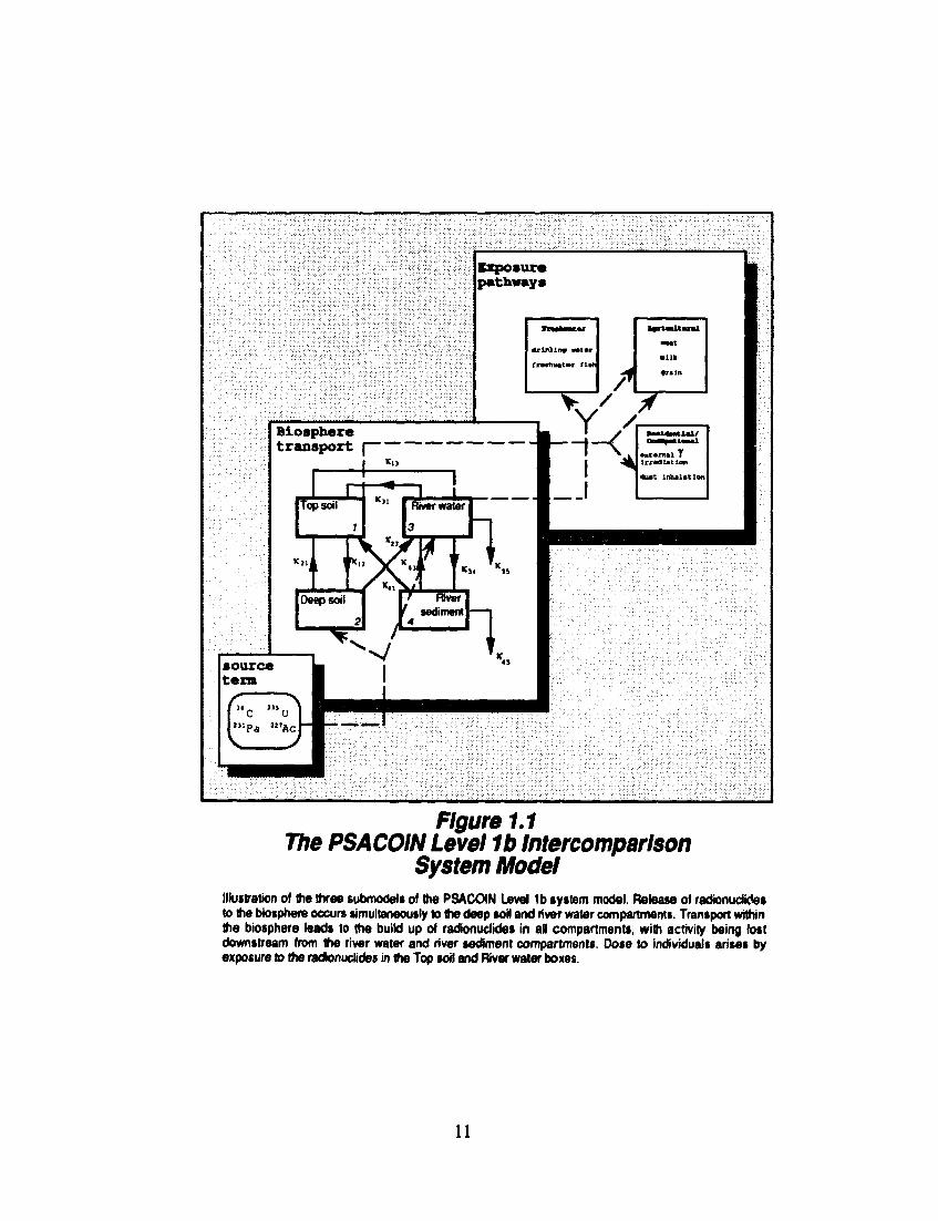
Figure 1.1 The PSACOIN Level 1b Intercomparlson
System Model Illustration of the three submodels of the PSACOIN Level lb system model. Release of radionuclides to the biosphere occurs simultaneously to the deep soil and river water compartments. Transport within the biosphere leads to the build up of radionuclides in aH compartments, with activity being lost downstream from the river water and river sediment compartments. Dose to individuals arises by exposure to the radionuclides in the Top soil and River water boxes.
11
1.2 Purpose of the Level lb exercise.
The principal aims of the Level lb exercise were:
• to gain experience in the application of probabilistic systems assessment methodology to transport and radiological exposure submodels for the biosphere and hence to methods of estimating the total risk to individuals, or groups of individuals;
• to contribute to the verification of biosphere transport and exposure submodels used by the participants;
• to investigate the effects of parameter uncertainty in the biosphere transport and exposure submodels on the estimate of mean dose* to individuals exposed via several exposure pathways.
In addition to these aims, participants in the exercise were encouraged to investigate any other performance assessment related aspects of the case which might prove to be of interest.
1.3 Problem Specification
The PSACOIN Level lb case specification (given in full in Annex A) describes three submodels - a source of radionuclides to the biosphere, a compartment model for biosphere transport and an exposure pathway submodel - which together form a complete assessment model for evaluating the consequences of the release of radionuclides to the biosphere. The relationship of the Level lb submodels is shown in Figure 1.1.
Starting from an initial radionuclide inventory a simple constant fractional leach rate is assumed for the source term which, together with radioactive decay and ingrowth, defines the release rate of radionuclides into the biosphere. This release submodel was chosen to give a timescale of release which is representative of those which may be expected in assessments of the geologic disposal of radioactive waste. The selection of radionuclides for the case study is discussed in Section 1.5 below. The release of radionuclides occurs to a section of the biosphere represented by the four compartments: Top soil, Deep soil, River water and River sediment, representing an inland river section. The source term is partitioned between river water and soil according to the relative areas of the river and agricultural land. The characteristics of the biosphere were chosen to represent an area of land from which a small farming community could obtain all its basic food requirements.
Activity entering each compartment is assumed to be instantaneously well mixed throughout the bulk of the box and the transfer of activity between the
lln this text the word dose is taken to mean the effective dose equivalent, and is the sum of weighted committed dose equivalents in specific organs from the intake of radionuclides into the body in one year, plus the sum of weighted dose equivalents from external irradiation in one year. This definition is consistent with the concept of dose given in ICRP-26'1 -5h
12
compartments is described in terms of the mean annual transfer coefficients (or rate constants), K , between boxes i and j of the model. This leads to a set of coupled first order linear differential equations, which give the time variation (r) of the contents N{ of box i as
dN ~T= I VVj + V*i + W - [ K ^ - Xtfi (l.l)
The first three terms on the right hand side (see Annex A for a full definition of the terms) represent transfers into box i from transport, ingrowth from the parent radionuclide M (with decay constant XM), in box i, and the source term, respectively. The remaining two terms represent losses from box i via transport and radioactive decay (at rate XN) respectively. The solution to this set of equations gives the radionuclide inventories in the compartments as a function of time. These are then used in the exposure pathway submodel to calculate the doses to individuals via the seven exposure pathways: drinking water and freshwater fish consumption, meat and milk consumption, grain consumption, external y-irradiation and dust inhalation.
The mechanisms involved in translating the top soil and river water activity concentrations into annual individual doses are represented here by conversion factors so that, in general terms, the total annual individual dose from radionuclides A', via exposure pathways p in the i boxes of the model can be written as
n,i,p,e*p
where Ep is the exposure rate for pathway p, P^n± is a processing factor for converting the inventory of radionuclide n in compartment i, Nifl, into a concentration for the exposure pathway p at which the exposure takes place. Dexpfl
converts the intake of radioactivity (Bq y1) into an annual individual dose (Sv y-') for the intake mechanism exp (ingestion or inhalation).
The Level lb case study there are 115 input parameters, 52 in the source and transport submodels and 63 in the dose model. Of these parameters, uncertainty is taken into account in the case of 26 (19 in the transport model and 7 in the dose model). The radionuclides chosen for the study were 14C and the 235U chain (with daughters 231Pa and 227Ac). In the context of the principal aims of the intercomparison the influence of the choice of parameter values on the results of the model are discussed in Section 1.4 below and the reasons for the selection of the radionuclides are outlined in Section 1.5 below.
The Level lb questionnaire requests details of the time evolution of the quantities described in the Equations (1.1) and (1.2) above. The questionnaires used to obtain results in a standard form for the intercomparison are shown in Annex B.
13
All the input parameters values and functional relationships are stated in the case specification. Although this leaves little scope for additional interpretation of the case by participants, it does contribute to the verification of the methods and coding used to solve the transport equation (Equation 1.1) which plays a central role i 1 many of the computer codes used in biosphere modelling for the performance assessment of radioactive waste repositories. The case therefore provides a useful benchmark against which the other codes can be compared. Furthermore, additional work carried out by the participants in the exercise, and discussed in Chapter 3 of this report, contributes to the understanding of biosphere models for performance assessments and in particular illustrates that such models have a useful part to play in PSA.
1.4 Parameterisation of the Level lb Models
The transport of radionuclides in the PSACOIN Level lb biosphere is governed by the intercompartment transfer coefficients, K . There are ten of these coefficients in the PSACOIN Level lb model and, in principle, it would be feasible for a given site to measure these transfer rates directly although the complexities inherent in such a system and the long measurement times required to fully characterise all the relevant timescales make this practically impossible for all but the most simple features, events and processes. It can, however, be argued that it is preferable to model the mechanisms which influence the transfer rates. This allows a clearer definition of the features, events and processes (FEPs) at work in the model. Furthermore the physical, chemical and biological properties of the system can be more easily determined under field conditions than can the transfer rates themselves, and these then become the fundamental input parameters of the overall transport model. This approach is taken in this exercise.
For example, the transfer rate of radionuclides from the top soil compartment (box 1) to the deep soil (box 2) is given as
4»in • 4ri (R - l)B + D K'2 = Relu
+ R l„ min(/,„/d,) ( U )
where the advective processes of rainfall and irrigation (rates dnin + d^ m yl), the diffusion process (coefficient D), and the bioturbation process (coefficient B) are all included. R is the retention coefficient fcr radionuclides in soil and it is in turn parameterised as
R = 1 + % (1.4) £
in terms of the element dependent soil-groundwater distribution coefficient kd, the bulk density of soil, p, and the porosity of soil, e.
14
The advantages of mechanistic parameterisation include:
• the same model can be applied to different sites, differences in site performance can then be identified with differences in site parameters which in turn are derived from measurable site characteristics;
• parameters important in determining the transport of radionuclides in the environment can be identified;
• estimation of parameter uncertainty, and consequent uncertainty in the overall system performance, can be done on a rational, systematic basis.
This final point is particularly important for probabilistic studies such as the Level lb exercise. It would be extremely difficult to assign ranges of uncertainty to the Ky values directly. Moreover, since some of the mechanistic parameters enter more than one way into the K-J, correlations between the KJJ are generated in a realistic and self consistent way.
It is recognised that the particular parameterisation adopted for the Level lb exercise is by no means universally applicable. However, it should be adequate for the purposes of the exercise, to demonstrate the principles of the probabilistic uncertainty analysis, and to indicate the kinds of conclusions about parameter sensitivity that can be drawn. The model used is based on the MiniBIOS model'16', which has previously been used in the BIOMOVS B7 exercise"7' and the CEC's PACOMA project'18!. An example of the further development of the parameterisation of biosphere compartment models can be found in the Terrestrial -Aquatic Model of the Environment (TAME)VW which has recently been developed in Switzerland. In Level lb, uncertainty has not been attributed to every parameter -the parameters that were assigned a distribution were those that had previously been shown to be significant in other studies'1-7'1-8'1-10'.
In the dose model, parameters such as root uptake factors for radionuclides in crops could be highly site dependent and subject to many uncertainties. In the present study, no attempt has been made to quantify the uncertainties in this class of parameter. Attention has instead been focused on uncertainties in the exposure rates as determined by an individual's dietary preferences and total food energy intake.
1.5 Choice of Radionuclides
14C and the 235U chain (including 231Pa and 227Ac), were selected because of the wide range of differing properties. 14C is very mobile in the biosphere and has a relatively short half-life (5.7 103 years). The uranium chain members show a range of mobilities in the biosphere with protactinium and actinium both being
highly sorbed. 235U has a 7.0 108 year half life, 231Pa, 3.3 104 years, and 227Ac, 22 years. Another important feature is that the dose per unit intake values for the chain members differ according to the type of intake. As is typical for the admitting actinides the inhalation dose per unit intake can be much higher than
15
via the ingestion pathway - in the case of 227Pa the ratio is 450. This feature can have a significant influence on the exposure pathways contributing most to the total annual individual dose.
It is recognised that the approach taken here for the behaviour of I4C in the environment might not be the most appropriate and that a specific activity model1110] in particular might be more suitable and indeed simpler in terms of the dose calculations derived from the presence of uV radionuclide in the food chain.
Letter
A
B C D E F G
Code
MiniBlOSIACTIVfil SYVAC 3.05 MASCOT-3B
IMA Methodology IB.2* BIOPATH/PRISM*
CIRCLE SYVAC-3.08
ESP-MiniBIOS
Establishment
Paul Scherrer Institute^
AEA Technology^ IMA/CIEMA'F
Studsvik^ JAERI0
AECL NRPB
Country
Switzerland
UK Spain
Sweden Japan
Canada UK
Stochastic case Sampling Method® and sample number
MC 1000
MC 1000 LHS 1000 LHS 200 MC 1000 MC 1000 LHS 1000
Notes:
© t
MC =* Monte Carlo Sampling, LHS =* Latin Hypercube Sampling. Solution of the transport equation performed by the BIOPATH equation solver ACTIVI. Solution of the transport equation performed by the BIOPATH equation solver UNDIF. Solution of the transport equation performed by the BIOPATH equation solver UNDIF. In the deterministic calculations two methods were used, in the following Chapter these are distinguished by Dl and D2:
Dl LINDIF D2 IMPEX
In the subsequent stochastic calculations the LINDIF solution method was used. Participants contributing additional sensitivity analyses.
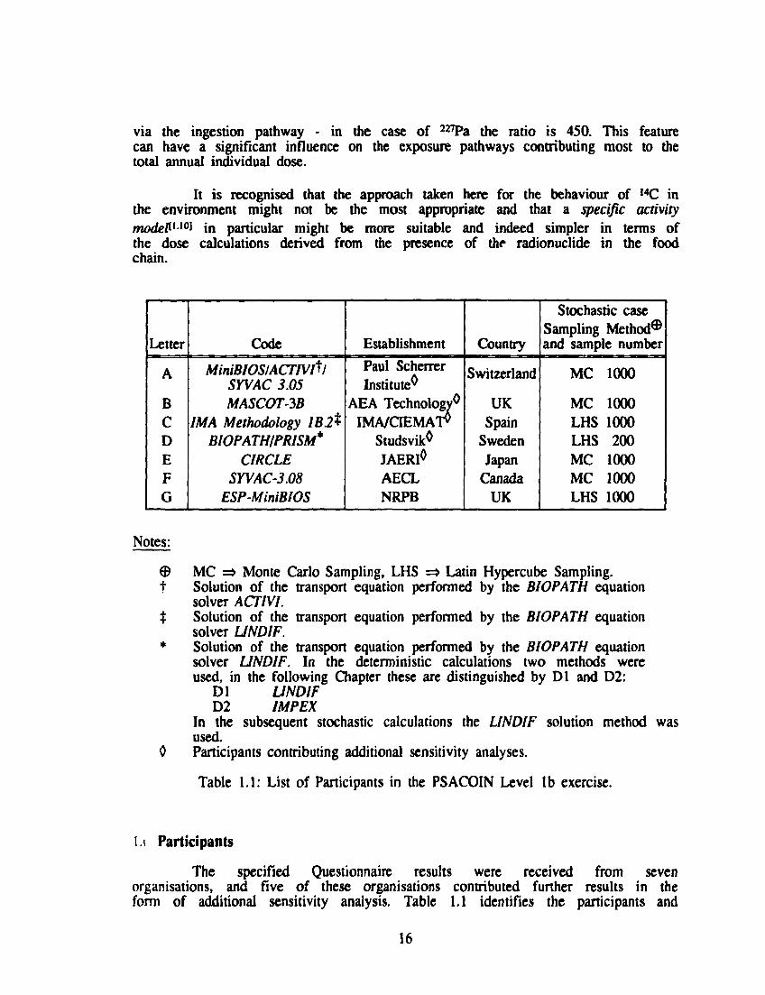
Table 1.1: List of Participants in the PSACOIN Level lb exercise.
1< Participants
The specified Questionnaire results were received from seven organisations, and five of these organisations contributed further results in the form of additional sensitivity analysis. Table 1.1 identifies the participants and
16
codes used and provides a unique letter for each contribution to identify it in the tables provided in Chapters 2 and 3 of this report. Brief code and methodology descriptions, provided by the contributing organisations, are given in Annex C.
17
2. QUESTIONNAIRE RESULTS.
2.1 Overview of the Questionnaire.
2.1.1 Introduction.
The performance assessment quantities used in the PSACOIN exercises are related to the overall radiological impact of the disposal concept under study. This means that the end points of the exercises are doses or risks to individuals and groups, although there may be a wide variety of intermediate quantities that might be calculated in the course of the modelling work. This is also the case in the Level lb exercise, where the biosphere transport and dose submodels are quite distinct. The main stochastic results from the exercise therefore concentrate on the time evolution of the doses to individuals and the rankings of the various exposure pathways. In addition, a code verification step was required, in order to confirm the correct workings of the transport and dose submodels. The Questionnaire therefore comprises two stages - deterministic and stochastic. Only when agreement had been reached in the deterministic case was it possible to proceed to the stochastic case. The deterministic Questionnaire relates to the second objective (verification) whereas the stochastic results address the third of the aims (uncertainty analysis), with the first of the aims (gaining experience) being covered by the exercise as a whole, and by the request to participants to carry out any additional analyses that they felt were appropriate. This chapter deals with the results of the Questionnaire and the additional work carried out is discussed in the next chapter.
2.1.2 The Deterministic Results Questionnaire.
The correct functioning of the codes used in the case was demonstrated by the comparison of the results from a deterministic central case, in which the central values (medians) of the distributed parameters were used. Two tables of deterministic results were requested: one to test the correct operation of the transport submodel and one to test the dose submodel.
The first Questionnaire table (Table B.l of Annex B) is designed to ensure that the transfer coefficients used in the case are calculated correctly and hence that the codes used to solve the transport equation (Equation 1.1) perform correctly. This is achieved by calculating the four compartment inventories of each of the four radionuclides at specified times. The times chosen (1, 103 and 105 years) provide a severe test of the numerical accuracy of the solver codes, since they specify the first year after the commencement of the release, when the daughters of the 235U chain have had only a short time for ingrowth so that the inventories are very small. Similarly the inventories of the ,4C at the third time (105 years) are also very small, because of radioactive decay.
The coding of the dose model (Equation 1.2) is tested by the second Questionnaire table (Table B.2 in Annex 2). In this table the seven individual exposure pathway doses are requested, for each of the four radionuclides, at each of the three times specified in Table B.l.
18
2.1.3 The Stochastic Results Questionnaire.
The two end points of the Level lb calculations were chosen to be the total annual individual dose for 14C, summed over all exposure pathways and the total dose for the 235U chain, summed over all the decay chain members and pathways. Table B.3 of Annex B requests the mean and standard deviation of these two quantities, together with a confidence bound for each mean value. The Case Specification does not specify the method to be used in arriving at the confidence bounds and, in their responses to the Questionnaire, the participants placed differing interpretations on this requirement. In this report the confidence bounds used are chosen to be those based on Chebyshev's Theorem and the responses from the participants have been amended accordingly. For an estimated mean quantity, \i, and a standard deviation, a, the Chebyshev 95% confidence interval is ji ± T95, where
^95 = (2.1) 0.05N
where N is the number of samples. This formula is based on the standard Monte Carlo sampling method and can also be used with Latin Hypercube sampling. It would, however, need modifying if Importance Sampling were used'2-1 J, but since this was not the case for any contribution to the present study, the formula, as given, could be used to convert the supplied means and standard deviations to the confidence bound as necessary.
The final Questionnaire table (Table B.4 of Annex B) deals with the rankings of the individual exposure pathways as a function of time.
2.2 The Deterministic Results.
The agreement achieved between the contributions in response to the strict case specification was excellent. The discussion of the deterministic results can therefore concentrate on general trends and features of biosphere modelling for performance assessment in the context of the Level lb case. The individual results received from the participants are presented in Annex D.
2.2.1 The Source Term.
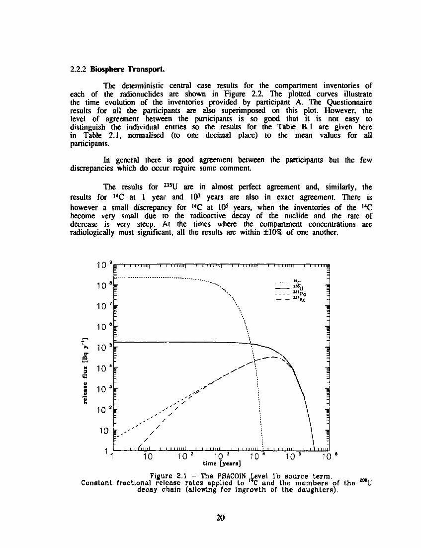
The time variation of the Level lb source term is given in Figure 2.1. This illustrates the output from th, source before it is partitioned between the biosphere compartments receiving the radionuclide flux (the deep soil and the river water) according to the area of the compartments. These plots of release vs time for the four radionuclides provide a useful reference when comparing accumulation of the radionuclides in the biosphere. The first features to note are the plateaux and decay characteristics of the constant fractional release rate source terms for ,4C and the chain parent, 235U, and the ingrowth and decay of the chain daughters. Second, the ,4C source term is limited by radioactive decay (with a half-life of 5.7 103 years), whereas the chain source terms are limited by the depletion of the source, with the constant fractional release rate of 105 y1.
19
2.2.2 Biosphere Transport.
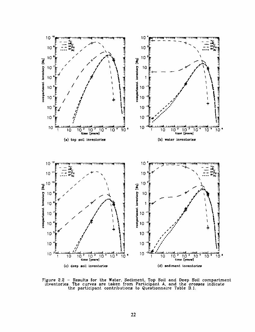
The deterministic central case results for the compartment inventories of each of the radionuclides are shown in Figure 2.2. The plotted curves illustrate the time evolution of the inventories provided by participant A. The Questionnaire results for all the participants are also superimposed on this plot. However, the level of agreement between the participants is so good that it is not easy to distinguish the individual entries so the results for the Table B.l are given here in Table 2.1, normalised (to one decimal place) to the mean values for all participants.
In general there is good agreement between the participants but the few discrepancies which do occur require some comment.
The results for 235U are in almost perfect agreement and, similarly, the results for ,4C at 1 year and 103 years are also in exact agreement. There is however a small discrepancy for ,4C at 105 years, when the inventories of the ,4C become very small due to the radioactive decay of the nuclide and the rate of decrease is very steep. At the times where the compartment concentrations are radiologically most significant, all the results are within ±10% of one another.
CO
10 9
10 e
10 7
10 8
i—i i 11mij 1 i i tim|—i—i 11MII|—i i i m i i |— i i i im i |— i i M m j
» 1 0 ' *
5 104
c | 10 3
z
10 2
10 k
1
«£ii 331 327 E
.'' ' ,*' /
/ /
-L-.J-L ^••"1 ' ' ' " m l I I i I mi l i
10 102 10 3 104
time [years] 10 10
Figure 2.1 - The PSACOIN Level lb source term. Constant fractional release rates applied to C and the members of the
decay chain (allowing for ingrowth of the daughters). DU
20
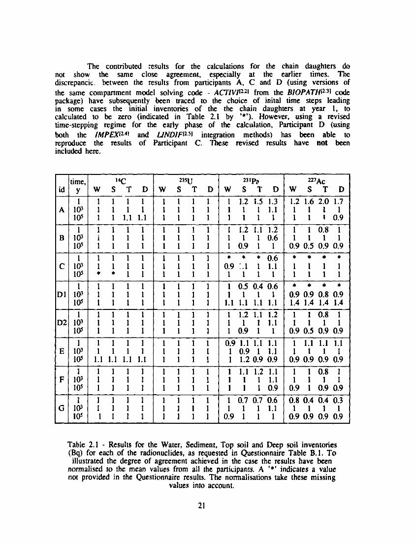
The contributed results for the calculations for the chain daughters do not show the same close agreement, especially at the earlier times. The discrepancie between the results from participants A, C and D (using versions of the same compartment model solving code - ACTIVI[22] from the BIOPATHl23* code package) have subsequently been traced to the choice of inital time steps leading in some cases the initial inventories of the the chain daughters at year 1, to calculated to be zero (indicated in Table 2.1 by '* ' ) . However, using a revised time-stepping regime for the early phase of the calculation, Participant D (using both the IMPEXPV and UNDIF®^ integration methods) has been able to reproduce the results of Participant C. These revised results have not been included here.
id
A
B
C
Dl
D2
E
F
G
time, y 1
103
105
1 103
10s
1 103
lO5
1 103
105
1 lO3
105
1 103
lO5
1 103
105
1 103
105
14C W S T D
1 1 1 1 1 1
1 1 1 1 1 1
1 1 1 1 * *
1 1 1 1 1 1
1 1 1 1 1 1
1 1 1 1
1.1 1.1
1 1 1 1 1 1
1 1 1 1 1 1
1 1 1 1
1.1 1.1
1 1 1 1 1 1
1 1 1 1 1 1
1 1 1 1 1 1
1 1 1 1 1 1
1 1 1 1
1.1 1.1
1 1 1 1 1 1
1 1 1 1 1 1
2351J
W S T D
1 1 1 1 1 1 1 1 1 1 1 1
1 1 1 1 1 1 1 1 1 1 1 1
1 1 1 1 1 1 1 1 1 1 1 1
1 1 1 1 1 1 1 1 1 1 1 1
1 1 1 1 1 1 1 1 1 1 1 1
1 1 1 1 1 1 1 1 1 1 1 1
1 1 1 1 1 1 1 1 1 1 1 1
1 1 1 1 1 1 1 1 1 1 1 1
2 3 1 P J
W S T D
1 1.2 1.5 1.3 1 1 1 1.1 1 1 1 1
1 1.2 1.1 1.2 1 1 1 0.6 1 0.9 1 1
* * * 0.6 0.9 M 1 1.1 1 1 1 1
1 0.5 0.4 0.6 1 1 1 1
1.1 1.1 1.1 1.1
1 1.2 1.1 1.2 1 1 1 1.1 1 0.9 1 1
0.9 1.1 1.1 1.1 1 0.9 1 1.1 1 1.2 0.9 0.9
1 1.1 1.2 1.1 1 1 1 1.1 1 1 1 0.9
1 0.7 0.7 0.6 1 1 1 1.1
0.9 1 1 1
227 Ac W S T D
1.2 1.6 2.0 1.7 1 1 1 1 1 1 1 0.9
1 1 0.8 1 1 1 1 1
0.9 0.5 0.9 0.9 * * * *
1 1 1 1 1 1 1 1 * * * *
0.9 0.9 0.8 0.9 1.4 1.4 1.4 1.4
1 1 0.8 1 1 1 1 1
0.9 0.5 0.9 0.9
1 1.1 1.1 1.1 1 1 1 1
0.9 0.9 0.9 0.9
1 1 0.8 1 1 1 1 1
0.9 1 0.9 0.9
0.8 0.4 0.4 0.3 1 1 1 1
0.9 0.9 0.9 0.9
Table 2.1 - Results for the Water, Sediment, Top soil and Deep soil inventories (Bq) for each of the radionuclides, as requested in Questionnaire Table B.l. To illustrated the degree of agreement achieved in the case the results have been
normalised to the mean values from all the participants. A '*' indicates a value not provided in the Questionnaire results. The normalisations take these missing
values into account.
21
1010
10*
10*
10 7
10*
10*
10 4
1 0 :
1 0 :
10
tm;—i 11inii| i mil"—rrrTTna—rra^—i lima;—rrmi
» < D .
— "'Ac ,
' ' ' ' / /
~-4
. ^ . /
• ' X /
/
/
/
/
u
\ ]
I;
mil I I mini I I mud • li I i m n i l il I 1111 til
1 10 10 2 10 3 10 * 1 0 s 1 0 '
time [yean]
(a) top soil inventories
10 4
1 0 s
- 1 0 '
s t 10
s e
S 1 i 10 -'t-
n—i 11 ma;—i i mm—i I niRq—rrmrn—i imnq—i I M I I :4 - — — — _ _ 'V -
- - M , P o , . . . . » ' * =
s | 1 0 " %
10 "5
%
.A
10 "J
/.•••
' \ 1 / > \ I
li ' " ' • i n i m l I I l l l l l j LXUll I l l I l in i i r f i l Uliul in
1 10 10 2 10 3 10* 10 * 10 "
time [jean]
(b) water inventories
1 0 '2g"1 MHIIlq lllllllll IlllillH I 1111 im I MIHH| ' I lllllj
10 " r - - = P o
«?1 0
£ 10
I 10'r
| 1 0 ' f c
I 10
1 0 5fcr
10 4
10 '
X * ^ N
/
y
f / ' /O*
/
/
/ /
s l i V I I _
I ml i i imill f f • iniil i i mini i i imii l ' i '" i" l • i m m 1 10 10 s 10 J 10 4 1 0 s 10*
time [yean]
(c) deep soil inventories
10 4
10 '
? 1 ° J
s. £ 10 e
I 1 W 110 •w S 1 0 "2
in|—i niini wiijini j j i ' i in—i 11inn—i IIIIIII|—i m m - —4- _ _ ur -
\ . . . . »>c = \
\
' >f \ i t' I \ 1
' V ;
10 ' %
10
10
/
A'
/ / / /
t ' ' • I / -Jt / iiir 11
I iiuul LXUIUII i miiij LXUUUI • • ' i i mm
1 10 10 1 1 0 3 10 4 1 0 s 10 "
time [yean]
(d) sediment inventories
Figure 2.2 - Results for the Water, Sediment, Top Soil and Deep Soil compartment inventories. The curves are taken from Participant A, and the crosses indicate
the participant contributions to Questionnaire Table B. 1.
22
'«c
time, lyi
i
103
105
participant
A B C D E F G
A B C D E F G
A B C D E r G
drinking water
1 l i 1 1 1 1
1 1 1 1 1 1 1
1.2
1.2 0.4 1.1 1.1
freshwater fish
1.1
0.9
grain
0.9 1.1 1
0.9
meat
1 1 1 1 1 1 1
1 1 1 1 1 1 1
1.1 i 1
0.9 1.1 1 1
milk
1.1
1.1 1
dust inhalation
1 1 1 1 1 1 1
1 1 1 1 1 1 1
1.1
i 1.1 i
0.9
235u
time, lyi
i
103
105
participant
A B c D E F G
A B C D E F G
A B C D E F G
drinking water
freshwater fish
1.2
gram meat
i i 1 1 i i 1
0.9 0.9 1.5 0.9 0.9 0.9 0.9
0.9 0.9 1.5 0.9 0.9 0.9 0.9
milk dust
inhalation ext-
rnal>
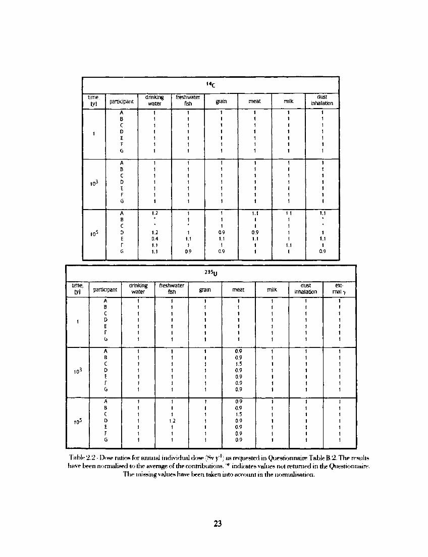
Table 2.2 - Dose rutios for annual individual dose (Sv y'1) as requested in Questionnaire Table B.2. The results have been normalised to the average of the contributions. '*' indicates values not returned in the Questionnaire.
The nussing values have been taken into account in the normalisation.
23
2 3 1Pa
time.
i
103
105
participant
A B c D E F G
A B C D E F G
A B C D E F G
drinking water
0.8 0.8 0.8 0.8 0.7 2.4 0.8
1 1
0.9 1.3 0.9 1
0.9
1 1 1 1
0.9 1 1
freshwater fish
1
1 1 1 i
1 1 1 1
0.9 1 1
1 1 1 1
0.9 1 1
grain
1.3
1 1 1
0.7
1 1 1 1
0.9 1 1
1 1 1 1
0.9 1 1
meat
1.1
t 1 l
0.9
1 i 1 1 1 1 1
1 1 i i
0.9 1 1
milk
0.8
2.1 0.7 0.8 1
1 1 1 1 1 1 1
1 1 * 1
1.9 1 1
dust inhalation
0.8
1.1 1.2 1.1 0.8
0.9 1
0.9 1.4 0.9 1
0.9
1 1 1 1
0.9 1 1
external y
1.4
i i i
0.7
1 1 1 1
0.9 1 1
1 1 1 1
0.9 1 1
2 2 7 Ac
time,
i
103
105
participant
A B C D E F G
A B C D E F G
A B C D E F G
drinking water
1.2
1 1 1
0.8
1 1 1 1 1 1 1
1 1
1.1 1 1 1 1
freshwater fish
1.3
0.9 1 1
0.8
1 1 1
1.1 1 1 1
1 1
1.1 1 1 1 1
grain
1.3
1 i 1
0.8
1 1 1 1 1 1 1
1 1
1.1 1 1 1 1
meat
1.3
0.9 1 1
0.8
1 1
0.9 0.9 1 1 1
1 1
1.1 1 1 1 f
milk
1.3
0.9 1 1
0.8
1 1 1 1 1 1 1
1 1
1.1 1 1 1 1
dust inhalation
0.5
1.2 1.6 1.2 0.5
1 1 1 1 1 1 1
1 1
1.1 1 1 1 1
external y
2.0
0.8
1.1 0.8 0.4
1 1 1 1 1 1 1
1 1
1.1 1 1 1 1
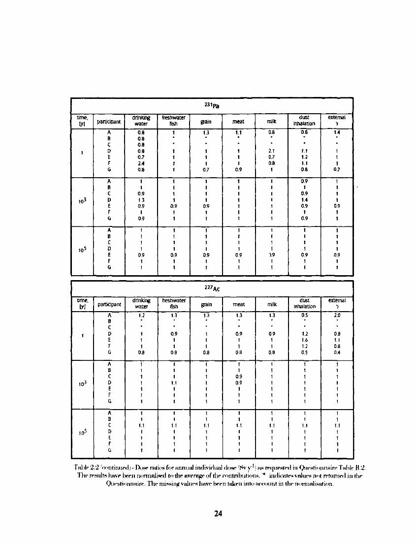
Table 2.2 'continued) - Dose ratios for annual individual dose 'Sv y"') as requested in Questionnaire Table B.2. The results have been normalised to the average of the contributions. * indicates values not returned in the
Questionnaire. The missing values have been taken into account in the normalisation.
24
In the course of the exercise it was found that many of the participants required several iterations before the final agreement was reached over the compartment contents in Table B.l. Some coding errors were identified and corrected but a significant source of error in the initial calculation of the: transfer coefficients by some participants was the units of the input parameters. Throughout the case specification the data are given in terms of metres, kilograms and years. In the input data files of some of the older codes these units were not consistently used, the units being taken from the original source of the data, and the process of converting these data into forms suitable for the codes gave rise to some erroneous initial results, before the data sets were checked and corrected.
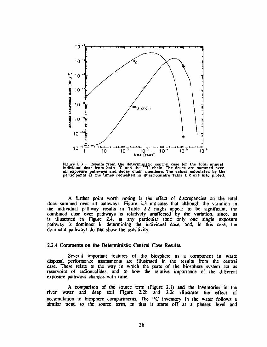
2.2.3 Individual Dose.
The results for Questionnaire Table B.2 are illustrated in Figure 2.3, where the time evolution of the total annual individual dose arising from 14C and the 235U chain are plotted, summed over exposure pathways and decay chain members, according to equation 1.2. The results from the participants' contributions to Table B.2 are also plotted. As with the compartment inventories, plotted above, the agreement is so close, in most cases, that it is not possible to distinguish the separate values. Table 2.2 gives the results from Table B.2, again normalised to the mean of the contributions.
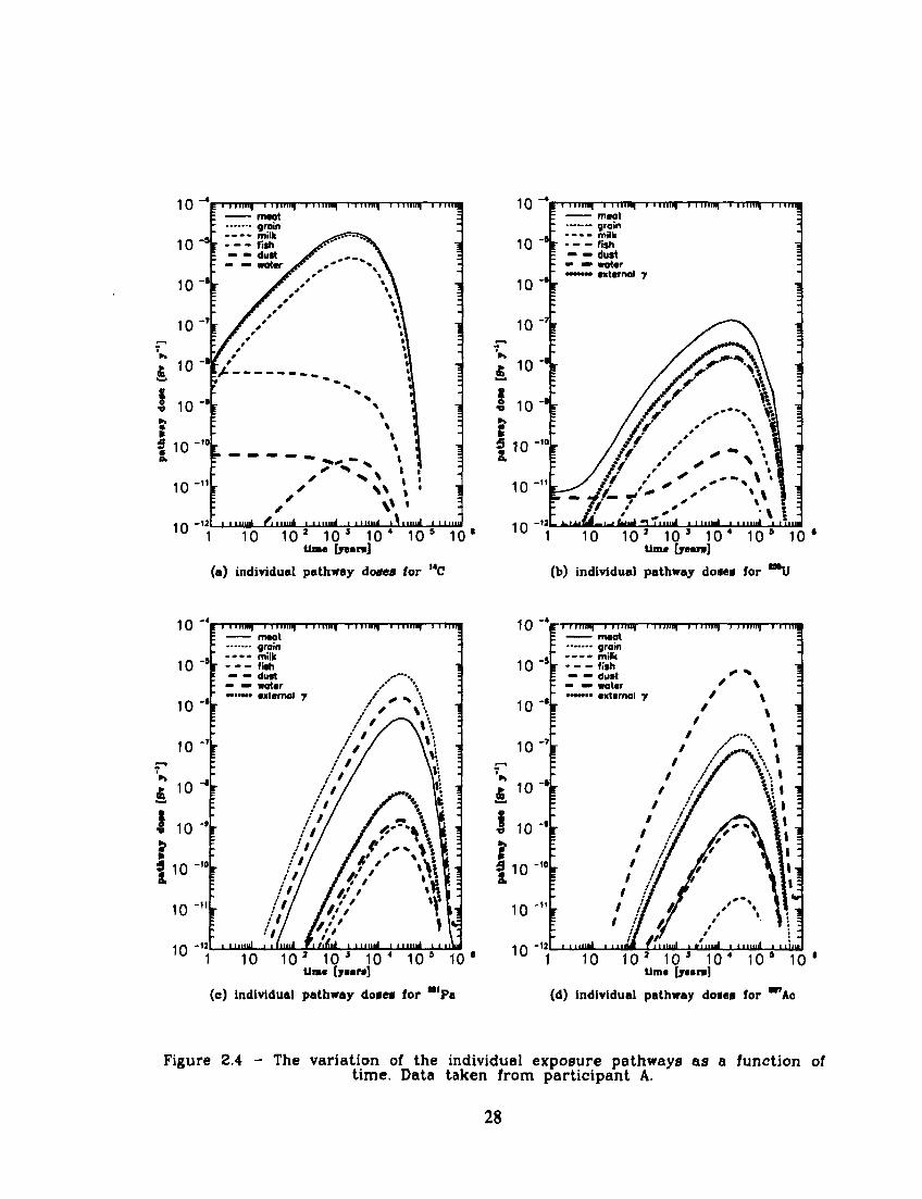
The full time dependence, as calculated by participant A, of the seven exposure pathways is illustrated in Figure 2.4 for each of the four radionuclides. These plots can be used to compare how the relative importance of the different pathways changes with time. Although this information was not sought in the deterministic Questionnaire, the ranking of the exposure pathways, as a function of time, was requested in the stochastic Questionnaire. These results from the deterministic case provide a useful point of comparison and illustrate some important features of biosphere modelling.
Figure 2.3 and Table 2.2 again indicate the agreement between the participants is, on the whole, very good, especially for the I4C and the 235U. The results for the chain daughters show a less close agreement overall. As with the calculation of the compartment inventories, discussed in Section 2.2.2, such discrepancies as do arise can generally be explained in terms of the internal accuracy of the codes used to solve the compartment model equation, since the doses from each of the exposure pathways are derived from constant factors applied to either the topsoil or river water concentration.
The numerical problems in the results for 14C seen in Table 2.1 are also present in Table 2 _ at 105 years, when the compartment inventories are low and falling rapidly. The results for 235U show very good agreement at all times for all the exposure pathways, although the meat pathway shows some unexplained variation. As in Table 2.1, Table 2.2 shows that for 23,Pa and 227Ac the numerical variation in the calculation of the compartment inventories for the chain daughters is reflected in the doses by exposure pathway but again it must be noted that this effect is principally seen at the times at which the compartment inventories are low. In the case of the chain daughters this is the earlier times.
25
1 0 " I—I i 111111; 1 i i lri i i | 1 i i i m i | 1 i i i m i |
10
i I I I I I I 1—i m i n t
1rr ' ' I I I I l l l l l l ' i ' ' " " ! ' i ' " ' " I ' ' • ' " " I ' ' ' • " "
10 10 2 1 0 3 10 4 10 5
time [yean] 10
Figure 2.3 - Results from the deterministic central case for the total annual individual dose from both C and the U chain. The doses are summed over all exposure pathways and decay chain members. The values calculated by the participants at the times requested in Questionnaire Table B.2 are also pfoted.
A further point worth noting is the effect of discrepancies on the total dose summed over all pathways. Figure 2.3 indicates that although the variation in the individual pathway results in Table 2.2 might appear to be significant, the combined dose over pathways is relatively unaffected by the variation, since, as is illustrated in Figure 2.4, at any particular time only one single exposure pathway is dominant in determining the individual dose, and, in this case, the dominant pathways do not show the sensitivity.
2.2.4 Comments on the Deterministic Central Case Results.
Several important features of the biosphere as a component in waste disposal performanje assessments are illustrated in the results from the central case. These relate to the way in which the parts of the biosphere system act as reservoirs of radionuclides, and to how the relative importance of the different exposure pathways changes with time.
A comparison of the source term (Figure 2.1) and the inventories in the river water and deep soil Figure 2.2b and 2.2c illustrate the effect of accumulation in biosphere compartments. The ,4C inventory in the water follows a similar trend to the source term, in that it starts off at a plateau level and
26
decays away. The 235U however shows an increase in the river water inventory over its initial plateau level beginning at a few hundred years after the release has commenced. In the deep soil compartment the inventories at early times (up to around 5 103 years) show the gradual increase as a result of the constant source term.
An important process affecting the accumulation of the radionuclides in the soils is sorption onto solid materials. This is very well demonstrated in the case of 235U. In the Case Specification the water compartment receives activity from the source term directly and from the top soil layer as a result of eroded material being washed into the river. There is also an exchange with the river bed sediment. The relatively high soil-groundwater kd for 235U means that activity entering the top soil accumulates due to sorption. The erosion of the top soil to the river water therefore constitutes a secondary source term to the river water which is of comparable strength to the main source term at later times when the concentration of 235U in the soil has built up.
The same situation does not arise for the 14C because the sorption is much less so there is not the same degree of accumulation in the top soil. The reasons for this will be examined in greater detail in Chapter 3, which deals with the results of the additional uncertainty analyses carried out by some of the participants.
This feature illustrates the different emphasis on sorption in the biosphere and the geosphere from a performance assessment perspective. In the geosphere high sorption is preferable since it delays the transit of the radionuclide along the migration path allowing greater time for radioactive decay and ultimately lower doses on the release of the radionuclide to the biosphere -the process is one of retardation. In the biosphere, however, higher ifcds lead to greater retention and hence slower dilution and dispersion, leading to increased concentrations and which can lead to higher doses.
Figure 2.4 and Table 2.4 give a comparison of the relative importance of the seven exposure pathways as a function of time and this provides a useful way of examining the performance of the Level lb model, in terms of the accumulation processes at work in the biosphere. As far as the 14C is concerned, there is little variation in the ranking of the pathways with time, the only changes occurring after 2 years, as the build up of activity in the soil means that the dose due to milk consumption becomes a greater contributor to the total dose than the drinking water pathway, and at around 103 years where the dose arising from the inhalation of contaminated dust from soil becomes greater than the drinking water dose, as the source term decays away. It is interesting to note that the meat consumption and grain consumption pathways are almost equally important at the time of the peak dose from 14C, with milk consumption accounting for only 11% of the total dose.
27
! i iiuiif—rrrmn—rrnini|—i I iiinj—i 11 imq—i iniq
I 5 l 0 - , 0 r x
10
10 • < < •"•* l^nnui i I I I I IUI i iniiri n i m i i i i HUB 1 10 10* 10 * 10 4 10 * 10*
time [jrears]
(a) individual pathway doses for ,4C
1 0 g i 11nil i imm—r-rm™—I nirai—i iinin|—i i n n meot groin
-»L mi" ,
10 r « * - - dust « •» water
»••• external 7
~r
r id ' ~" \ * -u 1 10 10 2 10 3 10 4 10* 1 0 *
time {jean]
(b) individual pathway doses for m U
i i
1 0 ~ g i i m i l i i imn i i nun i i mm i 11 mnf l i n n mtot flroin
4 _ . . . milk - - dust - •» water ••••»• externol y
10 "%
10 -7
10
10
i lo
ur"
1 0 " " • Ilinul i . f i inJ Fn,f,.i • llln.ll I,,,mi
1 10 10* 1 0 3 1 0 4 1 0 s 10* time [years]
(c) individual pathway doses for *"Pa
-s
10 -*
10
10
1 0 - 7
£ 1 0
I 10-k 1 J i o -
1 0 ' "
1 0 " "
t I MIIIR|—I IIIIM| I Hill" IIIIIIH| I I I Hill) l l l l i q — meot —•• grain - - milk
F fith
- - — woter ' \ ••••"• external y f \
r / » -,
11 mini 11 mi 1 10 10 * 10 * 10 4 1 0 ' 1 0 '
Ume [years]
(d) individual pathway doses for '"Ac
Figure 2.4 - The variation of the individual exposure pathways as a function of time. Data taken from participant A.
28
time, y
1
103
105
rank
1 2 3 4 5 6 7
1 2 3 4 5 6 7
1 2 3 4 5 6 7
14C
pathway
meat grain fish milk water dust
meat ifain milk fish dust
water
meat grain milk fish dust
water
14C
dose, Sv yl
1.0 10* 8.4 1(H> 6.3 109
2.4 10' 5.0 10-" 2.4 10-"
1.5 lfr* 1.3 10-5
3.6 10-6
3.7 10-9
3.7 10-» 3.4 10-''
3.0 10-" 2.5 lO-ii 7.1 10-i2
3.2 10-is 7.4 IO-17
3.0 lO"
relative contrib.
0.37 0.31 0.23 0.09
< 0.005 < 0.005
0.47 0.41 0.11
< 0.005 < 0.005 < 0.005
0.48 0.40 0.11
< 0.005 < 0.005 < 0.005
235U chain
pathway
meat water fish
grain milk
external y dust
dust grain meat
externa] y milk water fish
dust grain meat
external y water milk fish
235U chain dose, Sv y-i
7.1 10-12
5.1 IO-12
1.1 lfr" 1.6 lfr" 4.5 10-14
5.0 IO-14
2.0 10"14
6.3 10* 4.3 10-« 1.9 10-* 4.7 10-9
1.1 10-1° 4.7 10-n 1.8 IO-11
2.5 lfr6
1.7 10-6
1.5 10 7
2.8 10-8 9.6 10-i° 4.3 10-1° 4.3 10-1°
relative contrib.
0.52 0.38 0.08 0.01
< 0.005 < 0.005 < 0.005
0.49 0.33 0.15 0.04
< 0.005 < 0.005 < 0.005
0.57 0.39 0.03 0.01
< 0.005 < 0.005 < 0.005
Table 2.4 - Ranking of the individual pathway doses at three times for 14C and the 235U chain (summed over chain members). Data taken from Participant A.
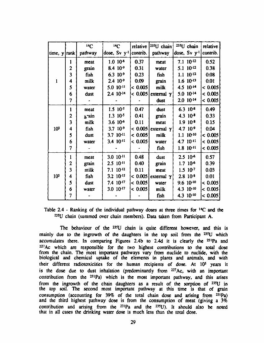
The behaviour of the 235U chain is quite different however, and this is mainly due to the ingrowth of the daughters in the top soil from the 235U which accumulates there. In comparing Figures 2.4b to 2.4d it is clearly the 23tPa and 227Ac which are responsible for the two highest contributions to the total dose from the chain. The most important pathways vary from nuclide to nuclide, with the biological and chemical uptake of the elements in plants and animals, and with their different radiotoxicities for the human recipients of dose. At 105 years it is the dose due to dust inhalation (predominantly from 227Ac, with an important contribution from the 23,Pa) which is the most important pathway, and this arises from the ingrowth of the chain daughters as a result of the sorption of 23SU in the top soil. The second most important pathway at this time is that of grain consumption (accounting for 39% of the total chain dose and arising from 231Pa) and the third highest pathway dose is from the consumption of meat (giving a 3% contribution and arising from the 231Pa and the 235U). It should also be noted that in all cases the drinking water dose is much less than the total dose.
29
2.3 Stochastic Results.
2.3.1 Individual Dose as a Function of Time.
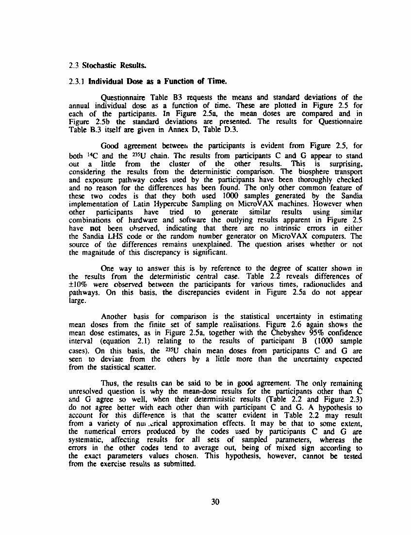
Questionnaire Table B3 requests die means and standard deviations of the annual individual dose as a function of time. These are plotted in Figure 2.5 for each of die participants. In Figure 2.5a, the mean doses are compared and in Figure 2.5b the standard deviations are presented. The results for Questionnaire Table B.3 itself are given in Annex D, Table D.3.
Good agreement between die participants is evident from Figure 2.5, for both 14C and the 235U chain. The results from participants C and G appear to stand out a little from the cluster of die otfier results. This is surprising, considering the results from the deterministic comparison. The biosphere transport and exposure pathway codes used by the participants have been thoroughly checked and no reason for the differences has been found. The only other common feature of these two codes is that they both used 1000 samples generated by the Sandia implementation of Latin Hypercube Sampling on MicroVAX machines. However when other participants have tried to generate similar results using similar combinations of hardware and software the outlying results apparent in Figure 2.5 have not been observed, indicating that there are no intrinsic errors in either the Sandia LHS code or the random number generator on MicroVAX computers. The source of the differences remains unexplained. The question arises whether or not the magnitude of this discrepancy is significant.
One way to answer this is by reference to the degree of scatter shown in the results from the deterministic central case. Table 2.2 reveals differences of ±10% were observed between the participants for various times, radionuclides and pathways. On this basis, the discrepancies evident in Figure 2.5a do not appear large.
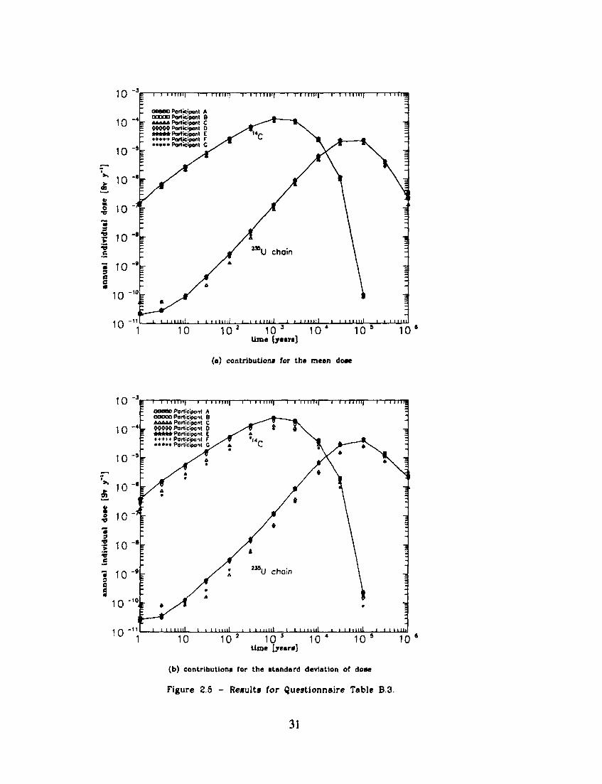
Another basis for comparison is the statistical uncertainty in estimating mean doses from the finite set of sample realisations. Figure 2.6 again shows the mean dose estimates, as in Figure 2.5a, together with the Chebyshev 95% confidence interval (equation 2.1) relating to the results of participant B (1000 sample cases). On this basis, the 235U chain mean doses from participants C and G are seen to deviate from the others by a little more than the uncertainty expected from the statistical scatter.
Thus, the results can be said to be in good agreement. The only remaining unresolved question is why the mean-dose results for the participants other than C and G agree so well, when their deterministic results (Table 2.2 and Figure 2.3) do not agree better with each other than with participant C and G. A hypothesis to account for this difference is that the scatter evident in Table 2.2 may result from a variety of nui .wrical approximation effects. It may be that to some extent, the numerical errors produced by the codes used by participants C and G are systematic, affecting results for all sets of sampled parameters, whereas the errors in the other codes tend to average out, being of mixed sign according to the exact parameters values chosen. This hypothesis, however, cannot be tested from the exercise results as submitted.
30
10
10
10
- 3 .
Participonl A aaoao Participant B AA&OA Participant C
_ 00000 Participant D - * * * * * Participant C Z ***** Porticipont F
Porticipont C
i i i mi ' i 1 i 11111n 1 i i m i i | 1 i i 111IT| 1—i i m i i |
(a) contributions for the mean dose
1 0 °
i o - 4
10
I I I m i l l — I I I I I I
00660 Porticipcnt A OOOOO Participant B AOAAA Porticipont C
, 04049 Participant D = * * * * * Participant E : ++-f++ Participant F
• • • > • Participant Q
£ 1 0 " I 10
1 1 0 ~ 8 1
10 - 9
10 " ° r
i i i MII| 1 i 11 iin| i i i trni| 1 i i mi l
U chain
i n - " L — i ' ' ' ""I i i 11 im! I I I i i i n mil i i i mill i i i mill
1 10 10* 103 104 10* 10s
time [years]
(b) contributions for the itandard deviation of dose
Figure 2.5 - Results for Questionnaire Table B.3.
31
10 "3
1 10 10* 10 3 10* 10 5 10* time [yean]
Figure 2.6 - Mean doses from all participants in relation to the Chebyshev 95* confidence interval.
2.3.2 Ranking of the Exposure Pathways as a Function of Time.
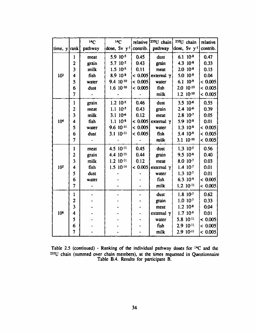
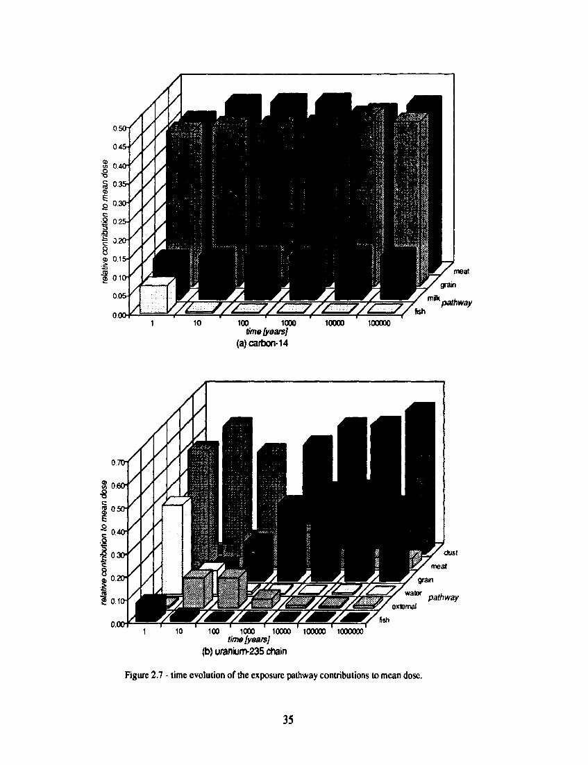
The rankings of the exposure pathways contributing to the annual individual doses for 14C and the ^ U chain were found to be in excellent agreement: only one pathway was ranked differently by one participant. The exact values of the pathway doses themselves showed some slight variation (see Table D.4 of Annex D) but the rankings were unaffected by this. The results for Questionnaire Table B.4 are illustrated by the rankings provided by participant B (Table 2.5). The extra time points called for in Table B.4 (compared with Table B.2) make it possible to represent graphically die time variation in the relative contribution to the mean dose, for each of the pathways doses. This is shown in Figure 2.7.
In the case of UC the relative balance quickly becomes established after the start of the release, so that there is little variation after 10 years. The meat and grain consumption pathways each account for around 40% of the mean dose,
32
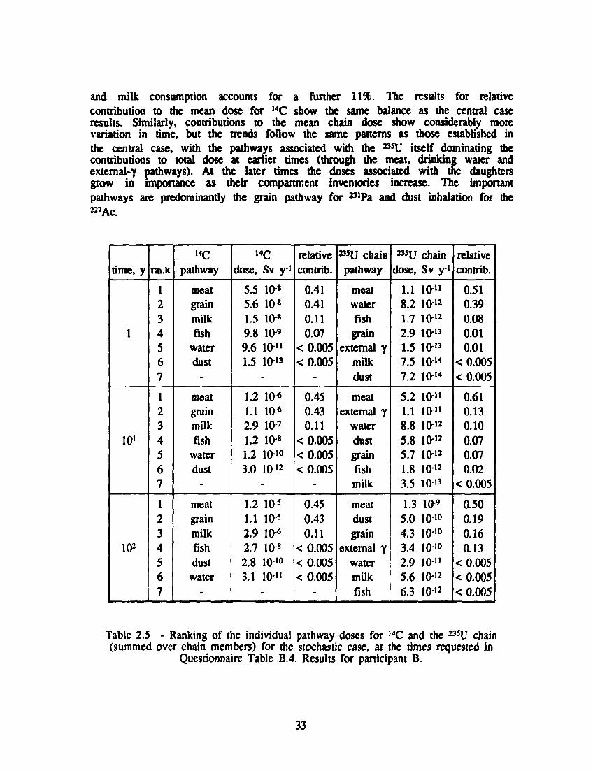
and milk consumption accounts for a further 11%. The results for relative contribution to the mean dose for I4C show the same balance as the central case results. Similarly, contributions to the mean chain dose show considerably more variation in time, but the trends follow the same patterns as those established in the central case, with the pathways associated with the 235U itself dominating the contributions to total dose at earlier times (through the meat, drinking water and external-Y pathways). At the later times the doses associated with the daughters grow in importance as their compartment inventories increase. The important pathways are predominantly the grain pathway for ^'Pa and dust inhalation for the 2^Ac.
time, y
1
10'
1(F
raiJc
1 2 3 4 5 6 7
1 2 3 4 5 6 7
1 2 3 4 5 6 7
,4C pathway
meat grain milk fish
water dust
meat grain milk fish
water dust
meat grain milk fish dust water
dose, Sv y1
5.5 lfr* 5.6 10* 1.5 10-* 9.8 109 9.6 10-" 1.5 10-13
1.2 10* 1.1 10-* 2.9 10-7
1.2 10* 1.2 10»° 3.0 10-"
1.2 10-5
1.1 10-5 2.9 106
2.7 10-8 2.8 lO'o 3.1 10»
relative contrib.
0.41 0.41 0.11 0.07
< 0.005 < 0.005
0.45 0.43 0.11
< 0.005 < 0.005 < 0.005
0.45 0.43 0.11
< 0.005 < 0.005 < 0.005
»5U chain pathway
meat water fish grain
external y milk dust
meat external y
water dust grain fish milk
meat dust grain
external y water milk fish
^ U chain dose, Sv y1
1.1 10-" 8.2 10-" 1.7 10-12
2.9 10-" 1.5 10-13
7.5 10-" 7.2 10-"
5.2 10-" 1.1 10-" 8.8 10-" 5.8 10-" 5.7 10-" 1.8 10-" 3.5 10-"
1.3 10* 5.0 10»° 4.3 10-'° 3.4 10-»° 2.9 10" 5.6 10" 6.3 10"
relative contrib.
0.51 0.39 0.08 0.01 0.01
< 0.005 < 0.005
0.61 0.13 0.10 0.07 0.07 0.02
< 0.005
0.50 0.19 0.16 0.13
< 0.005 < 0.005 < 0.005
Table 2.5 - Ranking of the individual pathway doses for ,4C and the 235U chain (summed over chain members) for the stochastic case, at the times requested in
Questionnaire Table B.4. Results for participant B.
33
time, y
103
10*
105
106
rank
1 2 3 4 5 6 7
1 2 3 4 5 6 7
1 2 3 4 5 6 7
1 2 3 4 5 6 7
14 C
pathway
meat grain milk fish
water dust
grain meat milk fish
water dust
meat grain milk fish dust
water
-
dose, Sv y-1
5.9 105
5.7 105
1.5 10-5
8.9 10« 9.4 10 1 0
1.6 10'°
1.2 105
1.1 10 5
3.1 10-6
1.1 108
9.6 10" 3.1 10"
4.5 10-" 4.4 10-" 1.2 10-" 1.5 10-'4
-
relative contrib.
0.45 0.43 0.11
< 0.005 < 0.005 < 0.005
0.46 0.43 0.12
< 0.005 < 0.005 < 0.005
0.45 0.44 0.12
< 0.005
-
»SU chain pathway
dust grain meat
external y water fish milk
dust grain meat
external y water fish milk
dust grain meat
external y water fish milk
dust grain meat
external y water fish milk
235U chain dose, Sv y i
6.1 10-8
4.3 10-8
2.0 10-8
5.0 lO-' 6.1 lO-9
2.0 1010
1.2 101 0
3.5 10* 2.4 10-6
2.8 10-7
5.9 108
1.3 lO-8
5.4 lO-9
3.1 10-'°
1.3 lO"5
9.5 10* 8.0 107
1.4 10 7
1.3 10 7
6.3 109
1.2 10 •»
1.8 10-7
1.0 107
1.2 10-8 1.7 lO-9
5.8 10-" 2.9 lO-ii 2.9 10"
relative contrib.
0.47 0.33 0.15 0.04
< 0.005 < 0.005 < 0.005
0.55 0.39 0.05 0.01
< 0.005 < 0.005 < 0.005
0.56 0.40 0.03 0.01 0.01
< 0.005 < 0.005
0.62 0.33 0.04 0.01
< 0.005 < 0.005 < 0.005
Table 2.5 (continued) - Ranking of the individual pathway doses for ,4C and the 235U chain (summed over chain members), at the times requested in Questionnaire
Table B.4. Results for participant B.
34
pathway
100 1000 time(years]
(a) carbon-14
100000
to 0
pathway
10 100 1000 10000 100000 1000000 time [years]
(b) urankim-235 chain
Figure 2.7 - time evolution of the exposure pathway contributions to mean dose.
35
1 0 ~3E—i i I I I I H I — i i I m i i | — r
1 0 ~4=" GSB60 stochastic deterministic
_ 10-5r
I I I M l l | 1 I I I I I I ! ) 1 I I l l l ( l | 1—I I I I I U
•"• • • " " ' ' • » • " " l ' ' ' " " l l ' • ' " ' " l i i i n m i i i i i n n
1 10 10* 10J 10* 10D 10* time [years]
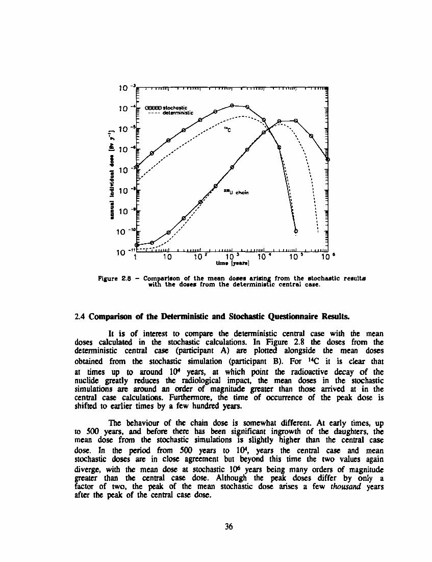
Figure 2.8 - Comparison of the mean doses arising from the stochastic results with the doses from the deterministic central case.
2.4 Comparison of the Deterministic and Stochastic Questionnaire Results.
It is of interest to compare the deterministic central case with the mean doses calculated in the stochastic calculations. In Figure 2.8 the doses from the deterministic central case (participant A) are plotted alongside the mean doses obtained from the stochastic simulation (participant B). For 14C it is clear that at times up to around 10* years, at which point the radioactive decay of the nuclide greatly reduces the radiological impact, the mean doses in the stochastic simulations are around an order of magnitude greater than those arrived at in the central case calculations. Furthermore, the time of occurrence of the peak dose is shifted to earlier times by a few hundred years.
The behaviour of the chain dose is somewhat different. At early times, up to 500 years, and before there has been significant ingrowth of the daughters, the mean dose from the stochastic simulations is slightly higher than the central case dose. In the period from 500 years to 104, years the central case and mean stochastic doses are in close agreement but beyond this time the two values again diverge, with the mean dose at stochastic 106 years being many orders of magnitude greater than the central case dose. Although the peak doses differ by only a factor of two, the peak of the mean stochastic dose arises a few thousand years after the peak of the central case dose.
36
It can be seen that some aspects of the stochastic data set used in the PSACOIN Level lb case study influence the importance of the retention and accumulation processes in the biosphere, and hence the magnitude of the peak dose and, because the retention processes are affected, the time to reach the peak dose can be altered. The accumulation processes in the biosphere can also be characterised by the time span for which the annual individual dose remains above, say, 90% of the peak value. Table 2.9 illustrates the difference between the two cases.
For 14C the width of the curve is unchanged, only die magnitude of the dose is different. For the chain there is a considerable broadening of the peak, indicating that the time of the peak is strongly influenced by the parameter uncertainty in the case.
nuclide
14C
M5U chain
deterministic case
3 500
4.4 104
stochastic case
3 500
5.6 105
Table 2.9 - time span (years) for which the annual individual dose remains above 90% of the peak value.
A comparison of the results for the ranking of the exposure pathways given in Tables 2.4 and 2.5 shows that the parameter uncertainty in the Level lb data set has little influence on the ranking of the exposure pathways, although the overall magnitude of the doses is affected.
2.5 Summary of the Analysis of the Questionnaire Response.
The first aim of the PSACOIN Level lb case study, to gain experience in the probabilistic modelling of the biosphere, has been met by the contributions of the seven participants who took part in the exercise and the second aim (to help verify the participating codes), has been achieved via the results presented in Tables 2.1 and 2.2 (and D.l and D.2 of Annex D). These results indicate that the codes used by the participants in the exercise have given good agreement in all the submodels of the case and, that although the results of the case may be dependent on the model structure, this case provides a potentially valuable benchmark of the codes for the solution of both the compartment model transport equation and the exposure pathway model.
The results from the stochastic case (illustrated in Figure 2.5, and given in Tables D.3 and D.4 of Annex D) confirm that the agreement between the participating codes extends to a range of parameter combinations. Not only is there evidence of the correct implementation of the submodels in the case but also the sampling and statistical postprocessing functions behave correctly.
37
The third of the aims of the exercise (the investigation of the influence of parameter uncertainty of the mean annual individual dose) has been illustrated in the comparison of the deterministic and central case results. The effects of individual model parameters are discussed in the sensitivity analyses in the following chapter.
38
3. ADDITIONAL ANALYSES.
3.1 Introduction.
In addition to the questionnaire results specified in Annex B, five of the participating organisations contributed additional results. These serve to illustrate the behaviour of the PSACOIN Level lb biosphere model, which itself contains features common to many biosphere models used for waste disposal assessments. The techniques employed are: a global sensitivity analysis, in which all the distributed parameters are allowed to vary through their assigned ranges simultaneously; an extension of the parametric Mncertainty analysis of the distribution of annual individual dose from die preceding chapter; a local sensitivity analysis, in which selected parameters are set to die extremes of the assigned ranges for comparison with die central values, to investigate the effect of different input parameter assumptions for die model representation of die study biosphere. Analysis of these results illustrates die advantages of die modelling approach taken in die study.
3.2 Uncertainty and Global Sensitivity Analysis of the PSACOIN Level lb Results.
3.2.1 Distribution of Annual Individual Dose.
The influence of die parameter uncertainty specified in die PSACOIN Level lb data set can be seen in die distribution of annual individual doses which emerge from die full set of stochastic simulations in die Level lb case. Figure 3.1 gives histograms of die total annual individual dose for both UC and die 235U chain at times close to die peaks of each of die respective dose-histories given in Figure 2.8. The figure was generated from 1000 Monte Carlo samples by Participant A.
The distribution of doses for 14C at 103 years is approximately log-triangular, witii a median around 7 10-5 Sv y1, and a mean of ?round 1.3 10-4 Sv y1. The range in outcomes from the 1000 sample runs covers nearly three and a half orders of magnitude, widi some combinations of parameters leading to doses as high as 3 10*3 Sv y1, a value which in itself would exceed regulatory limits. The distribution of die doses from die 23SU chain at 10s years shows an almost log-uniform distribution, again spanning tiiree and a half orders of magnitude, with a median of 5 10* Sv y1, a mean of 2.5 10*5 Sv y1, and a maximum value of around 5 10^ Sv yi.
Given this uncertainty in die potential outcome of die Level lb model as a result of die uncertainty of a limited number of input parameters, it is important to identify die parameters contributing most to this uncertainty. This is discussed in die following section. It should be remembered, however, mat because of die very simplistic assumptions about the form of die source term, die results presented here are not representative of a real site, and that die absolute values of die doses calculated are noi typical of those arising from die disposal concepts in operation or under investigation by OECD member states. The
39
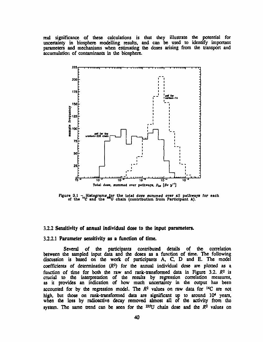
real significance of these calculations is that they illustrate the potential for uncertainty in biosphere modelling results, and can be used to identify important parameters and mechanisms when estimating the doses arising from the transport and accumulation of contaminants in the biosphere.
225
200
175
150 >> o c V §•125 £ 0 g.100 6
s
75
50
25 ft)"* 10"' 10-* 10^* 1 0 ^ W*^
Total dote, gummed over pathways, Dm [$v y*']
Figure 3.1 - Histograms-lor the total dose summed over all pathways /or each of the C ana the U chain (contribution from Participant A).
3.2.2 Sensitivity of annual individual dose to the input parameters.
3.2.2.1 Parameter sensitivity as a function of time.
Several of the participants contributed details of the correlation between the sampled input data and the doses as a function of time. The following discussion is based on the work of participants A, C, D and E. The model coefficients of determination (R2) for the annual individual dose are plotted as a function of time for both the raw and rank-transformed data in Figure 3.2. R2 is crucial to the interpretation of the results by regression correlation measures, as it provides an indication of how much uncertainty in the output has been accounted for by the regression model. The R2 values on raw data for I4C are not high, but those on rank-transformed data are significant up to around 104 years, when the loss by radioactive decay removed almost all of the activity from the system. The same trend can be seen for the 235U chain dose and the R2 values on
40
T—I I I l l l l | 1—I I I Ml l | rm\ 1—i i 11 n i | 1—I i 11 n i | 1—n-
pof for the uronium-235 ehoin i
'pdf far lc«ton-14
• • • • • " ' i i ' *» — • •
rank-transformed data are high (R2 > 0.8) for most of the time range. The rank correlation is therefore used as a sensitivity estimator in the following analysis.
The values of the rank correlation coefficients for all the parameters which showed correlations above the 95% significance level (CR £ 0.18) are plotted
in Figure 3.3. Ten of the input parameters reached this significance level for 14C (above) and nine input parameters did so for the ^HJ chain (below). This figure allows the influence of each of the sensitive parameters to be discussed in turn.
Groundwater velocity vf:
For ,4C (for which significant exposure rates only occur up to around 104
years, when radioactive decay masks all other FEPs), vg has a positive correlation up to the time at which the source terms stops releasing more of the nuclide to the biosphere. This means that the effect of vg is felt strongly (CR » 0.S) as a mechanism for the transport of the poorly sorbed contaminant from the deep soil to the surface soil. Beyond 104 years the negative correlation indicates that this parameter's principal effect is to wash the 14C out of the biosphere system into the river and hence downstream. In contrast, for the much more strongly sorbed 235U chain members, the influence of vg is only marginal, the value of CR peaking
between 102 and 103 years.
Release area At and groundwater release angle 0: The release area is a diluting factor, and so has an important negative
correlation, which is almost constant for 14C. For the ^ U chain however, the magnitude varies in time in response lo the relative importance of the other parameters. The maximum influence on the dose from the chain arises around 103
years. The other geosphere/biosphere interface parameter, the groundwater release angle, is indicated as being moderately important to the 14C dose, where, for similar reasons to the groundwater release velocity, it is important in transferring the mobile species to the surface soil.
Bioturbation, B, and diffusion, D: In the case of 14C, the rank correlation coefficient for bioturbation is
fairly constant up to 104 years. For the chain, however, the total dose is very sensitive to the bioturbation rate at early times. This means that, although the doses themselves are not very high (compared to the peak dose), the bioturbation mechanism is potentially important in the upward migration of highly sorbed species, since the bioturbation process is represented in the Level lb model as acting on the contaminants sorbed onto the solid material. These highly sorbed nuclides are relatively immobile in groundwater because only a small fraction of the total compartment inventory moves in the water phase, and this is confirmed by the insensitivity of the chain dose to the diffusion coefficient. In contrast, the relatively poorly sorbed ,4C has a higher sensitivity to the diffusion constant than it does to die bioturbation coefficient.
41
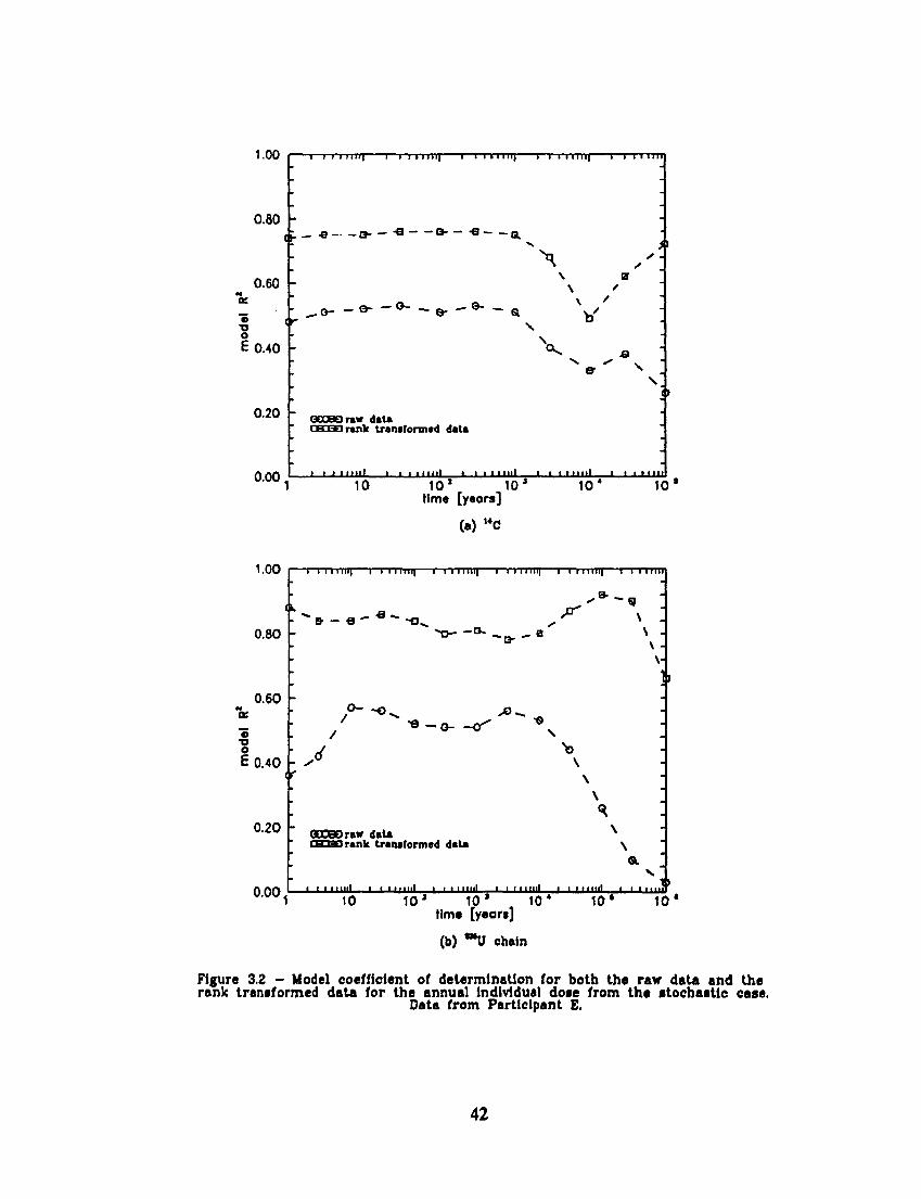
1.00 I i—i i i mil i—i i I I I I I | 1—i i 111ii| 1—i i i nn| 1—i i i mi
0.80
0.60
0 •a o E0.40
0.20
i — -a - - B — ~° o - - - e a
X • -
- 0 _ _ G - - » - - e . - ® -
\ ' \ '
GQOaOraw data Irank transformed data
QAQ • » ' ' " ' " ' ' ' • ' " " ' ' i i,i mi l l i . i i nu l l 1 10 10* 10 * 10* 10 *
time [years]
(a) MC
1.00
0.8O
0.6O
I E0.4O
0.20 -
O.OO
I I I l l l l l | 1 I I l l l l l | 1 I I l l l l l | 1 I I l l l l l | 1 I I l l l l l | I I I HIM
& - e ' ' B - -o . f <?
> ° - - 0 - - B . ' e \ . \ V
^~ -O JO ^
- s
QCOSOraw data Irank transformed data
i i i m i l l • ' ' • • • ' • ' • • • • • " • ! — ' • " • " • l " ' • • • • • " •
10 10* 1 0 ' 10* time [years]
(b) *"U chain
10* 1 0 *
Figure 3.2 - Model coefficient of determination for both the raw data and the rank transformed data for the annual individual dose from the stochastic case.
Data from Participant E.
42
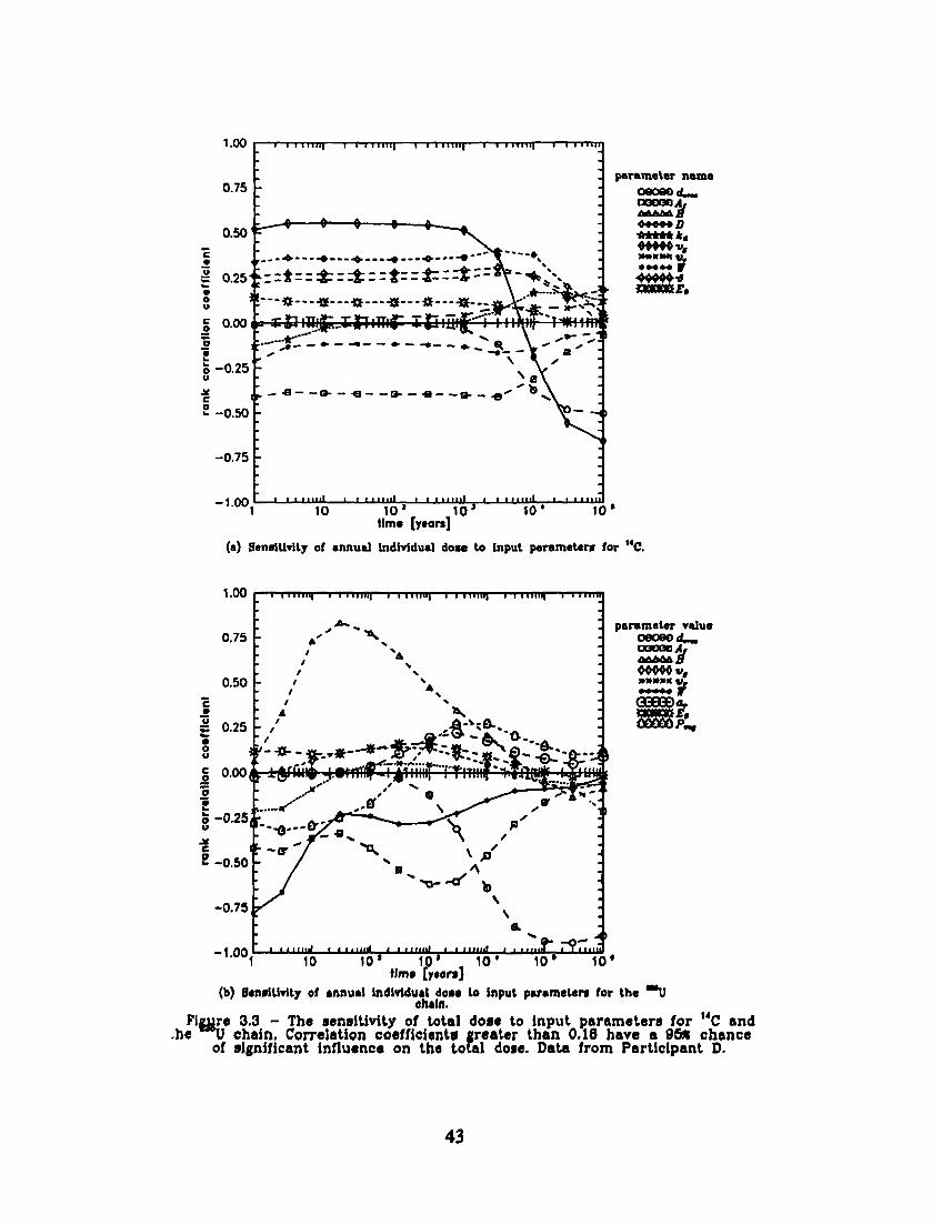
1.00
0.75
0.50
5 0.25
S § 0.00
£ -0 .25
-0.50
-0.75 -
-1 .00
-i—i i m i i | 1 i 11 u i i | 1 i i I I I I I | — i — i i I I I H I — r — i 111m
• & — . $ - - - . £ — - g — - J D f S9(—^
K-^ J»
i i Mini i i i in i i l i i • •••••i • i i ••••.! • i i nu l l 1 0 W U p t O 5 10 •
tlma [yaars]
parameter name oeoeodu.
~)A.
WWWWW Cat
v * W v , ***** w
(a) Senaitlvity of annual individual doae to input parametera for 14C.
1.00
0.75
0.50
g 0.25
§ 0.00,
-1.00
i i mini i i I I I I I I I—i i mini i i I I I I I I I—I- I imill—i i I I I I I I
* * * , • "
parameter value oeogodU. oaoaeAj
I
9- - O - -I I I I lllll ' • " " " ' • • .••'..! < • mint 1 i f f " I • T 10 10* 10* 10"* HT 1 0 '
Mme [yaors] (b) Senallivlty of annual Individual doae to input parameters for the "*U
chain. Figure 3.3 - The sensitivity of total dose to input parameters for i4C and
-he U chain. Correlation coefficients greater than 0.16 have a 95* chance of significant influence on the total dose. Data from Participant D.
43
Soil - groundwater distribution coefficient, kd: Somewhat surprisingly, this global sensitivity analysis does not indicate
that the results for total dose are very sensitive to the soil kd. Only the soil
kd for 14C is sensitive, and then only slightly at the very early times when the inventory is increasing and at the very late times when the inventory is effectively zero. At very early times the influence is negative, as it acts to retard the transport of contaminants from the deep soil to the surface soil. The influence becomes positive between 103 and 104 years, where the effect is to retain the activity in the surface soil. This emphasises die dual nature of the kd
in die biosphere. Under some circumstances the assumption of low kd values is conservative because the species are then more mobile. In other situations the converse is true: high kds are pessimistic because the contaminants are immobile in die parts of die biosphere where doses arise.
Soil erosion rate d^,: By far die strongest sensitivity of die total dose to any of the input
parameters is seen for the chain dose to die soil erosion rate. From 104 years onwards die correlation is very strongly negative, and a similar feature is seen in die corresponding plot for 14C, although it is less pronounced. The reason for die influence of this parameter on die doses is that in this model, die effect of soil erosion is to remove contaminated material from die surface soil and, because no net erosion is assumed, ie no decrease in surface soil thickness or boundary movement widi respect to die deep soil layer, diere is effectively replacement of die surface soil material by an uncontaminated external source of top soil.
River volumetric flow, W, and river water velocity, vr-These two parameters, which characterise die aquatic environment in the
model, have little influence on die annual individual doses at die times at which die maximum doses occur. For I4C die river water velocity is insignificant at all times. For die ^ U chain, it has a mild negative correlation at very early times, when die concentration of die uranium itself is building up, since vr is a loss term from die system. The influence of die volumetric flow rate (which is effectively a dilution term for activity entering die river water in die model) hovers around die margins of sensitivity after a moderate negative correlation at die times when die 14C water concentration is building up. The effect is much stronger for 235U at die earlier times, and die relative importance of this parameter remains moderate for a long period, reflecting die influence of the catde drinking water-milk/meat patiiway on die total dose from die chain (see Figure 2.7).
Dust concentration, a,, food-energy intake, EQ, degree of vegetarianism, Pvef: The parameters in die exposure padiways submodel which are varied do not
have a great deal of influence on die total dose, summed over all padiways. The total food energy intake verges on being significant diroughout much of die time in die 14C plot, widi a maximum at die start of die release to die biosphere. In die case of die chain, E0 has a peak significance around 103 years, when die 231Pa
and 227Ac grow in and tiieir influence on die total dose becomes greater. Also, the
44
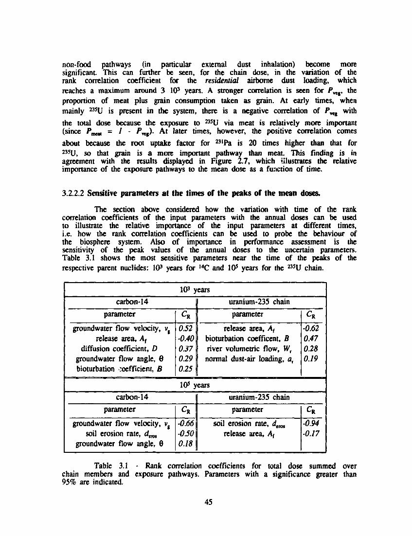
non-food pathways (in particular external dust inhalation) become more significant. This can further be seen, for the chain dose, in the variation of the rank correlation coefficient for the residential airborne dust loading, which reaches a maximum around 3 103 years. A stronger correlation is seen for Pwev the proportion of meat plus grain consumption taken as grain. At early times, when mainly 235U is present in the system, there is a negative correlation of Pvef with
the total dose because the exposure to 235U via meat is relatively more important (since P^^ = / - P^). At later times, however, the positive correlation comes
about because the root uptake factor for 23IPa is 20 times higher than that for 235U, so that grain is a more important pathway than meat. This finding is in agreement with the results displayed in Figure 2.7, which illustrates the relative importance of the exposure pathways to the mean dose as a function of time.
3.2.2.2 Sensitive parameters at the times of the peaks of the mean doses.
The section above considered how the variation with time of the rank correlation coefficients of the input parameters with the annual doses can be used to illustrate the relative importance of the input parameters at different times, i.e. how the rank correlation coefficients can be used to probe the behaviour of the biosphere system. Also of importance in performance assessment is the sensitivity of the peak values of the annual doses to the uncertain parameters. Table 3.1 shows the most sensitive parameters near the time of the peaks of the respective parent nuclides: 103 years for ,4C and 10s years for the 235U chain.
carbon-14
parameter
groundwater flow velocity, vg
release area, Af
diffusion coefficient, D groundwater flow angle, 6 bioturbation coefficient, B
carbon-14
parameter
groundwater flow velocity, vg
soil erosion rate, dmt
groundwater flow angle, 6
103 years
CR
0.52 •0.40 0.37 0.29 0.25
10s y
CR
•0.66 -0.50 0.18
uranium-235 chain
parameter
release area, Af
bioturbation coefficent, B river volumetric flow, Wr
normal dust-air loading, at
ears
uranium-235 chain
parameter
soil erosion rate, rferoi
release area, A{
CK
-0.62 0.47 0.28 0.19
CR
-0.94 •0.17
Table 3.1 - Rank correlation coefficients for total dose summed over chain members and exposure pathways. Parameters with a significance greater than 95% are indicated.
45
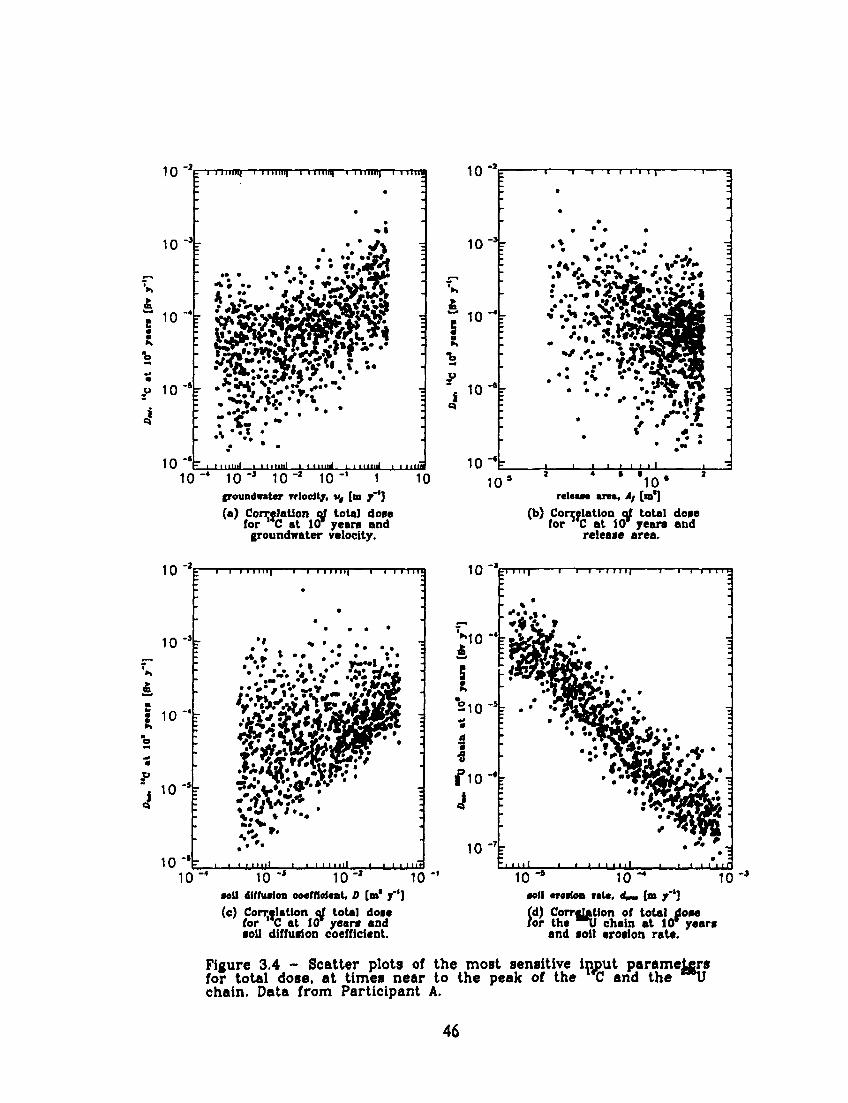
1 0 fc ' ' "ini|—i 111iui|—II I Ini i |—i 11mm—r
10
>> £
1 0 - 4 -
« 10
«?
-»
io -% 10
Ti™
i 11 mill i 11 mill i i mini • • ""•• ' i i m «
10 "3 10 "2 10"' 1 groundwater rrlodlj, v, [m f']
(a) Correlation oi total dose for C at 10 years and
groundwater velocity.
10
10
10
10 - r
s 10
10
-I 1 - 1 — l l l l l
1 0 s
. • -• • 7
• : • :
-I l l l l l • ( 10 •
rclcw* «re», 4 / [m*]
(b) Correlation oi total dose for C at 10 years and
release area.
10 -l I—i i 1111 > • | i i n 11111 1—i 111 H I
10
£
• 1 0 "
i o -
1 0 -10
* «» » I »-••*,. .'&&*
• >
v >
I I I l l l l l i i m l _i I I I I I
1 0 - 1 0 - 10 Mil diffusion ooeffleiont, D [m* y"']
(c) Correlation of total dose for C at 10 years and soil diffusion coefficient.
10 11 i i | 1—i i i 11 H I
10 ** 10 •oil crotloa rate, dmm
10 {» y"l
(d) Correlation of total dose for the ^U chain at 10* yei
and soil erosion rate. years
Figure 3.4 - Scatter plots of the most sensitive input parameters for total dose, at times near to the peak of the C and the ^ J chain. Data from Participant A.
46
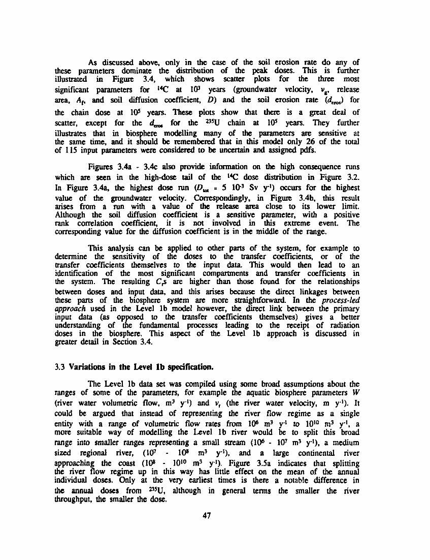
As discussed above, only in the case of the soil erosion rate do any of these parameters dominate the distribution of the peak doses. This is further illustrated in Figure 3.4, which shows scatter plots for the three most significant parameters for ,4C at 103 years (groundwater velocity, vg, release area, Af, and soil diffusion coefficient, D) and the soil erosion rate (dttm) for
the chain dose at 10s years. These plots show that there is a great deal of scatter, except for the d^, for the ^ U chain at 105 years. They further illustrates that in biosphere modelling many of the parameters are sensitive at the same time, and it should be remembered that in this model only 26 of the total of 115 input parameters were considered to be uncertain and assigned pdfs.
Figures 3.4a - 3.4c also provide information on die high consequence runs which are seen in the high-dose tail of the 14C dose distribution in Figure 3.2. In Figure 3.4a, the highest dose run (D^ = 5 103 Sv y1) occurs for the highest value of the groundwater velocity. Correspondingly, in Figure 3.4b, this result arises from a run with a value of the release area close to its lower limit. Although the soil diffusion coefficient is a sensitive parameter, with a positive rank correlation coefficient, it is not involved in this extreme event. The corresponding value for the diffusion coefficient is in the middle of the range.
This analysis can be applied to other parts of the system, for example to determine the sensitivity of the doses to die transfer coefficients, or of the transfer coefficients themselves to the input data. This would then lead to an identification of the most significant compartments and transfer coefficients in the system. The resulting C,s are higher than those found for the relationships between doses and input data, and this arises because die direct linkages between these parts of the biosphere system are more straightforward. In the process-led approach used in the Level lb model however, the direct link between the primary input data (as opposed to die transfer coefficients diemselves) gives a better understanding of die fundamental processes leading to die receipt of radiation doses in die biosphere. This aspect of the Level lb approach is discussed in greater detail in Section 3.4.
3.3 Variations in the Level lb specification.
The Level lb data set was compiled using some broad assumptions about die ranges of some of the parameters, for example the aquatic biosphere parameters W (river water volumetric flow, m3 y1) and vr (die river water velocity, m y1). It could be argued that instead of representing die river flow regime as a single entity widi a range of volumetric flow rates from 106 m3 yx to 1010 m3 y1, a more suitable way of modelling die Level lb river would be to split this broad range into smaller ranges representing a small stream (106 - 107 m3 y l) , a medium sized regional river, (107 - 10* m3 y1), and a large continental river approaching die coast (10* - 1010 m3 y1). Figure 3.5a indicates mat splitting die river flow regime up in this way has little effect on die mean of die annual individual doses. Only at die very earliest times is there a notable difference in die annual doses from 23SU, although in general terms die smaller die river throughput, die smaller me dose.
47
10 ~ s |—• i i Mini—i i I I I I I I I — i i I I I I I I I — i 11 I I I I I I—i i i I I I I I I—i i i u i |
**• ' " " ' I • • . • • . . ! • . i t t i . i l . I m i n i • • • m i l l
10 10* 10* 10* 10* 10* Una fjrars]
Bos* east: 10*,* W « 10" m' y'\ Low rang*: 10. « W « 101 r% y ; Hid rang*: 10'» W « 10* ,m* y"' , High rang*: 10* % W * to" m* »*'
(a) The effect of different river flow regime* on the total don. 10 "c
10
10-*
! 1 0 -
-J 10 "r
• ^ * * Xi*a • J t i rfbUKi - P^SKf jWBg
. * * •
'•
•
-• . •
r :.J_L±J-L i
i i i i i i 11 —1 1 1—1 1 1 1 Ij
M I I I no boundary transport COOCO boundary transport
^ » LaL» •££.« H^AflM •
•^95HK&TA*° i* ilt»sB^^j^* leyHHflnJl
*t?^S • •o f r i 0»i«fl i*
'
-
:
-
i*i»
•fe^L'-•S&S^* 3 ' | D K A ; ®WBB '^»Wf •*? = i i I I I I I I * io-» 10'» 1 0 -
•oil eroeion rate, aVw [m y*1]
(b) Scatter plot illustrating the lack of influence when aoil erosion ia .treated aa a boundary transport problem.
Data r.e for the ^ J chain doa* at 10 years and the aoil erosion rate.
Figure 3.5 - Results for variations on the Basic Level lb specification. (Data provided by Participant A).
46
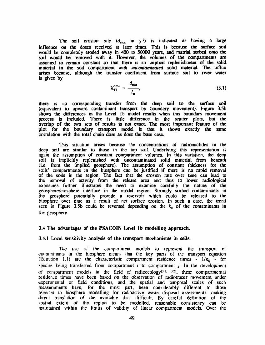
The soil erosion rate (detos m y1) is indicated as having a large influence on the doses received at later times. This is because the surface soil would be completely eroded away in 400 to 50000 years, and matrial sorbed onto the soil would be removed with it. However, the volumes of the compartments are assumed to remain constant so that there is an implicit replenishment of the solid material in the soil compartment with uncontaminated solid material. The influx arises because, although the transfer coefficient from surface soil to river water is given by
KT = 4^-- (31)
there is no corresponding transfer from the deep soil to the surface soil (equivalent to upward contaminant transport by boundary movement). Figure 3.5b shows the differences in the Level lb model results when this boundary movement process is included. There is little difference in the scatter plots, but the overlap of the two sets of results is not exact. The most important feature of the plot for the boundary transport model is that it shows exactly the same correlation with the total chain dose as does the base case.
This situation arises because the concentrations of radionuclides in the deep soil are similar to those in the top soil. Underlying this representation is again the assumption of constant compartment volumes. In this variation, the deep soil is implicitly replenished with uncontaminated solid material from beneath (i.e. from the implied geosphere). The assumption of constant thickness for the soils' compartments in the biosphere can be justified if there is no rapid removal of the soils in the region. The fact that the erosion rate over time can lead to the removal of activity from the release area and thus to lower radiological exposures further illustrates the need to examine carefully the nature of the geosphere/biosphere interface in the model region. Strongly sorbed contaminants in the geosphere potentially provide a reservoir which could be released to the biosphere over time as a result of net surface erosion. In such a case, the trend seen in Figure 3.5b coula be reversed depending on the kA of the contaminants in the geosphere.
3.4 The advantages of the PSACOIN Level lb modelling approach.
3.4.1 Local sensitivity analysis of the transport mechanisms in soils.
The use of the compartment models to represent the transport of contaminants in the biosphere means that the key parts of the transport equation (Equation 1.1) are the characteristic compartment residence times - 1/K^ - for species being transferred from compartment i to compartment j . In the development of compartment models in the field of radioecology'31- 3-2>, these compartmental residence times have been based on the observation of radiotracer movement under experimental or field conditions, and the spatial and temporal scales of such measurements have, for the most part, been considerably different to those relevant to biosphere modelling for radioactive waste disposal assessments, making direct translation of the available data difficult. By careful definition of the spatial exteit of the region to be modelled, reasonable consistency can be maintained v/ithin the limits of validity of linear compartment models. Over the
49
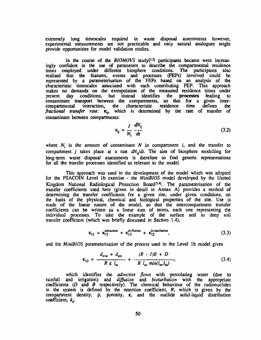
extremely long timescales required in waste disposal assessments however, experimental measurements are not practicable and only natural analogues might provide opportunities for model validation studies.
In the course of the BIOMOVS studyl33) participants became were increasingly confident in the use of parameters to describe the compartmental residence times employed under different biosphere conditions. The participants also realised that the features, events and processes (FEPs) involved could be represented by a parameterisation of the FEPs based on an analysis of the characteristic timescales associated with each contributing FEP. This approach makes no demands on the extrapolation of the measured residence times under present day conditions, but instead identifies the processes leading to contaminant transport between die compartments, so that for a given inter-compartmental interaction, the characteristic residence time defines the fractional transfer rate: Kjj, which is determined by the rate of transfer of contaminant between compartments:
K, = i (3.2) ^ Ni dt
where N{ is the amount of contaminant N in compartment i, and the transfer to compartment j takes place at a rate dN^dt. The aim of biosphere modelling for long-term waste disposal assessments is therefore to find generic representations for all the transfer processes identified as relevant to the model.
This approach was used in the development of the model which was adopted for the PSACOIN Level lb exercise - the MiniBIOS model developed by the United Kingdom National Radiological Protection Board'3-41. The parameterisation of the transfer coefficients used here (given in detail in Annex A) provides a method of determining the transfer coefficients for a given site, under given conditions, on the basis of the physical, chemical and biological properties of the site. Use is made of die linear nature of die model, so that the intercompartment transfer coefficients can be written as a linear sum of terms, each one representing the individual processes. To take the example of the surface soil to deep soil transfer coefficient (which was briefly discussed in Section 1.4),
_ ^dvection diffusion Jbiocuibation ,* o-. K12 - N 2 + K12 + K12 ' \->-->)
and the MiniBIOS parameterisation of the process used in the Level lb model gives
<U + 4n (R- DB + D K,2 = + , (3.4) 12 R e /,, R /„ min(livlj
which identifies the advective flows widi percolating water (due to rainfall and irrigation) and diffusion and bioturbation with the appropriate coefficients (D and 5 respectively). The chemical behaviour of the radionuclides in the system is defined by the retention coefficient, /?, which is given by the compartment density, p, porosity, e, and the nuclide solid-liquid distribution coefficient, kd:
50
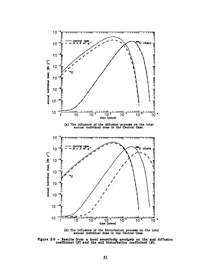
10 "4E i • mm 1 1 I I 1 1 1 1 1 | 1 I I l l l l l | 1 I I l l l l l j I I I l l l l l | 1 I I I I 1 B
^*U chain -=
(a) The influence of the diffusion process on the total annual individual dose in the Central Case.
10 "4
10
10 "'
10 "7
10 "'
central caae r — — B = 0 m' y
i i mill—i i i nun—i i i niii|—i i i iiiir;—i i iiini|—i i nnij
rTufir i i i mill i i i mill i i i mill i i i mil l ' • • • " " 10 10 ' 10J 10 ' 10s 10 '
time [jctf]
(b) The influence of the bioturbation process on the total annual individual dose in the Central Case.
3.6 - Results from a local sensitivity analysis on the soil diffusion coefficient (D) and the soil bioturbation coefficient (B).
51
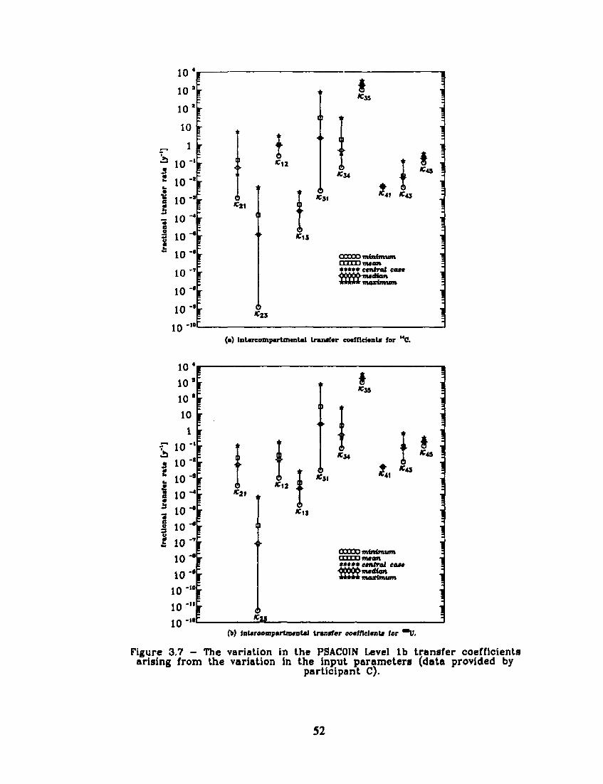
10 4
10 s
10*
io r
l i 10
i o -
10-r
, 10 c
I io i o -i o -i o -i o -io-°
f * 1 2
6 «2»
6 * 3 1
0 Kl3
6 <25
I «35
* 3 4
t «45 !
* 4 3
00000 minimum LULLU i7uan ***** ctnlrol COM •yOyvfr'WmfiQtt AAAAN fnanmuni
]
1
(•) intcrcomparttncnUl trmiurfcr cMfflcftnte for M0.
10 4i
10 s
io»i 10 1
5 10 J 1 0 - C
| 10
% io-c
I io-i 10"* 10-t
IO - i 10 -E
10 -"*
6 *2I
H
*« u
I «3S
*J4
*JI
1 6 *13
O00OO minimum LLLLUmton
M emtral COM* mtdfea fTlOnflttlfTt
<13
I * 4 S
(b) iBUrooapartnwoUI transfer coefficient* /or "U.
Figure 3.7 - The variation in the PSACOIN Level lb transfer coefficients arising from the variation in the input parameters (data provided by
participant C).
52
R = 1 + ^kd (3.5) e
The compartment thicknesses are given by /„ for the surface soil, and /d, for the deep soil compartment. The effects of this linearity are illustrated
by the local sensitivity analysis contributed by participant A'35) and discussed below.
The effects of diffusion and bioturbation (as represented in this model) have been investigated by comparing the results for the total dose summed over pathways and decay chain members, calculated from the deterministic central case with results obtained by setting first the bioturbation coefficient B to zt.o, and second by setting the diffusion coefficient D to zero. This is equivalent to modelling situations where each of these transfer processes is not taken into account.
Figure 3.6 indicates that diffusion affects only the I4C with the central case value leading to a two-fold increase in the annual individual dose compared to the situation where the process is not included. The bioturbation process, in contrast, affects the doses received from both the 14C and the 235U chain, although the effect on the chain dose is much more significant - a factor of five increase in the peak annual individual dose and a shift in the time of occurrence of the peak to earlier times by around 80000 years. This confirms the results of the analysis of the global sensitivity analysis in Section 3.2.2.1.
These results can be understood when the detailed representations of the two transport mechanisms in the Level lb model are considered. The diffusive term in Equation 3.3 is
R lu min(l„,ldJ
with a similar expression for the return diffusive transfer, ^ j " " " 0 0 , since diffusion is a two-way process. The bioturbative transfer, given by
u - * • (R • l ) B
12 " Rl„min(l„,lJ '
also has a similar form for the reverse transfer. The difference in the effects of these two terms is that the diffusive term deals with the contaminants in solution whereas the bioturbative term deals with the contaminants sorbed onto the solid material in the respective compartments. The partition of contaminants between the liquid and solid phases is determined by the retention coefficient, R (given in Equation 3.4 above), so that the fraction of the contaminant in the compartment in solution is given by 1IR and the fraction sorbed onto the compartmental solids is (R - 1)/R. The dependence of R on the solid-liquid kA means that the relatively
poorly sorbed MC is little influenced by the bioturbation process, whereas the members of the 235U chain are much more strongly sorbed, and as a consequence move
53
predominantly with the solid material involved in the bioturbation. Conversely, the poorly sorbed 14C has a higher fraction remaining in solution, causing diffusion to be an important process. Diffusion is, however, unimportant for the more highly sorbed species since they are bound to solid material.
3.4.2 The range of the transfer coefficients in the Level lb model.
Participant C has provided data which further illustrate the advantages of the process-led approach taken in the PSACOIN Level lb exercise. Figure 3.7 indicates the range of values generated in the stochastic calculations for each of the 10 transfer coefficients involved in the transport of radionuclides in the biosphere (excluding the source term). Results for 14C are plotted above, and for 235U below. The means, medians and deterministic central case values are also plotted.
In the absence of a process-led description of the biosphere, one potential alternative would be simply to estimate the ranges of the transfer coefficients themselves, on the basis of expert knowledge. It is an open question whether expert knowledge would generate the range of values, or could adequately characterise the correlations between the transfer coefficients seen here. The figure also illustrates the range in the fractional transfer rates exhibited in the model, from 10n y1 for K23 (deep soil to r sr water) to 5 103 yl for K35
(downstream transport in the river). The influence of the soil kd, bioturbation and diffusion can again be seen in the differences in the inter-soil compartment transfer rates for the carbon and uranium species (K2I and K]2 respectively).
3.5 Summary of the additional analyses.
The additional analyses carried out by participants in the PSACOIN Level lb exercise have illustrated some important features of biosphere models for radioactive waste disposal assessments. The global sensitivity analysis demonstrates that in the Level lb model no single parameter dominates the sensitivity of annual individual dose. The sensitivity of dose is fairly evenly distributed among several of the parameters that were chosen to be variable in the exercise. In the context of this exercise, the parameters used in modelling the transport of the radionuclides in the biosphere were shown to have a greater influence on the mean annual individual dose than the sampled parameters in the exposure pathway submodel, which were chosen to represent a range of different exposure rates for the exposure pathways.
The analysis of the important parameters in the system highlights the importance of solid material transport (particularly involving the bioturbation and erosion processes) for the highly sorbing radionuclides. The representation of erosion in the model has also illustrated the importance of modelling assumptions about the geosphere/biosphere interface. Finally, The area of the re'ease from the geosphere is indicated as having a potentially significant effect on the radiological impact of the release.
54
4. SUMMARY AND CONCLUSIONS
4.1 Principal aims of the PSACOIN Level lb Exercise.
The aims of the PSACOIN Level lb exercise have been
1 to gain experience in the application of probabilistic systems assessment methodology to transport and radiological exposure sub-models and hence to methods of estimating the total risk to individuals, or groups of individuals, arising from the release of radionuclides to the biosphere;
2 to contribute to the verification of biosphere transport and exposure sub-models used by the participants in the case;
3 to investigate the effects of uncertainty in the biosphere transport and exposure sub-models on the estimate of mean dose (which is equivalent to risk in this formulation) to individuals simultaneously exposed via several exposure pathways.
The experience gained by the participants in the exercise in applying the case model to the assessments of the radiological consequences of the release of radionuclides to the biosphere when doses can be received via multiple exposure pathways confirms the approach a as practicable modelling option in the context of probabilistic assessments (Aim 1). Some participants used established codes and methodologies, while others used the case to develop, or to further enhance, capabilities in biosphere modelling in the context of probabilistic safety assessments. The responses to the Level lb Questionnaire, in both deterministic and stochastic phases, showed that good agreement was achieved between the participating codes and methodologies, and this serves to verify the correct working of all the codes and sub-models involved (Aim 2).
Aim 3 is model specific. It concerns the contributions to the overall Level lb uncertainty estimates from each of the sub-models that make up the case model. Of these three sub-models - source term, biosphere transport and exposure pathways - the latter two contained parameters with associated probability distribution functions from which the sample values for the stochastic runs were generated. For the models and codes used in this study, the uncertainties associated with the biosphere transport processes have a greater influence on the overall uncertainty in the mean annual individual dose than does the influence of human behaviour in respect of the exposure pathways by which radiation doses to the exposed population would be delivered.
4.2 The wider implications of the results from the additional analyses.
The PSACOIN Level lb Task Group recognises that the results of the
55
analyses contained in this report depend strongly on the nature of the Level lb conceptual model. The biosphere represented in the exercise was that of an agricultural region associated with a river and the biosphere transport and exposure pathway sub-models described in the case specification represent only one possible interpretation of the biosphere features, events and processes (FEPs). The parameterisation of the processes is likewise not unique. However, in accordance with the first of the aims, the case can be used as a test-bed for this type of biosphere representation, which is commonly employed in several Member countries of the OECD for waste disposal assessments. The results of this exercise are therefore particularly useful for investigating methods for estimating die total risk to individuals arising from releases of radionuclides to the biosphere and should not be interpreted as being relevant to any one site or any particular type of disposal concept. Consequently the source term was chosen to allow time for various features important in biosphere modelling for waste disposal systems to be illustrated and similarly the radionuclides employed in the study were chosen to illustrate the effects of a broad range of relevant physical, chemical and radiological properties.
That the study was designed to illustrate a broad range of biosphere features is one reason why the analysis in Chapter 3 indicated that no single parameter or group of parameters dominated the sensitivity of the dose to the input parameters. However, the fact that different parameters in the study were significant at different times shows that simplifications of this representation of this particular biosphere would be difficult to justify because such FEPs as are included here (and their corresponding parameterisation) each potentially has a role to play in determining the radiological consequences. The parameterisation in this model provides a means of quantifying the FEPs in the system and, because the sensitivity is equally distributed amongst the parameters, there is no reason to single out any particular parameter (and by implication FEP) as a candidate to be deleted from the FEP list in the model. It might be argued that the relative lack of sensitivity in this model to the sampled parameters in the exposure pathway sub-model could be used to justify a reduction in the number of exposure pathways modelled. However the comparison of the relative importance of the different exposure pathways in Chapter 2 suggests that deletion of pathways could only be done by a consideration of the properties of the individual radionuclides and/or on the basis of the relevant timescale of the assessment.
In biosphere modelling for performance assessments a fundamental problem is the inherent unknowability of the state of the biosphere at the time of the release from the geosphere. In estimating the radiological impact of the release to the biosphere it is important not to underestimate the doses (hence the assumptions underlying the exposure rates used in this exercise). This intention has naturally had a large influence in the way in which currently existing biosphere models have been designed. Traditionally the inclusion and addition of FEPs in biosphere models has proceeded on an ad hoc basis and the same situation arises in the case of the parameterisation of the FEPs. Simplification of biosphere models, or their tuning for specific assessment tasks can only proceed on the basis of a thorough review of the relevant FEPs for biosphere modelling. It is also necessary to review the ways in which the FEPs are modelled. These two objectives are being undertaken in the BIOMOVS II study by the Reference Biospheres Working Group[4.1] and the Complementary Studies Working Group[4.2]. These two groups have been specifically constituted to consider the problems of the long-term modelling of the biosphere for waste disposal assessments, and will
56
be working closely together in a series of intercomparisons which began in January 1993.
4.3 Overall Conclusions.
Although the specification of the PSACOIN Level lb model is only one representation of the biosphere, and it is not expected be universally applicable to all biosphere systems, the following conclusions can be drawn on the basis of the analysis of the participants' responses to this exercise. (The corresponding Level lb objective is given in brackets.)
• The different codes and routines used used by the participants to solve the compartment model transport equation performed equally well. This is true not only of the deterministic central case, but also extends to the ranges and combinations of parameters specified in the stochastic phase of the exercise. Some apparently systematic variation was seen in the stochastic results, but it is largely possible to account for this in terms of the scatter seen in the deterministic results. However the precise nature of this feature could not be fully understood with the data available and investigations should continue if similar features are seen in subsequent probabilistic intercomparisons (1, 2);
• The biosphere is a complex system potentially containing many feedback loops. One consequence of this is that no single parameter dominates the uncertainty in the biosphere as modelled here. Different parameters have a significant effect on the overall uncertainty in dose at different times. Thus the issue of timescales becomes important, as well as the influence of the repository release time and the transport time in the geosphere, both of which have not been addressed here (1, 3);
• It is not easy to account for the uncertainties in biosphere transport and accumulation processes with simpler models of the biosphere than the one specified in this exercise. However the successful application of the Level lb model demonstrates that such relatively complex biosphere models can be implemented in PSA codes for waste disposal assessments. The use of such models is recommended since they demonstrate time-dependent features not available from simpler systems (1);
• In this exercise the peak mean dose calculated in the stochastic runs was around a factor of five greater than the peak dose in the deterministic central case (3).;
• The relative importance of the various exposure pathways can vary as a function of time. This feature can be important for decay chains and is particularly apparent when the properties of the daughter radionuclides that govern transport and accumulation in the exposure pathways are different to those of the parent and in this case it was illustrated that doses via the consumption of contaminated drinking water may not in every case provide a reliable (or pessimistic) estimate of the radiological impact of the release of radionuclides to the biosphere (1, 3);
• The analyses here confirm that exposure pathways other than those associated with the transport of groundwater can lead to increased annual doses, l'his is particularly noticeable when the dose via the inhalation mechanism is calculated (1, 3);
57
• The transport of sorbed contaminants on solid materials (for example as a result of erosion or bioturbation) is a potentially important process affecting the long-term transport and accumulation of radionuclides in the biosphere (1, 3);
• The nature of the interface between the geosphere and the biosphere requires careful consideration. The size of the recipient area is a significant factor affecting individual doses in the release region. Some of the modelling boundary conditions assumed in this exercise indicate that surface erosion could, in some circumstances, have a role regarding the input of radionuclides to the biosphere from the geosphere, at the interface between the models (1, 3).
58
REFERENCES.
[1.1] NEA PSAC User Group, 1987, PSACOIN Level 0 Intercomparison. Edited by A Saltelli, E Sartori, T H Andres, B W Goodwin and S G Carlyle. NEA/OECD, Paris.
[1.2] NEA PSAC User Group, 1989, PSACOIN Level E Intercomparison. Edited by B W Goodwin, J-M Laurens, J E Sinclair, D A Galson and E Sartori. NEA/OECD, Paris.
[1.3] NEA PSAC User Group, 1989, PSACOIN Level la Intercomparison. Edited by A Nies, J-M Laurens, D A Galson and S Webster. NEA/OECD, Paris.
[1.4] NEA PS AG, 1990, The International Probabilistic Systems Assessment Group: Background and Results. Edited by J E Sinclair. NEA/OECD, Paris.
[1.5] Recommendations of the International Commission on Radiological Protection, ICRP Publication 26. Ann. ICRP, Vol. 1(3) 1977.
[1.6] J S Martin, S F Mobbs, R A Klos and I M Barraclough, 1992, User Guide for MiniBIOSJA, NRPB-M283, NRPB, Chilton.
[1.7] T Zeevaert, (ed) 1990, BIOMOVS Technical Report 10: Scenario B7: Transport of Contaminated Groundwater to a River, NIRP, Stockholm
[1.8] S F Mobbs, R A Klos, J S Martin, J-M Laurens, K H Winters, J M Bealby, and G Dalrymple, 1991, PACOMA: Performance Assessment of the Confinement Options of Medium-active and Alpha-bearing Wastes: Assessment of disposal in a clay formation in the United Kingdom, EUR13143, CEC Brussels.
[1.91 R A Klos, H Muller-Lemans, F van Dorp and B Baeyens, 1993, TAME: the Terrestrial - Aquatic Model of the Environment, Nagra Technical Report, NTB-93-04, Wettingen.
[1.10] G M Smith, H S Fearn, K R Smith, J P Davies and R A Klos, 1988, Assessment of the Radiological Impact of Disposal of Solid Radioactive Waste at Drigg, NRPB-M147, NRPB, Chilton.
[2.1] NEA PSAC User Group, 1989, PSACOIN Level E Intercomparison. Edited by B W Goodwin, J-M Laurens, J E Sinclair, D A Galson and E Sartori. NEA/OECD, Paris.
[2.2] ACTIVI - Description in reference [2.3].
[2.3] U Bergstrem, O Edlund, S Evans and B Rojder, 1982, BIOPATH - A Computer Code for Calculation of the Turnover of Nuclides in the Biosphere, Studsvik Report, STUDSVIK/NW-82/261.
59
[2.4] B Lindberg, 1973, 1MPEX 2: a Procedure for Solution of Systems of Stiff Differential Equations, Report TRITA-NA-7303, Department of Information and Computer Science, The Royal Institute of Technology, Stockholm.
[2.5] LJNDIF - Description in reference [2.3].
[3.1] K Godfrey, 1983, Compartmental Models and Their Application, Academic Press.
[3.2] D H Anderson, 1983, Compartmental Modelling and Tracer Kinetics, Springer Verlag.
[3.3] H A Grogan, 1990, BIOMOVS' Contribution to Long Term Radioactive Waste Assessment, BIOMOVS Proceedings, Symposium on the Validity of Environmental Transfer Models, Stockholm.
[3.4] J S Manin, S F Mobbs, R A Klos and I M Barraclough, 1992, User Guide for MiniBIOSJA, NRPB-M283, NRPB, Chilton.
[3.5] R A Klos, J E Sinclair, C Torres, S F Mobbs and D A Galson, 1990, The PSACOIN Level lb Exercise: A Probabilistic Code Intercomparison Involving a Four Compartment Biosphere Model, BIOMOVS Proceedings, Symposium on the Validity of Environmental Transfer Models, Stockholm.
[4.1] F Van Dorp, Report from the Reference Biospheres Working Group, BIOMOVS II Progress Report No.3, BIOMOVS, Intera Information Technologies, Henley-on-Thames, 1993.
[4.2] R A Klos, BIOMOVS II Complementary Studies: Case Specification for Phase 1, BIOMOVS, Intera Information Technologies, Henley-on-Thames, 1993.
60
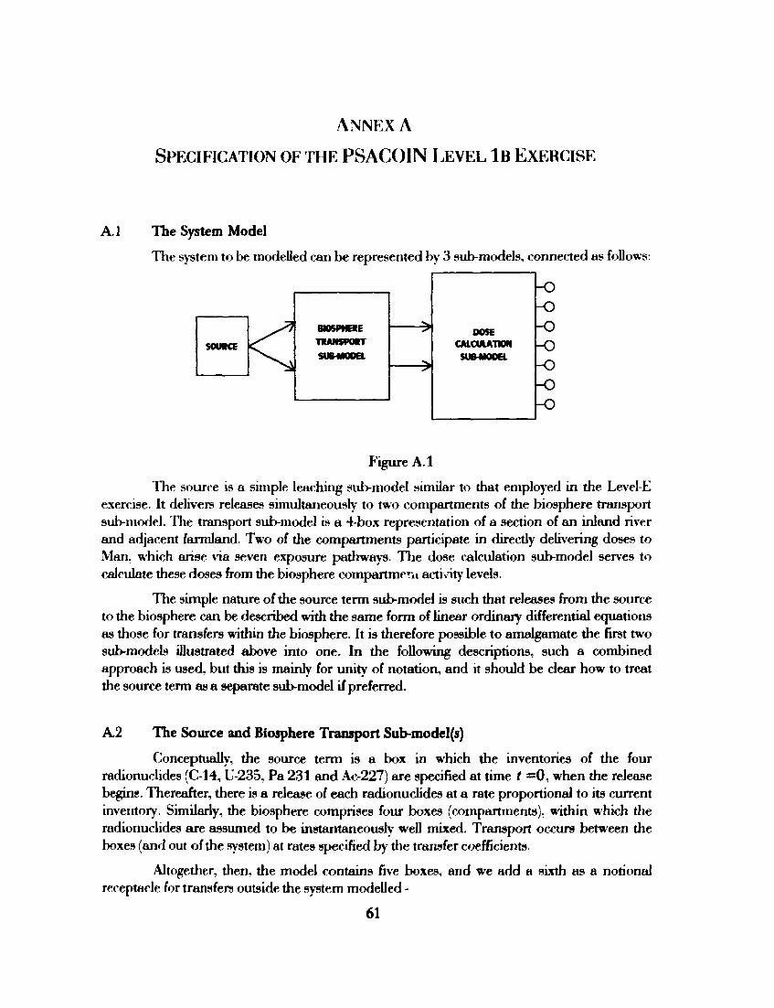
ANNEX A
SPECIFICATION OF THE PSACOIN LEVEL 1B EXERCISE
A.1 The System Model
The system to be modelled can be represented by 3 submodels, connected as follows:
SOURCE
<
BIOSPHERE
TRANSPORT
SUB-MODEL
"S
s
DOSE CALCULATION
SUBMODEL
-o -o -o -0 -o -o -o
Figure A.l
The source is a simple leaching sub-model similar to that employed in the Level-E exercise. It delivers releases simultaneously to two compartments of the biosphere transport submodel. The transport sub-model is a 4-box representation of a section of an inland river and adjacent farmland. Two of the compartments participate in directly delivering doses to Man, which arise via seven exposure pathways. The dose calculation submodel serves to calculate these doses from the biosphere compartment activity levels.
The simple nature of the source term sub-model is such that releases from the source to the biosphere can be described with the same form of linear ordinary differential equations as those for transfers within the biosphere. It is therefore possible to amalgamate the first two submodels illustrated above into one. In the following descriptions, such a combined approach is used, but this is mainly for unity of notation, and it should be clear how to treat the source term as a separate sub-model if preferred.
A2 The Source and Biosphere Transport Sub-model(s)
Conceptually, the source term is a box in which the inventories of the four radionuclides (C-14, U-235, Pa 231 and Ac-227) are specified at time t =0, when the release begins. Thereafter, there is a release of each radionuclides at a rate proportional to its current inventory. Similarly, the biosphere comprises four boxes (compartments), within which the radionuclides are assumed to be instantaneously well mixed. Transport occurs between the boxes (and out of the system) at rates specified by the transfer coefficients.
Altogether, then, the model contains five boxes, and we add a sixth as a notional receptacle for transfers outside the system modelled -
61
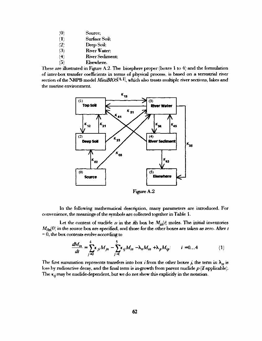
(0) Source; (1) Surface Soil; (2) Deep Soil; (3) River Water. (4) River Sediment: (5) Elsewhere.
These are illustrated in Figure A.2. The biosphere proper (boxes 1 to 4) and the formulation of inter-box transfer coefficients in terms of physical process, is based on a terrestrial river section of the NRPB model MiniBIO&^\ which also treats multiple river sections, lakes and the marine environment.
(1) Top Soil
\
1 *12
I * 2 1
(2) Deep SoH
/
(0)
S
* 1 5
"s i
"S S (3)
River water
1 A
(4) River Sediment
*45
(5) Elsewhere f
V.
55
Figure A.2
In the following mathematical description, many parameters are introduced. For convenience, the meanings of the symbols are collected together in Table 1.
Let the content of nuclide n in the Jth box be M^t) moles. The initial inventories MQJIO) in the source box are specified, and those for the other boxes are taken as zero. After / = 0, the box contents evolve according to
4 5
= J / / / ^ * - 5>«/M>, -KM*, +\pMip. i -0...4 (1) dMt in
dt j*> j*
The first summation represents transfers into box /from the other boxes / the term in X^ is loss by radioactive decay, and the final term is in-growth from parent nuclide p (if applicable). The Kyinay be nuclide-dependent, but we do not show this explicitly in the notation.
62
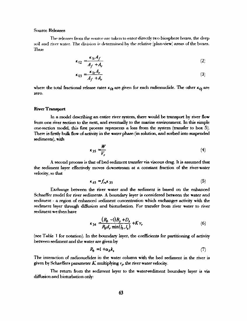
Source Releases
The releases from the source are taken to enter directly two biosphere boxes, the deep soil and river water. The division is determined by the relative (plan-view) areas of the boxes. Thus
Af +Ar
*0 3 ^ ^ A r v3]
where die total fractional release rates Kfy are given for each radionuclide. The other KQ: are zero.
River Transport
In a model describing an entire river system, there would be transport by river flow from one river section to the next, and eventually to the marine environment. In this simple one-section model, this first process represents a loss from the system (transfer to box 5). There is firstly bulk flow of activity in the water phase (in solution, and sorbed into suspended sediments), with
W
' r
A second process is that of bed-sediment transfer via viscous drag. It is assumed that the sediment layer effectively moves downstream at a constant fraction of the river-water velocity, so that
*45 ~frsK 35 (5)
Exchange between the river water and the sediment is based on the enhanced Schaeffer model for river sediments. A boundary layer is considered between the water and sediment - a region of enhanced sediment concentration which exchanges activity with the sediment layer through diffusion and bioturbation. For transfer from river water to river sediment we then have
J f r -1)2?, +D, i „.. K 14 = -, r +A V- (6)
(see Table 1 for notation). In the boundary layer, the coefficients for partitioning of activity between sediment and the water are given by
h =1 +<*bK (7)
The interaction of radionuclides in the water column with the bed sediment in the river is given by Schaeffer's parameter K, multiplying vr the river water velocity.
The return from the sediment layer to the water-sediment boundary layer is via diffusion and bioturbation only:
63
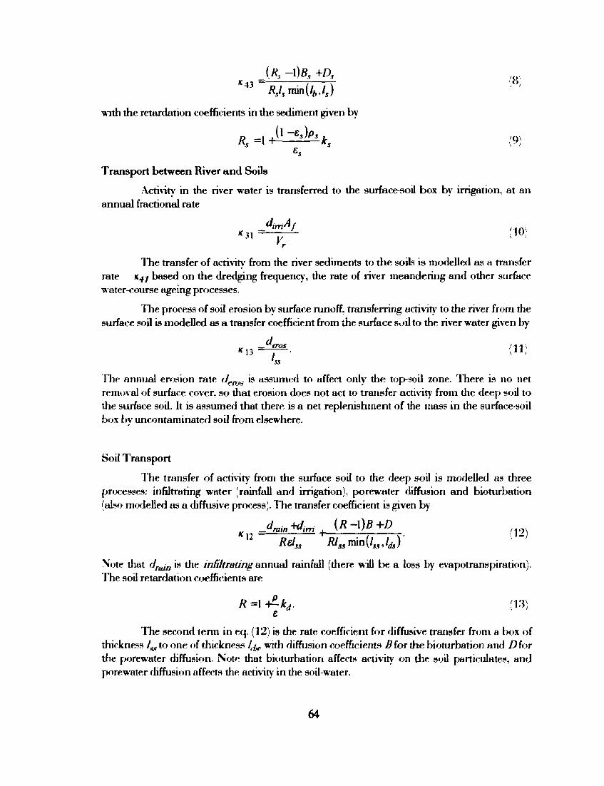
iRs -\)BS +D, RJsnm{lb,ls)
<di = — — — . / . . v (8)
with the retardation coefficients in the sediment given by
Rs =1 +1 —k, (9)
Transport between River and Soils
Activity in the river water is transferred to the surface-soil box by irrigation, at an annual fractional rate
*31 ^ ' (10) ' r
The transfer of activity from the river sediments to the soils is modelled as a transfer rate K4J based on the dredging frequency, the rate of river meandering and other surface water-course ageing processes.
The process of soil erosion by surface runoff, transferring activity to the river from the surface soil is modelled as a transfer coefficient from the surface soil to the river water given by
The annual erosion rate detos is assumed to affect only the top-soil zone. There is no net removal of surface cover, so that erosion does not act to transfer activity from the deep soil to the surface soil. It is assumed that there is a net replenishment of the mass in the surface-soil box bv uncontaminated soil from elsewhere.
Soil Transport
The transfer of activity from the surface soil to the deep soil is modelled as three processes: infiltrating water (rainfall and irrigation), porewater diffusion and bioturbation (also modelled as a diffusive process). The transfer coefficient is given by
K JrainHrri , ( * - Q * + * > (]0, 12 Relss fl/J5min(/„,/J' ' " ;
Note that <irtun is the infiltrating annual rainfall (there will be a loss by evapotranspiration). The soil retardation coefficients are
R =1 -£kd. (13) e
The second term in eq. (12) is the rate coefficient for diffusive transfer from a box of thickness /^ to one of diickness / ^ with diffusion coefficients B for the bioturbation and Dior the porewater diffusion. Note that bioturbation affects activity on die soil particulates, and porewater diffusion affects the activity in the soil-water.
64
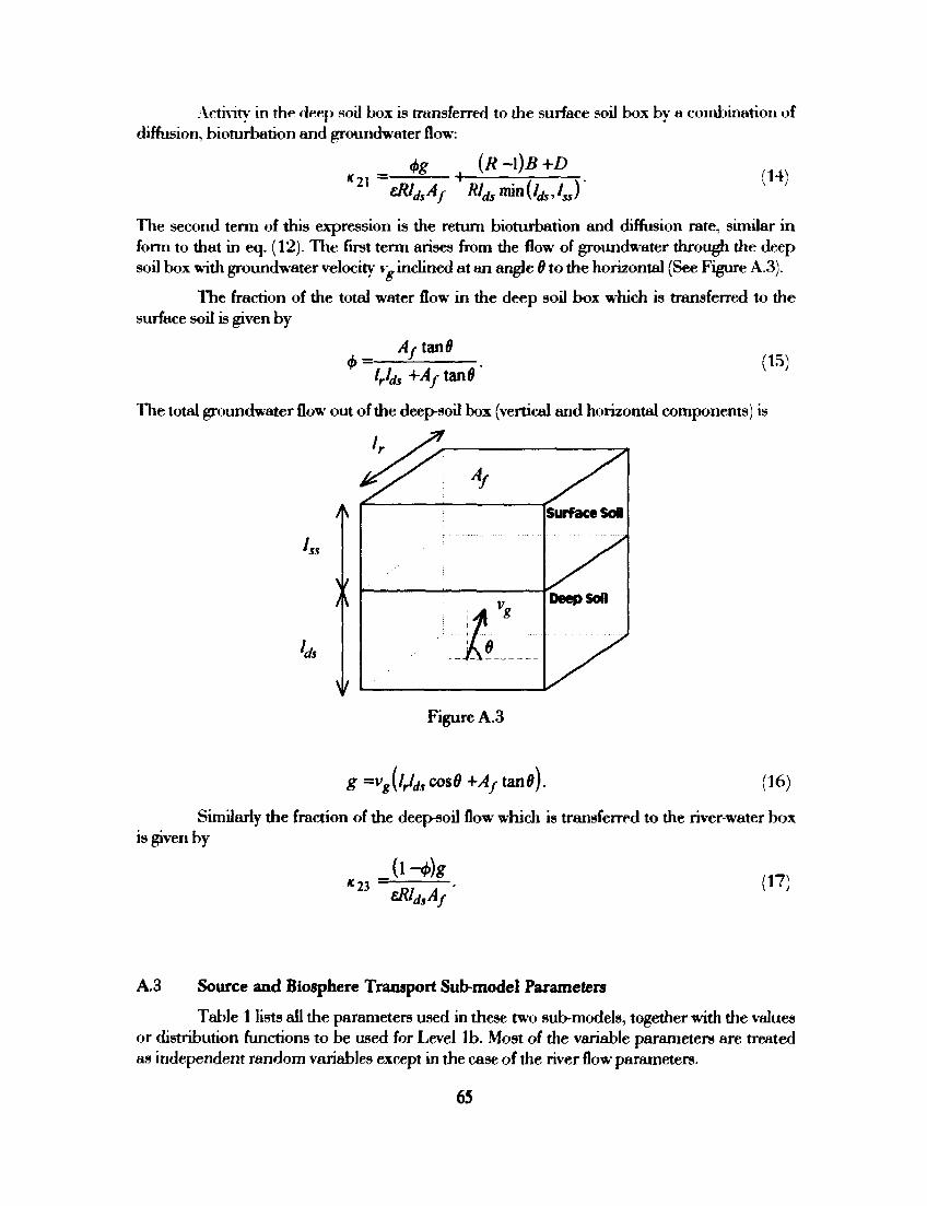
Activity in the deep soil box is transferred to the surface soil box by a combination of diffusion, bioturbation and groundwater flow:
{R -\)B +D *21
_ 4>g sRldsAf ' Rl^minil^jJ
(14)
The second term of this expression is the return bioturbation and diffusion rate, similar in form to that in eq. (12). The first term arises from the flow of groundwater through the deep soil box with groundwater velocity v. inclined at an angle 0 to the horizontal (See Figure A.3).
The fraction of the total water flow in the deep soil box which is transferred to the surface soil is given by
Af tan0 <t> lrlds +Af tan0
The total groundwater flow out of the deep-soil box (vertical and horizontal components) is
(15)
'ss
'ds
Figure A.3
g =vg(lrlds cosB +Af tanfl). (16)
Similarly the fraction of the deep-soil flow which is transferred to the river-water box is given by
*23 eRldsAf (17)
A 3 Source and Biosphere Transport Sub-model Parameters
Table 1 lists all the parameters used in these two sub-models, together with the values or distribution functions to be used for Level lb. Most of the variable parameters are treated as independent random variables except in the case of the river flow parameters.
65
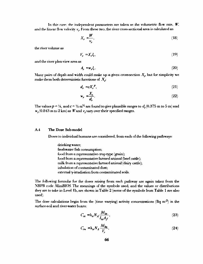
In this oa?e. the independent parameters are taken as the volumetric flow rate, W. and the linear flow velocity vr From these two, the river cross-sectional area is calculated as
W Xr *=- , (18)
the river volume as
K =Xrlr, (19)
and die river plan-view area as
Ar = V r . (20)
Many pairs of depth and width could make up a given cross-section Xr but for simplicity we make them both deterministic functions of X/
dr =cX/, (21)
wr J k (22) dr
The values p = Vi, and C-V2 m1/2 are found to give plausible ranges to dr (0.375 m to 5 m) and wr(0.843 m to 2 km) as JFand vrvary over their specified ranges.
A.4 The Dose Sub-model
Doses to individual humans are considered, from each of the following pathways:
drinking water; freshwater fish consumption; food from a representative crop type (grain); food from a representative farmed animal (beef cattle); milk from a representative farmed animal (dairy cattle); inhalation of contaminated dust; external 7-irradiation from contaminated soils.
The foUowing formula? for the doses arising from each pathway are again taken from the XRPB code MiniBIOS. The meanings of the symbols used, and the values or distributions they are to take in Level lb, are shown in Table 2 (some of the symbols from Table 1 are also used).
The dose calculations begin from the (time -varying) activity concentrations (Bq nr3) in the surface-soil and river-water boxes:
C„ =X„*4 ^ , (24)
66
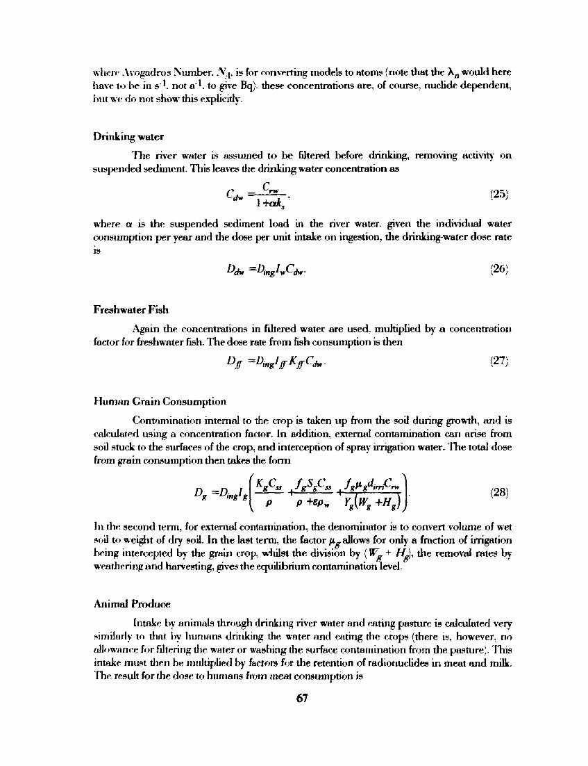
where Avogadros Number. .Y.j, is for converting models to atoms (note that the \ n would here have to be in s'^. not a 1 , to give Bq). these concentrations are, of course, nuclide dependent, but we do not show this explicitly.
Drinking water
The river water is assumed to be filtered before drinking, removing activity on suspended sediment. This leaves the drinking water concentration as
\+aks
where a is the suspended sediment load in the river water, given the individual water consumption per year and the dose per unit intake on ingestion, the drinking-water dose rate is
Ddw -DingKCdw (26)
Freshwater Fish
Again the concentrations in filtered water are used, multiplied by a concentration factor for freshwater fish. The dose rate from fish consumption is then
% =Dingi/rK/rcd»- (27)
Human Grain Consumption
Contamination internal to the crop is taken up from the soil during growth, and is calculated using a concentration factor. In addition, external contamination can arise from soil stuck to the surfaces of the crop, and interception of spray irrigation water. The total dose from grain consumption then takes the form
D* = Z W * P P +*>„ Yg(wg +Hg)^ (28)
In the second term, for external contamination, the denominator is to convert volume of wet soil to weight of dry soil. In the last term, the factor \k~ allows for only a fraction of irrigation being intercepted by the grain crop, whilst the division by (W„ + / / J , the removal rates by weathering and harvesting, gives the equilibrium contamination level.
Animal Produce
Intake by animals through drinking river water and eating pasture is calculated very similarly to that by humans drinking the water and eating the crops (there is, however, no allowance for filtering the water or washing the surface contamination from the pasture). This intake must then be multiplied by factors for the retention of radionuclides in meat and milk. The result for the dose to humans from meat consumption is
67
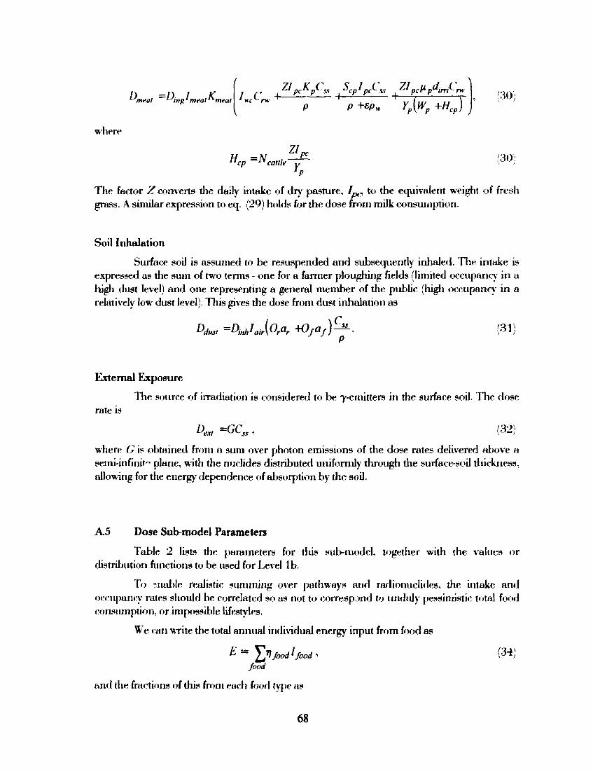
^meat ing* meal meat . ,y " p c P *s | cp pc^ss , ^'pc^pairrr rw
p p +epw Yp{Wp +Hcp) wc nv (30;
.here
z/ ^ =^a„/V -f- (30;
/>
The factor 2T converts the daily intake of dry pasture, 7™ to the equivalent weight of fresh grass. A similar expression to eq. (29) holds for the dose from milk consumption.
Soil Inhalation
Surface soil is assumed to be resuspended and subsequently inhaled. The intake is expressed as the sum of two terms - one for a fanner ploughing fields (limited occupancy in a high dust level) and one representing a general member of the public (high occupancy in a relatively low dust level). This gives die dose from dust inhalation as
Afar =DMlIair(0rar +Ofaf) ^ . (31) P
External Exposure
Hie source of irradiation is considered to be 7-ernitters in the surface soil. The dose rate is
where G is obtained from a sum over photon emissions of the dose rates delivered above a semi-infinif" plane, with the nuclides distributed uniformly through the surface-soil thickness, allowing for the energy dependence of absorption by the soil.
A.5 Dose Sub-model Parameters
Table 2 lists the parameters for this sub-model, together with the values or distribution functions to be used for Level 1 b.
To •enable realistic summing over pathways and radionuclides, the intake and occupancy rates should be correlated so as not to correspond to unduly pessimistic total food consumption, or impossible lifestyles.
We ran write the total annual individual energy input from food as
E ~ ^J\ food1 food •> ( 3 4) food
and the fractions of this from each food type as
68
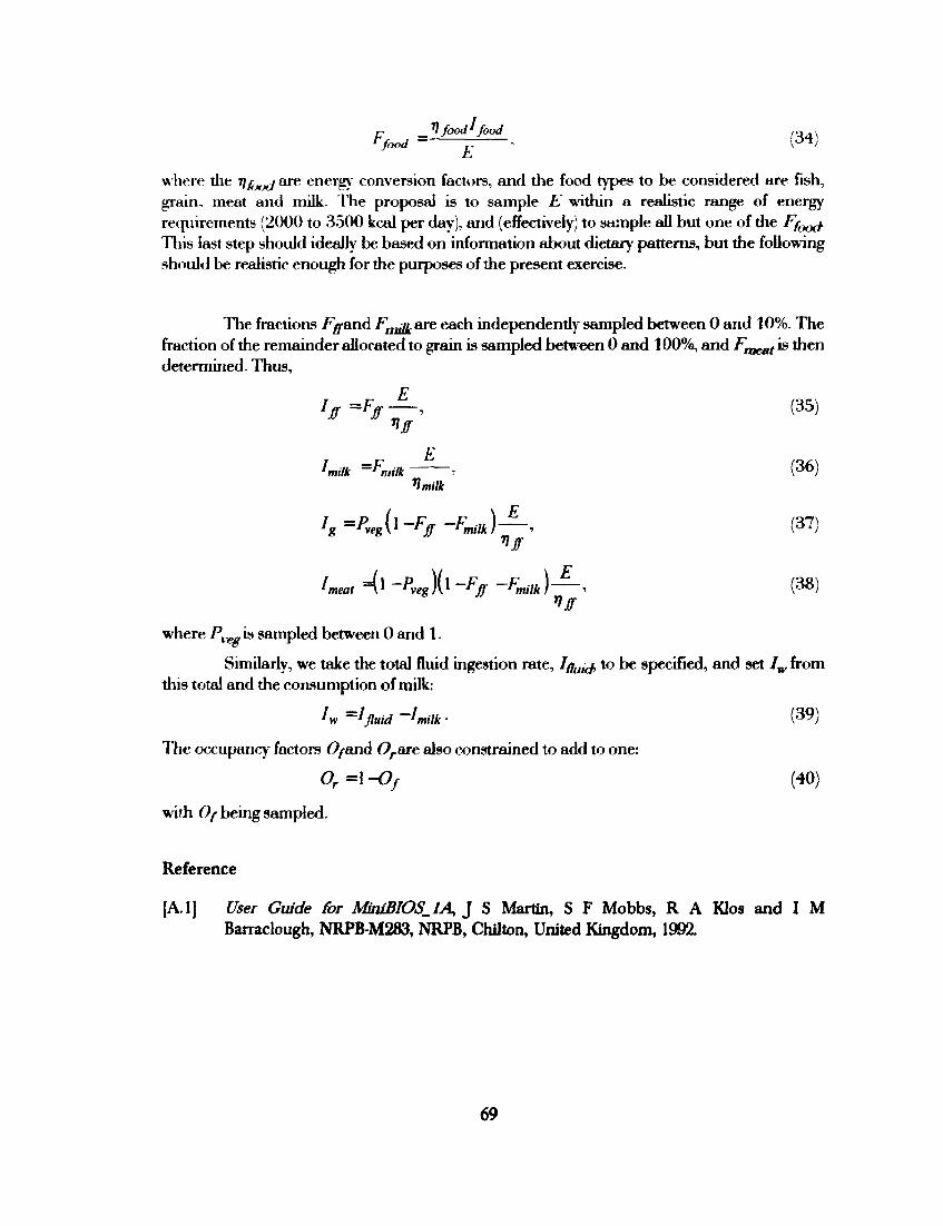
r _*l food'food , o 4 \
where the VflWtj are energy conversion factors, and the food types to be considered are fish, grain, meat and milk. The proposal is to sample E within a realistic range of energy requirements (2000 to 3500 kcal per day), and (effectively) to sample all but one of the Ff0(Xf This last step should ideally be based on information about dietary patterns, but the following should be realistic enough for the purposes of the present exercise.
The fractions Fffand Fmjjcarc each independently sampled between 0 and 10%. The fraction of the remainder allocated to grain is sampled between 0 and 100%, and Fmeat is then determined. Thus,
/ # = F * (35) Vff
Imilk =r7miik •> (36) Vmilk
Ig=Pveg(\-Fff-Fmilk)-^-, (37) Vff
Lea, =(l - 0 ( 1 -Fff -/Wft) — , (38) Iff
where Pvef,i9 sampled between 0 and 1.
Similarly, we take the total fluid ingestion rate, I/j^rf, to be specified, and aet Iw from this total and the consumption of milk:
K =1 fluid "'milk • (3 9)
The occupancy factors Ofand Orare also constrained to add to one:
Or =1 -Of (40)
with Of being sampled.
Reference
[A.1] User Guide for MiniBIOSJA, J S Martin, S F Mobbs, R A Klos and I M Barraclough, NRPB-M283, NRPB, Chilton, United Kingdom, 1992.
69

Table 1
Parameters for the Source and Biosphere Transport Sub-models
Parameter distributions are indicated using the code U(a,b): uniform; LU(fl,6): log-uniform; N(a,6): normal; LN(a,6): log-normal. In each case, the (a,b) are the lower and upper limits of the distribution. Normal and log-normal distributions are truncated at 3 standard deviations (of the logarithm in the case of log-normal), then re-normalised.
Symbol
A,
At
B
Bt
c
D
dClM
<*M
Dt
d.
rfmin
fn
8
K
Meaning
Area of farmland adjacent to the river
Plan-view area of the river section
Soil bioturbation coefficient
Sediment bioturbation coefficient
Coefficient in Eq. (21)
Soil diffusion coefficient
Annual soil erosion
Annual depth of irrigation water
Sediment diffusion coefficient
Depth of the river
Annua! infiltration of rainwater
Sediment flow rate fraction
Groundwater flow out of deep soil
Schaeffer sediment parameter
Value, Distribution or Equation
U(2.0E5,2.0E6)
Eq. (20)
LU(3.0E-5,1.0E-2)
3.2E-5
0.5
LU(3.8E-4,4.7E-2)
LU(6.4E-6,7.6E-4)
U(0.1,0.15)
3.2E-2
Eq. (21)
N(0.14,0.49)
1.0E-4
Eq. (16)
LU(1.0E-10,1.0E-5)
Units
m2
m2
m2/a
m2/a
m»
m2/a
m/a
m/a
m2/a
m
m/a
-
m3/a
m-1
70
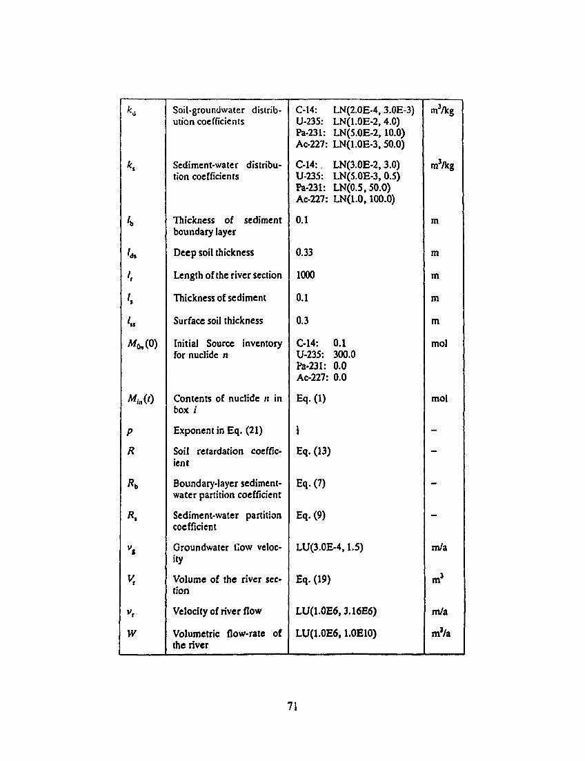
*d
K
4,
' *
>r
u L
Wo„(0)
Min«)
P
R
* b
* ,
vt
K
vt
w
Soil-groundwater distribution coefficients
Sediment-water distribution coefficients
Thickness of sediment boundary layer
Deep soil thickness
Length of the river section
Thickness of sediment
Surface soil thickness
Initial Source inventory for nuclide n
Contents of nuclide n in box i
Exponent in Eq. (21)
Soil retardation coefficient
Boundary-layer sediment-water partition coefficient
Sediment-water partition coefficient
Groundwater tlow velocity
Volume of the river section
Velocity of river flow
Volumetric flow-rate of the river
C-14: LN(2.0E-4,3.0E-3) U-235: LN(1.0E-2,4.0) Pa-231: LN(5.0E-2, 10.0) Ac-227: LN(1.0E-3, 50.0)
C-14: LN(3.0E-2,3.0) U-235: LN(5.0E-3,0.5) Pa-231: LN(0.5,50.0) Ac-227: LN(1.0,100.0)
0.1
0.33
1000
0.1
0.3
C-14: 0.1 U-235: 300.0 Pa-231: 0.0 Ac-227: 0.0
Eq. (1)
J Eq.(13)
Eq. (7)
Eq. (9)
LU(3.0E-4,1.5)
Eq. (19)
LU(1.0E6,3.16E6)
LU(1.0E6,1.0E10)
rnVkg
m3/kg
m
m
m
m
m
mol
mol
-
—
-
—
m/a
m
m/a
m3/a
71
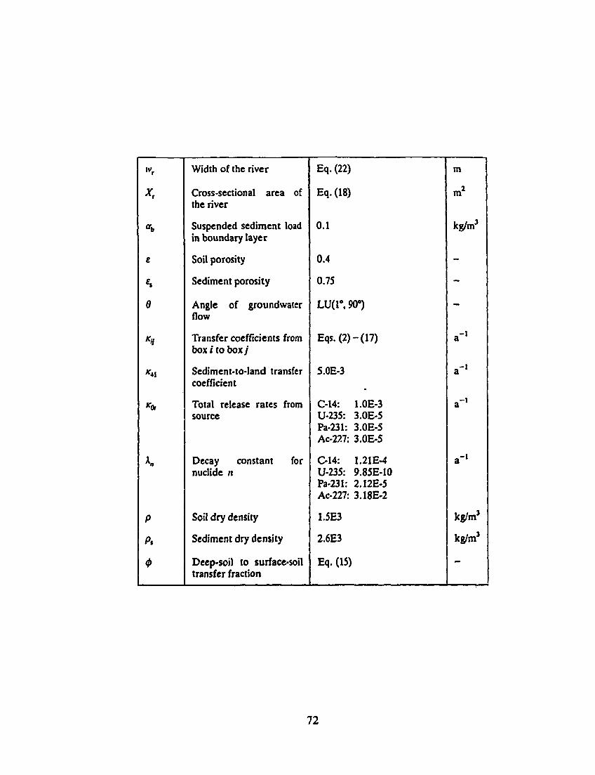
w,
x,
*b
£
«,
d
*;i
K*\
KQ/
K
p
P.
<t>
Width of the river
Cross-sectional area of the river
Suspended sediment load in boundary layer
Soil porosity
Sediment porosity
Angle of groundwater flow
Transfer coefficients from box i to boxy
Sediment-to-land transfer coefficient
Total release rates from source
Decay constant for nuclide n
Soil dry density
Sediment dry density
Deep-soil to surface-soil transfer fraction
Eq.(22)
Eq.(18)
0.1
0.4
0.75
LU(1°, 90°)
Eqs.(2)-(17)
5.0E-3
C-14: l.OE-3 U-235: 3.0E-5 Pa-231: 3.0E-5 Ac-227: 3.0E-5
C-14: 1.21E-4 U-235: 9.85E-10 Pa-231: 2.12E-5 Ac-227: 3.18E-2
1.5E3
2.6E3
Eq. (15)
m
m2
kg/m3
-
-
-
a"1
a"'
a"'
a"'
kg/m3
kg/m3
—
72
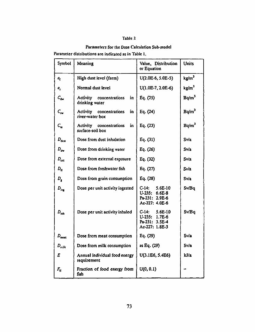
Table 2
Parameters for the Dose Calculation Sub-model
Parameter distributions are indicated as in Table 1.
Symbol
"(
flr
Qw
c„
c„
A*,.
A*
A«
Ar
Di
An,
Anh
Ane.t
A.i;:*<
E
F*
Meaning
High dust level (farm)
Normal dust level
Activity concentrations in drinking water
Activity concentrations in river-water box
Activity concentrations in surface-soil box
Dose from dust inhalation
Dose from drinking water
Dose from external exposure
Dose from freshwater fish
Dose from grain consumption
Dose per unit activity ingested
Dose per unit activity inhaled
Dose from meat consumption
Dose from milk consumption
Annual individual food energy requirement
Fraction of food energy from fish
Value, Distribution or Equation
U(2.0E-6,5.0E-5)
U(1.0E-7,2.0E-6)
Eq.(25)
Eq. (24)
Eq.(23)
Eq.(31)
Eq.(26)
Eq. (32)
Eq.(27)
Eq. (28)
C-14: 5.6E-10 U-235: 6.6E-8 Pa-231: 2.9E-6 Ac-227: 4.0E-6
C-14: 5.6E-10 U-235: 1.7E-6 Pa-231: 3.5E-4 Ac-227: 1.8E-3
Eq. (29)
as Eq. (29)
U(3.1E6,5.4E6)
U(0,0.1)
Units
kg/m3
kg/m3
Bq/m3
Bq/m3
Bq/m3
Sv/a
Sv/a
Sv/a
Sv/a
Sv/a
Sv/Bq
Sv/Bq
Sv/a
Sv/a
kJ/a
—
73
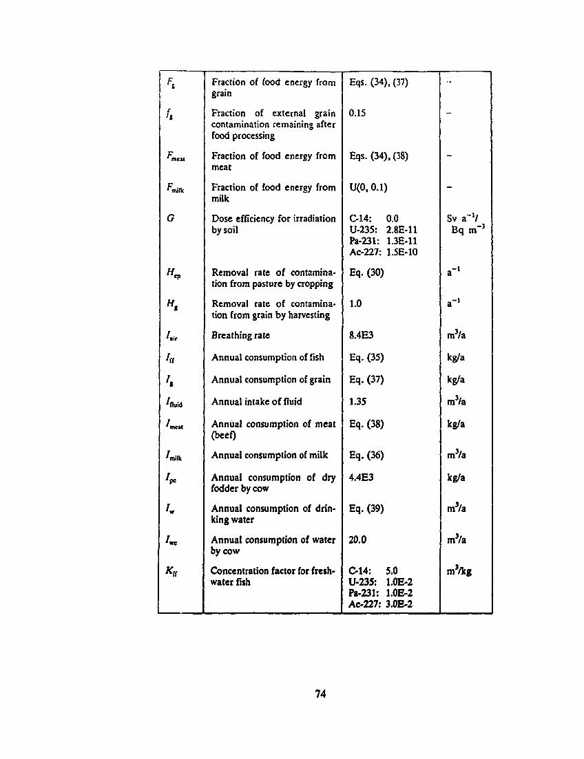
Fl
/ .
F 1 meat
'milk
G
Ho
" •
U hi
' .
Aiuid
'meat
Anilk
'p .
K
u *u
Fraction of food energy from grain
Fraction of external grain contamination remaining after food processing
Fraction of food energy from meat
Fraction of food energy from milk
Dose efficiency for irradiation by soil
Removal rate of contamination from pasture by cropping
Removal rate of contamination from grain by harvesting
Breathing rate
Annual consumption of fish
Annual consumption of grain
Annual intake of fluid
Annual consumption of meat (beef)
Annual consumption of milk
Annual consumption of dry fodder by cow
Annual consumption of drinking water
Annual consumption of water by cow
Concentration factor for freshwater fish
Eqs. (34), (37)
0.15
Eqs. (34), (38)
U(0,0.1)
C-14: 0.0 U-235: 2.8E-U Pa-231: 1.3E-11 Ac-227: 1.5E-10
Eq. (30)
1.0
8.4E3
Eq. (35)
Eq. (37)
1.35
Eq. (38)
Eq. (36)
4.4E3
Eq. (39)
20.0
C-14: 5.0 U-235: 1.0E-2 Pa-231: l.OE-2 Ac-227: 3.0E-2
-
-
-
Sv a~V Bq m~3
a"1
a"1
m3/a
kg/a
kg/a
m3/a
kg/a
m3/a
kg/a
m3/a
m3/a
m3/kg
74
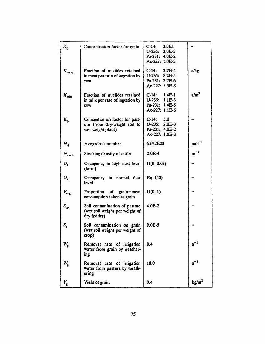
*c
"mea l
^milk
* P
"A
^catife
of
o,
pvtt
J«p
*•
w»
%
n
Concentration factor for grain
Fraction of nuclides retained in meat per rate of ingestion by cow
Fraction of nuclides retained in milk per rate of ingestion by cow
Concentration factor for pasture (from dry-weight soil to wet-weight plant)
Avogadro's number
Stocking density of cattle
Occupancy in high dust level (farm)
Occupancy in normal dust level
Proportion of grain+meat consumption taken as grain
Soil contamination of pasture (wet soil weight per weight of dry fodder)
Soil contamination on grain (wet soil weight per weight of crop)
Removal rate of irrigation water from grain by weathering
Removal rate of irrigation water from pasture by weathering
Yield of grain
C-14: 3.0E1 U-235: 2.0E-3 Pa-231: 4.0E-2 Ac-227: l.OE-3
C-14: 2.7E-4 U-235: 8.2E-5 Pa-231: 2.7E-6 Ac-227: 5.5E-8
C-14: 1.4E-1 U-235: 1.1E-3 Pa-231: 1.4E-5 Ac-227: 1.1E-6
C-14: 5.0 U-235: 2.0E-3 Pa-231: 4.0E-2 Ac-227: l.OE-3
6.022E23
2.0E-4
U(0,0.03)
Eq. (40)
U(0,1)
4.0E-2
9.0E-5
8.4
18.0
0.4
a/kg
aV
mol"'
m"2
-
-
-
a"1
a"'
kg/m2
75
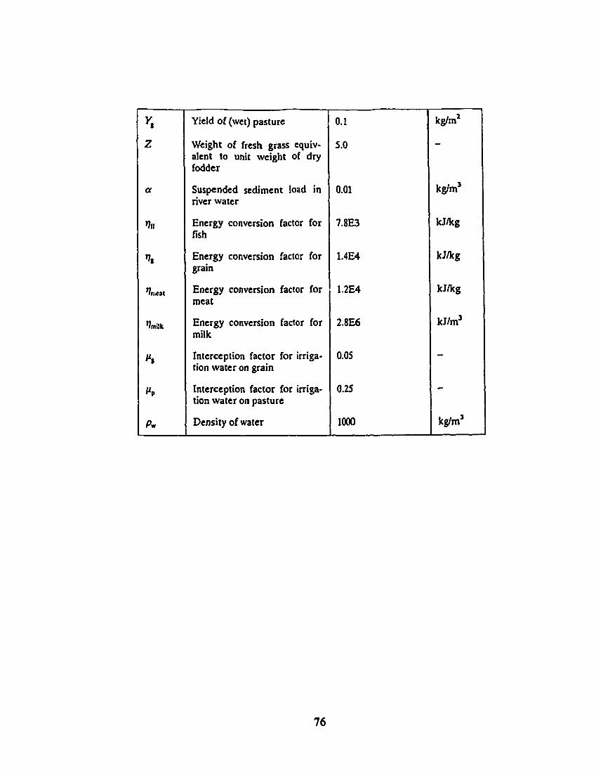
n z
Of
%
\
'?n.«t
fmillc
^
^P
Pw
Yield of (wet) pasture
Weight of fresh grass equivalent to unit weight of dry fodder
Suspended sediment load in river water
Energy conversion factor for fish
Energy conversion factor for grain
Energy conversion factor for meat
Energy conversion factor for milk
Interception factor for irrigation water on grain
Interception factor for irrigation water on pasture
Density of water
0.1
5.0
0.01
7.8E3
1.4E4
1.2E4
2.8E6
0.05
0.25
1000
kg/tn2
'
kg/m3
kJ/kg
kJ/kg
kJ/kg
kJ/m3
—
—
kg/m3
76
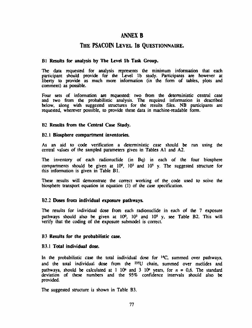
ANNEX B
THE PSACOIN LEVEL 1B QUESTIONNAIRE.
Bl Results for analysis by The Level lb Task Group.
The data requested for analysis represents the minimum information that each participant should provide for the Level lb study. Participants are however at liberty to provide as much more information (in the form of tables, plots and comment) as possible.
Four sets of information are requested: two from the deterministic central case and two from the probabilistic analysis. The required information is described below, along with suggested structures for the results files. NB participants are requested, wherever possible, to provide these data in machine-readable form.
B2 Results from the Central Case Study.
B2.1 Biosphere compartment inventories.
As an aid to code verification a deterministic case should be run using the central values of the sampled parameters given in Tables Al and A2.
The inventory of each radionuclide (in Bq) in each of the four biosphere compartments should be given at 10°, 103 and 105 y. The suggested structure for this information is given in Table Bl.
These results will demonstrate the correct working of the code used to solve the biosphere transport equation in equation (1) of the case specification.
B2.2 Doses from individual exposure pathways.
The results for individual dose from each radionuclide in each of the 7 exposure pathways should also be given at 10°, 103 and 105 y, see Table B2. This will verify that the coding of the exposure submodel is correct.
B3 Results for the probabilistic case.
B3.1 Total individual dose.
In the probabilistic case the total individual dose for 14C, summed over pathways, and the total individual dose from the 235U chain, summed over nuclides and pathways, should be calculated at 1 10" and 3 10" years, for n = 0,6. The standard deviation of these numbers and the 95% confidence intervals should also be provided.
The suggested structure is shown in Table B3.
77
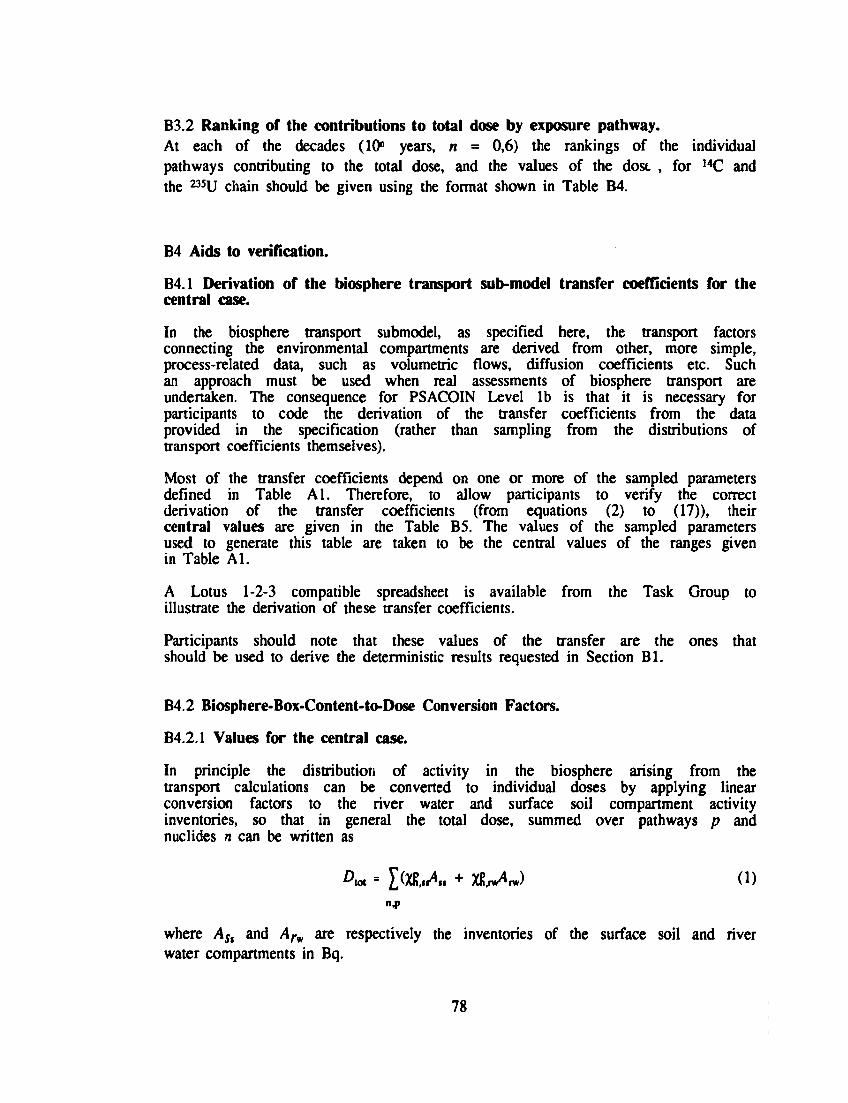
B3.2 Ranking of the contributions to total dose by exposure pathway. At each of the decades (lO1 years, n = 0,6) the rankings of the individual pathways contributing to the total dose, and the values of the dose , for 14C and the 235U chain should be given using the format shown in Table B4.
B4 Aids to verification.
B4.1 Derivation of the biosphere transport sub-model transfer coefficients for the central case.
In the biosphere transport submodel, as specified here, the transport factors connecting the environmental compartments are derived from other, more simple, process-related data, such as volumetric flows, diffusion coefficients etc. Such an approach must be used when real assessments of biosphere transport are undertaken. The consequence for PSACOIN Level lb is that it is necessary for participants to code the derivation of the transfer coefficients from the data provided in the specification (rather than sampling from the distributions of transport coefficients themselves).
Most of the transfer coefficients depend on one or more of the sampled parameters defined in Table Al. Therefore, to allow participants to verify the correct derivation of the transfer coefficients (from equations (2) to (17)), their central values are given in the Table B5. The values of the sampled parameters used to generate this table are taken to be the central values of the ranges given in Table Al.
A Lotus 1-2-3 compatible spreadsheet is available from the Task Group to illustrate the derivation of these transfer coefficients.
Participants should note that these values of the transfer are the ones that should be used to derive the deterministic results requested in Section Bl.
B4.2 Biosphere-Box-Content-to-Dose Conversion Factors.
B4.2.1 Values for the central case.
In principle the distribution of activity in the biosphere arising from the transport calculations can be converted to individual doses by applying linear conversion factors to the river water and surface soil compartment activity inventories, so that in general the total dose, summed over pathways p and nuclides n can be written as
n,p
where ASt and Arw are respectively the inventories of the surface soil and river water compartments in Bq.
78
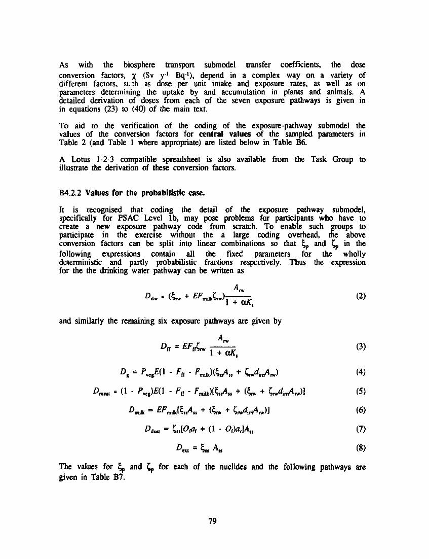
As with the biosphere transport submodel transfer coefficients, the dose conversion factors, x (Sv y1 Bq1), depend in a complex way on a variety of different factors, su:h as dose per unit intake and exposure rates, as well as on parameters determining the uptake by and accumulation in plants and animals. A detailed derivation of doses from each of the seven exposure pathways is given in in equations (23) to (40) of the main text.
To aid to the verification of the coding of the exposure-pathway submodel the values of the conversion factors for central values of the sampled parameters in Table 2 (and Table 1 where appropriate) are listed below in Table B6.
A Lotus 1-2-3 compatible spreadsheet is also available from the Task Group to illustrate the derivation of these conversion factors.
B4.2.2 Values for the probabilistic case.
It is recognised that coding the detail of the exposure pathway submodel, specifically for PSAC Level lb, may pose problems for participants who have to create a new exposure pathway code from scratch. To enable such groups to participate in the exercise without the a large coding overhead, the above conversion factors can be split into linear combinations so that ^ and £p in the following expressions contain all the fixed parameters for the wholly deterministic and partly probabilistic fractions respectively. Thus the expression for the the drinking water pathway can be written as
Ddw = ($w + £FmilkCrw)T-—- (2)
and similarly the remaining six exposure pathways are given by
D«= EF^ rr^ (3)
1 + cut,
Dg = Pveg£(l - Ftt • F m i l k )M„ + C n A ^ J (4)
Anc, - d " fvegW " Fn * F*MJ» + & • + CnAn/Wl (5)
0milk = £ * W $ , A , + & . + CnAArM (6)
D,m = UPA + 0 - Of)at]A» (7)
*>«, « $m A , (8)
The values for 2^ and Cp for each of the nuclides and the following pathways are given in Table B7.
79
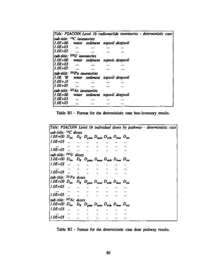
Title: PSACOIN Level lb radionuclide inventories - deterministic case sub-title: ,4C inventories l.OE+00 water sediment topsoil deepsoil 1.0E+03 1.0E+05 sub-title: 23SU inventories l.OE+00 water sediment topsoil deepsoil l.OE+03 ... ... 1.0E+05 sub-title: ^'Pa inventories l.OE V water sediment topsoil deepsoil 1.0E+J3 1.0E+05 ... ... sub-title: 227Ac inventories l.OE+00 water sediment topsoil deepsoil l.OE+03 ... ... 1.0E+05 ... ...
Table Bl - Format for the deterministic case box-inventory results.
Title: PSACOIN Level lb individual doses by pathway - deterministic case sub-title: lAC doses l.OE+00 Ddw DH Dtnin Dmert D^ DdM DM
l.OE+03
1.0E+05 ".'.. sub-title: 235U doses l.OE+00 Ddw Dtt £>gnin
l.OE+03
1.0E+05 ".'.. sub-title: 23iPa doses 1.0E+00 Ddw Dn Dinin
l.OE+03
1.0E+05 ".'.. sub-title: 221Ac doses l.OE+00 Ddw DH Dtnin
l.OE+03
1.0E+05 '"...
Aneit Anilk ^ d u « ^exi
^ m e u Anilk Alui i ^ex i
".'.. ".'.. ".'.. '"...
^ m e a Anilk £\«uit ^e t t
Table B2 - Format for the deterministic case dose pathway results.
80
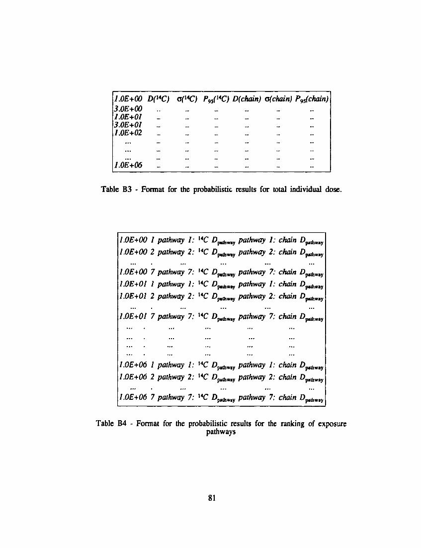
l.OE+00 D(l*C) oO*C) P9S("C) D(chain) a( chain) P95(chain) 3.0E+00 l.OE+01 3.0E+01 1.0E+02
1.0E+06 I
Table B3 - Format for the probabilistic results for total individual dose.
l.OE+00 1 pathway 1:
l.OE+00 2 pathway 2:
l.OE+00 7 pathway 7:
l.OE+01 1 pathway 1:
l.OE+01 2 pathway 2:
l.OE+01 7 pathway 7:
1.0E+06 1 pathway 1:
1.0E+06 2 pathway 2:
1.0E+06 7 pathway 7:
Table B4 - Format for the probabilistic results for the ranking of exposure pathways
4C 0p«hw.y pathway 1: 4C flpwhwy pathway 2:
4C 0p.tf.wy pathway 7: 4C 0p„hw.y pathway 1: 4C 0p„hw.y pathway 2:
4C £>p.u,w.y pathway 7:
chain D^^y
chain D^^
chain £>p,Aw»y chain D^^
chain D^^
chain D^^
l4C 0p«hw.y pathway 1: chain D ^ , , UC ^ y pathway 2: chain D^^
UC I>p,o,w.y pathway 7: chain D thw,y
81
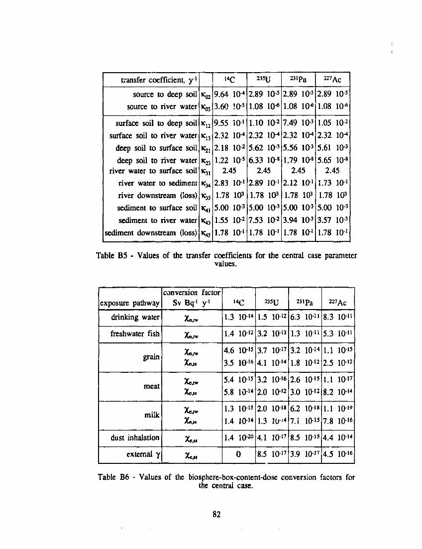
transfer coefficient, y i
source to deep soil
source to river water
surface soil to deep soil
surface soil to river water
deep soil to surface soil
deep soil to river water river water to surface soil
river water to sediment
river downstream (loss)
sediment to surface soil
sediment to river water
sediment downstream (loss)
^
^
K,2
K13
K31
K34
K35
K43
K45
14 C
9.64 10"»
3.60 10-5
9.55 10-1
2.32 10-4
2.18 10-2
1.22 10 s
2.45
2.83 10-1
1.78 103
5.00 10-3
1.55 10-2
1.78 10-1
235IJ
2.89 10-5
1.08 10*
1.10 10-2
2.32 10-4
5.62 10-3
6.33 10-8 2.45
2.89 lO-i
1.78 103
5.00 10-3
7.53 10-2
1.78 10-'
23ipa
2.89 10-5
1.08 10-6
7.49 10-3
2.32 10-4
5.56 lO3
1.79 10-8
2.45
2.12 10-1
1.78 103
5.00 103
3.94 10-3
1.78 101
227Ac
2.89 10-5
1.08 10-6
1.05 10-2
2.32 10^
5.61 10-3
5.65 10-8 2.45
1.73 10-1
1.78 103
5.00 10-3
3.57 10-3
1.78 101
Table B5 - Values of the transfer coefficients for the central case parameter values.
exposure pathway
drinking water
freshwater fish
grain
meat
milk
dust inhalation
external y
conversion factor Sv Bq-i yi
Xn,iw
Xn,rw
Xn,rw
Xn,n
Xn«rw
Xfl,M
Xn/iv
Xn,n
Xn,u
1 4 C
1.3 IO-14
1.4 IO12
4.6 1015
3.5 10'6
5.4 1015
5.8 lO-i*
1.3 1015
1.4 1 0 "
1.4 IO20
0
235TJ
1.5 IO-12
3.2 10-13
3.7 IO-17
4.1 1 0 "
3.2 lO-i*
2.0 IO12
2.0 10-18
1.3 1 0 "
4.1 IO-17
8.5 10'7
23 ip a
6.3 i o n
1.3 IO-11
3.2 IO-"
1.8 IO-12
2.6 10-15
3.0 1012
6.2 lO-i8
7.1 1015
8.5 10-15
3.9 10'7
227AC
8.3 10-u
5.3 10-u
1.1 10-15
2.5 10'2
1.1 1017
8.2 10-K
1.1 lO-i'
7.8 10-16
4.4 lO-i4
4.5 10'6
Table B6 - Values of the biosphere-box-content-dose conversion factors for the central case.
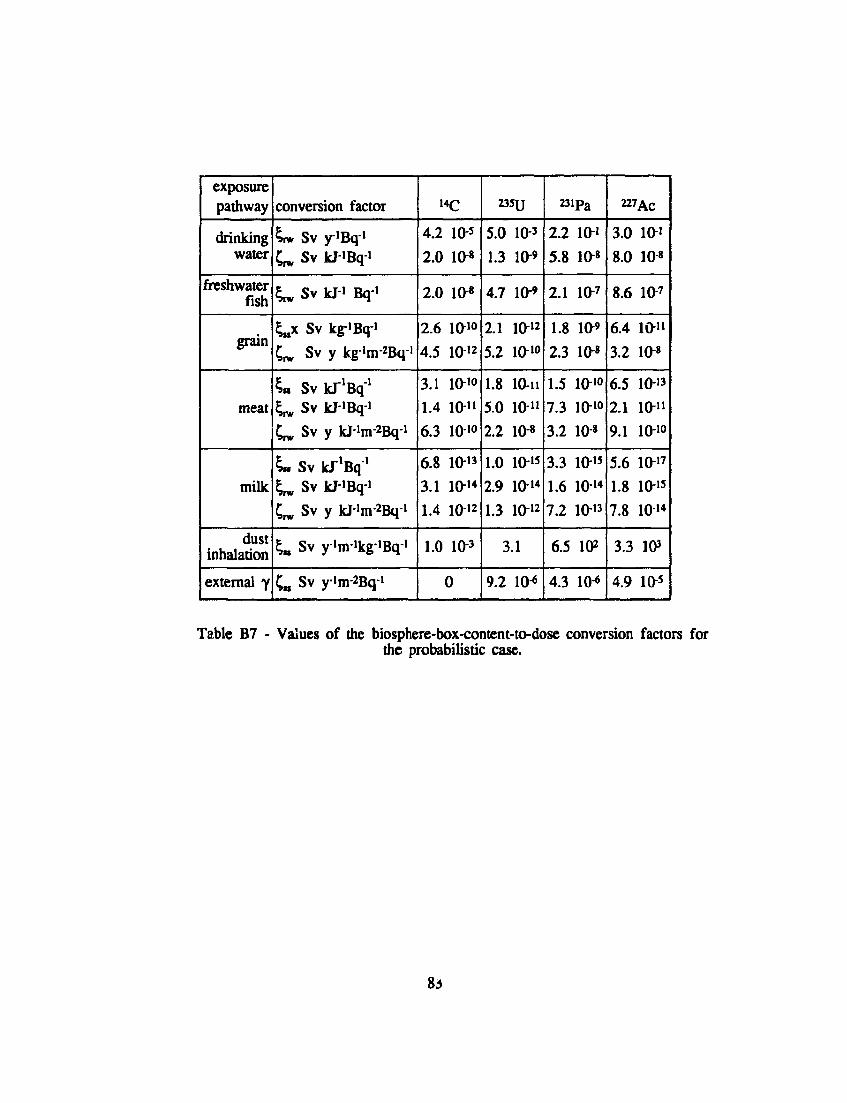
exposure pathway
drinking water
freshwater fish
grain
meat
milk
dust inhalation
external y
conversion factor
£m Sv y'Bq-i Cw Sv kJ-iBqi
U Sv kJ-i Bq«
£„x Sv kg-iBq-i
U Sv y kgim-2Bqi
*>» Sv kT'Bq'1
^ Sv kJ-iBqi
Cw Sv y kJim-2Bqi
%m Sv kT'Bq"1
^ Sv kJ-iBqi
Cw Sv y kJim-2Bq-i
£„ Sv y^m-ikg-JBqi
C„ Sv y^m^Bqi
14C
4.2 10-5
2.0 10-*
2.0 10-«
2.6 lOio
4.5 1012
3.1 10-1° 1.4 10" 6.3 10 io
6.8 10-13
3.1 1014
1.4 lOi2
1.0 10-3
0
235U
5.0 10-3
1.3 10-9
4.7 10-'
2.1 10-12
5.2 10-1°
1.8 10-n
5.0 10-11
2.2 lO-8
1.0 10-15
2.9 IO-14
1.3 IO-12
3.1
9.2 lO-*
23ipa
2.2 10-1
5.8 lO-8
2.1 10-7
1.8 10»
2.3 10-8
1.5 10-1°
7.3 lO-io
3.2 lO-8
3.3 10-15
1.6 10-14
7.2 10-13
6.5 102
4.3 10-6
22?AC
3.0 10-1
8.0 108
8.6 10-7
6.4 10-n
3.2 lO-8
6.5 10-13
2.1 10-n
9.1 lO-io
5.6 10-17
1.8 10-15
7.8 10-14
3.3 103
4.9 10-5
Table B7 - Values of the biosphere-box-content-to-dose conversion factors for the probabilistic case.
83
Participant A: Code: Contact person: Address:
tel: fax:
ANNEX C
Descriptions of Participating Codes.
Paul Scherrer Institute, MiniBIOS/A CTIVI/SYVAC. R A Klos, Paul Scherrer Institute, YVurenlingen and Villigen, CH-5232 Villigen PSI, Switzerland. + 41 56 99 24 18 + 41 56 99 28 21
Three individual computer codes were employed by PSI in the implementation of this exercise. A code for the system of transfer coefficients defined in the input specification (ie the MiniBIOS model transport model) was interfaced with the ACTIVI code. ACTIVI is the transport equation solving part of the BIOPATH suite of environmental analysis programs and the IMPEX routines within ACTIVI were employed. In order to run the stochastic phase of the intercomparison both of these stand-alone codes were incorporated into SYVAC 3.05 as subroutines. The calculations were performed on a MicroVAX 3X00.
For the main analysis SYVACs' internal Monte Carlo sampling routines where used, involving 1000 samples. Additional analysis was performed using the Sandia National Laboratories Latin Hypercube sampling program. For this phase 200 samples were used.
As part of the ongoing development of probabilistic safety assessment a set of post-processing statistical analysis routines, POSTPROC-II, has been developed.
Participant B: Code: Contact person-
Address:
tel: fax:
AEA Technology, MASCOT-3B. J E Sinclair, AEA Decommissioning and Radwaste, Harwell Laboratory, Didcot, Oxfordshire, United Kingdom OX11 ORA. + 44 235 43 32 16 + 44 235 43 65 79
This exercise was run entirely using existing standard submodels in MASCOT. The source term was provided using MASCOTs Simple Leaching submodel, which delivers a constant, nuclide-dependent fraction per unit time of the decayed inventory, remaining in the repository. The source term output was divided into two parts, to provide fluxes into the river water and deep soil compartments in the required ratio, using the Distributor submodel. Finally, the Compartment Biosphere submodel was used to calculate, not only time-dependent inventories of the radionuclides in
K4
the four boxes, but also the doses arising via the different pathways. All of these submodels can be solved analytically after Laplace transformation of the time variable. MASCOT calculates the Laplace-transformed outputs by multiplying the submodel responses (equivalent to convoluting the source term with the unit impulse response of the transport submodel). The time-domain outputs are obtained by a numerical inversion algorithm due to Talbot.
Most of the complexity of the Level lb specification is in the formulae for calculating the transfer coefficients and the pathway doses per unit box inventories. These formula;, including PDFs for the sampled parameters and constants for the others, were coded into the MASCOT input file and interpreted at run time. The processes of sampling from the PDFs, and applying the algebraic formula: to produce values for all the submodel ;fficients for each realisation. are carried out using the built-in facilities of MASCOT.
Participant C: CIEMAT, Code: PRYMA METHODOLOGY version lb.2. Contact person: Carlos Torres, Address: Avenida Complutense 22,
SP-28040 Madrid, Spain.
lei: + 34 1 346 6683 fax: + 34 1 346 6121
The starting point of this methodology is the IMA code. It was developed for the scenario A4 of BIOMOVS exercise and verified in it. The version lb.2 is a new one specially developed for the Level IB exercise of the NEA/OECD.
Its structure consists of several modules that include the codes used for the calculations. The method provides best estimate and probabilistic results. The methodology propagates the uncertainties of the parameters through the different modules and submodules and allows the carrying out of sensitivity analysis in the different models. It is implemented on a VAX 3300 and run under the VMS operating system.
There are five important modules with the subsequent codes in them:
Executive Module: GESTOR. This module manages all files and codes included in the methodology and it is the interface between users and the information system. It is written in DCL command Language and it was developed in IMA/CIEMAT.
Preprocessor Module: The generation of the Sample Spaces is done with the PRISM (from Studsvik, Sweden) or LHS (from Sandia Laboratories, USA) r ides. These do a simple Monte Carlo or Latin Hypercube Sampling with the theoretical distributions of the input parameters.
Environmental Transfer Module: This module is divided in two submodules: (I) The first one calculates the transfer coefficients of the environmental
85
model. It is done with the code of the same name, from IMA/CIEMAT.
(2) The second one is the environmental model. It calculates the environmental concentrations of radionuclides. It uses the BIOPATH code (from Studsvik. Sweden). A semianalytical numerical method (LINDIF) was selected for solving the transport equations.
Dose Paths, ay Module: This module calculates the dose for each pathway with the DOSE PATHWAY LEVELIB code written at IMA/CIEMAT.
Postprocessor Module. This module allows the carrying out of sensitivity and uncertainty analysis of each of the outputs from the different modules and submodules. It can also process the output data set to present the results in the right way. For the sensitivity analysis the codes PCC-SRC (from Sandia Laboratories, USA) and SPOP (from Environmental Institute of ISPRA research Center, CEC) are used. The uncertainty analysis is done with the codes SPOP (Ispra), STATGRAPHICS and some programs developed by IMA/CIEMAT. The VMS version of LOTUS 1-2-3 has also been used in the calculations.
Participant Code:
D:
Contact person: Address:
tel: fax:
Studsvik Nuklear, BIOPATH/PRISM. Ulla Bergstrom Studsvik Nuklear, S-611 82 Nykoping Sweden. + 46 155 221 652 + 46 155 263 117
The exercise was run on existing codes, developed at Studsvik. Subprograms within the BIOPATH code package were used for solving the differential equations. Two solution methods were applied; LINDIF - a semi-analytical method; and IMPEX which is an implicit numerical solution method.
BIOPATH is a set of codes for use in general environmental modelling situations. The probabilistic calculations were carried out using the PRISM-syslem in connection with the ACTIVI (containing the IMPEX and LINDIF subroutines) part of BIOPATH. PRISM has been developed to be a general tool for statistical error propagation, using latin-hypercube sampling for generation of parameter values and it also includes correlation and regression analyses to identify relations between parameters and responses. The calculations were performed on an IBM-PC.
The source term in the scenario description was handled as one compartment, implying that the annual source of radioactivity entering the model was treated in the same way as the transfers between the compartments.
86
Participant E: Code: Contact person: Address:
tel: fax:
Japan Atomic Energy Research Institute, CIRCLE, version 2.1. T. Honima, Japan Atomic Energy Research Institute, Tokai Research Establishment, Tokai-mura, Naka-gun, Ibaraki-kan 319-11, Japan. + 81 292 82 61 70 + 81 292 82 58 20
CIRCLE has been developed to simulate the environmental transfer of radionuclides. CIRCLE is a mathematical tool to solve a set of rate equations which describe the system model considered. The user can select one of the three numerical methods for solving the rate equations: the exponential approximation, the Runge-Kutta formula by Fehlberg, or Gear method for stiff problems. CIRCLE is a flexible program to allow the user to input the values of transfer rate coefficients directly or by algebraic formula. It allows the user to implement the stochastic calculations with use of the PREP utility in the LISA package.
Participant F: Code: Contact person:
Address:
tel: fax:
AECL Whiteshell, SYVAC 3.0H. Terry Andres {MULT1C and SYVAC3), Bruce Goodwin (AECL assessments), Michael Stevens (Results), Carolee Saunders (LIB20J code). Environmental and Safety Assessment Branch, AECL Research Whiteshell Laboratories, Pinawa, Manitoba, Canada ROE 1L0 + 1 204 753 23 11 + 1 204 753 24 55
AECL Whiteshell Code for the PSACOIN Level IB Exercise.
Method of Solution: SYVAC3 has long had built-in routines to solve for the amount of nuclide in a single compartment, given an arbitrary input and arbitrary output capacity, and linear loss rates. The routines have been extensively and successfully used in various AECL models. The PSACOIN Level IB exercise was first attempted by using these routines iteratively to solve for the multiple interconnected compartments. Results were unsatisfactory.
Goertzel and Traili give an efficient solution to the equations for a linear multi-compartment system in the form of a matrix equation involving convolution of matrix exponentials (Goertzel, Gerald, and Nunzio Traili. I960. Some Mathematical
87
Methods of Physics. McGraw-Hill Book Company Inc.. Toronto, Canada). They show that the matrix exponentials can be readily found if the eigenvalues and eigenvectors of the matrix expressing the interactions between the compartments are known. The chief difficulty in implementing this solution is calculating the exponential of an arbitrary matrix. In SYVAC3, that matrix would be generated with randomly-generated data. While not impossible, developing robust code to solve for eigenvalues and eigenvectors that could cover all cases would be a challenge.
Instead, Terry Andres expressed the matrix exponentials in terms of a scaled Taylor series expansion, truncated to achieve a specified level of accuracy given the maximum magnitude of interaction between the compartments. (See. e.g. Cleve Moler and Charles van Loan, Society for Industrial and Applied Mathematics Review, Vol. 20, No.4, October 1978, pp. 801-836).
The solution has been coded as a new routine, MULTIC (MULTIpk Compartment), that will be installed in SYVAC3, and a Level IB model code has been developed that is compatible with the SYVAC3 executive. The complete executable code is called SYVAC309-L1B201 (SKstems Variability Assessment Code, Generation 3, Version 09 -PS AC Level IB Exercise, Generation 2, Version 01). We had 254 sampled and calculated parameters, and 1557 consequence parameters (more than required to supply the minimum results, but the effect on run time should be negligible).
The simulations were performed on Vax 6510 and 6440 computers. We limited SYVAC to a maximum of 150 time points per time series, included 13 fixed times at which results had to be generated, and used a target fractional error of 0.5% for all time series. A set of 250 simulations took about 38.5 CPU hours (52 hours real time) on the 6510, and about 69.5 CPU hours (97 hours real time) on the 6440. Four sets of 250 simulations were carried out.
Participant Code:
G:
Contact person: Address:
tel: fax:
National Radiological Protection Board, ESP-MiniBIOS. Shelly Mobbs, NRPB, Chilton, Didcot, Oxfordshire, United Kingdom OX11 0RQ. + 44 235 83 16 00 + 44 235 83 38 91
The ESP code (Executive Sampling Procedure) uses Latin hypercube sampling to select paramenter values from the ranges specified and can be run with a variety of submodels. The version of ESP set up for this intercomparison contained the MiniBIOS submodel. MiniBIOS is a simplified version of the biosphere code BIOS developed by the NRPB. It is a box model of the biosphere and includes transport of radionuclides in the deep soil, surface soil, marine and freshwater bodies and transfer from sea to land via seaspray. The MiniBIOS model has three components: the first takes the input data and calculates the transfer coefficients between the boxes (MiniPREP), the second calculates the time dependence of the inventories in the boxes (MiniBIOS), and the third calculated the doses arising from these inventories (MiniBIOS). MiniPREP and MiniREAD are in FORTRAN, MiniBIOS itself uses the Harwell code FACSIMILE to solve the differential equations and hence is
88
written in "FACSIMILE". FACSIMILE uses Gears' method to solve the differential equations and chooses its own timesteps depending upon the input parameters. A special version of MiniREAD was created for this intercomparison to provide the required output.
89
ANNEX D
RESPONSES TO THE PSAGOIN LEVEL 1 B QUESTIONNAIRE.
The following sets of tables provide the complete set of participants' responses to the PSACOIN Level lb Questionnaire. The format of the tables is given in Annex B.
90
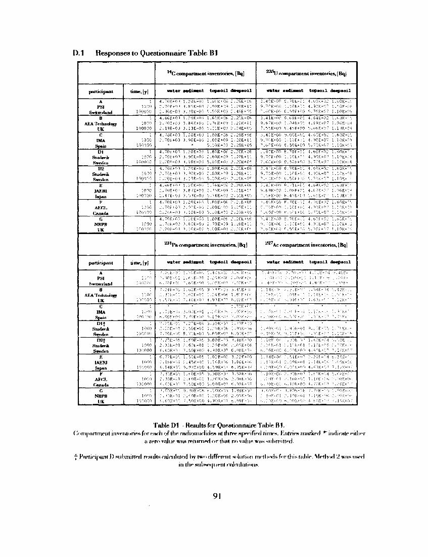
D. 1 Responses to Questionnaire Table Bl
participant
A PSI
Swttserland
B
AEA Technology
UK
C IMA
Spain 1)1
Studaiuk Sweden
D 2 Studsvik Sweden
E IAKH1 Japan
V AEC1.
Canafla
r, NRPB
UK
u™=,[y|
i 1000
l o o o o o 1
1000 1 0 0 0 0 0
1000 1 0 0 0 0 0
1 1000
100000
1 I 000
100000
1 1000
100000
1 1000
100000
1 1000
in on,or*
participant
A PSI
Switzerland
B APIA Technology
UK
C IMA
Spain
Dlt Stuffarifc Sweden
D2f StudffTik Sweden
K JAKR1 Japan
F AEOI.
Canada G
NHPB UK
um<-, jy)
lonor-o
10 00
i o o o o o
10 t l i 00
! 000 1000 00
1 1000
100000
1 1000
10O000
1
1000 100000
1 001; 100000
C compartment inventories, [Bq]
watar awdinant t o p a o i l dawpioi l
4 . 7 0 E + 0 3 1 .20E+03 1 .30E+06 2 . 2 0 E + 0 8 2 . 7 0 E r 0 1 3.9OE+03 2 . 8 0 E + 09 1 . 2 0 E + 1 1 2 . 3 C E - 0 3 3 . 3 0 E - 0 3 0 .50F .*03 2 .40E+O5
4 . 6 6 E * 0 3 1.2OE+03 1.B1E + 06 2.21F.+ 08 2 . 7 0 E + 0 3 3.8SEt-03 2 . 7 t ' E + 0 9 1 . 2 1 E + 1 ! 2 . 1 9 E - 0 3 3 . 1 3 E - 0 3 5 . 1 1 E + 0 3 2 . 2 4 E + 0 5
4 . 7 0 E + 0 3 1.2OE*03 1 .S0E + 06 2 .20E+QB 2 . 7 0 E + 0 3 3 . 9 0 E + 0 3 2 . 8 0 E + 0 9 1 . 2 0 E + U
* * O.lOE-t-03 2 .20E1-05
4.70E>-03 1 .20E+03 1 . 8 0 E * 0 f 2 . 2 0 E t - 0 8 2 . 7 0 E + 0 3 3 .9OE+03 2 . 8 0 E + 09 1 . 2 0 E + 1 ! 2 . 2 0 E - 0 3 3 . 1 0 E - 0 3 5 . 1 0 E + 0.< 2 .2GE + 0'i
4 . 7 Q E f 0 3 1 .20E+03 1 .80E+06 2 . 2 0 E + 0 8 r . 7 0 E * 0 3 3.9OE»-03 2 . 8 0 E + 0 9 1 .20E + U 2 . 2 0 E - 0 3 3 . 1 9 E - 0 3 5.10E*-03 2 . 2 0 E * 0 5
4 . 6 6 E + 0 3 1 .20R+03 1 .76E+06 2.20F.-r08 2 . 7 u E * 0 ' 3 . 8 7 E + 0 3 2 . 7 i E t 0 9 1 .21E+11 2 . 4 7 E - 0 3 3 . 5 3 E - 0 3 5.74E»-03 2 .y .E«-C0
4 .70EK13 1 .20EH13 1.80E+Q6 2 . 2 0 F > 0 8 2 . 7 0 E + 0 ! 3.9OEt-03 2 . 8 0 E H 1 9 l . O O E t l l 2 . 2 0 E - 0 J 3 . 1 0 E - 0 3 O.lOEt-03 2 ' .29F>0 ' j
4 . 7 0 E . C 3 1 . 2 O E t 0 3 1 . 8 0 E » 0 6 2 . 2 0 E f 0 8 2 . 7 0 E + 0 3 3.8OE+03 2 - 7 0 E + 0 9 1 .20E+11 .T . 2 0 F _ fi 3 3 .1OE-03 L..00F,+ O< 2 . 2 0 E * 0 ' ,
Pa compartment inventories, [Bq]
water a a d i n n t t o p a o l l daapso i l
' . 2OE-0C 1.7OE-O0 1.40F.-C2 3 .SOEKIC 7 . 3 0 E - 0 1 2 . 6 0 E - 9 1 I.2OE-KJ0 2 . OOE >•!); f . . 7 0 F t 0 r ' ' . f .0F,t r '0 O.COr>0. ' 7 . 00F .» ' | "
7 . 2 4 K - J 1 , l . r ,2F.-0" , 9 - 7 H E - 0 3 3 . 4 =; E ' :i. : : . ? : E - r i . " . f O F - o : i . : M F > 0 b \.w-i>. ( . . M E ' J O 7.40E»Of'i 4 .9"<K»-M7 f . . 62E>(7
1.70E t'-0 . . . uOE-01 3 . 0 0 E - 0 1 :. . 'OE»2-> :..OOF>00 i-;.0OEt0O 7.70E4.00 W 0 K + O 7 7.0OK',"••"'
7 . / O E - 0 0 7 . 2 0 E - 0 6 3 . 3 0 E - 3 3 i . l O F ' O O ,0.. '.OE- f :l 2 , ' jOE-OI i . i O E t O O 1.90F.-t-9b 7 . 7 0 E - 0 C S . 7 0 E + 0 0 O.SOF.wy fi.00E>-",7
. ' . 2 0 E - 1 ' , 1 . 6 0 E - 0 5 9 . 8 0 E - 0 3 3.40F>nn 2 . 3 O E - 0 1 2 . 6 0 E - 0 1 1.2OF.+06 2 . 0 0 K t O b f'.ftOF.Kiu 7 .50EH10 4 . ' l O E t 0 7 6.HC!F.f07
6 . 7 7 E - 0 0 l . ' j O E - n S 1.O2F.-02 3.22F. + 00 2 . l 6 E - 0 ' i 2 .4" )E-0 ' . l . l t ' . E t O b I .86EK1O O.14EI-00 9 . 9 7 E K J 0 4.=>9E*rj7 6 .35E+07
7 .30F. -0S 1 . f .0E-n^ 9 .OOE-03 3.c.0F,*ft0 2 . 3 0 E - 0 1 2 . 6 0 E - 0 1 1.2OF>0t, O.OOF.tOO b.SOE'OO 7 . ' , 0 E » 0 0 O.OOF.tOT 6.90E.if ,7
' .OOK-0 ' , ( i , 3 0 E - 0 6 0.tiOF*.-03 1.80E»0O : . <o?;-ni O.OOE-OI I.>:OF>OO o.ooFtfn, O.OOF.iOO . ' .VlEtOO 4.9C)F.l07 ft.80F-'j'
compartment inventories, [ Bq j 1
watar aadiaatnt t o p a o i l uaapaoil
3 . 4 0 E ' 0 O e . ' O E - 0 1 4 . 6 0 E » 0 2 1.60E*0'-. 9.70F>OC 1 .10E+31 4 . 9 0 E + 0 7 i.lOF.fOf' 7.60E+0C- 8.00EKJO ' ' . 7 0 E + 07 I . l O E t O ; ,
3 .41E*0C 8 . t 8 F - 0 1 4 . 6 4 E * 0 2 i . e 3 E f " i 9 . 6 7 E * 0 0 i . 0 3 E + 9 ! 4 .S9L ' f07 l.OOEn'Jt! 7 . 5 5 E * 0 0 6 . 4 5 E + 0 0 0 . 6 6 E + 0 7 1.13E*0S
3 .4CE*00 9 . 0 0 E - O I 4 . 6 0 E ^ 0 2 l.fcOF.rDi, 9 . 7 0 E ^ 0 0 1 .10E+01 4 . 9 0 E f 0 7 1 .10F>03 i .6OE»0C 8 . 5 0 E + 00 =..7fJE-07 1 . 1 0 E - 0 =
. . .40E+00 B .7OE-01 4 . 6 0 E - O 2 ; .c ' ,0E+0: 9.7OE*0O 1 .10E»Oi 4 .90? . 4-07 !.irjEK"'d 7.6OE+0O S.5OE+.90 5.7i;.F.+,07 ! . ! 0 E t 0 6
3.4OEV0O 8 . 7 0 E - 0 1 4 . 6 0 E + 0 2 I.bQE*-?'.-9.70Et-0'J l . l O E f - d l 4 . 9 0 E + 0 7 L l C E t O S 7.>:r;E*or; s . ^ o E r o o I . I O E ' O 1 I . I O E - ' 1
3.42E+0O 8 . 7 1 E - 0 1 4 . b 4 E * 0 2 1 . 6 3 E t C : 9 . 6 9 E ' 0 C I .OSE+Ol 4 . 8 7 E i - P 1 1.06E>C1 :
7 . 0 6 E t 0 O 8 .40E»0 ' ' ' l.i~~Z*Vl 1.13E*'1H
3.40F.tOO 8 . 7 O E - 0 I 4 . 7 0 E + 12 1 . 6 0 E * " , 9 . ' ' 0F>0 r l l . lOF. t f i l 4 .9f)E*07 ! . 1 0 F > 0 i ;
~',i..0E'-0''i H.or'F.^Ou 0- 7 OE*07 1 . 1 0 E * : -
"'.40EK10 9 . 7 0 E - 0 1 4.bOE>02 l.r.jF.>:-.. fi.'.'OE-OO 1.1OE+01 4 . 9 0 E + 07 l . lCE*01i ''.-.OEi-fO ".50F.+ 10 i . lOF.^O-1 ! , i ) F , . - (
Ac c o m p a r t m e n t i n v e n t o r i e s , [ Bq]
w a t e r a a d i m a n t t o p s o i l d a a p a o i l
'. .40F.-9. . 3 .70E-O7 4 .O0E-C4 9 . 4 0 E - " . .OOK-o: 2 . H ' E - 0 i 1.10F.» Or 2.0C-E-• . 4 r ' f>0 0' - .O^FrOO 4 . 8 - ' ? > ' ' ' . l ' ' F '
I . H E - ' ! ! . 2 . . - 0 E - 0 ' - l .S4F.-"J4 '.•. 42E- ... : . : ' F . - ' 1 .•''RE- : ' i . 14E*"- .' . ' ' • - • ' • • . • 9 F . , ; f . ' . .OOF'" ! ' •• . 6 9 F. - •" "• "'.".2F,>"
• . 'OE'OO ...OOF'OO 3 . 0 0 E - - T ' 1 . ' , 3 F . , '
l . ' -OE-Ol : . 8 O K - 0 ! 9 . . 0 F . - 0 S ; . " ' n t> . ' . .
1.10F.-0-" : . 3 0 F - ' i 7 l . f , 0 E - 0 4 0 .O0E- .. r . 2 ' F , - 0 1 2 , 1 0 F . - 0 i ! . 1 0 E » ' ' 0 . ' . " • O E ' l -K..-0EH10 f. .nOEffp'O 4.r.OE>f.7 7 . 1 0 F > 0 "
'. . ! 4 E - 0 e l . ' .01F.-O7 O.OIE-O.l O . I O E - ' . ' ; . ' . 7 E - 0 1 r .- . f l iE-ol l . U E T f •'.OOF.tO-.. p-.20F.tOO O . O U > 0 0 4 . 6 3 K * 0 7 7 . l ; ' E » ' i
1.10r.-0r ' . ••..'•0E-O7 ! . t ,0F.-O4 ' j . F.OF.-O." : .OOF.-Oi / . l O E - o i i . m F . t O r . :-.:iOF>oo '... >0E»0O . . . l " K » n n 4 . /C.E'0.7 7 . 2 0 E t ' '
*.<,0F.-07 9.f)OE-Of; 7.7OF.- f :0 i . ' ' 0 F . - o ; . ' . 10E-01 O. IOE-Oi ! . i0E-O»' , ; : . 0 0 F ' O . ' . . ."OE'OO - , . onh t0 f ' 4 . 'v" iE ' f ' ' ; . 1 0 F 9 0 '
Table D1 - ResultB for Questionnaire Table Bl. (Vinipnrtrricn) inventories for each of ihr radionuclides at three sjierified titnes. Mntries marked '*' indieate «-it)]>-r
a zero value, was rRtnrned r>r that no value WHS HiiWrt'itted.
f Pnrtiripajil D .tubmitlerl r»-wiltH ralnilate/J by two different solution methods fortius table. Method 2 wis lined in the subsequent calculation*.
91
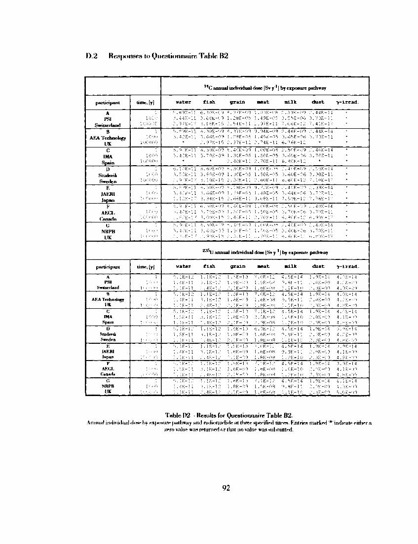
D.2 Resf>onses to Questionnaire Tabic B2
p a r t i c i p a n t
A PSI
S w i t z e r l a n d
B
A E A T e c h n o l o g y
UK
C
IMA
S p a i n
D
S tudsv ik
S w e d e n
K
JAFJU
Japan
F
A E C I .
C a n a d a
G
N R P B
U K
time, [yl
1
1 0 0 ' j
IGciOi'iO
1
10 !30
lOOOfiO
10 On 1 0 0 0 Oil
1 l i j f 0
1 0 0 0 0 0
1 0''!i : i i "
1 0 - MO
1
part ic ipant
A PSI
Switzerland
B
AKA Technology UK
r, fMA
.Spam D
Sludiml Sweden
E JAKHI Japan
r AKCI,
Canada G
NHPB l/K
t ime , [y |
] ; - / , , !
1,-.:.M
T
1 0 0 0
1 1 •'•:•:;
1 0.!!!
1
I '•' o 0 ' < 0'
C a n n u a l i n d i v i d u a l d o s e [Sv y J by e x p o s u r e p a t h w a y
w a t e r f i s h g r a i n m e a t m i l k d u s t - y - i r r a d .
0 . H 9 E - 1 1 6 . 3 0 E - 0 9 S . 3 7 E - 0 9 1 . 0 0 E - 0 8 2 . 3 9 E - 0 9 2 . 4 4 F . - 1 4 *
3 . 4 4 H - 1 1 3 . 6 8 E - 0 9 I . 2 8 E - 0 5 L . 4 9 E - 0 5 O . S S E - O o 3 . 7 3 E - U
2 . 9 7 E > r r 3 . 1 8 E - 1 5 3 . S . 4 E - 1 1 3 . 9 7 F . - 1 1 7 . 0 6 E - 1 2 7 . 4 1 E - 1 7
5 . 8 9 E - 1 1 h . 3 0 E - 0 9 8 . 3 7 E - 0 9 9 . 9 4 E - 0 9 2 . 4 6 E - 0 9 2 . 4 4 E - I 4
3 . 4 2 E - 1 1 3 . 6 6 E - 0 9 I . 2 S E - 0 S 1 . 4 S E - 0 5 3 . 6 5 E - 0 6 3 . 7 3 E - 1 1
3 . 9 7 E - 1 5 2 . 3 7 E - 1 1 2 . 7 4 E - 1 1 6 . 7 6 E - 1 2
. S . 9 0 E - 1 1 b . 3 0 E - 0 9 8 . 4 0 E - 0 9 t . 0 0 E - O 8 2 . 5 O E - 0 9 2 . 4 0 E - 1 4
3 . 4 0 E - 1 1 3 . 7 0 F . - 0 9 1 . 3 0 E - O 5 1 . 5 0 E - O 5 3 . 6 0 E - 0 6 3 . 7 0 E - 1 1
* 2 . 4 0 E - 1 1 2 . 7 0 E - 1 1 6 . 8 0 E - 1 2 *
o . l o i F . - l l 6 . 6 0 E - 0 9 8 . 3 0 E - 0 9 I . O C ' E - O H 2 . 4 ! > F . - 0 9 2 . 5 9 F . - 1 4
3 . 5 0 E - 1 1 3 . 8 0 F . - 0 9 1 . 3 0 E - 0 5 1 . 5 0 E - 0 5 3 . 6 0 E - 0 6 3 . 9 0 E - 1 1
3 . a 0 ! F , - 1 7 3 - 1 0 E - 1 5 2 . 3 0 E - 1 1 2 - 6 0 E - 1 1 b . e 0 E - 1 2 7 . 1 0 E - 1 7
S . 8 9 F . - 1 1 t i . 3 0 E - 0 9 9 . 1 8 E - 0 9 9 . / 3 E - 0 9 2 . 4 0 E - 0 9 2 . 3 9 F . - 1 4
3 . 4 2 E - 1 1 3 . 6 < 5 E - 0 9 1 . 2 3 E - 0 5 1 . 4 3 E - 0 5 3 . O 4 E - 0 6 3 - 7 2 E - 1 1
1 . 1 2 E - I 7 3 . 3 4 E - l b 2 . 6 6 E - 1 1 3 . 0 8 E - 1 1 7 . F , 9 E - I 2 " ' . 7 6 E - 1 7
•3. 9 i . 'E- l" i • S . 3 0 E - O 9 8 . 4 o i E - 0 9 ! . 0 f i E - 0 8 2 . 5 0 E - U 9 , . . 4 0 1
1 . 4 0 E - 1 I 3 . 7 . 3 E - 0 9 1 . 3 O E - 0 5 l . S 0 E - O r i 3 . 7 O F . - 0 6 3 . 7 n f
.''-. 9 ' . 'E-1 1 0 . 3 0 E - 0 9 H . - 1 I - ; E - I : 9 1 . 0 O F . - O 8 2 . 4 0 E - O 9 2 . 4 i ' l
3 . 4 0 E - U 3 . 6 0 E - 0 ? t . j O E - . , ' 1 . . S O E - 0 5 3 . 6 0 E - 0 6 3 . 7 0 J
2 . ' ' O E - ! . ' . ' . 9 0 K - 1 . ' b 2 . 3 0 E - ! : 2 . 7 0 F - 1 I 6 . h r E - 1 2 . , . 8 0 i -
- 1 4
- 1 1
- 1 4
- U - 1 7
2 3 5 , , a n n u a l i n d i v i d u a l d o s e [ S v y ' j by e x p o s u r e p a t h w a y I
w a t e r f i s h g r a i n m e a t m i l k d u s t y - i r r a d .
r ; . l E - 1 2 1 . 1 F - 1 2 l . [ ) E - 1 3 7 . 0 F . - 1 2 4 . 5 E - 1 4 1 . 9 E - H 4 . 0 E - I 4 1 . 4 E - 1 1 3 . 1 E - 1 2 1 . 8 E - D 9 1 . 5 E - 0 8 3 . 8 E - 1 1 2 . 0 E - 0 9 4 . 2 E - 7 9 l . i E - 1 1 2 . 4 E - I 2 2 . 1 E - 0 9 1 . 8 E - 0 8 1 . 1 E - 1 . 0 2 . 3 E - 0 9 4 . 9 F - 0 9 C , . 1 E - 1 2 l . I E - 1 2 1 . 5 E - 1 3 7 . 0 E - 1 2 4 . S E - J 4 1 . 9 E - 1 4 4 . 0 E - 1 4
I . 4 E - 1 1 i O l F - 1 3 1 . 8 E - " 9 1 . 6 E - 0 8 9 . 9 F . - 1 1 2 . 0 F - O 9 4 . 2 F . - " ' »
I . I E - 1 1 2 . 4 F - 1 2 2 . I E - 0 9 1 . 8 E - 0 8 1 . 1 E - 1 0 O . i E - 0 9 4 . 3 F . - " 7 j
S . I E - K : l . I E - 1 2 l . . r > E - 1 3 7 . 1 E - 1 2 4 . 5 E - 1 4 1 . 9 E - 1 4 4 . 0 E - 1 4
1 . 3 E - H J . J E - 1 2 l . H E - 0 9 2 . 5 E - 0 8 1 . 0 E - 1 0 2 . 0 F . - 0 9 4 . 1 E - ' " ' 9
1 . 1 E - 1 1 2 . 1 E - 1 2 2 . 1 F . - 0 9 2 . 9 E - 0 8 1 . 2 F . - 1 0 2 . 3 E - 0 9 4 . 8 E - 0 9
; > . 1 F , - 1 2 1 . 1 E - 1 2 1 . 3 E - 1 3 6 . 9 E - 1 2 4 . t i E - 1 4 1 . 9 E - 1 4 3 . 9 F - 1 4
l . E E - 1 1 3 . 1 F . - 1 2 1 . 8 E - 0 9 1 . 6 E - 0 8 9 . 8 E - 1 1 2 . 0 E - 0 9 4 . 2 E - 0 9
1 . 1 K - 1 1 2 . 4 E - 1 2 2 . 1 E - 0 9 1 . H E - O S 1 . 1 E - 1 0 3 . 3 E - 0 9 4 . M E - 0 9
=.. 1F.-1 2 1 . 1 F - 1 2 l . [ : . E - 1 3 7 . 0 E - 1 2 4 . 5 E - 1 4 I . 3 E - 1 4 3 . 9 E - 1 4
1 . 4 E - 1 1 3 . 1 E - 1 2 1 . 8 E - 0 9 1 . 6 E - 0 8 9 . 9 E - 1 1 2 . 0 E - 0 9 4 . 1 E - 0 9
1 . 1 F . - 1 1 2 . 4 F - 1 2 2 . 1 F - 0 9 1 . 8 E - 0 8 1 . 2 E - J 0 2 . 3 E - 0 9 4 . 8 F . - ' 0 )
0 . 1 K - 1 2 1 . 1 E - 1 2 1 . r : F , - r i 7 . •'"'R-l. ' ' 4 . ^ - 1 4 1 . 9 F . - 1 4 3 . 9 F . - 1 4
l . O H - 1 1 7 . . I E - 1 2 1 . 8 E - 0 9 1 . 6 E - 0 8 1 . 0 E - 1 O 2 . f i E - 0 9 4 . 1 F ' , - ; i 9
T . If-:—! 1 7 . 4 F - I 2 2 . ! r - 0 9 1 . 8 E - O H 1 . 2 K - K I 2 . 1 F . - f i 9 4 . H F . - 0 9
J . I E - 1 2 I . 1 E - 1 2 l . i J E - 1 ' 3 7 . 1 E - 1 2 4 . [ ) F . - 1 4 1 . 9 E - 1 4 4 . 1 E - 1 1
1 . 4 E - M " i . l K - 1 . 3 1 . 8 F - f : 9 1 . 5 F . - 0 8 9 . H E - 1 1 2 . 0 E - 0 9 4 . 3 F . - 0 9
i . l K - ' . l 2 . 4 E - 1 2 2 . i F , - 0 9 1 . 8 F . - 0 8 l . j E - 1 0 2 . 3 F . - 0 9 r ) . 0 F - 0 9
Table D2 - Results for Questionnaire Table B2. Annual individual dose by exposure pathway and radionuclide at three specified litres. F.ntries marked '*' indicate either a
zero valup was returned r>r thai no valtie was submitted
92
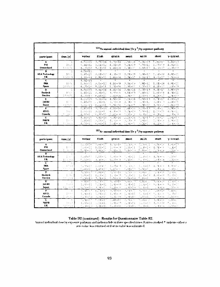
p a r t i c i p a n t
A PSI
Switicrtand
B AEA Technology
c IMA
Spain
D Studmnli Sweden
V. JAKH1 lapan
F AECI,
Canada
0 IVRPB
tnc
U m e , [ y ]
, J,!;;;;
l i "'00
1 0 u 0 o 0 1
1
1
! - . ' • , ' . ,
par t i c ipant
A PSI
Switzerland
R
AKA Technology UK
C IMA
Spain
Stiidnrik Swrdrn
r, IAI-HI
Japan ¥
KVAA,
Canada
r, NHPB
l/K
t i m e , [ y |
,
\
,
' , • • ' "
P a •mniini i n d i v i d u a l done [Sv y ] b y e x p o s u r e p a t h w a y
water f ish grain neat milk dust >-irrad.
4 . 5 F - L 5 9 . 7 E - 1 6 5 . 7 E - 1 6 , ' . S E - > : - r . J E - 1 9 S . 5 E - 1 " 5 . 4 E - I ' - t
1 . 4 E - 1 1 3 . 1 E - 1 3 4 . 0 E - 0 8 3 . ; F . - 0 ? 7 . 7 E - 1 I : 1 . 0 E - 0 8 4 . 9 E - 1 1
4 . J E - 1 0 9 . 0 E - 1 I l . o E - 0 ' j l . J E - " " 7 3 . 1 E - 1 0 4 . 0 E - 0 7 O . O E - ' ^
4 . S E - 1 5 * . . . . .
1 . 4 E - 1 1 3 . 1 E - 1 3 4 . 0 E - 0 8 3 . 2 E - 0 " 7 . 9 E - 1 . : 1 . 0 E - 0 8 4 . 9 E - 1 1
4 . 1 E - 1 0 8 . R E - 1 1 1 . 6 E - 0 6 1 . 3 E - 0 7 3 . 1 E - 1 0 4 . 3 E - Q 7 1 . 9 E - . ' j a
4 . b E - 1 5 » « • * * *
1 . 4 E - 1 1 3 . 1 E - 1 3 . 4 . 1 E - 0 8 3 . 0 E - 0 9 f . S E - 1 0 1 . 0 E - O S 4 . 8 E - 1 1
4 . 3 . E - 1 0 O . I E - 1 1 1 . 7 E - 0 6 1 . 3 E - 3 7 3 . 3 E - L O 4 . 3 E - 0 7 t . O E - n ?
4 . 5 E - 1 5 9 . 4 E - 1 6 4 . 4 E - 1 6 7 J . 4 E - 1 6 5 . ? E - l < a . 3 . 3 E - 1 7 3 . f i F . - l r '
1 . 4 E - 1 1 3 . 0 E - 1 2 3 . H E - 0 b 3 . 1 E - 0 9 " \ 4 E - i : : l . f E - C f i 4 . 7 E - 1 1
4 . 3 E - 1 0 H . n F . - l ! l . o E - O b 1 . 3 E - V ' " 3 . 0 F . - K ' 4 . : . F . - 0 ' " 1 . 9 E - ' ^ '
4 . : E - i b " J . 0 E - I 6 4 . 5 E - 1 6 . " . . 7 . E - 1 6 F, . = > E - 1 9 9 . " E - 1 7 4 . C E - 1 9
1 . 4 E - I 1 0 . 3 E - 1 . : i . 7 E - : . ' « i . 0 F . - . ' 9 7 . 3 K - 1 0 9 . r f E - ' ' 9 • i . ' i E - i :
> . " E - i r i " . : E - H ; . L E - G O I . . ' : E - : / 7 : . 9 E - i ' " ' J . ^ K - . V ; 1 . 3 E - 7 -
1 . 4 F - 1 4 9 . " ' F . - l n 1 . 4 F - 1 6 . " . 4 F . - 1 0 ' . . 3 F - 1 ' 1 * . 3 E - 1 7 3 . ' 1 E - " : - '
l . h E - l i 3 . 1 E - 1 . . 4 . 0 E - 0 - 3 . 2 E - u J 7 . ' > F - 1 3 1 . 1 E - 0 H 4 . 9 E - 1 1
4 . I F - ! ' " ' > < . « " . - 1 1 ; . . ) E - ' J 6 ! . 3 F. - ."'V 3 . . . F . - 1 0 4 . . ' E - | V ' . " ' O ' E - 7 1
4 . 4 E - 1 7 ' -> .4F, - l .o 3 . 3 E - 1 6 ¥.-\n r>. 4 E". - 1 ?' 0 . 3 E - 1 ; . J . 3 E - i ' >
: . 4 E - i : / . I F - : . 4 . i ' F - " « • . . : F - ^ " > ' . B E - ; ; \ .•'•?,-<<>• 4 . ' - F , - r .
4 . 1 K - I -.' 3 . 3 F - U ! . > : E - ! ' » ) ! . 3 E - 3 7 - . IE, - 1 •. - 1 . . . F . - ' ' - ' :..'¥,-•>'>
At- n n n u a l indivirhia l done (Sv y | b y e x p o s u r e p a t h w a y
w a t e r f i s h g r a i n n e a t m i l k o u s t - v - i r r a d .
: E - 1 ':•
- • . if-:-1 o
1 '"!;":', \
f ' . i ' : F . - ' t •:• 1
" ' . U , - l ; '
: . I F . - l ' i 3
'• 4 E - • ' •..•
o . : E - : '•> '
I . " E - : i i
O . l F - i - 3
t ; E - i ~ 4 . ' ' i K - i ^ :.::¥.-:'• : . . : F - . " 1 - . ^ F - I ^ i . . - F . - i " -
l E - u i . iE-".—•:• i . j E - i i : . . : K - i i - i . n E - - . ' ! - - • . . • £ - :
- I F . - ! - ' !•'>. f E - "3 r ; . 4 F , - l > " ' ' . 1 F . - 1 . ' :.'¥. —'•>; . . . I F . - " - .
" F - n : . ( F - ' - ' 1 : . ~<r,-\ i : . . T - ' . < . I . ' F - ••-. • . : F - :
) F , - ' . ' . b..'¥.-•.* •'-. 3 F - 1 - ! . 3 F . - i . . : . . ' F - ' j b . . . . I E - . ' -
I F . - l ! " : . . E - ' ! 9 ; . . " F - l : ; . . F - I 3 4 / " f : - " ' - 4 . ' ' * F - F ' .
u F . - : . ' ' •,.>•,¥,-••'• r.'<¥.-':•• ':;. W.-\ F - : ' - » . ' . i F - ••-•
« K - V I . " F . - 1 M ' ' . . . ' F . - . 7 ' - . " K - .' . ' . • •F . - l ' " ' ' ; . ' F , -
, : F . - I I ; . . : E - I ' ' : . . : E - 1 ! ; . . . F - : i - I . ^ E - ' " ? r . ' • ? : - : • • •
I F , - ! ' 1 ' - . i F - " 3 ' . . I F . - l " ' . U . - l ". . . " K - , ; » . ' . " . K - ' -
• . 'K- l • i . - F - U - ' ' . o E - . . " " . ' . I E - . . 3 . . , E - 1 " i . - K - ! " -
i F . - ! - O . . F . - ' ^ : . . . . l F - ' . ' i ; . . ' i F . - l . , . ' E - " t ; . . . : F . - ' "
••F. - i ' o . T : - I - i ' . ' - E - . • " ' . : F - . ;• ' . : F - : > ' ' . . I F - .
1 F . - U ! . ? F - ' ! " : . ( E - ! 1 1 . . F - 1 ' ' • . F - - : . . . E - i '
< F . - i . ' S . 7 F . - ' ' M ' - . i F - l ' i ' - . I F - ' i . . - . ' • F . - ' ' ' b . • • . , .F , - ' " - .
1 F. — 1 ' . . 4 F . - 1 " •.•>¥.-.•• ' . . - E . - . .' ' . - F . - ! H ' . 4 K - .
u : - i i I . . < F - - 7 ; . . i E - : i : . . F - i •• 4 . > F - > J ' . • [ • . - : •
Table D2 (continued) - Results for Questionnaire Table B2. Anniinl itiHividunl dose liy exposure pathway and radinnurlide at three Hpei'ified times. Knlries rnnrkrvl * indirafe either;
zero value was returned or that no value w»* submitted.
93
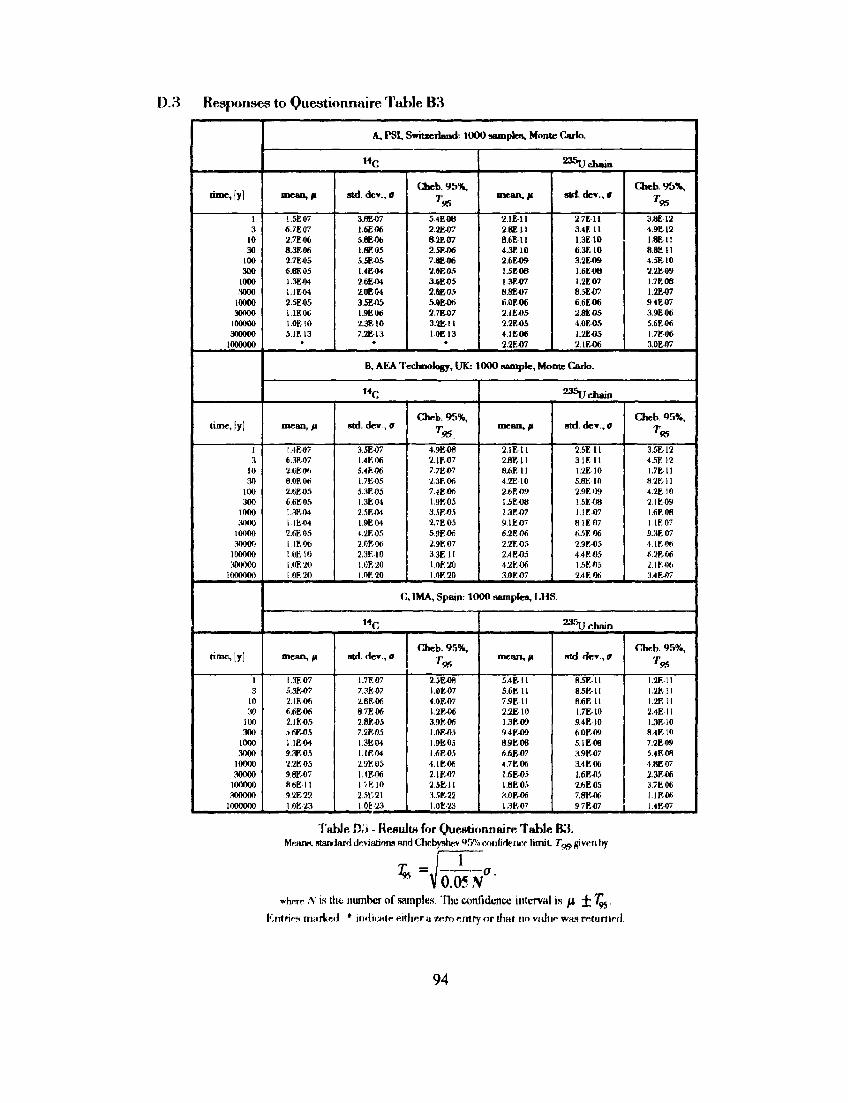
D.3 Responses to Questionnaire Table B3
time,(y]
1 3
10 30
100 300
1000 3000
10000 30000
100000 300000
1000000
time, [y]
1 3
10 30
100 300
1000 3000
10000 30000
100000 300000
1000000
time, [y]
1 3
10 30
100 300
1000 3000
10000 30000
100000 300000
1000000
mean, ft
1.5E07 6.7E07 2.7E-06 8.3E06 2.7E41S 6.8E0S 1.3E4H 1.1E4H 2.SE05 1.IE06 I.0EIO 5.1E-13
*
mean, fi
l.4E4>7 6.3E07 26E06 8.0E06 2.6K05 6.6E-0.5 I.3E04 1.1E-04 '2.6EAS l.IE-06 1.UE10 I.OF, 20 1.0E2O
mean, 41
l.3E«7 5.3E-07 2.1E-0C 6.6E-06 2.1E-05 .ifiE-05 1.1R4H 9.3K-05 2.2E05 9.8E-07 8.6E [ 1 9.2K-22 1.0E-23
A, PSI, Switzerland: 11)00 samples, Monte Carlo.
"c
std. dcv., a
3.BE-07 1.6E0* 5.8E4J6 I.8E05 S.5E4)S I.4&04 2.6E-04 2.0E04 3.5E4>5 I.9E06 2.3E 10 7.2E-13
•
Cheh. 95%, r95
5.4E4J6 2.2E4J7 8.2E07 2.5E4)6 7.8E4J6 2.0EO5 3.6E05 2.8E05 5.0E4K) 2.7E07 3.2E 11 1.0E13
•
2 3 5 U chain
mean, p
2.1E11 2 BE 11 8.6EU 4.3E10 2.6E09 1.5E08 1.3E4T7 8.8E07 6.0E4J6 2!E«5 2.2EA5 4.1E06 2.2E4>7
strl. dev., ff
2.7E11 3.4E11 I.3E 10 6.3E10 3.2E09 1.6E0B 1.2E07 8.5EW 6.6E-06 2.8E05 4.0E4K 1.2E4W 2.1E4J6
B, AEA Technology, UK: 1000 wimple, Monte Carlo.
» C
std. dev-, 0
3.5E-07 1.4E06 5.4E06 1.7E05 5.3F.05 1.3E4M 2..5E-04 1.9EA4 4.2E-0S 2.0E06 2.3E-10 1.0E-20 1 OP. 20
Cheb. 95%, T96
4.9E4M 24F.«7 7.7&07 2.3E06 7.4E06 I.9E-05 3iV.J}S XTtAS S.9E-06 2.9E07 3.3E11 1.0E20 1.0E20
23SU chain
mean, p
2.1E11 2.8E11 S^Ell 4.2E10 2.6E09 1.5E4J8 13EOT 9.1E07 6.2E06 2.2E05 2.4 f. 05 4.2E-06 3.0EO7
Btd. dev., o
2.SEU 3.1E11 1.2E10 5.8E 10 2.9E09 15E08 1.1E-07 8.1E07 6.5E06 2.9E-05 4.4EA5 I..SEA5 2.4 E 06
C, IMA, Spain: 1000 sample*, I.HS.
MC
Btd. dev., o
I.7E07 7.3B-07 2.8R06 8.7K06 2.8P.fl5 7.2B-05 I3E04 1.IR04 2.9ED5 l.HMW UK 10 2.51',2I 1.0r-23
Cheb. 95%,
2.5E4W I.OE-07 4.0E4)7 1.2R06 3.9E4J6 I.0E4W 1.9E0S I.6E05 4.IE06 2.1E07 2.SE-11 3.5K22 I.OE-23
^ J chain
mean,/i
5.4E 11 5.6E11 7.9E1I 2.2EI0 1.3E09 9.4F.4B 8.9E0B 6.6E-07 4.7E06 1.6E0.5 1.8E05 3.0F-O6 1.3E-07
std. dcv., a
B.5F.U 8.5E-11 8.6EU I.7E-10 9.4E-10 fi.OE-09 S.1E4» 3.9E-07 3.4E4» 1.6E05 2.6E05 7.8TW6 9.7E-07
Cheb. 95%, T95
3.8E12 4.9E12 I.8E1I 8.8E11 4.SE 10 2.2R09 I.7E-08 1.2E417 94E417 3.9E4)6 5.6E416 l.7E4» 3.0E4)7
Cheb. 95%, T95
3.5E12 4.5F. 12 1.7E1I 8.2E-11 4.2E10 2. IE 09 1.6E08 1.1E07 9.3E07 4.1E06 «.2E-06 2. IE 06 3.4EJ17
Chrb. 95%,
1.2F.11 1.2E11 I.2EI1 2.4E 11 1.3E-10 8.4F,10 7.2E4» 5.4E08 4.8E07 2.3R416 3.7F.06 I.JE4>6 I.4E-07
Table D.i - ReBulte for Questjonnaire Table B3. Mean*, standard deviations and Chebyshev 95% confidence bmit, TQQ given l>y
whirr A' is the number of samples Hie confidence interval is \X i.%$
Ktrtrif-s rrwrked * indii>itp eittirr a zero ffntry or tfiat no value was returned.
94
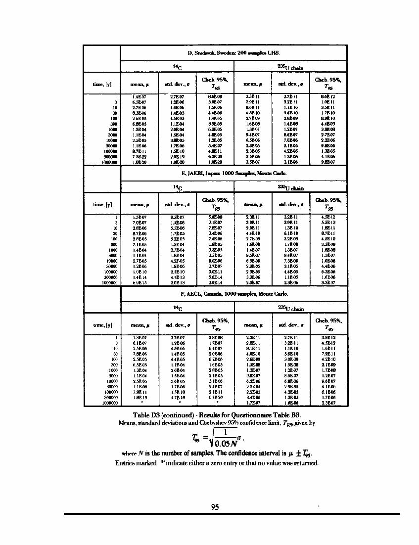
time, [y]
1 3
10 30
100 300
1000 3000
10000 30000
100000 300000
1000000
t i m e l y )
1 3
10 30
100 300
1000 3000
10000 30000
100000 300000
1000000
time, [y]
1 3
10 30
100 300
1000 3000
10000 30000
100000 300000
1000000
mean, a
1.4E07 6.5E-07 2.7E06 8.3K4K 2.6E4M 6.8E4W 1.3E04 1.1E4M 2.5E4W l.iE-06 8.7BI1 7.3E-22 10E20
mean , p
l.5E4>7 7.0&07 2.8E4* 8.7E06 2.8E05 7.1E4M 1.4E04 1 1E-04 2.7E05 1.2EA6 1.0E10 1.4E-14 6.9E15
m e a n , u
1.3F,07 6.1EA7 2.5E46 7.8E06 2.5E4J5 6.5EA5 I.3E4M 1 1E04 2.5E05 I.1E06 7.9E11 1.8E19
•
D, Studsvik, Sweden: 2 0 0 samples LHS.
"c
std. dev., o
2.7E07 1.2E4* 4.6E06 1.4E-05 4.SR05 1.1E4M 2.0EO4 l.SE-04 3.8t05 1.7E-06 1.5E10 2.0&19 I.OE-20
Cheb 95%, T95
8.6E08 3.8E4)7 1.5E4J6 4.4E06 1.4E4)5 3.5EAS 6.3E4W 4.8E45 1.2E4J5 5.4E4>7 4.8E11 6.3E20 1.0E20
2 3 5 U chain
mean, a
2.3E11 2.9E11 8.6E11 4.3E10 2.7E4J9 1.6E08 1.3E4)7 9.4E4T7 6.5E46 2.3E4U 2.3E4W 3.5E06 3.5E07
std dev. , O
2.7fcll 3.2E11 I.1E-10 M R 10 2.8E09 I.4E4W l.2fc07 8.6E4T7 7.0E4K 3.1E05 4.2E«5 1.3E4U 3.1E4K
E, JAERI, Japan: 1 0 0 0 Samples, Monte Carlo.
'«C
std. dev. , O
3.5&07 1.5E4J6 5.5E06 1.7E-05 5.2E05 1.3E4M 2.3E4M 1.8E4M 4.2T-05 1.9E4H 2.1E10 4 IE 13 2.0E-13
Cheb. 95%,
T9S
5.0E4» 2.1E4)7 7.8&07 2.4E4* 7.4E4* 18E05 3.3E4W 2.5E415
e.otoc 2.7E4J7 3.0&11 58E14 2.9EI4
S 3 ^ chain
mean, a
2.3E11 3.0E11 9.0E-11 4.4E10 2.7E-09 1.6E4W 1.4E4>7 9.SE417 6.5E4* 2.3E4W 2.3E4)5 3.3E4J6 2.3E4)7
std. d e v . , o
3.2E-11 3.9&U 1.3E10 6.1E10 3.2E09 1.7E4W 1.3E4W 9.4R07 7.3E06 3.1E05 4.4E05 1.1E4W 2.3E4»
F, AECL, Canada, 1 0 0 0 samples, Monte Carlo.
"c
std. dev., o
i.Tim 1.2E06 4.5E06 1.4E4W 4.4M5 1.1EW 2.0E04 1.5E4M 3.6E05 1.7E4W 1.5E-10 4.7&I9
•
Cheb 95%,
T95
38&08 1.7E4W 6.4E07 2.0RO6 6.2E06 1.6E4W 2.8EA5 2.1E05 5.1E06 2.4EA7 2 IE 11 6.7&20
*
2 3 5 U chain
mean , / i
2.2E-11 2.8E1I 8.1E-11 4.0E10 2.6E09 1.5E08 1.3E4W 9.0E4)7 6.2E4W 2.2E4J5 2.2E-05 3.4E4K 1.7E4J7
std. dev., 0
2.7E11 3.2E11 1.1E10 56E10 3.0&O9 1.5E-08 1.2E07 8.5E07 6.8RO6 2.9E05 4.3E4M 1.2E4J5 1.6E06
Cheb. 95%, T*
8.6E12 l.OEU 3.5EU 1.7E10 8.9EI0 4.4K09 3.8E08 2-7E4J7 2.2EA6 9.8EA6 1.3E05 4.1E06 9.8E07
Cheb 95%,
T95
4.SE12 S.SE12 1.8E11 8.7E11 4.5E10 2.3E-09 I.8E4W 1.3E07 1.0EO6 4.4E06 6.3E06 1.6E06 3.3E07
Cheb. 95%,
^95
3.8E12 4.5E12 1.6E11 7.9E11 4.2E10 2.1E09 1.7E06 1.2E07 9.6E«7 4.1E06 6.1E06 1.7E06 2.3E07
Table D3 (continued) - Results for Questionnaire Table B3. Means, standard deviations and Chebyshev 95% confidence limit, Tg^ given by
where N is the number of samples. The confidence interval is u ± XJ$.
Entries marked '*' indicate either a zero entry or that no value was returned.
95
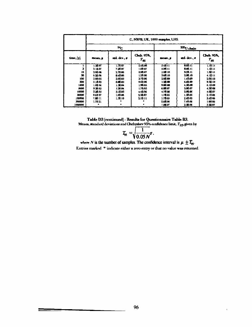
timely]
l 3
10 30
100 300
1000 3000
10000 30000
100000 300000
10000OO
mean,?
1.3E07 5.1E07 2.0EO6 6.2E06 2.0EO5 5.IE-05 I.0E-04 9.3E-05 2.2R05 9.6E07 7.8&11 1.7E-21
•
C, NRPB, UK, 1000 samptea, LHS
"C
atd.dev.,«
1.7E07 7.2E07 2.7E06 8.4E06 2.6E05 68E05 1.3&04 1.2E04 3.1E05 1.6E06 1.5R10
• •
Cheb.95%, T*
2.4E08 I.0E4W 3.9E07 1.2E06 3.7E06 9.6E06 1.9R05 1.7E05 4.4E06 2.3E07 2.1&I1
• *
m e a n , *
M E 11 5 .^11 1.0E10 3.6R10 2.0E09 1.2EOS 9JB08 6.8E07 4.7E06 1.7E05 1.7E05 2.6EOS I.9B07
235U chun
atd.dev.,9
8.0E-11
aottt 9 .2 t l l 2JE10 14E09 6.6E09 4.3t08 3.0EO7 2.9E06 IJE05 2.4R05 7.4E06 2.3EOS
Oieb.95%, TK
1.1E11 1.1E11 1.3T11 4.1E11 XOE-10 93E10 6.1E09 43E0B 4.0E07 2.1E46 3.4E06 1.0E06 3.3E07
Table D3 (continued) - Results for Questionnaire Table B3. Means, standard deviations and Qiebyahev 95% confidence limit, TM, given by
V 0.057V where N is (he number of samples. The confidence interval is /x ±T9S.
Entries marked '*' indicate either a zero entry or mat no value was returned.
96
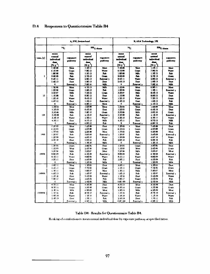
D.4 Responses to Questionnaire Table B4
tunc, |y]
l
10
100
1000
10000
100000
inooono
A , P S I , S w « j e r U i i d
, 4 C
mean • • — • - a l
individual doSC
7.5E4» 6 IF.08 1.8E4W 90E09 9.4EII 2.4EI3
0 1.5EA6 1.2E06 3.5E4)7 1 1E08 1.2EI0 4.4E 12
0 I.5E05 I2E05 3.5E4* 3.3E08 3.3E 10 4.3EII
0 7.2E05 ri.lE05 1 .7E 05 1 2K 07 1.2E09 2.0E 10
0 1.2E05 1 IK 05 3.2E0S 8.8K09 a.iEti 3.0E 11
0 .VnF. 11 4.IK 11 1.3E 11 fi.tiF. 15 I.IK 16 7.0K17
0 8.7K 14 8.5K 11 2.3E 14 l.lElli 1 OF. IH 2. IK 19
1)
exposure pathway
Mm Grain Milk Fish
Water Duit
External 7
Meat Grain Milk fall
Water Dust
External 7 Meat Grain Milk Pith
Water Dust
External 7 Meal Grain Milk Fish
Water Dust
External y Grain Meat Milk Fish
Water Dent
External -y Meat Grain Milk Fish Dust Water
External 7 Meat Grain Milk Fish
Waler Dust
External 7
1 3 ^
•lumal individual
doac
1.1EI1 7.9&12 1.5E12 27E13 2.0EI3 1.0E13 7.0EI4 4.I&13 1.6E12 7.2&12 B.0E12 8.4EI2 1.5E11 6.9E11 16EW 6.4E10 5.0E 10 4.1E10 2.3E11 9.7EI2 6.0EI2 7.4E4J8 46E06 2.2E08 5.6F.09 4.6EI0 2.0E10 I.3E 10 3.9E06 2.4E06 3.0E-07 6.3EA8 9.8E09 4.6F.09 1.2E09 1.3E05 7.7E06 7.8E07 1.4E07 9.4E09 3.6R09 2.0E09 9.3E08 3.5K08 fi.9E09 8.7E (0 1 IK 10 1.7K11 t..9r* 12
- * • * " •
eapoaure pathway
Meat Water Pish
Grain External 7
Dust Milk
Milk Fish
Grain Dust
Waler External 7
Meat
Meat Dust
Grain External 7
Water Milk Fish
Dust Grain Meat
Externa) 7 Water Fish Milk
Dust Grain Meat
External 7 Water Fish Milk
Dust Grain Meat
External 7 Water fish Milk
Dust Grain Meat
External 7 Water Fish Milk
B , AEA Textusology, UK
««e
*A 1.11*1 indiriduatl
doac
i s . , 1 , 7 5E4J8 6.1E48 1.8E48 9.0E09 9.4EI1 2.4E13
0 1.5E4* 1.2E06 3.5E4J7 1.1E08 1.2EI0 4.4E12
0 1.5E4K 1.2E05 3.5EA6 3.3E08 3.3E10 4.3E1I
0 7.2E05 6.1E05 1.7E05 J.2E07 1.2EA9 2.0E 10
0 1.2E05 I. IE 05 3.2E06 B.8E09 8.4X 11 3.0EI1
0 5.6E 11 4.1E11 I.3EII 5 .6EI* I l K l e 7.0E 17 OOF. '00
8.7K II 8.5F.14
2.3E 14 I.IK 16 I.1E10 2.4E 19 O.OE'OO
capoeurc pathway
Meat Grain Milk
Fish Water Dust
External 7
Meat Grain Milk Fish
Water Dust
External 7
Meat Grain Milk Fish
Water Dust
External 7
Meal Grain Milk Fish
Water Dust
External 7
Grain Meat Milk Fish
Water Dust
External 7
Meat Grain Milk Fish Dust
Water External 7
Meat Grain Milk Fish
Water Dust
External 7
**V
B O J U U I
individual
doac
1.IE1I
7 .9RI2 I .SEI2 2 .7E13 2 .0EI3 1.0E13 7.0E14
6.9EI1 1.5E-11 8 .4E12
8.0E-12 7 .2E12 1 6 E 1 2 4.IE 13
1 6 E 0 9 6 .4E10 5 .0E10 4 IE10 2.3E11 9.7E-12 6.0F, 12
7.4E4M 4 6 E 0 8 2 .2E08 5.6E4» 4 . 6 E I 0 2.0E10 1.3EI0
3.9E06 24E06 3.0E417 6.3E08 9.BE09 4.6ED9 1.2EA9 I.3E05 7.7E06 7.8E07 1.4E07 9.4E4» 3.6E09 2.0E09 9.3EA8 3.5E08 •J.9ETO 8.7E 10 l.iEW 1.7R11 ri.PE 12
**»»in
exposure pathway
Meat Water Fish
Grain External 7
Dust Milk Meat
External 7 Water Dust Grain Fish Milk Meat Dust Grain
External 7 Water Milk Fish Dust
Grain Meat
External 7 Water Fish Milk Dust Grain Meat
External 7 Water Fish Milk Dust Grain Meat
External 7 Water Fish Milk Dust
Grain Meat
External 7 Water Fish Milk
Tabic IM - Results for Questionnaire Table B4.
Hanknui nf mniil i i i t i im.t tn nipan annual individual Hew by expiv.Mirr pathway at sfwrifieH lime;*.
97
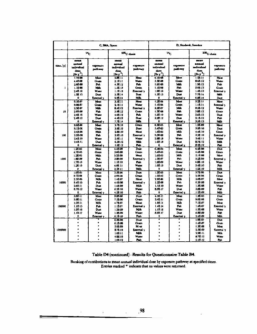
t imely]
1
10
100
1000
10000
I00000
1000000
C. IMA, Spun
' \ :
•DUB
annual individual
dose
7.7E-CB 4.4E08 2.6E4* I.IE«3 2.4&I0 I.2EI3
0 9.5E07 9.0E4W 2.3E4T7 2.6E08 2.4EI0 2.4H2
0 9.6E4* 9.1KW 2.4E4* 2.5E08 2.4E-10 2.4E-11
0 1.2E45 4.7R05 1.2R05 1.8E08 1.7E-I0 1.2E-10
0 1.0R05 9.7B06 2.5t06 9.4E10 2.6E-11 8.7E-12
0 3.8E11 3.8E-I1 1.0E11 1 1RJ5 1.0E-16 1.1E-17
0
exposure pathway
Meet Gram Fish Milk Water Dust
External 7 Meet Grim Milk Fish
Water Dim
External) Meat Grain Milk Rah
Water Dust
External y Meat Gram Milk Fish
Water Dint
External 7 Meal Grain Milk Rih Dust
Water External 7
Meat Grain Milk Fun Dust
Water External y
23eV
mean annual
individual done
I S e y ' l Z8E11 2.IEI1 4.5E-12 1.5E13 I.IE13 5.5E14 2-9tl* 3.5E11 2.1E11 8.4E12 S.0E-J2 4.6E12 4.4&12 7.7E14 37E-10 3.6E10 2.8E10 2.6E10 2.6E11 6.3E-12 1.6E12
4.4E08 3.6&OS 5.2E09 3.8E09 1.1EI0 4.0&11 2.5EU 2.5E06 2.0EO6 1.4E07 4.4E4W 1.4E09 6.2E-10 4.21V 10 9.8E-06 7.SE06 4.7Efl7 1.1&07 1.3E-09 1.3&09 6.1E-10
III
8.7E-10 1.0E-11 4.8E-10 I.6E-I2
» * • • • «
exposure ptaSear
Meat Water Fnh
Grain External y
Dust Milk Meat Water
External 7 Grain Pish Dust Mdk Grain Dust Meal
External 7 Water MUk Fun Dun Grain Meal
External 7 Fhh
Water MUk Dust Grain Meat
External 7 MUk
Water Fish Dust Grain Meat
External 7 MOk Water Fish Dual Grain M a t
External 7 Milk Water Fish
D , Student, Swedes
, 4 C
•Bean •fm"%|
individual dea*
[ S V T ' 1 6.1E4M 5.3W8 I.6E4W i.iE«e 1.0E10 1.5E-13
0 1.2E4H 1.1E06 33E-07 l.3E4» 1.2E-10 3.2E-I2
0 6.3E4J5 5.4E4J5 1.6E4I5 3.3E48 2.8E10 I.6E-10
0 6.3E4J5 5.4E45 I.6E4IS 1.2E4T7 I.0E4» 1.0R10
0 1.2E-05 1.0E05 2.9E06 1.2E08 1.1E-10 8.9E17
0 4.3R11 3.4E-U 10EI1 1.4E-14 t.iE-ie 8.9E17
0
exposure pathway
Meat Grain Milk Fnh
Water Dust
External y Meat Gran Milk Fish
Water Dust
External y Meat Grab] Milk Rih
Water Dust
External 7 Meat Gram Milk Fish
Water Dust
External 7 Meat Grain Milk Fun
Water Dust
External 7 Meat Grain MUk Fish
Warn Dust
External 7
a 3 S u
mean annual
flBfa^ewTaainn a»l
dose I S . , 1 ! 1 2E 11 S6E-12 1.9E-12 3.0E13 1.4E13 7.7rVl4 6.8E-14 5.2E11 1.1E-11 9.5E12 5.8E12 5.6E-12 2.1E-12 3.5E13 1.3fr09 5.0E-10 4.4E-10 3.5E-I0 3.4E11 8.7E-I2 8.2E-12 6.2£4» 4.4E46 2.1E48 5.2E-09 6.8E-10 2.4E-10 I.2E10 3.7E06 2.5E-06 3.0E-O7 6.3E-08 1.3E48 5.8£09 1.2E-09 1.3E-05 9.0&O6 7.IE-07 1.4&07 I.5E-08 ft.8E-09 2.4E-09 1.9E-07 1.4E-07 I.3E48 2.3E.09 2.9E-U 8.7E-12 2.IE-I2
chain
expoaure pathway
Meat Water Fish
Grain External 7
Milk Dust Meal
External 7 Water Grain Dust Fish Milk Meat Dust
Grain External 7
Water Milk Fish Dust
Grain Meat
External 7 Water Fish Milk Dust
Grain Meal
External y Water Fish Milk Dust
Grain Meat
External 7 Water Fish Milk Dust Grain Meat
External 7 Milk
Water Fish
Table D4 (continued) - Results for Questionnaire Table B4.
Ranking of contibutions to mean annual individual dose by exposure pathway at specified times. Entries marked '*' indicate that no values were returned.
98
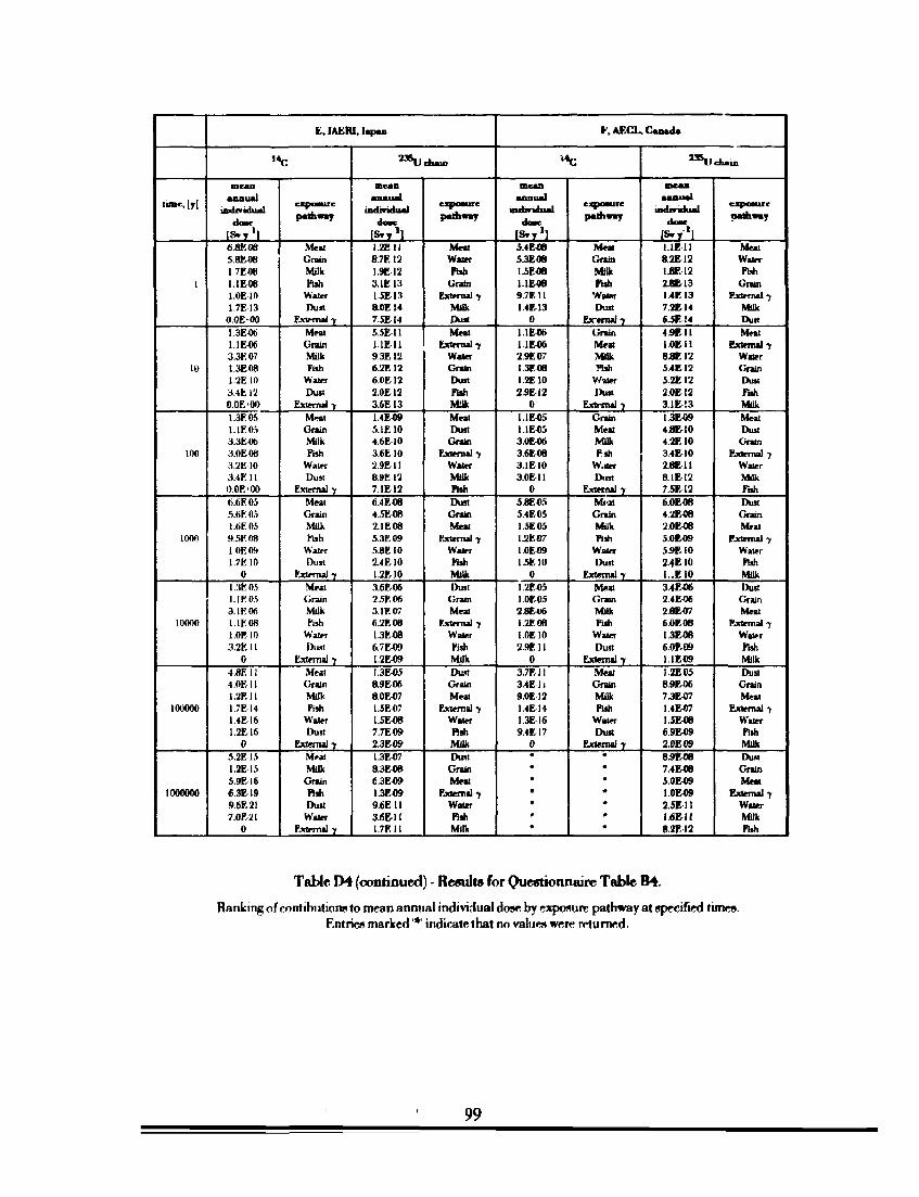
tunc, [y]
I
10
I0O
1000
10000
100000
1000000
E . I A E R I , Japan
s*e mean
annual individual
d o *
6.8E0S 5.8E08 I.7E08 I.IE08 1.0E10 1.7E13
O.OE0O 1.3E4X) 1.IE06 3.3K07 1.3E08 1.2E 10 3.4E 12 0.0E*0O
1.3E^>5 1.1E05 3.3EW 3.0E08 3.2E10 3.4E11 O.OE'OO
6.6E4)S 5.6R05 1.6E0S
9.5F.-0B 1.0E09 1.7E10
0 1.3E05 1. IE-OS 3.1E06 1.1E08 1.0E10 3.2E 11
0 4.8E 11 4.0EI1 1.2E11 1.7F.14 M E 16 1.2Elfi
0 5.2E 15 1.2E-I5 5.9E16 6.3E19 9.6E21 7.0E21
0
capoaure path war
Meat Grain Milk Fish
Wain Dust
External 7
Meat Grain Milk Fish
Water Oust
External 7
Meat Grain Milk Fish
Water Dust
External 7
Meat Grain Milk Fish
Water Dust
External 7
Meat Grain Milk Fish
Water Dust
External 7
Meal Grain Milk Fish
Water Dust
External 7
Meat Milk
Grain Fish Dust
Water External 7
" t l
mean annual
individual doac
I S v , 1 ! 12E11 8.7E12 1.9E12 3.1E13 1.5E13 8.0E14 7.5EI4 5.5E11 1.1E1I 93E12 6.2E12 6.0EI2 2.0E12 3.6E13 14EA9 5.IE10 4.6E10 3.6EI0 2.9E1I 8.9EI2 7.1EI2 t)4E08 4.5E4» 2, IE 08 5.3E09 5.8E 10 2.4E10 1.2R10 3.6E-06 2.5E-06 3.1EA7 6.2E4J6 1.3E08 6.7E4» I.2E4J9 I.3E05 8.9E06 8.0E417 1.5E07 I.5E08 7.7E09 2.3B09 1.3E07 8.3E08 6.3&09 1.3E-09 9.6E-11 3.6E-II l.7F,ll
chain
eaposurc pathway
Meal Water Fish
Grain External 7
Milk Dust Meat
External 7 Water Grain Dust Fish Milk Meat Dust Grain
External 7 Water Milk Fish Dust Grain Meat
External 7 Water Fish Milk Dust
Grain Meat
External 7 Water Fish Milk Dust Grain Meat
External 7 Water Fish Milk Dust
Grain Meat
External 7 Water Fish Milk
F.AF.CL. Canada
'«C
mean nnrft'ia*
individual d o e
ISvy ' l 5.4E46 5.3E08 I.5E-08 1.1E46 9.7E11 1.4E13
0 1.1E46 I.1E06 2.9E4)7 1.3E4J8 1.2E10 2.9EI2
0 I.1E45 I.1E4J5 3.QE06 3.6E08 3.1EI0 3.0E-I1
0 5.8E4>5 S.4E05 1.5E45 1.2E07 1.0E09 1.SE10
0 1.2E-0S 1.0E05 2.8E4I6 1.2E08 1.0E10 2.9E 11
0 3.7EI1 3.4Eh 9.0E12 I.4E14 I.3E16 9.4E-I7
0 • • • * • • •
exposure pathway
Meat Grain Milk Fish
Water Dust
ExYmaf 7 Grain Meat Milk Pish
Water Dust
Externa! 7 Grain Meat Milk Fsh
W.iter Dust
External 7 M«at Grain Milk Fish
Water Dust
External 7 Meat Grain Milk Fish
Water Dust
External 7 Meat Grain Milk Ptsh
Water Dust
External 7
^^lJ chain
mean annual
individual dose
i s v y ' l 1.1E11 8.2EI2 1.8E12 2.8BI3 I.4E-13 7.2E-14 6.5E14 4 9E11 I.0E-I1 8.8F.12 5.4E-12 5.2E12 2.0E12 3.1E13 1.3E419 4.8E-10 4.2E 10 3.4EI0 2.8E1I 8.1EI2 7.5E12 6.0EO8 4.2EOB 2.0E08 5.0E-09 5.9EI0 2.4RI0 I..EI0 3.4E-06 2.4E06 2.8E-07 6.0E08 13E-08 6.0&09 I.IEA9 I.2E05 8.9E06 7.3t07 1.4E07 I.5E08 69R09 2.0E4J9 8.9E0B 7.4EOB 5.0E09 1.0EO9 2.5E1I I.6E-1I 8.2E-12
capoaure pathway
Meat Water Fish
Grain External 7
Milk Dust Meat
External 7 Water Grain Dust Fish Milk Meat Dust Grain
External 7 Water Milk Fish Dust Grain Meat
External 7 Water Fish Milk Dust Grain Meat
External 7 Water Pish Milk Dust Grain Meat
External 7 Water Fish Milk Dust
Grain Meat
External 7 Water Milk Fish
Table D4 (continued) - Results for Questionnaire Table B4.
Ranking of contibutions to mean anntial individual dose by exposure pathway at specified times. Entries marked '*' indicate that no values were returned.
99
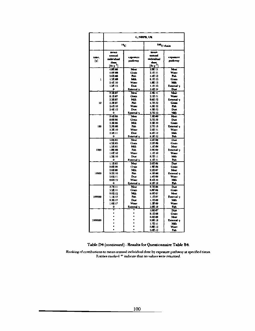
time.
1
10
100
1000
10000
100000
1000000
<:, NRPB.UK
"»c
nacan annual
indmdual daw
4.8E4W 4.0E4» 2.6E08 I .2E« 2.4E10 1.2E13
0 9.SE4T7 8.IE4T7 2.3R07 2.5E-07 2.4&10 2.4R12
0 9.4E46 &0E46 2.3E06 25E08 2.3E10 2.3E-1I
0 50EC5 4.2E05 I.2EOS 1.8E4W 1.6E-10 12E10
0 1.1E05 ROE 06 2.6E46 9.2E10 2.6E-11 8.6E12
0 3.7EII 3.2B11 9.0E-12 1.1E15 9.3&17 1.0E17
0
• * • • * • *
exposure pathway
M m Grain Fish Milk
Wafer Dim
External? M m Grain Milk «sh
Water Dust
External? Meat Grain Milk Fish
Water Dust
External 7 M m Grain Milk Fish
Water Dust
External y M m Grain MUk Pish Dint
Water External 7
M m Grain Milk Fish Dust
Water External-y
aasy
annual mdrnchlal
doac [ S . T 1 ] 2.8E11 2.1E11 4.4EI2 61E13 ME-13 LIE 13 5.4EI4 5.9E11 2.IE1I 8.6E12 4.7EJ2 4.5E12 4.3E12 3.7E-13 I.0E4W 3.7H0 3.3E10 2.7E10 2.6EU 6.4E-12 6.3E12 4.6E4W 3.2E08 1.3E08 3.9E49 J.IE 10 8.7E-I1 4.IE II 2.6E06 1.8E46 2.2E07 4SE08 1.4E4W 8.4E10 6.2E10 9.7E06 6.8E06 6.0E4/7 I.IEC7 1.7E4W I.3E09 5.9E10 I.0EO7 8.IE-08 6.6E4J9 9.9E10 1.7E-I1 6.8EI2 3.0F,I2
chain
exposure pathway
M m Water Ftsh
Grain Milk
External-) Dual M m Water
External y Grata Fish Dust Milk M m Dust
Oiain External >
Water Milk Fish Dust
Grain Mtat
External y Water Milk Fish Dust
Grain Mtat
External y Water Milk Rah Dust
Grain Meal
External-)' Milk
Water Fiih Dust
Grain Meat
External 7 Milk
Water Fish
Table D4 (continued) - Results for Questionnaire Table B4.
Ranking of eontibutions to mean annual individual dose by exposure pathway at specified times. Entries marked '*' indicate that no values were returned.
MAIN SALES OUTLETS OF OECD PUBLICATIONS PRINCIPAUX POINTS DE VENTE DES PUBLICATIONS DE L'OCDE
ARGENTINA - ARGENTINE Carlo* Hirsch S R.L Galena Giicmes. Florida 165.4° Piso 1333 Buenos Aires Tel. (I) 331.1787 y 331.2391
Telefax: (1) 331.1787
AUSTRALIA - AUSTRALIE DA. Information Services 648 Whilrhorse Road. PO.B 163 Mitcham. Vicioria 3132 Tel. (03) 873.4411
Telefax (03) 873.5679
AUSTRIA - ALTRICHE Ceroid & Co Graben 31 Wienl Tel. (0222* 533.50.14
BELGIUM - BELGIQUE Jean De Lannoy Avenue du Roi 202 B-1060 Bnuelles Tel (02) 538.51.69/538.08.41
Telefax: (02) 538.08.41
CANADA Renouf Publishing Company Lid. 1294 Algoma Road Ottawa. ON KIB 3W8 Tel
Telefax: Stores: 61 Sparks Street Ottawa. ON KIP 5RI 211 Yonge Street Toronto, ON M5B IM4
(613)741.4333 (613)741.5439
Tel. (613) 238.8985
Tel. Telefax:
(416) 363.3171 (416)363.59.63
Les Editions La Liberie Inc. 3020 Chemin Sainte-Foy Sainte-Foy, PQ G1X 3V6 Tel. (418) 658.3763
Telefax: (418) 658.3763
Federal Publications 165 University Avenue Toronto, ON M5H 3B8 Tel. (416) 581.1552
Telefax: (416) 581.1743 Lcs Publications Federates 1185 Avenue de ('Universite' Montreal. PQ H3B 3A7 Tel. (5 i 4) 954.1633
Telefax : (514) 954.1633
CHINA - CHINE China National Publications Import Export Corporation (CNPIEC) 16 Gongti E. Road, Chaoyang District P.O. Box 88 or 50 Beijing I0O7O4 PR Tel. (01) 506.6688
Telefax: (01) 506.3101
DENMARK - DANEMARK Munksgaard Export and Subscription Service 35. N0rre Sagade. PO. Box 2148 DK-I0I6 Kabenhavn K Tel. (33) 12.85.70
Telefax: (33) 12.93.87
FINLAND - FINLANDE Akateeminen Kirjakauppa Keskuskatu I. P.O. Box 128 00100 Helsinki Tel. (358 0) 12141
Telefax: (358 ••., 121.4441
FRANCE OECD/OCDE Mail Orders/Commandes par correspondance: 2. rue Andrf Pascal 75775 Paris Cedex 16 Tel. (331) 45.24.82.00 Telefax: (33-1) 45.24.81.76 or (331) 45 24.85.00
Telex: 640048 OCDE
OECD Bookshop/l.ibrairic de IOCDE : 33, rue Ociavc-Feuillet 75016 Paris Tel. (331) 45.24 81.67
(331) 45.24.81.81
Documentation Franchise 29. quai Voltaire 75007 Paris
Gibert Jeune (Droit Economic) 6. place Saint-Michel 75006 Paris
Tel. 40.15.70.00
Tel. 43.25.91.19
Libraine du Commerce International 10, avenue d'Kna 75016 Paris Tel. 40.73.34.60
Librairie Dunod University Paris-Dauphine Place du Marechal de Lattrc dc Tassigny 75016 Paris Tel. 47.27.18.56
Librairie Lavoisier 11, rue Lavoisier 75008 Paris Tel. 42.65.39.95
Monlchresiien Librairie L.G.DJ. 20, me Sovfllot 75005 Paris
Librairie des Sciences Politiques 30. rue Saint-Guillaume
Tel. 46.33.89.85
75007 Paris
P.U.F. 49. boulevard Saint-Michel 75005 Paris
Librairie de i'Universite' 12a. rue Nazareth 13100 Aix-en-Provence
Documentation Franchise 165, rue Garibaldi 69003 Lyon
Librairie Decitre 29, place Bellecour 69002 Lyon
Tel. 45.48.36.02
Tel. 43.25.83.40
Tel. (16)41.26.18.08
Tel. (16)78.63.32.23
Tel. (16)72.40.54.54
GERMANY - ALLEMAGNE OECD Publications and Information Centre August-Bebel-Allee 6 D-W 5300 Bonn 2 Tel. (0228) 959.120
Telefax: (0228) 959.12.17
GREECE - GRECE Librairie Kauffmann Mavrokordatou 9 106 78 Athens
HONG-KONG Swindon Book Co. Ltd. 13-15 Lock Road Kowloon, Hong Kong
Tel. 322.21.60 Telefax: 363.39.67
Tel. 366.80.31 Telefax: 739.49.75
HUNGARY - HONGRIE Euro Info Service POB 1271 1464 Budapest Tel. (I) 111.62.16
Telefax : (I) 111.60.61
ICELAND - ISLANDE Mai Mog Menning Laugavegi 18. Postholf 392 121 Reykjavik Tel. 162.35.23
INDIA - INDE Oxford Book and Stationery Co. Scindia House New Delhi 110001 Tel.(ll) 331.5896/5308
Telefax: (11)332.5993 17 Park Street Calcutta 700016 Tel. 240832
IRELAND - IRLANDE TDC Publishers - Library Suppliers 12 North Frederick Street Dublin 1 Tel. 74.48.35/74.96.77
Telefax: 74.84.16
ISRAEL Electronic Publications only Publications itectroniques seutement Sophist Systems Ltd. 71 Allcnby Street Tel-Aviv 65134 Tel. 3-29.00.21
Telefax: 3-29.92.39
ITALY - ITALIE Libreria Commissionaria Sansoni Via Duca di Calabria l/l 50125 Fireiue Tel. (055) 64.54.15
Telefax: (055) 64.12.57 Via Bartolini 29 20155 Milano Tel. (02) 36.50.83
Editnce e Libnria Herder Piazza Momecitorio 120 00186 Roma
Libreria Hoepli Via Hoepli 5 20121 Milano
Tel. 679.46.28 Telefax: 678.47.51
Tel. (02) 86.54.46 Telefax: (02) 805.28.86
Libreria Sciemirka Don. Lucio de Biasio 'Aeiou' Via Coronelli. 6 20146 Milano Tel. (02) 48.95.45.52
Telefax: (02) 48.95.45.48
JAPAN - JAPON OECD Publications and Information Centre Landic Akasaka Building 2-3-4 Akasaka, Minato-ku Tokyo 107 Tel (81 3) 3586.2016
Telefax: (81.3) 3584.7929
KOREA - COREE Kyobo Book Centre Co. Ltd. P.O. Box 1658, Kwang Hwa Moon Seoul Tel. 730.78.91
Telefax: 735.00.30
MALAYSIA - MALAISIE Co-operative Bookshop Ltd. University of Malaya P.O. Box 1127, Jalan Pamai Bam 59700 Kuala Lumpur Malaysia Tel. 756.5000/756,5425
Telefax: 757.3661
MEXICO - MEXIQUE Revistas y Periodicos Inleoiacionales S.A. de C.V. Florencia 57 - 1004 Mexico, D,F. 0660O Tel. 207,81.00
Telefax : 208.39.79
NETHERLANDS - PAYS-BAS SDU Uitgeverij Christoffel Plantijnstraat 2 Postbus 20014 2500 EA's-Gravenhage Tel. (070 3) 78,99.11 Voor beslellingen: Tel. (070 3) 78.98.80
Telefax: (070 3)47.63.51
INDONESIA - INDONESIE Pdii-Lipi PO, Box 269/JKSMG/88 Jakam 12790 Tel. 583467
Telex: 62 875
NEW ZEALAND NOUVELLE-ZELANDE legislation Services P.O. Box 12418 Thomdon. Wellington Tel. (04) 496.5652
Telefax: (04) 496.5698
NORWAY - NORVEGE Narvesen Info Ccnltr - NIC Bertram! Narvesens vei 2 P.O Box 6125 EtBrstad 0602 Oslo 6 Tel. (02) 57.33.00
Telefax: (02) 68 19.0!
PAKISTAN Mina Book Agency 65 Shahrah Quaid-E-Azam Lahore 54000 Tel. (42) 353.60!
Telefax: (42) 231.730
PHILIPPINE - PHILIPPINES International Book Center 5th Floor. Filipinas Life Bldg Ayala Avenue Metro Manila Tel. 81.96.76
Telex 23312 RHP PH
PORTUGAL Livrana Portugal Rua do Carmo 70-74 Apart. 2681 Ill7l.ishoaCodex Tel.: (01)347.49.82/3/4/5
Telefax: (01) 347.02.64
SINGAPORE - SINGAPOUR Information Publication* Pte Ltd. 41. Kaliang Pudding. No 04-03 Singapore 1334 Tel. 741.5166
Telefax: 742.9356
SPAIN - ESPAGNE Mundi-Prensa Libros S.A. Castello 37, Apanado 1223 Madrid 2800! Tel. (VI) 431 33.99
Telefax: (91) 575.39.98
Librena Jnternacional AEDOS Consejo dc Cientu 391 08009 - Barcelona Tel. (93) 488.34.92
Telefax: (93) 487.76.59 Llibreria de la Gcneralitat Palau Mnja Rambladels Estudis. 118 08002 - Barcelona
(Subscriptions) Tel. (93) 318.80.12 (Publicacions) Tel. (93) 302.67.23
Telefax: (93)412.18.54
SRI LANKA Centre for Policy Research c/o Colombo Agencies Ltd. No. 300-304, Galle Road Colombo 3 Tel. (I) 574240. 573551-2
Telefax: (1)575394, 510711
S W E D E N - S U E D E Frilzes Fackboksfbretaget Box 16356 Regcringsgataii 12 103 27 Stockholm Tel. (08) 690.90.90
Telefax: (08) 2050.21
Subscription Agency-Agence d'abonnements Wennergren-Williams AB P.O. Box 1305 171 25 Solna Tel. (08) 705.97.50
Telefax . (08) 27.00.71
SWITZERLAND - SUISSE Madifcc S.A. (Book*, and Periodicals - Lures et periodiques) Chemin des Palettes 4 Case postale 2066 1020 Renens 1 Tel. (021) 635.08.65
Telefax: (021) 635.07.80
Librairie Payot S.A. 4, place ftpinet 1003 Lausanne
Librairie Unilivres 6. rue de Candolle 1205 Geneve
Tel. (021)341.33.48 Telefax: (021)341.33.45
Tel (022) 320.26.23 Telefax: (022) 329.73.18
Subscription Agency - Agencc d'abonnement Dynapresse Marketing S.A. 38 avenue Vibert 1227 Carouge Tel.: (022) 308.07.89
Telefax : (022) 308.07.99
See also - Voir aussi : OECD Publications and Informalion Centre August-Bebcl-AUcc 6 D-W 5300 Bonn 2 (Germany) Tel. (0228) 959.120
Telefax: (0228)959.12.17
TAIWAN - FORMOSE Good Faith Worldwide Int'l. Co. Ltd. 9th Floor, No. 118. Sec. 2 Chung Hsiao E. Road Taipei Tel. (02) 391.7396/391.7397
Telefax: (02) 394.9176
THAILAND - T H A I L A N D E Suksil Siam Co. Ltd. 113. 115 Fuang Nakhon Rd. Opp. Wat Rajbopith Bangkok 10200 Tel. (662) 251.1630
Telefax: (662) 236.7783
TURKEY - TURQUIE Kiiltur Yayinliri Is Turk Ltd. Sti Atatiirk Bulvari No. 191/Kal 13 Kavaklidere/Ankara Tel. 428.11 40 Ext 2458 Dolmabahce Cad. No. 29 Bcsiktas/IsUnbul Tel. 260.71.88
Telex: 43482B
UNITED KINGDOM - ROYAUMEUNI HMSO Gen. enquiries Tel (071) 873 0011 Postal orders only: P.O. Box 276. London SW8 5DT Personal Callers HMSO Bookshop 49 High Holbom. London WCIV 6HB
Telefax: (071) 873 8200 Branches at: Belfast, Birmingham. Bristol. Edinburgh, Manchester
UNITED STATES - ETATS-UNIS OECD Publications and Information Centre 2001 L Street N.W., Suite 700 Washington. D.C. 20036-4910 Tel. (202) 785.6323
Telefax: (202) 785.0350
VENEZUELA Libreria del Este Avda F. Miranda 52. Aptdo. 60337 Edificio Galipan Caracas 106 Tel 951.1705/951.2307/951.1297
Telegram: Libresle Caracas
Subscription to OECD periodicals may also be placed through main subscription agencies.
Lcs abonnements aux publications ntriodiques de I'OCDE peuvent Sire souscrits aupres des
incipales agences d'abonnement.
Orders and inquiries from countries where Distributors have not yet been appointed should be sent to: OECD Publications Service, 2 rue Andre-Pascal, 75775 Paris Cedex 16, France.
Les commandes provenant de pays oil I'OCDE n'a pas encore design* de distribuieur devraient etre adre.uees a : OCDE, Service des Publications. 2, rue Andre-Pascal. 75775 Paris Cedex 16. France.
04-1993
OECO PUBLICATIONS. 2 n » Andr*-Piscal, 7S775 PARIS CEDEX 16 - No. 780341993 PRINTED IN FRANCE