ib diploma programme
TRANSCRIPT
I B D I P LO M A P R O G R A M M EDavid Homer
O X F O R D I B P R E P A R E D
PHYSICS
iii
Introduction iv
1 Measurements and uncertainties
1.1 Measurements in physics 21.2 Uncertainties and errors 51.3 Vectors and scalars 7
2 Mechanics
2.1 Motion 102.2 Forces 132.3 Work, energy and power 172.4 Momentum 21
3 Thermal physics
3.1 Temperature and energy changes 253.2 Modelling a gas 28
4 Oscillations and waves
4.1 Oscillations 344.2 Travelling waves 364.3 Wave characteristics 404.4 Wave behaviour 434.5 Standing waves 47
5 Electricity and magnetism
5.1 Electric fields 525.2 Heating effect of an electric current 555.3 Electric cells 595.4 Magnetic effects of electric currents 61
6 Circular motion and gravity
6.1 Circular motion 666.2 Newton’s law of gravitation 68
7 Atomic, nuclear and particle physics
7.1 Discrete energy and radioactivity 727.2 Nuclear reactions 767.3 The structure of matter 78
8 Energy production
8.1 Energy sources 848.2 Thermal energy transfer 88
9 Wave phenomena (AHL)
9.1 Simple harmonic motion 929.2 Single-slit diffraction 969.3 Interference 979.4 Resolution 1019.5 The Doppler effect 102
10 Fields (AHL)
10.1 Describing fields 10610.2 Fields at work 109
11 Electromagnetic induction (AHL)
11.1 Electromagnetic induction 11611.2 Power generation and transmission 11811.3 Capacitance 122
12 Quantum and nuclear physics (AHL)
12.1 The interaction of matter with radiation 12812.2 Nuclear physics 133
13 Data-based and practical questions (Section A) 140
A Relativity
A.1 Beginnings of relativity 146A.2 Lorentz transformations 148A.3 Spacetime diagrams 152A.4 Relativistic mechanics (AHL) 156A.5 General relativity (AHL) 158
B Engineering physics
B.1 Rigid bodies and rotational dynamics 164B.2 Thermodynamics 168B.3 Fluids and fluid dynamics (AHL) 174B.4 Forced vibrations and resonance (AHL) 178
C Imaging
C.1 Introduction to imaging 182C.2 Imaging instrumentation 188C.3 Fibre optics 193C.4 Medical imaging (AHL) 196
D Astrophysics
D.1 Stellar quantities 202D.2 Stellar characteristics and stellar evolution 205D.3 Cosmology 210D.4 Stellar processes (AHL) 214D.5 Further cosmology (AHL) 217
Internal assessment 221
Practice exam papers 226
Index 241
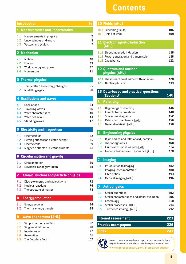
Contents
Answers to questions and exam papers in this book can be found on your free support website. Access the support website here:
www.oxfordsecondary.com/ib-prepared-support
iii
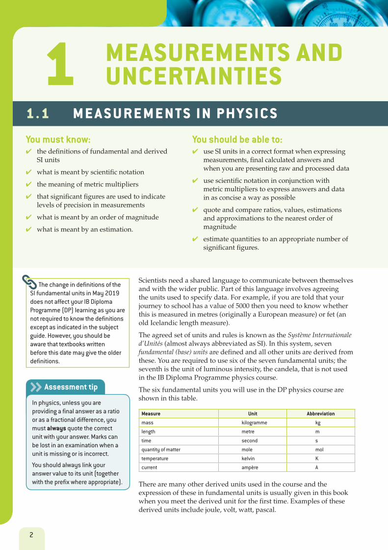
You must know: ✔ the definitions of fundamental and derived
SI units
✔ what is meant by scientific notation
✔ the meaning of metric multipliers
✔ that significant figures are used to indicate levels of precision in measurements
✔ what is meant by an order of magnitude
✔ what is meant by an estimation.
You should be able to: ✔ use SI units in a correct format when expressing
measurements, final calculated answers and when you are presenting raw and processed data
✔ use scientific notation in conjunction with metric multipliers to express answers and data in as concise a way as possible
✔ quote and compare ratios, values, estimations and approximations to the nearest order of magnitude
✔ estimate quantities to an appropriate number of significant figures.
Scientists need a shared language to communicate between themselves and with the wider public. Part of this language involves agreeing the units used to specify data. For example, if you are told that your journey to school has a value of 5000 then you need to know whether this is measured in metres (originally a European measure) or fet (an old Icelandic length measure).
The agreed set of units and rules is known as the Système Internationale d’Unités (almost always abbreviated as SI). In this system, seven fundamental (base) units are defined and all other units are derived from these. You are required to use six of the seven fundamental units; the seventh is the unit of luminous intensity, the candela, that is not used in the IB Diploma Programme physics course.
The six fundamental units you will use in the DP physics course are shown in this table.
The change in definitions of the SI fundamental units in May 2019 does not affect your IB Diploma Programme (DP) learning as you are not required to know the definitions except as indicated in the subject guide. However, you should be aware that textbooks written before this date may give the older definitions.
Measure Unit Abbreviation
mass kilogramme kg
length metre m
time second s
quantity of matter mole mol
temperature kelvin K
current ampère A
There are many other derived units used in the course and the expression of these in fundamental units is usually given in this book when you meet the derived unit for the first time. Examples of these derived units include joule, volt, watt, pascal.
Assessment tip
In physics, unless you are providing a final answer as a ratio or as a fractional difference, you must always quote the correct unit with your answer. Marks can be lost in an examination when a unit is missing or is incorrect.
You should always link your answer value to its unit (together with the prefix where appropriate).
MEASUREMENTS AND UNCERTAINTIES1
1 . 1 M E A S U R E M E N T S I N P H Y S I C S
2
Often, the use of a derived unit avoids a long string of fundamental units at the end of a number, so 1 volt ≡ 1 J C−1 ≡ 1 kg m2 s−3 A−1.
There are also some units used in the course that are not SI. Examples include MeV c−2, light year and parsec. These have special meaning in some parts of the subject and are used by scientists in those fields. Their meaning is explained when you meet them in this book.
The SI also specifies how data in science should be written. Numbers in physics can be very large or very small. Expressing the diameter of an atom as 0.000 000 000 12 m is unhelpful; 1.2 × 10⁻¹⁰ m is much better. This format of n.nn × 10n is known as scientific notation and should be used whenever possible. It can also be combined with the SI prefixes that are permitted.
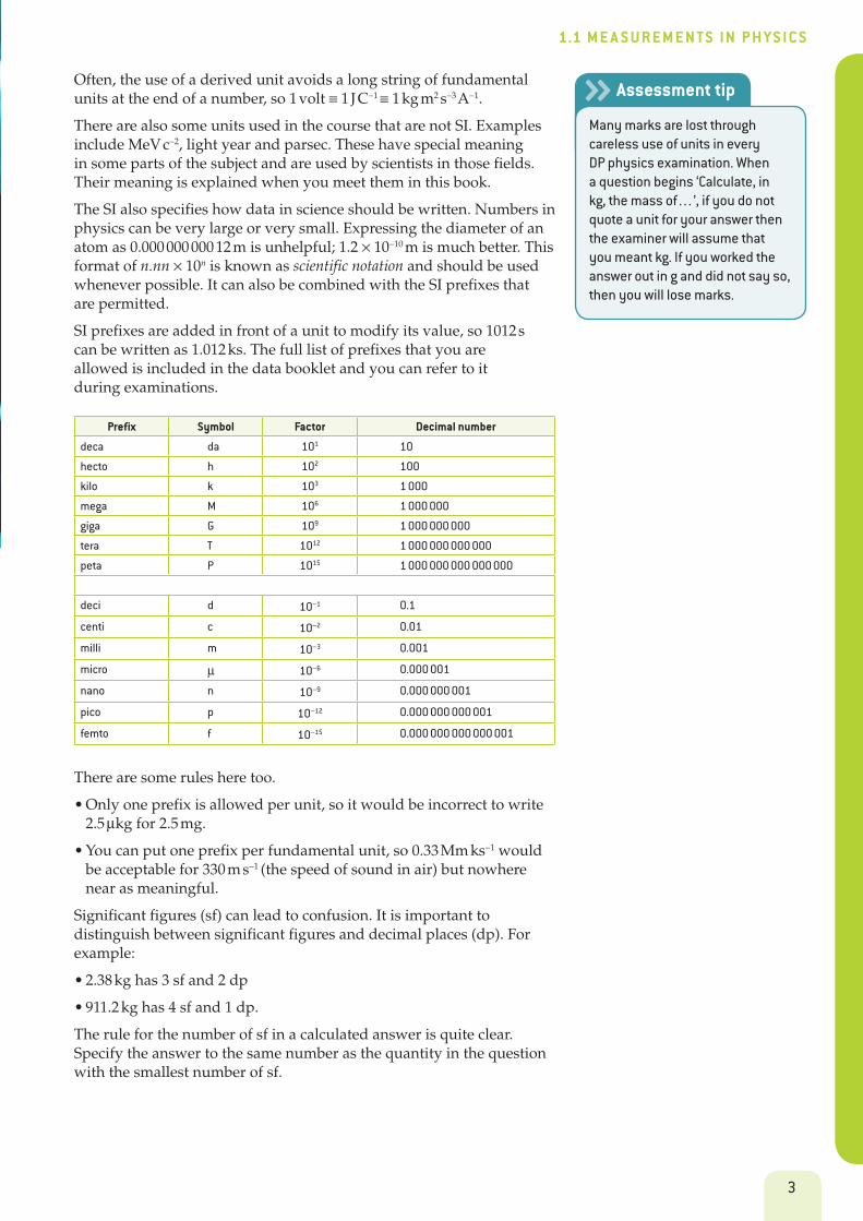
SI prefixes are added in front of a unit to modify its value, so 1012 s can be written as 1.012 ks. The full list of prefixes that you are allowed is included in the data booklet and you can refer to it during examinations.
Prefix Symbol Factor Decimal number
deca da 101 10
hecto h 102 100
kilo k 103 1 000
mega M 106 1 000 000
giga G 109 1 000 000 000
tera T 1012 1 000 000 000 000
peta P 1015 1 000 000 000 000 000
deci d 10−1 0.1
centi c 10−2 0.01
milli m 10−3 0.001
micro µ 10−6 0.000 001
nano n 10−9 0.000 000 001
pico p 10−12 0.000 000 000 001
femto f 10−15 0.000 000 000 000 001
There are some rules here too.
• Only one prefix is allowed per unit, so it would be incorrect to write 2.5 µkg for 2.5 mg.
• You can put one prefix per fundamental unit, so 0.33 Mm ks−1 would be acceptable for 330 m s−1 (the speed of sound in air) but nowhere near as meaningful.
Significant figures (sf) can lead to confusion. It is important to distinguish between significant figures and decimal places (dp). For example:
• 2.38 kg has 3 sf and 2 dp
• 911.2 kg has 4 sf and 1 dp.
The rule for the number of sf in a calculated answer is quite clear. Specify the answer to the same number as the quantity in the question with the smallest number of sf.
Assessment tip
Many marks are lost through careless use of units in every DP physics examination. When a question begins ‘Calculate, in kg, the mass of…’, if you do not quote a unit for your answer then the examiner will assume that you meant kg. If you worked the answer out in g and did not say so, then you will lose marks.
3
1.1 M E A S U R E M E N TS I N P H YS I CS
Sometimes estimations are required in physics. This is because either:
• an educated guess is needed for all or some of the quantities in a calculation, or
• there is an assumption involved in a calculation.
Often it will be appropriate to express your answer to an order of magnitude, meaning rounded to the nearest power of ten. The best way to express any order of magnitude answers is as 10n, where n is an integer.
Example 1.1.1
A snail travels a distance of 33.5 cm in 5.2 minutes.
Calculate the speed of the snail.
State the answer to an appropriate number of significant figures.
SolutionThe answer, to 7 sf, is 1.073718 × 10⁻³ m s−1.
It is incorrect to quote the answer to this precision as the time is only quoted to 2 sf (the fact that 5.2 minutes is 312 s is not important). The appropriate answer is 1.1 × 10⁻³ m s−1 (or 1.1 mm s−1 if you prefer).
Example 1.1.2
Estimate the number of air molecules in a room.
SolutionThe calculation is left for you, but you should use the following steps.
• Estimate the volume of a room by making an educated guess at its dimensions, in metres.
• The density of air is about 1.3 kg m−3—call it 1 kg m−3 to make the numbers easy later.
• The mass of 1 mol of oxygen molecules is 32 g and 1 mol of nitrogen is 28 g—call the answer 30 g for both gases combined.
• Each mole contains 6 × 10²³ molecules.
The volume and density → mass of gas in room and molar mass → number of moles and Avogadro’s number → answer.
Assessment tip
In Example 1.1.1, rounding up is needed. You should do this for every calculation– but only at the very end of the calculation. Rounding answers mid-solution leads to inaccuracies that may take you out of the allowed tolerance for the answer. Keep all possible sf in your calculator until the end and only make a decision about the sf in the last line. In Example 1.1.1, an examiner would be very happy to see …
= 1.073718 × 10⁻³ m s−1 so the speed of the snail is 1.1 × 10⁻³ m s−1 (to 2 sf) … as your working is then completely clear.
Assessment tip
You may see order of magnitude answers in Paper 1 (multiple choice) written as a single integer. When the response is, say, 7, this will mean 107.
It is also permissible to talk about ‘a difference of two orders of magnitude’; this means a ratio of 100 (102) between the two quantities.
Assessment tip
If the command term ‘Estimate’ is used in the examination, it will always be clear what is required as you will lack some or all data for your calculation if an educated guess is needed. In estimation questions, such as Example 1.1.2, make it clear what numbers you are providing for each step and how they fit into the overall calculation.
4
1 MEASUREMENTS AND UNCERTAINTIES
All measurement is prone to error. The Heisenberg uncertainty principle (Topic 12) reminds us of the fundamental limits beyond which science cannot go. However, even when the data collected are well above this limit, then two basic types of error are implicit in the data you collect: random error and systematic error.
Random errors lead to an uncertainty in a value. One way to assess their impact on a measurement is to repeat the measurement several times and then use half the range of the outlying values as an estimate of the absolute uncertainty.
You must know: ✔ what is meant by random errors and systematic
errors
✔ what is meant by absolute, fractional and percentage uncertainties
✔ that error bars are used on graphs to indicate uncertainties in data
✔ that gradients and intercepts on graphs have uncertainties.
You should be able to: ✔ explain how random and systematic errors can
be identified and reduced
✔ collect data that include absolute and/or fractional uncertainties and go on to state these as an uncertainty range
✔ determine the overall uncertainty when data with uncertainties are combined in calculations involving addition, subtraction, multiplication, division and raising to a power
✔ determine the uncertainty in gradients and intercepts of graphs.
1 . 2 U N C E R TA I N T I E S A N D E R R O R S
Random errors are unpredictable changes in data collected in an experiment. Examples include fluctuations in a measuring instrument or changes in the environmental conditions where the experiment is being carried out.
Systematic errors are often produced within measuring instruments. Suppose that an ammeter gives a reading of +0.1 A when there is no current between the meter terminals. This means that every reading made using the meter will read 0.1 A too high. The effect of a systematic error can produce a non-zero intercept on a graph where a line through the origin is expected.
Uncertainty in measurement is expressed in three ways.
Absolute uncertainty: the numerical uncertainty associated with a quantity. For example, when a length of quoted value 5.00 m has an actual value somewhere between 4.95 m and 5.05 m, the absolute uncertainty is ± 0.05 m.
The length will be expressed as (5.00 ± 0.05) m.
Fractional uncertainty =absolute uncertainty in quantity
numerical value of quantity.
A fractional uncertainty has no unit.
Percentage uncertainty = fractional uncertainty 100× expressed as a percentage. There is no unit.
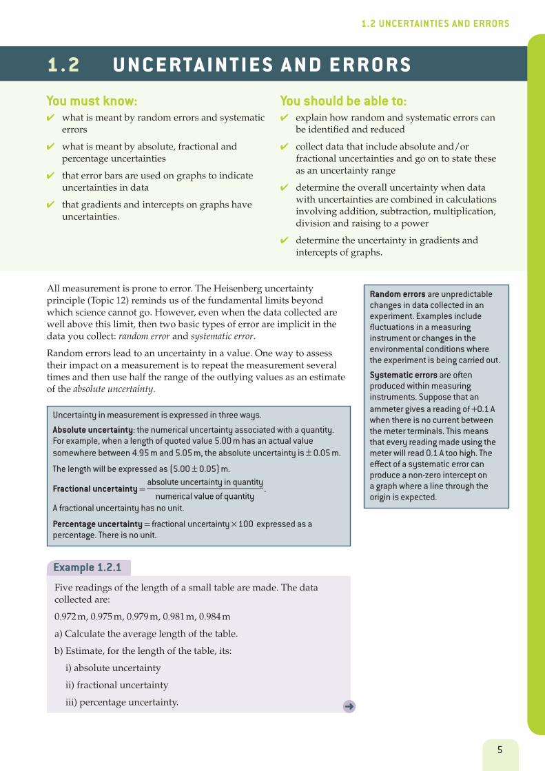
Example 1.2.1
Five readings of the length of a small table are made. The data collected are:
0.972 m, 0.975 m, 0.979 m, 0.981 m, 0.984 m
a) Calculate the average length of the table.
b) Estimate, for the length of the table, its:
i) absolute uncertainty
ii) fractional uncertainty
iii) percentage uncertainty.
5
1.2 UNCERTAINTIES AND ERRORS
Solutiona) The average length is:
(0.972 + 0.975 + 0.979 + 0.981 + 0.984)5
= 0.978(2)m
b) i) The outliers are 0.972 and 0.984 which differ by 0.012 m. Half this value is 0.006 m and this is taken to be the absolute uncertainty.
The length should be expressed as (0.978 ± 0.006) m.
(This absolute error is an estimate; another estimate is the standard deviation of the set of measurements which in this case is 0.004 m. 0.006 m is thus an overestimate.)
ii) The fractional uncertainty is = =0.006
0.97820.006(13) 0.006.
This is a ratio of lengths and has no unit.
iii) The percentage uncertainty is 0.006 × 100 = 0.6%.
Combining uncertainties
The two sides of a table have lengths (180 ± 5) cm and (60 ± 3) cm. What is the total perimeter of the table?
The absolute uncertainties are added when quantities are added and subtracted.
When y a b= ± then ∆ = ∆ + ∆y a bIn this case, the perimeter of the table is 180 + 180 + 60 + 60 = 480 m. The absolute uncertainty is 5 + 5 + 3 + 3 = 16 cm. The perimeter is (480 ± 16) cm or 4.8 ± 0.2 m.
Notice that when the quantities themselves are subtracted, the uncertainties are still added.
What is the area of the table?
When yabc
= then ∆
= ∆ + ∆ + ∆yy
aa
bb
cc
The fractional uncertainties are added when quantities are multiplied or divided.
The area is 1.8 × 0.60 = 1.08 m2. The two fractional uncertainties are
= =0.051.8
0.028 and0.030.6
0.050.
The sum is 0.078 and this is the fractional uncertainty of the answer.
The absolute uncertainty in the area = × =0.078 1.08 0.084.
The answer should be expressed as (1.08 ± 0.08) m2.
When the answer is found by division, the fractional uncertainties are still added.
Raising quantities to a power
When 2=y a , this is the same as a × a so using the
algebraic rule above: ∆
= ∆ + ∆ = ∆yy
aa
aa
aa
2.
In the general case, when y an= , ∆
= ∆yy
na
a, where ||
means the absolute value or magnitude of the expression.
When a quantity is raised to a power n, the fractional uncertainty is multiplied by n.
The radius of a sphere is (0.20 ± 0.01) m. What is the volume of the sphere?
Volume of sphere is: 43
=0.03353rπ m3
where r is the radius.
Fractional uncertainty of radius = =0.010.20
0.05
So, the fractional uncertainty of the radius cubed is 3 × 0.05 = 0.15.
The absolute uncertainty is 0.335 × 0.15 = 0.0050 m3.
The volume of the sphere is (0.335 ± 0.005) m3.
It is possible that data points, all with an associated error, are presented on a graph. Therefore, there are errors associated with the gradient and any intercept on the graph. The way to treat these errors is to add error bars to the graph. These are vertical or horizontal lines, centred on each data point, that are equal to the length of the absolute errors.
There is more information about this topic in Chapter 13, which deals with Paper 3, Section A.
You will often need to combine quantities mathematically: a pair of lengths, both with uncertainty, may need to be added to give a total length. This derived quantity will also have an uncertainty.
6
1 MEASUREMENTS AND UNCERTAINTIES
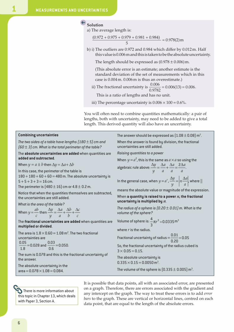
Maximum and minimum best-fit lines can then be drawn each side of the true best-fit line. The gradients of these maximum–minimum lines give a range of values that corresponds to the error in the gradient. The intercepts of the maximum–minimum lines also have a range in values that can be associated with the error in the true intercept.
For the graph in Figure 1.2.1, the gradient is 1.6 with a range between 2.1 and 1.1, so (1.6 ± 0.5) m s−1.
The intercept is −2.4 with a range of 1.0 to −5.8, so (−2.4 ± 3.4) m.
You must know: ✔ what are meant by vector and scalar quantities
✔ that vectors can be combined and resolved (split into two separate vectors).
You should be able to: ✔ solve vector problems graphically and
algebraically.
1 . 3 V E C T O R S A N D S C A L A R S
Quantities in DP physics are either scalars or vectors. (There is a third type of physical quantity but this is not used at this level.)
A vector can be represented by a line with an arrow. When drawn to scale, the length of the line represents the magnitude, and the direction is as drawn.
Both scalars and vectors can be added and subtracted. Scalar quantities add just as any other number in mathematics. With vectors, however, you need to take the direction into account.
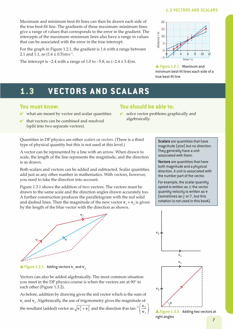
Figure 1.3.1 shows the addition of two vectors. The vectors must be drawn to the same scale and the direction angles drawn accurately too. A further construction produces the parallelogram with the red solid and dashed lines. Then the magnitude of the new vector v1 + v2 is given by the length of the blue vector with the direction as shown.
Scalars are quantities that have magnitude (size) but no direction. They generally have a unit associated with them.
Vectors are quantities that have both magnitude and a physical direction. A unit is associated with the number part of the vector.
For example, the scalar quantity speed is written as v; the vector quantity velocity is written as v (sometimes as v v
or , but this notation is not used in this book).
Figure 1.2.1. Maximum and minimum best-fit lines each side of a true best-fit line
–5
0
5
10
15
20
2 4 6 8 10 12
time / s
dist
ance
/ m
0
Figure 1.3.1. Adding vectors v1 and v2
v
v2
v1
Vectors can also be added algebraically. The most common situation you meet in the DP physics course is when the vectors are at 90° to each other (Figure 1.3.2).
As before, addition by drawing gives the red vector which is the sum of
v1 and v2. Algebraically, the use of trigonometry gives the magnitude of
the resultant (added) vector as +v v12
22 and the direction θ as
vv
tan 1 2
1
− . Figure 1.3.2. Adding two vectors at
right angles
v2
v2
v1
v1
θ
v2
v2
v1
v1
θ
7
1.3 VECTORS AND SCALARS
Example 1.3.1
A girl walks 500 m due north and then 1200 m due east. Calculate her position relative to her starting point.
SolutionThis is similar to the situation in Figure 1.3.2 where the first vector has a magnitude of 500 m and the second a magnitude of 1200 m.
The magnitude of the resultant is + =500 1200 13002 2 m.
θ is
= °−tan
5001200
22.61 .
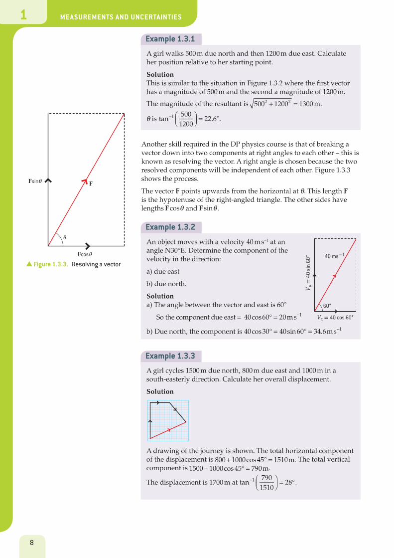
Another skill required in the DP physics course is that of breaking a vector down into two components at right angles to each other – this is known as resolving the vector. A right angle is chosen because the two resolved components will be independent of each other. Figure 1.3.3 shows the process.
The vector F points upwards from the horizontal at θ. This length F is the hypotenuse of the right-angled triangle. The other sides have lengths θF cos and θF sin .
Figure 1.3.3. Resolving a vector
F
θ
θ
Fcos
θFsin
Example 1.3.2
An object moves with a velocity 40 m s−1 at an angle N30°E. Determine the component of the velocity in the direction:
a) due east
b) due north.
Solutiona) The angle between the vector and east is 60°
So the component due east = ° = −40cos60 20ms 1
b) Due north, the component is ° = ° = −40cos30 40sin60 34.6ms 1
Example 1.3.3
A girl cycles 1500 m due north, 800 m due east and 1000 m in a south-easterly direction. Calculate her overall displacement.
Solution
A drawing of the journey is shown. The total horizontal component of the displacement is + ° =800 1000cos 45 1510m. The total vertical component is − ° =1500 1000cos 45 790m.
The displacement is 1700 m at
= °−tan
7901510
281 .
Vx = 40 cos 60°
40 ms−1
Vy =
40
sin
60°
60°
8
1 MEASUREMENTS AND UNCERTAINTIES
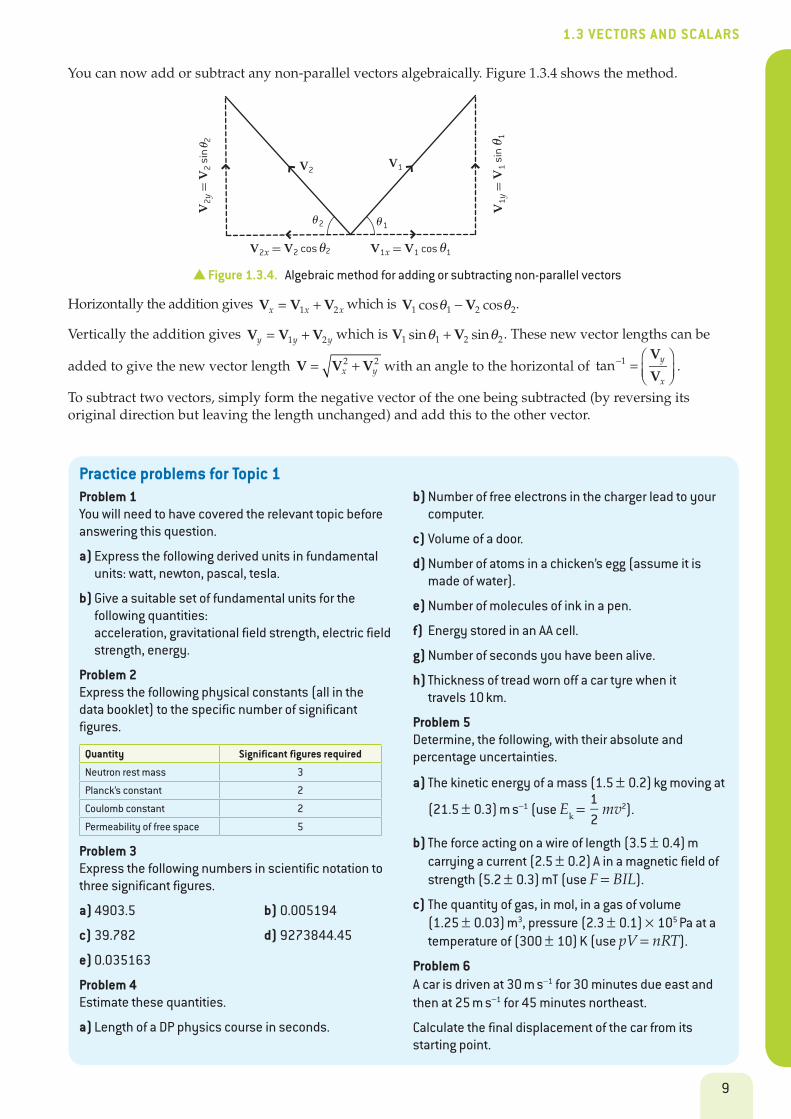
Horizontally the addition gives = +V V Vx x x1 2 which is θ θ−V Vcos cos1 1 2 2.
Vertically the addition gives = +V V Vy y y1 2 which is θ θ+V Vsin sin1 1 2 2. These new vector lengths can be
added to give the new vector length = +V V Vx y2 2 with an angle to the horizontal of =
− V
Vtan y
x
1 .
To subtract two vectors, simply form the negative vector of the one being subtracted (by reversing its original direction but leaving the length unchanged) and add this to the other vector.
You can now add or subtract any non-parallel vectors algebraically. Figure 1.3.4 shows the method.
Practice problems for Topic 1Problem 1You will need to have covered the relevant topic before answering this question.
a) Express the following derived units in fundamental units: watt, newton, pascal, tesla.
b) Give a suitable set of fundamental units for the following quantities: acceleration, gravitational field strength, electric field strength, energy.
Problem 2Express the following physical constants (all in the data booklet) to the specific number of significant figures.
Quantity Significant figures required
Neutron rest mass 3
Planck’s constant 2
Coulomb constant 2
Permeability of free space 5
Problem 3Express the following numbers in scientific notation to three significant figures.
a) 4903.5 b) 0.005194
c) 39.782 d) 9273844.45
e) 0.035163
Problem 4Estimate these quantities.
a) Length of a DP physics course in seconds.
b) Number of free electrons in the charger lead to your computer.
c) Volume of a door.
d) Number of atoms in a chicken’s egg (assume it is made of water).
e) Number of molecules of ink in a pen.
f) Energy stored in an AA cell.
g) Number of seconds you have been alive.
h) Thickness of tread worn off a car tyre when it travels 10 km.
Problem 5Determine, the following, with their absolute and percentage uncertainties.
a) The kinetic energy of a mass (1.5 ± 0.2) kg moving at
(21.5 ± 0.3) m s−1 (use Ek = 12
mv2).
b) The force acting on a wire of length (3.5 ± 0.4) m carrying a current (2.5 ± 0.2) A in a magnetic field of strength (5.2 ± 0.3) mT (use F = BIL).
c) The quantity of gas, in mol, in a gas of volume (1.25 ± 0.03) m3, pressure (2.3 ± 0.1) × 105 Pa at a temperature of (300 ± 10) K (use pV = nRT).
Problem 6A car is driven at 30 m s−1 for 30 minutes due east and then at 25 m s−1 for 45 minutes northeast.
Calculate the final displacement of the car from its starting point.
V1x = V1 cos 1θ
V1
V1y
= V
1 si
n 1θ
1θ2
2
θ
V2x = V2 cos θ
V2
V2y
= V
2 si
n 2θ
Figure 1.3.4. Algebraic method for adding or subtracting non-parallel vectors
9
1.3 VECTORS AND SCALARS
O X F O R D I B P R E P A R E D
9 780198 423713
ISBN 978-0-19-842371-3
I B D I P LO M A P R O G R A M M E
Author
David Homer
PHYSICSOffering an unparalleled level of assessment support at SL and HL, IB Prepared: Physics has been developed directly with the IB to provide the most up-to-date and authoritative guidance on DP assessment.
You can trust IB Prepared resources to:
➜ Consolidate essential knowledge and facilitate more effective exam preparation via concise summaries of course content
➜ Ensure that learners fully understand assessment requirements with clear explanations of each component, past paper material and model answers
➜ Maximize assessment potential with strategic tips, highlighted common errors and sample answers annotated with expert advice
➜ Build students’ skills and confidence using exam-style questions, practice papers and worked solutions
FOR FIRST ASSESSMENT IN 2016
Support material available at www.oxfordsecondary.co.uk/ib-prepared-support
Also available, from Oxford978 0 19 8392132
SAMPLE STUDENT ANSWER
Example 10.1.1
A precipitation system collects dust particles in a chimney. It consists of two large parallel vertical plates, separated by 4.0 m, maintained at potentials of +25 kV and −25 kV.
a) Explain what is meant by an equipotential surface.
b) A small dust particle moves vertically up the centre of the chimney, midway between the plates.The charge on the dust particle is + 5.5 nC.
i) Show that there is an electrostatic force on the particle of about 0.07 mN.
ii) The mass of the dust particle is 1.2 × 10⁻⁴ kg and it moves up the centre of the chimney at a constant vertical speed of 0.80 m s−1.
Calculate the minimum length of the plates so that the particle strikes one of them. Air resistance is negligible.
Solutiona) An equipotential surface is a surface of constant potential. This
means that no work is done in moving charge around on the surface.
b) i) The force on particle = =qEVqd
where d is the distance between
the plates. The potential difference is 50 kV.
So force = × × ×
= ×−
−5.0 10 5.5 104.0
6.875 10 N4 9
5
ii) The horizontal acceleration = =×
×=
−
−−force
mass6.875 101.2 10
0.573 m s5
42 .
The particle is in the centre of the plates, so has to move 2.0 m
horizontally to reach a plate. Using = +s ut at12
2 and knowing
that the particle has no initial horizontal component of
speed gives = × +×
t t t2.0 012
0.573 so =2 2.00.573
2 = 2.63 m and,
therefore, the length must be 2.63 × 0.8 = 2.1 m.
Explain what is meant by the gravitational potential at the surface of a planet. [2] This answer could have achieved 2/2 marks:
It is the work done per unit mass to bring a small test mass
from a point of infinity (zero PE) to the surface of that planet
(in the gravitational field).
▲▲ There are two marks for this question and two points to make – this answer has them both: work done per unit mass, and the idea of taking the mass (it does not have to be ‘small’ in a potential definition) from infinity to the surface.
Figure 10.1.3. Field lines and equipotentials around a planet
–80 V
–90 V
–100 V
Figure 10.1.3 shows the gravitational field due to a spherical planet Points on the green surface are at the same distance from the centre of the sphere and so have the same potential. When a mass moves on the green surface no overall work is done. This gives an equipotential surface, on which a charge or mass can move without work being transferred.
Because work is done when a charge or mass moves along a field line, equipotentials must always meet field lines at 90°.
Assessment tip
Example 10.1.1 b) i) is a ‘show that’ question. You must convince the examiner that you have completed all the steps to carry out the calculation. The way to do this is to quote the final answer to at least one more significant figure (sf) than the question quoted. Here it is quoted to 4 sf – and in this situation this is fine.
10 FIELDS (AHL)
108
842371_IB-Prep-Phys_U10.indd 108 24/01/19 21:11
Assessment questions and sample student responses provide practice opportunities and useful feedback
Key syllabus material is explained alongside key definitions
Assessment tips offer guidance and warn against common errors
What's on the cover? A visual representation of the Higgs boson particle
web www.oxfordsecondary.com/ib