Prospects for scalable 3D FFTs on heterogeneousexascale systems

Chris McClanahan∗, Kent Czechowski∗, Casey Battaglino†,Kartik Iyer‡, P.-K. Yeung†,‡, Richard Vuduc†

Georgia Institute of Technology, Atlanta, GA∗ School of Computer Science

† School of Computational Science and Engineering‡ School of Aerospace Engineering

{chris.mcclanahan,kentcz,cbattaglino3,kartik.iyer,pk.yeung,richie}@gatech.edu

ABSTRACTWe consider the problem of implementing scalable three-dimensional fast Fourier transforms with an eye toward fu-ture exascale systems comprised of graphics co-processor(GPUs) or other similarly high-density compute units. Wedescribe a new software implementation; derive and cali-brate a suitable analytical performance model; and use thismodel to make predictions about potential outcomes at ex-ascale, based on current and likely technology trends. Weevaluate the scalability of our software and instantiate mod-els on real systems, including 64 nodes (192 NVIDIA“Fermi”GPUs) of the Keeneland system at Oak Ridge National Lab-oratory. We use our analytical model to quantify the impactof both inter- and intra-node communication that impedefurther scalability. Among various observations, a key pre-diction is that although inter-node all-to-all communicationis expected to be the bottleneck of distributed FFTs, it isactually intra-node communication that may play an evenmore critical role.

1. INTRODUCTIONThe considerable interest in graphics co-processors (GPUs)for high-end computing systems raises numerous questionsabout performance, for both application developers and sys-tem architects alike. In essence, relative to current CPU-only clusters, GPUs imply clusters with fewer nodes hav-ing much higher per-node compute-densities than previouslyseen. However, this shift in compute density poses new chal-lenges for overall scalability, both within the node and acrossthe entire system.

In this paper, we ask what impact such a change will have onalgorithm design and implementation, in the specific contextof the three-dimensional fast Fourier transform (3D FFT).In nearly all modern implementations, the main communi-cation step is an all-to-all exchange. As such, one would

reasonably expect network bandwidth to dominate all otherperformance factors, especially at exascale.

Contributions. Contrary to this intuition, we argue that itis actually the intra-node design that may play the more crit-ical role, under business-as-usual assumptions. This claimis not just true today, where, unsurprisingly, relatively slowI/O bus communication (i.e., PCIe) can dominate perfor-mance. Rather, the surprise is that in the long-run, PCIedoes not matter because current technology trends suggestthat it is intra-node memory bandwidth actually scales moreslowly than either I/O bus or network bandwidth.

To build this argument, this paper makes what we believeare three contributions to our current understanding of therole high-density compute nodes will have on future 3D FFTalgorithms and implementations, summarized as follows.

1. Software: To better understand the impact GPU-enabled nodes will have on the 3D FFT, we first portthe P3DFFT library [15, 40] to GPUs, and study itsperformance on two of the major United States-basedGPU clusters.1 P3DFFT uses the so-called pencil de-composition, making our GPU port the first pencil--based 3D FFT for a GPU cluster. Pending review ofthis paper, we will release this port as a set of open-source (GPL) patches to P3DFFT, which we refer to asDiGPUFFT (pronounced “dig-puffed,” for DistributedGPU FFT ).

2. Modeling: Based on this implementation, we cre-ate an analytical performance model that accounts forcomputation and both inter- and intra- node commu-nication. The inter-node terms can account for topol-ogy; the intra-node terms include memory bandwidth,cache, and I/O-bus (PCIe) effects, giving us a basis forstudying how performance changes as machine param-eters vary; how alternative 3D FFT algorithms mightbehave; and what the future may hold (below). Weinstantiate and validate this model experimentally onexisting systems.

1Namely, the Tesla C1060-based Lincoln system at NationalCenter for Supercomputing Applications (NCSA) as well asthe M2070 “Fermi”-based Keeneland system at Oak RidgeNational Laboratory (ORNL).

1

3. Predictions: Using our model, we consider trends inarchitecture and FFT performance over the past 20-30years and make a number of predictions about whatwe might expect approximately ten years hence, at ex-ascale. One possible surprise is that even if the GPUwere to remain a discrete device, it is actually mem-ory bandwidth rather than I/O-bus bandwidth (today,PCIe) that is likely to be the intra-node limiter, bar-ring certain memory technology changes as discussedbelow.

Limitations. Among our claimed contributions, we acknowl-edge several limitations.

First, our DiGPUFFT software does not employ novel al-gorithms per se. However, for GPU-based systems, it is anovel implementation, relative to the current state-of-the-art PKUFFT [6]. In particular, DiGPUFFT uses the muchmore scalable pencil decomposition rather than the slab de-composition of PKUFFT; and we evaluate DiGPUFFT onup to 192 NVIDIA “Fermi” GPUs on 64 nodes with QDRInfiniband of Keeneland, achieving roughly 700 Gflop/s on alarge problem size, compared to 32 GPUs on 16 nodes and 1GigE at 120 Gflop/s for PKUFFT. More importantly, DiG-PUFFT is the concrete basis for our performance model andpredictions study.

Secondly, our model omits several factors that could play keyroles in future systems. Chief among these are microscopememory and network contention effects, which we accountfor implicitly through parameter calibration. The net effectof this simplification is that our estimates are likely to beoptimistic, as we show when we try to validate the model.

Lastly, regarding our predictions, we recall Niels Bohr’s fa-mous quote that,“Prediction is very difficult, especially aboutthe future.” Indeed, some of these predictions rely criti-cally on business-as-usual trends that is subject to dramaticshifts. We do discuss some specific threats to validity, includ-ing, for instance, viability and impact of stacked memory onintra-node FFT performance. Our main purpose in makingany predictions at all is to influence the future rather thanto obtain the “strictly correct answer.”

2. RELATED WORKThere is a flurry of current research activity in performanceanalysis and modeling, both for exascale in general and inparticular for the 3D FFT algorithms and software at allscales of parallelism. Our paper most closely follows threerecent studies.

The first study is the other major currently published dis-tributed memory GPU 3D FFT code by Chen et al. [6], asmentioned in Section 1.

The second study is by Pennycook et al., who also considerinter- vs. intra-node communication issues in the context ofthe NAS-LU benchmark (parallel wavefront stencil), lever-aging their earlier empirical modeling work [42]. Our modelis by contrast more explicit about particular intra-node pa-rameters, such as bandwidth, cache size, and I/O bus fac-

tors, and so our model adds improved algorithm-architectureunderstanding relative to this prior work.

The third study is Gahvari’s and Gropp’s theoretical anal-ysis of feasible latency and bandwidth regimes at exascale,using LogGP modeling and pencil/transpose-based FFTs asone benchmark [21]. Their model is more general than oursin that it is agnostic about specific architectural forms atexascale; however, ours may be more prescriptive about thenecessary changes by explicitly modeling particular archi-tectural features in making our projections.

Beyond these key studies, there is a vast literature on 3DFFTs [2–4, 7, 9–12, 17, 18, 22, 24, 26, 32, 44, 45, 47]. We callattention to just a few of these. For large problem sizes, thespeed record is roughly 10-11 Tflop/s (1D) on the Cray XT5and NEC SX-9 machines [1]. At our performance level (≈700 Gflop/s), the closest report is for a 2005 Cray XT3 run,which used over 5000 nodes (and one processor per node) [1]compared to our 64 nodes and 3 GPUs per node. For rela-tively small problem sizes, the most impressive strong scal-ing demonstration is the 323 run on the Anton system, whichuses custom ASIC network chips and fixed-point arithmetic,completing a 323 3D FFT in 4 µs (614 Gflop/s) [47], whichour code can only attain for relatively much larger problemsizes (see Section 4).

Among the other 3D FFT implementations, there are twobroad classes that complement and would improve our work.The first class considers highly-optimized all-to-all imple-mentations with a variety of sophisticated tricks like non-blocking asynchronous execution, overlap, and off-loading [12,28, 29], which might improve our implementations by 10-30%.2 The second class of implementations are single GPUFFTs, which are a building block for our code [23, 38, 39].However, at present we believe from experiment and com-parison to published results that the current NVIDIA imple-mentation on which we rely compares well with these otherapproaches.

3. BACKGROUND ON THE 3D FFTThe vast majority of modern FFT implementations use somevariation of the standard Cooley-Tukey algorithm. The clas-sical parallel algorithms are the binary exchange and trans-pose algorithms [34]. The basic high-level trade-off betweenthem is that, in 1D, the binary exchange method on p pro-

cessors sends O (log p) messages of total volume O(

np

log p)

words, compared to the transpose algorithm’s O (p) mes-

sages of total volume O(

np

), ignoring overlap. (Recall from

Section 2 that overlap may result in up to 10-30% improve-ments in practice.) Thus, we expect better performancefrom the transpose algorithm at large n, where we will bebound by network- or memory-bandwidth; and just the op-posite for small n, where we expect to be latency bound.

Of these, nearly all modern parallel 3D FFT implementa-tions use the transpose algorithm, for which there are twomajor variants: the so-called slab and pencil decomposi-tions. We illustrate these variants in Figure 1.

2There are 2× demonstrations of improvement in the collec-tive itself for very slow networks [13].

2

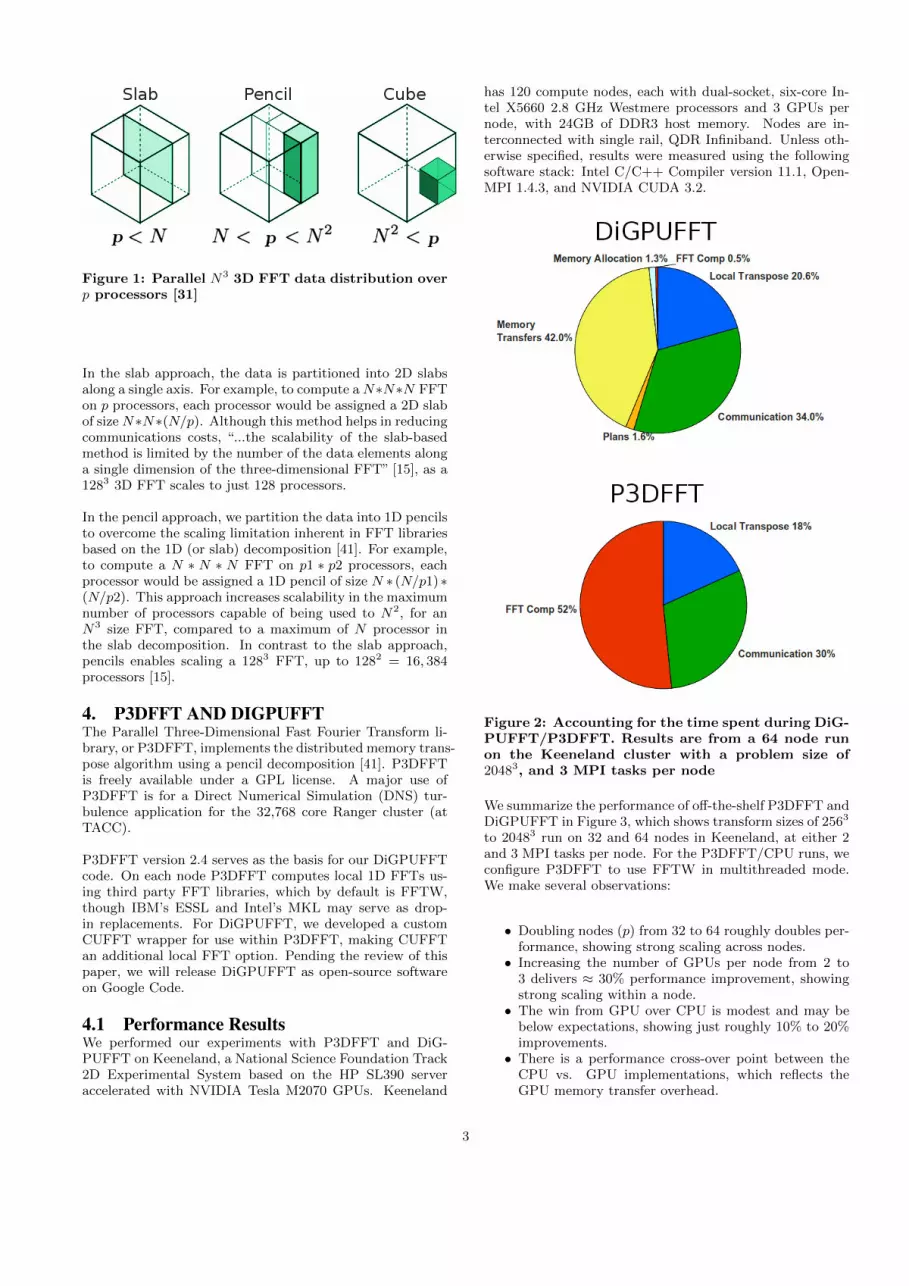
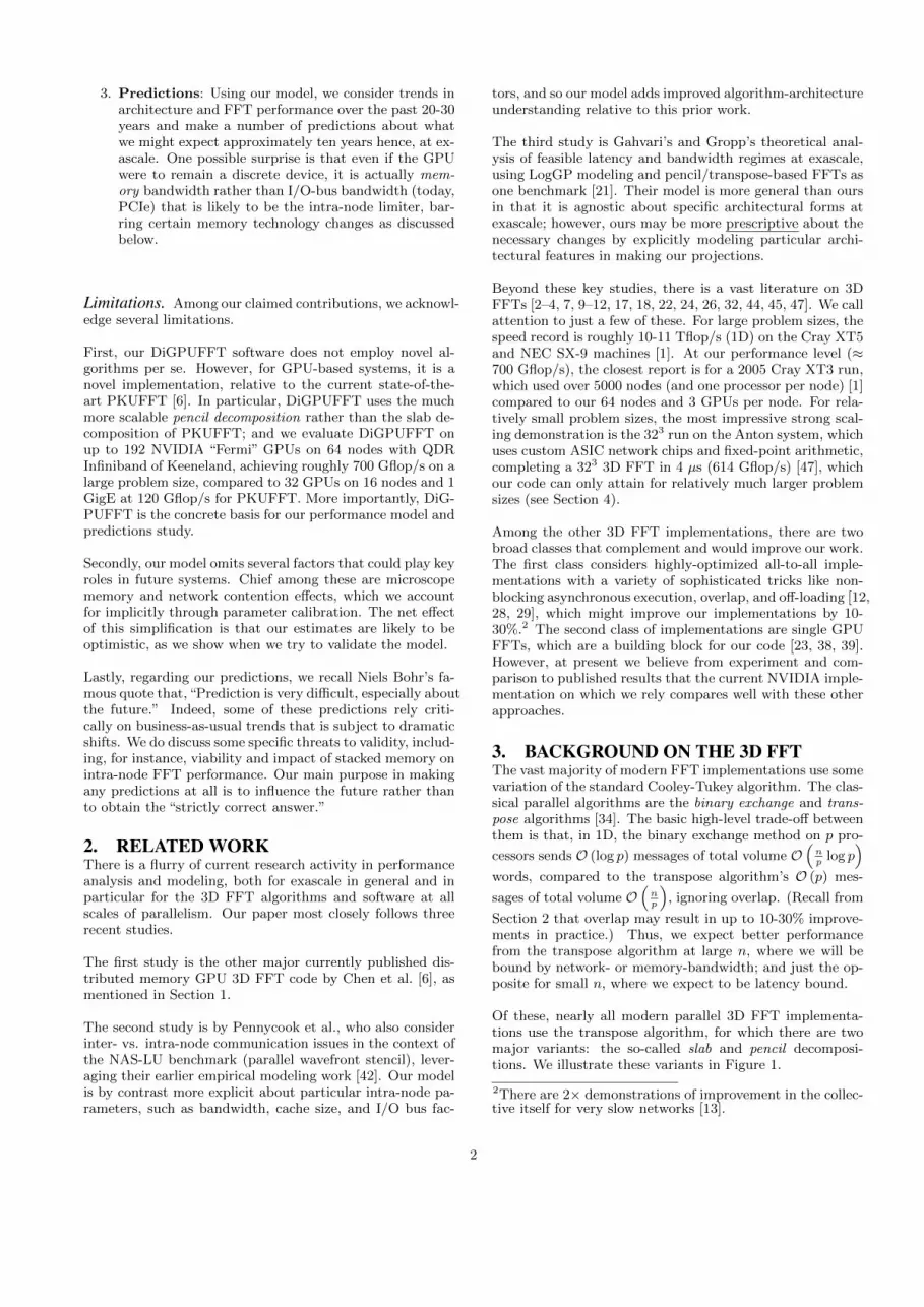
Figure 1: Parallel N3 3D FFT data distribution overp processors [31]

In the slab approach, the data is partitioned into 2D slabsalong a single axis. For example, to compute aN∗N∗N FFTon p processors, each processor would be assigned a 2D slabof sizeN∗N∗(N/p). Although this method helps in reducingcommunications costs, “...the scalability of the slab-basedmethod is limited by the number of the data elements alonga single dimension of the three-dimensional FFT” [15], as a1283 3D FFT scales to just 128 processors.

In the pencil approach, we partition the data into 1D pencilsto overcome the scaling limitation inherent in FFT librariesbased on the 1D (or slab) decomposition [41]. For example,to compute a N ∗ N ∗ N FFT on p1 ∗ p2 processors, eachprocessor would be assigned a 1D pencil of size N ∗ (N/p1)∗(N/p2). This approach increases scalability in the maximumnumber of processors capable of being used to N2, for anN3 size FFT, compared to a maximum of N processor inthe slab decomposition. In contrast to the slab approach,pencils enables scaling a 1283 FFT, up to 1282 = 16, 384processors [15].

4. P3DFFT AND DIGPUFFTThe Parallel Three-Dimensional Fast Fourier Transform li-brary, or P3DFFT, implements the distributed memory trans-pose algorithm using a pencil decomposition [41]. P3DFFTis freely available under a GPL license. A major use ofP3DFFT is for a Direct Numerical Simulation (DNS) tur-bulence application for the 32,768 core Ranger cluster (atTACC).

P3DFFT version 2.4 serves as the basis for our DiGPUFFTcode. On each node P3DFFT computes local 1D FFTs us-ing third party FFT libraries, which by default is FFTW,though IBM’s ESSL and Intel’s MKL may serve as drop-in replacements. For DiGPUFFT, we developed a customCUFFT wrapper for use within P3DFFT, making CUFFTan additional local FFT option. Pending the review of thispaper, we will release DiGPUFFT as open-source softwareon Google Code.

4.1 Performance ResultsWe performed our experiments with P3DFFT and DiG-PUFFT on Keeneland, a National Science Foundation Track2D Experimental System based on the HP SL390 serveraccelerated with NVIDIA Tesla M2070 GPUs. Keeneland

has 120 compute nodes, each with dual-socket, six-core In-tel X5660 2.8 GHz Westmere processors and 3 GPUs pernode, with 24GB of DDR3 host memory. Nodes are in-terconnected with single rail, QDR Infiniband. Unless oth-erwise specified, results were measured using the followingsoftware stack: Intel C/C++ Compiler version 11.1, Open-MPI 1.4.3, and NVIDIA CUDA 3.2.

Figure 2: Accounting for the time spent during DiG-PUFFT/P3DFFT. Results are from a 64 node runon the Keeneland cluster with a problem size of20483, and 3 MPI tasks per node

We summarize the performance of off-the-shelf P3DFFT andDiGPUFFT in Figure 3, which shows transform sizes of 2563

to 20483 run on 32 and 64 nodes in Keeneland, at either 2and 3 MPI tasks per node. For the P3DFFT/CPU runs, weconfigure P3DFFT to use FFTW in multithreaded mode.We make several observations:

• Doubling nodes (p) from 32 to 64 roughly doubles per-formance, showing strong scaling across nodes.• Increasing the number of GPUs per node from 2 to

3 delivers ≈ 30% performance improvement, showingstrong scaling within a node.• The win from GPU over CPU is modest and may be

below expectations, showing just roughly 10% to 20%improvements.• There is a performance cross-over point between the

CPU vs. GPU implementations, which reflects theGPU memory transfer overhead.

3

N

Gflo

p/s

0100200300400500600700

0100200300400500600700

p=32

●

●● ●

●

●● ●

256256256256 512512512512 1024102410241024 2048204820482048256256256256 512512512512 1024102410241024 2048204820482048

p=64

●

●

●●

●

●

●●

256256256256 512512512512 1024102410241024 2048204820482048256256256256 512512512512 1024102410241024 2048204820482048

q=2

q=3

Processor

● CPU

GPU

Figure 3: DiGPUFFT performance on an N ×N ×N FFT problem, using p nodes of Keeneland with q MPItasks per node. The CPU curves are MPI + multithreaded FFTW; GPU curves use CUFFT on a total ofp · q GPUs.

• The CPU’s performance levels off more quickly thanthe GPU’s performance, showing at least some modestscalability improvements due to the use of GPUs.

At smaller FFT sizes such as 2563, the CPU outperforms theGPU, due partly to the CPU still doing the local transposes,and the high cost of host-to-device memory transfers, asshown in Figure 2. As the FFT sizes grow, the GPU’s fastercompute time quickly overcomes this additional overhead.We analyze Figure 2 in the following sections.

4.2 Memory ConstraintsNVIDIA’s high-end GPUs provide up to 6 GB of memory,significantly less than typical host memory sizes. For largedata-sets, memory space can become a scarce commodity.For FFT kernels, GPU memory must hold the frequencyvalues as well as the O (n) “twiddle factors” that are gen-erated with the CUFFT planning procedures. Such plansmimic the equivalent construct in FFTW. A plan generatedby CUFFT for an FFT of size n will use 168 MB of over-head plus an additional O (n) bytes to store the twiddlefactors. For DiGPUFFT, this memory constraint limits thenumber of plans that can be precomputed or overlapped be-cause there is not enough memory to store them all for theduration of the FFT calculation.

As Figure 2 shows, 1.3% of the time along the critical pathis spent computing the CUFFT plans. An additional 1.6%of the time is spent allocating and de-allocating memory onthe GPU to accommodate the different pencil batch sizesused during the FFT computation. With enough memoryto compute all of the plans and allocate all of the blocksahead of time, we would expect to see a 3% speedup. More

GPU memory would also make it possible to run FFTs withlarger pencil lengths.

4.3 PCIe BottleneckFigure 2 also shows that 52% of the time along the criticalpath is spent transferring frequency values from the hostmemory to GPU memory then transferring the computedresults back to host memory before transferring them acrossthe network.

Consider the 1D FFT using the transpose algorithm of sizen with p GPUs. During the first phase, n/p words are trans-ferred across the PCIe bus to the GPU memory, a local FFTis computed on the n/p values, and the resulting n/p valuesare transferred back across the PCIe bus to the host mem-ory. Using the peak bandwidth of the PCIe bus (βPCIe=8GB/s) and the peak GPU computational throughput for alocal FFT (Cfft=380 Gflop/s; see Table 1), we can calculatethe effective computation time for the GPU, Tcufft:

Tcufft(n) =5n logn

Ccufft+ 2

n

βPCIe(1)

versus the time for the time for the CPU version, which doesnot involve transfers across the PCIe bus:

Tfftw(n) =5n logn

Cfftw(2)

Comparing Tcufft(n) and Tfftw(n) for realistic values of n,(210 ≤ n ≤ 230), we observe that the effective speedup of theGPU is only 2.1× to 3.8×, significantly less than the 14×speedup suggested by Table 1. In fact, the GPU only reachesthe Ccufft peak reported in Table 1 on a few special-casevalues of n. For most values of n, the GPU only achieves a

4

small fraction of Ccufft and no value of n greater than 4096achieves more than 240 Gflop/s.

Single Core of aCPU

One GPU

Model 6-core IntelX5660 2.8 GHz

NVIDIA TeslaM2070

FFT Software FFTW 3.2.1 CUFFT 3.2HardwarePeak

22.4 Gflop/s 1030 Gflop/s

ObservedFFT Peak

4.7 Gflop/s 338 Gflop/s

Table 1: Local FFT Performance: CPU vs GPU

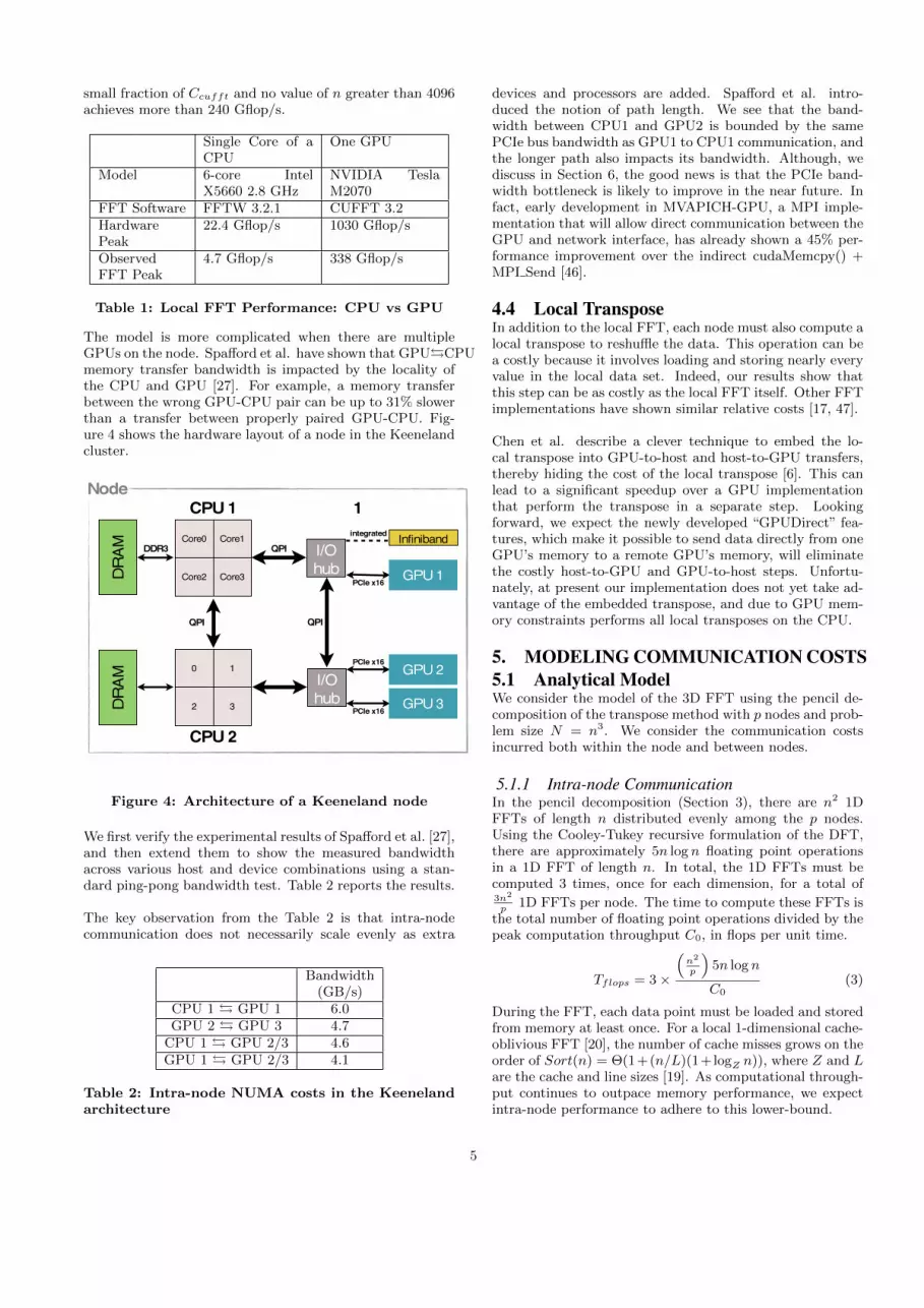
The model is more complicated when there are multipleGPUs on the node. Spafford et al. have shown that GPU�CPUmemory transfer bandwidth is impacted by the locality ofthe CPU and GPU [27]. For example, a memory transferbetween the wrong GPU-CPU pair can be up to 31% slowerthan a transfer between properly paired GPU-CPU. Fig-ure 4 shows the hardware layout of a node in the Keenelandcluster.

Core0 Core1

Core2 Core3

CPU 1

DR

AM

1

Infiniband

0 1

2 3

CPU 2

DR

AM

QPI

DDR3 QPI I/O hub

I/O hub

QPI

integrated

PCIe x16

PCIe x16

PCIe x16

GPU 1

GPU 2

GPU 3

Node

Figure 4: Architecture of a Keeneland node

We first verify the experimental results of Spafford et al. [27],and then extend them to show the measured bandwidthacross various host and device combinations using a stan-dard ping-pong bandwidth test. Table 2 reports the results.

The key observation from the Table 2 is that intra-nodecommunication does not necessarily scale evenly as extra

Bandwidth(GB/s)

CPU 1 � GPU 1 6.0GPU 2 � GPU 3 4.7

CPU 1 � GPU 2/3 4.6GPU 1 � GPU 2/3 4.1

Table 2: Intra-node NUMA costs in the Keenelandarchitecture

devices and processors are added. Spafford et al. intro-duced the notion of path length. We see that the band-width between CPU1 and GPU2 is bounded by the samePCIe bus bandwidth as GPU1 to CPU1 communication, andthe longer path also impacts its bandwidth. Although, wediscuss in Section 6, the good news is that the PCIe band-width bottleneck is likely to improve in the near future. Infact, early development in MVAPICH-GPU, a MPI imple-mentation that will allow direct communication between theGPU and network interface, has already shown a 45% per-formance improvement over the indirect cudaMemcpy() +MPI Send [46].

4.4 Local TransposeIn addition to the local FFT, each node must also compute alocal transpose to reshuffle the data. This operation can bea costly because it involves loading and storing nearly everyvalue in the local data set. Indeed, our results show thatthis step can be as costly as the local FFT itself. Other FFTimplementations have shown similar relative costs [17, 47].

Chen et al. describe a clever technique to embed the lo-cal transpose into GPU-to-host and host-to-GPU transfers,thereby hiding the cost of the local transpose [6]. This canlead to a significant speedup over a GPU implementationthat perform the transpose in a separate step. Lookingforward, we expect the newly developed “GPUDirect” fea-tures, which make it possible to send data directly from oneGPU’s memory to a remote GPU’s memory, will eliminatethe costly host-to-GPU and GPU-to-host steps. Unfortu-nately, at present our implementation does not yet take ad-vantage of the embedded transpose, and due to GPU mem-ory constraints performs all local transposes on the CPU.

5. MODELING COMMUNICATION COSTS5.1 Analytical ModelWe consider the model of the 3D FFT using the pencil de-composition of the transpose method with p nodes and prob-lem size N = n3. We consider the communication costsincurred both within the node and between nodes.

5.1.1 Intra-node CommunicationIn the pencil decomposition (Section 3), there are n2 1DFFTs of length n distributed evenly among the p nodes.Using the Cooley-Tukey recursive formulation of the DFT,there are approximately 5n logn floating point operationsin a 1D FFT of length n. In total, the 1D FFTs must becomputed 3 times, once for each dimension, for a total of3n2

p1D FFTs per node. The time to compute these FFTs is

the total number of floating point operations divided by thepeak computation throughput C0, in flops per unit time.

Tflops = 3×

(n2

p

)5n logn

C0(3)

During the FFT, each data point must be loaded and storedfrom memory at least once. For a local 1-dimensional cache-oblivious FFT [20], the number of cache misses grows on theorder of Sort(n) = Θ(1+(n/L)(1+logZ n)), where Z and Lare the cache and line sizes [19]. As computational through-put continues to outpace memory performance, we expectintra-node performance to adhere to this lower-bound.

5

CPU GPU CPU GPU inToday Today 10 years 10 years

Model (ms) (ms) (ms) (ms)Tflops 71 6 .1 .1Tmem 224 13 19 1Tcomm 229 229 11 11

Table 3: Example model times for a given machine

The n3

pdata points on the node also need to be reshuf-

fled before being exchanged with other nodes. This step isthe local transpose step. The time for these memory accessis the number of memory accesses divided by the memorybandwidth βmem.

Thus, for some constant A and sufficiently large n, a 3DFFT will incur the following memory costs within a node:

Tmem = 3× n2

p· A(1 + (n/L)(1 + logZ n)) · L

βmem

+ 2×2n3

p

βmem(4)

5.1.2 Inter-node CommunicationDuring the 3D FFT, the node must exchange its n3

pdata

points with other nodes on the network at least twice, typ-ically with the MPI_AllToAll collective. Technically, only(p−1)(n3)

p2data points are exchanged per round, but we sim-

plify it to n3

pbecause p−1

pis nearly 1 for typical values of p.

The communication time is therefore bounded by the totalnumber of words exchanged across the network divided bythe network bandwidth in/out of the node, denoted βlink.In the following subsections we will look more closely at howthe network topology impacts the communication time. Asa strict lower bound (i.e, on a fully connected network withfull overlap):

Tcomm ≥ 2×2n3

p

βlink(5)

Comparing the relative times for the Tflops, Tmem, andTcomm provides an easy way to explore the potential bottle-necks of a machine represented by the C0, βmem, and βlink

values. Table 3 shows the computed values for Keeneland us-ing only CPUs or only GPUs. In the CPU case we see thattime for the floating point calculations is relatively minorcompared to the network times, as expected. But the moresurprising result is that memory access time is significantlymore than the flops and relatively close to the network time.The use of the three GPUs on each node boosts the memoryand floating point throughput and has a profound impacton the relative value of Tmem in comparison to Tlink. Un-fortunately, as our DiGPUFFT analysis shows, intra-nodecommunication bottlenecks prevent the GPU from reachingthis potential. These times roughly correspond to the timedistributions reported from the P3DFFT experiments.

If it were somehow possible to drive Tmem to zero, thenthe all-to-all personalized communication step becomes thelimiter and optimizing this collective becomes critical to im-

proving performance [33]. For instance, maximizing commu-nication overlap of this collective minimizes time lost due tolatency. One state-of-the-art implementation achieves 95%overlap on the BlueGene/L [13].

In our model we assume that inter-node communicationtime (Tcomm) and intra-node communication time (Tnode =max(Tflops, Tmem)) are independent: Ttotal = Tcomm+Tnode,although in an ideal case they could be perfectly overlapped.

In the 3D FFT, we estimate communication time on a hy-percube to be the cost of performing two all-to-all commu-nication steps [34]:

TTcomm = 2×

[(p− 1)αlink +

n(p− 1)

p2 · βlink

]where αlink is inter-node latency. We use TT

comm to de-note the transpose algorithm, as distinct from the binary-exchange algorithm modeled below.

For a torus topology, Eleftheriou et al. give lower-boundson the all-to-all communication time with the expression

T ≥ VreceivedNhops

Nlinksβ · f

Where Nhops is the average number of hops and Nlinks isthe number of links connected to any node. This expressionis constant regardless of the dimension of the torus [17].

5.1.3 Algorithm SelectionOne notable FFT method that does not involve an all-to-allcommunication is the Binary Exchange algorithm. This al-gorithm requires more bandwidth than the transpose methodby a factor of log p but requires log p communication stepswith neighboring nodes, compared with the single globalcommunication step required for the transpose method. Thiscan decrease communication time in high-latency networks,or in the case of strong-scaling when the volume of data isnot enough to take advantage of all of a machine’s band-width. In the 3D case, we must carry this out in threephases:

TBcomm = 3×

[(log p)α+

n log p

p · β

]

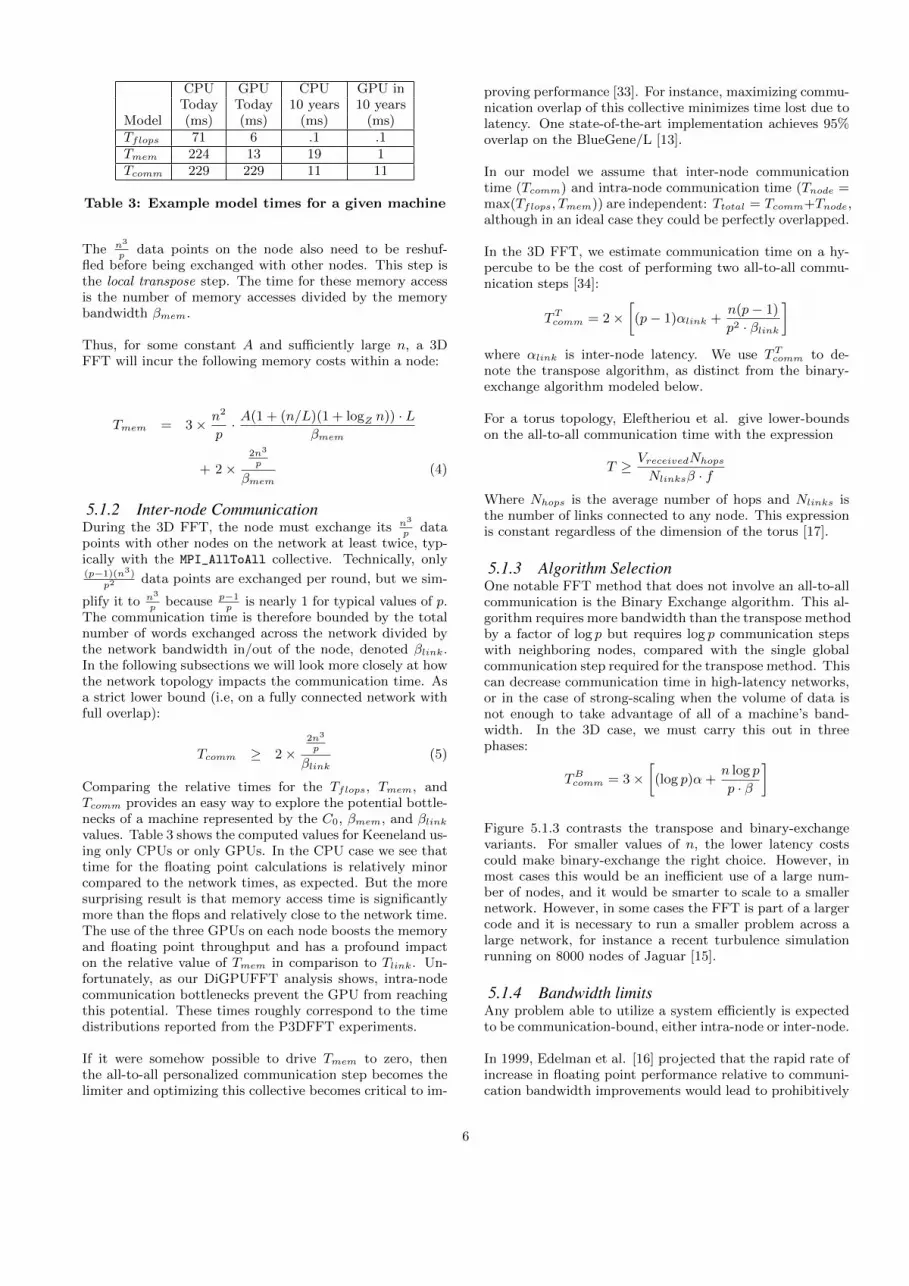
Figure 5.1.3 contrasts the transpose and binary-exchangevariants. For smaller values of n, the lower latency costscould make binary-exchange the right choice. However, inmost cases this would be an inefficient use of a large num-ber of nodes, and it would be smarter to scale to a smallernetwork. However, in some cases the FFT is part of a largercode and it is necessary to run a smaller problem across alarge network, for instance a recent turbulence simulationrunning on 8000 nodes of Jaguar [15].

5.1.4 Bandwidth limitsAny problem able to utilize a system efficiently is expectedto be communication-bound, either intra-node or inter-node.

In 1999, Edelman et al. [16] projected that the rapid rate ofincrease in floating point performance relative to communi-cation bandwidth improvements would lead to prohibitively

6

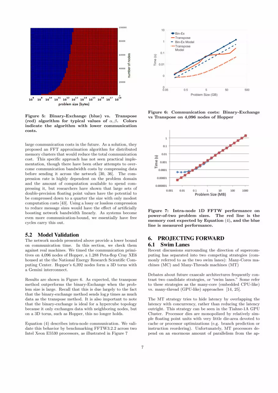
Figure 5: Binary-Exchange (blue) vs. Transpose(red) algorithm for typical values of α, β. Colorsindicate the algorithm with lower communicationcosts.

large communication costs in the future. As a solution, theyproposed an FFT approximation algorithm for distributedmemory clusters that would reduce the total communicationcost. This specific approach has not seen practical imple-mentation, though there have been other attempts to over-come communication bandwidth costs by compressing databefore sending it across the network [30, 36]. The com-pression rate is highly dependent on the problem domainand the amount of computation available to spend com-pressing it, but researchers have shown that large sets ofdouble-precision floating point values have the potential tobe compressed down to a quarter the size with only modestcomputation costs [43]. Using a lossy or lossless compressionto reduce message sizes would have the effect of artificiallyboosting network bandwidth linearly. As systems becomeeven more communication-bound, we essentially have freecycles carry this out.

5.2 Model ValidationThe network models presented above provide a lower boundon communication time. In this section, we check themagainst real machines. We timed the communication primi-tives on 4,096 nodes of Hopper, a 1.288 Peta-flop Cray XE6housed at the the National Energy Research Scientific Com-puting Center. Hopper’s 6,392 nodes form a 3D torus witha Gemini interconnect.

Results are shown in Figure 6. As expected, the transposemethod outperforms the binary-Exchange when the prob-lem size is large. Recall that this is due largely to the factthat the binary-exchange method sends log p times as muchdata as the transpose method. It is also important to notethat the binary-exchange is ideal for a hypercube topologybecause it only exchanges data with neighboring nodes, buton a 3D torus, such as Hopper, this no longer holds.

Equation (4) describes intra-node communication. We vali-date this behavior by benchmarking FFTW3.2.2 across twoIntel Xeon E5530 processors, as illustrated in Figure 7

0.05 0.5 5 50 5000

0

0.01

0.1

1

10Bin-ExTransposeBin-Ex ModelTranspose Model

Problem Size (GB)

Tim

e (

s)

Figure 6: Communication costs: Binary-Exchangevs Transpose on 4,096 nodes of Hopper

Figure 7: Intra-node 1D FFTW performance onpower-of-two problem sizes. The red line is thememory cost expected by Equation (4), and the blueline is measured performance.

6. PROJECTING FORWARD6.1 Swim LanesRecent discussions surrounding the direction of supercom-puting has separated into two competing strategies (com-monly referred to as the two swim lanes): Many-Cores ma-chines (MC) and Many-Threads machines (MT)

Debates about future exascale architectures frequently con-trast two candidate strategies, or “swim lanes.” Some referto these strategies as the many-core (embedded CPU-like)vs. many-thread (GPU-like) approaches [14, 25].

The MT strategy tries to hide latency by overlapping thelatency with concurrency, rather than reducing the latencyoutright. This strategy can be seen in the Tiahne-1A GPUCluster. Processor dies are monopolized by relatively sim-ple floating point units with very little die-area devoted tocache or processor optimizations (e.g. branch prediction orinstruction reordering). Unfortunately, MT processors de-pend on an enormous amount of parallelism from the ap-

7

doubling 10-yearKeeneland time increase

Parameter values (in years) factor

Cores: pcpu 12 1.87 40.7×pgpu 448Peak: pcpu · Ccpu 268 Gflop/s 1.7 59.0×pgpu · Cgpu 1 Tflop/sMemory bandwidth: βcpu 25.6 GB/s 3.0 9.7×βgpu 144 GB/sFast memory: Zcpu 12 MB 2.0 32.0×Zgpu 1MBI/O device: βI/O 8 GB/s 2.39 18.1×Network bandwidth, βlink 10 GB/s 2.25 21.8×

Table 4: Using the hardware trends we can makepredictions about relative performance of futurehardware.

plication and implement a wide SIMD vector width becausethe memory bandwidth necessary to fetch instruction forthousands of processors every cycle can be prohibitive. TheMT strategy results in very high floating point density, andtherefore have fewer nodes than their MC counterparts.

Alternatively, the MC strategy takes aggressive measuresto reduce latency. Large portions of the processor die aredevoted to caches with the aim of reducing the number ofout-of-die accesses. These machines are exemplified by thedirection of the Blue Gene line of clusters.

While the concepts of the two swim lanes are still rathernebulous and evolving on a regular basis, its not too soon tobegin thinking about how the differences between MC andMT machines impacts particular algorithms. In the case ofthe FFT, the models presented in this paper can be used tocompare and contrast the two strategies.

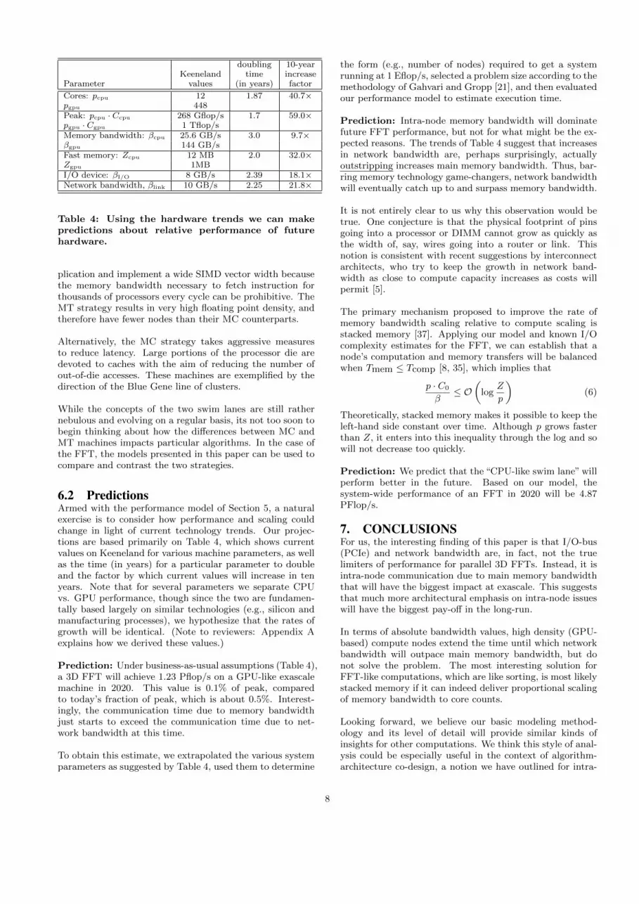
6.2 PredictionsArmed with the performance model of Section 5, a naturalexercise is to consider how performance and scaling couldchange in light of current technology trends. Our projec-tions are based primarily on Table 4, which shows currentvalues on Keeneland for various machine parameters, as wellas the time (in years) for a particular parameter to doubleand the factor by which current values will increase in tenyears. Note that for several parameters we separate CPUvs. GPU performance, though since the two are fundamen-tally based largely on similar technologies (e.g., silicon andmanufacturing processes), we hypothesize that the rates ofgrowth will be identical. (Note to reviewers: Appendix Aexplains how we derived these values.)

Prediction: Under business-as-usual assumptions (Table 4),a 3D FFT will achieve 1.23 Pflop/s on a GPU-like exascalemachine in 2020. This value is 0.1% of peak, comparedto today’s fraction of peak, which is about 0.5%. Interest-ingly, the communication time due to memory bandwidthjust starts to exceed the communication time due to net-work bandwidth at this time.

To obtain this estimate, we extrapolated the various systemparameters as suggested by Table 4, used them to determine

the form (e.g., number of nodes) required to get a systemrunning at 1 Eflop/s, selected a problem size according to themethodology of Gahvari and Gropp [21], and then evaluatedour performance model to estimate execution time.

Prediction: Intra-node memory bandwidth will dominatefuture FFT performance, but not for what might be the ex-pected reasons. The trends of Table 4 suggest that increasesin network bandwidth are, perhaps surprisingly, actuallyoutstripping increases main memory bandwidth. Thus, bar-ring memory technology game-changers, network bandwidthwill eventually catch up to and surpass memory bandwidth.

It is not entirely clear to us why this observation would betrue. One conjecture is that the physical footprint of pinsgoing into a processor or DIMM cannot grow as quickly asthe width of, say, wires going into a router or link. Thisnotion is consistent with recent suggestions by interconnectarchitects, who try to keep the growth in network band-width as close to compute capacity increases as costs willpermit [5].

The primary mechanism proposed to improve the rate ofmemory bandwidth scaling relative to compute scaling isstacked memory [37]. Applying our model and known I/Ocomplexity estimates for the FFT, we can establish that anode’s computation and memory transfers will be balancedwhen Tmem ≤ Tcomp [8, 35], which implies that

p · C0

β≤ O

(log

Z

p

)(6)

Theoretically, stacked memory makes it possible to keep theleft-hand side constant over time. Although p grows fasterthan Z, it enters into this inequality through the log and sowill not decrease too quickly.

Prediction: We predict that the “CPU-like swim lane” willperform better in the future. Based on our model, thesystem-wide performance of an FFT in 2020 will be 4.87PFlop/s.

7. CONCLUSIONSFor us, the interesting finding of this paper is that I/O-bus(PCIe) and network bandwidth are, in fact, not the truelimiters of performance for parallel 3D FFTs. Instead, it isintra-node communication due to main memory bandwidththat will have the biggest impact at exascale. This suggeststhat much more architectural emphasis on intra-node issueswill have the biggest pay-off in the long-run.

In terms of absolute bandwidth values, high density (GPU-based) compute nodes extend the time until which networkbandwidth will outpace main memory bandwidth, but donot solve the problem. The most interesting solution forFFT-like computations, which are like sorting, is most likelystacked memory if it can indeed deliver proportional scalingof memory bandwidth to core counts.

Looking forward, we believe our basic modeling method-ology and its level of detail will provide similar kinds ofinsights for other computations. We think this style of anal-ysis could be especially useful in the context of algorithm-architecture co-design, a notion we have outlined for intra-

8

node designs elsewhere [8].

References[1] The HPC Challenge benchmark. http://icl.cs.utk.

edu/hpcc.

[2] R. Agarwal, F. Gustavson, and M. Zubair. An effi-cient parallel algorithm for the 3-D FFT NAS paral-lel benchmark. In Proceedings of IEEE Scalable HighPerformance Computing Conference, pages 129–133.IEEE Comput. Soc. Press, 1994.

[3] G. Almasi et al. Cellular supercomputing with system-on-a-chip. In 2002 IEEE International Solid-StateCircuits Conference. Digest of Technical Papers (Cat.No.02CH37315), pages 196–197. Ieee, 2002.

[4] C. Bell, D. Bonachea, R. Nishtala, and K. Yelick. Opti-mizing Bandwidth Limited Problems Using One-SidedCommunication and Overlap. In Proceedings 20thIEEE International Parallel & Distributed ProcessingSymposium, pages 1–10. IEEE, 2006.

[5] R. Brightwell, K. T. Pedretti, K. D. Underwood, andT. Hudson. Seastar interconnect: Balanced bandwidthfor scalable performance. IEEE Micro, 26:41–57, May2006.

[6] Y. Chen, X. Cui, and H. Mei. Large-scale FFT on GPUclusters. ICS’10, 2010.

[7] C. E. Cramer and J. Board. The development and inte-gration of a distributed 3D FFT for a cluster of worksta-tions. In Proceedings of the 4th Annual Linux Showcase& Conference, Atlanta, GA, USA, 2000.

[8] K. Czechowski, C. Battaglino, C. McClanahan,A. Chandramowlishwaran, and R. Vuduc. Balanceprinciples for algorithm-architecture co-design. InProc. USENIX Wkshp. Hot Topics in Parallelism(HotPar), Berkeley, CA, USA, May 2011. (accepted).

[9] K. Datta, D. Bonachea, and K. Yelick. Titanium Per-formance and Potential: An NPB Experimental Study.In Proceedings of the Languages and Compilers forParallel Computing (LCPC) Workshop, volume LNCS4339, pages 200–214, 2006.

[10] H. Q. Ding, R. D. Ferraro, and D. B. Gennery. APortable 3D FFT Package for Distributed-MemoryParallel Architectures. In Proceedings of 7th SIAMConference on Parallel Processing, pages 70—-71.SIAM Press, 1995.

[11] P. Dmitruk, L.-P. Wang, W. H. Mattaeus, R. Zhang,and D. Seckel. Scalable parallel FFT for spectral sim-ulations on a Beowulf cluster. Parallel Computing,27(14):1921–1936, Dec. 2001.

[12] J. Doi and Y. Negishi. Overlapping Methods of All-to-All Communication and FFT Algorithms for Torus-Connected Massively Parallel Supercomputers. In2010 ACM/IEEE International Conference for HighPerformance Computing, Networking, Storage andAnalysis, number November, pages 1–9. IEEE, Nov.2010.

[13] J. Doi and Y. Negishi. Overlapping methods ofall-to-all communication and FFT algorithms fortorus-connected massively parallel supercomputers.Supercomputing, pages 1–9, 2010.

[14] J. Dongarra et al. The international exascale softwareproject roadmap. IJHPCA, 25(1):3–60, 2011.

[15] D. Donzis, P. Yeung, and D. Pekurovsky. Turbulencesimulations on o(104) processors. 2008.

[16] A. Edelman, P. McCorquodale, and S. Toledo. The fu-ture fast Fourier transform? SIAM Journal on ScientificComputing, 20(3), 1999.

[17] M. Eleftheriou, B. Fitch, A. Rayshubskiy, T. Ward,and R. Germain. Scalable framework for 3D FFTson the Blue Gene/L supercomputer: implementationand early performance measurements. IBM Journal ofResearch and Development, 49(2.3):457–464, 2005.

[18] B. FANG, Y. DENG, and G. MARTYNA. Performanceof the 3D FFT on the 6D network torus QCDOC paral-lel supercomputer. Computer Physics Communications,176(8):531–538, Apr. 2007.

[19] M. Frigo, C. E. Leiserson, H. Prokop, and S. Ramachan-dran. Cache-oblivious algorithms. In Proceedings of the40th Annual Symposium on Foundations of ComputerScience, FOCS ’99, pages 285–, Washington, DC, USA,1999. IEEE Computer Society.

[20] M. Frigo, Steven, and G. Johnson. The design and im-plementation of FFTW3. In Proceedings of the IEEE,pages 216–231, 2005.

[21] H. Gahvari and W. Gropp. An introductory exascalefeasibility study for ffts and multigrid. IEEE, 2010.

[22] L. Giraud, R. Guivarch, and J. Stein. Parallel Dis-tributed FFT-Based Solvers for 3-D Poisson Problemsin Meso-Scale Atmospheric Simulations. InternationalJournal of High Performance Computing Applications,15(1):36–46, Feb. 2001.

[23] N. Govindaraju, B. Lloyd, Y. Dotsenko, B. Smith,and J. Manferdelli. High performance discreteFourier transforms on graphics processors. In 2008SC - International Conference for High PerformanceComputing, Networking, Storage and Analysis, numberNovember, pages 1–12, Austin, TX, USA, Nov. 2008.IEEE.

[24] L. Gu, X. Li, and J. Siegel. An empirically tuned2D and 3D FFT library on CUDA GPU. InProceedings of the 24th ACM International Conferenceon Supercomputing - ICS ’10, page 305, Tsukuba,Japan, 2010. ACM Press.

[25] Z. Guz, E. Bolotin, I. Keidar, A. Kolodny, A. Mendel-son, and U. C. Weiser. Many-core vs. many-thread ma-chines: Stay away from the valley. IEEE ComputerArchitecture Letters, 8:25–28, 2009.

[26] J. Hein, H. Jagode, U. Sigrist, A. Simpson, andA. Trew. Parallel 3D-FFTs for multi-core nodes ona mesh communication network. In Proceedings ofthe Cray User’s Group (CUG) Meeting, pages 1–15,Helsinki, Finland, 2008.

9

[27] K. Jeffrey and S. Vetter. Quantifying NUMA and Con-tention Effects in Multi-GPU Systems. 2011.

[28] L. Kale, S. Kumar, and K. Varadarajan. A frame-work for collective personalized communication. InProceedings International Parallel and DistributedProcessing Symposium, volume 00, page 9. IEEE Com-put. Soc, 2003.

[29] K. Kandalla, H. Subramoni, K. Tomko, D. Pekurovsky,N. Dandapanthula, S. Sur, and D. K. D. K. Panda. Im-proving Parallel 3D FFT Performance using HardwareOffloaded Collective Communication on Modern Infini-Band Clusters, 2010.

[30] J. Ke, M. Burtscher, and E. Speight. Runtime com-pression of MPI messanes to improve the performanceand scalability of parallel applications. In Proceedingsof the 2004 ACM/IEEE conference on Supercomputing,page 59. IEEE Computer Society, 2004.

[31] J. Kim. Blue waters : Sustained petas-cale computing. PDF, https://wiki.ncsa.

illinois.edu/download/attachments/17630761/

INRIA-NCSA-WS4-dtakahashi.pdf.

[32] S. Kumar, Y. Sabharwal, R. Garg, and P. Heidel-berger. Optimization of All-to-All Communicationon the Blue Gene/L Supercomputer. In 2008 37thInternational Conference on Parallel Processing, pages320–329. IEEE, Sept. 2008.

[33] S. Kumar, Y. Sabharwal, R. Garg, and P. Heidelberger.Optimization of all-to-all communication on the BlueGene/L supercomputer. In Proceedings of the 200837th International Conference on Parallel Processing,ICPP ’08, pages 320–329, Washington, DC, USA, 2008.IEEE Computer Society.

[34] V. Kumar, A. Grama, A. Gupta, and G. Karypis.Introduction to parallel computing: design and analysisof algorithms. Benjamin-Cummings Publishing Co.,Inc., Redwood City, CA, USA, 1994.

[35] H. T. Kung. Memory requirements for balanced com-puter architectures. In Proceedings of the ACM Int’l.Symp. Computer Architecture (ISCA), Tokyo, Japan,1986.

[36] P. Lindstrom and M. Isenburg. Fast and efficientcompression of floating-point data. Visualizationand Computer Graphics, IEEE Transactions on,12(5):1245–1250, 2006.

[37] G. H. Loh. 3D-Stacked Memory Architecturesfor Multi-core Processors. In 2008 InternationalSymposium on Computer Architecture, pages 453–464.IEEE, June 2008.

[38] A. Nukada and S. Matsuoka. Auto-tuning 3-DFFT library for CUDA GPUs. In Proceedingsof the Conference on High Performance ComputingNetworking, Storage and Analysis - SC ’09, number 30,page 1, New York, New York, USA, 2009. ACM Press.

[39] A. Nukada, Y. Ogata, T. Endo, and S. Matsuoka.Bandwidth Intensive 3-D FFT kernel for GPUs us-ing CUDA. In Proceedings of the ACM/IEEE Conf.Supercomputing (SC), volume 11pages.

[40] D. Pekurovsky. P3DFFT introduction. http://code.

google.com/p/p3dfft/, November 2010.

[41] D. Pekurovsky and J. H. Goebbert. P3DFFT – highlyscalable parallel 3d fast fourier transforms library.http://www.sdsc.edu/us/resources/p3dfft, Novem-ber 2010.

[42] S. J. Pennycook, S. D. Hammond, S. A. Jarvis, andG. R. Mudalige. Performance analysis of a hybridMPI/CUDA implementation of the NAS-LU bench-mark. In Proceedings of the International Workshop onPerformance Modeling, Benchmarking and Simulation(PMBS), New Orleans, LA, USA, Nov. 2010.

[43] P. Ratanaworabhan, J. Ke, and M. Burtscher. Fast loss-less compression of scientific floating-point data. 2006.

[44] U. Sigrist. Optimizing parallel 3D fast Fourier transformations for a cluster of IBM POWER5 SMP nodes.PhD thesis, The University of Edinburgh, 2007.

[45] D. Takahashi. A Parallel 3-D FFT Algorithm on Clus-ters of Vector SMPs. In Proceedings of Applied ParallelComputing: New Paradigms for HPC in Industry andAcademia, volume LNCS 1947, pages 316–323, 2001.

[46] H. Wang, S. Potluri, M. Luo, A. Singh, S. Sur,and D. Panda. MVAPICH2-GPU: optimized GPU toGPU communication for InfiniBand clusters. ComputerScience-Research and Development, pages 1–10.

[47] C. Young, J. Bank, R. Dror, J. Grossman, J. Salmon,and D. Shaw. A 32x32x32, spatially distributed 3DFFT in four microseconds on Anton. In Proceedingsof the Conference on High Performance ComputingNetworking, Storage and Analysis, page 23. ACM, 2009.

10

Year GB/s

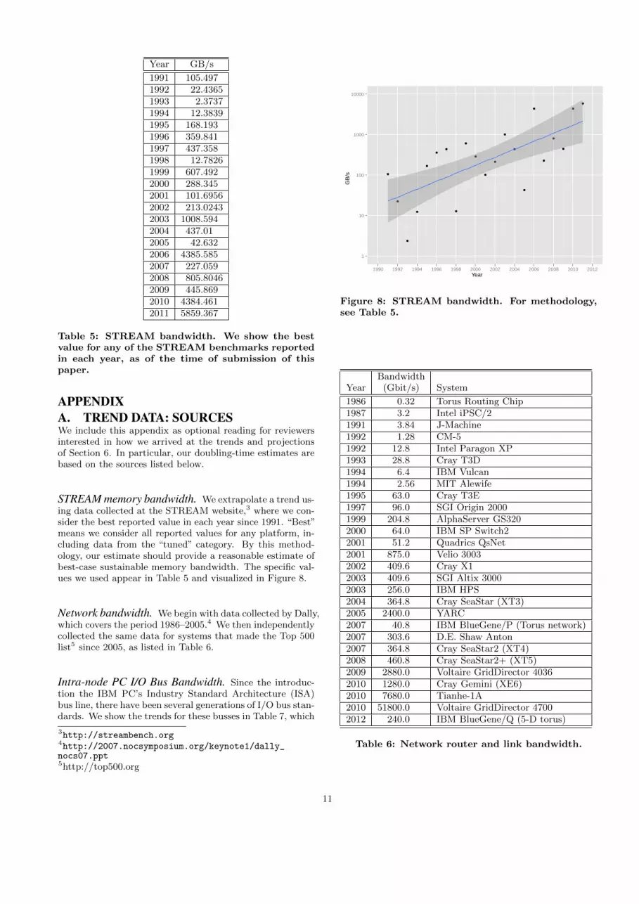
1991 105.4971992 22.43651993 2.37371994 12.38391995 168.1931996 359.8411997 437.3581998 12.78261999 607.4922000 288.3452001 101.69562002 213.02432003 1008.5942004 437.012005 42.6322006 4385.5852007 227.0592008 805.80462009 445.8692010 4384.4612011 5859.367

Table 5: STREAM bandwidth. We show the bestvalue for any of the STREAM benchmarks reportedin each year, as of the time of submission of thispaper.

APPENDIXA. TREND DATA: SOURCESWe include this appendix as optional reading for reviewersinterested in how we arrived at the trends and projectionsof Section 6. In particular, our doubling-time estimates arebased on the sources listed below.

STREAM memory bandwidth. We extrapolate a trend us-ing data collected at the STREAM website,3 where we con-sider the best reported value in each year since 1991. “Best”means we consider all reported values for any platform, in-cluding data from the “tuned” category. By this method-ology, our estimate should provide a reasonable estimate ofbest-case sustainable memory bandwidth. The specific val-ues we used appear in Table 5 and visualized in Figure 8.

Network bandwidth. We begin with data collected by Dally,which covers the period 1986–2005.4 We then independentlycollected the same data for systems that made the Top 500list5 since 2005, as listed in Table 6.

Intra-node PC I/O Bus Bandwidth. Since the introduc-tion the IBM PC’s Industry Standard Architecture (ISA)bus line, there have been several generations of I/O bus stan-dards. We show the trends for these busses in Table 7, which

3http://streambench.org4http://2007.nocsymposium.org/keynote1/dally_nocs07.ppt5http://top500.org

Year

GB

/s

1

10

100

1000

10000

●

●

●

●

●

●

●

●

●

●

●

●

●

●

●

●

●

●

●

●

●

1990 1992 1994 1996 1998 2000 2002 2004 2006 2008 2010 2012

Figure 8: STREAM bandwidth. For methodology,see Table 5.

BandwidthYear (Gbit/s) System

1986 0.32 Torus Routing Chip1987 3.2 Intel iPSC/21991 3.84 J-Machine1992 1.28 CM-51992 12.8 Intel Paragon XP1993 28.8 Cray T3D1994 6.4 IBM Vulcan1994 2.56 MIT Alewife1995 63.0 Cray T3E1997 96.0 SGI Origin 20001999 204.8 AlphaServer GS3202000 64.0 IBM SP Switch22001 51.2 Quadrics QsNet2001 875.0 Velio 30032002 409.6 Cray X12003 409.6 SGI Altix 30002003 256.0 IBM HPS2004 364.8 Cray SeaStar (XT3)2005 2400.0 YARC2007 40.8 IBM BlueGene/P (Torus network)2007 303.6 D.E. Shaw Anton2007 364.8 Cray SeaStar2 (XT4)2008 460.8 Cray SeaStar2+ (XT5)2009 2880.0 Voltaire GridDirector 40362010 1280.0 Cray Gemini (XE6)2010 7680.0 Tianhe-1A2010 51800.0 Voltaire GridDirector 47002012 240.0 IBM BlueGene/Q (5-D torus)

Table 6: Network router and link bandwidth.

11

Year

GB

/s

0.01

0.1

1

10

100

1000

10000

●

●●

●

●

●

●

●

●

●

●

●●

●

● ●

●

●

●

●

●●

●

●

●

●

●

●

1986 1988 1990 1992 1994 1996 1998 2000 2002 2004 2006 2008 2010 2012

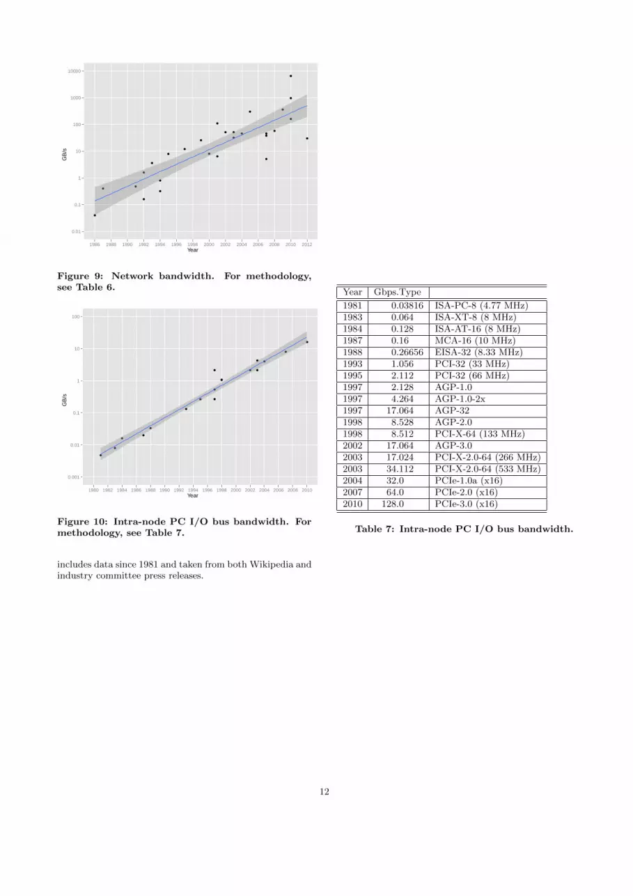
Figure 9: Network bandwidth. For methodology,see Table 6.

Year

GB

/s

0.001

0.01

0.1

1

10

100

●

●

●●

●

●

● ●

●

●

●●

● ●

● ●

●

●

1980 1982 1984 1986 1988 1990 1992 1994 1996 1998 2000 2002 2004 2006 2008 2010

Figure 10: Intra-node PC I/O bus bandwidth. Formethodology, see Table 7.

includes data since 1981 and taken from both Wikipedia andindustry committee press releases.

Year Gbps.Type

1981 0.03816 ISA-PC-8 (4.77 MHz)1983 0.064 ISA-XT-8 (8 MHz)1984 0.128 ISA-AT-16 (8 MHz)1987 0.16 MCA-16 (10 MHz)1988 0.26656 EISA-32 (8.33 MHz)1993 1.056 PCI-32 (33 MHz)1995 2.112 PCI-32 (66 MHz)1997 2.128 AGP-1.01997 4.264 AGP-1.0-2x1997 17.064 AGP-321998 8.528 AGP-2.01998 8.512 PCI-X-64 (133 MHz)2002 17.064 AGP-3.02003 17.024 PCI-X-2.0-64 (266 MHz)2003 34.112 PCI-X-2.0-64 (533 MHz)2004 32.0 PCIe-1.0a (x16)2007 64.0 PCIe-2.0 (x16)2010 128.0 PCIe-3.0 (x16)

Table 7: Intra-node PC I/O bus bandwidth.

12