international conference on exascale applications and software

PROCEEDINGS OF THE 3RD INTERNATIONAL CONFERENCE ON

EXASCALE APPLICATIONS AND SOFTWARE

EASC 2015, 21st to 23rd April 2015, Edinburgh, UK

EDITED BY A GRAY, L SMITH & M WEILAND

Published by The University of Edinburgh This work is licensed under a Creative Commons Attribution-NoDerivatives 4.0 International License. ISBN: 978-0-9926615-1-9

i

Contents Editors’ Introduction .................................................................................... iii Synthetic Program Analysis with Aspen Vetter & Meredith .................................................................................... 1 From 11 to 14.4 PFLOPs: Performance Optimization for Finite Volume Flow Solver Hadjidoukas, Rossinelli, Hejazialhosseini & Koumoutsakos ................... 7 The Impact of Process Placement and Oversubscription on Application Performance Wende, Steinke & Reinefeld ................................................................. 13 Radiative Transfer Modeling at High Performance Computers Using Self-Adjoint Transport Equation Olkhovskaya, Chetverushkin & Gasilov ................................................ 19 Ensuring Efficiency of Exascale Supercomputer Centers Voevodin & Voevodin ............................................................................ 24 Sniper: Simulation-Based Instruction-Level Statistics for Optimizing Software on Future Architectures Heirman, Isaev & Hur ............................................................................ 29 Support Operators Technique for 3D Simulations of Dissipative Processes at High Performance Computers Gasilova, Poveshenko, Boldarev, Bagdasarov & Iakobovski ............... 32 Efficiently Scheduling Task Dataflow Parallelism: A Comparison Between Swan and QUARK Vandierendonck .................................................................................... 36 Portability and Performance of Nuclear Reactor Simulations on Many-Core Architectures Rahaman, Medina, Lund, Tramm, Warburton & Siegel ........................ 42 Exploiting Hierarchical Exascale Hardware using a PGAS Approach Fürlinger ................................................................................................ 48 Enabling Adaptive, Fault-tolerant MPI Applications with Dynamic Resource Allocation Szpindler ............................................................................................... 53 Evaluating Stencil Codes at Scale Modani, Ford, Johnson & Evangelinos ................................................. 58

ii

Exascale Computing for Everyone: Cloud-based, Distributed and Heterogeneous Inggs, Thomas, Hung & Luk ................................................................. 65 Flexible, Scalable Mesh and Data Management using PETSc DMPlex Lange, Knepley & Gorman .................................................................... 71 Prototyping for Exascale Vinter, Kristensen, Lund, Blum & Skovhede ......................................... 77 ExaSHARK+GASPI: Reducing the burden to program large HPC systems since 2014 Vander Aa, Chakroun, Wuyts, Rahn & Simmendinger ......................... 82 Towards Resilient Chapel Panagiotopoulou & Loidl ....................................................................... 86 HPC and CFD in the Marine Industry: Past, Present and Future Mizzi, Kellet, Demirel, Martin & Turan ................................................... 92 Swift: task-based hydrodynamics and gravity for cosmological simulations Theuns, Chalk, Schaller & Gonnet ........................................................ 98 Thread Parallelism for Highly Irregular Computation in Anisotropic Mesh Adaptation Rokos, Gorman, Jensen & Kelly ......................................................... 103 Paradigm Shift for EXASCALE Computing Matheou, Evripidou & Kyriacou ........................................................... 109 Large-scale Ultrasound Simulations Using the Hybrid OpenMP/MPI Decomposition Jaros, Nikl & Treeby ............................................................................ 115 Algorithms in the parallel partitioning tool GridSpiderPar for large mesh decomposition Golovchenko, Kornilina & Yakobovskiy .............................................. 120 Improving Performance Portability and Exascale Software Productivity with the Nabla Numerical Programming Language Camier ................................................................................................. 126 A highly scalable Met Office NERC Cloud model Brown, Weiland, Hill, Shipway, Maynard, Allen & Rezny .................... 132

iii

Editors’ Introduction

The 3rd International Conference on Exascale Applications and Software, EASC 2015, was hosted by EPCC, The University of Edinburgh (in cooperation with SIGHPC) from 21st-23rd April 2015 in Edinburgh.

The scale of today’s leading HPC systems, which operate at the petascale, has put a strain on many simulation codes – both scientific and commercial. Only a small number of applications worldwide have, to date, demonstrated performance at the petaflop/s level. Many of the scientific challenges behind these codes are driving the need for the next generation of exascale HPC systems. Example scientific challenges originate from energy, climate, nanotechnology and medicine and are widely accepted to be of global significance. For simulation codes that are already struggling to scale up to petaflop levels, major investment is required to enable these codes to run at the exascale. Application optimisation and algorithmic modifications only represent part of this challenge. Systems of the scale envisaged present enormous challenges in terms of reliability, programmability, power consumption and usability. Programming models, libraries, languages, compilers and tools all need adaption and improvement. Applications must interact with many of these software aspects to be able to exploit exascale systems efficiently. The aim of this conference was to bring together all of the stakeholders involved in solving the software challenges of the exascale – from application developers, through numerical library experts, programming model developers and integrators, to tools designers.

The event was extremely successful in the dissemination of progress, the discussion of new ideas and the creation of new collaborations. This book contains a selection of proceedings from the conference, which we hope can disseminate the presented research to a wider audience.

Alan Gray, Lorna Smith and Michèle Weiland, Editors

Synthetic Program Analysis with Aspen

Jeffrey S. VetterOak Ridge National Laboratory and

Georgia Institute of [email protected]

Jeremy S. MeredithOak Ridge National Laboratory

[email protected]

ABSTRACTOur community is facing major challenges in the next decade:power, performance, resilience, and productivity. EmergingHPC systems have novel new features, like tightly-integratedheterogeneous computing and nonvolatile memory, that helpsolve one problem but at the cost of introducing considerablenew complexity into the system design. Simply put, we seemore complexity and uncertainty in emerging architecturesthan we have in the last two decades. Given this open de-sign space, architects, applications scientists, and softwaredesigners need tools to estimate performance and resourcerequirements, while taking into account end-to-end designprinciples. In this paper, we demonstrate how our Aspenperformance modeling language can be used to explore im-portant properties of these application design spaces andinform the development of future architectures. We includeexamples from various applications, and show results fromAspen for idealized concurrency, memory capacity, compu-tational intensity, and others.

KeywordsAspen, performance modeling, program analysis

1. INTRODUCTIONOur community is facing major challenges in the next

decade: power, performance, resilience, and productivity.Although these challenges have been with us for some time,they are growing more acute as facilities and scientists arebeing confronted with a new level of complexity and requiredinvestment, deriving from the complex new architectureswith a multitude of features and dynamically-controlled feed-back. Poor decisions in architecting or procuring these nextgeneration systems could have devastating consequences onscientists, sponsors, facilities, and vendors. In fact, manyexperts feel that we will experience the most uncertainty incomputer architectures in two decades. Hence, it is imper-ative to have tools that facilitate end-to-end design [7] anddesign space exploration [10] of HPC systems.

1.1 Surveying the HPC LandscapeOne need look no further than contemporary extreme

scale systems being deployed and procured [11,12]. As moreevidence, recent announcements of future HPC systems inDOE support this point. Titan, Aurora, and Summit willhave entirely new features and configurations that have notbe present in earlier systems. System software, program-ming environments, and applications must be improved to

use these new systems. Given the current outlook as illus-trated in Table 1, it is should be noted that no two architec-tures may be the same. Even if they have similar processors,the memory and storage hierarchy may be different. So, itis very important that these improvements be performanceportable, in order to help hide this complexity.

In particular, several trends are already emerging: het-erogeneous computing, nonvolatile memory, and small or noincreases in storage bandwidth.

First, heterogeneous computing is apparent in many of to-day’s top HPC systems. In earlier systems, such as Titan [2]and Tsubame2 [5], the addition of GPUs to systems gaveperformance improvements while keeping power constraintssatisfied. As this capabilities evolves, we see tighter inte-grations of heterogeneous and special purpose capabilitiesonto general processors. For example, over the past severalyears, Intel has integrated GPUs, compression and encryp-tion engines, random number generators, and other capabil-ities directly onto their main processors [1]. Although thisfunctionality may be exposed to users in a number of ways,it will be imperative to provide portable solutions to HPCusers. As seen in Table 1, both Titan and Summit will haveheterogeneous ISAs within the node that scientists will needto carefully program and orchestrate. Meanwhile, the sameapplications will be expected to run on other platforms likeCori and Aurora.

Second, nonvolatile memory (NVM) systems in additionto alternative memory architectures are emerging as a so-lution to the limits of DRAM scaling, power, and cost [13].Depending on the architectural solution, this change to thememory system could be more disruptive to applicationsteams than the change to heterogeneous computing. NVMdevices have major differences from DRAM [13]: lower writedurability; higher latencies and power costs for writes rel-ative to reads; and, persistent state without the need forstandby power. Again, as with heterogeneous systems, pro-gramming systems, system software, and architectures willneed to hide these often subtle differences from applications.Although NVM devices have been transparently introducedinto existing systems as replacements for hard-disk drives(HDD), they typically use existing I/O block-oriented in-terfaces, though the software stacks have been optimized.In the Summit and Aurora configurations, we must prepareapplications for potentially tigher integration of these NVMdevices with main memory and processors, bypassing theI/O interface [6, 13].

In both of these cases, a number of open research ques-tions about high-level system design remain. These ques-

Proceedings of the 3rd International Conference on Exascale Applications and Software 1

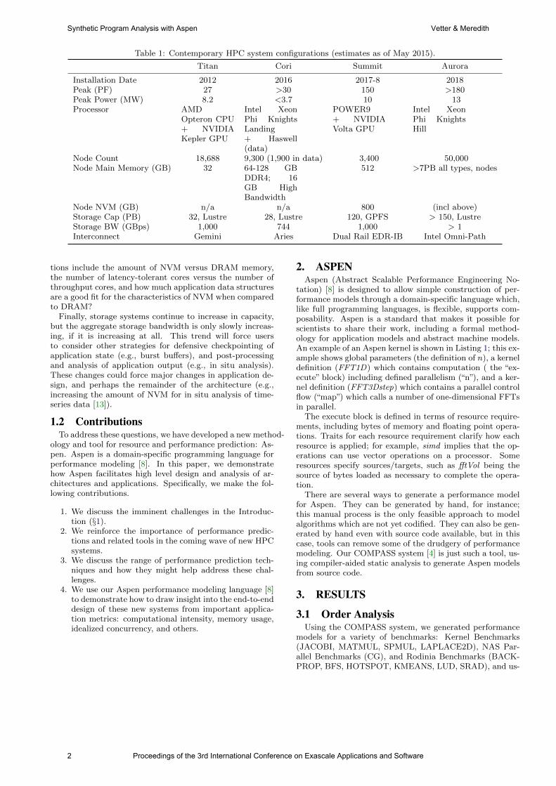
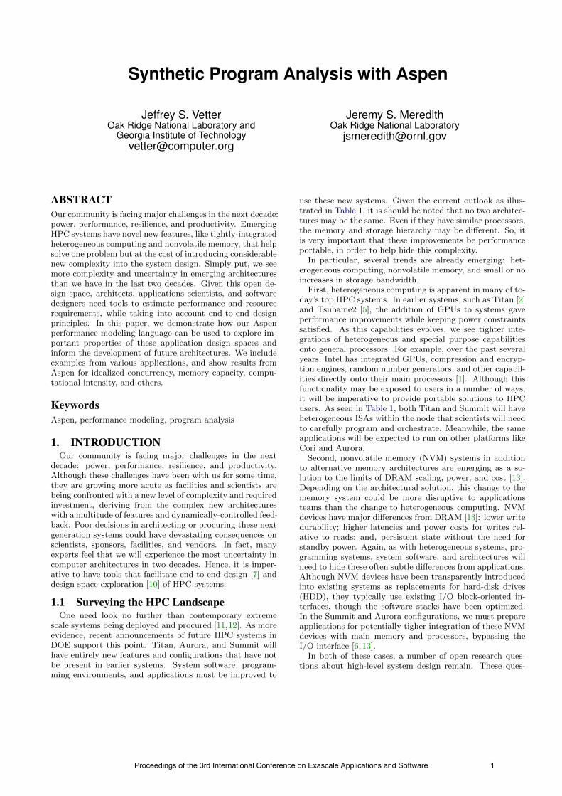
Table 1: Contemporary HPC system configurations (estimates as of May 2015).

Titan Cori Summit Aurora

Installation Date 2012 2016 2017-8 2018Peak (PF) 27 >30 150 >180Peak Power (MW) 8.2 <3.7 10 13Processor AMD

Opteron CPU+ NVIDIAKepler GPU

Intel XeonPhi KnightsLanding+ Haswell(data)

POWER9+ NVIDIAVolta GPU

Intel XeonPhi KnightsHill

Node Count 18,688 9,300 (1,900 in data) 3,400 50,000Node Main Memory (GB) 32 64-128 GB

DDR4; 16GB HighBandwidth

512 >7PB all types, nodes

Node NVM (GB) n/a n/a 800 (incl above)Storage Cap (PB) 32, Lustre 28, Lustre 120, GPFS > 150, LustreStorage BW (GBps) 1,000 744 1,000 > 1Interconnect Gemini Aries Dual Rail EDR-IB Intel Omni-Path

tions include the amount of NVM versus DRAM memory,the number of latency-tolerant cores versus the number ofthroughput cores, and how much application data structuresare a good fit for the characteristics of NVM when comparedto DRAM?

Finally, storage systems continue to increase in capacity,but the aggregate storage bandwidth is only slowly increas-ing, if it is increasing at all. This trend will force usersto consider other strategies for defensive checkpointing ofapplication state (e.g., burst buffers), and post-processingand analysis of application output (e.g., in situ analysis).These changes could force major changes in application de-sign, and perhaps the remainder of the architecture (e.g.,increasing the amount of NVM for in situ analysis of time-series data [13]).

1.2 ContributionsTo address these questions, we have developed a new method-

ology and tool for resource and performance prediction: As-pen. Aspen is a domain-specific programming language forperformance modeling [8]. In this paper, we demonstratehow Aspen facilitates high level design and analysis of ar-chitectures and applications. Specifically, we make the fol-lowing contributions.

1. We discuss the imminent challenges in the Introduc-tion (§1).

2. We reinforce the importance of performance predic-tions and related tools in the coming wave of new HPCsystems.

3. We discuss the range of performance prediction tech-niques and how they might help address these chal-lenges.

4. We use our Aspen performance modeling language [8]to demonstrate how to draw insight into the end-to-enddesign of these new systems from important applica-tion metrics: computational intensity, memory usage,idealized concurrency, and others.

2. ASPENAspen (Abstract Scalable Performance Engineering No-

tation) [8] is designed to allow simple construction of per-formance models through a domain-specific language which,like full programming languages, is flexible, supports com-posability. Aspen is a standard that makes it possible forscientists to share their work, including a formal method-ology for application models and abstract machine models.An example of an Aspen kernel is shown in Listing 1; this ex-ample shows global parameters (the definition of n), a kerneldefinition (FFT1D) which contains computation ( the “ex-ecute” block) including defined parallelism (“n”), and a ker-nel definition (FFT3Dstep) which contains a parallel controlflow (“map”) which calls a number of one-dimensional FFTsin parallel.

The execute block is defined in terms of resource require-ments, including bytes of memory and floating point opera-tions. Traits for each resource requirement clarify how eachresource is applied; for example, simd implies that the op-erations can use vector operations on a processor. Someresources specify sources/targets, such as fftVol being thesource of bytes loaded as necessary to complete the opera-tion.

There are several ways to generate a performance modelfor Aspen. They can be generated by hand, for instance;this manual process is the only feasible approach to modelalgorithms which are not yet codified. They can also be gen-erated by hand even with source code available, but in thiscase, tools can remove some of the drudgery of performancemodeling. Our COMPASS system [4] is just such a tool, us-ing compiler-aided static analysis to generate Aspen modelsfrom source code.

3. RESULTS

3.1 Order AnalysisUsing the COMPASS system, we generated performance

models for a variety of benchmarks: Kernel Benchmarks(JACOBI, MATMUL, SPMUL, LAPLACE2D), NAS Par-allel Benchmarks (CG), and Rodinia Benchmarks (BACK-PROP, BFS, HOTSPOT, KMEANS, LUD, SRAD), and us-

2 Proceedings of the 3rd International Conference on Exascale Applications and Software

Synthetic Program Analysis with Aspen Vetter & Meredith

1 param n = 102423 kernel FFT1D4 5 execute [n]6 7 flops [5 * log2(n)]8 as dp, complex , simd9 loads [a * max(1, log(n)/log(Z))]

10 of size [wordSize]11 from fftVol12 13 1415 kernel FFT3Dstep16 17 map [n^2]18 19 call FFT1D20 21

Listing 1: Aspen Kernel Example for 1D FFT

ing Aspen, we ran a performance prediction for each bench-mark. As mentioned, one of the strengths of analytical per-formance modeling tools like Aspen is the ability to generateresults symbolically. Here, we used Aspen to generate theseequations and perform extra simplification on them, effec-tively treating all arithmetic involving constants as identityoperations and simplifying them away.

For each benchmark, we identified key model parametersto leave as identifiers, but substituted values from applica-tion model and machine model parameters during the sim-plification process. Equations like n∗n+n∗n∗n get factoredduring the process into (1 +n) ∗ (n ∗n), the constant elided,and finally simplified back to n ∗ n ∗ n. In essence, the re-sults give us the order of the runtime (cf. Big O notation)in terms of key application parameters.

The results are shown in Table 2. As a concrete example,we see that the runtime of MATMUL (matrix multiply) re-turns an order of runtime of N ∗M ∗ P ; this is for a matrixmultiply for matrices of size N×M and M×P . In the case ofsquare matrices (where N == M == P ), this simplifies toN3; a result we can easily validate against our expectations.

Benchmark Runtime OrderBACKPROP H ∗O + H ∗ IBFS nodes + edgesCFD nelr ∗ ndimCG nrow + ncolHOTSPOT simtime ∗ rows ∗ colsJACOBI m size ∗m sizeKMEANS nAttr ∗ nClustersLAPLACE2D n2

LUD matrix dim3

MATMUL N ∗M ∗ PNW max cols2

SPMUL size + nonzeroSRAD niter ∗ rows ∗ cols

Table 2: Order analysis, showing Big O runtime for eachbenchmark in terms of its key parameters.

3.2 Computational IntensityThe design of Aspen allows for the ability to represent

and extract key features of computational kernels. One ofthe most common algorithmic features of interest in appli-cations is computational intensity, the ratio of floating pointoperations to the number of bytes loaded. This can be usedto gauge an algorithm’s performance on architectures whichare not defined in vast detail except for key features suchas peak FLOPS rates and memory bandwidth. The well-known roofline plot is a common example — it shows systemperformance for a range of computational intensity values; ifone is interested in measuring system performance in termsof FLOPS, one must have a sufficiently intensive algorithm.

To explore computational intensity for an application indetail, we took a COMPASS-generated model of the USDOE hydrodynamic proxy application, LULESH [3], andasked Aspen to return FLOPS:byte ratios for each majorroutine. The results are shown in Table 3. We see routineswith both low and high computational intensity. Some evenhave zero; those routines simply exist to rearrange memoryfor future computation and perform no floating point oper-ations at all.

Method Name FLOPS/byteInitStressTermsForElems 0.03CalcElemShapeFunctionDerivatives 0.44SumElemFaceNormal 0.50CalcElemNodeNormals 0.15SumElemStressesToNodeForces 0.06IntegrateStressForElems 0.15CollectDomainNodesToElemNodes 0.00VoluDer 1.50CalcElemVolumeDerivative 0.33CalcElemFBHourglassForce 0.15CalcFBHourglassForceForElems 0.17CalcHourglassControlForElems 0.19CalcVolumeForceForElems 0.18CalcForceForNodes 0.18CalcAccelerationForNodes 0.04ApplyAccelerationBoundaryCond 0.00CalcVelocityForNodes 0.13CalcPositionForNodes 0.13LagrangeNodal 0.18AreaFace 10.25CalcElemCharacteristicLength 0.44CalcElemVelocityGrandient 0.13CalcKinematicsForElems 0.24CalcLagrangeElements 0.24CalcMonotonicQGradientsForElems 0.46CalcMonotonicQRegionForElems 0.21CalcMonotonicQForElems 0.21CalcQForElems 0.39CalcPressureForElems 0.08Release 0.04CalcEnergyForElems 0.10CalcSoundSpeedForElems 0.13EvalEOSForElems 0.09ApplyMaterialPropertiesForElems 0.09UpdateVolumesForElems 0.13LagrangeElements 0.22CalcCourantConstraintForElems 0.14CalcHydroConstraintForElems 0.20CalcTimeConstraintsForElems 0.16LagrangeLeapFrog 0.19

Table 3: Computational intensity (bytes loaded or storedper floating point operation) for methods in in the LULESHproxy application.



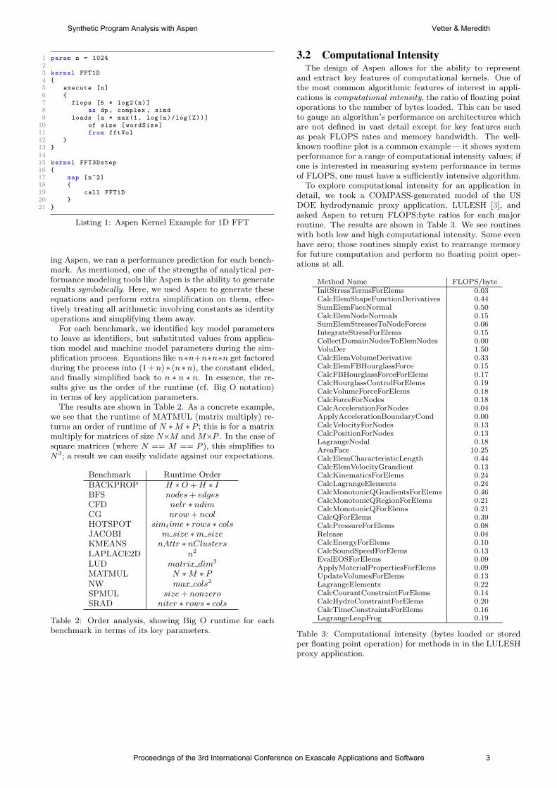
3.3 Memory UsageAnother algorithmic feature commonly of interest is the

amount of memory used by an algorithm. More useful thanmerely the total memory used by the application, a more de-tailed per-kernel breakdown allows a number of further anal-yses. For example, armed with the size of all arrays touchedby each kernel, and the CPU and GPU performance of eachkernel, we can search for an optimal combination of kernelswhich should be offloaded to a GPU – specifically, the setwhich still fits in GPU memory and results in the best over-all performance (including not just per-kernel CPU/GPUperformance, but also any necessary PCI-Express transfertimes for all arrays which are required on both host anddevice).

An example analysis of each major routine in LULESH isshown in Table 4. Note that exclusive memory usage is self-only, and inclusive memory usage includes any arrays usedby any methods called directly or indirectly for each rou-tine. Variables passed directly to a routine are not counted,and so some even computationally-intense routines have anexclusive memory footprint of zero.

Method Name Memory UsageExclusive Inclusive

InitStressTermsForElems 3.6e+06 3.6e+06CalcElemShapeFunctionDerivatives 0 0SumElemFaceNormal 0 0CalcElemNodeNormals 0 0SumElemStressesToNodeForces 1.7e+07 1.7e+07IntegrateStressForElems 2.9e+07 2.9e+07CollectDomainNodesToElemNodes 2.3e+06 2.3e+06VoluDer 0 0CalcElemVolumeDerivative 0 0CalcElemFBHourglassForce 0 0CalcFBHourglassForceForElems 6.6e+07 6.6e+07CalcHourglassControlForElems 4.2e+07 7.0e+07CalcVolumeForceForElems 0 7.3e+07CalcForceForNodes 2.3e+06 7.3e+07CalcAccelerationForNodes 5.4e+06 5.5e+06ApplyAccelerationBoundaryCond 2.4e+06 2.4e+06CalcVelocityForNodes 4.7e+06 4.7e+06CalcPositionForNodes 4.7e+06 4.7e+06LagrangeNodal 0 7.7e+07AreaFace 0 0CalcElemCharacteristicLength 0 0CalcElemVelocityGrandient 192 192CalcKinematicsForElems 1.1e+07 1.1e+07CalcLagrangeElements 2.9e+06 1.1e+07CalcMonotonicQGradientsForElems 1.3e+07 1.3e+07CalcMonotonicQRegionForElems 7.3e+06 7.3e+06CalcMonotonicQForElems 0 7.3e+06CalcQForElems 0 1.9e+07CalcPressureForElems 3.6e+06 3.6e+06Release 7.3e+05 7.3e+05CalcEnergyForElems 1.1e+07 1.2e+07CalcSoundSpeedForElems 4.7e+06 4.7e+06EvalEOSForElems 1.4e+07 1.7e+07ApplyMaterialPropertiesForElems 2.6e+06 1.9e+07UpdateVolumesForElems 1.5e+06 1.5e+06LagrangeElements 0 3.7e+07CalcCourantConstraintForElems 0 2.6e+06CalcHydroConstraintForElems 0 1.1e+06CalcTimeConstraintsForElems 2.2e+06 2.6e+06LagrangeLeapFrog 0 1.0e+08

Table 4: Memory array bytes touched within a method (ex-clusive) and within either a method or its callees (inclusive)in the LULESH proxy application.

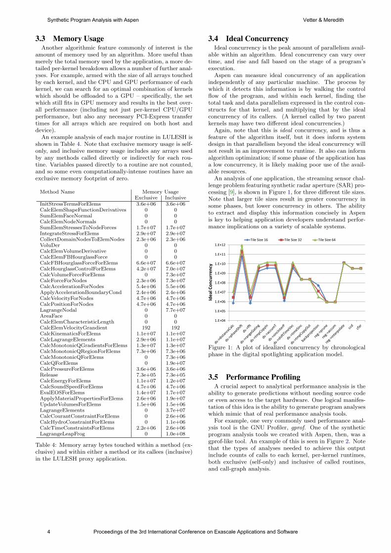
3.4 Ideal ConcurrencyIdeal concurrency is the peak amount of parallelism avail-

able within an algorithm. Ideal concurrency can vary overtime, and rise and fall based on the stage of a program’sexecution.

Aspen can measure ideal concurrency of an applicationindependently of any particular machine. The process bywhich it detects this information is by walking the controlflow of the program, and within each kernel, finding thetotal task and data parallelism expressed in the control con-structs for that kernel, and multiplying that by the idealconcurrency of its callers. (A kernel called by two parentkernels may have two different ideal concurrencies.)

Again, note that this is ideal concurrency, and is thus afeature of the algorithm itself, but it does inform systemdesign in that parallelism beyond the ideal concurrency willnot result in an improvement to runtime. It also can informalgorithm optimization; if some phase of the application hasa low concurrency, it is likely making poor use of the avail-able resources.

An analysis of one application, the streaming sensor chal-lenge problem featuring synthetic radar aperture (SAR) pro-cessing [9], is shown in Figure 1, for three different tile sizes.Note that larger tile sizes result in greater concurrency insome phases, but lower concurrency in others. The abilityto extract and display this information concisely in Aspenis key to helping application developers understand perfor-mance implications on a variety of scalable systems.

1.E+04

1.E+05

1.E+06

1.E+07

1.E+08

1.E+09

1.E+10

1.E+11

1.E+12

Ide

al C

on

curr

en

cy

Tile Size 16 Tile Size 32 Tile Size 64

Figure 1: A plot of idealized concurrency by chronologicalphase in the digital spotlighting application model.

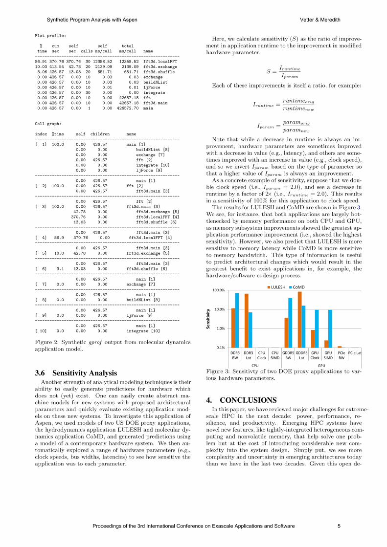
3.5 Performance ProfilingA crucial aspect to analytical performance analysis is the

ability to generate predictions without needing source codeor even access to the target hardware. One logical manifes-tation of this idea is the ability to generate program analyseswhich mimic that of real performance analysis tools.

For example, one very commonly used performance anal-ysis tool is the GNU Profiler, gprof. One of the syntheticprogram analysis tools we created with Aspen, then, was agprof-like tool. An example of this is seen in Figure 2. Notethat the types of analyses needed to achieve this outputinclude counts of calls to each kernel, per-kernel runtimes,both exclusive (self-only) and inclusive of called routines,and call-graph analysis.



Flat profile:

% cum self self totaltime sec sec calls ms/call ms/call name------------------------------------------------------------86.91 370.76 370.76 30 12358.52 12358.52 fft3d.localFFT10.03 413.54 42.78 20 2139.09 2139.09 fft3d.exchange3.06 426.57 13.03 20 651.71 651.71 fft3d.shuffle0.00 426.57 0.00 10 0.03 0.03 exchange0.00 426.57 0.00 10 0.03 0.03 buildNList0.00 426.57 0.00 10 0.01 0.01 ljForce0.00 426.57 0.00 30 0.00 0.00 integrate0.00 426.57 0.00 10 0.00 42657.18 fft0.00 426.57 0.00 10 0.00 42657.18 fft3d.main0.00 426.57 0.00 1 0.00 426572.70 main

Call graph:

index %time self children name------------------------------------------------------------[ 1] 100.0 0.00 426.57 main [1]

0.00 0.00 buildNList [8]0.00 0.00 exchange [7]0.00 426.57 fft [2]0.00 0.00 integrate [10]0.00 0.00 ljForce [9]

------------------------------------------------------------0.00 426.57 main [1]

[ 2] 100.0 0.00 426.57 fft [2]0.00 426.57 fft3d.main [3]

------------------------------------------------------------0.00 426.57 fft [2]

[ 3] 100.0 0.00 426.57 fft3d.main [3]42.78 0.00 fft3d.exchange [5]370.76 0.00 fft3d.localFFT [4]13.03 0.00 fft3d.shuffle [6]

------------------------------------------------------------0.00 426.57 fft3d.main [3]

[ 4] 86.9 370.76 0.00 fft3d.localFFT [4]------------------------------------------------------------

0.00 426.57 fft3d.main [3][ 5] 10.0 42.78 0.00 fft3d.exchange [5]------------------------------------------------------------

0.00 426.57 fft3d.main [3][ 6] 3.1 13.03 0.00 fft3d.shuffle [6]------------------------------------------------------------

0.00 426.57 main [1][ 7] 0.0 0.00 0.00 exchange [7]------------------------------------------------------------

0.00 426.57 main [1][ 8] 0.0 0.00 0.00 buildNList [8]------------------------------------------------------------

0.00 426.57 main [1][ 9] 0.0 0.00 0.00 ljForce [9]------------------------------------------------------------

0.00 426.57 main [1][ 10] 0.0 0.00 0.00 integrate [10]

Figure 2: Synthetic gprof output from molecular dynamicsapplication model.

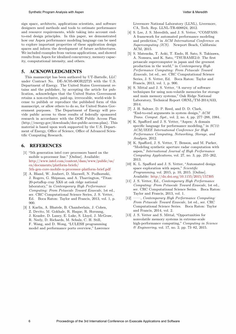
3.6 Sensitivity AnalysisAnother strength of analytical modeling techniques is their

ability to easily generate predictions for hardware whichdoes not (yet) exist. One can easily create abstract ma-chine models for new systems with proposed architecturalparameters and quickly evaluate existing application mod-els on these new systems. To investigate this application ofAspen, we used models of two US DOE proxy applications,the hydrodynamics application LULESH and molecular dy-namics application CoMD, and generated predictions usinga model of a contemporary hardware system. We then au-tomatically explored a range of hardware parameters (e.g.,clock speeds, bus widths, latencies) to see how sensitive theapplication was to each parameter.

Here, we calculate sensitivity (S) as the ratio of improve-ment in application runtime to the improvement in modifiedhardware parameter.

S =Iruntime

Iparam

Each of these improvements is itself a ratio, for example:

Iruntime =runtimeorigruntimenew

Iparam =paramorig

paramnew

Note that while a decrease in runtime is always an im-provement, hardware parameters are sometimes improvedwith a decrease in value (e.g., latency), and others are some-times improved with an increase in value (e.g., clock speed),and so we invert Iparam based on the type of parameter sothat a higher value of Iparam is always an improvement.

As a concrete example of sensitivity, suppose that we dou-ble clock speed (i.e., Iparam = 2.0), and see a decrease inruntime by a factor of 2× (i.e., Iruntime = 2.0). This resultsin a sensitivity of 100% for this application to clock speed.

The results for LULESH and CoMD are shown in Figure 3.We see, for instance, that both applications are largely bot-tlenecked by memory performance on both CPU and GPU,as memory subsystem improvements showed the greatest ap-plication performance improvement (i.e., showed the highestsensitivity). However, we also predict that LULESH is moresensitive to memory latency while CoMD is more sensitiveto memory bandwidth. This type of information is usefulto predict architectural changes which would result in thegreatest benefit to exist applications in, for example, thehardware/software codesign process.

0.1%

1.0%

10.0%

100.0%

DDR3BW

DDR3Lat

CPUClock

CPUSIMD

GDDR5BW

GDDR5Lat

GPUClock

GPUSIMD

PCIeBW

PCIe Lat

CPU GPU

Sen

siti

vity

LULESH CoMD

Figure 3: Sensitivty of two DOE proxy applications to var-ious hardware parameters.

4. CONCLUSIONSIn this paper, we have reviewed major challenges for extreme-

scale HPC in the next decade: power, performance, re-silience, and productivity. Emerging HPC systems havenovel new features, like tightly-integrated heterogeneous com-puting and nonvolatile memory, that help solve one prob-lem but at the cost of introducing considerable new com-plexity into the system design. Simply put, we see morecomplexity and uncertainty in emerging architectures todaythan we have in the last two decades. Given this open de-



sign space, architects, applications scientists, and softwaredesigners need methods and tools to estimate performanceand resource requirements, while taking into account end-to-end design principles. In this paper, we demonstratedhow our Aspen performance modeling language can be usedto explore important properties of these application designspaces and inform the development of future architectures.We included examples from various applications, and showedresults from Aspen for idealized concurrency, memory capac-ity, computational intensity, and others.

5. ACKNOWLEDGMENTSThis manuscript has been authored by UT-Battelle, LLC

under Contract No. DE-AC05-00OR22725 with the U.S.Department of Energy. The United States Government re-tains and the publisher, by accepting the article for pub-lication, acknowledges that the United States Governmentretains a non-exclusive, paid-up, irrevocable, world-wide li-cense to publish or reproduce the published form of thismanuscript, or allow others to do so, for United States Gov-ernment purposes. The Department of Energy will pro-vide public access to these results of federally sponsoredresearch in accordance with the DOE Public Access Plan(http://energy.gov/downloads/doe-public-access-plan). Thismaterial is based upon work supported by the U.S. Depart-ment of Energy, Office of Science, Office of Advanced Scien-tific Computing Research.

6. REFERENCES[1] “5th generation intel core processors based on the

mobile u-processor line.” [Online]. Available:http://www.intel.com/content/dam/www/public/us/en/documents/platform-briefs/5th-gen-core-mobile-u-processor-platform-brief.pdf

[2] A. Bland, W. Joubert, D. Maxwell, N. Podhorszki,J. Rogers, G. Shipman, and A. Tharrington, “Titan:20-petaflop cray XK6 at oak ridge nationallaboratory,” in Contemporary High PerformanceComputing: From Petascale Toward Exascale, 1st ed.,ser. CRC Computational Science Series, J. S. Vetter,Ed. Boca Raton: Taylor and Francis, 2013, vol. 1, p.900.

[3] I. Karlin, A. Bhatele, B. Chamberlain, J. Cohen,Z. Devito, M. Gokhale, R. Haque, R. Hornung,J. Keasler, D. Laney, E. Luke, S. Lloyd, J. McGraw,R. Neely, D. Richards, M. Schulz, C. H. Still,F. Wang, and D. Wong, “LULESH programmingmodel and performance ports overview,” Lawrence

Livermore National Laboratory (LLNL), Livermore,CA, Tech. Rep. LLNL-TR-608824, 2012.

[4] S. Lee, J. S. Meredith, and J. S. Vetter, “COMPASS:A framework for automated performance modelingand prediction,” in ACM International Conference onSupercomputing (ICS). Newport Beach, California:ACM, 2015.

[5] S. Matsuoka, T. Aoki, T. Endo, H. Sato, S. Takizawa,A. Nomura, and K. Sato, “TSUBAME2.0: The firstpetascale supercomputer in japan and the greenestproduction in the world,” in Contemporary HighPerformance Computing: From Petascale TowardExascale, 1st ed., ser. CRC Computational Science

Series, J. S. Vetter, Ed. Boca Raton: Taylor andFrancis, 2013, vol. 1, p. 900.

[6] S. Mittal and J. S. Vetter, “A survey of softwaretechniques for using non-volatile memories for storageand main memory systems,” Oak Ridge NationalLaboratory, Technical Report ORNL/TM-2014/633,2014.

[7] J. H. Saltzer, D. P. Reed, and D. D. Clark,“End-to-end arguments in system design,” ACMTrans. Comput. Syst., vol. 2, no. 4, pp. 277–288, 1984.

[8] K. Spafford and J. S. Vetter, “Aspen: A domainspecific language for performance modeling,” in SC12:ACM/IEEE International Conference for HighPerformance Computing, Networking, Storage, andAnalysis, 2012.

[9] K. Spafford, J. S. Vetter, T. Benson, and M. Parker,“Modeling synthetic aperture radar computation withaspen,” International Journal of High PerformanceComputing Applications, vol. 27, no. 3, pp. 255–262,2013.

[10] K. L. Spafford and J. S. Vetter, “Automated designspace exploration with aspen,” ScientificProgramming, vol. 2015, p. 10, 2015. [Online].Available: http://dx.doi.org/10.1155/2015/157305

[11] J. S. Vetter, Ed., Contemporary High PerformanceComputing: From Petascale Toward Exascale, 1st ed.,ser. CRC Computational Science Series. Boca Raton:Taylor and Francis, 2013, vol. 1.

[12] ——, Contemporary High Performance Computing:From Petascale Toward Exascale, 1st ed., ser. CRCComputational Science Series. Boca Raton: Taylorand Francis, 2014, vol. 2.

[13] J. S. Vetter and S. Mittal, “Opportunities fornonvolatile memory systems in extreme-scalehigh-performance computing,” Computing in Science& Engineering, vol. 17, no. 2, pp. 73–82, 2015.



http://www.intel.com/content/dam/www/public/us/en/documents/platform-briefs/5th-gen-core-mobile-u-processor-platform-brief.pdf



http://dx.doi.org/10.1155/2015/157305

From 11 to 14.4 PFLOPs:Performance Optimization for Finite Volume Flow Solver

Panagiotis E. [email protected]

Diego [email protected]

Babak [email protected]

Petros [email protected]

Chair of Computational Science, D-MAVT ETH Zürich, 8092 Switzerland

ABSTRACTCUBISM-MPCF is a compressible, two-phase flow solverthat has performed unprecedented flow simulations, employ-ing 13 trillion computational elements to study cavitationcollapse of a cloud composed of 15’000 bubbles. The codehad been deployed on 1.6 million cores of the Sequoia IBMBlueGene/Q supercomputer, reaching initially 11 PFLOPs,corresponding to 55% of its nominal peak performance. Thispaper reports, for the first time, the techniques used toextend the performance of the code by 30% reaching 14.4PFLOPs on BlueGene/Q systems. The achieved 72% ofthe peak performance constitutes to date the best perfor-mance for flow simulations in supercomputer architectures.Our techniques take advantage of the underlying hardwarecapabilities and were applied through all levels in the soft-ware abstraction aiming at full exploitation of the inherentinstruction/data-,thread- and cluster-level parallelism. Thesoftware advances by two to three orders of magnitude thestate-of-the-art both in terms of time to solution and geo-metric complexity of the flow. We believe that the presentmethods are relevant to all grid based solvers and as suchthey may serve to enhance the capabilities across differentareas of simulation based science.

KeywordsHigh performance computing, flow simulations, supercom-puters

1. INTRODUCTIONVehicles operating with liquid fluids are the most domi-

nant form of transportation and they account for more than20% of the world‘s energy resources. Their energy efficientoperation is of paramount importance as further reductionin CO2 emissions requires improving the efficiency of inter-nal combustion engines which in turn implies high-pressurefuel injection systems. Precise fuel injection control andenhanced fuel-air mixing implies high liquid fuel injectionpressures. In such conditions, liquid fuel can undergo va-porization and subsequent re-condensation in the combus-tion chamber. Clusters of vapor bubbles incepted in suchflow conditions are referred to as “cloud cavitation”. Theircollapse induces pressure peaks up to two orders of mag-nitude larger than the ambient pressure [10]. When suchpressures are exerted on solid walls they can cause materialerosion of the combustion chamber and limit the lifetimeof the fuel injectors. The damaging effects of cloud cavita-

tion collapse are also detrimental to the operation of marinepropellers and turbomachinery yet they can be harnessed inmedical applications ranging from kidney lithotripsy to drugdelivery [7].

Realistic simulations require two phase flow solvers ca-pable of capturing interactions between multiple deform-ing bubbles, pressure waves and shocks and their interac-tion with turbulent flow fields. CUBISM-MPCF is a highthroughput software (ACM Gordon Bell Prize 2013) [8] thataddresses challenges critical to flow simulations in terms offloating point operations, memory traffic and storage capac-ity. The software has been designed to take advantage ofthe features of the IBM BlueGene/Q (BGQ) platform tosimulate cavitation collapse dynamics using up to 13 trillioncomputational elements. The performance of the softwarehas been shown to reach an unprecedented 14.4 PFLOP/son 1.6 million cores corresponding to 72% of the peak onthe 20 PFLOP/s Sequoia supercomputer. Furthermore, thesoftware introduces a first of its kind efficient wavelet basedcompression scheme, in order to decrease the I/O time andthe footprint of the simulations. The scheme delivers com-pression rates up to 100 : 1 and takes less than 1% of thetotal simulation time.

As collapsing bubbles cover about 50% of the computa-tional domain, we chose a uniform resolution over an adap-tive mesh refinement [2] or a multi resolution technique [11]for the discretization of this flow field. By performing simu-lations that resolve collapsing clouds with up to 15’000 bub-bles, CUBISM-MPCF improved by two orders of magnitudethe previous state of the art, set by Adams and Schmidt[1]. Considering uniform resolution solvers, simulations ofnoise propagation of jet engines were performed on Sequoiausing similar number of computational elements but withsignificantly lower performance in terms of time to solutionand percentage of the peak [3]. Regarding performance, anearlier version of the present software achieved 30% of thenominal peak on 47k cores of Cray XE6 Monte Rosa [4] forstudies of shock-bubble interactions.

In this work, we first discuss our key software design de-cisions for addressing simulation challenges with regard tofloating point operations and memory traffic. Then, wepresent and evaluate optimization techniques that allowedus to improve the initial performance of CUBISM-MPCFfrom 55% to 72% of the theoretical peak on BGQ systems,which is translated to the increase from 11 to 14.4 PFLOP/son Sequoia. These techniques take advantage of the under-lying hardware capabilities and were applied at the three


abstraction layers of the software (core, node, and cluster),aiming at full exploitation of the inherent instruction/data-,thread- and cluster-level parallelism.

The paper is organized as follows: in Section 2 we brieflypresent the governing equations and their numerical dis-cretization. In Sections 4 and 3 we present CUBISM-MPCFand summarize the main features of the BGQ platform, re-spectively. In Section5 we present the optimization tech-niques that improved the efficiency of our solver. Detailedperformance results of the improved solver are presented inSection 6. Finally, we conclude in Section 7.

2. EQUATIONS AND DISCRETIZATIONCavitation dynamics involve a complex interplay of physi-

cal processes associated with compressibility, convective andviscous dissipation effects. We simulated cavitation in in-viscid, compressible, two-phase flows using a finite-volumediscretisation of the governing Euler equations. The evolu-tion of density, momenta and the total energy of the flow isdescribed with the following system of equations:

∂ρ

∂t+∇ · (ρu) = 0,

∂(ρu)

∂t+∇ · (ρuuT + pI) = 0,

∂(E)

∂t+∇ · ((E + p)u) = 0. (1)

The evolution of the vapor and liquid phases is determinedby another set of advection equations:

∂φ

∂t+ u · ∇φ = 0, (2)

where φ = (Γ,Π) with Γ = 1/(γ − 1) and Π = γpc/(γ −1). The specific heat ratio γ and the correction pressure ofthe mixture pc are coupled to the system of equations (1)through a stiffened equation of state of the form Γp + Π =E − 1/2ρ|u|2.

We discretize these equations using a finite volume methodin space and evolving the cell averages in time with anexplicit time discretization. Each simulation step involvesthree kernels: DT, RHS and UP. The DT kernel computesa time step that is obtained by a global data reduction ofthe maximum characteristic velocity. The RHS kernel en-tails the evaluation of the Right-Hand Side (RHS) of thegoverning equations for every cell-average. The UP kernelupdates the flow quantities using a Total Variation Dimin-ishing (TVD) scheme. Depending on the chosen time dis-cretization order, RHS and UP kernels are executed multipletimes per step.

The spatial reconstruction of the flow field is carried outon velocity and pressure ([6]) while their zero jump condi-tions across the contact discontinuities are maintained by re-constructing special functions of the specific heat ratios andcorrection pressures. Quantities at the cell boundaries arereconstructed through the fifth-order Weighted EssentiallyNon-Oscillatory (WENO) scheme [5]. In order to advancethe system, we compute the numerical fluxes by using theHLLE (Harten, Lax, van Leer, Einfeldt) scheme [12]. Theevaluation of RHS requires information exchange of adjacentsubdomains due to the WENO scheme. The RHS evalua-tion includes five stages/microkernels: a conversion stagefrom conserved to primitive quantities (CONV), a spatialreconstruction (WENO) using neighboring cells, evaluation

Table 1: BGQ node performance table.Cores 16, 4-way SMT, 1.6 GHzMemory 16KB L1, 32MB L2, 16GB DDR3Peak performance 204.8 GFLOP/sL2 bandwidth 185 GB/s (measured)DDR3 bandwidth 28 GB/s (measured)

of the numerical flux (HLLE) at the cell boundaries, sum-mation of the fluxes (SUM) and a final stage for writing backthe results (BACK).

3. HARDWARE PLATFORMOur target platform was the IBM Blue Gene/Q super-

computer. This platform is based on the BGQ computechip which is equipped with 16 symmetric cores operatingat 1.6 GHz. A per-core Quad floating-point Processing Unitimplements the QPX instruction set and has a SIMD-widthof 4. Each core supports 4 hardware threads, offering a max-imum concurrency of 64 on a single BGQ node. A 16 KB L1data cache is shared across the hardware threads of a singlecore. Each core accesses the shared L2 data cache througha crossbar. L2 is organized in 16 slices of 2 MB and mem-ory addresses are scattered across these slices. An L1 cacheprefetching unit aims at hiding possible latencies from theL2 data cache and DDR memory.

Table 1 summarizes the main performance features of asingle BGQ node. Node boards consist of 32 compute nodesand are grouped in 32 to form a rack, with a nominal com-pute performance of 0.21 PFLOP/s. BGQ nodes are placedin a five-dimensional network topology, with a network band-width of 2 GB/s for sending and 2 GB/s for receiving data,respectively. Due to the relatively low ridge point of theplatform, kernels that exhibit operational intensities higherthan 7.3 FLOP/off-chip Bytes are compute-bound.

4. SOFTWARE LAYOUTCUBISM-MPCF is designed to minimize compulsory mem-

ory traffic by using low-storage time stepping schemes thatreduce the overall memory footprint and high-order spa-tiotemporal discretization schemes that decrease the totalnumber of steps. In its current version, the solver employsa third-order low-storage TVD Runge-Kutta time steppingscheme, combined with a fifth order WENO scheme. Toavoid degradation of operation intensity, we employ datareordering and cache-aware techniques. Data reordering isachieved by grouping the computational elements into 3Dblocks of contiguous memory, organized in an AoS format.To effectively operate on blocks we consider SIMD-friendlytemporary data structures, in SoA format, that allow for ex-tensive use of vector intrinsics In addition, to increase tem-poral locality we employ computation reordering techniqueswhen evaluating the RHS.

CUBISM-MPCF is written in C++ and parallelized usingthe MPI and OpenMP programming models. It is concep-tually decomposed into three layers: cluster, node, and core.

The cluster layer is responsible for the domain decomposi-tion and the inter-rank information exchange based on MPI.The computational domain is decomposed into subdomainsacross the ranks in a cartesian topology with a constant sub-domain size. The subdomains are further decomposed intoconstant-sized blocks of data, which are divided into halo


From 11 to 14.4 PFLOPs: Performance Optimization for Finite Volume Flow Solver Hadjidoukas, Rossinelli, Hejazialhosseini & Koumoutsakos

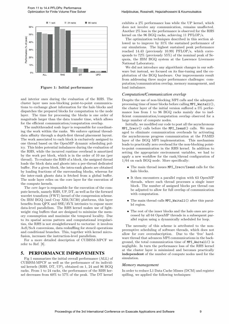
Figure 1: Initial performance

and interior ones during the evaluation of the RHS. Thecluster layer uses non-blocking point-to-point communica-tions to exchange ghost information for the halo blocks anddispatches the prepared blocks for computation to the nodelayer. The time for processing the blocks is one order ofmagnitude larger than the data transfer time, which allowsfor the efficient communication/computation overlap.

The multithreaded node layer is responsible for coordinat-ing the work within the ranks. We enforce optimal thread-data affinity through a depth-first thread placement layout.The work associated to each block is exclusively assigned toone thread based on the OpenMP dynamic scheduling pol-icy. This hides potential imbalances during the evaluation ofthe RHS, while the incurred runtime overhead is amortizedby the work per block, which is in the order of 10 ms (perthread). To evaluate the RHS of a block, the assigned threadloads the block data and ghosts into a per-thread dedicatedbuffer. For a given block, the intra-rank ghosts are obtainedby loading fractions of the surrounding blocks, whereas forthe inter-rank ghosts data is fetched from a global buffer.The node layer relies on the core layer for the execution ofthe compute kernels.

The core layer is responsible for the execution of the com-pute kernels, namely RHS, UP, DT, as well as for the forwardwavelet transform (FWT) kernel of the compression scheme.On IBM BGQ (and Cray XE6/XC30) platforms, this layerbenefits from QPX and SSE/AVX intrinsics to expose moredata-level parallelism. The RHS kernel makes use of light-weight ring buffers that are designed to minimize the mem-ory consumption and maximize the temporal locality. Dueto its spatial access pattern and computational irregulari-ties, the RHS is not straightforward to vectorize: it involvesAoS/SoA conversions, data reshuffling for stencil operationsand conditional branches. This, together with kernel micro-fusion, increases the instruction-level parallelism.

For a more detailed description of CUBISM-MPCF werefer to Ref. [8].

5. PERFORMANCE IMPROVEMENTSFig 1 summarizes the initial overall performance (ALL) of

CUBISM-MPCF as well as the performance of its individ-ual kernels (RHS, DT, UP), obtained on 1, 24 and 96 BGQracks. From 1 to 24 racks, the performance of the RHS ker-nel decreases from 60% to 57% of the peak. The DT kernel

exhibits a 2% performance loss while the UP kernel, whichdoes not involve any communication, remains unaffected.Another 2% loss in the performance is observed for the RHSkernel on the 96 BGQ racks, achieving 11 PFLOP/s.

The optimization techniques described in this section al-lowed us to improve by 31% the sustained performance ofour simulations. The highest sustained peak performancereached 14.43 (previously 10.99) PFLOP/s, which corre-sponds to 72% (previously 55%) of the nominal peak of Se-quoia, the IBM BGQ system at the Lawrence LivermoreNational Laboratory.

We did not introduce any algorithmic changes in our soft-ware but instead, we focused on its fine-tuning and the ex-ploitation of the BGQ hardware. Our improvements resultfrom addressing three major performance challenges: com-putation/communication overlap, memory management, andload imbalance.

Computation/Communication overlapDespite the use of non-blocking MPI calls and the adequateprocessing time of inner blocks before calling MPI_Waitall(),the cluster layer of the initial version suffered a 5% perfor-mance loss from 1 to 96 BGQ racks mainly due to inef-ficient communication/computation overlap observed for alarge number of compute nodes.

Initially, we modified our code to post all the asynchronousMPI_Irecv() calls before the MPI_Isend() calls. We man-aged to eliminate communication overheads by activatingthe asynchronous progress communication at the PAMIDlayer of the BGQ MPI implementation. This mechanismleads to practically zero overhead for the non-blocking point-to-point communication in the RHS kernel. In addition tosetting the appropriate environment variables, we had toapply a new workflow for the rank/thread configuration of1/64 on each BGQ node. More specifically:

• The main thread issues MPI_Irecv/Isend calls for thehalo blocks.

• It then encounters a parallel region with 63 OpenMPthreads, where each thread processes a single innerblock. The number of assigned blocks per thread canbe adjusted to allow for full overlap of communicationwith computation.

• The main thread calls MPI_Waitall() after this paral-lel region.

• The rest of the inner blocks and the halo ones are pro-cessed by all 64 OpenMP threads in a subsequent par-allel region using a dynamically scheduled for loop.

The necessity of this scheme is attributed to the non-preemptive scheduling of software threads, which does notallow for core oversubscription. Due to the ‘free’ hard-ware thread that advances MPI communications in the back-ground, the total communication time of MPI_Waitall() isnegligible. In turn the performance loss of the RHS kernelat the cluster layer is minimized and becomes practicallyindependent of the number of compute nodes used for thesimulation.

Memory managementIn order to reduce L1 Data Cache Misses (DCM) and registerspilling, we applied the following techniques:



1. Linear stream prefetching of data was activated withthe confirmed mode and depth equal to one (defaultis two). A stream is confirmed when there are two L1cache misses within 128 bytes.

2. Deactivation of compiler-based unrolling of a loop thatinvokes the QPX-based WENO kernel. The initiallyused pragma unroll(4) compiler directive was affect-ing performance due to register spilling.

3. Faster loading of ghost data both at the node and clus-ter layer due to more efficient unpacking of the receiveddata. This was achieved by extensive use of the built-in __bcopy() function.

Load imbalanceThe load imbalance at the cluster layer was originally mani-fested by significant times spent at MPI_Allreduce. Besidesthe varying times of MPI_Waitall, load imbalance was in-troduced by the intra-node scheduling scheme for block pro-cessing and the boundary conditions at the cluster level. wemade the following code modifications:

1. Besides fine tuning of computation/communication over-lap, the adopted block processing workflow improvesload balancing because blocks are distributed evenly tothe OpenMP threads of the two parallel regions men-tioned above. For instance, for a typical cubic sub-domain of 163 = 4096 blocks per node, 63 blocks areinitially processed and then 4033 blocks are dynam-ically distributed among 64 threads. In contrast, thepreviously used workflow first assigns 2744 inner blocksand then 1352 halo blocks to 64 threads, increasing thepossibility that some OpenMP threads to become idle.

2. Boundary conditions are enforced by using loop un-rolling and copying memory with the __bcopy() func-tion. This minimizes per-block overheads and com-bined with the faster loading of ghost data leads tomore uniform block-processing time across the com-pute nodes and, thus, in better load balancing.

Additional fine tuning optionsWe observed minor performance improvements (<0.5%) inour solver for the following options:

• Use of the same optimization flag (“-O3”) for all thethree layers of the software: the core layer was previ-ously compiled with “-O5” .

• Decrease of the stack size of OpenMP threads from1MB to 512KB.

Numerical accuracyIn addition to these advances, we extended the level of accu-racy in our simulations, by introducing an additional secondpass in the Newton-Raphson scheme used for the compu-tation of the reciprocals. The previously employed single-pass scheme achieves 13.79 PFLOP/s of peak performancefor the RHS Kernel. The two-pass scheme increases thecomputational intensity with respect to the single-pass, atthe expense of slightly higher time-to-solution (12%). This,combined with the better exploitation of memory subsys-tem and the communication and load imbalance advancesallowed us to reach 14.43 PFLOP/s for the RHS kernel.

6. PERFORMANCE RESULTSWe compiled CUBISM-MPCF with the same software stack

and version of the IBM XL C/C++ compiler (v12.1) andused the IBM Hardware Performance Monitor (HPM) Toolkitfor BGQ for measuring performance figures.

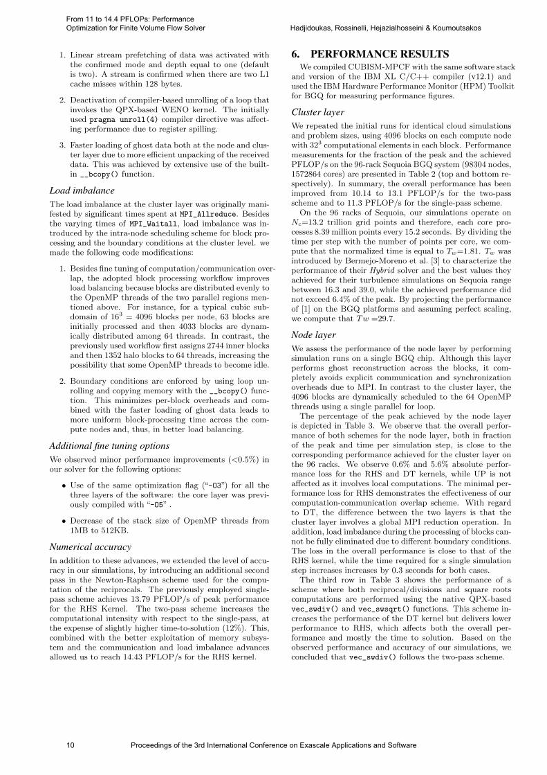
Cluster layerWe repeated the initial runs for identical cloud simulationsand problem sizes, using 4096 blocks on each compute nodewith 323 computational elements in each block. Performancemeasurements for the fraction of the peak and the achievedPFLOP/s on the 96-rack Sequoia BGQ system (98304 nodes,1572864 cores) are presented in Table 2 (top and bottom re-spectively). In summary, the overall performance has beenimproved from 10.14 to 13.1 PFLOP/s for the two-passscheme and to 11.3 PFLOP/s for the single-pass scheme.

On the 96 racks of Sequoia, our simulations operate onNc=13.2 trillion grid points and therefore, each core pro-cesses 8.39 million points every 15.2 seconds. By dividing thetime per step with the number of points per core, we com-pute that the normalized time is equal to Tw=1.81. Tw wasintroduced by Bermejo-Moreno et al. [3] to characterize theperformance of their Hybrid solver and the best values theyachieved for their turbulence simulations on Sequoia rangebetween 16.3 and 39.0, while the achieved performance didnot exceed 6.4% of the peak. By projecting the performanceof [1] on the BGQ platforms and assuming perfect scaling,we compute that Tw =29.7.

Node layerWe assess the performance of the node layer by performingsimulation runs on a single BGQ chip. Although this layerperforms ghost reconstruction across the blocks, it com-pletely avoids explicit communication and synchronizationoverheads due to MPI. In contrast to the cluster layer, the4096 blocks are dynamically scheduled to the 64 OpenMPthreads using a single parallel for loop.

The percentage of the peak achieved by the node layeris depicted in Table 3. We observe that the overall perfor-mance of both schemes for the node layer, both in fractionof the peak and time per simulation step, is close to thecorresponding performance achieved for the cluster layer onthe 96 racks. We observe 0.6% and 5.6% absolute perfor-mance loss for the RHS and DT kernels, while UP is notaffected as it involves local computations. The minimal per-formance loss for RHS demonstrates the effectiveness of ourcomputation-communication overlap scheme. With regardto DT, the difference between the two layers is that thecluster layer involves a global MPI reduction operation. Inaddition, load imbalance during the processing of blocks can-not be fully eliminated due to different boundary conditions.The loss in the overall performance is close to that of theRHS kernel, while the time required for a single simulationstep increases increases by 0.3 seconds for both cases.

The third row in Table 3 shows the performance of ascheme where both reciprocal/divisions and square rootscomputations are performed using the native QPX-basedvec_swdiv() and vec_swsqrt() functions. This scheme in-creases the performance of the DT kernel but delivers lowerperformance to RHS, which affects both the overall per-formance and mostly the time to solution. Based on theobserved performance and accuracy of our simulations, weconcluded that vec_swdiv() follows the two-pass scheme.



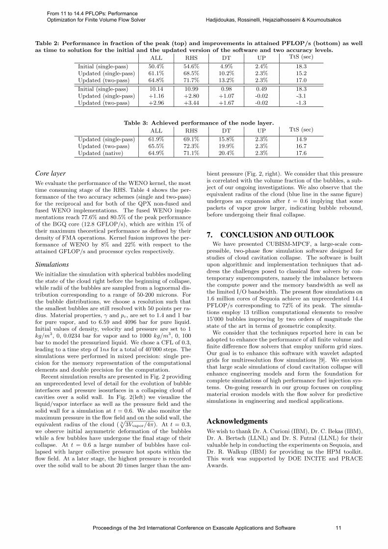
Table 2: Performance in fraction of the peak (top) and improvements in attained PFLOP/s (bottom) as wellas time to solution for the initial and the updated version of the software and two accuracy levels.

ALL RHS DT UP TtS (sec)

Initial (single-pass) 50.4% 54.6% 4.9% 2.4% 18.3Updated (single-pass) 61.1% 68.5% 10.2% 2.3% 15.2Updated (two-pass) 64.8% 71.7% 13.2% 2.3% 17.0

Initial (single-pass) 10.14 10.99 0.98 0.49 18.3Updated (single-pass) +1.16 +2.80 +1.07 -0.02 -3.1Updated (two-pass) +2.96 +3.44 +1.67 -0.02 -1.3

Table 3: Achieved performance of the node layer.

ALL RHS DT UP TtS (sec)

Updated (single-pass) 61.9% 69.1% 15.8% 2.3% 14.9Updated (two-pass) 65.5% 72.3% 19.9% 2.3% 16.7Updated (native) 64.9% 71.1% 20.4% 2.3% 17.6

Core layerWe evaluate the performance of the WENO kernel, the mosttime consuming stage of the RHS. Table 4 shows the per-formance of the two accuracy schemes (single and two-pass)for the reciprocal and for both of the QPX non-fused andfused WENO implementations. The fused WENO imple-mentations reach 77.6% and 80.5% of the peak performanceof the BGQ core (12.8 GFLOP/s), which are within 1% oftheir maximum theoretical performance as defined by theirdensity of FMA operations. Kernel fusion improves the per-formance of WENO by 8% and 22% with respect to theattained GFLOP/s and processor cycles respectively.

SimulationsWe initialize the simulation with spherical bubbles modelingthe state of the cloud right before the beginning of collapse,while radii of the bubbles are sampled from a lognormal dis-tribution corresponding to a range of 50-200 microns. Forthe bubble distributions, we choose a resolution such thatthe smallest bubbles are still resolved with 50 points per ra-dius. Material properties, γ and pc, are set to 1.4 and 1 barfor pure vapor, and to 6.59 and 4096 bar for pure liquid.Initial values of density, velocity and pressure are set to 1kg/m3, 0, 0.0234 bar for vapor and to 1000 kg/m3, 0, 100bar to model the pressurized liquid. We chose a CFL of 0.3,leading to a time step of 1ns for a total of 40’000 steps. Thesimulations were performed in mixed precision: single pre-cision for the memory representation of the computationalelements and double precision for the computation.

Recent simulation results are presented in Fig. 2 providingan unprecedented level of detail for the evolution of bubbleinterfaces and pressure isosurfaces in a collapsing cloud ofcavities over a solid wall. In Fig. 2(left) we visualize theliquid/vapor interface as well as the pressure field and thesolid wall for a simulation at t = 0.6. We also monitor themaximum pressure in the flow field and on the solid wall, theequivalent radius of the cloud ( 3

√3Vvapor/4π). At t = 0.3,

we observe initial asymmetric deformation of the bubbleswhile a few bubbles have undergone the final stage of theircollapse. At t = 0.6 a large number of bubbles have col-lapsed with larger collective pressure hot spots within theflow field. At a later stage, the highest pressure is recordedover the solid wall to be about 20 times larger than the am-

bient pressure (Fig. 2, right). We consider that this pressureis correlated with the volume fraction of the bubbles, a sub-ject of our ongoing investigations. We also observe that theequivalent radius of the cloud (blue line in the same figure)undergoes an expansion after t = 0.6 implying that somepackets of vapor grow larger, indicating bubble rebound,before undergoing their final collapse.

7. CONCLUSION AND OUTLOOKWe have presented CUBISM-MPCF, a large-scale com-

pressible, two-phase flow simulation software designed forstudies of cloud cavitation collapse. The software is builtupon algorithmic and implementation techniques that ad-dress the challenges posed to classical flow solvers by con-temporary supercomputers, namely the imbalance betweenthe compute power and the memory bandwidth as well asthe limited I/O bandwidth. The present flow simulations on1.6 million cores of Sequoia achieve an unprecedented 14.4PFLOP/s corresponding to 72% of its peak. The simula-tions employ 13 trillion computational elements to resolve15’000 bubbles improving by two orders of magnitude thestate of the art in terms of geometric complexity.

We consider that the techniques reported here in can beadopted to enhance the performance of all finite volume andfinite difference flow solvers that employ uniform grid sizes.Our goal is to enhance this software with wavelet adaptedgrids for multiresolution flow simulations [9]. We envisionthat large scale simulations of cloud cavitation collapse willenhance engineering models and form the foundation forcomplete simulations of high performance fuel injection sys-tems. On-going research in our group focuses on couplingmaterial erosion models with the flow solver for predictivesimulations in engineering and medical applications.

AcknowledgmentsWe wish to thank Dr. A. Curioni (IBM), Dr. C. Bekas (IBM),Dr. A. Bertsch (LLNL) and Dr. S. Futral (LLNL) for theirvaluable help in conducting the experiments on Sequoia, andDr. R. Walkup (IBM) for providing us the HPM toolkit.This work was supported by DOE INCITE and PRACEAwards.



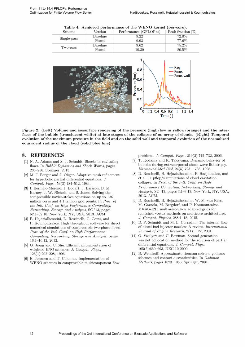
Table 4: Achieved performance of the WENO kernel (per-core).Scheme Version Performance (GFLOP/s) Peak fraction [%]

Single-passBaseline 9.22 72.0%Fused 9.93 77.6%

Two-passBaseline 9.62 75.2%Fused 10.30 80.5%

Figure 2: (Left) Volume and isosurface rendering of the pressure (high/low in yellow/orange) and the inter-faces of the bubble (translucent white) at late stages of the collapse of an array of clouds. (Right) Temporalevolution of the maximum pressure in the field and on the solid wall and temporal evolution of the normalizedequivalent radius of the cloud (solid blue line)

8. REFERENCES[1] N. A. Adams and S. J. Schmidt. Shocks in cavitating

flows. In Bubble Dynamics and Shock Waves, pages235–256. Springer, 2013.

[2] M. J. Berger and J. Oliger. Adaptive mesh refinementfor hyperbolic partial differential equations. J.Comput. Phys., 53(3):484–512, 1984.

[3] I. Bermejo-Moreno, J. Bodart, J. Larsson, B. M.Barney, J. W. Nichols, and S. Jones. Solving thecompressible navier-stokes equations on up to 1.97million cores and 4.1 trillion grid points. In Proc. ofthe Intl. Conf. on High Performance Computing,Networking, Storage and Analysis, SC ’13, pages62:1–62:10, New York, NY, USA, 2013. ACM.

[4] B. Hejazialhosseini, D. Rossinelli, C. Conti, andP. Koumoutsakos. High throughput software for directnumerical simulations of compressible two-phase flows.Proc. of the Intl. Conf. on High PerformanceComputing, Networking, Storage and Analysis, pages16:1–16:12, 2012.

[5] G. Jiang and C. Shu. Efficient implementation ofweighted ENO schemes. J. Comput. Phys.,126(1):202–228, 1996.

[6] E. Johnsen and T. Colonius. Implementation ofWENO schemes in compressible multicomponent flow

problems. J. Comput. Phys., 219(2):715–732, 2006.

[7] T. Kodama and K. Takayama. Dynamic behavior ofbubbles during extracorporeal shock-wave lithotripsy.Ultrasound Med Biol, 24(5):723 – 738, 1998.

[8] D. Rossinelli, B. Hejazialhosseini, P. Hadjidoukas, andet al. 11 pflop/s simulations of cloud cavitationcollapse. In Proc. of the Intl. Conf. on High

Performance Computing, Networking, Storage andAnalysis, SC ’13, pages 3:1–3:13, New York, NY, USA,2013. ACM.

[9] D. Rossinelli, B. Hejazialhosseini, W. M. van Rees,M. Gazzola, M. Bergdorf, and P. Koumoutsakos.MRAG-I2D: multi-resolution adapted grids forremeshed vortex methods on multicore architectures.J. Comput. Physics, 288:1–18, 2015.

[10] D. P. Schmidt and M. L. Corradini. The internal flowof diesel fuel injector nozzles: A review. InternationalJournal of Engine Research, 2(1):1–22, 2001.

[11] O. Vasilyev and C. Bowman. Second-generationwavelet collocation method for the solution of partialdifferential equations. J. Comput. Phys.,165(2):660–693, DEC 10 2000.

[12] B. Wendroff. Approximate riemann solvers, godunovschemes and contact discontinuities. In GodunovMethods, pages 1023–1056. Springer, 2001.



The Impact of Process Placement and Oversubscription onApplication Performance

A Case Study for Exascale Computing

Florian Wende Thomas Steinke Alexander ReinefeldZuse Institute Berlin (ZIB), Takustraße 7, 14195 Berlin

wende,steinke,[email protected]

ABSTRACTWith the upcoming transition from petascale to exascale comput-ers radically new methods for scalable and robust computing arerequired. Computing at the speed of exascale, that is, more than1018 floating point operations per second, will only be possible onsystems with millions of processing units. Unfortunately, the largenumber of functional components like computing cores, memorychips and network interfaces will greatly increase the probabilityof failures, and it can thus not be expected that an exascale appli-cation will complete its execution on exactly the same resources itwas started. In this paper, we investigate the impact of unfavorableprocess placement and oversubscription of compute resources onthe performance and scalability of typical application workloadslike CP2K, MOM5 and BQCD. We provide results on two HPCarchitectures, a Cray XC40 with proprietary Aries network routersand dragonfly topology, and an InfiniBand cluster.

KeywordsFault-tolerance, Process placement, Oversubscription, Applicationperformance, Hyper-Threading, Concurrent program execution

1. INTRODUCTIONCurrent petascale computer installations comprise 105 compute

nodes that are connected by custom network interconnects with ahierarchical abstraction of the entire machine down to the single-node level. For exascale computing a couple of architectural is-sues—also affecting today’s installations already—need to be ap-proached, two of which are the scalability of the network in termsof latency and bandwidth across the entire machine, and the steadilyincreasing number of compute resources within single nodes con-trasted with only slightly increasing network and main memorybandwidths.

Alongside scaling the hardware to exascale, user applicationsneed to adapt as well, e.g., by utilizing hybrid MPI plus thread-ing in order to minimize inter-process communication, heteroge-neous programming involving hardware accelerators as one meansto approach exascale, vectorization (SIMD), parallel I/O, and so-phisticated load balancing on a final note. For many existing codebases—possibly even those that are believed to be well optimized—it might be expected that without appropriate adaption it will notbe possible to use the hardware efficiently. Small imbalances inthe program execution, due to MPI and I/O, for instance, can resultalready in a certain amount of compute resources run idle [1].

A further issue is component failure, which becomes more likelywith increasing number of functional units and size of the instal-lation. Restarting an exascale application after component failureis expected to work efficiently with in-memory checkpointing to-

gether with, e.g., erasure-coding [2]. Thereby, the restart needs tohappen almost immediately after the crash on an adapted and possi-bly reduced node allocation. One central question that arises in thatcontext is whether the restarted application can utilize that alloca-tion efficiently if the latter is unfavorable? and if not, what can bedone to compensate for that? For exascale computing this questionis relevant twice, first because of an increased component failurerate and possibly unfavorable resource allocation at restart, whichthen in turn might cause additional imbalances throughout the pro-gram execution, and second, because of the possibility that evenan optimized application cannot fully utilize the available computeresources of modern processors.

We address these points in this paper targeting two different HPCsystems, which together with the workloads CP2K, MOM5 andBQCD will be introduced in Section 2 and 3, respectively. In Sec-tion 4, we investigate the impact of unfavorable process placementsfor two of these applications. Section 5 approaches the resource uti-lization issue, including results for oversubscription and concurrentprogram execution.

2. TARGET HPC SYSTEMSExperiments for which results are reported in this paper have

been carried out on two current HPC systems: a Cray XC40 su-percomputer and an InfiniBand cluster. Both systems are brieflydescribed subsequently.

2.1 Cray XC40 with Aries InterconnectThe Cray XC40 integrates the Aries interconnect together with

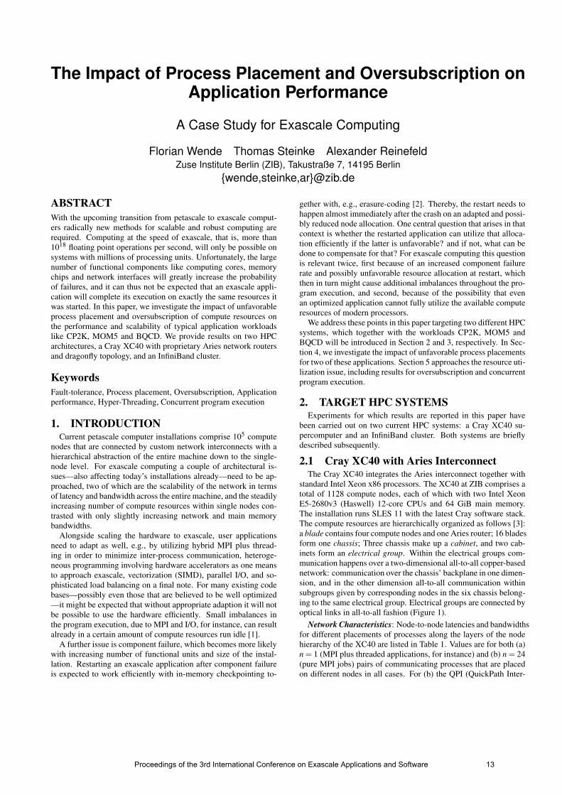
standard Intel Xeon x86 processors. The XC40 at ZIB comprises atotal of 1128 compute nodes, each of which with two Intel XeonE5-2680v3 (Haswell) 12-core CPUs and 64 GiB main memory.The installation runs SLES 11 with the latest Cray software stack.The compute resources are hierarchically organized as follows [3]:a blade contains four compute nodes and one Aries router; 16 bladesform one chassis; Three chassis make up a cabinet, and two cab-inets form an electrical group. Within the electrical groups com-munication happens over a two-dimensional all-to-all copper-basednetwork: communication over the chassis’ backplane in one dimen-sion, and in the other dimension all-to-all communication withinsubgroups given by corresponding nodes in the six chassis belong-ing to the same electrical group. Electrical groups are connected byoptical links in all-to-all fashion (Figure 1).

Network Characteristics: Node-to-node latencies and bandwidthsfor different placements of processes along the layers of the nodehierarchy of the XC40 are listed in Table 1. Values are for both (a)n = 1 (MPI plus threaded applications, for instance) and (b) n = 24(pure MPI jobs) pairs of communicating processes that are placedon different nodes in all cases. For (b) the QPI (QuickPath Inter-


Cray XC40 with Aries Interconnect

Electrical Group (E-Group)

Blade

Chassis

E-Gr

oup 1

E-Gr

oup 2

E-Gr

oup 3

E-Gr

oup 4

E-Gr

oup 5

E-Gr

oup 6

E-Gr

oup 7

Aries

Node

Cabinet

Optical Links

E-Gr

oup 8

Figure 1: Schematic of the Cray Aries Interconnect. Communication within electricalgroups happens over a two-dimensional all-to-all copper-based network. Electricalgroups are connected via optical links in all-to-all fashion.

connect) latency adds to the network latency twice, as the networkinterface is connected to CPU socket 0 but not 1.

According to Table 1 latencies only slightly decrease from intra-blade to inter-electrical-group communication, and from n = 1 ton = 24 groups. Extending the XC40 by additional electrical groupsdoes not lower the latencies further. Bandwidths are almost homo-geneous across the entire machine. However, it takes multiple MPIprocesses to saturate the network.

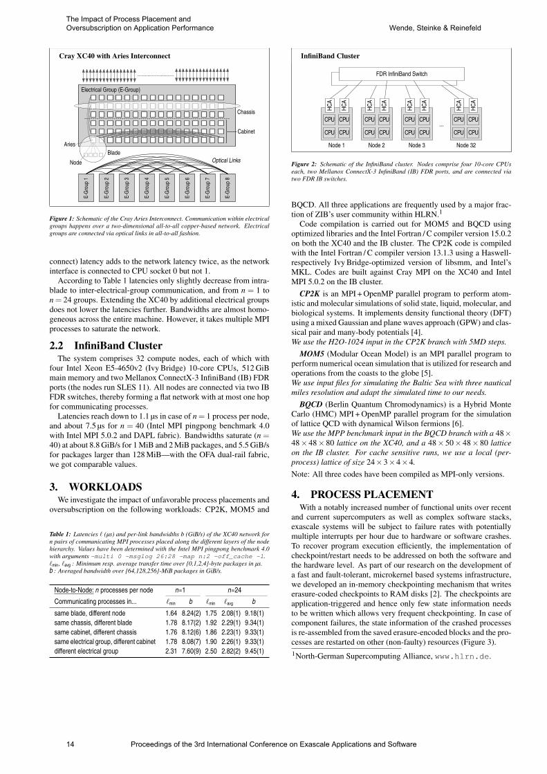
2.2 InfiniBand ClusterThe system comprises 32 compute nodes, each of which with

four Intel Xeon E5-4650v2 (Ivy Bridge) 10-core CPUs, 512 GiBmain memory and two Mellanox ConnectX-3 InfiniBand (IB) FDRports (the nodes run SLES 11). All nodes are connected via two IBFDR switches, thereby forming a flat network with at most one hopfor communicating processes.

Latencies reach down to 1.1 µs in case of n = 1 process per node,and about 7.5 µs for n = 40 (Intel MPI pingpong benchmark 4.0with Intel MPI 5.0.2 and DAPL fabric). Bandwidths saturate (n =40) at about 8.8 GiB/s for 1 MiB and 2 MiB packages, and 5.5 GiB/sfor packages larger than 128 MiB—with the OFA dual-rail fabric,we got comparable values.

3. WORKLOADSWe investigate the impact of unfavorable process placements and

oversubscription on the following workloads: CP2K, MOM5 and

Table 1: Latencies ` (µs) and per-link bandwidths b (GiB/s) of the XC40 network forn pairs of communicating MPI processes placed along the different layers of the nodehierarchy. Values have been determined with the Intel MPI pingpong benchmark 4.0with arguments -multi 0 -msglog 26:28 -map n:2 -off_cache -1.`min, `avg : Minimum resp. average transfer time over 0,1,2,4-byte packages in µs.b : Averaged bandwidth over 64,128,256-MiB packages in GiB/s.

Node-to-Node: n processes per node n=1 n=24Communicating processes in... `min b `min `avg bsame blade, different node 1.64 8.24(2) 1.75 2.08(1) 9.18(1)same chassis, different blade 1.78 8.17(2) 1.92 2.29(1) 9.34(1)same cabinet, different chassis 1.76 8.12(6) 1.86 2.23(1) 9.33(1)same electrical group, different cabinet 1.78 8.08(7) 1.90 2.26(1) 9.33(1)different electrical group 2.31 7.60(9) 2.50 2.82(2) 9.45(1)

InfiniBand Cluster

CPU CPU

CPU CPU

HCA

CPU CPU

CPU CPU

HCA

CPU CPU

CPU CPU

HCA

CPU CPU

CPU CPU

HCA

...

Node 1 Node 2 Node 3 Node 32

HCA

HCA

HCA

HCA

FDR InfiniBand Switch

Figure 2: Schematic of the InfiniBand cluster. Nodes comprise four 10-core CPUseach, two Mellanox ConnectX-3 InfiniBand (IB) FDR ports, and are connected viatwo FDR IB switches.

BQCD. All three applications are frequently used by a major frac-tion of ZIB’s user community within HLRN.1

Code compilation is carried out for MOM5 and BQCD usingoptimized libraries and the Intel Fortran / C compiler version 15.0.2on both the XC40 and the IB cluster. The CP2K code is compiledwith the Intel Fortran / C compiler version 13.1.3 using a Haswell-respectively Ivy Bridge-optimized version of libsmm, and Intel’sMKL. Codes are built against Cray MPI on the XC40 and IntelMPI 5.0.2 on the IB cluster.

CP2K is an MPI + OpenMP parallel program to perform atom-istic and molecular simulations of solid state, liquid, molecular, andbiological systems. It implements density functional theory (DFT)using a mixed Gaussian and plane waves approach (GPW) and clas-sical pair and many-body potentials [4].We use the H2O-1024 input in the CP2K branch with 5MD steps.

MOM5 (Modular Ocean Model) is an MPI parallel program toperform numerical ocean simulation that is utilized for research andoperations from the coasts to the globe [5].We use input files for simulating the Baltic Sea with three nauticalmiles resolution and adapt the simulated time to our needs.

BQCD (Berlin Quantum Chromodynamics) is a Hybrid MonteCarlo (HMC) MPI + OpenMP parallel program for the simulationof lattice QCD with dynamical Wilson fermions [6].We use the MPP benchmark input in the BQCD branch with a 48×48× 48× 80 lattice on the XC40, and a 48× 50× 48× 80 latticeon the IB cluster. For cache sensitive runs, we use a local (per-process) lattice of size 24×3×4×4.Note: All three codes have been compiled as MPI-only versions.

4. PROCESS PLACEMENTWith a notably increased number of functional units over recent

and current supercomputers as well as complex software stacks,exascale systems will be subject to failure rates with potentiallymultiple interrupts per hour due to hardware or software crashes.To recover program execution efficiently, the implementation ofcheckpoint/restart needs to be addressed on both the software andthe hardware level. As part of our research on the development ofa fast and fault-tolerant, microkernel based systems infrastructure,we developed an in-memory checkpointing mechanism that writeserasure-coded checkpoints to RAM disks [2]. The checkpoints areapplication-triggered and hence only few state information needsto be written which allows very frequent checkpointing. In case ofcomponent failures, the state information of the crashed processesis re-assembled from the saved erasure-encoded blocks and the pro-cesses are restarted on other (non-faulty) resources (Figure 3).1North-German Supercomputing Alliance, www.hlrn.de.


The Impact of Process Placement and Oversubscription on Application Performance Wende, Steinke & Reinefeld

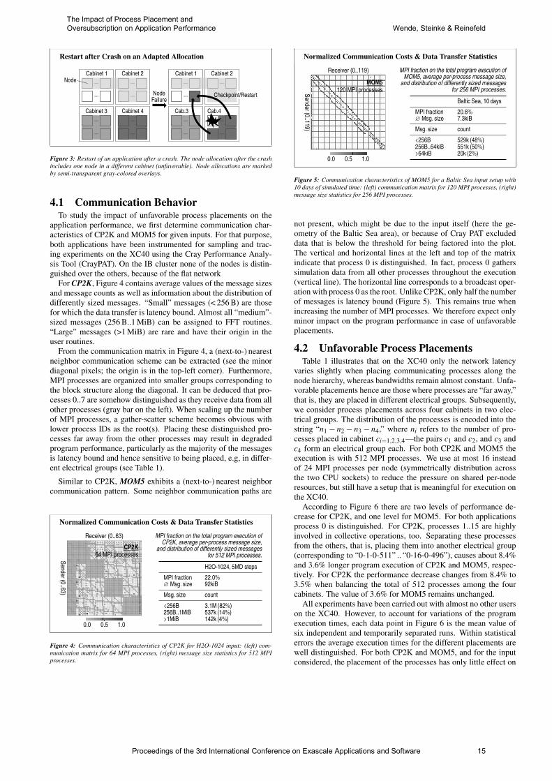
Restart after Crash on an Adapted Allocation

NodeFailure

...

...

...

...

...

...

...

...

Cabinet 1 Cabinet 2

Cabinet 3 Cabinet 4

......

...

...

...

...

...

Cabinet 1 Cabinet 2

Cab.3 Cab.4

Checkpoint/Restart

Node

Figure 3: Restart of an application after a crash. The node allocation after the crashincludes one node in a different cabinet (unfavorable). Node allocations are markedby semi-transparent gray-colored overlays.

4.1 Communication BehaviorTo study the impact of unfavorable process placements on the

application performance, we first determine communication char-acteristics of CP2K and MOM5 for given inputs. For that purpose,both applications have been instrumented for sampling and trac-ing experiments on the XC40 using the Cray Performance Analy-sis Tool (CrayPAT). On the IB cluster none of the nodes is distin-guished over the others, because of the flat network

For CP2K, Figure 4 contains average values of the message sizesand message counts as well as information about the distribution ofdifferently sized messages. “Small” messages (< 256 B) are thosefor which the data transfer is latency bound. Almost all “medium”-sized messages (256 B..1 MiB) can be assigned to FFT routines.“Large” messages (>1 MiB) are rare and have their origin in theuser routines.

From the communication matrix in Figure 4, a (next-to-) nearestneighbor communication scheme can be extracted (see the minordiagonal pixels; the origin is in the top-left corner). Furthermore,MPI processes are organized into smaller groups corresponding tothe block structure along the diagonal. It can be deduced that pro-cesses 0..7 are somehow distinguished as they receive data from allother processes (gray bar on the left). When scaling up the numberof MPI processes, a gather-scatter scheme becomes obvious withlower process IDs as the root(s). Placing these distinguished pro-cesses far away from the other processes may result in degradedprogram performance, particularly as the majority of the messagesis latency bound and hence sensitive to being placed, e.g, in differ-ent electrical groups (see Table 1).

Similar to CP2K, MOM5 exhibits a (next-to-) nearest neighborcommunication pattern. Some neighbor communication paths are

Normalized Communication Costs & Data Transfer Statistics

Receiver (0..63)

Sender (0..63)

CP2K64 MPI processes

0.0 0.5 1.0

MPI fraction on the total program execution ofCP2K, average per-process message size,

and distribution of differently sized messagesfor 512 MPI processes.

H2O-1024, 5MD stepsMPI fraction 22.0%∅ Msg. size 92kiBMsg. size count<256B 3.1M (82%)256B..1MiB 537k (14%)>1MiB 142k (4%)

Figure 4: Communication characteristics of CP2K for H2O-1024 input: (left) com-munication matrix for 64 MPI processes, (right) message size statistics for 512 MPIprocesses.

Normalized Communication Costs & Data Transfer Statistics

Receiver (0..119)

Sender (0..119)

0.0 0.5 1.0

MOM5120 MPI processes

MPI fraction on the total program execution ofMOM5, average per-process message size,

and distribution of differently sized messagesfor 256 MPI processes.

Baltic Sea, 10 daysMPI fraction 20.6%∅ Msg. size 7.3kiBMsg. size count<256B 529k (48%)256B..64kiB 551k (50%)>64kiB 20k (2%)

Figure 5: Communication characteristics of MOM5 for a Baltic Sea input setup with10 days of simulated time: (left) communication matrix for 120 MPI processes, (right)message size statistics for 256 MPI processes.

not present, which might be due to the input itself (here the ge-ometry of the Baltic Sea area), or because of Cray PAT excludeddata that is below the threshold for being factored into the plot.The vertical and horizontal lines at the left and top of the matrixindicate that process 0 is distinguished. In fact, process 0 gatherssimulation data from all other processes throughout the execution(vertical line). The horizontal line corresponds to a broadcast oper-ation with process 0 as the root. Unlike CP2K, only half the numberof messages is latency bound (Figure 5). This remains true whenincreasing the number of MPI processes. We therefore expect onlyminor impact on the program performance in case of unfavorableplacements.

4.2 Unfavorable Process PlacementsTable 1 illustrates that on the XC40 only the network latency

varies slightly when placing communicating processes along thenode hierarchy, whereas bandwidths remain almost constant. Unfa-vorable placements hence are those where processes are “far away,”that is, they are placed in different electrical groups. Subsequently,we consider process placements across four cabinets in two elec-trical groups. The distribution of the processes is encoded into thestring “n1− n2− n3− n4,” where ni refers to the number of pro-cesses placed in cabinet ci=1,2,3,4—the pairs c1 and c2, and c3 andc4 form an electrical group each. For both CP2K and MOM5 theexecution is with 512 MPI processes. We use at most 16 insteadof 24 MPI processes per node (symmetrically distribution acrossthe two CPU sockets) to reduce the pressure on shared per-noderesources, but still have a setup that is meaningful for execution onthe XC40.

According to Figure 6 there are two levels of performance de-crease for CP2K, and one level for MOM5. For both applicationsprocess 0 is distinguished. For CP2K, processes 1..15 are highlyinvolved in collective operations, too. Separating these processesfrom the others, that is, placing them into another electrical group(corresponding to “0-1-0-511” .. “0-16-0-496”), causes about 8.4%and 3.6% longer program execution of CP2K and MOM5, respec-tively. For CP2K the performance decrease changes from 8.4% to3.5% when balancing the total of 512 processes among the fourcabinets. The value of 3.6% for MOM5 remains unchanged.

All experiments have been carried out with almost no other userson the XC40. However, to account for variations of the programexecution times, each data point in Figure 6 is the mean value ofsix independent and temporarily separated runs. Within statisticalerrors the average execution times for the different placements arewell distinguished. For both CP2K and MOM5, and for the inputconsidered, the placement of the processes has only little effect on



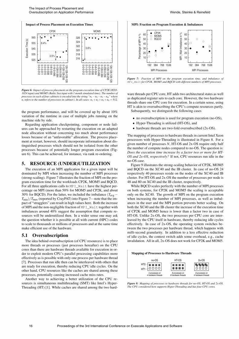
Impact of Process Placement on Execution Times

525

535

545

555

565

0-0-0-5120-1-0-5110-2-0-5100-4-0-5080-8-0-5040-16-0-4960-128-0-3840-256-0-2560-128-128-256128-128-128-128

Exec

ution

Time[

s]CP2K

3.5%

8.4%

316318320322324326

0-0-0-5120-1-0-5110-2-0-5100-4-0-5080-8-0-5040-16-0-4960-128-0-3840-256-0-2560-128-128-256128-128-128-128

MOM5

3.6%

Figure 6: Impact of process placement on the program execution time of CP2K (H2O-1024 input) and MOM5 (Baltic Sea input with 1 month simulated time). The number ofprocesses in each of four cabinets is encoded into the string “n1−n2−n3−n4,” whereni refers to the number of processes in cabinet i. In all cases: n1 +n2 +n3 +n4 = 512.

the program performance, and will be covered up by about 10%variation of the runtime in case of multiple jobs running on themachine side by side.

Regarding application checkpointing, component or node fail-ures can be approached by restarting the execution on an adaptednode allocation without concerning too much about performancelosses because of an “unfavorable” allocation. The process place-ment at restart, however, should incorporate information about dis-tinguished processes which should not be isolated from the otherprocesses because of potentially longer program execution (Fig-ure 6). This can be achieved, for instance, via rank re-ordering.

5. RESOURCE (UNDER)UTILIZATIONThe execution of an MPI application for a given input will be

dominated by MPI when increasing the number of MPI processes(strong-scaling). Figure 7 illustrates the fraction of MPI on the pro-gram execution time for the workloads CP2K, MOM5 and BQCD.For all three applications calls to MPI_Wait have the highest per-centage on MPI (more than 50% for MOM5 and CP2K, and about30% for BQCD). For the latter, we included the imbalance (Tavg−Tmin)/Tmax (reported by CrayPAT) into Figure 7—note that the im-pact of “stragglers” can result in high values here. Both the increaseof MPI and the non-negligible fraction of MPI_Wait together withimbalances around 40% suggest the assumption that compute re-sources will be underutilized then. In a wider sense one may askthe question whether it is possible at all with current (HPC) codesto scale to thousands or millions of processors and at the same timemake efficient use of the hardware.

5.1 OversubscriptionThe idea behind oversubscription (of CPU resources) is to place

more threads or processes (just processes hereafter) on the CPUcores than there are hardware threads available for execution in or-der to exploit modern CPU’s parallel processing capabilities moreeffectively as is possible with only one process per hardware thread[7]. Processes that run idle then can be interleaved with others thatare ready for execution, thereby reducing CPU idle cycles. On theother hand, CPU resources like the caches are shared among theseprocesses, potentially causing increased cache miss rates.

Another way to achieving a better utilization of the CPU re-sources is simultaneous multithreading (SMT) like Intel’s Hyper-Threading (HT) [1]. While caches are shared among the two hard-

MPI: Fraction on Program Execution & Imbalances

102030405060

Perce

ntage

ofMP

Iin%

192 384 768 1536

MPI Processes

CP2KMOM5BQCD

102030405060

MPI_W

aitIm

balan

cein

%

192 384 768 1536

MPI Processes

Figure 7: Fraction of MPI on the program execution time, and imbalance ofMPI_Wait for CP2K, MOM5 and BQCD with different numbers of MPI processes.

ware threads per CPU core, HT adds two architectural states as wellas duplicated register sets to each core. However, the two hardwarethreads share one CPU core for execution. In a certain sense, usingHT is akin to oversubscribing the CPU’s compute resources partly.

Subsequently, we distinguish the following cases

• no oversubscription is used for program execution (no-OS),• Hyper-Threading is utilized (HT-OS), and• hardware threads are two-fold oversubscribed (2x-OS).

The mapping of processes to hardware threads in current Intel Xeonprocessors with Hyper-Threading is illustrated in Figure 8. For agiven number of processes N, HT-OS and 2x-OS require only halfthe number of compute nodes compared to no-OS. The question is:Does the execution time increase by a factor two or more for HT-OS and 2x-OS, respectively? If not, CPU resources run idle in theno-OS case.

Figure 9 illustrates the strong-scaling behavior of CP2K, MOM5and BQCD on the XC40 and the IB cluster. In case of no-OS 24respectively 40 processes reside on the nodes of the XC40 and IBcluster. For HT-OS and 2x-OS the number of processes per node is48 and 80 on XC40 and the IB cluster, respectively.

While BQCD scales perfectly with the number of MPI processeson both systems, for CP2K and MOM5 the scaling is acceptableonly on the XC40. The growth of MPI on the program executionwhen increasing the number of MPI processes, as well as imbal-ances in the user and the MPI portion prevents better scaling. Onboth the XC40 and the IB cluster the increase of the execution timeof CP2K and MOM5 hence is lower than a factor two in case ofHT-OS. Unlike 2x-OS, the two processes per CPU core are inter-leaved by the CPU itself in hardware, thereby reducing idle cycleseffectively. In case of 2x-OS, the operating system switches be-tween the two processes per hardware thread, which happens withmilli-second granularity. In addition to a less effective reductionof idle cycles, the context switch adds some overhead, e.g., cacheinvalidation. All in all, 2x-OS does not work for CP2K and MOM5.

Mapping of Processes to Hardware Threads

HT0HT1

no-OS HT-OS 2x-OS

4 processes on4 hardware threads



Figure 8: Mapping of processes to hardware threads for no-OS, HT-OS and 2x-OS.The CPU considered here supports Hyper-Threading and has four CPU cores.



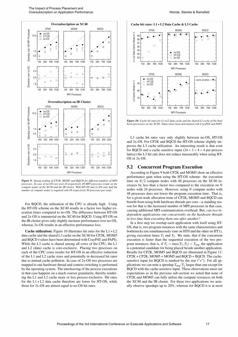
Oversubscription on XC40

0.5

1.0

10.0

Spee

dup

over

192

MPIP

roce

sses

192 384 768 1536

CP2K

192 384 768 1536

MOM5

192 384 768 1536

BQCD

1.6

2.0

2.4

Slow

down

over

no-O

S

192 384 768 1536 192 384 768 1536

MPI Processes

192 384 768 1536

no-OSHT-OS2x-OS

Oversubscription on IB Cluster

0.5

1.0

10.0

Spee

dup

over

160

MPIP

roce

sses

160 320 640 1200

CP2K

160 320 640 1200

MOM5

160 320 640 1200

BQCD

1.6

2.0

2.4

Slow

down

over

no-O

S

160 320 640 1200 160 320 640 1200

MPI Processes

160 320 640 1200

no-OSHT-OS2x-OS

Figure 9: Strong-scaling of CP2K, MOM5 and BQCD for different numbers of MPIprocesses. In case of no-OS (see text) 24 respectively 40 MPI processes reside on thecompute nodes of the XC40 and the IB cluster. With HT-OS and 2x-OS only half thenumber of compute nodes is required with 48 respectively 80 processes per node.

For BQCD, the utilization of the CPU is already high. Usingthe HT-OS scheme on the XC40 results in a factor two higher ex-ecution times compared to no-OS. The difference between HT-OSand 2x-OS is immaterial on the XC40 for BQCD. Using HT-OS onthe IB cluster gives only slightly increase performance over no-OS,whereas 2x-OS results in an effective performance loss.

Cache utilization: Figure 10 illustrates hit rates for the L1 + L2data cache and the shared L3 cache on the XC40 for CP2K, MOM5and BQCD (values have been determined with CrayPAT and PAPI).While the L3 cache is shared among all cores of the CPU, the L1and L2 (data) cache is core-exclusive. Placing two processes oneach of the CPU cores results for HT-OS in an effective reductionof the L1 and L2 cache sizes and potentially in decreased hit ratesdue to mutual cache pollution. In case of 2x-OS two processes aremapped to one hardware thread and context switching is performedby the operating system. The interleaving of the process executionsin that case happens on a much coarser granularity, thereby render-ing the L1 and L2 cache more or less process-exclusive. Hit ratesfor the L1 + L2 data cache therefore are lower for HT-OS, whilethose for 2x-OS are almost equal to no-OS hit rates.

Cache hit rates: L1 + L2 Data Cache & L3 Cache

93949596979899

L1+L

2Data

Cach

eHitra

tein

%

192 384 768 1536

CP2K

192 384 768 1536

MPI Processes

MOM5

192 384 768 1536

BQCD

no-OSHT-OS2x-OS

70

80

90

L3Ca

cheH

itrate

in%

192 384 768 1536

CP2K

192 384 768 1536

MPI Processes

MOM5

192 384 768 1536

BQCD

cache sensitive→no-OSHT-OS2x-OS

Figure 10: Cache hit rates for L1+L2 data cache and the shared L3 cache of the IntelXeon processors on the XC40. Values have been determined with CrayPAT and PAPI.

L3 cache hit rates vary only slightly between no-OS, HT-OSand 2x-OS. For CP2K and BQCD the HT-OS scheme slightly im-proves the L3 cache utilization. An interesting result is that evenfor BQCD and a cache sensitive input (24× 3× 4× 4 per-processlattice) the L3 hit rate does not reduce measurably when using HT-OS or 2x-OS.

5.2 Concurrent Program ExecutionAccording to Figure 9 both CP2K and MOM5 show an effective

performance gain when using the HT-OS scheme: the executiontime on N/2 compute nodes with 48 processes on the XC40 in-creases by less than a factor two compared to the execution on Nnodes with 24 processes. However, using N compute nodes with48 processes does not lower the program execution time. That is,for a given node allocation none of CP2K, MOM5 and BQCD canbenefit from using both hardware threads per core—a standing rea-son for that is the increased number of MPI processes in that case,causing additional MPI communication overhead. But, can two in-dependent applications run concurrently on the hardware threadsin less time than executing them one after another?

In a first step we overlap each application with itself using HT-OS, that is, two program instances with the same characteristics andbottlenecks run simultaneously (one on HT0 and the other on HT1),giving execution times T1 and T2. We state, that if the concurrentexecution is faster than the sequential execution of the two pro-gram instances, that is, if T|| = max(T1,T2) < Tseq, the applicationis a potential candidate for being placed beside another application.Results for CP2K, MOM5 and BQCD are illustrated in Figure 11:CP2K + CP2K, MOM5 + MOM5 and BQCD + BQCD. The cache-sensitive input for BQCD is marked by the star (“?”). For all ap-plications we can note a speedup Tseq/T|| larger than one except forBQCD with the cache-sensitive input. These observations meet ourexpectations as in the previous sub-section we noted that none ofCP2K and MOM5 can fully utilize the compute resources on boththe XC40 and the IB cluster. For these two applications we actu-ally observe speedups up to 20%, whereas for BQCD it is at most



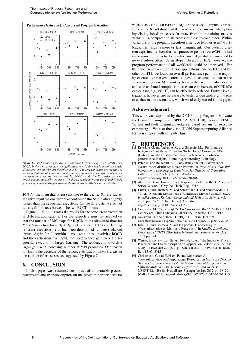
Performance Gain due to Concurrent Program Execution

1.0

1.1

1.2

384 768 1536

BQCD + BQCD

384 768 1536

BQCD + CP2K

384 768 1536

BQCD + MOM5

1.0

1.1

1.2

Spee

dupo

verS

eque

ntial

Exec

ution

384 768 1536

BQCD⋆ + BQCD⋆

384 768 1536

BQCD⋆ + CP2K

384 768 1536

BQCD⋆ + MOM5

1.0

1.1

1.2

384 768 1536

CP2K + CP2K

384 768 1536

MPI Processes

CP2K + MOM5

384 768 1536

MOM5 + MOM5

XC40IB Cluster

Figure 11: Performance gain due to a concurrent execution of CP2K, MOM5 andBQCD. In the concurrent case two applications run simultaneously on the same nodeallocation: one on HT0 and the other on HT1. The speedup values are the ratio ofthe sequential execution time for running the two applications one after another, andthe concurrent execution time (see text). For BQCD we additionally consider a cache-sensitive setup, marked by the star (“?”). For all combinations we use 24 and 40 MPIprocesses per node and application on the XC40 and the IB cluster, respectively.

10% for the input that is not sensitive to the cache. For the cache-sensitive input the concurrent execution on the XC40 takes slightlylonger than the sequential execution. On the IB cluster we do notsee any differences between the two BQCD inputs.

Figure 11 also illustrates the results for the concurrent executionof different applications. For the respective runs, we adapted ei-ther the number of MC steps for BQCD or the simulated time forMOM5 so as to achieve T1 ≈ T2, that is, almost 100% overlappingprogram execution—Tseq has been determined for these adaptedinputs. Again for all combinations, except those involving BQCDand the cache-sensitive input, the performance gain over the se-quential execution is larger than one. The tendency is towards alarger gain with increasing number of MPI processes. One reasonfor that is the decrease of the resource utilization when increasingthe number of processes, as suggested by Figure 7.

6. CONCLUSIONIn this paper we presented the impact of unfavorable process

placements and oversubscription on the program performance for

workloads CP2K, MOM5 and BQCD and selected inputs. Our re-sults on the XC40 show that the increase of the runtime when plac-ing distinguished processes far away from the remaining ones iswithin 10% compared to all processes close to each other. Withinvariations of the program execution times due to other users’ work-loads, this value is more or less insignificant. Our oversubscrip-tion experiments show that two processes per hardware CPU threadcause more than a factor two performance degradation compared tono oversubscription. Using Hyper-Threading (HT), however, theprogram performance of all workloads could be improved. Forthe concurrent execution of two applications, one on HT0 and theother on HT1, we found an overall performance gain in the major-ity of cases. Our investigations suggest the assumption that in thestrong-scaling case MPI wait cycles together with imbalances dueto access to shared compute resource cause an increase of CPU idlecycles, that, e.g., via HT, can be effectively reduced. Further inves-tigations, however, are necessary to better understand, e.g, the roleof caches in these scenarios, which we already started in this paper.

AcknowledgmentThis work was supported by the DFG Priority Program “Softwarefor Exascale Computing” (SPPEXA, SPP 1648), project FFMK,“A fast and fault tolerant microkernel-based system for exascalecomputing.” We also thank the HLRN Supercomputing Alliancefor their support with computer time.

7. REFERENCES[1] Drysdale, G. and Valles, A. C. and Gillespie, M., “Performance

Insights to Intel Hyper-Threading Technology,” November 2009.[Online]. Available: https://software.intel.com/en-us/articles/performance-insights-to-intel-hyper-threading-technology

[2] Peter, K. and Reinefeld, A., “Consistency and fault tolerance forerasure-coded distributed storage systems,” in Proceedings of the fifthinternational workshop on Data-Intensive Distributed ComputingDate, 2012, pp. 23–32. [Online]. Available:http://doi.acm.org/10.1145/2286996.2287002

[3] Alverson, B. and Froese, E. and Kaplan, L. and Roweth, D., “Cray XCSeries Network,” Cray Inc., Tech. Rep., 2012.

[4] Hutter, J. and Iannuzzi, M. and Schiffmann, F. and VandeVondele, J.,“CP2K: Atomistic Simulations of Condensed Matter Systems,” WileyInterdisciplinary Reviews: Computational Molecular Science, vol. 4,no. 1, pp. 15–25, 2014. [Online]. Available:http://dx.doi.org/10.1002/wcms.1159

[5] Griffies, S. M., Elements of the Modular Ocean Model (MOM), NOAAGeophysical Fluid Dynamics Laboratory, Princeton, USA, 2012.

[6] Nakamura, Y. and Stüben, H., “BQCD—Berlin QuantumChromodynamics Program,” PoS, vol. LATTICE2010, p. 040, 2010.

[7] Iancu, C. and Hofmeyr, S. and Blagojevic, F. and Zheng, Y.,“Oversubscription on Multicore Processors,” in Parallel DistributedProcessing (IPDPS), 2010 IEEE International Symposium on, April2010, pp. 1–11.

[8] Wende, F. and Steinke, Th. and Reinefeld, A., “The Impact of ProcessPlacement and Oversubscription on Application Performance: A CaseStudy for Exascale Computing,” ZIB, Takustr. 7, 14195 Berlin, Tech.Rep. 15-05, 2015.

[9] Christmann, C. and Hebisch, E. and Weisbecker, A.,“Oversubscription of Computational Resources on Multicore DesktopSystems,” in Proceedings of the 2012 International Conference onSoftware Multicore Engineering, Performance, and Tools, ser.MSEPT’12. Berlin, Heidelberg: Springer-Verlag, 2012, pp. 18–29.[Online]. Available: http://dx.doi.org/10.1007/978-3-642-31202-1_3



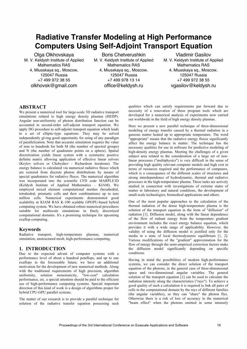
Radiative Transfer Modeling at High Performance Computers Using Self-Adjoint Transport Equation Olga Olkhovskaya

M. V. Keldysh Institute of Applied Mathematics RAS

4, Miusskaya sq., Moscow, 125047 Russia

+7 499 972 38 55 [email protected]

Boris Chetverushkin M. V. Keldysh Institute of Applied

Mathematics RAS 4, Miusskaya sq., Moscow,

125047 Russia +7 499 978 13 14

[email protected]

Vladimir Gasilov M. V. Keldysh Institute of Applied

Mathematics RAS 4, Miusskaya sq., Moscow,

125047 Russia +7 499 972 38 55

[email protected]

ABSTRACT We present a numerical tool for large-scale 3D radiative transport simulations related to high energy density plasmas (HEDP). Angular non-uniformity of photon distribution function can be accounted in second-order self-adjoint transport equation. We apply DG procedure to self-adjoint transport equation which leads to a set of elliptic-type equations. They may be solved independently giving good opportunity for using of any paradigm of parallelization. Note that accurate simulation requires the value of tens to hundreds for both M (the number of spectral groups) and N (the number of quadrature points on a sphere). Spatial discretization yields linear system with a symmetric positive definite matrix allowing application of effective linear solvers (Krylov solvers or Chebyshev - Richardson iterations). The energy balance is calculated via numerical radiative fluxes which are restored from discrete photon distributions by means of special quadratures for radiative fluxes. The numerical algorithm was incorporated into the scientific CFD code MARPLE3D (Keldysh Institute of Applied Mathematics – KIAM). We employed mixed element computational meshes (hexahedral, tetrahedral, prismatic cells and their combinations) up to tens million cells. Numerical experiments demonstrated good scalability at KIAM RAS K-100 scalable GPGPU-based hybrid computing system. We have obtained robust numerical procedures suitable for multiscale simulations in finely discretized computational domains. It's a promising technique for upcoming exaflop computing.

Keywords Radiative transport, high-temperature plasmas, numerical simulation, unstructured mesh, high-performance computing.

1. INTRODUCTION Due to the expected advent of computer systems with a performance level of about a hundred petaflops, and up to one exaflops in the foreseeable future, we have an additional motivation for the development of new numerical methods. Along with the traditional requirements of high precision, algorithm uniformity, solution monotonicity, "low-cost" calculation performance, etc. a special attention should be paid to the efficient use of high-performance computing systems. Special important direction of this kind of work is a design of algorithms proper for hybrid CPU-GPU parallel systems.

The matter of our research is to provide a parallel technique for solution of the radiative transfer equation possessing such

qualities which can satisfy requirements put forward due to necessity of a renovation of those program tools which are developed for a numerical analysis of experiments now carried out worldwide in the field of high energy density plasmas.

Here we present a new parallel technique of three-dimensional modeling of energy transfer caused by a thermal radiation in a gaseous matter heated up to appropriate temperature. The word "appropriate" means that the radiative energy fluxes significantly affect the energy balance in matter. The technique has the necessary qualities for use in software for predictive modeling of high-density energy plasmas. Meeting the challenges of a given subject area related to the consideration of a large set of non-linear processes ("multiphysics") is very difficult in the sense of providing high quality relevant computer models and high cost in terms of resources required and the performance of computers, which is a consequence of the different scales of structures and strong interdependence of hydrodynamic, thermal and radiative processes in the high-temperature plasma. These tasks are actively studied in connection with investigations of extreme states of matter in laboratory and natural conditions, the development of small-scale technologies, biomedical applications and others.

One of the most popular approaches to the calculation of the thermal radiation of the dense high-temperature plasma is the solution of the transport equation in the form of "diffusion" of radiation [1]. Diffusion model, along with the linear dependence of the flow of radiant energy from the temperature gradient environment includes the exact energy balance equation, which provides it with a wide range of applicability. However, the validity of using the diffusion model is justified only for the media in a state of local thermodynamic equilibrium [1, 2]. Various modifications of the "gradient" approximation for the flow of energy through the semi-empirical correction factors make the diffusion model significantly depending on specific conditions.

Having in mind the possibilities of modern high-performance systems, we can consider the direct solution of the transport equation of the photons, in the general case of three-dimensional space and two-dimensional angular variables. The general solution of the transport equation [1] can be used to calculate the radiation intensity along the characteristics ("rays"). To achieve a good quality of such a calculation it is required to link all pairs of cells in the computational domain by the rays of different families (the angular variables), so they can "share" the photon flux. Otherwise there is a risk of loss of accuracy in the numerical "beam effect" when the photons emitted in some intensely


radiating subdomain does not affect the energy balance in the other subdomains [2]. Experimental evaluation conducted for various unstructured computational grids show that acceptable accuracy calculation of grid-characteristic method is very costly. In addition, the corresponding algorithm does not scale well in the case of the parallel solution of a general system of equations of radiation plasmodynamics geometric domain decomposition.

Other known approaches to solving the problems of radiation in hydrodynamics (methods of spherical harmonic, moments, discrete ordinates, etc.) are also not free from the said drawbacks to a greater or lesser extent. If one needs a full account of heterogeneity of the environment, or the angular distribution of the radiation intensity, these methods are either not applicable or quite costly [2, 3].

For these reasons, with the aim to develop software for predictive modeling of high energy density plasma with highly variable emissivity and absorption coefficients, it's advisable to look for a replacement of diffusion and grid-characteristic methods for calculation of the radiation field.

Computational algorithm with good scalability, which, besides all, accounts for the angular dependence of the photon distribution function (or emission intensity), and significantly reduces the negative impact of "beam effect" can be built, if the original problem for the first order transport equation is replaced by the problem for the second-order equation with self-adjoint differential operator. And such passing from the original equation to the transformed one is possible. In 1951, V. Vladimirov [4] proposed a variational principle for velocity transport equation and studied classical correct formulation of the problem for the transport equation of the second order. In 1986, B. Chetverushkin [2] proposed to use similar approach for solving problems of radiative heat transfer, and showed in numerical experiments with model tasks practical suppression of the "beam effect" at moderate computational cost when solving transport problems using this method. In this paper, we propose the development of the technique [2] for the implementation on multiprocessor computers.

2. SELF-ADJOINT EQUATION OF RADIATIVE TRANSFER Generally radiative transfer processes are analyzed by means of a stationary transport equation for the spectral radiation intensity

( ) ( ), , , , ,I d d h c f v t d dν

ν ν νΩ = ⋅ Ωr rΩ Ω

which can be written as:

( )( ) ( ) ( ) ( ) , , ,I I Jν ν ν νλ ∇ + =r r r rΩ Ω Ω (1)

where we use common notations:

f is a photon distribution function which arguments are the radius vector of the observation point, photon frequency ν, direction of a photon movement Ω and time t, λ = 1 / χ is the photon mean free path (i.e. the reciprocal of the opacity coefficient χ), and Jν is emissivity coefficient per unit volume of a substance (the amount of energy emitted per unit time in one steradian). In many cases of practical importance it is possible to assume that the emissivity depends only on a thermodynamic state of a substance, and almost has no dependence on the radiative intensity. Optical properties of a radiative medium are strongly depend on its density and temperature, and can vary for different frequency bands of the

emitted/absorbed photons. Having the radiative intensity distribution over space and angle variables one can account for the radiative heat transfer, radiative losses or contributions into the energy balance of a plasma substance using expressions for the radiation energy density U and radiation flux W:

4 4

0 0 0 0

1 , .U Id d Id d

c

π π

ν ν∞ ∞

= Ω = Ω∫ ∫ ∫ ∫W Ω

The effect of radiation on the energy of matter can be described by introducing a source term into the energy balance equation:

= divRadQ − W .

In certain cases (astrophysical problems, etc.) plasmodynamic model also includes the effect of the momentum carried by the photons, but this is a question we have not discussed, because it has no direct relation to the contents of this work.

An essential element of the radiation field description in multicharged plasmas is a multigroup approach. It is used as a tool for reasonably adequate representation of opacities and emissivities corresponding to different parts of the spectrum. Sometimes a multigroup model is used in certain computational procedures aimed at iterative refinement of photon absorption coefficients depending on the calculated intensity distribution (see [3] for quasi-diffusion or Eddington factor method). The essence of this widespread approach is the superposition principle, which is valid for the equation (1) by virtue of its linearity.

A total range of most representative photon frequencies (necessary to achieve the goals of modeling) is divided into M

intervals (frequency groups) 1 i M=0<...< <...< <ν ν ν ∞ , the

transport equation (1) is solved for each group of this partition. To solve the equation (1) we use integral values of the intensity and spectral energy for the group i:

1 1

[ ] [ ] (1 )., , i i

i ii i i MI I d U U d

ν ν

ν νν ν

ν ν+ +

≤ ≤= =∫ ∫

It is assumed that the opacity (absorption) and emissivity coefficients within each group are independent of the photon energy:

[ ] 1( , , ) ( , ) when .ii iT Tνχ ρ ν χ ρ ν ν ν += < <

The total intensity of the radiated energy is calculated by summing over spectral groups:

[ ]10

( , , )M

ii

I t I d Iνν

∞

=

Ω = =∑∫r .

For correct calculation of the energy balance we need, as a rule, just a few tens of spectral bands. In situations where the principal studied object is the emitted radiation spectrum essentially finer spectrum representation may be required, i.e. for more precise analysis we may need several hundred or even thousand spectral groups. Calculations for some spectral group are implemented independently from the others. The calculation formulas for all spectral intervals are identical and differ only in the values of emissivity and opacity coefficients.


Radiative Transfer Modeling at High Performance Computers Using Self-Adjoint Transport Equation Olkhovskaya, Chetverushkin & Gasilov

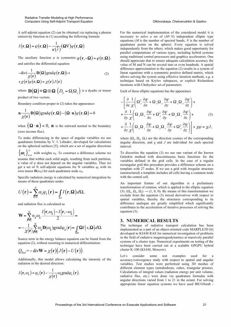
A self-adjoint equation (2) can be obtained via replacing a photon emissivity function in (1) according the following formula

( ) ( )( )

( ) ( )1, , ,Ir

ϕ ϕκ

= − ∇r r rrΩ Ω Ω Ω

The auxiliary function φ is symmetric: ( ) ( ), ,ϕ ϕ− =r rΩ Ω ,

and satisfies the differential equation

( )( ) ( )

( ) ( ) ( ) ( )

1div( grad , )

, J

ϕχ

χ ϕ χ

− +

+ =

D rr

r r r r

Ω Ω

Ω

(2)

where ( ) ( ) ij i jD⊗ =ΩΩD Ω Ω Ω= is a dyadic or tensor

product of two vectors.

Boundary condition proper to (2) takes the appearance:

( )( ) ( ) ( ) ( )1 grad , , 0ϕ ϕ

χ− ⋅ =n D r n r

rΩ Ω Ω Ω

when ( ) 0, ⋅ <n nΩ is the outward normal to the boundary (zero income flux).

To make differencing in the space of angular variables we use quadrature formulas by V. I. Lebedev, developed for calculations on the spherical surfaces [5], which are a set of angular directions

1

N

k k=ω with weights αk. To construct a difference scheme we

assume that within each solid angle, resulting from such partition, a value of φ does not depend on the angular variables. Thus we get a set of N self-adjoint equations for N variables φk with its own tensor D(ωk) for each quadrature node ωk.

Specific radiation energy is calculated by numerical integration by means of these quadrature nodes

( ) ( ) ( )1 4

, ,N

k kk

U I dπ

α ϕ=

= ≈ Ω∑ ∫r r r Ω

and radiation flux is calculated as

( ) ( )

( ) ( ) ( )1

1 4

, ,2

1 ( )grad , .

N k kk k

kN

k k kk

I Iw

I x dπ

ω ωω

α ω ϕχ

=

=

− −= =

=− ≈ Ω

∑

∑ ∫

r rW

D rr Ω Ω

Source term in the energy balance equation can be found from the equation (2), without resorting to numerical differentiation:

( ) ( ) ( )( )= divRadQ J Uχ− = −W r r r .

Additionally, this model allows calculating the intensity of the radiation in the desired direction:

( ) ( )( )

( )1, grad .k k k kI ω ϕ ω ϕχ

= −r r rr

For the numerical implementation of the considered model it is necessary to solve a set of (M×N) independent elliptic type equations (M is the number of spectral bands, N is the number of quadrature points on the sphere). Every equation is solved independently from the others, which makes good opportunity for parallel computations of various types, including hybrid systems using traditional central processors and graphics accelerators. One should appreciate that to ensure adequate calculation accuracy the value of M and N can be several tens or even hundreds. A spatial difference approximation to the equation (2) results in a system of linear equations with a symmetric positive defined matrix, which allows solving the system using effective iteration methods, e.g. a technique based on Krylov subspaces, or explicit Richardson iterations with Chebyshev set of parameters.

Each of these elliptic equations has the appearance

2

2

2

(3)

1

1

1 ,

x x y x z

x y y y z

x z y z y

x x y z

y x y z

Jz x y z

ϕ ϕ ϕχ

ϕ ϕ ϕχ

ϕ ϕ ϕχϕ χ

χ

⎡ ⎛ ⎞∂ ∂ ∂ ∂− Ω +Ω Ω +Ω Ω +⎢ ⎜ ⎟∂ ∂ ∂ ∂⎝ ⎠⎣

⎛ ⎞∂ ∂ ∂ ∂+ Ω Ω +Ω +Ω Ω +⎜ ⎟∂ ∂ ∂ ∂⎝ ⎠

⎤⎛ ⎞∂ ∂ ∂ ∂+ Ω Ω +Ω Ω +Ω + =⎥⎜ ⎟∂ ∂ ∂ ∂⎝ ⎠⎦

where (Ωx, Ωy, Ωz) are the direction cosines of the corresponding angular direction, and χ and J are individual for each spectral interval.

To discretize the equation (3) we use one variant of the known Galerkin method with discontinuous basis functions for the variables defined in the grid cells. In the case of a regular rectangular grid this procedure provides a difference scheme on a template with 27 nodes. If we use a grid with irregular structure (unstructured) a template includes all cells having a common node with the central cell.

An important feature of our algorithm is a preliminary transformation of rotation, which is applied to the elliptic equation (3): (Ωx, Ωy, Ωz) → (1, 0, 0). By means of this transformation we exclude from the equation (3) mixed derivatives with respect to spatial variables, thereby the structures corresponding to its difference analogue are greatly simplified which significantly contributes to the acceleration of iterative processes of solving the equation (3).

3. NUMERICAL RESULTS The technique of radiative transport calculation has been implemented as a part of an object-oriented code MARPLE3D [6] developed in KIAM RAS for numerical investigation of problems in the field of radiative magnetogasdynamics at massively parallel systems of a cluster type. Numerical experiments on testing of the technique have been carried out at a scalable GPGPU hybrid cluster K-100 (KIAM, Moscow).

Let’s consider some test examples used for a accuracy/convergence study with respect to spatial and angular variables. Test studies were performed using 3D meshes of different element types (tetrahedrons, cubes, triangular prisms). Calculations of integral values (radiation energy per unit volume, radiative flux, etc.) were done via quadrature formulas with angular directions varied from 1 to 21 in the octant. For solving appropriate linear equation systems we have used BICGSstab -



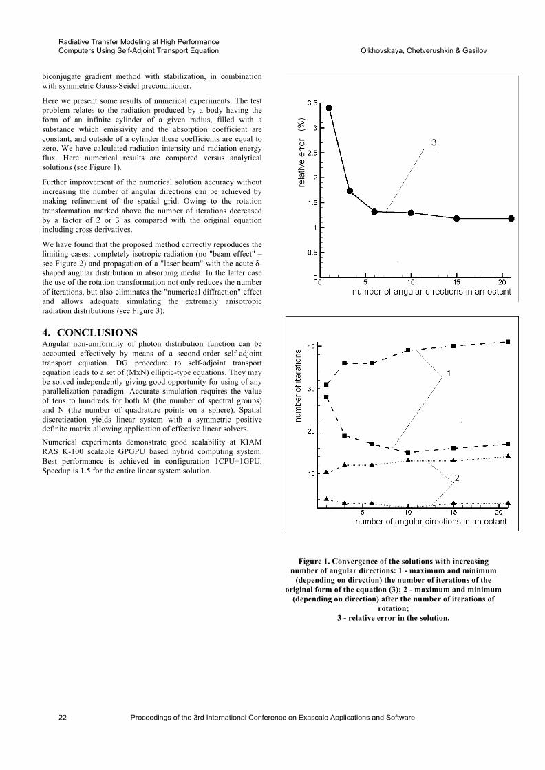
biconjugate gradient method with stabilization, in combination with symmetric Gauss-Seidel preconditioner.

Here we present some results of numerical experiments. The test problem relates to the radiation produced by a body having the form of an infinite cylinder of a given radius, filled with a substance which emissivity and the absorption coefficient are constant, and outside of a cylinder these coefficients are equal to zero. We have calculated radiation intensity and radiation energy flux. Here numerical results are compared versus analytical solutions (see Figure 1).

Further improvement of the numerical solution accuracy without increasing the number of angular directions can be achieved by making refinement of the spatial grid. Owing to the rotation transformation marked above the number of iterations decreased by a factor of 2 or 3 as compared with the original equation including cross derivatives.

We have found that the proposed method correctly reproduces the limiting cases: completely isotropic radiation (no "beam effect" – see Figure 2) and propagation of a "laser beam" with the acute δ-shaped angular distribution in absorbing media. In the latter case the use of the rotation transformation not only reduces the number of iterations, but also eliminates the "numerical diffraction" effect and allows adequate simulating the extremely anisotropic radiation distributions (see Figure 3).

4. CONCLUSIONS Angular non-uniformity of photon distribution function can be accounted effectively by means of a second-order self-adjoint transport equation. DG procedure to self-adjoint transport equation leads to a set of (MxN) elliptic-type equations. They may be solved independently giving good opportunity for using of any parallelization paradigm. Accurate simulation requires the value of tens to hundreds for both M (the number of spectral groups) and N (the number of quadrature points on a sphere). Spatial discretization yields linear system with a symmetric positive definite matrix allowing application of effective linear solvers.

Numerical experiments demonstrate good scalability at KIAM RAS K-100 scalable GPGPU based hybrid computing system. Best performance is achieved in configuration 1CPU+1GPU. Speedup is 1.5 for the entire linear system solution.

Figure 1. Convergence of the solutions with increasing

number of angular directions: 1 - maximum and minimum (depending on direction) the number of iterations of the

original form of the equation (3); 2 - maximum and minimum (depending on direction) after the number of iterations of

rotation; 3 - relative error in the solution.



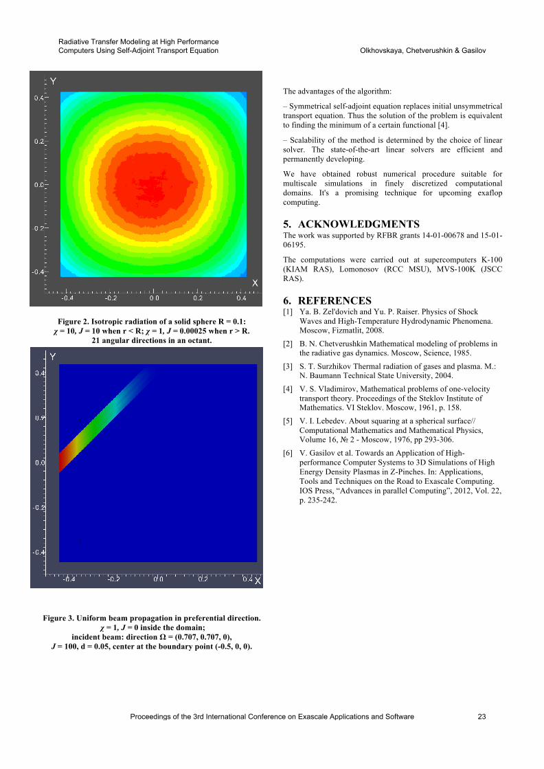
Figure 2. Isotropic radiation of a solid sphere R = 0.1: χ = 10, J = 10 when r < R; χ = 1, J = 0.00025 when r > R.

21 angular directions in an octant.

Figure 3. Uniform beam propagation in preferential direction.

χ = 1, J = 0 inside the domain; incident beam: direction Ω = (0.707, 0.707, 0),

J = 100, d = 0.05, center at the boundary point (-0.5, 0, 0).

The advantages of the algorithm:

– Symmetrical self-adjoint equation replaces initial unsymmetrical transport equation. Thus the solution of the problem is equivalent to finding the minimum of a certain functional [4].

– Scalability of the method is determined by the choice of linear solver. The state-of-the-art linear solvers are efficient and permanently developing.

We have obtained robust numerical procedure suitable for multiscale simulations in finely discretized computational domains. It's a promising technique for upcoming exaflop computing.

5. ACKNOWLEDGMENTS The work was supported by RFBR grants 14-01-00678 and 15-01-06195.

The computations were carried out at supercomputers K-100 (KIAM RAS), Lomonosov (RCC MSU), MVS-100K (JSCC RAS).

6. REFERENCES [1] Ya. B. Zel'dovich and Yu. P. Raiser. Physics of Shock

Waves and High-Temperature Hydrodynamic Phenomena. Moscow, Fizmatlit, 2008.

[2] B. N. Chetverushkin Mathematical modeling of problems in the radiative gas dynamics. Moscow, Science, 1985.

[3] S. T. Surzhikov Thermal radiation of gases and plasma. M.: N. Baumann Technical State University, 2004.

[4] V. S. Vladimirov, Mathematical problems of one-velocity transport theory. Proceedings of the Steklov Institute of Mathematics. VI Steklov. Moscow, 1961, p. 158.

[5] V. I. Lebedev. About squaring at a spherical surface// Computational Mathematics and Mathematical Physics, Volume 16, 2 - Moscow, 1976, pp 293-306.

[6] V. Gasilov et al. Towards an Application of High-performance Computer Systems to 3D Simulations of High Energy Density Plasmas in Z-Pinches. In: Applications, Tools and Techniques on the Road to Exascale Computing. IOS Press, “Advances in parallel Computing”, 2012, Vol. 22, p. 235-242.



Ensuring Efficiency of Exascale Supercomputer Centers

Vladimir Voevodin RCC MSU

119234, Leninskie Gory, 1, bld. 4 Moscow, Russia

+7-495-939-51-66 [email protected]

Vadim Voevodin RCC MSU

119234, Leninskie Gory, 1, bld. 4 Moscow, Russia

+7-495-939-52-16 [email protected]

ABSTRACT In this paper, we describe a set of systems aimed to ensure efficiency of supercomputer centers at every level of concern. This includes application and cluster performance monitoring and analysis, user and resource management, supercomputer reliability and viability. Each system is addressed to solve one particular field of research, but they are designed to be interrelated allowing for more holistic and deep efficiency analysis overall.

Keywords Exascale, supercomputer, high-performance computing, performance, efficiency of applications, efficiency of supercomputers, reliability, monitoring, visualization, user management, resource management, efficiency analysis.

1. INTRODUCTION We are used to the colossal abilities of supercomputers and expect corresponding returns from them. These expectations may be justified, but real life is not always so favorable. Everyone is aware of how poorly supercomputers perform on real-life applications: in most cases it’s at just a small percentage of the peak performance characteristics. But only a few actually suspect what the efficiency of a supercomputing center is in general [1]. While a supercomputer is about as efficient as a steam engine for a single application, the efficiency of an entire supercomputing center is only a fraction of that figure. While losses may be barely visible at each specific step, they increase manifold as multiple user applications are processed. No detail is too small here, and every element of a supercomputing center must be reviewed thoroughly – from the task queuing policy and the application flow structure to system software setup and the efficient operation of engineering infrastructure.

The efficiency of supercomputing applications is only one aspect of the issue. An equally important issue today is control over the proper operation of the computing environment of supercomputing systems. The main reason is the unprecedented growth of parallelism degree. Thousands of users and applications, hundreds of thousands of computing nodes, processors, accelerators, ports, cables, software and hardware components, millions of processing cores, processes, events, messages… And all this has to work in complete harmony as a single system. A task scheduler hangs – and powerful resources are wasted idling. An error occurred in a single InfiniBand cable resulting in many broken and resent packets – and application performance drops (and this usually goes unnoticed by users). Skillful control over the state of supercomputer components is needed to promptly detect and isolate failures and errors. This control is a daunting task, due to the immense set of components

to be monitored. But the main challenge is to ensure complete and continual monitoring. Such efficiency-related issues are important today, but their importance will grow significantly for future exascale supercomputers [2].

To ensure the efficiency of large supercomputing centers, we use an approach based on a set of interrelated software systems, technologies and instruments. It is designed for a coordinated analysis of the entire hierarchy of a supercomputing center: from hardware and operating system to users and their applications. This analysis requires going through both system level (CPU-related data, network performance, I/O operations, memory subsystem, etc.) and the upper level of entire supercomputing center (users, applications, queues, task flows, supercomputer sections, etc.).

The paper is organized as follows. Next section includes brief description some of the most interesting researches and tools for the discussed and related problems. In section 3 we propose set of software systems intended for ensuring efficiency, with each system described in separate subsection. Finally, last section contains conclusions and acknowledgments.

2. RELATED WORK Our suggested approach touches upon a number of issues related to the efficiency of supercomputer systems. These can be logically broken down into several areas – monitoring, system reliability and viability, efficiency analysis of individual user applications and the entire supercomputer system. Each of these areas has been thoroughly studied individually. We will cite several important works that touch upon related issues in each case. It should be mentioned that all these systems are intended to address one of the selected areas, while our ultimate goal is to create a single set of interrelated solutions that helps analyzing all aspects of cluster system’s efficiency.

There are many systems for distributed monitoring of the status of a computing system. Some of the most common names in the HPC area are open source solutions such as Ganglia, Nagios, Zabbix, Zenoss [3], as well as various commercial software suites, like HP Network Node Manager [4], ClustrX [5], etc.

A large set of issues is related to comprehensive behavior analysis of individual applications. Different methods are used for this purpose (tracing, profiling, emulating program execution, etc.), and a number of effective tools have been developed which apply these approaches in the HPC area. These include, for example, Intel Vtune and Intel Parallel Studio XE [6], Scalasca, Vampir, Score-P [7], Valgrind, and many others.

In addition to analysis of the behavior of individual programs, it is also needed to analyze the efficiency of the entire system. In


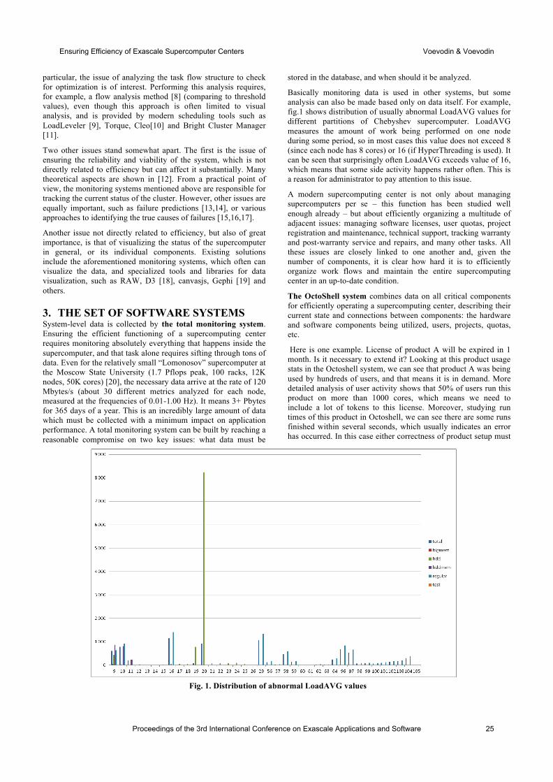
particular, the issue of analyzing the task flow structure to check for optimization is of interest. Performing this analysis requires, for example, a flow analysis method [8] (comparing to threshold values), even though this approach is often limited to visual analysis, and is provided by modern scheduling tools such as LoadLeveler [9], Torque, Cleo[10] and Bright Cluster Manager [11].

Two other issues stand somewhat apart. The first is the issue of ensuring the reliability and viability of the system, which is not directly related to efficiency but can affect it substantially. Many theoretical aspects are shown in [12]. From a practical point of view, the monitoring systems mentioned above are responsible for tracking the current status of the cluster. However, other issues are equally important, such as failure predictions [13,14], or various approaches to identifying the true causes of failures [15,16,17].

Another issue not directly related to efficiency, but also of great importance, is that of visualizing the status of the supercomputer in general, or its individual components. Existing solutions include the aforementioned monitoring systems, which often can visualize the data, and specialized tools and libraries for data visualization, such as RAW, D3 [18], canvasjs, Gephi [19] and others.

3. THE SET OF SOFTWARE SYSTEMS System-level data is collected by the total monitoring system. Ensuring the efficient functioning of a supercomputing center requires monitoring absolutely everything that happens inside the supercomputer, and that task alone requires sifting through tons of data. Even for the relatively small “Lomonosov” supercomputer at the Moscow State University (1.7 Pflops peak, 100 racks, 12K nodes, 50K cores) [20], the necessary data arrive at the rate of 120 Mbytes/s (about 30 different metrics analyzed for each node, measured at the frequencies of 0.01-1.00 Hz). It means 3+ Pbytes for 365 days of a year. This is an incredibly large amount of data which must be collected with a minimum impact on application performance. A total monitoring system can be built by reaching a reasonable compromise on two key issues: what data must be

stored in the database, and when should it be analyzed.

Basically monitoring data is used in other systems, but some analysis can also be made based only on data itself. For example, fig.1 shows distribution of usually abnormal LoadAVG values for different partitions of Chebyshev supercomputer. LoadAVG measures the amount of work being performed on one node during some period, so in most cases this value does not exceed 8 (since each node has 8 cores) or 16 (if HyperThreading is used). It can be seen that surprisingly often LoadAVG exceeds value of 16, which means that some side activity happens rather often. This is a reason for administrator to pay attention to this issue.

A modern supercomputing center is not only about managing supercomputers per se – this function has been studied well enough already – but about efficiently organizing a multitude of adjacent issues: managing software licenses, user quotas, project registration and maintenance, technical support, tracking warranty and post-warranty service and repairs, and many other tasks. All these issues are closely linked to one another and, given the number of components, it is clear how hard it is to efficiently organize work flows and maintain the entire supercomputing center in an up-to-date condition.

The OctoShell system combines data on all critical components for efficiently operating a supercomputing center, describing their current state and connections between components: the hardware and software components being utilized, users, projects, quotas, etc.

Here is one example. License of product A will be expired in 1 month. Is it necessary to extend it? Looking at this product usage stats in the Octoshell system, we can see that product A was being used by hundreds of users, and that means it is in demand. More detailed analysis of user activity shows that 50% of users run this product on more than 1000 cores, which means we need to include a lot of tokens to this license. Moreover, studying run times of this product in Octoshell, we can see there are some runs finished within several seconds, which usually indicates an error has occurred. In this case either correctness of product setup must

Fig. 1. Distribution of abnormal LoadAVG values .


Ensuring Efficiency of Exascale Supercomputer Centers Voevodin & Voevodin

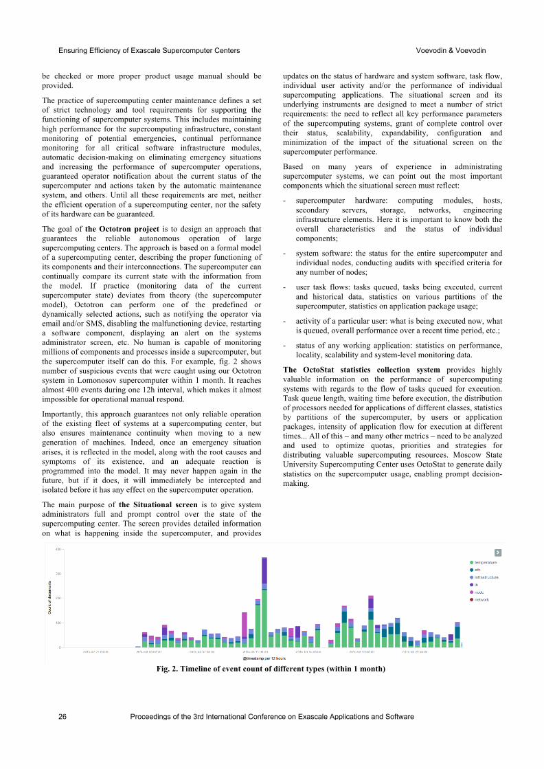
be checked or more proper product usage manual should be provided.

The practice of supercomputing center maintenance defines a set of strict technology and tool requirements for supporting the functioning of supercomputer systems. This includes maintaining high performance for the supercomputing infrastructure, constant monitoring of potential emergencies, continual performance monitoring for all critical software infrastructure modules, automatic decision-making on eliminating emergency situations and increasing the performance of supercomputer operations, guaranteed operator notification about the current status of the supercomputer and actions taken by the automatic maintenance system, and others. Until all these requirements are met, neither the efficient operation of a supercomputing center, nor the safety of its hardware can be guaranteed.

The goal of the Octotron project is to design an approach that guarantees the reliable autonomous operation of large supercomputing centers. The approach is based on a formal model of a supercomputing center, describing the proper functioning of its components and their interconnections. The supercomputer can continually compare its current state with the information from the model. If practice (monitoring data of the current supercomputer state) deviates from theory (the supercomputer model), Octotron can perform one of the predefined or dynamically selected actions, such as notifying the operator via email and/or SMS, disabling the malfunctioning device, restarting a software component, displaying an alert on the systems administrator screen, etc. No human is capable of monitoring millions of components and processes inside a supercomputer, but the supercomputer itself can do this. For example, fig. 2 shows number of suspicious events that were caught using our Octotron system in Lomonosov supercomputer within 1 month. It reaches almost 400 events during one 12h interval, which makes it almost impossible for operational manual respond.

Importantly, this approach guarantees not only reliable operation of the existing fleet of systems at a supercomputing center, but also ensures maintenance continuity when moving to a new generation of machines. Indeed, once an emergency situation arises, it is reflected in the model, along with the root causes and symptoms of its existence, and an adequate reaction is programmed into the model. It may never happen again in the future, but if it does, it will immediately be intercepted and isolated before it has any effect on the supercomputer operation.

The main purpose of the Situational screen is to give system administrators full and prompt control over the state of the supercomputing center. The screen provides detailed information on what is happening inside the supercomputer, and provides

updates on the status of hardware and system software, task flow, individual user activity and/or the performance of individual supercomputing applications. The situational screen and its underlying instruments are designed to meet a number of strict requirements: the need to reflect all key performance parameters of the supercomputing systems, grant of complete control over their status, scalability, expandability, configuration and minimization of the impact of the situational screen on the supercomputer performance.

Based on many years of experience in administrating supercomputer systems, we can point out the most important components which the situational screen must reflect:

- supercomputer hardware: computing modules, hosts, secondary servers, storage, networks, engineering infrastructure elements. Here it is important to know both the overall characteristics and the status of individual components;

- system software: the status for the entire supercomputer and individual nodes, conducting audits with specified criteria for any number of nodes;

- user task flows: tasks queued, tasks being executed, current and historical data, statistics on various partitions of the supercomputer, statistics on application package usage;

- activity of a particular user: what is being executed now, what is queued, overall performance over a recent time period, etc.;

- status of any working application: statistics on performance, locality, scalability and system-level monitoring data.

The OctoStat statistics collection system provides highly valuable information on the performance of supercomputing systems with regards to the flow of tasks queued for execution. Task queue length, waiting time before execution, the distribution of processors needed for applications of different classes, statistics by partitions of the supercomputer, by users or application packages, intensity of application flow for execution at different times... All of this – and many other metrics – need to be analyzed and used to optimize quotas, priorities and strategies for distributing valuable supercomputing resources. Moscow State University Supercomputing Center uses OctoStat to generate daily statistics on the supercomputer usage, enabling prompt decision-making.

Fig. 2. Timeline of event count of different types (within 1 month) .



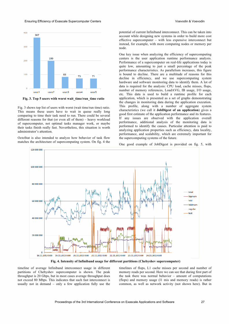
Fig. 3 shows top list of users with worst (wait time/run time) ratio. This means these users have to wait in queue really long comparing to time their task need to run. There could be several different reasons for that (or even all of them) – heavy workload of supercomputer, not optimal tasks manager work, or maybe their tasks finish really fast. Nevertheless, this situation is worth administrator’s attention.

OctoStat is also intended to analyze how behavior of task flow matches the architecture of supercomputing system. On fig. 4 the

timeline of average Infiniband interconnect usage in different partitions of Chebyshev supercomputer is shown. The peak throughput is 20 Gbps, but in most cases average throughput does not exceed 80 Mbps. This indicates that such fast interconnect is usually not in demand – only a few application fully use the

potential of current Infiniband interconnect. This can be taken into account while designing new systems in order to build more cost effective supercomputer – with less expensive interconnect but instead, for example, with more computing nodes or memory per node.

One key issue when analyzing the efficiency of supercomputing centers is the user application runtime performance analysis. Performance of a supercomputer on real-life applications today is quite low, amounting to just a small percentage of the peak performance characteristics. As parallelism increases, this figure is bound to decline. There are a multitude of reasons for this decline in efficiency, and we use supercomputing system hardware and software monitoring data to identify them. A lot of data is required for the analysis: CPU load, cache misses, flops, number of memory references, LoadAVG, IB usage, I/O usage, etc. This data is used to build a runtime profile for each application, which is presented as a set of graphs demonstrating the changes in monitoring data during the application execution. This profile, along with a number of aggregate system characteristics (we call it JobDigest of an application) gives a good first estimate of the application performance and its features. If any issues are observed with the application overall performance, additional analysis of the monitoring data is performed to identify the causes. Particular attention is paid to analyzing application properties such as efficiency, data locality, performance, and scalability, which are extremely important for the supercomputing systems of the future.

One good example of JobDigest is provided on fig. 5, with

timelines of flops, L1 cache misses per second and number of memory reads per second. Here we can see that during first part of the task there was normal behavior – amount of computations (flops) and memory usage (l1 mis and memory reads) is rather common, as well as network activity (not shown here). But in

Fig. 3. Top 5 users with worst wait_time/run_time ratio

Fig. 4. Intensity of Infiniband usage for different partitions (Chebyshev supercomputer) .



second part all activity besides memory reads drop nearly to zero. No data sent over network, no cache misses, no flops – generally this means that task fell into infinite loop, asking only for loop counter. So it is necessary to inform user that created this task about abnormal task behavior. It is worth mentioning that in this case average system characteristics could not help to find this anomaly because of rather long first part.

All the systems described above are closely linked to one another, ensuring high efficiency for large supercomputing centers. Of course, they were designed while taking all key aspects of maintenance and usage into account for existing supercomputers. At the same time, the architecture of these systems was designed to be able to adopt large scale, complexity, high degree of parallelism and performance of the forthcoming exascale supercomputers.

4. CONCLUSIONS A set of software systems presented is this article is intended to help users as well as administrators of supercomputers to ensure efficiency of every level of supercomputing center usage – from individual users tasks to the whole cluster. This includes a range of different efficiency issues, concerning not only performance monitoring and analysis but also visualization and reliability problems. This set is being actively developed and used by a team from research computing center at the Moscow State University.

Acknowledgments. The results were obtained with the financial support of the Ministry of Education and Science of the Russian Federation, Agreement N 14.607.21.0006 (unique identifier RFMEFI60714X0006).

5. REFERENCES [1] Voevodin Vladimir. Medical practice: diagnostics, treatment and

surgery in supercomputing centers. Presentation at the International Advanced Research Workshop on High Performance Computing, Cetraro, Italy, 2014. Available at: http://www.hpcc.unical.it/hpc2014/pdfs/voevodin.pdf. Date accessed: 08 May. 2015.

[2] Cappello, Franck et al. Toward Exascale Resilience: 2014 update. Supercomputing frontiers and innovations, [S.l.], v. 1, n. 1, p. 5-28, jun. 2014. ISSN 2313-8734. Available at: http://superfri.org/superfri/article/view/14. Date accessed: 08 May. 2015. doi:http://dx.doi.org/10.14529/jsfi140101.

[3] List of different monitoring tools. http://www.slac.stanford.edu/xorg/nmtf/nmtf-tools.html

[4] HP Network Node Manager main page. http://www8.hp.com/us/en/software-solutions/network-node-manager-i-network-management-software/index.html

[5] ClustrX description. http://www.t-platforms.com/products/software/clustrxproductfamily.html

[6] Intel Parallel Studio XE main page. https://software.intel.com/en-us/intel-parallel-studio-xe

[7] Score-P main page. http://www.vi-hps.org/projects/score-p/

[8] Feitelson D. G., Rudolph L. Toward convergence in job schedulers for parallel supercomputers //Job Scheduling Strategies for Parallel Processing. – Springer Berlin Heidelberg, 1996. – С. 1-26.

[9] LoadLeveler description. http://www-03.ibm.com/software/products/en/tivoliworkloadschedulerloadleveler

[10] Cleo description and source code. http://sourceforge.net/projects/cleo-bs/

[11] Bright Cluster Manager main page. http://www.brightcomputing.com/Bright-Cluster-Manager

[12] Snir M, Wisniewski R, Abraham J, Adve S, Bagchi S, Balaji P, Belak J, Bose P, Cappello F, Carlson B and others. 2014. Addressing Failures in Exascale Computing. International Journal of High Performance Computing Applications

[13] Hoffmann, G. A. 2006. Failure Prediction in Complex Computer Systems: A Probabilistic Approach. Shaker Verlag

[14] Murray, J., Hughes, G., and Kreutz-Delgado, K. 2003. Hard drive failure prediction using non-parametric statistical methods. Proceedings of ICANN/ICONIP.

[15] Lu K. et al. Iaso: an autonomous fault-tolerant management system for supercomputers //Frontiers of Computer Science. – 2014. – Т. 8. – . 3. – С. 378-390.

[16] Chuah E. et al. Diagnosing the root-causes of failures from cluster log files //High Performance Computing (HiPC), 2010 International Conference on. – IEEE, 2010. – С. 1-10.

[17] Bodik P. et al. Fingerprinting the datacenter: automated classification of performance crises //Proceedings of the 5th European conference on Computer systems. – ACM, 2010. – С. 111-124.

[18] D3 site. http://d3js.org/

[19] Gephi main page. http://gephi.github.io/

[20] V. Sadovnichy, A. Tikhonravov, Vl. Voevodin, and V. Opanasenko "Lomonosov": Supercomputing at Moscow State University. In Contemporary High Performance Computing: From Petascale toward Exascale (Chapman & Hall/CRC Computational Science), pp.283-307, Boca Raton, USA, CRC Press, 2013.

Fig. 5. Timeline of flops, L1-cache misses and memory reads for a particular task

.



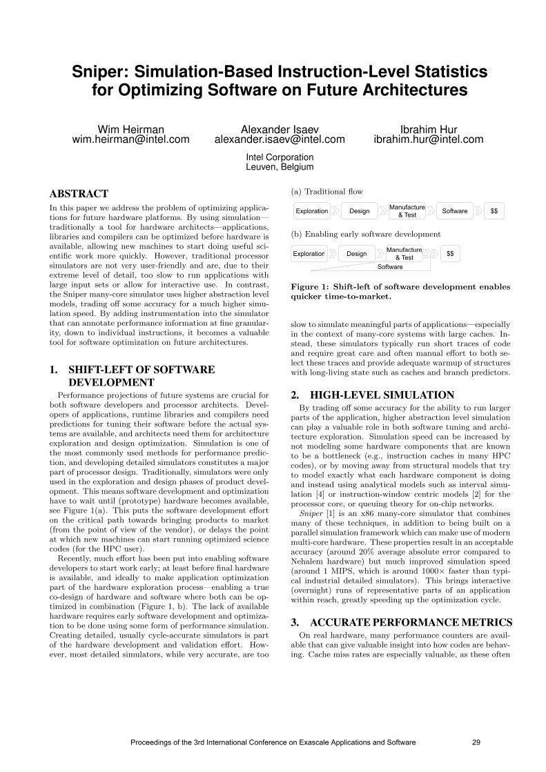
Sniper: Simulation-Based Instruction-Level Statisticsfor Optimizing Software on Future Architectures

Wim [email protected]

Alexander [email protected]

Intel CorporationLeuven, Belgium

Ibrahim [email protected]

ABSTRACTIn this paper we address the problem of optimizing applica-tions for future hardware platforms. By using simulation—traditionally a tool for hardware architects—applications,libraries and compilers can be optimized before hardware isavailable, allowing new machines to start doing useful sci-entific work more quickly. However, traditional processorsimulators are not very user-friendly and are, due to theirextreme level of detail, too slow to run applications withlarge input sets or allow for interactive use. In contrast,the Sniper many-core simulator uses higher abstraction levelmodels, trading off some accuracy for a much higher simu-lation speed. By adding instrumentation into the simulatorthat can annotate performance information at fine granular-ity, down to individual instructions, it becomes a valuabletool for software optimization on future architectures.

1. SHIFT-LEFT OF SOFTWAREDEVELOPMENT

Performance projections of future systems are crucial forboth software developers and processor architects. Devel-opers of applications, runtime libraries and compilers needpredictions for tuning their software before the actual sys-tems are available, and architects need them for architectureexploration and design optimization. Simulation is one ofthe most commonly used methods for performance predic-tion, and developing detailed simulators constitutes a majorpart of processor design. Traditionally, simulators were onlyused in the exploration and design phases of product devel-opment. This means software development and optimizationhave to wait until (prototype) hardware becomes available,see Figure 1(a). This puts the software development efforton the critical path towards bringing products to market(from the point of view of the vendor), or delays the pointat which new machines can start running optimized sciencecodes (for the HPC user).

Recently, much effort has been put into enabling softwaredevelopers to start work early; at least before final hardwareis available, and ideally to make application optimizationpart of the hardware exploration process—enabling a trueco-design of hardware and software where both can be op-timized in combination (Figure 1, b). The lack of availablehardware requires early software development and optimiza-tion to be done using some form of performance simulation.Creating detailed, usually cycle-accurate simulators is partof the hardware development and validation effort. How-ever, most detailed simulators, while very accurate, are too

(a) Traditional flow

Exploration DesignManufacture

& TestSoftware $$

(b) Enabling early software development

Software

Exploration DesignManufacture

& Test$$

Figure 1: Shift-left of software development enablesquicker time-to-market.

slow to simulate meaningful parts of applications—especiallyin the context of many-core systems with large caches. In-stead, these simulators typically run short traces of codeand require great care and often manual effort to both se-lect these traces and provide adequate warmup of structureswith long-living state such as caches and branch predictors.

2. HIGH-LEVEL SIMULATIONBy trading off some accuracy for the ability to run larger

parts of the application, higher abstraction level simulationcan play a valuable role in both software tuning and archi-tecture exploration. Simulation speed can be increased bynot modeling some hardware components that are knownto be a bottleneck (e.g., instruction caches in many HPCcodes), or by moving away from structural models that tryto model exactly what each hardware component is doingand instead using analytical models such as interval simu-lation [4] or instruction-window centric models [2] for theprocessor core, or queuing theory for on-chip networks.

Sniper [1] is an x86 many-core simulator that combinesmany of these techniques, in addition to being built on aparallel simulation framework which can make use of modernmulti-core hardware. These properties result in an acceptableaccuracy (around 20% average absolute error compared toNehalem hardware) but much improved simulation speed(around 1 MIPS, which is around 1000× faster than typi-cal industrial detailed simulators). This brings interactive(overnight) runs of representative parts of an applicationwithin reach, greatly speeding up the optimization cycle.

3. ACCURATE PERFORMANCE METRICSOn real hardware, many performance counters are avail-

able that can give valuable insight into how codes are behav-ing. Cache miss rates are especially valuable, as these often


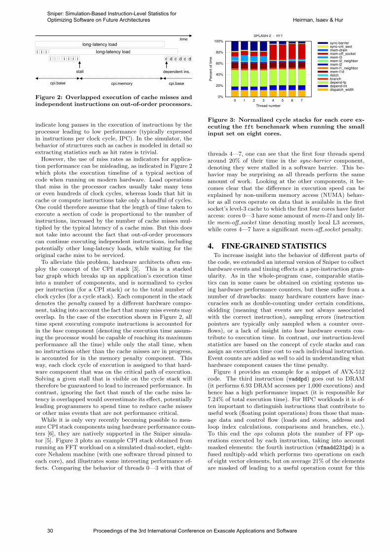
long-latency load

long-latency loadi i i

i i i i i i i

time

stall

d

dependent ins.

cpi.base cpi.basecpi.memory

d d d d d

Figure 2: Overlapped execution of cache misses andindependent instructions on out-of-order processors.

indicate long pauses in the execution of instructions by theprocessor leading to low performance (typically expressedin instructions per clock cycle, IPC). In the simulator, thebehavior of structures such as caches is modeled in detail soextracting statistics such as hit rates is trivial.

However, the use of miss rates as indicators for applica-tion performance can be misleading, as indicated in Figure 2which plots the execution timeline of a typical section ofcode when running on modern hardware. Load operationsthat miss in the processor caches usually take many tensor even hundreds of clock cycles, whereas loads that hit incache or compute instructions take only a handful of cycles.One could therefore assume that the length of time taken toexecute a section of code is proportional to the number ofinstructions, increased by the number of cache misses mul-tiplied by the typical latency of a cache miss. But this doesnot take into account the fact that out-of-order processorscan continue executing independent instructions, includingpotentially other long-latency loads, while waiting for theoriginal cache miss to be serviced.

To alleviate this problem, hardware architects often em-ploy the concept of the CPI stack [3]. This is a stackedbar graph which breaks up an application’s execution timeinto a number of components, and is normalized to cyclesper instruction (for a CPI stack) or to the total number ofclock cycles (for a cycle stack). Each component in the stackdenotes the penalty caused by a different hardware compo-nent, taking into account the fact that many miss events mayoverlap. In the case of the execution shown in Figure 2, alltime spent executing compute instructions is accounted forin the base component (denoting the execution time assum-ing the processor would be capable of reaching its maximumperformance all the time) while only the stall time, whenno instructions other than the cache misses are in progress,is accounted for in the memory penalty component. Thisway, each clock cycle of execution is assigned to that hard-ware component that was on the critical path of execution.Solving a given stall that is visible on the cycle stack willtherefore be guaranteed to lead to increased performance. Incontrast, ignoring the fact that much of the cache miss la-tency is overlapped would overestimate its effect, potentiallyleading programmers to spend time to reduce cache missesor other miss events that are not performance critical.

While it is only very recently becoming possible to mea-sure CPI stack components using hardware performance coun-ters [6], they are natively supported in the Sniper simula-tor [5]. Figure 3 plots an example CPI stack obtained fromrunning an FFT workload on a simulated dual-socket, eight-core Nehalem machine (with one software thread pinned toeach core), and illustrates some interesting performance ef-fects. Comparing the behavior of threads 0—3 with that of

0%

20%

40%

60%

80%

100%

0 1 2 3 4 5 6 7

Pe

rce

nt

of

tim

e

Thread number

SPLASH-2 - FFT

dispatch_widthdepend-intdepend-fpbranchifetchmem-l1dmem-l1_neighbormem-l2mem-l2_neighbormem-l3mem-off_socketmem-dramsync-crit_sectsync-barrier

Figure 3: Normalized cycle stacks for each core ex-ecuting the fft benchmark when running the smallinput set on eight cores.

threads 4—7, one can see that the first four threads spendaround 20% of their time in the sync-barrier component,denoting they were stalled in a software barrier. This be-havior may be surprising as all threads perform the sameamount of work. Looking at the other components, it be-comes clear that the difference in execution speed can beexplained by non-uniform memory access (NUMA) behav-ior as all cores operate on data that is available in the firstsocket’s level-3 cache to which the first four cores have fasteraccess: cores 0—3 have some amount of mem-l3 and only lit-tle mem-off socket time denoting mostly local L3 accesses,while cores 4—7 have a significant mem-off socket penalty.

4. FINE-GRAINED STATISTICSTo increase insight into the behavior of different parts of

the code, we extended an internal version of Sniper to collecthardware events and timing effects at a per-instruction gran-ularity. As in the whole-program case, comparable statis-tics can in some cases be obtained on existing systems us-ing hardware performance counters, but these suffer from anumber of drawbacks: many hardware counters have inac-curacies such as double-counting under certain conditions,skidding (meaning that events are not always associatedwith the correct instruction), sampling errors (instructionpointers are typically only sampled when a counter over-flows), or a lack of insight into how hardware events con-tribute to execution time. In contrast, our instruction-levelstatistics are based on the concept of cycle stacks and canassign an execution time cost to each individual instruction.Event counts are added as well to aid in understanding whathardware component causes the time penalty.

Figure 4 provides an example for a snippet of AVX-512code. The third instruction (vaddpd) goes out to DRAM(it performs 6.93 DRAM accesses per 1,000 executions) andhence has a high performance impact (it is responsible for7.24% of total execution time). For HPC workloads it is of-ten important to distinguish instructions that contribute touseful work (floating point operations) from those that man-age data and control flow (loads and stores, address andloop index calculations, comparisons and branches, etc.).To this end the ops column plots the number of FP op-erations executed by each instruction, taking into accountmasked elements: the fourth instruction (vfmadd231pd) is afused multiply-add which performs two operations on eachof eight vector elements, but on average 21% of the elementsare masked off leading to a useful operation count for this


Sniper: Simulation-Based Instruction-Level Statistics for Optimizing Software on Future Architectures Heirman, Isaev & Hur

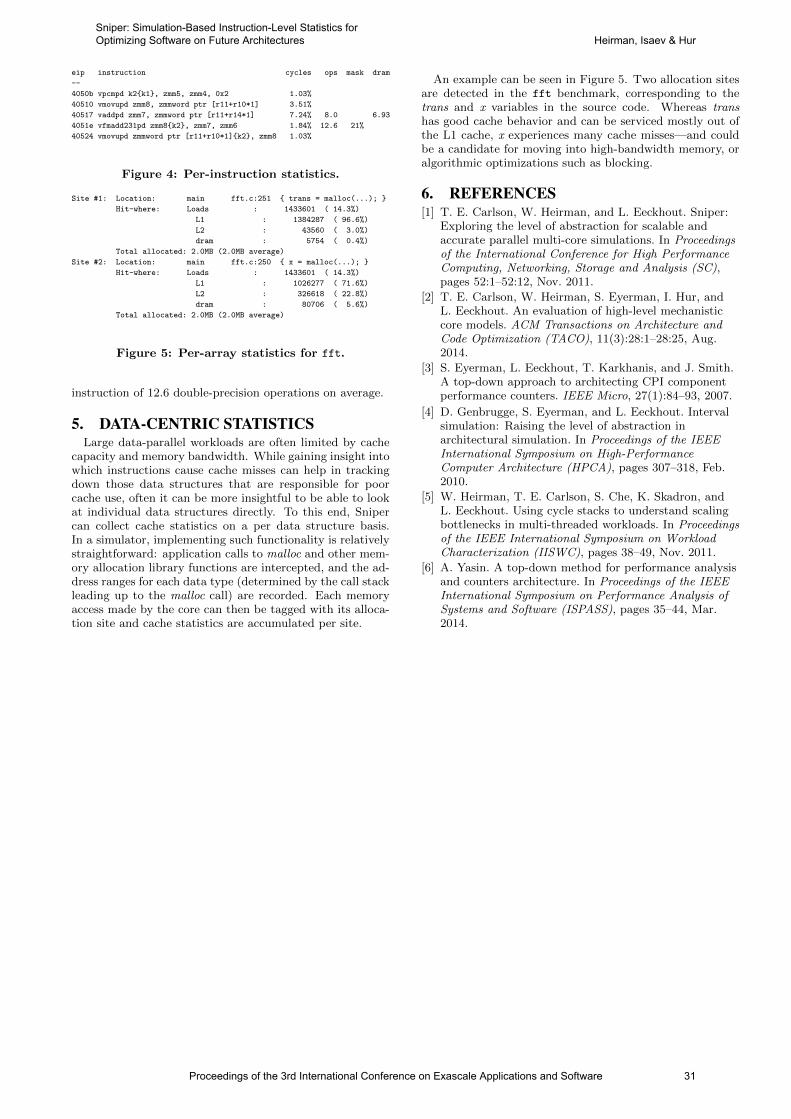
eip instruction cycles ops mask dram

--

4050b vpcmpd k2k1, zmm5, zmm4, 0x2 1.03%

40510 vmovupd zmm8, zmmword ptr [r11+r10*1] 3.51%

40517 vaddpd zmm7, zmmword ptr [r11+r14*1] 7.24% 8.0 6.93

4051e vfmadd231pd zmm8k2, zmm7, zmm6 1.84% 12.6 21%

40524 vmovupd zmmword ptr [r11+r10*1]k2, zmm8 1.03%

Figure 4: Per-instruction statistics.

Site #1: Location: main fft.c:251 trans = malloc(...);

Hit-where: Loads : 1433601 ( 14.3%)

L1 : 1384287 ( 96.6%)

L2 : 43560 ( 3.0%)

dram : 5754 ( 0.4%)

Total allocated: 2.0MB (2.0MB average)

Site #2: Location: main fft.c:250 x = malloc(...);

Hit-where: Loads : 1433601 ( 14.3%)

L1 : 1026277 ( 71.6%)

L2 : 326618 ( 22.8%)

dram : 80706 ( 5.6%)

Total allocated: 2.0MB (2.0MB average)

Figure 5: Per-array statistics for fft.

instruction of 12.6 double-precision operations on average.

5. DATA-CENTRIC STATISTICSLarge data-parallel workloads are often limited by cache

capacity and memory bandwidth. While gaining insight intowhich instructions cause cache misses can help in trackingdown those data structures that are responsible for poorcache use, often it can be more insightful to be able to lookat individual data structures directly. To this end, Snipercan collect cache statistics on a per data structure basis.In a simulator, implementing such functionality is relativelystraightforward: application calls to malloc and other mem-ory allocation library functions are intercepted, and the ad-dress ranges for each data type (determined by the call stackleading up to the malloc call) are recorded. Each memoryaccess made by the core can then be tagged with its alloca-tion site and cache statistics are accumulated per site.

An example can be seen in Figure 5. Two allocation sitesare detected in the fft benchmark, corresponding to thetrans and x variables in the source code. Whereas transhas good cache behavior and can be serviced mostly out ofthe L1 cache, x experiences many cache misses—and couldbe a candidate for moving into high-bandwidth memory, oralgorithmic optimizations such as blocking.

6. REFERENCES[1] T. E. Carlson, W. Heirman, and L. Eeckhout. Sniper:

Exploring the level of abstraction for scalable andaccurate parallel multi-core simulations. In Proceedingsof the International Conference for High PerformanceComputing, Networking, Storage and Analysis (SC),pages 52:1–52:12, Nov. 2011.

[2] T. E. Carlson, W. Heirman, S. Eyerman, I. Hur, andL. Eeckhout. An evaluation of high-level mechanisticcore models. ACM Transactions on Architecture andCode Optimization (TACO), 11(3):28:1–28:25, Aug.2014.

[3] S. Eyerman, L. Eeckhout, T. Karkhanis, and J. Smith.A top-down approach to architecting CPI componentperformance counters. IEEE Micro, 27(1):84–93, 2007.

[4] D. Genbrugge, S. Eyerman, and L. Eeckhout. Intervalsimulation: Raising the level of abstraction inarchitectural simulation. In Proceedings of the IEEEInternational Symposium on High-PerformanceComputer Architecture (HPCA), pages 307–318, Feb.2010.

[5] W. Heirman, T. E. Carlson, S. Che, K. Skadron, andL. Eeckhout. Using cycle stacks to understand scalingbottlenecks in multi-threaded workloads. In Proceedingsof the IEEE International Symposium on WorkloadCharacterization (IISWC), pages 38–49, Nov. 2011.

[6] A. Yasin. A top-down method for performance analysisand counters architecture. In Proceedings of the IEEEInternational Symposium on Performance Analysis ofSystems and Software (ISPASS), pages 35–44, Mar.2014.


Sniper: Simulation-Based Instruction-Level Statistics for Optimizing Software on Future Architectures Heirman, Isaev & Hur

Support Operators Technique for 3D Simulations ofDissipative Processes at High Performance Computers

Irina GasilovaKeldysh Institute of Applied

Mathematics RASMiusskaya sq., 4

125047, Russia, [email protected]

Yuri PoveshenkoKeldysh Institute of Applied



Aleksey BoldarevKeldysh Institute of Applied



Gennady BagdasarovKeldysh Institute of Applied



Mikhail IakobovskiKeldysh Institute of Applied



ABSTRACTThis paper describes an efficient method for 3D compu-tational fluid dynamics (CFD) simulations on high perfor-mance computers. The problems related to the robustnessand stability of numerical algorithms for distributed simu-lations are considered. On the example of common scalardivergence problem the rotationally-invariant finite differ-ence scheme based on support operators technique is builtand essential properties of the scheme are depicted. Theresults of the numerical simulations of the implemented inMARPLE3D package algorithm and the results of the scal-ing of the developed software on cluster are presented.

KeywordsSupport operators technique; finite differencing; unstruc-tured meshes; high performance computing.

1. INTRODUCTIONNowadays due to the rapid developments in the area ofhigh performance computing there appeared the possibil-ity to perform predictive numerical simulations in the areaof CFD in the complex-shaped domains on the meshes ofhuge dimensions. These meshes are very finely discretizedthus one can simulate highly multiscale physical processeswhich on its turn requires simulations using robust and sta-ble numerical algorithms. These algorithms should possessa number of properties such as: conservativity, monotonic-ity, stability in a wide range of flow parameters, high res-olution, positivness/nonpositiveness, self-adjointness of dif-ference operators, etc [3], which lead to the solutions withguaranteed quality. The support operators method is re-markable as it allows building approximations to differentialoperators using general meshes (block-structured, unstruc-tured, mortar etc.) while the resulting difference operatorspreserve not only basic properties mentioned above, but,additionally, they provide rotationally-invariant differenceschemes [2]. It’s important to pay special attention to therotational invariance while working with systems describingdeformations and dissipations in gas or liquid media, e.g.Navier-Stokes equations.

2. SUPPORT OPERATORS TECHNIQUEIn the area O with the bounadry ∂O let’s consider a com-mon scalar-divergence boundary problem with, for example,Dirichlet boundary condition:

divXu = f(r)

Xu = K∇u, u|∂O = u∗(x) (1)

Here u – scalar (temperature, pressure and so on), X – arbi-trary vector, Xu – flows, induced by the gradient of functionu in the media with the conduction properties, defined bytensor K. Traditional approach to the approximation ofdifferential operators consists in the independent approxi-mation of differential operators using the Gauss Theorem:∫

O

divX dV =

∫∂O

X dS,

∫O

gradu dV =

∫∂O

u dS

Support operators method – is a technique with the consis-tent approximation of differential operators. The system ofequations (1) is considered along with the following identicalintegral equation:∫

O

(X,∇u) dv +

∫O

u · divX dv =

∫∂O

u (X, ds) (2)

One operator (div or grad) is approximated directly; theother one is approximated in the way, that it satisfies thedifference analogue of the integral equation (2).

3. DIFFERENCE SCHEMETo construct a difference scheme it is needed to introduce adifference mesh in the computational domain and to definemesh functions which will approximate functions of the con-tinuous argument. Depending on the physical origin of thevalues and on the way of their definition on the mesh some-times it is more convenient to approximate one or anotherdifferential operator directly. In the example given in thispaper the support operators scheme was built using grad asa support operator.


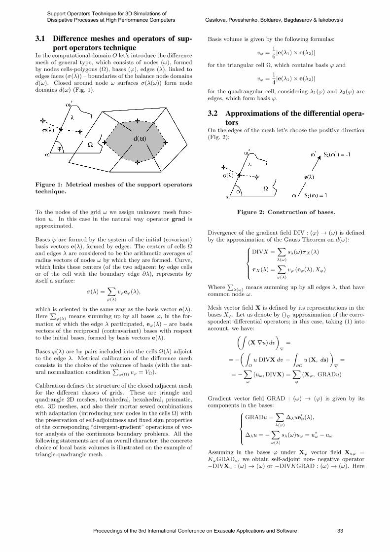
3.1 Difference meshes and operators of sup-port operators technique

In the computational domain O let’s introduce the differencemesh of general type, which consists of nodes (ω), formedby nodes cells-polygons (Ω), bases (ϕ), edges (λ), linked toedges faces (σ(λ)) – boundaries of the balance node domainsd(ω). Closed around node ω surfaces σ(λ(ω)) form nodedomains d(ω) (Fig. 1).

Figure 1: Metrical meshes of the support operatorstechnique.

To the nodes of the grid ω we assign unknown mesh func-tion u. In this case in the natural way operator grad isapproximated.

Bases ϕ are formed by the system of the initial (covariant)basis vectors e(λ), formed by edges. The centers of cells Ωand edges λ are considered to be the arithmetic averages ofradius vectors of nodes ω by which they are formed. Curve,which links these centers (of the two adjacent by edge cellsor of the cell with the boundary edge ∂λ), represents byitself a surface:

σ(λ) =∑ϕ(λ)

vϕeϕ(λ),

which is oriented in the same way as the basis vector e(λ).Here

∑ϕ(λ) means summing up by all bases ϕ, in the for-

mation of which the edge λ participated, eϕ(λ) – are basisvectors of the reciprocal (contravariant) bases with respectto the initial bases, formed by basis vectors e(λ).

Bases ϕ(λ) are by pairs included into the cells Ω(λ) adjointto the edge λ. Metrical calibration of the difference meshconsists in the choice of the volumes of basis (with the nat-ural normalization condition

∑ϕ(Ω) vϕ = VΩ).

Calibration defines the structure of the closed adjacent meshfor the different classes of grids. These are triangle andquadrangle 2D meshes, tetrahedral, hexahedral, prismatic,etc. 3D meshes, and also their mortar sewed combinationswith adaptation (introducing new nodes in the cells Ω) withthe preservation of self-adjointness and fixed sign propertiesof the corresponding “divergent-gradient” operations of vec-tor analysis of the continuous boundary problems. All thefollowing statements are of an overall character; the concretechoice of local basis volumes is illustrated on the example oftriangle-quadrangle mesh.

Basis volume is given by the following formulas:

vϕ =1

6|e(λ1)× e(λ2)|

for the triangular cell Ω, which contains basis ϕ and

vϕ =1

4|e(λ1)× e(λ2)|

for the quadrangular cell, considering λ1(ϕ) and λ2(ϕ) areedges, which form basis ϕ.

3.2 Approximations of the differential opera-tors

On the edges of the mesh let’s choose the positive direction(Fig. 2):

Figure 2: Construction of bases.

Divergence of the gradient field DIV : (ϕ) → (ω) is definedby the approximation of the Gauss Theorem on d(ω):

DIVX =∑λ(ω)

sλ(ω)τX(λ)

τX(λ) =∑ϕ(λ)

vϕ (eϕ(λ), Xϕ)

Where∑λ(ω) means summing up by all edges λ, that have

common node ω.

Mesh vector field X is defined by its representations in thebases Xϕ. Let us denote by ()∇ approximation of the corre-spondent differential operators; in this case, taking (1) intoaccount, we have:(∫

(X ∇u) dv

)∇

=

= −(∫

O

u DIVX dv −∫∂O

u (X, ds)

)∇

=

= −∑ω

(uω,DIVX) =∑ϕ

(Xϕ, GRADu)

Gradient vector field GRAD : (ω) → (ϕ) is given by itscomponents in the bases:

GRADu =∑λ(ϕ)

∆λue′ϕ(λ),

∆λu = −∑ω(λ)

sλ(ω)uω = u∗ω − uω

Assuming in the bases ϕ under Xϕ vector field Xuϕ =KϕGRADu, we obtain self-adjoint non- negative operator−DIVXu : (ω) → (ω) or −DIVKGRAD : (ω) → (ω). Here


Support Operators Technique for 3D Simulations of Dissipative Processes at High Performance Computers Gasilova, Poveshenko, Boldarev, Bagdasarov & Iakobovski

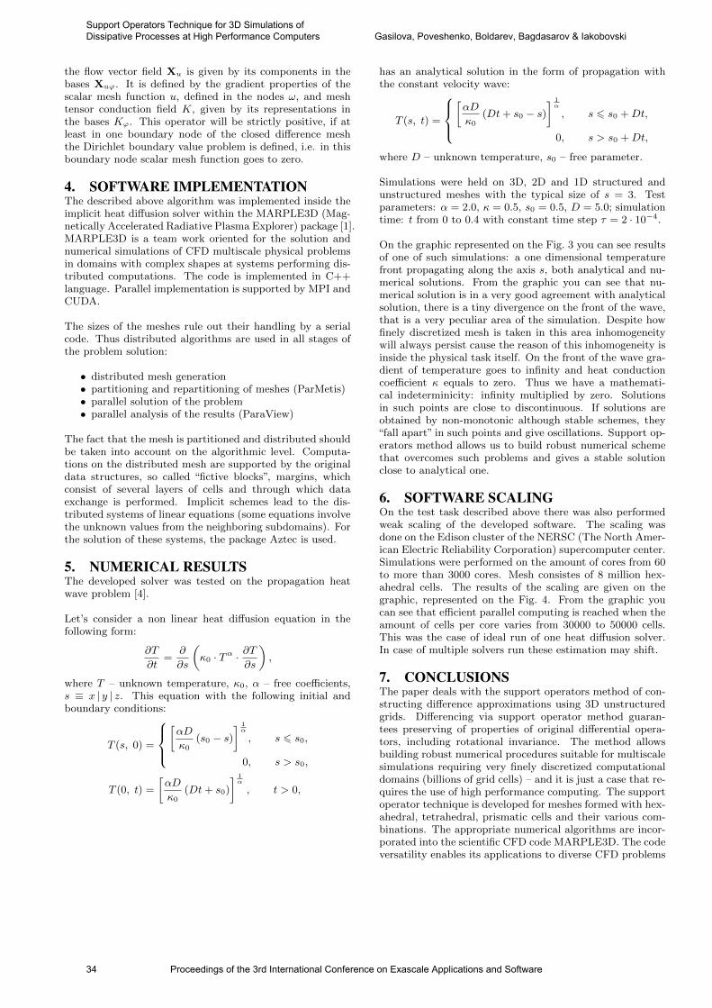
the flow vector field Xu is given by its components in thebases Xuϕ. It is defined by the gradient properties of thescalar mesh function u, defined in the nodes ω, and meshtensor conduction field K, given by its representations inthe bases Kϕ. This operator will be strictly positive, if atleast in one boundary node of the closed difference meshthe Dirichlet boundary value problem is defined, i.e. in thisboundary node scalar mesh function goes to zero.

4. SOFTWARE IMPLEMENTATIONThe described above algorithm was implemented inside theimplicit heat diffusion solver within the MARPLE3D (Mag-netically Accelerated Radiative Plasma Explorer) package [1].MARPLE3D is a team work oriented for the solution andnumerical simulations of CFD multiscale physical problemsin domains with complex shapes at systems performing dis-tributed computations. The code is implemented in C++language. Parallel implementation is supported by MPI andCUDA.

The sizes of the meshes rule out their handling by a serialcode. Thus distributed algorithms are used in all stages ofthe problem solution:

• distributed mesh generation• partitioning and repartitioning of meshes (ParMetis)• parallel solution of the problem• parallel analysis of the results (ParaView)

The fact that the mesh is partitioned and distributed shouldbe taken into account on the algorithmic level. Computa-tions on the distributed mesh are supported by the originaldata structures, so called “fictive blocks”, margins, whichconsist of several layers of cells and through which dataexchange is performed. Implicit schemes lead to the dis-tributed systems of linear equations (some equations involvethe unknown values from the neighboring subdomains). Forthe solution of these systems, the package Aztec is used.

5. NUMERICAL RESULTSThe developed solver was tested on the propagation heatwave problem [4].

Let’s consider a non linear heat diffusion equation in thefollowing form:

∂T

∂t=

∂

∂s

(κ0 · Tα ·

∂T

∂s

),

where T – unknown temperature, κ0, α – free coefficients,s ≡ x | y | z. This equation with the following initial andboundary conditions:

T (s, 0) =

[αD

κ0(s0 − s)

] 1α

, s 6 s0,

0, s > s0,

T (0, t) =

[αD

κ0(Dt+ s0)

] 1α

, t > 0,

has an analytical solution in the form of propagation withthe constant velocity wave:

T (s, t) =

[αD

κ0(Dt+ s0 − s)

] 1α

, s 6 s0 +Dt,

0, s > s0 +Dt,

where D – unknown temperature, s0 – free parameter.

Simulations were held on 3D, 2D and 1D structured andunstructured meshes with the typical size of s = 3. Testparameters: α = 2.0, κ = 0.5, s0 = 0.5, D = 5.0; simulationtime: t from 0 to 0.4 with constant time step τ = 2 · 10−4.

On the graphic represented on the Fig. 3 you can see resultsof one of such simulations: a one dimensional temperaturefront propagating along the axis s, both analytical and nu-merical solutions. From the graphic you can see that nu-merical solution is in a very good agreement with analyticalsolution, there is a tiny divergence on the front of the wave,that is a very peculiar area of the simulation. Despite howfinely discretized mesh is taken in this area inhomogeneitywill always persist cause the reason of this inhomogeneity isinside the physical task itself. On the front of the wave gra-dient of temperature goes to infinity and heat conductioncoefficient κ equals to zero. Thus we have a mathemati-cal indeterminicity: infinity multiplied by zero. Solutionsin such points are close to discontinuous. If solutions areobtained by non-monotonic although stable schemes, they“fall apart” in such points and give oscillations. Support op-erators method allows us to build robust numerical schemethat overcomes such problems and gives a stable solutionclose to analytical one.

6. SOFTWARE SCALINGOn the test task described above there was also performedweak scaling of the developed software. The scaling wasdone on the Edison cluster of the NERSC (The North Amer-ican Electric Reliability Corporation) supercomputer center.Simulations were performed on the amount of cores from 60to more than 3000 cores. Mesh consistes of 8 million hex-ahedral cells. The results of the scaling are given on thegraphic, represented on the Fig. 4. From the graphic youcan see that efficient parallel computing is reached when theamount of cells per core varies from 30000 to 50000 cells.This was the case of ideal run of one heat diffusion solver.In case of multiple solvers run these estimation may shift.

7. CONCLUSIONSThe paper deals with the support operators method of con-structing difference approximations using 3D unstructuredgrids. Differencing via support operator method guaran-tees preserving of properties of original differential opera-tors, including rotational invariance. The method allowsbuilding robust numerical procedures suitable for multiscalesimulations requiring very finely discretized computationaldomains (billions of grid cells) – and it is just a case that re-quires the use of high performance computing. The supportoperator technique is developed for meshes formed with hex-ahedral, tetrahedral, prismatic cells and their various com-binations. The appropriate numerical algorithms are incor-porated into the scientific CFD code MARPLE3D. The codeversatility enables its applications to diverse CFD problems



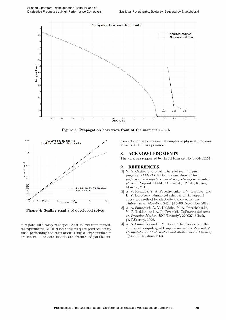
Figure 3: Propagation heat wave front at the moment t = 0.4.

Figure 4: Scaling results of developed solver.

in regions with complex shapes. As it follows from numeri-cal experiments, MARPLE3D ensures quite good scalabilitywhen performing the calculations using a large number ofprocessors. The data models and features of parallel im-

plementation are discussed. Examples of physical problemssolved via HPC are presented.

8. ACKNOWLEDGMENTSThe work was supported by the RFFI grant No. 14-01-31154.

9. REFERENCES[1] V. A. Gasilov and et Al. The package of applied

programs MARPLE3D for the modelling at highperformance computers pulsed magnetically acceleratedplasma. Preprint KIAM RAS No. 20, 125047, Russia,Moscow, 2011.

[2] A. V. Koldoba, Y. A. Poveshchenko, I. V. Gasilova, andE. Y. Dorofeeva. Numerical schemes of the supportoperators method for elasticity theory equations.Mathematical Modeling, 24(12):86–96, November 2012.

[3] A. A. Samarskii, A. V. Koldoba, Y. A. Poveshchenko,V. F. Tishkin, and A. P. Favorskii. Difference Schemeson Irregular Meshes. JSC ’Kriteriy’, 220027, Minsk,pr. F.Scoriny, 1999.

[4] A. A. Samarskii and I. M. Sobol. The examples of thenumerical computing of temperature waves. Journal ofComputational Mathematics and Mathematical Physics,3(4):702–718, June 1963.



Efficiently Scheduling Task Dataflow Parallelism:A Comparison Between Swan and QUARK

Hans VandierendonckQueen’s University Belfast

United [email protected]

ABSTRACTIncreased system variability and irregularity of parallelism inapplications put increasing demands on the efficiency of dy-namic task schedulers. This paper presents a new design fora work-stealing scheduler supporting both Cilk-style recur-sively parallel code and parallelism deduced from dataflowdependences. Initial evaluation on a set of linear algebra ker-nels demonstrates that our scheduler outperforms PLASMA’sQUARK scheduler by up to 12% on a 16-thread Intel Xeonand by up to 50% on a 32-thread AMD Bulldozer.

1. INTRODUCTIONThe many-core roadmap for processors dictates that the

number of cores on a processor chip increases at an expo-nential rate. Moreover, cores tend to operate at differentspeeds due to process variability and thermal constraints.As such, parallel task schedulers in the exascale era mustmake dynamic (runtime) scheduling decisions [1].

The task dataflow notation has been studied widely asa viable approach to facilitate the specification of highlyparallel codes [2, 3, 4]. Task dataflow dependences specify anordering of tasks (they leverage a task graph), which by itsnature exposes a higher degree of parallelism than barrier-based models where threads wait periodically for all runningtasks to complete. Dynamic schedulers are, however, proneto result in less performance than static schedulers due toruntime task scheduling overhead.

This work investigates a new design for a task dataflowdynamic scheduler. The key design goal is to minimize run-time overhead without affecting the task dataflow program-ming interface. The scheduler supports programs mixingrecursive divide-and-conquer parallelism and task dataflowparallelism. This hybrid design simplifies, for instance, theexploitation of parallelism across multiple kernels called insuccession. The scheduler combines the efficiency of Cilk’swork stealing scheduler [5] for recursively parallel programswith the efficiency of the steal-half queue [6] for programsgenerating large numbers of simultaneously ready tasks.

We evaluate our design experimentally and compare againstPLASMA’s QUARK [2] scheduler on a set of level-3 BLASkernels with irregular parallelism. In comparison to QUARK,our scheduler reduces end-to-end execution time of severallinear algebra kernels by up to 12% on an Intel Xeon (SandyBridge) and by up to 50% on an AMD Bulldozer.

2. RELATED WORKSeveral approaches to task dataflow scheduling have been

experimented with. Several authors have implemented Toma-sulo’s algorithm in software [7, 8]. QUARK [2] is a work-stealing scheduler tuned to linear algebra problems. QUARKattempts to optimize data locality. QUARK records andenforces dependences using the starting address of a taskargument. As such it is dependent on a fixed argument size.SMPSs [9] uses a comparable work stealing design with manydesign decisions that are similar from a high level point ofview. An SMPSs extension for strided and sparse access pat-terns incurs a high performance penalty by scanning acrossall outstanding tasks when scheduling a task [10].

PARSeC/DAGuE is a distributed task scheduler [3]. Itpre-computes and distributes the task graph in order to ob-tain low overhead scheduling.

StarPU [4] schedules tasks according to predicted task la-tency. Task latency is predicted using performance modelsselected by the programmer.

Swan [11] is a task dataflow scheduler built as an extensionto Cilk [12]. As such, it fully supports nested parallelism.Contrary to other approaches, Swan attempts to keep thetask graph small during execution and only expands it whennecessary to discover parallelism. In the initial design, taskgraphs were retained centrally with the parent procedure.In this paper, a distributed storage of the task graph amongthe worker threads is proposed.

OpenSTREAM [13] is focused on stream parallelism. Assuch, the scheduler is organized the matching of producerswith consumers.

XKaapi [14] employs a number of pattern-specific schedul-ing heuristics in order to reduce scheduling overhead. Othershave similarly proposed heuristics to reduce the overhead ofspecific parallel patterns [15].

3. SWANSwan is a task based programming model that extends

the Cilk language with dataflow annotations and dataflow-driven execution [11, 16]. In this language, the spawn key-word is inserted before a function call to indicate that thecall may proceed in parallel with the continuation of thecalling procedure. The sync keyword indicates that the exe-cution of the procedure should be delayed until all spawnedprocedures have finished execution.

Figure 1 shows an example Swan program that imple-ments matrix multiply. The various components of the pro-gramming model are explained below.

3.1 ObjectsObjects are special program variables of type versioned


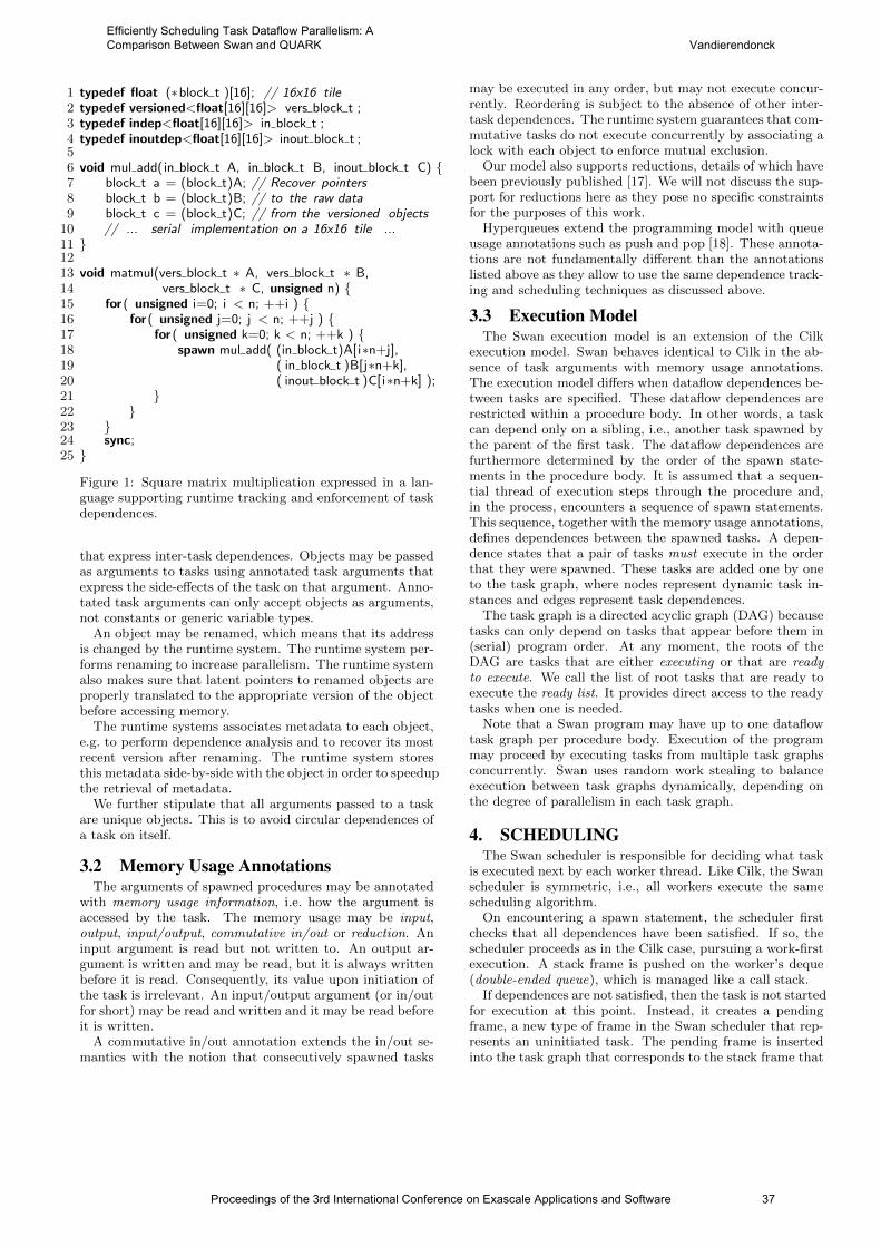
1 typedef float (∗block t )[16]; // 16x16 tile2 typedef versioned<float[16][16]> vers block t ;3 typedef indep<float[16][16]> in block t ;4 typedef inoutdep<float[16][16]> inout block t ;56 void mul add(in block t A, in block t B, inout block t C) 7 block t a = (block t)A; // Recover pointers8 block t b = (block t)B; // to the raw data9 block t c = (block t)C; // from the versioned objects

10 // ... serial implementation on a 16x16 tile ...11 1213 void matmul(vers block t ∗ A, vers block t ∗ B,14 vers block t ∗ C, unsigned n) 15 for( unsigned i=0; i < n; ++i ) 16 for( unsigned j=0; j < n; ++j ) 17 for( unsigned k=0; k < n; ++k ) 18 spawn mul add( (in block t)A[i∗n+j],19 ( in block t )B[j∗n+k],20 ( inout block t )C[i∗n+k] );21 22 23 24 sync;25

Figure 1: Square matrix multiplication expressed in a lan-guage supporting runtime tracking and enforcement of taskdependences.

that express inter-task dependences. Objects may be passedas arguments to tasks using annotated task arguments thatexpress the side-effects of the task on that argument. Anno-tated task arguments can only accept objects as arguments,not constants or generic variable types.

An object may be renamed, which means that its addressis changed by the runtime system. The runtime system per-forms renaming to increase parallelism. The runtime systemalso makes sure that latent pointers to renamed objects areproperly translated to the appropriate version of the objectbefore accessing memory.

The runtime systems associates metadata to each object,e.g. to perform dependence analysis and to recover its mostrecent version after renaming. The runtime system storesthis metadata side-by-side with the object in order to speedupthe retrieval of metadata.

We further stipulate that all arguments passed to a taskare unique objects. This is to avoid circular dependences ofa task on itself.

3.2 Memory Usage AnnotationsThe arguments of spawned procedures may be annotated

with memory usage information, i.e. how the argument isaccessed by the task. The memory usage may be input,output, input/output, commutative in/out or reduction. Aninput argument is read but not written to. An output ar-gument is written and may be read, but it is always writtenbefore it is read. Consequently, its value upon initiation ofthe task is irrelevant. An input/output argument (or in/outfor short) may be read and written and it may be read beforeit is written.

A commutative in/out annotation extends the in/out se-mantics with the notion that consecutively spawned tasks

may be executed in any order, but may not execute concur-rently. Reordering is subject to the absence of other inter-task dependences. The runtime system guarantees that com-mutative tasks do not execute concurrently by associating alock with each object to enforce mutual exclusion.

Our model also supports reductions, details of which havebeen previously published [17]. We will not discuss the sup-port for reductions here as they pose no specific constraintsfor the purposes of this work.

Hyperqueues extend the programming model with queueusage annotations such as push and pop [18]. These annota-tions are not fundamentally different than the annotationslisted above as they allow to use the same dependence track-ing and scheduling techniques as discussed above.

3.3 Execution ModelThe Swan execution model is an extension of the Cilk

execution model. Swan behaves identical to Cilk in the ab-sence of task arguments with memory usage annotations.The execution model differs when dataflow dependences be-tween tasks are specified. These dataflow dependences arerestricted within a procedure body. In other words, a taskcan depend only on a sibling, i.e., another task spawned bythe parent of the first task. The dataflow dependences arefurthermore determined by the order of the spawn state-ments in the procedure body. It is assumed that a sequen-tial thread of execution steps through the procedure and,in the process, encounters a sequence of spawn statements.This sequence, together with the memory usage annotations,defines dependences between the spawned tasks. A depen-dence states that a pair of tasks must execute in the orderthat they were spawned. These tasks are added one by oneto the task graph, where nodes represent dynamic task in-stances and edges represent task dependences.

The task graph is a directed acyclic graph (DAG) becausetasks can only depend on tasks that appear before them in(serial) program order. At any moment, the roots of theDAG are tasks that are either executing or that are readyto execute. We call the list of root tasks that are ready toexecute the ready list. It provides direct access to the readytasks when one is needed.

Note that a Swan program may have up to one dataflowtask graph per procedure body. Execution of the programmay proceed by executing tasks from multiple task graphsconcurrently. Swan uses random work stealing to balanceexecution between task graphs dynamically, depending onthe degree of parallelism in each task graph.

4. SCHEDULINGThe Swan scheduler is responsible for deciding what task

is executed next by each worker thread. Like Cilk, the Swanscheduler is symmetric, i.e., all workers execute the samescheduling algorithm.

On encountering a spawn statement, the scheduler firstchecks that all dependences have been satisfied. If so, thescheduler proceeds as in the Cilk case, pursuing a work-firstexecution. A stack frame is pushed on the worker’s deque(double-ended queue), which is managed like a call stack.

If dependences are not satisfied, then the task is not startedfor execution at this point. Instead, it creates a pendingframe, a new type of frame in the Swan scheduler that rep-resents an uninitiated task. The pending frame is insertedinto the task graph that corresponds to the stack frame that


Efficiently Scheduling Task Dataflow Parallelism: A Comparison Between Swan and QUARK Vandierendonck

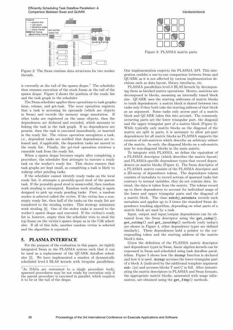
exte

nd

ed

sp

aw

n d

eq

ue

exte

nd

ed

sp

aw

n d

eq

ue

root

pending frames

per-workerready list

parent linkcall stack

Legend

stack framefull framepending frame

dataflow edge

parent linkcall stack

Legend

stack framefull framepending frame

dataflow edge

Figure 2: The Swan runtime data structures for two workerthreads.

is currently at the tail of the spawn deque.1 The schedulerthen resumes execution of the stack frame at the tail of thespawn deque. Figure 2 shows the position of the ready listand the task graph in the scheduler.

The Swan scheduler applies three operations to task graphs:issue, release, and get-task. The issue operation registersthat a task is accessing its operands (which are objectsin Swan) and records the memory usage annotation. Ifother tasks are registered on the same objects, then thedependences are deduced and recorded, which amounts tolinking the task in the task graph. If no dependences arepresent, then the task is executed immediately, or insertedin the ready list. The release operation unregisters a task,i.e., dependent tasks are notified that dependences are re-leased and, if applicable, the dependent tasks are moved tothe ready list. Finally, the get-task operation retrieves arunnable task from the ready list.

When a spawn deque becomes empty after completing aprocedure, the scheduler first attempts to execute a readytask on the worker’s ready list. This choice ensures thattask graphs are kept small, as completing a task is likely towakeup other pending tasks.

If the scheduler cannot identify ready tasks on the localready list, it attempts a provably-good steal of the parenttask. If the provably-good steal is unsuccesful, then randomwork stealing is attempted. Random work stealing is againdesigned to pick up ready pending tasks. First, a randomworker is selected called the victim. If the victim has a non-empty ready list, then half of the tasks on the ready list aretransfered to the stealing worker. This strategy minimizeswork stealing [6]. One of the stolen tasks is moved to theworker’s spawn deque and executed. If the vicitim’s readylist is, however, empty then the scheduler tries to steal thetop frame on the victim’s spawn deque as in the Cilk sched-uler. If all of this fails, another random victim is selectedand the algorithm is repeated.

5. PLASMA INTERFACEFor the purpose of the evaluation in this paper, we tightly

integrated Swan in the PLASMA system such that it canbe used as a replacement of the QUARK dataflow sched-uler [2]. We have implemented a number of dynamicallyscheduled level-3 BLAS kernels with irregular parallelism.

1As DAGs are restrained to a single procedure body,spawned procedures may be not ready for execution only ifthe parent procedure is executed in parallel, which requiresit to be at the tail of the deque.

Figure 3: PLASMA matrix parts

Our implementation respects the PLASMA API. This inte-gration enables a one-to-one comparison between Swan andQUARK as it is not affected by various implementation de-cisions such as data layout, library interfaces, etc.

PLASMA parallelizes level-3 BLAS kernels by decompos-ing them as blocked matrix operations. Hereto, matrices aredecomposed in blocks, assuming an internally tuned blocksize. QUARK uses the starting addresses of matrix blocksto track dependences: a matrix block is shared between twotasks only if they both take the starting address of that blockas an argument. Some tasks only access part of a matrixblock and QUARK takes this into account. The commonlyoccurring parts are the lower triangular part, the diagonaland the upper triangular part of a matrix block (Figure 3).While typically only matrix blocks on the diagonal of thematrix are split in parts, it is necessary to allow per-partdependences for all matrix blocks as PLASMA supports thecreation of sub-matrices which describe an arbitrary subsetof the matrix. As such, the diagonal blocks on a sub-matrixmay be non-diagonal blocks in the main matrix.

To integrate with PLASMA, we define the equivalent ofa PLASMA descriptor (which describes the matrix layout)and PLASMA-specific dependence types that record depen-dences on matrix blocks (Figure 4). The Swan descriptor ofa PLASMA matrix consists of the PLASMA descriptor anda 2D-array of dependence tokens. The dependence tokensconsists of metadata to record actions of spawned tasks butcontrary to normal variables, they do not contain data. In-stead, the data is taken from the matrix. The tokens recordup to three dependences to account for individual usage ofthe lower and upper triangular parts and the diagonal ofa matrix block. The class subobj_metadata records suchmetadata and applies up to 3 times the standard Swan de-pendence tracking algorithm, depending on what parts of amatrix block are used by a task.

Input, output and input/output dependences can be ob-tained from the Swan descriptor using the get_indep(),get_outdep() and get_inoutdep() methods (only indep’sare shown in Figure 4, other dependence types are definedsimilarly). These dependences hold a pointer to the cor-responding token and the starting address of the matrixblock’s data.

Given the definition of the PLASMA matrix descriptorand dependence types in Swan, linear algebra kernels can beexpressed in Swan and scheduled using task dataflow paral-lelism. Figure 5 shows how the dormqr function is declaredand how it is used. dormqr accesses the lower-triangular partof a block A (indicated by the additional template argumentsub::lo) and accesses blocks T and C in full. After instanti-ating the matrix descriptors in PLASMA and Swan formats,the appropriate matrix blocks, annotated with usage infor-mation, are obtained using the get_X dep() methods.



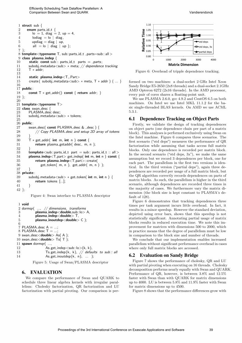
1 struct sub 2 enum parts id t 3 lo = 1, diag = 2, up = 4,4 lodiag = lo | diag ,5 updiag = diag | up,6 all = lo | diag | up ;7 ;8 template<typename T, sub::parts id t parts=sub:: all>9 class plasma indep

10 static const sub :: parts id t parts = parts ;11 subobj metadata<sub> ∗ meta; // dependence tracking12 T ∗ addr;1314 static plasma indep<T, Part>15 create ( subobj metadata<sub> ∗ meta, T ∗ addr ) ... 1617 public :18 const T ∗ get addr() const return addr; 19 ;2021 template<typename T>22 class swan desc 23 PLASMA desc desc;24 subobj metadata<sub> ∗ tokens;2526 public :27 swan desc( const PLASMA desc & desc ) 28 // Copy PLASMA desc and setup 2D array of tokens29 30 T ∗ get addr( int m, int n ) const 31 return plasma getaddr( desc, m, n );32 33 template<sub::parts id t part = sub:: parts id t :: all>34 plasma indep<T,part> get indep( int m, int n ) const 35 return plasma indep<T,part>::create(36 get token( m, n ), get addr( m, n ) );37 38 private :39 subobj metadata<sub> ∗ get token( int m, int n ) 40 return tokens [...];41 42 ;

Figure 4: Swan interface to PLASMA descriptor

1 void2 dormqr( ..., // dimensions, transforms3 plasma indep<double,sub::lo> A,4 plasma indep<double> T,5 plasma inoutdep<double> C );67 PLASMA desc A = ...;8 PLASMA desc T = ...;9 swan desc<double> As( A );

10 swan desc<double> Ts( T );11 spawn dormqr( ...,12 As.get indep<sub::lo>(k, k),13 Ts.get indep(k, k), // defaults to sub :: all14 As.get inoutdep(k, n), ... );

Figure 5: Usage of Swan/PLASMA descriptor

6. EVALUATIONWe compare the performance of Swan and QUARK to

schedule three linear algebra kernels with irregular paral-lelism: Cholesky factorization, QR factorization and LUfactorization with partial pivoting. Our comparison is per-

0.80

0.85

0.90

0.95

1.00

1.05

1.10

0 1000 2000 3000 4000

Rela%v

e Time

Matrix Dimension

std deps

std deps, 3x

par4al deps

Figure 6: Overhead of tripple dependence tracking.

formed on two machines: a dual-socket 2 GHz Intel XeonSandy Bridge E5-2650 (2x8 threads) and a dual-socket 2.1GHzAMD Opteron 6272 (2x16 threads). In the AMD processor,every pair of cores shares a floating-point unit.

We use PLASMA 2.6.0, gcc 4.9.2 and CentOS 6.5 on bothmachines. On Intel we use Intel MKL 11.1.2 for the ba-sic single-threaded BLAS kernels. On AMD we use ACML5.3.1.

6.1 Dependence Tracking on Object PartsFirstly, we validate the design of tracking dependences

on object parts (one dependence chain per part of a matrixblock). This analyses is performed exclusively using Swan onthe Intel machine. Figure 6 compares three scenarios. Thefirst scenario (“std deps”) measures the performance of QRfactorization while assuming that tasks access full matrixblocks. Only one dependence is recorded per matrix block.In the second scenario (“std deps, 3x”), we make the sameassumption but we record 3 dependences per block, one foreach part. The parallelism in the first two versions is iden-tical. In the third version (“partial deps”), again three de-pendences are recorded per usage of a full matrix block, butthe QR algorithm correctly records dependences on parts ofmatrix blocks. As such, the parallelism is higher in the thirdscenario, although dependences are recorded three times inthe majority of cases. We furthermore vary the matrix di-mension (the block size is kept constant to PLASMA’s de-fault of 128).

Figure 6 demonstrates that tracking dependences threetimes per task argument incurs little overhead. In fact, itresults in a minor speedup. However the standard deviation,depicted using error bars, shows that this speedup is notstatistically significant. Annotating partial usage of matrixblocks results in reduced execution time. We note this im-provement for matrices with dimensions 500 to 2000, whichin practice means that the degree of parallelism must be lowin comparison to the block size and number of threads.

We conclude that our implementation enables increasedparallelism without significant performance overhead in caseswhere only full matrix blocks are accessed.

6.2 Evaluation on Sandy BridgeFigure 7 shows the performance of cholesky, QR and LU

with partial pivoting when executing on 16 threads. Choleskydecomposition performs nearly equally with Swan and QUARK.Performance of QR, however, is between 3.8% and 12.5%faster with Swan than with QUARK for matrix dimensionsup to 4000. LU is between 5.8% and 11.9% faster with Swanfor matrix dimensions up to 4500.

Figure 8 shows that the performance differences grow with



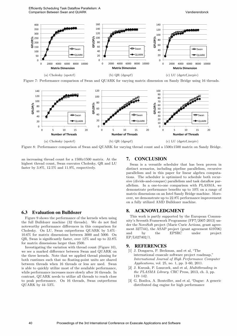
0

50

100

150

200

250

300

350

400

0 2000 4000 6000 8000 10000

GFLOP/s

Matrix Dimension

Swan

QUARK

(a) Cholesky (spotrf)

0

20

40

60

80

100

120

140

160

0 2000 4000 6000 8000 10000

GFLOP/s

Matrix Dimension

Swan

QUARK

(b) QR (dgeqrf)

0

20

40

60

80

100

120

140

0 2000 4000 6000 8000 10000

GFLOP/s

Matrix Dimension

Swan

QUARK

(c) LU (dgetrf incpiv)

Figure 7: Performance comparison of Swan and QUARK for varying matrix dimension on Sandy Bridge using 16 threads.

0

20

40

60

80

100

120

140

0 5 10 15 20

GFLOP/s

Number of Threads

Swan

QUARK


0

20

40

60

80

100

120

0 5 10 15 20

GFLOP/s

Number of Threads

Swan

QUARK

(b) QR (dgeqrf)

0 10 20 30 40 50 60 70 80 90 100

0 5 10 15 20

GFLOP/s

Number of Threads

Swan

QUARK


Figure 8: Performance comparison of Swan and QUARK for varying thread count and a 1500x1500 matrix on Sandy Bridge.

an increasing thread count for a 1500x1500 matrix. At thehighest thread count, Swan executes Cholesky, QR and LUfaster by 3.8%, 12.5% and 11.9%, respectively.

6.3 Evaluation on BulldozerFigure 9 shows the performance of the kernels when using

the full Bulldozer machine (32 threads). We do not findnoteworthy performance differences in this comparison forCholesky. On LU, Swan outperforms QUARK by 5.6%–10.6% for matrix dimensions between 3000 and 5000. OnQR, Swan is significantly faster, over 12% and up to 22.8%for matrix dimensions larger than 2500.

Investigating the variation with thread count (Figure 10),we see a marked difference between Swan and QUARK onthe three kernels. Note that we applied thread pinning forboth runtimes such that no floating-point units are sharedbetween threads when 16 threads or less are used. Swanis able to quickly utilize most of the available performance,while performance increases more slowly after 16 threads. Incontrast, QUARK needs to utilize all threads to reach closeto peak performance. On 16 threads, Swan outperformsQUARK by 44–53%.

7. CONCLUSIONSwan is a versatile scheduler that has been proven in

distinct scenarios, including pipeline parallelism, recursiveparallelism and in this paper for linear algebra computa-tions. The scheduler is optimized to schedule both recur-sive (divide-and-conquer) parallelism and task dataflow par-allelism. In a one-to-one comparison with PLASMA, wedemonstrate performance benefits up to 10% on a range ofmatrix dimensions on an Intel Sandy Bridge machine. More-over, we demonstrate up to 22.8% performance improvementon a fully utilized AMD Bulldozer machine.

8. ACKNOWLEDGMENTThis work is partly supported by the European Commu-

nity’s Seventh Framework Programme (FP7/2007-2013) un-der the NovoSoft project (Marie Curie Actions, grant agree-ment 327744), the ASAP project (grant agreement 619706)and by the EPSRC under projectEP/L027402/1.

9. REFERENCES[1] J. Dongarra, P. Beckman, and et al, “The

international exascale software project roadmap,”International Journal of High Performance ComputerApplications, vol. 25, no. 1, pp. 3–60, 2011.

[2] J. Kurzak, P. Luszczek, and et al, Multithreading inthe PLASMA Library. CRC Press, 2013, ch. 3, pp.119–142.

[3] G. Bosilca, A. Bouteiller, and et al, “Dague: A genericdistributed dag engine for high performance



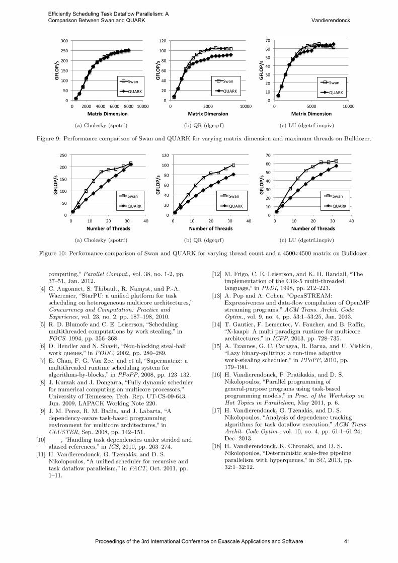
0

50

100

150

200

250

300

0 2000 4000 6000 8000 10000

GFLOP/s

Matrix Dimension

Swan

QUARK


0

20

40

60

80

100

120

0 5000 10000

GFLOP/s

Matrix Dimension

Swan

QUARK

(b) QR (dgeqrf)

0

10

20

30

40

50

60

70

0 5000 10000

GFLOP/s

Matrix Dimension

Swan

QUARK


Figure 9: Performance comparison of Swan and QUARK for varying matrix dimension and maximum threads on Bulldozer.

0

50

100

150

200

250

0 10 20 30 40

GFLOP/s

Number of Threads

Swan

QUARK


0

20

40

60

80

100

120

0 10 20 30 40

GFLOP/s

Number of Threads

Swan

QUARK

(b) QR (dgeqrf)

0

10

20

30

40

50

60

70

0 10 20 30 40

GFLOP/s

Number of Threads

Swan

QUARK


Figure 10: Performance comparison of Swan and QUARK for varying thread count and a 4500x4500 matrix on Bulldozer.

computing,” Parallel Comput., vol. 38, no. 1-2, pp.37–51, Jan. 2012.

[4] C. Augonnet, S. Thibault, R. Namyst, and P.-A.Wacrenier, “StarPU: a unified platform for taskscheduling on heterogeneous multicore architectures,”Concurrency and Computation: Practice andExperience, vol. 23, no. 2, pp. 187–198, 2010.

[5] R. D. Blumofe and C. E. Leiserson, “Schedulingmultithreaded computations by work stealing,” inFOCS. 1994, pp. 356–368.

[6] D. Hendler and N. Shavit, “Non-blocking steal-halfwork queues,” in PODC, 2002, pp. 280–289.

[7] E. Chan, F. G. Van Zee, and et al, “Supermatrix: amultithreaded runtime scheduling system foralgorithms-by-blocks,” in PPoPP, 2008, pp. 123–132.

[8] J. Kurzak and J. Dongarra, “Fully dynamic schedulerfor numerical computing on multicore processors,”University of Tennessee, Tech. Rep. UT-CS-09-643,Jun. 2009, LAPACK Working Note 220.

[9] J. M. Perez, R. M. Badia, and J. Labarta, “Adependency-aware task-based programmingenvironment for multicore architectures,” inCLUSTER, Sep. 2008, pp. 142–151.

[10] ——, “Handling task dependencies under strided andaliased references,” in ICS, 2010, pp. 263–274.

[11] H. Vandierendonck, G. Tzenakis, and D. S.Nikolopoulos, “A unified scheduler for recursive andtask dataflow parallelism,” in PACT, Oct. 2011, pp.1–11.

[12] M. Frigo, C. E. Leiserson, and K. H. Randall, “Theimplementation of the Cilk-5 multi-threadedlanguage,” in PLDI, 1998, pp. 212–223.

[13] A. Pop and A. Cohen, “OpenSTREAM:Expressiveness and data-flow compilation of OpenMPstreaming programs,” ACM Trans. Archit. CodeOptim., vol. 9, no. 4, pp. 53:1–53:25, Jan. 2013.

[14] T. Gautier, F. Lementec, V. Faucher, and B. Raffin,“X-kaapi: A multi paradigm runtime for multicorearchitectures,” in ICPP, 2013, pp. 728–735.

[15] A. Tzannes, G. C. Caragea, R. Barua, and U. Vishkin,“Lazy binary-splitting: a run-time adaptivework-stealing scheduler,” in PPoPP, 2010, pp.179–190.

[16] H. Vandierendonck, P. Pratikakis, and D. S.Nikolopoulos, “Parallel programming ofgeneral-purpose programs using task-basedprogramming models,” in Proc. of the Workshop onHot Topics in Parallelism, May 2011, p. 6.

[17] H. Vandierendonck, G. Tzenakis, and D. S.Nikolopoulos, “Analysis of dependence trackingalgorithms for task dataflow execution,” ACM Trans.Archit. Code Optim., vol. 10, no. 4, pp. 61:1–61:24,Dec. 2013.

[18] H. Vandierendonck, K. Chronaki, and D. S.Nikolopoulos, “Deterministic scale-free pipelineparallelism with hyperqueues,” in SC, 2013, pp.32:1–32:12.



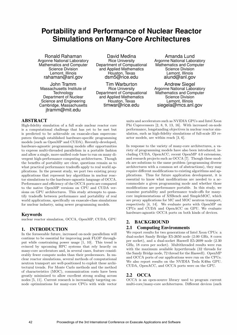
Portability and Performance of Nuclear ReactorSimulations on Many-Core Architectures

Ronald RahamanArgonne National LaboratoryMathematics and Computer

Science DivisionLemont, Illinois

[email protected]

David MedinaRice University

Department of Compuationaland Applied Mathematics

Houston, [email protected]

Amanda LundArgonne National LaboratoryMathematics and Computer


[email protected] Tramm

Massachusetts Institute ofTechnology

Department of NuclearScience and Engineering

Cambridge, [email protected]

Tim WarburtonRice University

Department of Compuationaland Applied Mathematics

Houston, [email protected]

Andrew SiegelArgonne National LaboratoryMathematics and Computer


[email protected]

ABSTRACTHigh-fidelity simulation of a full scale nuclear reactor coreis a computational challenge that has yet to be met butis predicted to be achievable on exascale-class supercom-puters through established hardware-specific programmingmodels (such as OpenMP and CUDA). Recently-developed,hardware-agnostic programming models offer opportunitiesto express multi-threaded parallelism in a portable fashionand allow a single, more-unified code base to run on many di-vergent high-performance computing architectures. Thoughthe benefits of portability are clear, questions remain as towhat practical performance tradeoffs apply to real world ap-plications. In the present study, we port two existing proxyapplications that represent key algorithms in nuclear reac-tor simulations to the hardware-agnostic language of OCCA.Performance and efficiency of the OCCA ports are comparedto the native OpenMP versions on CPU and CUDA ver-sions on GPU architectures. This study attempts to quan-tify tradeoffs between performance and portability of realworld applications, specifically on exascale-class simulationsfor nuclear industry, using newer programming models.

Keywordsnuclear reactor simulation, OCCA, OpenMP, CUDA, GPU

1. INTRODUCTIONIn the foreseeable future, increased on-node parallelism willcontinue to be essential for improving peak FLOP through-put while constraining power usage [1, 10]. This trend isevinced by upcoming HPC systems that rely heavily onmany-core accelerators and, in several cases, feature consid-erably fewer compute nodes than their predecessors. In nu-clear reactor simulations, several methods of computationalneutron transport are well-positioned to exploit these archi-tectural trends. For Monte Carlo methods and the methodof characteristics (MOC), communication costs have beengreatly minimized to allow excellent strong scaling acrossnodes [5, 11]. Current research is increasingly targeting on-node optimizations for many-core CPUs with wide vector

units and accelerators such as NVIDIA GPUs and Intel XeonPhi Coprocessors [2, 8, 9, 13, 16]. With increased on-nodeperformance, longstanding objectives in nuclear reactor sim-ulation, such as high-fidelity simulations of full-scale 3D re-actor models, are within reach [3, 6].

In response to the variety of many-core architectures, a va-riety of programming models have also been introduced, in-cluding CUDA, OpenACC, recent OpenMP 4.0 extensions,and research projects such as OCCA [7]. Though these mod-els are solutions to the same problem (programming diversearchitectures with a common set of abstractions), they mayrequire different modifications to existing algorithms and ap-plications. Thus for future application development, it isessential to know what modifications are needed to a ac-commodate a given programming mode and whether thosemodifications are performance portable. In this study, weexamine portability and performance trade-offs for many-core implementations of XSBench and SimpleMOC, whichare proxy applications for MC and MOC neutron transport,respectively [4, 14]. We evaluate ports with OpenMP onCPUs and CUDA and OpenACC on GPU. We evaluatehardware-agnostic OCCA ports on both kinds of devices.

2. BACKGROUND2.1 Computing EnvironmentsWe report results for two generations of Intel Xeon CPUs: adual-socket Sandy Bridge E5-2650 node (2.00 GHz, 8 coresper socket), and a dual-socket Haswell E5-2699 node (2.30GHz, 18 cores per socket). Multithreaded results were runwith the maximum available hyperthreads (32 threads forthe Sandy Bridge node, 72 thread for the Haswell). OpenMPand OCCA ports of our applications were run on the CPUs.We also report results on the NVIDIA Tesla K40m GPU.CUDA, OpenACC, and OCCA ports were on the GPU.

2.2 OCCAOCCA is an open-source library used to program currentmulti-core/many-core architectures. Different devices (such


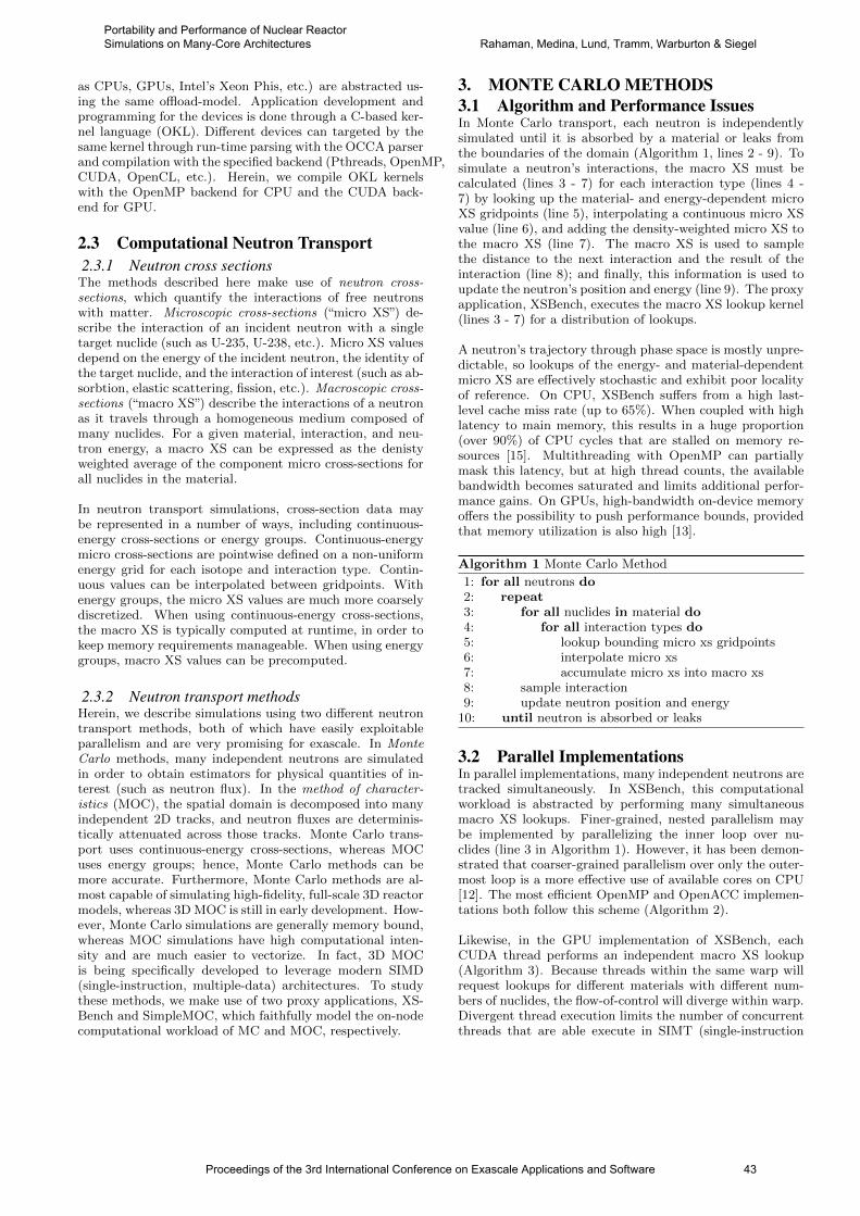
as CPUs, GPUs, Intel’s Xeon Phis, etc.) are abstracted us-ing the same offload-model. Application development andprogramming for the devices is done through a C-based ker-nel language (OKL). Different devices can targeted by thesame kernel through run-time parsing with the OCCA parserand compilation with the specified backend (Pthreads, OpenMP,CUDA, OpenCL, etc.). Herein, we compile OKL kernelswith the OpenMP backend for CPU and the CUDA back-end for GPU.

2.3 Computational Neutron Transport2.3.1 Neutron cross sections

The methods described here make use of neutron cross-sections, which quantify the interactions of free neutronswith matter. Microscopic cross-sections (“micro XS”) de-scribe the interaction of an incident neutron with a singletarget nuclide (such as U-235, U-238, etc.). Micro XS valuesdepend on the energy of the incident neutron, the identity ofthe target nuclide, and the interaction of interest (such as ab-sorbtion, elastic scattering, fission, etc.). Macroscopic cross-sections (“macro XS”) describe the interactions of a neutronas it travels through a homogeneous medium composed ofmany nuclides. For a given material, interaction, and neu-tron energy, a macro XS can be expressed as the denistyweighted average of the component micro cross-sections forall nuclides in the material.

In neutron transport simulations, cross-section data maybe represented in a number of ways, including continuous-energy cross-sections or energy groups. Continuous-energymicro cross-sections are pointwise defined on a non-uniformenergy grid for each isotope and interaction type. Contin-uous values can be interpolated between gridpoints. Withenergy groups, the micro XS values are much more coarselydiscretized. When using continuous-energy cross-sections,the macro XS is typically computed at runtime, in order tokeep memory requirements manageable. When using energygroups, macro XS values can be precomputed.

2.3.2 Neutron transport methodsHerein, we describe simulations using two different neutrontransport methods, both of which have easily exploitableparallelism and are very promising for exascale. In MonteCarlo methods, many independent neutrons are simulatedin order to obtain estimators for physical quantities of in-terest (such as neutron flux). In the method of character-istics (MOC), the spatial domain is decomposed into manyindependent 2D tracks, and neutron fluxes are determinis-tically attenuated across those tracks. Monte Carlo trans-port uses continuous-energy cross-sections, whereas MOCuses energy groups; hence, Monte Carlo methods can bemore accurate. Furthermore, Monte Carlo methods are al-most capable of simulating high-fidelity, full-scale 3D reactormodels, whereas 3D MOC is still in early development. How-ever, Monte Carlo simulations are generally memory bound,whereas MOC simulations have high computational inten-sity and are much easier to vectorize. In fact, 3D MOCis being specifically developed to leverage modern SIMD(single-instruction, multiple-data) architectures. To studythese methods, we make use of two proxy applications, XS-Bench and SimpleMOC, which faithfully model the on-nodecomputational workload of MC and MOC, respectively.

3. MONTE CARLO METHODS3.1 Algorithm and Performance IssuesIn Monte Carlo transport, each neutron is independentlysimulated until it is absorbed by a material or leaks fromthe boundaries of the domain (Algorithm 1, lines 2 - 9). Tosimulate a neutron’s interactions, the macro XS must becalculated (lines 3 - 7) for each interaction type (lines 4 -7) by looking up the material- and energy-dependent microXS gridpoints (line 5), interpolating a continuous micro XSvalue (line 6), and adding the density-weighted micro XS tothe macro XS (line 7). The macro XS is used to samplethe distance to the next interaction and the result of theinteraction (line 8); and finally, this information is used toupdate the neutron’s position and energy (line 9). The proxyapplication, XSBench, executes the macro XS lookup kernel(lines 3 - 7) for a distribution of lookups.

A neutron’s trajectory through phase space is mostly unpre-dictable, so lookups of the energy- and material-dependentmicro XS are effectively stochastic and exhibit poor localityof reference. On CPU, XSBench suffers from a high last-level cache miss rate (up to 65%). When coupled with highlatency to main memory, this results in a huge proportion(over 90%) of CPU cycles that are stalled on memory re-sources [15]. Multithreading with OpenMP can partiallymask this latency, but at high thread counts, the availablebandwidth becomes saturated and limits additional perfor-mance gains. On GPUs, high-bandwidth on-device memoryoffers the possibility to push performance bounds, providedthat memory utilization is also high [13].

Algorithm 1 Monte Carlo Method

1: for all neutrons do2: repeat3: for all nuclides in material do4: for all interaction types do5: lookup bounding micro xs gridpoints6: interpolate micro xs7: accumulate micro xs into macro xs8: sample interaction9: update neutron position and energy

10: until neutron is absorbed or leaks

3.2 Parallel ImplementationsIn parallel implementations, many independent neutrons aretracked simultaneously. In XSBench, this computationalworkload is abstracted by performing many simultaneousmacro XS lookups. Finer-grained, nested parallelism maybe implemented by parallelizing the inner loop over nu-clides (line 3 in Algorithm 1). However, it has been demon-strated that coarser-grained parallelism over only the outer-most loop is a more effective use of available cores on CPU[12]. The most efficient OpenMP and OpenACC implemen-tations both follow this scheme (Algorithm 2).

Likewise, in the GPU implementation of XSBench, eachCUDA thread performs an independent macro XS lookup(Algorithm 3). Because threads within the same warp willrequest lookups for different materials with different num-bers of nuclides, the flow-of-control will diverge within warp.Divergent thread execution limits the number of concurrentthreads that are able execute in SIMT (single-instruction


Portability and Performance of Nuclear Reactor Simulations on Many-Core Architectures Rahaman, Medina, Lund, Tramm, Warburton & Siegel

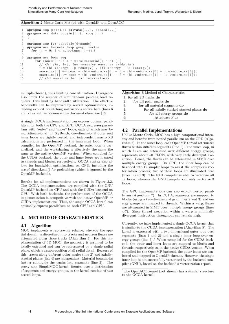
Algorithm 2 Monte Carlo Method with OpenMP and OpenACC

1 #pragma omp p a r a l l e l private ( . . . ) , shared ( . . . )2 #pragma acc data copyin ( . . . ) , copy ( . . . )3 4 . . .5 #pragma omp for schedu le ( dynamic )6 #pragma acc k e rn e l s loop gang , vec to r7 for ( i = 0 ; i < n lookups ; i++) 8 . . .9 #pragma acc loop seq

10 for ( nuc=0; nuc < n nucs ( mate r i a l ) ; nuc++) 11 // Get ( hi , l o ) , the bounding micro xs g r i d po i n t s12 f = ( hi−>energy − p−>energy ) / ( hi−>energy − lo−>energy ) ;13 macro xs [ 0 ] += conc ∗ ( hi−>micro xs [ 0 ] − f ∗ ( hi−>micro xs [ 0 ] − lo−>micro xs [ 0 ] ) ;14 macro xs [ 1 ] += conc ∗ ( hi−>micro xs [ 1 ] − f ∗ ( hi−>micro xs [ 1 ] − lo−>micro xs [ 1 ] ) ;15 // Get macro xs f o r a l l i n t e r a c t i o n s . . .

multiple-thread), thus limiting core utilization. Divergencealso limits the number of simultaneous pending load re-quests, thus limiting bandwidth utilization. The effectivebandwidth can be improved by several optimizations, in-cluding explicit prefetching instructions shown here (lines 6and 7) as well as optimizations discussed elsewhere [13].

A single OCCA implementation can express optimal paral-lelism for both the CPU and GPU. OCCA expresses parael-lism with “outer” and “inner” loops, each of which may bemultidimensional. In XSBench, one-dimensional outer andinner loops are tightly nested, and independent macro XScalculations are performed in the innermost loop. Whencompiled for the OpenMP backend, the outer loop is par-allelized, and the worksharing is effectively the same thesame as the native OpenMP version. When compiled forthe CUDA backend, the outer and inner loops are mappedto threads and blocks, respectively. OCCA syntax also al-lows for bandwidth optimizations on GPU, including theuse of directLoad() for prefetching (which is ignored by theOpenMP backend).

Results for all implementations are shown in Figure 3.2.The OCCA implementations are compiled with the GNUOpenMP backend on CPU and with the CUDA backend onGPU. With both backends, the performance of the OCCAimplementation is competitive with the native OpenMP orCUDA implemenations. Thus, the single OCCA kernel canoptimally express parallelism on both CPU and GPU.

4. METHOD OF CHARACTERISTICS

4.1 AlgorithmMOC implements a ray-tracing scheme, whereby the spa-tial domain is discretized into tracks and neutron fluxes areattenuated along those tracks (Algorithm 5). For this im-plementation of 3D MOC, the geometry is assumed to beaxially extruded and can be represented by a single radialplane, which is a superposition of all radial detail. Because ofthis, tracks along different polar angles (line 2) and axially-stacked planes (line 4) are independent. Material boundariesfurther subdivide the tracks into segments (line 3). Theproxy app, SimpleMOC-kernel, iterates over a distributionof segments and energy groups, so the kernel consists of twonested loops.

Algorithm 5 Method of Characteristics

1: for all 2D tracks do2: for all polar angles do3: for all material segments do4: for all axially-stacked stacked planes do5: for all energy groups do6: Attenuate Flux

4.2 Parallel ImplementationsUnlike Monte Carlo, MOC has a high computational inten-sity and benefits from nested parallelism on the CPU (Algo-rithm 6). In the outer loop, each OpenMP thread attenuatesfluxes within different segments (line 1). The inner loop, inwhich fluxes are attenuated over different energy groups,represents about 50 FLOPs with very little divergent exe-cution. Hence, the fluxes can be attenuated in SIMD overmultiple energy groups. On CPU, the inner loop can befissioned into 12 simpler loops to assist the compiler’s vec-torization process; two of these loops are illustrated here(lines 3 and 9). The Intel compiler is able to vectorize all12 loops, whereas the GNU compiler can only vectorize 3loops.

The GPU implementations can also exploit nested paral-lelism (Algorithm 7). In CUDA, segments are mapped toblocks (using a two-dimensional grid, lines 2 and 3) and en-ergy groups are mapped to threads. Within a warp, fluxesare attenuated in SIMT over multiple energy groups (lines4-7). Since thread execution within a warp is minimallydivergent, instruction throughput can remain high.

Currently, we have implemented a single OCCA kernel thatis similar to the CUDA implementation (Algorithm 8). Thekernel is expressed with a two-dimensional outer loop oversegments (lines 1 and 2) and a single inner loop over en-ergy groups (line 5).1 When compiled for the CUDA back-end, the outer and inner loops are mapped to blocks andthreads, respectively, as in the native CUDA version. Whencompiled for the OpenMP backend, the outer loops are coa-lesced and mapped to OpenMP threads. However, the singleinner loop is not successfully vectorized by the backend com-piler (GNU), based on the backend’s vectorization report.

1The OpenACC kernel (not shown) has a similar structureto the OCCA kernel.



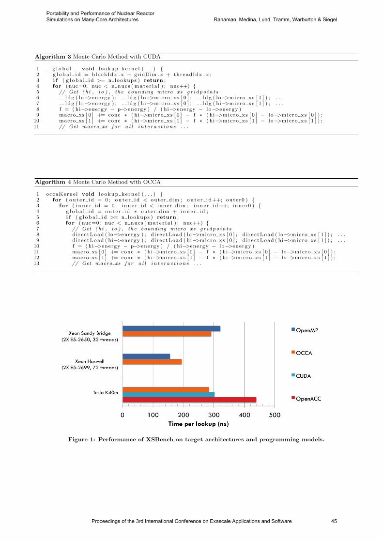
Algorithm 3 Monte Carlo Method with CUDA

1 g l o b a l void l ookup ke rne l ( . . . ) 2 g l o b a l i d = blockIdx . x + gridDim . x + threadIdx . x ;3 i f ( g l o b a l i d >= n lookups ) return ;4 for ( nuc=0; nuc < n nucs ( mate r i a l ) ; nuc++) 5 // Get ( hi , l o ) , the bounding micro xs g r i d po i n t s6 l d g ( lo−>energy ) ; l d g ( lo−>micro xs [ 0 ] ; l d g ( lo−>micro xs [ 1 ] ) ; . . .7 l d g ( hi−>energy ) ; l d g ( hi−>micro xs [ 0 ] ; l d g ( hi−>micro xs [ 1 ] ) ; . . .8 f = ( hi−>energy − p−>energy ) / ( hi−>energy − lo−>energy )9 macro xs [ 0 ] += conc ∗ ( hi−>micro xs [ 0 ] − f ∗ ( hi−>micro xs [ 0 ] − lo−>micro xs [ 0 ] ) ;

10 macro xs [ 1 ] += conc ∗ ( hi−>micro xs [ 1 ] − f ∗ ( hi−>micro xs [ 1 ] − lo−>micro xs [ 1 ] ) ;11 // Get macro xs f o r a l l i n t e r a c t i o n s . . .

Algorithm 4 Monte Carlo Method with OCCA

1 occaKernel void l ookup ke rne l ( . . . ) 2 for ( ou t e r i d = 0 ; ou t e r i d < outer dim ; ou t e r i d++; outer0 ) 3 for ( i n n e r i d = 0 ; i n n e r i d < inner dim ; i nn e r i d++; inner0 ) 4 g l o b a l i d = ou t e r i d ∗ outer dim + inn e r i d ;5 i f ( g l o b a l i d >= n lookups ) return ;6 for ( nuc=0; nuc < n nucs ( mate r i a l ) ; nuc++) 7 // Get ( hi , l o ) , the bounding micro xs g r i d po i n t s8 di rectLoad ( lo−>energy ) ; d i rectLoad ( lo−>micro xs [ 0 ] ; d i rectLoad ( lo−>micro xs [ 1 ] ) ; . . .9 d i rectLoad ( hi−>energy ) ; d i rectLoad ( hi−>micro xs [ 0 ] ; d i rectLoad ( hi−>micro xs [ 1 ] ) ; . . .

10 f = ( hi−>energy − p−>energy ) / ( hi−>energy − lo−>energy )11 macro xs [ 0 ] += conc ∗ ( hi−>micro xs [ 0 ] − f ∗ ( hi−>micro xs [ 0 ] − lo−>micro xs [ 0 ] ) ;12 macro xs [ 1 ] += conc ∗ ( hi−>micro xs [ 1 ] − f ∗ ( hi−>micro xs [ 1 ] − lo−>micro xs [ 1 ] ) ;13 // Get macro xs f o r a l l i n t e r a c t i o n s . . .

Figure 1: Performance of XSBench on target architectures and programming models.



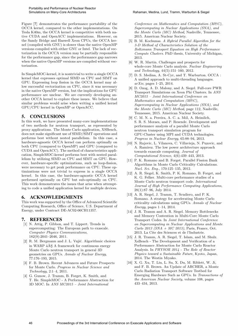
Figure [?] demonstrates the performance portability of theOCCA kernel, compared to the other implementations. OnTesla K40m, the OCCA kernel is competitive with both na-tive CUDA and OpenACC implementations. However, onthe Sandy Bridge and Haswell Xeon CPUs, the OCCA ker-nel (compiled with GNU) is slower than the native OpenMPversions compiled with either GNU or Intel. The lack of vec-torization in the OCCA version may be partially responsiblefor the performance gap, since the performance gap narrowswhen the native OpenMP versions are compiled without vec-torization.

In SimpleMOC-kernel, it is nontrivial to write a single OCCAkernel that expresses optimal SIMD on CPU and SIMT onGPU. Expressing loop fission in the OCCA kernel may al-low successful vectorization on CPU, since it was necessaryin the native OpenMP version, but the implications for GPUperformance are unclear. We are currently developing an-other OCCA kernel to explore these issues. We believe thatsimilar problems would arise when writing a unified kernelGPU/CPU kernel in OpenMP or OpenACC.

5. CONCLUSIONSIn this work, we have presented many-core implementationsof two methods for neutron transport, as represented byproxy applications. The Monte Carlo application, XSBench,does not make significant use of SIMD/SIMT operations andperforms best without nested parallelism. In this case, ahardware-agnostic OCCA kernel can perform optimally onboth CPU (compared to OpenMP) and GPU (compared toCUDA and OpenACC). The method of characteristics appli-cation, SimpleMOC-kernel performs best with nested paral-lelism by utilizing SIMD on CPU and SIMT on GPU. How-ever, hardware-specific optimizations, such as loop-fission,were necessary to get peak performance on CPU. These op-timizations were not trivial to express in a single OCCAkernel. In this case, the hardware-agnostic OCCA kernelperformed optimally on GPU but sub-optimally on CPU.This work demonstrates the issues that arise when attempt-ing to code a unified application kernel for multiple devices.

6. ACKNOWLEDGMENTSThis work was supported by the Office of Advanced ScientificComputing Research, Office of Science, U.S. Department ofEnergy, under Contract DE-AC02-06CH11357.

7. REFERENCES[1] N. Attig, P. Gibbon, and T. Lippert. Trends in

supercomputing: The European path to exascale.Computer Physics Communications,182(9):2041–2046, 2011.

[2] R. M. Bergmann and J. L. Vujic. Algorithmic choices

in WARP aAS A framework for continuous energyMonte Carlo neutron transport in general 3Dgeometries on GPUs. Annals of Nuclear Energy,77:176–193, 2015.

[3] F. B. Brown. Recent Advances and Future Prospectsfor Monte Carlo. Progress in Nuclear Science andTechnology, 2:1–4, 2011.

[4] G. Gunow, J. Tramm, B. Forget, K. Smith, andT. He. SimpleMOC - A Performance Abstraction for3D MOC. In ANS MC2015 – Joint International

Conference on Mathematics and Computation (M&C),Supercomputing in Nuclear Applications (SNA), andthe Monte Carlo (MC) Method, Nashville, Tennessee,2015. American Nuclear Society.

[5] B. M. Kochunas. A Hybrid Parallel Algorithm for the3-D Method of Characteristics Solution of theBoltzmann Transport Equation on High PerformanceCompute Clusters. PhD thesis, University of Michigan,2013.

[6] W. R. Martin. Challenges and prospects forwhole-core Monte Carlo analysis. Nuclear Engineeringand Technology, 44(5):151–160, 2012.

[7] D. S. Medina, A. St-Cyr, and T. Warburton. OCCA :A unified approach to multi-threading languages.arXiv, pages 1–25, 2014.

[8] D. Ozog, A. D. Malony, and A. Siegel. Full-core PWRTransport Simulations on Xeon Phi Clusters. In ANSMC2015 – Joint International Conference onMathematics and Computation (M&C),Supercomputing in Nuclear Applications (SNA), andthe Monte Carlo (MC) Method, page 112, Nashville,Tennessee, 2015. American Nuclear Society.

[9] C. M. N. a. Pereira, A. C. a. Mol, A. Heimlich,S. R. S. Moraes, and P. Resende. Development andperformance analysis of a parallel Monte Carloneutron transport simulation program forGPU-Cluster using MPI and CUDA technologies.Progress in Nuclear Energy, 65:88–94, 2013.

[10] N. Rajovic, L. Vilanova, C. Villavieja, N. Puzovic, andA. Ramirez. The low power architecture approachtowards exascale computing. Journal ofComputational Science, 4(6):439–443, 2013.

[11] P. K. Romano and B. Forget. Parallel Fission BankAlgorithms in Monte Carlo Criticality Calculations.Nucl. Sci. Eng., 170:125–135, 2012.

[12] A. R. Siegel, K. Smith, P. K. Romano, B. Forget, andK. G. Felker. Multi-core performance studies of aMonte Carlo neutron transport code. InternationalJournal of High Performance Computing Applications,28(1):87–96, July 2014.

[13] A. R. Siegel, J. Tramm, T. Scudiero, and P. K.Romano. A strategy for accelerating Monte Carlocriticality calculations using GPUs. Annals of NuclearEnergy, pages 1–14, 2014.

[14] J. R. Tramm and A. R. Siegel. Memory Bottlenecksand Memory Contention in Multi-Core Monte CarloTransport Codes. In Joint International Conferenceon Supercomputing in Nuclear Applications and MonteCarlo 2013 (SNA + MC 2013), Paris, France, Oct.2013. La Cite des Sciences et de l’Industrie.

[15] J. R. Tramm, A. R. Siegel, T. Islam, and M. Shulz.XsBench - The Development and Verification of aPerformance Abstraction for Monte Carlo ReactorAnalysis. In PHYSOR 2014 - The Role of ReactorPhysics toward a Sustainable Future, Kyoto, Japan,2014. The Westin Miyako.

[16] X. G. Xu, T. Liu, L. Su, X. Du, M. Riblett, W. Ji,and F. B. Brown. An Update of ARCHER, a MonteCarlo Radiation Transport Software Testbed forEmerging Hardware Such as GPUs. In Transactions ofthe American Nuclear Society, volume 108, pages433–434, 2013.



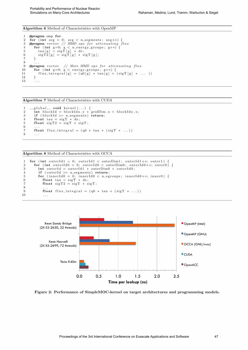
Algorithm 6 Method of Characteristics with OpenMP

1 #pragma omp for2 for ( int seg = 0 ; seg < n segments ; seg++) 3 #pragma vec to r // SIMD ops fo r a t t enua t ing f l u x4 for ( int g=0; g < n energy groups ; g++) 5 tau [ g ] = sigT [ g ] ∗ ds ;6 sigT2 [ g ] = sigT [ g ] ∗ sigT [ g ] ;7 8 . . .9 #pragma vec to r // More SIMD ops fo r a t t enua t ing f l u x

10 for ( int g=0; g < energy groups ; g++) 11 f l u x i n t e g r a l [ g ] = ( q0 [ g ] ∗ tau [ g ] + ( sigT [ g ] ∗ . . . ) )12 13 . . .

Algorithm 7 Method of Characteristics with CUDA

1 g l o b a l void ke rne l ( . . . ) 2 int blockId = blockIdx . y ∗ gridDim . x + blockIdx . x ;3 i f ( b lockId >= n segments ) return ;4 f loat tau = sigT ∗ ds ;5 f loat sigT2 = sigT ∗ sigT ;6 . . .7 f loat f l u x i n t e g r a l = ( q0 ∗ tau + ( sigT ∗ . . . ) )8 . . .

Algorithm 8 Method of Characteristics with OCCA

1 for ( int outer Id1 = 0 ; outer Id1 < outerDim1 ; outer Id1++; outer1 ) 2 for ( int outer Id0 = 0 ; outer Id0 < outerDim0 ; outer Id0++; outer0 ) 3 int outer Id = outer Id1 ∗ outerDim0 + outer Id0 ;4 i f ( oute r Id >= n segments ) return ;5 for ( inner Id0 = 0 ; inner Id0 < n egroups ; inner Id0++; inner0 ) 6 f loat tau = sigT ∗ ds ;7 f loat sigT2 = sigT ∗ sigT ;8 . . .9 f loat f l u x i n t e g r a l = ( q0 ∗ tau + ( sigT ∗ . . . ) )

10 . . .

Figure 2: Performance of SimpleMOC-kernel on target architectures and programming models.



Exploiting Hierarchical Exascale Hardware using a PGASApproach

Karl FürlingerDepartment of Computer Science

Ludwig-Maximilians-Universität (LMU) MünchenMunich, Germany

[email protected]

ABSTRACTHardware architectures that enable Exascale-level perfor-mance are expected to break some long-held programma-bility assumptions on the node level and will come with aplethora of additional challenges that make the productivedevelopment of efficient applications difficult. One criticalissue is data locality, which will become even more importantthan it is today. A shift towards data-centric programmingmodels will be required to exploit the full potential of thesemachines. We present an overview of our work in progresson DASH, a data-structure oriented PGAS library imple-mented in C++, with which we attempt to address someof the challenges posed by upcoming hardware architecturesby focusing on flexible data layout and by supporting a hi-erarchical locality model.

KeywordsExascale challenges, PGAS, data-oriented programming, mul-tilevel locality.

1. INTRODUCTIONA number of daunting challenges have been identified onthe way to Exascale computing [2]. Hardware architecture(particularly on the node-level) must change to achieve thedesired performance and energy efficiency goals and this willhave profound implications for the way in which high per-formance applications have to be written. Locality of dataaccess will become an even more important aspect than itis today, as hardware vendors are forced to abandon node-wide cache coherence, several types of RAM (3D-Stacked,DRAM, NVRAM) are included, and complex on-chip net-works interconnect are employed.

To accommodate these radical changes in hardware, pro-gramming models must transition from being compute-centricto being data-centric [16]. We argue that PGAS (parti-tioned global address space) approaches are particularly wellsuited for this transition and describe DASH, our own data-oriented PGAS approach realized in the form of a C++ tem-plate library as a step towards this goal.

In this paper we describe our ongoing work within the DASHproject as well as our plans for the future and we show howPGAS approaches are well suited for the expected hard-ware characteristics of Exascale class machines – especiallyif a data-structure oriented approach is followed instead ofa compute-centric one.

The rest of this paper is organized as follows: In Section 2we summarize some of the challenges that have been identi-fied for Exascale computing and describe how they impactprogramming of upcoming systems, especially on the nodelevel. In Section 3 we describe DASH and our plans to ad-dress some of the identified challenges. Section 4 is dedicatedto related work and in Section 5 we conclude and describedirections for future work.

2. EXASCALE CHALLENGESIt is expected that the hardware architectures employed inExascale systems will differ significantly from current sys-tems, especially on the node level. Below we summarize aselection of the most important challenges on the way toExascale that have been identified in literature [3, 2] and wethen describe how we plan to address these challenges withDASH in Sect. 3.

Core Heterogeneity: There will be different types of com-pute cores on a single chip: latency optimized“fat cores”andthroughput optimized “thin cores”, along with the possibil-ity of on-chip accelerator cores similar to those found oncurrent PCIe accelerator cards.

Performance Heterogeneity: Even among homogenouscores, several factors will lead to inherent performance vari-ability of the compute characteristics, such as near-thresholdvoltage operation, automatic hardware error correction, andhardware frequency throttling to avoid thermal hotspots.

Complex On-Chip Networks: Cores will be connectedby significantly more complex on-chip networks and localityto memory and the other cores will thus become a muchstronger concern than in current machines.

Noncoherence: The memory system hierarchy will be sub-divided into coherence domains. Cache coherence will onlybe provided between subsets of cores. Manual managementof data coherence will be required between those coherencydomains. It will thus become necessary to manage verticallocality more explicitly.

Deep Memory Hierarchies: The memory hierarchy willbecome deeper with different bandwidth and latency char-acteristics on different levels. This will most likely includea configurable scratchpad memory that must be manuallymanaged. Thus, for some applications, a radical shift in


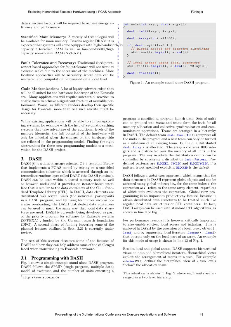
data structure layouts will be required to achieve energy ef-ficiency and performance.

Stratified Main Memory: A variety of technologies willbe available for main memory. Besides regular DRAM it isexpected that systems will come equipped with high-bandwidth/lowcapacity 3D-stacked RAM as well as low-bandwidth/highcapacity non-volatile RAM (NVRAM).

Fault Tolerance and Recovery: Traditional checkpoint-restart based approaches for fault-tolerance will not work atextreme scales due to the sheer size of the machines. Morelocalized approaches will be necessary, where data can berecovered and computation be resumed on a local level.

Code Modernization: A lot of legacy software exists thatwill be ill suited for the hardware landscape of the Exascaleera. Many applications will require substantial rewrites toenable them to achieve a significant fraction of available per-formance. Worse, as different vendors develop their specificdesign for Exascale, more than one such rewrite might benecessary.

While existing applications will be able to run on upcom-ing systems, for example with the help of automatic cachingsystems that take advantage of the additional levels of thememory hierarchy, the full potential of the hardware willonly be unlocked when the changes on the hardware sideare reflected in the programming model. Finding the rightabstractions for these new programming models is a moti-vation for the DASH project.

3. DASHDASH [8] is a data-structure oriented C++ template librarythat implements a PGAS model by relying on a one-sidedcommunication substrate which is accessed through an in-termediate runtime layer called DART (the DASH runtime).DASH can be used within a shared memory node as wellas between nodes and it provides an iterator-based inter-face that is similar to the data containers of the C++ Stan-dard Template Library (STL). In DASH, data elements aredistributed over several units (the individual participantsin a DASH program) and by using techniques such as op-erator overloading, the DASH distributed data containerscan be used in much the same way that local data struc-tures are used. DASH is currently being developed as partof the priority program for software for Exascale systems(SPPEXA)1, funded by the German research foundation(DFG). A second phase of funding (covering some of theplanned features outlined in Sect. 3.2) is currently underreview.

The rest of this section discusses some of the features ofDASH and how they can help address some of the challengesfaced when transitioning to Exascale hardware.

3.1 Programming with DASHFig. 1 shows a simple example stand-alone DASH program.DASH follows the SPMD (single program, multiple data)model of execution and the number of units executing a

1http://www.sppexa.de

1 int main(int argc , char* argv [])2 3 dash::init(&argc , &argv);4

5 dash::Array <int > a(1000);6

7 if( dash::myid()==0 ) 8 // global access and standard algorithms9 std::sort(a.begin(), a.end());

10 11

12 // local access using local iterators13 std::fill(a.lbegin(), a.lend(), 23+ myid);14

15 dash:: finalize ();16

Figure 1: An example stand-alone DASH program.

program is specified at program launch time. Sets of unitscan be grouped into teams and teams form the basis for allmemory allocation and collective synchronization and com-munication operations. Teams are arranged in a hierarchyin DASH. The default team dash::Team::All() comprises allthe units in the program and a new team can only be formedas a sub-team of an existing team. In line 5, a distributeddash::Array a is allocated. The array a contains 1000 inte-gers and is distributed over the memory of all units in theprogram. The way in which the distribution occurs can becontrolled by specifying a distribution dash::Pattern. Pre-defined patterns are BLOCKED, CYCLIC and BLOCKCYCLIC, if apattern is not specified explicitly, BLOCKED is the default.

DASH follows a global-view approach, which means that thedata structures in DASH represent global objects and can beaccessed using global indices; i.e., for the same index i theexpression a[i] refers to the same array element, regardlessof which unit evaluates the expression. Global-view pro-gramming is an important productivity feature, because itallows distributed data structures to be treated much likeregular local data structures or STL containers. In fact,DASH arrays can be used with standard STL algorithms, asshown in line 9 of Fig. 1.

For performance reasons it is however critically importantto also enable efficient local access and indexing. This isachieved in DASH by the provision of a local proxy object (.local) and by supporting local iterators .lbegin(), .lend()

that operate only on the local part of an array. An examplefor this mode of usage is shown in line 13 of Fig. 1.

Besides local and global access, DASH supports hierarchicalviews on data and hierarchical iterators. Hierarchical viewsexploit the arrangement of teams in a tree. For examplea.hview<2>() defines the hierarchical view of a two levels“below” the allocation team.

This situation is shown in Fig. 2 where eight units are ar-ranged in a two level hierarchy.


Exploiting Hierarchical Exascale Hardware using a PGAS Approach Fürlinger

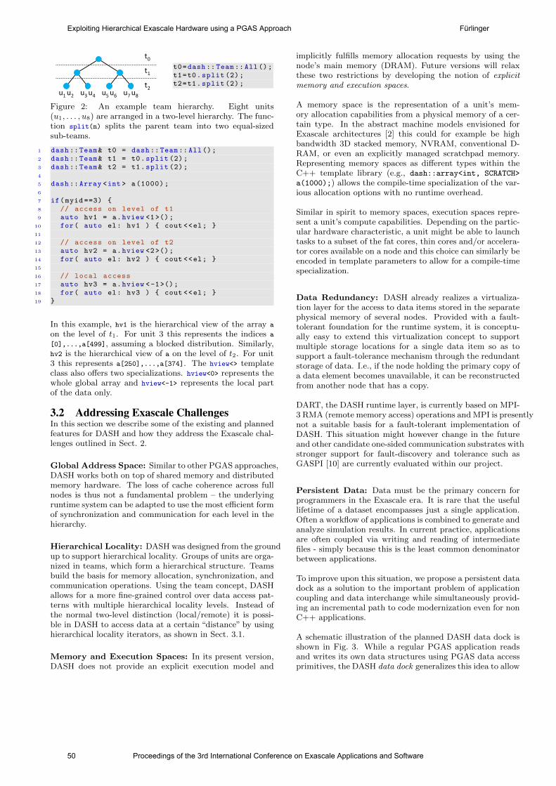
u2u1 u4u3 u6u5 u8u7

t0

t1

t2

t0=dash::Team::All();t1=t0.split (2);t2=t1.split (2);

Figure 2: An example team hierarchy. Eight units(u1, . . . , u8) are arranged in a two-level hierarchy. The func-tion split(n) splits the parent team into two equal-sizedsub-teams.

1 dash::Team& t0 = dash::Team::All();2 dash::Team& t1 = t0.split (2);3 dash::Team& t2 = t1.split (2);4

5 dash::Array <int > a(1000);6

7 if(myid ==3) 8 // access on level of t19 auto hv1 = a.hview <1>();

10 for( auto el: hv1 ) cout <<el; 11

12 // access on level of t213 auto hv2 = a.hview <2>();14 for( auto el: hv2 ) cout <<el; 15

16 // local access17 auto hv3 = a.hview <-1>();18 for( auto el: hv3 ) cout <<el; 19

In this example, hv1 is the hierarchical view of the array a

on the level of t1. For unit 3 this represents the indices a

[0],...,a[499], assuming a blocked distribution. Similarly,hv2 is the hierarchical view of a on the level of t2. For unit3 this represents a[250],...,a[374]. The hview<> templateclass also offers two specializations. hview<0> represents thewhole global array and hview<-1> represents the local partof the data only.

3.2 Addressing Exascale ChallengesIn this section we describe some of the existing and plannedfeatures for DASH and how they address the Exascale chal-lenges outlined in Sect. 2.

Global Address Space: Similar to other PGAS approaches,DASH works both on top of shared memory and distributedmemory hardware. The loss of cache coherence across fullnodes is thus not a fundamental problem – the underlyingruntime system can be adapted to use the most efficient formof synchronization and communication for each level in thehierarchy.

Hierarchical Locality: DASH was designed from the groundup to support hierarchical locality. Groups of units are orga-nized in teams, which form a hierarchical structure. Teamsbuild the basis for memory allocation, synchronization, andcommunication operations. Using the team concept, DASHallows for a more fine-grained control over data access pat-terns with multiple hierarchical locality levels. Instead ofthe normal two-level distinction (local/remote) it is possi-ble in DASH to access data at a certain “distance” by usinghierarchical locality iterators, as shown in Sect. 3.1.

Memory and Execution Spaces: In its present version,DASH does not provide an explicit execution model and

implicitly fulfills memory allocation requests by using thenode’s main memory (DRAM). Future versions will relaxthese two restrictions by developing the notion of explicitmemory and execution spaces.

A memory space is the representation of a unit’s mem-ory allocation capabilities from a physical memory of a cer-tain type. In the abstract machine models envisioned forExascale architectures [2] this could for example be highbandwidth 3D stacked memory, NVRAM, conventional D-RAM, or even an explicitly managed scratchpad memory.Representing memory spaces as different types within theC++ template library (e.g., dash::array<int, SCRATCH>

a(1000);) allows the compile-time specialization of the var-ious allocation options with no runtime overhead.

Similar in spirit to memory spaces, execution spaces repre-sent a unit’s compute capabilities. Depending on the partic-ular hardware characteristic, a unit might be able to launchtasks to a subset of the fat cores, thin cores and/or accelera-tor cores available on a node and this choice can similarly beencoded in template parameters to allow for a compile-timespecialization.

Data Redundancy: DASH already realizes a virtualiza-tion layer for the access to data items stored in the separatephysical memory of several nodes. Provided with a fault-tolerant foundation for the runtime system, it is conceptu-ally easy to extend this virtualization concept to supportmultiple storage locations for a single data item so as tosupport a fault-tolerance mechanism through the redundantstorage of data. I.e., if the node holding the primary copy ofa data element becomes unavailable, it can be reconstructedfrom another node that has a copy.

DART, the DASH runtime layer, is currently based on MPI-3 RMA (remote memory access) operations and MPI is presentlynot a suitable basis for a fault-tolerant implementation ofDASH. This situation might however change in the futureand other candidate one-sided communication substrates withstronger support for fault-discovery and tolerance such asGASPI [10] are currently evaluated within our project.

Persistent Data: Data must be the primary concern forprogrammers in the Exascale era. It is rare that the usefullifetime of a dataset encompasses just a single application.Often a workflow of applications is combined to generate andanalyze simulation results. In current practice, applicationsare often coupled via writing and reading of intermediatefiles - simply because this is the least common denominatorbetween applications.

To improve upon this situation, we propose a persistent datadock as a solution to the important problem of applicationcoupling and data interchange while simultaneously provid-ing an incremental path to code modernization even for nonC++ applications.

A schematic illustration of the planned DASH data dock isshown in Fig. 3. While a regular PGAS application readsand writes its own data structures using PGAS data accessprimitives, the DASH data dock generalizes this idea to allow



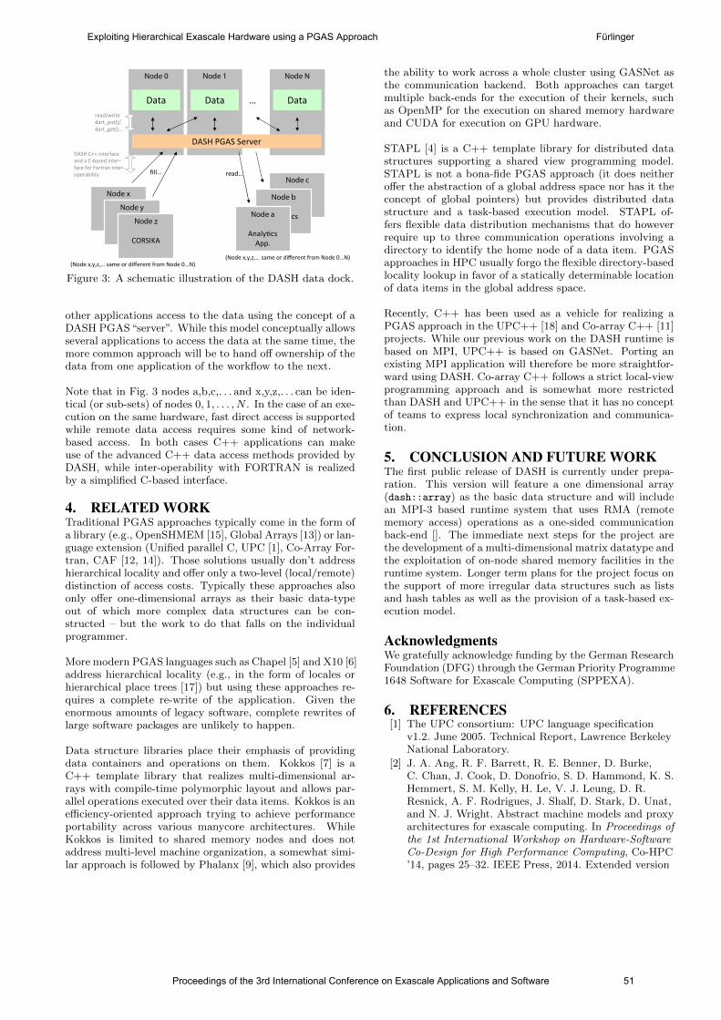
Node NNode 1Node 0

Data

DASH PGAS Server

DataData …read/writedart_put()/dart_get()…

Node x

CORSIKANode y

CORSIKANode z

CORSIKA

Node c

AnalyticsApp.

fill…

Node b

AnalyticsApp.

Node a

AnalyticsApp.

read…

DASH C++ interface and a C-based inter-face for Fortran inter-operability

(Node x,y,z,… same or different from Node 0…N)(Node x,y,z,… same or different from Node 0…N)

Figure 3: A schematic illustration of the DASH data dock.

other applications access to the data using the concept of aDASH PGAS“server”. While this model conceptually allowsseveral applications to access the data at the same time, themore common approach will be to hand off ownership of thedata from one application of the workflow to the next.

Note that in Fig. 3 nodes a,b,c,. . . and x,y,z,. . . can be iden-tical (or sub-sets) of nodes 0, 1, . . . , N . In the case of an exe-cution on the same hardware, fast direct access is supportedwhile remote data access requires some kind of network-based access. In both cases C++ applications can makeuse of the advanced C++ data access methods provided byDASH, while inter-operability with FORTRAN is realizedby a simplified C-based interface.

4. RELATED WORKTraditional PGAS approaches typically come in the form ofa library (e.g., OpenSHMEM [15], Global Arrays [13]) or lan-guage extension (Unified parallel C, UPC [1], Co-Array For-tran, CAF [12, 14]). Those solutions usually don’t addresshierarchical locality and offer only a two-level (local/remote)distinction of access costs. Typically these approaches alsoonly offer one-dimensional arrays as their basic data-typeout of which more complex data structures can be con-structed – but the work to do that falls on the individualprogrammer.

More modern PGAS languages such as Chapel [5] and X10 [6]address hierarchical locality (e.g., in the form of locales orhierarchical place trees [17]) but using these approaches re-quires a complete re-write of the application. Given theenormous amounts of legacy software, complete rewrites oflarge software packages are unlikely to happen.

Data structure libraries place their emphasis of providingdata containers and operations on them. Kokkos [7] is aC++ template library that realizes multi-dimensional ar-rays with compile-time polymorphic layout and allows par-allel operations executed over their data items. Kokkos is anefficiency-oriented approach trying to achieve performanceportability across various manycore architectures. WhileKokkos is limited to shared memory nodes and does notaddress multi-level machine organization, a somewhat simi-lar approach is followed by Phalanx [9], which also provides

the ability to work across a whole cluster using GASNet asthe communication backend. Both approaches can targetmultiple back-ends for the execution of their kernels, suchas OpenMP for the execution on shared memory hardwareand CUDA for execution on GPU hardware.

STAPL [4] is a C++ template library for distributed datastructures supporting a shared view programming model.STAPL is not a bona-fide PGAS approach (it does neitheroffer the abstraction of a global address space nor has it theconcept of global pointers) but provides distributed datastructure and a task-based execution model. STAPL of-fers flexible data distribution mechanisms that do howeverrequire up to three communication operations involving adirectory to identify the home node of a data item. PGASapproaches in HPC usually forgo the flexible directory-basedlocality lookup in favor of a statically determinable locationof data items in the global address space.

Recently, C++ has been used as a vehicle for realizing aPGAS approach in the UPC++ [18] and Co-array C++ [11]projects. While our previous work on the DASH runtime isbased on MPI, UPC++ is based on GASNet. Porting anexisting MPI application will therefore be more straightfor-ward using DASH. Co-array C++ follows a strict local-viewprogramming approach and is somewhat more restrictedthan DASH and UPC++ in the sense that it has no conceptof teams to express local synchronization and communica-tion.

5. CONCLUSION AND FUTURE WORKThe first public release of DASH is currently under prepa-ration. This version will feature a one dimensional array(dash::array) as the basic data structure and will includean MPI-3 based runtime system that uses RMA (remotememory access) operations as a one-sided communicationback-end []. The immediate next steps for the project arethe development of a multi-dimensional matrix datatype andthe exploitation of on-node shared memory facilities in theruntime system. Longer term plans for the project focus onthe support of more irregular data structures such as listsand hash tables as well as the provision of a task-based ex-ecution model.

AcknowledgmentsWe gratefully acknowledge funding by the German ResearchFoundation (DFG) through the German Priority Programme1648 Software for Exascale Computing (SPPEXA).

6. REFERENCES[1] The UPC consortium: UPC language specification

v1.2. June 2005. Technical Report, Lawrence BerkeleyNational Laboratory.

[2] J. A. Ang, R. F. Barrett, R. E. Benner, D. Burke,C. Chan, J. Cook, D. Donofrio, S. D. Hammond, K. S.Hemmert, S. M. Kelly, H. Le, V. J. Leung, D. R.Resnick, A. F. Rodrigues, J. Shalf, D. Stark, D. Unat,and N. J. Wright. Abstract machine models and proxyarchitectures for exascale computing. In Proceedings ofthe 1st International Workshop on Hardware-SoftwareCo-Design for High Performance Computing, Co-HPC’14, pages 25–32. IEEE Press, 2014. Extended version



available online at http://www.cal-design.org/

publications/publications2.

[3] K. Bergman, S. Borkar, D. Campbell, W. Carlson,W. Dally, M. Denneau, P. Franzon, W. Harrod,K. Hill, J. Hiller, et al. Exascale computing study:Technology challenges in achieving exascale systems.Defense Advanced Research Projects AgencyInformation Processing Techniques Office (DARPAIPTO), Tech. Rep, 15, 2008.

[4] A. Buss, I. Papadopoulos, O. Pearce, T. Smith,G. Tanase, N. Thomas, X. Xu, M. Bianco, N. M.Amato, L. Rauchwerger, et al. STAPL: standardtemplate adaptive parallel library. In Proceedings ofthe 3rd Annual Haifa Experimental SystemsConference, page 14. ACM, 2010.

[5] B. L. Chamberlain, D. Callahan, and H. P. Zima.Parallel programmability and the Chapel language.International Journal of High Performance ComputingApplications, 21:291–312, August 2007.

[6] P. Charles, C. Grothoff, V. Saraswat, C. Donawa,A. Kielstra, K. Ebcioglu, C. Von Praun, andV. Sarkar. X10: an object-oriented approach tonon-uniform cluster computing. ACM Sigplan Notices,40(10):519–538, 2005.

[7] H. C. Edwards and C. R. Trott. Kokkos: Enablingperformance portability across manycorearchitectures. In Extreme Scaling Workshop (XSW),2013, pages 18–24. IEEE, 2013.

[8] K. Furlinger, C. Glass, A. Knupfer, J. Tao, D. Hunich,K. Idrees, M. Maiterth, Y. Mhedeb, and H. Zhou.Dash: Data structures and algorithms with supportfor hierarchical locality. In Euro-Par 2014 Workshops(Porto, Portugal), 2014.

[9] M. Garland, M. Kudlur, and Y. Zheng. Designing aunified programming model for heterogeneousmachines. In Proceedings of the 2012 InternationalConference for High Performance Computing,Networking, Storage and Analysis (SC’12), Nov. 2012.Salt Lake City, UT, USA.

[10] GASPI - global adress space programming interfacewebpage http://www.gaspi.de. Retrieved Jan. 2012.

[11] T. A. Johnson. Coarray C++. In 7th International

Conference on PGAS Programming Models, 2013.Edinburgh, Scotland.

[12] J. Mellor-Crummey, L. Adhianto, W. N. Scherer, andG. Jin. A new vision for coarray Fortran. InProceedings of the Third Conference on PartitionedGlobal Address Space Programing Models (PGAS ’09),New York, NY, USA, 2009. ACM.

[13] J. Nieplocha, R. J. Harrison, and R. J. Littlefield.Global arrays: A nonuniform memory accessprogramming model for high-performance computers.The Journal of Supercomputing, 10:169–189, 1996.

[14] R. W. Numrich and J. Reid. Co-array fortran forparallel programming. SIGPLAN Fortran Forum,17(2):1–31, Aug. 1998.

[15] S. W. Poole, O. Hernandez, J. A. Kuehn, G. M.Shipman, A. Curtis, and K. Feind. Openshmem -toward a unified rma model. In D. Padua, editor,Encyclopedia of Parallel Computing, pages 1379–1391.Springer US, 2011.

[16] A. Tate, A. Kamil, A. Dubey, A. Großlinger,

B. Chamberlain, B. Goglin, C. Edwards, C. J.Newburn, D. Padua, D. Unat, E. Jeannot, F. Hannig,T. Gysi, H. Ltaief, J. Sexton, J. Labarta, J. Shalf,K. Furlinger, K. O’Brien, L. Linardakis, M. Besta,M.-C. Sawley, M. Abraham, M. Bianco, M. Pericas,N. Maruyama, P. H. J. Kelly, P. Messmer, R. B. Ross,R. Cledat, S. Matsuoka, T. Schulthess, T. Hoefler, andV. J. Leung. Programming Abstractions for DataLocality. Research report, PADAL Workshop 2014,April 28–29, Swiss National Supercomputing Center(CSCS), Lugano, Switzerland, Nov. 2014.

[17] Y. Yan, J. Zhao, Y. Guo, and V. Sarkar. HierarchicalPlace Trees: A portable abstraction for taskparallelism and data movement. In Proceedings of the22nd international conference on Languages andCompilers for Parallel Computing, LCPC’09, pages172–187. Springer-Verlag, 2010.

[18] Y. Zheng, A. Kamil, M. B. Driscoll, H. Shan, andK. Yelick. UPC++: A PGAS extension for C++. In28th IEEE International Parallel & DistributedProcessing Symposium, 2014.



Enabling Adaptive, Fault-tolerant MPI Applications withDynamic Resource Allocation

Maciej SzpindlerInterdisciplinary Centre for Mathematical and Computational Modelling

University of [email protected]

ABSTRACTDominant execution mode for the most of HPC applicationsusing MPI or hybrid parallel model rely on static resourceallocation. While this is explicitly mapped to both MPI us-age scenarios and runtime systems, it entails restrictions forefficient dynamic execution. This limitation becomes criti-cal when fault tolerance of MPI applications is concerned.Also some classes of applications require dynamic processcreation. This paper discusses enabling of dynamic resourceallocation for adaptive execution and fault tolerance in MPIapplications. Existing functionality of the MPI library andunderlying layers and required interactions are described.Implementation and common usage scenarios are presented.Practicality is discussed, showing performance and limita-tions on synthetic experiments.

1. INTRODUCTIONRecent HPC systems build their computational capabilitiesand performance on extreme number of processing elements- either multicore nodes, hyperthreaded cores, acceleratednodes or other constructs. This requires applications to beextremely parallel and scalable to run efficiently on thosesystems and benefit from their peak performance. On theother hand, in real usage several applications share one largesystem at the same time. It is quite obvious since such sys-tems are expensive and consume a lot of resources even whenidle. Parallel applications need fair and optimal sharing ofthe computational resources which is usually provided byresource manager or queuing system.

One of the common constraints for programmers in the de-scribed shared computing environment is static resource al-location. Although MPI and other parallel programmingmodels have constructs that allow dynamic process creationand management, it is not easily manageable in a sharedmulti-task system. Newly created processes must use al-ready allocated resources which leads to either waste of re-sources that need to be preallocated or processes oversub-scription which likely results in performance degradation.Moreover fault tolerance of parallel applications becomes areal need. Common scenarios for process fault recovery as-sume a repair stage which implies dynamic creation of newprocesses.

In this work a simple model for the complete dynamic multi-process execution is proposed. The approach uses existingmethods for resource allocation resizing in the Slurm envi-ronment. It allows dynamic multi-process applications in a

shared environment. The latter gives more opportunities forbetter resource utilization and allows programmers to cre-ate more flexible applications that may allocate resourcesdynamically and exclusively which is usually required toachieve full performance and essential when addressing faultrecovery.

This paper is organized as follows: section 2 is a study ofa current context for most popular MPI implementationsand their integration with scheduling systems. MPICH andOpenMPI projects are addressed and Slurm system as re-source manager. Section 3 describes application of the dy-namic resource re-allocation for failure recovery of the MPIjobs. An analysis of MPI communicator reconstruction andprocess failure recovery is discussed. Performance study forsynthetic scenarios are described in section 4.

The key contributions of the described work include:

• A simple model for MPI user application with batchscheduler interaction.

• An implementation of the proposed model.

• An analysis of the available MPI communicator repairmechanisms and its integration with resource alloca-tion.

• A study of a failure recovery performance for simplemodel application.

2. PROCESS AND RESOURCE MANAGE-MENT INTERACTION

Most HPC systems that support multiple applications ex-ecution separate resource allocation and actual applicationexecution. Queueing system or resource manager is usu-ally responsible for allocation which is preceding step toapplication startup. Application processes management ismore system-wide task and possibly many components areinvolved. MPI implementations introduce a form of processencapsulation for better execution control. Nevertheless allthese components interact closely as shown on figure 1.

2.1 MPI levelMPI standard [7] defines functionality for process creationand management. There are library calls that allow dynamicprocess creation. It is MPI runtime responsibility to create


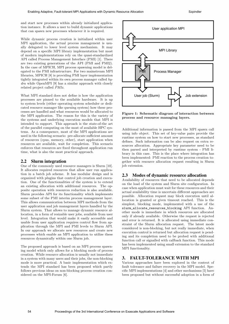
and start new processes within already initialized applica-tion instance. It allows a user to build dynamic applicationsthat can spawn new processes whenever it is required.

While dynamic process creation is initialized within userMPI application, the actual process management is usu-ally delegated to lower level system mechanism. It maydepend on a specific MPI library implementation but mostof modern implementations rely on the quasi-standardizedAPI called Process Management Interface (PMI) [1]. Thereare two existing generations of the API (PMI and PMI2).In the case of MPICH, MPI process spawning model is del-egated to the PMI infrastructure. For two mainstream MPIlibraries, MPICH [8] is providing PMI layer implementationtightly integrated within its own process manager called hy-dra while OpenMPI [9] has a similar approach with closelyrelated project called PMIx.

What MPI standard does not define is how the applicationprocesses are pinned to the available hardware. It is upto system levels (either operating system scheduler or dedi-cated resource manager like queuing system) how these pro-cesses are handled and what resources would be allocated tothe MPI application. The reason for this is the variety ofthe systems and underlying execution models that MPI isintended to support. This approach is the state-of-the artof the parallel computing on the most of available HPC sys-tems. As a consequence, most of the MPI applications areused in the following scenario: pre-allocate sufficient amountof resources (cpus, memory, other), start application whenresources are available, wait for completion. This scenarioenforces that resources are fixed throughout application runtime, what is also the most practical approach.

2.2 Slurm integrationOne of the commonly used resource managers is Slurm [10].It allocates required resources that allow user run applica-tion in a batch job scheme. It has modular design and isorganized with plugins that control job creation and execu-tion. One of the functionalities of the system is to extendan existing allocation with additional resources. The op-posite operation with resources reduction is also available.Slurm provides API for its functionality which implementssome subset of the PMI interim process management layer.This allows communication between MPI methods from theuser application and job management layers handled by theSlurm system. That allows to manage dynamic resource al-location, in a form of resizable user jobs, available from userlevel. Integration that would make it easily accessible andusable from user application requires control flow from ap-plication through the MPI and PMI levels to Slurm API.In our approach we allocate new resources and create newprocesses which enable an MPI application to utilize theseresources dynamically within one Slurm job.

The proposed approach is based on an MPI process spawn-ing model which only allows for a blocking mode of processcreation. While resource allocation is usually not immediatein a system with many users and their jobs, the non-blockingmode is more practical. A basic implementation which ex-tends the MPI standard has been proposed which partlyfollows previous ideas on non-blocking process creation con-sidered on the MPI-Forum [6].

Process ManagerPMI

User job (Slurm) Job extension

User application MPI

MPI Library

Figure 1: Schematic diagram of interaction betweenprocess and resource managing layers.

Additional information is passed from the MPI spawn callusing info object. This set of key-value pairs provide theruntime system on how to start new processes, as standarddefines. Such information can be also request on extra re-sources allocation. Appropriate key parameter need to bethen parsed and interpreted by runtime system - PMI li-brary in this case. This is the place where integration hasbeen implemented: PMI reaction to the process creation to-gether with resource allocation request resulting in Slurmjob extension.

2.3 Modes of dynamic resource allocationAvailability of resources that need to be allocated dependson the load of the system and Slurm site configuration. Incase when application must wait for these resources and theiractual availability time is uncertain different approaches arepossible. Allocation request may block execution until al-location is granted or given timeout reached. This is thesimplest, blocking mode, implemented with a use of theslurm_allocate_resources_blocking API function. An-other mode is immediate in which resources are allocatedonly if already available. Otherwise the request is rejectedand error is returned. It is allocated using immediate con-straint of the Slurm allocation request. The latest modeconsidered is non-blocking, but not really immediate, whenexecution control is returned but allocation request is pend-ing and its completion need to be probed with additionalfunction call or signalled with callback function. This modehas been implemented using small extension to the standardMPI functionality.

3. FAULT-TOLERANCE WITH MPIVarious approaches have been explored in the context offault tolerance and failure recovery in the MPI model. Spe-cific MPI implementations [4] and other mechanisms [5] havebeen proposed but without successful adoption in a form of


Enabling Adaptive, Fault-tolerant MPI Applications with Dynamic Resource Allocation Szpindler

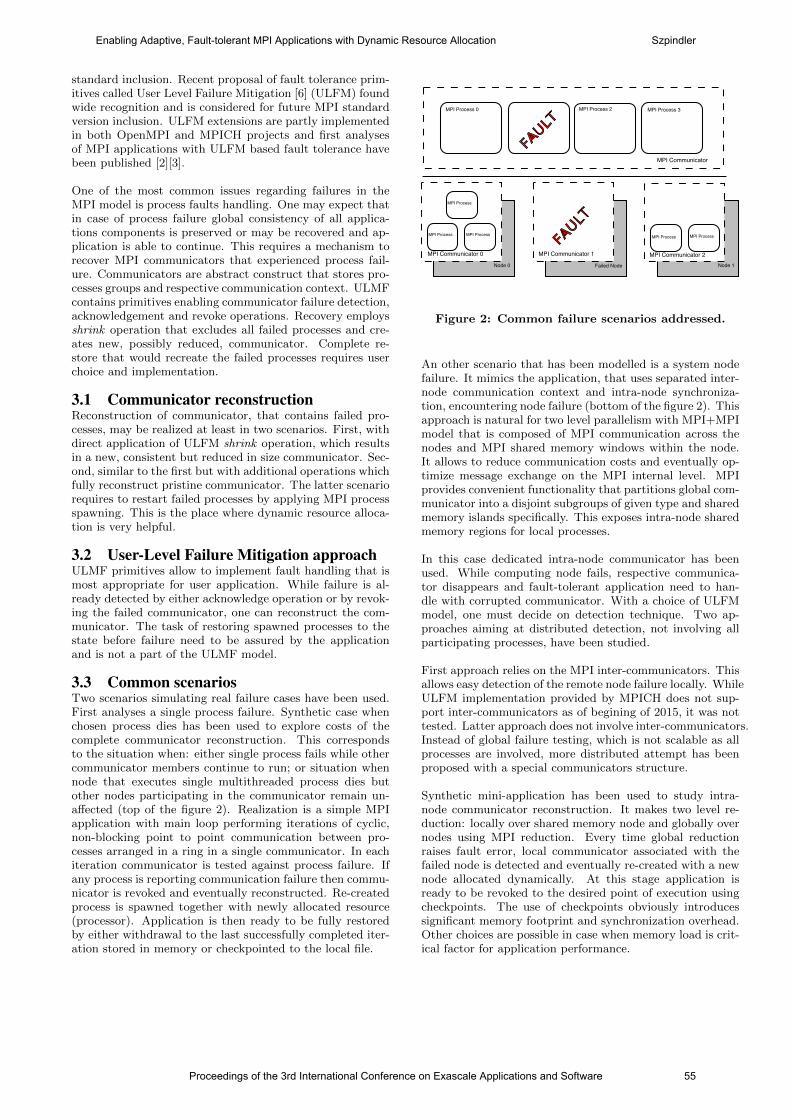
standard inclusion. Recent proposal of fault tolerance prim-itives called User Level Failure Mitigation [6] (ULFM) foundwide recognition and is considered for future MPI standardversion inclusion. ULFM extensions are partly implementedin both OpenMPI and MPICH projects and first analysesof MPI applications with ULFM based fault tolerance havebeen published [2][3].

One of the most common issues regarding failures in theMPI model is process faults handling. One may expect thatin case of process failure global consistency of all applica-tions components is preserved or may be recovered and ap-plication is able to continue. This requires a mechanism torecover MPI communicators that experienced process fail-ure. Communicators are abstract construct that stores pro-cesses groups and respective communication context. ULMFcontains primitives enabling communicator failure detection,acknowledgement and revoke operations. Recovery employsshrink operation that excludes all failed processes and cre-ates new, possibly reduced, communicator. Complete re-store that would recreate the failed processes requires userchoice and implementation.

3.1 Communicator reconstructionReconstruction of communicator, that contains failed pro-cesses, may be realized at least in two scenarios. First, withdirect application of ULFM shrink operation, which resultsin a new, consistent but reduced in size communicator. Sec-ond, similar to the first but with additional operations whichfully reconstruct pristine communicator. The latter scenariorequires to restart failed processes by applying MPI processspawning. This is the place where dynamic resource alloca-tion is very helpful.

3.2 User-Level Failure Mitigation approachULMF primitives allow to implement fault handling that ismost appropriate for user application. While failure is al-ready detected by either acknowledge operation or by revok-ing the failed communicator, one can reconstruct the com-municator. The task of restoring spawned processes to thestate before failure need to be assured by the applicationand is not a part of the ULMF model.

3.3 Common scenariosTwo scenarios simulating real failure cases have been used.First analyses a single process failure. Synthetic case whenchosen process dies has been used to explore costs of thecomplete communicator reconstruction. This correspondsto the situation when: either single process fails while othercommunicator members continue to run; or situation whennode that executes single multithreaded process dies butother nodes participating in the communicator remain un-affected (top of the figure 2). Realization is a simple MPIapplication with main loop performing iterations of cyclic,non-blocking point to point communication between pro-cesses arranged in a ring in a single communicator. In eachiteration communicator is tested against process failure. Ifany process is reporting communication failure then commu-nicator is revoked and eventually reconstructed. Re-createdprocess is spawned together with newly allocated resource(processor). Application is then ready to be fully restoredby either withdrawal to the last successfully completed iter-ation stored in memory or checkpointed to the local file.

Node 1Failed NodeNode 0

MPI Communicator

MPI Communicator 0 MPI Communicator 2

MPI Process 0 MPI Process 2 MPI Process 3

MPI Process

MPI Process MPI Process MPI ProcessMPI Process

MPI Communicator 1

Figure 2: Common failure scenarios addressed.

An other scenario that has been modelled is a system nodefailure. It mimics the application, that uses separated inter-node communication context and intra-node synchroniza-tion, encountering node failure (bottom of the figure 2). Thisapproach is natural for two level parallelism with MPI+MPImodel that is composed of MPI communication across thenodes and MPI shared memory windows within the node.It allows to reduce communication costs and eventually op-timize message exchange on the MPI internal level. MPIprovides convenient functionality that partitions global com-municator into a disjoint subgroups of given type and sharedmemory islands specifically. This exposes intra-node sharedmemory regions for local processes.

In this case dedicated intra-node communicator has beenused. While computing node fails, respective communica-tor disappears and fault-tolerant application need to han-dle with corrupted communicator. With a choice of ULFMmodel, one must decide on detection technique. Two ap-proaches aiming at distributed detection, not involving allparticipating processes, have been studied.

First approach relies on the MPI inter-communicators. Thisallows easy detection of the remote node failure locally. WhileULFM implementation provided by MPICH does not sup-port inter-communicators as of begining of 2015, it was nottested. Latter approach does not involve inter-communicators.Instead of global failure testing, which is not scalable as allprocesses are involved, more distributed attempt has beenproposed with a special communicators structure.

Synthetic mini-application has been used to study intra-node communicator reconstruction. It makes two level re-duction: locally over shared memory node and globally overnodes using MPI reduction. Every time global reductionraises fault error, local communicator associated with thefailed node is detected and eventually re-created with a newnode allocated dynamically. At this stage application isready to be revoked to the desired point of execution usingcheckpoints. The use of checkpoints obviously introducessignificant memory footprint and synchronization overhead.Other choices are possible in case when memory load is crit-ical factor for application performance.



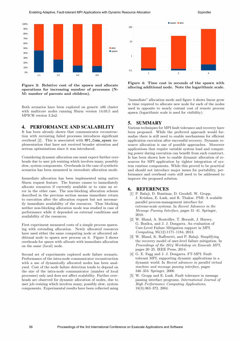
Figure 3: Relative cost of the spawn and allocateoperations for increasing number of processes (N-M: number of parents and children).

Both scenarios have been explored on generic x86 clusterwith multicore nodes running Slurm version 14.03.5 andMPICH version 3.2a2.

4. PERFORMANCE AND SCALABILITYIt has been already shown that communicator reconstruc-tion with recreating failed processes introduces significantoverhead [2]. This is associated with MPI_Comm_spawn im-plementation that have not received broader attention andserious optimizations since it was introduced.

Considering dynamic allocation one must expect further over-heads due to user job resizing which involves many, possiblyslow, system components. Overheads in the case of syntheticscenarios has been measured in immediate allocation mode.

Immediate allocation has been implemented using nativeSlurm request feature. The feature causes to immediatelyallocate resources if currently available or to raise an er-ror in the other case. The non-blocking allocation schemedescribed in the previous section means immediate returnto execution after the allocation request but not necessar-ily immediate availability of the resources. Thus blockingneither non-blocking allocation mode was studied in case ofperformance while it depended on external conditions andavailability of the resources.

First experiment measured costs of a simple process spawn-ing with extending allocation. Newly allocated resourceshave used either the same computing node or allocated ad-ditional node to spawn new process on it. Figure 3 showsoverheads for spawn with allocate with immediate allocationon the same (local) node.

Second set of experiments explored node failure scenario.Performance of the intra-node communicator reconstructionwith a use of dynamically allocated nodes has been anal-ysed. Cost of the node failure detection tends to depend onthe size of the intra-node communicator (number of localprocesses) only and does not affect scalability. Further over-heads are observed for dynamic allocation of nodes, due touser job resizing which involves many, possibly slow, systemcomponents. Experimental results have been collected using

Figure 4: Time cost in seconds of the spawn withallocing additional node. Note the logarithmic scale.

”immediate” allocation mode and figure 4 shows linear growin time required to allocate new node for each of the nodesused in opposite to nearly costant cost of remote processspawn (logarithmic scale is used for visibility).

5. SUMMARYVarious techniques for MPI fault tolerance and recovery havebeen proposed. While the preferred approach would for-malize there is still need to enable mechanisms for efficientapplication execution after successful recovery. Dynamic re-source allocation is one of possible approaches. Moreoverapplications that require variable system load and comput-ing power during execution can benefit from such construct.Is has been shown how to enable dynamic allocation of re-sources for MPI application by tighter integration of sys-tem runtime components. While this proved to be practicaland should not introduce major issues for portability, per-formance and overhead costs still need to be addressed toimprove the proposed solution.

6. REFERENCES[1] P. Balaji, D. Buntinas, D. Goodell, W. Gropp,

J. Krishna, E. Lusk, and R. Thakur. PMI: A scalableparallel process-management interface forextreme-scale systems. In Recent Advances in theMessage Passing Interface, pages 31–41. Springer,2010.

[2] W. Bland, A. Bouteiller, T. Herault, J. Hursey,G. Bosilca, and J. J. Dongarra. An evaluation ofUser-Level Failure Mitigation support in MPI.Computing, 95(12):1171–1184, 2013.

[3] W. Bland, K. Raffenetti, and P. Balaji. Simplifyingthe recovery model of user-level failure mitigation. InProceedings of the 2014 Workshop on Exascale MPI,pages 20–25. IEEE Press, 2014.

[4] G. E. Fagg and J. J. Dongarra. FT-MPI: Faulttolerant MPI, supporting dynamic applications in adynamic world. In Recent advances in parallel virtualmachine and message passing interface, pages346–353. Springer, 2000.

[5] W. Gropp and E. Lusk. Fault tolerance in messagepassing interface programs. International Journal ofHigh Performance Computing Applications,18(3):363–372, 2004.



[6] MPI Forum. Message Passing Interface (MPI) ForumHome Page. http://www.mpi-forum.org/.

[7] MPI Forum. MPI: A Message-Passing InterfaceStandard. Version 3.0, September 21 2012. Availableat: http://www.mpi-forum.org.

[8] MPICH: High-Performance Portable MPI. Available

at: http://www.mpich.org/.

[9] Open MPI: Open Source High PerformanceComputing. Available at: http://www.open-mpi.org.

[10] Slurm Workload Manager. Available at:http://slurm.schedmd.com.



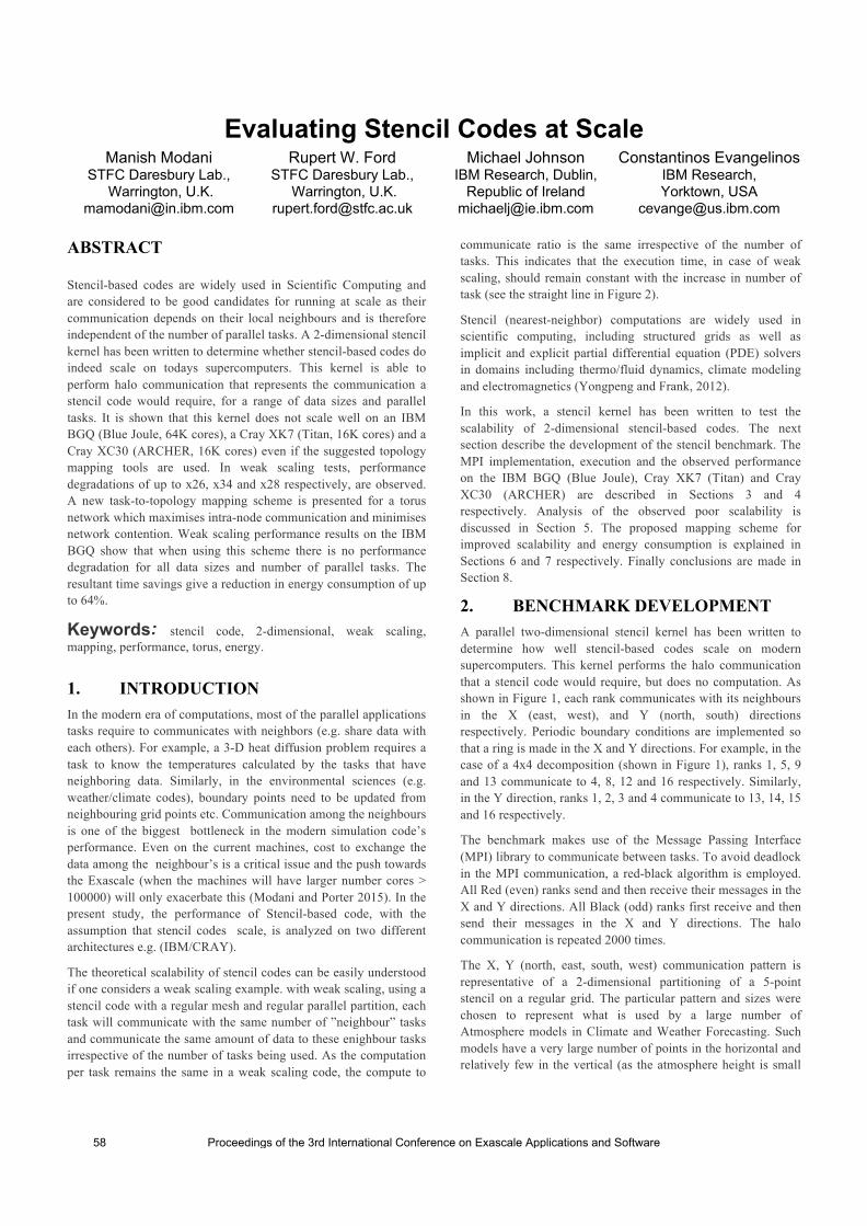
Evaluating Stencil Codes at Scale Manish Modani

STFC Daresbury Lab., Warrington, U.K.

[email protected]

Rupert W. Ford STFC Daresbury Lab.,

Warrington, U.K. [email protected]

Michael Johnson IBM Research, Dublin,

Republic of Ireland [email protected]

Constantinos Evangelinos IBM Research, Yorktown, USA

[email protected]

ABSTRACT Stencil-based codes are widely used in Scientific Computing and are considered to be good candidates for running at scale as their communication depends on their local neighbours and is therefore independent of the number of parallel tasks. A 2-dimensional stencil kernel has been written to determine whether stencil-based codes do indeed scale on todays supercomputers. This kernel is able to perform halo communication that represents the communication a stencil code would require, for a range of data sizes and parallel tasks. It is shown that this kernel does not scale well on an IBM BGQ (Blue Joule, 64K cores), a Cray XK7 (Titan, 16K cores) and a Cray XC30 (ARCHER, 16K cores) even if the suggested topology mapping tools are used. In weak scaling tests, performance degradations of up to x26, x34 and x28 respectively, are observed. A new task-to-topology mapping scheme is presented for a torus network which maximises intra-node communication and minimises network contention. Weak scaling performance results on the IBM BGQ show that when using this scheme there is no performance degradation for all data sizes and number of parallel tasks. The resultant time savings give a reduction in energy consumption of up to 64%.

Keywords: stencil code, 2-dimensional, weak scaling, mapping, performance, torus, energy.

1. INTRODUCTION In the modern era of computations, most of the parallel applications tasks require to communicates with neighbors (e.g. share data with each others). For example, a 3-D heat diffusion problem requires a task to know the temperatures calculated by the tasks that have neighboring data. Similarly, in the environmental sciences (e.g. weather/climate codes), boundary points need to be updated from neighbouring grid points etc. Communication among the neighbours is one of the biggest bottleneck in the modern simulation code’s performance. Even on the current machines, cost to exchange the data among the neighbour’s is a critical issue and the push towards the Exascale (when the machines will have larger number cores > 100000) will only exacerbate this (Modani and Porter 2015). In the present study, the performance of Stencil-based code, with the assumption that stencil codes scale, is analyzed on two different architectures e.g. (IBM/CRAY). The theoretical scalability of stencil codes can be easily understood if one considers a weak scaling example. with weak scaling, using a stencil code with a regular mesh and regular parallel partition, each task will communicate with the same number of ”neighbour” tasks and communicate the same amount of data to these enighbour tasks irrespective of the number of tasks being used. As the computation per task remains the same in a weak scaling code, the compute to

communicate ratio is the same irrespective of the number of tasks. This indicates that the execution time, in case of weak scaling, should remain constant with the increase in number of task (see the straight line in Figure 2). Stencil (nearest-neighbor) computations are widely used in scientific computing, including structured grids as well as implicit and explicit partial differential equation (PDE) solvers in domains including thermo/fluid dynamics, climate modeling and electromagnetics (Yongpeng and Frank, 2012). In this work, a stencil kernel has been written to test the scalability of 2-dimensional stencil-based codes. The next section describe the development of the stencil benchmark. The MPI implementation, execution and the observed performance on the IBM BGQ (Blue Joule), Cray XK7 (Titan) and Cray XC30 (ARCHER) are described in Sections 3 and 4 respectively. Analysis of the observed poor scalability is discussed in Section 5. The proposed mapping scheme for improved scalability and energy consumption is explained in Sections 6 and 7 respectively. Finally conclusions are made in Section 8.

2. BENCHMARK DEVELOPMENT A parallel two-dimensional stencil kernel has been written to determine how well stencil-based codes scale on modern supercomputers. This kernel performs the halo communication that a stencil code would require, but does no computation. As shown in Figure 1, each rank communicates with its neighbours in the X (east, west), and Y (north, south) directions respectively. Periodic boundary conditions are implemented so that a ring is made in the X and Y directions. For example, in the case of a 4x4 decomposition (shown in Figure 1), ranks 1, 5, 9 and 13 communicate to 4, 8, 12 and 16 respectively. Similarly, in the Y direction, ranks 1, 2, 3 and 4 communicate to 13, 14, 15 and 16 respectively. The benchmark makes use of the Message Passing Interface (MPI) library to communicate between tasks. To avoid deadlock in the MPI communication, a red-black algorithm is employed. All Red (even) ranks send and then receive their messages in the X and Y directions. All Black (odd) ranks first receive and then send their messages in the X and Y directions. The halo communication is repeated 2000 times. The X, Y (north, east, south, west) communication pattern is representative of a 2-dimensional partitioning of a 5-point stencil on a regular grid. The particular pattern and sizes were chosen to represent what is used by a large number of Atmosphere models in Climate and Weather Forecasting. Such models have a very large number of points in the horizontal and relatively few in the vertical (as the atmosphere height is small


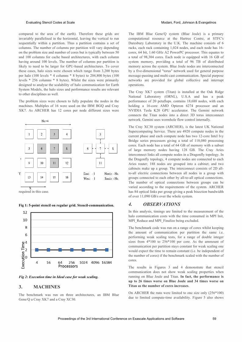
compared to the area of the earth). Therefore these grids are invariably parallelised in the horizontal, leaving the vertical to run sequentially within a partition. Thus a partition contains a set of columns. The number of columns per partition will vary depending on the problem size and number of cores but is typically between 50 and 100 columns for cache based architectures, with each column having around 100 levels. The number of columns per partition is likely to need to be larger for GPU-based architectures. To cover these cases, halo sizes were chosen which range from 3,200 bytes per halo (100 levels * 4 columns * 8 bytes) to 204,800 bytes (100 levels * 256 columns * 8 bytes). Whilst the sizes were primarily designed to analyse the scalability of halo communication for Earth System Models, the halo sizes and performance results are relevant to other disciplines as well. The problem sizes were chosen to fully populate the nodes in the machines. Multiples of 16 were used on the IBM BGQ and Cray XK7. As ARCHER has 12 cores per node different sizes were

required in this case.

Fig 1: 5-point stencil on regular grid. Stencil-communication.

Fig 2: Execution time in Ideal case for weak scaling. 3. MACHINES The benchmark was run on three architectures, an IBM Blue Gene/Q a Cray XK7 and a Cray XC30.

The IBM Blue Gene/Q system (Blue Joule) is a primary computational resource at the Hartree Centre, at STFC's Daresbury Laboratory in the U.K. The machine consists of 6 racks, each rack containing 1,024 nodes, and each node has 16-cores, 64 bit, 1.60 GHz A2 PowerPC processor. This equates to a total of 98,304 cores. Each node is equipped with 16 GB of system memory, providing a total of 96 TB of distributed memory across the system. Blue Joule nodes are interconnected by a five-dimensional "torus" network used for general purpose message-passing and multi-cast communication. Special purpose networks are provided for global collective and interrupt operations. The Cray XK7 system (Titan) is installed at the Oak Ridge National Laboratory (ORNL), U.S.A and has a peak performance of 20 petaflops. contains 18,688 nodes, with each holding a 16-core AMD Opteron 6274 processor and an NVIDIA Tesla K20 GPU accelerator. The Gemini network connects the Titan nodes into a direct 3D torus interconnect network. Gemini uses wormhole flow control internally. The Cray XC30 system (ARCHER), is the latest UK National Supercomputing Service. There are 4920 compute nodes in the current phase and each compute node has two 12-core Intel Ivy Bridge series processors giving a total of 118,080 processing cores. Each node has a total of 64 GB of memory with a subset of large memory nodes having 128 GB. The Cray Aries interconnect links all compute nodes in a Dragonfly topology. In the Dragonfly topology, 4 compute nodes are connected to each Aries router; 188 nodes are grouped into a cabinet; and two cabinets make up a group. The interconnect consists of 2D all-to-all electric connections between all nodes in a group with groups connected to each other by all-to-all optical connections. The number of optical connections between groups can be varied according to the requirements of the system. ARCHER has 84 optical links per group giving a peak bisection bandwidth of over 11,090 GB/s over the whole system.

4. OBSERVATIONS

In this analysis, timings are limited to the measurement of the halo communication costs with the time consumed in MPI Init, MPI_Reduce and MPI_Finalize being excluded. The benchmark code was run on a range of cores whilst keeping the amount of communication per partition the same i.e. performing weak scaling tests, for a range of double integer sizes from 4*100 to 256*100 per core. As the ammount of communication per partition stays constant for weak scaling one would expect the time to remain constant (i.e. be independent of the number of cores) if the benchmark scaled with the number of cores. The results in Figures 3 and 4 demonstrate that stencil communication does not show weak scaling properties when running on Blue Joule and Titan. In fact, the performance is up to 26 times worse on Blue Joule and 34 times worse on Titan as the number of cores increases. On ARCHER the runs were limited to one size only (256*100) due to limited compute-time availability. Figure 5 also shows


Evaluating Stencil Codes at Scale Modani, Ford, Johnson & Evangelinos

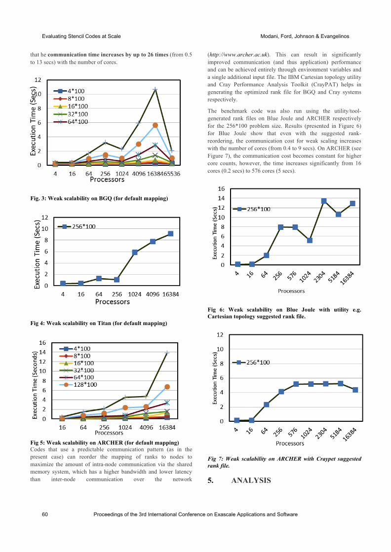
that he communication time increases by up to 26 times (from 0.5 to 13 secs) with the number of cores.

Fig. 3: Weak scalability on BGQ (for default mapping)

Fig 4: Weak scalability on Titan (for default mapping)

Fig 5: Weak scalability on ARCHER (for default mapping) Codes that use a predictable communication pattern (as in the present case) can reorder the mapping of ranks to nodes to maximize the amount of intra-node communication via the shared memory system, which has a higher bandwidth and lower latency than inter-node communication over the network

(http://www.archer.ac.uk). This can result in significantly improved communication (and thus application) performance and can be achieved entirely through environment variables and a single additional input file. The IBM Cartesian topology utility and Cray Performance Analysis Toolkit (CrayPAT) helps in generating the optimized rank file for BGQ and Cray systems respectively. The benchmark code was also run using the utility/tool-generated rank files on Blue Joule and ARCHER respectively for the 256*100 problem size. Results (presented in Figure 6) for Blue Joule show that even with the suggested rank-reordering, the communication cost for weak scaling increases with the number of cores (from 0.4 to 9 secs). On ARCHER (see Figure 7), the communication cost becomes constant for higher core counts, however, the time increases significantly from 16 cores (0.2 secs) to 576 cores (5 secs).

Fig 6: Weak scalability on Blue Joule with utility e.g. Cartesian topology suggested rank file.

Fig 7: Weak scalability on ARCHER with Craypet suggested rank file. 5. ANALYSIS



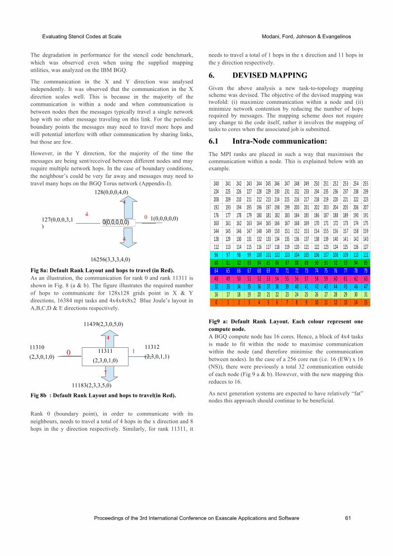
The degradation in performance for the stencil code benchmark, which was observed even when using the supplied mapping utilities, was analyzed on the IBM BGQ. The communication in the X and Y direction was analysed independently. It was observed that the communication in the X direction scales well. This is because in the majority of the communication is within a node and when communication is between nodes then the messages typically travel a single network hop with no other message traveling on this link. For the periodic boundary points the messages may need to travel more hops and will potential interfere with other communication by sharing links, but those are few. However, in the Y direction, for the majority of the time the messages are being sent/received between different nodes and may require multiple network hops. In the case of boundary conditions, the neighbour’s could be very far away and messages may need to travel many hops on the BGQ Torus network (Appendix-I).

Fig 8a: Default Rank Layout and hops to travel (in Red). As an illustration, the communication for rank 0 and rank 11311 is shown in Fig. 8 (a & b). The figure illustrates the required number of hops to communicate for 128x128 grids point in X & Y directions, 16384 mpi tasks and 4x4x4x8x2 Blue Joule’s layout in A,B,C,D & E directions respectively. Fig 8b : Default Rank Layout and hops to travel(in Red).

Rank 0 (boundary point), in order to communicate with its neighbours, needs to travel a total of 4 hops in the x direction and 8 hops in the y direction respectively. Similarly, for rank 11311, it

needs to travel a total of 1 hops in the x direction and 11 hops in the y direction respectively.

6. DEVISED MAPPING Given the above analysis a new task-to-topology mapping scheme was devised. The objective of the devised mapping was twofold: (i) maximize communication within a node and (ii) minimize network contention by reducing the number of hops required by messages. The mapping scheme does not require any change to the code itself, rather it involves the mapping of tasks to cores when the associated job is submitted.

6.1 Intra-Node communication:

The MPI ranks are placed in such a way that maximises the communication within a node. This is explained below with an example.

Fig9 a: Default Rank Layout. Each colour represent one compute node. A BGQ compute node has 16 cores. Hence, a block of 4x4 tasks is made to fit within the node to maximise communication within the node (and therefore minimise the communication between nodes). In the case of a 256 core run (i.e. 16 (EW) x 16 (NS)), there were previously a total 32 communication outside of each node (Fig 9 a & b). However, with the new mapping this reduces to 16.

As next generation systems are expected to have relatively “fat” nodes this approach should continue to be beneficial.

0(0,0,0,0,0)

240 241 242 243 244 245 246 247 248 249 250 251 252 253 254 255224 225 226 227 228 229 230 231 232 233 234 235 236 237 238 239208 209 210 211 212 213 214 215 216 217 218 219 220 221 222 223192 193 194 195 196 197 198 199 200 201 202 203 204 205 206 207176 177 178 179 180 181 182 183 184 185 186 187 188 189 190 191160 161 162 163 164 165 166 167 168 169 170 171 172 173 174 175144 145 146 147 148 149 150 151 152 153 154 155 156 157 158 159128 129 130 131 132 133 134 135 136 137 138 139 140 141 142 143112 113 114 115 116 117 118 119 120 121 122 123 124 125 126 12796 97 98 99 100 101 102 103 104 105 106 107 108 109 110 11180 81 82 83 84 85 86 87 88 89 90 91 92 93 94 9564 65 66 67 68 69 70 71 72 73 74 75 76 77 78 7948 49 50 51 52 53 54 55 56 57 58 59 60 61 62 6332 33 34 35 36 37 38 39 40 41 42 43 44 45 46 4716 17 18 19 20 21 22 23 24 25 26 27 28 29 30 310 1 2 3 4 5 6 7 8 9 10 11 12 13 14 15

1(0,0,0,0,0)

16256(3,3,3,4,0)

128(0,0,0,4,0)

127(0,0,0,3,1)

0 4 4

4

11312 (2,3,0,1,1)

11439(2,3,0,5,0)

11310 (2,3,0,1,0)

1

7

0 11311 (2,3,0,1,0)

11183(2,3,3,5,0)

4



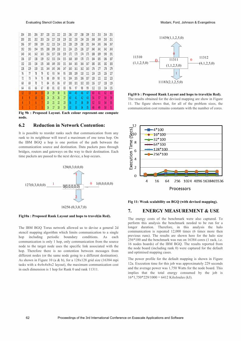
Fig 9b : Proposed Layout. Each colour represent one compute node.

6.2 Reduction in Network Contention: It is possible to reorder ranks such that communication from any rank to its neighbour will travel a maximum of one torus hop. On the IBM BGQ a hop is one portion of the path between the communication source and destination. Data packets pass through bridges, routers and gateways on the way to their destination. Each time packets are passed to the next device, a hop occurs.

Fig10a : Proposed Rank Layout and hops to travel(in Red).

The IBM BGQ Torus network allowed us to devise a general 2d stencil mapping algorithm which limits communication to a single hop including periodic boundary conditions. As each communication is only 1 hop, only communication from the source node to the target node uses the specific link associated with the hop. Therefore there is no contention between messages from different nodes (or the same node going to a different destination). As shown in Figure 10 (a & b), for a 128x128 grid size (16384 mpi tasks with a 4x4x4x8x2 layout), the maximum communication cost in each dimension is 1 hop for Rank 0 and rank 11311.

Fig10 b : Proposed Rank Layout and hops to travel(in Red). The results obtained for the devised mapping are show in Figure 11. The figure shows that, for all of the problem sizes, the communication cost remains constants with the number of cores.

Fig 11: Weak scalability on BGQ (with devised mapping). 7. ENERGY MEASUREMENT & USE The energy costs of the benchmark were also captured. To perform this analysis the benchmark needed to be run for a longer duration. Therefore, in this analysis the halo communication is repeated 12,000 times (6 times more then previous runs). The results are shown here for the halo size 256*100 and the benchmark was run on 16384 cores (1 rack, i.e. 16 nodes boards) of the IBM BGQ. The results reported from the node board (including rank 0) were captured for the default and optimised mapping cases.

The power profile for the default mapping is shown in Figure 12a. Execution time for this job was approximately 229 seconds and the average power was 1,750 Watts for the node board. This implies that the total energy consumed by the job is 16*1,750*229/1000 = 6412 KiloJoules (kJ).

0(0,0,0,0,0)

204 205 206 207 220 221 222 223 236 237 238 239 252 253 254 255200 201 202 203 216 217 218 219 232 233 234 235 248 249 250 251196 197 198 199 212 213 214 215 228 229 230 231 244 245 246 247192 193 194 195 208 209 210 211 224 225 226 227 240 241 242 243140 141 142 143 156 157 158 159 172 173 174 175 188 189 190 191136 137 138 139 152 153 154 155 168 169 170 171 184 185 186 187132 133 134 135 148 149 150 151 164 165 166 167 180 181 182 183128 129 130 131 144 145 146 147 160 161 162 163 176 177 178 17976 77 78 79 92 93 94 95 108 109 110 111 124 125 126 12772 73 74 75 88 89 90 91 104 105 106 107 120 121 122 12368 69 70 71 84 85 86 87 100 101 102 103 116 117 118 11964 65 66 67 80 81 82 83 96 97 98 99 112 113 114 11512 13 14 15 28 29 30 31 44 45 46 47 60 61 62 638 9 10 11 24 25 26 27 40 41 42 43 56 57 58 594 5 6 7 20 21 22 23 36 37 38 39 52 53 54 550 1 2 3 16 17 18 19 32 33 34 35 48 49 50 51

1(0,0,0,0,0)

16256 (0,3,0,7,0)

128(0,3,0,0,0)

127(0,3,0,0,0) 0

1

2

1

11312 (1,1,2,5,0)

11183(2,1,2,5,0)

11439(1,1,2,5,0)

11310 (1,1,2,5,0) 0

1

0 11311 (1,1,2,5,0)

0



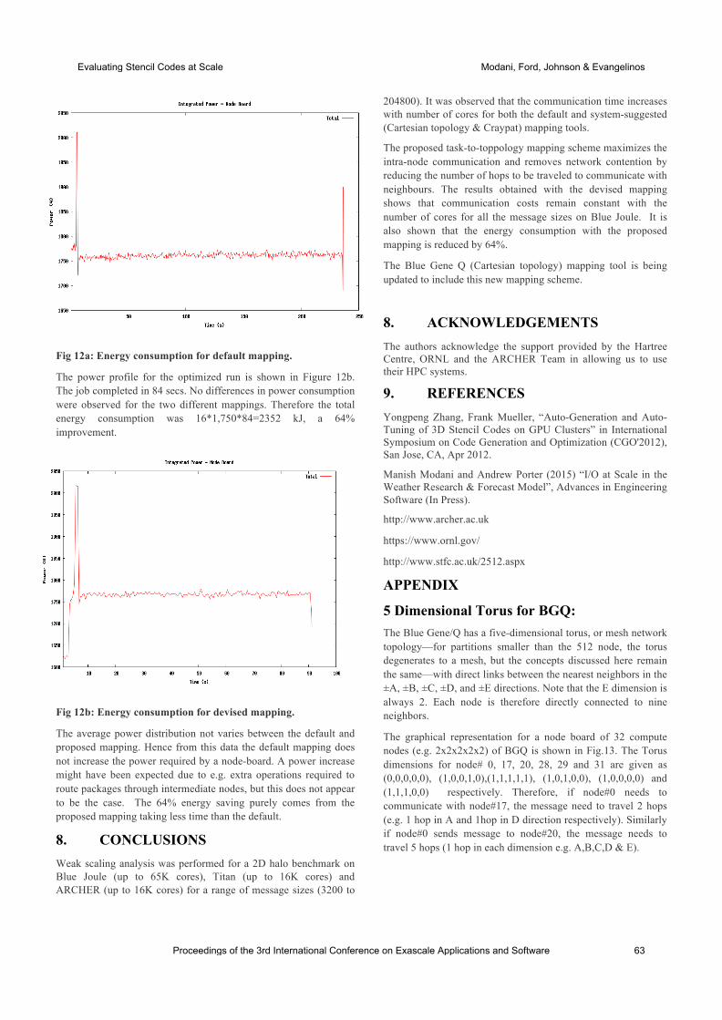
Fig 12a: Energy consumption for default mapping. The power profile for the optimized run is shown in Figure 12b. The job completed in 84 secs. No differences in power consumption were observed for the two different mappings. Therefore the total energy consumption was 16*1,750*84=2352 kJ, a 64% improvement.

Fig 12b: Energy consumption for devised mapping. The average power distribution not varies between the default and proposed mapping. Hence from this data the default mapping does not increase the power required by a node-board. A power increase might have been expected due to e.g. extra operations required to route packages through intermediate nodes, but this does not appear to be the case. The 64% energy saving purely comes from the proposed mapping taking less time than the default.

8. CONCLUSIONS Weak scaling analysis was performed for a 2D halo benchmark on Blue Joule (up to 65K cores), Titan (up to 16K cores) and ARCHER (up to 16K cores) for a range of message sizes (3200 to

204800). It was observed that the communication time increases with number of cores for both the default and system-suggested (Cartesian topology & Craypat) mapping tools. The proposed task-to-toppology mapping scheme maximizes the intra-node communication and removes network contention by reducing the number of hops to be traveled to communicate with neighbours. The results obtained with the devised mapping shows that communication costs remain constant with the number of cores for all the message sizes on Blue Joule. It is also shown that the energy consumption with the proposed mapping is reduced by 64%. The Blue Gene Q (Cartesian topology) mapping tool is being updated to include this new mapping scheme.

8. ACKNOWLEDGEMENTS

The authors acknowledge the support provided by the Hartree Centre, ORNL and the ARCHER Team in allowing us to use their HPC systems.

9. REFERENCES

Yongpeng Zhang, Frank Mueller, “Auto-Generation and Auto-Tuning of 3D Stencil Codes on GPU Clusters” in International Symposium on Code Generation and Optimization (CGO'2012), San Jose, CA, Apr 2012.

Manish Modani and Andrew Porter (2015) “I/O at Scale in the Weather Research & Forecast Model”, Advances in Engineering Software (In Press). http://www.archer.ac.uk https://www.ornl.gov/ http://www.stfc.ac.uk/2512.aspx

APPENDIX

5 Dimensional Torus for BGQ: The Blue Gene/Q has a five-dimensional torus, or mesh network topology—for partitions smaller than the 512 node, the torus degenerates to a mesh, but the concepts discussed here remain the same—with direct links between the nearest neighbors in the ±A, ±B, ±C, ±D, and ±E directions. Note that the E dimension is always 2. Each node is therefore directly connected to nine neighbors.

The graphical representation for a node board of 32 compute nodes (e.g. 2x2x2x2x2) of BGQ is shown in Fig.13. The Torus dimensions for node# 0, 17, 20, 28, 29 and 31 are given as (0,0,0,0,0), (1,0,0,1,0),(1,1,1,1,1), (1,0,1,0,0), (1,0,0,0,0) and (1,1,1,0,0) respectively. Therefore, if node#0 needs to communicate with node#17, the message need to travel 2 hops (e.g. 1 hop in A and 1hop in D direction respectively). Similarly if node#0 sends message to node#20, the message needs to travel 5 hops (1 hop in each dimension e.g. A,B,C,D & E).



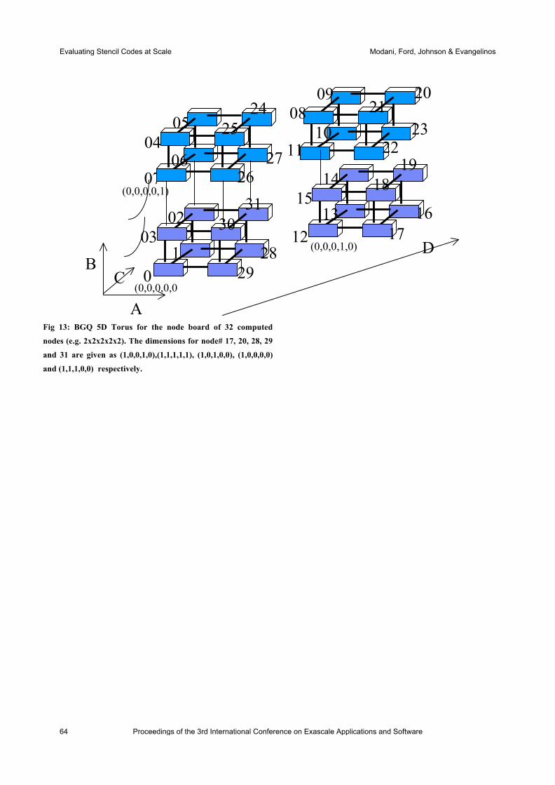
Fig 13: BGQ 5D Torus for the node board of 32 computed

nodes (e.g. 2x2x2x2x2). The dimensions for node# 17, 20, 28, 29

and 31 are given as (1,0,0,1,0),(1,1,1,1,1), (1,0,1,0,0), (1,0,0,0,0)

and (1,1,1,0,0) respectively.

D

B C

A

0 29

03 1

12

07

28

02 13

06

31

14

05

30

15

04 25

08 24 09

27

10 11

26

21 20

23 22

17

16

19

18

(0,0,0,0,0)

(0,0,0,1,0)

(0,0,0,0,1))



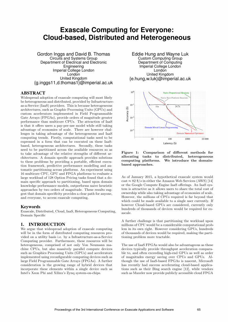
Exascale Computing for Everyone:Cloud-based, Distributed and Heterogeneous

Gordon Inggs and David B. ThomasCircuits and Systems Group

Department of Electrical and ElectronicEngineering

Imperial College LondonLondon

United Kingdomg.inggs11,[email protected]

Eddie Hung and Wayne LukCustom Computing GroupDepartment of ComputingImperial College London

LondonUnited Kingdom

e.hung,[email protected]

ABSTRACTWidespread adoption of exascale computing will most likelybe heterogeneous and distributed, provided by Infrastructure-as-a-Service (IaaS) providers. This is because heterogeneousarchitectures, such as Graphic Processing Units (GPUs) andcustom accelerators implemented in Field ProgrammableGate Arrays (FPGAs), provide orders of magnitude greaterperformance than multicore CPUs. The attraction of IaaSis that it offers users a pay-per-use model while still takingadvantage of economies of scale. There are however chal-lenges in taking advantage of the heterogeneous and IaaScomputing trends. Firstly, computational tasks need to beexpressed in a form that can be executed on these IaaS-based, heterogeneous architectures. Secondly, these tasksneed to be partitioned across the available resources so asto take advantage of the relative strengths of different ar-chitectures. A domain specific approach provides solutionsto these problems by providing a portable, efficient execu-tion framework, predictive performance modelling and au-tomatic partitioning across platforms. An experiment using16 multicore CPU, GPU and FPGA platforms to evaluate alarge workload of 128 Option Pricing tasks found that a do-main specific approach to partitioning, based upon domainknowledge performance models, outperforms naive heuristicapproaches by two orders of magnitude. These results sug-gest that domain specificity provides a clear path for anyone,and everyone, to access exascale computing.

KeywordsExascale, Distributed, Cloud, IaaS, Heterogeneous Computing,Domain Specific

1. INTRODUCTIONWe argue that widespread adoption of exascale computingwill be in the form of distributed computing resources pro-vided on a utility basis i.e. by a Infrastructure-as-a-ServiceComputing provider. Furthermore, these resources will beheterogeneous, comprised of not only Von Neumann ma-chine CPUs, but also massively parallel compute devicessuch as Graphics Processing Units (GPUs) and acceleratorsimplemented using reconfigurable computing devices such aslarge Field Programmable Gate Arrays (FPGAs). A furtherconsideration is the growing range of hybrid devices thatincorporate these elements within a single device such asIntel’s Xeon Phi and Xilinx’s Zynq system-on-chips.

1 10 100 1000 10 000

10-3

10-2

10-1

100

Latency (S)

Accu

racy

($)

Domain Mixed Linear Programming

Domain Numerical Optimiser

Naive Proportional Heuristic

Naive Best Platform Heuristic

11x 24.7x

Figure 1: Comparison of different methods forallocating tasks to distributed, heterogeneouscomputing platforms. We introduce the domain-based approaches.

As of January 2015, a hypothetical exascale system wouldcost ≈ 82 $/s in either the Amazon Web Services (AWS) [14]or the Google Compute Engine IaaS offerings. An IaaS sys-tem is attractive as it allows users to share the total cost ofownership while also taking advantage of economies of scale.However, the millions of CPUs required is far beyond thatwhich could be made available to a single user currently. Ifhowever Cloud-based GPUs are considered, currently onlyhundreds of thousands of devices would be required for ex-ascale.

A further challenge is that partitioning the workload uponmillions of CPU would be a considerable computational prob-lem in its own right. However considering GPUs, hundredsof thousands of devices would be required, making the parti-tioning problem more tractable.

The use of IaaS FPGAs would also be advantageous as thesedevices typically provide throughput acceleration compara-ble to, and often exceeding high-end GPUs as well as orderof magnitudes energy saving over CPUs and GPUs. Al-though the use of IaaS-based FPGAs is nascent, Microsofthas recently had success accelerating cloud-based applica-tions such as their Bing search engine [12], while vendorssuch as Maxeler now provide publicly accessible cloud FPGA


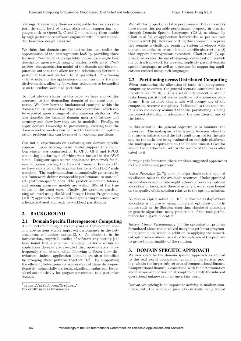
offerings. Increasingly these reconfigurable devices also sup-port the same level of design abstraction, supporting lan-guages such as OpenCL, C and C++, making them usableby high performance software engineers with limited embed-ded hardware design expertise.

We claim that domain specific abstractions can realise theopportunities of the heterogeneous IaaS by providing threefeatures: Portability - the capability to execute a single taskdescription upon a wide range of platforms efficiently. Pred-ication - characterisation models of the domain specific com-putation outputs that allow for the relationship between aparticular task and platform to be quantified. Partitioning- the structure of the application domain can unify the pre-dictive models, allowing for various techniques to be appliedso as to produce workload partitions.

To illustrate our claims, in this paper we have applied thisapproach to the demanding domain of computational fi-nance. We show how the fundamental concepts within thedomain can be captured as types and operations, which canbe executed upon a range of heterogeneous platforms. Wealso describe the financial domain metrics of latency andaccuracy and show how they can be modelled. Finally, weapply domain knowledge to partitioning, showing that thedomain metric models can be used to formulate an optimi-sation problem that can be solved for optimal partitions.

Our initial experiments on evaluating our domain specificapproach upon heterogeneous cluster support this claim.Our cluster was comprised of 16 CPU, GPU and FPGAcomputing platforms, 6 of which were located in the AWScloud. Using our open source application framework for fi-nancial option pricing, the Forward Financial Framework1,we have validated all three properties for a PetaFLOP scaleworkload. The implementations automatically generated byour framework deliver comparable performance to state-of-art, platform-specific ones. The predictive domain latencyand pricing accuracy models are within 10% of the truevalues in the worst case. Finally, the workload partitio-ning achieved using the Mixed Integer Linear Programming(MILP) approach shows a 100% or greater improvement overa heuristic-based approach to workload partitioning.

2. BACKGROUND2.1 Domain Specific Heterogeneous ComputingAn important finding in recent years is that domain spe-cific abstractions enable improved performance in the het-erogeneous computing context [3, 8]. As alluded to in theintroduction, empirical studies of software engineering [11]have found that a small set of design patterns within anapplication domain are executed disproportionately morefrequently than others, often following a Power Law dis-tribution. Indeed, application domains are often identifiedby grouping these patterns together [13]. By supportingthe efficient, heterogeneous acceleration of these dispropor-tionately influentially patterns, significant gains can be re-alised automatically for programs restricted to a particulardomain.

1https://github.com/Gordonei/ForwardFinancialFramework

We call this property portable performance. Previous workshave shown this portable performance property in practicethrough Domain Specific Languages (DSL), as shown byChafi et al [3], or application frameworks, as per our ownprevious work [8]. However putting this approach into prac-tice remains a challenge, requiring system developers withdomain expertise to create domain specific abstractions [8]that support heterogeneous execution. Chafi et al’s [3] ap-proach advocates the use of language virtualisation, provid-ing both a framework for creating implicitly parallel domainspecific languages as well as a runtime for supporting appli-cations created using such languages.

2.2 Partitioning across Distributed ComputingWhen considering the allocation of tasks to heterogeneouscomputing resources, the general scenario considered in theliterature, i.e. [2, 10, 5, 4] is a set of independent or atomictasks being partitioned across multiple heterogeneous plat-forms. It is assumed that a task will occupy any of thecomputing resource completely if allocated to that resource.It is also commonly assumed that the partitioning is beingperformed statically, in advance of the execution of any ofthe tasks.

In this scenario, the general objective is to minimise themakespan. The makespan is the latency between when thefirst task is initiated until the last result returned for the taskset. As the tasks are being evaluated on multiple platforms,the makespan is equivalent to the longest time it takes forany of the platforms to return the results of the tasks allo-cated to it.

Surveying the literature, there are three suggested approachesto the partitioning problem:

Naive Heuristics [2, 7]: a simple algorithmic rule is appliedto allocate tasks to the available resources. Under specifiedcircumstances such a rule might achieve a provably optimalallocation of tasks, and there is usually a worst case boundon the quality of the solution relative to the optimal solution.

Numerical Optimisation [5, 10]: a feasible task-platformallocation is improved using numerical optimisation tech-niques such as the Simplex algorithm, simulated annealingor genetic algorithms using predictions of the task perfor-mance for a given allocation.

Integer Linear Programming [4]: the optimisation problemformulated above can be solved using integer linear program-ming techniques, which in addition to applying the numeri-cal optimisation above use a dual formulation of the problemto prove the optimality of the solution.

3. DOMAIN SPECIFIC APPROACHWe now describe the domain specific approach as appliedto the real world application domain of derivatives pric-ing, within the larger subject area of computational finance.Computational finance is concerned with the determinationand management of risk, an attempt to quantify the inherentoperational unknowns in an uncertain world.

Derivatives pricing is an important activity in modern com-merce, with the volume of products currently being traded


Exascale Computing for Everyone: Cloud-based, Distributed and Heterogeneous Inggs, Thomas, Hung & Luk

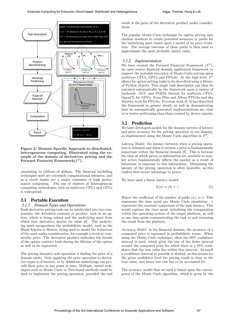
https://github.com/Gordonei/ForwardFinancialFramework

https://github.com/Gordonei/ForwardFinancialFramework

Task Description

Result

Platform Benchmarking

Trade-off Selection

Computation

import ForwardFinancialFramework as F3

U_II = F3.Heston(0.05,100,0.09,1,-0.3,2,0.09)

O_2 = F3.Barrier(U_II,True,100,5,4096,True,120)

O_2.get_price(interactive=True)

print(O_2.price)

>>> $0.12 +- $0.01

Multicore CPU

Confidence Interval

Late

ncy

FPGA

Confidence Interval

Late

ncy

F^3 System Dialog

Confidence Interval

Late

ncy

Heterogeneous System

GPU

Confidence Interval

Late

ncy

WorkloadPartitioning

Figure 2: Domain Specific Approach to distributed,heterogeneous computing. Illustrated using the ex-ample of the domain of derivatives pricing and theForward Financial Framework(F 3).

amounting to trillions of dollars. The financial modellingtechniques used are extremely computational intensive, andas a result banks are a major consumer of high perfor-mance computing. The use of clusters of heterogeneouscomputing technologies such as multicore CPUs and GPUsis widespread.

3.1 Portable Execution3.1.1 Domain Types and Operations

Each derivative pricing task can be subdivided into two com-ponents, the derivative contract or product, such as an op-tion, which is being valued and the underlying asset fromwhich that derivative derives its value [6]. The underly-ing asset encapsulates the probabilistic model, such as theBlack-Scholes or Heston, being used to model the behaviourof the asset under consideration, for example a stock or com-modity price. The derivative product embodies the detailsof the option contract both during the lifetime of the optionas well at its expiration.

The pricing domain’s sole operation is finding the price of adomain entity. Only applying the price operation to deriva-tive types is of interest, as by definition underlyings can pro-vide their price at any point in time. Multiple, varied tech-niques such as Monte Carlo or Tree-based methods could beused to implement the pricing operation, provided the end

result is the price of the derivative product under consider-ation.

The popular Monte Carlo technique for option pricing usesrandom numbers to create potential scenarios or paths forthe underlying asset based upon a model of its price evolu-tion. The average outcome of these paths is then used toapproximate the most probable option value.

3.1.2 ImplementationWe have created the Forward Financial Framework (F 3),an open source financial domain application framework tosupport the portable execution of Monte Carlo pricing uponmulticore CPUs, GPUs and FPGAs. At the high level, F 3

allows for option pricing tasks to be described using a libraryof Python objects. This single task description can then beexecuted automatically by the framework upon a variety ofbackends: GCC and POSIX threads for multicore CPUs,OpenCL for GPUs, Xeon Phis and Altera FPGAs and theMaxeler tools for FPGAs. Previous work [8, 9] has describedthe framework in greater detail, as well as demonstratingthat its automatically generated implementations are closeto or better performing than those created by device experts.

3.2 PredictionWe have developed models for the domain metrics of latencyand price accuracy for the pricing operation in our domain,as implemented using the Monte Carlo algorithm in F 3.

Latency Model : the latency between when a pricing opera-tion is initiated and when it returns a price is fundamentallyimportant within the financial domain [6]. This is becausethe time at which prices or information are available to mar-ket actors fundamentally affects the market as a result ofbehaviour in response to this information. Minimising thelatency of the pricing operation is often desirable, as thisconfers first-mover advantage to pricer.

We have used a linear latency model:

L(n) = βn+ γ (1)

Where the coefficient of the number of paths (n), is β. Thisrepresents the time spent per Monte Carlo simulation. γrepresents the constant component of the task latency. Thiswould capture the time spent initialising the computationwithin the operating system of the target platform, as wellas any time spent communicating the task to and returningthe result from the platform.

Accuracy Model : in the financial domain, the accuracy of acomputed price is expressed in probabilistic terms. Whenusing the Monte Carlo technique, often the 95% confidenceinterval is used, which gives the size of the finite intervalaround the computed price for which there is a 95% confi-dence that the true value lies within that interval. As smalla confidence interval as possible is desired, as this means forthe given confidence level the pricing result is close to thetrue value, and hence less risk has to be accounted for.

The accuracy model that we used is based upon the conver-gence of the Monte Carlo algorithm, which is given by the



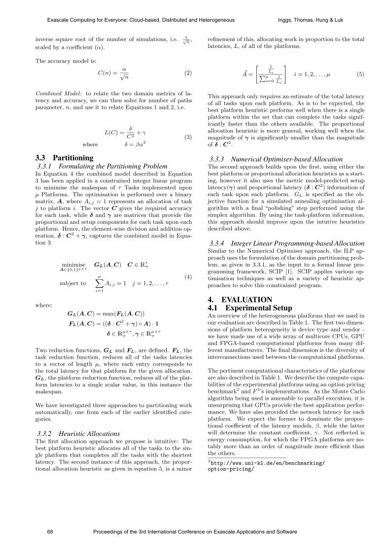
inverse square root of the number of simulations, i.e. 1√n

,

scaled by a coefficient (α).

The accuracy model is:

C(n) =α√n

(2)

Combined Model : to relate the two domain metrics of la-tency and accuracy, we can then solve for number of pathsparameter, n, and use it to relate Equations 1 and 2, i.e.

L(C) =δ

C2+ γ

where δ = βα2(3)

3.3 Partitioning3.3.1 Formulating the Partitioning Problem

In Equation 4 the combined model described in Equation3 has been applied in a constrained integer linear programto minimise the makespan of τ Tasks implemented uponµ Platforms. The optimisation is performed over a binarymatrix, A, where Ai,j = 1 represents an allocation of taskj to platform i. The vector C gives the required accuracyfor each task, while δ and γ are matrices that provide theproportional and setup components for each task upon eachplatform. Hence, the element-wise division and addition op-eration, δ : C2 + γ, captures the combined model in Equa-tion 3

minimiseA∈0,1µ×τ

GL(A,C) C ∈ Rτ+

subject to

µ∑i=1

Ai,j = 1 j = 1, 2, . . . , τ(4)

where:

GL(A,C) = max(FL(A,C))

FL(A,C) = ((δ : C2 + γ) A) · 1δ ∈ Rµ×τ+ ,γ ∈ Rµ×τ+

Two reduction functions, GL and FL, are defined. FL, thetask reduction function, reduces all of the tasks latenciesto a vector of length µ, where each entry corresponds tothe total latency for that platform for the given allocation.GL, the platform reduction function, reduces all of the plat-form latencies to a single scalar value, in this instance themakespan.

We have investigated three approaches to partitioning workautomatically, one from each of the earlier identified cate-gories.

3.3.2 Heuristic AllocationsThe first allocation approach we propose is intuitive: Thebest platform heuristic allocates all of the tasks to the sin-gle platform that completes all the tasks with the shortestlatency. The second instance of this approach, the propor-tional allocation heuristic as given in equation 5, is a minor

refinement of this, allocating work in proportion to the totallatencies, L, of all of the platforms.

~A =

[ 1

Li∑µo=0

1

Lo

]i = 1, 2, . . . , µ (5)

This approach only requires an estimate of the total latencyof all tasks upon each platform. As is to be expected, thebest platform heuristic performs well when there is a singleplatform within the set that can complete the tasks signif-icantly faster than the others available. The proportionalallocation heuristic is more general, working well when themagnitude of γ is significantly smaller than the magnitudeof δ : C2.

3.3.3 Numerical Optimiser-based AllocationThe second approach builds upon the first, using either thebest platform or proportional allocation heuristics as a start-ing, however it also uses the metric model-predicted setuplatency(γ) and proportional latency (δ : C2) information ofeach task upon each platform. GL is specified as the ob-jective function for a simulated annealing optimisation al-gorithm with a final “polishing” step performed using thesimplex algorithm. By using the task-platform information,this approach should improve upon the intutive heuristicsdescribed above.

3.3.4 Integer Linear Programming-based AllocationSimilar to the Numerical Optimiser approach, the ILP ap-proach uses the formulation of the domain partitioning prob-lem, as given in 3.3.1, as the input to a formal linear pro-gramming framework, SCIP [1]. SCIP applies various op-timisation techniques as well as a variety of heuristic ap-proaches to solve this constrained program.

4. EVALUATION4.1 Experimental SetupAn overview of the heterogeneous platforms that we used inour evaluation are described in Table 1. The first two dimen-sions of platform heterogeneity is device type and vendor -we have made use of a wide array of multicore CPUs, GPUand FPGA-based computational platforms from many dif-ferent manufacturers. The final dimension is the diversity ofinterconnections used between the computational platforms.

The pertinent computational characteristics of the platformsare also described in Table 1. We describe the compute capa-bilities of the experimental platforms using an option pricingbenchmark2 and F 3’s implementations. As the Monte Carloalgorithm being used is amenable to parallel execution, it isunsurprising that GPUs provide the best application perfor-mance. We have also provided the network latency for eachplatform. We expect the former to dominate the propor-tional coefficient of the latency models, β, while the latterwill determine the constant coefficient, γ. Not reflected isenergy consumption, for which the FPGA platforms are no-tably more than an order of magnitude more efficient thanthe others.2http://www.uni-kl.de/en/benchmarking/option-pricing/



http://www.uni-kl.de/en/benchmarking/option-pricing/

http://www.uni-kl.de/en/benchmarking/option-pricing/

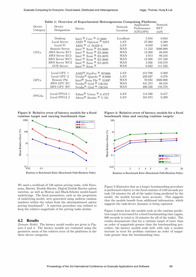
Table 1: Overview of Experimental Heterogeneous Computing Platforms

DeviceCategory

DeviceDesignation Device

NetworkLocation

ApplicationPerformance(GFLOPS)

NetworkRTT(mS)

CPUs

Desktop Intel R© Core R© i7-2600 Localhost 5.916 0.024Local Server AMD R© Opteron R© 6272 LAN 27.002 0.380

Local Pi ARM R© 11 76JZF-S LAN 0.049 2.463Remote Server Intel R© Xeon R© E5-2680 WAN 11.523 3300.000

AWS Server EC1 Intel R© Xeon R© E5-2680 WAN 12.269 88.859AWS Server EC2 Intel R© Xeon R© E5-2670 WAN 4.913 88.216AWS Server WC1 Intel R© Xeon R© E5-2680 WAN 12.200 157.100AWS Server WC2 Intel R© Xeon R© E5-2670 WAN 4.926 159.578

GCE Server Intel R© Xeon R© WAN 6.022 111.232

GPUs

Local GPU 1 AMDR© FirePro R© W5000 LAN 212.798 0.269Local GPU 2 NvidiaR© Quardo R© K4000 LAN 250.027 0.278Remote Phi IntelR© Xeon Phi R© 3120P WAN 70.850 3300.000

AWS GPU EC NvidiaR© Grid R© GK104 WAN 441.274 88.216AWS GPU WC NvidiaR© Grid R© GK104 WAN 406.230 159.578

FPGAsLocal FPGA 1 XilinxR© Virtex R© 6 475T LAN 114.590 0.217Local FPGA 2 AlteraR© Stratix R© V D5 LAN 161.074 0.299

Figure 3: Relative error of latency models for a fixedruntime target and varying benchmark time

0.05 0.1 1

1000

0.1

1

10

100

Runtime to Benchmark Ratio (Benchmark Paths/Runtime Paths)

Mea

n R

elat

ive

Erro

r (%

)

Multicore CPUsGPUsFPGAs

We used a workload of 128 option pricing tasks, with Euro-pean, Barrier, Double Barrier, Digital Double Barrier optionvarieties, as well as Heston and Black-Scholes model-basedunderlyings. The fixed parameters, such as the proprietiesof underlying model, were generated using uniform randomnumbers within the values from the aforementioned optionpricing benchmark2. A rejection procedure was utilised tokeep the relative magnitude of the pricing tasks similar.

4.2 ResultsDomain Model : The latency model results are given in Fig-ures 3 and 4. The latency models are evaluated using thegeometric mean of the relative error of the platforms in thethree device categories.

Figure 4: Relative error of latency models for a fixedbenchmark time and varying runtime targets

1 102 3 4 5 20

100

0.01

0.1

1

10

Runtime to Benchmark Ratio (Benchmark Paths/Runtime Paths)

Mea

n R

elat

ive

Erro

r (%

)

Multicore CPUsGPUsFPGAs

Figure 3 illustrates that as a longer benchmarking procedureis performed relative to the fixed runtime of 4.69 seconds pertask (10 minutes for all of the tasks) being predicted by themodel, the models became more accurate. This suggeststhat the models benefit from additional information, whichsuggests the task-device dynamic is being captured.

Figure 4 shows how the models scale as the runtime predic-tion target is increased for a fixed benchmarking time (again,600 seconds in total or 10 minutes for all of the tasks). Theresults demonstrate that for a runtime target of more thanan order of magnitude greater than the benchmarking pro-cedure, the latency models scale well, with only a modestincrease in error for problem runtimes an order of magni-tude greater than the benchmarking time.



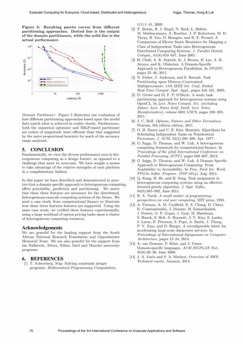
Figure 5: Resulting pareto curves from differentpartitioning approaches. Dotted line is the outputof the domain partitioners, while the solid line is theactual performance

1 10 100 1 000

10-3

10-2

10-1

100

Latency (S)

Accu

racy

($)

MILPNumerical OptimiserProportional Heuristics

Domain Partitioner : Figure 5 illustrates our evaluation ofhow different partitioning approaches based upon the modeldata match what is achieved in reality closely. Furthermore,both the numerical optimiser and MILP-based partitionerare orders of magnitude more efficient than that suggestedby the naive proportional heuristic for much of the accuracyrange analysed.

5. CONCLUSIONFundamentally, we view the diverse performance seen in het-erogeneous computing as a design feature, as opposed to achallenge that must be overcome. We have sought a meansto take advantage of the relative strengths of each platformin a complimentary fashion.

In this paper we have described and demonstrated in prac-tice that a domain specific approach to heterogeneous computingoffers portability, prediction and partitioning. We assertthat these three features are necessary for the distributed,heterogeneous exascale computing systems of the future. Weused a case study from computational finance to illustratehow these three features features are supported. Using thesame case study, we verified these features experimentally,using a large workload of option pricing tasks upon a clusterof heterogeneous computing resources.

AcknowledgementsWe are grateful for the funding support from the SouthAfrican National Research Foundation and OppenheimerMemorial Trust. We are also grateful for the support fromthe Nallatech, Altera, Xilinx, Intel and Maxeler universityprograms.

6. REFERENCES[1] T. Achterberg. Scip: Solving constraint integer

programs. Mathematical Programming Computation,

1(1):1–41, 2009.

[2] T. Braun, H. J. Siegel, N. Beck, L. Boloni,M. Muthucumaru, A. Reuther, J. P. Robertson, M. D.Theys, B. Yao, D. Hensgen, and R. F. Freund. AComparison of Eleven Static Heuristics for Mapping a

Class of Independent Tasks onto HeterogeneousDistributed Computing Systems. J. Parallel Distrib.Comput., 61(6):810–837, June 2001.

[3] H. Chafi, A. K. Sujeeth, K. J. Brown, H. Lee, A. R.Atreya, and K. Olukotun. A Domain-SpecificApproach to Heterogeneous Parallelism. In PPOPP,pages 35–46, 2011.

[4] N. Fisher, J. Anderson, and S. Baruah. TaskPartitioning upon Memory-ConstrainedMultiprocessors. 11th IEEE Int. Conf. Embed.Real-Time Comput. Syst. Appl., pages 416–421, 2005.

[5] D. Grewe and M. F. P. O’Boyle. A static taskpartitioning approach for heterogeneous systems usingOpenCL. In Lect. Notes Comput. Sci. (includingSubser. Lect. Notes Artif. Intell. Lect. NotesBioinformatics), volume 6601 LNCS, pages 286–305,2011.

[6] J. C. Hull. Options, Futures and Other Derivatives.Pearson, 8th edition edition, 2011.

[7] O. H. Ibarra and C. E. Kim. Heuristic Algorithms forScheduling Independent Tasks on NonidenticalProcessors. J. ACM, 24(2):280–289, Apr. 1977.

[8] G. Inggs, D. Thomas, and W. Luk. A heterogeneouscomputing framework for computational finance. InProceedings of the 42nd International Conference onParallel Processing (ICPP), pages 688–697, 2013.

[9] G. Inggs, D. Thomas, and W. Luk. A Domain SpecificApproach to Heterogeneous Computing: FromAvailability to Accessibility. In Proc. First Int. Work.FPGAs Softw. Program. (FSP 2014), Aug. 2014.

[10] Q. Kang, H. He, and H. Song. Task assignment inheterogeneous computing systems using an effectiveiterated greedy algorithm. J. Syst. Softw.,84(6):985–992, June 2011.

[11] B. A. Nardi. A small matter of programming:perspectives on end user computing. MIT press, 1993.

[12] A. Putnam, A. M. Caulfield, E. S. Chung, D. Chiou,K. Constantinides, J. Demme, H. Esmaeilzadeh,J. Fowers, G. P. Gopal, J. Gray, M. Haselman,S. Hauck, S. Heil, A. Hormati, J. Y. Kim, S. Lanka,J. Larus, E. Peterson, S. Pope, A. Smith, J. Thong,P. Y. Xiao, and D. Burger. A reconfigurable fabric foraccelerating large-scale datacenter services. InProceedings of International Symposium on ComputerArchitecture, pages 13–24, 2014.

[13] A. van Deursen, P. Klint, and J. Visser.Domain-specific languages. ACM SIGPLAN Not.,35(6):26–36, June 2000.

[14] J. A. Varia and S. A. Mathew. Overview of AWS.Technical report, Amazon, 2014.



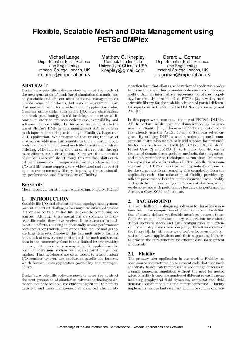
Flexible, Scalable Mesh and Data Management usingPETSc DMPlex

Michael LangeDepartment of Earth Science

and EngineeringImperial College London, [email protected]

Matthew G. KnepleyComputation Institute

University of Chicago, [email protected]

Gerard J. GormanDepartment of Earth Science

and EngineeringImperial College London, UK

[email protected]

ABSTRACTDesigning a scientific software stack to meet the needs ofthe next-generation of mesh-based simulation demands, notonly scalable and efficient mesh and data management ona wide range of platforms, but also an abstraction layerthat makes it useful for a wide range of application codes.Common utility tasks, such as file I/O, mesh distribution,and work partitioning, should be delegated to external li-braries in order to promote code re-use, extensibility andsoftware interoperability. In this paper we demonstrate theuse of PETSc’s DMPlex data management API to performmesh input and domain partitioning in Fluidity, a large scaleCFD application. We demonstrate that raising the level ofabstraction adds new functionality to the application code,such as support for additional mesh file formats and mesh re-ordering, while improving simlutation startup cost throughmore efficient mesh distribution. Moreover, the separationof concerns accomplished through this interface shifts criti-cal performance and interoperability issues, such as scalableI/O and file format support, to a widely used and supportedopen source community library, improving the sustainabil-ity, performance, and functionality of Fluidity.

KeywordsMesh, topology, partitioning, renumbering, Fluidity, PETSc

1. INTRODUCTIONScalable file I/O and efficient domain topology managementpresent important challenges for many scientific applicationsif they are to fully utilise future exascale computing re-sources. Although these operations are common to manyscientific codes they have received little attention in opti-misation efforts, resulting in potentially severe performancebottlenecks for realistic simulations that require and gener-ate large data sets. Moreover, due to a multitude of formatsand a lack of convergence on standards for mesh and outputdata in the community there is only limited interoperabilityand very little code reuse among scientific applications forcommon operations, such as reading and partitioning inputmeshes. Thus developers are often forced to create customI/O routines or even use application-specific file formats,which further limits application portability and interoper-ability.

Designing a scientific software stack to meet the needs ofthe next-generation of simulation software technologies de-mands, not only scalable and efficient algorithms to performdata I/O and mesh management at scale, but also an ab-

straction layer that allows a wide variety of application codesto utilise them and thus promotes code reuse and interoper-ability. Such an intermediate representation of mesh topol-ogy has recently been added to PETSc [3], a widely usedscientific library for the scalable solution of partial differen-tial equations, in the form of the DMPlex data managementAPI [14].

In this paper we demonstrate the use of PETSc’s DMPlexAPI to perform mesh input and domain topology manage-ment in Fluidity [17], a large scale CFD application codethat already uses the PETSc library as its linear solver en-gine. By utilising DMPlex as the underlying mesh man-agement abstraction we not only add support for new meshfile formats, such as Exodus II [20], CGNS [18], Gmsh [9],Fluent Case [2] and MED [1], to Fluidity, but also enablethe use of domain decomposition methods, data migration,and mesh renumbering techniques at run-time. Moreover,the separation of concerns allows PETSc parallel data man-agement and HDF5 support to be independently optimizedfor the target platform, removing this complexity from theapplication code. Our refactoring of Fluidity provides sig-nificant performance benefits due to improved cache localityand mesh distribution during simulation initialisation, whichwe demonstrate with performance benchmarks performed onArcher, a Cray XC30 architecture.

2. BACKGROUNDThe key challenge in designing software for large scale sys-tems lies in the composition of abstractions and the defini-tion of clearly defined yet flexible interfaces between them.Code reuse and inter-disciplinary cooperation necessitatedeeper software stacks and thus configuration and exten-sibility will play a key role in designing the software stack ofthe future [5]. In this paper we therefore focus on the inter-action between applications and their supporting librariesto provide the infrastructure for efficient data managementat exascale.

2.1 FluidityThe primary user application in our work is Fluidity, anopen source unstructured finite element code that uses meshadaptivity to accurately represent a wide range of scales ina single numerical simulation without the need for nestedgrids. Fluidity is used in a number of different scientific areasincluding geophysical fluid dynamics, computational fluiddynamics, ocean modelling and mantle convection. Fluidityimplements various finite element and finite volume discreti-


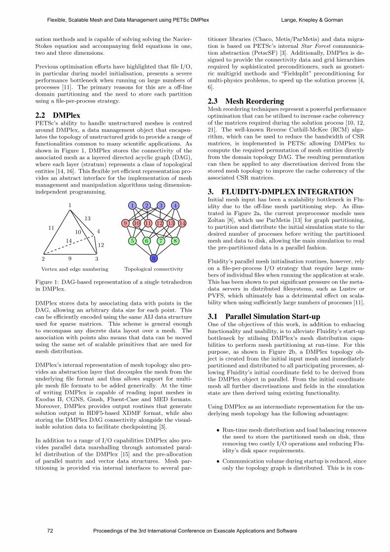
sation methods and is capable of solving solving the Navier-Stokes equation and accompanying field equations in one,two and three dimensions.

Previous optimisation efforts have highlighted that file I/O,in particular during model initialisation, presents a severeperformance bottleneck when running on large numbers ofprocesses [11]. The primary reasons for this are a off-linedomain partitioning and the need to store each partitionusing a file-per-process strategy.

2.2 DMPlexPETSc’s ability to handle unstructured meshes is centredaround DMPlex, a data management object that encapsu-lates the topology of unstructured grids to provide a range offunctionalities common to many scientific applications. Asshown in Figure 1, DMPlex stores the connectivity of theassociated mesh as a layered directed acyclic graph (DAG),where each layer (stratum) represents a class of topologicalentities [14, 16]. This flexible yet efficient representation pro-vides an abstract interface for the implementation of meshmanagement and manipulation algorithms using dimension-independent programming.

2 3

4

1

9

1412

1110

13

Vertex and edge numbering

0

5 6 7 8

9 10 11 12 13 14

1 2 3 4

Topological connectivity

Figure 1: DAG-based representation of a single tetrahedronin DMPlex.

DMPlex stores data by associating data with points in theDAG, allowing an arbitrary data size for each point. Thiscan be efficiently encoded using the same AIJ data structureused for sparse matrices. This scheme is general enoughto encompass any discrete data layout over a mesh. Theassociation with points also means that data can be movedusing the same set of scalable primitives that are used formesh distribution.

DMPlex’s internal representation of mesh topology also pro-vides an abstraction layer that decouples the mesh from theunderlying file format and thus allows support for multi-ple mesh file formats to be added generically. At the timeof writing DMPlex is capable of reading input meshes inExodus II, CGNS, Gmsh, Fluent-Case and MED formats.Moreover, DMPlex provides output routines that generatesolution output in HDF5-based XDMF format, while alsostoring the DMPlex DAG connectivity alongside the visual-isable solution data to facilitate checkpointing [3].

In addition to a range of I/O capabilities DMPlex also pro-vides parallel data marshalling through automated paral-lel distribution of the DMPlex [15] and the pre-allocationof parallel matrix and vector data structures. Mesh par-titioning is provided via internal interfaces to several par-

titioner libraries (Chaco, Metis/ParMetis) and data migra-tion is based on PETSc’s internal Star Forest communica-tion abstraction (PetscSF) [3]. Additionally, DMPlex is de-signed to provide the connectivity data and grid hierarchiesrequired by sophisticated preconditioners, such as geomet-ric multigrid methods and “Fieldsplit” preconditioning formulti-physics problems, to speed up the solution process [4,6].

2.3 Mesh ReorderingMesh reordering techniques represent a powerful performanceoptimisation that can be utilised to increase cache coherencyof the matrices required during the solution process [10, 12,21]. The well-known Reverse Cuthill-McKee (RCM) algo-rithm, which can be used to reduce the bandwidth of CSRmatrices, is implemented in PETSc allowing DMPlex tocompute the required permutation of mesh entities directlyfrom the domain topology DAG. The resulting permutationcan then be applied to any discretisation derived from thestored mesh topology to improve the cache coherency of theassociated CSR matrices.

3. FLUIDITY-DMPLEX INTEGRATIONInitial mesh input has been a scalability bottleneck in Flu-idity due to the off-line mesh partitioning step. As illus-trated in Figure 2a, the current preprocessor module usesZoltan [8], which use ParMetis [13] for graph partitioning,to partition and distribute the initial simulation state to thedesired number of processes before writing the partitionedmesh and data to disk, allowing the main simulation to readthe pre-partitioned data in a parallel fashion.

Fluidity’s parallel mesh initialisation routines, however, relyon a file-per-process I/O strategy that require large num-bers of individual files when running the application at scale.This has been shown to put significant pressure on the meta-data servers in distributed filesystems, such as Lustre orPVFS, which ultimately has a detrimental effect on scala-bility when using sufficiently large numbers of processes [11].

3.1 Parallel Simulation Start-upOne of the objectives of this work, in addition to enhacingfunctionality and usability, is to alleviate Fluidity’s start-upbottleneck by utilising DMPlex’s mesh distribution capa-bilities to perform mesh partitioning at run-time. For thispurpose, as shown in Figure 2b, a DMPlex topology ob-ject is created from the initial input mesh and immediatelypartitioned and distributed to all participating processes, al-lowing Fluidity’s initial coordinate field to be derived fromthe DMPlex object in parallel. From the initial coordinatemesh all further discretisations and fields in the simulationstate are then derived using existing functionality.

Using DMPlex as an intermediate representation for the un-derlying mesh topology has the following advantages:

• Run-time mesh distribution and load balancing removesthe need to store the partitioned mesh on disk, thusremoving two costly I/O operations and reducing Flu-idity’s disk space requirements.

• Communication volume during startup is reduced, sinceonly the topology graph is distributed. This is in con-


Flexible, Scalable Mesh and Data Management using PETSc DMPlex Lange, Knepley & Gorman

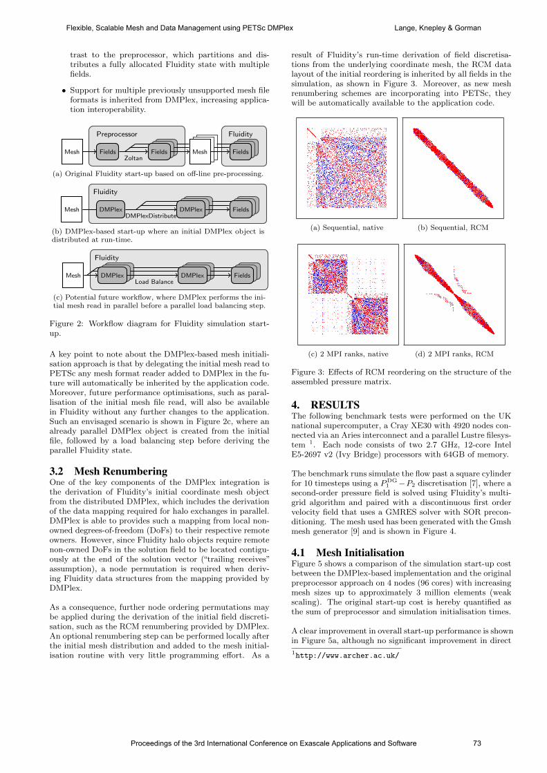
trast to the preprocessor, which partitions and dis-tributes a fully allocated Fluidity state with multiplefields.

• Support for multiple previously unsupported mesh fileformats is inherited from DMPlex, increasing applica-tion interoperability.

Mesh Fields Fields Mesh Fields

Preprocessor Fluidity

Zoltan

(a) Original Fluidity start-up based on off-line pre-processing.

Mesh DMPlex DMPlex Fields

Fluidity

DMPlexDistribute

(b) DMPlex-based start-up where an initial DMPlex object isdistributed at run-time.

Mesh DMPlex DMPlex Fields

Fluidity

Load Balance

(c) Potential future workflow, where DMPlex performs the ini-tial mesh read in parallel before a parallel load balancing step.

Figure 2: Workflow diagram for Fluidity simulation start-up.

A key point to note about the DMPlex-based mesh initiali-sation approach is that by delegating the initial mesh read toPETSc any mesh format reader added to DMPlex in the fu-ture will automatically be inherited by the application code.Moreover, future performance optimisations, such as paral-lisation of the initial mesh file read, will also be availablein Fluidity without any further changes to the application.Such an envisaged scenario is shown in Figure 2c, where analready parallel DMPlex object is created from the initialfile, followed by a load balancing step before deriving theparallel Fluidity state.

3.2 Mesh RenumberingOne of the key components of the DMPlex integration isthe derivation of Fluidity’s initial coordinate mesh objectfrom the distributed DMPlex, which includes the derivationof the data mapping required for halo exchanges in parallel.DMPlex is able to provides such a mapping from local non-owned degrees-of-freedom (DoFs) to their respective remoteowners. However, since Fluidity halo objects require remotenon-owned DoFs in the solution field to be located contigu-ously at the end of the solution vector (“trailing receives”assumption), a node permutation is required when deriv-ing Fluidity data structures from the mapping provided byDMPlex.

As a consequence, further node ordering permutations maybe applied during the derivation of the initial field discreti-sation, such as the RCM renumbering provided by DMPlex.An optional renumbering step can be performed locally afterthe initial mesh distribution and added to the mesh initial-isation routine with very little programming effort. As a

result of Fluidity’s run-time derivation of field discretisa-tions from the underlying coordinate mesh, the RCM datalayout of the initial reordering is inherited by all fields in thesimulation, as shown in Figure 3. Moreover, as new meshrenumbering schemes are incorporating into PETSc, theywill be automatically available to the application code.

(a) Sequential, native (b) Sequential, RCM

(c) 2 MPI ranks, native (d) 2 MPI ranks, RCM

Figure 3: Effects of RCM reordering on the structure of theassembled pressure matrix.

4. RESULTSThe following benchmark tests were performed on the UKnational supercomputer, a Cray XE30 with 4920 nodes con-nected via an Aries interconnect and a parallel Lustre filesys-tem 1. Each node consists of two 2.7 GHz, 12-core IntelE5-2697 v2 (Ivy Bridge) processors with 64GB of memory.

The benchmark runs simulate the flow past a square cylinderfor 10 timesteps using a PDG

1 −P2 discretisation [7], where asecond-order pressure field is solved using Fluidity’s multi-grid algorithm and paired with a discontinuous first ordervelocity field that uses a GMRES solver with SOR precon-ditioning. The mesh used has been generated with the Gmshmesh generator [9] and is shown in Figure 4.

4.1 Mesh InitialisationFigure 5 shows a comparison of the simulation start-up costbetween the DMPlex-based implementation and the originalpreprocessor approach on 4 nodes (96 cores) with increasingmesh sizes up to approximately 3 million elements (weakscaling). The original start-up cost is hereby quantified asthe sum of preprocessor and simulation initialisation times.

A clear improvement in overall start-up performance is shownin Figure 5a, although no significant improvement in direct

1http://www.archer.ac.uk/



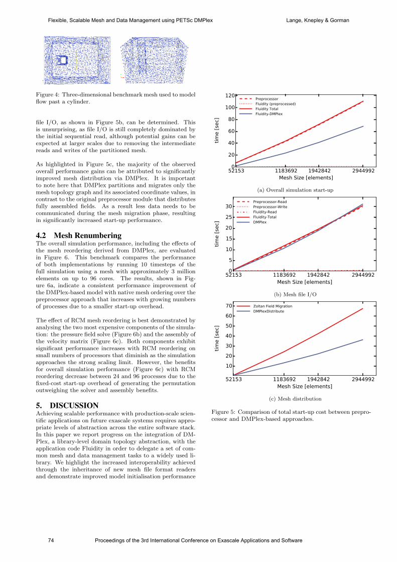
Figure 4: Three-dimensional benchmark mesh used to modelflow past a cylinder.

file I/O, as shown in Figure 5b, can be determined. Thisis unsurprising, as file I/O is still completely dominated bythe initial sequential read, although potential gains can beexpected at larger scales due to removing the intermediatereads and writes of the partitioned mesh.

As highlighted in Figure 5c, the majority of the observedoverall performance gains can be attributed to significantlyimproved mesh distribution via DMPlex. It is importantto note here that DMPlex partitions and migrates only themesh topology graph and its associated coordinate values, incontrast to the original preprocessor module that distributesfully assembled fields. As a result less data needs to becommunicated during the mesh migration phase, resultingin significantly increased start-up performance.

4.2 Mesh RenumberingThe overall simulation performance, including the effects ofthe mesh reordering derived from DMPlex, are evaluatedin Figure 6. This benchmark compares the performanceof both implementations by running 10 timesteps of thefull simulation using a mesh with approximately 3 millionelements on up to 96 cores. The results, shown in Fig-ure 6a, indicate a consistent performance improvement ofthe DMPlex-based model with native mesh ordering over thepreprocessor approach that increases with growing numbersof processes due to a smaller start-up overhead.

The effect of RCM mesh reordering is best demonstrated byanalysing the two most expensive components of the simula-tion: the pressure field solve (Figure 6b) and the assembly ofthe velocity matrix (Figure 6c). Both components exhibitsignificant performance increases with RCM reordering onsmall numbers of processors that diminish as the simulationapproaches the strong scaling limit. However, the benefitsfor overall simulation performance (Figure 6c) with RCMreordering decrease between 24 and 96 processes due to thefixed-cost start-up overhead of generating the permutationoutweighing the solver and assembly benefits.

5. DISCUSSIONAchieving scalable performance with production-scale scien-tific applications on future exascale systems requires appro-priate levels of abstraction across the entire software stack.In this paper we report progress on the integration of DM-Plex, a library-level domain topology abstraction, with theapplication code Fluidity in order to delegate a set of com-mon mesh and data management tasks to a widely used li-brary. We highlight the increased interoperability achievedthrough the inheritance of new mesh file format readersand demonstrate improved model initialisation performance

52153 1183692 1942842 2944992Mesh Size [elements]

0

20

40

60

80

100

120

tim

e [

sec]

PreprocessorFluidity (preprocessed)Fluidity TotalFluidity-DMPlex

(a) Overall simulation start-up


0

5

10

15

20

25

30

tim

e [

sec]

Preprocessor-ReadPreprocessor-WriteFluidity-ReadFluidity-TotalDMPlex

(b) Mesh file I/O


10

20

30

40

50

60

70

tim

e [

sec]

Zoltan Field MigrationDMPlexDistribute

(c) Mesh distribution

Figure 5: Comparison of total start-up cost between prepro-cessor and DMPlex-based approaches.



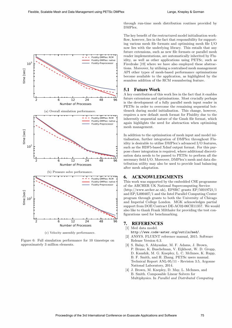
2 6 12 24 48 96Number of Processes

103

tim

e [

sec]

Fluidity-DMPlex: RCMFluidity-DMPlex: nativeFluidity-Preprocessor

(a) Overall simulation performance.


102

tim

e [

sec]


(b) Pressure solve performance.


102

tim

e [

sec]


(c) Velocity assembly performance.

Figure 6: Full simulation performance for 10 timesteps onapproximately 3 million elements.

through run-time mesh distribution routines provided byDMPlex.

The key benefit of the restructured model initialisation work-flow, however, lies in the fact that responsibility for support-ing various mesh file formats and optimising mesh file I/Onow lies with the underlying library. This entails that anyfuture extensions, such as new file formats or parallel meshreader implementations, are automatically inherited by Flu-idity, as well as other applications using PETSc, such asFiredrake [19] where we have also employed these abstrac-tions. Moreover, by utilising a centralised mesh managementAPI other types of mesh-based performance optimisationsbecome available to the application, as highlighted by theseamless addition of the RCM renumbering feature.

5.1 Future WorkA key contribution of this work lies in the fact that it enablesfuture extensions and optimisations. Most crucially perhapsis the development of a fully parallel mesh input reader inPETSc in order to overcome the remaining sequential bot-tleneck during model initialisation. This change, however,requires a new default mesh format for Fluidity due to theinherently sequential nature of the Gmsh file format, whichagain highlights the need for abstraction when optimisingmesh management.

In addition to the optimisation of mesh input and model ini-tialisation, further integration of DMPlex throughout Flu-idity is desirable to utilise DMPlex’s advanced I/O features,such as the HDF5-based Xdmf output format. For this pur-pose closer integration is required, where additional discreti-sation data needs to be passed to PETSc to perform all thenecessary field I/O. Moreover, DMPlex’s mesh and data dis-tribution utility may also be used to provide load balancingafter mesh adaptation.

6. ACKNOWLEDGMENTSThis work was supported by the embedded CSE programmeof the ARCHER UK National Supercomputing Service(http://www.archer.ac.uk), EPSRC grants EP/M019721/1and EP/L000407/1 and the Intel Parallel Computing Centerprogram through grants to both the University of Chicagoand Imperial College London. MGK acknowledges partialsupport from DOE Contract DE-AC02-06CH11357. We wouldalso like to thank Frank Milthaler for providing the test con-figurations used for benchmarking.

7. REFERENCES[1] Med data model.

http://www.code-aster.org/outils/med/.

[2] ANSYS. FLUENT reference manual, 2015. SoftwareRelease Version 6.3.

[3] S. Balay, S. Abhyankar, M. F. Adams, J. Brown,P. Brune, K. Buschelman, V. Eijkhout, W. D. Gropp,D. Kaushik, M. G. Knepley, L. C. McInnes, K. Rupp,B. F. Smith, and H. Zhang. PETSc users manual.Technical Report ANL-95/11 - Revision 3.5, ArgonneNational Laboratory, 2014.

[4] J. Brown, M. Knepley, D. May, L. McInnes, andB. Smith. Composable Linear Solvers forMultiphysics. In Parallel and Distributed Computing



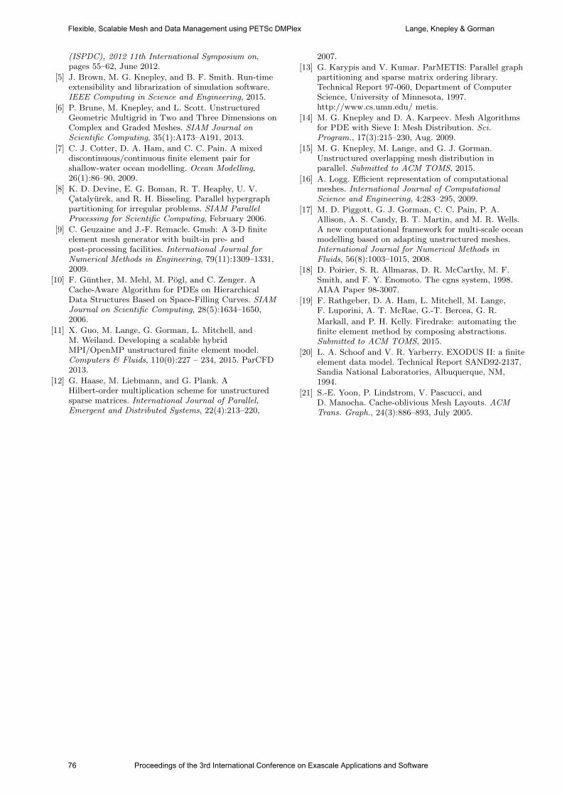
(ISPDC), 2012 11th International Symposium on,pages 55–62, June 2012.

[5] J. Brown, M. G. Knepley, and B. F. Smith. Run-timeextensibility and librarization of simulation software.IEEE Computing in Science and Engineering, 2015.

[6] P. Brune, M. Knepley, and L. Scott. UnstructuredGeometric Multigrid in Two and Three Dimensions onComplex and Graded Meshes. SIAM Journal onScientific Computing, 35(1):A173–A191, 2013.

[7] C. J. Cotter, D. A. Ham, and C. C. Pain. A mixeddiscontinuous/continuous finite element pair forshallow-water ocean modelling. Ocean Modelling,26(1):86–90, 2009.

[8] K. D. Devine, E. G. Boman, R. T. Heaphy, U. V.Catalyurek, and R. H. Bisseling. Parallel hypergraphpartitioning for irregular problems. SIAM ParallelProcessing for Scientific Computing, February 2006.

[9] C. Geuzaine and J.-F. Remacle. Gmsh: A 3-D finiteelement mesh generator with built-in pre- andpost-processing facilities. International Journal forNumerical Methods in Engineering, 79(11):1309–1331,2009.

[10] F. Gunther, M. Mehl, M. Pogl, and C. Zenger. ACache-Aware Algorithm for PDEs on HierarchicalData Structures Based on Space-Filling Curves. SIAMJournal on Scientific Computing, 28(5):1634–1650,2006.

[11] X. Guo, M. Lange, G. Gorman, L. Mitchell, andM. Weiland. Developing a scalable hybridMPI/OpenMP unstructured finite element model.Computers & Fluids, 110(0):227 – 234, 2015. ParCFD2013.

[12] G. Haase, M. Liebmann, and G. Plank. AHilbert-order multiplication scheme for unstructuredsparse matrices. International Journal of Parallel,Emergent and Distributed Systems, 22(4):213–220,

2007.

[13] G. Karypis and V. Kumar. ParMETIS: Parallel graphpartitioning and sparse matrix ordering library.Technical Report 97-060, Department of ComputerScience, University of Minnesota, 1997.http://www.cs.umn.edu/ metis.

[14] M. G. Knepley and D. A. Karpeev. Mesh Algorithmsfor PDE with Sieve I: Mesh Distribution. Sci.Program., 17(3):215–230, Aug. 2009.

[15] M. G. Knepley, M. Lange, and G. J. Gorman.Unstructured overlapping mesh distribution inparallel. Submitted to ACM TOMS, 2015.

[16] A. Logg. Efficient representation of computationalmeshes. International Journal of ComputationalScience and Engineering, 4:283–295, 2009.

[17] M. D. Piggott, G. J. Gorman, C. C. Pain, P. A.Allison, A. S. Candy, B. T. Martin, and M. R. Wells.A new computational framework for multi-scale oceanmodelling based on adapting unstructured meshes.International Journal for Numerical Methods inFluids, 56(8):1003–1015, 2008.

[18] D. Poirier, S. R. Allmaras, D. R. McCarthy, M. F.Smith, and F. Y. Enomoto. The cgns system, 1998.AIAA Paper 98-3007.

[19] F. Rathgeber, D. A. Ham, L. Mitchell, M. Lange,F. Luporini, A. T. McRae, G.-T. Bercea, G. R.

Markall, and P. H. Kelly. Firedrake: automating thefinite element method by composing abstractions.Submitted to ACM TOMS, 2015.

[20] L. A. Schoof and V. R. Yarberry. EXODUS II: a finiteelement data model. Technical Report SAND92-2137,Sandia National Laboratories, Albuquerque, NM,1994.

[21] S.-E. Yoon, P. Lindstrom, V. Pascucci, andD. Manocha. Cache-oblivious Mesh Layouts. ACMTrans. Graph., 24(3):886–893, July 2005.



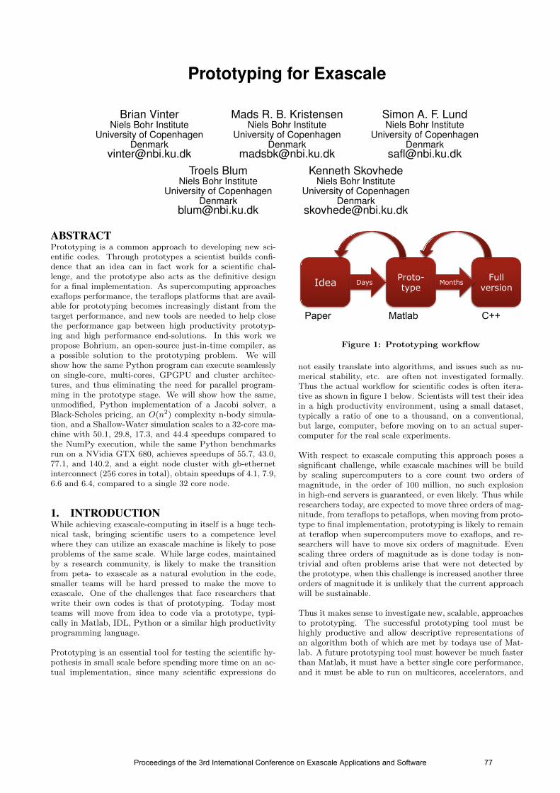
Prototyping for Exascale

Brian VinterNiels Bohr Institute

University of CopenhagenDenmark

[email protected]

Mads R. B. KristensenNiels Bohr Institute


[email protected]

Simon A. F. LundNiels Bohr Institute


[email protected] Blum

Niels Bohr InstituteUniversity of Copenhagen

[email protected]

Kenneth SkovhedeNiels Bohr Institute


[email protected]

ABSTRACTPrototyping is a common approach to developing new sci-entific codes. Through prototypes a scientist builds confi-dence that an idea can in fact work for a scientific chal-lenge, and the prototype also acts as the definitive designfor a final implementation. As supercomputing approachesexaflops performance, the teraflops platforms that are avail-able for prototyping becomes increasingly distant from thetarget performance, and new tools are needed to help closethe performance gap between high productivity prototyp-ing and high performance end-solutions. In this work wepropose Bohrium, an open-source just-in-time compiler, asa possible solution to the prototyping problem. We willshow how the same Python program can execute seamlesslyon single-core, multi-cores, GPGPU and cluster architec-tures, and thus eliminating the need for parallel program-ming in the prototype stage. We will show how the same,unmodified, Python implementation of a Jacobi solver, aBlack-Scholes pricing, an O(n2) complexity n-body simula-tion, and a Shallow-Water simulation scales to a 32-core ma-chine with 50.1, 29.8, 17.3, and 44.4 speedups compared tothe NumPy execution, while the same Python benchmarksrun on a NVidia GTX 680, achieves speedups of 55.7, 43.0,77.1, and 140.2, and a eight node cluster with gb-ethernetinterconnect (256 cores in total), obtain speedups of 4.1, 7.9,6.6 and 6.4, compared to a single 32 core node.

1. INTRODUCTIONWhile achieving exascale-computing in itself is a huge tech-nical task, bringing scientific users to a competence levelwhere they can utilize an exascale machine is likely to poseproblems of the same scale. While large codes, maintainedby a research community, is likely to make the transitionfrom peta- to exascale as a natural evolution in the code,smaller teams will be hard pressed to make the move toexascale. One of the challenges that face researchers thatwrite their own codes is that of prototyping. Today mostteams will move from idea to code via a prototype, typi-cally in Matlab, IDL, Python or a similar high productivityprogramming language.

Prototyping is an essential tool for testing the scientific hy-pothesis in small scale before spending more time on an ac-tual implementation, since many scientific expressions do

Idea Days Proto-type

Full version

Months

Matlab C++ Paper

Figure 1: Prototyping workflow

not easily translate into algorithms, and issues such as nu-merical stability, etc. are often not investigated formally.Thus the actual workflow for scientific codes is often itera-tive as shown in figure 1 below. Scientists will test their ideain a high productivity environment, using a small dataset,typically a ratio of one to a thousand, on a conventional,but large, computer, before moving on to an actual super-computer for the real scale experiments.

With respect to exascale computing this approach poses asignificant challenge, while exascale machines will be buildby scaling supercomputers to a core count two orders ofmagnitude, in the order of 100 million, no such explosionin high-end servers is guaranteed, or even likely. Thus whileresearchers today, are expected to move three orders of mag-nitude, from teraflops to petaflops, when moving from proto-type to final implementation, prototyping is likely to remainat teraflop when supercomputers move to exaflops, and re-searchers will have to move six orders of magnitude. Evenscaling three orders of magnitude as is done today is non-trivial and often problems arise that were not detected bythe prototype, when this challenge is increased another threeorders of magnitude it is unlikely that the current approachwill be sustainable.

Thus it makes sense to investigate new, scalable, approachesto prototyping. The successful prototyping tool must behighly productive and allow descriptive representations ofan algorithm both of which are met by todays use of Mat-lab. A future prototyping tool must however be much fasterthan Matlab, it must have a better single core performance,and it must be able to run on multicores, accelerators, and


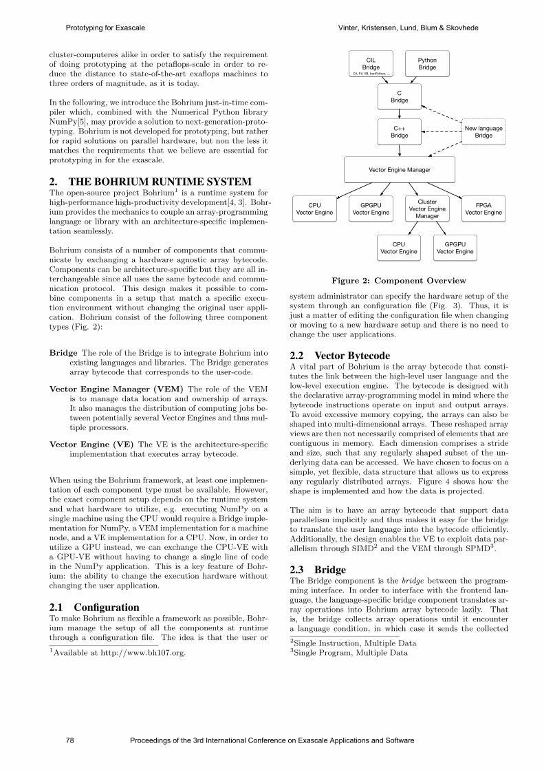
cluster-computeres alike in order to satisfy the requirementof doing prototyping at the petaflops-scale in order to re-duce the distance to state-of-the-art exaflops machines tothree orders of magnitude, as it is today.

In the following, we introduce the Bohrium just-in-time com-piler which, combined with the Numerical Python libraryNumPy[5], may provide a solution to next-generation-proto-typing. Bohrium is not developed for prototyping, but ratherfor rapid solutions on parallel hardware, but non the less itmatches the requirements that we believe are essential forprototyping in for the exascale.

2. THE BOHRIUM RUNTIME SYSTEMThe open-source project Bohrium1 is a runtime system forhigh-performance high-productivity development[4, 3]. Bohr-ium provides the mechanics to couple an array-programminglanguage or library with an architecture-specific implemen-tation seamlessly.

Bohrium consists of a number of components that commu-nicate by exchanging a hardware agnostic array bytecode.Components can be architecture-specific but they are all in-terchangeable since all uses the same bytecode and commu-nication protocol. This design makes it possible to com-bine components in a setup that match a specific execu-tion environment without changing the original user appli-cation. Bohrium consist of the following three componenttypes (Fig. 2):

Bridge The role of the Bridge is to integrate Bohrium intoexisting languages and libraries. The Bridge generatesarray bytecode that corresponds to the user-code.

Vector Engine Manager (VEM) The role of the VEMis to manage data location and ownership of arrays.It also manages the distribution of computing jobs be-tween potentially several Vector Engines and thus mul-tiple processors.

Vector Engine (VE) The VE is the architecture-specificimplementation that executes array bytecode.

When using the Bohrium framework, at least one implemen-tation of each component type must be available. However,the exact component setup depends on the runtime systemand what hardware to utilize, e.g. executing NumPy on asingle machine using the CPU would require a Bridge imple-mentation for NumPy, a VEM implementation for a machinenode, and a VE implementation for a CPU. Now, in order toutilize a GPU instead, we can exchange the CPU-VE witha GPU-VE without having to change a single line of codein the NumPy application. This is a key feature of Bohr-ium: the ability to change the execution hardware withoutchanging the user application.

2.1 ConfigurationTo make Bohrium as flexible a framework as possible, Bohr-ium manage the setup of all the components at runtimethrough a configuration file. The idea is that the user or

1Available at http://www.bh107.org.

PythonBridge

C++Bridge

CILBridge

C#, F#, VB, IronPython, …

CBridge

Vector Engine Manager

New languageBridge

CPUVector Engine

GPGPUVector Engine

ClusterVector Engine

Manager

CPUVector Engine

GPGPUVector Engine

FPGAVector Engine

Figure 2: Component Overview

system administrator can specify the hardware setup of thesystem through an configuration file (Fig. 3). Thus, it isjust a matter of editing the configuration file when changingor moving to a new hardware setup and there is no need tochange the user applications.

2.2 Vector BytecodeA vital part of Bohrium is the array bytecode that consti-tutes the link between the high-level user language and thelow-level execution engine. The bytecode is designed withthe declarative array-programming model in mind where thebytecode instructions operate on input and output arrays.To avoid excessive memory copying, the arrays can also beshaped into multi-dimensional arrays. These reshaped arrayviews are then not necessarily comprised of elements that arecontiguous in memory. Each dimension comprises a strideand size, such that any regularly shaped subset of the un-derlying data can be accessed. We have chosen to focus on asimple, yet flexible, data structure that allows us to expressany regularly distributed arrays. Figure 4 shows how theshape is implemented and how the data is projected.

The aim is to have an array bytecode that support dataparallelism implicitly and thus makes it easy for the bridgeto translate the user language into the bytecode efficiently.Additionally, the design enables the VE to exploit data par-allelism through SIMD2 and the VEM through SPMD3.

2.3 BridgeThe Bridge component is the bridge between the program-ming interface. In order to interface with the frontend lan-guage, the language-specific bridge component translates ar-ray operations into Bohrium array bytecode lazily. Thatis, the bridge collects array operations until it encountera language condition, in which case it sends the collected

2Single Instruction, Multiple Data3Single Program, Multiple Data


Prototyping for Exascale Vinter, Kristensen, Lund, Blum & Skovhede

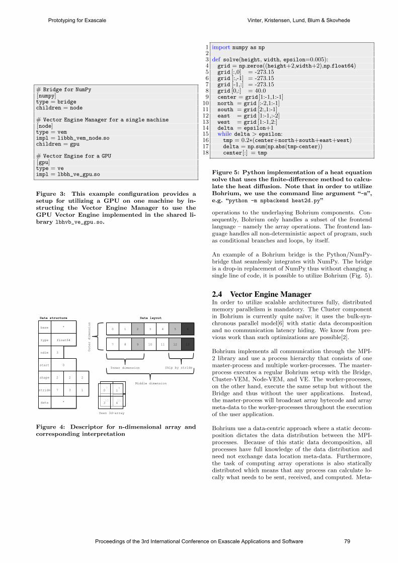
# Bridge for NumPy[numpy]type = bridgechildren = node

# Vector Engine Manager for a single machine[node]type = vemimpl = libbh_vem_node.sochildren = gpu

# Vector Engine for a GPU[gpu]type = veimpl = lbbh_ve_gpu.so

Figure 3: This example configuration provides asetup for utilizing a GPU on one machine by in-structing the Vector Engine Manager to use theGPU Vector Engine implemented in the shared li-brary lbhvb_ve_gpu.so.

base

type

ndim

start

shape

stride

data

*

*

float64

3

0

2 2 2

7 3 1

0 1 2 3 4 5 6

7 8 9 10 11 12 13

Inner dimension

Middle dimension

Outer dimension

Data structure Data layout

Skip by stride

7 8

11 10

0 1

3 4

Seen 3d-array

Figure 4: Descriptor for n-dimensional array andcorresponding interpretation

1 import numpy as np23 def solve(height, width, epsilon=0.005):4 grid = np.zeros((height+2,width+2),np.float64)5 grid [:,0] = -273.156 grid [:,-1] = -273.157 grid [-1,:] = -273.158 grid [0,:] = 40.09 center = grid [1:-1,1:-1]

10 north = grid [:-2,1:-1]11 south = grid [2:,1:-1]12 east = grid [1:-1,:-2]13 west = grid [1:-1,2:]14 delta = epsilon+115 while delta > epsilon:16 tmp = 0.2∗(center+north+south+east+west)17 delta = np.sum(np.abs(tmp-center))18 center[:] = tmp

Figure 5: Python implementation of a heat equationsolve that uses the finite-difference method to calcu-late the heat diffusion. Note that in order to utilizeBohrium, we use the command line argument “-m”,e.g. “python -m npbackend heat2d.py”

operations to the underlaying Bohrium components. Con-sequently, Bohrium only handles a subset of the frontendlanguage – namely the array operations. The frontend lan-guage handles all non-deterministic aspect of program, suchas conditional branches and loops, by itself.

An example of a Bohrium bridge is the Python/NumPy-bridge that seamlessly integrates with NumPy. The bridgeis a drop-in replacement of NumPy thus without changing asingle line of code, it is possible to utilize Bohrium (Fig. 5).

2.4 Vector Engine ManagerIn order to utilize scalable architectures fully, distributedmemory parallelism is mandatory. The Cluster componentin Bohrium is currently quite naıve; it uses the bulk-syn-chronous parallel model[6] with static data decompositionand no communication latency hiding. We know from pre-vious work than such optimizations are possible[2].

Bohrium implements all communication through the MPI-2 library and use a process hierarchy that consists of onemaster-process and multiple worker-processes. The master-process executes a regular Bohrium setup with the Bridge,Cluster-VEM, Node-VEM, and VE. The worker-processes,on the other hand, execute the same setup but without theBridge and thus without the user applications. Instead,the master-process will broadcast array bytecode and arraymeta-data to the worker-processes throughout the executionof the user application.

Bohrium use a data-centric approach where a static decom-position dictates the data distribution between the MPI-processes. Because of this static data decomposition, allprocesses have full knowledge of the data distribution andneed not exchange data location meta-data. Furthermore,the task of computing array operations is also staticallydistributed which means that any process can calculate lo-cally what needs to be sent, received, and computed. Meta-



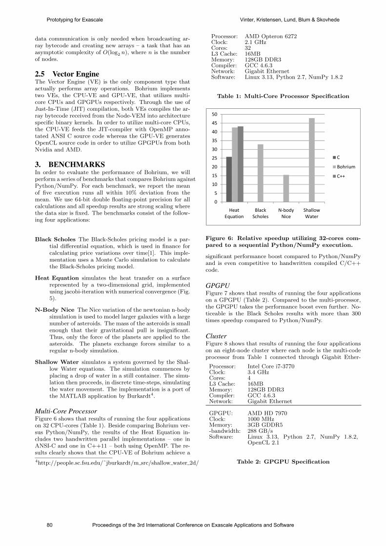
data communication is only needed when broadcasting ar-ray bytecode and creating new arrays – a task that has anasymptotic complexity of O(log2 n), where n is the numberof nodes.

2.5 Vector EngineThe Vector Engine (VE) is the only component type thatactually performs array operations. Bohrium implementstwo VEs, the CPU-VE and GPU-VE, that utilizes multi-core CPUs and GPGPUs respectively. Through the use ofJust-In-Time (JIT) compilation, both VEs compiles the ar-ray bytecode received from the Node-VEM into architecturespecific binary kernels. In order to utilize multi-core CPUs,the CPU-VE feeds the JIT-compiler with OpenMP anno-tated ANSI C source code whereas the GPU-VE generatesOpenCL source code in order to utilize GPGPUs from bothNvidia and AMD.

3. BENCHMARKSIn order to evaluate the performance of Bohrium, we willperform a series of benchmarks that compares Bohrium againstPython/NumPy. For each benchmark, we report the meanof five execution runs all within 10% deviation from themean. We use 64-bit double floating-point precision for allcalculations and all speedup results are strong scaling wherethe data size is fixed. The benchmarks consist of the follow-ing four applications:

Black Scholes The Black-Scholes pricing model is a par-tial differential equation, which is used in finance forcalculating price variations over time[1]. This imple-mentation uses a Monte Carlo simulation to calculatethe Black-Scholes pricing model.

Heat Equation simulates the heat transfer on a surfacerepresented by a two-dimensional grid, implementedusing jacobi-iteration with numerical convergence (Fig.5).

N-Body Nice The Nice variation of the newtonian n-bodysimulation is used to model larger galaxies with a largenumber of asteroids. The mass of the asteroids is smallenough that their gravitational pull is insignificant.Thus, only the force of the planets are applied to theasteroids. The planets exchange forces similar to aregular n-body simulation.

Shallow Water simulates a system governed by the Shal-low Water equations. The simulation commences byplacing a drop of water in a still container. The simu-lation then proceeds, in discrete time-steps, simulatingthe water movement. The implementation is a port ofthe MATLAB application by Burkardt4.

Multi-Core ProcessorFigure 6 shows that results of running the four applicationson 32 CPU-cores (Table 1). Beside comparing Bohrium ver-sus Python/NumPy, the results of the Heat Equation in-cludes two handwritten parallel implementations – one inANSI-C and one in C++11 – both using OpenMP. The re-sults clearly shows that the CPU-VE of Bohrium achieve a

4http://people.sc.fsu.edu/˜jburkardt/m src/shallow water 2d/

Processor: AMD Opteron 6272Clock: 2.1 GHzCores: 32L3 Cache: 16MBMemory: 128GB DDR3Compiler: GCC 4.6.3Network: Gigabit EthernetSoftware: Linux 3.13, Python 2.7, NumPy 1.8.2

Table 1: Multi-Core Processor Specification

!

""

Figure 6: Relative speedup utilizing 32-cores com-pared to a sequential Python/NumPy execution.

significant performance boost compared to Python/NumPyand is even competitive to handwritten compiled C/C++code.

GPGPUFigure 7 shows that results of running the four applicationson a GPGPU (Table 2). Compared to the multi-processor,the GPGPU takes the performance boost even further. No-ticeable is the Black Scholes results with more than 300times speedup compared to Python/NumPy.

ClusterFigure 8 shows that results of running the four applicationson an eight-node cluster where each node is the multi-codeprocessor from Table 1 connected through Gigabit Ether-

Processor: Intel Core i7-3770Clock: 3.4 GHzCores: 4L3 Cache: 16MBMemory: 128GB DDR3Compiler: GCC 4.6.3Network: Gigabit Ethernet

GPGPU: AMD HD 7970Clock: 1000 MHzMemory: 3GB GDDR5-bandwidth: 288 GB/sSoftware: Linux 3.13, Python 2.7, NumPy 1.8.2,

OpenCL 2.1

Table 2: GPGPU Specification



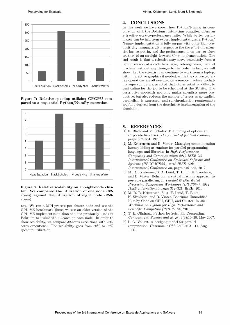
Figure 7: Relative speedup utilizing GPGPU com-pared to a sequential Python/NumPy execution.

!"

Figure 8: Relative scalability on an eight-node clus-ter. We compared the utilization of one node (32-cores) against the utilization of eight node (256-cores).

net. We run a MPI-process per cluster node and use theCPU-VE benchmark (here, we use an older version of theCPU-VE implementation than the one previously used) inBohrium to utilize the 32-cores on each node. In order toshow scalability, we compare 32-cores executions with 256-cores executions. The scalability goes from 50% to 95%speedup utilization.

4. CONCLUSIONSIn this work we have shown how Python/Numpy in com-bination with the Bohrium just-in-time compiler, offers anattractive work-to-performance ratio. While better perfor-mance can be had from expert implementations, a Python/Numpy implementation is fully on-par with other high-pro-ducitivity languages with respect to the the effort the scien-tist has to put in, and the performance is on-par, or closeto, that of an straight forward C++ implementation. Theend result is that a scientist may move seamlessly from a

laptop version of a code to a large, heterogeneous, parallelmachine, without any changes to the code. In fact, we willshow that the scientist can continue to work from a laptop,with interactive graphics if needed, while the contracted ar-ray operations are all executed on a remote machine, includ-ing supercomputers, granted that the scientist is willing towait online for the job to be scheduled at the SC site. Thedescriptive approach not only makes scientists more pro-ductive, but also reduces the number of errors as no explicitparallelism is expressed, and synchronization requirementsare fully derived from the descriptive implementation of thealgorithm.

5. REFERENCES[1] F. Black and M. Scholes. The pricing of options and

corporate liabilities. The journal of political economy,pages 637–654, 1973.

[2] M. Kristensen and B. Vinter. Managing communicationlatency-hiding at runtime for parallel programminglanguages and libraries. In High PerformanceComputing and Communication 2012 IEEE 9thInternational Conference on Embedded Software andSystems (HPCC-ICESS), 2012 IEEE 14thInternational Conference on, pages 546–555, 2012.

[3] M. R. Kristensen, S. A. Lund, T. Blum, K. Skovhede,and B. Vinter. Bohrium: a virtual machine approach toportable parallelism. In Parallel & DistributedProcessing Symposium Workshops (IPDPSW), 2014IEEE International, pages 312–321. IEEE, 2014.

[4] M. R. B. Kristensen, S. A. F. Lund, T. Blum,K. Skovhede, and B. Vinter. Bohrium: UnmodifiedNumPy Code on CPU, GPU, and Cluster. In 4thWorkshop on Python for High Performance andScientific Computing (PyHPC’13), 2013.

[5] T. E. Oliphant. Python for Scientific Computing.Computing in Science and Engg., 9(3):10–20, May 2007.

[6] L. G. Valiant. A bridging model for parallelcomputation. Commun. ACM, 33(8):103–111, Aug.1990.



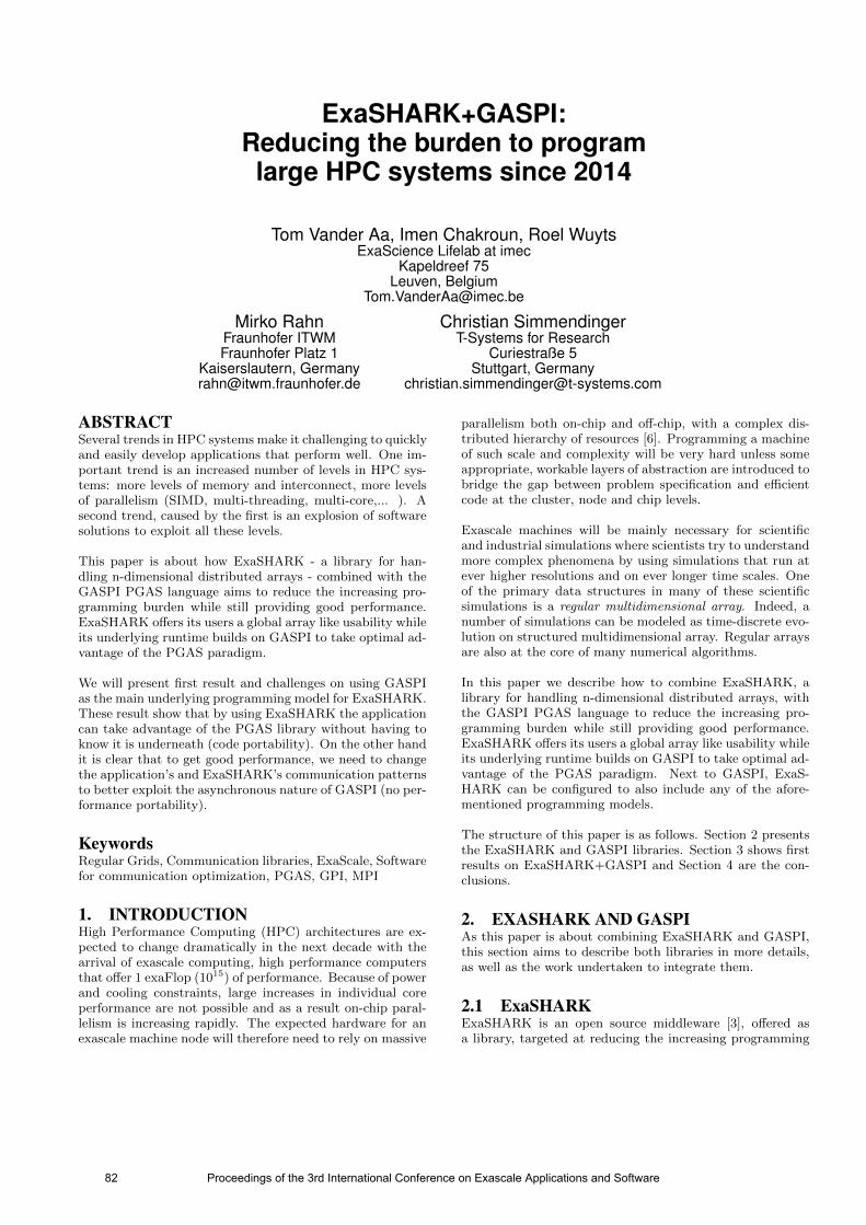
ExaSHARK+GASPI:Reducing the burden to programlarge HPC systems since 2014

Tom Vander Aa, Imen Chakroun, Roel WuytsExaScience Lifelab at imec

Kapeldreef 75Leuven, Belgium

[email protected]

Mirko RahnFraunhofer ITWMFraunhofer Platz 1

Kaiserslautern, [email protected]

Christian SimmendingerT-Systems for Research

Curiestraße 5Stuttgart, Germany

[email protected]

ABSTRACTSeveral trends in HPC systems make it challenging to quicklyand easily develop applications that perform well. One im-portant trend is an increased number of levels in HPC sys-tems: more levels of memory and interconnect, more levelsof parallelism (SIMD, multi-threading, multi-core,... ). Asecond trend, caused by the first is an explosion of softwaresolutions to exploit all these levels.

This paper is about how ExaSHARK - a library for han-dling n-dimensional distributed arrays - combined with theGASPI PGAS language aims to reduce the increasing pro-gramming burden while still providing good performance.ExaSHARK offers its users a global array like usability whileits underlying runtime builds on GASPI to take optimal ad-vantage of the PGAS paradigm.

We will present first result and challenges on using GASPIas the main underlying programming model for ExaSHARK.These result show that by using ExaSHARK the applicationcan take advantage of the PGAS library without having toknow it is underneath (code portability). On the other handit is clear that to get good performance, we need to changethe application’s and ExaSHARK’s communication patternsto better exploit the asynchronous nature of GASPI (no per-formance portability).

KeywordsRegular Grids, Communication libraries, ExaScale, Softwarefor communication optimization, PGAS, GPI, MPI

1. INTRODUCTIONHigh Performance Computing (HPC) architectures are ex-pected to change dramatically in the next decade with thearrival of exascale computing, high performance computersthat offer 1 exaFlop (1015) of performance. Because of powerand cooling constraints, large increases in individual coreperformance are not possible and as a result on-chip paral-lelism is increasing rapidly. The expected hardware for anexascale machine node will therefore need to rely on massive

parallelism both on-chip and off-chip, with a complex dis-tributed hierarchy of resources [6]. Programming a machineof such scale and complexity will be very hard unless someappropriate, workable layers of abstraction are introduced tobridge the gap between problem specification and efficientcode at the cluster, node and chip levels.

Exascale machines will be mainly necessary for scientificand industrial simulations where scientists try to understandmore complex phenomena by using simulations that run atever higher resolutions and on ever longer time scales. Oneof the primary data structures in many of these scientificsimulations is a regular multidimensional array. Indeed, anumber of simulations can be modeled as time-discrete evo-lution on structured multidimensional array. Regular arraysare also at the core of many numerical algorithms.

In this paper we describe how to combine ExaSHARK, alibrary for handling n-dimensional distributed arrays, withthe GASPI PGAS language to reduce the increasing pro-gramming burden while still providing good performance.ExaSHARK offers its users a global array like usability whileits underlying runtime builds on GASPI to take optimal ad-vantage of the PGAS paradigm. Next to GASPI, ExaS-HARK can be configured to also include any of the afore-mentioned programming models.

The structure of this paper is as follows. Section 2 presentsthe ExaSHARK and GASPI libraries. Section 3 shows firstresults on ExaSHARK+GASPI and Section 4 are the con-clusions.

2. EXASHARK AND GASPIAs this paper is about combining ExaSHARK and GASPI,this section aims to describe both libraries in more details,as well as the work undertaken to integrate them.

2.1 ExaSHARKExaSHARK is an open source middleware [3], offered asa library, targeted at reducing the increasing programming


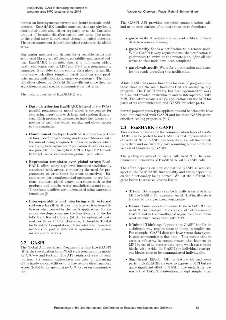
burden on heterogeneous current and future exascale archi-tectures. ExaSHARK handles matrices that are physicallydistributed block-wise, either regularly or as the Cartesianproduct of irregular distributions on each axis. The accessto the global array is performed through a logical indexing.The programmer can define halos/ghost regions in the globalarray.

Our major architectural drivers for a scalable structuredgrid-based library are efficiency, portability and ease of cod-ing. ExaSHARK is portable since it is built upon widelyused technologies such as MPI and C++ as a programminglanguage. It provides simple coding via a global-arrays-likeinterface which offers template-based functions (dot prod-ucts, matrix multiplications, unary expressions). The func-tionalities offered by ExaSHARK are efficient since they useasynchronous and specific communication patterns.

The main properties of ExaSHARK are:

• Data distribution ExaSHARK is based on the PGASparallel programming model which is convenient forexpressing algorithms with large and random data ac-cess. Each process is assumed to have fast access to aportion of each distributed matrix, and slower accessto the remainder.

• Communication layer ExaSHARK supports a plethoraof lower level programming models and libraries withthe aim of being adequate to exascale systems whichare highly heterogeneous. Application developers mayuse pure MPI and/or hybrid MPI + OpenMP threadsto target coarse and medium-grained parallelism.

• Expression templates over global arrays ExaS-HARK offers many high-level functions traditionallyassociated with arrays, eliminating the need for pro-grammers to write these functions themselves. Ex-amples are basic mathematical operators, unary func-tions, standard global arrays operations such as dotproducts and matrix vector multiplication,and so on.These functionalities are implemented using expressiontemplates [9].

• Inter-operability and interfacing with externalsoftware ExaSHARK can interface with external li-braries when needed by the user’s application. For ex-ample, developers can use the functionality of the In-tel’s Math Kernel Library (MKL) for optimized mathroutines [5] or PETSc (Portable, Extensible Toolkitfor Scientific Computation) [1] for advanced numericalmethods for partial differential equations and sparsematrix computations.

2.2 GASPIThe Global Address Space Programming Interface (GASPI[4]) is the specification for a PGAS style programming modelfor C/C++ and Fortran. The API consists of a set of basicroutines. Its communication layer can take full advantageof the hardware capabilities to utilize remote direct memoryaccess (RDMA) for spending no CPU cycles on communica-tion.

The GASPI API provides one-sided communication callsand at its core consists of no more than there functions:

• gaspi write Schedules the write of a block of localdata to a remote memory.

• gaspi notify Sends a notification to a remote node.While GASPI is very asynchronous, the notification isguaranteed to arrive at the remote side, after all thewrites to that node have been completed.

• gaspi wait notify Waits for a notification and hencefor the reads preceding this notification.

While GASPI has more functions for ease of programming,these three are the main functions that are needed by anyprogram. The GASPI library has been optimized to workin a multi-threaded environment and is interoperable withMPI. The latter means a single application can use MPI forparts of its communication and GASPI for other parts.

Several popular proto-type applications and benchmarks havebeen implemented with GASPI and for these GASPI showsexcellent scaling properties [8, 7].

2.3 ExaSHARK + GASPIThis section outlines how the communication layer of ExaS-HARK can be ported to use GASPI. A first implementationof ExaSHARK on GASPI has been done, i.e. all functional-ity is there and we currently have a working but non-optimalversion of Shark using GASPI.

The porting consists of replacing calls to MPI in the com-munication primitives of ExaSHARK with GASPI calls.

The effort depends on how compatible GASPI is with re-spect to the ExaSHARK functionality and varies dependingon the functionality being ported. We list the different de-grees below to serve as lessons learnt:

• Trivial: Some aspects can be trivially translated fromMPI to GASPI. For example: An MPI Win allocate istranslated to a gaspi segment create

• Easier: Some aspects are easier to do in GASPI thanin MPI. For example: The concept of notifications inGASPI makes the handling of asynchronous commu-nication much easier than with MPI.

• Minimal Thinking: Aspects that GASPI handles ina different way require some thinking to implement.For example: GASPI does not have vector data-types.It only communicates flat data. This means that incases a sub-array is communicated this happens inMPI by use of an hvector data-type, which can containblocks with stride. In GASPI the individual contigu-ous blocks have to be communicated individually.

• Significant Effort: MPI is feature-rich and someparts in ExaSHARK are easy to express in MPI but re-quire significant effort in GASPI. The underlying rea-son is that GASPI is intentionally kept simpler than


ExaSHARK+GASPI: Reducing the burden to program large HPC systems since 2014 Vander Aa, Chakroun, Wuyts, Rahn & Simmendinger

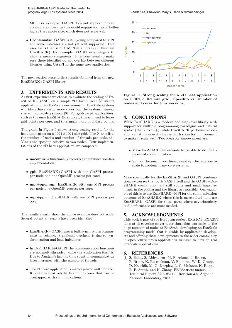
MPI. For example: GASPI does not support remoteaccumulation because this would require additional bu↵er-ing at the remote site, which does not scale well.

• Problematic: GASPI is still young compared to MPIand some use-cases are not yet well supported. Oneuse-case is the use of GASPI in a library (in this caseExaSHARK). For example: GASPI uses integers toidentify memory segments. It is non-trivial to makesure these identifies do not overlap between di↵erentlibraries using GASPI in the same user application.

The next section presents first results obtained from the newExaSHARK+GASPI library.

3. EXPERIMENTS AND RESULTSAs first experiment we choose to evaluate the scaling of Ex-aSHARK+GASPI on a simple 2D Jacobi heat [2] stencilapplication in an ExaScale environment. ExaScale systemswill likely have many more cores but the system memorysize will not scale as much [6]. For grid-based applications,such as the ones ExaSHARK support, this will lead to fewergrid points per core, and thus much more boundary points.

The graph in Figure 1 shows strong scaling results for theheat application on a 1024 1024 size grid. The X-axis liststhe number of nodes and number of threads per node, theY-axis the speedup relative to two nodes. Four implemen-tations of the 2D heat application are compared:

• nocomm: a functionally incorrect communication-freeimplementation;

• gpi: ExaSHARK+GASPI with one GASPI processper node and one OpenMP process per core;

• mpi+openmp: ExaSHARK with one MPI processper node one OpenMP process per core;

• mpi+ppn: ExaSHARK with one MPI process percore.

The results clearly show the above example does not scale.Several potential reasons have been identified.

• ExaSHARK+GASPI uses a bulk synchronous commu-nication scheme. Significant overhead is due to syn-chronization and load imbalance.

• In ExaSHARK+GASPI the communication functionsare not multi-threaded, while the application itself is.Due to Amdahl’s law the time spent in communicationlayer increases with the number of threads.

• The 2D heat application is memory-bandwidth bound.It contains relatively little computations that can beoverlapped with communications.

Slide?22

ExaScaling IS-hard

0

5

10

15

20

25

1 1 2 2 4 1 4 8 2 4 8 8

2 4 2 4 2 8 4 2 8 8 4 8

nocomm

gpi

mpi+openmp

mpi+ppn

nodes-/-cores

spee

dup-

Figure 1: Strong scaling for a 2D heat application

on a 1024 1024 size grid. Speedup vs. number of

nodes and cores for four versions.

4. CONCLUSIONSWhile ExaSHARK is a modern and high-level library withsupport for multiple programming paradigms and naturalsyntax (thank to c++), while ExaSHARK performs reason-ably well at node-level, there is much room for improvementto make it scale well. Two ideas for improvement are:

• Make ExaSHARK thread-safe to be able to do multi-threaded communication.

• Support for much more fine-grained synchronization toscale to modern many-core systems.

More specifically for the ExaSHARK and GASPI combina-tion, we can see that both GASPI itself and the GASPI+Exa-SHARK combination are still young and much improve-ments in the coding and the library are possible. One exam-ple of this is to use ExaSHARK+MPI for the communicationpatterns of ExaSHARK where this is more suited, and useExaSHARK+GASPI for those parts where asynchronicityand performance are more needed.

5. ACKNOWLEDGMENTSThis work is part of the European project EXA2CT. EXA2CTaims at discovering solver algorithms that can scale to thehuge numbers of nodes at ExaScale, developing an ExaScaleprogramming model that is usable by application develop-ers and o↵ering these developments to the wider communityin open-source proto-applications as basis to develop realExaScale applications.

6. REFERENCES[1] S. Balay, S. Abhyankar, M. F. Adams, J. Brown,

P. Brune, K. Buschelman, V. Eijkhout, W. D. Gropp,D. Kaushik, M. G. Knepley, L. C. McInnes, K. Rupp,B. F. Smith, and H. Zhang. PETSc users manual.Technical Report ANL-95/11 - Revision 3.5, ArgonneNational Laboratory, 2014.



[2] J. M. Cecilia, J. M. Garcıa, and M. Ujaldon. CUDA 2DStencil Computations for the Jacobi Method. InK. Jonasson, editor, PARA (1), volume 7133 of LectureNotes in Computer Science, pages 173–183. Springer,2010.

[3] I. Chakroun, T. Vander Aa, B. De Fraine, T. Haber,R. Wuyts, and W. Demeuter. ExaShark: A scalablehybrid array kit for exascale simulation. In 23rd HighPerformance Computing Symposium (HPC 2015), 2015.

[4] D. Grunewald and C. Simmendinger. The GASPI APIspecification and its implementation GPI 2.0. In 7thInternational Conference on PGAS ProgrammingModels, 2011.

[5] Intel. Using intel math kernel library for matrixmultiplication.https://software.intel.com/en-us/mkl 11.2 tut c pdf.

[6] P. Kogge and J. Shalf. Exascale computing trends:

Adjusting to the ”new normal” for computerarchitecture. Computing in Science and Engineering,15(6):16–26, 2013.

[7] F.-J. Pfreundt and D. Stoyanov. Hybrid-parallel sparsematrix-vector multiplication and iterative linear solverswith the communication library GPI. In WSEASTRANSACTIONS on INFORMATION SCIENCE andAPPLICATIONS, 2014.

[8] C. Simmendinger, J. Jagerskupper, R. Machado, andC. Lojewski. A PGAS-based implementation for theunstructured CFD solver TAU. In PGAS 2011: FifthConference on Partitioned Global Address SpaceProgramming Models, 2011.

[9] T. Veldhuizen. Expression templates. In C++ Report,volume 7, pages 26–31, June 1995.



Towards Resilient Chapel

Design and implementation of a transparent resilience mechanism for Chapel

Konstantina PanagiotopoulouSchool of Mathematical and Computer Sciences

Heriot-Watt UniversityRiccarton, [email protected]

Hans-Wolfgang LoidlSchool of Mathematical and Computer Sciences

Heriot-Watt UniversityRiccarton, Edinburgh

[email protected]

ABSTRACTThe exponential increase of components in modern HighPerformance Computing (HPC) systems poses a challengeon their resilience: predictions of time between failures onExaScale systems range from hours to minutes, yet the preva-lent HPC programming model today does not tolerate faults.In this paper, we describe the design and prototype imple-mentation of transparent resilience support for Chapel [1], aparallel HPC language with focus on scalability, portabilityand productivity, following the Partitioned Global AddressSpace (PGAS) [2] programming model.

KeywordsResilience, Fault tolerance, PGAS, Chapel, Runtime sys-tems

1. INTRODUCTIONThe use of manycore commodity hardware in a hierarchi-cal structure on modern HPC systems, gives rise to rapidlydeteriorating Mean Time Between Failures (MTBF) [3, 4]rates. This leads HPC systems to waste capacity on re-launching entire executions after failures. Many real worldapplications, from molecular dynamics to simulation algo-rithms take anywhere from a few hours to days to complete.Over this time horizon, failures can no longer be ignoredon ExaScale architectures. Resilience [5] is the ability of asystem to maintain state awareness and an accepted level ofoperational normalcy in response to disturbances, includingthreats of an unexpected and malicious nature. We addresscases of failure, in particular hardware failure of one or mul-tiple nodes, during execution on a distributed setup. Ourgoal is for Chapel programs to terminate successfully in thepresence of failures.

In this work we embed support for resilience into Chapel’sruntime system (RTS) using detection and recovery mech-anisms together with automatic task adoption. Our goalis to provide transparent built-in resilience to the end user(Chapel programmer), without the requirement of extra pro-gramming effort. Our design employs data redundancy, re-taining information about exported work and a dedicatedresilience communication protocol to recover from failures.This design provides flexibility and scalability on a small setof assumptions, following similar design principles to Re-silient X10’s Place-Zero Based Finish [6]. Resilient taskparallelism support is enhanced by employing non-blockingcommunication and by enabling asynchronous recovery offailed tasks on non-failed locations/nodes in the system.

2. CHAPEL OVERVIEWComputation in Chapel is expressed using tasks that can beexecuted in parallel. The target architecture is abstractedvia the concept of locales: a unit with storage and executioncapabilities, such as a multi-core processor. A multi-localeprogram starts execution on Locale 0 and scales out to otherlocales, building the locale tree. Below, we provide a briefoverview on aspects of relevance to the support for resilience.

2.1 Language ConstructsThe on construct is the main language mechanism for taskmigration, used by the Chapel programmer to explicitly con-trol locality of the executed task. The migrated task is alogical continuation of the initial task at a different place inthe system. The body of an on block is viewed as a singleblocking task by the controlling thread of the parent locale.

The three language constructs that create parallel tasks arebegin, cobegin and coforall statements. Unstructuredparallelism introduced by begin creates a new task, for ex-ecution on a new thread, while the rest of the program con-tinues. The result of the begin statement is returned ata later point in the execution. Completion is tracked eitherby an enclosing explicit synchronisation block or the implicitsynchronisation of the main function.

With the block-structured task creation employed by cobe-

gin a new task is created for each statement in the block,while coforall, cobegin’s equivalent in loop form, createsone task per iteration. For cobegin and coforall, thereexists an implicit synchronisation point at the end of theblock/loop, while the tasks are launched asynchronously.The control flow returns when all tasks have reached thesynchronisation point and the program continues.

2.2 Runtime StructureChapel’s runtime system (RTS) is the lower level of the soft-ware stack, supporting language constructs and program ac-tivities. The runtime is composed of a set of layers, writtenin C, and standardised interfaces, written in Chapel, andrelies on third-party services (Figure 1). The main layersare: communication, tasking, threading and memory.

2.3 The GASNet Communication LayerChapel uses GASNet [7] as the default instantiation of thecommunication layer. GASNet is a network- and language-independent interface for Global Address Space languages.It is portable and supports multiple low-level communication


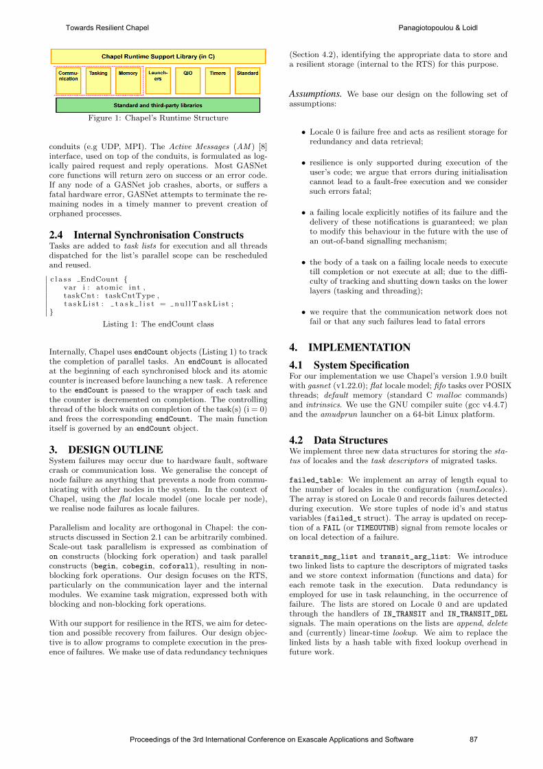
Figure 1: Chapel’s Runtime Structure

conduits (e.g UDP, MPI). The Active Messages (AM ) [8]interface, used on top of the conduits, is formulated as log-ically paired request and reply operations. Most GASNetcore functions will return zero on success or an error code.If any node of a GASNet job crashes, aborts, or suffers afatal hardware error, GASNet attempts to terminate the re-maining nodes in a timely manner to prevent creation oforphaned processes.

2.4 Internal Synchronisation ConstructsTasks are added to task lists for execution and all threadsdispatched for the list’s parallel scope can be rescheduledand reused.

c l a s s EndCount var i : atomic int ,taskCnt : taskCntType ,t a s kL i s t : t a s k l i s t = nu l lTa skL i s t ;

Listing 1: The endCount class

Internally, Chapel uses endCount objects (Listing 1) to trackthe completion of parallel tasks. An endCount is allocatedat the beginning of each synchronised block and its atomiccounter is increased before launching a new task. A referenceto the endCount is passed to the wrapper of each task andthe counter is decremented on completion. The controllingthread of the block waits on completion of the task(s) (i = 0)and frees the corresponding endCount. The main functionitself is governed by an endCount object.

3. DESIGN OUTLINESystem failures may occur due to hardware fault, softwarecrash or communication loss. We generalise the concept ofnode failure as anything that prevents a node from commu-nicating with other nodes in the system. In the context ofChapel, using the flat locale model (one locale per node),we realise node failures as locale failures.

Parallelism and locality are orthogonal in Chapel: the con-structs discussed in Section 2.1 can be arbitrarily combined.Scale-out task parallelism is expressed as combination ofon constructs (blocking fork operation) and task parallelconstructs (begin, cobegin, coforall), resulting in non-blocking fork operations. Our design focuses on the RTS,particularly on the communication layer and the internalmodules. We examine task migration, expressed both withblocking and non-blocking fork operations.

With our support for resilience in the RTS, we aim for detec-tion and possible recovery from failures. Our design objec-tive is to allow programs to complete execution in the pres-ence of failures. We make use of data redundancy techniques

(Section 4.2), identifying the appropriate data to store anda resilient storage (internal to the RTS) for this purpose.

Assumptions. We base our design on the following set ofassumptions:

• Locale 0 is failure free and acts as resilient storage forredundancy and data retrieval;

• resilience is only supported during execution of theuser’s code; we argue that errors during initialisationcannot lead to a fault-free execution and we considersuch errors fatal;

• a failing locale explicitly notifies of its failure and thedelivery of these notifications is guaranteed; we planto modify this behaviour in the future with the use ofan out-of-band signalling mechanism;

• the body of a task on a failing locale needs to executetill completion or not execute at all; due to the diffi-culty of tracking and shutting down tasks on the lowerlayers (tasking and threading);

• we require that the communication network does notfail or that any such failures lead to fatal errors

4. IMPLEMENTATION4.1 System SpecificationFor our implementation we use Chapel’s version 1.9.0 builtwith gasnet (v1.22.0); flat locale model; fifo tasks over POSIXthreads; default memory (standard C malloc commands)and intrinsics. We use the GNU compiler suite (gcc v4.4.7)and the amudprun launcher on a 64-bit Linux platform.

4.2 Data StructuresWe implement three new data structures for storing the sta-tus of locales and the task descriptors of migrated tasks.

failed_table: We implement an array of length equal tothe number of locales in the configuration (numLocales).The array is stored on Locale 0 and records failures detectedduring execution. We store tuples of node id’s and statusvariables (failed_t struct). The array is updated on recep-tion of a FAIL (or TIMEOUTNB) signal from remote locales oron local detection of a failure.

transit_msg_list and transit_arg_list: We introducetwo linked lists to capture the descriptors of migrated tasksand we store context information (functions and data) foreach remote task in the execution. Data redundancy isemployed for use in task relaunching, in the occurrence offailure. The lists are stored on Locale 0 and are updatedthrough the handlers of IN_TRANSIT and IN_TRANSIT_DEL

signals. The main operations on the lists are append, deleteand (currently) linear-time lookup. We aim to replace thelinked lists by a hash table with fixed lookup overhead infuture work.


Towards Resilient Chapel Panagiotopoulou & Loidl

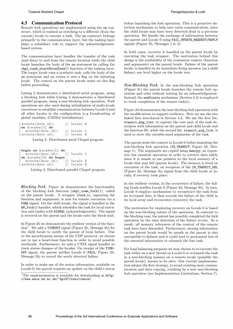
4.3 Communication ProtocolRemote fork operations are implemented using the on con-struct, which is realised as switching to a different (from thecurrent) locale to execute a task. The on construct belongsprimarily to the communication layer, but the tasking layerplays a subsidiary role to support the acknowledgement-based system.

The communication layer handles the transfer of the task(and data) to and from the remote location while the childlocale launches the body of the on statement by calling thechpl_task_startMovedTask() function of the tasking layer.The target locale runs a synthetic task; calls the body of theon statement and on return it sets a flag on the initiatinglocale. The control on the parent locale waits on this flagbefore proceeding.

Listing 2 demonstrates a distributed serial program, usinga blocking fork while Listing 3 demonstrates a distributedparallel program, using a non-blocking fork operation. Forkoperations are also used during initialisation of multi-localeexecutions to establish communication between Locale 0 andall other locales in the configuration (e.g broadcasting ofglobal variables, GASNet initialisation).

wr i t e l n ( here . id ) ; // l o c a l e 0on Loca l e s [ 1 ] do

wr i t e l n ( here . id ) ; // l o c a l e 1wr i t e l n ( here . id ) ; // l o c a l e 0

Listing 2: Distributed serial Chapel program

begin on Loca l e s [ 1 ] dowr i t e l n ( here . id ) ; // l o c a l e 1

on Loca l e s [ 2 ] do beginwr i t e l n ( here . id ) ; // l o c a l e 2

wr i t e l n ( here . id ) ; // l o c a l e 0

Listing 3: Distributed parallel Chapel program

Blocking Fork. Figure 2a demonstrates the functionalityof the blocking fork function (chpl_comm_fork()), calledon the parent locale. A wrapper (fork_t), capturing thefunction and arguments, is sent for remote execution via aFORK signal. On the child locale, the signal is handled in theAM_fork() handler, which schedules the task for local execu-tion and replies with SIGNAL (acknowledgement). The signalis received on the parent and the locale exits the block-wait.

In Figure 2b we demonstrate the resilient version of the func-tion1. We add a TIMEOUT signal (Figure 2b, Message 4b) forthe child locale to notify the parent of local failure. Dueto the asynchronous nature of the UDP protocol, we choosenot to use a heart-beat function in order to avoid possibleoverheads. Furthermore, we add a UNIX signal handler totrack status changes of the locales. On receipt of the TIME-

OUT signal, the parent notifies Locale 0 (FAIL, Figure 2b,Message 5b) to record the newly detected failure.

In order to make use of the status information, available onLocale 0, the parent requests an update on the child’s status

1The implementation is available for downloading at http://www.macs.hw.ac.uk/~kp167/resilience/

before launching the fork operation. This is a proactive de-tection mechanism to help save extra communication, sincethe child locale may have been detected dead in a previousoperation. We handle the exchange of information betweenthe parent and Locale 0 using FAIL_UPDATE_REQUEST/REPLY

signals (Figure 2b, Messages 1 & 2).

In both cases, recovery is handled on the parent locale byexecuting the task wrapper. The motivation behind thisdesign is the availability of the evaluation context (functionand arguments) on the parent locale. Failure of the parentlocale, is handled on its immediate living ancestor (as a childfailure) one level higher on the locale tree.

Non-Blocking Fork. In the non-blocking fork operation(Figure 2c) the parent locale launches the remote fork op-eration and exits without waiting for an acknowledgement.Instead, the endCounts mechanism (Section 2.4) is employedto track completion of the remote task(s).

Figure 2d demonstrates the non-blocking fork operation withthe modifications to support resilience. Here we use the twolinked lists introduced in Section 4.2. We use the first list,transit_msg_list, to capture the core part of the task de-scriptor with information on the parent and child locale andthe function ID, while the second list, transit_arg_list, isused to store the variable-sized arguments of the task.

The parent sents the context to Locale 0 before launching thenon-blocking fork operation (IN_TRANSIT, Figure 2d, Mes-sage 1). The arguments are copied using memcpy; an expen-sive but essential operation in order to retrieve data safelysince it is unsafe to use pointers to the local memory of alocale that may fail (parent locale). The memory is freed onexecution of the task, on reception of the IN_TRANSIT_DEL

(Figure 2d, Message 3a) signal from the child locale or lo-cally, if recovery took place.

In the resilient version, in the occurrence of failure, the fail-ing locale notifies Locale 0 (Figure 2d, Message 3b). In turn,Locale 0 employs mechanisms to reconstruct the task fromits in-transit lists; it then records the failure of the child inits local array and re-executes (recovers) the task.

The motivation for employing recovery on Locale 0 is basedon the non-blocking nature of the operation. In contrast tothe blocking case, the parent has possibly completed the forkoperation by the time detection of the failure occurs. As aresult, all memory references of the context of the remotetask have been discarded. Furthermore, storing informationon the parent locale would be unsafe as the parent is alsosusceptible to failures and it could lead to permanent loss ofthe essential information to relaunch the lost task.

For load balancing purposes we may choose to re-execute thetask either on a new thread on Locale 0 or re-launch the taskin a non-blocking manner on a remote locale (possibly theparent locale), known to be alive. Our current implementa-tion adopts the first strategy, to avoid creating more commu-nication and data copying, resulting by a new non-blockingfork operation (see Implementation Limitations, Section 7).



http://www.macs.hw.ac.uk/~kp167/resilience/

http://www.macs.hw.ac.uk/~kp167/resilience/

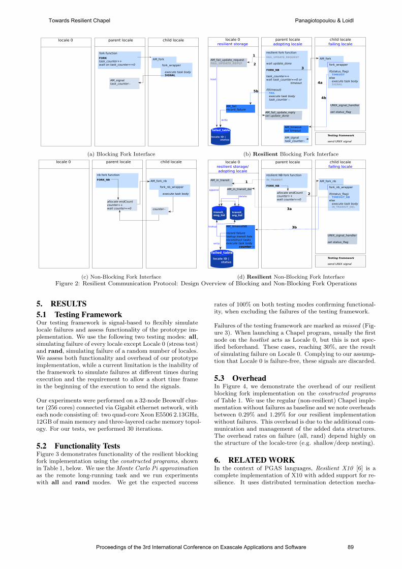
fork function

FORKtask_counter++wait on task_counter==0

AM_fork

fork_wrapper

execute task body SIGNAL

parent locale locale 0 child locale

AM_signaltask_counter--

(a) Blocking Fork Interface

failed_table

locale ID | status

AM_fail_update_requestFAIL_UPDATE_REPLY

AM_failrecord_failure

resilient fork function

FAIL_UPDATE_REQUEST

wait update_done

FORK_NB

task_counter++wait task_counter==0 or timeout

if(timeout) FAIL execute task body task_counter --

AM_fork

fork_wrapper

if(status_flag) TIMEOUTelse execute task body SIGNAL

UNIX_signal_handler

set status_flag

Testing framework

send UNIX signal

parent localeadopting locale

locale 0 resilient storage

child locale failing locale

write

read

1

2

AM_signaltask_counter--

AM_fail_update_replyset update_done

AM_timeoutset timeout

3

4a

4b

5b

(b) Resilient Blocking Fork Interface

nb fork function

FORK_NB AM_fork_nb

fork_nb_wrapper

execute task body

parent locale locale 0 child locale

allocate endCountcounter++wait counter==0 counter--

(c) Non-Blocking Fork Interface

failed_table

locale ID | status

AM_in_transit

AM_timeoutNB

record failurelookup transit listsreconstruct tasksexecute task body counter --

resilient NB fork function

IN_TRANSIT

FORK_NB

append

AM_fork_nb

fork_nb_wrapper

if(status_flag) TIMEOUT_NBelse execute task body IN_TRANSIT_DEL

UNIX_signal_handler

set status_flag

Testing framework

send UNIX signal

parent locale locale 0 resilient storage/adopting locale

child locale failing locale

AM_in_transit_del

transit_msg_list

transit_arg_list

delete

write

lookup

allocate endCountcounter++wait counter==0

1

2

3b

3a

(d) Resilient Non-Blocking Fork Interface

Figure 2: Resilient Communication Protocol: Design Overview of Blocking and Non-Blocking Fork Operations

5. RESULTS5.1 Testing FrameworkOur testing framework is signal-based to flexibly simulatelocale failures and assess functionality of the prototype im-plementation. We use the following two testing modes: all,simulating failure of every locale except Locale 0 (stress test)and rand, simulating failure of a random number of locales.We assess both functionality and overhead of our prototypeimplementation, while a current limitation is the inability ofthe framework to simulate failures at different times duringexecution and the requirement to allow a short time framein the beginning of the execution to send the signals.

Our experiments were performed on a 32-node Beowulf clus-ter (256 cores) connected via Gigabit ethernet network, witheach node consisting of: two quad-core Xeon E5506 2.13GHz,12GB of main memory and three-layered cache memory topol-ogy. For our tests, we performed 30 iterations.

5.2 Functionality TestsFigure 3 demonstrates functionality of the resilient blockingfork implementation using the constructed programs, shownin Table 1, below. We use the Monte Carlo Pi approximationas the remote long-running task and we run experimentswith all and rand modes. We get the expected success

rates of 100% on both testing modes confirming functional-ity, when excluding the failures of the testing framework.

Failures of the testing framework are marked as missed (Fig-ure 3). When launching a Chapel program, usually the firstnode on the hostlist acts as Locale 0, but this is not spec-ified beforehand. These cases, reaching 30%, are the resultof simulating failure on Locale 0. Complying to our assump-tion that Locale 0 is failure-free, these signals are discarded.

5.3 OverheadIn Figure 4, we demonstrate the overhead of our resilientblocking fork implementation on the constructed programsof Table 1. We use the regular (non-resilient) Chapel imple-mentation without failures as baseline and we note overheadsbetween 0.29% and 1.29% for our resilient implementationwithout failures. This overhead is due to the additional com-munication and management of the added data structures.The overhead rates on failure (all, rand) depend highly onthe structure of the locale-tree (e.g. shallow/deep nesting).

6. RELATED WORKIn the context of PGAS languages, Resilient X10 [6] is acomplete implementation of X10 with added support for re-silience. It uses distributed termination detection mecha-



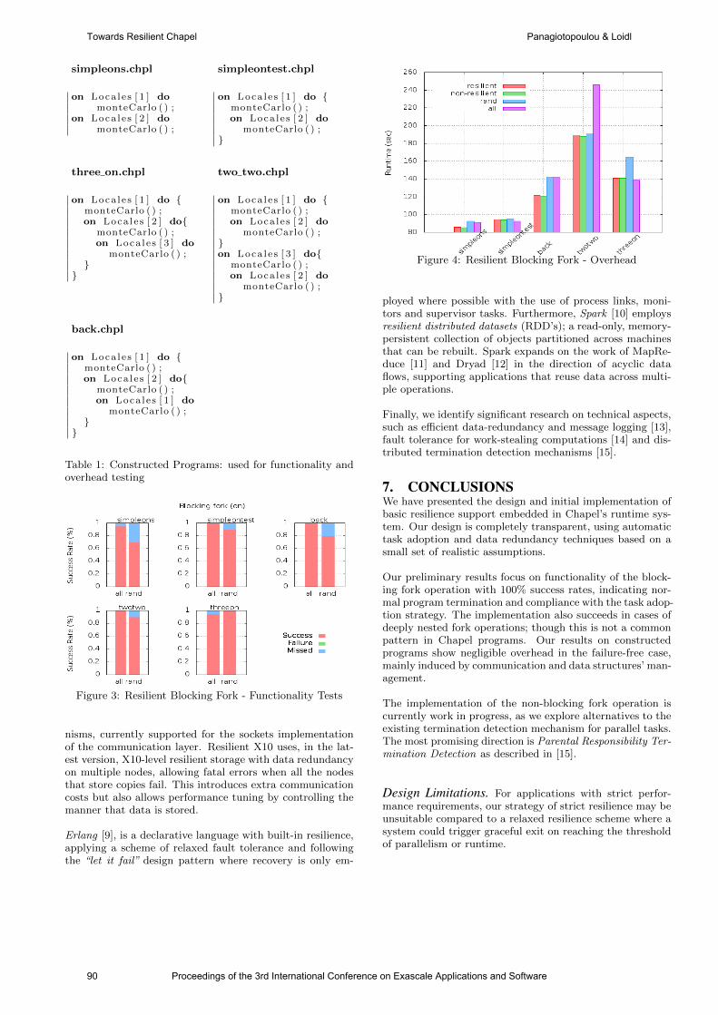
simpleons.chpl simpleontest.chpl

on Loca l e s [ 1 ] domonteCarlo ( ) ;

on Loca l e s [ 2 ] domonteCarlo ( ) ;

on Loca l e s [ 1 ] do monteCarlo ( ) ;on Loca l e s [ 2 ] do

monteCarlo ( ) ;

three on.chpl two two.chpl


monteCarlo ( ) ;on Loca l e s [ 3 ] do

monteCarlo ( ) ;




monteCarlo ( ) ;

back.chpl



monteCarlo ( ) ;

Table 1: Constructed Programs: used for functionality andoverhead testing

Figure 3: Resilient Blocking Fork - Functionality Tests

nisms, currently supported for the sockets implementationof the communication layer. Resilient X10 uses, in the lat-est version, X10-level resilient storage with data redundancyon multiple nodes, allowing fatal errors when all the nodesthat store copies fail. This introduces extra communicationcosts but also allows performance tuning by controlling themanner that data is stored.

Erlang [9], is a declarative language with built-in resilience,applying a scheme of relaxed fault tolerance and followingthe “let it fail” design pattern where recovery is only em-

Figure 4: Resilient Blocking Fork - Overhead

ployed where possible with the use of process links, moni-tors and supervisor tasks. Furthermore, Spark [10] employsresilient distributed datasets (RDD’s); a read-only, memory-persistent collection of objects partitioned across machinesthat can be rebuilt. Spark expands on the work of MapRe-duce [11] and Dryad [12] in the direction of acyclic dataflows, supporting applications that reuse data across multi-ple operations.

Finally, we identify significant research on technical aspects,such as efficient data-redundancy and message logging [13],fault tolerance for work-stealing computations [14] and dis-tributed termination detection mechanisms [15].

7. CONCLUSIONSWe have presented the design and initial implementation ofbasic resilience support embedded in Chapel’s runtime sys-tem. Our design is completely transparent, using automatictask adoption and data redundancy techniques based on asmall set of realistic assumptions.

Our preliminary results focus on functionality of the block-ing fork operation with 100% success rates, indicating nor-mal program termination and compliance with the task adop-tion strategy. The implementation also succeeds in cases ofdeeply nested fork operations; though this is not a commonpattern in Chapel programs. Our results on constructedprograms show negligible overhead in the failure-free case,mainly induced by communication and data structures’ man-agement.

The implementation of the non-blocking fork operation iscurrently work in progress, as we explore alternatives to theexisting termination detection mechanism for parallel tasks.The most promising direction is Parental Responsibility Ter-mination Detection as described in [15].

Design Limitations. For applications with strict perfor-mance requirements, our strategy of strict resilience may beunsuitable compared to a relaxed resilience scheme where asystem could trigger graceful exit on reaching the thresholdof parallelism or runtime.



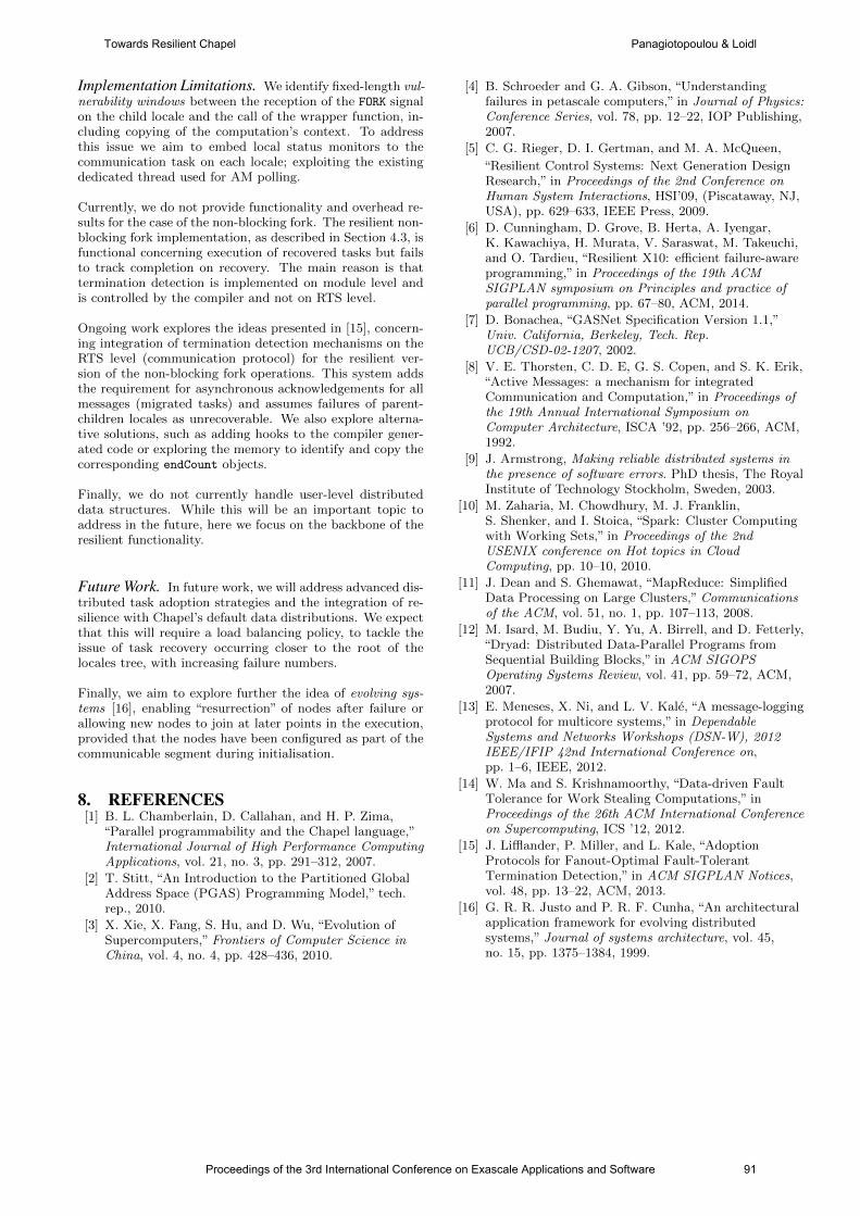
Implementation Limitations. We identify fixed-length vul-nerability windows between the reception of the FORK signalon the child locale and the call of the wrapper function, in-cluding copying of the computation’s context. To addressthis issue we aim to embed local status monitors to thecommunication task on each locale; exploiting the existingdedicated thread used for AM polling.

Currently, we do not provide functionality and overhead re-sults for the case of the non-blocking fork. The resilient non-blocking fork implementation, as described in Section 4.3, isfunctional concerning execution of recovered tasks but failsto track completion on recovery. The main reason is thattermination detection is implemented on module level andis controlled by the compiler and not on RTS level.

Ongoing work explores the ideas presented in [15], concern-ing integration of termination detection mechanisms on theRTS level (communication protocol) for the resilient ver-sion of the non-blocking fork operations. This system addsthe requirement for asynchronous acknowledgements for allmessages (migrated tasks) and assumes failures of parent-children locales as unrecoverable. We also explore alterna-tive solutions, such as adding hooks to the compiler gener-ated code or exploring the memory to identify and copy thecorresponding endCount objects.

Finally, we do not currently handle user-level distributeddata structures. While this will be an important topic toaddress in the future, here we focus on the backbone of theresilient functionality.

Future Work. In future work, we will address advanced dis-tributed task adoption strategies and the integration of re-silience with Chapel’s default data distributions. We expectthat this will require a load balancing policy, to tackle theissue of task recovery occurring closer to the root of thelocales tree, with increasing failure numbers.

Finally, we aim to explore further the idea of evolving sys-tems [16], enabling “resurrection” of nodes after failure orallowing new nodes to join at later points in the execution,provided that the nodes have been configured as part of thecommunicable segment during initialisation.

8. REFERENCES[1] B. L. Chamberlain, D. Callahan, and H. P. Zima,

“Parallel programmability and the Chapel language,”International Journal of High Performance ComputingApplications, vol. 21, no. 3, pp. 291–312, 2007.

[2] T. Stitt, “An Introduction to the Partitioned GlobalAddress Space (PGAS) Programming Model,” tech.rep., 2010.

[3] X. Xie, X. Fang, S. Hu, and D. Wu, “Evolution ofSupercomputers,” Frontiers of Computer Science inChina, vol. 4, no. 4, pp. 428–436, 2010.

[4] B. Schroeder and G. A. Gibson, “Understandingfailures in petascale computers,” in Journal of Physics:Conference Series, vol. 78, pp. 12–22, IOP Publishing,2007.

[5] C. G. Rieger, D. I. Gertman, and M. A. McQueen,

“Resilient Control Systems: Next Generation DesignResearch,” in Proceedings of the 2nd Conference onHuman System Interactions, HSI’09, (Piscataway, NJ,USA), pp. 629–633, IEEE Press, 2009.

[6] D. Cunningham, D. Grove, B. Herta, A. Iyengar,K. Kawachiya, H. Murata, V. Saraswat, M. Takeuchi,and O. Tardieu, “Resilient X10: efficient failure-awareprogramming,” in Proceedings of the 19th ACMSIGPLAN symposium on Principles and practice ofparallel programming, pp. 67–80, ACM, 2014.

[7] D. Bonachea, “GASNet Specification Version 1.1,”Univ. California, Berkeley, Tech. Rep.UCB/CSD-02-1207, 2002.

[8] V. E. Thorsten, C. D. E, G. S. Copen, and S. K. Erik,“Active Messages: a mechanism for integratedCommunication and Computation,” in Proceedings ofthe 19th Annual International Symposium onComputer Architecture, ISCA ’92, pp. 256–266, ACM,1992.

[9] J. Armstrong, Making reliable distributed systems inthe presence of software errors. PhD thesis, The RoyalInstitute of Technology Stockholm, Sweden, 2003.

[10] M. Zaharia, M. Chowdhury, M. J. Franklin,S. Shenker, and I. Stoica, “Spark: Cluster Computingwith Working Sets,” in Proceedings of the 2ndUSENIX conference on Hot topics in CloudComputing, pp. 10–10, 2010.

[11] J. Dean and S. Ghemawat, “MapReduce: SimplifiedData Processing on Large Clusters,” Communicationsof the ACM, vol. 51, no. 1, pp. 107–113, 2008.

[12] M. Isard, M. Budiu, Y. Yu, A. Birrell, and D. Fetterly,“Dryad: Distributed Data-Parallel Programs fromSequential Building Blocks,” in ACM SIGOPSOperating Systems Review, vol. 41, pp. 59–72, ACM,2007.

[13] E. Meneses, X. Ni, and L. V. Kale, “A message-loggingprotocol for multicore systems,” in DependableSystems and Networks Workshops (DSN-W), 2012IEEE/IFIP 42nd International Conference on,pp. 1–6, IEEE, 2012.

[14] W. Ma and S. Krishnamoorthy, “Data-driven FaultTolerance for Work Stealing Computations,” inProceedings of the 26th ACM International Conferenceon Supercomputing, ICS ’12, 2012.

[15] J. Lifflander, P. Miller, and L. Kale, “AdoptionProtocols for Fanout-Optimal Fault-TolerantTermination Detection,” in ACM SIGPLAN Notices,vol. 48, pp. 13–22, ACM, 2013.

[16] G. R. R. Justo and P. R. F. Cunha, “An architecturalapplication framework for evolving distributedsystems,” Journal of systems architecture, vol. 45,no. 15, pp. 1375–1384, 1999.



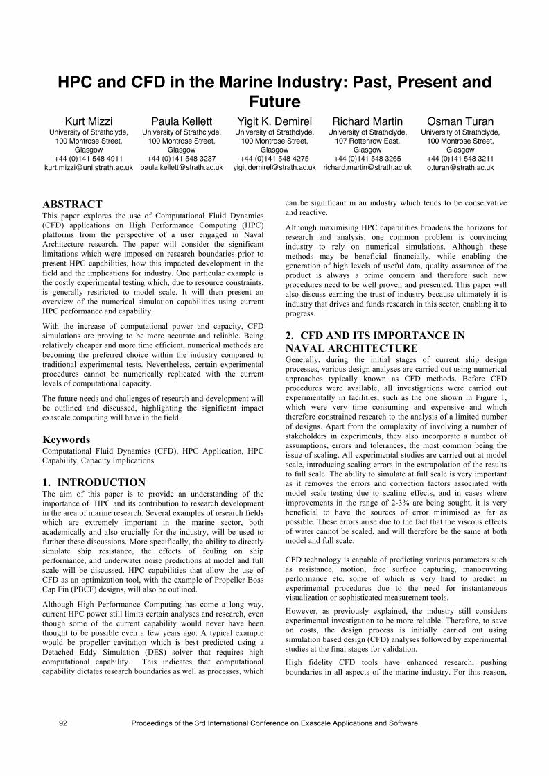
HPC and CFD in the Marine Industry: Past, Present and Future

Kurt Mizzi University of Strathclyde,

100 Montrose Street, Glasgow

+44 (0)141 548 4911 [email protected]

Paula Kellett University of Strathclyde,


+44 (0)141 548 3237 [email protected]

Yigit K. Demirel University of Strathclyde,


+44 (0)141 548 4275 [email protected]

Richard Martin University of Strathclyde,

107 Rottenrow East, Glasgow

+44 (0)141 548 3265 [email protected]

Osman Turan University of Strathclyde,


+44 (0)141 548 3211 [email protected]

ABSTRACT This paper explores the use of Computational Fluid Dynamics (CFD) applications on High Performance Computing (HPC) platforms from the perspective of a user engaged in Naval Architecture research. The paper will consider the significant limitations which were imposed on research boundaries prior to present HPC capabilities, how this impacted development in the field and the implications for industry. One particular example is the costly experimental testing which, due to resource constraints, is generally restricted to model scale. It will then present an overview of the numerical simulation capabilities using current HPC performance and capability.

With the increase of computational power and capacity, CFD simulations are proving to be more accurate and reliable. Being relatively cheaper and more time efficient, numerical methods are becoming the preferred choice within the industry compared to traditional experimental tests. Nevertheless, certain experimental procedures cannot be numerically replicated with the current levels of computational capacity.

The future needs and challenges of research and development will be outlined and discussed, highlighting the significant impact exascale computing will have in the field.

Keywords Computational Fluid Dynamics (CFD), HPC Application, HPC Capability, Capacity Implications

1. INTRODUCTION The aim of this paper is to provide an understanding of the importance of HPC and its contribution to research development in the area of marine research. Several examples of research fields which are extremely important in the marine sector, both academically and also crucially for the industry, will be used to further these discussions. More specifically, the ability to directly simulate ship resistance, the effects of fouling on ship performance, and underwater noise predictions at model and full scale will be discussed. HPC capabilities that allow the use of CFD as an optimization tool, with the example of Propeller Boss Cap Fin (PBCF) designs, will also be outlined.

Although High Performance Computing has come a long way, current HPC power still limits certain analyses and research, even though some of the current capability would never have been thought to be possible even a few years ago. A typical example would be propeller cavitation which is best predicted using a Detached Eddy Simulation (DES) solver that requires high computational capability. This indicates that computational capability dictates research boundaries as well as processes, which

can be significant in an industry which tends to be conservative and reactive.

Although maximising HPC capabilities broadens the horizons for research and analysis, one common problem is convincing industry to rely on numerical simulations. Although these methods may be beneficial financially, while enabling the generation of high levels of useful data, quality assurance of the product is always a prime concern and therefore such new procedures need to be well proven and presented. This paper will also discuss earning the trust of industry because ultimately it is industry that drives and funds research in this sector, enabling it to progress.

2. CFD AND ITS IMPORTANCE IN NAVAL ARCHITECTURE Generally, during the initial stages of current ship design processes, various design analyses are carried out using numerical approaches typically known as CFD methods. Before CFD procedures were available, all investigations were carried out experimentally in facilities, such as the one shown in Figure 1, which were very time consuming and expensive and which therefore constrained research to the analysis of a limited number of designs. Apart from the complexity of involving a number of stakeholders in experiments, they also incorporate a number of assumptions, errors and tolerances, the most common being the issue of scaling. All experimental studies are carried out at model scale, introducing scaling errors in the extrapolation of the results to full scale. The ability to simulate at full scale is very important as it removes the errors and correction factors associated with model scale testing due to scaling effects, and in cases where improvements in the range of 2-3% are being sought, it is very beneficial to have the sources of error minimised as far as possible. These errors arise due to the fact that the viscous effects of water cannot be scaled, and will therefore be the same at both model and full scale.

CFD technology is capable of predicting various parameters such as resistance, motion, free surface capturing, manoeuvring performance etc. some of which is very hard to predict in experimental procedures due to the need for instantaneous visualization or sophisticated measurement tools.

However, as previously explained, the industry still considers experimental investigation to be more reliable. Therefore, to save on costs, the design process is initially carried out using simulation based design (CFD) analyses followed by experimental studies at the final stages for validation. High fidelity CFD tools have enhanced research, pushing boundaries in all aspects of the marine industry. For this reason,


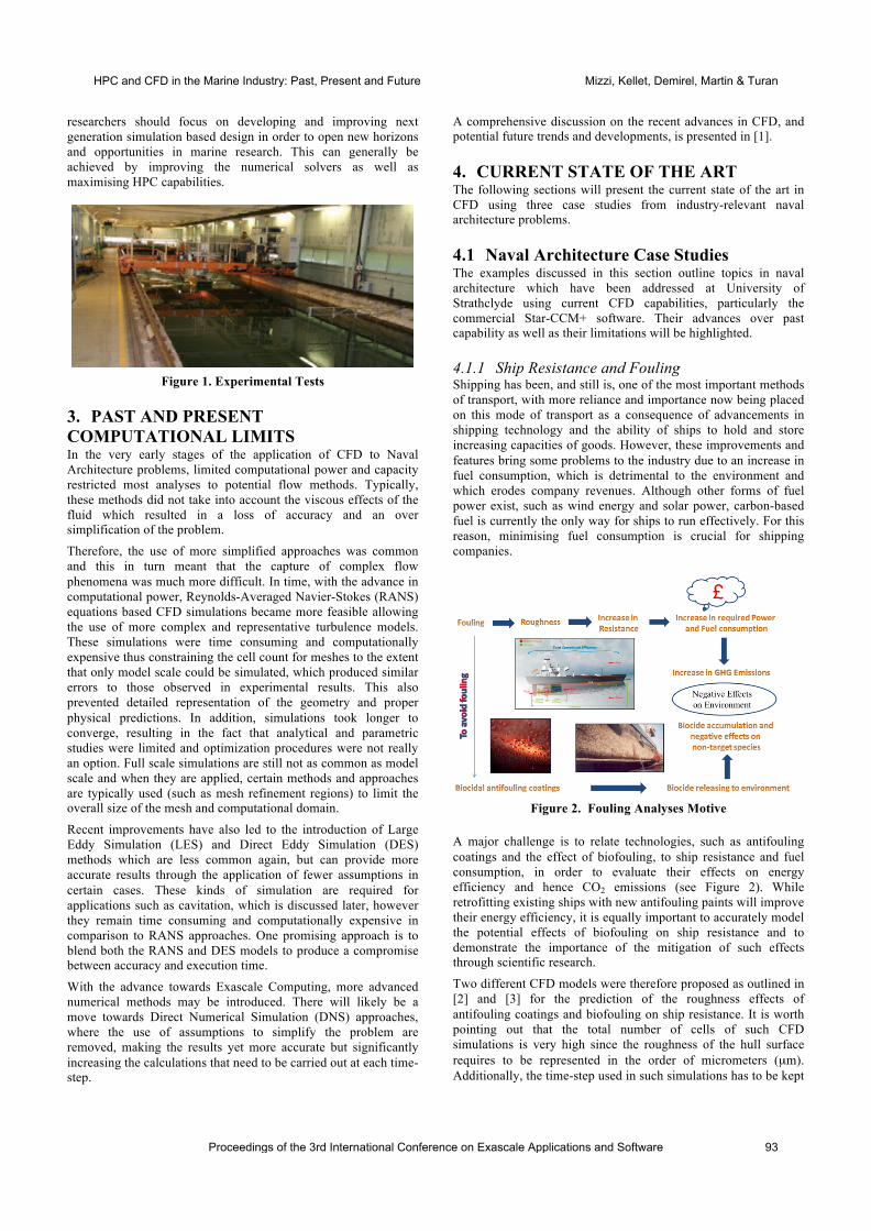
researchers should focus on developing and improving next generation simulation based design in order to open new horizons and opportunities in marine research. This can generally be achieved by improving the numerical solvers as well as maximising HPC capabilities.

Figure 1. Experimental Tests

3. PAST AND PRESENT COMPUTATIONAL LIMITS In the very early stages of the application of CFD to Naval Architecture problems, limited computational power and capacity restricted most analyses to potential flow methods. Typically, these methods did not take into account the viscous effects of the fluid which resulted in a loss of accuracy and an over simplification of the problem.

Therefore, the use of more simplified approaches was common and this in turn meant that the capture of complex flow phenomena was much more difficult. In time, with the advance in computational power, Reynolds-Averaged Navier-Stokes (RANS) equations based CFD simulations became more feasible allowing the use of more complex and representative turbulence models. These simulations were time consuming and computationally expensive thus constraining the cell count for meshes to the extent that only model scale could be simulated, which produced similar errors to those observed in experimental results. This also prevented detailed representation of the geometry and proper physical predictions. In addition, simulations took longer to converge, resulting in the fact that analytical and parametric studies were limited and optimization procedures were not really an option. Full scale simulations are still not as common as model scale and when they are applied, certain methods and approaches are typically used (such as mesh refinement regions) to limit the overall size of the mesh and computational domain.

Recent improvements have also led to the introduction of Large Eddy Simulation (LES) and Direct Eddy Simulation (DES) methods which are less common again, but can provide more accurate results through the application of fewer assumptions in certain cases. These kinds of simulation are required for applications such as cavitation, which is discussed later, however they remain time consuming and computationally expensive in comparison to RANS approaches. One promising approach is to blend both the RANS and DES models to produce a compromise between accuracy and execution time.

With the advance towards Exascale Computing, more advanced numerical methods may be introduced. There will likely be a move towards Direct Numerical Simulation (DNS) approaches, where the use of assumptions to simplify the problem are removed, making the results yet more accurate but significantly increasing the calculations that need to be carried out at each time-step.

A comprehensive discussion on the recent advances in CFD, and potential future trends and developments, is presented in [1].

4. CURRENT STATE OF THE ART The following sections will present the current state of the art in CFD using three case studies from industry-relevant naval architecture problems.

4.1 Naval Architecture Case Studies The examples discussed in this section outline topics in naval architecture which have been addressed at University of Strathclyde using current CFD capabilities, particularly the commercial Star-CCM+ software. Their advances over past capability as well as their limitations will be highlighted.

4.1.1 Ship Resistance and Fouling Shipping has been, and still is, one of the most important methods of transport, with more reliance and importance now being placed on this mode of transport as a consequence of advancements in shipping technology and the ability of ships to hold and store increasing capacities of goods. However, these improvements and features bring some problems to the industry due to an increase in fuel consumption, which is detrimental to the environment and which erodes company revenues. Although other forms of fuel power exist, such as wind energy and solar power, carbon-based fuel is currently the only way for ships to run effectively. For this reason, minimising fuel consumption is crucial for shipping companies.

Figure 2. Fouling Analyses Motive

A major challenge is to relate technologies, such as antifouling coatings and the effect of biofouling, to ship resistance and fuel consumption, in order to evaluate their effects on energy efficiency and hence CO2 emissions (see Figure 2). While retrofitting existing ships with new antifouling paints will improve their energy efficiency, it is equally important to accurately model the potential effects of biofouling on ship resistance and to demonstrate the importance of the mitigation of such effects through scientific research.

Two different CFD models were therefore proposed as outlined in [2] and [3] for the prediction of the roughness effects of antifouling coatings and biofouling on ship resistance. It is worth pointing out that the total number of cells of such CFD simulations is very high since the roughness of the hull surface requires to be represented in the order of micrometers (µm). Additionally, the time-step used in such simulations has to be kept


HPC and CFD in the Marine Industry: Past, Present and Future Mizzi, Kellet, Demirel, Martin & Turan

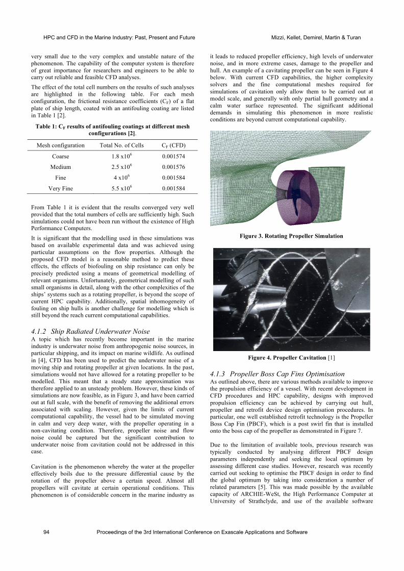
very small due to the very complex and unstable nature of the phenomenon. The capability of the computer system is therefore of great importance for researchers and engineers to be able to carry out reliable and feasible CFD analyses.

The effect of the total cell numbers on the results of such analyses are highlighted in the following table. For each mesh configuration, the frictional resistance coefficients (CF) of a flat plate of ship length, coated with an antifouling coating are listed in Table 1 [2].

Table 1: CF results of antifouling coatings at different mesh configurations [2].

Mesh configuration Total No. of Cells CF (CFD)

Coarse 1.8 x106 0.001574

Medium 2.5 x106 0.001576

Fine 4 x106 0.001584

Very Fine 5.5 x106 0.001584

From Table 1 it is evident that the results converged very well provided that the total numbers of cells are sufficiently high. Such simulations could not have been run without the existence of High Performance Computers.

It is significant that the modelling used in these simulations was based on available experimental data and was achieved using particular assumptions on the flow properties. Although the proposed CFD model is a reasonable method to predict these effects, the effects of biofouling on ship resistance can only be precisely predicted using a means of geometrical modelling of relevant organisms. Unfortunately, geometrical modelling of such small organisms in detail, along with the other complexities of the ships’ systems such as a rotating propeller, is beyond the scope of current HPC capability. Additionally, spatial inhomogeneity of fouling on ship hulls is another challenge for modelling which is still beyond the reach current computational capabilities.

4.1.2 Ship Radiated Underwater Noise A topic which has recently become important in the marine industry is underwater noise from anthropogenic noise sources, in particular shipping, and its impact on marine wildlife. As outlined in [4], CFD has been used to predict the underwater noise of a moving ship and rotating propeller at given locations. In the past, simulations would not have allowed for a rotating propeller to be modelled. This meant that a steady state approximation was therefore applied to an unsteady problem. However, these kinds of simulations are now feasible, as in Figure 3, and have been carried out at full scale, with the benefit of removing the additional errors associated with scaling. However, given the limits of current computational capability, the vessel had to be simulated moving in calm and very deep water, with the propeller operating in a non-cavitating condition. Therefore, propeller noise and flow noise could be captured but the significant contribution to underwater noise from cavitation could not be addressed in this case.

Cavitation is the phenomenon whereby the water at the propeller effectively boils due to the pressure differential cause by the rotation of the propeller above a certain speed. Almost all propellers will cavitate at certain operational conditions. This phenomenon is of considerable concern in the marine industry as

it leads to reduced propeller efficiency, high levels of underwater noise, and in more extreme cases, damage to the propeller and hull. An example of a cavitating propeller can be seen in Figure 4 below. With current CFD capabilities, the higher complexity solvers and the fine computational meshes required for simulations of cavitation only allow them to be carried out at model scale, and generally with only partial hull geometry and a calm water surface represented. The significant additional demands in simulating this phenomenon in more realistic conditions are beyond current computational capability.

Figure 3. Rotating Propeller Simulation

Figure 4. Propeller Cavitation [1]

4.1.3 Propeller Boss Cap Fins Optimisation As outlined above, there are various methods available to improve the propulsion efficiency of a vessel. With recent development in CFD procedures and HPC capability, designs with improved propulsion efficiency can be achieved by carrying out hull, propeller and retrofit device design optimisation procedures. In particular, one well established retrofit technology is the Propeller Boss Cap Fin (PBCF), which is a post swirl fin that is installed onto the boss cap of the propeller as demonstrated in Figure 7.

Due to the limitation of available tools, previous research was typically conducted by analysing different PBCF design parameters independently and seeking the local optimum by assessing different case studies. However, research was recently carried out seeking to optimise the PBCF design in order to find the global optimum by taking into consideration a number of related parameters [5]. This was made possible by the available capacity of ARCHIE-WeSt, the High Performance Computer at University of Strathclyde, and use of the available software



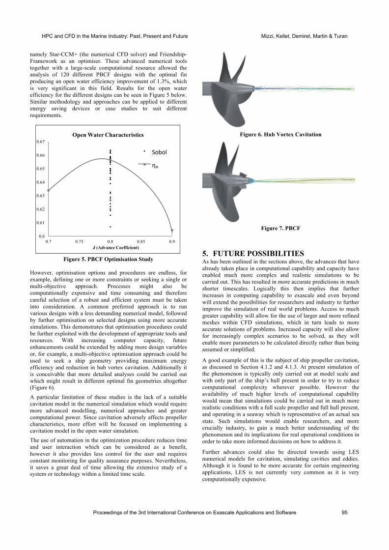
namely Star-CCM+ (the numerical CFD solver) and Friendship-Framework as an optimiser. These advanced numerical tools together with a large-scale computational resource allowed the analysis of 120 different PBCF designs with the optimal fin producing an open water efficiency improvement of 1.3%, which is very significant in this field. Results for the open water efficiency for the different designs can be seen in Figure 5 below. Similar methodology and approaches can be applied to different energy saving devices or case studies to suit different requirements.

Figure 5. PBCF Optimisation Study

However, optimisation options and procedures are endless, for example, defining one or more constraints or seeking a single or multi-objective approach. Processes might also be computationally expensive and time consuming and therefore careful selection of a robust and efficient system must be taken into consideration. A common preferred approach is to run various designs with a less demanding numerical model, followed by further optimisation on selected designs using more accurate simulations. This demonstrates that optimisation procedures could be further exploited with the development of appropriate tools and resources. With increasing computer capacity, future enhancements could be extended by adding more design variables or, for example, a multi-objective optimisation approach could be used to seek a ship geometry providing maximum energy efficiency and reduction in hub vortex cavitation. Additionally it is conceivable that more detailed analyses could be carried out which might result in different optimal fin geometries altogether (Figure 6).

A particular limitation of these studies is the lack of a suitable cavitation model in the numerical simulation which would require more advanced modelling, numerical approaches and greater computational power. Since cavitation adversely affects propeller characteristics, more effort will be focused on implementing a cavitation model in the open water simulation. The use of automation in the optimization procedure reduces time and user interaction which can be considered as a benefit, however it also provides less control for the user and requires constant monitoring for quality assurance purposes. Nevertheless, it saves a great deal of time allowing the extensive study of a system or technology within a limited time scale.

Figure 6. Hub Vortex Cavitation

Figure 7. PBCF

5. FUTURE POSSIBILITIES As has been outlined in the sections above, the advances that have already taken place in computational capability and capacity have enabled much more complex and realistic simulations to be carried out. This has resulted in more accurate predictions in much shorter timescales. Logically this then implies that further increases in computing capability to exascale and even beyond will extend the possibilities for researchers and industry to further improve the simulation of real world problems. Access to much greater capability will allow for the use of larger and more refined meshes within CFD simulations, which in turn leads to more accurate solutions of problems. Increased capacity will also allow for increasingly complex scenarios to be solved, as they will enable more parameters to be calculated directly rather than being assumed or simplified.

A good example of this is the subject of ship propeller cavitation, as discussed in Section 4.1.2 and 4.1.3. At present simulation of the phenomenon is typically only carried out at model scale and with only part of the ship’s hull present in order to try to reduce computational complexity wherever possible. However the availability of much higher levels of computational capability would mean that simulations could be carried out in much more realistic conditions with a full scale propeller and full hull present, and operating in a seaway which is representative of an actual sea state. Such simulations would enable researchers, and more crucially industry, to gain a much better understanding of the phenomenon and its implications for real operational conditions in order to take more informed decisions on how to address it.

Further advances could also be directed towards using LES numerical models for cavitation, simulating cavities and eddies. Although it is found to be more accurate for certain engineering applications, LES is not currently very common as it is very computationally expensive.

0.6

0.61

0.62

0.63

0.64

0.65

0.66

0.67

0.7 0.75 0.8 0.85 0.9J (Advance Coefficient)

Open Water Characteristics

Sobol

ηₒ



Although optimization methods are available, their use is not common practice due to the computational capacity required. Hull and propeller optimization using RANS simulations would greatly benefit the industry allowing the analyses of multiple designs at a reasonable expense when compared to experimental procedures. Looking further into the future there is likely to be a venture into optimization methods in real operational conditions and optimization using LES or DNS numerical models.

As explained above, the increase of computational power, both in terms of capability and capacity, introduces endless possibilities to the marine industry and research in general.

However looking at short term improvements, the ability to create mesh configurations with higher cell numbers would increase accuracy, allow more full scale simulations and would make it easier for engineers to satisfy the validation and verification requirements (V&V) of their simulations which in turn would create increased credibility for their work and generate more trust from within industry.

One other significant improvement would be to allow more interaction between the HPC and the user i.e. creating a better graphical user interface allowing for interactive simulations. Some CFD engineers find it best to monitor their work while the job is running ensuring that the simulation is running adequately, and sometimes also making modifications during the run. This is commonly practiced when carrying out minor jobs on a personal computer. However, when running jobs on a HPC, although some visual elements are allowed, this is somewhat limited. Extending and expanding visual capabilities in HPC would definitely help engineers carry out their work more efficiently.

However in the present economic climate, researchers and industry are not at liberty to research and develop whichever techniques and capabilities they choose over an undefined timescale. Nor would access to such computational capability be granted for free. The following sections will discuss the implications of access to such capability from the perspective of research and of industry.

5.1 Technical Implications Stern et al. outlined three HPC challenges in state of the art CFD simulations; System Memory, Interconnection and Input/output [6]. They explain that 10% of the current system memory (RAM), which is generally 2GB, is dedicated for system usage. In high fidelity complex simulations, a good portion of this is used to store the data to be solved, leaving limited memory for the solver. In some cases, marine applications require the processing of vast amounts of data which do not fit within a single computer node, which may generally be equipped with tens of processor cores. Future advances, such as Exascale computers, may allow transition from a multi–core to many-core systems equipped with many more cores on a single node. Therefore the continuous increase of number of processors within one node will allow more complex simulations with higher volumes of data to be solved within a single shared-memory system. On the other hand, due to the associated costs, a decrease in memory size per core is predicted and therefore it is vital for the CFD engineer to minimise memory usage in CFD simulations and processes.

The interconnection between the nodes is also an issue that requires attention. The network bandwidth and communication latency are the determining factors for network interconnect performance. Therefore while computer engineers are likely to focus on avoiding or reducing latency and increasing network

bandwidth, flow simulation engineers should develop solvers that require less communication. In addition, high fidelity flow simulations require processes to read and write vast amounts of data which may result in a great number of nodes or cores to processing in parallel the input/output data. This might make data handling unmanageable and will also be affected by interconnect bandwidth and the performance of the available storage. Consequently, this could deteriorate simulation performance and could be costly.

Such issues require attention not only from the computer engineering perspective but also from the software developers with the former aiming to maximise HPC capability and the latter minimising the need for high data volumes, handling and communication. Together they should aim to improve the system performance and the scalability of the simulations.

5.2 Implications for Research The direction that research takes is as much dictated by political agendas, funding sources and industry requirements as it is by computational capability. Political agendas tend to dictate “hot topics” which are perceived to be of upmost importance to society at a given juncture. This in turn influences the funding which becomes available for research or facilities which support development in these key areas. These developments can then have an impact in two ways: by producing new techniques or technologies which become available to industry, or through highlighting concerns which impact on industry where they lead to standards and regulations. The process then comes full circle as industry turns to the research community, seeking support in dealing with these new discoveries.

In the particular case of significant advancements in computational capability to Exascale Computing, access to such facilities and the funds to develop applications to take advantage of them would not necessarily be directly linked to the advancements themselves. Instead, it would most likely arise as a means of improving current knowledge and understanding of a key politically-supported topic, or investigating a particular concern raised by industry. This in effect means that just because the capability becomes available, the required developments in CFD and hence the advantages and possibilities outlined within this paper would not necessarily follow directly. For this reason, it is of great importance to all parties that key developments and their possible implications in other fields gain suitable publicity and are appreciated by as wide an audience as possible.

5.3 Implications for Industry The marine industry has typically been conservative and reactive, meaning that new developments and techniques are not immediately trusted. Even the current state of the art capability in CFD simulation is not widely trusted, and where the results are accepted, they inevitably need to be well supported by costly experimental testing results. Due to the perceived complexity of CFD, where it is not understood, it is not trusted. It is therefore of vital importance that where the capability for sophisticated simulations is available, all possible steps are taken to ensure that the processes are transparent, well validated and can prove to provide accurate and high quality results. Validation and verification (V&V) procedures, e.g. [7] and [8], is a research topic in its own right, with engineers constantly improving the quality of CFD results with continuous developments in tools and computational power leading to new CFD methods.



If this can be achieved and if trust can be developed in the use of these approaches, the benefits for industry would be significant. As has already been outlined, model scale experimental tests are limited in what can be recreated and are also subject to inherent scaling errors. Carrying out such tests is time-consuming and costly, and any design changes would require a new model to be built and a new set of experiments to be run. By contrast, future CFD simulations could be run at full scale, removing any inherent scaling errors. As computational capacity increases, the timescales and costs involved will continue to reduce. Therefore, design changes could be made and analysed more easily, and simulations of realistic scenarios could be conducted. This latter advantage would have a significant benefit in terms of ship safety and, in what is probably more appealing to industry, efficiency. Improved efficiency means a lower fuel bill and the ability to predict the efficiency of a vessel in a range of realistic operational conditions rather than at just one design condition. This will lead to more informed decisions on design and installation, producing vessels that are much better adapted to their typical operating profile than at present.

The challenges which lie ahead for the industry in arriving at this point are significant, with many aspects to consider, but if it can be achieved, the benefits will be universal in the field.

6. CLOSING REMARKS Numerical solvers have developed significantly over the past few years. This has allowed marine, and more specifically ship hydrodynamics, research to progress in parallel. The continuous improvement of HPC capabilities and the move towards Exascale Computing will allow research methods to be exploited even further, opening up new possibilities previously not possible due to the constraints of the available computing capabilities. With this in mind, numerical solvers should be further developed taking into consideration the power and capacity of Exascale Computing platforms that will open up new windows of opportunity. In time this will result in more robust, accurate, scaleable, high fidelity, state of the art simulations, even when employing optimization procedures.

7. ACKNOWLEDGMENTS Results were obtained using the EPSRC funded ARCHIE-WeSt High Performance Computer (www.archie-west.ac.uk). EPSRC grant no. EP/K000586/1.

8. REFERENCES [1] F. Stern, Z. Wang, J. Yang, M. M. H Sadat-Hosseini, S.

Bushan, M. Diaz, S. H. Yoon, P. C. Wu, S. Mo, R. S. Thodal and J. L. Grenestedt, "Recent Progress in CFD for Naval Architecture and Ocean Engineering," in 11th International Conference on Hydrodynamics , 2014.

[2] Y. K. Demirel, M. Khorasanchi, O. Turan, A. Incecik and M. P. Schultz, "A CFD model for the frictional resistance prediction of antifouling coatings," Ocean Engineering Vol. 89, pp. 21-31, 2014.

[3] Y. K. Demirel, M. Khorasanchi, O. Turan and A. Incecik, "Prediction of the effect of hull fouling on ship resistance using CFD," in 17th International Congress on Marine Corrosion and Fouling (ICMCF), Singapore, 2014.

[4] P. Kellett, O. Turan and A. Incecik, "A Study of Numerical Ship Underwater Noise Prediction," Ocean Engineering Vol.66, pp. 113-120, Jul. 2013.

[5] K. Mizzi, Y. K. Demirel, C. Banks and O. Turan, "PBCF design optimisation and propulsion efficiency impact," in RINA International Conference on Influence of EEDI on Ship Design, London, 2014.

[6] F. Stern, J. Yang, Z. Wang, H. Sadat-Hosseni, M. Mousaviraad, S. Bhushan and T. Xing, "Computational Ship Hydrodynamics: Nowadays and Way Forward," in 29th Symposium on Naval Hydrodynamics, Gothenburg, Sweden, 2012.

[7] I. B. Celik, U. Ghia, P. J. Roache, C. J. Freitas, H. Coleman and P. E. Raad, "Procedure for Estimation and Reporting of Uncertainty Due to Discretization in CFD Applications," Journal of Fluids Engineering, vol. 130, no. 7, 2008.

[8] F. Stern, R. Wilson and J. Shao, "Quantitative V&V of CFD simulations and certification of CFD codes," International Journal for Numerical Methods in Fluids, vol. 50, pp. 1335-1355, 2006.



Swift: task-based hydrodynamics and gravity forcosmological simulations

Tom TheunsInstitute for Computational

CosmologyDepartment of Physics

Durham UniversityDurham DH1 3LE, UK

Aidan ChalkSchool of Engineering and

Computing SciencesDurham University

Durham DH1 3LE, UK

Matthieu SchallerInstitute for Computational

CosmologyDepartment of Physics

Durham UniversityDurham DH1 3LE, UK

Pedro GonnetSchool of Engineering and

Computing SciencesDurham University

Durham DH1 3LE, UKand

Google Switzerland GmbHBrandschenkestr. 110

8002 Zurich, Switzerland

ABSTRACTSimulations of galaxy formation follow the gravitational andhydrodynamical interactions between gas, stars and darkmatter through cosmic time. The huge dynamic range ofsuch calculations severely limits strong scaling behaviour ofthe community codes in use, with load-imbalance, cache inef-ficiencies and poor vectorisation limiting performance. Thenew swift code exploits task-based parallelism designed formany-core compute nodes interacting via MPI using asyn-chronous communication to improve speed and scaling. Agraph-based domain decomposition schedules interdependenttasks over available resources. Strong scaling tests on real-istic particle distributions yield excellent parallel efficiency,and efficient cache usage provides a large speedup comparedto current codes even on a single core. swift is designedto be easy to use by shielding the astronomer from com-putational details such as the construction of the tasks orMPI communication. The techniques and algorithms usedin swift may benefit other computational physics areas aswell, for example that of compressible hydrodynamics. Fordetails of this open-source project, see www.swiftsim.com

KeywordsTask-based parallelism, Asynchronous data transfer

1. INTRODUCTIONThe main aim of cosmological simulations of the formationof structures in the Universe is to understand which physi-cal processes play in role in how galaxies form and evolve.For example, what determines whether a galaxy becomes aspiral or an elliptical? What is the origin of the morphology-density relation - the observation that elliptical galaxies clus-ter much more strongly than spirals? What sets the coloursof galaxies? How does the rate of galaxy formation evolveover cosmic time? What is the nature of high-redshift galax-ies? A better understanding of these processes will be re-quired to take full advantage of the rich data sets being

collected now, or promised by future observatories such asthe James Webb space telescope1, ESO’s Extremely-Largetelescope 2 or the Square Kilometre Array 3.

Such cosmological simulations start from initial conditionsmotivated by observations of the cosmic microwave back-ground (CMB). The CMB provides a directly observableimprint of the small density fluctuations that will eventu-ally grow due to gravity into galaxies and clusters of galaxiestoday. In an expanding universe, regions which are slightlyover-dense become denser and eventually collapse due to theself-gravity of their dark matter. These collapsing ‘halos’accrete gas that cools radiatively and makes stars. The sim-ulations follow the build-up of the dark matter halos andthe accretion, shock-heating, and radiative cooling of thegas onto halos.

The gas densities above which stars form are orders of mag-nitude higher than the typical density in a galaxy and thislarge dynamic range is one of the most challenging aspectsof these computations. The radiation and winds of recentlyformed stars, and the energy injected by super nova ex-plosions, strongly limit the rate at which a galaxy’s gas isturned into stars. As a result, only ∼ 17 per cent of all gasin the Universe has been converted into stars to date [3].The tremendous dynamic range in mass, length and time,between gas accreting onto a halo and turning into stars pre-vents simulations to model these crucial processes in detail.‘Subgrid’ schemes are therefore used to model processes thatcannot (yet) be resolved numerically, not unlike what is donein other multi-scale calculations such as for example weatheror climate modelling. Limiting the impact of these subgridmodels by actually resolving some of the underlying physicsis a tremendously exciting and computationally demanding

1http://www.jwst.nasa.gov/2http://www.eso.org/public/teles-instr/e-elt/3https://www.skatelescope.org/


www.swiftsim.com

http://www.jwst.nasa.gov/

http://www.eso.org/public/teles-instr/e-elt/

https://www.skatelescope.org/

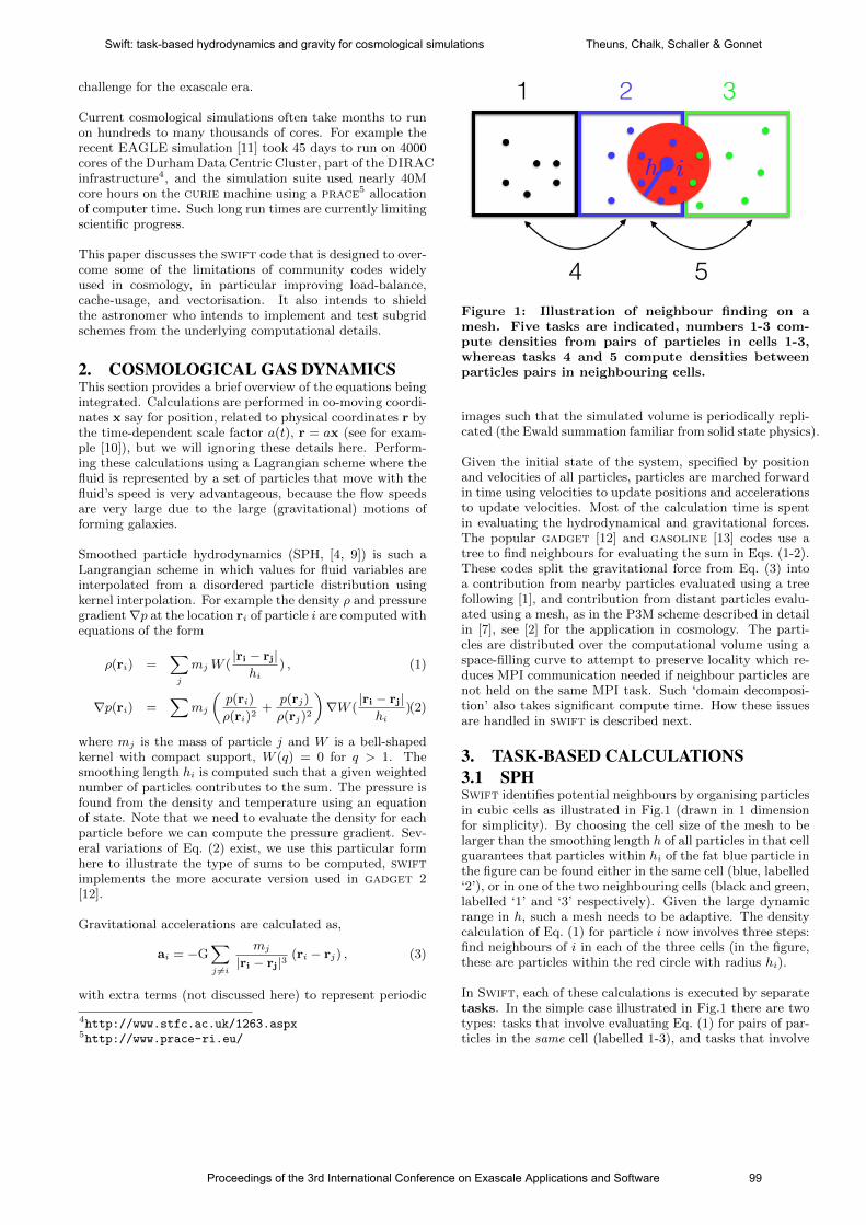
challenge for the exascale era.

Current cosmological simulations often take months to runon hundreds to many thousands of cores. For example therecent EAGLE simulation [11] took 45 days to run on 4000cores of the Durham Data Centric Cluster, part of the DIRACinfrastructure4, and the simulation suite used nearly 40Mcore hours on the curie machine using a prace5 allocationof computer time. Such long run times are currently limitingscientific progress.

This paper discusses the swift code that is designed to over-come some of the limitations of community codes widelyused in cosmology, in particular improving load-balance,cache-usage, and vectorisation. It also intends to shieldthe astronomer who intends to implement and test subgridschemes from the underlying computational details.

2. COSMOLOGICAL GAS DYNAMICSThis section provides a brief overview of the equations beingintegrated. Calculations are performed in co-moving coordi-nates x say for position, related to physical coordinates r bythe time-dependent scale factor a(t), r = ax (see for exam-ple [10]), but we will ignoring these details here. Perform-ing these calculations using a Lagrangian scheme where thefluid is represented by a set of particles that move with thefluid’s speed is very advantageous, because the flow speedsare very large due to the large (gravitational) motions offorming galaxies.

Smoothed particle hydrodynamics (SPH, [4, 9]) is such aLangrangian scheme in which values for fluid variables areinterpolated from a disordered particle distribution usingkernel interpolation. For example the density ρ and pressuregradient∇p at the location ri of particle i are computed withequations of the form

ρ(ri) =∑j

mj W (|ri − rj|hi

) , (1)

∇p(ri) =∑

mj

(p(ri)

ρ(ri)2+

p(rj)

ρ(rj)2

)∇W (

|ri − rj|hi

)(2)

where mj is the mass of particle j and W is a bell-shapedkernel with compact support, W (q) = 0 for q > 1. Thesmoothing length hi is computed such that a given weightednumber of particles contributes to the sum. The pressure isfound from the density and temperature using an equationof state. Note that we need to evaluate the density for eachparticle before we can compute the pressure gradient. Sev-eral variations of Eq. (2) exist, we use this particular formhere to illustrate the type of sums to be computed, swiftimplements the more accurate version used in gadget 2[12].

Gravitational accelerations are calculated as,

ai = −G∑j 6=i

mj

|ri − rj|3(ri − rj) , (3)

with extra terms (not discussed here) to represent periodic

4http://www.stfc.ac.uk/1263.aspx5http://www.prace-ri.eu/

Figure 1: Illustration of neighbour finding on amesh. Five tasks are indicated, numbers 1-3 com-pute densities from pairs of particles in cells 1-3,whereas tasks 4 and 5 compute densities betweenparticles pairs in neighbouring cells.

images such that the simulated volume is periodically repli-cated (the Ewald summation familiar from solid state physics).

Given the initial state of the system, specified by positionand velocities of all particles, particles are marched forwardin time using velocities to update positions and accelerationsto update velocities. Most of the calculation time is spentin evaluating the hydrodynamical and gravitational forces.The popular gadget [12] and gasoline [13] codes use atree to find neighbours for evaluating the sum in Eqs. (1-2).These codes split the gravitational force from Eq. (3) intoa contribution from nearby particles evaluated using a treefollowing [1], and contribution from distant particles evalu-ated using a mesh, as in the P3M scheme described in detailin [7], see [2] for the application in cosmology. The parti-cles are distributed over the computational volume using aspace-filling curve to attempt to preserve locality which re-duces MPI communication needed if neighbour particles arenot held on the same MPI task. Such ‘domain decomposi-tion’ also takes significant compute time. How these issuesare handled in swift is described next.

3. TASK-BASED CALCULATIONS3.1 SPHSwift identifies potential neighbours by organising particlesin cubic cells as illustrated in Fig.1 (drawn in 1 dimensionfor simplicity). By choosing the cell size of the mesh to belarger than the smoothing length h of all particles in that cellguarantees that particles within hi of the fat blue particle inthe figure can be found either in the same cell (blue, labelled‘2’), or in one of the two neighbouring cells (black and green,labelled ‘1’ and ‘3’ respectively). Given the large dynamicrange in h, such a mesh needs to be adaptive. The densitycalculation of Eq. (1) for particle i now involves three steps:find neighbours of i in each of the three cells (in the figure,these are particles within the red circle with radius hi).

In Swift, each of these calculations is executed by separatetasks. In the simple case illustrated in Fig.1 there are twotypes: tasks that involve evaluating Eq. (1) for pairs of par-ticles in the same cell (labelled 1-3), and tasks that involve


Swift: task-based hydrodynamics and gravity for cosmological simulations Theuns, Chalk, Schaller & Gonnet

http://www.stfc.ac.uk/1263.aspx

http://www.prace-ri.eu/

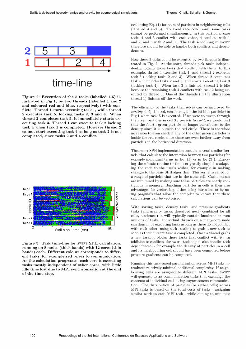
Figure 2: Execution of the 5 tasks (labelled 1-5) il-lustrated in Fig.1, by two threads (labelled 1 and 2and coloured red and blue, respectively) with con-flicts. Thread 1 starts executing task 1, while thread2 executes task 5, locking tasks 2, 3 and 4. Whenthread 2 completes task 5, it immediately starts ex-ecuting task 3. Thread 1 can execute task 2 lockingtask 4 when task 1 is completed. However thread 2cannot start executing task 4 as long as task 2 is notcompleted, since tasks 2 and 4 conflict.

Figure 3: Task time-line for swift SPH calculation,running on 8 nodes (thick bands) with 12 cores (thinbands) each. Different colours corresponds to differ-ent tasks, for example red refers to communication.As the calculation progresses, each core is executingtasks mostly independent of other cores, with littleidle time lost due to MPI synchronisation at the endof the time step.

evaluating Eq. (1) for pairs of particles in neighbouring cells(labelled 4 and 5). To avoid race conditions, some taskscannot be performed simultaneously, in this particular casetasks 4 and 5 conflict with each other, 4 conflicts with 1and 2, and 5 with 2 and 3 . The task scheduling in swifttherefore should be able to handle both conflicts and depen-dencies.

How these 5 tasks could be executed by two threads is illus-trated in Fig. 2. At the start, threads pick tasks indepen-dently, locking those tasks that conflict with them. In thisexample, thread 1 executes task 1, and thread 2 executestask 5 (locking tasks 2 and 3). When thread 2 completestask 5 it unlocks tasks 2 and 3, and starts executing task 3(locking task 4). When task 3 is finished, thread 2 is idlebecause the remaining task 4 conflicts with task 2 being ex-ecuted by thread 1. One of the threads (in the illustrationthread 1) finishes off the work.

The efficiency of the tasks themselves can be improved bysorting [6, 5]. Indeed, consider again the fat blue particle i inFig.1 when task 5 is executed. If we were to sweep throughthe green particles in cell 3 from left to right, we would findthat the fourth green particle no longer contributes to thedensity since it is outside the red circle. There is thereforeno reason to even check if any of the other green particles isinside the red circle, since these are even further away fromparticle i in the horizontal direction.

The swift SPH implementation contains several similar ‘ker-nels’ that calculate the interaction between two particles (forexample individual terms in Eq. (1) or in Eq (2)). Expos-ing these basic routine to the user greatly simplifies adapt-ing the code to the user’s wishes, for example in makingchanges to the basic SPH algorithm. This kernel is called fora range of particles that are in the same cell. Cache-missesare minimised by making sure these particles are nearly con-tiguous in memory. Bunching particles in cells is then alsoadvantages for vectorising, either using intrinsics, or by us-ing pragma’s that allow the compiler to known that thesecalculations can be vectorised.

With sorting tasks, density tasks, and pressure gradientstasks (and gravity tasks, described next) combined for allcells, a science run will typically contain hundreds or evenmillions of tasks. Individual threads on a many-core nodecan thus all be executing tasks as long as these do not conflictwith each other, using task stealing to grab a new task assoon as their current task is completed. Once a thread grabsa new task, it blocks those tasks that conflict with it. Inaddition to conflicts, the swift task engine also handles taskdependencies - for example the density of particles in a celland its neighbouring cell should have been computed beforepressure gradients can be computed.

Running this task-based parallelisation across MPI tasks in-troduces relatively minimal additional complexity. If neigh-bouring cells are assigned to different MPI tasks, swiftwill generate extra communication tasks that exchange thecontents of individual cells using asynchronous communica-tion. The distribution of particles (or rather cells) acrossMPI tasks is based on the total costs of tasks - assigningsimilar work to each MPI task - while aiming to minimise



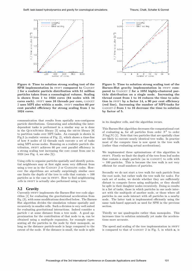
Figure 4: Time to solution strong scaling test of theSPH implementation in swift compared to Gadget2 for a realistic particle distribution with 51 millionparticles taken from a cosmological volume. Scalingis shown from 1 to 1024 cores (64 nodes with 16cores each). swift uses 16 threads per core, gadget2 uses MPI also within a node. swift reaches 60 percent parallel efficiency for strong scaling from 1 to1024 cores.

communication that results from spatially non-contiguousparticle distributions. Generating and scheduling the inter-dependent tasks is performed in a similar way as is donein the QuickSched library [5] using the metis library [8]to partition tasks over MPI tasks. An example is shown inFig.3 (a realistic version of Fig. 2), which shows a time-lineof how 8 nodes of 12 threads each execute a set of tasksusing MPI across nodes. Running on a realistic particle dis-tribution, swift achieves 60 per cent parallel efficiency ina strong scaling test increasing the core count from one to1024 (see Fig. 4, see also [5]).

Using cells to organise particles spatially and identify poten-tial neighbours may at first sight seem very different fromusing a tree as in the Gadget 2 or Gasoline codes. How-ever the algorithms are actually surprisingly similar onceone limits the depth of the tree to cells that contain ∼ 100particles as is the case in swift. How to find neighbouringcells in swift is actually also performed using a tree.

3.2 GravityCurrently swift implements the Barnes-Hut tree code algo-rithm [1] for evaluating the gravitational acceleration fromEq. (3), with some modifications described below. The Barnes-Hut algorithm divides the simulation volume spatially andrecursively in smaller cells. Such a division is very well suitedfor evaluating gravitational interactions. Indeed consider aparticle i at some distance from a tree node. A good ap-proximation for the contribution of that node to ai can beobtained using a multipole expansion, for example repre-senting all the particles in the node by their monopole, aslong as the distance particle-node is large compared to theextent of the node. If the distance is small, the node is split

Figure 5: Time to solution strong scaling test of theBarnes-Hut gravity implementation in swift com-pared to Gadget 2 for a 10M highly-clustered par-ticle distribution on a single node. Increasing thethread count from 1 to 16 reduces the time to solu-tion in swift by a factor 14, a 90 per cent efficiency(red line). Increasing the number of MPI-tasks forgadget-2 from 1 to 16 decrease the time to solutionby factor of 5.

in its daughter cells, and the algorithm recurs.

This Barnes-Hut algorithm decreases the computational costof evaluating ai for all particles from order N2 to orderN log(N) [1]. Note that two particles that are spatially closeare likely to execute nearly identical tree walks. In practisemost of the compute time is now spent in the tree walk(rather than evaluating actual accelerations).

We implemented three optimisations of this algorithm inswift. Firstly we limit the depth of the tree from leaf nodesthat contain a single particle (as in gadget) to cells with∼ 100 particles. This is because the tree walk is not veryefficient for small numbers of particles.

Secondly we do not start a tree walk for each particle fromthe root node, but rather walk the tree walk for nodes. Foreach set of nodes, we decide whether they are sufficientlydistant to compute forces using multipoles, or they shouldbe split in their daughter nodes recursively. Doing so resultsin a list of tasks, those in which particles in one node inter-act with the multipole of another node, or those where allparticles in one node interact with all particles in a nearbynode. The latter task is implemented efficiently using thesame task-based approach as used for SPH in the previoussection.

Thirdly we use quadrupoles rather than monopoles. Thisincreases time to solution minimally yet make the accelera-tions more accurate.

The speed and scaling of the tree implementation in swiftis compared to that of gadget 2 in Fig. 5, in which ai is



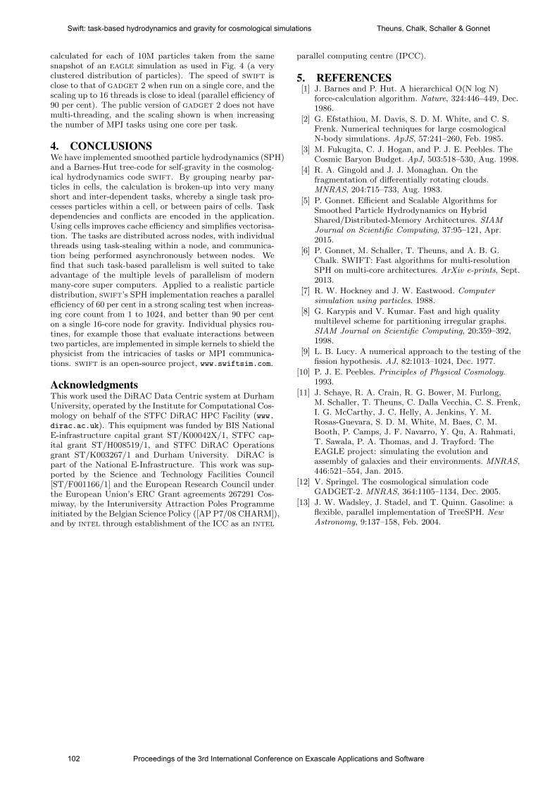
calculated for each of 10M particles taken from the samesnapshot of an eagle simulation as used in Fig. 4 (a veryclustered distribution of particles). The speed of swift isclose to that of gadget 2 when run on a single core, and thescaling up to 16 threads is close to ideal (parallel efficiency of90 per cent). The public version of gadget 2 does not havemulti-threading, and the scaling shown is when increasingthe number of MPI tasks using one core per task.

4. CONCLUSIONSWe have implemented smoothed particle hydrodynamics (SPH)and a Barnes-Hut tree-code for self-gravity in the cosmolog-ical hydrodynamics code swift. By grouping nearby par-ticles in cells, the calculation is broken-up into very manyshort and inter-dependent tasks, whereby a single task pro-cesses particles within a cell, or between pairs of cells. Taskdependencies and conflicts are encoded in the application.Using cells improves cache efficiency and simplifies vectorisa-tion. The tasks are distributed across nodes, with individualthreads using task-stealing within a node, and communica-tion being performed asynchronously between nodes. Wefind that such task-based parallelism is well suited to takeadvantage of the multiple levels of parallelism of modernmany-core super computers. Applied to a realistic particledistribution, swift’s SPH implementation reaches a parallelefficiency of 60 per cent in a strong scaling test when increas-ing core count from 1 to 1024, and better than 90 per centon a single 16-core node for gravity. Individual physics rou-tines, for example those that evaluate interactions betweentwo particles, are implemented in simple kernels to shield thephysicist from the intricacies of tasks or MPI communica-tions. swift is an open-source project, www.swiftsim.com.

AcknowledgmentsThis work used the DiRAC Data Centric system at DurhamUniversity, operated by the Institute for Computational Cos-mology on behalf of the STFC DiRAC HPC Facility (www.dirac.ac.uk). This equipment was funded by BIS NationalE-infrastructure capital grant ST/K00042X/1, STFC cap-ital grant ST/H008519/1, and STFC DiRAC Operationsgrant ST/K003267/1 and Durham University. DiRAC ispart of the National E-Infrastructure. This work was sup-ported by the Science and Technology Facilities Council[ST/F001166/1] and the European Research Council underthe European Union’s ERC Grant agreements 267291 Cos-miway, by the Interuniversity Attraction Poles Programmeinitiated by the Belgian Science Policy ([AP P7/08 CHARM]),and by intel through establishment of the ICC as an intel

parallel computing centre (IPCC).

5. REFERENCES[1] J. Barnes and P. Hut. A hierarchical O(N log N)

force-calculation algorithm. Nature, 324:446–449, Dec.1986.

[2] G. Efstathiou, M. Davis, S. D. M. White, and C. S.Frenk. Numerical techniques for large cosmologicalN-body simulations. ApJS, 57:241–260, Feb. 1985.

[3] M. Fukugita, C. J. Hogan, and P. J. E. Peebles. TheCosmic Baryon Budget. ApJ, 503:518–530, Aug. 1998.

[4] R. A. Gingold and J. J. Monaghan. On thefragmentation of differentially rotating clouds.MNRAS, 204:715–733, Aug. 1983.

[5] P. Gonnet. Efficient and Scalable Algorithms forSmoothed Particle Hydrodynamics on HybridShared/Distributed-Memory Architectures. SIAMJournal on Scientific Computing, 37:95–121, Apr.2015.

[6] P. Gonnet, M. Schaller, T. Theuns, and A. B. G.Chalk. SWIFT: Fast algorithms for multi-resolutionSPH on multi-core architectures. ArXiv e-prints, Sept.2013.

[7] R. W. Hockney and J. W. Eastwood. Computersimulation using particles. 1988.

[8] G. Karypis and V. Kumar. Fast and high qualitymultilevel scheme for partitioning irregular graphs.SIAM Journal on Scientific Computing, 20:359–392,1998.

[9] L. B. Lucy. A numerical approach to the testing of thefission hypothesis. AJ, 82:1013–1024, Dec. 1977.

[10] P. J. E. Peebles. Principles of Physical Cosmology.1993.

[11] J. Schaye, R. A. Crain, R. G. Bower, M. Furlong,M. Schaller, T. Theuns, C. Dalla Vecchia, C. S. Frenk,I. G. McCarthy, J. C. Helly, A. Jenkins, Y. M.Rosas-Guevara, S. D. M. White, M. Baes, C. M.Booth, P. Camps, J. F. Navarro, Y. Qu, A. Rahmati,T. Sawala, P. A. Thomas, and J. Trayford. TheEAGLE project: simulating the evolution andassembly of galaxies and their environments. MNRAS,446:521–554, Jan. 2015.

[12] V. Springel. The cosmological simulation codeGADGET-2. MNRAS, 364:1105–1134, Dec. 2005.

[13] J. W. Wadsley, J. Stadel, and T. Quinn. Gasoline: aflexible, parallel implementation of TreeSPH. NewAstronomy, 9:137–158, Feb. 2004.



www.swiftsim.com

www.dirac.ac.uk

www.dirac.ac.uk

Thread Parallelism for Highly Irregular Computation inAnisotropic Mesh Adaptation

Georgios RokosImperial College LondonLondon, United Kingdom

[email protected]

Gerard J. GormanImperial College LondonLondon, United Kingdom

[email protected] Ejlebjerg Jensen

Imperial College LondonLondon, United Kingdom

[email protected]

Paul H. J. KellyImperial College LondonLondon, United Kingdom

[email protected]

ABSTRACTThread-level parallelism in irregular applications with mu-table data dependencies presents challenges because the un-derlying data is extensively modified during execution of thealgorithm and a high degree of parallelism must be real-ized while keeping the code race-free. In this article we de-scribe a methodology for exploiting thread parallelism fora class of graph-mutating worklist algorithms, which guar-antees safe parallel execution via processing in rounds ofindependent sets and using a deferred update strategy tocommit changes in the underlying data structures. Scalabil-ity is assisted by atomic fetch-and-add operations to createworklists and work-stealing to balance the shared-memoryworkload. This work is motivated by mesh adaptation algo-rithms, for which we show a parallel efficiency of 60% and50% on IntelR©XeonR© Sandy Bridge and AMD OpteronTM

Magny-Cours systems, respectively, using these techniques.

Keywordsanisotropic mesh adaptivity, irregular data, shared-memoryparallelism, manycore, parallel worklist algorithm, topologymutation, graph colouring, work-stealing, deferred update

1. INTRODUCTIONFinite element/volume methods (FEM/FVM) are commonlyused in the numerical solution of partial differential equa-tions (PDEs). Unstructured meshes, where the spatial do-main has been discretised into simplices (i.e. triangles in2D, tetrahedra in 3D), are of particular interest in applica-tions where the geometric domain is complex and structuredmeshes are not practical. Simplices are well suited to vary-ing mesh resolution throughout the domain, allowing for lo-cal coarsening and refinement of the mesh without hangingnodes. On the other hand, this flexibility introduces compli-cations of its own, such as management of mesh quality andcomputational overheads arising from indirect addressing.

Computational mesh resolution is often the limiting factor insimulation accuracy. Being able to accurately resolve physi-cal processes at the small scale coupled with larger scale dy-namics is key to improving the fidelity of numerical modelsacross a wide range of applications (e.g. [15, 20]). A diffi-culty with mesh-based modelling is that the mesh is gener-ated before the solution is known, however, the local solution

error is related to the local mesh resolution. Overly coarsemeshes lead to low accuracy whereas over-refined meshescan greatly increase the computational cost.

Mesh adaptation methods provide an important means tominimise computational cost while still achieving the re-quired accuracy [16, 12]. In order to use mesh adaptationwithin a simulation, the application code requires a methodto estimate the local solution error. Given an error estimateit is then possible to compute a solution to a specified errortolerance while using the minimum resolution everywhere inthe domain and maintaining element quality constraints.

Previous work has described how adaptive mesh methodscan be parallelised for distributed-memory systems usingMPI (e.g. [12, 10]). However, there is a continuous trendtowards an increasing number of cores per compute node inthe world’s most powerful supercomputers and it is assumedthat the nodes of a future exascale system will each containthousands of cores [7]. Therefore, it is important that algo-rithms are developed with very high levels of parallelism andusing thread-parallel programming models, such as OpenMP[5], that exploit the memory hierarchy. However, irregu-lar applications are hard to parallelise effectively on shared-memory architectures for reasons described in [13].

In this article we take a fresh look at anisotropic adaptivemesh methods and parallelise them using new scalable tech-niques suitable for modern multicore and manycore architec-tures. These concepts have been implemented in the opensource framework PRAgMaTIc (Parallel anisotRopic Adap-tive Mesh ToolkIt)1. The remainder of the paper is laid outas follows: §2 gives an overview of the mesh adaptation pro-cedure; §3 describes the new irregular compute methodologyused to parallelise the adaptive algorithms; and §4 illustrateshow well our framework performs in 2D and 3D benchmarks.We conclude the paper in §5.

2. MESH ADAPTIVITY BACKGROUNDIn this section we give an overview of anisotropic mesh adap-tation, focusing on the element quality as defined by an errormetric and the adaptation kernels which iteratively improvelocal mesh quality as measured by the worst local element.

1http://meshadaptation.github.io/


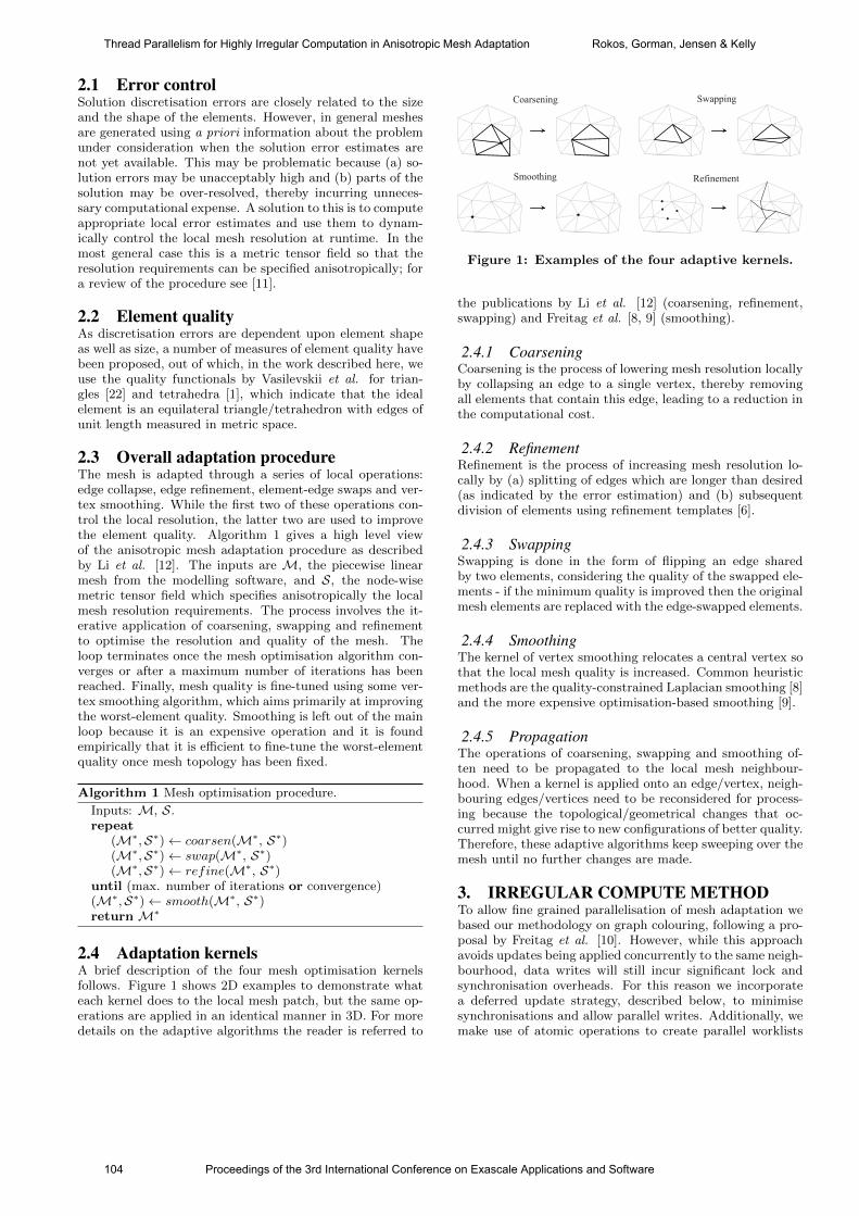
2.1 Error controlSolution discretisation errors are closely related to the sizeand the shape of the elements. However, in general meshesare generated using a priori information about the problemunder consideration when the solution error estimates arenot yet available. This may be problematic because (a) so-lution errors may be unacceptably high and (b) parts of thesolution may be over-resolved, thereby incurring unneces-sary computational expense. A solution to this is to computeappropriate local error estimates and use them to dynam-ically control the local mesh resolution at runtime. In themost general case this is a metric tensor field so that theresolution requirements can be specified anisotropically; fora review of the procedure see [11].

2.2 Element qualityAs discretisation errors are dependent upon element shapeas well as size, a number of measures of element quality havebeen proposed, out of which, in the work described here, weuse the quality functionals by Vasilevskii et al. for trian-gles [22] and tetrahedra [1], which indicate that the idealelement is an equilateral triangle/tetrahedron with edges ofunit length measured in metric space.

2.3 Overall adaptation procedureThe mesh is adapted through a series of local operations:edge collapse, edge refinement, element-edge swaps and ver-tex smoothing. While the first two of these operations con-trol the local resolution, the latter two are used to improvethe element quality. Algorithm 1 gives a high level viewof the anisotropic mesh adaptation procedure as describedby Li et al. [12]. The inputs are M, the piecewise linearmesh from the modelling software, and S, the node-wisemetric tensor field which specifies anisotropically the localmesh resolution requirements. The process involves the it-erative application of coarsening, swapping and refinementto optimise the resolution and quality of the mesh. Theloop terminates once the mesh optimisation algorithm con-verges or after a maximum number of iterations has beenreached. Finally, mesh quality is fine-tuned using some ver-tex smoothing algorithm, which aims primarily at improvingthe worst-element quality. Smoothing is left out of the mainloop because it is an expensive operation and it is foundempirically that it is efficient to fine-tune the worst-elementquality once mesh topology has been fixed.

Algorithm 1 Mesh optimisation procedure.

Inputs: M, S.repeat

(M∗,S∗)← coarsen(M∗, S∗)(M∗,S∗)← swap(M∗, S∗)(M∗,S∗)← refine(M∗, S∗)

until (max. number of iterations or convergence)(M∗,S∗)← smooth(M∗, S∗)return M∗

2.4 Adaptation kernelsA brief description of the four mesh optimisation kernelsfollows. Figure 1 shows 2D examples to demonstrate whateach kernel does to the local mesh patch, but the same op-erations are applied in an identical manner in 3D. For moredetails on the adaptive algorithms the reader is referred to

Coarsening Swapping

Smoothing Refinement

Figure 1: Examples of the four adaptive kernels.

the publications by Li et al. [12] (coarsening, refinement,swapping) and Freitag et al. [8, 9] (smoothing).

2.4.1 CoarseningCoarsening is the process of lowering mesh resolution locallyby collapsing an edge to a single vertex, thereby removingall elements that contain this edge, leading to a reduction inthe computational cost.

2.4.2 RefinementRefinement is the process of increasing mesh resolution lo-cally by (a) splitting of edges which are longer than desired(as indicated by the error estimation) and (b) subsequentdivision of elements using refinement templates [6].

2.4.3 SwappingSwapping is done in the form of flipping an edge sharedby two elements, considering the quality of the swapped ele-ments - if the minimum quality is improved then the originalmesh elements are replaced with the edge-swapped elements.

2.4.4 SmoothingThe kernel of vertex smoothing relocates a central vertex sothat the local mesh quality is increased. Common heuristicmethods are the quality-constrained Laplacian smoothing [8]and the more expensive optimisation-based smoothing [9].

2.4.5 PropagationThe operations of coarsening, swapping and smoothing of-ten need to be propagated to the local mesh neighbour-hood. When a kernel is applied onto an edge/vertex, neigh-bouring edges/vertices need to be reconsidered for process-ing because the topological/geometrical changes that oc-curred might give rise to new configurations of better quality.Therefore, these adaptive algorithms keep sweeping over themesh until no further changes are made.

3. IRREGULAR COMPUTE METHODTo allow fine grained parallelisation of mesh adaptation webased our methodology on graph colouring, following a pro-posal by Freitag et al. [10]. However, while this approachavoids updates being applied concurrently to the same neigh-bourhood, data writes will still incur significant lock andsynchronisation overheads. For this reason we incorporatea deferred update strategy, described below, to minimisesynchronisations and allow parallel writes. Additionally, wemake use of atomic operations to create parallel worklists


Thread Parallelism for Highly Irregular Computation in Anisotropic Mesh Adaptation Rokos, Gorman, Jensen & Kelly

in a synchronisation-free fashion and, finally, try to balancethe workload among threads using work-stealing [3].

3.1 HazardsThere are two types of hazards when running mesh optimi-sation algorithms in parallel: topological hazards; and dataraces. The former refers to the situation where an adaptiveoperation results in invalid or non-conforming edges and el-ements. For example in coarsening, if some vertex VB col-lapses onto another vertex VA, then VA cannot collapse ontosome other vertex at the same time. Data races can oc-cur when two threads try to update the same adjacency listof a vertex concurrently. For example in coarsening, twoneighbours of some vertex VA can collapse onto VA concur-rently, then VA’s adjacency list has to be updated to reflectthe changes made by the coarsening operations. Concurrentaccess to VA’s adjacency list may lead to race conditions.

3.2 ColouringTopological hazards for all adaptive algorithms are avoidedby colouring a graph whose nodes are defined by the meshvertices and edges are defined by the mesh edges. The adap-tive algorithm then processes the mesh in batches of inde-pendent sets. The fact that topological changes are madeto the mesh means that colouring is invalidated frequentlyand the mesh has to be re-coloured before proceeding to thenext iteration of the adaptive algorithm. Therefore, we needto use a fast and scalable colouring algorithm (see [18]).

3.3 Deferred UpdateColouring does not eliminate data races when updating ad-jacency lists. A 2-distance colouring was not considered hereas it is expensive and increases the chromatic number, effec-tively reducing the exposed parallelism. Instead, in a shared-memory environment with N threads, each thread allocatesa private collection of N lists. When the adjacency list ofsome vertex Vi has to be updated, the thread executing theadaptive kernel does not commit the update immediately;instead, it pushes the operation back into the list for threadtid = ID(Vi)%N , where ID(Vi) is the integer identifier ofVi. After processing an independent set and before pro-ceeding to the next one, every thread Ti visits the privatecollections of all threads, locates the list reserved for Ti andcommits the updates stored there. This way, it is guaranteedthat one and only thread will update the adjacency list ofany given vertex. We call this technique the deferred update.Code Snippet 1 demonstrates a typical usage scenario. Animportant advantage of this strategy is that we always readthe most up-to-date data when executing an adaptive kernel(as if we used an “as we go” write-back scheme), eliminatingthe risk of mesh data corruption in coarsening, refinementand swapping and having a faster-converging Gauss-Seidel-style iteration process in smoothing.

3.4 Worklists and Atomic-CaptureThere are many cases where it is necessary to create a work-list of items which need to be processed, e.g. for propagationof adaptive operations. New work items generated locally bya thread need to be accumulated into a global worklist overwhich the next invocation of the adaptive kernel will iterate.The classic approach based on prefix sums [2] requires thread

1 typede f std : : vector<Updates> DefUpdList ;2 i n t N = omp_get_max_threads ( ) ;3

4 // N c o l l e c t i o n s o f de f e r red−update l i s t s5 std : : vector< std : : vector<DefUpdList> > defUpd ( N ) ;6

7 #pragma omp p a r a l l e l8 9 i n t tid = omp_get_thread_num ( ) ;

10 // Al l o ca t e one l i s t f o r each thread .11 defUpd [ tid ] . resize ( N ) ;12

13 // Process the independent s e t in p a r a l l e l14 #pragma omp f o r15 f o r ( i n t i=0; i<nVerticesInSet ; ++i )16 update = execute_kernel ( i ) ;17 // To be committed by thread i%N.18 defUpd [ tid ] [ i%N ] . push_back ( update ) ;19 20

21 // Commit updates t i d i s r e s p on s i b l e f o r .22 f o r ( i n t i=0; i<N ; ++i )23 commit_all_updates ( defUpd [ i ] [ tid ] ) ;24

25 // Proceed to the next independent s e t . . .26

Code Snippet 1: Example of the deferred update scheme.

synchronisation and was found limiting in terms of scalabil-ity. A better method is based on atomic fetch-and-add on aglobal integer which stores the size of the worklist needed sofar. Every thread increments this integer atomically whilecaching the old value. This way, the thread knows where tocopy its private data and increments the integer by the sizeof this data, so the next thread to access the integer knows inturn where to copy its private data. An example of using thistechnique via OpenMP’s atomic-capture clause [14] is givenin Code Snippet 2, where it is shown that no thread syn-chronisation is needed to generate the global worklist (notethe nowait clause). The overhead/spinlock associated withatomic-capture operations was found to be insignificant.

1 i n t worklistSize = 0;2 std : : vector<Item> globalWorklist ( prealloc_size ) ;3

4 #pragma omp p a r a l l e l5 6 std : : vector<Item> private_list ;7

8 #pragma omp f o r nowait9 f o r ( all items which need to be processed )

10 new_item = do_some_work ( ) ;11 private_list . push_back ( new_item ) ;12 // No need to synchron i s e at end o f loop .13

14 i n t idx ;15 #pragma omp atomic capture16 17 idx = worklistSize ;18 worklistSize += private_list . size ( ) ;19 20

21 memcpy (&globalWorklist [ idx ] , &private_list [ 0 ] ,22 private_list . size ( ) ∗ s i z e o f ( Item ) ) ;23

Code Snippet 2: Creating a worklist using atomic-capture.

3.5 Work-stealingWork-stealing [3] is a sophisticated technique aiming at bal-ancing workload among threads while keeping scheduling



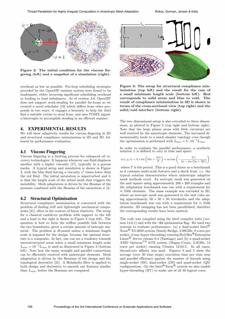
Figure 2: The initial condition for the viscous fin-gering (left) and a snapshot of a simulation (right).

overhead as low as possible. For-loop scheduling strategiesprovided by the OpenMP runtime system were found to beinadequate, either incurring significant scheduling overheador leading to load imbalances. As of version 4.0, OpenMPdoes not support work-stealing for parallel for-loops so wecreated a novel scheduler [19] which differs from other pro-posals in two ways: it engages a heuristic to help the thieffind a suitable victim to steal from; and uses POSIX signal-s/interrupts to accomplish stealing in an efficient manner.

4. EXPERIMENTAL RESULTSWe will show adaptivity results for viscous fingering in 2Dand structural compliance minimisation in 2D and 3D, fol-lowed by performance evaluation.

4.1 Viscous FingeringViscous fingering is a limiting process for enhanced oil re-covery technologies. It happens whenever one fluid displacesanother with a higher viscosity [17], typically in a porousmedia. A typical setup and simulation is shown in Figure2, with the blue fluid having a viscosity e2 times lower thanthe red fluid. The initial saturation is unperturbed and itis thus the length scale of the initial mesh that triggers theinstability. Mesh adaptation is driven by the Hessian of thepressure combined with the Hessian of the saturation φ [4].

4.2 Structural OptimisationStructural compliance minimisation is concerned with theproblem of finding stiff and lightweight mechanical compo-nents [21], often in the context of linear elasticity. The setupfor a classical cantilever problem with support to the leftand a load to the right is shown in Figure 3 (top left). Thequestion is how to form the stiffest possible link betweenthe two boundaries, given a certain amount of isotropic ma-terial. The problem is ill-posed unless a minimum lengthscale is imposed for the design, because the optimal struc-ture is a composite. In fact, one can see a tendency towardsmicrostructured areas when a small minimum length scaleLmin = 10−3Lchar is used as illustrated in Figure 3 (bottomleft). Note how the many straight and parallel connectionscan be efficiently resolved with anisotropic elements. Meshadaptation is driven by the Hessians of the design and thetopological derivative [21]. A Helmholtz filter is applied toboth design and derivative to smooth out features smallerthan Lmin, before the Hessians are computed.

Figure 3: The setup for structural compliance min-imisation (top left) and the result for the case ofa small minimum length scale (bottom left). Redcorresponds to solid areas and blue to void. Theresult of compliance minimisation in 3D is shown interms of the cross-sectional view (top right) and thesolid/void interface (bottom right).

The two dimensional setup is also extruded to three dimen-sions, as plotted in Figure 3 (top right and bottom right).Note that the large planar areas with little curvature arewell resolved by the anisotropic elements. The increased di-mensionality leads to a much simpler topology even thoughthe optimisation is performed with Lmin = 5 · 10−3Lchar.

In order to evaluate the parallel performance, a syntheticsolution ψ is defined to vary in time and space:

ψ(x, y, t) = 0.1 sin

(50x+

2πt

T

)+ arctan

(−

0.1

2x− sin(5y + 2πt

T

))

where T is the period. This is a good choice as a benchmarkas it contains multi-scale features and a shock front, i.e. thetypical solution characteristics where anisotropic adaptivemesh methods excel. An isotropic mesh was generated onthe unit square using approximately 200×200 triangles andthe adaptation benchmark was run with a requirement for≈ 550k elements. The same example was extruded in 3D,where an isotropic mesh was generated in the unit cube us-ing approximately 50 × 50 × 50 tetrahedra and the adap-tation benchmark was run with a requirement for ≈ 210kelements. 3D swapping has not been parallelised, thereforethe corresponding results have been omitted.

The code was compiled using the Intel compiler suite (ver-sion 14.0.1) and with the -O3 optimisation flag. We used twosystems to evaluate performance: (a) a dual-socket IntelR©

XeonR© E5-2650 system (Sandy Bridge, 2.00GHz, 8 cores persocket, 2-way hyper-threading) running Red HatR©EnterpriseLinuxR© Server release 6.4 (Santiago) and (b) a quad-socketAMD OpteronTM 6176 system (Magny-Cours, 2.3GHz, 12cores per socket) running Ubuntu 12.04.5. In all cases,thread-core affinity was used. Figures 4 and 5 show theaverage (over 50 time steps) execution time per time stepand parallel efficiency against the number of threads usingsingle-socket (SS), dual-socket (DS) and quad-socket (QS)configurations. On the IntelR©XeonR© system we also enablehyper-threading (HT) to make use of all 40 logical cores.



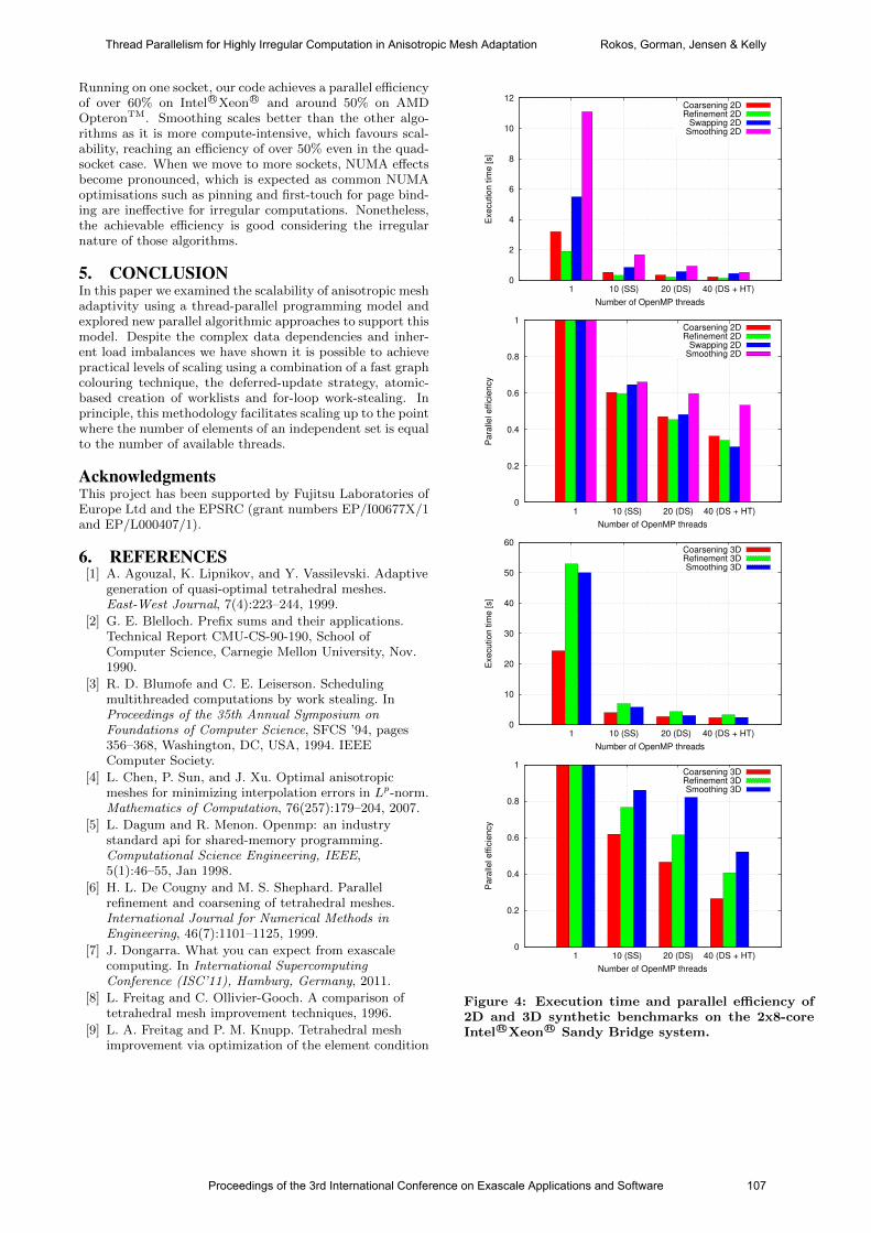
Running on one socket, our code achieves a parallel efficiencyof over 60% on IntelR©XeonR© and around 50% on AMDOpteronTM. Smoothing scales better than the other algo-rithms as it is more compute-intensive, which favours scal-ability, reaching an efficiency of over 50% even in the quad-socket case. When we move to more sockets, NUMA effectsbecome pronounced, which is expected as common NUMAoptimisations such as pinning and first-touch for page bind-ing are ineffective for irregular computations. Nonetheless,the achievable efficiency is good considering the irregularnature of those algorithms.

5. CONCLUSIONIn this paper we examined the scalability of anisotropic meshadaptivity using a thread-parallel programming model andexplored new parallel algorithmic approaches to support thismodel. Despite the complex data dependencies and inher-ent load imbalances we have shown it is possible to achievepractical levels of scaling using a combination of a fast graphcolouring technique, the deferred-update strategy, atomic-based creation of worklists and for-loop work-stealing. Inprinciple, this methodology facilitates scaling up to the pointwhere the number of elements of an independent set is equalto the number of available threads.

AcknowledgmentsThis project has been supported by Fujitsu Laboratories ofEurope Ltd and the EPSRC (grant numbers EP/I00677X/1and EP/L000407/1).

6. REFERENCES[1] A. Agouzal, K. Lipnikov, and Y. Vassilevski. Adaptive

generation of quasi-optimal tetrahedral meshes.East-West Journal, 7(4):223–244, 1999.

[2] G. E. Blelloch. Prefix sums and their applications.Technical Report CMU-CS-90-190, School ofComputer Science, Carnegie Mellon University, Nov.1990.

[3] R. D. Blumofe and C. E. Leiserson. Schedulingmultithreaded computations by work stealing. InProceedings of the 35th Annual Symposium onFoundations of Computer Science, SFCS ’94, pages356–368, Washington, DC, USA, 1994. IEEEComputer Society.

[4] L. Chen, P. Sun, and J. Xu. Optimal anisotropicmeshes for minimizing interpolation errors in Lp-norm.Mathematics of Computation, 76(257):179–204, 2007.

[5] L. Dagum and R. Menon. Openmp: an industrystandard api for shared-memory programming.Computational Science Engineering, IEEE,5(1):46–55, Jan 1998.

[6] H. L. De Cougny and M. S. Shephard. Parallelrefinement and coarsening of tetrahedral meshes.International Journal for Numerical Methods inEngineering, 46(7):1101–1125, 1999.

[7] J. Dongarra. What you can expect from exascalecomputing. In International SupercomputingConference (ISC’11), Hamburg, Germany, 2011.

[8] L. Freitag and C. Ollivier-Gooch. A comparison oftetrahedral mesh improvement techniques, 1996.

[9] L. A. Freitag and P. M. Knupp. Tetrahedral meshimprovement via optimization of the element condition

0

2

4

6

8

10

12

1 10 (SS) 20 (DS) 40 (DS + HT)

Execution tim

e [s]

Number of OpenMP threads

Coarsening 2DRefinement 2D

Swapping 2DSmoothing 2D

0

0.2

0.4

0.6

0.8

1

1 10 (SS) 20 (DS) 40 (DS + HT)

Para

llel effic

iency




0

10

20

30

40

50

60

1 10 (SS) 20 (DS) 40 (DS + HT)

Execution tim

e [s]


Coarsening 3DRefinement 3DSmoothing 3D

0

0.2

0.4

0.6

0.8

1

1 10 (SS) 20 (DS) 40 (DS + HT)

Para

llel effic

iency



Figure 4: Execution time and parallel efficiency of2D and 3D synthetic benchmarks on the 2x8-coreIntel R©Xeon R© Sandy Bridge system.



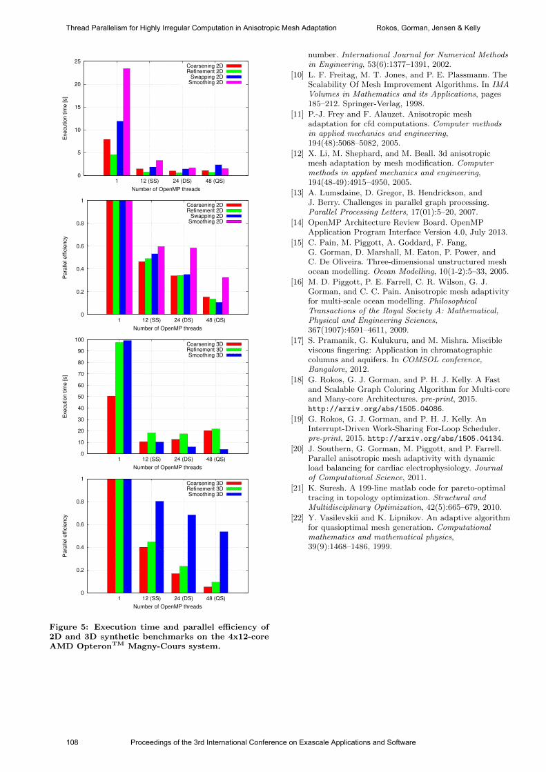
0

5

10

15

20

25

1 12 (SS) 24 (DS) 48 (QS)

Execution tim

e [s]




0

0.2

0.4

0.6

0.8

1

1 12 (SS) 24 (DS) 48 (QS)

Para

llel effic

iency




0

10

20

30

40

50

60

70

80

90

100

1 12 (SS) 24 (DS) 48 (QS)

Execution tim

e [s]



0

0.2

0.4

0.6

0.8

1

1 12 (SS) 24 (DS) 48 (QS)

Para

llel effic

iency



Figure 5: Execution time and parallel efficiency of2D and 3D synthetic benchmarks on the 4x12-coreAMD OpteronTM Magny-Cours system.

number. International Journal for Numerical Methodsin Engineering, 53(6):1377–1391, 2002.

[10] L. F. Freitag, M. T. Jones, and P. E. Plassmann. TheScalability Of Mesh Improvement Algorithms. In IMAVolumes in Mathematics and its Applications, pages185–212. Springer-Verlag, 1998.

[11] P.-J. Frey and F. Alauzet. Anisotropic meshadaptation for cfd computations. Computer methodsin applied mechanics and engineering,194(48):5068–5082, 2005.

[12] X. Li, M. Shephard, and M. Beall. 3d anisotropicmesh adaptation by mesh modification. Computermethods in applied mechanics and engineering,194(48-49):4915–4950, 2005.

[13] A. Lumsdaine, D. Gregor, B. Hendrickson, andJ. Berry. Challenges in parallel graph processing.Parallel Processing Letters, 17(01):5–20, 2007.

[14] OpenMP Architecture Review Board. OpenMPApplication Program Interface Version 4.0, July 2013.

[15] C. Pain, M. Piggott, A. Goddard, F. Fang,G. Gorman, D. Marshall, M. Eaton, P. Power, andC. De Oliveira. Three-dimensional unstructured meshocean modelling. Ocean Modelling, 10(1-2):5–33, 2005.

[16] M. D. Piggott, P. E. Farrell, C. R. Wilson, G. J.Gorman, and C. C. Pain. Anisotropic mesh adaptivityfor multi-scale ocean modelling. PhilosophicalTransactions of the Royal Society A: Mathematical,Physical and Engineering Sciences,367(1907):4591–4611, 2009.

[17] S. Pramanik, G. Kulukuru, and M. Mishra. Miscibleviscous fingering: Application in chromatographiccolumns and aquifers. In COMSOL conference,Bangalore, 2012.

[18] G. Rokos, G. J. Gorman, and P. H. J. Kelly. A Fastand Scalable Graph Coloring Algorithm for Multi-coreand Many-core Architectures. pre-print, 2015.http://arxiv.org/abs/1505.04086.

[19] G. Rokos, G. J. Gorman, and P. H. J. Kelly. AnInterrupt-Driven Work-Sharing For-Loop Scheduler.pre-print, 2015. http://arxiv.org/abs/1505.04134.

[20] J. Southern, G. Gorman, M. Piggott, and P. Farrell.Parallel anisotropic mesh adaptivity with dynamicload balancing for cardiac electrophysiology. Journalof Computational Science, 2011.

[21] K. Suresh. A 199-line matlab code for pareto-optimaltracing in topology optimization. Structural andMultidisciplinary Optimization, 42(5):665–679, 2010.

[22] Y. Vasilevskii and K. Lipnikov. An adaptive algorithmfor quasioptimal mesh generation. Computationalmathematics and mathematical physics,39(9):1468–1486, 1999.



http://arxiv.org/abs/1505.04086

http://arxiv.org/abs/1505.04134

Paradigm Shift for EXASCALE Computing

George MatheouDepartment of Computer

Science,University of Cyprus, [email protected]

Paraskevas EvripidouDepartment of Computer

Science,University of Cyprus, Cyprus

[email protected]

Costas KyriacouComputer Science and

Engineering Department,Frederick University, Cyprus

[email protected]

ABSTRACTIn this paper we propose a paradigm shift for exascale com-puting by using a Hybrid Data-Flow/Control-Flow model ofexecution. Programming of High Performance Computersis mainly done through parallel extension of the sequentialmodel like MPI and OpenMP. Even though these extensionsfacilitate high productivity parallel programming, they suf-fer from the inability to tolerate long latencies.

The Data-Flow model of execution enforces only a partialordering as dictated by the true data-dependencies. This isvery beneficial for parallel processing because it allows toexploit the maximum parallelism. Furthermore it toleratessynchronization and communication latencies. We believethat a paradigm shift to a hybrid Data-Flow and Control-Flow system will improve the performance of High Perfor-mance Computing (HPC).

Data Driven Multithreading (DDM), a threaded Data-Flowprogramming/execution model, could be the platform forthe HPC paradigm shift. Our work on DDM showed thatDDM can efficiently run on state-of-the-art sequential ma-chines, resulting in a Hybrid Data-Flow/Control-Flow sys-tem.

Evaluation results of DDM implementations on a varietyof platforms showed that DDM can indeed tolerate syn-chronization and communication latency. When comparingDDM with OpenMP, DDM performed better for all bench-marks used. This is primarily due to the fact that DDMeffectively tolerates latency. Similar results were also ob-tained when comparing DDM implemented on a Cell pro-cessor, with CellSs and Sequoia.

KeywordsParallel Programming, Data-Flow, Data Driven Multi-threading

1. INTRODUCTIONHigh Performance Computers and Supercomputers targetlarge problems that have a high degree of parallelism. Pro-gramming of such machines is mainly done through parallelextensions of the sequential models like MPI and OpenMP.These extensions do facilitate high productivity parallel pro-gramming, but also suffer from the limitations of the se-quential synchronization and their inability to tolerate longlatencies. Arvind and Iannucci [4], Data-Flow proponents,have been warning us since the 1980’s about the two fun-

damental issues in Multiprocessing: “long memory latenciesand waits due to synchronization events”. In their questto develop an exascale supercomputer, the United States,through its DARPA agency, commissioned a study [14, 15] in2007 to determine what kind of technologies will be neededto build such a supercomputer. Peter Kogge, the leaderof the DARPA/USA study group for exascale computing,confirmed that the communication and synchronization la-tencies of the sequential model are getting out of hand forHPC/Exascale machines. Furthermore, Kogge, states thatthe power consumption of an exascale computer, will bearound 500 MW. Michael Flynn stated in his keynote speechat FPL 2012 [9] that “We have multi-threaded, superscalarcores with limited ILP; worse yet, most of the die area (80%)is devoted to two or three levels of cache to support theillusion of sequential model”. Thus, a paradigm shift forexascale computing is necessary.

Data-Flow is a programming/execution model that providestolerance to communication and synchronization latencies.Data-Flow has been proposed by a number of researchersas an alternative to the Control-Flow model [7, 11, 4]. Aparadigm shift to Data-Flow based systems can reduce thepower consumption by architectural and organization opti-mizations. Deterministic prefetching to scratch-pad mem-ories, driven by Data-Flow, can reduce the SDRAM needsof the multi/many-core systems considerably. Furthermore,Data-Flow systems do not need complex modules such asout-of-order execution, thus, the real-estate needs and thepower consumption could be reduced. The partial orderingof the Data-Flow model reduces significantly the synchro-nization latencies to only the true data-dependencies. Data-Flow does not need cache coherence because it adheres tothe single assignment semantics. Thus, there is no need forbarriers and critical sections. In short, the Data-Flow modelcan address some of the major issues that can help towardsthe development of an exascale supercomputer.

SWARM (SWiFt Adaptive Runtime Machine) aims in Scal-able Performance Optimizations for multi-core/multi-nodesystems. SWARM is based on the codelets model which wasdeveloped by the Data-Flow group of an earlier Data-Flowbased project, the EARTH project [12]. SWARM dividesa program into tasks, with runtime dependencies and con-straints that can be executed when all runtime dependenciesand constraints are met. The runtime schedules the tasksfor execution based on resource availability. SWARM is ob-ject oriented with a two-level threading system: the first


level is heavy-weight bound to processing resources, and thesecond level it consists of light-weight threads that run non-preemptively. SWARM was compared with the current su-percomputing state-of-the-art: OpenMP and MPI. Resultsdemonstrated that SWARM can outperform OpenMP evenin embarrassingly parallel applications such as the Barrness-Hut. When compared with MPI on the Graph500 bench-mark, SWARM showed consistent speedups up to 14.5 onfour supercomputers: Sandia Redsky with 8 processors pernode, and TACC Lonestar, Intel Endeavor, ORNL Jaquarwith 12 processors per node.

Data-Driven Multithreading (DDM) [17] is an executionmodel that allows Data-Driven scheduling on sequential pro-cessors. The core of the DDM model is the Thread Schedul-ing Unit (TSU) which schedules threads dynamically at run-time based on data availability. In DDM, a program isdivided into a number of threads. For each thread it col-lects meta-data that enable the TSU to manage the depen-dencies among the threads and determine when a threadcan be scheduled for execution. Data-Driven scheduling en-forces only a partial ordering as dictated by the true data-dependencies which is the minimum synchronization possi-ble. This is very beneficial for parallel processing becauseit exploits the maximum possible parallelism. Furthermore,DDM can be implemented on state-of-the-art Control-Flowmachines, running in a threaded Data-Flow mode, with theprogrammer or the system being able to switch between theControl-Flow and the Data-Flow modes of execution. Thus,resulting in a Hybrid Data-Flow/Control-Flow system.

The DDM model was evaluated by four different softwareimplementations: the Data-Driven Network of Workstations(D2Now) [17], the Thread Flux Parallel Processing Plat-form (TFlux) [21], the Data-Driven Multithreading VirtualMachine (DDM-VM) [2], and DDM++, the latest softwareDDM implementation. DDM++ is an object oriented im-plementation of DDM that takes advantage of object ori-ented techniques such as maintainability, re-usability, data-abstraction and encapsulation. DDM++ programs are de-veloped faster and easier because there is no need of usingmacros, like in the previous DDM implementations. In theprevious DDM systems, the threads’ code was embodied inthe main function of the program, and macros were usedfor executing them, using GOTO commands. In DDM++the threads’ code is embodied in standard C functions. It isnoteworthy that the DDM applications developed in DDM-VM are more than two times larger than in the DDM++implementation. DDM was also evaluated by two hardwareimplementations where the TSU with an 8-core processorwere built on an FPGA.

Evaluation results of DDM on a variety of platforms showedthat DDM can indeed tolerate synchronization and com-munication latencies. DDM outperformed OpenMP for allbenchmarks. Similar results were obtained when comparingDDM implemented on a cluster of four Cell processors, withCellSs and Sequoia.

Our work on CacheFlow, the memory hierarchy system forDDM, showed that the TSU is aware of the threads sched-uled for execution in the near future, and hence the datathat will be needed in the near future. This enables the

implementation of optimized cache placement and replace-ment policies, resulting in the need of smaller caches, or thereplacement of the cache with a small scratch-pad memory.Furthermore, taking advantage of the near future memoryreferences results in more efficient cache replacement policiesthat reduce bus/network traffic and power consumption.

Data-Flow provides tolerance to communication and syn-chronization latencies, and has the potential of making theprocessor smaller and more power efficient. Thus, it makessense to consider a shift to the Data-Flow paradigm now.

2. DATA-DRIVEN MULTITHREADINGThe Data-Driven Multithreading (DDM) [17] is a non-blocking multithreading model that allows data-drivenscheduling on sequential processors. A DDM thread (calledDThread) is scheduled for execution after all of its requireddata have been produced, thus no synchronization or com-munication latencies are experienced after a DThread beginsexecution. In the DDM model, DThreads have producer-consumer relationships. DThreads’ instructions are exe-cuted by the CPU sequentially in a Control-Flow manner.This allows the exploitation of Control-Flow optimizations,either by the CPU at runtime or statically by the compiler.

In DDM, a program consists of the DThreads code, theThread Templates and the Dependency Graph. A ThreadTemplate holds the meta-data of a DThread. The lat-ter describes the consumer-producer dependencies amongstthe DThreads. DDM is utilizing the Thread SchedulingUnit (TSU), a special module responsible for schedulingthe DThreads in a data-driven manner. The TSU uses theThread Templates and the Dependency Graph to scheduleDThreads for execution when all of their producer-threadscompleted their execution. This ensures that all data neededby a DThread is available, before it is scheduled for execu-tion.

2.1 DDM ImplementationsThe DDM model was evaluated by several software imple-mentations. The first implementation, the D2Now [17], wastargeting Networks of Workstations. It has illustrated themajor components of DDM such as the TSU and CacheFlow[16]. The evaluation was done using execution driven sim-ulations. That was followed by two other implementations,the TFlux [21] and the DDM-VM [2]. Both TFlux andDDM-VM were targeting data-driven concurrency on se-quential multiprocessors. DDM-VM supported distributedmulti-core systems for both homogeneous and heterogeneoussystems. TFlux also developed the TFlux directives and asource-to-source compiler. The TFlux compiler was grad-ually extended to support all DDM systems. The latestsoftware DDM implementation, the DDM++, is an objectoriented implementation that takes advantage of object ori-ented techniques such as maintainability, re-usability, data-abstraction and encapsulation.

DDM was also evaluated by two hardware implementations.In the first one, the TSU was implemented as a hardware pe-ripheral in the Verilog language and it was evaluated througha Verilog-based simulation [18]. The results show that theTSU module can be implemented on an FPGA device with amoderate hardware budget. The second one [19] was the full


Paradigm Shift for EXASCALE Computing Matheou, Evripidou & Kyriacou

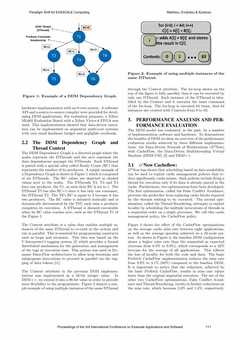
Figure 1: Example of a DDM Dependency Graph.

hardware implementation with an 8-core system. A softwareAPI and a source-to-source compiler were provided for devel-oping DDM applications. For evaluation purposes, a XilinxML605 Evaluation Board with a Xilinx Virtex-6 FPGA wasused. This implementation showed that data-driven execu-tion can be implemented on sequential multi-core systemswith very small hardware budget and negligible overheads.

2.2 The DDM Dependency Graph andThread Context

The DDM Dependency Graph is a directed graph where thenodes represent the DThreads and the arcs represent thedata dependencies amongst the DThreads. Each DThreadis paired with a special value called Ready Count (RC) thatrepresents the number of its producers. A simple example ofa Dependency Graph is shown in Figure 1 which is composedof six DThreads. The RC values are depicted as shadedvalues next to the nodes. The DThreads T2, T3 and T4have one producer, the T1, as such their RC is set to 1. TheDThread T5 has also RC=1 since it has only one consumer,the DThread T2. The T6’s RC is equal to 2 because it hastwo producers. The RC value is initiated statically and isdynamically decremented by the TSU each time a producercompletes its execution. A DThread is deemed executablewhen its RC value reaches zero, such as the DThread T1 ofthe Figure 1.

The Context attribute is a value that enables multiple in-stances of the same DThread to co-exist in the system andrun in parallel. This is essential for programming constructssuch as loops and recursion. This idea was based on theU-Interpreter’s tagging system [5] which provides a formaldistributed mechanism for the generation and managementof the tags at execution time. This system was used in Dy-namic Data-Flow architectures to allow loop iterations andsubprogram invocations to proceed in parallel via the tag-ging of data tokens [11].

The Context attribute in the previous DDM implemen-tations was implemented as a 32-bit integer value. InDDM++, we extend it into a 96-bit value in order to providemore flexibility to the programmers. Figure 2 depicts a sim-ple example of using multiple instances of the same DThread

Figure 2: Example of using multiple instances of thesame DThread.

through the Context attribute. The for-loop shown on thetop of the figure is fully parallel, thus it can be executed byonly one DThread. Each instance of the DThread is iden-tified by the Context and it executes the inner commandof the for-loop. The for-loop is executed 64 times, thus 64instances are created with Contexts from 0 to 63.

3. PERFORMANCE ANALYSIS AND PER-FORMANCE EVALUATION

The DDM model was evaluated, in the past, by a numberof implementation, software and hardware. To demonstratethe benefits of DDM we show an overview of the performanceevaluation results achieved by three different implementa-tions: the Data-Driven Network of Workstations (D2Now)with CacheFlow, the Data-Driven Multithreading VirtualMachine (DDM-VM) [3] and DDM++.

3.1 D2Now Cacheflow:D2Now has shown that scheduling based on data availabilitycan be used to exploit cache management policies that re-duce significantly cache misses. Such policies include firing athread for execution only if its data is already placed in thecache. Furthermore, two optimizations have been developed.The first optimization, called the False Conflict Avoidance,prevents the prefetcher from replacing cache blocks requiredby the threads waiting to be executed. The second opti-mization, called the Thread Reordering, attempts to exploitlocality by scheduling the multiple invocations of threads ina sequential order on a single processor. We call this cachemanagement policy, the CacheFlow policy.

Figure 3 shows the effect of the CacheFlow optimizationson the average cache miss rate between eight applications,as well as the average speedup achieved on a 32-node sys-tem. As shown in Figure 3, the baseline DDM configurationshows a higher miss rate than the sequential as expected(increase from 6.9% to 9.8%), which corresponds to a 42%increase for the average of all applications. This reflectsthe loss of locality for both the code and data. The basicPrefetch CacheFlow implementation reduces the miss ratefrom 9.8% to 3.1% (68%) compared to the baseline DDM.It is important to notice that the reduction, achieved bythe basic Prefetch CacheFlow, results in miss rate valueslower than the original sequential execution. The use of theother two CacheFlow optimizations, False Conflict Avoid-ance and Thread Reordering, results in further reductions onthe miss rate, which becomes 2.0% and 1.4%, respectively.



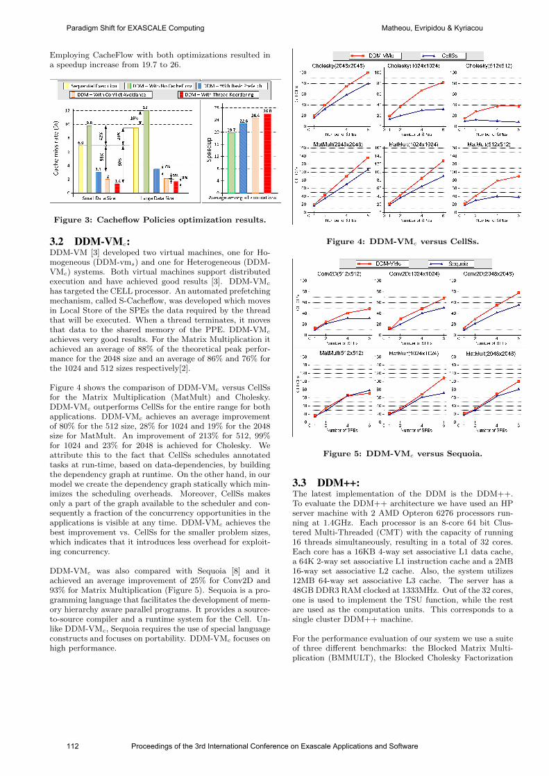
Employing CacheFlow with both optimizations resulted ina speedup increase from 19.7 to 26.

Figure 3: Cacheflow Policies optimization results.

3.2 DDM-VMc:DDM-VM [3] developed two virtual machines, one for Ho-mogeneous (DDM-vms) and one for Heterogeneous (DDM-VMc) systems. Both virtual machines support distributedexecution and have achieved good results [3]. DDM-VMc

has targeted the CELL processor. An automated prefetchingmechanism, called S-Cacheflow, was developed which movesin Local Store of the SPEs the data required by the threadthat will be executed. When a thread terminates, it movesthat data to the shared memory of the PPE. DDM-VMc

achieves very good results. For the Matrix Multiplication itachieved an average of 88% of the theoretical peak perfor-mance for the 2048 size and an average of 86% and 76% forthe 1024 and 512 sizes respectively[2].

Figure 4 shows the comparison of DDM-VMc versus CellSsfor the Matrix Multiplication (MatMult) and Cholesky.DDM-VMc outperforms CellSs for the entire range for bothapplications. DDM-VMc achieves an average improvementof 80% for the 512 size, 28% for 1024 and 19% for the 2048size for MatMult. An improvement of 213% for 512, 99%for 1024 and 23% for 2048 is achieved for Cholesky. Weattribute this to the fact that CellSs schedules annotatedtasks at run-time, based on data-dependencies, by buildingthe dependency graph at runtime. On the other hand, in ourmodel we create the dependency graph statically which min-imizes the scheduling overheads. Moreover, CellSs makesonly a part of the graph available to the scheduler and con-sequently a fraction of the concurrency opportunities in theapplications is visible at any time. DDM-VMc achieves thebest improvement vs. CellSs for the smaller problem sizes,which indicates that it introduces less overhead for exploit-ing concurrency.

DDM-VMc was also compared with Sequoia [8] and itachieved an average improvement of 25% for Conv2D and93% for Matrix Multiplication (Figure 5). Sequoia is a pro-gramming language that facilitates the development of mem-ory hierarchy aware parallel programs. It provides a source-to-source compiler and a runtime system for the Cell. Un-like DDM-VMc, Sequoia requires the use of special languageconstructs and focuses on portability. DDM-VMc focuses onhigh performance.

Figure 4: DDM-VMc versus CellSs.

Figure 5: DDM-VMc versus Sequoia.

3.3 DDM++:The latest implementation of the DDM is the DDM++.To evaluate the DDM++ architecture we have used an HPserver machine with 2 AMD Opteron 6276 processors run-ning at 1.4GHz. Each processor is an 8-core 64 bit Clus-tered Multi-Threaded (CMT) with the capacity of running16 threads simultaneously, resulting in a total of 32 cores.Each core has a 16KB 4-way set associative L1 data cache,a 64K 2-way set associative L1 instruction cache and a 2MB16-way set associative L2 cache. Also, the system utilizes12MB 64-way set associative L3 cache. The server has a48GB DDR3 RAM clocked at 1333MHz. Out of the 32 cores,one is used to implement the TSU function, while the restare used as the computation units. This corresponds to asingle cluster DDM++ machine.

For the performance evaluation of our system we use a suiteof three different benchmarks: the Blocked Matrix Multi-plication (BMMULT), the Blocked Cholesky Factorization



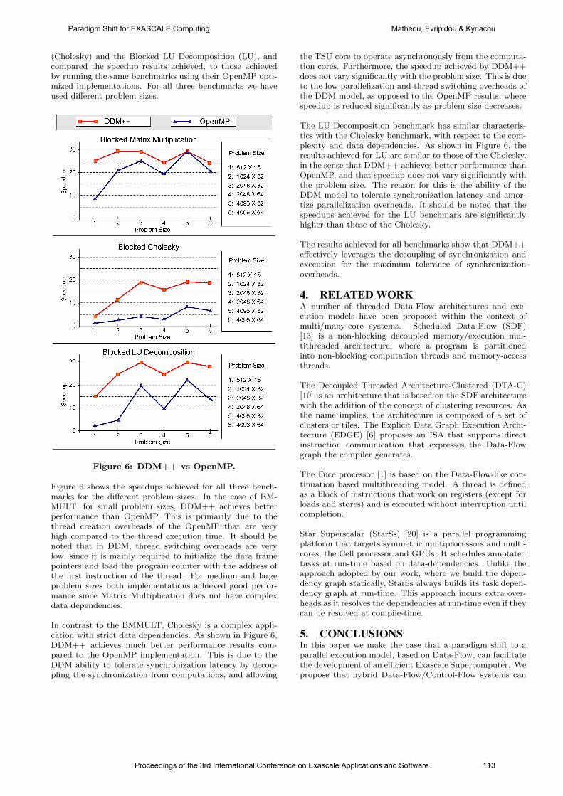
(Cholesky) and the Blocked LU Decomposition (LU), andcompared the speedup results achieved, to those achievedby running the same benchmarks using their OpenMP opti-mized implementations. For all three benchmarks we haveused different problem sizes.

Figure 6: DDM++ vs OpenMP.

Figure 6 shows the speedups achieved for all three bench-marks for the different problem sizes. In the case of BM-MULT, for small problem sizes, DDM++ achieves betterperformance than OpenMP. This is primarily due to thethread creation overheads of the OpenMP that are veryhigh compared to the thread execution time. It should benoted that in DDM, thread switching overheads are verylow, since it is mainly required to initialize the data framepointers and load the program counter with the address ofthe first instruction of the thread. For medium and largeproblem sizes both implementations achieved good perfor-mance since Matrix Multiplication does not have complexdata dependencies.

In contrast to the BMMULT, Cholesky is a complex appli-cation with strict data dependencies. As shown in Figure 6,DDM++ achieves much better performance results com-pared to the OpenMP implementation. This is due to theDDM ability to tolerate synchronization latency by decou-pling the synchronization from computations, and allowing

the TSU core to operate asynchronously from the computa-tion cores. Furthermore, the speedup achieved by DDM++does not vary significantly with the problem size. This is dueto the low parallelization and thread switching overheads ofthe DDM model, as opposed to the OpenMP results, wherespeedup is reduced significantly as problem size decreases.

The LU Decomposition benchmark has similar characteris-tics with the Cholesky benchmark, with respect to the com-plexity and data dependencies. As shown in Figure 6, theresults achieved for LU are similar to those of the Cholesky,in the sense that DDM++ achieves better performance thanOpenMP, and that speedup does not vary significantly withthe problem size. The reason for this is the ability of theDDM model to tolerate synchronization latency and amor-tize parallelization overheads. It should be noted that thespeedups achieved for the LU benchmark are significantlyhigher than those of the Cholesky.

The results achieved for all benchmarks show that DDM++effectively leverages the decoupling of synchronization andexecution for the maximum tolerance of synchronizationoverheads.

4. RELATED WORKA number of threaded Data-Flow architectures and exe-cution models have been proposed within the context ofmulti/many-core systems. Scheduled Data-Flow (SDF)[13] is a non-blocking decoupled memory/execution mul-tithreaded architecture, where a program is partitionedinto non-blocking computation threads and memory-accessthreads.

The Decoupled Threaded Architecture-Clustered (DTA-C)[10] is an architecture that is based on the SDF architecturewith the addition of the concept of clustering resources. Asthe name implies, the architecture is composed of a set ofclusters or tiles. The Explicit Data Graph Execution Archi-tecture (EDGE) [6] proposes an ISA that supports directinstruction communication that expresses the Data-Flowgraph the compiler generates.

The Fuce processor [1] is based on the Data-Flow-like con-tinuation based multithreading model. A thread is definedas a block of instructions that work on registers (except forloads and stores) and is executed without interruption untilcompletion.

Star Superscalar (StarSs) [20] is a parallel programmingplatform that targets symmetric multiprocessors and multi-cores, the Cell processor and GPUs. It schedules annotatedtasks at run-time based on data-dependencies. Unlike theapproach adopted by our work, where we build the depen-dency graph statically, StarSs always builds its task depen-dency graph at run-time. This approach incurs extra over-heads as it resolves the dependencies at run-time even if theycan be resolved at compile-time.

5. CONCLUSIONSIn this paper we make the case that a paradigm shift to aparallel execution model, based on Data-Flow, can facilitatethe development of an efficient Exascale Supercomputer. Wepropose that hybrid Data-Flow/Control-Flow systems can



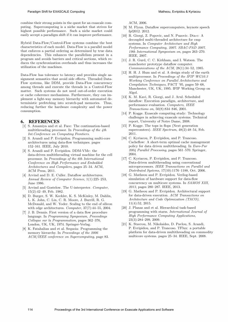
combine their strong points in the quest for an exascale com-puting. Supercomputing is a niche market that strives forhighest possible performance. Such a niche market couldeasily accept a paradigm shift if it can improve performance.

Hybrid Data-Flow/Control-Flow systems combine the bestcharacteristics of each model. Data-Flow is a parallel modelthat enforces a partial ordering as determined by true datadependencies. This enhances the parallelism present in aprogram and avoids barriers and critical sections, which re-duces the synchronization overheads and thus increases theutilization of the machines.

Data-Flow has tolerance to latency and provides single as-signment semantics that avoid side effects. Threaded Data-Flow systems, like DDM, provide Data-Flow concurrencyamong threads and execute the threads in a Control-Flowmatter. Such systems do not need out-of-order executionor cache coherence mechanisms. Furthermore, they can im-plement a light-way memory hierarchy with automated de-terministic prefetching into scratch-pad memories. Thus,reducing further the hardware complexity and the powerconsumption.

6. REFERENCES[1] S. Amamiya and et al. Fuce: The continuation-based

multithreading processor. In Proceedings of the 4thInt.Conference on Computing Frontiers.

[2] S. Arandi and P. Evripidou. Programming multi-corearchitectures using data-flow techniques. pages152–161. IEEE, July 2010.

[3] S. Arandi and P. Evripidou. DDM-VMc: thedata-driven multithreading virtual machine for the cellprocessor. In Proceedings of the 6th InternationalConference on High Performance and EmbeddedArchitectures and Compilers, pages 25–34. ACM,ACM Press, 2011.

[4] Arvind and D. E. Culler. Dataflow architectures.Annual Review of Computer Science, 1(1):225–253,June 1986.

[5] Arvind and Gostelow. The U-interpreter. Computer,15(2):42–49, Feb. 1982.

[6] D. Burger, S. W. Keckler, K. S. McKinley, M. Dahlin,L. K. John, C. Lin, C. R. Moore, J. Burrill, R. G.McDonald, and W. Yoder. Scaling to the end of siliconwith edge architectures. Computer, 37(7):44–55, 2004.

[7] J. B. Dennis. First version of a data flow procedurelanguage. In Programming Symposium, ProceedingsColloque sur la Programmation, pages 362–376,London, UK, UK, 1974. Springer-Verlag.

[8] K. Fatahalian and et al. Sequoia: Programming thememory hierarchy. In Proceedings of the 2006ACM/IEEE conference on Supercomputing, page 83.

ACM, 2006.

[9] M. Flynn. Dataflow supercomputers, keynote speechfpl2012. 2012.

[10] R. Giorgi, Z. Popovic, and N. Puzovic. Dta-c: Adecoupled multi-threaded architecture for cmpsystems. In Computer Architecture and HighPerformance Computing, 2007. SBAC-PAD 2007.19th International Symposium on, pages 263–270.IEEE, 2007.

[11] J. R. Gurd, C. C. Kirkham, and I. Watson. Themanchester prototype dataflow computer.Communications of the ACM, 28(1):34–52, 1985.

[12] H. H. J. Hum and et al. A design study of the earthmultiprocessor. In Proceedings of the IFIP WG10.3Working Conference on Parallel Architectures andCompilation Techniques, PACT ’95, pages 59–68,Manchester, UK, UK, 1995. IFIP Working Group onAlgol.

[13] K. M. Kavi, R. Giorgi, and J. Arul. Scheduleddataflow: Execution paradigm, architecture, andperformance evaluation. Computers, IEEETransactions on, 50(8):834–846, 2001.

[14] P. Kogge. Exascale computing study: Technologychallenges in achieving exascale systems. Technicalreport, University of Notre Dame, 2008.

[15] P. Kogge. The tops in flops (Next generationsupercomters). IEEE Spectrum, 48(2):48–54, Feb.2011.

[16] C. Kyriacou, P. Evripidou, and P. Trancoso.Cacheflow: A short-term optimal cache managementpolicy for data driven multithreading. In Euro-Par2004 Parallel Processing, pages 561–570. Springer,2004.

[17] C. Kyriacou, P. Evripidou, and P. Trancoso.Data-driven multithreading using conventionalmicroprocessors. IEEE Transactions on Parallel andDistributed Systems, 17(10):1176–1188, Oct. 2006.

[18] G. Matheou and P. Evripidou. Verilog-basedsimulation of hardware support for data-flowconcurrency on multicore systems. In SAMOS XIII,2013, pages 280–287. IEEE, 2013.

[19] G. Matheou and P. Evripidou. Architectural supportfor data-driven execution. ACM Transactions onArchitecture and Code Optimization (TACO),11(4):52, 2015.

[20] J. Planas and et al. Hierarchical task-basedprogramming with starss. International Journal ofHigh Performance Computing Applications,23(3):284–299, 2009.

[21] K. Stavrou, M. Nikolaides, D. Pavlou, S. Arandi,P. Evripidou, and P. Trancoso. TFlux: a portableplatform for data-driven multithreading on commoditymulticore systems. pages 25–34. IEEE, Sept. 2008.



Large-scale Ultrasound Simulations Using the HybridOpenMP/MPI Decomposition

Jiri JarosFaculty of Information

TechnologyBrno University of Technology

Bozetechova 2612 66 Brno, CZ

[email protected]

Vojtech NiklFaculty of Information

TechnologyBrno University of Technology

Bozetechova 2612 66 Brno, CZ

[email protected]

Bradley E. TreebyDept. of Medical Physics and

Biomedical EngineeringUniversity College London

Malet Place Eng BldgLondon WC1E 6BT, [email protected]

ABSTRACTThe simulation of ultrasound wave propagation through biologicaltissue has a wide range of practical applications including plan-ning therapeutic ultrasound treatments of various brain disorderssuch as brain tumours, essential tremor, and Parkinson’s disease.The major challenge is to ensure the ultrasound focus is accuratelyplaced at the desired target within the brain because the skull cansignificantly distort it. Performing accurate ultrasound simulations,however, requires the simulation code to be able to exploit severalthousands of processor cores and work with datasets on the order oftens of TB. We have recently developed an efficient full-wave ultra-sound model based on the pseudospectral method using pure-MPIwith 1D slab domain decomposition that allows simulations to beperformed using up to 1024 compute cores. However, the slab de-composition limits the number of compute cores to be less or equalto the size of the longest dimension, which is usually below 1024.

This paper presents an improved implementation that exploits2D hybrid OpenMP/MPI decomposition. The 3D grid is first de-composed by MPI processes into slabs. The slabs are further par-titioned into pencils assigned to threads on demand. This allows 8to 16 times more compute cores to be employed compared to thepure-MPI code, while also reducing the amount of communicationamong processes due to the efficient use of shared memory withincompute nodes.

The hybrid code was tested on the Anselm Supercomputer (IT4-Innovations, Czech Republic) with up to 2048 compute cores andthe SuperMUC supercomputer (LRZ, Germany) with up to 8192compute cores. The simulation domain sizes ranged from 2563

to 10243 grid points. The experimental results show that the hy-brid decomposition can significantly outperform the pure-MPI onefor large simulation domains and high core counts, where the effi-ciency remains slightly below 50%. For a domain size of 10243,the hybrid code using 8192 cores enables the simulations to be ac-celerated by a factor of 4 compared to the pure-MPI code. Deploy-ment of the hybrid code has the potential to eventually bring thesimulation times within clinically meaningful timespans, and allowdetailed patient specific treatment plans to be created.

KeywordsUltrasound simulations; 2D domain decomposition; OpenMP/MPIHybrid programming; Performance evaluation; Supercomputing,k-Wave toolbox.

1. INTRODUCTIONThe simulation of ultrasound wave propagation through biologi-

cal tissue has a wide range of practical applications. Recently, highintensity focused ultrasound has been applied to functional neuro-surgery as an alternative, non-invasive treatment of various braindisorders such as brain tumours, essential tremor, and Parkinson’sdisease. The technique works by sending a focused beam of ul-trasound into the tissue, typically using a large transducer. At thefocus, the acoustic energy is sufficient to cause cell death in a lo-calised region while the surrounding tissue is left unharmed. Themajor challenge is to ensure the focus is accurately placed at thedesired target within the brain because the skull can significantlydistort it.

Performing accurate ultrasound simulations, however, requiresthe simulation code to be able to operate on large domains and de-liver the results in a clinically meaningful time. Apart from thephysical complexity, the main obstacle in implementing new ultra-sound treatment planning procedures in clinical practice is the com-putational complexity. Considering the domain of interest encom-passing the ultrasound transducer and the treatment area (normallyon the order of centimetres in each Cartesian direction), and the sizeof the acoustic wavelength (on the order of hundreds of microme-ters at the maximum frequency of interest), we have to simulatethe wave propagation over hundreds or thousands of wavelengths.A sufficiently fine discretisation of the simulation domain whichavoids numerical dispersion and instability can easily lead to gridsizes exceeding 1012 elements. Storing all the necessary acousticquantities for such a large simulation domain in computer memoryrequires petabytes of memory and its processing reaches the orderof exascale.

We have recently developed a pure-MPI pseudospectral simula-tion code using 1D domain decomposition that has allowed us torun reasonable sized simulations using up to 1024 compute cores[3]. However, this implementation suffers from the maximum par-allelism being limited by the largest size of the 3D grid used. Atthe age of exascale, more and more systems will have numbers ofprocessing cores far exceeding this limit. For example, a realis-tic ultrasound simulation performed by the k-Wave toolbox mightuse a grid size of 10243. Here, the 1D pure-MPI decompositionwould only scale up to 1024 cores at most leading to calculationtimes exceeding clinically acceptable times (in this case between30 and 72 hours). In contrast, top supercomputer facilities disposewith several hundred thousand compute cores and could providethe simulation result within an hour, if efficiently employed.

The second problem arising from limited parallelism is the totalamount of memory that can be used to store simulation data. Not


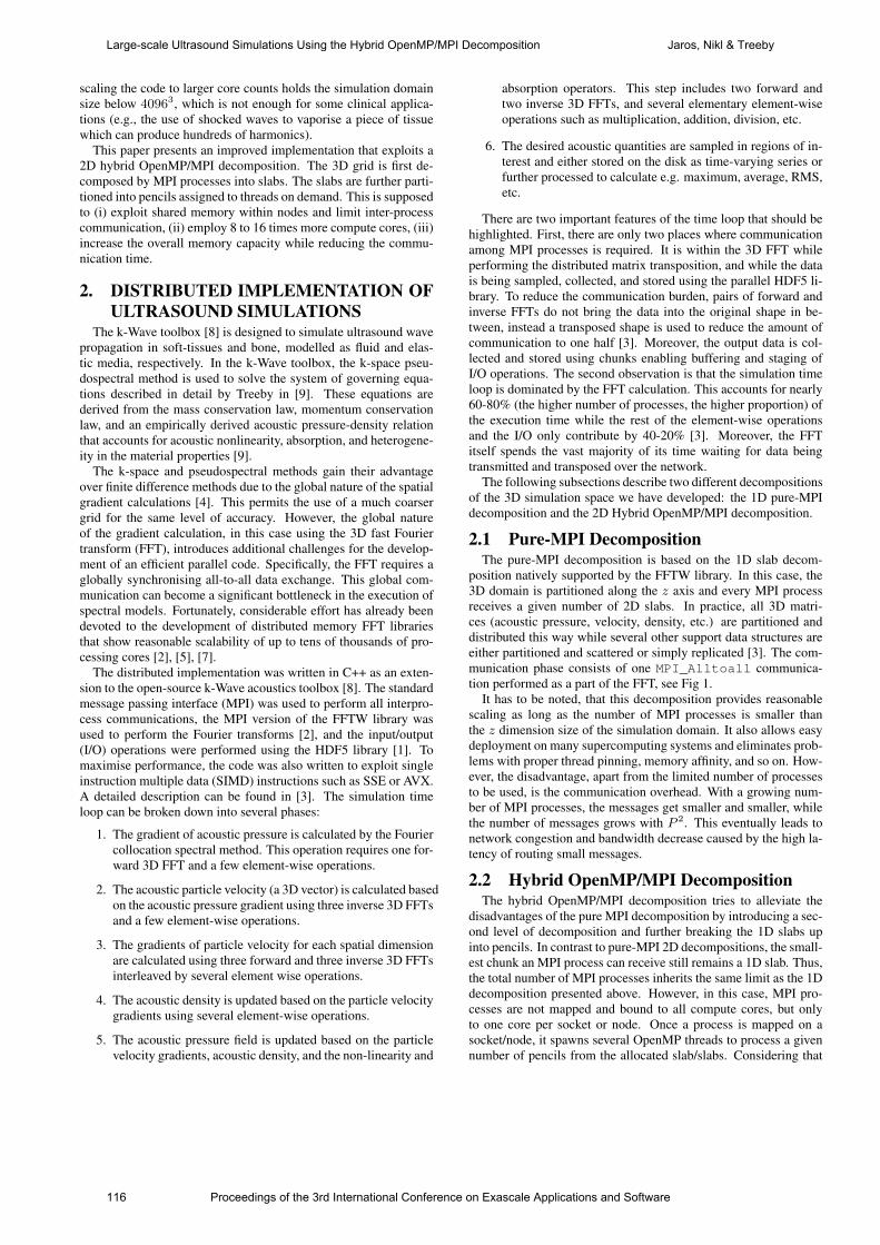
scaling the code to larger core counts holds the simulation domainsize below 40963, which is not enough for some clinical applica-tions (e.g., the use of shocked waves to vaporise a piece of tissuewhich can produce hundreds of harmonics).

This paper presents an improved implementation that exploits a2D hybrid OpenMP/MPI decomposition. The 3D grid is first de-composed by MPI processes into slabs. The slabs are further parti-tioned into pencils assigned to threads on demand. This is supposedto (i) exploit shared memory within nodes and limit inter-processcommunication, (ii) employ 8 to 16 times more compute cores, (iii)increase the overall memory capacity while reducing the commu-nication time.

2. DISTRIBUTED IMPLEMENTATION OFULTRASOUND SIMULATIONS

The k-Wave toolbox [8] is designed to simulate ultrasound wavepropagation in soft-tissues and bone, modelled as fluid and elas-tic media, respectively. In the k-Wave toolbox, the k-space pseu-dospectral method is used to solve the system of governing equa-tions described in detail by Treeby in [9]. These equations arederived from the mass conservation law, momentum conservationlaw, and an empirically derived acoustic pressure-density relationthat accounts for acoustic nonlinearity, absorption, and heterogene-ity in the material properties [9].

The k-space and pseudospectral methods gain their advantageover finite difference methods due to the global nature of the spatialgradient calculations [4]. This permits the use of a much coarsergrid for the same level of accuracy. However, the global natureof the gradient calculation, in this case using the 3D fast Fouriertransform (FFT), introduces additional challenges for the develop-ment of an efficient parallel code. Specifically, the FFT requires aglobally synchronising all-to-all data exchange. This global com-munication can become a significant bottleneck in the execution ofspectral models. Fortunately, considerable effort has already beendevoted to the development of distributed memory FFT librariesthat show reasonable scalability of up to tens of thousands of pro-cessing cores [2], [5], [7].

The distributed implementation was written in C++ as an exten-sion to the open-source k-Wave acoustics toolbox [8]. The standardmessage passing interface (MPI) was used to perform all interpro-cess communications, the MPI version of the FFTW library wasused to perform the Fourier transforms [2], and the input/output(I/O) operations were performed using the HDF5 library [1]. Tomaximise performance, the code was also written to exploit singleinstruction multiple data (SIMD) instructions such as SSE or AVX.A detailed description can be found in [3]. The simulation timeloop can be broken down into several phases:

1. The gradient of acoustic pressure is calculated by the Fouriercollocation spectral method. This operation requires one for-ward 3D FFT and a few element-wise operations.

2. The acoustic particle velocity (a 3D vector) is calculated basedon the acoustic pressure gradient using three inverse 3D FFTsand a few element-wise operations.

3. The gradients of particle velocity for each spatial dimensionare calculated using three forward and three inverse 3D FFTsinterleaved by several element wise operations.

4. The acoustic density is updated based on the particle velocitygradients using several element-wise operations.

5. The acoustic pressure field is updated based on the particlevelocity gradients, acoustic density, and the non-linearity and

absorption operators. This step includes two forward andtwo inverse 3D FFTs, and several elementary element-wiseoperations such as multiplication, addition, division, etc.

6. The desired acoustic quantities are sampled in regions of in-terest and either stored on the disk as time-varying series orfurther processed to calculate e.g. maximum, average, RMS,etc.

There are two important features of the time loop that should behighlighted. First, there are only two places where communicationamong MPI processes is required. It is within the 3D FFT whileperforming the distributed matrix transposition, and while the datais being sampled, collected, and stored using the parallel HDF5 li-brary. To reduce the communication burden, pairs of forward andinverse FFTs do not bring the data into the original shape in be-tween, instead a transposed shape is used to reduce the amount ofcommunication to one half [3]. Moreover, the output data is col-lected and stored using chunks enabling buffering and staging ofI/O operations. The second observation is that the simulation timeloop is dominated by the FFT calculation. This accounts for nearly60-80% (the higher number of processes, the higher proportion) ofthe execution time while the rest of the element-wise operationsand the I/O only contribute by 40-20% [3]. Moreover, the FFTitself spends the vast majority of its time waiting for data beingtransmitted and transposed over the network.

The following subsections describe two different decompositionsof the 3D simulation space we have developed: the 1D pure-MPIdecomposition and the 2D Hybrid OpenMP/MPI decomposition.

2.1 Pure-MPI DecompositionThe pure-MPI decomposition is based on the 1D slab decom-

position natively supported by the FFTW library. In this case, the3D domain is partitioned along the z axis and every MPI processreceives a given number of 2D slabs. In practice, all 3D matri-ces (acoustic pressure, velocity, density, etc.) are partitioned anddistributed this way while several other support data structures areeither partitioned and scattered or simply replicated [3]. The com-munication phase consists of one MPI_Alltoall communica-tion performed as a part of the FFT, see Fig 1.

It has to be noted, that this decomposition provides reasonablescaling as long as the number of MPI processes is smaller thanthe z dimension size of the simulation domain. It also allows easydeployment on many supercomputing systems and eliminates prob-lems with proper thread pinning, memory affinity, and so on. How-ever, the disadvantage, apart from the limited number of processesto be used, is the communication overhead. With a growing num-ber of MPI processes, the messages get smaller and smaller, whilethe number of messages grows with P 2. This eventually leads tonetwork congestion and bandwidth decrease caused by the high la-tency of routing small messages.

2.2 Hybrid OpenMP/MPI DecompositionThe hybrid OpenMP/MPI decomposition tries to alleviate the

disadvantages of the pure MPI decomposition by introducing a sec-ond level of decomposition and further breaking the 1D slabs upinto pencils. In contrast to pure-MPI 2D decompositions, the small-est chunk an MPI process can receive still remains a 1D slab. Thus,the total number of MPI processes inherits the same limit as the 1Ddecomposition presented above. However, in this case, MPI pro-cesses are not mapped and bound to all compute cores, but onlyto one core per socket or node. Once a process is mapped on asocket/node, it spawns several OpenMP threads to process a givennumber of pencils from the allocated slab/slabs. Considering that


Large-scale Ultrasound Simulations Using the Hybrid OpenMP/MPI Decomposition Jaros, Nikl & Treeby

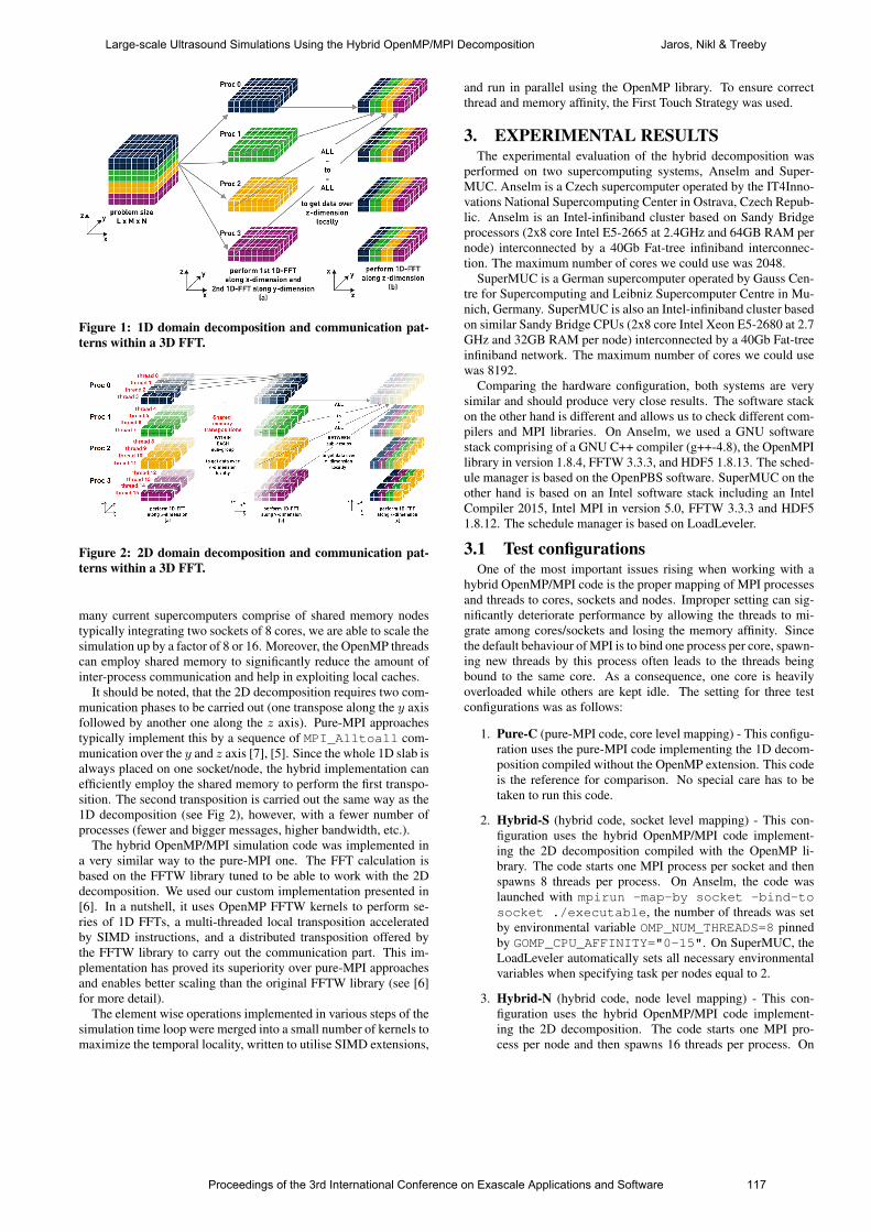
Figure 1: 1D domain decomposition and communication pat-terns within a 3D FFT.

Figure 2: 2D domain decomposition and communication pat-terns within a 3D FFT.

many current supercomputers comprise of shared memory nodestypically integrating two sockets of 8 cores, we are able to scale thesimulation up by a factor of 8 or 16. Moreover, the OpenMP threadscan employ shared memory to significantly reduce the amount ofinter-process communication and help in exploiting local caches.

It should be noted, that the 2D decomposition requires two com-munication phases to be carried out (one transpose along the y axisfollowed by another one along the z axis). Pure-MPI approachestypically implement this by a sequence of MPI_Alltoall com-munication over the y and z axis [7], [5]. Since the whole 1D slab isalways placed on one socket/node, the hybrid implementation canefficiently employ the shared memory to perform the first transpo-sition. The second transposition is carried out the same way as the1D decomposition (see Fig 2), however, with a fewer number ofprocesses (fewer and bigger messages, higher bandwidth, etc.).

The hybrid OpenMP/MPI simulation code was implemented ina very similar way to the pure-MPI one. The FFT calculation isbased on the FFTW library tuned to be able to work with the 2Ddecomposition. We used our custom implementation presented in[6]. In a nutshell, it uses OpenMP FFTW kernels to perform se-ries of 1D FFTs, a multi-threaded local transposition acceleratedby SIMD instructions, and a distributed transposition offered bythe FFTW library to carry out the communication part. This im-plementation has proved its superiority over pure-MPI approachesand enables better scaling than the original FFTW library (see [6]for more detail).

The element wise operations implemented in various steps of thesimulation time loop were merged into a small number of kernels tomaximize the temporal locality, written to utilise SIMD extensions,

and run in parallel using the OpenMP library. To ensure correctthread and memory affinity, the First Touch Strategy was used.

3. EXPERIMENTAL RESULTSThe experimental evaluation of the hybrid decomposition was

performed on two supercomputing systems, Anselm and Super-MUC. Anselm is a Czech supercomputer operated by the IT4Inno-vations National Supercomputing Center in Ostrava, Czech Repub-lic. Anselm is an Intel-infiniband cluster based on Sandy Bridgeprocessors (2x8 core Intel E5-2665 at 2.4GHz and 64GB RAM pernode) interconnected by a 40Gb Fat-tree infiniband interconnec-tion. The maximum number of cores we could use was 2048.

SuperMUC is a German supercomputer operated by Gauss Cen-tre for Supercomputing and Leibniz Supercomputer Centre in Mu-nich, Germany. SuperMUC is also an Intel-infiniband cluster basedon similar Sandy Bridge CPUs (2x8 core Intel Xeon E5-2680 at 2.7GHz and 32GB RAM per node) interconnected by a 40Gb Fat-treeinfiniband network. The maximum number of cores we could usewas 8192.

Comparing the hardware configuration, both systems are verysimilar and should produce very close results. The software stackon the other hand is different and allows us to check different com-pilers and MPI libraries. On Anselm, we used a GNU softwarestack comprising of a GNU C++ compiler (g++-4.8), the OpenMPIlibrary in version 1.8.4, FFTW 3.3.3, and HDF5 1.8.13. The sched-ule manager is based on the OpenPBS software. SuperMUC on theother hand is based on an Intel software stack including an IntelCompiler 2015, Intel MPI in version 5.0, FFTW 3.3.3 and HDF51.8.12. The schedule manager is based on LoadLeveler.

3.1 Test configurationsOne of the most important issues rising when working with a

hybrid OpenMP/MPI code is the proper mapping of MPI processesand threads to cores, sockets and nodes. Improper setting can sig-nificantly deteriorate performance by allowing the threads to mi-grate among cores/sockets and losing the memory affinity. Sincethe default behaviour of MPI is to bind one process per core, spawn-ing new threads by this process often leads to the threads beingbound to the same core. As a consequence, one core is heavilyoverloaded while others are kept idle. The setting for three testconfigurations was as follows:

1. Pure-C (pure-MPI code, core level mapping) - This configu-ration uses the pure-MPI code implementing the 1D decom-position compiled without the OpenMP extension. This codeis the reference for comparison. No special care has to betaken to run this code.

2. Hybrid-S (hybrid code, socket level mapping) - This con-figuration uses the hybrid OpenMP/MPI code implement-ing the 2D decomposition compiled with the OpenMP li-brary. The code starts one MPI process per socket and thenspawns 8 threads per process. On Anselm, the code waslaunched with mpirun -map-by socket -bind-tosocket ./executable, the number of threads was setby environmental variable OMP_NUM_THREADS=8 pinnedby GOMP_CPU_AFFINITY="0-15". On SuperMUC, theLoadLeveler automatically sets all necessary environmentalvariables when specifying task per nodes equal to 2.

3. Hybrid-N (hybrid code, node level mapping) - This con-figuration uses the hybrid OpenMP/MPI code implement-ing the 2D decomposition. The code starts one MPI pro-cess per node and then spawns 16 threads per process. On



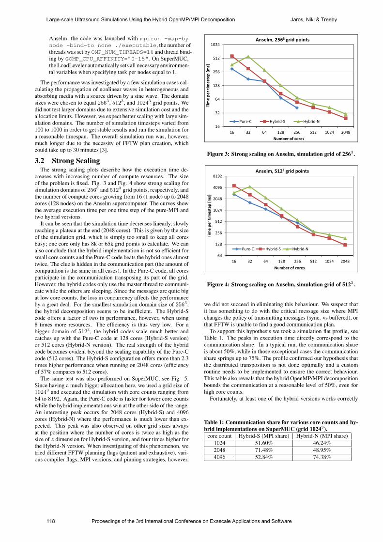
Anselm, the code was launched with mpirun -map-bynode -bind-to none ./executable, the number ofthreads was set by OMP_NUM_THREADS=16 and thread bind-ing by GOMP_CPU_AFFINITY="0-15". On SuperMUC,the LoadLeveler automatically sets all necessary environmen-tal variables when specifying task per nodes equal to 1.

The performance was investigated by a few simulation cases cal-culating the propagation of nonlinear waves in heterogeneous andabsorbing media with a source driven by a sine wave. The domainsizes were chosen to equal 2563, 5123, and 10243 grid points. Wedid not test larger domains due to extensive simulation cost and theallocation limits. However, we expect better scaling with large sim-ulation domains. The number of simulation timesteps varied from100 to 1000 in order to get stable results and run the simulation fora reasonable timespan. The overall simulation run was, however,much longer due to the necessity of FFTW plan creation, whichcould take up to 30 minutes [3].

3.2 Strong ScalingThe strong scaling plots describe how the execution time de-

creases with increasing number of compute resources. The sizeof the problem is fixed. Fig. 3 and Fig. 4 show strong scaling forsimulation domains of 2563 and 5123 grid points, respectively, andthe number of compute cores growing from 16 (1 node) up to 2048cores (128 nodes) on the Anselm supercomputer. The curves showthe average execution time per one time step of the pure-MPI andtwo hybrid versions.

It can be seen that the simulation time decreases linearly, slowlyreaching a plateau at the end (2048 cores). This is given by the sizeof the simulation grid, which is simply too small to keep all coresbusy; one core only has 8k or 65k grid points to calculate. We canalso conclude that the hybrid implementation is not so efficient forsmall core counts and the Pure-C code beats the hybrid ones almosttwice. The clue is hidden in the communication part (the amount ofcomputation is the same in all cases). In the Pure-C code, all coresparticipate in the communication transposing its part of the grid.However, the hybrid codes only use the master thread to communi-cate while the others are sleeping. Since the messages are quite bigat low core counts, the loss in concurrency affects the performanceby a great deal. For the smallest simulation domain size of 2563,the hybrid decomposition seems to be inefficient. The Hybrid-Scode offers a factor of two in performance, however, when using8 times more resources. The efficiency is thus very low. For abigger domain of 5123, the hybrid codes scale much better andcatches up with the Pure-C code at 128 cores (Hybrid-S version)or 512 cores (Hybrid-N version). The real strength of the hybridcode becomes evident beyond the scaling capability of the Pure-Ccode (512 cores). The Hybrid-S configuration offers more than 2.3times higher performance when running on 2048 cores (efficiencyof 57% compares to 512 cores).

The same test was also performed on SuperMUC, see Fig. 5.Since having a much bigger allocation here, we used a grid size of10243 and executed the simulation with core counts ranging from64 to 8192. Again, the Pure-C code is faster for lower core countswhile the hybrid implementations win at the other side of the range.An interesting peak occurs for 2048 cores (Hybrid-S) and 4096cores (Hybrid-N) where the performance is much lower than ex-pected. This peak was also observed on other grid sizes alwaysat the position where the number of cores is twice as high as thesize of z dimension for Hybrid-S version, and four times higher forthe Hybrid-N version. When investigating of this phenomenon, wetried different FFTW planning flags (patient and exhaustive), vari-ous compiler flags, MPI versions, and pinning strategies, however,

16

32

64

128

256

512

1024

16 32 64 128 256 512 1024 2048

Tim

e p

er

tim

est

ep

[m

s]

Number of cores

Anselm, 2563 grid points

Pure-C Hybrid-S Hybrid-N

Figure 3: Strong scaling on Anselm, simulation grid of 2563.

64

128

256

512

1024

2048

4096

8192

16 32 64 128 256 512 1024 2048

Tim

e p

er

tim

est

ep

[m

s]

Number of cores

Anselm, 5123 grid points


Figure 4: Strong scaling on Anselm, simulation grid of 5123.

we did not succeed in eliminating this behaviour. We suspect thatit has something to do with the critical message size where MPIchanges the policy of transmitting messages (sync. vs buffered), orthat FFTW is unable to find a good communication plan.

To support this hypothesis we took a simulation flat profile, seeTable 1. The peaks in execution time directly correspond to thecommunication share. In a typical run, the communication shareis about 50%, while in those exceptional cases the communicationshare springs up to 75%. The profile confirmed our hypothesis thatthe distributed transposition is not done optimally and a customroutine needs to be implemented to ensure the correct behaviour.This table also reveals that the hybrid OpenMP/MPI decompositionbounds the communication at a reasonable level of 50%, even forhigh core counts.

Fortunately, at least one of the hybrid versions works correctly

Table 1: Communication share for various core counts and hy-brid implementations on SuperMUC (grid 10243).

core count Hybrid-S (MPI share) Hybrid-N (MPI share)1024 51.60% 46.24%2048 71.48% 48.95%4096 52.84% 74.38%



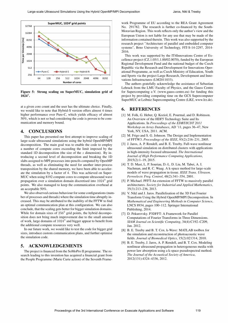
256

512

1024

2048

4096

8192

16384

32768

64 128 256 512 1024 2048 4096 8192

Tim

e p

er

tim

est

ep

[m

s]

Number of cores

SuperMUC, 10243 grid points


Figure 5: Strong scaling on SuperMUC, simulation grid of10243.

at a given core count and the user has the ultimate choice. Finally,we would like to note that Hybrid-S version offers almost 4 timeshigher performance over Pure-C, which yields efficacy of almost50%, which is not so bad considering the code is proven to be com-munication and memory bound.

4. CONCLUSIONSThis paper has presented our first attempt to improve scaling of

large-scale ultrasound simulations using the hybrid OpenMP/MPIdecomposition. The main goal was to enable the code to employa number of compute cores exceeding the limit imposed by thestandard 1D decomposition (the size of the z dimension). By in-troducing a second level of decomposition and breaking the 1Dslabs assigned to MPI processes into pencils computed by OpenMPthreads, as well as eliminating the need for another inter-processtransposition by the shared memory, we have been able to acceler-ate the simulation by a factor of 4. This was achieved on Super-MUC when using 8192 compute cores to compute ultrasound wavepropagation over a simulation domain discretised into 10243 gridpoints. We also managed to keep the communication overhead atan acceptable 50%.

We also observed curious behaviour for some configurations (num-ber of processes and threads) where the simulation time abruptly in-creased. This may be attributed to the inability of the FFTW to findan optimal communication plan at this configuration. We can alsoconclude, that the scaling gets better for bigger simulation domains.While for domain sizes of 2563 grid points, the hybrid decompo-sition does not bring much improvement due to the small amountof work, large domains of 10243 and bigger appear to benefit fromthe additional compute resources very well.

In our future work, we would like to test the code for bigger gridsizes, introduce custom communication plans, and further optimisethe simulation code.

5. ACKNOWLEDGEMENTSThe project is financed from the SoMoPro II programme. The re-

search leading to this invention has acquired a financial grant fromthe People Programme (Marie Curie action) of the Seventh Frame-

work Programme of EU according to the REA Grant AgreementNo. 291782. The research is further co-financed by the South-Moravian Region. This work reflects only the author’s view and theEuropean Union is not liable for any use that may be made of theinformation contained therein. This work was also supported by theresearch project "Architecture of parallel and embedded computersystems", Brno University of Technology, FIT-S-14-2297, 2014-2016.

This work was supported by the IT4Innovations Centre of Ex-cellence project (CZ.1.05/1.1.00/02.0070), funded by the EuropeanRegional Development Fund and the national budget of the CzechRepublic via the Research and Development for Innovations Oper-ational Programme, as well as Czech Ministry of Education, Youthand Sports via the project Large Research, Development and Inno-vations Infrastructures (LM2011033).

The authors gratefully acknowledge the assistance of SebastianLehrack from the LMU Faculty of Physics, and the Gauss Centrefor Supercomputing e.V. (www.gauss-centre.eu) for funding thisproject by providing computing time on the GCS SupercomputerSuperMUC at Leibniz Supercomputing Centre (LRZ, www.lrz.de).

6. REFERENCES[1] M. Folk, G. Heber, Q. Koziol, E. Pourmal, and D. Robinson.

An Overview of the HDF5 Technology Suite and ItsApplications. In Proceedings of the EDBT/ICDT 2011Workshop on Array Databases, AD ’11, pages 36–47, NewYork, NY, USA, 2011. ACM.

[2] M. Frigo and S. G. Johnson. The Design and Implementationof FFTW3. Proceedings of the IEEE, 93(2):216–231, 2005.

[3] J. Jaros, A. P. Rendell, and B. E. Treeby. Full-wave nonlinearultrasound simulation on distributed clusters with applicationsin high-intensity focused ultrasound. The InternationalJournal of High Performance Computing Applications,2015(2):1–19, 2015.

[4] T. D. Mast, L. P. Souriau, D.-L. D. Liu, M. Tabei, A. I.Nachman, and R. C. Waag. A k-space method for large-scalemodels of wave propagation in tissue. IEEE Trans. Ultrason.Ferroelectr. Freq. Control, 48(2):341–354, 2001.

[5] P. Michael. PFFT-An extension of FFTW to massively parallelarchitectures. Society for Industrial and Applied Mathematics,35(3):213–236, 2013.

[6] V. Nikl and J. Jaros. Parallelisation of the 3D Fast FourierTransform Using the Hybrid OpenMP/MPI Decomposition. InMathematical and Engineering Methods in Computer Science,LNCS 8934, pages 100–112. Springer InternationalPublishing, 2014.

[7] D. Pekurovsky. P3DFFT: A Framework for ParallelComputations of Fourier Transforms in Three Dimensions.SIAM Journal on Scientific Computing, 34(4):C192–C209,Jan. 2012.

[8] B. E. Treeby and B. T. Cox. k-Wave: MATLAB toolbox forthe simulation and reconstruction of photoacoustic wavefields. Journal of Biomedical Optics, 15(2):021314, 2010.

[9] B. E. Treeby, J. Jaros, A. P. Rendell, and B. T. Cox. Modelingnonlinear ultrasound propagation in heterogeneous media withpower law absorption using a k-space pseudospectral method.The Journal of the Acoustical Society of America,2012(131):4324–4336, 2012.



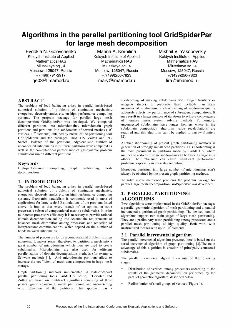
Algorithms in the parallel partitioning tool GridSpiderPar for large mesh decomposition

Evdokia N. Golovchenko Keldysh Institute of Applied

Mathematics RAS Miusskaya sq., 4

Moscow, 125047, Russia +7(499)791-2917

[email protected]

Marina A. Kornilina Keldysh Institute of Applied


Moscow, 125047, Russia +7(499)250-7823

[email protected]

Mikhail V. Yakobovskiy Keldysh Institute of Applied


Moscow, 125047, Russia +7(499)250-7823

[email protected]

ABSTRACT The problem of load balancing arises in parallel mesh-based numerical solution of problems of continuum mechanics, energetics, electrodynamics etc. on high-performance computing systems. The program package for parallel large mesh decomposition GridSpiderPar was developed. We compared different partitions into microdomains, microdomain graph partitions and partitions into subdomains of several meshes (108 vertices, 109 elements) obtained by means of the partitioning tool GridSpiderPar and the packages ParMETIS, Zoltan and PT-Scotch. Balance of the partitions, edge-cut and number of unconnected subdomains in different partitions were compared as well as the computational performance of gas-dynamic problem simulations run on different partitions.

Keywords High-performance computing, graph partitioning, mesh decomposition.

1. INTRODUCTION The problem of load balancing arises in parallel mesh-based numerical solution of problems of continuum mechanics, energetics, electrodynamics etc. on high-performance computing systems. Geometric parallelism is commonly used in most of applications for large-scale 3D simulations of the problems listed above. It implies that every branch of an application code processes a subset of computational mesh (a subdomain). In order to increase processors efficiency it is necessary to provide rational domain decomposition, taking into account the requirements of balanced mesh distribution among processors and reduction of interprocessor communications, which depend on the number of bonds between subdomains.

The number of processors to run a computational problem is often unknown. It makes sense, therefore, to partition a mesh into a great number of microdomains which then are used to create subdomains. Microdomains are also used for efficient parallelization of domain decomposition methods (for example, Schwarz method) [1]. And microdomain partitions allow to increase the coefficient of mesh data compression in large mesh storage.

Graph partitioning methods implemented in state-of-the-art parallel partitioning tools ParMETIS, Jostle, PT-Scotch and Zoltan are based on multilevel algorithms consisting of three phases: graph coarsening, initial partitioning and uncoarsening with refinement of the partitions. That approach has a

shortcoming of making subdomains with longer frontiers or irregular shapes. In particular these methods can form unconnected subdomains. Such worsening of subdomain quality adversely affects the performance of subsequent computations. It may result in a larger number of iterations to achieve convergence of iterative linear system solving methods. Furthermore, unconnected subdomains have longer frontiers where in the subdomain composition algorithm value recalculations are required and this algorithm can’t be applied to narrow frontiers [2].

Another shortcoming of present graph partitioning methods is generation of strongly imbalanced partitions. This shortcoming is the most prominent in partitions made by ParMETIS, where number of vertices in some subdomains can be twice as large as in others. The imbalance can cause significant performance problems, especially in exascale computing.

Moreover, partitions into large number of microdomains can’t always be obtained by the present graph partitioning methods.

To solve above mentioned problems the program package for parallel large mesh decomposition GridSpiderPar was developed.

2. PARALLEL PARTITIONING ALGORITHMS Two algorithms were implemented in the GridSpiderPar package: a parallel geometric algorithm of mesh partitioning and a parallel incremental algorithm of graph partitioning. The devised parallel algorithms support two main stages of large mesh partitioning. They are a preliminary mesh partitioning among processors and a parallel mesh partitioning of high quality. Both work with unstructured meshes with up to 109 elements.

2.1 Parallel incremental algorithm The parallel incremental algorithm presented here is based on the serial incremental algorithm of graph partitioning [3].The main advantage of this algorithm is creation of principally connected subdomains.

The parallel incremental algorithm consists of the following stages:

• Distribution of vertices among processors according to the results of the geometric decomposition performed by the parallel geometric algorithm, described below.

• Redistribution of small groups of vertices (Figure 1).


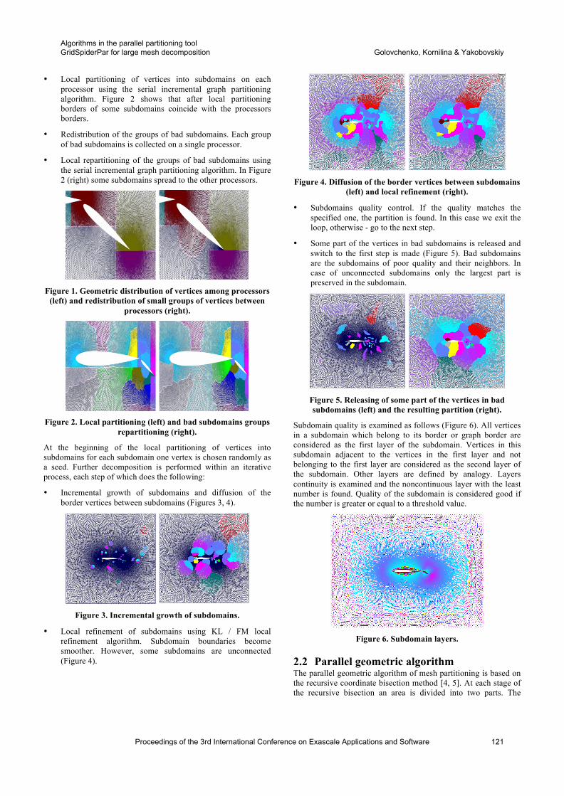
• Local partitioning of vertices into subdomains on each processor using the serial incremental graph partitioning algorithm. Figure 2 shows that after local partitioning borders of some subdomains coincide with the processors borders.

• Redistribution of the groups of bad subdomains. Each group of bad subdomains is collected on a single processor.

• Local repartitioning of the groups of bad subdomains using the serial incremental graph partitioning algorithm. In Figure 2 (right) some subdomains spread to the other processors.

Figure 1. Geometric distribution of vertices among processors

(left) and redistribution of small groups of vertices between processors (right).

Figure 2. Local partitioning (left) and bad subdomains groups

repartitioning (right).

At the beginning of the local partitioning of vertices into subdomains for each subdomain one vertex is chosen randomly as a seed. Further decomposition is performed within an iterative process, each step of which does the following:

• Incremental growth of subdomains and diffusion of the border vertices between subdomains (Figures 3, 4).

Figure 3. Incremental growth of subdomains.

• Local refinement of subdomains using KL / FM local refinement algorithm. Subdomain boundaries become smoother. However, some subdomains are unconnected (Figure 4).

Figure 4. Diffusion of the border vertices between subdomains (left) and local refinement (right).

• Subdomains quality control. If the quality matches the specified one, the partition is found. In this case we exit the loop, otherwise - go to the next step.

• Some part of the vertices in bad subdomains is released and switch to the first step is made (Figure 5). Bad subdomains are the subdomains of poor quality and their neighbors. In case of unconnected subdomains only the largest part is preserved in the subdomain.

Figure 5. Releasing of some part of the vertices in bad subdomains (left) and the resulting partition (right).

Subdomain quality is examined as follows (Figure 6). All vertices in a subdomain which belong to its border or graph border are considered as the first layer of the subdomain. Vertices in this subdomain adjacent to the vertices in the first layer and not belonging to the first layer are considered as the second layer of the subdomain. Other layers are defined by analogy. Layers continuity is examined and the noncontinuous layer with the least number is found. Quality of the subdomain is considered good if the number is greater or equal to a threshold value.

Figure 6. Subdomain layers.

2.2 Parallel geometric algorithm The parallel geometric algorithm of mesh partitioning is based on the recursive coordinate bisection method [4, 5]. At each stage of the recursive bisection an area is divided into two parts. The


Algorithms in the parallel partitioning tool GridSpiderPar for large mesh decomposition Golovchenko, Kornilina & Yakobovskiy

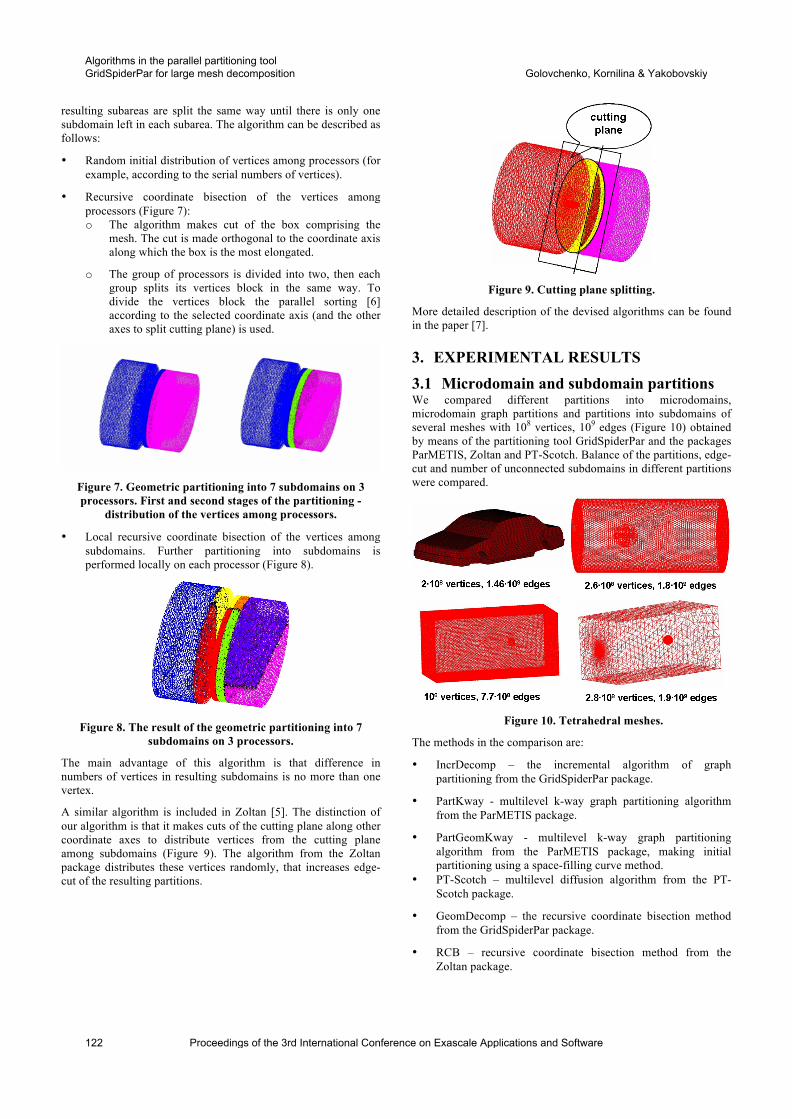
resulting subareas are split the same way until there is only one subdomain left in each subarea. The algorithm can be described as follows:

• Random initial distribution of vertices among processors (for example, according to the serial numbers of vertices).

• Recursive coordinate bisection of the vertices among processors (Figure 7): o The algorithm makes cut of the box comprising the

mesh. The cut is made orthogonal to the coordinate axis along which the box is the most elongated.

o The group of processors is divided into two, then each group splits its vertices block in the same way. To divide the vertices block the parallel sorting [6] according to the selected coordinate axis (and the other axes to split cutting plane) is used.

Figure 7. Geometric partitioning into 7 subdomains on 3 processors. First and second stages of the partitioning -

distribution of the vertices among processors.

• Local recursive coordinate bisection of the vertices among subdomains. Further partitioning into subdomains is performed locally on each processor (Figure 8).

Figure 8. The result of the geometric partitioning into 7 subdomains on 3 processors.

The main advantage of this algorithm is that difference in numbers of vertices in resulting subdomains is no more than one vertex.

A similar algorithm is included in Zoltan [5]. The distinction of our algorithm is that it makes cuts of the cutting plane along other coordinate axes to distribute vertices from the cutting plane among subdomains (Figure 9). The algorithm from the Zoltan package distributes these vertices randomly, that increases edge-cut of the resulting partitions.

Figure 9. Cutting plane splitting.

More detailed description of the devised algorithms can be found in the paper [7].

3. EXPERIMENTAL RESULTS 3.1 Microdomain and subdomain partitions We compared different partitions into microdomains, microdomain graph partitions and partitions into subdomains of several meshes with 108 vertices, 109 edges (Figure 10) obtained by means of the partitioning tool GridSpiderPar and the packages ParMETIS, Zoltan and PT-Scotch. Balance of the partitions, edge-cut and number of unconnected subdomains in different partitions were compared.

Figure 10. Tetrahedral meshes.

The methods in the comparison are:

• IncrDecomp – the incremental algorithm of graph partitioning from the GridSpiderPar package.

• PartKway - multilevel k-way graph partitioning algorithm from the ParMETIS package.

• PartGeomKway - multilevel k-way graph partitioning algorithm from the ParMETIS package, making initial partitioning using a space-filling curve method.

• PT-Scotch – multilevel diffusion algorithm from the PT-Scotch package.

• GeomDecomp – the recursive coordinate bisection method from the GridSpiderPar package.

• RCB – recursive coordinate bisection method from the Zoltan package.



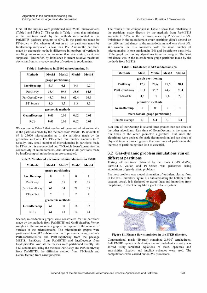
First, all the meshes were partitioned into 25600 microdomains (Table 1 and Table 2). The results in Table 1 show that imbalance in the partitions made by the methods incorporated in the ParMETIS package amounts to 60%, in the partitions made by PT-Scotch – 8%, whereas almost in all the partitions made by IncrDecomp imbalance is less than 1%. And in the partitions made by geometric methods difference in numbers of vertices in resulting microdomains is no more than one vertex, as it was supposed. Hereinafter, by imbalance is meant relative maximum deviation from an average number of vertices in subdomains.

Table 1. Imbalance in 25600 microdomains, %

Methods Mesh1 Mesh2 Mesh3 Mesh4

graph partitioning

IncrDecomp 3,5 0,1 0,3 0,2

PartKway 53,4 59,8 58,6 64,3

PartGeomKway 48,7 50,4 62,4 56,5

PT-Scotch 8,3 8,3 8,3 8,3

geometric methods

GeomDecomp 0,01 0,01 0,02 0,01

RCB 0,01 0,01 0,02 0,01

We can see in Table 2 that number of unconnected microdomains in the partitions made by the methods from ParMETIS amounts to 69 in 25600 microdomains as in the partitions made by the geometric methods. For PT-Scotch this number amounts to 7. Usually, only small number of microdomains in partitions made by PT-Scotch is unconnected but PT-Scotch doesn’t guarantee the connectivity of microdomains. And almost in all partitions made by IncrDecomp all microdomains are connected.

Table 2. Number of unconnected microdomains in 25600


graph partitioning

IncrDecomp 0 0 0 1

PartKway 69 35 37 29

PartGeomKway 67 34 28 37

PT-Scotch 7 0 2 4

geometric methods

GeomDecomp 62 38 16 33

RCB 64 43 14 44

Second, microdomain graphs were constructed for the partitions made by the methods from ParMETIS and GridSpiderPar. Vertex weights in the microdomain graphs correspond to the number of vertices in the microdomains. The microdomain graphs were partitioned into 512 subdomains on 1 processor using methods PartGraphRecursive and PartGraphKway from the package METIS, PartKway from ParMETIS and IncrDecomp from GridSpiderPar. And all the meshes were partitioned directly into 512 subdomains using the methods PartKway and ParGeomKway from ParMETIS, the diffusion method from PT-Scotch and GeomDecomp from GridSpiderPar.

The results of the comparison in Table 3 show that imbalance in the partitions made directly by the methods from ParMETIS amounts to 50%, in the partitions made by PT-Scotch – 5%. Imbalance in the microdomain graph partitions didn’t depend on the different imbalance in the microdomains and was about 5%. We assume that it’s connected with the small number of microdomains in one subdomain (50) and insufficient sensitivity of the graph partitioning algorithms to vertex weights. The least imbalance was in the microdomain graph partitions made by the methods from METIS.

Table 3. Imbalance in 512 subdomains, %


graph partitioning

PartKway 12,9 20,6 17,6 28,4

PartGeomKway 31,1 35,7 44,2 51,4

PT-Scotch 4,9 1,7 2,8 2,9

geometric methods

GeomDecomp 0 0 0 0

microdomain graph partitioning

Simple average 5,3 5,4 3,7 5,1

Run time of IncrDecomp is several times greater than run times of the other algorithms. Run time of GeomDecomp is the same as run times of the other geometric algorithms. But since the algorithms were devised for static decomposition and run times of physical tasks are much greater than run times of partitioners the increase of partitioning time isn't so essential.

3.2 Gas-dynamic problem simulations run on different partitions Testing of partitions obtained by the tools GridSpiderPar, ParMETIS, Zoltan and PT-Scotch was performed using simulations of gas-dynamic problems.

First test problem was model simulation of turbulent plasma flow in the ITER divertor (Figure 11). Situated along the bottom of the vacuum vessel, it is designed to extract heat and impurities from the plasma, in effect acting like a giant exhaust system.

Figure 11. Plasma flow simulation in the ITER divertor.

Computational mesh (divertor) contained 2,8·106 tetrahedrons. Full RMHD system with dissipation and turbulent viscosity was solved using tabulated equations of state, opacities and emissivities. Explicit and implicit schemes were used. The computations were carried out on 256 processors.



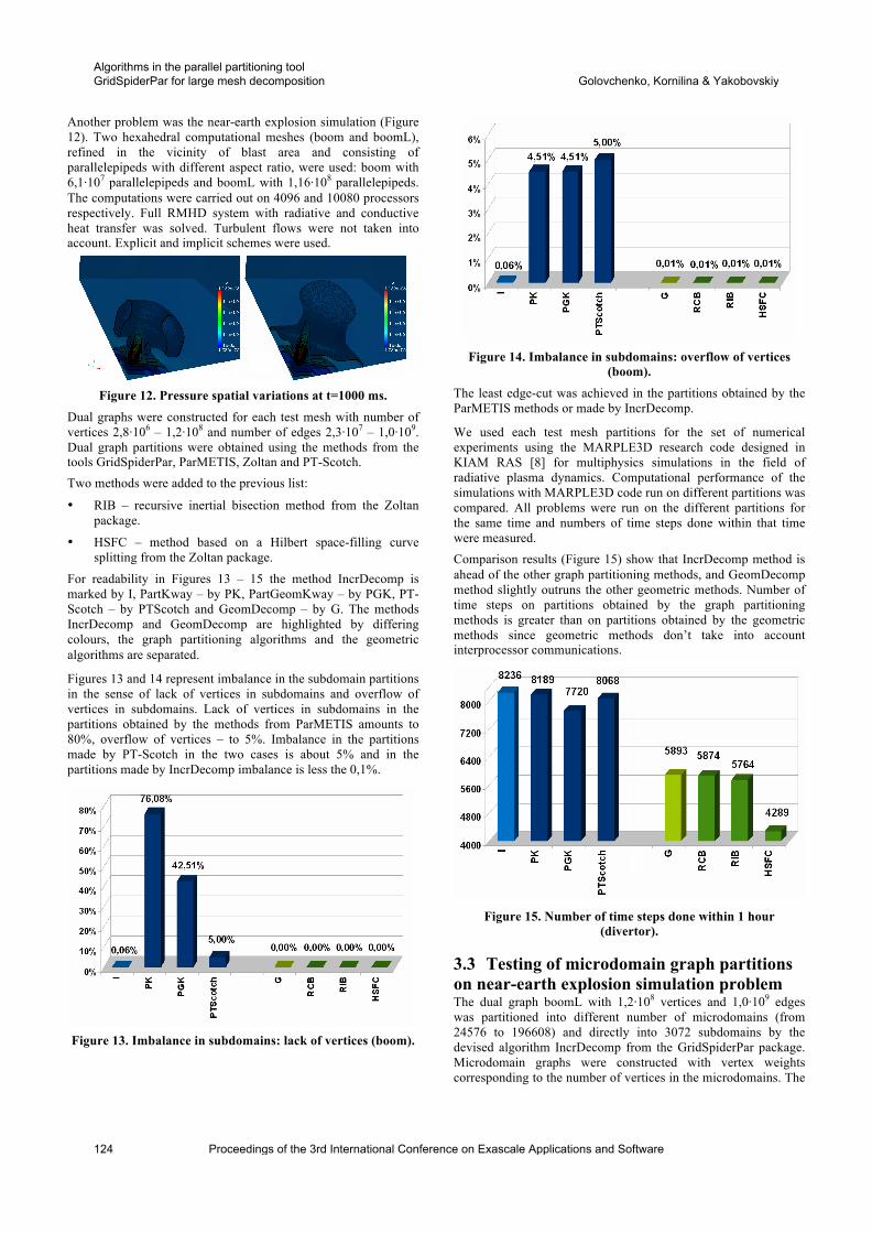
Another problem was the near-earth explosion simulation (Figure 12). Two hexahedral computational meshes (boom and boomL), refined in the vicinity of blast area and consisting of parallelepipeds with different aspect ratio, were used: boom with 6,1·107 parallelepipeds and boomL with 1,16·108 parallelepipeds. The computations were carried out on 4096 and 10080 processors respectively. Full RMHD system with radiative and conductive heat transfer was solved. Turbulent flows were not taken into account. Explicit and implicit schemes were used.

Figure 12. Pressure spatial variations at t=1000 ms.

Dual graphs were constructed for each test mesh with number of vertices 2,8·106 – 1,2·108 and number of edges 2,3·107 – 1,0·109. Dual graph partitions were obtained using the methods from the tools GridSpiderPar, ParMETIS, Zoltan and PT-Scotch. Two methods were added to the previous list:

• RIB – recursive inertial bisection method from the Zoltan package.

• HSFC – method based on a Hilbert space-filling curve splitting from the Zoltan package.

For readability in Figures 13 – 15 the method IncrDecomp is marked by I, PartKway – by PK, PartGeomKway – by PGK, PT-Scotch – by PTScotch and GeomDecomp – by G. The methods IncrDecomp and GeomDecomp are highlighted by differing colours, the graph partitioning algorithms and the geometric algorithms are separated.

Figures 13 and 14 represent imbalance in the subdomain partitions in the sense of lack of vertices in subdomains and overflow of vertices in subdomains. Lack of vertices in subdomains in the partitions obtained by the methods from ParMETIS amounts to 80%, overflow of vertices – to 5%. Imbalance in the partitions made by PT-Scotch in the two cases is about 5% and in the partitions made by IncrDecomp imbalance is less the 0,1%.

Figure 13. Imbalance in subdomains: lack of vertices (boom).

Figure 14. Imbalance in subdomains: overflow of vertices

(boom). The least edge-cut was achieved in the partitions obtained by the ParMETIS methods or made by IncrDecomp.

We used each test mesh partitions for the set of numerical experiments using the MARPLE3D research code designed in KIAM RAS [8] for multiphysics simulations in the field of radiative plasma dynamics. Computational performance of the simulations with MARPLE3D code run on different partitions was compared. All problems were run on the different partitions for the same time and numbers of time steps done within that time were measured. Comparison results (Figure 15) show that IncrDecomp method is ahead of the other graph partitioning methods, and GeomDecomp method slightly outruns the other geometric methods. Number of time steps on partitions obtained by the graph partitioning methods is greater than on partitions obtained by the geometric methods since geometric methods don’t take into account interprocessor communications.

Figure 15. Number of time steps done within 1 hour

(divertor).

3.3 Testing of microdomain graph partitions on near-earth explosion simulation problem The dual graph boomL with 1,2·108 vertices and 1,0·109 edges was partitioned into different number of microdomains (from 24576 to 196608) and directly into 3072 subdomains by the devised algorithm IncrDecomp from the GridSpiderPar package. Microdomain graphs were constructed with vertex weights corresponding to the number of vertices in the microdomains. The



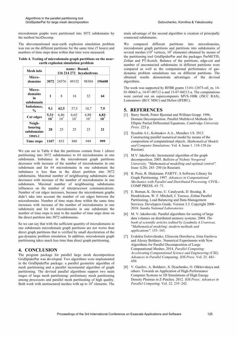
microdomain graphs were partitioned into 3072 subdomains by the method IncrDecomp.

The abovementioned near-earth explosion simulation problem was run on the different partitions for the same time (5 hours) and numbers of time steps done within that time were measured.

Table 4. Testing of microdomain graph partitions on the near-earth explosion simulation problem

Mesh info name: BoomL 116 214 272 hexahedrons

Micro- domains

3072 24576 49152 98304 196608

Micro- domains

in subdomain

1 8 16 32 64

Imbalance, % 9,1 62,5 37,5 18,7 7,9

Cut edges 5,31· 107

6,46· 107

6,65· 107

6,88· 107

6,82· 107

Neigh- bouring

subdomains (max.)

28 25 25 23 21

Time steps 1107 833 880 949 999 We can see in Table 4 that the partitions contain from 1 (direct partitioning into 3072 subdomains) to 64 microdomains in one subdomain. Imbalance in the microdomain graph partitions decreases with increase of the number of microdomains in one subdomain and for 64 microdomains in one subdomain the imbalance is less than in the direct partition into 3072 subdomains. Maximal number of neighbouring subdomains also decreases with increase of the number of microdomains in one subdomain. Maximal number of neighbouring subdomains influences on the number of interprocessor communications. Number of cut edges increases, because the microdomain graphs didn’t take into account the number of cut edges between the microdomains. Number of time steps done within the same time increases with increase of the number of microdomains in one subdomain and for 64 microdomains in one subdomain the number of time steps is near to the number of time steps done on the direct partition into 3072 subdomains.

So we can say that with the sufficient quantity of microdomains in one subdomain microdomain graph partitions are not worse than direct graph partitions that is verified by small deceleration of the gas-dynamic problem simulation. In addition, microdomain graph partitioning takes much less time than direct graph partitioning.

4. CONCLUSION The program package for parallel large mesh decomposition GridSpiderPar was developed. Two algorithms were implemented in the GridSpiderPar package: a parallel geometric algorithm of mesh partitioning and a parallel incremental algorithm of graph partitioning. The devised parallel algorithms support two main stages of large mesh partitioning: preliminary mesh partitioning among processors and parallel mesh partitioning of high quality. Both work with unstructured meshes with up to 109 elements. The

main advantage of the second algorithm is creation of principally connected subdomains.

We compared different partitions into microdomains, microdomain graph partitions and partitions into subdomains of several meshes (108 vertices, 109 elements) obtained by means of the partitioning tool GridSpiderPar and the packages ParMETIS, Zoltan and PT-Scotch. Balance of the partitions, edge-cut and number of unconnected subdomains in different partitions were compared as well as the computational performance of gas-dynamic problem simulations run on different partitions. The obtained results demonstrate advantages of the devised algorithms.

The work was supported by RFBR grants 13-01-12073-ofi_m, 14-01-00663-a, 14-07-00712-а and 15-07-04213-a. The computations were carried out on supercomputers MVS-100K (JSCC RAS), Lomonosov (RCC MSU) and Helios (IFERC).

5. REFERENCES [1] Barry Smith, Petter Bjorstad and William Gropp. 1996.

Domain Decomposition. Parallel Multilevel Methods for Elliptic Partial Differential Equations. Cambridge University Press. 225 p.

[2] Ilyushin A.I., Kolmakov A.A., Menshov I.S. 2012. Constructing parallel numerical model by means of the composition of computational objects. Mathematical Models and Computer Simulations. Vol. 4. Issue 1. 118-128 (in Russian).

[3] M.V. Iakobovski. Incremental algorithm of the graph decomposition. 2005. Bulletin of Nizhniy Novgorod University, "Mathematical modelling and optimal control". Issue 1(28). 243–250 (in Russian).

[4] R. Preis, R. Diekmann. PARTY: A Software Library for Graph Partitioning. 1997. Advances in Computational Mechanics with Parallel and Distributed Processing. CIVIL-COMP PRESS. 63–71.

[5] E. Boman, K. Devine, U. Catalyurek, D. Bozdag, B. Hendrickson, W. F. Mitchell, J. Teresco. Zoltan Parallel Partitioning, Load Balancing and Data-Management Services. Developers Guide, Version 3.3. Copyright 2000–2010. Sandia National Laboratories.

[6] M. V. Iakobovski. Parallel algorithms for sorting of large data volumes on distributed memory systems. 2004. The book of scientific articles (edited by Lyudmila A.Uvarova), "Mathematical modeling: modern methods and applications". 153–163.

[7] Evdokia Golovchenko, Elizaveta Dorofeeva, Irina Gasilova and Alexey Boldarev. Numerical Experiments with New Algorithms for Parallel Decomposition of Large Computational Meshes. 2014. Parallel Computing: Accelerating Computational Science and Engineering (CSE). Advances in Parallel Computing. IOS Press. Vol. 25. 441-450.

[8] V. Gasilov, A. Boldarev, S. Dyachenko, O. Olkhovskaya and others. Towards an Application of High-Performance Computer Systems to 3D Simulations of High Energy Density Plasmas in Z-Pinches. 2012. IOS Press: Advances in Parallel Computing. Vol. 22. 235–242.



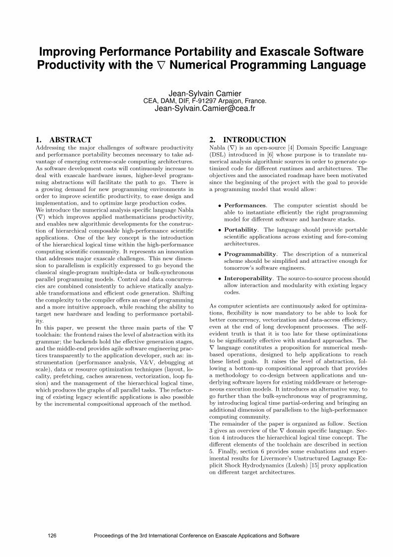
Improving Performance Portability and Exascale SoftwareProductivity with the ∇ Numerical Programming Language

Jean-Sylvain CamierCEA, DAM, DIF, F-91297 Arpajon, France.

[email protected]

1. ABSTRACTAddressing the major challenges of software productivityand performance portability becomes necessary to take ad-vantage of emerging extreme-scale computing architectures.As software development costs will continuously increase todeal with exascale hardware issues, higher-level program-ming abstractions will facilitate the path to go. There isa growing demand for new programming environments inorder to improve scientific productivity, to ease design andimplementation, and to optimize large production codes.We introduce the numerical analysis specific language Nabla(∇) which improves applied mathematicians productivity,and enables new algorithmic developments for the construc-tion of hierarchical composable high-performance scientificapplications. One of the key concept is the introductionof the hierarchical logical time within the high-performancecomputing scientific community. It represents an innovationthat addresses major exascale challenges. This new dimen-sion to parallelism is explicitly expressed to go beyond theclassical single-program multiple-data or bulk-synchronousparallel programming models. Control and data concurren-cies are combined consistently to achieve statically analyz-able transformations and efficient code generation. Shiftingthe complexity to the compiler offers an ease of programmingand a more intuitive approach, while reaching the ability totarget new hardware and leading to performance portabil-ity.In this paper, we present the three main parts of the ∇toolchain: the frontend raises the level of abstraction with itsgrammar; the backends hold the effective generation stages,and the middle-end provides agile software engineering prac-tices transparently to the application developer, such as: in-strumentation (performance analysis, V&V, debugging atscale), data or resource optimization techniques (layout, lo-cality, prefetching, caches awareness, vectorization, loop fu-sion) and the management of the hierarchical logical time,which produces the graphs of all parallel tasks. The refactor-ing of existing legacy scientific applications is also possibleby the incremental compositional approach of the method.

2. INTRODUCTIONNabla (∇) is an open-source [4] Domain Specific Language(DSL) introduced in [6] whose purpose is to translate nu-merical analysis algorithmic sources in order to generate op-timized code for different runtimes and architectures. Theobjectives and the associated roadmap have been motivatedsince the beginning of the project with the goal to providea programming model that would allow:

• Performances. The computer scientist should beable to instantiate efficiently the right programmingmodel for different software and hardware stacks.

• Portability. The language should provide portablescientific applications across existing and fore-comingarchitectures.

• Programmability. The description of a numericalscheme should be simplified and attractive enough fortomorrow’s software engineers.

• Interoperability. The source-to-source process shouldallow interaction and modularity with existing legacycodes.

As computer scientists are continuously asked for optimiza-tions, flexibility is now mandatory to be able to look forbetter concurrency, vectorization and data-access efficiency,even at the end of long development processes. The self-evident truth is that it is too late for these optimizationsto be significantly effective with standard approaches. The∇ language constitutes a proposition for numerical mesh-based operations, designed to help applications to reachthese listed goals. It raises the level of abstraction, fol-lowing a bottom-up compositional approach that providesa methodology to co-design between applications and un-derlying software layers for existing middleware or heteroge-neous execution models. It introduces an alternative way, togo further than the bulk-synchronous way of programming,by introducing logical time partial-ordering and bringing anadditional dimension of parallelism to the high-performancecomputing community.The remainder of the paper is organized as follow. Section3 gives an overview of the ∇ domain specific language. Sec-tion 4 introduces the hierarchical logical time concept. Thedifferent elements of the toolchain are described in section5. Finally, section 6 provides some evaluations and exper-imental results for Livermore’s Unstructured Lagrange Ex-plicit Shock Hydrodynamics (Lulesh) [15] proxy applicationon different target architectures.


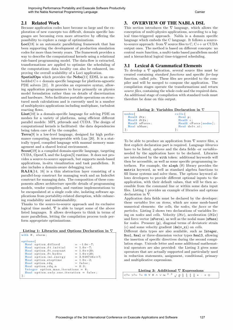
2.1 Related WorkBecause application codes have become so large and the ex-ploration of new concepts too difficult, domain specific lan-guages are becoming even more attractive by offering thepossibility to explore a range of optimizations.Loci[18] is an automatic parallelizing framework that hasbeen supporting the development of production simulationcodes for more than twenty years. The framework provides away to describe the computational kernels using a relationalrule-based programming model. The data-flow is extracted,transformations are applied to optimize the scheduling ofthe computations; data locality can also be enhanced, im-proving the overall scalability of a Loci application.SpatialOps which provides the Nebo[11] EDSL is an em-bedded C++ domain specific language for platform-agnosticPDE solvers [21]. It provides an expressive syntax, allow-ing application programmers to focus primarily on physicsmodel formulation rather than on details of discretizationand hardware. Nebo facilitates portable operations on struc-tured mesh calculations and is currently used in a numberof multiphysics applications including multiphase, turbulentreacting flows.Liszt[10] is a domain-specific language for solving PDE onmeshes for a variety of platforms, using efficient differentparallel models: MPI, pthreads and CUDA. The design ofcomputational kernels is facilitated: the data dependenciesbeing taken care of by the compiler.Terra[9] is a low-level language, designed for high perfor-mance computing, interoperable with Lua [20]. It is a stat-ically typed, compiled language with manual memory man-agement and a shared lexical environment.Scout[19] is a compiled domain-specific language, targetingCUDA, OpenCL and the Legion[5] runtime. It does not pro-vides a source-to-source approach, but supports mesh-basedapplications, in-situ visualization and task parallelism. Italso includes a domain-aware debugging tool.RAJA[14, 16] is a thin abstraction layer consisting of aparallel-loop construct for managing work and an IndexSetconstruct for managing data. The composition of these com-ponents allows architecture specific details of programmingmodels, vendor compilers, and runtime implementations tobe encapsulated at a single code site, isolating software ap-plications from portability-related disruption, while enhanc-ing readability and maintainability.Thanks to the source-to-source approach and its exclusivelogical time model, ∇ is able to target some of the abovelisted languages. It allows developers to think in terms ofmore parallelism, letting the compilation process tools per-form appropriate optimizations.

Listing 1: Libraries and Options Declaration in ∇with ℵ , slurm ;

optionsReal o p t i o n d t f i x e d = −1.0e−7;Real opt i on δ t i n i t i a l = 1 .0 e−7;Real opt i on δ t courant = 1 .0 e +20;Real opt i on δ t hydro = 1 .0 e +20;Real o p t i o n i n i e n e r g y = 3.948746 e+7;Real opt ion s topt ime = 1 .0 e−2;Bool opt ion rdq = f a l s e ;Real opt i on rdq α = 0 . 3 ;Integer op t i on max i t e r a t i on s = 8 ;Bool o p t i o n o n l y o n e i t e r a t i o n = f a l s e ;

;

3. OVERVIEW OF THE NABLA DSLThis section introduces the ∇ language, which allows theconception of multi-physics applications, according to a log-ical time-triggered approach. Nabla is a domain specificlanguage which embeds the C language. It follows a source-to-source approach: from∇ source files to C, C++ or CUDAoutput ones. The method is based on different concepts: nocentral main function, a multi-tasks based parallelism modeland a hierarchical logical time-triggered scheduling.

3.1 Lexical & Grammatical ElementsTo develop a ∇ application, several source files must becreated containing standard functions and specific for-loopfunction, called jobs. These files are provided to the com-piler and will be merged to compose the application. Thecompilation stages operate the transformations and returnsource files, containing the whole code and the required data.An additional stage of compilation with standard tools musttherefore be done on this output.

Listing 2: Variables Declaration in ∇nodes ce l l s

Real3 ∂ tx ; Real p ;Real3 ∂ t2x ; Real3 ε ;Real3 nForce ; Real3 cForce [ nodes ] ;Real nMass ; Real d e l v x i ;

; ;

To be able to produce an application from ∇ source files, afirst explicit declaration part is required. Language librarieshave to be listed, options and the data fields -or variables-needed by the application have to be declared. Librariesare introduced by the with token: additional keywords willthen be accessible, as well as some specific programming in-terfaces. For example, the aleph (ℵ) library provides thematrix keyword, as well as standard algebra functions tofill linear systems and solve them. The options keyword al-lows developers to provide different optional inputs to theapplication, with their default values, that will be then ac-cessible from the command line or within some data inputfiles. Listing 1 provides an example of libraries and optionsdeclaration in ∇.Application data fields must be declared by the developer:these variables live on items, which are some mesh-basednumerical elements: the cells, the nodes, the faces or theparticles. Listing 2 shows two declarations of variables liv-ing on nodes and cells. Velocity (∂tx), acceleration (∂t2x)and force vector (nForce), as well as the nodal mass (nMass)for nodes. Pressure (p), diagonal terms of deviatoric strain(ε) and some velocity gradient (delv_xi) on cells.Different data types are also available, such as Integer,Bool, Real or three-dimension vector types Real3, allowingthe insertion of specific directives during the second compi-lation stage. Unicode letter and some additional mathemat-ical operators are also provided: the Listing 3 gives someoperators that are actually supported and particularly usedin reduction statements, assignment, conditional, primaryand multiplicative expressions.

Listing 3: Additional ∇ Expressions<?= >?= ?= @ ∀ ℵ ∧ ∨ ∞ 2 3 √ 3

√ 12

13

14

18 ? · × ⊗


Improving Performance Portability and Exascale Software Productivity with the Nabla Numerical Programming Language Camier

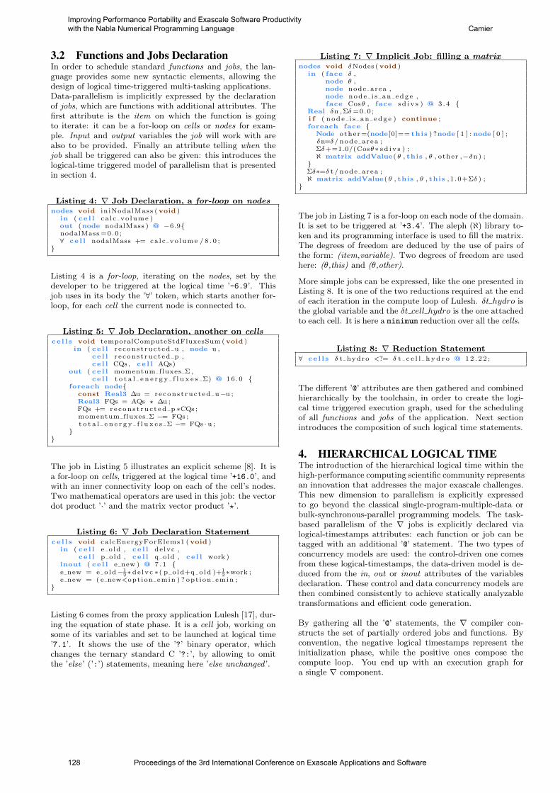
3.2 Functions and Jobs DeclarationIn order to schedule standard functions and jobs, the lan-guage provides some new syntactic elements, allowing thedesign of logical time-triggered multi-tasking applications.Data-parallelism is implicitly expressed by the declarationof jobs, which are functions with additional attributes. Thefirst attribute is the item on which the function is goingto iterate: it can be a for-loop on cells or nodes for exam-ple. Input and output variables the job will work with arealso to be provided. Finally an attribute telling when thejob shall be triggered can also be given: this introduces thelogical-time triggered model of parallelism that is presentedin section 4.

Listing 4: ∇ Job Declaration, a for-loop on nodesnodes void iniNodalMass (void )

in ( ce l l ca lc vo lume )out (node nodalMass ) @ −6.9nodalMass =0.0;∀ ce l l nodalMass += calc vo lume / 8 . 0 ;

Listing 4 is a for-loop, iterating on the nodes, set by thedeveloper to be triggered at the logical time ’-6.9’. Thisjob uses in its body the ’∀’ token, which starts another for-loop, for each cell the current node is connected to.

Listing 5: ∇ Job Declaration, another on cellsce l l s void temporalComputeStdFluxesSum (void )

in ( ce l l r econs t ructed u , node u ,ce l l r econs t ructed p ,ce l l CQs, ce l l AQs)

out ( ce l l momentum fluxes Σ ,ce l l t o t a l e n e r g y f l u x e s Σ) @ 16 .0

foreach nodeconst Real3 ∆u = recons t ructed u−u ;Real3 FQs = AQs ? ∆u ;FQs += recons t ruc t ed p ∗CQs ;momentum fluxes Σ −= FQs ;t o t a l e n e r g y f l u x e s Σ −= FQs · u ;

The job in Listing 5 illustrates an explicit scheme [8]. It isa for-loop on cells, triggered at the logical time ’+16.0’, andwith an inner connectivity loop on each of the cell’s nodes.Two mathematical operators are used in this job: the vectordot product ’·’ and the matrix vector product ’?’.

Listing 6: ∇ Job Declaration Statementce l l s void calcEnergyForElems1 (void )

in ( ce l l e o ld , ce l l delvc ,ce l l p old , ce l l q old , ce l l work )

inout ( ce l l e new ) @ 7 .1 e new = e o ld−1

2∗ de lvc ∗( p o ld+q o ld )+12∗work ;

e new = ( e new<opt ion emin ) ? opt ion emin ;

Listing 6 comes from the proxy application Lulesh [17], dur-ing the equation of state phase. It is a cell job, working onsome of its variables and set to be launched at logical time’7.1’. It shows the use of the ’?’ binary operator, whichchanges the ternary standard C ’?:’, by allowing to omitthe ’else’ (’:’) statements, meaning here ’else unchanged ’.

Listing 7: ∇ Implicit Job: filling a matrixnodes void δNodes (void )

in ( face δ ,node θ ,node node area ,node node i s an edge ,face Cosθ , face sd i v s ) @ 3 .4

Real δn ,Σδ=0.0;i f ( node i s an edge ) continue ;foreach face

Node other=(node[0]== this ) ?node [ 1 ] : node [ 0 ] ;δn=δ/ node area ;Σδ+=1.0/(Cosθ∗ sd i v s ) ;ℵ matrix addValue( θ , this , θ , other ,−δn) ;

Σδ∗=δ t / node area ;ℵ matrix addValue( θ , this , θ , this ,1 .0+Σδ ) ;

The job in Listing 7 is a for-loop on each node of the domain.It is set to be triggered at ’+3.4’. The aleph (ℵ) library to-ken and its programming interface is used to fill the matrix.The degrees of freedom are deduced by the use of pairs ofthe form: (item,variable). Two degrees of freedom are usedhere: (θ,this) and (θ,other).

More simple jobs can be expressed, like the one presented inListing 8. It is one of the two reductions required at the endof each iteration in the compute loop of Lulesh. δt hydro isthe global variable and the δt cell hydro is the one attachedto each cell. It is here a minimum reduction over all the cells.

Listing 8: ∇ Reduction Statement∀ ce l l s δ t hydro <?= δ t c e l l h y d r o @ 1 2 . 2 2 ;

The different ’@’ attributes are then gathered and combinedhierarchically by the toolchain, in order to create the logi-cal time triggered execution graph, used for the schedulingof all functions and jobs of the application. Next sectionintroduces the composition of such logical time statements.

4. HIERARCHICAL LOGICAL TIMEThe introduction of the hierarchical logical time within thehigh-performance computing scientific community representsan innovation that addresses the major exascale challenges.This new dimension to parallelism is explicitly expressedto go beyond the classical single-program-multiple-data orbulk-synchronous-parallel programming models. The task-based parallelism of the ∇ jobs is explicitly declared vialogical-timestamps attributes: each function or job can betagged with an additional ’@’ statement. The two types ofconcurrency models are used: the control-driven one comesfrom these logical-timestamps, the data-driven model is de-duced from the in, out or inout attributes of the variablesdeclaration. These control and data concurrency models arethen combined consistently to achieve statically analyzabletransformations and efficient code generation.

By gathering all the ’@’ statements, the ∇ compiler con-structs the set of partially ordered jobs and functions. Byconvention, the negative logical timestamps represent theinitialization phase, while the positive ones compose thecompute loop. You end up with an execution graph fora single ∇ component.



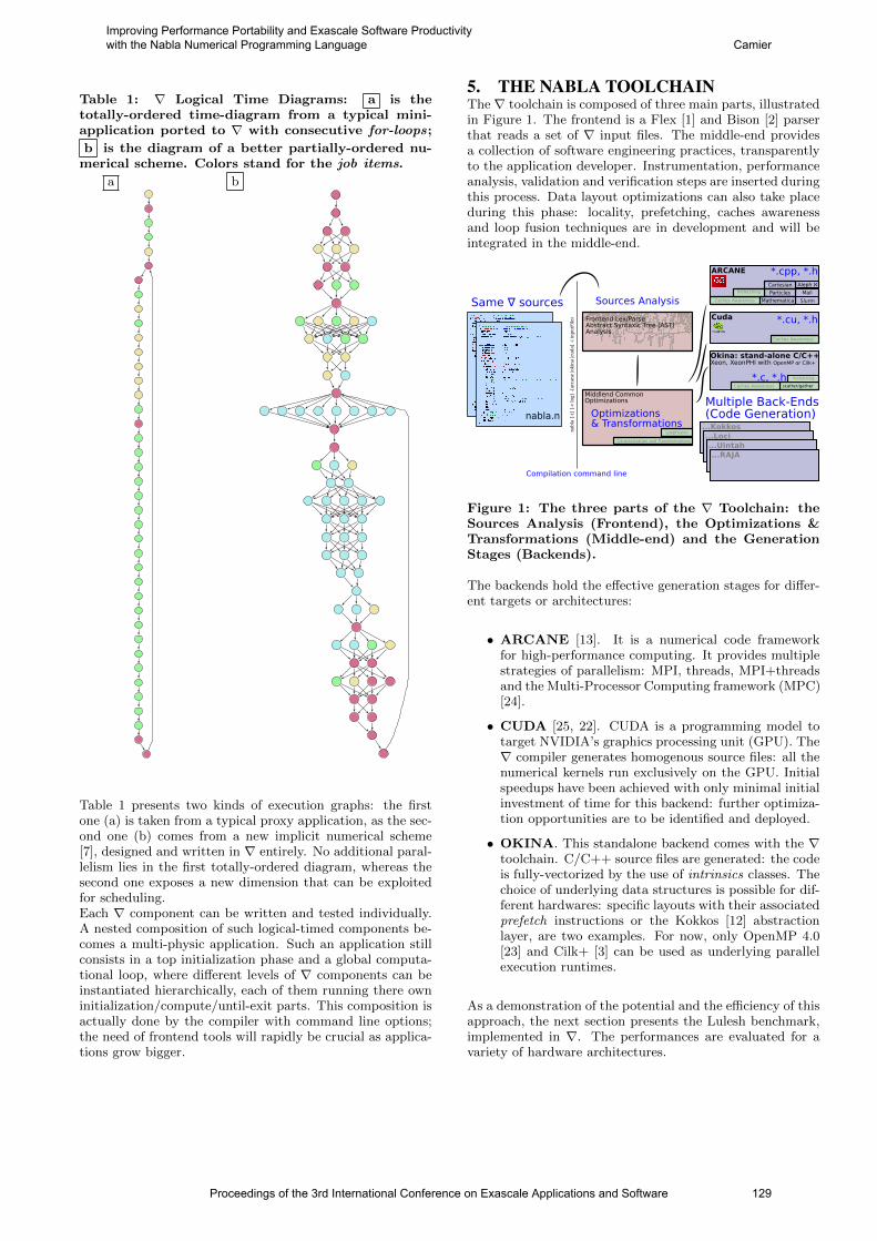
Table 1: ∇ Logical Time Diagrams: a is thetotally-ordered time-diagram from a typical mini-application ported to ∇ with consecutive for-loops;

b is the diagram of a better partially-ordered nu-merical scheme. Colors stand for the job items.

a b

Table 1 presents two kinds of execution graphs: the firstone (a) is taken from a typical proxy application, as the sec-ond one (b) comes from a new implicit numerical scheme[7], designed and written in ∇ entirely. No additional paral-lelism lies in the first totally-ordered diagram, whereas thesecond one exposes a new dimension that can be exploitedfor scheduling.Each ∇ component can be written and tested individually.A nested composition of such logical-timed components be-comes a multi-physic application. Such an application stillconsists in a top initialization phase and a global computa-tional loop, where different levels of ∇ components can beinstantiated hierarchically, each of them running there owninitialization/compute/until-exit parts. This composition isactually done by the compiler with command line options;the need of frontend tools will rapidly be crucial as applica-tions grow bigger.

5. THE NABLA TOOLCHAINThe ∇ toolchain is composed of three main parts, illustratedin Figure 1. The frontend is a Flex [1] and Bison [2] parserthat reads a set of ∇ input files. The middle-end providesa collection of software engineering practices, transparentlyto the application developer. Instrumentation, performanceanalysis, validation and verification steps are inserted duringthis process. Data layout optimizations can also take placeduring this phase: locality, prefetching, caches awarenessand loop fusion techniques are in development and will beintegrated in the middle-end.

Figure 1: The three parts of the ∇ Toolchain: theSources Analysis (Frontend), the Optimizations &Transformations (Middle-end) and the GenerationStages (Backends).

The backends hold the effective generation stages for differ-ent targets or architectures:

• ARCANE [13]. It is a numerical code frameworkfor high-performance computing. It provides multiplestrategies of parallelism: MPI, threads, MPI+threadsand the Multi-Processor Computing framework (MPC)[24].

• CUDA [25, 22]. CUDA is a programming model totarget NVIDIA’s graphics processing unit (GPU). The∇ compiler generates homogenous source files: all thenumerical kernels run exclusively on the GPU. Initialspeedups have been achieved with only minimal initialinvestment of time for this backend: further optimiza-tion opportunities are to be identified and deployed.

• OKINA. This standalone backend comes with the ∇toolchain. C/C++ source files are generated: the codeis fully-vectorized by the use of intrinsics classes. Thechoice of underlying data structures is possible for dif-ferent hardwares: specific layouts with their associatedprefetch instructions or the Kokkos [12] abstractionlayer, are two examples. For now, only OpenMP 4.0[23] and Cilk+ [3] can be used as underlying parallelexecution runtimes.

As a demonstration of the potential and the efficiency of thisapproach, the next section presents the Lulesh benchmark,implemented in ∇. The performances are evaluated for avariety of hardware architectures.



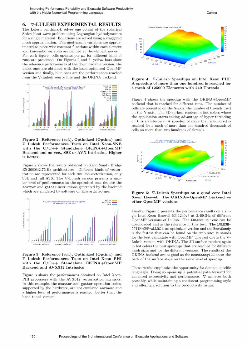
6. ∇-LULESH EXPERIMENTAL RESULTSThe Lulesh benchmark solves one octant of the sphericalSedov blast wave problem using Lagrangian hydrodynamicsfor a single material. Equations are solved using a staggeredmesh approximation. Thermodynamic variables are approx-imated as piece-wise constant functions within each elementand kinematic variables are defined at the element nodes.For each figure, cells-updates-per-µs for different kind ofruns are presented. On Figures 2 and 3, yellow bars showthe reference performances of the downloadable version, theviolet ones are obtained with the hand-optimized OpenMPversion and finally, blue ones are the performances reachedfrom the ∇-Lulesh source files and the OKINA backend.

Figure 2: Reference (ref.), Optimized (Optim.) and∇ Lulesh Performances Tests on Intel Xeon-SNBwith the C/C++ Standalone OKINA+OpenMPBackend and no-vec., SSE or AVX Intrinsics. Higheris better.

Figure 2 shows the results obtained on Xeon Sandy [email protected] architectures. Different kinds of vector-ization are represented for each run: no-vectorization, onlySSE and full AVX. The ∇-Lulesh version presents a simi-lar level of performances as the optimised one, despite thescatter and gather instructions generated by the backendwhich are emulated by software on this architecture.

Figure 3: Reference (ref.), Optimized (Optim.) and∇ Lulesh Performances Tests on Intel Xeon PHIwith the C/C++ Standalone OKINA+OpenMPBackend and AVX512 Intrinsics

Figure 3 shows the performances obtained on Intel Xeon-PHI processors with the AVX512 vectorization intrinsics.In this example, the scatter and gather operation codes,supported by the hardware, are not emulated anymore anda higher level of performances is reached, better than thehand-tuned version.

Figure 4: ∇-Lulesh Speedups on Intel Xeon PHI:A speedup of more than one hundred is reached fora mesh of 125000 Elements with 240 Threads

Figure 4 shows the speedup with the OKINA+OpenMPbackend that is reached for different runs. The number ofcells are presented on the X-axis, the number of threads usedon the Y-axis. The 3D-surface renders in hot colors wherethe application starts taking advantage of hyper-threadingon this architecture. A speedup of more than a hundred isreached for a mesh of more than one hundred thousands ofcells on more than two hundreds of threads.

Figure 5: ∇-Lulesh Speedups on a quad core IntelXeon Haswell: the OKINA+OpenMP backend vsother OpenMP versions

Finally, Figure 5 presents the performance results on a sin-gle Intel Xeon Haswell E3-1240v3 at 3.40GHz of differentOpenMP versions of Lulesh. The LULESH-OMP one can bedownloaded and is the reference in this test. The LULESH-

OPTIM-OMP-ALLOC is an optimized version and the BestSandyis the fastest that can be found on the web site: it standsfor the best candidate with OpenMP. The last one is the ∇-Lulesh version with OKINA. The 3D-surface renders againin hot colors the best speedups that are reached for differentmesh sizes and for the different versions. The results of theOKINA backend are as good as the BestSandyICC ones: theback of the surface stays on the same level of speedup.

These results emphasize the opportunity for domain-specificlanguages. Doing so opens up a potential path forward forenhanced expressivity and performance. ∇ achieves bothportably, while maintaining a consistent programming styleand offering a solution to the productivity issues.



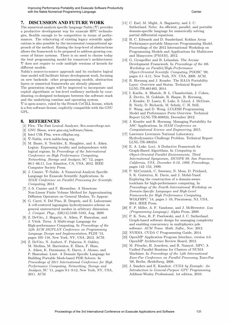
7. DISCUSSION AND FUTURE WORKThe numerical-analysis specific language Nabla (∇) providesa productive development way for exascale HPC technolo-gies, flexible enough to be competitive in terms of perfor-mances. The refactoring of existing legacy scientific appli-cations is also possible by the incremental compositional ap-proach of the method. Raising the loop-level of abstractionsallows the framework to be prepared to address growing con-cerns of future systems. There is no need to choose todaythe best programming model for tomorrow’s architectures:∇ does not require to code multiple versions of kernels fordifferent models.Nabla’s source-to-source approach and its exclusive logicaltime model will facilitate future development work, focusingon new backends: other programming models, abstractionlayers or numerical frameworks are already planned.The generation stages will be improved to incorporate andexploit algorithmic or low-level resiliency methods by coor-dinating co-designed techniques between the software stackand the underlying runtime and operating system.∇ is open-source, ruled by the French CeCILL license, whichis a free software license, explicitly compatible with the GNUGPL.

8. REFERENCES[1] Flex: The Fast Lexical Analyzer, flex.sourceforge.net.

[2] GNU Bison, www.gnu.org/software/bison.

[3] Intel Cilk Plus, www.cilkplus.org.

[4] ∇-Nabla, www.nabla-lang.org.

[5] M. Bauer, S. Treichler, E. Slaughter, and A. Aiken.Legion: Expressing locality and independence withlogical regions. In Proceedings of the InternationalConference on High Performance Computing,Networking, Storage and Analysis, SC ’12, pages66:1–66:11, Los Alamitos, CA, USA, 2012. IEEEComputer Society Press.

[6] J. Camier. ∇-Nabla: A Numerical-Analysis SpecificLanguage for Exascale Scientific Applications. InSIAM Conference on Parallel Processing for ScientificComputing, 2014.

[7] J.-S. Camier and F. Hermeline. A MonotoneNon-Linear Finite Volume Method for ApproximatingDiffusion Operators on General Meshes, To Appear.

[8] G. Carre, S. Del Pino, B. Despres, and E. Labourasse.A cell-centered lagrangian hydrodynamics scheme ongeneral unstructured meshes in arbitrary dimension.J. Comput. Phys., 228(14):5160–5183, Aug. 2009.

[9] Z. DeVito, J. Hegarty, A. Aiken, P. Hanrahan, andJ. Vitek. Terra: A Multi-stage Language forHigh-performance Computing. In Proceedings of the34th ACM SIGPLAN Conference on ProgrammingLanguage Design and Implementation, PLDI ’13,pages 105–116, New York, NY, USA, 2013. ACM.

[10] Z. DeVito, N. Joubert, F. Palacios, S. Oakley,M. Medina, M. Barrientos, E. Elsen, F. Ham,A. Aiken, K. Duraisamy, E. Darve, J. Alonso, andP. Hanrahan. Liszt: A Domain Specific Language forBuilding Portable Mesh-based PDE Solvers. InProceedings of 2011 International Conference for HighPerformance Computing, Networking, Storage andAnalysis, SC ’11, pages 9:1–9:12, New York, NY, USA,2011. ACM.

[11] C. Earl, M. Might, A. Bagusetty, and J. C.Sutherland. Nebo: An efficient, parallel, and portabledomain-specific language for numerically solvingpartial differential equations.

[12] H. C. Edwards and D. Sunderland. Kokkos ArrayPerformance-portable Manycore Programming Model.Proceedings of the 2012 International Workshop onProgramming Models and Applications for Multicoresand Manycores (PMAM), 2012.

[13] G. Grospellier and B. Lelandais. The ArcaneDevelopment Framework. In Proceedings of the 8thWorkshop on Parallel/High-PerformanceObject-Oriented Scientific Computing, POOSC ’09,pages 4:1–4:11, New York, NY, USA, 2009. ACM.

[14] R. Hornung and J. Keasler. The RAJA PortabilityLayer: Overview and Status. Technical ReportLLNL-TR-661403, 2014.

[15] I. Karlin, A. Bhatele, B. L. Chamberlain, J. Cohen,Z. Devito, M. Gokhale, R. Haque, R. Hornung,J. Keasler, D. Laney, E. Luke, S. Lloyd, J. McGraw,R. Neely, D. Richards, M. Schulz, C. H. Still,F. Wang, and D. Wong. LULESH ProgrammingModel and Performance Ports Overview. TechnicalReport LLNL-TR-608824, December 2012.

[16] J. Keasler and R. Hornung. Managing Portability forASC Applications. In SIAM Conference onComputational Science and Engineering, 2015.

[17] Lawrence Livermore National Laboratory.Hydrodynamics Challenge Problem. Technical ReportLLNL-TR-490254.

[18] E. A. Luke. Loci: A Deductive Framework forGraph-Based Algorithms. In Computing inObject-Oriented Parallel Environments, ThirdInternational Symposium, ISCOPE 99, San Francisco,California, USA, December 8-10, 1999, Proceedings,pages 142–153, 1999.

[19] P. McCormick, C. Sweeney, N. Moss, D. Prichard,S. K. Gutierrez, K. Davis, and J. Mohd-Yusof.Exploring the construction of a domain-awaretoolchain for high-performance computing. InProceedings of the Fourth International Workshop onDomain-Specific Languages and High-LevelFrameworks for High Performance Computing,WOLFHPC ’14, pages 1–10, Piscataway, NJ, USA,2014. IEEE Press.

[20] F. P. Miller, A. F. Vandome, and J. McBrewster. Lua(Programming Language). Alpha Press, 2009.

[21] P. K. Notz, R. P. Pawlowski, and J. C. Sutherland.Graph-based software design for managing complexityand enabling concurrency in multiphysics pdesoftware. ACM Trans. Math. Softw., Nov. 2012.

[22] NVIDIA. CUDA C Programming Guide, 2014.

[23] OpenMP Application Program Interface, version 4.0.OpenMP Architecture Review Board, 2013.

[24] M. Perache, H. Jourdren, and R. Namyst. MPC: AUnified Parallel Runtime for Clusters of NUMAMachines. In Proceedings of the 14th InternationalEuro-Par Conference on Parallel Processing, Euro-Par’08, Berlin, Heidelberg, 2008.

[25] J. Sanders and E. Kandrot. CUDA by Example: AnIntroduction to General-Purpose GPU Programming.Addison-Wesley Professional, 1st edition, 2010.



A highly scalable Met Office NERC Cloud model

Nick BrownEPCC, James Clerk MaxwellBuilding, Peter Guthrie Tait

Road, [email protected]

Michele WeilandEPCC, James Clerk MaxwellBuilding, Peter Guthrie Tait

Road, Edinburgh

Adrian HillUK Met Office, FitzRoy Road,

Exeter, Devon

Ben ShipwayUK Met Office, FitzRoy Road,

Exeter, Devon

Chris MaynardUK Met Office, FitzRoy Road,

Exeter, Devon

Thomas AllenUK Met Office, FitzRoy Road,

Exeter, Devon

Mike ReznyUK Met Office, FitzRoy Road,

Exeter, Devon

ABSTRACTLarge Eddy Simulation is a critical modelling tool for scien-tists investigating atmospheric flows, turbulence and cloudmicrophysics. Within the UK, the principal LES model usedby the atmospheric research community is the Met OfficeLarge Eddy Model (LEM). The LEM was originally devel-oped in the late 1980s using computational techniques andassumptions of the time, which means that the it does notscale beyond 512 cores. In this paper we present the MetOffice NERC Cloud model, MONC, which is a re-write ofthe existing LEM. We discuss the software engineering andarchitectural decisions made in order to develop a flexible,extensible model which the community can easily customisefor their own needs. The scalability of MONC is evaluated,along with numerous additional customisations made to fur-ther improve performance at large core counts. The result ofthis work is a model which delivers to the community signifi-cant new scientific modelling capability that takes advantageof the current and future generation HPC machines.

KeywordsMONC, LEM, Large Eddy Simulation, Met Office

1. INTRODUCTIONLarge Eddy Simulation is a computational fluid dynamicstechnique used to efficiently simulate and study turbulentflows. In atmospheric science, LES are often coupled tocloud microphysics and radiative transfer schemes, to createa high resolution modelling framework that is employed todevelop and test physical parametrisations and assumptionsused in numerical weather and climate prediction. In theUK, the Met Office Large Eddy Model (LEM) is the prin-cipal LES that is used within the Met Office and academia.It includes a detailed cloud microphysics representation anda version of the operational radiative transfer scheme. TheLEM was initially developed in the 1980s and, whilst the sci-entific output from the model is cutting edge, the code itselfhas become outdated. Hard coded assumptions made aboutparallelism, which were sensible 20 years ago, are now thesource of severe limitations and this means that the modeldoes not scale beyond 512 cores. This prevents scientistsfrom carrying out very high resolution modelling on the lat-est HPC machines.

As machines become larger, and significantly different fromthe architectures that a code was initially designed for, itcan sometimes be easier to re-write poorly performing ap-plications rather than attempt to modernise them throughre-factoring. The Met Office NERC Cloud model (MONC)is a complete re-write of the LEM, providing the atmosphericscientific community with a tool for modelling atmosphericflows, turbulence and clouds at very high resolutions and/ornear real time. The fact that this aspires to be a commu-nity code, along with the desire to future proof to as greatan extent as possible, has heavily influenced the design ofthe code. We have adopted a “plug in” architecture, de-scribed in section 3.1, where the model is organised as aseries of distinctive, independent, components which can beselected at run-time. This approach, which we discuss indetail, not only allows for a variety of science to be easilyintegrated but it also supports development targeting differ-ent architectures and technologies by simply replacing onecomponent with another.

Other innovative aspects of the code are presented and inparticular our approach to data analysis and processing (sec-tion 3.2), which is a major feature of the model. Thesemodels analyse their raw data to produce higher level in-formation, for instance the average temperature in a cloudor tracking of how specific clouds move through the atmo-sphere. The existing LEM, like many codes, performs dataanalysis inline as part of the model timestep which, alongwith the I/O operation time, is a major bottleneck. In con-trast MONC uses the notion of an I/O server, where typ-ically one core per processor is dedicated to handling andanalysing the data produced by the model, which is runningon the remaining cores. In this manner, MONC can act in a“fire and forget” fashion, asynchronously sending data to the“local” I/O server and continuing on with the next timestepwhilst it is being processed.

Based upon the innovative approaches adopted, we presentin section 4 performance and scalability results of MONCand discuss some of the lessons learnt, both in terms of largescale parallelism and software engineering techniques, thathave become apparent in order to reach the level of scalabil-ity and performance demanded by the community. Section


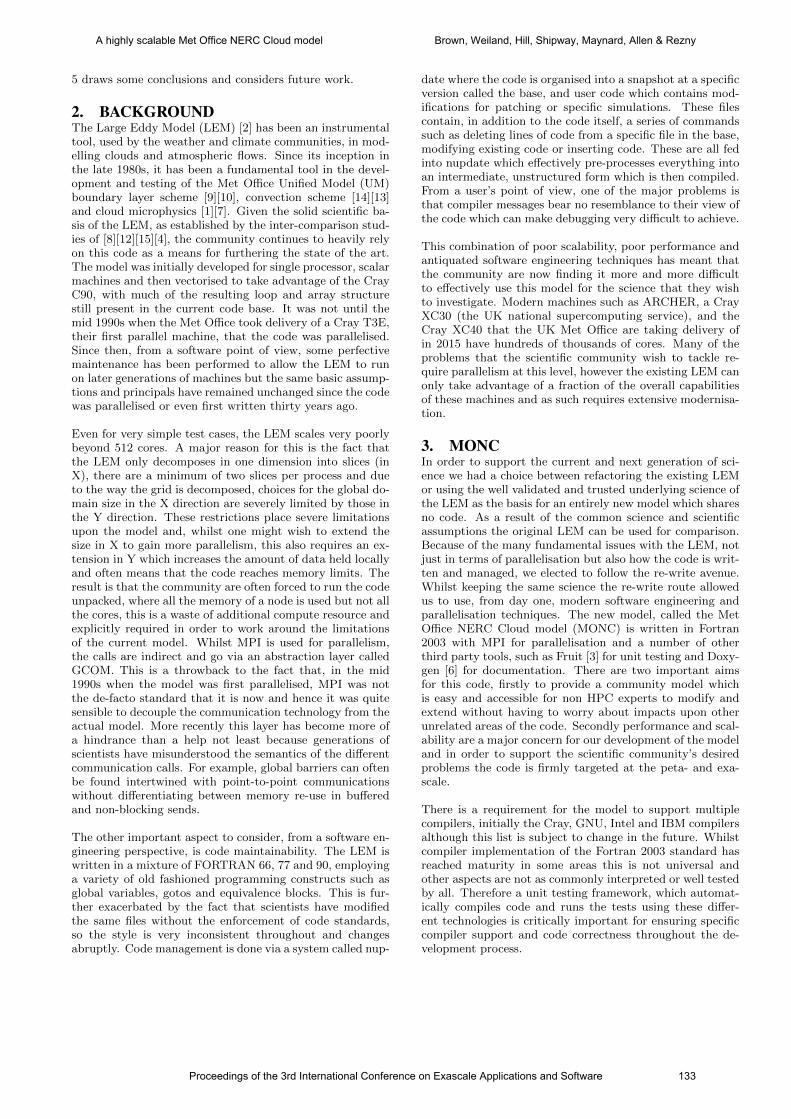
5 draws some conclusions and considers future work.

2. BACKGROUNDThe Large Eddy Model (LEM) [2] has been an instrumentaltool, used by the weather and climate communities, in mod-elling clouds and atmospheric flows. Since its inception inthe late 1980s, it has been a fundamental tool in the devel-opment and testing of the Met Office Unified Model (UM)boundary layer scheme [9][10], convection scheme [14][13]and cloud microphysics [1][7]. Given the solid scientific ba-sis of the LEM, as established by the inter-comparison stud-ies of [8][12][15][4], the community continues to heavily relyon this code as a means for furthering the state of the art.The model was initially developed for single processor, scalarmachines and then vectorised to take advantage of the CrayC90, with much of the resulting loop and array structurestill present in the current code base. It was not until themid 1990s when the Met Office took delivery of a Cray T3E,their first parallel machine, that the code was parallelised.Since then, from a software point of view, some perfectivemaintenance has been performed to allow the LEM to runon later generations of machines but the same basic assump-tions and principals have remained unchanged since the codewas parallelised or even first written thirty years ago.

Even for very simple test cases, the LEM scales very poorlybeyond 512 cores. A major reason for this is the fact thatthe LEM only decomposes in one dimension into slices (inX), there are a minimum of two slices per process and dueto the way the grid is decomposed, choices for the global do-main size in the X direction are severely limited by those inthe Y direction. These restrictions place severe limitationsupon the model and, whilst one might wish to extend thesize in X to gain more parallelism, this also requires an ex-tension in Y which increases the amount of data held locallyand often means that the code reaches memory limits. Theresult is that the community are often forced to run the codeunpacked, where all the memory of a node is used but not allthe cores, this is a waste of additional compute resource andexplicitly required in order to work around the limitationsof the current model. Whilst MPI is used for parallelism,the calls are indirect and go via an abstraction layer calledGCOM. This is a throwback to the fact that, in the mid1990s when the model was first parallelised, MPI was notthe de-facto standard that it is now and hence it was quitesensible to decouple the communication technology from theactual model. More recently this layer has become more ofa hindrance than a help not least because generations ofscientists have misunderstood the semantics of the differentcommunication calls. For example, global barriers can oftenbe found intertwined with point-to-point communicationswithout differentiating between memory re-use in bufferedand non-blocking sends.

The other important aspect to consider, from a software en-gineering perspective, is code maintainability. The LEM iswritten in a mixture of FORTRAN 66, 77 and 90, employinga variety of old fashioned programming constructs such asglobal variables, gotos and equivalence blocks. This is fur-ther exacerbated by the fact that scientists have modifiedthe same files without the enforcement of code standards,so the style is very inconsistent throughout and changesabruptly. Code management is done via a system called nup-

date where the code is organised into a snapshot at a specificversion called the base, and user code which contains mod-ifications for patching or specific simulations. These filescontain, in addition to the code itself, a series of commandssuch as deleting lines of code from a specific file in the base,modifying existing code or inserting code. These are all fedinto nupdate which effectively pre-processes everything intoan intermediate, unstructured form which is then compiled.From a user’s point of view, one of the major problems isthat compiler messages bear no resemblance to their view ofthe code which can make debugging very difficult to achieve.

This combination of poor scalability, poor performance andantiquated software engineering techniques has meant thatthe community are now finding it more and more difficultto effectively use this model for the science that they wishto investigate. Modern machines such as ARCHER, a CrayXC30 (the UK national supercomputing service), and theCray XC40 that the UK Met Office are taking delivery ofin 2015 have hundreds of thousands of cores. Many of theproblems that the scientific community wish to tackle re-quire parallelism at this level, however the existing LEM canonly take advantage of a fraction of the overall capabilitiesof these machines and as such requires extensive modernisa-tion.

3. MONCIn order to support the current and next generation of sci-ence we had a choice between refactoring the existing LEMor using the well validated and trusted underlying science ofthe LEM as the basis for an entirely new model which sharesno code. As a result of the common science and scientificassumptions the original LEM can be used for comparison.Because of the many fundamental issues with the LEM, notjust in terms of parallelisation but also how the code is writ-ten and managed, we elected to follow the re-write avenue.Whilst keeping the same science the re-write route allowedus to use, from day one, modern software engineering andparallelisation techniques. The new model, called the MetOffice NERC Cloud model (MONC) is written in Fortran2003 with MPI for parallelisation and a number of otherthird party tools, such as Fruit [3] for unit testing and Doxy-gen [6] for documentation. There are two important aimsfor this code, firstly to provide a community model whichis easy and accessible for non HPC experts to modify andextend without having to worry about impacts upon otherunrelated areas of the code. Secondly performance and scal-ability are a major concern for our development of the modeland in order to support the scientific community’s desiredproblems the code is firmly targeted at the peta- and exa-scale.

There is a requirement for the model to support multiplecompilers, initially the Cray, GNU, Intel and IBM compilersalthough this list is subject to change in the future. Whilstcompiler implementation of the Fortran 2003 standard hasreached maturity in some areas this is not universal andother aspects are not as commonly interpreted or well testedby all. Therefore a unit testing framework, which automat-ically compiles code and runs the tests using these differ-ent technologies is critically important for ensuring specificcompiler support and code correctness throughout the de-velopment process.


A highly scalable Met Office NERC Cloud model Brown, Weiland, Hill, Shipway, Maynard, Allen & Rezny

3.1 ArchitectureMONC has been designed around pluggable componentswhere the majority of the code complexity, including all ofthe science and parallelisation, are contained within theseindependent units. They are managed by a registry andat run-time the user selects, via a configuration file, whichcomponents to enable. The aim was to make it trivial fora user to add their own components. To encourage this astandard means of definition and interaction with the modelhas been specified. The majority of a component’s function-ality is contained within optional callback procedures, whichare called by the model at three stages: upon initialization,for each timestep and upon model completion. There are noglobal variables in MONC, but instead a user derived typeis used to represent the current state of the model and thisis passed into each callback which may modify the state.Using this approach means that the model’s current state isrepresented in a structured manner and the type representsa single point of truth about the model’s status at any pointin time.

Figure 1 illustrates the outline of a MONC component, thefunction test get descriptor provides a descriptor of the com-ponent which contains its name, version number and (op-tionally) populated procedure pointers that represent thecallbacks. It can be seen that in this component callbackshave been provided for model initialisation and timestep-ping. The initialisation callback and timestep callback pro-cedures are the actual callbacks themselves and the currentmodel’s state is provided via the current state argumentwhich is of a Fortran derived type and similar to C structs.This model state type derived type contains the current sta-tus of the model in a structured manner which the call-back procedures may modify. This component is containedwithin a Fortran module and is picked up by the MONCbuild system at compile time, and enabled by the user viatest component enabled=.true. in the configuration file. TheMONC registry, which manages these components, also al-lows for the user to provide more detailed configuration, forinstance, determining the order in which components arerun for each different callback.

Alongside the numerous components representing scientific,parallelism or miscellaneous functionality there is also a modelcore. This core contains a minimal amount of code to startthe model and both manage and support the componentsthemselves. The way in which the core manages compo-nents is via a registry, which stores central information abouteach component and a list of procedure pointers for initial-isation, timestepping and finalisation which are called it-eratively rather than having to parse each component forevery callback. Whilst components are entirely independentfrom each other and strictly do not interact, it was identifiedearly on in the development process that they often sharesome common functionality requirements such as the needfor logging, data conversions or mathematical functionality.Therefore a series of utilities have been added to the modelcore, exposed via an API, which provide common functionsthat components might require and this saves one reinvent-ing the wheel each time a new component is added.

The model core is mature and the project restrict who maycheck code in, it is well documented and unit tested to pro-

vide a solid foundation for the model. In summary the ben-efits of adopting a component based architecture for MONCare:

• Trivial to add new components: Following the stan-dard format these are picked up, included in the modeland then simply enabled in the configuration file. Be-cause components are independent and share no codeor variables then they simply plug in and out.

• Can add immature components without polluting therest of the code base: Due the independent nature ofthese facets, new functionality can be developed with-out having to modify existing code. This is impor-tant as it allows for additional science to be developed,tested and checked into the code repository withoutimpacting other areas of MONC.

• Simple run-time configuration to customise the model :A component represents some aspect of the model suchas scientific functionality. By adopting this high levelapproach it is very obvious what functionality is repre-sented in each component and users can easily turn offaspects which are of no interest to their specific run.It is also trivial for users to develop replacement com-ponents for areas that they wish to modify or improve.These plug-in via a structure manner. In existing mod-els functionality can often be found a number of levelsdown in the code, and it can be not only difficult tofind calls to disable but also to understand how thismight impact the rest of the model.

• Conceptual simplicity : From a code point of view therunning of the model and how each component worksvia its own callback procedures is a simple concept tounderstand.

The model core also contains an options database, whichacts as a centralised store for all model configuration op-tions. When the model is started this database is populated,either from a text configuration file for new simulations oran existing model checkpoint file for continuing simulations.The utilities API of the model core exposes functions tocomponents so that they can check for and retrieve infor-mation from this database. Upon a model checkpoint writethis centralised store is written to the checkpoint file whichallows for simple model restarting.

3.2 I/O serverIn addition to the simulation itself which produces raw (prog-nostic) results, lower level data is transformed into higherlevel (diagnostic) information. This data analysis is a cru-cial aspect of these models. Traditional approaches inlinethe data analytical aspect with the rest of a model and runit within in a specific timestep after prognostic data has beengenerated. However this is not optimal, not just because thedata analytics involves significant I/O so the model can bestalled waiting for filesystem access, but also because dataanalysis work commonly involves intensive communications,for instance when calculating the average values of a globalfield, and ideally one would overlap this with compute.

134


module test_component

type(component_descriptor_type) function test_get_descriptor()

test_get_descriptor%name="test_component"

test_get_descriptor%version=0.1

test_get_descriptor%initialisation=>initialisation_callback

test_get_descriptor%timestep=>timestep_callback

end function test_get_descriptor

subroutine initialisation_callback(current_state)

type(model_state_type), target, intent(inout) :: current_state

...

end subroutine initialisation_callback

subroutine timestep_callback(current_state)

type(model_state_type), target, intent(inout) :: current_state

...

end subroutine timestep_callback

end module test_component

Figure 1: Component standard interface

MONC uses an IO server where some of the processes, in-stead of running the model, are instead dedicated to han-dling the diagnostic and IO aspects. Typically one core ina processor will run the IO server and this supports the re-maining cores running the model. MONC then asynchronously“fires and forgets” the raw prognostic data to the IO serverfor handling. The user configures the IO server via a struc-tured XML configuration file such that the IO server in-structs its MONC processes about the specific type of datarequired and when. Generic actions for handling this dataare included with the IO server, which can be added to ifrequired, and are configured in a high level fashion by theuser via the IO server XML configuration file. An exampleof this data analysis to produce two diagnostic outputs; themean value of a field at each vertical level and secondly themaximum value of a field at each level. The same, horizon-tal reduction action is used by, the first instance configuredwith the mean operator and the second instance configuredwith the max operator. Their high level configuration is allthat is required, with the action and underlying frameworktaking care of the tricky and lower level details such as hav-ing to perform inter IO server communications once localvalues have been computed. The MONC IO server uses athreading approach, where a pool will supply a thread forhandling communications from a model process.

There are a number of alternative IO server implementationsin use by the community and integration with our own IOserver is not mandatory. At the current time of writing, noexisting third party IO servers are entirely satisfactory forthe diagnostics that the community required from MONC.However, it is important to future proof the model and fromthe MONC model’s point of view it is simply a component,io bridge which will interface with our IO server. Replace-ment components, such as xios bridge can be written to,for instance, interface with the XIOS [11] IO server instead.This illustrates an important aspect of the model, wherefollowing this pluggable pattern has meant that intricateaspects, such as the handling of diagnostics, is trivial to re-place rather than being hard coded in the LEM and othertraditional approaches.

Figure 2: MONC scaling experiment

4. PERFORMANCE AND SCALINGPerformance and scalability testing has been conducted withthe dry boundary layer test case which models a dry, neutralboundary layer with a constant geostrophic wind. Experi-ments have been run on the UK national super computingservice, ARCHER, a Cray XC30. Each run has modelled10000 simulation seconds and involves dynamics, pressuresolving and the subgrid scheme. The grid is Cartesian, wherethe size in the vertical (Z) is 64 and that of X and Y is n2,where the value of n is determined by the desired global size.

Figure 2 illustrates MONC scaling. From the strong scalingresults it can be seen that, as the number of processes isincreased, the run-time for the simulation decreases. How-ever, there is only a small run-time improvement (100 sec-onds) between running on 16384 and 32768 cores. The weakscaling results, involve 65536 grid points per process (z=64,x=y=32) and provide a clearer picture of the scaling be-haviour at larger core counts. The weak scaling run-timeresults, up until 8096 cores, are reasonably flat howeverwhen weak scaling at 16384 cores (global problem size of

135


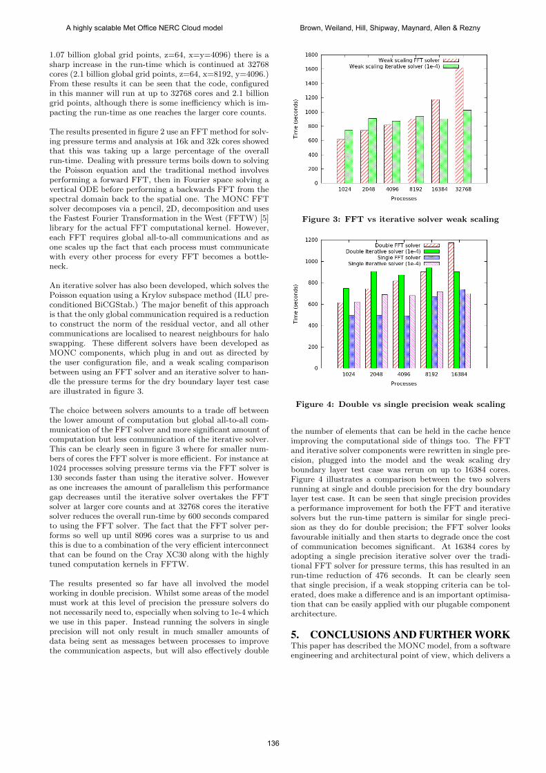
1.07 billion global grid points, z=64, x=y=4096) there is asharp increase in the run-time which is continued at 32768cores (2.1 billion global grid points, z=64, x=8192, y=4096.)From these results it can be seen that the code, configuredin this manner will run at up to 32768 cores and 2.1 billiongrid points, although there is some inefficiency which is im-pacting the run-time as one reaches the larger core counts.

The results presented in figure 2 use an FFT method for solv-ing pressure terms and analysis at 16k and 32k cores showedthat this was taking up a large percentage of the overallrun-time. Dealing with pressure terms boils down to solvingthe Poisson equation and the traditional method involvesperforming a forward FFT, then in Fourier space solving avertical ODE before performing a backwards FFT from thespectral domain back to the spatial one. The MONC FFTsolver decomposes via a pencil, 2D, decomposition and usesthe Fastest Fourier Transformation in the West (FFTW) [5]library for the actual FFT computational kernel. However,each FFT requires global all-to-all communications and asone scales up the fact that each process must communicatewith every other process for every FFT becomes a bottle-neck.

An iterative solver has also been developed, which solves thePoisson equation using a Krylov subspace method (ILU pre-conditioned BiCGStab.) The major benefit of this approachis that the only global communication required is a reductionto construct the norm of the residual vector, and all othercommunications are localised to nearest neighbours for haloswapping. These different solvers have been developed asMONC components, which plug in and out as directed bythe user configuration file, and a weak scaling comparisonbetween using an FFT solver and an iterative solver to han-dle the pressure terms for the dry boundary layer test caseare illustrated in figure 3.

The choice between solvers amounts to a trade off betweenthe lower amount of computation but global all-to-all com-munication of the FFT solver and more significant amount ofcomputation but less communication of the iterative solver.This can be clearly seen in figure 3 where for smaller num-bers of cores the FFT solver is more efficient. For instance at1024 processes solving pressure terms via the FFT solver is130 seconds faster than using the iterative solver. Howeveras one increases the amount of parallelism this performancegap decreases until the iterative solver overtakes the FFTsolver at larger core counts and at 32768 cores the iterativesolver reduces the overall run-time by 600 seconds comparedto using the FFT solver. The fact that the FFT solver per-forms so well up until 8096 cores was a surprise to us andthis is due to a combination of the very efficient interconnectthat can be found on the Cray XC30 along with the highlytuned computation kernels in FFTW.

The results presented so far have all involved the modelworking in double precision. Whilst some areas of the modelmust work at this level of precision the pressure solvers donot necessarily need to, especially when solving to 1e-4 whichwe use in this paper. Instead running the solvers in singleprecision will not only result in much smaller amounts ofdata being sent as messages between processes to improvethe communication aspects, but will also effectively double

Figure 3: FFT vs iterative solver weak scaling

Figure 4: Double vs single precision weak scaling

the number of elements that can be held in the cache henceimproving the computational side of things too. The FFTand iterative solver components were rewritten in single pre-cision, plugged into the model and the weak scaling dryboundary layer test case was rerun on up to 16384 cores.Figure 4 illustrates a comparison between the two solversrunning at single and double precision for the dry boundarylayer test case. It can be seen that single precision providesa performance improvement for both the FFT and iterativesolvers but the run-time pattern is similar for single preci-sion as they do for double precision; the FFT solver looksfavourable initially and then starts to degrade once the costof communication becomes significant. At 16384 cores byadopting a single precision iterative solver over the tradi-tional FFT solver for pressure terms, this has resulted in anrun-time reduction of 476 seconds. It can be clearly seenthat single precision, if a weak stopping criteria can be tol-erated, does make a difference and is an important optimisa-tion that can be easily applied with our plugable componentarchitecture.

5. CONCLUSIONS AND FURTHER WORKThis paper has described the MONC model, from a softwareengineering and architectural point of view, which delivers a

136


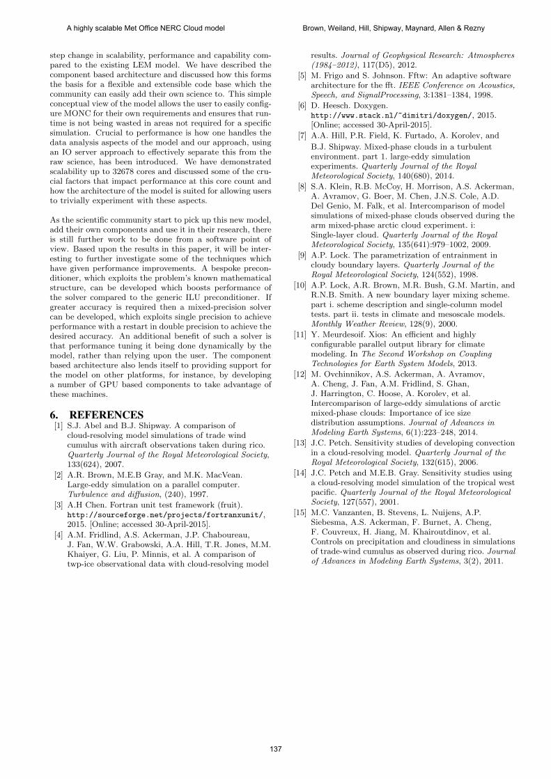
step change in scalability, performance and capability com-pared to the existing LEM model. We have described thecomponent based architecture and discussed how this formsthe basis for a flexible and extensible code base which thecommunity can easily add their own science to. This simpleconceptual view of the model allows the user to easily config-ure MONC for their own requirements and ensures that run-time is not being wasted in areas not required for a specificsimulation. Crucial to performance is how one handles thedata analysis aspects of the model and our approach, usingan IO server approach to effectively separate this from theraw science, has been introduced. We have demonstratedscalability up to 32678 cores and discussed some of the cru-cial factors that impact performance at this core count andhow the architecture of the model is suited for allowing usersto trivially experiment with these aspects.

As the scientific community start to pick up this new model,add their own components and use it in their research, thereis still further work to be done from a software point ofview. Based upon the results in this paper, it will be inter-esting to further investigate some of the techniques whichhave given performance improvements. A bespoke precon-ditioner, which exploits the problem’s known mathematicalstructure, can be developed which boosts performance ofthe solver compared to the generic ILU preconditioner. Ifgreater accuracy is required then a mixed-precision solvercan be developed, which exploits single precision to achieveperformance with a restart in double precision to achieve thedesired accuracy. An additional benefit of such a solver isthat performance tuning it being done dynamically by themodel, rather than relying upon the user. The componentbased architecture also lends itself to providing support forthe model on other platforms, for instance, by developinga number of GPU based components to take advantage ofthese machines.

6. REFERENCES[1] S.J. Abel and B.J. Shipway. A comparison of

cloud-resolving model simulations of trade windcumulus with aircraft observations taken during rico.Quarterly Journal of the Royal Meteorological Society,133(624), 2007.

[2] A.R. Brown, M.E.B Gray, and M.K. MacVean.Large-eddy simulation on a parallel computer.Turbulence and diffusion, (240), 1997.

[3] A.H Chen. Fortran unit test framework (fruit).http://sourceforge.net/projects/fortranxunit/,2015. [Online; accessed 30-April-2015].

[4] A.M. Fridlind, A.S. Ackerman, J.P. Chaboureau,J. Fan, W.W. Grabowski, A.A. Hill, T.R. Jones, M.M.Khaiyer, G. Liu, P. Minnis, et al. A comparison oftwp-ice observational data with cloud-resolving model

results. Journal of Geophysical Research: Atmospheres(1984–2012), 117(D5), 2012.

[5] M. Frigo and S. Johnson. Fftw: An adaptive softwarearchitecture for the fft. IEEE Conference on Acoustics,Speech, and SignalProcessing, 3:1381–1384, 1998.

[6] D. Heesch. Doxygen.http://www.stack.nl/~dimitri/doxygen/, 2015.[Online; accessed 30-April-2015].

[7] A.A. Hill, P.R. Field, K. Furtado, A. Korolev, and

B.J. Shipway. Mixed-phase clouds in a turbulentenvironment. part 1. large-eddy simulationexperiments. Quarterly Journal of the RoyalMeteorological Society, 140(680), 2014.

[8] S.A. Klein, R.B. McCoy, H. Morrison, A.S. Ackerman,A. Avramov, G. Boer, M. Chen, J.N.S. Cole, A.D.Del Genio, M. Falk, et al. Intercomparison of modelsimulations of mixed-phase clouds observed during thearm mixed-phase arctic cloud experiment. i:Single-layer cloud. Quarterly Journal of the RoyalMeteorological Society, 135(641):979–1002, 2009.

[9] A.P. Lock. The parametrization of entrainment incloudy boundary layers. Quarterly Journal of theRoyal Meteorological Society, 124(552), 1998.

[10] A.P. Lock, A.R. Brown, M.R. Bush, G.M. Martin, andR.N.B. Smith. A new boundary layer mixing scheme.part i. scheme description and single-column modeltests. part ii. tests in climate and mesoscale models.Monthly Weather Review, 128(9), 2000.

[11] Y. Meurdesoif. Xios: An efficient and highlyconfigurable parallel output library for climatemodeling. In The Second Workshop on CouplingTechnologies for Earth System Models, 2013.

[12] M. Ovchinnikov, A.S. Ackerman, A. Avramov,A. Cheng, J. Fan, A.M. Fridlind, S. Ghan,J. Harrington, C. Hoose, A. Korolev, et al.Intercomparison of large-eddy simulations of arcticmixed-phase clouds: Importance of ice sizedistribution assumptions. Journal of Advances inModeling Earth Systems, 6(1):223–248, 2014.

[13] J.C. Petch. Sensitivity studies of developing convectionin a cloud-resolving model. Quarterly Journal of theRoyal Meteorological Society, 132(615), 2006.

[14] J.C. Petch and M.E.B. Gray. Sensitivity studies usinga cloud-resolving model simulation of the tropical westpacific. Quarterly Journal of the Royal MeteorologicalSociety, 127(557), 2001.

[15] M.C. Vanzanten, B. Stevens, L. Nuijens, A.P.Siebesma, A.S. Ackerman, F. Burnet, A. Cheng,F. Couvreux, H. Jiang, M. Khairoutdinov, et al.Controls on precipitation and cloudiness in simulationsof trade-wind cumulus as observed during rico. Journalof Advances in Modeling Earth Systems, 3(2), 2011.

137


international conference on exascale applications and software

Documents