properties of prediction sorting

JOURNAL OF CHEMOMETRICSJ. Chemometrics 2004; 18: 92–102Published online in Wiley InterScience (www.interscience.wiley.com). DOI: 10.1002/cem.852

Properties of prediction sorting

IngunnBerget1,2* and TormodN�s1,31MATFORSK,Oslovn1, N-1430—s,Norway2Departmentof AnimalandAquacultural Sciences,Agricultural Universityof Norway,Norway3DepartmentofMathematics,StatisticsDivision,UniversityofOslo,Oslo,Norway

Received 29 May 2003; Revised 20 March 2004; Accepted 20 March 2004

One of the major sources of unwanted variation in an industrial process is the rawmaterial quality.

However, if the raw materials are sorted into more homogeneous groups before production, each

group can be treated differently. In this way the raw materials can be better utilized and the

stability of the end product may be improved. Prediction sorting is a methodology for doing this.

The procedure is founded on the fuzzy c-means algorithm where the distance in the objective

function is based on the predicted end product quality. Usually empirical models such as linear

regression are used for predicting the end product quality. By using simulations and bootstrap-

ping, this paper investigates how the uncertainties connected with empirical models affect the

optimization of the splitting and the corresponding process variables. The results indicate that the

practical consequences of uncertainties in regression coefficients are small. Copyright # 2004 John

Wiley & Sons, Ltd.

KEYWORDS: raw material variability; sorting; robustness; fuzzy clustering

1. INTRODUCTION

Raw materials of different quality will in practice often need

different process settings to obtain the same end product

quality. Therefore variable raw material quality is a potential

problem in commercial industry. One approach to this

problem is to sort the raw materials into more homogeneous

categories and process them with optimal process settings

for each category [1–4]. In this way the raw materials can be

better utilized. In addition, there will be less need for

frequent process adjustment, because only one category

will be processed at a time.

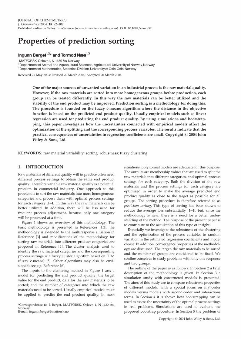
Figure 1 shows an overview of this methodology. The

basic methodology is presented in References [1,2], the

methodology is extended to the multiresponse situation in

Reference [3] and modifications of the methodology for

sorting raw materials into different product categories are

proposed in Reference [4]. The cluster analysis used to

identify the raw material categories and the corresponding

process settings is a fuzzy cluster algorithm based on FCM

(fuzzy c-means) [5]. Other algorithms may also be envi-

sioned; see e.g. Reference [6].

The inputs to the clustering method in Figure 1 are: a

model for predicting the end product quality; the target

value for the end product; data for the raw materials to be

sorted; and the number of categories into which the raw

materials need to be sorted. Usually empirical models must

be applied to predict the end product quality; in most

situations, polynomial models are adequate for this purpose.

The outputs are membership values that are used to split the

raw materials into different categories, and optimal process

settings for each category. Both the division of the raw

materials and the process settings for each category are

optimized in order to make the average predicted end

product quality as close to the target as possible for all

groups. The sorting procedure is therefore referred to as

prediction sorting. This type of sorting has been shown to

reduce the average loss substantially [1–4], but, since the

methodology is new, there is a need for a better under-

standing of the method. The purpose of the present paper is

to contribute to the acquisition of this type of insight.

Especially we investigate the robustness of the clustering

and the optimization of the process variables to random

variation in the estimated regression coefficients and model

choice. In addition, convergence properties of the methodol-

ogy are discussed. The target, the raw materials to be sorted

and the number of groups are considered to be fixed. We

confine ourselves to study problems with only one response

and two groups.

The outline of the paper is as follows. In Section 2 a brief

description of the methodology is given. In Section 3 a

simulation study with constructed models is presented.

The aims of this study are to compare robustness properties

of different models, with a special focus on first-order

models versus models with second-order and interactions

terms. In Section 4 it is shown how bootstrapping can be

used to assess the uncertainty of the optimal process settings

in real problems. Simulations are used to evaluate the

proposed bootstrap procedure. In Section 5 the problem of

*Correspondence to: I. Berget, MATFORSK, Oslovn 1, N-1430 As,Norway.E-mail: [email protected]

Copyright # 2004 John Wiley & Sons, Ltd.

model selection is illustrated with data from a baking

experiment, and the bootstrap methodology from Section 4

is used to estimate the standard deviation of the optimal

process variable.

2. INTRODUCTION TO PREDICTIONSORTING

2.1. Sorting procedureIt is assumed that a model for predicting end product

quality (y) from raw material (z) and process (x) variables

is available. This model is written as yy ¼ fðx; zÞ and is

assumed to be a polynomial in x and z (see e.g. Equations

(7) and (10)–(13)). Here bold letters indicate vectors such that

x ¼ ½x1; x2; . . . ; xkx� and z ¼ ½z1; z2; . . . ; zkz�. Note, however,

that x and z could also be univariate, in which case italics

will be used, i.e. x and z.

The general sorting procedure described below aims at

finding the best way of partitioning a fixed set of raw

materials with N objects into C different categories with

possibly different process settings. The partitioning is opti-

mized with the purpose of minimizing the loss, which is the

average squared deviation between the predicted end pro-

duct quality and a predefined target value (T). When each

group of raw materials is processed with different process

settings, the distance between object i and category j can be

defined as

d2ij ¼ ð fðzi; x�j Þ � TÞ2 ¼ ðyyij � TÞ2

i ¼ 1; . . . ;N; j ¼ 1; . . . ;Cð1Þ

Here yy is the end product quality and dij is the loss from

object i when it is processed with the settings for the jth

category.

The optimal partitioning of a fixed set of raw materials, Z,

is obtained by minimizing

Jðm;ZÞ ¼XCj¼1

XNi¼1

umij d2ij subject to

XCj¼1

uij ¼ 1 ð2Þ

Here uij is the membership of object i in category j, which

is a relative measure of how much object i belongs to the

jth cluster. The membership values are between one and

zero. The parameter m determines the fuzziness of the

clustering. Usually m is equal to two for fuzzy cluster-

ing [7]. If m is set to be equal to one, on the other hand, a

crisp clustering with uij equal to either one or zero is

obtained.

The objective function J is minimized with respect to

D ¼ fd2ijg for given U ¼ fuijg and vice versa. The algorithm

for minimizing J is as follows.

1. Initialize U either randomly or according to prior knowl-

edge.

2. Optimise x for given U and calculate the distances in

Equation (1). The optimal x values are found from

xj ¼ argminx�

Xni¼1

umij ð fðzi; x�j Þ � TÞ2

!ð3Þ

3. Update membership values according to

uij ¼XCt¼1

d2ij=d

2it

!m�1

ð4Þ

4. Check convergence. A convenient stopping criterion is to

compare the criterion function with the value obtained in

the previous iteration: in this case, stop if jJnew � Joldj < ",

else go to step 2. However, other stopping criteria can also

be applied.

When the procedure has converged, the raw material

categories are defined by allocating each object to

the cluster where it has the largest membership value.

For more details about the methodology see References

[1–4].

Note that z is measured on a continuous scale and that

there may not necessarily be any natural grouping in the

data that need to be sorted. This is different from the

regular use of clustering, where the focus is to find groups

in data. The data in Z can be measurements for the raw

materials to be sorted, or Z can consist of simulated data

points reflecting the expected distribution of the incoming

raw materials.

In practice, the sorting methodology could either work

as a calibration method to construct a classification rule,

or the membership values could be calculated for new

samples directly. In the latter case, dij is calculated with

the optimal settings obtained from sorting of historical

data or artificial data generated inside the region of

interest from a distribution reflecting the expected dis-

tribution of the incoming raw materials.

2.2. Cluster validity and evaluationThroughout this paper we will use the average loss for

evaluation of the clustering. This is directly interpretable

since it focuses on the end product quality. The expected

Figure 1. Overviewof thesortingmethodology.

Properties of prediction sorting 93

Copyright # 2004 John Wiley & Sons, Ltd. J. Chemometrics 2004; 18: 92–102

loss obtained with sorting will be compared with the loss

obtained without sorting and is estimated as

EEðlossÞ ¼ 1

N

XNi

ðyyðiÞ � TÞ2 ð5Þ

where yyðiÞ is the predicted end product quality of object i

when it is assigned to the category where it has the highest

membership value. Without sorting, all objects are allocated

to one category.

When it is natural to compare the loss for different models,

we use the so-called gain, which is calculated as a percentage

of the loss without sorting, i.e. as

G ¼ 100 1 � EEðlossÞsorted

EEðlossÞnotsorted

!ð6Þ

Note that other aspects, e.g. the cost associated with

sorting, may also be relevant to take into account when a

concrete decision has to be made.

3. SIMULATION STUDIES

A simulation study was carried out in order to study the

robustness properties of the discussed methodology. We

wanted to compare the robustness properties of different

types of models; however, we confine ourselves to models

that are univariate in both x and z.

3.1. Constructed modelsIn each simulation, data were generated according to the

statistical model

y ¼ fðx; zÞ þ e ¼ y0 þ e ð7Þ

The random error e is normally distributed with variance �2.

The term y0 denotes the true end product quality, which

would be equal to the measured quality y if there was no

noise present in the data. Nine different models were tested

using the general second-order model expressed as

y ¼ �0 þ �1xþ �2zþ �3xzþ �4x2 þ �5z

2 þ e

¼ y0 þ eð8Þ

In each model the coefficients b ¼ ½�0; �1; . . . ; �5�T are set in

such a way as to cover a wide range of possibilities. The nine

different models are presented in Figure 2.

It is assumed that the interval ½�1:0; 1:0� defines the region

of interest for both variables and that the regression coeffi-

cients b ¼ ½�0; �1; . . . ; �5�T are unknown and must be esti-

mated from data. The regression coefficients are estimated

by least squares (LS).

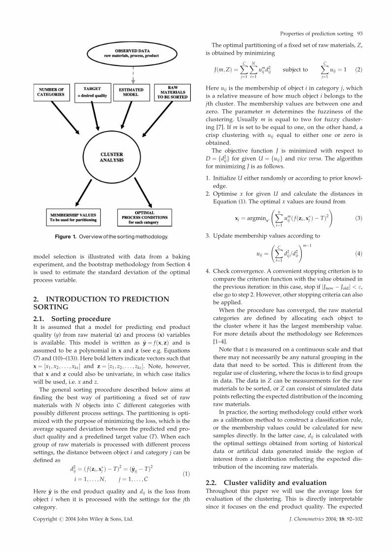
Figure 2 shows both the equations for the models and

the response surface for the loss function, which is

L ¼ ðfðx; zÞ � TÞ2. For each model the target T is equal to

�0, which is the y value at the centre of the simulated design.

The models are numbered 1–9. The first three models

include only first-order terms in both x and z (i.e.

Figure 2. Contour plots of the loss function for the constructedmodels.The thick lines show theminimumloss for all z.Note that inmodel 3 theminimum line is on the borders of the investigated region, for lowandhighz.Thisisalso the case for low z inmodel 6.Inmodels 6 and 9 thereexist noxvalueswhichgivezero lossforhighz.

94 I. Berget and T. Næs


�3 ¼ �4 ¼ �5 ¼ 0), whereas the rest are full, second-order

models. The models beneath each other have the same

coefficients for the first-order terms and increasing coeffi-

cients for the second-order terms. In the first column the

effects of x and z are of the same size. In the second column

the effect of x is larger than that of z, whereas in the third

column the effect of z is much larger than that of x. To

exaggerate effects, the non-linear terms are made higher than

they will typically be in most practical situations.

3.2. SimulationsFor each model, data were generated according to a repli-

cated, full factorial design in x and z. The levels were

f�1; 0; 1g for both variables, and the whole design was

replicated three times. This resulted in 3 � 3 � 3 ¼ 27 obser-

vations for each data set. The true y value (y0) was calculated

for all points in the design. Then normally distributed error

was added to y0 according to the statistical model described

by Equation (7) with � ¼ f1; 2; 4; 6; 8; 10g. In total, 100 in-

dependent data sets with 27 observations were generated for

each model at each level of �. For each data set the LS

estimate of b was obtained. For models 1–3 the regression

coefficients were estimated by assuming both the full model

in Equation (8) and the model with �3 ¼ �4 ¼ �5 ¼ 0.

A summary of the R2 between the predicted and the

observed y is given in Table I. The smallest R2 obtained is

approximately 0.75. We consider that for models with lower

R2 (larger �) the sorting algorithm will not be relevant

because of poor prediction ability.

The sorting procedure was carried out for both the true

and the estimated models. The N data points (‘batches’) to

be sorted were set to be Z ¼ ½�1:00;�0:99; . . . ; 0:99; 1:00�, i.e.

points uniformly distributed over the region of interest. The

sorting algorithm was applied to sort these points into C ¼ 2

groups. In the optimization of the process variables, x was

constrained to be within ½�1:0; 1:0�.

3.3. Results3.3.1. Convergence propertiesWhen the sorting algorithm was applied to the true models,

it converged in 5–15 iterations, and there was no sensitivity

to different initializations. When applied to the estimated

models, it converged in less than 40 iterations for all simula-

tions. The first-order models converged faster than the

second-order models.

Generally the procedure was insensitive to the initializa-

tion of U. However, it was observed that for some data sets

of models 3, 5 and 9 a few initializations led to uij ¼ 0:5 for all

i and j. This complete fuzzy solution cannot be used to

partition Z; nevertheless, it is always a stable solution

because it gives di1 ¼ di2 for all i. Hence there will be no

change when u and d are updated in steps 2 and 3 of the

algorithm. Although no sensitivity to different initializations

has been detected in previous work, or for the other models,

these observations show that the sorting procedure may not

be completely insensitive to the starting point. Therefore

different initializations should always be tested before the

final conclusions are drawn.

In approximately 5% of the simulations of model 6 the

complete fuzzy solution was obtained not only for a few but

for all initializations of U when there were constraints on x.

However, when the constraints were removed, a partitioning

of Z could be obtained in all simulations. This shows that the

partitioning is affected by active constraints on the process

variables and that with such constraints a partitioning may

be difficult to obtain, because the process variables that

minimize the loss for a group of raw materials are outside

the feasible region.

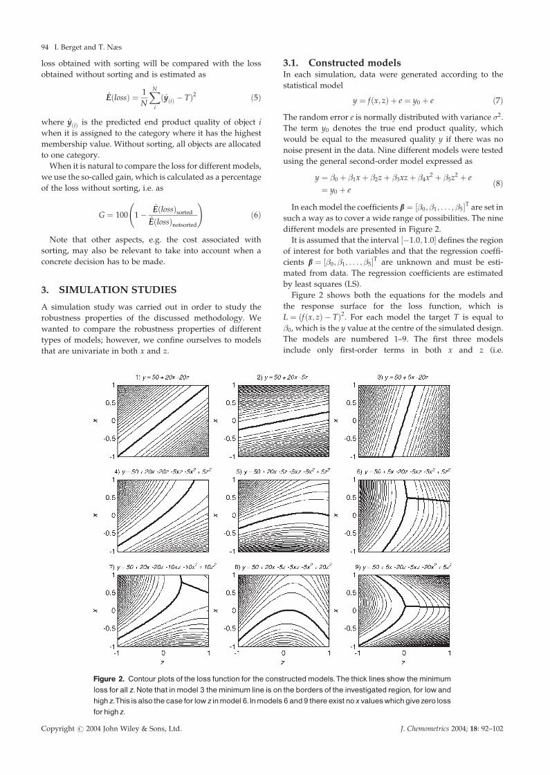
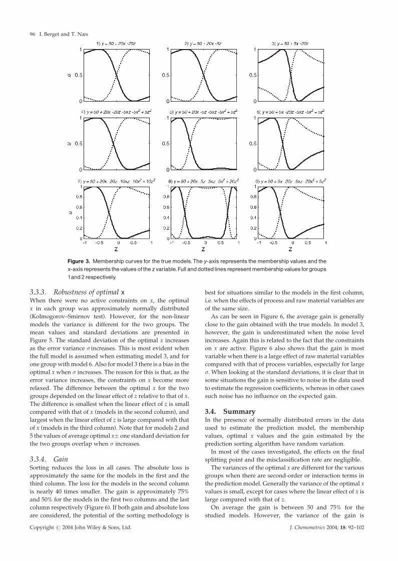
3.3.2. Membership valuesThe membership values for the true models are shown in

Figure 3.

For the linear models the splitting point equals zero, which

is the mean of Z. When there are no active constraints on x,

there is no variation in the membership values. With model 3

there are active constraints, hence the membership values

are variable. If the full model in Equation (8) is assumed, the

membership values are variable for all three linear models.

These results are confirmed in unpublished results and are

expected to hold for all linear models when the points in Z

are symmetrically distributed.

For the non-linear models, i.e. the models where second-

order and interaction terms are added, the splitting point

is shifted away from zero. In extreme cases, second-order

terms may lead to several splitting points (model 8,

Figure 3). For all the non-linear models the membership

values varied between different simulations. Generally

points close to the splitting point or other points with

membership values close to 0.5, e.g. the end points, had

more variable membership values than the rest. Moreover,

the variability of the membership values was smaller for

models in the third row than for those in the second row.

This means that high second order terms may stabilize the

membership values.

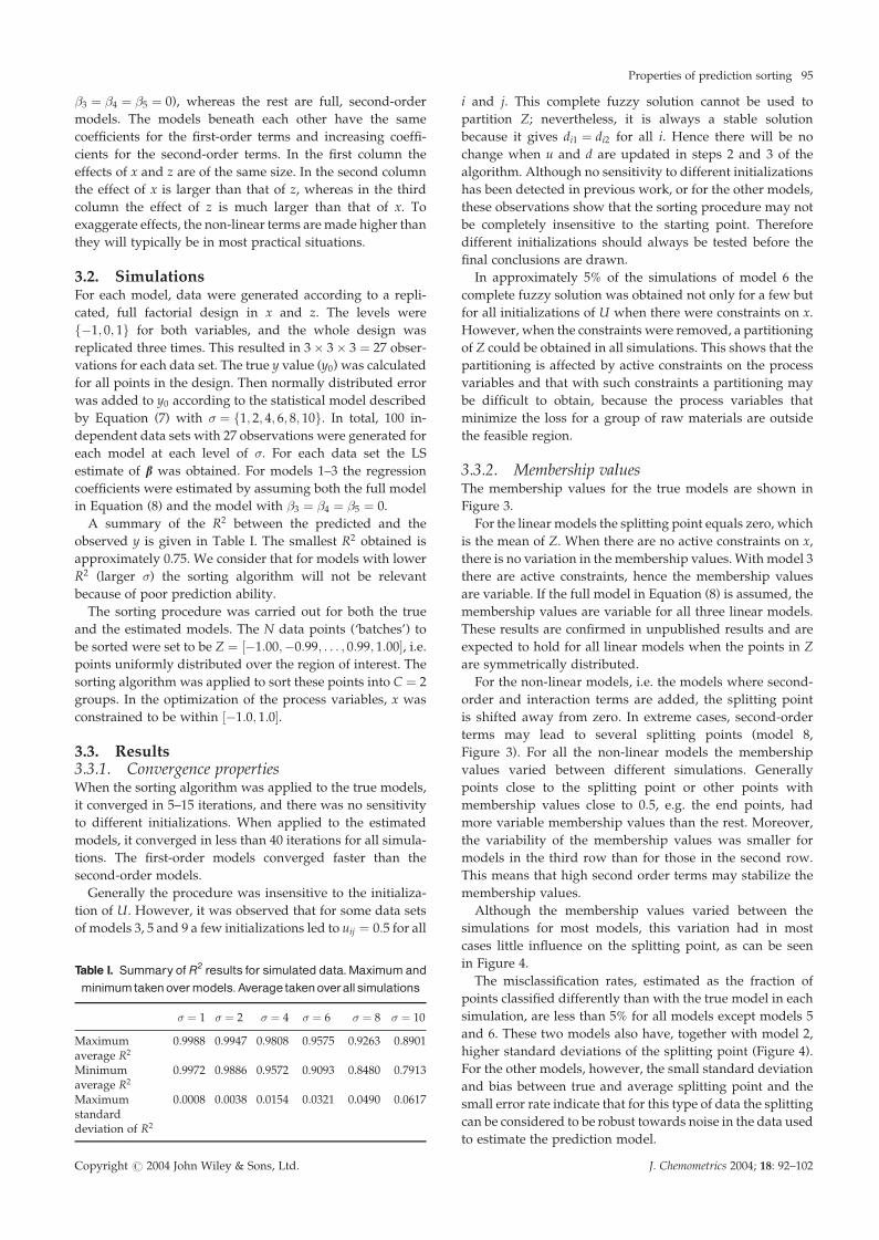
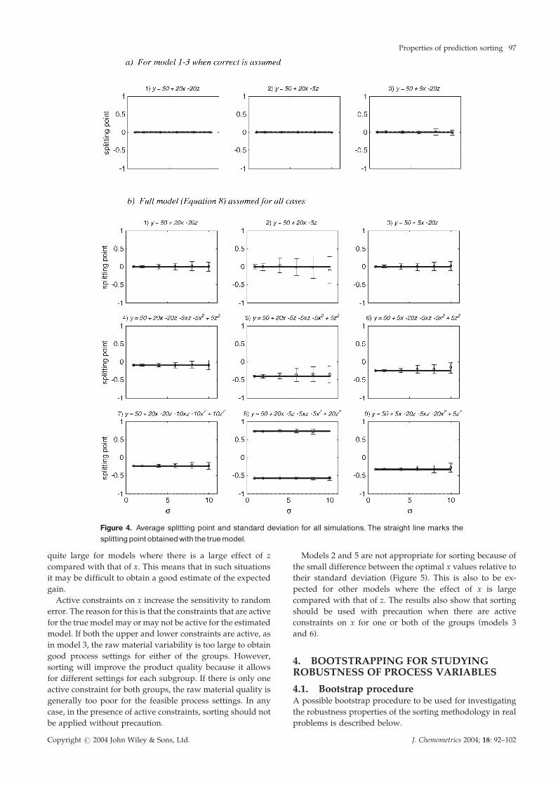
Although the membership values varied between the

simulations for most models, this variation had in most

cases little influence on the splitting point, as can be seen

in Figure 4.

The misclassification rates, estimated as the fraction of

points classified differently than with the true model in each

simulation, are less than 5% for all models except models 5

and 6. These two models also have, together with model 2,

higher standard deviations of the splitting point (Figure 4).

For the other models, however, the small standard deviation

and bias between true and average splitting point and the

small error rate indicate that for this type of data the splitting

can be considered to be robust towards noise in the data used

to estimate the prediction model.

Table I. Summary of R2 results for simulated data.Maximumandminimumtakenovermodels.Average takenoverallsimulations

� ¼ 1 � ¼ 2 � ¼ 4 � ¼ 6 � ¼ 8 � ¼ 10

Maximum 0.9988 0.9947 0.9808 0.9575 0.9263 0.8901average R2

Minimum 0.9972 0.9886 0.9572 0.9093 0.8480 0.7913average R2

Maximum 0.0008 0.0038 0.0154 0.0321 0.0490 0.0617standarddeviation of R2



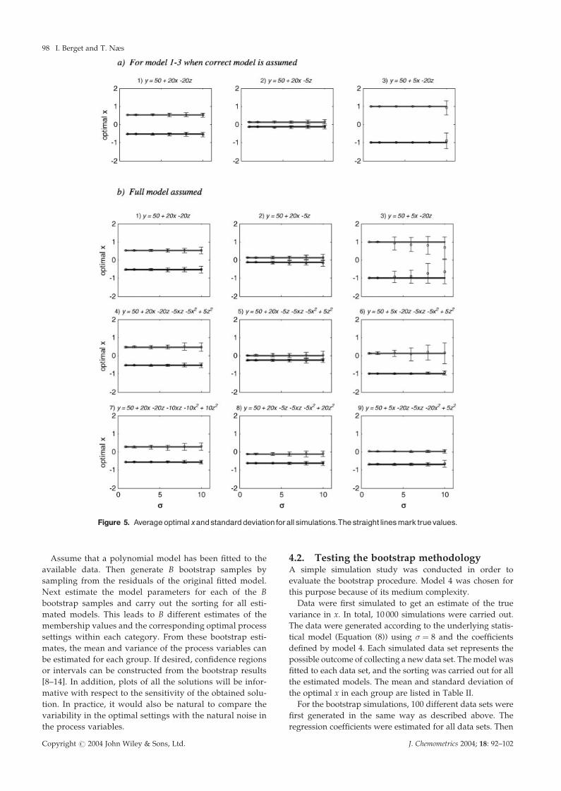
3.3.3. Robustness of optimal xWhen there were no active constraints on x, the optimal

x in each group was approximately normally distributed

(Kolmogorov–Smirnov test). However, for the non-linear

models the variance is different for the two groups. The

mean values and standard deviations are presented in

Figure 5. The standard deviation of the optimal x increases

as the error variance � increases. This is most evident when

the full model is assumed when estimating model 3, and for

one group with model 6. Also for model 3 there is a bias in the

optimal x when � increases. The reason for this is that, as the

error variance increases, the constraints on x become more

relaxed. The difference between the optimal x for the two

groups depended on the linear effect of z relative to that of x.

The difference is smallest when the linear effect of z is small

compared with that of x (models in the second column), and

largest when the linear effect of z is large compared with that

of x (models in the third column). Note that for models 2 and

5 the values of average optimal x� one standard deviation for

the two groups overlap when � increases.

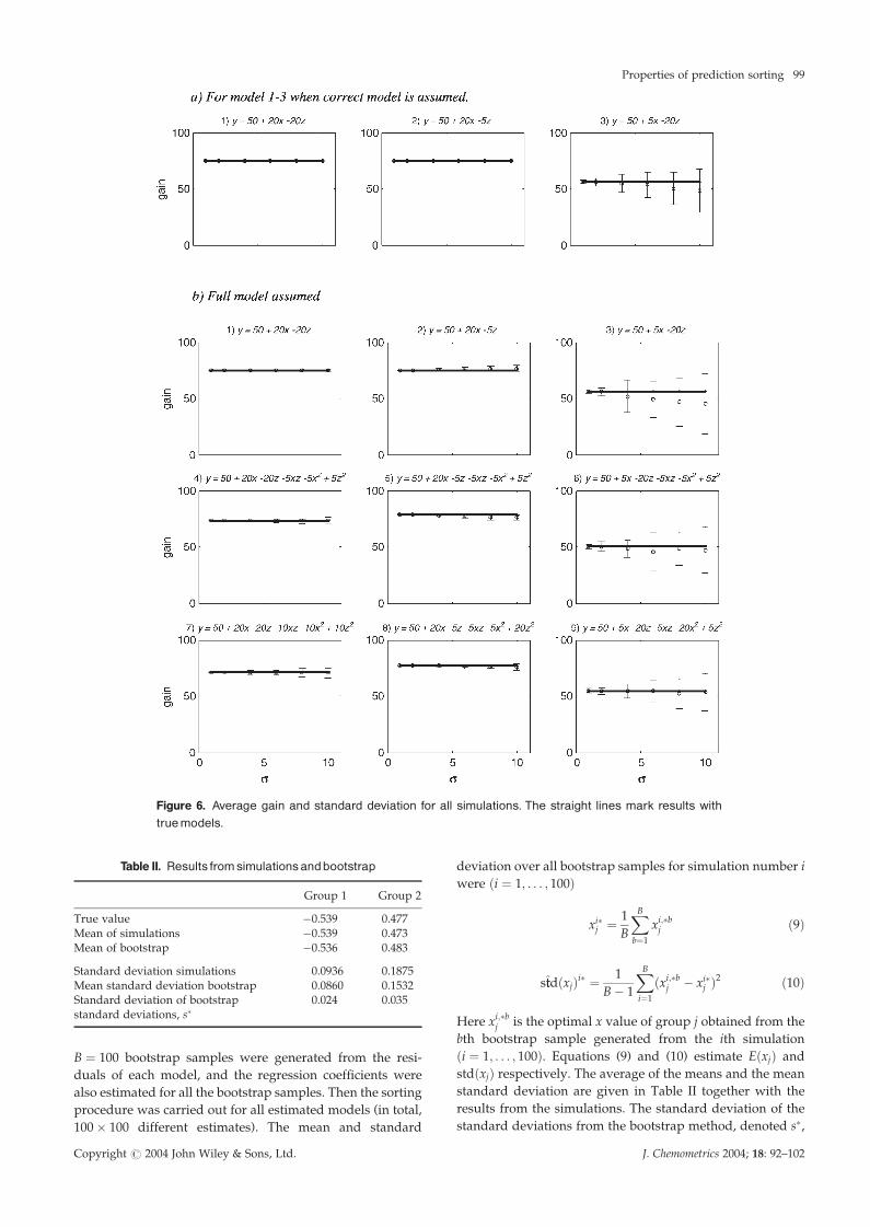
3.3.4. GainSorting reduces the loss in all cases. The absolute loss is

approximately the same for the models in the first and the

third column. The loss for the models in the second column

is nearly 40 times smaller. The gain is approximately 75%

and 50% for the models in the first two columns and the last

column respectively (Figure 6). If both gain and absolute loss

are considered, the potential of the sorting methodology is

best for situations similar to the models in the first column,

i.e. when the effects of process and raw material variables are

of the same size.

As can be seen in Figure 6, the average gain is generally

close to the gain obtained with the true models. In model 3,

however, the gain is underestimated when the noise level

increases. Again this is related to the fact that the constraints

on x are active. Figure 6 also shows that the gain is most

variable when there is a large effect of raw material variables

compared with that of process variables, especially for large

�. When looking at the standard deviations, it is clear that in

some situations the gain is sensitive to noise in the data used

to estimate the regression coefficients, whereas in other cases

such noise has no influence on the expected gain.

3.4. SummaryIn the presence of normally distributed errors in the data

used to estimate the prediction model, the membership

values, optimal x values and the gain estimated by the

prediction sorting algorithm have random variation.

In most of the cases investigated, the effects on the final

splitting point and the misclassification rate are negligible.

The variances of the optimal x are different for the various

groups when there are second-order or interaction terms in

the prediction model. Generally the variance of the optimal x

values is small, except for cases where the linear effect of x is

large compared with that of z.

On average the gain is between 50 and 75% for the

studied models. However, the variance of the gain is

Figure 3. Membership curves for the true models.The y-axis represents the membership values and thex-axis represents thevaluesof the zvariable.Fullanddottedlines representmembershipvalues forgroups1and2 respectively.



quite large for models where there is a large effect of z

compared with that of x. This means that in such situations

it may be difficult to obtain a good estimate of the expected

gain.

Active constraints on x increase the sensitivity to random

error. The reason for this is that the constraints that are active

for the true model may or may not be active for the estimated

model. If both the upper and lower constraints are active, as

in model 3, the raw material variability is too large to obtain

good process settings for either of the groups. However,

sorting will improve the product quality because it allows

for different settings for each subgroup. If there is only one

active constraint for both groups, the raw material quality is

generally too poor for the feasible process settings. In any

case, in the presence of active constraints, sorting should not

be applied without precaution.

Models 2 and 5 are not appropriate for sorting because of

the small difference between the optimal x values relative to

their standard deviation (Figure 5). This is also to be ex-

pected for other models where the effect of x is large

compared with that of z. The results also show that sorting

should be used with precaution when there are active

constraints on x for one or both of the groups (models 3

and 6).

4. BOOTSTRAPPING FOR STUDYINGROBUSTNESS OF PROCESS VARIABLES

4.1. Bootstrap procedureA possible bootstrap procedure to be used for investigating

the robustness properties of the sorting methodology in real

problems is described below.

Figure 4. Average splitting point and standard deviation for all simulations. The straight line marks thesplittingpoint obtainedwith the truemodel.



Assume that a polynomial model has been fitted to the

available data. Then generate B bootstrap samples by

sampling from the residuals of the original fitted model.

Next estimate the model parameters for each of the B

bootstrap samples and carry out the sorting for all esti-

mated models. This leads to B different estimates of the

membership values and the corresponding optimal process

settings within each category. From these bootstrap esti-

mates, the mean and variance of the process variables can

be estimated for each group. If desired, confidence regions

or intervals can be constructed from the bootstrap results

[8–14]. In addition, plots of all the solutions will be infor-

mative with respect to the sensitivity of the obtained solu-

tion. In practice, it would also be natural to compare the

variability in the optimal settings with the natural noise in

the process variables.

4.2. Testing the bootstrap methodologyA simple simulation study was conducted in order to

evaluate the bootstrap procedure. Model 4 was chosen for

this purpose because of its medium complexity.

Data were first simulated to get an estimate of the true

variance in x. In total, 10 000 simulations were carried out.

The data were generated according to the underlying statis-

tical model (Equation (8)) using � ¼ 8 and the coefficients

defined by model 4. Each simulated data set represents the

possible outcome of collecting a new data set. The model was

fitted to each data set, and the sorting was carried out for all

the estimated models. The mean and standard deviation of

the optimal x in each group are listed in Table II.

For the bootstrap simulations, 100 different data sets were

first generated in the same way as described above. The

regression coefficients were estimated for all data sets. Then

Figure 5. Averageoptimalxandstandarddeviation forallsimulations.Thestraight linesmark truevalues.



B ¼ 100 bootstrap samples were generated from the resi-

duals of each model, and the regression coefficients were

also estimated for all the bootstrap samples. Then the sorting

procedure was carried out for all estimated models (in total,

100 � 100 different estimates). The mean and standard

deviation over all bootstrap samples for simulation number i

were ði ¼ 1; . . . ; 100Þ

xi�j ¼ 1

B

XBb¼1

xi;�bj ð9Þ

sttdðxjÞi� ¼1

B� 1

XBi¼1

ðxi;�bj � xi�j Þ2 ð10Þ

Here xi;�bj is the optimal x value of group j obtained from the

bth bootstrap sample generated from the ith simulation

ði ¼ 1; . . . ; 100Þ. Equations (9) and (10) estimate EðxjÞ and

stdðxjÞ respectively. The average of the means and the mean

standard deviation are given in Table II together with the

results from the simulations. The standard deviation of the

standard deviations from the bootstrap method, denoted s�,

Table II. Results fromsimulationsandbootstrap

Group 1 Group 2

True value �0.539 0.477Mean of simulations �0.539 0.473Mean of bootstrap �0.536 0.483

Standard deviation simulations 0.0936 0.1875Mean standard deviation bootstrap 0.0860 0.1532Standard deviation of bootstrap 0.024 0.035standard deviations, s�

Figure 6. Average gain and standard deviation for all simulations. The straight lines mark results withtruemodels.



is also given. Table II shows that the overall mean is close to

the true x value in each group but that the mean standard

deviation underestimates the standard deviation of x.

5. BAKING EXAMPLE

In this section the bootstrap procedure is illustrated on a real

data set. To investigate the importance of model selection in

the sorting context, the sorting results from four different

models fitted to the same data will be compared. The data

come from a baking experiment originally presented in

Reference [4] and briefly described below.

5.1. ExperimentalThe objective of this example is to optimize bread loaf

volume of hearth bread, which is bread baked without a

pan, when flours of different quality are used for baking. The

process variable to be optimized is proofing time. This is the

resting time from when the breads are formed until they

are baked. Typically the volume increases as the proofing

time increases; however, if the proofing time is too long, the

breads become flat. The target for bread loaf volume was

therefore set at an intermediate level. Another option would

have been to include both form and volume in the sorting

criterion as in References [3,4].

A mixture design was applied to generate flours of differ-

ent quality. The flour blends were mixtures of two different

wheat varieties and a wheat/bran mix. The wheat varieties

differed in protein content and quality, so the three sources

of variation in this design were bran, protein content and

protein quality. Protein content and quality were, however,

confounded. Therefore only protein content was used to-

gether with bran to describe the raw material quality. The

protein content was measured in per cent. The bran fractions

were determined from the design.

For each blend the proofing time was varied at three levels

(30, 40 and 50 min). Because of practical limitations, proofing

time was nested within dough, such that all doughs were

divided into three pieces which were given different proof-

ing times. The mixtures were only blended once, but two

doughs were made separately from each blend. Therefore

there is also a split-plot structure in the experiment. In the

original experiment, doughs were made both with and

without an additive called DATEM. Here we only consider

breads baked with DATEM. In total, there were 60 observa-

tions for the data set to be used in this paper.

5.2. Fitted modelsAn important part of developing empirical models is to

choose the best model. Many strategies and criteria for

variable selection exist, but the various strategies and criteria

may not always give the same results. Therefore it can

sometimes be difficult to determine which model is best.

Moreover, in some situations the established methods for

variable selection may not be adequate, as in the presented

split-plot example where regular variable selection based on

t-tests is more difficult to justify than in fully randomized

experiments.

Clearly the model choice may have an impact on both the

splitting and the optimal process settings. Four different

models fitted to the data from this experiment are presented

below. Since variable selection as such is not the main focus

here, we have used a simple ad hoc procedure for model

selection based on the R2, the adjusted R2 and residual plots

for the different variables.

Let v be the predicted volume, x the proofing time, z1 the

protein content and z2 the bran fraction of each flour blend.

The predictor variables x, z1 and z2 are centred and scaled.

The selected models were as follows.

A. Linear model:

v ¼ 362:57 þ 25:44xþ 21:28z1 � 30:70z2 ð11Þ

B. Model with only significant terms:

v ¼ 378:15 þ 25:44xþ 21:83z1 � 21:54z2

� 5:07z1z2 � 15:85z22

ð12Þ

C. Full second-order model:

v ¼ 385:83 þ 25:44xþ 21:19z1 � 22:73z2

þ 4:08xz1 � 6:99xz2 þ 2:61z1z2

� 5:02x2 � 3:68z21 � 16:19z2

2 ð13Þ

D. Full second-order model with z32 added:

v ¼ 390:79 þ 25:44xþ 20:86z1 � 32:73z2

þ 4:08xz1 � 6:99xz2 þ 2:36z1z2

� 5:02x2 � 3:93z21 � 25:12z2

2 þ 7:16z32 ð14Þ

The first model (A) is a linear model. The second model (B)

is obtained by fitting a full second-order model, but only the

significant terms are kept in the model. Significance is

determined by regular t-tests, which are not exact in this

case because of the split-plot structure. The third model (C)

is the full second-order model, whereas the fourth model (D)

is the full second-order model with the third order effect of

bran (z2) added. This last term was added because there

were systematic errors in the residuals for the full second-

order model. In Reference [4] the most complex model,

model D, was used. The regression diagnostics for each

model are listed in Table III. Note that, with the exception

of the linear model which has a poorer fit than the rest, all

models have approximately the same performance with

respect to the cross-validated RMSEP.

5.3. Comparison of modelsFor each of the four models, B ¼ 1000 bootstrap samples

with N ¼ 60 observations in each sample were generated

and the regression coefficients were estimated for each

sample. Then the sorting procedure was carried out for all

estimated models. The data to be sorted were selected as a

uniform grid of points generated in the region spanned by z1

Table III. R2, adjusted R2 and calibrated and validated RMSEP(rootmeansquareerrorofprediction) foreachmodel (A^D)

A B C D

R2 0.768 0.893 0.910 0.920Adj R2 0.755 0.883 0.893 0.904RMSEP (cal) 20.61 14.01 12.05 12.05RMSEP (val) 22.38 17.02 16.99 16.40



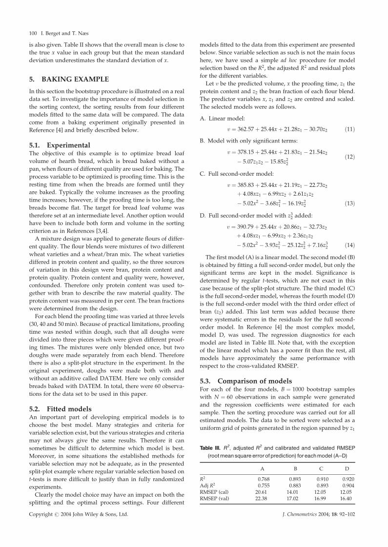
and z2 (see Figure 7). Hence the sorting is carried out on a

different data set than the data from the experimental de-

sign. By using a uniform grid of points, it is assumed that the

incoming flours will be evenly distributed within the experi-

mental region. The generated points simulate flours of

different quality varying in protein content/quality and

bran content. They were sorted into two groups and the

target was set equal to T ¼ 370 ml. The proofing time was

restricted to be within the experimental region determined

by the interval [30,50] min.

In approximately 1% of the bootstrap replicates of each

model the sorting procedure did not converge. Otherwise

the sorting algorithm converged in less than 90 iterations

(Table IV). In 3–5% of the bootstrap replicates of the two

most complex models (C and D) the algorithm ended up

with all membership values equal to 0.5 in both groups.

These cases were kept out of the further analyses. A sum-

mary of the results is given in Table IV.

The membership values varied between the bootstrap

replicates and between the four models investigated. Based

on the membership values from all bootstrap simulations,

the grid points could be characterized as belonging to

group 1, group 2 or the splitting region. The splitting region

consists of all points which have a member of the other

group as one of their nearest neighbours in one or more of

the bootstrap replicates. In Figure 7, all the grid points are

shown using different ‘colouring’ for the two groups and a

different symbol for points within the splitting region. The

flours in group 1 have a low bran fraction and a high protein

content, whereas group 2 consists of points representing

flours with a low protein content (left) or a high bran content

(upper points).

The separation obtained with model A was most different

from the others. For the other three models the splitting

regions are similar and overlapping. Based on the results in

Section 3, we believe that the variability in the splitting

regions has small practical consequences.

For a more thorough investigation of the consequences of

the model choice, the bread loaf volume was predicted for all

points in the grid with the partitioning and optimal process

Table IV. Convergenceproperties:minimumandmaximumnumberofiterationsbeforeconvergence.Averagegainobtainedbysorting (%)andoptimalxwithout sortingand for the twogroupswithsorting.Standarddeviationsaregiveninparentheses

Convergence Gain obtained Optimal x Optimal x Optimal xModel properties by sorting (%) without sorting group 1 group 2

A 26–77 69.75 (1.09) 42.60 (0.91) 35.64 (1.26) 47.68 (1.27)B 24–70 57.30 (3.98) 39.69 (0.68) 34.71 (0.86) 45.10 (0.87)C 14–95 62.99 (3.72) 37.84 (1.07) 33.12 (1.58) 46.50 (1.15)D 9–88 64.49 (3.64) 37.12 (1.17) 32.28 (1.49) 47.79 (1.26)

Figure 7. Thegridpoints.Full circlesmarkpointsallocated togroup1forallbootstrapreplicates, weher-eas open circlesmark points allocated to group 2.The dotsmark points that are on the border betweenthe twogroups foroneormorebootstrapreplicates.Foreachmodel theregionwith dotsis referred toasthesplittingregion.



settings obtained in each bootstrap replicate for all four

models. Then yy at each point was averaged over all bootstrap

simulations, and the mean difference between models k and l

was calculated as

mean difference ¼

ffiffiffiffiffiffiffiffiffiffiffiffiffiffiffiffiffiffiffiffiffiffiffiffiffiffiffiffiffiffiffiffiffi1

N

XNi¼1

ð�yyyyik � �yyyyilÞ2

vuut ð15Þ

where N ¼ 219 is the number of points in the grid and �yyyyikand �yyyyil are the mean predicted values of point i from models k

and l respectively. The calculated values are listed in Table

V.

In practice, model C or D would have been chosen,

because these models have the largest adjusted R2 and the

smallest RMSEP. The mean error between these two models

is 5.84 (Table V). This means that if the ‘wrong’ model were

chosen, the average error for the predicted values would be

approximately 5.84. For a comparison, the validated RMSEP

values for these models are 16.99 and 16.40. This indicates

that the error of prediction is clearly larger than the potential

error of choosing the wrong model. These two models also

had very similar mean values and standard deviations for

gain and optimal x (Table IV).

The most complex model is perhaps less robust than the

others, because some bootstrap replicates gave solutions that

did not lead to a splitting. Otherwise the robustness of the

membership values and process variables does not seem to

be too much affected by model choice. These results show

that, for models that have approximately the same perfor-

mance with respect to commonly used regression diagnos-

tics, it may not matter too much which model is chosen.

6. CONCLUSIONS

Simulations of constructed models and bootstrapping of

existing data have been applied to investigate robustness

properties of the prediction sorting methodology. The results

show that, when normally distributed error is present in the

data used to estimate the prediction model, both member-

ship values and process variables will be uncertain. How-

ever, the simulations show that the classification error due to

variability in membership values is low. If the effect of the

process settings is large compared with that of the raw

material variables, the variability in the optimal x may be

larger than the difference between the optimal x in the two

groups. The variability of the gain depends on the model

used for prediction, but there is always a positive gain by

sorting, and in some situations the gain is hardly affected at

all. The variability in the gain was largest for models where

the raw materials ðzÞ had a large effect relative to the process

variables ðxÞ.In real problems, bootstrapping may be applied to assess

the uncertainty of the optimal process variables. Simulation

results with a constructed model indicate that the bootstrap

has reasonable properties but underestimates the standard

deviation of the optimal process settings. Bootstrap results

with several models fitted to the same data show that, for

models that have reasonably good performance with respect

to the usual regression diagnostics, the possible error of

choosing the ‘wrong’ model will be small compared with

the prediction error.

AcknowledgementsThe authors would like to thank Dr Øyvind Langsrud

and Dr Gunvor Dingstad for helpful comments on the

manuscript.

REFERENCES

1. Næs T, Mevik BH. The flexibility of fuzzy clusteringillustrated by examples. J. Chemometrics 1999; 13: 435–444.

2. Berget I, Næs T. Optimal sorting of raw materials basedon predicted end product quality. Qual. Eng. 2002; 14:459–478.

3. Berget I, Næs T. Sorting of raw materials with focus onmultiple end product properties. J. Chemometrics 2002;16: 263–273.

4. Berget I, Aamodt A, Færgestad EM, Næs T. Optimalsorting of raw materials for use in different products.Chemometrics Intell. Lab. Syst. 2003; 67: 79–93.

5. Bezdek, JC. Pattern Recognition with Fuzzy Objective Func-tion Algorithms. Plenum: New York, 1981.

6. Rousseeuw PJ, Kaufman L, Trauwaert E. Fuzzy cluster-ing using scatter matrices. Comput. Statist. Data Anal.1996; 23: 135–151.

7. Krishnapuram R, Keller JM. The possibilistic C-meansalgorithm: insights and recommendations. IEEE Trans.Fuzzy Syst. 1996; 4: 385–396.

8. Effron B, Tibshirani RJ. An Introduction to the Bootstrap.Chapman and Hall: New York, 1993.

9. Johnson RA, Wichern DW. Applied Multivariate StatisticalAnalysis (3rd edn). Prentice-Hall: Englewood Cliffs, NJ,1982.

10. Box GEP, Hunter JS. A confidence region for thesolution of a set of simultaneous equations with anapplication to experimental design. Biometrika 1953; 41:190–199.

11. Mevik BH, Færgestad EM, Ellekjær MR, Næs T. Usingraw material measurements in robust process opti-mization. Chemometrics Intell. Lab. Syst. 2001; 55:133–145.

12. Owen A. Empirical likelihood ratio confidence-regions.Ann. Statist. 1990; 18: 90–120.

13. Hall P. On the bootstrap and likelihood-based confi-dence regions. Biometrika 1987; 74: 481–493.

14. Yeh AB, Singh K. Balanced confidence regions based onTukey’s depth and the bootstrap. J. R. Statist. Soc. B 1997;59: 639–652.

TableV. Squareroot of themeansquareddifferencebetweenpre-dictedvolumeswith thedifferentmodelswhensortedandwithop-

timizedproofing timesforeachgroup

Full FullLinear Significant second-order second-order

Model model (A) terms (B) model (C) model with z32 (D)

A 0.00 11.86 13.78 15.16B 11.86 0.00 9.01 11.03C 13.78 9.01 0.00 5.84D 15.16 11.03 5.84 0.00



properties of prediction sorting

Documents