arX

iv:0

805.

4178

v2 [

nucl

-th]

24

Jun

2008

Properties of Nucleon Resonances by means of a Genetic Algorithm

C. Fernandez-Ramırez,1, ∗ E. Moya de Guerra,2, 3 A. Udıas,4 and J.M. Udıas2, †

1Center for Theoretical Physics, Laboratory for Nuclear Science and Department of Physics,Massachusetts Institute of Technology, 77 Massachusetts Ave., Cambridge, MA 02139, USA

2Grupo de Fısica Nuclear, Departamento de Fısica Atomica, Molecular y Nuclear,Facultad de Ciencias Fısicas, Universidad Complutense de Madrid,

Avda. Complutense s/n, E-28040 Madrid, Spain3Instituto de Estructura de la Materia, CSIC, Serrano 123, E-28006 Madrid, Spain

4Departamento de Estadıstica e Investigacion Operativa,Escuela Superior de Ciencias Experimentales y Tecnologıa,

Universidad Rey Juan Carlos, Camino del Molino s/n, E-28943 Fuenlabrada, Spain(Dated: June 24, 2008)

We present an optimization scheme that employs a Genetic Algorithm (GA) to determine theproperties of low-lying nucleon excitations within a realistic photo-pion production model basedupon an effective Lagrangian. We show that with this modern optimization technique it is possibleto reliably assess the parameters of the resonances and the associated error bars as well as to identifyweaknesses in the models. To illustrate the problems the optimization process may encounter, weprovide results obtained for the nucleon resonances ∆(1230) and ∆(1700). The former can be easilyisolated and thus has been studied in depth, while the latter is not as well known experimentally.

PACS numbers: 14.20.Gk, 13.60.Le, 02.60.Pn, 02.70.-c

I. INTRODUCTION

In recent years, in order to study the properties oflow-lying nucleon resonances and assess their parame-ters (masses, widths, and electromagnetic coupling con-stants), significant experimental and theoretical effortshave been devoted to the process of meson productionfrom the nucleon, which is achieved by exciting thenucleon resonances by means of photonic or electronicprobes, and to the study of the decays of these reso-nances into mesons (mainly pions) [1]. The parametersof these resonances, predicted by several theoretical mod-els of baryons – lattice Quantum Chromodynamics [2],Skyrme models [3], quark models [4] – can be comparedto the ones extracted from experimental data, which usu-ally requires the aid of reaction models. This process ofextracting the nucleon excitations parameters from ex-perimental data is thus a crucial requirement in order tovalidate different hadron models, as it provides a guidefor improving hadron models and for identifying the mostreliable ones [5]. Together with pion scattering off thenucleon, single pion photoproduction is the most suit-able process for studying the low-lying baryon spectrum.In fact, in recent years the experimental database [6]has increased considerably and many experimental pro-grams have been run at different facilities such as LEGS(Brookhaven) [7] and MAMI (Mainz) [8].

The extraction of the parameters of the resonances bymeans of a comparison of the results of reaction modelsto experimental data is an excellent example of a highly

∗Electronic address: cefera@mit.edu†Electronic address: jose@nuc2.fis.ucm.es

involved optimization task. Problems in which a set ofparameters must be established through comparison withexperimental data are ubiquitous in physics. Often, op-timization has been considered a minor topic (at timeseven trivial) by the particle and nuclear physics com-munity which has relied on gradient-based optimizationtools such as MINUIT [10]. Sometimes, however, op-timization problems are very complicated and gradient-based routines alone are not sufficient for the purpose,because the function to fit presents a complex structurewith many local optima in which the codes get trappedbefore reaching anywhere near the desired absolute op-timum. Thus, until relatively recently, fitting model pa-rameters to data has been a kind of art. This was par-ticularly the case when thousands of data needed to becompared to the results of sophisticated models that de-pended on more than just a few parameters. In suchcases, many instances of the optimization procedure haveto be repeated, after manually adjusting the parameters,and specific care must be taken to prevent the optimiza-tion procedure from getting stuck at the many possiblelocal minima positions.

Recently, in nuclear and particle physics, more creditis being given to modern optimization procedures [11, 12,13, 14, 15, 16] and to error estimations on the parametersstemming from the fits. Modern and sophisticated opti-mization techniques such as simulated annealing [17] andgenetic algorithms (GA) [18] have been developed overthe last twenty years and have been applied to problemswhich are impossible to tackle with conventional tools.

In this paper we present a hybrid optimization proce-dure which combines a GA with a gradient-based (”hill-climbing”) routine E04FCF from the NAG library [9]. TheGA performs the bulk of the optimization efforts, ensur-ing that the parameter space is fully surveyed and lo-

2

cal minima are avoided, while the conventional gradient-based routine, when applied to the preliminary minimafound by the GA, provides fine-tuning and speeds upconvergence. We have applied this tool to a complex,multi-parametric optimization problem, namely the de-termination of nucleon resonances parameters by com-paring the results of a realistic model for the photo-pionproduction reaction to data. As a by-product, the opti-mization procedure provides insight into the reliability ofthe values (error bars) of the parameters extracted andinformation on their physical significance.

This paper is organized as follows: in Section II webriefly present the model for pion photoproduction onfree nucleons from threshold up to 1.2 GeV developed inRefs. [13, 14, 15]. In Section III we present the strategyapplied to solve the problem. In Section IV we presentthe GA in detail. In Section V we show the results ob-tained by the algorithm, analyze its performance andcomment on the error bar estimates and the physical sig-nificance of the parameters extracted. Finally, in SectionVI we present our conclusions.

II. THE REACTION MODEL

The reaction model is based upon a phenomenologi-cal Lagrangian and it allows us to isolate the contribu-tion of the resonances, calculate their bare properties,and compare these properties with the values providedby nucleonic models [13, 19]. In addition to Born terms(those which involve only photons, nucleons and pions)and vector-meson exchange terms (ρ and ω), the modelincludes all four star resonances quoted in the ParticleData Group (PDG) [20] up to 1.8 GeV of mass andup to spin-3/2: ∆(1232), N(1440), N(1520), ∆(1620),N(1650), ∆(1700), and N(1720). The internal structureof the nucleonic excitations shows up in the values ofthe electromagnetic coupling constants that appear inthe Lagrangian. The model displays chiral symmetry,gauge invariance, and crossing symmetry, and incorpo-rates a consistent treatment of the interaction with spin-3/2 particles that avoids well-known pathologies of pre-vious models [13, 14, 21]. Furthermore, the dressing ofthe resonances is considered by means of a phenomeno-logical width which takes into account decays into oneand two π’s and one η. This width is included in a waythat fulfils crossing symmetry and thus it contributes toboth the direct and crossed channels of the resonances.We assume that the final state interactions (FSI) in theπN rescattering factorize and can be included throughthe distortion of the πN final state wave function. Weinclude this distortion in a phenomenological way by in-corporating a phase δFSI to the electromagnetic multi-poles. We fix this phase so that the total phase of theelectromagnetic multipole is identical to that of the en-ergy dependent solution of SAID [6]. In this way, wedisentangle the parameters of the electromagnetic vertexfrom the FSI effects.

III. MINIMIZATION STRATEGY

Our minimization procedure follows the one in [12]although we use a more sophisticated GA and employthe E04FCF routine from the NAG library [9] instead ofMINUIT [10] code. We apply the minimization schemeto a realistic meson production model and the aim ofour minimization is different. While in [12] the aim wasto establish the existence of certain resonances, in thispaper our goal is to determine the parameters of well-established nucleon resonances and to obtain estimateson the reliability of these parameters and their associ-ated error bars.

The function to minimize is the χ2 defined by

χ2 =∑

j

(

Mexpj −Mth

j (λ1, . . . , λn))2

(

∆Mexpj

)2 , (1)

where Mexp stands for the current energy independentextraction of the multipole analysis of SAID up to 1.2GeV for E0+, M1−, E1+, M1+, E2−, and M2− multi-poles in the three isospin channels I = 3

2 , p, n for the

γp → π0p process [6]. ∆Mexp is the experimental errorand Mth is the multipole value given by the model. Itdepends on parameters λ1, . . . ,λn. We have taken intoaccount 1,880 data for the real part of the multipoles andthe same amount for the imaginary part. Thus, 3,760data points have been used in the fits. Unlike cross-sections or asymmetries, electromagnetic multipoles arenot directly measured quantities and some elaborationof the raw experimental data is needed to obtain thesemultipoles. However, we have chosen, as it is very oftendone in this field, to fit electromagnetic multipoles in-stead of other observables. Several reasons are mentionedwhen fitting to multipoles. On one hand, electromagneticmultipoles are more sensitive to coupling properties thanother observables, so deficiencies in the model may showup more clearly. The second reason is that, in principle,all the observables can be expressed in terms of multi-poles. Thus, if the multipoles are properly fitted by themodel, so should be other observables.

In order to determine the resonance parameters thatbest fit the data, we have written a hybrid optimizationcode based on a GA combined with the E04FCF routinefrom the NAG library [9]. Although GA, are compu-tationally more expensive than other algorithms, in aminimization problem it is much less likely for them toget stuck at local minima than it is for other methods,namely gradient-based minimization methods. GAs al-low us to explore a large parameter space more efficiently.Thus, in a multi-parameter minimization such as the onewe face here, they are probably a very efficient way ofsearching for the best minimum. In the next section wewill go through the details of the GA.

The parameters for the model (λj) are divided into twodifferent kinds: (i) Those that are obtained from modelsor experiments other than pion photoproduction, namelyvector-meson coupling constants (three parameters) and

3

masses and widths of the nucleon resonances (fourteenparameters, one mass and one width for each resonancewhich have been taken from [22]), and (ii) those that areextracted from pion photoproduction data, namely elec-tromagnetic coupling constants (fifteen parameters) andthe cutoff Λ for Born terms and vector-meson exchanges.We have allowed the algorithm to vary all the parameters(see Tables I and II). However, the parameters in the firstgroup have been varied within a very small range, theexperimentally allowed values for the vector-meson cou-pling constants and ±2 MeV for the masses and widthsof the nucleon resonances. The reason for allowing theseparameters to vary, even though the range of variation isminimal, is to make room for the algorithm to search forthe global minimum and to take into account the errorbars for these parameters into the possible solution. Thisshould help to prevent the algorithm for being trappedin local minima.

The variation range for the second group of parametersare chosen to explore a large region of parameter space.Hence we avoid introducing prejudgments on their val-ues based on previous analysis. We prefer to use thehelicity amplitudes (for their definition and connectionwith coupling constants see Refs. [13, 14, 20]) to de-fine the ranges, instead of the electromagnetic couplingconstants. We allow them to vary in the range [−1, 1]GeV−1/2.

The cut-off Λ is included in the form factors that multi-ply the Born terms and vector-meson exchange invariantamplitudes. We use the form factors suggested in [23],which respect gauge invariance and crossing symmetry.For these Born terms

FB(s, u, t) =F (s) + F (u) + G(t) − F (s)F (u)

− F (s)G(t) − F (u)G(t) + F (s)F (u)G(t),

(2)

where

F (l) =[

1 +(

l − M2)2

/Λ4]−1

, l = s, u; (3)

G(t) =[

1 +(

t − m2π

)2/Λ4

]−1

. (4)

and s, u, and t are the Mandelstam variables. For vectormesons, we adopt FV (t) = G(t) with the change mπ →mV . To reduce the number of free parameters for themodel we use the same Λ for both vector mesons andBorn terms.

The form factors take non-resolved structure effectsand higher order terms in the scattering matrix expansioninto account. Thus, the cut-off Λ is related to the energyscale of the effective theory and the sensible values for Λshould be of the order of the nucleon mass (actually, inour best fit we obtain Λ = 0.943 MeV). For this reason,in the minimization process, we restrict Λ to the range[0.1, 2.0] GeV.

In order to perform the minimization, the range of vari-ation of each parameter is mapped into the [0, 1] interval

1

10

100

0 50 100 150 200 250 300 350 400

χ2 /χ2 m

in (

loga

rithm

ic s

cale

)

Generation

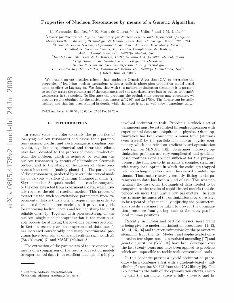
FIG. 1: Example of the evolution for a champion in one run ofthe GA. For the first generations (up to generation 40 or 50)evolution is driven by crossover. After this, small improve-ments are seen due to mutations.

for the GA and into (−∞, +∞) for the E04FCF routine.This latter step is done by means of the transformation

xj = arcsin

[

λj − λmaxj

λmaxj − λmin

j − 1

]

, (5)

where λj is the model parameter, xj is the mapping of λj

into (−∞, +∞), λmaxj is the highest value of the range

of variation, and λminj is the lowest value. With regard

to the range of variation allowed for the parameters, wemust note that gradient routines work more efficientlyif variations of similar magnitude on each of the searchparameters introduce a similar variation on the functionto minimize. The E04FCF user is advised to explore theregion of parameters to minimize and to provide ade-quate rescaling of the problem before calling the routine.While the NAG library provides tools that help in thistask, in our combined algorithm we take advantage ofthe knowledge obtained on the variation of the objec-tive function during the previous evaluations performedby the GA. We use this exploration to normalize the χ2

to unity and to rescale all the parameters affecting thisfunction so that, according to the last evaluations of thebest individuals explored by the GA, after rescaling ofboth the parameters and the function to optimize, theregion explored by the NAG E04FCF routine in its searchfor the minima is expected to lie in a hypercube of unitvolume. We have indeed verified that this normalizationand rescaling procedure improves NAG routine perfor-mance.

Our minimization strategy includes the following as-pects:

1. A first generation is made out of individuals ran-domly generated within reasonable values of theparameters.

2. Next, the GA is run for 400 generations (see defi-nition further on). This number is determined af-

4

TABLE I: Ranges for the parameter values of the nucleonresonances. Masses and decay widths have been taken withinthe ranges provided by [22]. The helicity amplitudes are de-noted by AI

λ, where I stands for isospin and λ for the helicityof the initial photon-nucleon state.

M∗ (GeV) Γ (GeV) AIλ (GeV−1/2)

∆(1232) [1.215,1.219] [0.094,0.098] [-1,1]

N(1440) [1.381,1.385] [0.314,0.318] [-1,1]

N(1520) [1.502,1.506] [0.110,0.114] [-1,1]

N(1535) [1.523,1.527] [0.100,0.104] [-1,1]

∆(1620) [1.605,1.609] [0.146,0.150] [-1,1]

N(1650) [1.661,1.665] [0.238,0.242] [-1,1]

∆(1700) [1.724,1.728] [0.116,0.120] [-1,1]

N(1720) [1.740,1.755] [0.119,0.278] [-1,1]

TABLE II: Ranges for the values of the parameters of vectormesons and cut-off Λ.

FωNN [20.61, 21.11]

Kω [−0.17,−0.15]

Kρ [6.1, 6.3]

Λ (GeV) [0.1, 2.0]

Generation i

Scaling

25% Best 75% Remainder

New population

25% Best 25% Fight25%

Half-elitistCrossover

25%RandomCrossover

ScalingNext iteration

Champion Rest of the population

Mutation(individuals randomly selected)

Generation (i + 1)

Reached final generation?

Solution

-?

Start

?

??

?

?

?

?

?Yes

No

6

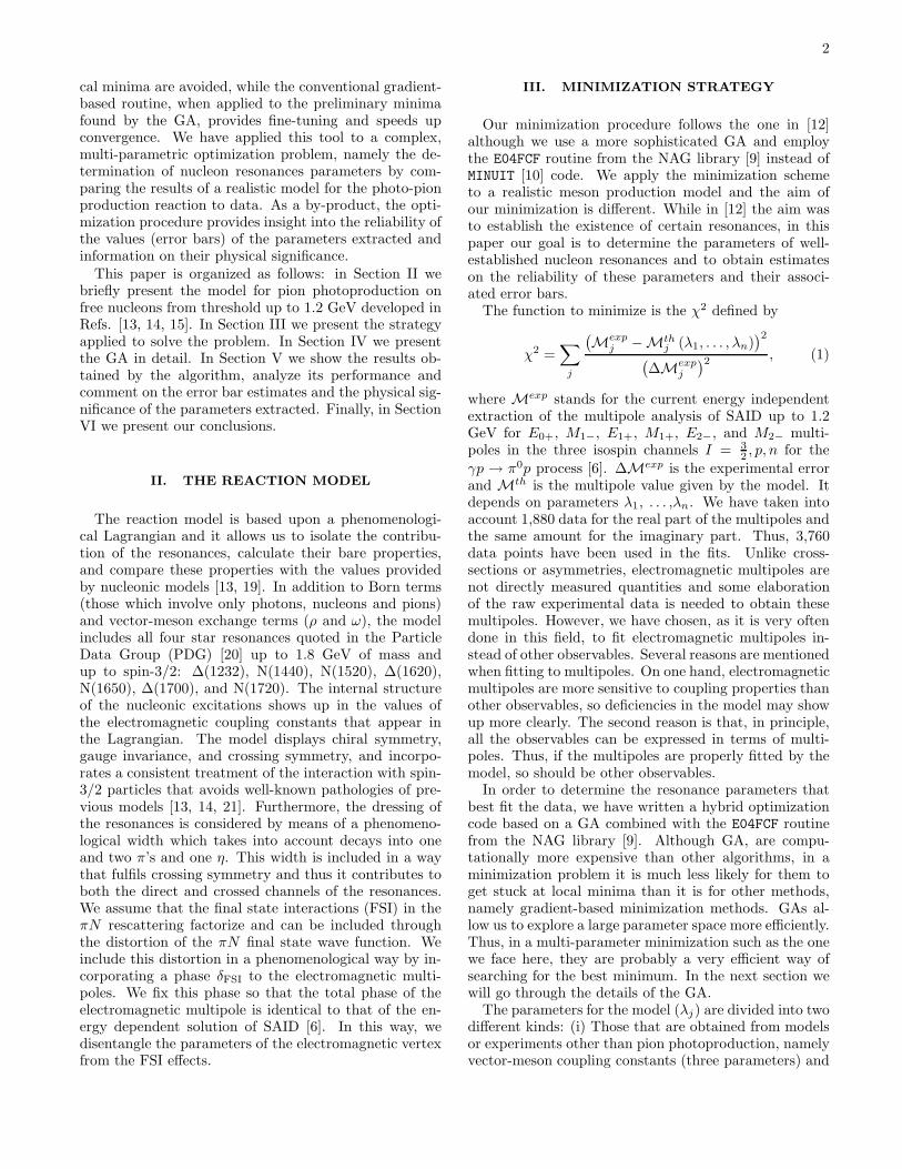
FIG. 2: GA scheme (see text in section IV).

ter inspecting the best individual evolution for eachgeneration and from comparisons with benchmarkproblems of similar size. We do not really need thatmany as 400 generations (see Fig. 1), but we pre-ferred to let the algorithm run for more generationsthan necessary in order to ensure that convergencewas achieved.

3. After the 400 generations have been run, we intro-duce the GA solution as the initial value for theE04FCF routine from NAG libraries [9]. We usethe routine for fine-tuning. The E04FCF routineimplements an algorithm that looks for the uncon-strained minimum of a sum of squares

Minimize[

F (x1, . . . , xn) =m

∑

j=1

|fj (x1, . . . , xn) |2]

, (6)

of m nonlinear functions in n variables (m ≥ n).This algorithm does not require the derivatives to

be known. From a starting point x(1)1 , . . . , x

(1)n (in

our case supplied by the GA) the routine appliesa Quasi-Newton method in order to find the mini-mum. This method uses a finite-difference approx-imation to the Hessian matrix to define the searchdirection. It is a very accurate and fast convergingalgorithm once we have an initial solution that isclose to the minimum we seek. Therefore, it is wellsuited for our fine-tuning purpose.

We note that many attempts to solve our op-timization procedure solely by means of E04FCF

completely failed, even when we guided the initialranges of the parameters by hand. The NAG rou-tine got stuck in the first local minimum, usuallyvery far from the one obtained by the GA.

4. We store the solution obtained by the combinedalgorithm and we start again, by generating a dif-ferent random seed for the initial population of theGA. After running the minimization code twentytimes, we obtain twenty different minima. If wefind that all the χ2 divided by χ2

min (the minimumχ2 among all the fits) are close to unity, we stopthe fitting procedure.

IV. GENETIC ALGORITHM

Genetic Algorithms are a specific kind of stochasticoptimization methods based upon the idea of evolution.There are many excellent textbooks on GA [18]. Herewe will describe the main features of GA that are neededto understand our implementation. GAs encode the pos-sible solutions to the proposed problem and deal withmany of these solutions at the same time. Indeed, aset of these possible solutions (also called individuals orgenes) form a population. Each individual in the popula-tion is classified according to its fitness value, computed

5

20

15

10

5

0

E0

+p

(mF

)

Real partImaginary part

4

2

0

-2

M1

-p

(mF

)

60

40

20

0

-20

M1

+3

/2

(mF

)

4

2

0

-2

-4

1.21.00.80.60.40.2

E1

+3

/2 (m

F)

Eγ (GeV)

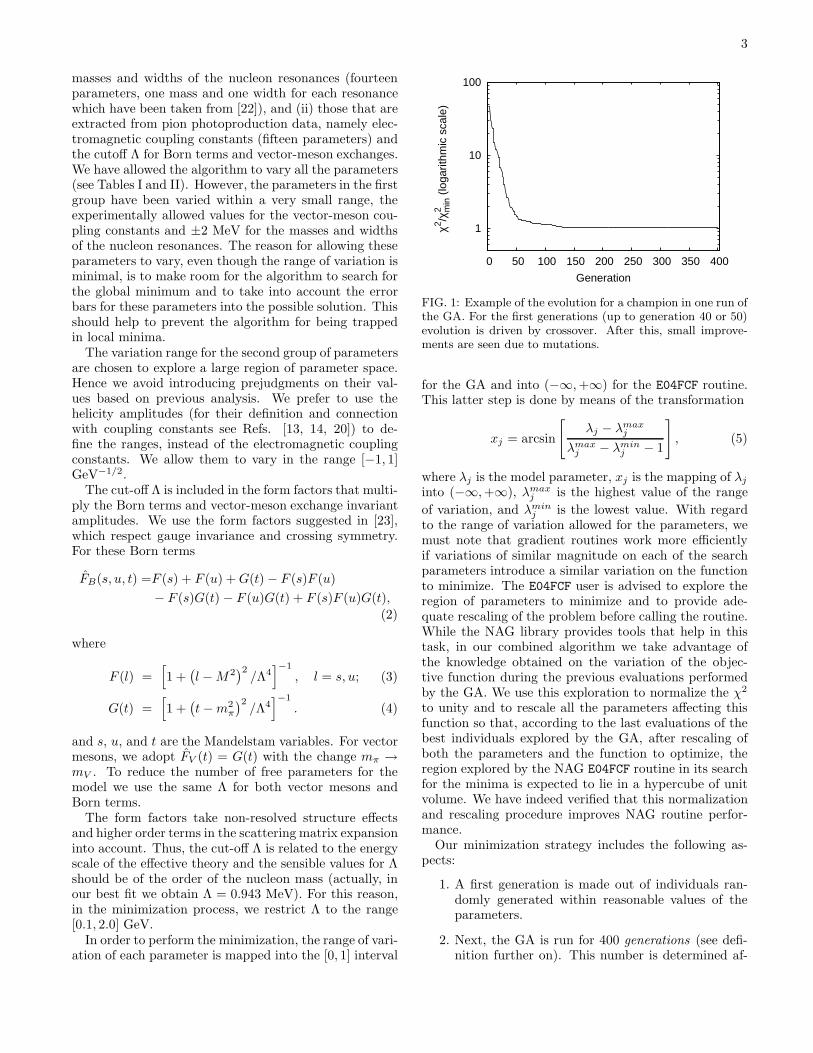
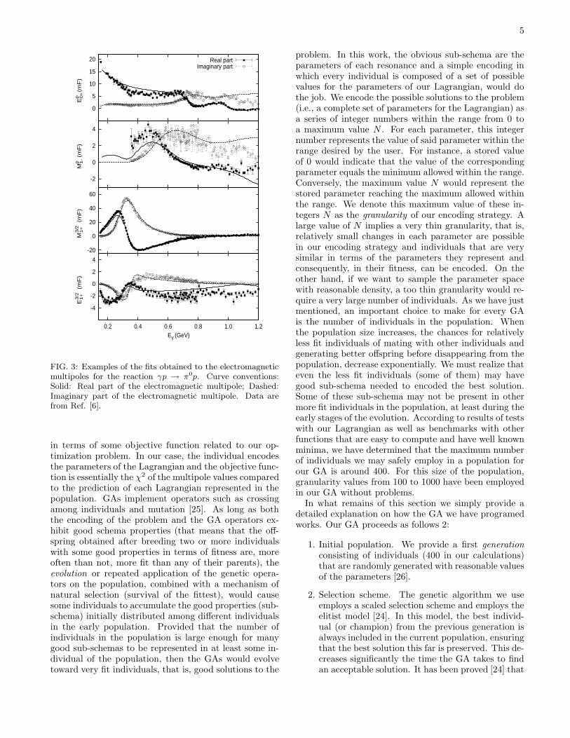
FIG. 3: Examples of the fits obtained to the electromagneticmultipoles for the reaction γp → π0p. Curve conventions:Solid: Real part of the electromagnetic multipole; Dashed:Imaginary part of the electromagnetic multipole. Data arefrom Ref. [6].

in terms of some objective function related to our op-timization problem. In our case, the individual encodesthe parameters of the Lagrangian and the objective func-tion is essentially the χ2 of the multipole values comparedto the prediction of each Lagrangian represented in thepopulation. GAs implement operators such as crossingamong individuals and mutation [25]. As long as boththe encoding of the problem and the GA operators ex-hibit good schema properties (that means that the off-spring obtained after breeding two or more individualswith some good properties in terms of fitness are, moreoften than not, more fit than any of their parents), theevolution or repeated application of the genetic opera-tors on the population, combined with a mechanism ofnatural selection (survival of the fittest), would causesome individuals to accumulate the good properties (sub-schema) initially distributed among different individualsin the early population. Provided that the number ofindividuals in the population is large enough for manygood sub-schemas to be represented in at least some in-dividual of the population, then the GAs would evolvetoward very fit individuals, that is, good solutions to the

problem. In this work, the obvious sub-schema are theparameters of each resonance and a simple encoding inwhich every individual is composed of a set of possiblevalues for the parameters of our Lagrangian, would dothe job. We encode the possible solutions to the problem(i.e., a complete set of parameters for the Lagrangian) asa series of integer numbers within the range from 0 toa maximum value N . For each parameter, this integernumber represents the value of said parameter within therange desired by the user. For instance, a stored valueof 0 would indicate that the value of the correspondingparameter equals the minimum allowed within the range.Conversely, the maximum value N would represent thestored parameter reaching the maximum allowed withinthe range. We denote this maximum value of these in-tegers N as the granularity of our encoding strategy. Alarge value of N implies a very thin granularity, that is,relatively small changes in each parameter are possiblein our encoding strategy and individuals that are verysimilar in terms of the parameters they represent andconsequently, in their fitness, can be encoded. On theother hand, if we want to sample the parameter spacewith reasonable density, a too thin granularity would re-quire a very large number of individuals. As we have justmentioned, an important choice to make for every GAis the number of individuals in the population. Whenthe population size increases, the chances for relativelyless fit individuals of mating with other individuals andgenerating better offspring before disappearing from thepopulation, decrease exponentially. We must realize thateven the less fit individuals (some of them) may havegood sub-schema needed to encoded the best solution.Some of these sub-schema may not be present in othermore fit individuals in the population, at least during theearly stages of the evolution. According to results of testswith our Lagrangian as well as benchmarks with otherfunctions that are easy to compute and have well knownminima, we have determined that the maximum numberof individuals we may safely employ in a population forour GA is around 400. For this size of the population,granularity values from 100 to 1000 have been employedin our GA without problems.

In what remains of this section we simply provide adetailed explanation on how the GA we have programedworks. Our GA proceeds as follows 2:

1. Initial population. We provide a first generation

consisting of individuals (400 in our calculations)that are randomly generated with reasonable valuesof the parameters [26].

2. Selection scheme. The genetic algorithm we useemploys a scaled selection scheme and employs theelitist model [24]. In this model, the best individ-ual (or champion) from the previous generation isalways included in the current population, ensuringthat the best solution this far is preserved. This de-creases significantly the time the GA takes to findan acceptable solution. It has been proved [24] that

6

the GA which introduces elitism (that is, the guar-anteed survival of the champion at every step ofthe GA evolution) will eventually converge to theabsolute optimum, while, in general, the ones thatdo not protect the champion will never reach theoptimum [27].

With regard to the remainder of the population, be-sides the champion, the individuals from the previ-ous generation (that is, the population in its earlierstate) are ranked according to the fitness function,in our case the χ2 value. After this step, we in-troduce scaling of the population [28] determiningthe probability that an individual has to mate andsurvive. We provide a 0.8 probability to the worstindividual and 1.0 to the best one. This is donein order to maintain genetic diversity. Indeed, it isnecessary to prevent that the best and the worst in-dividuals have a too different survival probability.If we do not take care to preserve genetic diversityin this way, the appearance of a very fit individ-ual would make the forthcoming offspring collapseto the characteristics of that particularly fit indi-vidual too soon. Another important technique tomaintain diversity is mutation, which is discussedfurther on.

3. After scaling, we classify the population into twosets. Set (a) is composed of the best 25% of theindividuals and set (b) by the remaining 75%. Weproduce the new generation in the following way:

• 25% of the individuals are taken from the mostfit ones from the previous generation. That is,set (a) is copied into the next generation.

• Another 25% is selected through a fight amongall the individuals (tournament). The out-come of the fight is randomly decided, depend-ing on probability. Even in the least favorablecase (that is, if the worse individual fights withthe best one), the winning probability of (theworst) individual is 15%. Winning probabili-ties are computed accordingly to the fitness ofeach contender.

• Another 25% is obtained by means of half-elitist crossover. This means that we mate anindividual from the best 25% of the previousgeneration (set (a)) with any other individualin sets (a) or (b). Both individuals are pickedrandomly from their respective sets.

• The remaining 25% of the offspring are gen-erated by mating individuals that are selectedrandomly without restrictions from sets (a) or(b).

We apply two different kinds of crossover: one

point crossover and arithmetic crossover [28]. Inone point crossover, a random crossover point forboth parents is selected. We split each chromosome

from the parents into two pieces. We take the sec-ond piece of the second parent and attach it to thefirst piece of the first parent. In this way we obtainan individual that is a mixture of the two origi-nal ones. For the arithmetic crossover, we chooseat random a number r between 0 and 1, and theoffspring is calculated weighting the parents withweight r and (1 − r).

λoffspringi = r · λparent 1

i + (1 − r) · λparent 2i (7)

Half of the crossovers our GA implements are onepoint and the other half are arithmetic. The kindof crossover to apply to a given pair of parents ischosen at random.

4. We evaluate the new population and identify thenew champion. As previously mentioned, it willbe preserved (elitism). We select other individualsto mutate from the rest of the population exclud-ing the champion. Indeed, in each iteration of ourGA we introduce as many mutations as the numberof individuals in the population divided by three.These mutations are distributed at random amongall the individuals (excluding the champion) of thepopulation generated following the previous steps.We apply two types of mutation [29]. The per-

mutation mutation exchanges two parameters se-lected at random. The gaussian mutation changesthe value of a parameter by a small amount. Theamount of change induced by this mutation is ran-dom within a small range. The reason to introducemutations is that, quite often, the crossover op-erator and the selection method are too effectiveand they end up driving the GA toward a pop-ulation of individuals that are almost exactly thesame. When the population consists of similar in-dividuals, the likelihood of finding new solutionstypically decreases. The mutation operator intro-duces an additional randomness into the search. Ithelps to maintain diversity and to find solutionsthat crossover alone might not discover.

5. After these steps are taken, we say that a new gen-eration is built. If we have not reached the limitin the number of generations, we run the algorithmagain with the current set of individuals as the ini-tial population.

When the maximum number of generations hasbeen reached, we take the set of parameters en-coded by the champion as the solution given byGA to our problem. If sufficient generations havebeen run, most of the individuals will have closevalues for the fitness function.

It has been proven that there is no optimal algorithmthat adapts well (that is, reaches a solution in the leastnumber of evaluations) to all kind of problems. This is

7

TABLE III: Helicity amplitudes obtained in the fits inGeV−1/2.

Ap1/2

A∆

1/2 An1/2 Ap

3/2A∆

3/2 An3/2

∆(1232) – −0.120 – – −0.229 –

N(1440) 0.060 – −0.089 – – –

N(1520) −0.007 – 0.032 0.107 – −0.085

N(1535) 0.014 – −0.137 – – –

∆(1620) – −0.023 – – – –

N(1650) −0.022 – 0.003 – – –

∆(1700) – 0.139 – – −0.127 –

N(1720) 0.143 – 0.126 −0.004 – −0.444

often referred to as the no free lunch theorem in optimiza-tion [30]. Our goal here however is not to find the opti-mal algorithm that obtains the minimum to our problemin less evaluations but, rather, to develop a general toolthat can be applied to many different models of param-eter data fitting without specific fine-tuning nor humanintervention, even if the performance of the tool is sub-optimal in terms of the number of operations. In thisregard, GAs are a handy choice, as they are suitable formany different problems. Thanks to scaling and elitism,our GA converges neither too quickly nor too slowly andgenerally it is able to find good candidates for the globaloptimum.

When the individuals are very fit, it can be hard forthe GA to evolve further, mainly because the path tothe best individual may involve two or more consecutivemutations where each of these mutations on their ownwill produce a less fit individual that will sooner be re-moved from the population. The occurrence of such twofavorable mutations in the same individual is unlikelyand tailored procedures must be implemented to intro-duce specific mutations that are adequate for particularproblems, or more complex operators like the ’tunnel-ing algorithm’ [31] or complex rules to encode the valuesof the functions, like Mendelian operators implementinga non-dominant character for some genes [32]. In ourwork, however, we prefer to employ a hybrid optimiza-tion method that combines a standard hill-climbing al-gorithm with a GA. Hybrid optimization methods havebeen under study intensively [12, 33]. We have comparedseveral ways of hybridizing GAs and conventional gradi-ent based hill-climbing algorithms, such as introducingthe hill-climbing algorithm as another mutation opera-tor. However, we have noticed that this will only makethe GA converge sooner, very often too soon, resulting init getting stuck at any of the many local minima. Fromour experience, if the hill-climbing procedure is intro-duced just at the end of the evolution, when the GA hasconverged, the best results are achieved and a robust al-gorithm that requires no human intervention is this wayconfigured. Also, no granularity is introduced in this fi-nal step of optimization. Indeed, the NAG routine is notrestricted to integer values of the parameters, but instead

1.04

1.03

1.02

1.01

1

20151050

χ2 /χ2 m

in

Evaluation

GeneticGenetic+NAG

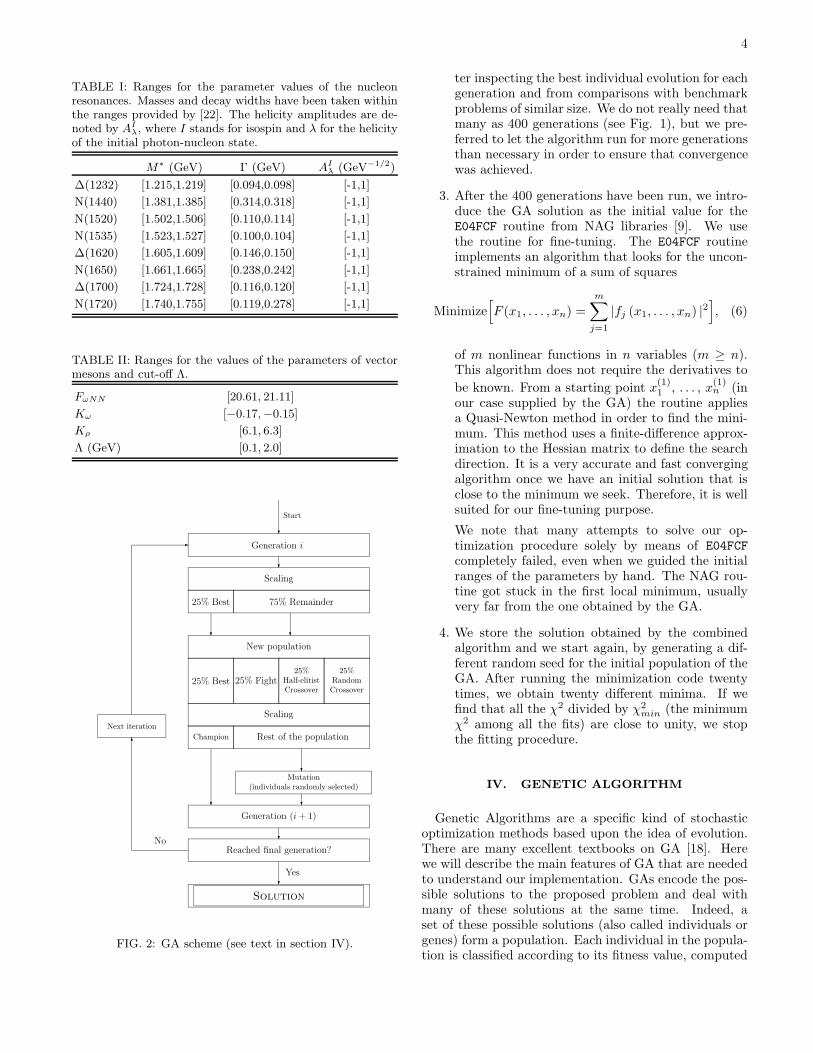
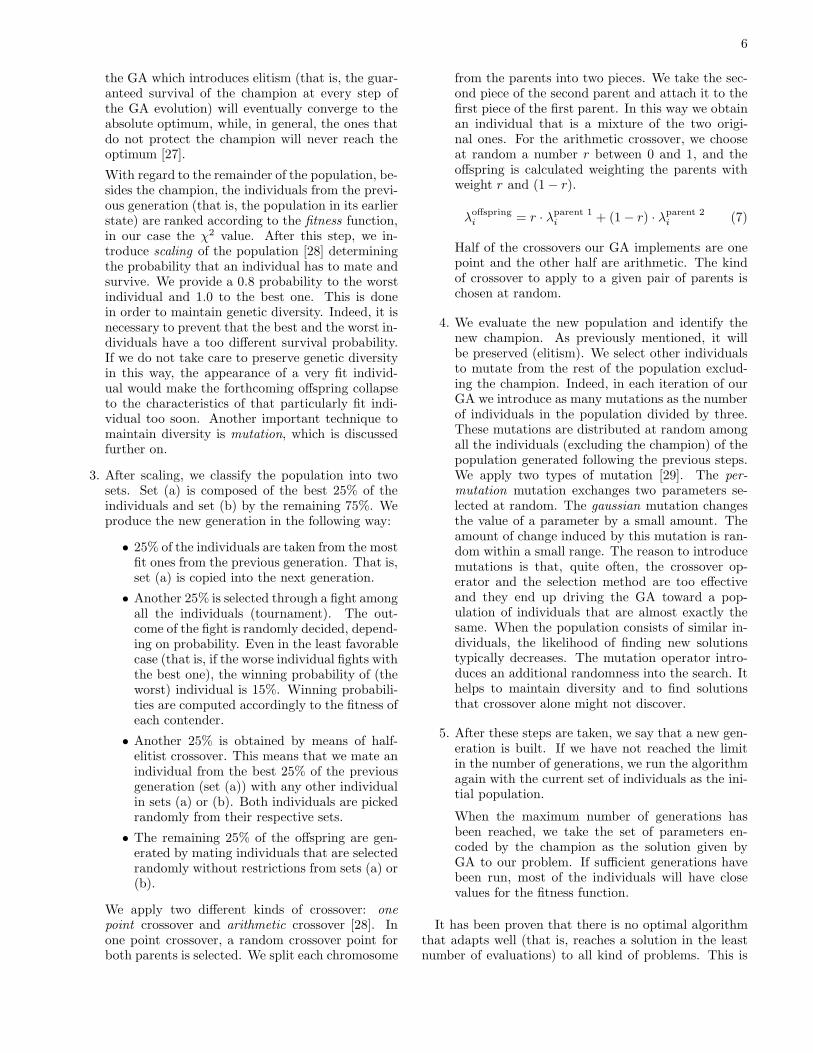
FIG. 4: Many local minima and the effect of the fine tun-ing performed by the E04FCF routine in the χ2/χ2

min areshown. Conventions: Open circles, χ2/χ2

min obtained by theGA alone (400 generations with 300 individuals each); Solidsquares: χ2/χ2

min obtained by the GA plus the NAG routine.

represents each parameter as floating point values. Thus,we can also consider that the GA finds the best optimumthat can be represented within the grid implied by thegranularity N , and starting from this point of the grid,the NAG routine refines a search not bound to any gridvalues.

V. RESULTS

In Fig. 3 we show examples of fits to electromagneticmultipoles for the γp → π0p process and the overallagreement obtained. The values of the parameters aresummarized in Table III. In Fig. 1 we display an exampleof the evolution of the champion along the generations.Two hundred generations are sufficient enough to achieveconvergence, but we run the algorithm for another twohundred generations to see the effects of mutations, whichcan reach areas of the parameter space that are not beingfully surveyed by means of crossover.

We observe that at the early stages of the evolution thefitness function improves quickly, as crossover works toconcentrate the good schema from other individuals intoa good individual. Actually, a very steep slope in thisregion might indicate that evolution is too fast and thatless fit individuals could disappear from the populationbefore their good properties are transmitted to more fitindividuals.

When a jump in the χ2/χ2min happens, it is due to

the appearance of a more fit new individual, either dueto crossover or to mutation. In Fig. 4 we can verifythe existence of many local minima (so this is certainlyan ill-posed optimization problem) and the fine tuningachieved by the NAG routine which improves minima byapproximately 2%.

An important issue to consider in GAs is efficiency.As we have already mentioned, the parameter space has

8

1.025

1.020

1.015

1.010

1.005

1.000

-0.118-0.119-0.120-0.121

χ2 /χ2 m

in

A1/2∆ (GeV-1/2)

(a)

1.025

1.020

1.015

1.010

1.005

1.000

-0.22-0.23-0.24

χ2 /χ2 m

in

A3/2∆ (GeV-1/2)

(b)

-0.118

-0.119

-0.120

-0.121-0.220-0.225-0.23-0.235-0.240

A1/

2∆

(G

eV-1

/2)

A3/2∆ (GeV-1/2)

(c)

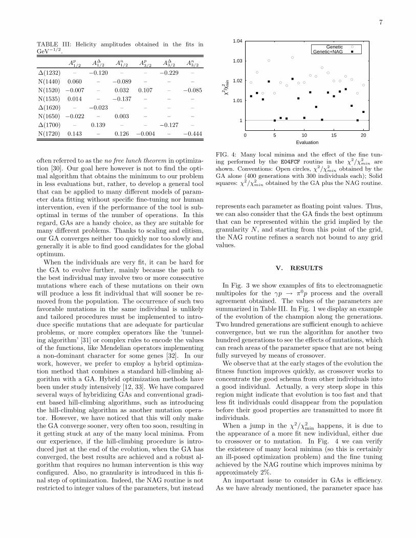
FIG. 5: Helicity amplitudes (equivalent to the coupling constants of the Lagrangians) of the ∆(1232). In all the figures weshow the twenty minima obtained in the full minimization procedure (GA+NAG, see Fig. 4). The upper-left hand figure (a)shows the χ2/χ2

min versus the amplitude A∆

1/2. The lower-left hand figure (b) shows the χ2/χ2min versus the amplitude A∆

3/2.

The right panel (c) shows A∆

1/2versus A∆

3/2parameters.

to be discretized with a certain granularity and the algo-rithm searches for the best solution within the discretizedversion of the parameter space. The size of this spacesignificantly affects the efficiency of the algorithm, thusa balance between granularity and computing time hasto be achieved. The gradient based routine allows us togain precision and efficiency because we do not need theGA to reach the minimum, we simply need it to providea value close enough for the E04FCF routine can reachit. In other words the GA has to reach the region wherethe minimum lies, and once in this region, reaching theminimum is a task for the gradient-based routine.

We must emphasize that the use of our algorithm isunattended. That is, we submit the script that starts20 instances of the GA+NAG procedure, and after theequivalent to five CPU-days (Opteron, 2 GHz), we getthe results for the optimized set of parameters. No fur-ther human intervention was needed to choose initial val-ues of the parameters or to guide the evolution. Whilethe GA+NAG may require more (costly) evaluations ofthe objective function, it is robust and needs no train-ing nor good guesses of the initial parameters. Now thatcomputer power seems to be an increasingly availableresource, the unattended mode of operation makes thishybrid algorithm a very interesting alternative for theseoptimization problems.

Figs. 5 and 6 show a typical situation that may arise

when the parameters are being determined. For ∆(1232)the minimum is well-established and all the minima areconstrained in a small region. The size of the regionwhere the minima lie may provide a better estimationof the error associated with the parameters than the oneprovided by the correlation matrix. On the other hand, inFig. 5 the value for the A∆

1/2 helicity amplitude appears

to be in one of two split regions that are too close to bephysically distinguished (left-upper panel). One regionis centered at −0.120 and the other at −0.119 GeV−1/2.The identification of these regions is one of the functional-ities that GAs provide and one of their main advantages.When multiple regions containing minima of similar qual-ity appear, the possible physical implications should beconsidered and further analysis to assess whether thesedifferent regions hold physical meaning (see subsectionVA) is required.

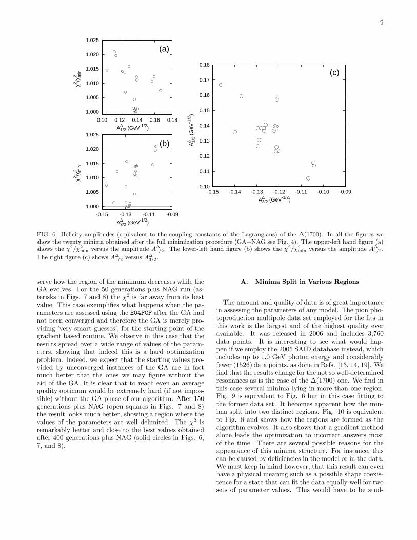
We also show the minima of the ∆(1700) that are con-strained in just one region. However, this region is largerthan for the ∆(1232) and the experimental informationavailable for this resonance, thus, yields parameters thatare not as well established as for other nucleon excita-tions.

The evolution of the position of the parameters for dif-ferent instances of the GA+NAG procedure as the num-ber of generations employed in the GA increases, is shownfor the ∆(1700) resonance in Figs. 7 and 8. We can ob-

9

1.025

1.020

1.015

1.010

1.005

1.000

0.180.160.140.120.10

χ2 /χ2 m

in

A1/2∆ (GeV-1/2)

(a)

1.025

1.020

1.015

1.010

1.005

1.000

-0.09-0.11-0.13-0.15

χ2 /χ2 m

in

A3/2∆ (GeV-1/2)

(b)

0.18

0.17

0.16

0.15

0.14

0.13

0.12

0.11

0.10-0.09-0.10-0.11-0.12-0.13-0,14-0.15

A1/

2∆

(G

eV-1

/2)

A3/2∆ (GeV-1/2)

(c)

FIG. 6: Helicity amplitudes (equivalent to the coupling constants of the Lagrangians) of the ∆(1700). In all the figures weshow the twenty minima obtained after the full minimization procedure (GA+NAG see Fig. 4). The upper-left hand figure (a)shows the χ2/χ2

min versus the amplitude A∆

1/2. The lower-left hand figure (b) shows the χ2/χ2

min versus the amplitude A∆

1/2.

The right figure (c) shows A∆

1/2versus A∆

3/2.

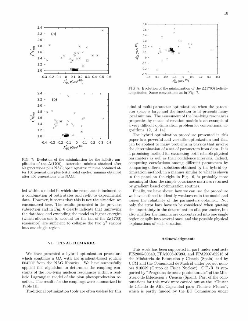
serve how the region of the minimum decreases while theGA evolves. For the 50 generations plus NAG run (as-terisks in Figs. 7 and 8) the χ2 is far away from its bestvalue. This case exemplifies what happens when the pa-rameters are assessed using the E04FCF after the GA hadnot been converged and therefore the GA is merely pro-viding ’very smart guesses’, for the starting point of thegradient based routine. We observe in this case that theresults spread over a wide range of values of the param-eters, showing that indeed this is a hard optimizationproblem. Indeed, we expect that the starting values pro-vided by unconverged instances of the GA are in factmuch better that the ones we may figure without theaid of the GA. It is clear that to reach even an averagequality optimum would be extremely hard (if not impos-sible) without the GA phase of our algorithm. After 150generations plus NAG (open squares in Figs. 7 and 8)the result looks much better, showing a region where thevalues of the parameters are well delimited. The χ2 isremarkably better and close to the best values obtainedafter 400 generations plus NAG (solid circles in Figs. 6,7, and 8).

A. Minima Split in Various Regions

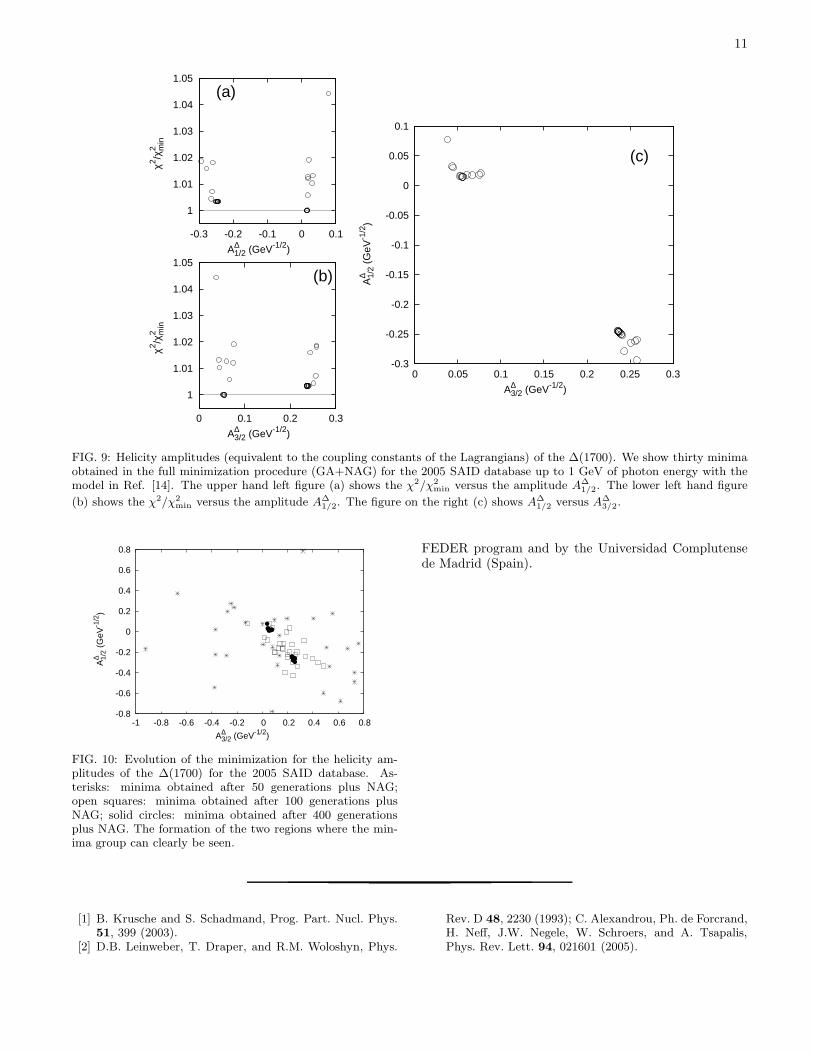
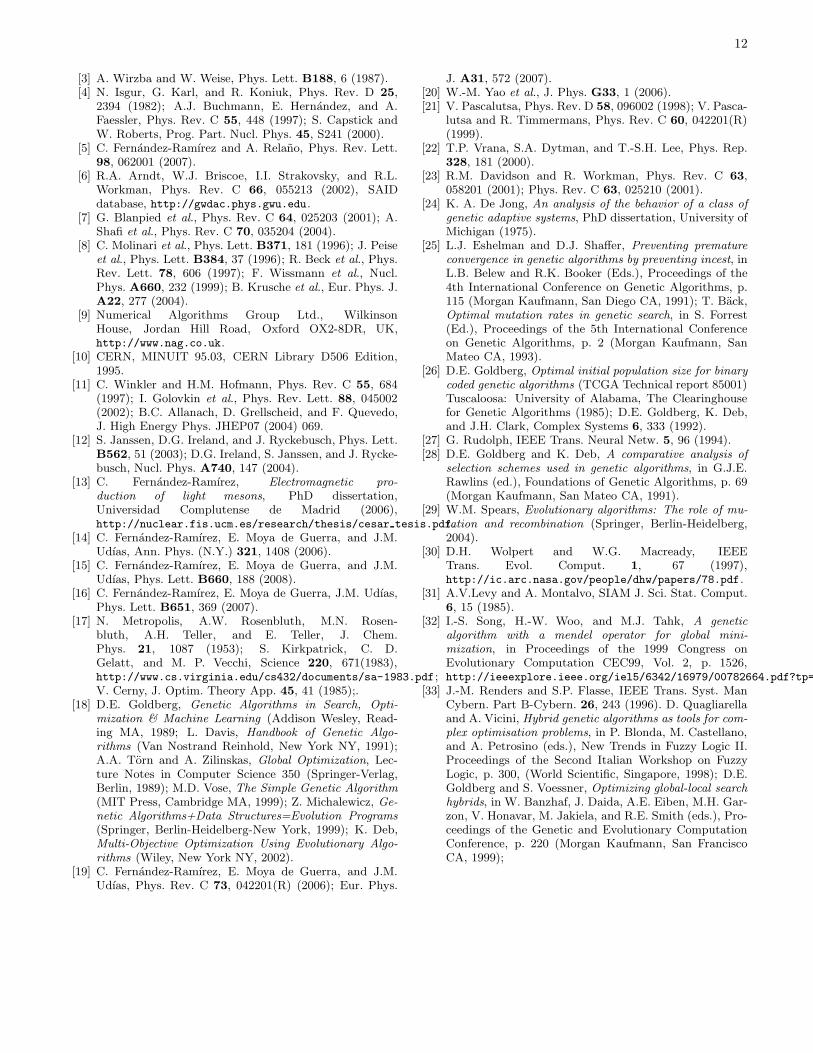
The amount and quality of data is of great importancein assessing the parameters of any model. The pion pho-toproduction multipole data set employed for the fits inthis work is the largest and of the highest quality everavailable. It was released in 2006 and includes 3,760data points. It is interesting to see what would hap-pen if we employ the 2005 SAID database instead, whichincludes up to 1.0 GeV photon energy and considerablyfewer (1526) data points, as done in Refs. [13, 14, 19]. Wefind that the results change for the not so well-determinedresonances as is the case of the ∆(1700) one. We find inthis case several minima lying in more than one region.Fig. 9 is equivalent to Fig. 6 but in this case fitting tothe former data set. It becomes apparent how the min-ima split into two distinct regions. Fig. 10 is equivalentto Fig. 8 and shows how the regions are formed as thealgorithm evolves. It also shows that a gradient methodalone leads the optimization to incorrect answers mostof the time. There are several possible reasons for theappearance of this minima structure. For instance, thiscan be caused by deficiencies in the model or in the data.We must keep in mind however, that this result can evenhave a physical meaning such as a possible shape coexis-tence for a state that can fit the data equally well for twosets of parameter values. This would have to be stud-

10

2.4

2.2

2.0

1.8

1.6

1.4

1.2

1.0

-0.3 -0.2 -0.1 0 0.1 0.2 0.3 0.4 0.5 0.6

χ2 /χ2 m

in

A1/2∆ (GeV-1/2)

(a)

2.4

2.2

2.0

1.8

1.6

1.4

1.2

1.0

-0.4 -0.3 -0.2 -0.1 0 0.1 0.2 0.3 0.4

χ2 /χ2 m

in

A3/2∆ (GeV-1/2)

(b)

FIG. 7: Evolution of the minimization for the helicity am-plitudes of the ∆(1700). Asterisks: minima obtained after50 generations plus NAG; open squares: minima obtained af-ter 150 generations plus NAG; solid circles: minima obtainedafter 400 generations plus NAG.

ied within a model in which the resonance is included asa combination of both states and re-fit to experimentaldata. However, it seems that this is not the situation weencountered here. The results presented in the previoussubsection and in Fig. 6 clearly indicate that improvingthe database and extending the model to higher energies(which allows one to account for the tail of the ∆(1700)resonance) are sufficient to collapse the two χ2 regionsinto one single region.

VI. FINAL REMARKS

We have presented a hybrid optimization procedurewhich combines a GA with the gradient-based routineE04FCF from the NAG libraries. We have successfullyapplied this algorithm to determine the coupling con-stants of the low-lying nucleon resonances within a real-istic Lagrangian model of the pion photoproduction re-action. The results for the couplings were summarized inTable III.

Traditional optimization tools are often useless for this

-0.3

-0.2

-0.1

0

0.1

0.2

0.3

0.4

0.5

0.6

-0.4 -0.3 -0.2 -0.1 0 0.1 0.2 0.3 0.4

A1/

2∆

(G

eV-1

/2)

A3/2∆ (GeV-1/2)

FIG. 8: Evolution of the minimization of the ∆(1700) helicityamplitudes. Same conventions as in Fig. 7.

kind of multi-parameter optimizations when the param-eter space is large and the function to fit presents manylocal minima. The assessment of the low-lying resonancesproperties by means of reaction models is an example ofa very difficult optimization problem for conventional al-gorithms [12, 13, 14].

The hybrid optimization procedure presented in thispaper is a powerful and versatile optimization tool thatcan be applied to many problems in physics that involvethe determination of a set of parameters from data. It isa promising method for extracting both reliable physicalparameters as well as their confidence intervals. Indeed,computing correlations among different parameters bycomparing different solutions obtained by the hybrid op-timization method, in a manner similar to what is shownin the panel on the right in Fig. 6, is probably moremeaningful than the simple covariance matrices returnedby gradient based optimization routines.

Finally, we have shown how we can use the procedurewe have outlined to identify weaknesses in the model andassess the reliability of the parameters obtained. Notonly the error bars have to be considered when quotingthe uncertainty in the determination of a parameter, butalso whether the minima are concentrated into one singleregion or split into several ones, and the possible physicalexplanations of such situation.

Acknowledgments

This work has been supported in part under contractsFIS2005-00640, FPA2006-07393, and FPA2007-62216 ofthe Ministerio de Educacion y Ciencia (Spain) and byUCM and the Comunidad de Madrid under project num-ber 910059 (Grupo de Fısica Nuclear). C.F.-R. is sup-ported by ”Programa de becas posdoctorales” of the Min-isterio de Educacion y Ciencia (Spain). Part of the com-putations for this work were carried out at the “Clusterde Calculo de Alta Capacidad para Tecnicas Fısicas”,which is partly funded by the EU Commission under

11

1.05

1.04

1.03

1.02

1.01

1

0.10-0.1-0.2-0.3

χ2 /χ2 m

in

A1/2∆ (GeV-1/2)

(a)

1.05

1.04

1.03

1.02

1.01

1

0.30.20.10

χ2 /χ2 m

in

A3/2∆ (GeV-1/2)

(b)

0.1

0.05

0

-0.05

-0.1

-0.15

-0.2

-0.25

-0.30.30.250.20.150.10.050

A1/

2∆

(G

eV-1

/2)

A3/2∆ (GeV-1/2)

(c)

FIG. 9: Helicity amplitudes (equivalent to the coupling constants of the Lagrangians) of the ∆(1700). We show thirty minimaobtained in the full minimization procedure (GA+NAG) for the 2005 SAID database up to 1 GeV of photon energy with themodel in Ref. [14]. The upper hand left figure (a) shows the χ2/χ2

min versus the amplitude A∆

1/2. The lower left hand figure

(b) shows the χ2/χ2

min versus the amplitude A∆

1/2. The figure on the right (c) shows A∆

1/2versus A∆

3/2.

-0.8

-0.6

-0.4

-0.2

0

0.2

0.4

0.6

0.8

-1 -0.8 -0.6 -0.4 -0.2 0 0.2 0.4 0.6 0.8

A1/

2∆

(G

eV-1

/2)

A3/2∆ (GeV-1/2)

FIG. 10: Evolution of the minimization for the helicity am-plitudes of the ∆(1700) for the 2005 SAID database. As-terisks: minima obtained after 50 generations plus NAG;open squares: minima obtained after 100 generations plusNAG; solid circles: minima obtained after 400 generationsplus NAG. The formation of the two regions where the min-ima group can clearly be seen.

FEDER program and by the Universidad Complutensede Madrid (Spain).

[1] B. Krusche and S. Schadmand, Prog. Part. Nucl. Phys.51, 399 (2003).

[2] D.B. Leinweber, T. Draper, and R.M. Woloshyn, Phys.

Rev. D 48, 2230 (1993); C. Alexandrou, Ph. de Forcrand,H. Neff, J.W. Negele, W. Schroers, and A. Tsapalis,Phys. Rev. Lett. 94, 021601 (2005).

12

[3] A. Wirzba and W. Weise, Phys. Lett. B188, 6 (1987).[4] N. Isgur, G. Karl, and R. Koniuk, Phys. Rev. D 25,

2394 (1982); A.J. Buchmann, E. Hernandez, and A.Faessler, Phys. Rev. C 55, 448 (1997); S. Capstick andW. Roberts, Prog. Part. Nucl. Phys. 45, S241 (2000).

[5] C. Fernandez-Ramırez and A. Relano, Phys. Rev. Lett.98, 062001 (2007).

[6] R.A. Arndt, W.J. Briscoe, I.I. Strakovsky, and R.L.Workman, Phys. Rev. C 66, 055213 (2002), SAIDdatabase, http://gwdac.phys.gwu.edu.

[7] G. Blanpied et al., Phys. Rev. C 64, 025203 (2001); A.Shafi et al., Phys. Rev. C 70, 035204 (2004).

[8] C. Molinari et al., Phys. Lett. B371, 181 (1996); J. Peiseet al., Phys. Lett. B384, 37 (1996); R. Beck et al., Phys.Rev. Lett. 78, 606 (1997); F. Wissmann et al., Nucl.Phys. A660, 232 (1999); B. Krusche et al., Eur. Phys. J.A22, 277 (2004).

[9] Numerical Algorithms Group Ltd., WilkinsonHouse, Jordan Hill Road, Oxford OX2-8DR, UK,http://www.nag.co.uk.

[10] CERN, MINUIT 95.03, CERN Library D506 Edition,1995.

[11] C. Winkler and H.M. Hofmann, Phys. Rev. C 55, 684(1997); I. Golovkin et al., Phys. Rev. Lett. 88, 045002(2002); B.C. Allanach, D. Grellscheid, and F. Quevedo,J. High Energy Phys. JHEP07 (2004) 069.

[12] S. Janssen, D.G. Ireland, and J. Ryckebusch, Phys. Lett.B562, 51 (2003); D.G. Ireland, S. Janssen, and J. Rycke-busch, Nucl. Phys. A740, 147 (2004).

[13] C. Fernandez-Ramırez, Electromagnetic pro-duction of light mesons, PhD dissertation,Universidad Complutense de Madrid (2006),http://nuclear.fis.ucm.es/research/thesis/cesar tesis.pdf.

[14] C. Fernandez-Ramırez, E. Moya de Guerra, and J.M.Udıas, Ann. Phys. (N.Y.) 321, 1408 (2006).

[15] C. Fernandez-Ramırez, E. Moya de Guerra, and J.M.Udıas, Phys. Lett. B660, 188 (2008).

[16] C. Fernandez-Ramırez, E. Moya de Guerra, J.M. Udıas,Phys. Lett. B651, 369 (2007).

[17] N. Metropolis, A.W. Rosenbluth, M.N. Rosen-bluth, A.H. Teller, and E. Teller, J. Chem.Phys. 21, 1087 (1953); S. Kirkpatrick, C. D.Gelatt, and M. P. Vecchi, Science 220, 671(1983),http://www.cs.virginia.edu/cs432/documents/sa-1983.pdf;V. Cerny, J. Optim. Theory App. 45, 41 (1985);.

[18] D.E. Goldberg, Genetic Algorithms in Search, Opti-mization & Machine Learning (Addison Wesley, Read-ing MA, 1989; L. Davis, Handbook of Genetic Algo-rithms (Van Nostrand Reinhold, New York NY, 1991);A.A. Torn and A. Zilinskas, Global Optimization, Lec-ture Notes in Computer Science 350 (Springer-Verlag,Berlin, 1989); M.D. Vose, The Simple Genetic Algorithm(MIT Press, Cambridge MA, 1999); Z. Michalewicz, Ge-netic Algorithms+Data Structures=Evolution Programs(Springer, Berlin-Heidelberg-New York, 1999); K. Deb,Multi-Objective Optimization Using Evolutionary Algo-rithms (Wiley, New York NY, 2002).

[19] C. Fernandez-Ramırez, E. Moya de Guerra, and J.M.Udıas, Phys. Rev. C 73, 042201(R) (2006); Eur. Phys.

J. A31, 572 (2007).[20] W.-M. Yao et al., J. Phys. G33, 1 (2006).[21] V. Pascalutsa, Phys. Rev. D 58, 096002 (1998); V. Pasca-

lutsa and R. Timmermans, Phys. Rev. C 60, 042201(R)(1999).

[22] T.P. Vrana, S.A. Dytman, and T.-S.H. Lee, Phys. Rep.328, 181 (2000).

[23] R.M. Davidson and R. Workman, Phys. Rev. C 63,058201 (2001); Phys. Rev. C 63, 025210 (2001).

[24] K. A. De Jong, An analysis of the behavior of a class ofgenetic adaptive systems, PhD dissertation, University ofMichigan (1975).

[25] L.J. Eshelman and D.J. Shaffer, Preventing prematureconvergence in genetic algorithms by preventing incest, inL.B. Belew and R.K. Booker (Eds.), Proceedings of the4th International Conference on Genetic Algorithms, p.115 (Morgan Kaufmann, San Diego CA, 1991); T. Back,Optimal mutation rates in genetic search, in S. Forrest(Ed.), Proceedings of the 5th International Conferenceon Genetic Algorithms, p. 2 (Morgan Kaufmann, SanMateo CA, 1993).

[26] D.E. Goldberg, Optimal initial population size for binarycoded genetic algorithms (TCGA Technical report 85001)Tuscaloosa: University of Alabama, The Clearinghousefor Genetic Algorithms (1985); D.E. Goldberg, K. Deb,and J.H. Clark, Complex Systems 6, 333 (1992).

[27] G. Rudolph, IEEE Trans. Neural Netw. 5, 96 (1994).[28] D.E. Goldberg and K. Deb, A comparative analysis of

selection schemes used in genetic algorithms, in G.J.E.Rawlins (ed.), Foundations of Genetic Algorithms, p. 69(Morgan Kaufmann, San Mateo CA, 1991).

[29] W.M. Spears, Evolutionary algorithms: The role of mu-tation and recombination (Springer, Berlin-Heidelberg,2004).

[30] D.H. Wolpert and W.G. Macready, IEEETrans. Evol. Comput. 1, 67 (1997),http://ic.arc.nasa.gov/people/dhw/papers/78.pdf.

[31] A.V.Levy and A. Montalvo, SIAM J. Sci. Stat. Comput.6, 15 (1985).

[32] I.-S. Song, H.-W. Woo, and M.J. Tahk, A geneticalgorithm with a mendel operator for global mini-mization, in Proceedings of the 1999 Congress onEvolutionary Computation CEC99, Vol. 2, p. 1526,http://ieeexplore.ieee.org/iel5/6342/16979/00782664.pdf?tp=&is

[33] J.-M. Renders and S.P. Flasse, IEEE Trans. Syst. ManCybern. Part B-Cybern. 26, 243 (1996). D. Quagliarellaand A. Vicini, Hybrid genetic algorithms as tools for com-plex optimisation problems, in P. Blonda, M. Castellano,and A. Petrosino (eds.), New Trends in Fuzzy Logic II.Proceedings of the Second Italian Workshop on FuzzyLogic, p. 300, (World Scientific, Singapore, 1998); D.E.Goldberg and S. Voessner, Optimizing global-local searchhybrids, in W. Banzhaf, J. Daida, A.E. Eiben, M.H. Gar-zon, V. Honavar, M. Jakiela, and R.E. Smith (eds.), Pro-ceedings of the Genetic and Evolutionary ComputationConference, p. 220 (Morgan Kaufmann, San FranciscoCA, 1999);