1

Probabilistic Track Coverage in Cooperative Sensor NetworksS. Ferrari†, G. Zhang†, and T. A. Wettergren§

Abstract— The quality of service of a network performingcooperative track detection is represented by the probabilityof obtaining multiple elementary detections over time, along atarget track. Recently, two different lines of research, distributedsearch theory and geometric transversals, have been used inthe literature for deriving the probability of track detectionas a function of random and deterministic sensors’ positions,respectively. In this paper, we prove that these two approaches areequivalent under the same problem formulation. Also, we presenta new performance function that is derived by extending thegeometric transversals approach to the case of random sensors’positions using Poisson flats. As a result, a unified approach foraddressing track detection in both deterministic and probabilisticsensor networks is obtained. The new performance function isvalidated through numerical simulations, and is shown to bringabout considerable computational savings both for deterministicand probabilistic sensor networks.

Index Terms— Track coverage, sensor networks, target track-ing, geometric transversals, Poisson flats, probability, track de-tection, search theory.

I. INTRODUCTION

The problem of track detection by cooperative sensor net-works arises in many applications, including security andsurveillance, environmental and atmospheric monitoring, andtracking of endangered species. The performance of thesenetworks can be characterized by their area and track coverage,both of which have received considerable attention in theliterature [1]–[10]. Area coverage is defined as the unionof the areas representing the sensors’ fields-of-view (FOVs),divided by the area of the region of interest (ROI) [3]–[5].Area coverage is related to the probability of obtaining single,independent target detections in the ROI [5]. Track coverageis defined as a Lebesgue measure of the tracks that intersectmultiple FOVs, divided by the measure of all possible tracksthrough the ROI [8]. As shown in [8], track coverage is relatedto the probability of cooperatively detecting target tracks overtime. A track is said to be detected when it can be formedfrom multiple independent sensor detections using an assumedprior spatio-temporal model. Multiple independent detectionsare required by cost-effective (e.g., low-cost, passive) sensorsthat have limited detection capabilities, and are subject tofrequent false alarms. As in previous formulations [1]–[10],in this paper we consider passive targets (e.g., aircraft andunderwater vehicles) that can be assumed to move at constantspeed and heading throughout a fixed ROI.

The probability of track detection of a uniformly-distributedsensor network with constant detection ranges was first ob-

This work was supported by the Office of Naval Research (Code 321), andby the National Science Foundation (CAREER ECS 0448906).

†Department of Mechanical Engineering and Materials Science, DukeUniversity, Durham, NC 27708, USA; e-mail: sferrari@duke.edu. §NavalUndersea Warfare Center, 1176 Howell St., Newport, RI 02841; e-mail:t.a.wettergren@ieee.org.

tained in [11], [12] by modeling the moving target as a two-state Markov processes. This approach, however, is not appli-cable to sensor networks that are not uniformly distributed,such as networks in which sensors’ positions are optimized orare a function of time. Early studies in search theory obtainedthe probability that a single platform will detect a moving tar-get at any time during a fixed and finite time horizon [13]–[16].More recently, with the advent of wireless communicationtechnologies, distributed-search theory has been successfullyapplied to cooperative sensor networks, and has been used toderive the probability of track detection of a non-uniformly-distributed sensor network [9]. The problem formulation in [9]assumes that the targets move at constant speed and headingthrough the ROI, and that the sensors’ positions and tracks’parameters are random and continuous in both space and time.Along a different line of research, the track coverage andthe probability of track detection of a deterministic sensornetwork were derived in [8] using a geometric transversalsapproach. The problem formulation in [8] assumes that thesensors’ positions are deterministic and continuous in bothspace and time, and that the targets move at constant speedand heading that are uniformly distributed over their ranges.

The advantage of the geometric-transversals approach overother approaches is that the resulting performance metrics aretrigonometric functions of the sensors’ positions and detec-tion ranges that can be efficiently optimized using sequentialquadratic programming [8]. The advantage of the distributed-search approach in is that it can account for random sensors’and tracks’ parameters that are not necessarily uniformly dis-tributed [9]. In this paper, we prove that the distributed-searchapproach presented in [9] and the geometric transversals ap-proach presented in [8] are equivalent under the same problemformulation and assumptions. A new function representing theprobability of track detection is derived using Poisson flats,thereby extending the geometric transversals approach in [8] tothe case of random sensors’ positions and tracks’ parameters.As a result, a unified geometric transversals approach isobtained that can be used to analyze track detection in bothdeterministic and probabilistic sensor networks.

The paper is organized as follows. The distributed-searchand geometric-transversals approaches are reviewed in SectionII. The problem formulation adopted in this paper is describedin Section III, and the new probability function for trackdetection is derived in Section IV. The analysis in Section Vshows that the distributed-search and geometric-transversalsapproaches differ in the manner by which they construct thethree-dimensional region of integration for the joint proba-bility density function of the sensors’ positions and tracks’parameters. The theoretical results are validated numericallyin Section VI, demonstrating that the new probability functionalso brings about considerable computational savings.

II. BACKGROUND ON TRACK DETECTION

The problem of track detection is concerned with theprobability that a target is formed by a cooperative sensornetwork using elementary detections over time [12]. Thus, thetrack-detection decision is made at the data- or detection-reportlevel only when the track can be formed from a minimum ofk detections in an approach known as track-before-detect [9].By this approach, the tracks of targets unknown in numbercan be formed from data of multiple consecutive frames ofobservations using multiple hypothesis tracking (MHT) [17]or geometric invariants [2]. Track detection also provides anatural mechanism for providing tracking information concur-rently with detection reports, and for mitigating false alarms.

The performance of a sensor network performing coopera-tive track detection, also known as track coverage [7], [8], canbe represented by the probability of track detection, defined asthe probability of obtaining k independent detections when oneor more targets are present in the ROI. In [9], the probabilityof track detection was obtained for a nonuniform, probabilisticsensor network using the theory of distributed search. Along adifferent line of research, the track coverage of a nonuniform,deterministic sensor network was developed in [8] usinggeometric transversals theory. In a deterministic network, thesensors’ positions are viewed as vectors in Euclidean space,whereas in a probabilistic network they are viewed as randomvariables sampled from a probability density function (PDF).Typically, the deterministic view is well suited to networksof small to medium size, whose positions can be accuratelydetermined or controlled. The probabilistic view, on the otherhand, is well suited to large sensor networks, and to networksthat are subject to greater uncertainty.

This paper proves that the distributed-search approach andthe geometric-transversals approach, reviewed in the next sub-sections, are equivalent under the same problem formulationand assumptions (described in Section III).

A. Review of Distributed-Search Approach to CooperativeTrack Detection

The distributed-search approach presented in [9] assumesthat the sensors’ positions and the target track’s parametersare random variables, and that the detection events may bemodeled by a spatial Poisson process. Assume a network ofn ≥ k omnidirectional sensors is deployed in a square ROI,denoted by A ⊂ R2, in order to track and detect movingtargets. A sensor j positioned at xj ∈ A provides a detectionreport whenever a target at xT ∈ R2 comes within the sensor’sdetection range, which is defined as the maximum range atwhich the received signal exceeds a desired threshold, and isdenoted by r. All n sensors are assumed to have the same valueof r, and are represented by omnidirectional binary models.It follows that the FOV of the jth sensor can be representedby a circle Cj = C(xj , r) that is centered at xj and has aconstant radius r. Furthermore, the jth sensor’s probability ofdetection is equal to one everywhere in Cj , and is equal tozero elsewhere. The targets are assumed to move at a constantspeed V and heading θ, and to maintain a constant sourceamplitude.

Then, the probability of track detection is obtained as afunction of the PDF of the sensors’ positions, fx(xj), and ofthe PDFs of the targets’ speed, fV (V ), heading, fθ(θ), andinitial position, fT (x′T0

). The distributed-search approach in[9] is based on the detection region ΩT ⊂ A that is grownisotropically from the target track,

xT (t) = x′T0+ V (t− t0)[cos θ sin θ]T (1)

over a time interval ∆t, where t0 ≤ t ≤ t0 + ∆t, andxT (t0) = x′T0

∈ A is the target’s initial position, as illustratedin Fig. 1. Let the event Dj = 1, 0 represent the setof all possible mutually-exclusive outcomes corresponding tosensor j reporting (1) or not reporting (0) a target detection.Then, assuming the targets are distributed uniformly in A, theprobability of a detection being reported by sensor j is givenby a spatial Poisson process,

PrDj = 1 | xT (t) ∈ A = 1− e−φt (2)

where,

φt(x′T0, V, θ) =

∫ΩT (x′T0

,θ,V∆t)

fx(xj)dxj (3)

is the coverage factor of a sensor with a detection region ΩT .

Target track

x T (t) x T (t0) = 0Tx′

ΩT r

Fig. 1. Detection region ΩT around a straight target track over the timeinterval ∆t = t − t0 (adapted from [9]).

In a network of n sensors, the set of events D1, . . . , Dnis reported to a central processor or to other sensors in thenetwork to attempt to form a target track, and a successfultrack detection is declared when

∑nj=1Dj ≥ k. Then, the

probability of a successful track detection by at least ksensors can be described using Bernoulli trials [18, Section3.1]. Assume the individual detection events are statisticallyidentical and independent, and φt << 1 and n >> 1. Then,using Poisson theorem and the Taylor series expansion ofthe exponential function, the probability of successful trackdetection in an ROI A can be approximated by the integralfunction,

Pt = Pr(n∑j=1

Dj ≥ k | xT (t) ∈ A) (4)

= 1−∫ 2π

0

∫ Vmax

Vmin

∫Ae−nφt(x

′T0,V,θ)fT (x′T0

)

× fV (V )fθ(θ)k−1∑m=0

[nφt(x′T0, V, θ)]m

m!dx′T0

dV dθ

as shown in [9]. Where, Vmin and Vmax are the target’sminimum and maximum speeds, respectively, and the functionφt(x′T0

, V, θ) is defined in (3). Using (4), the probability oftrack detection can be evaluated for different sensor distri-butions [9], and an approximately optimal sensor distribution

2

can be determined in the form of a parameterized Gaussianmixture, as shown in [19].

An alternative performance function for cooperative trackdetection was developed in [8] using the geometric transversalsapproach reviewed in the next subsection.

B. Review of Geometric Transversals Approach to Coopera-tive Track Detection

Geometric transversal theory is concerned with the analysisof the space of transversals to a family of compact convexbodies in Rd [20], [21]. A set of convex bodies in Rd is saidto have a j-transversal when the objects are simultaneouslyintersected by a j-dimensional flat or translate of a linearspace. A line transversal (j = 1), referred to as stabber, withd = 2 and k ≥ 1, is a straight line that intersects at leastk members of a family of objects in R2. When the target’sheading θ remains constant in A its track can be representedby a one-dimensional flat in R2. Therefore, a target track thatis detected by k sensors at time t ∈ ∆t is a stabber of thefamily of n circles of radius r representing the detection circlesof the sensors at t.

In [8], the geometric properties of circles and cones wereused to construct efficient closed-form representations of setsof stabbers for families of circles representing omnidirectionalsensors. These representations are based on the result thatevery set of stabbers of a detection circle Cj is contained bya so-called coverage cone generated by Cj , and is measuredby the cone’s opening angle. Where, given a nonempty subsetX of Rn, the cone generated by X , denoted by cone(X), isthe set of all nonnegative combinations of the elements of X[22]. Place an inertial xy-frame along two sides A, such thatall target tracks traverse A in the positive orthant R2

+. LetK(Cj , by) = cone(Cj) denote the coverage cone of the jth

sensor with origin at the y-intercept by , as illustrated in Fig.2. Then, as proven in [8], the set of all tracks through by thatare detected by the jth sensor are contained by the coveragecone K(Cj , by), which is finitely generated by the unit vectors,

hj =[

cosαj − sinαjsinαj cosαj

]vj‖vj‖

≡ Q+(αj) vj (5)

and

lj =[

cosαj sinαj− sinαj cosαj

]vj‖vj‖

≡ Q−(αj) vj (6)

where vj ≡ xj − xT0 , xT0 = [0 by]T , αj = sin−1(r/‖vj‖),and ‖·‖ denotes the L2-norm. Q+(·) and Q−(·) denote coun-terclockwise and clockwise rotation matrices, respectively, and(·) denotes a unit vector. It follows that K(Cj , by) and itsopening angle,

ψ(Cj , by) = 2αj = H(‖lj × hj‖) sin−1(‖lj × hj‖) (7)

are functions of r and xj . Where, H(·) is the Heavisidefunction.

The unit vectors in (5)-(6) are also used to determine thek-coverage cones containing stabbers of k members in afamily of n circles, S = C1, . . . , Cn. As proven in [8],the set of stabbers through y = by for a family of k circles

xj

x

K(Cj , by) y

xT0

ψ(Cj, by)

Cj(xj, r)

by

r

θ possible track

αj

γj

Fig. 2. Coverage cone K(Cj , by) of an omnidirectional sensor positionedat xj .

Sk = C1, . . . , Ck ⊂ S is contained by a k-coverage coneKk(Sk, by) that is finitely generated by two unit vectorsselected from the set hj , lj | j = 1, . . . , n using linearoperations. It was also shown in [8] that the opening angleof Kk(Sk, by), denoted by ψ(Sk, by), is a Lebesgue measureover the set of stabbers of Sk.

Place a second inertial x′y′-frame of reference along theremaining two sides of A. Then, Lebesgue measures on thestabbers with intercepts x = bx, y′ = by′ , and x′ = bx′ canbe obtained from the opening angles of the corresponding k-coverage cones, denoted by ζ, ξ, and ρ, respectively. The setof stabbers traversing A and intersecting at least k members inS is approximated by the union of the k-coverage cones over afinite set of intercept values indexed by the superscript `. Theintercept values are obtained by discretizing the perimeter ofthe ROI, ∂A, using a constant interval, δb. Finally, a Lebesguemeasure can be assigned to the space of line transversalstrough an ROI A = [0, L]2 to obtain the following trackcoverage performance measure:

T kA =12

L/δb∑`=1

q∑j=1

(−1)j+1∑Iq

ψ(S i1,j

p , b`y) + ξ(S i1,jp , b`y′)

+

12

(L/δb−1)∑`=0

q∑j=1

(−1)j+1∑Iq

ζ(S i1,j

p , b`x) + ρ(S i1,jp , b`x′)

(8)

Where, q = n!/(n−k)!k! is the binomial coefficient n choosek, and Silp denotes the ithl p-subset of S (see [23] for thedefinition of p-subset). The set Iq contains all [q!/(q − j)!j!]distinct integer j-tuples (i1, ..., ij) satisfying 1 ≤ i1 < ij ≤q. The proof for (8) is based on the principle of inclusion-exclusion, and can be found in [8].

The track coverage measure (8) is a trigonometric functionof the sensors’ positions and detection ranges that can beefficiently optimized via sequential quadratic programming,as shown in [8]. Besides assuming deterministic sensors’positions, (8) differs from the performance function in (4)in that it uses a sensor-centric approach instead of a track-centric approach. This paper shows that, when applied to thesame problem formulation described in the next section, thetrack-centric approach obtains the same probability of trackdetection as the sensor-centric, but is more computationallyefficient.

3

III. PROBLEM FORMULATION AND ASSUMPTIONS

The track detection problem treated in this paper is to deter-mine the probability that a random target moving at constantspeed and heading through A will lead to k independentdetections in a network of n ≥ k omnidirectional sensors thatare randomly distributed in A. The problem formulation is intwo-dimensional Eucledian space and relies on the followingassumptions: (i) the target moves with constant speed V > 0and heading θ; (ii) the ROI is a square A = [0, L]2; (iii)the sensors’ positions xj ∈ R2, j = 1, . . . , n, are identicallyand independently distributed (i.i.d.) random vectors; (iv) theFOV of each sensor can be represented by a circle C(xj , r);(v) the probability of detection everywhere in C(xj , r) is equalto one; and (vi) the sensors remain in A until the target hastraversed A.

The sensor network is represented by the family of circlesS = C1, . . . , Cn, where Cj = C(xj , r), and r is a knownconstant. The probability of a sensor j being located at arandom position xj = [xj yj ]T is described by the PDFfx(xj). The complexity of the track spatio-temporal model isa function of the size of the ROI and of the expected targetdynamics. Based on assumptions (i) and (vi), every target trackcan be represented by a ray or half line Rθ(xT0) in R2

+, withslope θ, and intercept xT0 (Fig. 2). Since the tracks’ parametersV , θ, and xT0 are typically uncorrelated, information about thetarget is provided by the PDFs fV (V ), fθ(θ), and fT (xT0).Without loss of generality, the initial target position can beassumed to be an element of the boundary set of A in R2,denoted by ∂A. Thus, letting t = t0 when the target firstenters A, it follows that xT (t0) = xT0 ∈ ∂A. Then, a hit ordetection event by sensor j, denoted by Dj = 1 in Section II-A, occurs with probability one when Rθ(xT0)∩C(xj , r) 6= ∅.

In the next section, the probability of track detection in Ais derived by viewing target tracks as Poisson flats, therebyextending the geometric-transversals approach to random sen-sors’ positions and tracks’ parameters.

IV. PROBABILISTIC TRACK COVERAGE

Poisson flats are random arrangements of hyperplanesplaced in Rd according to a Poisson law. More precisely, aj-dimensional flat in Rd is a j-dimensional linear manifold inRd, and a Poisson j-flat process with d/2 ≤ r < d−1 in Rd isa Poisson point process on the phase space of all j-flats in Rd[24]. The mean j-content of j-flats per unit d-volume is theintensity of the Poisson process. The properties of Poisson flatprocesses are reviewed in [25]–[28], and of particular interestare Poisson lines randomly placed in the plane, with j = 1 andd = 2. Then, the Poisson line process is uniquely determinedby the process intensity and the chosen probability measureon [0, π) [24]. The results more closely related to the problemtreated in this paper pertain to the probability that n (i.i.d.)Poisson flats meeting a fixed ball in Rd have a common pointinside the ball [29].

In this section, we seek the probability that Poisson lines inR2 meet at least k circles in the family S = C1, . . . , Cn thatare randomly placed in A according to fx(xj). The probabilityof track detection is obtained by formulating the intensity of

the Poisson line process in terms of the coverage cones (Fig.2) generated by the circles in S. In the next subsection, thisapproach is used to derive the probability of having at leastone track detection when the y-intercept by is fixed and given.Then, in Section IV-B the probability of having at least kdetections for all possible random tracks in A is obtained usingthe geometric transversals approach reviewed in Section II-B,and the theory of Bernoulli trials.

A. Probability of Track Detection by a Single Sensor for aFixed Track Intercept

As a first step, in this subsection we derive the probabilitythat a single ray Rθ(xT0) with a fixed and known interceptxT0 ∈ ∂A, and a random heading angle θ ∈ [0, π/2] withPDF fθ(θ), will intersect a circle C(xj , r) that is placed ata random position xj ∈ A with PDF fx(xj). The approachpresented in this paper builds on the novel observation that theexperiment of placing the ray Rθ(xT0) in R2

+ is analogous tothe experiment of placing random points on a line, becauseRθ(xT0) can be viewed as a point in θ-phase space. Basedon this analogy, the theory of random Poisson points andrepeated trials can be applied to the target tracks, which can beconsidered as Poisson flats, and the approach in Section II-Bcan be extended to the probabilistic track coverage problemformulated in Section III.

From the theory on Poisson distributions, reviewed compre-hensively in [14], [30], if mI points are placed independentlyand at random on a line of finite length I , denoted by theinterval (0, I), then the probability that any one of these pointslies in an interval (i1, i2) of length l is l/I . By the binomialdistribution law, the probability that exactly k of the mI pointswill be found in the interval of length l is,

Pr(k points in (i1, i2)) =(mI)!

k!(mI − k)!

(l

I

)k (1− l

I

)mI−k(9)

and, as I → ∞, (9) approaches the Poisson distribution withparameter φ,

P (k, φ) =φk

k!e−φ (10)

where, φ represents the expected value of k [30, p. 94]. ThePoisson distribution also holds for inhomogeneous processes,such as the experiment of placing points that are not uniformlydistributed on a line [14, pg. 28]. Letting z denote a coordinatealong the line, and performing a one-to-one transformation, itcan be shown that (10) also holds for points distributed on aline with a density f(z) [14, pg. 28]. In this case, the expectednumber of points that fall in an interval (z1, z2) is,

φ =∫ z2

z1

f(z)dz (11)

and provides the parameter for the Poisson distribution (10).It was also shown in [14, pg. 86] that the Poisson dis-

tribution (10) can be used to determine the probability thatpoints distributed in a plane, or a volume, fall in a givensmall region, based solely on the coverage factor φ. Where,by extending the above definition of φ for a line Poissonprocess, the coverage factor of a spatial Poisson process can

4

be defined as the expected value of the number of points thatfall in a small region or subset of a Euclidean space [14, pg.29]. Based on assumptions (iv) and (v) in Section III, everypoint that falls into this region corresponds to a detection eventDj = 1. Therefore, by defining a suitable coverage factor, thePoisson distribution can be used to determine the probabilityof hitting a static target, or that of detecting a moving target inan ROI based on the covered area, as shown in [14] and [9],respectively. Let E denote the experiment of placing a circleCj at xj . In this subsection, we determine the probability of thesubsequent success of a detection event (Dj = 1), such thatmultiple detections by n sensors can be viewed as independenttrials of E, as shown in Section IV-B.

Target tracks through xT0 are viewed as Poisson flats thatare placed in the open cone or half space (x, y) | x >0∪xT0 with a density fθ(θ). In θ-phase space, the coveragecone K(Cj ,xT0) can be viewed as an interval of lengthψ(Cj ,xT0) = 2αj , randomly placed in [0, π]. Since ψ isa function of the random variable xj , the coverage cone isa random interval. Thus, the expected number of Poissonflats that fall in K(Cj ,xT0) can be obtained by writing itsendpoints, or extremals, in rectangular coordinates through achange of variables, and by taking the expectation with respectto xj , using the PDF fx(xj). Then, from (11), the probabilityof a detection event Dj = 1 can be obtained from a Poissondistribution with coverage factor

φs(xT0) = Exj

[∫ γj+αj

γj−αj

fθ(θ)dθ

]

=∫Afx(xj)

∫ g2(xj ,xT0 )

g1(xj ,xT0 )

fθ(θ)dθdxj (12)

Where, the limits of integration in rectangular coordinates,

g1,2(xj ,xT0) ≡ γj ± αj = sin−1 [(yj − by)/‖xj‖]± sin−1 (r/‖xj − xT0‖) (13)

are the extremals of K(Cj ,xT0), and are derived from thecoverage cone equations in Section II-B. The coverage factor(12) represents the expected number of rays that fall inK(Cj ,xT0), as well as the approximate probability that at leastone ray Rθ(xT0) will fall in K(Cj ,xT0), and intersect Cj . Infact, from (10) the probability of having at least one trackdetection can be approximated as follows,

Pr(n∑j=1

Dj > 0 | xT0 ∈ ∂A) =∞∑k=1

P (k, φs) = 1− P (0, φs)

= 1− e−φs = 1−∞∑i=0

(−φs)i

i!≈ φs, for φs << 1 (14)

using the Maclaurin series. The results in this subsection areutilized in the next subsection to obtain the probability ofmultiple track detections using Bernoulli trials.

B. Probability of Multiple Track Detections by a ProbabilisticSensor Network

In the theory of probability, the concept of repeated trialscan be interpreted as the creation of an experiment defined

as E = E1 × · · · × En, where × denotes the Cartesianproduct, and E is obtained by combination on n experimentsE1, . . ., En [30]. Then, E is a new experiment whose eventsconsist of all of the cartesian products between all eventsof all n experiments, E1, . . ., En, as well as their unionsand intersections. A special case of repeated trials is that inwhich the same experiment is repeated n times, through nindependent trials [30]. In this case, suppose E denotes aBernoulli experiment, which has only two possible outcomesthat are mutually exclusive, i.e., B is an event of E suchthat if Pr(B) = p and Pr(B) = q, then p + q = 1,where B denotes the complement of B in E. Then, if Eis repeated n independent times, the product space of theresulting experiment is En = E×· · ·×E, and the probabilitythat the event B occurs exactly k times is given by,

Pr(B occurs k times in any order) =(nk

)pkqn−k

=n!

k!(n− k)!pkqn−k (15)

which is a fundamental result in Bernoulli trials (see [30,pg. 53] for the proof). Where, n!

k!(n−k)! is the number of allpossible distinct combinations of events, also known as thebinomial coefficient n choose k.

Assuming that all n sensors in S are independently andidentically sampled from the same distribution fx(xj), mul-tiple detections can be viewed as repeated trials of the sameexperiment E (defined in Section IV-A). Then, the probabilitythat a detection event occurs exactly k times, in any order, canbe obtained from (15) and (14), and is given by,

Pr(n∑j=1

Dj = k | xT0 ∈ ∂A) =(nk

)φks(1− φs)n−k (16)

with φs defined in (12). Since the probability of having at leastk detections is the complementary probability of having 0, 1,. . ., k − 1 detections, it follows that

Pr(n∑j=1

Dj ≥ k | xT0 ∈ ∂A)

= 1−k−1∑m=0

Pr(n∑j=1

Dj = m | xT0 ∈ ∂A)

= 1−k−1∑m=0

n!m!(n−m)!

φms (1− φs)n−m (17)

If n and k are large, the above equation may be hard tocompute numerically because of the repeated factorials insidethe summation. In this case, Poisson’s theorem can be used toderive a convenient approximation to (17) for networks withφs << 1 and n >> 1. As reviewed in more detail in [30,pg. 113], Poisson’s theorem states that if p→ 0 and n→∞,such that np→ λ, where λ is a constant, then the probabilityin (15) can be approximated by the limit

n!k!(n− k)!

pkqn−k → e−λλk

k!, as n→∞, and k = 0, 1, 2, . . .

(18)

5

Thus, by substituting (12) in (15), and writing (18) with respectto m, the probability of having at least k detections in (17)can be approximated by,

Pr(n∑j=1

Dj ≥ k | xT0 ∈ ∂A) ≈ 1− e−nφs

k−1∑m=0

(nφs)m

m!(19)

assuming that φs and n diverge to the two extremes, φs → 0and n→∞, such that nφs remains constant.

So far, all probabilities are conditioned on the target enteringA at a fixed and known position xT0 ∈ ∂A. Consider nowthe case in which xT0 also is a random variable, and theprobability that the target enters A at xT0 is described bya PDF fT (xT0) defined over the boundary set ∂A. Then, theprobability that a target in A is detected at least k times isobtained by marginalizing (19) over all possible values of xT0 ,i.e.:

Ps = Pr(n∑j=1

Dj ≥ k | xT (t) ∈ A) (20)

= 1−∫∂A

fT (xT0)e−nφs(xT0 )

k−1∑m=0

[nφs(xT0)]m

m!dxT0

The above performance function represents the track coverageof a probabilistic sensor network with PDF fx(xj), computedin terms of coverage cones with extremals g1 and g2, as shownin (12)-(13). Its deterministic counterpart in (8) represents thetrack coverage of a sensor network as function of deterministicsensors’ positions in A. While (8) assumes that the targettracks’ parameters xT0 and θ are uniformly distributed overtheir ranges [8], the newly-derived performance function (20)is applicable to random tracks with nonuniform PDFs fT (xT0)and fθ(θ). This performance function can be applied tomultiple targets provided all targets have tracks’ parameterscharacterized by the same PDFs, and all detections are as-signed to the corresponding targets by means of a multisensor-multitarget data association algorithm [31]–[33]. Furthermore,the approach presented in this section can be extended tomaneuvering targets using a Markov target model, as will beshown in a separate paper.

The next section shows that the approach presented in thissection obtains the same probability of track detection obtainedby the distributed-search approach reviewed in Section II-A.

V. RELATIONSHIP BETWEEN GEOMETRIC-TRANSVERSALSAND DISTRIBUTED-SEARCH APPROACHES

The geometric-transversals approach in Section IV can beconsidered as sensor-centric because it is based on a conerepresentation of the tracks detected by each sensor in thenetwork. The distributed search approach presented in [9],on the other hand, is based on an area representation of thesensors’ positions that detect each target track in A. Therefore,it can be considered as a track-centric approach. In this section,we show that the two approaches are equivalent under the sameproblem formulation and assumptions, described in Section III.In particular, we prove that the probability of track detection in(20) is equivalent to the probability of track detection derivedfrom (4) using the distributed search approach in [9].

As a first step, the performance function in (4) is applied tothe problem formulation in Section III, in which sensors candetect the target at any time t0 ≤ t ≤ tf in A. Then, (4) can beused to represent the probability of track detection by letting(tf − t0) >

√L2/2 Vmin, and by imposing the condition

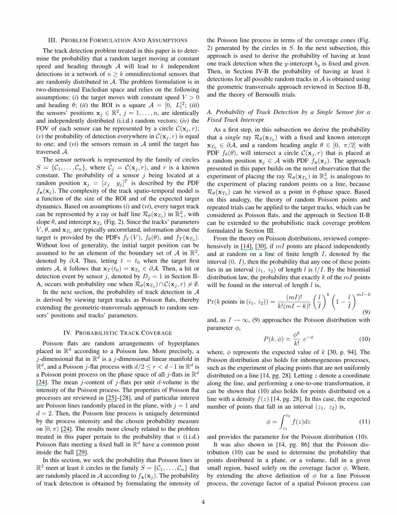
that the initial target position is on the ROI boundary. Thenew probability of track detection is obtained by performinga transformation from the initial position x′T0

∈ A, defined inSection II-A, to the initial position denoted by xT0 ∈ ∂A,and defined in Section IV. The unprimed notation is usedto distinguish between the different ranges of these variables.When xT0 is on the y-axis, as illustrated by the example inFig. 3, this change of variable amounts to performing thetransformation xT0 = [0 (x′0 − y′0 tan θ)]T , where θ andx′T0

= [x′0 y′0]T are sampled from the PDFs fθ(θ) and

fT (x′T0), respectively. Similar transformations can be obtained

for all xT0 ∈ ∂A. In every case, xT0 is independent of thespeed V . Thus, the joint PDF of xT0 and θ, denoted bygT (xT0 , θ), is a derived distribution that can be computed fromfθ(θ) and fT (x′T0

), using the aforementioned transformationsto express xT0 in terms of x′T0

. The standard procedure forderiving a distribution using the Jacobian of the transformationis described in [18, Section 1.7].

x

y

0Tx

0Tx′

r

θ

possible track

ΩT (θ, 0Tx′ , VΔt)

Ω’T (θ, 0Tx′ )

Fig. 3. Transformation from x′T0to xT0 .

In performing this transformation, the detection regionΩT (x′T0

, θ, V∆t), defined in Section II-A, is transformed intoa new detection region that is independent of V and ∆t, and isdenoted by Ω′T (xT0 , θ), as shown in Fig. 3. Where, Ω′T (xT0 , θ)is obtained by growing the entire track isotropically by r, fromthe target’s point of entry in A to its exit point. As a result, thecoverage factor in (3) is now integrated over the new detectionregion, and can be written as

φ′t(xT0 , θ) =∫

Ω′T (xT0 ,θ)

fx(xj)dxj (21)

After the coverage factor (21) and the derived distributiongT (xT0 , θ) are substituted in (4), the probability of trackdetection obtained by the distributed search approach can be

6

simplified to,

Pt = 1−∫ 2π

0

∫∂A

e−nφ′t(xT0 ,θ)gT (xT0 , θ)

×k−1∑m=0

[nφ′t(xT0 , θ)]m

m!dxT0dθ

∫ Vmax

Vmin

fV (V )dV

= 1−∫ 2π

0

∫∂A

e−nφ′t(xT0 ,θ)gT (xT0 , θ)

×k−1∑m=0

[nφ′t(xT0 , θ)]m

m!dxT0dθ (22)

because the integral of the PDF fV (V ) over its limits is alwaysequal to one.

Now, let φ′′t (xT0) denote the expected coverage factor as afunction of the intercept xT0 , which is obtained by applyingthe expected value rule [34, pg. 145] to the function (21), i.e.,

φ′′t (xT0) =∫ 2π

0

φ′t(xT0 , θ)fθ(θ)dθ

=∫ 2π

0

fθ(θ)∫

Ω′T (xT0 ,θ)

fx(xj)dxjdθ (23)

where, θ ∈ [0, 2π] when Rθ(xT0) ∈ R2+. Then, (22) can be

rewritten as,

Pt = 1−∫∂A

e−nφ′′t (xT0 ,θ)

k−1∑m=0

[nφ′′t (xT0 , θ)]m

m!(24)∫ 2π

0

gT (xT0 , θ)dθdxT0

= 1−∫∂A

fT (xT0) e−nφ′′t (xT0 ,θ)

k−1∑m=0

[nφ′′t (xT0 , θ)]m

m!dxT0

because the inner integral in (24) amounts to marginalizingthe joint PDF gT (xT0 , θ) over θ, which results in the marginaldistribution fT (xT0).

Comparing (24) to (20), it can be seen that the distributed-search and geometric-transversals approaches lead to thesame equation for the probability of track detection, providedthe coverage factors in (12) and (23) are equivalent, i.e.,φs(xT0) = φ′′t (xT0). Without loss of generality, we provethat this equality holds for the case of xT0 = 0. For allother initial positions xT0 ∈ ∂A, the same proof can beapplied by translating the xy-coordinate frame such that itsorigin coincides with xT0 . When xT0 = 0, the coveragefactors φs and φ′′t are two constants that can be evaluatedfrom the triple integrals (12) and (23), respectively. Since thesensors’ positions are independently and identically sampledfrom fx(xj), the coverage factor in (12), obtained by thegeometric transversals approach, can be written as

φs =∫A

∫ g2(xj)

g1(xj)

fx(xj)fθ(θ)dθdxj , for xT0 = 0. (25)

Since the target heading, θ, is independent of the sensors’positions, when xT0 = 0 the coverage factor in (23), obtainedby the distributed search approach, can be written as

φ′′t =∫ 2π

0

∫Ω′

T (θ)

fθ(θ)fx(xj)dxjdθ, for xT0 = 0. (26)

Since xj and θ are independent random variables, the in-tegrands of (25) and (26) each represent the joint PDF ofxj and θ, i.e., fx,θ(xj , θ) = fx(xj)fθ(θ). Then, φs andφ′′t each represent the probability mass of xj and θ in thethree-dimensional regions of integration of (25) and (26),respectively. Where, the probability mass of xj and θ in athree-dimensional region V ⊂ R3 is defined as the probabilitythat the point (xj , θ) is in V , given the density fx,θ(xj , θ) [30,pg. 172]. From (13) and (25), the region of integration of φsis the region spanned by the coverage cone K(Cj ,xT0 = 0)≡ K(Cj), for all xj ∈ A. Thus, the projection of this regionof integration onto A at a sample value of xj is the coveragecone K(Cj) illustrated in Fig. 4. From (21) and (26), the regionof integration of φ′′t is the region spanned by Ω′T (θ), for allθ ∈ [0, π/2]. Thus, the projection of this region of integrationonto A at a sample value of θ is the detection region Ω′T (θ)illustrated in Fig. 4. As an example, the region of integrationof φ′′t is plotted in Fig. 5, for L = 105 and r = 5.

x

y

xj

ψ(Cj)

r θ

γj

Cj

K(Cj)

Ω′T (θ)

r

A

Fig. 4. Detection region Ω′

T (θ) and coverage cone K(Cj) for xT0 = 0.

0

50

100

150

0

50

1000

0.5

1

1.5

2

θθ

yy xx

Fig. 5. Region of integration of φ′′t (xT0 ) in (26).

From the probability masses in (25) and (26), it can be seenthat the coverage factors (12) and (23) are equivalent providedthe region of integration in (25) is equivalent to that in (26).This last step of the proof is carried out by showing that thevolume of the region of integration in (25), defined as,

vs =∫A

∫ g2(xj)

g1(xj)

dθdxj (27)

7

is equivalent to the volume of the region of integration in (26),defined as:

vt =∫ 2π

0

∫Ω′

T (θ)

dxjdθ (28)

In order to avoid singularities, the above volumes are evaluatedby assuming that Cj ∈ A, i.e., letting r ≤ xj , yj ≤ L − r.Using the notation in Fig. 4, the limits in (27) can be expressedin polar coordinates, and (27) can be simplified as follows

vs =∫A

∫ γj+ψj/2

γj−ψj/2

dθdxj =∫A

2 arcsin(r

||xj ||)dxj (29)

Since the geometry of Ω′T (θ) changes with θ, (28) is evaluatedby dividing the range of θ into five intervals, such that,

θ ∈ [0, π/2] = [θ0, θ1] ∪ [θ1, θ2] ∪ [θ2, θ3] ∪ [θ3, θ4] ∪ [θ4, θ5](30)

where, θ0 = 0, θ5 = π/2, and

θ1 ≡ arcsinr√

(L− r)2 + r2+ arctan

r

(L− r)

θ2 ≡ π

4− arcsin

r√2(L− r)

θ3 ≡ arcsinr√

(L− r)2 + r2+π

4

θ4 ≡ arctan(L− r)

r− arcsin

r√r2 + (L− r)2

Then, the volume in (28) can be written as,

vt =4∑i=0

∫ θi+1

θi

∫Ω′

T (θ)

dxjdθ =4∑i=0

∫ θi+1

θi

fi+1(θ)dθ (31)

where

f1(θ) ≡ 12(L tan θ +

2rcos θ

− 2r)(L− 2r)

f2(θ) ≡ (L− 2r)2 − 12(L− r − r cos θ + r

sin θ)

× [(L− r) tan θ − r

cos θ− r] (32)

+ (L− 2r)[2(L− r)− L tan θ − 2rcos θ

]

f3(θ) ≡ (L− 2r)2 − 12[(L− r)− r cos θ + r

sin θ]

× [(L− r) tan θ − r

cos θ− r] (33)

+ [(L− r) cos θ − r

sin θ− r](L− r − r tan θ − r

cos θ)

f4(θ) ≡ (L− 2r)2 − 12(L− 2r)(

L cos θ + 2rsin θ

− 2r)

+ [(L− r) cos θ − r

sin θ− r](L− r − r tan θ − r

cos θ)

f5(θ) ≡ 12(L− 2r)(

L cos θ + 2rsin θ

− 2r)

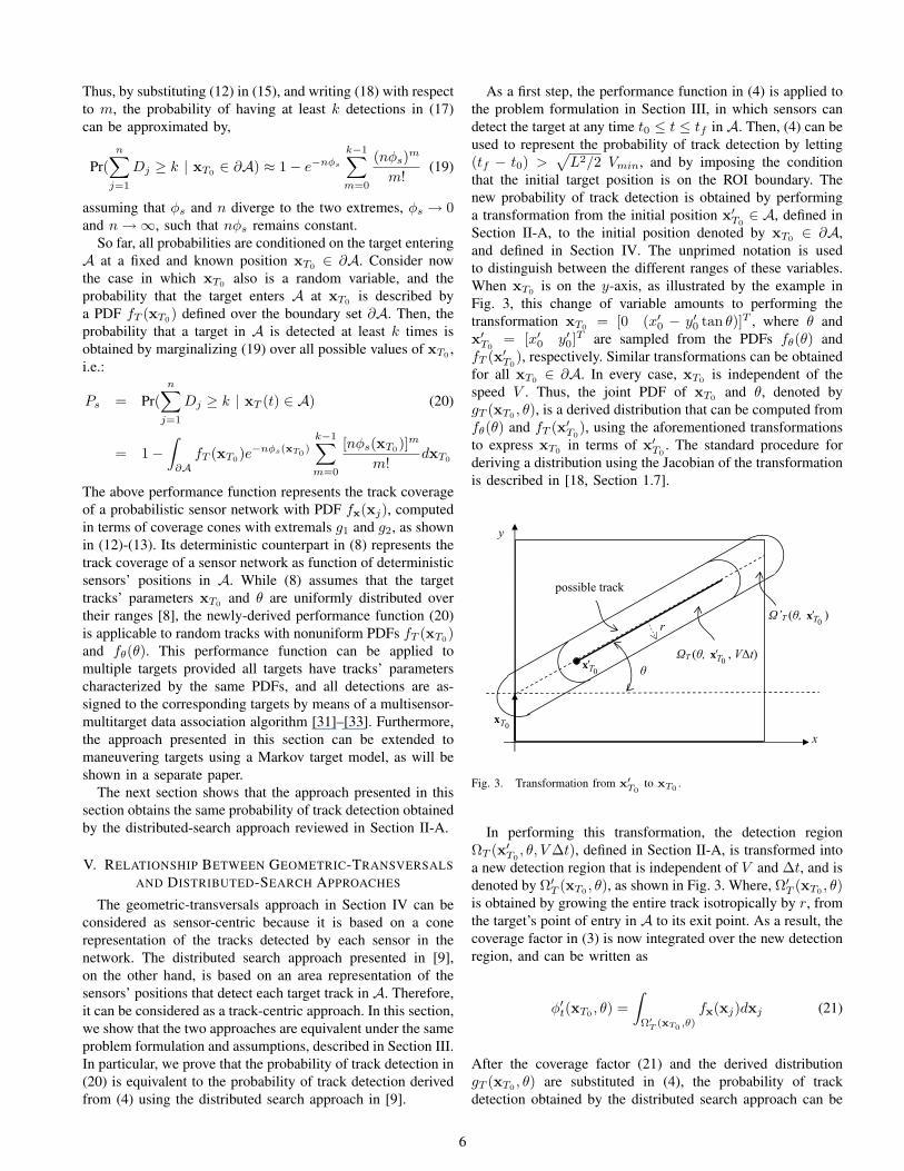
Finally, vt in (31) is integrated analytically and, althoughthe analytic solution is omitted for brevity, its value is plottedin Fig. 6(a) for a representative range of the parameters L andr. The volume vs in (29) is first integrated analytically withrespect to yj . Then, since an explicit solution for the outerintegral in xj could not be determined, vs is obtained using

the recursive adaptive Lobatto quadrature, which approximatesthe outer integral to within an error of O(10−6) [35]. Forcomparison, the value of vs is plotted in Fig. 6(b) usingthe same range of parameters used for vt. For all parametervalues considered in the simulations the difference betweenvs and vt is on the order of the Lobatto quadrature error.Thus, it can be concluded that the two volumes are equivalent,and that so are the coverage factors in (12) and (23). Itfollows that the probabilities of track detection obtained by thegeometric-transversals and distributed-search approaches, (20)and (24), are equivalent. However, the two approaches differin the manner by which they integrate the probability densityfunctions over the space of all possible target tracks andsensors’ positions. As illustrated by the corresponding regionsof integration, the distributed search approach considers thearea containing all sensors’ positions that detect a single track,and then integrates over all possible target tracks. Instead, thegeometric transversals approach considers the cone containingall target tracks that are detected by a single sensor position,and then integrates over all possible sensors’ positions in A.

02

46

810

5060

7080

90100

0

500

1000

1500

2000

2500

r

v t

υt

r X(L − r)

(a)

0

5

10

5060

7080

90100

0

500

1000

1500

2000

2500

r

v sυs

r X(L − r)

(b)

Fig. 6. The volume vt (a) is compared to vs (b) for a range of parametersL and r.

In the next section, the theoretical results are validatedthrough numerical simulations. These simulations confirm thatthe two approaches lead to the same probability of trackdetection and, thus, can be reliably utilized to optimize thedesign and deployment of cooperative sensor networks.

8

VI. NUMERICAL SIMULATIONS AND RESULTS

The theoretical results obtained in the previous sectionsare demonstrated through numerical simulations involvingprobabilistic and sampled networks, for different sensor pa-rameters and PDFs. In Section VI-A, the new performancefunction derived by the geometric transversals approach inSection IV is evaluated numerically, and is compared tothe performance function obtained by the distributed searchapproach in Section V. The numerical results show that thetwo performance functions and corresponding coverage factorsare always equivalent, but require different computation times.As shown in [8], the track coverage function in (8) can beused to deploy small to medium size networks effectively.However, when the sensor network is very large and is subjectto large errors and uncertainties, the PDF fx(xj) can beused to deploy sensor networks via sampling [36]. In thiscase, an optimal PDF can be obtained by optimizing theprobabilistic track coverage function in (20) with respectto a parameterized Gaussian mixture. In Section VI-B, thisapproach is demonstrated by considering several examples ofsensor deployments obtained by sampling the PDF fx(xj)using both finite mixture sampling [37, Section 1.4] and en-tropic sampling [36] techniques. Subsequently, the networks’probability of track detection is evaluated numerically usingthe geometric-transversals and distributed-search approaches.The numerical results show that when the two approaches areapplied to sensor networks sampled from various PDFs theystill lead to the same probability of track detection.

A. Probability of Track Detection by Probabilistic SensorNetworks

In this subsection, the proof in Section V is validated bydemonstrating that the probability of track detection Ps in (20)and the probability of track detection Pt in (24) are equivalentfor different forms of the PDF fx(xj). It is assumed that thetrack parameters are unknown and, thus, can be described byuniform PDFs fT (xT0) and fθ(θ) [38]. The ROI is a squareA = [0, 100]2, and all sensors have a constant detection ranger = 5. The PDF fx(xj) is set equal to zero outside the region[r, (L − r)]2 = [5, 95]2, to ensure that all circles in S arecontained in A. The number of sensors, n, is varied from 0 to150, and the number of required detections, k, is varied from0 to 10. The maximum number of sensors, 150, is chosensuch that a network could be contained in A with little or nooverlapping between FOVs. The support of the random vectorxj , given by [5, 95]2, and the support of xT0 , given by ∂A, arediscretized by the constant intervals ∆xj = ∆xT0 = [1 1]T .In this subsection, the PDF fx(xj) is modeled as a uniformdistribution over [5, 95]2, and as the mixed normal PDF

fx(xj) =1

600πe−

(xj−20)2

200 −(yj−20)2

200

+1

600πe−

(xj−60)2

200 −(yj−40)2

200 +1

600πe−

(xj−75)2

200 −(yj−75)2

200 (34)

For every form of fx(xj), the probability of track detectionPs in (20) is computed numerically by evaluating the coveragefactor in (12) for every discrete value of xT0 , denoted by x`T0

,

summing over all discrete values of xj , denoted by xıj , suchthat

φs(x`T0) ≈

∑xı

j∈Aψ(xıj ,x

`T0

)fx(xıj)∆xj (35)

Where, the opening angle ψ(·) is computed using (7). From(20), the probability of track detection is approximated by

Ps ≈ 1−∑

x`T0∈∂A

fT (x`T0)e−nφs(x`

T0)k−1∑m=0

[nφs(x`T0)]m

m!∆xT0

(36)For comparison, the probability of track detection in (24)also is computed numerically by discretizing the range of θ,given by [0, π/2], using the constant interval ∆θ = 0.01 rad.The coverage factor in (23) is evaluated by summing over alldiscrete values of θ, denoted by θ

φ′′t (x`T0

) ≈∑

θ∈[0, π/2]

Ω′T (x`T0, θ)fθ(θ)∆θ (37)

Where, Ω′T (·) is evaluated using f1 through f5 in (31), andfrom (24) the probability of track detection is approximatedby

Pt ≈ 1−∑

x`T0∈∂A

fT (x`T0) e−nφ

′′t (x`

T0)k−1∑m=0

[nφ′′t (x`T0

)]m

m!∆xT0

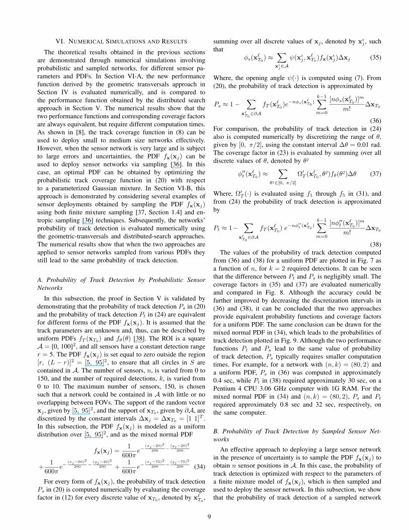
(38)The values of the probability of track detection computed

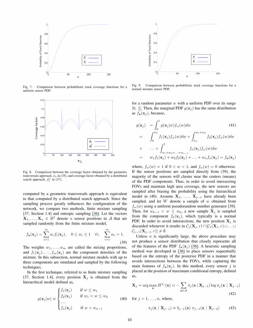
from (36) and (38) for a uniform PDF are plotted in Fig. 7 asa function of n, for k = 2 required detections. It can be seenthat the difference between Pt and Ps is negligibly small. Thecoverage factors in (35) and (37) are evaluated numericallyand compared in Fig. 8. Although the accuracy could befurther improved by decreasing the discretization intervals in(36) and (38), it can be concluded that the two approachesprovide equivalent probability functions and coverage factorsfor a uniform PDF. The same conclusion can be drawn for themixed normal PDF in (34), which leads to the probabilities oftrack detection plotted in Fig. 9. Although the two performancefunctions Pt and Ps lead to the same value of probabilityof track detection, Ps typically requires smaller computationtimes. For example, for a network with (n, k) = (80, 2) anda uniform PDF, Ps in (36) was computed in approximately0.4 sec, while Pt in (38) required approximately 30 sec, on aPentium 4 CPU 3.06 GHz computer with 1G RAM. For themixed normal PDF in (34) and (n, k) = (80, 2), Ps and Ptrequired approximately 0.8 sec and 32 sec, respectively, onthe same computer.

B. Probability of Track Detection by Sampled Sensor Net-works

An effective approach to deploying a large sensor networkin the presence of uncertainty is to sample the PDF fx(xj) toobtain n sensor positions in A. In this case, the probability oftrack detection is optimized with respect to the parameters ofa finite mixture model of fx(xj), which is then sampled andused to deploy the sensor network. In this subsection, we showthat the probability of track detection of a sampled network

9

0 50 100 1500

0.2

0.4

0.6

0.8

1

Prob

abili

ty o

f Tra

ck D

etec

tion

sP

tP

n

Fig. 7. Comparison between probabilistic track coverage functions for auniform sensor PDF.

0 50 100 150 200 250 300 350 4000

0.02

0.04

0.06

0.08

0.1

0.12

Cov

erag

e fa

ctor

s

sφ

tφ ′′

0Tx

Fig. 8. Comparison between the coverage factor obtained by the geometrictransversals approach, φs in (35), and coverage factor obtained by a distributedsearch approach, φ′′t in (37).

computed by a geometric transversals approach is equivalentto that computed by a distributed search approach. Since thesampling process greatly influences the configuration of thenetwork, we compare two methods, finite mixture sampling[37, Section 1.4] and entropic sampling [36]. Let the vectorsX1, . . . ,Xn ∈ R2 denote n sensor positions in A that aresampled randomly from the finite mixture model,

fx(xj) =m∑i=1

wifi(xj), 0 ≤ wi ≤ 1 ∀i,m∑i=1

wi = 1.

(39)The weights w1, . . . , wm are called the mixing proportions,and f1(xj), . . . , fm(xj) are the component densities of themixture. In this subsection, normal mixture models with up tothree components are simulated and sampled by the followingtechniques.

In the first technique, referred to as finite mixture sampling[37, Section 1.4], every position Xj is obtained from thehierarchical model defined as,

g(xj |w) ≡

f1(xj) if w ≤ w1

f2(xj) if w1 < w ≤ w2

. . .

fn(xj) if w > wn−1

(40)

0 50 100 1500

0.2

0.4

0.6

0.8

1

Prob

abili

ty o

f Tra

ck D

etec

tion

sP

tP

n

Fig. 9. Comparison between probabilistic track coverage functions for anormal mixture sensor PDF.

for a random parameter w with a uniform PDF over its range[0, 1]. Then, the marginal PDF g(xj) has the same distributionas fx(xj), because,

g(xj) =∫ 1

0

g(xj |w)fw(w)dw (41)

=∫ w1

0

f1(xj)fw(w)dw +∫ w1+w2

w1

f2(xj)fw(w)dw

+ . . .+∫ 1

w1+w2+...+wn−1

fn(xj)fw(w)dw

= w1f1(xj) + w2f2(xj) + . . .+ wnfn(xj) = fx(xj)

where, fw(w) = 1 if 0 < w < 1, and fw(w) = 0 otherwise.If the sensor positions are sampled directly from (39), themajority of the sensors will cluster near the centers (means)of the PDF components. Thus, in order to avoid intersectingFOVs and maintain high area coverage, the new sensors aresampled after biasing the probability using the hierarchicalmodel in (40). Assume X1, . . . , Xj−1 have already beensampled, and let W denote a sample of w obtained fromfw(w) using a uniform pseudorandom number generator [39].Then, for wk−1 < w ≤ wk, a new sample Xj is sampledfrom the component fk(xj), which typically is a normalPDF. In order to avoid intersections, the new position Xj isdiscarded whenever it results in Cj(Xj , r)∩ [C1(X1, r)∪ . . .∪Cj−1(Xj−1, r)] 6= ∅.

Unless n is significantly large, the above procedure maynot produce a sensor distribution that closely represents allof the features of the PDF fx(xj) [36]. A heuristic samplingmethod was developed in [36] to place sensors sequentiallybased on the entropy of the posterior PDF in a manner thatavoids intersections between the FOVs, while capturing themain features of fx(xj). In this method, every sensor j isplaced at the position of maximum conditional entropy, definedas,

Xj = arg maxx

Hπj (x) ≡ −∑x∈A

πj(x |Xj−1) log πj(x | Xj−1)

(42)for j = 1, . . . , n, where,

πj(x | Xj−1) ∝ bj−1(x) πj−1(x | Xj−2) (43)

10

is the posterior PDF updated after placing the (j−1)th sensor,and bj(x) is a binary operator that is equal to zero for allx ∈ Cj , and is equal to one elsewhere. As in Bayes recursion,at every iteration the posterior of a previous sensor placementbecomes the prior, and the new posterior is used to placean additional sensor, thereby decreasing the probability thatmultiple sensors are placed at the same location.

Since through entropic sampling the sensors’ positions arenot identically and independently sampled (Section III), theexact probability of track detection cannot be determined bythe performance metrics in (20) and (24). After the networkis sampled, however, its probability of track detection can beaccurately determined from the deterministic track coveragefunction T kA in (8), reviewed in Section II-B. Using geometrictransversals it was shown in [8] that the probability of trackdetection of a network deployed at X1, . . . , Xn is given by

PA =δb

π(L+ δb)T kA (44)

Thus, PA can be considered as the deterministic counterpart ofPs in (20). Since there currently is no deterministic counterpartfor Pt in (24), in this subsection PA is compared to the proba-bility obtained by direct evaluation of the detection events Dj ,denoted by Pk. A logical array or truth table, denoted by Bj ,is evaluated such that every element corresponds to a pair ofdiscretized track parameters (x`T0

, θ) (obtained as explainedin Section VI-A), and is set equal to 1 or 0, depending onwhether the track has been detected (1) or missed (0) by thejth sensor. After the array Bj is obtained for every sampledsensor, the logical array,

Tk =

n∑j=1

Bj ≥ k

(45)

indicates whether each possible track in A has been detectedby at least k sensors. Then, the number of ones in Tk dividedby its number of elements provides an estimate Pk for theprobability of track detection.

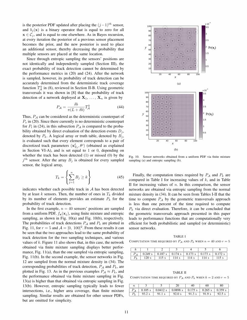
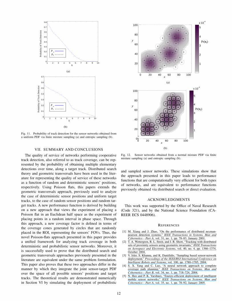
In the first example, n = 40 sensors’ positions are sampledfrom a uniform PDF, fx(xj), using finite mixture and entropicsampling, as shown in Fig. 10(a) and Fig. 10(b), respectively.The probabilities of track detections PA and Pk are plotted inFig. 11, for r = 5 and A = [0, 100]2. From these results it canbe seen that the two approaches lead to the same probability oftrack detection for the two sampling techniques, and variousvalues of k. Figure 11 also shows that, in this case, the networkobtained via finite mixture sampling displays better perfor-mance, Fig. 11(a), than the one sampled via entropic sampling,Fig. 11(b). In the second example, the sensor networks in Fig.12 are sampled from the normal mixture density in (34). Thecorresponding probabilities of track detection, PA and Pk, areplotted in Fig. 13. As in the previous examples PA ≈ Pk, andthe performance obtained via finite mixture sampling in Fig.13(a) is higher than that obtained via entropic sampling in Fig.13(b). However, entropic sampling typically leads to fewerintersections, i.e., higher area coverage, than finite mixturesampling. Similar results are obtained for other sensor PDFs,but are omitted for simplicity.

20 40 60 80 100

10

20

30

40

50

60

70

80

90

100

0.5

1

1.5

2

2.5

3

3.5x 10

-4

y Pr(xj)

x

(a)

20 40 60 80 100

10

20

30

40

50

60

70

80

90

100

0.5

1

1.5

2

2.5

3

3.5x 10

-4

y Pr(xj)

x

(b)

Fig. 10. Sensor networks obtained from a uniform PDF via finite mixturesampling (a) and entropic sampling (b).

Finally, the computation times required by PA and Pk arecompared in Table I for increasing values of k, and in TableII for increasing values of n. In this comparison, the sensornetworks are obtained via entropic sampling from the normalmixture density in (34). It can be seen from Tables I-II that thetime to compute PA by the geometric transversals approachis less than one percent of the time required to computePk via direct evaluation. Therefore, it can be concluded thatthe geometric transversals approach presented in this paperleads to performance functions that are computationally veryefficient for both probabilistic and sampled (or deterministic)sensor networks.

TABLE ICOMPUTATION TIME REQUIRED BY PA AND Pk WHEN n = 40 AND r = 5

k 1 2 3 4 5 6PA 0.249 s 0.187 s 0.174 s 0.173 s 0.173 s 0.172 sPk 120 s 115 s 114 s 114 s 114 s 115 s

TABLE IICOMPUTATION TIME REQUIRED BY PA AND Pk WHEN k = 2 AND r = 5

n 3 5 20 40 60 80PA 0.105 s 0.0412 s 0.0898 s 0.175 s 0.265 s 0.359 sPk 93.2 s 91.1 s 92.0 s 91.3 s 91.9 s 92.5 s

11

1 2 3 4 5 6 7 8 9 100

0.1

0.2

0.3

0.4

0.5

0.6

0.7

0.8

Prob

abili

ty o

f Tra

ck D

etec

tion

Pk

PA

k

(a)

1 2 3 4 5 6 7 8 9 100

0.1

0.2

0.3

0.4

0.5

0.6

0.7

Prob

abili

ty o

f Tra

ck D

etec

tion

Pk

PA

k

(b)

Fig. 11. Probability of track detection for the sensor networks obtained froma uniform PDF via finite mixture sampling (a) and entropic sampling (b).

VII. SUMMARY AND CONCLUSIONS

The quality of service of networks performing cooperativetrack detection, also referred to as track coverage, can be rep-resented by the probability of obtaining multiple elementarydetections over time, along a target track. Distributed searchtheory and geometric transversals have been used in the liter-ature for representing the quality of service of these networksas a function of random and deterministic sensors’ positions,respectively. Using Poisson flats, this papers extends thegeometric transversals approach, previously used to analyzethe case of deterministic sensor positions and uniform targettracks, to the case of random sensor positions and random tar-get tracks. A new performance function is derived by buildingon a new approach that views the experiment of placing aPoisson flat in an Euclidean half space as the experiment ofplacing points in a random interval in phase space. Throughthis approach, a new coverage factor is defined in terms ofthe coverage cones generated by circles that are randomlyplaced in the ROI, representing the sensors’ FOVs. Thus, thenovel Poisson-flats approach presented in this paper providesa unified framework for analyzing track coverage in bothdeterministic and probabilistic sensor networks. Moreover, itis successfully used to prove that the distributed search andgeometric transversals approaches previously presented in theliterature are equivalent under the same problem formulation.This paper also proves that these two approaches differ in themanner by which they integrate the joint sensor-target PDFover the space of all possible sensors’ positions and targettracks. The theoretical results are demonstrated numericallyin Section VI by simulating the deployment of probabilistic

0 20 40 60 80 100

20

40

60

80

100

1

2

3

4

5

x 10-4

y Pr(xj)

x

(a)

0 20 40 60 80 1000

20

40

60

80

100

1

2

3

4

5

x 10-4

y Pr(xj)

x

(b)

Fig. 12. Sensor networks obtained from a normal mixture PDF via finitemixture sampling (a) and entropic sampling (b).

and sampled sensor networks. These simulations show thatthe approach presented in this paper leads to performancefunctions that are computationally very efficient for both typesof networks, and are equivalent to performance functionspreviously obtained via distributed search or direct evaluation.

ACKNOWLEDGMENTS

This work was supported by the Office of Naval Research(Code 321), and by the National Science Foundation (CA-REER ECS 0448906).

REFERENCES

[1] M. Xiang and J. Zhao, “On the performance of distributed neyman-pearson detection systems,” IEEE Transactions in Systems, Man andCybernetics - Part A, vol. 31, no. 1, pp. 78–83, January 2001.

[2] T. A. Wettergren, R. L. Streit, and J. R. Short, “Tracking with distributedsets of proximity sensors using geometric invariants,” IEEE Transactionson Aerospace and Electronic Systems, vol. 40, no. 4, pp. 1366–1374,October 2004.

[3] V. Isler, S. Khanna, and K. Daniilidis, “Sampling based sensor-networkdeployment,” Proceedings of the IEEE/RSJ International Conference onIntelligent Robots and Systems, vol. 100, pp. 1780–1785, 2004.

[4] S. X. Yang and C. Luo, “A neural network approach to completecoverage path planning,” IEEE Transactions on Systems, Man andCybernetics - Part B, vol. 34, no. 1, pp. 718–724, 2004.

[5] N. Heo and P. K. Varshney, “Energy-efficient deployment of intelligentmobile sensor networks,” IEEE Transactions on Systems, Man andCybernetics - Part A, vol. 35, no. 1, pp. 78–92, January 2005.

12

1 2 3 4 5 6 7 8 9 100

0.1

0.2

0.3

0.4

0.5

0.6

0.7

Pk

PA

Prob

abili

ty o

f Tra

ck D

etec

tion

k

(a)

1 2 3 4 5 6 7 8 9 100

0.1

0.2

0.3

0.4

0.5

0.6

0.7

Pk

PA

Prob

abili

ty o

f Tra

ck D

etec

tion

k

(b)

Fig. 13. Probability of track detection for the sensor networks obtained froma normal mixture PDF via finite mixture sampling (a) and entropic sampling(b).

[6] V. Giordano, P. Ballal, F. Lewis, B. Turchiano, and J. Zhang, “Supervi-sory control of mobile sensor networks: math formulation, simulation,and implementation,” IEEE Transactions on Systems, Man and Cyber-netics - Part B, vol. 36, no. 4, pp. 806–819, 2006.

[7] S. Ferrari, “Track coverage in sensor networks,” Proceedings of theAmerican Control Conference, pp. 1–10, 2006.

[8] K. C. Baumgartner and S. Ferrari, “A geometric transversal approachto analyzing track coverage in sensor networks,” IEEE Transactions onComputers, vol. 57, no. 8, pp. 1113–1128, 2008.

[9] T. A. Wettergren, “Performance of search via track-before-detect fordistributed sensor networks,” IEEE Transactions on Aerospace andElectronic Systems, vol. 44, no. 1, pp. 314–325, January 2008.

[10] M. Ranasingha, M. Murthi, K. Premaratne, and X. Fan, “Transmissionrate allocation in multisensor target tracking over a shared network,”IEEE Transactions on Systems, Man and Cybernetics - Part B, vol. 39,no. 2, pp. 348–362, 2009.

[11] H. Cox, “Cumulative detection probabilities for a randomly movingsource in a sparse field of sensors,” in Proc. Asilomar Conference, 1989,pp. 384–389.

[12] J.-P. LeCadre and G. Souris, “Searching tracks,” IEEE Transactions onAerospace and Electronic Systems, vol. 36, no. 4, pp. 1149–1166, 2000.

[13] B. Koopman, Search and Screening: General Principles with HistoricalApplicaitons. Pergamon Press, 1980.

[14] P. Morse and G. Kimball, Methods of Operations Research. DoverPublications, 2003.

[15] L. Stone, Theory of Optimal Search. Academic Press, 1975.[16] D. Castanon, “Optimal search strategies in dynamic hypothesis testing,”

IEEE Transactions on Systems, Man and Cybernetics, vol. 25, no. 7, pp.1130–1138, 1995.

[17] G. V. Keuk, “Sequential track extraction,” IEEE Transactions onAerospace and Electronic Systems, vol. 34, no. 4, pp. 1135–1148, 1998.

[18] R. V. Hogg, J. W. McKean, and A. T. Craig, Introduction to Mathemat-ical Statistics. Upper Saddle River, NJ: Prentice Hall, 2005.

[19] Z. Kone, E. G. Rowe, and T. A. Wettergren, “Sensor repositioning toimprove undersea sensor field coverage,” in Proceedings of OCEANS2007, September 2007, pp. 1–6.

[20] E. Helly, “uber mengen konvexer korper mit gemeinschaftlichen punk-

ten,” Jahresbericht der Deutschen MathematikerVereiningung, vol. 32,pp. 175–176, 1923.

[21] J. Goodman, R. Pollack, and R. Wenger, “Geometric transversal theory,”in New Trends in Discrete and Computational Geometry, J. Pach, Ed.Springer Verlag, 1991, pp. 163–198.

[22] D. P. Bertsekas, Convex Analysis and Optimization. Belmont, MA:Athena Scientific, 2003.

[23] S. Skiena, “Generating k-subsets,” in Implementing Discrete Mathemat-ics: Combinatorics and Graph Theory with Mathematica. Reading,MA: Addison-Wesley, 1990, pp. 44–46.

[24] J. Mecke, “Extremal properties of some geometric processes,” ActaApplicandae Mathematicae, vol. 9, pp. 61–69, 1987.

[25] G. Matheron, Random Sets and Integral Geometry. New York, NY:Wiley, 1975.

[26] R. E. Miles, “A synopsis of poisson flats in eucledian spaces,” inStochastic Geometry, E. Harding and D. Kendall, Eds. New York,NY: Wiley, 1974.

[27] Santalo, Integral Geometry and Geometric Probability. London, UK:Addison-Wesley, 1976.

[28] D. Stoyan, W. Kendall, and J. Mecke, Stochastic Geometry. New York,NY: Wiley, 1987.

[29] J. Mecke, “Random r-flats meeting a ball,” Archiv der Mathematik,vol. 51, no. 4, pp. 378–384, 1988.

[30] A. Papoulis and S. U. Pillai, Probability, Random Variables, andStochastic Processes. New York, NY: McGraw-Hill, 2002.

[31] A. Poore and N. Rijavec, “A numerical study of some data associationproblems arising in multitarget tracking,” Computational Optimizationand Applications, vol. 3, no. 1, pp. 27–57, 1994.

[32] R. Popoli, “The sensor management imperative,” in Multitarget-Multisensor Tracking: Advanced Applications, Vol. II, Bar-Shalom, Ed.Artech House, 1992.

[33] S. Deb, K. R. Pattipati, and Y. Bar-Shalom, “A multisensor-multitargetdata association algorithm forheterogeneous sensors,” IEEE Transactionson Aerospace and Electronic Systems, vol. 29, no. 2, pp. 560–568, 1993.

[34] D. P. Bertsekas and J. N. Tsitsiklis, Introduction to Probability. Bel-mont, MA: Athena Scientific, 2002.

[35] Mathworks, Matlab. [Online]. Avaliable: http://www.mathworks.com,2004, function: quadl.

[36] R. Costa and T. A. Wettergren, “Assessing design tradeoffs in deployingundersea distributed sensor networks,” in Proceedings of OCEANS 2007,Vancouver, BC, September 2007, pp. 1–5.

[37] G. McLachlan, Finite Mixture Models. New York, NY: Wiley Inter-science, 2000.

[38] H. L. V. Trees, Optimum Array Processing (Detection, Estimation, andModulation Theory, Part IV), 1st ed. Wiley-Interscience, 2002.

[39] Mathworks, Matlab. [Online]. Avaliable: http://www.mathworks.com,2004, functions: rand,mvnrnd.

13