BOĞAZİÇİ ÜNİVERSİTESİ

ISS/EC-2001-05

Private Provision of a Public Good in a

General Equilibrium Model

Antonio Villanacci

Unal Zenginobuz

ARAŞTIRMA RAPORU

RESEARCH PAPERS

Boğaziçi University Department of Economics Research Papers are of preliminary nature, circulated to promote scientific discussion. They are not to be quoted without written permission of the

author(s).

Private Provision of a Public Good in aGeneral Equilibrium Model¤

Antonio Villanacciy and Ünal Zenginobuzz

April 27th, 2001

Abstract

We analyze a general equilibrium model of a completely decen-tralized pure public good economy. Competitive …rms using privategoods as inputs produce the public good, which is privately providedby households. Previous studies on private provision of public goodstypically use one private good, one public good models in which thepublic good is produced through a constant returns to scale technol-ogy. Two distinguishing features of our model are the presence ofseveral private goods and non-linear, in fact strictly concave, produc-tion technology for the public good.

In this more general framework we revisit the question of ”neu-trality” - or non-e¤ectiveness - of government interventions on privateprovision equilibrium outcomes. We con…rm the well-known neutral-ity results when all households are contributing to the provision ofthe public goods and the non-neutrality results when there are somenon-contributing households. We also show that relative price e¤ects,which are absent with a single private good and under constant re-turns to scale technology for public good production, come to play animportant role and generate new non-neutrality results. Speci…cally,

¤We would like to thank Svetlana Boyarchenko, David Cass, Julio Davila, GeorgeMailath, Steve Matthews, Nicola Persico, and Andrew Postlewaite for helpful discussionsand comments.

yCorresponding author. Department of Mathematics for Decision Theory (Di.Ma.D),University of Florence, via Lombroso 6/17, 50134 Firenze, Italy; e-mail: villanac@uni….it.

zDepartment of Economics,Bo¼gaziçi University, 80815 Bebek, Istanbul, Turkey; e-mail:zenginob@boun.edu.tr.

1

if the number of private goods is greater than one, typically there ex-ists a redistribution of endowments of the private good among non-contributors which increases the total supply of public good. Moreimportantly, if a condition involving the number of households andprivate goods holds, typically there exists a choice of taxes on …rmsthat Pareto improves upon the equilibrium outcome. Therefore, ageneral non-neutrality result (in terms of utilities) holds even if allhouseholds are contributors.

2

1 IntroductionIn this paper, we analyze a general equilibrium model of a completely decen-tralized pure public good economy. Competitive …rms using private goods asinputs produce the public good, which is ”…nanced”, or ”privately provided”,or ”voluntarily contributed”, by households. Previous studies on private pro-vision of public goods typically use one private good, one public good modelsin which the public good is produced through a constant returns to scale tech-nology. Two distinguishing features of our model are the presence of severalprivate goods and non-linear, in fact strictly concave, production technologyfor the public good. In this more general framework we revisit the questionof ”neutrality” of government interventions on private provision equilibriumoutcomes. We show that relative price e¤ects, which are absent with a singleprivate good and under constant returns to scale technology for public goodproduction, come to play an important role in our more general framework.Relative price e¤ects provide a powerful channel through which governmentinterventions can bring about redistributive wealth e¤ects, which, in turn,will change equilibrium outcomes.

The interest in a general equilibrium model with private provision ofpublic goods lies in the fact that it serves as a benchmark extension of ananalysis of completely decentralized private good economies to public goodeconomies. Moreover, there are some relevant situations in which publicgoods are in fact privately provided: e.g., private donations to charity ata national and international level, campaign funds for political parties orspecial interests groups, and certain economic activities inside a family.

Warr (1983) provides the …rst statement of the fact that in a privateprovision model of voluntary public good supply, small income redistributionsamong contributors to a public good are ”neutralized” by changes in amountscontributed in equilibrium. Consumption of the private good and the totalsupply of the public good remain exactly the same as before redistribution.Warr (1982) also observes that small government contributions to a publicgood, paid for by lump sum taxes on contributors, will be o¤set completelyby reductions in private contributions. Warr’s results are derived in a partialequilibrium framework. Bernheim (1986) and Andreoni (1988) extend Warr’sresult to show that distortionary taxes and subsidies may also be neutralizedby changes in private contributions.

Bergstrom, Blume and Varian (1986) - from now on quoted as BBV -discuss Warr’s results in a simple general equilibrium model with one private

3

and one public good and constant returns to scale in the production of thepublic good. They allow non-in…nitesimal redistributions and possibility ofzero contribution by some of the households.1 They show that redistributionis not, in general, neutral if the amount of income distributed away from anyhousehold is more than his private contribution to the public good in theoriginal equilibrium. Andreoni and Bergstrom (1996) argue that the neutral-ity results obtained in previous models all involve redistribution schemes inwhich only ”small” changes in incomes, namely changes that do not exceedanyone’s original equilibrium private contribution, are allowed. We show inthis paper that it is not the ”smallness” of redistributions allowed but theabsence of relative price e¤ects, through which further income e¤ects arise,that leads to the neutrality results.2

With only one private good, assuming constant returns to scale, andtherefore linearity of the production function, implies that there is no lossof generality in normalizing prices of both the private and the public goodto one. These assumptions also allow taking pro…ts of …rms equal to zero,with the implication that the presence of …rms basically plays no role inthe model. With non-constant returns to scale in production allowed, suchnormalization of prices is not possible in our framework, even in the caseof only one private good. For that reason, taxes and subsidies will havedi¤erent e¤ects in our framework than that of BBV’s. In BBV’s model,taxes on a subset of individuals change the distribution of wealth amongthose individuals, but not among individuals outside that subset. In ourmodel, taxing any subset of households leads to changes in relative prices andtherefore may a¤ect the wealth of any household. This simple observationexplains why some of our results will be di¤erent from those of BBV. Relativeprice e¤ects, which are absent in BBV’s setup, play a redistributive role inour framework.

With more than one private good and non-constant returns to scale, mod-eling of how the public good is produced becomes an issue. If a pro…t-maximizing (private) …rm is assumed to produce the public good, then howthe (non-zero) pro…ts of the …rm are apportioned among its shareholders willhave an impact on equilibrium outcomes. Alternatively, one can consider theproduction of the public good as being carried out by a non-pro…t (public)

1See also the related papers Bergstrom, Blume and Varian (1992) and Fraser (1992).2In a more recent contribution on the e¤ects of taxation in an economy with private

provision of public goods, Brunner and Falkinger (1999) consider a model with two privategoods and public good, but the prices of the goods are taken as given in their model.

4

…rm subject to a balanced budget constraint. In that case the contributionsin monetary amounts collected from households would …nance the cost of pro-ducing the public good. The amount of public good to be produced by thenon-pro…t …rm can be taken as the maximum amount that can be producedwith the amount collected. Such a model assumes the presence of either thegovernment itself or a non-pro…t …rm in the production of the public good,which raises a host of issues related to what the objective functions of suchentities should be.3

In the present paper, we study the alternative that we believe is theone most consistent with a decentralized framework, namely that pro…t-maximizing …rms produce the public good in a competitive market.4 Thus,the government is not involved in the production of the public good andonly has the role of enforcing taxes and subsidies, if there are any, on house-holds and …rms. In analyzing crowding-out e¤ects of government provisionof public goods, it will be assumed that government makes purchases fromthe …rms at market prices. We take this set of assumptions as describinga completely free market oriented policy benchmark applicable in principleto provision of any type of public good. The model can also be seen as adescriptive one covering cases in which a public institution purchases fromprivate producers goods that will be consumed by households involved aspublic goods. Examples include ‡uoride purchased by a public agency to ‡u-oridate a public water supply, pesticides purchased by government, packagesof medicine bought by an international charitable organization for use in anunderdeveloped country to control an epidemic disease, and so on.

As for the behavior of households, each household starts with endow-ments in private good only. Households also hold shares in the …rms thatproduce the public good. There is no public good initially. Taking as giventhe prices of private goods, the price of the public good, the pro…ts of the…rms they hold shares in, as well as the amount of public good provided byothers, each household determines their private good consumption bundleand the amount of public good they will privately provide. Private provisioncan take the form of each household actually purchasing the good in theamount they desire directly from a producer, or donating to a public or avoluntary organization a monetary amount with which the same amount can

3We analyze such a model in a forthcoming paper.4The presence of more than one public good can be incorporated into our model, leaving

the basic results unchanged - see Section 6.1.

5

be purchased by this agency at the equilibrium price for the public good.Note that in making their decisions on how much to contribute to the publicgood, the households will take into consideration relative prices. If the pricesof medicines, doctor services, lab tests doubles, an household may choose tocontribute more to fund raising for an hospital. When there are taxes orsubsidies imposed by the government, households take these as given in theirbudget constraints. We assume that households fully understand and takeinto account the government’s budget constraint.

Observe that household behavior described above amounts to assumingthat the prices of private goods as well as the public good are taken as givenby households in their maximization problem, while there is strategic inter-action among them regarding the quantities chosen as private contribution tothe public good. This type of behavior is plausible when the set of prospec-tive consumers of the public good are ’small’ with respect to the economy inwhich they are embedded. Thus the households’ choices of the public gooda¤ects neither the prices of inputs that goes into production of the publicgood nor the price of the public good produced for the economy at large,while it does have an impact on others’ choices locally involved in the con-sumption of the good. For example, consider donations to a large agencythat is involved in projects to eradicate poverty in Africa. Eradication ofpoverty in Africa is the public good for those who care about it in this case,and their cash or in kind contributions to the agency are not going to a¤ectthe prices of goods that go into the activities of the agency.5

Since the modeling of production technology for the public good is a keyfeature that distinguishes our model from that of BBV’s, we further discussit below.

With many inputs linearity of a production function implies constantreturns to scale, but the converse will not hold (except for the single inputcase). Therefore, BBV’s results extend to the case of many inputs only if theproduction function is linear.

When the production function is linear, and …rms produce a strictly pos-itive quantity of output, prices are completely determined by the productioncoe¢cients. Therefore, equilibrium prices are ”…xed by the technology”, i.e.,they change only if technology changes, and they are not a¤ected by changes

5The above discussion points out that goods may be (locally) public or private accordingto their use and not on the basis of their physical characteristics. Analysis of such a ’local’public good model that explicitly takes into account the possibility that goods can beprivate or public according to their use is going to be the subject of another paper.

6

in endowments or preferences. Outside the case of linear production func-tion, equilibrium prices are only partially …xed by the technology if returnsto scale are constant, or they are not …xed at all by the technology if theproduction function is strictly concave.6 Since price e¤ects are the crucialfactor in our analysis, we conjecture that our results apply to all situations inwhich prices are not …xed by the technology. That is, not only does it apply,to the case of strictly concave technology, as we show here, but it should alsoapply to the case of concave production functions with and without constantreturns to scale.7 Therefore, we can claim that, within the space of convexproduction technologies, our framework covers all but the rather extremelinear case.

Below are some of the results for the one good, linear technology casethat are relevant to our analysis. All of the results except the last one, whichis due to Cornes and Sandler (2000), are due to BBV. In all results, thedistinction between contributors, i.e. the households that provide a strictlypositive amount of public good, and non-contributors plays a crucial role.The tax schemes referred to involve small perturbations of the initial endow-ment distribution; hence named local tax schemes:

1. An equilibrium exists (BBV, Theorem 2, page 33) and is unique undera demand normality condition for the public good.

All the following results refer to an equilibrium situation.2.a. Any local tax scheme applied to contributors only has no e¤ect on

the total supply of the public good (BBV, Theorem 1, page 29).2.b. Any local tax scheme that redistributes wealth from non-contributors

to contributors increases the total supply of the public good (BBV, Theorem4.ii, page 36).

3. Suppose that the government supplies some amount of the public good,which it pays for through a local tax scheme among households. Then,

3a. If local positive taxes are imposed on contributors, the total supply ofpublic good does not change: there is complete crowding-out (BBV, Theorem6.i, page 42).

3b. If local positive taxes are imposed on non-contributors, then the totalsupply of public good increases (BBV, Theorem 6.ii, page 42).

6See, for example, the discussion on properties of equilibria with constant returns toscale in production by Mas-Colell et al. (1995), Section 17.F, pages 606-616.

7The investigation of this conjecture is in fact the content of a forthcoming paper ofours.

7

4. Cornes and Sandler (2000) investigate the possibility for a governmentto increase all households’ welfare via an increase in the total supply of thepublic good. They observe that the possibility of such Pareto improvementsis positively related to the number of non-contributors, marginal evaluationof the public good by noncontributors, and the change in the private provisionof public good resulting from an increase in contributors’ total wealth.

Our approach is based on di¤erential techniques, which amount to com-puting the derivative of the ”goal function” - the total amount of providedpublic good or household welfare levels - with respect to some policy tools -taxes and/or government’s direct provision of the public good - on the equilib-rium manifold. Therefore, all our arguments are ”local” in their nature. Wealso note that, since price e¤ects may in principle go in any direction, all ournon-neutrality results hold only typically in the relevant space of economies.First we observe that

1*. An equilibrium exists.Existence of equilibrium, together with some regularity properties of equi-

libria that we use in the present paper, are proved in another paper by Vil-lanacci and Zenginobuz (2001). Note that while BBV present their analysisin the case of unique equilibria, we allow for multiple equilibria.

The results of the present paper can be summarized as follows:2a*. A neutrality result of the type described in 2a. holds and, in fact,

it can be slightly generalized.2b*. Local redistribution of wealth from non-contributors to contributors

has the same e¤ect as in the linear case.2c*. If the number of private goods is greater than one, typically in

the subset of economies for which there exist at least two non-contributors,there exists a redistribution of endowments of the private good among non-contributors which increases the total supply of public good.

3*. Results about crowding-out hold also in our case; more precisely, inour framework, results 3a. of BBV holds typically.

4*. If the number of households is smaller than the number of privategoods, typically in the set of economies, there exists a choice of taxes on …rms’inputs and outputs that Pareto improves or impairs upon the equilibriumoutcome. Therefore, a general non neutrality result (in terms of utlities)holds even if all households are contributors.

In relation to our result 4*, observe that other types of Pareto improvinginterventions could be studied applying the same general technique used inthe paper.

8

An interesting feature of the model analyzed in the paper is that it allowsan (partial) answer to a more general problem. Several ”imperfections” canbe considered in a standard general equilibrium model. Is government inter-vention more or less e¤ective when more than one imperfection is present?Does including one more imperfection in the presence of an initial one makegovernment intervention more or less e¤ective? Results 2a and 3a in BBVapply to general equilibrium models with incomplete markets or restrictedparticipation besides public goods. Government intervention would have noe¤ect in those cases if the economy also involves public goods that are pri-vately provided. It is well known that, under certain assumptions a wellchosen local redistribution among all households in a model with incom-plete markets leads to a Pareto superior equilibrium (see Geanakoplos andPolemarchakis (1986) and Citanna et al. (1998)). The above observationssuggest that a government intervention that would be e¤ective against a sin-gle imperfection may turn out to be ine¤ective when the existence of otherimperfections is taken into account. On the other hand, the analysis ofPareto improvement possibilities described above strongly supports the fol-lowing result: In the case of the presence of two imperfections, there existsa well-chosen intervention which can reach the same goals as in the case ofone imperfection.

The plan of our paper is as follows. In section 2, we present the set up ofthe model and the existence and regularity results proved in Villanacci andZenginobuz (2001).

In sections 3, 4 and 5, following a strategy described, for example, inCitanna, Kajii and Villanacci (1998), we prove our main results on the pos-sibility of a government intervention to in‡uence the total amount of publicgood and household welfare.8

2 Setup of the Model

We consider a general equilibrium exchange model with private provision ofa public good.

There are C, C ¸ 1, private commodities, labelled by c = 1; 2; :::; C.There are H households, H > 1, labelled by h = 1; 2; :::; H. Let H =f1; :::; Hg denote the set of households. Let xch denote consumption of private

8A more detailed version of the paper, containing even elementary proofs is availablefrom the authors.

9

commodity c by household h; ech embodies similar notation for the endowmentin private goods.

The following standard notation is also used:

² xh ´ (xch)Cc=1, x ´ (xh)

Hh=1 2 RCH

++ .

² eh ´ (ech)Cc=1, e ´ (eh)

Hh=1 2 RCH

++ .

² pc is the price of private good c, with p ´ (pc)Cc=1; and pg is the priceof the public good. Let bp ´ (p; pg) :

² gh 2 R+ is the amount of public good that consumer h provides: Letg ´ (gh)

Hh=1, G ´ PH

h=1 gh, and Gnh ´ G¡ gh:

Household h’s preferences over the private goods and the public good arerepresented by a utility function uh : RC

++£R1++ ! R. Note that households’

preferences are de…ned over the total amount of the public good, i.e. we haveuh : (xh; G) 7! uh (xh; G).

Assumption 1 uh(xh; G) is a smooth, di¤erentiably strictly increasing (i.e.,for every (xh; G) 2 RC+1++ , Duh(xh; G) À 0)9; di¤erentiably strictly con-cave function (i.e., for every (xh; G) 2 RC+1++ , D2uh(xh; G) is negativede…nite), and the closure (in the topology of RC+1) of the indi¤erencesurfaces is contained in RC+1++ .

There are F …rms, indexed by subscript f; that use a production tech-nology represented here by a transformation function tf : RC+1 ! R, wheretf :

¡yf ; y

gf

¢7! tf

¡yf ; y

gf

¢.

Assumption 2 tf¡yf ; y

gf

¢is a C2, di¤erentiably strictly decreasing (i.e.,

Df¡yf ; y

gf

¢¿ 0), and di¤erentiably strictly concave (i.e., D2f

¡yf ; y

gf

¢

is negative de…nite) function, with f (0) = 0.

De…ne byf ´¡yf ; y

gf

¢and by ´ (byf )Ff=1. Using the convention that input

components of the vector¡yf ; y

gf

¢are negative and output components are

9For vectors y; z, y ¸ z (resp. y À z) means every element of y is not smaller (resp.strictly larger) than the correponding element of z; y > z means that y ¸ z but y 6= z.

10

positive, the pro…t maximization problem for …rm f is: For given p 2 RC++,

pg 2 R++;Max

(yf ;yg)2RC+1pyf + p

gygf

s.t. tf¡yf ; y

gf

¢¸ 0 (®f)

; (1)

where the term in parenthesis next to the constraint is the associated Kuhn-Tucker multiplier.10

Remark 1 From Assumption 2, it follows that if the above problem (1) hasa solution, it is a unique one characterized by the Kuhn-Tucker (in fact,Lagrange) conditions.

Let sh be the share of the …rm pro…ts owned by household h, and de…ne

s ´ (sh)Hh=1 2 SH¡1 ´

(s0 ´ (s0h)

Hh=1 2 RH

+ :HX

h=1

s0h = 1

);

the (H ¡ 1) dimensional simplex.Household’s maximization problem is then the following: For given p 2

RC++; p

g 2 R++; sh 2 [0; 1] ; eh 2 RC++; Gnh 2 R+; (by) 2 RC+1;

Max(xh;gh)2RC+1++

uh¡xh; gh +Gnh

¢

s.t. ¡p (xh ¡ eh)¡ pggh + bpPFf=1 byf ¸ 0 (¸h)

gh ¸ 0 (¹h)

(2)

Remark 2 From Assumption 1, it follows that the above problem (2) has aunique solution characterized by Kuhn-Tucker conditions.

Remark 3 By de…nition of uh, observe that we must haveP

h gh > 0 and,therefore,

1. since gh ¸ 0 for all h, there exists h0 such that gh0 > 0; and2.

PFf=1 y

gf > 0.

10We will follow this convention of writing the Kuhn-Tucker multipliers next to theassociated constraints throughout the paper.

11

Market clearing conditions are:

¡PHh=1 xh +

PHh=1 eh +

PFf=1 yf = 0

¡PHh=1 gh +

PFf=1 y

gf = 0:

The set of all utility functions of household h that satisfy Assumption1 is denoted by Uh; the set of all transformation functions of …rm f thatsatisfy Assumption 2 is denoted by Tf . Moreover de…ne U 0 ´ £H

h=1Uh andT ´ £F

f=1Tf .

Assumption 3 U 0 and T are endowed with the subspace topology of theC2 uniform convergence topology on compact sets11.

De…nition 1 An economy is a vector ¼ ´ (e; s; u; t) 2 ¦0, where ¦0 ´RCH++ £ SH¡1 £ U 0£T .

Summing up consumers’ budget constraints, and observing thatPH

h=1 sh =1, we get

¡pÃ

HX

h=1

xh ¡HX

h=1

eh + y

!¡ pg

ÃHX

h=1

gh + yg

!= 0;

i.e., the Walras law. Therefore, the market clearing condition for good C,for example, is redundant. Moreover, we can normalize the price of privategood C without a¤ecting the budget constraints of any household. Withlittle abuse of notation, we denote the normalized private and public goodprices with p ´

¡pn; 1

¢and pg, respectively.

Using Remarks 1-3, we can give the following de…nition:

De…nition 2 A vector (x; g; pn; pg; by) is an equilibrium for an economy ¼ 2¦0 i¤:

1. the …rm maximizes, i.e., (by) solves problem (1) at p 2 RC++; p

g 2 R++;

2. households maximize, i.e., for h = 1; :::; H; (xh; gh) solves problem (2)at pn 2 RC¡1

++ ; pg 2 R++; eh 2 RC

++; Gnh 2 R+; sh 2 (0; 1) ; (by) 2RC+1; and

11A sequence of functions fn with domain an open set A of Rm converges to f if andonly if fn, Dfnand D2fn uniformly converge to f , Df and D2f , respectively, on anycompact subset of A.

12

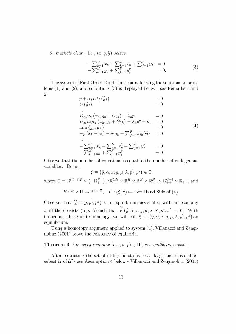
3. markets clear , i.e., (x; g; by) solves

¡PHh=1 xh +

PHh=1 eh +

PFf=1 yf = 0

¡PHh=1 gh +

PFf=1 y

gf = 0:

(3)

The system of First Order Conditions characterizing the solutions to prob-lems (1) and (2), and conditions (3) is displayed below - see Remarks 1 and2.

bp + ®fDtf (byf ) = 0tf (byf) = 0:::Dxhuh

¡xh; gh +Gnh

¢¡ ¸hp = 0

Dghuhuh¡xh; gh +Gnh

¢¡ ¸hpg + ¹h = 0

min fgh; ¹hg = 0

¡p (xh ¡ eh)¡ pggh +PF

f=1 sfhbpbyf = 0:::

¡PHh=1 x

nh +

PHh=1 e

nh +

PFf=1 y

nf = 0

¡PHh=1 gh +

PFf=1 y

gf = 0

(4)

Observe that the number of equations is equal to the number of endogenousvariables. De…ne

» ´¡by; ®; x; g; ¹; ¸; pn; pg

¢2 ¥

where ¥ ´ R(C+1)F £¡¡RF

++

¢£RCH

++ £ RH £ RH £ RH++ £ RC¡1

++ £ R++, and

F : ¥£ ¦! Rdim¥; F : (»; ¼) 7! Left Hand Side of (4).

Observe that¡by; x; g; pn; pg

¢is an equilibrium associated with an economy

¼ i¤ there exists (®; ¹; ¸) such that bbF¡by; ®; x; g; ¹; ¸; pn; pg; ¼

¢= 0: With

innocuous abuse of terminology, we will call » ´¡by;®; x; g; ¹; ¸; pn; pg

¢an

equilibrium.Using a homotopy argument applied to system (4), Villanacci and Zengi-

nobuz (2001) prove the existence of equilibria.

Theorem 3 For every economy (e; s; u; f ) 2 ¦0, an equilibrium exists.

After restricting the set of utility functions to a ”large and reasonable”subset U of U 0 - see Assumption 4 below - Villanacci and Zenginobuz (2001)

13

also show that there exists an open and dense subset ¦¤ of ¦ ´ RCH++ £

SH¡1 £ U £ T such that

8 ¼¤ 2 ¦¤; 8»¤ 2 F¡1¼¤ (0) ; rank D»F¼¤ (»¤) is full.

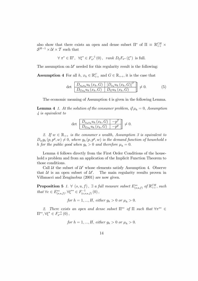
The assumption on U 0 needed for this regularity result is the following:

Assumption 4 For all h; xh 2 RC++ and G 2 R++; it is the case that

det

�Dxhxhuh (xh; G) [Dxhuh (xh; G)]

T

DGxhuh (xh;G) DGuh (xh; G)

¸6= 0: (5)

The economic meaning of Assumption 4 is given in the following Lemma.

Lemma 4 1. At the solution of the consumer problem, if ¹h = 0; Assumption4 is equivalent to

det

�Dxhxhuh (xh; G) ¡pTDGxhuh (xh; G) ¡pg

¸6= 0:

2. If w 2 R++ is the consumer’s wealth, Assumption 3 is equivalent toDwgh (p; p

g; w) 6= 0; where gh (p; pg; w) is the demand function of household’sh for the public good when gh > 0 and therefore ¹h = 0:

Lemma 4 follows directly from the First Order Conditions of the house-hold’s problem and from an application of the Implicit Function Theorem tothose conditions.

Call U the subset of U 0 whose elements satisfy Assumption 4. Observethat U is an open subset of U 0. The main regularity results proven inVillanacci and Zenginobuz (2001) are now given.

Proposition 5 1. 8 (s; u; f) ; 9 a full measure subset E¤¤(s;u;f ) of RCH++ ; such

that 8e 2 E¤¤(s;u;f); 8»¤¤ 2 F¡1(e;s;u;f) (0) ;

for h = 1; :::; H; either gh > 0 or ¹h > 0:

2. There exists an open and dense subset ¦¤¤ of ¦ such that 8¼¤¤ 2¦¤¤; 8»¤ 2 F¡1¼¤¤ (0) ;

for h = 1; :::; H; either gh > 0 or ¹h > 0:

14

Proposition 6 1. 8 (s; u; f) ; 9 a full measure subset E¤(s;u;f ) of RCH++ ; such

that 8e 2 E¤(s;u;f); 8»¤ 2 F¡1(e;s;u;f ) (0) ;

rank D»F¼¤ (»¤) = dim¥:

2. There exists and open and dense subset ¦¤ contained in ¦¤¤ such thatfor all ¼¤ 2 ¦¤; and for all »¤ 2 F¡1¼¤ (0), we have that

rank D»F¼¤ (»¤) = dim¥:

The following result is needed in the next Sections.

Lemma 7 In a an open and dense subset S¤¤ of the endowment space, inequilibrium, …rms are active.

Proof. It is a simple consequence of Proposition 6 and of the ParametricTransversality Theorem.

3 Redistribution of Wealth and Quantity ofPublic Good

In this Section, we show the following results.1. For all economies, ”local redistributions”12 of endowments of a private

good among contributors do not change the set of equilibria.2. For a generic subset of the economies for which there exists at least

one non-contributor, there exists a redistribution of endowments of a privategood between contributors and non-contributors which increases the level ofprovided public good;

3. For a generic subset of economies for which there exist at least two noncontributors, there exists a redistribution of endowments of a private goodamong non-contributors which increases the level of provided public good.

The proof of statement 1. above is due to BBV. To prove statements 2, 3as well as the main Theorems in the next Sections, we use a general method-ology described, for example, in Citanna, Kajii and Villanacci (1998). Wesummarize this methodology, which is presented in the Appendix (”Di¤eren-tial Analysis on the Equilibrium Manifold”), below:

12By ”local redistribution” we mean redistribution in a small enough neighborhood ofa given endowment.

15

a. We de…ne an ”equilibrium” function F1 taking into account the e¤ectsof the planner’s intervention on agents’ behaviors via some policy tools ½.

b. We introduce a function F2 describing the constraints on planner’sbehavior and we consider a function eF ´ (F1; F2) whose zeros are equilibriawith planner’s intervention.

c. We observe that there are values of ½ at which equilibria with andwithout planner’s intervention coincide.

d. We de…ne a goal function G:e. We study the local e¤ect of a change in (a subvector of) ½ on G when

endogenous variables move along the equilibrium manifold.

3.1 Redistributions among Contributors

The following Theorem is due to BBV.

Theorem 8 Consider an equilibrium associated with an arbitrary economyand a redistribution of the private numeraire good among contributing house-holds such that no household loses more wealth than her original contribu-tion. All the equilibria after the redistribution are such that the consumptionof private goods and the total amount of consumed public good are the sameas before the redistribution.

As a simple Corollary to Theorem 8, we get the following:

Proposition 9 The set of equilibria after a local redistribution from an arbi-trary set of non-contributors to one contributor is equal to the set of equilibriaafter a local redistribution from that same arbitrary set of non-contributorsto an arbitrary set of contributors.

The above result also explains why in all of the di¤erent types of plannerinterventions considered, we tax only one contributor.13

Remark 4 Theorem 8 applies to all equilibrium models in which the con-straint set for each household’s problem is convex and utility functions arestrictly quasi concave and continuous. Therefore, it holds true also for the

13As we will see, for example in Lemma 12, showing non-neutrality amounts to showingthat a well chosen Jacobian matrix has full rank. In fact, taxing more than one contributorwould imply that matrix has two linearly dependent columns.

16

cases of exchange economies with a public good and incomplete markets orrestricted participation14, and a …rm producing the public good, whatever ob-jective functions it may have.

The case of more than one public good is analyzed in BBV and it couldeasily be analyzed in our framework as well. All of our non-neutrality resultswill hold a fortiori in their case as well.

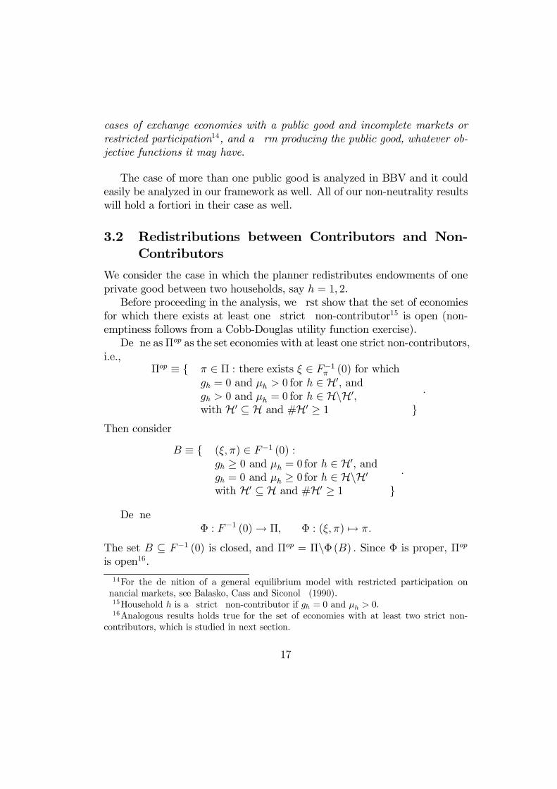
3.2 Redistributions between Contributors and Non-Contributors

We consider the case in which the planner redistributes endowments of oneprivate good between two households, say h = 1; 2.

Before proceeding in the analysis, we …rst show that the set of economiesfor which there exists at least one ”strict” non-contributor15 is open (non-emptiness follows from a Cobb-Douglas utility function exercise).

De…ne as¦op as the set economies with at least one strict non-contributors,i.e.,

¦op ´ f ¼ 2 ¦ : there exists » 2 F¡1¼ (0) for whichgh = 0 and ¹h > 0 for h 2 H0; andgh > 0 and ¹h = 0 for h 2 HnH0;with H0 µ H and #H0 ¸ 1 g

:

Then consider

B ´ f (»; ¼) 2 F¡1 (0) :gh ¸ 0 and ¹h = 0 for h 2 H0; andgh = 0 and ¹h ¸ 0 for h 2 HnH0

with H0 µ H and #H0 ¸ 1 g:

De…ne© : F¡1 (0) ! ¦; © : (»; ¼) 7! ¼:

The set B µ F¡1 (0) is closed, and ¦op = ¦n©(B) : Since © is proper, ¦op

is open16.

14For the de…nition of a general equilibrium model with restricted participation on…nancial markets, see Balasko, Cass and Siconol… (1990).

15Household h is a ”strict” non-contributor if gh = 0 and ¹h > 0:16Analogous results holds true for the set of economies with at least two strict non-

contributors, which is studied in next section.

17

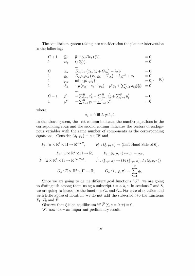
The equilibrium system taking into consideration the planner interventionis the following:

C + 1 byf bp+ ®fDtf (byf ) = 01 ®f tf (byf ) = 0

:::C xh Dxhuh

¡xh; gh +Gnh

¢¡ ¸hp = 0

1 gh Dghuhuh¡xh; gh +Gnh

¢¡ ¸hpg + ¹h = 0

1 ¹h min fgh; ¹hg = 0

1 ¸h ¡p (xh ¡ eh + ½h)¡ pggh +PF

f=1 sfhbpbyf = 0:::

C ¡ 1 pn ¡PHh=1 x

nh +

PHh=1 e

nh +

PFf=1 y

nf = 0

1 pg ¡PHh=1 gh +

PFf=1 y

gf = 0

; (6)

where½h ´ 0 i¤ h 6= 1; 2:

In the above system, the …rst column indicates the number equations in thecorresponding rows and the second column indicates the vectors of endoge-nous variables with the same number of components as the correspondingequations. Consider (½1; ½h) ´ ½ 2 R2 and

F1 : ¥£ R2 £ ¦! Rdim¥; F1 : (»; ½; ¼) 7! (Left Hand Side of 6),

F2 : ¥£ R2 £ ¦! R; F2 : (»; ½; ¼) 7! ½1 + ½h0;

eF : ¥£ R2 £ ¦ ! Rdim¥+1; eF : (»; ½; ¼) 7! (F1 (»; ½; ¼) ; F2 (»; ½; ¼))

Ga : ¥£ R2 £ ¦! R; Ga : (»; ½; ¼) 7!HX

h=1

gh:

Since we are going to de…ne di¤erent goal functions "G", we are goingto distinguish among them using a subscript i = a; b; c: In sections 7 and 8,we are going to introduce the functions Gb and Gc: For ease of notation andwith little abuse of notation, we do not add the subscript i to the functionsF1; F2 and eF .

Observe that » is an equilibrium i¤ eF (»; ½ = 0; ¼) = 0:We now show an important preliminary result.

18

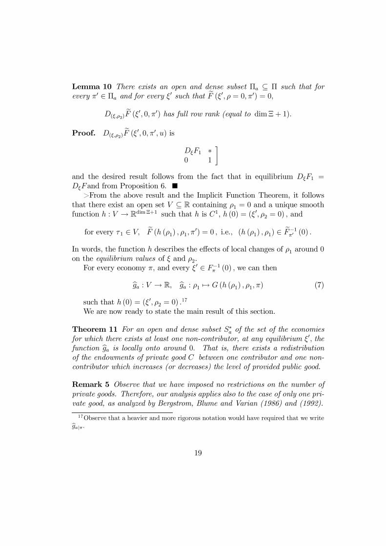
Lemma 10 There exists an open and dense subset ¦a µ ¦ such that forevery ¼0 2 ¦a and for every »0 such that eF (»0; ½ = 0; ¼0) = 0;

D(»;½2)eF (»0; 0; ¼0) has full row rank (equal to dim¥ + 1):

Proof. D(»;½2)eF (»0; 0; ¼0; u) is

�D»F1 ¤0 1

¸

and the desired result follows from the fact that in equilibrium D»F1 =D»Fand from Proposition 6.

>From the above result and the Implicit Function Theorem, it followsthat there exist an open set V µ R containing ½1 = 0 and a unique smoothfunction h : V ! Rdim¥+1 such that h is C1; h (0) = (»0; ½2 = 0) ; and

for every ¿ 1 2 V; eF (h (½1) ; ½1; ¼0) = 0 ; i.e.; (h (½1) ; ½1) 2 eF¡1¼0 (0) :

In words, the function h describes the e¤ects of local changes of ½1 around 0on the equilibrium values of » and ½2.

For every economy ¼; and every »0 2 F¡1¼ (0) ; we can then

bga : V ! R; bga : ½1 7! G (h (½1) ; ½1; ¼) (7)

such that h (0) = (»0; ½2 = 0) :17

We are now ready to state the main result of this section.

Theorem 11 For an open and dense subset S¤a of the set of the economiesfor which there exists at least one non-contributor, at any equilibrium »0; thefunction bga is locally onto around 0: That is, there exists a redistributionof the endowments of private good C between one contributor and one non-contributor which increases (or decreases) the level of provided public good.

Remark 5 Observe that we have imposed no restrictions on the number ofprivate goods. Therefore, our analysis applies also to the case of only one pri-vate good, as analyzed by Bergstrom, Blume and Varian (1986) and (1992).

17Observe that a heavier and more rigorous notation would have required that we writebgaj¼:

19

Remark 6 Because of Lemma 4, the local changes in the endowments men-tioned in the statement of Theorem 11 can be made small enough to leaveunchanged the set of households for which gh > 0, i.e., the set of contributors.

As explained for example in the Appendix, to prove Theorem 11 it su¢cesto show the following:

Lemma 12 There exists an open and dense subset S¤a µ ¦ such that forevery ¼0 2 S¤a and for every »0 2 eF¡1¼0 (0) ;

D(»;½) eF (»0; 0; ¼0) has full rank:

Lemma 12 is equivalent to the following one:

Lemma 13 In an open and dense set of ¦, the following system computedat eF (»; 0; ¼) = 0 has no solutions in the unknowns bd

bdT�D ~FDG

¸= 0

bdT bd¡ 1 = 0

(8)

Proof.Openness: De…ne the projection

Á : eF¡1 (0) ! ¦; Á : (»; ¼) 7! ¼

andM ´ f (»; ½; ¼) 2 ¥£ R2 £ ¦ : eF (»; ½; ¼) = 0 , ½ = 0 and

rankhD»;½

³eF;G

´i< n + 2 g :

Observe that Á (M) = E¤: Consider all the square submatrices ofhD»;½

³eF;G

´i

of dimension smaller than (n+ 2) : The rank condition in the de…nition ofMrequires that the determinants of all those submatrices are zero. Since thefunction determinant is a continuous function, M is a closed subset of theclosed set F ¡1 (0) :

If the function Á is proper, then Á(M) = E¤ is closed, as desired. Theproof of properness of Á is (almost) identical to the proof of Lemma 8 byVillanacci and Zenginobuz (2001).

20

Density: The proof of density goes through some steps. We …rst compute³D eF ;DG

´: We perform some elementary row and column operations. We

write system (8) at » such that eF (»; 0; ¼) = 0. Finally, distinguishing twocases, we prove the desired result.

For simplicity of notation, we take h = 1 as the household who is acontributor and whose corresponding columns are used to clean up columnsof the matrix under analysis; h = 2 as a non-contributor who is taxed; h = 3as a contributor who is not taxed; and h = 4 as a non-contributor who is nottaxed.

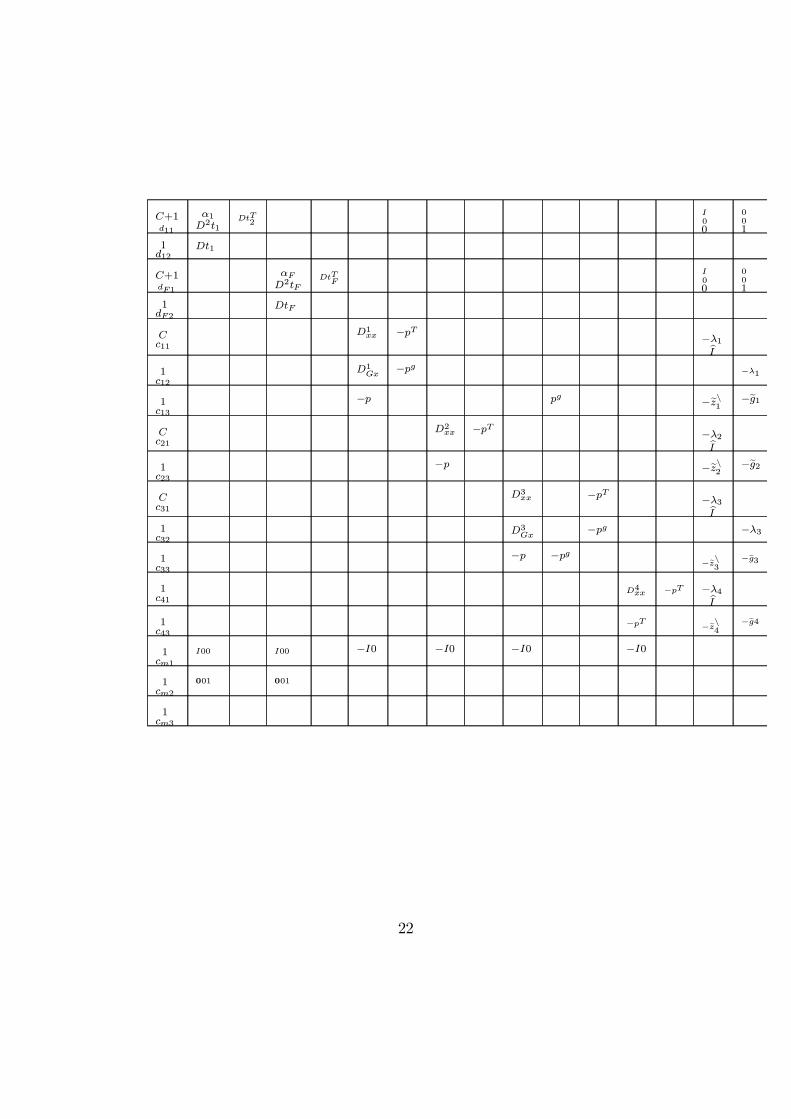
We display below the matrix³D eF ;DG

´after we performed the elemen-

tary row and column operations mentioned above:

21

C+1d11

®1D2t1

DtT2

I00

001

1d12

Dt1

C+1dF1

®FD2tF

DtTF

I00

001

1dF2

DtF

Cc11

D1xx ¡pT ¡¸1

bI1c12

D1Gx

¡pg ¡¸1

1c13

¡p pg ¡ezn1 ¡eg1

Cc21

D2xx ¡pT ¡¸2

bI1c23

¡p ¡ezn2 ¡eg2

Cc31

D3xx ¡pT ¡¸3

bI1c32

D3Gx

¡pg ¡¸3

1c33

¡p ¡pg¡ezn

3¡eg3

1c41

D4xx ¡pT ¡¸4bI

1c43

¡pT ¡ezn4¡eg4

1cm1

I00 I00 ¡I0 ¡I0 ¡I0 ¡I0

1cm2

001 001

1cm3

22

where

bI ´�

IC¡112£(C¡1)

¸;

bbI ´�

IC¡102£(C¡1)

¸; eI ´

�0(C+1)£101£1

¸;

and for each h

ezh ´ xh ¡ eh ¡X

f

sfhyf and egh ´ gh +X

f

sfhygf :

Next to each super row in the above matrix, we wrote the subvector ofbd ´ (b; d) that multiplies the elements in that super row18; and the numberabove each subvector is the number of its components.19

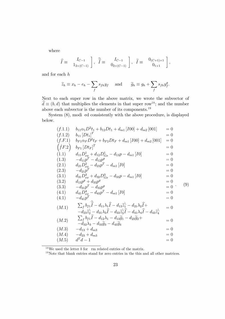
System (8), modi…ed consistently with the above procedure, is displayedbelow.

(f:1:1) b11®1D2t1 + b12Dt1 + dm1 [I00] + dm2 [001] = 0

(f:1:2) b11 [Dt1]T = 0

(f:F:1) bF1®FD2tF + bF2DtF + dm1 [I00] + dm2 [001] = 0³_fF:2

´bF1 [DtF ]

T = 0

(1:1) d11D1xx + d12D

1Gx ¡ d13p¡ dm1 [I0] = 0

(1:3) ¡d11pT ¡ d12pg = 0(2:1) d21D2

xx ¡ d23pT ¡ dm1 [I0] = 0(2:3) ¡d21pT = 0(3:1) d31D

3xx + d32D

3Gx ¡ d33p¡ dm1 [I0] = 0

(3:2) d13pg + d33p

g = 0(3:3) ¡d31pT ¡ d32pg = 0(4:1) d41D4

xx ¡ d43pT ¡ dm1 [I0] = 0(4:1) ¡d41pT = 0

(M:1)P

f bf1bbI ¡ d11¸1bI ¡ d13ezn1 ¡ d21¸2bI+

¡d23ezn2 ¡ d31¸3bI ¡ d33ezn3 bI ¡ d41¸4bI ¡ d43ezn4= 0

(M:2)

Pf bf1

eI ¡ d12¸1 ¡ d13eg1 ¡ d23eg2+¡d32¸3 ¡ d33eg3 ¡ d43eg4

= 0

(M:3) ¡d13 + dm3 = 0(M:4) ¡d23 + dm3 = 0(M:5) dTd¡ 1 = 0

: (9)

18We used the letter b for …rm related entries of the matrix.19Note that blank entries stand for zero entries in the this and all other matrices.

23

The perturbation of the transformation function we are going to use hasthe following form

tf¡yf ; y

Gf

¢= tf

¡yf ; y

Gf

¢+

¡¡yf ; y

Gf

¢¡

¡¡y¤f ; y

G¤f

¢¢¢T ¢Af ¢¡¡yf ; y

Gf

¢¡

¡¡y¤f ; y

G¤f

¢¢¢;

where¡y¤f ; y

G¤f

¢are equilibrium values, and Af is a symmetric negative de…-

nite matrix. Observe that the above proposed perturbation of the transfor-mation function can be done because, generically, in equilibrium yGf 6= 0 - seeLemma 7: Moreover, the derivative of df1 ¢ Af with respect to the elementsof Af has full row rank i¤ df1 6= 0.

The perturbation of the utility function we are going to use has the fol-lowing form:

uh (xh; gh) = u (xh; gh)+((xh; gh)¡ (x¤h; g¤h))T�Ahxx 00 ahgg

¸((xh; gh)¡ (x¤h; g¤h)) ;

where (x¤h; g¤h) are equilibrium values, Ahxx is a symmetric negative de…nite

matrix and ahgg is a strictly negative number. Using the utility function per-turbation proposed above, we can perturb independently equations (h:1) and(h:2) as long as dh1 6= 0 and dh2 6= 0: In fact, the derivative of

£dh1 dh2

¤�Ahxx 00 ahgg

¸

with respect to the elements of Ahxx and ahgg is the following:

26666664

a11 a21 aC1 ::: a22 aC2 aCC agg

d1h1 d2h1 dCh1:::

d1h1::: d2h1 dCh1

::: ::: ::: ::: ::: ::: ::: ::: ::: ::: ::: :::

d1h1::: d2h1 dCh1

::: dh2

37777775: (10)

We denote the utility function perturbation via the Hessian perturba-tion relative to private goods and public good for a generic household hby ¢(dh1) and ¢(dh2) : In fact, in this Section, we are going to use only¢(dh1) :20 We denote the transformation function perturbation by ¢(df1) :

20For a detailed account of the use of this methodology of proof, see Citanna, Kajii andVillanacci (1998) and also Villanacci et al. (forthcoming).

24

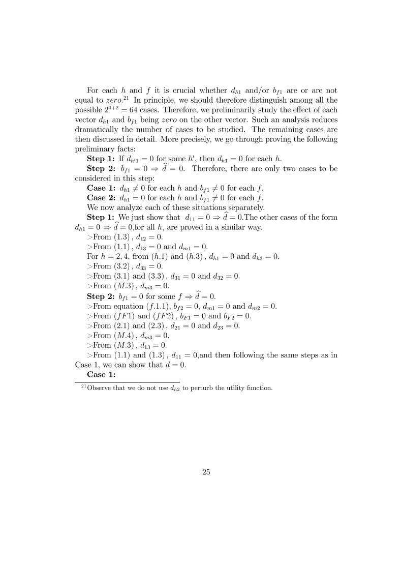
For each h and f it is crucial whether dh1 and/or bf1 are or are notequal to zero.21 In principle, we should therefore distinguish among all thepossible 24+2 = 64 cases. Therefore, we preliminarily study the e¤ect of eachvector dh1 and bf1 being zero on the other vector. Such an analysis reducesdramatically the number of cases to be studied. The remaining cases arethen discussed in detail. More precisely, we go through proving the followingpreliminary facts:

Step 1: If dh01 = 0 for some h0, then dh1 = 0 for each h:Step 2: bf1 = 0 ) bd = 0: Therefore, there are only two cases to be

considered in this step:Case 1: dh1 6= 0 for each h and bf1 6= 0 for each f:Case 2: dh1 = 0 for each h and bf1 6= 0 for each f:We now analyze each of these situations separately.Step 1: We just show that d11 = 0 ) bd = 0:The other cases of the form

dh1 = 0 ) bd = 0;for all h, are proved in a similar way.>From (1:3) ; d12 = 0:>From (1:1) ; d13 = 0 and dm1 = 0:For h = 2; 4; from (h:1) and (h:3) ; dh1 = 0 and dh3 = 0:>From (3:2) ; d33 = 0:>From (3:1) and (3:3) ; d31 = 0 and d32 = 0:>From (M:3) ; dm3 = 0:

Step 2: bf1 = 0 for some f ) bd = 0:>From equation (f:1:1), bf2 = 0; dm1 = 0 and dm2 = 0:>From (fF 1) and (fF 2) ; bF1 = 0 and bF2 = 0:>From (2:1) and (2:3) ; d21 = 0 and d23 = 0:>From (M:4) ; dm3 = 0:>From (M:3) ; d13 = 0:>From (1:1) and (1:3) ; d11 = 0;and then following the same steps as in

Case 1, we can show that d = 0:Case 1:

21Observe that we do not use dh2 to perturb the utility function.

25

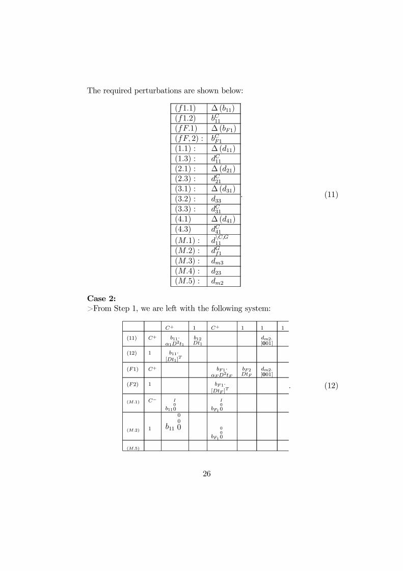
The required perturbations are shown below:

(f1:1) ¢ (b11)(f1:2) bC11(fF:1) ¢ (bF1)(fF; 2) : bCF1(1:1) : ¢ (d11)(1:3) : dC11(2:1) : ¢ (d21)(2:3) : dC21(3:1) : ¢ (d31)(3:2) : d33(3:3) : dC31(4:1) ¢ (d41)(4:3) dC41(M:1) : d

nC;G11

(M:2) : dGf1(M:3) : dm3(M:4) : d23(M:5) : dm2

: (11)

Case 2:>From Step 1, we are left with the following system:

C+ 1 C+ 1 1 1

(11) C+ b11¢®1D2t1

b12Dt1

dm2¢[001]

(12) 1 b11¢[Dt1]

T

(F1) C+ bF1¢®FD

2tF

bF2DtF

dm2¢[001]

(F2) 1 bF 1¢[DtF ]

T

(M:1) C¡

b11

I00 bF1

I00

(M:2) 1 b11

00

0bF1

000

(M:5)

: (12)

26

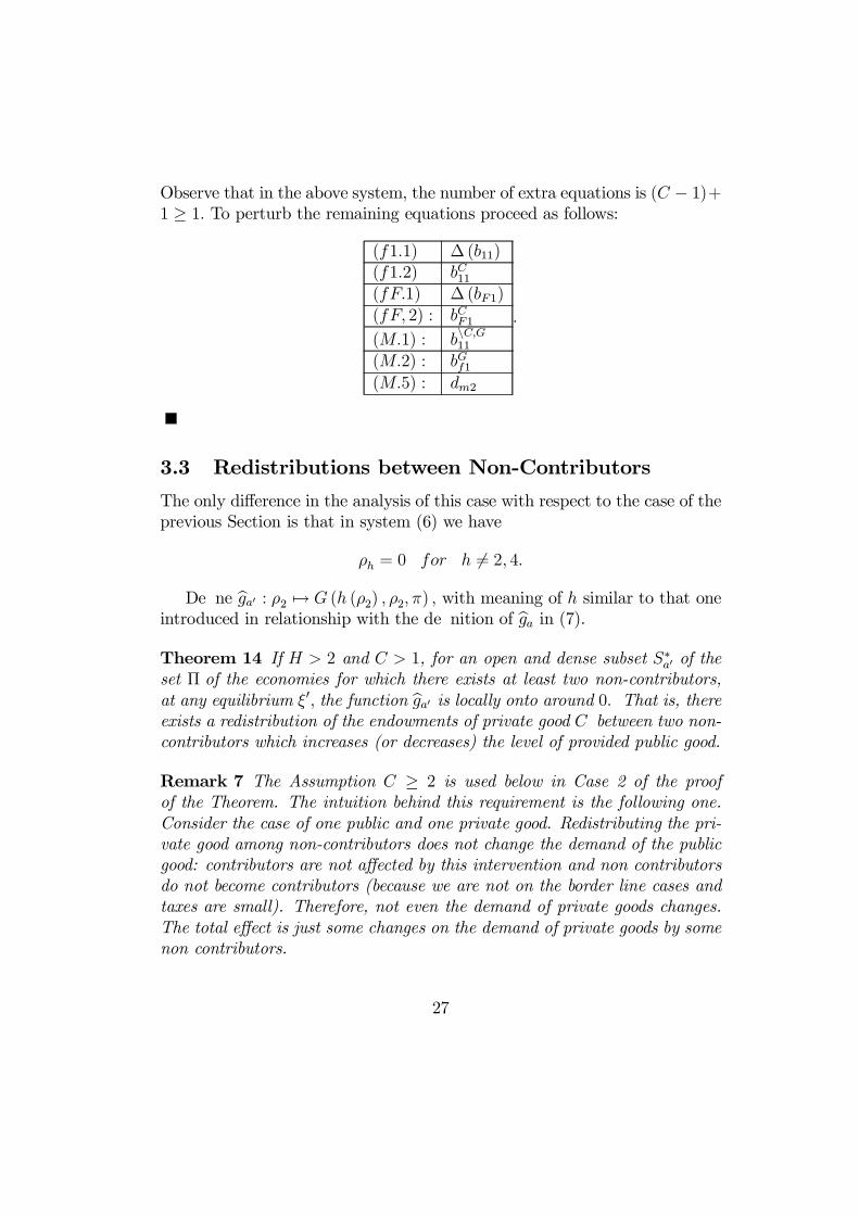
Observe that in the above system, the number of extra equations is (C ¡ 1)+1 ¸ 1: To perturb the remaining equations proceed as follows:

(f1:1) ¢ (b11)(f1:2) bC11(fF:1) ¢ (bF1)(fF; 2) : bCF1(M:1) : bnC;G11

(M:2) : bGf1(M:5) : dm2

:

3.3 Redistributions between Non-Contributors

The only di¤erence in the analysis of this case with respect to the case of theprevious Section is that in system (6) we have

½h = 0 for h 6= 2; 4:

De…ne bga0 : ½2 7! G (h (½2) ; ½2; ¼) ; with meaning of h similar to that oneintroduced in relationship with the de…nition of bga in (7).

Theorem 14 If H > 2 and C > 1, for an open and dense subset S¤a0 of theset ¦ of the economies for which there exists at least two non-contributors,at any equilibrium »0; the function bga0 is locally onto around 0: That is, thereexists a redistribution of the endowments of private good C between two non-contributors which increases (or decreases) the level of provided public good.

Remark 7 The Assumption C ¸ 2 is used below in Case 2 of the proofof the Theorem. The intuition behind this requirement is the following one.Consider the case of one public and one private good. Redistributing the pri-vate good among non-contributors does not change the demand of the publicgood: contributors are not a¤ected by this intervention and non contributorsdo not become contributors (because we are not on the border line cases andtaxes are small). Therefore, not even the demand of private goods changes.The total e¤ect is just some changes on the demand of private goods by somenon contributors.

27

Proof. The only di¤erence between this system and system (6) above isthe fact that d43 and not d13 appears in equation (M:3) : As in Subsection3.2, we preliminary study the e¤ect of each vector dh1 and bf1 being zero onthe other vectors, and then we analyze the relevant cases. More precisely, wego through the following steps:

Step 1: [d11 = 0 or d31 = 0] ) bd = 0;Step 2: d21 = 0 , d41 = 0;

Step 3: bf 01 = 0 )h(bf1)

Ff=1 = 0 and d21 = d41 = 0

i: Therefore, the

following cases are possible:Case 1: 8 f; bf1 6= 0 and 8h; dh1 6= 0:Case 2: 8 f; bf1 6= 0; d21 = d41 = 0 and d11 6= 0; d31 6= 0:Case 3: 8 f; bf1 6= 0 and 8h; dh1 = 0:Case 4: 8 f; bf1 = 0; d21 = d41 = 0 and d11 6= 0; d31 6= 0:The argument in Steps 1, 2, 3 and in Cases 1 and 3 of Step 3 is very

similar to that the analogous ones in Subsection 3.2. Therefore we are leftwith analyzing Cases 2 and 4.

Case 2: 8 f; bf1 6= 0; d21 = d41 = 0 and d11 6= 0; d31 6= 0:

Lost unknowns # Lost equations # # Eqns. we can erased21 C (2:1) Cd23 1 (2:3) 1d41 C (4:1) Cd43 1 (4:3) 1dm1 C ¡ 1 C ¡ 1dm3 1 (M:3) 1

(M:4) 1 ¡1¡¡¡¡¡¡¡(C ¡ 1)¡ 1 in total

In the above table, by ”lost unknowns” we mean unknowns that are equalto zero, and by ”lost equations” we mean equations which, in the case underanalysis, take the form of identity 0 = 0:

Observe from the table above that we have more equations than unknownsi¤ C ¸ 2: Since we assumed so, we can then proceed with the perturbationused in Case 1. Observe that we lost unknowns we were using to perturbequations we lost as well: for example, in Case 1 to perturb equation (f:1:1)we use b11. Here we lose both those equations and unknowns.

28

Case 4: 8 f; bf1 = 0; d21 = d41 = 0 and d11 6= 0; d31 6= 0:

Lost unknowns # Lost equations # # Eqns. we can eraseb11 C + 1 (11) C + 1b12 1 (12) 1bF1 C + 1 (F:1) C + 1bF2 1 (F:2) 1d11 C (1:1) Cd23 1 (2:3) 1d41 C (4:1) Cd43 1 (4:3) 1dm1 C ¡ 1 C ¡ 1dm3 1 (M:3) 1dm2 (M:4) 1

¡¡¡¡¡¡¡(C ¡ 1) in total

Since C ¡ 1 ¸ 1; we can erase equation (M:5) and perturb the otherequation as we did in Case 1.

4 Crowding-out E¤ectsWe will show that a planner can increase G if her intervention is as describedbelow:

1. She taxes all non contributors and one contributor by an amount ½hof the numeraire good;

2. She uses those taxes to …nance the purchase of an amount µg of thepublic good. This purchase occurs on the market at market equilibriumprices.

Equilibrium with planner intervention:1. For each h, the amount of consumed public good is

PHh=1 gh + µ

g;2. The budget set has to take into account the tax ½h for h = 2;3. The purchase of µg has to be …nanced with the revenue from tax

collection, i.e.,½2 ¡ pgµg = 0:

29

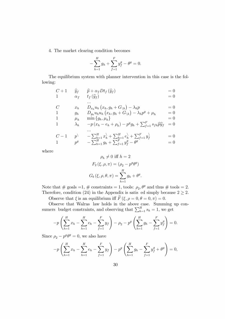
4. The market clearing condition becomes

¡HX

h=1

gh +FX

f=1

ygf ¡ µg = 0:

The equilibrium system with planner intervention in this case is the fol-lowing:

C + 1 byf bp + ®fDtf (byf ) = 01 ®f tf (byf) = 0

:::C xh Dxhuh

¡xh; gh +Gnh

¢¡ ¸hp = 0

1 gh Dghuhuh¡xh; gh +Gnh

¢¡ ¸hpg + ¹h = 0

1 ¹h min fgh; ¹hg = 0

1 ¸h ¡p (xh ¡ eh + ½h)¡ pggh +PF

f=1 sfhbpbyf = 0:::

C ¡ 1 pn ¡PHh=1 x

nh +

PHh=1 e

nh +

PFf=1 y

nf = 0

1 pg ¡PHh=1 gh +

PFf=1 y

gf ¡ µg = 0

where½h 6= 0 i¤ h = 2

F2 (»; ½; ¼) = (½2 ¡ pgµg)

Gb (»; ½; µ; ¼) =HX

h=1

gh + µg:

Note that # goals =1, # constraints = 1, tools: ½2; µg and thus # tools = 2.

Therefore, condition (24) in the Appendix is satis…ed simply because 2 ¸ 2.Observe that » is an equilibrium i¤ eF (»; ½ = 0; µ = 0; ¼) = 0:Observe that Walras’ law holds in the above case. Summing up con-

sumers’ budget constraints, and observing thatPH

h=1 sh = 1, we get

¡pÃ

HX

h=1

xh ¡HX

h=1

eh ¡FX

f=1

yf

!¡ ½2 ¡ pg

ÃHX

h=1

gh ¡FX

f=1

ygf

!= 0:

Since ½2 ¡ pgµg = 0, we also have

¡pÃ

HX

h=1

xh ¡HX

h=1

eh ¡FX

f=1

yf

!¡ pg

ÃHX

h=1

gh ¡FX

f=1

ygf + µg

!= 0;

30

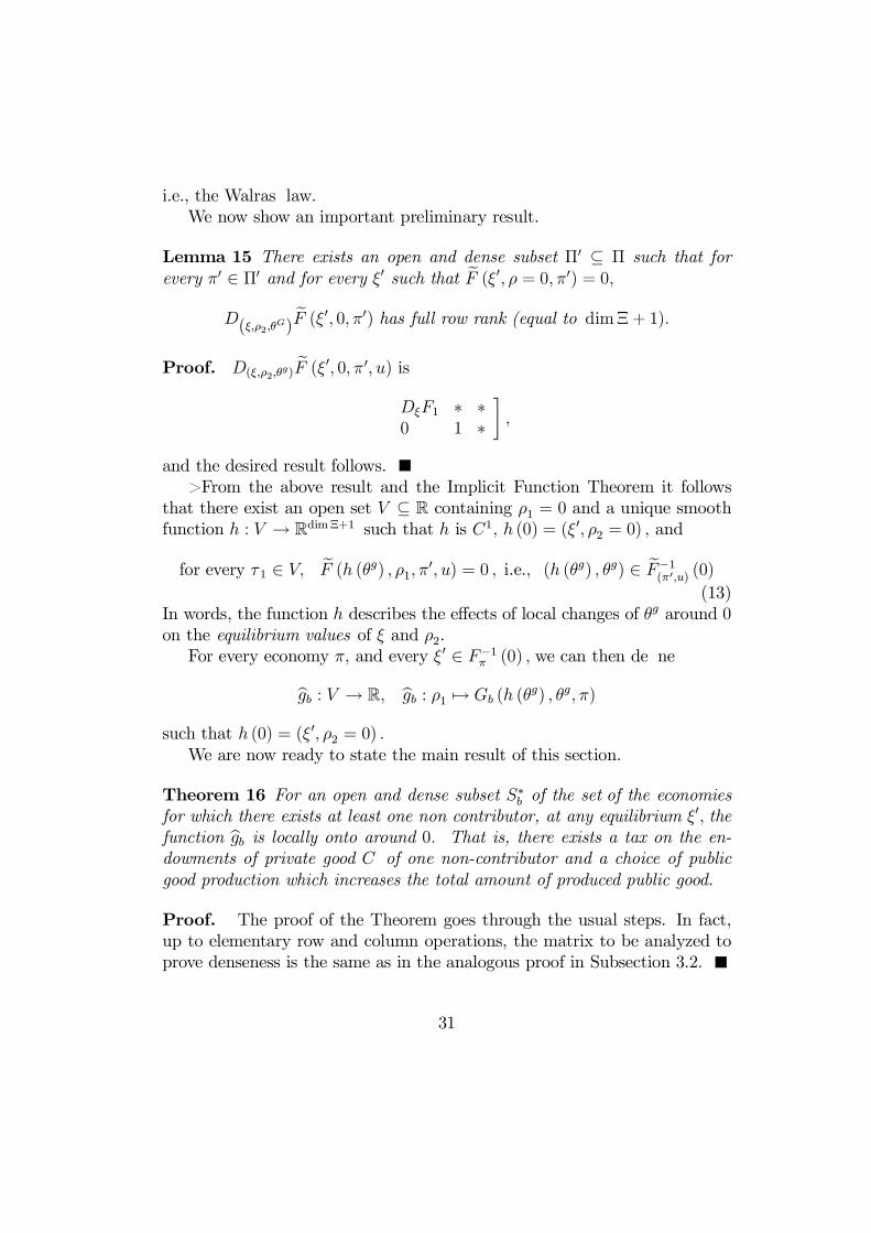
i.e., the Walras’ law.We now show an important preliminary result.

Lemma 15 There exists an open and dense subset ¦0 µ ¦ such that forevery ¼0 2 ¦0 and for every »0 such that eF (»0; ½ = 0; ¼0) = 0;

D(»;½2;µG)eF (»0; 0; ¼0) has full row rank (equal to dim¥ + 1):

Proof. D(»;½2;µg)eF (»0; 0; ¼0; u) is

�D»F1 ¤ ¤0 1 ¤

¸;

and the desired result follows.>From the above result and the Implicit Function Theorem it follows

that there exist an open set V µ R containing ½1 = 0 and a unique smoothfunction h : V ! Rdim¥+1 such that h is C1; h (0) = (»0; ½2 = 0) ; and

for every ¿ 1 2 V; eF (h (µg) ; ½1; ¼0; u) = 0 ; i.e.; (h (µg) ; µg) 2 eF¡1(¼0;u) (0)(13)

In words, the function h describes the e¤ects of local changes of µg around 0on the equilibrium values of » and ½2.

For every economy ¼; and every »0 2 F¡1¼ (0) ; we can then de…ne

bgb : V ! R; bgb : ½1 7! Gb (h (µg) ; µg; ¼)

such that h (0) = (»0; ½2 = 0) :We are now ready to state the main result of this section.

Theorem 16 For an open and dense subset S¤b of the set of the economiesfor which there exists at least one non contributor, at any equilibrium »0; thefunction bgb is locally onto around 0: That is, there exists a tax on the en-dowments of private good C of one non-contributor and a choice of publicgood production which increases the total amount of produced public good.

Proof. The proof of the Theorem goes through the usual steps. In fact,up to elementary row and column operations, the matrix to be analyzed toprove denseness is the same as in the analogous proof in Subsection 3.2.

31

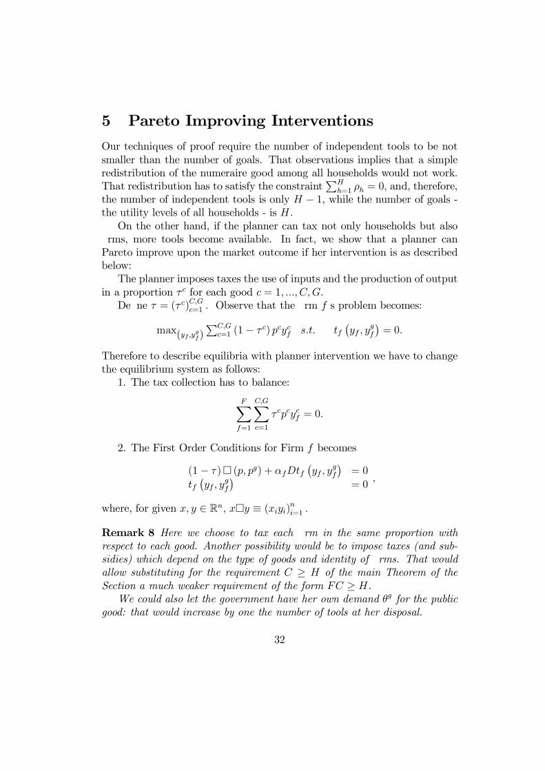
5 Pareto Improving InterventionsOur techniques of proof require the number of independent tools to be notsmaller than the number of goals. That observations implies that a simpleredistribution of the numeraire good among all households would not work.That redistribution has to satisfy the constraint

PHh=1 ½h = 0; and, therefore,

the number of independent tools is only H ¡ 1, while the number of goals -the utility levels of all households - is H .

On the other hand, if the planner can tax not only households but also…rms, more tools become available. In fact, we show that a planner canPareto improve upon the market outcome if her intervention is as describedbelow:

The planner imposes taxes the use of inputs and the production of outputin a proportion ¿ c for each good c = 1; :::; C;G.

De…ne ¿ = (¿ c)C;Gc=1 : Observe that the …rm f ’s problem becomes:

max(yf ;ygf)PC;G

c=1 (1¡ ¿ c) pcycf s:t: tf¡yf ; y

gf

¢= 0:

Therefore to describe equilibria with planner intervention we have to changethe equilibrium system as follows:

1. The tax collection has to balance:

FX

f=1

C;GX

c=1

¿ cpcycf = 0:

2. The First Order Conditions for Firm f becomes

(1¡ ¿ )¤ (p; pg) + ®fDtf¡yf ; y

gf

¢= 0

tf¡yf ; y

gf

¢= 0

;

where, for given x; y 2 Rn; x¤y ´ (xiyi)ni=1 :

Remark 8 Here we choose to tax each …rm in the same proportion withrespect to each good. Another possibility would be to impose taxes (and sub-sidies) which depend on the type of goods and identity of …rms. That wouldallow substituting for the requirement C ¸ H of the main Theorem of theSection a much weaker requirement of the form FC ¸ H.

We could also let the government have her own demand µg for the publicgood: that would increase by one the number of tools at her disposal.

32

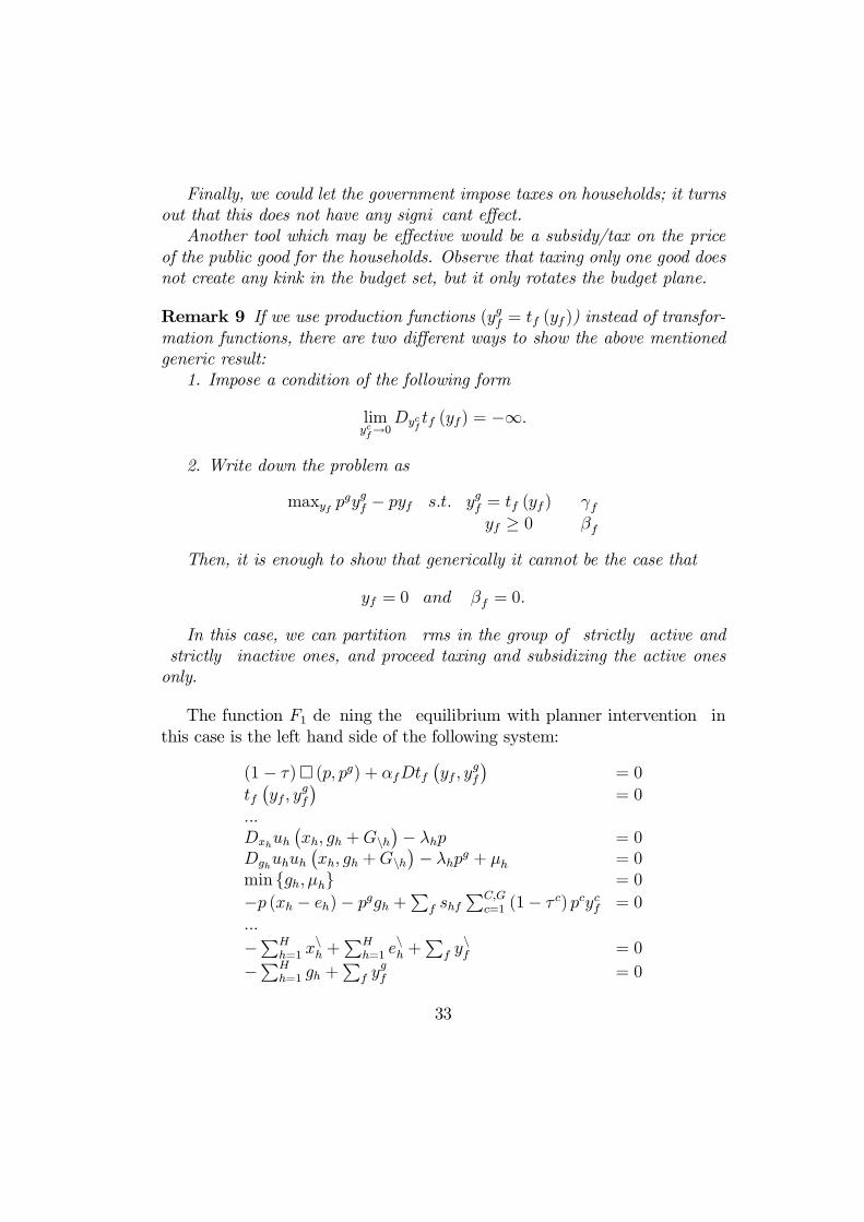
Finally, we could let the government impose taxes on households; it turnsout that this does not have any signi…cant e¤ect.

Another tool which may be e¤ective would be a subsidy/tax on the priceof the public good for the households. Observe that taxing only one good doesnot create any kink in the budget set, but it only rotates the budget plane.

Remark 9 If we use production functions (ygf = tf (yf )) instead of transfor-mation functions, there are two di¤erent ways to show the above mentionedgeneric result:

1. Impose a condition of the following form

limycf!0

Dycftf (yf) = ¡1:

2. Write down the problem as

maxyf pgygf ¡ pyf s:t: ygf = tf (yf ) °f

yf ¸ 0 ¯f

Then, it is enough to show that generically it cannot be the case that

yf = 0 and ¯f = 0:

In this case, we can partition …rms in the group of ”strictly” active and”strictly” inactive ones, and proceed taxing and subsidizing the active onesonly.

The function F1 de…ning the ”equilibrium with planner intervention” inthis case is the left hand side of the following system:

(1¡ ¿)¤ (p; pg) + ®fDtf¡yf ; y

gf

¢= 0

tf¡yf ; y

gf

¢= 0

:::Dxhuh

¡xh; gh +Gnh

¢¡ ¸hp = 0

Dghuhuh¡xh; gh +Gnh

¢¡ ¸hpg + ¹h = 0

min fgh; ¹hg = 0

¡p (xh ¡ eh)¡ pggh +P

f shfPC;G

c=1 (1¡ ¿ c) pcycf = 0:::

¡PHh=1 x

nh +

PHh=1 e

nh +

Pf y

nf = 0

¡PHh=1 gh +

Pf y

gf = 0

33

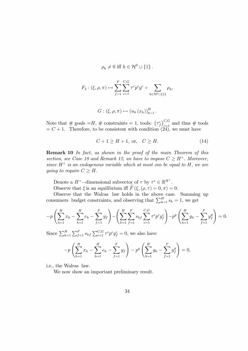
½h 6= 0 i¤ h 2 H0 [ f1g :

F2 : (»; ½; ¼) 7!FX

f=1

C;GX

c=1

¿ cpcyc +X

h2H0[f1g½h;

G : (»; ½; ¼) 7! (uh (xh))Hh=1 :

Note that # goals =H, # constraints = 1, tools:¡¿ cf

¢C;Gc=1

and thus # tools= C + 1. Therefore, to be consistent with condition (24), we must have

C + 1 ¸ H + 1; or, C ¸ H: (14)

Remark 10 In fact, as shown in the proof of the main Theorem of thissection, see Case 18 and Remark 12, we have to impose C ¸ H+: Moreover,since H+ is an endogenous variable which at most can be equal to H, we aregoing to require C ¸ H.

Denote a H+¡dimensional subvector of ¿ by ¿¤ 2 RH+.

Observe that » is an equilibrium i¤ eF (»; (½; ¿ ) = 0; ¼) = 0:Observe that the Walras’ law holds in the above case. Summing up

consumers’ budget constraints, and observing thatPH

h=1 sh = 1, we get

¡pÃ

HX

h=1

xh ¡HX

h=1

eh ¡FX

f=1

yf

!¡

ÃHX

h=1

FX

f=1

shf

C;GX

c=1

¿ cpcycf

!¡pg

ÃHX

h=1

gh ¡FX

f=1

ygf

!= 0:

SincePH

h=1

PFf=1 shf

PC;Gc=1 ¿

cpcycf = 0, we also have

¡pÃ

HX

h=1

xh ¡HX

h=1

eh ¡FX

f=1

yf

!¡ pg

ÃHX

h=1

gh ¡FX

f=1

ygf

!= 0;

i.e., the Walras’ law.We now show an important preliminary result.

34

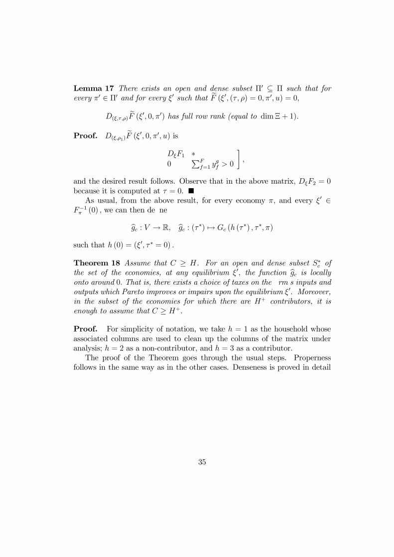
Lemma 17 There exists an open and dense subset ¦0 µ ¦ such that forevery ¼0 2 ¦0 and for every »0 such that eF (»0; (¿; ½) = 0; ¼0; u) = 0;

D(»;¿;½) eF (»0; 0; ¼0) has full row rank (equal to dim¥ + 1):

Proof. D(»;½1)eF (»0; 0; ¼0; u) is

�D»F1 ¤0

PFf=1 y

gf > 0

¸;

and the desired result follows. Observe that in the above matrix, D»F2 = 0because it is computed at ¿ = 0:

As usual, from the above result, for every economy ¼; and every »0 2F¡1¼ (0) ; we can then de…ne

bgc : V ! R; bgc : (¿ ¤) 7! Gc (h (¿¤) ; ¿ ¤; ¼)

such that h (0) = (»0; ¿ ¤ = 0) :

Theorem 18 Assume that C ¸ H. For an open and dense subset S¤c ofthe set of the economies, at any equilibrium »0; the function bgc is locallyonto around 0: That is, there exists a choice of taxes on the …rm’s inputs andoutputs which Pareto improves or impairs upon the equilibrium »0: Moreover,in the subset of the economies for which there are H+ contributors, it isenough to assume that C ¸ H+:

Proof. For simplicity of notation, we take h = 1 as the household whoseassociated columns are used to clean up the columns of the matrix underanalysis; h = 2 as a non-contributor, and h = 3 as a contributor.

The proof of the Theorem goes through the usual steps. Propernessfollows in the same way as in the other cases. Denseness is proved in detail

35

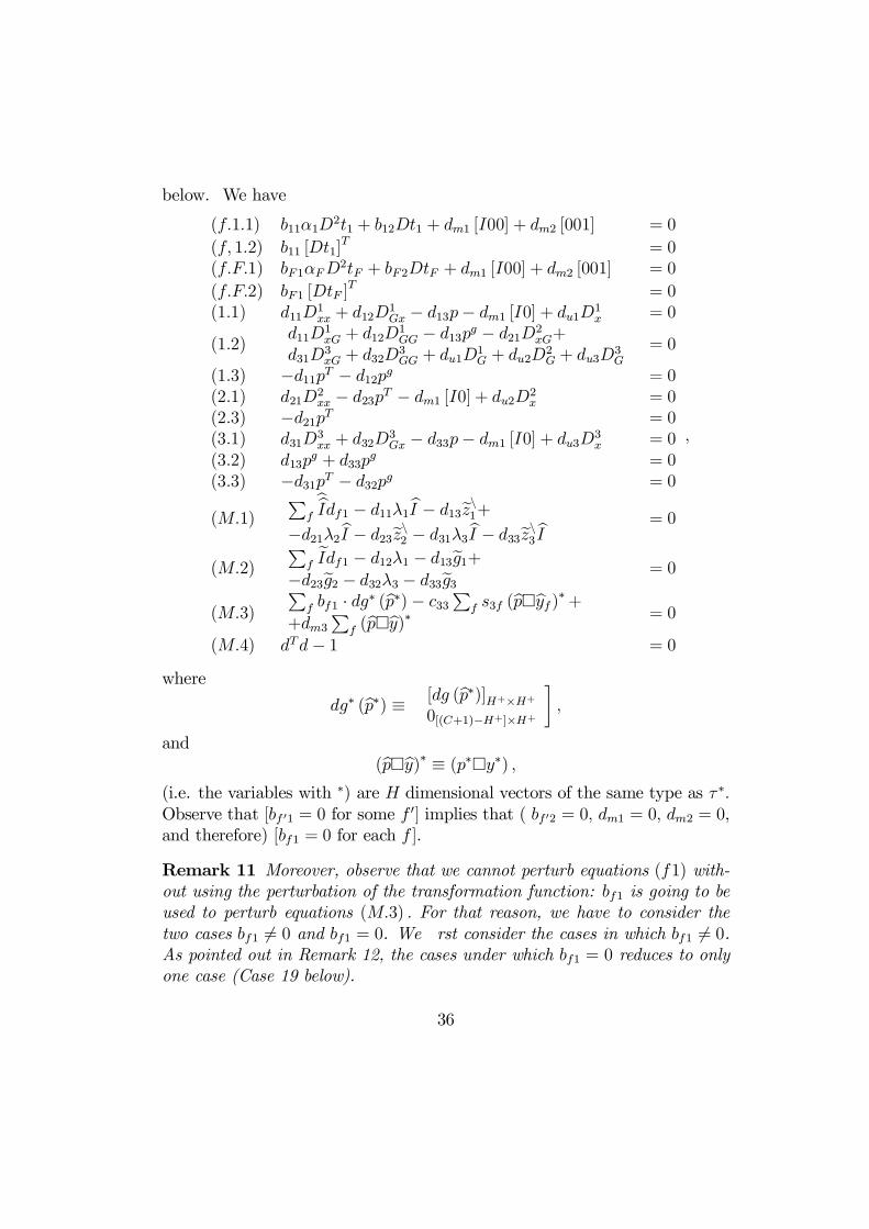
below. We have

(f:1:1) b11®1D2t1 + b12Dt1 + dm1 [I00] + dm2 [001] = 0

(f; 1:2) b11 [Dt1]T = 0

(f:F:1) bF1®FD2tF + bF2DtF + dm1 [I00] + dm2 [001] = 0

(f:F:2) bF1 [DtF ]T = 0

(1:1) d11D1xx + d12D

1Gx ¡ d13p¡ dm1 [I0] + du1D1

x = 0

(1:2)d11D

1xG + d12D

1GG ¡ d13pg ¡ d21D2

xG+d31D3

xG + d32D3GG + du1D

1G + du2D

2G + du3D

3G

= 0

(1:3) ¡d11pT ¡ d12pg = 0(2:1) d21D2

xx ¡ d23pT ¡ dm1 [I0] + du2D2x = 0

(2:3) ¡d21pT = 0(3:1) d31D

3xx + d32D

3Gx ¡ d33p¡ dm1 [I0] + du3D3

x = 0(3:2) d13p

g + d33pg = 0

(3:3) ¡d31pT ¡ d32pg = 0

(M:1)P

fbbIdf1 ¡ d11¸1bI ¡ d13ezn1+

¡d21¸2bI ¡ d23ezn2 ¡ d31¸3bI ¡ d33ezn3 bI= 0

(M:2)

Pf

eIdf1 ¡ d12¸1 ¡ d13eg1+¡d23eg2 ¡ d32¸3 ¡ d33eg3

= 0

(M:3)

Pf bf1 ¢ dg¤ (bp¤)¡ c33

Pf s3f (bp¤byf )¤+

+dm3P

f (bp¤by)¤ = 0

(M:4) dTd¡ 1 = 0

;

where

dg¤ (bp¤) ´�[dg (bp¤)]H+£H+

0[(C+1)¡H+]£H+

¸;

and(bp¤by)¤ ´ (p¤¤y¤) ;

(i.e. the variables with ¤) are H dimensional vectors of the same type as ¿ ¤:Observe that [bf 01 = 0 for some f 0] implies that ( bf 02 = 0; dm1 = 0; dm2 = 0,and therefore) [bf1 = 0 for each f ].

Remark 11 Moreover, observe that we cannot perturb equations (f1) with-out using the perturbation of the transformation function: bf1 is going to beused to perturb equations (M:3) : For that reason, we have to consider thetwo cases bf1 6= 0 and bf1 = 0. We …rst consider the cases in which bf1 6= 0.As pointed out in Remark 12, the cases under which bf1 = 0 reduces to onlyone case (Case 19 below).

36

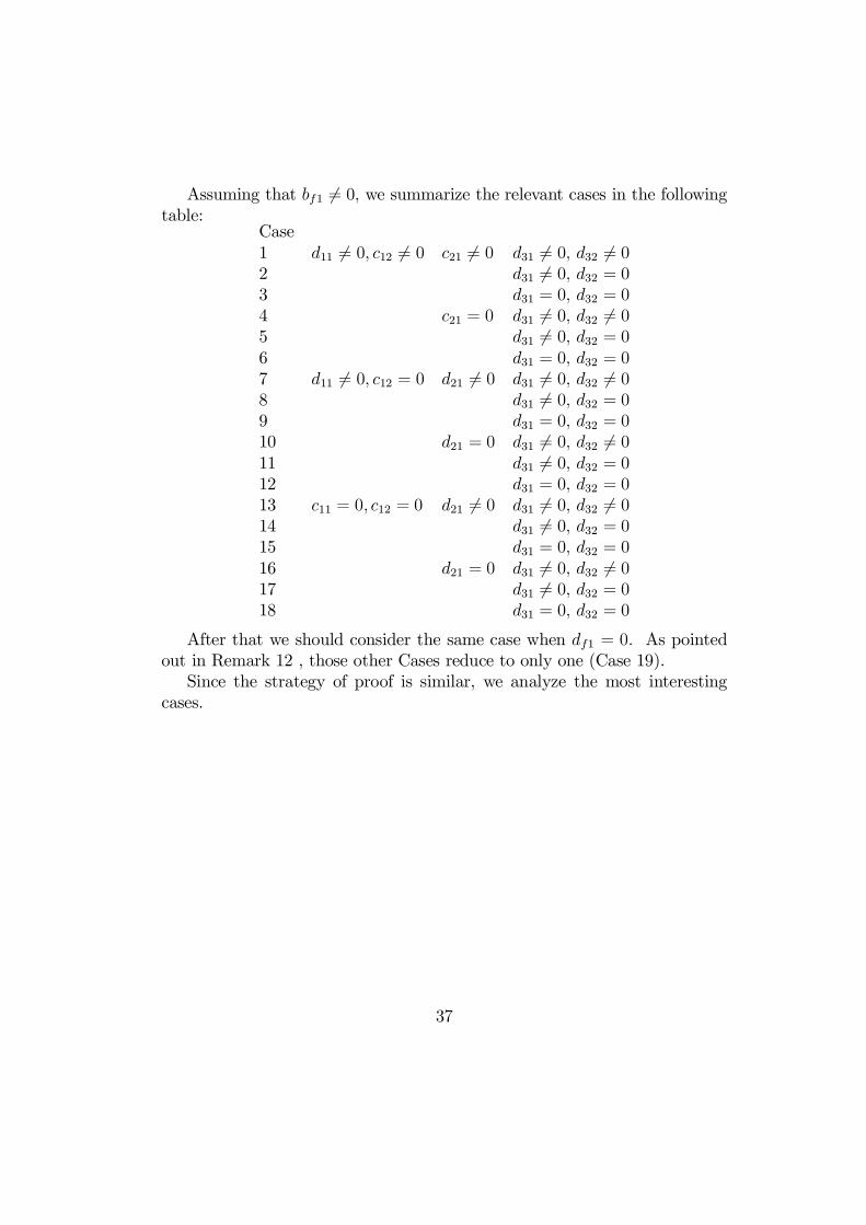
Assuming that bf1 6= 0; we summarize the relevant cases in the followingtable:

Case1 d11 6= 0; c12 6= 0 c21 6= 0 d31 6= 0; d32 6= 02 d31 6= 0; d32 = 03 d31 = 0; d32 = 04 c21 = 0 d31 6= 0; d32 6= 05 d31 6= 0; d32 = 06 d31 = 0; d32 = 07 d11 6= 0; c12 = 0 d21 6= 0 d31 6= 0; d32 6= 08 d31 6= 0; d32 = 09 d31 = 0; d32 = 010 d21 = 0 d31 6= 0; d32 6= 011 d31 6= 0; d32 = 012 d31 = 0; d32 = 013 c11 = 0; c12 = 0 d21 6= 0 d31 6= 0; d32 6= 014 d31 6= 0; d32 = 015 d31 = 0; d32 = 016 d21 = 0 d31 6= 0; d32 6= 017 d31 6= 0; d32 = 018 d31 = 0; d32 = 0

After that we should consider the same case when df1 = 0: As pointedout in Remark 12 , those other Cases reduce to only one (Case 19).

Since the strategy of proof is similar, we analyze the most interestingcases.

37

Case 1: bf1 6= 0; for h 2 H dh1 6= 0; for h 2 H+ d2h 6= 0:22

(f:1) ¢ (bf1)(f:2) bCf1(1:1) ¢ (d11)(1:2) ¢ (d12)(1:3) dC11(2:1) ¢ (d21)(2:3) dC21(3:1) ¢ (d31)(3:3) dC31(M:1) d

nh1

(M:2) dh2; h 2 H+

(M:3) bnCf1

(M:4) duh as long as d12 6= 0 and dh1 6= 0

(15)

We now show in more detail the perturbation of equation (M:4) :

(M:4) à duh à (1:2) à ¢(d12)à (h:1) à ¢(dh1)

: (16)

Observe that we could perturb equation (M:4) also using dm2 - as longas d12 6= 0 and dfi 6= 0:23

Case 18. d11 = 0; d12 = 0; d21 = 0; d31 = 0; d32 = 0:

Lost unkns. # Lost eqns. # # Eqns. we can erase Eqns. we erase #d11 C C (M:3) Hd12 1 (1:3) 1 (M:4) 1d21 C (2:3) 1 C ¡ 1 …rst (C ¡ 1) in (2:1) C ¡ 1d31 C C …rst (C ¡ 1) in (3:1) C ¡ 1d32 1 (3:3)

¡¡¡3C ¡ 1 in total

¡¡¡2C +H

(17)

22If c12 = 0; we have to erase (1:2) : To perturb (f:2), we need to use a dcf1 with

c 6= 1; :::;H. We take dCf1to perturb (f:2), because dC

f1 does not appear in (M:3) :23See Remark 12 for the reason for which we didn’t choose cm2 as the perturbing variable.

38

Then, proceed as illustrated in the following table:

(f:1) ¢ (bf1)(f:2) bCf1(1:1) dm1; du1(1:2) dm2(1:3) cancelled(2:1) du2(2:3) cancelled(3:1) du3(3:3) cancelled(M:1) d

nC;Gf1

(M:2) dnC;Gf1

(M:3) cancelled(M:4) cancelled

: (18)

Remark 12 We should now analyze the other remaining 18 Cases in whichbf1 = 0 for each f: But it is enough to observe what follows.

1. If bf1 = 0; then we have the following situation:

Lost unkns. # Lost eqns. # # Eqns. we can erase Eqns. we erase #bf1 C + 1 (f:1) C + 1 (H:7) Hbf2 1 (f:2) 1dm1 C ¡ 1 C ¡ 1dm2 1 1

¡¡¡C in total

¡¡¡H

:

In all …rst 17 cases, we never used dm2 and we used bf1 and bf2 to perturbequations (f:1), (f:2) and (M:3) which we erased.

2. The case in which all the perturbing variables are equal to zero isanalyzed below.

Proof. Case 19. bf1 = 0 for each f ; dh1 = 0 for h 2 H ; and d2h = 0 forh 2 H+:

39

>From (f:1) ; bf2 = 0; dm1 = 0; and dm2 = 0: Therefore, the systemreduces to the following:

(1:1) C ¡d13p

du1D1x

12 1 ¡d13pg

du1D1G

du2D2G

du3D3G

(2:1) C ¡d23p

du2D2x

(3:1) C ¡d33p

du3D3x

(3:2) 1 d13pg

¡d33pg

(M:1) C¡ ¡d13ezn1

¡d23ezn2

¡d33ezn3

(M:2) 1 ¡d13eg1

¡d23eg2

¡d33eg3

(M:3) H+ ¡d13s1(bp¤by)¤

¡d23s2(bp¤by)¤

¡d33s3(bp¤by)¤

dm3(bp¤by)¤

(M:4) 1

: (19)

Using the …rst order conditions of households’ problems, we can rewritethe …rst part of the system as follows:

(1:1C) 1 ¡c13 cu1¸1

(1:2) 1 ¡c13 cu1¸1 cu2¸2 cu3¸3

(2:1C) 1 ¡c23 cu2¸2

(3:1C) 1 ¡c33 cu3¸3

(3:2) 1 c13 ¡c33

:

Using (1:1C) in (1:2) ; we get

(1:1C) 1 ¡d13 du1¸1

(1:2) 1 du2¸2 du3

¸3

(2:1C) 1 ¡d23 du2¸2

(3:1C) 1 ¡d33 du3¸3

(3:2) 1 d13 ¡d33

: (20)

>From (3:2) ; d13 = d33:

40

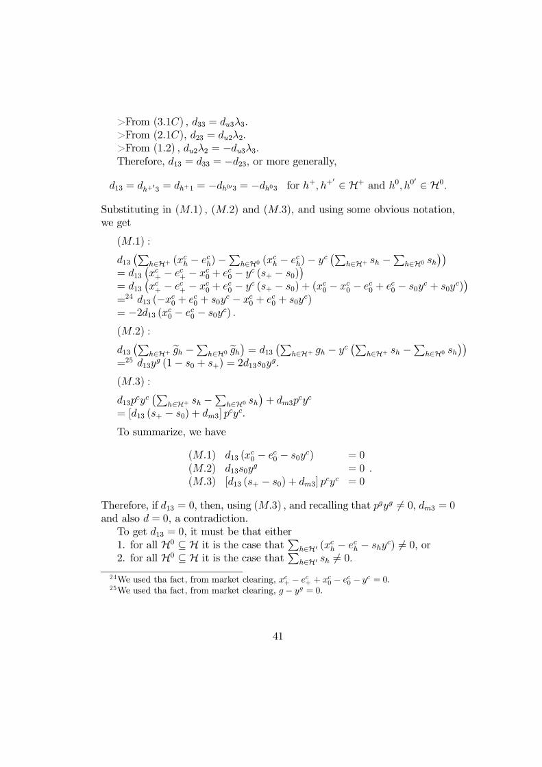
>From (3:1C) ; d33 = du3¸3:>From (2:1C), d23 = du2¸2:>From (1:2) ; du2¸2 = ¡du3¸3:Therefore, d13 = d33 = ¡d23; or more generally,

d13 = dh+03 = dh+1 = ¡dh003 = ¡dh03 for h+; h+0 2 H+ and h0; h0

0 2 H0:

Substituting in (M:1) ; (M:2) and (M:3), and using some obvious notation,we get

(M:1) :

d13¡P

h2H+ (xch ¡ ech)¡P

h2H0 (xch ¡ ech)¡ yc¡P

h2H+ sh ¡ Ph2H0 sh

¢¢

= d13¡xc+ ¡ ec+ ¡ xc0 + ec0 ¡ yc (s+ ¡ s0)

¢

= d13¡xc+ ¡ ec+ ¡ xc0 + ec0 ¡ yc (s+ ¡ s0) + (xc0 ¡ xc0 ¡ ec0 + ec0 ¡ s0yc + s0yc)

¢

=24 d13 (¡xc0 + ec0 + s0yc ¡ xc0 + ec0 + s0yc)= ¡2d13 (xc0 ¡ ec0 ¡ s0yc) :(M:2) :

d13¡P

h2H+ egh ¡ Ph2H0 egh

¢= d13

¡Ph2H+ gh ¡ yc

¡Ph2H+ sh ¡ P

h2H0 sh¢¢

=25 d13yg (1¡ s0 + s+) = 2d13s0yg:

(M:3) :

d13pcyc

¡Ph2H+ sh ¡ P

h2H0 sh¢+ dm3p

cyc

= [d13 (s+ ¡ s0) + dm3] pcyc:To summarize, we have

(M:1) d13 (xc0 ¡ ec0 ¡ s0yc) = 0

(M:2) d13s0yg = 0

(M:3) [d13 (s+ ¡ s0) + dm3] pcyc = 0:

Therefore, if d13 = 0; then, using (M:3) ; and recalling that pgyg 6= 0; dm3 = 0and also d = 0; a contradiction.

To get d13 = 0, it must be that either1. for all H0 µ H it is the case that

Ph2H0 (xch ¡ ech ¡ shyc) 6= 0, or

2. for all H0 µ H it is the case thatP

h2H0 sh 6= 0:24We used tha fact, from market clearing, xc

+ ¡ ec+ + xc

0 ¡ ec0 ¡ yc = 0:

25We used tha fact, from market clearing, g ¡ yg = 0:

41

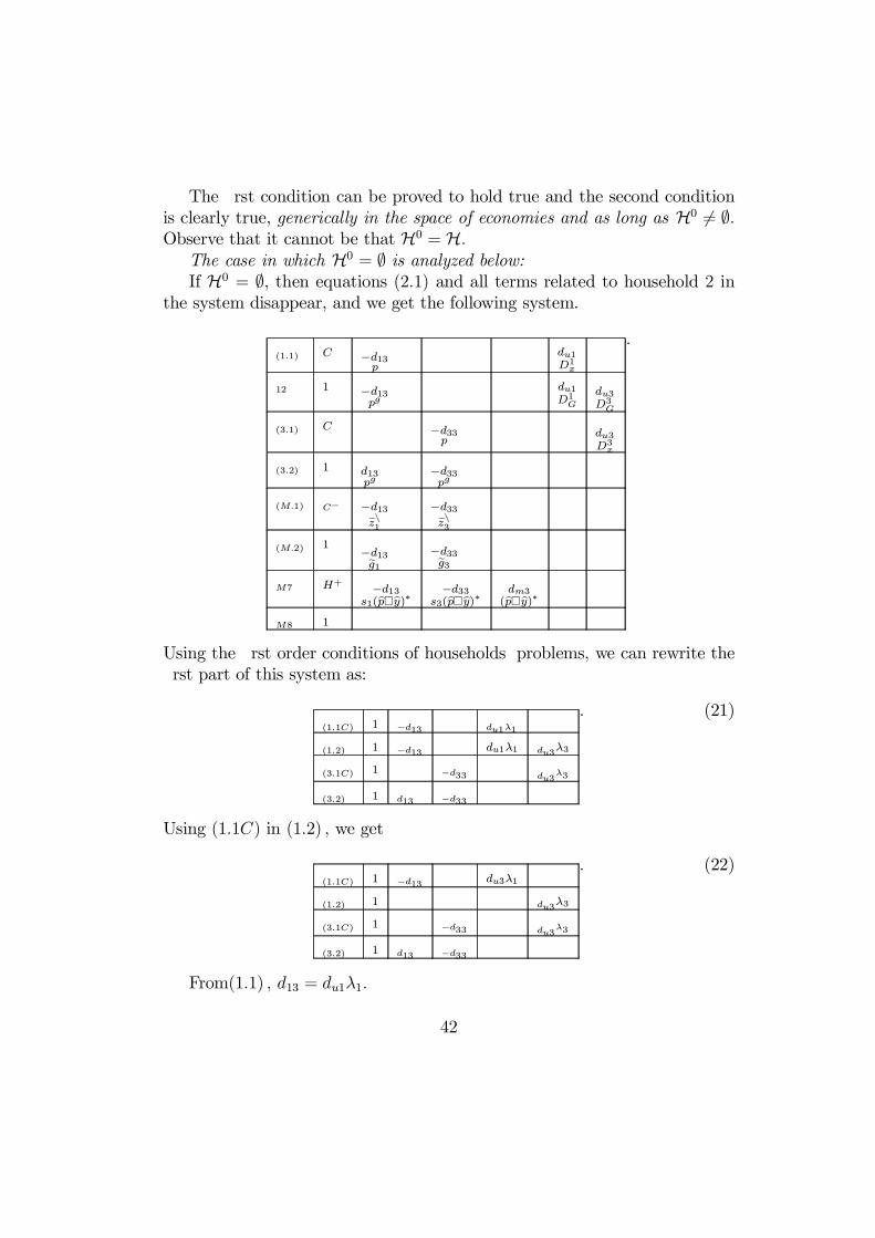
The …rst condition can be proved to hold true and the second conditionis clearly true, generically in the space of economies and as long as H0 6= ;:Observe that it cannot be that H0 = H:

The case in which H0 = ; is analyzed below:If H0 = ;, then equations (2:1) and all terms related to household 2 in

the system disappear, and we get the following system.

(1:1) C ¡d13p

du1D1x

12 1 ¡d13pg

du1D1G

du3D3G

(3:1) C ¡d33p

du3D3x

(3:2) 1 d13pg

¡d33pg

(M:1) C¡ ¡d13ezn1

¡d33ezn3

(M:2) 1 ¡d13eg1

¡d33eg3

M7 H+ ¡d13s1(bp¤by)¤

¡d33s3(bp¤by)¤

dm3(bp¤by)¤

M8 1

:

Using the …rst order conditions of households’ problems, we can rewrite the…rst part of this system as:

(1:1C) 1 ¡d13 du1¸1

(1:2) 1 ¡d13 du1¸1 du3¸3

(3:1C) 1 ¡d33 du3¸3

(3:2) 1 d13 ¡d33

: (21)

Using (1:1C) in (1:2) ; we get

(1:1C) 1 ¡d13 du3¸1

(1:2) 1 du3¸3

(3:1C) 1 ¡d33 du3¸3

(3:2) 1 d13 ¡d33

: (22)

From(1:1) ; d13 = du1¸1:

42

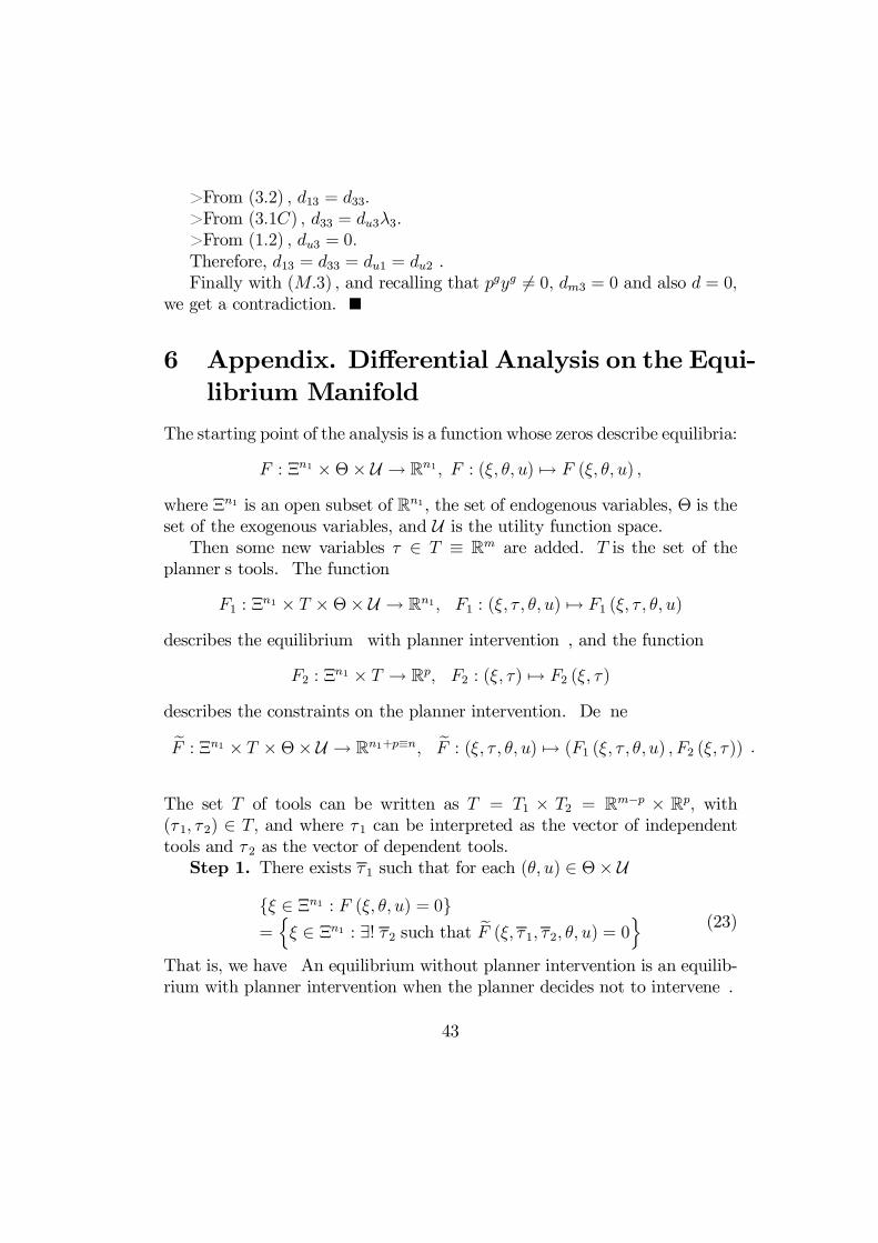
>From (3:2) ; d13 = d33:>From (3:1C) ; d33 = du3¸3:>From (1:2) ; du3 = 0:Therefore, d13 = d33 = du1 = du2 .Finally with (M:3) ; and recalling that pgyg 6= 0; dm3 = 0 and also d = 0;

we get a contradiction.

6 Appendix. Di¤erential Analysis on the Equi-librium Manifold

The starting point of the analysis is a function whose zeros describe equilibria:

F : ¥n1 £££ U ! Rn1; F : (»; µ; u) 7! F (»; µ; u) ;

where ¥n1 is an open subset of Rn1, the set of endogenous variables, £ is theset of the exogenous variables, and U is the utility function space.

Then some new variables ¿ 2 T ´ Rm are added. T is the set of theplanner’s tools. The function

F1 : ¥n1 £ T £££ U ! Rn1; F1 : (»; ¿ ; µ; u) 7! F1 (»; ¿ ; µ; u)

describes the equilibrium ”with planner intervention”, and the function

F2 : ¥n1 £ T ! Rp; F2 : (»; ¿) 7! F2 (»; ¿ )

describes the constraints on the planner intervention. De…ne

eF : ¥n1 £ T £££ U ! Rn1+p´n; eF : (»; ¿ ; µ; u) 7! (F1 (»; ¿ ; µ; u) ; F2 (»; ¿ )) :

The set T of tools can be written as T = T1 £ T2 = Rm¡p £ Rp; with(¿ 1; ¿ 2) 2 T; and where ¿ 1 can be interpreted as the vector of independenttools and ¿ 2 as the vector of dependent tools.

Step 1. There exists ¿ 1 such that for each (µ; u) 2 ££ U

f» 2 ¥n1 : F (»; µ; u) = 0g=

n» 2 ¥n1 : 9! ¿ 2 such that eF (»; ¿ 1; ¿2; µ; u) = 0

o (23)

That is, we have ”An equilibrium without planner intervention is an equilib-rium with planner intervention when the planner decides not to intervene”.

43

In fact, we want to study the e¤ects of changes in ¿ 1 around ¿ 1:Finally, G describes the goals of the planner:

G : ¥n1 £ T £££ U ! Rk; G : (»; ¿ ; µ; u) 7! G (»; ¿; µ; u) :

Step 2. For every u 2 U ; there exists an open and full measure sub-set £u of £ such that for every µ0 2 £u and for every »0 2 ¥ such thateF (»0; ¿1; ¿ 2; µ; u) = 0;

rank D(»;¿2)eF (»0; ¿ 1; ¿2; µ; u) is full.

Usually, the above result follows from the fact that D(»;¿2)eF (»0; ¿1; ¿ 2; µ; u) is

�D»F1 D¿2F1D»F2 D¿2F2

¸;

and, from a Regularity Lemma, D»F1 has full row rank in an open and fullmeasure subset of £u, the fact that D»F2 = 0; and that D¿2F2 has full rowrank.

De…ning

bg : T1 ! Rk; bg : ¿1 7! G (» (¿ 1) ; ¿ 2 (¿1) ; ¿ 1) ;

we want to show that in an open and dense set of economies dbg¿1 is ontoand, therefore, bg is locally onto around ¿ 1: As explained in Citanna, Kajiiand Villanacci (1998), that condition is implied by the following one.

There exists an open and dense subset S¤ µ £ £ U such that for every(µ0; u0) 2 ££ U and for every »0 2 ¥n1 such that eF (»0; ¿ 1; ¿ 2; µ; u) = 0

rankhD(»;¿) eF (»0; ¿ 1; ¿ 2; µ; u)

i(n1+p+k)£(n1+m)

= n1 + p + k:

The above condition implies that it must be

m ¸ p + k;

i.e.,

(number of tools ¸ (number of constraints on planner intervention) +(number of goals)

(24)

44

orm¡ p ¸ k;

i.e., (number of independent tools)¸ (number of goals).The above statement is equivalent to showing that for (µ; u) 2 S¤ the

following system has no solutions (»; c) 2 ¥n1 £ Rn1+p+k :

8><>:

eF (»; ¿1; ¿ 2; µ; u) = 0

cThD(»;¿)

³eF;G

´(»; ¿ ; µ; u)

i= 0

cT c¡ 1 = 0;

;

or, using condition (23), that the following system has no solutions:8><>:

F (»; µ; u) = 0

cThD(»;¿)

³eF;G

´(»; ¿ ; µ; u)

i= 0

cT c¡ 1 = 0:

: (25)

Step 3. Openness of S¤:Since

M ´ f(»; µ; u) 2 ¥£££ U : system (25) has a solution at ¿ = 0g

is closed, it is su¢cient to show that the following function is proper:

pr : F¡1 (0) ! ££ U ; pr : (»; µ; u) 7! (µ; u) :

Step 4. Density of S¤:We apply the Parametric Transversality Theorem to the function de…ned

by the left hand side of system (25). That amounts to show that the followingmatrix has full row rank:

» c ; ®u

F (»; µ; u) D»F (»; c; µ; ua) B (»; c; µ; ua)

cThD(»;¿)

³eF;G

´(»; ¿ ; µ; u)

i

cT c¡ 1¤ A (»; ¿; c; µ; ua)

;

where ®u is an element of an Euclidean space which is a …nite dimensionallocal parametrization of the utility function space.

45

Again from a Regularity result, D»F has full row rank in an open anddense subset of £ £ U : Moreover, it is crucial to have B (»; c; µ; ua) = 0: Ifthat is the case, to get the result in Step 4, it is enough to show that thefollowing matrix has full row rank

A (»; ¿ ; µ; u) =

" hD(»;¿ )

³eF;G

´(»; ¿ ; µ; u)

iTN (®u)

c 0

#:

7 References

Andreoni, J. (1988), Privately Provided Public Goods in a Large Economy:The Limits of Altruism”, Journal of Public Economics, 35, 57-73.

Andreoni, J. and T. Bergstrom (1996), Do Government Subsidies Increasethe Private Supply of Public Goods”, Public Choice, 88, 295-308.

Balasko, Y., D. Cass and P.Siconol… (1990), The Structure of FinancialEquilibrium with Exogenous Yields: The Case of Restricted Participa-tions, Journal of Mathematical Economics, 19, 195-216.

Bergstrom, T., Blume, L. and H. Varian, (1986), On the Private Provisionof Public Goods, Journal of Public Economics, 29, 25-49.

Bergstrom, T., Blume, L. and H. Varian, (1992), Uniqueness of Nash Equi-librium in Private Provision of Public Goods, An Improved Proof, Jour-nal of Public Economics, 49, 391-392.

Bernheim, D. (1986), On the Voluntary and Involuntary Provision of PublicGoods, American Economic Review, 76, 789-793.

Brunner, J. K. and J. Falkinger (1999), Taxation in an Economy with Pri-vate Provision of Public Goods, Review of Economic Design, 4, 357-379.

Citanna, A., Kajii, A. and A. Villanacci (1998), Constrained Suboptimalityin Incomplete Markets: A General Approach and Two Applications,Economic Theory, 11, 495-521.

Cornes, R., and T. Sandler (2000), Pareto Improving Redistribution in thePure Public Good Model,” German Economic Review, 1, 169-186.

46

J. Geanakoplos and H. Polemarchakis (1986), Existence, Regularity andConstrained Suboptimality of Competitive Allocations When the AssetMarket is Incomplete, in: Heller W, R. Starr and D. Starrett (eds.),Uncertainty, Information and Communication, Volume 3, CambridgeUniversity Press, Cambridge, 65-95.

Fraser, C. D. (1992), The uniqueness of Nash Equilibrium in Private Pro-vision of Public Goods, An Alternative Proof, Journal of Public Eco-nomics, 49, 389-390.

Mas-Colell, A., M. D. Whinston and J. R. Green (1995), MicroeconomicTheory, Oxford University Press, New York.

Villanacci, A., Battinelli, A., Benevieri, P., Carosi, L. (forthcoming), Di¤er-ential Topology, Non-linear Equations and Smooth Economies, KluwerAcademic Publishers, Dordrecht, The Netherlands.

Villanacci, A. and U. Zenginobuz (2000), A Note on Existence of Lindahland Private Provision Equilibria with Complete and Incomplete Mar-kets, manuscript.

Villanacci, A. and U. Zenginobuz (2001), Existence and Regularity of Equi-libria in a General Equilibrium Model with Private Provision of a PublicGood, manuscript.

Warr, P. (1982), Pareto Optimal Redistribution and Private Charity, Jour-nal of Public Economics, 19, 131-138.

Warr, P. (1983), The Private Provision of Public Goods is Independent ofthe Distribution of Income, Economics Letters, 13, 207-211.

47