applied sciences

Article

Prediction of Friction Resistance for SlurryPipe Jacking

Yichao Ye , Limin Peng, Yang Zhou, Weichao Yang *, Chenghua Shi and Yuexiang Lin

School of Civil Engineering, Central South University, Changsha 410075, China; tunnelye@163.com (Y.Y.);lmpeng@csu.edu.cn (L.P.); csu.zy@csu.edu.cn (Y.Z.); csusch@163.com (C.S.); csulyx2010@foxmail.com (Y.L.)* Correspondence: weic_yang@163.com; Tel.: +86-137-8723-2438

Received: 18 November 2019; Accepted: 23 December 2019; Published: 26 December 2019 �����������������

Featured Application: The new approach established in this paper can provide accuracy predictionof friction resistance for slurry pipe jacking with various soil conditions, which lays a goodfoundation for better future design and less construction costs.

Abstract: Friction resistance usually constitutes one of the two main components for the calculationof required jacking force. This paper provides a new approach to predict the friction resistance ofslurry pipe jacking. First, the existing prediction equations and their establishment methods andessential hypotheses used were carefully summarized and compared, providing good foundationsfor the establishment of the new model. It was found that the friction resistance can be uniformlycalculated by multiplying an effective friction coefficient and the normal force acting on the externalsurface of the pipe. This effective friction coefficient is introduced to reflect the effect of contact stateof pipe-soil-slurry, highly affected by the effect of lubrication and the interaction of pipe-soil-slurry.The critical quantity of pipe-soil contact angle (or width) involved may be calculated by Persson’scontact model. Then, the equation of normal force was rederived and determined, in which thevertical soil stress should be calculated by Terzaghi’s silo model with parameters proposed by theUK Pipe Jacking Association. Different from the existing prediction models, this new approachhas taken into full consideration the effect of lubrication, soil properties (such as internal frictionangle, cohesion, and void ratio), and design parameters (such as buried depth, overcut, and pipediameter). In addition, four field cases and a numerical simulation case with various soils and designparameters were carefully selected to check out the capability of the new model. There was greatersatisfaction with the measured data as compared to the existing models and the numerical simulationapproach, indicating that the new approach not only has higher accuracy but is also more flexible andhas a wider applicability. Finally, the influence of buried depth, overcut, and pipe diameter on thefriction resistance and lubrication efficiency were analyzed, and the results can be helpful for thefuture design.

Keywords: slurry pipe jacking; friction resistance; effective friction coefficient; pipe-soil-slurryinteraction; lubrication efficiency

1. Introduction

In many parts of the world, the numerous constructions of municipal tunnels are creatingunforeseen problems, such as blocking of roads, existing pipelines failure, and buildings subsidence.This has motivated attempts at the development of trenchless construction technology, such as pipejacking, especially in metropolitan cities [1,2]. Pipe jacking is defined as a trenchless excavationtechnique, which employs hydraulic jacks to thrust specially made pipes through the ground behinda jacking machine, from a drive shaft to a reception shaft, as illustrated in Figure 1. It has many

Appl. Sci. 2020, 10, 207; doi:10.3390/app10010207 www.mdpi.com/journal/applsci

Appl. Sci. 2020, 10, 207 2 of 20

technical merits, such as a short time limit, high security, low environmental effect, and little trafficdisturbance [3–6]. Because of that, pipe jacking has been widely used in the construction of infrastructurefor traffic and transportation systems in cities [7,8].

In pipe jacking, the jacking force is a critical factor that determines the thickness of pipe andreaction wall, selection or design of jacking machine and lubricant requirements [9]. The accuracy ofprediction of jacking force is directly related to the structural safety and construction cost.

The main component of the jacking force is due to frictional resistance. Application of a lubricantsuch as bentonite slurry in pipe jacking (so-called ‘slurry pipe jacking’) is essential to reduce the frictionresistance and, therefore, the jacking force [3,10–13]. However, the use of slurry makes it more complexto calculate or predict the friction resistance because of the change in contact conditions between thepipe and soil and lubricant slurry. The new contact state, which is due to the pipe-soil-slurry interaction,is affected by factors such as pipe diameter, soil properties, overcut [3,9], lubrication efficiency [9],pipeline misalignments [10,14–16], and stoppages [9,14,17–19]. The existing prediction models havenot fully taken these factors into consideration, leading to an overestimation or underestimation ofthe friction resistance [9,20–23]. It is therefore obvious that a new prediction approach or model isimperatively needed to be established to solve the problem in slurry pipe jacking [24].

Appl. Sci. 2020, 10, x FOR PEER REVIEW 2 of 20

a jacking machine, from a drive shaft to a reception shaft, as illustrated in Figure 1. It has many technical merits, such as a short time limit, high security, low environmental effect, and little traffic disturbance [3–6]. Because of that, pipe jacking has been widely used in the construction of infrastructure for traffic and transportation systems in cities [7,8].

In pipe jacking, the jacking force is a critical factor that determines the thickness of pipe and reaction wall, selection or design of jacking machine and lubricant requirements [9]. The accuracy of prediction of jacking force is directly related to the structural safety and construction cost.

The main component of the jacking force is due to frictional resistance. Application of a lubricant such as bentonite slurry in pipe jacking (so-called ‘slurry pipe jacking’) is essential to reduce the friction resistance and, therefore, the jacking force [3,10–13]. However, the use of slurry makes it more complex to calculate or predict the friction resistance because of the change in contact conditions between the pipe and soil and lubricant slurry. The new contact state, which is due to the pipe-soil-slurry interaction, is affected by factors such as pipe diameter, soil properties, overcut [3,9], lubrication efficiency [9], pipeline misalignments [10,14–16], and stoppages [9,14,17–19]. The existing prediction models have not fully taken these factors into consideration, leading to an overestimation or underestimation of the friction resistance [9,20–23]. It is therefore obvious that a new prediction approach or model is imperatively needed to be established to solve the problem in slurry pipe jacking [24].

Figure 1. Schematic of slurry pipe jacking.

2. Overview of the Existing Prediction Models of Friction Resistance

Numerous models that calculate the friction resistance of pipe jacking have been proposed by authors from all over the world. The superposition principle is usually used, which holds that the comprehensive outcome of two or more linear factors of a system is equal to the accumulation of the effect of each factor. In pipe jacking, the linear factors to generate friction resistance are due to the weight of pipe (fW), soil pressure (fs), slurry pressure (fm), pipe-soil cohesion (fsc), and pipe-slurry cohesion (fmc). Their equations can be expressed as [5,6,9,10,14,19,21,22,25,26].

Wf sW μ= (1)

Nf ss μ= (2)

Nf mm μ= (3)

sssc Bcf = (4)

mmmc Bcf = (5)

Hydranlic Jacks

Pipes Pipe-jacking machine

Drive shaft Reception shaft

Slurry injecting equipment

Reaction wall

Figure 1. Schematic of slurry pipe jacking.

2. Overview of the Existing Prediction Models of Friction Resistance

Numerous models that calculate the friction resistance of pipe jacking have been proposed byauthors from all over the world. The superposition principle is usually used, which holds that thecomprehensive outcome of two or more linear factors of a system is equal to the accumulation of theeffect of each factor. In pipe jacking, the linear factors to generate friction resistance are due to theweight of pipe (fW), soil pressure (fs), slurry pressure (fm), pipe-soil cohesion (fsc), and pipe-slurrycohesion (fmc). Their equations can be expressed as [5,6,9,10,14,19,21,22,25,26].

fW = µsW (1)

fs = µsN (2)

fm = µmN (3)

fsc = csBs (4)

fmc = cmBm (5)

Appl. Sci. 2020, 10, 207 3 of 20

where µs and µm are the kinematic friction coefficient of pipe-soil and pipe-slurry, respectively; W isthe weight of pipe per unit length, kN/m; N is the total normal force acting on the pipe, kN/m; cs andcm are the pipe-soil cohesion resistance and pipe-slurry cohesion resistance, respectively, kPa; Bs andBm are the pipe-soil contact width and pipe-slurry contact width, respectively, m.

Some hypotheses have been made to establish the prediction models, by which one or some of theitems listed above should be considered. Typical hypotheses are:

Hypothesis 1. The excavated tunnel is self-stable, the pipeline simply slides along the bottom of the tunnel dueto its own weight (see Figure 2a) [9,10,14].

Hypothesis 2. The angular space due to overcut is completely filled with lubricant slurry, and the excavatedtunnel is stable under the slurry pressure (see Figure 2b) [22,25].

Hypothesis 3. The excavated tunnel is unstable, the surrounding soil collapses and is in full contact with thewhole area of the jacking pipes (see Figure 2c) [5,6,9,21,26].

Hypothesis 4. The excavated tunnel is stable under the pressure of slurry, and part of the pipe comes in contactwith the surrounding soil (see in Figure 2d) [3].

Appl. Sci. 2020, 10, x FOR PEER REVIEW 3 of 20

where μs and μm are the kinematic friction coefficient of pipe-soil and pipe-slurry, respectively; W is the weight of pipe per unit length, kN/m; N is the total normal force acting on the pipe, kN/m; cs and cm are the pipe-soil cohesion resistance and pipe-slurry cohesion resistance, respectively, kPa; Bs and Bm are the pipe-soil contact width and pipe-slurry contact width, respectively, m.

Some hypotheses have been made to establish the prediction models, by which one or some of the items listed above should be considered. Typical hypotheses are:

Hypothesis 1. The excavated tunnel is self-stable, the pipeline simply slides along the bottom of the tunnel due to its own weight (see Figure 2a) [9,10,14].

Hypothesis 2. The angular space due to overcut is completely filled with lubricant slurry, and the excavated tunnel is stable under the slurry pressure (see Figure 2b) [22,25].

Hypothesis 3. The excavated tunnel is unstable, the surrounding soil collapses and is in full contact with the whole area of the jacking pipes (see Figure 2c) [5,6,9,21,26].

Hypothesis 4. The excavated tunnel is stable under the pressure of slurry, and part of the pipe comes in contact with the surrounding soil (see in Figure 2d) [3].

(a) (b) (c) (d)

Figure 2. The models to calculate friction resistance according to different hypotheses: (a) Hypothesis 1; (b) Hypothesis 2; (c) Hypothesis 3; (d) Hypothesis 4.

According to Hypothesis 1, there are two kinds of prediction models, in which the item of fw has to be taken into consideration. The first one assumes that the friction resistance is only due to the weight of pipe [9,21]. It is given as

Wf sμ= (6) )2/(tan φμ =s (7)

The second one also takes the pipe-soil cohesion resistance (item of fsc) into account [10,14,21], which is given by

sss BcWf += μ (8) where the pipe-soil contact width Bs is calculated by Hertzian contact model, as [10,14,21]

2/1)(6.1 eds CPkB = (9)

s

s

p

pe

pc

pcd E

vE

vC

DDDD

k22 11

, −+

−=

−= (10)

where Dc and Dp are the internal diameter of cavity and external diameter of pipe, respectively, m; νp and νs are the Poisson’s ratio for pipe and soil material, respectively; Ep and Es are the elasticity modulus of the pipe and soil, respectively, kPa; and P is the effective external force acting on the center of the pipe, kN/m, usually it is considered as equal to the weight of pipe per unit length W.

Bs

W

Pm

σv

σaσa

σv

σv

σa

σv

Pσa

Figure 2. The models to calculate friction resistance according to different hypotheses: (a) Hypothesis1; (b) Hypothesis 2; (c) Hypothesis 3; (d) Hypothesis 4.

According to Hypothesis 1, there are two kinds of prediction models, in which the item of fw hasto be taken into consideration. The first one assumes that the friction resistance is only due to theweight of pipe [9,21]. It is given as

f = µsW (6)

µs = tan(ϕ/2) (7)

The second one also takes the pipe-soil cohesion resistance (item of fsc) into account [10,14,21],which is given by

f = µsW + csBs (8)

where the pipe-soil contact width Bs is calculated by Hertzian contact model, as [10,14,21]

Bs = 1.6(PkdCe)1/2 (9)

kd =DcDp

Dc −Dp, Ce =

1− v2p

Ep+

1− v2s

Es(10)

where Dc and Dp are the internal diameter of cavity and external diameter of pipe, respectively, m;νp and νs are the Poisson’s ratio for pipe and soil material, respectively; Ep and Es are the elasticitymodulus of the pipe and soil, respectively, kPa; and P is the effective external force acting on the centerof the pipe, kN/m, usually it is considered as equal to the weight of pipe per unit length W.

Appl. Sci. 2020, 10, 207 4 of 20

According to Hypothesis 2, the friction resistance is related only to the properties of lubricantslurry, and the only model found was one that takes both the items of fm and fmc into account [22,25].

f = µmN + cmBm (11)

N = πDpPm (12)

Bm = πDp (13)

where Pm is the mud slurry pressure.It is noted that most of the studies completed to date have focused exclusively on the prediction

models established by Hypothesis 3. This may be attributed to the assumption of full contact of the pipeand soil that leads to a large prediction value of friction resistance, or in other words, Hypothesis 3 isconservative. Because of that, this kind of model is widely accepted by authorities and standards fromall over the world, such as Japan Sewage Association (JSA) [22], UK Pipe Jacking Association (PJA) [27],Chinese Trenchless Technology Association (CTTA) [28], and Germany Standard (AVT A-161) [29].This kind of model can be summarized and divided into the following four categories.

f = µsN (14)

f = µsN + µsW (15)

f = µsN + µsW + csBs (16)

f = βµsN + µsW + csBs (17)

The fourth kind of model (Equation (17)) introduces an empirical constant β (smaller than 1) onthe basis of the third model (Equation (16)) to reflect the effect of lubrication.

For the models summarized above, the item of fs (=µsN) has to be taken into consideration.Thus, the key problem for this kind of model is exactly focused on the calculation of soil pressure N.CTTA suggests N to be calculated by Rankine’s formula, which gives that [28]

N = 2(1 + K)Dpσv (18)

σv = γh (19)

K = tan2(π/4−φ/2) (20)

where σv is the vertical soil stress; K is the coefficient of soil pressure above the pipe; γ is the unitweight of soil; h is the overburden depth of the pipeline; and ϕ is the internal friction angle of soil.

However, JSA suggests using Terzaghi’s silo model, the expression of N is then expressed as [22]

N = πDpσv (21)

σv =bγ− 2cs

2K tan(δ)

(1− e−2K tan(δ)h/b

)(22)

where cs is the cohesion of soil; δ is the friction angle between the pipe and soil; b is the influencing silowidth of soil above the pipe, and the other symbols have the same meanings as before.

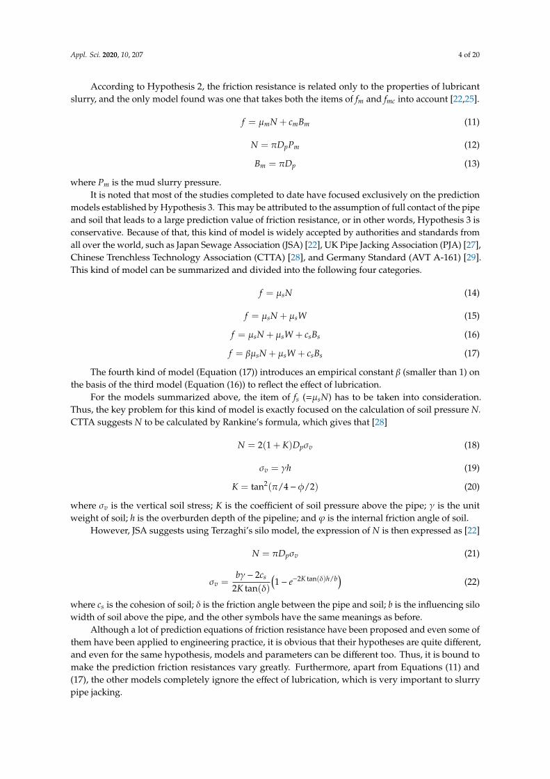
Although a lot of prediction equations of friction resistance have been proposed and even some ofthem have been applied to engineering practice, it is obvious that their hypotheses are quite different,and even for the same hypothesis, models and parameters can be different too. Thus, it is bound tomake the prediction friction resistances vary greatly. Furthermore, apart from Equations (11) and(17), the other models completely ignore the effect of lubrication, which is very important to slurrypipe jacking.

Appl. Sci. 2020, 10, 207 5 of 20

In the design philosophy of slurry pipe jacking, the angular space due to overcut is expected tobe completely filled with lubricant slurry, to reduce the friction resistance with maximum efficiency,creating a ‘filter cake’ layer around the cavity and is then pressurized to the support pressure requiredfor the soil (see Figure 2b) [3,10]. In this case, the friction resistance should be only related to theslurry pressure and the friction coefficient between slurry and the pipe. From this point of view,the expression Equation (11) seems a convincing explanation here.

However, the more general case is that the excavated tunnel is stable under pressure of slurryand part of the pipe inevitably comes in contact with the soil (see Figure 2d) [3]. The reasons for theoccurrence of pipe-soil contact can be complex, such as insufficient design and control of groutingamount of slurry, the pipeline deviates from the intended line and level, irregular deformation of thesurrounding soil, and interpenetration between the soil and slurry. Thereby, the state of contact canchange from ‘pipe-slurry’ into ‘pipe-soil-slurry’ (Figure 2b,d). In such a case, a simple form of Equation(17) seems more suitable to reflect the effect of lubricant slurry. However, it is logical that the greater thecontact width between the pipe and the soil, the smaller the effect of lubrication will be, and, therefore,the greater the friction resistance will be. Thus, the value of β should be highly affected by the pipe-soilcontact width. For different soils, grouting amount of slurry and design parameters (such as burieddepth and overcut) is bound to lead to completely different contact widths of pipe-soil. Thus, β shouldbe in a large range, and it would be rather difficult to pick out a value to use in application.

In fact, a successful prediction model of friction resistance should not only consider the effect oflubrication but also needs to be able to reflect the effect of pipe-soil-slurry interaction. It is based onthis understanding that the following model comes into being.

3. Calculation of Friction Resistance for Slurry Pipe Jacking

The general contact state of pipe-soil-slurry due to the interaction of the pipe, surrounding soil,and lubricant slurry is shown in Figure 3. In the picture, the position of pipe-soil contact is arbitrary,with a contact width of Bs and the corresponding contact angle of 2ε.

Appl. Sci. 2020, 10, x FOR PEER REVIEW 5 of 20

for the soil (see Figure 2b) [3,10]. In this case, the friction resistance should be only related to the slurry pressure and the friction coefficient between slurry and the pipe. From this point of view, the expression Equation (11) seems a convincing explanation here.

However, the more general case is that the excavated tunnel is stable under pressure of slurry and part of the pipe inevitably comes in contact with the soil (see Figure 2d) [3]. The reasons for the occurrence of pipe-soil contact can be complex, such as insufficient design and control of grouting amount of slurry, the pipeline deviates from the intended line and level, irregular deformation of the surrounding soil, and interpenetration between the soil and slurry. Thereby, the state of contact can change from ‘pipe-slurry’ into ‘pipe-soil-slurry’ (Figure 2b,d). In such a case, a simple form of Equation (17) seems more suitable to reflect the effect of lubricant slurry. However, it is logical that the greater the contact width between the pipe and the soil, the smaller the effect of lubrication will be, and, therefore, the greater the friction resistance will be. Thus, the value of β should be highly affected by the pipe-soil contact width. For different soils, grouting amount of slurry and design parameters (such as buried depth and overcut) is bound to lead to completely different contact widths of pipe-soil. Thus, β should be in a large range, and it would be rather difficult to pick out a value to use in application.

In fact, a successful prediction model of friction resistance should not only consider the effect of lubrication but also needs to be able to reflect the effect of pipe-soil-slurry interaction. It is based on this understanding that the following model comes into being.

3. Calculation of Friction Resistance for Slurry Pipe Jacking

The general contact state of pipe-soil-slurry due to the interaction of the pipe, surrounding soil, and lubricant slurry is shown in Figure 3. In the picture, the position of pipe-soil contact is arbitrary, with a contact width of Bs and the corresponding contact angle of 2ε.

Figure 3. The general contact state of pipe-soil-slurry.

From Figure 3, it is obvious that to calculate friction resistance f, both of the items of fs and fm

have to be taken into account, which can be expressed as

mmssms NNffNf μμμ +=+== (23)

where μ is an effective friction coefficient introduced to reflect the effect of lubrication and the influence of pipe-soil contact width. It is generally accepted that μs = tan(φ/2) for the coefficient of kinematic friction between soil and the pipe [21,22]; μm for the coefficient of kinematic friction between mud slurry and the pipe can be taken as 0.01, according to the test result reported by Guo [30]. Ns and Nm are the total normal force of pipe-soil and pipe-slurry in contact, respectively.

Rp

Rc

ΔRP

OcOp

2ε

Bs

Soil

Mixture of soil and slurry

Slurry

Jacking pipe

1

2

3

4

1234

Figure 3. The general contact state of pipe-soil-slurry.

From Figure 3, it is obvious that to calculate friction resistance f, both of the items of fs and fm haveto be taken into account, which can be expressed as

f = µN = fs + fm = µsNs + µmNm (23)

Appl. Sci. 2020, 10, 207 6 of 20

where µ is an effective friction coefficient introduced to reflect the effect of lubrication and the influenceof pipe-soil contact width. It is generally accepted that µs = tan(ϕ/2) for the coefficient of kinematicfriction between soil and the pipe [21,22]; µm for the coefficient of kinematic friction between mudslurry and the pipe can be taken as 0.01, according to the test result reported by Guo [30]. Ns and Nm

are the total normal force of pipe-soil and pipe-slurry in contact, respectively.To calculate Ns and Nm precisely, the location of pipe-soil contact and the magnitude of contact

angle (or contact width) and the contact force have to be determined. For various reasons leading tothe occurrence of pipe-soil contact, it seems impossible to calculate these quantities in a target sectionof the pipeline. However, if taking the whole pipeline into consideration, and assuming that thepipe-soil contact can occur at any position of a section of the pipeline with a same probability and thecontact force is approximately equal to the soil pressure in the contact area, this problem can be greatlysimplified. In this case, we have the following equations:

P = Ns =Bs

CN =

επ

N (24)

Nm =Bm

CN (25)

where C (=πDp) is the external circumference of pipe and ε is the semi-angle of contact (Figure 3).By substituting Equations (24) and (25) in Equation (23), after some algebra, giving that

µ = µsλs + µmλm

λs =BsC = ε

π , λm = BmC

(26)

Bm = C−Bs

1 + e(27)

where e is the void ratio of soil.By substituting Equation (27) in Equation (26), the expression of µ can be further rewritten as

µ = µsεπ+ µm

(1−

ε

π(1 + e)

)(28)

According to Equation (28), the calculation of ε is essential to calculate µ. Hertzian model providesa simple way for the calculation of the width of contact (or contact angle) as we have mentioned before(see Equations (8) and (10)); however, the Hertzian contact problem is approached only when theapplied force is small, or the large radial clearance is large, and the limited angle of contact is smallerthan about 30◦ [31]. Due to the technical limitations, most of the pipe jacking projects encounter clay orsandy soils and with a small overcut, it is therefore important that the applicability of the Hertziancontact model should be extremely limited here. Actually, the Hertzian contact model is just a specialcase of the Persson’s contact model with a small contact width (or angle) [31]. If a large contact angle(larger than 30◦) occurs, the more general contact model proposed by Persson should be taken as thefirst choice. The following singular integro-differential governing equation of contact angle is derivedby Persson, as [31,32]

B = 4(1− β) − 2(1− α)

+ξ∫−ξ

q(t)dt

1 + t2 −π2(1 + α)

Ep∆R

(1− v2p)P

(29)

or

π(1 + α)Ep∆R

(1− v2p)P

= 4(1− β) − 2(1− α)

+ξ∫−ξ

q(t)dt

1 + t2 − B (30)

Appl. Sci. 2020, 10, 207 7 of 20

The involved auxiliary variables are defined as [31]

∆R =Dc−Dp

2 , ξ = tan(ε2

),

α =1−η1+η , β = λ

2(1+η) ,

η =EpEs

1−v2s

1−v2p

, λ =1−2vp1−vp

− η 1−2vs1−vs

(31)

After some approximate treatments, the key terms of Equation (30) have been solved byMichele [32], as follows:

+ξ∫−ξ

q(t)dt

1 + t2 =1

2πIb

ξ2(ξ2 + 1)+

ξ2

ξ2 + 1(32)

Ib = π log(ξ2 + 1) (33)

B =2ξ4 + 2ξ2

− 1ξ2(ξ2 + 1)

(34)

By substituting these equations into Equation (29), Michele obtained an approximate form ofgeneral contact angle relation.

π(α+ 1)Ep∆R

(1− v2p)P

=(α− 1)[ln(ξ2 + 1) + 2ξ4] + 2

(ξ2 + 1)ξ2 − 4β (35)

As compared with Equation (9), Equation (35) is a far more complex nonlinear equation. It can befurther simplified with respect to that the elastic modulus of soil Es is generally much smaller than thatof pipe Ep (the difference between the two can be three orders of magnitude). Thus, from Equation (30),the magnitude of auxiliary variable η should be very large, and, therefore, the following approximaterelations can be obtained:

π(α+1)Ep

(1−v2p)≈

2πEs(1−v2

s ),

α ≈ −1,β ≈ 1−2vs

2(1−vs)

(36)

Using Equation (36), Equation (35) can be then simplified as

πEs∆R(1− v2

s )P+

1− 2vs

1− vs=

1− [ln(ξ2 + 1) + 2ξ4]

(ξ2 + 1)ξ2 (37)

From Equation (37), it is essential to calculate P, which requires one to calculate the total normalforce N. It can be gained by integrating the normal stress σn on an element of the pipe surface and isdetermined on the basis of vertical and horizontal soil stresses.

σn = σv sinθ+ σa cosθ (38)

N = 4∫ π/2

0σn

Dp

2dθ (39)

where θ is defined as the angle between the corresponding radius line and the horizontal line at eachpoint of the pipe (Figure 4).

By substituting Equation (38) in Equation (39), it is easy to obtain the equation of N, which has thesame form as Equation (18).

To calculate Equation (18), the vertical soil stress σv has to be first determined. It is noted that atthe present time, by far the most commonly used model for soil pressure calculation is Terzaghi’s silomodel (Equation (22)) [5,6,9,19,21,26]. According to Equation (22), the calculation of the vertical soil

Appl. Sci. 2020, 10, 207 8 of 20

stress requires some physical parameters that may be determined with some accuracy, such as theheight of cover h, the cohesion cs, and the unit weight of soil γ, but also some empirical parameters,such as b, δ, and K. The definition of these empirical parameters varies from one author to another.Here, typical approaches of Terzaghi, Germany Standard ATV-A 161 E-90 [29], Chinese Standard GB50332-2002 [33], UK Standard BS EN 1594-09 [34], US Standard ASTM F 1962-11 [35], UK PJA [27],Japan JMTA [36], and Japan JSA [22] would be discussed and compared.

For the calculation of silo width b, three kinds of boundary planes of wedge failure assumed bydifferent authors and the corresponding equations are clearly illustrated in Figure 5. The width of theboundary plane is related to the ‘vault’ effect of soil. Generally, a smaller b means a lower ‘vault’ effectof soil, leading to a larger vertical soil stress.

Appl. Sci. 2020, 10, x FOR PEER REVIEW 8 of 20

such as b, δ, and K. The definition of these empirical parameters varies from one author to another. Here, typical approaches of Terzaghi, Germany Standard ATV-A 161 E-90 [29], Chinese Standard GB 50332-2002 [33], UK Standard BS EN 1594-09 [34], US Standard ASTM F 1962-11 [35], UK PJA [27], Japan JMTA [36], and Japan JSA [22] would be discussed and compared.

For the calculation of silo width b, three kinds of boundary planes of wedge failure assumed by different authors and the corresponding equations are clearly illustrated in Figure 5. The width of the boundary plane is related to the ‘vault’ effect of soil. Generally, a smaller b means a lower ‘vault’ effect of soil, leading to a larger vertical soil stress.

For the determination of δ, most of the guidelines, such as PJA, JSA, JMTA, BS EN 1594-90, and GB 50332-2002 assume shear planes as perfectly rough and take an angle of friction in the shear planes δ equal to the soil internal friction angle φ. However, ATV-A 161 E-90 and ASTM F 1962-11 make a more cautious assumption and only takes into account half the internal friction angle φ/2.

Figure 4. The earth pressure and the normal stress acting on the pipe.

Figure 5. Boundary planes of wedge failure assumed by different authors. JSA: Japan Sewage Association; PJA: UK Pipe Jacking Association;

θσn

σa

σv

Op

σn

σv

σa

σv

σa

dθ

Terzaghi, BS EN 1594-09 b/2=Dp /2+Dp tan(α)

b/2=Dp/2 tan(β)

β

α=π/4 φ/2

β=π/4+α/2

h

Dp

ASTM F-1692-11, GB 50332 b/2=Dp/2+Dp/2 tan(α)

α

JMTA, JSA, PJA, ATV-A 161 E-90

α

α

Figure 4. The earth pressure and the normal stress acting on the pipe.

Appl. Sci. 2020, 10, x FOR PEER REVIEW 8 of 20

such as b, δ, and K. The definition of these empirical parameters varies from one author to another. Here, typical approaches of Terzaghi, Germany Standard ATV-A 161 E-90 [29], Chinese Standard GB 50332-2002 [33], UK Standard BS EN 1594-09 [34], US Standard ASTM F 1962-11 [35], UK PJA [27], Japan JMTA [36], and Japan JSA [22] would be discussed and compared.

For the calculation of silo width b, three kinds of boundary planes of wedge failure assumed by different authors and the corresponding equations are clearly illustrated in Figure 5. The width of the boundary plane is related to the ‘vault’ effect of soil. Generally, a smaller b means a lower ‘vault’ effect of soil, leading to a larger vertical soil stress.

For the determination of δ, most of the guidelines, such as PJA, JSA, JMTA, BS EN 1594-90, and GB 50332-2002 assume shear planes as perfectly rough and take an angle of friction in the shear planes δ equal to the soil internal friction angle φ. However, ATV-A 161 E-90 and ASTM F 1962-11 make a more cautious assumption and only takes into account half the internal friction angle φ/2.

Figure 4. The earth pressure and the normal stress acting on the pipe.

Figure 5. Boundary planes of wedge failure assumed by different authors. JSA: Japan Sewage Association; PJA: UK Pipe Jacking Association;

θσn

σa

σv

Op

σn

σv

σa

σv

σa

dθ

Terzaghi, BS EN 1594-09 b/2=Dp /2+Dp tan(α)

b/2=Dp/2 tan(β)

β

α=π/4 φ/2

β=π/4+α/2

h

Dp

ASTM F-1692-11, GB 50332 b/2=Dp/2+Dp/2 tan(α)

α

JMTA, JSA, PJA, ATV-A 161 E-90

α

α

Figure 5. Boundary planes of wedge failure assumed by different authors. JSA: Japan SewageAssociation; PJA: UK Pipe Jacking Association.

Appl. Sci. 2020, 10, 207 9 of 20

For the determination of δ, most of the guidelines, such as PJA, JSA, JMTA, BS EN 1594-90, and GB50332-2002 assume shear planes as perfectly rough and take an angle of friction in the shear planes δequal to the soil internal friction angle ϕ. However, ATV-A 161 E-90 and ASTM F 1962-11 make a morecautious assumption and only takes into account half the internal friction angle ϕ/2.

For the lateral pressure coefficient K above the tunnel, Terzaghi assumes K coefficient is equal to 1,which corresponds to the range of values encountered in clayey soils. PJA, ASTM F 1962-11, and GB50332-2002 suggest K = Ka (calculated by Rankine’s formula of active soil pressure coefficient), whileBS EN 1594 and ATV-A 161 assume K = K0 (calculated by Rankine’s formula of soil pressure coefficientat rest). Moreover, according to ATV-A 161, this K coefficient is equal to 0.5, which corresponds to aninternal soil friction angle of 30◦, a typical value for sandy soils.

Parameters of b, δ, and K chosen by the different authors have been summarized in Table 1.

Table 1. Definition of the empirical parameters in Terzaghi’s silo model by different authors [37].

Parameters b δ K c

Terzaghi (Japan) Dp(1 + 2tan α) ϕ 1 cJMTA (Japan) (Dp + 0.08)tan β ϕ 1 cJSA (Japan) (Dp + 0.1)tan β ϕ 1 cPJA (UK) Dptan β ϕ Ka = tan2 α c

BS EN 1594 (UK) Dp(1 + 2tan α) ϕ K0 = 1 − sin ϕ cAVT A-161 (Germany) 1.732Dp ϕ/2 K0 = 0.5 NoneASTM F 1962-11 (US) 1.5Dp ϕ/2 Ka = tan2 α None

GB 50332-2002 (China) Dp(1 + tan α) ϕ Ka = tan2 α None

Note: α = π/4 − ϕ/2; β = π/4 + α/2.

It is noted that none of the approaches use the same parameters. Consequently, the vertical soilstress calculated by these approaches would be quite different. Thus, it is not convincing to pick out anapproach to use without checking the field data. This work will be carried out in the next section.

Thus far, all the equations needed to calculate friction resistance have been determined. If theparameters needed for the prediction equations are quantified, by using Equations (18) and (22) thetotal normal force N can be determined, then together with Equations (23), (24), (27), (31), and (37),the contact angle 2ε, the effective friction coefficient µ, and the friction force f now can be uniquelyidentified. The flow chart is shown in Figure 6.

Appl. Sci. 2020, 10, x FOR PEER REVIEW 9 of 20

For the lateral pressure coefficient K above the tunnel, Terzaghi assumes K coefficient is equal to 1, which corresponds to the range of values encountered in clayey soils. PJA, ASTM F 1962-11, and GB 50332-2002 suggest K = Ka (calculated by Rankine’s formula of active soil pressure coefficient), while BS EN 1594 and ATV-A 161 assume K = K0 (calculated by Rankine’s formula of soil pressure coefficient at rest). Moreover, according to ATV-A 161, this K coefficient is equal to 0.5, which corresponds to an internal soil friction angle of 30°, a typical value for sandy soils.

Parameters of b, δ, and K chosen by the different authors have been summarized in Table 1.

Table 1. Definition of the empirical parameters in Terzaghi’s silo model by different authors [37].

Parameters b δ K c Terzaghi (Japan) Dp(1 + 2tan α) φ 1 c

JMTA (Japan) (Dp + 0.08)tan β φ 1 c JSA (Japan) (Dp + 0.1)tan β φ 1 c PJA (UK) Dptan β φ Ka = tan2 α c

BS EN 1594 (UK) Dp(1 + 2tan α) φ K0 = 1 − sin φ cAVT A-161 (Germany) 1.732Dp φ/2 K0 = 0.5 NoneASTM F 1962-11 (US) 1.5Dp φ/2 Ka = tan2 α None

GB 50332-2002 (China) Dp(1 + tan α) φ Ka = tan2 α NoneNote: α = π/4 − φ/2; β = π/4 + α/2.

It is noted that none of the approaches use the same parameters. Consequently, the vertical soil stress calculated by these approaches would be quite different. Thus, it is not convincing to pick out an approach to use without checking the field data. This work will be carried out in the next section.

Thus far, all the equations needed to calculate friction resistance have been determined. If the parameters needed for the prediction equations are quantified, by using Equations (18) and (22) the total normal force N can be determined, then together with Equations (23), (24), (27), (31), and (37), the contact angle 2ε, the effective friction coefficient μ, and the friction force f now can be uniquely identified. The flow chart is shown in Figure 6.

Figure 6. Flow chart of friction resistance prediction.

Apparently, the effective friction coefficient here is not just related to the interfriction angle of soil φ but also the state of pipe-soil contact and the effect of lubrication.

4. The Verification of the Effectiveness of the Proposed New Approach

4.1. Comparison between the Predicted Friction Resistances and the Field Data

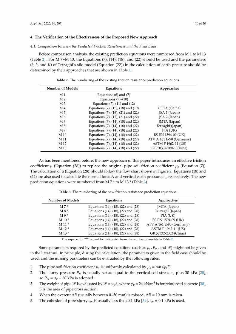
Before comparison analysis, the existing prediction equations were numbered from M 1 to M 13 (Table 2). For M 7~M 13, the Equations (7), (14), (18), and (22) should be used and the parameters (b,

Figure 6. Flow chart of friction resistance prediction.

Apparently, the effective friction coefficient here is not just related to the interfriction angle of soilϕ but also the state of pipe-soil contact and the effect of lubrication.

Appl. Sci. 2020, 10, 207 10 of 20

4. The Verification of the Effectiveness of the Proposed New Approach

4.1. Comparison between the Predicted Friction Resistances and the Field Data

Before comparison analysis, the existing prediction equations were numbered from M 1 to M 13(Table 2). For M 7~M 13, the Equations (7), (14), (18), and (22) should be used and the parameters(b, δ, and K) of Terzaghi’s silo model (Equation (22)) in the calculation of earth pressure should bedetermined by their approaches that are shown in Table 1.

Table 2. The numbering of the existing friction resistance prediction equations.

Number of Models Equations Approaches

M 1 Equations (6) and (7)M 2 Equations (7)–(10)M 3 Equations (7), (11) and (12)M 4 Equations (7), (15), (18) and (19) CTTA (China)M 5 Equations (7), (16), (21) and (22) JSA 1 (Japan)M 6 Equations (7), (17), (21) and (22) JSA 2 (Japan)M 7 Equations (7), (14), (18) and (22) JMTA (Japan)M 8 Equations (7), (14), (18) and (22) Terzaghi (Japan)M 9 Equations (7), (14), (18) and (22) PJA (UK)

M 10 Equations (7), (14), (18) and (22) BS EN 1594-09 (UK)M 11 Equations (7), (14), (18) and (22) ATV A 161 E-90 (Germany)M 12 Equations (7), (14), (18) and (22) ASTM F 1962-11 (US)M 13 Equations (7), (14), (18) and (22) GB 50332-2002 (China)

As has been mentioned before, the new approach of this paper introduces an effective frictioncoefficient µ (Equation (28)) to replace the original pipe-soil friction coefficient µs (Equation (7)).The calculation of µ (Equation (28)) should follow the flow chart shown in Figure 2. Equations (18) and(22) are also used to calculate the normal force N and vertical earth pressure σv, respectively. The newprediction equations were numbered from M 7 * to M 13 * (Table 3).

Table 3. The numbering of the new friction resistance prediction equations.

Number of Models Equations Approaches

M 7 * Equations (14), (18), (22) and (28) JMTA (Japan)M 8 * Equations (14), (18), (22) and (28) Terzaghi (Japan)M 9 * Equations (14), (18), (22) and (28) PJA (UK)

M 10 * Equations (14), (18), (22) and (28) BS EN 1594-09 (UK)M 11 * Equations (14), (18), (22) and (28) ATV A 161 E-90 (Germany)M 12 * Equations (14), (18), (22) and (28) ASTM F 1962-11 (US)M 13 * Equations (14), (18), (22) and (28) GB 50332-2002 (China)

The superscript “*” is used to distinguish from the number of models in Table 2.

Some parameters required by the predicted equations (such as µs, Pm, and W) might not be givenin the literature. In principle, during the calculation, the parameters given in the field case should beused, and the missing parameters can be evaluated by the following rules:

1. The pipe-soil friction coefficient µs is uniformly calculated by µs = tan (ϕ/2).2. The slurry pressure Pm is usually set as equal to the vertical soil stress σv plus 30 kPa [28],

so Pm = σv + 30 kPa is adopted.3. The weight of pipe W is evaluated by W = γpS, where γp = 24 kN/m3 is for reinforced concrete [38],

S is the area of pipe cross section.4. When the overcut ∆R (usually between 0~50 mm) is missed, ∆R = 10 mm is taken.5. The cohesion of pipe-slurry cm is usually less than 0.1 kPa [39], cm = 0.1 kPa is used.

Appl. Sci. 2020, 10, 207 11 of 20

6. The average values of soil parameters (such as γs, cs, ϕ, and e) can be obtained from the GeologicalEngineering Handbook.

Parameters in each of the four cases were finally determined, which are given in Table 4 [2,9,22].These cases encountered some representative soils, such as silt, clay, sand, and gravels. Furthermore,they have different overburden depths of 2.72~8.5 m, overcut of 0~20 mm, and pipe diameters of0.66~4.06 m. All of these characteristics provide good foundations for identifying the capability of theprediction models.

Table 4. Parameters that are needed to calculate the prediction equations in each case.

Cases C 1 (H City) C 2 (Shanghai) C 3 (F City) C 4 (Neuilly)

Geotechnical Description Organic Silt Silty Clay Fine Sand Sand and Gravels

Parameters

h (m) 8.15 8.5 2.72 5Dp (m) 0.96 4.06 1.2 0.66∆R (mm) 10 20 10 0γ (kN/m3) 18 19.5 20.5 21cs (kPa) 10 30 0 0ϕ (◦) 10 25 30 40Es (MPa) 12 25 30 35vs 0.35 0.3 0.25 0.2e 2 1.5 1 0.4cm (kPa) 0.1 0.1 0.1 0.1β 0.6 0.5 0.85 0.5W (kN/m) 5.5 90.2 8.5 2.2µm 0.01 0.01 0.01 0.01Pm (kPa) 89.97 110.54 62.28 45.94

In Table 5, for each of the drives, measured frictional force values are presented and comparedto values calculated by the approaches of the existing models. One can see that, for most cases,the prediction results of the models (M 1 and M 2) established based on Hypothesis 1 are generally toosmall. This is because it is correct only when the overcut is stable and the pipeline slides on its baseinside the annular gap remaining open. The same problem is encountered in M3 (established based onHypothesis 2), which is probably more due to ignoring the occurrence of pipe-soil contact decreasingthe magnitude of the effective friction coefficient. Obviously, for slurry pipe jacking, the predictionfriction based on these two assumptions may be insufficient and unsafe.

Table 5. Comparison of friction resistances calculated by the existing models and the measured data.

Cases C 1 C 2 C 3 C 4

Ratio Ratio Ratio Ratio

f mea. (kN/m) 1.5 36.16 3.78 9.75

f cal. (kN/m)

M 1 0.48 32% 20.00 55% 2.28 60% 0.80 8%M 2 2.68 179% 76.10 210% 2.28 60% 0.80 8%M 3 3.02 201% 15.37 43% 2.72 72% 1.16 12%M 4 42.47 2832% 439.47 1215% 50.09 1325% 62.22 638%M 5 39.72 2648% 575.39 1591% 32.65 864% 12.06 124%M 6 38.36 2557% 489.02 1352% 20.50 542% 6.43 66%M 7 11.14 743% 218.77 605% 38.35 1014% 13.96 143%M 8 14.28 952% 267.04 738% 41.52 1098% 15.32 157%M 9 9.42 628% 198.74 550% 37.56 994% 28.88 296%

M 10 16.68 1112% 247.43 684% 40.31 1066% 26.36 270%M 11 30.06 2004% 392.61 1086% 45.37 1200% 37.86 388%M 12 30.24 2016% 370.94 1026% 41.90 1108% 42.29 434%M 13 24.99 1666% 332.53 920% 36.72 972% 27.63 283%

Note: f mea. is the measured friction resistance; f cal. is the calculated friction resistance.

Appl. Sci. 2020, 10, 207 12 of 20

The calculated results of M4 are much larger than the measured data, which presumably resultfrom ignoring the ‘vault effect’ of soil, so that the soil pressure has been overestimated. Apart fromM4, the other models established based on Hypothesis 3 (M5~13) have shown some applicability incase 4, in which the overcut of C4 is equal to zero, which is exactly in line with the assumption of thefull contact of pipe-soil of Hypothesis 3. Except for C4, the prediction results of other cases are muchlarger, and the amplitude may be up to 30 times the measured data. Therefore, for slurry pipe jacking,Hypothesis 3 is generally over-conservative. Although it can ensure the structural safety of the design,it may also cause a much higher construction cost.

From what we have analyzed above, the existing models have good prediction results only whenthe field case is consistent with the basic hypothesis of each model. However, it is also these hypothesesthat determine their limited applicability.

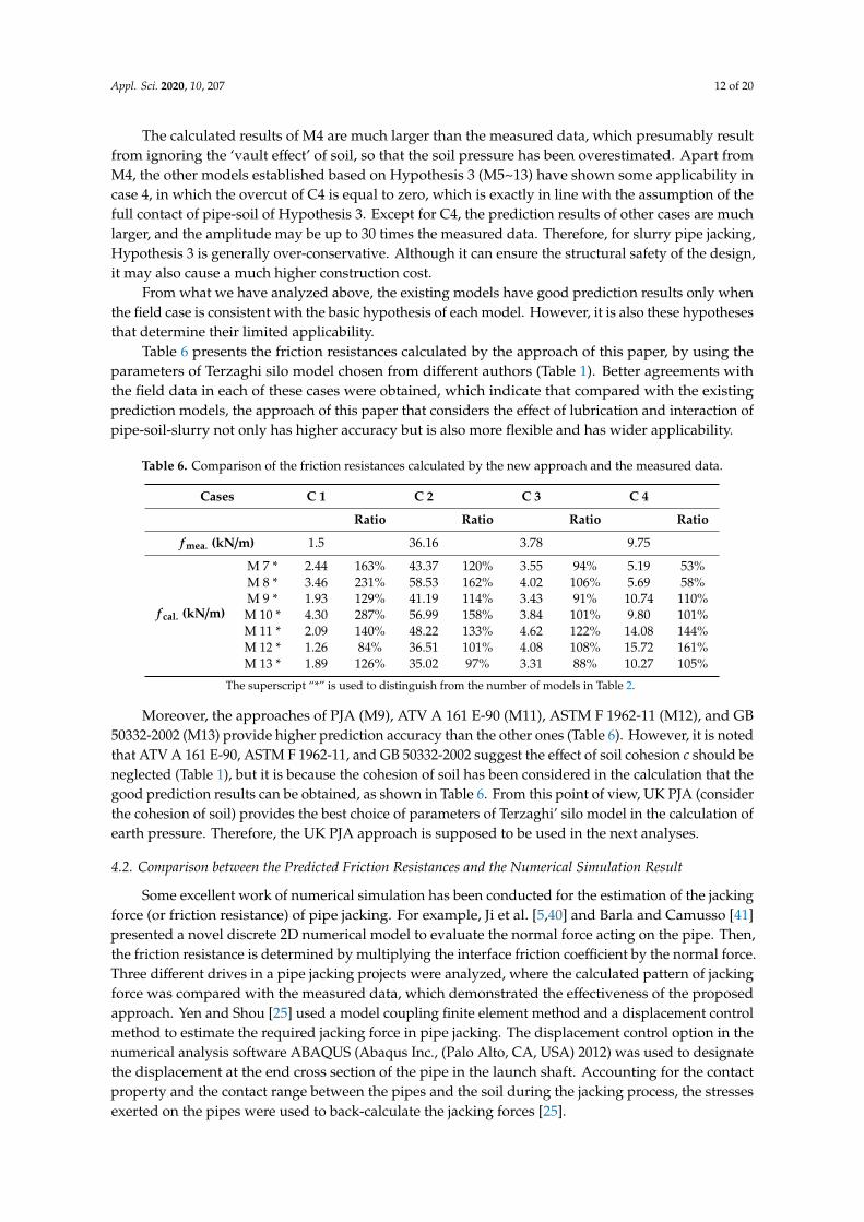
Table 6 presents the friction resistances calculated by the approach of this paper, by using theparameters of Terzaghi silo model chosen from different authors (Table 1). Better agreements withthe field data in each of these cases were obtained, which indicate that compared with the existingprediction models, the approach of this paper that considers the effect of lubrication and interaction ofpipe-soil-slurry not only has higher accuracy but is also more flexible and has wider applicability.

Table 6. Comparison of the friction resistances calculated by the new approach and the measured data.

Cases C 1 C 2 C 3 C 4

Ratio Ratio Ratio Ratio

f mea. (kN/m) 1.5 36.16 3.78 9.75

f cal. (kN/m)

M 7 * 2.44 163% 43.37 120% 3.55 94% 5.19 53%M 8 * 3.46 231% 58.53 162% 4.02 106% 5.69 58%M 9 * 1.93 129% 41.19 114% 3.43 91% 10.74 110%M 10 * 4.30 287% 56.99 158% 3.84 101% 9.80 101%M 11 * 2.09 140% 48.22 133% 4.62 122% 14.08 144%M 12 * 1.26 84% 36.51 101% 4.08 108% 15.72 161%M 13 * 1.89 126% 35.02 97% 3.31 88% 10.27 105%

The superscript “*” is used to distinguish from the number of models in Table 2.

Moreover, the approaches of PJA (M9), ATV A 161 E-90 (M11), ASTM F 1962-11 (M12), and GB50332-2002 (M13) provide higher prediction accuracy than the other ones (Table 6). However, it is notedthat ATV A 161 E-90, ASTM F 1962-11, and GB 50332-2002 suggest the effect of soil cohesion c should beneglected (Table 1), but it is because the cohesion of soil has been considered in the calculation that thegood prediction results can be obtained, as shown in Table 6. From this point of view, UK PJA (considerthe cohesion of soil) provides the best choice of parameters of Terzaghi’ silo model in the calculation ofearth pressure. Therefore, the UK PJA approach is supposed to be used in the next analyses.

4.2. Comparison between the Predicted Friction Resistances and the Numerical Simulation Result

Some excellent work of numerical simulation has been conducted for the estimation of the jackingforce (or friction resistance) of pipe jacking. For example, Ji et al. [5,40] and Barla and Camusso [41]presented a novel discrete 2D numerical model to evaluate the normal force acting on the pipe. Then,the friction resistance is determined by multiplying the interface friction coefficient by the normal force.Three different drives in a pipe jacking projects were analyzed, where the calculated pattern of jackingforce was compared with the measured data, which demonstrated the effectiveness of the proposedapproach. Yen and Shou [25] used a model coupling finite element method and a displacement controlmethod to estimate the required jacking force in pipe jacking. The displacement control option in thenumerical analysis software ABAQUS (Abaqus Inc., (Palo Alto, CA, USA) 2012) was used to designatethe displacement at the end cross section of the pipe in the launch shaft. Accounting for the contactproperty and the contact range between the pipes and the soil during the jacking process, the stressesexerted on the pipes were used to back-calculate the jacking forces [25].

Appl. Sci. 2020, 10, 207 13 of 20

The numerical simulation strategy of Yen and Shou [25] is quite consistent with the analyticalapproach of this paper. Therefore, the numerical simulation approach of Yen and Shou will be describedin the next section and its estimated result of friction resistance will be discussed and compared withthat calculated by the analytical approach of this paper.

One of the analyses focused on a case of slurry pipe jacking in the Taichung Science Park, the basicparameters of this case were summarized in Table 7. In the numerical simulation, the lateral boundarieswere fixed by roller, and hinges were used to constrain the bottom boundary. The three dimensionalhexahedron element (C3D8R) with eight nodes was used in the simulation. To verify the jacking forceobtained from the displacement control simulation, overcut and lubrication were included in the modelby setting the contact range (1/3, 1/2, and 1 pipe-soil contact) and the frictional coefficient (Figure 7a–c).The results suggested the 1/3 contact case can estimate the jacking force with a better accuracy towardsthe middle and the final stage of the pipe jacking process (Figure 8).

Table 7. The details of the slurry pipe jacking in Taichung Science Park.

Geology h (m) Dp (m) ∆R (mm) γ (kN/m3) c (kPa) ϕ (◦) Es (MPa) vs e

Gravel 13.0 2.85 10 21 15 37 33 0.20 1

Appl. Sci. 2020, 10, x FOR PEER REVIEW 13 of 20

The numerical simulation strategy of Yen and Shou [25] is quite consistent with the analytical approach of this paper. Therefore, the numerical simulation approach of Yen and Shou will be described in the next section and its estimated result of friction resistance will be discussed and compared with that calculated by the analytical approach of this paper.

One of the analyses focused on a case of slurry pipe jacking in the Taichung Science Park, the basic parameters of this case were summarized in Table 7. In the numerical simulation, the lateral boundaries were fixed by roller, and hinges were used to constrain the bottom boundary. The three dimensional hexahedron element (C3D8R) with eight nodes was used in the simulation. To verify the jacking force obtained from the displacement control simulation, overcut and lubrication were included in the model by setting the contact range (1/3, 1/2, and 1 pipe-soil contact) and the frictional coefficient (Figure 7a–c). The results suggested the 1/3 contact case can estimate the jacking force with a better accuracy towards the middle and the final stage of the pipe jacking process (Figure 8).

Table 7. The details of the slurry pipe jacking in Taichung Science Park.

Geology h (m) Dp (m) ΔR (mm) γ (kN/m3) c (kPa) φ (°) Es (MPa) vs e

Gravel 13.0 2.85 10 21 15 37 33 0.20 1

(a) (b) (c)

Figure 7. The setting of pipe-soil contact range and frictional coefficient in the numerical simulation. (a) 1/3 of the pipe-soil contact; (b) 1/2 of the pipe-soil contact; (c) 1 of the pipe-soil contact.

In Figure 8, the slope of the linear regression for the scattered points represents frictional resistance, and the intercept represents face resistance. For the calculated result of this paper, the measured face resistance is used, and the frictional resistance (fcal. = 57.7 kN/m) is calculated by the new approach (Section 3) using parameters of UK PJA in Terzaghi’s silo model (Table 1). For the result of numerical simulation, the decrease of jacking force in the initial stage of drives (before 62.5 m) is explained by authors that the weight of the pipe jacking machine (the material of which is steel, featuring a larger unit weight) directly pressing on the soil, causing a larger face resistance. After the drives of 62.5 m, the influence exerted by the machine weight decreased gradually and the increase of jacking force is caused by the accumulation of friction resistance [25]. In other words, the slope of regression from drives of 62.5 to 100 m represents the friction resistance estimated by numerical simulation (fnum. = 64.4 kN/m).

It is obvious that both the predicted friction resistances of the analytical equations (fcal. = 57.7 kN/m) and the numerical simulation (fnum. = 64.4 kN/m) are acceptable as compared to the measured data (fmea. = 41.5 kN/m). However, better accuracy (especially towards the first 80 m of drives) is obtained by the approach of this paper.

Pipe-soil contact

Pipe-slurry contactμm=0

μs=0.4

120° 180°

Pipe-soil contact

Pipe-slurry contact

μs=0.4

μm=0

Pipe-soil contactμs=0.4

360°

Figure 7. The setting of pipe-soil contact range and frictional coefficient in the numerical simulation.(a) 1/3 of the pipe-soil contact; (b) 1/2 of the pipe-soil contact; (c) 1 of the pipe-soil contact.

In Figure 8, the slope of the linear regression for the scattered points represents frictional resistance,and the intercept represents face resistance. For the calculated result of this paper, the measured faceresistance is used, and the frictional resistance (f cal. = 57.7 kN/m) is calculated by the new approach(Section 3) using parameters of UK PJA in Terzaghi’s silo model (Table 1). For the result of numericalsimulation, the decrease of jacking force in the initial stage of drives (before 62.5 m) is explainedby authors that the weight of the pipe jacking machine (the material of which is steel, featuring alarger unit weight) directly pressing on the soil, causing a larger face resistance. After the drives of62.5 m, the influence exerted by the machine weight decreased gradually and the increase of jackingforce is caused by the accumulation of friction resistance [25]. In other words, the slope of regressionfrom drives of 62.5 to 100 m represents the friction resistance estimated by numerical simulation(f num. = 64.4 kN/m).

It is obvious that both the predicted friction resistances of the analytical equations (f cal. = 57.7 kN/m)and the numerical simulation (f num. = 64.4 kN/m) are acceptable as compared to the measured data(f mea. = 41.5 kN/m). However, better accuracy (especially towards the first 80 m of drives) is obtainedby the approach of this paper.

Appl. Sci. 2020, 10, 207 14 of 20Appl. Sci. 2020, 10, x FOR PEER REVIEW 14 of 20

Figure 8. The comparison of jacking forces from monitoring, the numerical simulation, and the predicted equations of this paper.

The predicted accuracy of friction resistance by the numerical simulation approach is highly affected by the setting of pipe-soil contact angle. The pipe-soil contact angle of 71 degrees is that calculated by the analytical equations for this field case. Thus, it seems that the pipe-soil contact angle of 120 degrees (1/3 contact) in the simulation is set too large, resulting in the calculated result slightly larger than the measured data. From this point of view, the numerical simulation approach can accurately predict the friction resistance, but the contact angle of pipe-soil in the simulation needs to be set reasonably to obtain good prediction results. Conversely, in the approach of this paper, the pipe-soil contact angle is theoretically calculated with respect to soil property, overcut, pipe diameter, etc., while human factors or empirical factors can be eliminated as far as possible.

5. Influence of Design Factors on Lubrication Efficiency and Friction Resistance

For a better design of slurry pipe jacking in the future, it is meaningful to study the influence of design parameters (such as buried depth h, pipe diameter Dp, and the overcut ΔR) on lubrication efficiency and friction resistance. To achieve this objective, a set of reference parameters is used, and then, by changing a target parameter according to the design rules, the effect of that parameter on friction resistance and lubrication efficiency can be obtained. The designed cases were shown in Table 8.

Table 8. The reference parameters and cases designed to study the influence of factors on friction resistance.

Reference Parameters h = 10 m, Dp = 2 m, ΔR = 20 mm, γ = 20 kN/m3, cs = 15 kPa, φ = 25°, Es = 25 Mpa, vs

= 0.25, e = 1, μm = 0.01

Designed cases

h (m) 5→8→10→15→20→25→30

Dp (m) 1→1.5→2→2.5→3→3.5→4

ΔR (m) 0→5→10→20→30→40→50

5.1. Influence of Design Factors on Friction Resistance

0

1000

2000

3000

4000

5000

6000

7000

8000

9000

0 10 20 30 40 50 60 70 80 90 100 110 120 130 140 150

Jack

ing

Forc

e (k

N)

Distance (m)

Measured dataResult of numerical simulationCalculated result of this paper

fnum.=64.4kN/m

fcal.=57.7kN/m

fmea.=41.5kN/m

Slope=Friction resistance

Intercept=Face resistance

Figure 8. The comparison of jacking forces from monitoring, the numerical simulation, and thepredicted equations of this paper.

The predicted accuracy of friction resistance by the numerical simulation approach is highlyaffected by the setting of pipe-soil contact angle. The pipe-soil contact angle of 71 degrees is thatcalculated by the analytical equations for this field case. Thus, it seems that the pipe-soil contactangle of 120 degrees (1/3 contact) in the simulation is set too large, resulting in the calculated resultslightly larger than the measured data. From this point of view, the numerical simulation approach canaccurately predict the friction resistance, but the contact angle of pipe-soil in the simulation needs to beset reasonably to obtain good prediction results. Conversely, in the approach of this paper, the pipe-soilcontact angle is theoretically calculated with respect to soil property, overcut, pipe diameter, etc., whilehuman factors or empirical factors can be eliminated as far as possible.

5. Influence of Design Factors on Lubrication Efficiency and Friction Resistance

For a better design of slurry pipe jacking in the future, it is meaningful to study the influenceof design parameters (such as buried depth h, pipe diameter Dp, and the overcut ∆R) on lubricationefficiency and friction resistance. To achieve this objective, a set of reference parameters is used,and then, by changing a target parameter according to the design rules, the effect of that parameteron friction resistance and lubrication efficiency can be obtained. The designed cases were shownin Table 8.

Table 8. The reference parameters and cases designed to study the influence of factors on friction resistance.

Reference Parameters h = 10 m, Dp = 2 m, ∆R = 20 mm, γ = 20 kN/m3, cs = 15 kPa, ϕ = 25◦,Es = 25 Mpa, vs = 0.25, e = 1, µm = 0.01

Designed casesh (m) 5→8→10→15→20→25→30Dp (m) 1→1.5→2→2.5→3→3.5→4∆R (m) 0→5→10→20→30→40→50

Appl. Sci. 2020, 10, 207 15 of 20

5.1. Influence of Design Factors on Friction Resistance

The influences of design factors (h, Dp, and ∆R) on the critical quantities of effective frictioncoefficient µ, normal force acting on the pipe N, and friction resistance f are respectively shown inFigure 9a–c, Figure 9d–f, Figure 9g–i.

Appl. Sci. 2020, 10, x FOR PEER REVIEW 15 of 20

The influences of design factors (h, Dp, and ΔR) on the critical quantities of effective friction coefficient μ, normal force acting on the pipe N, and friction resistance f are respectively shown in Figure 9a–c, Figure 9d–f, Figure 9g–i.

(a) (b) (c)

(d) (e) (f)

(g) (h) (i)

Figure 9. The influence of factors of h, Dp, and ΔR on the quantities of μ (a–c), N (d–f), and f (g–i).

It is evident that increasing buried depth and pipe diameter led to a double action for the increasing of friction resistance. Firstly, this increase then increased the possibility of contact between the pipe and soil, and, therefore, increase the effective friction coefficient μ on the interface. Secondly, the increasing of buried depth increases the vertical soil stress, while the increasing of pipe diameter increases the contact area, both effects of them increase normal force N acting on the pipes. The main difference between the two is that buried depth causes both of the effective friction coefficient and normal force to slightly increase and then gradually stabilize, while they approximately linearly increase with pipe diameter. Especially for the normal force induced by pipe diameter, which is strongly increased from 29.83 to 991.34 kN, this leads to a notable increase of friction resistance from 0.34 to 48.16 kN/m. Thus, the additional friction is strongly affected by the pipe diameter but appears not to be greatly affected by the buried depth.

Different from the buried depth and pipe diameter, the overcut with small values has no effect on the normal force (Figure 9h). However, it has a strongly negative effect on the effective friction coefficient on the interface (Figure 9g). In fact, it does determine the volume of injected lubricant slurry, which has a significant influence on the occurrence of the pipe-soil contact, and, therefore,

0.00

0.02

0.04

0.06

0.08

0.10

5 10 15 20 25 30

μ

h (m)

0

200

400

600

800

1000

5 10 15 20 25 30

N (k

N/m

)

h (m)

0

10

20

30

40

50

5 10 15 20 25 30

f (kN

/m)

h (m)

0.00

0.02

0.04

0.06

0.08

0.10

1 1.5 2 2.5 3 3.5 4

μ

Dp (m)

0

200

400

600

800

1000

1 1.5 2 2.5 3 3.5 4

N (k

N/m

)

Dp (m)

0

10

20

30

40

50

1 1.5 2 2.5 3 3.5 4f (

kN/m

)

Dp (m)

0.00

0.02

0.04

0.06

0.08

0.10

0 10 20 30 40 50

μ

ΔR (mm)

0

200

400

600

800

1000

0 10 20 30 40 50

N (k

N/m

)

ΔR (mm)

0

10

20

30

40

50

0 10 20 30 40 50

f (kN

/m)

ΔR (mm)

Figure 9. The influence of factors of h, Dp, and ∆R on the quantities of µ (a–c), N (d–f), and f (g–i).

It is evident that increasing buried depth and pipe diameter led to a double action for the increasingof friction resistance. Firstly, this increase then increased the possibility of contact between the pipe andsoil, and, therefore, increase the effective friction coefficient µ on the interface. Secondly, the increasingof buried depth increases the vertical soil stress, while the increasing of pipe diameter increases thecontact area, both effects of them increase normal force N acting on the pipes. The main differencebetween the two is that buried depth causes both of the effective friction coefficient and normal forceto slightly increase and then gradually stabilize, while they approximately linearly increase with pipediameter. Especially for the normal force induced by pipe diameter, which is strongly increased from29.83 to 991.34 kN, this leads to a notable increase of friction resistance from 0.34 to 48.16 kN/m. Thus,the additional friction is strongly affected by the pipe diameter but appears not to be greatly affectedby the buried depth.

Different from the buried depth and pipe diameter, the overcut with small values has no effecton the normal force (Figure 9h). However, it has a strongly negative effect on the effective frictioncoefficient on the interface (Figure 9g). In fact, it does determine the volume of injected lubricant

Appl. Sci. 2020, 10, 207 16 of 20

slurry, which has a significant influence on the occurrence of the pipe-soil contact, and, therefore,determine the magnitude of the effective friction coefficient. Thus, it has a strongly negative effect onthe friction resistance.

5.2. Influence of Design Factors on Lubrication Efficiency

Except for friction resistance, engineers are also concerned about the lubrication efficiency [9,42,43].According to Equation (27), the magnitude of µ is between the pipe-slurry friction coefficient µm andthe pipe-soil friction coefficient µs. If there is no contact between the pipe and the soil, the angularspace due to overcut is completely filled with lubricant slurry, the effective friction coefficient is equal toµm; and if the soil is in full contact with the external surface of the pipe, the effective friction coefficientmainly depends on the pipe-soil nature and approximately equals to µs. Thus, the lubrication efficiencycan be defined as

χ =

(1−

µ− µm

µs

)× 100% (40)

By substituting Equation (28) in Equation (31), and considering that µm is far smaller than µs,the χ can approximately be expressed by Equation (41).

χ =(1−

επ

)× 100% (41)

If pipe-soil contact angle ε = 0, χ = 100% for maximum lubrication efficiency, and if ε = π, χ = 0%for minimum lubrication efficiency. It is noted that χ = 0% is not going to happen. According to thePasson model (Equation (37)), the result calculated by the left terms of Equation (37) should be not lessthan zero, while the right term of Equation (37) is a monotonically decreasing function of pipe-soilcontact angle. In other words, when the right term of Equation (37) is equal to zero, the pipe-soilcontact angle reaches its maximum value, which is solved by ε = εmax = 72◦ = 0.4π, corresponding tothe minimum lubrication efficiency of 60% (i.e., χ is theoretically between 60% and 100% on the basisof Passon contact model). Although it is not theoretically correct as compared to that counted by Pelletand Kastner as between 45% and 90% [9] and tested by Zhou as between 47.8% and 78.6% [5], it seemspractical to estimate the efficiency of lubrication by the approach of this paper.

The pipe-soil contact angle and the corresponding lubrication efficiency calculated by Equation(41) has been shown in Figure 10a–c, Figure 10d–f, respectively. It is found that, as compared to thelow effect of overburden depth, special attention should be paid to the effect of pipe diameter andthe overcut.

Figure 10f shows that the lubrication efficiency strongly increases from 64% to 91%, while theovercut increases only from 0 to 15 mm, and after that, the effect of overcut is significantly reduced.This observation confirms the importance of overcut, which has to be sufficiently wide so that thedecrease of tunnel diameter induced by the elastic ground unloading does not lead to the closure of theannular space. Moreover, Figure 10e shows that the increasing of pipe diameter from 1 to 4 m causesobvious efficiency losses of lubrication from 99% to 82%. Thus, one can conclude that the larger thepipe diameter, the lager the overcut is needed.

The buried depth h is determined by the intended line and level of the tunnel, which is oftenlimited by geological conditions and distributions of the existing buildings and structures, while thepipe diameter Dp highly depends on the practical use or traffic requirements. It seems that there are notmany options for the buried depth h and pipe diameter Dp in the design. From this point of view, bothfor lubrication efficiency and friction reaction, more attention should be paid to the design of overcut.

Parts of the conclusions analytically discussed above have been verified by authors from fieldobservations [9,20], which in turn again confirm the feasibility of the approach of this paper.

Appl. Sci. 2020, 10, 207 17 of 20Appl. Sci. 2020, 10, x FOR PEER REVIEW 17 of 20

(a) (b) (c)

(d) (e) (f)

Figure 10. The influences of factors of h, Dp, and ΔR on the pipe-soil contact angle 2ε (a–c) and lubrication efficiency χ (d–f).

6. Conclusions

Some typical prediction models of friction resistance have been presented and detailed comparisons and analyses have also been made. Then, a new approach considering both the effect of lubrication and the interaction of pipe-soil-slurry, by introducing an effective friction coefficient, has been established. Values of friction resistance calculated using them have been compared with values measured in four field cases and a numerical simulation case with various soils and design parameters. Better agreements are obtained, which indicate a more flexible and wider applicability of the approach in this paper as compared to the existing prediction models and numerical simulation approach. Explanations have also been sought for limited use of the existing models that may be attributed to their hypotheses not that suitable for slurry pipe jacking. The numerical simulation approach can accurately predict the friction resistance, but it is hard to determine the contact angle of pipe-soil reasonably with respect to various soils, overcut, and other conditions to obtain good prediction results.

Using the approach of this paper, for higher prediction accuracy, the cohesion of soil has to be taken into account in the calculation for drives in clayey soils. The Terzaghi’s silo model together with parameters determined by the approach of UK PJA is verified as the most well-considered to calculate earth pressure.

For better design in the future, the influences of design factors (buried depth, pipe diameter, and overcut) on friction resistance and lubrication efficiency have been analyzed too. The increase of pipe diameter has a strong influence on the increase of friction resistance; however, the friction amplitude appears not to be greatly affected by the buried depth. As the selection of pipe diameter and buried depth are limited by various objective conditions, special attention should be paid on the design of overcut. The overcut has to be sufficiently wide. When the overcut is small (for example smaller than 15 mm), the decrease of overcut strongly affects the decrease of lubrication efficiency, and, therefore, leads to a notable increase in friction resistance. Moreover, pipe diameter has an obvious influence on the effect of overcut on lubrication efficiency, the larger the pipe diameter the larger the overcut needed.

Author Contributions: L.P. and C.S. put forward the methodology; Y.Z. and Y.L. collected cases’ data; Y.Y. derived the formulas and wrote the paper; W.Y. reviewed and edited the paper.

0

30

60

90

120

150

5 10 15 20 25 30

2ε (d

eg.)

h (m)

0

30

60

90

120

150

1 1.5 2 2.5 3 3.5 4

2ε (d

eg.)

Dp (m)

0

30

60

90

120

150

0 10 20 30 40 50

2ε (d

eg.)

ΔR (mm)

60%

70%

80%

90%

100%

5 10 15 20 25 30

χ

h (m)

60%

70%

80%

90%

100%

1 1.5 2 2.5 3 3.5 4

χ

Dp (m)

60%

70%

80%

90%

100%

0 10 20 30 40 50

χ

ΔR (mm)

Figure 10. The influences of factors of h, Dp, and ∆R on the pipe-soil contact angle 2ε (a–c) andlubrication efficiency χ (d–f).

6. Conclusions

Some typical prediction models of friction resistance have been presented and detailed comparisonsand analyses have also been made. Then, a new approach considering both the effect of lubrication andthe interaction of pipe-soil-slurry, by introducing an effective friction coefficient, has been established.Values of friction resistance calculated using them have been compared with values measured infour field cases and a numerical simulation case with various soils and design parameters. Betteragreements are obtained, which indicate a more flexible and wider applicability of the approach in thispaper as compared to the existing prediction models and numerical simulation approach. Explanationshave also been sought for limited use of the existing models that may be attributed to their hypothesesnot that suitable for slurry pipe jacking. The numerical simulation approach can accurately predict thefriction resistance, but it is hard to determine the contact angle of pipe-soil reasonably with respect tovarious soils, overcut, and other conditions to obtain good prediction results.

Using the approach of this paper, for higher prediction accuracy, the cohesion of soil has to betaken into account in the calculation for drives in clayey soils. The Terzaghi’s silo model together withparameters determined by the approach of UK PJA is verified as the most well-considered to calculateearth pressure.

For better design in the future, the influences of design factors (buried depth, pipe diameter,and overcut) on friction resistance and lubrication efficiency have been analyzed too. The increaseof pipe diameter has a strong influence on the increase of friction resistance; however, the frictionamplitude appears not to be greatly affected by the buried depth. As the selection of pipe diameterand buried depth are limited by various objective conditions, special attention should be paid on thedesign of overcut. The overcut has to be sufficiently wide. When the overcut is small (for examplesmaller than 15 mm), the decrease of overcut strongly affects the decrease of lubrication efficiency, and,therefore, leads to a notable increase in friction resistance. Moreover, pipe diameter has an obviousinfluence on the effect of overcut on lubrication efficiency, the larger the pipe diameter the larger theovercut needed.

Appl. Sci. 2020, 10, 207 18 of 20

Author Contributions: L.P. and C.S. put forward the methodology; Y.Z. and Y.L. collected cases’ data; Y.Y. derivedthe formulas and wrote the paper; W.Y. reviewed and edited the paper. All authors have read and agreed to thepublished version of the manuscript.

Funding: The authors acknowledge the financial support of the National Natural Science Foundation of China(No. 51878670).

Conflicts of Interest: The authors declare no conflict of interest.

Abbreviations

f friction force per meter length driveµ effective friction coefficient for slurry pipe jackingµs soil-pipe friction coefficientµm slurry-pipe friction coefficientδ pipe-soil friction angleN normal force due to soil pressure acting on pipeP effective external load applied at the center of the pipesσn normal soil stress acting on any point of pipesσv vertical soil stressσa horizontal soil stressh overburden depthDc internal diameter of cavityDp external diameter of pipeRc internal radius of cavityRp external radius of pipe∆R radial clearance (or overcut)Bs width of contact between the pipe and soilBm width of contact between the pipe and mud slurryb influencing width of soil above the pipeε semi-angle of contact areac soil cohesionϕ inner friction angle of soilγ unit weight of soile void ratio of soilK lateral coefficient of soil pressure above the pipeEp elasticity modulus of pipeEs elasticity modulus of soilvp Poisson’s ratio of pipevs Poisson’s ratio of soil

References

1. Ji, X.; Zhao, W.; Jia, P.; Qiao, L.; Barla, M.; Ni, P.; Wang, L. Pipe Jacking in Sandy Soil under a River inShenyang, China. Indian Geotech. J. 2017, 47, 246–260. [CrossRef]

2. Wang, J.F.; Wang, K.; Zhang, T.; Wang, S. Key aspects of a DN4000 steel pipe jacking project in China: A casestudy of a water pipeline in the Shanghai Huangpu River. Tunn. Undergr. Space Technol. 2018, 72, 323–332.[CrossRef]

3. Khazaei, S.; Shimada, H.; Kawai, T.; Yotsumoto, J.; Matsui, K. Monitoring of over cutting area and lubricationdistribution in a large slurry pipe jacking operation. Geotech. Geol. Eng. 2006, 24, 735–755. [CrossRef]

4. Ji, X.; Ni, P.; Barla, M.; Zhao, W.; Mei, G.X. Earth pressure on shield excavation face for pipe jackingconsidering arching effect. Tunn. Undergr. Space Technol. 2018, 72, 17–27. [CrossRef]

5. Ji, X.; Zhao, W.; Ni, P.; Barla, M.; Han, J.; Jia, P.; Chen, Y.; Zhang, C. A method to estimate the jacking force forpipe jacking in sandy soils. Tunn. Undergr. Space Technol. 2019, 90, 119–130. [CrossRef]

6. Ong, D.E.L.; Choo, C.S. Assessment of non-linear rock strength parameters for the estimation of pipe-jackingforces. Part 1. Direct shear testing and backanalysis. Eng. Geol. 2019, 244, 159–172. [CrossRef]

Appl. Sci. 2020, 10, 207 19 of 20

7. Ren, D.J.; Xu, Y.S.; Shen, J.S.; Zhou, A.; Arulrajah, A. Prediction of ground deformation during pipe-jackingconsidering multiple factors. Appl. Sci. 2018, 8, 1051. [CrossRef]

8. Zhang, Y.; Yan, Z.G.; Zhu, H.H. A full-scale experimental study on the performance of jacking prestressedconcrete cylinder pipe with misalignment angle. In Proceedings of Geo. Shanghai 2018 International Conference:Multi-physics Processes in Soil Mechanics and Advances in Geotechnical Testing; Springer: Singapore, 2018;pp. 345–354.

9. Pellet-Beaucour, A.L.; Kastner, R. Experimental and analytical study of friction forces during microtunnelingoperations. Tunn. Undergr. Space Technol. 2002, 17, 83–97. [CrossRef]

10. Milligan, G.W.E.; Norris, P. Pipe-soil interaction during pipe jacking. Proc. Inst. Civ. Eng. Geotech. Eng. 1999,137, 27–44. [CrossRef]

11. Shou, K.J.; Yen, J.; Liu, M. On the frictional property of lubricants and its impact on jacking force and soil-pipeinteraction of pipe-jacking. Tunn. Undergr. Space Technol. 2010, 25, 469–477. [CrossRef]

12. Yang, X.; Liu, Y.; Yang, C. Research on the slurry for long-distance large-diameter pipe jacking in expansivesoil. Adv. Civ. Eng. 2018, 2018, 9040471. [CrossRef]

13. Sterling, R.L. Developments and research directions in pipe jacking and microtunneling. Undergr. Space 2018,in press. [CrossRef]

14. Milligan, G.W.E.; Norris, P. Site-based research in pipe jacking-objectives, procedures and a case history.Tunn. Undergr. Space Technol. 1996, 11, 3–24. [CrossRef]

15. Cui, Q.L.; Xu, Y.S.; Shen, S.L.; Yin, Z.-Y.; Horpibulsuk, S. Field performance of concrete pipes during jackingin cemented sandy silt. Tunn. Undergr. Space Technol. 2015, 49, 336–344. [CrossRef]

16. Cheng, W.C.; Ni, J.C.; Arulrajah, A.; Huang, H.W. A simple approach for characterising tunnel bore conditionsbased upon pipe-jacking data. Tunn. Undergr. Space Technol. 2018, 71, 494–504. [CrossRef]

17. Cheng, W.C.; Ni, J.C.; Shen, S.L.; Huang, H.W. Investigation into factors affecting jacking force: A case study.Proc. Inst. Civ. Eng. Geotech. Eng. 2017, 170, 322–334. [CrossRef]

18. Zhang, P.; Behbahani, S.S.; Ma, B.; Iseley, T.; Tan, L. A jacking force study of curved steel pipe roof in Gongbeitunnel: Calculation review and monitoring data analysis. Tunn. Undergr. Space Technol. 2018, 72, 305–322.[CrossRef]

19. O’Dwyer, K.G.; McCabe, B.A.; Sheil, B.B. Interpretation of pipe-jacking and lubrication records for drives insilty soil. Undergr. Space 2019, in press.

20. Chapman, D.N.; Ichioka, Y. Prediction of jacking forces for microtunnelling operations. Trenchless Technol. Res.1999, 14, 31–41. [CrossRef]

21. Sofianos, A.I.; Loukas, P.; Chantzakos, C. Pipe jacking a sewer under Athens. Tunn. Undergr. Space Technol.2004, 19, 193–203. [CrossRef]

22. Shimada, H.; Khazaei, S.; Matsui, K. Small diameter tunnel excavation method using slurry pipe-jacking.Geotech. Geol. Eng. 2004, 22, 161–186. [CrossRef]

23. Barla, M.; Camusso, M.; Aiassa, S. Analysis of jacking forces during microtunnelling in limestone. Tunn. Undergr.Space Technol. 2006, 21, 668–683. [CrossRef]

24. Chapman, D.N.; Rogers, C.D.F.; Burd, H.J. Research needs for new construction using trenchless technologies.Tunn. Undergr. Space Technol. 2007, 22, 491–502. [CrossRef]

25. Yen, J.; Shou, K. Numerical simulation for the estimation the jacking force of pipe jacking. Tunn. Undergr.Space Technol. 2015, 49, 218–229. [CrossRef]

26. Zhang, H.; Zhang, P.; Zhou, W.; Dong, S.; Ma, B. A new model to predict soil pressure acting on deep burialjacked pipes. Tunn. Undergr. Space Technol. 2016, 60, 183–196. [CrossRef]

27. PJA. Guide to Best Practice for the Installation of Pipe Jacks and Microtunnels; Pipe Jacking Association: London,UK, 1995.

28. CTTA. Specifications for Construction and Acceptance of Pipe Jacking; China Trenchless Technology Association(CTTA): Wuhan, China, 2006; pp. 38–39.

29. ATV-A 161 E-90. Structural Calculation of Driven Pipes; German ATV Rules and Standards: Hennef, Germany,1990; pp. 18–20.

30. Guo, W.; Xie, H.; Wu, R.; Zhou, B. Experimental study on bentonite lubrication during pipe jackingconstruction. J. Henan Sci. Technol. 2015, 555, 115–118. (In Chinese)

31. Michele, C.; Paolo, D. The state of stress induced by the plane frictionless cylindrical contact. I. The case ofelastic similarity. Int. J. Solids Struct. 2001, 38, 4507–4523.

Appl. Sci. 2020, 10, 207 20 of 20

32. Michele, C.; Paolo, D. The state of stress induced by the plane frictionless cylindrical contact. II. The generalcase (elastic dissimilarity). Int. J. Solids Struct. 2001, 38, 4523–4533.

33. GB 50332-2002. Structural Design Code for Pipeline of Water Supply and Waste Water Engineering; The Ministryof Construction of China & General Administration of Quality Supervision, Inspection and Quarantine ofthe People’s Republic of China: Beijing, China, 2002; pp. 23–24.

34. BS EN:1594-09. Gas Supply System-Pipelines for Maximum Operating Pressure over 16 Bar-Functional Requirements;British Standards Institution: Brussels, UK, 2009; pp. 76–78.

35. ASTM F 1962-11. Standard Guide for Use of Maxi-Horizontal Directional Drilling for Placement of PolyethylenePipe or Conduit under Obstacles Including River Crossings; American Society for Testing and Materials:West Conshohocken, PA, USA, 2011.

36. JMTA. Mictotunnelling Methods Serious II, Design, Construction Management and Rudiments; Japan MicrotunnellingAssociation (JMTA): Tokyo, Japan, 2013; pp. 69–72.

37. Cheng, W.C.; Wang, L.; Xue, Z.F.; Ni, J.C.; Rahman, M.M.; Arulraja, A. Lubrication performance of pipejackingin soft alluvial deposits. Tunn. Undergr. Space Technol. 2019, 91, 102991. [CrossRef]

38. ASCE/CI 27-17. Standard Practice for Direct Design of Precast Concrete Pipe for Jacking in Trenchless Construction;American Society of Civil Engineering: Reston, VA, USA, 2001; p. 22.

39. GB-50268-2008. Code for Construction and Acceptance of Water and Sewerage Pipeline Words; The Ministry ofConstruction of China & General Administration of Quality Supervision, Inspection and Quarantine of thePeople’s Republic of China: Beijing, China, 2008.

40. Ji, X. Estimation of Jacking Force during Jacking Pipes in Shenyang Sandy Stratum. Ph.D. Thesis, NortheasternUniversity, Shenyang, China, 2017.

41. Barla, M.; Camusso, M. A method to design microtunnelling installations in randomly cemented Torinoalluvial soil. Tunn. Undergr. Space Technol. 2013, 33, 73–81. [CrossRef]

42. Khazaei, S.; Wu, W.; Shimada, H.; Matsui, K. Effect of lubrication strength on efficiency of slurry pipe jacking.In Underground Construction and Ground Movement, Proceedings of the Geo. Shanghai International Conference2006, Shanghai, China, 6–8 June 2006; American Society of Civil Engineers: Reston, VA, USA, 2006.

43. Zhou, S.; Wang, Y.; Huang, X. Experimental study on the effect of injecting slurry inside a jacking pipe tunnelin silt stratum. Tunn. Undergr. Space Technol. 2009, 24, 466–471. [CrossRef]

© 2019 by the authors. Licensee MDPI, Basel, Switzerland. This article is an open accessarticle distributed under the terms and conditions of the Creative Commons Attribution(CC BY) license (http://creativecommons.org/licenses/by/4.0/).