Predicting Armed Conflict, 2010–2050∗

Havard HegreDepartment of Political Science, University of Oslo,

Centre for the Study of Civil War, PRIO

Joakim KarlsenØstfold University College, Centre for the Study of Civil War, PRIO

Havard M. NygardCentre for the Study of Civil War, PRIO

Havard StrandCentre for the Study of Civil War, PRIO

Henrik UrdalCentre for the Study of Civil War, PRIO

Contact: havard.hegre@stv.uio.no

10,283 words, many numbers

July 11, 2009

Abstract

The paper predicts changes in global and regional incidences of armed conflict for the 2008–2050period. The predictions are based on a dynamic multinomial logit model estimation on a 1970–2008cross-sectional dataset of changes between no armed conflict, minor conflict, and major conflict. Coreexogenous explanatory variables in the estimation model are population size, infant mortality rates,demographic composition, neighborhood characteristics, and education levels. Predictions are obtainedthrough simulating the behavior of the conflict variable implied by the estimates from this model. For thedemographic variables, we use projections from the UN World Population Prospects. For education, weuse a projection of education data developed by the International Institute for Applied Systems Analysis.The education projection covers the the 2005–2050 period, and is age- and gender-specific. We treatconflicts, recent conflict history, and neighboring conflicts as endogenous variables. The out-of-samplevalidation of prediction performance indicates the simulations are able to predict about half of all conflictseight years in advance and generate a small number of false positives. We predict a continued decline inthe proportion of the world’s countries that have internal armed conflict, and that the remaining conflictcountries increasingly are concentrated in East, Central, and South Africa and in East and South Asia.We also investigates two alternative forecast scenarios for the predictor variables.

∗An earlier version of this paper was presented to the ISA Annual Convention 2009, New York, 15–18 Feb. The researchwas funded by the Norwegian Research Council grant no. 163115/V10. Thanks to Bjørn Høyland, Naima Mouhleb, GeraldSchneider, and Phil Schrodt for valuable comments.

1

1 Motivation

This article predicts the future development of the incidence of internal armed conflict up to 2050. We

define armed conflict as done by Harbom and Wallensteen (2009), as a contested incompatability between a

government and an organized opposition group causing at least 25 battle-related deaths during a calendar

year.

Our predictions are based on a statistical model estimated on data for the 1970–2008 period, using data on

socio-economic and demographic characteristics in addition to information on previous conflicts and conflicts

in neighboring countries. We have selected a set of explanatory variables for which there exist predictions

made by the UN and the International Institute for Applied Systems Analysis (IIASA) covering the period

until 2050.

We predict that the incidence of minor conflict is likely to decrease further in the future, but that the

incidence of major conflicts (more than 1000 battle-related deaths per year) will remain stable. The article

presents predictions for three different scenarios based on different projections for the demographic and

educational variables. In the most pessimistic scenario, where population growth and infant mortality rates

are high, the incidence of conflict will remain constant. We also show that the predictions to some extent

depend on the specification of the statistical model.

Despite the uncertainty involved, we still believe it is worthwhile to make predictions of internal armed

conflict. Statistical models are far from capturing all the idiosyncratic factors that combine to lead a country

into conflict. Our exercise essentially is a very systematic way of stating that armed conflict happens more

frequently in large, poor countries like India than in small, rich countries like Luxembourg. The exercise still

has several potential advantages.1

First, an ability to predict conflicts before they happen is useful to help prevent conflicts and avoid much

human suffering. We predict, for instance, a 37% probability that Tanzania has a conflict in 2030. If this is

a good prediction, the UN should take early steps to prevent this conflict from happening.

Second, even though country-level predictions are uncertain, we believe it is possible to generate quite

accurate predictions when aggregated to regional and global levels. The different scenarios yield different1See Hewitt (2010) for a related project and a further discussion.

2

levels of predicted global incidence of conflict. They show that the implementation of policies that help

increase education levels and reduce poverty (as measured by infant mortality rates) do have an impact on

global conflict levels. Predictions of the sort we develop here can help assess the benefits of such policies in

terms of conflict reduction.

Third, the prediction methodology developed can be extended to calculate the expected reduction in

conflict risk from interventions such as UN peace-keeping missions. These risk reduction estimates, again,

can be used to greatly improve the cost-benefit calculations of these policies along the lines of Collier, Chauvet

and Hegre (2008).

Finally, predictive ability is a useful way to evaluate the quality of the empirical models used by scholars

that are primarily interested in showing that certain causal mechanisms work to facilitate or prevent conflicts.

One thing is that our simulations indicate the amount of uncertainty in such models. Another is that the

complete effect of interventions such as foreign aid that succeeds in increasing education is not restricted to

the change in the risk of conflict onset the year after. This risk reduction also transmits into neighboring

countries, since education reduces the risk that these countries experience a destabilizing conflict in the

neighborhood.

2 Prediction Methodology: Simulation

Our simulation approach is based on a statistical model of how the probabilities of conflict onset, escalation,

and termination depend on a set of exogenous variables such as population size and infant mortality rates.2

These, probabilities, however, are also dependent on the conflict history in each country and in their imme-

diate neighborhood. For instance, Gleditsch (2007) finds that conflicts in one country increases the risk of

conflict in the neighboring countries.

This can be captured by including a variable ‘neighbor in war’ in the statistical model. This makes

forecasting more complex, however, and necessitates a simulation program. If we predict an onset of a new

conflict in a country for a given year, this will be reflected as a change in the ‘neighbor in war’ variable for

its neighbors and therefore affect their subsequent probability of experiencing conflict. Likewise, the impact2In this article, we treat these variables as exogenous. We intend to relax this assumption in future iterations of the project.

3

of a previous conflict on the likelihood of renewed conflict can be captured. Our statistical model estimates

these relationships, but only simulation techniques can allow researchers to take these complexities fully into

account when attempting to forecast conflict levels. The simulation procedure reported below is designed to

model this endogeneity completely and flexibly.

2.1 Transition probability matrix

Table 1 cross-tabulates the conflict level observed in all countries in the 1970–2008 period with the conflict

level these countries had the year before. The three conflict levels reported in the Uppsala/PRIO conflict

data set (Harbom and Wallensteen, 2009) are ‘no conflict’ or less than 25 battle-related deaths reported in

a year; ‘minor conflict’ or between 25 and 999 battle-related deaths per year; and ‘major conflict’ which

occurs when more than 1000 battle-related deaths per year are reported. The row proportions are given in

parentheses. 0.963 or 96.3% of the countries that had no conflict in year t− 1 did not have conflict in year t.

3.3% of them transitioned into minor conflict, and 0.4% into major conflict. Table 1 also shows that 70.6%

of the countries with minor conflict continued to have minor conflict the year after.

Table 1: Transition probability matrix: Conflict at t vs. at t− 1, 1970–2008(Conflict level at t)

Conflict at t-1 No conflict Minor conflict Major conflict TotalNo conflict 4168 (0.963) 144 (0.033) 17 (0.004) 4329 (1.000)Minor conflict 134 (0.182) 519 (0.706) 82 (0.112) 735 (1.000)Major conflict 23 (0.077) 79 (0.264) 197 (0.659) 299 (1.000)Observations 4325 742 296 5363Row proportions in parentheses.

2.2 Simulation setup

The general setup of the simulation procedure is shown in figure 1 and described below:

1. Specify and estimate the underlying statistical model (see Section 2.3).

2. Make assumptions about the distribution of values for all exogenous predictor variables for the first

year of simulation and about future changes to these. In this paper, we base the simulations on UN

projections for demographic varibles and IIASA projections for education (see Section 4).

4

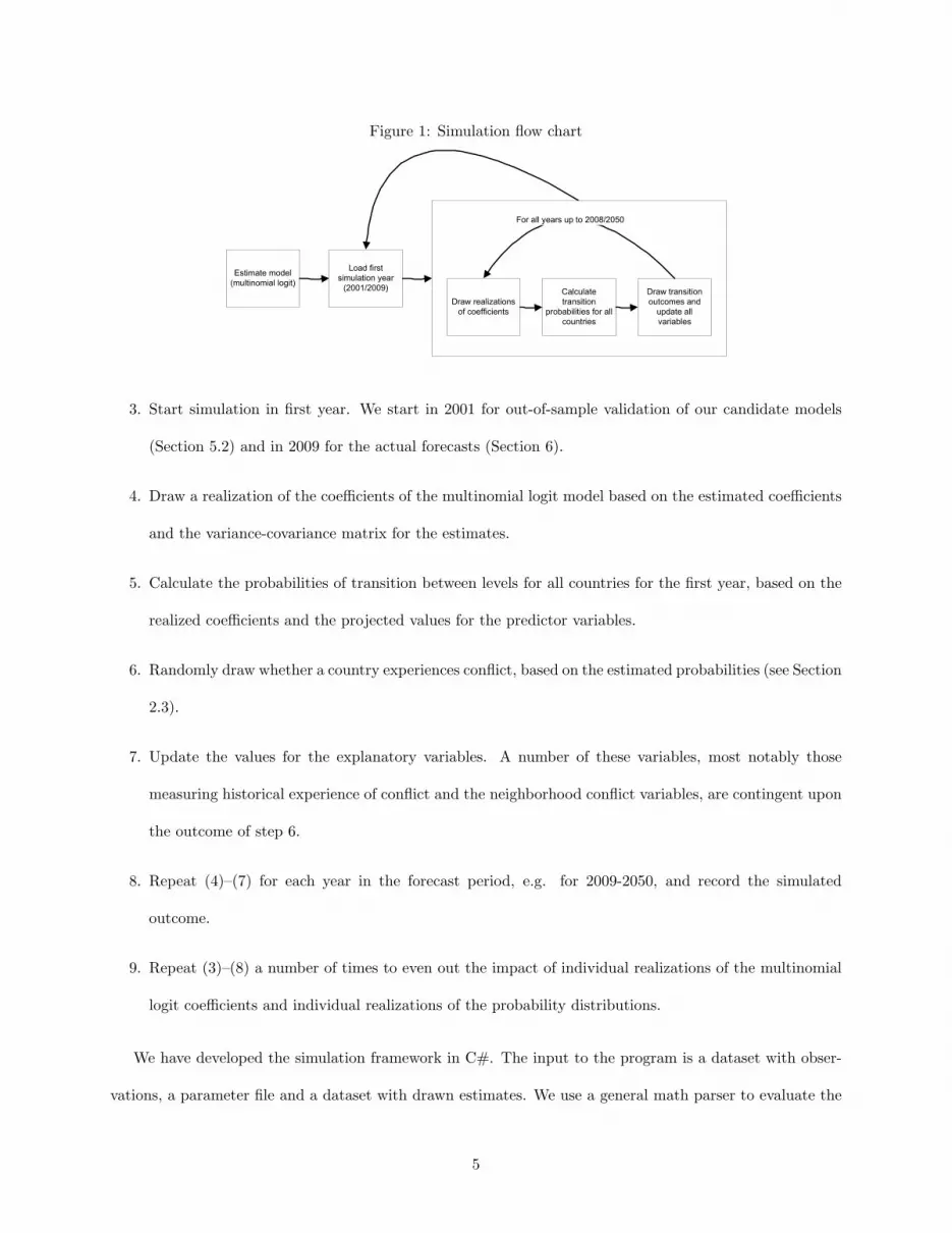
Figure 1: Simulation flow chart

Estimate model

(multinomial logit)

Load first

simulation year

(2001/2009) Calculate

transition

probabilities for all

countries

Draw transition

outcomes and

update all

variables

For all years up to 2008/2050

Draw realizations

of coefficients

3. Start simulation in first year. We start in 2001 for out-of-sample validation of our candidate models

(Section 5.2) and in 2009 for the actual forecasts (Section 6).

4. Draw a realization of the coefficients of the multinomial logit model based on the estimated coefficients

and the variance-covariance matrix for the estimates.

5. Calculate the probabilities of transition between levels for all countries for the first year, based on the

realized coefficients and the projected values for the predictor variables.

6. Randomly draw whether a country experiences conflict, based on the estimated probabilities (see Section

2.3).

7. Update the values for the explanatory variables. A number of these variables, most notably those

measuring historical experience of conflict and the neighborhood conflict variables, are contingent upon

the outcome of step 6.

8. Repeat (4)–(7) for each year in the forecast period, e.g. for 2009-2050, and record the simulated

outcome.

9. Repeat (3)–(8) a number of times to even out the impact of individual realizations of the multinomial

logit coefficients and individual realizations of the probability distributions.

We have developed the simulation framework in C#. The input to the program is a dataset with obser-

vations, a parameter file and a dataset with drawn estimates. We use a general math parser to evaluate the

5

expressions in the parameter file (MuParser). The statistical estimation is done in Stata. The program is

designed so that new models can easily be added. So far we have only implemented the multinomial logit

model. New functions can relatively easy be coded and added as an extension to the math parser. A Stata

plug-in written in C++ functions as an interface between the statistical package, Stata, and the application.

In addition, we have coded a Stata ado-file which reads the parameter file, runs the estimations and draws

estimates before the simulation routine begins.

2.3 Dynamic multinomial logit model

One may estimate the transition probability matrix using a multinomial logit model with the conflict level

at t as the outcome variable, and the level at t− 1 as a set of dummy variables. This type of model is often

referred to as a ‘dynamic multinomial model’.3 The multinomial model (see Greene, 1997, 914–917) for the

three outcomes (j = 0 : ‘no conflict’, j = 1 : ‘minor conflict’, j = 2 : ‘major conflict’) is then

p(Yi = j) =exβj∑2k=0 e

xβk

(1)

To identify the model, we set ‘no conflict’ as the base outcome. The probabilities of the three outcomes

are then given by:

p(Yi = j) =exβj∑2k=0 e

xβk

(2)

The estimates β1 reported below, then, are interpreted as the impact of the explanatory variable on the

probability of being in ‘minor conflict’ relative to ‘no conflict’. The β2 estimates approximate the probability

of ‘major conflict’ relative to ‘no conflict’.

If we enter only the state at t − 1 as explanatory variable(s) (i.e., lagged dependent variables), the

predicted probabilities from estimating this model are identical to those reported in Table 1. The purpose

of formulating this as a multinomial logit model, however, is to be able to account for a set of explanatory

variables, discussed in section 4. The estimates for the lagged dependent variables and the constant terms

then estimate the transition probability matrix for the case where all explanatory variables are zero. We3Przeworski et al. (2000), for instance, refer to their related model as a dynamic probit model.

6

refer to this as the ‘underlying transition probability matrix’ below.

Using a ‘dynamic multinomial logit model’ is useful since it allows capturing that some variables may

increase the risk of conflict onset, but not its duration. This is achieved by adding interaction terms between

the state at t− 1 and predictor variables.

The transition probability matrix in Table 1 only takes the state at t − 1 into account. We also include

information on the conflict state at earlier points in time by adding to the model a function of the number

of years in each state up to t− 2.

Our dynamic multinomial logit model sets this article apart from other recent conflict prediction projects.

Hewitt (2008; 2010), ?), Goldstone and ... (2010) all restrict their attention to the onset of conflict, exclude

countries with ongoing conflicts, and base their estimations on logistic regression.

3 Conflict Predictors

We specify a model with explanatory variables that have been shown to be related to the risk of conflict, and

for which good projections up to 2050 are available. In this section, we discuss previous research on these

indicators’ relationship to the risk of armed conflict. In Section 4, we detail the specific operationalizations

and the data sources for the variables we use.

3.1 Former conflicts

A variable that is almost invariably included in country-level studies of civil war is whether a country has had

a previous conflict. Results are somewhat inconclusive. It is clear that conflicts that end have a discouragingly

high risk of recurrence. Collier, Chauvet and Hegre (2008) estimate the risk of conflict reversal to be around

40% during the first post-conflict decade, and Elbadawi, Hegre and Milante (2008) find an even higher rate

using a more inclusive definition of conflict. Country-level studies that control for other risk factors, on

the other hand, do not always find recent conflicts to increase the estimated risk of new onsets over and

beyond. These studies, however, to some extent mask the fact that conflicts have strong adverse effects on

the major risk factors included in these models. In particular, conflicts may have a catastrophic impact on

average income. Accordingly, Collier et al. (2003, ch. 4) show that there is a considerable ‘conflict trap’

7

Figure 2: Map of conflicts ongoing in 2008

Legend

No ConflictMinor Armed ConflictMajor Armed Conflict

Source: Harbom and Wallensteen (2009)

tendency. They estimate that about half of post-conflict countries return to conflict. A third of the post-

conflict countries succeed in keeping the peace beyond the first 10 years, but enter a category of countries

that they classify as ‘marginalized countries at peace’ (roughly the same class of countries as the ‘bottom

billion’ countries; cf. Collier and Rohner (2008)). This group of countries is characterized by low incomes

and sluggish growth, and has a markedly higher risk of conflict than other countries. Only one sixth of

post-conflict countries end up in the group of ‘successful developers’ and succeed in drastically reducing the

danger of renewed conflict (Collier et al., 2003: 109).

3.2 Neighborhoods and regions

An inspection of the global map of conflicts in Figure 2 shows that the armed conflicts in 2008 are clustered

in a few geographical regions.4 This clustering is partly due to the fact that factors such as poverty that

have been shown to increase the risk of conflict are also clustered. In addition, several studies also show that

conflicts tend to spill over borders when controlling for the presence of these factors (Gleditsch, 2007, Hegre4The PRIO/UCDP dataset records a conflict in the US in 2008. This is the conflict between the US government and Al-Qaida.

It is coded as located in the US because of the attack on Pentagon in 2001.

8

and Sambanis, 2006, Collier et al., 2003). There are several explanations for this tendency of conflict spillover

(Salehyan and Gleditsch, 2006). Some studies point to the importance of ethnic groups involved in conflicts

that have kins in neighboring countries, especially in conjunction with significant refugee flows. Others point

to how the detrimental economic effects of conflicts contaminate neighbors (Murdoch and Sandler, 2004),

thereby exacerbating the factors that contribute to facilitating conflicts.

3.3 Population

Almost all cross-national empirical studies find that populous countries have more internal conflicts than

small countries. A country the size of Nigeria has an estimated risk that is about 3 times higher than

a country the size of Liberia.5 The increase in the risk of conflict does not increase proportionally with

population, however – the per-capita risk of civil war onset decreases with country size.6 The typical study

finds that a 1% increase in population leads to a 0.3% increase in risk of conflict onset.

Studies of the duration of civil war find little evidence that the size of the country’s population affects

how long it lasts (Fearon, 2004, Collier, Hoeffler and Soderbom, 2004, Buhaug and Lujala, 2005). Whether

the severity of conflict is roughly proportional to a country’s population is contested. Lacina (2006) does

not find this to be the case, but Gleditsch, Hegre and Strand (2009) do. Even the results in the latter study

imply that the per-capita risk of being killed in battle is much higher in small countries than in large ones.

Studies of the location of conflict within countries is also somewhat indeterminate on the effect of popu-

lation concentrations. Hegre and Raleigh (n.d.) find in a very fine-grained analysis that conflict events in a

sample of African countries tend to be most frequent in populous locations – rebel groups and governments

tend to target each other in valuable locations such as cities. Buhaug and Rød (2006), focusing on the more

general area of operation, find that this area tends to be located in relatively sparsely populated regions.

Buhaug (2006) also find that geographically large countries are more likely to have territorial or secessionist

conflicts, but that size does not affect the risk of conflicts over government.5This is based on an estimate of 0.3 which is typical for cross-national logistic regression models with a log population

variable. A host of studies obtain estimates for log population larger than 0 but smaller than 1 (Collier and Hoeffler, 2004,Collier and Rohner, 2008, de Soysa, 2002, Elbadawi and Sambanis, 2002, Fearon and Laitin, 2003, Gleditsch and Ruggeri, 2007,Gleditsch, Hegre and Strand, 2009, Thyne, 2006, Urdal, 2005; 2006).

6This is also noted by Collier and Hoeffler (2004).

9

3.4 Education

The most comprehensive study of education and armed conflict is Thyne (2006). Using Fearon and Laitin

(2003)’s model as the baseline, Thyne studied the impact of several educational variables on civil war onset.

While the strongest effects were found for primary enrollment and secondary male enrollment, he also found

pacifying effects of alternative measures like education expenditure as share of GDP, and of literacy. The level

of tertiary education, however, appears to be unrelated to conflict onset. The pacifying effect of education

has previously been identified in other studies. Paul Collier and colleagues have found that secondary male

enrollment is associated both with lower risk of outbreak of civil war (Collier and Hoeffler, 2004), and with

shorter wars (Collier, Hoeffler and Soderbom, 2004). Barakat and Urdal (2008) replicate Thyne’s findings

using secondary male attainment rates, and low-intensity armed conflict onset data. Hence, there appears

to be a consensus in the empirical literature that higher education levels reduce conflict risks. While Collier

and Hoeffler (2004) find education to be an alternative measure of level of development, both Thyne (2006)

and Barakat and Urdal (2008) demonstrate that education may have a pacifying effect even after controlling

for level of income.

3.5 Youth bulges

A few cross-national studies address the relationship between young age structure and armed conflict.

Mesquida and Wiener (1996) found that large youth cohorts, measured as the ratio between 15–29 year

old males and males of 30 years and above, were associated with higher intensity levels (manifested in the

number of conflict related deaths) in intrastate and interstate conflicts. Esty et al. (1998) found some effect

of youth bulges (15–29/15+) on ethnic conflict. Collier and Hoeffler (2004) and Fearon and Laitin (2003)

report to have initially included youth bulges as one among a high number of variables. Both studies failed to

find effects of youth bulges on civil war and middle-intensity conflict and report these results only in passing.

Cincotta, Engelman and Anastasion (2003) and Urdal (2006) have reported increasing risks of armed conflict

onset associated with youth bulges (defined as those aged 15-29 and 15-24 respectively compared to the total

adult population of 15 years and above). Further, Urdal (2006) shows that the youth bulge measure used by

Collier and Hoeffler (2004) and Fearon and Laitin (2003), 15–24/total population, fail to capture the theo-

10

retical concept of youth bulges due to the inclusion of the youngest cohorts (0–14) in the denominator. An

emerging consensus is that youth bulges appear to matter for low-intensity conflict, but not for high-intensity

civil war.

3.6 Infant mortality

Infant mortality has been promoted as an alternative measure of level of development (Goldstone, 2001),

capturing a broader set of developmental factors than the standard measure of income levels (GDP per

capita). Esty et al. (1998) found very strong effects of infant mortality on state failure and conflict, and

Urdal (2005) found high infant mortality rates to be strongly associated with an increased risk of armed

conflict onset. Abouharb and Kimball (2007) have assembled the most complete dataset of infant mortality

rates dating back to 1816 for all states in the international system. Replicating Urdal (2005), they found a

similarly strong predictive ability of infant mortality on conflict onset. Generally, infant mortality appears

to perform very similar to other measures of general development.7

4 Data

4.1 Conflict data

Our conflict data are from the 2009 update of the UCDP/PRIO Armed Conflict Dataset (Harbom and

Wallensteen, 2009, Gleditsch et al., 2002), which records conflicts at two levels. Minor conflicts are those

that pass the 25 battle-related deaths threshold but have less than 1000 deaths in a year. Major conflicts

are those conflicts that pass the 1000 deaths threshold. We only look at internal armed conflicts, and only

include the countries whose governments are included in the primary conflict dyad (i.e., we exclude other

countries that intervene in the internal conflict).

We include information on conflict status (no conflict, minor, or major conflict) at t− 1, the year before

the year of observation. The log of the number of years in each of these states up to t− 2 is also included, a7Per-capita income is among the most robust predictors of internal armed conflict. Almost all scholars find it to be associated

with a high risk of the onset of conflict (Hegre and Sambanis, 2006), and GDP per capita is included in virtually all studies of therisk of armed conflict onset. In the models estimated below, we do not include income as a variable. This is partly because wedo not have access to good projections for this variable, partly because education levels, infant mortality rates, and per-capitaincome are so highly correlated. Also note that

11

Table 2: List of regionsNumber Region Name

2 South America, Central America, and the Caribbean3 Western and Southern Europe, North America, and Oceania4 Eastern Europe5 Western Asia and North Africa6 Western Africa7 East, Central, and Southern Africa8 South and Central Asia9 Eastern and South-East Asia

set of variables we refer to jointly as ‘conflict history’ variables.

4.2 Neighborhood and region data

The neighborhood of a country A is defined as all n countries [B1...Bn] that share a border with A, as defined

by Gleditsch and Ward (2000). More specifically, we define ‘sharing a border’ as having less than 100 km

between any points of their territories. The spatial lag of conflict is a dummy variable measuring whether

there is conflict in the neighborhood or not. Since the dependent variable is nominal, we construct two spatial

lags, one for minor conflicts and one for major conflicts. Islands with no borders are considered as their own

neighborhood when coding the exogenous predictor variables, but have by definition no neighboring conflicts.

We define 8 regions as listed in Table 2. The list is a condensed version of the UN region definition.8

These regions are used as predictor variables in all our models. Dummy variables that capture inter-regional

heterogeneity certainly improve the quality of predictions for the immediate future, since they help maximiz-

ing the explained variance in the observed data. We cannot be certain it improves predictions for the future

beyond the first decade, however, since it may be untenable to assume that these heterogeneities persist

indefinitely.

Since our aim is to predict, we are best served by a spatial lag of conflict as our measure of neighborhood

effects. In our estimated models, we rely on observed levels of conflict in the direct neighborhood of each

country. In our simulation models, we update these variables based on the results from the simulation itself.

We also include the neighborhood average of each predictor variable as another set of exogenous predictor

variables in the model.8The UN list is found at http://www.un.org/depts/dhl/maplib/worldregions.htm.

12

4.3 Education Data

Education data originate from a new dataset compiled by researchers at the International Institute for Ap-

plied Systems Analysis (Lutz and Sanderson, 2007), providing historical estimates for 120 countries for the

1970-2000 period. The dataset is based on individual-level educational attainment data from recent Demo-

graphic Health Surveys (DHS), Labour Force Surveys (LFS), and national censuses. Historical estimates are

constructed by five-year age groups and gender using demographic multi-state methods for back projections,

and taking into account gender and education-specific differences in mortality. The dataset measures educa-

tional attainment using definitions and categories that are consistent over countries and time, representing a

vast improvement over previous education data. The four categories of educational attainment are consistent

with the International Standard Classification of Education (ISCED) categories: No education (no formal

education); Primary (those with uncompleted primary to uncompleted lower secondary, ISCED 1); Secondary

(those with completed lower secondary to uncompleted first level of tertiary, ISCED 2, 3, and 4); Tertiary

(those with at least completed first level of tertiary, ISCED 5 and 6). By disregarding national classification

systems, the standardization of education categories facilitates cross-national and time-series comparison of

education levels.

For this study we follow Barakat and Urdal (2008) and employ a measure of male secondary education,

defined as the proportion of males aged 20–24 years with secondary or higher education of all males aged

20–24.

A recent addition to Lutz and Sanderson (2007) is a projection scenario for educational attainment

until 2050 (Samir et al., 2008). Our base scenario is the General Trend Scenario, for which the projection

takes into account the current (2000) distribution of educational attainment, assumptions about education-

specific fertility, mortality, and migration rates, and assuming that a country’s educational expansion will

converge on an expansion trajectory based on the historical global trend. In addition to the General Trend

Scenario we have constructed two alternative educational scenarios. The low education scenario is based on

an assumption of no improvement in relative educational attainment after 2008, i.e. that the share of young

men receiving secondary education is constant. This is consistent with the IIASA Constant Enrollment Ratio

(CER) scenario. The high education scenario assumes a trajectory with an annual increase in enrollment

13

which is 0.5% higher than the baseline trend scenario, converging towards 100% of young men aged 20-24

having secondary education.

4.4 Imputation of the education variable

The issue of missing data is particularly problematic for prediction purposes: The general problem is that an

instance of missing observation does not occur at random, but is most likely correlated with both education

and conflict. Furthermore, it is very important that our prediction can apply to all countries in the world.

Since our dataset is a combination of historical data and forcasts, we were forced to follow several strategies.

To ameliorate the problem of missing data in the IIASA education data (120 countries only), missing data

have mainly been imputed based on male secondary enrollment from Barro and Lee (2000), covering the

same period as the IIASA data. We regressed the Barro/Lee variable on the IIASA variable and thereby

scaled the imputed variable in order to account for possible systematic differences in methodology between

the two datasets. After this first procedure for imputation, a total of 27 countries in our dataset were still

lacking education data. For 24 of these countries UNESCO has data on secondary male enrollment, but

only for a limited number of years around year 2000. Based on the UNESCO data, we matched the missing

observations with cases we found to be reasonably similar and assumed the same trajectory for the historical

data. We primarily use countries from the same region as models, but for the few cases where we could not

identify a neighboring country with a reasonably similar enrollment profile, we used a model country with a

similar profile from another region. The data on future levels of education and the residual countries from

the previous step where then imputed based on the model country approach. For some countries we assumed

a slightly higher or lower trajectory than the model country, based on differentials in enrollment rates in year

2000.9

9The following model countries were used (the corresponding countries for which education data were imputed are in brackets):Tunisia (Libya; Lebanon; Yemen), Rumania (Yugoslavia; Albania at a 10% lower trajectory), Paraguay (Surinam), Papua NewGuinea (Solomon Islands), Malaysia (Brunei), Macedonia (Bosnia-Herzegovina; Moldova; Belarus at a 10% lower trajectory),Kyrgyz Republic (Tajikistan), Ethiopia (Burundi, Angola), Costa Rica (Cape Verde), Benin (Guinea-Bissau; Equatorial Guinea),Bangladesh (Bhutan), Bahrain (Qatar; United Arab Emirates at a 10% lower trajectory; Oman at a 10% lower trajectory),Armenia (Georgia, Azerbaijan), Vietnam (Laos at a 10% lower trajectory). For the three remaining countries for which neitherdatabase had any information on education levels, we chose a neighboring model country that we assumed could act as areasonable proxy: Ethiopia (for Somalia and Djibouti), Vietnam (for North Korea, but at a 10% lower trajectory).

14

4.5 Demographic Data

The demographic variables originate from the World Population Prospects 2006 (UN, 2007) produced by the

United Nations Population Division. This is the most authoritative global population dataset, covering all

states in the international system between 1950 and 2005 and providing projections for the 2005–2050 period.

Three key demographic indicators are used in this study. Total population is defined as the de facto

population in a country as of 1 July of the year indicated, and expressed in thousands. The measure has

been log-transformed following an expectation of a declining marginal effect on conflict risk of increasing

population size. Infant mortality is defined as the probability of dying between birth and exact age 1 year,

expressed as the number of infant deaths per 1000 live births. Youth bulges are measured as the percentage

of the population aged 15–24 years of all adults aged 15 years and above. Age-specific population numbers

are provided by the UN (2007) for five-year groups of de facto population, measured in thousands.

Only one scenario exists for each indicator for the 1950–2005 period. Estimates are based on a range of

different historical sources, including population censuses, demographic and health surveys, and population

registers. The UN estimates are revised biannually, and each revision incorporates all new and relevant

information about past demographic trends. Consequently, historical estimates may change between revisions.

Several different demographic projection scenarios are provided by the UN Population Division. For each

country, the starting point is the 2005 mid-year population estimate. In order to project the population until

2050, assumptions have to be made about future trends in fertility, mortality, and international migration.

Projecting such trends necessarily involves considerable uncertainty. For this project, we use the three

main scenarios from the population projections. These differ from each other exclusively as a result of

different assumptions regarding future fertility trajectories. In the medium scenario, total fertility rates for

all countries are assumed to converge towards 1.85 children per woman assumed to follow a path similar

to historical experiences of fertility decline. However, not all countries are projected to reach the level of

1.85 by the end of the period. Under the high fertility scenario, fertility is projected to remain 0.5 children

higher than the medium projection (i.e. converge towards 2.35), while in the low fertility scenario, fertility is

assumed to be 0.5 children lower than the medium scenario (converging towards 1.35). For all three scenarios,

mortality is assumed to follow models for change in life expectancy developed by the UN Population Division,

15

with increasingly smaller gains at higher levels of life expectancy. The international migration assumptions

are based on past international migration estimates as well as considerations of states’ migration policies

with regards to future international migration.

The three main projection scenarios are used to construct three different scenarios for total population

and for youth bulges. For countries that currently (2005) experience high fertility levels, the three different

fertility trajectories lead to significant differences in population size estimates by 2050. For the youth bulge

measure, the three scenarios yield identical estimates until 2024 since the relevant youth cohorts were already

born by 2005. Beyond 2025, the different fertility assumptions lead to significant variation in the youth bulge

projections for many countries. For infant mortality, the UN Population Division (UN, 2007) only provides

one projection scenario. However, given the considerable fluctuation in infant mortality associated with

different economic, social, and political conditions, it is plausible to expect significant uncertainty associated

with future trends. For the purpose of this analysis, we have constructed two alternative scenarios. For the

high infant mortality scenario, we assume a correction in the infant mortality rate identical to a 0.5% increase

for each successive year compared to the UN projected baseline. For the low infant mortality scenario, we

conversely assume a downward correction in the infant mortality of 0.5% per year compared to the UN

projected baseline. This implies that absolute variation will be greatest in countries with high levels of infant

mortality, and that over a 40-year period the correction will be approximately 20% higher and 20% lower

than the baseline UN projection for our high and low infant mortality scenarios respectively.

4.6 Temporal Dummies

We could fit the model better to the data at hand by adding yearly fixed effects. However, trying to predict

the level of violence in 2034, it is not very helpful to know that 2034 is not the year 1976. Furthermore, it is

not unproblematic to add a large number of correlated variables to a non-linear model like the multinomial

logit.

On the other hand, there are good reasons to believe that the underlying transition probability matrix

for a country with a given set of characteristics is not constant over the observed period. At least we know

that the end of the Cold War led to the eruption of an unusually high number of new conflicts, but at the

16

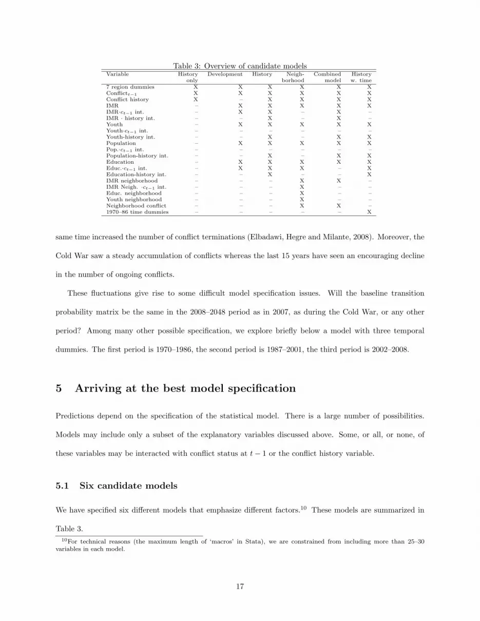
Table 3: Overview of candidate modelsVariable History Development History Neigh- Combined History

only borhood model w. time7 region dummies X X X X X XConflictt−1 X X X X X XConflict history X – X X X XIMR – X X X X XIMR·ct−1 int. – X X – X –IMR · history int. – – X – X –Youth – X X X X XYouth·ct−1 int. – – – – – –Youth-history int. – – X – X XPopulation – X X X X XPop.·ct−1 int. – – – – – –Population-history int. – – X – X XEducation – X X X X XEduc.·ct−1 int. – X X X – XEducation-history int. – – X – – XIMR neighborhood – – – X X –IMR Neigh. ·ct−1 int. – – – X – –Educ. neighborhood – – – X – –Youth neighborhood – – – X – –Neighborhood conflict – – – X X –1970–86 time dummies – – – – – X

same time increased the number of conflict terminations (Elbadawi, Hegre and Milante, 2008). Moreover, the

Cold War saw a steady accumulation of conflicts whereas the last 15 years have seen an encouraging decline

in the number of ongoing conflicts.

These fluctuations give rise to some difficult model specification issues. Will the baseline transition

probability matrix be the same in the 2008–2048 period as in 2007, as during the Cold War, or any other

period? Among many other possible specification, we explore briefly below a model with three temporal

dummies. The first period is 1970–1986, the second period is 1987–2001, the third period is 2002–2008.

5 Arriving at the best model specification

Predictions depend on the specification of the statistical model. There is a large number of possibilities.

Models may include only a subset of the explanatory variables discussed above. Some, or all, or none, of

these variables may be interacted with conflict status at t− 1 or the conflict history variable.

5.1 Six candidate models

We have specified six different models that emphasize different factors.10 These models are summarized in

Table 3.10For technical reasons (the maximum length of ‘macros’ in Stata), we are constrained from including more than 25–30

variables in each model.

17

All models include conflict status at t−1 and the region variable defined in Table 2 implemented as seven

dummy variables with region 2 as the reference category.

The ‘History only’ model adds the ‘conflict history’ variables to the lagged dependent variables (see

Section 4.1).

The ‘Development’ model excludes the ‘conflict history’ variables but includes main terms for all predictor

variables. It also includes interactions between ‘IMR’ and ‘Education’ and conflict status at t− 1 to capture

differences in the extent to which these variables predict onset or termination of conflict. The model focuses

on the socio-economic characteristics of countries and is sensitive to changes in these, but ignores much of

the history and geographical context of these countries.

The ‘History’ model includes all the terms in the ‘Development’ model, but also includes the ‘conflict

history’ variables and their interactions with IMR, Youth, Population, and Education. The model is sensitive

to countries’ conflict history over the last few decades, but ignores information on conflicts in neighboring

countries.

The ‘History with time’ model is identical to the ‘History’ model, but also includes a dummy variable for

the 1970–86 period to be able to capture whether the Cold War period was significantly different from the

post-Cold War period.

The ‘Neighborhood’ model includes most of the terms in the ‘Development’ model, and adds a variable

denoting whether there was a conflict in a neighboring country at t − 1 as well as a number of variables

representing the average values of the explanatory variables in the neighborhood. This model is much more

sensitive to the geographical context of the country than the ‘Development’ model.

The ‘Combined’ model combines features from the ‘Development’, ‘History’, and ‘Neighborhood’ models.

Terms that were clearly not statistically significant were removed from the model. The model includes

information on conflict history, all socio-economic and demographic indicators and selected interactions with

conflict at t − 1 and the number of years without conflict, information on IMR in the neighborhood, and

whether there was conflict ongoing in the neighborhood at t− 1.

18

Table 4: AUCs for six models estimated on data for 1970–2000. Predictions compared to observed conflicts2001–2008

Model N R2 AUC St. AUC St. Correct False2001–2008 error 2008 error Pred. Pred.

History only 4526 0.518 0.881 0.016 0.874 0.035 6/25 2/144Development 4526 0.463 0.898 0.012 0.838 0.039 7/25 3/144History 4420 0.537 0.904 0.013 0.892 0.035 14/25 7/144Neighborhood 4420 0.537 0.906 0.012 0.893 0.032 11/25 4/144History & period 4526 0.538 0.904 0.013 0.886 0.036 14/25 6/144Combined 4526 0.536 0.918 0.011 0.907 0.025 13/25 5/144

5.2 Out-of-sample prediction assessment

The multinomial logit estimates for these six models are reported in Appendix Table A-1. To help selecting

the best model, we use a split-sample design where we estimated each candidate model on data for the period

1970–2000. We then use our simulation program to obtain predictions for the 2001–2008 period, and compare

our predictions with the observed conflicts for that period (as reported in Harbom and Wallensteen (2009)).11

We ran 500 simulations for each of the six models.

The results from the split-sample evaluation are presented in Table 4. We want to identify the model

that yields the predictions that most closely reflect what we actually observed in 2001–2008. Evaluations of

predictions are more straightforward for dichotomous variables than for variables with three categories, so

we group the cases where we predict either minor or major conflict into one category and compare with a

similarly dichotomous observed variable. We then summarize all simulated outcomes for each country-year as

the share of simulations where we predict conflict and the share where we predict no conflict. These predicted

shares are in turn paired with the observed outcomes. As a goodness-of-fit measure we use the area under the

Receiver Operator Curve (AUC – ‘Area Under the Curve’).12 The AUC is equal to the probability that the

simulation predicts a randomly chosen positive observed instance higher than a randomly chosen negative

one. The ROC curves for the five models are presented in Figure 3. The figure shows that the ‘Combined’

model (the heavy solid line) performs best for most prediction thresholds.

Columns two and three in Table 4 report the number of observations going into the multinomial logit

model and the ‘pseudo-R2’ of the model. The fourth column shows the AUC when comparing predicted

and observed conflict values for the entire 2001–2008 period. The estimated standard error of this area11See Ward and Hoff (2007) for an application of this procedure in conflict research.12See Hosmer and Lemeshow (2000, p. 156–164) for an introduction to Receiver Operator Curves, AUC, and the related

concepts of sensitivity and specificity in the context of logistic regression.

19

Figure 3: Receiver Operator Curves (ROC), 2001–2008

estimate is given in the fifth column. Column six and seven show the same two figures for 2008 only. The

two final columns report the number of conflict country years in 2008 that were correctly predicted (true

positives) using p > 0.5 as the prediction threshold as well as the number of no-conflict country years that

were incorrectly predicted (false positives).

Over the entire 2001–2008 period, the predictive performance of the six models are roughly similar. The

‘Combined’ model has the largest AUC values, but they are not significantly better than the other models.

The ‘History only’ model performs clearly worse than the other models – the AUC is low, and the number of

true positives is low. The ‘Combined’ model has a slightly lower number of true positives than the ‘History’

models, but also has fewer false positives. If we set predicted probability > 0.50 as the cutoff, the model

predicts conflict in 18 countries. 13 of these were correct (predicting half of the actual conflicts), and 5

(28%) were false positives. All in all, this is the one with the best predictive properties for the 2001–2008

predictions. This is the model we use for the 2009–2050 predictions.

20

5.3 Implications of model choice for predictions

Before turning to the results for the 2009–2050, it may be useful to take a closer look at predictions for

individual countries. Table 5 lists for each country the proportion of the 500 simulations in which the

program predicted a minor or major conflict. The table includes all countries with conflict in 2008 as well as

all countries with predicted risk higher than 0.30 in at least one of the models, or predicted risk higher than

0.20 in the ‘Combined’ model. Cells with values larger than 0.300 and 0.500 are highlighted by two shades

of gray.

The table is sorted by conflict status in 2008 as reported in Harbom and Wallensteen (2009) and then by

our simulated probability of conflict. Column 2 reports whether the country was coded as in conflict in 2008.

Column 3 indicates the conflict history known in 2000 and therefore available to the simulation procedure.

The 13 correct predictions from the ‘Combined’ model appear as entries with probabilities > 0.500. We

predict three of the five wars in 2008, but fail to predict the wars in Somalia and Sri Lanka. The former

falls below the 0.500 line because of the 1997–2000 period with no recorded conflict in the dataset.13 The

recent conflict history is a very important predictor, and even four years of no conflict reduces the estimated

risk considerably. We fail to predict the latter conflict because it scores relatively well on the socio-economic

development indicators – the exogenous variables also contribute significantly to the quality of predictions.

All the minor conflicts that are correctly predicted were ongoing in 2000. The only conflict country in

2008 that did not have a recent conflict history in 2000 is USA.14 This conflict was not predicted by any of

the models. The countries with more distant conflicts (Niger, Mali, Thailand, Peru, and Georgia) turn up

with conflicts in between 15 and 26% of the simulations.

The false positives from the ‘Combined’ model are predicted conflicts in Uganda, Indonesia, Nepal,

Rwanda, and Angola. All of these had conflict in 2000. In fact, by 2005 only the conflict in Rwanda had

ended. The conflict in Uzbekistan (which ended in 2004) is also a near false positive. The model correctly

predicts termination in three other countries, however, namely in Senegal, Guinea, and Sierra Leone.

Figure 4 shows the predicted global incidence of armed conflict produced by four of these models. In these13Somalia was certainly not peaceful – the UCDP/PRIO dataset records the warfare in these years as non-state conflict

because of the absence of a functional central government.14The conflict in the USA is the conflict with al-Qaida, coded by UCDP as located in the US because of the attack in New

York in 2001.

21

Table 5: Highest predicted risk of conflict in 2008Country Conflict Conflicts History Development History Neigh- Com- Com-

observed up to only bor bined binedin 2008 2000 hood War

Pakistan Major 1996 .356 .696 .566 .520 .690 .244Afghanistan Major 2000 .504 .744 .798 .538 .628 .172Iraq Major 1996 .220 .484 .548 .492 .558 .142Somalia Major 1996 .258 .384 .398 .432 .342 .152Sri Lanka Major 2000 .538 .272 .396 .226 .210 .036

India Minor 2000 .520 .736 .798 .794 .844 .258Ethiopia Minor 2000 .422 .586 .704 .650 .758 .242Sudan Minor 2000 .348 .594 .718 .750 .730 .348Myanmar Minor 2000 .530 .422 .660 .534 .656 .074Iran Minor 2000 .554 .504 .624 .360 .624 .178Turkey Minor 2000 .382 .398 .614 .328 .616 .108Philippines Minor 2000 .546 .408 .610 .566 .602 .040Chad Minor 2000 .398 .388 .622 .538 .596 .240Burundi Minor 2000 .420 .422 .620 .696 .582 .230Congo, D.R. Minor 2000 .478 .538 .714 .670 .564 .320Algeria Minor 2000 .360 .446 .606 .588 .476 .120Colombia Minor 2000 .216 .210 .418 .218 .448 .058Russia Minor 2000 .122 .128 .482 .358 .316 .112Niger Minor 1997 .148 .242 .318 .450 .258 .106Mali Minor 1994 .120 .538 .250 .248 .244 .116Thailand Minor 1982 .156 .166 .098 .154 .182 .026Israel Minor 2000 .392 .082 .214 .234 .176 .028Peru Minor 1999 .198 .130 .382 .154 .174 .066Georgia Minor 1993 .138 .096 .164 .078 .154 .044USA Minor – .022 .096 .016 .014 .076 .008

Uganda No 2000 .416 .518 .716 .712 .710 .218Indonesia No 2000 .574 .450 .656 .618 .704 .040Nepal No 2000 .556 .316 .664 .404 .654 .120Rwanda No 2000 .442 .498 .638 .654 .652 .384Angola No 2000 .466 .566 .684 .638 .640 .282Uzbekistan No 2000 .474 .402 .554 .428 .430 .160Cameroon No 1984 .298 .340 .428 .314 .422 .270Bangladesh No 1992 .218 .592 .392 .320 .408 .230Cote d’Ivoire No – .020 .246 .090 .088 .400 .082Eritrea No 1999 .456 .268 .460 .416 .398 .212Cen. Afr. Rep. No – .064 .288 .104 .052 .382 .184Egypt No 1998 .324 .326 .512 .462 .382 .198Nigeria No 1970 .030 .324 .170 .138 .340 .054Yemen No 1994 .158 .438 .384 .266 .336 .168China No 1959 .182 .438 .352 .458 .334 .154Tajikistan No 1998 .434 .360 .418 .288 .334 .216Congo No 1999 .438 .196 .398 .354 .316 .170Senegal No 2000 .228 .168 .434 .320 .312 .048Guinea No 2000 .224 .152 .388 .432 .300 .110Azerbaijan No 1995 .242 .258 .278 .190 .290 .106Laos No 1990 .264 .268 .242 .058 .290 .146Mozambique No 1992 .196 .424 .404 .366 .288 .172Djibouti No 1999 .400 .178 .368 .43 .286 .162Cambodia No 1998 .312 .290 .370 .192 .272 .072Kenya No 1982 .074 .408 .276 .276 .268 .172Tanzania No – .072 .488 .236 .290 .260 .188Sierra Leone No 2000 .222 .154 .408 .452 .246 .116Lesotho No 1998 .396 .184 .304 .042 .196 .088South Africa No 1988 .132 .136 .228 .380 .154 .007Liberia No 2000 .228 .266 .320 .198 .174 .042

22

Figure 4: Observed and simulated proportion of countries in conflict, four validation models, both conflictlevels, all countries, 1960–2050

figures, we merge the two conflict levels into one, and plot the proportion of the countries in our dataset that

has an ongoing conflict of either intensity level. The line to the left of the vertical line present the observed

proportion of countries in conflict. To the right of the vertical line we see our projections. The solid line

is the proportion of countries in conflict averaged over all simulations. The dashed line represents the 10th

percentile of proportion of conflict in conflict for every year. The dotted line represents the 90th percentile

of proportion of conflicts. That is, in 80% of our simulations the predicted proportion of countries in conflict

were found between the dashed and dotted lines.

Figure 4 shows that the simulated global proportion of countries in conflict depends on the model spec-

ification. The ‘History only’ model predicts a constant proportion of countries in conflict at about 11%

after an initial swift drop, reflecting that this model does not take improvements in development levels into

account. The ‘Development’ model predicts an initial increase (probably because of population increases)

and then a decline to about 10% in 2050 (because of the development variables). The ‘History’ model yields

a similar decline. The ‘Neighborhood’ model indicates a strong decrease to under 5% of the world’s countries

23

Table 6: Estimation results, final model, 1970–2008Minor conflict equation Major conflict equation

Minor conflict at t− 1 2.487∗∗ (3.11) 3.232∗ (2.26)Major conflict at t− 1 2.898∗ (2.24) 3.139 (1.84)ln(Years in no conflict) -1.227∗∗∗ (-14.04) -1.562∗∗∗ (-9.34)ln(Years in minor conflict) 1.035∗∗∗ (9.08) 0 (.)ln(Years in major conflict) 0 (.) 1.193∗∗∗ (6.67)

ln(IMR)t−1 0.00424 (1.40) 0.0145∗∗ (3.15)ln(IMR)t−1· Minor at t− 1 -0.324 (-1.75) -0.441 (-1.37)ln(IMR)t−1· Minor at t− 1 -0.309 (-1.02) -0.210 (-0.54)ln(IMR)t−1· Years in no conflict 0.179∗ (2.06) 0.00428 (0.02)Youth t−1 0.00721 (0.34) 0.0174 (0.52)Youtht−1· Years in no conflict -0.00799 (-0.68) 0.00401 (0.18)ln(Population)t−1 0.307∗∗∗ (5.70) 0.256∗∗ (3.23)ln(Population)t−1· Years in no conflict -0.00501 (-0.22) 0.0262 (0.57)Educationt−1 -0.727 (-1.67) -0.0806 (-0.12)

Average ln(IMR)t−1 in neighborhood -0.135 (-0.85) 0.248 (0.96)Minor conflictt−1 in neighborhood 0.183 (1.20) 0.510∗ (2.11)Major conflictt−1 in neighborhood 0.0389 (0.22) 0.332 (1.28)

W. and S. Europe and N. America 0.183 (0.51) -0.901 (-1.09)E. Europe -0.268 (-0.60) 0.417 (0.61)W. Asia and N. Africa 0.653∗∗ (2.74) 0.229 (0.68)W. Africa -0.0900 (-0.30) -2.306∗∗∗ (-4.00)E., C., and S. Africa 0.382 (1.48) -0.333 (-0.92)S. and C. Asia 0.396 (1.34) -0.0772 (-0.19)E. and S.E. Asia 0.717∗∗ (2.82) -0.263 (-0.69)Constant -4.116∗∗∗ (-3.62) -7.397∗∗∗ (-3.67)N 5208

t statistics in parentheses.∗ p < 0.05, ∗∗ p < 0.01, ∗∗∗ p < 0.001South and Central America is baseline category for the region variable.

in conflict in 2050. In this model, the model possibly over-estimates a diffusion of peace from stable and

peaceful countries to their countries.

5.4 Final model

Table 6 shows the results of re-estimating the preferred model specification for the entire 1970–2008 period.

The left pair of columns contain the estimates for the minor conflict equation, the right pair those for major

conflicts.

Space constraints preclude a detailed discussion of these estimates, but a brief review helps evaluating

the predictions presented below. First, the lagged conflict and conflict history variables model the strong

tendency for internal conflicts to last for several subsequent years. The negative estimate for the ‘ln(Years

in minor conflict)’ variable indicates that the probability of minor conflict increases the longer the country

has been in minor conflict. The year after a minor conflict has broken out, the odds of minor conflict is

estimated to be 12 times higher than before the onset. When the conflict has lasted for two years, the odds

are 24 times higher. After 10 years, the estimated odds are 100 times higher. The estimates for ‘ln(Years

24

in major conflict)’ shows the same pattern for major conflict, whereas the negative estimate for ‘ln(Years in

minor conflict)’ reflects that the probability of conflict is decreasing strongly for each additional year without

conflict. After 10 years of peace, the odds is only 5% of the odds immediately after conflict termination.

High infant mortality rates increases the risk of conflict, partly by increasing the risk of major conflict,

partly by diminishing the tendency of a peaceful history to reduce the risk of minor conflict. The log

population variable is positive and strongly significant, and there are strong signs of spillover from conflicts

in a country’s neighborhood. We find no clear effect of youth bulges in this model, nor of education or infant

mortality rates in the countries’ neighborhood.15

Controlling for these variables, we find quite a bit of regional residual variation. The ‘Western Asia and

North Africa’ and ‘Eastern and South-Eastern Asia’ regions have more minor conflicts than expected. West

African countries have much less major conflicts than their socio-economic and demographic indicators imply.

6 Prediction results 2009–2050

We then generated predictions for the 169 countries for which we have data. We ran 1,000 separate simulations

for three different scenarios. In the first, we use the projections for the demographic and education variables

that the UN and the IIASA find most plausible (the projections they refer to as ‘best’, see Sections 4.3 and

4.5). In Section 6.3, we evaluate simulations based on a more pessimistic and a more optimistic scenario.

6.1 The ‘best projection’ scenario

Figure 5 shows the observed incidence of conflict from 1960 to 2008 and the corresponding simulated incidence

for 2009–2050.16 The observed proportion increased steadily up to 1992 and then declined to the year 2003,

after which the incidence of conflict increased somewhat. In 2008, about 14% of the countries in the dataset

were in conflict. Our simulations imply that we are likely to see a continued decrease in the proportion in

conflict over the next few decades, from 14% to about 9% in 2050. A comparison with the projections from

the other models (Figure 4) shows that our preferred specification yields a less steep global decline in conflict

15Note that most of the empirical studies referred to above are studies of conflict onset and may not be directly comparableto our joint onset and duration model.

16See the discussion of Figure 4 for a detailed explanation.

25

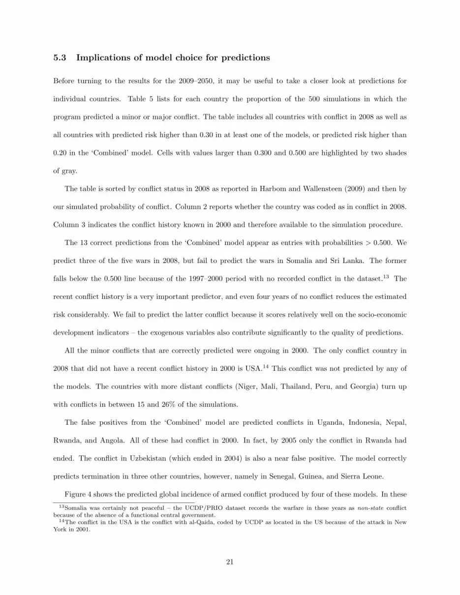
Figure 5: Observed and simulated proportion of countries in conflict, ‘combined’ model, both conflict levels,all countries, 1960–2050

than the ‘Neighborhood’ model, but a slightly stronger decline than the other models.

The simulation shows an immediate decrease from 2008 to 2010, and thereafter a slight increase over the

next couple of years. A similar pattern is evident in the graphs in Figure 4. This is probably an artifact of

the simulation procedure and due to a transition from the initial distribution of conflicts to the steady-state

distribution implied by the estimated transition matrix. Since the average probability of conflict termination

is higher than that of conflict onset, the simulation first removes poorly predicted conflicts such as those in

Sri Lanka and Mali, and then more slowly fills in high-risk countries without conflict in 2008 (e.g., Uganda,

Angola, and Nepal).

Table 7 shows the simulated risk of conflict in 2010 for the set of countries listed in Table 5. The simulations

imply that the major conflicts in Pakistan, Somalia, Afghanistan and Iraq are more likely to continue than to

end, although the three latter more frequently are simulated as minor than as major conflict. The simulation

predicts the termination of the conflict in Sri Lanka. Likewise, the minor conflicts in Chad, Peru, Georgia,

Israel, Niger, and Mali appear as conflicts in less than half of the simulations, indicating that these conflicts

26

are likely to end soon. The simulations further imply that conflicts are likely to (re-)commence in Uganda

and Angola. Figure 6 shows the same information in map form for all countries in the world.

Hewitt (2008; 2010), Rost, Schneider and Kleibl (forthcoming) also publish lists of the countries with

the highest risk of conflict onset. The predictions are not directly comparable, though. Rost, Schneider

and Kleibl (forthcoming) only predict major conflicts and censor ongoing conflict years. Hewitt (2008; 2010)

predict the onset of a wider set of political instability events (as do Goldstone and ... (2010)).17 Moreover,

these studies include predictors such as regime type and state repression for which we do not have forecasts

up to 2050. Still, many similarities exist. African countries are disproportionally represented in all these

lists – Iraq and Afghanistan are the only non-African countries among the top 25 in Hewitt (2010), Rost,

Schneider and Kleibl (forthcoming) has 16 African out of 25.

The column labeled ‘Major’ shows the proportion of simulations with major conflict in the given country.

Major conflict risks are predicted to be highest in Afghanistan, Iraq, and Somalia, due to the seriousness

of the recent conflicts in these countries. Major conflict risks are also predicted to be high in Pakistan, Sri

Lanka, Burundi, Angola, and the Central African Republic. None of these predicted probabilities exceed 0.5,

however.

Table 8 shows predicted probability of conflict in 2016, 2030, and 2050. The table is sorted by the

simulated proportion in either conflict level in 2016, eight years after the last year for which we have conflict

data. Ten countries are predicted to be in conflict in 2016: Afghanistan, Ethiopia, India, Iran, Iraq, Myanmar,

Pakistan, Sudan, and Uganda.18 Our prediction assessment (section 5) indicated that we are able to predict

correctly about half of the conflict countries eight year in advance, and to generate about 28% false positives.

This implies that seven of these will happen with a high probability, and that we will see about seven others

in 2016.

The simulations indicate that the conflicts in Somalia, USA, Russia, Niger, Mali, Georgia, Colombia,

Sri Lanka, Peru, and Israel are more likely to have ended than to continue in 2016. Figure 7 presents the

predicted probabilities in map form.

The two right-most columns in Table 8 report countries’ predicted probability of conflict in 2030 and17Goldstone and ... (2010) do not report a list of country predictions.18Another 4–6 countries are close to 0.5 in predicted probability of conflict.

27

Table 7: Highest predicted risk of conflict in 2010Country Conflict Conflicts Minor Major Both

observed up toin 2008 2008

Pakistan Major 2008 .464 .256 .720Afghanistan Major 2008 .154 .462 .616Iraq Major 2008 .131 .449 .580Somalia Major 2008 .199 .385 .584Sri Lanka Major 2008 .215 .153 .368

India Minor 2008 .656 .125 .781Ethiopia Minor 2008 .505 .134 .639Turkey Minor 2008 .614 .039 .653Thailand Minor 2008 .623 .007 .630Sudan Minor 2008 .529 .083 .612USA Minor 2008 .576 .005 .581Myanmar Minor 2008 .527 .042 .569Iran Minor 2008 .513 .051 .564Algeria Minor 2008 .550 .012 .562Philippines Minor 2008 .527 .018 .545Burundi Minor 2008 .305 .231 .536Colombia Minor 2008 .435 .035 .470Russia Minor 2008 .425 .038 .463Congo, Dem. Rep. Minor 2008 .385 .054 .439Georgia Minor 2008 .248 .104 .352Chad Minor 2008 .325 .074 .399Israel Minor 2008 .333 .003 .336Niger Minor 2008 .310 .021 .331Peru Minor 2008 .297 .023 .320Mali Minor 2008 .272 .016 .288

Uganda No 2007 .457 .176 .633Angola No 2007 .382 .172 .554Nepal No 2006 .302 .133 .435Indonesia No 2005 .335 .055 .390Azerbaijan No 2005 .132 .096 .228Nigeria No 2004 .177 .039 .216Central Afr. Rep. No 2006 .151 .140 .191Rwanda No 2002 .120 .044 .164Cote d’Ivoire No 2004 .129 .025 .154Uzbekistan No 2004 .095 .051 .146Cambodia No 1998 .101 .026 .127Bangladesh No 1992 .089 .025 .114China No 1959 .082 .022 .107Egypt No 1998 .072 .028 .100Senegal No 2003 .086 .013 .099Eritrea No 2003 .074 .024 .098Cameroon No 1984 .066 .019 .085Liberia No 2003 .074 .008 .082Djibouti No 1999 .054 .027 .081Guinea No 2000 .070 .010 .080Congo No 2002 .053 .025 .078Mozambique No 1992 .059 .010 .069Yemen No 1994 .058 .011 .069Tanzania No – .051 .015 .066Kenya No 1982 .037 .020 .057Sierra Leone No 2000 .046 .009 .055Laos No 1990 .041 .010 .051Tajikistan No 1998 .031 .015 .046Lesotho No 1998 .038 .003 .041South Africa No 1988 .039 .001 .040

28

Table 8: Highest predicted risk of conflict in 2016, 2030, and 2050Country Conflict Conflict 2016 2030 2050

observed up to Minor Major Either Either Eitherin 2008 2008

Pakistan Major 2008 .440 .232 .672 .662 .628Afghanistan Major 2008 .369 .225 .593 .597 .620Iraq Major 2008 .366 .151 .517 .365 .270Somalia Major 2008 .244 .130 .374 .266 .219Sri Lanka Major 2008 .137 .044 .181 .066 .023

India Minor 2008 .058 .222 .802 .787 .779Ethiopia Minor 2008 .457 .233 .690 .646 .575Sudan Minor 2008 .461 .228 .689 .656 .605Turkey Minor 2008 .467 .134 .601 .487 .341Myanmar Minor 2008 .498 .100 .598 .544 .530Iran Minor 2008 .353 .185 .538 .401 .289Chad Minor 2008 .298 .201 .499 .435 .355Thailand Minor 2008 .445 .050 .495 .359 .234Algeria Minor 2008 .353 .126 .479 .337 .193Philippines Minor 2008 .436 .033 .469 .337 .263Burundi Minor 2008 .279 .169 .448 .369 .315Congo, Dem. Rep. Minor 2008 .293 .128 .421 .325 .292USA Minor 2008 .339 .029 .365 .205 .129Niger Minor 2008 .277 .073 .350 .238 .187Russia Minor 2008 .197 .188 .315 .200 .112Mali Minor 2008 .217 .057 .274 .174 .140Colombia Minor 2008 .194 .051 .245 .083 .048Georgia Minor 2008 .129 .080 .209 .109 .057Peru Minor 2008 .121 .030 .151 .049 .028Israel Minor 2008 .097 .016 .113 .048 .024

Uganda No 2007 .345 .188 .533 .464 .428Indonesia No 2005 .430 .043 .473 .463 .456Nepal No 2006 .308 .108 .426 .330 .269Rwanda No 2002 .204 .136 .340 .394 .360Angola No 2007 .309 .174 .483 .430 .359Bangladesh No 1992 .219 .090 .309 .378 .352China No 1959 .286 .081 .367 .566 .627Central Afr. Rep. No 2006 .171 .137 .308 .209 .135Egypt No 1998 .179 .039 .218 .252 .236Nigeria No 2004 .223 .033 .256 .244 .218Azerbaijan No 2005 .148 .101 .249 .224 .162Cambodia No 1998 .155 .065 .220 .244 .176Cameroon No 1984 .132 .077 .209 .218 .180Tanzania No – .128 .073 .201 .366 .387Uzbekistan No 2004 .121 .076 .197 .189 .146Mozambique No 1992 .138 .049 .187 .233 .219Cote d’Ivoire No 2004 .154 .022 .176 .148 .082Kenya No 1982 .099 .069 .168 .254 .239Yemen No 1994 .118 .032 .150 .164 .141Eritrea No 2003 .084 .046 .130 .107 .060Congo No 2002 .083 .044 .127 .081 .045Laos No 1990 .092 .028 .120 .149 .122Senegal No 2003 .103 .014 .117 .099 .076South Africa No 1988 .085 .025 .110 .115 .100Guinea No 2000 .083 .016 .099 .086 .047Djibouti No 1999 .060 .037 .097 .080 .041Liberia No 2003 .066 .018 .084 .125 .107Sierra Leone No 2000 .072 .008 .080 .059 .044Tajikistan No 1998 .054 .022 .076 .086 .086Lesotho No 1998 .044 .009 .053 .064 .048

Table sorted by conflict level in 2008 and proportion simulated in ‘Either conflict’ in 2016.

29

Figure 6: Map of conflict predictions in 2010

0.000 - 0.0020.003 - 0.0070.008 - 0.0190.020 - 0.0490.050 - 0.1240.125 - 0.2990.300 - 0.4990.500 - 0.6990.700 - 0.8500.851 - 1.000

2010Figure 7: Map of conflict predictions in 2016

0.000 - 0.0020.003 - 0.0070.008 - 0.0190.020 - 0.0490.050 - 0.1240.125 - 0.2990.300 - 0.4990.500 - 0.6990.700 - 0.8500.851 - 1.000

2016

Proportion of simulations in minor or major conflict

Figure 8: Map of conflict predictions in 2030

0.000 - 0.0020.003 - 0.0070.008 - 0.0190.020 - 0.0490.050 - 0.1240.125 - 0.2990.300 - 0.4990.500 - 0.6990.700 - 0.8500.851 - 1.000

2030Figure 9: Map of conflict predictions in 2050

0.000 - 0.0020.003 - 0.0070.008 - 0.0190.020 - 0.0490.050 - 0.1240.125 - 0.2990.300 - 0.4990.500 - 0.6990.700 - 0.8500.851 - 1.000

2050

Proportion of simulations in minor or major conflict

2050. India, Afghanistan, Pakistan, Ethiopia, and Sudan remain at the top of the list. A few countries have

increased the simulated probability of conflict. China is predicted to have a high risk of conflict in 2050,

mostly due to its size. Some poor countries that have avoided conflicts up to 2008 are predicted to have

a fairly high risk of conflict in a few decades’ time. This is particularly evident for Tanzania, Malawi, and

Zambia.

For projections beyond the first decade, the demographic and socio-economic variables are most important

for our predictions. The conflict history variables observed up to 2008 explain less as the simulation procedure

generates new outbreaks and terminations of conflict. By 2050, Tanzania has had a recent conflict in about

half of the simulations we run, just as is the case for Uganda.

30

Figure 10: Observed and simulated proportion of countries in conflict, ‘combined’ model, either conflict level,by region, 1960–2050

For some years around the end of the Cold War, more than 50% of the countries in the South and Central Asia region were inconflict. This y-axis of this graph has been truncated at 0.50 to increase readability of the other graphs.

6.2 Regional predictions

Figure 10 shows the projected incidence of conflict broken down on individual regions (see Table 2 for the list

of regions). The decline in the incidence of conflict is not uniform across different parts of the world. Europe

and the Americas are projected to experience continued decrease from low levels. From 2030 onwards, it is

most likely that these regions have no conflicts at all.

The most optimistic forecasts are found in the ‘Western Asia and North Africa’ region (MENA), where

the incidence of conflict is predicted to be reduced by almost two thirds, from over 20% in 2008 to under

10% in 2050. The favorable demographic and socio-economic forecasts for this region is likely to bring this

region close to the recent conflict levels of South and Central America.

Western Africa has had fewer conflicts than the rest of Sub-Saharan Africa, and our simulations predict a

further decrease. East, Central, and South Africa, on the other hand, is not predicted to see such a decrease.

In 2050, almost 20% of the countries are predicted to remain in conflict. In the two Eastern Asian regions, a

large proportion of countries have been at conflict in the 1960–2008 period. We predict a slight decrease in

31

Figure 11: Observed and simulated proportion of countries in conflict, ‘combined’ model, major conflict, byregion, 1960–2050

this incidence in South and Central Asia, but not in East and South-East Asia.

Figure 11 presents the same results for major conflicts. Overall, our simulations project only a slight

decline in the proportion of countries with major conflict – this figure is predicted to remain stable at about

4–5% of the world’s countries. The figure shows that also these conflicts will be most frequent in the Eastern,

Central and Southern African region as well as in the South and Central Asian regions.

6.3 Optimistic and Pessimistic Scenarios

The predictions presented so far depend on the accuracy of the UN/IIASA forecasts. How does the pro-

jected global incidence of conflict change if the world develops differently? In Section 4, we described two

alternative forecasts for the demographic and socio-economic variables. We combine these alternatives into

one ‘optimistic’ and one ‘pessimistic’ scenario. Figure 12 shows the predicted global incidence of conflict

(both levels) for the optimistic scenario. Here, infant mortality rates decrease annually 0.5% quicker than the

UN projection, and education levels increase 0.5% more rapidly. The demographic variables are assumed to

follow UN’s low-population growth scenario. If the countries in the dataset have smaller populations, lower

32

Figure 12: Optimistic scenario: Observed and simulated proportion of countries in conflict, ‘combined’ model,both conflict levels, all countries, 1960–2050

infant mortality rates and smaller youth bulges, the predicted incidence is clearly lower than in Figure 5. In

2050, the global incidence is reduced to about 8%.

Figure 13 shows the corresponding simulation results for the pessimistic scenario where education levels

remain constant at the 2008 level in all countries, the demographic variables follow the UN high-population

growth scenario, and infant mortality rates decrease at 0.5% lower annual rate than the UN projection. This

scenario yields a much less favorable development in conflict incidence. After the initial ‘correction decrease’,

the global incidence remains constant at about 12%.

The comparisons of these scenarios accentuate the importance of improvement in education levels and

other aspects of poverty reduction for continued reduction in the global incidence of conflict.

7 Conclusion

We have specified a model to predict the incidence of minor and major conflict based on education and

demographic variables for which we have observed data back to 1970s and projections up to 2050. We use

33

Figure 13: Pessimistic scenario: Observed and simulated proportion of countries in conflict, ‘combined’model, both conflict levels, all countries, 1960–2050

out-of-sample validation to select a model specification – we estimated a set of models for the 1970–2000

period, predicted conflict up to 2008, and compared with the actual conflicts observed over those eight years.

The assessment indicates that we are able to predict (with probability threshold > 0.5) about half of ongoing

conflicts eight years into the future. Moreover, only 5 of 144 no-conflict countries were predicted to have

conflict.

Our predictions indicate that the global incidence of conflict is likely to continue to decrease from the

current level, and probably be reduced to about two thirds the number of conflicts in 2048. The predictions

are quite dependent on the UN projections being accurate, however. A simulation based on a more optimistic

set of forecasts yields an even stronger decline in the global incidence of conflict, whereas a more pessimistic

projection gives a predicted incidence of conflict just below the current level. We also conclude that over the

next few decades an increasing proportion of conflicts will occur in East, Central, and Southern Africa as

well as in East and South Asia.

All our exogenous variables contribute to the predictions. In addition, the recent conflict history also

34

contributes strongly to the simulated outcome. We have shown that a few years of peace changes the risk

considerably. This finding highlights the importance of assistance to post-conflict countries in the form of

peace-keeping operations and other interventions.

The project presented here has considerable expansion potential. First, it should take into account other

variables found to be important to predict internal armed conflict such as ethnic composition, oil resources,

economic growth, political institutions, and UN peace-keeping operations. A major obstacle to incorporating

some of these variables is that they are clearly endogenous to conflict. Their inclusion requires an expansion

of the simulation procedure. Another extension is to use the simulation methodology to develop much more

precise cost-benefit estimates of possible interventions (e.g. UN peace-keeping operations) along the lines of

Collier, Chauvet and Hegre (2008). The simulation procedure enables constructing a much more realistic

counterfactual than the methods used in previous studies.

References

Abouharb, M. Rodwan and Anessa L Kimball. 2007. “A New Dataset on Infant Mortality Rates, 1816-2002.”Journal of Peace Research 44(6):743–754.

Barakat, Bilal and Henrik Urdal. 2008. “Breaking the Waves? Does Education Mediate the Relationship Be-tween Youth Bulges and Political Violence?” Paper presented at 49th Annual Meeting of the InternationalStudies Association, San Francisco, CA, USA, 26–29 March 2008.

Barro, Robert J. and Jong-Wha Lee. 2000. “International Data on Educational Attainment: Updates andImplications.”. CID Working Paper No. 42, April, Harvard University.

Buhaug, Halvard. 2006. “Rebel Capability and Rebel Objective in Civil War.” Journal of Peace Research43(6):691–708.

Buhaug, Halvard and Jan Ketil Rød. 2006. “Local Determinants of African Civil Wars, 1970-2001.” PoliticalGeography 25(2006):315–335.

Buhaug, Halvard and Paivi Lujala. 2005. “Accounting for Scale: Measuring Geography in QuantitativeStudies of Civil War.” Political Geography 24(4):399–418.

Cincotta, Richard P., Robert Engelman and Daniele Anastasion. 2003. The Security Demographic: Populationand Civil Conflict After the Cold War. Washington, DC: Population Action International.

Collier, Paul and Anke Hoeffler. 2004. “Greed and Grievance in Civil War.” Oxford Economic Papers56(4):563–595.

Collier, Paul, Anke Hoeffler and Mans Soderbom. 2004. “On the Duration of Civil War.” Journal of PeaceResearch 41(3):253–273.

Collier, Paul and Dominic Rohner. 2008. “Democracy, Development and Conflict.” Journal of the EuropeanEconomic Association 6:531–540.

35

Collier, Paul, Lani Elliot, Havard Hegre, Anke Hoeffler, Marta Reynal-Querol and Nicholas Sambanis. 2003.Breaking the Conflict Trap. Civil War and Development Policy. Oxford: Oxford University Press.

Collier, Paul, Lisa Chauvet and Havard Hegre. 2008. “‘The Security Challenge in Conflict-Prone Countries.A Challenge Paper for the Copenhagen Consensus’.”URL:http://www.copenhagenconsensus.com/Default.aspx?ID=1145.

de Soysa, Indra. 2002. “Paradise is a Bazaar? Greed, Creed, and Governance in Civil War, 1989–99.” Journalof Peace Research 39(4):395–416.

Elbadawi, Ibrahim A., Havard Hegre and Gary Milante. 2008. “The Aftermath of Civil War.” Journal ofPeace Research 45(4):451–459.

Elbadawi, Ibrahim A. and Nicholas Sambanis. 2002. “How Much War Will We See? Explaining the Prevalenceof Civil War.” Journal of Conflict Resolution 46(3):307–334.

Esty, Daniel C., Jack A. Goldstone, Ted Robert Gurr, Barbara Harff, Marc Levy, Geoffrey D. Dabelko,Pamela Surko and Alan N. Unger. 1998. State Failure Task Force Report: Phase II Findings. McLean,VA: Science Applications International, for State Failure Task Force.

Fearon, James D. 2004. “Why Do Some Civil Wars Last So Much Longer Than Others?” Journal of PeaceResearch 41(3):275–301.

Fearon, James D. and David D. Laitin. 2003. “Ethnicity, Insurgency, and Civil War.” American PoliticalScience Review 97(1):75–90.

Gleditsch, Kristian S. and Andrea Ruggeri. 2007. “Political Opportunity Structures, Democracy, and CivilWar.” Paper read at the 48th Annual International Science Association Convention, Chicago, IL, USA, 27Feb-3 March, 2007.

Gleditsch, Kristian S. and Michael D. Ward. 2000. “War and Peace in Space and Time: The Role ofDemocratization.” International Studies Quarterly 44(1):1–29. file://R:0and

Gleditsch, Kristian Skrede. 2007. “Transnational Dimensions of Civil War.” Journal of Peace Research44(3):293–309.

Gleditsch, Nils Petter, Havard Hegre and Havard Strand. 2009. Democracy and Civil War. In Handbook ofWar Studies III, ed. Manus Midlarsky. Ann Arbor, MI: University of Michigan Press.

Gleditsch, Nils Petter, Peter Wallensteen, Mikael Eriksson, Margareta Sollenberg and Havard Strand. 2002.“Armed Conflict 1946-2001: A New Dataset.” Journal of Peace Research 39(5):615–637.

Goldstone, Jack and ... 2010. “A Global Model for Forecasting Political Instability.” American Journal ofPolitical Science 54(X):000–000.

Goldstone, Jack A. 2001. Demography, Environment, and Security. In Environmental Conflict, ed. Paul F.Diehl and Nils Petter Gleditsch. Boulder, CO: Westview pp. 84–108.

Greene, William H. 1997. Econometric Analysis. 3rd. ed. Upper Saddle River, NJ: Prentice-Hall.

Harbom, Lotta and Peter Wallensteen. 2009. “Armed Conflicts, 1946–2008.” Journal of Peace Research46(4):000–000.

Hegre, Havard and Clonadh Raleigh. n.d. “Population size, Concentration and Civil War.” Political GeographyX(X):000–000.

Hegre, Havard and Nicholas Sambanis. 2006. “Sensitivity Analysis of Empirical Results on Civil War Onset.”Journal of Conflict Resolution 50(4):508–535.

Hewitt, J. Joseph. 2008. The peace and conflict instability ledger: Ranking states on future risks. In Peace andConflict 2008, ed. J. Joseph Hewitt, Jonathan Wilkenfeld and Ted Robert Gurr. Boulder, CO: Paradigm.

36

Hewitt, J. Joseph. 2010. The peace and conflict instability ledger: Ranking states on future risks. In Peace andConflict 2010, ed. J. Joseph Hewitt, Jonathan Wilkenfeld and Ted Robert Gurr. Boulder, CO: Paradigm.

Hosmer, David W and Stanley Lemeshow. 2000. Applied Logistic Regression. Second Edititon. New York,NY: Wiley.

Lacina, Bethany. 2006. “Explaining the Severity of Civil War.” Journal of Conflict Resolution 50(2):276–289.

Lutz, Wolfgang; Anne Goujon, Samir K.C. and Warren Sanderson. 2007. Reconstruction of Population byAge, Sex and Level of Educational Attainment for 120 Countries 1970–2000. Laxenburg, Austria: IIASA.

Mesquida, Christian G. and Neil I. Wiener. 1996. “Human Collective Aggression: A Behavioral EcologyPerspective.” Ethology and Sociobiology 17(.):247–262.

Murdoch, James C. and Todd Sandler. 2004. “Civil Wars and Economic Growth: Spatial Dispersion.”American Journal of Political Science 48(1):138–151. file://R:20and

Przeworski, Adam, Michael E. Alvarez, Jose Antonio Cheibub and Fernando Limongi. 2000. Democracyand Development. Political Institutions and Well-Being in the World, 1950-1990. Cambridge: CambridgeUniversity Press.

Rost, Nicolas, Gerald Schneider and Johannes Kleibl. forthcoming. “A Global Risk Assessment Model forCivil Wars.” Social Science Research X:000–000.

Salehyan, Idean and Kristian S. Gleditsch. 2006. “Refugees and the Spread of Civil War.” InternationalOrganization 60(2):335–366.

Thyne, Clayton. 2006. “ABC’s, 123’s, and the Golden Rule: The Pacifying Effect of Education on Civil War,1980–1999.” International Studies Quarterly 50(4):733–754.

UN. 2007. World Population Prospects: The 2006 Revision. New York, NJ: United Nations.

Urdal, Henrik. 2005. “People vs. Malthus: Population Pressure, Environmental Degradation and ArmedConflict Revisited.” Journal of Peace Research 42(4):417–434.

Urdal, Henrik. 2006. “A Clash of Generations? Youth Bulges and Political Violence.” International StudiesQuarterly 50(3):607–630.

Ward, Michael D. and Peter D. Hoff. 2007. “Persisent Patterns of International Commerce.” Journal of PeaceResearch 44(2):157–175.

37

APPENDIX

38

Table A-1: Estimation results, validation models, 1970–2000(1) (2) (3) (4) (5) (6)

History Only Simple Neighbour History History with td CombinedMinor conflict equationlc1 0.889∗∗∗ 7.029∗∗∗ 1.470 0.503 0.690 1.299lc2 1.335∗∗∗ 1.119 -1.236 1.178 3.493 2.016ltsc0 -0.988∗∗∗ -1.157∗∗∗ -1.135∗∗∗ -0.914∗∗∗ -1.159∗∗∗

ltsc1 1.142∗∗∗ 1.131∗∗∗ 1.117∗∗∗ 1.113∗∗∗ 1.134∗∗∗

ltsc2 0 0 0 0 0r3 -0.00480 0.0656 0.427 0.453 0.839∗ 0.350r4 -0.528 -0.234 -0.00864 -0.0193 0.796 -0.119r5 0.649∗∗ 0.428∗ 0.700∗∗ 0.672∗∗ 0.784∗∗ 0.680∗∗

r6 0.352 -0.361 -0.0183 -0.170 0.0102 0.0457r7 0.627∗∗ 0.0625 0.378 0.244 0.273 0.461r8 0.903∗∗ 0.526 0.500 0.480 0.840∗ 0.555r9 1.139∗∗∗ 0.508∗ 0.837∗∗ 0.830∗∗ 0.785∗∗ 0.809∗∗

llimr 0.00481 0.00214 0.00625∗ 0.00776∗∗ 0.00329limrc1 -0.769∗∗ -0.0832 -0.0231limrc2 0.209 0.437 -0.0875lyou 0.0495∗ 0.0278 0.0146 -0.0342 0.0286llpop 0.313∗∗∗ 0.248∗∗∗ 0.220∗∗∗ 0.258∗∗∗ 0.248∗∗∗

ledu -1.335∗ -0.935 -0.988 -0.362 -0.330leduc1 -0.508 0.246 1.024 0.421leduc2 2.671 2.297 1.454 0.840limrts0 0.150 0.157lyouts0 -0.00825 0.00863 -0.00764lpopts0 0.000132 0.0204 0.000679leduts0 0.137 -0.0145td7086 -0.233ltd1c1 0.601ltd1c2 -0.418ltd1ts0 -0.127llimrn -0.419 -0.124limrnc1 -0.0189limrnc2 -0.634ledun -0.556lyoun 0.155∗∗∗

lnc1 0.0655 0.148lnc2 -0.164 -0.0918Constant -1.318∗∗∗ -7.240∗∗∗ -4.598∗∗∗ -4.031∗∗∗ -6.067∗∗∗ -4.499∗∗∗

Major conflict equationlc1 0.956∗∗ 7.997∗∗∗ 4.978 1.022 3.836 2.390lc2 1.950∗∗∗ 10.80∗∗∗ 6.181 2.151∗ 4.387 3.271ltsc0 -1.462∗∗∗ -1.564∗∗∗ -1.579∗∗∗ -1.378∗∗∗ -1.552∗∗∗

ltsc1 0 0 0 0 0ltsc2 1.391∗∗∗ 1.314∗∗∗ 1.385∗∗∗ 1.335∗∗∗ 1.339∗∗∗

r3 -1.923 -1.832 -1.229 -1.126 -0.555 -0.855r4 -0.324 0.140 0.663 0.693 1.967∗ 1.246r5 0.430 0.308 0.333 0.456 0.547 0.411r6 -0.820 -2.071∗∗∗ -1.868∗∗ -1.794∗∗ -1.923∗∗ -2.014∗∗

r7 0.838∗ 0.0556 0.0817 0.173 -0.0970 0.00134r8 0.860∗ 0.493 0.0861 0.230 0.443 0.0496r9 0.532 -0.162 -0.117 -0.0496 -0.0137 -0.0266llimr 0.0214∗∗∗ 0.0184∗∗∗ 0.0148∗∗∗ 0.0151∗∗∗ 0.0140∗∗

limrc1 -0.863 -0.622 -0.240limrc2 -1.026 -0.695 -0.238lyou 0.0755∗ 0.0757 0.0467 0.00513 0.0636llpop 0.264∗∗∗ 0.277∗∗ 0.238∗∗ 0.237∗∗ 0.251∗∗

ledu 1.935 2.150 1.087 2.110 0.594leduc1 -2.073 -2.290 -0.452 -1.536leduc2 -2.454 -2.210 -0.543 -1.194limrts0 0.0874 0.0340lyouts0 0.00824 0.0128 0.00922lpopts0 -0.0317 -0.0311 -0.00846leduts0 0.0464 0.102td7086 -0.768ltd1c1 1.145∗

ltd1c2 0.616ltd1ts0 0.415llimrn 0.260 0.397limrnc1 -0.531limrnc2 -0.488ledun -0.896lyoun 0.136∗

lnc1 0.315 0.415lnc2 0.191 0.293Constant -2.067∗∗∗ -11.79∗∗∗ -9.694∗∗∗ -7.342∗∗∗ -11.74∗∗∗ -9.944∗∗∗

Observations 4011 4011 4011 4011 3926 4011∗ p < 0.05, ∗∗ p < 0.01, ∗∗∗ p < 0.001

39