How Does Armed Conflict Shape Investment?Evidence from the Mining Sector*

Graeme Blair†

Darin Christensen‡ andValerie Wirtschafter§

This Draft: August 15, 2020

Abstract

How does conflict affect firms’ investment decisions? Past results are mixed: a third of stud-ies we reviewed report null or mixed correlations; some suggest conflict increases investment.We rationalize these results, arguing that armed conflict has divergent effects depending onfirms’ exposure to violence. Conflict can deter investment by disrupting production or raisinguncertainty. Yet, conflict can encourage investment by hampering government oversight. Weargue each mechanism operates over different geographic extents. We use data from the min-ing sector to test these claims and report three main results. Firms operating at conflict sitesdramatically reduce investments. By contrast, firms operating in territory surrounding conflict,but at a remove from fighting, actually increase investment. Firms far from violence see asmall negative effect. These divergent responses cannot be inferred from aggregate flows: weshow conflict depresses aggregate investment, but this reflects responses among firms far fromfighting.

*We thank Maryam Aljafen, Matthew Amengual, Witold Henisz, Leslie Johns, Ethan Kapstein, In Song Kim, EricMin, Margaret Peters, Jan Pierskalla, Michael Ross, Aaron Rudkin, Renard Sexton, Mehdi Shadmehr, Jacob Shapiro,and participants at the Strategy and the Business Environment conference 2019, Empirical Studies of Conflict confer-ence 2019, American Political Science Association conference 2019, University College of London, the VancouverSchool of Economics, the Symposium on Natural Resource Governance for Young Scholars, and the UCLA IDSSWorkshop for helpful comments. Blair and Christensen received support from the Project on Resources and Gover-nance.

†Assistant Professor of Political Science, UCLA, graeme.blair@ucla.edu, https://graemeblair.com‡Assistant Professor of Public Policy and Political Science, UCLA, darinc@luskin.ucla.edu, https://

darinchristensen.com§Ph.D. candidate in political science, UCLA, vwirtschafter@ucla.edu.

When firms and individuals fear that future economic returns will be destroyed or expropri-ated, they have little incentive to invest. This foundational tenet of development motivates a largeliterature in comparative and international political economy which identifies institutions that re-assure potential domestic (e.g., North 1981; Stasavage 2002; Acemoglu, Johnson and Robinson2005; Besley and Persson 2011) and foreign investors (e.g., Vernon 1971; Jensen 2003; Li andResnick 2003; Buthe and Milner 2008; Kerner 2009).1 Limiting armed conflict is of primary im-portance: civil war has been concisely described as “development in reverse” (Collier et al. 2003).By monopolizing violence, states allay fears of predation and realize the “colossal [economic]gains from providing domestic tranquility” (Olson 1993, 567).

In this paper, we argue that armed conflict — the breakdown of institutions — has divergenteffects on investment among firms operating within the same country and industry, depending oneach firm’s geographic proximity to violence. We propose three channels through which armedconflict affects firms’ investment decisions.2 First, conflict can disrupt or destroy production,discouraging investment. Second, conflict can undermine state capacity, which has theoreticallyambiguous effects on investment: firms may enjoy reduced oversight but lament the withdrawal ofprotection and public services.3 Finally, conflict can increase uncertainty about the government’sstanding or policy agenda, leading to divestment.

Critically, we argue that these mechanisms apply to different geographic areas surroundingan armed conflict. Threats to production, we claim, are very local, affecting the small proportionof investments located at the sites of conflict. State capacity should be diminished in buffer zones— areas affected by armed conflict where the state’s control over territory is disputed, but fightingis not active. Both claims reflect the scale of modern armed conflicts, which are characterized byrelatively small, sporadic battles that affect limited territory (Berman, Felter and Shapiro 2018).Finally, uncertainty around policy changes or reputation risk impacts all firms operating in a coun-try with conflict. Conflict should not, thus, have a uniform effect on firms’ investment decisions: afirm’s proximity to violence shapes how it responds (see Figure 1 for an illustration). And conflictmay not always deter investment — a point underscored in recent work by Osgood and Simonelli(2019), who show that firms with higher exit costs are less responsive to violence.4

1 For a recent review of the literature in international political economy, see Pandya (2016).2 We are not the first to note that firms operating in the same country and sector can be differentiallyaffected by conflict (e.g., Kobrin 1978; Collier and Duponchel 2013).

3 Our focus here is on the determinants of investment; we take no stand on whether such investmentis welfare-enhancing.

4 Jamison (2019) and Lee (2017) report heterogeneous effects of conflict on investment depending,respectively, on if a sector enjoys a natural monopoly and the host states’ anti-terrorism capacity.

1

Social scientists have long worked to quantify the impact of instability on investment (for anearly contribution, see Bennett and Green 1972): our systematic review finds 75 published empir-ical studies of this relationship since 1990. Most papers (64 percent) report a negative conditionalcorrelation. Yet, almost all of these past studies use aggregate data to estimate the relationshipbetween conflict and investment at the country level. This recovers a weighted average of effectsfor firms operating near and far from fighting. When these effects push in different directions, theweighted average masks heterogeneous firm responses.5

We advance the literature by addressing this ecological inference problem and offering em-pirical tests of our theoretical claims, which predict divergent firm-level responses. We assembleglobal panel data on the investments and projects of mining firms, which enable us to measurewhere armed conflicts occur relative to firms’ operations. Our outcome data measure how mucheach firm invests in exploration activities in every country and in every year between 1997 and2014. Our data enable a research design in which we compare investment among firms near andfar from conflict, before and after the violence occurs. We include firm-by-year, firm-by-country,and country-by-year fixed effects in our models to rule out a large set of potential confounds. Be-yond providing a unique source of data, mining is an important domain for evaluating the effectsof conflict on investment: the extractives sector accounted for over 30 percent of greenfield FDIin low-income countries in 2011 (UNCTAD 2012, 64) and features in foundational work on theproperty rights and decision-making of foreign investors (e.g., Vernon 1971; Moran 1974).

We find that a small number of firms with operations at conflict sites (within five kilometers ofan armed conflict) reduce their investments dramatically following violence. Yet, firms operatingin the territory surrounding conflict but at a remove from the actual fighting (up to 60 kilometersfrom an armed conflict) actually increase their investment. This effect is largest for firms withan operation that is 30 to 40 kilometers from an armed conflict. These firms appear to be a safedistance from the violence, and yet they are close enough to benefit from how conflict diminishesstates’ oversight capacity. Finally, we find that firms well-removed from violence see a smallnegative effect. As this last group constitutes the largest share of firms, this small effect contributesmost to the country-level finding and, thus, masks responses among the firms more proximatelyaffected by violence. To empirically illustrate the ecological inference problem, we aggregate ourdata to the country-year level and show that armed conflict depresses aggregate investment.

We incorporate auxiliary data to explore several mechanisms. First, using mine-level paneldata from projects across Africa, we show that armed conflict disrupts production, but only formines located at conflict sites (within five kilometers of the violence). The likelihood that a mine5 See Barry (2016) on the opportunities presented by firm-level data.

2

produces anything falls by 30 percentage points two years after nearby conflict. Second, drawingon country-year data, we show that the elasticity between mineral production and tax revenuesfrom natural resources falls after countries experience armed conflicts involving the state. Thisis consistent with the claim that conflict undermines the state’s ability to tax mining activity, onedimension of state capacity that may be affected in buffer zones. Finally, at the country-year level,we show that conflict reduces government stability in conflict-affected states.

We make three contributions: conducting a formal, “systematic review” of prior empiricalwork; developing a theoretical framework that relates firms’ investment responses to their geo-graphic exposure to conflict; and providing new evidence on how and why firms respond, bothpositively and negatively, to armed conflict. Our theory and analyses help decompose aggre-gate findings and, in so doing, reveal that analyses of aggregate investment flows can miss theinvestment-promoting effect of conflict among a subset of firms.

We help advance debates in comparative and international political economy. Influential workin comparative politics argues that states may not monopolize the use of violence; in fact, theircapacity does not always extend far beyond capitals or into borderlands (Herbst 2000; Boone 2003;Scott 2009). More recent empirical work maps states’ limited capacity (Lee and Zhang 2017;Pierskalla, Schultz and Wibbels 2017). We build on this research by describing the behavior offirms operating in grey zones, where the state’s authority is contested. Consistent with case studiesfrom Guidolin and La Ferrara (2010) and Christensen, Nguyen and Sexton (2019), we find thatcertain firms can benefit from the state’s incomplete control.

Seminal work in international political economy argues that investors shy away from countriesthat cannot credibly protect their property rights (e.g., Vernon 1971; Moran 1974). More recentcontributions expand upon this argument, showing how the characteristics of host governments(e.g., Jensen 2008; Lee 2017; Pinto and Zhu 2018), industries (e.g., Burger, Ianchovichina andRijkers 2015; Lee 2016; Wright and Zhu 2018; Jamison 2019), and individual firms (e.g., Barry2018; Osgood and Simonelli 2019) affect investment responses to instability and other forms ofpolitical risk. We make a complementary contribution, showing that firms’ geographic exposure toviolence moderates their response to instability.

Finally, the vast majority of papers identified through our systematic review focus on country-level measures of conflict and aggregate investment. We adopt a firm-centered view and introducea key source of heterogeneity in firms’ investment behavior: conflict exposure. In doing so, weparallel developments elsewhere in international political economy in the study of trade (for areview, see Kim and Osgood 2019) and, more recently, foreign investment (Barry 2016; Zhu andShi 2019; Doctor and Bagwell 2020), which use firm-level data to develop and test new theories.

3

1. Systematic Review of Existing Empirical WorkNearly five decades ago scholars began quantitatively studying how political instability shapes

investment, using newly-available cross-national data (Bennett and Green 1972; Green and Cun-ningham 1975). To assess the weight of this evidence, we conduct a formal systematic review.6 Thegoal is to surface and summarize all research that meets pre-specified criteria, rather than focusingon a researcher-selected subset which may, for example, exclude earlier work or research fromadjacent disciplines. Using the protocol detailed in Appendix H.1, we examined 15,583 books andarticles to identify 75 peer-reviewed studies that meet four criteria: (1) published in 1990 or later;(2) published in a peer-reviewed social science or business journal or by a university press; (3)examines the relationship between conflict and foreign investment, with a measure of conflict asan independent variable and investment as a dependent variable; and (4) includes a point estimate(see Figure A.15).7

Table A.1 describes the individual studies. The data used in each study cover multiple years,spanning 1950 to 2013, with the bulk of the observations coming from the four decades between1970 and 2010. 64 percent find a negative conditional correlation between instability or conflictand investment (see Table 1).8 Scholars have identified this negative relationship in broad cross-national samples, in industrialized democracies, and in low-income countries.

In the paper most immediately relevant to our own, Guidolin and La Ferrara (2007) turnthe conventional wisdom on its head: they find that diamond mining companies benefitted fromAngola’s civil war. The sudden end of the conflict in 2002 led to a four-percentage-point dropin cumulative abnormal returns for companies holding concessions in Angola. (Seven percentagepoints relative to a control portfolio of mining companies not invested in Angola.) “No matter howhigh the costs to be borne by diamond mining firms in Angola during the conflict,” they write, “thewar appears to have generated some counterbalancing ‘benefits’ that in the eye of investors morethan outweighed these costs” (1978).

Many studies fail to consistently find a significant correlation between conflict or instabilityand investment. Null or mixed findings make up more than one third of the studies.

6 We follow the Preferred Reporting Items for Systematic Reviews and Meta-Analyses (PRISMA)guidelines (see Appendix H).

7 Related studies measure firm exit or entry as a categorical variable (e.g., Barry 2018; Camachoand Rodriguez 2013). While our criteria led to the exclusion of these studies, these edge casesrepresent important contributions to the literature.

8 Our coding reflects both the sign and statistical significance (at any level) of the point estimate.Appendix H describes our rules for selecting among multiple models.

4

Table 1: Mixed Findings from Past Studies of Instability and Investment

Effect Direction Studies Unit Fixed Effects Time Fixed Effects Instrumental Variables

Negative 40 25 7 4No effect 21 6 4 1Positive 6 4 0 3

Mixed* 8 2 1 0

All studies 75 37 12 8

* Studies are coded as mixed if they report point estimates that are not all of the same sign and statistical signifi-cance.

Table 1 summarizes our systematic review. We tabulate the number of studies that report positive, null, negativeresults, or mixed results (where in a single paper key results were a mix of positive, negative, and/or null). Columns3 and 4 report the number of studies that employ unit and time fixed effects, respectively; and Column 5, reports thenumber employing instrumental variables designs. See Table A.1 for the list of studies and their results.

The papers in this literature differ along several dimensions, relying on different samples, de-pendent variables, measures of conflict or instability, and exploiting different sources of variation.This makes it difficult to pinpoint whether and why their findings diverge. We focus on three com-mon features of past studies. First, only half of the studies include unit fixed effects (see Table 1).Without them, estimates may reflect omitted variable bias from characteristics that make countriessusceptible to conflict and inhospitable to investment (e.g., autocracy). Few (12) include time fixedeffects, which raises the additional possibility that estimates are confounded by investment boomsor price cycles that happen to coincide with changes in the frequency of armed conflict. Second, 40percent of the studies rely on a composite measure of political risk, of which violent events is onlyone component (for a critique of these subjective measures, see Henisz 2000, 3).9 Finally, likelydue to data availability, more than 80 percent of the studies focus on country-level measures ofinvestment and violence. Yet, investment decisions are made at the firm- or project-level, and theviolence these firms confront is increasingly localized — sporadic insurgent attacks, rather thanlarge-scale wars (Berman, Felter and Shapiro 2018).

2. Theory of Conflict Exposure and InvestmentPast theoretical work has highlighted that instability and conflict can have very different ef-

fects on firms operating in the same country. Kobrin (1978, 114) lays out the firm’s calculus:

9 A common measure is the Worldwide Governance Indicators variable “Political Stability andAbsence of Violence/Terrorism,” which does not directly measure violence; instead, it captures“perceptions of the likelihood that the government will be destabilized or overthrown by uncon-stitutional or violent means, including politically-motivated violence and terrorism” (Kaufmann,Kraay and Mastruzzi 2011, 4).

5

“The manager should be interested in political instability only to the extent that it islikely to constrain actual or potential operations. One must ask two questions. Whatis the probability of a given irregular event occurring and, given that event, what is theprobability it will affect my firm? . . . Political risk is not a homogenous phenomenon;vulnerability is clearly industry, firm, and even project specific.”

Recent empirical work uncovers firm-level heterogeneity. Osgood and Simonelli (2019), for ex-ample, find that U.S. multinational corporations (MNCs) with immobile assets are less responsiveto terrorist violence. Relatedly, Barry (2018, 283) finds that conflict deters new ventures, but thatestablished firms attempt to weather low-level conflict. Others argue that political connections (Fis-man 2001) and diversification (Witte et al. 2016; Dai, Eden and Beamish 2017) moderate firms’exposure to instability and conflict.10

Recognizing this heterogeneity, we develop a framework to predict how investors’ responsesto armed conflict vary based on their proximity to violence. First, conflict could disrupt productionby making operations unsafe or infeasible. Second, it could undermine state capacity and, thus,hamper oversight or undermine property rights or public services. Third, conflict may increaseuncertainty around the government’s domestic or international policy agendas. Finally, firms mayfear their reputations will be damaged from operating in a conflict-affected state. These mecha-nisms can generate countervailing effects. Production stoppages might discourage investment, butless regulation could be a boon for the private sector. Limited oversight might reduce operatingcosts, and yet, firms’ reputations could take a hit for working amid conflict or alongside a govern-ment embroiled in civil conflict. As The Economist (2000) summarizes, “for brave businessfolk,there are thus rich pickings in grim places. But there are also immense obstacles and risks.” Aninvestor’s response to conflict, thus, depends on which of these mechanisms apply to its projectsand their relative magnitudes.

We argue that these mechanisms apply to different areas around an armed conflict event.11

We delineate three concentric extents: (1) the conflict site, where fighting actually takes place; (2)the buffer zone surrounding the conflict site, where the state’s control may be disputed but fightingis not active; and (3) the country with conflict. Figure 1 illustrates these three extents of exposure

10 Notably, Witte et al. (2016) do not find that armed conflict affects FDI among firms in resource-related sectors; their confidence intervals permit both sizable positive or negative effects on FDIby resource-related firms.

11 While they do not enumerate the same mechanisms or geographic extents, Dai, Eden andBeamish (2013, 557) show that proximity to armed conflict affects the survival of Japanese firms’subsidiaries.

6

Figure 1: Geographic Extents at which Conflict Affects Firm Activity

●

●

Firm B

Firm A

6°N

7°N

8°N

9°N

10°N

13°W 12°W 11°W 10°W

Conflict SiteBuffer ZoneCountry with Conflict

Figure 1 uses a hypothetical conflict in Sierra Leone to define three concentric areas around conflict events: (1) aconflict site (black); (2) a buffer zone (dark grey); and (3) a country with conflict (light grey). Two mining projects aredepicted to illustrate their exposure to conflict. Firm A’s project is in the buffer zone and Firm B’s project is operatingin the country with conflict, but outside the buffer zone. In Section 3.3, we precisely define the distances used toconstruct these areas.

for a hypothetical conflict in Sierra Leone. To demarcate the conflict site and buffer zone, we usecircular buffers that emanate from where fighting takes place.12

Firms operating at conflict sites are directly threatened by violence and most likely to see theiroperations disrupted. Mihalache-O’keef and Vashchilko (2010) offer examples from insuranceclaims submitted to the Overseas Private Investment Corporation, a US government agency thatprovides political risk insurance to US firms. In 1979, government troops and Sandinistas tookturns occupying and bombarding American Standard’s facilities in Nicaragua. In 1977, FreeportMineral’s copper mine in West Papua, Indonesia was targeted by separatists; the firm paid formilitary personnel to secure its site. For these firms, violence threatened physical capital or criticalinfrastructure, discouraging continued investment.

12 This is a stylized example; in our empirical analysis, we vary the radii of these buffers, permittingfiner demarcations.

7

Armed civil conflict, almost by definition, implies that the state has lost its monopoly on vio-lence in some part of its territory. Beyond the specific sites of battles, the buffer zones surroundingconflicts are often regarded as ungoverned or no-go areas, where the legitimacy or capacity ofthe central state is contested. This could benefit firms operating in buffer zones around conflictif it inhibits the state’s capacity to tax firms (formally or informally) or enforce regulations (e.g.,environmental or labor standards). If conflict renders buffer zones inaccessible or unsafe for bu-reaucrats, firms can more easily evade tax and regulatory efforts (Ch et al. 2018).

Le Billon (2008b, 1) outlines the challenge facing governments attempting to oversee miningfirms in buffer zones (see also Guidolin and La Ferrara 2007; van den Boogaard et al. 2018):

“Governments often suffer from lack of knowledge about the resources available forexploitation and recent developments in the sector — due, for example, to lapses insurveys, undocumented wartime resource exploitation, death or flight of qualified per-sonnel, and outdated training. As a result, governments fail to maximize revenuecollection, especially when negotiating with better informed companies.”

In addition to a reduced tax burden, mining firms may also be able to engage in cost-saving mea-sures only possible with limited state oversight: encroaching on land without prior consent orcompensation, engaging in unlicensed activity (e.g., starting production on an exploration license),or employing methods that violate environmental or labor standards (see Smith and Rosenblum2011).

Recent empirical work generalizes these arguments, finding that internal conflict depressesstates’ fiscal capacity across sectors (e.g., Thies 2010; Chowdhury and Murshed 2016).13 Besleyand Persson (2008, 528), for example, find that countries facing internal conflict have a tax-to-GDPratio that is seven percent lower than non-conflict countries. Moreover, governments may providespecial financing, supplemental insurance coverage, or statutory tax relief for firms that continueto operate despite nearby conflicts (Berman 2000).

However, diminished state capacity could also harm firms operating in buffer zones and causethem to reduce investment. A capacitated state may secure firms’ property rights by both protectingassets (Besley and Persson 2008; McDougal 2010) and limiting extortion by state or non-stateactors (e.g., protection rackets run by corrupt local officials or rebel groups) (Le Billon 2008a;Keen 1998; Collier 1999).14 Moreover, if firms rely on infrastructure impacted by conflict (e.g.,13 While these studies emphasize taxation, conflict also hampers non-state (e.g., civil society, jour-

nalistic) efforts to enforce standards that can increase firms’ costs.14McDougal (2010) recounts managers’ experiences of looting around Monrovia during the

Liberian Civil War. For a detailed account of pillage by the Congolese armed forces in East-ern Congo, see Garrett, Sergiou and Vlassenroot (2009).

8

road networks that have been damaged or disrupted by road blocks), this could increase operatingcosts (Stewart 1993; Collier 1999; Mills and Fan 2006). Finally, while less of a concern in enclaveindustries like mining (Banerjee et al. 2014), the state’s provision of public services or utilities maybe disrupted, forcing firms to devise costly stopgaps or delay activities while they await permits.These risks could sour investors, inhibiting firms’ access to finance.

Most firms mine far from violence. Armed conflict in the borderlands of northern Myanmar,for example, does not directly impact coal mines located hundreds of kilometers away. This re-flects an important feature of modern armed conflicts: they are not geographically encompassingcampaigns, but rather “small wars” (Berman, Felter and Shapiro 2018). Blattman and Miguel(2010, 39) observe that “civil wars are also often localized and fought with small arms and muni-tions, so they do not necessarily see the large-scale destruction of capital caused by bombing” (ondownward trends in battle deaths, see also Lacina, Gleditsch and Russett 2006). This is apparent inour data: for firms operating within 20 kilometers of fighting, the average conflict they are exposedto involves only 5.6 deaths on average.

Research on political risk argues that firms far from fighting can still be adversely impacted,as armed conflict could cause policy changes. “If instability is to affect significantly foreign in-vestors,” Kobrin (1978, 115) writes, “it is most likely to do so through a change in governmentpolicy.” If violence in northern Myanmar, to continue our example, affects the government’s do-mestic or international standing or generates other policy uncertainty, this unpredictability coulddeter investment. At one extreme, would-be investors may worry about regime change (Bates2001) or the expropriation of assets or income flows (Jensen 2003) provoked by the fiscal demandsof conflict.15 Short of government turnover or expropriation, investors may fear changes relatedto license fees, the terms of joint ventures with the state, foreign currency restrictions or currencydevaluations, or travel restrictions (for a theory of when governments breach contracts with foreignfirms, see Wellhausen 2014).

A distinct, country-level mechanism concerns the reputation of firms among shareholdersor consumers, who may avoid companies operating in conflict-affected states (Henisz 2017). The

Economist observes that “firms doing business in countries with unpleasant governments have beenpilloried by non-governmental organizations (NGOs), endangering the most priceless of assets,their good name” (qtd. in Bennett 2001, 2). Blanton and Blanton (2007, 145) use Apple’s rapiddivestment from Myanmar as an example of companies avoiding countries with poor human rightsrecords, a characteristic correlated with civil conflict.15 The need to redeploy funding to security services could also deprive other parts of government,

generating uncertainty around policy implementation.

9

Table 2: Mechanisms Linking Violence to Investment

Geographic Scale

MechanismEffect

DirectionConflict

SiteBufferZone

Countrywith Conflict

Disrupted ProductionFighting disrupts operations. − X

State CapacityTax and regulatory obligations declinein disputed territory. + X X

Ability to protect property rights and maintaincritical infrastructure and services declinesin disputed territory. − X X

Policy ChangeConflict increases uncertainty aroundthe standing or actions of government. − X X X

ReputationConflict creates risk of reputation lossfrom investors, home governments,media, or NGOs. − X X X

We collect these mechanisms in Table 2. Armed conflict could amplify or deter investmentdepending on a firm’s proximity to violence and the relative magnitudes of these mechanisms.Relying on aggregate data, existing empirical work has been unable to estimate the effects of thesedifferent extents of conflict exposure. We do so in this paper and test the following four hypotheses:

H1 (conflict site). Firms reduce their investment in countries where their operations are located atconflict sites.

H2 (buffer zone). Firms change their investment in countries where their operations are locatedin a buffer zone around armed conflict, with the direction of change depending on the mag-nitude of countervailing mechanisms.

H3 (country with conflict). Firms reduce their investment in conflict-affected countries wheretheir operations are distant from armed conflict.

H4 (aggregate effect). As most firms’ operations are distant from armed conflict, the effect ofarmed conflict on aggregate investment in a country is negative.

10

3. DataWe take advantage of fine-grained data from the mining sector to test these theoretical pre-

dictions using a research design that overcomes inferential challenges in past work. Mining is aneconomically important sector, particularly in developing, conflict-prone countries. 40 percent ofgreenfield FDI in low- and lower-middle-income countries between 2003 and 2015 went into ex-tractives projects (fDi Markets 2019). The next largest sectors are real estate, communications, andfinancial services. Over 50 countries globally depended on natural resources for more than 20 per-cent of exports or 10 percent of GDP between 1995 and 2015 (Davy and Tang-Lee 2018, 2). Thescale of the sector has attracted academic attention. Influential work on the political economy offoreign investment focuses on the mining sector (e.g., Vernon 1971; Moran 1974), and conflict hasbeen an important outcome for scholars studying the consequences of extractive industries (e.g.,Berman et al. 2017; Christensen 2019).

Without comparable firm-country-year investment data from other sectors, we cannot assesswhether our estimates generalize to other industries. Past work suggests that mining investmentsmay be less vulnerable to violence. First, mining is tied to fixed geologic features and, thus, noteasily relocated. In response to conflict, mining firms — unlike manufacturers — cannot easilyrelocate to protect their assets (e.g., Bates and Lien 1985; Boix 2003).16 Second, recognizing thatexit is not possible, mining firms may also spend more on private security and utilities to reducetheir vulnerability to conflict. The World Bank, for example, reports that “many mining companies[in sub-Saharan Africa] are still opting to supply their own electricity with diesel generators ratherthan buy power from the grid — often because of shortcomings in national power systems in theregion” (Banerjee et al. 2014). The immovability of mining investments and firms’ endogenousexpenditure on private precautions likely dampen the effect of conflict on investments relative toother sectors. However, using data from fDi Markets (2019), we find no evidence that armed con-flict has differential effects on aggregate investment in the natural resource sectors (Figure A.11)or, specifically, metals and minerals (Table A.9) relative to other economic sectors (Appendix Edescribes these data and analyses).

3.1 Investment DataOur outcome is mining firms’ exploration investment (deflated to real USD in 1997), based

on data from SNL Metals and Mining. SNL Metals and Mining obtains data through a survey ofcompanies and, in the event of nonresponse or refusal, the budgets are compiled by SNL and sentto the firms for confirmation or adjustment. The data are at the firm-country-year level: we observehow much the same firm invests in different countries in the same year. The data provide globalcoverage from 1997 to 2014 for major minerals, including base metals (e.g., copper, tin), diamonds,

16 This also limits spillovers that result from the rapid reallocation of investment across space.

11

gold, iron, platinum group metals, rare earths, silver, uranium, and others.17 This investment is notexclusively FDI, as it includes investments by domestically owned firms; nonetheless, Figure A.1shows that aggregate exploration investment and net FDI inflows are positively correlated.

To understand the expenses that firms include under exploration investment, we randomlysampled 80 firm-year observations where conflict occurred within 30 kilometers of a firm’s miningoperation. All of the available annual reports (62) discuss exploration spending in detail, listingcosts related to drilling, surveying, assaying, scoping, and pre-feasibility and feasibility studies.We also checked whether firms include security-related costs under exploration, and only 17 men-tion security concerns: seven do not list any security expenditure; nine explicitly exclude securityspending from exploration spending, including it instead under general, administrative, or othercosts; and only one (Torex Gold Resources Inc. in 2014) lists security spending under explo-ration. Companies exposed to conflict may expend more on security, but this is not captured byour outcome variable.

Our data include 4,331 firms investing in 177 countries (the decision not to invest is also anobservation in our data). This is not a balanced panel: a firm does not enter our dataset until itinvests in at least one country. The data excludes small investments, totaling less than 100,000USD; nonetheless, SNL estimates that this covers 95 percent of commercially-oriented nonferrousexploration expenditure.18 Table A.2 provides additional detail on the regions and commoditiesthat comprise our data.

Figure A.2 shows that total annual investment over our study period closely tracks globalprices for metals. While developing a mine is a long-term investment, exploration activity respondsrapidly to changes in prices and market sentiment. This is because most exploration is undertakenby small, “junior” firms that rely on fickle equity financing (Humphreys 2015, 129). The typicalmining exploration firm invests in a small number of countries: the average firm invests for roughlysix years in just over two countries. This average level of diversification is pulled up by outliers: avery small number of firms invest globally, in up to 60 countries. The modal firm concentrates itsinvestments in a single country, and, even when firms do invest in multiple countries, they tend toconcentrate spending in a single country. We show this in Figure A.3(a) by plotting the effectivenumber of countries in which firms invest.19

17 Expenditure on iron ore exploration was added in 2011. Fuel minerals, such as coal, oil, andnatural gas, are not included.

18 Mining investments typically exceed this threshold given the high costs of specialized inputs.19 The average country-year includes over twenty different firms making investments. Fig-

ure A.3(b) plots the distribution of the number of firms by country.

12

This low level of diversification highlights that the largest mining companies (e.g., BHP orRio Tinto) do not represent the vast majority of firms. Indeed, globally there are only 100–150“major” mining firms (Humphreys 2015, 10), whereas our sample includes exploration investmentby 4,331 firms. Most companies engaged in mining exploration are “junior” mining firms —small companies that often specialize in exploration and mine development; 91 percent of miningprojects in our data are owned exclusively by these junior firms.

Descriptions of these junior firms suggest that they prefer weakly regulated environments.They “[take] ‘short cuts’ by using bribes and other corrupt inducements to attain their objectives”and often fail to meet environmental or social standards (Marshall 2001, 17). Junior companiesdo not boast the large corporate social responsibility programs of their major counterparts. Rather,they often fail to engage their host communities, manage their environmental impacts, or encour-age sustainable development (Dougherty 2013). This tendency to skirt regulations and industrystandards relates to three common features of these companies: (1) their financiers typically do notrequire compliance with environmental and social standards; (2) these little-known firms do notworry about scandals damaging their reputations; and (3) these companies (sometimes describedas “cowboys”) lack strong corporate governance and, instead, reward employees who advanceshort-term objectives using unethical or corrupt methods (Marshall 2001; Dougherty 2013).

3.2 Armed Conflict DataTo code our independent variable, we use the Uppsala Conflict Data Program’s Georeferenced

Event Dataset (UCDP GED).20 A conflict event is “an incident where armed force was used by anorganized actor against another organized actor, or against civilians, resulting in at least one directdeath at a specific location and a specific date” (Croicu and Sundberg 2017). When conductinganalyses at the firm-country-year level, we only retain those conflicts that can be geocoded to anexact location or nearby place-name (see Figure A.5 for a mapping of all such events; Table A.3summarizes the severity of conflict across continent and sub-region).21 We further restrict attentionto events between 1997 and 2014, the years for which we have exploration investment data.

We also separately examine three different types of conflict classified in the UCDP data: (1)state-based events: an organized actor uses armed force against another organized actor, of which

20 We exclude the Quebec Biker War — a turf war in Montreal between the Hells Angels and theRock Machine, which took place between 1994 and 2002. Canada is otherwise coded as havingan eight-year armed conflict.

21 For the countries and years in our sample, just over 27 percent of events can only be geocodedto the second-order administrative district (e.g., counties in the US). As our analyses hinge onmeasures of proximity, we exclude such events. This does not distort our results. We drop allfirm-country-years where a firm operated in a project in an ADM2 (and year) with an excludedevent; our point estimates remain stable, and our inferences are unchanged (see Table A.5).

13

at least one is the central government; (2) one-sided events: the government uses armed forceagainst civilians; and (3) non-state events: an organized actor uses armed force against anotherorganized actor, neither of which is the government.

3.3 Measuring Exposure to Armed ConflictSNL provides data on the locations of commercial (non-fuel) mining projects (see Figure A.4).22

We know the owners of each project (and their respective shares) and use this information to linkprojects to the firms making exploration investments.23

By mapping both mining projects and armed conflicts, we can determine whether a conflictoccurred within a certain distance (e.g., 10 kilometers) of a project (partially) owned by a spe-cific firm. For example, we know that Randgold Resources Limited operated a mining projectin the Democratic Republic of the Congo that fell within 10 kilometers of an armed conflict in1997. Rather than choosing a single distance cutoff for exposure, we use multiple bandwidths —buffers around mining projects of varying radii (see Figure A.6). For every firm-country-year, wecount the number of conflicts that occur within a given bandwidth across all of their projects. Byconstruction, a firm can only be directly exposed to conflict if it already operates a project in thecountry where violence takes place.

The Euclidean distance between conflicts and mining projects has attractive features: it is easyto understand, can be computed globally and does not vary over time, does not require auxiliarydata, and follows past work from Dai, Eden and Beamish (2013; 2017). Yet, mining projectsoperating in the buffer zones around armed conflict are often in rural and rugged parts of low- andmiddle-income countries — settings with limited infrastructure, where travel is difficult. Using aglobal dataset of roads, we estimate how long you would have to travel to get from the conflict siteto a mining operation that falls in the first, 5–20 kilometer buffer zone (see Appendix C.1). Whilethe average Euclidean distance is 13.7 kilometers, the average path distance along any known roadis three times larger (39.3 kilometers). Yet, even this shortest path distance is an understatement,as it does not account for road quality. (Moreover, for four percent of cases, the roads closestto the conflict do not even connect to the roads closest to the mine.) Using weights that reflectthe estimated travel speeds along different roads, we estimate that the average weighted distancefrom conflict sites to mines is over 71. That is, these sites are separated by a “travel distance”equivalent to getting on a clear freeway and driving just over 71 kilometers, which is five times the

22 A subset of this data is used in Berman et al. (2017) and Christensen (2019).23 We use the detailed work histories associated with each project to extract the first and last years

that activity took place at each mining site. This allows us to incorporate early-stage projects thathave not yet started producing, but where prospecting or construction has started.

14

average crow-flies distance. Travel costs dampen mines’ exposure to nearby conflicts.24 Exposurecould, of course, be measured in other ways given additional data (e.g., the destruction of transportinfrastructure).

Christensen (2019) finds that relatively few commercial mines in Africa have been the sites ofarmed conflicts. Those results are consistent with what we find globally: we identify just 94 firm-country-years where a conflict occurred within 10 kilometers of a mining project in the same orprevious year, but 914 firm-country-years where conflict occurred within 60 kilometers of a miningproject in the same or previous year (see Table A.4). These 914 firm-country-year observationsrepresent 3.31 billion USD of exploration investment.

4. Research DesignWe evaluate the effects of conflict exposure on firms’ investments in conflict-affected coun-

tries. We estimate three causal effects that correspond to different extents of exposure: (1) theeffect for firms with operations at a conflict site (τsite); (2) the effect for firms with operationsin the buffer zone (τbuffer); and (3) the effect for firms with operations within a conflict-affectedcountry, but outside the buffer zone (τcountry).

If a firm has a project at a conflict site, that project is also within a buffer zone and in aconflict-affected country. Our model allows us to decompose the total effects that we estimate and,thus, separate the potentially cross-cutting effects of operating near a conflict site that is nested ina larger buffer zone. Specifically, we assume:

τsite = ζ +η +θ

τbuffer = η +θ

τcountry = θ

where ζ parameterizes the effect attributable to operating at a conflict site; η , to operating inbuffer zones; and θ to operating in a conflict-affected country.25 With three equations and threeunknowns (ζ ,η ,θ ), we use our estimates to recover these parameters (e.g., ζ = τ

site− τbuffer).

We also estimate the effect of armed conflict on aggregate investment. This both helps to relateour setting to past studies of aggregate investment and is a relevant quantity for those interested in

24 Firms operating in buffer zones may, of course, engage combatants, seeking reassurances thattheir projects will not become enmeshed in violence.

25 We take the natural logarithm of our dependent variable, so the additivity assumption is a claimabout the percentage change differing, and not a claim about the absolute levels.

15

predicting total cross-border flows. This effect (τ) is a weighted sum of τsite, τ

buffer, and τcountry,

with weights equal to the number of firms within each extent of exposure in a country-year:

τ = Nsite · τsite +Nbuffer · τbuffer +Ncountry · τcountry (1)

This equation highlights the danger associated with inferring firms’ behavior from changes inaggregate investment. If τ

site is negative but τbuffer is positive, the aggregate effect could appear

to be zero. Yet, the inference that firms do not respond to conflict in their investments would beexactly wrong in that case: they respond, just in opposing directions. Conflict may create winnersand losers among mining firms who are exposed to violence at different levels. However, thisheterogeneity cannot be uncovered in the aggregate data.

In our data, we observe how much a firm separately invests in each country annually (i.e.,an observation is the firm-country-year). To estimate the causal effects of different extents ofconflict exposure, we employ a generalized difference-in-differences design, leveraging the dif-ferential change in investment among exposed firms (technically, firm-countries) relative to thechange among unexposed firms. This design invokes the standard parallel trends assumption —namely, that exposed and unexposed firms would have experienced the same trends in investmentabsent any exposure to conflict.26

We fit a linear two-way fixed effects model with firm-country and firm-year fixed effects.Firm-country fixed effects absorb time-invariant features that explain why firms’ investment lev-els differ across countries (e.g., political connections in a specific state). Firm-year fixed effectsaddress time-varying, firm-specific factors (e.g., changes in management) that could affect invest-ment across the countries in a firm’s portfolio. This also rules out confounding from time-varyingglobal shocks. We estimate:

yict = αic +δit +θCct +k

∑κkDk

ict +νict (2)

where i ∈ {1,2, . . . ,4331} indexes firms, c ∈ {1,2, . . . ,177} indexes countries; t ∈ {1,2, . . . ,18},year. yict is exploration investment (logged). Cct is an indicator for whether an armed conflictoccurred in country c in year t or in the previous year t−1. Dk

ict , our measure of conflict exposure,is an indicator for whether a conflict occurred in bandwidth k for any of firm i’s projects in countryc and year t or t− 1. This coding captures changes in firms’ investment that manifest in the yearof and after conflict, recognizing that instantaneous adjustment may not be possible. νict is a firm-country-year-specific error term. We cluster our standard errors at the firm-year level.

26 We also invoke stable unit treatment-value and a no-carryover assumptions.

16

In a second specification, we omit Cct and include a third set of fixed effects, at the country-year level, which account for any time-varying factors affecting conflict and investment at thecountry-level (e.g., regime change):

yict = αic +δit + γct +k

∑κkDk

ict +νict (3)

This represents a generalized triple-difference design. Our results are consistent using differentsets of fixed effects. We present results from Equations 2 and 3 below and include results from asimpler model with firm-country and year fixed effects in Table A.6.

For the analysis of aggregate investment, we rely on a two-way fixed effects design withcountry and year fixed effects, comparing changes in investment between countries that are differ-entially affected by armed conflict. We estimate the following panel model:

Yct = Ac +∆t +βCct + εct (4)

where Yct is aggregate investment (logged), Ac represents the country fixed effects, ∆t representsthe year fixed effects, and our notation is otherwise unchanged from Equation 2. We cluster ourstandard errors on country.

5. Results5.1 Effect on Investment at the Firm-Country Level

Across specifications and samples in Table 3, we consistently find three main results. First,firms dramatically reduce their exploration investment in countries where their operations are lo-cated at conflict sites (within five kilometers of an armed conflict). Second, firms actually increasetheir investment in countries where their operations fall between 5 and 60 kilometers of armedconflict. Finally, firms modestly reduce their investment in conflict-affected countries where theiroperations reside far from the fighting (beyond 60 kilometers).

In the first two models of Table 3 we first report estimates from Equation 2. Model (1) includesa larger set of bandwidths, which code whether a firm has operations in a country within 0–5, 5–20, 20–30, 30–40, 40–50, or 50–60 kilometers of an armed conflict; model (2) collapses several ofthese bandwidths, coding just whether a firm has operations within 0–5 or 5–60 kilometers of anarmed conflict. As these models do not include country-year fixed effects, we can also estimate theresponse of firms in conflict-affected countries but operating beyond 60 kilometers from fighting.In models (3) and (4) we replicate the first two models but include country-year fixed effects perEquation 3. These additional fixed effects absorb the effect of operating further than 60 kilometersfrom an armed conflict.

17

Table 3: Effect of Armed Conflict on Investment at the Firm-Country Level

Dependent variable:

Log(Exploration Investment + 1)

(1) (2) (3) (4) (5) (6) (7)

0-5 km −2.48∗∗ −2.43∗ −2.43∗ −2.39∗ −3.54∗ −3.82(1.26) (1.25) (1.26) (1.25) (1.89) (2.41)

5-20 km 1.52∗∗∗ 1.54∗∗∗ 1.73∗∗∗ 2.12∗∗∗ 1.36∗∗∗

(0.45) (0.45) (0.51) (0.70) (0.52)20-30 km 1.15∗∗ 1.16∗∗ 1.96∗∗∗ 1.01 1.07∗

(0.49) (0.49) (0.64) (0.71) (0.56)30-40 km 2.87∗∗∗ 2.87∗∗∗ 2.80∗∗∗ 2.59∗∗∗ 2.68∗∗∗

(0.43) (0.43) (0.53) (0.72) (0.49)40-50 km 1.64∗∗∗ 1.65∗∗∗ 1.25∗∗ 1.10 1.65∗∗∗

(0.44) (0.43) (0.57) (0.74) (0.48)50-60 km 0.83∗ 0.83∗ 0.67 1.31 1.19∗∗

(0.46) (0.46) (0.59) (0.86) (0.51)5-60 km 1.63∗∗∗ 1.64∗∗∗

(0.24) (0.24)Beyond 60 km −0.002∗ −0.002∗

(0.001) (0.001)

Firm Sample All All All AllSinglecountry

Singleproject All

Country-YearSample All All All All All All

No projectsat conflict site

Firm-Country FE 768,888 768,888 768,888 768,888 768,888 735,373 768,518Firm-Year FE 42,544 42,544 42,544 42,544 36,933 33,919 42,544Country-Year FE 0 0 3,186 3,186 3,186 2,832 3,168Observations 7,530,288 7,530,288 7,530,288 7,530,288 6,537,141 5,992,771 7,482,685

Table 3 reports results from OLS models estimated using Equation 2 (models 1–2) and 3 (models 3–7). We clusterstandard errors at the firm-year level, shown in parentheses. The dependent variable is exploration investment (loggedplus one). The independent variable in models (1) and (3) codes whether a fatal conflict occurred in a given year (t)or in the year prior (t-1) between 0–5 km, 5–20 km, 20–30 km, 30–40 km, 40–50 km, or 50–60 km from a miningproject (see Figure A.6). In models (2) and (4), we employ only two bandwidths: 0–5 km or 5–60 km. Models 3–7include country-year fixed effects, which absorbs the “Beyond 60 km” term. In models (5) and (6) we subset to firmsthat invest in only a single country (5) or only a single project (6). In model (7), we subset to countries that have noprojects at the conflict site. Significance: ∗p<0.1; ∗∗p<0.05; ∗∗∗p<0.01.

We find that firms cut their investment in countries where their operations abut the site ofan armed conflict (i.e., fall within 0–5 kilometers). After excluding firm-country pairs with noinvestment over our study period, average exploration investment (logged) is 5.9 (sd = 5). Inmodel (1), the estimated effect of having operations within 0–5 kilometers of conflict is roughly40 percent of this mean (or half of a standard deviation). This coefficient remains stable whenwe include the additional country-year fixed effects in model (3). While large, these estimates areimprecise given the small number of firms within this extent of conflict exposure (see Table A.4).

18

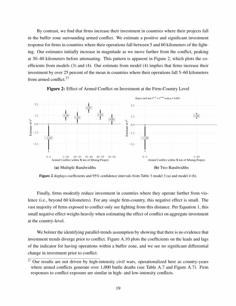
By contrast, we find that firms increase their investment in countries where their projects fallin the buffer zone surrounding armed conflict. We estimate a positive and significant investmentresponse for firms in countries where their operations fall between 5 and 60 kilometers of the fight-ing. Our estimates initially increase in magnitude as we move further from the conflict, peakingat 30–40 kilometers before attenuating. This pattern is apparent in Figure 2, which plots the co-efficients from models (3) and (4). Our estimate from model (4) implies that firms increase theirinvestment by over 25 percent of the mean in countries where their operations fall 5–60 kilometersfrom armed conflict.27

Figure 2: Effect of Armed Conflict on Investment at the Firm-Country Level

−2.43

1.541.16

2.87

1.65

0.83

−3.5

−1.5

0.0

1.5

3.5

0−5 5−20 20−30 30−40 40−50 50−60Armed Conflict within X km of Mining Project

Est

imat

e of

τk

(a) Multiple Bandwidths

−2.39

1.64

−3.5

−1.5

0.0

1.5

3.5

0−5 5−60Armed Conflict within X km of Mining Project

Est

imat

e of

τk

Reject null that τ0−5 = τ5−60 with p < 0.005

(b) Two Bandwidths

Figure 2 displays coefficients and 95% confidence intervals from Table 3 model 3 (a) and model 4 (b).

Finally, firms modestly reduce investment in countries where they operate further from vio-lence (i.e., beyond 60 kilometers). For any single firm-country, this negative effect is small. Thevast majority of firms exposed to conflict only see fighting from this distance. Per Equation 1, thissmall negative effect weighs heavily when estimating the effect of conflict on aggregate investmentat the country-level.

We bolster the identifying parallel-trends assumption by showing that there is no evidence thatinvestment trends diverge prior to conflict. Figure A.10 plots the coefficients on the leads and lagsof the indicator for having operations within a buffer zone, and we see no significant differentialchange in investment prior to conflict.

27 Our results are not driven by high-intensity civil wars, operationalized here as country-yearswhere armed conflicts generate over 1,000 battle deaths (see Table A.7 and Figure A.7). Firmresponses to conflict exposure are similar in high- and low-intensity conflicts.

19

We parameterized the effect of operating at a conflict site as ζ , of operating in a buffer zone asη , and being in a country with conflict as θ . Using model (2), we present estimates for these threeparameters in Table 4.28 First, operating at the site of battles dramatically reduces investment (ζ =

−4.06). Second, operating in a buffer zone encourages investment by mining firms (η = 1.63).Finally, operating in a country with conflict deters investment, though the effect is minimal if afirm is far from the fighting (θ = −0.002). The effects are all significantly different from zero atthe α = 0.05 level. The difference in effects between the conflict site and buffer zone and betweenthe conflict site and conflict-affected country are each significant at the α = 0.01 level.

Table 4: Parameter Estimates

Parameter Estimate Std. Error 2.5 % 97.5 %

Conflict site ζ −4.060 1.313 −6.633 −1.488Buffer zone η 1.636 0.257 1.132 2.140Conflict-affected country θ −0.002 0.001 −0.004 0.000

Table 4 estimates based on Table 3, model (2); standard errors computed via the delta method.

Table 4 also relates our findings to our first three hypotheses: we find a large negative responsein countries where firms operate at conflict sites; a smaller, but still substantial, positive responsewhere firms operate in buffer zones; and a small negative effect in countries where firms’ operationsare well-removed from the fighting. While there could still be offsetting considerations withinbuffer zones — firms may both enjoy weakened oversight and lament weakened property rights— the investment-encouraging mechanisms appear to dominate. Two characteristics of the miningsector may mitigate the negative effects: firms cannot relocate their assets in response to conflict,because mines are tied to geological features; and, as a consequence, firms may increase spendingon security and other services that the government can no longer provide, mitigating harms thatmight make other firms halt investment.

We might worry that firms reallocate from conflictual to more peaceful environments and thatthis response amplifies our estimates. Our context helps to mitigate such concerns. Explorationportfolios cannot be quickly adjusted. Adding properties to an exploration portfolio, particularlyfrom a new country, typically takes years and requires several time-consuming steps: (1) localincorporation, which may take one to three months; (2) exploration license application writingand review process, at least three months; (3) access approval from surface rights holders andindigenous consultations, at least two months; (4) water permitting, at least a month; and (5) anenvironmental impact study, at least three months. Our estimates reflect firms’ investment response

28 We use the following mapping: τsite = κ

[0−5]; τbuffer = κ

[5−60]; τcountry = θ .

20

in the year of or immediately following conflict; reallocation over such a short time scale would beexceptional (Haldar 2018).

We use sub-group analysis to empirically assess the plausibility of such reallocation. Weexpect firms invested in multiple countries to be better able to reallocate exploration resources inresponse to conflict.29 We drop firm-years in our sample that were invested in multiple countriesbased on a two-year running lag, and reestimate Equation 3 in model (5). Our inferences areunchanged (see Figure A.8). Even if a firm is working in a single country, perhaps it can reallocateacross multiple projects. No firm in our data has projects affected by conflict at the site of violenceand in buffer zones. Similarly, no firm has operations in buffer zones and far from violence in aconflict-affected country. In model (6), to address the possibility of reallocation, we restrict thesample to those firms with a single project and reestimate Equation 3. Our inferences are againunchanged (see Figure A.9).

Specialized capital and labor employed by mines at conflict sites might flee violence, leadingto increased supply in the surrounding area. Firms in the buffer zone (or beyond) might increaseinvestment to take advantage of lower resulting input prices. Our data allow us to rule out thisconcern. First, conflict rarely occurs at mining sites, making displacement unlikely (Table A.4).When we observe a firm operating within a buffer zone around conflict, there is often no miningoperation at the conflict site from which capital or labor might have fled. Nevertheless, in model(7), we drop country-years where any mining project is at a conflict site and continue to find thatfirms increase their investment in countries where they have operations within the buffer zonesurrounding conflict.

A final related concern is that firms reallocate their exploration investment over time. Specif-ically, firms operating projects in buffer zones may ramp up their investments in an effort to com-plete exploration before nearby conflicts escalate or creep closer. Such behavior is inconsistentwith the business strategy literature, which argues that firms typically adopt a “wait and see” ap-proach and avoid committing major resources when facing emerging risks (Courtney, Kirklandand Viguerie 1997, 8). Moreover, we assess this empirically by looking at whether heightenedinvestment in buffer zones immediately after conflict is then followed by reduced investment —the pattern consistent with shifting the timing of investment without changing the overall level.Figure A.10 and Table A.8 demonstrate that, in fact, the positive effects of exposure to conflict inthe buffer zone persist for several years, ruling out such temporal displacement.

29 As noted above, junior miners, who represent the vast majority of firms, tend to concentrate theirinvestments in a single country, or even on a single project (see Figure A.3).

21

5.2 Effect on Investment at Country LevelOur results at the country level, which provide a test of Hypothesis 4, are consistent with a

majority of the existing literature: the incidence of fatal armed conflict reduces exploration in-vestment. Table 5 reports consistent estimates from Equation 4 using both different samples andmeasures of conflict.

Table 5: Effect of Armed Conflict on Investment at the Country Level

Dependent variable:

Log(Exploration Investment + 1)

(1) (2) (3) (4) (5) (6) (7)

1(Conflicts > 0) −0.65∗∗ −0.56(0.32) (0.34)

1(Conflicts = 1) −0.41(0.37)

1(Conflicts > 1) −0.74∗∗

(0.37)1(State-Based > 0) −0.17 0.07

(0.39) (0.39)1(One-Sided > 0) −0.87∗∗∗ −0.85∗∗∗

(0.31) (0.32)1(Non-State > 0) −0.69 −0.62

(0.45) (0.46)

F-stat 4.15 2.72 2.11 0.2 7.86 2.32 3.23p-value 0.04 0.1 0.12 0.65 0.01 0.13 0.02

yct 9.98 12.19 9.98 9.98 9.98 9.98 9.98

Country-YearSample All Recipients All All All All All

Country FE 177 145 177 177 177 177 177Year FE 18 18 18 18 18 18 18

Table 5 reports the results from OLS models estimated using Equation 4. We cluster standard errors at the countrylevel, shown in parentheses. The dependent variable is exploration investment (logged plus one). The main indepen-dent variable codes whether conflict occurred in a given year (t) or in the year prior (t-1). Models 2–7 report estimatesfrom Equation 4 using different samples or measures of conflict. Significance: ∗p<0.1; ∗∗p<0.05; ∗∗∗p<0.01.

Model (1) includes our full sample — 177 countries over 18 years — and finds that theincidence of at least one fatal armed conflict in the current or previous year reduces aggregateinvestment by 0.77 log points. This is just over one quarter of the average within-country standarddeviation (2.78) and roughly eight percent of the mean (yct = 9.98). Model (2) drops countries withno investment (32 countries). Across both models, our estimates are of similar magnitudes. We

22

also examine the extensive margin: conflict reduces the number of firms operating in the countrywith conflict (see Table A.10).

These country-level results are consistent with the estimates from our model based on the firm-level analyses above. The vast majority of firms investing (or considering investing) in a countryoperate outside of conflict sites and buffer zones. When we aggregate the effects of conflict to thecountry-level, the largest component of that sum is the negative effect of these firms with minimalconflict exposure. η and ζ can be sizable, but if they only apply to a relatively small proportion offirms, they will be washed out when we aggregate the data.

Finally, we investigate how effects vary by the type and intensity of violence. Model (3)shows, intuitively, that settings with multiple conflicts see a larger reduction in exploration invest-ment; however, both coefficients are negative, and the magnitudes are not significantly different.Models (4) to (7) look at whether different types of fatal armed conflict — state-based, one-sided,or non-state — have differential effects on exploration investment. Focusing attention on model(7), we find that one-sided and non-state conflicts have larger, negative effects.30

In Appendix F.1, we report analyses that separate “major” and multinational mining firms —firms that, by virtue of their size and visibility, may be especially concerned about their reputations(see Table A.12). We do not find a significantly different response among these subsets of firms.However, while the interaction term is not significant, major mining firms may respond moreaversely to state-based armed conflict, which could reflect greater concern about their brands beingassociated with repressive governments (as suggested in Henisz 2017). This analysis does not, ofcourse, rule out reputational effects — these could act on all firms, or large firms may have othercompensating features.

Our empirical strategy assumes parallel trends in investment (logged) among countries thatare and are not affected by fatal armed conflict. While untestable, we bolster this assumptionby showing that investment does not change in anticipation of conflict. Figure A.12 plots thecoefficients on the leads and lags of the indicator for a fatal armed conflict (see also Table A.11).We see no differential change in investment prior to conflict (i.e., the coefficients on the leads areclose to zero), suggesting that the countries that will be attacked are not seeing a spike or fall off ininvestment in the years before conflict breaks out. The figure also reveals that the negative effectson investment materialize in the first and second years after conflict. The effect on investment isnot immediate, suggesting that the allocation of exploration investment may not be updated in realtime but adjusted annually (e.g., at the start of the fiscal year).30 This variation requires investigation beyond the scope of this paper. One ex-post rationalization

would be that state-based violence involves well-defined combatants; one-sided and non-stateconflicts may be less predictable and involve greater uncertainty about the extent of collateraldamage.

23

6. MechanismsWe incorporate auxiliary data to explore the mechanisms outlined in Section 2: that conflict

disrupts production at proximate mining operations, undermines state capacity, and creates pol-icy uncertainty or reputation risk. We regard these as secondary, and typically more speculative,analyses given data and design limitations that we note below.

6.1 Disrupted ProductionMihalache-O’keef and Vashchilko (2010) recount stories of operations being seized or sus-

pended during conflicts. Local violence threatens staff, severs supply chains, and can destroy crit-ical infrastructure, none of which is good for business. Ksoll, Macchiavello and Morjaria (2016,3) find, for example, that flower exporters in regions affected by Kenya’s post-election violencesaw their exports fall by 38 percent. At the height of the violence, half of their employees werenot showing up for work. Looney (2006, 995) argues that conflict and insurgency in Iraq led tothe downsizing or closing of firms in the formal sector. Research in Sierra Leone (Collier andDuponchel 2013) and Colombia (Camacho and Rodriguez 2013) echo these findings, showinglower production and more business closures in high-conflict areas.

We assess this mechanism using the subset of mining projects in Africa, for which we haveannual production data (e.g., how many tons of lead or ounces of silver a mine pulled out of theground). A single mine can produce multiple minerals, so our unit of analysis is the project-mineral-year. We look at the change in production at projects near the site of a recent conflict(within five kilometers) versus further afield. Employing a specification similar to Equation 3,but with project, year, and mineral fixed effects, we find changes on the extensive and intensivemargins for mines at conflict sites: the probability of any production declines by twenty percentagepoints; the quantity produced (logged) falls by about twenty percent of the mean (see Table A.13).The latter, while sizable, is not significant.31 For projects in a buffer zone but outside of a conflictsite (5–60 kilometers from a recent conflict), we find small and insignificant negative effects on thelikelihood and intensity of production. The effect of being within 5 to 60 kilometers of a conflictis an order of magnitude smaller than being next to the fighting (model 2). While these differencesare large in magnitude, our estimates are imprecise, and we cannot rule out the null hypothesis ofno difference between projects located at conflict sites or further afield.

This pattern of results is consistent with our earlier findings on investment: operating at a con-flict site can hamper production and, as a consequence, limit companies’ capacity or willingness31 Standard errors are clustered on project. Our independent variable here captures whether a

conflict occurred in that bandwidth in any of the three previous years, i.e., from t− 1 to t− 3.A shorter lag structure generates results in the same direction but of smaller magnitudes. Ourestimates from a dynamic panel model (Figure A.13) indicate that production for mines at conflictsites continues to decline three years after violence takes place.

24

to invest. Yet, these dampening effects are not apparent in the broader buffer zone that surroundsthese conflict sites.

6.2 State CapacityConflict could be a boon for mining companies if it reduces costly oversight. We assess

whether conflict reduces the tax revenues derived from natural resource production. We emphasizethat this is not the only aspect of state capacity that may affect firms’ decisions in buffer zonesaround conflict. It is, however, one dimension that we can measure systematically. We estimatethe elasticity between natural resource production and resource tax revenues, and whether thiselasticity is reduced (i.e., less tax revenue is derived from production) in countries that recentlyexperienced a fatal armed conflict.

We lack firm-level data on tax payments and rely on a country-level measure of resourcetax revenues from the International Centre for Tax and Development (ICTD).32 We also compiledata from the World Mineral Statistics on annual production for roughly 100 minerals for nearlyevery country.33 To compute the value of natural resource production, we merge this productiondata with world commodity prices tracked by the World Bank, US Geological Survey, and USEnergy Information Administration. Thus, for every year, we can calculate the dollar value ofresources produced (our independent variable) and the amount of resource tax revenue collected(our dependent variable). We log both measures to estimate an elasticity, and interact our measureof resource production with a country-level indicator for armed conflict. We focus on the changein this elasticity, as the direct effect of conflict on tax revenues conflates conflict-induced changesin both production and fiscal capacity. Our goal here is to better isolate the latter.

As is apparent in Figure A.14 (see also Table A.14), the production elasticity of resource taxrevenues is lower in countries affected by one-sided or state-based conflicts in the current or pre-vious year (models 1 and 3). For a given amount of mineral production, governments recentlyaffected by these types of conflicts collect less in taxes — a finding that is consistent with conflictdiminishing fiscal capacity.34 We find no significant effect of non-state conflicts, which do not in-volve the government. These results suggest that armed conflict involving the state may underminefiscal capacity.32 ICTD’s Government Revenue Dataset (GRD) combines information from six cross-country

sources, including the IMF, the World Bank, the OECD and CEPAL, to create a comprehensive,standardized dataset of government revenue from taxation. We focus on countries that report anyrevenues from natural resources in 1997, at the start of our study period.

33The WMS extends back to 1913 and draws on “home and overseas government departments,national statistics offices, specialist commodity authorities, company reports, and a network ofcontacts throughout the world” (British Geological Survey 2017).

34 The direct effects of conflict on taxation are included in all models in Table A.14 but are omittedfrom the table.

25

While we cannot specify where the state’s fiscal capacity erodes, our findings align withcase studies of mining companies profiting from operations in ungoverned areas (e.g., Reno 1999;Vanden Eynde 2015). They could also help to explain why we see greater exploration investmentamong companies operating projects in the buffer zones that surround recent fatal armed conflicts:the companies in these grey zones suffer minor production disruptions while benefitting from lessoversight.

6.3 Policy ChangeWe look at whether conflict raises concerns about changes in policy due to, for example,

government turnover. Concretely, we estimate Equation 4 using two different outcomes. First, as amanipulation check, we look at whether the incidence of UCDP armed conflicts shifts the “InternalConflict Index” compiled by the International Country Risk Guide (ICRG) — a dataset used byfirms that contains measures of multiple components of political risk.35 We find that the armedconflicts we use in our analyses raise concerns that political violence will impact the country’sgovernance (see Table A.15). In the year of or immediately following the incidence of a fatalarmed conflict, ICRG’s Internal Conflict Index falls a half point on a 12-point scale (50 percentof the average within-country standard deviation for this index). While the UCDP data includessmall skirmishes and battles, these events shape country-level assessments of internal violence andits impacts on governance.

Second, we consider the effect of fatal armed conflict on ICRG’s Government Stability In-dex, which provides an “assessment both of the government’s ability to carry out its declaredprogram(s), and its ability to stay in office” (PRS Group 2012).36 This measure operationalizestwo concerns raised in arguments about investors’ aversion to policy change: investors worry bothabout whether the current government will survive in office and, if so, whether it will be forced tochange course. We find that the incidence of fatal armed conflict decreases assessments of gov-ernment stability (model 4 of Table A.15): a reduction of 0.2 is roughly 15 percent of the averagewithin-country standard deviation for the Government Stability Index. This finding is robust tomultiple ways of measuring conflict (model 5). The effect is larger for non-state and one-sidedconflicts (model 6).

We also look at whether conflict deters entry by new companies. As new entrants are unlikelyto invest at conflict sites and will not be subject to taxation for several years, the estimated effect

35 ICRG’s Internal Conflict Index is an “assessment of political violence in the country and itsactual or potential impact on governance” and consists of three items: “civil war/coup threat,”“terrorism/political violence,” and “civil disorder” (PRS Group 2012).

36 The index is a composite of three items, measuring “government unity,” “legislative strength,”and “popular support.”

26

among these firms helps us isolate the aggregate country-level effect, which we attribute to in-creased uncertainty around policy changes or reputation risk.37 We estimate Equation 4, but limitour dependent variable to exploration investment in country c in year t to firms that had not pre-viously invested in country c. Our estimates in Table A.16 are comparable in magnitude to thosereported for the full sample. Conflict does deter investment by potential new entrants to a country.

7. DiscussionEarlier empirical work largely supports the oft-repeated claim that conflict is bad for business.

This idea underlies policy efforts to prevent and end armed conflict that assume private sector sup-port. A 2016 report from the World Economic Forum, for example, argues that “Internationaland local businesses have a critical role to play in finding ways to minimize fragility and buildresilience in violence-affected societies. A key reason, among others, is because fragility — in-cluding conflict and crime — is bad for business. It generates direct and indirect opportunity costsall along the value chain” (World Economic Forum February 2016).

Yet, the past research supporting this claim relies overwhelmingly on cross-national analy-sis, which masks the differential effects that conflict has on firms operating (or considering newoperations) in the same country. Theoretically, we argue that conflict may deter investment bydisrupting production or raising policy uncertainty, but that it may encourage investment where ithampers oversight. Moreover, whether these mechanisms apply to a firm depends on its geographicexposure to violence.

Using firm-level panel data on mining exploration investments, we show that effects dependon the conflict exposure of firms. We show that mining firms pull back investments at the sites ofviolence and that the disruption of mineral production may explain why. However, in the bufferzone surrounding the fighting — where neither the state nor its armed challengers fully controlthe territory — firms seem to double down on exploration investment. In these areas of imperfectcontrol, the state may be unable to oversee the sector, thereby lowering costs in the short term. Wefind that effective mineral tax rates decline during conflict. Finally, we show that armed conflictsraise concerns that political violence will impact governance and undermine government stability.This suggests that conflict could deter investment by raising the likelihood of policy change orgovernment turnover.

These results demonstrate that conflict is not uniformly bad for business. Indeed, some firmsmay benefit from how conflict weakens state capacity. Where firms can privately secure theirproperty and do not depend on public services, they may associate improved state capacity with

37 The effect of policy uncertainty or reputation risk on investment may be different for existingand new investors. We only estimate the latter in this exercise.

27

costly regulation or taxation. Different sectors and firms can, thus, vary in their propensity toinvest in weak and fragile states. These findings expand upon past case studies (e.g., Fisman2001), which find that conflict and instability benefit (or only harm) certain companies. The resultsalso parallel efforts to understand when states selectively tolerate or even encourage instability inungoverned spaces (Callen et al. 2019). Our findings suggests new directions for research into howheterogeneous exposure to conflict — and the ungoverned grey zones created by conflict — affectconflict termination, postwar economic growth, and the distributional consequences of war.

We focus on the effects of armed civil conflict, which is only one factor included in commonlyused measures of political risk. As Snider (2005) points out, the measurement of political risk isatheoretical: the ICRG, for example, weights armed conflict heavily, but does not articulate whyinternal conflict receives twice the weight of democratic accountability or three times the weightof bureaucratic quality. We note at least three ways that political risks differ: (1) specificity (dothey apply to all or a subset of firms); (2) severity (what is the scale of potential losses); and(3) mitigation (can firms mitigate the risk through private precautions). As we describe earlier,modern armed conflicts tend to be localized, and individual conflict events near mining projectsinvolve relatively few fatalities. Moreover, firms can employ private security or contract with statesecurity forces to protect their operations. By contrast, nationalization of an industry affects allfirms in a sector, implies the loss of immobile assets, and would be difficult for any individualfirm to mitigate. We, thus, think of the latter risk as being less specific, more severe, and harderto mitigate than localized armed conflicts. Future research could provide a richer framework fordifferentiating political risks, as well as empirical assessments of how these different risks (ordimensions of risk) affect investment behavior.

28

ReferencesAcemoglu, Daron, Simon Johnson and James A. Robinson. 2005. Institutions as a Fundamental Cause of

Long-Run Growth. In Handbook of Economic Growth, ed. Philippe Aghion and Steven N. Durlauf. North

Holland.

Banerjee, Sudeshna Ghosh, Zayra Romo, Gary McMahon, Perrine Toledano, Peter Robinson and Ines

Perez Arroyo. 2014. The Power of the Mine: A Transformative Opportunity for Sub-Saharan Africa.

The World Bank.

Barry, Colin M. 2016. “Bringing the Company Back In: A Firm-Level Analysis of Foreign Direct Invest-

ment.” International Interactions 42(2):244–270.

Barry, Colin M. 2018. “Peace and Conflict at Different Stages of the FDI Lifecycle.” Review of International

Political Economy 25(2):270–292.

Bates, Robert H. 2001. Prosperity and Violence: The Political Economy of Development. W W Norton &

Co Inc.

Bates, Robert H. and Da-Hsiang Donald Lien. 1985. “A Note on Taxation, Development, and Representative

Government.” Politics & Society 14(1):53–70.

Bennett, Juliette. 2001. “Business in Zones of Conflict: The Role of the Multinational in Promoting Regional

Stability.” UN Global Compact Policy Dialogues .

Bennett, Peter D. and Robert T. Green. 1972. “Political Instability as a Determinant of Direct Foreign

Investment in Marketing.” Journal of Marketing Research 9(2):182–186.

Berman, Eli, Joseph H. Felter and Jacob N. Shapiro. 2018. Small Wars, Big Data: The Information Revolu-

tion in Modern Conflict. Princeton University Press.

Berman, Jonathan. 2000. “Boardrooms and Bombs.” Harvard International Review 22(3):28.

Berman, Nicolas, Mathieu Couttenier, Dominic Rohner and Mathias Thoenig. 2017. “This Mine Is Mine!

How Minerals Fuel Conflicts in Africa.” American Economic Review 107(6):1564–1610.

Besley, Timothy and Torsten Persson. 2008. “Wars and State Capacity.” Journal of the European Economic

Association 6(2-3):522–530.

Besley, Timothy and Torsten Persson. 2011. Pillars of Prosperity. Princeton University Press.

Blanton, Shannon Lindsey and Robert G. Blanton. 2007. “What Attracts Foreign Investors? An Examination

of Human Rights and Foreign Direct Investment.” The Journal of Politics 69(1):143–155.

Blattman, Christopher and Edward Miguel. 2010. “Civil War.” Journal of Economic Literature 48(1):3–57.

Boix, Carles. 2003. Democracy and Redistribution. Cambridge University Press.

29

Boone, Catherine. 2003. Political Topographies of the African State: Territorial Authority and Institutional

Choice. Cambridge University Press.

British Geological Survey. 2017. “World Mineral Statistics Electronic Archive.” https://www.bgs.ac.

uk/mineralsUK/statistics/worldStatistics.html.

Burger, Martijn, Elena Ianchovichina and Bob Rijkers. 2015. “Risky Business: Political Instability and

Sectoral Greenfield Foreign Direct Investment in the Arab World.” The World Bank Economic Review

30(2):306–331.

Buthe, Tim and Helen V. Milner. 2008. “The Politics of Foreign Direct Investment into Developing Coun-

tries: Increasing FDI through International Trade Agreements?” American Journal of Political Science

52(4):741–762.

Callen, Michael, Saad Gulzar, Arman Rezaee and Jacob N. Shapiro. 2019. “Choosing Ungoverned Space:

The Removal of Pakistan’s Frontier Crimes Regulation.” Working Paper.

Camacho, Adriana and Catherine Rodriguez. 2013. “Firm Exit and Armed Conflict in Colombia.” Journal

of Conflict Resolution 57(1):89–116.

Ch, Rafael, Jacob Shapiro, Abbey Steele and Juan F Vargas. 2018. “Endogenous Taxation in Ongoing

Internal Conflict: The Case of Colombia.” American Political Science Review 112(4):996–1015.

Chowdhury, Abdur R. and Syed Mansoob Murshed. 2016. “Conflict and Fiscal Capacity.” Defence and

Peace Economics 27(5):583–608.

Christensen, Darin. 2019. “Concession Stands: How Mining Investments Incite Protest in Africa.” Interna-

tional Organization 73(1):65–101.

Christensen, Darin, Mai Nguyen and Renard Sexton. 2019. “Strategic Violence during Democratization:

Evidence from Myanmar.” World Politics 71(2):332–366.

Collier, Paul. 1999. “Doing Well Out of War.” Working paper.

Collier, Paul, Lani Elliot, Havard Hegre, Anke Hoeffler, Marta Reynal-Querol and Nicholas Sambanis. 2003.

Breaking the Conflict Trap: Civil War and Development Policy. Oxford: Oxford University Press.

Collier, Paul and Marguerite Duponchel. 2013. “The Economic Legacy of Civil War: Firm-Level Evidence

from Sierra Leone.” Journal of Conflict Resolution 57(1):65–88.

Courtney, Hugh, Jane Kirkland and Patrick Viguerie. 1997. “Strategy Under Uncertainty.” Harvard Business

Review 75(6):67–79.

Croicu, Mihai and Ralph Sundberg. 2017. “UCDP GED Codebook Version 18.1.” Technical Report, De-

partment of Peace and Conflict Research, Uppsala University.

30

Dai, Li, Lorraine Eden and Paul W. Beamish. 2013. “Place, Space, and Geographical Exposure: Foreign

Subsidiary Survival in Conflict Zones.” Journal of International Business Studies 44(6):554–578.

Dai, Li, Lorraine Eden and Paul W. Beamish. 2017. “Caught in the Crossfire: Dimensions of Vulner-

ability and Foreign Multinationals’ Exit from War-afflicted Countries.” Strategic Management Journal

38(7):1478–1498.

Davy, Aidan and Diane Tang-Lee. 2018. “Social Progress in Mining-Dependent Countries: Analysis through

the Lens of the SDGs.” International Council on Mining and Metal.

Doctor, Austin C. and Stephen Bagwell. 2020. “Risky Business: Foreign Direct Investment and the Eco-

nomic Consequences of Electoral Violence.” Journal of Global Security Studies 5(2):339–360.

Dougherty, Michael L. 2013. “The Global Gold Mining Industry: Materiality, Rent-seeking, Junior Firms

and Canadian Corporate Citizenship.” Competition & Change 17(4):339–354.

Financial Times Ltd. 2019. “fDi Markets Database.” https://www.fdimarkets.com/.

Fisman, Raymond. 2001. “Estimating the Value of Political Connections.” The American Economic Review

91(4):1095–1102.

Garrett, Nicholas, Sylvia Sergiou and Koen Vlassenroot. 2009. “Negotiated Peace for Extortion: The Case

of Walikale Territory in Eastern DR Congo.” Journal of Eastern African Studies 3(1):1–21.

Green, Robert T. and William H. Cunningham. 1975. “The Determinants of U.S. Foreign Investment: An

Empirical Examination.” Management International Review 15(2-3):113–120.

Guidolin, Massimo and Eliana La Ferrara. 2007. “Diamonds are Forever, Wars are Not: Is Conflict Bad for

Private Firms?” The American Economic Review 97(5):1978–1993.

Guidolin, Massimo and Eliana La Ferrara. 2010. “The Economic Effects of Violent Conflict: Evidence from

Asset Market Reactions.” Journal of Peace Research 47(6):671–684.

Haldar, Swapan Kumar. 2018. Mineral Exploration: Principles and Applications. Elsevier.

Henisz, Witold J. 2000. “The Institutional Environment for Multinational Investment.” The Journal of Law,

Economics, and Organization 16(2):334–364.

Henisz, Witold J. 2017. Corporate Diplomacy: Building Reputations and Relationships with External

Stakeholders. Routledge.

Herbst, Jeffrey. 2000. States and Power in Africa. Princeton University Press.

Humphreys, David. 2015. The Remaking of the Mining Industry. Palgrave Macmillan.

Jamison, Anne Spencer. 2019. “The Subnational Political Economy of Political Violence and Foreign Direct

Investment.” Working Paper.

31

Jensen, Nathan. 2008. “Political Risk, Democratic Institutions, and Foreign Direct Investment.” The Journal

of Politics 70(4):1040–1052.

Jensen, Nathan M. 2003. “Democratic Governance and Multinational Corporations: Political Regimes and

Inflows of Foreign Direct Investment.” International Organization 57(3):587–616.

Kaufmann, Daniel, Aart Kraay and Massimo Mastruzzi. 2011. “The Worldwide Governance Indicators:

Methodology and Analytical Issues.” Hague Journal on the Rule of Law 3(2):220–246.

Keen, David. 1998. “The Economic Functions of Violence in Civil Wars.” The Adelphi Papers 38(320).

Kerner, Andrew. 2009. “Why Should I Believe You? The Costs and Consequences of Bilateral Investment

Treaties.” International Studies Quarterly 53(1):73–10.

Kim, In Song and Iain Osgood. 2019. “Firms in Trade and Trade Politics.” Annual Review of Political

Science 22.

Kobrin, Stephen J. 1978. “When Does Political Instability Result in Increased Investment Risk?.” Columbia

Journal of World Business 13(3):113–122.

Ksoll, Christopher, Rocco Macchiavello and Ameet Morjaria. 2016. “Guns and Roses: Flower Exports

and Electoral Violence in Kenya.” Buffet Institute Global Poverty Research Lab Working Paper Series

17-102.

Lacina, Bethany, Nils Petter Gleditsch and Bruce Russett. 2006. “The Declining Risk of Death in Battle.”

International Studies Quarterly 50(3):673–680.

Le Billon, Philippe. 2008a. “Corrupting Peace? Peacebuilding and Post-Conflict Corruption.” International

Peacekeeping 15(3):344–361.

Le Billon, Philippe. 2008b. “Resources for Peace? Managing Revenues from Extractive Industries in Post-

Conflict Environments.” PERI Working Papers.

Lee, Chia-Yi. 2017. “Terrorism, Counterterrorism Aid, and Foreign Direct Investment.” Foreign Policy

Analysis 13(1):168–187.

Lee, Hoon. 2016. “Does Armed Conflict Reduce Foreign Direct Investment in the Petroleum Sector?”

Foreign Policy Analysis 13(1):188–214.

Lee, Melissa M. and Nan Zhang. 2017. “Legibility and the Informational Foundations of State Capacity.”

The Journal of Politics 79(1):118–132.

Li, Chengchun, Syed Mansoob Murshed and Sailesh Tanna. 2017. “The Impact of Civil War on Foreign

Direct Investment Flows to Developing Countries.” The Journal of International Trade & Economic De-

velopment 26(4):488–507.

32

Li, Quan and Adam Resnick. 2003. “Reversal of Fortunes: Democratic Institutions and Foreign Direct

Investment Inflows to Developing Countries.” International Organization 57(1):175–211.

Looney, Robert. 2006. “Economic Consequences of Conflict: The Rise of Iraq’s Informal Economy.” Jour-

nal of Economic Issues 40(4):991–1007.

Marshall, Ian E. 2001. “A Survey of Corruption Issues in the Mining and Mineral Sector.” International

Institute for Environment and Development 15:3–52.

McDougal, Topher L. 2010. “How Production Firms Adapt to War: The Case of Liberia.” WIDER Working

Paper No. 2010/69.

Mihalache-O’keef, Andreea and Tatiana Vashchilko. 2010. “Chapter Seven: Foreign Direct Investors in

Conflict Zones.” Adelphi Series 50(412-413):137–156.

Mills, Rob and Qimiao Fan. 2006. The Investment Climate in Post-Conflict Situations. Technical report.

Moran, Theodore H. 1974. Multinational Corporations and the Politics of Dependence. Princeton Univer-

sity Press.

North, Douglass Cecil. 1981. Structure and Change in Economic History. W W Norton & Co Inc.

Olson, Mancur. 1993. “Dictatorship, Democracy, and Development.” American Political Science Review

87(3):567–576.

Osgood, Iain and Corina Simonelli. 2019. “Nowhere to Go: FDI, Terror, and Market-specific Assets.”

Working Paper.

Pandya, Sonal S. 2016. “Political Economy of Foreign Direct Investment: Globalized Production in the

Twenty-first Century.” Annual Review of Political Science 19:455–475.

Pierskalla, Jan, Anna Schultz and Erik Wibbels. 2017. “Order, Distance, and Local Development over the

Long-Run.” Quarterly Journal of Political Science 12(4):375–404.

Pinto, Pablo M. and Boliang Zhu. 2018. “Brewing Violence: Foreign Investment and Civil Conflict.” Work-

ing Paper.

PRS Group. 2012. “International Country Risk Guide Methodology.” Codebook.

Reno, William. 1999. Warlord Politics and African States. Boulder, Colorado: Lynne Rienner Publishers.

Scott, James C. 2009. The Art of Not Being Governed. Yale University Press.

Smith, Erin and Peter Rosenblum. 2011. “Enforcing the Rules.” Revenue Watch Institute Report.

Snider, Lewis W. 2005. “Political Risk: The Institutional Dimension.” International Interactions 31(3):203–

222.

Stasavage, David. 2002. “Private Investment and Political Institutions.” Economics & Politics 14(1):41–63.

33

Stewart, Frances. 1993. “War and Underdevelopment: Can Economic Analysis Help Reduce the Costs?”

Journal of International Development 5(4):357–380.

The Economist. 2000. “Business in Difficult Places: Risky Returns.” The Economist pp. 101–102.

Thies, Cameron G. 2010. “Of Rulers, Rebels, and Revenue: State Capacity, Civil War Onset, and Primary

Commodities.” Journal of Peace Research 47(3):321–332.

UNCTAD, Geneva. 2012. “World Investment Report: Towards a New Generation of Investment Policies.”

United Nations. New York and Geneva pp. 1–204.

van den Boogaard, Vanessa, Wilson Prichard, Matthew S Benson and Nikola Milicic. 2018. “Tax Rev-

enue Mobilization in Conflict-affected Developing Countries.” Journal of International Development

30(2):345–364.

Vanden Eynde, Oliver. 2015. “Mining Royalties and Incentives for Security Operations: Evidence from

India’s Red Corridor.” PSE Working Papers 42:1–38.

Vernon, Raymond. 1971. Sovereignty at Bay: The Multinational Spread of U.S. Enterprises. Basic Books.

Wellhausen, Rachel L. 2014. The Shield of Nationality: When Governments Break Contracts with Foreign

Firms. Cambridge: Cambridge University Press.

Witte, Caroline T., Martijn J. Burger, Elena I. Ianchovichina and Enrico Pennings. 2016. “Dodging Bullets:

The Heterogeneous Effect of Political Violence on Greenfield FDI.” World Bank Working Paper Series.

World Economic Forum. February 2016. “Responsible Private Sector Action to Address Fragility, Conflict

and Violence.”.

Wright, Joseph and Boliang Zhu. 2018. “Monopoly Rents and Foreign Direct Investment in Fixed Assets.”

International Studies Quarterly 62(2):341–356.

Zhu, Boliang and Weiyi Shi. 2019. “Greasing the Wheels of Commerce? Corruption and Foreign Invest-

ment.” The Journal of Politics 81(4):1311–1327.

34

Supporting Information

How Does Armed Conflict Shape Investment?Evidence from the Mining Sector

Following text to be published online.

ContentsA Systematic Review A1

B Descriptives A3B.1 Exploration Investment and Mining Projects . . . . . . . . . . . . . . . . . . . . . A3B.2 Armed Conflict . . . . . . . . . . . . . . . . . . . . . . . . . . . . . . . . . . . . A8

C Defining Exposure to Conflict A10C.1 Path Distance between Conflicts and Mining Projects . . . . . . . . . . . . . . . . A11

D Firm-Country-Year Results A12

E Sector-Country-Year Results A19

F Country-Year Results A22F.1 Heterogeneous Effects by Type of Firm . . . . . . . . . . . . . . . . . . . . . . . A25

G Evidence on Mechanisms A27G.1 Disrupted Production . . . . . . . . . . . . . . . . . . . . . . . . . . . . . . . . . A27G.2 State Capacity . . . . . . . . . . . . . . . . . . . . . . . . . . . . . . . . . . . . . A29G.3 Policy Change . . . . . . . . . . . . . . . . . . . . . . . . . . . . . . . . . . . . . A31

H Details of Systematic Review A33H.1 Coding Rules for Systematic Review . . . . . . . . . . . . . . . . . . . . . . . . . A33H.2 PRISMA Checklist for Systematic Reviews . . . . . . . . . . . . . . . . . . . . . A35

A. Systematic ReviewTable A.1: Studies in Systematic Review

Author(s) & Year Effect Region∗ Years Unit of Analysis Unit FE?§ Time FE?∗∗ IV?‖

Koechlin (1992) - G (23) 1966-1985 country-2 yearPerotti (1994) - G (26) 1960-1985 countryAlesina and Perotti (1996) - G (71) 1960-1985 countryResnick (2001) - G (19) 1971-1993 country-yearGloberman and Shapiro (2002) - G (144) 1995-1997 countryStasavage (2002) - G (74) 1971-1994 country-year XSun, Tong and Yu (2002) - China (1) 1986-1998 province-year XAbadie and Gardeazabal (2003) - Spain (1) 1998-2000 firm-trading sessions†

Fielding (2003a) - N. Ireland (1) 1960-1995 sector-yearo XFielding (2003b) - Israel (1) 1988-1998 firmAsiedu (2006) - SSA (21) 1984-2000 country-year XAysan et al. (2007) - MENA (33) 1970-2002 country-year XBusse and Hefeker (2007) - G (83) 1984-2003 country-4 year‡ XDaude and Stein (2007) - G (152) 1982-2002 country-year XGani (2007) - G (17) 1996-2002 country-year XMalefane (2007) - Lesotho (1) 1973-2004 yearNaude and Krugell (2007) - Africa (43) 1970-1990 country-5 year X XAlfaro et al. (2008)⊥ - G (34) 1984-1997 country-year XSuliman and Mollick (2009) - SSA (29) 1980-2003 country-year XBussmann (2010) - G (154) 1980-2000 country-year X XRamasamy and Yeung (2010) - G (23) 1980-2003 country-year XBaek and Qian (2011) - G (116) 1984-2003 country-year XDaniele and Marani (2011) - Italy (1) 2002-2006 province-yearMengistu and Adhikary (2011) - Asia (15) 1996-2007 country-year XOh and Oetzel (2011) - G (101) 2001-2006 firm-country-year XMorrissey et al. (2012) - G (46) 1996-2009 country-yearPowers and Choi (2012) - G (123) 1980-2008 country-year XRamasamy et al. (2012) - G (59) 2006-2008 country-yearSolomon and Ruiz (2012) - G (28) 1985-2004 country-year XAl-Khouri and Khalik (2013) - MENA (16) 1984-2011 country-year XBandyopadhyay et al. (2013) - G (78) 1984-2008 country-year X XHayakawa et al. (2013) - G (89) 1985-2007 country-3 year X XSingh (2013) - India (1) 1981-1990 district-year X XBurger et al. (2015)⊥ - MENA (17) 2003-2012 country-year; country-quarter XEzeoha and Ugwu (2015) - Africa (41) 1997-2012 country-year XMijiyawa (2015) - Africa (53) 1970-2009 country-5 year X XLee (2016) - G (50) 1980-2006 country-year X XLee (2017) - G (114) 1987-2006 country-year XBrown and Hibbert (2017) - G (65) 1997-2012 country-year XCabral et al. (2019) - Mexico (1) 2005-2015 state-quarter X

A1

Studies in Systematic Review (Continued)

Author(s) & Year Effect Region∗ Years Unit of Analysis Unit FE?§ Time FE?∗∗ IV?‖

Brunetti and Weder (1998) -/∼ G (60) 1974-1989 countryTuman and Emmert (1999) -/∼ LAC (12) 1979-1992 country-yearBohn and Deacon (2000) -/∼ G (125) 1955-1988 country-yearEnders et al. (2006) -/∼ G (69) 1989-1999 country-quarter XLi, Murshed and Tanna (2017)∓ -/∼ G (128) 2003-2012 country-sector-year XCarter et al. (2018) -/∼ G (40) 1980-2010 country-year XTuman and Emmert (2004) -/+ LAC (15) 1979-1996 country-yearLi (2006)⊥ -/∼/+ G (129) 1976-1996 country-yearWheeler and Mody (1992)⊥ ∼ G (42) 1982-1988 country-year XLiu et al. (1997) ∼ China (1) 1983-1994 country-year XFeng (2001) ∼ G (40) 1978-1988 countryAsiedu (2002) ∼ G (71) 1988-1997 countryGloberman and Shapiro (2003) ∼ G (143) 1995-1997 country-yearBevan and Estrin (2004) ∼ Europe (11) 1994-2000 dyad-yearLe (2004) ∼ G (25) 1975-1995 country-year XBiglaiser and DeRouen Jr. (2007)⊥ ∼ G (126) 1966-2002 country-year XKinda (2010) ∼ G (77) 2000-2006 country-sector-yearLi and Vashchilko (2010) ∼ G (58) 1980-2000 dyad-year XCleeve (2012) ∼ SSA (40) 1988-2008 country-year XJadhav (2012) ∼ BRICS (5) 2000-2009 country-yearKolstad and Wiig (2012) ∼ G (142) 2003-2006 countryVadlamannati (2012) ∼ G (101) 1997-2007 country-year X XAshby and Ramos (2013) ∼ Mexico (1) 2004-2010 country-state-sector-year XSissani and Belkacem (2014) ∼ Algeria (1) 1990-2012 yearKariuki (2015) ∼ Africa (35) 1984-2010 country-year X XOkafor (2015) ∼ SSA (23) 1996-2010 country-yearKim (2016) ∼ G (95) 1980-2000 country-yearShahzad et al. (2016) ∼ Pakistan (1) 1988-2010 quarterWilliams (2017) ∼ G (68) 1975-2005 country-5 yearCampos and Nugent (2003) + G (94) 1960-1985 country-5 year XBiglaiser and DeRouen Jr. (2006)⊥ + LAC (15) 1980-1996 country-year XGuidolin and La Ferrara (2007) + Angola (1) 1998-2002 firm-day XAsiedu and Lien (2011)⊥ + G (86) 1982-2007 country-4 year X XJadhav and Katti (2012) + BRICS (5) 2001-2010 country-year XAziz and Khalid (2017) + G (60) 1990-2013 country-year X∗ Regional acronyms include: G for global; LAC for Latin America & Caribbean; SSA for sub-Saharan Africa; MENA for Middle East and North Africa; and BRICS for

Brazil, Russia, India, China and South Africa. The number of countries is included in parentheses.- Finds a statistically significant negative relationship between conflict and investment.∼ Finds no statistically significant relationship between conflict and investment.+ Finds a statistically significant positive relationship between conflict and investment.§ Paper includes a unit fixed effects model as the main analysis.∗∗ Paper includes a time fixed effects model as the main analysis.‖ Paper uses an instrumental variables model as the main analysis.† “Trading sessions” represents total returns from stock market trading periods for Basque and Non-Basque firm portfolios.o “Sector-year”: annual investment by sector in the sample period. In Fielding (2003a), sectors include: (1) food, drink and tobacco; (2) engineering; (3) transport equipment;

(4) textiles; and (5) other. In Burger, Ianchovichina and Rijkers (2015), sectors include: (1) resources and energy; (2) non-resource manufacturing; (3) tradable services;and (4) non-tradables.

‡ 4- or 5-year reflects temporal resolution of the panel.⊥ Found through independent search, not systematic review process.∓

Mixed findings come from separate models with DVs based on FDI in different sectors.

A2

B. DescriptivesB.1 Exploration Investment and Mining Projects

Figure A.1: Relationship between Exploration Investment and Net FDI Inflows

β = 4.2 (s.e. = 1.9)

−25

0

25

50

−1 0 1 2Exploration Investment (% GDP)

Demeaned by Country

Net

FD

I Inf

low

s (%

GD

P)

Dem

eane

d by

Cou

ntry

Figure A.1 displays the bivariate correlation between exploration investment and net FDI inflows. We normalize bothexploration investment and net foreign direct investment (FDI) by GDP. We then demean both series (i.e., residualizingwith country fixed effects) and plot the correlation. The OLS coefficient from regressing net FDI on explorationinvestment with country fixed effects is 5.28 and statistically significant, with standard errors clustered on country.

A3

Table A.2: Mines and Investment by Region

Proportion of Mines InvestmentContinent Region # Mines Gold Copper Iron ore (USD) Top countries by investmentAfrica Central 573 17 26 13 3.0B D.R. Congo (62%); Angola (27%)

East 1,145 41 18 3 3.3B Tanzania (37%); Zambia (29%)North 188 35 11 7 0.3B Morocco (39%); Egypt (30%)Southern 1,442 18 6 4 4.4B South Africa (61%); Namibia (20%)West 1,505 71 1 8 5.3B Ghana (25%); Burkina Faso (20%)Total 4,853 40 10 6 16.3B South Africa (16%); D.R. Congo (11%)

Americas Central 1,690 54 14 3 6.8B Mexico (86%); Guatemala (4%)North 12,969 48 12 2 27.0B Canada (68%); USA (31%)South 3,985 45 23 8 19.7B Peru (27%); Chile (26%)Total 18,644 48 15 3 53.4B Canada (34%); USA (16%)

Asia Central 613 47 13 3 1.5B Kazakhstan (57%); Kyrgyzstan (22%)East 2,643 43 16 12 4.8B China (68%); Mongolia (29%)South 459 9 17 35 0.7B India (52%); Iran (23%)Southeast 1,129 47 17 8 4.1B Indonesia (54%); Philippines (31%)Western 410 49 25 6 1.0B Turkey (56%); Saudi Arabia (22%)Total 5,254 42 17 12 12.2B China (27%); Indonesia (18%)

Oceania Total 5,111 39 15 12 17.0B Australia (87%); Papua New Guinea (9%)

Europe Eastern 1,156 38 13 16 4.7B Russia (89%); Poland (4%)Western 873 28 16 6 2.6B Finland (26%); Sweden (25%)Total 2,029 34 14 12 7.3B Russia (57%); Finland (9%)

Total Total 35,891 44 14 7 106.1B Canada (17%); Australia (14%)

Table A.2 displays data on mining projects from the SNL Metals & Mining Group on the total number of mines byregion (column 3); the proportion of mines in each region that extract gold (column 4), copper (column 5), and ironore (column 6) which are the largest three commodities in terms of the number of mines globally; the total amount ofinvestment in U.S. dollars in each region from 1997 to 2014 (column 7); and the top two host countries of investmentsin each region from 1997 to 2014 (column 8) along with the proportion of regional investment made in that country.

A4

Figure A.2: Trends in Exploration Investment and Mineral Prices

0

5

10

1998 2002 2006 2010 2014

Glo

bal E

xplo

ratio

n In

vest

men

t (B

illio

ns)

(a) Total Investment, 1997-2014

●

● ●

●● ●

●

●

●

●

●

●

●

●●

●

●

●

25

50

75

100

125

1998 2002 2006 2010 2014

Pric

e In

dex

(201

0 =

100

; rea

l 201

0 U

SD

)● Metals & minerals

BasePrecious

(b) Mineral Prices (indexed), 1997-2014

Figure A.2(a): we plot data on total levels of investment in exploration for minerals globally from SNL Metals &Mining Group. Figure A.2(b): we plot annual price indices from the World Bank Commodity “Pink Sheet” for (a)metals and minerals; (b) base metals (“base”), excluding iron ore; and (c) precious metals (“precious”).

A5

Figure A.3: Firms Concentrate Investment in Small Number of Countries

0

20

40

60

1 2 5 10Effective Number of Countries

Per

cent

of F

irms

(a) Effective Countries Invested by Firm

0

4

8

12

1 2 5 10 20 50 100 250 500Number of Unique Firms (log scale)

Per

cent

of C

ount

ries

(b) Firms Invested by Country

Figure A.3(a): for each firm, we compute the effective number of countries that it invests in (1/∑c s2ic) and average

this measure across years. The figure plots the distribution of this measure. Figure A.3(b): for each country, wedetermine the unique number of firms making positive investments and average this number across years. (We excludecountry-years with no investment.) The figure plots the distribution of this measure.

A6

Figure A.4: SNL Mining Projects

Figure A.4 maps the locations of mining projects in the SNL data.

A7

B.2 Armed ConflictFigure A.5: UCDP Conflict Events

Figure A.5 maps the sites of conflict events in the UCDP data from 1997 to 2014. We only retain events geocodedbased on the exact location or within 25 km of a known point.

A8

Table A.3: Conflict by Region

Event TypeContinent Region # Events % Fatal # Deaths % State % Nonstate % One-sided

Africa Central 4,378 87 99,630 36 9 56East 7,962 79 162,471 64 16 21North 5,541 92 78,492 71 9 21Southern 85 49 236 14 69 16West 3,920 88 58,669 36 22 41Total 21,886 86 399,498 55 14 31

Americas Central 1,813 82 16,860 1 95 4North 25 100 3,050 8 88 4South 4,388 93 21,436 66 7 27Total 6,226 90 41,346 47 33 20

Asia Central 152 88 1,537 84 16 0East 29 72 292 38 10 52South 42,914 93 224,902 82 3 16Southeast 8,250 94 30,808 58 3 39Western 9,814 93 74,891 81 3 16Total 61,159 93 332,430 78 3 19

Oceania Total 38 97 257 55 42 3

Europe Eastern 3,401 80 23,459 93 0 7Western 139 78 449 86 0 14Total 3,540 79 23,908 93 0 7

Total 94,348 90 807,749 72 7 21

Table A.3 presents an overview of the UCDP conflict data by region. For each region, we provide the total number ofconflict events, the percentage of those events that were fatal, the total number of deaths, and the percentage of eventsthat were state-based, non-state-based, and one-sided.

Table A.4: Number of Firm-Country-Year Observations and Investment by Exposure toConflict

0-5 5-20 20-30 30-40 40-50 50-60 Beyond 60

Num. firm-country-years 18 243 143 178 176 156 2,316,088Investment (million USD) 79 734 290 685 781 743 32,490

Table A.4 reports the total number of firm-country-years that experience conflict 0–5 km, 5–20 km, 20–30 km, 30–40km, 40–50 km, 50–60 km, and more than 60 km from a mine. We also report the total exploration investment (inmillion USD) for firms with projects within these distance thresholds.

A9

C. Defining Exposure to ConflictDk

ict is an indicator for whether a conflict occurred in bandwidth k for any of firm i’s projects incountry c and year t. Figure A.6 illustrates how the kth bandwidth is constructed for the estimatesdisplayed in Figure 2.

Figure A.6: How Bandwidths are Constructed around Mining Projects

k=1 k=2 k=3 k=4 k=5 k=6

−60

−30

0

30

60

−60 −30 0 30 60

(a) Multiple Bandwidths

k = 1 k = 2

−60

0

60

−60 0 60

(b) Two Bandwidths

Figure A.6(a) illustrates how we construct the bandwidths for the estimates in Figure 2(a). Figure A.6(b) illustrateshow we construct the bandwidths for the estimates in Figure 2(b). In both cases, the centroid of the circle represents afirm’s mining project.

A10

C.1 Path Distance between Conflicts and Mining ProjectsWe use Euclidean distance to construct the bandwidths in Figure A.6. To provide a better

sense for the space and time that separates armed conflict events and mining projects, we also cal-culate the (weighted) path distance (i.e., the distance traveled along roads) between armed conflictevents and mining projects that fall in the 5–20 kilometer buffer zone. Mining projects exposedto armed conflict are often located in rugged and rural parts of middle- and low-income countries,where infrastructure is limited. As such, the Euclidean distance understates how long one wouldhave to travel to move between a conflict site and a mining project.

We use the gRoads data, which maps known roads across the world between 1980–2010. (Weprefer this more historic data as contemporary maps may include roads that did not exist duringour study period.) Let lc be the location (i.e., coordinates) of a conflict and lm be the location of amine. Moreover, let vc be the vertex (i.e., point) on any road network that is closest to lc in termsof Euclidean distance; vm, the vertex on any road network that is closest to lm.

We first measure d(lc,vc) and d(lm,vm), where d(·) computes the Euclidean distance betweentwo points. We then measure the shortest path distance (i.e., the shortest route along roads) betweenvc and vm: pd(vc,vm). For 26 (of 594) conflict-mine pairs, we cannot compute pd because the roadsclosest to the conflict do not even connect to the roads closest to the mine. The (unweighted) pathdistance is from lc to lm is then: d(lm,vm)+ pd(vm,vc)+d(vc, lc).

We know that road quality affects travel costs. We use the dodgr package in R to assignsweights to different types of roads. These are best thought of as the relative costs of traveling 1km along different types of roads. The package assigns travel along a motorway (e.g., freeway) abase weight of 1. Travel along a service road, for example, receives a weight of 2.5; unclassifiedroads receive a weight of 1.67. After weighting the segments of our road networks, we re-computethe shortest weighted path distance: pd′(vm,vc). We further weight d(lc,vc) and d(lm,vm) by 2.5,which is equivalent to assuming that travel from the mine or conflict to the road network follows aperfectly straight service road. (This likely understates the cost of travel from the mine or conflict tothe road network). The weighted path distance is then: d(lm,vm)∗2.5+ pd′(vm,vc)+d(vc, lc)∗2.5.

The average Euclidean distance between conflicts and mines in the 5–20 km buffer zone is13.7 km, the average unweighted path distance is 39.2 km, and the average weighted path distanceis 71.2 km. (The 26 mine-conflict pairs for which we cannot compute the path distance are dropped,which likely attenuates these averages.) Conflict sites and mining projects are separated by a“travel distance” that is equivalent to getting on a clear freeway and driving just over 71 km, whichis five times the average crow-flies distance. These distance measure all positively correlated, thecorrelation between the Euclidean and unweighted path distance is 0.3; the correlation between theunweighted and weighted path distance measures exceeds 0.99.

A11

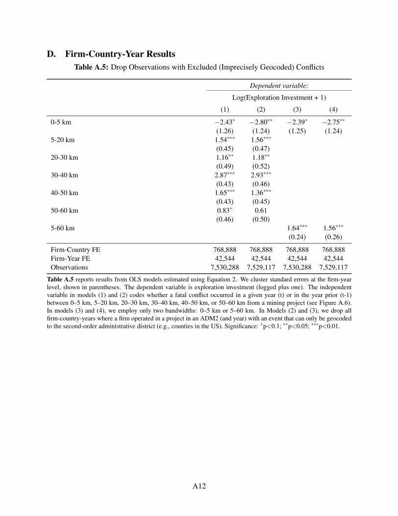
D. Firm-Country-Year ResultsTable A.5: Drop Observations with Excluded (Imprecisely Geocoded) Conflicts

Dependent variable:

Log(Exploration Investment + 1)

(1) (2) (3) (4)

0-5 km −2.43∗ −2.80∗∗ −2.39∗ −2.75∗∗

(1.26) (1.24) (1.25) (1.24)5-20 km 1.54∗∗∗ 1.56∗∗∗

(0.45) (0.47)20-30 km 1.16∗∗ 1.18∗∗

(0.49) (0.52)30-40 km 2.87∗∗∗ 2.93∗∗∗

(0.43) (0.46)40-50 km 1.65∗∗∗ 1.36∗∗∗

(0.43) (0.45)50-60 km 0.83∗ 0.61

(0.46) (0.50)5-60 km 1.64∗∗∗ 1.56∗∗∗

(0.24) (0.26)

Firm-Country FE 768,888 768,888 768,888 768,888Firm-Year FE 42,544 42,544 42,544 42,544Observations 7,530,288 7,529,117 7,530,288 7,529,117

Table A.5 reports results from OLS models estimated using Equation 2. We cluster standard errors at the firm-yearlevel, shown in parentheses. The dependent variable is exploration investment (logged plus one). The independentvariable in models (1) and (2) codes whether a fatal conflict occurred in a given year (t) or in the year prior (t-1)between 0–5 km, 5–20 km, 20–30 km, 30–40 km, 40–50 km, or 50–60 km from a mining project (see Figure A.6).In models (3) and (4), we employ only two bandwidths: 0–5 km or 5–60 km. In Models (2) and (3), we drop allfirm-country-years where a firm operated in a project in an ADM2 (and year) with an event that can only be geocodedto the second-order administrative district (e.g., counties in the US). Significance: ∗p<0.1; ∗∗p<0.05; ∗∗∗p<0.01.

A12

Table A.6: Effect of Armed Conflict on Investment at the Firm-Country Level with Firm-Country and Year Fixed Effects

Dependent variable:

Log(Exploration Investment + 1)

(1) (2)

0-5 km −2.49∗ −2.45∗

(1.32) (1.32)5-20 km 1.54∗∗∗

(0.48)20-30 km 1.17∗∗

(0.52)30-40 km 2.88∗∗∗

(0.45)40-50 km 1.67∗∗∗

(0.46)50-60 km 0.82∗

(0.49)5-60 km 1.65∗∗∗

(0.26)Beyond 60 km −0.002∗ −0.002∗

(0.001) (0.001)

Firm-Country FE 768,888 768,888Year FE 18 18Observations 7,530,288 7,530,288

Table A.6 reports results from OLS models estimated using a modified version of Equation 2, which differs fromEquation 2 in that year fixed effects are estimated instead of firm-year fixed effects. We cluster standard errors atthe firm-year level, shown in parentheses. The dependent variable is exploration investment (logged plus one). Theindependent variable in model (1) codes whether a fatal conflict occurred in a given year (t) or in the year prior (t-1)between 0–5 km, 5–20 km, 20–30 km, 30–40 km, 40–50 km, 50–60 km, or beyond 60 km from a mining project (seeFigure A.6). In model (2), we employ two bandwidths: 0–5 km, 5–60 km, or beyond 60 km. Significance: ∗p<0.1;∗∗p<0.05; ∗∗∗p<0.01.

A13

Table A.7: Effects of Conflict Exposure on Investment by Intensity of Conflict

Dependent variable:

Log(Exploration Investment + 1)

(1) (2) (3) (4)

0-5 km −2.39∗ −2.51 −2.43∗ −2.50(1.25) (1.55) (1.25) (1.55)

0-5 km x Conflict intensity 0.31 0.18(2.65) (2.64)

5-60 km 1.64∗∗∗ 1.76∗∗∗ 1.63∗∗∗ 1.78∗∗∗

(0.24) (0.30) (0.24) (0.30)5-60 km x Conflict intensity −0.27 −0.34

(0.38) (0.38)Beyond 60 km −0.002∗ 0.0001

(0.001) (0.001)Beyond 60 x Conflict intensity −0.02∗∗∗

(0.002)

Firm-Country FE 768,888 768,888 768,888 768,888Firm-Year FE 42,544 42,544 42,544 42,544Country-Year FE 3,186 3,186 0 0Observations 7,530,288 7,530,288 7,530,288 7,530,288

Table A.7 reports results from OLS models estimated using Equation 2. We cluster standard errors at the firm-yearlevel, shown in parentheses. The dependent variable is exploration investment (logged plus one). The independentvariable codes whether a conflict occurred in a given year (t) or in the year prior (t-1) between 0–5 km or 5–60 km.Models (1) and (3) replicate our results in Table 3. In models (2) and (4), we fully interact conflict with the intensityof the conflict in the country-year. High intensity is defined as more than 1,000 fatalities in a country-year using ourGED conflict outcome data. Models (1) and (2) include country-year fixed effects, which absorbs the “Beyond 60 km”term included in models (3) and (4) (see Figure A.7). Significance: ∗p<0.1; ∗∗p<0.05; ∗∗∗p<0.01.

A14

Figure A.7: Effects of Conflict Exposure on Investment by Intensity of Conflict

−2.54

1.981.27

2.7

1.34 1.35

−5.0

−2.5

0.0

2.5

0−5 5−20 20−30 30−40 40−50 50−600−5 5−20 20−30 30−40 40−50 50−60Armed Conflict within X km of Mining Project

Est

imat

e of

τk

(a) Low Intensity

−2.38

0.79 1.03

3.06

2.03

0.22

−5.0

−2.5

0.0

2.5

0−5 5−20 20−30 30−40 40−50 50−600−5 5−20 20−30 30−40 40−50 50−60Armed Conflict within X km of Mining Project

Est

imat

e of

τk

(b) High Intensity

Figure A.7 displays effects from Equation 2 fully interacted with the intensity of the conflict in the country-year.High intensity is defined as more than 1,000 fatalities in a country-year using our GED conflict outcome data (seeTable A.7).

A15

Figure A.8: Coefficient Stability when Excluding Multi-Country Firms

●

●●

●

●

●

−3.7

0.0

1.4

0−5 5−20 20−30 30−40 40−50 50−60Armed Conflict within X km of Mining Project

Est

imat

e of

τk

Sample● Full

Excl. Multi−Country Firms (t−2)

Figure A.8 displays effects from Equation 4, excluding firms that invest in multiple countries. In one specification,we include the full sample. In another specification, we drop firms with investments in multiple countries in t−2.

Figure A.9: Coefficient Stability when Excluding Multi-Project Firm-Countries

●

●●

●

●

●

−3.7

0.0

1.4

0−5 5−20 20−30 30−40 40−50 50−60Armed Conflict within X km of Mining Project

Est

imat

e of

τk

Sample● Full

Excl. Multi−Project Firm−Countries (t−2)

Figure A.9 displays effects from Equation 2, excluding firms that invest in multiple projects in the same country.In one specification, we include the full sample. In another specification, we drop observations when the firm hadmultiple projects in that country in t−2.

A16

Table A.8: Dynamic Panel Estimates of Effects of Conflict Exposure in Buffer Zone onInvestment

Dependent variable:

Log(Exploration Investment + 1)

0-5 km, lead 3 −1.49∗

(0.86)0-5 km, lead 2 −5.10∗

(3.06)0-5 km, lead 1 −0.03

(0.84)0-5 km, contemporaneous −2.82

(2.02)0-5 km, lag 1 −2.69

(2.07)0-5 km, lag 2 −3.42

(2.36)0-5 km, lag 3 0.89

(1.34)5-60 km, lead 3 −0.37

(0.40)5-60 km, lead 2 −0.07

(0.39)5-60 km, lead 1 0.61

(0.40)5-60 km, contemporaneous 1.23∗∗∗

(0.39)5-60 km, lag 1 1.44∗∗∗

(0.42)5-60 km, lag 2 0.95∗∗

(0.39)5-60 km, lag 3 1.47∗∗∗

(0.41)

Firm-Country FE 526,221Firm-Year FE 19,214Country-Year FE 2,124Observations 3,400,878

Table A.8 reports results from OLS models estimated using a version of Equation 2 modified to include leads andlags. We cluster standard errors at the firm-year level, shown in parentheses. The dependent variable is explorationinvestment (logged plus one). The independent variable codes whether conflict occurred in a given year, in one of thethree years prior, or in one of the three years after within a given distance of a firm’s mining projects. We report theeffects between 0–5 km and 5–60 km (see Figure A.10). Significance: ∗p<0.1; ∗∗p<0.05; ∗∗∗p<0.01.

A17

Figure A.10: Dynamic Panel: Effect of Exposure to Armed Conflict in Buffer Zone onInvestment

−0.37−0.07

0.61

1.231.44

0.95

1.47

−2

−1

0

1

2

3

t−3 t−2 t−1 Conflict t+1 t+2 t+3

Effe

ct o

n E

xplo

ratio

n In

vest

men

t (lo

gged

)

Figure A.10 displays dynamic panel estimates for the effects of exposure to conflict in the buffer zone around violence,defining the buffer zone as 5–60 km from conflict. We display contemporaneous effects and effects three years priorto and three years following conflict (see Table A.8).

A18

E. Sector-Country-Year ResultsIn this section, we report on analyses of the effect of armed conflict on investment in sectors

beyond mining. We construct data at the sector-country-year level using the fDi Markets (2019)dataset. The fDi Markets data records data about investment projects, including the total valueand number of jobs anticipated to be created, initial year of investment, sector, owner firm, andlocation. We collapse the data to the sector-country-year level, calculating total investment valueand number of projects.38

We conduct two analyses. First, we fit the following sector-country-year model:

ysct = ωs +Ac +∆t +βCct +s

∑ζsCct + εsct (5)

where Ysct is aggregate investment (logged) at the sector-country-year level, ωs represents sec-tor fixed effects, Ac represents country fixed effects, ∆t year fixed effects, Cct is an indicator forwhether an armed conflict occurred in country c in year t or in the previous year t−1, and ζs is asector-specific estimate of the effect of armed conflict (i.e., an interaction between the sector andarmed conflict indicators). We cluster our standard errors on country.

In Figure A.11, we display a histogram of ζs, highlighting natural resource sectors. This anal-ysis suggests that, while there is variation across sectors, the resource sectors (metals; minerals;coal, oil, and natural gas; and wood products) are not anomalous. Second, we fit the same modelbut combine the mining and metals sectors into a single sector. Table A.9 displays the regressioncoefficients for ωs for mining and metals, β , and ζs for mining and metals. We, again, do not findevidence that the mining and metals sectors that we study differ significantly in their investmentresponse to armed conflict.

38 Given that investments in the fDi Markets data are lumpy and not presented as yearly flows, wecannot construct data comparable to our exploration investment outcome. This is an importantdifference — after a project has been launched, we cannot observe firms curtailing investmentsin response to armed conflict.

A19

Figure A.11: Histogram of Sector-Armed Conflict Interactions

0

2

4

6

−0.1 0.0 0.1 0.2Estimated interaction coefficient

Num

ber

of s

ecto

rs

Sector Non−Resource Resource

Figure A.11 displays coefficient estimates of the interaction between an armed conflict indicator and the sector ofinvestment in a model fit on sector-country-year data. Natural resource sectors are highlighted, including metals;minerals; coal, oil, and natural gas; and wood products.

A20

Table A.9: Differential Effects of Conflict on Aggregate Investment by Sector

Dependent variable:

Log(N Investments + 1) Log(Total Investment + 1) Log(N Firms + 1)

(1) (2) (3)

1(Conflicts > 0) (Cct) −0.002 −0.03 −0.004(0.01) (0.03) (0.01)

Minerals sector 0.14∗∗∗ 0.61∗∗∗ 0.14∗∗∗

(0.02) (0.09) (0.02)Minerals sector ·Cct 0.04 0.16 0.04

(0.03) (0.12) (0.03)

F-stat 13.4 18.28 13.88p-value 0.00 0.00 0.00

ysct 0.41 1.22 0.39

Sector FE 37 37 37Country FE 160 160 160Year FE 12 12 12Observations 74,880 74,880 74,880

Table A.9 reports results from OLS models estimated using Equation 5. We cluster standard errors at the country level,shown in parentheses. The three models report on three dependent variables: the number of foreign direct investments(logged plus one) in a sector-country year; the total value of those investments (logged plus one); and the number offirms making investments (logged plus one). The independent variables code whether conflict occurred in a given yearor the preceding year, whether the sector is metals and minerals (i.e., reporting one of the sector fixed effects), and theinteraction. The model includes sector, country, and year fixed effects. Significance: ∗p<0.1; ∗∗p<0.05; ∗∗∗p<0.01.

A21

F. Country-Year ResultsTable A.10: Effect of Armed Conflict on the Number of Firms Investing at the CountryLevel

Dependent variable:

Log(N Firms + 1)

(1) (2) (3) (4) (5) (6) (7)

1(Conflicts > 0) −0.13∗∗ −0.11∗∗

(0.05) (0.05)1(Conflicts = 1) −0.12∗∗

(0.05)1(Conflicts > 1) −0.13∗∗

(0.06)1(State-Based > 0) −0.08 −0.05

(0.05) (0.05)1(One-Sided > 0) −0.12∗∗ −0.10∗

(0.06) (0.06)1(Non-State > 0) −0.09 −0.08

(0.07) (0.07)

F-stat 5.90 4.41 3.75 2.26 4.14 1.82 1.99p-value 0.02 0.04 0.02 0.13 0.04 0.18 0.11

yct 1.26 1.54 1.26 1.26 1.26 1.26 1.26

Country-YearSample All Recipients All All All All All

Country FE 177 145 177 177 177 177 177Year FE 18 18 18 18 18 18 18Observations 3,186 2,610 3,186 3,186 3,186 3,186 3,186

Table A.10 reports results from OLS models estimated using Equation 4. We cluster standard errors at the coun-try level, shown in parentheses. The dependent variable is the total number of firms (logged plus one). The mainindependent variable codes whether conflict occurred in a given year (t) or in the year prior (t-1). Models (2)-(7)report estimates from Equation 4 using different samples or measures of conflict. Significance: ∗p<0.1; ∗∗p<0.05;∗∗∗p<0.01.

A22

Figure A.12: Dynamic Panel Estimates: Country-level Effect of Conflict on Investment

−0.08

−0.42−0.27

−0.03−0.18

0.19

−0.4

−1.5

−1.0

−0.5

0.0

0.5

1.0

t−3 t−2 t−1 Conflict t+1 t+2 t+3

Effe

ct o

n E

xplo

ratio

n In

vest

men

t (lo

gged

)

Figure A.12 displays point estimates and 95% confidence intervals (thicker bars: 90% CIs) on the leads and lags ofarmed conflict incidence. Equation 4 is only amended to include these leads and lags and then estimated using OLS.The independent variable codes whether conflict occurred in a given year, in one of the three years prior, or in one ofthe three years after within a given distance of a firm’s mining projects. Standard errors are clustered on country (seeTable A.11).

A23

Table A.11: Dynamic Panel Estimates of Effect of Armed Conflict on Investment at theCountry Level

Dependent variable:

Log(Exploration Investment + 1)

Lead 3 −0.40(0.32)

Lead 2 0.19(0.31)

Lead 1 −0.18(0.35)

Contemporaneous −0.08(0.31)

Lag 1 −0.42(0.35)

Lag 2 −0.27(0.43)

Lag 3 −0.03(0.30)

F-stat 0.91p-value 0.5

yct 9.75

Country FE 177Year FE 12Observations 2,124

Table A.11 reports results from OLS models estimated using Equation 4. We cluster standard errors at the countrylevel, shown in parentheses. The dependent variable is exploration investment (logged plus one). The independentvariable codes whether conflict occurred in a country in a given year, in one of the three years prior, or in one of thethree years after (see Figure A.12). Significance: ∗p<0.1; ∗∗p<0.05; ∗∗∗p<0.01.

A24

F.1 Heterogeneous Effects by Type of FirmWe have limited information on the characteristics of firms in our sample. To assess whether

reputational risks explain the investment response of firms operating in conflict-affected countries,we identify two types of firms that we expect to be more concerned about their reputations. First,we code firms as mining “majors” or “juniors” based on market capitalization using data from2014, at the end of our sample period, from mineweb’s list of firms which we match by hand toour firm names. While there is no consensus definition of mining majors, we code the top 100by market capitalization as majors. Second, we code firms with investments in more than threecountries as multinationals.

We separately aggregate investment to the country-year by firm type. We then fit a version ofEquation 4, where we interact our conflict variable with our indicator for firm type. This allows usto assess whether the effects of armed conflict on exploration investment differ by firm type.

We present the results in Table A.12. We do not detect significant differences in how differenttypes of firms respond to armed conflict (see models 1 and 3). While our estimates are not signifi-cant, our point estimates suggest (model 2) that major firms pull back more sharply in response tostate-based conflicts (while junior firms react more strongly to one-sided and non-state conflicts).If association with a repressive state poses a larger reputational risk for major firms (as suggestedin Henisz 2017), then these results are consistent with those firms acting to more aggressively limitthat risk.

A25

Table A.12: Differential Effects of Conflict on Aggregate Investment by Firm Type

Dependent variable:

Log(Exploration Investment + 1)

Majors Multinationals

(1) (2) (3) (4)

1(Conflicts > 0) −0.54∗ −0.56(0.32) (0.53)

1(State-Based > 0) −0.03 −0.19(0.44) (0.56)

1(One-Sided > 0) −0.73∗∗ −1.03∗

(0.30) (0.57)1(Non-State > 0) −0.61 −0.30

(0.44) (0.49)Large firm · 1(Conflicts > 0) 0.003 −0.09

(0.52) (0.51)Large firm · 1(State-Based > 0) −0.37 −0.01

(0.49) (0.60)Large firm · 1(One-Sided > 0) 0.50 0.29

(0.51) (0.67)Large firm · 1(Non-State > 0) 0.56 0.16

(0.66) (0.64)

F-stat 0.52 8.5 1.13 5.03p-value 1.00 0.00 0.04 0.00

yct 7.5 7.5 8.06 8.06

Country FE 177 177 177 177Year FE 18 18 18 18Observations 6,372 6,372 6,372 6,372

Table A.12 reports the results from OLS models estimated using Equation 4, fit on identical stacked data with twodifferent outcomes and an indicator for which outcome was used in order to test the hypothesis that effects differbetween the two outcomes. In Model 1, the two outcomes are exploration investment of mining major firms (top100 firms by market capitalization) and exploration investment of junior mining firms. In Model 3, by multinationalfirms (investment in > 3 countries) and non-multinational firms. Models 2 and 4 are identical except with differentpredictors. We cluster standard errors at the country level, shown in parentheses. The dependent variable is explorationinvestment (logged plus one). The main independent variable codes whether conflict occurred in a given year (t) or inthe year prior (t-1), in Models 1 and 3. Models 2 and 4 report estimates from Equation 4 using alternative measures ofconflict by conflict type. Significance: ∗p<0.1; ∗∗p<0.05; ∗∗∗p<0.01.

A26

G. Evidence on MechanismsG.1 Disrupted Production

Table A.13: Effect of Armed Conflict on Production at the Project-Level (Africa Only)

Dependent variable:

1(Production > 0) Log(Production + 1) 1(Production > 0) Log(Production + 1)

(1) (2) (3) (4)

0-5 km −0.19∗ −2.12 −0.20∗ −2.13(0.11) (1.31) (0.11) (1.32)

5-60 km −0.03 −0.05(0.03) (0.33)

5-20 km −0.04 −0.10(0.05) (0.54)

20-30 km −0.04 −0.09(0.06) (0.67)

30-40 km 0.02 0.51(0.04) (0.45)

40-50 km −0.06 −0.41(0.06) (0.79)

50-60 km −0.01 −0.23(0.06) (0.64)

F-stat 2.01 1.32 0.88 0.75p-value 0.13 0.27 0.51 0.61

yict 0.88 9.9 0.88 9.9

Project FE 605 605 605 605Mineral FE 35 35 35 35Year FE 23 23 23 23Observations 7,926 7,926 7,926 7,926

Table A.13 reports results from OLS models with project, year, and mineral fixed effects. We cluster standard errorson project, shown in parentheses. The dependent variable is annual mineral production, measured as both a dummyvariable for positive production and the total production (logged plus one). In models (1) and (2) the independentvariable codes whether conflict occurred in the one of the three years prior (t-1, t-2, and/or t-3) within 0–5 km or5–60 km from firm’s mine. Models (3) and (4) further subdivide these geographic bandwidths (see Figure A.6). Dataavailability is limited to mining projects in Africa. Significance: ∗p<0.1; ∗∗p<0.05; ∗∗∗p<0.01.

A27

Figure A.13: Dynamic Panel: Effect of Armed Conflict within 5 km of a Mine on Pro-duction

0.27

−0.16

−0.3

−0.08−0.02

0.23

−0.040.04

−1.0

−0.5

0.0

0.5

1.0

t−3 t−2 t−1 Conflict t+1 t+2 t+3 t+4

Effe

ct o

f Con

flict

on

Pr(

Any

Pro

duct

ion)

Figure A.13 reports point estimates and 95% confidence intervals (thicker bars: 90% CIs) on the leads and lags ofarmed conflict incidence within 5 km of a mining site. Estimates based on a linear probability model with project,year, and mineral fixed effects. We cluster standard errors on project. Data availability is limited to mining projects inAfrica.

A28

G.2 State CapacityFigure A.14: Elasticity of Resource Production and Taxes amid Conflict

No Conflict UCDP One−sided

−2 −1 0 1 2 −2 −1 0 1 2

−2

−1

0

1

Residualized Resource Production (logged)

Res

idua

lized

Res

ourc

e Ta

xes

(logg

ed)

Figure A.14 displays the elasticity between natural resource production and resource tax revenues in countries withoutconflict (left) and with a one-sided conflict (right). Both series are logged to compute the elasticity; we also residualizeusing country fixed effects (see Table A.14).

A29

Table A.14: Elasticity of Resource Production and Taxes as a Function of Conflict

Dependent variable:

Log(Resource Tax Revenues + 1)

(1) (2) (3) (4)

Pt−1 0.562∗∗∗ 0.485∗∗∗ 0.534∗∗∗ 0.453∗∗∗

(0.112) (0.127) (0.117) (0.123)Pt−1×1(One-sided > 0) −0.088∗∗

(0.037)Pt−1×1(State-based > 0) −0.045

(0.036)Pt−1×1(State-based | One-sided > 0) −0.062∗

(0.033)Pt−1×1(Non-state > 0) 0.089

(0.064)

F-stat 8.63 5.39 7.73 6.41p-value 0.00 0.00 0.00 0.00

yct 21.98 21.98 21.98 21.98

Country FE 32 32 32 32Region-Year FE 75 75 75 75Observations 441 441 441 441

Table A.14 reports results from OLS models with country and region-by-year fixed effects. We use log-log specifi-cations to estimate the elasticity, in which resource tax revenues are the dependent variable, and mineral productionvalue interacted with conflict incidence is the independent variable. We cluster standard errors on country, shown inparentheses (see Figure A.14). Significance: ∗p<0.1; ∗∗p<0.05; ∗∗∗p<0.01.

A30

G.3 Policy ChangeTable A.15: Country-level Effect of Armed Conflict on Government Stability

Dependent variable:

Internal Conflict Index Government Stability Index

(1) (2) (3) (4) (5) (6)

1(Conflicts > 0) −0.49∗∗∗ −0.20∗

(0.15) (0.11)1(Conflicts = 1) −0.19 −0.23∗

(0.15) (0.12)1(Conflicts > 1) −0.62∗∗∗ −0.18

(0.16) (0.13)1(State-Based > 0) −0.54∗∗∗ 0.20

(0.15) (0.13)1(One-Sided > 0) −0.41∗∗∗ −0.24∗

(0.13) (0.13)1(Non-State > 0) −0.37∗∗ −0.45∗∗∗

(0.17) (0.13)

F-stat 11.21 7.81 9.41 3.1 2.18 6.67p-value 0.00 0.00 0.00 0.08 0.11 0.00

yct 9.2 9.2 9.2 8.56 8.56 8.56

Country FE 134 134 134 134 134 134Year FE 18 18 18 18 18 18Observations 2,394 2,394 2,394 2,394 2,394 2,394

Table A.15 reports the results from OLS models estimated using Equation 4. We cluster standard errors at the countrylevel, shown in parentheses. The dependent variables come from ICRG: models (1)–(3), Internal Conflict Index;models (4)–(6), Government Stability Index. The main independent variable codes whether conflict occurred in agiven year (t) or in the year prior (t-1). Significance: ∗p<0.1; ∗∗p<0.05; ∗∗∗p<0.01.

A31

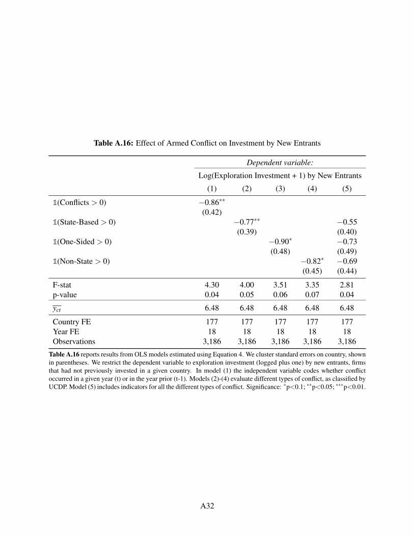
Table A.16: Effect of Armed Conflict on Investment by New Entrants

Dependent variable:

Log(Exploration Investment + 1) by New Entrants

(1) (2) (3) (4) (5)

1(Conflicts > 0) −0.86∗∗

(0.42)1(State-Based > 0) −0.77∗∗ −0.55

(0.39) (0.40)1(One-Sided > 0) −0.90∗ −0.73

(0.48) (0.49)1(Non-State > 0) −0.82∗ −0.69

(0.45) (0.44)

F-stat 4.30 4.00 3.51 3.35 2.81p-value 0.04 0.05 0.06 0.07 0.04

yct 6.48 6.48 6.48 6.48 6.48

Country FE 177 177 177 177 177Year FE 18 18 18 18 18Observations 3,186 3,186 3,186 3,186 3,186

Table A.16 reports results from OLS models estimated using Equation 4. We cluster standard errors on country, shownin parentheses. We restrict the dependent variable to exploration investment (logged plus one) by new entrants, firmsthat had not previously invested in a given country. In model (1) the independent variable codes whether conflictoccurred in a given year (t) or in the year prior (t-1). Models (2)-(4) evaluate different types of conflict, as classified byUCDP. Model (5) includes indicators for all the different types of conflict. Significance: ∗p<0.1; ∗∗p<0.05; ∗∗∗p<0.01.

A32

H. Details of Systematic ReviewThe aim of a systematic review is to “identify, appraise and synthesize all the empirical evi-

dence that meets pre-specified eligibility criteria to answer a specific research question” (Higginsand Green 2011). In this appendix, we present additional details on how we conducted the system-atic review as well as our PRISMA systematic review reporting statement.

H.1 Coding Rules for Systematic ReviewMeasure of Violent Events We exclusively measure counts or incidences of violent events.Where papers measure additional factors related to conflict, we consider this an aggregate riskmeasure.

Model Selection In order to characterize this literature, we first determine which model we willevaluate from the papers that met our filtering criteria. Based on the table the author(s) highlightas their main empirical results, we select the model that uses unit fixed effects at the same level astheir cross-sectional unit of analysis. If unit fixed effects (FE) are not used in the paper, or are notat the same level as the paper’s cross-sectional unit of analysis, we select the model that uses aninstrumental variable (IV) to instrument for conflict/instability.

In situations where the author(s) neither use FE nor an IV approach, we use their preferredmodel specification as the main model, if it is favored for reasons that enhance the credibility ofthe causal inference (i.e., they justify why they have to control for an important confounder). Inthe absence of author preference, we select the simplest model that relates conflict to investment.When analyses use both an aggregated and a disaggregated measure of conflict/risk, we select theaggregate measure.

We consider this model the main model of the paper. We use this model to characterize thestudies in our systematic review.

Study Characteristics Following the selection of the main model, we code a range of char-acteristics from each paper, which we include in Table A.1. These include: (1) effect; (2) re-gion/countries; (3) years; (4) geographic and time unit of analysis; (5) fixed effects; and (6) instru-mental variable. The rationale behind these coding choices is included below:

(A) Effect+, −, ∼ (null), or mixed (includes at least two of the three above)We code the effect of conflict on investment based on both the sign and statistical significance(at any level) of the point estimate of the main model (detailed above). Based on the relevantmodel, we identify the effect variable in three different ways: (1) from a single main modelwith a single measure of conflict (e.g., the International Country Risk Guide (ICRG) political

A33

instability index); (2) from a single main model with multiple measures of conflict (e.g.,revolutions and assassinations); and (3) from multiple main models, with different dependentvariables, and a single measure of conflict (e.g., investment by sectors). The latter twostrategies may lead to a “mixed” effect of conflict on investment, as some coefficients may besignificantly positive or significantly negative while others may have no effect. By contrast,the first strategy will only lead to an effect of conflict on investment that is significantlypositive, significantly negative, or null.

All eight “mixed” studies report significantly negative results alongside null and/or signifi-cantly positive correlations between instability or conflict and investment. Results from onestudy, Li, Murshed and Tanna (2017), rely on separate models due to the use of FDI fromdifferent sectors as dependent variables.

(B) Region/countriesG (global), LAC, SSA, MENA, BRICS, or country nameWe identify the regional focus of the research from the main text of the paper. In addition, weinclude a variable for the number of countries evaluated in the paper. We code the region(s)and the number of countries used in the analyses based on the countries that receive invest-ments in the data, rather than the number where investment originates (for example, if thedata represent FDI from 37 OECD countries in China we would code that as a single countryin Asia). Where possible, we use the number of countries listed in the main model. Whenthis information is unavailable, we code the number of countries the author(s) reference inthe main text of the paper.

(C) YearsWe code years based on the year range provided in main text of the paper. On rare occasions,a paper may subset further down for analysis purposes. If this is the case, we code the morerestricted year range if it is used in the main model and available in the main text of thepaper.

(D) Geographic and Time Unit of AnalysisWe code the geographic and time unit of analysis based on the most disaggregated level ofdata used in the model (e.g., country-year, sector-month). We identify the unit of analysisbased on the subscript in the model equation, when available. Otherwise, we infer thisinformation from the main text of the paper.

(E) Fixed EffectsWe identify if a paper uses both unit and/or time fixed effects. We code unit fixed effects if

A34

the paper utilizes unit fixed effects at their cross-sectional unit of analysis (e.g., country forcountry-year panels). We code time fixed effects if the author(s) use time fixed effects at thetemporal level of the panel data (e.g., year for country-year panels). As such, we do not codefixed effects if those used in the paper are based on aggregated time periods (i.e. five-yearperiods rather than years) or geographic units (i.e. continents rather than countries). Weidentify whether the author(s) use unit and/or time fixed effects based on the model equation(when available) or from the table of the main model.

(F) Instrumental VariablesWe code a study as having used instrumental variables if the author(s) specify that they areinstrumenting for conflict/instability. We identify whether the author(s) use an instrumentalvariable from the table of the main model, when possible, or from the main text of the paper.

H.2 PRISMA Checklist for Systematic ReviewsThe Preferred Reporting Items for Systematic Reviews and Meta-Analyses (PRISMA) is a

standard checklist for reporting on systematic reviews (Liberati et al. 2009). We document ourresponse to each item on the checklist below.

(1) Title (p. 4)Identify the report as a systematic review, meta-analysis, or both.

- See text.

(2) Structured Summary (p. 4-5)Provide a structured summary including, as applicable: background; objectives; data sources; study eligi-bility criteria, participants, and interventions; study appraisal and synthesis methods; results; limitations;conclusions and implications of key findings; systematic review registration number.

- See text. We do not provide information about participants, interventions, or a systematic review registrationnumber.

(3) Rationale (p. 4)Describe the rationale for the review in the context of what is already known.

- See text.

(4) Objectives (p. 4)Provide an explicit statement of questions being addressed with reference to participants, interventions, com-parisons, outcomes, and study design (PICOS).

- See text.

(5) Protocol and registration (p. 4, Appendix H.1)Indicate if a review protocol exists, if and where it can be accessed (e.g., Web address), and, if available,provide registration information including registration number.

- See text for review protocol. We do not register our systematic review.

A35

(6) Eligibility criteria (pg. 4 and Table A.1)Specify study characteristics (e.g., PICOS, length of follow-up) and report characteristics (e.g., years consid-ered, language, publication status) used as criteria for eligibility, giving rationale.

- Study characteristics are provided in Table A.1. The rationale for our eligibility criteria is as follows: (1)published in 1990 or later – given advances made in quantitative social science, we restrict our analysis topost-1990; (2) published in a peer-reviewed social science or business journal or by a university press –the peer review filter serves as a quality control; (3) examines the relationship between conflict and foreigninvestment – this filter ensures that the papers in our review focus on the same IV and DV we evaluate; and(4) includes a point estimate – a point estimate restricts the papers to quantitative social science research andserves as the basis on which we code the effect direction.

(7) Information source (p. 4)Describe all information sources (e.g., databases with dates of coverage, contact with study authors to identifyadditional studies) in the search and date last searched.

- We use Google Scholar to compile a database of articles. Our Google Scholar search occurred on September11, 2018, where we pulled 950 articles that met our keyword criteria. We also included three additionalrelevant articles. We then conduct a “spider” search in Google Scholar of the articles that made it throughall pre-specified inclusion filters. This means that we compiled and assessed all studies that cite any of thearticles from the first search (42 total). We conducted the “spider” search from February 9 to February 11,2019 and on January 17, 2020.

(8) Search (p. 4)Present full electronic search strategy for at least one database, including any limits used, such that it could berepeated.

- Our search takes the form: (conflict OR violence OR coups OR revolutions OR assassinations OR politicalrisk OR war OR political instability) AND (investment OR firms).

(9) Study selection (p. 4)State the process for selecting studies (i.e., screening, eligibility, included in systematic review, and, if applica-ble, included in the meta-analysis).

- Prior to evaluating the full list of articles from Google Scholar, we specify eligibility criteria for inclusion inthe systematic review (see item #6). We then employ a combination of automated review (e.g., the correctyears) and manual review to implement the remainder of the filtering process.

(10) Data collection process (p. 4)Describe method of data extraction from reports (e.g., piloted forms, independently, in duplicate) and anyprocesses for obtaining and confirming data from investigators.

- We extract the sign and statistical significance of the coefficient on conflict/instability in regressions whereinvestment is the dependent variable. When a study reports more than one relevant model, we favor theinstrumental variable or fixed effects model results if available, given stronger claims of causal identification.However, for one article, we report results from multiple models due to slightly different dependent variables.These are noted in Table A.1. We then review each article to identify other relevant characteristics of thestudies, which we present in Table A.1. We do not collect original data from these papers.

A36

(11) Data items (Table A.1)List and define all variables for which data were sought (e.g., PICOS, funding sources) and any assumptionsand simplifications made.

- We code the following features of each article: effect direction and significance, use of fixed effects, use ofinstrumental variables, unit of analysis, year range, use of composite risk score, number of countries, regionof focus, authors, journal, and year of publication.

(12) Risk of bias in individual studies (Table A.1)Describe methods used for assessing risk of bias of individual studies (including specification of whether thiswas done at the study or outcome level), and how this information is to be used in any data synthesis.

- Where applicable, we note which studies utilize a fixed effects or an instrumental variable research design.In these cases, we report the effect directions with statistical significance presented in those models. If astudy does not employ FE or IV, then we focus on their primary/preferred specification. We also excludenon-peer reviewed working papers from our review. In our summary Table 1, we provide details on howmany studies use either fixed effects or instrumental variables, organized by effect direction.

(13) Summary measures (p. 4-5 and Table A.1)State the principal summary measures (e.g., risk ratio, difference in means).

- The principle summary measure is the coefficient sign and statistical significance (significantly positive,unable to reject the null, and significantly negative) for variables that measure conflict or instability in re-gressions where the dependent variable is investment. We only extract coefficients that evaluate the effect ofconflict/instability on investment.

(14) Synthesis of results (N/A)Describe the methods of handling data and combining results of studies, if done, including measures of consis-tency (e.g., I2) for each meta-analysis.

(15) Risk of bias across studies (N/A)Specify any assessment of risk of bias that may affect the cumulative evidence (e.g., publication bias, selectivereporting within studies).

(16) Additional analyses (N/A)Describe methods of additional analyses (e.g., sensitivity or subgroup analyses, meta-regression), if done,indicating which were pre-specified.

(17) Study selection (pg. 4 and Figure A.15)Give numbers of studies screened, assessed for eligibility, and included in the review, with reasons for exclu-sions at each stage, ideally with a flow diagram.

- See the Flow Diagram presented in Figure A.15. We exclude studies at each stage because they fail to satisfythe inclusion criteria outlined in advance of the systematic review.

(18) Study characteristics (Table A.1)For each study, present characteristics for which data were extracted (e.g., study size, PICOS, follow-up period)and provide the citations.

- We provide select study characteristics to demonstrate the geographic scope and temporal focus of this bodyof research.

A37

(19) Risk of bias within studies (Table A.1)Present data on risk of bias of each study and, if available, any outcome level assessment (see item 12).

- We note which studies we consider less prone to bias based on their use of a fixed effects or an instrumentalvariable design (Table A.1).

(20) Results of individual studies (Table A.1)For all outcomes considered (benefits or harms), present, for each study: (a) simple summary data for eachintervention group (b) effect estimates and confidence intervals, ideally with a forest plot.

- We report three types of effect directions (significantly positive, unable to reject the null, significantly nega-tive) from the main models in each individual study.

(21) Synthesis of results (N/A)Present results of each meta-analysis done, including confidence intervals and measures of consistency.

(22) Risk of bias across studies (N/A)Present results of any assessment of risk of bias across studies (see Item 15).

(23) Additional analyses (N/A)Give results of additional analyses, if done (e.g., sensitivity or subgroup analyses, meta-regression [see Item16])

(24) Summary of evidence (Table 1)Summarize the main findings including the strength of evidence for each main outcome; consider their rele-vance to key groups (e.g., healthcare providers, users, and policy makers).

- See Table 1.

(25) Limitations (pg. 5)Discuss limitations at study and outcome level (e.g., risk of bias), and at review-level (e.g., incomplete retrievalof identified research, reporting bias).

- See text. Google Scholar restricts our first search to the top 950 articles. As a result, we did a second GoogleScholar search to collect all the papers that cited articles from the first search that met our filter requirements.

(26) Conclusions (pg. 5)Provide a general interpretation of the results in the context of other evidence, and implications for futureresearch.

- Results form this country-level research motivate our focus on the firm-level.

(27) Funding (N/A)Describe sources of funding for the systematic review and other support (e.g., supply of data); role of fundersfor the systematic review.

- We did not receive any funding to conduct this systematic review.

A38

Figure A.15: PRISMA Flow Diagram

From: Moher D, Liberati A, Tetzlaff J, Altman DG, The PRISMA Group (2009). Preferred Reporting Items for Systematic Reviews and Meta-Analyses: The PRISMA Statement. PLoS Med 6(7): e1000097. doi:10.1371/journal.pmed1000097

For more information, visit www.prisma-statement.org.

PRISMA 2009 Flow Diagram

Records identified through database searching

(n = 15,583)

Scre

enin

g In

clud

ed

Elig

ibili

ty

Iden

tific

atio

n

Additional records identified through other sources

(n = 7)

Records after duplicates removed (n = 9,116)

Records screened (n = 9,116)

Records excluded (n = 8,080)

Full-text articles assessed for eligibility (n = 1,059)

Full-text articles excluded, with reasons

(n = 984)

Studies included in qualitative synthesis

(n = 75)

Studies included in quantitative synthesis

(meta-analysis) (n = N/A)

A39

Appendix ReferencesAbadie, Alberto and Javier Gardeazabal. 2003. “The Economic Costs of Conflict: A Case Study

of the Basque Country.” The American Economic Review 91(1):113–132.

Al-Khouri, Ritab and M. Umaima Abdul Khalik. 2013. “Does Political Risk Affect the Flowof Foreign Direct Investment into the Middle East North African Region?” Journal of Global

Business and Technology 9(2):47–59.

Alesina, Alberto and Roberto Perotti. 1996. “Income Distribution, Political Instability, and Invest-ment.” European Economic Review 40(6):1203–1228.

Alfaro, Laura, Sebnem Kalemli-Ozcan and Vadym Volosovych. 2008. “Why Doesn’t CapitalFlow from Rich to Poor Countries? An Empirical Investigation.” The Review of Economics and

Statistics 90(2):347–368.

Ashby, Nathan J. and Miguel A. Ramos. 2013. “Foreign Direct Investment and Industry Responseto Organized Crime: The Mexican Case.” European Journal of Political Economy 30:80–91.

Asiedu, Elizabeth. 2002. “On the Determinants of Foreign Direct Investment to Developing Coun-tries: Is Africa Different?” World Development 30(1):107–119.

Asiedu, Elizabeth. 2006. “Foreign Direct Investment in Africa: The Role of Natural Re-sources, Market Size, Government Policy, Institutions and Political Instability.” World Economy

29(1):63–77.

Asiedu, Elizabeth and Donald Lien. 2011. “Democracy, Foreign Direct Investment and NaturalResources.” Journal of International Economics 84(1):99–111.

Aysan, Ahmet Faruk, Mustapha Kamel Nabli and Marie-Ange Veganzones-Varoudakis. 2007.“Governance Institutions and Private Investment: An Application to the Middle East and NorthAfrica.” The Developing Economies 45(3):339–377.

Aziz, Nusrate and Usman Khalid. 2017. “Armed Conflict, Military Expenses and FDI Inflow toDeveloping Countries.” Defence and Peace Economics 30(2):1–14.

Baek, Kyeonghi and Xingwan Qian. 2011. “An Analysis on Political Risks and the Flow of ForeignDirect Investment in Developing and Industrialized Economies.” Economics, Management and

Financial Markets 6(4):60–91.

Bandyopadhyay, Subhayu, Todd Sandler and Javed Younas. 2013. “Foreign Direct Investment,Aid, and Terrorism.” Oxford Economic Papers 66(1):25–50.

A40

Bevan, Alan A. and Saul Estrin. 2004. “The Determinants of Foreign Direct Investment intoEuropean Transition Economies.” Journal of Comparative Economics 32(4):775–787.

Biglaiser, Glen and Karl DeRouen Jr. 2006. “Economic Reforms and Inflows of Foreign DirectInvestment in Latin America.” Latin American Research Review pp. 51–75.

Biglaiser, Glen and Karl DeRouen Jr. 2007. “Following the flag: Troop deployment and US foreigndirect investment.” International Studies Quarterly 51(4):835–854.

Bohn, Henning and Robert T. Deacon. 2000. “Ownership Risk, Investment, and the Use of NaturalResources.” American Economic Review 90(3):526–549.

Brown, Leanora and Keva Hibbert. 2017. “The Effect of Crime on Foreign Direct Investment: AMulti-Country Panel Data Analysis.” The Journal of Developing Areas 51(1):295–307.

Brunetti, Aymo and Beatrice Weder. 1998. “Investment and Institutional Uncertainty: A Compar-ative Study of Different Uncertainty Measures.” Weltwirtschaftliches Archiv 134(3):513–533.

Busse, Matthias and Carsten Hefeker. 2007. “Political Risk, Institutions and Foreign Direct Invest-ment.” European Journal of Political Economy 23(2):397–415.

Bussmann, Margit. 2010. “Foreign Direct Investment and Militarized International Conflict.” Jour-

nal of Peace Research 47(2):143–153.

Cabral, Rene, Andre Varella Mollick and Eduardo Saucedo. 2019. “Foreign Direct Investment inMexico, Crime, and Economic Forces.” Contemporary Economic Policy 37(1):68–85.

Campos, Nauro F. and Jeffrey B. Nugent. 2003. “Aggregate Investment and Political Instability:An Econometric Investigation.” Economica 70(279):533–549.

Carter, David B., Rachel L. Wellhausen and Paul K. Huth. 2018. “International Law, TerritorialDisputes, and Foreign Direct Investment.” International Studies Quarterly 63(1):58–71.

Cleeve, Emmanuel. 2012. “Political and Institutional Impediments to Foreign Direct InvestmentInflows to Sub-Saharan Africa.” Thunderbird International Business Review 54(4):469–477.

Daniele, Vittorio and Ugo Marani. 2011. “Organized Crime, the Quality of Local Institutions andFDI in Italy: A Panel Data Analysis.” European Journal of Political Economy 27(1):132–142.

Daude, Christian and Ernesto Stein. 2007. “The Quality of Institutions and Foreign Direct Invest-ment.” Economics & Politics 19(3):317–344.

Enders, Walter, Adolfo Sachsida and Todd Sandler. 2006. “The Impact of Transnational Terrorismon US Foreign Direct Investment.” Political Research Quarterly 59(4):517–531.

A41

Ezeoha, Abel Ebeh and John Okereke Ugwu. 2015. “Interactive Impact of Armed Conflicts onForeign Direct Investments in Africa.” African Development Review 27(4):456–468.

Feng, Yi. 2001. “Political Freedom, Political Instability, and Policy Uncertainty: A Study of Po-litical Institutions and Private Investment in Developing Countries.” International Studies Quar-

terly 45(2):271–294.

Fielding, David. 2003a. “Investment, Employment, and Political Conflict in Northern Ireland.”Oxford Economic Papers 55(3):512–535.

Fielding, David. 2003b. “Modelling Political Instability and Economic Performance: Israeli In-vestment During the Intifada.” Economica 70(277):159–186.

Gani, Azmat. 2007. “Governance and Foreign Direct Investment Links: Evidence from Panel DataEstimations.” Applied Economics Letters 14(10):753–756.

Globerman, Steven and Daniel Shapiro. 2002. “Global Foreign Direct Investment Flows: The Roleof Governance Infrastructure.” World Development 30(11):1899–1919.

Globerman, Steven and Daniel Shapiro. 2003. “Governance Infrastructure and US Foreign DirectInvestment.” Journal of International Business Studies 34(1):19–39.

Hayakawa, Kazunobu, Fukunari Kimura and Hyun-Hoon Lee. 2013. “How Does Country RiskMatter for Foreign Direct Investment?” The Developing Economies 51(1):60–78.

Higgins, Julian P.T. and Sally Green. 2011. Cochrane Handbook for Systematic Reviews of Inter-

ventions. Vol. 4 John Wiley & Sons.

Jadhav, Pravin. 2012. “Determinants of Foreign Direct Investment in BRICS Economies: Analysisof Economic, Institutional and Political Factor.” Procedia-Social and Behavioral Sciences 37:5–14.

Jadhav, Pravin and Vijaya Katti. 2012. “Institutional and Political Determinants of Foreign DirectInvestment: Evidence from BRICS Economies.” Poverty & Public Policy 4(3):49–57.

Kariuki, Caroline. 2015. “The Determinants of Foreign Direct Investment In the African Union.”Journal of Economics, Business and Management 3(3):346–351.

Kim, Dongkyu. 2016. “The Effects of Inter-State Conflicts on Foreign Investment Flows to theDeveloping World: Enduring vs Ephemeral Risk of Conflicts.” International Political Science

Review 37(4):422–437.

Kinda, Tidiane. 2010. “Investment Climate and FDI in Developing Countries: Firm-Level Evi-dence.” World Development 38(4):498–513.

A42

Koechlin, Timothy. 1992. “The Determinants of the Location of USA Direct Foreign Investment.”International Review of Applied Economics 6(2):203–216.

Kolstad, Ivar and Arne Wiig. 2012. “What Determines Chinese Outward FDI?” Journal of World

Business 47(1):26–34.

Le, Quan V. 2004. “Political and Economic Determinants of Private Investment.” Journal of Inter-

national Development 16(4):589–604.

Li, Quan. 2006. Chapter 11: Political Violence and Foreign Direct Investment. In Regional Eco-

nomic Integration, ed. Michele Fratianni. United Kingdom: Emerald Group Publishing Limitedpp. 225–249.

Li, Quan and Tatiana Vashchilko. 2010. “Dyadic Military Conflict, Security Alliances, and Bilat-eral FDI Flows.” Journal of International Business Studies 41(5):765–782.

Liberati, Alessandro, Douglas G. Altman, Jennifer Tetzlaff, Cynthia Mulrow, Peter C. Gøtzsche,John P.A. Ioannidis, Mike Clarke, Philip J. Devereaux, Jos Kleijnen and David Moher. 2009.“The PRISMA Statement for Reporting Systematic Reviews and Meta-analyses of Stud-ies that Evaluate Health Care Interventions: Explanation and Elaboration.” PLoS Medicine

6(7):e1000100.

Liu, Xiaming, Haiyan Song, Yingqi Wei and Peter Romilly. 1997. “Country Characteristics andForeign Direct Investment in China: A Panel Data Analysis.” Review of World Economics

133(2):313–329.

Malefane, Malefa Rose. 2007. “Determinants of Foreign Direct Investment in Lesotho: Evidencefrom Co-Integration and Error Correction Modeling: Economics.” South African Journal of

Economic and Management Sciences 10(1):99–106.

Mengistu, Alemu Aye and Bishnu Kumar Adhikary. 2011. “Does Good Governance Matter forFDI inflows? Evidence from Asian Economies.” Asia Pacific Business Review 17(3):281–299.

Mijiyawa, Abdoul’Ganiou. 2015. “What Drives Foreign Direct Investment in Africa? An Empiri-cal Investigation with Panel Data.” African Development Review 27(4):392–402.

Morrissey, Oliver and Manop Udomkerdmongkol. 2012. “Governance, Private Investment andForeign Direct Investment in Developing Countries.” World Development 40(3):437–445.

Naude, Wim A. and Waldo F. Krugell. 2007. “Investigating Geography and Institutions asDeterminants of Foreign Direct Investment in Africa Using Panel Data.” Applied Economics

39(10):1223–1233.

A43

Oh, Chang Hoon and Jennifer Oetzel. 2011. “Multinationals’ Response to Major Disasters: HowDoes Subsidiary Investment Vary in Response to the Type of Disaster and the Quality of CountryGovernance?” Strategic Management Journal 32(6):658–681.

Okafor, Godwin. 2015. “Locational Determinants of US Outward FDI into Sub-saharan Africa.”The Journal of Developing Areas 49(1):187–205.

Perotti, Roberto. 1994. “Income Distribution and Investment.” European Economic Review 38(3-4):827–835.

Powers, Matthew and Seung-Whan Choi. 2012. “Does Transnational Terrorism Reduce ForeignDirect Investment? Business-related Versus Non-business-related Terrorism.” Journal of Peace

Research 49(3):407–422.

Ramasamy, Bala and Matthew Yeung. 2010. “The Determinants of Foreign Direct Investment inServices.” World Economy 33(4):573–596.

Ramasamy, Bala, Matthew Yeung and Sylvie Laforet. 2012. “China’s Outward Foreign DirectInvestment: Location Choice and Firm Ownership.” Journal of World Business 47(1):17–25.

Resnick, Adam L. 2001. “Investors, Turbulence, and Transition: Democratic Transitionand Foreign Direct Investment in Nineteen Developing Countries.” International Interactions

27(4):381–398.

Shahzad, Syed Jawad Hussain, Muhammad Zakaria, Mobeen Ur Rehman, Tanveer Ahmed andBashir Ahmed Fida. 2016. “Relationship between FDI, Terrorism and Economic Growth inPakistan: Pre and Post 9/11 Analysis.” Social Indicators Research 127(1):179–194.

Singh, Prakarsh. 2013. “Impact of Terrorism on Investment Decisions of Farmers: Evidence fromthe Punjab Insurgency.” The Journal of Conflict Resolution 57(1):143–168.

Sissani, Midoun and Zairi Belkacem. 2014. “The Impact of Country Risk Components on Al-geria Attractiveness for Foreign Direct Investments (1990-2012).” Applied Econometrics and

International Development 14(1):133–146.

Solomon, Blen and Isabel Ruiz. 2012. “Political Risk, Macroeconomic Uncertainty, and the Pat-terns of Foreign Direct Investment.” The International Trade Journal 26(2):181–198.

Suliman, Adil H. and Andre Varella Mollick. 2009. “Human Capital Development, War and For-eign Direct Investment in Sub-Saharan Africa.” Oxford Development Studies 37(1):47–61.

Sun, Qian, Wilson Tong and Qiao Yu. 2002. “Determinants of Foreign Direct Investment AcrossChina.” Journal of International Money and Finance 21(1):79–113.

A44

Tuman, John P. and Craig F. Emmert. 1999. “Explaining Japanese Foreign Direct Investment inLatin America, 1979-1992.” Social Science Quarterly pp. 539–555.

Tuman, John P. and Craig F. Emmert. 2004. “The Political Economy of U.S. Foreign DirectInvestment in Latin America: A Reappraisal.” Latin American Research Review pp. 9–28.

Vadlamannati, Krishna Chaitanya. 2012. “Impact of Political Risk on FDI Revisited—An Aggre-gate Firm-Level Analysis.” International Interactions 38(1):111–139.

Wheeler, David and Ashoka Mody. 1992. “International Investment Location Decisions: The Caseof U.S. Firms.” Journal of International Economics 33(1-2):57–76.

Williams, Kevin. 2017. “Foreign Direct Investment, Economic Growth, and Political Instability.”Journal of Economic Development 42(2):17.

A45