power system modeling and fault analysis of nampower’s 330 kv hvac transmission line

Journal of Energy and Power Engineering 8 (2014) 1432-1442

Power System Modelling and Fault Analysis of

NamPower’s 330 kV HVAC Transmission Line

Innocent Davidson and Immanuel Mbangula

HVDC/Smart Grid Research Centre, University of KwaZulu-Natal, Durban 4041, South Africa

Received: December 20, 2013 / Accepted: March 21, 2014 / Published: August 31, 2014.

Abstract: Electric power systems usually cover large geographical areas and transmission facilities are continuously increasing. These power systems are exposed to different environmental conditions which may cause faults to occur on the system. Different types of studies are usually done on electric power systems to determine how the system behaves before, during and after a fault condition. The behaviour of variables of interest such as currents, voltage, rotor angle and active and reactive power under fault conditions are studied and observed to help determine possible causes of faults in a power system. The objective of this paper is to investigate a fault that occurred on the 330 kV transmission line between Ruacana power station and Omburu sub-station, the fault caused all the generators at Ruacana power station to trip and consequently caused a blackout at the power station that lasted for 6 h. Preliminary findings showed that the observed fault was an earth fault but the exact type of earth fault was however not known at the time. This research investigation sets out to determine the exact fault that occurred; the most probable cause of the fault, and propose possible solutions to prevent reoccurrence of such a fault. The section of the power network in which the fault occurred was modelled using DigSilent Power Factory software tool, and transient fault analysis was carried out on the model for different fault conditions. Results obtained were then compared with data obtained from NamPower records to ascertain the type of fault. Key words: Fault analysis, power system, transient stability.

1. Introduction

A disturbance in one section of the power network

propagates to remote points of the system. Fault

analysis aims to quantify waveforms of interest, such

as currents and voltages, under extraordinary

operating conditions [1]. The magnitude of the fault

currents give the engineer the current settings for the

protection to be used and the ratings of the circuit

breakers [2]. A fault occurred on the 330 kV

transmission line between Ruacana power station and

Omburu substation, causing the line to trip on March

18, 2012. Omburu substation is the hub that evacuates

power generated from the 330 MW Ruacana Hydro

power station into the Namibian grid.

Preliminary investigations of the fault suggest that

the line trip was caused by an earth fault. The fault

Corresponding author: Innocent Davidson, director,

research fields: modern electric power systems, smart grids and clean energy technologies. E-mail: [email protected].

caused the CB (circuit breaker) at Omburu sub-station

to trip, 1.7 s later the CB near Ruacana power station

tripped as well. The tripping of the transmission line

caused all the generators at the power station to go

out of step and trip and therefore caused a major

power outage which lasted for 6 h, before the

generators were re-excited, ran up and power supply

restored.

The observed fault was classified as transient

disturbance on the power network, and it caused

transient instability of the power system. Faults that

occur on power networks are usually of different

origins, a fault may originate from a mechanical,

electrical or operational error [3]. Various methods are

used for mitigation against faults that occur on electric

power networks. These methods are therefore used to

increase the stability of the power system. Ruacana

hydro power station is Namibia’s only hydro-electric

power station [4]. It has Namibia’s single largest

D DAVID PUBLISHING

Power System Modelling and Fault Analysis of NamPower’s 330 kV HVAC Transmission Line

1433

installed generation capacity of 332 MW, which

makes up 67% of the total power generated. Any

major disturbance that occurs at or affects Ruacana

power station will have a negative impact on the

Namibian power system. It is therefore crucial to

ensure that severe faults on the national grid are

minimal, especially those that might significantly

affect the generators at Ruacana or any other power

stations in Namibia.

A reliable and stable network ensures that the

security of power supply is not compromised.

Reliability is the ability of the power system to supply

the aggregate electric power and energy requirements

of the customer at all times [5]. The stability of a

power system is its ability to return to normal or stable

operation after having being subjected to some form

of disturbance [3]. This is achieved with a significant

reduction in power outages due to any various

disturbances on the network such as major faults.

Section 2 of this paper gives a brief review of

literature on faulted power systems and power systems

stability. In Section 3, the modelling of the faulted

section of the power system is done. Presentation and

analysis of the simulation results is done in Section 4.

Conclusions drawn based on the simulation results are

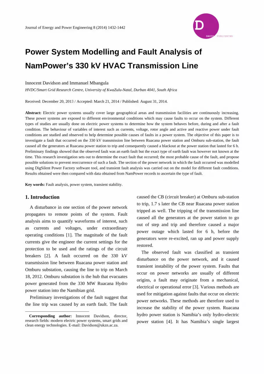
given in Section 5. Fig. 1 shows Namibia’s

transmission grid and the major power generation and

transmission stations. Table 1 shows NamPower’s

plant portfolio.

Table 1 NamPower’s generation portfolio [4].

Power station Installed generation capacity (MW)

Ruacana hydroelectric power station 332

Van Eck coal fired power station 120

Paratus diesel generator power station 24

Anixas heavy-fuel power station 22.5

Fig. 1 Namibia’s high voltage electric power transmission system [4].


1434

2. Literature Review

2.1 Faulted Power Systems

A fault in electrical power systems is the

unintentional and undesirable creation of a conducting

path (a short circuit) or blockage of current (an open

circuit) [6]. Some indicators of an abnormal condition

on the power system are: over speed of generators and

motors, overvoltage and under-voltage, under

frequency, loss of excitation of generators,

overheating stator and rotor of an alternator [3]. Faults

are divided into two main classes: symmetrical faults

and unsymmetrical faults [7]. Three phase faults are

called symmetrical faults [8]. In a three phase fault, all

the three phases of the transmission line are short

circuited. The three phases may either be short

circuited without being short-circuited to ground

(L-L-L fault) or they may be short circuited to ground

(L-L-L-G). Symmetrical faults are usually treated as

standard faults for determining the fault level of the

electrical power system. Open circuit faults occur

when one or more phase conductor breaks or a joint

on the overhead lines fails. Such situations may also

arise when all three phases of a circuit breaker fails [9].

The most severe type of fault is a three-phase short

circuit [10].

2.2 Power Systems Stability

The observed fault is said to have caused transient

instability on the system. The cost of losing

synchronous through transient instability is extremely

high in modern power systems. Consequently, utility

engineers often perform a large number of stability

studies in order to avoid the problem from reoccurring

[11]. Under steady state condition, there is equilibrium

between the input mechanical torque and the output

electrical torque of each machine and the speed

remains constant [12]. It is important for the system to

be stable because the maximum power transmittable,

the stability limit under a fault condition, is less than

that for the corresponding steady-state condition [9]. It

is therefore important to ensure that the electric power

system is stable at all times in order to allow for

maximum power flow and the generation of voltage at

system frequency and at the same phase angle for all

the machines [6].

Power system stability is classified into three main

classes, namely: steady state stability, transient

stability and small-signal or dynamic stability. Steady

state stability relates to the response of a synchronous

machine to a gradually increasing load [10]. Transient

stability involves the response of synchronous

machines to large disturbances [13]. A power system

is transiently stable if it reaches an acceptable steady

state operating condition following a large disturbance

[14]. Dynamic stability is the ability of the power

system, when operating under given load conditions,

to retain synchronism when subjected to small

disturbances [2].

When a fault occurs, a number of measures can be

taken to prevent the instability limit from being

crossed: when these measures are taken at generator,

network or load level, they either prevent instability

due to the fault or help fight against it effectively right

from the start [15]. Examples of methods used to

enhance transient stability of a power system are: the

use of high mechanical inertia of generator sets, high

speed re-closure of circuit breakers [16], high speed

fault clearing, reduction of transmission system

reactance, regulated shunt compensation, reactor

switching, controlled system separation and load

shedding [17].

Stability assessment of power systems involves the

study of a set of non-linear differential equations

describing the fault on system and post fault system

[14]. Such analysis will aid both system planners and

system operators in evaluating the power system

networks ability to withstand any disturbance [18]. In

simple network cases, i.e., networks containing only

one machine (possibly two) and passive loads, the

analytical description of machine parameter evolution

if a fault occurs are feasible [15]. In large complex


1435

networks, the digital simulation approach is used to

carry out power system stability analysis. This method

is the one universally used today, whereby a computer

digitally solves the equation systems describing the

network behaviour [15]. The different methods used

for power system stability analysis are integrated into

different software, which allows the digital simulation

approach to be used to analyse power system stability

with the use of a digital computer. Some of the

methods used for dynamic and transient stability

analysis of a power system network are: TD (time

domain) approach, EEAC (extended equal area

criterion), and the Lyapunov’s direct method. With the

time-domain approach, numerical integration methods,

such as Runge-Kutta methods, are used iteratively to

approximate the solution of ordinary differential

equations [18].

Newton-Raphson method is a numerical method for

finding the solution to a set of simultaneous nonlinear

equations [19]. The Newton-Raphson method is more

efficient and practical for large power systems. Main

advantage of this method is that the number of

iterations required to obtain a solution is independent

of the size of the problem and computationally it is

very fast [20]. The Newton-Raphson recursion

formula for iterative estimates is given by:

1

( )

'( )n

n nn

f xx x

f x (1)

In DigSilent Power Factory, the nodal equations

used to represent the analysed networks are

implemented using two different formulations:

Newton-Raphson (current equations);

Newton-Raphson (power equations, classical).

In both formulations, the resulting non-linear

equation systems must be solved by an iterative

method. Power Factory uses the Newton-Raphson

method as its non-linear equation solver. The selection

of the method used to formulate the nodal equations is

user-defined, and should be selected based on the type

of network to be calculated. For large transmission

systems, especially when heavily loaded, the standard

Newton-Raphson algorithm using the “Power

Equations” formulation usually converges best [21].

3. Model Development

System modelling for stability analysis purposes is

one of the most critical issues in the field of power

system analysis. Depending on the accuracy of the

implemented model, large-signal validity, available

system parameters and applied faults or tests, nearly

any result could be produced and arguments could be

found for its justification [21].

Given the complexity of a transient analysis

problem, the Power Factory modelling philosophy is

targeted towards a strictly hierarchical system

modelling approach, which combines both graphical

and script-based modelling methods.

The basis for the modelling approach is formed by

the basic hierarchical levels of time-domain

modelling:

The DSL (DigSilent Simulation Language) block

definitions, based on the “DSL”, form the basic

building blocks to represent transfer functions and

differential equations for the more complex transient

models;

The built-in models and common models. The

built-in models or elements are the transient Power

Factory models for standard power system equipment,

such as generators, motors, static VAr compensators,

The common models are based on the DSL block

definitions and are the front-end of the user-defined

transient models;

The composite models are based on composite

frames and are used to combine and interconnect

several elements (built-in models) and/or common

models. The composite frames enable the reuse of the

basic structure of the composite model [21].

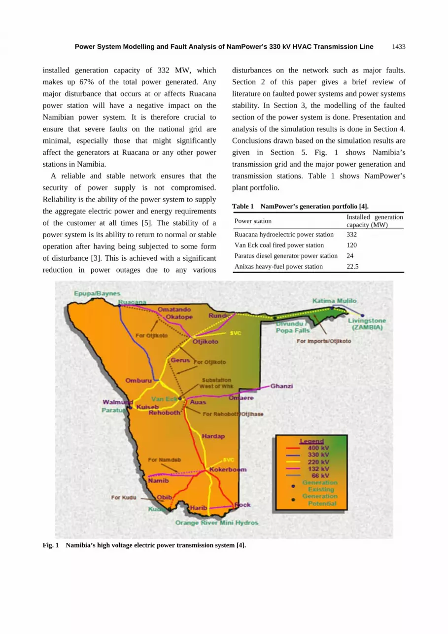
The aim was to create a model that accurately

represents the physical existing power network, using

the DigSilent software. Fig. 2 shows a one-line

diagram of the modelled power network. The software

was used to carry out load flow and fault analysis of


1436

Fig. 2 One-line diagram of NamPower’s electric power grid (Ruacana power station and Omburu substation).

the power network. The mathematical formulation of

the power flow problem is given by:

0 1,

n ni ii i j i j Jj j

i

P jQV y y V j i

v

(2)

3.1 Modelling Procedure

The different components needed to build the

electrical network were created in the equipment

library in DigSilent power factory software by using

the equipment basic data for each component. The

summarized basic equipment data and parameters

used for modelling are shown in Tables 2-4.

The model comprises of four main parts:

Ruacana hydroelectric power station;

Omburu transmission substation;

Ruacana transmission substation;

330 kV high voltage transmission line.

The NamPower transmission grid was created and

the various generation and transmission stations were

built on it using the components in the equipment and

global libraries. The power station and substations

were then connected to each other using the 330 kV

transmission line.

All simulations were carried using the stability tool

box in DigSilent Powerfactory. Since the

hydro-turbine generators at Ruacana power station are

low speed machines, they were modelled with salient

pole rotors. Additional control models were added to

the generators during modelling of the power station.

These are the software inbuilt control models and they

include the governor and turbine controllers (IEEE

pcu_HYGOV) as well as the automatic voltage

regulator (vco_IEEET1). These additional control

models were added to make the analysis of the

observed transient fault more realistic as the machines

in the physical network have controls.

3.2 Model Validation

An accuracy analysis of the modelled power system

Table 2 Transformer parameters.

Name Rated power (MVA)

Tap position (Max)

Additional voltage/tap (%)

Positive sequence impedance (%)

Vector group

Gen Transformer 1, 2 and 3 11/330 (kV)

90 17 1.25 12.3 YNd1

Gen Transformer 4 11/330 (kV) 100 17 1.25 1.24 YNd1

Ruacana TRFR11 66/11 (kV) 2.5 17 1.25 9.52 YNd1

Omburu Coupling TRFR1 315/315/40 17 1.25 10.8/18.413/20.063 YN0yn0d1

Omburu Coupling TRFR2 315/315/40 17 1.25 10.2/20.19/20.44 YN0yn0d1

Omburu SVC1 TRFR 60 17 1.25 8 YNd7

Table 3 Transmission line parameters.

Name Voltage (kV) Rated current (kA) Max operation temperature (°C)

Conductor material Line length (km)

Ruacana-Omburu 330 1 80 Aluminium 570

Omburu sub. line 1 22 1 80 Aluminium -

Omburu sub. line 2 22 1 80 Aluminium -

Ruacana station

330 kV Ruacana-Omburu sun-station line

Omburu


1437

Table 4 Generator parameters.

Name Nominal apparent power (MVA) Nominal voltage (kV) Power factor (%) Frequency (Hz)

Ruacana Gen 1, 2 and 3 88.888 11 90 50

Ruacana Gen 4 100 11 90 50

is carried out in order to validate the modelled

electrical network (see Table 5). The accuracy of a

modelled component in the electrical network is given

by the following formula:

1 t m

T

A AA

A

(3)

where，

A = relative accuracy;

At = true value of quantity;

Am = measured value of quantity.

The percentage accuracy is given by:

100%a A x (4)

From Table 5, it can be seen that the power system

has been modelled to a relative accuracy level of

0.935 and a percentage accuracy of 93.5%. This is

fairly accurate and the results obtained as well as the

conclusions drowned based on those results are valid.

The following steps were taken to set up the

transient simulations:

setting initial conditions;

defining short circuit event;

defining switching events;

defining results objects and variable sets;

executing transient simulation and creating

plotted curves.

4. Simulation Results

The simulation results for various short circuit

scenarios are presented to show the system behaviour

in steady state, during fault conditions and post-fault

conditions (transient state). The busbar voltage at

Ruacana is 330 kV and of interest to be analysed. The

simulation results are presented in Figs. 3-8. All the

results except Fig. 9 were generated using the

transient stability toolbox (DigSilent Powerfactory

simulation software). Fig. 9 was retrieved from

NamPower’s SCADA (supervisory control and data

acquisition) system. A comparison is made between

the simulation result curves and the graphs obtained

from NamPower records in order to determine

which fault scenario best fits the behaviour of the 330

kV busbar voltage from the simulation results.

From Fig. 3, it is observed that during steady-state

the busbar voltage is constant at approximately 330

kV.

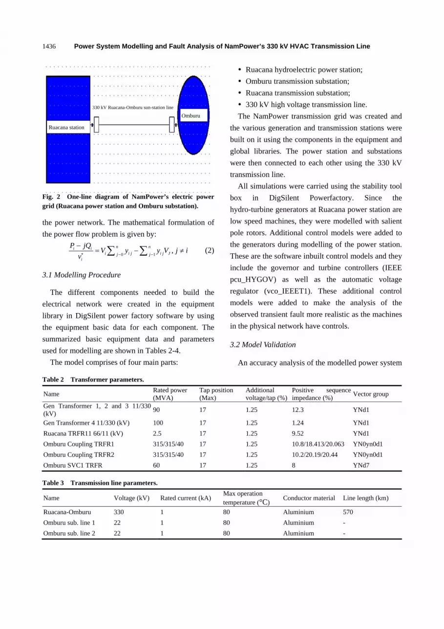
Fig. 4 shows that before the fault occurred, the

busbar voltage was constant at 330 kV. When the fault

occurred at 0.6 s, the busbar voltage instantly dropped

to zero. The Ruacana breaker then opened at 0.8 s and

the voltage sharply went up to 280 kV, after which it

started to increase gradually until it reached a

maximum value of 350 kV at 1 s. The generating units

then began to trip on over voltage and the voltage

began to drop until if eventually dropped to zero when

all generators fell out of step and tripped.

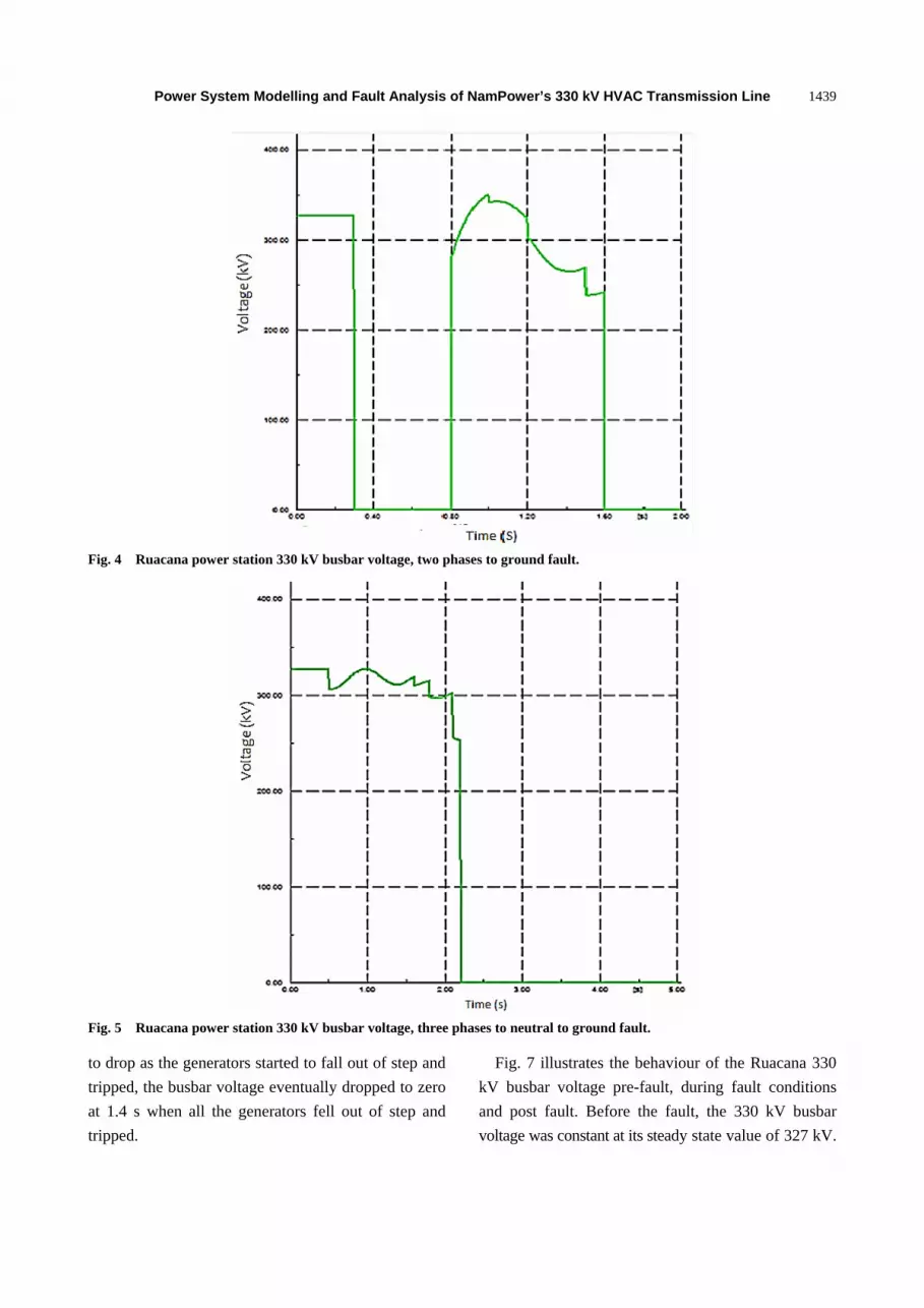
Fig. 5 shows that before the fault, the 330 kV

busbar voltage was constant at 327 kV. When the fault

occurred at 200 ms, the voltages remained at its steady

state value and only dropped at 300 ms when the

Omburu breaker opened. This result was however

unexpected. At 600 ms, the 330 kV busbar voltage

steadily rose to approximately 327 kV, it then started

to drop as the generators lost synchronism and started

to trip. The voltage ultimately drops to zero when all

the generators tripped.

Fig. 6 shows that when the three phase fault

occurred at 300 ms, the 330 kV busbar voltage

instantly drops to zero. When the breaker at Omburu

opened, the busbar voltage remained at zero. After the

breaker at Ruacana opened at 800 ms, the 330 kV

busbar voltage went up to approximately 100 kV, it

remained constant for 400 ms after which it then started


1438

Table 5 Power system model accuracy.

Component name At Am A a

Ruacana 330 kV busbar 330 327 0.991 99.1

Omburu 220 kV busbar 220 225 0.977 97.7

Gen 1 active power MW 82 80.9 0.987 98.7

Gen 2 active power MW 82 80 0.976 97.6

Gen 3 active power MW 82 80 0.976 97.6

Gen 4 active power MW 90 90 1 100

Gen 1 reactive power MVAr 9.8 9 0.918 91.8



Gen 4 reactive power MVAr 35 10 0.286 28.6

Gen 1 stator terminal kV 11 11 1 100




Gen 1 stator current kA 4.67 4.25 0.910 91.0




Gen 1 frequency Hz 50 50 1 100




Mean accuracy 0.935 93.5

Fig. 3 Ruacana power station 330 kV busbar voltage, steady state.


1439

Fig. 4 Ruacana power station 330 kV busbar voltage, two phases to ground fault.

Fig. 5 Ruacana power station 330 kV busbar voltage, three phases to neutral to ground fault.

to drop as the generators started to fall out of step and

tripped, the busbar voltage eventually dropped to zero

at 1.4 s when all the generators fell out of step and

tripped.

Fig. 7 illustrates the behaviour of the Ruacana 330

kV busbar voltage pre-fault, during fault conditions

and post fault. Before the fault, the 330 kV busbar

voltage was constant at its steady state value of 327 kV.


1440

Fig. 6 Ruacana power station 330 kV busbar voltage, three phase fault.

Fig. 7 Ruacana power station 330 kV busbar voltage, two phase fault.


1441

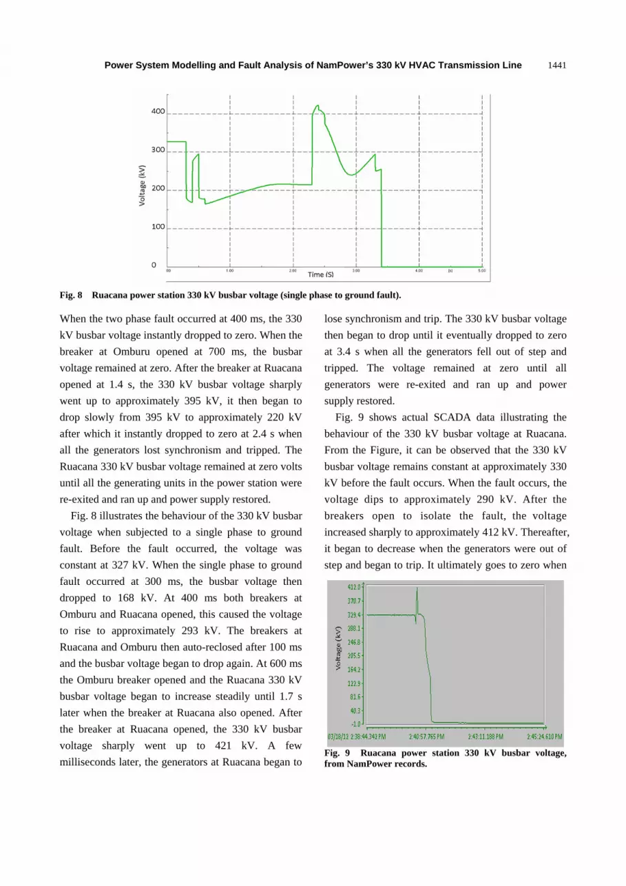
Fig. 8 Ruacana power station 330 kV busbar voltage (single phase to ground fault).

When the two phase fault occurred at 400 ms, the 330

kV busbar voltage instantly dropped to zero. When the

breaker at Omburu opened at 700 ms, the busbar

voltage remained at zero. After the breaker at Ruacana

opened at 1.4 s, the 330 kV busbar voltage sharply

went up to approximately 395 kV, it then began to

drop slowly from 395 kV to approximately 220 kV

after which it instantly dropped to zero at 2.4 s when

all the generators lost synchronism and tripped. The

Ruacana 330 kV busbar voltage remained at zero volts

until all the generating units in the power station were

re-exited and ran up and power supply restored.

Fig. 8 illustrates the behaviour of the 330 kV busbar

voltage when subjected to a single phase to ground

fault. Before the fault occurred, the voltage was

constant at 327 kV. When the single phase to ground

fault occurred at 300 ms, the busbar voltage then

dropped to 168 kV. At 400 ms both breakers at

Omburu and Ruacana opened, this caused the voltage

to rise to approximately 293 kV. The breakers at

Ruacana and Omburu then auto-reclosed after 100 ms

and the busbar voltage began to drop again. At 600 ms

the Omburu breaker opened and the Ruacana 330 kV

busbar voltage began to increase steadily until 1.7 s

later when the breaker at Ruacana also opened. After

the breaker at Ruacana opened, the 330 kV busbar

voltage sharply went up to 421 kV. A few

milliseconds later, the generators at Ruacana began to

lose synchronism and trip. The 330 kV busbar voltage

then began to drop until it eventually dropped to zero

at 3.4 s when all the generators fell out of step and

tripped. The voltage remained at zero until all

generators were re-exited and ran up and power

supply restored.

Fig. 9 shows actual SCADA data illustrating the

behaviour of the 330 kV busbar voltage at Ruacana.

From the Figure, it can be observed that the 330 kV

busbar voltage remains constant at approximately 330

kV before the fault occurs. When the fault occurs, the

voltage dips to approximately 290 kV. After the

breakers open to isolate the fault, the voltage

increased sharply to approximately 412 kV. Thereafter,

it began to decrease when the generators were out of

step and began to trip. It ultimately goes to zero when

Fig. 9 Ruacana power station 330 kV busbar voltage, from NamPower records.


1442

all the generators lost synchronism and tripped. The

busbar voltage remained at zero voltage until the

generating units were re-excited and ran up and

electric power supply was restored.

5. Conclusion

Based on the qualitative analysis of the obtained

results, it can be concluded that the observed fault is

most probably a single phase to ground fault. This

conclusion was arrived at on the basis of close

correlation in the observed behaviour of the Ruacana

power station 330 kV busbar voltage in the plots

obtained from the single phase to ground fault

simulations and the behaviour of that same variable as

shown in the graph of the behavioural pattern of the

330 kV busbar voltage in Fig. 9 which was obtained

from NamPower records. This is however not the case

for the two phases to ground fault, three phase fault,

two phase fault and the three phases to neutral to

ground fault scenarios, hence the conclusion is a

single phase to ground fault.

Acknowledgments

This work has been supported in part by the Faculty

of Engineering & Information Technology Research

Centre at the University of Namibia NamPower, the

University of KwaZulu-Natal Research/Publications

Office, and the HVDC/Smart Grid Research Centre.

References

[1] Stankovic, A. M., and Aydin, T. 2000. “Analysis of Symmetrical Faults in Power Systems Using Dynamic Phasors.” IEEE Transection on Power System 15 (3): 1063-8.

[2] Weedy, B. M., and Cory, B. J. 1999. Electric Power Systems. London: John Wiley & Sons, Inc..

[3] Pre've', C. 2006. Protection of Electrical Networks. London: ISTE Ltd..

[4] Shilamba, P. 2011. NamPower Annual Report, 2011. Annual report.

[5] Kundur, P., Perseba, J., Ajjarapu, V., Anderson, G., Bose, A., and Canizares, C. 2004. “Definition and Classification of Power System Stability.” IEEE Transection on Power System Stability 19 (2): 1387-93.

[6] Gross, C. A. 1986. Power System Analysis. New York:

John Wiley & Sons.

[7] Ram, B., and Vishwakarna, D. N. 1995. Power System

Protection and Switchgear. New Delhi: Tata

McGraw-Hill.

[8] Anderson, P. M. 1995. Analysis of Faulted Power

Systems. New York: Wiley-IEEE Press.

[9] Tleis, A. N. 2008. Power System Modelling and Fault

Analysis. USA: Elsvier Ltd..

[10] Nasar, S. A., and Trutt, F. C. 1999. Electric Power

Systems. Florida: CRC Press LLC.

[11] Gan, D., Thomas, R. J., and Zimmerman, R. D. 2000.

“Stability-Constrained Optimal Power Flow.” IEEE

Transections on Power Systems 15 (2): 535-40.

[12] Kundur, P. 1994. Power Systems Stability and Control.

USA: McGraw-Hill Professional.

[13] Elmore, W. A. 1994. Protective Relaying Theory and

Applications. New York: Marcel Dekker. Inc..

[14] Chiang, H., Wu, F. F., and Varaiya, P. P. 1994. “A BCU

Method for Direct Analysis of Power System Transient

Stability.” IEEE Transection on Power Systems 9 (3):

1-5.

[15] Demetz, N., and Jeanjean, G. 1997. “Dynamic Stability

of Electrical Industrial Networks.” Cashier Techniques

185: 1-14.

[16] Glover, J. D., Sarma, M. S., and Overbye, T. J. 2008.

Power Systems Analysis and Design. Toronto: Chris

Carson.

[17] Song, Y. H., and Johns, A. T. 1999. FACTS (Flexible AC

Transmission Systems). London: The Institution of

Electrical Engineers.

[18] Choo, Y. C., Muttaqi, K. M., and Negnevitsky, M. 2006.

“Transient Stability Assesment of a Small Power System

Subjected to Large Disturbances.” In Proceedings of the

Australasian Universities Power Engineering Conference,

1-13.

[19] Ortega, J. M., and Rheinboldt, W. C. 1970. Iterative

Solutions of Nonlinear Equations in Several Variables.

New York: Academic Press.

[20] Das, D. 2006. Electrical Power Systems. New Delhi:

New Age International (P) Limited.

[21] DigSilent PowerFactory. 2011. User’s Manual. Germany:

DigSilent GmbH Heinrich-Hertz.

power system modeling and fault analysis of nampower’s 330 kv hvac transmission line

Documents