1

Planing Hull Model Tests for CFD ValidationEric Thornhill, Dan Oldford, Neil Bose, Brian Veitch, Pengfei Liu

ABSTRACT

A set of bare hull resistance tests were performed on a 1/8 scale model of an 11.8 m long planing hull. Themodel was tested over a range of speeds and ballast conditions in calm water. Measurements were made oftow force, running trim, and sinkage. Wetted areas and lengths were determined using underwater video.Flush mounted pressure taps gave gauge pressures at various locations on the hull surface. Wave profileswere measured using an array of capacitance probes positioned laterally in the tank. Boundary layervelocity profiles were resolved at two locations on the hull for several model speeds using a laser Dopplervelocimeter (LDV). Selected results from the tests are presented.

INTRODUCTION

Model scale experiments were done to collect data to validate developments in computational fluid dynamicsmethods. The experiments were performed in the Clearwater Towing Tank at the National Research Council ofCanada's Institute for Marine Dynamics and consisted of a series of resistance tests with a planing craft. Tests weredone over a range of speeds and in 6 different ballast configurations (displacement and longitudinal center ofgravity). Measurements were made of tow force, running trim and sinkage, hull pressures, wetted surface area, andwave profiles. Additional tests were done to measure the boundary layer thickness at two locations along the hullusing a laser Doppler velocimeter. These were done for four speeds in a single ballast configuration. The boundarylayer at each position and at each speed was delineated using about 20 runs. This paper describes the model and testsetup, the test program, and examples of the measured data.

MODEL & TOW ARRANGEMENT

Planing Boat ModelThe hull shape used in the experiments discussed in this paper was a 1:8 scale model of a full scale vessel

currently in operation. It was constructed out of carbon fiber reinforced plastic strengthened with transverse andlongitudinal stiffeners, a watertight bulkhead near the stern, and a shear deck with coaming. A plastic splash guardcover was fitted during tests.

The hull surface, shown in Figure 1, was marked with station numbers on the bottom and port side. Knife edgesextending 1mm from the hull surface, were fitted along the chines to promote flow separation. The hull was notprismatic but did have a simple shape as shown in Figure 2. This cross section was constant from the transom forabout 2/3 the length of the hull (covering the wetted length of the model for all ballast conditions when planing). Asmall flat bottom area at the centerline turns to a low deadrise of 5.9°. This deadrise then turns sharply to 40.8° nearthe chine (see Figure 2).

Figure 1. Model Hull (LOA = 1.475m).

6th Canadian Marine Hydromechanics and Structures Conference. 23-26 May, 2001. Vancouver BC

2

Figure 2. Model Hull Cross Section.

Tow ArrangementThe model was fitted to the tow carriage using a gimbal and yaw restraint. Tow force was transmitted from the

heave post through a linear bearing to an ‘S’-shaped load cell (max. load = 50 lb.) and then through a universal jointto the model (see Figure 3). The universal joint allowed the model to pitch and roll freely and the heave post wasfree to move vertically in the tow post arrangement. The model was prohibited from rotating about the heave post bya yaw restraint which was counterbalanced so that it did not affect the ballast. The tow arrangement is shown inFigure 4.

Figure 3. Gimbal. Figure 4. Tow Arrangement.

TEST PROGRAMThe test program consisted of two phases. The first phase focused on testing the effects of different ballast

conditions over a range of speeds. Measurements were made of tow force, running trim, sinkage, hull pressures,wetted surface areas, and wave profiles. The second phase was performed solely at the design ballast condition, andwas used to measure boundary layer velocity profiles below the hull surface using a laser Doppler velocimeter(LDV).

As planing craft performance is sensitive to ballast condition, tests were performed over a range of displacementsand locations of the longitudinal center of gravity (LCG). These conditions are given in Table 1, which also showsthe static trim angles of the model. The first column lists the three displacements (design displacement ±15%) andthe first row lists the three LCG positions (design LCG ±7%). LCG position was referenced from the transom base.

A plan view of the model hull bottom is given in Figure 5 showing the relative locations of the LDV windows,pressure transducers (labeled P1 through P9), tow point, and LCGs.

3

Displacement LCG =0.49 m

LCG =0.53 m

LCG =0.57 m

25.2 kg - 1.0° -29.6 kg 2.0° 1.1° 0.4°33.9 kg - 1.3° -

Table 1. Static trim angles for ballast conditions.

Figure 5. Instrument Positions in Model

RESULTS

ResistanceThe resistance curves for the model were typical for a planing vessel and had the characteristic ‘hump’ speed at

the onset of planing. Figure 6 shows the resistance results for the various ballast conditions. Only the designcondition was tested over the full speed range. The curves closest to the design condition show the effect of a 7%change of LCG (both fore and aft) on resistance, while the two more distant curves show the effect of a 15% changein displacement.

Resistance Results

0

5

10

15

20

25

30

35

40

45

50

55

60

0.0 0.5 1.0 1.5 2.0 2.5 3.0 3.5 4.0 4.5 5.0 5.5 6.0 6.5 7.0 7.5 8.0 8.5

Model Speed [m/s]

25.2 kg, 0.53 m29.6 kg, 0.49 m29.6 kg, 0.53 m29.6 kg, 0.57 m33.9 kg, 0.53 m

Figure 6. Model Scale Resistance.

4

Running TrimTrim angle is an important factor in planing craft performance as it changes the geometry of the hull relative to the

water. The running trim angles for this model followed similar trends as the resistance curves, clearly identifying the‘hump’ speed at which planing begins. Shown in Figure 7 are the absolute running trims for the various ballastconditions.

Running Trim Results

0.0

1.0

2.0

3.0

4.0

5.0

6.0

7.0

8.0

0.0 0.5 1.0 1.5 2.0 2.5 3.0 3.5 4.0 4.5 5.0 5.5 6.0 6.5 7.0 7.5 8.0 8.5

Model Speed [m/s]

25.2 kg, 0.53 m29.6 kg, 0.49 m29.6 kg, 0.53 m29.6 kg, 0.57 m33.9 kg, 0.53 m

Figure 7. Running Trim.

It can be seen from the plots that the different ballast conditions were not tested to the same maximum speeds. Forinstance, the aft LCG ballast condition was only tested to 6.0 m/s and the forward LCG condition was tested to8.0 m/s. This occurred because the model was prone to dynamic instability, or porpoising, at high speeds. The aftLCG position made the model susceptible to this instability at speeds above 6.0 m/s and therefore it was not testedbeyond that limit.

Another way of presenting the running trim results is to plot the change in trim angle developed at speed from thestatic trim angle at rest (given in Table 1). This plot, Figure 8, shows that when in the planing regime, the thresholdabove which porpoising occurred was when the change in trim angle dropped below approximately 2.1°. Moredetails of the porpoising characteristics of this model can be found in Thornhill et al. (2000).

Running Trim Results

0.0

1.0

2.0

3.0

4.0

5.0

6.0

7.0

0.0 0.5 1.0 1.5 2.0 2.5 3.0 3.5 4.0 4.5 5.0 5.5 6.0 6.5 7.0 7.5 8.0 8.5 9.0

Model Speed [m/s]

25.2 kg, 0.53 m29.6 kg, 0.49 m29.6 kg, 0.53 m29.6 kg, 0.57 m33.9 kg, 0.53 m

PorpoisingThreshold

Figure 8. Change in Trim.

5

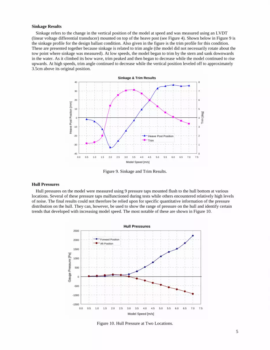
Sinkage ResultsSinkage refers to the change in the vertical position of the model at speed and was measured using an LVDT

(linear voltage differential transducer) mounted on top of the heave post (see Figure 4). Shown below in Figure 9 isthe sinkage profile for the design ballast condition. Also given in the figure is the trim profile for this condition.These are presented together because sinkage is related to trim angle (the model did not necessarily rotate about thetow point where sinkage was measured). At low speeds, the model began to trim by the stern and sank downwardsin the water. As it climbed its bow wave, trim peaked and then began to decrease while the model continued to riseupwards. At high speeds, trim angle continued to decrease while the vertical position leveled off to approximately3.5cm above its original position.

Sinkage & Trim Results

-40

-30

-20

-10

0

10

20

30

40

0.0 0.5 1.0 1.5 2.0 2.5 3.0 3.5 4.0 4.5 5.0 5.5 6.0 6.5 7.0 7.5

Model Speed [m/s]

0

1

2

3

4

5

6

7

8

Heave Post PositionTrim

Figure 9. Sinkage and Trim Results.

Hull PressuresHull pressures on the model were measured using 9 pressure taps mounted flush to the hull bottom at various

locations. Several of these pressure taps malfunctioned during tests while others encountered relatively high levelsof noise. The final results could not therefore be relied upon for specific quantitative information of the pressuredistribution on the hull. They can, however, be used to show the range of pressure on the hull and identify certaintrends that developed with increasing model speed. The most notable of these are shown in Figure 10.

Hull Pressures

-1500

-1000

-500

0

500

1000

1500

2000

2500

0.0 0.5 1.0 1.5 2.0 2.5 3.0 3.5 4.0 4.5 5.0 5.5 6.0 6.5 7.0 7.5

Model Speed [m/s]

Forward PositionAft Position

Figure 10. Hull Pressure at Two Locations.

6

The figure gives the results from two pressure transducers located fore and aft at the same longitudinal plane inthe model (P1 and P6 shown in Figure 5). The forward transducer records increasing pressure with increasing speed,while the aft transducer shows the opposite trend, with negative pressure values at high speeds. These negativepressure values correspond to increased flow velocities near the hull as discussed in a later section.

Wave ProfilesThe surface wave profiles produced by the model at speed were captured by a transverse array of capacitance

probes located midway along the tow tank. The 23 probes were spaced 7 inches apart, the first being 7 inches fromthe side of the model as it passed by. Sampled at 100 hz, the time traces from the probes show the wave elevations atthe various longitudinal cuts. A proximity switch was used to correlate the position of the model with the probe data:when the switch was triggered, the model’s bow was in line with the probe array. The probe array is shown in Figure11 attached to a beam fixed to the tank wall. An example of the data collected from the probes is shown in Figure12.

Figure 11. Wave Probe Array in Tank.

Figure 12. Wave Probe Data

7

Boundary Layer Velocity ProfilesThe second phase of the experimental program was dedicated to determining velocity profiles in the boundary

layer at two locations for four different model speeds in the design ballast condition. The measurements were madeusing a laser Doppler velocimeter (LDV) fitted in the model. This instrument has several advantages over othermore common techniques for velocity measurements such as pitot tubes and hot-film anemometry. The primaryadvantage of the LDV is its non-intrusiveness; only the laser beams enter the water, so they do not influence the thinlayer of fluid where measurements are being taken.

The LDV uses intersecting laser beams to make velocity measurements. Strictly speaking, the LDV measures thevelocity of particles in the flow and not the flow itself. A particle, when traveling through the volume of intersectionof the beams, reflects light as it passes through an interference pattern of light and dark bands caused by the lasers ofmatching wavelength. Processors in the LDV determine the frequency of this pulsating reflected light picked up bysensors in the probe. As the distance between the interference bands is known, the processor can then calculate thevelocity of the particle. Numerous particle measurements are averaged to determine the mean flow velocity.Particles are added as “seed” to the flow and are generally in the size range of 0.5 – 5.0 microns. The measurementvolume of the LDV depends on both the beam diameter and the angle of intersection. For these experiments thevolume was an ellipsoid 0.64 mm in height (perpendicular to the hull) and 76 µm in diameter.

Seeding is an important part of LDV testing as it controls both the data rate (the number of particles passingthrough the intersection volume per second) and validation (the percentage of particles that could be processed intovelocity measurements). For these experiments, seed was added for each test by aiming a small stream of aconcentrated water/seed mix in the path of the model. Several types of seed were used, including silver-coated glassmicro-balloons and pre-sifted all-purpose flour. Data rates for the experiments ranged from 30 Hz to 3 kHz withvalidation between 60-95%. Typical values for most tests were data rates around 500 Hz with 75% validation.

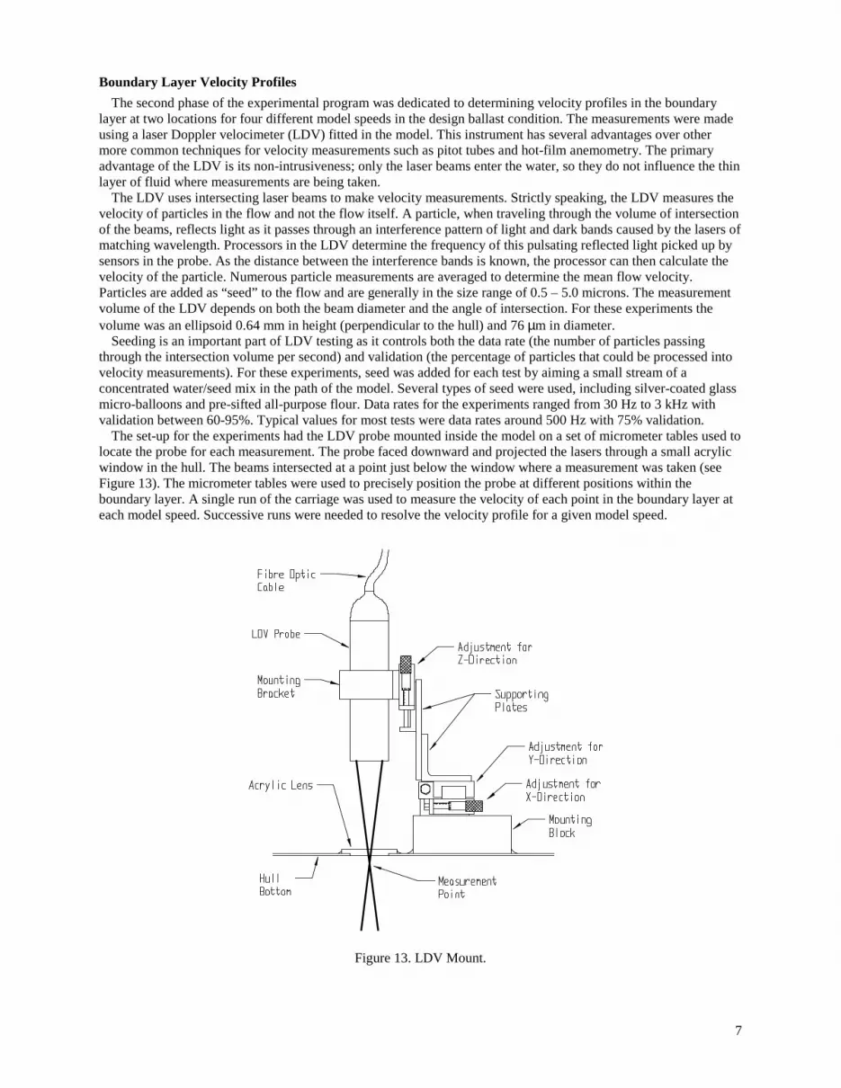
The set-up for the experiments had the LDV probe mounted inside the model on a set of micrometer tables used tolocate the probe for each measurement. The probe faced downward and projected the lasers through a small acrylicwindow in the hull. The beams intersected at a point just below the window where a measurement was taken (seeFigure 13). The micrometer tables were used to precisely position the probe at different positions within theboundary layer. A single run of the carriage was used to measure the velocity of each point in the boundary layer ateach model speed. Successive runs were needed to resolve the velocity profile for a given model speed.

Figure 13. LDV Mount.

8

Raw data from a typical test is given in Figure 14. It shows the acceleration, constant speed, and decelerationportions of the run. The figure also shows that the raw velocity data fell onto equally spaced discrete values (seen asbands of points). This feature is an artifact of the LDV’s internal processors that determine the particle velocities.The width between these bands can be changed, but doing so also alters the range of velocities which can bemeasured. A smaller bandwidth results in a smaller velocity range. These experiments used a bandwidth ofapproximately 0.1 m/s.

Forward Position, Model Speed 4m/s, 8.5mm from Hull

0

0.5

1

1.5

2

2.5

3

3.5

4

4.5

5

10 12 14 16 18 20 22 24 26 28 30 32 34 36 38 40 42 44 46 48 50 52 54Time [sec]

Figure 14. Typical LDV Data.

Boundary layer velocity profiles for two positions on the hull for each of four model speeds (4 m/s, 5 m/s, 6 m/sand 6.5 m/s) were measured. Results for the model speed of 4 m/s are given below in Figure 15.

Boundary Layer Velocities (Model Speed = 4 m/s)

0

1

2

3

4

5

6

7

8

9

10

11

12

13

14

15

2.5 2.6 2.7 2.8 2.9 3.0 3.1 3.2 3.3 3.4 3.5 3.6 3.7 3.8 3.9 4.0 4.1 4.2 4.3 4.4

Flow Velocity [m/s]

Forward PositionAft Position

Figure 15. Boundary Layer Velocities (Vm = 4 m/s).

9

The results from these measurements clearly show the boundary layer velocity form, thickness, and the freestream velocity for both of the two locations at each speed tested (for a total of 8 profiles). In the figure, the forwardposition shows a boundary layer thickness of about 4 mm with a free stream velocity equal to the model velocity.The aft position shows that the boundary layer had grown thicker and that the flow achieved a greater free streamvelocity, exceeding that of the model speed. This is consistent with the negative pressures measured in the aft regionof the hull. Profiles at the other model speeds tested were qualitatively similar as those shown in Figure 15. Thepercentage increase in free stream velocity from the forward to the aft position decreased as the model speedincreased (trim angle also decreased). The boundary layer thickness also decreased with increasing model speed.This drop in pressure and increase in speed in the after region of the hull can be partially explained by taking intoconsideration the potential head due to depth of immersion, a factor that is omitted in simple classical planing theorywhich predicts only positive pressures over the length of a planing surface. However, the pressure drops and speedincreases for the corresponding trim and sinkage conditions were somewhat larger than expected from this causealone. It is planned to investigate this behaviour further using CFD simulations.

The positions of the forward and aft measurement positions relative to the leading edge of the wetted hull area fora given model speed are shown below in Figure 16.

Figure 16. Vessel Attitude (4 m/s).

One difficulty with the technique used to determine the boundary layer velocity profile was the determination ofthe reference or zero position of the hull surface. The procedure for finding this zero position consisted ofsystematically moving the measurement point closer to the lens until the photo-detectors gave an overload error.This meant that the measurement volume was inside the lens, and that the beams were reflecting directly back to thedetectors. It was, however, possible that measurements could be taken with a small portion of the measurementvolume inside of the lens, without overloading the photo-detectors. The size of this overlap could not be determined.The orientation of the probe meant that the largest dimension of the measurement volume (0.64mm) wasperpendicular to the hull. It was assumed that measurements could not be made if more than half of themeasurement volume was inside the lens. This gives an uncertainty in the hull zero position for the LDVmeasurements of approximately 0.32mm. The shape of the profiles is not affected by this bias, which would shift theentire curve up or down.

Another result from the analysis of the raw LDV data came from the standard deviations of the samples used tocalculate the mean flow velocities. Shown Figure 17, the standard deviations followed a similar trend as thevelocities. High standard deviations were measured close to the hull, while in the free stream they leveled off. Thehigher values close to the hull can be attributed to two primary factors: turbulence and velocity gradient. Wallbounded turbulence in the boundary layer can cause fluctuations in velocity that would result in increased standarddeviation. The large velocity gradient close to the hull would also result in increased standard deviation since abroader range of velocities spanning from the bottom to the top of the measurement volume would have beencaptured.

10

LDV Fwd (Model Speed = 4 m/s)

0

0.05

0.1

0.15

0.2

0.25

0.3

0.35

0.4

0.0 1.0 2.0 3.0 4.0 5.0 6.0 7.0 8.0 9.0

Distance from Hull [mm]

Figure 17. Standard Deviations from LDV Data.

SUMMARYTests were performed on a 1/8 scale model of a planing vessel to generate a set of performance data to be used in

future validation of numerical simulations. Sample results were presented for the measurements of resistance,running trim, sinkage, hull pressures, wave profiles, and boundary layer velocity profiles. Resistance and runningtrim results showed characteristics common to planing craft. Hull pressures were found to increase in the forwardpart of the hull but decrease and become negative in the aft. Boundary layer thicknesses were found to increase inthe direction of flow and to decrease with increasing model speeds as expected. Velocities measured just outside theboundary layer were found to be greater than free stream in the aft part of the hull, showing an acceleration from theforward position.

ACKNOWLEDGEMENTSThese experiments were performed at the National Research Council of Canada’s Institute for Marine Dynamics

(NRC/IMD). In addition to NRC/IMD, funding and technical assistance was also provided by Memorial Universityof Newfoundland, Oceanic Consulting Corporation, and NSERC (Natural Sciences and Engineering ResearchCouncil).

NRC/ Institute for Marine Dynamics http://www.nrc.ca/imd/Memorial University of Newfoundland http://www.engr.mun.ca/Ocean Engineering Research Centre http://www.engr.mun.ca/OERC/Oceanic Consulting Corporation http://www.oceaniccorp.com/NSERC http://www.nserc.ca/

REFERENCESThornhill E., Veitch B., Bose N., “Dynamic Instability of a High Speed Planing Boat Model”. Marine Technology,July 2000.Savitsky D., “Hydrodynamic Design of Planing Hulls”, Marine Technology, vol. 1, no. 1, pp. 71 – 95, October 1964.Du Cane P., High Speed Small Craft 3rd Ed. Temple Press Books, London. 1964.Payne P.R., Design of High Speed Boats Volume 1: Planing. Fishergate Inc. Annapolis. 1988.